ddjc-sharpe defense distribution depot: femwater … · ddjc-sharpe defense distribution depot:...

ERDC/CHL CHETN-XI-1 March 2004

DDJC-Sharpe Defense Distribution Depot: FEMWATER 3D Transport Model of TCE

Plume Migration with Natural Attenuation by Barbara P. Donnell and the ERDC-CHL Groundwater Team

PURPOSE: This Coastal and Hydraulics Engineering Technical Note summarizes results from a three-dimensional (3-D) groundwater numerical model of plume migration comparisons between a no-pumping scenario and a proposed pump-and-treat extraction configuration at the Defense Distribution Depot San Joaquin Sharpe (DDJC), in Lathrop, CA. The variably saturated 3-D numerical model FEMWATER was used to predict long-term (30 years beyond 3Q-2002) trichloroethylene (TCE) plume migration with natural attenuation.

BACKGROUND: The DDJC-Sharpe army depot is located near Lathrop, CA (Figure 1). It has been active for many years and solvents used in degreasing operations have contaminated the groundwater. To address the contamination problem, the installation operates three pump-and-treat remediation systems, (north, central, and south shown in Figure 2) to contain the TCE plumes and to treat the contaminated groundwater. In 1997, the U.S. Army Engineer Research and Development Center (ERDC), Coastal and Hydraulics Laboratory (CHL) was asked by the Huntsville Engineering and Support Center to collaborate in the development of a comprehensive regional groundwater model to make predictions of flow and transport over a wide range of hydrologic conditions. The site contractor responsible for operation and monitoring of the existing pump-and-treat remediation system was URS Corporation, Sacramento, CA. Several scenarios have been investigated, including sitings of new municipal water wells, variations in the surface-water drainage and storm-water retention ponds, and guidelines for shutdown and placement of extraction wells to get better contaminant capture for less cost. These model investigations are described in Donnell et al. (2003).

FEMWATER MODEL: FEMWATER is a general purpose, unstructured finite element 3-D flow and transport groundwater model for variably saturated mediums. Its governing equations are fully described in Lin et al. (1997). It was deemed the model of choice because of its ability to address complexities in groundwater flow problems not suitably addressed by other numerical models.

GMS. The FEMWATER model is integrated into the Department of Defense Groundwater Modeling System (GMS). GMS contains a state-of-the-art graphical user environment that allows efficient model conceptualization, setup of boundary conditions and visualization. More information on GMS is described in Groundwater Modeling Team (2004).

Stratigraphic Conceptualization. The hydrogeology within the Sharpe project domain is complex. The DDJC-Sharpe site overlies geologic strata that provide numerous conceptualization difficulties. The San Joaquin Valley contains depositional features that are difficult to determine from a discrete sampling of boreholes (over 130 borings). The apparent depth and thickness of the different aquifers are highly variable throughout the site. Previous subsurface conceptualizations have categorized the aquifers into A, B, C, and D zones. Because of the lateral discontinuity of the

Report Documentation Page Form ApprovedOMB No. 0704-0188

Public reporting burden for the collection of information is estimated to average 1 hour per response, including the time for reviewing instructions, searching existing data sources, gathering andmaintaining the data needed, and completing and reviewing the collection of information. Send comments regarding this burden estimate or any other aspect of this collection of information,including suggestions for reducing this burden, to Washington Headquarters Services, Directorate for Information Operations and Reports, 1215 Jefferson Davis Highway, Suite 1204, ArlingtonVA 22202-4302. Respondents should be aware that notwithstanding any other provision of law, no person shall be subject to a penalty for failing to comply with a collection of information if itdoes not display a currently valid OMB control number.

1. REPORT DATE MAR 2004 2. REPORT TYPE

3. DATES COVERED 00-00-2004 to 00-00-2004

4. TITLE AND SUBTITLE DDJC-Sharpe Defense Distribution Depot: FEMWATER 3D TransportModel of TCE Plume Migration with Natural Attenuation

5a. CONTRACT NUMBER

5b. GRANT NUMBER

5c. PROGRAM ELEMENT NUMBER

6. AUTHOR(S) 5d. PROJECT NUMBER

5e. TASK NUMBER

5f. WORK UNIT NUMBER

7. PERFORMING ORGANIZATION NAME(S) AND ADDRESS(ES) Army Engineer Research and Development Center,Coastal andHydraulics Laboratory,3909 Halls Ferry Road,Vicksburg,MS,39180

8. PERFORMING ORGANIZATIONREPORT NUMBER

9. SPONSORING/MONITORING AGENCY NAME(S) AND ADDRESS(ES) 10. SPONSOR/MONITOR’S ACRONYM(S)

11. SPONSOR/MONITOR’S REPORT NUMBER(S)

12. DISTRIBUTION/AVAILABILITY STATEMENT Approved for public release; distribution unlimited

13. SUPPLEMENTARY NOTES

14. ABSTRACT

15. SUBJECT TERMS

16. SECURITY CLASSIFICATION OF: 17. LIMITATION OF ABSTRACT Same as

Report (SAR)

18. NUMBEROF PAGES

21

19a. NAME OFRESPONSIBLE PERSON

a. REPORT unclassified

b. ABSTRACT unclassified

c. THIS PAGE unclassified

Standard Form 298 (Rev. 8-98) Prescribed by ANSI Std Z39-18


Figure 1. DDJC-Sharpe and DDJC-Tracy location map

2

•

San Francisco

PACIFIC OCEAN

CAUFORNIA

San

•Bolt•-

15 30

SCALE IN MILES


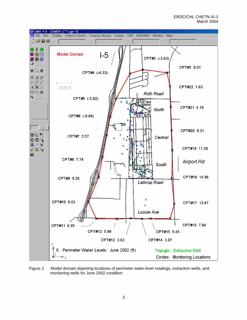
Figure 2. Model domain depicting locations of perimeter water-level readings, extraction wells, and monitoring wells for June 2002 condition

3

• I tt

li§ File Edit Display Feature Objects Drawing Objects Images DXF MODAEM Window Help

N ;4 K ·.· ;(- )

ftE/ DOA

~

till! k: ·~i tt t~ iii ~§:~: '<! ~~ 69

~

] b J b ] J Model Domain I/ ,r- CPT#3 (-3.63)/'

CPT#4 (-4.33)

2000 ft

CPT#5 (-3.82)

CPT#6 (-0.48) • -

~. '" ...

• • . • CPT#7 2.57

• •

•

~· \liL

____::] [e

CPT#S 7.74

CPT#9 9.26

CPT#10 8.03

\ r /A

CPT#11 6.95 :=.._____/ I CPT#12 5.88 I

CPT#13 3.63 '{

k_:erimeter Water Levels: June 2002 (ft)

X

CPT#1 0.01

CPT#22 1.63

~

CPT#21 4.15

i==

CPT#20 8.21

Central

lJ, CPT#19 11.26 •

~ . ...

South ~ 1\

Airporl Rd

~ Jl •• CPT#18 14.96

Lathrop Road

CPT#17 12.47

LouiseAve j

\

\ CPT#16 7.04

CPT#15 5.45

CPT#14 3.07

Triangle: Extraction Well

Circles: Monitoring Locations


clay layers above and below the aquifer layers, the aquifer behaves as a system with aquifer layers from the A, B, C, and D zones in hydraulic contact. Consequently the four-zone conceptualization was adopted for the regional groundwater model. The lower vertical limit of the model is equal to the average elevation of the D-zone, which is the Corcoran clay contact.

Model Domain. The numerical model domain is bounded by Airport Road, Louise Ave, I-5, and north of Roth Road, and is depicted by the red line in Figure 2.

Synoptic Survey. In preparation for the numerical modeling, all extraction and monitoring locations within the Sharpe site were rectified, both vertically and horizontally, to a common datum. This datum is CA State Plane Zone-403 NAD83. A synoptic survey of all known sources and sinks was conducted during June 2002. The June 2002 synoptic survey included perimeter and monitoring well water-level readings, locations, and rates of injection and extraction, and concentration readings at monitoring locations. Figure 2 shows the footprint of the DDJC-Sharpe site and displays solid circles for the internal monitoring locations, X for the perimeter wells, and triangles for the extraction wells.

Head boundary conditions. The numerical model domain corresponds with 22 strategically placed perimeter wells that provide guidance in assigning the head boundary conditions (Dirichlet boundary conditions). The perimeter head difference across the site is 19.29 ft, with 14.96 ft being the highest water level on the southeast edge, down to the lowest of -4.33 ft on the northwestern corner. The assigned head boundary conditions along the perimeter of the model domain were constant in the vertical. The synoptic data set also included water-level readings at all operative interior monitoring locations within the model domain (approximately 287 locations). These interior monitoring readings were used as observations to verify the numerical model flow and transport simulations.

The San Joaquin irrigation district canal runs north/south along the eastern border of the DDJC-Sharpe property. Although there were no water-level data collected in the canal, the field data suggested that the canal be included in the simulation. Head boundary conditions were assigned to surface nodes representing a V-shaped cross section of the canal. The irrigation canal head values ranged from 4.6 ft on the north edge to 13.1 ft on the southern edge.

Sources and sink boundary conditions. There were no man-made sources active during the synoptic survey: no injection wells, no unlined storm-water retention ponds, all known buried contaminants have been removed. However, there were numerous sinks within the DDJC-Sharpe numerical model domain during the synoptic survey: 44 extraction wells, 1 Shad extraction well, and 2 municipal pumping wells as shown as green triangles in Figure 2.

Mesh Resolution. The 3-D mesh used for the simulations described in this memorandum are the same as that described in the Appendix D of the main report, Donnell et al. (2003). The 3-D mesh, shown in Figure 3a, contained 409,792 nodes, 790,655 elements, and 8 material types, for a total of 31 layers. The mesh was divided into material types representative of the A, B, C, and D zone elevations. The bottom of the mesh, z-elevation of -220 ft, corresponds to the top of the Corcoran

4


a. Oblique view of 3-D finite element mesh, z-scale magnified

b. Plan view of 3-D finite element mesh extraction well resolution c. Screen resolution

Figure 3. Three-dimensional finite element mesh

5


clay layer, which is considered to be impermeable. Figure 3b shows a plan view of the resolution density surrounding extraction wells, EWA5 is shown for an example. The 3-D elements range in size from 156 ft3 nearest extraction wells to 10.6e + 6 ft3 along the model domain perimeter nearest the Corcoran clay. Figure 3c illustrates an oblique cut-away view of the vertical resolution for EWA5, depicting how numerical pump nodes are assigned within the wells screen interval. The 31-layer resolution permitted reasonable representative definition for placement of numerical pump nodes to represent the extraction well screen intervals.

Flow Parameters. The numerical parameters for flow are the same as those described in the main report. They are briefly summarized as follows:

a. Hydraulic conductivity (K) was assigned by material layer. Horizontal K values ranged from 0.4 ft/hr to 4.0 ft/hr. Vertical K values were 1/10 to 1/20th of the horizontal assignment. The hydraulic conductivity values were calibrated during flow verification. Baseline values were derived from analysis of 1984 Lathrop PW No. 5 testing conducted by Engineering Technologies Associates, (ETA) (1992).

b. Soil property curves defining the moisture content, relative conductivity, and water capacity as a function of pressure head were assigned for the unsaturated zone.

c. Infiltration rate due to rainfall of 1 in./year (9.58e - 6 ft/hr) was assigned globally as a flux rate to the top surface of the mesh. The average yearly rainfall for the region is approxi-mately 14 in./year.

d. Percolation rate for retention pond analysis, (4.77 gal/sq ft/day, 0.22532 ft/hr), was not used for the simulations described in this report because no ponds were active. However, it is included for completeness since an entire suite of scenarios tested the effects of percolation pond placement, Appendix C of Donnell et al. (2003).

e. Fluid properties such as the constant for the acceleration of gravity (4.173 × 108ft/hr2), density of water (1.94 slugs/ft3), dynamic viscosity of water (6.5 × 10-9 lb-hr/ft2), and the compressibility of fresh water (5.5 × 10-17 ft-hr2/slug) were assigned.

Flow Verification. Over the course of this Sharpe study, the FEMWATER flow model was verified to numerous data sets. The most reliable verification corresponds to the June 2002 field data set. There were four flow verification data sets:

a. October 1991 steady state verification, using Engineering Technologies Associates, (ETA) offsite head boundary conditions, ETA (1992).

b. Transient flow model results were compared to the 1985 transient pump test for the Lathrop municipal pump well, PW-5. The pump test consisted of 66 hr of pumping at 950 gpm followed by a 30-hr recovery. See main report, illustrated in Figures 18-21, Donnell et al. (2003).

c. August 1998 steady state reverification check using synoptic water-level readings. ERDC notified Huntsville of a potential datum discrepancy after dozens of simulations using a variety of hydrogeologic parameters indicated a problem.

6


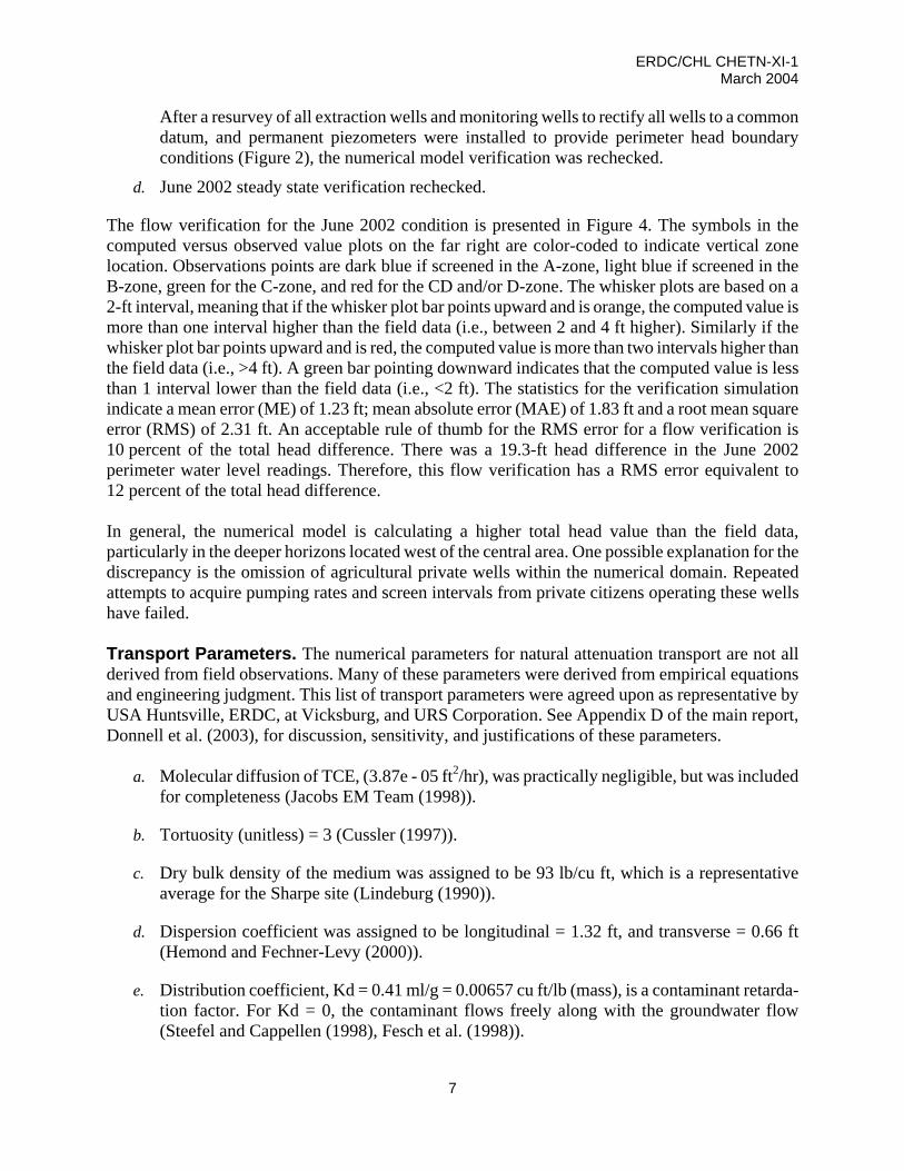
After a resurvey of all extraction wells and monitoring wells to rectify all wells to a common datum, and permanent piezometers were installed to provide perimeter head boundary conditions (Figure 2), the numerical model verification was rechecked.

d. June 2002 steady state verification rechecked.

The flow verification for the June 2002 condition is presented in Figure 4. The symbols in the computed versus observed value plots on the far right are color-coded to indicate vertical zone location. Observations points are dark blue if screened in the A-zone, light blue if screened in the B-zone, green for the C-zone, and red for the CD and/or D-zone. The whisker plots are based on a 2-ft interval, meaning that if the whisker plot bar points upward and is orange, the computed value is more than one interval higher than the field data (i.e., between 2 and 4 ft higher). Similarly if the whisker plot bar points upward and is red, the computed value is more than two intervals higher than the field data (i.e., >4 ft). A green bar pointing downward indicates that the computed value is less than 1 interval lower than the field data (i.e., <2 ft). The statistics for the verification simulation indicate a mean error (ME) of 1.23 ft; mean absolute error (MAE) of 1.83 ft and a root mean square error (RMS) of 2.31 ft. An acceptable rule of thumb for the RMS error for a flow verification is 10 percent of the total head difference. There was a 19.3-ft head difference in the June 2002 perimeter water level readings. Therefore, this flow verification has a RMS error equivalent to 12 percent of the total head difference. In general, the numerical model is calculating a higher total head value than the field data, particularly in the deeper horizons located west of the central area. One possible explanation for the discrepancy is the omission of agricultural private wells within the numerical domain. Repeated attempts to acquire pumping rates and screen intervals from private citizens operating these wells have failed. Transport Parameters. The numerical parameters for natural attenuation transport are not all derived from field observations. Many of these parameters were derived from empirical equations and engineering judgment. This list of transport parameters were agreed upon as representative by USA Huntsville, ERDC, at Vicksburg, and URS Corporation. See Appendix D of the main report, Donnell et al. (2003), for discussion, sensitivity, and justifications of these parameters.

a. Molecular diffusion of TCE, (3.87e - 05 ft2/hr), was practically negligible, but was included for completeness (Jacobs EM Team (1998)).

b. Tortuosity (unitless) = 3 (Cussler (1997)).

c. Dry bulk density of the medium was assigned to be 93 lb/cu ft, which is a representative average for the Sharpe site (Lindeburg (1990)).

d. Dispersion coefficient was assigned to be longitudinal = 1.32 ft, and transverse = 0.66 ft (Hemond and Fechner-Levy (2000)).

e. Distribution coefficient, Kd = 0.41 ml/g = 0.00657 cu ft/lb (mass), is a contaminant retarda-tion factor. For Kd = 0, the contaminant flows freely along with the groundwater flow (Steefel and Cappellen (1998), Fesch et al. (1998)).

7


Figure 4. FEMWATER flow verification. Total head contours and GMS statistical analysis of ground-water level model results versus all monitoring locations for the 10-12 June 2002 verification synoptic data set

f. Radioactive decay constant (1/time) was zero.

g. First-order biodegradation rate through dissolved phase (9.51e - 5/day = 3.962e - 06/hr) was assigned.1

h. Ratio of effective to total porosity (unit less) = 0.476 (effective porosity = 0.21, total porosity = 0.441).1

Natural Attenuation TCE Transport Verification. The FEMWATER transport verification consisted of a 3-year transport simulation (3Q-1999 to 3Q-2002), using the natural attenuation parameters previously described. The TCE concentration initial condition were representative of the 3Q-1999 data set. The FEMWATER steady state flow field used for this simulation were representative of boundary heads, percolation basins, and pumping events from the 1998 period.

1 Personal communication, 29 January 1993, T. Cudzilo and M. Thomas, URS Corporation, Sacramento, CA.

8


Figure 5a shows a plan view of the initial condition representative of 3Q-1999. The maximum TCE concentration found within the designated vertical elevation equivalent to the A, B, C, and D-zones (-220 < Z < 0 ft) is plotted. The TCE concentration initial condition was difficult to construct and is an important aspect of any transport simulation. The difficulty comes when interpreting the sparse monitoring field data concentration values onto the mesh nodal values to obtain an initial con-centration. With few exceptions, the observed values at the extraction wells were less than the observed values of nearby monitoring wells, for the same zones. For instance, compare MW437C and EWCC1, which are only a few feet apart and are screened in the same zone. The most recent historical field TCE concentration measurements for MW437C are: 650 parts per billion (ppb) for 1Q-02, 300 ppb for 3Q-01, 130 ppb for 3Q-00, and 360 ppb for 3Q-99. In contrast, extraction well EWCC1, had TCE concentration observations between 12 and 67 ppb for the same analysis period. Perhaps this is from dilution occurring within the pump screen. This highlights two points: the initial condition for the simulation is an estimate derived from interpolation techniques, and the concen-tration field observation at extractions wells may be misleading.

a. TCE maximum concentration distri-

bution in all zones representing initial condition for 3Q-1999

b. TCE maximum concentration distri-bution in all zones predicted by a 3-year model verification 1999-2002

c. TCE maximum concentration distri-bution in all zones. Projected result from 3Q-02 representative field samples using EarthvisionTM

Figure 5. Visual comparison of 3-year transport verification results with field measurements

At the end of the third year of the transport simulation, model results are compared with field obser-vations. One method of comparing the FEMWATER 3-year transport verification is a visual com-parison of concentration contours. The 3-D solution files from the natural attenuation 3-year transport simulation were analyzed to compute the maximum TCE concentration found within the designated vertical elevation equivalent to the A, B, C, and D zones (-220 < Z < 0 ft). These maximums were then projected onto a 2-D plane. A side by side comparison of model versus field data is now permissible.

9


Figure 5b shows the model results as compared with the EarthvisionTM interpretation of field samples collected in 2002 (Figure 5c). Since the monitoring rotation cycle at the site does not collect data at every monitoring well every quarter, it should be noted that data used to create Figure 5c is not always data collected in 3Q-2002, but is the most recent field data available at a given location. Figure 5c was provided by URS Corp. In general, the 5 ppb cleanup level contour is smaller for the model results than the field sample contours created by EarthvisionTM. The highest concentration for the field data for 2002 is in the central zone, as shown in Figure 5c. This corresponds to 650 ppb, the field representation used for MW437C. Since the numerical model had assumed zero TCE sources, it is impossible for the model to predict a value higher than what can be supplied by the initial condition of 3Q-99. The transport simulation should continue to show a decrease in concentration due the attenuation and from extraction by active pumping. The GMS interface, Groundwater Modeling Team (2004), provides a statistical means of comparing model results at the end of the third year of the transport simulation with field observations. Observations were made for all available monitoring stations representing the 3Q-2002 data set. As shown in Figure 6, the RMS error is 22.83 ppb for the verification. The symbols in the computed versus observed value plots on the far right are color-coded to indicate vertical zone. All extraction wells are colored black, while monitoring locations are dark blue if located in the A-zone, light blue if located in the B-zone, green for the C-zone, and red for the CD and/or D-zone. The largest discrepancy is at the extraction wells themselves. Long-Term Natural Attenuation TCE Transport. Long-term FEMWATER transport simu-lations were conducted using the steady state flow simulations representative of the June 2002 conditions. The numerical model was run starting with an initial condition of TCE concentration derived from field data quarterly monitoring (3Q-2002) and predicted plume behavior for decades into the future. The natural attenuation parameters previously described were used to predict plume behavior for each scenario. Two scenarios will be compared. The first scenario is named “No-Pumping,” meaning that none of the DDJC-Sharpe extraction wells are pumping. Second is a scenario named “Shutdown 9-Add 1,” meaning that nine extraction wells are removed from the June 2002 DDJC-Sharpe pumping array and one additional well in the west central zone is added. Figure 7a shows the location of the pumping array as it existed in June 2002. Note, however, that for this simulation, all of these extraction wells are inactive, as indicated by the red X, for the no-pumping condition. Figure 7b depicts the active extraction wells with blue triangles, the inactive or “shutdown” wells with a red X, and the additional extraction C-zone well is circled. The pump rate for the new C-zone well was chosen to be 66 gpm. Scenario Comparisons. Both the flow and transport aspects of the two scenarios will be compared. Flow comparisons. First the FEMWATER numerical model was run to a steady state in flow-only mode. Figure 8 compares the results from the two flow scenarios. Figure 8 displays the linear total head contours with constant length velocity vectors for the A, B, C, and D zones. Vectors are

10


Figure 6. FEMWATER transport verification. Computed versus observation data of TCE 3-year transport (3Q-99 to 3Q-02) using natural attenuation parameters

plotted for every 20th computational point for purposes of readability. As depicted by the alteration of the groundwater contours, the active pumping wells are drawing down the groundwater levels on the site. Transport comparisons. The steady state flow results were assumed to represent future hydrologic conditions and were used as input for the long-term transport simulations. The 3-D solution files from the natural attenuation transport scenarios were analyzed to compute the maximum TCE concentration found within a designated vertical elevation comprising the zones of interest, and project those results onto a 2-D plane. Maximum TCE concentration in A-zone. For each (x,y) location, the maximum concentration found within the A-zone, -28 < Z < 0 ft is plotted. Figure 9a and 9b compare the two scenarios after year 10 of the simulation. The pumping scenario is quickly diminishing the north (also called north balloon) TCE plume in the A-zone. Figure 9c and 9d compare the two scenarios after year 20 of the simulation. Figure 9e and 9f compare the two scenarios after year 30 of the simulation. The pumping scenario is eliminating the higher zones of concentration and decreasing the overall plume size.

11


a. No pumping scenario b. Shutdown 9 – Add 1, pumping scenario Figure 7. Extraction well locations for the “Shutdown 9 – Add 1” and the “No Pumping” scenario

The arrow points to the same location for each of these plots, allowing for a quick comparison. For the “no pumping” scenario the concentration decreases from 14 ppb at year 10 to 12.3 ppb at year 20, to 11.6 ppb at year 30. In comparison of this same point, the pumping scenario has a decrease of concentration from 14.2 ppb at year 10 to 11.6 ppb at year 20, and 8.9 ppb at year 30.

12


a. No pumping scenario b. Shutdown 9 – Add 1, pumping scenario

Figure 8. Total head contour and constant length velocity vector scenario comparisons from FEMWATER steady state flow results

Maximum TCE concentration in B-zone. For each (x,y) location, the maximum concentration found within the B-zone, -70 < Z < -28 ft is plotted. Figure 10a and 10b compare the two scenarios after year 10 of the simulation. The pumping scenario is quickly diminishing the north and south (also called south balloon) TCE plume in the B-zone. Figure 10c and 10d compare the two scenarios after year 20 of the simulation. Figure 10e and 10f compare the two scenarios after year 30 of the simulation. By year 20, the B-zone central plume for the “no pumping” scenario is traveling off the Sharpe site to the northwest, but the pumping scenario does not allow the plume to escape and is continuing to eliminate the higher zones of concentration and is decreasing the overall plume size. Again the arrow allows for a quick comparison at one location. For the “no pumping” scenario the concentration decreases from 27.4 ppb at year 10 to 25.4 ppb at year 20, to 21.7 ppb at year 30. In comparison of this same point, the pumping scenario has a decrease of concentration from 23.3 ppb at year 10 to 17.1 ppb at year 20, and 12.5 ppb at year 30.

13


a. No pumping scenario, A year = 10 b. Shutdown 9 – Add 1 scenario, A year = 10

c. No pumping scenario, A year = 20 d. Shutdown 9 – Add 1 scenario, A year = 20

Figure 9. Maximum TCE found in vertical (-28 < Z < 0 ft), corresponding to the A-zone, for year 10, 20, and 30 of the natural attenuation TCE transport simulation (Continued)

14


e. No pumping scenario, A year = 30 f. Shutdown 9 – Add 1 scenario, A year = 30

Figure 9. (Concluded)

a. No pumping scenario, B year = 10 b. Shutdown 9 – Add 1 scenario, B year = 10

Figure 10. Maximum TCE found in vertical (-70 < Z < -28 ft), corresponding to the B-zone, for year 10, 20, and 30 of the natural attenuation TCE transport simulation (Continued)

15


c. No pumping scenario, B year = 20 d. Shutdown 9 – Add 1 scenario, B year = 20

e. No pumping scenario, B year = 30 f. Shutdown 9 – Add 1 scenario, B year = 30


16


Maximum TCE concentration in C-zone. For each (x,y) location, the maximum concentration found within the B-zone, -140 < Z < -70 ft is plotted. Figure 11a and 11b compare the two scenarios after year 10 of the simulation. Figure 11c and 11d compare the two scenarios after year 20 of the simulation. Figure 11e and 11f compare the two scenarios after year 30 of the simulation. By year 10 of the no pumping simulation, the C-zone north and central plume have traveled off the Sharpe site to the northwest, but the pumping scenario is not allowing the plume to escape and is continuing to decrease the overall plume size.

Again the arrow allows for a quick comparison at one location. For the “no pumping” scenario the concentration decreases from 61.9 ppb at year 10 to 18.9 ppb at year 20, to 9.8 ppb at year 30. In comparison of this same point, the pumping scenario has a decrease of concentration from 31.0 ppb at year 10 to 17.4 ppb at year 20, and 10.3 ppb at year 30.

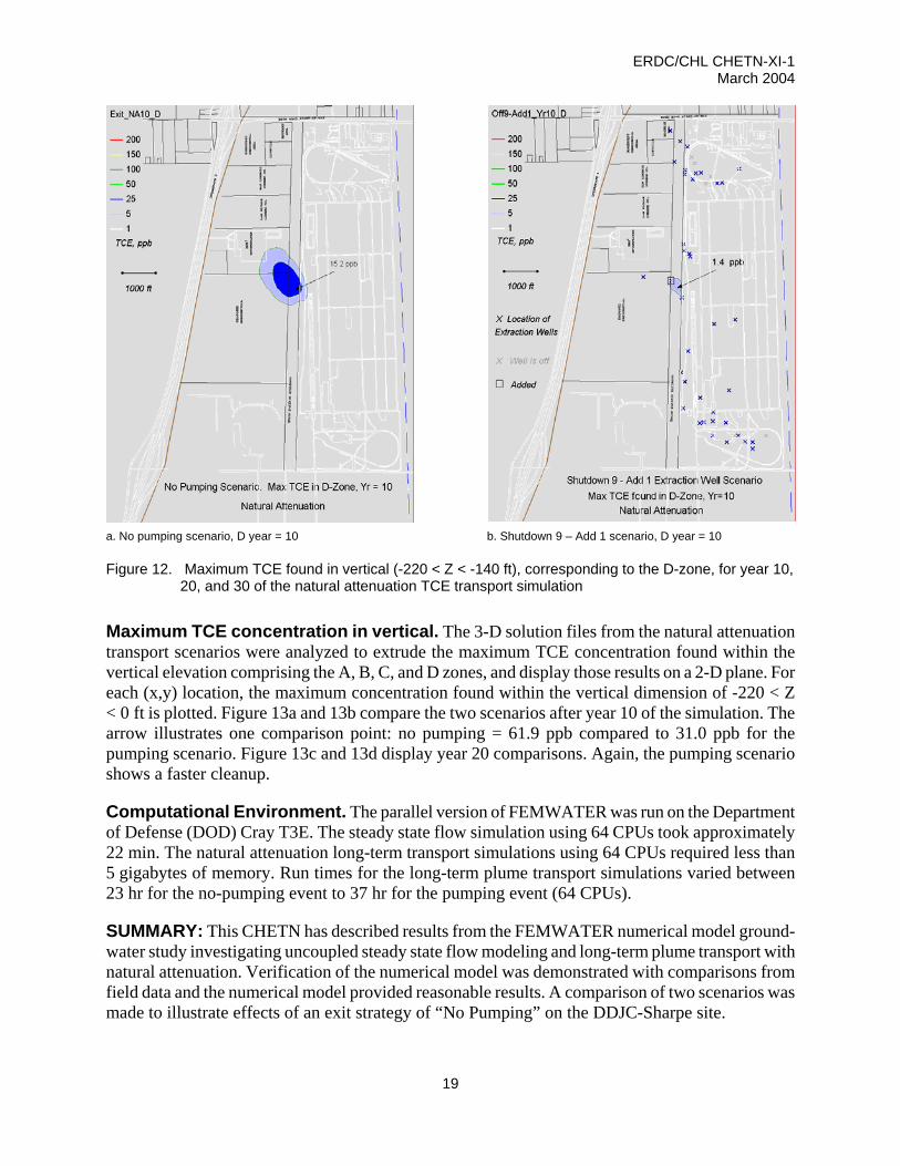
Maximum TCE concentration in D-zone. For each (x,y) location, the maximum concentration found within the D-zone, -220 < Z < -140 ft is plotted. Figure 12a and 12b compare the two scenarios after year 10 of the simulation.

a. No pumping scenario, C year = 10 b. Shutdown 9 – Add 1 scenario, C year = 10

Figure 11. Maximum TCE found in vertical (-140 < Z < -70 ft), corresponding to the C-zone, for year 10, 20, and 30 of the natural attenuation TCE transport simulation (Continued)

17


c. No pumping scenario, C year = 20 d. Shutdown 9 – Add 1 scenario, C year = 20

e. No pumping scenario, C year = 30 f. Shutdown 9 – Add 1 scenario, C year = 30


18


a. No pumping scenario, D year = 10 b. Shutdown 9 – Add 1 scenario, D year = 10

Figure 12. Maximum TCE found in vertical (-220 < Z < -140 ft), corresponding to the D-zone, for year 10, 20, and 30 of the natural attenuation TCE transport simulation

Maximum TCE concentration in vertical. The 3-D solution files from the natural attenuation transport scenarios were analyzed to extrude the maximum TCE concentration found within the vertical elevation comprising the A, B, C, and D zones, and display those results on a 2-D plane. For each (x,y) location, the maximum concentration found within the vertical dimension of -220 < Z < 0 ft is plotted. Figure 13a and 13b compare the two scenarios after year 10 of the simulation. The arrow illustrates one comparison point: no pumping = 61.9 ppb compared to 31.0 ppb for the pumping scenario. Figure 13c and 13d display year 20 comparisons. Again, the pumping scenario shows a faster cleanup.

Computational Environment. The parallel version of FEMWATER was run on the Department of Defense (DOD) Cray T3E. The steady state flow simulation using 64 CPUs took approximately 22 min. The natural attenuation long-term transport simulations using 64 CPUs required less than 5 gigabytes of memory. Run times for the long-term plume transport simulations varied between 23 hr for the no-pumping event to 37 hr for the pumping event (64 CPUs).

SUMMARY: This CHETN has described results from the FEMWATER numerical model ground-water study investigating uncoupled steady state flow modeling and long-term plume transport with natural attenuation. Verification of the numerical model was demonstrated with comparisons from field data and the numerical model provided reasonable results. A comparison of two scenarios was made to illustrate effects of an exit strategy of “No Pumping” on the DDJC-Sharpe site.

19


a. No pumping scenario, year = 10 b. Shutdown 9 – Add 1 scenario, year = 10

c. No pumping scenario, year = 20 d. Shutdown 9 – Add 1 scenario, year = 20

Figure 13. Long-term natural attenuation transport results comparing the two scenarios. For each (x,y) location, the maximum concentration found in the vertical (-220 < Z < 0 ft) is plotted

20


CONCLUSION: From the analysis made in this CHETN, the numerical model has predicted that the proposed pump and treat system (shutdown 9 existing extraction wells and add 1 extraction well) is a far better alternative for TCE plume management than turning off the extraction system.

POINT OF CONTACT: For additional information, contact Ms. Barbara Donnell (Voice: (601) 634-2730, e-mail: [email protected]).

REFERENCES

Cussler, E. L. (1997). Diffusion – Mass transfer in fluid systems. 2nd ed., Cambridge University Press, 580 pp.

Donnell, B. P., Richards, D. R., Edris, E. V., McGehee, T. L., and May, J. H. (2003). “Development of a comprehensive groundwater model of the Defense Distribution Depot, San Joaquin (DDJC) Sharpe Site, Lathrop, California,” U.S. Army Engineer Research and Development Center, Vicksburg, MS.

Engineering Technologies Associates. (1992). “Remedial well-field design using three-dimensional ground water flow and transport modeling, DDRW-Sharpe, Lathrop, California,” Engineering Technologies Associates, Inc., Ellicott City, MD.

Fesch, C., Simon, W., Haderlein, S. B., Reichert, P., and Schwarzenbach, R. P. (1998). “Nonlinear sorption and nonequilibrim solute transport in aggregated porous media: Experiment, process identification and modeling,” Journal of Contaminant Hydrology 31, 373-407.

Groundwater Modeling Team. (2004). GMS, http://chl.erdc.usace.army.mil/software/gms/, U.S. Army Engineer Research and Development Center, Vicksburg, MS.

Hemond, H. F., and Fechner-Levy, E. J. (2000), Chemical fate and transport in the environment. 2nd ed., Academic Press, 433 pp.

Jacobs EM Team. (1998). Hydraulic containment and contaminant transport evaluation for the northeast plume at the Paducah Gaseous Diffusion Plant, Paducah, Kentucky. Jacobs Environmental Management, Kevil, KY.

Lin, H. J., Richards, D. R., Yeh, J., Cheng J., Cheng, H., and Jones, N. L. (1997). “FEMWATER: A three-dimensional finite element computer model for simulating density dependent flow and transport, TR CHL-97-12, U.S. Army Engineer Waterways Experiment Station, Vicksburg, MS.

Lindeburg, M. R. (1990). Civil engineering reference manual, 7th ed., Professional Publications, Inc., Belmont, CA., 9-11.

Steefel, C. I., and Cappellen, P. V. (1998). “Reactive transport modeling of natural systems,” Journal of Hydrology 209, 1-7.

NOTE: The contents of this technical note are not to be used for advertising, publication, or promotional purposes. Citation of trade names does not constitute an official endorsement or

approval of the use of such products.

21

ddjc-sharpe defense distribution depot: femwater … · ddjc-sharpe defense distribution depot:...

Documents