DATA STRUCTERS WITH C 10CS35

Eduoncloud.com Page 1

DATA STRUCTURES WITH C

(Common to CSE & ISE)

Subject Code: 10CS35 I.A. Marks : 25

Hours/Week : 04 Exam Hours: 03

Total Hours : 52 Exam Marks: 100

PART – A UNIT - 1 8 Hours BASIC CONCEPTS: Pointers and Dynamic Memory Allocation, Algorithm Specification, Data

Abstraction, Performance Analysis, Performance Measurement

UNIT -2 6 Hours ARRAYS and STRUCTURES: Arrays, Dynamically Allocated Arrays, Structures and Unions,

Polynomials, sparse Matrices, Representation of Multidimensional Arrays

UNIT - 3 6 Hours STACKS AND QUEUES: Stacks, Stacks Using Dynamic Arrays, Queues, Circular Queues Using

Dynamic Arrays, Evaluation of Expressions, Multiple Stacks and Queues.

UNIT - 4 6 Hours LINKED LISTS: Singly Linked lists and Chains, Representing Chains in C, Linked Stacks and Queues,

Polynomials, Additional List operations, Sparse Matrices, Doubly Linked Lists

UNIT - 5 6 Hours

PART - B

TREES – 1: Introduction, Binary Trees, Binary Tree Traversals, Threaded Binary Trees, Heaps.

UNIT – 6 6 Hours TREES – 2, GRAPHS: Binary Search Trees, Selection Trees, Forests, Representation of Disjoint Sets,

Counting Binary Trees, The Graph Abstract Data Type.

UNIT - 7 6 Hours PRIORITY QUEUES Single- and Double-Ended Priority Queues, Leftist Trees, Binomial Heaps,

Fibonacci Heaps, Pairing Heaps.

UNIT - 8 8 Hours EFFICIENT BINARY SEARCH TREES: Optimal Binary Search Trees, AVL Trees, Red-Black Trees,

Splay Trees.

Text Book:

1. Horowitz, Sahni, Anderson-Freed: Fundamentals of Data Structures in C, 2nd Edition, Universities Press, 2007.

(Chapters 1, 2.1 to 2.6, 3, 4, 5.1 to 5.3, 5.5 to 5.11, 6.1, 9.1 to 9.5, 10)

Reference Books:

1. Yedidyah, Augenstein, Tannenbaum: Data Structures Using C and C++, 2nd Edition, Pearson Education, 2003.

2. Debasis Samanta: Classic Data Structures, 2nd Edition, PHI, 2009.

3. Richard F. Gilberg and Behrouz A. Forouzan: Data Structures A Pseudocode Approach with C, Cengage

Learning, 2005.

4. Robert Kruse & Bruce Leung: Data Structures & Program Design in C, Pearson Education, 2007.

DATA STRUCTERS WITH C 10CS35

Eduoncloud.com Page 2

TABLE OF CONTENTS

TABLE OF CONTENTS .............................................................................................................................. 1

UNIT – 1: BASIC CONCEPTS .................................................................................................................... 4

1.1-Pointers and Dynamic Memory Allocation ......................................................................................... 4

1.2. Algorithm Specification ..................................................................................................................... 8

1.3. Data Abstraction ................................................................................................................................. 9

1.4. Performance Analysis ...................................................................................................................... 10

1.5. Performance Measurement ............................................................................................................... 11

1.6 RECOMMENDED QUESTIONS .......................................................................................................... 13

DATA STRUCTERS WITH C 10CS35

Eduoncloud.com Page 3

UNIT – 1: BASIC CONCEPTS

1.1-Pointers and Dynamic Memory Allocation:

In computer science, a pointer is a programming language data type whose value refers directly to (or

"points to") another value stored elsewhere in the computer memory using its address. For high-level

programming languages, pointers effectively take the place of general purpose registers in low-level

languages such as assembly language or machine code, but may be in available memory. A pointer

references a location in memory, and obtaining the value at the location a pointer refers to is known as

dereferencing the pointer. A pointer is a simple, more concrete implementation of the more abstract

reference data type. Several languages support some type of pointer, although some have more restrictions

on their use than others.

Pointers to data significantly improve performance for repetitive operations such as traversing strings,

lookup tables, control tables and tree structures. In particular, it is often much cheaper in time and space

to copy and dereference pointers than it is to copy and access the data to which the pointers point.Pointers

are also used to hold the addresses of entry points for called subroutines in procedural programming and

for run-time linking to dynamic link libraries (DLLs). In object-oriented programming, pointers to functions

are used for binding methods, often using what are called virtual method tables.

Declaring a pointer variable is quite similar to declaring an normal variable all you have to do is to insert

a star '*' operator before it.

General form of pointer declaration is -

type* name;

where type represent the type to which pointer thinks it is pointing to.

Pointers to machine defined as well as user-defined types can be made

Pointer Intialization: variable_type *pointer_name = 0;

or

variable_type *pointer_name = NULL;

char *pointer_name = "string value here";

The operator that gets the value from pointer variable is * (indirection operator). This is called the

reference to pointer.

P=&a

So the pointer p has address of a and the value that that contained in that address can be accessed by : *p

So the operations done over it can be explained as below:

a++;

a=a+1;

*p=*p+1;

DATA STRUCTERS WITH C 10CS35

DEPT OF ISE, SJBIT Page 14

UNIT -2 : ARRAYS and STRUCTURES

2.1 ARRAY:

Definition :Array by definition is a variable that hold multiple elements which has the same data type.

Declaring Arrays :

We can declare an array by specify its data type, name and the number of elements the array holds

between square brackets immediately following the array name. Here is the syntax:

1 data_type array_name[size];

For example, to declare an integer array which contains 100 elements we can do as follows:

1 int a[100];

There are some rules on array declaration. The data type can be any valid C data types including structure

and union. The array name has to follow the rule of variable and the size of array has to be a positive

constant integer.We can access array elements via indexes array_name[index]. Indexes of array starts

from 0 not 1 so the highest elements of an array is array_name[size-1]

Initializing Arrays :

It is like a variable, an array can be initialized. To initialize an array, you provide initializing values which

are enclosed within curly braces in the declaration and placed following an equals sign after the array

name. Here is an example of initializing an integer array.

int list[5] = {2,1,3,7,8};

Array Representation

Operations require simple implementations.

Insert, delete, and search, require linear time

Inefficient use of space

It is appropriate that we begin our study of data structures with the array. The array is often the only

means for structuring data which is provided in a programming language. Therefore it deserves a

significant amount of attention. If one asks a group of programmers to define an array, the most often

quoted saying is: a consecutive set of memory locations. This is unfortunate because it clearly reveals a

common point of confusion, namely the distinction between a data structure and its representation. It is

true that arrays are almost always implemented by using consecutive memory, but not always.

Intuitively, an array is a set of pairs, index and value. For each index which is defined, there is a value

DATA STRUCTERS WITH C 10CS35

DEPT OF ISE, SJBIT Page 15

associated with that index. In mathematical terms we call this a correspondence or a mapping. However,

as computer scientists we want to provide a more functional definition by giving the operations which

are permitted on this data structure. For arrays this means we are concerned with only two operations

which retrieve and store values. Using our notation this object can be defined as:

structure ARRAY(value, index)

declare CREATE( ) array

RETRIEVE(array,index) value

STORE(array,index,value) array;

for all A array, i,j index, x value let

RETRIEVE(CREATE,i) :: = error

RETRIEVE(STORE(A,i,x),j) :: =

if EQUAL(i,j) then x else RETRIEVE(A,j)

end

end ARRAY

The function CREATE produces a new, empty array. RETRIEVE takes as input an array and an index,

and either returns the appropriate value or an error. STORE is used to enter new index-value pairs. The

second axiom is read as "to retrieve the j-th item where x has already been stored at index i in A is

equivalent to checking if i and j are equal and if so, x, or search for the j-th value in the remaining array,

A." This axiom was originally given by J. McCarthy. Notice how the axioms are independent of any

representation scheme. Also, i and j need not necessarily be integers, but we assume only that an

EQUAL function can be devised.

If we restrict the index values to be integers, then assuming a conventional random access memory we can implement STORE and RETRIEVE so that they operate in a constant amount of time. If we interpret

the indices to be n-dimensional, (i1,i2, ...,in), then the previous axioms apply immediately and define n- dimensional arrays. In section 2.4 we will examine how to implement RETRIEVE and STORE for multi-

dimensional arrays using consecutive memory locations.

Array and Pointer:

Each array element occupies consecutive memory locations and array name is a pointer that points to the

first element. Beside accessing array via index we can use pointer to manipulate array. This program

helps you visualize the memory address each array elements and how to access array element using

pointer.

01 #include <stdio.h>

02

03 void main()

04 {

05

06 const int size = 5;

DATA STRUCTERS WITH C 10CS35

DEPT OF ISE, SJBIT Page 16

07

08 int list[size] = {2,1,3,7,8};

09

10 int* plist = list;

11

12 // print memory address of array elements

13 for(int i = 0; i < size;i++)

14 {

15 printf("list[%d] is in %d\n",i,&list[i]);

16

17 }

18

19 // accessing array elements using pointer

20 for(i = 0; i < size;i++)

21 {

22 printf("list[%d] = %d\n",i,*plist);

23

24 /* increase memory address of pointer so it go to the next

25 element of the array */

26 plist++;

27 }

28

29 }

Here is the output

DATA STRUCTERS WITH C 10CS35

DEPT OF ISE, SJBIT Page 17

list[0] is in 1310568

list[1] is in 1310572

list[2] is in 1310576

list[3] is in 1310580

list[4] is in 1310584

list[0] = 2

list[1] = 1

list[2] = 3

list[3] = 7

list[4] = 8

You can store pointers in an array and in this case we have an array of pointers. This code snippet uses an

array to store integer pointer.

1 int *ap[10];

Multidimensional Arrays:

An array with more than one index value is called a multidimensional array. The entire array above is

called single-dimensional array. To declare a multidimensional array you can do follow syntax

1 data_type array_name[][][];

The number of square brackets specifies the dimension of the array. For example to declare two

dimensions integer array we can do as follows:

1 int matrix[3][3];

Initializing Multidimensional Arrays :

You can initialize an array as a single-dimension array. Here is an example of initialize an two

dimensions integer array:

1 int matrix[3][3] =

2 {

3 {11,12,13},

4 {21,22,23},

5 {32,31,33},

6 };

Dynamically Allocated Arrays: One-Dimensional Arrays

In C, arrays must have their extents defined at compile-time. There's no way to postpone the definition of

the size of an array until runtime. Luckily, with pointers and malloc, we can work around this limitation.

DATA STRUCTERS WITH C 10CS35

DEPT OF ISE, SJBIT Page 18

To allocate a one-dimensional array of length N of some particular type, simply use malloc to allocate

enough memory to hold N elements of the particular type, and then use the resulting pointer as if it were

an array. For example, the following code snippet allocates a block of N ints, and then, using array

notation, fills it with the values 0 through N-1:

int *A = malloc (sizeof (int) * N);

int i;

for (i = 0; i < N; i++)

A[i] = i;

This idea is very useful for dealing with strings, which in C are represented by arrays of chars, terminated

with a '\0' character. These arrays are nearly always expressed as pointers in the declaration of functions,

but accessed via C's array notation. For example, here is a function that implements strlen:

int strlen (char *s)

{

int i;

for (i = 0; s[i] != '\0'; i++)

;

return (i)

}

2.2. Dynamically Allocating Multidimensional Arrays

We've seen that it's straightforward to call malloc to allocate a block of memory which can simulate an

array, but with a size which we get to pick at run-time. Can we do the same sort of thing to simulate

multidimensional arrays? We can, but we'll end up using pointers to pointers. If we don't know how many

columns the array will have, we'll clearly allocate memory for each row (as many columns wide as we

like) by calling malloc, and each row will therefore be represented by a pointer. How will we keep track

of those pointers? There are, after all, many of them, one for each row. So we want to simulate an array of

pointers, but we don't know how many rows there will be, either, so we'll have to simulate that array (of

pointers) with another pointer, and this will be a pointer to a pointer.

This is best illustrated with an example:

#include <stdlib.h>

int **array;

array = malloc(nrows * sizeof(int *));

DATA STRUCTERS WITH C 10CS35

DEPT OF ISE, SJBIT Page 19

if(array == NULL)

{

fprintf(stderr, "out of memory\n");

exit or return

}

for(i = 0; i < nrows; i++)

{

array[i] = malloc(ncolumns * sizeof(int));

if(array[i] == NULL)

{

fprintf(stderr, "out of memory\n");

exit or return

}

}

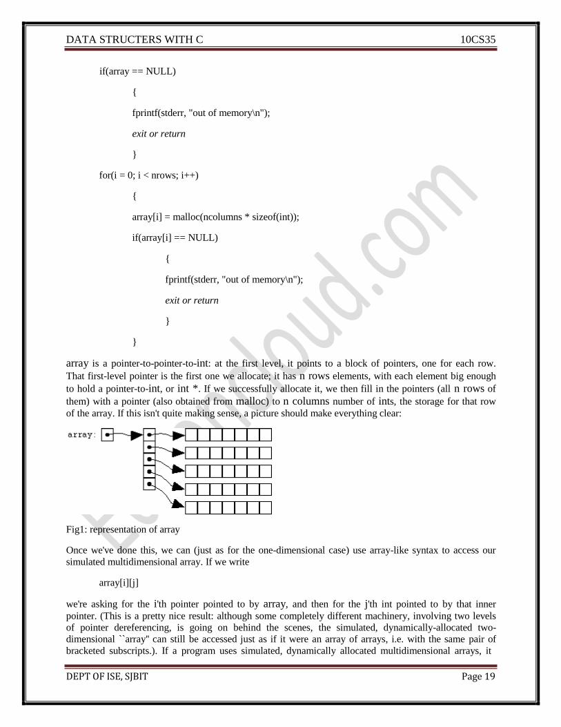
array is a pointer-to-pointer-to-int: at the first level, it points to a block of pointers, one for each row.

That first-level pointer is the first one we allocate; it has n rows elements, with each element big enough

to hold a pointer-to-int, or int *. If we successfully allocate it, we then fill in the pointers (all n rows of

them) with a pointer (also obtained from malloc) to n columns number of ints, the storage for that row

of the array. If this isn't quite making sense, a picture should make everything clear:

Fig1: representation of array

Once we've done this, we can (just as for the one-dimensional case) use array-like syntax to access our

simulated multidimensional array. If we write

array[i][j]

we're asking for the i'th pointer pointed to by array, and then for the j'th int pointed to by that inner

pointer. (This is a pretty nice result: although some completely different machinery, involving two levels

of pointer dereferencing, is going on behind the scenes, the simulated, dynamically-allocated two-

dimensional ``array'' can still be accessed just as if it were an array of arrays, i.e. with the same pair of

bracketed subscripts.). If a program uses simulated, dynamically allocated multidimensional arrays, it

DEPT OF ISE, SJBIT Page 20

becomes possible to write ``heterogeneous'' functions which don't have to know (at compile time) how

big the ``arrays'' are. In other words, one function can operate on ``arrays'' of various sizes and shapes.

The function will look something like

func2(int **array, int nrows, int ncolumns)

{

}

This function does accept a pointer-to-pointer-to-int, on the assumption that we'll only be calling it with

simulated, dynamically allocated multidimensional arrays. (We must not call this function on arrays like

the ``true'' multidimensional array a2 of the previous sections). The function also accepts the dimensions

of the arrays as parameters, so that it will know how many ``rows'' and ``columns'' there are, so that it can

iterate over them correctly. Here is a function which zeros out a pointer-to-pointer, two-dimensional

``array'':

void zeroit(int **array, int nrows, int ncolumns)

{

int i, j;

for(i = 0; i < nrows; i++)

{

for(j = 0; j < ncolumns; j++)

array[i][j] = 0;

}

}

Finally, when it comes time to free one of these dynamically allocated multidimensional ``arrays,'' we

must remember to free each of the chunks of memory that we've allocated. (Just freeing the top-level

pointer, array, wouldn't cut it; if we did, all the second-level pointers would be lost but not freed, and

would waste memory.) Here's what the code might look like:

for(i = 0; i < nrows; i++)

free(array[i]);

free(array);

2.3. Structures and Unions:

Structure:

A structure is a user-defined data type. You have the ability to define a new type of data considerably

more complex than the types we have been using. A structure is a collection of one or more variables,

possibly of different types, grouped together under a single name for convenient handling. Structures are

called ―records‖ in some languages, notably Pascal. Structures help organize complicated data,

DEPT OF ISE, SJBIT Page 21

particularly in large programs, because they permit a group of related variables to be treated as a unit

instead of as separate entities.

Today‘s application requires complex data structures to support them. A structure is a collection

of related elements where element belongs to a different type. Another way to look at a structure is a

template – a pattern. For example graphical user interface found in a window requires structures typical

example for the use of structures could be the file table which holds the key data like logical file name,

location of the file on disc and so on. The file table in C is a type defined structure - FILE. Each element

of a structure is also called as field. A field has a many characteristic similar to that of a normal variable.

An array and a structure are slightly different. The former has a collection of homogeneous elements but

the latter has a collection of heterogeneous elements. The general format for a structure in C is shown

struct {field_list} variable_identifier;

struct struct_name

{

type1 fieldname1;

type2 fieldname2;

.

.

.

typeN fieldnameN;

};

struct struct_name variables;

The above format shown is not concrete and can vary, so different `

flavours of structure declaration is as shown.

struct

{

….

} variable_identifer;

Example

struct mob_equip;

{

long int IMEI;

char rel_date[10];

DEPT OF ISE, SJBIT Page 22

char model[10];

char brand[15];

};

The above example can be upgraded with typedef. A program to illustrate the

working of the structure is shown in the previous section.

typedef struct mob_equip;

{

long int IMEI;

char rel_date[10];

char model[10];

char brand[15];

int count;

} MOB; MOB m1;

struct tag

{

…….

};

struct tag variable_identifers;

typedef struct

{

……..

} TYPE_IDENITIFIER;

TYPE_IDENTIFIER variable_identifers;

Accessing a structure

A structure variable or a tag name of a structure can be used to access the members of a structure with the

help of a special operator ‗.‘ –also called as member operator . In our previous example To access the idea

of the IMEI of the mobile equipment in the structure mob_equip is done like this Since the structure

variable can be treated as a normal variable All the IO functions for a normal variable holds good for the

structure variable also with slight. The scanf statement to read the input to the IMEI is given below

scanf (“%d”,&m1.IMEI);

DEPT OF ISE, SJBIT Page 23

Increment and decrement operation are same as the normal variables this includes postfix and prefix also.

Member operator has more precedence than the increment or decrement. Say suppose in example quoted

earlier we want count of student then

m1.count++; ++m1.count

Unions

Unions are very similar to structures, whatever discussed so far holds good for unions also then why do

we need unions? Size of unions depends on the size of its member of largest type or member with largest

size, but this is not son in case of structures.

Example union abc1

{

int a;

float b;

char c;

};

The size of the union abc1 is 4bytes as float is largest type. Therefore at any point of time we can access

only one member of the union and this needs to remembered by programmer.

Using structure data Now that we have assigned values to the six simple variables, we can do anything we desire with them. In

order to keep this first example simple, we will simply print out the values to see if they really do exist as

assigned. If you carefully inspect the printf statements, you will see that there is nothing special about

them. The compound name of each variable is specified because that is the only valid name by which we

can refer to these variables. Structures are a very useful method of grouping data together in order to

make a program easier to write and understand.

2.4 .Polynomials:

In mathematics, a polynomial (from Greek poly, "many" and medieval Latin binomium, "binomial"[1] [2]

[3]) is an expression of finite length constructed from variables (also known as indeterminates) and

constants, using only the operations of addition, subtraction, multiplication, and non-negative integer

exponents. For example, x2

− 4x + 7 is a polynomial, but x2

− 4/x + 7x3/2

is not, because its second term involves division by the variable x (4/x) and because its third term contains an exponent that is not a whole number (3/2). The term "polynomial" can also be used as an adjective, for quantities that can be expressed as a polynomial of some parameter, as in "polynomial time" which is used in computational complexity theory.

Polynomials appear in a wide variety of areas of mathematics and science. For example, they are used to

form polynomial equations, which encode a wide range of problems, from elementary word problems to

complicated problems in the sciences; they are used to define polynomial functions, which appear in

settings ranging from basic chemistry and physics to economics and social science; they are used in

calculus and numerical analysis to approximate other functions. In advanced mathematics, polynomials

are used to construct polynomial rings, a central concept in abstract algebra and algebraic geometry.

DEPT OF ISE, SJBIT Page 24

A polynomial is made up of terms that are only added, subtracted or multiplied.

A polynomial looks like this:

example of a polynomial

this one has 3 terms

Fig 2:

Polynomial comes form poly- (meaning "many") and -nomial (in this case meaning "term") ... so it says

"many terms"

A polynomial can have:

constants (like 3, -20, or ½)

variables (like x and y)

exponents (like the 2 in y2) but only 0, 1, 2, 3, ... etc

That can be combined using:

+ addition,

- subtraction, and

× Multiplication

... but not division!

Those rules keeps polynomials simple, so they are easy to work with!

Polynomial or Not?

DEPT OF ISE, SJBIT Page 25

Fig 3:

These are polynomials:

3x

x - 2

-6y2

- (7/9)x

3xyz + 3xy2z - 0.1xz - 200y + 0.5

512v5+ 99w

5

1

(Yes, even "1" is a polynomial, it has one term which just happens to be a constant).

And these are not polynomials

2/(x+2) is not, because dividing is not allowed

1/x is not

3xy-2

is not, because the exponent is "-2" (exponents can only be 0,1,2,...)

√x is not, because the exponent is "½" (see fractional exponents)

But these are allowed:

x/2 is allowed, because it is also (½)x (the constant is ½, or 0.5)

also 3x/8 for the same reason (the constant is 3/8, or 0.375)

√2 is allowed, because it is a constant (= 1.4142...etc)

Monomial, Binomial, Trinomial

There are special names for polynomials with 1, 2 or 3 terms:

DEPT OF ISE, SJBIT Page 26

How do you remember the names? Think cycles!

Fig 4:(There is also quadrinomial (4 terms) and quintinomial (5 terms),

but those names are not often used)

2.5. Sparse Matrices:

A sparse matrix is a matrix that allows special techniques to take advantage of the large number of zero

elements. This definition helps to define "how many" zeros a matrix needs in order to be "sparse." The

answer is that it depends on what the structure of the matrix is, and what you want to do with it. For

example, a randomly generated sparse matrix with entries scattered randomly throughout the

matrix is not sparse in the sense of Wilkinson.

Next: Advanced Graphics Up: Sparse matrix computations Previous: Sparse matrix computations

Creating a sparse matrix:

If a matrix A is stored in ordinary (dense) format, then the command S = sparse(A) creates a copy of the

matrix stored in sparse format. For example:

>> A = [0 0 1;1 0 2;0 -3 0]

A =

0 0 1

1 0 2

0 -3 0

>> S = sparse(A)

S =

(2,1) 1

(3,2) -3

DEPT OF ISE, SJBIT Page 27

(1,3) 1

(2,3) 2

>> whos

Name Size Bytes Class

A 3x3 72 double array

S 3x3 64 sparse array

Grand total is 13 elements using 136 bytes

Unfortunately, this form of the sparse command is not particularly useful, since if A is large, it can be

very time-consuming to first create it in dense format. The command S = sparse(m,n) creates an zero matrix in sparse format. Entries can then be added one-by-one:

>> A = sparse(3,2)

A =

All zero sparse: 3-by-2

>> A(1,2)=1;

>> A(3,1)=4;

>> A(3,2)=-1;

>> A

A =

(Of course, for this to be truly useful, the nonzeros would be added in a loop.)

Another version of the sparse command is S = sparse(I,J,S,m,n,maxnz). This creates an sparse

matrix with entry (I(k),J(k)) equal to . The optional argument maxnz

causes Matlab to pre-allocate storage for maxnz nonzero entries, which can increase efficiency in the

case when more nonzeros will be added later to S.

The most common type of sparse matrix is a banded matrix, that is, a matrix with a few nonzero

diagonals. Such a matrix can be created with the spdiags command. Consider the following matrix:

>> A

A =

(3,1) 4

(1,2) 1

(3,2) -1

DEPT OF ISE, SJBIT Page 28

64 -16 0 -16 0 0 0 0 0

-16 64 -16 0 -16 0 0 0 0

0 -16 64 0 0 -16 0 0 0

-16 0 0 64 -16 0 -16 0 0

0 -16 0 -16 64 -16 0 -16 0

0 0 -16 0 -16 64 0 0 -16

0 0 0 -16 0 0 64 -16 0

0 0 0 0 -16 0 -16 64 -16

0 0 0 0 0 -16 0 -16 64

This is a matrix with 5 nonzero diagonals. In Matlab's indexing scheme, the nonzero diagonals of A

are numbers -3, -1, 0, 1, and 3 (the main diagonal is number 0, the first subdiagonal is number -1, the first

superdiagonal is number 1, and so forth). To create the same matrix in sparse format, it is first necessary

to create a matrix containing the nonzero diagonals of A. Of course, the diagonals, regarded as

column vectors, have different lengths; only the main diagonal has length 9. In order to gather the various

diagonals in a single matrix, the shorter diagonals must be padded with zeros. The rule is that the extra

zeros go at the bottom for subdiagonals and at the top for superdiagonals. Thus we create the following

matrix:

>> B = [

-16 -16 64 0 0

-16 -16 64 -16 0

-16 0 64 -16 0

-16 -16 64 0 -16

-16 -16 64 -16 -16

-16 0 64 -16 -16

0 -16 64 0 -16

0 -16 64 -16 -16

0 0 64 -16 -16

];

(notice the technique for entering the rows of a large matrix on several lines). The spdiags command also

needs the indices of the diagonals:

>> d = [-3,-1,0,1,3];

DEPT OF ISE, SJBIT Page 29

The matrix is then created as follows:

S = spdiags(B,d,9,9);

The last two arguments give the size of S.

Perhaps the most common sparse matrix is the identity. Recall that an identity matrix can be created, in

dense format, using the command eye. To create the identity matrix in sparse format, use I =

speye(n).

Another useful command is spy, which creates a graphic displaying the sparsity pattern of a matrix. For

example, the above penta-diagonal matrix A can be displayed by the following command; see Figure 6:

>> spy(A)

Fig 5: The sparsity pattern of a matrix

2.6. Representation of Multidimensional arrays

For a two-dimensional array, the element with indices i,j would have address B + c · i + d · j, where the

coefficients c and d are the row and column address increments, respectively.

More generally, in a k-dimensional array, the address of an element with indices i1, i2, …, ik is

B + c1 · i1 + c2 · i2 + … + ck · ik

This formula requires only k multiplications and k−1 additions, for any array that can fit in memory.

Moreover, if any coefficient is a fixed power of 2, the multiplication can be replaced by bit shifting.

The coefficients ck must be chosen so that every valid index tuple maps to the address of a distinct

element. If the minimum legal value for every index is 0, then B is the address of the element whose

indices are all zero. As in the one-dimensional case, the element indices may be changed by changing the

base address B. Thus, if a two-dimensional array has rows and columns indexed from 1 to 10 and 1 to 20,

respectively, then replacing B by B + c1 - − 3 c1 will cause them to be renumbered from 0 through 9 and

4 through 23, respectively. Taking advantage of this feature, some languages (like FORTRAN 77) specify

that array indices begin at 1, as in mathematical tradition; while other languages (like Fortran 90, Pascal

and Algol) let the user choose the minimum value for each index.

DEPT OF ISE, SJBIT Page 30

Compact layouts Often the coefficients are chosen so that the elements occupy a contiguous area of memory. However, that

is not necessary. Even if arrays are always created with contiguous elements, some array slicing

operations may create non-contiguous sub-arrays from them.

There are two systematic compact layouts for a two-dimensional array. For example, consider the matrix

In the row-major order layout (adopted by C for statically declared arrays), the elements of each row are

stored in consecutive positions:

In Column-major order (traditionally used by Fortran), the elements of each column are consecutive in

memory:

For arrays with three or more indices, "row major order" puts in consecutive positions any two elements

whose index tuples differ only by one in the last index. "Column major order" is analogous with respect

to the first index. In systems which use processor cache or virtual memory, scanning an array is much

faster if successive elements are stored in consecutive positions in memory, rather than sparsely scattered.

Many algorithms that use multidimensional arrays will scan them in a predictable order. A programmer

(or a sophisticated compiler) may use this information to choose between row- or column-major layout

for each array. For example, when computing the product A·B of two matrices, it would be best to have A

stored in row-major order, and B in column-major order.

The Representation of Multidimensional Arrays:

N-dimension, A[M0][M2]. . .[Mn-1]

– Address of any entry A[i0][i1]...[in-1]

base

i0 M 1M 2 M n 1

i1M 2 M 3 M n 1

i2 M 3 M 4 M n 1

in 2

M n 1

in 1

base + n-1

i ja j , a

where{ j

n 1

k j 1

j=0 an 1 1

Array resizing:

Static arrays have a size that is fixed at allocation time and consequently do not allow elements to be

inserted or removed. However, by allocating a new array and copying the contents of the old array to it, it

,0 j n 1

DEPT OF ISE, SJBIT Page 31

is possible to effectively implement a dynamic or growable version of an array; see dynamic array. If this

operation is done infrequently, insertions at the end of the array require only amortized constant time.

Some array data structures do not reallocate storage, but do store a count of the number of elements of the

array in use, called the count or size. This effectively makes the array a dynamic array with a fixed

maximum size or capacity; Pascal strings are examples of this.

Non-linear formulas More complicated ("non-linear") formulas are occasionally used. For a compact two-dimensional

triangular array, for instance, the addressing formula is a polynomial of degree 2.

Efficiency

Both store and select take (deterministic worst case) constant time. Arrays take linear (O(n)) space in the

number of elements n that they hold. In an array with element size k and on a machine with a cache line

size of B bytes, iterating through an array of n elements requires the minimum of ceiling(nk/B) cache

misses, because its elements occupy contiguous memory locations. This is roughly a factor of B/k better

than the number of cache misses needed to access n elements at random memory locations. As a

consequence, sequential iteration over an array is noticeably faster in practice than iteration over many

other data structures, a property called locality of reference (this does not mean however, that using a

perfect hash or trivial hash within the same (local) array, will not be even faster - and achievable in

constant time).

Memory-wise, arrays are compact data structures with no per-element overhead. There may be a per-array

overhead, e.g. to store index bounds, but this is language-dependent. It can also happen that elements

stored in an array require less memory than the same elements stored in individual variables, because

several array elements can be stored in a single word; such arrays are often called packed arrays. An

extreme (but commonly used) case is the bit array, where every bit represents a single element.

Linked lists allow constant time removal and insertion in the middle but take linear time for indexed

access. Their memory use is typically worse than arrays, but is still linear. An alternative to a

multidimensional array structure is to use a one-dimensional array of references to arrays of one

dimension less.

For two dimensions, in particular, this alternative structure would be a vector of pointers to vectors, one

for each row. Thus an element in row i and column j of an array A would be accessed by double indexing

(A[i][j] in typical notation). This alternative structure allows ragged or jagged arrays, where each row

may have a different size — or, in general, where the valid range of each index depends on the values of

all preceding indices. It also saves one multiplication (by the column address increment) replacing it by a

bit shift (to index the vector of row pointers) and one extra memory access (fetching the row address),

which may be worthwhile in some architectures.

2.7. RECOMMENDED QUESTIONS

1. How does a structure differ from an union? Mention any 2 uses of structure

2. Explain the single-dimensional array.

3. Explain the declaration & initialization of 2-D array.

4. How transposing of a matrix done.

5. Explain the representation of multidimensional array.

6. Explain the sparse matrix representation.