data mining with decision trees theory and applications
TRANSCRIPT


DATA MINING WITH DECISION TREES Theory and Applications

SERIES IN MACHINE PERCEPTION AND ARTIFICIAL INTELLIGENCE*
Editors: H. Bunke (Univ. Bern, Switzerland)P. S. P. Wang (Northeastern Univ., USA)
Vol. 54: Fundamentals of Robotics — Linking Perception to Action(M. Xie)
Vol. 55: Web Document Analysis: Challenges and Opportunities(Eds. A. Antonacopoulos and J. Hu)
Vol. 56: Artificial Intelligence Methods in Software Testing(Eds. M. Last, A. Kandel and H. Bunke)
Vol. 57: Data Mining in Time Series Databases y(Eds. M. Last, A. Kandel and H. Bunke)
Vol. 58: Computational Web Intelligence: Intelligent Technology forWeb Applications(Eds. Y. Zhang, A. Kandel, T. Y. Lin and Y. Yao)
Vol. 59: Fuzzy Neural Network Theory and Application(P. Liu and H. Li)
Vol. 60: Robust Range Image Registration Using Genetic Algorithmsand the Surface Interpenetration Measure(L. Silva, O. R. P. Bellon and K. L. Boyer)
Vol. 61: Decomposition Methodology for Knowledge Discovery and Data Mining:Theory and Applications(O. Maimon and L. Rokach)
Vol. 62: Graph-Theoretic Techniques for Web Content Mining(A. Schenker, H. Bunke, M. Last and A. Kandel)
Vol. 63: Computational Intelligence in Software Quality Assurance(S. Dick and A. Kandel)
Vol. 64: The Dissimilarity Representation for Pattern Recognition: Foundationsand Applications(Elóbieta P“kalska and Robert P. W. Duin)
Vol. 65: Fighting Terror in Cyberspace(Eds. M. Last and A. Kandel)
Vol. 66: Formal Models, Languages and Applications(Eds. K. G. Subramanian, K. Rangarajan and M. Mukund)
Vol. 67: Image Pattern Recognition: Synthesis and Analysis in Biometrics(Eds. S. N. Yanushkevich, P. S. P. Wang, M. L. Gavrilova andS. N. Srihari )
Vol. 68 Bridging the Gap Between Graph Edit Distance and Kernel Machines(M. Neuhaus and H. Bunke)
Vol. 69 Data Mining with Decision Trees: Theory and Applications(L. Rokach and O. Maimon)
*For the complete list of titles in this series, please write to the Publisher.
Steven - Data Mining with Decision.pmd 10/31/2007, 2:44 PM2

Series in Machine Perception and Artificial Intelligence - Vol. 69
DATA MINING WITH DECISION TREES Theory and Applications
Lior Rokach Ben-Gurion University, Israel
Oded Maimon Tel-Aviv University, Israel
vp World Scientific N E W JERSEY LONDON - SINGAPORE - B E l J l N G - S H A N G H A I * HONG KONG * TAIPEI - CHENNAI

British Library Cataloguing-in-Publication DataA catalogue record for this book is available from the British Library.
For photocopying of material in this volume, please pay a copying fee through the CopyrightClearance Center, Inc., 222 Rosewood Drive, Danvers, MA 01923, USA. In this case permission tophotocopy is not required from the publisher.
ISBN-13 978-981-277-171-1ISBN-10 981-277-171-9
All rights reserved. This book, or parts thereof, may not be reproduced in any form or by any means,electronic or mechanical, including photocopying, recording or any information storage and retrievalsystem now known or to be invented, without written permission from the Publisher.
Copyright © 2008 by World Scientific Publishing Co. Pte. Ltd.
Published by
World Scientific Publishing Co. Pte. Ltd.
5 Toh Tuck Link, Singapore 596224
USA office: 27 Warren Street, Suite 401-402, Hackensack, NJ 07601
UK office: 57 Shelton Street, Covent Garden, London WC2H 9HE
Printed in Singapore.
Series in Machine Perception and Artificial Intelligence — Vol. 69DATA MINING WITH DECISION TREESTheory and Applications
Steven - Data Mining with Decision.pmd 10/31/2007, 2:44 PM1

November 7, 2007 13:10 WSPC/Book Trim Size for 9in x 6in DataMining
In memory of Moshe Flint–L.R.
To my family–O.M.
v

November 7, 2007 13:10 WSPC/Book Trim Size for 9in x 6in DataMining
This page intentionally left blankThis page intentionally left blank

November 7, 2007 13:10 WSPC/Book Trim Size for 9in x 6in DataMining
Preface
Data mining is the science, art and technology of exploring large and com-plex bodies of data in order to discover useful patterns. Theoreticians andpractitioners are continually seeking improved techniques to make the pro-cess more efficient, cost-effective and accurate. One of the most promisingand popular approaches is the use of decision trees. Decision trees are sim-ple yet successful techniques for predicting and explaining the relationshipbetween some measurements about an item and its target value. In ad-dition to their use in data mining, decision trees, which originally derivedfrom logic, management and statistics, are today highly effective tools inother areas such as text mining, information extraction, machine learning,and pattern recognition.
Decision trees offer many benefits:
• Versatility for a wide variety of data mining tasks, such as classifi-cation, regression, clustering and feature selection• Self-explanatory and easy to follow (when compacted)• Flexibility in handling a variety of input data: nominal, numeric
and textual• Adaptability in processing datasets that may have errors or missing
values• High predictive performance for a relatively small computational
effort• Available in many data mining packages over a variety of platforms• Useful for large datasets (in an ensemble framework)
This is the first comprehensive book about decision trees. Devotedentirely to the field, it covers almost all aspects of this very importanttechnique.
vii

November 7, 2007 13:10 WSPC/Book Trim Size for 9in x 6in DataMining
viii Data Mining with Decision Trees: Theory and Applications
The book has twelve chapters, which are divided into three main parts:
• Part I (Chapters 1-3) presents the data mining and decision treefoundations (including basic rationale, theoretical formulation, anddetailed evaluation).• Part II (Chapters 4-8) introduces the basic and advanced algo-
rithms for automatically growing decision trees (including splittingand pruning, decision forests, and incremental learning).• Part III (Chapters 9-12) presents important extensions for improv-
ing decision tree performance and for accommodating it to certaincircumstances. This part also discusses advanced topics such as fea-ture selection, fuzzy decision trees, hybrid framework and methods,and sequence classification (also for text mining).
We have tried to make as complete a presentation of decision trees indata mining as possible. However new applications are always being intro-duced. For example, we are now researching the important issue of datamining privacy, where we use a hybrid method of genetic process with deci-sion trees to generate the optimal privacy-protecting method. Using thefundamental techniques presented in this book, we are also extensively in-volved in researching language-independent text mining (including ontologygeneration and automatic taxonomy).
Although we discuss in this book the broad range of decision trees andtheir importance, we are certainly aware of related methods, some withoverlapping capabilities. For this reason, we recently published a comple-mentary book ”Soft Computing for Knowledge Discovery and Data Min-ing”, which addresses other approaches and methods in data mining, suchas artificial neural networks, fuzzy logic, evolutionary algorithms, agenttechnology, swarm intelligence and diffusion methods.
An important principle that guided us while writing this book was theextensive use of illustrative examples. Accordingly, in addition to decisiontree theory and algorithms, we provide the reader with many applicationsfrom the real-world as well as examples that we have formulated for explain-ing the theory and algorithms. The applications cover a variety of fields,such as marketing, manufacturing, and bio-medicine. The data referred toin this book, as well as most of the Java implementations of the pseudo-algorithms and programs that we present and discuss, may be obtained viathe Web.
We believe that this book will serve as a vital source of decision treetechniques for researchers in information systems, engineering, computer

November 7, 2007 13:10 WSPC/Book Trim Size for 9in x 6in DataMining
Preface ix
science, statistics and management. In addition, this book is highly usefulto researchers in the social sciences, psychology, medicine, genetics, busi-ness intelligence, and other fields characterized by complex data-processingproblems of underlying models.
Since the material in this book formed the basis of undergraduate andgraduates courses at Tel-Aviv University and Ben-Gurion University, it canalso serve as a reference source for graduate/advanced undergraduate levelcourses in knowledge discovery, data mining and machine learning. Practi-tioners among the readers may be particularly interested in the descriptionsof real-world data mining projects performed with decision trees methods.
We would like to acknowledge the contribution to our research and tothe book to many students, but in particular to Dr. Barak Chizi, Dr.Shahar Cohen, Roni Romano and Reuven Arbel. Many thanks are owed toArthur Kemelman. He has been a most helpful assistant in proofreadingand improving the manuscript.
The authors would like to thank Mr. Ian Seldrup, Senior Editor, andstaff members of World Scientific Publishing for their kind cooperation inconnection with writing this book. Thanks also to Prof. H. Bunke and ProfP.S.P. Wang for including our book in their fascinating series in machineperception and artificial intelligence.
Last, but not least, we owe our special gratitude to our partners, fami-lies, and friends for their patience, time, support, and encouragement.
Beer-Sheva, Israel Lior RokachTel-Aviv, Israel Oded Maimon
October 2007

November 7, 2007 13:10 WSPC/Book Trim Size for 9in x 6in DataMining
This page intentionally left blankThis page intentionally left blank
November 7, 2007 13:10 WSPC/Book Trim Size for 9in x 6in DataMining
Contents
Preface vii
1. Introduction to Decision Trees 1
1.1 Data Mining and Knowledge Discovery . . . . . . . . . . . 11.2 Taxonomy of Data Mining Methods . . . . . . . . . . . . . 31.3 Supervised Methods . . . . . . . . . . . . . . . . . . . . . . 4
1.3.1 Overview . . . . . . . . . . . . . . . . . . . . . . . . 41.4 Classification Trees . . . . . . . . . . . . . . . . . . . . . . 51.5 Characteristics of Classification Trees . . . . . . . . . . . . 8
1.5.1 Tree Size . . . . . . . . . . . . . . . . . . . . . . . . 91.5.2 The hierarchical nature of decision trees . . . . . . 9
1.6 Relation to Rule Induction . . . . . . . . . . . . . . . . . . 11
2. Growing Decision Trees 13
2.0.1 Training Set . . . . . . . . . . . . . . . . . . . . . . 132.0.2 Definition of the Classification Problem . . . . . . . 142.0.3 Induction Algorithms . . . . . . . . . . . . . . . . . 162.0.4 Probability Estimation in Decision Trees . . . . . . 16
2.0.4.1 Laplace Correction . . . . . . . . . . . . . 172.0.4.2 No Match . . . . . . . . . . . . . . . . . . 18
2.1 Algorithmic Framework for Decision Trees . . . . . . . . . 182.2 Stopping Criteria . . . . . . . . . . . . . . . . . . . . . . . 19
3. Evaluation of Classification Trees 21
3.1 Overview . . . . . . . . . . . . . . . . . . . . . . . . . . . . 213.2 Generalization Error . . . . . . . . . . . . . . . . . . . . . 21
xi
November 7, 2007 13:10 WSPC/Book Trim Size for 9in x 6in DataMining
xii Data Mining with Decision Trees: Theory and Applications
3.2.1 Theoretical Estimation of Generalization Error . . . 223.2.2 Empirical Estimation of Generalization Error . . . 233.2.3 Alternatives to the Accuracy Measure . . . . . . . . 243.2.4 The F-Measure . . . . . . . . . . . . . . . . . . . . 253.2.5 Confusion Matrix . . . . . . . . . . . . . . . . . . . 273.2.6 Classifier Evaluation under Limited Resources . . . 28
3.2.6.1 ROC Curves . . . . . . . . . . . . . . . . . 303.2.6.2 Hit Rate Curve . . . . . . . . . . . . . . . 303.2.6.3 Qrecall (Quota Recall) . . . . . . . . . . . 323.2.6.4 Lift Curve . . . . . . . . . . . . . . . . . . 323.2.6.5 Pearson Correlation Coefficient . . . . . . 323.2.6.6 Area Under Curve (AUC) . . . . . . . . . 343.2.6.7 Average Hit Rate . . . . . . . . . . . . . . 353.2.6.8 Average Qrecall . . . . . . . . . . . . . . . 353.2.6.9 Potential Extract Measure (PEM) . . . . . 36
3.2.7 Which Decision Tree Classifier is Better? . . . . . . 403.2.7.1 McNemar’s Test . . . . . . . . . . . . . . . 403.2.7.2 A Test for the Difference of Two
Proportions . . . . . . . . . . . . . . . . . 413.2.7.3 The Resampled Paired t Test . . . . . . . 433.2.7.4 The k-fold Cross-validated Paired t Test . 43
3.3 Computational Complexity . . . . . . . . . . . . . . . . . . 443.4 Comprehensibility . . . . . . . . . . . . . . . . . . . . . . . 443.5 Scalability to Large Datasets . . . . . . . . . . . . . . . . . 453.6 Robustness . . . . . . . . . . . . . . . . . . . . . . . . . . . 473.7 Stability . . . . . . . . . . . . . . . . . . . . . . . . . . . . 473.8 Interestingness Measures . . . . . . . . . . . . . . . . . . . 483.9 Overfitting and Underfitting . . . . . . . . . . . . . . . . . 493.10 “No Free Lunch” Theorem . . . . . . . . . . . . . . . . . . 50
4. Splitting Criteria 53
4.1 Univariate Splitting Criteria . . . . . . . . . . . . . . . . . 534.1.1 Overview . . . . . . . . . . . . . . . . . . . . . . . . 534.1.2 Impurity based Criteria . . . . . . . . . . . . . . . . 534.1.3 Information Gain . . . . . . . . . . . . . . . . . . . 544.1.4 Gini Index . . . . . . . . . . . . . . . . . . . . . . . 554.1.5 Likelihood Ratio Chi-squared Statistics . . . . . . . 554.1.6 DKM Criterion . . . . . . . . . . . . . . . . . . . . 554.1.7 Normalized Impurity-based Criteria . . . . . . . . . 56

November 7, 2007 13:10 WSPC/Book Trim Size for 9in x 6in DataMining
Contents xiii
4.1.8 Gain Ratio . . . . . . . . . . . . . . . . . . . . . . . 564.1.9 Distance Measure . . . . . . . . . . . . . . . . . . . 564.1.10 Binary Criteria . . . . . . . . . . . . . . . . . . . . 574.1.11 Twoing Criterion . . . . . . . . . . . . . . . . . . . 574.1.12 Orthogonal Criterion . . . . . . . . . . . . . . . . . 584.1.13 Kolmogorov–Smirnov Criterion . . . . . . . . . . . 584.1.14 AUC Splitting Criteria . . . . . . . . . . . . . . . . 584.1.15 Other Univariate Splitting Criteria . . . . . . . . . 594.1.16 Comparison of Univariate Splitting Criteria . . . . 59
4.2 Handling Missing Values . . . . . . . . . . . . . . . . . . . 59
5. Pruning Trees 63
5.1 Stopping Criteria . . . . . . . . . . . . . . . . . . . . . . . 635.2 Heuristic Pruning . . . . . . . . . . . . . . . . . . . . . . . 63
5.2.1 Overview . . . . . . . . . . . . . . . . . . . . . . . . 635.2.2 Cost Complexity Pruning . . . . . . . . . . . . . . . 645.2.3 Reduced Error Pruning . . . . . . . . . . . . . . . . 655.2.4 Minimum Error Pruning (MEP) . . . . . . . . . . . 655.2.5 Pessimistic Pruning . . . . . . . . . . . . . . . . . . 655.2.6 Error-Based Pruning (EBP) . . . . . . . . . . . . . 665.2.7 Minimum Description Length (MDL) Pruning . . . 675.2.8 Other Pruning Methods . . . . . . . . . . . . . . . 675.2.9 Comparison of Pruning Methods . . . . . . . . . . . 68
5.3 Optimal Pruning . . . . . . . . . . . . . . . . . . . . . . . 68
6. Advanced Decision Trees 71
6.1 Survey of Common Algorithms for Decision Tree Induction 716.1.1 ID3 . . . . . . . . . . . . . . . . . . . . . . . . . . . 716.1.2 C4.5 . . . . . . . . . . . . . . . . . . . . . . . . . . 716.1.3 CART . . . . . . . . . . . . . . . . . . . . . . . . . 716.1.4 CHAID . . . . . . . . . . . . . . . . . . . . . . . . . 726.1.5 QUEST . . . . . . . . . . . . . . . . . . . . . . . . . 736.1.6 Reference to Other Algorithms . . . . . . . . . . . . 736.1.7 Advantages and Disadvantages of Decision Trees . . 736.1.8 Oblivious Decision Trees . . . . . . . . . . . . . . . 766.1.9 Decision Trees Inducers for Large Datasets . . . . . 786.1.10 Online Adaptive Decision Trees . . . . . . . . . . . 796.1.11 Lazy Tree . . . . . . . . . . . . . . . . . . . . . . . 79

November 7, 2007 13:10 WSPC/Book Trim Size for 9in x 6in DataMining
xiv Data Mining with Decision Trees: Theory and Applications
6.1.12 Option Tree . . . . . . . . . . . . . . . . . . . . . . 806.2 Lookahead . . . . . . . . . . . . . . . . . . . . . . . . . . . 826.3 Oblique Decision Trees . . . . . . . . . . . . . . . . . . . . 83
7. Decision Forests 87
7.1 Overview . . . . . . . . . . . . . . . . . . . . . . . . . . . . 877.2 Introduction . . . . . . . . . . . . . . . . . . . . . . . . . . 877.3 Combination Methods . . . . . . . . . . . . . . . . . . . . 90
7.3.1 Weighting Methods . . . . . . . . . . . . . . . . . . 907.3.1.1 Majority Voting . . . . . . . . . . . . . . . 907.3.1.2 Performance Weighting . . . . . . . . . . 917.3.1.3 Distribution Summation . . . . . . . . . . 917.3.1.4 Bayesian Combination . . . . . . . . . . . 917.3.1.5 Dempster–Shafer . . . . . . . . . . . . . . 927.3.1.6 Vogging . . . . . . . . . . . . . . . . . . . 927.3.1.7 Naıve Bayes . . . . . . . . . . . . . . . . . 937.3.1.8 Entropy Weighting . . . . . . . . . . . . . 937.3.1.9 Density-based Weighting . . . . . . . . . . 937.3.1.10 DEA Weighting Method . . . . . . . . . . 937.3.1.11 Logarithmic Opinion Pool . . . . . . . . . 947.3.1.12 Gating Network . . . . . . . . . . . . . . . 947.3.1.13 Order Statistics . . . . . . . . . . . . . . . 95
7.3.2 Meta-combination Methods . . . . . . . . . . . . . 957.3.2.1 Stacking . . . . . . . . . . . . . . . . . . . 957.3.2.2 Arbiter Trees . . . . . . . . . . . . . . . . 977.3.2.3 Combiner Trees . . . . . . . . . . . . . . . 997.3.2.4 Grading . . . . . . . . . . . . . . . . . . . 100
7.4 Classifier Dependency . . . . . . . . . . . . . . . . . . . . . 1017.4.1 Dependent Methods . . . . . . . . . . . . . . . . . . 101
7.4.1.1 Model-guided Instance Selection . . . . . . 1017.4.1.2 Incremental Batch Learning . . . . . . . . 105
7.4.2 Independent Methods . . . . . . . . . . . . . . . . . 1057.4.2.1 Bagging . . . . . . . . . . . . . . . . . . . 1057.4.2.2 Wagging . . . . . . . . . . . . . . . . . . . 1077.4.2.3 Random Forest . . . . . . . . . . . . . . . 1087.4.2.4 Cross-validated Committees . . . . . . . . 109
7.5 Ensemble Diversity . . . . . . . . . . . . . . . . . . . . . . 1097.5.1 Manipulating the Inducer . . . . . . . . . . . . . . . 110
7.5.1.1 Manipulation of the Inducer’s Parameters 111

November 7, 2007 13:10 WSPC/Book Trim Size for 9in x 6in DataMining
Contents xv
7.5.1.2 Starting Point in Hypothesis Space . . . . 1117.5.1.3 Hypothesis Space Traversal . . . . . . . . . 111
7.5.2 Manipulating the Training Samples . . . . . . . . . 1127.5.2.1 Resampling . . . . . . . . . . . . . . . . . 1127.5.2.2 Creation . . . . . . . . . . . . . . . . . . . 1137.5.2.3 Partitioning . . . . . . . . . . . . . . . . . 113
7.5.3 Manipulating the Target Attribute Representation . 1147.5.4 Partitioning the Search Space . . . . . . . . . . . . 115
7.5.4.1 Divide and Conquer . . . . . . . . . . . . . 1167.5.4.2 Feature Subset-based Ensemble Methods . 117
7.5.5 Multi-Inducers . . . . . . . . . . . . . . . . . . . . . 1217.5.6 Measuring the Diversity . . . . . . . . . . . . . . . 122
7.6 Ensemble Size . . . . . . . . . . . . . . . . . . . . . . . . . 1247.6.1 Selecting the Ensemble Size . . . . . . . . . . . . . 1247.6.2 Pre Selection of the Ensemble Size . . . . . . . . . . 1247.6.3 Selection of the Ensemble Size while Training . . . 1257.6.4 Pruning — Post Selection of the Ensemble Size . . 125
7.6.4.1 Pre-combining Pruning . . . . . . . . . . . 1267.6.4.2 Post-combining Pruning . . . . . . . . . . 126
7.7 Cross-Inducer . . . . . . . . . . . . . . . . . . . . . . . . . 1277.8 Multistrategy Ensemble Learning . . . . . . . . . . . . . . 1277.9 Which Ensemble Method Should be Used? . . . . . . . . . 1287.10 Open Source for Decision Trees Forests . . . . . . . . . . . 128
8. Incremental Learning of Decision Trees 131
8.1 Overview . . . . . . . . . . . . . . . . . . . . . . . . . . . . 1318.2 The Motives for Incremental Learning . . . . . . . . . . . 1318.3 The Inefficiency Challenge . . . . . . . . . . . . . . . . . . 1328.4 The Concept Drift Challenge . . . . . . . . . . . . . . . . . 133
9. Feature Selection 137
9.1 Overview . . . . . . . . . . . . . . . . . . . . . . . . . . . . 1379.2 The “Curse of Dimensionality” . . . . . . . . . . . . . . . 1379.3 Techniques for Feature Selection . . . . . . . . . . . . . . . 140
9.3.1 Feature Filters . . . . . . . . . . . . . . . . . . . . . 1419.3.1.1 FOCUS . . . . . . . . . . . . . . . . . . . . 1419.3.1.2 LVF . . . . . . . . . . . . . . . . . . . . . . 141

November 7, 2007 13:10 WSPC/Book Trim Size for 9in x 6in DataMining
xvi Data Mining with Decision Trees: Theory and Applications
9.3.1.3 Using One Learning Algorithm as a Filterfor Another . . . . . . . . . . . . . . . . . 141
9.3.1.4 An Information Theoretic Feature Filter . 1429.3.1.5 An Instance Based Approach to Feature
Selection – RELIEF . . . . . . . . . . . . . 1429.3.1.6 Simba and G-flip . . . . . . . . . . . . . . 1429.3.1.7 Contextual Merit Algorithm . . . . . . . . 143
9.3.2 Using Traditional Statistics for Filtering . . . . . . 1439.3.2.1 Mallows Cp . . . . . . . . . . . . . . . . . 1439.3.2.2 AIC, BIC and F-ratio . . . . . . . . . . . . 1449.3.2.3 Principal Component Analysis (PCA) . . . 1449.3.2.4 Factor Analysis (FA) . . . . . . . . . . . . 1459.3.2.5 Projection Pursuit . . . . . . . . . . . . . . 145
9.3.3 Wrappers . . . . . . . . . . . . . . . . . . . . . . . . 1459.3.3.1 Wrappers for Decision Tree Learners . . . 145
9.4 Feature Selection as a Means of Creating Ensembles . . . . 1469.5 Ensemble Methodology as a Means for Improving Feature
Selection . . . . . . . . . . . . . . . . . . . . . . . . . . . . 1479.5.1 Independent Algorithmic Framework . . . . . . . . 1499.5.2 Combining Procedure . . . . . . . . . . . . . . . . . 150
9.5.2.1 Simple Weighted Voting . . . . . . . . . . 1519.5.2.2 Naıve Bayes Weighting using Artificial
Contrasts . . . . . . . . . . . . . . . . . . . 1529.5.3 Feature Ensemble Generator . . . . . . . . . . . . . 154
9.5.3.1 Multiple Feature Selectors . . . . . . . . . 1549.5.3.2 Bagging . . . . . . . . . . . . . . . . . . . 156
9.6 Using Decision Trees for Feature Selection . . . . . . . . . 1569.7 Limitation of Feature Selection Methods . . . . . . . . . . 157
10. Fuzzy Decision Trees 159
10.1 Overview . . . . . . . . . . . . . . . . . . . . . . . . . . . . 15910.2 Membership Function . . . . . . . . . . . . . . . . . . . . . 16010.3 Fuzzy Classification Problems . . . . . . . . . . . . . . . . 16110.4 Fuzzy Set Operations . . . . . . . . . . . . . . . . . . . . . 16310.5 Fuzzy Classification Rules . . . . . . . . . . . . . . . . . . 16410.6 Creating Fuzzy Decision Tree . . . . . . . . . . . . . . . . 164
10.6.1 Fuzzifying Numeric Attributes . . . . . . . . . . . . 16510.6.2 Inducing of Fuzzy Decision Tree . . . . . . . . . . . 166
10.7 Simplifying the Decision Tree . . . . . . . . . . . . . . . . 169

November 7, 2007 13:10 WSPC/Book Trim Size for 9in x 6in DataMining
Contents xvii
10.8 Classification of New Instances . . . . . . . . . . . . . . . 16910.9 Other Fuzzy Decision Tree Inducers . . . . . . . . . . . . . 169
11. Hybridization of Decision Trees with other Techniques 171
11.1 Introduction . . . . . . . . . . . . . . . . . . . . . . . . . . 17111.2 A Decision Tree Framework for Instance-Space Decom-
position . . . . . . . . . . . . . . . . . . . . . . . . . . . . 17111.2.1 Stopping Rules . . . . . . . . . . . . . . . . . . . . 17411.2.2 Splitting Rules . . . . . . . . . . . . . . . . . . . . . 17511.2.3 Split Validation Examinations . . . . . . . . . . . . 175
11.3 The CPOM Algorithm . . . . . . . . . . . . . . . . . . . . 17611.3.1 CPOM Outline . . . . . . . . . . . . . . . . . . . . 17611.3.2 The Grouped Gain Ratio Splitting Rule . . . . . . 177
11.4 Induction of Decision Trees by an Evolutionary Algorithm 179
12. Sequence Classification Using Decision Trees 187
12.1 Introduction . . . . . . . . . . . . . . . . . . . . . . . . . . 18712.2 Sequence Representation . . . . . . . . . . . . . . . . . . . 18712.3 Pattern Discovery . . . . . . . . . . . . . . . . . . . . . . . 18812.4 Pattern Selection . . . . . . . . . . . . . . . . . . . . . . . 190
12.4.1 Heuristics for Pattern Selection . . . . . . . . . . . 19012.4.2 Correlation based Feature Selection . . . . . . . . . 191
12.5 Classifier Training . . . . . . . . . . . . . . . . . . . . . . . 19112.5.1 Adjustment of Decision Trees . . . . . . . . . . . . 19212.5.2 Cascading Decision Trees . . . . . . . . . . . . . . . 192
12.6 Application of CREDT in Improving of InformationRetrieval of Medical Narrative Reports . . . . . . . . . . . 19312.6.1 Related Works . . . . . . . . . . . . . . . . . . . . . 195
12.6.1.1 Text Classification . . . . . . . . . . . . . . 19512.6.1.2 Part-of-speech Tagging . . . . . . . . . . . 19812.6.1.3 Frameworks for Information Extraction . 19812.6.1.4 Frameworks for Labeling Sequential Data 19912.6.1.5 Identifying Negative Context in Non-
domain Specific Text (General NLP) . . . 19912.6.1.6 Identifying Negative Context in Medical
Narratives . . . . . . . . . . . . . . . . . . 20012.6.1.7 Works Based on Knowledge Engineering . 20012.6.1.8 Works based on Machine Learning . . . . . 201

November 7, 2007 13:10 WSPC/Book Trim Size for 9in x 6in DataMining
xviii Data Mining with Decision Trees: Theory and Applications
12.6.2 Using CREDT for Solving the Negation Problem . 20112.6.2.1 The Process Overview . . . . . . . . . . . 20112.6.2.2 Step 1: Corpus Preparation . . . . . . . . 20112.6.2.3 Step 1.1: Tagging . . . . . . . . . . . . . . 20212.6.2.4 Step 1.2: Sentence Boundaries . . . . . . . 20212.6.2.5 Step 1.3: Manual Labeling . . . . . . . . . 20312.6.2.6 Step 2: Patterns Creation . . . . . . . . . 20312.6.2.7 Step 3: Patterns Selection . . . . . . . . . 20612.6.2.8 Step 4: Classifier Training . . . . . . . . . 20812.6.2.9 Cascade of Three Classifiers . . . . . . . . 209
Bibliography 215
Index 243

November 7, 2007 13:10 WSPC/Book Trim Size for 9in x 6in DataMining
Chapter 1
Introduction to Decision Trees
1.1 Data Mining and Knowledge Discovery
Data mining, the science and technology of exploring data in order to dis-cover previously unknown patterns, is a part of the overall process of knowl-edge discovery in databases (KDD). In today’s computer-driven world,these databases contain massive quantities of information. The accessi-bility and abundance of this information makes data mining a matter ofconsiderable importance and necessity.
Most data mining techniques are based on inductive learning (see[Mitchell (1997)]), where a model is constructed explicitly or implic-itly by generalizing from a sufficient number of training examples. Theunderlying assumption of the inductive approach is that the trained modelis applicable to future, unseen examples. Strictly speaking, any formof inference in which the conclusions are not deductively implied by thepremises can be thought of as induction.
Traditionally, data collection was regarded as one of the most importantstages in data analysis. An analyst (e.g., a statistician) would use theavailable domain knowledge to select the variables that were to be collected.The number of variables selected was usually small and the collection oftheir values could be done manually (e.g., utilizing hand-written records ororal interviews). In the case of computer-aided analysis, the analyst had toenter the collected data into a statistical computer package or an electronicspreadsheet. Due to the high cost of data collection, people learned to makedecisions based on limited information.
Since the dawn of the Information Age, accumulating data has becomeeasier and storing it inexpensive. It has been estimated that the amountof stored information doubles every twenty months [Frawley et al. (1991)].
1

November 7, 2007 13:10 WSPC/Book Trim Size for 9in x 6in DataMining
2 Data Mining with Decision Trees: Theory and Applications
Unfortunately, as the amount of machine-readable information increases,the ability to understand and make use of it does not keep pace with itsgrowth.
Data mining emerged as a means of coping with this exponential growthof information and data. The term describes the process of sifting throughlarge databases in search of interesting patterns and relationships. In prac-tise, data mining provides tools by which large quantities of data can beautomatically analyzed. While some researchers consider the term “datamining” as misleading and prefer the term “knowledge mining” [Klosgenand Zytkow (2002)], the former term seems to be the most commonly used,with 59 million entries on the Internet as opposed to 52 million for knowl-edge mining.
Data mining can be considered as a central step in the overall KDDprocess. Indeed, due to the centrality of data mining in the KDD process,there are some researchers and practitioners that regard “data mining” andthe complete KDD processas as synonymous.
There are various definintions of KDD. For instance [Fayyadet al. (1996)] define it as “the nontrivial process of identifying valid, novel,potentially useful, and ultimately understandable patterns in data”. [Fried-man (1997a)] considers the KDD process as an automatic exploratory dataanalysis of large databases. [Hand (1998)] views it as a secondary data anal-ysis of large databases. The term “secondary” emphasizes the fact that theprimary purpose of the database was not data analysis.
A key element characterizing the KDD process is the way it is dividedinto phases with leading researchers such as [Brachman and Anand (1994)],[Fayyad et al. (1996)], [Maimon and Last (2000)] and [Reinartz (2002)]proposing different methods. Each method has its advantages and disad-vantages. In this book, we adopt a hybridization of these proposals andbreak the KDD process into eight phases. Note that the process is iterativeand moving back to previous phases may be required.
(1) Developing an understanding of the application domain, the relevantprior knowledge and the goals of the end-user.
(2) Selecting a dataset on which discovery is to be performed.(3) Data Preprocessing: This stage includes operations for dimension re-
duction (such as feature selection and sampling); data cleansing (suchas handling missing values, removal of noise or outliers); and data trans-formation (such as discretization of numerical attributes and attributeextraction).
November 7, 2007 13:10 WSPC/Book Trim Size for 9in x 6in DataMining
Introduction to Decision Trees 3
(4) Choosing the appropriate data mining task such as classification, re-gression, clustering and summarization.
(5) Choosing the data mining algorithm. This stage includes selecting thespecific method to be used for searching patterns.
(6) Employing the data mining algorithm.(7) Evaluating and interpreting the mined patterns.(8) The last stage, deployment, may involve using the knowledge directly;
incorporating the knowledge into another system for further action; orsimply documenting the discovered knowledge.
1.2 Taxonomy of Data Mining Methods
It is useful to distinguish between two main types of data min-ing: verification-oriented (the system verifies the user’s hypothesis) anddiscovery-oriented (the system finds new rules and patterns autonomously)[Fayyad et al. (1996)]. Figure 1.1 illustrates this taxonomy. Each type hasits own methodology.
Discovery methods, which automatically identify patterns in the data,involve both prediction and description methods. Description meth-ods focus on understanding the way the underlying data operates whileprediction-oriented methods aim to build a behavioral model for obtainingnew and unseen samples and for predicting values of one or more variablesrelated to the sample. Some prediction-oriented methods, however, can alsohelp provide an understanding of the data.
Most of the discovery-oriented techniques are based on inductive learn-ing [Mitchell (1997)], where a model is constructed explicitly or implic-itly by generalizing from a sufficient number of training examples . Theunderlying assumption of the inductive approach is that the trained modelis applicable to future unseen examples. Strictly speaking, any form of infer-ence in which the conclusions are not deductively implied by the premisescan be thought of as induction.
Verification methods, on the other hand, evaluate a hypothesis proposedby an external source (like an expert etc.). These methods include the mostcommon methods of traditional statistics, like the goodness-of-fit test, thet-test of means, and analysis of variance. These methods are less associ-ated with data mining than their discovery-oriented counterparts becausemost data mining problems are concerned with selecting a hypothesis (outof a set of hypotheses) rather than testing a known one. The focus of tra-

November 7, 2007 13:10 WSPC/Book Trim Size for 9in x 6in DataMining
4 Data Mining with Decision Trees: Theory and Applications
���� �� �� ��� �� �� ���
�� �������
� � � � � � �� � � � � � � � � � �
��������������� ���������������������������� ��������
��� ��������� ���� ���
�����������������������������������������
������������
���� ���������
���� ������
�����������
��� ���
!� ������� ��
Fig. 1.1 Taxonomy of data mining Methods.
ditional statistical methods is usually on model estimation as opposed toone of the main objectives of data mining: model identification [Elder andPregibon (1996)].
1.3 Supervised Methods
1.3.1 Overview
In the machine learning community, prediction methods are commonly re-ferred to as supervised learning. Supervised learning stands opposed to un-supervised learning which refers to modeling the distribution of instancesin a typical, high-dimensional input space.
According to [Kohavi and Provost (1998)], the term “unsupervisedlearning” refers to “learning techniques that group instances without aprespecified dependent attribute”. Thus the term “unsupervised learn-ing” covers only a portion of the description methods presented in Figure1.1. For instance the term covers clustering methods but not visualizationmethods.
Supervised methods are methods that attempt to discover the relation-

November 7, 2007 13:10 WSPC/Book Trim Size for 9in x 6in DataMining
Introduction to Decision Trees 5
ship between input attributes (sometimes called independent variables) anda target attribute (sometimes referred to as a dependent variable). The re-lationship that is discovered is represented in a structure referred to as aModel . Usually models describe and explain phenomena, which are hid-den in the dataset, and which can be used for predicting the value of thetarget attribute when the values of the input attributes are known. Thesupervised methods can be implemented in a variety of domains such asmarketing, finance and manufacturing.
It is useful to distinguish between two main supervised models: Classi-fication Models (Classifiers) and Regression Models.Regression models mapthe input space into a real-valued domain. For instance, a regressor canpredict the demand for a certain product given its characteristics. On theother hand, classifiers map the input space into predefined classes. Forinstance, classifiers can be used to classify mortgage consumers as good(full mortgage pay back the on time) and bad (delayed pay back). Amongthe many alternatives for representing classifiers, there are, for example,support vector machines, decision trees, probabilistic summaries, algebraicfunction, etc.
This book deals mainly in classification problems. Along with regres-sion and probability estimation, classification is one of the most studiedapproaches, possibly one with the greatest practical relevance. The poten-tial benefits of progress in classification are immense since the techniquehas great impact on other areas, both within data mining and in its appli-cations.
1.4 Classification Trees
In data mining, a decision tree is a predictive model which can be used torepresent both classifiers and regression models. In operations research, onthe other hand, decision trees refer to a hierarchical model of decisions andtheir consequences. The decision maker employs decision trees to identifythe strategy most likely to reach her goal.
When a decision tree is used for classification tasks, it is more appro-priately referred to as a classification tree. When it is used for regressiontasks, it is called regression tree.
In this book we concentrate mainly on classification trees. Classificationtrees are used to classify an object or an instance (such as insurant) to apredefined set of classes (such as risky/non-risky) based on their attributes

November 7, 2007 13:10 WSPC/Book Trim Size for 9in x 6in DataMining
6 Data Mining with Decision Trees: Theory and Applications
values (such as age or gender). Classification trees are frequently used inapplied fields such as finance, marketing, engineering and medicine. Theclassification tree is useful as an exploratory technique. However it doesnot attempt to replace existing traditional statistical methods and there aremany other techniques that can be used classify or predict the membershipof instances to a predefined set of classes, such as artificial neural networksor support vector machines.
Figure 1.2 presents a typical decision tree classifier. This decision treeis used to facilitate the underwriting process of mortgage applications of acertain bank. As part of this process the applicant fills in an applicationform that include the following data: number of dependents (DEPEND),loan-to-value ratio (LTV), marital status (MARST), payment-to-income ra-tio (PAYINC), interest rate (RATE), years at current address (YRSADD),and years at current job (YRSJOB).
Based on the above information, the underwriter will decide if the appli-cation should be approved for a mortgage. More specifically, this decisiontree classifies mortgage applications into one of the following two classes:
• Approved (denoted as “A”) The application should be approved.• Denied (denoted as “D”) The application should be denied.• Manual underwriting (denoted as “M”) An underwriter should man-
ually examine the application and decide if it should be approved (insome cases after requesting additional information from the applicant).The decision tree is based on the fields that appear in the mortgageapplications forms.
The above example illustrates how a decision tree can be used to repre-sent a classification model. In fact it can be seen as an expert system, whichpartially automates the underwriting process and which was built manuallyby a knowledge engineer after interrogating an experienced underwriter inthe company. This sort of expert interrogation is called knowledge elicita-tion namely obtaining knowledge from a human expert (or human experts)for use by an intelligent system. Knowledge elicitation is usually difficultbecause it is not easy to find an available expert who is able, has the timeand is willing to provide the knowledge engineer with the information heneeds to create a reliable expert system. In fact, the difficulty inherent inthe process is one of the main reasons why companies avoid intelligent sys-tems. This phenomenon is known as the knowledge elicitation bottleneck.
A decision tree can be also used to analyze the payment ethics of cus-tomers who received a mortgage. In this case there are two classes:

November 7, 2007 13:10 WSPC/Book Trim Size for 9in x 6in DataMining
Introduction to Decision Trees 7
YRSJOB
<2 ≥2
LTV MARST
YRSADD DEPEND
Single
MarriedDivorced
AD
≥1.5<1.5
M
=0>0
AAD
M
≥75%<75%
Fig. 1.2 Underwriting Decision Tree.
• Paid (denoted as “P”) - the recipient has fully paid off his or her mort-gage.• Not Paid (denoted as “N”) - the recipient has not fully paid off his or
her mortgage.
This new decision tree can be used to improve the underwriting decisionmodel presented in Figure 9.1. It shows that there are relatively manycustomers pass the underwriting process but that they have not yet fullypaid back the loan. Note that as opposed to the decision tree presentedin Figure 9.1, this decision tree is constructed according to data that wasaccumulated in the database. Thus, there is no need to manually elicitknowledge. In fact the tree can be grown automatically. Such a kind ofknowledge acquisition is referred to as knowledge discovery from databases.
The use of a decision tree is a very popular technique in data mining.In the opinion of many researchers, decision trees are popular due to theirsimplicity and transparency. Decision trees are self-explanatory; there isno need to be a data mining expert in order to follow a certain decisiontree. Classification trees are usually represented graphically as hierarchi-cal structures, making them easier to interpret than other techniques. Ifthe classification tree becomes complicated (i.e. has many nodes) thenits straightforward, graphical representation become useless. For complex

November 7, 2007 13:10 WSPC/Book Trim Size for 9in x 6in DataMining
8 Data Mining with Decision Trees: Theory and Applications
YRSJOB
<3 ≥3.5
I. RatePAYINC
DEPEND
[3,6)
≥6%<3%
NP
≥20%<20%
N
=0>0
P
NP
Fig. 1.3 Actual behavior of customer.
trees, other graphical procedures should be developed to simplify interpre-tation.
1.5 Characteristics of Classification Trees
A decision tree is a classifier expressed as a recursive partition of the inst-ance space. The decision tree consists of nodes that form a rooted tree,meaning it is a directed tree with a node called a “root” that has no in-coming edges. All other nodes have exactly one incoming edge. A nodewith outgoing edges is referred to as an “internal” or “test” node. All othernodes are called “leaves” (also known as “terminal” or “decision” nodes).In the decision tree, each internal node splits the instance space into two ormore sub-spaces according to a certain discrete function of the input attri-bute values. In the simplest and most frequent case, each test considersa single attribute, such that the instance space is partitioned according tothe attributes value. In the case of numeric attributes, the condition refersto a range.
Each leaf is assigned to one class representing the most appropriate tar-

November 7, 2007 13:10 WSPC/Book Trim Size for 9in x 6in DataMining
Introduction to Decision Trees 9
get value. Alternatively, the leaf may hold a probability vector (affinityvector) indicating the probability of the target attribute having a certainvalue. Figure 1.4 describes another example of a decision tree that reasonswhether or not a potential customer will respond to a direct mailing. Inter-nal nodes are represented as circles, whereas leaves are denoted as triangles.Two or more branches may grow from each internal node (i.e. not a leaf).Each node corresponds with a certain characteristic and the branches cor-respond with a range of values. These ranges of values must give a partitionof the set of values of the given characteristic.
Instances are classified by navigating them from the root of the treedown to a leaf, according to the outcome of the tests along the path.Specifically, we start with a root of a tree; we consider the characteris-tic that corresponds to a root; and we define to which branch the observedvalue of the given characteristic corresponds. Then we consider the nodein which the given branch appears. We repeat the same operations for thisnode etc., until we reach a leaf.
Note that this decision tree incorporates both nominal and numericattributes. Given this classifier, the analyst can predict the response of apotential customer (by sorting it down the tree), and understand the behav-ioral characteristics of the entire potential customer population regardingdirect mailing. Each node is labeled with the attribute it tests, and itsbranches are labeled with its corresponding values.
In case of numeric attributes, decision trees can be geometrically inter-preted as a collection of hyperplanes, each orthogonal to one of the axes.
1.5.1 Tree Size
Naturally, decision makers prefer a decision tree that is not complex sinceit is apt to be more comprehensible. Furthermore, according to [Breimanet al. (1984)], tree complexity has a crucial effect on its accuracy. Usuallythe tree complexity is measured by one of the following metrics: the totalnumber of nodes, total number of leaves, tree depth and number of attri-butes used. Tree complexity is explicitly controlled by the stopping criteriaand the pruning method that are employed.
1.5.2 The hierarchical nature of decision trees
Another characterstic of decision trees is their hierarchical nature. Imaginethat you want to develop a medical system for diagnosing patients according

November 7, 2007 13:10 WSPC/Book Trim Size for 9in x 6in DataMining
10 Data Mining with Decision Trees: Theory and Applications
���
������
��� ���
�� ��
�� ��
��������
����
��
�������
Fig. 1.4 Decision Tree Presenting Response to Direct Mailing.
to the results of several medical tests. Based on the result of one test, thephysician can perform or order additional laboratory tests. Specifically,Figure 1.5 illustrates the diagnosis process, using decision trees, of patientsthat suffer from a certain respiratory problem. The decision tree employsthe following attributes: CT finding (CTF); X-ray finding (XRF); chestpain type (CPT); and blood test finding (BTF). The physician will orderan X-ray, if chest pain type is “1”. However, if chest pain type is “2”, thenthe phsician will not oder a X-ray but will order a blood test. Thus medical

November 7, 2007 13:10 WSPC/Book Trim Size for 9in x 6in DataMining
Introduction to Decision Trees 11
tests are perfomed just when needed and the total cost of medical tests isreduced.
CPT
Type 2 Type 1
XRFBTF
PositiveNegat
ive
PN
PositiveNegat
ivePCTF
PositiveNegat
ive
PN
Fig. 1.5 Decision Tree For Medical Applications.
1.6 Relation to Rule Induction
Decision tree induction is closely related to rule induction. Each path fromthe root of a decision tree to one of its leaves can be transformed into a rulesimply by conjoining the tests along the path to form the antecedent part,and taking the leaf’s class prediction as the class value. For example, oneof the paths in Figure 1.4 can be transformed into the rule: “If customerage is less than or equal to 30, and the gender of the customer is male —then the customer will respond to the mail”. The resulting rule set canthen be simplified to improve its comprehensibility to a human user, andpossibly its accuracy [Quinlan (1987)].

November 7, 2007 13:10 WSPC/Book Trim Size for 9in x 6in DataMining
This page intentionally left blankThis page intentionally left blank

November 7, 2007 13:10 WSPC/Book Trim Size for 9in x 6in DataMining
Chapter 2
Growing Decision Trees
2.0.1 Training Set
In a typical supervised learning scenario, a training set is given and thegoal is to form a description that can be used to predict previously unseenexamples.
The training set can be described in a variety of ways. Most frequently,it is described as a bag instance of a certain bag schema. A bag instanceis a collection of tuples (also known as records, rows or instances) thatmay contain duplicates. Each tuple is described by a vector of attributevalues. The bag schema provides the description of the attributes and theirdomains. In this book, a bag schema is denoted as B(A∪y) where A denotesthe set of input attributes containing n attributes: A = {a1, . . . , ai, . . . , an}and y represents the class variable or the target attribute.
Attributes (sometimes called field, variable or feature) are typicallyone of two types: nominal (values are members of an unordered set), ornumeric (values are real numbers). When the attribute ai, it is useful todenote its domain values by dom(ai) = {vi,1, vi,2, . . . , vi,|dom(ai)|}, where|dom(ai)| stands for its finite cardinality. In a similar way, dom(y) ={c1, . . . , c|dom(y)|} represents the domain of the target attribute. Numericattributes have infinite cardinalities.
The instance space (the set of all possible examples) is defined as aCartesian product of all the input attributes domains: X = dom(a1) ×dom(a2) × . . . × dom(an). The universal instance space (or the labeledinstance space) U is defined as a Cartesian product of all input attributedomains and the target attribute domain, i.e.: U = X × dom(y).
The training set is a bag instance consisting of a set of m tuples. For-mally the training set is denoted as S(B) = (〈x1, y1〉, . . . , 〈xm, ym〉) wherexq ∈ X and yq ∈ dom(y).
13

November 7, 2007 13:10 WSPC/Book Trim Size for 9in x 6in DataMining
14 Data Mining with Decision Trees: Theory and Applications
Usually, it is assumed that the training set tuples are generated ran-domly and independently according to some fixed and unknown joint prob-ability distribution D over U . Note that this is a generalization of the deter-ministic case when a supervisor classifies a tuple using a function y = f(x).
This book uses the common notation of bag algebra to present pro-jection (π) and selection (σ) of tuples ([Grumbach and Milo (1996)].For example given the dataset S presented in Table 2.1, the expressionπa2,a3σa1=”Y es” AND a4>6S corresponds with the dataset presented in Ta-ble 2.2.
Table 2.1 Illustration of a dataset Swith five attributes.
a1 a2 a3 a4 y
Yes 17 4 7 0No 81 1 9 1Yes 17 4 9 0No 671 5 2 0Yes 1 123 2 0Yes 1 5 22 1No 6 62 1 1No 6 58 54 0
No 16 6 3 0
Table 2.2 The result of the expressionπa2,a3σa1=“Y es“ANDa4>6
S based on Ta-
ble 2.1.
a2 a3
17 417 41 5
2.0.2 Definition of the Classification Problem
The machine learning community was among the first to introduce theproblem of concept learning . Concepts are mental categories for ob-jects, events, or ideas that have a common set of features. Acco-rding to [Mitchell (1997)]: “each concept can be viewed as describ-ing some subset of objects or events defined over a larger set” (e.g.,the subset of a vehicle that constitues trucks). To learn a concept isto infer its general definition from a set of examples. This definition

November 7, 2007 13:10 WSPC/Book Trim Size for 9in x 6in DataMining
Growing Decision Trees 15
may be either explicitly formulated or left implicit, but either way itassigns each possible example to the concept or not. Thus, a concept can beregarded as a function from the instance space to the Boolean set, namely:c : X → {−1, 1}. Alternatively one can refer a concept c as a subset of X ,namely: {x ∈ X : c(x) = 1}. A concept class C is a set of concepts.
To learn a concept is to infer its general definition from a set of examples.This definition may be either explicitly formulated or left implicit, buteither way it assigns each possible example to the concept or not. Thus, aconcept can be formally regarded as a function from the set of all possibleexamples to the Boolean set {True, False}.
Other communities, such as the KDD community prefer to deal with astraightforward extension of concept learning, known as the classificationproblem. In this case we search for a function that maps the set of allpossible examples into a predefined set of class labels which are not limitedto the Boolean set. Most frequently the goal of the classifiers inducers isformally defined as:
Given a training set S with input attributes set A = {a1, a2, . . . , an}and a nominal target attribute y from an unknown fixed distribution D
over the labeled instance space, the goal is to induce an optimal classifierwith minimum generalization error.
The generalization error is defined as the misclassification rate over thedistribution D. In case of the nominal attributes it can be expressed as:
ε(DT (S), D) =∑
〈x,y〉∈U
D(x, y) · L(y, DT (S)(x)) (2.1)
where L(y, DT (S)(x) is the zero one loss function defined as:
L(y, DT (S)(x)) ={
0 if y = DT (S)(x)1 if y �= DT (S)(x)
(2.2)
In case of numeric attributes the sum operator is replaced with theintegration operator.
Consider the training set in Table 2.3 containing data about ten cus-tomers. Each customer is characterized by three attributes: Age, Genderand Last Reaction (an indication whether the customer has positively re-sponded to the last previous direct mailing campaign). The last attribute(“Buy”) describes whether that customer was willing to purchase a prod-uct in the current campaign. The goal is to induce a classifier that most

November 7, 2007 13:10 WSPC/Book Trim Size for 9in x 6in DataMining
16 Data Mining with Decision Trees: Theory and Applications
accurately classifies a potential customer to “Buyers” and “Non-Buyers” inthe current campaign, given the attributes: Age, Gender, Last Reaction.
Table 2.3 An Illustration of Direct Mailing Dataset.
Age Gender Last Reaction Buy
35 Male Yes No
26 Female No No
22 Male Yes Yes
63 Male No Yes
47 Female No No
54 Male No No
27 Female Yes Yes
38 Female No Yes
42 Female Yes Yes
19 Male No No
2.0.3 Induction Algorithms
An induction algorithm, or more concisely an inducer (also known aslearner), is an entity that obtains a training set and forms a model thatgeneralizes the relationship between the input attributes and the targetattribute. For example, an inducer may take as an input specific trainingtuples with the corresponding class label, and produce a classifier .
The notation DT represents a decision tree inducer and DT (S) repre-sents a classification tree which was induced by performing DT on a trainingset S. Using DT (S) it is possible to predict the target value of a tuple xq.This prediction is denoted as DT (S)(xq).
Given the long history and recent growth of the machine learning field,it is not surprising that several mature approaches to induction are nowavailable to the practitioner.
2.0.4 Probability Estimation in Decision Trees
The classifier generated by the inducer can be used to classify an unseentuple either by explicitly assigning it to a certain class (crisp classifier) or byproviding a vector of probabilities representing the conditional probabilityof the given instance to belong to each class (probabilistic classifier). Indu-cers that can construct probabilistic classifiers are known as probabilisticinducers. In decision trees, it is possible to estimate the conditional prob-ability PDT (S)(y = cj |ai = xq,i ; i = 1, . . . , n) of an observation xq. Note

November 7, 2007 13:10 WSPC/Book Trim Size for 9in x 6in DataMining
Growing Decision Trees 17
the addition of the “hat” — ˆ — to the conditional probability estimationis used for distinguishing it from the actual conditional probability.
In classification trees, the probability is estimated for each leaf sepa-rately by calculating the frequency of the class among the training instancesthat belong to the leaf.
Using the frequency vector as is, will typically over-estimate the proba-bility. This can be problematic especially when a given class never occursin a certain leaf. In such cases we are left with a zero probability. Thereare two known corrections for the simple probability estimation which avoidthis phenomenon. The following sections describe these corrections.
2.0.4.1 Laplace Correction
According to Laplace’s law of succession [Niblett (1987)], the probability ofthe event y = ci where y is a random variable and ci is a possible outcomeof y which has been observed mi times out of m observations is:
mi+kpa
m+k (2.3)
where pa is an a-priori probability estimation of the event and k is theequivalent sample size that determines the weight of the a-priori estimationrelative to the observed data. According to [Mitchell (1997)] k is called“equivalent sample size” because it represents an augmentation of the m
actual observations by additional k virtual samples distributed accordingto pa. The above ratio can be rewritten as the weighted average of thea-priori probability and the posteriori probability (denoted as pp):
mi+k·pa
m+k
= mi
m · mm+k + pa · k
m+k
= pp · mm+k + pa · k
m+k == pp · w1 + pa · w2
(2.4)
In the case discussed here the following correction is used:
PLaplace(ai = xq,i |y = cj ) =
∣∣σy=cj AND ai=xq,i S∣∣+ k · p∣∣σy=cj S
∣∣+ k(2.5)
In order to use the above correction, the values of p and k should be se-lected. It is possible to use p = 1/ |dom(y)| and k = |dom(y)|. [Ali andPazzani (1996)] suggest using k = 2 and p = 1/2 in any case even if
November 7, 2007 13:10 WSPC/Book Trim Size for 9in x 6in DataMining
18 Data Mining with Decision Trees: Theory and Applications
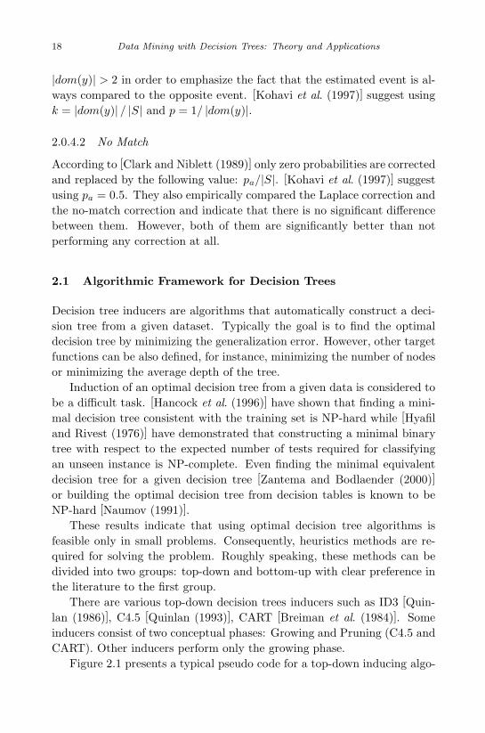
|dom(y)| > 2 in order to emphasize the fact that the estimated event is al-ways compared to the opposite event. [Kohavi et al. (1997)] suggest usingk = |dom(y)| / |S| and p = 1/ |dom(y)|.
2.0.4.2 No Match
According to [Clark and Niblett (1989)] only zero probabilities are correctedand replaced by the following value: pa/|S|. [Kohavi et al. (1997)] suggestusing pa = 0.5. They also empirically compared the Laplace correction andthe no-match correction and indicate that there is no significant differencebetween them. However, both of them are significantly better than notperforming any correction at all.
2.1 Algorithmic Framework for Decision Trees
Decision tree inducers are algorithms that automatically construct a deci-sion tree from a given dataset. Typically the goal is to find the optimaldecision tree by minimizing the generalization error. However, other targetfunctions can be also defined, for instance, minimizing the number of nodesor minimizing the average depth of the tree.
Induction of an optimal decision tree from a given data is considered tobe a difficult task. [Hancock et al. (1996)] have shown that finding a mini-mal decision tree consistent with the training set is NP-hard while [Hyafiland Rivest (1976)] have demonstrated that constructing a minimal binarytree with respect to the expected number of tests required for classifyingan unseen instance is NP-complete. Even finding the minimal equivalentdecision tree for a given decision tree [Zantema and Bodlaender (2000)]or building the optimal decision tree from decision tables is known to beNP-hard [Naumov (1991)].
These results indicate that using optimal decision tree algorithms isfeasible only in small problems. Consequently, heuristics methods are re-quired for solving the problem. Roughly speaking, these methods can bedivided into two groups: top-down and bottom-up with clear preference inthe literature to the first group.
There are various top-down decision trees inducers such as ID3 [Quin-lan (1986)], C4.5 [Quinlan (1993)], CART [Breiman et al. (1984)]. Someinducers consist of two conceptual phases: Growing and Pruning (C4.5 andCART). Other inducers perform only the growing phase.
Figure 2.1 presents a typical pseudo code for a top-down inducing algo-

November 7, 2007 13:10 WSPC/Book Trim Size for 9in x 6in DataMining
Growing Decision Trees 19
rithm of a decision tree using growing and pruning. Note that these algo-rithms are greedy by nature and construct the decision tree in a top-down,recursive manner (also known as divide and conquer). In each iteration, thealgorithm considers the partition of the training set using the outcome ofdiscrete input attributes. The selection of the most appropriate attributeis made according to some splitting measures. After the selection of anappropriate split, each node further subdivides the training set into smallersubsets, until a stopping criterion is satisfied.
2.2 Stopping Criteria
The growing phase continues until a stopping criterion is triggered. Thefollowing conditions are common stopping rules:
(1) All instances in the training set belong to a single value of y.(2) The maximum tree depth has been reached.(3) The number of cases in the terminal node is less than the minimum
number of cases for parent nodes.(4) If the node were split, the number of cases in one or more child nodes
would be less than the minimum number of cases for child nodes.(5) The best splitting criterion is not greater than a certain threshold.

November 7, 2007 13:10 WSPC/Book Trim Size for 9in x 6in DataMining
20 Data Mining with Decision Trees: Theory and Applications
TreeGrowing (S,A,y,SplitCriterion,StoppingCriterion)
Where:
S - Training Set
A - Input Feature Set
y - Target Feature
SplitCriterion - the method for evaluating a certain split
StoppingCriterion - the criteria to stop the growing process
Create a new tree T with a single root node.
IF StoppingCriterion(S) THEN
Mark T as a leaf with the most
common value of y in S as a label.
ELSE
∀ai ∈ A find a that obtain the best SplitCriterion(ai, S).Label t with a
FOR each outcome vi of a:
Set Subtreei= TreeGrowing (σa=viS, A, y).Connect the root node of tT to Subtreei with
an edge that is labelled as vi
END FOR
END IF
RETURN TreePruning (S,T,y)
TreePruning (S,T,y)
Where:
S - Training Set
y - Target Feature
T - The tree to be pruned
DO
Select a node t in T such that pruning it
maximally improve some evaluation criteria
IF t �= Ø THEN T = pruned(T, t)UNTIL t = Ø
RETURN T
Fig. 2.1 Top-Down Algorithmic Framework for Decision Trees Induction.

November 7, 2007 13:10 WSPC/Book Trim Size for 9in x 6in DataMining
Chapter 3
Evaluation of Classification Trees
3.1 Overview
An important problem in the KDD process is the development of efficientindicators for assessing the quality of the analysis results. In this chapter weintroduce the main concepts and quality criteria in decision trees evaluation.
Evaluating the performance of a classification tree is a fundamental as-pect of machine learning. As stated above, the decision tree inducer receivesa training set as input and constructs a classification tree that can classifyan unseen instance. Both the classification tree and the inducer can beevaluated using evaluation criteria. The evaluation is important for under-standing the quality of the classification tree and for refining parameters inthe KDD iterative process
While there are several criteria for evaluating the predictive performanceof classification trees, other criteria such as the computational complexityor the comprehensibility of the generated classifier can be important aswell.
3.2 Generalization Error
Let DT (S) represent a classification tree trained on dataset S. The gener-alization error of DT (S) is its probability to misclassify an instance selectedaccording to the distribution D of the labeled instance space. The classifi-cation accuracy of a classification tree is one minus the generalization error.The training error is defined as the percentage of examples in the trainingset correctly classified by the classification tree, formally:
21

November 7, 2007 13:10 WSPC/Book Trim Size for 9in x 6in DataMining
22 Data Mining with Decision Trees: Theory and Applications
ε(DT (S), S) =∑
〈x,y〉∈S
L (y, DT (S)(x)) (3.1)
where L(y, DT (S)(x)) is the zero-one loss function defined in Equation 2.2.In this book, classification accuracy is the primary evaluation criterion
for experiments.Although generalization error is a natural criterion, its actual value is
known only in rare cases (mainly synthetic cases). The reason for that isthat the distribution D of the labeled instance space is not known.
One can take the training error as an estimation of the generalizationerror. However, using the training error as is will typically provide anoptimistically biased estimate, especially if the inducer over-fits the trainingdata. There are two main approaches for estimating the generalizationerror: Theoretical and Empirical. In this book we utilize both approaches.
3.2.1 Theoretical Estimation of Generalization Error
A low training error does not guarantee low generalization error. There isoften a trade-off between the training error and the confidence assigned tothe training error as a predictor for the generalization error, measured bythe difference between the generalization and training errors. The capacityof the inducer is a major factor in determining the degree of confidencein the training error. In general, the capacity of an inducer indicates thevariety of classifiers it can induce. The VC-dimension presented below canbe used as a measure of the inducers capacity.
Decision trees with many nodes, relative to the size of the trainingset, are likely to obtain a low training error. On the other hand, theymight just be memorizing or overfitting the patterns and hence exhibita poor generalization ability. In such cases, the low error is likely to bea poor predictor of the higher generalization error. When the oppositeoccurs, that is to say, when capacity is too small for the given number ofexamples, inducers may underfit the data, and exhibit both poor trainingand generalization error.
In “Mathematics of Generalization”, [Wolpert (1995)] discuss four the-oretical frameworks for estimating the generalization error: PAC, VC andBayesian, and statistical physics. All these frameworks combine the trainingerror (which can be easily calculated) with some penalty function expressingthe capacity of the inducers.

November 7, 2007 13:10 WSPC/Book Trim Size for 9in x 6in DataMining
Evaluation of Classification Trees 23
3.2.2 Empirical Estimation of Generalization Error
Another approach for estimating the generalization error is the holdoutmethod in which the given dataset is randomly partitioned into two sets:training and test sets. Usually, two-thirds of the data is considered for thetraining set and the remaining data are allocated to the test set. First, thetraining set is used by the inducer to construct a suitable classifier and thenwe measure the misclassification rate of this classifier on the test set. Thistest set error usually provides a better estimation of the generalization errorthan the training error. The reason for this is the fact that the trainingerror usually under-estimates the generalization error (due to the overfittingphenomena). Nevertheless since only a proportion of the data is used toderive the model, the estimate of accuracy tends to be pessimistic.
A variation of the holdout method can be used when data is limited. Itis common practice to resample the data, that is, partition the data intotraining and test sets in different ways. An inducer is trained and tested foreach partition and the accuracies averaged. By doing this, a more reliableestimate of the true generalization error of the inducer is provided.
Random subsampling and n-fold cross-validation are two common meth-ods of resampling. In random subsampling, the data is randomly parti-tioned several times into disjoint training and test sets. Errors obtainedfrom each partition are averaged. In n-fold cross-validation, the data israndomly split into n mutually exclusive subsets of approximately equalsize. An inducer is trained and tested n times; each time it is tested on oneof the k folds and trained using the remaining n− 1 folds.
The cross-validation estimate of the generalization error is the overallnumber of misclassifications divided by the number of examples in the data.The random subsampling method has the advantage that it can be repeatedan indefinite number of times. However, a disadvantage is that the test setsare not independently drawn with respect to the underlying distribution ofexamples. Because of this, using a t-test for paired differences with randomsubsampling can lead to an increased chance of type I error, i.e., identifyinga significant difference when one does not actually exist. Using a t-test onthe generalization error produced on each fold lowers the chances of typeI error but may not give a stable estimate of the generalization error. Itis common practice to repeat n-fold cross-validation n times in order toprovide a stable estimate. However, this, of course, renders the test setsnon-independent and increases the chance of type I error. Unfortunately,there is no satisfactory solution to this problem. Alternative tests suggested

November 7, 2007 13:10 WSPC/Book Trim Size for 9in x 6in DataMining
24 Data Mining with Decision Trees: Theory and Applications
by [Dietterich (1998)] have a low probability of type I error but a higherchance of type II error that is, failing to identify a significant differencewhen one does actually exist.
Stratification is a process often applied during random subsampling andn-fold cross-validation. Stratification ensures that the class distributionfrom the whole dataset is preserved in the training and test sets. Stratifi-cation has been shown to help reduce the variance of the estimated errorespecially for datasets with many classes.
Another cross-validation variation is the bootstraping method which isa n-fold cross validation, with n set to the number of initial samples. Itsamples the training instances uniformly with replacement and leave-one-out. In each iteration, the classifier is trained on the set of n − 1 samplesthat is randomly selected from the set of initial samples, S. The testing isperformed using the remaining subset.
3.2.3 Alternatives to the Accuracy Measure
Accuracy is not a sufficient measure for evaluating a model with an imbal-anced distribution of the class. There are cases where the estimation of anaccuracy rate may mislead one about the quality of a derived classifier. Insuch circumstances, where the dataset contains significantly more major-ity class than minority class instances, one can always select the majorityclass and obtain good accuracy performance. Therefore, in these cases, thesensitivity and specificity measures can be used as an alternative to theaccuracy measures [Han and Kamber (2001)].
Sensitivity (also known as recall) assesses how well the classifier canrecognize positive samples and is defined as
Sensitivity =true positive
positive(3.2)
where true positive corresponds to the number of the true positive samplesand positive is the number of positive samples.
Specificity measures how well the classifier can recognize negative sam-ples. It is defined as
Specificity =true negative
negative(3.3)

November 7, 2007 13:10 WSPC/Book Trim Size for 9in x 6in DataMining
Evaluation of Classification Trees 25
where true negative corresponds to the number of the true negative exam-ples and negative the number of samples that is negative.
Another well-known performance measure is precision. Precision mea-sures how many examples classified as “positive” class are indeed “positive”.This measure is useful for evaluating crisp classifiers that are used to classifyan entire dataset. Formally:
Precision =true positive
true positive + false positive(3.4)
Based on the above definitions the accuracy can be defined as a functionof sensitivity and specificity:
Accuracy = Sensitivity · positivepositive+negative +
Specificity · negativepositive+negative
(3.5)
3.2.4 The F-Measure
Usually there is a tradeoff between the precision and recall measures. Try-ing to improve one measure often results in a deterioration of the secondmeasure. Figure 3.1 illustrates a typical precision-recall graph. This two-dimensional graph is closely related to the well-known receiver operatingcharacteristics (ROC) graphs in which the true positive rate (recall) is plot-ted on the Y-axis and the false positive rate is plotted on the X-axis [Ferriet al. (2002)]. However unlike the precision-recall graph, the ROC diagramis always convex.
Precision
Recall
Fig. 3.1 A Typical precision-recall diagram.
Given a probabilistic classifier, this trade-off graph may be obtained bysetting different threshold values. In a binary classification problem, the

November 7, 2007 13:10 WSPC/Book Trim Size for 9in x 6in DataMining
26 Data Mining with Decision Trees: Theory and Applications
classifier prefers the class “not pass” over the class “pass” if the probabilityfor “not pass” is at least 0.5. However, by setting a different thresholdvalue other than 0.5, the trade-off graph can be obtained.
The problem here is described as multi-criteria decision-making(MCDM). The simplest and the most commonly used method to solveMCDM is the weighted sum model. This technique combines the crite-ria into a single value by using appropriate weighting. The basic princi-ple behind this technique is the additive utility assumption. The criteriameasures must be numerical, comparable and expressed in the same unit.Nevertheless, in the case discussed here, the arithmetic mean can mislead.Instead, the harmonic mean provides a better notion of “average”. Morespecifically, this measure is defined as [Van Rijsbergen (1979)]:
F =2 · P ·RP + R
(3.6)
The intuition behind the F-measure can be explained using Figure 3.2.Figure 3.2 presents a diagram of a common situation in which the rightellipsoid represents the set of all defective batches and the left ellipsoidrepresents the set of all batches that were classified as defective by a certainclassifier. The intersection of these sets represents the true positive (TP),while the remaining parts represent false negative (FN) and false positive(FP). An intuitive way of measuring the adequacy of a certain classifieris to measure to what extent the two sets match, namely to measure thesize of the unshaded area. Since the absolute size is not meaningful, itshould be normalized by calculating the proportional area. This value isthe F-measure:
Proportion of unshaded area =2·(True Positive)
False Positive + False Negative + 2·(True Positve) = F(3.7)
The F-measure can have values between 0 to 1. It obtains its highestvalue when the two sets presented in Figure 3.2 are identical and it obtainsits lowest value when the two sets are mutually exclusive. Note that eachpoint on the precision-recall curve may have a different F-measure. Fur-thermore, different classifiers have different precision-recall graphs.

November 7, 2007 13:10 WSPC/Book Trim Size for 9in x 6in DataMining
Evaluation of Classification Trees 27
Fig. 3.2 A graphic explanation of the F-measure.
3.2.5 Confusion Matrix
The confusion matrix is used as an indication of the properties of a classi-fication (discriminant) rule. It contains the number of elements that havebeen correctly or incorrectly classified for each class. We can see on its maindiagonal the number of observations that have been correctly classified foreach class; the off-diagonal elements indicate the number of observationsthat have been incorrectly classified. One benefit of a confusion matrix isthat it is easy to see if the system is confusing two classes (i.e. commonlymislabelling one as an other).
For every instance in the test set, we compare the actual class to theclass that was assigned by the trained classifier. A positive (negative)example that is correctly classified by the classifier is called a true positive(true negative); a positive (negative) example that is incorrectly classifiedis called a false negative (false positive). These numbers can be organizedin a confusion matrix shown in Table 3.1.
Table 3.1 A confusion matrix
Predictednegative
Predictedpositive
NegativeExamples
A B
PositiveExamples
C D
Based on the values in Table 3.1, one can calculate all the measures

November 7, 2007 13:10 WSPC/Book Trim Size for 9in x 6in DataMining
28 Data Mining with Decision Trees: Theory and Applications
defined above:
• Accuracy is: (a+d)/(a+b+c+d)• Misclassification rate is: (b+c)/(a+b+c+d)• Precision is: d/(b + d)• True positive rate (Recall) is: d/(c + d)• False positive rate is: b/(a + b)• True negative rate (Specificity) is: a/(a + b)• False negative rate is: c/(c + d)
3.2.6 Classifier Evaluation under Limited Resources
The above mentioned evaluation measures are insufficient when probabilis-tic classifiers are used for choosing objects to be included in a limited quota.This is a common situation that arises in real-life applications due to re-source limitations that require cost-benefit considerations. Resource limita-tions prevent the organization from choosing all the instances. For example,in direct marketing applications, instead of mailing everybody on the list,the marketing efforts must implement a limited quota, i.e., target the mail-ing audience with the highest probability of positively responding to themarketing offer without exceeding the marketing budget.
Another example deals with a security officer in an air terminal. Follow-ing September 11, the security officer needs to search all passengers whomay be carrying dangerous instruments (such as scissors, penknives andshaving blades). For this purpose the officer is using a classifier that is ca-pable of classifying each passenger either as class A, which means, “Carrydangerous instruments” or as class B, “Safe”.
Suppose that searching a passenger is a time-consuming task and thatthe security officer is capable of checking only 20 passengers prior to eachflight. If the classifier has labeled exactly 20 passengers as class A, then theofficer will check all these passengers. However if the classifier has labeledmore than 20 passengers as class A, then the officer is required to decidewhich class A passenger should be ignored. On the other hand, if less than20 people were classified as A, the officer, who must work constantly, hasto decide who to check from those classified as B after he has finished withthe class A passengers.
There also cases in which a quota limitation is known to exist but itssize is not known in advance. Nevertheless, the decision maker would liketo evaluate the expected performance of the classifier. Such cases occur,

November 7, 2007 13:10 WSPC/Book Trim Size for 9in x 6in DataMining
Evaluation of Classification Trees 29
for example, in some countries regarding the number of undergraduate stu-dents that can be accepted to a certain department in a state university.The actual quota for a given year is set according to different parametersincluding governmental budget. In this case, the decision maker would liketo evaluate several classifiers for selecting the applicants while not knowingthe actual quota size. Finding the most appropriate classifier in advanceis important because the chosen classifier can dictate what the importantattributes are, i.e. the information that the applicant should provide theregistration and admission unit.
In probabilistic classifiers, the above mentioned definitions of precisionand recall can be extended and defined as a function of a probability thresh-old τ . If we evaluate a classifier based on a given a test set which consistsof n instances denoted as (< x1, y1 >, ..., < xn, yn >) such that xi repre-sents the input features vector of instance i and yi represents its true class(“positive” or “negative”), then:
Precision (τ) =
∣∣∣{< xi, yi >: PDT (pos |xi ) > τ, yi = pos}∣∣∣∣∣∣{< xi, yi >: PDT (pos |xi ) > τ
∣∣∣ (3.8)
Recall (τ) =
∣∣∣{< xi, yi >: PDT (pos |xi ) > τ, yi = pos}∣∣∣
|{< xi, yi >: yi = pos}| (3.9)
where DT represents a probabilistic classifier that is used to estimate theconditional likelihood of an observation xi to “positive” which is denoted asPDT (pos |xi ). The typical threshold value of 0.5 means that the predictedprobability of “positive” must be higher than 0.5 for the instance to bepredicted as “positive”. By changing the value of τ,one can control thenumber of instances that are classified as “positive”. Thus, the τ value canbe tuned to the required quota size. Nevertheless because there might beseveral instances with the same conditional probability, the quota size isnot necessarily incremented by one.
The above discussion is based on the assumption that the classifica-tion problem is binary. In cases where there are more than two classes,adaptation could be easily made by comparing one class to all the others.

November 7, 2007 13:10 WSPC/Book Trim Size for 9in x 6in DataMining
30 Data Mining with Decision Trees: Theory and Applications
3.2.6.1 ROC Curves
Another measure is the receiver operating characteristic (ROC) curveswhich illustrate the tradeoff between true positive to false positive rates[Provost and Fawcett (1998)]. Figure 3.3 illustrates a ROC curve in whichthe X-axis represents a false positive rate and the Y-axis represents a truepositive rate. The ideal point on the ROC curve would be (0,100), that is,all positive examples are classified correctly and no negative examples aremisclassified as positive.
True positive rate
False positive
rate 0.20.40.60.81
1
0.8
0.6
0.4
Fig. 3.3 A Typical ROC curve.
The ROC convex hull can also be used as a robust method of identi-fying potentially optimal classifiers [Provost and Fawcett (2001)]. Givena family of ROC curves, the ROC convex hull can include points that aremore towards the north-west frontier of the ROC space. If a line passesthrough a point on the convex hull, then there is no other line with the sameslope passing through another point with a larger true positive (TP) inter-cept. Thus, the classifier at that point is optimal under any distributionassumptions in tandem with that slope.
3.2.6.2 Hit Rate Curve
The hit rate curve presents the hit ratio as a function of the quota size[Anand Wang (2001)]. Hit rate is calculated by counting the actual positivelabeled instances inside a determined quota. More precisely for a quota ofsize j and a ranked set of instances, hit rate is defined as:

November 7, 2007 13:10 WSPC/Book Trim Size for 9in x 6in DataMining
Evaluation of Classification Trees 31
HitRate(j) =
j∑k=1
t[k]
j(3.10)
where t[k] represents the truly expected outcome of the instance located inthe k’th position when the instances are sorted according to their condi-tional probability for “positive” by descending order. Note that if the k’thposition can be uniquely defined (i.e. there is exactly one instance that canbe located in this position) then t[k] is either 0 or 1 depending on the actualoutcome of this specific instance. Nevertheless if the k’th position is notuniquely defined and there are mk,1 instances that can be located in thisposition, and mk,2 of which are truly positive, then:
t[k] = mk,2/mk,1(3.11)
The sum of t[k] over the entire test set is equal to the number of instancesthat are labeled “positive”. Moreover Hit − Rate(j) ≈ Precision(p[j])where p[j] denotes the j’th order of PI(pos |x1 ), ..., PI(pos |xm ). The valuesare strictly equal when the value of j ’th is uniquely defined.
It should be noted that the hit rate measure was originally defined with-out any reference to the uniqueness of a certain position. However, thereare some classifiers that tend to provide the same conditional probabilityto several different instances. For instance, in a decision tree, any instancesin the test set that belongs to the same leaf get the same conditional prob-ability. Thus, the proposed correction is required in those cases. Figure 3.4illustrates a hit-curve.
Hit-Rate [%]
Quota 100 200 300 400 500
100
80
60
40
Fig. 3.4 A typical hit curve.

November 7, 2007 13:10 WSPC/Book Trim Size for 9in x 6in DataMining
32 Data Mining with Decision Trees: Theory and Applications
3.2.6.3 Qrecall (Quota Recall)
The hit-rate measure, presented above, is the “precision” equivalent forquota-limited problems. Similarly, we suggest the Qrecall (for quota recall)to be the “recall” equivalent for quota-limited problems. The Qrecall fora certain position in a ranked list is calculated by dividing the number ofpositive instances, from the head of the list until that position, by the totalpositive instances in the entire dataset. Thus, the Qrecall for a quota of j
is defined as:
Qrecall(j) =
j∑k=1
t[k]
n+(3.12)
The denominator stands for the total number of instances that are clas-sified as positive in the entire dataset. Formally it can be calculated as:
n+ = |{< xi, yi >: yi = pos}| (3.13)
3.2.6.4 Lift Curve
A popular method of evaluating probabilistic models is lift [Coppock(2002)]. After a ranked test set is divided into several portions (usuallydeciles), lift is calculated as follows: the ratio of really positive instances ina specific decile is divided by the average ratio of really positive instances inthe population. Regardless of how the test set is divided, a good model isachieved if the lift decreases when proceeding to the bottom of the scoringlist. A good model would present a lift greater than 1 in the top deciles anda lift smaller than 1 in the last deciles. Figure 3.5 illustrates a lift chart fora typical model prediction. A comparison between models can be done bycomparing the lift of the top portions, depending on the resources availableand cost/benefit considerations.
3.2.6.5 Pearson Correlation Coefficient
There are also some statistical measures that may be used as performanceevaluators of models. These measures are well-known and can be foundin many statistical books. In this section we examine the Pearson correla-tion coefficient. This measure can be used to find the correlation betweenthe ordered estimated conditional probability (p[k]) and the ordered actual

November 7, 2007 13:10 WSPC/Book Trim Size for 9in x 6in DataMining
Evaluation of Classification Trees 33
10
8
6
4
2
1 2 3 4 5 6 7 8 9 Deciles
Lift
Fig. 3.5 A typical lift chart.
expected outcome (t[k]). A Pearson correlation coefficient can have anyvalue between -1 and 1 where the value 1 represents the strongest positivecorrelation. It should be noticed that this measure take into account notonly the ordinal place of an instance but also its value (i.e. the estimatedprobability attached to it). The Pearson correlation coefficient for two ran-dom variables is calculated by dividing the co-variance by the product ofboth standard deviations. In this case, the standard deviations of the twovariables assuming a quota size of j are:
σp(j) =
√√√√1j
j∑i=1
(p[i] − p(j)
); σt(j) =
√√√√1j
j∑i=1
(t[i] − t(j)
)(3.14)
where p(j), t(j) represent the average of p[i]’s and t[i]’s respectively:
p(j) =
j∑i=1
p[i]
j; t(j) =
j∑i=1
t[i]
j= HitRate(j) (3.15)
The co-variance is calculated as follows:
Covp,t(j) =1j
j∑i−1
(p[i] − p(j)
)(t[i] − t(j)
)(3.16)
Thus, the Pearson correlation coefficient for a quota j, is:

November 7, 2007 13:10 WSPC/Book Trim Size for 9in x 6in DataMining
34 Data Mining with Decision Trees: Theory and Applications
ρp,t(j) =Covp,t(j)
σp(j) · σt(j)(3.17)
3.2.6.6 Area Under Curve (AUC)
Evaluating a probabilistic model without using a specific fixed quota is nota trivial task. Using continuous measures like hit curves, ROC curves andlift charts, mentioned previously, is problematic. Such measures can givea definite answer to the question “Which is the best model?” only if onemodel dominates in the curve space, meaning that the curves of all theother model are beneath it or equal to it over the entire chart space. If adominating model does not exist, then there is no answer to that question,using only the continuous measures mentioned above.. Complete orderdemands no intersections of the curves. Of course, in practice there isalmost never one dominating model. The best answer that can be obtainedis in regard to which areas one model outperforms the others. As shown inFigure 3.6, every model gets different values in different areas. If a completeorder of model performance is needed, another measure should be used.
True positive
False positive 0.2 0.4 0.6 0.8 1
1
0.8
0.6
0.4
0.2
Fig. 3.6 Areas of dominancy. A ROC curve is an example of a measure that givesareas of dominancy and not a complete order of the models. In this example the equally
dashed line model is the best for f.p (false positive) < 0.2. The full line model is thebest for 0.2 < f.p <0.4. The dotted line model is best for 0.4 < f.p < 0.9 and from 0.9to 1 again the dashed line model is the best.
Area under the ROC curve (AUC) is a useful metric for classifier per-formance since it is independent of the decision criterion selected and prior

November 7, 2007 13:10 WSPC/Book Trim Size for 9in x 6in DataMining
Evaluation of Classification Trees 35
probabilities. The AUC comparison can establish a dominance relationshipbetween classifiers. If the ROC curves are intersecting, the total AUC isan average comparison between models [Lee (2000)]. The bigger it is, thebetter the model is. As opposed to other measures, the area under theROC curve (AUC) does not depend on the imbalance of the training set[Kolcz (2003)]. Thus, the comparison of the AUC of two classifiers is fairerand more informative than comparing their misclassification rates.
3.2.6.7 Average Hit Rate
The average hit rate is a weighted average of all hit-rate values. If themodel is optimal, then all the really positive instances are located in thehead of the ranked list, and the value of the average hit rate is 1. The use ofthis measure fits an organization that needs to minimize type II statisticalerror (namely, to include a certain object in the quota although in fact thisobject will be labeled as “negative”). Formally the Average Hit Rate forbinary classification problems is defined as:
AverageHitRate =
n∑j=1
t[j] ·HitRate(j)
n+(3.18)
where t[j] is defined as in Equation 4 and is used as a weighting factor. Notethat the average hit rate ignores all hit rate values on unique positions thatare actually labeled as “negative” class (because t[j]=0 in these cases).
3.2.6.8 Average Qrecall
Average Qrecall is the average of all the Qrecalls which extends from theposition that is equal to the number of positive instances in the test setto the bottom of the list. Average Qrecall fits an organization that needsto minimize type I statistical error (namely, not including a certain objectin the quota although in fact this object will be labeled as “positive”).Formally, average Qrecall is defined as:
n∑j=n+
Qrecall(j)
n− (n+ − 1)(3.19)
where n is the total number of instances and n+ is defined in Equa-tion (3.13).

November 7, 2007 13:10 WSPC/Book Trim Size for 9in x 6in DataMining
36 Data Mining with Decision Trees: Theory and Applications
Table 3.2 illustrates the calculation of average Qrecall and average hit-rate for a dataset of ten instances. The table presents a list of instancesin descending order according to their predicted conditional probability tobe classified as “positive”. Because all probabilities are unique, the thirdcolumn (t[k]) indicates the actual class (“1” represent “positive” and “0”represents “negative”). The average values are simple algebraic averages ofthe highlighted cells.
Table 3.2 An example for calculating Average Qrecall and AverageHit-rate
Place inlist (j)
Positiveproba-bility
t[k] Qrecall Hit rate
1 0.45 1 0.25 1
2 0.34 0 0.25 0.5
3 0.32 1 0.5 0.667
4 0.26 1 0.75 0.75
5 0.15 0 0.75 0.6
6 0.14 0 0.75 0.5
7 0.09 1 1 0.571
8 0.07 0 1 0.5
9 0.06 0 1 0.444
10 0.03 0 1 0.4
Average: 0.893 0.747
Note that both average Qrecall and average hit rate get the value 1 inan optimum classification, where all the positive instances are located atthe head of the list. This case is illustrated in Table 3.3. A summary ofthe key differences are provided in Table 3.4.
3.2.6.9 Potential Extract Measure (PEM)
To better understand the behavior of Qrecall curves, consider the cases ofrandom prediction and optimum prediction.
Suppose no learning process was applied on the data and the list pro-duced as a prediction would be the test set in its original (random) order.On the assumption that positive instances are distributed uniformly in thepopulation, then a quota of random size contains a number of positive inst-ances that are proportional to the a-priori proportion of positive instancesin the population. Thus, a Qrecall curve that describes a uniform distribu-

November 7, 2007 13:10 WSPC/Book Trim Size for 9in x 6in DataMining
Evaluation of Classification Trees 37
Table 3.3 Qrecall and Hit-rate in an optimum prediction
Place inlist (j)
Positiveproba-bility
t[k] Qrecall Hit rate
1 0.45 1 0.25 1
2 0.34 1 0. 5 1
3 0.32 1 0.75 1
4 0.26 1 1 1
5 0.15 0 1 0.8
6 0.14 0 1 0.667
7 0.09 0 1 0.571
8 0.07 0 1 0.5
9 0.06 0 1 0.444
10 0.03 0 1 0.4
Average: 1 1
Table 3.4 Characteristics of Qrecall and Hit-rate
Parameter Hit-rate Qrecall
Function increas-ing/decreasing
Non monotonic Monotonically in-creasing
End point Proportion of posi-tive samples in theset
1
Sensitivity of themeasures value topositive instances
Very sensitive topositive instancesat the top of thelist. Less sensitiveon going down tothe bottom of thelist.
Same sensitivity topositive instancesin all places in thelist.
Effect of negativeclass on the mea-sure
A neg-ative instance af-fects the measure
and cause its valueto decrease.
A negative inst-ance does not af-fect the measure.
Range 0≤ Hit-rate ≤1 0≤ Qrecall ≤1
tion (which can be considered as a model that predicts as well as a randomguess, without any learning) is a linear line (or semi-linear because valuesare discrete) which starts at 0 (for zero quota size) and ends in 1.
Suppose now that a model gave an optimum prediction, meaning thatall positive instances are located at the head of the list and below them, allthe negative instances. In this case, the Qrecall curve climbs linearly until

November 7, 2007 13:10 WSPC/Book Trim Size for 9in x 6in DataMining
38 Data Mining with Decision Trees: Theory and Applications
a value of 1 is achieved at point n+ (n+ = number of positive samples).From that point any quota that has a size bigger than n+, fully extractstest set potential and the value 1 is kept until the end of the list.
Note that a “good model”, which outperforms random classification,though not an optimum one, will fall “on average” between these two curves.It may drop sometimes below the random curve but generally, more area isdelineated between the “good model” curve and the random curve, abovethe latter than below it. If the opposite is true then the model is a “badmodel” that does worse than a random guess.
The last observation leads us to consider a measure that evaluates theperformance of a model by summing the areas delineated between the Qre-call curve of the examined model and the Qrecall curve of a random model(which is linear). Areas above the linear curve are added and areas be-low the linear curve are subtracted. The areas themselves are calculatedby subtracting the Qrecall of a random classification from the Qrecall ofthe model’s classification in every point as shown in Figure 3.7. The ar-eas where the model performed better than a random guess increase themeasure’s value while the areas where the model performed worse than arandom guess decrease it. If the last total computed area is divided in thearea delineated between the optimum model Qrecall curve and the randommodel (linear) Qrecall curve, then it reaches the extent to which the poten-tial is extracted, independently of the number of instances in the dataset.
Formally, the PEM measure is calculated as:
PEM =S1 − S2
S3(3.20)
where S1 is the area delimited by the Qrecall curve of the examined modelabove the Qrecall curve of a random model; S2 is the area delimited by theQrecall curve of the examined model under the Qrecall curve of a randommodel; and S3 is the area delimited by the optimal Qrecall curve and thecurve of the random model. The division in S3 is required in order tonormalize the measure, thus datasets of different size can be compared. Inthis way, if the model is optimal, then PEM gets the value 1. If the modelis as good as a random choice, then the PEM gets the value 0. If it givesthe worst possible result (that is to say, it puts the positive samples at thebottom of the list), then its PEM is -1. Based on the notations definedabove, the PEM can be formulated as:

November 7, 2007 13:10 WSPC/Book Trim Size for 9in x 6in DataMining
Evaluation of Classification Trees 39
0
0.2
0.4
0.6
0.8
1
1 19 37 55 73 91
quota size
Qre
call
Random ClassifierOptimum ClassifierExamined Classifier
S3
S1
S2
Fig. 3.7 A qualitative representation of PEM.
PEM =S1 − S2
S3=
n∑j=1
(qrecall(j)− j
n
)n+∑j=1
(j
n+
)+ n− −
n∑j=1
(jn
) (3.21)
=
n∑j=1
(qrecall(j))− (n+1)2
(n++1)2 + n− − (n+1)
2
=
n∑j=1
(qrecall(j))− (n+1)2
n−2
(3.22)
where n− denotes the number of instances that are actually classified as“negative”. Table 3.5 illustrates the calculation of PEM for the instancesin Table 3.2. Note that the random Qrecall does not represent a certainrealization but the expected values. The optimal qrecall is calculated as ifthe “positive” instances have been located in the top of the list.
Note that the PEM somewhat resembles the Gini index produced fromLorentz curves which appear in economics when dealing with the distribu-tion of income. Indeed, this measure indicates the difference between thedistribution of positive samples in a prediction and the uniform distribu-tion. Note also that this measure gives an indication of the total lift of
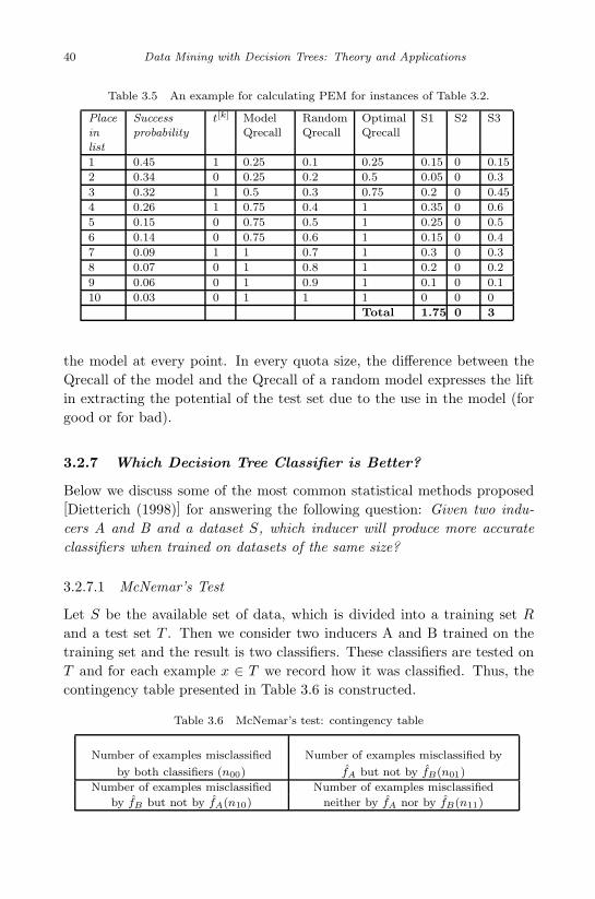
November 7, 2007 13:10 WSPC/Book Trim Size for 9in x 6in DataMining
40 Data Mining with Decision Trees: Theory and Applications
Table 3.5 An example for calculating PEM for instances of Table 3.2.
Placeinlist
Successprobability
t[k] ModelQrecall
RandomQrecall
OptimalQrecall
S1 S2 S3
1 0.45 1 0.25 0.1 0.25 0.15 0 0.15
2 0.34 0 0.25 0.2 0.5 0.05 0 0.3
3 0.32 1 0.5 0.3 0.75 0.2 0 0.45
4 0.26 1 0.75 0.4 1 0.35 0 0.6
5 0.15 0 0.75 0.5 1 0.25 0 0.5
6 0.14 0 0.75 0.6 1 0.15 0 0.4
7 0.09 1 1 0.7 1 0.3 0 0.3
8 0.07 0 1 0.8 1 0.2 0 0.2
9 0.06 0 1 0.9 1 0.1 0 0.1
10 0.03 0 1 1 1 0 0 0
Total 1.75 0 3
the model at every point. In every quota size, the difference between theQrecall of the model and the Qrecall of a random model expresses the liftin extracting the potential of the test set due to the use in the model (forgood or for bad).
3.2.7 Which Decision Tree Classifier is Better?
Below we discuss some of the most common statistical methods proposed[Dietterich (1998)] for answering the following question: Given two indu-cers A and B and a dataset S, which inducer will produce more accurateclassifiers when trained on datasets of the same size?
3.2.7.1 McNemar’s Test
Let S be the available set of data, which is divided into a training set R
and a test set T . Then we consider two inducers A and B trained on thetraining set and the result is two classifiers. These classifiers are tested onT and for each example x ∈ T we record how it was classified. Thus, thecontingency table presented in Table 3.6 is constructed.
Table 3.6 McNemar’s test: contingency table
Number of examples misclassified Number of examples misclassified by
by both classifiers (n00) fA but not by fB(n01)
Number of examples misclassified Number of examples misclassified
by fB but not by fA(n10) neither by fA nor by fB(n11)

November 7, 2007 13:10 WSPC/Book Trim Size for 9in x 6in DataMining
Evaluation of Classification Trees 41
The two inducers should have the same error rate under the null hy-pothesis H0. McNemar’s test is based on a χ2 test for goodness-of-fit thatcompares the distribution of counts expected under null hypothesis to theobserved counts. The expected counts under Ho are presented in Table 3.7.
Table 3.7 Expected counts under Ho
n00 (n01 + n10)/2)
(n01 + n10)/2) n11)
The following statistic, s, is distributed as χ2 with 1 degree of freedom.It incorporates a “continuity correction” term (of -1 in the numerator) toaccount for the fact that the statistic is discrete while the χ2 distributionis continuous:
s =(|n10 − n01| − 1)2
n10 + n01(3.23)
According to the probabilistic theory [Athanasopoulos, 1991], if the nullhypothesis is correct, the probability that the value of the statistic, s, isgreater than χ2
1,0.95 is less than 0.05, i.e. P (|s| > χ21,0.95) < 0.05. Then, to
compare the inducers A and B, the induced classifiers fA and fB are testedon T and the value of s is estimated as described above. Then if |s| > χ2
1,0.95,the null hypothesis could be rejected in favor of the hypothesis that the twoinducers have different performance when trained on the particular trainingset R.
The shortcomings of this test are:
(1) It does not directly measure variability due to the choice of the train-ing set or the internal randomness of the inducer. The inducers arecompared using a single training set R. Thus McNemar’s test shouldbe only applied if we consider that the sources of variability are small.
(2) It compares the performance of the inducers on training sets, whichare substantially smaller than the size of the whole dataset. Hence wemust assume that the relative difference observed on training sets willstill hold for training sets of size equal to the whole dataset.
3.2.7.2 A Test for the Difference of Two Proportions
This statistical test is based on measuring the difference between the errorrates of algorithms A and B [Snedecor and Cochran (1989)]. More specifi-

November 7, 2007 13:10 WSPC/Book Trim Size for 9in x 6in DataMining
42 Data Mining with Decision Trees: Theory and Applications
cally, let pA = (n00 +n01)/n be the proportion of test examples incorrectlyclassified by algorithm A and let pB = (n00 + n10)/n be the proportionof test examples incorrectly classified by algorithm B. The assumption un-derlying this statistical test is that when algorithm A classifies an examplex from the test set T, the probability of misclassification is pA. Then thenumber of misclassifications of n test examples is a binomial random vari-able with mean npA and variance pA(1− pA)n.
The binomial distribution can be well approximated by a normal distri-bution for reasonable values of n. The difference between two independentnormally distributed random variables is itself normally distributed. Thus,the quantity pA − pB can be viewed as normally distributed if we assumethat the measured error rates pA and pB are independent. Under the nullhypothesis, Ho, the quantity pA − pB has a mean of zero and a standarddeviation error of
se =
√2p ·
(1− pA + pB
2
)/n (3.24)
where n is the number of test examples.Based on the above analysis, we obtain the statistic:
z =pA − pB√2p(1− p)/n
(3.25)
which has a standard normal distribution. According to the probabilistictheory, if the z value is greater than Z0.975, the probability of incorrectlyrejecting the null hypothesis is less than 0.05. Thus, if |z| > Z0.975 = 1.96,the null hypothesis could be rejected in favor of the hypothesis that thetwo algorithms have different performances. Two of the most importantproblems with this statistic are:
(1) The probabilities pA and pB are measured on the same test set andthus they are not independent.
(2) The test does not measure variation due to the choice of the trainingset or the internal variation of the learning algorithm. Also it measuresthe performance of the algorithms on training sets of a size significantlysmaller than the whole dataset.
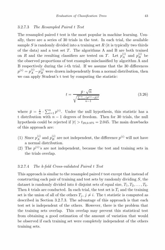
November 7, 2007 13:10 WSPC/Book Trim Size for 9in x 6in DataMining
Evaluation of Classification Trees 43
3.2.7.3 The Resampled Paired t Test
The resampled paired t test is the most popular in machine learning. Usu-ally, there are a series of 30 trials in the test. In each trial, the availablesample S is randomly divided into a training set R (it is typically two thirdsof the data) and a test set T . The algorithms A and B are both trainedon R and the resulting classifiers are tested on T . Let p
(i)A and p
(i)B be
the observed proportions of test examples misclassified by algorithm A andB respectively during the i-th trial. If we assume that the 30 differencesp(i) = p
(i)A −p
(i)B were drawn independently from a normal distribution, then
we can apply Student’s t test by computing the statistic:
t =p · √n√∑ni=1(p
(i)−p)2
n−1
(3.26)
where p = 1n ·∑n
i=1 p(i). Under the null hypothesis, this statistic has at distribution with n − 1 degrees of freedom. Then for 30 trials, the nullhypothesis could be rejected if |t| > t29,0.975 = 2.045. The main drawbacksof this approach are:
(1) Since p(i)A and p
(i)B are not independent, the difference p(i) will not have
a normal distribution.(2) The p(i)’s are not independent, because the test and training sets in
the trials overlap.
3.2.7.4 The k-fold Cross-validated Paired t Test
This approach is similar to the resampled paired t test except that instead ofconstructing each pair of training and test sets by randomly dividing S, thedataset is randomly divided into k disjoint sets of equal size, T1, T2, . . . , Tk.Then k trials are conducted. In each trial, the test set is Ti and the trainingset is the union of all of the others Tj, j �= i. The t statistic is computed asdescribed in Section 3.2.7.3. The advantage of this approach is that eachtest set is independent of the others. However, there is the problem thatthe training sets overlap. This overlap may prevent this statistical testfrom obtaining a good estimation of the amount of variation that wouldbe observed if each training set were completely independent of the otherstraining sets.
November 7, 2007 13:10 WSPC/Book Trim Size for 9in x 6in DataMining
44 Data Mining with Decision Trees: Theory and Applications
3.3 Computational Complexity
Another useful criterion for comparing inducers and classifiers is their com-putational complexity. Strictly speaking computational complexity is theamount of CPU consumed by each inducer. It is convenient to differentiatebetween three metrics of computational complexity:
• Computational complexity for generating a new classifier: This is themost important metric, especially when there is a need to scale thedata mining algorithm to massive datasets. Because most of the algo-rithms have computational complexity, which is worse than linear inthe numbers of tuples, mining massive datasets might be prohibitivelyexpensive.• Computational complexity for updating a classifier: Given new data,
what is the computational complexity required for updating the currentclassifier such that the new classifier reflects the new data?• Computational complexity for classifying a new instance: Generally
this type of metric is neglected because it is relatively small. However,in certain methods (like k-nearest neighborhood) or in certain real-timeapplications (like anti-missiles applications), this type can be critical.
3.4 Comprehensibility
Comprehensibility criterion (also known as interpretability) refers to howwell humans grasp the induced classifier. While the generalization errormeasures how the classifier fits the data, comprehensibility measures the“mental fit” of that classifier.
Many techniques, like neural networks or support vector machines(SVM), are designed solely to achieve accuracy. However, as their classifiersare represented using large assemblages of real valued parameters, they arealso difficult to understand and are referred to as black-box models.
However it is often important for the researcher to be able to inspectan induced classifier. For such domains as medical diagnosis, users mustunderstand how the system makes its decisions in order to be confident ofthe outcome. Since data mining can also play an important role in theprocess of scientific discovery, a system may discover salient features in theinput data whose importance was not previously recognized. If the repre-sentations formed by the inducer are comprehensible, then these discoveriescan be made accessible to human review [Hunter and Klein (1993)].

November 7, 2007 13:10 WSPC/Book Trim Size for 9in x 6in DataMining
Evaluation of Classification Trees 45
Comprehensibility can vary between different classifiers created by thesame inducer. For instance, in the case of decision trees, the size (numberof nodes) of the induced trees is also important. Smaller trees are preferredbecause they are easier to interpret. There also other reasons for preferringsmaller decision trees. According to a fundamental principle in science,known as the Occam’s razor, when searching for the explanation of anyphenomenon, one should make as few assumptions as possible, and elim-inating those that make no difference in the observable predictions of theexplanatory hypothesis. The implication in regard to decision trees is thatthe tree which can be defined as the smallest decision tree that is consistentwith the training set is the one that is most likely to classify unseen inst-ances correctly. However, this is only a rule of thumb; in some pathologiccases a large and unbalanced tree can still be easily interpreted [Buja andLee (2001)]. Moreover the problem of finding the smallest consistent treeis known to be NP-complete [Murphy and McCraw (1991)].
As the reader can see, the accuracy and complexity factors can be quan-titatively estimated; the comprehensibility is more subjective.
3.5 Scalability to Large Datasets
Scalability refers to the ability of the method to construct the classificationmodel efficiently given large amounts of data. Classical induction algo-rithms have been applied with practical success in many relatively simpleand small-scale problems. However, trying to discover knowledge in reallife and large databases introduces time and memory problems.
As large databases have become the norm in many fields (includingastronomy, molecular biology, finance, marketing, health care, and manyothers), the use of data mining to discover patterns in them has becomea potentially very productive enterprise. Many companies are staking alarge part of their future on these “data mining” applications, and lookingto the research community for solutions to the fundamental problems theyencounter.
While a very large amount of available data used to be a dream of anydata analyst, nowadays the synonym for “very large” has become “ter-abyte”, a hardly imaginable volume of information. Information-intensiveorganizations (like telecom companies and banks) are supposed to accumu-late several terabytes of raw data every one to two years.
However, the availability of an electronic data repository (in its en-

November 7, 2007 13:10 WSPC/Book Trim Size for 9in x 6in DataMining
46 Data Mining with Decision Trees: Theory and Applications
hanced form known as a “data warehouse”) has caused a number of pre-viously unknown problems, which, if ignored, may turn the task of effi-cient data mining into mission impossible. Managing and analyzing hugedata warehouses requires special and very expensive hardware and soft-ware, which often causes a company to exploit only a small part of thestored data.
According to [Fayyad et al. (1996)] the explicit challenges for the datamining research community is to develop methods that facilitate the use ofdata mining algorithms for real-world databases. One of the characteristicsof a real-world databases is high volume data.
Huge databases pose several challenges:
• Computing complexity: Since most induction algorithms have a com-putational complexity that is greater than linear in the number of attri-butes or tuples, the execution time needed to process such databasesmight become an important issue.• Poor classification accuracy due to difficulties in finding the correct
classifier. Large databases increase the size of the search space, andthus it increases the chance that the inducer will select an over fittedclassifier that is not valid in general.• Storage problems: In most machine learning algorithms, the entire
training set should be read from the secondary storage (such as mag-netic storage) into the computer’s primary storage (main memory) be-fore the induction process begins. This causes problems since the mainmemory’s capability is much smaller than the capability of magneticdisks.
The difficulties in implementing classification algorithms as-is on high vol-ume databases derives from the increase in the number of records/instancesin the database and from the increase in the number of attributes/featuresin each instance (high dimensionality).
Approaches for dealing with a high number of records include:
• Sampling methods — statisticians are selecting records from a popula-tion by different sampling techniques.• Aggregation — reduces the number of records either by treating a group
of records as one, or by ignoring subsets of “unimportant” records.• Massively parallel processing — exploiting parallel technology — to
simultaneously solve various aspects of the problem.
November 7, 2007 13:10 WSPC/Book Trim Size for 9in x 6in DataMining
Evaluation of Classification Trees 47
• Efficient storage methods — enabling the algorithm to handle manyrecords. For instance [Shafer et al. (1996)] presented the SPRINT whichconstructs an attribute list data structure.• Reducing the algorithm’s search space — For instance the PUBLIC
algorithm [Rastogi and Shim (2000)] integrates the growing and prun-ing of decision trees by using MDL (Minimum Description Length)approach in order to reduce the computational complexity.
3.6 Robustness
The ability of the model to handle noise or data with missing values andmake correct predictions is called robustness. Different decision trees algo-rithms have different robustness levels. In order to estimate the robustnessof a classification tree, it is common to train the tree on a clean training setand then train a different tree on a noisy training set. The noisy trainingset is usually the clean training set to which some artificial noisy instanceshave been added. The robustness level is measured as the difference in theaccuracy of these two situations.
3.7 Stability
Formally, stability of a classification algorithm is defined as the degree towhich an algorithm generates repeatable results, given different batchesof data from the same process. In mathematical terms, stability is theexpected agreement between two models on a random sample of the origi-nal data, where agreement on a specific example means that both modelsassign it to the same class. The instability problem raises questions aboutthe validity of a particular tree provided as an output of a decision-treealgorithm. The users view the learning algorithm as an oracle. Obviously,it is difficult to trust an oracle that says something radically different eachtime you make a slight change in the data.
Existing methods of constructing decision trees from data suffer froma major problem of instability. The symptoms of instability include varia-tions in the predictive accuracy of the model and in the model’s topology.Instability can be revealed not only by using disjoint sets of data, but evenby replacing a small portion of training cases, like in the cross-validationprocedure. If an algorithm is unstable, the cross-validation results becomeestimators with high variance which means that an algorithm fails to make

November 7, 2007 13:10 WSPC/Book Trim Size for 9in x 6in DataMining
48 Data Mining with Decision Trees: Theory and Applications
a clear distinction between persistent and random patterns in the data. Aswe will see below, certain type of decision trees can be used to solve theinstability problem [Last et al. (2002)].
3.8 Interestingness Measures
The number of classification patterns generated could be very large and itis possible that different approaches result in different sets of patterns. Thepatterns extracted during the classification process could be represented inthe form of rules, known as classification rules. It is important to evalu-ate the discovered patterns identifying the ones that are valid and providenew knowledge. Techniques that aim at this goal are broadly referred toas interestingness measures and the interestingness of the patterns that arediscovered by a classification approach may also be considered as anotherquality criterion. Some representative measures [Hilderman and Hamilton,1999] for ranking the usefulness and utility of discovered classification pat-terns (each path from the root to the leaf represents a different pattern)are:
• Rule-Interest Function. Piatetsky-Shapiro introduced the rule-interest[Piatetsky-Shapiro, (1991)] that is used to quantify the correlationbetween attributes in a classification rule. It is suitable only for singleclassification rules, i.e. rules where both the left- and right-hand sidescorrespond to a single attribute.• Smyth and Goodman’s J-Measure. The J-measure [Smyth and Good-
man (1991)] is a measure for probabilistic classification rules and isused to find the best rules relating discrete-valued attributes. A prob-abilistic classification rule is a logical implication, X → Y , satisfiedwith some probability p. The left- and right-hand sides of this implica-tion correspond to a single attribute. The right-hand side is restrictedto simple single-valued assignment expressions while the left-hand-sidemay be a conjunction of simple expressions.• General Impressions. In [Liu et al., 1997] general impression is proposed
as an approach for evaluating the importance of classification rules. Itcompares discovered rules to an approximate or vague description ofwhat is considered to be interesting. Thus a general impression can beconsidered as a kind of specification language.• Gago and Bento’s Distance Metric. The distance metric [Gago and
Bentos, 1998] measures the distance between classification rules and is
November 7, 2007 13:10 WSPC/Book Trim Size for 9in x 6in DataMining
Evaluation of Classification Trees 49
used to determine the rules that provide the highest coverage for thegiven data. The rules with the highest average distance to the otherrules are considered to be most interesting.
3.9 Overfitting and Underfitting
The concept of overfitting is very important in data mining. It refers tothe situation in which the induction algorithm generates a classifier whichperfectly fits the training data but has lost the capability of generalizing toinstances not presented during training. In other words, instead of learning,the classifier just memorizes the training instances. Overfitting is generallyrecognized to be a violation of the principle of Occams razor presented inSection 3.4.
In decision trees overfitting usually occurs when the tree has too manynodes relative to the amount of training data available. By increasing thenumber of nodes, the training error usually decreases while at some pointthe generalization error becomes worse.
Figure 3.8 illustrates the overfitting process. The figure presents thetraining error and the generalization error of a decision tree as a functionof the number of nodes for a fixed training set. The training error continuesto decline as the tree become bigger. On the other hand, the generalizationerror declines at first then at some point starts to increase due to overfitting.The optimal point for the generalization error is obtained for a tree with130 nodes. In bigger trees the classifier is overfitted. In smaller trees theclassifier is underfitted.
Another aspect of overfitting is presented in Figure 3.9. This graphpresents the generalization error for increasing training set sizes. The gen-eralization error decreases with the training set size. This can be explainedby the fact that for a small training set, it is relatively hard to generalize,and the classifier memorizes all instances.
It was found that overfitting decreases prediction accuracy in decisiontrees either in the presence of significant noise or when the input attributesare irrelevant to the classification problem [Schaffer (1991)].
In order to avoid overfitting, it is necessary to estimate when furthertraining will not result in a better generalization. In decision trees thereare two mechanisms that help to avoid overfitting. The first is to avoidsplitting the tree if the split is not useful (for instance by approving onlystatistically significant splits). The second approach is to use pruning; after

November 7, 2007 13:10 WSPC/Book Trim Size for 9in x 6in DataMining
50 Data Mining with Decision Trees: Theory and Applications
0
5
10
15
20
25
30
0 100 200 300 400
Tree Size (Number of Nodes)
Err
or
Train Error
Generalization Error
Fig. 3.8 Overfitting in Decision Trees.
growing the tree, we prune unnecessary nodes.
3.10 “No Free Lunch” Theorem
Empirical comparison of the performance of different approaches and theirvariants in a wide range of application domains has shown that each per-forms best in some, but not all, domains. This has been termed the selectivesuperiority problem [Brodley (1995)].
It is well known that no induction algorithm can be the best in allpossible domains; each algorithm contains an explicit or implicit bias[Mitchell (1980)] that leads it to prefer certain generalizations over others.The algorithm will be successful only insofar as this bias matches the char-acteristics of the application domain [Brazdil et al. (1994)]. Furthermore,other results have demonstrated the existence and correctness of the “con-servation law” [Schaffer (1994)] or “no free lunch theorem” [Wolpert (1996)]:if one inducer is better than another in some domains, then there are nec-essarily other domains in which this relationship is reversed.
The “no free lunch theorem” implies that for a given problem, a cer-

November 7, 2007 13:10 WSPC/Book Trim Size for 9in x 6in DataMining
Evaluation of Classification Trees 51
0
5
10
15
20
25
30
35
0 1000 2000 3000 4000
Training Set Size
Tra
inin
g E
rro
r
Fig. 3.9 Overfitting in Decision Trees.
tain approach can yield more information from the same data than otherapproaches.
A distinction should be made between all the mathematically possibledomains, which are simply a product of the representation languages used,and the domains that occur in the real world, and are therefore the onesof primary interest [Rao et al. (1995)]. Without doubt there are manydomains in the former set that are not in the latter, and average accuracyin the realworld domains can be increased at the expense of accuracy in thedomains that never occur in practice. Indeed, achieving this is the goal ofinductive learning research. It is still true that some algorithms will matchcertain classes of naturallyoccurring domains better than other algorithms,and so achieve higher accuracy than these algorithms. While this maybe reversed in other realworld domains, it does not preclude an improvedalgorithm from being as accurate as the best in each of the domain classes.
Indeed, in many application domains, the generalization error of eventhe best methods is far above 0%, and the question of whether it canbe improved, and if so how, is an open and important one. One aspectin answering this question is determining the minimum error achievableby any classifier in the application domain (known as the optimal Bayes

November 7, 2007 13:10 WSPC/Book Trim Size for 9in x 6in DataMining
52 Data Mining with Decision Trees: Theory and Applications
error). If existing classifiers do not reach this level, new approaches areneeded. Although this problem has received considerable attention (see forinstance [Tumer and Ghosh (1996)]), no generally reliable method has sofar been demonstrated.
The “no free lunch” concept presents a dilemma to the analyst ap-proaching a new task: Which inducer should be used?
If the analyst is looking for accuracy only, one solution is to try each onein turn, and by estimating the generalization error, to choose the one thatappears to perform best [Schaffer (1994)]. Another approach, known asmultistrategy learning [Michalski and Tecuci (1994)], attempts to combinetwo or more different paradigms in a single algorithm. Most research inthis area has been concerned with combining empirical approaches withanalytical methods (see for instance [Towell and Shavlik (1994)]. Ideally, amultistrategy learning algorithm would always perform as well as the bestof its “parents” obviating the need to try each one and simplifying theknowledge acquisition task. Even more ambitiously, there is hope that thiscombination of paradigms might produce synergistic effects (for instanceby allowing different types of frontiers between classes in different regionsof the example space), leading to levels of accuracy that neither atomicapproach by itself would be able to achieve.
Unfortunately, this approach has often been used with only moderatesuccess. Although it is true that in some industrial applications (like inthe case of demand planning) this strategy proved to boost the error per-formance, in many other cases the resulting algorithms are prone to becumbersome, and often achieve an error that lies between those of theirparents, instead of matching the lowest.
The dilemma of what method to choose becomes even greater, if otherfactors such as comprehensibility are taken into consideration. For instance,for a specific domain, a neural network may outperform decision trees inaccuracy. However, from the comprehensibility aspect, decision trees areconsidered better. In other words, even if the researcher knows that neuralnetwork is more accurate, he still has a dilemma what method to use.

November 7, 2007 13:10 WSPC/Book Trim Size for 9in x 6in DataMining
Chapter 4
Splitting Criteria
4.1 Univariate Splitting Criteria
4.1.1 Overview
In most decision trees inducers discrete splitting functions are univariate,i.e., an internal node is split according to the value of a single attribute.Consequently, the inducer searches for the best attribute upon which toperform the split. There are various univariate criteria which can be char-acterized in different ways, such as:
• according to the origin of the measure: Information Theory, Depen-dence, and Distance.• according to the measure structure: Impurity Based criteria, Normal-
ized Impurity Based criteria and Binary criteria.
The following section describes the most common criteria appearing inthe literature.
4.1.2 Impurity based Criteria
Given a random variable x with k discrete values, distributed according toP = (p1, p2, . . . , pk), an impurity measure is a function φ:[0, 1]k → R thatsatisfies the following conditions:
• φ (P)≥0• φ (P) is minimum if ∃i such that component pi = 1.• φ (P) is maximum if ∀i, 1 ≤ i ≤ k, pi = 1/k.• φ (P) is symmetric with respect to components of P .• φ (P) is smooth (differentiable everywhere) in its range.
53

November 7, 2007 13:10 WSPC/Book Trim Size for 9in x 6in DataMining
54 Data Mining with Decision Trees: Theory and Applications
It should be noted that if the probability vector has a component of 1(the variable x gets only one value), then the variable is defined as pure.On the other hand, if all components are equal the level of impurity reachesmaximum.
Given a training set S the probability vector of the target attribute y
is defined as:
Py(S) =
(|σy=c1S||S| , . . . ,
∣∣σy=c|dom(y)|S∣∣
|S|
)(4.1)
The goodness-of-split due to discrete attribute ai is defined as reductionin impurity of the target attribute after partitioning S according to thevalues vi,j ∈ dom(ai):
∆Φ(ai, S) = φ(Py(S))−|dom(ai)|∑
j=1
|σai=vi,j S||S| · φ(Py(σai=vi,j S)) (4.2)
4.1.3 Information Gain
Information Gain is an impurity-based criteria that uses the entropy mea-sure (originating from information theory) as the impurity measure [Quin-lan (1987)].
InformationGain(ai, S) =
Entropy(y, S)− ∑vi,j∈dom(ai)
|σai=vi,jS|
|S| ·Entropy(y, σai=vi,j S) (4.3)
where:
Entropy(y, S) =∑
cj∈dom(y)
−∣∣σy=cj S
∣∣|S| · log2
∣∣σy=cj S∣∣
|S| (4.4)
Information gain is closely related to the Maximum likelihood esti-mation (MLE), which is a popular statistical method used to make in-ferences about parameters of the underlying probability distribution froma given data set.

November 7, 2007 13:10 WSPC/Book Trim Size for 9in x 6in DataMining
Splitting Criteria 55
4.1.4 Gini Index
The Gini index is an impurity-based criteria that measures the divergencesbetween the probability distributions of the target attributes values. TheGini index has been used in various works such as [Breiman et al. (1984)]and [Gelfand et al. (1991)] and it is defined as:
Gini(y, S) = 1−∑
cj∈dom(y)
(∣∣σy=cj S∣∣
|S|
)2
(4.5)
Consequently the evaluation criterion for selecting the attribute ai isdefined as:
GiniGain(ai, S) = Gini(y, S)−∑vi,j∈dom(ai)
|σai=vi,jS|
|S| ·Gini(y, σai=vi,j S) (4.6)
4.1.5 Likelihood Ratio Chi-squared Statistics
The likelihood-ratio is defined as [Attneave (1959)]
G2(ai, S) = 2 · ln(2) · |S| · InformationGain(ai, S) (4.7)
This ratio is useful for measuring the statistical significance of theinformation gain criterion. The zero hypothesis (H0) is that both theinput and target attributes are conditionally independent. If H0 holds,the test statistic is distributed as χ2 with degrees of freedom equal to:(dom(ai)− 1) · (dom(y)− 1).
4.1.6 DKM Criterion
The DKM criterion is an impurity-based splitting criteria designed forbinary class attributes [Dietterich et al. (1996)] and [Kearns and Man-sour (1999)]. The impurity-based function is defined as:
DKM(y, S) = 2 ·√( |σy=c1S|
|S|)·( |σy=c2S|
|S|)
(4.8)

November 7, 2007 13:10 WSPC/Book Trim Size for 9in x 6in DataMining
56 Data Mining with Decision Trees: Theory and Applications
It has been theoretically proved that this criterion requires smaller treesfor obtaining a certain error than other impurity-based criteria (informationgain and Gini index).
4.1.7 Normalized Impurity-based Criteria
The impurity-based criterion described above is biased towards attributeswith larger domain values. Namely, it prefers input attributes with manyvalues over those with less values [Quinlan (1986)]. For instance, an inputattribute that represents the national security number will probably getthe highest information gain. However, adding this attribute to a decisiontree will result in a poor generalized accuracy. For that reason, it is usefulto “normalize” the impurity-based measures, as described in the followingsections.
4.1.8 Gain Ratio
The gain ratio normalizes the information gain as follows [Quinlan (1993)]:
GainRatio(ai, S) =InformationGain(ai, S)
Entropy(ai, S)(4.9)
Note that this ratio is not defined when the denominator is zero. Fur-thermore, the ratio may tend to favor attributes for which the denominatoris very small. Accordingly it is suggested that the ratio be carried out intwo stages. First the information gain is calculated for all attributes. As aconsequence of considering only attributes that have performed at least aswell as the average information gain, the attribute that has obtained thebest ratio gain is selected. [Quinlan (1988)] has shown that the gain ratiotends to outperform simple information gain criteria, both in accuracy andin terms of classifier complexity. A penalty is assessed for the informationgain of a continuous attribute with many potential splits.
4.1.9 Distance Measure
The Distance Measure, like the Gain Ratio, normalizes the impurity mea-sure. However, it suggests normalizing it in a different way [Lopez deMantras (1991)]:

November 7, 2007 13:10 WSPC/Book Trim Size for 9in x 6in DataMining
Splitting Criteria 57
∆Φ(ai, S)
− ∑vi,j∈dom(ai)
∑ck∈dom(y)
|σai=vi,j AND y=ckS|
|S| · log2
|σai=vi,j AND y=ckS|
|S|(4.10)
4.1.10 Binary Criteria
The binary criteria are used for creating binary decision trees. These mea-sures are based on division of the input attribute domain into two subdo-mains.
Let β(ai, dom1(ai), dom2(ai), S) denote the binary criterion value forattribute ai over sample S when dom1(ai) and dom2(ai) are its correspond-ing subdomains. The value obtained for the optimal division of the attributedomain into two mutually exclusive and exhaustive subdomains is used forcomparing attributes, namely:
β∗(ai, S) = max∀dom1(ai); dom2(ai)
β(ai, dom1(ai), dom2(ai), S) (4.11)
4.1.11 Twoing Criterion
The Gini index may encounter problems when the domain of the targetattribute is relatively wide [Breiman et al. (1984)]. In such cases it ispossible to employ binary criterion called twoing criterion. This criterionis defined as:
twoing(ai, dom1(ai), dom2(ai), S) =
0.25 · |σai∈dom1(ai)S||S| · |σai∈dom2(ai)S|
|S| ·( ∑ci∈dom(y)
∣∣∣∣ |σai∈dom1(ai) AND y=ciS|
|σai∈dom1(ai)S| − |σai∈dom2(ai) AND y=ciS|
|σai∈dom2(ai)S|∣∣∣∣)2 (4.12)
When the target attribute is binary the Gini and twoing criteria areequivalent. For multi-class problems the twoing criteria prefers attributeswith evenly divided splits.

November 7, 2007 13:10 WSPC/Book Trim Size for 9in x 6in DataMining
58 Data Mining with Decision Trees: Theory and Applications
4.1.12 Orthogonal Criterion
The ORT criterion was presented by [Fayyad and Irani (1992)]. This binarycriterion is defined as:
ORT (ai, dom1(ai), dom2(ai), S) = 1− cosθ(Py,1, Py,2) (4.13)
where θ(Py,1, Py,2) is the angle between two vectors Py,1 and Py,2. Thesevectors represent the probability distribution of the target attribute in thepartitions σai∈dom1(ai)S and σai∈dom2(ai)S respectively.
It has been shown that this criterion performs better than the informa-tion gain and the Gini index for specific constellations of problems.
4.1.13 Kolmogorov–Smirnov Criterion
A binary criterion that uses Kolmogorov–Smirnov distance has been pro-posed by [Friedman (1977)] and [Rounds (1980)]. Assuming a binary targetattribute, namely dom(y) = {c1, c2}, the criterion is defined as:
KS(ai, dom1(ai), dom2(ai), S) =∣∣∣∣ |σai∈dom1(ai) AND y=c1S||σy=c1S| − |σai∈dom1(ai) AND y=c2S|
|σy=c2 S|∣∣∣∣ (4.14)
This measure was extended by [Utgoff and Clouse (1996)] to handletarget attribute with multiple classes and missing data values. Their resultsindicate that the suggested method outperforms the gain ratio criteria.
4.1.14 AUC Splitting Criteria
The idea of using the AUC metric as a splitting criterion was recentlyproposed by [Ferri et al. (2002)]. The attribute that obtains the maximalarea under the convex hull of the ROC curve is selected. It has been shownthat the AUC-based splitting criterion outperforms other splitting criteriaboth with respect to classification accuracy and area under the ROC curve.It is important to note that unlike impurity criteria, this criterion does notperform a comparison between the impurity of the parent node with theweighted impurity of the children after splitting.

November 7, 2007 13:10 WSPC/Book Trim Size for 9in x 6in DataMining
Splitting Criteria 59
4.1.15 Other Univariate Splitting Criteria
Additional univariate splitting criteria can be found in the literature, suchas permutation statistic [Li and Dubes (1986)]; mean posterior improvement[Taylor and Silverman (1993)]; and hypergeometric distribution measure[Martin (1997)].
4.1.16 Comparison of Univariate Splitting Criteria
Over the past 30 years, several researchers have conducted comparativestudies of splitting criteria both those described above and others. Amongthese researchers are: [Breiman (1996)]; [Baker and Jain (1976)]; [Ben-Bassat (1978)]; [Mingers (1989)]; [Fayyad and Irani (1992)]; [Buntine andNiblett (1992)]; [Loh and Shih (1997)]; [Loh and Shih (1999)]; and [Limet al. (2000)]. The majority of the comparisons are based on empiricalresults, although there are some theoretical conclusions.
Most of the researchers point out that in nearly all of the cases the choiceof splitting criteria will not make much difference on the tree performance.As the no-free lunch theorem suggests, each criterion is superior in somecases and inferior in others.
4.2 Handling Missing Values
Missing values are a common experience in real-world datasets. This situa-tion can complicate both induction (a training set where some of its valuesare missing) as well as classification of a new instance that is missing certainvalues.
The problem of missing values has been addressed by several researcherssuch as [Friedman (1977)], [Breiman et al. (1984)] and [Quinlan (1989)].[Friedman (1977)] suggests handling missing values in the training set inthe following way. Let σai=?S indicate the subset of instances in S whose ai
values are missing. When calculating the splitting criteria using attributeai, simply ignore all instances whose values in attribute ai are unknown.Instead of using the splitting criteria ∆Φ(ai, S) we use ∆Φ(ai, S−σai=?S).
On the other hand, [Quinlan (1989)] argues that in case of missingvalues, the splitting criteria should be reduced proportionally as nothinghas been learned from these instances. In other words, instead of using thesplitting criteria ∆Φ(ai, S), we use the following correction:

November 7, 2007 13:10 WSPC/Book Trim Size for 9in x 6in DataMining
60 Data Mining with Decision Trees: Theory and Applications
|S − σai=?S||S| ∆Φ(ai, S − σai=?S). (4.15)
In cases where the criterion value is normalized (as in the case of gainratio), the denominator should be calculated as if the missing values rep-resent an additional value in the attribute domain. For instance, the gainratio with missing values should be calculated as follows:
GainRatio(ai, S) =|S−σai=?S|
|S| InformationGain(ai,S−σai=?S)
− |σai=?S||S| log(
|σai=?S||S| )− ∑
vi,j∈dom(ai)
|σai=vi,jS|
|S| log(|σai=vi,j
S||S| )
(4.16)
Once a node is split, [Quinlan (1989)] suggests adding σai=?S toeach one of the outgoing edges with the following corresponding weight:∣∣σai=vi,j S
∣∣/|S − σai=?S|.The same idea is used for classifying a new instance with missing attri-
bute values. When an instance encounters a node where its splitting criteriacan be evaluated due to a missing value, it is passed through to all outgoingedges. The predicted class will be the class with the highest probability inthe weighted union of all the leaf nodes at which this instance ends up.
Another approach known as surrogate splits was presented by [Breimanet al. (1984)] and is implemented in the CART algorithm. The idea is tofind for each split in the tree a surrogate split which uses a different inputattribute and which most resembles the original split. If the value of theinput attribute used in the original split is missing, then it is possible touse the surrogate split. The resemblance between two binary splits oversample S is formally defined as:
res(ai, dom1(ai), dom2(ai), aj , dom1(aj), dom2(aj), S) =∣∣∣σai∈dom1(ai) AND aj∈dom1(aj) S∣∣∣
|S| +
∣∣∣σai∈dom2(ai) AND aj∈dom2(aj) S∣∣∣
|S|(4.17)
where the first split refers to attribute ai and it splits dom(ai) into dom1(ai)and dom2(ai). The alternative split refers to attribute aj and splits itsdomain to dom1(aj) and dom2(aj).
The missing value can be estimated based on other instances [Loh andShih (1997)]. On the learning phase, if the value of a nominal attribute

November 7, 2007 13:10 WSPC/Book Trim Size for 9in x 6in DataMining
Splitting Criteria 61
ai in tuple q is missing, then it is estimated by its mode over all instanceshaving the same target attribute value. Formally,
estimate(ai, yq, S) = argmaxvi,j∈dom(ai)
∣∣σai=vi,j AND y=yq S∣∣ (4.18)
where yq denotes the value of the target attribute in the tuple q. If themissing attribute ai is numeric, then, instead of using mode of ai, it ismore appropriate to use its mean.

November 7, 2007 13:10 WSPC/Book Trim Size for 9in x 6in DataMining
This page intentionally left blankThis page intentionally left blank

November 7, 2007 13:10 WSPC/Book Trim Size for 9in x 6in DataMining
Chapter 5
Pruning Trees
5.1 Stopping Criteria
The growing phase continues until a stopping criterion is triggered. Thefollowing conditions are common stopping rules:
(1) All instances in the training set belong to a single value of y.(2) The maximum tree depth has been reached.(3) The number of cases in the terminal node is less than the minimum
number of cases for parent nodes.(4) If the node were split, the number of cases in one or more child nodes
would be less than the minimum number of cases for child nodes.(5) The best splitting criteria is not greater than a certain threshold.
5.2 Heuristic Pruning
5.2.1 Overview
Employing tight stopping criteria tends to create small and underfitteddecision trees. On the other hand, using loose stopping criteria tends togenerate large decision trees that are overfitted to the training set. To solvethis dilemma, [Breiman et al. (1984)] developed a pruning methodologybased on a loose stopping criterion and allowing the decision tree to overfitthe training set. Then the overfitted tree is cut back into a smaller treeby removing sub-branches that are not contributing to the generalizationaccuracy. It has been shown in various studies that pruning methods canimprove the generalization performance of a decision tree, especially innoisy domains.
Another key motivation of pruning is “trading accuracy for simplicity”
63

November 7, 2007 13:10 WSPC/Book Trim Size for 9in x 6in DataMining
64 Data Mining with Decision Trees: Theory and Applications
as presented by [Bratko and Bohanec (1994)]. When the goal is to produce asufficiently accurate, compact concept description, pruning is highly useful.Since within this process the initial decision tree is seen as a completelyaccurate one, the accuracy of a pruned decision tree indicates how close itis to the initial tree.
There are various techniques for pruning decision trees. Most performtop down or bottom up traversal of the nodes. A node is pruned if thisoperation improves a certain criteria. The following subsections describethe most popular techniques.
5.2.2 Cost Complexity Pruning
Cost complexity pruning (also known as weakest link pruning or error com-plexity pruning) proceeds in two stages [Breiman et al. (1984)]. In the firststage, a sequence of trees T0, T1, . . . , Tk is built on the training data whereT0 is the original tree before pruning and Tk is the root tree.
In the second stage, one of these trees is chosen as the pruned tree,based on its generalization error estimation.
The tree Ti+1 is obtained by replacing one or more of the sub-trees inthe predecessor tree Ti with suitable leaves. The sub-trees that are prunedare those that obtain the lowest increase in apparent error rate per prunedleaf:
α =ε(pruned(T, t), S)− ε(T, S)
|leaves(T )| − |leaves(pruned(T, t))| (5.1)
where ε(T, S) indicates the error rate of the tree T over the sample S and|leaves(T )| denotes the number of leaves in T . pruned(T, t) denotes thetree obtained by replacing the node t in T with a suitable leaf.
In the second phase, the generalization error of each pruned treeT0, T1, . . . , Tk is estimated. The best pruned tree is then selected. If thegiven dataset is large enough, the authors suggest breaking it into a trainingset and a pruning set. The trees are constructed using the training set andevaluated on the pruning set. On the other hand, if the given dataset isnot large enough, they propose using cross-validation methodology, despitethe computational complexity implications.

November 7, 2007 13:10 WSPC/Book Trim Size for 9in x 6in DataMining
Pruning Trees 65
5.2.3 Reduced Error Pruning
A simple procedure for pruning decision trees, known as Reduced ErrorPruning, has been suggested by [Quinlan (1987)]. While traversing overthe internal nodes from the bottom to the top, the procedure checks eachinternal node to determine whether replacing it with the most frequentclass does not reduce the trees accuracy. The node is pruned if accuracyis not reduced. The procedure continues until any further pruning woulddecrease the accuracy.
In order to estimate the accuracy [Quinlan (1987)] proposes using apruning set. It can be shown that this procedure ends with the smallestaccurate sub-tree with respect to a given pruning set.
5.2.4 Minimum Error Pruning (MEP)
Minimum error pruning, proposed by [Niblett and Bratko (1986)], involvesbottom-up traversal of the internal nodes. This technique compares, in eachnode, the l-probability error rate estimation with and without pruning.
The l-probability error rate estimation is a correction to the simpleprobability estimation using frequencies. If St denotes the instances thathave reached a leaf t, then the expected error rate in this leaf is:
ε′(t) = 1− maxci∈dom(y)
|σy=ciSt|+ l · papr(y = ci)|St|+ l
(5.2)
where papr(y = ci) is the a-priori probability of y getting the value ci, andl denotes the weight given to the a-priori probability.
The error rate of an internal node is the weighted average of the errorrate of its branches. The weight is determined according to the proportionof instances along each branch. The calculation is performed recursively upto the leaves.
If an internal node is pruned, then it becomes a leaf and its error rate iscalculated directly using the last equation. Consequently, we can comparethe error rate before and after pruning a certain internal node. If pruningthis node does not increase the error rate, the pruning should be accepted.
5.2.5 Pessimistic Pruning
Pessimistic pruning avoids the need of a pruning set or cross validation anduses the pessimistic statistical correlation test instead [Quinlan (1993)].

November 7, 2007 13:10 WSPC/Book Trim Size for 9in x 6in DataMining
66 Data Mining with Decision Trees: Theory and Applications
The basic idea is that the error ratio that was estimated using thetraining set is not reliable enough. Instead, a more realistic measure, knownas the continuity correction for binomial distribution, should be used:
ε′(T, S) = ε(T, S) +|leaves(T )|
2 · |S| (5.3)
However, this correction still produces an optimistic error rate. Con-sequently, [Quinlan (1993)] suggests pruning an internal node t if its errorrate is within one standard error from a reference tree, namely:
ε′(pruned(T, t), S) ≤ ε′(T, S) +
√ε′(T, S) · (1− ε′(T, S))
|S| (5.4)
The last condition is based on the statistical confidence interval forproportions. Usually the last condition is used such that T refers to a sub-tree whose root is the internal node t and S denotes the portion of thetraining set that refers to the node t.
The pessimistic pruning procedure performs top-down traversal over theinternal nodes. If an internal node is pruned, then all its descendants areremoved from the pruning process, resulting in a relatively fast pruning.
5.2.6 Error-Based Pruning (EBP)
Error-based pruning is an evolution of the pessimistic pruning. It is imple-mented in the well-known C4.5 algorithm.
As in pessimistic pruning, the error rate is estimated using the upperbound of the statistical confidence interval for proportions.
εUB(T, S) = ε(T, S) + Zα ·√
ε(T, S) · (1 − ε(T, S))|S| (5.5)
where ε(T, S) denotes the misclassification rate of the tree T on the trainingset S; Z is the inverse of the standard normal cumulative distribution; andα is the desired significance level.
Let subtree(T, t) denote the subtree rooted by the node t. Letmaxchild(T, t) denote the most frequent child node of t (namely most ofthe instances in S reach this particular child) and let St denote all instances

November 7, 2007 13:10 WSPC/Book Trim Size for 9in x 6in DataMining
Pruning Trees 67
in S that reach the node t. The procedure traverses bottom-up all nodesand compares the following values:
(1) εUB(subtree(T, t), St)(2) εUB(pruned(subtree(T, t), t), St)(3) εUB(subtree(T, maxchild(T, t)), Smaxchild(T,t))
According to the lowest value, the procedure either leaves the tree asis; prune the node t; or replaces the node t with the subtree rooted bymaxchild(T, t).
5.2.7 Minimum Description Length (MDL) Pruning
The Minimum Description Length can be used for evaluating the gener-alized accuracy of a node [Rissanen (1989)], [Quinlan and Rivest (1989)]and [Mehta et al. (1995)]. This method measures the size of a decision treeby means of the number of bits required to encode the tree. The MDLmethod prefers decision trees that can be encoded with fewer bits. [Mehtaet al. (1995)] indicate that the cost of a split at a leaf t can be estimatedas:
Cost(t) =∑
ci∈dom(y)
|σy=ciSt| · ln |St||σy=ci
St| +|dom(y)|−1
2 ln |St|2 +
ln π|dom(y)|
2
Γ( |dom(y)|2 )
(5.6)
where St denotes the instances that have reached node t. The splittingcost of an internal node is calculated based on the cost aggregation of itschildren.
5.2.8 Other Pruning Methods
There are other pruning methods reported in the literature. [Wallaceand Patrick (1993)] proposed a Minimum Message Length (MML) pruningmethod while [Kearns and Mansour (1998)] provide a theoretically-justifiedpruning algorithm. [Mingers (1989)] proposed the Critical Value Pruning(CVP). This method, which prunes an internal node if its splitting criterionis not greater than a certain threshold, is similar to a stopping criterion.However, contrary to a stopping criterion, a node is not pruned if at leastone of its children does not fulfill the pruning criterion.

November 7, 2007 13:10 WSPC/Book Trim Size for 9in x 6in DataMining
68 Data Mining with Decision Trees: Theory and Applications
5.2.9 Comparison of Pruning Methods
Several studies compare the performance of different pruning techniques:([Quinlan (1987)], [Mingers (1989)] and [Esposito et al. (1997)]). The resultsindicate that some methods (such as Cost-Complexity Pruning, ReducedError Pruning) tend to over-pruning, i.e. creating smaller but less accuratedecision trees. Other methods (like error-based pruning, pessimistic errorpruning and minimum error pruning) bias toward under-pruning. Mostof the comparisons concluded that the no free lunch theorem also appliesto pruning, namely, there is no pruning method that outperforms otherpruning methods.
5.3 Optimal Pruning
The issue of finding the optimal pruning method has been studied by[Bratko and Bohanec (1994)] and [Almuallim (1996)]. [Bratko and Bo-hanec (1994)] introduce an algorithm which guarantees optimality, knowsas OPT. This algorithm finds the optimal pruning technique based on dy-namic programming, with the complexity of Θ(|leaves(T )|2), where T isthe initial decision tree. [Almuallim (1996)] introduced an improvementof OPT called OPT-2, which also performs optimal pruning using dynamicprogramming. However, the time and space complexities of OPT-2 are bothΘ(|leaves(T ∗)|·|internal(T )|), where T ∗ is the target (pruned) decision treeand T is the initial decision tree.
Since the pruned tree is habitually much smaller than the initial tree andthe number of internal nodes is smaller than the number of leaves, OPT-2is usually more efficient than OPT in terms of computational complexity.
According to Almuallim, when pruning a given decision tree (DT ) withs leaves, it is common to progressively replace various sub-trees of DTby leaves, thus leading to a sequence of pruned decision trees, DT s−1,DT s−2,. . . , DT i,. . . ,DT 1, such that each DT i has at most i leaves. Whenseeing the error as the difference from the original tree (DT), the trees inthe sequence are of increasing error. The goal in choosing the best treefrom the above sequence of pruned trees, according to some appropriatecriteria, is to achieve a good balance between the trees size and accuracy.
In their paper, [Bratko and Bohanec (1994)] address the following prob-lem: “Given a completely accurate but complex definition of a concept,simplify the definition, possibly at the expanse of accuracy, so that thesimplified definition still corresponds to the concept ‘sufficiently’ well”. In

November 7, 2007 13:10 WSPC/Book Trim Size for 9in x 6in DataMining
Pruning Trees 69
this context “concepts” are represented by decision trees and the methodof simplification is tree pruning. Therefore, the problem can be stated as:“Given a decision tree that accurately specifies a concept, the problem is tofind the smallest pruned tree that still represents the concept within somespecified accuracy”.
In (Almuallim, 1996) a new algorithm, OPT-2, which also performsoptimal pruning, is introduced. The problem of optimal pruning is formallypresented in this paper as follows: “Given a decision tree DT and a positiveinteger C, find a pruned decision tree DT ’ from DT such that s(DT
′) ≤ C
and error(DT′) is minimized.” where s(DT ’) is the size of DT
′(number of
leaves in DT′) and error(DT
′) is the proportion of cases that are incorrectly
handled by DT ’.The OPT-2 algorithm is based on dynamic programming. In its most
basic form, the time and space complexities of OPT-2 are both Θ(nC),where nis the number of internal nodes in the initial decision tree and C
is the number of leaves in the target (pruned) decision tree. This is an im-provement of the OPT algorithm presented by Bohanec and Bratko (1994).One important characteristic of the OPT-2 algorithm is its significant flex-ibility. The OPT-2 works sequentially, generating the trees of the sequenceone after the other in increasing order of the number of leaves (that is inthe order DT 1, DT 2, DT 3,. . . .). This differs from OPT which simultane-ously generates the whole sequence of pruned trees. Sequence generation inOPT-2 can be terminated once a tree with adequate predetermined criteriais found.
Given that trees DT 1, DT 2,. . . ,DT i−1 have already been generated,OPT-2 finds DT i in time Θ(n), where n is the number of the internalnodes of the initial decision tree. Thus if the number of leaves of the targettree is C, the total running time of OPT-2 will be Θ(nC). Since the goalis to prune the tree, C is habitually much smaller then s. Additionally, n
is smaller than s, specifically in the case of attributes with many values.Hence, OPT-2 is usually more efficient than OPT in terms of executiontime.
Although both OPT and OPT-2 are based on dynamic programmingthe two algorithms differ substantially in the way the problem is dividedinto sub-problems. The approach adopted in OPT is usually viewed asa “bottom-up” approach, where the idea is to compute solutions for thesub-trees rooted at the lowest level of the tree. These solutions are thenused to compute the nodes of the next upper level. This process is repeated

November 7, 2007 13:10 WSPC/Book Trim Size for 9in x 6in DataMining
70 Data Mining with Decision Trees: Theory and Applications
until the root of the initial tree is reached. A basic characteristic of this“bottom-up” approach is that the trees DT i of the pruning sequence aresimultaneously computed as we advance towards the root. These prunedtrees are not final unless we reach the root. However, once it is reached,the whole sequence becomes available at once.
The OPT-2 produces the pruned trees one after the other using analgorithm derivative of a dynamic programming method given by Johnson& Niemi (1983). Unlike the bottom-up approach of OPT, processing inOPT-2 is done in a left to right fashion: Given that we have already com-puted trees DT 1, DT 2,. . . ,DT i−1 and that necessary intermediate resultsfor these computations are kept in memory the OPT-2 algorithm finds DT i
from these through a linear ‘left to right’ pass over the tree.In optimal pruning the error of each DT i in the sequence should be a
minimum over all pruned trees of i (or less) leaves. To date, the only twoworks that address optimal pruning are Bohanec and Bratko’s paper (1994)and Almuallim’s paper (1996).

November 7, 2007 13:10 WSPC/Book Trim Size for 9in x 6in DataMining
Chapter 6
Advanced Decision Trees
6.1 Survey of Common Algorithms for Decision Tree In-duction
6.1.1 ID3
The ID3 algorithm is considered to be a very simple decision tree algorithm[Quinlan (1986)]. Using information gain as splitting criteria, the ID3 ceasesto grow when all instances belong to a single value of a target feature orwhen best information gain is not greater than zero. ID3 does not apply anypruning procedure nordoes it handle numeric attributes or missing values.
6.1.2 C4.5
C4.5, an evolution of ID3, presented by the same author [Quinlan (1993)],uses gain ratio as splitting criteria. The splitting ceases when the numberof instances to be split is below a certain threshold. Error-based pruningis performed after the growing phase. C4.5 can handle numeric attributes.It can also induce from a training set that incorporates missing values byusing corrected gain ratio criteria as presented above.
6.1.3 CART
CART stands for Classification and Regression Trees. It was developed by[Breiman et al. (1984)] and is characterized by the fact that it constructsbinary trees, namely each internal node has exactly two outgoing edges.The splits are selected using the Twoing Criteria and the obtained tree ispruned by Cost-Complexity Pruning. When provided, CART can considermisclassification costs in the tree induction. It also enables users to provide
71

November 7, 2007 13:10 WSPC/Book Trim Size for 9in x 6in DataMining
72 Data Mining with Decision Trees: Theory and Applications
prior probability distribution.An important feature of CART is its ability to generate regression trees.
In regression trees, the leafs predict a real number and not a class. In caseof regression, CART looks for splits that minimize the prediction squarederror (the least-squared deviation). The prediction in each leaf is based onthe weighted mean for node.
6.1.4 CHAID
Starting from the early Seventies, researchers in applied statistics deve-loped procedures for generating decision trees, such as: AID [Sonquistet al. (1971)]; MAID [Gillo (1972)]; THAID [Morgan and Messenger (1973)];and CHAID [Kass (1980)]. CHIAD (Chi-squared-Automatic-Interaction-Detection) was originally designed to handle nominal attributes only. Foreach input attribute ai, CHAID finds the pair of values in Vi that is leastsignificantly different with respect to the target attribute. The significantdifference is measured by the p value obtained from a statistical test. Thestatistical test used depends on the type of target attribute. An F test isused if the target attribute is continuous; a Pearson chi-squared test if it isnominal; and a likelihood ratio test if it is ordinal.
For each selected pair of values, CHAID checks if the p value obtained isgreater than a certain merge threshold. If the answer is positive, it mergesthe values and searches for an additional potential pair to be merged. Theprocess is repeated until no significant pairs are found.
The best input attribute to be used for splitting the current node isthen selected, such that each child node is made of a group of homogeneousvalues of the selected attribute. Note that no split is performed if theadjusted p value of the best input attribute is not less than a certain splitthreshold. This procedure stops also when one of the following conditionsis fulfilled:
(1) Maximum tree depth is reached.(2) Minimum number of cases in a node for being a parent is reached, so
it can not be split any further.(3) Minimum number of cases in a node for being a child node is reached.
CHAID handles missing values by treating them all as a single valid cate-gory. CHAID does not perform pruning.

November 7, 2007 13:10 WSPC/Book Trim Size for 9in x 6in DataMining
Advanced Decision Trees 73
6.1.5 QUEST
The QUEST (Quick, Unbiased, Efficient Statistical Tree) algorithm sup-ports univariate and linear combination splits [Loh and Shih (1997)]. Foreach split, the association between each input attribute and the target attri-bute is computed using the ANOVA F-test or Levene’s test (for ordinal andcontinuous attributes) or Pearson’s chi-square (for nominal attributes). AnANOVA F-statistic is computed for each attribute. If the largest F-statisticexceeds a predefined threshold value, the attribute with the largest F-valueis selected to split the node. Otherwise, Levene’s test for unequal variancesis computed for every attribute. If the largest Levene is greater than apredefined threshold value, the attribute with the largest Levene value isused to split the node. If no attribute exceeded either threshold, the nodeis split using the attribute with the largest ANOVA F-value.
If the target attribute is multinomial, two-means clustering is used tocreate two super-classes. The attribute that obtains the highest associationwith the target attribute is selected for splitting. Quadratic DiscriminantAnalysis (QDA) is applied to find the optimal splitting point for the inputattribute. QUEST has negligible bias and yields a binary decision tree.Ten-fold cross-validation is used to prune the trees.
6.1.6 Reference to Other Algorithms
Table 6.1 describes other decision tree algorithms available in the literature.Although there are many other algorithms which are not included in thistable, nevertheless, most are a variation of the algorithmic framework pre-sented above. A profound comparison of the above algorithms and manyothers has been conducted in [Lim et al. (2000)].
6.1.7 Advantages and Disadvantages of Decision Trees
Several advantages of the decision tree as a classification tool appear in theliterature:
(1) Decision trees are self-explanatory and when compacted they are alsoeasy to follow. That is to say, if the decision tree has a reasonablenumber of leaves it can be grasped by non-professional users. Further-more, since decision trees can be converted to a set of rules, this sortof representation is considered as comprehensible.
(2) Decision trees can handle both nominal and numeric input attributes.

November 7, 2007 13:10 WSPC/Book Trim Size for 9in x 6in DataMining
74 Data Mining with Decision Trees: Theory and Applications
Table 6.1 Additional Decision Tree Inducers.
Algorithm Description Reference
CAL5 Designed specifically for numerical-valued attributes
[Muller and Wysotzki (1994)]
FACT An earlier version of QUEST. Usesstatistical tests to select an attributefor splitting each node and then usesdiscriminant analysis to find the splitpoint.
[Loh and Vanichsetakul (1988)]
LMDT Constructs a decision tree based onmultivariate tests which are linear com-binations of the attributes.
[Brodley and Utgoff (1995)]
T1 A one-level decision tree that classi-fies instances using only one attribute.Missing values are treated as a “spe-cial value”. Support both continuousan nominal attributes.
[Holte (1993)]
PUBLIC Integrates the growing and pruning byusing MDL cost in order to reduce thecomputational complexity.
[Rastogi and Shim (2000)]
MARS A multiple regression function is ap-proximated using linear splines andtheir tensor products.
[Friedman (1991)]
(3) Decision tree representation is rich enough to represent any discrete-value classifier.
(4) Decision trees can handle datasets that may have errors.(5) Decision trees can deal with handle datasets that may have missing
values.(6) Decision trees are considered to be a nonparametric method, i.e., deci-
sions tress do not include any assumptions about the space distributionand on the classifier structure.
(7) When classification cost is high, decision trees may be attractive in thatthey ask only for the values of the features along a single path from theroot to a leaf.
Among the disadvantages of decision trees are:
(1) Most of the algorithms (like ID3 and C4.5) require that the targetattribute will have only discrete values.

November 7, 2007 13:10 WSPC/Book Trim Size for 9in x 6in DataMining
Advanced Decision Trees 75
(2) As decision trees use the “divide and conquer” method, they tend toperform well if a few highly relevant attributes exist, but less so ifmany complex interactions are present. One of the reasons for thishappening is that other classifiers can compactly describe a classifierthat would be very challenging to represent using a decision tree. Asimple illustration of this phenomenon is the replication problem ofdecision trees [Pagallo and Huassler (1990)]. Since most decision treesdivide the instance space into mutually exclusive regions to representa concept, in some cases the tree should contain several duplications ofthe same subtree in order to represent the classifier. The replicationproblem forces duplication of subtrees into disjunctive concepts Forinstance, if the concept follows the following binary function: y = (A1∩A2)∪(A3∩A4) then the minimal univariate decision tree that representsthis function is illustrated in Figure 6.1. Note that the tree containstwo copies of the same subtree.
(3) The greedy characteristic of decision trees leads to another disadvantagethat should be pointed out. The over-sensitivity to the training set, toirrelevant attributes and to noise [Quinlan (1993)] make decision treesespecially unstable: a minor change in one split close to the root willchange the whole subtree below. Due to small variations in the trainingset, the algorithm may choose an attribute which is not truly the bestone.
(4) The fragmentation problem causes partitioning of the data into smallerfragments. This usually happens if many features are tested along thepath. If the data splits approximately equally on every split, then a uni-variate decision tree cannot test more than O(logn) features. This putsdecision trees at a disadvantage for tasks with many relevant features.Note that replication always implies fragmentation, but fragmentationmay happen without any replication
(5) Another problem refers to the effort needed to deal with missing values[Friedman et al. (1996)]. While the ability to handle missing valuesis considered to be advantage, the extreme effort which is required toachieve it is considered a drawback. The correct branch to take is un-known if a feature tested is missing, and the algorithm must employspecial mechanisms to handle missing values. In order to reduce the oc-currences of tests on missing values, C4.5 penalizes the information gainby the proportion of unknown instances and then splits these instancesinto subtrees. CART uses a much more complex scheme of surrogatefeatures.

November 7, 2007 13:10 WSPC/Book Trim Size for 9in x 6in DataMining
76 Data Mining with Decision Trees: Theory and Applications
(6) The myopic nature of most of the decision tree induction algorithmsis reflected by the fact that the inducers look only one level ahead.Specifically, the splitting criterion ranks possible attributes based ontheir immediate descendants. Such strategy prefers tests that score highin isolation and may overlook combinations of attributes. Using deeperlookahead strategies is considered to be computationally expensive andhas not proven useful.
Fig. 6.1 Illustration of Decision Tree with Replication.
6.1.8 Oblivious Decision Trees
Oblivious decision trees are those in which all nodes at the same level testthe same feature. Despite its restriction, oblivious decision trees are ef-fective for feature selection. [Almuallim and Dietterich (1994)] as well as[Schlimmer (1993)] have proposed a forward feature selection procedure byconstructing oblivious decision trees, whereas [Langley and Sage (1994)]suggested backward selection using the same means. [Kohavi and Sommer-field (1998)] have shown that oblivious decision trees can be converted to adecision table. Recently [Maimon and Last (2000)] suggested a new algo-rithm IFN (Information Fuzzy Network) for constructing oblivious decisiontrees. Based on information theory, the main advantage of IFN is it com-pactness. In regular decision trees, like CART the height of a decision treemay exceed the number of input attributes. In IFN the height of a decisiontree will never exceed the number of input attributes.

November 7, 2007 13:10 WSPC/Book Trim Size for 9in x 6in DataMining
Advanced Decision Trees 77
Figure 6.2 illustrates a typical oblivious decision tree with four inputfeatures: Glucose level (G), Age (A), Hypertension (H) and Pregnant (P)and the Boolean target feature representing whether that patient suffersfrom diabetes. Each layer is uniquely associated with an input feature byrepresenting the interaction of that feature and the input features of theprevious layers. The number that appears in the terminal nodes indicatesthe number of instances that fit this path. For example, regarding patientswhose glucose level is less than 107 and whose age is greater than 50, tenare positively diagnosed with diabetes while two are not diagnosed withdiabetes.
The principal difference between the oblivious decision tree and a reg-ular decision tree structure is the constant ordering of input attributes atevery terminal node of the oblivious decision tree. This latter property isnecessary for minimizing the overall subset of input attributes (resulting indimensionality reduction). The arcs that connect the terminal nodes andthe nodes of the target layer are labelled with the number of records thatfit this path.
An oblivious decision tree is usually built by a greedy algorithm, whichtries to maximize the mutual information measure in every layer. Therecursive search for explaining attributes is terminated when there is noattribute that explains the target with statistical significance.
Fig. 6.2 Illustration of Oblivious Decision Tree.

November 7, 2007 13:10 WSPC/Book Trim Size for 9in x 6in DataMining
78 Data Mining with Decision Trees: Theory and Applications
6.1.9 Decision Trees Inducers for Large Datasets
With the recent growth in the amount of data collected by informationsystems there is a need for decision trees that can handle large datasets.[Catlett (1991)] has examined two methods for efficiently growing deci-sion trees from a large database by reducing the computation complex-ity required for induction. However, the Catlett method requires that alldata will be loaded into the main memory before induction. Namely, thelargest dataset that can be induced is bounded by the memory size. [Fi-field (1992)] suggests parallel implementation of the ID3 algorithm. How-ever, like Catlett it assumes that all dataset can fit in the main memory.[Chan and Stolfo (1997)] suggest partioning the datasets into several dis-jointed datasets so that each dataset is loaded separately into the memoryand used to induce a decision tree. The decision trees are then combinedto create a single classifier. However, the experimental results indicate thatpartition may reduce the classification performance. This means that theclassification accuracy of the combined decision trees is not as good as theaccuracy of a single decision tree induced from the entire dataset.
The SLIQ algorithm [Mehta et al. (1996)] does not require loading theentire dataset into the main memory. Instead it uses a secondary memory(disk). In other words, a certain instance is not necessarily resident inthe main memory all the time. While SLIQ creates a single decision treefrom the entire dataset, this method also has an upper limit for the largestdataset that can be processed. Because it uses a data structure that scaleswith the dataset size, this data structure must be resident in the mainmemory all the time.
The SPRINT algorithm uses a similar approach [Shafer et al. (1996)].This algorithm induces decision trees relatively quickly and removes all ofthe memory restrictions from decision tree induction. SPRINT scales anyimpurity-based split criteria for large datasets.
Gehrke et al.(2000) [Gehrke et al. (2000)] introduced RainForest; a uni-fying framework for decision tree classifiers that are capable of scaling anyspecific algorithms from the literature (including C4.5, CART and CHAID).In addition to its generality, RainForest improves SPRINT by a factor ofthree. However, in contrast to SPRINT, RainForest requires a certain min-imum amount of main memory proportional to the set of distinct valuesin a column of the input relation. This requirement, though, is consideredmodest and reasonable.
Other decision tree inducers for large datasets can be found in the

November 7, 2007 13:10 WSPC/Book Trim Size for 9in x 6in DataMining
Advanced Decision Trees 79
works of [Alsabti et al. (1998)], [Freitas and Lavington (1998)] and [Gehrkeet al. (1999)].
6.1.10 Online Adaptive Decision Trees
A classification scheme called online adaptive decision trees (OADT) wasproposed by [Basak (2004)]. As with the decision trees, OADT is a tree-structured network which is capable of online learning like neural networks.This leads to better generalization scores.
The fact that OADT can only handle two-class classification taskswith a given structure is a major drawback. The ExOADT algorithm[Basak (2006)] can handle multiclass classification tasks and is able to per-form function approximation. ExOADT is structurally similar to OADTextended with a regression layer.
6.1.11 Lazy Tree
In lazy tree algorithms learning is delayed until the query point is ob-served [Friedman et al. (1996)]. An ad hoc decision tree (actually a rule)is constructed just to classify a certain instance. The LazyDT algorithmconstructs the best decision tree for each test instance. In practice, only apath needs to be constructed. A caching scheme makes the algorithm runfast.
With the LazyDT algorithm, a single decision tree built from the train-ing set offers a compromise: the test at the root of each subtree is chosento be the best split on average. This “average” approach can lead to manyirrelevant splits for a given test instance, thus fragmenting the data un-necessarily. Such fragmentation reduces the significance of tests at lowerlevels since they are based on fewer instances. Classification paths, builtfor a specific instance may be much shorter and hence may provide a betterexplanation.
A generic pseudo-code of the LazyDT algorithm is described in Figure6.3. The lazy decision tree algorithm, which gets the test instance as partof the input, follows a separate-and-classify methodology: a test is selectedand the sub-problem containing the instances with the same test outcomeas the given instance is then solved recursively.

November 7, 2007 13:10 WSPC/Book Trim Size for 9in x 6in DataMining
80 Data Mining with Decision Trees: Theory and Applications
Require: x (an unlabelled instance I to classify), S (training set)Ensure: A label for instance x
1: If all instances in S have label l, then return l.2: if all instances in S have the same feature values, return the majority
class in S .3: select a test A and let v be the value of the test on the instance x.
recursively apply the algorithm to the set of instances in S with A = v.
Fig. 6.3 The LazyDT Algorithm.
6.1.12 Option Tree
Regular decision trees make a single test at each node and trace a single pathcorresponding to test outcomes until a leaf is reached and a prediction ismade. Option decision trees (also known as and-or trees), first introducedby [Buntine (1992)], generalize regular decision trees by allowing optionnodes in addition to decision nodes; such nodes make it possible to conductseveral possible tests instead of the commonly used single test. Classifi-cation is similar to regular decision trees, except that a rule is applied tooption nodes to combine the predictions of the children nodes.
There are several reasons for using option trees. Option decision treescan reduce the error of decision trees in handling real-world problems bycombining multiple options. This is similar to what we find when imple-menting ensemble methods that learn multiple models and combine thepredictions. However, unlike ensemble methods, an option decision treeyields a single tree, which is a compact representation of many possibletrees and which can be easily interpreted by humans. The myopic natureof top-down classification tree inducers and the stability of the classifiers arethe reasons for the option decision trees improved performance comparedto regular decision trees.
Figure 6.4 illustrates an option tree. Recall that the task is to clas-sify mortgage applications into: approved (“A”), denied (“D”) or manualunderwriting (“M”). The tree looks like any other decision tree with a sup-plement of an option node, which is denoted as a rectangle. If years atcurrent job (YRSJOB) is greater than or equals two years, then there aretwo options to choose from. Each option leads to a different subtree thatseparately solve the problem and make a classification.
In order to classify a new instance with an option tree, it is required toweight the labels predicted by all children of the option node. For example,

November 7, 2007 13:10 WSPC/Book Trim Size for 9in x 6in DataMining
Advanced Decision Trees 81
YRSJOB
<2 ≥2
LTV
MARSTDEPEND
Single
MarriedDivorce
d
AD M
=0>0
A
≥75%<75%
Option Node
D
MA
Fig. 6.4 Illustration of Option Tree.
in order to classify an instance with YRSJOB=3, MARST=“Married” andDEPEND=3, we need to combine the fifth leaf and the sixth leaf (from leftto right), resulting in the class “A” (since both are associated with class“A”). On the other hand, in order to classify an instance with YRSJOB=3,MARST=“Single” and DEPEND=3, then we need to combine the fourthleaf and sixth leaf, resulting in either class “A” or “D”. Since in simplemajority voting, the final class is selected arbitrarily, it never makes senseto create an option node with two children; Consequently the minimumnumber of choices for an option node is three. Nevertheless, assumingthat a probability vector is associated with each leaf, it is possible to usea Bayesian combination to obtain a non-arbitrary selection. In fact themodel presented in Figure 6.4 can be seen as combining the two regulardecision trees presented in Figure 6.5.
TDDTOP is a Top-Down Decision-Tree (TDDT) inducer which is quitesimilar to C4.5 but with the additional ability to create option nodes [Ko-havi and Kunz (1997)]. The principal modication to the basic TDDT algo-rithm is that instead of always selecting a single test, when several testsevaluate close to the best test, the TDDTOP algorithm creates an optionnode. All the data is sent to each child of an option node, which then splitsthe data according to its predetermined test. As for the pruning phase, the

November 7, 2007 13:10 WSPC/Book Trim Size for 9in x 6in DataMining
82 Data Mining with Decision Trees: Theory and Applications
YRSJOB
<2 ≥2
LTV DEPEND
M
=0>0
A
≥75%<75%
MA
YRSJOB
<2 ≥2
LTV MARST
Single
MarriedDivorce
d
AD
≥75%<75%
DMA
Fig. 6.5 Illustration of two Regular Trees which are equivalent to the Option Treepresented in Figure 6.4.
C4.5 pruning algorithm was modified so that the pessimistic error of anoption node was the average of the pessimistic errors of its children.
6.2 Lookahead
The splitting criteria in regular top-down decision tree inducers is usuallygreedy and local. Fixed-depth lookahead search is a standard techniquefor improving greedy algorithms. More extensive search quickly leads tointolerable time consumption. Moreover, limited lookahead search does notproduce significantly better decision trees [Murthy and Salzberg (1995)].On average, it produces trees with approximately the same generalization

November 7, 2007 13:10 WSPC/Book Trim Size for 9in x 6in DataMining
Advanced Decision Trees 83
error and size as greedy induction. In fact pruning methods are usually atleast as beneficial as limited lookahead.
Figure 6.6 specifies an algorithm of lookahead splitting criterion bywrapping a regular splitting criterion (denoted as SimpleSplitCriterion).Note that the proposed algorithm performs a lookahead of Depth levels.
Require: S - training set, f(a) - a function of the input attributes val-ues, SimpleSplitCriterion - a splitting criterion function, Depth - thelookahead depth.
Ensure: The lookahead criterion value1: if Depth = 1 then2: return SimpleSplitCriterion(S,f(A))3: end if4: Split S into subsets S1,...,Sk according to the values of f(A).5: for all subset Si do6: Find a function g(A) of the input attributes values which gets the best
value vi of LookAhead(Si, g(A), SimpleSplitCriterion, Depth− 1)7: end for8: Return weighted average of vi
Fig. 6.6 Algorithm for calculating lookahead splitting criterion.
LSID3 [Esmeir and Markovitch (2004)], a variation of the well knownID3 algorithm, invests more resources for making better split decisions. Forevery possible candidate split, LSID3 estimates the size of the resulting sub-tree, and prefers the one with the smallest expected size. For this purposeit uses a sample of the space of trees rooted at the evaluated attribute. Thesample is obtained by selecting attributes with a probability proportionalto its information gain.
6.3 Oblique Decision Trees
Regular top-down decision trees inducers, such as C4.5, use only a singleattribute in each node. Consequently these algorithms are partitioningthe instance space using only axis-parallel separating surfaces (typically,hyperplanes). Several cases presented in the literature use multivariatesplitting criteria.
In multivariate splitting criteria, several attributes may participate ina single node split test. Obviously, finding the best multivariate criteria

November 7, 2007 13:10 WSPC/Book Trim Size for 9in x 6in DataMining
84 Data Mining with Decision Trees: Theory and Applications
is more complicated than finding the best univariate split. Furthermore,although this type of criteria may dramatically improve the trees perfor-mance, these criteria are much less popular than the univariate criteria.
Figure 6.7 presents a typical algorithmic framework for top-down in-ducing of oblique decision trees. Note that this algorithm is very similar tothat presented in Figure 2.1. But, instead of looking for a split with a sin-gle attribute, it looks for the best function of the input attributes. In eachiteration, the algorithm considers the partition of the training set using theoutcome of a discrete function of the input attributes. The selection of themost appropriate function is made according to some splitting measures.After the selection of an appropriate split, each node further subdividesthe training set into smaller subsets, until no split gains sufficient split-ting measures or a stopping criterion is satisfied. Because there are endlessfunctions, the main challenge is to decide on which functions the algorithmshould concentrate.
Most of the Multivariate Splitting Criteria are based on the linear combi-nation of the input attributes. In this case the algorithm constructs hyper-planes that are oblique, that is, not parallel to a coordinate axis. Figure 6.8illustrates an Oblique Decision Tree. The left node in the second level tests alinear combination of the two input attributes 3·Y RSJOB−2·DEPEND.It is reasonable to assume that oblique decision trees would require severalless planes then a regular decision tree, resulting in a smaller tree.
Finding the best linear combination can be performed using greedysearch ([Breiman et al. (1984)], [Murthy (1998)]); linear programming([Duda and Hart (1973)], [Bennett and Mangasarian (1994)]); linear dis-criminant analysis ([Duda and Hart (1973)], [Friedman (1977)], [Sklanskyand Wassel (1981)], [Lin and Fu (1983)],[Loh and Vanichsetakul (1988)],[John (1996)] and others ([Utgoff (1989a)], [Lubinsky (1993)], [Sethi andYoo (1994)]).
Growing of oblique decision trees was first proposed as a linear combi-nation extension to the CART algorithm. This extension is known as theCART-LC [Biermann et al. (1982)]. OC1 (oblique classifier 1) is an inducerof oblique decision trees designed for training sets with numeric instances[Murthy et al. (1994)]. OC1 builds the oblique hyperplanes by using a lin-ear combinations of one or more numeric attributes at each internal node;these trees then partition the space of examples with both oblique andaxis-parallel hyperplanes.

November 7, 2007 13:10 WSPC/Book Trim Size for 9in x 6in DataMining
Advanced Decision Trees 85
TreeGrowing (S,A,y) Where: S - Training Set
A - Input Feature Set y - Target Feature
Create a new tree T with a single root node.
IF One of the Stopping Criteria is fulfilled THEN
Mark T as a leaf with the most
common value of y in S as a label.
ELSE
Find a discrete function f(A) of the input
attributes values such that splitting S
according to f(A)’s outcomes (v1, . . . , vn) gains
the best splitting metric.
IF best splitting metric > threshold THEN
Label t with f(A)FOR each outcome vi of f(A):
Set Subtreei= TreeGrowing (σf(A)=viS, A, y).
Connect the root node of tT to Subtreei with
an edge that is labelled as vi
END FOR
ELSE
Mark the root node in T as a leaf with the most
common value of y in S as a label.
END IF
END IF RETURN T
Fig. 6.7 Top-Down Algorithmic Framework for Oblique Decision Trees Induction.

November 7, 2007 13:10 WSPC/Book Trim Size for 9in x 6in DataMining
86 Data Mining with Decision Trees: Theory and Applications
3*YRSJOB-2*DEPEND
<1 ≥1
LTV
MARST
Single
MarriedDivorce
d
AD
≥75%
DMA
<75%
Fig. 6.8 Illustration of Oblique Decision Tree.

November 7, 2007 13:10 WSPC/Book Trim Size for 9in x 6in DataMining
Chapter 7
Decision Forests
7.1 Overview
Ensemble methodology, which builds a predictive model by integrating mul-tiple models, can be used for improving prediction performance and resea-rchers from various disciplines such as statistics, machine learning, patternrecognition, and data mining have seriously explored the use of ensem-ble methodology. This chapter presents an updated survey of ensemblemethods in classification tasks, describing the various combining methods,ensemble diversity generators and ensemble size determination.
7.2 Introduction
Supervised methods are methods that attempt to discover relationshipsbetween the input attributes and the target attribute. The relationshipdiscovered is represented in a structure referred to as a model. Usuallymodels can be used for predicting the value of the target attribute knowingthe values of the input attributes. It is useful to distinguish between twomain supervised models: classification models (classifiers) and regressionmodels.
Regression models map the input space into a real-valued domain,whereas classifiers map the input space into predefined classes. For inst-ance, classifiers can be used to classify mortgage consumers into good (fullypayback the mortgage on time) and bad (delayed payback).
In a typical supervised learning problem, a training set of labeled ex-amples is given and the goal is to form a description that can be used topredict previously unseen examples.
The main idea of an ensemble methodology is to combine a set of mod-
87

November 7, 2007 13:10 WSPC/Book Trim Size for 9in x 6in DataMining
88 Data Mining with Decision Trees: Theory and Applications
els, each of which solves the same original task, in order to obtain a bettercomposite global model, with more accurate and reliable estimates or deci-sions than can be obtained from using a single model. The idea of buildinga predictive model by integrating multiple models has been under investi-gation for a long time.
The history of ensemble methods starts as early as 1977 with Tukeystwicing, an ensemble of two linear regression models [Buhlmann and Yu(2003)]. Ensemble methods can be also used for improving the quality androbustness of clustering algorithms [Dimitriadou et al. (2003)]. Neverthe-less, in this chapter we focus on classifier ensembles.
In the past few years, experimental studies conducted by the machinelearning community show that combining the outputs of multiple classifiersreduces the generalization error [Domingos (1996); Quinlan (1996); Bauerand Kohavi (1999); Opitz and Maclin (1999)]. Ensemble methods are veryeffective, mainly due to the phenomenon that various types of classifiershave different “inductive biases” [Geman et al. (1995); Mitchell (1997)].Indeed, ensemble methods can effectively make use of such diversity toreduce the variance-error [Tumer and Ghosh (1999); Ali and Pazzani (1996)]without increasing the bias-error. In certain situations, an ensemble canalso reduce bias-error, as shown by the theory of large margin classifiers[Bartlett and Shawe-Taylor (1998)].
The ensemble methodology is applicable in many fields such as: fi-nance [Leigh et al. (2002)]; bioinformatics [Tan et al. (2003)]; medicine[Mangiameli et al. (2004); Park and Cho (2003); Walsh et al. (2004)];cheminformatics [Merkwirth et al. (2004)]; manufacturing [Maimon andRokach (2004)]; geography [Bruzzone et al. (2004)] and pattern recognition[Pang et al. (2003)].
Given the potential usefulness of ensemble methods, it is not surprisingthat a vast number of methods is now available to researchers and practi-tioners. Several surveys on ensemble are available in the literature, suchas [Clemen (1989)] for forecasting methods or [Dietterich (2000b)] for ma-chine learning. Nevertheless, this survey proposes an updated and profounddescription of issues related to ensemble of classifiers. This chapter aims toorganize all significant methods developed in this field into a coherent andunified catalog.
A typical ensemble framework for classification tasks contains the fol-lowing building blocks:
(1) Training set - A labeled dataset used for ensemble training. In semi-

November 7, 2007 13:10 WSPC/Book Trim Size for 9in x 6in DataMining
Decision Forests 89
supervised methods of ensemble generation, such as ASSEMBLE [Ben-nett et al. (2002)], unlabeled instances can be also used for the creationof the ensemble.
(2) Inducer – The inducer is an induction algorithm that obtains a trainingset and forms a classifier that represents the generalized relationshipbetween the input attributes and the target attribute.
(3) Ensemble generator – This component is responsible for generating thediverse classifiers.
(4) Combiner - The combiner is responsible for combining the classificationsof the various classifiers.
We use the notation Mi = I(Si) for representing a classifier Mi whichwas induced by inducer I on a training set Si. The notation of Mt, αt; t =1, . . . , T represents an ensemble of T classifiers.
The nature of each building block and the relation between them char-acterizes the ensemble framework design. The following list describes themain properties.
(1) Classifier dependency — During the classifier training how does eachclassifier affect the other classifiers? Classifiers may be dependent orindependent.
(2) Diversity generator — In order to make the ensemble more effec-tive, there should be some sort of diversity between the classifiers[Kuncheva (2005)]. Diversity may be obtained through different pre-sentations of the input data, as in bagging, variations in learner design,or by adding a penalty to the outputs to encourage diversity.
(3) Ensemble size — The number of classifiers in the ensemble and howthe undesirable classifiers are removed from the ensemble.
(4) Inducer usage — This property indicates the relation between the en-semble generator and the inducer used. Some ensemble have beenspecifically designed for a certain inducer and can not been used forother inducers.
(5) Combiner usage — This property specifies the relation between theensemble generator and the combiner.
(6) Training data overlap — This property indicates which portion of theinput data, used to induce a certain classifier, was also used to trainother classifiers.
The issues of classifier dependency and diversity are very closely linked.More specifically, it can be argued that any effective method for generating

November 7, 2007 13:10 WSPC/Book Trim Size for 9in x 6in DataMining
90 Data Mining with Decision Trees: Theory and Applications
diversity results in dependent classifiers (otherwise obtaining diversity isjust luck). Nevertheless, as we will explain later one can independentlycreate the classifiers and then, as a post-processing step, select the mostdiverse classifiers. Naturally there might be other properties which can beused to differentiate an ensemble scheme. We begin by surveying variouscombination methods. Following that we discuss and describe each one ofthe above mentioned properties in details.
7.3 Combination Methods
There are two main methods for combining classifiers: weighting methodsand meta-learning. The weighting methods are best suited for problemswhere the individual classifiers perform the same task and have comparablesuccess or when we would like to avoid problems associated with addedlearning (such as overfitting or long training time).
7.3.1 Weighting Methods
When combining classifiers with weights, a classifier’s classification has astrength proportional to its assigned weight. The assigned weight can befixed or dynamically determined for the specific instance to be classified.
7.3.1.1 Majority Voting
In this combining scheme, a classification of an unlabeled instance is per-formed according to the class that obtains the highest number of votes (themost frequent vote). This method is also known as the plurality vote (PV)or the basic ensemble method (BEM). This approach has frequently beenused as a combining method for comparing newly proposed methods.
Mathematically it can be written as:
class(x) = argmaxci∈dom(y)
(∑k
g (yk(x), ci)
)(7.1)
where yk(x) is the classification of the k’th classifier and g(y, c) is an indi-cator function defined as:

November 7, 2007 13:10 WSPC/Book Trim Size for 9in x 6in DataMining
Decision Forests 91
g (y, c) ={
1 y = c
0 y �= c(7.2)
Note that in case of a probabilistic classifier, the crisp classificationyk(x) is usually obtained as follows:
yk(x) = argmaxci∈dom(y)
PMk(y = ci |x) (7.3)
where Mk denotes classifier k and PMk(y = c |x ) denotes the probability of
y obtaining the value c given an instance x.
7.3.1.2 Performance Weighting
The weight of each classifier can be set proportional to its accuracy perfor-mance on a validation set [Opitz and Shavlik (1996)]:
αi =(1 − Ei)
T∑j=1
(1 − Ej)(7.4)
where Ei is a normalization factor which is based on the performance eval-uation of classifier i on a validation set.
7.3.1.3 Distribution Summation
The idea of the distribution summation combining method is to sum upthe conditional probability vector obtained from each classifier [Clark andBoswell (1991)]. The selected class is chosen according to the highest valuein the total vector. Mathematically, it can be written as:
Class(x) = argmaxci∈dom(y)
∑k
PMk(y = ci |x ) (7.5)
7.3.1.4 Bayesian Combination
In the Bayesian combination method the weight associated with each clas-sifier is the posterior probability of the classifier given the training set [Bun-

November 7, 2007 13:10 WSPC/Book Trim Size for 9in x 6in DataMining
92 Data Mining with Decision Trees: Theory and Applications
tine (1990)].
Class(x) = argmaxci∈dom(y)
∑k
P (Mk |S ) · PMk(y = ci |x) (7.6)
where P (Mk |S ) denotes the probability that the classifier Mk is correctgiven the training set S. The estimation of P (Mk |S ) depends on theclassifier’s representation. To estimate this value for decision trees thereader is referred to [Buntine (1990)].
7.3.1.5 Dempster–Shafer
The idea of using the Dempster–Shafer theory of evidence [Buchananand Shortliffe (1984)] for combining classifiers has been suggested in[Shilen (1990)]. This method uses the notion of basic probability assign-ment defined for a certain class ci given the instance x:
bpa(ci, x) = 1−∏k
(1− PMk
(y = ci |x ))
(7.7)
Consequently, the selected class is the one that maximizes the value of thebelief function:
Bel(ci, x) =1A· bpa(ci, x)1− bpa(ci, x)
(7.8)
where A is a normalization factor defined as:
A =∑
∀ci∈dom(y)
bpa(ci, x)1− bpa(ci, x)
+ 1 (7.9)
7.3.1.6 Vogging
The idea behind the vogging approach (Variance Optimized Bagging) is tooptimize a linear combination of base-classifiers so as to aggressively re-duce variance while attempting to preserve a prescribed accuracy [Derbekoet al. (2002)]. For this purpose, Derbeko et al.implemented the MarkowitzMean-Variance Portfolio Theory that is used for generating low varianceportfolios of financial assets.

November 7, 2007 13:10 WSPC/Book Trim Size for 9in x 6in DataMining
Decision Forests 93
7.3.1.7 Naıve Bayes
Using Bayes’ rule, one can extend the naıve Bayes idea for combining var-ious classifiers:
Class(x) = argmaxcj ∈ dom(y)P (y = cj) > 0
P (y = cj) ·∏k=1
PMk(y = cj |x )
P (y = cj)(7.10)
7.3.1.8 Entropy Weighting
The idea in this combining method is to give each classifier a weight thatis inversely proportional to the entropy of its classification vector.
Class(x) = argmaxci∈dom(y)
∑k:ci=argmax
cj∈dom(y)PMk
(y=cj|x )
E(Mk, x) (7.11)
where:
E(Mk, x) = −∑cj
PMk(y = cj |x) log
(PMk
(y = cj |x))
(7.12)
7.3.1.9 Density-based Weighting
If the various classifiers were trained using datasets obtained from differentregions of the instance space, it might be useful to weight the classifiersaccording to the probability of sampling x by classifier Mk, namely:
Class(x) = argmaxci∈dom(y)
∑k:ci=argmax
cj∈dom(y)PMk
(y=cj|x )
PMk(x) (7.13)
The estimation of PMk(x) depends on the classifier representation and can
not always be estimated.
7.3.1.10 DEA Weighting Method
Recently there has been attempt to use the data envelop analysis (DEA)methodology [Charnes et al. (1978)] in order to assign weights to differentclassifiers [Sohn and Choi (2001)]. These researchers argue that the weightsshould not be specified according to a single performance measure, butshould be based on several performance measures. Because there is a trade-off among the various performance measures, the DEA is employed in order

November 7, 2007 13:10 WSPC/Book Trim Size for 9in x 6in DataMining
94 Data Mining with Decision Trees: Theory and Applications
to figure out the set of efficient classifiers. In addition, DEA providesinefficient classifiers with the benchmarking point.
7.3.1.11 Logarithmic Opinion Pool
According to the logarithmic opinion pool [Hansen (2000)], the selection ofthe preferred class is performed according to:
Class(x) = argmaxcj∈dom(y)
e
∑k
αk·log(PMk(y=cj|x ))
(7.14)
where αk denotes the weight of the k-th classifier, such that:
αk ≥ 0;∑
αk = 1 (7.15)
7.3.1.12 Gating Network
Figure 7.1 illustrates an n-expert structure. Each expert outputs the condi-tional probability of the target attribute given the input instance. A gatingnetwork is responsible for combining the various experts by assigning aweight to each network. These weights are not constant but are functionsof the input instance x. The gating network selects one or a few experts(classifiers) which appear to have the most appropriate class distributionfor the example. In fact each expert specializes on a small portion of theinput space.
An extension to the basic mixture of experts, known as hierarchical mix-tures of experts (HME), has been proposed in [Jordan and Jacobs (1994)].This extension decomposes the space into sub-spaces, and then recursivelydecomposes each sub-space into sub-spaces.
Variations of the basic mixture of experts methods have been deve-loped to accommodate specific domain problems. A specialized modularnetworks called the Meta-pi network has been used to solve the vowel-speaker problem [Hampshire and Waibel (1992); Peng et al. (1996)]. Therehave been other extensions, such as nonlinear gated experts for time-series[Weigend et al. (1995)]; revised modular network for predicting the survivalof AIDS patients [Ohno-Machado and Musen (1997)]; and a new approachfor combining multiple experts for improving handwritten numeral recog-nition [Rahman and Fairhurst (1997)].

November 7, 2007 13:10 WSPC/Book Trim Size for 9in x 6in DataMining
Decision Forests 95
Fig. 7.1 Illustration of n-Expert Structure.
7.3.1.13 Order Statistics
Order statistics can be used to combine classifiers [Tumer andGhosh (2000)]. These combiners offer the simplicity of a simple weightedcombination method together with the generality of meta-combinationmethods (see the following section). The robustness of this method is help-ful when there are significant variations among classifiers in some part ofthe instance space.
7.3.2 Meta-combination Methods
Meta-learning means learning from the classifiers produced by the inducersand from the classifications of these classifiers on training data. The fol-lowing sections describe the most well-known meta-combination methods.
7.3.2.1 Stacking
Stacking is a technique for achieving the highest generalization accuracy[Wolpert (1992)]. By using a meta-learner, this method tries to inducewhich classifiers are reliable and which are not. Stacking is usually em-

November 7, 2007 13:10 WSPC/Book Trim Size for 9in x 6in DataMining
96 Data Mining with Decision Trees: Theory and Applications
ployed to combine models built by different inducers. The idea is to createa meta-dataset containing a tuple for each tuple in the original dataset.However, instead of using the original input attributes, it uses the pre-dicted classifications by the classifiers as the input attributes. The targetattribute remains as in the original training set. A test instance is firstclassified by each of the base classifiers. These classifications are fed intoa meta-level training set from which a meta-classifier is produced. Thisclassifier combines the different predictions into a final one.
It is recommended that the original dataset should be partitioned intotwo subsets. The first subset is reserved to form the meta-dataset andthe second subset is used to build the base-level classifiers. Consequently,the meta-classifier predications reflect the true performance of base-levellearning algorithms.
Stacking performance can be improved by using output probabilities forevery class label from the base-level classifiers. In such cases, the number ofinput attributes in the meta-dataset is multiplied by the number of classes.
It has been shown that with stacking the ensemble performs (at best)comparably to selecting the best classifier from the ensemble by cross-validation [Dzeroski and Zenko (2004)]. In order to improve the existingstacking approach, they employed a new multi-response model tree to learnat the meta-level and empirically showed that it performs better than ex-isting stacking approaches and better than selecting the best classifier bycross-validation.
The SCANN (for Stacking, Correspondence Analysis and NearestNeighbor) combining method [Merz (1999)] uses the strategies of stack-ing and correspondence analysis. Correspondence analysis is a method forgeometrically modelling the relationship between the rows and columns of amatrix whose entries are categorical. In this context Correspondence Anal-ysis is used to explore the relationship between the training examples andtheir classification by a collection of classifiers.
A nearest neighbor method is then applied to classify unseen examples.Here, each possible class is assigned coordinates in the space derived bycorrespondence analysis. Unclassified examples are mapped into the newspace, and the class label corresponding to the closest class point is assignedto the example.

November 7, 2007 13:10 WSPC/Book Trim Size for 9in x 6in DataMining
Decision Forests 97
7.3.2.2 Arbiter Trees
According to Chan and Stolfo’s approach [Chan and Stolfo (1993)], anarbiter tree is built in a bottom-up fashion. Initially, the training set israndomly partitioned into k disjoint subsets. The arbiter is induced from apair of classifiers and recursively a new arbiter is induced from the outputof two arbiters. Consequently for k classifiers, there are log2(k) levels inthe generated arbiter tree.
The creation of the arbiter is performed as follows. For each pair ofclassifiers, the union of their training dataset is classified by the two classi-fiers. A selection rule compares the classifications of the two classifiers andselects instances from the union set to form the training set for the arbiter.The arbiter is induced from this set with the same learning algorithm usedin the base level. The purpose of the arbiter is to provide an alternateclassification when the base classifiers present diverse classifications. Thisarbiter, together with an arbitration rule, decides on a final classificationoutcome, based upon the base predictions. Figure 7.2 shows how the finalclassification is selected based on the classification of two base classifiersand a single arbiter.
Fig. 7.2 A Prediction from Two Base Classifiers and a Single Arbiter.
The process of forming the union of data subsets; classifying it usinga pair of arbiter trees; comparing the classifications; forming a trainingset; training the arbiter; and picking one of the predictions, is recursivelyperformed until the root arbiter is formed. Figure 7.3 illustrate an arbitertree created for k = 4. T1 − T4 are the initial four training datasets fromwhich four classifiers M1−M4 are generated concurrently. T12 and T34 arethe training sets generated by the rule selection from which arbiters areproduced. A12 and A34 are the two arbiters. Similarly, T14 and A14 (rootarbiter) are generated and the arbiter tree is completed.
There are several schemes for arbiter trees; each is characterized by a

November 7, 2007 13:10 WSPC/Book Trim Size for 9in x 6in DataMining
98 Data Mining with Decision Trees: Theory and Applications
Fig. 7.3 Sample Arbiter Tree.
different selection rule. Here are three versions of selection rules:
• Only instances with classifications that disagree are chosen (group 1).• Like group 1 defined above, plus instances where their classifications
agree but are incorrect (group 2).• Like groups 1 and 2 defined above, plus instances that have the same
correct classifications (group 3).
Of the two versions of arbitration rules that have been implemented, eachcorresponds to the selection rule used for generating the training data atthat level:
• For selection rule 1 and 2, a final classification is made by a majorityvote of the classifications of the two lower levels and the arbiter’s ownclassification, with preference given to the latter.
• For selection rule 3, if the classifications of the two lower levels are notequal, the classification made by the sub-arbiter based on the first groupis chosen. In case this is not true and the classification of the sub-arbiterconstructed on the third group equals those of the lower levels, thenthis is the chosen classification. In any other case, the classification ofthe sub-arbiter constructed on the second group is chosen. In fact it ispossible to achieve the same accuracy level as in the single mode appliedto the entire dataset but with less time and memory requirements [Chanand Stolfo (1993)]. More specifically it has been shown that this meta-learning strategy required only around 30% of the memory used by

November 7, 2007 13:10 WSPC/Book Trim Size for 9in x 6in DataMining
Decision Forests 99
the single model case. This last fact, combined with the independentnature of the various learning processes, make this method robust andeffective for massive amounts of data. Nevertheless, the accuracy leveldepends on several factors such as the distribution of the data amongthe subsets and the pairing scheme of learned classifiers and arbitersin each level. The decision regarding any of these issues may influenceperformance, but the optimal decisions are not necessarily known inadvance, nor initially set by the algorithm.
7.3.2.3 Combiner Trees
The way combiner trees are generated is very similar to arbiter trees. Bothare trained bottom-up. However, a combiner, instead of an arbiter, is placedin each non-leaf node of a combiner tree [Chan and Stolfo (1997)]. In thecombiner strategy, the classifications of the learned base classifiers form thebasis of the meta-learner’s training set. A composition rule determines thecontent of training examples from which a combiner (meta-classifier) willbe generated. In classifying an instance, the base classifiers first generatetheir classifications and based on the composition rule, a new instance isgenerated. The aim of this strategy is to combine the classifications fromthe base classifiers by learning the relationship between these classificationsand the correct classification. Figure 7.4 illustrates the result obtained fromtwo base classifiers and a single combiner.
Fig. 7.4 A Prediction from Two Base Classifiers and a Single Combiner.
Two schemes for composition rules were proposed. The first one isthe stacking scheme. The second is like stacking with the addition of theinstance input attributes. It has been shown that the stacking scheme per

November 7, 2007 13:10 WSPC/Book Trim Size for 9in x 6in DataMining
100 Data Mining with Decision Trees: Theory and Applications
se does not perform as well as the second scheme [Chan and Stolfo (1995)].Although there is information loss due to data partitioning, combiner treescan sustain the accuracy level achieved by a single classifier. In a few cases,the single classifier’s accuracy was consistently exceeded.
7.3.2.4 Grading
This technique uses “graded” classifications as meta-level classes [Seewaldand Furnkranz (2001)]. The term ”graded” is used in the sense of classifica-tions that have been marked as correct or incorrect. The method transformsthe classification made by the k different classifiers into k training sets byusing the instances k times and attaching them to a new binary class ineach occurrence. This class indicates whether the k–th classifier yielded acorrect or incorrect classification, compared to the real class of the instance.
For each base classifier, one meta-classifier is learned whose task is toclassify when the base classifier will misclassify. At classification time, eachbase classifier classifies the unlabeled instance. The final classification isderived from the classifications of those base classifiers that are classified tobe correct by the meta-classification schemes. In case several base classifierswith different classification results are classified as correct, voting, or acombination considering the confidence estimates of the base classifiers,is performed. Grading may be considered as a generalization of cross-validation selection [Schaffer (1993)], which divides the training data into k
subsets, builds k − 1 classifiers by dropping one subset at a time and thenuses it to find a misclassification rate. Finally, the procedure simply choosesthe classifier corresponding to the subset with the smallest misclassification.Grading tries to make this decision separately for each and every instanceby using only those classifiers that are predicted to classify that instancecorrectly. The main difference between grading and combiners (or stacking)is that the former does not change the instance attributes by replacing themwith class predictions or class probabilities (or adding them to it). Insteadit modifies the class values. Furthermore, in grading several sets of meta-data are created, one for each base classifier. Several meta-level classifiersare learned from those sets.
The main difference between grading and arbiters is that arbiters useinformation about the disagreements of classifiers for selecting a trainingset; grading uses disagreement with the target function to produce a newtraining set.

November 7, 2007 13:10 WSPC/Book Trim Size for 9in x 6in DataMining
Decision Forests 101
7.4 Classifier Dependency
This property indicates whether the various classifiers are dependent orindependent. In a dependent framework the outcome of a certain clas-sifier affects the creation of the next classifier. Alternatively each classi-fier is built independently and their results are combined in some fashion.Some researchers refer to this property as “the relationship between mod-ules” and distinguish between three different types: successive, cooperativeand supervisory [Sharkey (1996)]. Roughly speaking, “successive” refers to“dependent” while “cooperative” refers to “independent”. The last typeapplies to those cases in which one model controls the other model.
7.4.1 Dependent Methods
In dependent approaches for learning ensembles, there is an interaction bet-ween the learning runs. Thus it is possible to take advantage of knowledgegenerated in previous iterations to guide the learning in the next iterations.We distinguish between two main approaches for dependent learning, as de-scribed in the following sections [Provost and Kolluri (1997)].
7.4.1.1 Model-guided Instance Selection
In this dependent approach, the classifiers that were constructed in previousiterations are used for manipulating the training set for the following itera-tion (see Figure 7.5). One can embed this process within the basic learningalgorithm. These methods usually ignore all data instances on which theirinitial classifier is correct and only learn from misclassified instances.
The most well known model-guided instance selection is boosting.Boosting (also known as arcing adaptive resampling and combining) isa general method for improving the performance of a weak learner (suchas classification rules or decision trees). The method works by repeatedlyrunning a weak learner (such as classification rules or decision trees), onvarious distributed training data. The classifiers produced by the weaklearners are then combined into a single composite strong classifier in orderto achieve a higher accuracy than the weak learners classifiers would havehad.
Freund and Schapire (1996) introduced the AdaBoost algorithm. Themain idea of this algorithm is to assign a weight in each example in thetraining set. In the beginning, all weights are equal, but in every round,

November 7, 2007 13:10 WSPC/Book Trim Size for 9in x 6in DataMining
102 Data Mining with Decision Trees: Theory and Applications
...�
Unlabeled�Tuples�
Predicted�Labels�
...�
Inducer 1� Inducer 2� Inducer T�
Dataset�Manipulator�
Dataset�Manipulator�
Dataset�Manipulator�
Dataset 1� Dataset 2� Dataset T�
Classifier 1� Classifier 2� Classifier T�
Training Set�
Classifiers Composer�
Fig. 7.5 Model–guided Instance Selection Diagram.
the weights of all misclassified instances are increased while the weights ofcorrectly classified instances are decreased. As a consequence, the weaklearner is forced to focus on the difficult instances of the training set. Thisprocedure provides a series of classifiers that complement one another.
The pseudo-code of the AdaBoost algorithm is described in Figure 7.6.The algorithm assumes that the training set consists of m instances, labeledas -1 or +1. The classification of a new instance is made by voting on allclassifiers {Mt}, each having a weight of αt. Mathematically, it can bewritten as:
H(x) = sign(T∑
t=1
αt ·Mt(x)) (7.16)
For using the boosting algorithm with decision trees, the decision treeinducer should be able to handle weighted instances. Some decision treesinducers (such as C4.5) can provide different treatments to different inst-ances. This is performed by weighting the contribution of each instance inthe analysis according to a provided weight (between 0 and 1). If weightedinstances are used, then one may obtain probability vectors in the leaf nodesthat consist of irrational numbers. This can be explained by the fact that

November 7, 2007 13:10 WSPC/Book Trim Size for 9in x 6in DataMining
Decision Forests 103
Require: I (a weak inducer), T (the number of iterations), S (trainingset)
Ensure: Mt, αt; t = 1, . . . , T
1: t←12: D1(i)← 1/m; i = 1, . . ., m
3: repeat4: Build Classifier Mt using I and distribution Dt
5: εt ←∑
i:Mt(xi) �=yi
Dt(i)
6: if εt > 0.5 then7: T ← t− 18: exit Loop.9: end if
10: αt ← 12 ln(1−εt
εt)
11: Dt+1(i) = Dt(i) · e−αtytMt(xi)
12: Normalize Dt+1 to be a proper distribution.13: t + +14: until t > T
Fig. 7.6 The AdaBoost Algorithm
counting weighted instances is not necessarily summed up with an integernumber.
The basic AdaBoost algorithm, described in Figure 7.6, deals withbinary classification. Freund and Schapire (1996) describe two versions ofthe AdaBoost algorithm (AdaBoost.M1, AdaBoost.M2), which are equiva-lent for binary classification and differ in their handling of multiclass clas-sification problems. Figure 7.7 describes the pseudo-code of AdaBoost.M1.The classification of a new instance is performed according to the followingequation:
H(x) = argmaxy∈dom(y)
(∑
t:Mt(x)=y
log1βt
) (7.17)
where βt is defined in Figure 7.7.All boosting algorithms presented here assume that the weak inducers
which are provided can cope with weighted instances. If this is not the case,an unweighted dataset is generated from the weighted data by a resamplingtechnique. Namely, instances are chosen with a probability according totheir weights (until the dataset becomes as large as the original training set).

November 7, 2007 13:10 WSPC/Book Trim Size for 9in x 6in DataMining
104 Data Mining with Decision Trees: Theory and Applications
Require: I (a weak inducer), T (the number of iterations), S (the trainingset)
Ensure: Mt, βt; t = 1, . . . , T
1: t← 12: D1(i)← 1/m; i = 1, . . ., m
3: repeat4: Build Classifier Mt using I and distribution Dt
5: εt ←∑
i:Mt(xi) �=yi
Dt(i)
6: if εt > 0.5 then7: T ← t− 18: exit Loop.9: end if
10: βt ← εt
1−εt
11: Dt+1(i) = Dt(i) ·{
βt
1Mt(xi) = yi
Otherwise12: Normalize Dt+1 to be a proper distribution.13: t + +14: until t > T
Fig. 7.7 The AdaBoost.M.1 Algorithm.
Boosting seems to improve performance for two main reasons:
(1) It generates a final classifier whose error on the training set is small bycombining many hypotheses whose error may be large.
(2) It produces a combined classifier whose variance is significantly lowerthan those produced by the weak learner.
On the other hand, boosting sometimes leads to a deterioration in gener-alization performance. According to Quinlan (1996), the main reason forboosting’s failure is overfitting. The objective of boosting is to constructa composite classifier that performs well on the data, but a large numberof iterations may create a very complex composite classifier, that is sig-nificantly less accurate than a single classifier. A possible way to avoidoverfitting is by keeping the number of iterations as small as possible. Ithas been shown that boosting approximates a large margin classifier suchas the SVM [Rudin et al. (2004)].
Another important drawback of boosting is that it is difficult to under-

November 7, 2007 13:10 WSPC/Book Trim Size for 9in x 6in DataMining
Decision Forests 105
stand. The resulting ensemble is considered to be less comprehensible sincethe user is required to capture several classifiers instead of a single classifier.Despite the above drawbacks, Breiman (1996) refers to the boosting ideaas the most significant development in classifier design of the Nineties.
7.4.1.2 Incremental Batch Learning
In this method the classification produced in one iteration is given as “priorknowledge” to the learning algorithm in the following iteration. The learn-ing algorithm uses the current training set together with the classificationof the former classifier for building the next classifier. The classifier con-structed at the last iteration is chosen as the final classifier.
7.4.2 Independent Methods
In independent ensemble methodology, the original dataset is partitionedinto several subsets from which multiple classifiers are induced. (Pleasesee Figure 7.8). The subsets created from the original training set may bedisjointed (mutually exclusive) or overlapping. A combination procedure isthen applied in order to produce a single classification for a given instance.Since the method for combining the results of induced classifiers is usuallyindependent of the induction algorithms, it can be used with different indu-cers at each subset. Moreover, this methodology can be easily parallelized.These independent methods aim either at improving the predictive powerof classifiers or decreasing the total execution time. The following sectionsdescribe several algorithms that implement this methodology.
7.4.2.1 Bagging
The most well-known independent method is bagging (bootstrap aggre-gating). The method aims to increase accuracy by creating an improvedcomposite classifier, I∗, by amalgamating the various outputs of learnedclassifiers into a single prediction.
Figure 7.9 presents the pseudo-code of the bagging algorithm[Breiman (1996)]. Each classifier is trained on a sample of instances takenwith a replacement from the training set. Usually each sample size is equalto the size of the original training set.
Note that since sampling with replacement is used, some of the originalinstances of S may appear more than once in St and some may not beincluded at all. To classify a new instance, each classifier returns the class
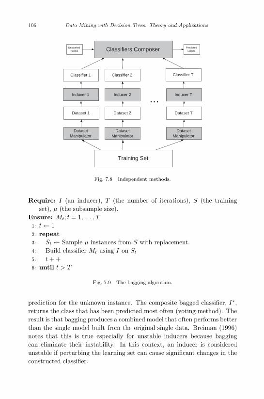
November 7, 2007 13:10 WSPC/Book Trim Size for 9in x 6in DataMining
106 Data Mining with Decision Trees: Theory and Applications
...�
Unlabeled�Tuples�
Predicted�Labels�
Inducer 1� Inducer 2� Inducer T�
Dataset�Manipulator�
Dataset�Manipulator�
Dataset�Manipulator�
Dataset 1� Dataset 2� Dataset T�
Classifier 1� Classifier 2� Classifier T�
Training Set�
Classifiers Composer�
Fig. 7.8 Independent methods.
Require: I (an inducer), T (the number of iterations), S (the trainingset), µ (the subsample size).
Ensure: Mt; t = 1, . . . , T
1: t← 12: repeat3: St ← Sample µ instances from S with replacement.4: Build classifier Mt using I on St
5: t + +6: until t > T
Fig. 7.9 The bagging algorithm.
prediction for the unknown instance. The composite bagged classifier, I∗,returns the class that has been predicted most often (voting method). Theresult is that bagging produces a combined model that often performs betterthan the single model built from the original single data. Breiman (1996)notes that this is true especially for unstable inducers because baggingcan eliminate their instability. In this context, an inducer is consideredunstable if perturbing the learning set can cause significant changes in theconstructed classifier.

November 7, 2007 13:10 WSPC/Book Trim Size for 9in x 6in DataMining
Decision Forests 107
Bagging, like boosting, is a technique for improving the accuracy of aclassifier by producing different classifiers and combining multiple models.They both use a kind of voting for classification in order to combine theoutputs of the different classifiers of the same type. In boosting, unlikebagging, each classifier is influenced by the performance of those built beforewith the new classifier trying to pay more attention to errors that were madein the previous ones and to their performances. In bagging, each instanceis chosen with equal probability, while in boosting, instances are chosenwith a probability proportional to their weight. Furthermore, accordingto Quinlan (1996), as mentioned above, bagging requires that the learningsystem should not be stable, where boosting does not preclude the use ofunstable learning systems, provided that their error rate can be kept below0.5.
7.4.2.2 Wagging
Wagging is a variant of bagging [Bauer and Kohavi (1999)] in which eachclassifier is trained on the entire training set, but each instance is stochasti-cally assigned a weight. Figure 7.10 presents the pseudo-code of the waggingalgorithm.
In fact bagging can be considered to be wagging with allocation ofweights from the Poisson distribution (each instance is represented in thesample a discrete number of times). Alternatively, it is possible to allocatethe weights from the exponential distribution, because the exponential dis-tribution is the continuous valued counterpart to the Poisson distribution[Webb (2000)].
Require: I (an inducer), T (the number of iterations), S (the trainingset), d (weighting distribution).
Ensure: Mt; t = 1, . . . , T
1: t← 12: repeat3: St ← S with random weights drawn from d.4: Build classifier Mt using I on St
5: t + +6: until t > T
Fig. 7.10 The Wagging Algorithm.

November 7, 2007 13:10 WSPC/Book Trim Size for 9in x 6in DataMining
108 Data Mining with Decision Trees: Theory and Applications
7.4.2.3 Random Forest
A random forest ensemble (also known as random subspace) [Breiman(2001)] uses a large number of individual, unpruned decision trees whichare created by randomizing the split at each node of the decision tree. Eachtree is likely to be less accurate than a tree created with the exact splits.But, by combining several of these ”approximate” trees in an ensemble, wecan improve the accuracy, often doing better than a single tree with exactsplits.
The individual trees are constructed using the algorithm presented inFigure 7.11. The input parameter N represents the number of input vari-ables that will be used to determine the decision at a node of the tree. Thisnumber should be much less than the number of attributes in the trainingset. Note that bagging can be thought of as a special case of random forestsobtained when N is set to the number of attributes in the original train-ing set. The IDT in Figure 7.11 represents any top-down decision treeinduction algorithm with the following modification: the decision tree isnot pruned and at each node, rather than choosing the best split among allattributes, the IDT randomly samples N of the attributes and chooses thebest split from among those variables. The classification of an unlabeledinstance is performed using majority vote.
Require: IDT (a decision tree inducer), T (the number of iterations), S
(the training set), µ (the subsample size). N (number of attributesused in each node)
Ensure: Mt; t = 1, . . . , T
1: t← 12: repeat3: St ← Sample µ instances from S with replacement.4: Build classifier Mt using IDT (N) on St
5: t + +6: until t > T
Fig. 7.11 The random forest algorithm.
There are other ways to obtain random forests. For example, insteadof using all the instances to determine the best split point for each feature,a sub-sample of the instances is used [Kamath and Cantu-Paz (2001)].This sub-sample varies with the feature. The feature and split value thatoptimize the splitting criterion are chosen as the decision at that node.

November 7, 2007 13:10 WSPC/Book Trim Size for 9in x 6in DataMining
Decision Forests 109
Since the split made at a node is likely to vary with the sample selected,this technique results in different trees which can be combined in ensembles.
Another method for randomization of the decision tree through his-tograms was proposed by [Kamath et al. (2002)]. The use of histogramshas long been suggested as a way of of making the features discrete, whilereducing the time to handle very large datasets. Typically, a histogramis created for each feature, and the bin boundaries used as potential splitpoints. The randomization in this process is expressed by selecting the splitpoint randomly in an interval around the best bin boundary.
Although the random forest was defined for decision trees, this approachis applicable to all types of classifiers. One important advantage of therandom forest method is its ability to handle a very large number of inputattributes [Skurichina and Duin (2002)]. Another important feature of therandom forest is that it is fast.
7.4.2.4 Cross-validated Committees
This procedure creates k classifiers by partitioning the training set intok-equal-sized sets and training, in turn, on all but the i-th set. Thismethod, first used by Gams (1989), employed 10-fold partitioning. Par-manto et al. (1996) have also used this idea for creating an ensemble of neu-ral networks. Domingos (1996) used cross-validated committees to speed uphis own rule induction algorithm RISE, whose complexity is O(n2), makingit unsuitable for processing large databases. In this case, partitioning isapplied by predetermining a maximum number of examples to which thealgorithm can be applied at once. The full training set is randomly dividedinto approximately equal-sized partitions. RISE is then run on each parti-tion separately. Each set of rules grown from the examples in partition p
is tested on the examples in partition p + 1, in order to reduce overfittingand to improve accuracy.
7.5 Ensemble Diversity
In an ensemble, the combination of the output of several classifiers is onlyuseful if they disagree about some inputs [Tumer and Ghosh (1996)].
Creating an ensemble in which each classifier is as different as possiblewhile still being consistent with the training set is theoretically known to bean important feature for obtaining improved ensemble performance [Kroghand Vedelsby (1995)]. According to [Hu (2001)], diversified classifiers lead
November 7, 2007 13:10 WSPC/Book Trim Size for 9in x 6in DataMining
110 Data Mining with Decision Trees: Theory and Applications
to uncorrelated errors, which in turn improve classification accuracy.In the regression context, the bias-variance-covariance decomposition
has been suggested to explain why and how diversity between individualmodels contribute toward overall ensemble accuracy. Nevertheless, in theclassification context, there is no complete and agreed upon theory [Brownet al. (2005)]. More specifically, there is no simple analogue of variance-covariance decomposition for the zero-one loss function. Instead, there areseveral ways to define this decomposition. Each way has its own assump-tions.
Sharkey [Sharkey (1999)] suggested a taxonomy of methods for creatingdiversity in ensembles of neural networks. More specifically, Sharkey’s tax-onomy refers to four different aspects: the initial weights; the training dataused; the architecture of the networks; and the training algorithm used.
Brown et al. [Brown et al. (2005)] suggest a different taxonomy whichconsists of the following branches: varying the starting points within thehypothesis space; varying the set of hypotheses that are accessible by theensemble members (for instance by manipulating the training set); andvarying the way each member traverses the space.
In this paper we suggest the following taxonomy. Note however thatthe components of this taxonomy are not mutually exclusive, namely, thereare a few algorithms which combine two of them.
(1) Manipulating the Inducer – We manipulate the way in which the baseinducer is used. More specifically each ensemble member is trainedwith an inducer that is differently manipulated.
(2) Manipulating the Training Sample – We vary the input that is usedby the inducer for training. Each member is trained from a differenttraining set.
(3) Changing the target attribute representation – Each classifier in theensemble solve a different target concept.
(4) Partitioning the search space – Each member is trained on a differentsearch subspace.
(5) Hybridization – Diversity is obtained by using various base inducers orensemble strategies.
7.5.1 Manipulating the Inducer
A simple method for gaining diversity is to manipulate the inducer usedfor creating the classifiers. Below we survey several strategies to gain thisdiversity.

November 7, 2007 13:10 WSPC/Book Trim Size for 9in x 6in DataMining
Decision Forests 111
7.5.1.1 Manipulation of the Inducer’s Parameters
The base inducer usually can be controlled by a set of parameters. Forexample, the well known decision tree inducer C4.5 has the confidence levelparameter that greatly affect learning.
In the neural network community, there were several attempts to gaindiversity by using different number of nodes. Nevertheless, these researchesconcludes that variation in numbers of hidden nodes is not effective methodof creating diversity in neural network ensembles. Nevertheless the CNNEalgorithm which simultaneously determines the ensemble size along withthe number of hidden nodes in individual NNs, has shown encouragingresults.
Another effective approach for ANNs is to use several network topolo-gies. For instance the Addemup algorithm [Opitz and Shavlik (1996)] usesgenetic algorithm to select the network topologies composing the ensem-ble. Addemup trains with standard backpropagation, then selects groupsof networks with a good error diversity according to the measurement ofdiversity.
7.5.1.2 Starting Point in Hypothesis Space
Some inducers can gain diversity by starting the search in the HypothesisSpace from different points. For example the simplest way to manipulatethe back-propagation inducer is to assign different initial weights to thenetwork [Kolen and Pollack (1991)]. Experimental study indicate that theresulting networks differed in the number of cycles in which they took toconverge upon a solution, and in whether they converged at all. While itis very simple way to gain diversity, it is now generally accepted that it isnot sufficient for achieving good diversity [Brown et al. (2005)].
7.5.1.3 Hypothesis Space Traversal
These techniques alter the way the inducer traverses the space, therebyleading different classifiers to converge to different hypotheses [Brownet al. (2005)]. We differentiate between two techniques for manipulating thespace traversal for gaining diversity: Random and Collective-Performance.
Random-based strategyThe idea in this case is to ”inject randomness” into the inducers in order
to increase the independence among the ensemble’s members. Ali and Paz-

November 7, 2007 13:10 WSPC/Book Trim Size for 9in x 6in DataMining
112 Data Mining with Decision Trees: Theory and Applications
zani [Ali and Pazzani (1996)] propose to change the rule learning HYDRAalgorithm in the following way: Instead of selecting the best literal at eachstage (using, for instance, an information gain measure), the literal is se-lected randomly such that its probability of being selected is proportional toits measured value. A similar idea has been implemented for C4.5 decisiontrees [Dietterich (2000a)]. Instead of selecting the best attribute in eachstage, it selects randomly (with equal probability) an attribute from theset of the best 20 attributes. MCMC (Markov Chain Monte Carlo) meth-ods can also be used for introducing randomness in the induction process[Neal (1993)].
Collective-Performance-based strategyIn this case the evaluation function used in the induction of each member
is extended to include a penalty term that encourages diversity. The moststudied penalty method is the Negative Correlation Learning [Liu (2005);Brown and Wyatt (2003); Rosen (1996)]. The idea of negative correlationlearning is to encourage different individual classifiers in the ensemble torepresent different subspaces of the problem. While simultaneously cre-ating the classifiers, the classifiers may interact with each other in orderto specialize (for instance by using a correlation penalty term in the errorfunction to encourage such specialization).
7.5.2 Manipulating the Training Samples
In this method, each classifier is trained on a different variation or subsetof the original dataset. This method is useful for inducers whose variance-error factor is relatively large (such as decision trees and neural networks).That is to say, small changes in the training set may cause a major change inthe obtained classifier. This category contains procedures such as bagging,boosting and cross-validated committees.
7.5.2.1 Resampling
The distribution of tuples among the different classifier could be random asin the bagging algorithm or in the arbiter trees. Other methods distributethe tuples based on the class distribution such that the class distribution ineach subset is approximately the same as that in the entire dataset. It hasbeen shown that proportional distribution as used in combiner trees [Chanand Stolfo (1993)] can achieve higher accuracy than random distribution.
November 7, 2007 13:10 WSPC/Book Trim Size for 9in x 6in DataMining
Decision Forests 113
Instead of perform sampling with replacement, some methods (like Ad-aBoost or Wagging) manipulate the weights that are attached to each inst-ance in the training set. The base inducer should be capable to take theseweights into account. Recently a novel framework was proposed in whicheach instance contributes to the committee formation with a fixed weight,while contributing with different individual weights to the derivation of thedifferent constituent classifiers [Christensen et al. (2004)]. This approachencourages model diversity without biasing the ensemble inadvertently to-wards any particular instance.
7.5.2.2 Creation
The DECORATE algorithm [Melville and Mooney (2003)] is a dependentapproach in which the ensemble is generated iteratively, learning a classifierat each iteration and adding it to the current ensemble. The first member iscreated by using the base induction algorithm on the original training set.The successive classifiers are trained on an artificial set that combines tuplesfrom the original training set and also on some fabricated tuples. In eachiteration, the input attribute values of the fabricated tuples are generatedaccording to the original data distribution. On the other hand, the targetvalues of these tuples are selected so as to differ maximally from the cur-rent ensemble predictions. Comprehensive experiments have demonstratedthat this technique is consistently more accurate than the base classifier,Bagging and Random Forests. Decorate also obtains higher accuracy thanboosting on small training sets, and achieves comparable performance onlarger training sets.
7.5.2.3 Partitioning
Some argue that classic ensemble techniques (such as boosting and bag-ging) have limitations on massive datasets, because the size of the datasetcan become a bottleneck [Chawla et al. (2004)]. Moreover, it is suggestedthat partitioning the datasets into random, disjoint partitions will not onlyovercome the issue of exceeding memory size, but will also lead to creatingan ensemble of diverse and accurate classifiers, each built from a disjointpartition but with the aggregate processing all of the data. This can im-prove performance in a way that might not be possible by subsampling.In fact, empirical studies have shown that the performance of the multipledisjoint partition approach is equivalent to the performance obtained by

November 7, 2007 13:10 WSPC/Book Trim Size for 9in x 6in DataMining
114 Data Mining with Decision Trees: Theory and Applications
popular ensemble techniques such as bagging. More recently a frameworkfor building thousands of classifiers that are trained from small subsetsof data in a distributed environment was proposed [Chawla et al. (2004)].It has been empirically shown that this framework is fast, accurate, andscalable.
Clustering techniques can be used to partitioning the sample. TheCBCD (cluster-based concurrent decomposition) algorithm first clustersthe instance space by using the K-means clustering algorithm. Then, itcreates disjoint sub-samples using the clusters in such a way that each sub-sample is comprised of tuples from all clusters and hence represents theentire dataset. An inducer is applied in turn to each sub-sample. A votingmechanism is used to combine the classifiers classifications. Experimentalstudy indicates that the CBCD algorithm outperforms the bagging algo-rithm.
7.5.3 Manipulating the Target Attribute Representation
In methods that manipulate the target attribute, instead of inducing asingle complicated classifier, several classifiers with different and usuallysimpler representations of the target attribute are induced. This manipula-tion can be based on an aggregation of the original target’s values (knownas Concept Aggregation) or more complicated functions (known as FunctionDecomposition).
Classical concept aggregation replaces the original target attribute witha function, such that the domain of the new target attribute is smaller thanthe original one.
Concept aggregation has been used to classify free text documents intopredefined topics [Buntine (1996)]. This application suggests breaking thetopics up into groups (co-topics) and then, instead of predicting the doc-ument’s topic directly, classifying the document into one of the co-topics.Another model is then used to predict the actual topic in that co-topic.
A general concept aggregation algorithm called Error-Correcting OutputCoding (ECOC) which converts multi-class problems into multiple, two-class problems has been suggested by [Dietterich and Bakiri (1995)]. Aclassifier is built for each possible binary partition of the classes. Expe-riments show that ECOC improves the accuracy of neural networks anddecision trees on several multi-class problems from the UCI repository.
The idea to convert K class classification problems into K-two classclassification problems has been proposed by [Anand et al. (1995)]. Each

November 7, 2007 13:10 WSPC/Book Trim Size for 9in x 6in DataMining
Decision Forests 115
problem considers the discrimination of one class to the other classes. Luand Ito [Lu and Ito (1999)] extend Anand’s method and propose a newmethod for manipulating the data based on the class relations among thetraining data. By using this method, they divide a K class classificationproblem into a series of K(K−1)/2 two-class problems where each problemconsiders the discrimination of one class to each one of the other classes.The researchers used neural networks to examine this idea.
Function decomposition was originally developed in the Fifties and Six-ties for designing switching circuits. It was even used as an evaluationmechanism for checker playing programs [Samuel (1967)]. This approachwas later improved by [Biermann et al. (1982)]. Recently the machine learn-ing community has adopted this approach. A manual decomposition of theproblem and an expert-assisted selection of examples to construct rules forthe concepts in the hierarchy was studied in [Michie (1995)]. Compared tostandard decision tree induction techniques, structured induction exhibitsabout the same degree of classification accuracy with the increased trans-parency and lower complexity of the developed models. A general-purposefunction decomposition approach for machine learning was proposed in [Zu-pan et al. (1998)]. According to this approach, attributes are transformedinto new concepts in an iterative manner to create a hierarchy of concepts.A different function decomposition which can be applied in data miningis the Bi-Decomposition [Long (2003)]. In this approach the original func-tion is decomposed into two decomposition functions that are connectedby a two-input operator called a ”gate”. Each of the decomposition func-tions depends on fewer variables than the original function. Recursive bi-decomposition represents a function as a structure of interconnected gates.
7.5.4 Partitioning the Search Space
The idea is that each member in the ensemble explores a different part ofthe search space. Thus, the original instance space is divided into severalsub-spaces. Each sub-space is considered independently and the total modelis a (possibly soft) union of such simpler models.
When using this approach, one should decide if the subspaces will over-lap. At one extreme, the original problem is decomposed into several mu-tually exclusive sub-problems, such that each subproblem is solved usinga dedicated classifier. In such cases, the classifiers may have significantvariations in their overall performance over different parts of the inputspace [Tumer and Ghosh (2000)]. At the other extreme, each classifier

November 7, 2007 13:10 WSPC/Book Trim Size for 9in x 6in DataMining
116 Data Mining with Decision Trees: Theory and Applications
solves the same original task. In such cases, “If the individual classifiersare then appropriately chosen and trained properly, their performances willbe (relatively) comparable in any region of the problem space. [Tumer andGhosh (2000)]”. However, usually the sub-spaces may have soft boundaries,namely sub-spaces are allowed to overlap.
There are two popular approaches for search space manipulations: di-vide and conquer approaches and feature subset-based ensemble methods.
7.5.4.1 Divide and Conquer
In the neural-networks community, Nowlan and Hinton [Nowlan and Hin-ton (1991)] examined the mixture of experts (ME) approach, which parti-tions the instance space into several subspaces and assigns different experts(classifiers) to the different subspaces. The subspaces, in ME, have softboundaries (i.e., they are allowed to overlap). A gating network then com-bines the experts’ outputs and produces a composite decision.
Some researchers have used clustering techniques to partition the space.The basic idea is to partition the instance space into mutually exclusivesubsets using K-means clustering algorithm. An analysis of the resultsshows that the proposed method is well suited for datasets of numeric inputattributes and that its performance is influenced by the dataset size and itshomogeneity.
NBTree [Kohavi (1996)] is an instance space decomposition method thatinduces a decision tree and a Naıve Bayes hybrid classifier. Naıve Bayes,which is a classification algorithm based on Bayes’ theorem and a Naıve in-dependence assumption, is very efficient in terms of its processing time. Toinduce an NBTree, the instance space is recursively partitioned accordingto attributes values. The result of the recursive partitioning is a decisiontree whose terminal nodes are Naıve Bayes classifiers. Since subjecting aterminal node to a Naıve Bayes classifier means that the hybrid classifiermay classify two instances from a single hyper-rectangle region into distinctclasses, the NBTree is more flexible than a pure decision tree. In order to de-cide when to stop the growth of the tree, NBTree compares two alternativesin terms of error estimation - partitioning into a hyper-rectangle region andinducing a single Naıve Bayes classifier. The error estimation is calculatedby cross-validation, which significantly increases the overall processing time.Although NBTree applies a Naıve Bayes classifier to decision tree terminalnodes, classification algorithms other than Naıve Bayes are also applicable.However, the cross-validation estimations make the NBTree hybrid com-

November 7, 2007 13:10 WSPC/Book Trim Size for 9in x 6in DataMining
Decision Forests 117
putationally expensive for more time-consuming algorithms such as neuralnetworks.
More recently Cohen et al. [Cohen et al. (2007)] generalizes the NBTreeidea and examines a decision-tree framework for space decomposition.According to this framework, the original instance-space is hierarchicallypartitioned into multiple subspaces and a distinct classifier (such as neu-ral network) is assigned to each subspace. Subsequently, an unlabeled,previously-unseen instance is classified by employing the classifier that wasassigned to the subspace to which the instance belongs.
The divide and conquer approach includes many other specific methodssuch as local linear regression, CART/MARS, adaptive subspace models,etc [Johansen and Foss (1992); Ramamurti and Ghosh (1999); Holmstromet al. (1997)].
7.5.4.2 Feature Subset-based Ensemble Methods
Another less common strategy for manipulating the search space is to ma-nipulate the input attribute set. Feature subset based ensemble methodsare those that manipulate the input feature set for creating the ensemblemembers. The idea is to simply give each classifier a different projection ofthe training set. Tumer and Oza. Feature subset-based ensembles poten-tially facilitate the creation of a classifier for high dimensionality data setswithout the feature selection drawbacks mentioned above. Moreover, thesemethods can be used to improve the classification performance due to thereduced correlation among the classifiers. Bryll et al. also indicate that thereduced size of the dataset implies faster induction of classifiers. Featuresubset avoids the class under-representation which may happen in instancesubsets methods such as bagging. There are three popular strategies forcreating feature subset-based ensembles: random-based, reduct-based andcollective-performance-based strategy.
Random-based strategyThe most straightforward techniques for creating feature subset-based
ensemble are based on random selection. Ho [Ho (1998)] creates a forestof decision trees. The ensemble is constructed systematically by pseudo-randomly selecting subsets of features. The training instances are projectedto each subset and a decision tree is constructed using the projected train-ing samples. The process is repeated several times to create the forest. Theclassifications of the individual trees are combined by averaging the condi-

November 7, 2007 13:10 WSPC/Book Trim Size for 9in x 6in DataMining
118 Data Mining with Decision Trees: Theory and Applications
tional probability of each class at the leaves (distribution summation). Hoshows that simple random selection of feature subsets may be an effectivetechnique because the diversity of the ensemble members compensates fortheir lack of accuracy.
Bay [Bay (1999)] proposed using simple voting in order to combineoutputs from multiple KNN (K-Nearest Neighbor) classifiers, each havingaccess only to a random subset of the original features. Each classifieremploys the same number of features. A technique for building ensemblesof simple Bayesian classifiers in random feature subsets was also examined[Tsymbal and Puuronen (2002)] for improving medical applications.
Reduct-based strategyA reduct is defined as the smallest feature subset which has the same
predictive power as the whole feature set. By definition, the size of theensembles that were created using reducts are limited to the number offeatures. There have been several attempts to create classifier ensemblesby combining several reducts. Wu et al. introduce the worst-attribute-drop-first algorithm to find a set of significant reducts and then combinethem using naıve Bayes.
Collective-Performance-based strategyCunningham and Carney [Cunningham and Carney (2000)] introduced
an ensemble feature selection strategy that randomly constructs the ini-tial ensemble. Then, an iterative refinement is performed based on a hill-climbing search in order to improve the accuracy and diversity of the baseclassifiers. For all the feature subsets, an attempt is made to switch (includeor delete) each feature. If the resulting feature subset produces a betterperformance on the validation set, that change is kept. This process is con-tinued until no further improvements are obtained. Similarly, Zenobi andCunningham [Zenobi and Cunningham (2001)] suggest that the search forthe different feature subsets will not be solely guided by the associated errorbut also by the disagreement or ambiguity among the ensemble members.
Tsymbal et al. [Tsymbal et al. (2004)] compare several feature selectionmethods that incorporate diversity as a component of the fitness function inthe search for the best collection of feature subsets. This study shows thatthere are some datasets in which the ensemble feature selection method canbe sensitive to the choice of the diversity measure. Moreover, no particularmeasure is superior in all cases.
Gunter and Bunke [Gunter and Bunke (2004)] suggest employing a fea-

November 7, 2007 13:10 WSPC/Book Trim Size for 9in x 6in DataMining
Decision Forests 119
ture subset search algorithm in order to find different subsets of the givenfeatures. The feature subset search algorithm not only takes the perfor-mance of the ensemble into account, but also directly supports diversity ofsubsets of features.
Combining genetic search with ensemble feature selection was also ex-amined in the literature. Opitz and Shavlik [Opitz and Shavlik (1996)]applied GAs to ensembles using genetic operators that were designed ex-plicitly for hidden nodes in knowledge-based neural networks. In a laterresearch, Opitz [Opitz (1999)] used genetic search for ensemble featureselection. This genetic ensemble feature selection (GEFS) strategy beginsby creating an initial population of classifiers where each classifier is gen-erated by randomly selecting a different subset of features. Then, newcandidate classifiers are continually produced by using the genetic opera-tors of crossover and mutation on the feature subsets. The final ensembleis composed of the most fitted classifiers.
Feature set partitioningFeature set partitioning is a particular case of feature subset-based en-
sembles in which the subsets are pairwise disjoint subsets. At the sametime, feature set partitioning generalizes the task of feature selection whichaims to provide a single representative set of features from which a classifieris constructed. Feature set partitioning, on the other hand, decomposes theoriginal set of features into several subsets and builds a classifier for eachsubset. Thus, a set of classifiers is trained such that each classifier employsa different subset of the original feature set. Subsequently, an unlabelledinstance is classified by combining the classifications of all classifiers.
Several researchers have shown that the partitioning methodology canbe appropriate for classification tasks with a large number of features [Ku-siak (2000)]. The search space of a feature subset-based ensemble containsthe search space of feature set partitioning, and the latter contains thesearch space of feature selection. Mutually exclusive partitioning has someimportant and helpful properties:
(1) There is a greater possibility of achieving reduced execution time com-pared to non-exclusive approaches. Since most learning algorithms havecomputational complexity that is greater than linear in the number offeatures or tuples, partitioning the problem dimensionality in a mutu-ally exclusive manner means a decrease in computational complexity[Provost and Kolluri (1997)].

November 7, 2007 13:10 WSPC/Book Trim Size for 9in x 6in DataMining
120 Data Mining with Decision Trees: Theory and Applications
(2) Since mutual exclusiveness entails using smaller datasets, the classi-fiers obtained for each sub-problem are smaller in size. Without themutually exclusive restriction, each classifier can be as complicated asthe classifier obtained for the original problem. Smaller classifiers con-tribute to comprehensibility and ease in maintaining the solution.
(3) According to Bay [Bay (1999)], mutually exclusive partitioning mayhelp avoid some error correlation problems that characterize featuresubset based ensembles. However Sharkey [Sharkey (1996)] argues thatmutually exclusive training sets do not necessarily result in low errorcorrelation. This point is true when each sub-problem is representative.
(4) In feature subset-based ensembles, different classifiers might generatecontradictive classifications using the same features. This inconsistencyin the way a certain feature can affect the final classification may in-crease mistrust among end-users. We claim that end-users can graspmutually exclusive partitioning much easier.
(5) The mutually exclusive approach encourages smaller datasets which aregenerally more practicable. Some data mining tools can process onlylimited dataset sizes (for instance, when the program requires thatthe entire dataset will be stored in the main memory). The mutuallyexclusive approach can ensure that data mining tools can be scaledfairly easily to large data sets [Chan and Stolfo (1997)].
In the literature there are several works that deal with feature set parti-tioning. In one research, the features are grouped according to the featuretype: nominal value features, numeric value features and text value fea-tures [Kusiak (2000)]. A similar approach was also used for developing thelinear Bayes classifier [Gama (2000)]. The basic idea consists of aggregatingthe features into two subsets: the first subset containing only the nominalfeatures and the second only the continuous features.
In another research, the feature set was decomposed according to thetarget class [Tumer and Ghosh (1996)]. For each class, the features with lowcorrelation relating to that class were removed. This method was appliedon a feature set of 25 sonar signals where the target was to identify themeaning of the sound (whale, cracking ice, etc.). Feature set partitioninghas also been used for radar-based volcano recognition [Cherkauer (1996)].The researcher manually decomposed a feature set of 119 into 8 subsets.Features that were based on different image processing operations weregrouped together. As a consequence, for each subset, four neural networkswith different sizes were built. A new combining framework for feature

November 7, 2007 13:10 WSPC/Book Trim Size for 9in x 6in DataMining
Decision Forests 121
set partitioning has been used for text-independent speaker identification[Chen et al. (1997)]. Other researchers manually decomposed the featuresset of a certain truck backer-upper problem and reported that this strategyhas important advantages [Jenkins and Yuhas (1993)].
The feature set decomposition can be obtained by grouping featuresbased on pairwise mutual information, with statistically similar featuresassigned to the same group [Liao and Moody (2000)]. For this purpose onecan use an existing hierarchical clustering algorithm. As a consequence,several feature subsets are constructed by selecting one feature from eachgroup. A neural network is subsequently constructed for each subset. Allnetworks are then combined.
In statistics literature, the well-known feature-oriented ensemble algo-rithm is the MARS algorithm [Friedman (1991)]. In this algorithm, a mul-tiple regression function is approximated using linear splines and their ten-sor products. It has been shown that the algorithm performs an ANOVAdecomposition, namely, the regression function is represented as a grandtotal of several sums. The first sum is of all basic functions that involveonly a single attribute. The second sum is of all basic functions that involveexactly two attributes, representing (if present) two-variable interactions.Similarly, the third sum represents (if present) the contributions from three-variable interactions, and so on.
A general framework that searches for helpful feature set partitioningstructures has also been proposed [Rokach and Maimon (2005b)]. Thisframework nests many algorithms, two of which are tested empirically overa set of benchmark datasets. The first algorithm performs a serial searchwhile using a new Vapnik-Chervonenkis dimension bound for multiple obliv-ious trees as an evaluating scheme. The second algorithm performs a multi-search while using a wrapper evaluating scheme. This work indicates thatfeature set decomposition can increase the accuracy of decision trees.
7.5.5 Multi-Inducers
In Multi-Inducer strategy, diversity is obtained by using different types ofinducers [Michalski and Tecuci (1994)]. Each inducer contains an explicit orimplicit bias [Mitchell (1980)] that leads it to prefer certain generalizationsover others. Ideally, this multi-inducer strategy would always perform aswell as the best of its ingredients. Even more ambitiously, there is hope thatthis combination of paradigms might produce synergistic effects, leading tolevels of accuracy that neither atomic approach by itself would be able to

November 7, 2007 13:10 WSPC/Book Trim Size for 9in x 6in DataMining
122 Data Mining with Decision Trees: Theory and Applications
achieve.Most research in this area has been concerned with combining empiri-
cal approaches with analytical methods (see for instance [Towell and Shav-lik (1994)]. Woods et al. [Woods et al. (1997)] combine four types of baseinducers (decision trees, neural networks, k-nearest neighbor, and quadraticBayes). They then estimate local accuracy in the feature space to choosethe appropriate classifier for a given new unlabled instance. Wang et al.[Wang et al. (2004)] examined the usefulness of adding decision trees to anensemble of neural networks. The researchers concluded that adding a fewdecision trees (but not too many) usually improved the performance. Lang-don et al. [Langdon et al. (2002)] proposed using Genetic Programming tofind an appropriate rule for combining decision trees with neural networks.
The model class selection (MCS) system fits different classifiers to dif-ferent subspaces of the instance space, by employing one of three classifica-tion methods (a decision-tree, a discriminant function or an instance-basedmethod). In order to select the classification method, MCS uses the char-acteristics of the underlined training-set, and a collection of expert rules.Brodley’s expert-rules were based on empirical comparisons of the methods’performance (i.e., on prior knowledge).
The NeC4.5 algorithm, which integrates decision tree with neural net-works [Zhou and Jiang (2004)], first trains a neural network ensemble.Then, the trained ensemble is employed to generate a new training setby replacing the desired class labels of the original training examples withthe output from the trained ensemble. Some extra training examples arealso generated from the trained ensemble and added to the new trainingset. Finally, a C4.5 decision tree is grown from the new training set. Sinceits learning results are decision trees, the comprehensibility of NeC4.5 isbetter than that of neural network ensembles.
Using several inducers can solve the dilemma which arises from the “nofree lunch” theorem. This theorem implies that a certain inducer will besuccessful only insofar its bias matches the characteristics of the applica-tion domain [Brazdil et al. (1994)]. Thus, given a certain application, thepractitioner need to decide which inducer should be used. Using the multi-inducer obviate the need to try each one and simplifying the entire process.
7.5.6 Measuring the Diversity
As stated above, it is usually assumed that increasing diversity maydecrease ensemble error [Zenobi and Cunningham (2001)]. For regres-

November 7, 2007 13:10 WSPC/Book Trim Size for 9in x 6in DataMining
Decision Forests 123
sion problems, variance is usually used to measure diversity [Krogh andVedelsby (1995)]. In such cases it can be easily shown that the ensembleerror can be reduced by increasing ensemble diversity while maintainingthe average error of a single model.
In classification problems, a more complicated measure is required toevaluate the diversity. There have been several attempts to define diversitymeasure for classification tasks.
In the neural network literature two measures are presented for exam-ining diversity:
• Classification coverage: An instance is covered by a classifier, if it yieldsa correct classification.• Coincident errors: A coincident error amongst the classifiers occurs
when more than one member misclassifies a given instance.
Based on these two measures, Sharkey (1997) defined four diversity levels:
• Level 1 - No coincident errors and the classification function is com-pletely covered by a majority vote of the members.• Level 2 - Coincident errors may occur, but the classification function is
completely covered by a majority vote.• Level 3 - A majority vote will not always correctly classify a given
instance, but at least one ensemble member always correctly classifiesit.• Level 4 - The function is not always covered by the members of the
ensemble.
Brown et al. [Brown et al. (2005)] claim that the above four-level schemeprovides no indication of how typical the error behaviour described by theassigned diversity level is. This claim, especially, holds when the ensembleexhibits different diversity levels on different subsets of instance space.
There are other more quantative measures which categorize these mea-sures into two types [Brown et al. (2005)]: pairwise and non-pairwise. Pair-wise measures calculate the average of a particular distance metric betweenall possible pairings of members in the ensemble, such as Q-statistic [Brownet al. (2005)] or kappa-statistic [Margineantu and Dietterich (1997)]. Thenon-pairwise measures either use the idea of entropy (such as [Cunninghamand Carney (2000)]) or calculate a correlation of each ensemble memberwith the averaged output. The comparison of several measures of diversityhas resulted in the conclusion that most of them are correlated [Kuncheva
November 7, 2007 13:10 WSPC/Book Trim Size for 9in x 6in DataMining
124 Data Mining with Decision Trees: Theory and Applications
and Whitaker (2003)].
7.6 Ensemble Size
7.6.1 Selecting the Ensemble Size
An important aspect of ensemble methods is to define how many componentclassifiers should be used. There are several factors that may determine thissize:
• Desired accuracy — In most cases, ensembles containing ten classifiersare sufficient for reducing the error rate [Hansen (1990)]. Neverthe-less, there is empirical evidence indicating that: when AdaBoost usesdecision trees, error reduction is observed in even relatively large en-sembles containing 25 classifiers [Opitz and Maclin (1999)]. In disjointpartitioning approaches, there may be a trade-off between the numberof subsets and the final accuracy. The size of each subset cannot betoo small because sufficient data must be available for each learningprocess to produce an effective classifier.• Computational cost — Increasing the number of classifiers usually in-
creases computational cost and decreases their comprehensibility. Forthat reason, users may set their preferences by predefining the ensemblesize limit.• The nature of the classification problem - In some ensemble methods,
the nature of the classification problem that is to be solved, determinesthe number of classifiers. For instance in the ECOC algorithm thenumber of classes determine the ensemble size.• Number of processors available — In independent methods, the number
of processors available for parallel learning could be put as an upperbound on the number of classifiers that are treated in paralleled process.
There three methods that are used to determine the ensemble size, asdescribed by the following subsections.
7.6.2 Pre Selection of the Ensemble Size
This is the most simple way to determine the ensemble size. Many ensemblealgorithms have a controlling parameter such as ”number of iterations”,which is can be set by the user. Algorithms such as Bagging belong to this

November 7, 2007 13:10 WSPC/Book Trim Size for 9in x 6in DataMining
Decision Forests 125
category. In other cases the nature of the classification problem determinethe number of members (such as in the case of ECOC).
7.6.3 Selection of the Ensemble Size while Training
There are ensemble algorithms that try to determine the best ensemble sizewhile training. Usually as new classifiers are added to the ensemble thesealgorithms check if the contribution of the last classifier to the ensembleperformance is still significant. If it is not, the ensemble algorithm stops.Usually these algorithms also have a controlling parameter which boundsthe maximum size of the ensemble.
An algorithm that decides when a sufficient number of classificationtrees have been created was recently proposed [Banfield et al. (2007)]. Thealgorithm uses the out-of-bag error estimate, and is shown to result in anaccurate ensemble for those methods that incorporate bagging into the con-struction of the ensemble. Specifically, the algorithm works by first smooth-ing the out-of-bag error graph with a sliding window in order to reduce thevariance. After the smoothing has been completed, the algorithm takes alarger window on the smoothed data points and determines the maximumaccuracy within that window. It continues to process windows until themaximum accuracy within a particular window no longer increases. At thispoint, the stopping criterion has been reached and the algorithm returnsthe ensemble with the maximum raw accuracy from within that window.
7.6.4 Pruning — Post Selection of the Ensemble Size
As in decision tree induction, it is sometimes useful to let the ensemblegrow freely and then prune the ensemble in order to get more effective andcompact ensembles. Post selection of the ensemble size allows ensemble op-timization for such performance metrics as accuracy, cross entropy, meanprecision, or the ROC area. Empirical examinations indicate that prunedensembles may obtain a similar accuracy performance as the original en-semble [Margineantu and Dietterich (1997)]. In another empirical studythat was conducted in order to understand the affect of ensemble sizes onensemble accuracy and diversity, it has been shown that it is feasible tokeep a small ensemble while maintaining accuracy and diversity similar tothose of a full ensemble [Liu et al., 2004].
The pruning methods can be divided into two groups: pre-combiningpruning methods and post-combining pruning methods.

November 7, 2007 13:10 WSPC/Book Trim Size for 9in x 6in DataMining
126 Data Mining with Decision Trees: Theory and Applications
7.6.4.1 Pre-combining Pruning
Pre-combining pruning is performed before combining the classifiers. Clas-sifiers that seem to perform well are included in the ensemble. Prodromidiset al. [Prodromidis et al. (1999)] present three methods for pre-combiningpruning: based on an individual classification performance on a separatevalidation set, diversity metrics, the ability of classifiers to classify correctlyspecific classes.
In attribute bagging, classification accuracy of randomly selected m-attribute subsets is evaluated by using the wrapper approach and onlythe classifiers constructed on the highest ranking subsets participate in theensemble voting.
7.6.4.2 Post-combining Pruning
In post-combining pruning methods, we remove classifiers based on theircontribution to the collective.
Prodromidis examines two methods for post-combining pruning as-suming that the classifiers are combined using meta-combination method:Based on decision tree pruning and the correlation of the base classifier tothe unpruned meta-classifier.
A forward stepwise selection procedure can be used in order to selectthe most relevant classifiers (that maximize the ensemble’s performance)among thousands of classifiers [Caruana et al. (2004)]. It has been shownthat for this purpose one can use feature selection algorithms. However,instead of selecting features one should select the ensemble’s members [Liuet al., 2004].
One can also rank the classifiers according to their ROC performance.Then, they suggest to plot a graph where the Y- axis displays a performancemeasure of the integrated classification. The X-axis presents the number ofclassifiers that participated in the combination. i.e., the first best classifiersfrom the list are combined by voting (assuming equal weights for now) withthe rest getting zero weights. The ensemble size is chosen when there areseveral sequential points with no improvement.
The GASEN algorithm was developed for selecting the most appropri-ate classifiers in a given ensemble [Zhou et al. (2002)]. In the initializationphase, GASEN assigns a random weight to each of the classifiers. Conse-quently, it uses genetic algorithms to evolve those weights so that they cancharacterize to some extent the fitness of the classifiers in joining the en-semble. Finally, it removes from the ensemble those classifiers whose weight

November 7, 2007 13:10 WSPC/Book Trim Size for 9in x 6in DataMining
Decision Forests 127
is less than a predefined threshold value.Recently a revised version of the GASEN algorithm called GASEN-b
has been suggested [Zhou and Tang (2003)]. In this algorithm, instead ofassigning a weight to each classifier, a bit is assigned to each classifier in-dicating whether it will be used in the final ensemble. In an experimentalstudy the researchers showed that ensembles generated by a selective en-semble algorithm, which selects some of the trained C4.5 decision trees tomake up an ensemble, may be not only smaller in size but also stronger inthe generalization than ensembles generated by non-selective algorithms.
A comparative study of pre combining and post combining methodswhen meta-combining methods are used has been performed in [Prodro-midis et al. (1999)]. The results indicate that the post-combining pruningmethods tend to perform better in this case.
7.7 Cross-Inducer
This property indicates the relation between the ensemble technique andthe inducer used.
Some implementations are considered as an inducer-dependent type,namely these ensemble generators which use intrinsic inducer, have beendeveloped specifically for a certain inducer. They can neither work norguarantee effectiveness in any other induction method. For instance, theworks of [Hansen (1990); Lu and Ito (1999); Sharkey (1996)] were developedspecifically for neural networks. The works of [Breiman (2001); Rokach andMaimon (2005b)] were developed specifically for decision trees.
Other implementations are considered to be the inducer-independenttype. These implementations can be performed on any given inducer andare not limited to a specific inducer like the inducer-dependent.
7.8 Multistrategy Ensemble Learning
Multistrategy ensemble learning combines several ensemble strategies. Ithas been shown that this hybrid approach increases the diversity of ensem-ble members.
MultiBoosting, an extension to AdaBoost expressed by adding wagging-like features [Webb (2000)], can harness both AdaBoost’s high bias andvariance reduction with wagging’s superior variance reduction. Using C4.5as the base learning algorithm, MultiBoosting, significantly more often than
November 7, 2007 13:10 WSPC/Book Trim Size for 9in x 6in DataMining
128 Data Mining with Decision Trees: Theory and Applications
the reverse, produces decision committees with lower error than either Ad-aBoost or wagging. It also offers the further advantage over AdaBoostof suiting parallel execution. MultiBoosting has been further extended byadding the stochastic attribute selection committee learning strategy toboosting and wagging [Webb and Zheng (2004)]. The latter’s research hasshown that combining ensemble strategies would increase diversity at thecost of a small increase in individual test error resulting in a trade-off thatreduced overall ensemble test error.
Another multistrategy method suggests to create the ensemble by de-composing the original classification problem into several smaller and moremanageable sub-problems. This multistrategy uses an elementary decom-position framework that consists of five different elementary decomposi-tions: Concept Aggregation, Function, Sample, Space and Feature Set. Theconcept of elementary decomposition can be used to obtain a complicateddecomposition by using the elementary decomposition concept recursively.Given a certain problem, the procedure selects the most appropriate ele-mentary decomposition (if any) to that problem. A suitable decomposerthen decomposes the problem and provides a set of sub-problems. A simi-lar procedure is performed on each sub-problem until no beneficial decom-position is anticipated. The selection of the best elementary decompositionfor a given problem is performed by using a meta-learning approach.
7.9 Which Ensemble Method Should be Used?
Recent research has experimentally evaluated bagging and seven otherrandomization-based approaches for creating an ensemble of decision treeclassifiers [Banfield et al. (2007)]. Statistical tests were performed on exper-imental results from 57 publicly available datasets. When cross-validationcomparisons were tested for statistical significance, the best method wasstatistically more accurate than bagging on only eight of the 57 datasets.Alternatively, examining the average ranks of the algorithms across thegroup of datasets, Banfield found that boosting, random forests, and ran-domized trees is statistically significantly better than bagging.
7.10 Open Source for Decision Trees Forests
There are two open source software packages which can be used for creatingdecision trees forests. Both systems, which are free, are distributed under

November 7, 2007 13:10 WSPC/Book Trim Size for 9in x 6in DataMining
Decision Forests 129
the terms of the GNU General Public License.
• The OpenDT [Banfield (2005)] package has the ability to output treesvery similar to C4.5, but has added functionality for ensemble creation.In the event that the attribute set randomly chosen provides a nega-tive information gain, the OpenDT approach is to randomly rechooseattributes until a positive information gain is obtained, or no furthersplit is possible. This enables each test to improve the purity of theresultant leaves. The system is written in Java.• The Weka package [Frank et. al (2005)] is an organized collection
of state-of-the-art machine learning algorithms and data preprocessingtools. The basic way of interacting with these methods is by invokingthem from the command line. However, convenient interactive graph-ical user interfaces are provided for data exploration, for setting uplarge-scale experiments on distributed computing platforms, and fordesigning configurations for streamed data processing. These inter-faces constitute an advanced environment for experimental data min-ing. Weka includes many decision tree learners: decision stumps, ID3,a C4.5 clone called “J48,” trees generated by reduced error pruning, al-ternating decision trees, and random trees and forests thereof, includingrandom forests, bagging, boosting, and stacking.

November 7, 2007 13:10 WSPC/Book Trim Size for 9in x 6in DataMining
This page intentionally left blankThis page intentionally left blank

November 7, 2007 13:10 WSPC/Book Trim Size for 9in x 6in DataMining
Chapter 8
Incremental Learning ofDecision Trees
8.1 Overview
To reflect new data that has become available, most decision trees indu-cers must be rebuilt from scratch. This is time-consuming and expen-sive and several researchers have addressed the issue of updating decisiontrees incrementally. Utgoff [Utgoff (1989b); Utgoff (1997)], for example,presents several methods for incrementally updating decision trees while[Crawford (1989)] describes an extension to the CART algorithm that iscapable of inducing incremental changes.
8.2 The Motives for Incremental Learning
In the ever-changing world of information technology there are two funda-mental problems to be addressed:
• Vast quantities of digital data continue to grow at staggering rates.In organizations such as e-commerce sites, large retailers and telecom-munication corporations, data increases of gigabytes per day are notuncommon. While this data could be extremely valuable to these or-ganizations, the tremendous volume makes it virtually impossible toextract useful information. This is due to the fact that KDD systemsin general, and traditional data mining algorithms in particular, arelimited by several crippling factors. These factors, referred to as com-putational resources, are the size of the sample to be processed, runningtime and memory. As a result, most of the available data is unusedwhich leads to underfitting. While there is enough data to model acompound phenomenon, there is no capability for fully utilizing this
131
November 7, 2007 13:10 WSPC/Book Trim Size for 9in x 6in DataMining
132 Data Mining with Decision Trees: Theory and Applications
data and unsatisfactorily simple models are produced.• Most machine learning algorithms, among them those underlying the
data mining process assume that the data, which needs to be learned(training data), serves as a random sample drawn from a stationary dis-tribution. (These algorithms include CART (Breiman et al. (1984)),ID3 (Quinlan, J.R., (1986)), C4.5 (Quinlan, J.R., 1986)), IFN (Mai-mon and Last (2000)) and very fast decision tree (VFDT) (Domingosand Hulten (2000).) The assumption is unfortunately violated by themajority of databases and data streams available for mining today.These databases accumulate over large periods of time, with the un-derlying processes generating them changing respectively and at timesquite drastically. This occurrence is known as concept drift. Accordingto [Domingos and Hulten (2001)] “in many cases... it is more accurateto assume that data was generated by ... a concept function with time-varying parameters.” Incorrect models are learned by the traditionaldata mining algorithms when these mistakenly assume that the under-lying concept is stationary, when it is, in fact, drifting. This may serveto degrade the predictive performance of the models.
A prime example of systems which may have to deal with the afore-mentioned problems are on-line learning systems, which use continuousincoming batches of training examples to induce rules for a classificationtask. Two instances in which these systems are currently utilized are creditcard fraud detection and real-time monitoring of manufacturing processes.
As a result of the above mentioned problems it is now common prac-tice to mine a sub-sample of the available data or to mine for a modeldrastically simpler than the data could support. Ideally, the KDD systemswill function continuously, constantly processing data received so that po-tentially valuable information is never lost. In order to achieve this goal,many methods have been developed. Termed incremental (online) learningmethods, these methods aim to extract patterns from changing streams ofdata.
8.3 The Inefficiency Challenge
According to [Domingos and Hulten (2001)], incremental learning algo-rithms suffer from numerous inadequacies from the KDD point of view.Whereas some of these algorithms are relatively efficient, they do not guar-

November 7, 2007 13:10 WSPC/Book Trim Size for 9in x 6in DataMining
Incremental Learning of Decision Trees 133
antee that the model that emerges will be similar to the one obtained bylearning on the same data in the non-incremental (batch) methods. Otherincremental learning algorithms produce the same model as the batch ver-sion, but at a higher cost in efficiency, which may mean longer trainingtimes.
In order to overcome this trade-off, Domingos and Hulten (2000) pro-posed VFDT a decision-tree learning method which is aimed at learningonline from high-volume data streams by using sub-sampling of the entiredata stream generated by a stationary process. This method uses constanttime per example and constant memory and can incorporate tens of thou-sands of examples per second using off-the-shelf hardware. This methodinvolves learning by seeing each example only once; there is no necessity forstoring them. As a result it is possible to directly mine online data sources.The sample size is determined in VFDT from distribution-free Hoeffdingbounds to guarantee that its output is asymptotically nearly identical tothat of a conventional learner.
8.4 The Concept Drift Challenge
The second problem, centered around concept drift, is also addressed by in-cremental learning methods that have been adapted to work effectively withcontinuous, time-changing data streams. Black and Hickey (1999) identifiedseveral important sub-tasks involved in handling drift within incrementallearning methods. The two most fundamental sub-tasks are identifying thatdrift is occurring and updating classification rules in the light of this drift.
Time-windowing is one of the most known and acceptable approachesfor dealing with these tasks. The basic concept of this approach is therepeated application of a learning algorithm to a sliding window, whichcontains a certain amount (either constant or changing) of examples. Asnew examples arrive, they are placed into the beginning of the window. Acorresponding number of examples are removed from the end of the window.The latest model is the one used for future prediction of incoming instancesuntil concept drift is detected. At this point the learner is reapplied on thelast window of instances and a new model is built.
FLORA, the time-windowing approach developed by [Widmer and Ku-bat (1996)] describes a family of incremental algorithms for learning in thepresence of drift. This method uses a currently trusted window of examplesas well as stored, old concept hypothesis description sets which are reacti-

November 7, 2007 13:10 WSPC/Book Trim Size for 9in x 6in DataMining
134 Data Mining with Decision Trees: Theory and Applications
vated if they seem to be valid again. The first realization of this frameworkof this family of incremental algorithms is FLORA2, which maintains a dy-namically adjustable window of the latest training examples. The methodof adjusting the size of the window is known as WAH (window adjustmentheuristic). Whenever a concept drift is suspected as a result of a drop inpredictive accuracy, the size of the window is decreased by disposing of theoldest examples. The window size is left unchanged if the concept appearsto be stable. If concept drift remains uncertain, none of the examples areforgotten, and thus the window size is gradually increased until a stableconcept description can be formed. As long as a relatively low rate of con-cept drift is preserved this strategy of window adjustment can detect radicalchanges in the underlying concept efficiently.
FLORA3 stores concepts for later use and reassesses their utility whena context change is perceived. FLORA4 is designed to be exceptionallyrobust with respect to noise in the training data since it is very difficult inincremental learning to distinguish between slight irregularities due to noiseand actual concept drift. Both of these algorithms serve as an extension ofFLORA2.
According to [Domingos and Hulten (2001)], as long as the window sizeis small relative to the rate of concept drift, the time-windowing procedureassures availability of a model reflecting the current concept generating thedata. However, if the window is too small, this may result in insufficientexamples to satisfactorily learn the concept. Furthermore, the computa-tional cost of reapplying a learner may be prohibitively high, especially ifexamples arrive at a rapid rate and the concept changes quickly.
To meet these challenges, Domingos and Hulten (2001) proposed anefficient algorithm for mining decision trees from continuously changingdata streams. Called CVFDT (concept-adapting very fast decision treeslearner), the algorithm is based on the ultra-fast VFDT decision treelearner. CVFDT, a VFDTn extension, maintains VFDTs speed and ac-curacy advantages but adds the ability to detect and respond to changes inthe example-generating process.
Like other systems with this capability, CVFDT works by keeping itsmodel consistent with a sliding window of examples. However, it does notneed to learn a new model from scratch every time a new example arrives;instead, it updates the sufficient statistics at its nodes by incrementingthe counts corresponding to the new example and by decrementing thecounts corresponding to the oldest example in the window (which nowmust be forgotten). This will statistically have no effect if the underlying

November 7, 2007 13:10 WSPC/Book Trim Size for 9in x 6in DataMining
Incremental Learning of Decision Trees 135
concept is stationary. If the concept is changing, however, some splitsthat previously passed the Hoeffding test will no longer do so because analternative attribute now has higher gain. In this case, CVFDT begins togrow an alternative sub-tree with the new best attribute at its root. Whenthis alternate sub-tree becomes more accurate on new data than the oldone, the new one replaces the old sub-tree. CVFDT learns a model which issimilar in accuracy to the one that would be learned by reapplying VFDTto a moving window of examples every time a new example arrives, butwith O(1) complexity per example, as opposed to O(w), where w is the sizeof the window.
Last (2001) presented an online classification system. The induced con-cept is represented in the form of an info-fuzzy network (IFN), a tree-likeclassification model. The proposed system, called OLIN (on-line informa-tion network) receives a continuous stream of data and repeatedly con-structs a new network from a sliding window of the latest examples. Con-currently, the system dynamically adapts the size of the training windowand the frequency of model re-construction to the current rate of conceptdrift. The dynamic adaptation consists of the increase of the update cyclewhen the concept appears stable, and the reduction in size of the trainingwindow whenever concept drift is detected. These two qualities work to-wards conserving computer resources. Once concept drift is detected (byan unexpected rise in the classification error rate), the size of the trainingwindow is re-calculated by using the principles of information theory andstatistics.
The latest model classifies the examples that arrive before the subse-quent network reconstruction. Though the cumulative accuracy of modelsproduced by OLIN may be somewhat lower than the accuracy of an incre-mental system that does not forget past examples, it still tends to be higherthan the accuracy acquired with a fixed-size sliding window.
Black and Hickey (1999) offer a new approach to handling the aforemen-tioned sub-tasks dealing with drift within incremental learning methods.Instead of utilizing the time-windowing approach presented thus far, theyemploy a new purging mechanism to remove examples that are no longervalid while retaining valid examples, regardless of age. As a result, theexample base grows, thus assisting good classification. Black and Hickeydescribe an algorithm called CD3, which utilizes ID3 with post-pruning,based on the time-stamp attribute relevance or TSAR approach.
In this approach, the time-stamp is treated as an attribute, and itsvalue is added as an additional input attribute to the examples description,

November 7, 2007 13:10 WSPC/Book Trim Size for 9in x 6in DataMining
136 Data Mining with Decision Trees: Theory and Applications
later to be used in the induction process. Consequently, if the time-stampattribute appears in the decision tree, the implication is that it is relevantto classification. This, in turn, means that drift has occurred. Routes wherethe value of the time-stamp attribute refers to the old period (or periods)represent invalid rules. When the process is stable for a sufficiently longperiod, the time-stamp attribute should not appear in any path of the tree.
The CD3 algorithm sustains a set of examples regarded as valid. Thisset, referred to as the current example base, must be updated before anotherround of learning can take place. Using invalid rules extracted from the CD3tree, any example whose description matches (i.e. is covered by) that of aninvalid rule can be removed from the current example set. This process ofdeletion is referred to as purging the current example set.

November 7, 2007 13:10 WSPC/Book Trim Size for 9in x 6in DataMining
Chapter 9
Feature Selection
9.1 Overview
Dimensionality (i.e., the number of dataset attributes or groups of attri-butes) constitutes a serious obstacle to the efficiency of most inductionalgorithms, primarily because induction algorithms are computationally in-tensive. Feature selection is an effective way to deal with dimensionality.
The objective of feature selection is to identify those features in thedataset which are important, and discard others as irrelevant and redun-dant. Since feature selection reduces the dimensionality of the data, datamining algorithms can be operated faster and more effectively by usingfeature selection. The reason for the improved performance is mainly dueto a more compact, easily interpreted representation of the target con-cept [George and Foster (2000)]. We differentiate between three mainstrategies for feature selection: filter, wrapper and embedded [Blum andLangley (1997)].
9.2 The “Curse of Dimensionality”
High dimensionality of the input (that is, the number of attributes)increases the size of the search space in an exponential manner and thusincreases the chance that the inducer will find spurious classifiers that arenot valid in general. It is well known that the required number of labeledsamples for supervised classification increases as a function of dimension-ality [Jimenez and Landgrebe (1998)]. [Fukunaga (1990)] showed that therequired number of training samples is linearly related to the dimensionalityfor a linear classifier and to the square of the dimensionality for a quadraticclassifier. In terms of nonparametric classifiers like decision trees, the situ-
137

November 7, 2007 13:10 WSPC/Book Trim Size for 9in x 6in DataMining
138 Data Mining with Decision Trees: Theory and Applications
ation is even more severe. It has been estimated that as the number of di-mensions increases, the sample size needs to increase exponentially in orderto have an effective estimate of multivariate densities ([Hwang et al. (1994)].
This phenomenon is usually referred to as the “curse of dimensional-ity”. Bellman (1961) was the first to coin this term, while working oncomplicated signal processing issues. Techniques like decision trees indu-cers that are efficient in low dimensions fail to provide meaningful resultswhen the number of dimensions increases beyond a “modest” size. Further-more, smaller classifiers, involving fewer features (probably less than 10),are much more understandable by humans. Smaller classifiers are also moreappropriate for user-driven data mining techniques such as visualization.
Most methods for dealing with high dimensionality focus on FeatureSelection techniques, i.e. selecting a single subset of features upon whichthe inducer (induction algorithm) will run, while ignoring the rest. Theselection of the subset can be done manually by using prior knowledge toidentify irrelevant variables or by using proper algorithms.
In the last decade, many researchers have become increasingly inter-ested in feature selection. Consequently many feature selection algorithmshave been proposed, some of which have reported as displaying remarkableimprovements in accuracy Since the subject is too broad to survey here,readers seeking further information about recent developments, should see:[Langley (1994); Liu and Motoda (1998)].
A number of linear dimension reducers have been developed overthe years. The linear methods of dimensionality reduction include pro-jection pursuit [Friedman and Tukey (1973)]; factor analysis [Kim andMueller (1978)]; and principal components analysis [Dunteman (1989)].These methods are not aimed directly at eliminating irrelevant and re-dundant features, but are rather concerned with transforming the observedvariables into a small number of “projections” or “dimensions”. The un-derlying assumptions are that the variables are numeric and the dimensionscan be expressed as linear combinations of the observed variables (and viceversa). Each discovered dimension is assumed to represent an unobservedfactor and thus provide a new way of understanding the data (similar tothe curve equation in the regression models).
The linear dimension reducers have been enhanced by constructiveinduction systems that use a set of existing features and a set of pre-defined constructive operators to derive new features [Pfahringer (1994);Ragavan and Rendell (1993)]. These methods are effective for high dimen-sionality applications only if the original domain size of the input feature

November 7, 2007 13:10 WSPC/Book Trim Size for 9in x 6in DataMining
Feature Selection 139
can be decreased dramatically.On the one hand, feature selection can be used as a preprocessing step
before building a decision tree. On the other hand, the decision tree canbe used as a feature selector for other induction methods.
At first glance, it seems redundant to use feature selection as a pre-process phase for the training phase. Decision trees inducers, as opposedto other induction methods, incorporate in their training phase a built-infeature selection mechanism. Indeed, all criteria described in Section 4.1are criteria for feature selection.
Still, it is well known that correlated and irrelevant features may de-grade the performance of decision trees inducers. This phenomenon can beexplained by the fact that feature selection in decision trees is performedon one attribute at a time and only at the root node over the entire deci-sion space. In subsequent nodes, the training set is divided into severalsub-sets and the features are selected according to their local predictivepower [Perner (2001)]. Geometrically it means that the selection of fea-tures is done in orthogonal decision subspaces, which do not necessarilyrepresent the distribution of the entire instance space. It has been shownthat the predictive performance of decision trees could be improved with anappropriate feature pre-selection phase. Moreover using feature selectioncan reduce the number of nodes in the tree making it more compact.
Formally, the problem of feature subset selection can be defined as fol-lows [Jain et al. (1997)]: Let A be the original set of features, with car-dinality n. Let d represent the desired number of features in the selectedsubset B, B ⊆ A. Let the feature selection criterion function for the set B
be represented by J(B). Without any loss of generality, a lower value of J
is considered to be a better feature subset (for instance if J represents thegeneralization error). The problem of feature selection is to find an optimalsubset B that solves the following optimization problem:
min J(Z)s.t.
Z ⊆ A
|Z| = d
(9.1)
An exhaustive search would require examining all n!d!·(n−d)! possible d-
subsets of the feature set A.

November 7, 2007 13:10 WSPC/Book Trim Size for 9in x 6in DataMining
140 Data Mining with Decision Trees: Theory and Applications
9.3 Techniques for Feature Selection
Feature selection techniques can be used in many applications from choosingthe most important social-economic parameters for determining whatevera person can return a bank loan to dealing an with chemical process andselecting the best set of ingredients.
The filter approach operates independently of the data mining methodemployed subsequently - undesirable features are filtered out of the databefore the learning of a filtering threshold begins. These fileterning algo-rithms use heuristics based on general characteristics of the data to evaluatethe merit of feature subsets. A sub-category of filter methods, refered to asrankers, includes methods that employ some criterion to score each featureand provide a ranking. From this ordering, several feature subsets can bechosen manually.
The wrapper approach [Kohavi and John (1998)] uses a learning algo-rithm as a black box along with a statistical re-sampling technique such ascross-validation to select the best feature subset according to some predic-tive measure.
The embedded approach [Guyon and Elisseeff] is similar to the wrapperapproach in the sense that the features are specifically selected for a certainlearning algorithm. . However, in the embedded approach the features areselected in the process of learning.
While most of the feature selection methods have been applied to super-vised methods (such as classification and regression) there are importantworks that deals with unsupervised methods [Wolf and Shashua (2005)].
Feature selection algorithms search through the space of feature subsetsin order to find the best subset. This subset search has four major properties[Langley (1994)]:
• Starting Point - Selecting a point in the feature subset space from whichto begin the search can affect the direction of the search.• Search Organization - A comprehensive search of the feature subspace
is prohibitive for all but a small initial number of features.• Evaluation Strategy - How feature subsets are evaluated (filter, wrapper
and ensemble).• Stopping Criterion - A feature selector must decide when to stop search-
ing through the space of feature subsets.
The next sections provide detailed description of feature selection tech-

November 7, 2007 13:10 WSPC/Book Trim Size for 9in x 6in DataMining
Feature Selection 141
niques for each property described above.
9.3.1 Feature Filters
Filter methods, the earliest approaches for feature selection, use generalproperties of the data in order to evaluate the merit of feature subsets.As a result, filter methods are generally much faster and practical thanwrapper methods, especially for use on data of high dimensionality.
9.3.1.1 FOCUS
The FOCUS algorithm is originally designed for attributes with Booleandomains [Almuallim and Dietterich (1994)]. FOCUS exhaustively searchesthe space of feature subsets until every combination of feature values isassociated with one value of the class. After selecting the subset, it passedto the ID3 algorithm which constructs a decision tree.
9.3.1.2 LVF
Similar algorithm to FOCUS is the LVF algorithm [Liu and Setiono (1996)].LVF is consistency-driven and can handle noisy domains if the approximatenoise level is known a-priori. During every round of implemention, LVFgenerates a random subset from the feature subset space. If the chosensubset is smaller than the current best subset, the inconsistency rate of thedimensionally reduced data described by the subset is compared with theinconsistency rate of the best subset. If the subset is at least as consistentas the best subset, the subset replaces the best subset.
9.3.1.3 Using One Learning Algorithm as a Filter for Another
Some works have explored the possibility of using a learning algorithm asa pre-processor to discover useful feature subsets for a primary learningalgorithm. Cardie (1995) describes the application of decision tree algo-rithms for selecting feature subsets for use by instance based learners. In[Provan and Singh (1996)], a greedy oblivious decision tree algorithm isused to select features to construct a Bayesian network. Holmes and Nevill-Manning (1995) apply Holte’s (1993) 1R system in order to estimate thepredictive accuracy of individual features. A program for inducing deci-sion table majority classifiers used for selecting features is presented in[Pfahringer (1995)].

November 7, 2007 13:10 WSPC/Book Trim Size for 9in x 6in DataMining
142 Data Mining with Decision Trees: Theory and Applications
DTM (decision table majority) classifiers are restricted to returningstored instances that are exact matches with the instance to be classified.When no instances are returned, the most prevalent class in the trainingdata is used as the predicted class; otherwise, the majority class of allmatching instances is used. In such cases, the minimum description lengthprinciple (MDL) guides the search by estimating the cost of encoding adecision table and the training examples it misclassifies with respect to agiven feature subset. The features in the final decision table are then usedwith other learning algorithms.
9.3.1.4 An Information Theoretic Feature Filter
There are many filters techniques that are based on information theory andprobabilistic reasoning [Koller and Sahami (1996)]. The rationale behindthis approach is that, since the goal of an induction algorithm is to estimatethe probability distributions over the class values, given the original featureset, feature subset selection should attempt to remain as close to theseoriginal distributions as possible.
9.3.1.5 An Instance Based Approach to Feature Selection – RE-LIEF
RELIEF [Kira and Rendell (1992)] uses instance based learning to assigna relevance weight to each feature. The weight for each feature reflects itsability to single out the class values. The features are ranked by its weightsand chosen by using a user-specified threshold. RELIEF randomly choosesinstances from the training data. For every instance, RELIEF samples thenearest instance of the same class (nearest hit) and finds the opposite class(nearest miss). The weight for each feature is updated according to howwell its values differentiate the sampled instance from its nearest hit andnearest miss. A feature will gain a high weight if it differentiates betweeninstances from different classes and has the same value for instances of thesame class.
9.3.1.6 Simba and G-flip
The SIMBA (iterative search margin based algorithm) technique introducesthe idea of measuring the quality of a set of features by the margin itinduces. To overcome the drawback of iterative search, a greedy featureflip algorithm G-flip is used [Gilad-Bachrach et al. (2004)] for maximizing

November 7, 2007 13:10 WSPC/Book Trim Size for 9in x 6in DataMining
Feature Selection 143
the margin function of a subset. The algorithm constantly iterates over thefeature set and updates the set of chosen features. During each iterationG-flip decides to eliminate or include the current feature to the selectedsubset by evaluating the margin with and without this feature.
9.3.1.7 Contextual Merit Algorithm
The contextual merit (CM) algorithm [Hong (1997)] uses a merit functionbased upon weighted distances between examples which takes into accountcomplete feature correlation’s to the instance class. This approach assumesthat features should be weighted according to their discrimination powerregarding instances that are close to each other (based on the Euclideandistance) but which are associated with different classes. The CM approachhas been used to select features for decision trees and an experimentalstudy shows that feature subset selection can help to improve the predictionaccuracy of the induced classifier [Perner (2001)].
The notation dir,s represents the distance between the value of feature
i in the instances r and s (i.e. the distance between xr,i and xs,i). Fornumerical attributes, the distance is min(1,
xr,i−xs,i
ti) where ti is usually 0.5
of the value range of the attribute i. For nominal attributes, the distanceis 0 if xr,i = xs,i, and 1 otherwise. The contextual merit for attributei is calculated as Mi =
∑mr=1
∑s∈{(x,y)∈S|yi �=yr }wi
r,sdir,s where m is the
training set size, {(x, y) ∈ S |yi �= yr } is the set of instances associated witha different class than the instance r, and wi
r,s is a weighting factor.
9.3.2 Using Traditional Statistics for Filtering
9.3.2.1 Mallows Cp
This method minimizes the mean square error of prediction [Mal-lows (1973)]:
Cp =RSSγ
σ2FULL
+ 2qγ − nCp =RSSγ
σ2FULL
+ 2qγ − n (9.2)
where, RSSγ is the residual sum of squares for the γth model and σ2FULL
is the usual unbiased estimate of σ2 based on the full model.The goal is to find the subset which has minimum Cp.

November 7, 2007 13:10 WSPC/Book Trim Size for 9in x 6in DataMining
144 Data Mining with Decision Trees: Theory and Applications
9.3.2.2 AIC, BIC and F-ratio
AIC (Akaike Information Criterion) and BIC (Bayesian Information Cri-terion) are criteria for choosing a subset of features. Letting lγ denotethe maximum log likelihood of the γth model, AIC selects the modelwhich maximizes (lγ − qγ) whereas BIC selects the model which maximizes(lγ − (logn)qγ2).
For the linear model, many of the popular selection criteria are a pe-nalized sum of squares criterion that can provide a unified framework forcomparisons. This criterion selects the subset model that minimizes:
RSSγ/σ2 + Fqγ (9.3)
where F is a preset “dimensionality penalty”. The above penalizesRSSγ/σ 2 by F times qγ, the dimension of the γth model. AIC and min-imum Cp are equivalent, corresponding to F = 2, and BIC is obtained byF = logn. Using a smaller penalty, AIC and minimum Cp will select largermodels than BIC (unless n is very small).
9.3.2.3 Principal Component Analysis (PCA)
Principal component analysis (PCA) is linear dimension reduction tech-nique [Jackson (1991)]. PCA based on the covariance matrix of the vari-ables, is a second-order method. PCA seeks to reduce the dimension ofthe data by finding a few orthogonal linear combinations (the PCs) of theoriginal features with the largest variance. The first PC, s1, is the linearcombination with the largest variance. We have s1 = xT w1, where thep-dimensional coefficient vector w1 = (w1,1 , . . . , w1, p)T solves:
w1 = arg max‖w=1‖
V ar{xT w
}(9.4)
The second PC is the linear combination with the second largest vari-ance and orthogonal to the first PC, and so on. There are as many PCs asthe number of original features. For many datasets, the first several PCsexplain most of the variance, so that the rest can be ignored with minimalloss of information.

November 7, 2007 13:10 WSPC/Book Trim Size for 9in x 6in DataMining
Feature Selection 145
9.3.2.4 Factor Analysis (FA)
Factor analysis (FA), a linear method based on the second-order data sum-maries, assumes that the measured features depend on some unknown fac-tors. Typical examples include features defined as various test scores ofindividuals that might to be related to a common intelligence factor. Thegoal of FA is to find out such relations, and thus it can be used to reducethe dimension of datasets following the factor model.
9.3.2.5 Projection Pursuit
Projection pursuit (PP) is a linear method which is more computationallyintensive than second-order methods. Given a projection index that definesthe merit of a direction, the algorithm looks for the directions that optimizethat index. As the Gaussian distribution is the least interesting distribu-tion, projection indices usually measure some aspect of non-Gaussianity.
9.3.3 Wrappers
The wrapper strategy for feature selection uses an induction algorithm toevaluate feature subsets. The motivation for this strategy is that the in-duction method that will eventually use the feature subset should providea better predictor of accuracy than a separate measure that has an entirelydifferent inductive bias [Langley (1994)].
Feature wrappers are often better than filters since they are tuned to thespecific interaction between an induction algorithm and its training data.Nevertheless, they tend to be much slower than feature filters because theymust repeatedly perform the induction algorithm.
9.3.3.1 Wrappers for Decision Tree Learners
The wrapper general framework for feature selection, has two degrees offeature relevance definitions that are used by the wrapper to discover rel-evant features [John et al. (1994)]. A feature Xi is said to be stronglyrelevant to the target concept(s) if the probability distribution of the classvalues, given the full feature set, changes when Xi is eliminated. A featureXi is said to be weakly relevant if it is not strongly relevant and the proba-bility distribution of the class values, given some subset which contains Xi,changes when Xi is removed. All features that are not strongly or weaklyrelevant are irrelevant.

November 7, 2007 13:10 WSPC/Book Trim Size for 9in x 6in DataMining
146 Data Mining with Decision Trees: Theory and Applications
Vafaie and De Jong (1995) and Cherkauer and Shavlik (1996) have bothapplied genetic search strategies in a wrapper framework in order to im-prove the performance of decision tree learners. Vafaie and De Jong (1995)present a system that has two genetic algorithm driven modules. The firstperforms feature selection while the second module performs constructiveinduction, which is the process of creating new attributes by applying log-ical and mathematical operators to the original features.
9.4 Feature Selection as a Means of Creating Ensembles
The main idea of ensemble methodology is to combine a set of models, eachof which solves the same original task, in order to obtain a better compositeglobal model, with more accurate and reliable estimates or decisions thancan be obtained from using a single model. Some of the drawbacks of wrap-pers and filters can be solved by using ensemble. As mentioned above filtersperform less than wrappers. Due to the voting process, noisy results arefiltered. Secondly, the drawback of wrappers which “cost” computing timeis solved by operating a group of filters. The idea of building a predictivemodel by integrating multiple models has been under investigation for along time.
Ensemble feature selection methods [Opitz (1999)] extend traditionalfeature selection methods by looking for a set of feature subsets that willpromote disagreement among the base classifiers. Simple random selectionof feature subsets may be an effective technique for ensemble feature selec-tion because the lack of accuracy in the ensemble members is compensatedfor by their diversity [Ho (1998)]. Tsymbal and Puuronen (2002) presenteda technique for building ensembles of simple Bayes classifiers in randomfeature subsets.
The hill climbing ensemble feature selection strategy [Cunningham andCarney (2000)], randomly constructs the initial ensemble. Then, an it-erative refinement is performed based on hill-climbing search in order toimprove the accuracy and diversity of the base classifiers. For all the fea-ture subsets, an attempt is made to switch (include or delete) each feature.If the resulting feature subset produces better performance on the valida-tion set, that change is kept. This process is continued until no furtherimprovements are obtained.
The GEFS (Genetic Ensemble Feature Selection) [Opitz (1999)] usesgenetic search for ensemble feature selection. This strategy begins with cre-

November 7, 2007 13:10 WSPC/Book Trim Size for 9in x 6in DataMining
Feature Selection 147
ating an initial population of classifiers where each classifier is generated byrandomly selecting a different subset of features. Then, new candidate clas-sifiers are continually produced by using the genetic operators of crossoverand mutation on the feature subsets. The final ensemble is composed ofthe most fitted classifiers.
Another method for creating a set of feature selection solutions using agenetic algorithm was proposed by [Oliveira et al. (2003)]. They create aPareto-optimal front in relation to two different objectives: accuracy on avalidation set and number of features. Following that they select the bestfeature selection solution.
In the statistics literature, the most well known feature oriented ensem-ble algorithm is the MARS algorithm [Friedman (1991)]. In this algorithm,a multiple regression function is approximated using linear splines and theirtensor products.
Tuv and Torkkola (2005) examined the idea of using ensemble of clas-sifiers such as decision trees in order to create a better feature ranker.They showed that this ensemble can be very effective in variable rankingfor problems with up to a hundred thousand input attributes. Note thatthis approach uses inducers for obtaining the ensemble by concentrating onwrapper feature selectors.
9.5 Ensemble Methodology as a Means for Improving Fea-ture Selection
The ensemble methodology can be employed as a filter feature selector.More specifically, the selected subset is a weighted average of subsetsobtained from various filter methods [Rokach et al. (2007), ].
The problem of feature selection ensemble is that of finding the bestfeature subset by combining a given set of feature selectors such that if aspecific inducer is run on it, the generated classifier will have the highestpossible accuracy. Formally the optimal feature subset with respect to aparticular inducer [Kohavi (1996)] is defined as:
Definition 9.1 Given an inducer I, a training set S with input featureset A = {a1, a2, ..., an} and target feature y from a fixed and unknowndistribution D over the labeled instance space, the subset B ⊆ A is saidto be optimal if the expected generalization error of the induced classifierI(πB∪yS) will be minimized over the distribution D.

November 7, 2007 13:10 WSPC/Book Trim Size for 9in x 6in DataMining
148 Data Mining with Decision Trees: Theory and Applications
where πB∪yS represents the corresponding projection of S and I(πB∪yS)represent a classifier which was induced by activating the induction methodI onto dataset πB∪yS.
Definition 9.2 Given an inducer I, a training set S with input featureset A = {a1, a2, ..., an} and target feature y from a fixed and unknowndistribution D over the labeled instance space, and an optimal subset B, aFeature Selector FS is said to be consistent if it selects an attribute ai ∈ B
with probability p > 1/2and it selects an attribute aj /∈ Bwith probabilityq < 1/2.
Definition 9.3 Given a set of feature subsets B1, ..., Bω the majoritycombination of features subsets is a single feature subset that contains anyattribute ai such that fc(ai, B1, ..., Bω) > ω
2 where fc(ai, B1, ..., Bω) =ω∑
j=1
g(ai, Bj) and g(ai, Bj) ={
1 ai ∈ Bj
0 otherwise
The last definition refers to a simple majority voting, in which attributeai is included in the combined feature subset if it appears in at least half ofthe base feature subsets B1, ..., Bω, where ω is the number of base featuresubsets. Note that fc(ai, B1, . . . , Bω) counts the number of base featuresubsets in which ai is included.
Lemma 9.1 A majority combination of feature subsets obtained froma given a set of independent and consistent feature selectors FS1, . . . , FSω
(where ω is the number of feature selectors) converges to the optimal featuresubset when ω →∞.
Proof. For ensuring that for attributes for which ai ∈ B are actuallyselected we need to show that:
limω→∞,p>1/2
p(fc(ai) >
ω
2
)= 1 (9.5)
We denote by pj,i > 1 the probability of FSj to select ai. We denoteby pi = min(pj,i). Note that pi > 1
2 . Because the feature selectors areindependent we can use approximation binomial distribution, i.e.:
limω→∞ p
(fc(ai) >
ω
2
)≤ lim
ω→∞,pi>1/2
ω2∑
k=0
(ω
k
)pk
i (1− pi)ω−k (9.6)

November 7, 2007 13:10 WSPC/Book Trim Size for 9in x 6in DataMining
Feature Selection 149
Due to the fact that ω → ∞ we can use the central limit theorem inwhich, µ = ωpi, σ =
√ωpi(1 − pi):
limω→∞,pi>1/2
p
(Z >
√ω(1/2− pi)√pi(1− pi)
)= p (Z > −∞) = 1 (9.7)
For ensuring that for attributes for which ai /∈ B are actually selectedwe need to show that:
limω→∞ p
(fc(ai) <
ω
2
)= 0 (9.8)
We denote by qj,i < 1/2 the probability of FSj to select ai. We denoteby qi = max(qj,i). Note that qi < 1
2 . Because the feature selectors areindependent we can use approximation binomial distribution, i.e.:
limω→∞ p
(fc(ai) <
ω
2
)≥ lim
ω→∞,qi<1/2
ω2∑
k=0
(ω
k
)qki (1 − qi)ω−k (9.9)
Due to the fact that ω →∞ we can use the central limit theorem againthis time: µ = ωqi, σ =
√ωqi(1− qi):
limω→∞,qi<1/2
ω2∑
k=0
(ω
k
)qki (1− qi)ω−k = lim
ω→∞,qi<1/2p
(Z >
ω2 − qiω√ωqi(1− qi)
)=
limω→∞,qi<1/2
p
(Z >
√ω(1/2− qi)√qi(1 − qi)
)= p (Z >∞) = 0 (9.10)
�
9.5.1 Independent Algorithmic Framework
Roughly speaking, the feature selectors in the ensemble can be created de-pendently or independently. In the dependent framework, the outcome ofa certain feature selector affects the creation of the next feature selector.Alternatively, each feature selector is built independently; the resulted fea-tures subsets are then combined in some fashion. Here we concentrate onan independent framework. Figure 9.1 presents the proposed algorithmic

November 7, 2007 13:10 WSPC/Book Trim Size for 9in x 6in DataMining
150 Data Mining with Decision Trees: Theory and Applications
framework. This simple framework receives as an input the following argu-ments:
(1) A Training set (S) – A labeled dataset used for feature selectors.(2) A set of feature selection algorithms {FS1, . . . , FSξ} – A feature selec-
tion algorithm is an algorithm that obtains a training set and outputsa subset of relevant features. Recall that we employ non-wrapper andnon-ranker feature selectors.
(3) Ensemble Size (ω)(4) Ensemble generator (G) – This component is responsible for generating
a set of ω pairs of feature selection algorithms and their correspondingtraining sets. We refer to G as a class that implements a method called“genrateEnsemble”.
(5) Combiner (C) – The combiner is responsible for creating the subsetsand combining them into a single subset. We refer to C as a class thatimplements the method “combine”.
The proposed algorithm simply uses the ensemble generator to createa set of feature selection algorithm pairs and their corresponding trainingsets. Then it calls the combine method in C to execute the feature selectionalgorithm on its corresponding dataset. The various feature subsets arethen combined into a single subset.
Require: S, {FS1, . . . , FSξ}, G, C
Ensure: A combined feature subset.1: (S1, FS1), . . . , (Sω , FSω) =G.genrateEnsemble(S, (FS1, . . . , FSξ), ω)2: Return C.combine ({(S1, FS1), . . . , (Sω, FSω)})
Fig. 9.1 Pseudo-code of Independent Algorithmic Framework for Feature Selection
9.5.2 Combining Procedure
We begin by describing two implementations for the combiner component.In the literature there are two ways of combining the results of the en-semble members: weighting methods and meta-learning methods. Here weconcentrate on weighting methods. The weighting methods are best suitedfor problems where the individual members have comparable success orwhen we would like to avoid problems associated with added learning (suchas over-fitting or long training time).

November 7, 2007 13:10 WSPC/Book Trim Size for 9in x 6in DataMining
Feature Selection 151
9.5.2.1 Simple Weighted Voting
Figure 9.2 presents an algorithm for selecting a feature subset based onthe weighted voting of feature subsets. As this is an implementation ofthe abstract combiner used in Figure 9.1, the input of the algorithm is aset of pairs; every pair is built from one feature selector and a trainingset. After executing the feature selector on its associated training set toobtain a feature subset, the algorithm employs some weighting method andattaches a weight to every subset. Finally it uses a weighted voting to decidewhich attribute should be included in the final subset. We considered thefollowing methods for weighting the subsets:
(1) Majority Voting – In this weighting method the same weight is at-tached to every subset such that the total weights is 1, i.e. if there areω subsets then the weight is simply 1/ω. Note that the inclusion ofa certain attribute in the final result requires that this attribute willappear in at least ω/2 subsets. This method should have a low falsepositive rate, because selecting an irrelevant attribute will take placeonly if at least ω/2 feature selections methods will decide to select thisattribute.
(2) “Take-It-All” – In this weighting method all subsets obtain a weightthat is greater than 0.5. This leads to the situation in which any attri-bute that has been in at least one of the subsets will be included in thefinal result. This method should have a low false negative rate, becauselosing a relevant attribute will take place only if all feature selectionsmethods will decide to filter out this attribute.
(3) “Smaller is Heavier” – The weight for each selector is defined byits bias to the smallest subset. Selectors that tend to provide smallsubsetss will gain more weight than selectors that tend to provide largesubsets. This approach is inspired by the fact that the precision rateof selectors tend to decrease as the size of the subset increases. Thisapproach can be used to avoid noise caused by feature selectors thattend to select most of the possible attributes. More specifically theweights are defined as:
wi =|Bi|
ω∑j=1
|Bj |
/ω∑
k=1
|Bk|ω∑
j=1|Bj |
(9.11)

November 7, 2007 13:10 WSPC/Book Trim Size for 9in x 6in DataMining
152 Data Mining with Decision Trees: Theory and Applications
Require: {(S1, FS1), . . . , (Sω, FSω)}Ensure: A Combined feature subset1: for all (Si, FSi) ∈ F do2: Bi = FSi.getSelectedFeatures(Si)3: end for4: {w1, . . . , wω} = getWeight ({B1, ..., Bω})5: B ← ∅6: for all aj ∈ A do7: totalWeight=08: for i = 1 to ω do9: if aj ∈ Bi then
10: totalWeight ← totalWeight+Wi
11: end if12: end for13: if totalWeight> 0.5 then14: B ← B ∪ aj
15: end if16: end for17: Return B
Fig. 9.2 Pseudo-code of combining procedure
9.5.2.2 Naıve Bayes Weighting using Artificial Contrasts
Using the Bayesian approach a certain attribute should be filtered outif: P (ai /∈ B |B1, ..., Bω) > 0.5 or P (ai /∈ B |B1, ..., Bω) > P (ai ∈B |B1, ..., Bω) where B ⊆ A denote the set of relevant features. By usingthe Bayes Theorem we obtain:
P (ai /∈ B |B1, ..., Bω) =P (B1, ..., Bω |ai /∈ B )P (ai /∈ B)
P (B1, ..., Bω)(9.12)
However, since calculating the above probability as is might be diffi-cult, we use the naive Bayes combination. This is a well-known combiningmethod due to its simplicity and its relatively outstanding results. Acco-rding to the naive Bayes assumption, the results of the feature selectorsare independent given the fact that the attribute ai is not relevant. Thus,using this assumption we obtain:

November 7, 2007 13:10 WSPC/Book Trim Size for 9in x 6in DataMining
Feature Selection 153
P (B1, ..., Bω |ai /∈ B )P (ai /∈ B)P (B1, ..., Bω)
=P (ai /∈ B)
ω∏j=1
P (Bj |ai /∈ B )
P (B1, ..., Bω)(9.13)
Using Bayes theorem again:
P (ai /∈B)ω∏
j=1P (Bj |ai /∈B )
P (B1,...,Bω) =P (ai /∈B)
ω∏j=1
P (ai /∈B|Bj )P (ai /∈B) P (Bj)
P (B1,...,Bω) =ω∏
j=1P (Bj)
ω∏j=1
P (ai /∈B|Bj )
P (B1,...,Bω)·P ω−1(ai /∈B)
(9.14)
Thus a certain attribute should be filtered out if:
ω∏j=1
P (Bj)ω∏
j=1P (ai /∈B|Bj )
P (B1,...,Bω)·P ω−1(ai /∈B) >
ω∏j=1
P (Bj)ω∏
j=1P (ai∈B|Bj )
P (B1,...,Bω)·P ω−1(ai∈B) (9.15)
or after omitting the common term from both sides:
ω∏j=1
P (ai /∈B|Bj )
P ω−1(ai /∈B) >
ω∏j=1
P (ai∈B|Bj )
P ω−1(ai∈B) (9.16)
Assuming that the a-priori probability for ai to be relevant is equal to thatof not being relevant:
ω∏j=1
P (ai /∈ B |Bj ) >ω∏
j=1
P (ai ∈ B |Bj ) (9.17)
Using the complete probability theorem:
ω∏j=1
P (ai /∈ B |Bj ) >
ω∏j=1
(1− P (ai /∈ B |Bj )) (9.18)
Because we are using non-ranker feature selectors the above probability isestimated using:
November 7, 2007 13:10 WSPC/Book Trim Size for 9in x 6in DataMining
154 Data Mining with Decision Trees: Theory and Applications
P (ai /∈ B |Bj ) ≈{
P (a /∈ B |a ∈ Bj ) if ai ∈ Bj
P (a /∈ B |a /∈ Bj ) if ai /∈ Bj(9.19)
Note that P (a /∈ B |a ∈ Bj ) does not refer to a specific attribute, but to thegeneral bias of the feature selector j. In order to estimate the remainingprobabilities, we are adding to the dataset a set of φ contrast attributesthat are known to be truly irrelevant and analyzing the number of artificialfeatures φj included in the subset Bjobtained by the feature selector j:
P (a ∈ Bj |a /∈ B ) =φj
φ; P (a /∈ Bj |a /∈ B ) = 1− φj
φ(9.20)
The artificial contrast variables are obtained by randomly permuting thevalues of the original n attributes across m instances. Generating just ran-dom attributes from some simple distribution, such as Normal Distribution,is not sufficient, because the values of original attributes may exhibit somespecial structure. Using Bayes theorem:
P (a /∈ B |a ∈ Bj ) =P (a /∈ B)P (a ∈ Bj |a /∈ B )
P (a ∈ Bj)=
P (a /∈ B)P (a ∈ Bj)
φj
φ(9.21)
P (a /∈ B |a /∈ Bj ) = P (a/∈B)P (a/∈Bj |a/∈B )P (a/∈Bj)
=P (a/∈B)
1−P (a∈Bj)(1− φj
φ )(9.22)
where P (a ∈ Bj) = |Bj |n+φ
9.5.3 Feature Ensemble Generator
In order to make the ensemble more effective, there should be some sort ofdiversity between the feature subsets. Diversity may be obtained throughdifferent presentations of the input data or variations in feature selectordesign. The following sections describe each one of the different approaches.
9.5.3.1 Multiple Feature Selectors
In this approach we simply use a set of different feature selection algorithms.The basic assumption is that since different algorithms have different in-ductive biases, they will create different feature subsets.
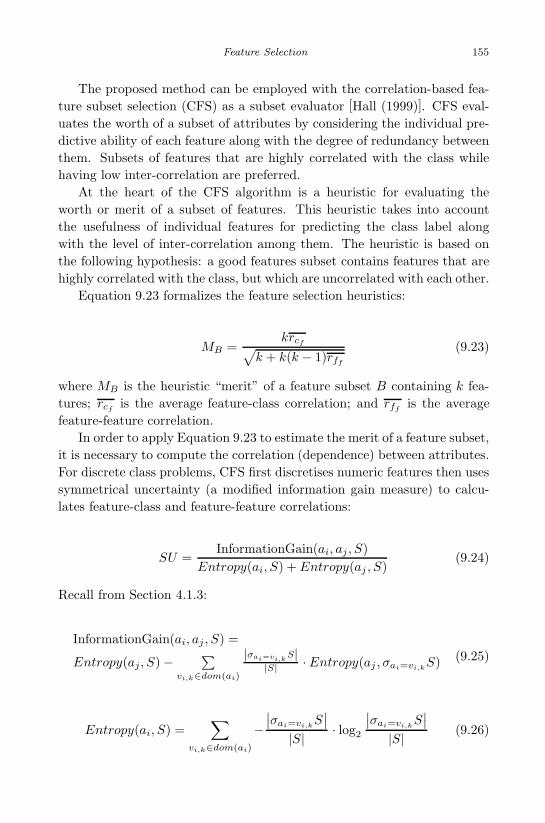
November 7, 2007 13:10 WSPC/Book Trim Size for 9in x 6in DataMining
Feature Selection 155
The proposed method can be employed with the correlation-based fea-ture subset selection (CFS) as a subset evaluator [Hall (1999)]. CFS eval-uates the worth of a subset of attributes by considering the individual pre-dictive ability of each feature along with the degree of redundancy betweenthem. Subsets of features that are highly correlated with the class whilehaving low inter-correlation are preferred.
At the heart of the CFS algorithm is a heuristic for evaluating theworth or merit of a subset of features. This heuristic takes into accountthe usefulness of individual features for predicting the class label alongwith the level of inter-correlation among them. The heuristic is based onthe following hypothesis: a good features subset contains features that arehighly correlated with the class, but which are uncorrelated with each other.
Equation 9.23 formalizes the feature selection heuristics:
MB =krcf√
k + k(k − 1)rff
(9.23)
where MB is the heuristic “merit” of a feature subset B containing k fea-tures; rcf
is the average feature-class correlation; and rffis the average
feature-feature correlation.In order to apply Equation 9.23 to estimate the merit of a feature subset,
it is necessary to compute the correlation (dependence) between attributes.For discrete class problems, CFS first discretises numeric features then usessymmetrical uncertainty (a modified information gain measure) to calcu-lates feature-class and feature-feature correlations:
SU =InformationGain(ai, aj , S)
Entropy(ai, S) + Entropy(aj , S)(9.24)
Recall from Section 4.1.3:
InformationGain(ai, aj , S) =
Entropy(aj , S)− ∑vi,k∈dom(ai)
|σai=vi,kS|
|S| ·Entropy(aj , σai=vi,kS) (9.25)
Entropy(ai, S) =∑
vi,k∈dom(ai)
−∣∣σai=vi,k
S∣∣
|S| · log2
∣∣σai=vi,kS∣∣
|S| (9.26)

November 7, 2007 13:10 WSPC/Book Trim Size for 9in x 6in DataMining
156 Data Mining with Decision Trees: Theory and Applications
Symmetrical uncertainty is used (rather than simple gain ratio) becauseit is a symmetric measure and can therefore be used to measure feature-feature correlations where there is no notion of one attribute being the“class” as such.
As for the search organization the following methods can be used: BestFirst Search; Forward Selection Search; Gain Ratio; Chi-Square; OneRclassifier; and Information Gain.
Beside the CFS, other evaluation methods can be considered including,consistency subset evaluator and the the wrapper subset evaluator withsimple classifiers (K-nearest neighbors, logistic regression and naıve bayes)
9.5.3.2 Bagging
The most well-known independent method is bagging (bootstrap aggregat-ing). In this case, each feature selector is executed on a sample of instancestaken with replacement from the training set. Usually each sample sizeis equal to the size of the original training set. Note that since samplingwith a replacement is used, some of the instances may appear more thanonce in the same sample and some may not be included at all. Althoughthe training samples are different from each other, they are certainly notindependent from a statistical point of view.
9.6 Using Decision Trees for Feature Selection
Using decision trees for feature selection has one important advantageknown as “anytime”. However, for highly dimensional datasets, the fea-ture selection process becomes computationally intensive.
Decision trees can be used to implement a trade-off between the perfor-mance of the selected features and the computation time which is requiredto find a subset. Top-down inducers of decision trees can be considered asanytime algorithms for feature selection, because they gradually improvethe performance and can be stopped at any time and provide sub-optimalfeature subsets.
Decision trees have been used as an evaluation means for directing thefeature selection search. For instance, a hybrid learning methodology thatintegrates genetic algorithms (GAs) and decision tree inducers in order tofind the best feature subset was proposed in [Bala et al. (1995)]. A GA isused to search the space of all possible subsets of a large set of candidatediscrimination features. In order to evaluate a certain feature subset, a
November 7, 2007 13:10 WSPC/Book Trim Size for 9in x 6in DataMining
Feature Selection 157
decision tree is trained and its accuracy is used as a measure of fitness forthe given feature set, which, in turn, is used by the GA to evolve betterfeature sets.
9.7 Limitation of Feature Selection Methods
Despite its popularity, the usage of feature selection methodologies for over-coming the obstacles of high dimensionality has several drawbacks:
• The assumption that a large set of input features can be reduced to asmall subset of relevant features is not always true; in some cases thetarget feature is actually affected by most of the input features, andremoving features will cause a significant loss of important information.• The outcome (i.e. the subset) of many algorithms for feature selec-
tion (for example, almost any of the algorithms that are based uponthe wrapper methodology) is strongly dependent on the training setsize. That is, if the training set is small, then the size of the reducedsubset will be small also. Consequently, relevant features might belost. Accordingly, the induced classifiers might achieve lower accuracycompared to classifiers that have access to all relevant features.• In some cases, even after eliminating a set of irrelevant features, the
researcher is left with relatively large numbers of relevant features.• The backward elimination strategy, used by some methods, is extremely
inefficient for working with large-scale databases, where the number oforiginal features is more than 100.
One way to deal with the above mentioned disadvantages is to use a verylarge training set (which should increase in an exponential manner as thenumber of input features increases). However, the researcher rarely enjoysthis privilege, and even if it does happen, the researcher will probablyencounter the aforementioned difficulties derived from a high number ofinstances.
Practically most of the training sets are still considered “small” not be-cause of their absolute size but rather due to the fact that they containtoo few instances given the nature of the investigated problem, namely theinstance space size, the space distribution and the intrinsic noise. Further-more, even if a sufficient dataset is available, the researcher will probablyencounter the aforementioned difficulties derived from a high number ofrecords.

November 7, 2007 13:10 WSPC/Book Trim Size for 9in x 6in DataMining
This page intentionally left blankThis page intentionally left blank

November 7, 2007 13:10 WSPC/Book Trim Size for 9in x 6in DataMining
Chapter 10
Fuzzy Decision Trees
10.1 Overview
There are two main types of uncertainty in supervised learning: statisticaland cognitive. Statistical uncertainty deals with the random behavior ofnature and all techniques described in previous chapters can handle theuncertainty that arises (or is assumed to arise) in the natural world fromstatistical variations or randomness. While these techniques may be appro-priate for measuring the likelihood of a hypothesis, they say nothing aboutthe meaning of the hypothesis.
Cognitive uncertainty, on the other hand, deals with human cognition.Cognitive uncertainty can be further divided into two sub-types: vaguenessand ambiguity. Ambiguity arises in situations with two or more alternativessuch that the choice between them is left unspecified. Vagueness arises whenthere is a difficulty in making a precise distinction in the world
Fuzzy set theory, first introduced by Zadeh in 1965, deals with cognitiveuncertainty and seeks to overcome many of the problems found in classicalset theory. For example, a major problem in the early days of control theoryis that a small change in input results in a major change in output. Thisthrows the whole control system into an unstable state. In addition therewas also the problem that the representation of subjective knowledge wasartificial and inaccurate.
Fuzzy set theory is an attempt to confront these difficulties and in thischapter we present some of it basic concepts. The main focus, however, ison those concepts used in the induction process when dealing with fuzzydecision trees. Since fuzzy set theory and fuzzy logic are much broader thanthe narrow perspective presented here, the interested reader is encouragedto read [Zimmermann (2005)].
159

November 7, 2007 13:10 WSPC/Book Trim Size for 9in x 6in DataMining
160 Data Mining with Decision Trees: Theory and Applications
10.2 Membership Function
In classical set theory, a certain element either belongs or does not belong toa set. Fuzzy set theory, on the other hand, permits the gradual assessmentof the membership of elements in relation to a set.
Definition 10.1 Let U be a universe of discourse, representing a col-lection of objects denoted generically by u. A fuzzy set A in a universeof discourse U is characterized by a membership function µA which takesvalues in the interval [0, 1]. Where µA(u) = 0 means that u is definitelynot a member of A and µA(u) = 1 means that u is definitely a member ofA.
The above definition can be illustrated on a vague set, that we will labelas young. In this case the set U is the set of people. To each person in U , wedefine the degree of membership to the fuzzy set young. The membershipfunction answers the question: “To what degree is person u young?”. Theeasiest way to do this is with a membership function based on the person’sage. For example Figure 10.1 presents the following membership function:
µY oung(u) =
0132−age(u)
16
age(u) > 32age(u) < 16otherwise
(10.1)
Given this definition, John, who is 18 years old, has degree of youth of0.875. Philip, 20 years old, has degree of youth of 0.75. Unlike probabilitytheory, degrees of membership do not have to add up to 1 across all objectsand therefore either many or few objects in the set may have high mem-bership. However, an objects membership in a set (such as “young”) andthe sets complement (“not young”) must still sum to 1.
The main difference between classical set theory and fuzzy set theory isthat the latter admits to partial set membership. A classical or crisp set,then, is a fuzzy set that restricts its membership values to {0, 1}, the end-points of the unit interval. Membership functions can be used to representa crisp set. For example, Figure 10.2 presents a crisp membership functiondefined as:
µCrispY oung(u) ={
0 age(u) > 221 age(u) ≤ 22
(10.2)

November 7, 2007 13:10 WSPC/Book Trim Size for 9in x 6in DataMining
Fuzzy Decision Trees 161
00.10.20.30.40.50.60.70.80.9
1
10 15 20 25 30 35
Age
Yo
un
g M
emb
ersh
ip
Fig. 10.1 Membership function for the young set.
10.3 Fuzzy Classification Problems
All classification problems we have discussed so far in this chapter assumethat each instance takes one value for each attribute and that each inst-ance is classified into only one of the mutually exclusive classes [Yuan andShaw (1995)].
To illustrate the idea, we introduce the problem of modeling the pref-erences of TV viewers. In this problem there are three input attributes:
A = {Time of Day,Age Group,Mood}
and each attribute has the following values:
• dom(Time of Day) = {Morning,Noon,Evening,Night}• dom(Age Group) = {Young,Adult}• dom(Mood) = {Happy,Indifferent,Sad,Sour,Grumpy}
The classification can be the movie genre that the viewer would like towatch, such as C = {Action,Comedy,Drama}.
All the attributes are vague by definition. For example, peoples feel-ings of happiness, indifference, sadness, sourness and grumpiness are vague

November 7, 2007 13:10 WSPC/Book Trim Size for 9in x 6in DataMining
162 Data Mining with Decision Trees: Theory and Applications
00.10.20.30.40.50.60.70.80.9
1
10 15 20 25 30 35
Age
Cri
sp Y
ou
ng
Mem
ber
ship
Fig. 10.2 Membership function for the crisp young set.
without any crisp boundaries between them. Although the vagueness of“Age Group” or “Time of Day” can be avoided by indicating the exact ageor exact time, a rule induced with a crisp decision tree may then have anartificial crisp boundary, such as “IF Age < 16 THEN action movie”. Buthow about someone who is 17 years of age? Should this viewer definitelynot watch an action movie? The viewer preferred genre may still be vague.For example, the viewer may be in a mood for both comedy and dramamovies. Moreover, the association of movies into genres may also be vague.For instance the movie “Lethal Weapon” (starring Mel Gibson and DannyGlover) is considered to be both comedy and action movie.
Fuzzy concept can be introduced into a classical problem if at leastone of the input attributes is fuzzy or if the target attribute is fuzzy. Inthe example described above, both input and target attributes are fuzzy.Formally the problem is defined as following[Yuan and Shaw (1995)]:
Each class cj is defined as a fuzzy set on the universe of objects U .The membership function µcj(u) indicates the degree to which object u
belongs to class cj . Each attribute ai is defined as a linguistic attributewhich takes linguistic values from dom(ai) = {vi,1, vi,2, . . . , vi,|dom(ai)|}.Each linguistic value vi,k is also a fuzzy set defined on U . The membershipµvi,k
(u) specifies the degree to which object u’s attribute ai is vi,k. Recallthat the membership of a linguistic value can be subjectively assigned or

November 7, 2007 13:10 WSPC/Book Trim Size for 9in x 6in DataMining
Fuzzy Decision Trees 163
transferred from numerical values by a membership function defined on therange of the numerical value.
10.4 Fuzzy Set Operations
Like classical set theory, fuzzy set theory includes such operations as union,intersection, complement, and inclusion, but also includes operations thathave no classical counterpart, such as the modifiers concentration and di-lation, and the connective fuzzy aggregation. Definitions of fuzzy set oper-ations are provided in this section.
Definition 10.2 The membership function of the union of two fuzzysets A and B with membership functions µA and µB respectively is definedas the maximum of the two individual membership functions µA∪B(u) =max{µA(u), µB(u)}.
Definition 10.3 The membership function of the intersection of twofuzzy sets A and B with membership functions µA and µB respectivelyis defined as the minimum of the two individual membership functionsµA∩B(u) = min{µA(u), µB(u)}.
Definition 10.4 The membership function of the complement of a fuzzyset A with membership function µA is defined as the negation of the spec-ified membership function µA(u) = 1− µA(u).
To illustrate these fuzzy operations, we elaborate on the previous exam-ple. Recall that John has a degree of youth of 0.875. Additionally John’shappiness degree is 0.254. Thus, the membership of John in the set Young ∪Happy would be max(0.875, 0.254) = 0.875, and its membership in Young∩ Happy would be min(0.875, 0.254) = 0.254.
It is possible to chain operators together, thereby constructing quitecomplicated sets. It is also possible to derive many interesting sets fromchains of rules built up from simple operators. For example John’s mem-bership in the set Y oung ∪ Happy would be max(1− 0.875, 0.254) = 0.254
The usage of the max and min operators for defining fuzzy union andfuzzy intersection, respectively is very common. However, it is importantto note that these are not the only definitions of union and intersectionsuited to fuzzy set theory.

November 7, 2007 13:10 WSPC/Book Trim Size for 9in x 6in DataMining
164 Data Mining with Decision Trees: Theory and Applications
10.5 Fuzzy Classification Rules
Definition 10.5 The fuzzy subsethood S(A, B) measures the degree towhich A is a subset of B.
S(A, B) =M(A ∩B)
M(A)(10.3)
where M(A) is the cardinality measure of a fuzzy set A and is defined as
M(A) =∑
u∈UµA(u) (10.4)
The subsethood can be used to measure the truth level of the rule ofclassification rules. For example given a classification rule such as “IFAge is Young AND Mood is Happy THEN Comedy” we have to calculateS(Hot ∩ Sunny, Swimming) in order to measure the truth level of theclassification rule.
10.6 Creating Fuzzy Decision Tree
There are several algorithms for induction of decision trees. In this sectionwe will focus on the algorithm proposed by [Yuan and Shaw (1995)]. Thisalgorithm can handle the classification problems with both fuzzy attributesand fuzzy classes represented in linguistic fuzzy terms. It can also handleother situations in a uniform way where numerical values can be fuzzifiedto fuzzy terms and crisp categories can be treated as a special case of fuzzyterms with zero fuzziness. The algorithm uses classification ambiguity asfuzzy entropy. The classification ambiguity, which directly measures thequality of classification rules at the decision node, can be calculated underfuzzy partitioning and multiple fuzzy classes.
The fuzzy decision tree induction consists of the following steps:
• Fuzzifying numeric attributes in the training set.• Inducing a fuzzy decision tree.• Simplifying the decision tree.• Applying fuzzy rules for classification.

November 7, 2007 13:10 WSPC/Book Trim Size for 9in x 6in DataMining
Fuzzy Decision Trees 165
10.6.1 Fuzzifying Numeric Attributes
When a certain attribute is numerical, it needs to be fuzzified into linguisticterms before it can be used in the algorithm. The fuzzification process canbe performed manually by experts or can be derived automatically usingsome sort of clustering algorithm. Clustering groups the data instancesinto subsets in such a manner that similar instances are grouped together;different instances belong to different groups. The instances are therebyorganized into an efficient representation that characterizes the populationbeing sampled.
Yuan and Shaw (1995) suggest a simple algorithm to generate a set ofmembership functions on numerical data. Assume attribute ai has numer-ical value x from the domain X . We can cluster X to k linguistic termsvi,j , j = 1, . . . , k. The size of k is manually predefined. For the first linguis-tic term vi,1, the following membership function is used:
µvi,1(x) =
1 x ≤ m1m2−x
m2−m1m1 < x < m2
0 x ≥ m2
(10.5)
For each vi,j when j = 2, . . . , k−1 has a triangular membership functionas follows:
µvi,j (x) =
0 x ≤ mj−1x−mj−1
mj−mj−1mj−1 < x ≤ mj
mj+1−xmj+1−mj
mj < x < mj+1
0 x ≥ mj+1
(10.6)
Finally the membership function of the last linguistic term vi,k is:
µvi,k(x) =
0 x ≤ mk−1x−mk−1
mk−mk−1mk−1 < x ≤ mk
1 x ≥ mk
(10.7)
Figure 10.3 illustrates the creation of four groups defined on the ageattribute: “young”, “early adulthood”, “middle-aged” and “old age”. Notethat the first set (“young”) and the last set (“old age”) have a trapezoidalform which can be uniquely described by the four corners. For example,the “young” set could be represented as (0, 0, 16, 32). In between, all other

November 7, 2007 13:10 WSPC/Book Trim Size for 9in x 6in DataMining
166 Data Mining with Decision Trees: Theory and Applications
sets (“early adulthood” and “middle-aged”) have a triangular form whichcan be uniquely described by the three corners. For example, the set “earlyadulthood” is represented as (16, 32, 48).
00.10.20.30.40.50.60.70.80.9
1
10 30 50 70
Age
Mem
ber
ship Young
Early adulthoodMiddle-agedOld Age
Fig. 10.3 Membership function for various groups in the age attribute.
The only parameters that need to be determined are the set of k cen-ters M = {m1, . . . , mk}. The centers can be found using the algorithmpresented in Figure 10.4. Note that in order to use the algorithm, a mono-tonic decreasing learning rate function should be provided.
10.6.2 Inducing of Fuzzy Decision Tree
The induction algorithm of fuzzy decision tree is presented in Figure 10.5.The algorithm measures the classification ambiguity associated with eachattribute and splits the data using the attribute with the smallest classifica-tion ambiguity. The classification ambiguity of attribute ai with linguisticterms vi,j , j = 1, . . . , k on fuzzy evidence S, denoted as G(ai|S), is theweighted average of classification ambiguity calculated as:
G(ai |S ) =k∑
j=‘1
w(vi,j |S) ·G(vi,j |S) (10.8)

November 7, 2007 13:10 WSPC/Book Trim Size for 9in x 6in DataMining
Fuzzy Decision Trees 167
Require: X - a set of values, η(t) - some monotonic decreasing scalarfunction representing the learning rate.
Ensure: M = {m1, . . . , mk}1: Initially set mi to be evenly distributed on the range of X .2: t← 13: repeat4: Randomly draw one sample x from X
5: Find the closest center mc to x.6: mc ← mc + η(t) · (x−mc)7: t← t + 18: D(X, M)← ∑
x∈X
mini ‖x−mi‖9: until D(X, M) converges
Fig. 10.4 Algorithm for fuzzifying numeric attributes
where w(vi,j |S) is the weight which represents the relative size of vi,j andis defined as:
w(vi,j |S) =M(vi,j |S)∑
k
M(vi,k |S)(10.9)
The classification ambiguity of vi,j is defined as G(vi,j |S) =g (�p (C |vi,j )), which is measured based on the possibility distribution vector
�p (C |vi,j ) =(p (c1 |vi,j ) , ..., p
(c|k| |vi,j
)).
Given vi,j , the possibility of classifying an object to class cl can bedefined as:
p (cl |vi,j ) =S(vi,j , cl)
maxk
S(vi,j , ck)(10.10)
where S(A, B) is the fuzzy subsethood that was defined in Definition 10.5.The function g (�p) is the possibilistic measure of ambiguity or nonspecificityand is defined as:
g (�p) =|p|∑i=1
(p∗i − p∗i+1
) · ln(i) (10.11)

November 7, 2007 13:10 WSPC/Book Trim Size for 9in x 6in DataMining
168 Data Mining with Decision Trees: Theory and Applications
where �p∗ =(p∗1, . . . , p
∗|p|)
is the permutation of the possibility distribution�p sorted such that p∗i ≥ p∗i+1.
All the above calculations are carried out at a predefined significantlevel α. An instance will take into consideration of a certain branch vi,j
only if its corresponding membership is greater than α. This parameter isused to filter out insignificant branches.
After partitioning the data using the attribute with the smallest clas-sification ambiguity, the algorithm looks for nonempty branches. For eachnonempty branch, the algorithm calculates the truth level of classifying allinstances within the branch into each class. The truth level is calculatedusing the fuzzy subsethood measure S(A, B).
If the truth level of one of the classes is above a predefined thresholdβ then no additional partitioning is needed and the node become a leaf inwhich all instance will be labeled to the class with the highest truth level.Otherwise the procedure continues in a recursive manner. Note that smallvalues of β will lead to smaller trees with the risk of underfitting. A higherβ may lead to a larger tree with higher classification accuracy. However, ata certain point, higher values β may lead to overfitting.
Require: S - Training Set A - Input Feature Set y - Target FeatureEnsure: Fuzzy Decision Tree1: Create a new fuzzy tree FT with a single root node.2: if S is empty OR Truth level of one of the classes ≥ β then3: Mark FT as a leaf with the most common value of y in S as a label.4: Return FT .5: end if6: ∀ai ∈ A find a with the smallest classification ambiguity.7: for each outcome vi of a do8: Recursively call procedure with corresponding partition vi.9: Connect the root node to the returned subtree with an edge that is
labeled as vi.10: end for11: Return FT
Fig. 10.5 Fuzzy decision tree induction

November 7, 2007 13:10 WSPC/Book Trim Size for 9in x 6in DataMining
Fuzzy Decision Trees 169
10.7 Simplifying the Decision Tree
Each path of branches from root to leaf can be converted into a rule withthe condition part representing the attributes on the passing branches fromthe root to the leaf and the conclusion part representing the class at the leafwith the highest truth level classification. The corresponding classificationrules can be further simplified by removing one input attribute term at atime for each rule we try to simplify. Select the term to remove with thehighest truth level of the simplified rule. If the truth level of this new ruleis not lower than the threshold β or the truth level of the original rule,the simplification is successful. The process will continue until no furthersimplification is possible for all the rules.
10.8 Classification of New Instances
In a regular decision tree, only one path (rule) can be applied for everyinstance. In a fuzzy decision tree, several paths (rules) can be applied forone instance. In order to classify an unlabeled instance, the following stepsshould be performed [Yuan and Shaw (1995)]:
• Step 1: Calculate the membership of the instance for the condition partof each path (rule). This membership will be associated with the label(class) of the path.• Step 2: For each class calculate the maximum membership obtained
from all applied rules.• Step 3: An instance may be classified into several classes with different
degrees based on the membership calculated in Step 2.
10.9 Other Fuzzy Decision Tree Inducers
There have been several fuzzy extensions to the ID3 algorithm. The UR-ID3 algorithm [Maher and Clair (1993)] starts by building a strict decisiontree, and subsequently fuzzifies the conditions of the tree. Tani and Sakoda(1992) use the ID3 algorithm to select effective numerical attributes. Theobtained splitting intervals are used as fuzzy boundaries. Regression is thenused in each subspace to form fuzzy rules. Cios and Sztandera (1992) usethe ID3 algorithm to convert a decision tree into a layer of a feedforwardneural network. Each neuron is represented as a hyperplane with a fuzzy

November 7, 2007 13:10 WSPC/Book Trim Size for 9in x 6in DataMining
170 Data Mining with Decision Trees: Theory and Applications
boundary. The nodes within the hidden layer are generated until somefuzzy entropy is reduced to zero. New hidden layers are generated untilthere is only one node at the output layer.
Fuzzy-CART [Jang (1994)] is a method which uses the CART algorithmto build a tree. However, the tree, which is the first step, is only used topropose fuzzy sets of the continuous domains (using the generated thresh-olds). Then, a layered network algorithm is employed to learn fuzzy rules.This produces more comprehensible fuzzy rules and improves the CART’sinitial results.
Another complete framework for building a fuzzy tree including severalinference procedures based on conflict resolution in rule-based systems andefficient approximate reasoning methods was presented in [Janikow, 1998].
Olaru and Wehenkel (2003) presented a new type of fuzzy decision treescalled soft decision trees (SDT). This approach combines tree-growing andpruning, to determine the structure of the soft decision tree. Refittingand backfitting are ised to improve its generalization capabilities. Theresearchers empirically showed that soft decision trees are significantly moreaccurate than standard decision trees. Moreover, a global model variancestudy shows a much lower variance for soft decision trees than for standardtrees as a direct cause of the improved accuracy.
Peng (2004) has used FDT to improve the performance of the classicalinductive learning approach in manufacturing processes. Peng proposedusing soft discretization of continuous-valued attributes. It has been shownthat FDT can deal with the noise or uncertainties existing in the datacollected in industrial systems.

November 7, 2007 13:10 WSPC/Book Trim Size for 9in x 6in DataMining
Chapter 11
Hybridization of Decision Trees withother Techniques
11.1 Introduction
Hybridization in artificial intelligence (AI) involves simultaneously usingtwo or more intelligent techniques in order to handle real world complexproblems, involving imprecision, uncertainty and vagueness. Hybridizationis frequently practiced in machine learning, to make more powerful andreliable classifiers.
The combination or integration of additional methodologies can be donein any form: by modularly integrating two or more intelligent method-ologies, which maintains the identity of each methodology; by fusing onemethodology into another; or by transforming the knowledge representa-tion in one methodology into another form of representation characteristicto another methodology.
Hybridization of decision trees with other AI techniques can be per-formed by using either a decision tree to partition the instance space forother induction techniques or other AI techniques for obtaining a betterdecision tree.
11.2 A Decision Tree Framework for Instance-SpaceDecomposition
In the first approach, termed instance-space decomposition (ISD) and in-volving hybrid decision tree with other inducers, the instance space of theoriginal problem is partitioned into several subspaces using a decision treewith a distinct classifier assigned to each subspace. Subsequently, an un-labeled, previously unseen instance is classified by employing the classifierthat was assigned to the subspace to which the instance belongs.
171

November 7, 2007 13:10 WSPC/Book Trim Size for 9in x 6in DataMining
172 Data Mining with Decision Trees: Theory and Applications
In an approach, which Cohen et al. (2007) term decision tree ISD, thepartition of the instance-space is attained by a decision tree. Along withthe decision tree, the ISD method employs another classification method,which classifies the tree’s leaves (the tree’s leaves represent the differentsubspaces). Namely, decision tree ISD methods produce decision tree s,in which the leaves are assigned classifiers rather than simple class labels.When a non- decision tree method produces the leaves’ classifiers, the com-posite classifier is sometimes termed a decision tree hybrid classifier.
The term “decision tree hybrid classifier”, however, is also used in abroader context, such as in cases where a sub-classification method decidesabout the growth of the tree and its pruning [Sakar and Mammone (1993)].
There are two basic techniques for implementing decision tree ISD. Thefirst technique is to use some decision tree method to create the tree andthen, in a post-growing phase, to attach classifiers to the tree’s leaves. Thesecond technique is to consider the classifiers as part of the tree-growingprocedure. Potentially, the latter technique can achieve more accurate com-posite classifiers. On the other hand, it usually requires more computation-ally intensive procedures.
Carvalho and Freitas [Carvalho and Freitas. (2004)] proposed a hybriddecision tree genetic-algorithm classifier, which grows a decision tree andassigns some of the leaves with class labels and the others with genetic-algorithm classifiers. The leaves with the classifiers are those that have asmall number of corresponding instances. A previously unseen instance issubsequently either directly assigned with a class label or is sub-classified bya genetic-algorithm classifier (depending on the leaf to which the instanceis sorted). Zhou and Chen [Zhou and Chen (2002)] suggested a method,called hybrid decision tree (HDT). HDT uses the binary information gainratio criterion to grow a binary decision tree in an instance-space that isdefined by the nominal explaining-attributes only. A feed-forward neuralnetwork, subsequently classifies the leaves, whose diversity exceeds a pre-defined threshold. The network only uses the ordinal explaining-attributes.
In this chapter, we focus on the second decision tree ISD technique,which considers the classifiers as part of the decision tree’s growth. NBTreeis a method which produces a decision tree naive-Bayes hybrid classifier[Kohavi (1996)]. In order to decide when to stop the recursive partition ofthe instance-space (i.e., stop growing the tree), NBTree compares two alter-natives: partitioning the instance-space further on (i.e., continue splittingthe tree) versus stopping the partition and producing a single naive Bayesclassifier. The two alternatives are compared in terms of their error esti-

November 7, 2007 13:10 WSPC/Book Trim Size for 9in x 6in DataMining
Hybridization of Decision Trees with other Techniques 173
mations, which are calculated by a cross-validation procedure. Naive Bayesclassification, by itself, is very efficient in terms of its processing time. How-ever, using cross-validation significantly increases the overall computationalcomplexity. Although Kohavi has used naive Bayes, to produce the classi-fiers, other classification methods are also applicable. However, due to thecross-validation estimations, NBTree becomes computationally expensivefor methods that are more time-consuming than naive Bayes (e.g., neuralnetworks).
We describe a simple framework for decision tree ISD, termed decisiontree framework for instance space decomposition (DFID). The frameworkhierarchically partitions the instance space using a top-down (pruning-free)decision tree procedure. Although various DFID implementations use dif-ferent stopping rules, split-validation examinations and splitting rules, inthis chapter we concentrate on a specific DFID method – contrasted popu-lations miner (CPOM). The splitting rule that this method uses – groupedgain ratio – combines the well-accepted gain ratio criterion with a heuristicgrouping procedure. CPOM can reduce the processing time while keepingthe composite classifier accurate.
Implementations of DFID consist of a decision-tree (as a wrapper) andanother embedded classification method (this method can, in principle,also be a decision tree). The embedded classification method generates themultiple classifiers for the tree’s leaves. The DFID sequence is illustratedby the pseudo code in Figure 10.1. DFID inputs are: training instances;a list of attributes (which will be examined as candidates for splitting thedecision tree); a classification method; and, optionally, (depending on thespecific implementation), some additional parameters.
The procedure begins by creating the decision tree’s root node. Theroot represents the entire instance space X . When constructed, each nodeis attached with a rule which defines the subspace of X that the noderepresents. The DFID framework considers rules that can be expressedin a conjunctive normal form. A rule may be, for example: “(A1 = 3 ∨A1 = 4)∧A2 = 1”. DFID then checks whether there should be a split fromthe root node (i.e., whether X should be partitioned). This check, whichuses some stopping rules, is represented, in Figure 10.1 by the generalfunction StoppingCriterion. The function receives some inputs (dependingon the specific implementation) and returns a Boolean value that indicateswhether the stopping rules are met. If the stopping rules are met, thenI is trained using all of the training instances. The classifier that resultsis attached to the root node and the procedure terminates. If, however,

November 7, 2007 13:10 WSPC/Book Trim Size for 9in x 6in DataMining
174 Data Mining with Decision Trees: Theory and Applications
the stopping-rules are not met, then DFID searches for a split, accordingto some splitting rule, represented in Figure 10.1 by the general functionsplit.
Splits in DFID are based on the values of a certain candidate attribute.We assume that there exists at least a single attribute that can create a split(or otherwise the stopping-rules would have indicated that there should beno more splits).
The function split receives a training set, a set of candidate attributesand optionally some additional inputs. It then returns the attribute uponwhose values the split is based and a set of descendents nodes. Recall thatupon its creation, each node is attached with a rule, which defines the sub-space of X that the node represents. The rules for the descendent nodesare conjunctions of the root’s rule and restrictions on the values of theselected attribute. The split that was found may be then subjected to avalidation examination, represented, in Figure 10.1 by the general functionvalidate. If a split is found to be invalid, then DFID will search for anothersplit (another attribute). If there are no more candidate attributes, I willbe trained using all the training instances and the classifier that resultswill be attached to the root node. As soon as a valid split is found, thedescendent nodes that were created by the split are recursively consideredfor further splits. Further splits are achieved by the recurrence of DFID.In the recurrence, only a subset of the training instances is relevant (theinstances that are actually sorted to the certain descendent node). In addi-tion, the attribute, which defined the current split, is removed from the listof candidate attributes. The descendents are finally linked to their parent(the root). Different DFID implementations may differ in all or some ofthe procedures that implement the three main framework components –stopping-rules (the function StoppingCriterion), splitting rules (the func-tion split) and split validation examinations (the function validate).
11.2.1 Stopping Rules
Stopping rules are checked by the general function StoppingCriterion (Fig-ure 10.1). However, it should be noticed that a negative answer by thisfunction is not the only condition that stops the DFID recurrence; another,and even more natural, condition, is the lack of any valid split.
According to the simple stopping rule that NBTree uses, no splits areconsidered when there are 30 instances or less in the examined node. Split-ting a node with only a few training instances will hardly affect the final

November 7, 2007 13:10 WSPC/Book Trim Size for 9in x 6in DataMining
Hybridization of Decision Trees with other Techniques 175
accuracy and will lead, on the other hand, to a complex and less comprehen-sible decision tree (and hence a complex and less comprehensible compositeclassifier). Moreover, since the classifiers are required to generalize from theinstances in their subspaces, they must be trained on samples of sufficientsize.
Kohavi’s stopping-rule can be revised into a rule that never considersfurther splits in nodes that correspond to β|S| instances or less, where 0 <
β < 1 is a proportion and |S| is the number of instances in original trainingset, S. When using this stopping rule (either in Kohavi’s way or in therevised version), a threshold parameter must be provided to DFID as well asto the function StoppingCriterion. Another heuristic stopping rule is neverto consider splitting a node, if a single classifier can accurately describethe node’s subspace (i.e., if a single classifier which was trained by all ofthe training instances, and using the classification method appear to beaccurate). Practically, this rule can be checked by comparing an accuracyestimation of the classifier to a pre-defined threshold (thus, using this rulerequires an additional parameter). The motivation for this stopping rule isthat if a single classifier is good enough, why replace it with a more complextree that also has less generalization capabilities? Finally, as mentionedabove, another (inherent) stopping-rule of DFID is the lack of even a singlecandidate attribute.
11.2.2 Splitting Rules
The core question of DFID is how to split nodes. The answer to thisquestion lies in the general function split (Figure 10.1). It should be notedthat any splitting rule that is used to grow a pure decision tree, is alsosuitable in DFID.
Kohavi [Kohavi (1996)] has suggested a new splitting rule, which selectsthe attribute with the highest value of a measure, which he refers to as the“utility”. Kohavi defines the utility as the fivefold cross-validation accu-racy estimation of using a naive-Bayes method for classifying the subspaceswhich will be generated by the considered split.
11.2.3 Split Validation Examinations
Since splitting rules, are heuristic, it may be beneficial to regard the splitsthey produce as recommendations that should be validated. Kohavi [Ko-havi (1996)] validated a split by estimating the reduction in error, which is

November 7, 2007 13:10 WSPC/Book Trim Size for 9in x 6in DataMining
176 Data Mining with Decision Trees: Theory and Applications
gained by the split and comparing it to a predefined threshold of 5% (i.e., ifit is estimated that the split will reduce the overall error rate by only 5% orless, the split is regarded as invalid). In an NBTree, it is enough to examineonly the first proposed split in order to conclude that there are no validsplits, if the one examined is invalid. This follows since in an NBTree, theattribute according to which the split is done is the one that maximizes theutility measure, which is strictly increasing with the reduction in error. If asplit, in accordance with the selected attribute cannot reduce the accuracyby more than 5%, then no other split can.
We suggest a new split validation procedure. In very general terms, asplit according to the values of a certain attribute is regarded as invalid ifthe subspaces that result from this split are similar enough to be groupedtogether.
11.3 The CPOM Algorithm
This section presents the contrasted population miner (CPOM), whichsplits nodes according to a novel splitting rule, termed grouped gain ratio.Generally speaking, this splitting rule is based on the gain ratio criterion(Quinlan, 1993), followed by a grouping heuristic. The gain ratio crite-rion selects a single attribute from the set of candidate attributes, and thegrouping heuristic thereafter groups together subspaces which correspondto different values of the selected attribute.
11.3.1 CPOM Outline
CPOM uses two stopping rules. First, the algorithm compares the numberof training instances to a pre-defined ratio of the number of instances inthe original training set. If the subset is too small, CPOM stops (sinceit is undesirable to learn from too small a training subset). Secondly,CPOM compares the accuracy estimation of a single classifier to a pre-defined threshold. It stops if the accuracy estimation exceeds the threshold(if a single classifier is accurate enough, there is no point in splitting furtheron). Therefore, in addition to the inputs in Figure 11.1, CPOM must receivetwo parameters: β, the minimal ratio of the training instances and acc, themaximal accuracy estimation that will still result in split considerations.
CPOM’s split validation procedure is directly based on grouped gainratio. The novel rule is described in detail, in the following subsection;

November 7, 2007 13:10 WSPC/Book Trim Size for 9in x 6in DataMining
Hybridization of Decision Trees with other Techniques 177
however, in general terms, the rule returns the splitting attribute and a setof descendent nodes. The nodes represent subspaces of X that are believedto be different. If the procedure returns just a single descendent node, thesplit it has generated is regarded as invalid.
11.3.2 The Grouped Gain Ratio Splitting Rule
Grouped gain ratio is based on the gain ratio criterion followed by a group-ing heuristic. The gain ratio criterion selects a single attribute from a set ofcandidate attributes. The instance subspace, whose partition we are nowconsidering, may, in principle, be partitioned so that each new sub-subspacewill correspond to a unique value of the selected attribute. Group gainratio avoids this alternative, through heuristically grouping sub-subspacestogether. By grouping sub-subspaces together, grouped gain ratio increasesthe generalization capabilities, since there are more instances in a group ofsub-subspaces than there are in the individual sub-subspaces.
Clearly, if we separately train I on each subset and obtain the sameexact classifier from each subset, then there is no point in the split, sinceusing this single classifier for the entire instance space is as accurate as usingthe multiple classifiers; it is also much simpler and understandable, and itcan generalize better. The other direction of this argument is slightly lessstraightforward. If the classifiers that were trained over the training subsetsare very different from one another, then none of them can classify X as one,and we can believe that the split is beneficial. Based on this observation,the grouped gain ratio splitting rule groups together subspaces that havesimilar classifiers.
The intuition regarding the classifier comparisons raises questions ofwhat is similar, what is different and how to compare classifiers? Althoughthere may be multiple classifiers, all of which must be simultaneously com-pared to each other, we begin answering these questions with the simplercase of exactly two classifiers, using a comparison heuristic, which we referto as cross-inspection (see Figure 10.2).
Cross-inspection is based on two mutually-exclusive training subsetsand a classification method as inputs. The comparison begins by randomlypartitioning each subset into a training sub-subset and a test sub-subset.Then, two classifiers are produced, by training the input method, once overeach training sub-subset. After producing the two classifiers, the cross-inspection heuristic calculates the error rates of each classifier over each ofthe test sub-subsets. If the error rate of the first classifier over the first test

November 7, 2007 13:10 WSPC/Book Trim Size for 9in x 6in DataMining
178 Data Mining with Decision Trees: Theory and Applications
sub-subset is significantly (with confidence level alpha) different from theerror of the first classifier over the second test sub-subset, or vice versa, thenthe two classifiers are regarded as different. The errors are compared bytesting the hypothesis that the errors are generated by the same binomialrandom variable [Dietterich (1998)].
The cross-inspection heuristic compares only two distinct classifiers.However, in the DFID framework, more than two classifiers must be com-pared at a time (if the attribute, which was selected by the gain ratiocriterion, has more than two possible values). For example, if it is believedthat graduate students from different schools behave differently, one mayconsider splitting according to the school’s name. The attribute ’school’ canreceive multiple values, all of which will have to be compared simultane-ously. A successful split will group similar schools together, while differentschools will be in different groups. Since an exhaustive search, over all thepossible groupings, is unacceptable in terms of complexity, grouped gainratio (see Figure 10.4) uses a greedy grouping heuristic, which is based oncross-inspection.
The procedure begins by using cross-inspection, to compare all the dis-tinct pairs of classifiers (if there are q classifiers, there are q(q-1)/2 com-parisons). For each instance-subspace, the procedure computes the numberof instances that belong to subspaces that are similar to it (by definitionthe similarity by cross-inspection is defined with regard to classifiers ratherthan subspaces; each subspace, however, is described by a classifier). Theclassifier that represents the subspace with the largest such number is re-garded as the classifier that covers the maximal number of instances. Thesubspaces of all the instances which are covered by this classifier are groupedtogether, and the procedure iterates. The heuristic does not explicitly guar-antee that any two classifiers in a group are equivalent, but equivalence isassumed to be a transitive relation. The greedy grouping procedure is asimple clustering method and other clustering methods, like graph coloring[Zupan et al. (1998)] may also be suitable here. Alternatively one could usethe Warshall algorithm [Warshall (1962)] for finding the transitive closureof the comparison matrix, which can be used for calculating supj . However,this form of calculation will not be convenient in this case because it willtend to group too much as the following example illustrates.
Cohen et al. (2007) demonstrated that CPOM improved the obtainedaccuracy compared to the examined embedded methods (naive Bayes, back-propagation and C4.5). Not only was CPOM more accurate than otherdecision tree ISD methods, the grouping heuristic significantly improved

November 7, 2007 13:10 WSPC/Book Trim Size for 9in x 6in DataMining
Hybridization of Decision Trees with other Techniques 179
the accuracy results, compared to a CPOM variation which does not group.Finally, using three synthetic datasets, CPOM distinguished between dif-ferent populations in an underlined dataset.
11.4 Induction of Decision Trees by an Evolutionary Algo-rithm
Evolutionary Algorithms (EAs) are stochastic search algorithms inspiredby the concept of Darwinian evolution. The motivation for applying EAsto data mining tasks is that they are robust, adaptive search techniquesthat perform a global search in the solution space [Freitas (2005)]. Since awell-designed EA continually considers new solutions, it can be viewed asan “anytime” learning algorithm capable of quite quickly producing a good-enough solution. It then continues to search the solution space, reportingthe new “best” solution whenever one is found.
Genetic algorithms (GA), a popular type of evolutionary algorithms,have been successfully used for feature selection. Figure 10.5 presents ahigh level pseudo code of GA adapted from [Freitas (2005)].
Genetic algorithms begin by randomly generating a population of L can-didate solutions. Given such a population, a genetic algorithm generates anew candidate solution (population element) by selecting two of the candi-date solutions as the parent solutions. This process is termed reproduction.Generally, parents are selected randomly from the population with a biastoward the better candidate solutions. Given two parents, one or morenew solutions are generated by taking some characteristics of the solutionfrom the first parent (the “father”) and some from the second parent (the“mother”). This process is termed “crossover”. For example, in geneticalgorithms that use binary encoding of n bits to represent each possible so-lution, we might randomly select a crossover bit location denoted as o. Twodescendant solutions could then be generated. The first descendant wouldinherit the first o string characteristics from the father and the remainingn−o characteristics from the mother. The second descendant would inheritthe first o string characteristics from the mother and the remaining n − o
characteristics from the father. This type of crossover is the most commonand it is termed one-point crossover. Crossover is not necessarily appliedto all pairs of individuals selected for mating: a Pcrossover probability isused in order to decide whether crossover will be applied. If crossover isnot applied, the offspring are simply duplications of the parents.

November 7, 2007 13:10 WSPC/Book Trim Size for 9in x 6in DataMining
180 Data Mining with Decision Trees: Theory and Applications
Finally, once descendant solutions are generated, genetic algorithms al-low characteristics of the solutions to be changed randomly in a processknown as mutation. In the binary encoding representation, according to acertain probability (Pmut), each bit is changed from its current value to theopposite value. Once a new population has been generated, it is decodedand evaluated. The process continues until some termination criterion issatisfied. A GA converges when most of the population is identical, or inother words, when the diversity is minimal.
Based on the pseudo code, one should provide the following ingredientswhen using a GA algorithm for decision trees: crossover operator, mutationoperator, fitness function, a method to create the initial population and astopping criterion.
Several GA-based systems, which learn decision trees in the top-downmanner have been proposed, such as BTGA [Chai et al. (1996)], OC1-ES[Cantu-Paz and Kamath (2003)] and DDT-EA [Krtowski (2004)]. Gener-ally, they apply an evolutionary approach to the test search, especially inthe form of hyper-planes.
The GDT-EA algorithm [Krtowski and Grze (2005)] that we describehere searches for the whole tree at once in contrast to greedy, top-downapproaches. The initial population is generated by applying a standardtop-down decision tree inducers but attributes are selected in a dipolarway. Specifically, two instances from different classes are randomly chosen.Then an attribute which differentiates between the two instances is selected.
The Fitness function is composed of two terms: the classification accu-racy on the training set and the tree complexity. Specifically, the fitnessfunction, which must be maximized, has the following form:
Fitness = Acc− α · S (11.1)
where Acc is the classification quality estimated on the learning set; S isthe size of the tree (number of nodes); and α - is a parameter which indicatethe relative importance of the complexity term. The value of α should beprovided by the user by tuning it to the specific problem that is solved.
The algorithm terminates if the fitness of the best individual in thepopulation does not improve during the fixed number of generations. Thisstatus indicates, that the algorithm has converged. Additionally, the max-imum number of generations is specified, which allows limiting the compu-tation time in case of a slow convergence.
Like many other GAs, the GDT-EA also has two operators: MutateNode

November 7, 2007 13:10 WSPC/Book Trim Size for 9in x 6in DataMining
Hybridization of Decision Trees with other Techniques 181
(for mutation) and CrossTrees (for crossover). The first operator MutateN-ode, which is applied with the given probability to every node of the tree,can modify the test or change the node structure. If a non-leaf node isconcerned it can be pruned to a leaf or its test can be altered. Specifically,there are four modification options in case of non-leaf node:
• A completely new test is applied with another randomly chosen attri-bute and threshold,• A new threshold is randomly chosen without changing the attribute
used in the test,• The current sub-tree is replaced by a sub-tree of an adjacent node.• The test can be exchanged with another test taken from randomly
chosen descendant-nodes.
If a leaf node is to be mutated, then there are two options:
• The leaf node is replaced with a non-leaf node with a new randomlychosen test.• The leaf node is replaced with a sub-tree generated using an appropriate
algorithm.
The CrossTrees operator is equivalent to the standard crossover oper-ator. It alters two solutions by exchanging certain parts of input trees.There are three possible exchange types: two types of sub-tree exchangesand an exchange of only tests. At the beginning, regardless of the type, onenode in each tree is randomly chosen. Then the type of exchange betweentrees is decided.
In the first CrossTree variant, the tests that are associated with thechosen nodes are substituted. This option is valid only when the chosennodes have the same number of outgoing branches. In the second CrossTreevariant, we substitute the sub-trees starting from the chosen nodes. Thethird CrossTree variant actually combines the first two variants. Brancheswhich start from the chosen nodes are exchanged in random order.

November 7, 2007 13:10 WSPC/Book Trim Size for 9in x 6in DataMining
182 Data Mining with Decision Trees: Theory and Applications
DFID (S,A,I)
Where:
S - Training Set
A - Input Feature Set
I - Inducer
Create a tree with a root node;
IF StoppingCriterion(S, A, I) THEN
Attach the classifier I(S, A) to the root;
ELSE
A∗ ← A;
valid← FALSE;
WHILE A∗ �= ∅ and NOT(valid)
(SplitAtt, nodes)← split(S, A∗);IF validate(nodes, SplitAtt, S) THEN
valid← TRUE;
A← A− SplitAtt;
FOR each node ∈ nodes
Generate classifier DFID(NodeInstances, A, I);Attach the classifier to node;
Link the node to root;
END FOR
ELSE
A∗ ← A ∗ −SplitAtt;
END WHILE
IF NOT (valid) THEN
Attach the classifier I(S, A) to the root;
END IF
END IF
RETURN tree;
Fig. 11.1 DFID outline: A DFID implementation recursively partitions the instancespace of the training set, according to the values of the candidate attributes. As therecursive partition ends, classifiers are attached to the leaves by employing the embeddedclassification method.

November 7, 2007 13:10 WSPC/Book Trim Size for 9in x 6in DataMining
Hybridization of Decision Trees with other Techniques 183
CrossInspection (S1,S2,I,α)
Where:
S1, S2 - Mutually-exclusive training sets
I - Inducer
α - Confidence level
S11 ← a random sample from S1;
S12 ← S1 − S11;
S21 ← a random sample from S2;
S22 ← S2 − S21;
H1 ← I(S11);H2 ← I(S21);FOR i, j ∈{1,2} DO
εi,j ← accuracy estimation of Hi over Sj,2;
END FOR
IF ε1,2 is different from ε1,1 with a confidence level α OR
ε2,1 is different from ε2,2 with a confidence level α THEN
return FALSE;
ELSE
return TRUE;
Fig. 11.2 The cross-inspection procedure outline: Searching for statistical significance,the procedure compares the accuracy estimations of two distinct classifiers.

November 7, 2007 13:10 WSPC/Book Trim Size for 9in x 6in DataMining
184 Data Mining with Decision Trees: Theory and Applications
GroupedGainRatio (S, A, I, root, α)
Where:
S - Training Set
A - Input Feature Set
I - Inducer
root - the node from which the split is considered
α - confidence level
Ai ← the attribute from A with the maximal gain ratio;
S1, S2, . . . , Sd(i) ← a partition of S, according to values of Ai;
FOR all j, k ∈ {1,2,... ,d(i)} so that j ≤ k
Ej,k ← CrossInspection(Sj, Sk, I, α)
Ek,j ← Ej,k;
END FOR
FOR all j ∈ {1,2,... ,d(i)}supj ← the number of instances in the
subsets Sk for which Ej,k=TRUE;
END FOR
L← a list of the subsets indices sorted descending by supj;
nodes← an empty set of nodes
WHILE L is not empty DO
Create a new node;
Attach the rule which is a conjecture of the root’s rule
and a disjoint of the values that correspond to
Sj the first member of L and the members
Sk for which Ej,k=TRUE;
Remove from L any member that is described by the newnode;
Add node to nodes;
END WHILE
RETURN (Ai, nodes)
Fig. 11.3 The grouped gain ratio procedure outline. The procedure groups together sim-ilar values of a candidate attribute. Similarity is based on the cross-inspection heuristic.

November 7, 2007 13:10 WSPC/Book Trim Size for 9in x 6in DataMining
Hybridization of Decision Trees with other Techniques 185
GA
Create initial population of individuals
(candidate solutions)
Compute the fitness of each individual
REPEAT
Select individuals based on fitness
Apply genetic operators to selected individuals,
creating new individuals
Compute fitness of each of the new individuals
Update the current population
(new individuals replace old individuals)
UNTIL (stopping criterion)
Fig. 11.4 A Pseudo code for GA.

November 7, 2007 13:10 WSPC/Book Trim Size for 9in x 6in DataMining
This page intentionally left blankThis page intentionally left blank
November 7, 2007 13:10 WSPC/Book Trim Size for 9in x 6in DataMining
Chapter 12
Sequence Classification UsingDecision Trees
12.1 Introduction
In this chapter we discuss how decision trees can be used for sequenceclassifications. The new method we present, Cascaded Regular ExpressionDecision Trees (CREDT), induces a cascaded ensemble of decision trees forclassifying sequences patterns. CREDT consists of four main steps: (1)sequence representation: a domain specific task designed to represent se-quences as a string of tokens; (2) pattern discovery: the automatic creationof a regular expression pattern from each pair of sequences; (3) patternselection: applying heuristics to select the best patterns for correct classifi-cation; (4) classifier training: training a cascaded decision tree classifier tocombine several patterns. The following sections describe each of the abovephases.
12.2 Sequence Representation
This step is domain specific and every application might require differentpreprocessing. Generally the sequences are represented as a string of to-kens. Each token may also include attributes that better characterize it.For instance, in order to discover interesting patterns in complicated man-ufacturing processes, each product manufacturing data is represented as astring of tokens, each token representing a different operation activity. Ifthe makespan factor is unimportant, then the representation is straightfor-ward. For instance, the production sequence 1-5-9-3-2 is represented as thestring “B 1 5 9 3 2 F”. If the makespan factor is important, then a morecomplicated representation is required. For this purpose we first need todecide what the desirable time granularity is. Time granularity should be
187

November 7, 2007 13:10 WSPC/Book Trim Size for 9in x 6in DataMining
188 Data Mining with Decision Trees: Theory and Applications
no more than the minimum operation duration in the database.After deciding what the desirable time granularity is, we can represent
the manufacturing process of each product instance as a string. Each timebucket is represented as a single letter. We denote by Σ the alphabet ofthe manufacturing process. Each letter in Σrepresents the identification ofthe operation performed in this time bucket. Idle time is also representedby a special letter (for instance “ ”). The size of Σ depends on the numberof operations that must be encoded. For instance, the string “B 1 1
3 3 3 F” represents a manufacturing sequence with the operation “1”being performed during the first two time buckets. Then, during the foursubsequent time buckets, no operations are performed. Three time bucketsthen follow in which operation “3” is performed.
In addition to the string we may keep for each token its attributes.For instance, we may keep the setting parameters of the machine (such asspeed) that participated in the operation “1”.
12.3 Pattern Discovery
The term sequence pattern usually refers to a set of short sequences thatis precisely specified by some formalism. Following much research that isbeing carried out now in bioinformatics, we also adopt regular expressionsin order to represent sequence patterns. A pattern is defined as any stringconsisting of a letter of the alphabet Σ and the wild-card character ’.’. Thewild-card (also known as the “don’t care” character) denotes a position thatcan be occupied by any letter of the alphabet Σ. For instance, the pattern“B 1 1 . . 3 . 3” can be matched against the following productionstrings “B 1 1 3 3 3”, “B 1 1 2 4 3 1 3”, “1 1 7 3 4 4”, etc.The pattern element “. ∗ ” denotes an arbitrary string of symbols (possiblyof length 0), “.{3,5}” to denote any string of between 3 and 5 characters.
In this research we examined two approaches for obtaining the regularexpressions: the longest common subsequence and the TEIRESIAS algo-rithm. Here we describe the first approach, in which we compare any pair ofsequences with the same class label. From each pair, we create the longestregular expression that fits the two sequences. For instance, assume we aregiven the following two sequences:
B 1 8 4 2 3 4 F
B 9 1 4 2 7 F
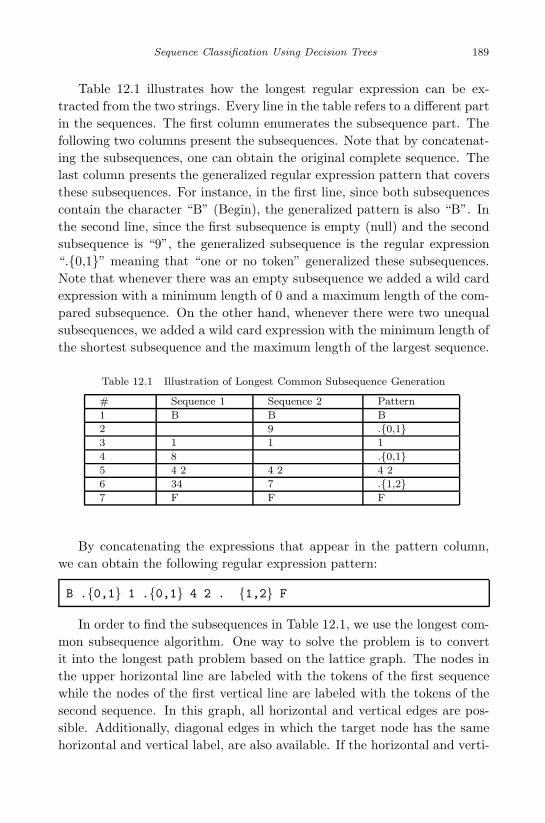
November 7, 2007 13:10 WSPC/Book Trim Size for 9in x 6in DataMining
Sequence Classification Using Decision Trees 189
Table 12.1 illustrates how the longest regular expression can be ex-tracted from the two strings. Every line in the table refers to a different partin the sequences. The first column enumerates the subsequence part. Thefollowing two columns present the subsequences. Note that by concatenat-ing the subsequences, one can obtain the original complete sequence. Thelast column presents the generalized regular expression pattern that coversthese subsequences. For instance, in the first line, since both subsequencescontain the character “B” (Begin), the generalized pattern is also “B”. Inthe second line, since the first subsequence is empty (null) and the secondsubsequence is “9”, the generalized subsequence is the regular expression“.{0,1}” meaning that “one or no token” generalized these subsequences.Note that whenever there was an empty subsequence we added a wild cardexpression with a minimum length of 0 and a maximum length of the com-pared subsequence. On the other hand, whenever there were two unequalsubsequences, we added a wild card expression with the minimum length ofthe shortest subsequence and the maximum length of the largest sequence.
Table 12.1 Illustration of Longest Common Subsequence Generation
# Sequence 1 Sequence 2 Pattern
1 B B B
2 9 .{0,1}3 1 1 1
4 8 .{0,1}5 4 2 4 2 4 2
6 34 7 .{1,2}7 F F F
By concatenating the expressions that appear in the pattern column,we can obtain the following regular expression pattern:
B .{0,1} 1 .{0,1} 4 2 . {1,2} F
In order to find the subsequences in Table 12.1, we use the longest com-mon subsequence algorithm. One way to solve the problem is to convertit into the longest path problem based on the lattice graph. The nodes inthe upper horizontal line are labeled with the tokens of the first sequencewhile the nodes of the first vertical line are labeled with the tokens of thesecond sequence. In this graph, all horizontal and vertical edges are pos-sible. Additionally, diagonal edges in which the target node has the samehorizontal and vertical label, are also available. If the horizontal and verti-

November 7, 2007 13:10 WSPC/Book Trim Size for 9in x 6in DataMining
190 Data Mining with Decision Trees: Theory and Applications
cal edges have zero length, and the diagonal edges have length of one, thenthe longest common subsequence corresponds to the longest path from thetop left corner to the bottom right corner. This graph is acyclic and is fre-quently solved using dynamic programming. The highlighted path presentsone of the longest paths. Note that the destination node of the highlighteddiagonal edges (B,1,4,2,F) is used in the regular expression, while the hor-izontal/vertical edges are converted to the wild-card expression.
12.4 Pattern Selection
Obviously there are many patterns that can be created via the LCS (eachpair of sequences with the same class label). In fact, initially too manypatterns are created and it is essential to stay within a manageable numberof patterns. For example, a training set of 100 sequences from class “A” and50 sequences of class “B” yielded 100*99/2 + 50*49/2=6175 patterns. Inthis chapter, we suggest using a two-phase pattern reduction as describedin the following sections. In the first phase, we introduce new patterns thatare created by merging existing patterns. In the second phase we reducethese sets of patterns using correlation-based feature selection.
12.4.1 Heuristics for Pattern Selection
Many of the generated patterns differ only in the distance between thetokens. Grouping such patterns by smoothing distances eliminates manypatterns. The proposed simple heuristic for pattern reduction is based onmerging two or more patterns into a single pattern. The merging is basedon the specific tokens used in each pattern while ignoring the wild-cards.For instance, the “specific token” representation of “B 1 2 .{2,7} 3 F” is“B 1 2 3 F”. All patterns with the same “specific token” representationare merged by the smoothing wild-card expressions. This is obtained bytaking the minimum and maximum For example, the patterns “B 1 2 .{2,7}3 F” and “B 1 2 .{3,9} 3 F” and “B 1 .{1,3} 2 .{3,4} 3 F” which all havethe same “specific token” representation of “B 1 2 3 F” are generalizedusing the pattern “B 1 .{0,3} 2 .{2,9} 3 F”. Moreover any two or morepatterns whose “specific token” representations are different in one position(a Hamming distance of one) are generalized by introducing a wild-card intothat position.

November 7, 2007 13:10 WSPC/Book Trim Size for 9in x 6in DataMining
Sequence Classification Using Decision Trees 191
12.4.2 Correlation based Feature Selection
Feature selection is the process of identifying relevant features in the datasetand discarding everything else as irrelevant and redundant. For this pur-pose, each “regular expression” pattern represents a different feature. Inthis work we use a non-ranker filter feature selection algorithm. Filteringmeans that the selection is performed independently of any learning algo-rithm. Non-ranker means that the algorithm does not score each patternbut only determines which pattern is relevant and which is not.
In this work we use the correlation-based feature subset selection (CFS)as a subset evaluator. CFS evaluates the worth of a subset of attributes byconsidering the individual predictive ability of each feature along with thedegree of redundancy between them. Subsets of features that are highlycorrelated with the class while having low inter-correlation are preferred.This approach is useful when there are many correlated patterns (for inst-ance, when one pattern generalizes another pattern).
The CFS algorithm was executed with best-first forward selection. Thissearch strategy searches the space of attribute subsets by greedy hill-climbing augmented with a backtracking facility. It starts with the emptyset of attributes and search forward.
12.5 Classifier Training
We are using a decision tree inducer as the base inducer. Using a decisiontree as a classifier in this case has several advantages. (1) The sequence isnot classified based on a single pattern, but on set of patterns, i.e. this clas-sifier can be used to indicate that a sequence is classified to the label “A”only if it matched two patterns and does not match a third pattern. Thisis more expressive than the classical approach in which the classification isbased on a single pattern. Moreover, in this way, instead of searching forcomplicated regular expressions, we can search for simple regular expres-sions and “rely” on the decision tree to combine them. In fact, in somecases, it is possible to express a tree path as a single complicated regularexpression; (2) The hierarchical structure of decision tree enforces an or-der (priority) in the usage of patterns, i.e. given a new sequence, not allpatterns should be matched in advance but one pattern at a time based onthe specific branch. In this way we inherently obtain a conflict resolutionmechanism; (3) As opposed to other classifiers (such as neural networks)the meaning of the classifier can be explained.

November 7, 2007 13:10 WSPC/Book Trim Size for 9in x 6in DataMining
192 Data Mining with Decision Trees: Theory and Applications
12.5.1 Adjustment of Decision Trees
Instead of using the C4.5 algorithm as is, we were required to make someadjustment to the splitting criterion. In the problem solved here, there aretwo types of attributes: the regular expressions (binary attributes indicat-ing if the expression is matched or not) and the attributes that characterizethe tokens. Note that the characterizing attributes of the tokens becomeavailable only when the corresponding token is matched. For instance, ifthe token “A” in the sequence has the attribute “var1” then we can use theattribute “var1” in a certain decision node only if a regular expression withthe token “A” has appeared in one of its ancestor nodes. This suggests forconsideration other criteria than the information gain ratio, such as:
• Select pattern with the largest support – If the support of a patternis relatively high, then there are sufficient training instances to grow ameaningful sub-tree.• Select the longest pattern – Longest sequence implies that the di-
mensionality (namely, the number of characterizing attributes) of thematched training instances is large enough to grow a meaningful sub-tree.
12.5.2 Cascading Decision Trees
Studying the training corpuses, the classification errors and patterns se-lected by the classifier, we noticed that it is possible to create a more pow-erful ensemble structure than the structure obtained from such a general-purpose ensemble method as Adaboost. More specifically, we noticed that:(1) training set size might be a limiting issue due to the computationalcomplexity of the machine learning algorithms used; (2) in the training andtest corpuses there are simple sequences versus compound sequences; and(3) some of the patterns yield very high precision.
These observations, as well as the improvement achieved using the Ad-aboost method, triggered the idea of constructing a cascade of classifiers.The idea is to build a cascade of classifiers. The selection of tree cascades isdue to the fact that in this case we assume the class is binary (positive andnegative): The first cascade includes only simple patterns obtained fromthe negative class, ensuring high precision (very few positive sequences willbe classified as negative).
The “errors” of the first cascade “Trained classifier 1”, meaning se-quences from the negative corpus that were not classified as negative by

November 7, 2007 13:10 WSPC/Book Trim Size for 9in x 6in DataMining
Sequence Classification Using Decision Trees 193
“Trained classifier 1”, are taken as the negative training corpus for thesecond cascade classifier (positive corpus remains the same as for the firstcascade). The second cascade is of negative patterns (learned from theoriginal corpus of negative sequences). The third cascade classifier includesalso positive patterns.
12.6 Application of CREDT in Improving of InformationRetrieval of Medical Narrative Reports
In this section, we illustrate how the CREDT algorithm can be used in a realworld application of information retrieval. Information retrieval from freetext is now an established and well known application with vast popularityamong Internet search engines such as Google. The limitations of naıvekeyword-based information retrieval are also well understood and manyresearch works are focused around this issue.
We illustrate the CREDT in improving the information retrieval frommedical narratives. Medical narratives present some unique problems thatare not normally encountered in other kinds of texts. When a physicianwrites an encounter note, a highly telegraphic form of language may beused. There are often very few (if any) grammatically proper sentencesand acronyms and abbreviations are frequently used. Many of these abbre-viations and acronyms are highly idiosyncratic and may not be found in ageneral dictionary.
Information retrieval from medical narratives has many applications:enrollment of patients into clinical trials; detecting adverse events; mod-ern evidence-based practice; and medical research in general. A typicalapplication scenario may involve a hospital-based medical investigator re-ceiving from a pharmaceutical company a patient profile for a plannedclinical trial. The profile includes attributes that cannot be used as is in astructured query of the hospital information systems. Example of such apatient profile is: “Male and female, 18 years and older; Female must notbe pregnant; Location of pain must be low back area; Pain must be presentfor three months or greater; No surgical intervention in the past 12 monthsnor plans for surgical intervention for the low back pain during the durationof the study”.
Most of the data needed for locating patients meeting the above profile isstored as electronic medical narratives in the hospital information systems.The medical investigator retrieves such records by a keyword-based search.

November 7, 2007 13:10 WSPC/Book Trim Size for 9in x 6in DataMining
194 Data Mining with Decision Trees: Theory and Applications
The keywords primarily include: diagnostic names, symptoms, procedures,medicine, etc. A useful knowledge source designed for resolving medicalterms is the Unified Medical Language System (UMLS) [Lindbergh andHumphreys (1993)].
The common use-case when searching in discharge summaries is look-ing for patients with specific symptom, for example, nausea. The issueof context is very important. Consider the sentence: “He complained atadmission of headache, nausea, vomiting, and neck soreness” versus “Thepatient denies any headache, nausea, vomiting, blurring vision and fever”.Both sentences will match a naıve keyword-based query containing the termnausea. We assume that the person initiating the query is looking for pa-tients with a specific symptom (e.g. nausea). For example, the sentence“The patient states she had fever and chills two nights prior to admissionwith a nonproductive cough”, taken from a discharge summary report isa positive example for fever and chills diagnoses, while another sentencefrom a discharge report: “The patient denied any cough, chest pain, urinarysymptoms or bowel symptoms” is a negative example for cough, chest pain,urinary symptoms and bowel symptoms diagnoses.
A search for patients with a specific symptom or set of findings mightresult in numerous records retrieved. The mere presence of a search term inthe text, however, does not imply that retrieved records are indeed relevantto the query. Depending upon the various contexts that a term might have,only a portion of the retrieved records may actually be relevant. Therefore,in addition to excluding negated concepts, there are additional contexts weopt to exclude. For example: “The patient as well as her daughter weregiven very clear instructions to call or return for any nausea, vomiting,bleeding, or any unusual symptoms.”; and the sentence: “The patient couldnot tolerate the nausea and vomiting associated with Carboplatin”; “She ismarried, lives with her husband and admits to drinking alcohol excessivelyin the remote past.” ; and more.
To cope with the natural ambiguity that these sentences and the variouscontexts suggest, we introduce here a new supervised method for inducinga sequence-aware (or sequence sensitive) classifier. First we automaticallydiscover a set of sequence patterns that are described as regular expressions.Then a classifier is induced to classify instances based on their matchingthe discovered set of sequence patterns. We show the advantages of thenew method by applying it to a well-known and well-defined problem inthe medical domain. The challenge is to increase information retrievalaccuracy from the common 60% baseline naıve search. This improvement

November 7, 2007 13:10 WSPC/Book Trim Size for 9in x 6in DataMining
Sequence Classification Using Decision Trees 195
is achieved by identifying the context of the query keyword (e.g. medicaldiagnosis such as nausea) being searched.
The issues encountered in dealing with this problem constitute a spe-cial case of context identification in free text, one of the key researchproblems in the field of text mining. We compare the results obtainedusing our proposed method to previous works which implement two pri-mary methodologies: knowledge engineering; and machine learning. Theknowledge engineering approach is based on handcrafted patterns for iden-tifying the negated context. Such methods yield high accuracy but arelabor-intensive, domain specific and tedious to maintain. The more mod-ern methods are based on machine learning techniques. The bag-of-wordsis considered as one of the prominent machine learning techniques for clas-sification problems. The negative context detection can be formulated asa text classification problem and solved using bag-of-words. The negationproblem is closely related to the part-of-speech tagging problem, which isproperly solved by frameworks for labeling sequential data, such as hid-den Markov model (HMM) and conditional random fields (CRF). In thiswork we compare our new method to the above mentioned techniques. Ournew method is much faster than manual knowledge engineering techniqueswith matching accuracy. We show that our new method achieves higheraccuracy compared to existing methods.
12.6.1 Related Works
The negation problem in medical reports can be solved in various ways.First, in addition to existing general purpose text classification methodsthat can be used. there are several information extraction methods thatcan also be implemented. After discussing these methods, we survey specificworks regarding the negation problem in general and in the medical domainin particular. Finally, we discuss evaluation measures that can be used forestimating the quality of the solutions.
12.6.1.1 Text Classification
From a comprehensive survey of the methods used for text categorizationand which describes recent research trends we see that the machine learn-ing paradigm to automatic classifier construction definitely supersedes theknowledge-engineering approach. Within the machine learning paradigm,a classifier is built by learning from a set of previously classified documents.
November 7, 2007 13:10 WSPC/Book Trim Size for 9in x 6in DataMining
196 Data Mining with Decision Trees: Theory and Applications
The advantages of the machine learning approach are its high degree of ef-fectiveness, a considerable savings in terms of expert manpower, and dom-ain independence.
Since texts cannot be directly interpreted by a classifier or by a classifier-building algorithm, it is necessary to uniformly apply a transformationprocedure to the text corpora in order to map a text dj into a compactrepresentation of its content. In text categorization (TC) a text dj is usuallyrepresented as a vector of term weights dj = (w1j ,. . . ,w |V |j) where V is theset of terms (sometimes called features) that occur at least once in at leastone document of Tr, and where 0 ≤ wkj ≤ 1 represents, loosely speaking,how many term tk contributes to the semantics of document dj . Differencesamong approaches are accounted for by (1) different ways to understandwhat a term is; (2) different ways to compute term weights. A typicalchoice for the first alternative is to identify terms with words. Dependingon whether weights are binary or not, this approach is often called either the“set of words” or the “bag-of- words” approach to document representation.
The following example demonstrates the bag-of-words representationapplied to our domain. Consider the two sentences: (1) The patientwas therefore admitted to the hospital and started on <MEDICINE> astreatments for <DIAGNOSIS>; and (2) The patient was ruled in for<DIAGNOSIS> and started <MEDICINE> for <DIAGNOSIS>.
One of the main drawbacks of the bag-of-words representation is in itsdestruction of semantic relations between words; the meaning of word com-binations is lost. This representation loses the meaning of important termssuch as “ruled in”. This bag-of-words limitation is especially important forthe negation detection.
Another popular choice for text representation is to identify terms withword sequences of length n. This n-gram vector text representation methodis used to classify text documents. One option is to select the normalizedfrequency with which the n-gram occurs in the document as the choice of2-term weight. Each vector identifies a point in a multidimensional space,and similar documents are expected to have points close to each other.Then the dot product between two histogram vectors is used as a measureof their similarity.
Caropreso et al. (2001) experimented with n-grams for text categoriza-tion on the Reuters dataset. They define an n-gram as an alphabeticallyordered sequence of n stems of consecutive words in a sentence (after stopwords were removed). The authors use both unigrams (bag-of-words) andbigrams as document features. They extract the top-scored features using

November 7, 2007 13:10 WSPC/Book Trim Size for 9in x 6in DataMining
Sequence Classification Using Decision Trees 197
various feature selection methods including mutual information. Their re-sults indicate that in general bigrams can better predict categories thanunigrams.
A regular expression is defined as any string that describes or matchesa set of strings according to certain syntax rules. Regular expressions areusually used to give a concise description of a set without having to list allelements. The regular expression consists of a letter of the alphabet andspecial characters. For example, the set containing the four strings: hat,hit, hot and hut can be described by the pattern “h.t” (or alternatively, itis said that the pattern matches each of the four strings). The wild-card(“.”) denotes a single position that can be occupied by any letter of thealphabet. The curly brackets are used to indicate a match between min andmax of the preceding characters. For instance the pattern “without .{0,10}<diagnosis>” can be matched against the following strings “without <
diagnosis >”, “without any < diagnosis >”, “without serious < diagnosis>”, etc.
Regular expressions are used by many text editors and utilities to searchand manipulate bodies of text based on certain patterns. Many program-ming languages support regular expressions for string manipulation. Forexample, Perl has a powerful regular expression engine built directly intotheir syntax. In our work we use the Java regular expression implementa-tion (package java.util.regex ).
The bag-of-words and n-gram representations are actually a special caseof the regular expression representation proposed in this work. A regularexpression feature such as “.{0,500} started .{0,500}” is actually equiva-lent to the word feature started in the bag-of-words representation. Theregular expression feature “.{0,500} ruled in .{0,500}” matches the bigramrepresentation of the two words phrase ruled in. An additional benefit ofour proposed regular expressions compared to bag-of-words is in handlingcompound sentences that include both positive and negative findings. Forexample, the sentence: “upon admission showed no <diagnosis 1> but didshow extensive <diagnosis 2> and <diagnosis 3> but there were no massesnoted”. The bag-of-words representation of such sentences is problematicsince the same features apply to both negative and positive contexts andthe algorithm cannot learn to distinguish between them. The regular ex-pressions representation can represent such structural features using thedistance and presence of additional diagnosis.

November 7, 2007 13:10 WSPC/Book Trim Size for 9in x 6in DataMining
198 Data Mining with Decision Trees: Theory and Applications
12.6.1.2 Part-of-speech Tagging
Part-of-speech tagging (POS tagging) refers to labeling words in a text ascorresponding to a particular part of speech based on both its definition,as well as its context—i.e., relationship with adjacent and related wordsin the text. POS tagging is hard mainly because some words may havemultiple part of speech tags and the correct tag depends on the context.POS tags indicate the basic syntactic function of that token, such as nounor verb, as well as other grammatical information, such as number andtense. POS tagging is a fundamental preprocessing step for many otherNLP (Natural Language Processing) applications (e.g., syntactic parsing).Typically, POS tags provide general shallow syntactic information to thesedownstream applications.
Machine learning methods have been shown to be more effective insolving POS tagging than classic NLP methods. POS tagging is closelyrelated to our problem. In fact, the negation detection problem can beregarded as a special case of POS tagging – we define a polarity tag (possiblevalues are Negative and Positive) that is applicable to the <diagnosis>terms only. The following sections present sequences labeling frameworksthat have been successfully used for POS tagging.
12.6.1.3 Frameworks for Information Extraction
A common information extraction (IE) task is to automatically extractentities and relationships from semi-structured or free text. For example,in the medical domain, an IE task is to automatically populate a structureddatabase from a discharge summary report.
Many works in IE propose learning approaches that automatically pro-cess free text and overcome the knowledge engineering bottleneck. Forexample Califf and Moony (1997) proposed the RAPIER system that in-duces pattern-match rules from rigidly structured text. Such systems focuson extracting entities and relationships. However there is no emphasis onspecial contexts, such as negation that might totally divert the meaningof the text. Apparently such cases are rare in the corpora used for eval-uating the above works (which is not true when dealing with dischargereports where more than 50% of the findings might actually be negated).More recent IE works are focused on hidden Markov model (HMM)techniques.

November 7, 2007 13:10 WSPC/Book Trim Size for 9in x 6in DataMining
Sequence Classification Using Decision Trees 199
12.6.1.4 Frameworks for Labeling Sequential Data
The Hidden Markov model (HMM) is a common machine learning tech-nique with published applications in sequential pattern recognition tasks.HMMs were successfully applied to related problems such as: IE, POS tag-ging and many more. Specifically, HMM was successfully applied to POStagging of bio-medical texts. Similarly, we can utilize HMM POS taggersfor solving the negation problem. Applying a HMM POS tagger to thenegation detection problem is not a trivial task since there are many pos-sible approaches for structuring the HMM. The hidden states are the POStags (e.g. noun, verb, adjective, etc.) and the arrows represent the possibletransitions between states.
Conditional random fields (CRFs) is a newer framework for labeling se-quential data. CRFs define a conditional probability over label sequencesgiven a certain observation sequence. This relaxes the unwarranted in-dependence assumptions about the sequences which HMMs make. LikeHMMs, CRFs have been successfully used for part-of-speech tagging. Acomparative study showed that CRFs outperform HMMs in this applica-tion.
12.6.1.5 Identifying Negative Context in Non-domain SpecificText (General NLP)
Negation is an active linguistic research topic with roots dating back to Aris-totle. Today this topic is still being widely studied. Negation is considereddifficult in natural language processing due to the overwhelming complexityof the form and the function of sentences with negation. Negation is one ofthe constants of classical logic and has complex and systematic interactionwith the other logical operators, especially quantifiers and modals.
In English grammar, negation is the process that turns a positive state-ment (“the patient has <diagnosis>”) into its opposite denial (“the patientdoes not have <diagnosis>”). Nouns as well as verbs can be negated witha negative adjective (“There is no <diagnosis>”); a negative pronoun (noone, nobody, neither, none, nothing); or a negative adverb (“he never was<diagnosis>”). It is easy to identify specific negation words such as: not,neither, and never, as well as for Not -negation, e.g., not, n’t, and No-negation. However, in many cases, these specific words are not presented,e.g., deny, fail, and lack. Words in this second category are called inher-ent negatives, i.e., they have a negative meaning but a positive form. Anadditional morphological form of negation is the affixal negation. Prefix
November 7, 2007 13:10 WSPC/Book Trim Size for 9in x 6in DataMining
200 Data Mining with Decision Trees: Theory and Applications
negations un- and in- , may create negation words unhappy, unwise, andunfit . Negations can also be created with suffixes such as -less, e.g., life-less. Another complexity arise from double negation, e.g. the sentence “itis not unlikely”. The neg-raising phenomenon adds additional complexity,e.g. sentences such as: “I don’t believe he is ill” or “I don’t think he is ill”.
We could not locate any NLP research on identifying negated conceptsin specific non-domain areas. However, some NLP techniques such as syn-tactic and semantic processing can be applied to a negation identificationframework, especially part of speech tagging and shallow parsing. Thesefeatures can be combined into a machine learning classification scheme fornegation identification. The effectiveness of such NLP techniques very muchdepends on the quality of the text, particularly its compliance with gram-matical rules. The language used in medical narratives, however, is oftengrammatically ill-formed. For example, the positive finding cough in thesentence “the patient reported she was not feeling well due to mild cough”.Thus NLP techniques that rely on grammatical sentences may not be suf-ficient for identification of negation in medical narratives.
12.6.1.6 Identifying Negative Context in Medical Narratives
Researchers in medical informatics have suggested methods for automat-ically extracting information contained in narrative reports for decisionsupport, guideline implementation, and detection and management of epi-demics. Some of the researches concentrate on methods for improving in-formation retrieval from narrative reports. A number of investigators havetried to cope with the problem of a negative context. These works can beclassified into two research domain categories, which are presented in thefollowing two sections.
12.6.1.7 Works Based on Knowledge Engineering
The knowledge engineering approach is based on human expert writing rulesor patterns. These rules and patterns are designed to capture syntactic andsemantic features of the free text. The methods used are mostly from theNLP research field utilizing also deep parsing technologies and sometimesrule engines. These methods are complex and very expensive to developand maintain, useful mostly when the target text is written according toproper language rules.

November 7, 2007 13:10 WSPC/Book Trim Size for 9in x 6in DataMining
Sequence Classification Using Decision Trees 201
12.6.1.8 Works based on Machine Learning
Many of the recent works in the field of text classification are based on themachine learning approach. Machine learning has proven effective for textclassification. The advantages are that such methods are much faster todevelop than knowledge engineering. In addition they are more effectivewhen the text is not written according to proper grammar rules.
12.6.2 Using CREDT for Solving the Negation Problem
We now show how the CREDT algorithm can be used to solve the negationproblem. Section 5.6.1 below explains the complete process of training aregular expression based classifier from an input of training and test cor-pora. Sections 5.6.2-12.6.2.8 specifiy in detail each of the steps. Finally,Section 5.6.6 suggests the concept of cascading several classifiers for im-proving the performance.
12.6.2.1 The Process Overview
We suggest the following process of training a classifier to predict nega-tion concepts using regular expressions patterns. The process includes foursteps:
Corpus preparation A domain specific task designed to normalize, gen-eralize and tag the free text so that it can be further processed.
Regular expression patterns learning The automatic creation of aregular expression patterns from the training set.
Patterns selection Applying heuristics and features selection techniquesto select the best patterns for correct classification of the concept.
Classifier training Training a decision tree classifier.
The following sections describe each of the above steps.
12.6.2.2 Step 1: Corpus Preparation
The objective of the corpus preparation phase is to transform the inputdischarge summaries data into a usable corpus for the training and testphases. The following sections describe each sub-step.

November 7, 2007 13:10 WSPC/Book Trim Size for 9in x 6in DataMining
202 Data Mining with Decision Trees: Theory and Applications
12.6.2.3 Step 1.1: Tagging
In the first step we parse all the discharge summaries. All known med-ical terms are tagged using a tagging procedure presented in [Rokach etal. (2004), ]. Consider for example the following text:
We use the UMLS metathesaurus, for tagging the sentence, i.e. replac-ing medical terms with their concept type. For example, when the parserreaches the term coronary it queries the UMLS for terms starting with“coronary*”. The result set includes several terms starting with coronary.The parser then uses a sliding window in order to match the longest pos-sible UMLS term to the given sentence. The UMLS terms relevant for theabove sentence are listed in Table 12.2.
Table 12.2 Tagging using the UMLS
ID Term Type CUI (concept uniqueidentifier)
1 coronary artery by-pass graft
Procedure 10010055
2 coronary artery dis-ease
Diagnosis 10010054
3 hypertension Diagnosis 10020538
4 diabetes mellitus Diagnosis 10011849
5 kidney stones Diagnosis 10022650
Since we are only interested in the generalized form of the sentence (thespecific diagnosis or procedure does not matter), the output text followingthe tagging process takes the following form:
12.6.2.4 Step 1.2: Sentence Boundaries
Physicians are trained to convey the salient features of a case concisely andunambiguously as the cost of miscommunication can be very high. Thusit is assumed that negations in dictated medical narrative are unlikely tocross sentence boundaries, and are also likely to be simple in structure.
An additional processing step includes breaking discharge summariesdocuments into sentences using a sentence boundary identifier as suggestedby [Averbuch et al. (2005)]. The sentence boundary is identified by search-ing for terminating signs such as {“.”, “?”, “!”}. This approach is notsufficient since periods and other signs are frequently appear inside sen-tences (for instance: “Patient was discharged on Lopressor 25 milligrams

November 7, 2007 13:10 WSPC/Book Trim Size for 9in x 6in DataMining
Sequence Classification Using Decision Trees 203
p.o. b.i.d.1”. We detect such exceptions using regular expressions (an ex-pression that describes a set of strings) to exclude expressions that mightmistakenly be considered end of sentence (Table 12.3).
Table 12.3 Regular expressions to exclude sentence end
(b|t|q)\.i\.d\.? p\.o\.? \.([0-9]+) cc\.p\.r\.n q\.d\.? \.of \.,and
q\.h\.s mg\. (Dr\.)(\s?)(\w+) \sq\.
12.6.2.5 Step 1.3: Manual Labeling
This step refers to the creation of the training corpus. Physicians shouldreview each document and label each medical term, indicating whetherit appears in positive or negative context. Since most sentences includemore than one diagnosis. it is necessary to tag each of them during themanual tagging process. Consider for instance the compound sentence:“She denied shortness of breath, but did have fever”. In this case “shortnessof breath” is negative while “fever” is positive. Thus, this sentence will berepresented in the dataset as two different instances – one for each diagnosisterm. Since each instance has one label (positive or negative), each hasexactly one anchor diagnosis term to which the label refers. This anchorterm is tagged as “<DIAGNOSIS>” while any other diagnosis terms inthe sentence will be denoted as “<DIAG>”. Note that we will be ableto obtain different patterns from the same sentence. For instance, in theexample, the pattern “.* denied <DIAGNOSIS> .*” can be learned foridentifying negative context, and the pattern “.* denied <DIAG> but .*<DIAGNOSIS>” can be learned for identifying positive context.
12.6.2.6 Step 2: Patterns Creation
For the reasons explained below, instead of using a single regular expressionrepresentation for the entire sentence, we use two regular expressions: onefor the string that precedes the targeted medical term (the seed) and onefor the string that follows it. This split may help to resolve some of theproblems that arise in compound sentences that include both positive andnegative contexts in the same sentence. Recall the example “The patientstates she had fever, but denies any chest pain or shortness of breath”.In this case, the appearance of the verb “denies” after the term “fever”
1From Latin: oral administration two times daily

November 7, 2007 13:10 WSPC/Book Trim Size for 9in x 6in DataMining
204 Data Mining with Decision Trees: Theory and Applications
indicates that the term “fever” is left in positive context. The appro-priate regular expression will be in this case as follows: “.{0,200}deniesany.{0,200}<DIAGNOSIS>”, where the distance 200 is arbitrary deter-mined per the expected sentence length in the domain.
To learn regular expressions, we have adapted two different algorithmsto our task and compared them . The first algorithm, LCS, is commonlyused to compare characters in a word. The second algorithm, Teiresias, wasdesigned for discovering motifs in biological sequences. We describe howwe adapted these algorithms to the task of learning regular expressions fornegation patterns below.
Learning regular expression patterns using longest commonsubsequence algorithm
The basis for discovering a regular expression is a method that comparestwo texts with the same context and incorporates the same concept types(i.e. diagnosis, medication, procedure, etc.). By employing the longestcommon subsequence (LCS) algorithm [Myers (1986)] on each part of thesentence (before the targeted term and after the targeted term) a regularexpression that fits these two sentences is created. The LCS employs abrute force policy: given a sequence X, determine all possible subsequencesof X, and check to see if each subsequence was a subsequence of Y, keepingtrack of the longest subsequence found. For instance, assume we are giventhe following two sentences:
The patient was therefore admitted to the hospital andstarted on <MEDICINE> as treatments for <DIAGNOSIS>.
The patient was ruled in for <DIAG> and started <MEDICINE>for <DIAGNOSIS>.
We execute the LCS algorithm on the two normalized sentences as pre-sented in Table 12.4.
Note that the LCS algorithm was revised to compare tokens as opposedto comparing characters in its classical implementation. It should also benoted that whenever there was only insertion (or only deletion) we addeda wild card string with a minimum length of 0 and a maximum lengthof the inserted string (including the leading and trailing spaces). On theother hand, whenever there was simultaneously insertion and deletion, we

November 7, 2007 13:10 WSPC/Book Trim Size for 9in x 6in DataMining
Sequence Classification Using Decision Trees 205
Table 12.4 Longest Common Subsequence Generation for Medical Text
Sentence 1 Sentence 2 Pattern
The patient was The patient was The patient was
therefore admitted tothe hospital
.{24,35}ruled in for <DIAG>
and started and started and started
on .{0,4}<MEDICINE> <MEDICINE> <MEDICINE>
as treatments .{0,15}for <DIAGNOSIS> for <DIAGNOSIS> for <DIAGNOSIS>
added a wild card string with the minimum length of the shortest stringand maximum length of the largest string (without leading and trailingspaces because they are part of the common substring).
As a result of running the LCS algorithm we obtain the following pat-tern. This pattern can now be used to classify concept of type medicationappearing in positive contexts.
The patient was .{24,35} and started .{0,4}<MEDICINE>.{0,15}for <DIAGNOSIS>
Learning regular expression patterns using Teiresias algorithmThe Teiresias algorithm was designed to discover motifs in biological
sequences, an important research problem [Rigoutsos and Floratos (1998)].The method is combinatorial in nature and able to produce all patternsthat appear in at least a (user-defined) minimum number of sequences,yet it manages to be very efficient by avoiding the enumeration of theentire pattern space. Furthermore, the reported patterns are maximal: anyreported pattern cannot be made more specific and still keep on appearingat the exact same positions within the input sequences.
Teiresias searches for patterns which satisfy certain density constraints,limiting the number of wild-cards occurring in any stretch of pattern. Morespecifically, Teiresias looks for maximal <L,W> patterns with the supportof at least K (i.e. in the corpus there are at least K distinct sequences ofthat match this pattern). A pattern P is called <L,W> pattern if everysub pattern of P with length of at least W words (combination of specificwords and “.” wild-cards) contains at least L specific words.
For example, given the following corpus of six negative sentences:

November 7, 2007 13:10 WSPC/Book Trim Size for 9in x 6in DataMining
206 Data Mining with Decision Trees: Theory and Applications
no further <diagnosis> was noted
no history of <diagnosis>
no intraoperative or immediate <diagnosis> were noted
no other <diagnosis>
past medical history no other <diagnosis>
patient had no further episodes of <diagnosis>
The Teiresias program (L=K=2, W=5) discovers six recurring patternsshown in the following file:
2 2 no other <diagnosis>
2 2 no further
2 2 of <diagnosis>
3 3 no . <diagnosis>
2 2 <diagnosis> . noted
2 2 no . . . <diagnosis>
The first two columns represent the support of the pattern. The dotrepresents a missing word. Note that the program yields also patterns thatdo not include the <diagnosis> seed. These patterns are not useful forour purpose and are filtered out. Next we transform the Teiresias patternsto regular expression patterns by replacing each dot (missing word) witha regular expression such as .{0,L}, where L is calculated by counting thenumber of dots and multiplying by the average word length (8 charactersas per our corpus).
The resulting regular expression patterns are presented in the followingexample:
no other <diagnosis>
of <diagnosis>
no .{0,8} <diagnosis>
<diagnosis> .{0,8} noted
no . {0,24} <diagnosis>
12.6.2.7 Step 3: Patterns Selection
Obviously there are many patterns that can be created via the LCS (eachpair of sentences with the same concept type and context). In fact, initially

November 7, 2007 13:10 WSPC/Book Trim Size for 9in x 6in DataMining
Sequence Classification Using Decision Trees 207
too many patterns are created and it is essential to keep a manageablenumber of patterns. For example, a training set of 140 negative sentencesand 140 positive sentences yielded 2*(140*139/2)=19,460 patterns.
Many of the generated patterns differ only in the distance of impor-tant keywords from the seed concept. Grouping such patterns by smooth-ing distances eliminates many patterns. For example, the patterns “hadno.{12,27}<diagnosis>” and “had no.{17,32}<diagnosis>” are general-ized using the pattern “had no.{10,40}<diagnosis>”. Trivial patterns suchas “a.{70,100} <diagnosis>” are omitted. For example from the original19,460 patterns, 17,235 were identified as redundant and trivial. Aftereliminating these patterns, only 2,225 patterns are remained.
Feature selection is the process of identifying relevant features in thedataset and discarding everything else as irrelevant and redundant. For thispurpose each “regular expression” pattern represents a different feature.
We use a non-ranker filter feature selection algorithm. Filtering meansthat the selection is performed independently of any learning algorithm.Non-ranker means that the algorithm does not score each pattern but onlyindicates which pattern is relevant and which is not. The rows are train-ing sentences (negative and positive); the first K columns are the regularexpression patterns; and the last column is the target class (negative / pos-itive). The cell value is 1 if the regular expression matches the sentence,otherwise it is 0. The matrix described above is the input to the featuresselection algorithm.
In this work we use the correlation-based feature subset selection (CFS)as a subset evaluator. CFS evaluates the worth of a subset of attributesby considering the individual predictive ability of each feature along withthe degree of redundancy among them. Subsets of features that are highlycorrelated with the class while having low inter-correlation are preferred.This approach is suitable to this case, because there are many correlatedpatterns (for instance, when one pattern generalized another pattern). Forexample the 2,225 remaining patterns create a dataset of 280 instanceswith 2,225 input binary attributes (0 if the pattern does not match thesentence; 1 if pattern matches sentence) and target attribute that representthe concept classification (“Positive” or “Negative”). The filter furtherreduced the set into 35 ‘relevant’ patterns.

November 7, 2007 13:10 WSPC/Book Trim Size for 9in x 6in DataMining
208 Data Mining with Decision Trees: Theory and Applications
12.6.2.8 Step 4: Classifier Training
The filtered matrix, together with the manual classification of eachconcept, is fed into a decision tree induction algorithm which cre-ates a classification decision tree. An illustrative example of deci-sion tree generated is presented in Figure 12.1. It describes a classi-fication decision path where pattern “.{0,200}have.{0,50}<diagnosis>”,learned from positive examples, indicates a positive context with prob-ability P5 in case the sentence does not match the three (neg-ative) patterns: .“{0,200}without.{0,10}<diagnosis>”; “.{0,200}ruleout.{0,10}<diagnosis>”; “.{0,200}had no.{0,10}<diagnosis>” (withprobabilities P1, P2, and P3 for negative) but matches the negative pat-tern “.{0,200}no.{0,50}<diagnosis>”. Here we denote “negative pattern”as a pattern learned from negative context examples. This demonstratesthe power of decision based on matching a sentence with multiple regularexpressions.
.{0,200}no.{0,50}<diagnosis> .{0,200}have.{0,50}<diagnosis> Match
Match No Match
Positive w/p P4 Positive w/p P5
Negative w/p P6
.{0,200}had no.{0,50}<diagnosis> MatchNegative w/p P3
.{0,200}rule out.{0,50}<diagnosis> MatchNegative w/p P2
.{0,200}without.{0,50}<diagnosis> MatchNegative w/p P1
No Match
No Match
No Match
No Match
Fig. 12.1 Example decision tree.

November 7, 2007 13:10 WSPC/Book Trim Size for 9in x 6in DataMining
Sequence Classification Using Decision Trees 209
12.6.2.9 Cascade of Three Classifiers
It is well known that the classification accuracy of a single decision treecan be significantly improved by growing an ensemble of trees and lettingthem vote for the most popular class. Analyzing the problem domain, webrought up the hypothesis that it is possible to create a more powerfulensemble structure than the structure obtained from such general purposeensembles method as Adaboost. Specifically, we noticed that: (1) trainingset size is a limiting issue due to the computational complexity of the ma-chine learning algorithms used; (2) in the corpus, there are simple sentencesversus compound sentences or instructions; (3) Some of the patterns yieldvery high precision. This is obvious since for some of the negation termsattached (anchored) to the seed, mean that the seed is negated. For exam-ple, in a sentence such as, “. . . denied nausea . . . ” the nausea is negatedwith near 100% probability. Thus, it makes sense to train a simple clas-sifier using only such (anchored) patterns, using it to identify the simpleinstances with very high precision. Then, only instances not classified asnegative by the first cascade are used to train a second classifier.
These observations triggered the idea of constructing a cascade of clas-sifiers. The idea is to build a cascade of classifiers. The selection of treecascades is due to the problem characteristics: the first cascade consists ofanchored patterns; the second cascade consists of negative patterns (learnedfrom negative sentences) and the third cascade classifier also includes pos-itive patterns.
The first cascade includes only anchored patterns, ensuring high preci-sion (very few positive sentences will be classified as negative). Anchoredpatterns are patterns where the word is anchored (no separating words)to the seed. For example, the following anchored patterns form the firstcascade classifier:
no <diagnosis>
denied <diagnosis>
denies <diagnosis>
not <diagnosis>
negative for <diagnosis>
without <diagnosis>
ruled out <diagnosis>
The training set of negated instances for the second cascade comprises

November 7, 2007 13:10 WSPC/Book Trim Size for 9in x 6in DataMining
210 Data Mining with Decision Trees: Theory and Applications
negation patterns that failed to classify as negative by the first cascade“Trained classifier 1”. The training set of positive instances for the firstcascade is used as is in the second cascade. In the third cascade we learnpatterns from the negative and positive corpora, taking only negative inst-ances which failed to classify as negative by the first and second cascades.The third cascade classifier includes also positive patterns (patterns learnedfrom the positive corpus). In that sense, these patterns are different fromthe previous works that rely only on negation patterns.
Figure 12.2 demonstrates how the cascaded classifiers perform the clas-sification of three unseen sentences. The first sentence “the patient denied<diagnosis>” is matched by an anchored pattern “denied <diagnosis>”and is classified negative by “Trained classifier 1”. The second sentence“the patient did not experience recent <diagnosis>” does not match withany of the “Trained classifier 1” anchored patterns, therefore it is fed into“Trained classifier 2” for further classification as negative due to the pat-terns comprising “Trained classifier 2”. The third sentence is classified asnegative by the “Trained classifier 3”. The last sentence is not classified asnegative by all three cascades and is therefore classified as positive.
An experimental study that was performed provides strong evidencethat in the negation problem, regular expressions are better than bag-of-words, in both accuracy and compactness (i.e. obtaining smaller models).In fact, regular expressions can be considered to be a generalization of thebag-of-words representation or any n-gram representation.
Using a decision tree as a base classifier in this case has several ad-vantages. (1) The sentence is not classified according to a single regularexpression, but is classified based on a set of regular expressions, i.e. thisclassifier can be used to indicate that a sentence is classified to the label“positive” only if it matched two regular expressions and does not match athird regular expression. This is more expressive than the classical approachin which the classification is based on a single regular expression. More-over, in this way, instead of searching for complicated regular expressions,we can search for simple regular expressions and “rely” on the decision treeto combine them. In some cases, it is possible to express a tree path com-prised of several simple regular expressions as a single complicated regularexpression; (2) The hierarchical structure of a decision tree enforces an or-der (priority) in the usage of regular expressions, i.e. given a new sentence,not all regular expressions should be matched in advance but one regularexpression at a time based on the specific branch traversing. In this way,the desired property of lexical analysis known as un-ambiguity (also known

November 7, 2007 13:10 WSPC/Book Trim Size for 9in x 6in DataMining
Sequence Classification Using Decision Trees 211
Trained
Classifier2
TrainedClassifier
2
Trained
Classifier1
1. The patient denied <diagnosis>
2. The patient did not experience
recent <diagnosis>
3. The patient was given
instructions to call in case of
<diagnosis>
Negative
Negative
Negative
4. She experienced <diagnosis> Classifies Sentence 1 as negative, all other
sentences are passed to
the next classifier
Classifies Sentence 2 as
negative, Sentences 3 and
4 are passed on.
Classifies Sentence 3 as
negative, Sentence 4 as
positive.
Fig. 12.2 Cascade classifier classification examples.
as conflict resolution in Expert Systems) which is usually resolved by thelongest match and rule priority is inherently resolved here; (3) As opposedto other classifiers (such as neural networks) the decision tree is a whitebox model whose meaning can be easily explained.
The experimental study strengthens the well-known fact that it is possi-ble to boost the predictive performance by combining several decision trees.Nevertheless, an important drawback of general-purpose ensemble methods,such as AdaBoost, is that they are difficult to understand. The resultingensemble is considered to be less comprehensible since the user is required tocapture several decision trees instead of a single decision tree. In addition,the ensemble members might even contradict one another. On the otherhand, in the proposed cascaded design, the classifiers do not compete witheach other and do not contradict one another, but they are complementing

November 7, 2007 13:10 WSPC/Book Trim Size for 9in x 6in DataMining
212 Data Mining with Decision Trees: Theory and Applications
each other. Specifically, we either make a decision in the current cascadeor postpone the decision to the next cascade. In any case the decision ismade by a single classifier and not by some voting mechanism. Moreover,the cascade increases precision by adding additional layers of decision treeclassifiers and easily regulates the classifier complexity / precision tradeoff.In addition, the cascaded design needs only three classifiers, as opposed tomuch larger ensemble size in the case of AdaBoost.
Beside the fact that the proposed method has provided a higher accu-racy than the HMM and the CRF classifiers, it can be easily transformedinto a maintainable source code. Modern programming languages, such asJava or C#, or script languages such as Perl and Python include inherentsupport for regular expressions. Any programmer can manipulate thesemodels quite easily as opposed to HMM or CRF models which requiresthat programmers be familiar with the notion of probability.
As indicated above, feature selection can be used to improve predic-tive power. The number of regular expressions (pre-feature selection) isusually greater than linear in the number of instances in the training set.For instance, if the paired LCS approach is used, then for every pair inthe training set we obtain a regular expression. At first glance, it seemsredundant to use feature selection as a preprocess phase for the trainingphase. Decision trees inducers, as opposed to other induction methods,incorporate in their training phase a built-in feature selection mechanism.Still, it is well known that correlated and irrelevant features may degradethe performance of decision trees inducers. Moreover, in the way we cre-ate regular expressions, there are many features that are correlative. Thisphenomenon can be explained by the fact that feature selection in deci-sion trees is performed on one attribute at a time and only at the rootnode over the entire decision space. In subsequent nodes, the training setis divided into several sub-sets and the features are selected according totheir local predictive power. Geometrically, it means that the selection offeatures is done in orthogonal decision subspaces, which do not necessarilyrepresent the distribution of the entire instance space. It has been shownthat the predictive performance of decision trees could be improved with anappropriate feature pre-selection phase. Moreover using feature selectioncan reduce the number of nodes in the tree, making it more compact.
Another way to avoid the “curse of dimensionality” in this case, is tomerge several expressions into one expression by generalizing them. How-ever, this increases the risk of over generalization. This is the typicalsensitivity-specificity problem. A criterion for merging regular expressions

November 7, 2007 13:10 WSPC/Book Trim Size for 9in x 6in DataMining
Sequence Classification Using Decision Trees 213
can be based on existing computational learning theoretical bounds (suchas the VC dimension) that trade training accuracy with model complexity.Merging regular expressions reduces a model’s complexity but at the sametime it might also reduce training accuracy (due to generalization). Themerging can be performed in any stage: pre-training, like feature selection,during the actual training of decision trees (as an extension to the splittingcriterion), or post growing as an extension to the pruning phase.
Regular expressions seem quite useful for the examined task but theydo have limitations. For instance, because they do not use syntax but onlywords and character length gaps, they can make mistakes due to, for ex-ample, a training set that only showed one adjective modifying a negatednoun (e.g., no persistent cough) but a test set that has multiple adjectivesintervening between the negation phrase and the negated concept. More-over, in order that a negative modifier will be included in the model, itshould be repeated at least twice in two different instances in the trainingset. This is because the regular expressions are created by comparing twostrings and identifying the common substring. If the modifier appears onlyonce, then it will never be included in any of the regular expressions.

November 7, 2007 13:10 WSPC/Book Trim Size for 9in x 6in DataMining
This page intentionally left blankThis page intentionally left blank

November 7, 2007 13:10 WSPC/Book Trim Size for 9in x 6in DataMining
Bibliography
Aha, D. W.; Kibler, D.; and Albert, M. K., Instancebased learning algorithms.Machine Learning 6(1):37-66, 1991.
A1-Sultan K. S., A tabu search approach to the clustering problem, PatternRecognition, 28:1443-1451,1995.
Al-Sultan K. S. , Khan M. M. : Computational experience on four algorithms forthe hard clustering problem. Pattern Recognition Letters 17(3): 295-308,1996.
Ali K. M., Pazzani M. J., Error Reduction through Learning Multiple Descrip-tions, Machine Learning, 24: 3, 173-202, 1996.
Almuallim H., An Efficient Algorithm for Optimal Pruning of Decision Trees.Artificial Intelligence 83(2): 347-362, 1996.
Almuallim H,. and Dietterich T.G., Learning Boolean concepts in the presence ofmany irrelevant features. Artificial Intelligence, 69: 1-2, 279-306, 1994.
Alsabti K., Ranka S. and Singh V., CLOUDS: A Decision Tree Classifier for LargeDatasets, Conference on Knowledge Discovery and Data Mining (KDD-98),August 1998.
An A. and Wang Y., ”Comparisons of classification methods for screening po-tential compounds”. In IEEE International Conference on Data Mining,2001.
Anand R, Methrotra K, Mohan CK, Ranka S. Efficient classification for multiclassproblems using modular neural networks. IEEE Trans Neural Networks,6(1): 117-125, 1995.
Anderson, J.A. and Rosenfeld, E. Talking Nets: An Oral History of Neural Net-work Research. Cambridge, MA: MIT Press, 2000.
Ashenhurst, R. L., The decomposition of switching functions, Technical report,Bell Laboratories BL-1(11), pp. 541-602, 1952.
Athanasopoulos, D. (1991). Probabilistic Theory. Stamoulis, Piraeus.Attneave F., Applications of Information Theory to Psychology. Holt, Rinehart
and Winston, 1959.Averbuch M., Maimon O., Rokach L., and Ezer E., Free-Text Information Re-
trieval System for a Rapid Enrollment of Patients into Clinical Trials, Clin-ical Pharmacology and Therapeutics, 77(2): 13-14, 2005.
215

November 7, 2007 13:10 WSPC/Book Trim Size for 9in x 6in DataMining
216 Data Mining with Decision Trees: Theory and Applications
Avnimelech R. and Intrator N., Boosted Mixture of Experts: an ensemble learningscheme, Neural Computations, 11(2):483-497, 1999.
Baker E., and Jain A. K., On feature ordering in practice and some finite sam-ple effects. In Proceedings of the Third International Joint Conference onPattern Recognition, pages 45-49, San Diego, CA, 1976.
Bala J., Huang J., Vafaie H., De Jong K., Wechsler H., Hybrid Learning UsingGenetic Algorithms and Decision Trees for Pattern Classification, IJCAIconference, 1995.
R. Banfield, OpenDT, http://opendt.sourceforge.net/, 2005.Robert E. Banfield, Lawrence O. Hall, Kevin W. Bowyer, W.P. Kegelmeyer, A
Comparison of Decision Tree Ensemble Creation Techniques, IEEE Trans-actions on Pattern Analysis and Machine Intelligence, vol. 29, no. 1, pp.173-180, Jan., 2007
Banfield J. D. and Raftery A. E. . Model-based Gaussian and non-Gaussian clus-tering. Biometrics, 49:803-821, 1993.
Bartlett P. and Shawe-Taylor J., Generalization Performance of Support VectorMachines and Other Pattern Classifiers, In “Advances in Kernel Methods,Support Vector Learning”, Bernhard Scholkopf, Christopher J. C. Burges,and Alexander J. Smola (eds.), MIT Press, Cambridge, USA, 1998.
Basak J., Online adaptive decision trees, Neural Computations, 16(9):1959-1981,2004.
Basak J., Online Adaptive Decision Trees: Pattern Classification and FunctionApproximation, Neural Computations, 18(9):2062-2101, 2006.
Bauer, E. and Kohavi, R., “An Empirical Comparison of Voting ClassificationAlgorithms: Bagging, Boosting, and Variants”. Machine Learning, 35: 1-38, 1999.
Baxt, W. G., Use of an artificial neural network for data analysis in clinicaldecision making: The diagnosis of acute coronary occlusion. Neural Com-putation, 2(4):480-489, 1990.
Bay, S., Nearest neighbor classification from multiple feature subsets. IntelligentData Analysis, 3(3): 191-209, 1999.
Bellman, R., Adaptive Control Processes: A Guided Tour, Princeton UniversityPress, 1961.
BenBassat M., Myopic policies in sequential classification. IEEE Trans. on Com-puting, 27(2):170-174, February 1978.
Kristin P. Bennett and Ayhan Demiriz and Richard Maclin, Exploiting unlabeleddata in ensemble methods, Proceedings of the eighth ACM SIGKDD inter-national conference on Knowledge discovery and data mining, pp. 289–296,ACM Press, New York, NY, USA, 2002.
Bennett X. and Mangasarian O.L., Multicategory discrimination via linear pro-gramming. Optimization Methods and Software, 3:29-39, 1994.
Bensusan H. and Kalousis A., Estimating the Predictive Accuracy of a Classi-fier, In Proc. Proceedings of the 12th European Conference on MachineLearning, pages 25-36, 2001.
Bentley J. L. and Friedman J. H., Fast algorithms for constructing minimalspanning trees in coordinate spaces. IEEE Transactions on Computers, C-

November 7, 2007 13:10 WSPC/Book Trim Size for 9in x 6in DataMining
Bibliography 217
27(2):97-105, February 1978. 275Bernard M.E., Decision trees and diagrams. Computing Surveys, 14(4):593-623,
1982.Berry M., and Linoff G., Mastering Data Mining, John Wiley & Sons, 2000.Bhargava H. K., Data Mining by Decomposition: Adaptive Search for Hypothesis
Generation, INFORMS Journal on Computing Vol. 11, Iss. 3, pp. 239-47,1999.
Biermann, A. W., Faireld, J., and Beres, T. (1982). Signature table systems andlearning. IEEE Trans. Syst. Man Cybern., 12(5):635-648.
Black, M. and Hickey, R.J., Maintaining the Performance of a Learned Classifierunder Concept Drift, Intelligent Data Analysis 3(1),pp. 453474, 1999.
Blum, A. L. and Langley, P., 1997, Selection of relevant features and examples inmachine learning, Artificial Intelligence, 97, pp.245-271.
Blum A., and Mitchell T., Combining Labeled and Unlabeled Data with CoTrain-ing. In Proc. of the 11th Annual Conference on Computational LearningTheory, pages 92-100, 1998.
Bonner, R., On Some Clustering Techniques. IBM journal of research and devel-opment, 8:22-32, 1964.
Booker L., Goldberg D. E., and Holland J. H., Classifier systems and geneticalgorithms. Artificial Intelligence, 40(1-3):235-282, 1989.
Brachman, R. and Anand, T., 1994, The process of knowledge discoveryin databases, in: Advances in Knowledge Discovery and Data Mining,AAAI/MIT Press, pp. 37-58.
Bratko I., and Bohanec M., Trading accuracy for simplicity in decision trees,Machine Learning 15: 223-250, 1994.
Brazdil P., Gama J., Henery R., Characterizing the Applicability of ClassificationAlgorithms using Meta Level Learning, in Machine Learning: ECML-94,F.Bergadano e L. de Raedt (eds.), LNAI No. 784: pp. 83-102, Springer-Verlag, 1994.
Breiman L., Bagging predictors, Machine Learning, 24(2):123-140, 1996.Breiman, L., Random forests. Machine Learn-ing, 45, 532, 2001.Breiman L., Friedman J., Olshen R., and Stone C.. Classification and Regression
Trees. Wadsworth Int. Group, 1984.Br Brodley, C. E., Automatic selection of split criterion during tree growing based
on node selection. In Proceedings of the Twelth International Conferenceon Machine Learning, 73-80 Taho City, Ca. Morgan Kaufmann, 1995.
Brodley C. E. and Utgoff. P. E., Multivariate decision trees. Machine Learning,19:45-77, 1995.
Brown G., Wyatt J. L., Negative Correlation Learning and the Ambiguity Familyof Ensemble Methods. Multiple Classifier Systems 2003: 266–275
Brown G., Wyatt J., Harris R., Yao X., Diversity creation methods: a survey andcategorisation, Information Fusion, 6(1):5–20.
Bruzzone L., Cossu R., Vernazza G., Detection of land-cover transitions by com-bining multidate classifiers, Pattern Recognition Letters, 25(13): 1491–1500, 2004.
Buchanan, B.G. and Shortliffe, E.H., Rule Based Expert Systems, 272-292,

November 7, 2007 13:10 WSPC/Book Trim Size for 9in x 6in DataMining
218 Data Mining with Decision Trees: Theory and Applications
Addison-Wesley, 1984.Buhlmann, P. and Yu, B., Boosting with L2 loss: Regression and classification,
Journal of the American Statistical Association, 98, 324338. 2003.Buja, A. and Lee, Y.S., Data mining criteria for tree based regression and clas-
sification, Proceedings of the 7th International Conference on KnowledgeDiscovery and Data Mining, (pp 27-36), San Diego, USA, 2001.
Buntine, W., A Theory of Learning Classification Rules. Doctoral dissertation.School of Computing Science, University of Technology. Sydney. Australia,1990.
Buntine, W. (1992), ”Learning Classification Trees”, Statistics and Computing,2, 63–73.
Buntine, W., “Graphical Models for Discovering Knowledge”, in U. Fayyad, G.Piatetsky-Shapiro, P. Smyth, and R. Uthurusamy, editors, Advances inKnowledge Discovery and Data Mining, pp 59-82. AAAI/MIT Press, 1996.
Buntine W., Niblett T., A Further Comparison of Splitting Rules for Decision-Tree Induction. Machine Learning, 8: 75-85, 1992.
Buczak A. L. and Ziarko W., “Neural and Rough Set Based Data Mining Methodsin Engineering”, Klosgen W. and Zytkow J. M. (Eds.), Handbook of DataMining and Knowledge Discovery, pages 788-797. Oxford University Press,2002.
Califf M.E. and Mooney R.J., Relational learning of pattern-match rules for infor-mation extraction. Proceedings of the Sixteenth National Conf. on ArtificialIntelligence, page 328-334, 1999.
Can F. , Incremental clustering for dynamic information processing, in ACMTransactions on Information Systems, no. 11, pp 143-164, 1993.
Cantu-Paz E., Kamath C., Inducing oblique decision trees with evolutionary algo-rithms, IEEE Trans. on Evol. Computation 7(1), pp. 54-68, 2003.
Cardie, C. (1995). Using decision trees to improve cased- based learning. In Pro-ceedings of the First International Conference on Knowledge Discovery andData Mining. AAAI Press.
Caropreso M., Matwin S., and Sebastiani F., A learner-independent evaluationof the useful-ness of statistical phrases for automated text categorization,Text Databases and Document Management: Theory and Practice. IdeaGroup Publishing , page 78-102, 2001.
Caruana R., Niculescu-Mizil A. , Crew G. , Ksikes A., Ensemble selection fromlibraries of models, Twenty-first international conference on Machine learn-ing, July 04-08, 2004, Banff, Alberta, Canada.
Carvalho D.R., Freitas A.A., A hybrid decision-tree - genetic algorithm methodfor data mining, Information Science 163, 13-35, 2004.
Catlett J., Mega induction: Machine Learning on Vary Large Databases, PhD,University of Sydney, 1991.
Chai B., Huang T., Zhuang X., Zhao Y., Sklansky J., Piecewise-linear classi-fiers using binary tree structure and genetic algorithm, Pattern Recognition29(11), pp. 1905-1917, 1996.
Chan P. K. and Stolfo, S. J., Toward parallel and distributed learning by meta-learning, In AAAI Workshop in Knowledge Discovery in Databases, pp.

November 7, 2007 13:10 WSPC/Book Trim Size for 9in x 6in DataMining
Bibliography 219
227-240, 1993.Chan P.K. and Stolfo, S.J., A Comparative Evaluation of Voting and Meta-
learning on Partitioned Data, Proc. 12th Intl. Conf. On Machine LearningICML-95, 1995.
Chan P.K. and Stolfo S.J, On the Accuracy of Meta-learning for Scalable DataMining, J. Intelligent Information Systems, 8:5-28, 1997.
Charnes, A., Cooper, W. W., and Rhodes, E., Measuring the efficiency of decisionmaking units, European Journal of Operational Research, 2(6):429-444,1978.
Chawla N. V., Moore T. E., Hall L. O., Bowyer K. W., Springer C., andKegelmeyer W. P.. Distributed learning with bagging-like performance. Pat-tern Recognition Letters, 24(1-3):455-471, 2002.
Chawla N. V., Hall L. O., Bowyer K. W., Kegelmeyer W. P., Learning Ensemblesfrom Bites: A Scalable and Accurate Approach, The Journal of MachineLearning Research archive, 5:421–451, 2004.
Chen K., Wang L. and Chi H., Methods of Combining Multiple Classifiers withDifferent Features and Their Applications to Text-Independent SpeakerIdentification, International Journal of Pattern Recognition and ArtificialIntelligence, 11(3): 417-445, 1997.
Cheeseman P., Stutz J.: Bayesian Classification (AutoClass): Theory and Re-sults. Advances in Knowledge Discovery and Data Mining 1996: 153-180
Cherkauer, K.J., Human Expert-Level Performance on a Scientific Image AnalysisTask by a System Using Combined Artificial Neural Networks. In WorkingNotes, Integrating Multiple Learned Models for Improving and Scaling Ma-chine Learning Algorithms Workshop, Thirteenth National Conference onArtificial Intelligence. Portland, OR: AAAI Press, 1996.
Cherkauer, K. J. and Shavlik, J. W., Growing simpler decision trees to facilitateknowledge discovery. In Proceedings of the Second International Conferenceon Knowledge Discovery and Data Mining. AAAI Press, 1996.
Chizi, B., Maimon, O. and Smilovici A. On Dimensionality Reduction of HighDimensional Data Sets, Frontiers in Artificial Intelligence and Applications,IOS press, pp. 230-236, 2002.
Christensen S. W. , Sinclair I., Reed P. A. S., Designing committees of mod-els through deliberate weighting of data points, The Journal of MachineLearning Research, 4(1):39–66, 2004.
Cios K. J. and Sztandera L. M., Continuous ID3 algorithm with fuzzy entropymeasures, Proc. IEEE lnternat. Con/i on Fuzz)’ Systems,1992, pp. 469-476.
Clark P., and Niblett T., The CN2 rule induction algorithm. Machine Learning,3:261-284, 1989.
Clark, P. and Boswell, R., “Rule induction with CN2: Some recent improve-ments.” In Proceedings of the European Working Session on Learning, pp.151-163, Pitman, 1991.
Clearwater, S., T. Cheng, H. Hirsh, and B. Buchanan. Incremental batch learning.In Proceedings of the Sixth International Workshop on Machine Learning,San Mateo CA:, pp. 366-370. Morgan Kaufmann, 1989.
Clemen R., Combining forecasts: A review and annotated bibliography. Interna-

November 7, 2007 13:10 WSPC/Book Trim Size for 9in x 6in DataMining
220 Data Mining with Decision Trees: Theory and Applications
tional Journal of Forecasting, 5:559–583, 1989S. Cohen, L. Rokach, O. Maimon, Decision Tree Instance Space Decomposition
with Grouped Gain-Ratio, Information Science, Volume 177, Issue 17, pp.3592-3612, 2007.
Coppock D. S., Data Modeling and Mining: Why Lift?, Published in DM Reviewonline, June 2002.
Crawford S. L., Extensions to the CART algorithm. Int. J. of ManMachine Stud-ies, 31(2):197-217, August 1989.
Cunningham P., and Carney J., Diversity Versus Quality in Classification Ensem-bles Based on Feature Selection, In: R. L. de Mntaras and E. Plaza (eds.),Proc. ECML 2000, 11th European Conf. On Machine Learning,Barcelona,Spain, LNCS 1810, Springer, 2000, pp. 109-116.
Curtis, H. A., A New Approach to the Design of Switching Functions, Van Nos-trand, Princeton, 1962.
Dhillon I. and Modha D., Concept Decomposition for Large Sparse Text DataUsing Clustering. Machine Learning. 42, pp.143-175. (2001).
Dempster A.P., Laird N.M., and Rubin D.B., Maximum likelihood from incom-plete data using the EM algorithm. Journal of the Royal Statistical Society,39(B), 1977.
Derbeko P. , El-Yaniv R. and Meir R., Variance optimized bagging, EuropeanConference on Machine Learning, 2002.
Dietterich, T. G., “Approximate statistical tests for comparing supervised classi-fication learning algorithms”. Neural Computation, 10(7): 1895-1924, 1998.
Dietterich, T. G., An Experimental Comparison of Three Methods for Construct-ing Ensembles of Decision Trees: Bagging, Boosting and Randomization.40(2):139-157, 2000.
Dietterich T., Ensemble methods in machine learning. In J. Kittler and F. Roll,editors, First International Workshop on Multiple Classifier Systems, Lec-ture Notes in Computer Science, pages 1-15. Springer-Verlag, 2000
Dietterich, T. G., and Ghulum Bakiri. Solving multiclass learning problems viaerror-correcting output codes. Journal of Artificial Intelligence Research,2:263-286, 1995.
Dietterich, T. G., and Kong, E. B., Machine learning bias, statistical bias, andstatistical variance of decision tree algorithms. Tech. rep., Oregon StateUniversity, 1995.
Dietterich, T. G., and Michalski, R. S., A comparative review of selected methodsfor learning from examples, Machine Learning, an Artificial Intelligenceapproach, 1: 41-81, 1983.
Dietterich, T. G., Kearns, M., and Mansour, Y., Applying the weak learningframework to understand and improve C4.5. Proceedings of the ThirteenthInternational Conference on Machine Learning, pp. 96-104, San Francisco:Morgan Kaufmann, 1996.
Dimitriadou E., Weingessel A., Hornik K., A cluster ensembles framework, Designand application of hybrid intelligent systems, IOS Press, Amsterdam, TheNetherlands, 2003.
Domingos, P., Using Partitioning to Speed Up Specific-to-General Rule Induction.

November 7, 2007 13:10 WSPC/Book Trim Size for 9in x 6in DataMining
Bibliography 221
In Proceedings of the AAAI-96 Workshop on Integrating Multiple LearnedModels, pp. 29-34, AAAI Press, 1996.
Dominigos P. (1999): MetaCost: A general method for making classifiers cost sen-sitive. In proceedings of the Fifth International Conference on KnowledgeDiscovery and Data Mining, pp. 155-164. ACM Press.
Domingos, P. and Hulten, G., Mining Time-Changing Data Streams, Proc. ofKDD-2001, ACM Press, 2001.
Domingos, P., & Pazzani, M., On the Optimality of the Naive Bayes Classifierunder Zero-One Loss, Machine Learning, 29: 2, 103-130, 1997.
Dougherty, J., Kohavi, R, Sahami, M., Supervised and unsupervised discretiza-tion of continuous attributes. Machine Learning: Proceedings of the twelfthInternational Conference, Morgan Kaufman pp. 194-202, 1995.
Duda, R., and Hart, P., Pattern Classification and Scene Analysis, New-York,Wiley, 1973.
Duda, P. E. Hart and D. G. Stork, Pattern Classification, Wiley, New York, 2001.Dunteman, G.H., Principal Components Analysis, Sage Publications, 1989.Dzeroski S., Zenko B., Is Combining Classifiers with Stacking Better than Select-
ing the Best One?, Machine Learning, 54(3): 255–273, 2004.Elder I. and Pregibon, D., “A Statistical Perspective on Knowledge Discovery in
Databases”, In U. Fayyad, G. Piatetsky-Shapiro, P. Smyth, and R. Uthu-rusamy editors., Advances in Knowledge Discovery and Data Mining, pp.83-113, AAAI/MIT Press, 1996.
Esmeir, S., and Markovitch, S. 2004. Lookahead-basedalgorithms for anytimeinduction of decision trees. InICML04, 257264.
Esposito F., Malerba D. and Semeraro G., A Comparative Analysis of Methodsfor Pruning Decision Trees. EEE Transactions on Pattern Analysis andMachine Intelligence, 19(5):476-492, 1997.
Ester M., Kriegel H.P., Sander S., and Xu X., A density-based algorithm for dis-covering clusters in large spatial databases with noise. In E. Simoudis, J.Han, and U. Fayyad, editors, Proceedings of the 2nd International Confer-ence on Knowledge Discovery and Data Mining (KDD-96), pages 226-231,Menlo Park, CA, 1996. AAAI, AAAI Press.
Estivill-Castro, V. and Yang, J. A Fast and robust general purpose clusteringalgorithm. Pacific Rim International Conference on Artificial Intelligence,pp. 208-218, 2000.
Fraley C. and Raftery A.E., “How Many Clusters? Which Clustering Method?Answers Via Model-Based Cluster Analysis”, Technical Report No. 329.Department of Statistics University of Washington, 1998.
Fayyad, U., Piatesky-Shapiro, G. & Smyth P., From Data Mining to KnowledgeDiscovery: An Overview. In U. Fayyad, G. Piatetsky-Shapiro, P. Smyth, &R. Uthurusamy (Eds), Advances in Knowledge Discovery and Data Mining,pp 1-30, AAAI/MIT Press, 1996.
Fayyad, U., Grinstein, G. and Wierse, A., Information Visualization in DataMining and Knowledge Discovery, Morgan Kaufmann, 2001.
Fayyad U., and Irani K. B., The attribute selection problem in decision treegeneration. In proceedings of Tenth National Conference on Artificial In-

November 7, 2007 13:10 WSPC/Book Trim Size for 9in x 6in DataMining
222 Data Mining with Decision Trees: Theory and Applications
telligence, pp. 104–110, Cambridge, MA: AAAI Press/MIT Press, 1992.Feigenbaum E. (1988): Knowledge Processing – From File Servers to Knowledge
Servers. In J.R. Queinlan ed., “Applications of Expert Systems”. Vol. 2,Turing Institute Press, Chpater 1, pp. 3-11
Ferri C., Flach P., and Hernandez-Orallo J., Learning Decision Trees Using theArea Under the ROC Curve. In Claude Sammut and Achim Hoffmann, ed-itors, Proceedings of the 19th International Conference on Machine Learn-ing, pp. 139-146. Morgan Kaufmann, July 2002
Fifield D. J., Distributed Tree Construction From Large Datasets, Bachelor’sHonor Thesis, Australian National University, 1992.
Fisher, D., 1987, Knowledge acquisition via incremental conceptual clustering, inmachine learning 2, pp. 139-172.
Fischer, B., “Decomposition of Time Series - Comparing Different Methods inTheory and Practice”, Eurostat Working Paper, 1995.
Fix, E., and Hodges, J.L., Discriminatory analysis. Nonparametric discrimination.Consistency properties. Technical Report 4, US Air Force School of AviationMedicine. Randolph Field, TX, 1957.
Fortier, J.J. and Solomon, H. 1996. Clustering procedures. In proceedings of theMultivariate Analysis, ’66, P.R. Krishnaiah (Ed.), pp. 493-506.
Fountain, T. Dietterich T., Sudyka B., “Mining IC Test Data to Optimize VLSITesting”, ACM SIGKDD Conference, 2000, pp. 18-25, 2000.
Frank E., Hall M., Holmes G., Kirkby R., Pfahringer B., WEKA - A MachineLearning Workbench for Data Mining, in O. Maimon, L. Rokach, editorsThe Data Mining and Knowledge Discovery Handbook, Springer, pp. 1305-1314, 2005.
Frawley W. J., Piatetsky-Shapiro G., and Matheus C. J., “Knowledge Discoveryin Databases: An Overview,” G. Piatetsky-Shapiro and W. J. Frawley,editors, Knowledge Discovery in Databases, 1-27, AAAI Press, Menlo Park,California, 1991.
Freitas A. (2005), ”Evolutionary Algorithms for Data Mining”, in O. Maimon andL. Rokach (Eds.), The Data Mining and Knowledge Discovery Handbook,Springer, pp. 435-467.
Freitas X., and Lavington S. H., Mining Very Large Databases With ParallelProcessing, Kluwer Academic Publishers, 1998.
Freund Y. and Schapire R. E., Experiments with a new boosting algorithm. InMachine Learning: Proceedings of the Thirteenth International Conference,pages 325-332, 1996.
Friedman J. H., A recursive partitioning decision rule for nonparametric classi-fiers. IEEE Trans. on Comp., C26:404-408, 1977.
Friedman, J. H., “Multivariate Adaptive Regression Splines”, The Annual OfStatistics, 19, 1-141, 1991.
Friedman, J.H. (1997a). Data Mining and Statistics: What is the connection?1997.
Friedman, J.H. (1997b). On bias, variance, 0/1 - loss and the curse of dimension-ality, Data Mining and Knowledge Discovery, 1: 1, 55-77, 1997.
Friedman, J.H. & Tukey, J.W., A Projection Pursuit Algorithm for Exploratory
November 7, 2007 13:10 WSPC/Book Trim Size for 9in x 6in DataMining
Bibliography 223
Data Analysis, IEEE Transactions on Computers, 23: 9, 881-889, 1973.Friedman N., Geiger D., and Goldszmidt M., Bayesian Network Classifiers, Ma-
chine Learning 29: 2-3, 131-163, 1997.Friedman, J., Kohavi, R., Yun, Y. 1996. Lazy decision trees. Proceedings of the
Thirteenth National Conference on Artificial Intelligence. (pp. 717-724).Cambridge, MA: AAAI Press/MIT Press.
Fukunaga, K., Introduction to Statistical Pattern Recognition. San Diego, CA:Academic, 1990.
Furnkranz, J., More efficient windowing, In Proceeding of The 14th nationalConference on Artificial Intelegence (AAAI-97), pp. 509-514, Providence,RI. AAAI Press, 1997.
Gallinari, P., Modular Neural Net Systems, Training of. In (Ed.) M.A. Arbib. TheHandbook of Brain Theory and Neural Networks, Bradford Books/MITPress, 1995.
Gama J., A Linear-Bayes Classifier. In C. Monard, editor, Advances on ArtificialIntelligence – SBIA2000. LNAI 1952, pp 269-279, Springer Verlag, 2000
Gams, M., New Measurements Highlight the Importance of Redundant Knowl-edge. In European Working Session on Learning, Montpeiller, France, Pit-man, 1989.
Gago, P. and Bentos, C. (1998). A metric for selection of the most promisingrules. In Proceedings of the 2nd European Conference on The Pronciples ofData Mining and Knowledge Discovery (PKDD’98).
Gardner M., Bieker, J., Data mining solves tough semiconductor manufacturingproblems. KDD 2000: pp. 376-383, 2000.
Gehrke J., Ganti V., Ramakrishnan R., Loh W., BOAT-Optimistic Decision TreeConstruction. SIGMOD Conference 1999: pp. 169-180, 1999.
Gehrke J., Ramakrishnan R., Ganti V., RainForest - A Framework for Fast Deci-sion Tree Construction of Large Datasets,Data Mining and Knowledge Dis-covery, 4 (2/3) 127-162, 2000.
Gelfand S. B., Ravishankar C. S., and Delp E. J., An iterative growing and prun-ing algorithm for classification tree design. IEEE Transaction on PatternAnalysis and Machine Intelligence, 13(2):163-174, 1991.
Geman S., Bienenstock, E., and Doursat, R., Neural networks and thebias/variance dilemma. Neural Computation, 4:1-58, 1995.
George, E. and Foster, D. (2000),Calibration and empirical Bayes variable selec-tion, Biometrika, 87(4):731-747.
Gilad-Bachrach, R., Navot, A. and Tisliby. (2004) N. Margin based feature selec-tion - theory and algorithms. Proceeding of the 21’st International Confer-enc on Machine Learning, 2004.
Gillo M. W., MAID: A Honeywell 600 program for an automatised survey analysis.Behavioral Science 17: 251-252, 1972.
Giraud–Carrier Ch., Vilalta R., Brazdil R., Introduction to the Special Issue ofon Meta-Learning, Machine Learning, 54 (3), 197-194, 2004.
Gluck, M. and Corter, J. (1985). Information, uncertainty, and the utility ofcategories. Proceedings of the Seventh Annual Conference of the Cogni-tive Science Society (pp. 283-287). Irvine, California: Lawrence Erlbaum

November 7, 2007 13:10 WSPC/Book Trim Size for 9in x 6in DataMining
224 Data Mining with Decision Trees: Theory and Applications
Associates.Grossman R., Kasif S., Moore R., Rocke D., and Ullman J., Data mining research:
Opportunities and challenges. Report of three NSF workshops on mininglarge, massive, and distributed data, 1999.
Grumbach S., Milo T., Towards Tractable Algebras for Bags. Journal of Computerand System Sciences 52(3): 570-588, 1996.
Guo Y. and Sutiwaraphun J., Knowledge probing in distributed data mining, inProc. 4h Int. Conf. Knowledge Discovery Data Mining, pp 61-69, 1998.
Guha, S., Rastogi, R. and Shim, K. CURE: An efficient clustering algorithm forlarge databases. In Proceedings of ACM SIGMOD International Conferenceon Management of Data, pages 73-84, New York, 1998.
Gunter S., Bunke H. , Feature Selection Algorithms for the generation of multipleclassifier systems, Pattern Recognition Letters, 25(11):1323–1336, 2004.
Guyon I. and Elisseeff A., ”An introduction to variable and feature selection”,Journal of Machine Learning Research 3, pp. 1157-1182, 2003.
Hall, M. Correlation- based Feature Selection for Machine Learning. Universityof Waikato, 1999.
Han, J. and Kamber, M. Data Mining: Concepts and Techniques. Morgan Kauf-mann Publishers, 2001.
Hancock T. R., Jiang T., Li M., Tromp J., Lower Bounds on Learning DecisionLists and Trees. Information and Computation 126(2): 114-122, 1996.
Hand, D., Data Mining – reaching beyond statistics, Research in Official Stat.1(2):5-17, 1998.
Hampshire, J. B., and Waibel, A. The meta-Pi network - building distributedknowledge representations for robust multisource pattern-recognition. Pat-tern Analyses and Machine Intelligence 14(7): 751-769, 1992.
Hansen J., Combining Predictors. Meta Machine Learning Methods andBias/Variance & Ambiguity Decompositions. PhD dissertation. AurhusUniversity. 2000.
Hansen, L. K., and Salamon, P., Neural network ensembles. IEEE Transactionson Pattern Analysis and Machine Intelligence, 12(10), 993–1001, 1990.
Hartigan, J. A. Clustering algorithms. John Wiley and Sons., 1975.Huang, Z., Extensions to the k-means algorithm for clustering large data sets
with categorical values. Data Mining and Knowledge Discovery, 2(3), 1998.He D. W., Strege B., Tolle H., and Kusiak A., Decomposition in Automatic
Generation of Petri Nets for Manufacturing System Control and Scheduling,International Journal of Production Research, 38(6): 1437-1457, 2000.
Hilderman, R. and Hamilton, H. (1999). Knowledge discovery and interesting-ness measures: A survey. In Technical Report CS 99-04. Department ofComputer Science, University of Regina.
Ho T. K., The Random Subspace Method for Constructing Decision Forests,IEEE Transactions on Pattern Analysis and Machine Intelligence, Vol. 20,No. 8, 1998, pp. 832-844.
Holmes, G. and Nevill-Manning, C. G. (1995) . Feature selection via the discoveryof simple classification rules. In Proceedings of the Symposium on IntelligentData Analysis, Baden- Baden, Germany.

November 7, 2007 13:10 WSPC/Book Trim Size for 9in x 6in DataMining
Bibliography 225
Holmstrom, L., Koistinen, P., Laaksonen, J., and Oja, E., Neural and statisticalclassifiers - taxonomy and a case study. IEEE Trans. on Neural Networks,8,:5–17, 1997.
Holte R. C., Very simple classification rules perform well on most commonly useddatasets. Machine Learning, 11:63-90, 1993.
Holte, R. C.; Acker, L. E.; and Porter, B. W., Concept learning and the problemof small disjuncts. In Proceedings of the 11th International Joint Conferenceon Artificial Intelligence, pp. 813-818, 1989.
Hong S., Use of Contextual Information for Feature Ranking and Discretiza-tion, IEEE Transactions on Knowledge and Data Engineering, 9(5):718-730,1997.
Hoppner F. , Klawonn F., Kruse R., Runkler T., Fuzzy Cluster Analysis, Wiley,2000.
Hrycej T., Modular Learning in Neural Networks. New York: Wiley, 1992.Hu, X., Using Rough Sets Theory and Database Operations to Construct a Good
Ensemble of Classifiers for Data Mining Applications. ICDM01. pp 233-240,2001.
Hubert, L. and Arabie, P. (1985) Comparing partitions. Journal of Classification,5. 193-218.
Hunter L., Klein T. E., Finding Relevant Biomolecular Features. ISMB 1993, pp.190-197, 1993.
Hwang J., Lay S., and Lippman A., Nonparametric multivariate density esti-mation: A comparative study, IEEE Transaction on Signal Processing,42(10): 2795-2810, 1994.
Hyafil L. and Rivest R.L., Constructing optimal binary decision trees is NP-complete. Information Processing Letters, 5(1):15-17, 1976
Jacobs, R. A., Jordan, M. I., Nowlan, S. J., and Hinton, G. E. Adaptive mixturesof local experts. Neural Computation 3(1):79-87, 1991.
Jackson, J., A User’s Guide to Principal Components. New York: John Wileyand Sons, 1991.
Jang J., ”Structure determination in fuzzy modeling: A fuzzy CART approach,”in Proc. IEEE Conf. Fuzzy Systems, 1994, pp. 480485.
Janikow, C.Z., Fuzzy Decision Trees: Issues and Methods, IEEE Transactions onSystems, Man, and Cybernetics, Vol. 28, Issue 1, pp. 1-14. 1998.
Jain, A.K. Murty, M.N. and Flynn, P.J. Data Clustering: A Survey. ACM Com-puting Surveys, Vol. 31, No. 3, September 1999.
Jain, A. and Zonker, D., Feature Selection: Evaluation, Application, and SmallSample Performance. IEEE Trans. on Pattern Analysis and Machine Intel-ligence, 19, 153-158, 1997.
Jenkins R. and Yuhas, B. P. A simplified neural network solution through problemdecomposition: The case of Truck backer-upper, IEEE Transactions onNeural Networks 4(4):718-722, 1993.
Jimenez, L. O., & Landgrebe D. A., Supervised Classification in High- Dimen-sional Space: Geometrical, Statistical, and Asymptotical Properties of Mul-tivariate Data. IEEE Transaction on Systems Man, and Cybernetics — PartC: Applications and Reviews, 28:39-54, 1998.

November 7, 2007 13:10 WSPC/Book Trim Size for 9in x 6in DataMining
226 Data Mining with Decision Trees: Theory and Applications
Johansen T. A. and Foss B. A., A narmax model representation for adaptive con-trol based on local model -Modeling, Identification and Control, 13(1):25-39, 1992.
John G. H., Robust linear discriminant trees. In D. Fisher and H. Lenz, editors,Learning From Data: Artificial Intelligence and Statistics V, Lecture Notesin Statistics, Chapter 36, pp. 375-385. Springer-Verlag, New York, 1996.
John G. H., Kohavi R., and Pfleger P., Irrelevant features and the subset selectionproblem. In Machine Learning: Proceedings of the Eleventh InternationalConference. Morgan Kaufmann, 1994.
John G. H., and Langley P., Estimating Continuous Distributions in BayesianClassifiers. Proceedings of the Eleventh Conference on Uncertainty in Ar-tificial Intelligence. pp. 338-345. Morgan Kaufmann, San Mateo, 1995.
Jordan, M. I., and Jacobs, R. A., Hierarchical mixtures of experts and the EMalgorithm. Neural Computation, 6, 181-214, 1994.
Jordan, M. I., and Jacobs, R. A. Hierarchies of adaptive experts. In Advances inNeural Information Processing Systems, J. E. Moody, S. J. Hanson, and R.P. Lippmann, Eds., vol. 4, Morgan Kaufmann Publishers, Inc., pp. 985-992,1992.
Joshi, V. M., “On Evaluating Performance of Classifiers for Rare Classes”, SecondIEEE International Conference on Data Mining, IEEE Computer SocietyPress, pp. 641-644, 2002.
Kamath, C., and E. Cantu-Paz, Creating ensembles of decision trees throughsampling, Proceedings, 33-rd Symposium on the Interface of ComputingScience and Statistics, Costa Mesa, CA, June 2001.
Kamath, C., Cant-Paz, E. and Littau, D. (2002). Approximate splitting for en-sembles of trees using histograms. In Second SIAM International Conferenceon Data Mining (SDM-2002).
Kanal, L. N., “Patterns in Pattern Recognition: 1968-1974”. IEEE Transactionson Information Theory IT-20, 6: 697-722, 1974.
Kargupta, H. and Chan P., eds, Advances in Distributed and Parallel KnowledgeDiscovery , pp. 185-210, AAAI/MIT Press, 2000.
Kaufman, L. and Rousseeuw, P.J., 1987, Clustering by Means of Medoids, InY. Dodge, editor, Statistical Data Analysis, based on the L1 Norm, pp.405-416, Elsevier/North Holland, Amsterdam.
Kaufmann, L. and Rousseeuw, P.J. Finding groups in data. New-York: Wiley,1990.
Kass G. V., An exploratory technique for investigating large quantities of cate-gorical data. Applied Statistics, 29(2):119-127, 1980.
Kearns M. and Mansour Y., A fast, bottom-up decision tree pruning algorithmwith near-optimal generalization, in J. Shavlik, ed., ‘Machine Learning:Proceedings of the Fifteenth International Conference’, Morgan KaufmannPublishers, Inc., pp. 269-277, 1998.
Kearns M. and Mansour Y., On the boosting ability of top-down decision treelearning algorithms. Journal of Computer and Systems Sciences, 58(1): 109-128, 1999.
Kenney, J. F. and Keeping, E. S. “Moment-Generating and Characteristic Func-

November 7, 2007 13:10 WSPC/Book Trim Size for 9in x 6in DataMining
Bibliography 227
tions,” “Some Examples of Moment-Generating Functions,” and “Unique-ness Theorem for Characteristic Functions.” §4.6-4.8 in Mathematics ofStatistics, Pt. 2, 2nd ed. Princeton, NJ: Van Nostrand, pp. 72-77, 1951.
Kerber, R., 1992, ChiMerge: Descretization of numeric attributes, in AAAI-92,Proceedings Ninth National Conference on Artificial Intelligence, pp. 123-128, AAAI Press/MIT Press.
Kim J.O. & Mueller C.W., Factor Analysis: Statistical Methods and PracticalIssues. Sage Publications, 1978.
Kim, D.J., Park, Y.W. and Park,. A novel validity index for determination ofthe optimal number of clusters. IEICE Trans. Inf., Vol. E84-D, no.2 (2001),281-285.
King, B. Step-wise Clustering Procedures, J. Am. Stat. Assoc. 69, pp. 86-101,1967.
Kira, K. and Rendell, L. A., A practical approach to feature selection. In MachineLearning: Proceedings of the Ninth International Conference., 1992.
Klosgen W. and Zytkow J. M., “KDD: The Purpose, Necessity and Chalanges”,Klosgen W. and Zytkow J. M. (Eds.), Handbook of Data Mining and Knowl-edge Discovery, pp. 1-9. Oxford University Press, 2002.
Kohavi, R., Bottom-up induction of oblivious read-once decision graphs, in F.Bergadano and L. De Raedt, editors, Proc. European Conference on Ma-chine Learning, pp. 154-169, Springer-Verlag, 1994.
Kohavi R., Scaling up the accuracy of naive-bayes classifiers: a decision-tree hy-brid. In Proceedings of the Second International Conference on KnowledgeDiscovery and Data Mining, pages 114–119, 1996.
Kohavi R., Becker B., and Sommerfield D., Improving simple Bayes. In Proceed-ings of the European Conference on Machine Learning, 1997.
Kohavi R. and John G., The Wrapper Approach, In Feature Extraction, Con-struction and Selection: A Data Mining Perspective, H. Liu and H. Motoda(eds.), Kluwer Academic Publishers, 1998.
Kohavi, R. and Kunz, C. (1997), Option decision trees with majority votes, in D.Fisher, ed., ‘Machine Learning: Proceedings of the Fourteenth InternationalConference’, Morgan Kaufmann Publishers, Inc., pp. 161–169.
Kohavi R., and Provost F., Glossary of Terms, Machine Learning 30(2/3): 271-274, 1998.
Kohavi R. and Quinlan J. R., Decision-tree discovery. In Klosgen W. and ZytkowJ. M., editors, Handbook of Data Mining and Knowledge Discovery, chapter16.1.3, pages 267-276. Oxford University Press, 2002.
Kohavi R. and Sommerfield D., Targeting business users with decision table clas-sifiers, in R. Agrawal, P. Stolorz & G. Piatetsky-Shapiro, eds, ‘Proceedingsof the Fourth International Conference on Knowledge Discovery and DataMining’, AAAI Press, pp. 249-253, 1998.
Kohavi R. and Wolpert, D. H., Bias Plus Variance Decomposition for Zero-OneLoss Functions, Machine Learning: Proceedings of the 13th InternationalConference. Morgan Kaufman, 1996.
Kolen, J. F., and Pollack, J. B., Back propagation is sesitive to initial conditions.In Advances in Neural Information Processing Systems, Vol. 3, pp. 860-867

November 7, 2007 13:10 WSPC/Book Trim Size for 9in x 6in DataMining
228 Data Mining with Decision Trees: Theory and Applications
San Francisco, CA. Morgan Kaufmann, 1991.Kolcz, A. Chowdhury, and J. Alspector, Data duplication: An imbalance problem
”In Workshop on Learning from Imbalanced Data Sets” (ICML), 2003.Koller, D. and Sahami, M. (1996). Towards optimal feature selection. In Ma-
chine Learning: Proceedings of the Thirteenth International Conference onmachine Learning. Morgan Kaufmann, 1996.
Kononenko, I., Comparison of inductive and Naive Bayes learning approaches toautomatic knowledge acquisition. In B. Wielinga (Ed.), Current Trends inKnowledge Acquisition, Amsterdam, The Netherlands IOS Press, 1990.
Kononenko, I., SemiNaive Bayes classifier, Proceedings of the Sixth EuropeanWorking Session on Learning, pp. 206-219, Porto, Portugal: SpringerVerlag,1991.
Krtowski M., An evolutionary algorithm for oblique decision tree induction, Proc.of ICAISC’04, Springer, LNCS 3070, pp.432-437, 2004.
Krtowski M., Grze M., Global learning of decision trees by an evolutionary algo-rithm (Khalid Saeed and Jerzy Peja), Information Processing and SecuritySystems, Springer, pp. 401-410, 2005.
Krogh, A., and Vedelsby, J., Neural network ensembles, cross validation andactive learning. In Advances in Neural Information Processing Systems 7,pp. 231-238 1995.
Kuhn H. W., The Hungarian method for the assignment problem. Naval ResearchLogistics Quarterly, 2:83–97, 1955.
Kuncheva L.I. Diversity in multiple classifier systems (Editorial), InformationFusion, 6 (1), 2005, 3-4.
Kuncheva, L., & Whitaker, C., Measures of diversity in classifier ensembles andtheir relationship with ensemble accuracy. Machine Learning, pp. 181–207,2003.
Kusiak, A., Decomposition in Data Mining: An Industrial Case Study, IEEETransactions on Electronics Packaging Manufacturing, Vol. 23, No. 4, pp.345-353, 2000.
Kusiak, A., Rough Set Theory: A Data Mining Tool for Semiconductor Manufac-turing, IEEE Transactions on Electronics Packaging Manufacturing, 24(1):44-50, 2001A.
Kusiak, A., 2001, Feature Transformation Methods in Data Mining, IEEE Trans-actions on Elctronics Packaging Manufacturing, Vol. 24, No. 3, pp. 214–221,2001B.
Kusiak A., Kurasek C., Data Mining of Printed-Circuit Board Defects, IEEETransactions on Robotics and Automation, 17(2): 191-196, 2001.
Kusiak, E. Szczerbicki, and K. Park, A Novel Approach to Decomposition ofDesign Specifications and Search for Solutions, International Journal ofProduction Research, 29(7): 1391-1406, 1991.
Langdon W. B., Barrett S. J., Buxton B. F., Combining decision trees and neuralnetworks for drug discovery, in: Genetic Programming, Proceedings of the5th European Conference, EuroGP 2002, Kinsale, Ireland, 2002, pp. 60–70.
Langley, P., Selection of relevant features in machine learning, in Proceedings ofthe AAAI Fall Symposium on Relevance, pp. 140-144, AAAI Press, 1994.
November 7, 2007 13:10 WSPC/Book Trim Size for 9in x 6in DataMining
Bibliography 229
Langley, P. and Sage, S., Oblivious decision trees and abstract cases. in WorkingNotes of the AAAI-94 Workshop on Case-Based Reasoning, pp. 113-117,Seattle, WA: AAAI Press, 1994.
Langley, P. and Sage, S., Induction of selective Bayesian classifiers. in Proceedingsof the Tenth Conference on Uncertainty in Artificial Intelligence, pp. 399-406. Seattle, WA: Morgan Kaufmann, 1994.
Larsen, B. and Aone, C. 1999. Fast and effective text mining using linear-timedocument clustering. In Proceedings of the 5th ACM SIGKDD, 16-22, SanDiego, CA.
Last, M., Online Classification of Nonstationary Data Streams, Intelligent DataAnalysis 5, IDA83, pp. 119, 2001.
Last M., Kandel A., Data Mining for Process and Quality Control in the Semicon-ductor Industry, in Data Mining for Design and Manufacturing: Methodsand Applications, D. Braha (ed.), Kluwer Academic Publishers, pp. 207-234, 2001.
Last M., Kandel A., Maimon O., Eberbach E., Anytime Algorithm for FeatureSelection. Rough Sets and Current Trends in Computing 2000: 532-539
Last, M., Maimon, O. and Minkov, E., Improving Stability of Decision Trees,International Journal of Pattern Recognition and Artificial Intelligence,16(2),145-159, 2002.
Lee, S., Noisy Replication in Skewed Binary Classification, Computational Statis-tics and Data Analysis, 34, 2000.
Leigh W., Purvis R., Ragusa J. M., Forecasting the NYSE composite index withtechnical analysis, pattern recognizer, neural networks, and genetic algo-rithm: a case study in romantic decision support, Decision Support Systems32(4): 361–377, 2002.
Lewis D., and Catlett J., Heterogeneous uncertainty sampling for supervisedlearning. In Machine Learning: Proceedings of the Eleventh Annual Con-ference, pp. 148-156 , New Brunswick, New Jersey, Morgan Kaufmann,1994.
Lewis, D., and Gale, W., Training text classifiers by uncertainty sampling, Inseventeenth annual international ACM SIGIR conference on research anddevelopment in information retrieval, pp. 3-12, 1994.
Li X. and Dubes R. C., Tree classifier design with a Permutation statistic, PatternRecognition 19:229-235, 1986.
Liao Y., and Moody J., Constructing Heterogeneous Committees via Input Fea-ture Grouping, in Advances in Neural Information Processing Systems,Vol.12, S.A. Solla, T.K. Leen and K.-R. Muller (eds.),MIT Press, 2000.
Lim X., Loh W.Y., and Shih X., A comparison of prediction accuracy, complexity,and training time of thirty-three old and new classification algorithms .Machine Learning 40:203-228, 2000.
Lin Y. K. and Fu K., Automatic classification of cervical cells using a binary treeclassifier. Pattern Recognition, 16(1):69-80, 1983.
Lindbergh D.A.B. and Humphreys B.L., The Unified Medical Language System.In: van Bemmel JH and McCray AT, 1993 Yearbook of Medical Informatics.IMIA, the Nether-lands, page 41-51, 1993.

November 7, 2007 13:10 WSPC/Book Trim Size for 9in x 6in DataMining
230 Data Mining with Decision Trees: Theory and Applications
Ling C. X., Sheng V. S., Yang Q., Test Strategies for Cost-Sensitive Decision TreesIEEE Transactions on Knowledge and Data Engineering,18(8):1055-1067,2006.
Liu Y.: Generate Different Neural Networks by Negative Correlation Learning.ICNC (1) 2005: 149-156
Liu, H., Hsu, W., and Chen, S. (1997). Using general impressions to analyzediscovered classification rules. In Proceedings of the Third InternationalConference on Knowledge Discovery and Data Mining (KDD’97). NewportBeach, California.
Liu H., Mandvikar A., Mody J., An Empirical Study of Building Compact En-sembles. WAIM 2004: pp. 622-627.
Liu H. & Motoda H., Feature Selection for Knowledge Discovery and Data Mining,Kluwer Academic Publishers, 1998.
Liu, H. and Setiono, R. (1996) A probabilistic approach to feature selection: Afilter solution. In Machine Learning: Proceedings of the Thirteenth Interna-tional Conference on Machine Learning. Morgan Kaufmann.
Loh W.Y.,and Shih X., Split selection methods for classification trees. StatisticaSinica, 7: 815-840, 1997.
Loh W.Y. and Shih X., Families of splitting criteria for classification trees. Statis-tics and Computing 9:309-315, 1999.
Loh W.Y. and Vanichsetakul N., Tree-structured classification via generalized dis-criminant Analysis. Journal of the American Statistical Association, 83:715-728, 1988.
Long C., Bi-Decomposition of Function Sets Using Multi-Valued Logic, Eng.Doc.Dissertation, Technischen Universitat Bergakademie Freiberg 2003.
Lopez de Mantras R., A distance-based attribute selection measure for decisiontree induction, Machine Learning 6:81-92, 1991.
Lu B.L., Ito M., Task Decomposition and Module Combination Based on ClassRelations: A Modular Neural Network for Pattern Classification, IEEETrans. on Neural Networks, 10(5):1244-1256, 1999.
Lu H., Setiono R., and Liu H., Effective Data Mining Using Neural Networks.IEEE Transactions on Knowledge and Data Engineering, 8 (6): 957-961,1996.
Luba, T., Decomposition of multiple-valued functions, in Intl. Symposium onMultiple-Valued Logic’, Bloomigton, Indiana, pp. 256-261, 1995.
Lubinsky D., Algorithmic speedups in growing classification trees by using anadditive split criterion. Proc. AI&Statistics93, pp. 435-444, 1993.
Maher P. E. and Clair D. C, Uncertain reasoning in an ID3 machine learningframework, in Proc. 2nd IEEE Int. Conf. Fuzzy Systems, 1993, pp. 712.
Maimon O. and Last M., Knowledge Discovery and Data Mining: The Info-Fuzzynetwork (IFN) methodology, Kluwer Academic Publishers, 2000.
Maimon O., and Rokach, L. Data Mining by Attribute Decomposition with semi-conductors manufacturing case study, in Data Mining for Design and Man-ufacturing: Methods and Applications, D. Braha (ed.), Kluwer AcademicPublishers, pp. 311-336, 2001.
Maimon O. and Rokach L., “Improving supervised learning by feature decom-

November 7, 2007 13:10 WSPC/Book Trim Size for 9in x 6in DataMining
Bibliography 231
position”, Proceedings of the Second International Symposium on Founda-tions of Information and Knowledge Systems, Lecture Notes in ComputerScience, Springer, pp. 178-196, 2002.
Maimon O., Rokach L., Ensemble of Decision Trees for Mining ManufacturingData Sets, Machine Engineering, vol. 4 No1-2, 2004.
Maimon O., Rokach L., Decomposition Methodology for Knowledge Discoveryand Data Mining: Theory and Applications, World Scientific Publishing,2005.
Mallows, C. L., Some comments on Cp . Technometrics 15, 661- 676, 1973.Mangiameli P., West D., Rampal R., Model selection for medical diagnosis deci-
sion support systems, Decision Support Systems, 36(3): 247–259, 2004.Mansour, Y. and McAllester, D., Generalization Bounds for Decision Trees, in
Proceedings of the 13th Annual Conference on Computer Learning Theory,pp. 69-80, San Francisco, Morgan Kaufmann, 2000.
Marcotorchino, J.F. and Michaud, P. Optimisation en Analyse Ordinale desDonns. Masson, Paris.
Margineantu D. and Dietterich T., Pruning adaptive boosting. In Proc. Four-teenth Intl. Conf. Machine Learning, pages 211–218, 1997.
Margineantu, D. (2001). Methods for Cost-Sensitive Learning. Doctoral Disser-tation, Oregon State University.
Martin J. K., An exact probability metric for decision tree splitting and stopping.An Exact Probability Metric for Decision Tree Splitting and Stopping, Ma-chine Learning, 28 (2-3):257-291, 1997.
Mehta M., Rissanen J., Agrawal R., MDL-Based Decision Tree Pruning. KDD1995: pp. 216-221, 1995.
Mehta M., Agrawal R. and Rissanen J., SLIQ: A fast scalable classifier for datamining: In Proc. If the fifth Int’l Conference on Extending Database Tech-nology (EDBT), Avignon, France, March 1996.
Melville P., Mooney R. J., Constructing Diverse Classifier Ensembles using Arti-ficial Training Examples. IJCAI 2003: 505-512
Meretakis, D. and Wthrich, B., Extending Nave Bayes Classifiers Using LongItemsets, in Proceedings of the Fifth International Conference on Knowl-edge Discovery and Data Mining, pp. 165-174, San Diego, USA, 1999.
Merkwirth C., Mauser H., Schulz-Gasch T., Roche O., Stahl M., Lengauer T., En-semble methods for classification in cheminformatics, Journal of ChemicalInformation and Modeling, 44(6):1971–1978, 2004.
Merz, C. J., Using Correspondence Analysis to Combine Classifier, MachineLearning, 36(1-2):33-58, 1999.
Merz, C. J. and Murphy. P.M., UCI Repository of machine learning databases.Irvine, CA: University of California, Department of Information and Com-puter Science, 1998.
Michalski R. S., A theory and methodology of inductive learning. Artificial Intel-ligence, 20:111- 161, 1983.
Michalski R. S., Understanding the nature of learning: issues and research direc-tions, in R. Michalski, J. Carbonnel and T. Mitchell,eds, Machine Learning:An Artificial Intelligence Approach, Kaufmann, Paolo Alto, CA, pp. 3–25,

November 7, 2007 13:10 WSPC/Book Trim Size for 9in x 6in DataMining
232 Data Mining with Decision Trees: Theory and Applications
1986.Michalski R. S., and Tecuci G.. Machine Learning, A Multistrategy Approach,
Vol. J. Morgan Kaufmann, 1994.Michie, D., Problem decomposition and the learning of skills, in Proceedings of
the European Conference on Machine Learning, pp. 17-31, Springer-Verlag,1995.
Michie D., Spiegelhalter D.J., Taylor C .C., Machine Learning, Neural and Sta-tistical Classification, Prentice Hall, 1994.
Mingers J., An empirical comparison of pruning methods for decision tree induc-tion. Machine Learning, 4(2):227-243, 1989.
Minsky M., Logical vs. Analogical or Symbolic vs. Connectionist or Neat vs.Scruffy, in Artificial Intelligence at MIT., Expanding Frontiers, Patrick H.Winston (Ed.), Vol 1, MIT Press, 1990. Reprinted in AI Magazine, 1991.
Mishra, S. K. and Raghavan, V. V., An empirical study of the performance ofheuristic methods for clustering. In Pattern Recognition in Practice, E. S.Gelsema and L. N. Kanal, Eds. 425436, 1994.
Mitchell, T., Machine Learning, McGraw-Hill, 1997.Mitchell, T., The need for biases in learning generalizations. Technical Report
CBM-TR-117, Rutgers University, Department of Computer Science, NewBrunswick, NJ, 1980.
Moody, J. and Darken, C., Fast learning in networks of locally tuned units. NeuralComputations, 1(2):281-294, 1989.
Morgan J. N. and Messenger R. C., THAID: a sequential search program for theanalysis of nominal scale dependent variables. Technical report, Institutefor Social Research, Univ. of Michigan, Ann Arbor, MI, 1973.
Muller W., and Wysotzki F., Automatic construction of decision trees for classi-fication. Annals of Operations Research, 52:231-247, 1994.
Murphy, O. J., and McCraw, R. L. 1991. Designing storage efficient decision trees.IEEE-TC 40(3):315320.
Murtagh, F. A survey of recent advances in hierarchical clustering algorithmswhich use cluster centers. Comput. J. 26 354-359, 1984.
Murthy S. K., Automatic Construction of Decision Trees from Data: A Multi-Disciplinary Survey. Data Mining and Knowledge Discovery, 2(4):345-389,1998.
Murthy S. K., Kasif S., and Salzberg S.. A system for induction of oblique decisiontrees. Journal of Artificial Intelligence Research, 2:1-33, August 1994.
Murthy, S. and Salzberg, S. (1995), Lookahead and pathology in decision treeinduction, in C. S. Mellish, ed., ‘Proceedings of the 14th International JointCon- ference on Articial Intelligence’, Morgan Kaufmann, pp. 1025-1031.
Myers E.W., An O(ND) Difference Algorithm and Its Variations, Algorithmica,1(1): page 251-266, 1986.
Naumov G.E., NP-completeness of problems of construction of optimal decisiontrees. Soviet Physics: Doklady, 36(4):270-271, 1991.
Neal R., Probabilistic inference using Markov Chain Monte Carlo methods.Tech. Rep. CRG-TR-93-1, Department of Computer Science, Universityof Toronto, Toronto, CA, 1993.

November 7, 2007 13:10 WSPC/Book Trim Size for 9in x 6in DataMining
Bibliography 233
Ng, R. and Han, J. 1994. Very large data bases. In Proceedings of the 20thInternational Conference on Very Large Data Bases (VLDB94, Santiago,Chile, Sept.), VLDB Endowment, Berkeley, CA, 144155.
Niblett T., Constructing decision trees in noisy domains. In Proceedings of theSecond European Working Session on Learning, pages 67-78, 1987.
Niblett T. and Bratko I., Learning Decision Rules in Noisy Domains, Proc. ExpertSystems 86, Cambridge: Cambridge University Press, 1986.
Nowlan S. J., and Hinton G. E. Evaluation of adaptive mixtures of competingexperts. In Advances in Neural Information Processing Systems, R. P. Lipp-mann, J. E. Moody, and D. S. Touretzky, Eds., vol. 3, pp. 774-780, MorganKaufmann Publishers Inc., 1991.
Nunez, M. (1988): Economic induction: A case study. In D. Sleeman (Ed.),Proceeding of the Third European Working Session on Learning. London:Pitman Publishing
Nunez, M. (1991): The use of Background Knowledge in Decision Tree Induction.Machine Learning, 6(1), pp. 231-250.
Oates, T., Jensen D., 1998, Large Datasets Lead to Overly Complex Models: AnExplanation and a Solution, KDD 1998, pp. 294-298.
Ohno-Machado, L., and Musen, M. A. Modular neural networks for medical prog-nosis: Quantifying the benefits of combining neural networks for survivalprediction. Connection Science 9, 1 (1997), 71-86.
Olaru C., Wehenkel L., A complete fuzzy decision tree technique, Fuzzy Sets andSystems, 138(2):221–254, 2003.
Oliveira L.S., Sabourin R., Bortolozzi F., and Suen C. Y. (2003) A Method-ology for Feature Selection using Multi-Objective Genetic Algorithms forHandwritten Digit String Recognition, International Journal of PatternRecognition and Artificial Intelligence, 17(6):903-930.
Opitz, D., Feature Selection for Ensembles, In: Proc. 16th National Conf. onArtificial Intelligence, AAAI,1999, pp. 379-384.
Opitz, D. and Maclin, R., Popular Ensemble Methods: An Empirical Study,Journal of Artificial Research, 11: 169-198, 1999.
Opitz D. and Shavlik J., Generating accurate and diverse members of a neural-network ensemble. In David S. Touretzky, Michael C. Mozer, and MichaelE. Hasselmo, editors, Advances in Neural Information Processing Systems,volume 8, pages 535–541. The MIT Press, 1996.
Pagallo, G. and Huassler, D., Boolean feature discovery in empirical learning,Machine Learning, 5(1): 71-99, 1990.
S. Pang, D. Kim, S. Y. Bang, Membership authentication in the dynamic groupby face classification using SVM ensemble. Pattern Recognition Letters, 24:215–225, 2003.
Park C., Cho S., Evolutionary Computation for Optimal Ensemble Classifier inLymphoma Cancer Classification. 521-530. Ning Zhong, Zbigniew W. Ras,Shusaku Tsumoto, Einoshin Suzuki (Eds.): Foundations of Intelligent Sys-tems, 14th International Symposium, ISMIS 2003, Maebashi City, Japan,October 28-31, 2003, Proceedings. Lecture Notes in Computer Science, pp.521-530, 2003.

November 7, 2007 13:10 WSPC/Book Trim Size for 9in x 6in DataMining
234 Data Mining with Decision Trees: Theory and Applications
Parmanto, B., Munro, P. W., and Doyle, H. R., Improving committee diagnosiswith resampling techinques. In Touretzky, D. S., Mozer, M. C., and Hes-selmo, M. E. (Eds). Advances in Neural Information Processing Systems,Vol. 8, pp. 882-888 Cambridge, MA. MIT Press, 1996.
Pazzani M., Merz C., Murphy P., Ali K., Hume T., and Brunk C. (1994): Re-ducing Misclassification costs. In Proc. 11th International conference onMachine Learning, 217-25. Morgan Kaufmann.
Pearl, J., Probabilistic Reasoning in Intelligent Systems: Networks of PlausibleInference. Morgan-Kaufmann, 1988.
Peng, F. and Jacobs R. A., and Tanner M. A., Bayesian Inference in Mixtures-of-Experts and Hierarchical Mixtures-of-Experts Models With an Applicationto Speech Recognition, Journal of the American Statistical Association 91,953-960, 1996.
Peng Y., Intelligent condition monitoring using fuzzy inductive learning, Journalof Intelligent Manufacturing, 15 (3): 373-380, June 2004.
Perkowski, M. A., A survey of literature on function decomposition, Technicalreport, GSRP Wright Laboratories, Ohio OH, 1995.
Perkowski, M.A., Luba, T., Grygiel, S., Kolsteren, M., Lisanke, R., Iliev, N.,Burkey, P., Burns, M., Malvi, R., Stanley, C., Wang, Z., Wu, H., Yang, F.,Zhou, S. and Zhang, J. S., Unified approach to functional decompositionsof switching functions, Technical report, Warsaw University of Technologyand Eindhoven University of Technology, 1995.
Perkowski, M., Jozwiak, L. and Mohamed, S., New approach to learning noisyBoolean functions, Proceedings of the Second International Conferenceon Computational Intelligence and Multimedia Applications, pp. 693–706,World Scientific, Australia, 1998.
Perner P., Improving the Accuracy of Decision Tree Induction by Feature Pre-Selection, Applied Artificial Intelligence 2001, vol. 15, No. 8, p. 747-760.
Pfahringer, B., Controlling constructive induction in CiPF, In Bergadano, F. andDe Raedt, L. (Eds.), Proceedings of the seventh European Conference onMachine Learning, pp. 242-256, Springer-Verlag, 1994.
Pfahringer, B., Compression- based feature subset selection. In Proceeding of theIJCAI- 95 Workshop on Data Engineering for Inductive Learning, pp. 109-119, 1995.
Pfahringer, B., Bensusan H., and Giraud-Carrier C., Tell Me Who Can Learn Youand I Can Tell You Who You are: Landmarking Various Learning Algo-rithms, In Proc. of the Seventeenth International Conference on MachineLearning (ICML2000), pages 743-750, 2000.
Piatetsky-Shapiro, G. (1991). Discovery analysis and presentation of strong rules.Knowledge Discovery in Databases, AAAI/MIT Press.
Poggio T., Girosi, F., Networks for Approximation and Learning, Proc. lEER,Vol 78(9): 1481-1496, Sept. 1990.
Pratt, L. Y., Mostow, J., and Kamm C. A., Direct Transfer of Learned Infor-mation Among Neural Networks, in: Proceedings of the Ninth NationalConference on Artificial Intelligence, Anaheim, CA, 584-589, 1991.
Prodromidis, A. L., Stolfo, S. J. and Chan, P. K., Effective and efficient pruning

November 7, 2007 13:10 WSPC/Book Trim Size for 9in x 6in DataMining
Bibliography 235
of metaclassifiers in a distributed data mining system. Technical reportCUCS-017-99, Columbia Univ., 1999.
Provan, G. M. and Singh, M. (1996). Learning Bayesian networks using featureselection. In D. Fisher and H. Lenz, (Eds.), Learning from Data, LectureNotes in Statistics, pages 291– 300. Springer- Verlag, New York.
Provost, F. (1994): Goal-Directed Inductive learning: Trading off accuracy forreduced error cost. AAAI Spring Symposium on Goal-Driven Learning.
Provost F. and Fawcett T. (1997): Analysis and visualization of Classifier Per-formance Comparison under Imprecise Class and Cost Distribution. In Pro-ceedings of KDD-97, pages 43-48. AAAI Press.
Provost F. and Fawcett T. (1998): The case against accuracy estimation for com-paring induction algorithms. Proc. 15th Intl. Conf. On Machine Learning,pp. 445-453, Madison, WI.
Provost, F. and Fawcett, T. (2001), Robust {C}lassification for {I}mprecise{E}nvironments, Machine Learning, 42/3:203-231.
Provost, F.J. and Kolluri, V., A Survey of Methods for Scaling Up InductiveLearning Algorithms, Proc. 3rd International Conference on KnowledgeDiscovery and Data Mining, 1997.
Provost, F., Jensen, D. and Oates, T., 1999, Efficient Progressive Sampling, InProceedings of the Fifth International Conference on Knowledge Discoveryand Data Mining, pp.23-32.
Quinlan, J.R. Learning efficient classification procedures and their application tochess endgames. R. Michalski, J. Carbonell, T. Mitchel. Machine learning:an AI approach. Los Altos, CA. Morgan Kaufman , 1983.
Quinlan, J.R., Induction of decision trees, Machine Learning 1, 81-106, 1986.Quinlan, J.R., Simplifying decision trees, International Journal of Man-Machine
Studies, 27, 221-234, 1987.Quinlan, J.R., Decision Trees and Multivalued Attributes, J. Richards, ed., Ma-
chine Intelligence, V. 11, Oxford, England, Oxford Univ. Press, pp. 305-318,1988.
Quinlan, J. R., Unknown attribute values in induction. In Segre, A. (Ed.), Pro-ceedings of the Sixth International Machine Learning Workshop Cornell,New York. Morgan Kaufmann, 1989.
Quinlan, J. R., Unknown attribute values in induction. In Segre, A. (Ed.), Pro-ceedings of the Sixth International Machine Learning Workshop Cornell,New York. Morgan Kaufmann, 1989.
Quinlan, J. R., C4.5: Programs for Machine Learning, Morgan Kaufmann, LosAltos, 1993.
Quinlan, J. R., Bagging, Boosting, and C4.5. In Proceedings of the ThirteenthNational Conference on Artificial Intelligence, pages 725-730, 1996.
Quinlan, J. R. and Rivest, R. L., Inferring Decision Trees Using The MinimumDescription Length Principle. Information and Computation, 80:227-248,1989.
Ragavan, H. and Rendell, L., Look ahead feature construction for learning hardconcepts. In Proceedings of the Tenth International Machine Learning Con-ference: pp. 252-259, Morgan Kaufman, 1993.

November 7, 2007 13:10 WSPC/Book Trim Size for 9in x 6in DataMining
236 Data Mining with Decision Trees: Theory and Applications
Rahman, A. F. R., and Fairhurst, M. C. A new hybrid approach in combiningmultiple experts to recognize handwritten numerals. Pattern RecognitionLetters, 18: 781-790,1997.
Ramamurti, V., and Ghosh, J., Structurally Adaptive Modular Networks forNon-Stationary Environments, IEEE Transactions on Neural Networks, 10(1):152-160, 1999.
Rand, W. M., Objective criteria for the evaluation of clustering methods. Journalof the American Statistical Association, 66: 846–850, 1971.
Rao, R., Gordon, D., and Spears, W., For every generalization action, is therereally an equal or opposite reaction? Analysis of conservation law. In Proc.of the Twelveth International Conference on Machine Learning, pp. 471-479. Morgan Kaufmann, 1995.
Rastogi, R., and Shim, K., PUBLIC: A Decision Tree Classifier that IntegratesBuilding and Pruning,Data Mining and Knowledge Discovery, 4(4):315-344,2000.
Ratsch G., Onoda T., and Muller K. R., Soft Margins for Adaboost, MachineLearning 42(3):287-320, 2001.
Ray, S., and Turi, R.H. Determination of Number of Clusters in K-Means Clus-tering and Application in Color Image Segmentation. Monash university,1999.
R’enyi A., Probability Theory, North-Holland, Amsterdam, 1970Buczak A. L. and Ziarko W., “Stages of The Discovery Process”, Klosgen W. and
Zytkow J. M. (Eds.), Handbook of Data Mining and Knowledge Discovery,pages 185-192. Oxford University Press, 2002.
Ridgeway, G., Madigan, D., Richardson, T. and O’Kane, J. (1998), “InterpretableBoosted Naive Bayes Classification”, Proceedings of the Fourth Interna-tional Conference on Knowledge Discovery and Data Mining, pp 101-104.
Rigoutsos I. and Floratos A., Combinatorial pattern discovery in biological se-quences: The TEIRESIAS algorithm., Bioinformatics, 14(2): page 229,1998.
Rissanen, J., Stochastic complexity and statistical inquiry. World Scientific, 1989.Rokach L., Averbuch M. and Maimon O., Information Retrieval System for Med-
ical Narra-tive Reports, Lecture Notes in Artificial intelligence 3055, page217-228 Springer-Verlag, 2004.
Rokach L., Chizi B., Maimon O., A Methodology for Improving the Performanceof Non-ranker Feature Selection Filters, International Journal of PatternRecognition and Artificial Intelligence, 21(5): 809-830, 2007.
Rokach L. and Maimon O., “Theory and Application of Attribute Decom-position”, Proceedings of the First IEEE International Conference on DataMining, IEEE Computer Society Press, pp. 473-480, 2001
Rokach L. and Maimon O., Top Down Induction of Decision Trees Classifiers: ASurvey, IEEE SMC Transactions Part C. Volume 35, Number 3, 2005a.
Rokach L. and Maimon O., Feature Set Decomposition for Decision Trees, Journalof Intelligent Data Analysis, Volume 9, Number 2, 2005b, pp 131-158.
Ronco, E., Gollee, H., and Gawthrop, P. J., Modular neural network and self-decomposition. CSC Research Report CSC-96012, Centre for Systems and
November 7, 2007 13:10 WSPC/Book Trim Size for 9in x 6in DataMining
Bibliography 237
Control, University of Glasgow, 1996.Rosen B. E., Ensemble Learning Using Decorrelated Neural Networks. Connect.
Sci. 8(3): 373-384 (1996)Rounds, E., A combined non-parametric approach to feature selection and binary
decision tree design, Pattern Recognition 12, 313-317, 1980.Rudin C., Daubechies I., and Schapire R. E., The Dynamics of Adaboost: Cyclic
behavior and convergence of margins, Journal of Machine Learning Resea-rch Vol. 5, 1557-1595, 2004.
Rumelhart, D., G. Hinton and R. Williams, Learning internal representationsthrough error propagation. In Parallel Distributed Processing: Explorationsin the Microstructure of Cognition, Volume 1: Foundations, D. Rumelhartand J. McClelland (eds.) Cambridge, MA: MIT Press., pp 2540, 1986.
Saaty, X., The analytic hierarchy process: A 1993 overview. Central EuropeanJournal for Operations Research and Economics, Vol. 2, No. 2, p. 119-137,1993.
Safavin S. R. and Landgrebe, D., A survey of decision tree classifier methodology.IEEE Trans. on Systems, Man and Cybernetics, 21(3):660-674, 1991.
Sakar A., Mammone R.J., Growing and pruning neural tree networks, IEEETrans. on Computers 42, 291-299, 1993.
Salzberg. S. L., On Comparing Classifiers: Pitfalls to Avoid and a RecommendedApproach. Data Mining and Knowledge Discovery, 1: 312-327, Kluwer Aca-demic Publishers, Bosto, 1997.
Samuel, A., Some studies in machine learning using the game of checkers II:Recent progress. IBM J. Res. Develop., 11:601-617, 1967.
Schaffer, C., When does overfitting decrease prediction accuracy in induced deci-sion trees and rule sets? In Proceedings of the European Working Sessionon Learning (EWSL-91), pp. 192-205, Berlin, 1991.
Schaffer, C., Selecting a classification method by cross-validation. Machine Learn-ing 13(1):135-143, 1993.
Schaffer J., A Conservation Law for Generalization Performance. In Proceedingsof the 11th International Conference on Machine Learning: pp. 259-265,1993.
Schapire, R.E., The strength of week learnability. In Machine learning 5(2), 197-227, 1990.
Schmitt , M., On the complexity of computing and learning with multiplicativeneural networks, Neural Computation 14: 2, 241-301, 2002.
Schlimmer, J. C. , Efficiently inducing determinations: A complete and systematicsearch algorithm that uses optimal pruning. In Proceedings of the 1993International Conference on Machine Learning: pp 284-290, San Mateo,CA, Morgan Kaufmann, 1993.
Seewald, A.K. and Furnkranz, J., Grading classifiers, Austrian research institutefor Artificial intelligence, 2001.
Selim, S.Z., and Ismail, M.A. K-means-type algorithms: a generalized conver-gence theorem and characterization of local optimality. In IEEE transac-tions on pattern analysis and machine learning, vol. PAMI-6, no. 1, January,1984.

November 7, 2007 13:10 WSPC/Book Trim Size for 9in x 6in DataMining
238 Data Mining with Decision Trees: Theory and Applications
Selim, S. Z. AND Al-Sultan, K. 1991. A simulated annealing algorithm for theclustering problem. Pattern Recogn. 24, 10 (1991), 10031008.
Selfridge, O. G. Pandemonium: a paradigm for learning. In Mechanization ofThought Processes: Proceedings of a Symposium Held at the NationalPhysical Laboratory, November, 1958, 513-526. London: H.M.S.O., 1958.
Servedio, R., On Learning Monotone DNF under Product Distributions. Infor-mation and Computation 193, pp. 57-74, 2004.
Sethi, K., and Yoo, J. H., Design of multicategory, multifeature split decisiontrees using perceptron learning. Pattern Recognition, 27(7):939-947, 1994.
Shapiro, A. D. and Niblett, T., Automatic induction of classification rules for achess endgame, in M. R. B. Clarke, ed., Advances in Computer Chess 3,Pergamon, Oxford, pp. 73-92, 1982.
Shapiro, A. D., Structured induction in expert systems, Turing Institute Press inassociation with Addison-Wesley Publishing Company, 1987.
Sharkey, A., On combining artificial neural nets, Connection Science, Vol. 8,pp.299-313, 1996.
Sharkey, A., Multi-Net Iystems, In Sharkey A. (Ed.) Combining Artificial NeuralNetworks: Ensemble and Modular Multi-Net Systems. pp. 1-30, Springer-Verlag, 1999.
Shafer, J. C., Agrawal, R. and Mehta, M. , SPRINT: A Scalable Parallel Clas-sifier for Data Mining, Proc. 22nd Int. Conf. Very Large Databases, T. M.Vijayaraman and Alejandro P. Buchmann and C. Mohan and Nandlal L.Sarda (eds), 544-555, Morgan Kaufmann, 1996.
Shilen, S., Multiple binary tree classifiers. Pattern Recognition 23(7): 757-763,1990.
Shilen, S., Nonparametric classification using matched binary decision trees. Pat-tern Recognition Letters 13: 83-87, 1992.
Sklansky, J. and Wassel, G. N., Pattern classifiers and trainable machines.SpringerVerlag, New York, 1981.
Skurichina M. and Duin R.P.W., Bagging, boosting and the random subspacemethod for linear classifiers. Pattern Analysis and Applications, 5(2):121–135, 2002
Smyth, P. and Goodman, R. (1991). Rule induction using information theory.Knowledge Discovery in Databases, AAAI/MIT Press.
Sneath, P., and Sokal, R. Numerical Taxonomy. W.H. Freeman Co., San Fran-cisco, CA, 1973.
Snedecor, G. and Cochran, W. (1989). Statistical Methods. owa State UniversityPress, Ames, IA, 8th Edition.
Sohn S. Y., Choi, H., Ensemble based on Data Envelopment Analysis, ECMLMeta Learning workshop, Sep. 4, 2001.
van Someren M.,Torres C. and Verdenius F. (1997): A systematic Descriptionof Greedy Optimisation Algorithms for Cost Sensitive Generalization. X.Liu, P.Cohen, M. Berthold (Eds.): “Advance in Intelligent Data Analysis”(IDA-97) LNCS 1280, pp. 247-257.
Sonquist, J. A., Baker E. L., and Morgan, J. N., Searching for Structure. Institutefor Social Research, Univ. of Michigan, Ann Arbor, MI, 1971.

November 7, 2007 13:10 WSPC/Book Trim Size for 9in x 6in DataMining
Bibliography 239
Spirtes, P., Glymour C., and Scheines, R., Causation, Prediction, and Search.Springer Verlag, 1993.
Steuer R.E.,Multiple Criteria Optimization: Theory, Computation and Applica-tion. John Wiley, New York, 1986.
Strehl A. and Ghosh J., Clustering Guidance and Quality Evaluation UsingRelationship-based Visualization, Proceedings of Intelligent EngineeringSystems Through Artificial Neural Networks, 5-8 November 2000, St. Louis,Missouri, USA, pp 483-488.
Strehl, A., Ghosh, J., Mooney, R.: Impact of similarity measures on web-pageclustering. In Proc. AAAI Workshop on AI for Web Search, pp 58–64, 2000.
Tadepalli, P. and Russell, S., Learning from examples and membership querieswith structured determinations, Machine Learning, 32(3), pp. 245-295,1998.
Tan A. C., Gilbert D., Deville Y., Multi-class Protein Fold Classification using aNew Ensemble Machine Learning Approach. Genome Informatics, 14:206–217, 2003.
Tani T. and Sakoda M., Fuzzy modeling by ID3 algorithm and its applicationto prediction of heater outlet temperature, Proc. IEEE lnternat. Conf. onFuzzy Systems, March 1992, pp. 923-930.
Taylor P. C., and Silverman, B. W., Block diagrams and splitting criteria forclassification trees. Statistics and Computing, 3(4):147-161, 1993.
Tibshirani, R., Walther, G. and Hastie, T. (2000). Estimating the number ofclusters in a dataset via the gap statistic. Tech. Rep. 208, Dept. of Statistics,Stanford University.
Towell, G. Shavlik, J., Knowledge-based artificial neural networks, Artificial In-telligence, 70: 119-165, 1994.
Tresp, V. and Taniguchi, M. Combining estimators using non-constant weightingfunctions. In Tesauro, G., Touretzky, D., & Leen, T. (Eds.), Advances inNeural Information Processing Systems, volume 7: pp. 419-426, The MITPress, 1995.
Tsallis C., Possible Generalization of Boltzmann-Gibbs Statistics, J. Stat.Phys.,52, 479-487, 1988.
Tsymbal A., and Puuronen S., Ensemble Feature Selection with the SimpleBayesian Classification in Medical Diagnostics, In: Proc. 15thIEEE Symp.on Computer-Based Medical Systems CBMS2002, Maribor, Slovenia,IEEECS Press, 2002, pp. 225-230.
Tsymbal A., and Puuronen S., and D. Patterson, Feature Selection for Ensem-bles of Simple Bayesian Classifiers,In: Foundations of Intelligent Systems:ISMIS2002, LNAI, Vol. 2366, Springer, 2002, pp. 592-600
Tsymbal A., Pechenizkiy M., Cunningham P., Diversity in search strategies forensemble feature selection. Information Fusion 6(1): 83-98, 2005.
Tukey J.W., Exploratory data analysis, Addison-Wesley, Reading, Mass, 1977.Tumer, K. and Ghosh J., Error Correlation and Error Reduction in Ensemble
Classifiers, Connection Science, Special issue on combining artificial neuralnetworks: ensemble approaches, 8 (3-4): 385-404, 1996.
Tumer, K., and Ghosh J., Linear and Order Statistics Combiners for Pattern

November 7, 2007 13:10 WSPC/Book Trim Size for 9in x 6in DataMining
240 Data Mining with Decision Trees: Theory and Applications
Classification, in Combining Articial Neural Nets, A. Sharkey (Ed.), pp.127-162, Springer-Verlag, 1999.
Tumer, K., and Ghosh J., Robust Order Statistics based Ensembles for Dis-tributed Data Mining. In Kargupta, H. and Chan P., eds, Advances inDistributed and Parallel Knowledge Discovery , pp. 185-210, AAAI/MITPress, 2000.
Turney P. (1995): Cost-Sensitive Classification: Empirical Evaluation of HybridGenetic Decision Tree Induction Algorithm. Journal of Artificial IntelligenceResearch 2, pp. 369-409.
Turney P. (2000): Types of Cost in Inductive Concept Learning. Workshop onCost Sensitive Learning at the 17th ICML, Stanford, CA.
Tuv, E. and Torkkola, K., Feature filtering with ensembles using artificial con-trasts. In Proceedings of the SIAM 2005 Int. Workshop on Feature Selectionfor Data Mining, Newport Beach, CA, 69-71, 2005.
Tyron R. C. and Bailey D.E. Cluster Analysis. McGraw-Hill, 1970.Urquhart, R. Graph-theoretical clustering, based on limited neighborhood sets.
Pattern recognition, vol. 15, pp. 173-187, 1982.Utgoff, P. E., Perceptron trees: A case study in hybrid concept representations.
Connection Science, 1(4):377-391, 1989.Utgoff, P. E., Incremental induction of decision trees. Machine Learning, 4:161-
186, 1989.Utgoff, P. E., Decision tree induction based on efficient tree restructuring, Ma-
chine Learning 29 (1):5-44, 1997.Utgoff, P. E., and Clouse, J. A., A Kolmogorov-Smirnoff Metric for Decision Tree
Induction, Technical Report 96-3, University of Massachusetts, Departmentof Computer Science, Amherst, MA, 1996.
Vafaie, H. and De Jong, K. (1995). Genetic algorithms as a tool for restructuringfeature space representations. In Proceedings of the International Confer-ence on Tools with A. I. IEEE Computer Society Press.
Valiant, L. G. (1984). A theory of the learnable. Communications of the ACM1984, pp. 1134-1142.
Van Rijsbergen, C. J., Information Retrieval. Butterworth, ISBN 0-408-70929-4,1979.
Van Zant, P., Microchip fabrication: a practical guide to semiconductor process-ing, New York: McGraw-Hill, 1997.
Vapnik, V.N., The Nature of Statistical Learning Theory. Springer-Verlag, NewYork, 1995.
Veyssieres, M.P. and Plant, R.E. Identification of vegetation state-and-transitiondomains in California’s hardwood rangelands. University of California,1998.
Wallace, C. S., MML Inference of Predictive Trees, Graphs and Nets. In A. Gam-merman (ed), Computational Learning and Probabilistic Reasoning, pp43-66, Wiley, 1996.
Wallace, C. S., and Patrick J., Coding decision trees, Machine Learning 11: 7-22,1993.
Wallace C. S. and Dowe D. L., Intrinsic classification by mml – the snob pro-

November 7, 2007 13:10 WSPC/Book Trim Size for 9in x 6in DataMining
Bibliography 241
gram. In Proceedings of the 7th Australian Joint Conference on ArtificialIntelligence, pages 37-44, 1994.
Walsh P., Cunningham P., Rothenberg S., O’Doherty S., Hoey H., Healy R., Anartificial neural network ensemble to predict disposition and length of stayin children presenting with bronchiolitis. European Journal of EmergencyMedicine. 11(5):259-264, 2004.
Wan, W. and Perkowski, M. A., A new approach to the decomposition of incom-pletely specified functions based on graph-coloring and local transforma-tions and its application to FPGAmapping, In Proc. of the IEEE EURO-DAC ’92, pp. 230-235, 1992.
Wang W., Jones P., Partridge D., Diversity between neural networks and decisiontrees for building multiple classifier systems, in: Proc. Int. Workshop onMultiple Classifier Systems (LNCS 1857), Springer, Calgiari, Italy, 2000,pp. 240–249.
Wang, X. and Yu, Q. Estimate the number of clusters in web documents via gapstatistic. May 2001.
Ward, J. H. Hierarchical grouping to optimize an objective function. Journal ofthe American Statistical Association, 58:236-244, 1963.
Warshall S., A theorem on Boolean matrices, Journal of the ACM 9, 1112, 1962.Widmer, G. and Kubat, M., 1996, Learning in the Presence of Concept Drift and
Hidden Contexts, Machine Learning 23(1), pp. 69101.Webb G., MultiBoosting: A technique for combining boosting and wagging. Ma-
chine Learning, 40(2): 159-196, 2000.Webb G., and Zheng Z., Multistrategy Ensemble Learning: Reducing Error by
Combining Ensemble Learning Techniques. IEEE Transactions on Knowl-edge and Data Engineering, 16 No. 8:980-991, 2004.
Weigend, A. S., Mangeas, M., and Srivastava, A. N. Nonlinear gated expertsfor time-series - discovering regimes and avoiding overfitting. InternationalJournal of Neural Systems 6(5):373-399, 1995.
Wolf L., Shashua A., Feature Selection for Unsupervised and Supervised Infer-ence: The Emergence of Sparsity in a Weight-Based Approach, Journal ofMachine Learning Research, Vol 6, pp. 1855-1887, 2005.
Wolpert, D.H., Stacked Generalization, Neural Networks, Vol. 5, pp. 241-259,Pergamon Press, 1992.
Wolpert, D. H., The relationship between PAC, the statistical physics framework,the Bayesian framework, and the VC framework. In D. H. Wolpert, editor,The Mathematics of Generalization, The SFI Studies in the Sciences ofComplexity, pages 117-214. AddisonWesley, 1995.
Wolpert, D. H., “The lack of a priori distinctions between learning algorithms,”Neural Computation 8: 1341–1390, 1996.
Woods K., Kegelmeyer W., Bowyer K., Combination of multiple classifiers usinglocal accuracy estimates, IEEE Transactions on Pattern Analysis and Ma-chine Intelligence 19:405–410, 1997.
Wyse, N., Dubes, R. and Jain, A.K., A critical evaluation of intrinsic dimension-ality algorithms, Pattern Recognition in Practice, E.S. Gelsema and L.N.Kanal (eds.), North-Holland, pp. 415–425, 1980.

November 7, 2007 13:10 WSPC/Book Trim Size for 9in x 6in DataMining
242 Data Mining with Decision Trees: Theory and Applications
Yuan Y., Shaw M., Induction of fuzzy decision trees, Fuzzy Sets and Systems69(1995):125-139.
Zahn, C. T., Graph-theoretical methods for detecting and describing gestalt clus-ters. IEEE trans. Comput. C-20 (Apr.), 68-86, 1971.
Zaki, M. J., Ho C. T., and Agrawal, R., Scalable parallel classification for datamining on shared- memory multiprocessors, in Proc. IEEE Int. Conf. DataEng., Sydney, Australia, WKDD99, pp. 198– 205, 1999.
Zaki, M. J., Ho C. T., Eds., Large- Scale Parallel Data Mining. New York:Springer- Verlag, 2000.
Zantema, H., and Bodlaender H. L., Finding Small Equivalent Decision Trees isHard, International Journal of Foundations of Computer Science, 11(2):343-354, 2000.
Zadrozny B. and Elkan C. (2001): Learning and Making Decisions When Costsand Probabilities are Both Unknown. In Proceedings of the Seventh Inter-national Conference on Knowledge Discovery and Data Mining (KDD’01).
Zeira, G., Maimon, O., Last, M. and Rokach, L,, Change detection in classifica-tion models of data mining, Data Mining in Time Series Databases. WorldScientific Publishing, 2003.
Zenobi, G., and Cunningham, P. Using diversity in preparing ensembles of classi-fiers based on different feature subsets to minimize generalization error. InProceedings of the European Conference on Machine Learning, 2001.
Zhou Z., Chen C., Hybrid decision tree, Knowledge-Based Systems 15, 515-528,2002.
Zhou Z., Jiang Y., NeC4.5: Neural Ensemble Based C4.5, IEEE Transactions onKnowledge and Data Engineering, vol. 16, no. 6, pp. 770-773, Jun., 2004.
Zhou Z. H., and Tang, W., Selective Ensemble of Decision Trees, in GuoyinWang, Qing Liu, Yiyu Yao, Andrzej Skowron (Eds.): Rough Sets, FuzzySets, Data Mining, and Granular Computing, 9th International Conference,RSFDGrC, Chongqing, China, Proceedings. Lecture Notes in ComputerScience 2639, pp.476-483, 2003.
Zhou, Z. H., Wu J., Tang W., Ensembling neural networks: many could be betterthan all. Artificial Intelligence 137: 239-263, 2002.
Zimmermann H. J., Fuzzy Set Theory and its Applications, Springer, 4th edition,2005.
Zupan, B., Bohanec, M., Demsar J., and Bratko, I., Feature transformation byfunction decomposition, IEEE intelligent systems & their applications, 13:38-43, 1998.
Zupan, B., Bratko, I., Bohanec, M. and Demsar, J., 2000, Induction of concepthierarchies from noisy data, in Proceedings of the Seventeenth InternationalConference on Machine Learning (ICML-2000), San Francisco, CA, pp.1199-1206.
November 7, 2007 13:10 WSPC/Book Trim Size for 9in x 6in DataMining
Index
Accuracy, 25Attribute, 13, 46
input, 5nominal, 13numeric, 9, 13target, 5
AUC, 58
bootstraping, 24
C4.5, 18, 71, 129CART, 18, 71Cascaded Regular Expression
Decision Trees (CREDT), 187CHAID, 72Classifer
crisp, 16probabilistic, 16
Classificationaccuracy, 21
Classification problem, 15Classification tree, 5Classifier, 5, 16Comprehensibility, 44Computational complexity, 44Concept, 14Concept class, 15Concept learning, 14Conservation law, 50Cost complexity pruning, 64Critical value pruning, 67Cross-validation, 23
Curse of dimensionality, 137
Data mining, 1, 3
Data warehouse, 46Decision tree, 5, 8, 18
oblivious, 76
Entropy, 54Error
generalization, 21training, 21
Error based pruning, 66
F-Measure, 25Factor analysis, 145Feature selection, 137, 157
embedded, 140filter, 140, 141wrapper, 140, 145
FOCUS, 141Fuzzy set, 159
Gain ratio, 56GEFS, 146Generalization error, 18Gini index, 55–57
Hidden Markov Model (HMM), 195High dimensionality, 46
ID3, 18, 71Impurity based criteria, 53
243

November 7, 2007 13:10 WSPC/Book Trim Size for 9in x 6in DataMining
244 Data Mining with Decision Trees: Theory and Applications
Inducer, 16Induction algorithm, 16Inductive learning, 1, 3Information gain, 54, 56Instance, 46Instance space, 13
universal, 13Interestingness measures, 48
KDD, 7Kolmogorov–Smirnov, 58
Laplace correction, 17Learner, 16Learning
supervised, 13Lift, 32Likelihood-ratio, 55Longest Common Subsequence
(LCS), 204
Minimum Description Length, 47pruning, 67
Minimum error pruning, 65Minimum Message Length
pruning, 67Model, 5Multistrategy learning, 52
No free lunch theorem, 50
Occam’s Razor, 45Optimal pruning, 68Orthogonal criterion, 58Over-fitting, 22
Overfitting, 22overfitting, 49
PAC, 22Pessimistic pruning, 65Precision, 25Prediction, 239Principal component analysis, 144Projection pursuit, 145
QUEST, 73
Recall, 24Reduced error pruning, 65Regression, 5RELIEF, 142Robustness, 47ROC curve, 58Rule extraction, 3
Sampling, 46Scalability, 45Sensitivity, 24SIMBA, 142SLIQ, 78Specificity, 24SPRINT, 78Stability, 47Stratification, 24Surrogate splits, 60
Teiresias algorithm, 205Training set, 3, 13Twoing criteria, 57