Data Mining TutorialData Mining Tutorial

D. A. Dickey

NCSU

and Miami grad!(before 1809)

What is it?• Large datasets• Fast methods• Not significance testing• Topics

– Trees (recursive splitting)– Nearest Neighbor– Neural Networks– Clustering– Association Analysis

Trees

• A “divisive” method (splits)

• Start with “root node” – all in one group

• Get splitting rules

• Response often binary

• Result is a “tree”

• Example: Loan Defaults

• Example: Framingham Heart Study

Recursive Splitting

X1=DebtToIncomeRatio

X2 = Age

Pr{default} =0.007 Pr{default} =0.012

Pr{default} =0.0001

Pr{default} =0.003

Pr{default} =0.006

No defaultDefault

Some Actual Data

• Framingham Heart Study

• First Stage Coronary Heart Disease – P{CHD} = Function of:

• Age - no drug yet! • Cholesterol• Systolic BP

Import

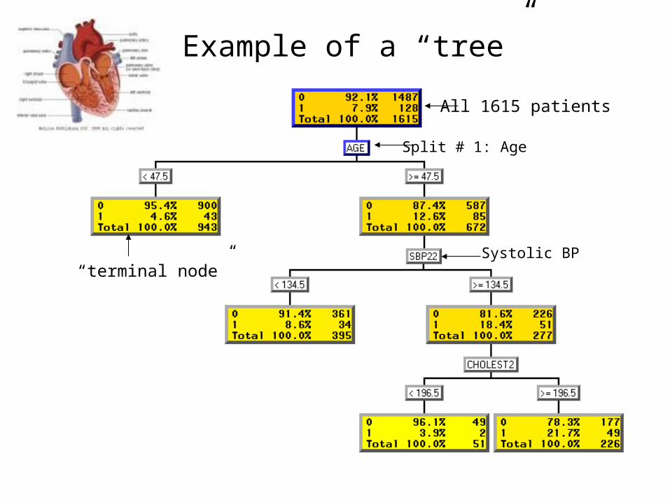
Example of a “tree”

All 1615 patients

Split # 1: Age

“terminal node”Systolic BP

How to make splits?

• Which variable to use?

• Where to split?– Cholesterol > ____– Systolic BP > _____

• Goal: Pure “leaves” or “terminal nodes”

• Ideal split: Everyone with BP>x has problems, nobody with BP<x has problems

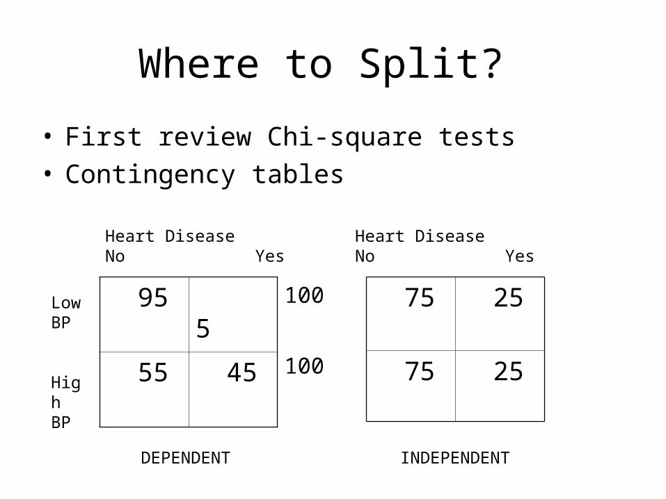
Where to Split?

• First review Chi-square tests• Contingency tables

95 5

55 45

Heart DiseaseNo Yes

LowBP

HighBP

100

100

DEPENDENT

75 25

75 25

INDEPENDENT

Heart DiseaseNo Yes

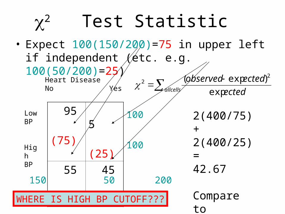
2 Test Statistic • Expect 100(150/200)=75 in upper left if

independent (etc. e.g. 100(50/200)=25)

95

(75)

5

(25)

55

(75)

45

(25)

Heart DiseaseNo Yes

LowBP

HighBP

100

100

150 50 200

allcells ected

ectedobserved

exp

)exp( 22

2(400/75)+2(400/25) = 42.67

Compare to Tables – Significant!WHERE IS HIGH BP CUTOFF???

Measuring “Worth” of a Split

• P-value is probability of Chi-square as great as that observed if independence is true. (Pr {2>42.67} is 6.4E-11)

• P-values all too small.

• Logworth = -log10(p-value) = 10.19

• Best Chi-square max logworth.

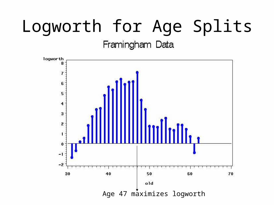
Logworth for Age Splits

Age 47 maximizes logworth

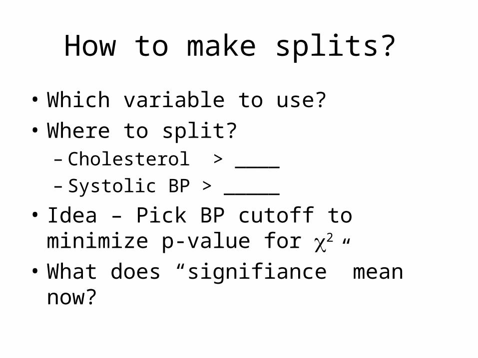
How to make splits?

• Which variable to use?

• Where to split?– Cholesterol > ____– Systolic BP > _____

• Idea – Pick BP cutoff to minimize p-value for 2

• What does “signifiance” mean now?

Multiple testing

• 50 different BPs in data, 49 ways to split • Sunday football highlights always look

good!• If he shoots enough baskets, even 95%

free throw shooter will miss.• Jury trial analogy• Tried 49 splits, each has 5% chance of

declaring significance even if there’s no relationship.

Multiple testing

= Pr{ falsely reject hypothesis 1}

= Pr{ falsely reject hypothesis 2}

Pr{ falsely reject one or the other} < 2Desired: 0.05 probabilty or lessSolution: use = 0.05/2Or – compare 2(p-value) to 0.05

Multiple testing

• 50 different BPs in data, m=49 ways to split

• Multiply p-value by 49

• Bonferroni – original idea

• Kass – apply to data mining (trees)

• Stop splitting if minimum p-value is large.

• For m splits, logworth becomes

-log10(m*p-value)

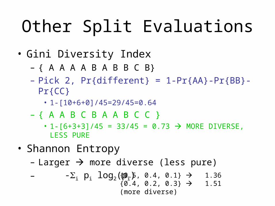
Other Split Evaluations

• Gini Diversity Index – { A A A A B A B B C B}– Pick 2, Pr{different} = 1-Pr{AA}-Pr{BB}-Pr{CC}

• 1-[10+6+0]/45=29/45=0.64

– { A A B C B A A B C C }• 1-[6+3+3]/45 = 33/45 = 0.73 MORE DIVERSE, LESS

PURE

• Shannon Entropy– Larger more diverse (less pure)

– -i pi log2(pi) {0.5, 0.4, 0.1} 1.36{0.4, 0.2, 0.3} 1.51 (more diverse)

Goals

• Split if diversity in parent “node” > summed diversities in child nodes

• Observations should be – Homogeneous (not diverse) within leaves– Different between leaves– Leaves should be diverse

• Framingham tree used Gini for splits

Cross validation

• Traditional stats – small dataset, need all observations to estimate parameters of interest.

• Data mining – loads of data, can afford “holdout sample”

• Variation: n-fold cross validation– Randomly divide data into n sets– Estimate on n-1, validate on 1– Repeat n times, using each set as holdout.

Pruning

• Grow bushy tree on the “fit data”

• Classify holdout data

• Likely farthest out branches do not improve, possibly hurt fit on holdout data

• Prune non-helpful branches.

• What is “helpful”? What is good discriminator criterion?

Goals

• Want diversity in parent “node” > summed diversities in child nodes

• Goal is to reduce diversity within leaves

• Goal is to maximize differences between leaves

• Use same evaluation criteria as for splits

• Costs (profits) may enter the picture for splitting or evaluation.

Accounting for Costs

• Pardon me (sir, ma’am) can you spare some change?

• Say “sir” to male +$2.00

• Say “ma’am” to female +$5.00

• Say “sir” to female -$1.00 (balm for slapped face)

• Say “ma’am” to male -$10.00 (nose splint)

Including Probabilities

True Gender

M

F

Leaf has Pr(M)=.7, Pr(F)=.3. You say:

M F

0.7 (2)

0.3 (-1)

0.7 (-10)

0.3 (5)

Expected profit is 2(0.7)-1(0.3) = $1.10 if I say “sir” Expected profit is -7+1.5 = -$5.50 (a loss) if I say “Ma’am”Weight leaf profits by leaf size (# obsns.) and sumPrune (and split) to maximize profits.

Additional Ideas

• Forests – Draw samples with replacement (bootstrap) and grow multiple trees.

• Random Forests – Randomly sample the “features” (predictors) and build multiple trees.

• Classify new point in each tree then average the probabilities, or take a plurality vote from the trees

• “Bagging” – Bootstrap aggregation• “Boosting” – Similar, iteratively reweights points

that were misclassified to produce sequence of more accurate trees.

* Lift Chart - Go from leaf of most to least response. - Lift is cumulative proportion responding.

Regression Trees

• Continuous response (not just class)

• Predicted response constant in regions

Predict 50

Predict 80

Predict 100

Predict 130 Predict

20

X1

X2

• Predict Pi in cell i.

• Yij jth response in cell i.

• Split to minimize i j (Yij-Pi)2

Predict 50

Predict 80

Predict 100

Predict 130 Predict

20

• Predict Pi in cell i.

• Yij jth response in cell i.

• Split to minimize i j (Yij-Pi)2

Logistic Regression

• “Trees” seem to be main tool.

• Logistic – another classifier

• Older – “tried & true” method

• Predict probability of response from input variables (“Features”)

• Linear regression gives infinite range of predictions

• 0 < probability < 1 so not linear regression.

• Logistic idea: Map p in (0,1) to L in whole real line

• Use L = ln(p/(1-p))• Model L as linear in temperature• Predicted L = a + b(temperature)• Given temperature X, compute a+bX then p

= eL/(1+eL)• p(i) = ea+bXi/(1+ea+bXi) • Write p(i) if response, 1-p(i) if not• Multiply all n of these together, find a,b to

maximize

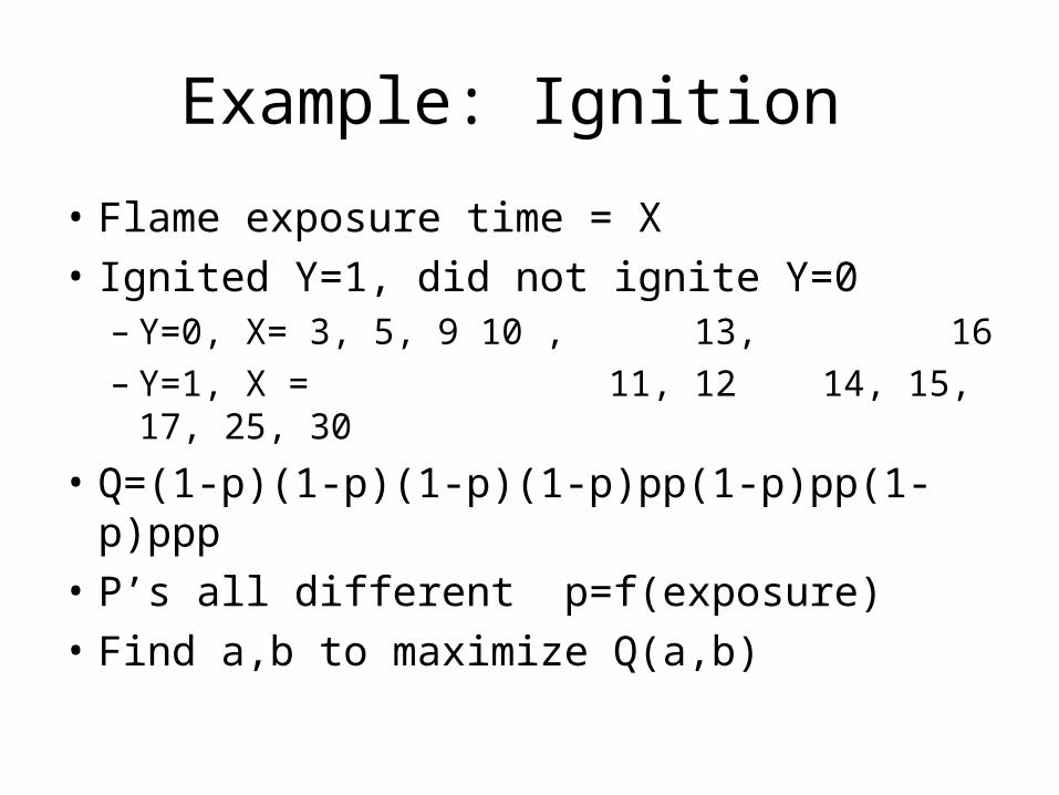
Example: Ignition

• Flame exposure time = X

• Ignited Y=1, did not ignite Y=0– Y=0, X= 3, 5, 9 10 , 13, 16 – Y=1, X = 11, 12 14, 15, 17, 25, 30

• Q=(1-p)(1-p)(1-p)(1-p)pp(1-p)pp(1-p)ppp

• P’s all different p=f(exposure)

• Find a,b to maximize Q(a,b)

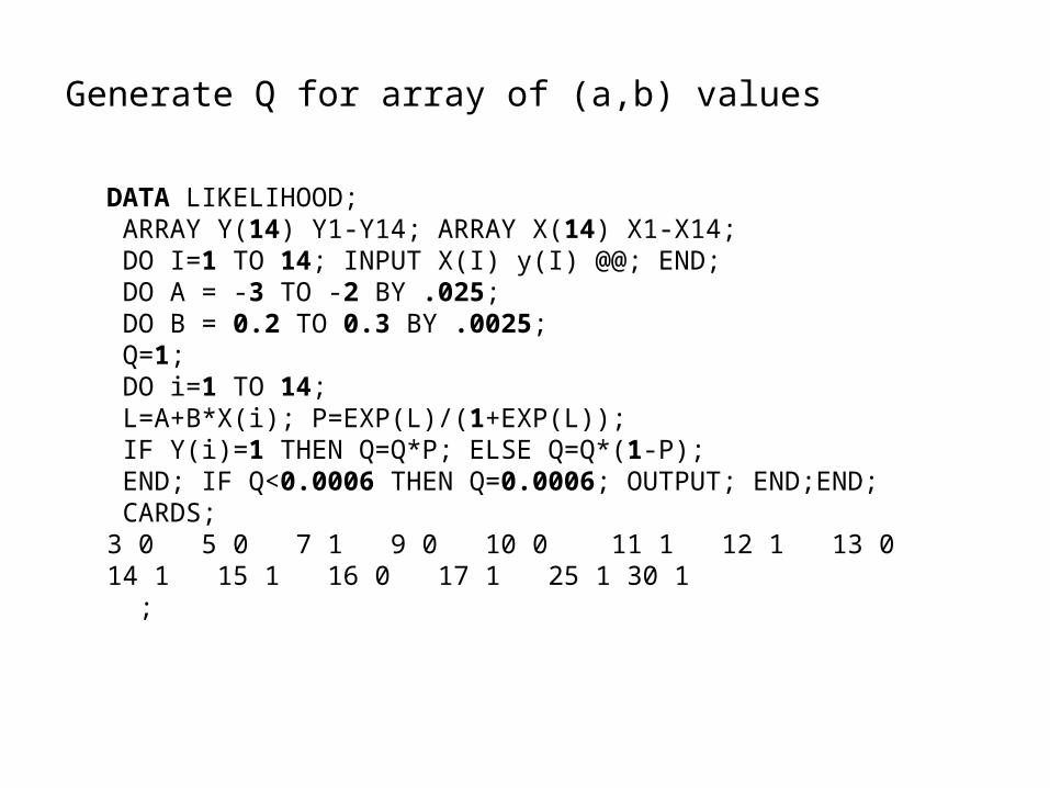
DATA LIKELIHOOD; ARRAY Y(14) Y1-Y14; ARRAY X(14) X1-X14; DO I=1 TO 14; INPUT X(I) y(I) @@; END; DO A = -3 TO -2 BY .025; DO B = 0.2 TO 0.3 BY .0025; Q=1; DO i=1 TO 14; L=A+B*X(i); P=EXP(L)/(1+EXP(L)); IF Y(i)=1 THEN Q=Q*P; ELSE Q=Q*(1-P); END; IF Q<0.0006 THEN Q=0.0006; OUTPUT; END;END; CARDS; 3 0 5 0 7 1 9 0 10 0 11 1 12 1 13 0 14 1 15 1 16 0 17 1 25 1 30 1 ;

Generate Q for array of (a,b) values

Likelihood function (Q)

-2.6

0.23

IGNITION DATA The LOGISTIC Procedure Analysis of Maximum Likelihood Estimates Standard WaldParameter DF Estimate Error Chi-Square Pr > ChiSqIntercept 1 -2.5879 1.8469 1.9633 0.1612TIME 1 0.2346 0.1502 2.4388 0.1184

Association of Predicted Probabilities and Observed Responses

Percent Concordant 79.2 Somers' D 0.583Percent Discordant 20.8 Gamma 0.583Percent Tied 0.0 Tau-a 0.308Pairs 48 c 0.792

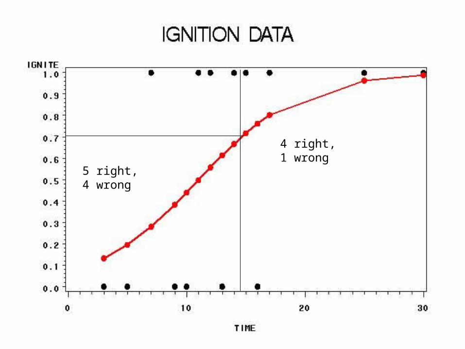
5 right, 4 wrong

4 right, 1 wrong

Example: Framingham• X=age • Y=1 if heart trouble, 0 otherwise

Framingham

The LOGISTIC Procedure

Analysis of Maximum Likelihood Estimates

Standard WaldParameter DF Estimate Error Chi-Square Pr>ChiSq

Intercept 1 -5.4639 0.5563 96.4711 <.0001age 1 0.0630 0.0110 32.6152 <.0001

Example: Shuttle Missions

• O-rings failed in Challenger disaster• Low temperature• Prior flights “erosion” and “blowby” in O-rings• Feature: Temperature at liftoff• Target: problem (1) - erosion or blowby vs. no

problem (0)

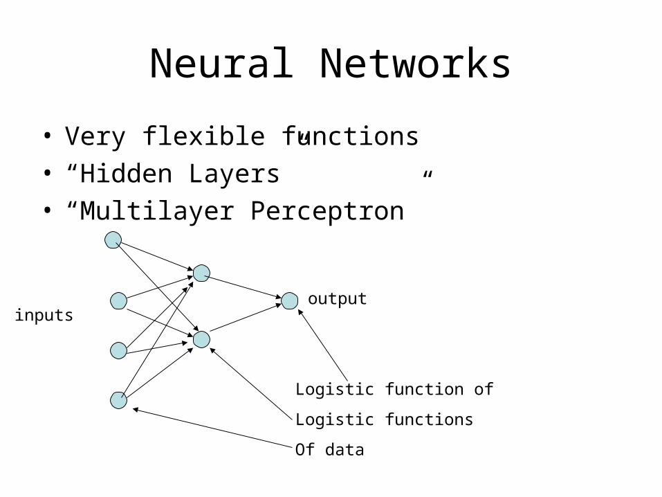
Neural Networks

• Very flexible functions• “Hidden Layers” • “Multilayer Perceptron”

Logistic function of

Logistic functions

Of data

outputinputs

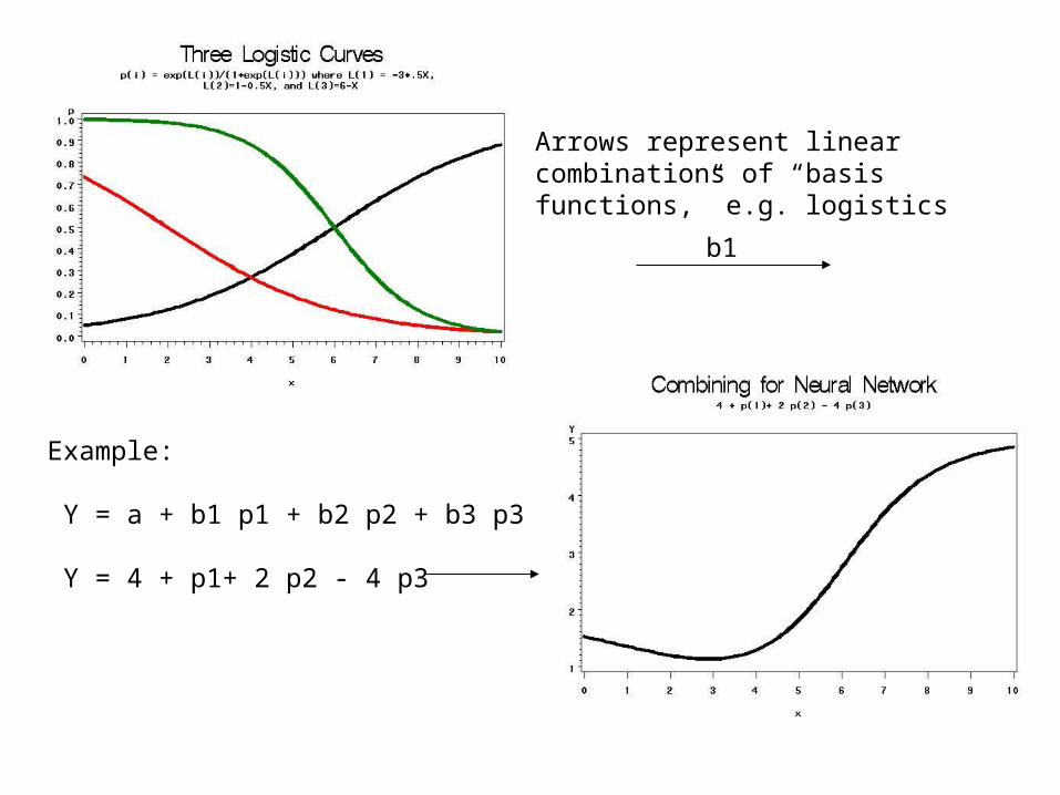
Arrows represent linear combinations of “basis functions,” e.g. logistics

b1

Example:

Y = a + b1 p1 + b2 p2 + b3 p3

Y = 4 + p1+ 2 p2 - 4 p3

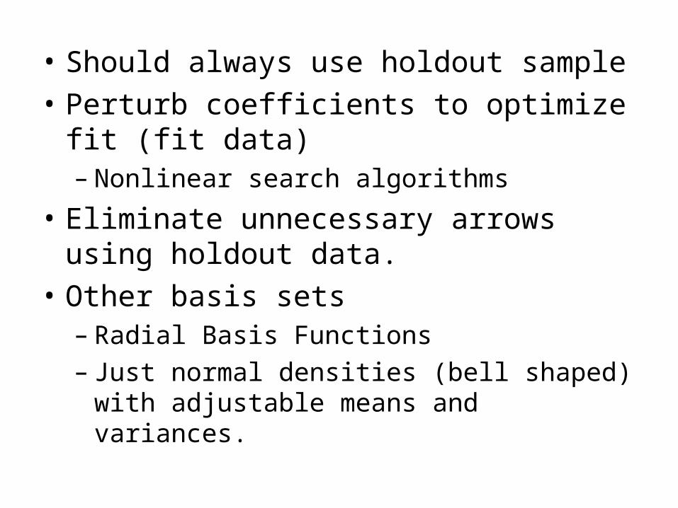
• Should always use holdout sample

• Perturb coefficients to optimize fit (fit data)– Nonlinear search algorithms

• Eliminate unnecessary arrows using holdout data.

• Other basis sets– Radial Basis Functions– Just normal densities (bell shaped) with

adjustable means and variances.

Terms• Train: estimate coefficients• Bias: intercept a in Neural Nets• Weights: coefficients b • Radial Basis Function: Normal density• Score: Predict (usually Y from new Xs)• Activation Function: transformation to target• Supervised Learning: Training data has

response.

Hidden LayerL1 = -1.87 - .27*Age – 0.20*SBP22H11=exp(L1)/(1+exp(L1))

L2 = -20.76 -21.38*H11Pr{first_chd} = exp(L2)/(1+exp(L2))“Activation Function”

Demo (optional)

• Compare several methods using SAS Enterprise Miner– Decision Tree – Nearest Neighbor– Neural Network

Unsupervised Learning

• We have the “features” (predictors)

• We do NOT have the response even on a training data set (UNsupervised)

• Clustering– Agglomerative

• Start with each point separated

– Divisive • Start with all points in one cluster then spilt

EM PROC FASTCLUS

• Step 1 – find “seeds” as separated as possible

• Step 2 – cluster points to nearest seed– Drift: As points are added, change seed

(centroid) to average of each coordinate– Alternatively: Make full pass then recompute

seed and iterate.

Clusters as Created

As Clustered

Cubic Clustering Criterion (to decide # of Clusters)

• Divide random scatter of (X,Y) points into 4 quadrants

• Pooled within cluster variation much less than overall variation

• Large variance reduction• Big R-square despite no real clusters• CCC compares random scatter R-square

to what you got to decide #clusters• 3 clusters for “macaroni” data.

Association Analysis

• Market basket analysis – What they’re doing when they scan your “VIP”

card at the grocery– People who buy diapers tend to also buy

_________ (beer?)– Just a matter of accounting but with new

terminology (of course ) – Examples from SAS Appl. DM Techniques, by

Sue Walsh:

Termnilogy

• Baskets: ABC ACD BCD ADE BCE

• Rule Support Confidence

• X=>Y Pr{X and Y} Pr{Y|X}

• A=>D 2/5 2/3

• C=>A 2/5 2/4

• B&C=>D 1/5 1/3

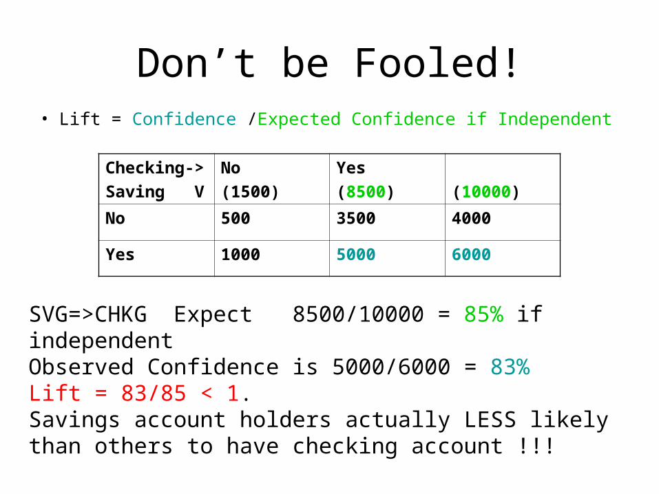
Don’t be Fooled!• Lift = Confidence /Expected Confidence if Independent

Checking->

Saving V

No

(1500)

Yes

(8500) (10000)

No 500 3500 4000

Yes 1000 5000 6000

SVG=>CHKG Expect 8500/10000 = 85% if independentObserved Confidence is 5000/6000 = 83%Lift = 83/85 < 1. Savings account holders actually LESS likely than others to have checking account !!!

Summary

• Data mining – a set of fast stat methods for large data sets

• Some new ideas, many old or extensions of old• Some methods:

– Decision Trees– Nearest Neighbor– Neural Nets– Clustering– Association