data mining and analysis of global happiness: a...
TRANSCRIPT

September 2011 CSMSC-11
DEPARTMENT OF COMPUTER SCIENCE
A dissertation submitted to the University of Bristol in accordance with the requirements
of the degree of Master of Science in the Faculty of Engineering
Data Mining and Analysis of GlobalHappiness: A Machine Learning Approach
Louise Millard

Declaration
This dissertation is submitted to the University of Bristol inaccordance with the requirements of the degree of Master of Science inthe Faculty of Engineering. It has not been submitted for any otherdegree or diploma of any examining body. Except wherespecifically acknowledged, it is all the work of the Author.
Louise Millard, September 2011

Executive Summary
The aim of the project was to explain and predict global happiness. This was a crosssectional study including 123 countries, each having a mean happiness value. This groundtruth was established from survey data, using the answer to a life satisfaction question. Thefeatures used to predict happiness were collected from online sources, and were chosen usingbackground knowledge gained from a review of previous work.
Initial data analysis was performed to discover patterns in the data using PCA, visualisa-tions and correlations. PCA found an interesting convex relationship between life satisfactionand gender equality. The data was prepared firstly by imputing missing values with the k-nearest neighbour method. Some variables were transformed using log where their relationshipwith life satisfaction was found to be exponential.
Prior to performing feature selection life satisfaction prediction was assessed, comparing aninitial feature set with economic variables using a t-test of the correlations of cross validationfolds. The feature set was found to be as predictive as the economic variables. Featureselection was performed using lasso, least squares and decision trees. The significance ofresults was determined by finding test statistic thresholds using permutation testing andbootstrapping. A key feature set was identified as:
Life expectancy Income distribution Proportion of women in parliamentFreedom Primary education enrolment Secondary education enrolmentMortality rate
These features were used with several learners to construct models to predict happiness. Modeltrees performed the best with a mean correlation of 0.86 across the cross validation folds. Thiswas not significantly more predictive than lasso (p = 0.52), indicating the relationship of thekey features with life satisfaction is highly linear. The key feature set was significantly morepredictive than using the larger original feature set (p = 2.12⇥10�16), highlighting the benefitsof feature selection. The performance of our key feature set was compared against economicvariables and gave a significantly better performance for both lasso and decision trees.
Bayes networks were used to assess the relationships of the variables using the followingmeasures of performance; percentage correct, ROC curve area and degrees of freedom. Noimprovement in performance was found when connecting GDP per capita directly with lifesatisfaction. This supports the notion that GDP allows other variables to occur which in turnimpact on life satisfaction, rather than GDP having a direct and significant impact.
Finally, Cherno↵ faces proved an e↵ective visualisation method for our multivariate dataset.This is an intuitive representation where happier faces correspond to higher life satisfaction,and hence patterns and anomalies can be easily identified. An interactive visualisation ofresults can be found at http://intelligentsystems.bristol.ac.uk/research/Millard/.
In summary, key highlights of this project are:
• PCA uncovered an interesting relationship between gender equality and life satisfaction• Decision trees proved an e↵ective method in both feature selection and life satisfaction
prediction• Our key features performed significantly better than economic variables• Graphical models helped investigate variable relationship structure• An e↵ective data visualisation method was used to demonstrate results
The work previously completed consists of a review of previous work and methods, whichcontribute to sections 2 and 3 respectively. Also, initial survey data analysis was performedto determine a ground truth of life satisfaction (contributing to section 4).

Acknowledgements
I wish to thank, first and foremost, my supervisor Professor Nello Cristianini, for his guidanceand advice throughout this project. This has been an invaluable and enjoyable experienceand I am grateful for his continued enthusiasm and interest in this project.
I am grateful to Dr Tijl De Bie, for a thoroughly interesting and useful Pattern Analysisand Statistical Learning module. Thank you for your patience and time answering my ques-tions. Also, many thanks to my Personal Tutor, Dr Tim Kovacs, for his time and advice.
Finally, thanks to my family and friends. I would like to thank my mother Alex, for hersupport whilst I returned to my studies. Thanks to my close friend Joanne for her continuedencouragement. To Chris, thank you for your thoughts, advice and support.

Contents
1 Introduction 11.1 Overview . . . . . . . . . . . . . . . . . . . . . . . . . . . . . . . . . . . . . . . . . 11.2 Methodology . . . . . . . . . . . . . . . . . . . . . . . . . . . . . . . . . . . . . . . 11.3 Report Structure . . . . . . . . . . . . . . . . . . . . . . . . . . . . . . . . . . . . . 2
2 Research Review 32.1 Measuring Happiness . . . . . . . . . . . . . . . . . . . . . . . . . . . . . . . . . . . 32.2 Establishing a Ground Truth . . . . . . . . . . . . . . . . . . . . . . . . . . . . . . 42.3 General Research . . . . . . . . . . . . . . . . . . . . . . . . . . . . . . . . . . . . . 52.4 Economic Research . . . . . . . . . . . . . . . . . . . . . . . . . . . . . . . . . . . . 6
2.4.1 Survey data and conflicting results . . . . . . . . . . . . . . . . . . . . . . . 82.4.2 Relative wealth . . . . . . . . . . . . . . . . . . . . . . . . . . . . . . . . . . 92.4.3 A study of relative income . . . . . . . . . . . . . . . . . . . . . . . . . . . . 9
2.5 Research of Other Indicators . . . . . . . . . . . . . . . . . . . . . . . . . . . . . . 112.5.1 Health . . . . . . . . . . . . . . . . . . . . . . . . . . . . . . . . . . . . . . . 112.5.2 Light . . . . . . . . . . . . . . . . . . . . . . . . . . . . . . . . . . . . . . . . 122.5.3 Climate . . . . . . . . . . . . . . . . . . . . . . . . . . . . . . . . . . . . . . 12
2.6 Causal Inferences . . . . . . . . . . . . . . . . . . . . . . . . . . . . . . . . . . . . . 14
3 Methods Overview 153.1 Data Preparation . . . . . . . . . . . . . . . . . . . . . . . . . . . . . . . . . . . . . 15
3.1.1 Feature construction . . . . . . . . . . . . . . . . . . . . . . . . . . . . . . . 153.1.2 Principle Component Analysis (PCA) . . . . . . . . . . . . . . . . . . . . . 153.1.3 Missing values . . . . . . . . . . . . . . . . . . . . . . . . . . . . . . . . . . 173.1.4 Imputation . . . . . . . . . . . . . . . . . . . . . . . . . . . . . . . . . . . . 18
3.2 Statistical & Machine Learning Methods . . . . . . . . . . . . . . . . . . . . . . . . 203.3 Statistical Tests . . . . . . . . . . . . . . . . . . . . . . . . . . . . . . . . . . . . . . 20
3.3.1 Pearson Product Moment Correlation Coe�cient (R) . . . . . . . . . . . . 203.3.2 T-Test . . . . . . . . . . . . . . . . . . . . . . . . . . . . . . . . . . . . . . . 203.3.3 Significance testing with permutation testing . . . . . . . . . . . . . . . . . 213.3.4 Linear Regression . . . . . . . . . . . . . . . . . . . . . . . . . . . . . . . . . 213.3.5 The Least Absolute Shrink and Selection Operator (Lasso) . . . . . . . . . 223.3.6 Decision Trees . . . . . . . . . . . . . . . . . . . . . . . . . . . . . . . . . . 233.3.7 Support Vector Machines . . . . . . . . . . . . . . . . . . . . . . . . . . . . 263.3.8 Bayesian Belief Networks . . . . . . . . . . . . . . . . . . . . . . . . . . . . 283.3.9 Testing the accuracy of classifiers . . . . . . . . . . . . . . . . . . . . . . . . 30
4 Survey Data Analysis 314.1 Results . . . . . . . . . . . . . . . . . . . . . . . . . . . . . . . . . . . . . . . . . . . 31
5 Data Collection & Description 345.1 Feature Collection & Construction . . . . . . . . . . . . . . . . . . . . . . . . . . . 345.2 Data Analysis . . . . . . . . . . . . . . . . . . . . . . . . . . . . . . . . . . . . . . . 36
5.2.1 Data correlations . . . . . . . . . . . . . . . . . . . . . . . . . . . . . . . . . 365.3 PCA . . . . . . . . . . . . . . . . . . . . . . . . . . . . . . . . . . . . . . . . . . . . 40
6 Data Preparation 436.1 Imputation . . . . . . . . . . . . . . . . . . . . . . . . . . . . . . . . . . . . . . . . 43
6.1.1 Imputation summary . . . . . . . . . . . . . . . . . . . . . . . . . . . . . . . 446.2 Transformations . . . . . . . . . . . . . . . . . . . . . . . . . . . . . . . . . . . . . 44

7 Models to Predict Life Satisfaction 467.1 Results and Analysis . . . . . . . . . . . . . . . . . . . . . . . . . . . . . . . . . . . 477.2 Statistical Methods . . . . . . . . . . . . . . . . . . . . . . . . . . . . . . . . . . . . 47
7.2.1 Conclusions . . . . . . . . . . . . . . . . . . . . . . . . . . . . . . . . . . . . 48
8 Feature Selection (1) 498.1 Lasso Feature Selection . . . . . . . . . . . . . . . . . . . . . . . . . . . . . . . . . 498.2 Least Squares Leave One Feature Out . . . . . . . . . . . . . . . . . . . . . . . . . 548.3 Lasso / Least Squares Results Comparison . . . . . . . . . . . . . . . . . . . . . . . 558.4 Results Summary . . . . . . . . . . . . . . . . . . . . . . . . . . . . . . . . . . . . . 56
9 Feature Selection (2) 579.1 Improved Feature Set . . . . . . . . . . . . . . . . . . . . . . . . . . . . . . . . . . 579.2 Initial Analysis and Correlations . . . . . . . . . . . . . . . . . . . . . . . . . . . . 589.3 Finding Significant Features: Decision Trees . . . . . . . . . . . . . . . . . . . . . . 609.4 Finding Significant Features: Lasso . . . . . . . . . . . . . . . . . . . . . . . . . . . 609.5 Assessing Significant Features . . . . . . . . . . . . . . . . . . . . . . . . . . . . . . 609.6 Frequent Subsets . . . . . . . . . . . . . . . . . . . . . . . . . . . . . . . . . . . . . 62
10 Best Prediction 6310.1 Optimising SVM . . . . . . . . . . . . . . . . . . . . . . . . . . . . . . . . . . . . . 6310.2 Results . . . . . . . . . . . . . . . . . . . . . . . . . . . . . . . . . . . . . . . . . . . 6310.3 DT & PCA . . . . . . . . . . . . . . . . . . . . . . . . . . . . . . . . . . . . . . . . 64
10.3.1 Results . . . . . . . . . . . . . . . . . . . . . . . . . . . . . . . . . . . . . . 64
11 Graphical Models 6611.1 Discretizing . . . . . . . . . . . . . . . . . . . . . . . . . . . . . . . . . . . . . . . . 6611.2 Network Structure . . . . . . . . . . . . . . . . . . . . . . . . . . . . . . . . . . . . 66
11.2.1 Metrics used for assessment . . . . . . . . . . . . . . . . . . . . . . . . . . . 6611.2.2 Results . . . . . . . . . . . . . . . . . . . . . . . . . . . . . . . . . . . . . . 68
12 Data Visualisation 7012.1 Label Value Inference . . . . . . . . . . . . . . . . . . . . . . . . . . . . . . . . . . 7012.2 Face Generation . . . . . . . . . . . . . . . . . . . . . . . . . . . . . . . . . . . . . 7012.3 Interactive Results . . . . . . . . . . . . . . . . . . . . . . . . . . . . . . . . . . . . 71
13 Project Conclusions 7313.1 Results Summary . . . . . . . . . . . . . . . . . . . . . . . . . . . . . . . . . . . . . 73
13.1.1 Feature selection & construction . . . . . . . . . . . . . . . . . . . . . . . . 7313.1.2 Key features & feature subsets . . . . . . . . . . . . . . . . . . . . . . . . . 7313.1.3 Key Models . . . . . . . . . . . . . . . . . . . . . . . . . . . . . . . . . . . . 7413.1.4 Graphical Models . . . . . . . . . . . . . . . . . . . . . . . . . . . . . . . . . 7413.1.5 Consistency of results & data quality . . . . . . . . . . . . . . . . . . . . . . 7413.1.6 Results visualisations . . . . . . . . . . . . . . . . . . . . . . . . . . . . . . 75
13.2 Assessing progress . . . . . . . . . . . . . . . . . . . . . . . . . . . . . . . . . . . . 7513.3 Areas of further work . . . . . . . . . . . . . . . . . . . . . . . . . . . . . . . . . . 75
14 Appendix A: Data Sources 76

1 Introduction
1.1 Overview
Happiness economics is an active area of research. The aim of this work is to use a machinelearning approach, to explain and predict global happiness. At present countries mainly use GDPto determine progress1 but this has come under increasing criticism as measuring “everything, inshort, except that which makes life worthwhile”. [Robert Kennedy, 1968]
We investigate a broad range of variables to discover more appropriate measures of progress,that impact on happiness. A focus is given to variables over which we have control and can changein order to improve quality of life, and those that governmental policy can directly a↵ect such aseducation and health. Environmental variables such as weather are also considered as these area↵ected by issues such as climate change on which government policy has an impact. This leadsus to state our meaning of happiness for the purposes of this project. We define happiness assynonymous with life satisfaction and corresponding to the longer term notion of the quality ofone’s life.
Figure 1.1 shows a happiness map generated in 2006 using various survey sources, and largeglobal variations of happiness are very apparent. Whilst a strong correlation between GDP andhappiness has been shown previously this is certainly not the whole picture, and other variablesare likely to play a key role; “Economic factors are not goals in themselves but are means foracquiring other types of social goals” [25].
Figure 1: Happiness map [52]
1.2 Methodology
Our contribution from a new perspective using machine learning techniques aims to provide anew insight into this area. Previous research has used statistical methods predominantly linearregression. Machine learning techniques will allow the application of powerful methods to thedataset to find new patterns, such as decision trees and support vector machines, each havingdi↵erent benefits.
1One exception is Bhutan, a small country in South Asia, which uses an alternative measure called GrossNational Happiness (GNH) to assess progress. This was established in 1972 by the fourth Dragon King, in orderto better reflect the important aspects of his peoples lives, centred on Buddhism and spirituality. [38] Morerecently even the UK is considering alternative measures with David Cameron announcing in 2010 plans to measurehappiness; “I believe a new measure wont give us the full story of our nation’s well-being ... but it could give us ageneral picture of whether life is improving”[11].
1

1.3 Report Structure
A review of previous work is given in section 2, followed by an overview of key statistical andmachine learning methods in section 3. Sections 4 - 11 are investigatory. A ground truth ofhappiness is established in section 4 and the reliability of this measure is also investigated. Dataanalysis is performed to uncover patterns, described in section 5.2. The predictive capabilities ofour initial feature set compared to economic variables is assessed in section 7. Feature selectionis performed in two stages (sections 8 and 9). Several methods are investigated to find the besthappiness prediction in section 10, and structural relationships are assessed in section 11. Finally,our results are visualised using an e↵ective representation (section 12).
2

2 Research Review
2.1 Measuring Happiness
Previously it was thought that you could not measure happiness but only behaviour.[31] However,there have been independent strands of research which provide strong evidence to the contrary.Biologically, it has been found that specific areas of the brain are active when a person experienceshappiness. An interesting piece of research ([30]) looked at brain activity with respect to theemotions of happiness, sadness and disgust. They found correlations between these emotions withactivity in multiple regions of the brain, some of which were shared for the di↵erent emotions whileothers were specific to the emotion and stimulus. The potential to assign a value of happinessdepending on brain activity highlights that happiness is a more tangible and measurable propertythan once thought.
A pertinent issue is the contribution of the genome to ones happiness as this could significantlya↵ect results (the “nature versus nurture” debate). We are interested in the “nurture” causes ofhappiness from living in di↵erent countries. Research published in 1996 ([33]) looked at the degreeto which happiness may be encoded in our genes. They did this using data of a happiness surveyquestion but where the recipients were twins, both monozygotic and dizygotic. Monozygotictwins have an identical genome, whereas dizygotic twins do not. 127 sets of twins were surveyedtwice, with a ten year gap. To investigate the degree to which genomes are responsible forhappiness the results were correlated within twins: (person1, survey1)! (person2, survey2) and(person2, survey1) ! (person1, survey2). The results were significantly di↵erent for the twinstypes, where monozygotic and dizygotic twins gave correlation of 0.4 and 0.07 respectively. Thetwins with identical genomes had a much stronger correlations between happiness levels. Theyconclude that happiness in adults is determined in equal measure by both genes and environmentalfactors.
A more recent paper by Frey [23] aimed to find specific genes which code for happiness, usinglongitudinal survey data and gene association. Gene association is the process of investigating thecorrelation between a genes’ expression and a particular trait (or phenotype). The gene 5HTTwas selected as the candidate gene as it is known to be involved in brain development and so mayhave implications on happiness. They describe happiness as having a baseline which is specific toeach individual and encoded in their genes, and happiness fluctuates about this value in responseto their environment and experiences. This paper highlights the complexity of happiness, wherethere is likely to be a complex combination of factors that contribute, including the cumulativee↵ect of multiple genes in addition to environmental factors.
A happiness coding gene however could potentially a↵ect the results. The central considera-tion for this is whether the global genetic distribution is clustered such that there would be anuneven spread across the globe. This is however not thought to be the case, where there has beensu�cient human migration to give an even distribution. There may still be e↵ects on results asfor instance, the existence of a baseline happiness may cause the variance of a countries happinessto remain fairly constant but the mean may change, as peoples happiness alters with respect totheir own baseline values.
A final point of consideration is how well subjective happiness represents the happiness of aperson. Previous research compared the consistency of happiness measures given from di↵erentsources. A 2009 study by Sandvik et al. ([45]) looked at the correlation between self-reportedhappiness and the values given by family and friends. They found these three assessments of apersons’ happiness to be highly consistent.
This discussion has highlighted the complexity of this trait, but also shown happiness tobe less abstract and intangible than was previously thought. Establishing a ground truth forhappiness is an important aspect of this project, which must accurately represent our notion ofhappiness. The following section investigates deriving a ground truth from the survey data.
3

2.2 Establishing a Ground Truth
A general consensus is that answers to survey questions provide representative values of happinessor life satisfaction. The three main global surveys used in this type of research are the WorldValue Survey (WVS), Gallup World Poll (GWP) and World Database of Happiness (WDH). Atypical question takes the form “how satisfied are you with your life as a whole these days?”with an answer scale typically 0 - 10 [16]. The GWP is a large scale survey carried out on adaily basis. However, the data is not freely available and we only have access to some limiteddata through the results of another study2. The WDH is a compilation of happiness values fromdi↵erent surveys, predominantly the WVS.
The ground truth we use can be either from a single source or a combined value of multiplesources. The choice we make will be dependent on results of data analysis. Previous workhas tended to keep di↵erent happiness labels separate (choosing one or working with severalsimultaneously) rather than fusing multiple sources. Using a single source however has shortcomings due to the validity of each source. Firstly, the WDH is a secondary source, a compilationof results from multiple survey sources. We prefer to use a primary source such that we havea better knowledge of the survey data. Secondly, the di↵erent surveys vary with respect to thecountries studied and various details regarding the survey format. This means that one cannotsimply be preferred over the other. Therefore, we will begin with primary data and establish aground truth from these values (which may mean several alternative labels). Section 4 investigatesthe available survey data and establishing a ground truth. Section 2.4.1 looks at conflicting resultsof previous work, and possible causes from di↵erences in surveys.
The Happy Planet Index ([3]) developed by The New Economics Foundation (NEF) is a globalmeasure indicating sustainable happiness, the happiness component of which came from the GWPlife satisfaction question. This work is of particular interest as data from multiple sources wasused to extend the dataset, using regression to infer a value for the GWP for additional countries.112 countries came from Gallup, 16 from WVS and 14 from GWP’s ladder of life question. Thismethod relies on countries with values for multiple surveys which means a relationship betweenthe survey values can be inferred. 68 countries had results for both GWP and WVS. Regressionwas performed using GWP and WVS as the dependent and independent variables respectively,such that GWP values are inferred from WVS values. [3]
Stepwise regression was used to improve the correlation between the survey datasets usingadditional variables. This is a recursive regression where a variable is added at each step . If thisvariable provides a significant improvement to the inference of the GWP value then it is kept,otherwise it is ignored.
The use of stepwise regression improved correlation, where they found that “four variablesare able to predict 91% of the variance” which included the Human Development Index andan education index amongst others. It is interesting to assess the variables that improved thecorrelation between the surveys, as they may indicate the di↵erences between them. For instance[16] noted that WVS tended to bias their surveying towards more intelligent people in certaincountries to make the sample “more comparable”. This may be consistent with the use of aneducation variable here, showing that the variance between the surveys may be accounted forto some degree by education levels. WVS has in e↵ect controlled for education by reducing thedi↵erence across countries.
Stepwise regression was also used to correlate the GWP life satisfaction data with the GWPladder of life data. This found di↵erent variables improved the correlation between the datasetsincluding life expectancy and geographical variables. [3] The ladder of life question asks therespondent their life satisfaction relative to their attainable levels; “Please imagine a ladder, withsteps numbered from 0 at the bottom to 10 at the top. The top of the ladder represents thebest possible life for you and the bottom of the ladder represents the worst possible life for you.On which step of the ladder would you say you personally feel you stand at this time?”. This
2Source is Happy Planet Index v2.0
4
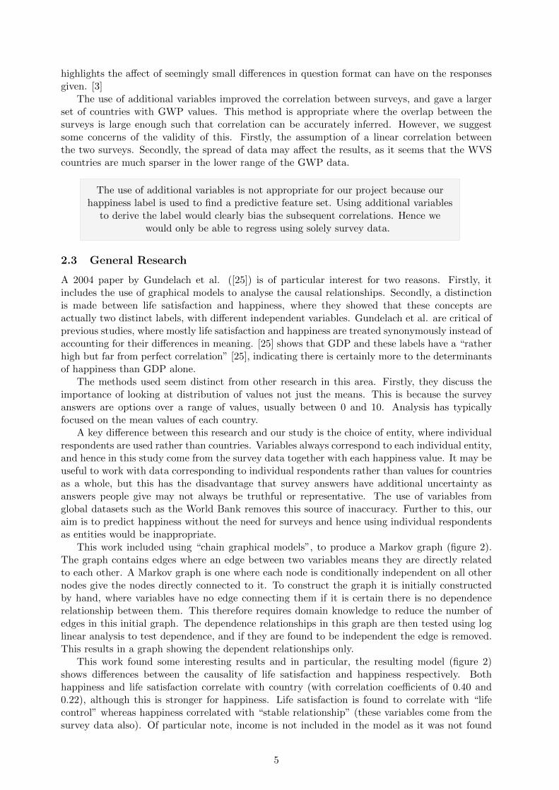
highlights the a↵ect of seemingly small di↵erences in question format can have on the responsesgiven. [3]
The use of additional variables improved the correlation between surveys, and gave a largerset of countries with GWP values. This method is appropriate where the overlap between thesurveys is large enough such that correlation can be accurately inferred. However, we suggestsome concerns of the validity of this. Firstly, the assumption of a linear correlation betweenthe two surveys. Secondly, the spread of data may a↵ect the results, as it seems that the WVScountries are much sparser in the lower range of the GWP data.
The use of additional variables is not appropriate for our project because ourhappiness label is used to find a predictive feature set. Using additional variables
to derive the label would clearly bias the subsequent correlations. Hence wewould only be able to regress using solely survey data.
2.3 General Research
A 2004 paper by Gundelach et al. ([25]) is of particular interest for two reasons. Firstly, itincludes the use of graphical models to analyse the causal relationships. Secondly, a distinctionis made between life satisfaction and happiness, where they showed that these concepts areactually two distinct labels, with di↵erent independent variables. Gundelach et al. are critical ofprevious studies, where mostly life satisfaction and happiness are treated synonymously instead ofaccounting for their di↵erences in meaning. [25] shows that GDP and these labels have a “ratherhigh but far from perfect correlation” [25], indicating there is certainly more to the determinantsof happiness than GDP alone.
The methods used seem distinct from other research in this area. Firstly, they discuss theimportance of looking at distribution of values not just the means. This is because the surveyanswers are options over a range of values, usually between 0 and 10. Analysis has typicallyfocused on the mean values of each country.
A key di↵erence between this research and our study is the choice of entity, where individualrespondents are used rather than countries. Variables always correspond to each individual entity,and hence in this study come from the survey data together with each happiness value. It may beuseful to work with data corresponding to individual respondents rather than values for countriesas a whole, but this has the disadvantage that survey answers have additional uncertainty asanswers people give may not always be truthful or representative. The use of variables fromglobal datasets such as the World Bank removes this source of inaccuracy. Further to this, ouraim is to predict happiness without the need for surveys and hence using individual respondentsas entities would be inappropriate.
This work included using “chain graphical models”, to produce a Markov graph (figure 2).The graph contains edges where an edge between two variables means they are directly relatedto each other. A Markov graph is one where each node is conditionally independent on all othernodes give the nodes directly connected to it. To construct the graph it is initially constructedby hand, where variables have no edge connecting them if it is certain there is no dependencerelationship between them. This therefore requires domain knowledge to reduce the number ofedges in this initial graph. The dependence relationships in this graph are then tested using loglinear analysis to test dependence, and if they are found to be independent the edge is removed.This results in a graph showing the dependent relationships only.
This work found some interesting results and in particular, the resulting model (figure 2)shows di↵erences between the causality of life satisfaction and happiness respectively. Bothhappiness and life satisfaction correlate with country (with correlation coe�cients of 0.40 and0.22), although this is stronger for happiness. Life satisfaction is found to correlate with “lifecontrol” whereas happiness correlated with “stable relationship” (these variables come from thesurvey data also). Of particular note, income is not included in the model as it was not found
5

The main results of the analysis are as follows:
1. Perceived happiness and life satisfaction are highly correlated butnot identical. The relationships between the dependent and inde-pendent variables differ, and this is evidence that they do notbelong to the same latent variable.
2. Perceived happiness and life satisfaction are both related to coun-try of residence.
3. The main influences on perceived happiness are the country of resi-dence and whether the respondent lives in a stable relationship.
4. The main influences on life satisfaction are the experience of lifecontrol—that is, the answer to “how much freedom and control therespondent feels he or she has over the way life turns out”—andcountry of residence.
It is equally interesting to look at some of the variables that did notcorrelate with the three dependent variables. For instance, whencontrolled for other variables, income is not related to perceivedhappiness or life satisfaction. This is somewhat unexpected. Stud-ies, for example, by Bradburn (1969) and Easterlin (1974) showcorrelations between the individual’s social status and self-ratedhappiness. There may be several reasons for this discrepancy. Oneexplanation may be technical and owing to problems in comparingself-reported income in different countries. To make comparisonssimple, the EVS questionnaire merely asked the respondents toplace their household income on a 10-point scale. The wording of
368 Cross-Cultural Research / November 2004
Life satisfaction
Happiness
Life control
Stable relationship
Country
.37
-.71
.48
.22
.40
Figure 1: Happiness and Life Satisfaction Graphical ModelNOTE: Numbers in boxes are correlation coefficients (partial γs). Only γs above .16and only edges that are of relevance for the dependent variables are included.
at University Library on February 15, 2011ccr.sagepub.comDownloaded from
Figure 2: Causal network [25]
to correlate strongly (with a correlation above 0.16) with either life satisfaction or happiness.However, Gundelach et al. explain this with the choice of sample where only European countrieswere used and hence the variance of wealth may be fairly small. However, we question this assince this study is on an individual basis it seems there would still be a fair amount of varianceof wealth within a population. This may therefore indicate that wealth is not a key factor inhappiness or perhaps is evidence supporting the Easterlin Paradox (see section 2.4).
The di↵erences in correlations for life satisfaction and happiness were attributed to the dif-ferences in meaning of the two terms where “happiness is more emotional and life satisfaction ismore cognitive” [25], which intuitively makes sense with regards to the particular correlates ofeach.
We are not concerned with the semantic di↵erences of these variables as we thinkboth contribute to our notion of happiness for this project, and consider both
types of label.
This work ([25]) shows strong evidence for the fact that happiness is not solely determined bywealth. The use of just EU countries was an e↵ective way of controlling for wealth such that othercorrelations could be determined more easily. It should be noted however, that construction ofsuch graphical models do not determine the direction of causality, and in this sense the directedgraph produced in [25] (figure 2) is misleading.
Bayesian networks (see section 3.3.8) are an appropriate machine learningapproach as an alternative to this method of graph construction, which instead
use conditional probabilities.
2.4 Economic Research
The common assumption that wealth causes happiness has led a large amount of research tofocus on this particular area. This research varies in many aspects such as: coverage (global, EUor a single country), type of data used (longitudinal or single instance), topic focused on (bothgeneral analysis and investigations of specific theories or previous findings). For a survey of suchpapers the reader is directed to [13]. It is generally agreed that life satisfaction is strongly andpositively correlated with income shown in much previous work such as [16].
A much debated theory is that of the Easterlin Paradox. Richard Easterlin, a Professor ofEconomics has contributed much to this area, most notably a paper written in 1974 entitled “DoesEconomic Growth Improve the Human Lot? Some Empirical Evidence” [17] Easterlin used twosurvey questions, and investigated them separately. The analysis performed included both withincountry (America) and cross country data. A key finding was the relationship between income
6

and happiness, which Easterlin found to be strongly positive for data within countries. However,the cross country analysis found a threshold of income above which there was no correlation.These findings were named the Easterlin Paradox.
The Easterlin Paradox has been a central focus of debate since then, and the findings are notdecisive. Easterlin notes; “China’s growth rate implies a doubling of real per capita income inless than 10 y ... one might think many of the people in these countries would be so happy, theydbe dancing in the streets” [18]. An early view by Robbins in 1938 suggests an opposing view,where after income has reached a certain level it allows happiness values to increase more, becausethen additional factors can contribute to life satisfaction levels as improvements to quality of lifebecome a↵ordable. The work by Robbins has been supported by more recent research such as[16], a 2008 study using the Gallup World Poll (GWP). This work showed that life satisfactionwas a↵ected more in the rich countries, shown by a noticeable change in the regression curve.
Easterlin’s most recent paper on this topic was that of “The happiness-income paradox revis-ited” in 2010 [18]. This is an extension of previous work that focused on America. This researchlooks at happiness over a number of years and for a wide range of countries (54 in total), usingtime series data from four survey sources. Regression was performed both with the datasets asa whole, and also with subsets where the countries were split into groups. The three groupswere; developing, developed and those in a state of change from communism to capitalism. OLSregression was used and this showed no significant correlation between rate of growth and lifesatisfaction in all regressions performed. Easterlin shows that while happiness does fluctuate witheconomic conditions, there is no correlation in the long term for the diverse range of countriesstudied. Previous research by Stevenson and Wolfers in 2008 finding that life satisfaction andgrowth are positively correlated but Easterlin comments that they use only short term datasets.He shows that while this is the case there is no evidence of a longer term correlation. [18]
This paper highlights the a↵ect that a few possibly unrepresentative data points can have oncorrelations. As an example, the results by Stevenson and Wolfers in 2008 were repeated removinga small number of results. A correlation that had been found for a dataset of 17 countries, wasre-tested with 2 data points removed and this change meant no significant correlation was thenfound. Easterlin also did this for another test with 32 countries, removing transition countriesand finding this again removed the significance. However, here 11 countries were removed whichis a large proportion and hence would more likely a↵ect the correlations found.
This paper has provided a valuable insight into the dual nature of correlation between growthand happiness (short term and long term), rather than the rather simplistic view that growthcauses happiness as found previously.
Solely GDP growth and time series data was used in this study. Our research isinterested in the happiness di↵erences between countries and hence it is moreappropriate to use point of time data. We also look at several alternativeindicators such as GDP and relative income, as well as GDP growth rate.
A possible issue with this research is the use of financial satisfaction as a label for LatinAmerican countries. However, this was due to a lack of reliable life data and therefore this wasprobably the most suitable alternative. A positive correlation would not prove a correlation be-tween life satisfaction and growth, but no correlation with financial satisfaction would render apositive correlation with life satisfaction highly unlikely as financial satisfaction is the componentof life satisfaction most related to GDP growth. In fact, financial satisfaction showed no relation-ship with GDP growth which is of much surprise, especially where Latin American countries aregrowing at 1 - 3% per year. [18]
7
2.4.1 Survey data and conflicting results
The debate regarding the Easterlin paradox may be due to di↵erences in survey data. It isimportant to understand possible a↵ects that di↵erent survey procedures may have to be awareof possible bias in results. Recent work in 2008 by Deaton ([16]) and Bjrnskov ([7]) respectivelyhas looked at the possible reasons that results from WVS support the Easterlin Paradox butresults from the GWP conflict.
There are some fundamental di↵erences of the surveys noted by Bjrnskov. Firstly, WDH isan accumulation of multiple sources (although primarily WVS). Secondly, the time point of thesurveys is di↵erent, having taken place at around 2000 for WVS compared to 2006 for GWP.[7] This is a large time gap and there could potentially have been noticeable changes in lifesatisfaction during this time.
Deaton notes how the GWP shows a much gentler slope for the correlation between happinessand GDP, whereas the WVS gives a much steeper rise for low income countries. Deaton accountsthis to several attributes of the surveys. Firstly, WVS includes a smaller set of low incomecountries and this part of the correlation may be skewed by the fact that these countries aremainly post Soviet Union. These countries may have much lower LS because of this, and withoutother poor countries to show a balanced view this has caused the sharp rise at the start of thegraph.
An additional possible cause is the sampling performed by the WVS, which in some casesis not representative of the population as a whole. The population sample in some countrieswas taken from those of higher intelligence.3 [16] This is quite surprising and means the datacould be skewed with higher happiness values for these countries. Deaton claims that this incombination with the Soviet countries mentioned previously has created two types of country inthe low income range, where they are either unusually satisfied or unusually unsatisfied. [16]
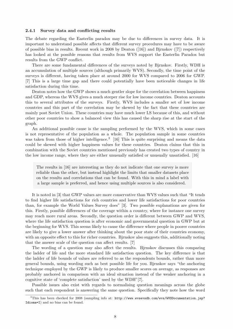
The results in [16] are interesting as they do not indicate that one survey is morereliable than the other, but instead highlight the limits that smaller datasets placeon the results and correlations that can be found. With this in mind a label witha large sample is preferred, and hence using multiple sources is also considered.
It is noted in [3] that GWP values are more conservative than WVS values such that “It tendsto find higher life satisfactions for rich countries and lower life satisfactions for poor countriesthan, for example the World Values Survey does” [3]. Two possible explanations are given forthis. Firstly, possible di↵erences of the coverage within a country, where for instance one surveymay reach more rural areas. Secondly, the question order is di↵erent between GWP and WVS,where the life satisfaction question is after economic and governmental question in GWP but atthe beginning for WVS. This seems likely to cause the di↵erence where people in poorer countriesare likely to give a lower answer after thinking about the poor state of their countries economy,with an opposite e↵ect to this for richer countries. Bjrnskov also suggests this, additionally notingthat the answer scale of the question can a↵ect results. [7]
The wording of a question may also a↵ect the results. Bjrnskov discusses this comparingthe ladder of life and the more standard life satisfaction question. The key di↵erence is thatthe ladder of life bounds of values are referred to as the respondents bounds, rather than moregeneral bounds, using wording such as best possible life for you. Bjrnskov says “the anchoringtechnique employed by the GWP is likely to produce smaller scores on average, as responses areprobably anchored in comparison with an ideal situation instead of the weaker anchoring in acognitive state of ‘complete satisfaction’ used by the WDH”[7].
Possible issues also exist with regards to normalising question meanings across the globesuch that each respondent is answering the same question. Specifically they note how the word
3This has been checked for 2008 (sampling info at: http://www.wvsevsdb.com/wvs/WVSDocumentation.jsp?
Idioma=I) and no bias can be found.
8

‘happy’ needs to be translated accurately across di↵erent languages and “the English word ‘happy’is notoriously di�cult to translate”. [7]
Whilst this work has focused on the correlation between GDP and happiness, it has highlightedmany general di↵erences of surveys which could a↵ect correlations of many other variables.
Small di↵erences in survey format can severely a↵ect results. The WVS andGWP surveys are both not ideal for di↵erent reasons; the selection of respondents
for WVS, and the position of the life satisfaction question in the GWP.
2.4.2 Relative wealth
A Lorenz curve (figure 3(b)) is a graphical representation of the distribution of wealth. The curveindicates the proportion of the wealth at each percentage of the population. The more convexthe curve the greater the inequality, where a larger proportion of the population has a smallerproportion of the wealth. A uniform distribution (straight line) represents complete equality.The Lorenz curve is the idea behind a common deprivation measure known as the Gini index,which is defined as:
Gini(A,B) =A
A+B, (1)
where B is the area under the curve and A is the shaded area above the curve. The valuesrange between zero and one from uniform to highly unequal respectively.
(a) Gini Index, Global Map [9]
% of population
Inco
me
shar
e
(b) Lorenz Curve [24]
Figure 3(a) shows global Gini index values from the CIA World Factbook4 2009. This shows alarge amount of variation between countries and even a visual comparison between global valuesof Gini index and happiness (figures 3(b) and 1.1 respectively) shows some similar patterns. Forinstance, countries in Europe generally has higher happiness levels and a lower Gini index thanthose in Africa.
Distribution of wealth may be a valuable indicator of happiness.
2.4.3 A study of relative income
Relative variables such as the Gini index may be valuable indicators of happiness. The variableswe will consider will represent relativity on a country level. Work by Mayraz et al. in 2009 ([34])investigated the a↵ects of relative income but considered di↵erent groups as the comparisonnamely friends, neighbourhood and colleagues. The data used were survey questions asking togive values for their relative income in relation to the di↵erent groups mentioned above, and alsothe importance they gave this comparison. In fact, these questions were designed by Mayrazspecifically for this research.
4World Factbook is a global dataset of information on each country and can be found athttps://www.cia.gov/library/publications/the-world-factbook/
9

Linear regression was used, with slightly di↵erent regression equations to answer di↵erentquestions. The regression methods are reviewed in detail as they show the flexibility of linearregression as a tool for data mining (see section 3.3.4).
The basic regression equation is:
Hi = ↵+ �YRi + �Yi +X
k
�kXki + "i (2)
This includes dependent variableH for life satisfaction, constant ↵ and error ". The regressionvariables include relative income YR, absolute income Yi and a set of control variables Xi. This isa standard regression function using control variables to account for variation in H due to otherfactors such as age and education.
Firstly, the correlation between relative income and life satisfaction was investigated usinga regression equation as above but using log absolute income. The regression was repeated foreach group and also with and without the absolute income variable. The regression results showquite surprising results, where a significant correlation is found between relative income and lifesatisfaction for men but not for women. The coe�cient values are smaller when log absoluteincome is included in the regression, which is expected as this shows that absolute income makessome contribution to a persons’ life satisfaction valuation.
A second investigation in this research looked at the relationship between a persons’ happiness,the importance they subjectively place on relative income, and the actual importance of relativeincome with respect to happiness. This is important to show that the subjective value is anadequate representation of the actual importance (as perhaps people perceive it to be importantbut in reality it does not a↵ect their happiness). To do this they use the regression formula ofequation 3, where the key di↵erence is the use of an interaction term, which is the product ofrelative income and subjective importance (see section 3.1.1 for details of interaction terms).
Hi = ↵+ �jYjRi
+ �0jI
jRi
+ �00j Y
jRiIjRi
+ �logYi +X
k
�kXki + "i (3)
Put simply, this equation is asking whether the correlation between actual income and happi-ness is dependent on the subjective importance of relative income. A result where the coe�cientof the interaction term is high, and the coe�cient of the other terms is reduced, would show thatthe interaction between relative income and perceived importance accounted for the variationof well being better than the individual variables. This would infer that a persons’ subjectiveimportance does bear relation to the actual importance of relative income with respect to happi-ness. Note how this contrasts to the standard regression equation with only independent variableswhere each contribute individually through summation to the dependent variables value. Theresults of this regression gave very low coe�cient values for the interaction term. This shows thatthe relationship between relative income and happiness is not governed by a persons perceivedimportance of relative income.
One potential weakness of the methods used was the use of surveys to retrieve values for allvariables including that of relative income. A more robust method may have been to surveyeach persons income, and record the individuals within the groups so that relative income canbe determined precisely. This however, would be a fairly arduous task. Mayraz tackles this issueby analysing the causality between happiness and subjective relative income. The concern waswhether a higher relative income caused people to be happier or whether happier people wereperhaps more optimistic in their estimations of relative income. To test this, relative income wasused as the dependent variable and an interaction term of happiness and importance was included.This was to test if the relationship between relative income and importance is dependent onhappiness, but the results showed that this was not the case. However this does not show whethersubjective relative income is representative of actual relative income on a more fundamental level.
A final investigation by Mayraz looked at whether the di↵erence in happiness from the meanis of equal magnitude either side for higher and lower relative income values. For instance, given
10

mean relative income mi with happiness mh, and person X with relative income mI + p andhappiness mH + q. If a person Y has relative income mi � p is his happiness mh � q? Thehypothesis tested is that those with low relative income lose more happiness that a person gainswho has high relative income, meaning that with each unit increase in relative income, the changein happiness decreases. Testing this with linear regression required transforming this hypothesisedcorrelation into a linear one, by way of a quadratic transformation (illustrated in figure 3). Thisis the third term in the regression formula (equation 4 below).
Quadratic transformation
True Correlation
Figure 3: Graphical explanation of quadratic regression
Hi = ↵+ �jYjRi
+ �0j(Y
jRi)2 + �logYi +
X
k
�kXki + "i (4)
Mayraz notes that the coe�cient for this quadratic variable will be negative if there is anasymmetric relationship. This is because the relationship hypothesised is concave and these resultin negative coe�cient values, in contrast to convex correlations which have positive coe�cientvalues. To see why take a simple regression equation y = ax2 + b and di↵erentiate with respectto x to give @y
@x = 2ax. It can be seen that negative values of a give a decreasing rate of change asx increases and hence a concave curve. The results for each group however give values very closeto zero, and in fact only 3 of these are negative values. This indicates that the rate of change ofhappiness with relative income does not decrease as relative income values increase.
This research has demonstrated the versatility of linear regression to answer a range of ques-tions regarding variable relationships, using both interaction terms and logarithmic and quadratictransformations. Of particular note is the use of interaction variables to analyse causality betweenvariables, showing an additional approach to using longitudinal data.
Other research looks at non economic variables, such as a 2005 paper by Oswald et al. “Doeshappiness adapt? A longitudinal study of disability with implications for economists and judges”[39]. Oswald et al. (2005) analysed time series data to investigate the a↵ect a disability hason well-being. The results showed a clear trend, where life satisfaction dropped significantly ongaining a disability, but remarkably bounced back to just below the original value showing thestrength of our ability to adapt in adversity.
2.5 Research of Other Indicators
2.5.1 Health
Health may have a marked e↵ect on happiness, a notion supported by previous research. Wesuggest a distinction between health variables depending on whether they are recoverable, dueto the psychological di↵erences between the two situations. For instance the paper above dis-cussing disabilities showed happiness values returning to previous levels. A long standing butnon permanent health issue however, may have a higher a↵ect on happiness, due to the beliefthat they could be healthier than they are. A person becoming disabled does not have this hopeand therefore adapts to this permanent change in their life.
11

Causality relationships with health may be particularly unclear, where conditionssuch as hypertension could be e↵ects rather than causes of happiness. This doesnot a↵ect a variables viability as an indicator and both types will be considered
for this project.
Blanchflower & Oswald have investigated the relationship between hypertension (high bloodpressure) and happiness [8], with an aim to incorporate hypertension as a variable in a well-beingindex. This research used life satisfaction and happiness responses from the Eurobarometersurvey, and the hypertension values were also derived from the survey data. Correlations wereassessed using both Pearsons and Spearmans rank tests, and OLS and logit regression5 were used.The R2 was used to validate the regression model (see section 3.3.1).
Individuals were used as entities with country dummy variables as controls (a binary variablefor each country where the country of the individual is ’on’ and the others are ’o↵’). Thedependent variables of the regression tests were hypertension and life satisfaction. The resultsshowed correlation between hypertension and happiness. For instance, when looking at the verysatisfied responses the countries with the lowest blood pressure gave significantly higher happinessvalues (48.5% compared with 22.5%).
While the results are encouraging, some aspects of this research may not be ideal. Firstly thedata sample is not quite small, consisting of just 16 countries. Also, the hypertension data camefrom the question “Would you say that you have had problems of high blood pressure?”, whichmakes this a subjective measure. We question whether hypertension can really be estimatedaccurately through self assessment, as for instance it does not distinguish between high bloodpressure and hypochondria. However, this was necessary for this research because the entitieswere individuals and hence the data needed to consist of happiness and hypertension values foreach person. It may be worth a study into the accuracy of this self assessment through askingthis question to individuals where actual blood pressure readings have been taken and can thusbe compared.
Our project, with country entities uses more concrete health indicators derivedfrom country records rather than self assessment such as life expectancy.
2.5.2 Light
Light may be an interesting correlate because of possible links with depression. Seasonal A↵ectiveDisorder (SAD) is a type of depression where the individuals are a↵ected only in the wintermonths. SAD is thought to be caused by the lack of light, which a↵ects the release of certainchemicals in the brain causing a change in mood [40]. Depression levels of SAD su↵erers canvary widely throughout the year and this suggests light may have be a contributor to happinesslevels, although no previous data mining work could be found regarding this. Previous researchhas however, found correlation between prevalence of SAD and latitude, such as [44].
Light may correlate with happiness and hence is considered as a feature.
2.5.3 Climate
Previous work has found evidence for a relationship between climate variables and happiness.The implications of a correlation between happiness and climate are vast. The threat of climatechange causing large shifts in weather patterns means that a relationship between climate andhappiness would likely cause changes in happiness levels. Climate variables add much complexityto this problem as they are likely to be closely related to other variables of interest. A key
5Regression where the data is fit to a logistic curve
12

example of this is health, where weather causes an increase of some illnesses. For instance, flu isknown to be higher in the colder months6.
Rehdanz & Maddison performed a comprehensive investigation into the relationship betweenclimate and happiness using a wide range of variables [42]. The choice of variables includes someinteresting options. Firstly the climate variables used were annual mean values of temperatureand rainfall and indicators of extremes such as the precipitation of the wettest month. Absolutelatitude was used to represent amount of daylight. Other variables were also included to controlfor other di↵erences. Of particular interest is the construction of a variable to control for thecountries that were previously communist, necessary as their initial analysis showed that thesecountries were the ones with the lowest temperature. A variable is needed to control for this orelse the results would be biased and incorrect. Other variables included are taken from previousresearch such as religion and life expectancy.
Of particular note was the pre-processing of the variables to produce appropriate indicators.This is needed to ensure the values are representative of the country as a whole, because climatevariables vary across countries and this is independent of the distribution of populations. Thevalues assigned should be values representative of the populated areas. [42] accounted for this bytaking the weighted average of several cities of a country, weighted by the population.
Care should be taken to ensure the variables are representative of a country, suchas by using a weighted average as in the example above.
Several regression tests were performed using di↵erent groups of climate variables, togetherwith the control variables. This segregation was needed to remove collinearity, which would a↵ectresults. For example, two variables are the average mean temperature and the number of monthswhere the temperature exceeds 20�C, and these variables clearly have a close relationship. Aregression equation with both these variables would attempt to attribute the same variance ofthe label to both of these variables.
This research performed separate regression using the di↵erent variable groups as explainedabove, and therefore it is interesting to compare these results. The results showed that the maxand min temperature variables correlate negatively and positively respectively, which is expectedas this infers people prefer medium temperatures to extremes. However, the regression usingcount variables of the number of cold and hot months, showed a negative correlation betweennumber of cold months and happiness and a positive correlation between the number of hotmonths and happiness, indicating a preference for warmer climates. This is supported by thefinal regression which used mean values, and found a strong positive correlation between annualmean temperature and happiness. The t-statistic was however lower than that of mean rainfallin this regression showing that this has a stronger correlation than mean temperature.
The variable groups represented similar concepts but resulted in di↵erentregression models, highlighting the sensitivity of variables selection and theimportance of trying di↵erent alternatives that represent similar concepts.
The regression with maximum / minimum values proved to be the best representation, withthe highest R2 value of 0.7918 (possible values range between 0 and 1 where 1 means the variablescompletely predict the dependent variable), although this is only marginally larger. In fact, allthree models showed significant correlations with happiness, with a highest f-statistic of 0.0081.Also, all models generated using the di↵erent groups of climate variables passed the RESET testshowing these models were able to represent correlation with happiness.
6Search trends show annual cycles indicating correlations between health and climate. Search for flu - http://www.google.com/trends\?q=flu&ctab=0&geo=gb&geor=all&date=all&sort=0
13

These results show interesting results, primarily that climate indicators are goodcorrelates with happiness.
2.6 Causal Inferences
Causality of happiness is an interesting subject as there are many possible correlates where thedirection of causality is unclear. There has been only a limited amount of work looking at this.
Investigating causality is beyond the scope of this project.
Previous work has found married people have higher happiness levels and research by Stutzeret al. in 2006 looked at the relationship between marriage and happiness [47]. Establishingcausality required the use of longitudinal data7; a dataset recording values related to the sameentity over time. The relationship between changes in variable values over time can indicatecausality. For instance, does happiness increase after marriage to infer that marriage makespeople happy? Or are happier people married because one is more likely to find love if they arehappy?
The dataset was split into three groups; remaining single, married and marry later in life. Thelife satisfaction scores were adjusted for di↵erent factors such as age and gender, but the methodsfor this are not specified. Even so, the results are fascinating, and simply through graphing thedata and visual examination interesting results can be detected. For instance, at age 20 the peoplewho go on later to marry have much higher life satisfaction than those that stay single. Alsofor these people, there was a steady increase in happiness in the years prior to marriage, whichreturns to the previous value in approximately the same length of time afterwards. Additionallythey find this trend is also found for people who marry and subsequently divorce but at lowerlevels of happiness. This shows that people who are less happy are less likely to marry and morelikely to divorce, indicating happiness causes marriage.
Longitudinal data analysis is a valuable way of determining causality and as can be seen fromthis paper the causality can often be very apparent. However, this has also highlighted the factthat happiness is often not changed suddenly, but gradually over a period of time. For instance,increased happiness caused by marriage is not suddenly altered but gradually increased over anumber of years prior to marriage, perhaps due to the hope and thoughts of marrying in thefuture or being in a long term stable relationship. This means that analysis needs to be over awide time span to fully investigate causal a↵ects.
This indicates that variables may have better correlation if several years are used.One option is to construct a weighted average where more distant years have less
contribution.
7Survey source: German Socio-Economic Panel Study (GSOEP)
14

3 Methods Overview
3.1 Data Preparation
The success of classifiers and prediction methods depend heavily on the quality and choice ofthe data used. [5] Domain knowledge is important to be able to choose features that are likelyto bring good results, and previous work reviewed in section 2 provides important backgroundinformation of this subject area. Data preparation and feature selection are two critical parts ofa data mining project.
3.1.1 Feature construction
The data collated can be used directly or can be manipulated to provide alternative featureswhich may be more e↵ective in models. This stage is an opportunity to use domain knowledge toconstruct appropriate features for analysis. This includes simple techniques such as combiningvalues into a single feature, or more complex methods such as principal component analysis(PCA).
Feature variables can be constructed in the following ways:
• Time correlations Time series data can be used to calculate the relative change of avariable, which can be used as a feature.
• Transformations Data transformations such as log, square-root, square and PCA (seebelow).
• Interactions Features can be constructed using mathematical functions on several vari-ables. Many of these are readily available such as GDP per capita.
Transformations Transformations are common in linear regression, as the linear naturewould otherwise be restrictive when non-linear relationships exist. Performing transformationsallows non linear correlations to be found when using linear techniques.
Transformations with logs is particularly common, and additionally this gives an additionalproperty beyond just changing the relationship between the variables. Standard variables corre-late with the dependent variable in the standard way of the formulation a = bx + c, such thatwhen the value of x changes by 1 the value of a changes by b. However the values of the coe�-cients produced depend on the units of the variables. Introducing logs changes this so that therelationship between the log of the independent variable and the dependent variable is now inpercentages such that it represents the relative rather than the average change. [20]
Interaction terms Interaction terms are useful when the relationship between several vari-ables needs investigating, such as where the correlation between an independent and the depen-dent variable may additionally depend on a third variable (see section 2.4.3 for an example usingthis). This is a simple regression function with two variables X and Y that are also interactionterms:
f(X) = �0 +Xj�j +Xk�k +X
XjYj�j , (5)
3.1.2 Principle Component Analysis (PCA)
PCA is a powerful method to find hidden patterns in datasets, by performing an orthogonal8
transformation of the dataset into a set of new variables called principal components. Given aset of data points we can view these as points in a multidimensional space, where the axes are
8Orthogonal refers to the fact that the axes of the principal components are perpendicular to each other, justas the x and y axis in a typical 2 dimensional space
15
just arbitrarily defined. The axes can be moved such that they correspond to the directions ofhighest variance, and this can reveal hidden patterns in the data.
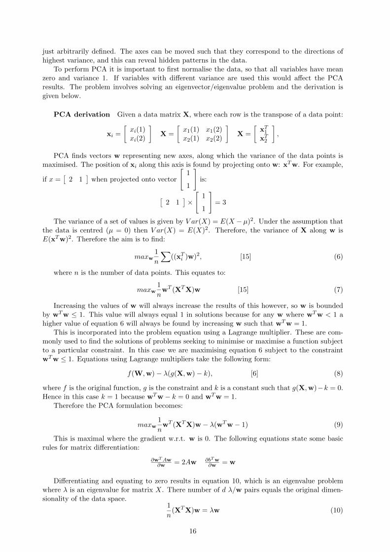
To perform PCA it is important to first normalise the data, so that all variables have meanzero and variance 1. If variables with di↵erent variance are used this would a↵ect the PCAresults. The problem involves solving an eigenvector/eigenvalue problem and the derivation isgiven below.
PCA derivation Given a data matrix X, where each row is the transpose of a data point:
xi =
xi(1)xi(2)
�X =
x1(1) x1(2)x2(1) x2(2)
�X =
xT1
xT2
�,
PCA finds vectors w representing new axes, along which the variance of the data points ismaximised. The position of xi along this axis is found by projecting onto w: xTw. For example,
if x =⇥2 1
⇤when projected onto vector
"1
1
#is:
⇥2 1
⇤⇥
"1
1
#= 3
The variance of a set of values is given by V ar(X) = E(X � µ)2. Under the assumption thatthe data is centred (µ = 0) then V ar(X) = E(X)2. Therefore, the variance of X along w isE(xTw)2. Therefore the aim is to find:
maxw1
n
X((xT
i )w)2, [15] (6)
where n is the number of data points. This equates to:
maxw1
nwT (XTX)w [15] (7)
Increasing the values of w will always increase the results of this however, so w is boundedby wTw 1. This value will always equal 1 in solutions because for any w where wTw < 1 ahigher value of equation 6 will always be found by increasing w such that wTw = 1.
This is incorporated into the problem equation using a Lagrange multiplier. These are com-monly used to find the solutions of problems seeking to minimise or maximise a function subjectto a particular constraint. In this case we are maximising equation 6 subject to the constraintwTw 1. Equations using Lagrange multipliers take the following form:
f(W,w)� �(g(X,w)� k), [6] (8)
where f is the original function, g is the constraint and k is a constant such that g(X,w)�k = 0.Hence in this case k = 1 because wTw� k = 0 and wTw = 1.
Therefore the PCA formulation becomes:
maxw1
nwT (XTX)w� �(wTw� 1) (9)
This is maximal where the gradient w.r.t. w is 0. The following equations state some basicrules for matrix di↵erentiation:
@wTAw@w = 2Aw @bTw
@w = w
Di↵erentiating and equating to zero results in equation 10, which is an eigenvalue problemwhere � is an eigenvalue for matrix X. There number of d �/w pairs equals the original dimen-sionality of the data space.
1
n(XTX)w = �w (10)
16

The w with the highest variance corresponds to the largest eigenvalue because:
1
n
(XTX)w
w= � (11)
1
n
wT (XTX)w
wTw= � (12)
and wTw = 1, hence:
1
nwT (XTX)w = �, (13)
and the left side equates to the variance (we are back to the original equation 6). [15] Theeigenvector w is a new axis and it’s eigenvalue � represents the degree of variance along it.
W is a matrix of vectors of the directions of greatest variance, ordered by eigenvalue. Thosew with low � typically have little variance and can often be ignored.
W =
"w1(1) w2(1)
w1(2) w2(2)
#(14)
The original data points can be transformed into the new space by projecting onto the vectorsin W:
Xnew = XW (15)
The relationship between eigenvalue and variance means that each principal component p1 topd, ordered by eigenvalue contains the highest amount of information (variance) not accountedfor by p1 to pd�1. This is important for data analysis as the key principal components are oftenhighly informative. Additionally, the dimensionality can often be reduced by using the PCsinstead of the original data and ignoring PCs containing a low proportion of the variance of theoriginal data.
3.1.3 Missing values
The data used in this project will contain some missing values, as it is collated from di↵erentsources. Machine learning methods often require that all the features have values, although manyhave inbuilt methods for dealing with this. We may prefer to choose to remove missing valuesprior to using ML methods and there are three main ways of doing this; reduction of the dataset,indicator variables, and imputation. Reducing the dataset involves removing entities where thedata is incomplete. This is not feasible for this project as this will remove whole countries fromthe analysis (although the coverage will be considered when choosing potential features).
In some cases there is an underlying reason why values are missing from the dataset andthis may in itself contribute valuable information. As an example, time series data of a countrymay have missing values during periods of conflict or natural disaster, and this may itself be acorrelate with happiness. Data analysis using background knowledge is important to determinethe significance of a null value and whether it may have relevance. If so the null values canbe replaced with an indicator variable to represent the underlying cause. [53] However, for thisproject it will usually be the case that the data is missing because a country was simply notincluded, as each data source will have slightly di↵erent coverage. Indicator variables may beappropriate in a minority of cases but inference of missing values (imputation) is likely to be ofmost use.
17
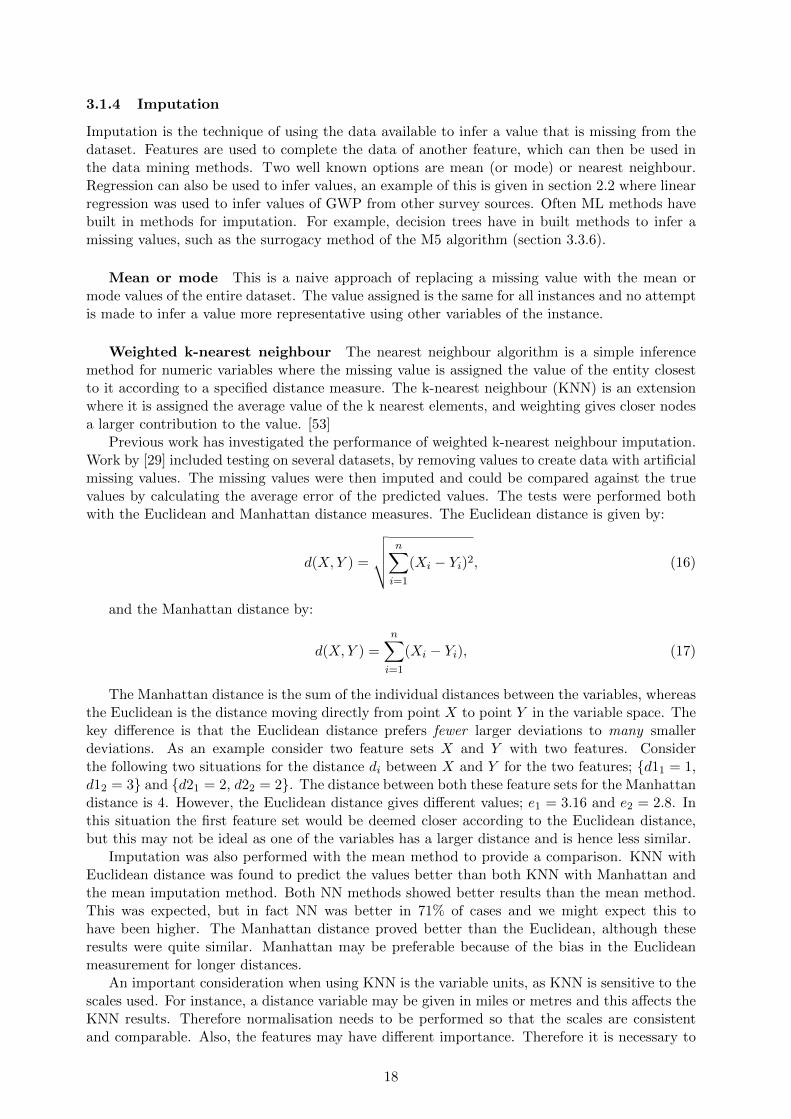
3.1.4 Imputation
Imputation is the technique of using the data available to infer a value that is missing from thedataset. Features are used to complete the data of another feature, which can then be used inthe data mining methods. Two well known options are mean (or mode) or nearest neighbour.Regression can also be used to infer values, an example of this is given in section 2.2 where linearregression was used to infer values of GWP from other survey sources. Often ML methods havebuilt in methods for imputation. For example, decision trees have in built methods to infer amissing values, such as the surrogacy method of the M5 algorithm (section 3.3.6).
Mean or mode This is a naive approach of replacing a missing value with the mean ormode values of the entire dataset. The value assigned is the same for all instances and no attemptis made to infer a value more representative using other variables of the instance.
Weighted k-nearest neighbour The nearest neighbour algorithm is a simple inferencemethod for numeric variables where the missing value is assigned the value of the entity closestto it according to a specified distance measure. The k-nearest neighbour (KNN) is an extensionwhere it is assigned the average value of the k nearest elements, and weighting gives closer nodesa larger contribution to the value. [53]
Previous work has investigated the performance of weighted k-nearest neighbour imputation.Work by [29] included testing on several datasets, by removing values to create data with artificialmissing values. The missing values were then imputed and could be compared against the truevalues by calculating the average error of the predicted values. The tests were performed bothwith the Euclidean and Manhattan distance measures. The Euclidean distance is given by:
d(X,Y ) =
vuutnX
i=1
(Xi � Yi)2, (16)
and the Manhattan distance by:
d(X,Y ) =nX
i=1
(Xi � Yi), (17)
The Manhattan distance is the sum of the individual distances between the variables, whereasthe Euclidean is the distance moving directly from point X to point Y in the variable space. Thekey di↵erence is that the Euclidean distance prefers fewer larger deviations to many smallerdeviations. As an example consider two feature sets X and Y with two features. Considerthe following two situations for the distance di between X and Y for the two features; {d11 = 1,d12 = 3} and {d21 = 2, d22 = 2}. The distance between both these feature sets for the Manhattandistance is 4. However, the Euclidean distance gives di↵erent values; e1 = 3.16 and e2 = 2.8. Inthis situation the first feature set would be deemed closer according to the Euclidean distance,but this may not be ideal as one of the variables has a larger distance and is hence less similar.
Imputation was also performed with the mean method to provide a comparison. KNN withEuclidean distance was found to predict the values better than both KNN with Manhattan andthe mean imputation method. Both NN methods showed better results than the mean method.This was expected, but in fact NN was better in 71% of cases and we might expect this tohave been higher. The Manhattan distance proved better than the Euclidean, although theseresults were quite similar. Manhattan may be preferable because of the bias in the Euclideanmeasurement for longer distances.
An important consideration when using KNN is the variable units, as KNN is sensitive to thescales used. For instance, a distance variable may be given in miles or metres and this a↵ects theKNN results. Therefore normalisation needs to be performed so that the scales are consistentand comparable. Also, the features may have di↵erent importance. Therefore it is necessary to
18

determine which features are most relevant. Incorporating features that bear no correlation tothe missing value can skew results. Variables may have di↵erent relative significance, and it maybe preferable to weight the distances according to this. [53]
A further di�culty is the choice of K, which needs to be optimised manually. A K that is toosmall means that only a few instances are used which may not give a good approximation of themissing value as it over fits the data. A K that is too large will mean instances that are quite far(and hence perhaps quite di↵erent) contribute to the instances value. Finding the optimal valueof K requires testing with di↵erent values. [4]
KNN will be useful to impute missing values in our dataset. The data available to us containsvariables representing di↵erent aspects of human life such as health, education and wealth withmultiple variables of each. We ideally would use a single variable representing a single concept toprevent dependence between features. The missing values of a feature could be imputed from theset of features representing the same concept, which is appropriate as the features are likely tohave a good correspondence with these variables. For example, using several educational variablesimpute missing values of another education variable may be e↵ective.
19

3.2 Statistical & Machine Learning Methods
We use both statistical and machine learning methods throughout this work. ML techniques canbe divided into two main types; black box or white box. The methods used to classify or regresscan be understood and analysed with white box techniques, which is useful to gain understandingof the relationships between the input and target variables. We intend to use several statisticaland ML methods, and describe those of particular interest.
3.3 Statistical Tests
The main statistical methods to determine results significance are correlation with R2, t-testsand permutation testing.
3.3.1 Pearson Product Moment Correlation Coe�cient (R)
R is a measure of correlation of two datasets with values ranging from -1 to 1 where -1 and 1represent perfect negative and positive correlations respectively. More specifically, this measurerepresents the variance of the label that is explained by the model relative to the unexplainedvariance. A value of 0 indicates that there is no correlation between the variables. R is thecovariance of the variables relative to their individual variance, given by the formula:
rx,y =Cx,y
�2x�
2y
, (18)
where C and �2 are the covariance and variance respectively.
Quantitative measure for results analysis A consistent measure is needed to compareresults and the correlation coe�cient (R) will be used. This is appropriate because it is a measureof the goodness of fit of a model. The correlation value is not a↵ected by the number of features ofthe model, which is important as we are comparing tests involving a variable number of features.
P-value A p-value indicates the significance of a result, representing the probability theresult would occur by chance. A low value means the result is unlikely to occur randomly andhence is statistically significant. Threshold values of 5% and 1% are commonly used, below whicha result can be stated as significant. Statistical tests can be relative to test parameters such asthe size of the dataset, and a p-value provides a comparable value that takes into account suchaspects of the data.
R2 and Adjusted R2 R2 is also known as the coe�cient of determination, and is anextension of the R value. It represents the proportion of variation in the label that can beaccounted for by the regression model. However R is relative to the number of variables used inthe model and therefore is not comparable when this di↵ers. Adjusted R2 takes into considerationthe number of variables used in the regression.
3.3.2 T-Test
A t-test calculates the likelihood that two datasets are generated from the same probabilitydistribution. We use this measure to compare results such as the performance of two learners. At-test performed on the results of 10 fold cross validation for instance determines the likelihoodthat these two results sets come from the same distribution. A result indicating they are fromdi↵erent distributions indicates that one performs significantly better.
20
3.3.3 Significance testing with permutation testing
Permutation testing is used to compute a p-value of results when the probability distribution isnot known. For instance, suppose we find a model with a correlation value and we wish to knowthe likelihood that a model with this correlation would occur by chance for data from the samedistribution. The null hypothesis states that the correlation is likely to occur on random data.Therefore the null hypothesis is rejected when the result is unlikely on random data and henceis significant.
Permutation tests amount to sampling from the distribution of a data set by randomly per-muting the data. The samples are taken many times and the test performed and this gives aprobability distribution of results for the random data. The proportion of times the results are‘better’ than that originally found is the p-value:
p� value =#p 2 P : T (p) � v
#p 2 P, (19)
where v is the original test value, P is the set of permutations and T is the test performed.Equivalently, a threshold value t� such that at most 5% of the permutation tests give a value‘better’ than this value can be found:
#p 2 P : T (p) � t�#p 2 P
0.05, (20)
This value can then be compared against all results to determine if it is significant. Thisis a useful alternative where the significance of several results needs assessing, because a singlethreshold value can be compared against many results rather than calculating a specific p-valuefor each.
3.3.4 Linear Regression
Linear regression is a method to model the output value as a linear contribution of the inputs.With respect to this project this can be used to determine a function f : X ! Y , where X is avector of feature values and Y is a happiness ground truth. The linear nature of the representationproduced can sometimes be too simplistic, as the target may not be linearly correlated with thefeature set. However, linear regression is well known to produce accurate results and can alsooutperform more complex non linear methods.
A typical regression formula is:
f(X) = �0 +nX
i=1
Xj�j , [27] (21)
with bias �0 and weight �j of feature j in X. The feature space is a multidimensional spaceand the aim is to find a line in this space that best fits the data points. �0 would then representthe intersect on the axis of f(X).
There are several methods to estimate the coe�cients �j for the model. These include; leastsquares, principal component regression, ridge regression and the lasso.
Least squares The least square is a simple and common measure of error of a regressionmodel given by;
RSS(�) =nX
i=1
(yi � f(xi))2. [27] (22)
with n elements in the training set, target value yi and regression output f(xi). Linearregression using this measure aims to minimise the sum of the squared error (or residue) on thetraining data. The square of the error is used instead of just the absolute error to give a preferencefor smaller deviations from the target values.
21

3.3.5 The Least Absolute Shrink and Selection Operator (Lasso)
A significant weakness of OLS regression is that it cannot regress to the correct function wherethe feature variables are not independent. There are three key methods which improve OLSregression; subset selection, ridge regression and lasso. [49] Lasso, was originally proposed in1996 by Tibshirani as an alternative to ridge regression and subset selection. [49]
Subset selection and ridge regression have some drawbacks and Tibshirani’s aim, describedin [49], was to combine the best of both, and he describes the following shortfalls with thesetechniques. Subset selection includes methods such as stepwise regression, and these methodsinvolve fairly large discrete changes to the model, as variables are added or removed. Also, thismethod is quite sensitive to changes to the input data. Ridge regression is an improvementon subset selection because it uses continuous changes to the model by altering the size of thecoe�cients in the regression function. However, it is unable to reduce any coe�cient to zero andtherefore does not remove any completely from the feature space. [49]
Ridge regression and lasso are both a specific type of regularisation method known as shrinkagemethods. Regularisation methods constrain the search space by using penalties, and specificallyfor shrinkage methods this reduces the size of the coe�cient in the regression function. Thesearch space is the set of all possible regression functions for a feature set, with all possiblecoe�cient values. As an example, the error calculation could incorporate the sum of squaresof all coe�cients, such that when the coe�cients have lower values the error is also lower (thisexample is the penalty for ridge regression as detailed below). [6] Regularisation prevents overfitting by imposing pressure towards simpler functions with small coe�cients.
The aim of lasso is to perform constrained regression, such that the minimum number offeatures are used that are required to explain the data. This is done by finding features thathighly correlate and removing all but one of these from the feature space. It does this by reducingthe coe�cient size in the regression function, such that some can be reduced to zero and henceare removed from the feature space. Therefore lasso combines the gradual changes of shrinkagemethods with the ability to reduce the feature set, the valuable aspects of ridge regression andsubset selection respectively.
Equation 23 shows the lasso optimisation problem, where n and m are the number of datapoints and features respectively.
min↵,w
nX
i=1
(yi � ↵�mX
j
wjxij) [49]
s.tX
j
|wj | t(23)
wj is the coe�cient of variable j in the model, and regularisation constrains the sum of thesecoe�cients. ↵ is the bias in model, such that under the assumption of standardised data suchthat
Pixij
N = 0 the data is centred and the ↵ can be omitted. [49] This results in the followingequation:
minw
nX
i=1
(yi � xTi w) + �
mX
j
|wj | [49] (24)
It is interesting to note just how similar this is to ridge regression, where the regularisingcomponent of the equation is instead �kwk2. [49] This di↵erence gives lasso the key property ofoften reducing coe�cient values to zero providing much value for feature selection.
How lasso works Lasso is not a greedy approach but uses least angle regression (LARS)to find the model. LARS is similar to forward stepwise regression (FSR). FSR works by firstlystarting with an empty model, finding the variable most correlated with the label and addingthis to the model. The residual is taken, which is the di↵erence between the label value and the
22

value predicted by the model. Then recursively the variable is found that is most correlated withthe residual and this is added to the model. Thus gradually the model accounts for more of thevariation in the model by incorporating more features.[48]
LARS is di↵erent because it does not add a variable to the model with the real coe�cientvalue. Instead the coe�cient is the lowest value such that it is not the variable most correlatedwith the label. This is done by increasing the coe�cient gradually and at each step taking theresidual. The correlations of this residual with each variable is taken until another variable hasthe same correlation with the residual as the original variable. LARS maintains a variable set,and the process is repeated with this gradually growing set of variables. The coe�cients ofthe variables in the set are increased together (equiangular such that it is proportionate to theircurrent coe�cient values), until another variable has the same correlation with the residual, whichis then added to this set.[19] This is continued gradually adding more variables until all predictorhave been incorporated. This can be demonstrated with a simple example, for the relationshipy = a+2b and the example data of table 4(a). The starting model is: y = �0 + �aa+ �bb, whereall � are zero.
y 3 5 5 6 8 7 9a 1 1 3 2 2 3 3b 1 2 1 2 3 2 3
(a) Example data
r corr a corr b0.5 0.7026 0.85250.7 0.7409 0.82220.8 0.7618 0.80380.9 0.7837 0.7828
(b) Step 1
�ab corr0.5 0.99091.5 0.32351.6 0.12161.7 -0.0708
(c) Step 2
Figure 4: Example lasso walk through
The steps taken to create a model are:
• Find correlations of each variable with the label (y): a = 0.6358 and b = 0.8954.
• b has the highest correlation. The coe�cient of b is increased until the correlation with theresidual is higher for variable a (table 4(b)): �b = 0.9.
• Find �ab: �ab(a + 0.9b), increasing until correlation is reduced to zero (which is the corre-lation of the bias variable because it is constant) (table 4(c)): �ab = 1.7.
• All predictors are now in the model therefore we can find the bias. Take the mean of theresidual: -0.5600.
• Therefore the model is: y = 1.7a+ (1.7 ⇤ 0.9b)� 0.56 ⌘ y = 1.7a+ 1.53b� 0.56.
• The sum of squared error (ss) is: 2.6056. Comparing this with a model where �ab is notincreased far enough and the error is higher: betaab = 1.0 then ss = 4.8400.
Lasso vs OLS Lasso is more stable than OLS regression because where several variables aresimilar they are both included equally in the model, rather than one representing both and theother being excluded.[49] The lasso uses LARS to generate the model but regularises to boundthe total size of the coe�cients.[48] Regularising reduces overfitting, as an unregularised modelcan have any coe�cient values and hence may fit the training data too closely. Lasso uses 10fold cross validation to find the best � value to regularise such that the error on the test set isminimised. A � value that is too large does not regularise su�ciently and the model overfits thetraining data. A � value that is too restrictive such that the model cannot represent the stablepatterns (that are present in both the training and test data).
3.3.6 Decision Trees
Decision trees are an e↵ective ML method, with a simple and intuitive construction algorithm.They are a white box technique where the generated tree can be analysed to gain understanding.
Tree construction takes a vector of instances as input, consisting of a set of input variablesand a target variable. The tree is constructed by starting at the root and choosing a variable ateach node to split the dataset, a process known as recursive partitioning. At each node down the
23
the tree this is repeated, with progressively smaller subsets of the original dataset. This processends when a stopping condition is met, such as a minimum number of instances at a node, andthis node is then a leaf of the tree.
Decision trees use a greedy approach where the best split at each node is used without lookingat the tree as a whole. This is necessary as the search space of all possible trees is too large tosearch exhaustively. This property means the tree may be sub-optimal, but also that it is a simpleand fast method that can be applied to big datasets.
Decision trees automatically perform feature selection where an impurity measures determinesthe variable chosen at each node, and hence variables that do not help predict the target valueare automatically ignored. This selection of variables with the highest information gain alsomeans there is a bias for smaller trees. Decision trees therefore seek to model relationships in thesimplest way. Also, there is no assumption of a specific type of correlation between the variablesand the target value, unlike other algorithms such as linear regression. [53]
The tree structure can give valuable insight into the strength of the correlation between eachvariable and the target value. In addition, the tree can be converted to a set of rules, known asclassification rules. This is done by starting at the root and constructing a rule for the path fromthe root to each leaf.
There are several algorithms for constructing decision trees, di↵ering in how they determinewhich attribute to use at each node to split the dataset. ID3 and C4.5 are common examplesbut these are not suitable for our needs as they are classifiers and cannot be applied to regressiontasks.
Regression trees There are several alternative construction algorithms for regression treeswhere the main di↵erence is the measure used to split the data at the internal nodes. A classifi-cation and regression tree (CART) uses the Gini index as an impurity measure, which is similarto entropy9 but for continuous values. The Gini gain indicates the increase in inequality in thechild nodes compared to the parent node, when splitting on a particular feature. Alternativelyvariance can be used such as the implementation of REPTree10 by Weka.
Model trees Regression trees can be further extended to contain linear regression func-tions at each leaf node, and these are known as model trees. [53] Model trees are built in thesame way as regression trees except that additionally linear regression is performed at each leafusing the instances assigned to it. The m5 algorithm is a model tree generation algorithm. Afurther alternative is logistic model trees, using logistic regression at each leaf rather than linearregression. This may be preferable where a logistic correspondence between features and labelsis more representative than a linear relationship.
Model trees have several benefits over regression trees including smaller trees and greateraccuracy. This is because a single leaf represents a range of values and thus a model can fit thesebetter than a single value. In addition, they can also be used for extrapolation, as the linearfunction generalises to values that are outside those of the original dataset.
Missing values Decision tree algorithms handle missing values automatically, using di↵er-ent methods to do this (or imputation can be performed prior to using ML, see section 3.1.3).CART and M5 algorithms use a technique called surrogate splitting. This involves a second vari-able at a node, that is used to split the instances where an instance does not have a value for themain variable. The split used for the second variable is chosen such that it is most representativeof the split of the first variable. [22]
9Entropy is used by ID3 and C4.5 and represents how well a particular attributes divides the dataset withrespect to the target variable.
10class weka.classifiers.trees.REPTree
24

0.5
0.55
0.6
0.65
0.7
0.75
0.8
0.85
0.9
0 10 20 30 40 50 60 70 80 90 100
Acc
ura
cy
Size of tree (number of nodes)
On training dataOn test data
Figure 5: Overfitting [37]
Overfitting Decision trees are prone to overfitting,where a tree fits the training data well but does not gen-eralise well to the unseen case and hence performs poorlyon test data. Pruning is a common technique which can becarried out either during or after tree construction, namedpre-pruning and post-pruning respectively. [53] Prepruningconstrains the tree size while it is being constructed, using astopping condition to prevent further child nodes. Commonly,the number of instances at each node is used, which ensuresthe rules in the tree are generalised to cover several instances.Prepruning model trees means the regression model at eachleaf is formed using more instances.
Post-pruning is carried out after the tree is built. This involves using a separate test set andchecking each node from the leaves to the root by comparing the error of each node with that ofit’s parent. If the parent has a lower error the child nodes can be pruned. This can be seen infigure 5, where a large tree has a low accuracy on the test set and this improves by reducing itssize until the test and training error values are similar (around size 20 in this example). Post-pruning can be more e↵ective than pre-pruning as it uses an independent dataset to test the rulesof the tree.
Decision tree critique Decision trees can be used for feature selection as explained above.Here we look in more detail at the algorithms behind tree construction to highlight any limitationsof using this learner for this purpose. We look specifically at Weka’s ([26]) M5P tree11 whichimplements the standard M5 model tree algorithm. [41] One concern for this algorithm is theconstruction of the linear models at the leaves as we would like to infer information from thesemodels, but if a linear model includes dependent variables the model is unstable and cannot beused in this way.
A
CB
Figure 6: Tree pruninglimitations
The M5P algorithm does make use of the information gained fromtree construction to create the leaf models. These models are gener-ated after post-pruning using only the features part of the sub-treejust pruned, and this reduces the likelihood of dependent variableswithin leaf models. Each leaf will use only the features most appro-priate for that portion of the dataset in its model.[51] However, de-pendent and irrelevant attributes can still occur, due to di↵erences insubtrees. For instance, given a subtree such as that in figure 6, wherepruning is performed such that node A is a leaf, and subtrees B andC are pruned. Attributes used at nodes B and C may be highly cor-relating dependent variables where small di↵erences in the instancesdown these branches meant one was preferred (marginally) over theother. These could be two variables representing similar concepts,health expenditure and immunisation rate for instance. Additionally,as the depth increases in tree construction the subsets at each node become smaller and thus itbecomes more likely that irrelevant / non optimal features are chosen.
The pruned nodes consist of rules that perform badly on unseen data and so are a poorgeneralisation. The features above this node in the tree are more stable splitting criteria because,they haven’t been pruned and so these rules are good generalisations to unseen data (largelybecause they were constructed using a larger proportion of the dataset because they are higherin the tree). Therefore, it is unclear why the variables of the pruned nodes are used to constructthe models rather than those of the nodes above.
M5P does attempt to drop terms from the leaf models with the aim of minimising the expectederror on unseen data (to prevent overfitting of the training data). This is done using equation 25,
11class: weka.classifiers.trees.M5P
25
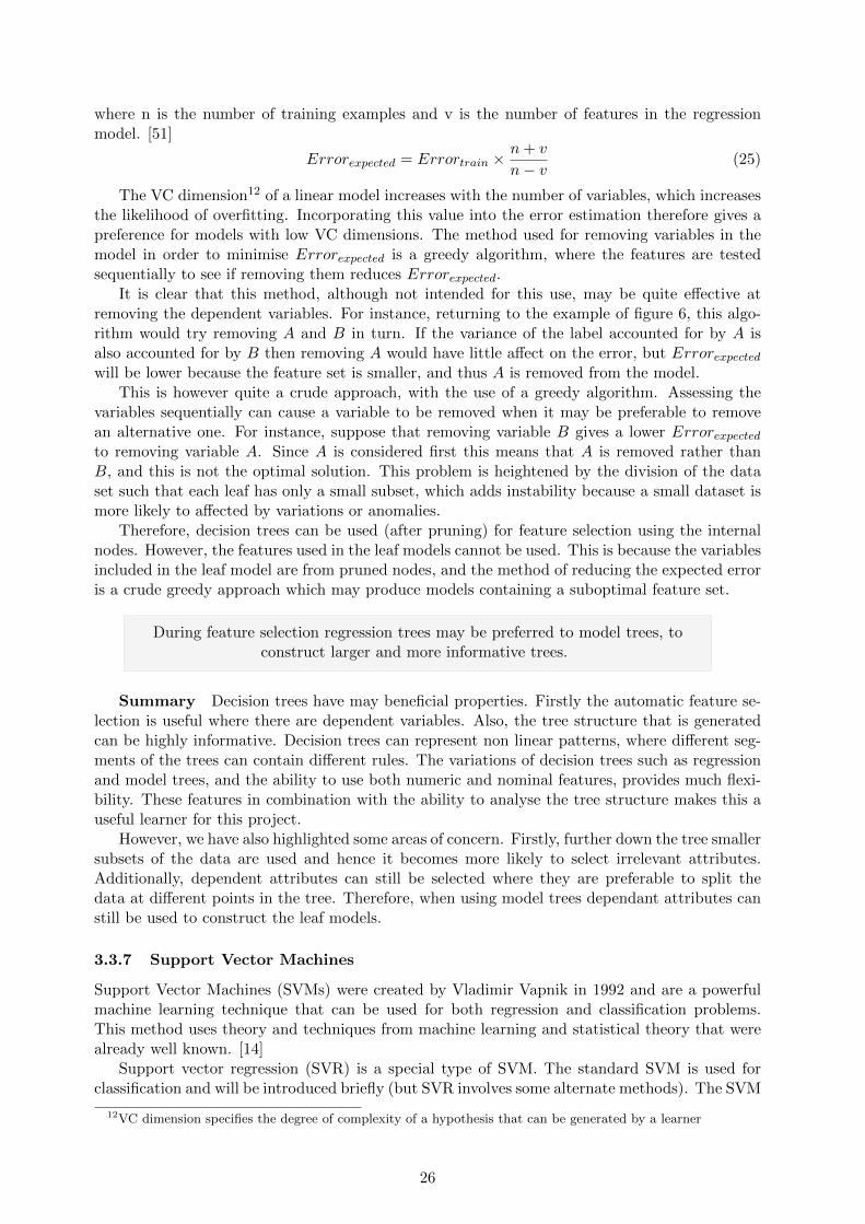
where n is the number of training examples and v is the number of features in the regressionmodel. [51]
Errorexpected = Errortrain ⇥n+ v
n� v(25)
The VC dimension12 of a linear model increases with the number of variables, which increasesthe likelihood of overfitting. Incorporating this value into the error estimation therefore gives apreference for models with low VC dimensions. The method used for removing variables in themodel in order to minimise Errorexpected is a greedy algorithm, where the features are testedsequentially to see if removing them reduces Errorexpected.
It is clear that this method, although not intended for this use, may be quite e↵ective atremoving the dependent variables. For instance, returning to the example of figure 6, this algo-rithm would try removing A and B in turn. If the variance of the label accounted for by A isalso accounted for by B then removing A would have little a↵ect on the error, but Errorexpectedwill be lower because the feature set is smaller, and thus A is removed from the model.
This is however quite a crude approach, with the use of a greedy algorithm. Assessing thevariables sequentially can cause a variable to be removed when it may be preferable to removean alternative one. For instance, suppose that removing variable B gives a lower Errorexpectedto removing variable A. Since A is considered first this means that A is removed rather thanB, and this is not the optimal solution. This problem is heightened by the division of the dataset such that each leaf has only a small subset, which adds instability because a small dataset ismore likely to a↵ected by variations or anomalies.
Therefore, decision trees can be used (after pruning) for feature selection using the internalnodes. However, the features used in the leaf models cannot be used. This is because the variablesincluded in the leaf model are from pruned nodes, and the method of reducing the expected erroris a crude greedy approach which may produce models containing a suboptimal feature set.
During feature selection regression trees may be preferred to model trees, toconstruct larger and more informative trees.
Summary Decision trees have may beneficial properties. Firstly the automatic feature se-lection is useful where there are dependent variables. Also, the tree structure that is generatedcan be highly informative. Decision trees can represent non linear patterns, where di↵erent seg-ments of the trees can contain di↵erent rules. The variations of decision trees such as regressionand model trees, and the ability to use both numeric and nominal features, provides much flexi-bility. These features in combination with the ability to analyse the tree structure makes this auseful learner for this project.
However, we have also highlighted some areas of concern. Firstly, further down the tree smallersubsets of the data are used and hence it becomes more likely to select irrelevant attributes.Additionally, dependent attributes can still be selected where they are preferable to split thedata at di↵erent points in the tree. Therefore, when using model trees dependant attributes canstill be used to construct the leaf models.
3.3.7 Support Vector Machines
Support Vector Machines (SVMs) were created by Vladimir Vapnik in 1992 and are a powerfulmachine learning technique that can be used for both regression and classification problems.This method uses theory and techniques from machine learning and statistical theory that werealready well known. [14]
Support vector regression (SVR) is a special type of SVM. The standard SVM is used forclassification and will be introduced briefly (but SVR involves some alternate methods). The SVM
12VC dimension specifies the degree of complexity of a hypothesis that can be generated by a learner
26
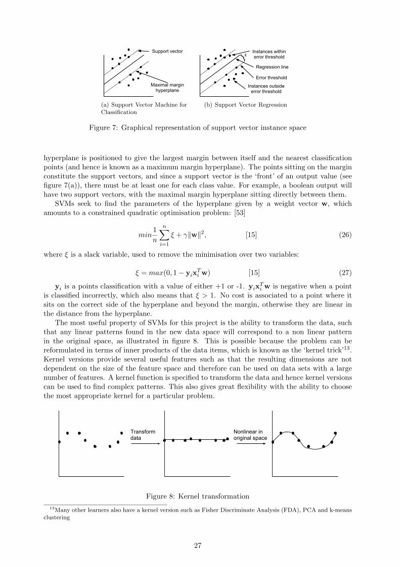
Support vector
Maximal margin hyperplane
(a) Support Vector Machine forClassification
Instances within error threshold
Instances outside error threshold
Regression line
}ε
Error threshold
(b) Support Vector Regression
Figure 7: Graphical representation of support vector instance space
hyperplane is positioned to give the largest margin between itself and the nearest classificationpoints (and hence is known as a maximum margin hyperplane). The points sitting on the marginconstitute the support vectors, and since a support vector is the ‘front’ of an output value (seefigure 7(a)), there must be at least one for each class value. For example, a boolean output willhave two support vectors, with the maximal margin hyperplane sitting directly between them.
SVMs seek to find the parameters of the hyperplane given by a weight vector w, whichamounts to a constrained quadratic optimisation problem: [53]
min1
n
nX
i=1
⇠ + �kwk2, [15] (26)
where ⇠ is a slack variable, used to remove the minimisation over two variables:
⇠ = max(0, 1� yixTi w) [15] (27)
yi is a points classification with a value of either +1 or -1. yixTi w is negative when a point
is classified incorrectly, which also means that ⇠ > 1. No cost is associated to a point where itsits on the correct side of the hyperplane and beyond the margin, otherwise they are linear inthe distance from the hyperplane.
The most useful property of SVMs for this project is the ability to transform the data, suchthat any linear patterns found in the new data space will correspond to a non linear patternin the original space, as illustrated in figure 8. This is possible because the problem can bereformulated in terms of inner products of the data items, which is known as the ‘kernel trick’13.Kernel versions provide several useful features such as that the resulting dimensions are notdependent on the size of the feature space and therefore can be used on data sets with a largenumber of features. A kernel function is specified to transform the data and hence kernel versionscan be used to find complex patterns. This also gives great flexibility with the ability to choosethe most appropriate kernel for a particular problem.
Nonlinear in original space
Transform data
Figure 8: Kernel transformation
13Many other learners also have a kernel version such as Fisher Discriminate Analysis (FDA), PCA and k-meansclustering
27

Two common kernel functions are the Radial Basis Function (RBF) and polynomial (equa-tions 28 and 29 respectively).
kernelRBF (xi, xj) = exp�✓kxi � xjk2
2�2
◆(28)
kernelPOLY (xi, xj) =�xTi · xj + 1
�d(29)
Support vector regression di↵ers slightly from the classification case, as a maximally marginhyperplane is not used. Alternatively, an ✏-insensitive loss function (equation 30) is used tominimise the error on the data. An ✏ value is specified which is a threshold distance from thehyperplane and instances are only said to result in an error if the error value falls outside of thisthreshold. Errors within this threshold are small enough and are thus synonymous with a correctclassification and impose no cost. [10] This provides a way of defining an error for regressionproblems that allow for some noise. The value chosen as ✏ determines the acceptable error sizeand therefore the degree to which the function fits the data. The cost of a point ⇠, is given by:
⇠ = max(0, |Xw� y|� ✏) (30)
The cost therefore depends on the distance from the hyperplane, and these two propertiesalways hold; ⇠ � 0 and ⇠ � |Xw� y|� ✏. A point nearer than ✏ to the hyperplane incurs no cost,and for those past this point the cost is linear in the distance (and these points constitute thesupport vector).
In addition to the loss, a parameter called the cost should also be optimised. This costparameter specifies the magnitude of the cost relative to the distance from the hyperplane, whereincreasing the cost means the fit will be closer and overfitting may occur. If the cost is toolow the fit is not representative of the data as the penalty for being far from the hyperplaneis too low. The RBF kernel additionally has a gamma value (�2 in equation 28), which is aregularisation parameter that specifies how closely the fit to the data. The polynomial kernelrequires an exponent parameter (d in equation 29).
In summary, SVMs are a powerful and flexible method for regression problems, in comparisonto standard linear techniques such as least squares. The two objectives, minimising both theerror and the complexity of the hypothesis (called optimisation and regularisation respectively)means SVMs are able to learn a hypothesis with an inbuilt method to prevent overfitting thedata. They have greater modelling capabilities due to the transformation of the feature spaceand hence can find non linear patterns. The appropriate kernel function can be chosen accordingto the problem. SVMs cope well with noisy data as they regularise to prevent overfitting andincorporate a margin to allow for a degree of deviation from the hyperplane. They are less a↵ectedby outliers as the cost function is linear in distance from the hyperplane, compared to quadraticfor least squares.
3.3.8 Bayesian Belief Networks
A Bayesian belief network (BBN) is a directed acyclic graph (DAG). BBNs are useful to visualisethe interaction between values, based on the conditional probabilities.
Each node represents one variable and contains a probability table. This states the condi-tional probability of each value given each value of the nodes that point to it. Each variable isconditionally independent of the other variables, given the value of its parents (the variables thatlead directly to it).14 [36]
The conditional probability tables are computed using the frequencies of the attribute valuesgiven each of the possible combinations of parent value. This means a variable with 4 nominalvalues having a parent with 3 would have 12 di↵erent probabilities in it’s table. Once the networkis constructed, the probability of a set of variable values called the joint probability can be found.
14X is conditionally dependent of Y given Z if where a value of Z is given X is not dependent on Y.
28

We will be able to determine the probability of a certain range of happiness given specific valuesof features. The joint probability15 is the product of the conditional probability values of thevariable values in each node. Formally:
P (y1, . . . , yn) =nY
i=1
P (yi | Parents(Yi)) (32)
The probabilities can be calculated using the frequencies of the variable values:
P (x = x1|y = y1) =|instancesx1,y1|+ n
|instancesy1|+ n ·N (33)
This creates a maximum likelihood BBN with respect to the probabilities (and not the struc-ture). The n and N variables incorporate a Laplace correction into the probabilities to ensurethat no values are ever zero in the probabilities. Data used to construct a BBN is only a smallsample used to represent more general concepts and so zero frequencies may exist in the samplewhere the true probability is small but non-zero. Incorporating a correction prevents zero prob-abilities which would give a large bias such that any joint probability calculated with it will bezero. The correction e↵ectively assigns each variable value to one extra instance. Therefore inthis case N is |x| · |y|, the number of possible combinations of these two variables, and n is theweight of this correction. A larger n value will reduce the ‘free’ probability assigned.
Discretization A Bayesian belief network can only use discrete values. Our variables in-cluding the happiness variable are continuous, and these need to be discretised prior to construct-ing the network. This involves defining a set of ‘bins’ which are categories (a range of values) ofthe variables, to convert from continuous to nominal values. Binning can be either equal intervalor equal frequency.[53] Equal interval splits the range into equal sized segments, whereas equalfrequency ensures the same number of elements occur in each bin. The latter is often preferableas where many elements are clustered around a similar value these values can be segmented to afiner degree and hence keep more information about the distribution of values.16
This is a possible drawback of BBN’s where discretising the values will inevitably lose someinformation in the data. As an example, consider the following situation:
Instance X : i = 10Instance Y : i = 11Instance Z : i = 19
Suppose two bins were for ranges 1-10 and 11-20. X would be assigned a di↵erent bin to Yand Z. Instances X and Y are very close but after discretising it performed it is Y and Z thatappear most similar. The number of bins chosen is important to represent the data most appro-priately in nominal form, to reduce the amount of information that is lost. If too many or toofew are used then the nominal values do not show some data patterns. Additionally, the degreesof freedom of a network (the number of changeable parameters) is exponential in the number ofbins. This should be minimised to reduce the complexity and prevent overfitting.
15The joint probability is derived by the chain rule. Generally P (A\B) = P (A | B)P (B). Given 3 nodes with thefollowing structure: A ! B ! C. C is conditionally independent of A given B such that P (C | A\B) = P (C | B).Therefore:
P (A \B \ C) = P (C | A \B)P (A \B) = P (C | B)P (B | A). (31)
16Weka provides a Bayesian network classifier.[43] All inputs must be discrete, pre-processing is not part of thetool. [43] Discretising can be done with Weka’s discretise tool, which provides both binning types described here.
29

Missing values Weka’s implementation of a BNN handles missing values by assigning themthe mean of the dataset. This is a naive approach and hence it may be preferable to impute thevalues before constructing the network.
The following are points to consider when creating a BBN:
• The number of nominal values or ‘bins’ to choose
• Equal interval or equal frequency binning
• Preprocessing of missing values (see section 3.1.3)
BBN will provide a useful tool for this project to visualise and assess the relationships betweenthe variables and happiness label. However, we must be aware that this method does not inferthe direction of causality, but just dependence between variables.
3.3.9 Testing the accuracy of classifiers
Overfitting is a common issue with ML algorithms, and occurs when the learned hypothesis tooclosely represents the training data such that it is unable to generalise to unseen examples. Thisresults in a low error on the training set but a much higher error on the test set. To determinethe accuracy on unseen data the dataset should be split into training and test sets. This canoften be problematic when there is limited data available.
With regards to this project, ideally survey data and feature variables from multiple yearswould be used, to provide independent sets of data on which to train and test. However, thisis unlikely as there is limited data available. Alternatively, methods exist to work with separatetraining and test sets, such as 10 fold cross validation. This makes best use of the data availableby testing the algorithms multiple times on the same dataset. The dataset is divided into 10parts, and the algorithm is run 10 times. Each time 9 parts are combined and used for trainingthe learner and 1 is used for testing. In this way the training and test sets are distinct and theaccuracy can be assessed with 10 di↵erent tests.
30
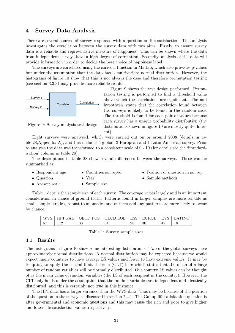
4 Survey Data Analysis
There are several sources of survey responses with a question on life satisfaction. This analysisinvestigates the correlation between the survey data with two aims. Firstly, to ensure surveydata is a reliable and representative measure of happiness. This can be shown where the datafrom independent surveys have a high degree of correlation. Secondly, analysis of the data willprovide information in order to decide the best choice of happiness label.
The surveys are correlated using the corrcoef function in Matlab, which also provides p-valuesbut under the assumption that the data has a multivariate normal distribution. However, thehistograms of figure 10 show that this is not always the case and therefore permutation testing(see section 3.3.3) may provide more reliable results.
CorrelationCorrelate
Survey 1
Survey 2
Figure 9: Survey analysis test design
Figure 9 shows the test design performed. Permu-tation testing is performed to find a threshold valueabove which the correlations are significant. The nullhypothesis states that the correlation found betweentwo surveys is likely to be found in the random case.The threshold is found for each pair of values becauseeach survey has a unique probability distribution (thedistributions shown in figure 10 are mostly quite di↵er-ent).
Eight surveys were analysed, which were carried out on or around 2008 (details in ta-ble 28,Appendix A), and this includes 4 global, 3 European and 1 Latin American survey. Priorto analysis the data was transformed to a consistent scale of 0 - 10 (for details see the ‘Standard-isation’ column in table 28).
The descriptions in table 28 show several di↵erences between the surveys. These can besummarised as:
• Respondent age
• Question
• Answer scale
• Countries surveyed
• Year
• Sample size
• Position of question in survey
• Sample methods
Table 1 details the sample size of each survey. The coverage varies largely and is an importantconsideration in choice of ground truth. Patterns found in larger samples are more reliable assmall samples are less robust to anomalies and outliers and any patterns are more likely to occurby chance.
WVS HPI GAL OECD POS OECD LOL ESS EUROB EVS LATINO57 112 33 34 25 30 47 18
Table 1: Survey sample sizes
4.1 Results
The histograms in figure 10 show some interesting distributions. Two of the global surveys haveapproximately normal distributions. A normal distribution may be expected because we wouldexpect many countries to have average LS values and fewer to have extreme values. It may betempting to apply the central limit theorem (CLT) here which states that the mean of a largenumber of random variables will be normally distributed. Our country LS values can be thoughtof as the mean value of random variables (the LS of each recipient in the country). However, theCLT only holds under the assumption that the random variables are independent and identicallydistributed, and this is certainly not true in this instance.
The HPI data has a larger variance than the WVS data. This may be because of the positionof the question in the survey, as discussed in section 2.4.1. The Gallup life satisfaction question isafter governmental and economic questions and this may cause the rich and poor to give higherand lower life satisfaction values respectively.
31

0 5 1005
1015
WVS
0 5 100
5
10HPI GAL
4 6 80
5
10OECD POS
4 6 80
5
10OECD LOL
4 6 86789
ESS
4 6 85
10EUROB
4 6 84
6
8EVS
6 8 105678
LATINO
0 5 100
5
10
HPI G
AL
0 5 1005
1015
6 8 100
5
10
6 8 100
5
10
6 8 106
8
10
6 8 105
10
0 5 105
10
6 8 105678
0 5 105678
OEC
D PO
S
0 5 105
10
0 5 1005
1015
0 5 100
5
10
0 5 106
8
10
0 5 105
10
0 5 105
10
0 5 105678
0 5 105678
OEC
D LO
L
0 5 105
10
0 5 100
5
10
0 5 100
5
10
0 5 106789
0 5 105
10
0 5 105
10
4 6 85678
6 8 104
6
8
ESS
6 8 105
10
6 8 100
5
10
6 8 100
5
10
6 8 100
5
10
6 8 105
10
6 8 105
10
0 0.5 10
0.5
1
0 5 104
6
8
EURO
B
0 5 105
10
0 5 100
5
10
0 5 100
5
10
0 5 106789
0 5 100
2
4
0 5 105
10
0 0.5 10
0.5
1
4 6 84
6
8
EVS
0 5 105
10
6 8 100
5
10
6 8 100
5
10
6 8 106789
6 8 105
10
0 5 100
5
10
4 6 84567
4 6 86789
LATI
NO
4 6 85
10
4 6 82468
4 6 84567
0 0.5 10
0.5
1
0 0.5 10
0.5
1
4 6 84567
4 6 80
5
Figure 10: Survey data correlations & distributions
The two types of OECD data do not show a normal distribution, and in particular the PositiveExperience Index (OECD POS in column/row 3) shows two clusters centred around 2.5 and 7.0.It is unclear why there is such a clear split for this survey. This measure is very di↵erent fromthe others, as it is a compiled index created from OECD consisting of data from six questionsrelated to what they call ‘positive experiences’. However, the answer scale was still 0 - 10 and aunimodal distribution was expected.
The distribution of Gallup life satisfaction (LS) and Gallup ladder of life (LOL) questionsshow the latter has a larger variance with lower values also. This is unexpected as we wouldexpect the LOL questions to give higher values because the question is relative to ones situation;‘best possible life for me’ rather than ‘best possible life’ for the LS question. The upper bound ofones’ attainable happiness decreases with decreasing life satisfaction, as the standard of life thatis reachable also decreases.
The results show a high degree of correlation between the data, shown in figure 10. Table 2shows the correlation values for each survey, and the p-values output from the corrcoef function.Each pair of surveys has a di↵erent number of countries in common and the p-value incorporatesa correction to account for this. The significant p-values are highlighted indicating 20 surveycross-correlations are significant compared with just 4 that are not. 3 of these are for this OECDPositive Experience Index with the anomalous distribution discussed above. 4 results give novalue where there is no overlap between the countries covered.
Permutation tests gave similar results, shown in table 3. A 1 value denotes a significantresult, such that the surveys were significantly more correlated than the random case. The maindi↵erences are with regards to correlations involving the OECD surveys, and this is consistent
32

WVS HPI GAL OECD POS OECD LOL ESS EUROB EVS LATINOWVS - 0.79 0.406 0.695 0.650 0.858 0.792 0.941HPI GAL 0.0000 - 0.468 0.940 0.344 0.870 0.865 0.82OECD POS 0.054 0.0069 - 0.483 0.300 0.486 0.560 0.99OECD LOL 0.0002 0.0000 0.0068 - 0.473 0.890 0.837 1ESS 0.0064 0.138 0.242 0.0064 - 0.71 0.628 NaNEUROB 0.0001 0.0000 0.0407 0.0000 0.0004 - 0.9 NaNEVS 0.0000 0.0000 0.0102 0.0000 0.0010 0.0000 - NaNLATINO 0.0005 0.0001 0.082 NaN NaN NaN NaN -
Table 2: Survey correlations: Pearson coe�cient values & p-values (significant results highlighted,0.05 threshold)
WVS HPI OECD POS OECD LOL ESS EUROB EVS LATINOWVS - 0.258 0.515 0.503 0.595 0.500 0.385 0.770HPI 1 - 0.337 0.340 0.396 0.349 0.291 0.461OECD POS 0 1 - 0.687 0.861 0.777 0.537 0.974OECD LOL 1 1 0 - 0.799 0.734 0.547 0.954ESS 1 0 0 0 - 0.841 0.647 0.971EUROB 1 1 0 1 0 - 0.607 0.991EVS 1 1 1 1 0 1 - 0.786LATINO 1 1 1 1 0 0 0 -
Table 3: Survey permutation test results: Threshold correlation values and significance (1: sig-nificant)
with the distributions which are not Gaussian. WVS, HPI(Gallup) and EVS all show Gaussiandistributions and the results for these in tables 2 and 3 are highly similar. It is interesting tosee how the correlation thresholds of the permutation testing results vary. Correlations involvingsurveys with smaller sample sizes need to be very high in order to be significant, because goodcorrelations are more likely to occur purely by chance for smaller datasets. For instance, thethresholds of the two largest and two smallest surveys are 0.258 and 0.971 respectively.
The results found above and the survey coverage are used to establish the best choice of lifesatisfaction ground truth. The unusual distribution of the OECD POS survey leads us to discardthis data source as a potential label. The LOL data is a small sample and much of the datamissing is for countries having lower values for the LS question. In a country listing, ranked byGallup LS value 26 countries (with LS values between 2.4 and 4.9) precede South Africa, whichhas the lowest LOL value of 2.05 (and having a LS value of 5.0). This adds further anomaly toour findings, as the LOL results have a lower minimum without the countries at the lower endof the scale. The close correlation of LS and LOL data indicates that if LOL did have values forthese countries this would decrease the lower bound of LOL values further.
This indicates two reasons why we should discard LOL as a happiness label. Firstly, we donot find it appropriate to use a measure that anchors responses by attainable life satisfaction.Secondly, the OECD LOL dataset is much smaller and lacking values for countries at the lowerend of the scale. Previous research has shown the sensitivity of analysis when using smallersamples. Furthermore, we will discard the three European and the Latin American dataset, aswe prefer to use global data. This gives us two happiness labels to use; WVS and Gallup LS.These have very strong correlations to each other with p � value < 0.0001 (or equivalently asignificance threshold of 0.258 with a high correlation of 0.79). However, there are fundamentaldi↵erences in survey methods which mean one cannot simply be preferred to the other.
In conclusion, these results are very encouraging. The independent surveys have very strongand often significant correlations showing that survey data can provide a consistent measureof happiness. The HPI (Gallup) and WVS data have been selected as appropriate happinesslabels, to be used in parallel throughout the study. These will be referred to as GAL and WVSthroughout this report.
33

5 Data Collection & Description
Features are collected from freely available online sources17, predominantly The World Bank. 20features are used initially (including economic variables), detailed in table 4 (full details can befound in table 13.3 in appendix A). These features are based around key areas, based on knowledgegained from a review of previous work (section 2). These areas are: Climate, Economic, Lifestyle,Environmental, Equality, Freedom, Health.
Topic Feature Code
ECONOMICGDP growth (annual %) GDP-growth EC1Employment to population ratio 15+, total (%) employment EC3GDP per capita (current US$) GDP-per-capita EC4
HEALTH
Life expectancy at birth, total (years) life-expectancy HE1Immunization, DPT (% of children ages 12-23 months) child-immunisation HE2Health expenditure per capita (current US$) health-expenditure HE3Mortality rate, under-5 (per 1,000) mortality-rate HE4
ENVIRONCO2 emissions (metric tons per capita) C02-emissions EN1Mammal species, threatened mammals-threatened EN2
EQUALITYRatio of gender labor participation rate gender-labour-ratio EQ2Proportion of seats held by women in national parliaments (%) proportion-women-parliament EQ3
FREEDOM Time required to start a business (days) time-start-business FR1EDUCATION Pupil-teacher ratio, primary pupil-teacher-ratio ED2CLIMATE Latitude weighted average by population (indicator for light) light CL2
LIFESTYLEPopulation growth (annual %) population-growth LI2Urban population (% of total) population-urban LI3Population density (people per sq. km of land area) population-density LI4
CRIME Intentional homicide, rate per 100,000 population homicide CR2
DISTRIB’NDistribution of family income - Gini index income-distribution DI1Population over 65 (%) % population-over-65 DI2
Table 4: Features collected and constructed
5.1 Feature Collection & Construction
Previous work (such as that described in section 2.5.3) has highlighted the importance of ensuringthe variables used are representative of the intended notion. Locating sources that give appro-priate representations of particular concepts, and there is di�culty locating good data sourceswith enough coverage.
Where required, features are constructed from the available data. For instance, to representgender labour equality a ratio was created from the individual variables of male and female labourparticipation rates. Also, latitude is used to represent light. This variable was also adjusted usingthe population of cities in a country, to ensure the latitude was most representative of the locationof the population in the country.
17This is to allow future integration of online visualisations with live data
34
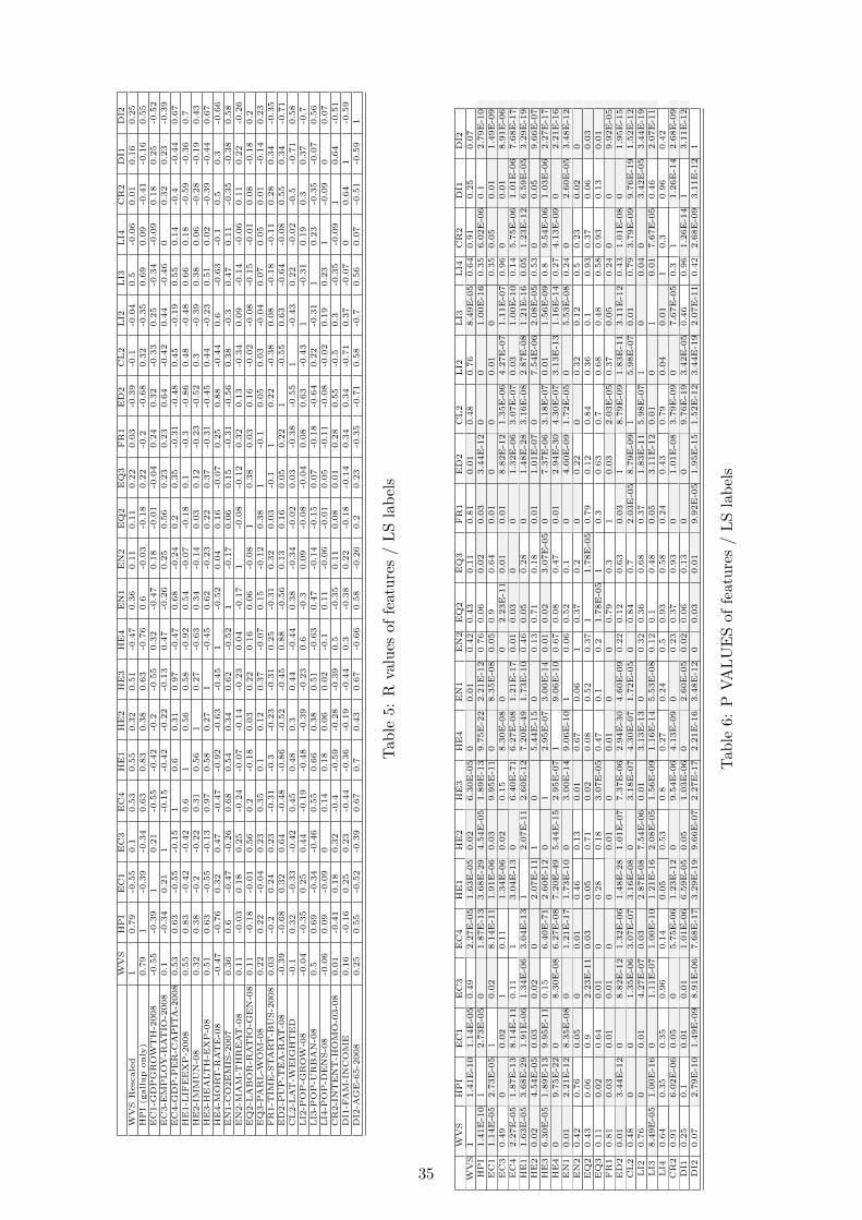
WVS
HPI
EC1
EC3
EC4
HE1
HE2
HE3
HE4
EN1
EN2
EQ2
EQ3
FR1
ED2
CL2
LI2
LI3
LI4
CR2
DI1
DI2
WVS
Resc
aled
10.79
-0.55
0.1
0.53
0.55
0.32
0.51
-0.47
0.36
0.11
0.11
0.22
0.03
-0.39
-0.1
-0.04
0.5
-0.06
0.01
0.16
0.25
HPI(g
allup
only)
0.79
1-0
.39
-0.34
0.63
0.83
0.38
0.63
-0.76
0.6
-0.03
-0.18
0.22
-0.2
-0.68
0.32
-0.35
0.69
0.09
-0.41
-0.16
0.55
EC1-G
DPGROW
TH-2
008
-0.55
-0.39
10.21
-0.55
-0.42
-0.2
-0.55
0.32
-0.47
0.18
-0.01
-0.04
0.24
0.32
-0.33
0.25
-0.34
-0.09
0.18
0.25
-0.52
EC3-E
MPLOY-R
ATIO
-2008
0.1
-0.34
0.21
1-0
.15
-0.42
-0.22
-0.13
0.47
-0.26
0.25
0.56
0.23
0.23
0.64
-0.42
0.44
-0.46
00.32
0.23
-0.39
EC4-G
DP-P
ER-C
APIT
A-2
008
0.53
0.63
-0.55
-0.15
10.6
0.31
0.97
-0.47
0.68
-0.24
0.2
0.35
-0.31
-0.48
0.45
-0.19
0.55
0.14
-0.4
-0.44
0.67
HE1-L
IFEEXP-2
008
0.55
0.83
-0.42
-0.42
0.6
10.56
0.58
-0.92
0.54
-0.07
-0.18
0.1
-0.3
-0.86
0.48
-0.48
0.66
0.18
-0.59
-0.36
0.7
HE2-IM
MUN-0
80.32
0.38
-0.2
-0.22
0.31
0.56
10.27
-0.63
0.34
-0.14
0.03
0.12
-0.23
-0.52
0.3
-0.39
0.38
0.06
-0.28
-0.19
0.43
HE3-H
EALTH-E
XP-0
80.51
0.63
-0.55
-0.13
0.97
0.58
0.27
1-0
.45
0.62
-0.23
0.22
0.37
-0.31
-0.45
0.44
-0.23
0.51
0.02
-0.39
-0.44
0.67
HE4-M
ORT-R
ATE-0
8-0
.47
-0.76
0.32
0.47
-0.47
-0.92
-0.63
-0.45
1-0
.52
0.04
0.16
-0.07
0.25
0.88
-0.44
0.6
-0.63
-0.1
0.5
0.3
-0.66
EN1-C
O2EM
IS-2
007
0.36
0.6
-0.47
-0.26
0.68
0.54
0.34
0.62
-0.52
1-0
.17
0.06
0.15
-0.31
-0.56
0.38
-0.3
0.47
0.11
-0.35
-0.38
0.58
EN2-M
AM
-THREAT-0
80.11
-0.03
0.18
0.25
-0.24
-0.07
-0.14
-0.23
0.04
-0.17
1-0
.08
-0.12
0.32
0.13
-0.34
0.09
-0.14
-0.06
0.11
0.22
-0.26
EQ2-L
ABOR-R
ATIO
-GEN-0
80.11
-0.18
-0.01
0.56
0.2
-0.18
0.03
0.22
0.16
0.06
-0.08
10.38
0.03
0.16
-0.02
-0.08
-0.15
-0.01
0.08
-0.18
0.2
EQ3-P
ARL-W
OM
-08
0.22
0.22
-0.04
0.23
0.35
0.1
0.12
0.37
-0.07
0.15
-0.12
0.38
1-0
.10.05
0.03
-0.04
0.07
0.05
0.01
-0.14
0.23
FR1-T
IME-S
TART-B
US-2
008
0.03
-0.2
0.24
0.23
-0.31
-0.3
-0.23
-0.31
0.25
-0.31
0.32
0.03
-0.1
10.22
-0.38
0.08
-0.18
-0.11
0.28
0.34
-0.35
ED2-P
UP-T
EA-R
AT-0
8-0
.39
-0.68
0.32
0.64
-0.48
-0.86
-0.52
-0.45
0.88
-0.56
0.13
0.16
0.05
0.22
1-0
.55
0.63
-0.64
-0.08
0.55
0.34
-0.71
CL2-L
AT-W
EIG
HTED
-0.1
0.32
-0.33
-0.42
0.45
0.48
0.3
0.44
-0.44
0.38
-0.34
-0.02
0.03
-0.38
-0.55
1-0
.43
0.22
-0.02
-0.5
-0.71
0.58
LI2
-POP-G
ROW
-08
-0.04
-0.35
0.25
0.44
-0.19
-0.48
-0.39
-0.23
0.6
-0.3
0.09
-0.08
-0.04
0.08
0.63
-0.43
1-0
.31
0.19
0.3
0.37
-0.7
LI3
-POP-U
RBAN-0
80.5
0.69
-0.34
-0.46
0.55
0.66
0.38
0.51
-0.63
0.47
-0.14
-0.15
0.07
-0.18
-0.64
0.22
-0.31
10.23
-0.35
-0.07
0.56
LI4
-POP-D
ENS-0
8-0
.06
0.09
-0.09
00.14
0.18
0.06
0.02
-0.1
0.11
-0.06
-0.01
0.05
-0.11
-0.08
-0.02
0.19
0.23
1-0
.09
00.07
CR2-INTENT-H
OM
O-0
3-0
80.01
-0.41
0.18
0.32
-0.4
-0.59
-0.28
-0.39
0.5
-0.35
0.11
0.08
0.01
0.28
0.55
-0.5
0.3
-0.35
-0.09
10.64
-0.51
DI1
-FAM
-INCOM
E0.16
-0.16
0.25
0.23
-0.44
-0.36
-0.19
-0.44
0.3
-0.38
0.22
-0.18
-0.14
0.34
0.34
-0.71
0.37
-0.07
00.64
1-0
.59
DI2
-AGE-6
5-2
008
0.25
0.55
-0.52
-0.39
0.67
0.7
0.43
0.67
-0.66
0.58
-0.26
0.2
0.23
-0.35
-0.71
0.58
-0.7
0.56
0.07
-0.51
-0.59
1
Tab
le5:
Rvalues
offeatures/LSlabels
WVS
HPI
EC1
EC3
EC4
HE1
HE2
HE3
HE4
EN1
EN2
EQ2
EQ3
FR1
ED2
CL2
LI2
LI3
LI4
CR2
DI1
DI2
WVS
11.41E-1
01.14E-0
50.49
2.27E-0
51.63E-0
50.02
6.30E-0
50
0.01
0.42
0.43
0.11
0.81
0.01
0.48
0.76
8.49E-0
50.64
0.91
0.25
0.07
HPI
1.41E-1
01
2.73E-0
50
1.87E-1
33.68E-2
94.54E-0
51.89E-1
39.75E-2
22.21E-1
20.76
0.06
0.02
0.03
3.44E-1
20
01.00E-1
60.35
6.02E-0
60.1
2.79E-1
0EC1
1.14E-0
52.73E-0
51
0.02
8.14E-1
11.91E-0
60.03
9.95E-1
10
8.35E-0
80.05
0.9
0.64
0.01
00
0.01
00.35
0.05
0.01
1.49E-0
9EC3
0.49
00.02
10.11
1.34E-0
60.02
0.15
8.30E-0
80
02.23E-1
10.01
0.01
8.82E-1
21.35E-0
64.27E-0
71.11E-0
70.96
00.01
8.91E-0
6EC4
2.27E-0
51.87E-1
38.14E-1
10.11
13.04E-1
30
6.40E-7
16.27E-0
81.21E-1
70.01
0.03
00
1.32E-0
63.07E-0
70.03
1.00E-1
00.14
5.75E-0
61.01E-0
67.68E-1
7HE1
1.63E-0
53.68E-2
91.91E-0
61.34E-0
63.04E-1
31
2.07E-1
12.60E-1
27.20E-4
91.73E-1
00.46
0.05
0.28
01.48E-2
83.16E-0
82.87E-0
81.21E-1
60.05
1.23E-1
26.59E-0
53.29E-1
9HE2
0.02
4.54E-0
50.03
0.02
02.07E-1
11
05.44E-1
50
0.13
0.71
0.18
0.01
1.01E-0
70
7.54E-0
62.08E-0
50.53
00.05
9.66E-0
7HE3
6.30E-0
51.89E-1
39.95E-1
10.15
6.40E-7
12.60E-1
20
12.95E-0
73.00E-1
40.01
0.02
3.07E-0
50
7.37E-0
63.18E-0
70.01
1.56E-0
90.8
9.54E-0
61.03E-0
62.27E-1
7HE4
09.75E-2
20
8.30E-0
86.27E-0
87.20E-4
95.44E-1
52.95E-0
71
9.06E-1
00.67
0.08
0.47
0.01
2.94E-3
04.30E-0
73.13E-1
31.16E-1
40.27
4.13E-0
90
2.21E-1
6EN1
0.01
2.21E-1
28.35E-0
80
1.21E-1
71.73E-1
00
3.00E-1
49.06E-1
01
0.06
0.52
0.1
04.60E-0
91.72E-0
50
5.53E-0
80.24
02.60E-0
53.48E-1
2EN2
0.42
0.76
0.05
00.01
0.46
0.13
0.01
0.67
0.06
10.37
0.2
00.22
00.32
0.12
0.5
0.23
0.02
0EQ2
0.43
0.06
0.9
2.23E-1
10.03
0.05
0.71
0.02
0.08
0.52
0.37
11.78E-0
50.79
0.12
0.84
0.36
0.1
0.93
0.37
0.06
0.03
EQ3
0.11
0.02
0.64
0.01
00.28
0.18
3.07E-0
50.47
0.1
0.2
1.78E-0
51
0.3
0.63
0.7
0.68
0.48
0.58
0.93
0.13
0.01
FR1
0.81
0.03
0.01
0.01
00
0.01
00.01
00
0.79
0.3
10.03
2.03E-0
50.37
0.05
0.24
00
9.92E-0
5ED2
0.01
3.44E-1
20
8.82E-1
21.32E-0
61.48E-2
81.01E-0
77.37E-0
62.94E-3
04.60E-0
90.22
0.12
0.63
0.03
18.79E-0
91.83E-1
13.11E-1
20.43
1.01E-0
80
1.95E-1
5CL2
0.48
00
1.35E-0
63.07E-0
73.16E-0
80
3.18E-0
74.30E-0
71.72E-0
50
0.84
0.7
2.03E-0
58.79E-0
91
5.98E-0
70.01
0.79
3.79E-0
99.76E-1
91.52E-1
2LI2
0.76
00.01
4.27E-0
70.03
2.87E-0
87.54E-0
60.01
3.13E-1
30
0.32
0.36
0.68
0.37
1.83E-1
15.98E-0
71
00.04
03.42E-0
53.44E-1
9LI3
8.49E-0
51.00E-1
60
1.11E-0
71.00E-1
01.21E-1
62.08E-0
51.56E-0
91.16E-1
45.53E-0
80.12
0.1
0.48
0.05
3.11E-1
20.01
01
0.01
7.67E-0
50.46
2.07E-1
1LI4
0.64
0.35
0.35
0.96
0.14
0.05
0.53
0.8
0.27
0.24
0.5
0.93
0.58
0.24
0.43
0.79
0.04
0.01
10.3
0.96
0.42
CR2
0.91
6.02E-0
60.05
05.75E-0
61.23E-1
20
9.54E-0
64.13E-0
90
0.23
0.37
0.93
01.01E-0
83.79E-0
90
7.67E-0
50.3
11.26E-1
42.68E-0
9DI1
0.25
0.1
0.01
0.01
1.01E-0
66.59E-0
50.05
1.03E-0
60
2.60E-0
50.02
0.06
0.13
00
9.76E-1
93.42E-0
50.46
0.96
1.26E-1
41
3.11E-1
2DI2
0.07
2.79E-1
01.49E-0
98.91E-0
67.68E-1
73.29E-1
99.66E-0
72.27E-1
72.21E-1
63.48E-1
20
0.03
0.01
9.92E-0
51.95E-1
51.52E-1
23.44E-1
92.07E-1
10.42
2.68E-0
93.11E-1
21
Tab
le6:
PVALUESof
features/LSlabels
35
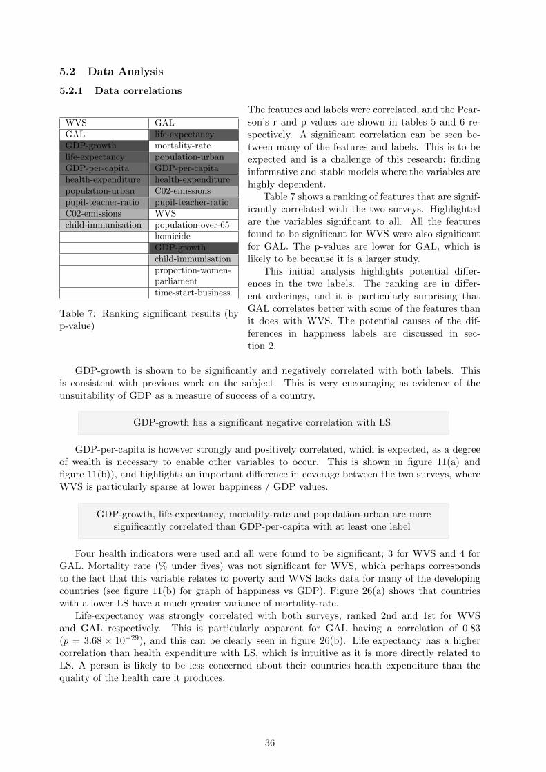
5.2 Data Analysis
5.2.1 Data correlations
WVS GALGAL life-expectancyGDP-growth mortality-ratelife-expectancy population-urbanGDP-per-capita GDP-per-capitahealth-expenditure health-expenditurepopulation-urban C02-emissionspupil-teacher-ratio pupil-teacher-ratioC02-emissions WVSchild-immunisation population-over-65
homicideGDP-growthchild-immunisationproportion-women-parliamenttime-start-business
Table 7: Ranking significant results (byp-value)
The features and labels were correlated, and the Pear-son’s r and p values are shown in tables 5 and 6 re-spectively. A significant correlation can be seen be-tween many of the features and labels. This is to beexpected and is a challenge of this research; findinginformative and stable models where the variables arehighly dependent.
Table 7 shows a ranking of features that are signif-icantly correlated with the two surveys. Highlightedare the variables significant to all. All the featuresfound to be significant for WVS were also significantfor GAL. The p-values are lower for GAL, which islikely to be because it is a larger study.
This initial analysis highlights potential di↵er-ences in the two labels. The ranking are in di↵er-ent orderings, and it is particularly surprising thatGAL correlates better with some of the features thanit does with WVS. The potential causes of the dif-ferences in happiness labels are discussed in sec-tion 2.
GDP-growth is shown to be significantly and negatively correlated with both labels. Thisis consistent with previous work on the subject. This is very encouraging as evidence of theunsuitability of GDP as a measure of success of a country.
GDP-growth has a significant negative correlation with LS
GDP-per-capita is however strongly and positively correlated, which is expected, as a degreeof wealth is necessary to enable other variables to occur. This is shown in figure 11(a) andfigure 11(b)), and highlights an important di↵erence in coverage between the two surveys, whereWVS is particularly sparse at lower happiness / GDP values.
GDP-growth, life-expectancy, mortality-rate and population-urban are moresignificantly correlated than GDP-per-capita with at least one label
Four health indicators were used and all were found to be significant; 3 for WVS and 4 forGAL. Mortality rate (% under fives) was not significant for WVS, which perhaps correspondsto the fact that this variable relates to poverty and WVS lacks data for many of the developingcountries (see figure 11(b) for graph of happiness vs GDP). Figure 26(a) shows that countrieswith a lower LS have a much greater variance of mortality-rate.
Life-expectancy was strongly correlated with both surveys, ranked 2nd and 1st for WVSand GAL respectively. This is particularly apparent for GAL having a correlation of 0.83(p = 3.68 ⇥ 10�29), and this can be clearly seen in figure 26(b). Life expectancy has a highercorrelation than health expenditure with LS, which is intuitive as it is more directly related toLS. A person is likely to be less concerned about their countries health expenditure than thequality of the health care it produces.
36
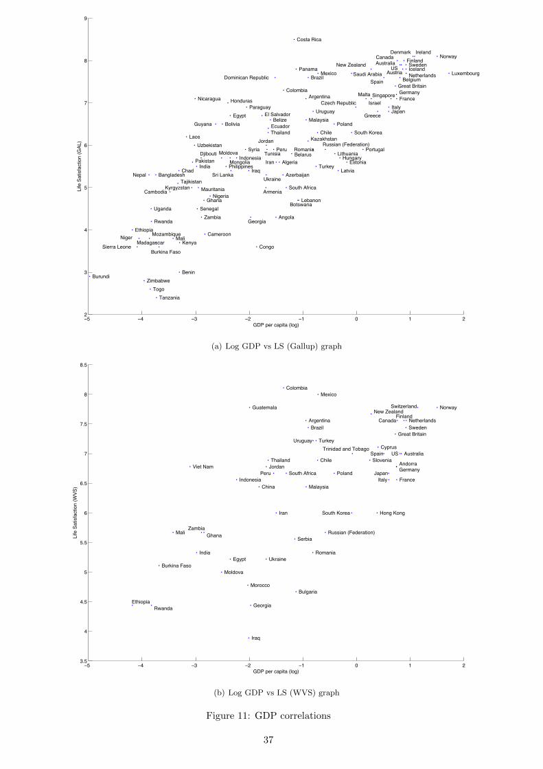
−5 −4 −3 −2 −1 0 1 22
3
4
5
6
7
8
9
GDP per capita (log)
Life
Sat
isfa
ctio
n (G
AL)
Algeria
Angola
Argentina
Armenia
Australia
Austria
AzerbaijanBangladesh
Belarus
Belgium
Belize
Benin
Bolivia
Botswana
Brazil
Burkina Faso
Burundi
Cambodia
Cameroon
Canada
Chad
Chile
Colombia
Congo
Costa Rica
Czech Republic
Denmark
Djibouti
Dominican Republic
Ecuador
Egypt El Salvador
Estonia
Ethiopia
Finland
France
Georgia
Germany
Ghana
GreeceGuyana
Honduras
Hungary
Iceland
IndiaIndonesia
IranIraq
Ireland
IsraelItalyJapan
Jordan Kazakhstan
Kenya
South Korea
Kyrgyzstan
Laos
Latvia
Lebanon
Lithuania
Luxembourg
Madagascar
Malaysia
Mali
Malta
Mauritania
Mexico
Moldova
Mongolia
Mozambique
Nepal
Netherlands
New Zealand
Nicaragua
Niger
Nigeria
Norway
Pakistan
Panama
Paraguay
Peru
Philippines
Poland
PortugalRomaniaRussian (Federation)
Rwanda
Saudi Arabia
Senegal
Sierra Leone
Singapore
South Africa
Spain
Sri Lanka
Sweden
Syria
Tajikistan
Tanzania
Thailand
Togo
Tunisia
Turkey
Uganda
Ukraine
Great Britain
US
Uruguay
Uzbekistan
Zambia
Zimbabwe
(a) Log GDP vs LS (Gallup) graph
−5 −4 −3 −2 −1 0 1 23.5
4
4.5
5
5.5
6
6.5
7
7.5
8
8.5
GDP per capita (log)
Life
Sat
isfa
ctio
n (W
VS)
Andorra
Argentina
Australia
Brazil
Bulgaria
Burkina Faso
Canada
Chile
China
Colombia
Cyprus
Egypt
Ethiopia
Finland
France
Georgia
Germany
Ghana
Guatemala
Hong Kong
India
Indonesia
Iran
Iraq
ItalyJapan
Jordan
South Korea
Malaysia
Mali
Mexico
Moldova
Morocco
NetherlandsNew Zealand
Norway
Peru Poland
Romania
Russian (Federation)
Rwanda
Serbia
Slovenia
South Africa
Spain
Sweden
Switzerland
Thailand
Trinidad and TobagoTurkey
Ukraine
Great Britain
US
Uruguay
Viet Nam
Zambia
(b) Log GDP vs LS (WVS) graph
Figure 11: GDP correlations
37
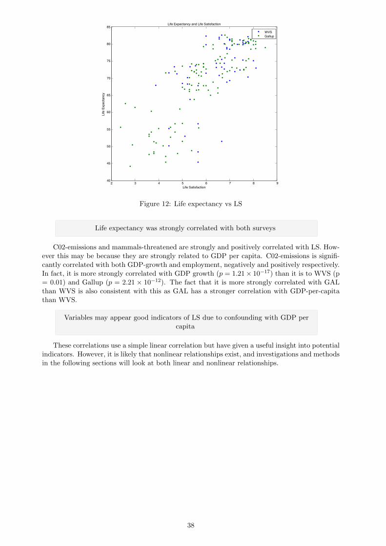
2 3 4 5 6 7 8 940
45
50
55
60
65
70
75
80
85
Life Satisfaction
Life
Exp
ecta
ncy
Life Expectancy and Life Satisfaction
WVSGallup
Student Version of MATLAB
Figure 12: Life expectancy vs LS
Life expectancy was strongly correlated with both surveys
C02-emissions and mammals-threatened are strongly and positively correlated with LS. How-ever this may be because they are strongly related to GDP per capita. C02-emissions is signifi-cantly correlated with both GDP-growth and employment, negatively and positively respectively.In fact, it is more strongly correlated with GDP growth (p = 1.21⇥ 10�17) than it is to WVS (p= 0.01) and Gallup (p = 2.21 ⇥ 10�12). The fact that it is more strongly correlated with GALthan WVS is also consistent with this as GAL has a stronger correlation with GDP-per-capitathan WVS.
Variables may appear good indicators of LS due to confounding with GDP percapita
These correlations use a simple linear correlation but have given a useful insight into potentialindicators. However, it is likely that nonlinear relationships exist, and investigations and methodsin the following sections will look at both linear and nonlinear relationships.
38

05
10−1
001020
WVS
EC1−GDPGROWTH−2008
05
10050100
WVS
EC3−EMPLOY−RATIO−2008
05
100510
x 10
4
WVS
EC4−GDP−PER−CAPITA−2008
05
1040608010
0
WVS
HE1−LIFEEXP−2008
05
10608010
0
WVS
HE2−IMMUN−08
05
100
5000
1000
0
WVS
HE3−HEALTH−EXP−08
05
100
100
200
WVS
HE4−MORT−RATE−08
05
100102030
WVS
EN1−CO2EMIS−2007
05
100
100
200
WVS
EN2−MAM−THREAT−08
05
100
0.51
1.5
WVS
EQ2−LABOR−RATIO−GEN−08
05
100204060
WVS
EQ3−PARL−WOM−08
05
100
100
200
WVS
FR1−TIME−START−BUS−2008
05
10050100
WVS
ED2−PUP−TEA−RAT−08
05
10−5
0000
5000
1000
0
WVS
CL2−LAT−WEIGHTED
05
10−2024
WVS
LI2−POP−GROW−08
05
10050100
WVS
LI3−POP−URBAN−08
05
100
5000
1000
0
WVS
LI4−POP−DENS−08
05
10050100
WVS
CR2−INTENT−HOMO−03−08
05
10204060
WVS
DI1−FAM−INCOME
05
100102030
WVS
DI2−AGE−65−2008
Stud
ent V
ersi
on o
f MA
TLA
B
(a)W
VSag
ainst
feature
set
05
10−1
001020
Gal
lup
EC1−GDPGROWTH−2008
05
10050100
Gal
lup
EC3−EMPLOY−RATIO−2008
05
10051015
x 10
4 Gal
lup
EC4−GDP−PER−CAPITA−2008
05
1040608010
0
Gal
lup
HE1−LIFEEXP−2008
05
10050100
Gal
lup
HE2−IMMUN−08
05
100
5000
1000
0
Gal
lup
HE3−HEALTH−EXP−08
05
100
100
200
300
Gal
lup
HE4−MORT−RATE−08
05
100102030
Gal
lup
EN1−CO2EMIS−2007
05
100
100
200
Gal
lup
EN2−MAM−THREAT−08
05
100
0.51
1.5
Gal
lup
EQ2−LABOR−RATIO−GEN−08
05
100204060
Gal
lup
EQ3−PARL−WOM−08
05
100
100
200
Gal
lup
FR1−TIME−START−BUS−2008
05
10050100
Gal
lup
ED2−PUP−TEA−RAT−08
05
10−5
0000
5000
1000
0
Gal
lup
CL2−LAT−WEIGHTED
05
10−50510
Gal
lup
LI2−POP−GROW−08
05
10050100
Gal
lup
LI3−POP−URBAN−08
05
100
5000
1000
0
Gal
lup
LI4−POP−DENS−08
05
10050100
Gal
lup
CR2−INTENT−HOMO−03−08
05
10204060
Gal
lup
DI1−FAM−INCOME
05
100102030
Gal
lup
DI2−AGE−65−2008
Stud
ent V
ersi
on o
f MA
TLA
B
(b)GALag
ainst
feature
set
Figure
13:Lab
el/feature
correlations
39
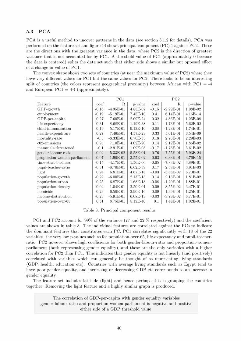
5.3 PCA
PCA is a useful method to uncover patterns in the data (see section 3.1.2 for details). PCA wasperformed on the feature set and figure 14 shows principal component (PC) 1 against PC2. Theseare the directions with the greatest variance in the data, where PC2 is the direction of greatestvariance that is not accounted for by PC1. A threshold value of PC1 (approximately 0 becausethe data is centered) splits the data set such that either side shows a similar but opposed e↵ectof a change in value of PC1.
The convex shape shows two sets of countries (at near the maximum value of PC2) where theyhave very di↵erent values for PC1 but the same values for PC2. There looks to be an interestingsplit of countries (the colors represent geographical proximity) between African with PC1 = -4and European PC1 = +4 (approximately).
PC1 PC2Feature coef R p-value coef R p-valueGDP-growth -0.16 -4.35E-01 4.85E-07 -0.15 -2.29E-01 1.08E-02employment -0.19 -5.19E-01 7.45E-10 0.41 6.14E-01 4.16E-14GDP-per-capita 0.27 7.60E-01 2.09E-24 0.32 4.86E-01 1.25E-08life-expectancy 0.31 8.68E-01 1.19E-38 -0.11 -1.73E-01 5.62E-02child-immunisation 0.19 5.17E-01 9.13E-10 -0.08 -1.23E-01 1.74E-01health-expenditure 0.27 7.46E-01 4.57E-23 0.33 5.01E-01 3.54E-09mortality-rate -0.3 -8.33E-01 6.70E-33 0.18 2.73E-01 2.29E-03c02-emissions 0.25 7.10E-01 4.02E-20 0.14 2.12E-01 1.86E-02mammals-threatened -0.1 -2.91E-01 1.09E-03 -0.17 -1.73E-01 5.61E-02gender-labour-ratio -0.02 -5.33E-02 5.58E-01 0.76 7.55E-01 5.93E-24proportion-women-parliament 0.07 1.90E-01 3.55E-02 0.63 6.33E-01 3.76E-15time-start-business -0.15 -4.17E-01 1.56E-06 -0.05 -7.83E-02 3.89E-01pupil-teacher-ratio -0.31 -8.70E-01 6.62E-39 0.17 2.58E-01 3.91E-03light 0.24 6.81E-01 4.67E-18 -0.03 -3.88E-02 6.70E-01population-growth -0.22 -6.00E-01 2.13E-13 0.14 2.13E-01 1.81E-02population-urban 0.25 6.87E-01 1.68E-18 -0.08 -1.20E-01 1.88E-01population-density 0.04 1.04E-01 2.50E-01 0.09 8.55E-02 3.47E-01homicide -0.23 -6.50E-01 3.90E-16 0.09 1.39E-01 1.25E-01income-distribution -0.23 -5.91E-01 6.08E-13 -0.03 -3.79E-02 6.77E-01population-over-65 0.31 8.75E-01 5.12E-40 0.1 1.48E-01 1.02E-01
Table 8: Principal component results
PC1 and PC2 account for 99% of the variance (77 and 22 % respectively) and the coe�cientvalues are shown in table 8. The individual features are correlated against the PCs to indicatethe dominant features that constitutes each PC. PC1 correlates significantly with 18 of the 22variables, the very low p-values such as for population-over-65, life-expectancy and pupil-teacher-ratio. PC2 however shows high coe�cients for both gender-labour-ratio and proportion-women-parliament (both representing gender equality), and these are the only variables with a highercorrelation for PC2 than PC1. This indicates that gender equality is not linearly (and positively)correlated with variables which can generally be thought of as representing living standards(GDP, health, education etc). Countries with average living standards such as Egypt tend tohave poor gender equality, and increasing or decreasing GDP etc corresponds to an increase ingender equality.
The feature set includes latitude (light) and hence perhaps this is grouping the countriestogether. Removing the light feature and a highly similar graph is produced.
The correlation of GDP-per-capita with gender equality variablesgender-labour-ratio and proportion-women-parliament is negative and positive
either side of a GDP threshold value
40

Colour key
Figure 14: PC1 vs PC2
A note on representing equality The gender equality variables are naturally convexin the sense that inequality can exist where the minority is either males or females. However inreality the data is such that the women are almost always in the minority. Only the gender-labour-ratio of Rwanda and Burundi and proportion-women-parliament of Rwanda ‘favour’ women. Wemanipulate the data such that the variables truly represent equality. Gender-labour-ratio ischanged to a value between 0 and 1, where 1 represents perfect equality:
V arnew = 1� abs(varold � 1) (34)
The proportion-women-parliament was originally a % and this is changed to a value between0 and 50, where 50 represents perfect equality (Since only Rwanda has a value above 50 thisamounts to just changing this value from 56.3 to 43.7):
V arnew = 50� abs(varold � 50) (35)
Data subset R (gend-lab-ratio) P (gend-lab-ratio) R (prop-wom-parl) P (prop-wom-parl)GDP <= 1.9973⇥ 103 -0.4059 0.0085 -0.2779 0.0785GDP > 1.9973⇥ 103 0.3823 0.0004 0.4666 9.9377⇥ 10�6
LS(GAL) <= 6.7 -0.3594 0.0017 -0.0979 0.4065LS(GAL) > 6.7 0.2885 0.0834 0.4727 0.0031
Table 9: GDP-per-capita vs gender equality (gender-labour-ratio and proportion-women-parliament)
To further investigate equality the data was split into two subsets to correlate these withGDP-per-capita and LS separately. The split was done using Egypt’s GDP value (1.9973⇥ 103)
41

and LS value (6.7) respectively as this country sits at the bottom of the convex relationshipshown in figure 14. The results, shown in table 9, clearly show two di↵erent correlations for thesesubsets. 5 are significant at the 0.05 level and a further 2 at the 0.1 level with signs consistentwith the PCA results.
The question is whether this is equality or inequality of a di↵erent form. For instance, isthe female/male labour ratio ‘better’ for low GDP countries because they have no choice butto work in order to survive, in contrast to countries with better conditions where they are morecomfortable and in e↵ect have the choice of inequality. However, this reasoning is less appropriatefor proportion-women-parliament and we cannot suggest a possible reason for a convex correlationof this feature. Investigating this is beyond the scope of this project, but this demonstrates thecomplexities of the semantics and relationships of these variables.
Figure 15 shows the correlations of labels against principal components. The GAL correlationsare expected, having a linear and convex correlation for PC1 and PC2 respectively. LS is stronglyand linearly correlated with many of the variables and as such the correlation with PC1 is linear.The WVS correlations are less clear because the sample is small. A convex relationship with PC2is not clear because WVS does not have many countries with low LS values and so in e↵ect mayonly be showing the upper portion of this relationship. The remaining PC’s account for verylittle of the variance and so are not considered here.
The correlation of LS (GAL) with gender equality variables gender-labour-ratioand proportion-women-parliament is convex (negative and positive either side of
a LS threshold value)
0 2 4 6 8 10−6
−4
−2
0
2
4
6
Gallup
PC1
0 2 4 6 8 10−4
−2
0
2
4
Gallup
PC2
0 2 4 6 8 10−4
−2
0
2
4
6
Gallup
PC3
0 2 4 6 8 10−4
−2
0
2
4
6
8
Gallup
PC4
0 2 4 6 8 10−4
−2
0
2
4
6
Gallup
PC5
0 2 4 6 8 10−5
0
5
Gallup
PC6
0 2 4 6 8 10−4
−2
0
2
4
6
Gallup
PC7
0 2 4 6 8 10−2
−1
0
1
2
3
4
Gallup
PC8
0 2 4 6 8 10−4
−2
0
2
4
Gallup
PC9
Student Version of MATLAB
(a) Principal components vs GAL
0 5 10−10
−5
0
5
10
WVS
PC1
0 5 10−4
−2
0
2
4
WVS
PC2
0 5 10−4
−2
0
2
4
6
WVSPC
3
0 5 10−5
0
5
10
WVS
PC4
0 5 10−4
−2
0
2
4
6
WVS
PC5
0 5 10−5
0
5
WVS
PC6
0 5 10−4
−2
0
2
4
6
WVS
PC7
0 5 10−2
−1
0
1
2
3
4
WVS
PC8
0 5 10−4
−2
0
2
4
WVS
PC9
Student Version of MATLAB
(b) Principal components vs WVS
Figure 15: LS / principal component correlations
42

6 Data Preparation
6.1 Imputation
Many of the features have at least some missing values (see table 13.3). Particularly pupil-teacher ratio has 30 missing values and so it is important to keep the error as low as possible.The following section details work to attempt to impute the missing values with minimal error.This involves firstly testing the imputation to investigate how to minimise the error.
The KNN method is used because previous work has shown that this method performs betterthan mean values (see section 3.1.4). There are two aspects a↵ecting the e↵ectiveness of KNN,the value of K and also the subset of features used to impute each variable. KNN is a↵ected byirrelevant attributes and therefore we will expect that a subset of relevant variables (specific foreach feature) will give the lowest imputation error. A test script was used to test the imputationof each feature for each value of k (see pseudocode of algorithm 1). The experiment was first runon the whole feature set and then repeated using our knowledge of the variables to restrict thefeatures used to impute each feature.
Table 10 shows the results, and table 11 shows a sample of results for imputing GDP-growthand income-distribution using various subsets. The RMSE is used to compare error results of asingle feature, whereas the average error is preferred to compare results between features becausethey use a variable number of tests and the RMSE is relative to this. These results show thatthe error can be reduced by removing irrelevant attributes.
Algorithm 1 KNN test script
comment: impute for each K, feature and instancefor k = 1! numK dofor i = 1! numFeatures do
for i = 1! numCountries dovalue data(i, j)
comment: remove value then imputedata(i, j) NaNDO impute
end forDO calculateError
end forDO SET resultsMatrixRMSE(k, i), avgError in resultsMatrix(k, i)
end forreturn resultsMatrixRMSE
EC1 EC3 EC4 HE1 HE2 HE3 HE4 EN1 EN2 EQ2 EQ3 FR1 ED2 CL2 LI2 LI3 LI4 CR2 DI1 DI2# NaN 2 2 2 1 1 2 1 1 0 2 3 2 30 0 0 0 0 1 7 0Best K 11 7 8 4 20 8 3 19 5 7 17 14 3 4 14 4 4 11 10 6RMSE 0.88 0.70 0.54 0.50 0.90 0.55 0.45 0.82 0.94 0.80 0.94 0.91 0.49 0.74 0.74 0.70 0.96 0.82 0.64 0.40AvgErr 0.67 0.69 0.67 0.71 0.67 0.67 0.72 0.67 0.69 0.69 0.67 0.67 0.72 0.71 0.67 0.71 0.71 0.67 0.67 0.70
Table 10: K value of each feature with lowest RMSE
Feature Imputed Features used RMSE Avg err K
GDP Growth
All 0.87 0.6575 11HE1, HE2 EN1, ED2, LI3, CR2, DI2 0.8524 0.6481 11HE1, HE3 0.9173 0.7342 11HE1, HE2 EN1 CR2, DI2 0.8581 0.6529 11
Income DistributionEC4 HE1 EC4 EC4 CL2 LI2 CR2 DI2 0.6114 0.4857 8CL2 CR2 0.6570 0.5146 10All Signif (12 in total) 0.6584 0.5338 10
Table 11: GDP-growth & income-distribution imputation results
43

6.1.1 Imputation summary
We need the data to be as accurate as possible and KNN has obvious shortcomings to imputevalues of features. After imputing and visualising the results it is clear some errors may bequite large. We therefore opt to improve the data by completing some missing data valuesusing alternative sources, to minimise the number of values that need imputing using KNN. Theremaining features were imputed using the optimum K (feature specific) and a subset of featureswhere this was found to give better inference during testing. This was done in a stepwise fashionstarting with the features with the fewest variables missing such that latter imputations coulduse more features to infer the values. This is an area of concern, as independent data sources canhave di↵erences due to collection methods. However, the number of missing values is very smalland so this will have a limited impact on the data.
Imputation with KNN did not give consistently low errors and therefore it waspreferred to instead find alternative reliable data sources where possible
6.2 Transformations
The relationship of each feature with the labels was assessed visually (Figure 13), to find anyclear nonlinear correlations, as these could be transformed to a linear relationship to use in ourinvestigations. This is beneficial as we use several linear methods and additionally decision treeswhich have linear decision boundaries.
It can be seen that the population density of Hong Kong is an outlier by Hong Kong’sextremely high population, and therefore these were re-plotted excluding Hong Kong to assessthe correlation (shown in figure 16), but these show no obvious relationship however.
4 5 6 7 80
100
200
300
400
500
600
WVS
Popu
latio
n D
ensi
ty (L
I4)
4 5 6 7 8 90
100
200
300
400
500
600
Gallup
Popu
latio
n D
ensi
ty (L
I4)
Student Version of MATLAB
Figure 16: Population-density with Hong Kong removed
The following 4 variables were found to have non linear relationships: GDP-per-capita health-expenditure, population-over-65 and C02-emissions. The transformations are shown in figure 17(a)and figure 17(b). A new feature set was created using the logs of these 4 variables18. The transfor-mations are used in conjunction with the standards features, as we will be using feature selectiontechniques which will enable the learner to choose itself which is more indicative.
18A value of zero has a log value of -Inf, and so this was altered to log(1⇥ 10�7) to solve the problem of dealingwith this
44
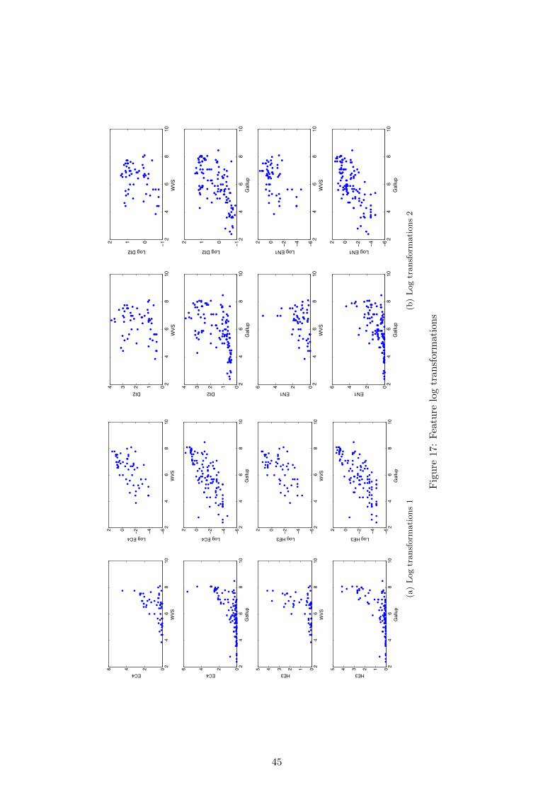
24
68
100246
WVS
EC4
24
68
10−6−4−202
WVS
Log EC4
24
68
100246
Gal
lup
EC4
24
68
10−6−4−202
Gal
lup
Log EC4
24
68
10012345
WVS
HE3
24
68
10−6−4−202
WVS
Log HE3
24
68
10012345
Gal
lup
HE3
24
68
10−6−4−202
Gal
lup
Log HE3
Stud
ent V
ersi
on o
f MA
TLA
B
(a)Log
tran
sformations1
24
68
1001234
WVS
DI2
24
68
10−1012
WVS
Log DI2
24
68
1001234
Gal
lup
DI2
24
68
10−1012
Gal
lup
Log DI2
24
68
100246
WVS
EN1
24
68
10−6−4−202
WVS
Log EN1
24
68
100246
Gal
lup
EN12
46
810
−6−4−202
Gal
lup
Log EN1
Stud
ent V
ersi
on o
f MA
TLA
B
(b)Log
tran
sformations2
Figure
17:Feature
logtran
sformations
45

7 Models to Predict Life Satisfaction
The aim of this section is to answer an initial question: Can LS be predicted using a feature setwithout GDP growth? More formally, the aim is to find a feature set such that the results oftests with and without GDP do not show a significantly worse result. This involves performingtests both with and without GDP and statistically comparing the results.
The main economic variable is GDP-per-capita. However, there are others that are likely tobe representations of this variable also, and these are also removed. This is somewhat subjectivedepending on how directly they are felt to represent the intended concept to provide beneficialinformation in results, rather than a confounder for economic success. As an example, C02-emissions is closely related to industry and thus GDP, and hence finding that this variable helpsto predict LS would likely mean that it confounds with GDP. Confounding is a big issue in thiswork, and for our next feature set (section 9) we will choose variables more carefully to attemptto avoid these problems. The variables removed are; GDP-growth, GDP-per-capita, population-growth, population-density, and C02-emissions. The choice of potentially confounding variables isselected cautiously, such that a larger set is preferred. This only makes our results more rigorousas a smaller feature set is less likely to be predictive than one also containing these features.
Three methods are used to investigate the predictive power of this feature set; decision trees,least squares, and lasso. 10 fold cross validation was used and a t-test (see section 3.3.2) performedon the correlations of the folds. The algorithm for DT’s and least squares involve standard CV,but the lasso method is a little more involved.
−8 −7 −6 −5 −4 −3 −2 −1
0.5
0.6
0.7
0.8
0.9
1
1.1
1.2
1.3
log(!)
Mea
n sq
uare
d er
ror +
/− s
td. e
rr
Nonzero elements
−8 −7 −6 −5 −4 −3 −2 −1
0.5
0.6
0.7
0.8
0.9
1
1.1
1.2
1.3
log(!)
Mea
n sq
uare
d er
ror +
/− s
td. e
rr
Nonzero elements20 18 18 17 10 6 0
min, nz = 11
Student Version of MATLAB
Figure 18: Lasso: optimisinglambda
Using lasso Lasso is a regularisation method andhence the regularisation parameter (�) needs to be op-timised. This should be done for each test, ratherthan the dataset as a whole as it is specific to thedata given to lasso. The pseudocode is shown in algo-rithm 2, and figure 18 shows how the error varies with� value, where the optimum � value minimises the er-ror on the test set. Sub-optimal � values either con-strain lasso too much such that it cannot model the pat-terns in the data, or not enough such that overfitting oc-curs.
Algorithm 2 Lasso 10 fold cross validationfor k = 1! numFolds do
comment: train lasso on training setlambda doF indLambda(trainData)model doLasso(lambda, trainData)
comment: compute correlation on test setcorrelations(i) doCorrelation(testData)
end forreturn correlations
46

7.1 Results and Analysis
Decision Trees Model trees are used (see section 3.3.6) where each leaf has a regressionmodel. This means that all trees generated are smaller as some of the data patterns are accountedfor in the leaf models. The trees constructed including GDP (for both labels) consisted of a singlenode with a regression model. This infers that labels can best be explained by simply using alinear model rather than a decision tree structure.
The trees constructed when excluding economic variables are shown in figure 19. The treeshave 3 and 2 leaf nodes respectively, splitting on health variables; health-expenditure and life-expectancy. This indicates the possibility of a more complex relationship between the featuresand labels. Subspaces of the attribute space are represented using separate models at the leaves.We will not analyse the coe�cients of the linear models as they may contain sets of dependentvariables and hence are likely to be unstable.
Life expectancy
LM 1
< 6.055 >= 6.055
Life expectancy
LM 2 LM 3
< 7.1625 >= 7.1625
(a) Gallup Tree
Health expenditure (log)
LM 1 LM 2
< 1.21 >= 1.21
(b) WVS Tree
Figure 19: Decision trees excluding GDP variables
Features selected are health variables; life-expectancy and log-health-expenditure
Transformations are e↵ective, as log-health-expenditure was selected rather thanthe original health-expenditure variable
7.2 Statistical Methods
Table 12 shows the results of 10 fold cross validation using the three methods with and with-out GDP-per-capita. The models give di↵erent correlation values. A t-test is used to test thestatistical significance of the di↵erence between the results, for each method/label. The t-testcompares the cross validation results to determine if these are likely to have come from the samedistribution. The null hypothesis states that the di↵erence between the results sets has a meanof zero, and hence a statistically significant t-test result indicates that the two result sets aresignificantly di↵erence. Therefore, we aim to show that the results are comparable such that H0
is not rejected (or the feature set excluding GDP-per-capita performs better and H0 is rejected).
47

Learner Survey Corr coe↵ with GDP Corr coe↵ without GDP* test statistic p-valueDec Tree
GAL0.88 0.89 0.55 0.59
Least Sq 0.8378 0.8285 1.9883 0.0780Lasso 0.87 0.88 -0.8560 0.4142Dec Tree
WVS0.64 0.65 0.97 0.35
Least Sq 0.8323 0.7797 5.3932 0.00044Lasso 0.66 0.78 -1.3204 0.2193
Table 12: Results of learners with and without GDP (* Excluding GDP excludes the variables:GDP-growth, GDP-per-capita, population-urban, population-density, C02-emissions)
7.2.1 Conclusions
Table 12 shows there is no significant di↵erence (p < 0.05) between the results when removingeconomic type variables, for 5 of the 6 tests performed. This is very encouraging, as we are usingjust 15 variables to predict LS and are able to do this without a significant di↵erence when GDPis removed. Its interesting to note that the correlation values of these tests are very similar, andin 4 of these tests actually increases with GDP-per-capita removed (although this di↵erence isnot significant). Additionally, it is likely that other variables that may be e↵ective in a model topredict happiness and these will be included later.
Result: Feature sets excluding economic variables are able to predict LS as wellas GDP-per-capita
48
8 Feature Selection (1)
We have shown that LS can be inferred when using a feature set excluding GDP. We now investi-gate which features in particular are key in these models. Two approaches are used for this; lassoand least squares regression. Permutation tests using bootstrapping are used to determine thesignificance of the results. This work amounts to a pattern discovery problem, where the patternsare feature subsets or individual features. Therefore the size of the pattern space is all possiblepatterns considered. There are 17 features (15 features plus 2 log versions) and hence the patternspaces are 217 for feature subsets and 17 for individual features. Significance of results is assessedusing permutation testing to provide a threshold test statistic t� (see section 3.3.3) such that:
p(T � t�) 0.05 (36)
where T is the test statistic on permuted data.
8.1 Lasso Feature Selection
Lasso19 finds a subset that gives a good correlation, but where there are several dependentvariables lasso results are inherently unstable as small changes in the data set supplied to thelearner can a↵ect the variables chosen in the model. This is because when several variables havevery similar relationships with the labels the learner chooses the best to include in the model,and repeating this on di↵erent data can cause the learner to select a di↵erent feature each time.Therefore performing lasso on di↵erent bootstrapped data subsets results in a set of models.Although the coe�cient values are unlikely to be the same, often the same subset of features areused (the coe�cients of the same feature set have not been reduced to zero). Therefore testsmust be performed many times to improve the stability of the results, by finding frequent exactsubsets.
Lasso is used here to find both dominant subsets of features and also individual features. Todiscover important feature sets we aim to identify key exact subsets where they are producedsignificantly often by lasso, which will indicate relationships between variables to predict LS.
The number of features is constrained to 6 in these tests20, as we are interested in smallpredictive subsets of features. Although the correlations will be slightly reduced it is still verycomparable to when not constraining (in fact some of the models produced when not constrainingthe model size are < 6)21. A t-test of constrained (< 6) against unconstrained gave p-values of0.6914 and 0.9077 for GAL and WVS respectively, showing the results are comparable.
The lasso tests aim to answer three questions. These are all based on a test method involvingbootstrapping 100 times, and returning an individual feature or feature subset and a test statisticusing the results of the bootstraps. Three questions are posed:
1. Are there feature subsets that are generated frequently by lasso? We will call this frequencythe vote.
H0: The most frequent subset generated is no more frequent than the most frequentsubset found on random data
Pattern: Feature subset
Output: Most voted (exact) subset.
Test statistic: Vote of most voted subset19glmnet Matlab library was used20default setting is numFeatures+ 121The models are also constrained to > 0 features, which is necessary because in permutation tests where there
is no correlation between (random)label and features lasso often prefers a model with no features (just a bias), butwe are interested in the best model containing at least 1 feature
49
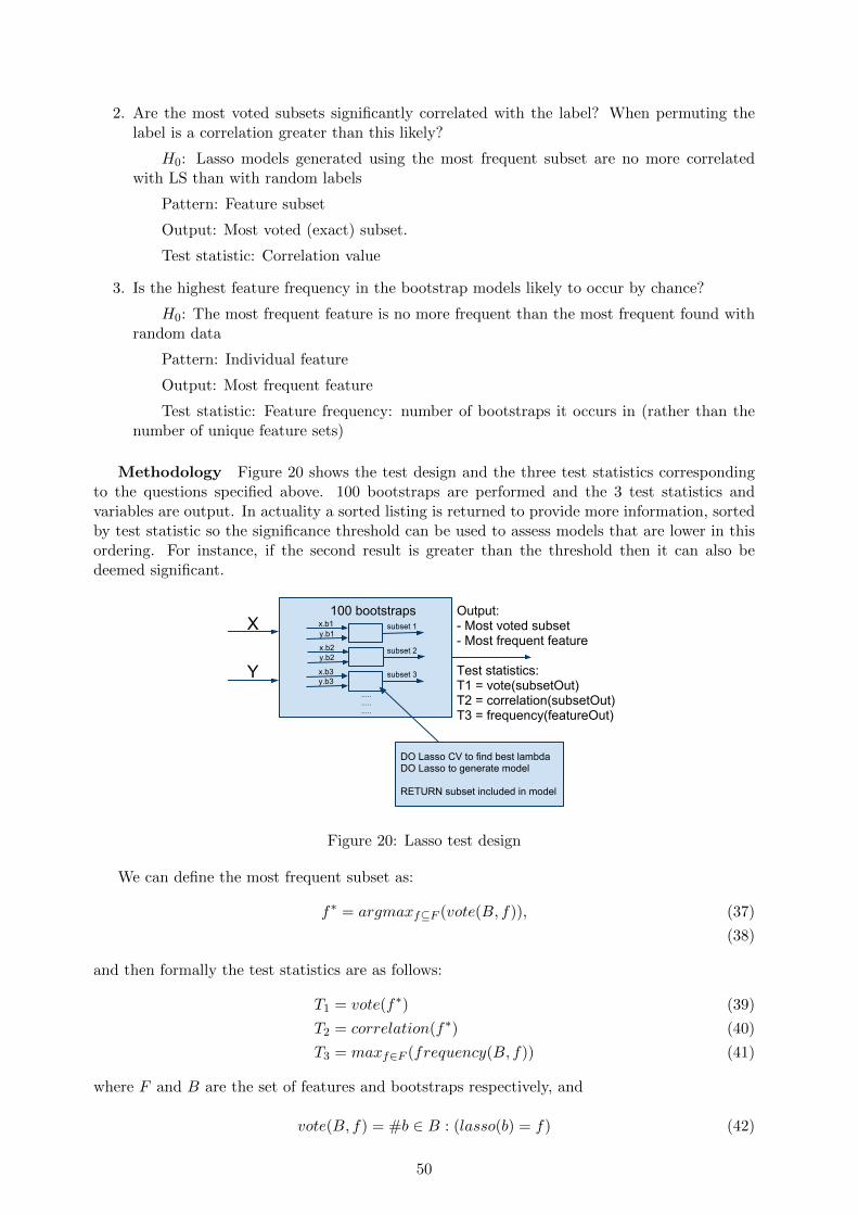
2. Are the most voted subsets significantly correlated with the label? When permuting thelabel is a correlation greater than this likely?
H0: Lasso models generated using the most frequent subset are no more correlatedwith LS than with random labels
Pattern: Feature subset
Output: Most voted (exact) subset.
Test statistic: Correlation value
3. Is the highest feature frequency in the bootstrap models likely to occur by chance?
H0: The most frequent feature is no more frequent than the most frequent found withrandom data
Pattern: Individual feature
Output: Most frequent feature
Test statistic: Feature frequency: number of bootstraps it occurs in (rather than thenumber of unique feature sets)
Methodology Figure 20 shows the test design and the three test statistics correspondingto the questions specified above. 100 bootstraps are performed and the 3 test statistics andvariables are output. In actuality a sorted listing is returned to provide more information, sortedby test statistic so the significance threshold can be used to assess models that are lower in thisordering. For instance, if the second result is greater than the threshold then it can also bedeemed significant.
100 bootstrapsx.b1
x.b2
x.b3
y.b1
y.b3
y.b2
subset 1
subset 2
subset 3
.....
.....
.....
X
Y
Output:- Most voted subset- Most frequent feature
Test statistics:T1 = vote(subsetOut)T2 = correlation(subsetOut)T3 = frequency(featureOut)
DO Lasso CV to find best lambdaDO Lasso to generate model
RETURN subset included in model
Figure 20: Lasso test design
We can define the most frequent subset as:
f⇤ = argmaxf✓F (vote(B, f)), (37)
(38)
and then formally the test statistics are as follows:
T1 = vote(f⇤) (39)
T2 = correlation(f⇤) (40)
T3 = maxf2F (frequency(B, f)) (41)
where F and B are the set of features and bootstraps respectively, and
vote(B, f) = #b 2 B : (lasso(b) = f) (42)
50

The significance thresholds t� are found with permutation testing. The test (figure 20) isrepeated many times with permuted labels, giving a set of T values. The value of T where it isgreater than 95% of these is the significance threshold (with p = 0.05):
0.05 � #p 2 P : T (Bp) � t�#p 2 P
, (43)
where P is the set of permutations, such that under H0:
p(T (B) � t�) 0.05 (44)
Results: Feature Subsets Tables 13 and 14 show the most voted subsets in 100 boot-straps. Permutation testing found significance thresholds for T1 of 7 for both labels. 3 significantmodels were found for GAL but none for WVS. The GAL significant subsets always containedlog-health-expenditure, income-distribution, health-expenditure and 2 of either mortality-rate,gender-labour-ratio, and proportion-women-parliament.
All GAL significant feature subsets contained: log-health-expenditure,income-distribution and health-expenditure
mortality-rate, gender-labour-ratio, and proportion-women-parliament were eachfound in 2 of the 3 significant GAL subsets
Lasso with WVS generated few repeated subsets with 88 di↵erent subsets for 100 bootstraps.Compared with GAL these results are much more unstable and this may be because WVS hasa smaller less varied sample of countries. The most voted model is however quite prominentwith a vote of 5 in comparison to votes of 1 or 2 for all other subsets found. This model con-tains: life-expectancy, child-immunization, log-health-expenditure, mammal-threatened, income-distribution, and health-expenditure.
The most voted WVS model also contains the three features found in allsignificant GAL models: log-health-expenditure, income-distribution and
health-expenditure
The significance thresholds for correlations of the most voted subsets (T2) were 0.3284 and0.4369 for GAL and WVS respectively. The correlations of all subsets were higher and thussignificant, with mean correlations of 0.8620 (GAL) and 0.7660 (WVS).
All subsets found are significantly predictive of LS (compared to random case)
Results: Individual Features Tables 13 and 14 show the feature frequencies in the modelsgenerated by lasso in the 100 bootstraps. A conservative approach to discarding features is takendue to the high dependency between variables. For instance, given two variables v1 and v2 thatare part of a feature set on which lasso is performed, and where v1 ⇠ v2. Due to the randomselection of instances in the bootstraps and the small di↵erences between v1 and v2 we can expectthat their vote will be shared approximately equally between them. Hence the votes of each arereduced and this could potentially cause two significant variables to fall outside of the significantrange.
51
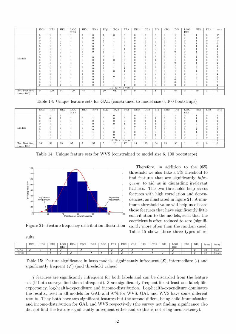
EC3 HE1 HE2 LOGHE3
HE4 EN2 EQ2 EQ3 FR1 ED2 CL2 LI2 CR2 DI1 LOGDI2
HE3 DI2 vote
Models
0 1 0 1 1 0 1 0 0 0 0 0 0 1 0 1 0 9*0 1 0 1 1 0 0 1 0 0 0 0 0 1 0 1 0 8*0 1 0 1 0 0 1 1 0 0 0 0 0 1 0 1 0 7*0 1 1 1 0 0 0 1 0 0 0 0 0 1 0 1 0 60 1 0 1 0 0 0 1 0 0 0 0 0 1 0 1 0 40 1 0 1 0 0 0 1 1 0 0 0 0 1 0 1 0 40 1 0 1 1 0 1 1 0 0 0 0 0 0 0 1 0 40 1 0 1 1 1 0 1 0 0 0 0 0 1 0 0 0 30 1 0 1 0 0 0 1 0 0 1 0 0 1 0 1 0 20 1 0 1 0 0 1 0 0 0 0 1 0 1 0 1 0 20 1 0 1 0 0 1 1 0 0 0 0 0 0 0 1 0 20 1 0 1 0 0 1 1 0 0 0 0 0 1 0 0 0 20 1 0 1 0 0 1 1 1 0 0 0 0 1 0 0 0 20 1 0 1 1 0 0 0 1 0 0 0 0 1 0 1 0 20 1 0 1 1 0 0 1 0 1 0 0 0 1 0 0 0 20 1 0 1 1 0 1 0 0 0 0 0 0 1 0 0 0 20 1 0 1 1 0 1 1 0 0 0 0 0 0 0 0 0 20 1 0 1 1 0 1 1 0 1 0 0 0 0 0 0 0 20 1 1 1 0 0 0 1 1 0 0 0 0 0 0 0 0 2
. . .& 32 with vote 1 1Tot Feat freq(max 100)
0 100 14 100 45 12 50 68 18 9 2 8 0 64 0 70 3 0
Table 13: Unique feature sets for GAL (constrained to model size 6, 100 bootstraps)
EC3 HE1 HE2 LOGHE3
HE4 EN2 EQ2 EQ3 FR1 ED2 CL2 LI2 CR2 DI1 LOGDI2
HE3 DI2 vote
Models
0 1 1 1 0 1 0 0 0 0 0 0 0 1 0 1 0 50 0 1 1 0 1 0 0 0 0 0 1 0 1 0 1 0 20 1 0 1 0 0 0 0 0 0 1 1 0 1 0 1 0 20 1 0 1 0 0 0 0 1 0 1 1 0 1 0 0 0 20 1 0 1 0 0 0 1 0 0 1 1 0 1 0 0 0 20 1 0 1 0 0 0 1 0 1 0 0 0 1 0 1 0 21 1 0 1 0 1 0 0 0 0 0 0 0 1 0 1 0 21 1 0 1 0 1 0 0 0 0 0 1 0 1 0 0 0 21 1 0 1 0 1 0 0 0 1 0 0 0 1 0 0 0 2
. . .& 79 with vote 1 1Tot Feat freq(max 100)
38 59 29 97 7 57 5 26 17 14 25 34 15 90 1 42 0 0
Table 14: Unique feature sets for WVS (constrained to model size 6, 100 bootstraps)
0 20 40 60 80 100 1200
20
40
60
80
100
120
140
160
Most frequent feature frequency
Boot
stra
p fre
quen
cy
Significantly infrequent (5%)
Significantly frequent (5%)
Figure 21: Feature frequency distribution illustration
Therefore, in addition to the 95%threshold we also take a 5% threshold tofind features that are significantly infre-quent, to aid us in discarding irrelevantfeatures. The two thresholds help assessfeatures with high correlation and depen-dencies, as illustrated in figure 21. A min-imum threshold value will help us discardthose features that have significantly littlecontribution to the models, such that thecoe�cient is often reduced to zero (signifi-cantly more often than the random case).Table 15 shows these three types of re-
sults.
EC3 HE1 HE2 LOGHE3
HE4 EN2 EQ2 EQ3 FR1 ED2 CL2 LI2 CR2 DI1 LOGDI2
HE3 DI2 t0.05 t0.95
GAL 7 X 7 X - 7 - - 7 7 7 7 7 - 7 - 7 32 89.8WVS - - 7 X 7 - 7 7 7 7 7 - 7 X 7 - 7 33 89.25
Table 15: Feature significance in lasso models: significantly infrequent (7), intermediate (-) andsignificantly frequent (X) (and threshold values)
7 features are significantly infrequent for both labels and can be discarded from the featureset (if both surveys find them infrequent). 3 are significantly frequent for at least one label; life-expectancy, log-health-expenditure and income-distribution. Log-health-expenditure dominatesthe results, used in all models for GAL and 97% for WVS. GAL and WVS have some di↵erentresults. They both have two significant features but the second di↵ers, being child-immunisationand income-distribution for GAL and WVS respectively (the survey not finding significance alsodid not find the feature significantly infrequent either and so this is not a big inconsistency).
52

Significantly frequent features: life-expectancy, log-health-expenditure,income-distribution
Notable features: employment, mortality-rate, mammals-threatened,gender-labour-ratio, proportion-women-parliament, population-growth,
health-expenditure
Significantly infrequent features: child-immunisation, time-start-business,pupil-teacher-ratio, light, homicide, log-population-over-65, population-over-65
The results indicate a set of core features present consistently in the models, andothers that are interchangeable and hence often present
Sample Models We can gain some insight from these generated models, and the type ofcontribution of each feature, indicated by the sign and size of the coe�cient values. Examplesequations 45 and 46 show two models for the top ranked subsets of GAL and WVS respectively.
LSGAL = 0.7815 + 0.7232 life� expectancy + 0.1569 log � health� expenditure � 0.1143 mortality � rate
�0.1588 gender � labour � ratio + 0.2694 income� distribution + 0.3291 health� expenditure(45)
LSWV S = 2.5259 + 0.1902 life� expectancy + 0.0906 child� immunisation + 0.3218 log � health� expenditure
+ 0.1525 mammals� threatened + 0.4660 income� distribution + 0.1968 health� expenditure
(46)
All health variables included in the models have an intuitive sign. For instance, mortality-ratehas a negative coe�cient because mortality rate is negatively correlated with LS. However, theremaining variables show unexpected coe�cients with respect to the concept each is representing.These variables are income-distribution, gender-labour-ratio and mammals-threatened.
The income-distribution coe�cient is positive indicating a higher value is associated withhigher LS. However, this is unexpected because high income-distribution means greater inequalityof income. At first thought, this may be due to confounding with GDP but the initial correlationsare not consistent with this. LS is correlated strongly and positively with GDP but GDP iscorrelated negatively with income-distribution.
In fact, work by Verme [50] details how previous results of the relationship between LS andrelative income have been inconsistent, finding both negative and positive correlations. It is notedhow the type of data might a↵ect the results such as using small datasets, particular noting cross-country studies. Hence, perhaps income-distribution may be more appropriate as an indicatorwhen people are entities and the relationship between LS and income equality can be directlyanalysed. One suggested explanation of a positive coe�cient is the a↵ect of relative income onsocial mobility.[50] A greater degree of income inequality relates to more potential to ‘climb theladder’, to have ambition and progress in life, which improves LS.
The variable mammals-threatened contributes positively to the WVS model. However, withhindsight it is unclear what this variable is representing and therefore will be discarded. A highergender-labour-ratio value corresponds with a more equal gender employment, but the GAL modelincludes gender-labour-ratio with a small but negative coe�cient. However, we showed with PCAanalysis in section 5.3 that gender equality has a convex correlation with life satisfaction andtherefore this may be the reason why the coe�cient is not intuitive.
53

The unexpected coe�cients highlight the restrictions of a linear model. Although the modelhas a high correlation it is constructed in a way which is contradictory to previous work and ourown intuition. Lasso is an e↵ective method for generating models, but these models are still onlysimple linear models and this is limiting. Further analysis with decision trees will be useful toinvestigate non linear patterns in the data.
Some features (e.g. mammals-threatened) have unexpected coe�cients and onepossible cause is confounding with economic success (GDP-per-capita)
8.2 Least Squares Leave One Feature Out
We use least squares to provide an independent alternative approach to finding key features, byanalysing the e↵ect on correlation values when removing a feature in turn from the feature set.
100 bootstraps
bootstrap 1
bootstrap 2
bootstrap 3
x.b1
x.b2
x.b3
y.b1
y.b2
y.b3
[d(f1), d(f2) ... d(fn)]
.....
.....
.....
X
Y
Variable output:featureOut = argmax(av(f))
Test statistic:T = av(featureOut)
DO corr <- regress(x,y)FOR EACH feature DO: x2 <- x less feature DO corr2 <- regress(x2, y) diff(i) <- corr2 - corr
RETURN [diff(f1), diff(f2) ...]
[d(f1), d(f2) ... d(fn)]
[d(f1), d(f2) ... d(fn)]
[av(f1), av(f2) ... av(fn)]
RETURN average diff for each feature across all bootstraps
aver
age
resu
lts
Figure 22: Least squares test design
Methodology Figure 22 shows the test design where the di↵erence in correlation is cal-culated for each bootstrap with and without each feature. These values are averaged for eachfeature, and the features are output, ranked by average reduction of correlation. The first featuretherefore causes the biggest reduction in correlation when removed from the feature set. The teststatistic is the average correlation di↵erence:
T = maxf2F (av(f)), (47)
where function av computes the average di↵erence for a feature over all bootstraps. The signif-icance threshold t� (with p = 0.05) is found by performing the test many times with permutedlabels and finding T such that 95% of the results on random data give a smaller test statistic.
Results Tables 23(a) and 24(a) show the results of these tests, with the features ranked bytest statistic. The permutation tests found significance thresholds of 0.0592 and 0.0571 for GALand WVS respectively. Therefore, the results are not significant compared to the random case.However this is likely to be because the features are highly related and thus removing one featureand another feature can in e↵ect represent much of the variance of the removed variable.
Tables 23(b) and 24(b) show t-test results of comparisons between the set of bootstrap outputsof each feature. This shows most are significant indicating the feature rankings found havesignificant di↵erences between the results of each feature (such that the ranking is stable and not
54

Feature Corr di↵LOG HE3 0.028DI1 0.027HE2 0.026HE1 0.025EQ3 0.021LOG DI2 0.020HE4 0.014CL2 0.011CR2 0.011EQ2 0.011HE3 0.011LI2 0.010EC3 0.010FR1 0.010ED2 0.010EN2 0.010DI2 0.008
(a) Correlation di↵er-ence ranking
LOGHE3
DI1 HE2 HE1 EQ3 LOGDI2
HE4 CL2 CR2 EQ2 HE3 LI2 EC3 FR1 ED2 EN2 DI2
LOGHE3
- 1 1 1 1 1 1 1 1 1 1 1 1 1 1 1 1
DI1 1 - 0 1 1 1 1 1 1 1 1 1 1 1 1 1 1HE2 1 0 - 1 1 1 1 1 1 1 1 1 1 1 1 1 1HE1 1 1 1 - 1 1 1 1 1 1 1 1 1 1 1 1 1EQ3 1 1 1 1 - 1 1 1 1 1 1 1 1 1 1 1 1LOGDI2
1 1 1 1 1 - 1 1 1 1 1 1 1 1 1 1 1
HE4 1 1 1 1 1 1 - 1 1 1 1 1 1 1 1 1 1CL2 1 1 1 1 1 1 1 - 0 0 1 1 1 1 1 1 1CR2 1 1 1 1 1 1 1 0 - 0 1 1 1 1 1 1 1EQ2 1 1 1 1 1 1 1 0 0 - 1 1 1 1 1 1 1HE3 1 1 1 1 1 1 1 1 1 1 - 1 1 1 1 1 1LI2 1 1 1 1 1 1 1 1 1 1 1 - 0 0 1 1 1EC3 1 1 1 1 1 1 1 1 1 1 1 0 - 0 1 1 1FR1 1 1 1 1 1 1 1 1 1 1 1 0 0 - 1 1 1ED2 1 1 1 1 1 1 1 1 1 1 1 1 1 1 - 0 1EN2 1 1 1 1 1 1 1 1 1 1 1 1 1 1 0 - 1DI2 1 1 1 1 1 1 1 1 1 1 1 1 1 1 1 1 -
(b) Significance of di↵erence between correlation di↵erences of each feature (GAL)
Figure 23: GAL least squares results
Feature Corr Di↵sLOG HE3 0.052EN2 0.032DI1 0.029ED2 0.026HE2 0.026CR2 0.026HE4 0.024HE1 0.023LOG DI2 0.022EC3 0.022FR1 0.021EQ3 0.020HE3 0.020CL2 0.018LI2 0.018EQ2 0.017DI2 0.012
(a) Correlation di↵er-ence ranking
LOGHE3
EN2 DI1 ED2 HE2 CR2 HE4 HE1 LOGDI2
EC3 FR1 EQ3 HE3 CL2 LI2 EQ2 DI2
LOGHE3
- 1 1 1 1 1 1 1 1 1 1 1 1 1 1 1 1
EN2 1 - 1 1 1 1 1 1 1 1 1 1 1 1 1 1 1DI1 1 1 - 1 1 1 1 1 1 1 1 1 1 1 1 1 1ED2 1 1 1 - 0 0 1 1 1 1 1 1 1 1 1 1 1HE2 1 1 1 0 - 0 1 1 1 1 1 1 1 1 1 1 1CR2 1 1 1 0 0 - 1 1 1 1 1 1 1 1 1 1 1HE4 1 1 1 1 1 1 - 0 1 1 1 1 1 1 1 1 1HE1 1 1 1 1 1 1 0 - 0 1 1 1 1 1 1 1 1LOGDI2
1 1 1 1 1 1 1 0 - 0 1 1 1 1 1 1 1
EC3 1 1 1 1 1 1 1 1 0 - 0 1 1 1 1 1 1FR1 1 1 1 1 1 1 1 1 1 0 - 0 1 1 1 1 1EQ3 1 1 1 1 1 1 1 1 1 1 0 - 0 1 1 1 1HE3 1 1 1 1 1 1 1 1 1 1 1 0 - 1 1 1 1CL2 1 1 1 1 1 1 1 1 1 1 1 1 1 - 0 1 1LI2 1 1 1 1 1 1 1 1 1 1 1 1 1 0 - 1 1EQ2 1 1 1 1 1 1 1 1 1 1 1 1 1 1 1 - 1DI2 1 1 1 1 1 1 1 1 1 1 1 1 1 1 1 1 -
(b) Significance of di↵erence between correlation di↵erences of each feature (WVS)
Figure 24: WVS least squares results
trivial). For example, log-health-expenditure is the first ranked feature and on removal caused areduction of correlation significantly di↵erent from the other variables.
log-health-expenditure is the top ranked feature for both labels, causing asignificantly larger reduction in correlation if excluded
8.3 Lasso / Least Squares Results Comparison
Feature selection using lasso and least squares has found some similar results. Firstly the featuresfound to be significant with lasso are near the top of the least squares rankings. In particularlog-health-expenditure is ranked first for both labels. Income-distribution was ranked second andthird in least squares and was present in 0.64 and 0.9 of the lasso models, for GAL and WVSrespectively. Life-expectancy is ranked fourth and eighth which is consistent with the lasso resultswhere this variable was found in 1.0 and 0.59 of lasso models for GAL and WVS respectively.
55

Both tests find log-health-expenditure, income-distribution and life-expectancy tobe important features
With respect to the highly infrequent features in the lasso’s model, least squares also foundpopulation-over-65 to be very infrequent.
population-over-65 has been found significantly less important than the otherfeatures in predicting LS
8.4 Results Summary
LS predictors Health variables have shown particular prominence in the results, partic-ularly health-expenditure and life-expectancy. These variables were key in tests of all threemethods, and were the only variables used as internal nodes in the decision trees. Health expen-diture is quite a general term and therefore this is now removed from the feature set as moredirect notions of health care quality are preferred.
The variables proportion-women-parliament and gender-labour-ratio, which were intended torepresent gender equality, were present in the significant feature subsets of the GAL lasso. It isinteresting to note how the top two feature subsets contained one of these, thus perhaps theyrepresent the same concept and lasso chose between them. This is also consistent with the factthat these features were neither significantly frequent of significantly infrequent (table 15).
The feature income-distribution was consistently a key component of the models with a pos-itive coe�cient, which infers that income inequality indicates LS. However, the reason for this isunclear, and previous work has shown conflicting results on this topic.
Methods Lasso and least squared gave some similar results but also many di↵erences. Lassois ‘fairer’ with respect to variable selection (see section 3.3.5) and therefore is more powerful andinformative than the greedy approach of least squares. Least squares provides a useful comparisonfor the lasso results but more importance will be given to the lasso results as it is able to copewith dependent variables better and so is more reliable. The models trees are very short due tothe regression models at the leaves and therefore it may be more informative to use regressiontrees. Lasso and least squares are restrictive because they produce linear models, and hence wewill investigate further machine learning approaches to find non linear patterns.
Features discarded The features discarded from this stage and reasons:
• health-expenditure, log-health-expenditure: Too general (replaced with more direct healthindicators)
• GDP-growth, GDP-per-capita: Economic variables
• population-urban, population-density, C02-emissions, mammals-threatened: Likely con-founding with GDP
• population-over-65, log-population-over-65, homicide, light,pupil-teacher-ratio, time-start-business: Significantly infrequent in lasso tests
56

9 Feature Selection (2)
9.1 Improved Feature Set
Table 16 shows the updated features set, including prominent features from the work of section 8and also new features (further details in appendix A, table 13.3).
Topic Feature Code
Existing
HEALTHLife expectancy % life-expectancy HE1Immunization % child-immunisation HE2Mortality rate mortality-rate HE4
EQUALITYRatio of gender labor participation rate gender-labour-ratio EQ2Proportion of seats held by women in national parliaments proportion-women-parliament EQ3Distribution of family income - Gini index income-distribution DI1
LIFEEmployment to population ratio employment EC3Population growth population-growth LI2
New
HEALTH Hospital beds hospital-beds BH1
FREEDOM% of the largest religion or religious brand percent-largest-religion BF1Number of unique incidents of religious conflict religious-confilict BF2Freedom of the world freedom BF3
CLIMATEMean temperature temp-mean BC1Min temperature temp-min BC2Max temperature temp-max BC3
EDUCATIONSchool enrolment (primary gross) primary-education-enrolment BE1School enrolment (secondary gross) secondary-education-enrolment BE2Literacy rate adult-literacy-rate BE3
CONFLICT Military expenditure (relative to health exp) military-expenditure BP2EQUALITY Secondary education (% female) education-gender BQ1
Table 16: Feature set 2
The additional features were chosen based on previous research and also the results found sofar. Climate has been found to a↵ect happiness such as work described in section 2. The resultsfor pupil-teacher-ratio were surprising and hence this is investigated further by using di↵erenteducation variables. Freedom is an important subject but only one variable, time-start-business,has been used to represent this which was perhaps not highly representative of freedom. Religiousindicators are also included to represent religious freedom / equality, as well as a generic freedomindex.
Freedom Index [28] We prefer to use primary sources but freedom is very di�cult toquantify, and therefore in this case we use a freedom index22. This is derived from surveydata and covers the following freedom areas; politics, expression and belief, religion, academic,associational and organizational rights, law and personal. The index values range from 1 to 7representing highly free and not free respectively, and figure 25 shows the freedom of the world.
Military Expenditure We investigate any relationship of military size with LS. The orig-inal variable is military expenditure as a percentage of GDP. The models generated included thisfeature with negative coe�cients. However, this may be due to confounding with GDP. Thisvariable is investigating the relationship:
↵MilExp
GDP= LS. (48)
Assuming that MilExp stays constant then ↵ would be strongly negative because GDP-per-capita has a strong positive correlation with LS. Therefore, where the covariance with LS ofmilitary expenditure is small compared to that of GDP, using this variable relative to GDP isin fact just incorporating a measure of GDP in the models, rather than military expenditure asintended. Therefore this variable is adapted to be relative to health expenditure instead. It cannow be thought of as a measure of the investment in military relative to the investment in healthcare. As is shown in the subsequent tests this variable gives di↵erent results to the original.
22produced by Freedom House [28]
57

Freedom Status Country Breakdown Population Breakdown (in billions)
FREE 90 (47%) 3.03 (46%)
PARTLY FREE 60 (31%) 1.19 (18%)
NOT FREE 43 (22%) 2.39 (36%)
TOTAL 193 (100%) 6.61 (100%)
(a) Map Key & Statistics
Nor th Pacific Ocean
Nor th Pacific Ocean
South Pacific Ocean
Nor th Atlantic Ocean
South Atlantic Ocean
Gulf of Mexico
Gulf of AlaskaBering Sea
Beaufort Sea
Arctic Ocean
Hudson Bay Labrador Sea
Caribbean Sea
Indian Ocean
South China Sea
EastChina Sea
Sea of Okhotsk
Tasman Sea
Bay of Bengal
Norwegian Sea
Greenland Sea
BAHAMAS
UNITED STATES OF AMERICA
CANADA
U.S.A.
GREENLAND(DENMARK)
ST. KITTS & NEVISANTIGUA & BARBUDA
DOMINICAST. LUCIAST. VINCENT & GRENADINES
BARBADOS
TRINIDAD & TOBAGO
GUYANASURINAME
FRENCH GUIANA (FRANCE)
GRENADA
DOM. REP.HAITI
CUBA
JAMAICABELIZE
HONDURAS
NICARAGUA
COSTA RICA
PANAMA
EL SALVADORGUATEMALA
MEXICO
ECUADOR
PERU
VENEZUELA
COLOMBIA
BRAZIL
BOLIVIA
CAPE VERDE
GUINEA BISSAU
THE GAMBIA
SENEGAL
MAURITANIA
GUINEA
SIERRA LEONE
LIBERIA
NIGERIA
NIGERCHAD
SUDAN
ERITREA
DJIBOUTI
YEMEN
SAUDI ARABIA
OMAN
SOMALILAND (SOMALIA)
ETHIOPIA
UGANDA
KENYA
SOMALIA
COMOROS
MALAWIZIMBABWE
ANGOLA
NAMIBIA
BOTSWANAMOZAMBIQUE
SWAZILAND
MADAGASCAR
MAURITIUS
SEYCHELLES
MALDIVES
SRI LANKA
BANGLADESH
INDIA
QATARBAHRAIN
EGYPTLIBYA
ALGERIA
MOROCCO
WESTERN SAHARA(MOROCCO)
JORDANISRAEL
PAKISTAN NEPALBHUTAN
BURMALAOS
SOUTH KOREA
NORTH KOREA
MONGOLIA
RUSSIA
KAZAKHSTAN
UZBEKISTAN
TURKMENISTANNAGORNOKARABAKH(ARMENIA/AZERBAIJAN)
KYRGYZSTAN
TAJIKISTAN
CAMBODIA
VIETNAM
HONG KONG (CHINA)
TAIWAN
JAPAN
CHINA
PHILIPPINES
BRUNEI
MALAYSIA
SINGAPORE
INDONESIA
EAST TIMOR
PAPUANEW GUINEA SOLOMON
ISLANDS
TUVALU
FIJI
TONGA
NAURU KIRIBATI
MARSHALLISLANDS
MICRONESIA
PALAU
VANUATU
AUSTRALIA
NEW ZEALAND
THAILAND
TIBET (CHINA)
KASHMIR (INDIA)
KASHMIR (PAKISTAN)AFGHANISTAN
IRAN
SYRIA
TURKEYARMENIA
GEORGIA
CHECHNYA (RUSSIA)
ABKHAZIA (GEORGIA)
MOLDOVAUKRAINE
TRANSNISTRIA (MOLDOVA)
BELARUSPOLAND
RUSSIA
SWEDENNORWAY
ICELAND
FINLAND
ESTONIALATVIA
LITHUANIA
ROMANIA
BULGARIAMACEDONIA
GREECEALBANIA
AZERBAIJAN
GERMANYCZECH REP.
SLOVAKIAAUSTRIA
LIECHTENSTEINLUXEMBOURG
BELGIUM
NETHERLANDS
U.K.DENMARK
IRELAND
PORTUGALANDORRA
SPAIN
FRANCE ITALYSWITZERLAND
MONACOSAN MARINO
KOSOVO (SERBIA)
MONTENEGROBOSNIA & HERZ.
SERBIACROATIASLOVENIA
HUNGARY
NORTHERNCYPRUS
CYPRUSMALTA
TUNISIA
KUWAIT
U.A.E.
IRAQLEBANON
ISRAELI OCCUPIED/PAL. AUTHO.
ZAMBIA
LESOTHOSOUTH AFRICA
CONGO (KINSHASA)
RWANDAGABON
BURUNDI
TANZANIA
CAMEROONCENTRAL AFRICAN
REPUBLIC
CÔTED’IVOIRE
SAO TOME & PRINCIPEEQUATORIAL GUINEA
GHANA
TOGO
CONGO (BRAZZAVILLE)
BURKINAFASO
MALI
BENIN
CHILE
PARAGUAY
ARGENTINA
URUGUAY
PUERTO RICO (U.S.A.)
(b) World Map
Figure 25: Freedom House world map [28]
9.2 Initial Analysis and Correlations
The new features (figure 26) do not show many clear relationships on visual inspection. Freedomappears linear (and negative) but quite ‘fat’, with alot of variance at each LS value. Secondaryenrolment does show a linear and positive correlation with LS. The di↵erence between primary andsecondary school enrolment is quite striking, where primary-education-enrolment has much lessvariance with LS. Also, the countries with lower LS appear to have greater variance of primary-education-enrolment, both above and below 100, whereas those with high LS are clustered muchtighter around the mean (100%). These enrolment variables are gross enrolment figures, relativeto the population that o�cially corresponds to that education level. Hence primary enrolmentmay be above 100% for countries of lower LS because there are older members of the populationtaking primary level education.
58
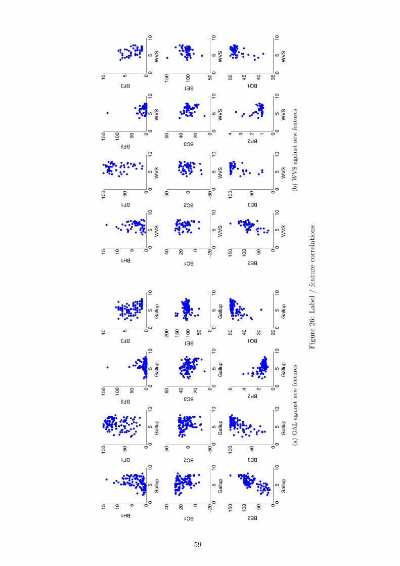
05
10051015
Gallup
BH1
05
10050100
Gallup
BF1
05
10050100
150
Gallup
BF2
05
100510
Gallup
BF3
05
10−2002040
Gallup
BC1
05
10−50050
Gallup
BC2
05
100204060
Gallup
BC3
05
10050100
150
200
Gallup
BE1
05
10050100
150
Gallup
BE2
05
10050100
Gallup
BE3
05
100246
Gallup
BP2
05
1020304050
Gallup
BQ1
Stud
ent V
ersi
on o
f MA
TLA
B
(a)GALag
ainst
new
features
05
10051015
WVS
BH1
05
10050100
WVS
BF1
05
10050100
150
WVS
BF2
05
100510
WVS
BF3
05
10−2002040
WVS
BC1
05
10−50050
WVS
BC2
05
100204060
WVS
BC3
05
1050100
150
WVS
BE1
05
10050100
150
WVS
BE2
05
10050100
WVS
BE3
05
1001234
WVS
BP2
05
1035404550
WVS
BQ1
Stud
ent V
ersi
on o
f MA
TLA
B
(b)W
VSag
ainst
new
features
Figure
26:Lab
el/feature
correlations
59
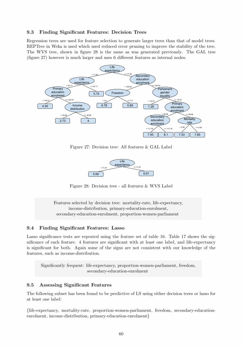
9.3 Finding Significant Features: Decision Trees
Regression trees are used for feature selection to generate larger trees than that of model trees.REPTree in Weka is used which used reduced error pruning to improve the stability of the tree.The WVS tree, shown in figure 28 is the same as was generated previously. The GAL tree(figure 27) however is much larger and uses 6 di↵erent features as internal nodes.
Life expectancy
Primary education enrolment
Life expectancy
5.75
4.55
2.73 4
Freedom
Primary education enrolment
5.896.78 7.28
Mortality rate
7.53 7.857.93 8.1
< 71.85 >= 71.85
< 63.11 >= 63.11
< 103.57 >= 103.57
< 40.06 >= 40.06
< 3.5 >= 3.5
< 100.93>= 100.93
< 19.75>= 19.75
< 99.98 >= 99.98
< 111.75 >= 111.75< 4.95 >= 4.95
Secondary education enrolment
Income distribution
Parliament gender equality
Secondary education enrolment
Figure 27: Decision tree: All features & GAL Label
Life expectancy
5.69 6.91
< 71.97 >= 71.97
Figure 28: Decision tree - all features & WVS Label
Features selected by decision tree: mortality-rate, life-expectancy,income-distribution, primary-education-enrolment,
secondary-education-enrolment, proportion-women-parliament
9.4 Finding Significant Features: Lasso
Lasso significance tests are repeated using the feature set of table 16. Table 17 shows the sig-nificance of each feature. 4 features are significant with at least one label, and life-expectancyis significant for both. Again some of the signs are not consistent with our knowledge of thefeatures, such as income-distribution.
Significantly frequent: life-expectancy, proportion-women-parliament, freedom,secondary-education-enrolment
9.5 Assessing Significant Features
The following subset has been found to be predictive of LS using either decision trees or lasso forat least one label:
{life-expectancy, mortality-rate, proportion-women-parliament, freedom, secondary-education-enrolment, income-distribution, primary-education-enrolment}
60

GAL WVSFeature Frequency Signif Frequency Signiflife-expectancy 100 X 86 Xchild-immunization 23 7 10 7mortality-rate 6 7 1 7gender-labour-ratio 22 7 1 7proportion-women-parliament 81 X 35 -income-distribution 44 - 76 -employment 2 7 32 -population-growth 6 7 38 -hospital-beds 3 7 10 7percent-largest-religion 40 - 4 7religious-conflict 0 7 15freedom 66 - 88 Xtemp-mean 1 7 0 7temp-min 17 7 13 7temp-max 3 7 4 7primary-education-enrolment 6 7 11 7secondary-education-enrolment 88 X 71 -adult-literacy-rate 0 7 16 7military-expenditure 19 7 7 7education-gender 34 - 36 -t0.05 31 31t0.95 87 85
Table 17: Lasso results
We compare this subset with GDP-per-capita as done previously using 10 fold cross valida-tion for lasso and decision trees. This test is comparing a single feature with a subset of features,hence the latter has a higher VC dimension. This means is can fit the data more closely duringtraining. The use of 10 fold CV is highly important here where the correlation is calculated onnew test data such that there is no advantage given to the larger feature set. If this feature setoverfits the training data it will perform badly on the test data. 10 sets of tests were performedto increase the reliability of the results (the folds are randomly chosen each time).
Lasso DTTest # Test GAL Mean WVS Mean GAL Mean WVS Mean1 GDP-per-capita only 0.6633 0.5337 0.7584 0.47322 log GDP-per-capita only 0.7764 0.5927 0.7735 0.56913 log GDP-per-capita & GDP-growth 0.7750 0.5907 0.7647 0.53024 subset* 0.8553 0.7786 0.8612 0.7456
t-test p-val (1 & 4) 1.7575⇥ 10�20 6.4391⇥ 10�9 4.5530⇥ 10�09 4.8387⇥ 10�11
t-test p-val (2 & 4) 1.7760⇥ 10�07 1.2577⇥ 10�5 7.9029⇥ 10�10 3.3353⇥ 10�07
t-test p-val (3 & 4) 1.4042⇥ 10�07 8.6039⇥ 10�7 2.1372⇥ 10�10 2.2592⇥ 10�09
Table 18: Lasso correlations & significance
Table 18 shows the mean correlations and the p-values of t-tests comparing the significantsubset(4) with variations of economic variables. Our feature subset gave significantly highercorrelation than all economic variable sets tested. This was the case for both labels and for bothlasso and DTs.
The feature set {life-expectancy, mortality-rate, proportion-women-parliament,freedom, secondary-education-enrolment, income-distribution,
primary-education-enrolment} can predict LS significantly better that economicvariables using Lasso and DTs
61

Comparing the lasso correlations with the previous results of table 12, they are marginallyreduced. However, the di↵erence is small and not significant, with p = 0.4451 and 0.2456 forGAL and WVS respectively. The first feature set contained 17 variables but the one used nowhas just 7, which shows some variables used initially contribute a small degree to the predictiveability of a LS model.
The feature set {life-expectancy, mortality-rate, proportion-women-parliament,freedom, secondary-education-enrolment, income-distribution,
primary-education-enrolment} can predict LS as well as the 17 original features
The GAL and WVS models are highly consistent. The most frequent model includes thesame features for both labels, and each coe�cient has the same sign. There are also similaritieswith regard to the coe�cient magnitude, such as having large coe�cients for life-expectancyand income-distribution for both labels, although the life-expectancy coe�cient seems quite abit larger for GAL. This may be due to the sample where GAL has many more poorer coun-tries with low health care which may make it more sensitive to changes of life expectancy.Primary-education-enrolment has a negative coe�cient and this is quite unexpected, especiallyas secondary-education-enrolment uses a positive coe�cient.
9.6 Frequent Subsets
life-expectancy
mortality-rate
proportion-w
omen
-parl
inco
me-distribution
freedom
primary-educa
tion-enrol
seco
ndary-educa
tion-enrol
vote
subset 1 1 0 1 1 1 1 1 43subset 2 1 0 1 1 1 0 1 13
Table 19: Lasso frequent subsets
Lasso was run again using just the 7 key featuresand GAL label in order to find frequent subsets.There are 7! = 5040 possible subsets. However over100 bootstraps lasso used just 17. The significancethreshold for subset vote is 13 at a 5% level, andtable 19 show the significant subsets found.
5 features are present in both frequent subsets.Mortality-rate is not included in either and addi-tionally it’s coe�cients are not stable as the signvaries in the results, whereas all other variables areonly ever included with the same sign. The votesshow that the first subset has a much lower p-value,whereas p ⇠ 0.05 for the second (because the voteequals the threshold). The only di↵erence is the inclusion of primary-education-enrolment andthis indicates this variable should be included in the model.
Significant features subsets:{life-expectancy, proportion-women-parliament, income-distribution, freedom,
primary-education-enrolment, secondary-education-enrolment}
{life-expectancy, proportion-women-parliament, income-distribution, freedom,secondary-education-enrolment}
62

10 Best Prediction
Linear and nonlinear methods are used to find the optimal prediction of LS. We test with boththe whole feature set (of stage 2) and our key feature set to provide a comparison. The GAL LSlabel is used as it provides better coverage, and again 10 fold cross validation is used to preventoverfitting.
10.1 Optimising SVM
SVM’s have several parameters that must be optimised for each dataset (See section 7 for moredetails). A grid search was used to optimise the loss and cost values. Two kernels were tried;RBF and poly. RBF is a gaussian kernel and hence the gamma parameter was optimised also.This was done after the grid search using the optimal loss and cost values, trying gamma valuesat 0.5 intervals. This gives a good but non optimal result as the gamma is not optimised inconjunction with the other parameters. However the optimal correlation was very near to thatfound with the original gamma value (that used in the grid search).
10.2 Results
Table 20 shows the p-values of t-tests comparing the results of 10 times 10 fold cross validation.This was done using linear and nonlinear learners and also using the significant features andwhole feature set to provide comparisons. These show a significantly better correlation for thekey feature set, compared with the whole feature set for both the model tree and SVM. Thelasso predictions did not significantly improve using only the key features, which indicates lassois e↵ective at feature selection.
Using key features significantly improved the best prediction found for modeltrees and SVMs
Key Features All FeaturesModel tree RBF Poly Lasso Model tree RBF Poly Lasso
Key
Model tree NaN 0.0197 0.0027 0.5150RBF 0.0197 NaN 0.0152 0.9996Poly 0.0027 0.0152 NaN 0.7917Lasso 0.5150 0.9996 0.7917 NaN
All
modeltree 0.0000 0.0000 0.0000 0.0000 NaN 0.1115 0.2627 0.0000RBF 0.0000 0.0000 0.0000 0.0000 0.1115 NaN 0.0006 0.0001poly 0.0000 0.0000 0.0000 0.0000 0.2627 0.0006 NaN 0.0000lasso 0.0476 0.2207 0.3852 0.2136 0.0000 0.0001 0.0000 NaN
mean correlation 0.8605 0.8503 0.8458 0.8504 0.7519 0.7648 0.7420 0.8326
Table 20: Prediction results comparison: p-values
Best mean correlation: 0.86 (model tree)
The best correlation was found for model trees with a correlation of 0.86. However, this wasnot significantly better than lasso which indicates a highly linear relationship such that LS canbe represented using a linear model.
The relationship between the features and LS is highly linear
Using the large feature set gave significantly worse performance. For instance, a t-test compar-ing the two feature sets for model trees gave a p-value of 2.1212⇥10�16. Decision trees naturallyperform features selection, but can still be a↵ected by irrelevant attributes as lower down the tree
63

the number of instances at each node reduces and the chance of choosing an irrelevant attributeto split the data increases. Also, model trees use a linear model at the leaves which irrelevantattributes can a↵ect. Lasso appears much more robust to irrelevant features, with no significantdi↵erence in performance between the two feature sets.
Lasso is robust to irrelevant features
10.3 DT & PCA
PCA can be an e↵ective transformation method when using decision trees because the varianceof the principal components are orthogonal to the axes (because the axes are by definition thedirection of highest variance in the data). Decision trees split the data into ‘boxes’ with boundariesthat are orthogonal to the axes and therefore principal components may be more easily split duringtree construction.
0 0.1 0.2 0.3 0.4 0.5 0.6 0.7 0.8 0.9 10
0.1
0.2
0.3
0.4
0.5
0.6
0.7
0.8
0.9
1
(a) Original data
) −0.8 −0.6 −0.4 −0.2 0 0.2 0.4 0.6 0.8−0.5
−0.4
−0.3
−0.2
−0.1
0
0.1
0.2
0.3
0.4
0.5
(c) Principal components
Figure 29: PCA demonstration
10.3.1 Results
Model RegressionKey features PCs Both Key features PCs Both
ModelKey - 5.63⇥ 10�8 9.85⇥ 10�2 6.98⇥ 10�5 6.35⇥ 10�7 2.77⇥ 10�5
PCs - 2.78⇥ 10�7 8.52⇥ 10�1 5.75⇥ 10�3 3.4428⇥ 10�1
Both - 5.47⇥ 10�4 3.25⇥ 10�7 1.44⇥ 10�4
RegressionKey - 1.86⇥ 10�2 2.33⇥ 10�1
PCs - 5.04⇥ 10�2
Both -0.8574 0.8179 0.8521 0.8157 0.7771 0.8057
Table 21: PCA decision tree results (10 x 10 fold Correlation)
The key features performed the same as using both principal components and key featuresalone. The results of table 21 show that using PCs alone gave significantly worse results. Usingonly key features gave the highest mean correlation across the folds. This is not significantlybetter (p = 0.0986) than using the combined features, which is expected due to the featureselection capabilities of trees (where if the PCs do not split the data well they can simply beignored). However, the p-value is significant with a 1% level and this again supports the resultsof section 10.2 where using only key features improved results.
The correlations of PCs against key features shown in table 22 indicate from which featuresthe principal components are composed. PC1 is clearly representing health and education, where
64
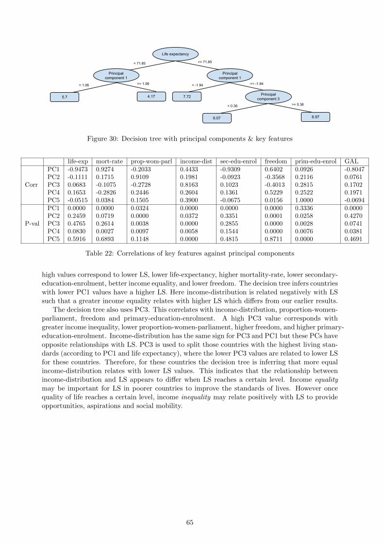
Life expectancy
< 71.85 >= 71.85
6.07 6.97
< 0.36 >= 0.36
Principal component 1
5.7 4.17
< 1.06 >= 1.06 < -1.94 >= -1.94
Principal component 1
7.72 Principal component 3
Figure 30: Decision tree with principal components & key features
life-exp mort-rate prop-wom-parl income-dist sec-edu-enrol freedom prim-edu-enrol GAL
Corr
PC1 -0.9473 0.9274 -0.2033 0.4433 -0.9309 0.6402 0.0926 -0.8047PC2 -0.1111 0.1715 0.9109 0.1981 -0.0923 -0.3568 0.2116 0.0761PC3 0.0683 -0.1075 -0.2728 0.8163 0.1023 -0.4013 0.2815 0.1702PC4 0.1653 -0.2826 0.2446 0.2604 0.1361 0.5229 0.2522 0.1971PC5 -0.0515 0.0384 0.1505 0.3900 -0.0675 0.0156 1.0000 -0.0694
P-val
PC1 0.0000 0.0000 0.0324 0.0000 0.0000 0.0000 0.3336 0.0000PC2 0.2459 0.0719 0.0000 0.0372 0.3351 0.0001 0.0258 0.4270PC3 0.4765 0.2614 0.0038 0.0000 0.2855 0.0000 0.0028 0.0741PC4 0.0830 0.0027 0.0097 0.0058 0.1544 0.0000 0.0076 0.0381PC5 0.5916 0.6893 0.1148 0.0000 0.4815 0.8711 0.0000 0.4691
Table 22: Correlations of key features against principal components
high values correspond to lower LS, lower life-expectancy, higher mortality-rate, lower secondary-education-enrolment, better income equality, and lower freedom. The decision tree infers countrieswith lower PC1 values have a higher LS. Here income-distribution is related negatively with LSsuch that a greater income equality relates with higher LS which di↵ers from our earlier results.
The decision tree also uses PC3. This correlates with income-distribution, proportion-women-parliament, freedom and primary-education-enrolment. A high PC3 value corresponds withgreater income inequality, lower proportion-women-parliament, higher freedom, and higher primary-education-enrolment. Income-distribution has the same sign for PC3 and PC1 but these PCs haveopposite relationships with LS. PC3 is used to split those countries with the highest living stan-dards (according to PC1 and life expectancy), where the lower PC3 values are related to lower LSfor these countries. Therefore, for these countries the decision tree is inferring that more equalincome-distribution relates with lower LS values. This indicates that the relationship betweenincome-distribution and LS appears to di↵er when LS reaches a certain level. Income equalitymay be important for LS in poorer countries to improve the standards of lives. However oncequality of life reaches a certain level, income inequality may relate positively with LS to provideopportunities, aspirations and social mobility.
65

11 Graphical Models
Bayesian networks are described in section 3.3.8. Our aim is to use BBNs to assess the relation-ships between the key features we have identified.
11.1 Discretizing
Bayesian networks require nominal data and so the data is converted from the original numericfeatures. Discretizing using equal width caused some bins to hold very few instances, which maycause more unreliable results because it is easily a↵ected by each of these instances. Thereforeequal frequency was used to give approximately the same number of instances in each bin in thenetwork. The bins are slightly di↵erent sizes because the number of instances cannot be dividedexactly into 4 bins. Some of the variables have only a small number of values such as freedomwhere the values are between 0 and 7 in 0.5 intervals. This means that the number of instancesin the bins is more variable, because of the groups of intervals with identical freedom values.
The number of bins was chosen by experimentation, where the class distribution of the binswas visually compared. A balance is needed between simplicity and loss of information. A smallnumber of bins is preferred such that the degree of freedom of the network is kept low. However,there needs to be a su�cient number of bins to capture relationships between the variables, asreducing the number of bins reduces the information content of the network. We found 4 bins tobe appropriate (named VLOW, LOW, HIGH, VHIGH respectively).
11.2 Network Structure
There are several methods for automatically generating networks, but these are not able toinfer causality and therefore the network structure is built manually. The probabilities are thencalculated using estimates of the probabilities (see section 3.3.8).
The networks use the key features, and additionally GDP-per-capita is included. Figure 31(a)shows a basic structure, which we are confident represents the variable relationships. This struc-ture represents the notion that GDP a↵ects the levels of other variables and these in turn impacton LS. We investigate some alterations to this basic network, shown in figures 31(b), 31(c) and31(d). These have one or two additional edges connecting GDP-per-capita to proportion-women-parliament, freedom and also to LS directly.
11.2.1 Metrics used for assessment
We use % correct, ROC curve area and degrees of freedom to assess the networks, to look at theperformance of each structure.
Structure (fig 31) # edges Degrees of FreedomA 13 1236B 14 4308C 14 4308D 15 16596
Table 23: BBN details
Degrees of Freedom The degrees offreedom (DF) are the number of parametersthat can change in a model. This is an im-portant consideration as models with higherDF are more easily able to fit to a pattern.
The DF of a network is the number ofprobabilities in the probability tables of eachnode. These are probabilities of each value ofthis node conditional on each combination of parent node values. For instance, one probabilityof node mortality-rate is p(mortality � rate = V LOW | LS = V LOW ). The number of valuesin a network is given by:
V =nX
i=1
(Ki · (Y
Xj✏parent(Xi)
Kj)), (49)
66

Life expectancy Freedom
Parliament gender equality
Secondary education enrolment
Mortality rate
GDP per capita
Life satisfaction
Primary education enrolment
Income distribution
(a) Basic Network (A)
Life expectancy Freedom
Parliament gender equality
Secondary education enrolment
Mortality rate
GDP per capita
Life satisfaction
Income distribution
Primary education enrolment
(b) Network B
Life expectancy Freedom
Parliament gender equality
Secondary education enrolment
Mortality rate
GDP per capita
Life satisfaction
Income distribution
Primary education enrolment
(c) Network C
Life expectancy Freedom
Parliament gender equality
Secondary education enrolment
Mortality rate
GDP per capita
Life satisfaction
Income Distribution
Primary education enrolment
(d) Network D
Figure 31: Network structures
where Ki is the number of discretised values of node (feature) i. Therefore the number ofvariables at each node grows exponentially in the number of edges leading to that node.23
Receiver Operating Characteristic (ROC) Curves A ROC curve is a graph of falsepositive rate against true positive rate. The area underneath (AUC) indicates how well thetest instances are classified. This combines both the rate the class is correctly identified (truepositive) and the extent that instances are classified as this class incorrectly (false positive).
!
!"#$%&'()%*+*,&
-./&'()%*+*,&
Figure 32: ROC curve (basicstructure low LS)
With respect to this work, a ROC curve is generated for eachband of LS, and figure 32 shows the ROC curve for VLOW LSand the network in figure 31(a).
Specifically, for a ROC curve of class c and given two ran-dom instances i1 and i2 where c(i1) = c and c(i2) = ¬c, havingp1 = p(c | i1) and p2 = p(c | i2). The AUC corresponds to theprobability that p1 > p2.[21] An instance that is misclassifiedbut only just such as if p(c | i1) is only slightly smaller thanp(¬c | i1), will reduce the area, but by less than if the di↵erencein these probabilities is much greater (given that the points ofother classes lie between these values). In this sense this value
can be seen to quantify the distribution of values in a confusion matrix into a single value.Each ROC curve corresponds to a class value (discretised LS value), and here we use the
average AUC (across LS values) as a measure of how well LS is predicted by each network. Avalue of 1 indicates no false positives and 100% true positives (and 0.5 is as good as the randomcase). Hence this metric is a useful measure as it indicates class prediction relative to other
23For our network all nodes have 4 values. None: 4, 1 : 42 = 16, 2 : 43 = 64, 3 : 44 = 256, 4 : 45 = 1024, 5 : 46 =4096, 6 : 47 = 16384
67

instances, rather than the actual prediction values. [21] Instances ranked in the correct order
(according to the ratio of p(c | i) and p(¬c | i) such that p(c|i)p(¬c|i) is always larger for instances of
class c) will give an optimal AUC, but in this case it is still feasible that the classifications areincorrect. For instance, if no instances are classified as V LOW but also if the V LOW instancesare ranked higher such that they are more likely to belong to this class than the other instances,then the ROC curve will be optimal. As such we combine use of this measure with others suchas the % correct to provide an overview of the e↵ectiveness of each network.
In addition, weighted ROC area is assessed. This takes into account the class distribution ofthe test instances of each fold24, and this gives more importance to the results of more frequentclasses.
11.2.2 Results
Table 24 shows the a↵ect of structural changes to the original network (figure 31(a)) whichare shown in figures 31(b),31(c) and 31(d). These results compare 10 sets of 10-fold cross-validation tests (100 result values per network)25. Firstly, the proportion correct is surprisinglylow (approximately 58%). This may be because the numeric data is discretised which loses muchof the information is contains. Confusion matrices shows the magnitude of the errors, such as thatof graph A (table 25) where mistakes of smaller magnitude are more common. For instance, nocountries with an extreme LS value (VLOW or VHIGH) were classified as the opposite extremevalue.
P-value H-value MeanA B C D A B C D
% correct
A - Same 0.0014 0.9863 - 0 1 0 58.4817B Same - 0.0014 0.9863 0 - 1 0 58.4817C 0.0014 0.0014 - 0.0003 1 1 - 1 56.8433D 0.9863 0.9863 0.0003 - 0 0 1 - 58.4740
ROC Area
A - 0.3197 0.0009 0.1939 - 0 1 0 0.7047B 0.3197 - 0.0008 0.1760 0 - 1 0 0.7049C 0.0009 0.0008 - 0.0165 1 1 - 1 0.6895D 0.1939 0.1760 0.0165 - 0 0 1 - 0.7007
Weighted ROC Area
A - 0.3197 0.1562 0.0395 - 0 0 1 0.7966B 0.3197 - 0.1733 0.0341 0 - 0 1 0.7965C 0.1562 0.1733 - 0.0050 0 0 - 1 0.7938D 0.0395 0.0341 0.0050 - 1 1 1 - 0.7993
Table 24: BBN t-test results comparison of networks of figure 31
(-inf-4.95] (4.95-5.85] (5.85-7.05] (7.05-inf)(-inf-4.95] 22 3 1 0(4.95-5.85] 4 14 6 3(5.85-7.05] 1 5 14 8(7.05-inf) 0 3 7 20ROC area 0.936 0.686 0.721 0.827
Table 25: Confusion matrix of graph A
The t-test result sets for the 3measured values are first consideredindependently. The % correct washighest for graph A, although thiswas not significant. In fact A andB showed identical results and nosignificant di↵erence was found be-tween A,B and D. Graph B gave thelargest ROC area, marginally largerthan A. Again, no significant di↵erence between A,B and D. The weighted ROC area results didhowever find a significant improvement, for graph D when compared to all other graphs.
Therefore, all three tests showed graph C performs significantly worse than the other network,with respect to the % correct and weighted and unweighted ROC curve areas. It also has a larger
24A weighted average of ROC areas of each class, uses the confusion matrix to find the weights, see class methodweka.classifiers.Evaluation.weightedAreaUnderROC()
25The division of instance to fold is random
68

degree of freedom than graph A and hence graph A is preferred for this reason also. With respectto graphs A,B and D, only weighted ROC curve area gives a significant di↵erence, and this isin favour of graph D. However with p = 0.0395 for graph A versus graph D this is significantat a 5% level but not at a 1% significance level. These results are less than definitive, and it isonly when considering model complexity that we prefer one graph over the others. Graph D has16596 degrees of freedom, which is much larger compared to 1236 of graph A. This means that Dis much more prone to overfitting as there are many more tunable parameters in the model. Thisreason leads us to believe it is reasonable to accept graph A as an appropriate graph comparedto the three variations considered. Also, according to Occam’s razor when two models performequally well then the simpler one should be preferred.
A degree of improvement was expected when connecting GDP-per-capita directly with LS.There are several possible justifications for this representation, firstly that this does indeed showthat GDP-per-capita has a direct impact on LS. Alternatively, this may have occurred if thereare other relationships not captured in our network involving variables we have not considered.The feature set considered is small compared with the potentially relevant features which mayimpact on LS, which is likely to be a large number of variables. Therefore, these results are inline with our expectations.
Connecting GDP-per-capita directly with LS shows no performance improvementof the network
69

12 Data Visualisation
Cherno↵ faces (CF) are a method for visualisation of multivariate data.[12] Each facial featurecorresponds to a feature in the data set and changes shape or size according to the feature value(relative to the values of the other data points). Facial expression is closely associated withhappiness and hence LS, and as such it is an ideal representation. Satisfied countries can beeasily identified using facial expression as well as di↵erences between particular facial features,and hence trends and anomalies are easy to identify. Two star visualisations have been generatedfor a comparison (figure 33(c) and 33(d)) and these are clearly much less intuitive.
12.1 Label Value Inference
To maximise the data available, we infer GAL values from the WVS where the GAL values aremissing, by regressing WVS against GAL. The resultant model isGAL = 0.9525 WV S + 0.1938 with p = 1.4054⇥ 10�10 and a correlation of 0.6287. Thereforewhile the overall correlation is good there are some di↵erences which may a↵ect the country orderfor the two labels.
12.2 Face Generation
The faces for each country are shown in figure 27 and these results are ordered by LS such thatthe trends can be identified. Table 26 shows the key for the face features, chosen such thathigh LS relates to happier looking faces. For example, eyebrow angle is used to represent genderequality and hence proportion-women-parliament was negated such that angry eyes relates topoor equality.
Face feature Data feature Visual meaningFace size life-expectancy large = highLength of nose mortality-rate large = highEyebrow angle proportion-women-parliament unhappy = unequalEye: dist between income-distribution close = equalForehead shape freedom round = more freeShape of jaw primary-education-enrolment round = highSmile secondary-education-enrolment smile = high
Table 26: Cherno↵ face key
Norway
Student Version of MATLAB
(a) Norway Zimbabwe
Student Version of MATLAB
(b) Zimbabwe
Norway
Student Version of MATLAB
(c) Norway Zimbabwe
Student Version of MATLAB
(d) Zimbabwe
Figure 33: Cherno↵ and star exam-ples
The similarities and di↵erences are easily recognisable,now the features are represented visually. For example,two countries having very low and high LS values are Zim-babwe and Norway respectively, shown in figures 33(a)and 33(b). These show very di↵erent values for each fea-ture. However we can see that primary education rate isvery similar (shape of jaw line). Even though Zimbabwe’sprimary enrolment is high, the secondary enrolment isvery low (sad smile). This highlights our findings thatsecondary education is more predictive of LS than pri-mary education.
Health was shown to significantly predict LS and ourCFs show this with both increasing face size (life ex-pectancy) and decreasing nose size (mortality rate).
70

life-exp mort-rate prop-women-parl income-dist sec-educ-enrol freedom prim-educ-enrolNorway 80.74 3.50 36.10 25.79 112.38 1.0 98.25Zimbabwe 44.21 93.40 15.20 50.10 40.99 6.5 103.60
Figure 34: Feature values for Zimbabwe and Norway
12.3 Interactive Results
A website26 was built to provide an interactive visualisation of the results. The core technologiesused are: Google maps, Google visualisations, HTML, JavaScript and JSON. The Cherno↵ faceswere overlayed onto a map such that the LS and feature values can be easily analysed by globallocation. The standard map pointers are replaced with faces, which when clicked display chartsof the feature values for this country next to the map (see figure 36). There is also a separatepage where the correlations between features can be viewed where on mouse over the countrydetails are displayed.
Figure 35: Website interactive happiness map
Figure 36: Example feature chart
26http://intelligentsystems.bristol.ac.uk/research/Millard/
71

Tanzania
Student Version of MATLAB
Togo
Student Version of MATLAB
Zimbabwe
Student Version of MATLAB
Burundi
Student Version of MATLAB
Benin
Student Version of MATLAB
Burkina Faso
Student Version of MATLAB
Congo
Student Version of MATLAB
Sierra Leone
Student Version of MATLAB
Kenya
Student Version of MATLAB
Madagascar
Student Version of MATLAB
Mali
Student Version of MATLAB
Mozambique
Student Version of MATLAB
Niger
Student Version of MATLAB
Cameroon
Student Version of MATLAB
Ethiopia
Student Version of MATLAB
Rwanda
Student Version of MATLAB
Angola
Student Version of MATLAB
Georgia
Student Version of MATLABZambia
Student Version of MATLAB
Senegal
Student Version of MATLAB
Uganda
Student Version of MATLAB
Bulgaria *
Student Version of MATLAB
Botswana
Student Version of MATLAB
Ghana
Student Version of MATLAB
Lebanon
Student Version of MATLAB
Morocco *
Student Version of MATLAB
Nigeria
Student Version of MATLAB
Cambodia
Student Version of MATLAB
Armenia
Student Version of MATLAB
Kyrgyzstan
Student Version of MATLAB
Mauritania
Student Version of MATLAB
South Africa
Student Version of MATLAB
Tajikistan
Student Version of MATLAB
Azerbaijan
Student Version of MATLAB
Bangladesh
Student Version of MATLAB
Nepal
Student Version of MATLABUkraine
Student Version of MATLAB
Chad
Student Version of MATLAB
Iraq
Student Version of MATLAB
Latvia
Student Version of MATLAB
Sri Lanka
Student Version of MATLAB
Serbia *
Student Version of MATLAB
India
Student Version of MATLAB
Philippines
Student Version of MATLAB
Turkey
Student Version of MATLAB
Algeria
Student Version of MATLAB
Estonia
Student Version of MATLAB
Iran
Student Version of MATLAB
Pakistan
Student Version of MATLAB
Djibouti
Student Version of MATLAB
Hungary
Student Version of MATLAB
Indonesia
Student Version of MATLAB
Moldova
Student Version of MATLAB
Mongolia
Student Version of MATLABBelarus
Student Version of MATLAB
Lithuania
Student Version of MATLAB
Peru
Student Version of MATLAB
Portugal
Student Version of MATLAB
Romania
Student Version of MATLAB
Russia
Student Version of MATLAB
Syria
Student Version of MATLAB
Tunisia
Student Version of MATLAB
Hong Kong *
Student Version of MATLAB
Jordan
Student Version of MATLAB
Uzbekistan
Student Version of MATLAB
Kazakhstan
Student Version of MATLAB
Laos
Student Version of MATLAB
Chile
Student Version of MATLAB
South Korea
Student Version of MATLAB
Thailand
Student Version of MATLAB
China *
Student Version of MATLAB
Ecuador
Student Version of MATLABBolivia
Student Version of MATLAB
Guyana
Student Version of MATLAB
Poland
Student Version of MATLAB
Belize
Student Version of MATLAB
Malaysia
Student Version of MATLAB
Andorra *
Student Version of MATLAB
Viet Nam *
Student Version of MATLAB
Egypt
Student Version of MATLAB
El Salvador
Student Version of MATLAB
Slovenia *
Student Version of MATLAB
Greece
Student Version of MATLAB
Japan
Student Version of MATLAB
Uruguay
Student Version of MATLAB
Trin & Tob *
Student Version of MATLAB
Czech Rep
Student Version of MATLAB
Italy
Student Version of MATLAB
Paraguay
Student Version of MATLAB
Cyprus *
Student Version of MATLABHonduras
Student Version of MATLAB
Argentina
Student Version of MATLAB
France
Student Version of MATLAB
Israel
Student Version of MATLAB
Malta
Student Version of MATLAB
Nicaragua
Student Version of MATLAB
Singapore
Student Version of MATLAB
Germany
Student Version of MATLAB
Colombia
Student Version of MATLAB
Great Britain
Student Version of MATLAB
Belgium
Student Version of MATLAB
Brazil
Student Version of MATLAB
Dominican Rep
Student Version of MATLAB
Spain
Student Version of MATLAB
Guatemala *
Student Version of MATLAB
Switzerland *
Student Version of MATLAB
Luxembourg
Student Version of MATLAB
Mexico
Student Version of MATLABNetherlands
Student Version of MATLAB
Saudi Arab
Student Version of MATLAB
Austria
Student Version of MATLAB
Iceland
Student Version of MATLAB
New Zealand
Student Version of MATLAB
Panama
Student Version of MATLAB
Australia
Student Version of MATLAB
Sweden
Student Version of MATLAB
US
Student Version of MATLAB
Canada
Student Version of MATLAB
Finland
Student Version of MATLAB
Denmark
Student Version of MATLAB
Ireland
Student Version of MATLAB
Norway
Student Version of MATLAB
Costa Rica
Student Version of MATLAB
Table 27: Cherno↵ faces ordered by LS (* GAL value inferred from WVS)
72

13 Project Conclusions
Drawing conclusions It is important to first note the extent to which conclusions can bedrawn from our results. We have found key features and models to represent and predict LS.However, justifying these results with common sense reasoning has limited worth as demonstratedby Paul Lazarsfield, a mathematician and Professor of Sociology. [2] Lazarsfield switched findingsof military research looking at the stress of soldiers. The research found that education waspositively related to the stress a soldier experiences, which could be justified by environmentaldi↵erences such that farmers are more used to the tough conditions. However when switchingthe result, he showed that this could just as easily be justified by another reason, that educationprovides skills to cope with stress. This shows how we should only be guided by results ratherthan our intuition and common sense. [32]
13.1 Results Summary
13.1.1 Feature selection & construction
Variables were constructed such that they were most representative of the intended concept. Forinstance, latitude was used to represent light, and this was weighted by population to ensure itwas representative of where people actually live.
Military expenditure was initially found to be significant. However, this variable was theamount relative to GDP per capita. Confounding was found to be the underlying reason forit’s inclusion. This was determined by altering the variable to military expenditure per healthexpenditure, after which it was no longer found to be a significant feature (see section 9.1).
We found much sensitivity to choice of variable to represent a concept. For example, severaleducation indicators were considered; primary enrolment, secondary enrolment, literacy rate andpupil teacher ratio. Literacy rate and pupil teacher ratio were not significant features, but theenrolment variables (particularly secondary) were prominent in the results.
Visualising the data indicated some variables have an exponential relationship with LS. Trans-forming these with logs was found to be beneficial, where these variables were often selectedinstead of the original (section 6.2).
13.1.2 Key features & feature subsets
The key features identified are:
• Health: life-expectancy, mortality-rate
• Education: primary-education-enrolment, secondary-education-enrolment
• Equality: proportion-women-parliament*, income-distribution
• Freedom: freedom index
* Additionally, PCA found an interesting relationship between gender equality and both LSand GDP per capita (section 5.3).
Although mortality rate was found to be significant as an individual feature, it was not presentin the significant feature subsets. The following frequent subsets were found using lasso tests:
{life-expectancy, proportion-women-parliament, income-distribution, freedom, primary-education-enrolment, secondary-education-enrolment}
{life-expectancy, proportion-women-parliament, income-distribution, freedom, secondary-education-enrolment}
73

13.1.3 Key Models
Tests have shown that our models using the key features are significantly more predictive of LSthan economic variables alone (section 7 and section 9.5). The best correlation used was 0.86for model trees. There was no significant di↵erent between the results of linear and nonlinearmethods, indicating the relationship of our feature set with LS is highly linear (section 10). Aregression tree for the GAL label is shown in figure 37.
Life expectancy
Primary education enrolment
Life expectancy
5.75
4.55
2.73 4
Freedom
Primary education enrolment
5.896.78 7.28
Mortality rate
7.53 7.857.93 8.1
< 71.85 >= 71.85
< 63.11 >= 63.11
< 103.57 >= 103.57
< 40.06 >= 40.06
< 3.5 >= 3.5
< 100.93>= 100.93
< 19.75>= 19.75
< 99.98 >= 99.98
< 111.75 >= 111.75< 4.95 >= 4.95
Secondary education enrolment
Income distribution
Parliament gender equality
Secondary education enrolment
Figure 37: Decision tree: Key features & GAL label (not standardised)
The models generated using lasso and least squares consist of coe�cient values that were oftenagainst intuition. For instance, primary education enrolment has a small negative coe�cient. Thisis to be expected as only using a small number of features are used and thus this is only a ‘good’but less than perfect model of life satisfaction. Therefore some compromises are built into thegenerated models to account for this as best as possible.
13.1.4 Graphical Models
Tests with Bayes networks investigated slight variations and found no significant improvementin prediction when connecting GDP per capita directly with life satisfaction. Additionally, theperformance was poor with a mean prediction of 59 %. This is likely to be due to discretisationwhere to keep the degrees of freedom low a small number of ‘buckets’ was used, which causesmuch of the information in the data to be lost.
13.1.5 Consistency of results & data quality
Tests results for WVS and GAL found some similar results but also some di↵erences. For instance,models for WVS preferred freedom whereas proportion-women-parliament was used for GAL. Lifeexpectancy however was a consistently significant feature throughout this work for both labels.
The availability of a suitable ground truth is a constraint of this project, where there aredi↵erences between the sources that are not ideal (see section 4). In brief, WVS is too smalland missing many countries with low LS, whilst GAL is larger but possibly skewed by questionpositioning. Additionally, the variables used as features included some missing values and thesewere inferred. This involved both using alternative sources and also imputation using the k-nearest neighbour method. Imputation (section 6.1) did not give good results and was used onlywhere reliable alternative sources could not be found. The reliability of alternative sources is aconcern, as small di↵erences between the sources can a↵ect the data. Therefore, future work inthis area will improve with better data availability and coverage.
74

13.1.6 Results visualisations
Cherno↵ faces provide an e↵ective visualisation of our key feature set. They have shown to bean excellent method to visualise multivariate data where patterns and anomalies can be easilyidentified. Facial expression was a particularly appropriate and intuitive representation for thiswork, corresponding to life satisfaction.
13.2 Assessing progress
The main objective was to predict happiness using a feature set excluding economic variables.Results surpassed expectations, having identified a feature set significantly more predictive thaneconomic variables. Structural tests that identified no direct relationship between GDP and lifesatisfaction further support the notion proposed: “Economic factors are not goals in themselvesbut a means for acquiring other types of social goals”. [25]
We have proven GDP to be inadequate as a measure of progress and shown the opportunityand value of an alternative concise but highly informative variable set. GDP by definition27
is driven by consumption, but this is not the case for our feature set. Therefore, a measure ofprogress incorporating these could help lead us to a happier, more sustainable and planet friendlyfuture.
13.3 Areas of further work
Our work found an interesting relationship between gender equality and GDP / life satisfactionand this needs further investigation. The two variables represent gender equality only (labourparticipation and equality in parliament), and hence more equality variables needs investigatingto look at other types of equality.
An interesting area of future work would be to learn using more structured data to allowinformation that cannot easily be expressed in typical attribute value learners. For instance,Tilde is an ILP learning system able to learn decision trees (including regression) using firstorder logic. This may be of much use to investigate relationships and structure in the worldsuch as political allies and country neighbours. Our results indicate close relationships betweencountries, such as the PCA graph (figure 14) where nearby countries have similar values of somevariables. It would be interesting to investigate the extent to which a country’s LS is determinedby their own actions or heavily constrained by other properties such as the countries they border.
Finally, the relationship between income distribution and LS is an open question, and theuncertainty behind this is highlighted by our conflicting results regarding this. The constrainingfactor regarding research into this is the lack of available data.
27Gross Domestic Product (GDP) is the value of the goods and services produced by a country in a year.Formally, GDP is: The sum of gross value added by all resident producers in the economy plus any product taxesand minus any subsidies not included in the value of the products. [1]
75

14
Appen
dix
A:Data
Sources
Sou
rce
Year#
respon
dents
# countries
Age
Question
&an
swer
Answ
erscale
Standardisation
World
Value
Survey(W
VS)
Primary
2008
Mostly>
1000
5516+,18+
Allthings
considered,how
satisfied
areyouwithyourlife
asa
wholethesedays?
(V22)
1(D
issatisfied),2,
3,4,
5,6,
7,8,
9,10
(Satisfied),-1
Don
tkn
ow,-
2Noan
swer,-3
Not
applicable,-4
Not
askedin
survey,-5
Missing;
Unkn
own
1-10
**Rescaled
from
1-10
to0-10
Hap
pyPlanet
Index(H
PI)
Secon
dary
(Gallup)
2006
Mostly>
1000
143(112
Gallup
life
sat’n)
15+
Allthings
considered,how
satisfied
areyouwithyourlife
asa
wholethesedays
0to
10,where0is
dissatisfied
and10
issatisfied
0-10
OECD
(Posi-
tive
experience
index)
Secon
dary
(Gallup)
2006
-08
Mostly>
1000
3515+
Positiveexperience
index
(com
bines
6qu
estion
sfrom
Gallup;well
rested,treatedwithrespect,
chosehow
timewas
spent,
proudof
somethingyo
udid,learnt
ordid
somethinginteresting,
enjoym
ent
ladder-of-lifequ
estion
s,whichaskrespon
dents
torate
theirlife
from
theworst
(0)to
thebest(10)
level,an
dreferto
theshareof
people
whorate
theirlife
(tod
ayan
din
thefuture)at
step
7or
higher.
0-
10(but
given
as%)
Rescaled
-di-
videby
10
OECD
(Lad
der
oflife)
Secon
dary
(Gallup)
2006
-08
Mostly>
1000
3515+
Pleaseim
aginealadder,withstepsnu
mbered
from
0at
thebot-
tom
to10
atthetop.Thetopof
theladder
representsthebest
possible
life
foryouan
dthebottom
oftheladder
representsthe
worst
possible
life
foryou.Onwhichstep
oftheladder
wou
ldyou
sayyoupersonally
feel
youstan
dat
this
time?
0-10
European
So-
cial
Survey
(ESS)
Primary
2008
1500
or800if
pop
ulation
<2million
2615+
Tak
ingallthings
together,how
hap
pywou
ldyo
usayyo
uare?
Extremelyunhap
py00,01
0203
0405
0607
0809,Extremely
hap
py10,(D
ontkn
ow)88
0-10
Eurobarom
eter
Primary
2008
1000
3115+
Onthewhole,
areyouvery
satisfied,fairly
satisfied,not
very
sat-
isfied
ornot
atallsatisfied
withthelife
youlead
?Verysatisfied,Fairlysatisfied,Not
very
satisfied,Not
atallsatis-
fied
,DK
%satis-
fied
Rescale
-di-
videby
10
European
Value
Sur-
vey(EVS)
Primary
2008
1500
4818+
Variable
v66:
how
satisfied
areyouwithyo
urlife
-5(other
missing),-4
(question
not
asked),
-3(nap
),-2
(na),-1
(dk),1(dissatisfied),2,
3,4,
5,6,
7,8,
9,10
(satisfied)
110
(-5
--1
in-
valid)
**Rescaled
from
1-10
to0-10
Latinob
arom
etrePrimary
2007
1000
-1200
1818
(16
Brazil
&Nicaragua)
Q1S
T.A
Ingeneral,wou
ldyousayyouaresatisfied
withyourlife?
Wou
ldyousayyouare....?
1(V
erysatisfied),2(Fairlysatisfied),3(not
very
satisfied),4(N
otsatisfied
atall),0NK
14(re-
versed*)
***R
escaled
andreversed
Tab
le28
:SurveysDescription
s:Surveysconsidered
ashap
pinesslabel
(**rescale(x)=
(x-1)*10
/9**
*rescale(x)=
10-(x-1)*10
/3)
76

IdType
Code
Yea
rFea
ture
Source
#missing
val-
ues
URL
EC1
ECONOMIC
EC1-G
DPGROW
TH-
2008
2008
GDP
growth
(annual%)
World
Ban
k2
http://data.w
orldbank.org/indicator/NY.G
DP.M
KTP.K
D.ZG
EC3
ECONOMIC
EC3-E
MPLOY-
RATIO
-2008
2008
Employmen
tto
populationratio,15+,
total(%
)W
orld
Ban
k2
http://data.w
orldbank.org/indicator/SL.E
MP.T
OTL.SP.ZS
EC4
ECONOMIC
EC4-G
DP-P
ER-
CAPIT
A-2008
2008
GDP
per
capita(curren
tUS$)
World
Ban
k2
http://data.w
orldbank.org/indicator/NY.G
DP.P
CAP.C
D
HE1
HEALTH
HE1-LIF
EEXP-200
82008
Lifeex
pectancy
atbirth
,total(yea
rs)
World
Ban
k1
http://data.w
orldbank.org/indicator/SP.D
YN.LE00
.IN
HE2
HEALTH
HE2-IM
MUN-08
2008
Immunization,
DPT
(%of
children
ages
12-23month
s)W
orld
Ban
k1
http://data.w
orldbank.org/indicator/SH.IMM.IDPT
HE3
HEALTH
HE3-HEALTH-E
XP-
08
2008
Hea
lthex
pen
diture
per
capita(curren
tUS$)
World
Ban
k2
http://data.w
orldbank.org/indicator/SH.X
PD.P
CAP
HE4
HEALTH
HE4-MORT-R
ATE-08
2008
Mortality
rate,under-5
(per
1,00
0)W
orld
Ban
k1
http://data.w
orldbank.org/indicator/SH.D
YN.M
ORT
EN1
ENVIR
ON
EN1-C
O2EMIS-2007
2007
CO2em
issions(m
etrictonsper
capita)
World
Ban
k1
http://data.w
orldbank.org/indicator/EN.A
TM.C
O2E.P
CEN2
ENVIR
ON
EN1-M
AM-T
HREAT-
08
2008
Mam
mal
species,
threaten
edW
orld
Ban
k0
http://data.w
orldbank.org/indicator/EN.M
AM.T
HRD.N
O
EQ2
EQUALIT
YEQ2-L
ABOR-R
ATIO
-GEN
2008
Ratio
of
gen
der
labor
participation
rate
HIG
HER=MORE
EQUAL
World
Ban
k2
http://data.w
orldbank.org/indicator/SL.T
LF.C
ACT.FE.ZS
http://data.w
orldbank.org/indicator/SL.T
LF.C
ACT.M
A.ZS
EQ3
EQUALIT
YEQ3-PARL-W
OM-08
2008
Proportionofseats
heldbywomen
innationalparliamen
ts(%
)W
orld
Ban
k3
http://data.w
orldbank.org/indicator/SG.G
EN.PARL.ZS
FR1
FREEDOM
FR1-T
IME-START-
BUS-2008
2008
Tim
erequired
tostart
abusiness
(day
s)W
orld
Ban
k2
http://data.w
orldbank.org/indicator/IC
.REG.D
URS
ED2
EDUCATIO
NED2-P
UP-T
EA-R
AT-
08
2008
Pupil-tea
cher
ratio,primary
World
Ban
k30
http://data.w
orldbank.org/indicator/SE.P
RM.E
NRL.T
C.ZS
CL2
CLIM
ATE
CL2-L
AT-
WEIG
HTED
2010
Latitu
deweighted
averagebypopula-
tion(indicatorforlight)
World
Gazetier,
geo
-hive,
wolfram
alpha
2
LI2
LIF
E-STYLE
LI2-P
OP-G
ROW
-08
2008
Pop
ulationgrowth
(annual
%)
World
Ban
k0
http://data.w
orldbank.org/indicator/SP.P
OP.G
ROW
LI3
LIF
E-STYLE
LI3-P
OP-U
RBAN-08
2008
Urb
anpop
ulation
(%of
total)
World
Ban
k0
http://data.w
orldbank.org/indicator/SP.U
RB.T
OTL.IN.ZS
LI4
LIF
E-STYLE
LI4-P
OP-D
ENS
2008
Pop
ulationden
sity
(peo
ple
per
sq.km
oflandarea)
World
Ban
k0
http://data.w
orldbank.org/indicator/EN.P
OP.D
NST
CR2
CRIM
ECR2-INTENT-
HOMO-03-08
2003-
2008
Intentionalhomicide,
rate
per
100,000
population
UN
DATA
1http://www.unodc.org/unodc/en/data-and-analysis/
homicide.html
DI1
DISTRIB
’NDI1-FAM-INCOME
1975
-2011
Distributionoffamilyinco
me-Giniin-
dex
CIA
World
Factbook
HIG
HER=MORE
UNEQUAL
7https://www.cia.gov/library/publications/
the-world-factbook/rankorder/2172rank.html
DI2
DISTRIB
’NDI2-A
GE-65-2008
2008
Age
distribution
U.S.
Cen
sus
Bureau
0http://www.census.gov/ipc/www/idb/groups.php
Tab
le29
:Features(1)
77

IdType
Code
Yea
rFea
ture
Source
URL
Missingva
lues
BH1
HEALTH
B-H
E-1-H
OSP
avg06-08(andea
r-lier
ifmissing)
Hospital
bed
s(p
er1,000peo
ple)
World
Ban
khttp://data.worldbank.org/
indicator/SH.MED.BEDS.ZS
Avg20
06-20
09&
missing:
use
earlieryea
r
BF1
FREEDOM
BF1-R
EL-
PROP
08
percentage
of
the
largest
religion
or
religious
brand
(LG1PCT08)
thea
rda
http://www.thearda.com/Archive/
Files/Downloads/IRF2008_DL2.asp
1:
United
States
(51.3%),
vietn
am
(9.3%)
both
from
https://www.cia.gov/library/publications/
the-world-factbook/geos/us.html,
china
(42.5%)
from
WorldChristianDatabase
BF2
FREEDOM
BF2-R
EL-
CONF
08
Number
ofuniqueinci-
den
tsofreligiousco
n-
flict(C
ONFL#08)
thea
rda
http://www.thearda.com/Archive/
Files/Downloads/IRF2008_DL2.asp
1:United
States-given
mea
nva
lue(7.18)
BF3
FREEDOM
BF3-W
OR-
FREE
08
Freed
om
ofth
eW
orld
2008
LOW
=MORE
FREE
Freed
om
Hou
sehttp://freedomhouse.org/
template.cfm?page=351&ana_page=
341&year=2008
-
BC1
CLIM
ATE
BCL1-M
EAN-
TEMP
1961-1990
Mea
nTem
perature
Tyndall
Cen
-tre
http://www.cru.uea.ac.uk/~timm/
cty/obs/TYN_CY_1_1.html
-
BC2
CLIM
ATE
BCL2-M
IN-
TEMP
1961-1990
Min
Tem
perature
Tyndall
Cen
-tre
http://www.cru.uea.ac.uk/~timm/
cty/obs/TYN_CY_1_1.html
-
BC3
CLIM
ATE
BCL3-M
AX-
TEMP
1961-1990
Max
Tem
perature
Tyndall
Cen
-tre
http://www.cru.uea.ac.uk/~timm/
cty/obs/TYN_CY_1_1.html
-
BQ1
EQUALIT
YBQ1-E
DU-
GENDER
Averag
e20
05-
2010(andea
rlierif
missing)
Secondary
educa
tion,
pupils
(%female).
Transform
edto
gen
der
equality:
50
-abs(x
-50)
World
Ban
khttp://data.worldbank.org/
indicator/SE.SEC.ENRL.FE.ZS
BE1
EDUCATIO
NBE1-G
ROSS-
PRI
Averag
e20
05-
2010(andea
rlierif
missing)
Sch
oolen
rolm
ent,
pri-
mary
(%gross)
World
Ban
khttp://data.worldbank.org/
indicator/SE.PRM.ENRR
missing:
Singapore
(from
Singapore
Yea
rofStatistics2011
[46](263.906/209.1
⇤100))
BE2
EDUCATIO
NBE2-G
ROSS-
SEC
Averag
e20
05-
2010(andea
rlierif
missing)
Sch
oolen
rolm
ent,
sec-
ondary
(%net)
World
Ban
khttp://data.worldbank.org/
indicator/SE.SEC.ENRR
missing1:Singapore
(Singapore
Yea
rbookofStatistics2011
[46](214.388/(125.3
+134)=
82.67))
BE3
EDUCATIO
NBE2-L
IT-
RATE
Averag
e20
00-
2010(andea
rlierif
missing)
Literacy
rate
World
Ban
khttp://data.worldbank.org/
indicator/SE.ADT.LITR.ZS
missing
8:
Serbia
(http://stats.uis.unesco.org/
unesco/TableViewer/tableView.aspx),
Andorra,
aus-
tralia,
austria,
belguim
,ca
nada,
Czech
Rep
ublic,
den
-mark
(https://www.cia.gov/library/publications/
the-world-factbook/fields/2103.html
BP1
CONFLIC
TBP1-M
IL-E
XP
2000(andea
rlierif
missing)
Military
expen
diture
(%ofGDP)
World
Ban
khttp://data.worldbank.org/
indicator/MS.MIL.XPND.GD.ZS
missing3:co
starica
(cia
world
factbookhttps://www.cia.
gov/library/publications/the-world-factbook/fields/
2034.html),
andorra
(no
o�cialmilitary
sogiven
themea
nva
lue2.04),
HongKong(d
efen
seis
resp
onsibility
ofch
ina-
therefore
given
thesameva
lueasch
ina)
BP2
CONFLIC
TBP2-M
IL-E
XP
2000(andea
rlierif
missing)
BP1-M
IL-E
XP
/Hea
lth
expen
diture,
total(%
ofGDP)
World
Ban
khea
lth
expen
diture:
http:
//data.worldbank.org/indicator/
SH.XPD.TOTL.ZS?page=2
missing:hongkong[35]59,661/1,234,964=
4.83%
Tab
le30
:Features(2)
78

References
[1] World bank: Gdp. http://data.worldbank.org/indicator/NY.GDP.PCAP.CD/countries.
[2] Biographical Memoirs. Number v. 56 in Biographical Memoirs. National Academies Press,1986.
[3] Saamah Abdallah, Sam Thompson, Juliet Michaelson, Nic Marks, and Nicola Steuer. Thehappy planet index 2.0: Why good lives dont have to cost the earth. NEF (the new economicsfoundation), June 2009.
[4] Edgar Acuna and Caroline Rodriguez. The treatment of missing values and its e↵ect onclassifier accuracy. In David Banks, Leanna House, Frederick R. McMorris, Phipps Ara-bie, and Wolfgang Gaul, editors, Classification, Clustering, and Data Mining Applications,volume 0 of Studies in Classification, Data Analysis, and Knowledge Organization, pages639–647. Springer Berlin Heidelberg, 2004. 10.1007/978-3-642-17103-1 60.
[5] Gustavo Batista and Maria Carolina Monard. A study of k-nearest neighbour as an impu-tation method. In Soft Computing Systems: Design, Management and Applications, SecondInternational Conference on Hybrid Intelligent Systems, Santiago, Chile, pages 251–260. IOSPress, 2002.
[6] C.M. Bishop. Pattern recognition and machine learning. Information science and statistics.Springer, 2006.
[7] Christian Bjornskov. How comparable are the gallup world poll life satisfaction data? Jour-nal of Happiness Studies, 11(1):41–60, 2010.
[8] David Blanchflower and Andrew J. Oswald. Hypertension and happiness across nations.The warwick economics research paper series (twerps), University of Warwick, Departmentof Economics, 2007.
[9] Washington’s Blog. Inequality in america is worse than in egypt, tunisia or yemen.http://www.globalresearch.ca/index.php?context=va&aid=22999. Gini Index Map.
[10] Robert Burbidge and Bernard Buxton. B.f.: An introduction to support vector machinesfor data mining. In Keynote Papers, Young OR12, University of Nottingham, OperationalResearch Society, Operational Research Society, pages 3–15, 2001.
[11] David Cameron. Prime minister speech on wellbeing. Transcript, November2010. http://www.number10.gov.uk/news/speeches-and-transcripts/2010/11/pm-speech-on-well-being-57569 [accessed April 23, 2011].
[12] Herman Cherno↵. The use of faces to represent points in k-dimensional space graphically.Journal of the American Statistical Association, 68(342):361–368, 1973.
[13] Andrew E. Clark, Paul Frijters, Michael A. Shields, Andrew E. Clark, Paul Frijters,Michael A. Shields, and Richie Davidson. Income and happiness: Evidence, explanationsand economic implications, 2006.
[14] Nello Cristianini and John Shawe-Taylor. An introduction to support Vector Machines: andother kernel-based learning methods. Cambridge University Press, New York, NY, USA,2000.
[15] Tijl de Bie. Pattern analysis and statistical learning, university of bristol (lecture notes).2011.
79

[16] Angus Deaton. Income, health, and well-being around the world: Evidence from the gallupworld poll. The Journal of Economic Perspectives, 22(2):53–72, 2008.
[17] R. A. Easterlin. Does economic growth improve the human lot? some empirical evidence. InPaul A. David and Melvin W. Reder, editors, Nations and Households in Economic Growth:Essays in Honor of Moses Abramowitz. Academic Press, 1974.
[18] Richard A. Easterlin, Laura Angelescu A. McVey, Malgorzata Switek, Onnicha Sawangfa,and Jacqueline Smith S. Zweig. The happiness-income paradox revisited. Proceedings ofthe National Academy of Sciences of the United States of America, 107(52):22463–22468,December 2010.
[19] Bradley Efron, Trevor Hastie, Iain Johnstone, and Robert Tibshirani. Least angle regression.Annals of Statistics, 32:407–499, 2004.
[20] David V. Glidden Eric Vittingho↵, Stephen C. Shiboski and Charles E. McCulloch. Re-gression methods in biostatistics: linear, logistic, survival, and repeated measures models.Statistics for biology and health. Springer, 2005.
[21] Tom Fawcett. An introduction to roc analysis. Pattern Recognition Letters, 27(8):861 – 874,2006. ROC Analysis in Pattern Recognition.
[22] Eibe Frank, Yong Wang, Stuart Inglis, Geo↵rey Holmes, and Ian H. Witten. Using modeltrees for classification. Machine Learning, 32:63–76, 1998. 10.1023/A:1007421302149.
[23] Bruno S. Frey. Genes, economics, and happiness. CREMA Working Paper Series 2010-01,Center for Research in Economics, Management and the Arts (CREMA), January 2010.
[24] Joseph L. Gastwirth. Estimation of the lorenz curve and gini index. The Review of Economicsand Statistics, 54(3):306–316, August 1972.
[25] P. Gundelach and S Kreiner. Happiness and life satisfaction in advanced european countries.Cross-Cultural Research, 38(4):359–386, November 2004.
[26] Mark Hall, Eibe Frank, Geo↵rey Holmes, Bernhard Pfahringer, Peter Reutemann, and Ian H.Witten. The WEKA data mining software: An update. SIGKDD Explorations, 11(1):10–18,2009.
[27] T. Hastie, R. Tibshirani, and J.H. Friedman. The elements of statistical learning: datamining, inference, and prediction. Springer series in statistics. Springer, 2009.
[28] Freedom House. Freedom in the world 2008. http://freedomhouse.org/template.cfm?
page=363&year=2008, 2008.
[29] Eduardo R. Hruschka, Estevam R. Hruschka Jr., and Nelson F. F. Ebecken. Evaluating anearest-neighbor method to substitute continuous missing values. In Tamas D. Gedeon andLance Chun Che Fung, editors, AI 2003: Advances in Artificial Intelligence, volume 2903of Lecture Notes in Computer Science, pages 723–734. Springer Berlin / Heidelberg, 2003.10.1007/978-3-540-24581-0 62.
[30] RD Lane, EM Reiman, GL Ahern, GE Schwartz, and RJ Davidson. Neuroanatomical cor-relates of happiness, sadness, and disgust. The American journal of psychiatry, 154(7), 071997.
[31] R Layard. Why subjective well-being should be the measure of progress. Available athttp://www.oecdworldforum2009.org, 2009.
[32] PAUL F. LAZARSFELD. The american solidier an expository review. Public OpinionQuarterly, 13(3):377–404, 1949.
80

[33] David T. Lykken and Auke Tellegen. Happiness is a stochastic phenomenon. PsychologicalScience, 7(3):186–189, May 1996.
[34] Guy Mayraz, Gert G. Wagner, and Jurgen Schupp. Life satisfaction and relative income:Perceptions and evidence. IZA Discussion Papers 4390, Institute for the Study of Labor(IZA), 2009.
[35] Ms S.Y.YUE Miss Eva LIU. Health care expenditure and financing in hong kong, 1998.
[36] Thomas M. Mitchell. Machine Learning. McGraw-Hill, Inc., New York, NY, USA, 1 edition,1997.
[37] Tom Mitchell. Decision tree learning. http://www-2.cs.cmu.edu/ tom/mlbook-chapter-slides.html (Accessed ).
[38] P.N. Mukherji and C. Sengupta. Indigeneity and universality in social science: a SouthAsian response. Sage Publications, 2004.
[39] Andrew J. Oswald and Nattavudh Powdthavee. Does happiness adapt? a longitudinal studyof disability with implications for economists and judges. Journal of Public Economics,92(5-6):1061 – 1077, 2008.
[40] Timo Partonen and Jouko Lnnqvist. Seasonal a↵ective disorder. The Lancet, 352(9137):1369– 1374, 1998.
[41] Ross J. Quinlan. Learning with continuous classes. In 5th Australian Joint Conference onArtificial Intelligence, pages 343–348, Singapore, 1992. World Scientific.
[42] Katrin Rehdanz and David James Maddison. Climate and happiness. Working PapersFNU-20, Research unit Sustainability and Global Change, Hamburg University, 2003.
[43] Remco Bouckaert Remco. Bayesian network classifiers in weka. Working paper series14/2004, University of Waikato, Hamilton, New Zealand, 2004.
[44] Leora N. Rosen, Steven D. Targum, Michael Terman, Michael J. Bryant, Howard Ho↵man,Siegfried F. Kasper, Joelle R. Hamovit, John P. Docherty, Betty Welch, and Norman E.Rosenthal. Prevalence of seasonal a↵ective disorder at four latitudes. Psychiatry Research,31(2):131 – 144, 1990.
[45] Ed Sandvik, Ed Diener, and Larry Seidlitz. Subjective well-being: The convergence andstability of self-report and non-self-report measures. In Ed Diener, editor, Assessing Well-Being, volume 39 of Social Indicators Research Series, pages 119–138. Springer Netherlands,2009. 10.1007/978-90-481-2354-4 6.
[46] Singapore. Yearbook of statistics, singapore, 2011.
[47] Alois Stutzer and Bruno S. Frey. Does marriage make people happy, or do happy peopleget married? Journal of Socio-Economics, 35(2):326 – 347, 2006. The Socio-Economics ofHappiness.
[48] R. Tibshirani. A simple explanation of the lasso and least angle regression. Journal, Year.
[49] Robert Tibshirani. Regression shrinkage and selection via the lasso. J. Roy. Statist. Soc.Ser. B, 58(1):267–288, 1996.
[50] Paolo Verme. Life satisfaction and income inequality. Review of Income and Wealth,57(1):111–127, 2011.
81

[51] Y. Wang and I. H. Witten. Induction of model trees for predicting continuous classes. InPoster papers of the 9th European Conference on Machine Learning. Springer, 1997.
[52] A White. A global projection of subjective well-being: Thefirst published map of world happiness 2006. Available athttp://news.bbc.co.uk/1/shared/bsp/hi/pdfs/28 07 06 happiness map.pdf [accessed March2011].
[53] Ian H. Witten and Eibe Frank. Data Mining: Practical Machine Learning Tools and Tech-niques, Second Edition (Morgan Kaufmann Series in Data Management Systems). MorganKaufmann Publishers Inc., San Francisco, CA, USA, 2005.
82