data-flow algorithms for parallel matrix computationsoleary/reprints/j19.pdf · parallel matrix...

Applications: Engineering and the

Data-Flow Algorithms for Sciences

Edward Ng Editor

Parallel Matrix Computations

DIANNE P. O’LEARY and G.W. STEWART

ABSTRACT: In this article we develop some algorithms and tools for solving matrix problems on parallel processing computers. Operations are synchronized through data-flow alone, which makes global synchronization unnecessary and enables the algorithms to be implemented on machines with very simple operating systems and communication protocols. As examples, zve present algorithms that form the main modules for solving Liapounou matrix equations. We compare this approach to wave front array processors and systolic arrays, and note its advantages in handling missized problems, in evaluating variations of algorithms or architectures, in moving algorithms from system to system, and in debugging parallel algorithms on sequential machines.

1. INTRODUCTION In this article we shall be concerned with algorithms partitioned into computational processes, called nodes, whose computations are triggered by the flow of data from neighboring nodes. Each node proceeds independently through cycles of waiting for data, computing, and sending data to other nodes. Such data-flow algorithms are well suited for parallel implementation on networks of processors, since they require no global control: once ;j data-flow algorithm is started, it contin- ues to completion without the need for external inter- vention.

Our purpose is to describe how data-flow algorithms may be applied to the parallel solution of problems in numerical linear algebra. There are three reasons why such an article is timely. First. the data-flow paradigm places a large number of parallel matrix algorithms,

0 1985 ACM ooo~-a782/a5/oaoo-oa40 75~.

derived from different points of view, into a common framework. Second, these algorithms form a nontrivial test bed for general data-flow schemes. Here it is particularly important that most of the algorithms are adapta- tions of existing sequential algorithins with well estab- lished numerical properties, so that one can ignore rounding error analysis and concentrate on data-flow properties. Finally, a detailed consideration of how data-flow algorithms for matrix computations might be implemented suggests architectural features that would be desirable in a data-flow computer for matrix compu.- tations.

Because the term data-flow is used variously in the literature it is important that we specify at the outset what we mean by it. We shall essentially follow Tre- leaven, Brownbridge, and Hopkins [Zl] in regarding a data-flow algorithm as a collection of “instructions” in a directed graph that represents the flow of data between the instructions. Instructions execute only when the data they require have arrived. However, our “instructions” can be rather complex algorithm segments that can vary their input requirements and can direct their outputs to different instructions at different times.’ To avoid confusion with the low-level instructions assumed in much of the data-flow literature, we shall call our instructions computational nodes (or, for short, sim- ply nodes) and the graphs in which they lie computational networks.

Parallel matrix algorithms are by no means new. Since the time of the ILLIAC IV, it has been recognized that many algorithms in numerical linear algebra have

’ Formally. our model of computation is the same as the one described by Karp and Miller [YI. with the exception that an operation is allowed to change Ihe parameters r&led 10 the input queues and the quantity of the output.

840 Conlnlutlicafiorls of /he ACM August 1985 Volume 28 Number 8

a great deal of arithmetic parallelism (see [16] for an example of an implementation of a parallel algorithm on the ILLIAC IV). Heller [8] has surveyed some of this early work. More recently, a number of researchers have devised parallel matrix algorithms for systolic arrays, which were introduced by H. T. Kung [12, 131. In closely related work, S. Y. Kung [14, 151 has designed parallel matrix algorithms using computational wave fronts, a notion introduced by Kuck, Muraoka, and Chen [lo].

Although all these algorithms have data-flow formu- lations, the operations in the algorithms are tightly synchronized: they march, at least conceptually, to the beat of a single drum. In our data-flow approach, we step back from global synchronization and ask only what each node needs to do its job and what it must pass on to other nodes. This separates the problem of scheduling computations from the problem of programming them and makes the latter far easier. In fact, we shall see that data-flow algorithms may be coded in ordinary sequential programming languages which have been augmented by a few communication primitives. The chief drawback to our approach is that it is also easy to design and code bad algorithms, as we shall see in Section 4.

illustrate the data-flow concepts with a relatively unso- phisticated algorithm. In the next section we begin by describing the parallelization of a particularly simple algorithm for computing the Cholesky decomposition of a symmetric matrix. The ideas from this example are used in Section 3 to develop our general data- flow scheme for matrix computations. In Section 4, we consider less trivial examples that illustrate the features of our approach more fully. In Section 5. we describe the simple operating system that supports the data-flow algorithms described in this article. A version of this system is currently running on the ZMOB, a research parallel computer under development at the University of Maryland [18]. The article ends with a summary and conclusions.

Our approach is not intended to replace systolic arrays and other highly synchronized schemes. In fact, the two approaches are complementary, with very different goals. The data-flow approach aims at the flexibility that a programmable parallel matrix machine would require, for which it sacrifices efficiency. Sys- tolic arrays, on the other hand, are fine tuned for speed at a prespecified task.

We shall also be concerned with the implementation of data-flow algorithms on multiple-instruction/multiple-data networks of processors. Briefly, we regard each node in a computational network as a process residing on a fixed member of a network of processors. We allow more than one node on a processor, which permits the solution of oversized problems. Since many nodes will be performing essentially the same functions, we allow nodes that share a processor to also share pieces of reentrant code, which we shall call node programs. Each processor has a resident operating system to receive and transmit messages from other processors and to awaken nodes when their data have arrived; for details, see Section 5.

2. THE CHOLESKY DECOMPOSITION In this section we shall consider an algorithm for fac- toring a symmetric positive definite matrix A of order n into the product LLT of a lower triangular matrix and its transpose. The sequential algorithm in Figure 1 overwrites the lower half of A with L and the upper half with LT (for a derivation see [19, Ch. 21).

It is evident that this algorithm has a great deal of arithmetic parallelism. For fixed k, each of the operations in the statements labeled cdiv and rdiv can be performed in parallel, after which all the operations labeled elim can be performed in parallel. This is sum- marized in Figure 2, in which operations that can be performed in parallel for k = 1 are in regions separated by double bars. In general, at step k the (n - k)' elimi- nations can be performed in parallel, and likewise the 2(n - k) divisions. Since k ranges from 1 to n, this argument shows that the Cholesky algorithm can potentially be implemented in such a way that it requires only O(n) time.

However, an argument from arithmetic parallelism is not in itself sufficient, since it fails to take into account the cost of bringing data together. Let us assume that it takes a unit of time to move a number from one block in Figure 2 to a neighboring block in the same row or

From this description, it is seen that our implementation of data-flow algorithms differs considerably from the kind of data-flow machines proposed by Dennis [7] and others. There the basic operations are finer grained and are distributed to any of several processing elements whenever a control system determines that they are ready for execution. It is worth noting that the two approaches serve different ends: ours to realize the parallelism known to exist in certain high-level algorithms, theirs to extract parallelism automatically from the precedence graph of an algorithm.

for k:=l to n loop sqrt: a fk,kl := sqrt(a(k,kl );

for i:=k+l to n loop cdiv : a Ii,kl := ali,k]/a fk,kl i

end loop ; for j:=k+l to n loop

rdiv: a fk,jl := a[k,j]/a (k,k) i end loop; for i:=k+l to n loop

for j:=k+l to n loop elim: a[i,jl := a[i,j] -

a(i,kl*a(k,jl; end loop;

end loop; end loop;

To keep this article accessible to those who are not specialists in numerical linear algebra, we shall first FIGURE 1. The Cholesky Algorithm

August 1985 Volume 28 Number 8 Communications of the ACM

Research Coutributiorrs

841

Research Confribufims

FIGURE 2. Parallelism in the Cholesky Algorithm

column. As can be seen from Figure 2, to perform the cdiv and rdiv operations. the element a[l, l] must propagate down the first column and across the first row. Moreover, to perform the elimination operations, the elements a[i, I] must propagate across their rows and the elements a[l, j] down their columns. Since, under our assumptions, the time required to move data down a column or across a row is proportional to the length of the column or row, the computational scheme in Figure 2 will require O(n) time to implement; and the entire alg,orithm will require O(n’) time.

to illustrate parallelism in a matrix algorithm, (Similar implementations of the Cholesky algorithm have ap- peared in [3] and [12].) In Section 4 we shall show by example that the approach illustrated here potentially covers a large part of the usual computations done with dense matrices. However, before we do this, we will describe our approach in general terms.

The parallelism lost to data transfers can be restored by considering what would happen if each computational node in Figure 2 were to perform its calculation at the time that the necessary data became available. This is illustrated in Figure 3. The letters s, d, and e refer to a square root computation, a division step, and an elimination step. The number associated with each letter is the value of k in Figure 1.

3. THE DATA-FLOW APPROACH In describing the parallel Cholesky algorithm, we have used the language of wave fronts, which are global con structs extending across the matrix. Let us now shift our point of view and ask what an element of the matrix A must do to transform itself into an element of the Cholesky factor. For definiteness we shall consider the element (3,4).

At the first step, the only computation that can be performed is the square root for k equal to 1. The result of this computation is passed along the first row and column to the (1,2) and (2,l) nodes, where divisions are performed. These nodes in turn pass information on to the (3,1), (2,2), and (1,3) nodes, where two divisions and one elimination are performed. It is thus seen that the computational scheme of Figure 2 can be implemented as a front of computations passing from the northwest corner to the southeast corner of the matrix.

6.

sl - - - - - - - - - - - - - - - 4

At first glance we do not appear to have accom- plished much, since the front corresponding to k = 1 requires n steps to pass through the matrix. However, at step four, after the first front has passed the (2,2) node, a second front, corresponding to k = 2, can begin and follow the first front through the matrix. At step seven, the third front begins, and at step ten, the process ends with the execution of a degenerate fourth front. In general, it will require 2n - 2 steps for the first front to reach the (n, n) node. Since the algorithm ter- minates after n fronts have passed that node, the process requires a total of 3n - 2 steps, which is the linear time suggested by the arithmetic parallelism in the Cholesky algorithm. The notion of a wave front in parallel computaiions is due to Kuck, Muraoka, and, Chen [lo], although S. Y. Kung [14, 151 seems to be the first to have applied it systematically to derive parallel matrix algorithms. Kuhn [ll] has considered the computer-aided extraction of wave fronts from ordinary sequential algorithms.

- - dt - - el - - dl’ _ - _ - - - -

- - - - - - - - - - - d3 - - d3 d2

4. - - - dl - s2 el - - el - - dl - - -

5.

9.

IO.

- - - - - - - - - - - - - - - e3

? - - - - - d2 el - d2 el - - el - -

- - - -

- - - -

- ‘- - -

- - - s4

We have deliberately chosen a very simple example FIGURE 3. Wave Front Implementation of the Cholesky Algorithm

842 Comn~unications of the ACM August 1985 Volume 28 Number 8

Research Contributions

Before (3,4) can do anything, it must receive the results of the divisions performed by (3,1) and (1,4). Since (3,4) is not connected to (3.1), it must depend on (3.1). (3,2), and (3.3) to pass this information on to it; and in turn (3,4) will be responsible for passing this information to (3.5). Similarly, it must receive information from (1.4) via (2.4) and pass it on to (4.4).

The following is a list of the operations that (3,4) must perform. The numbers preceding each item in the list refer to the wave fronts in Figure 3.

1. Wait for numbers from (3.3) and (2,4). When they arrive, use them to perform an elimination step, and pass the numbers to (3.5) and (4.4). respectively.

2. Wait for numbers from (3,3) and (2,4). When they arrive, use them to perform an elimination step, and pass the numbers to (3,5) and (4,4), respectively.

3. Wait for a number from (3,3). When it arrives, use it to perform a division step. Pass the number from (3,3) to (3,5) and pass the result of the division step to (4,4).

We see from this that the element (3,4) is in effect performing an ordinary sequential algorithm with input and output. From this point of view, the elements (3,3) and (2,4) are input devices which (3,4) interrogates- much as an interactive program might request input from a terminal. When the necessary data arrive, (3.4) performs a computation and passes data to the output devices, in this case the elements (3,5) and (4,4).

This decomposition of a parallel algorithm into sequential algorithms that perform computations on the basis of input that they themselves have requested is the core of our approach. Formally, our model of computation is a variant of a model developed by Karp and Miller 191.’ Informally, our model is a directed graph, called a computational network, with queues on its arcs. At the vertices, which we shall call computational nodes, lie sequential algorithms which can request information from the queues on the entering arcs and send information to the queues on the outgoing arcs.

We shall describe our algorithms in a sequential programming language, augmented by two communication primitives, send and await, that load and interrogate the queues. The send statement has the following syntax.

send((datalist.l):(nodeid.l)) . . . ((datalist.I):(nodeid.I));

The execution of this statement by a node ND causes the data specified by the data lists (datalist _ i) to

be sent to the queues lying on the arcs between ND and the nodes specified by the identifiers ( node id. i ). Each destination node must be.a neighbor of ND in the computational network.

ZSpecifically. in the notation of that paper. we allow the parameters T,, and UP, which determine the amount of input and output. to vary as the result of an operation. We also take TP = W,. However. these modifications do not affect the detcrminacy of computations in the model: no matter what order the nodes execute ill. each individual node receives the same input and generates the same output in the same order. For details see 117).

sqrt: a := sqrt(a); send(a:south) (a:east); fjnis;

etsif' k=J then cdiv : await(an:north);

a := a/an; send(an:south) (a:east); finis;

elsif k=I then rdiv: await(aw:west);

a := a/aw; send(aw:east) (a:south); finis;

else elim: await(an:north) (aw:west);

a := a - an*aw; send(an:south) (aw:east);

end if; end loop;

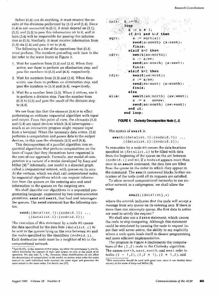
FIGURE 4. Cholesky Decomposition Node (I, J)

The syntax of await is

await((datalist.l):(nodeid.l)) . . . ((datalist.I):(nodeid.I));

Its execution by a node ND causes the data locations specified in (datalist. i) to be filled with data from the beginning of the queue on the arc between (nodeid. i) and ND. If a nodeid appears more than once in an await command, the data lists are filled from the queue in the order in which they appear in the command. The await command blocks further execution of the node until all its requests are satisfied.

To allow several computational networks to use another network as a subprogram, we shall allow the usage

await( (datalist) ,a)

where the asterisk indicates that the node will accept a message from any queue on its entering arcs. If there is more than one nonempty queue, the first data to arrive are used to satisfy the request.3

We shall also use a finis statement, which causes the node to stop computing. Although this statement could be simulated by causing the node to request input that will never arrive, the ability to say explicitly where a node quits lends itself to clearer programming and more efficient implementation.

The program in Figure 4 implements the computations of the ( I , J ) node in the Cholesky algorithm. The names north, east, south, and west refer to

nodes (I - l,J), (1,J + I), (I + l,J),and

a This convention should be used with great care. since it can destroy determinacy in the sense of Karp and Miller 191,

August 1985 Volume 28 Number 8 Communications of the ACM 843


( I , J - 1 ), respectively. In studying this program, the reader may find it helpful to compare its execution for the node (3,~) with the list of operations given above.

There are four comments to make about this algorithm--two i.echnical points and two general observations. First, there is no exit from the control loop of the algorithm except through the finis statements in the sections labeled sqrt, cdiv, and rdiv. Every matrix node will take one of those three exits. The other tech- nical point is that we have placed dummy nodes, called sinks, at the southern and eastern borders of the computational network. The progra:m for the sinks on the south might read

loop await(an:north);

end loop;

with a similar program for the eastern sinks. They sim- plify the program by absorbing messages that are sent by the boundary nodes. Without them the elimination block would have to be coded

elim: await(an:north)(aw:west); a := a - an*aw; if I#n then send(an:south); fi; if J#n then send(aw:east); fi;

with similar modifications for the other blocks. We shall use sinks throughout the programs in this article without providing explicit code for them.

The two general observations are central to our approach to parallel matrix computations. First, the algorithm requires no external synchronization; the flow of data alone is enough to ensure that the computations get done in the proper order. This is of course the es- sence of Treleaven, Brownbridge, and Hopkins’ defini- tion of a data-flow algorithm [21], and what we have shown with the Cholesky algorithm is that at least one matrix computation can be so implemented. In particular, one need not arrange for items required by a node to arrive at it synchronously, as one must do when designing systolic arrays.

The second observation is that the algorithm could be coded directl;y from the network in Figure 2 without reference to fronts of computations as in Figure 3. This means that once the data-flow pattern has been deter- mined an algorithm may be coded independently of the considerations that show it to be globally a good algorithm. Although a parallel algorithm must ultimately stand or fall on its ability to exploit the parallelism in a process, the sl?paration of coding from the analysis of the algorithm makes the former simpler (and some- times the latter more difficult). The examples of the next section will illustrate this point.

We shall di,scuss implementation issues more fully in Section 5. However, we wish to point out here that there are advantages to distinguishing between the computational nodes and the processors on which they

reside. In our implementation, nodes are processes on a network of processors (assumed to be general-purpose, sequential processors of sufficient capacity to run programs like that in Figure 4). The arcs in the network represent communication channels between the processors, and two processors so connected are said to be adjacent.4 Nodes from the computational network may be assigned arbitrarily to processors, subject only to the restriction that connected nodes are assigned to adjacent processors.

The fact that more than one computational node may be assigned to a processor gives us the flexibility to handle problems in which there are more nodes than processors. For example, consider the computational network associated with the Cholesky decomposition, and assume that a 6 X 6 network is to be implemented on a 4 x 4 grid of processors. One way to assign nodes to the processors is to partition the matrix in blocks. A typical partitioning is given in Figure 5. Another way is, to reflect the computational network off the southern and eastern boundaries of the grid of processors. This would lead to the assignments in Figure 6.

If the north and south boundaries of the grid of processors are connected and likewise the east and west, so that the configuration becomes a torus, the assignments, in Figure 7 are possible. Other topologies of processors (e.g., a Klein’s bottle) will result in different node assignments. A very attractive feature of the data-flow approach is that through all these changes of topology and assignments, the node programs remain the same.

There is another important consequence of our ability to assign nodes to processors in any way that assigns neighboring nodes to adjacent processors. Namely, it is possible to assign the nodes of an arbitrary network to a. single processor. This means that, given suitable systems support, preliminary debugging of data-flow algorithms can be done on an ordinary sequential computer.

The Cholesky algorithm also illustrates the econom- ies that can result from distinguishing between nodes and the programs that run them. It is evident that in the parallel Cholesky algorithm the state of the program is specified by the node identifier ( I, J ) and the current value of the variables a and k. If the program is compiled into reentrant code, this local information can be saved whenever the node executes an await statement, and other nodes can use the program. Thus, although some processors in the above figures contain as many as four nodes, no processor need contain more than one node program.

4. THREE EXAMPLES Data-flow techniques have wide applicability in matrix computations. H. T. Kung [13] cites systolic algorithms for matrix multiplication, the computation of LU and QR factorizations, and the solution of triangular systems (see also [z]). Recently, new data-flow algorithms

‘By convention a processor is adjacent to itself.

044 Communications of the ACM August 1985 Volume 28 Number 8


(1,1H1,2) (1,3H1,4) (13) (176) @,lM2,2) 63)(.W) cz5) GG) (3,WG’) (3,3H3,4) (3,5) (396) (4,1M4,2) (4,3N4,4) (495) (496)

(5,1M5,2) (5,3N5,4) (5s) W) (fLlN62) 1’364 (6.5) em

FIGURE 5. Assigment by Blocks

(f,V (12) (13X1 $1 (1,4X1 !5)

(ZV Fv) (2,3X2,6) GYPS)

(3vll (321 (3,3M3,6) (3,4U3,5) (691) (62) WXS,S) 6WS5)

(4,V (42) WM46) (4,4X4,5) (5.1) (5.21 15.3N5.61 (5.4X5.51

FIGURE 6. Assignment by Reflection

(l>lX1,5) (1,2X1 96) (1831 (1*4) (5,1X5,5) WYW (593) (594)

P,w3 (2,2N2,6) (2,3) e4) (6,WW GWW (6,3) (694) _

(3,1M3,5) KWW) (393) (3,4)

(4,vl4,5) KW,6) (4,3) (4,4)

FIGURE 7. TONS Assignments

have been developed for the solution of Toeplitz systems [5], the solution of the symmetric eigenvalue problem [4], and the computation of the singular value decomposition [6]. The purpose of this section is to give three other nontrivial examples of data-flow algorithms-algorithms for the solution of a triangular matrix Liapounov equation, the computation of a congruence transformation, and the iterative triangularization of a non-Hermitian matrix by Schur transformations. Taken together these algorithms furnish most of the wherewithal to implement a well-known, numerically stable method [l] for the solution of a general matrix Liapounov equation. Individually, the algorithms exem- plify different aspects of data-flow methods in numerical linear algebra. The first algorithm illustrates the use of multiple networks and the delayed use of arriving data; the second, the use of communication networks to simulate missing connections between processors; the third, how computational nodes need not necessarily be associated with individual matrix elements.

The computational networks for the first two examples will turn out to be square grids or toruses. As in Section 2, a node will be identified by its position ( I , J ) in the network. We adopt the convention, intro-

duced in Section 3, that north, east, south, and west, used in the node program for node ( I, J), are abbreviationsfornodes (I - l,J), (1,J + l), (I + l,J),and (1,J - l).Node (1,J) itselfwill be denoted by home. Comments in programs will be surrounded by the delimiters /* and */.

In principle, a data-flow algorithm is represented by a single computational network. In practice, as we shall see in the first example, certain subnetworks may perform such diverse functions that it is convenient to regard them as separate networks, with distinct names, which are linked by send and await commands. We shall adopt the convention that a node in one such network may reference another in a different network by the notation (net. name). (nodeid).

4.1 Solution of a Triangular Matrix Liapunov Equation In this example, we develop a data-flow algorithm for solving the matrix equation

AX + XB = C, (1)

where A is a lower triangular matrix and B is an upper triangular matrix, both nonsingular of order n. The element Ci, computed from (1) is

Clj = Jk aikxkl + i bljxil, k=l I=1

(2)

from which it follows that

i-l j-1

~1, - zl aikxkj - z, bljxil

xi, = a;i + bj, (3)

Because Xii depends only on Xkj(k < i) and Xi/ (I < j) the x’s can be computed sequentially from (3), say in the order x I,, x21. x127 x31, x22, x13. . .

A data-flow algorithm implementing (3) may be derived by considering the information required by node ( I, J ) to compute xll. For I > J this is

all! . . , al,/-I: alIs aJ./+l, , aJ,J-1, all

h/, . . , 4-w b,\

Xl/, f 1 X/-l./, X//Y x/+1./* . . . 3 Xl-1.1

x11. . . 9 q-1.

(41

On the other hand if I <J the information required is

afl, . . , al,I-1, alI bl,, . . , bl-1.1: h\, br+l.,, . . . , b/-l.,, bn Xl/, . . . , Xl-l.1

(5)

x11. f 7 XJ,J-1, XII, xJ.J+l, . , Xl./-1.

The x’s present no problems; once an x has been computed, it may be passed east and south, where in due course it will end up at the nodes that require it. On the other hand, the a’s in (4) are not as easily dealt with; for those which precede al, in the list are west of node ( I, J ), while those which follow are to the east.

August 1985 Volunle 28 Number 8 Communications of the ACM 645


Node pass-e.(I,J) Node pass+s.(I,J)

for k:=l to min(I,J-?l hop for k:=l to min{I-1,J) hop await(aw:west); await(bn:north); s&d(aw:solve.hogne) send(bn:sol&.home)

(aw:east); (bn.south); end loop; ‘j, __ ),. (4nd~ loop; if x,2 J then ‘aL ,:,;.b~~n-1,2-- I, .if I S J then ’ n

send{ a i east ) ; nl ...‘si.J,5,‘ ” 1 ~‘c .p P::“,~ ~ ‘, ;;.I send(b:south);

end if; s -._ ,.,:;; I) I'VE*,. j .. end if ; .finis; n,_^b n.l .',,,, ‘/ .' _'b , , finis;

_n (_ ‘Node pass-w.(T,J) _" :,.,..;,‘:li' Node passln.(I,J)

:n ," :,* if ISJthen send(b:solve.pame)

( a : w&#st ) ; (b:aorth)j : for k:=f+l to! J, loop

await(bs:soiith); send(bs:[email protected])

(ae:west) ; (bs:north); and laopi (- .s ,n end loop;

end ‘If; ,,,

I- +,_.,j _nI. n._ eqd: if i finis;

-# ; : .I,,; ) ; : ('_.‘ ~ *, - _ _'i. finis ; ji :en ' /',

FIGURE 8. Solution of a Triangular Liapounov Equation

Similarly, the b’s which precede bll in (5) are to the north of node ( I , J ) , while those which follow are to the south. In (either case, data must converge on node ( I , J ) from three different directions.

One way to circumvent the difficulty is to construct four networks to move the a’s and b’s around. Node programs for the node ( I , J ) are given in Figure 8. Initially, the nodes pass-e. ( I, J ) and pass- w. ( I, J ) contain the value aIl, and the nodes pass- n . ( I , J ) and pas s-s. ( I , J ) contain the value bl,. The node program for pass-e passes along all the a’s to the west of it before passing on its own value. As it receives each a it also passes it to the ( I, J ) node of the solve network, which implements (3). The node program for pass-w passes to the west; but this time it passes its own a first, so that it will arrive in the proper order. The programs pass-s and pass-n pass b’s south and north in a similar manner.

The actual computation is done in the network solve, whose nodes contain the cl/. The node program for solve. ( I , J ) is given in Figure 9. The first loop for the case I L J computes

I-1 Cl1 - c hkxkl + bkJXlk). (6)

k=l

The values of a and b come from the networks pass-e and pass-s, respectively. In the second loop, values of a from pass-w are used to subtract cL:i aI&/ from the current value of x. The final value of x is computed by dividing by all + b/t and is sent east and south to be used by other nodes. The colon in (4) indicates where the a’s come from: those to the left from pass-e, the

rest from pass-w. The computation for the case I < J is analogous.

Although the computations in this algorithm are forced to occur in their proper order, the arrival of data for a node is not synchronized with its use in the computation. For example, if I 2 J, the number ajl arrives at node solve. ( I, J ) almost immediately; however, it is not used until after (6) is computed in the first loop. This illustrates the importance of queueing data in a node in the order of its arrival. In this computation, it is obvious that the length of the queue is bounded by n. However, in more complicated algorithms, the memory requirements of a node may not be obvious.

4.2 Congruence Transformations The problem here is to compute a congruence transformation of a matrix A; that is, given two n x n matrices A and Q, compute C = QAQT. We will break the computation into two parts: B = QAT and C = QBT. The computation will be done by a network named tong with nodes labeled ( I , J ) as usual. We shall assume that node tong . ( I, J ) contains the numbers 911 and all and construct a subroutine, called qat, to compute b,, and store it in the same node. A second call to the subroutine with the data 911 and b,t will then produce Cl\.

The congruence algorithm may be derived by considering the equation

hk = ,$ 911aW (7l

If we generate each b,k by updating partial sums slk, the



-‘ \p, : X :e c; j .,n .,.. j

2.

if I L J then ,, -5, _* &se :I~: L*sU; */ for k:= 1 to J-1 loop jor.k:& Co I-1 loop

await(a:pass,e.home) await(a:pass,e.home) (xa:&orth) (x’a:north) (b:pass-s.home) (b:pass-s.home) (xb:west); (xb: west);

X := x - a*xa - b*xb X := x - arxa - b*xb; send(xa:so:th) send(xa:south)

(xb:east); (xb:east); end loop; end JOOpi for k:=J to I--l loop for k:=I to J-l loop

await(a:pass-w.home) await(b:pass,n.home) (xa:north); (xb:west);

X := x - a*xa; X := x - b*xb; send(xa:south); send(xb:east);

end loop; end loop; await(a:pass,w.home); await(a:pass,e.home) if I = J then (b:pass_n.home);

await(b:pass-n.home); X := x/(a + b)j else send(x:east)

await(b:pass-s.home); (x:south); end if; end if; X := x/(a -t b); finis; send(x:east)

(x:south);

FIGURE 9. Solution of a Triangular Liapounov Equation Node solve (I, J)

result is a series of updates of the form

Slk := Slk + @JakJ. (8)

This formula suggests that the updates be performed by streaming the Ith row of partial sums and the ]th column of a’s past node tong . ( I , J ) and performing updates according to (8). Since each node must see all the s’s in its row and all the a’s in its column, it is natural to configure the network,as a torus and allow the s’s and a’s to move cyclically around the torus.

Figure 10 contains an implementation of this scheme, with provisions for starting and storing partial sums. The subroutine qat is driven by a loop whose index k assumes values

I + 1, 1+2, . . . . n, 1, . . . . I. (9)

The algorithm has four phases, depending on where k is in the sequence (9).5

k=I+l,...,J-1 await and update partial sums ~11, . . , ~1.1-2. k=J start partial sum so.!-I. k=J+l await and store partial sum SI/. k = J + 2, . . . , I await and update partial sums SI,~+I, . . , SI.I-~.

’ Expressions like I- 1 or / + 1 are to be interpreted as the entry before or after 1 in (9).

The computations in a node proceed in bursts. In phase one above, the node ( I, J ) must wait roughly J - I steps for SII to arrive, after which it processes Sll, . . . . 51.1-2 and then sI,l-1 in phase two. In phase

subroutine qat(q,a,b) for kk:=I to n+I-1 loop

k := mod(kk,n) -I- 1; if k#J then /* update */

awaitwest( S := s + q+a;

else /*start a partial sum */ S := q*a;

end if; if k=mod(J,n)+l then

/* store completed partial sum */ b := s;

else /t transmit partial sum */ sendeast(

end if; sendnorth( if k#I then awaitsouth(

end loop

end qat;

qat(q,a,b); wt(q,b,c);

FIGURE 10. Congwnce Transformation Node Cong (I, J)



loop if J=x-I than

await(x,net:*); else

await(x,,net:east) j . end if if J=l then .

send (X net. home ) else

send (X net : west) end if

end 104pj

FIGURE 11. Nude torus-east (I, J)

three, the node must wait II steps for sq, which is generated in the node just east of it, to get around the torus, after which the rest of the partial sums are processed in phase four. The total number of time steps on a torus- connected grid of n2 processors would be 3n - 2.

While a node is hung up waiting for a partial sum, it cannot transmit the elements of A. This suggests that the algorithm may perform badly, as nodes await data not immediat’ely forthcoming or that the algorithm could even deadlock. In fact neither happens, but this is not obvious either from the derivation of the algorithm or from the code in Figure 10.

For communication we have used subroutines, like sendeast and .awaitwest. instead of the primitives send and await. The reason for this is that the subroutines make it easy to implement the algorithm on processor networks that are grid-connected but not torus- connected. For example, on a grid-connected set of processors we would create a second computational network, torus-east, that t.akes a data item from a node in another network at the eastern boundary of the grid, passes it west until it arrives at the western boundary of the grid, and then sends it back to the corresponding node of the original network. A node program for tlorus-east _ (I , J) is given in Figure 11. Both the data and the name of the network are passed to torus-east, the latter so that torus- east can pass the information back when it has arrived at the western boundary. Note the use of “*‘I to indicate that the message can come from any network.

Given the torus-east network, the sendeast subroutine can be coded as

subroutine sendeast if Jr% then

send(x:east); else

send(x,cong:torus-east.home); end if;

end sendeast;

Programs for awaitwest. sendnorth, awaitsouth, and node torus-north. ( I , J ) on a grid of processors are similar.

4.3 Iterative Reduction to Triangular Form In this example, we discuss the data-flow implementation of an algorithm for reducing a square matrix of order n to upper triangular form by means of Schur rotations [20]. Since the derivation of the algorithm is not germane to this article, we shall give only an overview of the operations involved.

The basic operators are Schur rotations, which are specified by two complex numbers c and s satisfying

ICI2 + ISI’ = 1. IW

The rotations originate in 2 X 2 diagonal blocks of the matrix, say in

[,p::, UEj. (11)

Once generated, a rotation must be applied to the rows and columns associated with the submatrix that generated it. For the rotation generated by (ll), the operations are

1. Uik := C&k + SUi,k+l

ai.k+l := -S&k + h&,k+l i = 1, 2, . . , n,

(12) 2, aki := cak, + sak+lvj

ak+i,j := -sakj + Cak+lj j = 1, 2, . . . , n.

The parallel implementation of this algorithm goes as follows. The rotations for all diagonal blocks (11) with k odd are generated simultaneously. These rotations are then passed to the four points of the compass. The rotations moving east and north will intersect in 2 x 2 blocks of the form

(13)

where i and j are odd and i c j. The two rotations are applied to this block, the northbound rotation according, to (12.1) and the eastbound according to (12.2). Simi- larly, the rotations moving west and south will intersect in 2 X 2 blocks of the form (13) with i and j odd andi>j.

The progress of the rotations away from the diagonal of the matrix is illustrated in Figure 12. In the first matrix, the rotations are generated in the 2 x 2 blocks labeled with a 1; in the second, the rotations are applied to the blocks adjacent to the diagonal; and in the third, to the blocks two elements farther out. At this point, it is possible to generate rotations in the even blocks; that is, blocks of the form (11) where k is even. These rotations, designated 2 in Figure 12 follow the first batch of rotations away from the diagonal of the matrix, until at the fifth step a third batch of rotations can be generated in the odd diagonal blocks. Note that there are places on the boundary where the single even rotations are applied to only two elements.

A data-flow algorithm for this procedure is rather easy to write. It is natural to associate nodes with 2 x 2 blocks of the matrix as in Figure 13, where the elements of the matrix are denoted by X. To allow rota-

648 Communications #of the ACM August 1985 Volume 28 Number 8

l.llxxxxxx 4.~22~~~11 llxxxxxx 2xx22xll xxllxxxx 2xx22xxx xxllxxxx x22xx22x xxxxllxx x22xx22x xxxxllxx xxx22xx2 xxxxxxll llx22xx2 xxxxxxll llXXX22X

2.xxllxxxx 5.33x22xXx xxtlxxxx 33~~x22~ Ilxxllxx ~~33x22~ lfxxllxx 2x33~~~2 xxllxxll 2~~x33~2 xxllxxll ~22x33~~ xxxxllxx ~22~~x33 xxxxllxx ~~~22x33

3. xxxxllxx 6. ~~33x22~ x22xllxx ~~33~~x2 x22xxxll 33~x33~2 xxx22xll 33xx33xx 11x22xxx xx33xx33 llxxx22x 2x33~~33 xxllx22x 2~~x33~~ xxllxxxx ~22x33~~

FIGURE 12. Propagation of the Rotations

the odd nodes. Code for an odd node is displayed in Figure 14. In it 1 * r * 1 is used as a generic symbol for a rotation, and ne, se, SW, and nw denote the nodes to the northeast, southeast, southwest, and northwest. The core of the computation is In the cases 1 I I < J < Nandll J < I < N. Herethenodewaitsfor matrix elements from the even nodes and rotations from its neighboring odd nodes, applies the rotations, and passes the matrix elements back to the odd nodes and the rotations on to the even nodes. The other cases take care of diagonal nodes, where rotations must be generated, or boundary nodes that must be treated specially.

This example differs from its predecessors in several respects. In the first place, the algorithm requires a more highly (though still locally] connected network of nodes than the algorithms for the Liapounov equation and congruence transformations. The nodes are associated with a computation (the application of a rotation to a z x 2 block) rather than an element within a matrix. Finally, the computations are tightly synchronized-so much so that the algorithm could easily be implemented as a systolic array.

5. IMPLEMENTATION

tions to pass from node to node, the nodes with even indices are connected in a grid, as are the nodes with odd indices. Even nodes are connected diagonally to odd nodes to allow the matrix element that is between them to pass back and forth.

The data-flow algorithm consists of two computational networks, one for the odd nodes and another for the even nodes. It is assumed that initially the even nodes contain the matrix elements that surround them and start the computation by sending the elements to

One advantage of data-flow algorithms is that they require little systems support. The purpose of this section is to sketch a node communication and control system (NCC) that sequences the execution of nodes on a processor and mediates communications between nodes. A version of this system has been implemented on the ZMOB [18], a parallel computer under development at the University of Maryland.

A copy of NCC resides on each processor of the network that implements the data-flow algorithm. The processors are assumed to be general purpose, sequential processors with their own, unshared memory (on the ZMOB a processor board contains a Z80 micropro- cessor, 64K bytes of memory, an Intel 8232 floating- point processor, and serial and parallel ports). As in

(0,s) (0,4) (0,6) x X

I x X I x X I x


FIGURE 13. Computational Network for the Jacobi-Schur Algorithm



loop elsif J=N then if I,(I<J.<N then

await(ane:even.nej awaft(anw:eyen.nw)

(asw:eyen.sw) (ase:even.se) (rw:west); (asw:even.sw) apply.the r~,tation; (anw:even.nw) send(anw:ev&n.nw) (rw: west) (atiW:eVCin.sw)j

(rS:SOUth)i ./ e ‘3 elsif l<I=J then apply t:he rotati&&~;b r>;:;q, ""1. ge await(ane:even.ne) send ( ane : even . ne 1 ;~“‘3*~~:~:~-~,’ ‘:;,:, (ase:even.se)

(ase:even.se),. -:~ ,‘,:“,~‘.“. (asw:even.sw) (asw:even.ew) )*’ ” :: (anw:even.nw) x .;‘

(anW:e~en.nw)j generate and dpply the

(rw:east) n, -.

FIGURE 14. Jacobi-Schur Reduction Node odd (I, J)

Section 3, we say that processors that can communicate directly with one another are adjacent and assume that the computational nodes for the algorithm in question have been mapped onto processors in such a way that adjacent nodes. lie on adjacent processors.

NCC is composed of a number of pieces, which are shown in Figure 15. We shall discuss each of them in turn.

Structures Node Structtwes. A node in NCC is specified by

three items: 1. A node identifier, which must be globally unique. 2. A pointer to a program that implements the node. 3. An auxiliary structure containing variables local

to the node.

The node programs are reentrant, so that they can be used by several. nodes. The auxiliary structures are

necessary to prevent variables local to a node from being overwritten by other nodes using the program.

The Node Table. The node table is an array containing the node structures for all nodes resident on the processor.

The Arrival List. This is a queue of all data that have arrived at the processor as a result of send commands. Each message is accompanied by a source-node identifier and a destination-node identifier.

The Want List. This is a list of pending await requests for data by nodes on the processor. Each entry consists of a source-node identifier, a destination-node identifier, and a pointer indicating where the data are to be placed.

Primitive Functions equal. This function takes two node identifiers as

arguments and returns true if they are the same.



Otherwise it returns false. The function is used to match messages with their destinations.

address. This function takes a node identifier as an argument and returns the address of the processor on which it resides. It is used by the output process to direct messages to the appropriate processors.

send. This function is used by a node to transmit data to other nodes. Its syntax was described in Section 3. The function communicates with other processors via the output process.

await. This function is used by a node to request data. Its syntax was described in Section 3. It causes the request to be entered onto the want list and the node to return control to NCC.

finis. This function is used by nodes to an- nounce to the system that they are finished executing. It causes control to return to NCC, after which the node is ignored by the control process. The finis function is included for efficiency. As we pointed out in Section 3, its effect can be simulated by executing an await with data that will never arrive, but this does not re- lieve the control process of the overhead of monitoring the node.

Processes Nodes. These are the raison dZtre for NCC. The Output Process. This process is invoked by the

send command. It determines the destination processor for each message, establishes communication with the input process on that processor, and transmits the message.

The Znpuf Process. This process accepts messages from other processors and places them on the arrival list.

The Control Process. This is the heart of the system. Its operation is sketched in Figure 16. Essentially, the control process on each processor loops endlessly trying to satisfy the requests on the want list with itemsin the arrival list. If it finds a node that has no requests pending, then it awakens the node by calling its node pro-

I. Structures a. Node structures b. The node table c. The arrival queue d. The want list

II. Primitive functions a. equal b. address c. send d. await e. finis

Ill. Processes a. Nodes b. The output process c.The input process d. The control process

FIGURE 15. Components of NCC

loop cyci.icaIly through the node table r;itisfied := true; loop thrbugh the want list

need: if the current entry in want list is from the current node then

loop through the arrival list

if the current arrival entry matches the want entry then

transfer data from the arrival queue and remove the entries from the want list and the arrival queue; leave need;

end If; end loop; satisfied := false;

need: end if; end loop; if satisfied then

awaken the current node; end if;

end loop;

FIGURE 16. The Control Process

gram at the point where the node last relinquished control.

There are several points to be made about this system. In outline it is quite simple, and in our experience it remains simple when one descends to the details. Our implementation of NCC is in the programming language C, which allows a natural description of the structures in the system. The fleshing out of Figure 16 requires little more than standard techniques for ma- nipulating the lists involved. The details of the input and output processes will depend on the way the network of processors communicate; for the ZMOB they were relatively easy to code. The major difficulties con- cern global problems of initialization (assigning nodes to processors and defining the address function), monitoring algorithms (taking snapshots of processor activi- ties to identify bottlenecks), and collecting results. We are currently designing a table-driven loader, which will sit on a single processor and perform some of these functions.

In a software implementation of NCC, communication overhead will dominate the calculations in the short node programs presented in this article. Fortu- nately, NCC itself has a great deal of inherent parallelism, which can be used to speed up the system. In particular, the input, output, and control processes



could reside on a triad of separate, dedicated processors that communicate by a shared memory. Moreover, if these processors are sufficiently fast, one incarnation of NCC could serve several slower processors that are de- voted solely 1.0 executing nodes. The precise features of an efficient hardware implementation must remain ob- scure until experiments with real algorithms show where the bottlenecks and tradeoffs lie; but we believe that the software version of hJCC has already laid the ground for informed speculation.

There are rnany possible extensions to NCC. One that we feel will be essential for computations with large dense matrices is the ability to broadcast data to several processors. For example, if a matrix is stored one column to a proc;essor, then the implementation of many common matrix algorithms will require that a single column be transferred to a set of different columns. Technically, this can be done by a network whose nodes pass on the column one element at a time; however, the cost to a node is a full NCC communication cycle for each element. The alternative is to define a path along which all the nodes shake hands before passing the column from node to node in burst mode.

6. CONCLUSIONS In this article, we have presented a way of organizing parallel matrix computations so that complicated algorithms can be implemented with comparatively simple programs and little global control. We have shown by citation and example that the set of matrix algorithms that can be so implemented is nontrivial and important. We have also made a case for the practicality of the approach by describing a simple system that supports data-flow algorithms on a network of processors. In this last section, we will make some general observations about the data3low approach.

Regarding programming languages, our data-flow algorithms req-uire little more ihan a standard language for their imple-mentation. This is surprising in view of the current interest in languages for parallel computation; but the paradox can be resolved by observing that a node program is a description of a local computation, not of a global (algorithm. In Section 4, we leaned heav- ily on verbal descriptions to communicate our algorithms, and it is difficult (though not impossible) to reconstruct the algorithms from the node programs. Thus, the data-flow approach does not obviate the need for research into systematic ways to describe parallel algorithms. However, we feel that an attempt to devise a formal language for parallel matrix computations may well be premature; too few matrix algorithms have ac- tually been cast in parallel form to provide a suitable base for general izing.

The main drawbacks of the data-flow approach are that it makes it easy to design bad algorithms and difficult to analyze igood ones, This is clear from our examples, where the potential for deadlock or data conges- tion cannot be lightly dismissed. Against this must be set the fact that data-flow algorithms lend themselves to an experimental approach; since node programs are

852 Communications of the ACM

easy to write, one can code an algorithm and see how i-: runs.

Another problem arises from the fact that we have effectively been multitasking nodes on processors. In a processor-rich environment, where only a few nodes reside on any one processor, scheduling presents few problems. However, with greatly oversized problems, which cause many nodes to be assigned to each processor, some attention must be paid to the order in which nodes are inspected by the NCC control process. Al- though preliminary investigation of the Cholesky algorithm of Section 13 suggests that it runs well under a variety of scheduling algorithms, this is an open research area.

The main advantages of the data-flow approach are that the node programs are independent of the relation between the size of the problem and the number of processors, are independent of the precise assignment of nodes to processors, and are independent of the precise physical adjacencies and physical communication structures between processors. Thus, it is easy to inves- tigate the impact of changes in parallel machine architectures on a given algorithm, or to study the perform- ance of an algorithm as the ratio of problem size to number of processors varies. The fact that the same node program can be used in a variety of situations also means that it is relatively easy to transfer algorithms from one system to another.

It is hard to overstress the convenience of being able to debug data-flow algorithms on sequential computers. We first brought up the node communication and control system, running the Cholesky algorithm on a single processor, before the multiple processor ZMOB system was available. All that was needed to make the system and the algorithm work on the ZMOB was to rewrite the NCC input and output processes to interface with the communication devices of the ZMOB.

Although we have been concerned in this article with algorithms from numerical linear algebra, the data-flow approach is not restricted to them. In describing the node communication and control system, we made no references to matrices or matrix algorithms. Thus, the system can be used to implement parallel algorithms for other tasks.

REFERENCES 1. Bartels. R.. and Stewart. G.W. Algorithm 432: The solution of the

matrix equation AX - BX = C. Commun. ACM 15, (1972). 820-826. 2. Bojanczyk, A., Brent, R.P., and Kung, H.T. Numerically stable solu-

tion of dense systems of linear equations using mesh-connected processors. SIAM. J. Sci. Stat. Cornput. 3. (1984) 95-104.

3. Brent. R.P.. and Luk, F.T. Comoutine the Choleskv factorization . I

using a systolic architecture. In Proceedings of the 6th Australian Compufer Science Conference, 1982, 295-302. Brent, R.P.. and Luk, F.T. A systolic architecture for almost linear- time solution of the symmetric eigenvalue problem. Tech. Rep. TR 82-525, Dept. of Computer Science, Cornell University. Ithaca, NY, 1982. Brent, R.P.. and Luk. F.T. A systolic array for the linear-time solution of Toeplitz systems of equations. J VLSI Ccmput. Sysf. I, (1983). l-22.

Brent, R.P., Luk. F.T., and Van Loan. C. Computation of the singular value decomposition using mesh-connected processors. Tech. Rep. TR 82-528. Dept. of Computer Science, Cornell University, Ithaca, NY, 1983.

August 1985 Volume 28 Number 8


7. Dennis, 1. Data flow supercomputers. IEEE Comput. 13, (1980). 48-56. 6. Heller, D. A survey of parallel algorithms in numerical linear alge-

bra. SlAM Rev. 20, (1978), 740-777. 9. Karp, R., and Miller, R. Properties of a model for parallel computa-

tions: Determinacy, termination, queuing. SIAM 1. Appl. Math. 24, (1966), 1390-1411.

10. Kuck, D.J., Muraoka. Y., and Chen, S-C. On the number of operations simultaneously executable in Fortran-like programs and their resulting speedup. lEEE Trans. Comput. C-21, (19721, 1293-1310.

11. Kuhn. R.H. Optimization and interconnection complexity for: Paral- lel processors, single-stage networks, and decision trees. Rep. UIUCDCS-R-80-1009, Computer Science Dept., University of Illinois at Urbana-Champaign, 1980.

12. Kung. H.T.. and Leiserson. C.E. Algorithms for VLSI processor arrays. In Introduction to VLSI Systems (by C. Mead and L. Conway). Addison-Wesley, Reading, Mass.. 1980. pp. 271-292.

13. Kung. H.T. Why systolic architectures? IEEE Comput. 15, (1982), 37-46.

14. Kung. S.Y. VLSI array processors for signal processing. In MIT Con- ference on Advanced Resenrch on I. C., Cambridge, Mass., 1980. Cited in [15].

15. Kung, S.Y.. Arun, K.S.. Bhaskar Rae. D.V.. Hu. Y.H. A matrix data flow language/architecture for parallel matrix operations based on computational wavefront concept. In VLSI Systems and Computntion. H.T. Kung. B. Sproull, and G. Steele, Eds. Computer Science Press. Rockville, Md.. 1981, pp. 235-244.

16. Luk. F. Computing the singular-value decomposition on the ILLIAC IV. ACM Trans. Math. Softw. 6, (1980), 524-539.

17. O’Leary. D.P.. and Stewart, G.W. A proof of determinacy for a model of data-flow computation. Tech. Rep. TR-1456. Dept. of Computer Science, University of Maryland, 1984.

16. Rieger, C. ZMOB: Hardware from a user’s viewpoint. In Proceedings of the 1EEE Computer Society, Conference on Pattern Recognition and Image Processing, 1981, pp. 399-408.

19.

20.

21.

Stewart, G.W. Introduction to Matrix Computations. Academic Press, New York, 1974. Stewart, G.W. A Jacobi-like algorithm for computing the Schur decomposition of a non-Hermitian matrix. Computer Science Tech. Rep. TR-1321, University of Maryland, 1983, SIAM 1. Sci. Stat. Com- put. to appear. Treleaven, PC. Brownbridge. D.R.. and Hopkins, R.P. Data-driven and demand-driven computer architecture. Comput. Surv. 14, (1982), 93-143.

CR Categories and Subject Descriptors: G.l.O[Numerical Analysis]: General--par&-l algorithms; G.1.3[Numerical Analysis]: Numerical Linear Algebra; Cl.2 [Processor Architectures]: Multiple Data-Stream Architectures (Multiprocessors)-parallel processors; D.4.l[Operating Systems]: Process Management-concurrency

General Terms: Algorithms Additional Key Words and Phrases: parallel algorithms, matrix algo-

rithms, data-flow synchronization. MIME networks

Received Z/84; revised 10/84; accepted Z/85

Authors’ Present Addresses: Dianne P. O’Leary and G.W. Stewart, De- partment of Computer Science, University of Maryland, College Park, MD 20742.

Permission to copy without fee all or part of this material is granted provided that the copies are not made or distributed for direct commer- cial advantage, the ACM copyright notice and the title of the publication and its date appear, and notice is given that copying is by permission of the Association for Computing Machinery. To copy otherwise, or to republish, requires a fee and/or specific permission.

SUBSCRIBE TO ACM PUBLICATIONS Whether you are a computing novice or a master of your craft, ACM has G publication that can meet your individual needs. Do you want broad-gauge, high quality, highly readable articles on key issues and major developments and trends in computer science? Read Communications of the ACM. Do you want to read comprehensive surveys, tutorials, and overview articles on topics of current and emerging importance: Computing Surveys is right for you. Are you interested in a publication that offers a range of scientific research designed to keep you abreast of the latest issues and developments? Read Journal of the ACM. What specific topics are worth exploring further? The various ACM transactions cover research and applications

in-depth-ACM Transactions on Mathematical Software, ACM Transactions on Database Systems, ACM Transac- tions on Programming Languages and Systems, ACM Transactions on Graphics, ACM Transactions on Office Information Systems, and ACM Transactions on Computer Systems. Do you need additional references on computing? Computing Reviews contains original reviews and abstracts of current books and journals. The ACM Guide to Comput- ing Literature is an important bibliographic guide to

ing literature. Collected Algorithms from ACM is a collection of ACM algorithms available in

printed version, on microfiche, or machine- readable tape.

For more information about ACM publications, write for your free copy of the ACM Publications Catalog to: The Publications Department, The Association for Computing Machinery, 11 West 42nd Street, New York, NY 10036.


data-flow algorithms for parallel matrix computationsoleary/reprints/j19.pdf · parallel matrix...

Documents