dario pozzoli - connecting repositories · the transition to work for italian university graduates...

WORKING PAPER 08-8

Dario Pozzoli

The Transition to Work for Italian University Graduates

Department of Economics ISBN 9788778823236 (print)

ISBN 9788778823243 (online)

The Transition to Work for Italian UniversityGraduates

Dario Pozzoli∗

Aarhus School of Business, Denmark

April 18, 2008

Abstract

This study investigates the hazard of first job for Italian graduates. The anal-ysis is in particular focused on the transition from university to work, taking intoaccount the graduates’ characteristics and the effects relating to degree subject.It is used a large data set from a survey on job opportunities for the 1998 Italiangraduates. The paper employs a non parametric discrete-time single risk modelsto study employment hazard. Alternative mixing distributions have also beenused to account for unobserved heterogeneity. The results obtained indicate thatthere is evidence of positive duration dependence after a short initial period ofnegative duration dependence. In addition, competing risk model with unob-served heterogeneity and non parametric baseline hazard have been estimated tocharacterize transitions out of unemployment.

JEL Classification: J64; C41; C50.Key words: discrete time survival model; unobserved heterogeneity, compet-

ing risk model.

∗Corresponding Author Address: Department of Economics, Aarhus School of Business, Prismet, Silkeborgvej 2, DK-8000 Aarhus C,

Denmark. Email: [email protected]. I thank Lorenzo Cappellari, Michael Rosholm, Peter Jensen, Michael Lechner and Pierpaolo Parrotta

for comments and an anonymous referee for very useful suggestions. Financial support from the Aarhus School of Business is gratefully

acknowledged. All errors are my own responsibility.

1

1 Introduction

The problem of high unemployment rates for young people has been featuring topof public policy discussion and of government policy-making in Italy in recent years.The difficulties of getting a job for young people are so relevant that we can consideryouth unemployment as a distinct and stable feature of Italian unemployment. Theoutstanding youth unemployment incidence constitutes a common element of SouthernEuropean labour markets. In Italy, youths of age between 15 and 24 years representabout 30% of the total population searching for a job in 1999. This situation is compa-rable only to the other Mediterranean countries (Spain and Greece). The peculiarityof the Italian situation is stressed by the fact that even in countries where the gen-eral unemployment rate is close to the Italian one (France), the youth unemploymentincidence is much lower (22%)1. Another important feature of Italian youth unemploy-ment is that it is above all concentrated among women and in the South. As a matterof fact, considering the age group from 15 to 24 years, female unemployment is 35%higher than the male one and the youth unemployment rate in the Southern regionsis almost three times as much as the one in the North of Italy2 . Moreover, the youthunemployment rate increases among the youths with a university degree. In particularthe university graduates face high unemployment rates especially in the first years af-ter graduation3. This is not true if we consider high school graduates who have morechances of getting the first job, mainly in the Northern regions. This suggests that thetransition from school to work has become more difficult and prolonged for individualswho get high levels of education4 . Could these difficulties be explained by the fact thatthe Italian educational system produces a lot of university graduates? The answer, inthis case, is negative because Italy is one of the countries where the percentage of uni-versity graduates is the lowest (8%, in 1995)5 . The most plausible explanations for thedifficult transition from university to work of Italian graduates are, among the others:i) possible mismatch between labour demand and supply; ii) excessive insiders’ pro-tection and new entrants’ relegation to temporary jobs; iii) shortages of incentive andflexible active labour market policies targeted to youth unemployment; iv) insufficienteconomic growth with a limited occupational content; v) manufacturing system basedon non-innovative small and middle-sized firms demanding more frequently technicaland executive staff than personnel with high education.

The experience of these new entrants into the labour market differs substantially,however, among individuals. Some take longer to get a job than others. The reasons forthese differences are worth exploring since the early labour market experience of school

1Source: Censis, Rapporto sulla situazione del Paese, anno 1999.2Source: elaborazioni su dati ISTAT, rilevazione delle forze lavoro, primo trimestre 1999.3The unemployment rate of university graduates two years and 5-6 years after graduation are

respectively 27% and 13.3% (Source: ISTAT, rapporto annuale 1998).4In the early nineties almost 80% of university graduates were employed 3 years after graduation.

The same percentage has descreased to 67% in 1995 and to 72% in 1998.5The same percentage for US and UK are respectively 24% and 12% (Source OCSE, Regard sur

l’education 1997).

2

leavers can have long-lasting effects on subsequent lifetime outcomes. The previousresearch has shown that school leavers entering the labour market who take longer toget a job have higher future probability of being unemployed and are more likely tohave lower future earnings. Several studies, for example, show that both the incidenceand duration of unemployment adversely affect the future probability of being in a job(Narendranathan and Elias; 1993; Omori 1997; Mroz and Savage 1999; Arulampalamet al; 2000). More importantly for school leavers is the fact that duration of time-to-first-job adversely affects subsequent employment outcomes (Margolis et al; 1999).

The problems of youth labour market highlighted previously explain why the analy-sis of the transition from university to labour market has received increasing attentionin the labour micro-econometric literature. The recent work has focused mostly onissues such as the ease and speed of transitions into jobs, the process of job search, therelationship between the degree course and the skills needed in the jobs held, and thedeterminants of graduates pay. Papers that I’m aware of include Tronti and Mariani(1994), Checchi (2001), Staffolani and Sterlacchini (2001), Vitale (1999), Ghirardiniand Pellinghelli (2000), Brunello and Cappellari (2007) and Makovec (2005). Gener-ally these papers analyse data on individual students from particular universities (oruniversity regions).

However very few studies investigate explicitly the problem of the time to obtain thefirst job. These exceptions are based on survival analysis, as this can deal with the cen-soring and truncation problems6 easily through appropriate specification of the samplelikelihood and can handle time-varying covariates reorganizing appropriately the dataset. The methods commonly used in economics (Ordinary Least Squares regressionsof survival times or binary dependent variable regression models with transition eventoccurrence as the dependent variable) cannot be applied in this context.

The work by Santoro and Pisati (1996) employs a continuous survival time Coxmodel, using a sample of students who graduated in 1993 from one of the universitiesof the Emilia-Romagna Region. They found that family background, high school type,university region, work experience while at university and age at the date of the degreedon’t impact on the time needed to obtain the first job. On the other hand, the specificcourse programme attended has a significant effect on the hazard of getting a job: Eco-nomics and Engineering are better than Law and Humanities. Santoro and Pisati alsofound that the hazard of employment is negatively correlated with the degree score:the most brilliant students are more likely to go on to further education (master, phdetc. . . ) or are choosy about proposed job opportunities. Contrary to mine, this studyhowever does not explicitly take into account unobserved heterogeneity between grad-uates. Many analyses (Lancaster, 1979; Nickell, 1979; Lynch, 1985) have emphasizedthe importance of incorporating unmeasured heterogeneity into the specification of thedistribution for unemployment duration because unmeasured heterogeneity leads to

6Whereas censoring means that we don’t know the exact length of a completed spell in total,truncation refers to whether or not we observe a spell or not in our data (sample selection on dependentvariable). It is possible to distinguish two types of censoring (left and right censoring) depending onwhether we don’t observe the spell start date or the spell end date. We may distinguish also two typesof truncation (left and right truncation) in relation to the survival time data collection method.

3

biased inference in duration models.Biggeri, Bini and Grilli (2000) evaluate the effectiveness of educational institutions

with respect to job opportunities using a multilevel discrete time survival model. Thepaper tackles the problem, analysing a large data set (13511) from a survey on jobopportunities for the 1992 Italian graduates conducted by ISTAT in 1995. The gradu-ates are nested in course programmes which are grouped into universities, so that dataset has a hierarchical three-level structure. It is estimated a multilevel version of thediscrete time model by introducing random effects at course programme and universitylevel (in particular a three level discrete time survival model where the logit of the haz-ard conditionally on the normal random effects is a linear function of the covariates).The individuals do not constitute a level in this structure because the hypothesis ofnormal unobserved heterogeneity between graduates was not supported by the data.They found that the hazard of obtaining the first job is monotonically decreasing intime and that the universities in the North of Italy are the most effective with respectto job opportunities. They also saw that there is an important gender differences in fa-vor of males which is more pronounced for graduates with low final marks and that thefinal mark has a positive effect but of low magnitude. This paper however imposes veryrestrictive parametric assumptions both on duration dependence ( third order polyno-mial of time) and on unobserved heterogeneity at different levels (normality). Theearly empirical social science literature found that conclusions about whether or notunobserved heterogeneity was important (effects on estimate of duration dependenceand estimates of the other coefficients) appeared to be sensitive to choice of shapeof distribution and that the choice of distributional shape was essentially arbitrary.This stimulated the development of non-parametric methods. Moreover subsequentempirical work suggests that the effects of unobserved heterogeneity are mitigated ifthe analyst uses a flexible baseline hazard specification. Contrary to Biggeri et al,in the present paper I will take into account these considerations by assuming a nonparametric specification for duration dependence and by trying different specificationfor individual unobserved heterogeneity distribution (gamma and discrete).

Hence the purpose of this paper is to extend the current literature based on Italy’sdata by appropriately incorporating individual unobserved heterogeneity into the econo-metric specification and using a flexible baseline hazard specification to study the fac-tors that determine the transition from university to work as well as to evaluate theeffectiveness of university and course programmes with respect to the labour marketoutcomes of their graduates. The results obtained indicate that there is a generalevidence of true positive duration dependence after a short initial period of negativeduration dependence with and without unobserved heterogeneity and under a non para-metric specification for the baseline function. According to Biggeri et al paper instead,the longer university leavers stay unemployed, the less likely they are to become em-ployed. This negative duration dependence, however, may be a result of unobservedheterogeneity (weeding out effect), which is not appropriately controlled for, as I men-tioned above. The true positive duration dependence could be explained by the factthat university graduates tend to be choosier with respect to job opportunities in thefirst quarters after graduation. As time proceeds, they become less selective because

4

they (feeling either discouraged or desperate) adjust their search effort and methodsover the course of a given spell: an individual may look initially only into the best jobsavailable for a person with his or her skills, but look into less desirable opportunitieslater in a spell. Another possible explanation for true positive duration could be thatduring the unemployment spell, university graduates get more and more informed onwhere and which job opportunities are available and this increased search ability influ-ences positively the hazard of getting the first job. Very similar results are obtainedusing the 2004 wave of the graduates’ employment survey.

With regards to the effects of covariates, older and female graduates, those whograduated in Humanities and Social Sciences, those who have parents with the lowestlevel of education and finally those who live in Southern and Central Italy are foundto have particularly lower hazard of getting their first job. Sensitivity analysis indicatethat there is some heterogeneity in the results by gender and by macro-regions.

Another novelty of this paper with respect to the previous works resides in itsidentification of 2 destination states, namely, open-ended employment and fixed-termcontracts. Results from competing risk model reveal that the use of an aggregateapproach sometimes compound distinct and contradictory effects. Thus, for example,the probability of finding employment in open-ended contracts is increasing with thelevel of education of parents. But these effects are completely absent if we considerexits to fixed-term contracts. Female graduates have a higher hazard of exit to fixedcontracts but a lower hazard of exit to open-ended employment compared to their malecounterparts. Those who live in the Centre of Italy are less likely to enter open-endedemployment than their Northern Italian counterparts, this is not true if we considerexit to fixed term contracts.

This study has five parts and has the following structure. Section 2 is devoted tothe description of the data and sample used in the empirical exercise carried out inthis study. Section 3 gives an account of the econometric specifications and methodsof estimation used for the purpose of studying the time to first job. Section 4 discussesthe estimation results obtained and the final section concludes the paper.

2 Data

In 2001, the National Statistical Institute (ISTAT) conducted the fourth survey on thetransition of Italian graduates into the labour market. The objective of the survey is toanalyse the occupational position of graduates three years after the completion of theiruniversity studies. Accordingly, the 2001 survey is conducted on those graduating in1998. The graduate population of 1998 consisted of 105,097 individuals (49,393 malesand 55,704 females). The ISTAT survey was based on a 25% sample of these studentsand was stratified on the basis of university attended, degree course taken and bysex of the individual student. The response rate was around 60%, yielding a data-setcontaining information on 20,844 graduates. The data contains information on: thecurriculum studied up to graduation in 1998, the occupational status and related work

5

details by 2001, the search processes of successful leavers used between 1998 and 2001,the student’s family background and personal characteristics.

For the present analysis, the sample of 20,844 records is reduced to 16,195 recordsby eliminating the individuals who: (i) started their current jobs while at university,since their post-graduation choices might be not comparable with those of the rest ofthe sample; (ii) declared that they were not interested in finding a job.

In this paper, the object of interest is the time to obtain the first job. The latteris grouped in quarters, because the survey indicates only the quarter of graduationand not its precise month. Here, it is possible to distinguish between temporary andpermanent jobs, but information on the contract type (part-time, full-time) is notprovided. The questionnaire allows us to make the latter classification only with respectto the job held at the date of the interview, which is not necessarily the first job. Thegraduates in 1998 were interviewed in December 2001, so the observable time to obtaintheir first job ranges from 1 to 16 quarters. The time for the graduates who were stillunemployed at the date of interview is right censored and assumes a value between 12and 16 depending on the quarter in which the individuals received their degree. Table 1reports the distribution of Italian graduates according to the duration of unemploymentprior to the first job. Results show that 34% of school leavers obtain a first job 3quarters after completion of university, 25% are unemployed for 4 to 7 quarters, andabout 27% are still unemployed 11 quarters after leaving university. Analysis by genderindicates that among young men and women differences in length of unemploymentare large: women are less likely than men to find a job 3 quarters after completingformal schooling (32% vs 37%), and they are much more likely to be still unemployed11 quarters after leaving the education system (32% versus 22%).

Although I am estimating reduced-form models of Italian graduates’ transition fromuniversity to work, the classical job search model can be useful in motivating the ex-planatory variables used. This model focuses on duration dependence and the incomeflow while unemployed, so it is natural to have elapsed spell duration and some proxiesof family income (parents’ education) among my explanatory variables. Some mea-sure of the local unemployment rate and of the labour market networks available tograduates enable me to evaluate the arrival rate of new jobs, that’s why I use somegeographical variables as proxy for local labour market conditions and the father’s oc-cupation as a proxy for networks. Similarly, I have also to find some pre-determinedmeasure of individuals’ past education (type of high school, degree subject, scores)and work experience (seasonal or occasional occupations during university) since thisimpacts on human capital as well as measuring attachment to the labour force. Unfor-tunately, the dataset lacks something like the wage distribution used in the job searchmodel to measure employment prospects.

The definitions of covariates used in the analysis are reported in the appendix Aalong with their sample means. Concerning the covariates the following clarificationsshould be made : (1) there are not time-varying covariates; (2) the dummy variable“military service” simply indicates whether the service was done after the degree asopposed to either being done before the degree or that the student was exemptedfrom it. Actually, the starting date of military service is unknown, but this lack of

6

information is not a serious problem here since military service was 1 year long, withthe possible call occurring within 1 year after graduation; hence a military servicecovariate equal to 1 indicates that the service started and ended within the observationperiod of the survey, thus controlling for a definitely prior event. I added this variable tocontrol for the fact that those graduates who did their military service after graduationwere temporarily out the labour force and they had, for this reason, a disadvantagein the speed of transition to first job compared to the other male graduates; (3) thesample employed in the analysis has 15 fields of study which I have further groupedinto 4 main categories7 : Scientific, Engineering, Humanities, Social Sciences; fromtable 1 we can see that graduates in scientific subjects represent nearly 22.75% of thewhole sample, while graduates in Engineering and Social sciences constitute 19.25% and33.97% respectively. Finally those who graduated in Humanities consist in only 24.03%;(4) the geographical dummies refer to the University regions; (5) the dummy “mobility”indicates whether the student transferred to another region to attend university; (6)parental background is described by 7 categorical variables summarizing both parents’educational level and by father’s occupation; as we can see from table 4 there is no clearcorrelation between unemployment spells and parental education; (7) as indicator ofacademic performance I used the variable “final mark” (ranging from 66 to 110). Thedistribution of final mark is highly right skewed. This suggest that there is a ceilingeffect which weakens the correctness of this covariate as an indicator of academic ability.To compensate partially for the previously mentioned deficiencies of the final mark, Iused also, as measures of ability, a dummy referred to whether or not the individualtook the degree in the institutional time, the score at high school and the type of highschool (general, vocational/technical or other).

3 Model Specifications and Methods of Estimation

The fact that the duration variable of interest (time to obtain the first job) is measuredin quarters means that the appropriate approach to modeling the duration of unem-ployment is the discrete-time hazard model. The estimation of discrete-time durationmodels requires expanded or person-period data set organized in such a way that therewill be as many data rows for each individual in the sample as there are time intervalsover which the individual in question is at risk of experiencing the event of interest(Jenkins 1995, 1997)- first job here. Following Meyer (1990), the discrete time hazardof exiting the state of unemployment can be modeled using the discrete-time propor-tional hazards model. In particular, the hazard of employment in the jth quarter, h(tj),for individual i with a vector of covariates, x, having spent t quarters in unemploymentand given that employment has not occurred before tj−1 can be given by:

7The grouping in particular is the following: Scientific (chemistry, pharmacy, biology, agricultural,geology); Engineering (engineering, architecture); Social sciences (political sciences, sociology, law,economics and statistics); Humanities (literature, foreign languages, psychology, pedagogy).

7

hij = 1− exp (− exp (γj (t) + (xiβ))) , where γj (t) =

∞∫−∞

ho(u)du (1)

γj (t) represents the baseline hazard which can be specified either parametrically orsemi-parametrically. I have assumed a non parametric specification 8. Rearranging (1)gives what is known as the complementary log-log transformation of the conditionalprobability of exiting the state of unemployment at time tj as:

ln (− ln (1− hij (tj|xi))) = x′iβ + γj (t) (2)

Given this complementary log-log transformation, the parameter β is interpretedas the effect of covariates in x on the hazard rate of employment in interval j, assumingthe hazard rate to be constant over the jth interval.

Assuming that we observe a person i’s spell from quarter k=1 through the end ofthe jth quarter, at which point i’s spell is either complete (ci=1) or right censored(ci=0), the log likelihood function for the whole sample can be written as:

LogL =n∑i=1

ci log

(hij

1− hij

)+

n∑i=1

j∑k=1

log(1− hik) (3)

Defining a new binary indicator variable yik=1 if person i makes a transition inquarter k, and yik=0 otherwise allows the likelihood function to be rewritten as:

LogL =n∑i=1

j∑k=1

yik log hik + (1− yik) log(1− hik) (4)

It is well established in the duration literature that not accounting for unobservedheterogeneity might lead to biased estimates of the baseline hazard as well as thecovariate effects on the hazard of exit from the state of unemployment (Lancaster, 1979,Heckman and Singer, 1984a; Heckman and Singer, 1984b; Van den Berg, 2001). Takingthis into account, an attempt has been made in this study to control for unobservedheterogeneity9. The standard practice in the literature is to introduce a positive-valued random variable (mixture), v, into the hazard specification. In the context of

8Each interval has different baseline hazard.9The unobserved individual characteristics are usually referred to as “frailty” in the bio-medical

sciences.

8

the proportional hazard approach, the augmented hazard function, which incorporatesa multiplicative mixture term, is given by:

ln (− ln (1− hij (tj|xi))) = x′iβ + γj (t) + ui (5)

where ui=log(vi). It is not possible to estimate the values of v themselves since,by construction, they are unobserved. However if we suppose that the distributionof v has a shape whose functional form is summarized in terms of only a few keyparameters, then it is possible to estimate those parameters with the available data.So after having specified a distribution for the random variable v, we derive the “frailty”survivor corresponding to this mixture distribution and we write the likelihood functionso that it refers to the original parameters and mixing distributional parameters ratherthan each v10. The unobserved heterogeneity term is assumed to be independent ofobserved covariates, xi, and the random duration variable, T, and has density . In theabsence of theoretical justification11 for using one or the other approach , I assume twoalternative distributions: gamma12 and discrete13.

Finally I have also distinguished between two exit modes out of unemployment(fixed-term contracts and open-ended contracts) estimating an independent competingrisks model. Hence I have defined the cause-specific hazard function to destination fc(fixed contracts) and to destination oc (open-ended contracts) as:

hfcij = 1− exp

− tj∫tj−1

θfc (t) dt

hocij = 1− exp

− tj∫tj−1

θoc (t) dt

10This is known as “integrating out” the random individual effect.11However, Abbring and van den Berg (2007) show that in duration models the heterogeneity

distribution usually converges to a Gamma distribution.12If v has a Gamma distribution with unit mean and variance σ2, as proposed by Meyer (1990), there

is a closed form expression for the frailty survivor function used to calculate the sample likelihood.13The non-parametric approach pioneered by Heckman and Singer (1984b) characterizes the frailty

distribution as a discrete distribution defined by a set of “mass points” along the support and corre-sponding probabilities of being located at each of these points . The position and probability of eachmass point is determined from the data themselves, conditional on the number of mass points chosenby the researcher (typically, one starts off with two mass points and can then try to increase theirnumber, although convergence is usually only achieved with a small number of mass points). Eachmass point can be interpreted as an estimated fixed effect for a group of people who share a certainunobserved ceteris paribus propensity to make the corresponding transition, and the probability ofeach mass point as the estimated share of the sample with this specific propensity. I have chosen toestimate the model with two mass points, because setting three or four mass points does not give ahigher maximized log-likelihood.

9

where θfc and θoc are the underlying destination-specific continuous time hazard.The overall discrete hazard and the survivor function for exit to any destination for tjare instead given by:

hij = 1−{[

1− hfcij] [

1− hocij]}

Sij = Sfcij Socij

To proceed further, I make the assumption that transitions can only occur at theboundaries of the intervals14 . Then the overall likelihood contribution for the personwith a spell length tj is given by:

Lij =(Lfcij

)δfc (Locij)δoc

(Lij)1−δfc−δoc

=

[hfcij

1− hfcij

]δfc

Sfcij

[hfcij

1− hfcij

]δfc

Socij (6)

where δfc and δoc are the destination-specific censoring indicators. Thus the likeli-hood contribution (4) partitions into a product of terms, each of which is a function ofa single destination-specific hazard only. Consequently, it is possible to estimate theoverall independent competing risk model by estimating separate destination-specificmodels having defined suitable destination-specific censoring variables. As in the pre-vious model, also in the competing risks one I have accommodated the presence ofobserved individual heterogeneity assuming a multiplicative error term associated witheach specific hazard function. I further assume that the errors are gamma distributedwith mean 1 and variance σ2.

4 Estimation Results and Discussion

In this section discussion of results from estimation will be made. The first set of resultsin this study is that which is based on non-parametric duration analysis, the secondset is from single risk duration models with unobserved heterogeneity. The third setof results is from independent competing risk models with unobserved heterogeneity.Finally I show sensitivity analysis of the main results.

14The assumption may not be an appropriate one in practice. So I have also estimated a multinomiallogit model, originally developed for intrinsically discrete data. If the interval hazard rate was relativelysmall, this model may provide estimates that are a close approximation to a model for grouped-datawith the assumption that the (continuous) hazard is constant within intervals.

10

4.1 Non-parametric Duration Analysis

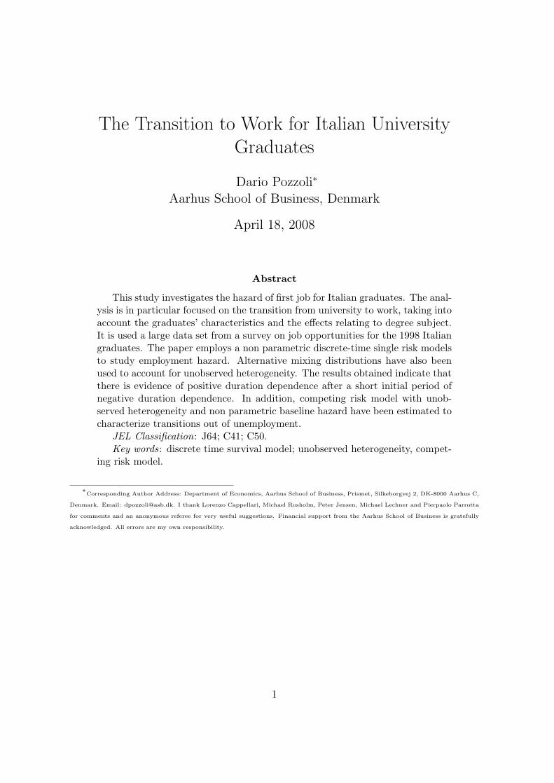
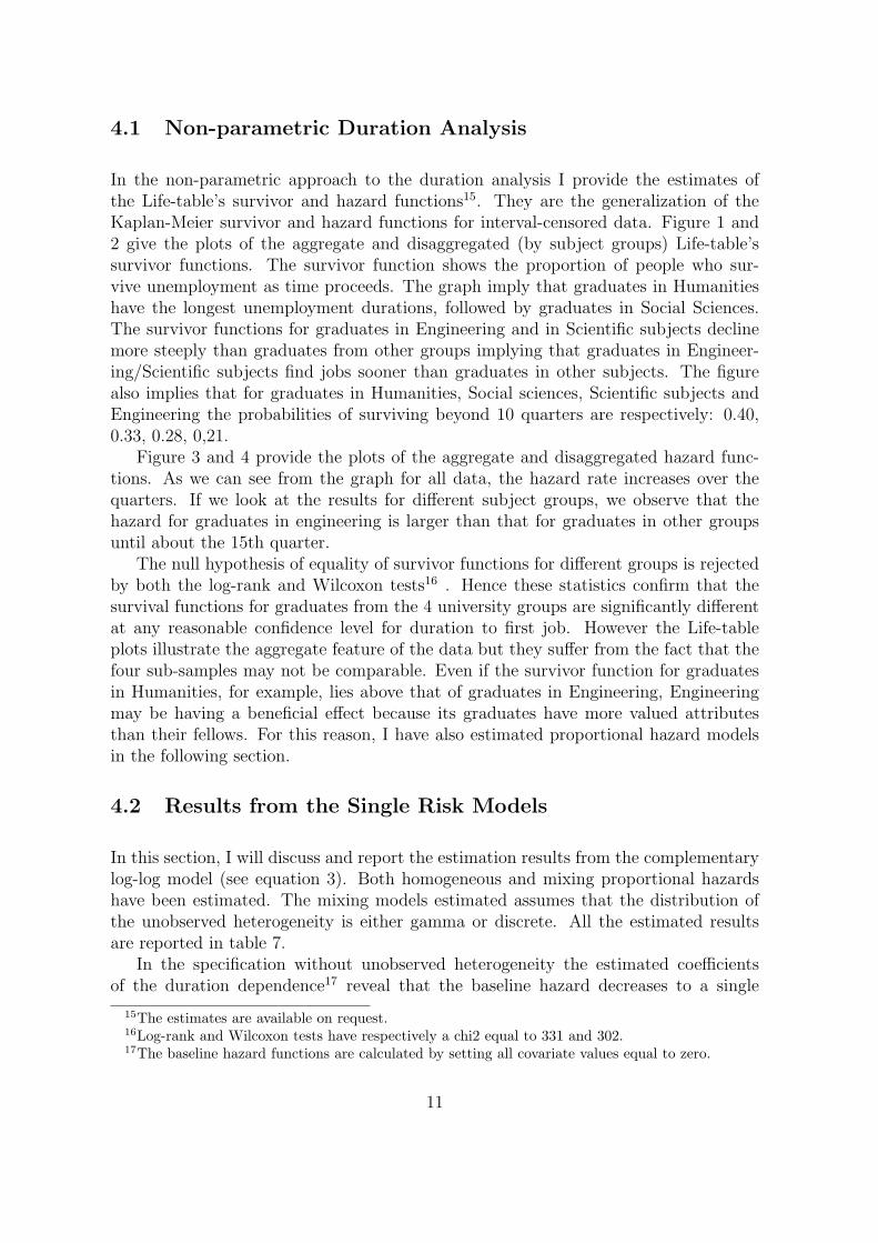
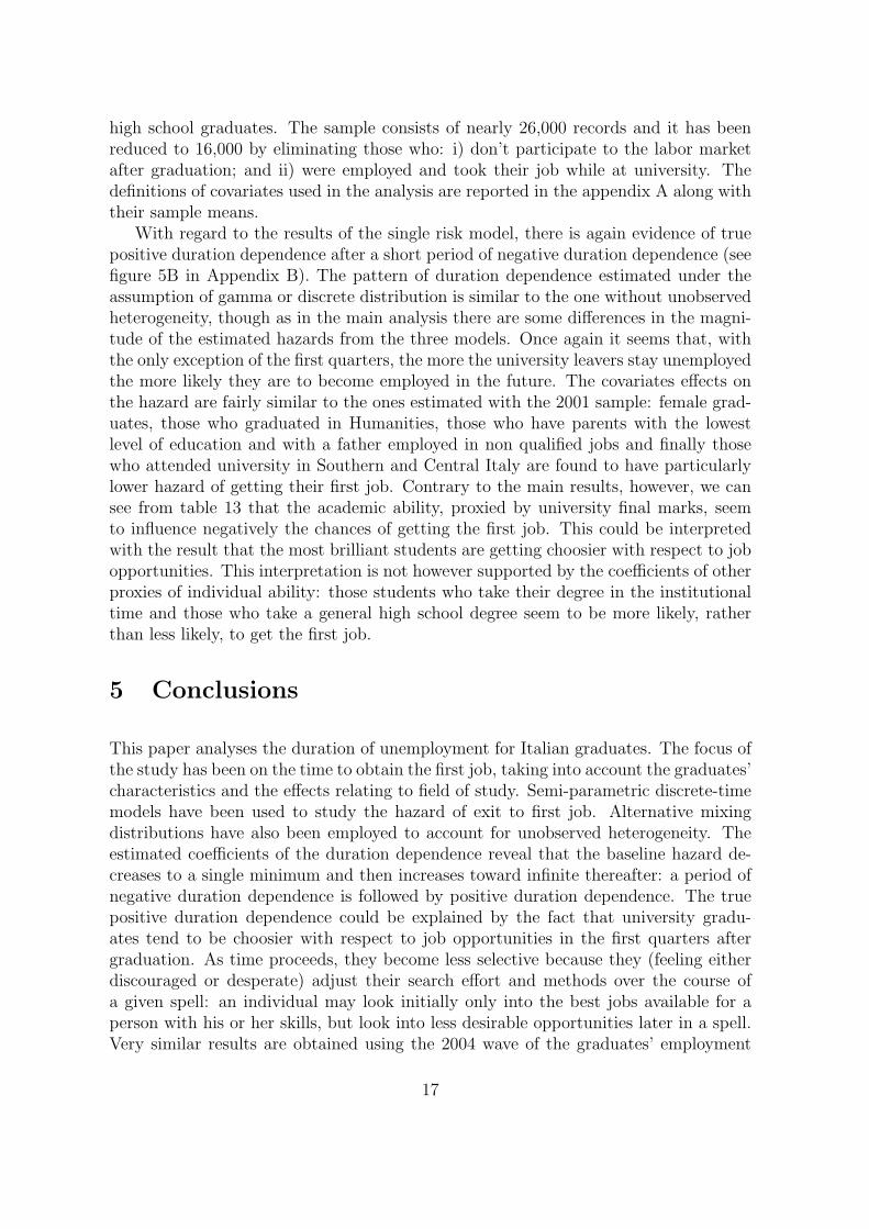
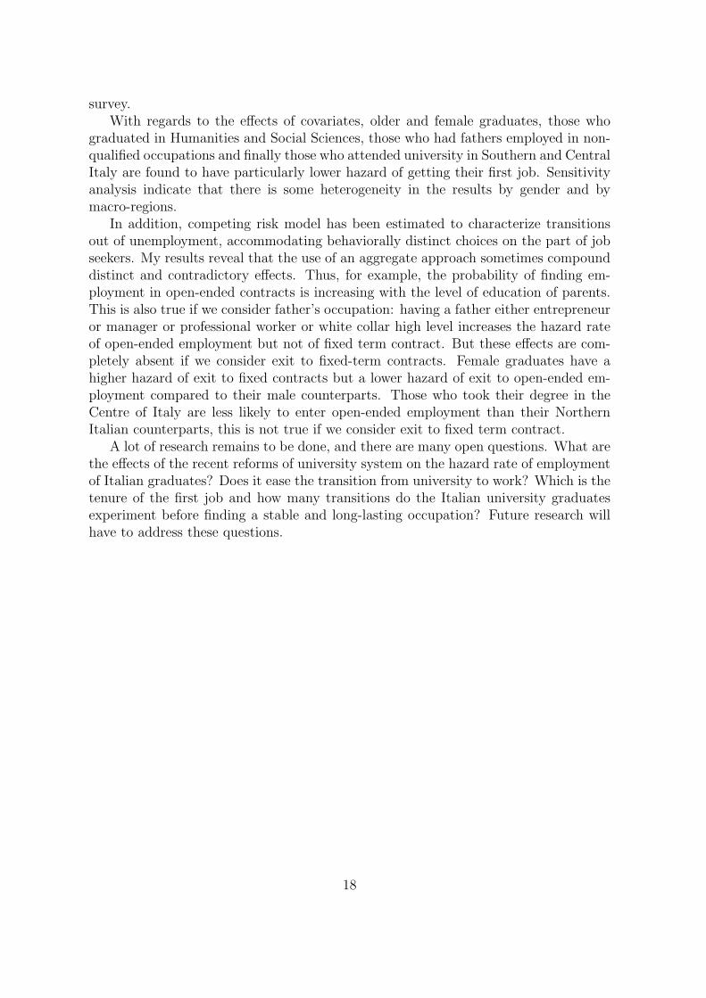
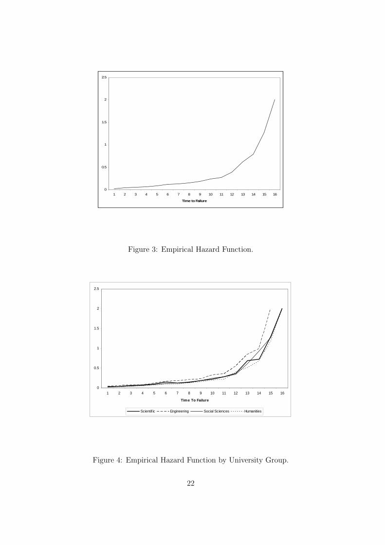
In the non-parametric approach to the duration analysis I provide the estimates ofthe Life-table’s survivor and hazard functions15. They are the generalization of theKaplan-Meier survivor and hazard functions for interval-censored data. Figure 1 and2 give the plots of the aggregate and disaggregated (by subject groups) Life-table’ssurvivor functions. The survivor function shows the proportion of people who sur-vive unemployment as time proceeds. The graph imply that graduates in Humanitieshave the longest unemployment durations, followed by graduates in Social Sciences.The survivor functions for graduates in Engineering and in Scientific subjects declinemore steeply than graduates from other groups implying that graduates in Engineer-ing/Scientific subjects find jobs sooner than graduates in other subjects. The figurealso implies that for graduates in Humanities, Social sciences, Scientific subjects andEngineering the probabilities of surviving beyond 10 quarters are respectively: 0.40,0.33, 0.28, 0,21.

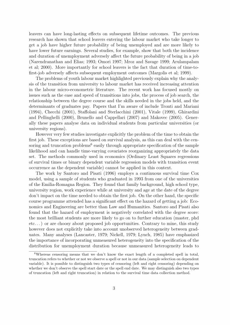
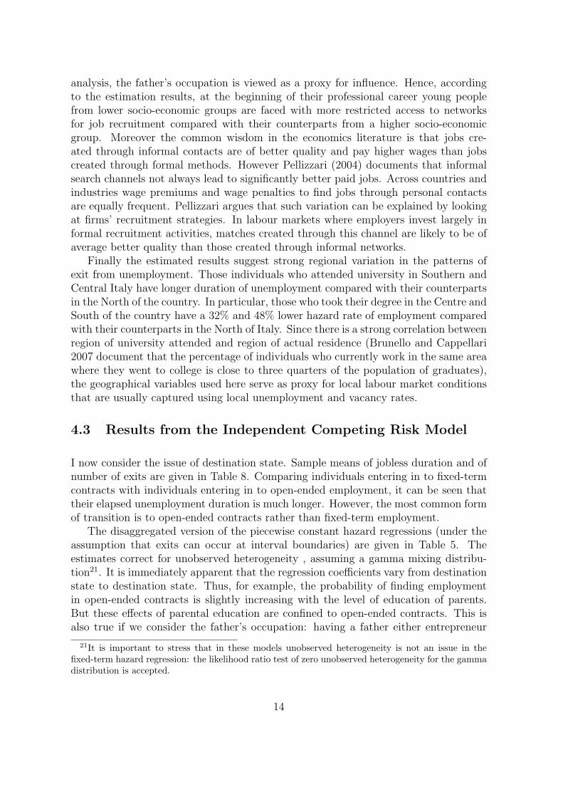
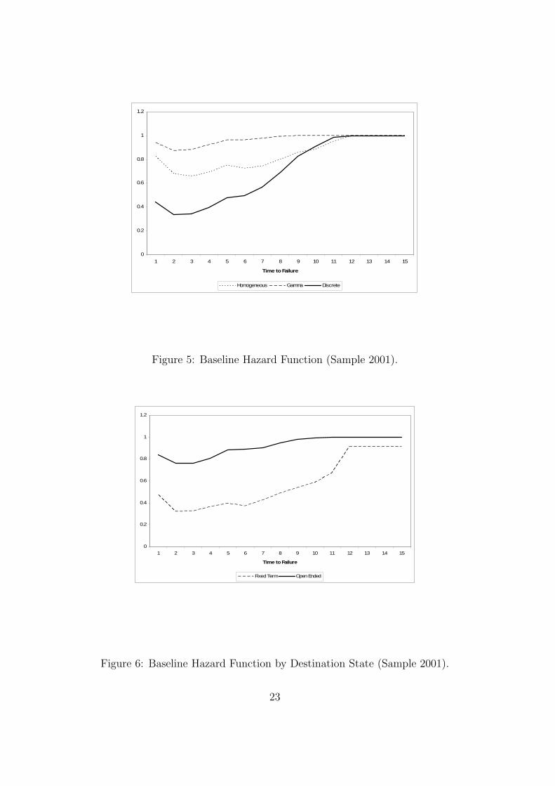
Figure 3 and 4 provide the plots of the aggregate and disaggregated hazard func-tions. As we can see from the graph for all data, the hazard rate increases over thequarters. If we look at the results for different subject groups, we observe that thehazard for graduates in engineering is larger than that for graduates in other groupsuntil about the 15th quarter.

The null hypothesis of equality of survivor functions for different groups is rejectedby both the log-rank and Wilcoxon tests16 . Hence these statistics confirm that thesurvival functions for graduates from the 4 university groups are significantly differentat any reasonable confidence level for duration to first job. However the Life-tableplots illustrate the aggregate feature of the data but they suffer from the fact that thefour sub-samples may not be comparable. Even if the survivor function for graduatesin Humanities, for example, lies above that of graduates in Engineering, Engineeringmay be having a beneficial effect because its graduates have more valued attributesthan their fellows. For this reason, I have also estimated proportional hazard modelsin the following section.

4.2 Results from the Single Risk Models

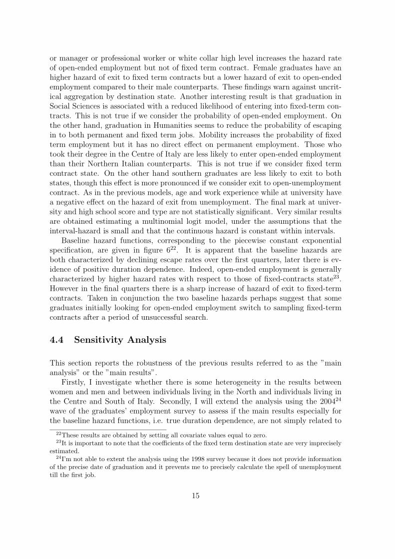
In this section, I will discuss and report the estimation results from the complementarylog-log model (see equation 3). Both homogeneous and mixing proportional hazardshave been estimated. The mixing models estimated assumes that the distribution ofthe unobserved heterogeneity is either gamma or discrete. All the estimated resultsare reported in table 7.

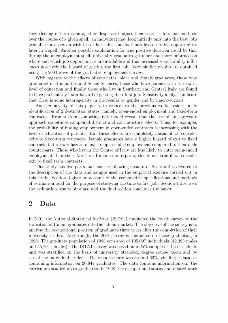
In the specification without unobserved heterogeneity the estimated coefficientsof the duration dependence17 reveal that the baseline hazard decreases to a single

15The estimates are available on request.16Log-rank and Wilcoxon tests have respectively a chi2 equal to 331 and 302.17The baseline hazard functions are calculated by setting all covariate values equal to zero.

11

minimum and then increases toward infinite thereafter. The baseline hazard functionestimated under the assumption of either gamma or discrete distribution is fairly similarto the one without unobserved heterogeneity, though there are some differences in themagnitude of the estimated hazards 18. Hence the results obtained indicate that thereis a general evidence of true positive duration dependence after a short initial periodof negative duration dependence. The initial negative duration dependence could beconsistent with the following explanations. On one hand, university graduates couldbe very selective with respect to job opportunities because they have very high labourmarket expectations. On the other hand, they could be temporarily out of the labourforce in the first quarters immediately after graduation as the extra utility obtainedfrom being unemployed (leisure) is high and positive, i.e. the disutility arising fromthe social stigma attached to being unemployed and the debilitating effects of beingunemployed are very low. The subsequent true positive duration dependence could beexplained by the fact that, as time proceeds, they become less selective because they(feeling either discouraged or desperate) adjust their search effort and methods over thecourse of a given spell: an individual may look initially only into the best jobs availablefor a person with his or her skills, but look into less desirable opportunities later ina spell. Another possible explanation for true positive duration could be that duringthe unemployment spell, university graduates get more and more informed on whereand which job opportunities are available and this increased search ability influencespositively the hazard of getting the first job.

The effects of covariates on the hazard of exit from unemployment are very similaracross the three models estimated, even though the estimated coefficients of the mixingproportional hazard models are generally greater in absolute terms than the ones ofthe homogeneous proportional hazard model. Comparing the maximum of the log-likelihoods from the models shows that the one with discrete unobserved heterogeneityhas an edge over the other two models. As a result, I will discuss the covariate effectson the hazard relying on the discrete unobserved heterogeneity.

Starting with the effect of personal characteristics on the hazard of exit out of unem-ployment, older graduates are found to have a lower hazard of employment comparedwith their younger counterparts: a one year rise in age is associated with a 6% lowerhazard rate. This could be explained by the fact that younger students are more likelyto be better students or signal themselves as more able individuals to firms becausethey might have received their degree in the institutional time established for the courseprogramme they attended. This is not however supported by the negative sign of thedummy variable equal to one if the individual has taken her degree in the institutionaltime: better students could also be choosier with respect to job opportunities thantheir counterparts taking longer to get their degree. With regard to gender differences,female graduates have a 20% lower hazard of employment compared with male gradu-ates. An explanation for this that best fits the labor economics literature is, of course,that men are generally expected to receive more job offers than women are, mainly

18This supports Meyer’s (1990) suggestion that using a flexible specification for the baseline hazardremoves the sensitivity of estimated parameters to the type of distribution assumed for unobservedheterogeneity.

12

due to the female labor market behavior that is (or perceived to be) characterized byfrequent interruptions.

Graduates who transferred into another region to attend university have not a sta-tistically different hazard of finding their first job. This could indicate that individualswho moved to another region to study may be not necessarily more motivated and bet-ter students than those who didn’t experience any transfer. This does not support theidea that in a labour market highly segmented at the regional level, like the Italian one,not only where people work, but also where people study matters for their occupationaloutcomes19. Graduates who were employed in the labour market while studying have a15% lower hazard of exit from unemployment: this is not in line with the a-priori thatemployers prefer individuals with some work experience, though seasonal or occasional;probably this result could be explained by the fact that these work experiences seemnot to provide those skills that are useful to obtain a job.

Considering the covariate related to academic ability, the university final markhas not a statistically significant effect on the probability of obtaining the first job.The low influence of the final mark might be explained by the previously mentionedceiling effect. The score and type of high school seem not to exert any impact onthe hazard of employment too. However there are significant differences in graduates’hazard of employment according to subject studied at university, even using the highlyaggregated set of 4 broad subject areas. Relative to students of Scientific subjects,Engineering students have a 28% higher hazard rate of getting the first job. Theequivalent hazards for Social sciences and Humanities students are respectively 14% and32% lower20. These results may stress that the links between universities and employersare closer for some degrees (Engineering and Scientific) than for others (Humanities).Universities and employers are in an interdependent relationship in which employersdepend on universities to supply educated workers and universities depend on employersto hire their graduates.

As regards the graduates’ social background, educational level of the parents at thedate of degree seems to have a positive effect on the probability of obtaining the firstjob. Thus for example, graduates with both parents with high school degree have a10% higher hazard of employment with respect to graduates with parents having thelowest level of education (illiteracy or primary school). Also the father’s occupationseems to have a positive influence on the graduates’ chances of employment: thosewith a father manager or entrepreneur have higher hazard rates with respect to thosewith a father employed in non-qualified occupations. As formulated by Rees and Gray(1982) and Pistaferri (1999), youth unemployment may depend on contacts or the in-fluence parents bear on the labour market (informal search channels). In this case, thegreater the parents’ influence, the lower the probability of being unemployed. In my

19See also Makovec (2005) who shows the existence of a positive and significant wage premiumassociated to attending university in the North rather than in the South.

20The lack of exclusion restrictions does not allow me to model simultaneously the hazard equationand an instrumented equation to control for endogeneity of the choice of college major. The estimatedcorrelations could give some useful guidance on the true causal effects given that I control for a largeset of covariates and for unobserved heterogeneity besides college major; this should at least attenuateomitted variable bias.

13

analysis, the father’s occupation is viewed as a proxy for influence. Hence, accordingto the estimation results, at the beginning of their professional career young peoplefrom lower socio-economic groups are faced with more restricted access to networksfor job recruitment compared with their counterparts from a higher socio-economicgroup. Moreover the common wisdom in the economics literature is that jobs cre-ated through informal contacts are of better quality and pay higher wages than jobscreated through formal methods. However Pellizzari (2004) documents that informalsearch channels not always lead to significantly better paid jobs. Across countries andindustries wage premiums and wage penalties to find jobs through personal contactsare equally frequent. Pellizzari argues that such variation can be explained by lookingat firms’ recruitment strategies. In labour markets where employers invest largely informal recruitment activities, matches created through this channel are likely to be ofaverage better quality than those created through informal networks.

Finally the estimated results suggest strong regional variation in the patterns ofexit from unemployment. Those individuals who attended university in Southern andCentral Italy have longer duration of unemployment compared with their counterpartsin the North of the country. In particular, those who took their degree in the Centre andSouth of the country have a 32% and 48% lower hazard rate of employment comparedwith their counterparts in the North of Italy. Since there is a strong correlation betweenregion of university attended and region of actual residence (Brunello and Cappellari2007 document that the percentage of individuals who currently work in the same areawhere they went to college is close to three quarters of the population of graduates),the geographical variables used here serve as proxy for local labour market conditionsthat are usually captured using local unemployment and vacancy rates.

4.3 Results from the Independent Competing Risk Model

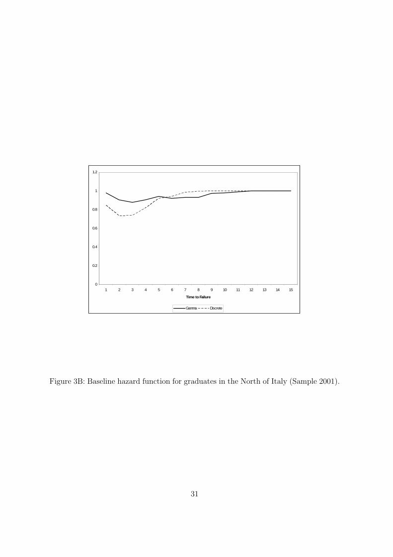
I now consider the issue of destination state. Sample means of jobless duration and ofnumber of exits are given in Table 8. Comparing individuals entering in to fixed-termcontracts with individuals entering in to open-ended employment, it can be seen thattheir elapsed unemployment duration is much longer. However, the most common formof transition is to open-ended contracts rather than fixed-term employment.

The disaggregated version of the piecewise constant hazard regressions (under theassumption that exits can occur at interval boundaries) are given in Table 5. Theestimates correct for unobserved heterogeneity , assuming a gamma mixing distribu-tion21. It is immediately apparent that the regression coefficients vary from destinationstate to destination state. Thus, for example, the probability of finding employmentin open-ended contracts is slightly increasing with the level of education of parents.But these effects of parental education are confined to open-ended contracts. This isalso true if we consider the father’s occupation: having a father either entrepreneur

21It is important to stress that in these models unobserved heterogeneity is not an issue in thefixed-term hazard regression: the likelihood ratio test of zero unobserved heterogeneity for the gammadistribution is accepted.

14

or manager or professional worker or white collar high level increases the hazard rateof open-ended employment but not of fixed term contract. Female graduates have anhigher hazard of exit to fixed term contracts but a lower hazard of exit to open-endedemployment compared to their male counterparts. These findings warn against uncrit-ical aggregation by destination state. Another interesting result is that graduation inSocial Sciences is associated with a reduced likelihood of entering into fixed-term con-tracts. This is not true if we consider the probability of open-ended employment. Onthe other hand, graduation in Humanities seems to reduce the probability of escapingin to both permanent and fixed term jobs. Mobility increases the probability of fixedterm employment but it has no direct effect on permanent employment. Those whotook their degree in the Centre of Italy are less likely to enter open-ended employmentthan their Northern Italian counterparts. This is not true if we consider fixed termcontract state. On the other hand southern graduates are less likely to exit to bothstates, though this effect is more pronounced if we consider exit to open-unemploymentcontract. As in the previous models, age and work experience while at university havea negative effect on the hazard of exit from unemployment. The final mark at univer-sity and high school score and type are not statistically significant. Very similar resultsare obtained estimating a multinomial logit model, under the assumptions that theinterval-hazard is small and that the continuous hazard is constant within intervals.

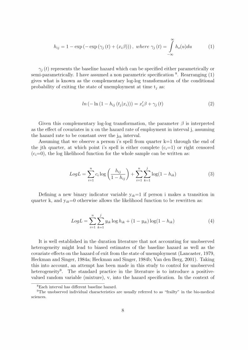
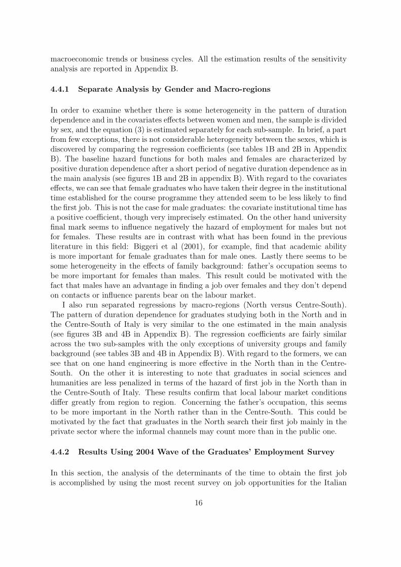
Baseline hazard functions, corresponding to the piecewise constant exponentialspecification, are given in figure 622. It is apparent that the baseline hazards areboth characterized by declining escape rates over the first quarters, later there is ev-idence of positive duration dependence. Indeed, open-ended employment is generallycharacterized by higher hazard rates with respect to those of fixed-contracts state23.However in the final quarters there is a sharp increase of hazard of exit to fixed-termcontracts. Taken in conjunction the two baseline hazards perhaps suggest that somegraduates initially looking for open-ended employment switch to sampling fixed-termcontracts after a period of unsuccessful search.

4.4 Sensitivity Analysis

This section reports the robustness of the previous results referred to as the ”mainanalysis” or the ”main results”.

Firstly, I investigate whether there is some heterogeneity in the results betweenwomen and men and between individuals living in the North and individuals living inthe Centre and South of Italy. Secondly, I will extend the analysis using the 200424

wave of the graduates’ employment survey to assess if the main results especially forthe baseline hazard functions, i.e. true duration dependence, are not simply related to

22These results are obtained by setting all covariate values equal to zero.23It is important to note that the coefficients of the fixed term destination state are very imprecisely

estimated.24I’m not able to extent the analysis using the 1998 survey because it does not provide information

of the precise date of graduation and it prevents me to precisely calculate the spell of unemploymenttill the first job.

15

macroeconomic trends or business cycles. All the estimation results of the sensitivityanalysis are reported in Appendix B.

4.4.1 Separate Analysis by Gender and Macro-regions

In order to examine whether there is some heterogeneity in the pattern of durationdependence and in the covariates effects between women and men, the sample is dividedby sex, and the equation (3) is estimated separately for each sub-sample. In brief, a partfrom few exceptions, there is not considerable heterogeneity between the sexes, which isdiscovered by comparing the regression coefficients (see tables 1B and 2B in AppendixB). The baseline hazard functions for both males and females are characterized bypositive duration dependence after a short period of negative duration dependence as inthe main analysis (see figures 1B and 2B in appendix B). With regard to the covariateseffects, we can see that female graduates who have taken their degree in the institutionaltime established for the course programme they attended seem to be less likely to findthe first job. This is not the case for male graduates: the covariate institutional time hasa positive coefficient, though very imprecisely estimated. On the other hand universityfinal mark seems to influence negatively the hazard of employment for males but notfor females. These results are in contrast with what has been found in the previousliterature in this field: Biggeri et al (2001), for example, find that academic abilityis more important for female graduates than for male ones. Lastly there seems to besome heterogeneity in the effects of family background: father’s occupation seems tobe more important for females than males. This result could be motivated with thefact that males have an advantage in finding a job over females and they don’t dependon contacts or influence parents bear on the labour market.

I also run separated regressions by macro-regions (North versus Centre-South).The pattern of duration dependence for graduates studying both in the North and inthe Centre-South of Italy is very similar to the one estimated in the main analysis(see figures 3B and 4B in Appendix B). The regression coefficients are fairly similaracross the two sub-samples with the only exceptions of university groups and familybackground (see tables 3B and 4B in Appendix B). With regard to the formers, we cansee that on one hand engineering is more effective in the North than in the Centre-South. On the other it is interesting to note that graduates in social sciences andhumanities are less penalized in terms of the hazard of first job in the North than inthe Centre-South of Italy. These results confirm that local labour market conditionsdiffer greatly from region to region. Concerning the father’s occupation, this seemsto be more important in the North rather than in the Centre-South. This could bemotivated by the fact that graduates in the North search their first job mainly in theprivate sector where the informal channels may count more than in the public one.

4.4.2 Results Using 2004 Wave of the Graduates’ Employment Survey

In this section, the analysis of the determinants of the time to obtain the first jobis accomplished by using the most recent survey on job opportunities for the Italian

16

high school graduates. The sample consists of nearly 26,000 records and it has beenreduced to 16,000 by eliminating those who: i) don’t participate to the labor marketafter graduation; and ii) were employed and took their job while at university. Thedefinitions of covariates used in the analysis are reported in the appendix A along withtheir sample means.

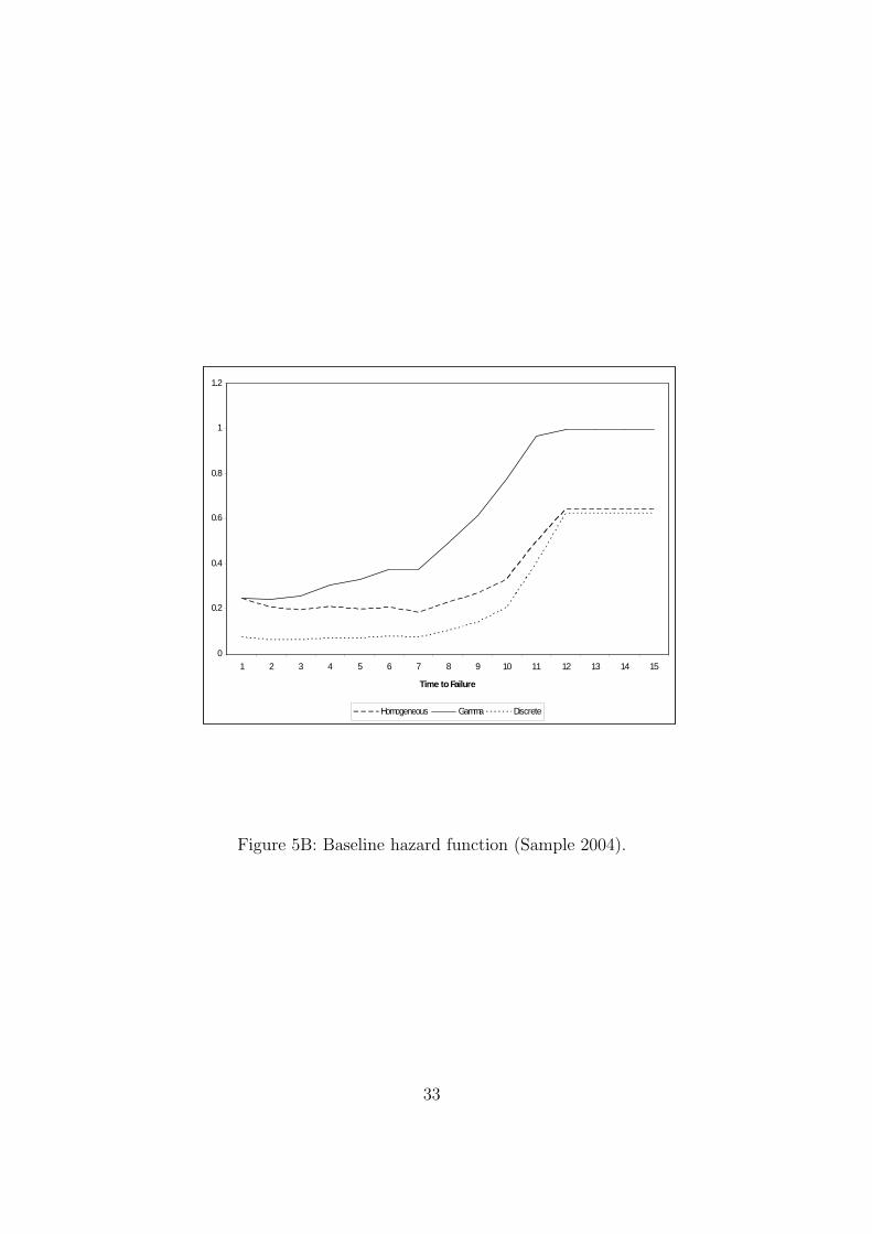
With regard to the results of the single risk model, there is again evidence of truepositive duration dependence after a short period of negative duration dependence (seefigure 5B in Appendix B). The pattern of duration dependence estimated under theassumption of gamma or discrete distribution is similar to the one without unobservedheterogeneity, though as in the main analysis there are some differences in the magni-tude of the estimated hazards from the three models. Once again it seems that, withthe only exception of the first quarters, the more the university leavers stay unemployedthe more likely they are to become employed in the future. The covariates effects onthe hazard are fairly similar to the ones estimated with the 2001 sample: female grad-uates, those who graduated in Humanities, those who have parents with the lowestlevel of education and with a father employed in non qualified jobs and finally thosewho attended university in Southern and Central Italy are found to have particularlylower hazard of getting their first job. Contrary to the main results, however, we cansee from table 13 that the academic ability, proxied by university final marks, seemto influence negatively the chances of getting the first job. This could be interpretedwith the result that the most brilliant students are getting choosier with respect to jobopportunities. This interpretation is not however supported by the coefficients of otherproxies of individual ability: those students who take their degree in the institutionaltime and those who take a general high school degree seem to be more likely, ratherthan less likely, to get the first job.

5 Conclusions

This paper analyses the duration of unemployment for Italian graduates. The focus ofthe study has been on the time to obtain the first job, taking into account the graduates’characteristics and the effects relating to field of study. Semi-parametric discrete-timemodels have been used to study the hazard of exit to first job. Alternative mixingdistributions have also been employed to account for unobserved heterogeneity. Theestimated coefficients of the duration dependence reveal that the baseline hazard de-creases to a single minimum and then increases toward infinite thereafter: a period ofnegative duration dependence is followed by positive duration dependence. The truepositive duration dependence could be explained by the fact that university gradu-ates tend to be choosier with respect to job opportunities in the first quarters aftergraduation. As time proceeds, they become less selective because they (feeling eitherdiscouraged or desperate) adjust their search effort and methods over the course ofa given spell: an individual may look initially only into the best jobs available for aperson with his or her skills, but look into less desirable opportunities later in a spell.Very similar results are obtained using the 2004 wave of the graduates’ employment

17

survey.With regards to the effects of covariates, older and female graduates, those who

graduated in Humanities and Social Sciences, those who had fathers employed in non-qualified occupations and finally those who attended university in Southern and CentralItaly are found to have particularly lower hazard of getting their first job. Sensitivityanalysis indicate that there is some heterogeneity in the results by gender and bymacro-regions.

In addition, competing risk model has been estimated to characterize transitionsout of unemployment, accommodating behaviorally distinct choices on the part of jobseekers. My results reveal that the use of an aggregate approach sometimes compounddistinct and contradictory effects. Thus, for example, the probability of finding em-ployment in open-ended contracts is increasing with the level of education of parents.This is also true if we consider father’s occupation: having a father either entrepreneuror manager or professional worker or white collar high level increases the hazard rateof open-ended employment but not of fixed term contract. But these effects are com-pletely absent if we consider exit to fixed-term contracts. Female graduates have ahigher hazard of exit to fixed contracts but a lower hazard of exit to open-ended em-ployment compared to their male counterparts. Those who took their degree in theCentre of Italy are less likely to enter open-ended employment than their NorthernItalian counterparts, this is not true if we consider exit to fixed term contract.

A lot of research remains to be done, and there are many open questions. What arethe effects of the recent reforms of university system on the hazard rate of employmentof Italian graduates? Does it ease the transition from university to work? Which is thetenure of the first job and how many transitions do the Italian university graduatesexperiment before finding a stable and long-lasting occupation? Future research willhave to address these questions.

18

References

[1] Abbring J.H. and Van den Berg G. J. (2007), “The Unobserved HeterogeneityDistribution in Unobserved Heterogeneity ” Biometrika, 94, 1: 87-99.

[2] Arulampalam W., Booth A.L., Taylor M.P. (2000), “Unemployment Persistence” Oxford Economic Papers, 52: 24-50.

[3] Biggeri L., Bini M. and Grilli L. (2000), “The transition from university to work:a multilevel approach to the analysis of the time to obtain the first job”, J. R.Statistical Society A, 164: 293-305.

[4] Brunello G. and Cappellari L. (2007), “The labour market effects of Alma Mater:Evidence from Italy”, forthcoming in: Economics of Education Review.

[5] Censis, “Rapporto sulla situazione del Paese, anno 1999”.

[6] Checchi D. (2001), “Primi risultati dell’indagine sui percorsi lavorativi dei laureatidell’ateneo di Milano: Facolta di Scienze Politiche”, mimeo, University of Milan.

[7] Ghirardini P. G. and Pellinghelli M. (2000), “I non disoccupati Laureati e diplo-mati nell’Italia della piena occupazione”, Mulino.

[8] Heckman J. and B. Singer (1984a) “The identifiability of The Proportional HazardModel”, Review of Economic Studies, LI: 231-241.

[9] Heckman J. and B. Singer (1984b) “ A Method for Minimizing the Impact ofDistributional Assumptions in Econometric Models for Duration Data”, Econo-metrica, 52(2): 271-320.

[10] ISTAT, “Rilevazione delle forze di lavoro, anno 1999”.

[11] ISTAT, “Rapporto annuale, 1998”.

[12] Jenkins S. P. (1995), “Easy Estimation Methods for Discrete-Time Duration Mod-els” Oxford Bulletin of Economics and Statistics, 57(1): 129-138.

[13] Jenkins, S. P. (1997), “sbe17: Estimation Methods for Discrete-Time (GroupedDuration Data) Proportional Hazard Models: PGMHAZ”, Stata Technical Bul-letin, 39: 1-12.

[14] Lancaster T. (1979), “Econometric Methods of the Duration of Unemployment”Econometrica, 47(4): 939-956.

[15] Lynch L. M. (1985), “State Dependency in Youth Unemployment: A Lost Gener-ation? ” Journal of Econometrics, April 1985: 71-84.

[16] Margolis D. N., Plug E., Simonnet V. and Vilhuber L. (1999), “The role of earlycareer experiences in determining later career success: An international compari-son” unpublished paper, TEAM-Universite de Paris 1 Pantheon-Sorbonne.

19

[17] Makovec M. (2005), “ Does it pay studying far from home? Explaining the returnsto geographic mobility of Italian graduates” IGIER discussion paper.

[18] Meyer B. D. (1990), “Unemployment Insurance and Unemployment Spells ”Econometrica 58: 757-782.

[19] Mroz T. A. and Savage T. H. (1999), “The long-term effects of youth unemploy-ment, Department of Economics ” University of North Carolina.

[20] Narendranathan W. and Elias P. (1993) “Influences of Past History on the Inci-dence of Youth Unemployment: Empirical Findings for the UK”, Oxford Bulletinof Economics and Statistics, 55: 161-85.

[21] Nickell S. (1979) “Estimating the probability of leaving unemployment ”, Econo-metrica 47: 1249-1266.

[22] OCSE, “Regard sur l’education ”, 1997.

[23] Omori Y. (1997), “Stigma Effects of Nonemployment” Economic Inquiry, vol. 35:394-416

[24] Pellizzari M. (2004), “Do Friends and Relatives Really Help in Getting a GoodJob?” CEP discussion paper No 623.

[25] Pistaferri L. (1999), “Informal Networks in the Italian Labor Market” Giornaledegli Economisti e Annali di Economia, 58(3-4): 355-375.

[26] Rees A. and Gray W. (1982), “Family effects in youth employment” in R. B.Freeman, The youth labor market problem: Its nature, causes and consequences.Chicago: University of Chicago Press.

[27] Santoro M. and Pisati M. (1996), “Dopo la laurea” Bologna: Il Mulino.

[28] Staffolani S. and Sterlacchini A., (2001), “Istruzione universitaria, occupazione, ereddito. Un analisi empirica sui laureati degli atenei marchigiani”, F.Angeli.

[29] Tronti L. and Mariani P. (1994), “La transizione Universita-Lavoro in Italia:un’esplorazione delle evidenze dell’indagine ISTAT sugli sbocchi professionali deilaureati”, Econ. Lav., 25, no. 3: 3-26.

[30] Van den Berg G. (2001), “Duration Models: Specification, Identification and Mul-tiple Durations”, in Handbook of Econometrics, edited by Heckman, James J. andLeamer Edward, V, North-Holland, Amsterdam.

[31] Vitale C. (1999), “Indagine sugli sbocchi dei laureati dell’universita di Salerno”,mimeo, Universita di Salerno.

20

0

0.2

0.4

0.6

0.8

1

1.2

1 2 3 4 5 6 7 8 9 10 11 12 13 14 15 16

Time to Failure

Figure 1: Empirical Survivor Function.

0

0.2

0.4

0.6

0.8

1

1.2

1 2 3 4 5 6 7 8 9 10 11 12 13 14 15 16

Time to Failure

Scientific Engineering Social Sciences Humanities

Figure 2: Empirical Survivor Function by University Group.

21

0

0.5

1

1.5

2

2.5

1 2 3 4 5 6 7 8 9 10 11 12 13 14 15 16

Time to Failure

Figure 3: Empirical Hazard Function.

0

0.5

1

1.5

2

2.5

1 2 3 4 5 6 7 8 9 10 11 12 13 14 15 16

Time To Failure

Scientif ic Engineering Social Sciences Humanities

Figure 4: Empirical Hazard Function by University Group.

22

0

0.2

0.4

0.6

0.8

1

1.2

1 2 3 4 5 6 7 8 9 10 11 12 13 14 15

Time to Failure

Homogeneous Gamma Discrete

Figure 5: Baseline Hazard Function (Sample 2001).

0

0.2

0.4

0.6

0.8

1

1.2

1 2 3 4 5 6 7 8 9 10 11 12 13 14 15

Time to Failure

Fixed Term Open Ended

Figure 6: Baseline Hazard Function by Destination State (Sample 2001).

23

Table 1: Distribution of university groups.

University groups N %

Scientific 3,684 22.75Engineering 3,118 19.25Social sciences 5,501 33.97Humanities 3,892 24.03

Total 16,195 100

Table 2: Length of graduates’ unemployment.

Total Females Males

from 0 to 3 quarters 34.13 32.07 36.45from 4 to 7 quarters 24.5 22.51 27.03from 7 to 11 quarters 14.54 14.01 15.08quarters ≥ 11 26.83 31.41 21.44

24

Table 3: Distribution of unemployment spells by parental education.

Unemployment spells Parental Educationlevel 1 level 2 level 3 level 4 level 5 level 6 level 7

from 0 to 3 quarters 12.47 9.78 15.06 17.89 19.35 15.03 10.41from 4 to 7 quarters 12.59 9.88 14.92 18.01 19.38 15.63 9.6from 7 to 11 quarters 13.5 8.63 14.15 18.72 18.03 17.61 9.36quarters ≥ 11 14.48 9.16 13.51 17.6 19.01 16.78 9.46Total 13.19 9.47 14.48 17.96 19.08 16.02 9.81

Notes: level 1: both parents elementary school; level 2: at least one parent juniorhigh school; level 3: both parents junior high school; level 4: at least one parent highschool; level 5: both parents high school; level 6: at least one parent university; level6: both parents university.

Table 4: Distribution of unemployment spells by university groups.

Unemployment spells University groupsscientific engineering social sciences humanities

from 0 to 3 quarters 23.94 25.13 32.48 18.45from 4 to 7 quarters 23.87 20.82 33.82 21.5from 7 to 11 quarters 21.32 17.79 35.12 25.77quarters ≥ 11 20.99 11.14 35.37 32.5

Table 5: Distribution by destination state and mean durations (2001).

first jobstatus noexit exit Total mean durationunemployed 100 0 19.51 16 (0)fixed-term 0 37.84 30.45 4.84 (3.95)open-ended 0 62.16 50.03 4.23 (3.64)

19.51 80.49 100

25

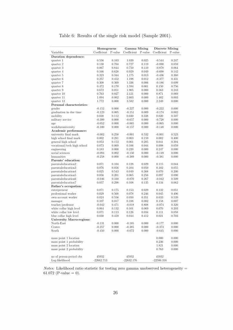
Table 6: Results of the single risk model (Sample 2001).

Homogeneus Gamma Mixing Discrete MixingVariables Coefficient P-value Coefficient P-value Coefficient P-value

Duration dependence:quarter 1 0.556 0.103 1.039 0.025 -0.544 0.247quarter 2 0.130 0.704 0.727 0.119 -0.890 0.059quarter 3 0.067 0.844 0.750 0.110 -0.878 0.064quarter 4 0.166 0.628 0.929 0.049 -0.698 0.142quarter 5 0.323 0.344 1.175 0.013 -0.436 0.360quarter 6 0.257 0.452 1.198 0.012 -0.377 0.431quarter 7 0.308 0.369 1.336 0.006 -0.186 0.699quarter 8 0.472 0.170 1.594 0.001 0.150 0.756quarter 9 0.672 0.051 1.905 0.000 0.563 0.243quarter 10 0.763 0.027 2.121 0.000 0.871 0.069quarter 11 1.094 0.002 2.603 0.000 1.402 0.003quarter 12 1.772 0.000 3.582 0.000 2.249 0.000Personal characteristics:gender -0.152 0.000 -0.227 0.000 -0.222 0.000graduation in due time -0.123 0.005 -0.151 0.009 -0.174 0.002mobility 0.038 0.112 0.030 0.338 0.020 0.507military service -0.399 0.000 -0.657 0.000 -0.728 0.000age -0.052 0.000 -0.065 0.000 -0.065 0.000workduruniversity -0.100 0.000 -0.157 0.000 -0.148 0.000Academic performance:university final mark -0.002 0.250 -0.001 0.532 -0.001 0.523high school final mark 0.002 0.281 0.003 0.159 0.002 0.400general high school 0.053 0.153 0.061 0.205 0.041 0.394vocational/tech high school 0.073 0.069 0.106 0.044 0.098 0.059engineering 0.183 0.000 0.220 0.000 0.247 0.000social sciences -0.094 0.002 -0.150 0.000 -0.149 0.000humanities -0.258 0.000 -0.389 0.000 -0.381 0.000Parents’ education:parentaleducation2 0.071 0.104 0.128 0.029 0.115 0.044parentaleducation3 0.076 0.056 0.104 0.050 0.102 0.055parentaleducation4 0.025 0.543 0.049 0.368 0.070 0.200parentaleducation5 0.056 0.201 0.065 0.256 0.097 0.090parentaleducation6 -0.046 0.340 -0.070 0.267 -0.042 0.509parentaleducation7 0.057 0.298 0.108 0.135 0.134 0.062Father’s occupation:entrepreneur 0.071 0.175 0.153 0.029 0.132 0.051professional worker 0.029 0.568 0.078 0.246 0.045 0.496own-account worker 0.024 0.556 0.050 0.351 0.033 0.539manager 0.107 0.017 0.188 0.002 0.158 0.007teacher/professor -0.042 0.471 -0.018 0.808 -0.074 0.320white collar high level 0.064 0.132 0.101 0.069 0.070 0.203white collar low level 0.071 0.113 0.126 0.034 0.111 0.058blue collar high level 0.030 0.459 0.044 0.412 0.021 0.703University Macro-regions:North-East -0.131 0.000 -0.185 0.000 -0.177 0.000Centre -0.257 0.000 -0.385 0.000 -0.373 0.000South -0.450 0.000 -0.672 0.000 -0.645 0.000

mass point 1 location 0.000 0.000mass point 1 probability 0.236 0.000mass point 2 location 1.821 0.000mass point 2 probability 0.763 0.000

no of person-period obs 45932 45932 45932Log-likelihood -22662.713 -22632.176 -22586.316

Notes: Likelihood ratio statistic for testing zero gamma unobserved heterogeneity =61.072 (P-value = 0).

26

Table 7: Results of the independent competing risks model (Sample 2001).

Fixed Term Open EndedVariables Coefficient P-value Coefficient P-value

Duration dependence:quarter 1 -0.445 0.446 0.586 0.333quarter 2 -0.943 0.108 0.358 0.558quarter 3 -0.927 0.114 0.350 0.569quarter 4 -0.791 0.178 0.499 0.419quarter 5 -0.692 0.239 0.765 0.219quarter 6 -0.760 0.196 0.794 0.205quarter 7 -0.587 0.318 0.844 0.181quarter 8 -0.406 0.490 1.066 0.093quarter 9 -0.261 0.657 1.379 0.032quarter 10 -0.129 0.827 1.532 0.018quarter 11 0.118 0.842 1.994 0.002quarter 12 0.902 0.125 2.577 0.000Personal characteristics:gender 0.124 0.003 -0.404 0.000graduation in due time -0.216 0.002 -0.043 0.548mobility 0.086 0.024 0.003 0.944military sevice -0.169 0.007 -0.756 0.000age -0.076 0.000 -0.035 0.023workduruniversity -0.107 0.003 -0.128 0.000Academic performance:university final mark 0.008 0.005 -0.007 0.011high school final mark -0.004 0.166 0.007 0.014general high school 0.064 0.253 0.043 0.489vocational/tech high school 0.019 0.757 0.116 0.081engineering -0.079 0.162 0.351 0.000social sciences -0.259 0.000 -0.013 0.785humanities -0.137 0.007 -0.504 0.000Parents’ education:parentaleducation2 0.018 0.802 0.163 0.026parentaleducation3 0.017 0.793 0.143 0.031parentaleducation4 -0.059 0.375 0.101 0.137parentaleducation5 -0.028 0.686 0.105 0.143parentaleducation6 -0.102 0.188 -0.022 0.785parentaleducation7 -0.035 0.692 0.161 0.075Father’s occupation:entrepreneur -0.075 0.388 0.261 0.003professional worker -0.138 0.105 0.196 0.019own-account worker 0.033 0.602 0.023 0.738manager 0.073 0.314 0.189 0.011teacher/professor -0.009 0.919 -0.042 0.657white collar high level -0.017 0.799 0.157 0.023white collar low level -0.012 0.863 0.178 0.016blue collar high level 0.016 0.803 0.048 0.479University Macro-regions:North-East -0.055 0.242 -0.214 0.000Centre -0.068 0.155 -0.491 0.000South -0.297 0.000 -0.716 0.000

no of person-period obs 45932 29260Log-likelihood -12217.018 -17193.746

Notes: Fixed Term Contract: Likelihood ratio statistic for testing zero gamma unob-served heterogeneity = 0.00001 (P-value = 1); Open Ended Employment: Likelihoodratio statistic for testing zero gamma unobserved heterogeneity= 44.303 (P-value =0).

27

Appendix A: Definitions of the Variables and Sample Averages.

Name and definition Sample 2001 Sample 2004

Time (in quarters, from 0 to 16) 4.377 2.922Mobility (1, transfer into another region; 0 otherwise) 0.286 0.318Sex (0, male; 1, female) 0.546 0.507Military service (0, done before degree or exempted; 1, otherwise) 0.123 -Age 28.374 27.961University final mark (integers from 66 to 110) 102.862 103.762High school mark (integers from 36 to 60) 48.821 49.139General high school 0.618 0.610Vocational/technical high school 0.272 0.326Other high school 0.110 0.064Workduruniversity (1, at least one job during university , 0, otherwise) 0.422 0.359Parentaleduc1 (both parents illiterate or with primary school certificate) 0.132 0.110Parentaleduc2 (at least one parent with middle school certificate) 0.095 0.099Parentaleduc3 (both parents with a middle school certificate) 0.145 0.141Parentaleduc4 (at least one parent with a high school certificate) 0.180 0.193Parentaleduc5 (both parents with high school certificate) 0.191 0.194Parentaleduc6 (at least one parent with a degree) 0.160 0.161Parentaleduc7 (both parents with a degree) 0.098 0.103North-west (university in the north-west of Italy) 0.275 0.277North-east (university in the north-east of Italy) 0.228 0.120Centre (university in the centre of Italy) 0.236 0.322South (university in the south of Italy) 0.261 0.280Scientific (graduation in scientific subjects) 0.227 0.228Engineering (graduation in engineering) 0.193 0.263Social sciences (graduation in social, economic and political subjects) 0.340 0.317Humanities (graduation in humanities) 0.240 0.192entrepreneur 0.055 0.054professional worker 0.079 0.067own-account worker 0.124 0.148manager 0.156 0.096teacher/professor 0.066 0.114white collar high level 0.159 0.189white collar low level 0.099 0.113blue collar high level 0.129 0.189other occupation 0.129 0.029

28

Appendix B: Figures and Tables of the Sensitivity Analysis.

0

0.2

0.4

0.6

0.8

1

1.2

1 2 3 4 5 6 7 8 9 10 11 12 13 14 15

Time to Failure

Gamma Discrete

Figure 1B: Baseline hazard function for female graduates (Sample 2001).

29

0.00

0.20

0.40

0.60

0.80

1.00

1.20

1 2 3 4 5 6 7 8 9 10 11 12 13 14 15

Time to Failure

Gamma Discrete

Figure 2B: Baseline hazard function for male graduates (Sample 2001).

30

0

0.2

0.4

0.6

0.8

1

1.2

1 2 3 4 5 6 7 8 9 10 11 12 13 14 15

Time to Failure

Gamma Discrete

Figure 3B: Baseline hazard function for graduates in the North of Italy (Sample 2001).

31

0.0

0.1

0.2

0.3

0.4

0.5

0.6

0.7

0.8

0.9

1.0

1 2 3 4 5 6 7 8 9 10 11 12 13 14 15

Time to Failure

Gamma Discrete

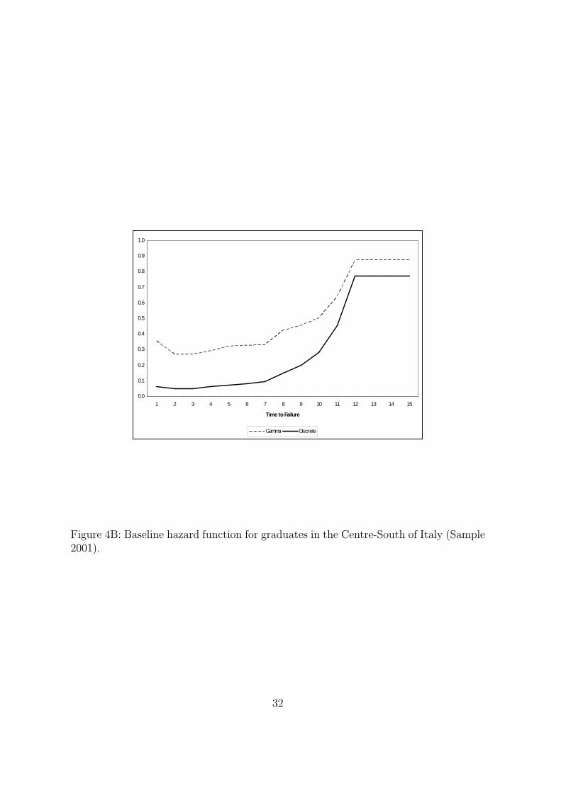
Figure 4B: Baseline hazard function for graduates in the Centre-South of Italy (Sample2001).

32

0

0.2

0.4

0.6

0.8

1

1.2

1 2 3 4 5 6 7 8 9 10 11 12 13 14 15

Time to Failure

Homogeneous Gamma Discrete

Figure 5B: Baseline hazard function (Sample 2004).

33

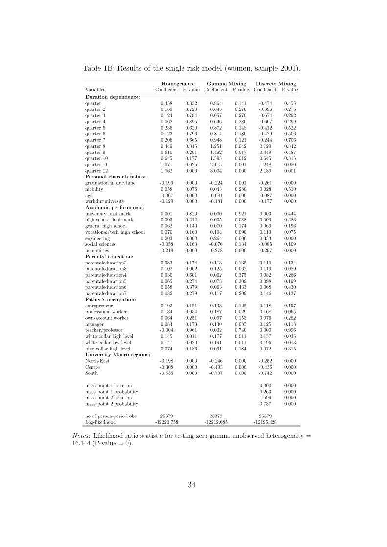
Table 1B: Results of the single risk model (women, sample 2001).


Duration dependence:quarter 1 0.458 0.332 0.864 0.141 -0.474 0.455quarter 2 0.169 0.720 0.645 0.276 -0.696 0.275quarter 3 0.124 0.794 0.657 0.270 -0.674 0.292quarter 4 0.062 0.895 0.646 0.280 -0.667 0.299quarter 5 0.235 0.620 0.872 0.148 -0.412 0.522quarter 6 0.123 0.796 0.814 0.180 -0.429 0.506quarter 7 0.206 0.665 0.948 0.121 -0.244 0.706quarter 8 0.449 0.345 1.251 0.042 0.129 0.842quarter 9 0.610 0.201 1.482 0.017 0.449 0.487quarter 10 0.645 0.177 1.593 0.012 0.645 0.315quarter 11 1.071 0.025 2.115 0.001 1.248 0.050quarter 12 1.762 0.000 3.004 0.000 2.139 0.001Personal characteristics:graduation in due time -0.199 0.000 -0.224 0.001 -0.261 0.000mobility 0.058 0.076 0.043 0.280 0.028 0.510age -0.067 0.000 -0.081 0.000 -0.087 0.000workduruniversity -0.129 0.000 -0.181 0.000 -0.177 0.000Academic performance:university final mark 0.001 0.820 0.000 0.921 0.003 0.444high school final mark 0.003 0.212 0.005 0.088 0.003 0.283general high school 0.062 0.140 0.070 0.174 0.069 0.196vocational/tech high school 0.070 0.160 0.104 0.090 0.113 0.075engineering 0.203 0.000 0.264 0.000 0.333 0.000social sciences -0.058 0.163 -0.076 0.134 -0.085 0.109humanities -0.219 0.000 -0.278 0.000 -0.297 0.000Parents’ education:parentaleducation2 0.083 0.174 0.113 0.135 0.119 0.134parentaleducation3 0.102 0.062 0.125 0.062 0.119 0.089parentaleducation4 0.030 0.601 0.062 0.375 0.082 0.266parentaleducation5 0.065 0.274 0.073 0.309 0.098 0.199parentaleducation6 0.058 0.379 0.063 0.433 0.068 0.430parentaleducation7 0.082 0.279 0.117 0.209 0.146 0.137Father’s occupation:entrepreneur 0.102 0.151 0.133 0.125 0.118 0.197professional worker 0.134 0.054 0.187 0.029 0.168 0.065own-account worker 0.064 0.251 0.097 0.153 0.076 0.282manager 0.084 0.173 0.130 0.085 0.125 0.118teacher/professor -0.004 0.961 0.032 0.740 0.000 0.996white collar high level 0.145 0.011 0.177 0.011 0.157 0.035white collar low level 0.141 0.020 0.191 0.011 0.196 0.013blue collar high level 0.074 0.186 0.091 0.184 0.072 0.315University Macro-regions:North-East -0.198 0.000 -0.246 0.000 -0.252 0.000Centre -0.308 0.000 -0.403 0.000 -0.436 0.000South -0.535 0.000 -0.707 0.000 -0.742 0.000




34

Table 2B: Results of the single risk model (men, sample 2001).


Duration dependence:quarter 1 0.358 0.490 0.823 0.311 -1.120 0.127quarter 2 -0.221 0.670 0.469 0.566 -1.594 0.031quarter 3 -0.302 0.562 0.540 0.511 -1.582 0.033quarter 4 -0.028 0.958 0.968 0.240 -1.199 0.107quarter 5 0.118 0.821 1.287 0.121 -0.908 0.225quarter 6 0.100 0.848 1.447 0.083 -0.739 0.327quarter 7 0.125 0.810 1.646 0.051 -0.488 0.521quarter 8 0.200 0.702 1.902 0.025 -0.148 0.847quarter 9 0.450 0.389 2.364 0.006 0.405 0.597quarter 10 0.614 0.242 2.780 0.002 0.828 0.274quarter 11 0.826 0.117 3.290 0.000 1.191 0.111quarter 12 1.490 0.005 4.486 0.000 1.943 0.009Personal characteristics:graduation in due time 0.002 0.974 -0.019 0.861 -0.073 0.434mobility 0.011 0.751 0.009 0.865 0.007 0.871military service -0.368 0.000 -0.792 0.000 -0.734 0.000age -0.030 0.034 -0.036 0.106 -0.030 0.132workduruniversity -0.058 0.066 -0.100 0.043 -0.106 0.014Academic performance:university final mark -0.005 0.033 -0.004 0.208 -0.007 0.022high school final mark 0.001 0.744 0.001 0.726 0.001 0.784general high school 0.023 0.763 0.025 0.831 -0.064 0.542vocational/tech high school 0.044 0.563 0.061 0.608 -0.004 0.971engineering 0.152 0.001 0.140 0.042 0.153 0.010social sciences -0.123 0.004 -0.265 0.000 -0.198 0.001humanities -0.342 0.000 -0.671 0.000 -0.537 0.000Parents’ education:parentaleducation2 0.077 0.222 0.183 0.061 0.104 0.206parentaleducation3 0.058 0.322 0.092 0.310 0.101 0.215parentaleducation4 0.025 0.680 0.011 0.902 0.042 0.608parentaleducation5 0.059 0.352 0.050 0.611 0.100 0.250parentaleducation6 -0.150 0.033 -0.261 0.016 -0.160 0.098parentaleducation7 0.039 0.620 0.103 0.400 0.113 0.286Father’s occupation:entrepreneur 0.039 0.609 0.232 0.062 0.156 0.126professional worker -0.079 0.290 -0.051 0.656 -0.077 0.449own-account worker -0.019 0.749 -0.017 0.858 -0.007 0.930manager 0.125 0.055 0.270 0.008 0.172 0.045teacher/professor -0.093 0.260 -0.111 0.376 -0.165 0.131white collar high level -0.031 0.618 0.004 0.967 -0.027 0.744white collar low level -0.010 0.879 0.042 0.681 0.007 0.932blue collar high level -0.027 0.657 -0.034 0.717 -0.047 0.562University Macro-regions:North-East -0.052 0.223 -0.101 0.131 -0.090 0.112Centre -0.190 0.000 -0.365 0.000 -0.287 0.000South -0.356 0.000 -0.657 0.000 -0.533 0.000




35

Table 3B: Results of the single risk model (Centre-South, sample 2001).


Duration dependence:quarter 1 -0.822 0.129 -0.823 0.130 -2.697 0.001quarter 2 -1.164 0.032 -1.164 0.033 -2.983 0.000quarter 3 -1.164 0.032 -1.164 0.033 -2.925 0.000quarter 4 -1.067 0.050 -1.066 0.052 -2.761 0.000quarter 5 -0.951 0.081 -0.950 0.083 -2.562 0.001quarter 6 -0.932 0.087 -0.930 0.091 -2.440 0.002quarter 7 -0.921 0.091 -0.919 0.097 -2.308 0.003quarter 8 -0.602 0.269 -0.599 0.280 -1.824 0.020quarter 9 -0.502 0.357 -0.498 0.373 -1.501 0.053quarter 10 -0.360 0.511 -0.355 0.530 -1.108 0.146quarter 11 0.006 0.991 0.012 0.984 -0.497 0.503quarter 12 0.720 0.188 0.728 0.219 0.390 0.593Personal characteristics:gender -0.166 0.000 -0.167 0.000 -0.216 0.000graduation in due time -0.109 0.152 -0.109 0.153 -0.091 0.342mobility 0.041 0.231 0.042 0.235 0.037 0.416military service -0.285 0.000 -0.286 0.000 -0.498 0.000age -0.030 0.025 -0.030 0.026 -0.022 0.216workduruniversity -0.161 0.000 -0.162 0.000 -0.214 0.000Academic performance:university final mark 0.001 0.624 0.001 0.625 0.003 0.361high school final mark 0.002 0.499 0.002 0.500 0.001 0.784general high school 0.064 0.257 0.064 0.259 0.065 0.380vocational/tech high school 0.051 0.402 0.052 0.404 0.078 0.331engineering 0.142 0.005 0.142 0.006 0.173 0.010social sciences -0.184 0.000 -0.185 0.000 -0.276 0.000humanities -0.329 0.000 -0.331 0.000 -0.461 0.000Parents’ education:parentaleducation2 0.069 0.291 0.070 0.303 0.133 0.121parentaleducation3 0.047 0.428 0.047 0.432 0.081 0.298parentaleducation4 0.090 0.145 0.091 0.152 0.186 0.024parentaleducation5 0.104 0.106 0.105 0.111 0.175 0.043parentaleducation6 0.045 0.527 0.045 0.529 0.123 0.198parentaleducation7 0.212 0.008 0.213 0.011 0.419 0.000Father’s occupation:entrepreneur -0.097 0.245 -0.097 0.249 -0.060 0.576professional worker -0.058 0.457 -0.058 0.458 -0.139 0.175own-account worker 0.044 0.463 0.044 0.464 0.065 0.402manager 0.066 0.334 0.067 0.341 0.040 0.660teacher/professor -0.129 0.106 -0.129 0.108 -0.284 0.008white collar high level 0.052 0.402 0.053 0.404 0.046 0.570white collar low level 0.111 0.079 0.112 0.083 0.114 0.167blue collar high level 0.091 0.137 0.091 0.138 0.037 0.639



Notes: Likelihood ratio statistic for testing zero gamma unobserved heterogeneity =0.001 (P-value = 0.969).

36

Table 4B: Results of the single risk model (North, sample 2001).


Duration dependence:quarter 1 1.338 0.004 1.338 0.002 0.626 0.324quarter 2 0.862 0.062 0.862 0.051 0.279 0.662quarter 3 0.754 0.103 0.754 0.088 0.292 0.650quarter 4 0.852 0.065 0.852 0.054 0.528 0.413quarter 5 1.052 0.023 1.052 0.017 0.922 0.156quarter 6 0.930 0.045 0.930 0.036 1.056 0.108quarter 7 0.989 0.033 0.989 0.026 1.419 0.032quarter 8 0.998 0.032 0.998 0.025 1.752 0.008quarter 9 1.310 0.005 1.310 0.003 2.356 0.000quarter 10 1.324 0.005 1.324 0.003 2.531 0.000quarter 11 1.616 0.001 1.616 0.000 2.876 0.000quarter 12 2.270 0.000 2.270 0.000 3.566 0.000Personal characteristics:gender -0.139 0.000 -0.139 0.000 -0.228 0.000graduation in due time -0.113 0.032 -0.113 0.032 -0.194 0.005mobility 0.001 0.975 0.001 0.975 -0.033 0.447military service -0.470 0.000 -0.470 0.000 -0.959 0.000age -0.069 0.000 -0.069 0.000 -0.107 0.000workduruniversity -0.058 0.048 -0.058 0.047 -0.110 0.005Academic performance:university final mark -0.006 0.007 -0.006 0.007 -0.007 0.012high school final mark 0.002 0.306 0.002 0.308 0.003 0.282general high school 0.048 0.316 0.048 0.316 0.018 0.782vocational/tech high school 0.086 0.097 0.086 0.097 0.085 0.227engineering 0.196 0.000 0.196 0.000 0.309 0.000social sciences -0.033 0.407 -0.033 0.406 -0.036 0.502humanities -0.200 0.000 -0.200 0.000 -0.300 0.000Parents’ education:parentaleducation2 0.098 0.096 0.098 0.096 0.117 0.134parentaleducation3 0.124 0.021 0.124 0.021 0.108 0.145parentaleducation4 0.023 0.677 0.023 0.677 0.017 0.818parentaleducation5 0.073 0.205 0.073 0.204 0.076 0.324parentaleducation6 -0.046 0.477 -0.046 0.478 -0.070 0.426parentaleducation7 0.015 0.838 0.015 0.838 -0.014 0.886Father’s occupation:entrepreneur 0.156 0.020 0.156 0.020 0.240 0.010professional worker 0.094 0.165 0.094 0.166 0.183 0.044own-account worker 0.033 0.554 0.033 0.554 0.066 0.383manager 0.134 0.024 0.134 0.025 0.244 0.002teacher/professor -0.032 0.700 -0.032 0.701 0.030 0.789white collar high level 0.089 0.120 0.089 0.120 0.142 0.069white collar low level 0.048 0.443 0.048 0.443 0.144 0.091blue collar high level 0.034 0.544 0.034 0.545 0.071 0.359



Notes: Likelihood ratio statistic for testing zero gamma unobserved heterogeneity =0.001 (P-value = 0.969).

37

Table 5B: Results of the single risk model (sample 2004).


Duration dependence:quarter 1 -1.261 0.000 -1.249 0.000 -2.559 0.000quarter 2 -1.463 0.000 -1.283 0.000 -2.725 0.000quarter 3 -1.533 0.000 -1.212 0.000 -2.753 0.000quarter 4 -1.458 0.000 -1.000 0.000 -2.628 0.000quarter 5 -1.509 0.000 -0.918 0.000 -2.618 0.000quarter 6 -1.476 0.000 -0.757 0.005 -2.514 0.000quarter 7 -1.598 0.000 -0.760 0.008 -2.559 0.000quarter 8 -1.354 0.000 -0.387 0.199 -2.219 0.000quarter 9 -1.169 0.000 -0.046 0.887 -1.901 0.000quarter 10 -0.910 0.000 0.404 0.258 -1.462 0.000quarter 11 -0.383 0.041 1.228 0.003 -0.667 0.009quarter 12 0.032 0.867 2.147 0.000 -0.023 0.916Personal characteristics:gender -0.046 0.072 -0.075 0.028 -0.061 0.039graduation in due time 0.068 0.035 0.133 0.002 0.102 0.005mobility -0.026 0.303 -0.067 0.048 -0.051 0.076age 0.013 0.430 0.027 0.211 0.022 0.254workduruniversity -0.141 0.000 -0.164 0.000 -0.147 0.000Academic performance:university final mark -0.022 0.042 -0.027 0.059 -0.023 0.061high school final mark 0.005 0.004 0.007 0.003 0.006 0.007general high school 0.162 0.002 0.164 0.017 0.151 0.012vocational/tech high school 0.186 0.001 0.222 0.002 0.197 0.002engineering 0.273 0.000 0.325 0.000 0.284 0.000social sciences -0.044 0.185 -0.059 0.178 -0.055 0.150humanities -0.182 0.000 -0.277 0.000 -0.243 0.000Parents’ education:parentaleducation2 0.114 0.025 0.131 0.049 0.122 0.035parentaleducation3 0.092 0.053 0.102 0.100 0.100 0.067parentaleducation4 0.150 0.001 0.174 0.005 0.164 0.002parentaleducation5 0.105 0.034 0.117 0.071 0.120 0.033parentaleducation6 0.127 0.019 0.161 0.024 0.146 0.018parentaleducation7 0.132 0.033 0.159 0.050 0.147 0.036Father’s occupation:entrepreneur 0.150 0.085 0.316 0.007 0.239 0.017professional worker 0.077 0.370 0.162 0.155 0.124 0.219own-account worker 0.065 0.418 0.098 0.346 0.077 0.401manager 0.005 0.957 0.059 0.587 0.032 0.739teacher/professor 0.003 0.974 0.034 0.751 0.008 0.936white collar high level 0.003 0.971 0.062 0.545 0.036 0.696white collar low level 0.025 0.755 0.074 0.486 0.042 0.656blue collar high level 0.015 0.852 0.049 0.637 0.023 0.798University Macro-regions:North-East -0.078 0.041 -0.117 0.021 -0.101 0.021Centre -0.160 0.000 -0.227 0.000 -0.194 0.000South -0.385 0.000 -0.564 0.000 -0.475 0.000




38

Department of Economics: Skriftserie/Working Paper: 2003: WP 03-1 Søren Harck: Er der nu en strukturelt bestemt langsigts-ledighed

i SMEC?: Phillipskurven i SMEC 99 vis-à-vis SMEC 94. ISSN 1397-4831.

WP 03-2 Beatrice Schindler Rangvid: Evaluating Private School Quality

in Denmark. ISSN 1397-4831. WP 03-3 Tor Eriksson: Managerial Pay and Executive Turnover in the

Czech and Slovak Republics. ISSN 1397-4831. WP 03-4 Michael Svarer and Mette Verner: Do Children Stabilize

Marriages? ISSN 1397-4831. WP 03-5 Christian Bjørnskov and Gert Tinggaard Svendsen: Measuring

social capital – Is there a single underlying explanation? ISSN 1397-4831.

WP 03-6 Vibeke Jakobsen and Nina Smith: The educational attainment of

the children of the Danish ‘guest worker’ immigrants. ISSN 1397-4831.

WP 03-7 Anders Poulsen: The Survival and Welfare Implications of

Altruism When Preferences are Endogenous. ISSN 1397-4831. WP 03-8 Helena Skyt Nielsen and Mette Verner: Why are Well-educated

Women not Full-timers? ISSN 1397-4831. WP 03-9 Anders Poulsen: On Efficiency, Tie-Breaking Rules and Role

Assignment Procedures in Evolutionary Bargaining. ISSN 1397-4831.

WP 03-10 Anders Poulsen and Gert Tinggaard Svendsen: Rise and Decline

of Social Capital – Excess Co-operation in the One-Shot Prisoner’s Dilemma

Game. ISSN 1397-4831.

WP 03-11 Nabanita Datta Gupta and Amaresh Dubey: Poverty and Fertility: An Instrumental Variables Analysis on Indian Micro Data. ISSN 1397-4831.

WP 03-12 Tor Eriksson: The Managerial Power Impact on Compensation –

Some Further Evidence. ISSN 1397-4831. WP 03-13 Christian Bjørnskov: Corruption and Social Capital. ISSN 1397-

4831. WP 03-14 Debashish Bhattacherjee: The Effects of Group Incentives in an

Indian Firm – Evidence from Payroll Data. ISSN 1397-4831.

WP 03-15 Tor Eriksson och Peter Jensen: Tidsbegränsade anställninger –

danska erfarenheter. ISSN 1397-4831. WP 03-16 Tom Coupé, Valérie Smeets and Frédéric Warzynski: Incentives,

Sorting and Productivity along the Career: Evidence from a Sample of Top Economists. ISSN 1397-4831.

WP 03-17 Jozef Koning, Patrick Van Cayseele and Frédéric Warzynski:

The Effects of Privatization and Competitive Pressure on Firms’ Price-Cost Margins: Micro Evidence from Emerging Economies. ISSN 1397-4831.

WP 03-18 Urs Steiner Brandt and Gert Tinggaard Svendsen: The coalition

of industrialists and environmentalists in the climate change issue. ISSN 1397-4831.

WP 03-19 Jan Bentzen: An empirical analysis of gasoline price

convergence for 20 OECD countries. ISSN 1397-4831. WP 03-20 Jan Bentzen and Valdemar Smith: Regional income convergence

in the Scandinavian countries. ISSN 1397-4831. WP 03-21 Gert Tinggaard Svendsen: Social Capital, Corruption and

Economic Growth: Eastern and Western Europe. ISSN 1397-4831.

WP 03-22 Jan Bentzen and Valdemar Smith: A Comparative Study of

Wine Auction Prices: Mouton Rothschild Premier Cru Classé. ISSN 1397-4831.

WP 03-23 Peter Guldager: Folkepensionisternes incitamenter til at arbejde. ISSN 1397-4831.

WP 03-24 Valérie Smeets and Frédéric Warzynski: Job Creation, Job

Destruction and Voting Behavior in Poland. ISSN 1397-4831. WP 03-25 Tom Coupé, Valérie Smeets and Frédéric Warzynski: Incentives

in Economic Departments: Testing Tournaments? ISSN 1397-4831.

WP 03-26 Erik Strøjer Madsen, Valdemar Smith and Mogens Dilling-

Hansen: Industrial clusters, firm location and productivity – Some empirical evidence for Danish firms. ISSN 1397-4831.

WP 03-27 Aycan Çelikaksoy, Helena Skyt Nielsen and Mette Verner:

Marriage Migration: Just another case of positive assortative matching? ISSN 1397-4831.

2004: WP 04-1 Elina Pylkkänen and Nina Smith: Career Interruptions due to

Parental Leave – A Comparative Study of Denmark and Sweden. ISSN 1397-4831.

WP 04-2 Urs Steiner Brandt and Gert Tinggaard Svendsen: Switch Point

and First-Mover Advantage: The Case of the Wind Turbine Industry. ISSN 1397-4831.

WP 04-3 Tor Eriksson and Jaime Ortega: The Adoption of Job Rotation:

Testing the Theories. ISSN 1397-4831. WP 04-4 Valérie Smeets: Are There Fast Tracks in Economic

Departments? Evidence from a Sample of Top Economists. ISSN 1397-4831.

WP 04-5 Karsten Bjerring Olsen, Rikke Ibsen and Niels Westergaard-

Nielsen: Does Outsourcing Create Unemployment? The Case of the Danish Textile and Clothing Industry. ISSN 1397-4831.

WP 04-6 Tor Eriksson and Johan Moritz Kuhn: Firm Spin-offs in

Denmark 1981-2000 – Patterns of Entry and Exit. ISSN 1397-4831.

WP 04-7 Mona Larsen and Nabanita Datta Gupta: The Impact of Health on Individual Retirement Plans: a Panel Analysis comparing Self-reported versus Diagnostic Measures. ISSN 1397-4831.

WP 04-8 Christian Bjørnskov: Inequality, Tolerance, and Growth. ISSN

1397-4831. WP 04-9 Christian Bjørnskov: Legal Quality, Inequality, and Tolerance.

ISSN 1397-4831. WP 04-10 Karsten Bjerring Olsen: Economic Cooperation and Social

Identity: Towards a Model of Economic Cross-Cultural Integration. ISSN 1397-4831.

WP 04-11 Iben Bolvig: Within- and between-firm mobility in the low-wage

labour market. ISSN 1397-4831. WP 04-12 Odile Poulsen and Gert Tinggaard Svendsen: Social Capital and

Market Centralisation: A Two-Sector Model. ISSN 1397-4831. WP 04-13 Aditya Goenka and Odile Poulsen: Factor Intensity Reversal and

Ergodic Chaos. ISSN 1397-4831. WP 04-14 Jan Bentzen and Valdemar Smith: Short-run and long-run

relationships in the consumption of alcohol in the Scandinavian countries.

ISBN 87-7882-010-3 (print); ISBN 87-7882-011-1 (online). WP 04-15 Jan Bentzen, Erik Strøjer Madsen, Valdemar Smith and Mogens

Dilling-Hansen: Persistence in Corporate Performance? Empirical Evidence from Panel Unit Root Tests.

ISBN 87-7882-012-X (print); ISBN 87-7882-013-8 (online). WP 04-16 Anders U. Poulsen and Jonathan H.W. Tan: Can Information

Backfire? Experimental Evidence from the Ultimatum Game. ISBN 87-7882-014-6 (print); ISBN 87-7882-015-4 (online). WP 04-17 Werner Roeger and Frédéric Warzynski: A Joint Estimation of

Price-Cost Margins and Sunk Capital: Theory and Evidence from the European Electricity Industry.

ISBN 87-7882-016-2 (print); ISBN 87-7882-017-0 (online).

WP 04-18 Nabanita Datta Gupta and Tor Eriksson: New workplace practices and the gender wage gap.

ISBN 87-7882-018-9 (print); ISBN 87-7882-019-7 (online). WP 04-19 Tor Eriksson and Axel Werwatz: The Prevalence of Internal

Labour Markets – New Evidence from Panel Data. ISBN 87-7882-020-0 (print); ISBN 87-7882-021-9 (online). WP 04-20 Anna Piil Damm and Michael Rosholm: Employment Effects of

Dispersal Policies on Refugee Immigrants: Empirical Evidence. ISBN 87-7882-022-7 (print); ISBN 87-7882-023-5 (online). 2005: WP 05-1 Anna Piil Damm and Michael Rosholm: Employment Effects of

Dispersal Policies on Refugee Immigrants: Theory. ISBN 87-7882-024-3 (print); ISBN 87-7882-025-1 (online). WP 05-2 Anna Piil Damm: Immigrants’ Location Preferences: Exploiting

a Natural Experiment. ISBN 87-7882-036-7 (print); ISBN 87-7882-037-5 (online). WP 05-3 Anna Piil Damm: The Danish Dispersal Policy on Refugee

Immigrants 1986-1998: A Natural Experiment? ISBN 87-7882-038-3 (print); ISBN 87-7882-039-1 (online). WP 05-4 Rikke Ibsen and Niels Westergaard-Nielsen: Job Creation and

Destruction over the Business Cycles and the Impact on Individual Job Flows in Denmark 1980-2001.

ISBN 87-7882-040-5 (print); ISBN 87-7882-041-3 (online). WP 05-5 Anna Maria Kossowska, Nina Smith, Valdemar Smith and Mette

Verner: Til gavn for bundlinjen – Forbedrer kvinder i topledelse og bestyrelse danske virksomheders bundlinje?

ISBN 87-7882-042-1 (print); ISBN 87-7882-043-X (online). WP 05-6 Odile Poulsen and Gert Tinggaard Svendsen: The Long and

Winding Road: Social Capital and Commuting. ISBN 87-7882-044-8 (print); ISBN 87-7882-045-6 (online). WP 05-7 Odile Poulsen and Gert Tinggaard Svendsen: Love Thy

Neighbor: Bonding versus Bridging Trust. ISBN 87-7882-062-6 (print); ISBN 87-7882-063-4 (online).

WP 05-8 Christian Bjørnskov: Political Ideology and Economic Freedom. ISBN 87-7882-064-2 (print); ISBN 87-7882-065-0 (online). WP 05-9 Sebastian Buhai and Coen Teulings: Tenure Profiles and

Efficient Separation in a Stochastic Productivity Model. ISBN 87-7882-066-9 (print); ISBN 87-7882-067-7 (online). WP 05-10 Christian Grund and Niels Westergård-Nielsen: Age Structure of

the Workforce and Firm Performance. ISBN 87-7882-068-5 (print); ISBN 87-7882-069-3 (online). WP 05-11 Søren Harck: AD-AS på dansk. ISBN 87-7882-070-7 (print); ISBN 87-7882-071-5 (online). WP 05-12 Søren Harck: Hviler Dansk Økonomi på en Cobb-Douglas

teknologi? ISBN 87-7882-092-8 (print); ISBN 87-7882-093-6 (online). 2006: WP 06-1 Nicolai Kristensen and Edvard Johansson: New Evidence on

Cross-Country Differences in Job Satisfaction Using Anchoring Vignettes.

ISBN 87-7882-094-4 (print); ISBN 87-7882-095-2 (online). WP 06-2 Christian Bjørnskov: How Does Social Trust Affect Economic

Growth? ISBN 87-7882-096-0 (print); ISBN 87-7882-097-9 (online). WP 06-3 Jan Bentzen, Erik Strøjer Madsen and Valdemar Smith: The

Growth Opportunities for SMEs? ISBN 87-7882-098-7 (print); ISBN 87-7882-099-5 (online). WP 06-4 Anna Piil Damm: Ethnic Enclaves and Immigrant Labour

Market Outcomes: Quasi-Experimental Evidence. ISBN 87-7882-100-2 (print); ISBN 87-7882-101-0 (online). WP 06-5 Svend Jespersen, Nicolai Kristensen og Lars Skipper: En kritik

af VEU-udvalgets arbejde. ISBN 87-7882-159-2 (print); ISBN 87-7882-160-6 (online). WP 06-6 Kræn Blume and Mette Verner: Welfare Dependency among

Danish Immigrants. ISBN 87-7882-161-4 (print); ISBN 87-7882-162-2 (online).

WP 06-7 Jürgen Bitzer, Wolfram Schrettl and Philipp J.H. Schröder:

Intrinsic Motivation versus Signaling in Open Source Software Development.

ISBN 87-7882-163-0 (print); ISBN 87-7882-164-9 (online). WP 06-8 Valérie Smeets, Kathryn Ierulli and Michael Gibbs: Mergers of

Equals & Unequals. ISBN 87-7882-165-7 (print); ISBN 87-7882-166-5 (online). WP 06-9 Valérie Smeets: Job Mobility and Wage Dynamics. ISBN 87-7882-167-3 (print); ISBN 87-7882-168-1 (online). WP 06-10 Valérie Smeets and Frédéric Warzynski: Testing Models of

Hierarchy: Span of Control, Compensation and Career Dynamics.

ISBN 87-7882-187-8 (print); ISBN 87-7882-188-6 (online). WP 06-11 Sebastian Buhai and Marco van der Leij: A Social Network

Analysis of Occupational Segregation. ISBN 87-7882-189-4 (print); ISBN 87-7882-190-8 (online). 2007: WP 07-1 Christina Bjerg, Christian Bjørnskov and Anne Holm: Growth,

Debt Burdens and Alleviating Effects of Foreign Aid in Least Developed Countries.

ISBN 87-7882-191-6 (print); ISBN 87-7882-192-4 (online). WP 07-2 Jeremy T. Fox and Valérie Smeets: Do Input Quality and

Structural Productivity Estimates Drive Measured Differences in Firm Productivity?

ISBN 87-7882-193-2 (print); ISBN 87-7882-194-0 (online). WP 07-3 Elisabetta Trevisan: Job Security and New Restrictive

Permanent Contracts. Are Spanish Workers More Worried of Losing Their Job?

ISBN 87-7882-195-9 (print); ISBN 87-7882-196-7 (online). WP 07-4 Tor Eriksson and Jaime Ortega: Performance Pay and the “Time

Squeeze”. ISBN 9788778822079 (print); ISBN 9788778822086 (online).

WP 07-5 Johan Moritz Kuhn: My Pay is Too Bad (I Quit). Your Pay is Too Good (You’re Fired).

ISBN 9788778822093 (print); ISBN 9788778822109 (online). WP 07-6 Christian Bjørnskov: Social trust and the growth of schooling. ISBN 9788778822116 (print); ISBN 9788778822123 (online). WP 07-7 Jan Bentzen and Valdemar Smith: Explaining champagne prices

in Scandinavia – what is the best predictor? ISBN 9788778822130 (print); ISBN 9788778822147 (online). WP 07-8 Sandra Cavaco, Jean-Michel Etienne and Ali Skalli: Identifying

causal paths between health and socio-economic status: Evidence from European older workforce surveys

ISBN 9788778822154 (print); ISBN 9788778822161 (online). WP 07-9 Søren Harck: Long-run properties of some Danish macro-

econometric models: an analytical approach. ISBN 9788778822390 (print); ISBN 9788778822406 (online). WP 07-10 Takao Kato and Hideo Owan: Market Characteristics, Intra-Firm

Coordination, and the Choice of Human Resource Management Systems: Evidence from New Japanese Data.

ISBN 9788778822413 (print); ISBN 9788778822420 (online). WP 07-11 Astrid Würtz: The Long-Term Effect on Children of Increasing

the Length of Parents’ Birth-Related Leave. ISBN 9788778822437 (print); ISBN 9788778822444 (online). WP 07-12 Tor Eriksson and Marie-Claire Villeval: Performance Pay,

Sorting and Social Motivation. ISBN 9788778822451 (print); ISBN 9788778822468 (online). WP 07-13 Jane Greve: Obesity and Labor Market Outcomes: New Danish

Evidence. ISBN 9788778822475 (print); ISBN 9788778822482 (online). 2008: WP 08-1 Sebastian Buhai, Miguel Portela, Coen Teulings and Aico van

Vuuren: Returns to Tenure or Seniority ISBN 9788778822826 (print); ISBN 9788778822833 (online).

WP 08-2 Flora Bellone, Patrick Musso, Lionel Nesta et Frédéric Warzynski: L’effet pro-concurrentiel de l’intégration européenne : une analyse de l’évolution des taux de marge dans les industries manufacturières françaises

ISBN 9788778822857 (print); ISBN 9788778822864 (online). WP 08-3 Erdal Yalcin: The Proximity-Concentration Trade-Off under

Goods Price and Exchange Rate Uncertainty ISBN 9788778822871 (print); ISBN 9788778822888 (online) WP 08-4 Elke J. Jahn and Herbert Brücker: Migration and the Wage

Curve: A Structural Approach to Measure the Wage and Employment Effects of Migration

ISBN 9788778822895 (print); ISBN 9788778822901 (online) WP 08-5 Søren Harck: A Phillips curve interpretation of error-correction

models of the wage and price dynamics ISBN 9788778822918 (print); ISBN 9788778822925 (online) WP 08-6 Elke J. Jahn and Thomas Wagner: Job Security as an

Endogenous Job Characteristic ISBN 9788778823182 (print); ISBN 9788778823199 (online) WP 08-7 Jørgen Drud Hansen, Virmantas Kvedaras and Jørgen Ulff-

Møller Nielsen: Monopolistic Competition, International Trade and Firm Heterogeneity - a Life Cycle Perspective -

ISBN 9788778823212 (print); ISBN 9788778823229 (online) WP 08-8 Dario Pozzoli: The Transition to Work for Italian University

Graduates ISBN 9788778823236 (print); ISBN 9788778823243 (online)

WP 08-9 Annalisa Cristini and Dario Pozzoli: New Workplace Practices

and Firm Performance: a Comparative Study of Italy and Britain ISBN 9788778823250 (print); ISBN 9788778823267 (online)

WP 08-10 Paolo Buonanno and Dario Pozzoli: Early Labour Market

Returns to College Subjects ISBN 9788778823274 (print); ISBN 9788778823281 (online)

dario pozzoli - connecting repositories · the transition to work for italian university graduates...

Documents