Cost behavior and analysts’ earnings forecasts

Dan Weiss Tel Aviv University

February 2009 The author is grateful for valuable discussions with and constructive suggestions from Yakov Amihud, Eli Amir, Itay Kama, Thomas Lys, Michael Maher, Ron Ofer, and N.V. Ramanan. Comments from the participants of the MAS Conference and Tel Aviv University seminar are highly appreciated.

1

Cost behavior and analysts’ earnings forecasts

February 2009

Abstract

This paper examines how firms’ asymmetric cost behavior influences analysts’

earnings forecasts, primarily the accuracy of analysts’ consensus earnings forecasts. I

show that firms with more sticky costs behavior have less accurate analysts’ earnings

forecasts than firms with less sticky costs behavior. Furthermore, findings indicate

that cost stickiness influences analysts’ coverage priorities and investors partially

consider sticky cost behavior in forming their beliefs on the value of firms. The paper

integrates a typical management accounting research topic, cost behavior, with three

standard financial accounting topics (namely, accuracy of analysts’ earnings forecasts,

analysts’ coverage, and market response to earnings surprises).

JEL classification: M41; G12 Key words: Analyst coverage, Forecast errors, Sticky costs

2

Cost behavior and analysts’ earnings forecasts

I. INTRODUCTION

Management accountants have traditionally focused on cost behavior as an important

aspect of profit analysis for managers. Financial analysts, however, estimate firms’

future costs in the process of forecasting future earnings. Predicting cost behavior is,

therefore, an essential part of earnings prediction. Yet, a potential relationship

between firms’ cost behavior and properties of analysts’ earnings forecasts has not yet

been explored. This study integrates the management and financial accounting

disciplines by showing effects of cost behavior on: (i) the accuracy of analysts’

consensus earnings forecasts, (ii) the extent of analyst coverage, and (iii) the market

response to earnings announcements.

Focusing on cost behavior, I build on a concept of sticky costs (Anderson et al.,

2003). Costs are termed sticky if they increase more when activity rises than they

decrease when activity falls by an equivalent amount. A firm with more sticky costs

shows a greater decline in earnings when activity level falls than a firm with less

sticky costs. Why? Because more sticky costs result in a smaller cost adjustment when

activity level declines and, therefore, lower cost savings. Lower cost savings result in

greater decrease in earnings. This greater decrease in earnings when activity level

falls increases the variability of the earnings distribution, resulting in less accurate

earnings prediction.

Results, based on a sample of 44,931 industrial firm quarters for 2,520 firms from

1986 through 2005, indicate that sticky cost behavior reduces the accuracy of

analysts’ consensus earnings forecasts, controlled for environmental uncertainty, the

amount of available firm-specific information, the forecast horizon, and industry

effects.

3

Classifying costs into sticky and anti-sticky costs,1 findings show that analysts’

absolute consensus earnings forecasts for firms with sticky cost behavior are, on

average, 25% less accurate than those for firms with anti-sticky cost behavior.

Evidently, cost behavior is an influential determinant of analysts’ forecast accuracy.

The results are robust to potential managerial discretion that might bias the cost

stickiness measure and to estimating cost stickiness over a long time window.

The findings extend Banker and Chen (2006), who show that recognizing cost

behavior explains a considerable part of analysts’ advantage over time-series models.

Cost stickiness is shown to influence the magnitude of analysts’ earnings forecast

errors, particularly when market conditions take a turn for the worse. Analysts’

understanding of cost behavior has important implications for accounting academics

who use the consensus forecast as a proxy for earnings expectations. The findings are

also useful for investors who use consensus earnings forecasts to value firms, as it

suggests that higher costs stickiness indicates more volatile future earnings.

Addressing the extent of analyst coverage, I examine the relationship between the

accuracy of earnings forecasts and the extent of analyst coverage. While Alford and

Berger (1999) and Weiss et al. (2008) document a positive relationship, Barth et al.

(2001) report that analysts tend to prefer covering firms with intangible assets

characterized by volatile performance. Thus, the evidence is mixed and this

relationship is an open empirical issue. I find that firms with more sticky cost

behavior (and less accurate earnings forecasts) have lower analyst coverage,

controlled for the amount of available information, environmental uncertainty,

intensity of R&D expenditures, and additional determinants of supply and demand for

analysts’ forecasts reported in the literature (e.g., Bhushan, 1989; Lang and

1 Costs are termed anti-sticky if they increase less when activity rises than they decrease when activity falls by an equivalent amount. See examples in Balakrishnan et al. (2004) and a discussion in section II.

4

Lundholm, 1996). Findings indicate that firms’ cost behavior affects analysts’

coverage priorities.

Finally, I examine whether investors understand cost stickiness in responding to

earnings announcements. As earnings predictability decreases, reported earnings

provide less useful information for the prediction of future earnings and the response

coefficient decreases (e.g., Lipe, 1990). If investors recognize cost stickiness to some

extent, being aware that cost stickiness diminishes the accuracy of the analysts’

earnings forecasts, then more sticky cost behavior causes investors to rely less on

realized earnings information because of its low predictability power. Similarly, I

find a weaker market response to earnings surprises for firms with more sticky cost

behavior. Overall, findings indicate that cost behavior matters in forming investors’

beliefs regarding the value of firms.

This empirical examination is facilitated by a new measure of cost stickiness at the

firm level. I estimate the difference in cost function slopes between upward and

downward activity adjustments. While Anderson et al. (2003) and subsequent studies

use cross-sectional and time-series regressions to estimate cost stickiness,2 the

proposed measure puts less demand on data and allows for testing the sensitivity of

the results to key cost model assumptions. The new measure corroborates prior

evidence on variation among firms’ cost stickiness and provides room for estimating

cost stickiness of firms operating in industries with a small number of firms, which

limits a meaningful estimation of regression models.3

This study expands the audience of cost behavior concepts. Traditionally, cost

behavior has attracted the attention of management accountants interested in decision-

making and control. The results show that financial analysts benefit from

understanding cost behavior as well. Further, the findings contribute to our 2 See, for instance, Banker et al. (2006) and Anderson et al. (2007). 3 For instance, Banker and Chen (2006) exclude from their sample four-digit SIC code industries with less than 20 firms.

5

understanding of how analysts use public information reported in financial statements

to recognize cost behavior (e.g., Abarbanell and Bushee, 1997; Brown et al. 1987).

In sum, the paper integrates a typical management accounting research topic, cost

behavior, with three standard financial accounting topics. The importance of

integrating both streams of research has long been recognized and several studies

have called for such integration (e.g., Hemmer and Labro, 2007).

The rest of the paper is organized as follows: the hypotheses are developed in section

II, the research design is described in section III, the empirical results are in section

IV. Section V offers a concluding remark on the prospects of integrating management

and financial accounting research.

II. DEVELOPMENT OF HYPOTHESES

Despite the wide interest in analysts’ earnings forecasts, prior research has not yet

investigated the relationship between firms’ cost behavior and properties of analysts’

earnings forecasts, notwithstanding the essential part that costs prediction plays in the

process of earnings prediction. Prior empirical studies support evidence that the

accuracy of analysts’ earnings forecasts increases in the amount of information

available regarding the firm (Atiase, 1985; Lang and Lundholm, 1996), increases in

firm size but not in firm complexity (Brown et al., 1987), and decreases in the level of

uncertainty in the firm’s production environment (Parkash et al. 1995). Recently,

Banker and Chen (2006) reported that cost behavior explains a considerable portion of

the analysts’ advantage in earnings prediction over various time-series models.

The recently developed concept of sticky costs provides a compelling setting for

exploring why and how cost behavior affects the accuracy of analysts’ earnings

forecasts. I build on Balakrishnan et al. (2004) to demonstrate the intuition

underlying the relationship between the extent of cost stickiness and the accuracy of

6

analysts’ earnings forecasts. Balakrishnan et al. (2004) argue that the level of

capacity utilization affects the managers’ response to a change in activity level.

Suppose a firm has high capacity utilization. The firm’s managers are likely to use a

decrease in activity level to relieve pressure on available resources. An increase in

activity level, however, may cross resource thresholds and trigger a disproportionate

increase in resources supplied. That is, the response to a decrease in activity level

would be lower than the response to a similar increase in activity level, resulting in

sticky costs – depicted by the thick solid line in Figure 1.1.

By contrast, suppose the same firm experiences excess capacity. Its managers are

likely to use the slack to absorb the demand from an increase in activity level.

However, an additional decrease in activity level is interpreted as confirming a

permanent reduction in demand and triggers a greater response. Under excess

capacity, the cost response to an activity level decrease exceeds the cost response to a

similar increase in activity level, resulting in anti-sticky costs – depicted by the

dashed line in Figure 1.1.

In case of a decrease in activity level, sticky cost behavior results in higher costs than

anti-sticky cost behavior because cost stickiness slows the process of downward cost

adjustment. That is, sticky costs result in a small cost adjustment when activity level

declines and, therefore, low cost savings. Lower cost savings result in greater

decrease in profits.4 Thus, profits would be lower under the sticky cost response to a

demand fall than under the anti-sticky cost response. This greater decrease in profits

increases the variability of the profits distribution, resulting in less accurate

prediction. Figure 1.2 depicts the profits under sticky costs and anti-sticky costs,

respectively. Apparently, the variability of the profits under sticky costs is greater

than under anti-sticky costs.

4 The terms profits and earnings are used interchangeably in the manuscript.

7

Now, suppose an analyst predicts future profits. For simplicity, I assume that future

activity level would either increase or decrease by an equivalent volume with equal

probabilities. I further suppose that the analyst recognizes cost behavior to a

reasonable extent. Assuming that the analyst announces expected profits as her

forecast (e.g., Ottaviani and Sorensen, 2006), the absolute forecast errors on both an

increase and a decrease in activity level are greater in the presence of sticky cost

behavior than in the presence of anti-sticky cost behavior. In other words, the

variability of the forecast errors increases in the extent of cost stickiness. An

adjustment costs model that formalizes the argument for both activity level decreases

and increases is presented in the Appendix. I hypothesize that analysts’ earnings

forecasts for firms with more sticky cost behavior are, on average, less accurate than

for firms with less sticky cost behavior. My first hypothesis is:

H1. Increased cost stickiness reduces the accuracy of analysts’ consensus earnings

forecasts.

Prior literature documents a relationship between the accuracy of analysts’ earnings

forecasts and the extent of analyst coverage (e.g., Alford and Berger, 1999).

Recently, Weiss et al. (2008, Table 7) report that firms with high analyst coverage

have more accurate earnings forecasts than firms with low analyst coverage. Stickel

(1992) reports that members of the Investor All-American Research Team have more

accurate forecasts than non-members. Analysts who find this competition to be of

major importance are likely to prefer covering firms with less sticky cost behavior to

achieve greater expected accuracy. Yet, Barth et al. (2001) report high coverage of

firms with intangible assets, characterized by low earnings predictability and high

earnings forecasts errors. While analysts are motivated to provide investors with

more accurate earnings forecasts, they may not shy away from following a firm with

8

low earnings predictability if they have an information advantage with respect to that

firm or if demand for forecasts is higher for that firm. In sum, the evidence on the

relationship between the accuracy of analysts’ earnings forecasts and the extent of

analyst coverage is mixed, and it remains an open empirical issue.

I examine whether sticky cost behavior impacts analyst coverage. Sticky cost

behavior would influence analysts’ coverage priorities if they recognize the

relationship between cost stickiness and accuracy of earnings forecasts hypothesized

above. I test a potential relationship between sticky cost behavior and the extent of

analyst coverage, controlled for the intensity of research and development, the amount

of available information, firm size, environmental uncertainty, and for additional

determinants of supply and demand for analysts’ forecasts reported in the literature.5

The following hypothesis is stated for convenience only and is not a prediction.

H2. Firms with more sticky cost behavior have lower analyst coverage.

There are two noteworthy points here. First, an analyst cannot enhance accuracy

determined by cost behavior even if she recognizes cost behavior and has perfect

information on the firms’ ex-ante earnings distributions. To see this, suppose firms A

and B are in the same industry and face the same environmental uncertainty.

Illustrating a cost behavior effect rather than a potential information advantage, I

further suppose that an analyst has perfect information on both firms.6 Perfect

information means that the analyst knows the ex-ante earnings distribution of both

firms. If costs of firm A are more sticky than costs of firm B then the variability of

the ex-ante earnings distribution of A is greater than that of B. Therefore, covering

5 Prior studies find that the number of analysts covering a firm increases in firm size (Bhushan, 1989), in industries with more stringent disclosure requirements (O’Brien and Bhushan, 1990), and in firms with more informative disclosure policies (Lang and Lundholm, 1996). 6 The argument holds if the analyst has any equivalent amount of information on both firms.

9

firm A is likely to result in higher absolute forecast error than covering firm B. In

other words, an analyst cannot influence accuracy determined by cost behavior.

The second point relates to the analyst’s attitude toward large negative forecast errors.

Ample evidence shows substantial declines in share price following a negative

forecast error (i.e., missing analysts’ consensus expectations). To some extent,

analysts’ short- and long-term benefits are affected by their relationships with

managers of covered firms (Lim, 2001). Therefore, analysts are likely to prefer

covering firms with low ex-ante probability of large negative forecast errors. Risk-

aversion reflected in a conventional concave loss-utility function captures those

preferences. I note that this interpretation implicitly assumes some disparity in risk

attitude to large negative forecast errors between investors and analysts or,

alternatively, that investors recognize cost stickiness to a limited extent.

As a final insight, I examine whether investors recognize cost behavior. If investors

(partially) understand that firms with more sticky costs tend to have less accurate

earnings forecasts, then cost behavior is likely to influence their response to surprises

in earnings announcements. As earnings predictability decreases, reported earnings

provide less useful information for valuation and prediction of future earnings,

resulting in a lower earnings response coefficient (e.g., Lipe, 1990). Abarbanell et al.

(1995) show that the earnings-price response coefficient increases in the forecast

precision. If investors recognize cost stickiness to some extent, being aware that cost

stickiness diminishes the accuracy of the analyst’s earnings forecasts, then more

sticky cost behavior causes investors to rely less on realized earnings information

because of its low predictability power. The third hypothesis summarizes the

argument:

H3. Market response to earnings surprises is weaker for firms with more sticky

cost behavior.

10

If the hypothesis holds then investors partially understand cost behavior in responding

to earnings surprises. In other words, the hypothesis says that cost behavior matters in

forming investors’ beliefs regarding the value of firms.

III. RESEARCH DESIGN

Focusing on asymmetric cost behavior, this study proposes a new measure of cost

stickiness at the firm level. Prior management accounting studies use a cross-

sectional regression model to estimate cost stickiness at the industry level or a time-

series regression model to estimate it at the firm level (Anderson et al., 2003, and

subsequent studies). Taking a different path, this study introduces a direct measure of

cost stickiness at the firm level. I estimate the difference between the slope of cost

decrease on the recent sales drop quarter and the slope of cost increase on the recent

sales rise quarter:

STICKYi,t = τi,∆SALE

∆COSTlogτi,∆SALE

∆COSTlog ⎟⎠⎞

⎜⎝⎛−⎟

⎠⎞

⎜⎝⎛ τ , τ ∈{t,..,t-3},

where τ is the most recent of the four recent quarters with a decrease in sales and τ

is the most recent of the four recent quarters with an increase in sales,

∆SALEit = SALEit - SALEi,t-1, (Compustat #2),

∆COSTit = (SALEit –EARNINGSit) - (SALEi,t-1 – EARNINGSi,t-1),

and EARNINGS is income before extraordinary items (Compustat #8).

STICKY is computed as the difference in the cost function slope between the two

most recent quarters from quarter t-3 through quarter t, such that sales decrease in one

quarter and increase in the other. If costs are sticky, i.e., if they increase more when

activity rises than they decrease when activity falls by an equivalent amount, then the

proposed measure has a negative value. A lower value of STICKY expresses a more

11

sticky cost behavior.7 That is, a negative (positive) value of STICKY indicates that

managers are less (more) inclined to respond to sales drops by reducing costs than

they are to increase costs when sales rise.

Following prior sticky costs studies, STICKY uses a change in sales as an imperfect

proxy for activity change because changes in activity level are not observable.

Employing sales as a fundamental stochastic variable is in line with Dechow et al.

(1998), who suggest a model of earnings, cash flow and accruals, assuming a random

walk sales process. Banker and Chen (2006) use sales as a fundamental stochastic

variable for predicting future earnings.

Since analysts estimate total costs in the process of earnings prediction, the stickiness

measure concentrates on total costs to gain insights on a potential relationship

between stickiness of total costs and the accuracy of analysts’ earnings predictions.

Investigating how cost stickiness affects analysts’ earnings forecasts, I use sales

minus earnings. Employing total costs for the proposed analysis also eliminates

managerial discretion in cost classifications (Anderson and Lanen, 2007). I also

assume that costs increase in activity level (as in the adjustment costs model presented

in the Appendix). This assumption means that a cost moves in the same direction as

activity and precludes cost increases when activity falls and cost decreases when

activity increases (Anderson and Lanen, 2007). For this reason, I do not use

observations with costs that move in opposite directions in estimating STICKY. The

ratio form and logarithmic specification make it easier to compare variables across

firms, as well as alleviating potential heteroskedasticity (Anderson et al., 2003).

The proposed measure has several advantages. First, and most important for this

study, STICKY estimates cost asymmetry at the firm level. Thus, it provides means

for investigating how cost behavior impacts analysts’ earnings forecasts. Moreover, it

7 The estimate of STICKY is consistent with the sign of the parameter α as defined in the model presented in the Appendix.

12

allows for a large-scale study without restricting the analysis to firms with at least 10

valid observations and at least three sales reductions during the sample period (see

Anderson et al., 2003, p. 56).8

Second, by design, the stickiness of a linear cost function is zero, i.e., STICKY=0 for

a traditional fixed-variable cost model with a constant slope for all activity levels

within a relevant range. That is, a zero value indicates that managers change costs

symmetrically in response to sales increases and declines.

Third, the proposed cost stickiness measure has a wider scope than Anderson et al.

(2003) because it allows for cost friction with respect to sales increases. For instance,

Chen et al. (2008, p. 2) argue that empire-building incentives are “likely to lead

managers to increase SG&A costs too rapidly when demand increases.” They report a

positive association between managerial empire building incentives and the degree of

cost asymmetry. STICKY allows for an examination of how cost asymmetry affects

the forecast accuracy, but also affords a distinction between the effect in the presence

of decreases in sales (i.e., as presented by Anderson et al. (2003)) and in the presence

of increases in sales. That is, estimating STICKY at firm level allows for a separate

examination of its effect on forecast accuracy on sales increases and sales decreases.

Nonetheless, there are potential measurement errors in the suggested cost stickiness

metric. First, the model assumes a piecewise linear specification of the cost function

within the relevant range of activity, which simplifies the analysis and allows for

measuring cost stickiness when the upward and downward activity changes do not

have the same magnitude. This approximation is consistent with prior studies on

sticky costs and reasonable in the context of investigating a relationship between

attributes of cost behavior and properties of analysts’ forecasts.

8 In measuring skewness of firm-specific earnings distributions, Gu and Wu (2003) require each firm to have at least 16 quarterly observations.

13

Second, the model assumes a realization of an exogenous state of the world that

determines activity level. However, growth or reduction in activity can occur not

only because of changes in activity level but also because of changes in prices of

products or resources or other managerial choices (Anderson and Lanen, 2007). I

restrict the sample to competitive industrial firms to partially alleviate this problem,

and later test the sensitivity of the results to potential managerial discretion.

To check consistency with prior literature, I compute the suggested measure for two

major cost categories investigated in prior literature. Specifically, COGS-STICKY

and SGA-STICKY substitute changes in total costs with changes in cost of goods

sold, hereafter COGS (Compustat #30) and SGA costs (Compustat #1), respectively.

The median proportion of COGS and SGA to sales in my sample is 64.7% and 23.1%,

respectively. However, the accounting classification of COGS and SGA is open to

some managerial judgment, which may introduce bias into the cost stickiness estimate

of specific cost components and the results are interpreted in light of this limitation.

Taken as a whole, the stickiness measure is expected to provide broad insights on the

relationship between cost behavior and properties of analysts’ earnings forecasts.

Measuring the accuracy of the analyst consensus forecast, I follow the model

prediction and employ the mean absolute earnings forecast errors as an inverse

accuracy measure. This accuracy gauge has been extensively used in the accounting

literature (e.g., Lang and Lundholm, 1996). Thus, the forecast error is defined as:

,Price

forecastanalystEPSactualFE

1ti,

ititit

−

−=

consensus

and the absolute forecast error is ABS-FEit = ⎮ FEit ⎮, where the analyst consensus

forecast is the mean of analyst forecasts for firm i and quarter t announced in the

month immediately preceding that of the earnings announcement. The relatively

narrow time window and the short forecast horizon control for the timeliness of the

14

forecasts and mitigate a potential trade-off between timing and accuracy (Clement and

Tse, 2003).

Testing hypothesis H1

In testing whether a more sticky cost behavior results in greater mean absolute analyst

consensus earnings forecast error, I control for the amount of available firm-specific

information, for the inherent uncertainty in the operations environment, and for the

forecast horizon. The literature reports that an increased amount of available firm-

specific information reduces the forecast error. The amount of information acquired

by analysts is positively related to firm size (Atiase, 1985; Collins et al. 1987;

Bhushan, 1989). Accordingly, I use firm size as a control variable and expect a

negative coefficient. Brown (2001) reports a disparity between the magnitude of

earnings surprises of profits and losses. I use a dummy variable to control for losses

since they reflect more timely information and are associated with larger absolute

forecast errors than are profits. The coefficient on losses is expected to be positive.

Bhushan (1989) and Parkash et al. (1995) use the number of analysts studying a firm

as a measure of the amount of information available about the firm. Intensive analyst

coverage suggests greater competition among analysts and is likely to indicate more

extensive analysis and deeper research, and hence more accurate forecasts (Weiss et

al., 2008). However, Frankel et al. (2006) report a negative relation between the

number of analysts and the informativeness of the forecast. I use the number of

analysts following a firm as a control variable, though its net effect on forecast

accuracy is ambiguous. Finally, I follow Matsumoto (2002) and control for potential

earnings guidance, which is likely to reduce the forecast error if it results in meeting

or slightly beating the consensus earnings forecast.

15

Environmental uncertainty is likely to influence the forecast accuracy. If the business

environment is highly volatile, then one would expect large forecast errors. I use two

proxies for the level of environmental uncertainty. First, the coefficient of variation

in sales is employed to directly capture sales volatility, which is in line with the above

proposition. Second, analyst forecast dispersion is used to measure other uncertainty

aspects of firms’ earnings (Barron et al. 1998). Brown et al. (1987) and Wiedman

(1996) report that the accuracy of analysts’ forecasts decreases in the dispersion of the

analysts’ forecasts, which is used to proxy variance of information observations.

In addition, management accounting textbooks (e.g., Maher et al. 2006) present cost-

volume-profit analysis and suggest that the slope of an earnings function depends on

the profit margin. In an early study, Adar et al.(1977) present a positive relationship

between profit margin and forecast error in a cost-volume-profit under uncertainty

setting. The profit margin varies across firms and industries and is likely to depend

on the firm-specific business environment, as well as macro-economic conditions,

such as economic prosperity or recession. The higher the margin of the firm, the

higher the expected error in the analysts’ earnings forecast. Therefore, I employ gross

margin as a proxy for profit margin and predict a positive coefficient.9

I also control for unexpected contemporaneous seasonal shocks to earnings. A

dummy variable, SEASON, indicates firm quarters with a positive change in earnings

from the same quarter in the prior year. This variable controls the relation between

the change in earnings and the forecast error (Matsumoto, 2002). A positive

coefficient estimate is predicted.

I estimate the following three cross-sectional regression models with two-digit SIC-

code industry effects:

9 Readers may find gross margin a meaningful variable from a costing point of view because it comprises both product price and costs. In that respect, a positive relationship between MARGIN and ABS-FE indicates another relationship between costs and the accuracy of analysts’ earnings forecasts. My approach is in line with Banker and Chen (2006), who use variable costs for earnings prediction.

16

Model 1(a)

ABS-FEit = β0 + β1 STICKYit + β2 MVit + β3 LOSSit + β4 FLLWit

+ β5 DOWNit + β6 VSALEit + β7 DISPit + β8 MARGINit + β9 SEASONit + εit,

Model 1(b)

ABS-FEit = β0 + β1 COGS-STICKYit + β2 MVit + β3 LOSSit + β4 FLLWit

+ β5 DOWNit + β6 VSALEit + β7 DISPit + β8 MARGINit + β9 SEASONit + εit,

Model 1(c)

ABS-FEit = β0 + β1 SGA-STICKYit + β2 MVit + β3 LOSSit + β4 FLLWit

+ β5 DOWNit + β6 VSALEit + β7 DISPit + β8 MARGINit + β9 SEASONit + εit,

where

MVit is the log of market value of equity (Compustat #61 x #14) at quarter end.

LOSSit is a dummy variable that equals 1 if the reported earnings (Compustat #8) are

negative and 0 otherwise.

FLLWit is the number of analysts’ earnings forecasts announced for firm i and

quarter t in the month immediately preceding that of the earnings announcement.

DOWNit is defined in Matsumoto (2002) and equals 1 if unexpected earnings

forecasts are negative and 0 otherwise.

VSALEit is the coefficient of variation of sales measured over four quarters from t-3

through t.

DISPit is the standard deviation of the analysts’ forecasts announced for firm i and

quarter t in the month immediately preceding that of the earnings announcement,

deflated by stock price at the end of quarter t-1.

MARGINit is the ratio between SALEit, minus COGS (Compustat #30) and SALEit.

Values below zero or above one are winsorized.

SEASONit is a dummy variable that equals 1 if the change in earnings from the same

quarter in the prior year (Compustat #8) is positive and 0 otherwise.

17

If the above metric captures cost stickiness, the hypothesis predicts β1<0 in all three

models, where lower values of STICKY (COGS-STICKY, SGA-STICKY) indicate a

more sticky cost behavior.

I further test the sensitivity of the results to the model’s assumptions and potential

measurement errors in three ways. First, I gain evidence with respect to the

meaningful assumption that analysts understand cost behavior to a reasonable extent;

thus they estimate the relation between costs and sales revenue separately for sales

increases versus decreases. If analysts understand cost behavior, then the mean

forecast error (not absolute error!) should not be affected by the level of cost

stickiness.10 In other words, if analysts recognize cost behavior then the extent of

cost stickiness will not influence the mean forecast error.

Second, I test the sensitivity of the cost stickiness measure to a longer time window. I

compute the ratio of change in total costs to change in sales using data on eight

quarters, from t-7 through t. Then, I use available data to estimate M-STICKY, that

is, the difference between the mean slope under downward adjustments and the mean

slope under upward adjustments. Thus, M-STICKY accounts for downward

adjustments and upward adjustments made on eight quarters. Comparing M-STICKY

with STICKY can provide insights on the perseverance of firms’ cost behavior over

up to eight quarters. To check the robustness of the coefficient estimates, I estimate

the following regression model:

Model 1(d)

ABS-FEit = β0 + β1 M-STICKYit + β2 MVit + β3 LOSSit + β4 FLLWit

+ β5 DOWNit + β6 VSALEit + β7 DISPit + β8 MARGINit + β9 SEASONit + εit.

Again, if the above metric captures the cost stickiness, then the hypothesis predicts

β1<0 in model 1(d).

10 In this argument, I have in mind that analysts announce expected earnings as their forecast. Even if analysts’ forecasts are biased (say, optimistically), there is no reason to believe that their bias depends on the level of cost stickiness.

18

Third, I partially examine effects of cost stickiness generated by past decisions, such

as technology choice and labor compensation contracts, on the absolute forecast

errors. Specifically, I consider two forms of managerial discretion: current decisions

made in response to realized market conditions on current quarter t, and past decisions

made on quarters prior to quarter t. I view adjustments of activity levels as responses

made in reaction to realized market conditions, in contrast with past decisions made in

advance. Substituting STICKYi,t-1 for STICKYi,t serves as a control for effects of

current decisions only. In other words, STICKYi,t-1 is a proxy for the extent of cost

stickiness estimated by an analyst on an earlier quarter, which excludes all managerial

discretionary choices made on quarter t, such as price discounts or accrual

manipulations.

Model 1(e)

ABS-FEit = β0 + β1 STICKYi,t-1 + β2 MVit + β3 LOSSit + β4 FLLWit

+ β5 DOWNit + β6 VSALEit + β7 DISPit + β8 MARGINit + β9 SEASONit + εit.

As before, the hypothesis predicts β1<0 in model 1(e).

Testing hypothesis H2

Testing the association between cost stickiness and analyst coverage, I regress FLLW

on cost stickiness and control variables. The analyses include independent variables to

control for the amount of available information, for environmental uncertainty, for the

intensity of research and development expenditures, for additional determinants of

supply and demand for analysts’ forecasts reported in the literature, and for year

effects and two-digit SIC-code industry effects.

Prior literature reports that firm size is a primary determinant of coverage (Bhushan,

1989; Hong et al. 2000; Das et al. 2006), perhaps because large firms have more

available firm-specific information than small firms (Collins et al., 1987). The extent

of information asymmetry between managers and investors is likely to enhance

19

demand for earnings forecasts, but analysts are required to invest more resources in

acquiring information. I use research and development expenditures as a proxy for

information asymmetry because firms with more intangible assets exhibit greater

information asymmetry (Barth et al., 2001; Barron et al. 2002).

Controlling for uncertainty in the forecasting environment, I employ the coefficient of

variation in sales as a direct measure for shocks in demand. In addition, analyst

forecast dispersion and the absolute forecast error on the prior quarter are included to

measure other uncertainty aspects of firms’ earnings (Brown et al., 1987 and

Matsumoto, 2002, respectively). Again, Das et al. (1998) argue that analysts extract

higher rents by following less predictable firms, because demand for private

information is the highest for these firms, but the accuracy of the forecasts is expected

to be lower. Thus, the net effect of uncertainty in the forecasting environment on an

increase in the extent of analyst following is ambiguous.

I also control for growth and trading volume (Lang and Lundholm, 1996), which

provide analysts with greater incentives to cover firms. Finally, Baik (2006) argues

that firms experiencing financial distress appear to suffer from self-selection by

analysts. Accordingly, I also control for losses.

Having count-data in the dependent variable, I follow the suggestion made by Rock et

al. (2001) and use the standard negative binomial distribution to estimate regression

models 2(a) through 2(c):

Model 2(a)

FLLWit = β0 + β1 STICKYit+ β2 MVit+ β3 RDit+ β4 VSALEit + β5 DISPit + β6 ABS-

FEit + β7 GROWTHit + β8 TVit + β9 LOSSit+ εit,

Model 2(b)

FLLWit = β0 + β1 M-STICKYit+ β2 MVit+ β3 RDit+ β4 VSALEit + β5 DISPit + β6

ABS-FEit+ β7 GROWTHit + β8 TVit + β9 LOSSit+ εit,

20

Model 2(c)

FLLWit = β0 + β1 STICKYi,t-1+ β2 MVit+ β3 RDit+ β4 VSALEit + β5 DISPit + β6 ABS-

FEit + β7 GROWTHit + β8 TVit + β9 LOSSit+ εit,

where two-digit SIC-code industry effects are added to all models, and,

GROWTHit = (SALEit/SALEi,t-4)0.25-1.

RDit is Compustat #4 for firm i in quarter t divided by SALEit. Observations with no

values are taken at zero and values are winsorized at 1.

TVit is quarterly trading volume in millions of shares.

I note that model 2(b) measures cost stickiness based on data from eight preceding

quarters and model 2(c) uses a lagged measure of cost stickiness estimated on a prior

quarter to strengthen the causality argument.

Market tests of hypothesis H3

The third hypothesis predicts that market response to earnings surprises is weaker for

firms with more sticky costs than for firms with less sticky costs. Testing this

hypothesis, I estimate a valuation model that regresses the cumulative abnormal return

on earnings surprise and the interaction between earnings surprise and cost stickiness,

while controlling for environmental uncertainty. I test the hypothesis using four

contemporaneous estimates of cost stickiness and an earlier quarter estimate in pooled

cross-sectional regression models:

Model 3(a)

CARit = β0 + β1 FEit + β2 FEit STICKYit + β3 DISPit + β4 VSALEit + εi,t,

Model 3(b)

CARit = β0 + β1 FEit + β2 FEit COGS-STICKYit + β3 DISPit + β4 VSALEit + εi,t,

Model 3(c)

CARit = β0 + β1 FEit + β2 FEit SGA-STICKYit + β3 DISPit + β4 VSALEit + εi,t,

21

Model 3(d)

CARit = β0 + β1 FEit + β2 FEit M-STICKYit + β3 DISPit + β4 VSALEit + εi,t, and,

Model 3(e)

CARit = β0 + β1 FEit + β2 FEit STICKYi,t-1 + β3 DISPit + β4 VSALEit + εi,t.

where CARi,t (cumulative abnormal return) is the three-trading-day cumulative value-

weighted market-adjusted abnormal return surrounding the earnings announcement

for firm i in quarter t.

Controlling for environmental uncertainty, Imhoff and Lobo (1992) use dispersion in

analysts’ earnings forecasts as a proxy and show that firms with high ex-ante earnings

uncertainty exhibit smaller price changes in response to earnings announcements than

firms with low ex-ante earnings uncertainty. Dispersion in analysts’ earnings

forecasts is likely to capture additional aspects of uncertainty other than those related

to cost behavior. To control for broad aspects of earnings uncertainty, I employ both

the dispersion in analysts’ forecasts, DISP, and VSALE as control variables in the

above models. If the coefficient estimate for the interaction variable turns statistically

significant when controlled by DISP and VSALE, then cost behavior matters in

forming investors’ beliefs regarding the value of firms. The earnings response

coefficient is predicted to be weaker for firms with more sticky cost behavior, β2>0.

Sample selection

The sample includes all industrial firms (SIC-codes 2000-3999) from 1986 to 2005.

The study is limited to industrial firms for two reasons. First, it allows examination of

the effects of a potential variation in cost stickiness of the COGS and SGA cost

components on the accuracy of the earnings forecasts. The homogenous structure of

the profit and loss statement among industrial firms allows insights into the effects of

sticky cost behavior among these two major cost components on the accuracy of

22

analysts’ earnings forecasts. Second, industrial firms (in contrast to utilities and other

regulated industries) generally operate in competitive markets, which partially

mitigates the measurement error due to a potential pricing effect, rather than to a

volume effect.

The data is obtained from Compustat, IBES, and CRSP. For each firm quarter, I use

the consensus forecast calculated as the average of all forecasts announced in the

month preceding that of the earnings announcement. Actual earnings are taken from

IBES, as they are more likely to be consistent with the forecast in treating

extraordinary items and some special items (Philbrick and Ricks, 1991). Following

Gu and Wu (2003), I require stock prices to be at least three dollars to avoid the small

deflator problem. Announcement dates are taken from Compustat rather than IBES,

which has more firm quarters with missing announcement dates. In line with the

model assumption, the sample is limited to firm-year observations, such that costs and

sales change in the same direction. The final sample consists of 44,931 firm quarters

for 2,520 firms.

Descriptive statistics and consistency with an earlier cost stickiness measure

Table 1 presents summary statistics for the relevant variables. The mean (median)

value of STICKY is -0.0174 (-0.0111). Consistent with prior literature, the mean

(median) value of SGA-STICKY is -0.0306 (-0.0326). Both means are negative and

significant (α=1%). Thus, on average, total costs and SGA costs exhibit cost

stickiness. The mean (median) value of COGS is positive, 0.0187 (0.0063). Thus,

while SGA costs exhibit, on average, a sticky cost behavior, COGS exhibit, on

average, anti-sticky cost behavior.11 The linear nature of raw materials consumption

may partially explain this disparity in cost behavior. Another potential explanation for

11 Similarly, Anderson and Lanen (2007, Table 7) report that, on average, the number of employees, labor costs, and PPE costs are anti-sticky.

23

this finding could be that salaries and advertising expenses are likely to be classified

as SGA. The cost stickiness of total costs is also in line with the negative skewness of

the earnings distribution reported by Givoly and Hayn (2000) and Gu and Wu (2003).

The standard devation of STICKY, SGA-STICKY, and COGS-STICKY is 0.4897,

0.6944 and 0.4707, respectively, indicating considerable variation among firms’ cost

behavior.

Examining whether the classification of per firm cost stickiness tends to remain

persistent over time, the likelihood of firm i keeping the same cost classification

(either sticky or anti-sticky) over two consecutive quarters is 75.2% (not tabulated).

The Spearman (Pearson) correlation between STICKY and M-STICKY reported in

Table 2 is 0.48 (0.45), indicating sensible perseverance over eight quarters.

Additionally, the Pearson (Spearman) coefficient between the STICKYi,t-1 and

STICKYit estimates is 0.43 (0.44), both significant at α=1% (not tabulated),

indicating that firms’ cost behavior is reasonably stable over quarters.

[Tables 1 and 2 about here]

As expected, STICKY is significantly and positively correlated with both COGS-

STICKY and SGA-STICKY. The correlation between COGS-STICKY and SGA-

STICKY is also positive and significant, indicating a pattern in firms’ cost behavior

with respect to total costs and to the two cost constituents. I note that the correlation

coefficient between STICKY and ABS-FE is negative and significant, suggesting a

negative relation between the cost stickiness and the absolute analysts’ earnings

forecast errors.

I concentrate on SGA costs to check the consistency of the proposed measure with the

stickiness measure and results reported by Anderson et al. (2003). I estimate the

stickiness of SGA costs using the following cross-sectional regression model for each

two-digit SIC-code industry:

24

Model 4

itε1ti,SALE

itSALElogitSALEDEC2

1ti,SALEitSALE

log101ti,SGA

itSGAlog +

⎥⎥

⎦

⎤

⎢⎢

⎣

⎡

−+

⎥⎥

⎦

⎤

⎢⎢

⎣

⎡

−+=

⎥⎥

⎦

⎤

⎢⎢

⎣

⎡

−λλλ

where SALEDECit equals 1 if SALEit<SALEi,t-1 and 0 otherwise.

Anderson et al. (2003) suggest the regression coefficient estimate λ2 as a cost

stickiness measure. I compute mean SGA-STICKY for each two-digit SIC-code

industry and examine the correlation with the estimated λ2. In addition, I also

estimate the correlation with industry-level coefficient estimates reported by

Anderson and Lanen (2007, Table 6, Panel B). I note that Anderson et al. (2003) and

Anderson and Lanen (2007) use a larger sample comprised of firms with and without

analyst coverage on one hand, but use annual data on the other hand. All correlation

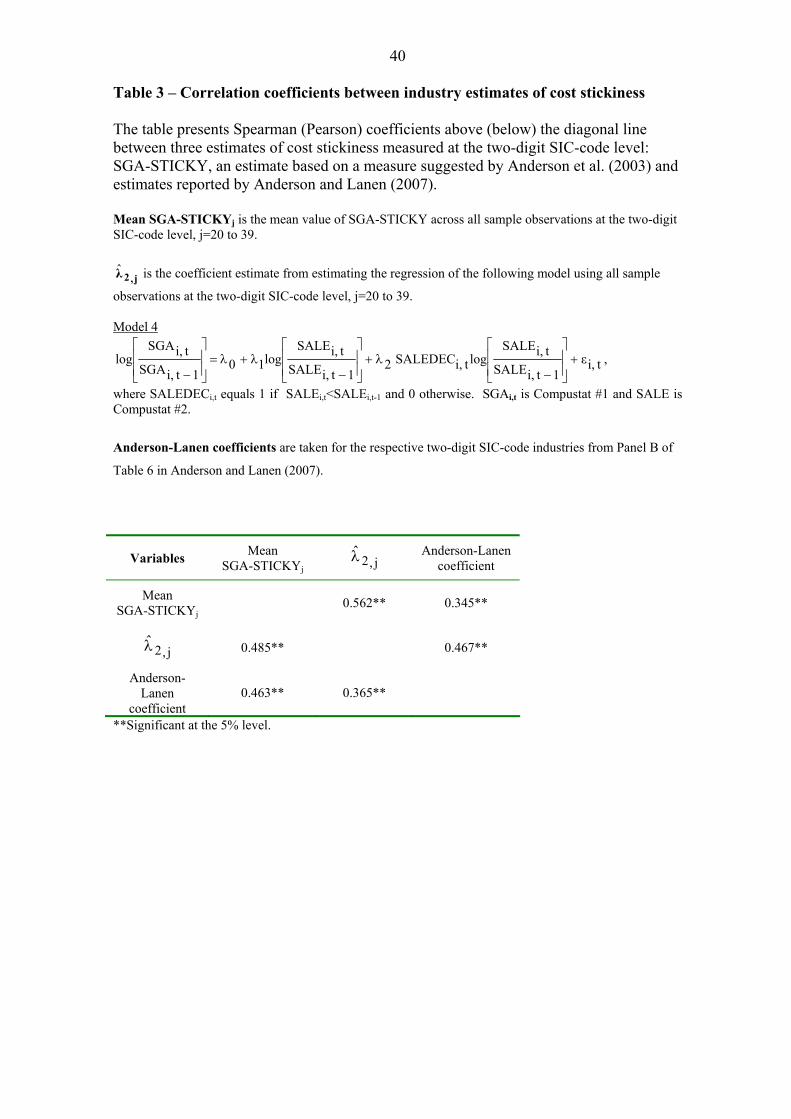
coefficients reported in Table 3 are positive and significant, indicating consistency

between the proposed cost stickiness measure and the earlier evidence on the

stickiness of SGA costs.

[Table 3 about here]

IV. EMPIRICAL RESULTS

Results of testing hypothesis H1

Testing whether more sticky cost behavior results in less accurate analysts’ earnings

forecasts, Table 4 presents the mean and median absolute analysts’ earnings forecast

errors contingent on sticky (STICKY<0) versus anti-sticky (STICKY≥0) cost

classification. The mean absolute error for firms with sticky cost behavior is 0.0080,

whereas that for firms with anti-sticky cost behavior is 0.0060. Thus, forecasts for

firms with anti-sticky cost behavior are, on average, more accurate by 25% = (0.0080-

0.0060)/0.0080 than forecasts for firms with sticky cost behavior. The difference is

statistically significant (α=5%) and economically meaningful.

25

[Tables 4 and 5 about here]

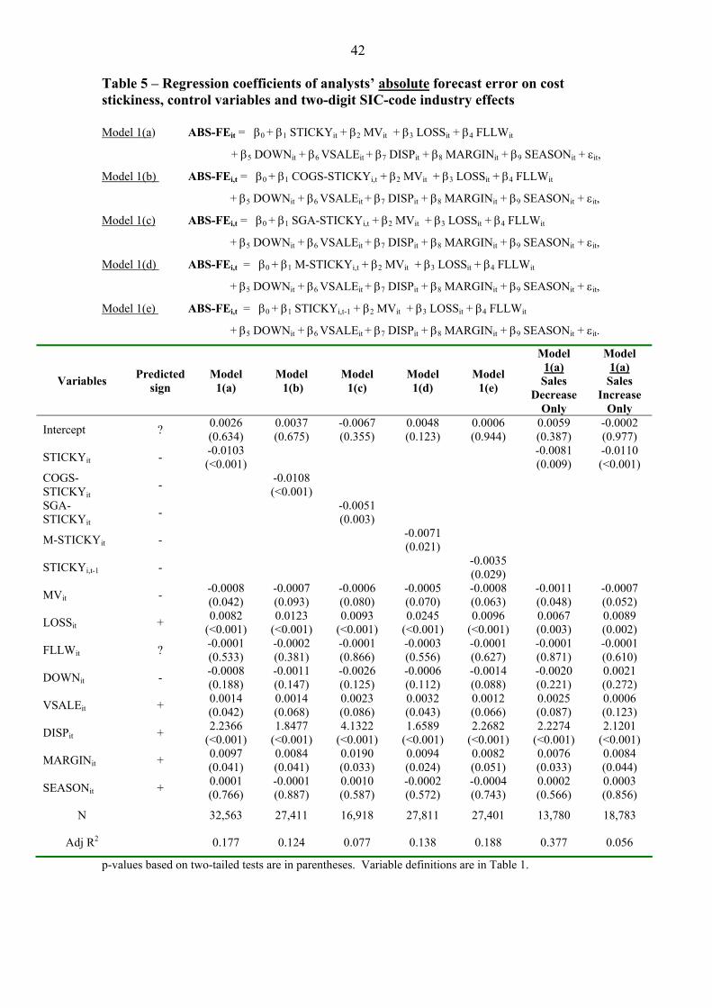
Table 5 presents coefficient estimates for the regression models. The coefficient on

STICKY in model 1(a) is -0.0103, statistically significant at p-value<0.001. The

coefficient on COGS-STICKY in model 1(b) is -0.0108, statistically significant at p-

value<0.001. The coefficient on SGA-STICKY in model 1(c) is -0.0051, statistically

significant at p-value=0.003. Adjusted R2 of the regressions vary from 7.7% to

17.7%. The results support the hypothesis, indicating that more sticky cost behavior

is associated with lower accuracy of analysts’ earnings forecasts.

As for the control variables, results for MV and LOSS are generally consistent with

expectations, indicating a positive and significant relationship between the amount of

available firm-specific information and forecast error. The coefficient estimates on

DOWN and FLLW are insignificant across the regression models, possibly due to

differences among analysts in the underlying costs, earnings models and access to

management information: a large number of analysts covering a firm can proxy

variation in the underlying costs and profits models, resulting in considerable noise.

As expected, the findings for DISP and to a limited extent for VSALE indicate a

positive and significant association between the absolute magnitude of the forecast

errors and the uncertainty in the firm’s environment of operations.

MARGIN is positively associated with ABS-FE, indicating that large gross margins

increase the analysts’ earnings forecast errors. The seasonal effect, SEASON, is also

insignificant across the regression models, indicating that analysts recognize the

seasonal effect and adjust their forecasts accordingly.

Results of two sensitivity models 1(d) and 1(e) are also reported in Table 5 and

provide further insights into additional aspects of the relationship between cost

behavior and the accuracy of analyst earnings forecasts. First, I examine the

sensitivity of the results to estimating cost stickiness over a longer time period.

26

Accordingly, M-STICKY measures cost stickiness based on cost responses in eight

quarters. Regression results for model 1(d) indicate a negative coefficient on M-

STICKY, -0.0071, statistically significant at p-value=0.021. The result supports the

hypothesis.

Second, I examine whether current (rather than past) managerial discretion affects the

hypothesized relationship. I check whether the regression coefficient estimates are

sensitive to discretionary choices made by managers on quarter t by replacing

STICKYit in model 1(a) with the cost stickiness measure estimated on quarter t-1,

STICKYi,t-1, which excludes all managerial choices made on quarter t.

Estimating regression model 1(e), the coefficient estimate on STICKYi,t-1 is -0.0035

(p-value=0.029). The negative and significant coefficient estimate indicates that more

sticky cost behavior observed in a preceding quarter is associated with higher absolute

analysts’ forecast errors. I conclude that cost stickiness estimated by analysts on a

preceding quarter affects the accuracy of the earnings prediction. Overall, the results

support the hypothesis.12

Focusing on cost stickiness, I now examine the effect of cost stickiness on absolute

forecast errors separately for sales decreases and sales increases. Evidence reported in

Table 5 indicates that the association is stronger for sales declines (adj R2=37.7%)

than for sales increases (adj R2=5.6%). Essentially, cost stickiness when sales decline

drives a considerable portion of the variability of analysts’ forecast errors.

Apparently, the association between cost stickiness and accuracy of analysts’ earnings

forecasts is more pronounced on sales decreases, which is line with the sticky cost

concept in Anderson et al. (2003).

Furthermore, evidence on the mean forecast error (not on the absolute error) reported

in Table 6 offers insights into the validity of assuming that analysts recognize cost 12 Further checking for a potential seasonality effect, I also computed the stickiness measure using cost responses relative to the same quarter of the preceding year. Results from estimating model 1 confirm the earlier results.

27

behavior. Results show that the mean forecast error of firms with sticky costs is

insignificantly different from that of firms with anti-sticky costs.13 Thus, the

evidence supports the assumption that analysts understand cost behavior to a

reasonable extent.

[Table 6 about here]

Results of testing hypothesis H2

Results showing that firms with more sticky cost behavior have lower analyst

coverage are presented in Table 7. Findings in Panel A indicate that, on average,

5.459 analysts follow firms with sticky cost behavior while 5.622 analysts follow

firms with anti-sticky cost behavior. The difference is statistically significant (p-value

<0.05). Panel B reports the results of three regression models, 2(a), 2(b), and 2(c).

The coefficients on STICKYit, M-STICKYit and STICKYi,t-1 are positive and highly

significant. Keeping in mind that lower values of STICKY indicate more sticky cost

behavior, the findings support H2.14

[Table 7 about here]

As for the control variables, the coefficient estimates of MV and TV are positive and

significant, in line with prior literature. The coefficient estimates of the proxies for

environmental uncertainty show mixed results. The coefficients of VSALE and ABS-

FE are negatively and significantly associated with the analyst following, while the

13 To see the intuition, suppose, on the contrary, that an analyst ignores cost stickiness. Consequently, her forecast would be upward biased in case of sticky costs (forecast error = reported earnings – forecast <0) because she under-estimates costs on demand falls. In a similar vein, her forecast would be downward biased in case of anti-sticky costs (forecast error = reported earnings – forecast >0) because she over-estimates costs on demand falls. Thus, sticky costs trigger a negative mean forecast error and anti-sticky costs trigger a positive mean forecast error (i.e., bias, not absolute forecast error). However, results reported in Table 6 indicate the mean forecast error is not significantly different for observations with sticky versus anti-sticky costs. Therefore, the data supports the assumption that analysts recognize cost stickiness to a reasonable extent. 14 The analysis implicitly assumes that an equivalent effort is expended for estimating sticky and anti-sticky costs. This assumption is sensible in this context because cost stickiness is estimated from public information reported in financial statements.

28

coefficient of DISP is positive and significant. The coefficients of GROWTH and

LOSS are insignificant.

The coefficient estimate of RD is also positive and highly significant, consistent with

Barth et al. (2001). To further check the robustness of the cost behavior effect, I

separately examine the cost stickiness effect on analyst coverage for firms with and

without R&D expenditures. Results (not tabulated) indicate that cost stickiness is

significantly associated with analyst coverage for firms with and without R&D

expenditures. In sum, the evidence indicates that firms with more sticky cost

behavior have lower analyst coverage.

Results of testing hypothesis H3

Table 8 presents results from testing whether market response to earnings surprises is

weaker for firms with more sticky cost behavior. In line with prior studies, coefficient

estimates β1 in all regression models are positive and highly significant, indicating a

positive market response to earnings surprises. The estimated coefficients for the

interaction variable are positive and significant when cost stickiness relates to total

costs (models 3(a) and 3(d)), but only marginally significant when cost stickiness

relates to SGA costs (model 3(c)), and insignificant with respect to stickiness of

COGS (model 3(b)).15 Findings indicate that investors tend to consider cost stickiness

with respect to total costs, but find it hard to figure stickiness of cost components.

The explanatory power in the models ranges between 1.8% and 2.9%, which is in line

with prior literature (e.g., Gu and Wu, 2003). To strengthen the evidence, I take a

predictive rather than contemporaneous approach in estimating cost stickiness. Model

3(e) shows a lower market reaction to earnings surprises for firms with less sticky

costs estimated on the preceding quarter (note that STICKY<0 indicates sticky costs).

15 Additionally, I estimate model 3(a) using a dummy variable for the classification of cost stickiness (sticky versus anti-sticky costs). Results confirm the above conclusions.

29

Overall, results indicate that market response to earnings surprises is weaker for firms

with more sticky cost behavior with respect to total costs, in support of H3.

[Table 8 about here]

The result contributes to the ongoing debate on investor rationality by documenting

that investors are able to process accounting information and partially infer cost

behavior in a rational way. With respect to the control variables, coefficient estimates

for DISP are generally insignificant and coefficient estimates for VSALE are only

marginally significant. Thus, dispersion of analysts’ forecasts and variation of sales

may not serve as appropriate proxies for ex-ante earnings uncertainty as perceived by

investors. This argument is supported by Diether et al. (2002), who interpret

dispersion in analysts’ earnings forecasts as a proxy for differences in opinion about

the stock (e.g., due to the employment of different valuation models). Overall,

findings indicate that investors partly understand firms’ cost behavior in responding to

earnings surprises.

V. A CONCLUDING REMARK

The study utilizes a managerial accounting concept, sticky costs, to gain insights into

how firms’ cost behavior impacts (i) the accuracy of analysts’ earnings forecasts, (ii)

analysts’ selection of covered firms, and (iii) market response to earnings

announcements. While implications of cost behavior are of primary interest to

management accountants, this study employs a management accounting concept for

addressing research questions usually raised by financial accountants. Although a

multi-disciplinary endeavor is rare in the literature, the insights indicate that

combining the perspectives of management and financial accounting is fruitful.

Further research is expected to build on this approach in exploring multi-disciplinary

30

accountings topics. Integrating management and financial accounting research is

expected to be beneficial to both disciplines.

31

References

Abarbanell, J.S., Bushee, B.J., 1997. Fundamental analysis, future earnings, and stock

returns. Journal of Accounting Research 35(1), 1-24.

Abarbanell, J.S., Lanen, W., Verrecchia, R., 1995. Analysts’ forecasts as proxies for

investor beliefs in empirical research. Journal of Accounting and Economics 20,

31-60.

Adar, Z., Barnea A., Lev, B., 1977. A comprehensive cost-volume-profit analysis

under uncertainty. The Accounting Review 52, 137-149.

Alford, W.A., Berger, P.G., 1999. A simultaneous equations analysis of forecast

accuracy, analyst following, and trading volume. Journal of Accounting, Auditing &

Finance 14, 219-240.

Anderson, M., Banker, R., Huang, R., Janakiraman, S., 2007. Cost behavior and

fundamental analysis of SGA costs. Journal of Accounting, Auditing and Finance,

22(1), 1-22.

Anderson, M., Banker, R., Janakiraman, S., 2003. Are selling, general, and

administrative costs ‘sticky’? Journal of Accounting Research 41, 47-63.

Anderson, S., Lanen, W., 2007. Understanding cost management: What can we learn

from the evidence on ‘sticky costs’? Working Paper, University of Melbourne.

Atiase, R., 1985. Predisclosure information, firm capitalization, and security price

behavior around earnings announcements. Journal of Accounting Research 23, 21-

36.

Baik, B., 2006. Self-selection in consensus analysts’ earnings forecasts. Asia-Pacific

Journal of Financial Studies 35(6), 141-168.

Balakrishnan, R., Gruca, T.S., 2008. Cost stickiness and core competency: A note.

Contemporary Accounting Research, 25(4), 993-1006.

32

Balakrishnan, R., Sivaramakrishnan, K., 2002. A critical overview of the use of full-

cost data for planning and pricing. Journal of Management Accounting Research

14, 3-31.

Balakrishnan, R., Peterson, M.J., Soderstrom, N.S., 2004. Does capacity utilization

affect the “stickiness” of costs? Journal of Accounting, Auditing and Finance 19(3),

283-299.

Banker, R., Chen, L., 2006. Predicting earnings using a model based on cost

variability and cost stickiness. The Accounting Review 81, 285-307.

Banker, R., Ciftci, M., Mashruwala, R., 2008. Managerial optimism, prior-period

sales changes, and sticky cost behavior. Working Paper, Temple University.

Banker, R., Hughes, J., 1994. Product costing and pricing. The Accounting Review

69, 479-494.

Barron, O.E., Byard, D., Kile, C., Riedl, E.J., 2002. High-technology intangibles and

analysts’ forecasts. Journal of Accounting Research 40(2), 289-312.

Barron, O.E., Kim, O., Lim, S., Stevens, D., 1998. Using analysts’ forecasts to

measure properties of analysts’ information environment. The Accounting Review

73, 421-433.

Barth, M.E., Kasznik, R., McNichols, M.F., 2001. Analyst coverage and intangible

assets. Journal of Accounting Research 39(1), 1-34.

Beja, A., Weiss, D., 2006. Some informational aspects of conservatism. European

Accounting Review 15, 585-604.

Bhushan, R., 1989. Firm characteristics and analyst following. Journal of

Accounting and Economics 11, 255-274.

Brown, L., 2001. A temporal analysis of earnings surprises: Profits versus losses.

Journal of Accounting Research 39, 221-241.

33

Brown, L., Richardson, G., Schwager, S., 1987. An information interpretation of

financial analyst superiority in forecasting earnings. Journal of Accounting

Research 25, 49-67.

Chen, C.X., Lu, H., Sougiannis, T., 2008. Managerial empire building, corporate

governance, and the asymmetrical behavior of selling, general, and administrative

costs. Working Paper, University of Illinois at Urbana-Champaign.

Clement, M., Tse, S., 2003. Do investors respond to analysts’ forecast revisions as if

forecast accuracy is all that matters? The Accounting Review 78, 227-249.

Collins, D.W., Kothari, S.P., Rayburn, J.D., 1987. Firm size and the information

content of prices with respect to earnings. Journal of Accounting and Economics 9,

111-138.

Das, S., Gou, R.J., Zhang, H., 2006. Analysts’ coverage and subsequent performance

of newly public firms. The Journal of Finance 61(3), 1159-1185.

Das, S., Levine, C., Sivaramakrishnan, K., 1998. Earnings predictability and bias in

analysts’ earnings forecasts. The Accounting Review 73, 277-294.

Dechow, P., Kothari, S., Watts, R., 1998. The relation between earnings and cash

flows. Journal of Accounting and Economics 25, 133-168.

Diether, K., Malloy, C., Scherbina, A., 2002. Differences of opinion and the cross

section of stock returns. The Journal of Finance 57, 2113-2141.

Frankel, R., Kothari, S., Weber, J., 2006. Determinants of the informativeness of

analyst research. Journal of Accounting and Economics 41, 29-54.

Givoly, D., Hayn, C., 2000. The changing time-series properties of earnings, cash

flows and accruals: Has financial reporting become more conservative? Journal of

Accounting and Economics 29, 287-320.

Gu, Z., Wu, J., 2003. Earnings skewness and analyst forecast bias. Journal of

Accounting and Economics 35, 5-29.

34

Hemmer, T., Labro, E., 2007. On the relation between the properties of managerial

and financial reporting systems. Working Paper, London School of Economics.

Hong, H., Lim, T., Stein, J.C., 2000. Bad news travels slowly: Size, analyst coverage,

and the profitability of momentum strategies. The Journal of Finance 55, 265-295.

Imhoff, E., Lobo, G., 1992. The effect of ex ante earnings uncertainty on earnings

response coefficients. The Accounting Review 67, 427-439.

Lang, M., Lundholm, R., 1996. Corporate disclosure policy and analyst behavior.

The Accounting Review 71, 467-492.

Lim, T., 2001. Rationality and analysts’ forecast bias. The Journal of Finance 56,

369-385.

Lipe, R., 1990. The relation between stock returns and accounting earnings given

alternative information. The Accounting Review 65, 49-71.

Maher, M., Lanen, W., Rajan, M., 2006. Fundamentals of Cost Accounting.

McGraw-Hill.

Matsumoto, D., 2002. Management’s incentives to avoid negative earnings surprises.

The Accounting Review 77, 483-514.

O’Brien, P.C., Bhushan, R., 1990. Analyst following and institutional ownership.

Journal of Accounting Research 28, 55-82.

Ottaviani, M., Sorensen, P., 2006. The strategy of professional forecasting. Journal

of Financial Economics 81, 441-66.

Parkash, M., Dhaliwal, D.S., Salatka, W.K., 1995. How certain firm-specific

characteristics affect the accuracy and dispersion of analysts’ forecasts. Journal of

Business Research 34, 161-169.

Philbrick, D., Ricks, W., 1991. Using value line and IBES analyst forecasts in

accounting research. Journal of Accounting Research 29, 397-471.

35

Rock,S., Sedo, S., Willenborg, M., 2001. Analyst following and count-data

econometrics. Journal of Accounting and Economics 30, 351-373.

Rothschild, M., 1971. On the cost of adjustment. Quarterly Journal of Economics

85, 601-622.

Stickel, S., 1992. Reputation and performance among security analysts. The Journal

of Finance 47, 1811-1836.

Weiss, D., Naik, P.N., Tsai, C.L., 2008. Extracting forward-looking information from

security prices: A new approach. The Accounting Review, 83(4), 1101-1124.

Wernerfelt, B., 1997. On the nature and scope of the firm: An adjustment-cost theory.

Journal of Business 80(4), 489-514.

Wiedman, C., 1996. The relevance of characteristics of the information environment

in the selection of a proxy for the market’s expectations for earnings: An extension

of Brown, Richardson, and Schwager. Journal of Accounting Research 34, 313-

324.

36

Figure 1 Figure 1.1 – Cost asymmetry

Figure 1.2 – Absolute forecast errors are greater in the presence of sticky costs than in the presence of anti-sticky costs on both activity level decrease (YL) and activity level increase (YH).

37

Table 1 - Descriptive statistics, pooled over time, 1986-2005.

Variables N Mean Std. dev. q1 Median q3 %

Negative STICKY 44,931 -0.0174 0.4897 -0.1551 -0.0111 0.1205 53.2

COGS-STICKY 37,521 0.0187 0.4707 -0.1564 0.0063 0.1823 48.7

SGA-STICKY 23,809 -0.0306 0.6944 -0.3870 -0.0326 0.3304 55.1

M-STICKY 44,931 -0.0117 0.2398 -0.0633 -0.0094 0.0501 54.9

FE 44,931 -0.0014 0.1182 -0.0010 0 0.0011 38.3

ABS-FE 44,931 0.0071 0.1180 0.0003 0.0011 0.0034 NA

MV 44,926 4.7037 2.1314 3.1508 4.6328 6.1997 NA LOSS 44,931 0.1628 0.3692 0 0 0 NA FLLW 44,931 5.5356 5.1759 2 4 8 NA DOWN 39,415 0.5702 0.4828 0 1 1 NA VSALE 44,926 0.1480 0.1478 0.0611 0.1026 0.1752 NA DISP 44,931 0.0018 0.0328 0.0001 0.0004 0.0012 NA MARGIN 44,559 0.3670 0.1819 0.2408 0.3530 0.4874 NA

SEASON 44,626 0.6111 0.4875 0 1 1 NA

GROWTH 35,864 0.0418 0.1310 0.0142 0.0247 0.0422 NA

RD 44,931 0.0482 0.0987 0 0 0.0620 NA

TV 42,029 5.3360 8.2114 1.8441 2.2254 6.1813 NA

Variable definitions for each firm i on quarter t:

FEit is the difference between reported earnings and the mean (consensus) forecasts announced in the

month immediately preceding that of the earnings announcement, deflated by the price at the end of the

prior quarter. ABS-FEit = ⎮ FEit ⎮.

STICKYit = ττ

⎟⎠⎞

⎜⎝⎛∆∆

−⎟⎠⎞

⎜⎝⎛∆∆

,i,i SALECOSTlog

SALECOSTlog , τ , τ ∈{t,..,t-3}, where τ is the most recent

quarter with sales decrease and τ is the most recent quarter with sales increase.

COSTit is sales (Compustat #2) minus net earnings (Compustat #8) for firm i in quarter t.

SALEit is Compustat #2 for firm i in quarter t.

COGS-STICKYit = ττ

⎟⎠⎞

⎜⎝⎛∆∆

−⎟⎠⎞

⎜⎝⎛∆∆

,i,i SALECOGSlog

SALECOGSlog , τ , τ ∈{t,..,t-3}, where τ is the most

recent quarter with sales decrease and τ is the most recent quarter with sales increase. COGSit is

Compustat #30 for firm i in quarter t.

SGA-STICKYit = ττ

⎟⎠⎞

⎜⎝⎛∆∆

−⎟⎠⎞

⎜⎝⎛∆∆

,i,i SALESGAlog

SALESGAlog , τ , τ ∈{t,..,t-3}, where τ is the most

recent quarter with sales decrease and τ is the most recent quarter with sales increase. SGAit is

Compustat #1 for firm i in quarter t.

38

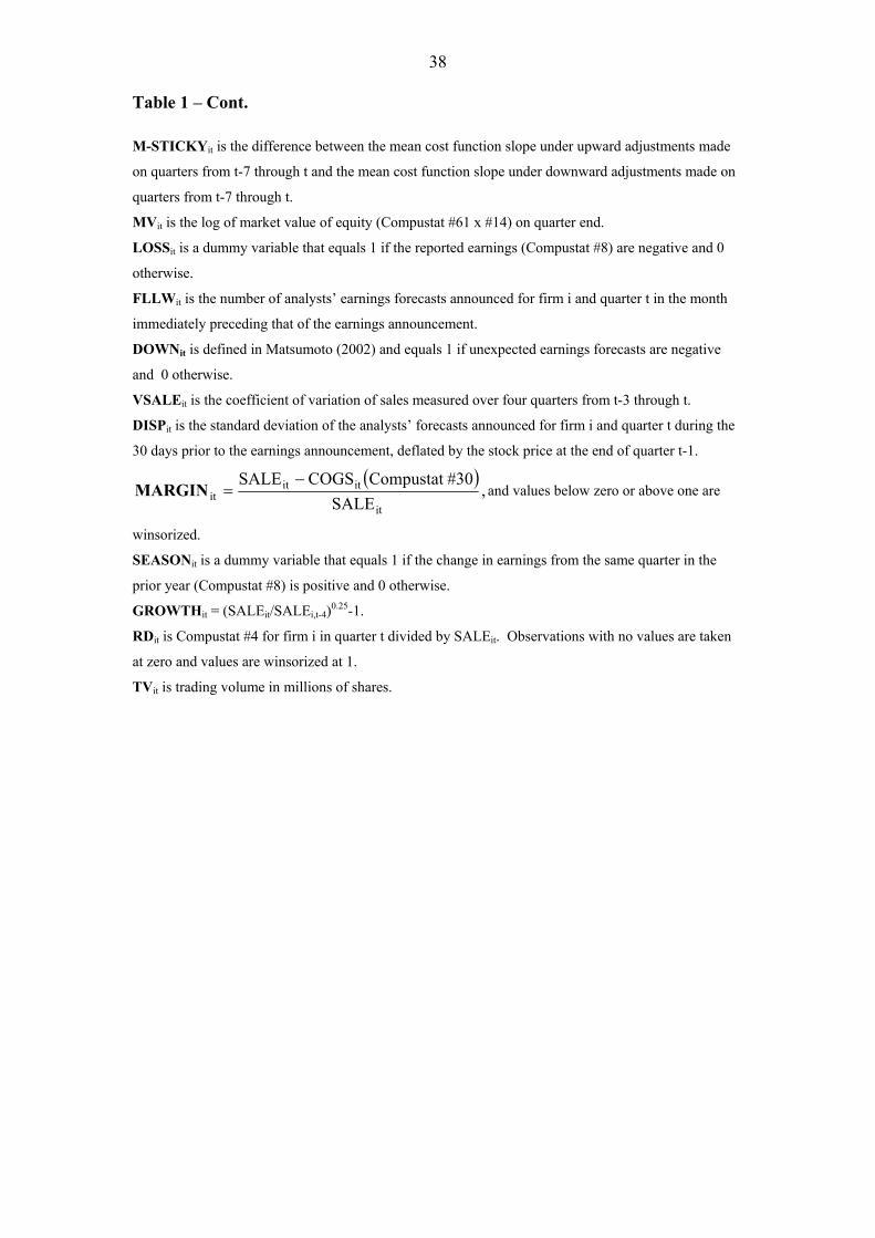
Table 1 – Cont.

M-STICKYit is the difference between the mean cost function slope under upward adjustments made

on quarters from t-7 through t and the mean cost function slope under downward adjustments made on

quarters from t-7 through t.

MVit is the log of market value of equity (Compustat #61 x #14) on quarter end.

LOSSit is a dummy variable that equals 1 if the reported earnings (Compustat #8) are negative and 0

otherwise.

FLLWit is the number of analysts’ earnings forecasts announced for firm i and quarter t in the month

immediately preceding that of the earnings announcement.

DOWNit is defined in Matsumoto (2002) and equals 1 if unexpected earnings forecasts are negative

and 0 otherwise.

VSALEit is the coefficient of variation of sales measured over four quarters from t-3 through t.

DISPit is the standard deviation of the analysts’ forecasts announced for firm i and quarter t during the

30 days prior to the earnings announcement, deflated by the stock price at the end of quarter t-1.

( ),

SALE#30Compustat COGSSALE

it

ititit

−=MARGIN and values below zero or above one are

winsorized.

SEASONit is a dummy variable that equals 1 if the change in earnings from the same quarter in the

prior year (Compustat #8) is positive and 0 otherwise.

GROWTHit = (SALEit/SALEi,t-4)0.25-1.

RDit is Compustat #4 for firm i in quarter t divided by SALEit. Observations with no values are taken

at zero and values are winsorized at 1.

TVit is trading volume in millions of shares.

39

Table 2 – Correlation coefficients Spearman coefficients are reported above the diagonal line and Pearson coefficients below the diagonal line.

Variables FE ABS-FE STICKY COGS- STICKY

SGA- STICKY

M- STICKY MV LOSS FLLW DOWN VSALE DISP MARGIN SEASON GROWTH RD TV

FE 0.00 0.18** 0.15** 0.09** 0.11** 0.11** -0.16** 0.05** 0.02 0.03** -0.02** 0.03* 0.28** 0.01** 0.02** 0.02**

ABS-FE -0.26** -0.03** -0.04** -0.01 -0.01** -0.35** 0.28** -0.33** -0.04** 0.16** 0.24** 0.10** -0.19** -0.01** -0.03** -0.04**

STICKY 0.03** -0.04** 0.48** 0.40** 0.48** 0.02** -0.17** 0.00 0.01 0.00 -0.03** -0.03* 0.26** 0.02** -0.01 0.01 COGS-

STICKY 0.02** -0.04** 0.49** 0.07** 0.32** 0.03** -0.10** 0.02** 0.02** 0.01 -0.05** -0.08** 0.18** 0.04** 0.04** 0.00 SGA-

STICKY 0.01** -0.03** 0.43** 0.18** 0.12** 0.01 -0.08** -0.02** 0.01 0.00 -0.02** 0.00 0.13** 0.05** -0.04** 0.00 M-

STICKY 0.04** -0.05** 0.45** 0.36** 0.12** 0.00 -0.09** 0.01** 0.05** 0.00 0.02** -0.02** 0.14** 0.02** -0.03** 0.02

MV 0.02** -0.03** 0.01** 0.02** 0.00 0.01 -0.10** 0.76** -0.02 -0.07** 0.13** 0.18** 0.09** 0.08** 0.14** 0.72**

LOSS -0.04** 0.06** -0.15** -0.08** -0.08** -0.07** -0.10** -0.10** -0.06** 0.25** 0.04** -0.04** -0.33** -0.04** 0.15** -0.05**

FLLW 0.01** -0.03** 0.02** 0.02** 0.00 0.02 0.74** -0.09** -0.07** -0.08** -0.01 -0.10** 0.04** 0.03** 0.10** 0.61**

DOWN 0.02 -0.03** 0.04** 0.01 0.02 0.04** 0.01 -0.05** 0.02 0.04** 0.01 0.02 0.00 0.00 0.05** 0.01

VSALE -0.01 0.02** 0.00 0.01 0.00 0.00 -0.02** 0.21** -0.14** 0.03** 0.03** -0.04* -0.03** 0.33** 0.09** 0.00

DISP 0.00 0.25** 0.01 0.00 -0.01 0.00 -0.02** 0.16** 0.34** 0.01 0.02** 0.02** -0.15** -0.01** 0.01** 0.00

MARGIN 0.01 0.03** -0.02** -0.09* 0.02* -0.01 0.27** -0.05** -0.07** 0.00 0.00 0.04** -0.05** 0.05** 0.08** 0.01

SEASON 0.03** -0.03** 0.21** 0.16** 0.13** 0.10** 0.09** -0.33** 0.05** 0.00 -0.05** -0.02** -0.01** 0.12** -0.06** 0.01

GROWTH 0.01** -0.01** 0.03** 0.04** 0.05** 0.03** 0.08** -0.05** 0.04** 0.00 0.34** -0.01** 0.04** 0.12** 0.09** 0.10**

RD -0.02** 0.03** -0.02** 0.04** -0.06** -0.02** 0.09 0.29** 0.08** 0.06** 0.19** 0.00 0.55** -0.09** 0.12** 0.13**

TV 0.02** -0.03** 0.01 0.01 0.01 0.01 0.70** -0.04** 0.58** 0.00 0.01 0.01 -0.02 0.00 0.06** 0.18**

**Significant at the 5% level. Variable definitions are in Table 1.

40

Table 3 – Correlation coefficients between industry estimates of cost stickiness The table presents Spearman (Pearson) coefficients above (below) the diagonal line between three estimates of cost stickiness measured at the two-digit SIC-code level: SGA-STICKY, an estimate based on a measure suggested by Anderson et al. (2003) and estimates reported by Anderson and Lanen (2007). Mean SGA-STICKYj is the mean value of SGA-STICKY across all sample observations at the two-digit SIC-code level, j=20 to 39.

j,2λ̂ is the coefficient estimate from estimating the regression of the following model using all sample

observations at the two-digit SIC-code level, j=20 to 39. Model 4

ti,ε1ti,SALE

ti,SALElogti,SALEDEC2

1ti,SALEti,SALE

log101ti,SGA

ti,SGAlog +

⎥⎥⎦

⎤

⎢⎢⎣

⎡

−λ+

⎥⎥⎦

⎤

⎢⎢⎣

⎡

−λ+λ=

⎥⎥⎦

⎤

⎢⎢⎣

⎡

−,

where SALEDECi,t equals 1 if SALEi,t<SALEi,t-1 and 0 otherwise. SGAi,t is Compustat #1 and SALE is Compustat #2.

Anderson-Lanen coefficients are taken for the respective two-digit SIC-code industries from Panel B of

Table 6 in Anderson and Lanen (2007).

Variables Mean SGA-STICKYj j,2λ̂ Anderson-Lanen

coefficient

Mean SGA-STICKYj

0.562** 0.345**

j,2λ̂ 0.485** 0.467**

Anderson-Lanen

coefficient 0.463** 0.365**

**Significant at the 5% level.

41

Table 4 – Absolute forecast errors (ABS-FE) for firms with sticky versus anti-sticky cost behavior

Cost behavior Mean Median N

Sticky costs: STICKYit <0 0.0080 0.0012 23,915

Anti-sticky costs: STICKYit ≥0 0.0060 0.0010 21,016

Difference 0.0020** 0.0002a **Significant at the 5% level. a – Mann-Whitney test indicates a significant difference between the medians at the 5% level.

42

Table 5 – Regression coefficients of analysts’ absolute forecast error on cost stickiness, control variables and two-digit SIC-code industry effects Model 1(a) ABS-FEit = β0 + β1 STICKYit + β2 MVit + β3 LOSSit + β4 FLLWit

+ β5 DOWNit + β6 VSALEit + β7 DISPit + β8 MARGINit + β9 SEASONit + εit, Model 1(b) ABS-FEi,t = β0 + β1 COGS-STICKYi,t + β2 MVit + β3 LOSSit + β4 FLLWit

+ β5 DOWNit + β6 VSALEit + β7 DISPit + β8 MARGINit + β9 SEASONit + εit, Model 1(c) ABS-FEi,t = β0 + β1 SGA-STICKYi,t + β2 MVit + β3 LOSSit + β4 FLLWit

+ β5 DOWNit + β6 VSALEit + β7 DISPit + β8 MARGINit + β9 SEASONit + εit, Model 1(d) ABS-FEi,t = β0 + β1 M-STICKYi,t + β2 MVit + β3 LOSSit + β4 FLLWit

+ β5 DOWNit + β6 VSALEit + β7 DISPit + β8 MARGINit + β9 SEASONit + εit, Model 1(e) ABS-FEi,t = β0 + β1 STICKYi,t-1 + β2 MVit + β3 LOSSit + β4 FLLWit

+ β5 DOWNit + β6 VSALEit + β7 DISPit + β8 MARGINit + β9 SEASONit + εit.

Variables Predicted sign

Model 1(a)

Model 1(b)

Model 1(c)

Model 1(d)

Model 1(e)

Model 1(a)

Sales Decrease

Only

Model 1(a)

Sales Increase

Only

Intercept ? 0.0026 (0.634)

0.0037 (0.675)

-0.0067 (0.355)

0.0048 (0.123)

0.0006 (0.944)

0.0059 (0.387)

-0.0002 (0.977)

STICKYit - -0.0103 (<0.001) -0.0081

(0.009) -0.0110 (<0.001)

COGS-STICKYit

- -0.0108 (<0.001)

SGA- STICKYit

- -0.0051 (0.003)

M-STICKYit - -0.0071 (0.021)

STICKYi,t-1 - -0.0035 (0.029)

MVit - -0.0008 (0.042)

-0.0007 (0.093)

-0.0006 (0.080)

-0.0005 (0.070)

-0.0008 (0.063)

-0.0011 (0.048)

-0.0007 (0.052)

LOSSit + 0.0082 (<0.001)

0.0123 (<0.001)

0.0093 (<0.001)

0.0245 (<0.001)

0.0096 (<0.001)

0.0067 (0.003)

0.0089 (0.002)

FLLWit ? -0.0001 (0.533)

-0.0002 (0.381)

-0.0001 (0.866)

-0.0003 (0.556)

-0.0001 (0.627)

-0.0001 (0.871)

-0.0001 (0.610)

DOWNit - -0.0008 (0.188)

-0.0011 (0.147)

-0.0026 (0.125)

-0.0006 (0.112)

-0.0014 (0.088)

-0.0020 (0.221)

0.0021 (0.272)

VSALEit + 0.0014 (0.042)

0.0014 (0.068)

0.0023 (0.086)

0.0032 (0.043)

0.0012 (0.066)

0.0025 (0.087)

0.0006 (0.123)

DISPit + 2.2366 (<0.001)

1.8477 (<0.001)

4.1322 (<0.001)

1.6589 (<0.001)

2.2682 (<0.001)

2.2274 (<0.001)

2.1201 (<0.001)

MARGINit + 0.0097 (0.041)

0.0084 (0.041)

0.0190 (0.033)

0.0094 (0.024)

0.0082 (0.051)

0.0076 (0.033)

0.0084 (0.044)

SEASONit + 0.0001 (0.766)

-0.0001 (0.887)

0.0010 (0.587)

-0.0002 (0.572)

-0.0004 (0.743)

0.0002 (0.566)

0.0003 (0.856)

N 32,563 27,411 16,918 27,811 27,401 13,780 18,783

Adj R2 0.177 0.124 0.077 0.138 0.188 0.377 0.056

p-values based on two-tailed tests are in parentheses. Variable definitions are in Table 1.

43

Table 6 – Forecast errors (FE) for firms with sticky versus anti-sticky cost behavior

Cost behavior Mean Median N

Sticky costs: STICKYit <0 -0.0016 0 23,915

Anti-sticky costs: STICKYit ≥0 -0.0012 0 21,016

Difference -0.0004b 0 b - Insignificant at the 10% level.

44

Table 7 – Association of cost behavior with analyst coverage Panel A - The mean number of analysts following firms with sticky versus anti-sticky

cost behavior.

Cost behavior Mean number of analyst coverage N

Sticky costs: STICKYit<0 5.459 23,915

Anti-sticky costs: STICKYit≥0 5.622 21,016

Difference 0.163**

**Significant at the 5% level.

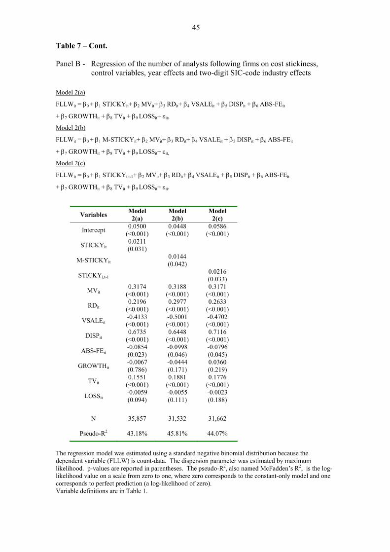
45

Table 7 – Cont. Panel B - Regression of the number of analysts following firms on cost stickiness,

control variables, year effects and two-digit SIC-code industry effects

Model 2(a)

FLLWit = β0 + β1 STICKYit+ β2 MVit+ β3 RDit+ β4 VSALEit + β5 DISPit + β6 ABS-FEit

+ β7 GROWTHit + β8 TVit + β9 LOSSit+ εit,

Model 2(b)

FLLWit = β0 + β1 M-STICKYit+ β2 MVit+ β3 RDit+ β4 VSALEit + β5 DISPit + β6 ABS-FEit

+ β7 GROWTHit + β8 TVit + β9 LOSSit+ εit,

Model 2(c)

FLLWit = β0 + β1 STICKYi,t-1+ β2 MVit+ β3 RDit+ β4 VSALEit + β5 DISPit + β6 ABS-FEit

+ β7 GROWTHit + β8 TVit + β9 LOSSit+ εit.

Variables Model 2(a)

Model 2(b)

Model 2(c)

Intercept 0.0500 (<0.001)

0.0448 (<0.001)

0.0586 (<0.001)

STICKYit 0.0211 (0.031)

M-STICKYit 0.0144 (0.042)

STICKYi,t-1 0.0216 (0.033)

MVit 0.3174

(<0.001) 0.3188

(<0.001) 0.3171

(<0.001)

RDit 0.2196

(<0.001) 0.2977

(<0.001) 0.2633

(<0.001)

VSALEit -0.4133 (<0.001)

-0.5001 (<0.001)

-0.4702 (<0.001)

DISPit 0.6735

(<0.001) 0.6448

(<0.001) 0.7116

(<0.001)

ABS-FEit -0.0854 (0.023)

-0.0998 (0.046)

-0.0796 (0.045)

GROWTHit -0.0067 (0.786)

-0.0444 (0.171)

0.0360 (0.219)

TVit 0.1551

(<0.001) 0.1881

(<0.001) 0.1776

(<0.001)

LOSSit -0.0059 (0.094)

-0.0055 (0.111)

-0.0023 (0.188)

N 35,857 31,532 31,662

Pseudo-R2 43.18% 45.81% 44.07%

The regression model was estimated using a standard negative binomial distribution because the dependent variable (FLLW) is count-data. The dispersion parameter was estimated by maximum likelihood. p-values are reported in parentheses. The pseudo-R2, also named McFadden’s R2, is the log-likelihood value on a scale from zero to one, where zero corresponds to the constant-only model and one corresponds to perfect prediction (a log-likelihood of zero). Variable definitions are in Table 1.

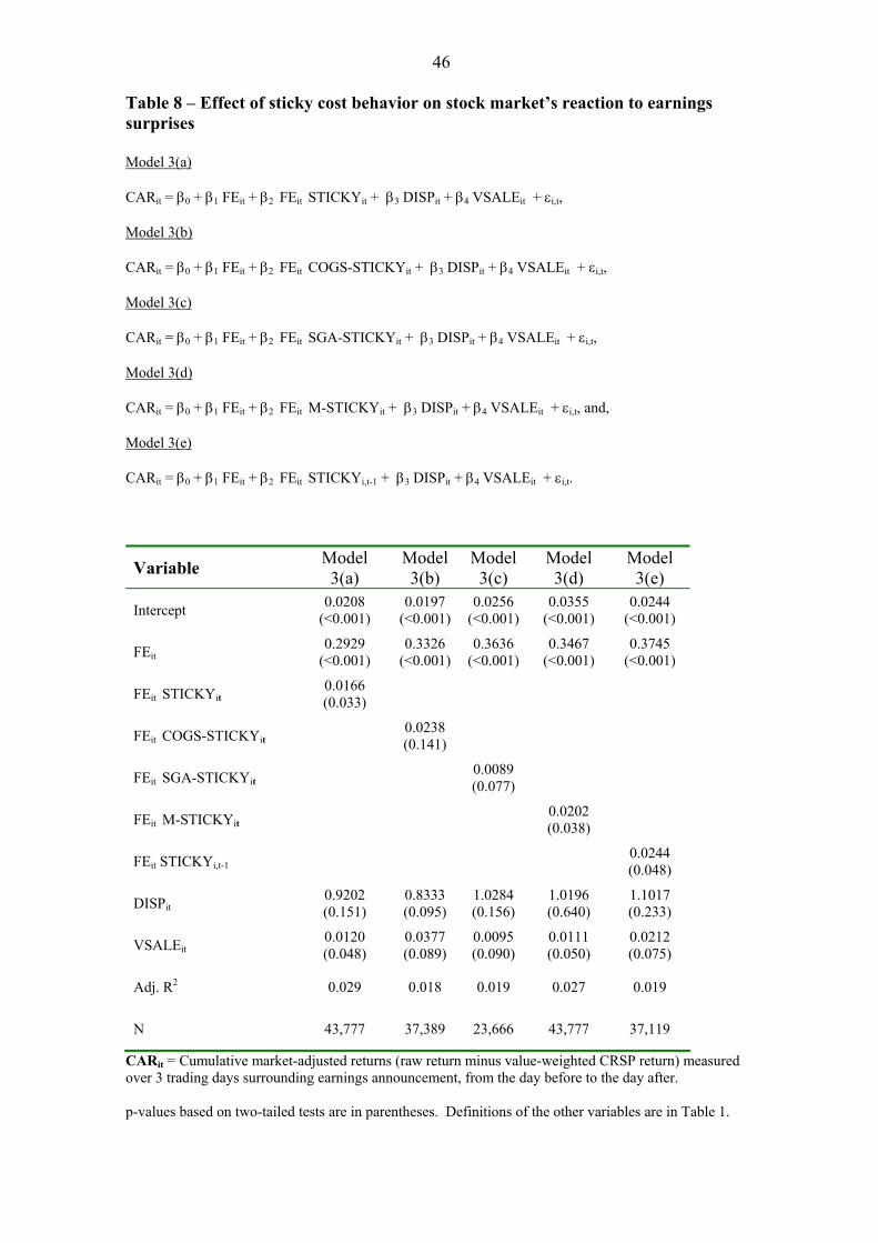
46

Table 8 – Effect of sticky cost behavior on stock market’s reaction to earnings surprises Model 3(a)

CARit = β0 + β1 FEit + β2 FEit STICKYit + β3 DISPit + β4 VSALEit + εi,t,

Model 3(b)

CARit = β0 + β1 FEit + β2 FEit COGS-STICKYit + β3 DISPit + β4 VSALEit + εi,t,

Model 3(c)

CARit = β0 + β1 FEit + β2 FEit SGA-STICKYit + β3 DISPit + β4 VSALEit + εi,t,

Model 3(d)

CARit = β0 + β1 FEit + β2 FEit M-STICKYit + β3 DISPit + β4 VSALEit + εi,t, and,

Model 3(e)

CARit = β0 + β1 FEit + β2 FEit STICKYi,t-1 + β3 DISPit + β4 VSALEit + εi,t.

Variable Model 3(a)

Model 3(b)

Model 3(c)

Model 3(d)

Model 3(e)

Intercept 0.0208 (<0.001)

0.0197 (<0.001)

0.0256 (<0.001)

0.0355 (<0.001)

0.0244 (<0.001)

FEit 0.2929

(<0.001) 0.3326

(<0.001) 0.3636

(<0.001) 0.3467

(<0.001) 0.3745

(<0.001)

FEit STICKYit 0.0166 (0.033)

FEit COGS-STICKYit 0.0238 (0.141)

FEit SGA-STICKYit 0.0089 (0.077)

FEit M-STICKYit 0.0202 (0.038)

FEit STICKYi,t-1 0.0244 (0.048)

DISPit 0.9202 (0.151)

0.8333 (0.095)

1.0284 (0.156)

1.0196 (0.640)

1.1017 (0.233)

VSALEit 0.0120 (0.048)

0.0377 (0.089)

0.0095 (0.090)

0.0111 (0.050)

0.0212 (0.075)

Adj. R2 0.029 0.018 0.019 0.027 0.019

N 43,777 37,389 23,666 43,777 37,119

CARit = Cumulative market-adjusted returns (raw return minus value-weighted CRSP return) measured over 3 trading days surrounding earnings announcement, from the day before to the day after. p-values based on two-tailed tests are in parentheses. Definitions of the other variables are in Table 1.

47

Appendix

Employing cost stickiness as a yardstick, I develop a simple two-period model to predict

a relationship between the level of cost stickiness and the accuracy of analysts’ earnings

forecasts. The primitive model input in the first period is a set of prior beliefs on the

state of the world, say demand y, which is a realization of a random variable y~ , drawn

from a distribution function, Φ(y), with a strictly positive and symmetric density, φ(y),

over the support [ y-λ, y+λ], y>λ>0. The second-period revenue function, R(y), is

assumed to be differentiable, increasing and concave.16 Costs in the second period are

modeled by:

C(y,α) = ( )⎩⎨⎧

≥α++<α++

yyifyvyfyyifyvf

f - a fixed cost of production, f≥0,

v - a variable cost per product unit, v≥0,

α - level of cost stickiness per product unit, -v < α < R′( y) - v.

The parameter α captures the level of cost stickiness in adjusting resources to changes in

the activity level. If α<0 then costs increase more when activity rises than they decrease

when activity falls by an equivalent amount; that is, a negative value of α indicates

sticky costs. Furthermore, if α>0, then costs increase less when activity rises than they

decrease when activity falls by an equivalent amount; that is, a positive value of α

indicates anti-sticky or adjustable costs. The difference between the cost of an upward

activity adjustment and the cost of a downward activity adjustment depends only on α:17

[C( y +1)-C( y )]-[C( y )-C( y -1)] = [v( y +1)+α y -v y -α y ]-[v y +α y -(v+α)( y -1)]= -α.

16 The revenue function depends on previously made managerial choices, like product price. See also Balakrishnan and Sivaramakrishnan (2002). 17 I note that cost stickiness does not depend on the operational leverage of the firm because the fixed cost component, f, does not influence the level of cost stickiness.

48

I use cost of adjustments to expand the conventional fixed-variable cost model and

estimate stickiness of firms’ cost functions. My approach follows Wernerfelt (1997),

who shows that the magnitude of an adjustment cost drives the form of the organization,

and Balakrishnan and Gruca (2008), who show that cost stickiness is greater for cost

functions that relate to an organization’s core competency. Rothschild (1971) models

properties of convex (concave) adjustment cost structures that result in asymmetric cost

functions due to the cost of producing marginal unit increases (decreases) in the activity

level.

Anderson et al. (2003) suggest that current managerial choices are also likely to affect

cost behavior due to economic forces acting to restrain or expedite resource adjustments.

For instance, an unexpected fall in demand may induce managers to purposely delay

reductions in committed resources until they receive more information about the

permanence of the decline in demand, resulting in cost stickiness.

In the proposed model, the earnings function, Π(y,α) = R(y)–C(y,α), is strictly

increasing in y and transforms demand y realized in the second period into earnings.

The ex-ante earnings expectations in the first period are denoted Π̂ ( y~ ,α). In the second

period, the firm truly reports its realized earnings, Π(y,α).

An analyst is delegated the task of producing accurate estimates of a firm’s earnings

expectations and the forecast is honest, as in, for example, Ottaviani and Sorensen

(2006). In the first period, the analyst announces Π̂ ( y~ ,α) as her most accurate forecast,

if her error loss function is symmetric and concave (e.g., a quadratic loss function).18

Focusing on the absolute earnings forecast error as an accuracy gauge, the proposition

below proves a negative relationship between the level of cost stickiness and the mean

absolute earnings forecast error. That is, higher values of α, i.e., less sticky cost

behavior, result in lower mean absolute analyst forecast errors.

18 A discussion on the properties of a symmetric error loss function appears in Beja and Weiss (2006).

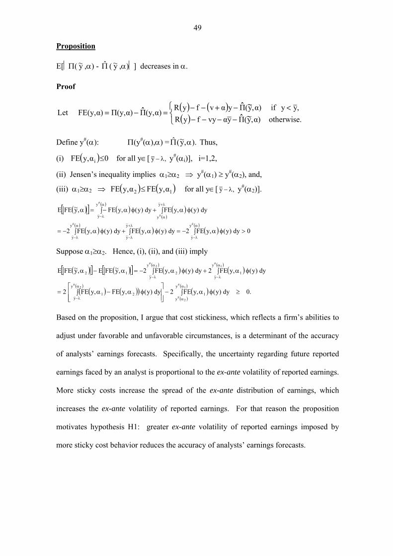
49

Proposition

E[⏐Π( y~ ,α) - Π̂ ( y~ ,α)⏐] decreases in α.

Proof

( ) ( )( )⎩

⎨⎧

−−−−<−+−−

=−=otherwise.α),y(ΠyαvyfyR

,yyifα),y(ΠyαvfyRα)(y,Πα)Π(y,α)FE(y,Let ~ˆ~ˆˆ

Define y#(α): Π(y#(α),α) = ).,y~(ˆ αΠ Thus,

(i) ( )iαy,FE ≤0 for all y∈[ ,y λ− y#(αi)], i=1,2,

(ii) Jensen’s inequality implies α1≥α2 ⇒ y#(α1) ≥ y#(α2), and,

(iii) α1≥α2 ⇒ ( )2αy,FE ≤ ( )1αy,FE for all y∈[ ,y λ− y#(α2)].

( )[ ] ( )( )

( )( )

( )( )

( ) ( )( )

0dy)y(,yFE2dy)y(,yFEdy)y(,yFE2

dy)y(,yFEdy)y(,yFE,y~FEE

##

#

#

y

y

y

y

y

y

y

y

y

y

>∫ φα−=∫ φα∫ +φα−=

φ∫ α∫ +φα−=α

α

λ−

λ+

λ−

α

λ−

λ+

α

α

λ−

Suppose α1≥α2. Hence, (i), (ii), and (iii) imply

( )[ ] ( )[ ] ( )( )

( )( )

( ) ( )( )( )

( )( )

( ).0dy)y(,yFE2dy)y(,yFE,yFE2

dy)y(,yFE2dy)y(,yFE2,y~FEE,y~FEE

1#

2#

2#

1#

2#

y

y1

y

y21

y

y1

y

y212

≥∫ φα−⎥⎥⎦

⎤

⎢⎢⎣

⎡∫ φα−α=

∫ φα+∫ φα−=α−α

α

α

α

λ−

α

λ−

α

λ−

Based on the proposition, I argue that cost stickiness, which reflects a firm’s abilities to

adjust under favorable and unfavorable circumstances, is a determinant of the accuracy

of analysts’ earnings forecasts. Specifically, the uncertainty regarding future reported

earnings faced by an analyst is proportional to the ex-ante volatility of reported earnings.

More sticky costs increase the spread of the ex-ante distribution of earnings, which

increases the ex-ante volatility of reported earnings. For that reason the proposition

motivates hypothesis H1: greater ex-ante volatility of reported earnings imposed by

more sticky cost behavior reduces the accuracy of analysts’ earnings forecasts.