DAMAGE ANALYSIS AND ASSESSMENT IN BRIDGE LIKE STRUCTURES

DUE TO

HIGH EXPLOSIVE BLAST LOAD

A THESIS SUBMITTED TO

THE GRADUATE SCHOOL OF NATURAL AND APPLIED SCIENCES

OF

MIDDLE EAST TECHNICAL UNIVERSITY

BY

ÖMER ERDOLU

IN PARTIAL FULFILLMENT OF THE REQUIREMENTS

FOR

THE DEGREE OF MASTER OF SCIENCE

IN

AEROSPACE ENGINEERING

DECEMBER 2016

Approval of the thesis:

DAMAGE ANALYSIS AND ASSESSMENT IN BRIDGE LIKE

STRUCTURES DUE TO HIGH EXPLOSIVE BLAST LOAD

submitted by ÖMER ERDOLU in partial fulfillment of the requirements for the

degree of Master of Science in Aerospace Engineering, Middle East Technical

University by,

Prof. Dr. Gülbin Dural Ünver ________________

Dean, Graduate School of Natural and Applied Sciences

Prof. Dr. Ozan Tekinalp ________________

Head of Department, Aerospace Engineering

Prof. Dr. Altan Kayran ________________

Supervisor, Aerospace Engineering Dept., METU

Examining Committee Members:

Assoc.Prof. Dr. Demirkan Çöker ________________

Aerospace Engineering Dept., METU

Prof. Dr. Altan Kayran ________________

Aerospace Engineering Dept., METU

Asst. Prof. Dr. Ercan Gürses ________________

Aerospace Engineering Dept., METU

Assoc. Prof. Dr. Ferhat Akgül ________________

Engineering Sciences Dept., METU

Asst. Prof. Dr. Mustafa Kaya ________________

Aeronautical Engineering Dept., YBU

Date: 26.12.2016

iv

I hereby declare that all information in this document has been obtained and

presented in accordance with academic rules and ethical conduct. I also declare

that, as required by these rules and conduct, I have fully cited and referenced

all material and results that are not original to this work.

Name, Last name : Ömer Erdolu

Signature :LatifKesemen

v

ABSTRACT

DAMAGE ANALYSIS AND ASSESSMENT IN BRIDGE LIKE

STRUCTURES DUE TO HIGH EXPLOSIVE BLAST LOAD

Erdolu, Ömer

M.Sc., Department of Aerospace Engineering

Supervisor : Prof. Dr. Altan Kayran

December 2016, 132 pages

In recent years, number of explosion attacks on civilian structures

is on rise. Fast methods for damage analysis of civilian structures

exposed to external blast loads are especially important in the

preliminary design stage of structures to implement frequent design

changes to come up with more resistant structures. Single degree of

freedom (SDOF) approach is a preferable method for fast damage

analysis of structures exposed to blast loads. In this thesis, a new

damage level calculation tool for external blast loaded bridge-like-

structures is developed based on the SDOF approach. The damage

assessment tool developed analyzes the blast phenomenon and the

subsequent damage induced in three phases. In the first phase, free

propagation of the blast wave up to structure is considered. In the

vi

second phase, accurate calculation of the impulsive work on the

structure is performed and in the third phase structural response is

used to compute the damage level. Free propagation of the blast wave

is taken into account by considering height of the burst, the scaled

distance and the cases; fully incident wave of close-in explosion,

combination of incident wave and Mach Stem and formation of full

Mach Stem. Impulsive work on the structure is calculated by

considering the spatial variation of the overpressure along the

structure as well as the temporal variation of the overpressure. For this

purpose, the structure is discretized into several pieces. For the

structural response, SDOF methodology is utilized in order to

determine the maximum deflection and hinge rotation in the concrete

column by means of the DoD response criteria for anti-terrorism

design. Case studies are performed for two concrete columns with

different cross-sections. For the two columns studied, optimum

number of divisions is determined for the calculation of the impulsive

work on the structure subjected to the blast load. For the verification

of the developed tool, comparison of the results obtained by the tool is

performed with the results obtained by the explicit finite element

solver AUTODYN and SDOF solver RC BLAST. The modeling in

AUTODYN is performed for the fine meshed column and using the

Euler domain in order to prevent leakage in the Euler-Lagrange

interaction. For the assessment of the damage level in AUTODYN

analyses, damage in the element level and damage in the column level

are determined respectively. In the element level, damage parameter is

computed and when the damage factor is equal to 1, the element is

assumed to fail and erode. For column failure, existence of non-

eroded elements in any section is checked. If elements are eroded

throughout the whole cross-section, the structure is assumed not to

sustain any load. Results show that the developed tool and RC Blast

yield similar results for the failure explosive mass. It is also seen that

vii

if same side-on overpressure levels are used in the developed tool as

determined by the AUTODYN analysis, failure explosive masss

predicted by the developed code and AUTODYN agree considerably

well.

Keywords: External Blast Loading, Blast Analysis, Concrete Column,

Damage Assessment, SDOF

viii

ÖZ

PATLAMA YÜKÜNÜN KÖPRÜ TİPİ YAPILAR ÜZERİNDE

OLUŞTURDUĞU HASARIN HESAPLANMASI VE DEĞERLENDİRİLMESİ

Erdolu, Ömer

Yüksek Lisans, Havacılık ve Uzay Mühendisliği Bölümü

Tez Yöneticisi : Prof. Dr. Altan Kayran

Aralık 2016, 132 sayfa

Son yıllarda, sivil yapı hedeflerine karşı gerçekleştirilen patlama saldırılarının

sayılarında artış meydana gelmiştir. Patlama yüküne maruz kalmış yapı hedeflerine

karşı hızlı bir şekilde hasar analizleri yapmak, özellikle sık tasarım değişikliklerine

olanak sağlayarak patlama yüküne daha dayanıklı yapı ön tasarımı için önemlidir.

Tek serbestlik dereceli sistem yaklaşımı, patlama yüküne maruz kalmış yapı

hedefleri için hızlı hasar analizi yapılması konusunda tercih edilen metottur. Bu

tezde, dış patlama yüküne maruz kalmış köprü tipi yapılar için yeni bir hasar

hesaplama aracı tek serbestlik dereceli sistem yaklaşımı kullanılarak geliştirilmiştir.

Geliştirilen hasar hesaplama aracı patlama yükünü ve bunun yarattığı hasarı üç

aşamada hesaplar: İlk aşamada, infilak ile oluşan blast dalgasının yapı hedefine

ulaşmadan serbest yayılımı dikkate alınır. İkinci aşamada, blast dalgasının yapı

hedefi üzerinde yaptığı impulsif işin yüksek doğrulukta hesaplanması gerçekleştirilir.

Üçüncü aşamada, yapı hedefinin impulsif iş üzerindeki yapısal tepkisi hesaplanarak

ix

yapının uğradığı hasar hesaplanır. Blast dalgasının serbest yayılımında, patlama

yüksekliği, ölçekli mesafenin bulunması dikkate alınır. Bununla birlikte, hedefe

yakın patlama durumunda tamamiyle gelen blast dalgalarından oluşan durum, hedefe

uzak patlama durumunda gelen blast dalgalarıyla beraber oluşan Mach Stem ve

tamamiyle Mach Stem bölgesinden oluşan durumlar hesaplama aracı tarafından

hesaba katılır. Yapı üzerinde yapılan impulsif iş, basıncın yapı üzerindeki değişimi

ve zamana göre değişimi dikkate alınarak hesaplanmaktadır. Bu amaçla, yapı hedefi

birkaç bölgeye ayrıklaştırılır. Yapısal tepkinin ve hasar miktarının hesaplanması, tek

serbestlik derecesi yöntemiyle yapı üzerindeki en yüksek sehim ve destek

bölgelerindeki açısal dönüş miktarları belirlenerek, DoD anti terörizm hasar seviyesi

kriterlerine göre gerçekleştirilir. Örnek olay incelemesi, farklı kesit alandaki iki

betonarme kolon üzerinde yapılmıştır. İki örnek kolon için, yapının maruz kaldığı

impulsif işin yüksek doğrulukta hesaplanması için en iyi bölünme sayısı

belirlenmiştir. Geliştirilen hasar hesaplama aracının doğrulanması, sonlu eleman

çözüm programı AUTODYN ve tek serbestlik derece yöntemini kullanan RC

BLAST programının sonuçlarının karşılaştırılması ile yapılmıştır. AUTODYN

modellemesi, yüksek eleman sayısı ile kolonun modellenmesi ve Euler-Lagrange

etkileşimi esnasında sızıntının olmaması için Euler alanının çözüm ağının

oluşturulmasına dikkat edilerek gerçekleştirilmiştir. AUTODYN analizlerinde hasar

değerlendirmesi yapılırken, eleman seviyesinde hasar ve kolon seviyesinde hasar

sırası ile belirlenmiştir. Eleman seviyesinde, hasar parametresi hesaplanması yapılır

ve hasar parametresinin bir olduğu durumda, eleman başarısızlığa uğrayarak

erozyona uğrar. Kolon seviyesinde ise, herhangi bir kesit alan üzerinde erozyona

uğramamış elemanları varlığı kontrol edilir. Tüm kesit alan boyunca elemanlar

erozyona uğramışsa, yapının artık yük taşıyamacağı varsayılmıştır. Sonuçlara

bakıldığında, geliştirilen hesaplama aracı ve RC BLAST programının kolonu

başarısızlığa uğratacak patlayıcı ağırlığı hesaplamasında yakın sonuçlar verdiği

görülmüştür. Ayrıca, AUTODYN analizlerindeki gelen dalga basınç değerleri ile

geliştirilen kodun basınç değerleri aynı değere getirildiğinde, kolonu başarısızlığa

uğratacak patlayıcı ağırlığı hesaplamasında geliştirilen kodun ve AUTODYN

programının önemli ölçüde uyumlu geldiği görülmüştür.

x

Anahtar Kelimeler: Dış Patlama Yükü, Blast Analizi, Betonarme Kolon, Hasar

Değerlendirmesi, Tek Serbestlik Derecesi

xi

To My Family

xii

ACKNOWLEDGEMENTS

The author wishes to express his deepest gratitude to his supervisor Prof. Dr. Altan

Kayran and Dr. Hüseyin Emrah Konokman for their guidance, advice, criticism,

encouragements and insight throughout the research.

This study was supported by The Scientific and Technological Research Council of

Turkey - Defense Industries Research and Development Institute (TÜBİTAK -

SAGE).

xiii

TABLE OF CONTENTS

ABSTRACT ..................................................................................................................... v

ÖZ ................................................................................................................................... viii

ACKNOWLEDGEMENTS ........................................................................................... xii

TABLE OF CONTENTS.............................................................................................. xiii

LIST OF TABLES ......................................................................................................... xv

LIST OF FIGURES...................................................................................................... xvii

LIST OF SYMBOLS .................................................................................................. xxiii

LIST OF ABBREVIATIONS ................................................................................... xxvii

1. INTRODUCTION .............................................................................................. 1

1.1. Literature Survey for Studies of Structures Exposed to Blast Load . 11

1.2. Objective and Outline of the Thesis ................................................... 19

2. THEORY .......................................................................................................... 21

2.1. ....... Blast Phenomenon and Propagation in Unconfined Free Air Burst

………………………………………………………………………….21

2.2. ......... Blast Propagation in Unconfined Air Burst and Formation of the

Mach Stem ............................................................................................................ 34

2.3. ..............................................................Impulsive Work on the Structure

………………………………………………………………………….40

2.4. ...................................... Material Behavior and the Structural Response

………………………………………………………………………….51

2.5. .... Single Degree of Freedom (SDOF) Method and the Failure Criteria

…………………………………………………………………………..59

xiv

3. DEVELOPMENT OF THE BLAST LOAD INDUCED DAMAGE

CALCULATION TOOL ......................................................................................67

3.1........................................................ Blast Propagation up to the Structure

………………………………………………………………………….69

3.2............................................ Interaction of Blast Wave with the Structure

………………………………………………………………………….77

3.3... Material Behavior and the Structural Response Due to Blast Loading

………………………………………………………………………….82

4. RESULTS OF DAMAGE ASSESSMENT OF STRUCTURES

SUBJECTED TO BLAST LOADING ................................................................85

4.1.................................... Effect of the Number of Divisions on the Results

………………………………………………………………………….88

4.2............................ Blast Induced Failure Assessment Using AUTODYN

…………………………………………………………………………..93

4.3............................. Blast Induced Failure Assessment Using RC BLAST

…………………………………………………………………………100

4.4.......................................................................... Assessment of the Results

…………………………………………………………………………104

5. CONCLUSION AND FUTURE WORK ......................................................... 119

REFERENCES ............................................................................................................. 123

APPENDICES .............................................................................................................. 129

APPENDIX A: VIEW OF THE DEVELOPED TOOL …………………129

APPENDIX B: DERIVATION OF MASS AND LOAD FACTOR …….130

xv

LIST OF TABLES

Table 1. Effect of Vehicle Bomb Attack on Civilian Areas [3] .................................... 3

Table 2. SDOF Method Compared to the Test Results [17]........................................ 17

Table 3. TNT Equivalency Factor For Some Explosives [23] .................................... 25

Table 4. KingeryBulmash Coefficients for the Calculation of the Side-on

Overpressure [29] ........................................................................................................... 30

Table 5. Kingery Coefficients for the Calculation of the Scaled Time of Arrival,

Scaled Positive Phase Duration and the Shock Front Velocity [29] ........................... 31

Table 6. Blast Loading Categories in Different Propagation Medium [32] ............... 34

Table 7. Scaled Triple Point Height as Function of Scaled Distance for Different

Scaled Charge Heights [37] ........................................................................................... 38

Table 8. Mach Stem Pressure as Function of the Angle of Incidence for Different

Scaled Charge Heights [37] ........................................................................................... 39

Table 9.Kingery Coefficients for the Calculation of the Shock Front Velocity......... 50

Table 10. Rear Wall Drag Coefficients [23] ................................................................. 50

Table 11. Dynamic Increase Factor for Far and Close-in Design Ranges [22] .......... 54

Table 12. Strength Increase Factor Values for Different Materials [42] ................... 54

Table 13. Age Factor for Concrete [19] ........................................................................ 54

Table 14. Failure Criteria Published by Department of Defense of the US Army for

Antiterrorism Design [23] .............................................................................................. 58

Table 15. Load and Mass Factors for Different Boundary Conditions and Loading

Used in the SDOF Method [43]..................................................................................... 61

Table 16. Maximum Resistance for Different Loading and Boundary Conditions for

a Beam/Column Structure Supported at Both Ends [43] ............................................. 64

Table 17. Elastic and Plastic Section Modulus for Rectangular Cross Section [44] . 65

xvi

Table 18. Stiffness of Beams/Columnsfor Different Loading and Boundary

Conditions [43] ................................................................................................................66

Table 19. Comparison of Side-on Overpressure Calculations .....................................72

Table 20. Comparison of Side-on Overpressure Calculations (Continued) ................74

Table 21. Fit Functions Used for the Calculation the Coefficient of Reflection for

Side-On Pressures in the Range 200 – 5000 Psi ...........................................................80

Table 22. Variation of the Required Amount of TNT Explosive Mass [kg] for Failure

of Sample Columns with theNumber of Divisions .......................................................92

Table 23. Explosive masses used in the Wedge Method ..............................................94

Table 24. Mesh Density used in Modeling the Concrete Column [7] .........................96

Table 25. Material Constants for Damage Factor Calculation .....................................98

Table 26. Failure Mass of the Explosive Calculated by RC-BLAST ....................... 103

Table 27. First Set of AUTODYN Analysis .............................................................. 105

Table 28. Results of First Set of AUTODYN Analysis............................................. 108

Table 29. Results of Second Set of AUTODYN Analysis ........................................ 109

Table 30. Comparison of Explosive Masses Calculated by the Present Study, RC-

Blast and AUTODYN .................................................................................................. 111

Table 31. Comparison of Peak Side-on Overpressures Obtained by AUTODYN and

the Developed Tool ...................................................................................................... 111

Table 32. Comparison of Explosive Masses by the Present Study and AUTODYN

....................................................................................................................................... 112

Table 33. Comparison of Failure Masses of the TNT Explosive Calculated by

AUTODYN and by the Developed Tool at Stand-off Distances 1m and 5 m ......... 117

xvii

LIST OF FIGURES

Figure 1. Strain Rate Range for Different Kinds of Loadings [1] ................................. 1

Figure 2. Amplitude vs Frequency Scale for Different Kinds of Loadings [2] ............ 2

Figure 3. A Bridge in Iraq Damaged by an Explosion [2] ............................................. 4

Figure 4. Difference in Lagrangian (b) and Eulerian (c) Approaches Using Diving

Dinosaur (a) Modeling [6] ............................................................................................... 7

Figure 5. Lagrangian Computation Cycle [4] ................................................................. 8

Figure 6. Eulerian Computation Cycle [4]...................................................................... 9

Figure 7. Euler-Lagrange Coupling in AUTODYN [4]............................................... 10

Figure 8. Gauge Placement in the Study of Sherkar et al. (2003) [7] ......................... 11

Figure 9. Comparison of Test and Analysis for Large Stand-off Distance [9] .......... 12

Figure 10. Comparison of Test and Analysis for Small Stand-off Distance [9] ........ 12

Figure 11. Comparison of Test and Analysis [10] ....................................................... 13

Figure 12. Comparison of Test and Analysis [11] ....................................................... 13

Figure 13. Effect of Concrete Column Deflection as a Function of the Stand-off

Distance [12] ................................................................................................................... 14

Figure 14. Pressure Variation on the Steel Plate Exposed to Blast Load [14] ........... 14

Figure 15. Principal Plastic Strain Variation on the Deck and the Girder Exposed to

Blast Load [16] ............................................................................................................... 15

Figure 16. High Level of Damage [19] ......................................................................... 16

Figure 17. Low Level of Damage [19] ......................................................................... 16

Figure 18. Process of Detonation of an Explosive [20] ............................................... 21

Figure 19. Propagation of the Blast Wave in Air Medium [21] .................................. 22

Figure 20. Side-on Pressure as Function of Stand-off Distance [12] .......................... 23

xviii

Figure 21. Pressure vs. Time Blast Curve [22] .............................................................24

Figure 22. Side-on Overpressure and Impulse , Reflected Overpressure and

Impulse , Time of Arrival , Time of Duration , Shock Velocity as a

Function of the Scaled Distance [22] .............................................................................28

Figure 23. Comparison of Blast-Wave Overpressure and Dynamic Pressure [31] ....32

Figure 24. Variation of the Dynamic Pressure with the Peak Side-on Overpressure

[32] ...................................................................................................................................33

Figure 25. Categorization of Unconfined Blast Propagation [34] ...............................34

Figure 26. Blast Wave Hitting the Ground and Mach Stem Formation [36] ..............35

Figure 27. Path of the Triple Point [22] .........................................................................36

Figure 28. Mach Stem Formation and its Interaction with the Structure [9] ..............40

Figure 29. Close-in Explosion and Fully Incident Wave Impinging on the Structure

..........................................................................................................................................40

Figure 30. Angle of Incidence with respect to the Different Points on the Structure .41

Figure 31. Comparison of the Face-on and the Side-on Overpressures [38] ..............42

Figure 32. Variation of the Coefficient of Reflection with the Angle of Incidence for

different Side-on Pressures [22] .....................................................................................43

Figure 33. Blast Loading on a Structure [19] ................................................................44

Figure 34. Front Wall Blast Loading Overpressure vs. Time Curve [22] ...................45

Figure 35. Height, Width and Length Definition for Sample Column ........................46

Figure 36. Sound Velocity as Function of the Peak Side-on Overpressure [23] ........46

Figure 37. Overpressure vs. Time Curve for the Rear Wall Loading [23] ..................47

Figure 38. Rear Wall Loading ........................................................................................48

Figure 39. Equivalent Load Factor [32] .................................................................49

Figure 40. Girder Type Bridge .......................................................................................51

Figure 41. Components of Girder Type Bridge [18] ....................................................52

xix

Figure 42. Strain Rate Effect on the Concrete [40] ...................................................... 53

Figure 43. Elastic, Elastic-Plastic and Plastic Regime................................................. 55

Figure 44. Plastic Hinge Formation for the Blast Loaded Column [19] and the Beam

[43] .................................................................................................................................. 56

Figure 45. Maximum Deflection and Support Rotation [23] ...................................... 57

Figure 46. SDOF Simplification of a Structural System ............................................. 59

Figure 47. Displacement Characteristics for Different Blast Loading [5] .................. 60

Figure 48. Conversion of the Continous Structural System into Discrete SDOF

System ............................................................................................................................. 61

Figure 49. Main Flowchart of the Assessment of Blast-Induced Damage ................. 67

Figure 50. Mach Stem Formation.................................................................................. 70

Figure 51. Analysis of the Blast Wave up to the Structure.......................................... 71

Figure 52. Calculation of the Equivalent Weight of the Explosive ............................ 71

Figure 53. Comparison of Side-on Pressures Determined by Tests and Calculated by

Kingery’s Empirical Formula ........................................................................................ 75

Figure 54. Analysis of the Interaction of the Blast Wave with the Structure ............. 77

Figure 55. Variation of the Scaled Distance Along the Structure ............................... 78

Figure 56. Variation of the Scaled Distance with the Height of the Structure ........... 78

Figure 57. Variation of the Scaled Distance Due to Increase in Distance .................. 79

Figure 58. Ratio of the Front Wall Loading to the Rear Wall Loading as a Function

of the Scaled Distance .................................................................................................... 81

Figure 59. Calculation of Dynamic Strength ................................................................ 82

Figure 60. Calculation of the Structural Response ....................................................... 83

Figure 61. Cross Sections of Sample Columns ............................................................ 88

Figure 62. Sample Column Division with 10 Segments without/with Mach Stem

Region (MSR)................................................................................................................. 89

xx

Figure 63. Variation of the Required Amount of TNT Explosive for the 1 m Stand-

Off Distance to Fail the Sample Columns with the Number of Divisions ..................90

Figure 64. Variation of the Required Amount of TNT Explosive for the 2.5 m Stand-

Off Distance to Fail the Sample Columns with the Number of Divisions ..................90

Figure 65. Variation of the Required Amount of TNT Explosive for the 5 m Stand-

Off Distance to Fail the Sample Columns with the Number of Divisions ..................91

Figure 66. Variation of the Required Amount of TNT Explosive for the 10 m Stand-

Off Distance to Fail the Sample Columns with the Number of Divisions ..................92

Figure 67. Wedge Modeling of TNT Explosive and Air ..............................................93

Figure 68. High Pressurized Gases and Wavefront in Wedge Modeling ....................94

Figure 69. Mapping of the Pressure and Velocity Information of High Pressurized

Gases into 3D Euler Domain ..........................................................................................95

Figure 70. Euler and Lagrange Domain for the Interaction .........................................97

Figure 71. Loss of Structural Integrity Utilizing the Failure Erosion Criteria ............99

Figure 72. General Member Properties for the Load-Deformation Curve ............... 100

Figure 73. Material and Section Properties for the Load-Deformation Curve......... 101

Figure 74. Sample Output of Moment-Curvature ...................................................... 101

Figure 75. Displacement vs. Time History Curve as a result of explosion of 10 kg of

TNT ............................................................................................................................... 102

Figure 76. Displacement vs. Time History Curve as a result of explosion of 20 kg of

TNT ............................................................................................................................... 103

Figure 77. Displacement vs. Time History Curve as a result of explosion of 25 kg of

TNT ............................................................................................................................... 103

Figure 78. Effect of 45 kg TNT Explosion on the 0.5x0.5x5m Concrete Column .. 106

Figure 79. Effect of 60 kg TNT Explosion on the 0.5x0.5x5m Concrete Column .. 107

Figure 80. Effect of 50 kg TNT Explosion on the 0.5x0.5x5m Concrete Column .. 110

Figure 81. Distribution of the Face on Overpressure along the Structure for a Stand-

off Distance of 1 m....................................................................................................... 113

xxi

Figure 82. Distribution of the Face on Overpressure along the Structure for a Stand-

off Distance of 3 m ....................................................................................................... 114

Figure 83. Distribution of the Face on Overpressure along the Structure for a Stand-

off Distance of 5 m ....................................................................................................... 114

Figure 84. Distribution of the Face on Overpressure along the Structure for a Stand-

off Distance of 10 m ..................................................................................................... 115

Figure 85. Effect of 450 kg TNT Explosion on the 0.5x0.5x5m Concrete Column 116

Figure 86. Distribution of the Face on Overpressure along the Structure Exposed to

450 kg of TNT Explosive for a Stand-off Distance of 5 m ....................................... 117

xxii

xxiii

LIST OF SYMBOLS

A Loaded area

Area of Reinforcement Bars

b Effective Width of R/C

c Damping Coefficient

C Mass of charge (explosive)

Drag Coefficient

Equivalent Uniform Pressure Factor

Sound Velocity

d Effective Depth of R/C

D Damage Factor

F Uniform or Point Load on Structure

Yield Strength of Concrete

Dynamic Yield Strength of Material

Dynamic ultimate strength of material

Shear Strength of Steel

Dynamic yield strength of material

Static ultimate strength of material

Static yield strength of material

G Maximum of Height or Width of Structure

Scaled Charge Height

Scaled Triple Point Height

I Impulse

Impulse of SDOF System

k Stiffness of SDOF System

Length of Structure

Positive Phase Wave Length

M Mass of Metal Casing

xxiv

Plastic Moment Capacity of Structure

Mass of SDOF System

m Lumped Mass of Structure in SDOF System

n Number of Reflective Surface

P(t) External Blast Load as Function of Time

Ambient Pressure

Effective Overpressure for Rear Wall

Face-on (Reflected) Overpressure

Stagnation Pressure

Side-on Overpressure

Face-on (Reflected) Overpressure

q Dynamic Pressure

Stand-off Distance

Maximum Resistance Force of SDOF System

s Rebar Spacing

S Minimum of Height or Width of Structure

Elastic Section Modulus of Structure

Distance from nearest free edge to point of interest

Time of Arrival

Clearing time

Positive Phase Duration

Equivalent Time

Rise time

T Period of SDOF System

Shock Front Velocity

V Dynamic Reaction of Supports

Shear Strength of R/C Contributed by Concrete

Shear Strength of R/C

Shear Strength of R/C Contributed by Steel Bars

Mass of Explosive

xxv

Impulsive Work Done on SDOF System

Work Limit for Elastic Deflection of SDOF System

Equivalent Mass of TNT Explosive

Uncased Mass of Explosive

Scaled Distance

Plastic Section Modulus of Structure

GREEK LETTERS

Angle of Incidence

Deflection

Accumulated plastic strain

Maximum Deflection

ɛ Angle Criteria for Mach Stem Formation

Failure strain

Support Rotation

Ductility Ratio

Air density of compressed zone

xxvi

xxvii

LIST OF ABBREVIATIONS

BC Boundary Condition

CoR Coefficient of Reflection

DIF Dynamic Increase Factor

ft feet

FW Front Wall

Ksi Kilopound-force per square inch

ln Natural Logarithm

m meter

NCHRP National Cooperative Highway Research Program

NoD Number of Division

Psi pound-force per square inch

R/C Reinforced Concrete

RW Rear Wall

SDOF Single Degree of Freedom

SIF Strength Increase Factor

TNT Trinitrotoluen

TPH Triple Point Height

xxviii

1

CHAPTER 1

1. INTRODUCTION

Blast is the sudden release of huge amount of energy due to an explosion within very

short period of time. A typical blast phenomenon lasts in the range of 0.5 to 1

milliseconds with the loading in the range of several thousands of psi [1]. Blast is a

type of dynamic loading. Civilian structures are exposed to dynamic type of loading

in nature such as wind and earthquake. Wind, compared to earthquake and blast, is a

low intensity loading and does not result in high level of damage, disregarding giant

typhoons. On the other hand, earthquakes cause civilian structure to damage

moderately or intensely due to the high transmitted energy coming from the ground.

Like earthquakes, blast is high intensity loading causing structures to be devastated.

Compared to earthquake, however, blast loading lasts in the range of milliseconds

while earthquake has a duration of couple of seconds. Therefore, blast loading can be

considered as the most disastrous and dangerous threat for civilian structures.

Intensity and duration of the blast load leads to strain rate phenomenon in structures.

Comparison of strain rate levels for structures exposed to dynamic loading is given in

Figure 1.

Figure 1. Strain Rate Range for Different Kinds of Loadings [1]

2

Different types of dynamic loading have different frequency and amplitude and

therefore have different effects on the structures. Figure 2 demonstrates the

amplitude versus frequency range for different kinds of loading. As seen in Figure 2,

blast has the highest amplitude, in other words the highest intensity loading and the

frequency range differs in a wide range from low to high.

Figure 2. Amplitude vs Frequency Scale for Different Kinds of Loadings [2]

Besides the damage that blast loading causes in the civilian structures, blast loading

also causes loss of civilian lives when civilian structures are the targets. Bureau of

Alcohol Tobacco Firearms and Explosives, a US federal organization, published a

table, given in Table 1, on the damage of vehicle bomb attack in civilian areas [3].

3

Table 1. Effect of Vehicle Bomb Attack on Civilian Areas [3]

One of the most highly targeted civilian structures for the blast threat is the bridge

structure. Collapse of the bridge due to blast not only causes the loss of structure, but

also results in interruption of transportation for some time. Interruption of the

transportation in a region disrupts lives of civilians and affects the economic activity

significantly. In Figure 3, a damaged bridge in Iraq is seen. The column of the bridge

is fully destroyed so that the span of the bridge is collapsed. The bridge cannot

function anymore after this attack.

4

Figure 3. A Bridge in Iraq Damaged by an Explosion [2]

Specialized tools are required to compute damage levels in structures subject to for

blast loading. Some finite element solvers such as AUTODYN [4] can handle blast

loading and perform damage analysis in the structures exposed to blast loading.

However, finite element solvers usually require very long execution times because,

due to the highly dynamic nature of the loading, explicit solutions are performed in

time domain using very short time intervals. On the other hand, fast responding tools,

such as the ones using the SDOF methodology, yield approximate results in couple

of seconds. Hence, fast responding tools for damage analysis of bridge like structures

subjected to blast loads are important in the preliminary design stage to implement

design changes to come up with more resistant structures. There are some tools for

this purpose. However, they are either not accessible or restricted to certain

scenarios. Fast responding damage assessment tool that is developed within the

scope of the thesis allows very fast calculation of damage levels in bridge like

structures subject to different blast loading scenarios.

When an explosive detonates, enormous amount of energy is released. High release

of energy results in the formation of blast (shock) wave propagating from the

detonation point to its surroundings. While the blast wave propagates, the medium is

compressed layer by layer. In the compressed zone, pressure rises to very high

5

values, such as several thousands of psi [1]. Pressure level reached is function of

mass of the explosive and the distance from the detonation point to the target, which

is known as the stand-off distance. Rise in the pressure level in the compressed zone

declines as the blast wave moves away from the detonation point. Depending on the

distance and the mass of explosive, the resulting pressure is the key parameter for the

damage on the targets.

Predicting the extent of damage incurred in the structures subject to blast loading is

very important to develop more resistant structures to blast loading. The blast effect

is either observed by conducting series of tests or performing analysis using certain

software tools. Conducting tests for blast effects is not practical for three reasons [2]:

It is troublesome to produce the same blast environment. The temperature,

humidity, dust conditions affect the results.

Due to huge amount of energy release and possible fragment effect, it is

difficult to ensure the reliability of sensors and data measurements.

Experimental blast tests should be conducted in specially designed facilities.

Hence, conducting blast tests are costly.

Because of non-practical use of conducting tests, blast analysis is the preferable

method to study the blast effects.

In general, there are two main analysis methods for predicting the blast effect on the

structures. Finite element method and single degree of freedom analysis method are

the two most commonly used methods for the analyzing the response of structures

exposed to blast loading. In this thesis, AUTODYN [4] is used as finite element

solver whereas RC-BLAST [5] is utilized for SDOF solver to check against the

results determined by the fast responding blast loading and damage assessment tool

based on SDOF approach which is developed in the thesis study.

AUTODYN is an explicit finite element solver, a hydrocode, mainly used to solve

dynamic problems involving high strain rates such as high velocity impact, blast

loading etc. Hydrocodes are able to solve time-dependent non-linear problems [6].

6

Fast-occurring high intensity loading such as impact, blast etc. are high strain rate

events [4].

Hydrocodes utilize two methods in order to solve non-linear dynamic problems;

Lagrangian and Eulerian approach. Both methods consider the the deformation of the

body. In the Lagrangian approach, the finite element mesh is attached to the body

and the elements in the body are connected with each other. When the body is

deformed by the external forces, elements attached to the body are also get distorted.

The flow properties are determined by tracking the motion and properties of the

particles in time. Lagrangian approach is commonly applicable to analyze low-strain-

rate (less than 105) events of solid materials. On the other hand, Eulerian approach is

utilized for high-strain-rateevents. Fluids are generally modeled using the Eulerian

approach. In the Eulerian approach, the fluid properties such as pressure, density and

velocity are written as functions of space and time. In this approach, the finite

elements are fixed and material flows through the elements. In other words, the

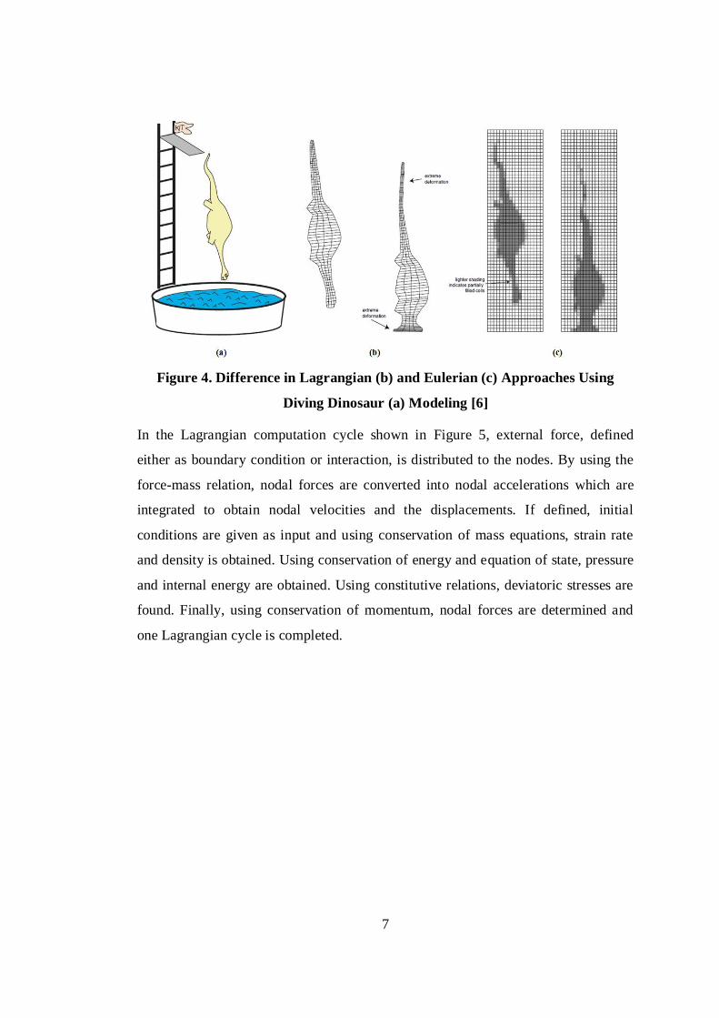
elements are not distorted [4]. In Figure 4, Eulerian and Lagrangian approaches are

compared for a dinasour diving event. A dinosaur impacts on the ground. In the

Lagrangian approach, in the extremely deformed parts of the dinosaur, such as tail

and head, the elements are also extremely deformed. In the Eulerian approach, the

elements are fixed and dinosaur itself is deformed and flows through fixed elements.

7

Figure 4. Difference in Lagrangian (b) and Eulerian (c) Approaches Using

Diving Dinosaur (a) Modeling [6]

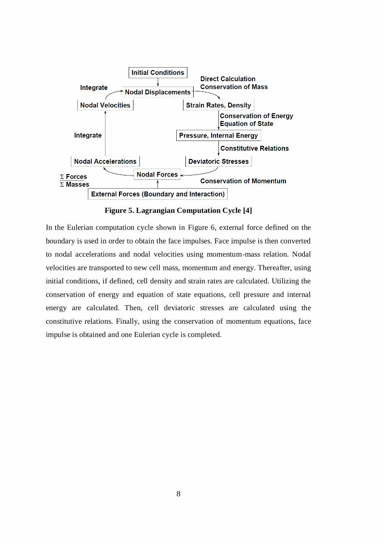
In the Lagrangian computation cycle shown in Figure 5, external force, defined

either as boundary condition or interaction, is distributed to the nodes. By using the

force-mass relation, nodal forces are converted into nodal accelerations which are

integrated to obtain nodal velocities and the displacements. If defined, initial

conditions are given as input and using conservation of mass equations, strain rate

and density is obtained. Using conservation of energy and equation of state, pressure

and internal energy are obtained. Using constitutive relations, deviatoric stresses are

found. Finally, using conservation of momentum, nodal forces are determined and

one Lagrangian cycle is completed.

8

Figure 5. Lagrangian Computation Cycle [4]

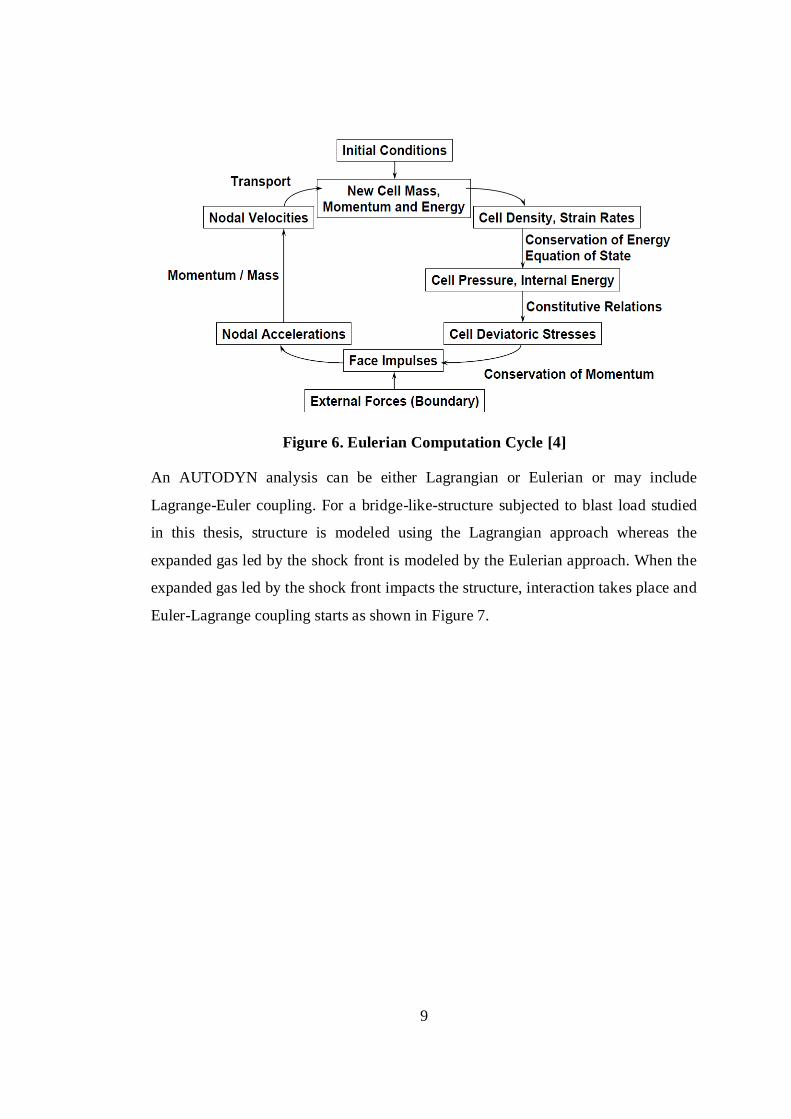
In the Eulerian computation cycle shown in Figure 6, external force defined on the

boundary is used in order to obtain the face impulses. Face impulse is then converted

to nodal accelerations and nodal velocities using momentum-mass relation. Nodal

velocities are transported to new cell mass, momentum and energy. Thereafter, using

initial conditions, if defined, cell density and strain rates are calculated. Utilizing the

conservation of energy and equation of state equations, cell pressure and internal

energy are calculated. Then, cell deviatoric stresses are calculated using the

constitutive relations. Finally, using the conservation of momentum equations, face

impulse is obtained and one Eulerian cycle is completed.

9

Figure 6. Eulerian Computation Cycle [4]

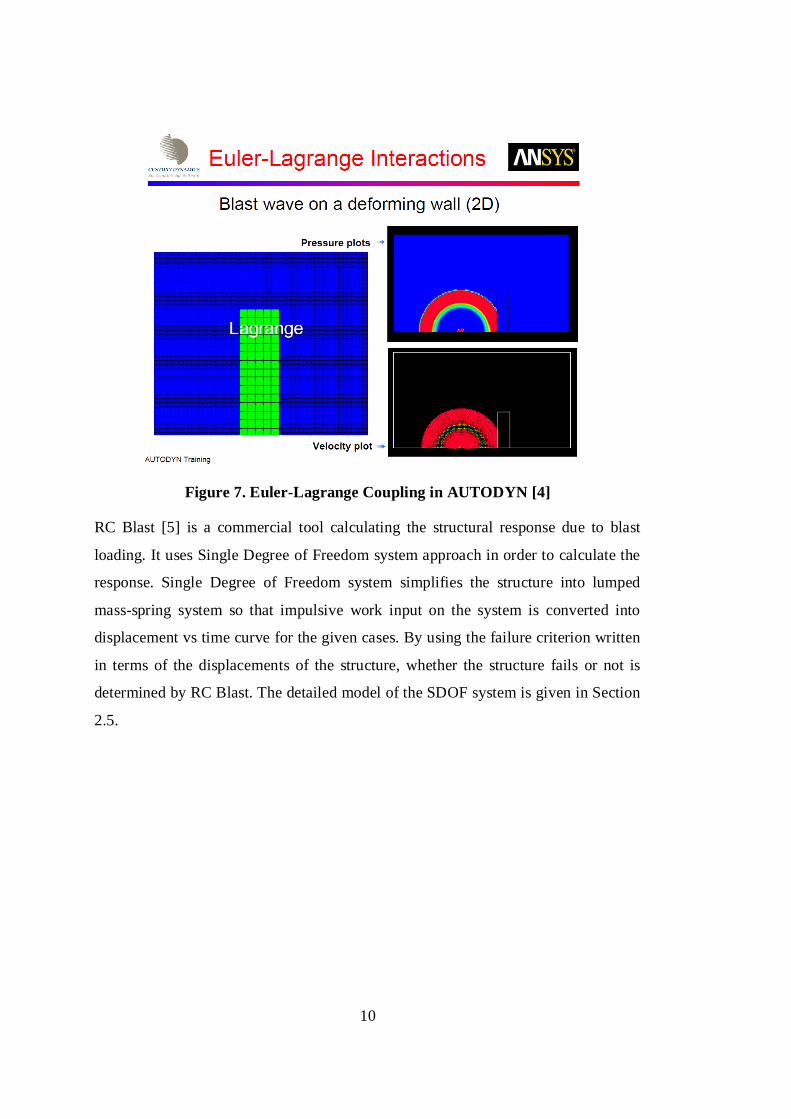
An AUTODYN analysis can be either Lagrangian or Eulerian or may include

Lagrange-Euler coupling. For a bridge-like-structure subjected to blast load studied

in this thesis, structure is modeled using the Lagrangian approach whereas the

expanded gas led by the shock front is modeled by the Eulerian approach. When the

expanded gas led by the shock front impacts the structure, interaction takes place and

Euler-Lagrange coupling starts as shown in Figure 7.

10

Figure 7. Euler-Lagrange Coupling in AUTODYN [4]

RC Blast [5] is a commercial tool calculating the structural response due to blast

loading. It uses Single Degree of Freedom system approach in order to calculate the

response. Single Degree of Freedom system simplifies the structure into lumped

mass-spring system so that impulsive work input on the system is converted into

displacement vs time curve for the given cases. By using the failure criterion written

in terms of the displacements of the structure, whether the structure fails or not is

determined by RC Blast. The detailed model of the SDOF system is given in Section

2.5.

11

1.1. Literature Survey for Studies of Structures Exposed to Blast Load

In literature, there are several studies conducting blast analysis and tests for some

scenarios. In the study of Sherkar et al. [7] finite element software LS-DYNA [8] is

used to investigate the blast resulted pressure on the structure. In this study, three

gauges are located on the front face of the concrete column as shown in Figure 8.

Pressures after reflection of blast wave on the column are measured. Gauge pressures

are compared with the test pressure data.

Figure 8. Gauge Placement in the Study of Sherkar et al. (2003) [7]

Williamson et al. [9] conducted experiments and analyses by the finite element

software LS-DYNA to study the failure response of a concrete column. Using

different explosive masss and different stand-off distances, which is the distance

between the detonation point and the target, failure of the concrete column is

analyzed. Figure 9 compares the analysis and large stand-off test results of the

concrete column that is studied by Williamson et al. [9]. As seen in Figure 9, in the

test, damage is observed at bottom of the concrete column and similarly in the

analysis; elements at the bottom of the column are seen to erode, as well. In another

test group, Williamson conducted small stand-off distance explosion tests. The

12

results of tests and analyses are compared. For both cases, flexural response of the

concrete column is observed as seen in Figure 11. In the analyses, midsection

elements are eroded and the concrete column becomes as if it is broken from

midsection.

Figure 9. Comparison of Test and Analysis for Large Stand-off Distance [9]

Figure 10. Comparison of Test and Analysis for Small Stand-off Distance [9]

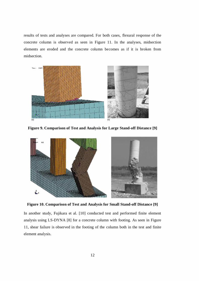
In another study, Fujikara et al. [10] conducted test and performed finite element

analysis using LS-DYNA [8] for a concrete column with footing. As seen in Figure

11, shear failure is observed in the footing of the column both in the test and finite

element analysis.

13

Figure 11. Comparison of Test and Analysis [10]

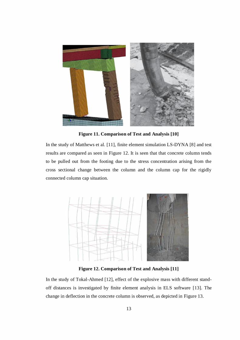
In the study of Matthews et al. [11], finite element simulation LS-DYNA [8] and test

results are compared as seen in Figure 12. It is seen that that concrete column tends

to be pulled out from the footing due to the stress concentration arising from the

cross sectional change between the column and the column cap for the rigidly

connected column cap situation.

Figure 12. Comparison of Test and Analysis [11]

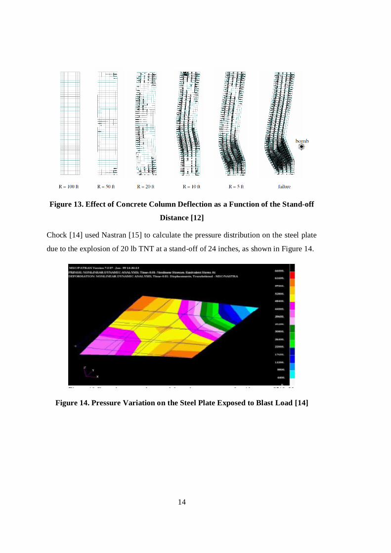
In the study of Tokal-Ahmed [12], effect of the explosive mass with different stand-

off distances is investigated by finite element analysis in ELS software [13]. The

change in deflection in the concrete column is observed, as depicted in Figure 13.

14

Figure 13. Effect of Concrete Column Deflection as a Function of the Stand-off

Distance [12]

Chock [14] used Nastran [15] to calculate the pressure distribution on the steel plate

due to the explosion of 20 lb TNT at a stand-off of 24 inches, as shown in Figure 14.

Figure 14. Pressure Variation on the Steel Plate Exposed to Blast Load [14]

15

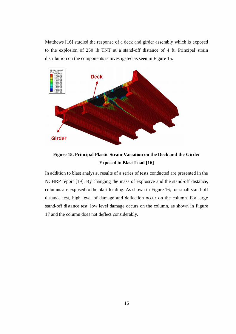
Matthews [16] studied the response of a deck and girder assembly which is exposed

to the explosion of 250 lb TNT at a stand-off distance of 4 ft. Principal strain

distribution on the components is investigated as seen in Figure 15.

Figure 15. Principal Plastic Strain Variation on the Deck and the Girder

Exposed to Blast Load [16]

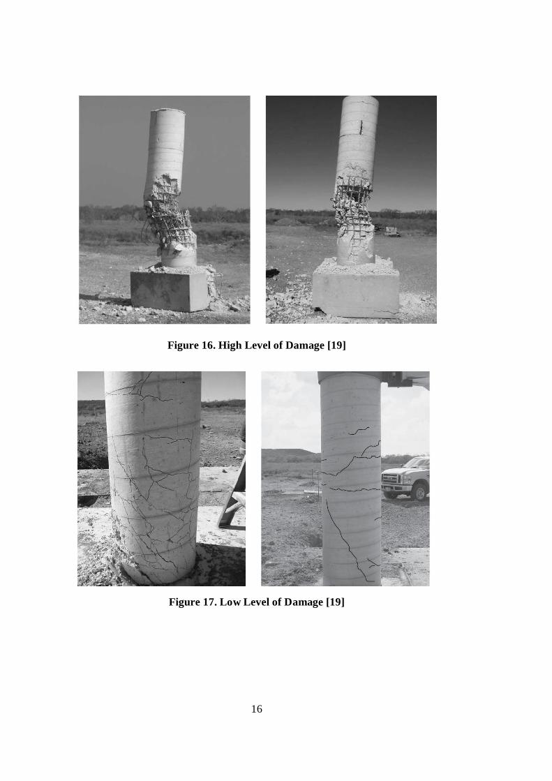
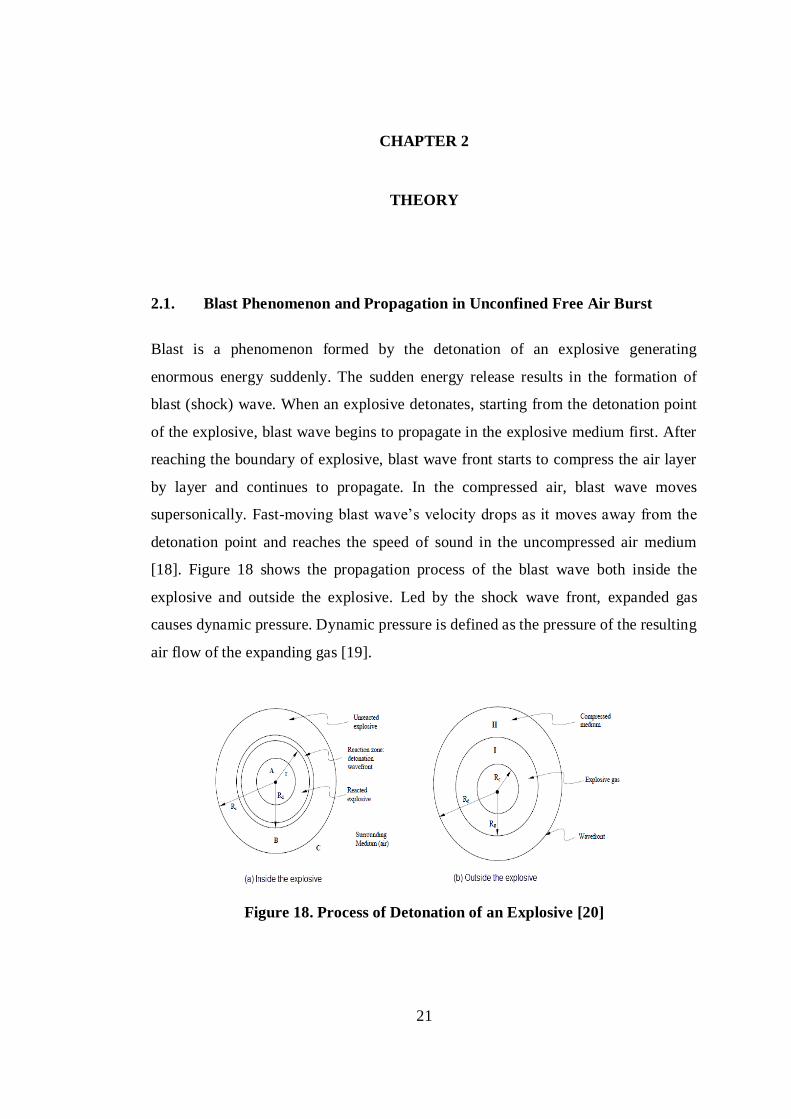
In addition to blast analysis, results of a series of tests conducted are presented in the

NCHRP report [19]. By changing the mass of explosive and the stand-off distance,

columns are exposed to the blast loading. As shown in Figure 16, for small stand-off

distance test, high level of damage and deflection occur on the column. For large

stand-off distance test, low level damage occurs on the column, as shown in Figure

17 and the column does not deflect considerably.

16

Figure 16. High Level of Damage [19]

Figure 17. Low Level of Damage [19]

17

In the study of Oswald et al. [17], series of tests are conducted. In the tests, close-in

explosions which have scaled distance less than 1.0 ft/lb1/3

are examined. Moreover,

a solver which uses SDOF method is utilized to analyze the response of the structure

for the same conditions. Each simply supported concrete slabshave 8000 psi

compressive strength and 0.66 reinforcement ratio. After conducting the tests,

maximum deflection and hinge rotations on the concrete slabs are measured. In

addition, maximum deflection and hinge rotation are computed for the same concrete

slabs using the SDOF method. Table 2 compares the test and analysis results

obtained by the SDOF analysis method. In the last column of Table 2, ratios of the

calculated and the measured maximum deformations are given. The ratio ranges

from 0.77 to 1.73. In the 6th

test, 0.97 ratio is obtained as the best result.

Table 2. SDOF Method Compared to the Test Results [17]

Test

No

Length

[in]

Thickness

[in]

Depth

[in]

Max.

Measured

Deflection

[in]

Hinge

Rotation

[deg]

Calculated

Max.

Deflection

[in]

Ratio of

Calculated/Measured

1 250 7.9 6.7 5.2 2.4 4.7 0.90

2 250 7.9 6.7 2.5 1.2 2.1 0.84

3 250 7.9 6.7 0.8 0.4 1.1 1.38

4 250 7.9 6.7 7.9 3.6 11.9 1.51

5 250 7.9 6.7 0.3 0.1 0.5 1.67

6 250 5.3 4.5 2.4 1.1 2.3 0.96

7 250 5.3 4.5 13.4 6.1 23.0 1.72

8 250 5.3 4.5 2.4 1.1 2.7 1.13

9 250 5.3 4.5 11.8 5.4 13.0 1.10

10 250 5.3 4.5 4.9 2.2 3.8 0.78

11 250 5.3 4.5 0.6 0.3 1.0 1.67

As some of the studies taken from the literature show, response of structures exposed

to blast loading due to explosion is frequently analyzed by the finite element

approach. It should be note that performing blast loading tests is expensive and also

dangerous, therefore reliable analysis methods are required to study the response of

structures exposed to blast loading in the design stage. However, one drawback of

using finite element analysis in studying the response of structures exposed to blast

18

loading is the high computational cost of the analyses due to the explicit solution

method used in the simulation of highly dynamic event such as the explosion.

Therefore, there is also a need to develop fast responding tools to obtain approximate

solutions for the blast response of the structures. It is considered that approximate

solutions can be used to reduce the total number of costly finite element simulations

of structures exposed to blast loading significantly. With the approximate solution

methods, one can have a baseline design for the structure studied to resist a certain

explosion induced loading or can determine an approximate failure explosive mass.

Detailed finite element analysis can then be performed utilizing the outcome of the

approximate solutions obtained by the fast responding analysis methods.

19

1.2. Objective and Outline of the Thesis

The main objective of the thesis is to develop a fast-responding tool which is

accurate enough for the damage assessment in the columns of bridge structures

subjected to blast loading. The objective of the damage assessment could be either

the determination of the explosive mass necessary for the complete failure of the

column or performing fast preliminary geometric design of concrete columns to

withstand the failure for a certain explosive mass. It is also considered that with the

developed tool a first estimate of the failure explosive mass can be obtained for

detailed AUTODYN analysis and number of AUTODYN trials to determine the

failure explosive mass can be reduced in the detailed design and analysis stage.

For this purpose, in this thesis;

The theory of blast phenomenon is explained in detail in Chapter 2.

The development of the blast damage tool is explained with aid of flowcharts

in Chapter 3.

Modeling in AUTODYN and RC BLAST is given Section 4.2 and Section

4.3, respectively.

The results of the developed fast responding tool, AUTODYN and RC

BLAST are compared and assessment of the results is presented in Section 0.

Concluding remarks and future work are given in Chapter 5.

In Appendix A, a view of the developed tool is given.

In Appendix B, derivation of load and mass factors used in SDOF conversion

is presented.

20

21

CHAPTER 2

2. THEORY

2.1. Blast Phenomenon and Propagation in Unconfined Free Air Burst

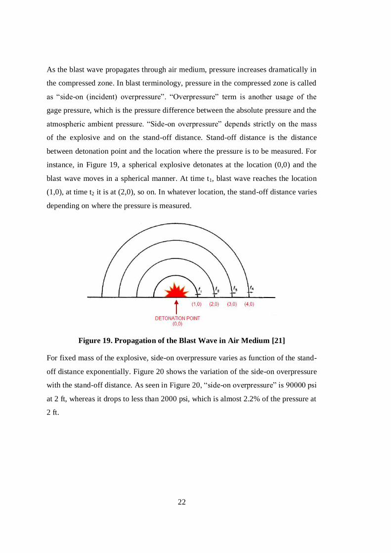
Blast is a phenomenon formed by the detonation of an explosive generating

enormous energy suddenly. The sudden energy release results in the formation of

blast (shock) wave. When an explosive detonates, starting from the detonation point

of the explosive, blast wave begins to propagate in the explosive medium first. After

reaching the boundary of explosive, blast wave front starts to compress the air layer

by layer and continues to propagate. In the compressed air, blast wave moves

supersonically. Fast-moving blast wave’s velocity drops as it moves away from the

detonation point and reaches the speed of sound in the uncompressed air medium

[18]. Figure 18 shows the propagation process of the blast wave both inside the

explosive and outside the explosive. Led by the shock wave front, expanded gas

causes dynamic pressure. Dynamic pressure is defined as the pressure of the resulting

air flow of the expanding gas [19].

Figure 18. Process of Detonation of an Explosive [20]

22

As the blast wave propagates through air medium, pressure increases dramatically in

the compressed zone. In blast terminology, pressure in the compressed zone is called

as “side-on (incident) overpressure”. “Overpressure” term is another usage of the

gage pressure, which is the pressure difference between the absolute pressure and the

atmospheric ambient pressure. “Side-on overpressure” depends strictly on the mass

of the explosive and on the stand-off distance. Stand-off distance is the distance

between detonation point and the location where the pressure is to be measured. For

instance, in Figure 19, a spherical explosive detonates at the location (0,0) and the

blast wave moves in a spherical manner. At time t1, blast wave reaches the location

(1,0), at time t2 it is at (2,0), so on. In whatever location, the stand-off distance varies

depending on where the pressure is measured.

Figure 19. Propagation of the Blast Wave in Air Medium [21]

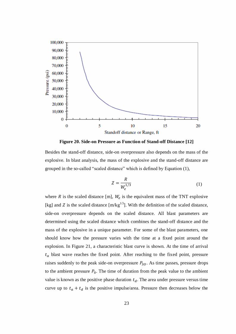
For fixed mass of the explosive, side-on overpressure varies as function of the stand-

off distance exponentially. Figure 20 shows the variation of the side-on overpressure

with the stand-off distance. As seen in Figure 20, “side-on overpressure” is 90000 psi

at 2 ft, whereas it drops to less than 2000 psi, which is almost 2.2% of the pressure at

2 ft.

23

Figure 20. Side-on Pressure as Function of Stand-off Distance [12]

Besides the stand-off distance, side-on overpressure also depends on the mass of the

explosive. In blast analysis, the mass of the explosive and the stand-off distance are

grouped in the so-called “scaled distance” which is defined by Equation (1),

(1)

where is the scaled distance [m], is the equivalent mass of the TNT explosive

[kg] and is the scaled distance [m/kg1/3

]. With the definition of the scaled distance,

side-on overpressure depends on the scaled distance. All blast parameters are

determined using the scaled distance which combines the stand-off distance and the

mass of the explosive in a unique parameter. For some of the blast parameters, one

should know how the pressure varies with the time at a fixed point around the

explosion. In Figure 21, a characteristic blast curve is shown. At the time of arrival

blast wave reaches the fixed point. After reaching to the fixed point, pressure

raises suddenly to the peak side-on overpressure . As time passes, pressure drops

to the ambient pressure . The time of duration from the peak value to the ambient

value is known as the positive phase duration . The area under pressure versus time

curve up to is the positive impulse/area. Pressure then decreases below the

24

ambient pressure and increases again until it converges to the ambient pressure value.

This region is called the negative phase and the area under the curve is the negative

impulse/area [22].

Figure 21. Pressure vs. Time Blast Curve [22]

To determine all the blast parameters caused by the blast pressure using the scaled

distance, one should define the mass of explosive for different conditions. In the blast

discipline, all explosives are defined in terms of TNT. Mass of the explosive is

calculated using the “TNT Equivalency Factor” for other explosives. For instance,

tritonal explosive has a TNT equivalency factor of 1.07 for the pressure and 0.96 for

the impulse. Table 3 gives the TNT equivalency factor for some explosives. For

instance, 100 kg of tritonal equals to 107 kg of TNT for the pressure calculation and

96 kg of TNT for the impulse calculation.

25

Table 3. TNT Equivalency Factor For Some Explosives [23]

26

27

Apart from the TNT equivalency factor, another factor which affects the mass of the

explosive is the casing factor. If the explosive is filled into a metal casing, like a

warhead, the effectiveness of the explosive decreases since the energy generated

from the detonation of the explosive should fracture the casing first and then release

its energy to the atmosphere. For this situation, considering tests of explosive with

casing, Fano proposed Equation (2) for the calculation of the uncased mass of the

explosive [24]

(2)

where is the uncased mass of explosive [kg], is the mass of explosive [kg],

M is the mass of the metal casing [kg], C is the explosive mass [kg]. Considering

both the TNT equivalency factor and the casing factor, one can define the equivalent

mass of TNT explosive, [kg], as,

[

] (3)

Using the equivalent mass of the explosive, one can then properly define the scaled

distance corresponding to a stand-off distance. Once the scaled distance is

determined, one can get the time of arrival, peak side-on overpressure, positive phase

duration etc. using Figure 22 which was generated by combining the test results of

series of experiments during 1960’s.

28

Figure 22. Side-on Overpressure and Impulse , Reflected Overpressure

and Impulse , Time of Arrival , Time of Duration , Shock Velocity as a

Function of the Scaled Distance [22]

Besides the test data, there are some empirical formulae for the calculation of the

blast parameters, especially for the calculation of the peak side-on overpressure.

Kinney proposed Equation (4) for the calculation of the peak side-on pressure

[25].

29

[ (

) ]

√ (

) √ (

) √ (

) (4)

where P0 is the ambient pressure [kPa], Z is the scaled distance [m/kg1/3

].

Brode suggested Equation (5) for the peak side-on pressure in different ranges of

the overpressure [26]

(5)

where the scaled distance is in [m/kg1/3

], side-on overpressure is in [bar]

Newmark proposed Equation (6) for the peak side-on overpressure ,

√

(6)

where equivalent mass of the TNT explosive is in [tons], stand-off distance is

in [m] and side-on overpressure is in [bar].

Mills introduced Equation (7) for the peak side-on pressure [28],

(7)

where the scaled distance is in [m/kg1/3

] and the side-on overpressure is in

[kPa].

Sadovski proposed Equation (8) for the peak side-on pressure [30],

(8)

where the equivalent mass of the explosive is in [kg], stand-off distance is in

[m] and side-on overpressure is in [atm].

30

Kingery and Bulmash defined a function given by Equation (9) for the determination

of the side-on peak pressure for different ranges of the scaled distance Z. As seen in

Equation (9), Kingery and Bulmash used sixth degree polynomial and exponential

function in order to fit the experimental data shown in Figure 22 accurately.

( ) ( ) ( ) ( ) ( ) ( ) (9)

In Equation (9), A-G are the coefficients defined for different ranges of the scaled

distance Z [m/kg1/3

], Table 4 gives the coefficients A-G used for the calculation of

the peak side-on overpressure.

Table 4. KingeryBulmash Coefficients for the Calculation of the Side-on

Overpressure [29]

Side-on Overpressure [kPa]

Range of Z

[m/kg1/3

] A B C D E F G

0.2-2.9 7.2106 -2.1069 0.3229 0.1117 0.0685 0 0

2.9-23.8 7.5938 -3.0523 0.40977 0.0261 -0.01267 0 0

23.8-198.5 6.0536 -1.4066 0 0 0 0 0

Equation (9), proposed by Kingery and Bulmash, can also be used for the calculation

of the time of arrival, positive phase duration and the shock front velocity.

Table 5 gives the the coefficients A-G used for the calculation of the time of arrival,

positive phase duration and the shock front velocity for different range of the scaled

distance Z.

31

Table 5. Kingery Coefficients for the Calculation of the Scaled Time of Arrival,

Scaled Positive Phase Duration and the Shock Front Velocity [29]

Scaled Time of Arrival [ms/kg1/3

]

Range of

Z

[m/kg1/3

]

A B C D E F G

0.06-1.50 -0.7604 1.8058 0.1257 -0.0437 -0.0310 -0.00669 0

1.50-40 -0.7137 1.5732 0.5561 -0.4213 0.1054 -0.00929 0

Scaled Positive Phase Duration [ms/kg1/3]

Range of

Z

[m/kg1/3

]

A B C D E F G

0.2-1.02 0.5426 3.2299 -1.5931 -5.9667 -4.0815 -0.9149 0

1.02-2.80 0.5440 2.7082 -9.7354 14.3425 -9.7791 2.8535 0

2.80-40 -2.4608 7.1639 -5.6215 2.2711 -0.44994 0.03486 0

Shock Front Velocity [km/s]

Range of

Z

[m/kg1/3

]

A B C D E F G

0.06-1.50 0.1794 -0.956 -0.0866 0.109 0.0699 0.01218 -

1.50-40 0.2597 -1.326 0.3767 0.0396 -0.0351 0.00432

Dynamic pressure resulting from the air flow due to the blast pressure is calculated

by Equation (10) [18],

(10)

where is the dynamic pressure in [Pa], is density of compressed air [kg/m3], is

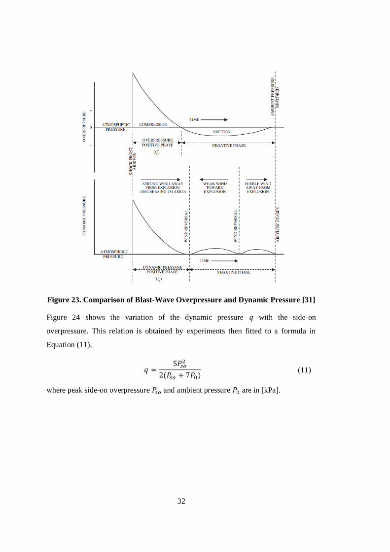
the shock front velocity in [m/s]. Figure 23 compares the variation of the blast wave

overpressure and the dynamic pressure with the time at a fixed point. It is noted that

in the negative phase zone, dynamic pressure is always greater than the atmospheric

pressure whereas the side-on overpressure is less than the atmospheric pressure.

32

Figure 23. Comparison of Blast-Wave Overpressure and Dynamic Pressure [31]

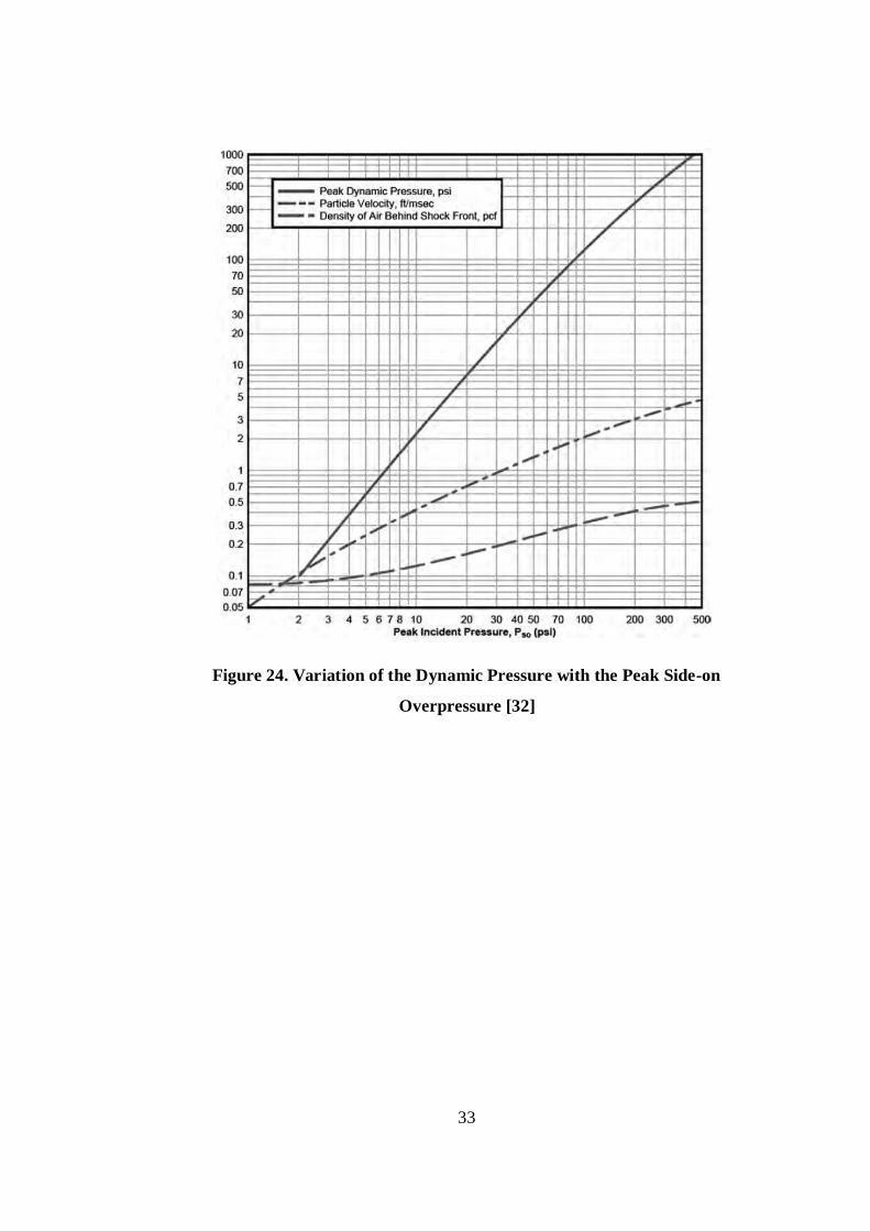
Figure 24 shows the variation of the dynamic pressure with the side-on

overpressure. This relation is obtained by experiments then fitted to a formula in

Equation (11),

( ) (11)

where peak side-on overpressure and ambient pressure are in [kPa].

33

Figure 24. Variation of the Dynamic Pressure with the Peak Side-on

Overpressure [32]

34

2.2. Blast Propagation in Unconfined Air Burst and Formation of the Mach

Stem

In section 2.1, blast propagation in free air burst is examined. Blast loading in

different propagation medium is categorized and tabulated in Table 6 [12].

Table 6. Blast Loading Categories in Different Propagation Medium [32]

BLAST LOADING CATEGORIES

Explosive

Confinement Category Pressure Loads

Unconfined Explosions

Free Air Burst Unreflected

Air Burst Reflected

Surface Burst Reflected

Confined Explosions

Fully Vented Internal Shock

Leakage

Partially Confined

Internal Shock

Internal Gas

Leakage

Fully Confined Internal Shock

Internal Gas

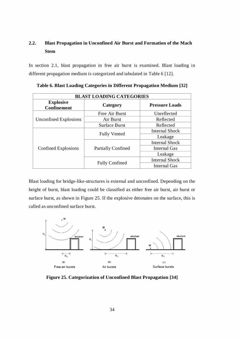
Blast loading for bridge-like-structures is external and unconfined. Depending on the

height of burst, blast loading could be classified as either free air burst, air burst or

surface burst, as shown in Figure 25. If the explosive detonates on the surface, this is

called as unconfined surface burst.

Figure 25. Categorization of Unconfined Blast Propagation [34]

35

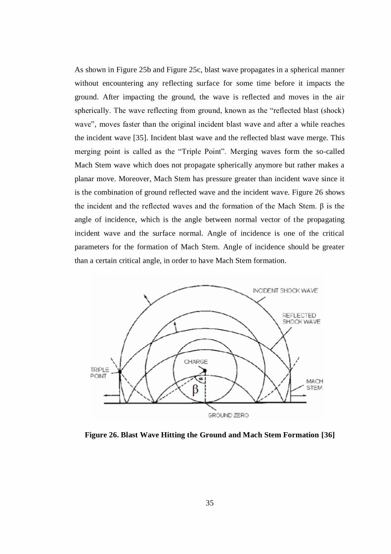
As shown in Figure 25b and Figure 25c, blast wave propagates in a spherical manner

without encountering any reflecting surface for some time before it impacts the

ground. After impacting the ground, the wave is reflected and moves in the air

spherically. The wave reflecting from ground, known as the “reflected blast (shock)

wave”, moves faster than the original incident blast wave and after a while reaches

the incident wave [35]. Incident blast wave and the reflected blast wave merge. This

merging point is called as the “Triple Point”. Merging waves form the so-called

Mach Stem wave which does not propagate spherically anymore but rather makes a

planar move. Moreover, Mach Stem has pressure greater than incident wave since it

is the combination of ground reflected wave and the incident wave. Figure 26 shows

the incident and the reflected waves and the formation of the Mach Stem. β is the

angle of incidence, which is the angle between normal vector of the propagating

incident wave and the surface normal. Angle of incidence is one of the critical

parameters for the formation of Mach Stem. Angle of incidence should be greater

than a certain critical angle, in order to have Mach Stem formation.

Figure 26. Blast Wave Hitting the Ground and Mach Stem Formation [36]

36

After merging of the incident and the reflected waves at the triple point, Mach Stem

grows and draws a path. This path is called as the path of the triple point and Figure

27 shows the path of the triple point and the growth of the Mach Stem.

Figure 27. Path of the Triple Point [22]

In general, for blast waves reflecting from the surface, the magnification of the

explosion is defined in terms of magnification in the mass of the explosive [18].

Equation (12) gives equivalent mass of the TNT explosive if reflecting surfaces

exist,

(12)

where n is number of reflective surface(s).

For the unconfined surface burst, ground is the reflective surface and mass of

explosive should be doubled to calculate the scaled distance. If an explosive

detonates at the corner with two reflective surfaces and the mass of explosive is

multiplied by 4. In calculating the mass of the explosive, surface is assumed to fully

reflect the blast wave and it is assumed that no energy is absorbed by the ground or

transmitted through the ground. Some studies were performed in order to find the

transmitting energy fraction and blast energy loss through the ground. Regarding this

loss, instead of using a magnification factor of 2, 1.7-1.8 is recommended. Mass of

37

explosive is found accordingly and then the scaled distance and the correlated blast

parameters are computed [36].

Besides the magnification factor used for the mass of the explosive, increasing

pressure effect of Mach Stem formation scenario is modeled by Miller [37]. In order

to find the triple point height just before it impacts the structure and the

corresponding Mach Stem pressure, by means of tests and analyses, Miller defined

new terms to calculate these parameters. A parameter , given by Equation (13), is

defined to decide on whether the Mach Stem forms or not.

(13)

In Equation (13), ambient pressure and side-on overpressure are in kPa. Using

the parameter critical angle for Mach Stem formation is determined using Equation

(14).

(14)

If the angle of incidence β (Figure 26) is greater than , then Mach Stem

forms [37]. After deciding on the Mach Stem formation, triple point height and Mach

Stem pressure should be determined with a series of computations. For the triple

point height, scaled charge height should be determined first using Equation (15). As

all “scaled” blast parameters, “scaled” means division by cube root of equivalent

mass of TNT explosive.

(15)

In Equation (15), is the scaled charge height [ft/lb

1/3], height of burst is in [ft],

is the equivalent mass of TNT explosive in [lb].

38

To determine the scaled triple point height, Miller divides the scaled charge height

into intervals of 1, 1.5, 2, 2.5, 3, 3.5, 4, 5, 6, 7. For all intervals, scaled triple point

height is defined as function of the scaled distance. For instance, for the scaled

charge height of 1, scaled triple point height is given by Equation (16).

(16)

For other scaled charge height parameter, Table 7 gives the scaled triple point height

as function of the scaled distance for different scaled charge heights. For any scaled

charge height parameter, interpolation could be performed. Note that parameters in

Table 7 are in British Unit System.

Table 7. Scaled Triple Point Height as Function of Scaled Distance for Different

Scaled Charge Heights [37]

Scaled charge height is function of the height of burst and the equivalent mass of

TNT explosive, scaled triple point height is function of the scaled charge height and

the scaled distance. Thus, scaled triple point height is function of the stand-off

distance, equivalent mass of explosive and the height of burst.

39

Mach Stem pressure is determined according to different scaled charge height

intervals. Miller gives formulae for the Mach Stem pressure in his thesis for the

scaled charge height values of 0.8, 1.9, 3, 5.3, 7.2, as shown in Table 8. Mach Stem

pressure is dependent on the scaled charge height and the angle of incidence β, which

depends on the height of burst and the stand-off distance. Since scaled charge height

depends on the height of burst and the equivalent mass of explosive, Mach Stem

pressure is function of the stand-off distance, height of burst and the equivalent mass

of the TNT explosive.

Table 8. Mach Stem Pressure as Function of the Angle of Incidence for

Different Scaled Charge Heights [37]

40

2.3. Impulsive Work on the Structure

Blast wave which impacts the structure, may be composed of either fully incident

wave, fully Mach Stem or mixed depending on the height of burst and the scaled

distance. In Figure 28, shelter is exposed to fully Mach Stem since the triple point at

the location of the shelter is greater than the height of the shelter.

Figure 28. Mach Stem Formation and its Interaction with the Structure [9]

If explosion occurs at a closer location, as shown in Figure 29, blast wave is a fully

incident wave. If the explosion location is neither close enough to be fully incident

nor far enough to be fully Mach Stem, mixed condition may occur.

Figure 29. Close-in Explosion and Fully Incident Wave Impinging on the

Structure

41

When the blast wave impacts on the structure, it makes an angle with the structure.

For instance, Figure 30 shows a spherical blast wave impacting on the column. The

explosion is close enough to the column so that it is a fully incident wave. The

incident wave has different angle of incidence with respect to different parts of the

column. The arrows emerging from the explosion point demonstrate the normal

direction of the spherical blast wave. Vector R1 makes an angle of with the surface

normal of the column. Vectors R2, R3, R4 have angles of incidence

respectively.

Figure 30. Angle of Incidence with respect to the Different Points on the

Structure

Side-on (incident) overpressure impacting on the structure at an angle of incidence is

magnified by a factor of “coefficient of reflection” and the resulting pressure is

named as the “face-on (reflected) overpressure” in blast terminology [22]. Referring

to Figure 30, pressure at the location G1 is the side-on overpressure whereas at the

same stand-off distance pressure at the location G2, just next to the structure is the

face-on overpressure. Figure 31 compares the side-on and the face-on pressures and

how they are measured with the pressure probes.

42

Figure 31. Comparison of the Face-on and the Side-on Overpressures [38]

The relation between the face-on overpressure and the side-on overpressure is given

by Equation (17) [12],

(17)

where is the face-on pressure and the coefficient of reflection ( ) is a function

of the side-on overpressure intensity and the angle of incidence. With series of

experiments performed in 1960’s, gauges were inserted at the same stand-off

distance but with different configurations, as shown in Figure 31. Test data for the

variations of the face-on with the side-on overpressure were recorded, and it was

observed that coefficient of reflection varies between 1 and 12.25. Figure 32 shows

the variation of the coefficient of reflection with the angle of incidence for different

side-on pressures. Angle of incidence “0” means that wave is fully reflected whereas

angle of incidence “90” means that incident wave is not reflected at all. Therefore,

for the incidence angle of 90, coefficient of reflection is 1 for all side-on pressure

values. Intermediate values of the incidence angle are for “oblique reflection” [22].

43

Figure 32. Variation of the Coefficient of Reflection with the Angle of Incidence

for different Side-on Pressures [22]

When blast wave interacts with the structure, structure is subjected to the face-on

pressure which varies with time as shown in Figure 31. In addition to the face-on

overpressure, impulse has significant role on the damage incurred on the structure.

The area under the face-on overpressure - time curve is the impulse per unit area.

Impulse per unit area could be found using different approaches. By means of

conducted tests, an empirical formula is proposed by Driels for the impulse per unit

area [18]. Pressure variation in time was recorded by gauges and impulse/area is

computed. The results are correlated to the scaled distance with formula fits.

Equation (18) gives the impulse per unit area proposed by Driels,

(

)

(

)

(18)

where is the scaled distance in [m/kg1/3

], I/A is the impulse/area [kPa.ms].

44

In Equation (18), only the positive phase impulse is taken into account. It should be

noted that although the negative phase has a longer duration than the positive phase,

difference in the peak overpressure values for the positive and the negative phases is

very high so that negative phase impulse is ignored [22].

In Figure 33, loading of a blast-exposed-structure is given. Structure is subjected to

the face-on overpressure on the front wall, side-on overpressure on the sides, roof

and the rear wall. Side-on overpressures on the sides cancel each other; thus, net

loading is

(19)

Figure 33. Blast Loading on a Structure [19]

In the report prepared by the U.S. Department of the Army [22], overpressure versus

time curve for a blast-exposed-structure is simplified and exponentially decaying

function of the face-on pressure shown in Figure 31 is converted into trapezoid and

triangular pulses. Figure 34 shows the simplified front wall loading of a structure.

45

Figure 34. Front Wall Blast Loading Overpressure vs. Time Curve [22]

In Figure 34, is the face-on overpressure, is the stagnation pressure which is

combination of the side-on overpressure and the dynamic pressure, is the positive

phase duration, is the equivalent time in which same impulse/area is calculated as

the simplified loading given in Figure 34. is clearing time in which clearing effect

occurs. Face-on overpressure along the structure varies since the scaled distance and

the angle of incidence change. During the clearing effect period, face-on

overpressure relieves toward the lower pressure zones at free edges. This forms a

relief wave propagating from the low to the high pressure zones.

Clearing time is determined using Equation (20). Instead of the shock front velocity,

sound velocity in the compressed zone as function of the peak side-on overpressure

is utilized as shown in Figure 36 [23],

(

)

(20)

where S is the minimum of width or height of the structural member [ft], G is the

maximum of width or height [ft], is the sound velocity in [ft/ms] and is the

clearing time in [ms]. Figure 35 demonstrates front and top view of a sample

structural member in which width, height and lengths are defined. For this case, since

height is greater than width, S is the width of the structural member while G is the

height of the structural member.

46

Figure 35. Height, Width and Length Definition for Sample Column

Figure 36. Sound Velocity as Function of the Peak Side-on Overpressure [23]

47

Stagnation overpressure is calculated by Equation (21) [23],

(21)

where is the drag coefficient and its recommended value is 1 for front wall

loading [23]. After determining the face-on overpressure, stagnation overpressure,

positive phase duration and the clearing time, impulse/area is computed as the area

under the simplified front wall loading curve shown in Figure 34. Utilizing the

known the impulse/area of the simplified front wall loading, equivalent time for the

equivalent triangular loading is calculated using Equation (22),

(

)

(22)

where is the face-on overpressure in [kPa], I/A is the impulse/area in [kPa-ms],

is the equivalent time in [ms].

Rear wall loading is similar to the side wall and roof loading [23]. Equivalent rear

wall loading is a triangular pulse as shown in Figure 32 which gives the variation of

the effective side-on overpressure with respect to time. The gauge pressure is

assumed to become zero at time , which is the sum of the rise time and

positive phase duration .

Figure 37. Overpressure vs. Time Curve for the Rear Wall Loading [23]

48

Effective overpressure , which is the combination of dynamic pressure and side-on

overpressure at rear side, is determined using Equation (23) [13],

(23)

where is the equivalent uniform pressure factor, which is defined as the reduction

factor of side-on overpressure at therear wall in [psi], is the drag coefficient,

is the side-on overpressure in [psi], is the dynamic pressure in [psi]. A schematic

figure for the rear loading is shown in Figure 38. Blast wave with a wavelength of

surpasses through the rear wall.

Equivalent uniform pressure factor is determined with aid of the graph presented

in Figure 39 in which equivalent uniform pressure factor is given as a function of the

ratio of the blast wave length to the span length L which is length of rear side of

the structural member as shown in Figure 38.

Figure 38. Rear Wall Loading

49

Figure 39. Equivalent Load Factor [32]

50

Blast wave length is determined by [23],

(24)

where is the positive phase duration in [ms], is the shock front velocity in

[km/s], is blast wave length in [m]. Shock front velocity is calculated by

evaluating the function given in Equation (9) using the Kingery coefficients, which

is the 1960’s experimental data fit for the shock front velocity. Table 9 gives the

Kingery coefficients used for the calculation for the shock front velocity.

Table 9.Kingery Coefficients for the Calculation of the Shock Front Velocity

Shock Front Velocity [km/s]

Range Z

[m/kg1/3

] A B C D E F G

0.06-1.50 0.1794 -0.956 -0.0866 0.109 0.0699 0.01218 0

1.50-40 0.2597 -1.326 0.3767 0.0396 -0.0351 0.00432 0

Drag coefficient for the rear loading is determined using the data given in Table 10.

Table 10. Rear Wall Drag Coefficients [23]

Rise time is determined by Equation (25) [18],

(25)

where is minimum of height or width of the rear side of the structure in [ft], is

the shock front velocity in [ft/ms].

51

2.4. Material Behavior and the Structural Response

Structures like columns, beams, slabs etc. experience static loading because of

carrying dead loads like their masss. In addition, as mentioned in Chapter 1, blast

loading is categorized as the dynamic type of loading. Unlike static loading, dynamic

loading includes inertia and damping effects. Moreover, dynamic loading in a very

short period of time causes material to behave differently compared to its behavior

under static loading. During the blast loading, structure is exposed to enormous

loading in a very short period of time and material is subjected to strain rate effects.

Blast loading has a strain rate in the range 102- 10

4 [s

-1]. Since concrete and steel are

the materials mostly used in bridge-like-structures, in this study material behavior of

bridge-like-structures is examined. Girder bridge, shown in Figure 40, is selected for

further examination since it is mostly used in the highways or used over the rivers

due to its convenience.

Figure 40. Girder Type Bridge

Figure 41 shows components of the girder type bridge. A typical girder type of

bridge consists of pier (column), bent (horizontal beam), girder (longitudinal beam)

and deck (slab). Piers, which are the main carriers, support bents from below. Piers

are generally made up of reinforced concrete. Bents and girders carry upper parts of

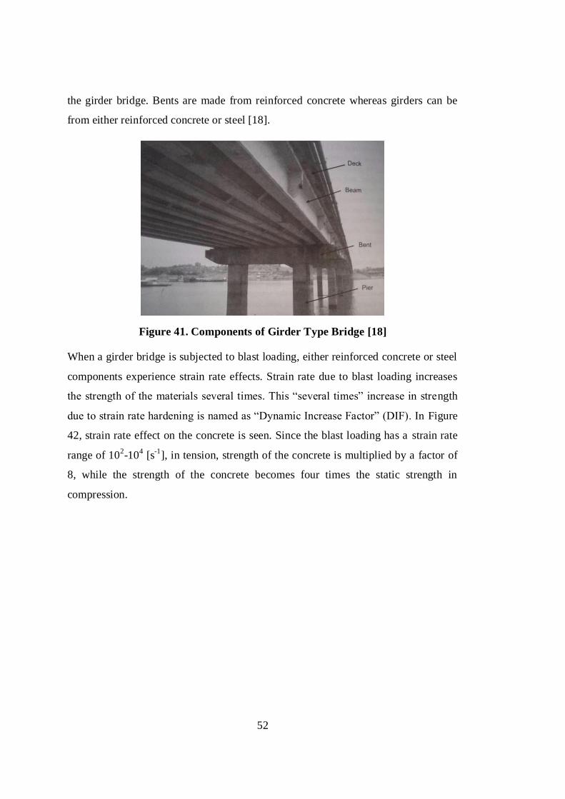
52

the girder bridge. Bents are made from reinforced concrete whereas girders can be

from either reinforced concrete or steel [18].

Figure 41. Components of Girder Type Bridge [18]

When a girder bridge is subjected to blast loading, either reinforced concrete or steel

components experience strain rate effects. Strain rate due to blast loading increases

the strength of the materials several times. This “several times” increase in strength

due to strain rate hardening is named as “Dynamic Increase Factor” (DIF). In Figure

42, strain rate effect on the concrete is seen. Since the blast loading has a strain rate

range of 102-10

4 [s

-1], in tension, strength of the concrete is multiplied by a factor of

8, while the strength of the concrete becomes four times the static strength in

compression.

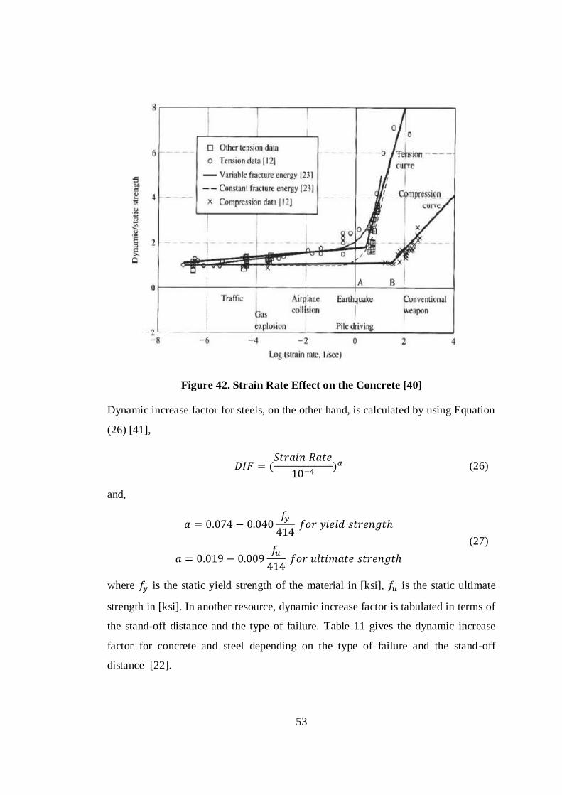
53

Figure 42. Strain Rate Effect on the Concrete [40]

Dynamic increase factor for steels, on the other hand, is calculated by using Equation

(26) [41],

(

) (26)

and,

(27)

where is the static yield strength of the material in [ksi], is the static ultimate

strength in [ksi]. In another resource, dynamic increase factor is tabulated in terms of

the stand-off distance and the type of failure. Table 11 gives the dynamic increase

factor for concrete and steel depending on the type of failure and the stand-off

distance [22].

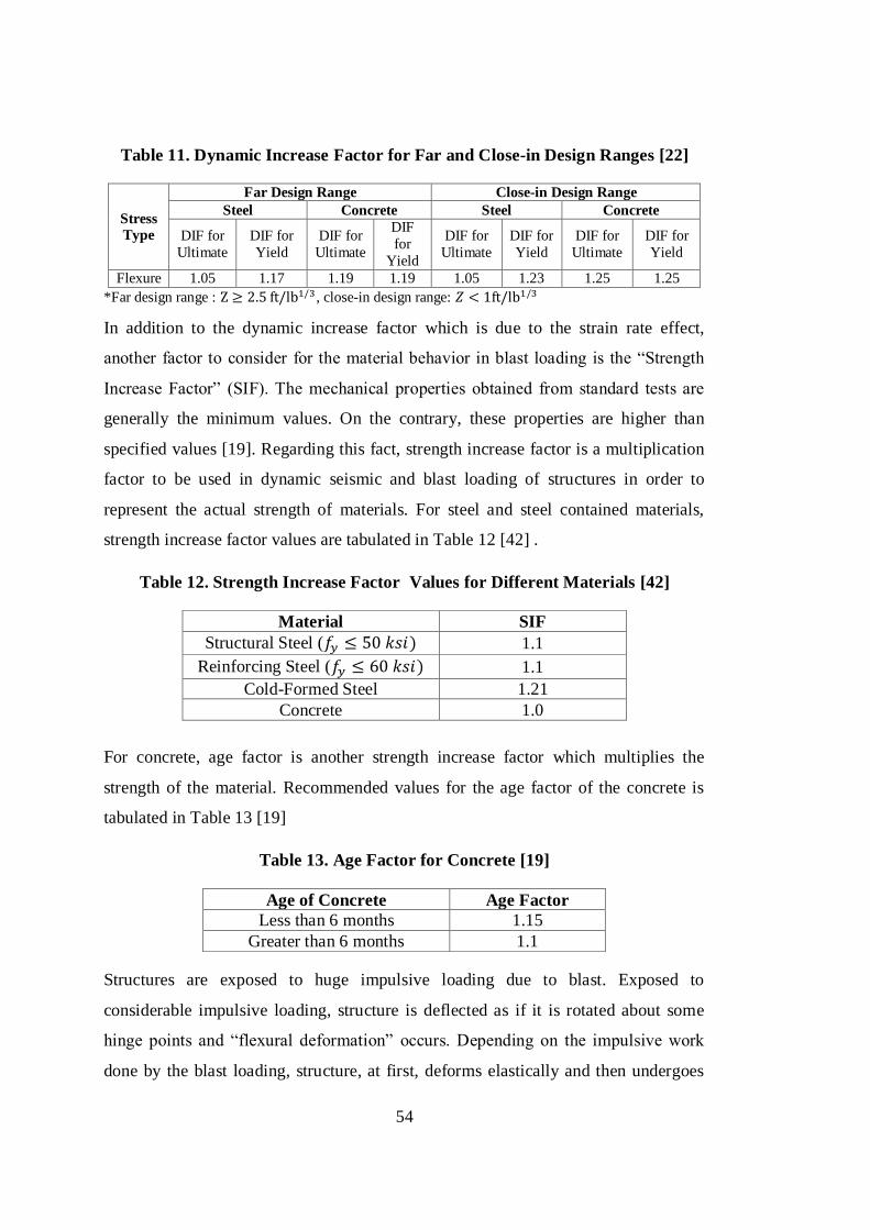
54

Table 11. Dynamic Increase Factor for Far and Close-in Design Ranges [22]

Stress Type

Far Design Range Close-in Design Range

Steel Concrete Steel Concrete

DIF for

Ultimate

DIF for

Yield

DIF for

Ultimate

DIF

for

Yield

DIF for

Ultimate

DIF for

Yield

DIF for

Ultimate

DIF for

Yield

Flexure 1.05 1.17 1.19 1.19 1.05 1.23 1.25 1.25

*Far design range : , close-in design range:

In addition to the dynamic increase factor which is due to the strain rate effect,

another factor to consider for the material behavior in blast loading is the “Strength

Increase Factor” (SIF). The mechanical properties obtained from standard tests are

generally the minimum values. On the contrary, these properties are higher than

specified values [19]. Regarding this fact, strength increase factor is a multiplication

factor to be used in dynamic seismic and blast loading of structures in order to

represent the actual strength of materials. For steel and steel contained materials,

strength increase factor values are tabulated in Table 12 [42] .

Table 12. Strength Increase Factor Values for Different Materials [42]

Material SIF

Structural Steel ( ) 1.1

Reinforcing Steel ( ) 1.1

Cold-Formed Steel 1.21

Concrete 1.0

For concrete, age factor is another strength increase factor which multiplies the

strength of the material. Recommended values for the age factor of the concrete is

tabulated in Table 13 [19]

Table 13. Age Factor for Concrete [19]

Age of Concrete Age Factor

Less than 6 months 1.15

Greater than 6 months 1.1

Structures are exposed to huge impulsive loading due to blast. Exposed to

considerable impulsive loading, structure is deflected as if it is rotated about some

hinge points and “flexural deformation” occurs. Depending on the impulsive work

done by the blast loading, structure, at first, deforms elastically and then undergoes

55

through the elastic-plastic regime. Finally, the structure is plastically deformed, as

shown in Figure 43.

Figure 43. Elastic, Elastic-Plastic and Plastic Regime

Plastic hinges occur at the vicinity of the end supports and at the closest stand-off

distance along the structure. For instance, if height of burst is half of the height of the

column, hinges are observed at end points and at the midpoint, which is closest

section of the structure to detonation point as shown in Figure 44 which also shows

the formation of the plastic hinges in the blast loaded column and the beam.

Assuming that the closest stand-off distance is at the midpoint of the structure, at the

hinge locations, bending moment, known as plastic moment, is maximized. Plastic

moment is the critical parameter to calculate damage in the structure [19].

56

Figure 44. Plastic Hinge Formation for the Blast Loaded Column [19] and the

Beam [43]

Maximum deflection of the structure, ductility ratio and the rotation of the structure

about the hinge points are the significant parameters to decide whether the structure

fails or not. Deflection of the column is related to the “ductility ratio” given by

[22],

(28)

where is maximum deflection of the blast loaded structure, is

allowable elastic deflection of the structure. In Figure 45, blast-loaded beam is

deflected such that the beam looks like as if it is broken and rotated about hinge

points. Maximum deflection and support rotation parameters are shown in

Figure 45.

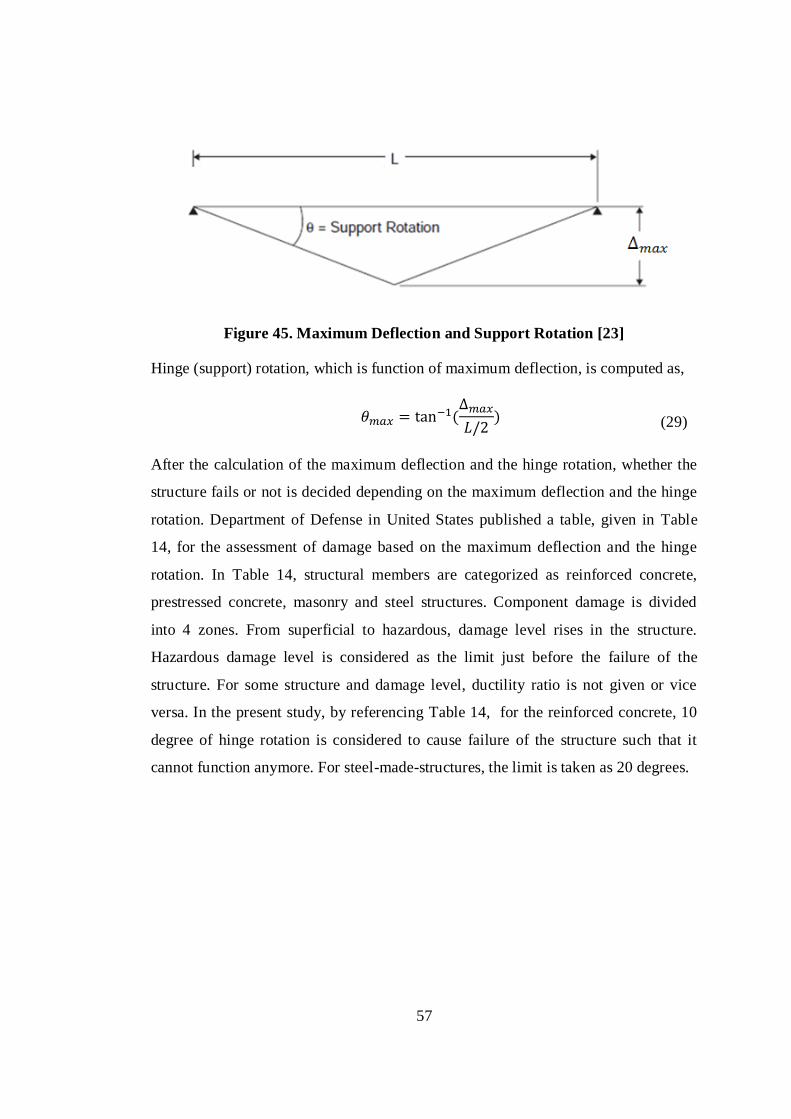
57

Figure 45. Maximum Deflection and Support Rotation [23]

Hinge (support) rotation, which is function of maximum deflection, is computed as,

(

) (29)

After the calculation of the maximum deflection and the hinge rotation, whether the

structure fails or not is decided depending on the maximum deflection and the hinge

rotation. Department of Defense in United States published a table, given in Table

14, for the assessment of damage based on the maximum deflection and the hinge

rotation. In Table 14, structural members are categorized as reinforced concrete,

prestressed concrete, masonry and steel structures. Component damage is divided

into 4 zones. From superficial to hazardous, damage level rises in the structure.

Hazardous damage level is considered as the limit just before the failure of the

structure. For some structure and damage level, ductility ratio is not given or vice

versa. In the present study, by referencing Table 14, for the reinforced concrete, 10

degree of hinge rotation is considered to cause failure of the structure such that it

cannot function anymore. For steel-made-structures, the limit is taken as 20 degrees.

58

Table 14. Failure Criteria Published by Department of Defense of the US Army

for Antiterrorism Design [23]

Element Type

Superficial Moderate Heavy Hazardous

Ductility

Ratio

Max

Hinge

Rotation

[deg]

Ductility

Ratio

Max

Hinge

Rotation

[deg]

Ductility

Ratio

Max

Hinge

Rotation

[deg]

Ductility

Ratio

Max

Hinge

Rotation

[deg]

Reinforced

Concrete

Single-reinforced

slab or beam 1 - - 2 - 5 - 10

Double-reinforced

slab or beam

without shear 1 - - 2 - 5 - 10

Double-reinforced

slab or beam with

shear 1 - - 4 - 6 - 10

Structural

Steel (hot-

rolled)

Beam with compact

section 1 - 3 3 12 10 25 20

Beam with

noncompact section 0.7 - 0.85 - 1 - 1.2

plate bent about

weak axis 4 1 8 2 20 6 40 12

Cold-

formed steel

Girt or purlin 1 - - 3 - 10 - 20

Stud with sliding

connection at top 0.5 - 0.8 - 0.9 - 1 -

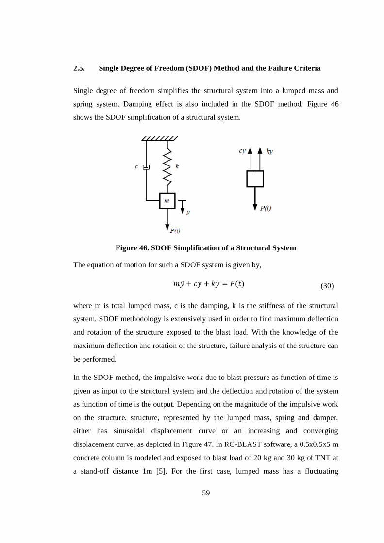
59

2.5. Single Degree of Freedom (SDOF) Method and the Failure Criteria

Single degree of freedom simplifies the structural system into a lumped mass and

spring system. Damping effect is also included in the SDOF method. Figure 46

shows the SDOF simplification of a structural system.

Figure 46. SDOF Simplification of a Structural System

The equation of motion for such a SDOF system is given by,

( ) (30)

where m is total lumped mass, c is the damping, k is the stiffness of the structural

system. SDOF methodology is extensively used in order to find maximum deflection

and rotation of the structure exposed to the blast load. With the knowledge of the

maximum deflection and rotation of the structure, failure analysis of the structure can

be performed.

In the SDOF method, the impulsive work due to blast pressure as function of time is

given as input to the structural system and the deflection and rotation of the system

as function of time is the output. Depending on the magnitude of the impulsive work

on the structure, structure, represented by the lumped mass, spring and damper,

either has sinusoidal displacement curve or an increasing and converging

displacement curve, as depicted in Figure 47. In RC-BLAST software, a 0.5x0.5x5 m

concrete column is modeled and exposed to blast load of 20 kg and 30 kg of TNT at

a stand-off distance 1m [5]. For the first case, lumped mass has a fluctuating

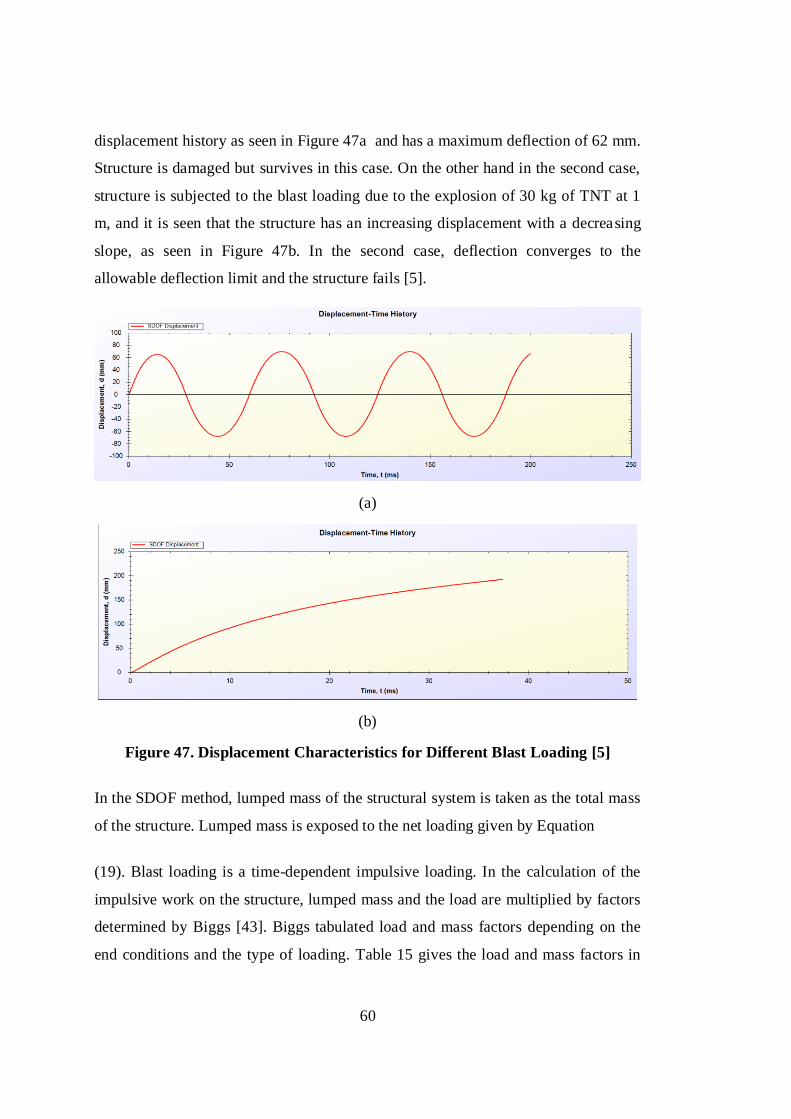
60

displacement history as seen in Figure 47a and has a maximum deflection of 62 mm.

Structure is damaged but survives in this case. On the other hand in the second case,

structure is subjected to the blast loading due to the explosion of 30 kg of TNT at 1

m, and it is seen that the structure has an increasing displacement with a decreasing

slope, as seen in Figure 47b. In the second case, deflection converges to the

allowable deflection limit and the structure fails [5].

(a)

(b)

Figure 47. Displacement Characteristics for Different Blast Loading [5]

In the SDOF method, lumped mass of the structural system is taken as the total mass

of the structure. Lumped mass is exposed to the net loading given by Equation

(19). Blast loading is a time-dependent impulsive loading. In the calculation of the

impulsive work on the structure, lumped mass and the load are multiplied by factors

determined by Biggs [43]. Biggs tabulated load and mass factors depending on the

end conditions and the type of loading. Table 15 gives the load and mass factors in

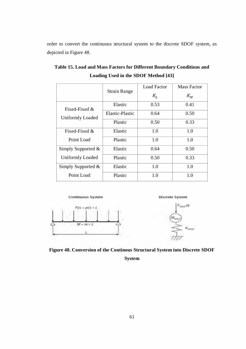
61

order to convert the continuous structural system to the discrete SDOF system, as

depicted in Figure 48.

Table 15. Load and Mass Factors for Different Boundary Conditions and

Loading Used in the SDOF Method [43]

Strain Range Load Factor

Mass Factor

Fixed-Fixed &

Uniformly Loaded

Elastic 0.53 0.41

Elastic-Plastic 0.64 0.50

Plastic 0.50 0.33

Fixed-Fixed &

Point Load

Elastic 1.0 1.0

Plastic 1.0 1.0

Simply Supported &

Uniformly Loaded

Elastic 0.64 0.50

Plastic 0.50 0.33

Simply Supported &

Point Load

Elastic 1.0 1.0

Plastic 1.0 1.0

Figure 48. Conversion of the Continous Structural System into Discrete SDOF

System

62

Using load and mass factors given by Biggs [43], SDOF conversion process is made

as follows:

Lumped mass is multiplied by mass factor to obtain the mass of the SDOF

system .

Blast load is multiplied by the load factor to obtain blast load of the SDOF

system

Stiffness of the structure is multiplied by the load factor to obtain stiffness

of the SDOF system .

Resistance force exerted by the structure is multiplied by load factor to

obtain the resistance force exerted by the spring of the SDOF system

.

Impulse of blast load is multiplied by load factor to obtain impulse of

discrete SDOF system .

Impulsive work done on the structure is multiplied by the load factor to

obtain impulsive work done on the discrete SDOF system.

During the positive phase duration, lumped mass of SDOF system is exposed to

impulse, which is equal to change in momentum of the lumped mass. Since velocity

of the lumped mass ( ) is zero at time zero, the relation between the momentum

and the impulse is given by Equation (31).

(31)

Impulse of blast load is converted to the kinetic energy of the lumped mass, which is

equal to the impulsive work done on the SDOF system. Thus,

(32)

Substituting from Equation (31) into Equation (32) yields the impulsive work

done on the SDOF system , which is given by Equation (33) [23],

63

(33)

where is the lumped mass of the SDOF system, is the impulse exerted

to the SDOF system. The impulsive work on the SDOF system causes the structure

to deflect. For a spring-mass system as shown in Figure 48, maximum resistance

force exerted by the spring on the lumped mass occurs at the time of

maximum deflection. Impulsive work on the SDOF system is simply

equivalent to resistance of the spring multiplied by maximum deflection

. Hence, maximum deflection of the system is calculated as [23],

(34)

For a beam/column, resistance force is tabulated by Biggs depending on the

loading type and boundary conditions in Table 16 [43].

64

Table 16. Maximum Resistance for Different Loading and Boundary Conditions

for a Beam/Column Structure Supported at Both Ends [43]

Strain Range

Fixed-Fixed &

Uniformly Loaded

Elastic

Elastic-Plastic

Plastic

Fixed-Fixed &

Point Load

Elastic

Plastic

Simply Supported &

Uniformly Loaded

Elastic

Plastic

Simply Supported &

Point Load

Elastic

Plastic

A structure subjected to blast load is deflected as shown in Figure 44 and enormous

bending moment is exerted by means of blast load. Depending on the geometry of

the structure, plastic moment capacity , which is the allowable bending moment

capacity, is determined by using Equation (35) [23],

( )

( )

(35)

where is the ductility ratio, is the elastic section moduli, is the plastic

section moduli, is the yield strength of the structure. Section modulus is

geometric property of the cross section of the beams, columns, or flexural members.

Depending on the deformation type, section modulus is computed for the elastic and

the plastic deformation separately. Elastic and plastic section moduli of the

beam/column cross-sections are listed in Table 17.

65

Table 17. Elastic and Plastic Section Modulus for Rectangular Cross Section

[44]

Elastic Section Modulus

Plastic Section Modulus

To check whether the structure is in the elastic or plastic regime, maximum elastic

work on the SDOF system should be calculated. At its elastic limit, impulsive work

done on the SDOF system is given by Equation (36).

(36)

Since the resistance force at the yield point is the stiffness of SDOF system

multiplied by deflection at elastic limit deflection , maximum impulsive work for

elastic deformation is calculated as [23],

(37)

If the impulsive work done on the SDOF system is greater than the maximum elastic

work on the system, the impulsively loaded structure is in the plastic regime.

To justify the impulsive loading assumption, it is recommended to satisfy the

following inequality [23],

(38)

66

where is the positive phase duration and is the period of the SDOF system.

Period of SDOF system is determined by [23],

√

(39)

where is the lumped mass of SDOF system, is the stiffness of SDOF

system. For beams/columns supported at both ends, stiffness of the converted SDOF

system, , is listed by Biggs in Table 18 [43].

Table 18. Stiffness of Beams/Columnsfor Different Loading and Boundary

Conditions [43]

Strain Range

Fixed-Fixed &

Uniformly Loaded

Elastic

Elastic-Plastic

Plastic -

Fixed-Fixed &

Point Load

Elastic

Plastic -

Simply Supported &

Uniformly Loaded

Elastic

Plastic -

Simply Supported &

Point Load

Elastic

Plastic -

67

CHAPTER 3

3. DEVELOPMENT OF THE BLAST LOAD INDUCED DAMAGE

CALCULATION TOOL

In this chapter, the methodology for predicting the blast-induced damage in bridge-

like-structures is explained in detail. Based on the methodology described in Chapter

2, a fast-responding tool is developed for the prediction of blast-induced damage in

bridge-like structures. In Chapter 2, the underlying theory for the relevant steps for

the prediction of blast-induced damage is presented. In this chapter, with aid of

flowcharts, the whole process of blast-induced damage is explained to aid the

understanding of the capability of the developed fast-responding tool. The main

process of assessing the blast-induced damage is shown in the flowchart given in

Figure 49.

Figure 49. Main Flowchart of the Assessment of Blast-Induced Damage

Analyzing the Travel of the Blast Wave up to the

Structure

Analyzing the Interaction of the Blast Wave with

the Structure

Calculation of the Structural Response

Calculation of the Damage Level in the

Structure

Detonation

68

After the detonation of the explosive, blast wave is formed and it propagates up to

the structure. Then, blast wave impacts the structure and interacts with it. Depending

on the impulsive work on the structure, structure is deflected and damaged. With the

use of relevant failure criteria, the damage level in the structure is predicted. The

main process of the damage assessement due to blast loading is explained in detail in

sections 3.1, 3.2, 3.3.

69

3.1. Blast Propagation up to the Structure

Figure 50 shows the flowchart which gives the analysis of the blast wave up to the

structure.When the blast wave propagates up to the structure; there are three different

cases that one has to consider.

Height of burst is high enough so that there is no Mach Stem formation. In

this case, blast wave is fully incident (side-on) wave.

Height of burst is at a certain height so that Mach Stem is formed. However,

triple point height is less than the height of the structure. In this case, the

structure is divided into two regions. First region is exposed to the Mach

Stem wave. Second region is exposed to the incident wave.

Height of burst is so low that Mach Stem is formed and triple point height is

higher than the height of structure. In this case, all the structure is subjected

to the Mach Stem.

70

Blast wave interactions for all three cases are shown with a flowchart in Figure

51.

Figure 50. Mach Stem Formation

Mach Stem Formation

Calculation of the critical angle αcritical

for the formation of Mach Stem

(Equations (13) and (14))

Angle of incidence β is

greater than the critical

angle αcritical ?

Yes

Mach Stem is formed

No

Mach Stem is not formed

71

Figure 51. Analysis of the Blast Wave up to the Structure

In all three cases, side-on overpressure should be calculated. Side-on overpressure is

calculated using the equivalent mass of the explosive. The process of calculating the

equivalent mass of the explosive is explained with the flowchart in Figure 52.

-

Figure 52. Calculation of the Equivalent Weight of the Explosive

Mach

Stem

Formed? Yes

Fully Incident

Wave Incident

Wave

Mach

Stem

Detonation

No

Mass of the

Explosive

Multiplication with TNT

Equivalency Factor (Table 3)

Cased or

Uncased

Explosive

Uncased Cased

Equivalent Masst of

the Explosive

Multiplication with the Casing

Factor (Equation (2))

Equivalent Mass of

the Explosive

72

After determining the equivalent mass of explosive, scaled distance should be

calculated in order to find blast parameters such as side-on overpressure, positive

phase duration etc. Most important parameter to be determined in a typical blast

curve, given by Figure 21, is the side-on overpressure. There are several approaches

followed in the literature to calculate the side-on overpressure. Equations (4), (5),

(6), (7), (8), (9) given in Chapter 2 are different formulae that are used for the

calculation of the side-on pressure. In order to find the best method to calculate the

side-on overpressure accurately, six different approaches are compared with the test

results obtained in 1960s and presented in Figure 22 in Chapter 2. For the

comparison purpose, test data in Figure 22 is transferred to the digital environment.

Side-on overpressures calculated by different approaches are compared with the

experimental results in Table 19 and Table 20.

Table 19. Comparison of Side-on Overpressure Calculations

Side-on Overpressure [kPa]

Scaled Distance

[m/kg^0.33]

Test Results

Kinney Equation

(2)

Difference [%]

Brode Equation

(3)

Difference [%]

Newmark Equation

(4)

Difference [%]

0.07 56091.30 47194.19 15.86% 2349953.35 -4089.51% 2396730.90 -4172.91%

0.08 48471.80 41678.54 14.01% 1419516.51 -2828.54% 1450748.49 -2892.97%

0.09 42360.50 37165.63 12.26% 932642.30 -2101.68% 955205.72 -2154.94%

0.10 37860.50 32824.96 13.30% 612762.98 -1518.48% 629237.30 -1561.99%

0.11 33460.70 29683.55 11.29% 445323.21 -1230.88% 458386.25 -1269.92%

0.13 28915.40 25794.07 10.79% 292603.37 -911.93% 302315.43 -945.52%

0.15 24708.40 22208.32 10.12% 192273.55 -678.17% 199563.62 -707.68%

0.17 21113.60 19314.84 8.52% 132881.66 -529.37% 138586.52 -556.39%

0.19 18245.50 16784.43 8.01% 93401.58 -411.92% 97941.82 -436.80%

0.22 15074.40 14270.33 5.33% 63493.44 -321.20% 67048.89 -344.79%

0.25 13026.70 11928.07 8.43% 42454.85 -225.91% 45224.15 -247.17%

0.29 10642.40 9546.60 10.30% 26558.61 -149.55% 28638.45 -169.10%

0.33 8694.55 7929.59 8.80% 18381.72 -111.42% 20047.15 -130.57%

0.38 7103.20 6406.62 9.81% 12314.48 -73.37% 13623.31 -91.79%

0.44 5803.11 4924.82 15.13% 7730.30 -33.21% 8718.43 -50.24%

0.51 4794.52 3923.43 18.17% 5284.36 -10.22% 6067.43 -26.55%

0.62 3384.90 2724.54 19.51% 2979.24 11.98% 3524.99 -4.14%

0.71 2673.74 2072.12 22.50% 1991.63 25.51% 2409.50 9.88%

0.84 1908.96 1454.48 23.81% 1223.59 35.90% 1518.53 20.45%

73

1.00 1393.90 1017.97 26.97% 778.70 44.14% 983.21 29.46%

1.16 984.08 721.26 26.71% 523.98 46.75% 663.24 32.60%

1.37 710.54 499.78 29.66% 360.44 49.27% 447.07 37.08%

1.54 513.03 381.32 25.67% 283.01 44.84% 339.00 33.92%

1.78 358.15 271.81 24.11% 218.23 39.07% 243.25 32.08%

2.05 258.60 196.06 24.18% 177.67 31.29% 178.78 30.86%

2.43 178.51 132.87 25.57% 146.92 17.70% 125.33 29.79%

2.81 131.82 95.48 27.57% 130.31 1.14% 93.25 29.26%

3.30 93.06 66.84 28.18% 118.62 -27.46% 67.88 27.06%

3.76 71.08 50.97 28.28% 112.65 -58.50% 53.22 25.12%

4.32 56.14 38.51 31.41% 108.31 -92.92% 41.17 26.67%

4.94 42.40 29.87 29.55% 105.55 -148.95% 32.40 23.59%

5.56 35.03 24.22 30.86% 103.90 -196.61% 26.39 24.65%

6.61 27.06 18.15 32.91% 102.32 -278.17% 19.64 27.39%

7.52 21.37 14.88 30.37% 101.57 -375.28% 15.85 25.82%

8.51 18.06 12.44 31.09% 101.09 -459.79% 12.95 28.27%

9.84 14.92 10.20 31.66% 100.70 -574.97% 10.24 31.38%

11.32 12.19 8.51 30.18% 100.46 -724.20% 8.19 32.82%

13.47 9.63 6.88 28.52% 100.27 -941.47% 6.23 35.31%

15.75 8.14 5.73 29.54% 100.17 -1131.30% 4.88 40.05%

18.22 6.35 4.87 23.43% 100.11 -1475.44% 3.89 38.74%

21.80 5.19 4.00 22.94% 100.06 -1827.51% 2.95 43.08%

25.36 4.44 3.40 23.27% 100.04 -2155.16% 2.34 47.15%

31.20 3.31 2.74 17.30% 100.02 -2919.31% 1.71 48.38%

36.70 2.62 2.32 11.48% 100.01 -3722.04% 1.34 48.93%

39.25 2.31 2.16 6.52% 100.01 -4224.50% 1.21 47.81%

74

Table 20. Comparison of Side-on Overpressure Calculations (Continued)

Side-on Overpressure [kPa]

Scaled Distance

[m/kg^0.33] Test Results

Mills Equation (5)

Difference [%]

Sadovski Equation (6)

Difference [%]

Kingery Equation

(7)

Difference [%]

0.07 56091.30 6190161.17 -10935.87% 2551416.40 -4448.68% - -

0.08 48471.80 3736621.47 -7608.86% 1548459.91 -3094.56% - -

0.09 42360.50 2453360.13 -5691.62% 1022009.78 -2312.65% - -

0.10 37860.50 1610664.73 -4154.21% 675010.25 -1682.89% - -

0.11 33460.70 1169777.09 -3395.97% 492775.91 -1372.70% - -

0.13 28915.40 767864.66 -2555.56% 325959.08 -1027.29% - -

0.15 24708.40 504010.15 -1939.83% 215845.21 -773.57% - -

0.17 21113.60 347932.35 -1547.91% 150323.79 -611.98% - -

0.19 18245.50 244258.83 -1238.73% 106535.78 -483.90% 18172.11 0.40%

0.22 15074.40 165786.47 -999.79% 73159.90 -385.33% 15305.89 -1.54%

0.25 13026.70 110640.24 -749.33% 49505.93 -280.03% 12847.50 1.38%

0.29 10642.40 69022.88 -548.56% 31464.23 -195.65% 10471.21 1.61%

0.33 8694.55 47642.97 -447.96% 22083.74 -154.00% 8883.77 -2.18%

0.38 7103.20 31799.14 -347.67% 15045.80 -111.82% 7375.48 -3.83%

0.44 5803.11 19846.37 -242.00% 9651.51 -66.32% 5865.07 -1.07%

0.51 4794.52 13479.09 -181.14% 6725.22 -40.27% 4801.91 -0.15%

0.62 3384.90 7489.20 -121.25% 3908.56 -15.47% 3460.91 -2.25%

0.71 2673.74 4927.86 -84.31% 2668.65 0.19% 2689.83 -0.60%

0.84 1908.96 2939.05 -53.96% 1676.33 12.19% 1926.76 -0.93%

1.00 1393.90 1788.49 -28.31% 1079.64 22.55% 1366.02 2.00%

1.16 984.08 1130.02 -14.83% 723.37 26.49% 974.72 0.95%

1.37 710.54 706.91 0.51% 483.42 31.96% 677.99 4.58%

1.54 513.03 506.09 1.35% 364.04 29.04% 518.12 -0.99%

1.78 358.15 337.40 5.79% 258.90 27.71% 370.05 -3.32%

2.05 258.60 230.99 10.68% 188.73 27.02% 267.83 -3.57%

2.43 178.51 149.24 16.40% 131.20 26.50% 183.04 -2.54%

2.81 131.82 104.18 20.97% 97.13 26.32% 133.36 -1.17%

3.30 93.06 71.50 23.17% 70.58 24.16% 94.77 -1.84%

3.76 71.08 54.14 23.83% 55.44 21.99% 73.27 -3.09%

4.32 56.14 40.88 27.19% 43.15 23.14% 56.19 -0.08%

4.94 42.40 31.87 24.82% 34.30 19.10% 44.13 -4.08%

5.56 35.03 26.06 25.60% 28.29 19.23% 36.09 -3.02%

6.61 27.06 19.86 26.61% 21.58 20.24% 27.25 -0.71%

7.52 21.37 16.51 22.75% 17.82 16.64% 22.37 -4.68%

75

8.51 18.06 14.00 22.49% 14.93 17.31% 18.67 -3.41%

9.84 14.92 11.66 21.87% 12.21 18.13% 15.22 -2.01%

11.32 12.19 9.87 19.01% 10.14 16.81% 12.60 -3.36%

13.47 9.63 8.12 15.70% 8.12 15.69% 10.05 -4.35%

15.75 8.14 6.85 15.81% 6.68 17.83% 8.23 -1.20%

18.22 6.35 5.88 7.53% 5.61 11.71% 6.86 -7.92%

21.80 5.19 4.89 5.90% 4.55 12.41% 5.47 -5.43%

25.36 4.44 4.19 5.55% 3.82 13.79% 4.51 -1.67%

31.20 3.31 3.40 -2.72% 3.03 8.49% 3.42 -3.34%

36.70 2.62 2.89 -10.59% 2.54 3.09% 2.72 -4.05%

39.25 2.31 2.71 -17.03% 2.36 -1.92% 2.47 -6.63%

The results show that Kingery’s results have the best fit with test results given in

Figure 22. Side-on overpressures determined by the tests and calculated by the

Kingery’s empirical formula are compared in the graph given in Figure 53.

Figure 53. Comparison of Side-on Pressures Determined by Tests and

Calculated by Kingery’s Empirical Formula

It is seen that empirical formulae other than Kingery’s have narrow ranges that fit

good. At this point there are two alternatives to follow for the calculation of the side-

on pressure. Either the side-on overpressure will be defined according to the scaled

distance range using different formulae or Kingery’s equation will be used for all

76

scaled distances. Looking at the percent differences given in Table 19 and Table 20,

even the narrow ranges of different formulae has higher percent difference from the

test results compared to the side-on pressure calculated by the Kingery’s formula. It

should be noted that unlike other empirical formulae, Kingery divided the considered

three different ranges of the scaled distance to fit experimental data well. For positive

phase duration and the shock front velocity, Kingery’s approach is used in the tool

developed within the scope of the thesis. For the positive phase duration and shock

front velocity, Kingery coefficients are listed in Table 5 in Chapter 2.

77

3.2. Interaction of Blast Wave with the Structure

Blast wave propagates through the air in a spherical manner and once it reaches the

structure, blast wave impacts the structure. At this point, second phase of the blast

analysis, which is the interaction of the blast wave with the structure, begins. In

Figure 54, main process for interaction with structure is explained via the flowchart.

Figure 54. Analysis of the Interaction of the Blast Wave with the Structure

Using the stand-off distance to the structure, scaled distance has to be calculated.

Scaled distance of a fixed mass of the explosive, or the stand-off distance, varies

along the structure. Figure 55 shows how the scaled distance varies along the

structure. Depending on the location of the explosive with respect to the structure

and the length of the structure, scaled distance changes. In Figure 55, the top point

Interaction of the Blast

Wave with the Structure

Calculation of the Stand-off Distance to the

Structure and the Scaled Distance (Equation (1))

Determination of the Related Blast Parameters using

Kingery Coefficients given in Table 4 and Table 5.

Determination of the Coefficient of Reflection using

Figure 32

Calculation of the Face-on (Reflected)

Overpressure on Structure

Calculation of the Front Wall Impulse

(Loading) using Figure 34

Calculation of the Rear Wall Impulse

(Loading) using Figure 37

Calculation of the Net Impulse

(Loading) using Equation (19)

78

has a scaled distance of Z1 whereas the midpoint has a scaled distance of Z4, and

bottom point has a scaled distance of Z7.

Figure 55. Variation of the Scaled Distance Along the Structure

Variation of the scaled distance along the structure depends on the height of the

structure and the position of the explosive with respect to the structure. In Figure 56,

two different structures with two different heights are seen. For both structures,

structure is divided into 7 segments. As shown in Figure 56, when the height of

structure increases, its effect on the scaled distance is higher compared to a structure

with low height.

Figure 56. Variation of the Scaled Distance with the Height of the Structure

79

In Figure 57, two structures with same height are shown. One of the structures is

exposed to near-field explosion, whereas the other structure is exposed to far-field

explosion. As shown in Figure 57, as the distance from the explosion location to the

structure increases, changes in the scaled distance at different segments in the

structure diminish.

Figure 57. Variation of the Scaled Distance Due to Increase in Distance

After calculating the scaled distances for each segment along the structure, side-on

overpressures for different segments are calculated. Following the calculation of the

side-on overpressures, utilizing the coefficient of reflection graph given in Figure 32,

and the angle of incidence given in Figure 30, face-on overpressure is computed. In

order to use Figure 32 for the calculation of the coefficient of reflection for different

side-on pressures automatically, the curves are divided into several regions so that

appropriate curve fits could be performed. In Table 21, fit functions are given for for

different side-on overpressures and different angle of incidence intervals. For

intermediate side-on pressures, the developed tool uses interpolation to calculate the

coefficient of reflection.

80

Table 21. Fit Functions Used for the Calculation the Coefficient of Reflection

for Side-On Pressures in the Range 200 – 5000 Psi

Side-on

Overpressure

[psi]

Angle of

Incidence

[deg]

Fit Function

5000 psi

0-45 y = -0.0011773701x2 - 0.0600908395x + 12.2816227670

46-52 y = 0.0637034115x3 - 9.4710081001x

2 + 468.7638751907x - 7,715.3712492941

53-85 y = -0.0002951941x3 + 0.0714568037x

2 - 5.7540106851x + 155.1177909063

86-90 1

3000 psi

0-43 y = -0.0017772559x2 - 0.0127160201x + 10.8444264516

44-52 y = -0.0839470084x2 + 7.9779657893x - 181.2190159583

53-85 y = -0.0002948220x3 + 0.0695927606x2 - 5.4767818525x + 144.9631400256

86-90 1

2000 psi

0-43 y = -0.0015412155x2 - 0.0128817509x + 10.0266771658

44-51 y = -0.0040936284x3 + 0.5020435095x

2 - 19.9451749237x + 261.3722933939

52-85 y = -0.0002965972x3 + 0.0689801503x2 - 5.3600800346x + 140.5430074971

86-90 1

1000 psi

0-43 y = -0.0005300796x2 - 0.0417335535x + 8.6495782176

44-53 y = 0.0110070728x3 - 1.6505526939x2 + 82.1116322599x - 1,348.5379263807

54-85 y = -0.0002311970x3 + 0.0544859734x2 - 4.2898844349x + 114.2248415517

86-90 1

500 psi

0-42 y = -0.0002920896x2 - 0.0407200922x + 7.8389110727

42-53 y = 0.0088228860x3 - 1.2985379395x2 + 63.3793658801x - 1,019.5566890884

54-85 y = -0.0001897874x3 + 0.0451890592x2 - 3.5992499994x + 97.2063024550

86-90 1

400 psi

0-40 y = -0.0008672048x2 - 0.0065661565x + 6.9840495122

41-50 y = -0.0399925756x2 + 3.6383806227x - 76.3138891658

51-85 y = -0.0001327854x3 + 0.0323332372x2 - 2.6441672834x + 73.8652252463

86-90 1

300 psi

0-39 y = -0.0007431326x2 - 0.0089131298x + 6.6160424347

40-50 y = -0.0288564900x2 + 2.5616439755x - 50.9107027162

51-85 y = -0.0000872903x3 + 0.0225575165x

2 - 1.9499414737x + 57.4337143452

86-90 1

200 psi

0-37 y = -0.0007967835x2 - 0.0003832897x + 5.9353381333

38-50 y = -0.0213043454x2 + 1.8155750911x - 33.3009141972

51-85 y = -0.0000503870x3 + 0.0133640838x2 - 1.2000410961x + 37.5386360980

86-90 1

81

Following calculation of the face-on overpressure, front and rear wall impulse/area

are calculated. It should be noted that, side-loading is not taken into account since

these loadings cancel each other. In the rear wall loading calculation, equivalent load

factor is defined in a certain range, as seen in Figure 39. Equivalent load factor

cannot be calculated for scaled distances less than 0.5 m/kg1/3

. In order to compare

the front and the rear wall loading, ratio of the front wall loading to the rear wall

loading is calculated for the 0.5x0.5x5 m column. Then, a curve is fit to data points

as shown in Figure 58. Calculation range of the scaled distance is taken up to 5

m/kg1/3

because for scaled distances greater than 5 m/kg1/3

, no damage occurs in the

structure [19].

Figure 58. Ratio of the Front Wall Loading to the Rear Wall Loading as a

Function of the Scaled Distance

For scaled distances less than 0.5 m/kg1/3

, rear wall loading cannot be calculated.

However as seen in Figure 58, front wall loading is very dominant over the rear wall

loading for low scaled distances.Therefore, in the developed tool, rear wall loading is

ignored for scaled distances less than 0.5 m/kg1/3

.

82

3.3. Material Behavior and the Structural Response Due to Blast Loading

As mentioned before, blast loading is a type of dynamic loading. Unlike other

dynamic loadings, such as wind and earthquakes, blast loading is an intensive

loading which occurs in a very short period of time. Consequently, materials

subjected to blast loading strengthen. In Figure 59, calculation of the dynamic

strength of reinforced concrete and steel structures is shown in a flowchart.

Figure 59. Calculation of Dynamic Strength

Once the dynamic strength of the structure is determined, structural response can be

calculated. For this purpose, as the first step, net impulse is calculated, as described

in Section 2.3. Net impulse is the external load applied to the SDOF system, in which

mass, stiffness and loads are converted to the SDOF system by means of load and

Reinforced Concrete or

Steel ?

Reinforced

Concrete Steel

Multiplication

with DIF

(Table 11)

Multiplication

with SIF

(Table 12)

Multiplication

with Age Factor

(Table 13)

Static Yield Strength of

Material

Dynamic Yield Strength of

Reinforced Concrete

Multiplication

with DIF

(Table 11)

Multiplication with

SIF (Table 12)

Dynamic Yield

Strength of

Steel

83

mass factors. Calculation of the structural response is explained in the flowchart

given in Figure 60.

Figure 60. Calculation of the Structural Response

For the calculation of the structural response using the SDOF method, the load can

be assumed to be either point load or uniform load. It should be noted that although

the two cases do not cover all loading possibilities, especially for the far-field

explosion, the loading tends to be uniform [12]. For the short stand-off distances, it is

more accurate to use uniform loading than the point load. Hence, in the developed

tool, uniform loading assumption is used. For the uniform loading assumption, a

comprehensive study is performed and presented in Section 0.

Another assumption that is used to complete the process of the calculation of the

structural response given in Figure 60 is that structure is assumed to be plastically

deformed. The developed tool calculates the required mass of the explosive to

destroy a given structure in the case studies. Since the developed code only aims to

determine the limit explosive weight, one can assume that the structure has to be

Net Impulse on the

Structure

Calculation of the Parameters of the SDOF

System (Table 15)

Calculation of the Impulsive Work Done on

the SDOF System (Equation (33))

Calculation of the Maximum Deflection and the

Support Rotation (Equation (34)) (Figure 45)

Calculation of the

Section Moduli of the

Structure (Table 17)

Calculation of the Plastic Moment Capacity of

the Structure (Equation (35))

Calculation of the Maximum Resistance Force

(Table 16)

Damage Assessment (Table 14)

84

plastically deformed. Thus, the tool uses plastic deformation cases presented in Table

15, Table 16 and Table 18. It should also be noted that, during the response analysis

of the structure due to blast loading, the developed tool also calculates whether the

structure is elastically or plastically deformed using Equation (37) for justification.

85

CHAPTER 4

4. RESULTS OF DAMAGE ASSESSMENT OF STRUCTURES SUBJECTED

TO BLAST LOADING

In Chapter 3, the proposed method for the fast responding blast induced damage

assessment tool is explained with flowcharts in detail. The tool is prepared in

MSExcel spreadsheet and presented in Appendix A. The MS Excel spreadsheet has

five regions.

In region 1 of the spreadsheet, the user gives the following as input:

location of the explosive

mass and the TNT equivalency of the explosive

metal mass to explosive mass ratio

location of the structure

dimensions of the structure

With these input, in region 1 of the spreadsheet, following calculations are made:

equivalent mass of the TNT explosive

average stand-off and scaled distances with respect to the midpoint of the

structure

average side-on overpressure and dynamic overpressure value

determination of whether the Mach Stem is formed or not

Triple point height and Mach Stem pressure value

In region 2 of the Excel spreadsheet structure is divided into segments in order to

calculate the impulsive loading accurately. Number of divisions that one can give as

86

input change from 1 to 10. In Section 4.1, a case study is performed in order to

investigate the effect of number of divisions on the results. After the structure is

divided into several zones, angles of incidence, scaled distances are calculated for all

zones. The position vector for each zone is taken from the detonation point to the

mid of the selected zone. After the calculation of the angle of incidence and scaled

distance for each zone, side-on overpressure, positive phase duration, coefficient of

reflection, face-on overpressure, dynamic overpressure, stagnation pressure, sound

velocity and clearing time for each zone, are calculated respectively.

Thereafter, front and rear wall and net impulse/area are calculated for each zone.

Impulse/area values are then multiplied by the loaded area of each zone and net

impulse on each zone is determined. Finally, impulses on each zone are summed up

and net impulse on the structure is determined.

In region 3 of the Excel spreadsheet, material and geometric properties of the

structure is computed. In the first part of the region, the following are given as input:

material of the structure (either reinforced concrete or steel)

boundary condition (either fixed-fixed or simply supported)

elastic and plastic section moduli

moment of inertia

static strength of the material

With these input, following calculations are made:

dynamic increase factor and strength increase factor values

load and mass factors

dynamic strength of the structure

87

In region 4, structural response calculation by means of SDOF methodology is

performed. In region 4, no external input is given but results of the calculatons made

in regions 1-3 are used in region 4 for the determination of the following:

total force on the structure

total impulse on the structure

whether the structure is plastically deformed or not

maximum deflection

In region 5, damage assessment of the structure is made. The output of region 5 is:

maximum deflection

hinge rotations

whether the structure failed or not (according to the allowable hinge rotation

criteria, see Table 14)

If not failed, damage percent of the structure is given. Linear trend is assumed

to determine damage percent. No blast load; i.e. no hinge rotation is regarded

as “0% damaged” whereas 10o of hinge rotation for concrete materials, 20

o of

hinge rotation for steel materials are considered as “100% damaged”. For

midranges, interpolation is performed.

88

4.1. Effect of the Number of Divisions on the Results

Since the scaled distance is the base point for determining the blast effect, scaled

distance must be calculated for each zone in the structure which is divided into

segments. In order to determine the optimum number of divisions, two different

sample concrete columns, with dimensions of 0.5x0.5x5 m and 1x0.5x5 m are

selected, as shown in Figure 61.

Figure 61. Cross Sections of Sample Columns

Columns are then exposed to the blast loading due to the explosion of TNT occuring

at four different stand-off distances. Stand-off distances are taken as 1m, 2.5m, 5m

and 10 m for the blast analysis of the two columns. For each analysis, mass of the

TNT explosive required to cause 100% damage in the concrete column is

determined. In other words, the required amount of explosive necessary for the

concrete column to have 10o of hinge rotation is determined for each case. The

sample columns are divided into 1, 2, 4, 6, 8 and 10 segments along the height of the

columns. For example, if the sample column is divided into 10, each zone of the

column is 0.5 m when Mach Stem is not formed. On the other hand, if Mach Stem is

89

formed, the column is divided into one Mach Stem region plus 10 segments, as

shown in Figure 62.

Figure 62. Sample Column Division with 10 Segments without/with Mach Stem

Region (MSR)

For the 1 m stand-off distance, Figure 63 shows the variation of the TNT explosive

mass required to fail the column with the number of divisions. It is seen that when

the column is taken as one-piece, the required amount of TNT explosive is largely

underestimated for the 1x0.5x5m column. For the 0.5x0.5x5m column, the scatter in

the amount of explosive is less but still when the number of divisions is less, the

amount of explosive to fail the structure is incorrectly estimated. For both columns, it

can be said that convergence of the amount of TNT explosive is achieved at

approximately 8 divisions.

90

Figure 63. Variation of the Required Amount of TNT Explosive for the 1 m

Stand-Off Distance to Fail the Sample Columns with the Number of Divisions

For the 2.5 m stand-off distance, Figure 64 shows the variation of the TNT explosive

required to fail the column with the number of divisions. When the number of

division is 1, explosion of 63.8 kg of TNT fails the 0.5x0.5x5 column, whereas

explosion of 104.1 kg of TNT fails the same column when 10 divisions are used. For

the 1x0.5x5 m column, explosion of 349.5 kg of TNT fails the column when only

one division is used, while explosion of 626.6 kg of TNT fails the same column for

when the number of divisions is 10.

Figure 64. Variation of the Required Amount of TNT Explosive for the 2.5 m

Stand-Off Distance to Fail the Sample Columns with the Number of Divisions

91

For the 5 m stand-off distance, Figure 65 shows the variation of the TNT explosive

required to fail the column with the number of divisions. When the number of

division is 2, explosion of 359.8 kg of TNT fails the 0.5x0.5x5 column, whereas

explosion of 364.3 kg of TNT fails the same column when 10 divisions are used. For

this case, there is no significant scattering. For the 1x0.5x5 m column, explosion of

2371.3 kg of TNT fails the column when 2 divisions are used while explosion of

2407 kg of TNT fails when 10 divisions are used.

Figure 65. Variation of the Required Amount of TNT Explosive for the 5 m

Stand-Off Distance to Fail the Sample Columns with the Number of Divisions

For the 10 m stand-off distance, Figure 66 shows the variation of the TNT explosive

required to fail the column with the number of divisions. In this case, explosion of

721.7 kg of TNT fails the 0.5x0.5x5 m column when 1 division is used, whereas

explosion of 727.2 kg of TNT fails the same column when 10 divisions are used. As

seen in Figure 66, as the stand-off distance increases, the effect of the number of

divisions used on the failure explosive mass becomes less and less. This is because

the position vectors from the detonation point to the center of each zone do not differ

much when the stand-off distance is increased. For the 1x0.5x5 m column, explosion

of 9021.6 kg of TNT fails the column when one division is used, whereas explosion

of 9421.5 kg of TNT fails the same column when 10 divisions are used.

92

Figure 66. Variation of the Required Amount of TNT Explosive for the 10 m

Stand-Off Distance to Fail the Sample Columns with the Number of Divisions

For all the cases studied, the required amount of TNT explosive required to cause

failure is given in Table 22. For near-field explosions such as 1 m stand-off distance,

explosive mass converges when the number of divisions is greater than 8. As stand-

off distance increases, for less number of divisions, the convergence is obtained. For

all possible cases, ten numbers of divisions is sufficient for convergence and

therefore number of divisons to be used is selected as 10 in the developed damage

assessment tool.

Table 22. Variation of the Required Amount of TNT Explosive Mass [kg] for

Failure of Sample Columns with theNumber of Divisions

Stand-off

Distance

[m]

Member

Dimension

Number of Division

10 8 6 4 2 1

1 0.5x0.5x5 20.7 21 20 26.8 26.9 30.8

1 1x0.5x5 127.2 130.9 120.5 145.7 162.7 19.9

2.5 0.5x0.5x5 104.1 104.3 106 106.1 107.3 63.8

2.5 1x0.5x5 626.6 626.2 625.6 623.8 631 349.5

5 0.5x0.5x5 364.3 363.9 363.7 363.1 359.8 330.8

5 1x0.5x5 2407 2405.5 2403.7 2398.7 2371.3 1959.1

10 0.5x0.5x5 727.2 727.1 727.1 726.8 725.7 721.7

10 1x0.5x5 9421.5 9417.7 9414.8 9410.3 9385.1 9021.6

93

4.2. Blast Induced Failure Assessment Using AUTODYN

To check the accuracy of the fast responding tool developed, two independent

analysis tools are also used to predict the failure explosive mass of concrete columns.

RC BLAST is one of the analysis tools which uses the SDOF approach and gives

quick results. RC BLAST [5] is explained briefly in Chapter 1. Another tool used for

comparison is the finite element software AUTODYN [4]. In this chapter, the

modeling of the blast analysis in AUTODYN is given in detail. As previously

mentioned in Chapter 1, AUTODYN uses Euler-Lagrange coupling for fluid-

structure interaction. In the blast phenomenon, after the detonation, explosive is

converted into fast moving expanding gases, led by the shock front. This part forms

the fluid part (Euler) of the analysis in AUTODYN. Before reaching to the structure,

shock front and the expanding gas propagate through the air freely. To model the free

propagation, 1-D wedge modeling of TNT explosive and the air is used as shown in

Figure 67. 1 mm elements are used in the wedge modeling as shown in the enlarged

view.

Figure 67. Wedge Modeling of TNT Explosive and Air

In the modeling, wedge domain is filled with air in order to solve free propagation up

to 1 m away concrete column. The wedge domain is then filled with TNT explosive

at time 0. TNT explosive is then detonated and very high pressurized gases, led by

94

wavefront, are formed as shown in Figure 68. Wedge modeling continues up to

wavefront reaches 1 m stand-off distance.

Figure 68. High Pressurized Gases and Wavefront in Wedge Modeling

In the analyses, different explosive masses are detonated and free propagation of the

blast wave up to the structure is modeled and solved. Masses of explosive used in the

analyses are listed in Table 23.

Table 23. Explosive masses used in the Wedge Method

Stand-off Distance [m] Mass of TNT Explosive [kg]

1 15

1 30

1 45

1 60

1 75

1 90

1 100

1 150

1 250

95

In the sample AUTODYN analysis described, the structure is located 1 m away from

the explosive and information in the wedge model is mapped into 3D Euler domain

shown in Figure 69 after wavefront moves by 1 m away from the detonation point.

Specifically, pressure and velocity information of the high pressurized expanding gas

and wavefront in the wedge modeling is transferred to the 3D Euler domain and blast

wave propagation continues on 3D Euler domain. Euler domain is modeled such that

flow out boundary condition is defined at the ±X, ±Z and +Y surfaces. There is no

flow out boundary condition defined at -Y surface because reflection from ground is

taken into account. Moreover, the column is fixed at both ends in the model for the

particular example.

Figure 69. Mapping of the Pressure and Velocity Information of High

Pressurized Gases into 3D Euler Domain

For modeling, element size is also important in the finite element method. For this

purpose, air filled Euler domain and Lagrange concrete column are meshed

according to some recommendations. In the reference [7], a 0.416x0.406x10 m

sample concrete column is modeled for blast-structure interaction analysis. In this

study, mesh dependency of the concrete column is also examined. Cubic elements

96

with 8 nodes are used in the analyses. Mesh density used in this study is given in

Table 24.

Table 24. Mesh Density used in Modeling the Concrete Column [7]

Mesh Configuration Number of Elements in Column

Coarse 360

Fine 4160

Very Fine 20000

By referring to Table 24, 0.5x0.5x5 m column is meshed with 10000 cubic elements

with element dimension of 50 mm. Aspect ratio of the elements used in meshing the

column is taken as 1 to improve the accuracy of the solution. For Euler-Lagrange

interaction, Euler domain is modeled such that an Euler element size is one half of

the Lagrange element size in order to prevent Euler leakage through the Lagrange

part [4]. When elements of Euler and Lagrange domain are not sized properly,

expanding gas and the wavefront do not pressurize the Lagrange domain fully.

Hence, Euler domain is modeled as 25 mm cubic elements with 8 nodes according to

the recommendation. Euler and Lagrange domains are shown in Figure 70.

97

Figure 70. Euler and Lagrange Domain for the Interaction

For failure assessment, an erosion criterion is defined for the concrete model.

Erosion could be defined in terms of user-defined elastic strain, plastic strain and

failure mode of the elements. For elastic and plastic strain erosion criterion, elements

are eroded when the elastic/plastic strain exceeds certain limit given as input by the

user. In the erosion failure criterion, AUTODYN computes the damage factor of the

elements by Equation (40) [45],

∑

(40)

where is the accumulated plastic strain and is the failure strain which is given

by,

(

) (41)

98

where is the static compressive strength of the concrete, is the spall strength

of the concrete, is the pressure exerted on the element, and are material

constants as given in Table 25.

Table 25. Material Constants for Damage Factor Calculation

0.4 1

AUTODYN calculates the damage factor by Equation (40). When damage factor is

greater than zero, the elements degrades and when it is equal to 1, the element is

assumed to fail and therefore it is eroded.

Failure of the concrete column can be assessed using the erosion criteria. In this case,

when an element is damaged; it starts to be degraded. When damage factor is equal

to 1, element fails and eroded, thus visually one can see how the respective sections

of the column fail by monitoring the level of erosion. Column failure is based on

checking the non-eroded elements in any section. For instance, in Figure 71

structural integrity loss of the 0.5x0.5x5 m column subjected to the blast load due to

the explosion of 75 kg of TNT is shown. In this case, element erosion method is used

to visually inspect the evolution of the failure in the column. Figure 71 shows that

erosion of the elements start at the hinge points at both ends of the column and at the

mid span. At 20 ms, most of the elements in the end and mid span sections are

eroded. At t=30 ms, all the elements in three sections, in the lower, upper end

supports and in the mid span section, are eroded. This is an indication that column

can not sustain any load anymore.

99

Figure 71. Loss of Structural Integrity Utilizing the Failure Erosion Criteria

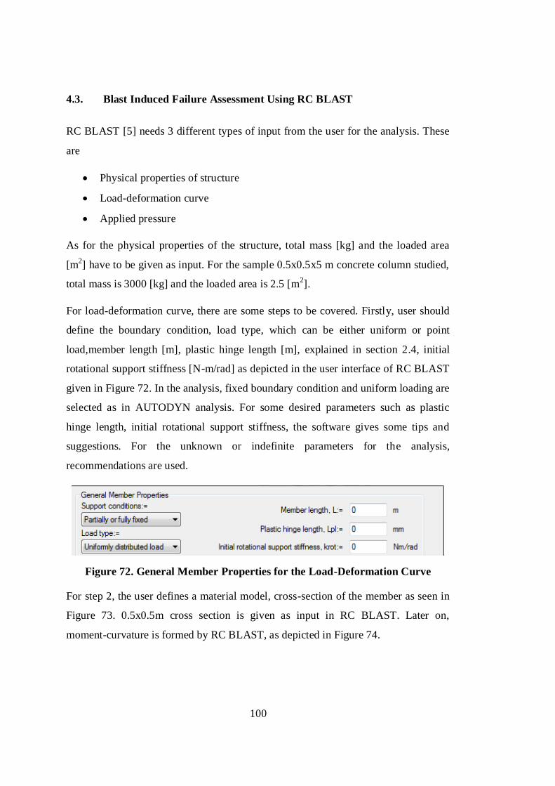
100

4.3. Blast Induced Failure Assessment Using RC BLAST

RC BLAST [5] needs 3 different types of input from the user for the analysis. These

are

Physical properties of structure

Load-deformation curve

Applied pressure

As for the physical properties of the structure, total mass [kg] and the loaded area

[m2] have to be given as input. For the sample 0.5x0.5x5 m concrete column studied,

total mass is 3000 [kg] and the loaded area is 2.5 [m2].

For load-deformation curve, there are some steps to be covered. Firstly, user should

define the boundary condition, load type, which can be either uniform or point

load,member length [m], plastic hinge length [m], explained in section 2.4, initial

rotational support stiffness [N-m/rad] as depicted in the user interface of RC BLAST

given in Figure 72. In the analysis, fixed boundary condition and uniform loading are

selected as in AUTODYN analysis. For some desired parameters such as plastic

hinge length, initial rotational support stiffness, the software gives some tips and

suggestions. For the unknown or indefinite parameters for the analysis,

recommendations are used.

Figure 72. General Member Properties for the Load-Deformation Curve

For step 2, the user defines a material model, cross-section of the member as seen in

Figure 73. 0.5x0.5m cross section is given as input in RC BLAST. Later on,

moment-curvature is formed by RC BLAST, as depicted in Figure 74.

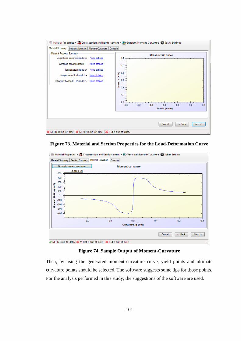
101

Figure 73. Material and Section Properties for the Load-Deformation Curve

Figure 74. Sample Output of Moment-Curvature

Then, by using the generated moment-curvature curve, yield points and ultimate

curvature points should be selected. The software suggests some tips for those points.

For the analysis performed in this study, the suggestions of the software are used.

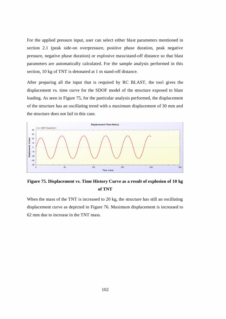
102

For the applied pressure input, user can select either blast parameters mentioned in

section 2.1 (peak side-on overpressure, positive phase duration, peak negative

pressure, negative phase duration) or explosive mass/stand-off distance so that blast

parameters are automatically calculated. For the sample analysis performed in this

section, 10 kg of TNT is detonated at 1 m stand-off distance.

After preparing all the input that is required by RC BLAST, the tool gives the

displacement vs. time curve for the SDOF model of the structure exposed to blast

loading. As seen in Figure 75, for the particular analysis performed, the displacement

of the structure has an oscillating trend with a maximum displacement of 30 mm and

the structure does not fail in this case.

Figure 75. Displacement vs. Time History Curve as a result of explosion of 10 kg

of TNT

When the mass of the TNT is increased to 20 kg, the structure has still an oscillating

displacement curve as depicted in Figure 76. Maximum displacement is increased to

62 mm due to increase in the TNT mass.

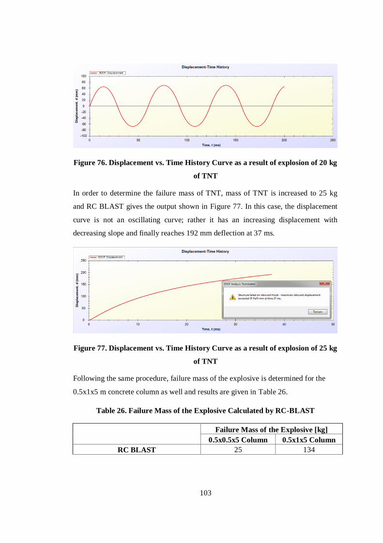
103

Figure 76. Displacement vs. Time History Curve as a result of explosion of 20 kg

of TNT

In order to determine the failure mass of TNT, mass of TNT is increased to 25 kg

and RC BLAST gives the output shown in Figure 77. In this case, the displacement

curve is not an oscillating curve; rather it has an increasing displacement with

decreasing slope and finally reaches 192 mm deflection at 37 ms.

Figure 77. Displacement vs. Time History Curve as a result of explosion of 25 kg

of TNT

Following the same procedure, failure mass of the explosive is determined for the

0.5x1x5 m concrete column as well and results are given in Table 26.

Table 26. Failure Mass of the Explosive Calculated by RC-BLAST

Failure Mass of the Explosive [kg]

0.5x0.5x5 Column 0.5x1x5 Column

RC BLAST 25 134

104

4.4. Assessment of the Results

In order to test the accuracy of the fast responding tool developed in the thesis study,

the failure assessment results obtained by the present code are compared with the

SDOF solver RC BLAST and also with the explicit finite element solver

AUTODYN. As mentioned in section 1.2, the aim of the tool is to give fast and

accurate enough results for bridge-like-structures exposed to external blast loading.

Since RC BLAST and the tool developed in the present study are fast-responding

tools, once the required parameters are given as input, failure assessment results can

be obtained in a few seconds. However, AUTODYN analyses last more than a day

depending on the model. Determining the required amount of explosive to fail the

bridge-like structures is not an easy process for AUTODYN. For each explosive

mass, one has to perform AUTODYN analysis to make failure assessment and this

process requires many reanalysis by changing the explosive mass. One of the

significant advantages of the developed tool is that the approximate failure explosive

mass can be determined very fast and predicted failure explosive mass can be used as

the initial explosive mass in AUTODYN analysis. This way number of detailed

AUTODYN analysis to be performed can be reduced significantly.

For comparison, two sample columns with the dimensions 0.5x0.5x5 m and 1x0.5x5

m are analyzed. For a stand-off distance of 1 m, structures are exposed to the blast

loading due to the explosion of 15, 30, 45, 60, 75, 90, 100, 150, 250 kg of TNT.

Table 27 lists the first set of analysis performed by AUTODYN.

105

Table 27. First Set of AUTODYN Analysis

Stand-

off

Distance

[m]

Mass of

TNT

Explosive

[kg] Member

1 15 Column (0.5x0.5x5)

1 30 Column (0.5x0.5x5)

1 45 Column (0.5x0.5x5)

1 60 Column (0.5x0.5x5)

1 75 Column (0.5x0.5x5)

1 90 Column (0.5x0.5x5)

1 100 Column (0.5x0.5x5)

1 150 Column (0.5x0.5x5)

1 250 Column (0.5x0.5x5)

1 15 Column (0.5x1x5)

1 30 Column (0.5x1x5)

1 45 Column (0.5x1x5)

1 60 Column (0.5x1x5)

1 75 Column (0.5x1x5)

1 90 Column (0.5x1x5)

1 100 Column (0.5x1x5)

1 150 Column (0.5x1x5)

1 250 Column (0.5x1x5)

For the first set of analysis, two sample columns are examined whether they fail or

not using the column failure criteria explained in Section 4.2 based on the erosion of

the elements throughout the whole cross section. Starting from 15 kg of TNT

explosive, mass of explosive is increased up to the failure of the structure. For the

15kg, 30kg and 45 kg of TNT, there exists no cross section throughout which all

elements are eroded. In other words, the column has not failed yet. Figure 78

demonstrates effect of 45 kg TNT explosion on the 0.5x0.5x5 m concrete column. At

the end supports, some elements start to be eroded at 5 ms. Although some elements

eroded at the column ends, erosion throughout the whole cross section does not

occur. Moreover, at the midspan, no erosion occurs and midspan does not deflect

much.

106

Figure 78. Effect of 45 kg TNT Explosion on the 0.5x0.5x5m Concrete Column

Since 45 kg TNT explosion is not enough to fail the concrete column, effect of 60 kg

TNT explosion is investigated. Figure 79 shows the effect of 60 kg TNT explosion

on the 0.5x0.5x5 concrete column. At 5 ms, some elements start to erode near the

end supports. At 10 ms, midspan elements also start to erode as well. It is seen that at

30 ms, most of the elements near the end supports and the midspan erode. At 50 ms,

throughout upper and lower end support, elements fully erode in the sections near the

upper and the lower end supports. Compared to the explosion of 45 kg TNT, at 30

ms, most of the elements erode in the sections nears the end supports for the

explosion of the 60 kg TNT. It is also seen that at the midspan, most of the elements

erode as a result of explosion of 60 kg TNT whereas no erosion exists in the midspan

for the explosion of 45 kg TNT.

107

Figure 79. Effect of 60 kg TNT Explosion on the 0.5x0.5x5m Concrete Column

Table 28 summarizes the results of first set of analysis. After the first set of analysis,

to narrow the range of the failure mass of TNT for 0.5x0.5x5 m column, second set

of analysis is performed.

108

Table 28. Results of First Set of AUTODYN Analysis

Stand-off

Distance[m]

Mass of

TNT

Explosive

[kg]

Member Column

Failure?

1 15 Column (0.5x0.5x5) No

1 30 Column (0.5x0.5x5) No

1 45 Column (0.5x0.5x5) No

1 60 Column (0.5x0.5x5) Yes

1 75 Column (0.5x0.5x5) Yes

1 90 Column (0.5x0.5x5) Yes

1 100 Column (0.5x0.5x5) Yes

1 150 Column (0.5x0.5x5) Yes

1 250 Column (0.5x0.5x5) Yes

1 15 Column (0.5x1x5) No

1 30 Column (0.5x1x5) No

1 45 Column (0.5x1x5) No

1 60 Column (0.5x1x5) No

1 75 Column (0.5x1x5) No

1 90 Column (0.5x1x5) No

1 100 Column (0.5x1x5) No

1 150 Column (0.5x1x5) No

1 250 Column (0.5x1x5) Yes

The results given in Table 28 show that 0.5x0.5x5 m concrete column fails due to the

explosion of 45-60 kg of TNT whereas 0.5x1x5 m concrete column fails due to the

explosion of 150-250 kg of TNT. To narrow the range, a second set of analysis is

performed and explosive masses causing the failure of the column are determined

and presented in Table 29.

109

Table 29. Results of Second Set of AUTODYN Analysis

Stand-

off

Distance

[m]

Mass of

TNT

Explosive

[kg]

Member Column Failure?

1 50 Column (0.5x0.5x5) Yes

1 55 Column (0.5x0.5x5) Yes

1 155 Column (0.5x1x5) No

1 160 Column (0.5x1x5) No

1 165 Column (0.5x1x5) No

1 170 Column (0.5x1x5) No

1 180 Column (0.5x1x5) Yes

1 190 Column (0.5x1x5) Yes

1 200 Column (0.5x1x5) Yes

1 210 Column (0.5x1x5) Yes

1 220 Column (0.5x1x5) Yes

1 230 Column (0.5x1x5) Yes

1 240 Column (0.5x1x5) Yes

Figure 80 shows the effect of 50 kg of TNT explosion on the 0.5x0.5x5 m column.

At 5 ms, elements begin to erode near the end supports. As time elapses, number of

eroded elements increase. At 30 ms, most of the elements in the sections near end

supports and at the midspan erode. However, erosion of all elements in the sections

near the end supports and at the midspan takes place 100 ms later at 140 ms. This is

an indication that 50 kg of TNT is certainly the limit on the failure mass of the TNT

explosive. It should be recalled that for the 60 kg of TNT explosion, the column fails

at 50 ms.

110

Figure 80. Effect of 50 kg TNT Explosion on the 0.5x0.5x5m Concrete Column

Failure response of the concrete columns determined by AUTODYN are compared

to the test and analysis results of Williamson, shown in Figure 10, and great

similarity is observed between the two simulations and tests. For concrete columns

exposed to the explosion with small scaled distance, it is seen that concrete columns

deflect such that as if they broken in the midsection. In other words, plastic hinges

are seen, as shown in Figure 44. This similarity in a way demonstrates that flexural

failure is modeled correctly in AUTODYN analyses.

The results of AUTODYN analyses show that considering the column failure

criterion which is based on checking the non-eroded element in any section of the

column, 0.5x0.5x5 m column fails as a result of explosion of 45 - 50 kg of TNT

while 0.5x1x5 m column fails as a result of explosion of 170 - 180 kg of TNT.

For the same case, results of the fast-responding RC BLAST, results obtained by the

developed tool and with the AUTODYN results are compared in Table 30. The

results show that the tool and RC BLAST, which use SDOF methodology, give close

results for both 0.5x0.5x5 m column and 0.5x1x5 m column. However, for both

111

columns failure masses of the explosive predicted by AUTODYN are higher than the

failure masses of the explosives determined by the developed tool and RC BLAST.

Table 30. Comparison of Explosive Masses Calculated by the Present Study,

RC-Blast and AUTODYN

Failure Mass of the Explosive [kg]

0.5x0.5x5m Column 0.5x1x5m Column

Present study 20.7 120.7

RC BLAST 25 134

AUTODYN 45 - 50 170 - 180

To investigate the reason for the difference in the failure masses obtained by

AUTODYN and predicted by the developed tool, side-on pressures obtained by the

developed tool and AUTODYN are compared. For different scaled distances, peak

side-on overpressures obtained by AUTODYN and the developed tool are compared

in Table 31. The results show that the developed tool (Equation (9) and Table 4)

overestimates the peak side-on overpressure compared to AUTODYN results.

Table 31. Comparison of Peak Side-on Overpressures Obtained by AUTODYN

and the Developed Tool

Mass of

TNT

Explosive

[kg]

Distance

[m]

Scaled

Distance

[m/kg^0.33]

AUTODYN

Side-on

Overpressure

[kPa]

Tool Side-on

Overpressure

[kPa]

Difference

[%]

15 0.5 0.20 13794 16794 17.86%

15 0.75 0.31 8042 9879 18.60%

15 1 0.41 5183 6631 21.84%

15 1.25 0.51 3536 4714 24.99%

15 1.5 0.61 2527 3474 27.26%

15 1.75 0.72 1897 2631 27.89%

15 2 0.82 1486 2037 27.05%

15 2.25 0.92 1184 1608 26.36%

15 2.5 1.02 957 1290 25.84%

After determining the difference in peak side-on pressures determined by the

developed tool and AUTODYN, the side-on overpressure calculated by the tool are

112

decreased to match the side-on overpressure determined by AUTODYN. With the

decreased side-on overpressure, failure masses of the explosive are calculated again

by repeating the analysis for the two columns having dimensions 0.5x0.5x5 m and

0.5x1x5 m for the stand-off distance of distance of 1m. Table 32 gives the updated

explosive mass calculated using the decreased side-on overpressure. From Table 32,

it seen that with the updated side-on overpressure, failure explosive masses

calculated by the developed tool are much closer to the AUTODYN results. It should

be noted that in the present study side-on overpressure is based on the experimentally

determined values and AUTODYN calculates it by analysis, therefore it is doubful

that side-on pressure calculated by AUTODYN analysis is absolutely correct. It is

noted that the developed tool, which is based on SDOF approach, calculates lower

failure explosive mass than AUTODYN. In this respect, the calculated failure

explosive mass forms the lower bound for the AUTODYN analyses. It can be

commented that the developed tool gives conservative values for the failure

explosive mass.

It is also considered that present set of analyses by the developed tool and

AUTODYN are performed for the stand-off distance of 1m which is small. In the

developed tool, loading is assumed to be uniform along the structure. For small

stand-off distances, distribution of the load along the structure may deviate from

uniform loading and this could also account for the differences obtained for the

failure explosive masses by the developed tool and AUTODYN.

Table 32. Comparison of Explosive Masses by the Present Study and

AUTODYN

Failure Mass of the Explosive [kg]

0.5x0.5x5m Column 0.5x1x5m Column

Present Study 20.7 120.7

Present Study with Updated

Side-on Overpressure 36.5 181.9

AUTODYN 45 - 50 170 - 180

In this section uniform load assumption used in the developed tool is studied. Recall

that in the developed tool, instead of point load, uniform loading assumption is done

113

for the SDOF conversion. In theory, it is not possible to represent the blast load by

either uniform load or point load. However, uniform loading assumption is more

reasonable since the loading is distributed along the structure.

To check the uniformity of the load, series of fast-responding analyses are

performed. 0.5x0.5x5 m concrete column, shown in Figure 61, is sampled and

divided as shown Figure 62 for the uniformity analyses. 60 kg of TNT is exploded at

a height of burst of 2.5 m. Stand-off distances are taken as 1m, 2m, 3m, 4m, 5m and

10 m.

At 1 m stand-off distance Mach Stem is not formed. Mach Stem is the 1st discrete

zone in all graphs. Figure 81 shows the distribution of the face on overpressure along

the structure for a stand-off distance of 1 m. As seen in Figure 81, load is maximized

in the mid-region whereas it is minimum at the upper and the lower ends. Loading is

symmetric since the height of burst is half of the column height. For small stand-off

distance, blast load varies so much along the column.

Figure 81. Distribution of the Face on Overpressure along the Structure for a

Stand-off Distance of 1 m

Figure 82 shows the distribution of the face on overpressure along the structure for a

stand-off distance of 3 m. For the stand-off distance of 3 m, Mach Stem forms and

the triple point height ruins the symmetry. However, in this case load is more

uniformly distributed along the structure compared to the 1 m stand-off distance

case.

114

Figure 82. Distribution of the Face on Overpressure along the Structure for a

Stand-off Distance of 3 m

Figure 83 shows the distribution of the face on overpressure along the structure for a

stand-off distance of 5 m. For the stand-off distance of 5 m, Mach Stem again forms

but its intensity diminishes since the stand-off distance increases and loading is more

uniform.

Figure 83. Distribution of the Face on Overpressure along the Structure for a

Stand-off Distance of 5 m

Figure 84 shows the distribution of the face on overpressure along the structure for a

stand-off distance of 10 m. For the stand-off distance of 10 m, loading is very close

to uniform load disregarding the Mach Stem Region.

115

Figure 84. Distribution of the Face on Overpressure along the Structure for a

Stand-off Distance of 10 m

In the overall, as the stand-off distance increases, uniform loading assumption

becomes more reliable approach for blast analysis. For 1 m stand-off distance,

loading is not uniform. For small stand-off distances, distribution of the load along

the structure is not uniform and this could account for the differences obtained for

the failure explosive masses by the developed tool and AUTODYN. To see the effect

of uniformity of the loading at the stand-off distance of 5 m, where loading could be

considered to be almost uniform, further analyses are performed in order to

determine the failure masses of the TNT explosive by the developed tool and

AUTODYN. For the 0.5x0.5x5 m concrete column, in the developed tool, failure

explosive mass is computed as 460 kg of TNT . To trace this clue, in AUTODYN,

440-500 kg of TNT explosive range is scanned to determine failure mass of the TNT

explosive.

For the 450 kg of TNT explosive at a stand-off distance of 5 m, time response of the

column is shown in Figure 85. It is seen that damage starts at the lower end support

at 5 ms. At 30 ms, many of the elements at the lower end support erode.

Furthermore, some elements at upper end support also erode. At 85 ms, the column

deflects considerably at lower end support and almost all elements erode. At 200 ms,

all elements at lower end support erode and the column fails.

116

Figure 85. Effect of 450 kg TNT Explosion on the 0.5x0.5x5m Concrete Column

It is seen that lower end support is damaged much more than the other plastic hinge

locations, which are at the upper end support and at the midsection. To investigate

the reason behind this, face-on overpressure distribution along the column is

analyzed by the developed tool as shown in Figure 86.

It is observed that Mach Stem is formed and impacts the target resulting in 27000

kPa approximately. On the other hand, other parts of the column are subjected to

face-on overpressures between 11000 and 14500 kPa. Face-on overpressure at the

Mach Stem region is almost 2.5 times the face-on overpressure on the other part of

the column. Higher face-on overpressure in the Mach Stem segment of the column

yields greater damage at the lower end support and column fails at the lower end of

the column.

117

Figure 86. Distribution of the Face on Overpressure along the Structure

Exposed to 450 kg of TNT Explosive for a Stand-off Distance of 5 m

In Table 33, the failure masses of explosives for the 0.5x0.5x5 m column are listed

for the 1m and 5 m stand-off distances. At 1 m stand-off distance, the difference is

11 kg when average of 45 and 50 kg of TNT explosive is considered. At 5 m stand-

off distance, the difference is 8.3 kg of TNT explosive. In terms of percent

difference, at higher stand-off distances, the difference in the failure explosive mass

calculated by the developed code and AUTODYN is much lower than the percent

difference for the low stand-off distance case for which the loading less uniform. It is

thus concluded that when the stand-off distance is increased, loading becomes more

uniform.

Table 33. Comparison of Failure Masses of the TNT Explosive Calculated by

AUTODYN and by the Developed Tool at Stand-off Distances 1m and 5 m

AUTODYN DEVELOPED TOOL

Failure Mass of

TNT Explosive at

Stand-off

Distance of 1 m

45 - 50 36.5

Failure Mass of

TNT Explosive at

Stand-off

Distance of 1 m

450 - 455 460.8

118

In addition to difference in the side-on overpressure calculated by the developed tool

and AUTODYN, and uniform load assumption used in developed tool, other

probable reasons for the differences between the failure explosive masses determined

by the developed tool and AUTODYN could be listed as:

The tool discretizes the structure into 10 segments. In reality, the structure is

composed of infinite segments.

The tool disregards negative phase loading. Negative phase diminishes

impulse on the structure. The decreased impulse results in higher mass of the

explosive necessary to fail the structure.

Failure criteria used by AUTODYN, RC BLAST and the tool are different.

There is no clue for failure criterion used in RC BLAST. Difference in failure

criteria may result in different results.

SDOF methodology requires several assumptions. In this method, a complex

concrete model is simplified into lumped mass-spring system. The

simplification is so sharp andthis also causes differences between the results

obtained by the developed tool and AUTODYN.

Although there are some differences between the failure explosive masses calculated

by the developed tool and AUTODYN, failure explosive masses calculated by the

developed tool are not very off from the failure masses calculated by AUTODYN.

As it is mentioned before, the calculated failure explosive mass by the developed tool

forms the lower bound for the expensive AUTODYN analyses. In this respect, the

developed tool can be used for fast estimation of the failure explosive mass and for

more refined analysis, failure explosive mass determined by the tool can be used as

the lower bound for AUTODYN analysis and the number of AUTODYN analysis to

be performed for the more accurate determination of the failure explosive mass can

be reduced significantly.

119

CHAPTER 5

5. CONCLUSION AND FUTURE WORK

The main objective of the thesis study is to develop a fast responding tool which is

accurate enough for the damage assessment in the columns of bridge structures

subjected to blast loading. In order to achieve this goal, available studies in the

literature are extensively examined to establish the background of the blast

phenomenon and also to determine the methodology for the developed tool. The

methodology of the fast responding blast induced damage calculation tool is

explained by means of flowcharts presented in Chapter 3. Key points of the

developed tool are the determination of the side-on overpressure up to the structure,

determination of the impulsive work on the structure and calculation of the structural

response. As for the determination of the side-on overpressure, Kingery’s empirical

formula is determined as the most accurate approach which gives the best fit to the

experimental results. In fact in the literature, Kingery’s empirical formulation is

extensively used for the calculation of blast parameters, especially for the side-on

overpressure. For the accurate calculation of the impulsive work on the structure,

Mach Stem phenomenon is investigated in detail and effect of the Mach Stem is

included in the developed tool. The most critical point on the determination of

impulsive work on the structure is to model the spatial distribution of the face-on

overpressure along the structure. For accurate calculation of the impulsive work on

the structure, the structure is divided into several segments. Thus, variation of the

stand-off distance and the angle of incidence along the structure is modeled

precisely. Furthermore, in order to determine the effect of the ratio of the the rear

wall loading to the front wall loading, a study is performed and this ratio is

determined as function of the scaled distance. It is shown that for small scaled

distances, front wall loading is really dominant over the rear wall loading. Hence, for

the scaled distance less than 0.5 m/kg1/3

, it is concluded that the rear wall loading is

negligible. For the calculation of the response of the structure, material behaviour of

concrete and steel structures is examined. Effects of dynamic increase factor,

120

strength increase factor, age factor are considered for determining the dynamic

strength of the material. Single Degree of Freedom (SDOF) approach is utilized for

the flexural response of the structure exposed to the blast loading. Biggs’ tables are

used for the conversion of the continous system into discrete SDOF system.

Maximum deflection and hinge (support) rotations are computed for damage

assessment of the structure. For the damage assessment, failure criteria published by

Department of Defense of the US army is used.

In addition to the studies performed to develop the fast responding analysis tool,

commercial programs RC BLAST and AUTODYN are used to assess damage in

structures subjected to blast loading for comparison purposes. As mentioned in

Section 4.3, RC BLAST is also a SDOF solver and gives deflection versus time

curve for the blast loaded concrete and steel structures. When sample structures are

subjected to relatively small amount of TNT explosion at 1 m stand off distance,

structures deflect with oscillation in a sinusoidal manner. Increasing the amount of

TNT explosive raises the amplitude of deflection, but thedeflection may still be in

oscillating form. Once the amount of TNT explosive is increased above a certain

limit, deflection of the structure increases with a decreasing slope and converge to

the failure deflection limit of the structure. RC BLAST gives a warning window

showing the failure mass of the TNT explosive and the time of failure. By using the

developed tool and RC BLAST, failure responses of two sample concrete columns

subjected to blast loading are determined. Failure response analyses of the same

sample columns are also performed by AUTODYN which is an explicit dynamic

finite element solver. Free propagation of the blast wave is solved using the wedge

modeling approach. By mapping the pressure and velocity information of high

pressurized expanding gas and the wavefront to the 3D Euler domain, interaction of

the blast wave with the structure is analyzed. The damage and failure is assessed in

two stages; element failure and the column failure. For the element level failure,

damage factor calculated by AUTODYN is used to decide on the failure of the

element and element is allowed to degrade when it starts to be damaged and element

fails when the damage parameter becomes equal to one. Concrete column failure is

based on checking the existence of non-eroded elements which havedamage factor

121

less than one in any section of the column. When all the elements in a section of the

column erode, it is considered that the column can not sustain load anymore. By

applying the two stage failure criterion, series of AUTODYN analyses are performed

and failure masses of the TNT explosive is determined for the two sample columns

studied. Failure explosive mass results obtained by the developed tool, RC Blast and

AUTODYN show that although the developed tool and RC BLAST yields close

results, they differ from AUTODYN significantly. To find out the reasons behind

this difference, side-on overpressure results obtained by AUTODYN and Kingery’s

formulation, which predicts test results very closely, as seen in Figure 53, are

compared. It is seen that AUTODYN yields lower side-on overpressure than

obtained by the Kingery’s formulation which is used in the developed tool. As a

follow-up study, side-on overpressure predicted by the developed tool is reduced to

match the side-on overpressure determined by AUTODYN. With the reduced side-on

overpressure, failure masses of the TNT explosive are recalculated. It is seen that

failure explosive masses determined by the updated side-on overpressure determined

are much closer to the AUTODYN results. For further investigation of the possible

source of the differences between the failure masses predicted by the developed tool

and AUTODYN, uniformity of the load as a function of the stand-off distance is

examined. It is seen that for the sample columns studied, the load is not uniform

when the stand-off distance is 1 m, and load becomes more and more uniform when

the stand-off distance is increased. For the 5m stand-off distance, failure masses of

the TNT explosive calculated by AUTODYN and the developed tool are compared

and it is seen that at high stand-off distance the difference in the failure masses

diminishes due to the enhanced load uniformity. Despite some differences between

the failure explosive masses calculated by the developed tool and by AUTODYN,

they are not very off from each other. When the computational time spent is

considered, the developed tool is very efficient compared to AUTODYN.

It is noted that the developed tool, which is based on the SDOF approach, calculates

lower failure explosive mass than AUTODYN. In this respect, the calculated failure

explosive mass forms the lower bound for the AUTODYN analysis. It can be

122

commented that the developed tool gives conservative values for the failure

explosive mass. Thus, the developed tool can be used for fast estimation of the

failure explosive mass and for more refined analysis, failure explosive mass

determined by the tool can be used as the lower bound for AUTODYN analysis and

the number of AUTODYN analysis to be performed for the more accurate

determination of the failure explosive mass can be reduced significantly.

In conclusion, the developed tool can be used for the design of bridge-like structures

in two main ways. Column dimensions can be optimized to withstand possible

detonation threats. By taking advantage of the very fast analysis capability of the

tool, preliminary design of the column can be performed. More refined analysis can

be performed by AUTODYN, if necessary. In addition, the explosive mass and the

detonation point to cause failure of the structure can be optimized by performing

parametric analysis and examining the effective blast parameters.

Regarding the future work, single column analysis can be extended to the blast

analysis of the whole bridge structure. Furthermore, the developed code can be

improved to estimate the damage of the whole bridge structure for various detonation

locations with the goal of determiningthe optimum detonation point to fail the whole

bridge. Moreover, graphical user interface can be developed for the fast responding

blast analysis tool. With such a graphical user interface, the ease of use of the tool

can be substantially increased.

123

REFERENCES

[1] Nago, T., Gupta, A., Ramsay, J., (2007). Blast Loading and Blast Effects on

the Structures: An Overview. Electronic Journal of Structural Engineering. Volume

10 (EJSE Special Issue). Retrieved from

<http:www.ejse.org/Archives/Fulltext/2007/Special/200707.pdf>.

[2] Agrawal, A.K., Yi, Z. (2009). Blast Load Effects on Highway Bridges. New

York, NY: American Society of Civil Engineers.

[3] AASHTO. (2002). National Needs Assessment for Ensuring Transportation

Infrastructure Security. < http://security.transportation.org/sites/ security/docs

/NatlNeedsAssess.pdf>.

[4] Autodyn [Computer Software]. (2016). Retrieved from <

http://www.ansys.com/products/structures/ANSYS-Autodyn>.

[5] RC Blast [Computer Software]. (2016). Retrieved from

<http://www.rcblast.ca>.

[6] Collins, G., S., (2002). An Introduction to Hydrocode. Claeys, New York:

Springer.

[7] Sherkar, P., Whittaker, A.S., Aref, A.J. (2010). Modeling the Effects of

Detonations of High Explosives to Inform Blast-Resistant Design (Technical Report

MCEER-10-0009). New York, NY: MCEER Thrust Area 3, Innovative

Technologies.

124

[8] LS-Dyna [Computer Software]. (2016). Retrieved from <

http://www.lstc.com/products/ls-dyna>.

[9] Williamson, E.B., Bayrak, O., Davis, C., Williams, G.D. (2011)

“Performance of Bridge Columns Subjected to Blast Loads II: Results and

Recommendations” J. Bridge Eng., pp. 586-59410.1061/(ASCE)1084-

0702.13:6(586).

[10] Fujikara, S., Bruneau, M., Lopez-Garcia, D. (2008). Experimental

Investigation of Multihazard Resistant Bridge Piers Having Concrete Filled Steel

Tube under Blast Loading. Journal of Bridge Engineering. Volume10 (1061). 586-

594. 1084-0702(2008)13:6(586).

[11] Matthews, T., Elwood, K. J., Hwang, S. J. (2007) Explosive Testing to

Evaluate Dynamic Amplification during Gravity Load Redistribution for Reinforced

Concrete Frames. 2007 ASCE Structures Congress, ASCE, Reston, VA.

[12] Tokal-Ahmed, Y.M. (2009). Response of Bridge Structures Subjected to Blast

Loads and Protection Techniques to Mitigate the Effect of Blast Hazards on Bridges.

The State University of New Jersey, New Jersey, USA.

[13] ELS [Computer Software]. (2016). Retrieved from <

http://www.extremeloading.com>.

[14] Chock, J.M. (1999). Review of Methods for Calculating Pressure Profiles of

Explosive Air Blast and its Sample Application. Virginia Polytechnic Institute and

State University, Blacksburg, Virginia, USA.

125

[15] Nastran [Computer Software]. (2016). Retrieved from <

http://www.mscsoftware.com/product/msc-nastran>.

[16] Matthews, D.S. (2008) Blast Effects on Prestressed Concrete Bridges.

Washington State University, Washington DC, USA.

[17] Oswald, C., Bazan, M. (2014) Comparison of SDOF Analysis Result to Test

Data for Different Types of Blast Loaded Components. Structures Congress 2014: pp.

117-130. DOI: 10.1061/9780784413357.012 .

[18] Driels, M., R., (2013). Weaponeering: Conventional Weapon System

Effectiveness Second Edition. Reston, VA: Greenham.

[19] Williamson, E.B., Bayrak, O., Williams, G.D. (2010) Blast-Resistant

Highway Bridges: Design and Detailing Guidelines (NCHRP Report 645).

Washington, D.C.: Transportation Research Board.

[20] Smith, P.D., Hetherington J.G. (1994). Blast and Ballistic Loading of

Structures. Shrivenham, England: CRC Press.

[21] Remennikov, A. (2007). The State of the Art of Explosive Loads

Characterisation. University of Wollongang, Australia.

[22] U.S. Department of the Army (1990) Structures to Resist the Effects of

Accidental Explosions (Technical Manual 5-1300). Alexandria, VA: Department of

the Army, the Navy and the Air Force.

[23] Dusenberry, D.O. (2010). Handbook for Blast-Resistant Design of Buildings.

Hoboken, NJ: John Wiley & Sons Inc.

[24] Needham, C.E. (2010). Blast Waves. New York, NY:Springer-Verlag.

126

[25] Kinney G. F., Graham K.J. (1985). Explosive Shocks in Air. Berlin, Germany:

Springer.

[26] Brode H.L. (1955). Numerical Solution of Spherical Blast Waves. New York,

NY: Springer.

[27] Newmark, N.M., Hansen R.J. (1961). Design of Blast Resistant Structures:

Shock and Vibration Handbook. New York, NY: McGraw Hill.

[28] Mills, C.A. (1987). The Design of Concrete Structures to Resist Explosions

and Weapon Effects. Proceedings of the 1st International Conference on Concree for

Hazard Protections, Edinburgh, UK, pp.61-73.

[29] Kingery, C.N. (1966). Air Blast Parameters versus Distance for

Hemispherical TNT Surface Bursts (Technical Report No: 1344). Aberdeen,

Maryland: Ballistic Resarch Laboratories.

[30] Boris, G. (2004). Translation from Russian to English the Book: Blast Effects

Caused by Explosions (Technical Report N62558-04-M-0004). London, England:

Eurepean Research Office.

[31] Glasstone, S., Dolan, P.J. (1997). The Effects of Nuclear Weapons, 3rd

Edition. Washington DC: United States Department of Defense.

[32] U.S. Army Corps of Engineers (2008). Structures to Resist the Effects of

Accidental Explosions (UFC 3-340-02). Washington, DC: Air Force Civil Engineer

Support Agency.

127

[33] Altunlu, K. (2008). Safety Assessment of R/C Columns Against Explosive

Attacks by Vehicle or Human from Exterior. Middle East Technical University,

Ankara, Turkey.

[34] Karlos, V., Solomos, G. (2013) Calculation Of Blast Loads For Application

To Structural Components (Jrc Technical Reports 32253-2011). Ispra, Italy: Joint

Research Center.

[35] Payne, C.M. (2010). Principles of Naval Weapons Systems. Annapolis, MD:

US Naval Institute Press.

[36] Bulson, P.S. (1997). Explosive Loading of Engineering Structures. New

York, NY:Chapman and Hall.

[37] Miller, P. (2004). TowardstheModelling of BlastLoads on Structures.

University of Toronto, Ontario, Canada.

[38] Rahman, S.,Timofeev, E. (2007). PressureMeasurements in Laboratory-

ScaleBlastWaveFlowFields: Review of Scientific Instruments, Vol. 78.

[39] U.S. Army Engineer Research and Development Center (2003). Bridge and

Tunnel Vulnerability Workshop sponsored by the Federal Highway Administration

Office of Bridge.

[40] Tedesco, J. (1999). Structural Dynamics: Theory and Approach. Menlo Park,

CA: AddisonWesleyLongman.

[41] Malvar, L.J., Crawford, J.E. (1998). Dynamic Increase Factors for Concrete.

28th Department of Defence Explosives Safety Seminar.

128

[42] American Society of Civil Engineers (1997). Design of Blast Resistant

Buildings in Petro-chemical Facilities. Reston, Virginia: ASCE.

[43] Biggs, J. (1964). Introduction to Structural Dynamics. New York, NY:

McGraw Hill.

[44] Budynas, R.G., Nisbett, J.K. (2013) Shigley’s Mechanical Engineering

Design. New York, NY: McGraw Hill.

[45] Brannon, M. R., Leelavanichkul, S. (2009). Survey of Four Damage Models

for Concrete (Technical Report SAND2009-5544). Livermore, CA: Sandia National

Laboratories.

[46] Shin, J., Whittaker, A., Aref, A. (2015). Near-field Blast Assessment of

Reinforced Concrete Components. International Journal of Protective Structures.

Volume 6(3). pp. 487-508.

129

APPENDICES

A. VIEW OF THE DEVELOPED TOOL

130

B. DERIVATION OF MASS AND LOAD FACTORS

In the study of Biggs [43], load and mass factors are given in Table 15. In Appendix

B, derivation of load and mass factors are given for the plastic regime. Uniformly

loaded structure fixed at both ends is shown schematically in Figure B1.

Figure B1. Uniformly Loaded Structure Fixed At Both Ends

LOAD FACTOR FOR THE UNIFORMLY LOADED FIX-FIX BEAM

Load factor is given by [43],

(B1)

where is the load factor, is the equivalent force on structure and is actual

force on structure. Equivalent force is given by,

∫ ( ) ( ) ∫ ( )

(B2)

where ( ) is force per unit length along the structure, ( ) is shape function. Shape

function is given by Equation (B3),

131

( ) ( )

(B3)

For a structure in the plastic regime, deflected shape is given in Figure B2.

Figure B2. Deflected Structure in the Plastic Regime

( ) is given by Equation (B4)

( )

( ) ( ) (B4)

and is given by Equation (B5).

(B5)

Thus, shape function ( ) is computed as,

132

( ) ( )

( ) ( )

( )

(

)

(B6)

Load factor is given by Equation (B7)

∫ ( ) ( ) ∫ ( ) ( )

(B7)

MASS FACTOR FOR UNIFORMLY LOADED FIX-FIX BEAM

Mass factor is given by [43],

(B8)

where is the mass factor, is the equivalent mass of structure and is the

actual mass of structure. Equivalent mass is calculated as,

∫ ( ) ( )

(B9)

where ( ) is the mass per unit length along the structure and ( ) is the shape

functiongiven by Equation (B6). Hence, mass factor is calculated as,

∫ ( ) ( )

∫ ( ) ( )

(B10)