)CUMENTAT1ON PAGE j fft •OnI,

AD-A277 861 -- -------- O--------- ----- -----IIEPORT OAT" -. - - PORT -p- ANM W- cc-

1 March 1994 Final Technical Renort-11/I/90-11/-.0/,4MU AND Sun= L | UJINO muva

Adaptive Methods for Compressible Flow AFOSR-91-0063

2304/CS 61102F

.AUTHOAS)

"Marsha Berger 94-10516

7. PMWOMG 31GAIZATIO XAME(S) AND "WAOOESS) ltil I l~111IINew York University pcj? l l0Courant Institute of Mathematical Sciences251 Mercer StreetNew York, NY 10012 MOSR'" 94 0131

J. 5OSPOft EGi MONITORING AGENCY NAMI(S) AND ADOAES5(1S) IL SPONSW WOW6IMOITI#

AFOSR/NM AGO= RONT MUMAE

110 Duncan-Avenue, Suite B115 AFOSR-91-0063Boiling AFB, DC 20332-0001 D T IC2

11. SPMETART MOTM ELECTEAPR 0 71994

_12& OdrTNIUUIIUAVAIAJTTM STATEMEN

Unlimited rlae"-Jpproved for publAO reless I

distribut ion unlimited.

13. AISNTACT (M2AsMn 200wW

The goal of this research is the development of adaptive computational methods to numer-

ically simulate fluid flows around complex configurations in an automatic fashion. Grid

generation continues to be a huge impediment for computer simulations of realistic fluid

0 flows. This is true for both body-fitted structured grid solvers and unstructured grid ap-

proaches. We are developing a Cartesian grid representation of the geometry, where the

object is simply "cut" out of the Cartesian grid. We are also investigating the suitability

of adaptive methods on parallel computers.

1)TIO QUAIXLY ici:~~ ~y is. NurNar OF PAin

Adaptive mesh refinement, compressible fluid flows, 8

Cartesian meshes. i6. Pau CODE

OP uPON "M H PAUE CO AB$7*ACF

Unclassified . Unclassified Unclassified UnlimitedNSN 7141-304500SF&awUoM 2" (R",. 149)

Approvc r "r' j p I cblt release;

AFOSR-TR. 9 4 0131

1W Acc"&woi, ForAdaptive Methods for Compressible Flow NT,

NTiS ;RAI -

Final ReportAFOSR-91-0063 Dy

Di;t, ibu: 'Marsha J. BergerCourant Institute251 Mercer Street -,or

New York, NY 10012 , C

1 Abstract

The goal of this research is the development of adaptive computational methods to numer-ically simulate fluid flows around complex configurations in an automatic fashion. Gridgeneration continues to be a huge impediment for computer simulations of realistic fluidflows. This is true for both body-fitted structured grid solvers and unstructured grid ap-proaches. We are developing a Cartesian grid representation of the geometry, where theobject is simply "cut" out of the Cartesian grid. We are also investigating the suitabilityof adaptive methods on parallel computers.

Here we summarize results of our previous work in the last three years, supported byAFOSR grant 91-0063.

2 Summary of Accomplishments

Our research in the last three years has concentrated on three fronts: (i) we have continuedto develop the basic adaptive methodology for compressible flows in the context of hyper-bolic conservation laws, (ii) we have developed a strategy for simulating time-dependentflows around complex geometries using a Cartesian grid representation in two space dimen-sions, and (iii) we have studied the suitability of local adaptive mesh refinement for massivelyparallel architectures such as the Connection Machine. I will describe these projects in turn.

The development of a (serial) three dimensional adaptive mesh refinement (henceforthAMR) algorithm for hyperbolic conservation laws has been completed. This work is in

1

-'DJTED 3

collaboration with John Bell and Michael Welcome, at Livermore National Laboratory, andJeff Saltzman, of Los Alamos National Laboratory. To test the algorithm we conductednumerical experiments of the interaction of a shock and an ellipsoidal bubble of Freon (seefigure 1. This is analogous to the laboratory experiments of Haas and Sturtevant. Our testsindicate that AMR reduced the computational cost by a factor of at least 20 over uniformfine grid computations of the same resolution. This work is described in [1]

Although most of the algorithm development was a straightforward extension of thetwo dimensional case, a new grid generation algorithm was developed. Our previous gridgeneration algorithm worked remarkably well at creating grids with efficiency ratings ofapproximately 50%, (i.e. at least half the points in the new fine grid needed to be refined),using no geometric information at all. (The rest of the points are included to make arectangular fine grid, but didn't need to be refined based on the error estimate criterion). Ifa fine grid was inefficient, it simply bisected the grid in the long direction, the flagged cellswere partitioned into their respective halves, and two new fine grids resulted. Unfortunately,when requesting efficiencies around 80%, this algorithm produced unacceptably many tinygrids. Since memory (to store the refined grids) and CPU time (to integrate them) is ata premium in three dimensions, we developed a better grid generation algorithm. Thenew procedure can be viewed as a "smart" bisection algorithm. Using techniques fromcomputer vision and pattern recognition, such as a variation of the Marr-Hildredth operatorand coordinate-based signatures, our new algorithm can obtain efficiencies around the 80%level, even if the feature is not aligned with a coordinate direction. This was described in[2].

In collaboration with Prof. Randy LeVeque at the University of Washington we havedeveloped an algorithm for computing time dependent flows around complex geometriesusing a non-body-fitted Cartesian grid. This strategy fits in naturally with our previouslydeveloped AMR strategy of using locally uniform meshes. We retain the advantages (effi-ciency and accuracy) of uniform grids and are able to resolve fine scale flow features inducedby complex geometries. We use our previously developed adaptive mesh refinement algo-rithm to achieve accuracy comparable to the body-fitted meshes, where grid points can bebunched in an a priori manner to improve the accuracy of the solution.

We have developed a rotated difference scheme for use at the irregular boundary cells.Essentially, this difference scheme uses an auxiliary coordinate system that is locally normaland tangential to the boundary. This "artificial" grid is obtained at each interface bycreating a box extending a distance h away from the interface in the normal and tangentialdirections. Solution values for the new box are obtained by conservatively averaging thestates in the underlying Cartesian grid. By differencing over a box of size h rather than theirregular neighboring cell with (potentially orders of magnitude) less cell volume, we retainstability using a time step At based on the uniform grid cells. Figure 2 shows a snapshotof a time-dependent computation of shocked flow around two cylinders. Notice that the

2

Figure I: Interaction of a shock and ellipsoidal bubble.

pressure plots around the cylinders show smooth pressure despite the irregularity of the cutcells adjacent to the cylinders.

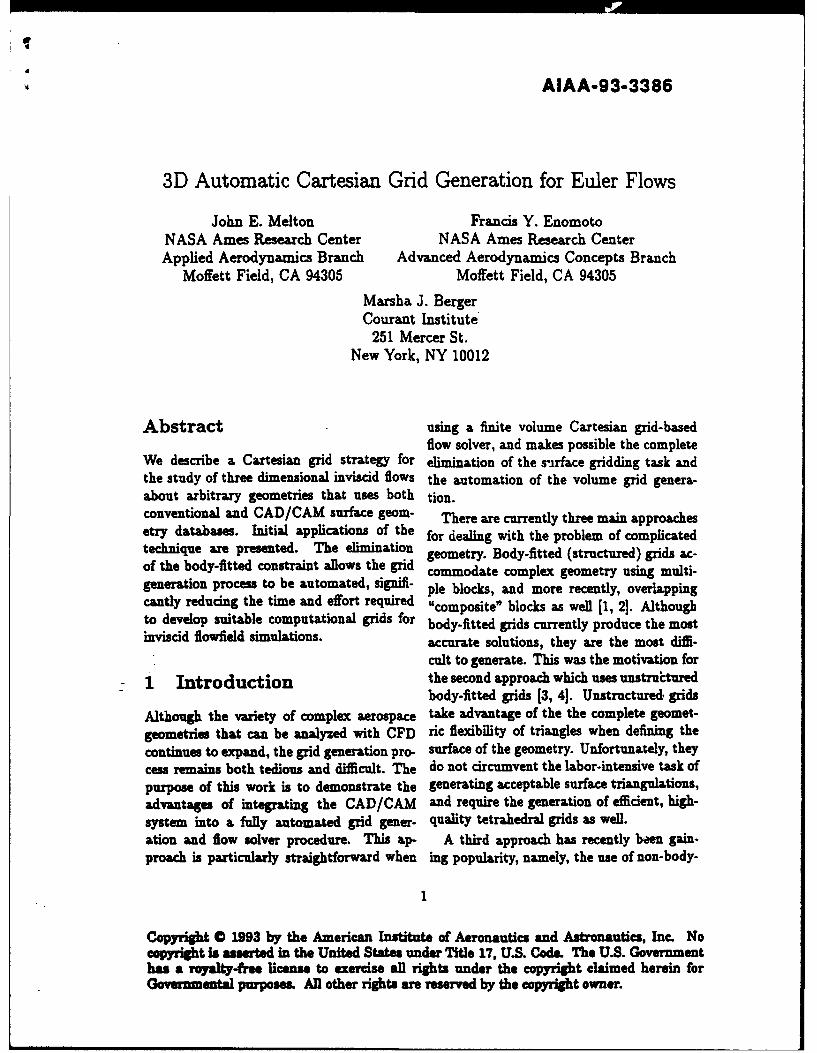
In more recent work with John Melton (at NASA Ames Research Center), we are de-veloping a steady state compressible flow solver around objects with complex geometryusing a Cartesian grid. With this work, since there is no time stepping stability limitation,we are concentrating on the accuracy question of irregular grid cells, and focusing on theissue of automating the geometry. We have developed an approach, using a given surfacetriangulation, to generate the volume information and data structures needed in the Cart e-sian grid program (4]. In addition, we have the beginnings of an automatic interface usirga CAD/CAM system. Figure 3 shows a sample calculation that illustrates the Cartesiangeometry.

As a preliminary part of this study, we have compared the use of hierarchical mesheswith rectangular indexing versus a completely unstructured linked list implementation. Anunstructured grid data structure has a lot of overhead associated with it, since each tetrahe-dron points to all its neighbors, its faces, its edges, etc. Typical numbers are approximately80 to 120 words of storage per grid point. A grid based data structure has much less over-head, but needs to refine more cells than the absolute minimum to form the rectangles. Wehave run some experiments comparing the approaches in three dimensions, for flow arounda wing, and a full aircraft. Although this is very simple it appears to have not been donebefore. For the wing test case, our results show that although the regular approach refinesone and a half times as many points, it has a factor of 5 less overhead, so it is still preferable.For the full aircraft, approximately twice as many points are used in the flow solver, butagain with less overhead. Additionally, the regular grid scheme vectorizes without using in-direct address and scatter gathers, so performance should be the same if not slightly betterthan the unstructured approach as well.

Together with Jeff Saltzman from Los Alamos National Laboratory, we have developeda fully adaptive two dimensional local mesh refinement algorithm for the Euler equationson the CM-2 and Cm-5. To our knowledge, this is the first time such an adaptive methodhas been implemented for structured meshes on a massively parallel machine. Again weuse the AMR approach to adaptive mesh refinement; a collection of logically rectangularmeshes makes up the coarse grid, refinements cover a subset of the domain and use smallerrectangular grid patches. (There is no complex geometry in this implementation). Manyof the original design choices in AMR were based on considerations of vectorization. Thequestion was whether this approach was still feasible, and even advantageous on a dataparallel massively parallel architecture.

The main issues in adapting the algorithm for a data parallel environment were parti-tioning the data to fill the machine (load balancing, rather simple on rectangular grids), andminimizing communication (which is the main issue for our hierarchical data structure). Wehave developed a data layout scheme which preserves locality between fine and coarse grids

4

U ~P PUKSUR. TIME * .f.COMPOSITE PRESSURE. TIME . 0.645. COMPOSITE

BOOYPLOT. TIME 0 .122. COXVOSITE 1

PREsSSUR. TIME 0. 3122. COMPOSITE

r

BOOYPLOT. TIME 0.310. COMPOSITE 2

00-'ýS,; * "" 313. COMPOSITE

0.94 0.25 0.5# 8.7s I1.,11

Figure 2shows prcssurc plots of the flowficld and the prcssurc along the cylinders. at several different times. The

location or cmbcddcd finec grids is indim~cd on thc contour plots.

Figure 3: Cartesian mesh representation of an airplane.

and minimizes global (router) communication. This data layout turned out to be an impor-tant component in equidistributing the communication (rather than the more typical loadbalancing of computation) even on the CM-5, with its unusual fat-tree interconnection. Thetwo-dimensional CM-2 results are described in [3]. Essentially, we obtained performanceon an 8K CM-2 that was equivalent to one head of a Cray Y-MP. The three-dimensionalCM-5 research is still underway. Eventually, we will implement a parallel version of adap-tive mesh refinement with complex geometry. This will not be simply a straightforwardimplementation, since the workloads have much more non-uniform, depending on whethera cell is adjacent to a solid object, or at the boundary of a finer or coarser level grid.

In addition to the above research, the research by Anders Szepessy on adaptive finiteelement methods for compressible fluid flow continued. For adaptive flow calculations, oneneeds:

1. a robust mesh generator

2. a stable and reasonable accurate discretization method,

3. an adaptive refinement criteria.

The work has concentrated on the less well understood areas (1) and (3). In joint workwith Jonathan Goodman and Margaret Symington, we have been developing a new meshgenerator based on successive not necessarily isotropic refinements using high aspect ratioelements around shocks and boundary layers. The most commonly used method for gener-ating anisotropic meshes is the advancing front technique, which is not very robust in myexperience. Computations with our new program show promise. The mesh generator isvery robust.

Currently we are working on techniques to improve the convergence rate when solv-ing the discrete equations. We have been improving the data structure in the program tomore efficiently handle multilevel techniques. The hierarchical multilevel structure natu-rally obtained in the successive refinements is known to work well in the case of isotropicrefinements. In our case of anisotropic discretizations and high aspect ratio elements thecondition numbers are even worse as compared to the isotropic case. Preliminary testsusing multilevel techniques indicate that one can obtain convergence rates independent ofthe mesh size also with the high aspect ratio elements in our program.

Reacting shock waves, in contrast to non-reacting shocks, sometimes need high resolutionto capture the correct physical behavior. It is therefore of interest to apply our program toreactions. In previous work with Claes Johnson we have constructed adaptive algorithmsbased on a posteriori error estimates for non-reacting shocks using mainly isotropic meshes.We are currently studying generalizations to reactions, relaxation effects and anisotropicmeshes including implementation aspects.

7

References

(1] J. Bell, M. J. Berger, J. Saltzman, and M. Welcome. Three dimensional adaptive meshrefinement for hyperbolic conservation laws. SIAM J. Sci. Stat., 15:127-138, January1994.

[2] M. J. Berger and I. Rigoutsos. An algorithm for point clustering and grid generation.IEEE Trans. Sys. Man and Cyber., 21:1278-1286, Sept./Oct. 1991.

[31 M. J. Berger and J. Saltzman. AMR on the CM-2. In Proceedings of Workshop onAdaptive Computational Methods, Troy, NY, June 1992. To appear, Applied Num.Math.

[4] J. Melton, F. Enomoto, and M. Berger. 3d automatic Cartesian grid generation foreuler flows. AIAA-93-3386, July 1993.

8

Unstructured Multigrid through Agglomeration

V. VenkatakrishnanComputer Sciences Corporation

M.S. T045-1, NAS Applied Research BranchNASA Ames Research Center, Moffett Field, CA 94035

D. J. MavriplisICASE

M.S. 132CNASA Langley Research Center, Hampton, VA 23681

M.J. BergerCourant Institute of Mathematical SciencesNew York University, New York, NY 10012

Abstract

In this work the compressible Euler equations are solved using finite volume tech-niques on unstructured grids. The spatial discretization employs a central differenceapproximation augmented by dissipative terms. Temporal discretization is done usinga multistage Runge-Kutta scheme. A multigrid technique is used to accelerate conver-gence to steady state. The coarse grids are derived directly from the given fine gridthrough agglomeration of the control volumes. This agglomeration is accomplishedby using a greedy-type algorithm and is done in such a way that the load, which isproportional to the number of edges, goes down by nearly a factor of 4 when movingfrom a fine to a coarse grid. The agglomeration algorithm has been implemented andthe grids have been tested in a multigrid code. An area-weighted restriction is appliedwhen moving from fine to coarse grids while a trivial injection is used for prolongation.Across a range of geometries and flows, it is shown that the agglomeration multigridscheme compares very favorably with an unstructured multigrid algorithm that makesuse of independent coarse meshes, both in terms of convergence and elapsed times.

1 Introduction

Multigrid techniques have been successfully used in computational aerodynamics for over adecade 11,2]. The main advantage of the multigrid method when solving steady flows is theenhanced convergence while requiring little additional storage. In addition, multigrid canbe used in conjunction with any convergent base scheme, with adequate care exercised inconstructing proper restriction and prolongation operators between the grids. Perhaps thebiggest advantage of multigrid is the fact that it deals directly with the nonlinear problemwithout requiring an elaborate linearization and the attendant storage required to storethe matrix that arises from the linearization. Thus, multigrid techniques have enabled thepractical solution of complex aerodynamic flows using millions of grid points.

The initial efforts in multigrid were directed towards the solution of flows on structuredgrids where coarse grids can easily be derived from a given fine grid. Typically, this is done

1

by omitting alternate grid lines in each dimension. These ideas have been extended to tri-angular grids in two dimensions and to tetrahedral meshes in three dimensions [3,4,5,6].In previous work by the second author, a sequence of unnested triangular grids of varyingcoarseness is constructed [3]. Piecewise linear interpolation operators are derived duringa preprocessing step by using efficient search procedures. The residuals are restricted tocoarse grids in a conservative manner. It has been shown that such a scheme can con-sistently obtain convergence rates comparable to those obtained with existing structuredgrid multigrid methods. For complex geometries, especially in three dimensions, however,constructing coarse grids that faithfully represent the complex geometries can become adifficult proposition. Thus, it is often desirable to derive the coarse grids directly from agiven fine grid.

The agglomeration multigrid strategy has been investigated by Lallemand et al. [7]and Smith [8]. Lallemand et al. use a base scheme where the variables are stored at thevertices of the triangular mesh, whereas Smith uses a scheme that stores the variables atthe centers of triangles. In the present work, a vertex-based scheme is employed. Twodimensional triangular grids contain twice as many cells as vertices (neglecting boundaryeffects), and three dimensional tetrahedral meshes contain 5 to 6 times more cells thanvertices. Thus, on a given grid, a vertex scheme incurs substantially less computationaloverhead than a cell-based scl eme.. Increased accuracy can be expected from a cell-basedscheme, since this involves the solution of a larger number of unknowns. However, theincrease in accuracy does not appear to justify the additional computational overheads,particularly in three dimensions.

The main idea behind the agglomeration strategy of Lallemand et al. [7] is to agglom-erate the control volumes for the vertices using heuristics. The centroidal dual, composedof segments of the median of the triangulation, is a collection of the control volumes overwhich the Euler equations in integral form are solved. On simple geometries, Lallemand etal. were able to show that the agglomerated multigrid technique performed as well as themultigrid technique which makes use of unnested coarse grids. However, the convergencerates, especially for the second order accurate version of the scheme, appeared to degradesomewhat. Furthermore, the validation of such a strategy for more complicated geometriesand much finer grids, as well as the incorporation of viscous terms for the Navier-Stokesequations remains to be demonstrated. The work of Smith [8] constitutes the basis ofa commercially available computational fluid dynamics code, and as such has been ap-plied to a number of complex geometries [9]. However, consistently competitive multigridconvergence rates have yet to be demonstrated.

In the present work, the agglomeration multigrid strategy is explored further. Theissues involved in a proper agglomeration and the implications for the choice of the re-striction and prolongation operators are addressed. Finally, flows over non-simple two-dimensional geometries are solved with the agglomeration multigrid strategy. This ap-proach is compared with the unstructured multigrid algorithm of Mavriplis [3] which makesuse of unnested coarse grids. Convergence rates as well as CPU times on a Cray Y-MP/1are compared using both methods.

2

2 Governing Equations and discretization

The Euler equations in integral form for a control volume Q with boundary Of? read

'judv+f F(un) dS=O. (1)

Here u is the solution vector comprised of the conservative variables: density, the twocomponents of momentum, and total energy. The vector F(u, n) represents the inviscidflux vector for a surface with normal vector n. Equation (1) states that the time rateof change of the variables inside the control volume is the negative of "he net flux of thevariables through the boundaries of the control volume. This net flux through the controlvolume boundary is termed the residual. In the present scheme the variables are stored atthe vertices of a triangular mesh. The control volumes are non-overlapping polygons whichsurround the vertices of the mesh. They form the dual of the mesh, which is composed ofsegments of medians. Associated with each edge of the original mesh is a (segmented) dualedge. The contour integrals in Equation (1) are replaced by discrete path integrals overthe edges of the control volume. Figure 1 shows a triangulation for a four-element airfoiland Figure 2 shows the centroidal dual. Each cell in Figure 2 represents a control volume.The path integrals are computed by using the trapezoidal rule. This can be shown to beequivalent to using a piecewise linear finite-element discretization. For dissipative terms,a blend of Laplacian and biharmonic operators is employed, the Laplacian term actingonly in the vicinity of shocks. A multi-stage Runge-Kutta scheme is used to advance thesolution in time. In addition, local time stepping, enthalpy damping and residual averagingare used to accelerate convergence. The principle behind the multigrid algorithm is thatthe errors associated with the high frequencies are annihilated by the carefully chosensmoother (the multi-stage Runge-Kutta scheme) while the errors associated with the lowfrequencies are annihilated on the coarser grids where these frequencies manifest themselvesas high frequencies. In previous work [3], as well as in the present work, only the Laplaciandissipative term (with constant coefficient) is used on the coarse grids. Thus the fine gridsolution itself is second order accurate, while the solver is only first order accurate on thecoarse grids.

3 Details of agglomeration

The agglomeration (referred to also as coarsening) algorithm is a variation on the one usedby Lallemana . -1. [7] and is given below:

1. Pick a starting vertex on the surface of one of the airfoils.

2. Agglomerate control volumes associated with its neighboring vertices which are notalready agglomerated.

3. Define a front as comprised of the exterior faces of the agglomerated control volumes.Place the exposed edges in a queue.

3

Figure 1: Grid about a four-element airfoil.

4. Pick the new starting vertex as the unprocessed vertex incident to a new startingedge which is chosen from the following choices given by order of priority:

"* An edge on the front that is on the solid wall.

"* An edge on the solid wall.

"* An edge on the front that is on the far field boundary.

"* An edge on the far field boundary.

"* The first edge in the queue.

5. Go to Step 2 until the control volumes for all vertices have been agglomerated.

There are many other ways of choosing the starting vertex in Step 4 of the algorithm,but we have found the above strategy to be the best. The efficiency of the agglomerationtechnique can be characterized by a histogram of the number of fine grid cells comprisingeach coarse grid cell. Ideally, each coarse grid cell will be made up of exactly four fine gridcells. The various strategies can be characterized by how close they come to this ideal case.One variation is to pick the starting edge randomly from the edges currently on the front.Figure 3 shows a plot of the number of coarse grid cells as a function of the number of finegrid cells comprising them, with our agglomeration algorithm described above, and withthe variation. It is clear that our agglomeration algorithm is superior to the variant. Thenumber of coarse grid cells having exactly one fine cell (singletons) is also much smallerwith our algorithm compared to the variant. We have also investigated another variationwhere the starting vertex in Step 4 is randomly picked from the field and this turns out bemuch worse. It is possible to identify the singleton cells and agglomerate them with theneighboring cells, but this has not been done.

The procedure outlined above is applied recursively to create coarser grids. Figure 4shows an example of the agglomerated coarse grid. The boundaries between the control

4

9

Figure 2: Centroidal dual for the triangulation of Figure 1.

volumes on the coarse grids are composed of the edges of the fine grid control volumes. We

have observed that the number of such edges only goes down by a factor of 2 when goingfrom a fine to a coarse grid. Since the computational load is proportional to the number ofedges, this is unacceptable in the context of multigrid. However, if we recognize that themultiple edges separating two control volumes can be replaced by a single edge connectingthe end points, then the number of edges does go down by a factor of 4. Since only afirst order discretization is used on the coarse grids, there is no approximation involved inthis step. If a flux function that involved the geometry in a nonlinear fashion were used,such as the Roe's approximate Riemann solver, this is still a very good approximation.It may also be seen from Figure 4 that once this approximation is made, the degree ofa node in this graph is still 3 i.e., each node in the interior has precisely three edgesemanating from it. Thus the agglomerated grid implies a triangulation of the vertices of adual graph of the coarse grid. Trying to reconstruct the triangulation is not a good idea,since this may result in a graph with intersecting edges (non planar graph), which leads tonon-valid triangulations. If a valid triangulation could always be constructed, it would bepossible to use the coarse grid triangulation for constructing piecewise linear operators forprolongation and restriction akin to the non-nested multiple grid scheme [3]. In practice,we have often found the implied coarse grid triangulations to be invalid and thereforethe coarse grids are only defined in terms of control volumes. This has some importantimplications for the multigrid algorithm discussed below.

Since the fine grid control volumes comprising a coarse grid control volume are known,the restriction is similar to that used for structured grids. The residuals are simply summedfrom the fine grid cells and the variables are interpolated in an area-weighted manner. Forthe prolongation operator, we use a simple injection (a piecewise constant interpolation).This is an unfortunate but unavoidable consequence of using the agglomeration strategy.A piecewise linear prolongation operator implies a triangulation, the avoiding of which is

5

o Pann doN

....... ........ .......

V

,II

1lo w . ............. .............. .............. ........... .............

00 : 0 g

9

0 2 4 6 8 10No. of fine grid cells

Figure 3: No. of coarse grid cells as a function of the fine grid cells they contain.

the main motivation for the agglomeration. However, additional smoothing steps may beemployed to minimize the adverse impact of the injection. This is achieved by applying an

averaging procedure to the injected corrections. In an explicit scheme, solution updatesare directly proportional to the computed residuals. Thus, by analogy, for the multigrid

scheme, corrections may be smoothed by a procedure previously developed for implicit

residual smoothing [3]. The implicit equations for the smoothed corrections are solvedusing two iterations of a Jacobi scheme after the prolongation at each grid level.

The agglomeration step is done as a preprocessing operation on a workstation. It isvery efficient and employs hashing to combine the multiple fine grid control volume edges

separating two coarse grid cells into one edge. The time taken to derive 5 coarse grids on

a Silicon Graphics work station model 4D/25 (20 MHz clock) for the grid shown in Figure1 with 11340 vertices is 83 seconds.

4 Results and discussion

Results are presented for two inviscid flow calculations and the performance of the agglom-

erated multigrid algorithm is compared with that of the non-nested multiple grid multigrid

algorithm of [3]. The first flow considered is flow over an NACA0012 airfoil at a fresstream

Mach number of 0.8 and angle of attack of 1.25*. The dual to the fine grid having 4224vertices is shown in Figure 5. The sequence of unnested grids (not shown) for use with

the non-nested multigrid algorithm contains 1088, 288 and 80 vertices, respectively. The

agglomerated grids are shown in Figure 6. These grids have 1088, 288 and 80 vertices

(regions) as well. Figure 7 shows the convergence histories obtained with the non-nested

and agglomeration multigrid algorithms. Both the multigrid strategies employ W-cycles.The convergence histories show that the multigrid algorithm slightly outperforms the ag-

glomeration algorithm. The CPU times required for 100 iterations on the Cray Y-MP/l

6

Figure 4: An example of an agglomerated coarse grid.

are 25 and 24 seconds, res ctivel . Thus the two schemes orm equally well.

0/0/

The next case considered is flow over a four-element airfoil. The freestreaxn Machnumber is 0.2 and the angle of attack. is 5*. The fine grid has 11340 vertices and isshown in Figure 1. The coarse grids for use with the non-nested multigrid algorithm (notshown) contain 2942 and 727 vertices. The two agglomerated grids are shown in Figure8. These grids contain 3027 and 822 vertices (regions), respectively. The convergencehistories of the non-nested and agglomeration multigrid algorithms are shown in Figure9. The convergence histories are comparable but the convergence is slightly better withthe agglomerated multigrid strategy. This is a bit surprising since the original multigridalgorithm employs a piecewise linear prolongation operator. A possible explanation is that

7

the agglomeration algorithm creates better coarse grids than those employed in the non-nested algorithm. The CPU times required on the Cray Y-MP are 59 and 58 seconds withthe original and the agglomerated multigrid, respectively, using three grids.

Perhaps the biggest advantage of the agglomeration algorithm lies in its ability togenerate very coarse grids without any user intervention. Such extremely coarse gridsshould be beneficial in multigrid. Figure 10 shows two coarser grids for the four elementairfoil case. These grids contain 63 and 22 vertices, respectively. With these grids it is nowpossible to use a 6 level agglomeration multigrid strategy. However, because these coarsegrids are rather nonuniform, it is imperative that the first order coarse grid operator be astrictly positive scheme (i.e. one can no longer rely on assumptions of grid smoothness asconditions for stability). With the original first order operator in place, which is composedof a central difference plus a dissipative flux, it is difficult to guarantee the positivity ofthe scheme for arbitrary grids. In fact, the scheme has been found to be unstable on someof the very coarse and distorted agglomerated meshes. However, if the flux is replaced by"a truly first order upwind flux, given for example by Roe's flux difference splitting [10],"a stable scheme can be recovered for these coarse agglomerated grids. Thus, for each ofthe coarse grids obtained by agglomeration, a check of the convergence properties of thecoarse grid operator at the desired flow conditions is carried out if problems are experiencedwith the multigrid. This step ensures that the coarse grid operators are convergent andthat the problems with the multigrid, if any, come from the inter-grid communication.Figure 11 shows the convergence history with the 6 grid level agglomerated multigridscheme. Also shown is the convergence with the 3 grid agglomeration multigrid scheme.In this particular case, Roe's upwind flux is used on the two coarsest grids, where centraldifferencing proved unreliable. The time taken for the 6 grid agglomeration multigrid is86 seconds. Thus the improved convergence rate is not entirely reflected in terms of therequired computational resources. This is attributed to the increased time required by theRoe's upwind scheme, which involves a substantial number of floating point operations.This case serves to demonstrate the importance of the stability of each of the individualcoarse grid operators in the multigrid scheme. Although first order upwinding has beenemployed on the distorted coarse meshes for demonstration purposes, it should be possibleto construct stable central difference operators on such meshes.

5 Conclusions

It has been shown that the agglomeration multigrid strategy can be made to approxi-mate the efficiency of the unstructured multigrid algorithm using independent, non-nestedcoarse meshes, in terms of both convergence rates and CPU times. It is further shown thatarbitrarily coarse grids can be obtained with the agglomeration technique, although caremust be taken to ensure that the coarse grid operator is convergent on these grids. Ag-glomeration has direct applications to three dimensions, where it may be difficult to derivecoarse grids that conform to the geometry. In future work, alternate methods of generatingcoarse grids will be investigated. These may include the creation of maximal independent

8

sets to create the coarse grid seed points and using these seed points to agglomerate thefine grid cells around them. A maximal independent set is a subset of the graph containingonly vertices that are distance 2 apart in the original graph. Since coarsening algorithmscan be viewed as partitioning strategies, there also exists a possible interplay between ag-glomerated multigrid techniques and distributed memory parallel implementations of thealgorithm, which should be further investigated. Finally, the implementation of the viscousterms for Navier-Stokes flows on arbitrary polygonal control volumes must be carried outfor this type of strategy to be applicable to viscous flows.

6 Acknowledgements

The first author thanks the NAS Applied Research branch at NASA Ames Research Cen-ter for funding this project under contract NAS 2-12961. The second author's work wassupported under NASA contract NAS1-19480. The third author was partially supportedby AFOSR Sl-0063, by DOE grant DE-FG02-88ER25053, by a PYI, NSF ASC-8858101and by the Research Institute for Advanced Computer Science (RIACS) under Coopera-tive Agreement NCC2-387 between the National Aeronautics and Space Administration(NASA) and the Universities Space Research Association (USRA).

References

[1] R.H. Ni. A Multiple Grid Scheme for Solving the Euler Equations Proc AIAA Journal,Vol 20, pp. 1565-1571, 1982.

[2] A. Jameson. Solution of the Euler Equations by a Multigrid Method. In Applied Math.and Comp., Vol. 13, pp. 327-356, 1983.

[3] D. J. Mavriplis and A. Jameson. Multigrid Solution of the Two-Dimensional EulerEquations on Unstructured Triangular Meshes. In AIAA Journal, Vol 26, No. 7, July1988, pp. 824-831.

[4] D. J. Mavriplis. Three Dimensional Multigrid for the Euler equations. Proc AIAA IOthComp. Fluid Dynamics Conf., Honolulu, Hawaii, June 1991, pp. 239-248.

[5] M. P. .Leclercq. Resolution des Equations d'Euler par des Methodes Multigrilles Con-ditions aux Limites en Regime Hypersonique. Ph.D Thesis, Applied Math, Universitede Saint-Etienne, April, 1990.

[6] J. Peraire, J. Peiro, and K. Morgan. A 3D Finite-Element Multigrid Solver for theEuler Equations. AIAA paper 92-0449, January 1992.

[7] M. Lallemand, H. Steve and A. Dervieux. Unstructured Multigridding by Volume Ag-glomeration: Current Status. In Computers and Fluids, Vol. 21, No. 3, pp. 397-433,1992.

9

[8] W. A. Smith. Multigrid Solution of Transonic Flow on Unstructured Grids. Proc Re-cent Advancei and Applications in Computational Fluid Dynamics, Proceedings of theASME Winter Annual Meeting, Ed. 0. Baysal, November, 1990.

[9] G. Spragle, W. A. Smith, and Y. Yadlin. Application of an Unstructured Flow Solverto Planes, Trains and Automobiles. AIAA Paper 93-0889, January 1993.

[10] P., L. Roe., Approximate Reimann Solvers, Parameter Vectors, and DifferenceSchemes. In Journal of Computational Physics, Vol. 43, pp. 357-372, 1981.

10

. . .

Figure 6: Three agglomerated coarse grids for the NACA0012 test case.

11

10

..... ..... . .too ...... w

.• .. ....... ................ ... • ............. .. - .............. -, ............ .

10..... ....... ............... ...............

V 10

0 10................. . ......

10

10

10 0 20 40 60 s0 100W-Cyclcs

Figure 7: Convergence histories with the agglomerated and original multigrid.

Figure 8: Two agglomerated coarse grids for the four-element test case.

12

10

10 0 0 4 60 80 10

10

~I10

10

W-cycles

Figure 9: Convergence histories with the agglomerated and original multigrid.

13

I.4nI &M 4.1#

~ .......... ........

Figure 10: Three coarser grids for the four-element test case.

14

10a -~6 b uhap

16 • .. . ...... " ............... ............... °. .. ......'...............10 \ : -

• -.' --. . .i............... .-..............- ...............

*0 l0 3- ........ " .. ..... .. .... ........

A io_ ........ ... +... ... i ............. : ......... ...... ............... "10

1020 4 60 s 100

W-cycles

Figure 11: Convergence histories with the 6-level and 3-level agglomerated multigrid algo-rithms.

15

AIAA-93-3386

3D Automatic Cartesian Grid Generation for Euler Flows

John E. Melton Francis Y. EnomotoNASA Ames Research Center NASA Ames Research CenterApplied Aerodynamics Branch Advanced Aerodynamics Concepts Branch

Moffett Field, CA 94305 Moffett Field, CA 94305

Marsha J. BergerCourant Institute

251 Mercer St.New York, NY 10012

Abstract using a finite volume Cartesian grid-basedflow solver, and makes possible the complete

We describe a Cartesian grid strategy for elimination of the suirface gridding task andthe study of three dimensional inviscid flows the automation of the volume grid genera-about arbitrary geometries that uses both tion.conventional and CAD/CAM surface geom- There are currently three main approachesetry databases. Initial applications of the for dealing with the problem of complicatedtechnique are presented. The elimination geometry. Body-fitted (structured) grids ac-of the body-fitted constraint allows the grid commodate complex geometry using multi-generation process to be automated, signifi- pIe blocks, and more recently, overlappingcantly reducing the time and effort required "composite" blocks as well [1, 2]. Althoughto develop suitable computational grids for body-fitted grids currently produce the mostinviscid flowfield simulations. accurate solutions, they are the most diffi-

cult to generate. This was the motivation for

1 Introduction the second approach which uses unstruturedbody-fitted grids (3, 4]. Unstructured, grids

Although the variety of complex aerospace take advantage of the the complete geomet-geometries that can be analyzed with CFD ric flexibility of triangles when defining thecontinues to expand, the grid generation pro- surface of the geometry. Unfortunately, theycess remains both tedious and difficult. The do not circumvent the labor-intensive task ofpurpose of this work is to demonstrate the generating acceptable surface triangulations,advantages of integrating the CAD/CAM and require the generation of efficient, high-system into a fully automated grid gener- quality tetrahedral grids as well.ation and flow solver procedure. This ap- A third approach has recently been gain-proach is particularly straightforward when ing popularity, namely, the use of non-body-

Copyright 0 1993 by the American Institute of Aeronautics and Astronautics, Inc. Nocopyright is anerted in the United States under Title 17, U.S. Code. The U.S. Governmenthas a royalty-free license to exercise all rights under the copyright claimed herein forGovenment purposes. All other rights are reserved by the copyright owner.

fitted Cartesian grids [5, 6, 7, 8]. (There algorithm for computing the inviscid flow-are at least 3 papers in this conference pro- fields about complex geometries. We useceedings using this technique.) There are the DTNURBS software library [10] to oh-several reasons why the use of this tech- tain the geometric quantities required fornique should be further explored. These in- the finite volume flow field computations.clude the ease with which high order accurate Our main objective is to demonstrate theintegration schemes and multigrid accelera- automatic grid generation procedure usingtion can be implemented, and the relative Cartesian grids. An unstructured Cartesiangeometric simplicity of the resulting grids, grid flow solver (TIGER) previously devel-Cartesian grids can fairly easily incorporate oped by uie author [11] was modified andan adaptive mesh refinement strategy to pro- used to integrate the Euler equations tovide increased grid resolution. Perhaps the steady state using Jameson's Runge Kuttamost widely known Cartesian grid method is timestepping algorithm with central differ-found in TRANAIR, used routinely at Boe- encing [12]. The modifications to the bound-ing and NASA Ames for the analysis of com- ary conditions were only first order accurate;plete and complex configurations [9]. the next phase of this work will be to further

The most exciting reason to investigate develop the flow solver for more accurate so-the Cartesian grid approach is the ease lution on Cartesian meshes.with which a CAD/CAM-compatible geom- Section 2 of this paper describes the flowetry definition can be incorporated into an solver as it has been adapted for use withautomated grid generation procedure. A non-body-fitted Cartesian grids. SectionCAD/CAM description of a collection of sur- 3 desc-ibes the geometry input definitionsfaces can be used directly in the computa- and the Cartesian grid generation algorithm.tion of the geometric quantities needed for a Computational results are presented in sec-flow solver using finite volume Cartesian grid tion 4. For a demonstration case, we coin-cells. The surface modelling algorithms and pute the transonic flow about the ONERAsoftware that are needed for these computa- M6 wing. We compare the results fromtions are typically proprietary and generally CAD/CAM and faceted geometry input. Weunavailable, but the source code for several also include a more complex configurationmodelling systems has recently become avail- (without the flow solution) to show the po-able, allowing this effort to proceed. tential of this type of Cartesian grid repre-

The drawbacks to the use of Cartesian sentation. Conclusions are in section 5.

grids stem primarily from the difficulty ofimposing solid wall boundary conditions ona non-aligned grid. The geometry can inter- 2 Cartosian Grid Flowsect the grid in an essentially arbitrary way. SolverFinite volume discretizations with sufficientaccuracy are needed for the irregular cells of The flow solver used in this report is a mod-the Cartesian grid adjacent to a body corn- ified version of Jameson's four stage Rungeponent. Kutta algorithm for the solution of the Euler

In this paper we describe a Cartesian mesh equations [12]. In integral form, the equa-

2

tions to be solved are X2 _

d wJJwdzdydz=-f f.ndS "1where w = (p, pu, pv, pw, pE)t and (a-.AA4I

( pv. n + 12x

f.n= Pvv.l n +Pnpwv.- n + pn

(pE + p)v. n I

These equations place no restrictions on

the shape of an individual control volume.The main difference between a regular (non- Figure 1: The normal vector can be corn-body-intersecting) hexabedral cell and an in- puted from the exposed cell lengths yly2,tersected cell is the addition of a boundary and xlx2.term in the surface integrals which is used toimpose the no normal-flux boundary condi-tions. The method uses central differencingin space, with second and fourth order dissi-pation added using a variable coefficient thatis scaled by the local value of the second dif-ference in pressure. At the irregular cells ad-jacent to the body, this scheme degeneratesto first order differencing in space. Figure 2: These two boundary surfaces have

To implement the no-flux boundary condi- the same geometric description, i.e. surfacetion, a surface area and a normal vector are normal and exposed cell face areas.required for the portion of the surface thatlies within each intersected cell. We use thefollowing observation to simplify the corn- by the difference in the exposed areas y2 -yl

putation of the surface normal within each and z2 - z1, respectively. Note that in thiscell. The components of the surface normal formulation the flow solver can not tell thevector can be obtained from the difference difference between the two surfaces shown inin exposed areas of opposing cell face pairs. figure 2.This follows directly from the fact that the At the outer boundary, variables are ex-sum of the normals of each face multiplied by trapolated or specified depending on the Rie-the area of the faces gives zero. Thus we do mann invariants. Currently, the basic Jame-not explicitly compute the area of the inter- son 4-stage Runge-Kutta algorithm with lo-section of the boundary surface within each cal time stepping is used to advance the solu-cell. For simplicity, this is illustrated in two tion. In future versions of the flow solver wedimensions in figure 1. The z and y compo- will include a multigrid strategy to acceleratenents of the surface normal vector are given the convergence to steady state.

3

3 Automatic Cartesian Grid amount of searching performed by the root-

Generation finding subroutines. Despite these complica-tions, there is no reason why these algorithms

From the finite volume formulation of the cannot be used in an approach that elimi-

Euler equations, the geometric information nates the tedious and time consuming tasks

needed for each control volume includes of interactive surface and volume grid gener-ation while retaining the complete geometric

"* Area of each cell face accuracy of the NURBS surface definition.

"We have chosen to use the DTNURBS col-b Direction of outward normal vector for lection of computational geometry routinesbody surface because of the availability of the FORTRAN

"* Centroids of cell faces and exposed cell source code, but many of the other propri-

volume (for second order schemes). etary packages contain essentially the samefunctionality. One limitation of the current

If steady state rather than time accurate so- version of DTNURBS is the lack of routines

lutions are required, the exposed cell vol- capable of operating on trimmed surfaces, so

ume is not actually necessary, and can be re- all of the geometries discussed in this report

placed by the hexahedral volume in the time- were composed of multiple natural surfaces.

stepping scheme. The creation of these NURBS surfaces is the

The automated grid generation techniques only part of the grid generation procedure

described in this report accept two basic sur- that requires human intervention.

face geometry input formats. For the first, Our goal then is to compute the finite vol-we use the NURBS format (Non-Uniform ume cell geometric information directly from

Rational B-Spline), used in most modern the NURBS description of a geometry ob-CAD/CAM systems as the typical entity tained from the CAD/CAM system via thefor geometry description [13]. NURBS are IGES file format [14]. The approach elim-able to represent complicated curved geome- inates the need to generate a surface dis-tries with a relatively small number of con- cretization before a volume (flowfield) gridtrol parameters, and provide a complete de- can be created. We generate the Carte-scription of the surface and its derivatives. sian volume grid in two steps. We beginOne difficulty in the use of NURBS is re- by creating a coarse, equi-spaced mesh offlected in the algorithms required for their cells. Each cell face is then checked for aninterrogation. For example, the calcula- intersection with the surface. For compu-tion of NURBS surface-surface intersections tational efficiency, this step is performed intypically requires finding all solutions to a three stages. In the first stage, the edgeshigh order nonlinear polynomial equation, of each face are checked for surface inter-thus requiring an iterative procedure and the sections. If none are found, each individualspecification of a root-finding tolerance. An grid cell face is then converted into a NURBSadditional difficulty is the lack of any guar- description and input to the surface-surfaceantee that all intersections will be found, intersection routine. This second stage at-A probability factor is used to control the tempts to detect any intersections between

4

the surface NURBS geometry and the inte- level. However, the DTNURBS package pro-rior of the cell face. If no intersections are vides a subroutine that calculates curvaturefound in the first two stages, a third stage is at a given point. Our plan is to use thisused to determine if the face is wholly inter- (and other) geometric refinement criterion innal or external to the surface. We proceed conjunction with flowfield criteria in orderin this way since the surface-surface inter- to develop a fully automated grid refinementsection algorithm is the least efficient of the- procedure applicable to arbitrary geometriesNURBS interrogation routines, and flow conditions.

Local refinement for the purpose of geome- The second geometry input format thattry definition is done as the grid is generated. this program accepts is the more familiar oneIf a cell needs to be refined, it is done during consisting of a collection of triangles describ-the first step immediately after ,rocessing ing the surface of the geometry. The only re-the parent cell. This saves some computa- quirements for the surface triangulation aretional expense. For example, after comput- that it not contain any zero-thickness com-ing intersections, we mark non-intersecting ponents and that it be watertight, i.e., allcell faces with a flag that denotes them as edges of each triangle must be matched byfully internal or fully external. If the cell is the edge of another triangle. The intersec-then refined, the children cells inherit this tions between the Cartesian grid cells andproperty and need not be further examined, the body triangles and the amount of face

After the cell vertices of the initial re- area external to the geometry can then befined grid have been established, the second determined using well known planar compu-step is the calculation of the face areas for tational geometry algorithms. With care-those cells that intersect the surface. DT- ful programming, many of these geometri-NURBS does not currently provide the ca- cal computations can be vectorized, resultingpability needed to do this with a single sub- in an efficient and automated Cartesian gridroutine call. Instead, we proceed in an in- generation algorithm for arbitrarily shapeddirect manner by first computing the spline triangulated geometries.curve describing the intersection of the plane The generation of the refined Cartesiancontaining the cell face and surface geometry. grid proceeds using the same two steps de-This spline is then converted into a piecewise scribed previously. First, each cell face islinear curve describing the body cross sec- checked for intersection with the triangulartion. This conversion is done with high accu- facets that compose the surface. Since bothracy using a curvature-sensitive DTNURBS the cell face and triangle are planar polygonssubroutine. Finally, the area of the portion this is a simple operation: each edge of eachof the cell face exterior to the body is com- polygon is checked for an intersection withinputed. (The details of this last step are ex- the interior of the other polygon. In the sec-plained in the discussion of the triangular ge- ond step, the cell areas exterior to the geom-ometry input format). etry are computed in the following manner.

When used with the NURBS geometry, we First, a planar cross-section of the surface tri-currently refine all cells that intersect the angulation is computed, yielding a collectionsurface geometry to a maximum prescribed of line segments coplanar with an intercepted

5

cell face. These segments are then orderedand joined into closed polygons describingthe cross-section. Finally, the Sutherland-Hodgman polygon clipping algorithm [15] isused to determine the portions of the cross-section polygons that lie within each rectan-gular cell face.

Because of the general nature of the sur- Figure 3: Illustration of the intersection-face geometry, the cross sections that result counting procedure for cross sections.from a planar slice can intersect the cell inan arbitary manner. For example, the crosssection of an engine nacelle located entirely conditions of Mach 0.84 and 3.06 degreeswithin the face of a coarse grid cell is shown angle of attack [16]. Two coarse grids ofin figure 3. One indication that further cell equivalent density were generated using therulinement is needed is given by the existence NURBS and triangle input geometry for-of multiple independent regions (such as A mats. The NURBS surface input file con-and B) within a cell. Care must therefore be tained four surfaces. The tip and the trail-taken to determine the topology of the cross ing edge thickness were modeled with singlesections, including those composed of multi- surfaces, and the remainder of the wing waspie independent and/or concentric polygons, split into two NURBS that defined the up-in order that decisions about additional cell per and lower surfaces. An additional finerefinements can be made automatically. One mesh was generated using the triangle inputstep of this topology determination process is file. Figure 5 shows the improvements in theillustrated in figure 3. We determine whether Cp distributions obtained on this fine grid.the area enclosed within each cross-section Figure 6 shows the fine grid and Mach num-polygon is interior or external to the geome- ber distribution along the centerline sym-try by casting a ray emanating from a point metry plane and at two outboard wing sta-on the cross-section and counting the num- tions. The various levels of surface grid re-ber of intersections that the ray makes with finement are also evident, and correspond toother cross sections. If this number is even, the different colorings of the wing surfacethe region enclosed by the contour must be triangles. These figures demonstrate thatinternal to the geometry. the lack of agreement between the NURBS

solution and the experimental data resultsfrom inadequate flowfield resolution (espe-

4 Computational Examples dally near the leading edge), and not fromany inaccuracies in the NURBS geometrical

We show three flow solutions computed for computations. The two coarse grids werethe ONERA M6 wing. The final example il- created on a Silicon Graphics Indigo Elanlustrates a grid generated for a complex con- workstation. For the NURBS definition offiguration without flow solution. the wing, the complete grid generation pro-

In figure 4, we show Cp distributions for cess required approximately four hours forthe ONERA M6 wing at the standard test a mesh of 20,804 cells, 3,286 of which in-

6

tersected the body geometry. The corre- grant 91-0063, and by a PYI, NSF ASC-sponding triangle geometry grid had 20,814 8858101.cells, but was generated in 5 minutes. Thehigh resolution grid was generated on the ReferencesNAS Cray C90, and required 124 seconds

to produce a total of 134,198 cells, 11,402 [1] J. Thompson. Numericul Grid Geueration.of which intersected the surface. The flow North-Holland, 1982.solver was run for each of the grids on the [2] J. Steger, Benek, and Dougherty. A Flex-NAS Cray C90, and executed at a rate of 8.8 ible Grid Embedding Technique With Ap-microseconds/cell/timestep. All of the solu- plication to the Euler Equations. AIAA-83-tions shown were converged to four orders of 1944, July 1983. 6th Computational Fluidmagnitude in the density residual. Figures Dynamics Conf., Danvers, Mass.7 and 8 show two views of a Cartesian grid [3] D. J. Mavriplis and A. Jameson. Multigridgenerated using a quadrilateral description Solution of the Euler Equations on Unstru-of an F16XL. Each quadrilateral was decom- tured and Adaptive Meshes. In Prec. Thirdposed into two triangles before being input to Copper Mountain Conf. Mulligrid Methods,Lecture Noete in Pure sad Applied Mat he-the grid generator. The resulting grid con- Lect , Notes in re port Mathe-

tained eight levels of refinement, with a total ats, 1987. ICASE Report No. 87-53.

of 277,657 cells in the flowfield and 56,205 [4] J. D. Baum and R. L~hner. Numerical

surface-intersecting cells. The grid required Design of a Passive Shock Deflector Usingan Adaptive Finite Element Scheme on Un-

375 seconds to generate on the Cray C90. structured Grids. AIAA-9,-0448, 1992.

[5] R. Gaffney, H. Hassan, and M. Salas. Eu-

5 Conclusions ler Calculations for Wings Using CartesianGrids. AIAA-87-0S56, January 1987.

The use of Cartesian grids generated di- [6] M.J. Berger and R.J. LeVeque. An Adap-

rectly from the CAD/CAM surface definition tive Cartesian Mesh Algorithm for the Eulermakesy possibe an A aut rfated gidgeinertion Equations in Arbitrary Geometries. AIAA-makes possible an automated grid generation 89-1930, June 1989. 9th Computationalprocedure applicable to arbitrary three di- Fluid Dynamics Conf., Buffalo, NY.mensional configurations. We have demon-menstrated confgeometrions cW ; thae d onet [7] D. DeZeeuw and K. Powell. An Adaptivelystrated the geometric capability; the next lRefined Cartesian Mesh Solver for the Eulerstep is improvement in the numerical algo- Equations. AIAA-91-1542, 1991.rithm for the flow simulation. This approachshw pois ordam ,4 redcin th [8] B. Epstein, A. Lunts, and A. Nach-shows promise for drama.•,Q! reducing the schon. Cartesian Euler Method for Arbi-time required to produce acc.urate CFD sire- trary Aircraft Configurations. AIAA Jour-ulations about complicated vehicles. nal, 30(3):679-687, March 1992.

[9] D. Young, I. Melvin, M. Bieterman,Acknowledgements F. Johnson, S. Samant, and J. Bussoletti.A Locally Refined Rectangular Grid Finite

Element Method: Application to Computa-M. Berger was supported in part by DOE tional Fluid Dynamics and Computational

grant DE-FGO2-88ER25053, by AFOSR Physics. J. Comp. Phys., January 1991.

7

[10] Boeing Computer Services. The DT-NURBS Spline Geometry Subprogram Li-brary User's Manual, Version 2.0. Technicalreport, October 1992.

[11] J. Melton, S. Thomas, and G. Cappuc-cio. Unstructured Euler Flow Solutions Us-ing Hexahedral Cell Refinement. AIAA-91-0637, January 1991. 29th Aerospace Sci-ences Mtg., Reno, Nevada.

[12] A. Jameson, W. Schmidt, and E. Turkel.Numerical Solutions of the Euler Equationsby Finite Volume Methods Using Ruge,-Kutta Time-Stepping Schemes. AIAA-81-1259.

[13] G. Farin. Curves and Surfaces for ComputerAided Geometric Design, a Practical Guide.Academic Press, 1988.

114] Kent Reed. The Initial Graphics ExchangeSpecification (IGES) Version 5.1. September1991.

[15] Foley, van Dam, Feiner, and Hughes. Com-puter Grapics, Principles and Practice.Addison Wesley, 1990.

[16) V. Schmitt and F. Charpin. Pressure Distri-butions on the ONERA M6-Wing at Tran-sonic Mach Numbers. AGARD Report AR-138, 1979.

8

-1.1 .1.

45 4

op OPo 0

OL 0.5

0 0. 0.5 0.75 1 0 ass a. 0.75

-1.% -1. 0

Op ho% P 4

00.-

0 Q25.5 0.75 1 a 0.5 o. 0.75

Figur 4: Co 're. grid Cp distrlbutions for the ONERA MS win, Moi 0.84, A*A 8.06

-1.5

.1.5

4 45

Op Op •

0.a 0.5

0 on1 0.5 0.75 1 a 0. C5 0.75

-1.5 -1.5

0 01 1

0 an2 as5 0.75 0 0.3 as5 0.75

Figur 5: Fine grid Cp distributions fair the ONERA M6 wing, Mach 0.84, ADA n 8.06

Pil

z0

10

60

Figu~re 7: Aft view of F16XL Cartesian Grid (277657 cells)

Figur 8:. Sieviwo...CatsanGi

Three Dimensional Adaptive Mesh Refinement for HyperbolicConservation Laws

John BeU Mara Berjr

Lawrene Lermoe Laboratr Comum ldlute, NYU

LivernoreCA 94550 NewYork,NY 10012

Jeff Saltkman Mike Welcome

LM Alams National Laboratory Lawrence Livermore Laboary

Los Mamas, NM 87545 Livermore. CA 94550

ABSTRACT

We descibe a local adaptive mesh refinemew algorithm for solving hyperbolic systems of conservation

laws in three space dimensions. The method is based on the use of local grid patches superimposed on a

coarse grid to achieve sufficient resolution in the solution. A numerical example computing the interaction

of a shock with a dense cloud in a suparsoic inviscid regime is presented. We give detailed timinp toilMusame the perfonance of the method in three dimensions.

1. Introductiom

Advanced finite difference methods, by themselves, are unable to provide adequate resolution of

three dimensional phenomena without overwhelming curretly available computer resources. High-

resolution 3D modeling requires algorithms that focus the computational effort where it is needed. In this

paper we extend the Adaptive Mesh Refinement (AMR) algorithm for hyperbolic conservation laws cri-

nally developed in (1] to three space dimensions. AMR is based on a sequence of nested grids with finer

and finer mesh spacing i both time and space. These fine grids are recursively embedded in coarser grids

until the solution is sufficiently resolved. An errm estimation pocedure automatically determines theaccuracy of the solution and grid geneamtion procedures dynamically create or remove rectangular fine grid

patches Special differlnce equations are used at the interface between cause and fine grid patches to

inswur conservation. This is all handled without user intervention by the AMR program.

-2-

Two dimensionml veram of the AMR algaithm described hat have been used to solve Alud Aow

problems in a vaiey of settion and has enabled the study of fluid flow phenomena tm previously possi-

b For example, the extPa resolution provided by AMR ebrled the computation ofa Kelvin-Helmhohz

type instability along the slip line in a study of Mach nteection off an oblique wedge [2], and aided in the

resolution of the weak von Neumann paradox in shock reflecton [3]. When comubmed with a mulifuid

cwbity, the algorithm was used to compute the interaction of a supernova rmnnant with an imerster

cloud (4], and to categorize refaction panerns when a shock hits an oblique material interface [5]. When

extended to use body-fited coorfte, AMR was used to study diffration of a shock over an obstacle [6].

In each of these caes the us of adaptive mesh refinement reduced the cost of the computation by more

than an order of magnitude. The improved efflency associated with using AMR may make similr ows

in three dimenions computationally tractable.

Them we several alternative approaches to focusing computational effort in the.diinnsina flows.

One approach uses a logically rectangular grid with moving grid points that adjust to the flow. There ae

several drawbacks to this approach. Fmu it is hard so implement a three dimensional high-resolution

integration scheme for moving rectilinear gids In our approach the mtegration need only be

defined for uniform rectangular grids; this avoids the complexity and computational cost associated with

metric coefficients in the moving grid approach. Furthermor in three dimensions it is extremely difficult

to effectively cluster points to capture unsteady phenomena while miainipg a grid with safficient

smnothless in both space and time to permit effective computation. Even if acceptable grid motion can be

determined, the entire computation is usually performed with a fixed number of zones throughout the com-

potation. The local grid refinement approach dynamically adjusts the number of zones to match the

rquirmens of the computation. The time step used in moving mesh codes is also limited by the smallest

cell size unless additional work is done by solving the equations implicitly or using techniques that allow

each cell to evolve with its own time step.

Another approach to three dimensional computations uses adaptive unstructured grids. Unstructured

grids offer the most flexibility in optimally placing zones; however, we favor locally uniform patches for

their accuracy and wave propagation properties. The development of discretization techniques that avoid

degradation for strong shocks on highly irregular meshes remains an open issue. Our use of uniform grids

allows us to directly use much of the high resolution difference scheme methodology developed for this

flow regime. Uniform patches also have low overhead, both from the computational and the storage point

of view. The extra information that is needed, in additio so the actual solution values, is pqpor to

the number of grids rather than the toD number of grid points. Scratch space needed during integnrtion is

also reduced by using uniform grids. The additional storage of AMR is negligible.

An indication of the robuste of the mesh refinement algorithm is that very few changes were

required in extending it from two to three dimensions. However, time-dependent three-dimensional com-

putations push the limits of current machine resources, both in trms of memory and CPU ume. For this

.3-

om, particular care was taken in the implnmentation, and the ri generation algorithm was improved to

i-mn e the overall ecency of die code.

The starting point for this paper is the version of AMJR presented in C2J and we me tde reader is

familiar with that pape. In section 2 we describe de differences in the three dimeniaml mesh refinement

algorithm which have to do with die grid generation algorithm and the ewor estimamor. In section 3 we

describe the operator split integration scheme used in the numerical experiment. In particular, this section

clarifies do interaction of the grid refineient and operator split boundary conditions on parbed grids

while maintaining conservation at grid inteaces. We include a brief section an impmentatin sine

some simple changes that produce a much deaer code have been ncorporated. We we also rewriting thecode in C++. The results of a numerical experiment of a shock-cloud interaction modeling the laboratoryexperiments of Stmuta and Has [7M am presented in section 5. Detailed timings are pasented as well

as memory usage and grid statistics demonstrating that AMR offers sianificant savings of computational

resources and can be an important tool in the study of three dimensional fluid dynamics

2. TIe Adaptive Mesh Refinement Algorithm

AMR uses a nested sequence of logically rectangular meshes to solve a PDE. In this work, we

assume the domain is a single rectangular parallelepiped although it may be decomposed into several

carse grids. W"ih the new grid genaut described below, grids at the sawe level of refinement do not

overlap. We require that the discrete solution be independent of the particular decomposition of the

domain into subgrids. Grids must be properly nested, Le. a fine grid should be at least one cell away from

the boundary of the next coarser grid unless it is touching the boundary of the physcal domain. However,

a fine grid can cross a coarser grid boundary and still be properly nested. In this cae, the fiee grid has more

than one parent grid. This is illustrated in Figure I in two dimension. (This set of grids was created for a

problem with initial conditions specifying a circular discontinuity).

AMR contains five relatively separate components. The e•ror numator uses Richardson exapola-

tion to estimate the local truncation eror, this determines where the solution accuracy is insufticien The

grid generator creates fine grid patches covering the regions needing refinement. Data srwucture routnes

manage the grid hierarchy allowing access to the individual grid patches as needed. Interalation routines

initialize a solution on a newly created fine grid and also provide the boundary conditions for integrating

the fine grids. Flux correction routines insure conservation at grid interfaces by modifying the coae grid

solution for comse cells that are adjacent to a fine grid.

When all these components ae assembled, a typical integration step proceeds as follows. The

integration steps on different grids are interleaved so that before advancing a grid all the finer level grids

have been integrated to the same time. One coarse grid cycle is then the basic unit of the algorithm. The

variable r denotes the mesh refinement factor in both space and time (typically 4), and level refers to the

number of refinements (the coarsest grid is at level 0). The regridding procedure is done every few steps,

so amy pulicul stop may or may not involve zegridding.

Recursive Procedue letgrMe Gavel)Repeat r1"d dazes

Repriding tdue? - wcr csumaaa and grid genwation for Level grids and finefstep t&.W on anS~sat~e~ Leveklif (levl +1) gris exist

integrat (lewl+l)couse vazw-iouxup~kewl, levl .. 1)

andMALd

level - 0 (0coawesgid level)hoatite, (level)

Single Coars Grid lmegzution Cydcl

All of thes steps awe described fuly in [2], with dfe exception of die grid generation algcuidhm.

Fgrem 1 illustit a coars grid wih two level of refined grds The grids ame jxeriy nested, but

may have mmr than One Waent grd.

S~-5"

2.1. Grid Gamratioa

The grid Seneration algorithm takes a list of coarse rid points agged as nen refinement and

Vomps tdim in cluster Fre grids we then defined by fiting die snallest possible rectngles around eah

cluster. M obydive of the grid generation is to produce efficient gids. i.e. rectangles containing a

minimum number of cells that are not tagged, without creating a large number of small grids wit poor

vect perfomance and excessive boundary ovedcad.

The grid generator in [2] uses a simple bisection algorithm. If a single enclosing rectangle is too

inefficient, it is bisected in the log direction. the tagged points ar souted into their respective halves. and

new enclosing rectaugles we calculated. The efficiency is measured by taking the ratio of tagged points to

aft points in a new fine grid. TI procedure is repeated recursively if any of the new mr ingles vs also

ineftient. Since this algorithm uses no geometric information from the tagged points, it often results in

too many tiny sbgrids and is followed by a merging step. Unfortunately, this results in overlapping grids.

Since the memory usage in three dimensional calculations is at a premium, we want to avoid overlapping.

Furthermore, we expect that them will be large nmnbers of grids in three dimensions which makes the

maeing sup costly.

We have developed a new clustering algorithm that uses a combination of signatures and edge detec-

ion. Both teclhiques vs common in the compute vision and patern recognition literature. After much

expermenatio described in [81, we have developed what amounts to a "smart bisection" algorithm.

Instead of cutting an inefficient rectangle in half, we look for an "edge" where a transition from a flagged

point region to a non-flagged one occurs. The most prominent such transition represents a natural line with

respet to which the original grid can be partitioned.

We describe the procedure in two dimensions for purposes of illustration. First, the signatures of the

flagged points am computed in each direction. Given a continuous function f (x y), the horizontal and vert-

ical signatures, Z. and Z' ae defined as

S=if(xy) dy

and

Z =if (x) dx

respectively. For discrete binary images, this is just the sum of the number of tagged points in each row and

column. If either signature contains a zero value, then clearly a rectangle can be partitioned into two

separate clusters in the appropriate direction. If not, an edge is found by lookxg for a zero crossing in the

second derivative of the signature. If there is more than one such zero crossing, the largest one determines

the locadn for the partitioning of the rectangle. If two zero crossings ve of equal smength, we use the one

closest to the center of the old rectangle to prevent the formation of long thin rectangles with poor vectori-

zadon. This procedure is also applied recursively if the resulting rectimnes do not meet the efliciency

-6-

cmimic, with die exceptiont dot if no good partition is found, and the efficiency is at law 50%, the recimn-gle is accepted; othewise it is bisected in the long direction a last resort In computational experimenus

in two space dimensions, for the same level of adccuacy the new algorithm reduces the CKU tme by

app ximely 20%.

Figure 2 illustrates the cat procedure on a sample set of points. The first column on eah side is the

signature, and next to it is the second derivative. After each partitioning of the points, a new enclosing rec-

tmng is calculated around the tagged points. In this figure, after 3 Steps, the fine grids are acceptably

efcient and the procedure stops.

2.2. Error Estimation

The second improvement over the basic approach in [2] is the addition of a purely spatial cam-

portent to the error estimation process to supplement Richardson extrapolation. In Richardson extrapola-

ion, the data on the gid where the error is being estimated is coarsened and then integrated for a timestep.

That result is then compared to dhe result of integrating first and then coarsening. For Smooth solutions, the

difference in these two results is proportional to the truncation error of the scheme. The motivation for

including an additional error measure is to identify structures that are missed by the averagg process

associated with the coarsening in dhe Richardson extrapolation. For example, in gas dynamics a slow-

moving or stationary contact surface generates liale or no error in the Richardson extrapolaon process. in

fact, the integrator is not generating any error in this case. However, failure to tag the contact will cause it

to be smeared over a coarser grid. The error associated with deciding whether or not to refine the contact

surface is associated only with the spatial resolution of dhe discontinuity, not with errrs in integration.

Should the contact need to be refined later, (for example if it interacts with another discontinuity), the ini-

tial conditions are no longer available to provide higher resolution. For certain special cases a similar

phenomenon can also occur for shocks. These problems can be avoided by providing the error estimation

routine with the unaveraged grid data so that spatial resolution can also be measured.

Along with the addition of a purely spatial component to the error estimation, we also directly con-

trol the process of tagging (and untagging) cells for refinement. For example, a user can insist that only a

certain part of the domain is of interest and that the ermr estimator should be ignored if it says refinement is

needed outside of the interesting regions. Similarly, it can force refinement in a particular region indepen-

dent of dte ezrr estimation result.

3. Integration Algorithm

For the computational examples presented in section 5, we use an operator-split second-order

Godunov integration scheme. However, the particular form of the integration scheme is independent of the

remainder of the AMR shell. Other integration methods and, in fact, other hyperbolic systems can be

eaily insered into the overall AMR framework. The only requirement for the integration scheme is that it

-7-

I A I•A

x x X x x 5 x x x xx 5

x x x x x 5 -3 x x x x x 5 -3X x 2 3 xx 2 2

x x x 3 -2 X x XXx x 2 xx

x x 20 xx

x x ~20 xxX X 20 x X

xx 20 x x

x x2 0X

S 7 7 2322 2 2 23 222 2

A -56-2 100 A -2 1 00

XXX XX

1X X X X XXXX

X X 2 0

XXX 1

X X X X

x XX

X X X X

X X X X

S XX X

1 2

A

Figure 2 shows the signature arrays E2 ,E, and the second derivatives A1 4, used to partition the

clusters

-8-

be writh in Auxform. Le,

UW÷-=Uok - at Fi+wi•-Fi'v'ijtkz . G•*•~ ij-% + HjA+% (3.1)

where FA,GH the numerical fluxes in the xyz directions respectively. In its cuMre form, dm

numerica fluxes are asumned to be explicitly computable from the values in cell ijk and a localized coliec.

tic. of is neighbors. as is typical of conventional explicit finite differnce methods. Whe the integr r is

invoked, it is provided data on the grid to be integrated as well as sufficient bounday data (bued on thscheme's stencil) to advance the solution on the given grid. No special sencils ane used at filn

interaces. Instead, coarse rd dama is linearly interpolated toh fine grid resolution to provide a bofe of

boundary cells, which is provided to the integramw along with die grid dam itself. Afke die integration step,

fluxes we adjusted to insure conservation at grid interfaces.

When operator splitting is used with local grid pathes, di only thing to not is that extra boindary

cells must be integrated during ft first sweep to provide accurate boundary values for subsequent sweeps.

For example, for a scheme with four points to the side in t stencil, 4 entire rows of dummy cells along the

topandbotom ofthegrid must be advanced in thex sweep, sothat 4 points ae available for they sweep

at dt next stage. For very small grids this additional boundary work can dominate the computational cost

of advancing a grid (particularly for difference methods having a broad stencil such as tie Godunov algo-

ridim we ame using). This additional boundary work, as well as the vectorization issues, place a premium on

genag lag but efficient grids during regridding.

As an example, if one 60 x 60 x 60 grid were replaced by two 30 x 60 x 60 grids, both grids would

redundantly integrate the overlapping boundary cells. This causes approximately 4% of the total computa-

tio to be redundan.

4. Implementation

Two simple decisions had a large impact on the implementation of AMR. The first concerned the

orgaization and separation of the problem dependent and problem independent parts of tie AMR code.

Tie problen dependent parts include die particular hyperbolic systems to be solved (and a suitable integra-

tion scheme), the initial and boundary conditions, the problem domain, and the arr estimation routines.

When a new problem is being set up the changes required to the code ame localized to a small number of

subromines. The integration subroutine advances the solution of the particular differential equations for a

single timestep on a rectangular subgrid, and returns fluxes that are required to insure conservation at

coarse-fine boundaries. Consequently, adapting an existing integration module for use with tt AMR algo-

rithm is routine. The remainder of the AMR shell trea the data in am of conswered variables where the

number of variables is specified as a paraimeer. Thus, the data structu, memory management., grid gen-

eration algorithms, t logic controlling Uth timestepping and subcyclipg on subgnds, interior boundary

conditons, and die interfacing between grids that insure conservation are completely divorced from Uth

-9-

particular system being solved.

The second impl tatndw detail that simplified the pro ammiag of AMR and also resulted inmuch deane code than in [2] is the use of a global integer index space covering the domain. These

ibege are used in describbng the locatio, of the grids. Based on the initial (user-specified) domain, given

in flo•ting point numbers, an integer lattice based on the number of cells in each dimanion (nxy and nz)

is determined. The domain may dtn be partitioned into sveral coarse grids, each located in subcubes with

indices between (1,1,1) and (x,ny ,nz). If the refinement ratio is r between level I and level 1+1, then the

fine grid cells corresponding to coar grid call i jt, in rLi+p•,r'j+pj~r k+pk where the pi.JA indelpen-

deany range from 0 to r-1. This completely eliminates round-off arr problems that would otherwise

requir careful coding to detemme whether two gris overlap or whether a coare grid is a parent to a fine

We are currently rewriting the AMR algorithm in C++ with calls to FORTRAN routines for the

numerically intenive parts. By constructing the appropriate classes we ae able to define a grid calculus in

which the computation of intersections and, in fact, the entir regridding process, is greatly simplified

Using the built in macro preprocessor, we are able to implement a large portion. of the code in a dimension

independent mamner with th dimension as a compile time parameter. With the data hiding inherent in C++

we are able to implement AMR in such a way that the underlying data representation is resticted to a few

model dependent classes. Changing the data representation, such as to a sparse data representation for a

multi-fluid veaio= of the code, would be restricted to the member functions of these classes. Since the

majority of the run time for AMR is spent integrating large rectangular meshes, the overhead experienced

by doing the data management in C++ is just a few percent over an implemnentatio done entirely in FOR-

TRAN. Further optimization of the most important member functions reduces the running time to a few

percent less than the pure FORTRAN code.

&. Namerical Example

To test the performance of the 3DAMR algorithm, we have modeled the inteaction of a Mach 1.25

shock in air hitting an ellipsoidal bubble of Freon-22. The case being modeled is analogous to one of the

experiments described by Haas and Sturevant [7]. The Freon is a factor of 3.0246 more dense than the

surrounding air which leads to a deceleration of the shock as it enters the cloud and a subsequent genera-

tion of vorticity that dramatically deforms the bubble.

The computational domain is a rectangular region with length (x) 22.5 cm and width (y) and height

(z) of 8.9 cm. The major axis of the bubble is 3.5cm and is aligned with the z-axis. The minor axes are

2.5 cm with circular cross-sections of the bubble in the x-y plane. The bubble is centered at the point

(x,y,z)= (10 cm,0 cm,0 cm). The shocked fluidisplaced at pointsless than orequal to 14.5cn in thex

direction. The shock moves in the direction of increasing x. We use the operator split second order

Godunov method of [9], with Strung splitting. Reflecting boundary conditions are set on the constant z and

-10-

consmn y phanes. Mhe minlow uad outflow velocities on fte corisan x planes, as well as the interior flud

velocities, am set so the ams of rafm ei shifted Ioa n which the post-shock velocity is zeo to

mminime the x extent of doe problem. The numerics preseve a four-fold symmetry mny and z, so we only

comopute on a quarter of the physical domain. (We have refected the data In the renderings; so that tie

manim domain is shown.)

We use a simplifed treatmnent of the equations of multifluid gas dynamics. The features of this

method include using a single flud solver, only having to advect one addtional quantity, and having a set

of equations in conservatio form.

We use a ylaw equation ofmsaefor each gas with,& =l1.4for air and yf 1 25 for Freon. Mixtures

of the two gases ame modeled with an equation of state defined usin both Y's.

r , =

for sound speeds and

for energy. Here, r, is used to compute an effective sound speed for the mixture with

C= r. P(5.1)

andf is the mass fiction of the freon The harmionic aveange used to compute r~, used by Colels, Fergu-

son and Ginz for multifluid computations [10], expresses die net volume change of a mixture of die gases

in terms of their individual compressiilifies. The sound speed defined by (5.1) is used in die integrationrouomn for defining characteristic speeds and for approximate solution of the Riemann probilem soluton.

We also assume that the two components of a mixed fluid cell all me at the same pressure. Pressure is

computed from density and internal energy using r., namely,

P =Or.-lpe

The harmonic average used to compute 17, hinsure that mixing of the two fluids at the same pressure does

not result in a pressure and internal energy change of the composite fluid.

The AMR algorithm was run with an initial coarse grid of 80x16x16 with two levels of refinement,

each by a facto of 4, for 100 coause grid time steps. The integration used 6 conserved quantities (mass,

momentun, energy, and mass of Freon). The addition of this extra conserved variable besides the usual 5

found in 3-dimensional pas dynamics doesn't change the AMAR structure). The error estimation procedure

was modified so that die finest level grids (level 3) only existed in a neighborhood of the bubble and so that

acoustic waves away from the bubble were not refined once the incident shock was well past the bubble.

The computation was performed on a Cray-2 and required 20.16 hours of CPUJ time. In Figure 3, we show

volume redings of the density fil at four times drng the evolution of the cloud. For the renderings,

we inerpolated all the data on to a uniformly fine grid. The effective result of the volume rendering is to

yield an isosurfa of the inerface between air and freon. The ewliest frame is shortly after the incident

shock has complly passed through the bubble. The bubble evolution qualitatively agrees with the exper-

imental results of Hams and SturtvauL The dominant featu= of the flow =e a strong jet coming from the

back of toe bubble and the unstable evolution of the roll-up of the outer portion of the bubble.

During the computation a total of 1.77x10' cells were advanced by the integration routine t

including boundary advancements requred by operator splitting) for an effective me of 40 IL-seconds per

zone including all of the AMR overhead. Figures 4 and 5 present a more detailed brekown of the algo-

rithm performance. Figm 4 is a histogrun of each linear dimension of the level 3 grids, an appiqu a

measure of the quality of the grids for an operator-split integration algorithm. For this compumion the

maximum grid dimension was limited to 50 and most grids were at least 24 cells wid in me dirction.

This was done to limit an individual grid size to 125000 zones times 6 variables per zone. Figure 5 shows

the number of level 3 cells as a function of time and indicates a growth in memory requireame as the

solution complexity grows. The maximum memory required at any point during the run was 22.6 Mwords.

Independent measurements of the integration algorithm on a single large grid 160x64x64 indicated a

time of 30 ;-nconds per zone. Thus, the additional boundary work. smaller vector lengths and AMR over-

head increased the time per zone by lOIL-seconds. However, to achieve the same resoltion, a uniform grid

1280dS26x256 would be required. Such a computation would require 500 Mwords of storage and 1100

hours of CPU time. The net speedup with AMR is a factor of 55.

Although it is difficult to predict in advance, only 40 of the 80 zones in the x direction played a

significant role in the computation. The difficulty in prediction of the extent of the problem is shown by

cruder mesh calculations which indicated a larger computation region. An outflow boundary condition to

handle the reflected shock off of the bubble could have eliminated a region of length 40 zones in the x

directimo Such a computation would require 251 Mwords of storage and 560 hours of CPU time. Alterna-

tively, we estimate that with a carefully designed, exponentially stretched computation mesh, the fixed grid

compuaimonal cost also could be halved; however, such an approach also requires substantial knowledge of

the solution in designing the mesh. Thus, even from a conservative viewpoint, AMR reduced the computa-

tional cost by more than a factor of 20 for this problem.

Of coutse the performance of AMR is highly problem dependent. For some problems the cost reduc-

tion may be greater and for some problems it may be less. However, AMR will be cost effective as long as

the average number of coarse cells per time step that require the fine level of refinement over the entire

course of the computation is less than 75% of the total number. We also note that sophisticated grid place-

met strategies can reduce the advantage of using AMR. However, these strategies require considerable

knowledge of the solution to be effective and may add considerable difficulties to problem setup. AMR

provides a high level of performance while making problem setup routine.

- 12-

The wornk of J. Dcl and M. Welicome, was perforned under dies auspies of the U.S. Department of

Energ by the Lawrence Livermore National Laboratory under contract No. W-7405-Eng-48. Partial sup-port under contact No. W-7405-Eng-48 was provided by do Applied Mathematical Sciene Progm ofthe Office of Energy Research and by DNA under IACRO 90-871. J. Salzman was suppoted by ft U.S.

Denpamn of Energy thrugh Los Alamos National Laboraty u r contract No. W-7405-ENG-36. M.

Berger was suppored in part by A]OSR Grant 86-0148, DOE Grant DE-FG024ER25053, and by a PYI

(NSF Grant ASC-8848101)

References

1. M. J. Berger and J. OHMgr, "Adaptive Mesh Refinement for Hyperbolic Partial Differntal Equa-

dons," J. Comp. Phys., vol. 53, pp. 484-512,1984.

2. M. J. Berger and P. Colella, "Local Adaptive Mesh Refinement for Shock Hydrodynamics," J.

Comp. Phys., vol. 82, pp. 64-84,1989.

3. P. Colebla and L F. Eenderson, "The von Neumann paradox for the diffraction of weak shock

waves," J. Fhud Mech., voL 213, pp. 71-94, 1990.

4. P. Colena, R. Klin, and C. McKee, "The Nolinear Interactio of Supernova Shocks with Galactic

Molecular Clouds," in Proceeding of the Physics of Compressible Turbulent Mixing Internaional

Workshop, Princeton, NJ, 1989.

5. L. F. Henderson, P. Colella, and E. G. Puckett, "On the Refraction of Shock Waves at a Slow-Fast

Gas Interface," J. Fhlid Mech., to appear.

6. L. L Glass, J. Kaca, D. L 2hang, IL M. Glaz, J. B. Bell, J. A. Trangensten, and P. Collins, "Diffrac-

tion of planar shock waves over half-diamond and semicircular cylinders: an experimental and

numerical comparison," in Proceeding of the 17th Internadonal Symposium on Shock Waves and

Shock Tubes, Bethlehem, PA. July 17-21,1989.

7. J.-F. Haas and B. Sturtevant, "Interaction of weak shock waves with cylindrical and spherical gas

inrmogpneizies," J. Fluid Mech, vol. 181, pp. 41-76, 1987.

8. M. J. Borger and L Rigotsos, "An Algorithm for Point Onstering and Grid Generation," NYU

Technical Report #501, NYU-CIMS, to appear in •EEE Tram. Systems, Man and Cybernetics.

9. P. Colela and I. M. Olaz, '"Aficient Solution Algorithms for the Rei•umn Problem for Real

Gases," J. Comput. Phys., vol. 59, pp. 264-289,1985.

10. P. Colela, R. E. Ferguson, and H. M. GOaz, MulufluidAlgoritun, to appear.

B

4)

a

:1a.5I

C

.11

B,

SC

I

p.1IC

I.5S

S.

I

- 14 -

Yz l03

6.00 LEVEL 3 GRID DISTRIBUTION

5.00

4.00 -

3.00 - a,

2.00

1.004

.0o.00 20.00 30.00 40.00 50.00

1g.4 hiusopuns dos linur dMUimunias of All d.e level 3 grids.

Yx10 6

1.70- MEMORY USAGE

1.60-

1.50-

1.40-

1.30- $

1.20-

1.10 - (Y

1.00 -

0.90 -

0.80 -_ _ _ _ _ _ _

0.70 -

0.60-

0.00 5.00 10.00 15.00

FPure diow dos number of Level 3 cells as a f•noon of time during fte cacuao

A Rotated Difference Scheme for Cartesian Grids in ComplexGeometries*

Marsha J. Berger Randall J. LeVequeCourant Institute of Mathematical Sciences Mathematics Departments

New York University University of Washington, Seattle. WA 98195New YodE, NY 10012 and ETH, Zurich, Switzerland

Abstract racy and resolution of the solution, particularly for com-

We present a Cartesian mesh algorithm with adap- plex flows with strong interacting shocks. High local

tive refinement to compute transient flows with strong resolution can be achieved where needed through local

shocks aromnd arbitrary geometries. We. develop a unifrmi fine grids patches which can be recursivelyrotated difference scheme for oe at the arbitrarily small nested for accury. This technology has been fully

cells wher the Cartesian grid intersects the body. Our demonstrated before [2.1,5]. Although the boundary

scheme is stable using a time step based on the regular scheme discussed below is somewhat more complex than

cells away from the body. Adaptive mesh refinement a the inmior scheme, this extra work is done only at boun-

used to achieve high resolution in the solution. We pro- des and it does no contribute significanty to the

pose a simple but useful test problem with a smooth overa cmp ial cost of a computation.

solution for comparing schemes for arbitrary geometries We use a finite volume method to solve the systemsuch as ours. of conservation laws

L Intoductio u, +f(u).+g(u),= 0.

We present a method for computing dynamic Let uw, be the approximate solution in ce (iJ) at

compressible flows with strong shodks about complex timestep n. Then in each time step we update the cell

geometries. The method combines three ingredients: a values using the flx differencing formula

high resolution shock capturing scheme of Godunov ..÷ * At

type, an adaptive mesh refinement msatey, and a new .-Cartesian mesh method for using rectangular meshes where the sum is over thde faces bounding the (Q1) cell,about arbitrary geometries. Since the first two Aq is the cell area, I is the length of the interface, and Fingredients have been well described elsewhere [9,1], we is the flux in the normal direction. Figure I shows a typ-concentrate on new problems that aie in Cartesian ical Cartemsm grid and the iregular cells near the solidmesh calculations about general geometries. Some pIel- wall boundary. Adjacent to the boundary, a cell caniminary numerical results confirm the usefulness of the have 3, 4 or 5 edges. Also note that cell areas can bemethod. orders of magnitude smaller than the area h2 of the regu-

The overall goal of this work is to preserve the ar, cells, as is the area of cell (2,1) in Figure 1. Equationadvantages of uniform grid methods even for flows about (1) is used to update all cells; however, the flux is com-complex geometries. These advantages include simpli- puted in a special way at the irregular boundary cells.city and efficiency of data structures, and greater accu- Tha we two main tWks in our treatment of the

•AIAAPpeCP-gI-1602. small irregular cells that arise at the boundary whae asolid object intersects the Cartesian mesh. The first is to

-2.

develop a stable difference sncheme for these boundary Carewa inveUstation of the order Of accuracy iscalls for use in conjuco with a tim dependent 6Wni often neglected for CFD methods, partcularly for com-volume scheme. The tame step should be based on dhe pier geometries where challenging test problems withame of the regular cells away feem die boundory. it must known solutions seem to be rim Here we propose aixit be consarained by tiny cells nar the boundary. simple test problem of expanding Blow through a curved

channel for which the exact steady state solution can be

L ~ ~ coptd -sn chiaricestic theory. Our currentmethod achieves only a first order convergence rate at

3the boundary, and a second order convergenc rat in theinterior. Since our soli wall boundary condition is still

_____ _____ _____only first order accurate, thins is the most we could

expect.

2 The difference scheme we have developed usesrotaed coordinates at each boundary ciell, in directions

______normal and tangential to the boundary. A similar differ-ence scheme, where the directions wet chosen to bealigned with die flow field, was developed in [131. Wedescribe our work in doe conutex of the MUSCL schmewe_ _ uwa topdatetdo callindie interior of die Bow fled.Howeve, these11 Mides extend naturally to other difference

1 2 3schemes, uad some of the meslts we show in the hast sec-tion woe obtained using an extmusion of central dif-

Figure 1 A typical Cartesian mesh. Call (2,1) is ferencing to this totated fhomework, with a Range Kuttatiny. Cell (2.2) has 5 edges. method for the time Mpqping.

Earlier work usin Carteuian meshes in the 1960'sMr. second task is to develop an approach that also used a central differencing method with Runge

maintains accuancy in regions of smooth Blow, even on Kutm in time. [8,10,14], as well as flux, vector splittingirregular grids. This appears to be much more difficult to [7. A newer approach [17], (presented at this confer-achieve and we can report here only partial success. We ence), also combuine a MUSCL type scheme with Runghave improved the Method Proposed in [3,A by introduc- Kumr tune stepping This new approach incorporatesing a piecewise linear representation near dhe boumdary adaptive grid refinement as well. All of these approachesin an attempt to compute second order accurate fluxes. are for steady mw compumuons. rune acciurae srmula-Typical second order accurate methods rely on cancella- docns, which we are focusing on, are particularly difficultdon of eam in the fluxes during dhe flux differencing. because of the stability issue for the smiall cells, and theThim occurs only for smoothly varying grids. Our imgu- difficulty in obtaining second order accuracy in time as1wi boundary cells are not at all smooth. However, recen Well as Space Unstady shock calculations for iaregularresults on "u~p~ augnnce" [16] indicate tha with grids are also, more difficult, than their steady counter-appropriate methods the local crawi can be one order parts [13]. We have previously investigated severallower than normally required in ineula grid cells ways in which stability can be achieved in the presencewithout the cuer accumulating to destroy dhe global of =iall cells [4,11.12]. The point of this work is toaccuracy. We are currently attempting to perform such improve the accuracy of the boundary scheme.analysis for methods of the type proposed here. The fluxndsrbto method of aChem sand Colefla [6] also its- L. The Rotated Difference Schemebilizes calculation with small cells but apparently at an We describe the imlmnainof the rotatedeve greater cost in accuracy. differene schemet in the context of a MUSCL schemne.

Great siniplificatiom. are possible however if it is imple-

-3-"'4

mened with a central difference scheme istad We

son with a very brief review of the MUSCL method,uing the approach of [9). To compute a flux at theinterface (i+1/2.j), for exuamie, left mid right states

ULi u at dhe midpoint of die interface and at time n +1/2re predicted. A solution to the Rieinuan problem with

this input data produces the flux +2 is used to

update tie solution in eq. (1). Since the flux is centeredat time n+1/2, it is second order accurate in time. ._Roughly speaking, a linear reconstruction of the solution,using limited slopes to prevent oversoos computes thesolution to second order accuracy in space at the cell J-_

edges.

Looking in mom detail athe Taylor series for the i 4

approximation of uL gives

=•+•= u÷.T + Tu, Figure 2 Tangential boxes consmucted fzi a veri-cal interface.

U4+ (2)2 -2 The fluxes fm d f awe computed based on

U•+--k A I" & appropriatdeM uL and . F ex••ple, in Figure 2 e'2I &x auJ-z 2 e tangential flux. at the vertical interface (zx,~,,2yj) would

In the MUSCL scheme we we employing, te dopes be computed based on data that approximates die aver-

uandu, are oximated using f differences and age vae of u in the boxes extmn g a disumce h from

slope limiting in te primitive variables. We have the interfac in die directions tangential to the boundary.

extended this to also obtain estimates of the gradient in A cell cnred approximation so the solut in thesboxes is computed by ara weighted averaging of the

ftraeglars cerivae tive, bndary. The most difficalltedmo solution on the underlying Cartesian mesh. Our previousthe trnves derivative, and is the most difficult term) 50t[o]- a egtdaeain ftepee

compte i ou rotteddiffenc schme.work 14,.5] used wu weighted averaging of the piece.-wise comsta function given by the cell averages 0.. A

f the derivatives are computed with first order seconi o aoximi is cm d by

accuracy, the resulting approximation at the interface is using a linear reconsrution of the solution on the Carlo-

second order accurate. For smooth grids, the leading sian grid instead, based on the slopes u. and Mý obtainedorder eartr terms cancel when fluxes are diffenned, previously via slope limiting. For central differencing,giving a local truncation error of Ordr (At'AX2 ). As indi" nothing more would be needed. For the MUSCL scheme,

caed above, the situation with iregular grids is less we also compute slopes for each box using areaclear, weighted averaging of the slopes in the underlying

Near die boundary, we replace the MUSCL Caresian grid. This gives a first order accurate approxi-scheme by a rotated version, in which the flux across mation to the gradient in the box. In two dimensions. theeach interface is computed as a linear combination of a tangential boxes intersect at most two grid cells. Theflux f.,w in the direction (a,c) normal to the boundary weighting coefficients can be precornputed for each

and a flux f,., in the orthogonal direction ( ta--) angen- boundary cell and used for the entire calculation.tial to the boundary. Here (uP) is the unit normal to w The motivation for using a rotated difference

boundary in ceil (iQj) as shown in Figure 2. The full flux scheme and choosing the data based on mea weighted

is then given by averaging is described in [41, where it is shown that this

A+I = P.A. - t.f,,.W approach leads to fluxes which cancel out to O(Aj)when we compute the flux differences in (1). This gives

-4-

stability even when the cell has a very small am A- Riemann problem is solved between qt and it to smisfyrelative to the uime step AS. Note dt for tny cells, this the boundary condiom of no normal flow. The value ikhas the effect of increasing the stencil of the scheme, so in the outbox of cell k is also used to help reconstruct thethat the numerical domain of dependence extends at la solution for the normal Riemann problem at intmrior cella distance k in all directions and the CFL condition edges, as described in the previous section. Since noremains satisfied. slopes anr used along with the inbox and outbox solution

Given the cell centerd states in the tangential runabon, this boundary conditio is only first order

boxes, left and right states at the interface are computed accura.

using eq. (2) appropiately roued into the tangentialframework The only missing poec is the transverse*=derivative. A discussion of this is deferred until after the [solid wall bunday condition is presented.

This same procedur is also applied in tde direc- k /tion normal to the boundary at each cell edge. However, &

the normal boxes my extend outside the flow field, intothe solid body itself (see figure 3). In this case we needvalues from outside the flowfield to use in the area - ,bm

weighted average of states, and we use the vai. - fromthe cells outbox which is described in the next section.In die present implemenaon, we do not use slopes incomputing left and right states at cell edges for the nor-mal Riemann problem.

We have been careful in designing de componens Piun 3 The boundary Ilux is computed by aof the algorithm, such as the slope limiting and boundary Rim n problem in the normal direc-transverse derivatives, to satisfy the following design cri- amo. The outbox contributes to the normalteron. If we compute flow through a straight channel Rimm problem for inte•r edges as wel.aligned with the grid, and dt data is one-dimensiona(varying only with length along the channel), then the To obtain the transverse derivative needed in thesolution should remain one-dimensional and not suffer MUSCL scheme for tangential Riemana problems, wetwo-dimensional distortion due to the small cells at the n s flux derivatives normal to the wallboundary. This requires that the fluxes for the irregular (c to the g. term in (2)). Two rows ofcells be consistent with the fluxes compu by the inboxs ae created normal to the boundary, each ofMUSCL scheme at the regular interfaces. length h in the normal direction. The approxima solu-

I. Solid WAll Boundary Conditions dLon in the second inbox is again computed sarea weighted averaging of the piecewise linear function

At the solid wall boundary itself the flux cam be defined on the Cartesian grid. Riemann problemscomputed more simply, by solving a single Riemann between qk and q2 give us one flux, call it g2. The bout-problem normal to the boundary. This is shown in figure dary Riemanm problem gives us anothe flux jj. The flux3. For each boundary segment we create a box of length diffaerence (g2 - jt)h appoximes the nomal deva-h in the direction (a,c). This is called the inbox for cell kv - 1 atn to first order.

L An approximate solution qk in this box is again

obtained using area weighted averages of the linearly In solving Riemann problems normal to the boun-

reconstructed soluto on the Cartesian mesh. The solu- dary, we also need to define transverse derivatives.

ow as rotaged into the boudary coordinate, framie a These are computed by solving Riemanm problems based

we then define jt, the value in die corresponding outbox on data in adjacent inboxes along the boundary How-

by negating the normal component of qk. A b~oundary ever, because the width of these inboxes varin and may

P -5-

be small relative to h, we actually combine the values plex. The pressure plot shows the two shock incident onfrom several inboxes, based again on area weighting the lower cylinder, just above the pressure peak at theaveraging, to define values over boxes of width h. leading edge. A third level of refinement could be used

to show more fine smtctue here. The incoming pressureratio for this problem is 9 to 1. The pressure ratio across

4. Computational Examples the reflected shock is roughly 40 to 1.

We present two computational examples illustrat-ing the use of this method. In the first problem an 4.2 Smooth test problem

incident shock reflects off two cylinders that are offset to In order to study the accuracy of our boundaryeach other. A complicated pattern of r•ection is set up treatment, we consider a steady stale problem consistingbetween the cylinders. The second test case, described of smooth flow in a curved channel. We choose thein Whitham [161, has a smooth steady state soluto, channel in such a way that the ezact solution consists ofAlthough we are not primaruy intersted in steady state a simple rarefaction wave and can be approximated tocalculations, we use this problem to compute the order of arbitrary accuracy using chaacteristic theory. We willaccur acy of the method, and pope it in general as a briefly describe this procedure here. More details can begood test problem for irregular grids. The code is writ- found in Section 6.17 of Whithain [16].ten to handle general geometries. The only difference The lower wall of the channel is given by the func-between these two examples is the description of the tiongeometry of the solid bodies.

0.30 z:50.14.1 Flow past two cylinders Y()= 0.302-0.3(x-0.1)2 0.1 S <z0.7

In the first example we study the behavior of an 0.194-0.36(x-0.7) 0.7 5X < 2.24

incident shock uaveling at Mach 2.31 and its reflection At t iow boundary we use a Mach 1.30 supersonicoff of two cylinders. The initial conditions ae flow given by

= 2.04511 I " . 3)U 1.0

Th opuainl 0.0 the l 0. thVnteasneo 0.0A 9.04545] 10J [9.04545

The computtionl domain is the unit square, and th ini- In the absenc of an upper wall, the resulting steady statetial shck location is at x=.27. We use a 50 by 50 course solution is a simple wave in which the flow variables aregrid, with one level of adaptive mesh refinement bya constant along characteristics, which ae straight lines.factor of 4. Figure 4 shows contour plots of the solution t = tanr'(y.(x)) be the angle of the. wal to theat several times, along with body plots of the pressure horizontal at each point x. Then the characteristic ori-around each cylinder at selected tumes. The body plots ginating at the point (x,y,(x)) makes an anglestr at the back of each cylinder and travel clockwise

wound the object. In the body plots, object one is the by solvingwth thear e ruai c etop cylinder, and object two is the lower cylinder. Thecontour plots also include an outline of the location of P ()I) - P (ji) = 0the refined grids. The approximate solution is taken from wherethe finest grid in the region. An indication of the gridspacing can be seen from the outline of the irregular cells P Qi) ffi 8•-t(an) -g)

at the solid wall boundary. with

Despite the complete irregularity of the boundary = -(Y -l).

cells, the pressure plots around the cylinders are quitesmooth. By time .3, the solution has become quite com- Here p is the characteristic angle in the free stream,

PRISUNE. TINE 0 S.M00. COMPOSITE PRESSURE. TINE 9.94S COMPOSITE

BODYPLOT. TIME - 1.122. COMPOSITE I

PRESSURE. TINE E 0.122. COMPOSITE

• 17.00

9.00 8.25 $.So 0.75 10

BODYPLOT. TIME 0 6.310. COMPOSITE 2

PRESSURE. TIME 8 0.310. COMPOSITE 3.0

0... 8.25 0.60 0.7S 1.00

Figure 4 shows pressure plots of the flowficld and thc pressure along the cylinders, aX several different times. The

location of embcddcd finc grids is indicatcd on the contour plots.

-7-

given by grid sizes. We mewiur the relative error in density only

P. - SIn(1/M,) (MO - Mach niunber). along dhe boundaries using die following L1 norm.

For a point (zxy,(x)) lying on the wall, we can k h I kcompute the value of the flow variables at this point andhence along the entire characteristic. We first compute whr h u isn ISonly over the irregular boumdaiy cells,die sounlsed a din terms; of th~e inlo sondspe divided by the same norm of the density. This weightedaO 1 'tO-/p0 norm counts the larger irregular cells more heavily thant

1/2 the5le tin ns n e orrectly aste mesh is refined.a =ao (-)I2ini (However, otherL I normis give sintilar results).

L 1 ('-1)(2sn~p) boundary error (MUSCL)The flow variables wre then given by .04 .78%

M=asOIne/i .02 AM%

v=acosO/sintt .01 .0

p - Ipla 2Table 1 The relative warc in density in the con-verged solution in an L1 norm along the boundary.

In our test problem, we define the upper wail to be astreunrlineof the flow, so that the exact solution is unal- The bounadary erraris reduced by afactor of2 when h isand by the introduction of the wall. In practice we *halved. The interior is converged to second arder accu-approxinmate this upper wall by a curve passin through a racy, &Wmit the less accuraw boundary scheme Thefinit nunber of poants. We first choose points (ipyl) error in the interior is an order of magnitude snaller thanwith Yj-y,,(i) AloM the lower wail and then far each the boundary warr. We have alo computed the localpon determine a corresponding paint Oj9j on the trnucation errr in the irregular cells, by takting a singeupper wall. The point (O,,9) lias on the characteristic time step of die method starting with the exact steadythrough the pon OIjjrj) at a distance determined by the tat as inital coniditIions These results, shown in Tablerequirenmen that die mass flum across each such cross- 2.also show adecrease by afactor of 2 ashis halved.section of die channel should be constant. After chaos- Thus the global error behavior is similar to the localing an initial width wo for the channel at binflow, we can behavior, rather than losing a powe of h as happens oneasily determine the corresponiding distnce at other uniform grids. For a comiparison, our previous methodpoints. In our test we have chosen wo = OIL. of are weighted averages using a piecewise constant

Finally, in order to evaluat the ame solution at an reconstruction of the solution gives approximately 30%arbitrary point (x~y) in the channel, we first find die point larger errora i boundary. Recen exeiet

(~y-) along the lower wall that lies on the same chara- linar exrplto n 2ttesldwl budr ie

icristic, and then evaluate the flow variables at OFJ) as factor of 2U imrvmnan the glba error ovr h

described above, To compute (ij) from (x~y), noe that results in Table 1.

the slope of the characteristic must be (6-y)I(F-z), lead- A I step error (MUSCL)ing to the nonlinearequtio A4'~ .9404)

.01 .3-)which we emn solve for 1 using a numerical root finder.Figur 5 shows die exact solution in die interior of the Table 2 The relative local truncation error in anflow field and along the walls. L I norm measuired along the boundary for the

We show the results of a convergence study in MUSCL Scheme.Table 1, using the MtJSCL scheme with several different

PRESSURE. TIME = 0.000. COMPOSITE

BO0YPLOT. TIME 0.01160. COMPOSITE 1 SOYPLOT. TIME - 0.110. COMPOSITE 2

0.0 16.N .. .

4.0 @2..

2.0i U .I ' * '" " " '. .s. ow ig .1•.56 2.0 6.65 6.1 i .N 2.26 3.0

Figure 5 Pressur contours of the otact solution and dte pmw along dte wafs.

We an continuing to investigath e behavior of Acknowledgnmentsthe am for irregular gids. Despite this uncertainty, we We would Mie t thank John Bell, Phil Cella.feel this is pomwisng new way to simplify te grid gen- Jonatha G and Jeff Salzman for helpfulwreon problem for c ows in compler t eometrall. Furacy cussopj This zesearch was supported in pan by the NSFwork will focus on improving die overall accuray, PYI program (DMS-8657319 and ASC-8858101). by thedeveloping beter limimrs for computing dte gradient ai AFOSR under Contract No. 91-0063, and by die Depar-the irregular ceils, and incorporating an improved solid ment of Energy under Conract No. DEFGO2ER2S53.wail boundary condition using the normal momentumeq•tmion to improve the prediction of die prssure in S. ReferencaregioMs of high crWvate. I1 M. Berger and P. Colela, "tocal Adaptive Mesh

Refinement for Shock Hydrodynamics'. To appear in J.Comp. Phys.

(2J AL Serg and A. Jameson. *Auomatic AdaptiveGrid Refinement for the Euler Equations-, AIAA 1. 23,

.9-

(1965), pp. 561-568. Dynamnics CoaL, July 1983.

[3] M4. Bftge and R. LeVeque. -Cartesian Meshes and [16] B. Wendroff and A. Whime Jr. -Some Supreconver-Adaptive Mesb Refinement for Hyperbolic Partial Dif- gent Schemes for Hyperbolic Eqluatons on Irregularferential qkuadioue". Proc. 3rd Intl. Coat. Hyperbolic Grids", Proc. 2nd Intl. Cost. Nonlinear HypndielicPmblem, Uppmala Swede%, Jun~e, 1990. Problems, Aacbien, 1988. (Notes on Numerical Fluid

[4] M4. Berger and R. LeVeque, -Stable Boundary Condi- Mechanics, Vol. 24)dons for Cartesian Grid Calculations%, ICASE Report [17] G. Whithain, LIna and Nonlinear Waves, Wiley-No. 90-37. May, 1990. Interscience, 1974.

[511M. Borger and R. LeVeque, -An Adaptiv Carsesian [18] D. Do Zecuw and IL Powell, "An Adaptively-Mesh Algorithm for die Euler Equations in Arbitrary Refined Caresiati Mesh Solver for the Euler Equations".Geometries", ALAA 89-1930, Buffalo, NY June, 1989. These pr~oedinigs, AIAA-91-1542.[6] L Cherm and P. CoaeLa "A Conservative FrontTracking Method for Hyperbolic Conservation Law".Submitted oo J. Comp. Phys. UCRL497=0 July 1987.

17i S. Choi and B. Grossman, "A Flux-Vector SplitFinift-Volume Method for Euler's Equations on Non-Mappe Grids", AIAA Pape 884227 Proc. 261h

-usc Science Mooting, Rooe, Neva&

[8] D. Clarke, I. Hassni, and 14. Sal, Teudor Calculadons for Multielement Airfoils Using Cartsan Grids,AIAA Paper 85-0291, Jan. 1965.[9] P. Coleus, "MIdI - msioci Upwind Methods forHyperbolic Conservation Laws" J. Comnp. Phys. 87,1990.[1011R. Gaffney, H. Haunem and X4 Sdalr "Euler Calcu-lbton for Wings Using Cnartsa Grids", AIAA Paper87-0356, Jauaory 1987.[11) RiJ. LeVeque, "High Resolution Finite VolumeMethods on Arbitrary Grids via Wave Propagation", I.Camp. ]Phys 78 (1988). pp. 36-63.

[12] R.J. LeVeque, "Cartesian Grid Methods for Flow inIregular Regions-, in Numerical Methods for FluidDynamics Ml, L.W. Morton and Mi. Baines, editors,Clarendon Press (198), pp. 375-382.113] D. Levy, IL Powell, and B. van Lea, "An Imple-mentation of a Grid Independent Upwind Scheme for theEuler Equations", AIAA Paper 89-1931-CP. Buffalo,NY.

[14] Ji. QuirVAn Adaptive Mesh Refinement Algo-rithmn for Shock Hydrodynamics", Cranfield Institute ofTechnolog CoA Report No. NFP89/07. Match * 1989.

[151 B. Wed~an and L South, "A Method for Solving theTransuonic Full-Potential Equations for General

Conigraton",Pm=c AIAA Computational Fluid

4

AMR on the CM-2

Marsha J. Berger and Jeff Saltzman

The Research Institute of Advanced Computer Science is operated by Universities Space ResearchAssociation, The American City Building, Suite 311, Columbia, MD 244, (301)730-2656

Work reported herein was supported in part by the NAS Systems Division of NASA via Cooperative Agree-ment NCC 2-387 between NASA and the University Space Research Association (USRA). Work was per-formed at the Research Institute for Advanced Computer Science (RIACS), NASA Ames Research Center,Moffett Field, CA 94035.

AMR on the CM-2

Marsha J. Berger Jeff S. SaltzmanCourant Institute Los Alamos National Laboratory251 Mercer Street MS B265

New York, NY 10012 Los Alamos, NM 87545

AbstractWe describe the development of a structured adaptive mesh algorithm (AMR) for the

CM-2. We develop a data layout scheme that preserves locality even for communicationbetween fine and coaer grids.On 8K of a 32K machine we achieve performance slightlyleas than I CPU of the Cray Y-MP. We apply our algorithm to an inviscid compressibleflow problem.

1 Introduction

Local Adaptive Mesh Refinement (AMR) is an algorithm that can efficiently compute com-plex flow fields where only a small fraction of the computational domain needs to be resolved.Its success has been demonstrated over the last ten years in [1, 4, 3, 15, 20, 21]. A naturalquestion is whether this approach is still viable on massively parallel architectures. In par-ticular, can we still take advantage of local regularity of the grids? Can the dynamic andadaptive character of AMR be maintained while balancing the load on a fine grained dataparallel/SIMD machine such as the CM-2? A new issue not found on serial architectures isminimizing inter-grid communication forced by the distributed memory.

In the last few years several adaptive unstructured mesh codes have been parallelized [7,22, 17]. Unstructured mesh methods tend to have much different overheads and efficienciesthan structured mesh codes. Their data structures are lists of elements/edges, leading tomore words of storage per node than structured methods use. However, this generality andflexibility lends itself to a natural extension to both coarse grained and fine grained parallelarchitectures. The issues in the parallelization of unstructured methods are the creation ofsubdomain partitions, and the mapping of the partitions onto individual processor nodes tominimize global communication and balance the load. The communication costs seem to bethe major source of inefficiency in these codes, even for non-adaptive unstructured parallelcodes. For example, Barth and Hammond [14] report 50% of the run time on the CM-2

1

is spent in communications tasks. The free-Lagrange code X3D [7] has been measured tospend 93% of its time in communication [18].

In contrast, very little work on structured meshes has been done. Gropp and Keyes havedeveloped interesting algorithms for adaptive elliptic equations on semi-structured meshes[13]. Similar looking meshes are found in the parallel AFAC algorithms of [19]. Dynamicallyadaptive parallel algorithms for hyperbolic equations on quad tree data structures have beendeveloped in [5, 6]. This work uses a coarse grained model of parallel computation, withthe ption coming from different ways of traversing the tree.

Most other work on parallelization of adaptive structured meshes, to our knowledge,has targeted AMR, and uses coarse-grained parallelization on small numbers of processors.Since the data structures in AMR keep track of entire grids, rather than individual gridpoints, a natural approach here is to distribute the grids to different processors. Berger[2] has done this on a shared memory Cray X-MP4/16, and Crutchlield [10, 11] on a 32node BBN TC2000. Neither of these approaches can take advantage of massively parallelcomputers. Our largest 3D application so far has used on the order of 500 grids at a giventime. Even allowing for future applications with several thousand grids, this coarse prainedapproach would not scale well for a machine with several thousand processors or more.

We have developed a data parallel implementation of a 2-D AMR code for the CM-2.(For a discussion of the CM-2 architecture see [16].) In this approach the individual pointsin a grid are distributed to processors. The key idea in our strategy is the data layout.We map the points of grids on different levels to minimize intergrid global communicationand preserve locality. In addition, the serial algorithm was modified in several ways, inparticular, we have restricted the adaptive grid patches to be a fixed size. We compare theefficiency of our implementation on an 8K CM-2 with a functionally equivalent implemen-tation on a Cray Y-MP. We measure that the ratio of integration time to total CPU timeof a typical run approaches 75% on the CM-2 while this ratio on the Cray Y-MP is closerto 85%. We also measure the grind time of our integration procedure, defined as the timeto update one grid point one timestep. This is roughly equivalent to the Cray Y-MP time.Thus, our performance on an 8K CM-2 is slightly less than one head of a Cray Y-MP.

Our work was hampered by inadequacies in the CM slicewise Fortran compiler. Thereare additional opportunities for a coarser grained parallelism to be used on top of thefine grained parallelism, within the data parallel framework. Unfortunately, we could notexploit it because version 1.1 of the slicewise compiler does not parallelize/vectorize theouter loop of a serial dimension. However, even without this additional parallelism wehave demonstrated the viability of the fine grained approach using the current compilertechnology. Future releases of the CM Fortran compiler may lead to further exploitation ofparallelism, as will extensions of our work to the CM-5. We hope that future releases alsoinclude richer array section constructions, and more flexible alignment and layout directives;the lack of which led to considerable programming headache during the course of this work.

The paper is organized as follows. Section 2 gives a brief overview of the serial AMR

2

algorithm. Section 3 describes the data parallel version of the algorithm. The importantpoints here are the data layout and grid generation. Section 4 discusses implementationdetails pertaining to the CM-2. Section 5 gives timings of the performance of the integra-tor alone and the overall AMR algorithm. We describe the numerical simulation of lasertrenching in an integrated circuit substrate using a 2-D gas dynamics approximation of thephysics in a simple geometry. In the conclusion we have several recommendations and adiscussion of the parallelism we currently cannot exploit and its potential impact on theperformance of the algorithm.

2 Overview of the AMR Algorithm

The AMR algorithm uses a nested sequence of rectangular grids to approximate the solutionto a partial differential equation. The state variables are cell-centered, and an explicit finitevolume scheme updates these values by computing fluxes at cell edges:

It =- Fi- 1/ 2 ,) _(Gij 112 -"G""-

When the solution resolution is insufficient, rather than refining a single grid cell at atime, rectangula fine grid patches are generated to cover those cells that need additionalrefinement. These grid patches have their own solution storage, with minimal storageoverhead needed to describe the location and size of the grid itself. Grids are properlynested and aligned with each other, i.e. for every cell in a level I grid there is at least onelevel I- 1 cell surrounding it in all directions, although these coarse cells may belong todifferent grids. The grids are not rotated with respect to each other. Note that a fine gridcan have more than one parent grid (see figure 1).

Each grid level has its own time step. Typically, if a grid is refined by a factor of 4,the time step is refined by a factor of 4 because of time step stability restrictions. Theintegration procedure on such a grid hierarchy then proceeds recursively: integrate on thecoarse grid (ignoring fine grids); then use the coarse grid values with space time interpolationto provide boundary conditions for fine grids so that they, too, may be advanced in time.The algorithm is recursive in that the fine grid is in turn used in advancing still finer grids.

There are four separate components to the AMR algorithm that together generate thisadaptive mesh hierarchy and advance the solution. For a complete description of the AMRalgorithm see [1, 3]. The error estimator decides where the solution accuracy on a givengrid level is insufficient and tags those grid cells as needing refinement. The grid generatorcreates mesh patches that cover all the flagged points. It takes as input the set of taggedpoints from the error estimator, and outputs a set of grid patches that together coverall the cells needing refinement. The inter-grid communication happens in the followingtwo components. The interpolation routines initialize a solution on a new fine mesh, from

3

4

Figure 1: There is a single level 1 grid, level 2 has 4 grids and level 3 has 2 grids in thishierarchy.

either old fine meshes (injection) or coarser grids (interpolation), and they provide enoughboundary values for fine meshes so that the integration stencil can be used at every interiorpoint in a fine grid. The flux correction routine insures conservation at grid interfaces bymodifying those coarse grid cells adjacent to a fine grid. We strictly enforce the conditionthat the flux out of a coarse grid cell during a single coarse time step equals the flux intothe adjacent fine grid cells over all the corresponding fine time steps. This component alsoincludes what we call updating; the fine grid cells update the coarse grid cell "underneath"using a conservative, volume weighted average of the fine grid values.

We typically use a high-order Godunov method to integrate a system of conservationlaws [8, 9]. The integrator can be operator split or unsplit, the system of equations canbe augmented by passively advected quantities, such as for multiple species, and the AMRshell doesn't change.

3 The SIMD AMR Algorithm

In our data parallel version of the AMR algorithm, individual grid points rather than entiregrids are mapped to processors. We make the restriction that all grid patches are a fixedsize. This allows us to design a data layout scheme for mapping points to processors tominimize inter-grid global communication and preserve locality. This is the key idea in ourapproach.

The grid size restriction is motivated by the following considerations. When we firstconsidered the mapping of grids to processors, we thought several grids of varying sizes

4

Figure 2: Three levels of grids are shown; each has the same number of grid points.

might be integrated at one time. A multi-dimensional type of bin packing could be used togroup the fine grid patches to fill up a two-dimensional view of the machine. However, theCM-2 at NASA Ames Research Center has 32K processors. One quarter of the machine(the typical amount attached to a sequencer) has 8K processors, but only 256 floating pointunits. This corresponds to a 16 by 16 mesh. To keep the floating point pipes full requiresa minimum of 4 grid points per processor. Hence a single 32 by 32 mesh can use onequarter of the machine and a single 64 by 64 grid patch can use the whole machine. Withtypical grid sizes in this range, a natural choice was to keep all grids the same size. Inpractice, on the order of 16-32 points per processor are usually needed for peak machineperformance. Therefore, what fixed size is chosen is extremely important to the performanceof the algorithm. Can we find a tile size small enough to use effectively in an adaptivesetting, yet large enough to be integrated efficiently? In sections 4 and 5 we discuss theramifications and efficiencies of this decision. Figure 2 shows an example of three levels ofgrids, each has the same number of grid points but smaller and smaller mesh widths, sothey occupy a decreasing amount of physical space.

Given this restriction of fixed sizes grids (either 32 or 64 in each dimension), we havedesigned a data layout scheme for both the coarse and fine grids that preserves localityand minimizes communication. The layout is best described using the following indexingnotation. We describe it using one space dimension. Higher dimensions use tensor productsof the one-dimensional case.

5

Mi- -c i 1 2 1 1 111 7 1 1 9 1 12 1 141 15 16Fnm Cdal= 1 2 3 4 5 6 7 8 9 10 11 12 13 14 15 16Cou•-•CAWau 1 5 9 13 2 6 10 14 3 7 11 15 4 8 12 16FiniCeI bdmz 17 118 119 -20 121 122 231 24 125 26 127 128 29 130 131 32Fim. CIndex 33 34 35 36 37 36 39 40 25 26 27 28 29 30 31 32

Table 1: lUlustration of the mapping from grid points to memory location for the grids infigure 3.

Each coarse grid cell in the computational domain is given a unique index. If thecomputational domain consists of a single coarse grid with tile size 32, the cells are numberedfrom I to 32. If there are 2 coarse grids in the computational domain, adjacent to eachother, the first is numbered from I to 32, and the second from 33 to 64. Suppose now thereis a single coarse grid, and it is completely covered by fine grid patches. If the refinementratio is 4, then 4 fine grids make up the computational domain. The 0th fine grid will benumbered from (i - 1) * 32 + 1 to i * 32, corresponding to coarse grid cells (i - 1) * 32/4 + 1to (i - 1) * 32/4 + 8. Of course, the fine grids do not have to start at location that aremultiples of 32; for example a fine grid can be numbered from 25 to 25 + 32 - 1 = 56.

Given this numbering convention, we can describe the two different layout strategies forthe fine and coarse grids. (More precisely, the grid patch is mapped to a two-dimensionalview of memory using the usual CM compiler default mapping, but we "interpret" it in adifferent way). Suppose for simplicity the tile size is 16. The finest grids are mapped tomemory so that cell i is in memory location i mod 16, or more precisely, (i- 1) mod 16+ 1.In other words, the grids are periodically wrapped as they are mapped to the CM memoryso that adjacent cells from adjacent fine grids are in adjacent memory location. This keepsthe injection operation from grids at the same level completely local.

The coarse grid layout is the complicated one. Suppose the refinement ratio is 4. Thencell 1 on the coarse grid corresponds to cells 1 through 4 on the fine level, coarse cell 2 tofine cells 5 through 8, etc. To keep the coarse/fine grid communication local, the rows andcolumns of the coarse grid are permuted so that no matter where the fine or coarse grid islocated, corresponding cells are within 4 of each other. This enables fast data movementusing nearest neighbor NEWS wires. For a single coarse grid as shown in figure 3, thegrid point to memory mapping is shown in table 1. Note that even for the second finegrid, the corresponding coarse points are "nearby". For example, point 17 on the fine gridis corresponds to cell 5 on the coarse grid, and is one memory location away. This samecorrespondence holds regardless of where the fine grid is located, or how many coarse gridsthere are.

This coarse grid permutation is derived by sequentially distributing the coarse gridpoints, skipping 4 memory locations between points (for a refinement ratio of 4). When the

6

Figure 3I One coarse grid with three refined grids, corresponding to the memory layout intable 1. for a tile size of sixteen

end is reached, wrap around to the next available memory location from the beginning.As often happens, an improvement to the serial AMR algorithm for proper nesting was

discovered by rethinking the algorithm for the SIMD implementation. The proper nestingrequirement for fine grids can be simply checked using a "domain calculus" with simplelogical operations and a bitmap of the domain. The description of the set of all grids ata given level is simple to compute regardless of how complicated the domain at that levelis. Given a domain at a certain level, properly nested subgrids must be one cell awayfrom the boundary of the domain. Again this is simply computed with some shifts andlogical operations. Previous (serial) implementations used complicated testing along finegrid boundaries to verify proper nesting.

The grid generation component of the AMIR algorithm was greatly simplified by the useof fixed sized tiles. The serial version uses a pattern recognition algorithm to find "edges" inthe tagged points; these edges form the edges of the new grid patches. (See [1] for details).Although rather sophisticated, this grid generation algorithm used negligible run time, andusually produced grids with approximately 80% efficiency, i.e., 80% of the points in thenew grids were tagged, only 20% were additionally included to keep grids rectangular. Thenew grid generator simply tiles the smallest rectangular region bounding all the tagged cellsusing the fixed size tiles. It may happen that tiles have no tagged points underneath them,(for example, if the tagged points form a large circle and the tile is inside the circle). In thiscase the tile is deleted. This unsophisticated approach produces refined grids around the50% efficiency level. Also, the use of fixed size tiles and the requirement of proper nestingmay necessitate the use of overlapping grids. This rarely happens in practise, although itdoes slightly increase programming complexity.

In the original work of [3], Richardson extrapolation was used to estimate the error inthe computation. This however had to be augmented by additional procedures depending

7

Two Dimensions Three DimensionsPatchSize 2 Ghost Cells 4 Ghost Cells 2 Ghost Cells 4 Ghost Cells

32 77% 56% 67% 42%64 88% 77% 82% 67%

Table 2: Percentage of interior cells au a function of tile size

on the type of fluid flow being computed, for example, density gradients or compressibilityand divergence were computed. We use only the latter, more ad hoc estimates in this work.

4 Implementation Details

The implementation decision with the most impact on performance concerned the treatmentof ghost cells. To avoid special boundary stencils, each grid is surrounded by the additionalnumber of points needed to apply the same finite volume stencil everywhere. Our simplifiedversion of the high-order Godunov method uses 3 points to the side. These so-called ghostcells, or dummy cells, are obtained from adjacent fine grids or interpolated from coarsergrids. Every grid contains space for these ghost cells along with the regular interior cells.For a grid of size 32, if there are 3 ghost cells on each side, only 26 cells are left for whatwe call the "real" interior grid cells. Since 26 is not divisible by 4 (our usual refinementratio), in fact we must allocate 4 ghost cells on each side (all 4 are actually used in the moresophisticated version of the integrator).

Table 2 shows the fraction of interior cells as a function of tile size for 2 and 3 spacedimensions. As can be seen, in 3 dimensional calculations for 32 sized tiles the fractiondrops below 50%. In 2 space dimensions, 32 sized tiles is a possibility, although there areother reasons to prefer the larger sized tile.

In section 5, we measure the efficiency of the algorithm using grind time (the time toupdate one cell one timestep). The effective grind time is computed as the total CPU timedivided by the number of interior zones. Strictly speaking, almost all the work for updatinga cell must also be done at the first ghost cell, so this measure overestimates the grindtime. This is due to the fact that for n cells, there are n + 1 fluxes, which use informationfrom both cells adjacent to it. The other ghost cells however are only used to calculateslope information and to add a little extra artificial viscosity for problems with very strongshocks. We investigated several approaches to eliminating the permanent storage of theseghost cells, or alternatively, using slightly larger grids so that the interior grid mapped to thefixed size tile, with borders that wrapped around the processor array. However, given therestricted layout and alignment directives, these approaches were much slower than the 30to 40% penalty paid by not using the ghost cell processors for the bulk of the computation.

8

This remains a problem with an unsatisfactory solution.There are two ways we take advantage of the additional communication on the CM-2

beyond treating it as a mesh machine: we use Fastgraph and the power of 2 NEWS wires.Although the calculation is adaptive, with most of the communication patterns changingdynamically through the course of the computation, there is a pattern that does not dependon grid placement and can be precomputed. The coarse grid is stored in memory using tLpermuted, or shuffled memory layout described in section 3. However, every now andthen the coarse grid itself is integrated. For this step the solution is unshufflied, and thenreshuffled at the end of the integration step. Regardless of how many levels there are, orwhere the grids are located, the permutation is identical (modulo the periodic offset). Weuse the communication compiler Fastgraph [12] to precompute an optimized routing forthe shuffling operation and its inverse. Fastgraph itself is expensive to use, but it is onlycalled once, it depends only on the refinement ratio, and the routing may be saved betweenruns, so we do not include Fastgraph in our run time results. Fastgraph saves a factorof 2 in the shuffling time over using the router; this is approximately 5% of the total runtime on a typical run. Other users have reported much larger time savings when using thecommunication compiler; we surmise that because the permutation itself is so simple, therouter does a good job of it to begin with. Nevertheless, for other classes of architecturesbesides a CM-2, and othe? .•pplications besides AMR, an optimized preconfigurable routingwould be extremely useful.

The second way we use the CM-2 as more than a mesh machine is with shifts (CSHIFT,EOSHIFT) of more than 1 location at a time. This is useful in the updating step of theAMR algorithm. For example, to compute the average of a 4 by 4 sub-block of fine gridcells so that the result may be injected onto the coarse grid, we sum by using a shift of oneand then two in each direction. In the reverse procedure, the sum is logarithmically spreadback to all 16 fine cells, so that the one lying on top of the coarse cell can do the actualinjection. This reduces the number of shifts from 3 to 2 in each dimension for the sum andthe spread, with the run time for this routine reduced by 1/3 as well. Even the NEWSnetwork communication is much more expensive than floating point operations, and theupdating routines involve very little computation. We also experimented with segmentedscas (adds and copies), but found our implementation faster for such small segment lengthsas 2 or 4.

5 Numerical Results

We present two types of measurement to indicate the performance of the AMRP algorithmon the CM-2. First, we demonstrate the performance of the integrator as a function of gridsize, without any adaptivity. The performance of the overall algorithm can be no betterthan this, since we count all other CPU time as overhead in the algorithm. Next we show

9

PatchSize 1 by 1 2 by 2 4 by 41 Integ. time BC time Integ. time BC time Integ. time BC time

32 1.93 .96 7.76 2.27 30.69 3.0764 5.40 3.25 21.55 7.56 86.45 19.34

128 18.60 7.34 74.55 29.05 298.82 73.41256 70.63 20.87 281.56 73.84 1125.93 289.27

Table 3: CPU times with no refinement as a function of grid size and number of grids

numerical results and timings for experiments with 3 levels of grids. All the timings use theCM timer with version 1.1 of the slicewise compiler with optimization, on one sequencerattached to 8K processors of the CM-2 at NASA Ames Research Center. Our results showonly the CM CPU time; the elapsed time (the sum of CPU and idle time) varies greatly,depending on how heavily loaded the CM/front end is. Our best idle times are typicallybetween 2 and 5% of CPU time, depending slightly on the grid size.

Table 3 shows the CPU time for the integrator and the periodic boundary conditionroutine as a function of tile size. For this experiment we do not use any refinement (i.e.only coarse grids at the base level), but we do use several grids at that level. Notice that forpatch sizes of 64 or more, doubling the number of points in each dimension gives integrationtimes that increase by a factor of 18.60/5.40 = 3.4, and 70.63/18.60 = 3.7, unfortunatelyless than, though close to 4. When we go from a patch size of 32 to 64, this is far from thecase (5.40/1.93 = 2.80). Although we would prefer to use the smaller patch size for greaterefficiency in resolving localized flow features in the solution, the extra cost of integrationon such a small patch makes this choice infeasible, at least for the current compilers. For 3dimensional calculations, we expect this to change.

The time for the periodic boundary conditions is sublinear. With one coarse grid, peri-odic boundary conditions must be applied at all four sides of the grid. This type of boundarycondition is the most expensive since data must be shifted approximately halfway acrossthe computational domain due to the ghost cells. (Reflecting wall boundary conditions areless expensive, but since they must be computed inside the integrator , the interpretationof the integration run-time as a function of tile size becomes more complicated.) Whenthere are several coarse grids in the computational domain, each grid also gets (interior)boundary conditions from the adjacent grids, which is an efficient operation.

The grind times for this problem (microseconds per cell per update) are summarized intable 4. For a given tile size, the grind times decrease due to the decreasing cost of theperiodic boundary conditions. For a fixed number of base grids, (looking down a column),the grind times decrease due to the better performance of the CM-2 on larger blocks ofdata. We feel that reasonable performance is possible with 64 sized patches, and use that

10

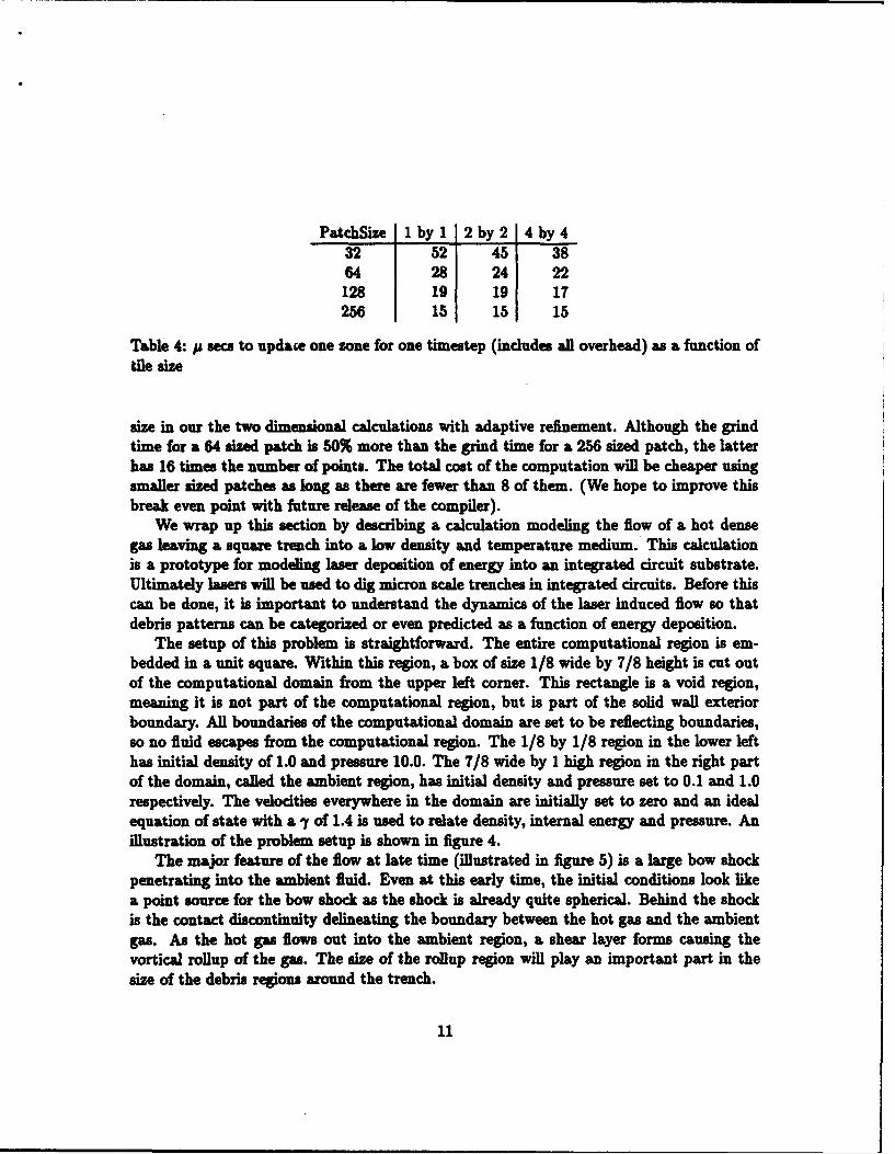
PatchSize 1iby1 2 by2 4by 432 52 45 3864 28 24 22128 19 19 17256 15 15 15

Table 4: n secs to update one zone for one timestep (includes all overhead) as a function oftile size

size in our the two dimensional calculations with adaptive refinement. Although the grindtime for a 64 sized patch is 50% more than the grind time for a 256 sized patch, the latterhas 16 times the number of points. The total cost of the computation will be cheaper usingsmaller sized patches as long as there are fewer than 8 of them. (We hope to improve thisbreak even point with future release of the compiler).

We wrap up this section by describing a calculation modeling the flow of a hot densegas leaving a square trench into a low density and temperature medium. This calculationis a prototype for modeling laser deposition of energy into an integrated circuit substrate.Ultimately lasers will be used to dig micron scale trenches in integrated circuits. Before thiscan be done, it is important to understand the dynamics of the laser induced flow so thatdebris patterns can be categorized or even predicted as a function of energy deposition.

The setup of this problem is straightforward. The entire computational region is em-bedded in a unit square. Within this region, a box of size 1/8 wide by 7/8 height is cut outof the computational domain from the upper left corner. This rectangle is a void region,meaning it is not part of the computational region, but is part of the solid wall exteriorboundary. All boundaries of the computational domain are set to be reflecting boundaries,so no fluid escapes from the computational region. The 1/8 by 1/8 region in the lower lefthas initial density of 1.0 and pressure 10.0. The 7/8 wide by I high region in the right partof the domain, called the ambient region, has initial density and pressure set to 0.1 and 1.0respectively. The velocities everywhere in the domain are initially set to zero and an idealequation of state with a -f of 1.4 is used to relate density, internal energy and pressure. Anillustration of the problem setup is shown in figure 4.

The major feature of the flow at late time (illustrated in figure 5) is a large bow shockpenetrating into the ambient fluid. Even at this early time, the initial conditions look likea point source for the bow shock as the shock is already quite spherical. Behind the shockis the contact discontinuity delineating the boundary between the hot gas and the ambientgas. As the hot gas flows out into the ambient region, a shear layer forms causing thevortical rollup of the gas. The size of the rollup region will play an important part in thesize of the debris regions around the trench.

11

* Rdktcting Boundary

*High Prem Regio

- Am = b Regim

Figure 4: A schematic of the initial conditions for the prototype calculation modeling laserdeposition of energy into an integrated circuit substrate.

Table 5 is a breakdown of CPU times for the AMR code when run for ten coarse gridtime steps. The bulk of the time taken outside of the integration routine is taken by theboundary conditions routines. Within this category, 72 % of the time is taken interpolatingfrom coarse grids to fine grids. The grind time for this calculation is 25.1 microseconds/cellwhich fits within the bounds shown in table 4. Although the grind time is a little undera factor of two for the best uniform case (256 x 256), the savings in computation costs isstill great as only a fraction of the computation region is computed using a fine mesh. Thenumber of cells advanced by the AMR algorithm is only 12% of the number of cells thatwould need to be advanced by the uniform case. Therefore a factor of four overall gain inefficiency is achieved.

6 Conclusions

Despite the disappointing performance of the CM-2 for small grid sizes, we feel that thetwo dimensional implementation of AMR is a useful tool. Our overall performance onan 8K CM-2 is roughly equivalent to a single head of the Y-MP. We hope in the futurethat richer array constructs, and layout and alignment directives will make possible furtherimprovements in the efficiency. Although our current choice of tile size does not scale touse the full machine in an efficient manner, we believe that three dimensional calculations,

12

RI

Figure 5: Prototype integrated circuit problem results at time .124 and cycle 70. Figure(a) is a raster plot of the logarithm of density, (b) and (c) are plots of x and y momentumrespectively, and (d) is a plot of the logarithm of total energy. Values range from the lowcolor blue (cold) to the high color red (hot).

13

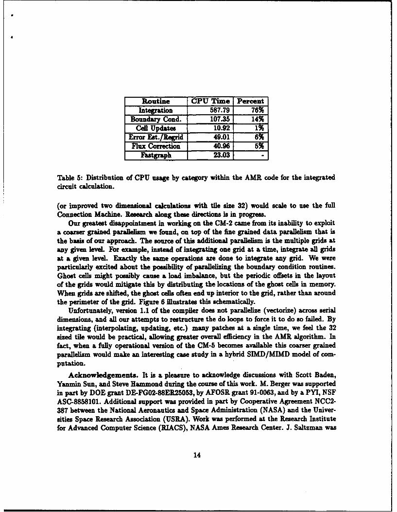
Routine CPU Time PercentIntegration 587.79 76%

Boundary Cond. 107.35 14%Cell Updates 10.92 1%

Error FAt./Regrid 49.011 69%Flux Correction 40.96 5%

Futgraph 23.031

Table 5: Distribution of CPU usage by category within the AMR code for the integratedcircuit calculation.

(or improved two dimensional calculations with tile size 32) would scale to use the fullConnection Machine. Research along these directions is in progress.

Our greatest disappointment in working on the CM-2 came from its inability to exploita coarser grained parallelism we found, on top of the fine grained data parallelism that isthe basis of our approach. The source of this additional parallelism is the multiple grids atany given level. For example, instead of integrating one grid at a time, integrate all gridsat a given level. Exactly the same operations are done to integrate any grid. We wereparticularly excited about the possibility of parallelizing the boundary condition routines.Ghost cells might possibly cause a load imbalance, but the periodic offsets in the layoutof the grids would mitigate this by distributing the locations of the ghost cells in memory.When grids are shifted, the ghost cells often end up interior to the grid, rather than aroundthe perimeter of the grid. Figure 6 mustrates this schematically.

Unfortunately, version 1.1 of the compiler does not parallelize (vectorize) across serialdimensions, and all our attempts to restructure the do loops to force it to do so failed. Byintegrating (interpolating, updating, etc.) many patches at a single time, we feel the 32sized tile would be practical, allowing greater overall efficiency in the AMR algorithm. Infact, when a fully operational version of the CM-5 becomes available this coarser grainedparallelism would make an interesting case study in a hybrid SIMD/MIMD model of com-putation.

Acknowledgements. It is a pleasure to acknowledge discussions with Scott Baden,Yanmin Sun, and Steve Hammond during the course of this work. M. Berger was supportedin part by DOE grant DE-FG02-88ER25053, by AFOSR grant 91-0063, and by a PYI, NSFASC-8858101. Additional support was provided in part by Cooperative Agreement NCC2-387 between the National Aeronautics and Space Administration (NASA) and the Univer-sities Space Research Association (USRA). Work was performed at the Research Institutefor Advanced Computer Science (RIACS), NASA Ames Research Center. J. Saltzman was

14

Figure 6: The boundary ghost cells are shaded on each grid patch. They are distributed toa different memory location in each patch.

supported by the U.S. Department of Energy through Los Alamos National Laboratory un-der contract No. W-7405-ENG-36 with additional support from the Center for Research inParallel Computation and DARPA/NSF grant DMS-8919074 UC-Berkeley. We would liketo thank the NAS systems division at NASA Ames for access to their Connection MachineCM-2.

References

[1] J. Bell, M. J. Berger, J. Saltzman, and M. Welcome. Three dimensional adaptive meshrefinement for hyperbolic conservation laws. Preprint UCRL-JC-108794, LawrenceLivermore National Laboratory, Livermore, CA, December 1991.

[2] M. J. Berger. Adaptive mesh refinement for parallel processors. In Proceedings of 1987SIAM Conference on Parallel Processing, Los Angeles, CA, December 1987.

[3] M. J. Berger and P. Colella. Local adaptive mesh refinement for shock hydrodynamics.Journal of Computational Physics, 82:64-84,1989.

[4] M. J. Berger and J. Oliger. Adaptive mesh refinement for hyperbolic partial differentialequations. Journal of Computational Physics, 53:482-512, 1984.

15

[5] R. Biswas. Parallel and Adaptive Methods for Hyperbolic PDES. PhD thesis, RPI,1991.

[6] L Biewas and J. Flaherty. Parallel and adaptive methods for hyperbolic partial dif-ferential equations. In Proceedings of the 7th IMACS International Conference onComputer Methods for Partial Differential Equations, New Brunswick, NJ, June 1992.

[7] J. Cerutti and H. Trease. The free-Lagrange method on the Connection Machine. InW. C. H. Trease, J. Fritts, editor, Proceedings of the Nezt Free-Lagrange Conference,Copper Mountain, Colorado, 1991.

[8] P. Colelia. Multidimensional upwind methods for hyperbolic conservation laws. Journalof Computational Physics, 87:171-200, 1990.

[9] P. Colella and P. Woodward. The piecewise parabolic method (ppm) for gas-dynamicalsimulations. Journal of Computational Physics, 54(1):174-201, April 1984.

[10] W. Crutchfield. Load balancing irregular algorithms. Preprint UCRL-JC-107679,Lawrence Livermore National Laboratory, Livermore, CA, July 1991.

[11] W. Crutchfield. Parallel adaptive mesh refinement: An example of parallel data en-capsulation. Preprint UCRL-JC-107680, Lawrence Livermore National Laboratory,Livermore, CA, July 1991. Submitted to Concurrency, Practice and Experience.

[12] E. D. Dahl. Mapping and compiled communication on the Connection Machine system.In Proceedings of The Fifth Distributed Memory Computering Conference, April 1990.

[13] W. Gropp and D. Keyes. Semi-structured refinement and parallel domain decompo-sition methods. In J. S. P. Mehrotra and R. Voigt, editors, Unstructured ScientificComputation on Scalable Multiprocesors. MIT Press, 1992.

[14] S. W. Hammond and T. J. Barth. An efficient massively parallel Euler solver forunstructured grids. AIAA Journal, 30(4):947-952, April 1992.

[15] L. F. Henderson, P. Colesla, and E. G. Puckett. On the refraction of shock waves at aslow-fast gas interface. Journal of Fluid Mechanics, 224:1-27, 1991.

[16] W. D. Hillis. The Connection Machine. MIT Press, 1985.

[17] Y. Kailinderis and A. Vidwans. Parallel adaptive-grid navier-stokes algorithm devel-opment and implementation. Technical report, University of Texas at Austin, 1992.Preprint.

16

[18] 0. Lubeck, M. Simmons, and H. Wasserman. The performance realities of massivelyparallel processors: A case study. Preprint LA-UR-92-1463, Los Alamos NationalLaboratory, Los Alamos, NM, 1992. Submitted to IEEE Supercomputing '92.

[19] S. McCormick and D. Quinlan. Dynamic grid refinement for partial differential equa-tions on parallel computers. In Proceedings of 7th International Conference on FiniteElement Methods in Flow Problems. University of Alabama, April 1989.

[20] J. Quirk. An adaptive grid agorithm for computational shock hydirdynamics. PhDthesis, College of Aeronautics, Crauiield Institute of Technology, 1991.

[21] M. Ruffert. Collisions between a white dwarf and a main-sequence star H. Simula-tions using multiple nested refined grids. Preprint MPA 657, Max Planck Institute forAstrophysics, Garching, March 1992. Submitted to Astronomy and Astrophysics.

[22] R. Williams. Performance of dynamic load balancing algorithms for unstructured meshcalculations. Concurrency: Practice and Experience, 3(5):457-481, October 1991.

17