d b xrf spectroscopy user guide spectrum gui… · 1 draft bruker xrf spectroscopy user guide:...
TRANSCRIPT
�1�
�
DRAFT�BRUKER�XRF�SPECTROSCOPY�USER�GUIDE:��
SPECTRAL�INTERPRETATION�AND�SOURCES�OF�INTERFERENCE�
TABLE�OF�CONTENTS�
TABLE�OF�CONTENTS� 1�
ABSTRACT� 3�
XRF�THEORY� 4�
INSTRUMENTATION� 6�
EDͲXRF�EQUIPMENT� 6�TRACER��� 8�SI�PIN�DIODE�DETECTOR�PARAMETERS� 8�ARTAX� 9�SI(LI)�SDD�DETECTOR�PARAMETERS� 9�
SPECTRAL�INTERPRETATION� 9�
INTERACTIONS�IN�THE�DETECTOR� 11�
SUM�PEAKS� 11�ESCAPE�PEAKS� 12�ESCAPE�PEAKS�(CONTINUED)� ERROR!�BOOKMARK�NOT�DEFINED.�HETEROGENEITY� 15�HETEROGENEITY�(CONTINUED)� 16�
INTERFERENCE�WITH�INSTRUMENTATION� 17�
EQUIPMENT�AND�INSTRUMENT�CONTRIBUTION� 17�EQUIPMENT�AND�INSTRUMENT�CONTRIBUTION�(CONTINUED)� 18�THIN�FILM�ANALYSIS�(BACKGROUND�CONTRIBUTION)� 19�
�2�
THIN�FILM�ANALYSIS�(BACKGROUND�CONTRIBUTION)� ERROR!�BOOKMARK�NOT�DEFINED.�
PHENOMENA�IN�THE�SAMPLE� 20�
RAYLEIGH�(ELASTIC)�SCATTERING� 20�RAYLEIGH�(ELASTIC)�SCATTERING�(CONTINUED)� 21�COMPTON�(INELASTIC)�SCATTERING� 22�MATRIX�EFFECTS� 23�BRAGG�SCATTERING� 24�BRAGG�SCATTERING�(CONTINUED)� ERROR!�BOOKMARK�NOT�DEFINED.�BRAGG�SCATTERING�(NIST�C�1122�EXAMPLES)� 26�BRAGG�SCATTERING�(GEMSTONE�EXAMPLES)� ERROR!�BOOKMARK�NOT�DEFINED.�BRAGG�SCATTERING�(GEMSTONE�EXAMPLES)� ERROR!�BOOKMARK�NOT�DEFINED.�
SIX�FIELD�APPLICATIONS� 28�
IDENTIFYING�GENUINE�ARTIFACTS�(CHELSEA�BULLFINCH�EXAMPLE)� 28�IDENTIFYING�TRUE�ORIGINS�(STONEWARE�EXAMPLE)� 29�MEASURING�CHLORINE�WITH�THE�TRACER���AND��OTHER��FIELD�APPLICATIONS� 30�
APPENDICES� 41�
APPENDIX�A� 43�APPENDIX�B� 48�APPENDIX�C� 49�APPENDIX�D� 50�APPENDIX�E� 51�
�
�
By�Dr�Bruce�Kaiser�and�Alex��Wright�
November�11,�2008�
�
�3�
�
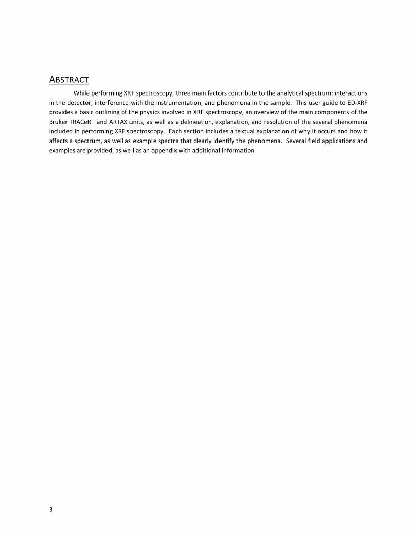
ABSTRACT�� While�performing�XRF�spectroscopy,�three�main�factors�contribute�to�the�analytical�spectrum:�interactions�in�the�detector,�interference�with�the�instrumentation,�and�phenomena�in�the�sample.��This�user�guide�to�EDͲXRF�provides�a�basic�outlining�of�the�physics�involved�in�XRF�spectroscopy,�an�overview�of�the�main�components�of�the�Bruker�TRACeR���and�ARTAX�units,�as�well�as�a�delineation,�explanation,�and�resolution�of�the�several�phenomena�included�in�performing�XRF�spectroscopy.��Each�section�includes�a�textual�explanation�of�why�it�occurs�and�how�it�affects�a�spectrum,�as�well�as�example�spectra�that�clearly�identify�the�phenomena.��Several�field�applications�and�examples�are�provided,�as�well�as�an�appendix�with�additional�information�

�4�
�
XRF�THEORY�General�Concept�Behind�XͲRay�Fluorescence�Spectroscopy�
� Every�element�has�a� characteristic�electron� structure.� �When� inner� shell�electrons�are�ejected� from�an�atom,�electrons�from�shells�with�less�binding�energy�fill�the�holes�and�may�release�x�ray�radiation�equivalent�to�the�difference� in�energy�between� the� level� the�electrons� came� from� to� that�which� they�went.� �The� x� ray� radiation�released�during�these�transitions�is�characteristic�to�the�element�and�has�a�specific�energy�(±�2�eV)�depending�on�the�transition�made�within�the�atom.��By�bombarding�a�sample�with�radiation�that�exceeds�the�binding�energy�of�the�electrons�in�the�atoms�of�which�the�material�is�composed�of�and�detecting�the�energy�and�number�of�resultant�characteristic� x� rays� emitted� from� each� element,� it� is�possible� to�determine� the� composition� and�proportional�concentrations�of�those�elements.���
Two�common�methods�of�XͲray�spectroscopy�exist:�Wavelength�Dispersive�XRF� (WDͲXRF)�and�Energy�Dispersive�XRF�(EDͲXRF).� �The�main�difference�between�the�two�methods� is�how�the�emitted�x�rays�are�measured;�WDͲXRF�uses�an�analyzing�crystal�to�diffract�the�different�x�ray�wavelengths�and�detectors�are�placed�at�the�various�angles�to�measure�the�number�x�rays�diffracted�at�each�angle.�A�single�detector�maybe�used�to�measure�all�the�various�energies� if�one�moves� the�detector� to� cover�all� the�angles,�because�each�energy� comes�out�of� the� crystal�at�a�different�angle.�
Energy�dispersive�x�ray�fluorescence�(EDͲXRF)�uses�a�detector�that�collects�x�rays�of�all�energies�and�sorts�out�each�x�ray�energy�by�the�amount�of�electrons�each�x�ray�knocks�free�in�the�detector�lattice,�typically�silicon.�The�number�of�electrons�knocked�free�depends�on�the�in�coming�x�ray�energy�and�the�particular�interaction�that�that�x�ray�has�with�the�material�lattice.��To�accurately�determine�the�x�ray�energy�all�the�electrons�from�each�event�that�occurs�in�the�detector�must�all�be�collected�and�converted�ultimately�to�a�digital�signal.�Thus�the�detector�measures�one�x�ray�at�a�time.�
Bremsstrahlung�Radiation��
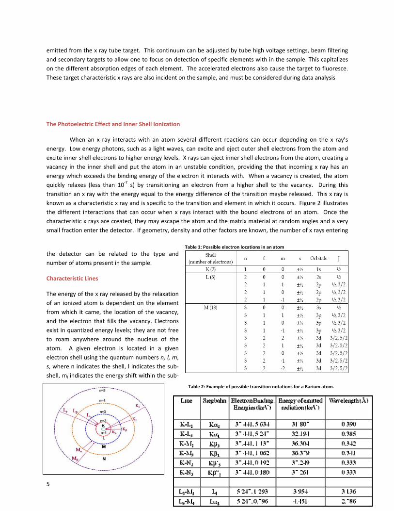
� In�most�xrf� systems� the�beam�of�x� rays� incident�on� the� sample�are�produced�with�a�vacuum� tube�and�created�by�bombarding�a�target�(such�as�Rh,�W,�Cu,�or�Mo)�with�highly�accelerated�electrons.��Shown�in�Figure�1,�as�the�electrons�penetrate�the�target�atoms,�they�may�have�their�direction�changed�as�they�pass�near�the�nucleus�of�the� target� atoms� causing� a� sudden� deceleration� and� loss� of� kinetic� energy.� � In� this� loss� of� kinetic� energy� the�
electron� may� emit� an� x� ray� with� energy�related�to�the�amount�of�energy�lost.��As�a�result�a�broad�spectrum�of�x�ray�energies,�known�as�a�Bremsstrahlung�continuum,� is�
Figure�1:��Diagram�of�the�Bremsstrahlung�effect�
Figure�2:��Diagram�of�possible�excitation�routes
Outbound�electron(decelerated�and�diverted)�
Atom�of�the�target�material�
Fast�inbound�electron�
�5�
emitted�from�the�x�ray�tube�target.��This�continuum�can�be�adjusted�by�tube�high�voltage�settings,�beam�filtering�and�secondary�targets�to�allow�one�to�focus�on�detection�of�specific�elements�with�in�the�sample.�This�capitalizes�on�the�different�absorption�edges�of�each�element.��The�accelerated�electrons�also�cause�the�target�to�fluoresce.��These�target�characteristic�x�rays�are�also�incident�on�the�sample,�and�must�be�considered�during�data�analysis��
�
�
The�Photoelectric�Effect�and�Inner�Shell�Ionization�
� When� an� x� ray� interacts�with� an� atom� several�different� reactions� can�occur�depending�on� the� x� ray’s�energy.��Low�energy�photons,�such�as�a�light�waves,�can�excite�and�eject�outer�shell�electrons�from�the�atom�and�excite�inner�shell�electrons�to�higher�energy�levels.��X�rays�can�eject�inner�shell�electrons�from�the�atom,�creating�a�vacancy� in� the� inner� shell�and�put� the�atom� in�an�unstable�condition,�providing� the� that� incoming�x� ray�has�an�energy�which�exceeds�the�binding�energy�of�the�electron� it� interacts�with.� �When�a�vacancy� is�created,�the�atom�quickly� relaxes� (less� than� 10Ͳ7� s)� by� transitioning� an� electron� from� a� higher� shell� to� the� vacancy.� �During� this�transition�an�x�ray�with�the�energy�equal�to�the�energy�difference�of�the�transition�maybe�released.��This�x�ray�is�known�as�a�characteristic�x�ray�and�is�specific�to�the�transition�and�element�in�which�it�occurs.��Figure�2�illustrates�the�different� interactions� that� can�occur�when� x� rays� interact�with� the�bound�electrons�of�an�atom.� �Once� the�characteristic�x�rays�are�created,�they�may�escape�the�atom�and�the�matrix�material�at�random�angles�and�a�very�small�fraction�enter�the�detector.��If�geometry,�density�and�other�factors�are�known,�the�number�of�x�rays�entering�
the� detector� can� be� related� to� the� type� and�number�of�atoms�present�in�the�sample.�
Characteristic�Lines�
The�energy�of�the�x�ray�released�by�the�relaxation�of�an� ionized�atom� is�dependent�on� the�element�from�which� it� came,� the� location�of� the�vacancy,�and� the�electron� that� fills� the� vacancy.�Electrons�exist�in�quantized�energy�levels;�they�are�not�free�to� roam� anywhere� around� the� nucleus� of� the�atom.� � A� given� electron� is� located� in� a� given�electron�shell�using�the�quantum�numbers�n,�l,�m,�s,�where�n� indicates�the�shell,� l� indicates�the�subͲshell,�ml�indicates�the�energy�shift�within�the�subͲ
Table�1:�Possible�electron�locations�in�an�atom�
Table�2:�Example�of�possible�transition�notations�for�a�Barium�atom.
�6�
shell,��and�ms�indicates�the�spin�of�the�electron.��Table�1�lists�some�of�the�possibilities�for�electron�locations�in�an�atom.�There�are�a�couple�ways�of�describing�an�x�ray�of�a�certain�transition.� � It�can�be�written� in�Line�notation,�Siegbahn�notation,�or�described�by�the�characteristic�energy�or�wavelength�connected�that�x�ray.��These�notations�are�shown�below�in�Table�2�with�an�example�of�Barium�electron�transitions. In�the�Siegbahn�notation,�the�Greek�subscript�denotes�the�probability�of�the�transition�(intensity),�proceeding�from�the�most�to�least�(ɲ,�ɴ,�ɶ,�etc.).�
INSTRUMENTATION�� The�TRACeR���and�ARTAX�are�both�EDͲXRF�units�with�Silicon�based�detectors.��The�TRACeR�is�a�handheld�unit�commercially�offered�by�Bruker�AXS�and�provides�for�quick�and�easy�qualitative�analysis�and�chemistries�for�elements� as� low� as�Mg.� The� Tracer� handheld� XRF� analyzer� provides� spectral� analysis� through� PXRF� analytical�software.� The� instrument’s� high� sensitivity� allows� the� user� to� identify� the� elements� in� a� sample�matrix,�with�concentrations� as� low� as� ppm.� The� PXRF� software� program� provides� qualitative� and� quantitative� analysis,� in�addition� to� the�voltage�and�current�control�of� the�XͲray�tube,�which�makes�possible�a�wider�range�of�elemental�analysis.� �The�ARTAX� is� the� first�commercially�available,�portable�microͲXRF�spectrometer�designed� to�meet� the�requirements� for� a� spectroscopic� analysis� of� unique� and� valuable� objects� on� site,� i.e.� in� archeometry� and� art�history.� �The�system�performs�a�simultaneous�multi�element�analysis� in�the�element�range�from�Na(11)�to�U(92)�and�reaches�a�spatial�resolution�of�down� to�30�µm.� �Both� instruments�allow�one� to�utilize� filters�and�secondary�target�to�adjust�the�incident�x�ray�beam�in�both�energy�distribution�and�intensity.�
EDͲXRF�EQUIPMENT�The�ARTAX�and�TRACeR�systems�have�several�separate�components�that�all�serve�their�own� function� in�
the�process�of� recording�XͲray� fluorescence.� �The�main�components� in� terms�of� functionality�are� the�XͲray� tube�system,�collimators,� filters,�detector�and�signal�processing�hardware�and�software.� �The�ARTAX�and� the�TRACeR�Turbo� are� very� similar� in� functionality.� � Both� units� employ� energy� dispersive� technology� and� a� Silicon� based�detector.��Being�a�handheld�unit,�the�TRACeR�is�battery�operated,�more�convenient,�but�has�a�beam�spot�size�of�3�by�4�mm�(much�larger�than�the�Artax).��The�ARTAX�is�portable;�however,�it�is�not�generally�used�in�the�field�like�the�battery� operated� handheld� TRACeR� unit.� � Both� units� can� use� a� variety� of� changeable� filters,� tube� voltage� and�current� settings� making� them� uniquely� capable� of� being� configured� to� maximize� their� sensitivity� to� specific�elements�of�interest.�
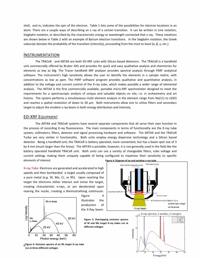
XͲray�Tube:�Electrons�are�generated�and�accelerated�to�high�speeds�and�then�bombarded� �a�target�usually�composed�of�a�pure�metal� (e.g.�W,�Mo,�Cr,�or�Rh).� �Upon� reaching� the�target� the� electrons� either� interact� and� ionize� the� target,�creating� characteristic� xͲrays,� or� are� decelerated� upon�nearing� the� nuclei,� creating� a� Bremsstrahlung� continuum.��
Figure� 4�illustrates� the�production� of�the�XͲRay�beam.��
Figure�4:�Diagram�of�an�end�window�xͲray�tube�
Figure�6:�Emission�spectra�of�an�Rh�target�XͲray�tube�run�at�three�different�voltages�
Figure� 5:�Overlapping� emission� spectra�of�W�and�Mo� target�XͲray� tubes� run�at�different�voltages�
�7�
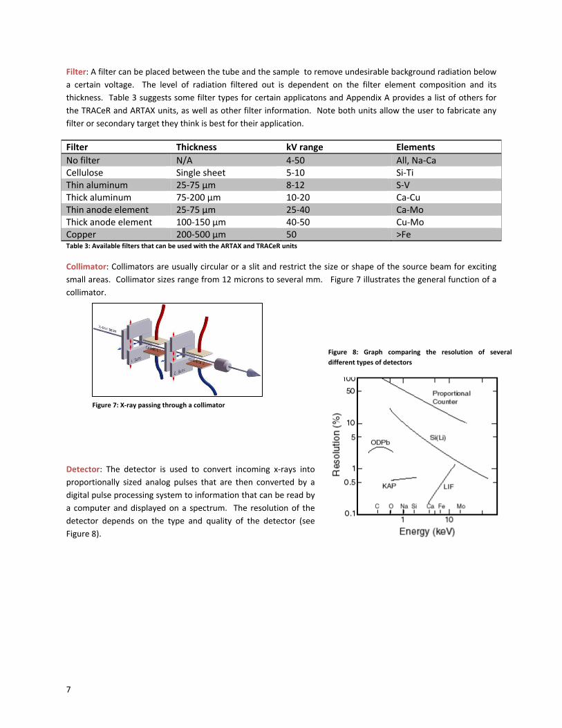
Filter:�A�filter�can�be�placed�between�the�tube�and�the�sample��to�remove�undesirable�background�radiation�below�a� certain� voltage.� � The� level� of� radiation� filtered� out� is� dependent� on� the� filter� element� composition� and� its�thickness.� �Table�3�suggests�some�filter�types�for�certain�applicatons�and�Appendix�A�provides�a� list�of�others�for�the�TRACeR�and�ARTAX�units,�as�well�as�other�filter�information.��Note�both�units�allow�the�user�to�fabricate�any�filter�or�secondary�target�they�think�is�best�for�their�application.�
Filter� Thickness� kV�range� Elements�No�filter� N/A� 4Ͳ50� All,�NaͲCa�Cellulose� Single�sheet� 5Ͳ10� SiͲTi�Thin�aluminum� 25Ͳ75�ʅm� 8Ͳ12� SͲV�Thick�aluminum� 75Ͳ200�ʅm� 10Ͳ20� CaͲCu�Thin�anode�element� 25Ͳ75�ʅm� 25Ͳ40� CaͲMo�Thick�anode�element� 100Ͳ150�ʅm� 40Ͳ50� CuͲMo�Copper� 200Ͳ500�ʅm� 50� >Fe�Table�3:�Available�filters�that�can�be�used�with�the�ARTAX�and�TRACeR�units�
Collimator:�Collimators�are�usually�circular�or�a�slit�and�restrict�the�size�or�shape�of�the�source�beam�for�exciting�small�areas.��Collimator�sizes�range�from�12�microns�to�several�mm.���Figure�7�illustrates�the�general�function�of�a�collimator.�
�
�
�
�
�
�
�
Detector:� The� detector� is� used� to� convert� incoming� xͲrays� into�proportionally� sized� analog�pulses� that� are� then� converted�by� a�digital�pulse�processing�system�to�information�that�can�be�read�by�a�computer�and�displayed�on�a�spectrum.� �The� resolution�of� the�detector� depends� on� the� type� and� quality� of� the� detector� (see�Figure�8).��
�
�
�
Figure�7:�XͲray�passing�through�a�collimator�
Figure� 8:� Graph� comparing� the� resolution� of� several�different�types�of�detectors�
�8�
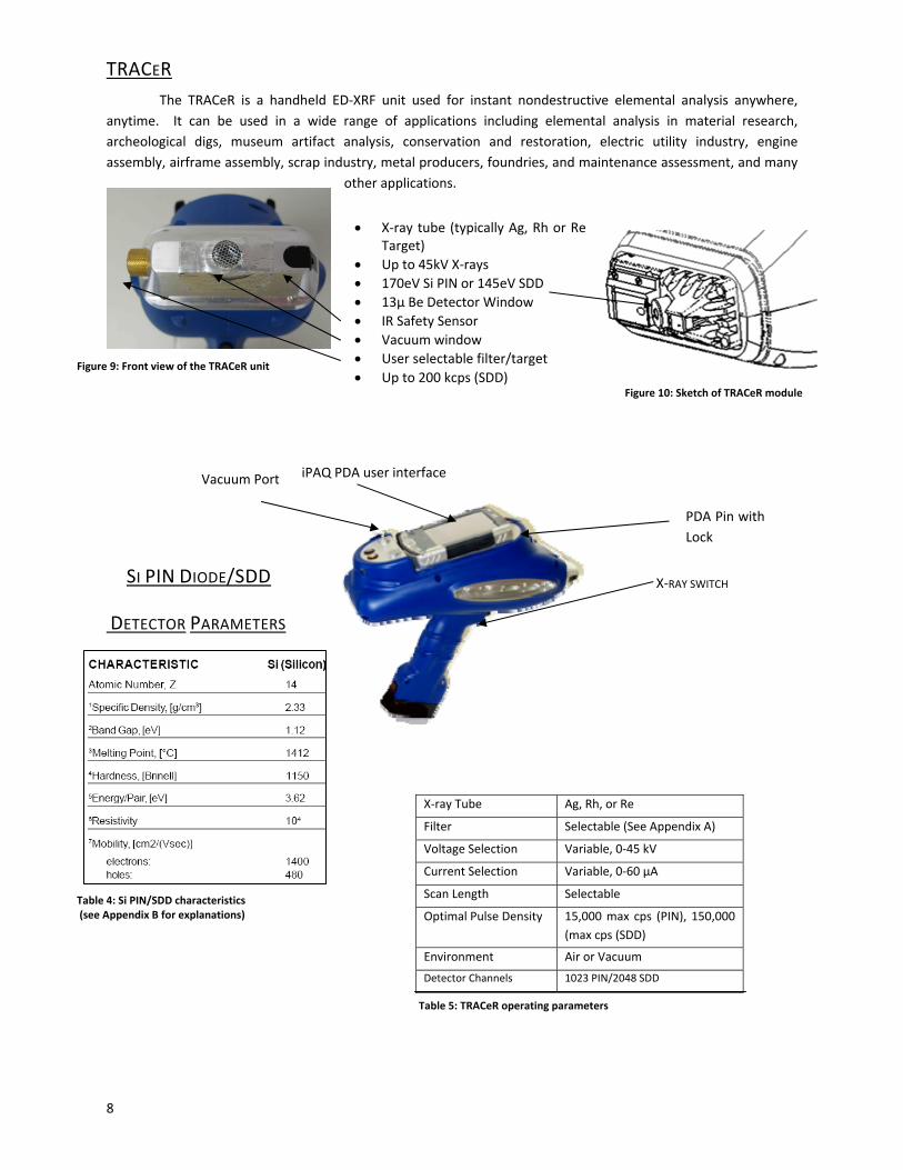
TRACER���� The� TRACeR� is� a� handheld� EDͲXRF� unit� used� for� instant� nondestructive� elemental� analysis� anywhere,�anytime.� � It� can� be� used� in� a� wide� range� of� applications� including� elemental� analysis� in� material� research,�archeological� digs,� museum� artifact� analysis,� conservation� and� restoration,� electric� utility� industry,� engine�assembly,�airframe�assembly,�scrap�industry,�metal�producers,�foundries,�and�maintenance�assessment,�and�many�
other�applications.�
��
�
�
�
�
�
��
�
�
�����SI�PIN�DIODE/SDD�
�DETECTOR�PARAMETERS�� �
� �
�
�
�
�
��
�
XͲray�Tube� Ag,�Rh,�or�Re��
Filter� Selectable�(See�Appendix�A)�
Voltage�Selection� Variable,�0Ͳ45�kV�
Current�Selection� Variable,�0Ͳ60�ʅA�
Scan�Length� Selectable�
Optimal�Pulse�Density� 15,000�max� cps� (PIN),�150,000�(max�cps�(SDD)�
Environment� Air�or�Vacuum�
Detector�Channels 1023�PIN/2048�SDD�
Table�5:�TRACeR�operating�parameters
Vacuum�Port� iPAQ�PDA�user�interface
XͲRAY�SWITCH
PDA�Pin�with�Lock�
x XͲray�tube�(typically�Ag,�Rh�or�Re�Target)�
x Up�to�45kV�XͲrays�x 170eV�Si�PIN�or�145eV�SDD�x 13ʅ�Be�Detector�Window�x IR�Safety�Sensor�x Vacuum�window�x User�selectable�filter/target�x Up�to�200�kcps�(SDD)�
Table�4:�Si�PIN/SDD�characteristics��(see�Appendix�B�for�explanations)�
Figure�9:�Front�view�of�the�TRACeR�unit�
Figure�10:�Sketch�of�TRACeR�module
�9�
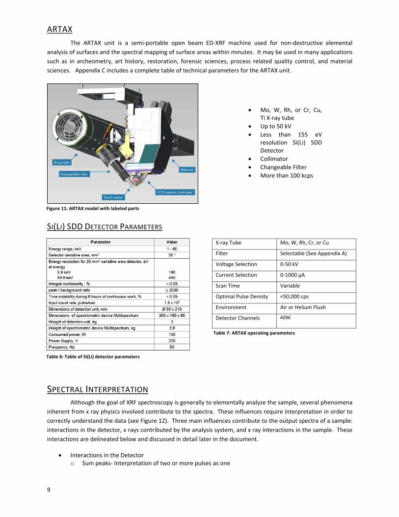
ARTAX�� The� ARTAX� unit� is� a� semiͲportable� open� beam� EDͲXRF� machine� used� for� nonͲdestructive� elemental�analysis�of�surfaces�and�the�spectral�mapping�of�surface�areas�within�minutes.��It�may�be�used�in�many�applications�such�as� in�archeometry,�art�history,� restoration,� forensic� sciences,�process� related�quality� control,�and�material�sciences.���Appendix�C�includes�a�complete�table�of�technical�parameters�for�the�ARTAX�unit.�
�
�
�
�
�
�
�
�
SI(LI)�SDD�DETECTOR�PARAMETERS�
�
��
�
�
�
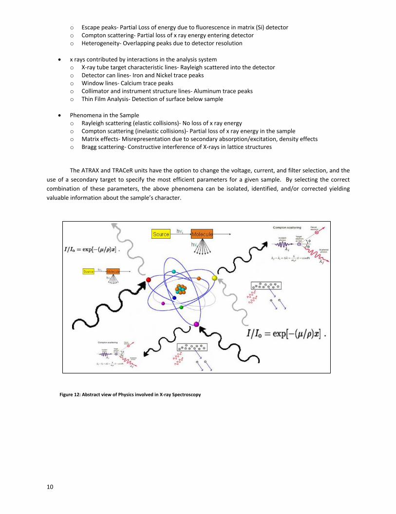
SPECTRAL�INTERPRETATION�� Although�the�goal�of�XRF�spectroscopy�is�generally�to�elementally�analyze�the�sample,�several�phenomena�inherent�from�x�ray�physics�involved�contribute�to�the�spectra.��These�influences�require�interpretation�in�order�to�correctly�understand�the�data�(see�Figure�12).��Three�main�influences�contribute�to�the�output�spectra�of�a�sample:�interactions�in�the�detector,�x�rays�contributed�by�the�analysis�system,�and�x�ray�interactions�in�the�sample.��These�interactions�are�delineated�below�and�discussed�in�detail�later�in�the�document.�
x Interactions�in�the�Detector�o Sum�peaksͲ�Interpretation�of�two�or�more�pulses�as�one�
XͲray�Tube� Mo,�W,�Rh,�Cr,�or�Cu�
Filter� Selectable�(See�Appendix�A)�
Voltage�Selection� 0Ͳ50�kV�
Current�Selection� 0Ͳ1000�ʅA�
Scan�Time� Variable�
Optimal�Pulse�Density� <50,000�cps�
Environment� Air�or�Helium�Flush�
Detector�Channels� 4096�
Table�7:�ARTAX�operating�parameters�
x Mo,�W,� Rh,� or� Cr,� Cu,�Ti�XͲray�tube�
x Up�to�50�kV�x Less� than� 155� eV�
resolution� Si(Li)� SDD�Detector�
x Collimator�x Changeable�Filter�x More�than�100�kcps�
Figure�11:�ARTAX�model�with�labeled�parts�
Table�6:�Table�of�Si(Li)�detector�parameters�
�10
o Escape�peaksͲ�Partial�Loss�of�energy�due�to�fluorescence�in�matrix�(Si)�detector�o Compton�scatteringͲ�Partial�loss�of�x�ray�energy�entering�detector�o HeterogeneityͲ�Overlapping�peaks�due�to�detector�resolution�
�x x�rays�contributed�by�interactions�in�the�analysis�system��
o XͲray�tube�target�characteristic�linesͲ�Rayleigh�scattered�into�the�detector�o Detector�can�linesͲ�Iron�and�Nickel�trace�peaks�o Window�linesͲ�Calcium�trace�peaks�o Collimator�and�instrument�structure�linesͲ�Aluminum�trace�peaks�o Thin�Film�AnalysisͲ�Detection�of�surface�below�sample�
�x Phenomena�in�the�Sample��
o Rayleigh�scattering�(elastic�collisions)Ͳ�No�loss�of�x�ray�energy��o Compton�scattering�(inelastic�collisions)Ͳ�Partial�loss�of�x�ray�energy�in�the�sample�o Matrix�effectsͲ�Misrepresentation�due�to�secondary�absorption/excitation,�density�effects�o Bragg�scatteringͲ�Constructive�interference�of�XͲrays�in�lattice�structures��
The�ATRAX�and�TRACeR�units�have�the�option�to�change�the�voltage,�current,�and�filter�selection,�and�the�use�of�a�secondary� target� to�specify� the�most�efficient�parameters� for�a�given�sample.� �By�selecting� the�correct�combination�of� these�parameters,� the� above�phenomena� can�be� isolated,� identified,� and/or� corrected� yielding�valuable�information�about�the�sample’s�character.��
�
�
�
�
�
�
�
�
�
�
Figure�12:�Abstract�view�of�Physics�involved�in�XͲray�Spectroscopy�
�11
�
�
�
INTERACTIONS�IN�THE�DETECTOR�
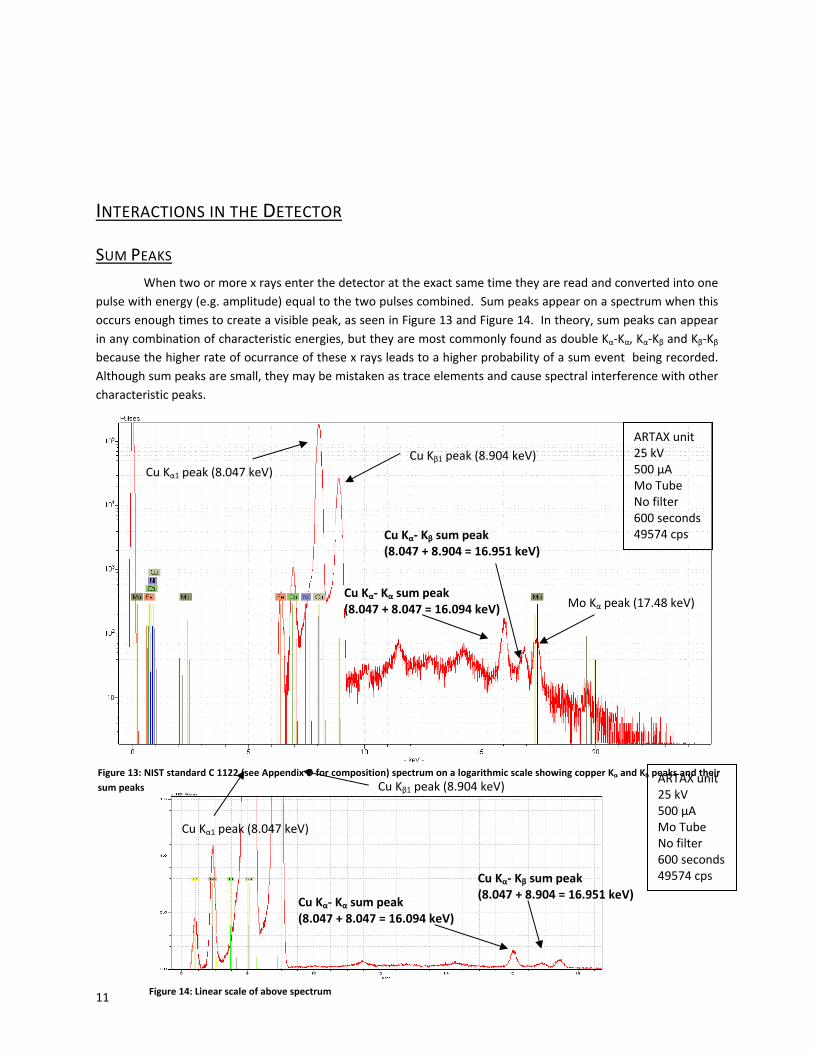
SUM�PEAKS�� When�two�or�more�x�rays�enter�the�detector�at�the�exact�same�time�they�are�read�and�converted�into�one�pulse�with�energy�(e.g.�amplitude)�equal�to�the�two�pulses�combined.��Sum�peaks�appear�on�a�spectrum�when�this�occurs�enough�times�to�create�a�visible�peak,�as�seen�in�Figure�13�and�Figure�14.��In�theory,�sum�peaks�can�appear�in�any�combination�of�characteristic�energies,�but�they�are�most�commonly�found�as�double�KɲͲKɲ,�KɲͲKɴ�and�KɴͲKɴ�because�the�higher�rate�of�ocurrance�of�these�x�rays�leads�to�a�higher�probability�of�a�sum�event��being�recorded.��Although�sum�peaks�are�small,�they�may�be�mistaken�as�trace�elements�and�cause�spectral�interference�with�other�characteristic�peaks.�
�
�
�� �
Figure�13:�NIST�standard�C�1122�(see�Appendix�D�for�composition)�spectrum�on�a�logarithmic�scale�showing�copper�Kɲ�and�Kb�peaks�and�theirsum�peaks�
ARTAX�unit25�kV�500�ʅA�Mo�Tube�No�filter�600�seconds�49574�cps�
Figure�14:�Linear�scale�of�above�spectrum
Cu�KɲͲ Kɲ sum�peak�(8.047�+�8.047�=�16.094�keV)�
Cu�KɲͲ Kɴ sum�peak��(8.047�+�8.904�=�16.951�keV)�
Cu�Kɴ1 peak�(8.904�keV)
Cu�Kɲ1�peak�(8.047�keV)�
ARTAX�unit25�kV�500�ʅA�Mo�Tube�No�filter�600�seconds�49574�cps�
Cu�Kɴ1 peak�(8.904�keV)
Cu�KɲͲ Kɲ sum�peak�(8.047�+�8.047�=�16.094�keV)�
Cu�KɲͲ Kɴ sum�peak�(8.047�+�8.904�=�16.951�keV)�
Cu�Kɲ1�peak�(8.047�keV)�
Mo�Kɲ�peak�(17.48�keV)
�12
�
�
�
�
�
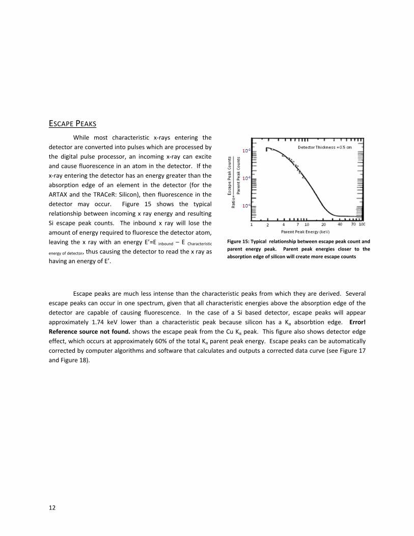
ESCAPE�PEAKS�� While� most� characteristic� xͲrays� entering� the�detector�are�converted�into�pulses�which�are�processed�by�the� digital� pulse� processor,� an� incoming� xͲray� can� excite�and�cause�fluorescence� in�an�atom� in�the�detector.� � If�the�xͲray�entering�the�detector�has�an�energy�greater�than�the�absorption� edge� of� an� element� in� the� detector� (for� the�ARTAX�and� the�TRACeR:�Silicon),� then� fluorescence� in� the�detector� may� occur.� � Figure� 15� shows� the� typical�relationship�between� incoming�x�ray�energy�and�resulting�Si� escape� peak� counts.� � The� inbound� x� ray�will� lose� the�amount�of�energy�required�to�fluoresce�the�detector�atom,�leaving� the� x� ray�with� an�energy�E’=E� inbound�–�E� Characteristic�energy�of�detector,�thus�causing�the�detector�to�read�the�x�ray�as�having�an�energy�of�E’.���
� �
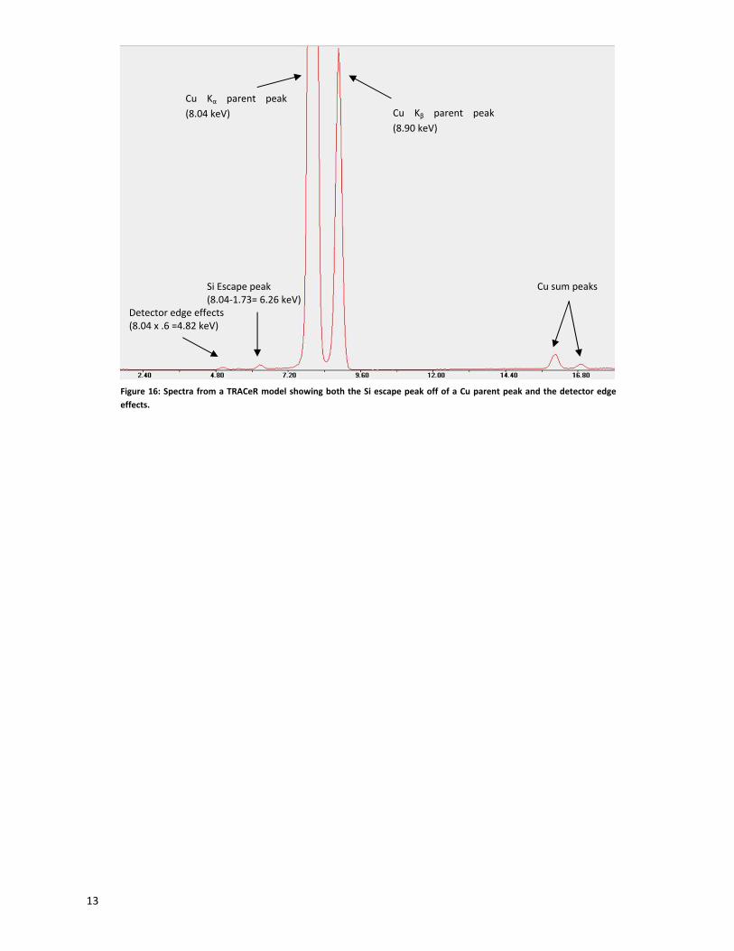
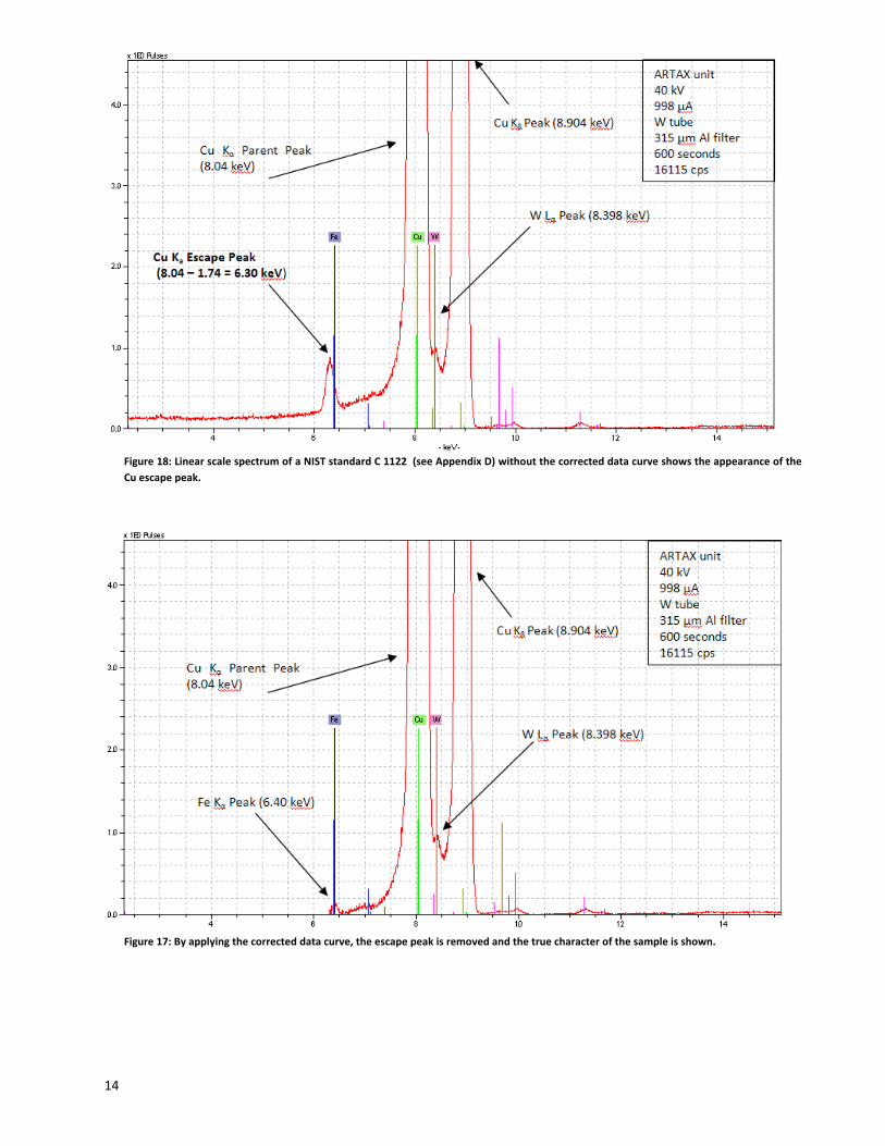
Escape�peaks�are�much� less� intense�than�the�characteristic�peaks�from�which�they�are�derived.� �Several�escape�peaks�can�occur� in�one�spectrum,�given�that�all�characteristic�energies�above�the�absorption�edge�of�the�detector� are� capable� of� causing� fluorescence.� � In� the� case� of� a� Si� based� detector,� escape� peaks� will� appear�approximately� 1.74� keV� lower� than� a� characteristic� peak� because� silicon� has� a� Kɲ� absorbtion� edge.� � Error!�Reference�source�not�found.�shows�the�escape�peak�from�the�Cu�Kɲ�peak.� �This�figure�also�shows�detector�edge�effect,�which�occurs�at�approximately�60%�of�the�total�Kɲ�parent�peak�energy.��Escape�peaks�can�be�automatically�corrected�by�computer�algorithms�and�software�that�calculates�and�outputs�a�corrected�data�curve�(see�Figure�17�and�Figure�18).���
Figure�15:�Typical��relationship�between�escape�peak�count�andparent� energy� peak.� � Parent� peak� energies� closer� to� theabsorption�edge�of�silicon�will�create�more�escape�counts��
�13
�
�
�
�
�
�
�
�
�
�
�
� Figure�16:�Spectra�from�a�TRACeR�model�showing�both�the�Si�escape�peak�off�of�a�Cu�parent�peak�and�the�detector�edgeeffects.�
Cu� Kɲ� parent� peak�(8.04�keV)� Cu� Kɴ� parent� peak�
(8.90�keV)�
Si�Escape�peak��(8.04Ͳ1.73=�6.26�keV)�
Detector�edge�effects��(8.04�x�.6�=4.82�keV)�
Cu�sum�peaks
�14
�
�
Figure�18:�Linear�scale�spectrum�of�a�NIST�standard�C�1122��(see�Appendix�D)�without�the�corrected�data�curve�shows�the�appearance�of�theCu�escape�peak.�
Figure�17:�By�applying�the�corrected�data�curve,�the�escape�peak�is�removed�and�the�true�character�of�the�sample�is�shown.��
�15
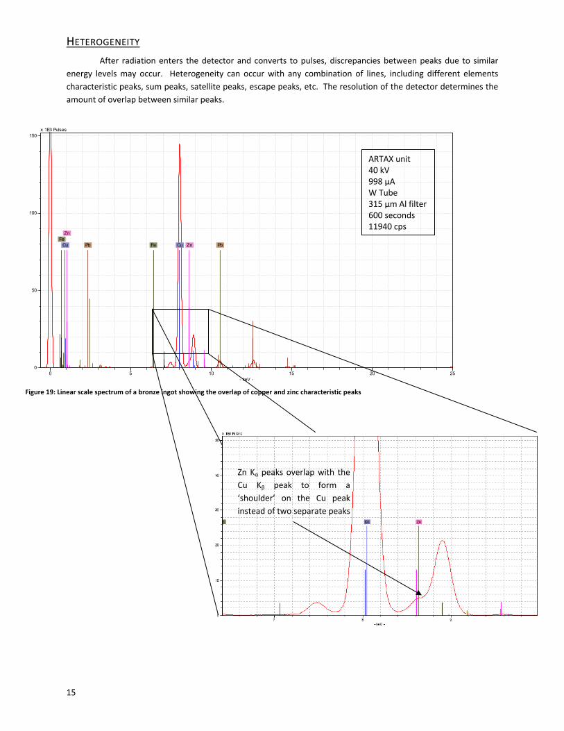
HETEROGENEITY�� After� radiation�enters� the�detector�and�converts� to�pulses,�discrepancies�between�peaks�due� to�similar�energy� levels�may�occur.� �Heterogeneity� can�occur�with� any� combination�of� lines,� including�different�elements�characteristic�peaks,�sum�peaks,�satellite�peaks,�escape�peaks,�etc.��The�resolution�of�the�detector�determines�the�amount�of�overlap�between�similar�peaks.�
�
�
�
�
�
�
�
�
�
�
�
�
�
�
�
�
�
�
�
�
�
�
Figure�19:�Linear�scale�spectrum�of�a�bronze�ingot�showing�the�overlap�of�copper�and�zinc�characteristic�peaks
0 5 10 15 20 25- keV -
0
50
100
150x 1E3 Pulses
Cu Cu Fe Fe
Zn
Zn
Pb Pb
Zn�Kɲ peaks�overlap�with� the�Cu� Kɴ� peak� to� form� a�‘shoulder’� on� the� Cu� peak�instead�of�two�separate�peaks�
ARTAX�unit�40�kV�998�ʅA�W�Tube�315�ʅm�Al�filter�600�seconds�11940�cps�
�16
HETEROGENEITY�(CONTINUED)�
�
�
�
�
�
�
�
�
�
�
�
2 4 6 8 10 12 14- keV -
0.0
1.0
2.0
3.0
4.0
x 1E3 Pulses
Fe Cu Zn Ni Pb Pb Sn
0 5 10 15 20 25- keV -
0
50
100
150x 1E3 Pulses
Cu Cu Fe Fe
Zn
Zn
Pb Pb
2 4 6 8 10 12 14- keV -
0.0
1.0
2.0
3.0
4.0
x 1E3 Pulses
Fe Cu Zn Ni Pb Pb Sn
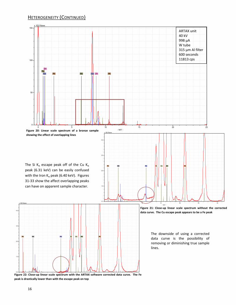
The� Si�Kɲ� escape�peak�off�of� the�Cu�Kɲ�peak� (6.31� keV)� can�be� easily� confused�with�the�Iron�Kɲ�peak�(6.40�keV).��Figures�31Ͳ33�show�the�affect�overlapping�peaks�can�have�on�apparent�sample�character.�
ARTAX�unit40�kV�998�ʅA�W�tube�315�ʅm�Al�filter�600�seconds�11813�cps�
Figure� 21:� CloseͲup� linear� scale� spectrum� without� the� correcteddata�curve.��The�Cu�escape�peak�appears�to�be�a�Fe�peak�
Figure� 20:� Linear� scale� spectrum� of� a� bronze� sampleshowing�the�effect�of�overlapping�lines�
Figure�22:�CloseͲup� linear�scale�spectrum�with�the�ARTAX�software�corrected�data�curve.� �The�Fepeak�is�drastically�lower�than�with�the�escape�peak�on�top�
The� downside� of� using� a� corrected�data� curve� is� the� possibility� of�removing�or�diminishing�true�sample�lines.�
�17
INTERFERENCE�WITH�INSTRUMENTATION�
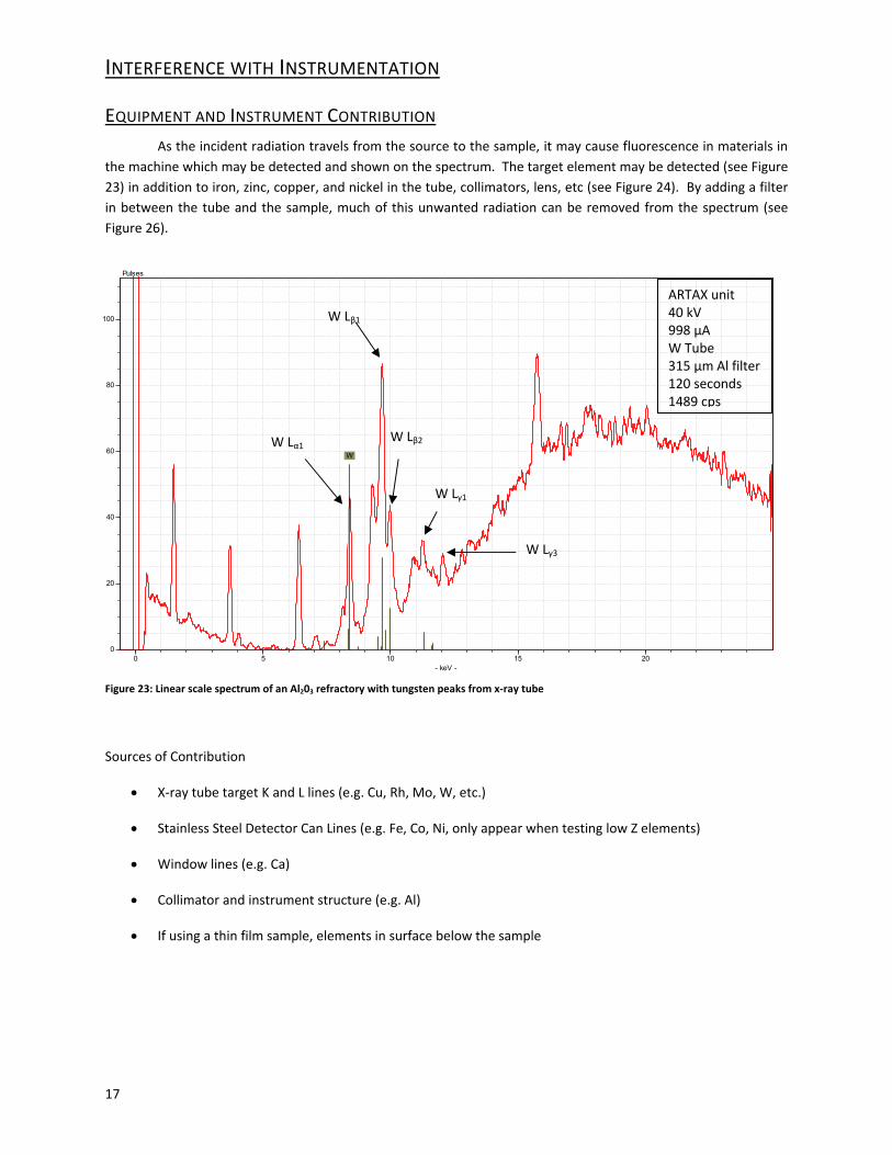
EQUIPMENT�AND�INSTRUMENT�CONTRIBUTION�� As�the�incident�radiation�travels�from�the�source�to�the�sample,�it�may�cause�fluorescence�in�materials�in�the�machine�which�may�be�detected�and�shown�on�the�spectrum.��The�target�element�may�be�detected�(see�Figure�23)�in�addition�to�iron,�zinc,�copper,�and�nickel�in�the�tube,�collimators,�lens,�etc�(see�Figure�24).��By�adding�a�filter�in�between�the�tube�and�the�sample,�much�of�this�unwanted�radiation�can�be�removed� from�the�spectrum� (see�Figure�26).��
Figure�23:�Linear�scale�spectrum�of�an�Al203�refractory�with�tungsten�peaks�from�xͲray�tube�
�
Sources�of�Contribution�
x XͲray�tube�target�K�and�L�lines�(e.g.�Cu,�Rh,�Mo,�W,�etc.)�
x Stainless�Steel�Detector�Can�Lines�(e.g.�Fe,�Co,�Ni,�only�appear�when�testing�low�Z�elements)��
x Window�lines�(e.g.�Ca)�
x Collimator�and�instrument�structure�(e.g.�Al)�
x If�using�a�thin�film�sample,�elements�in�surface�below�the�sample�
�
�
0 5 10 15 20- keV -
0
20
40
60
80
100
Pulses
W W�Lɲ1�
W�Lɴ1
W�Lɴ2
W�Lɶ1
W�Lɶ3
ARTAX�unit40�kV�998�ʅA�W�Tube�315�ʅm�Al�filter�120�seconds�1489�cps
�18
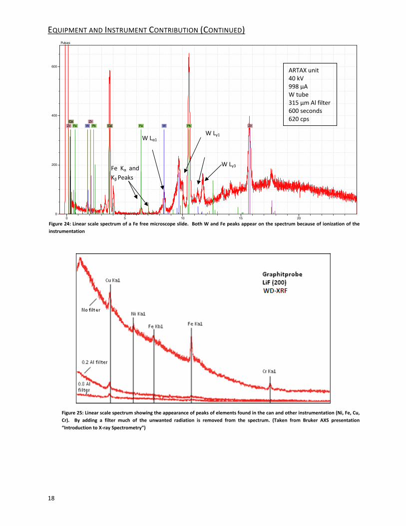
EQUIPMENT�AND�INSTRUMENT�CONTRIBUTION�(CONTINUED)�
�
�
�
�
�
�
�
�
�
�
0 5 10 15 20- keV -
0
200
400
600
Pulses
Fe Fe W W Ca Ca
Zr Zr
Zr Pb Pb
W�Lɴ1
W�Lɲ1�
W�Lɴ2
W�Lɶ1
W�Lɶ3Fe� Kɲ� and�Kɴ�Peaks�
Figure�24:�Linear�scale�spectrum�of�a�Fe�free�microscope�slide.� �Both�W�and�Fe�peaks�appear�on�the�spectrum�because�of� ionization�of�the�instrumentation�
Figure�25:�Linear�scale�spectrum�showing�the�appearance�of�peaks�of�elements�found�in�the�can�and�other�instrumentation�(Ni,�Fe,�Cu,Cr).� � By� adding� a� filter�much� of� the� unwanted� radiation� is� removed� from� the� spectrum.� (Taken� from� Bruker� AXS� presentation“Introduction�to�XͲray�Spectrometry”)�
ARTAX�unit�40�kV�998�ʅA�W�tube�315�ʅm�Al�filter�600�seconds�620�cps�
WDͲXRF�
�19
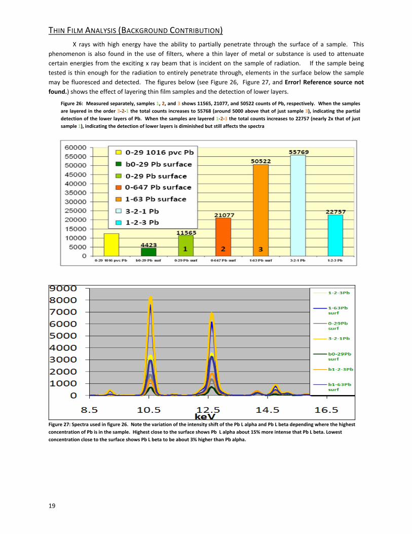
THIN�FILM�ANALYSIS�(BACKGROUND�CONTRIBUTION)�� X� rays�with�high� energy�have� the� ability� to�partially�penetrate� through� the� surface�of� a� sample.� � This�phenomenon� is� also� found� in� the�use�of� filters,�where� a� thin� layer�of�metal�or� substance� is�used� to� attenuate�certain�energies� from� the�exciting�x�ray�beam� that� is� incident�on� the�sample�of�radiation.� � � � If�the�sample�being�tested� is�thin�enough� for�the�radiation�to�entirely�penetrate�through,�elements� in�the�surface�below�the�sample�may�be�fluoresced�and�detected.� �The�figures�below�(see�Figure�26,� �Figure�27,�and�Error!�Reference�source�not�found.)�shows�the�effect�of�layering�thin�film�samples�and�the�detection�of�lower�layers.�
�
�Figure�27:�Spectra�used�in�figure�26.��Note�the�variation�of�the�intensity�shift�of�the�Pb�L�alpha�and�Pb�L�beta�depending�where�the�highest�concentration�of�Pb�is�in�the�sample.��Highest�close�to�the�surface�shows�Pb��L�alpha�about�15%�more�intense�that�Pb�L�beta.�Lowest�concentration�close�to�the�surface�shows�Pb�L�beta�to�be�about�3%�higher�than�Pb�alpha.�
�
Figure�26:��Measured�separately,�samples�1,�2,�and�3�shows�11565,�21077,�and�50522�counts�of�Pb,�respectively.��When�the�samples�are� layered� in�the�order�3Ͳ2Ͳ1�the�total�counts� increases�to�55768�(around�5000�above�that�of� just�sample�3),� indicating�the�partial�detection�of�the�lower�layers�of�Pb.��When�the�samples�are�layered�1Ͳ2Ͳ3�the�total�counts�increases�to�22757�(nearly�2x�that�of�just�sample�1),�indicating�the�detection�of�lower�layers�is�diminished�but�still�affects�the�spectra��
�20
PHENOMENA�IN�THE�SAMPLE�
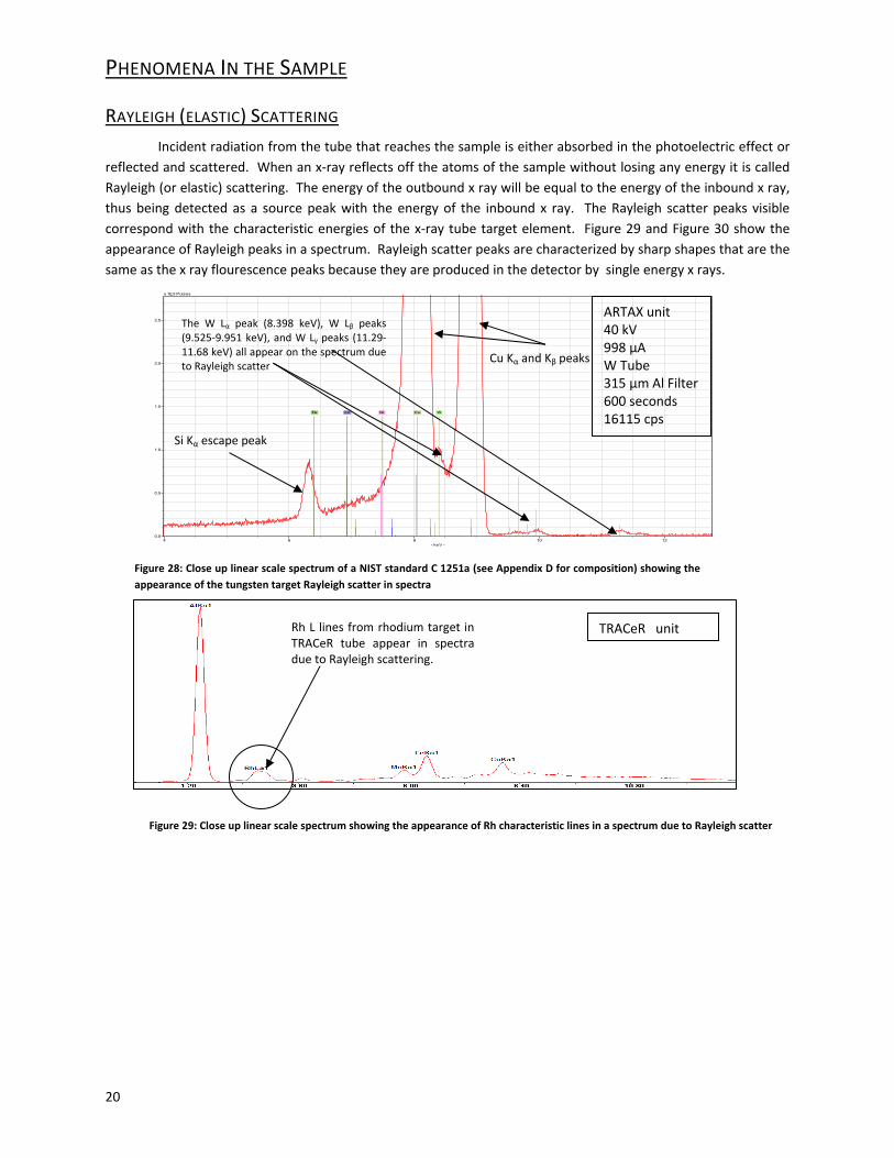
RAYLEIGH�(ELASTIC)�SCATTERING�� Incident�radiation�from�the�tube�that�reaches�the�sample�is�either�absorbed�in�the�photoelectric�effect�or�reflected�and�scattered.��When�an�xͲray�reflects�off�the�atoms�of�the�sample�without�losing�any�energy�it�is�called�Rayleigh�(or�elastic)�scattering.��The�energy�of�the�outbound�x�ray�will�be�equal�to�the�energy�of�the�inbound�x�ray,�thus�being�detected�as�a� source�peak�with� the�energy�of� the� inbound�x� ray.� �The�Rayleigh� scatter�peaks�visible�correspond�with�the�characteristic�energies�of�the�xͲray�tube�target�element.� �Figure�29�and�Figure�30�show�the�appearance�of�Rayleigh�peaks�in�a�spectrum.��Rayleigh�scatter�peaks�are�characterized�by�sharp�shapes�that�are�the�same�as�the�x�ray�flourescence�peaks�because�they�are�produced�in�the�detector�by��single�energy�x�rays.��
�
�
�
�
�
�
�
�
�
�
�
�
�
�
�
�
�
�
�
4 6 8 10 12- keV -
0.0
0.5
1.0
1.5
2.0
2.5
x 1E3 Pulses
Fe Co Ni Cu W
Figure�28:�Close�up�linear�scale�spectrum�of�a�NIST�standard�C�1251a�(see�Appendix�D�for�composition)�showing�theappearance�of�the�tungsten�target�Rayleigh�scatter�in�spectra�
TRACeR���unit�Rh�L� lines�from�rhodium�target� in�TRACeR� tube� appear� in� spectra�due�to�Rayleigh�scattering.�
Figure�29:�Close�up�linear�scale�spectrum�showing�the�appearance�of�Rh�characteristic�lines�in�a�spectrum�due�to�Rayleigh�scatter
ARTAX�unit�40�kV�998�ʅA�W�Tube�315�ʅm�Al�Filter�600�seconds�16115�cps�
The�W� Lɲ� peak� (8.398� keV),�W� Lɴ� peaks�(9.525Ͳ9.951�keV),�and�W�Lɶ�peaks� (11.29Ͳ11.68�keV)�all�appear�on�the�spectrum�due�to�Rayleigh�scatter�
Si�Kɲ�escape�peak�
Cu�Kɲ�and�Kɴ�peaks�
�21
�
�
�
�
RAYLEIGH�(ELASTIC)�SCATTERING�(CONTINUED)��
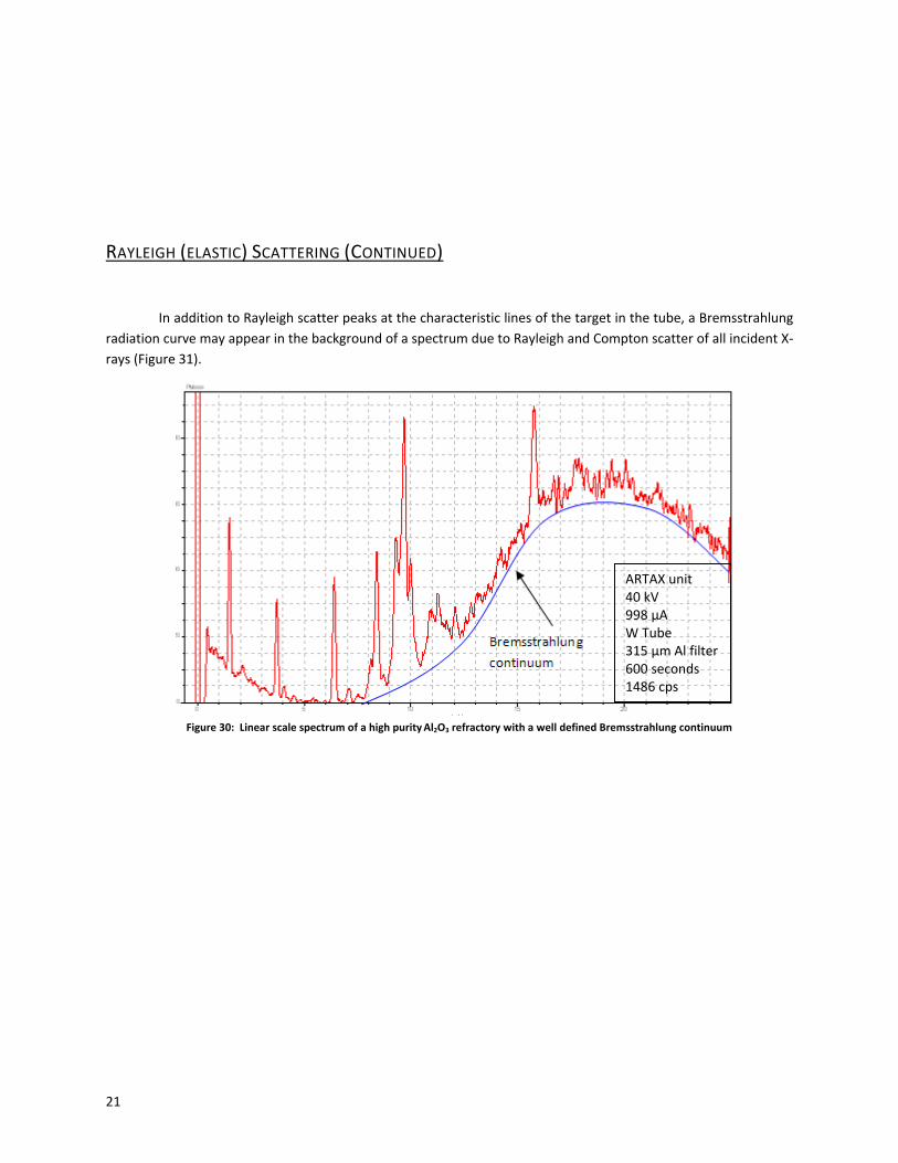
In�addition�to�Rayleigh�scatter�peaks�at�the�characteristic�lines�of�the�target�in�the�tube,�a�Bremsstrahlung�radiation�curve�may�appear�in�the�background�of�a�spectrum�due�to�Rayleigh�and�Compton�scatter�of�all�incident�XͲrays�(Figure�31).�
�
�
�
�
�
�
�
�
�
�
�
�
�
�
�
�
�
�
�
Figure�30:��Linear�scale�spectrum�of�a�high�purity�Al2O3 refractory with�a�well�defined�Bremsstrahlung�continuum
ARTAX�unit�40�kV�998�ʅA�W�Tube�315�ʅm�Al�filter�600�seconds�1486�cps�
�22
Figure� 31:� Compton� scattering� causes� a� shift� inwavelength�of�the�incident�x�ray�
�
�
�
�
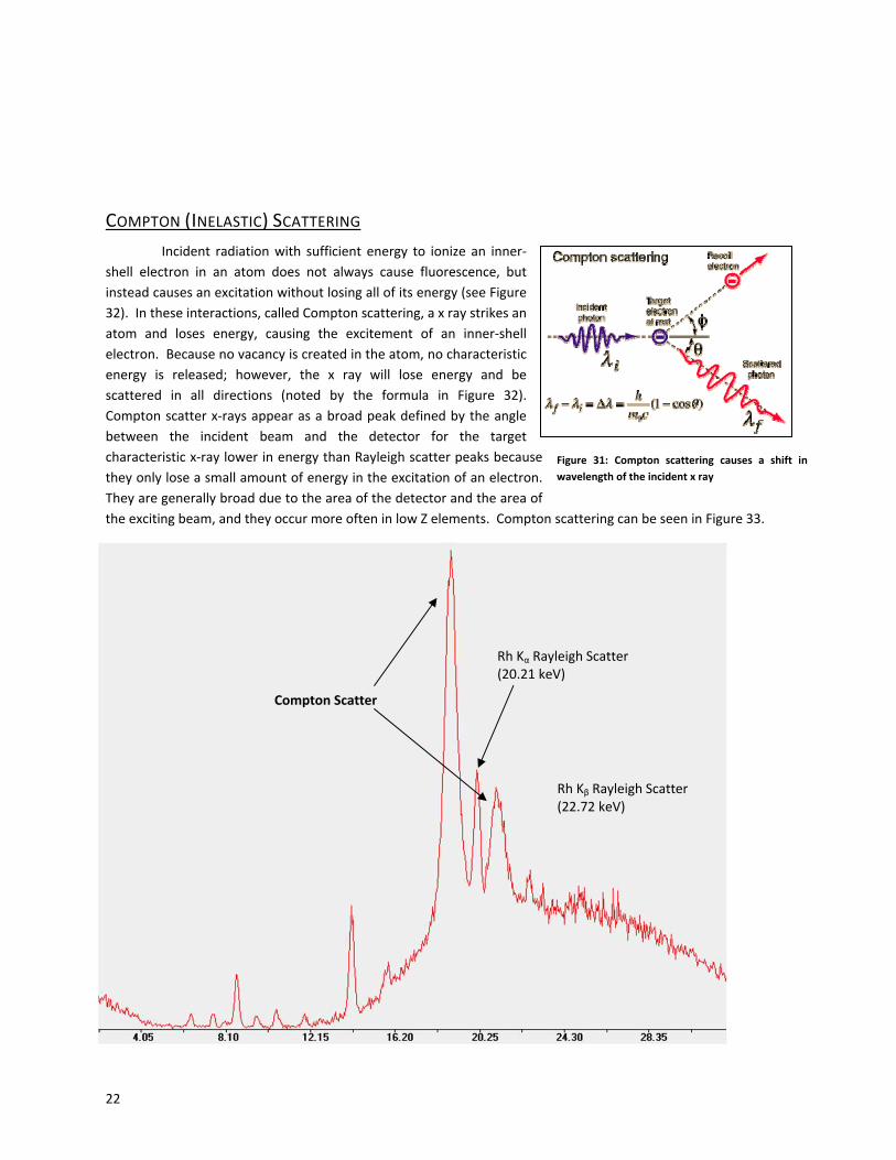
COMPTON�(INELASTIC)�SCATTERING�� �Incident� radiation�with� sufficient�energy� to� ionize�an� innerͲshell� electron� in� an� atom� does� not� always� cause� fluorescence,� but�instead�causes�an�excitation�without�losing�all�of�its�energy�(see�Figure�32).��In�these�interactions,�called�Compton�scattering,�a�x�ray�strikes�an�atom� and� loses� energy,� causing� the� excitement� of� an� innerͲshell�electron.��Because�no�vacancy�is�created�in�the�atom,�no�characteristic�energy� is� released;� however,� the� x� ray� will� lose� energy� and� be�scattered� in� all� directions� (noted� by� the� formula� in� Figure� 32).��Compton�scatter�xͲrays�appear�as�a�broad�peak�defined�by�the�angle�between� the� incident� beam� and� the� detector� for� the� target�characteristic�xͲray�lower�in�energy�than�Rayleigh�scatter�peaks�because�they�only�lose�a�small�amount�of�energy�in�the�excitation�of�an�electron.��They�are�generally�broad�due�to�the�area�of�the�detector�and�the�area�of�the�exciting�beam,�and�they�occur�more�often�in�low�Z�elements.��Compton�scattering�can�be�seen�in�Figure�33.�
Compton�Scatter
Rh�Kɲ Rayleigh�Scatter �(20.21�keV)�
Rh�Kɴ Rayleigh�Scatter�(22.72�keV)�
�23
��
� �
��
�
MATRIX�EFFECTS��
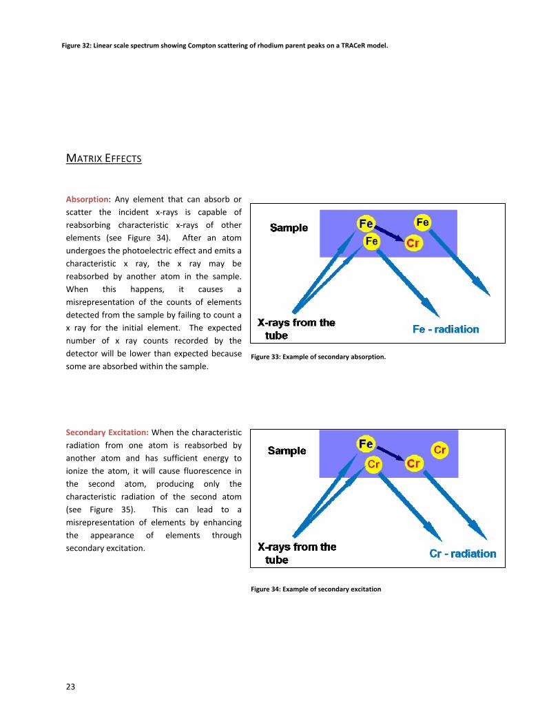
Absorption:� Any� element� that� can� absorb� or�scatter� the� incident� xͲrays� is� capable� of�reabsorbing� characteristic� xͲrays� of� other�elements� (see� Figure� 34).� � After� an� atom�undergoes�the�photoelectric�effect�and�emits�a�characteristic� x� ray,� the� x� ray� may� be�reabsorbed� by� another� atom� in� the� sample.��When� this� happens,� it� causes� a�misrepresentation� of� the� counts� of� elements�detected�from�the�sample�by�failing�to�count�a�x� ray� for� the� initial� element.� � The� expected�number� of� x� ray� counts� recorded� by� the�detector�will�be� lower� than�expected�because�some�are�absorbed�within�the�sample.��
�
�
Secondary�Excitation:�When�the�characteristic�radiation� from� one� atom� is� reabsorbed� by�another� atom� and� has� sufficient� energy� to�ionize� the� atom,� it�will� cause� fluorescence� in�the� second� atom,� producing� only� the�characteristic� radiation� of� the� second� atom�(see� Figure� 35).� � This� can� lead� to� a�misrepresentation� of� elements� by� enhancing�the� appearance� of� elements� through�secondary�excitation.�
�
�
�
�
Figure�32:�Linear�scale�spectrum�showing�Compton�scattering�of�rhodium�parent�peaks�on�a�TRACeR�model.
Figure�33:�Example�of�secondary�absorption.��
Figure�34:�Example�of�secondary�excitation
�24
�
�
�
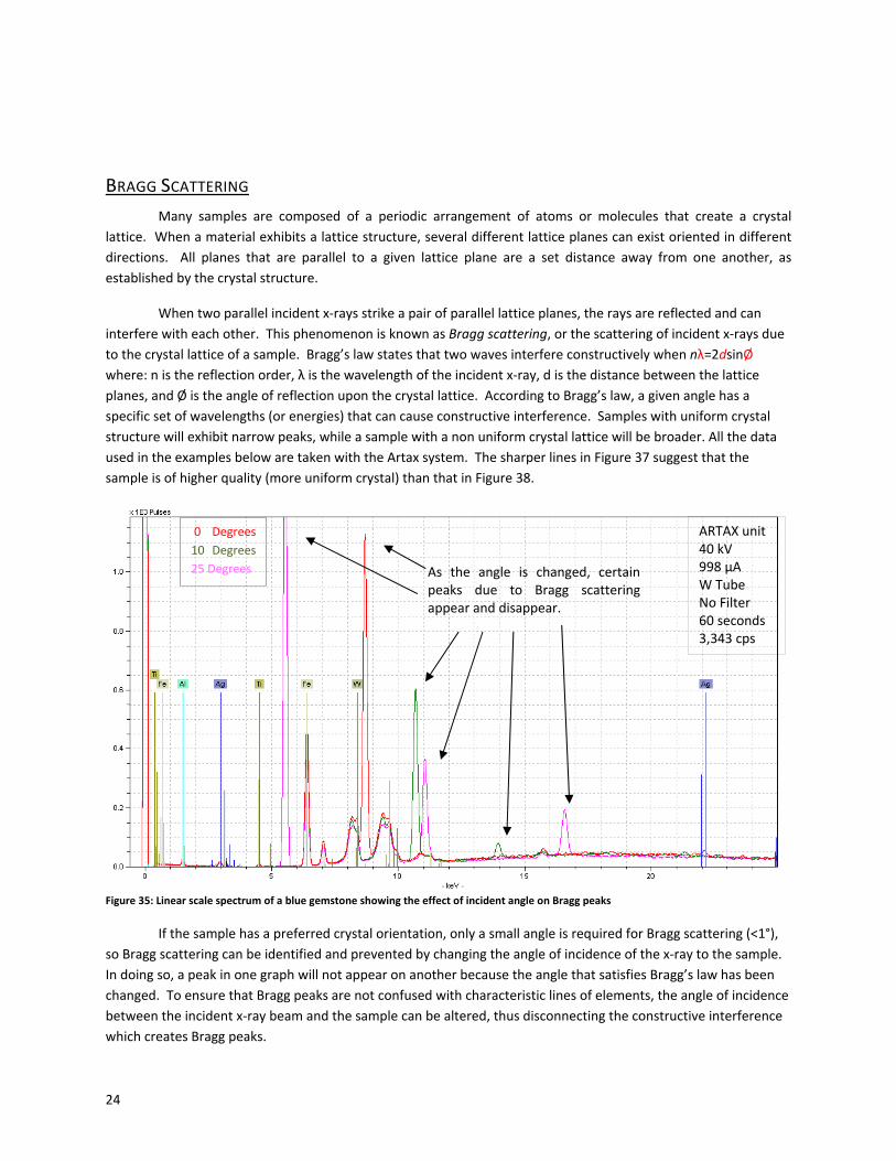
BRAGG�SCATTERING�� Many� samples� are� composed� of� a� periodic� arrangement� of� atoms� or�molecules� that� create� a� crystal�lattice.��When�a�material�exhibits�a�lattice�structure,�several�different�lattice�planes�can�exist�oriented�in�different�directions.� � All� planes� that� are� parallel� to� a� given� lattice� plane� are� a� set� distance� away� from� one� another,� as�established�by�the�crystal�structure.�
� When�two�parallel�incident�xͲrays�strike�a�pair�of�parallel�lattice�planes,�the�rays�are�reflected�and�can�interfere�with�each�other.��This�phenomenon�is�known�as�Bragg�scattering,�or�the�scattering�of�incident�xͲrays�due�to�the�crystal�lattice�of�a�sample.��Bragg’s�law�states�that�two�waves�interfere�constructively�when�nʄ=2dsinØ�where:�n�is�the�reflection�order,�ʄ�is�the�wavelength�of�the�incident�xͲray,�d�is�the�distance�between�the�lattice�planes,�and�Ø�is�the�angle�of�reflection�upon�the�crystal�lattice.��According�to�Bragg’s�law,�a�given�angle�has�a�specific�set�of�wavelengths�(or�energies)�that�can�cause�constructive�interference.��Samples�with�uniform�crystal�structure�will�exhibit�narrow�peaks,�while�a�sample�with�a�non�uniform�crystal�lattice�will�be�broader.�All�the�data�used�in�the�examples�below�are�taken�with�the�Artax�system.��The�sharper�lines�in�Figure�37�suggest�that�the�sample�is�of�higher�quality�(more�uniform�crystal)�than�that�in�Figure�38.�
�Figure�35:�Linear�scale�spectrum�of�a�blue�gemstone�showing�the�effect�of�incident�angle�on�Bragg�peaks�
If�the�sample�has�a�preferred�crystal�orientation,�only�a�small�angle�is�required�for�Bragg�scattering�(<1°),�so�Bragg�scattering�can�be�identified�and�prevented�by�changing�the�angle�of�incidence�of�the�xͲray�to�the�sample.��In�doing�so,�a�peak�in�one�graph�will�not�appear�on�another�because�the�angle�that�satisfies�Bragg’s�law�has�been�changed.��To�ensure�that�Bragg�peaks�are�not�confused�with�characteristic�lines�of�elements,�the�angle�of�incidence�between�the�incident�xͲray�beam�and�the�sample�can�be�altered,�thus�disconnecting�the�constructive�interference�which�creates�Bragg�peaks.�
�0� Degrees�10� Degrees�25�Degrees�
ARTAX�unit40�kV�998�ʅA�W�Tube�No�Filter�60�seconds�3,343�cps�
As� the� angle� is� changed,� certain�peaks� due� to� Bragg� scattering�appear�and�disappear.�
�25
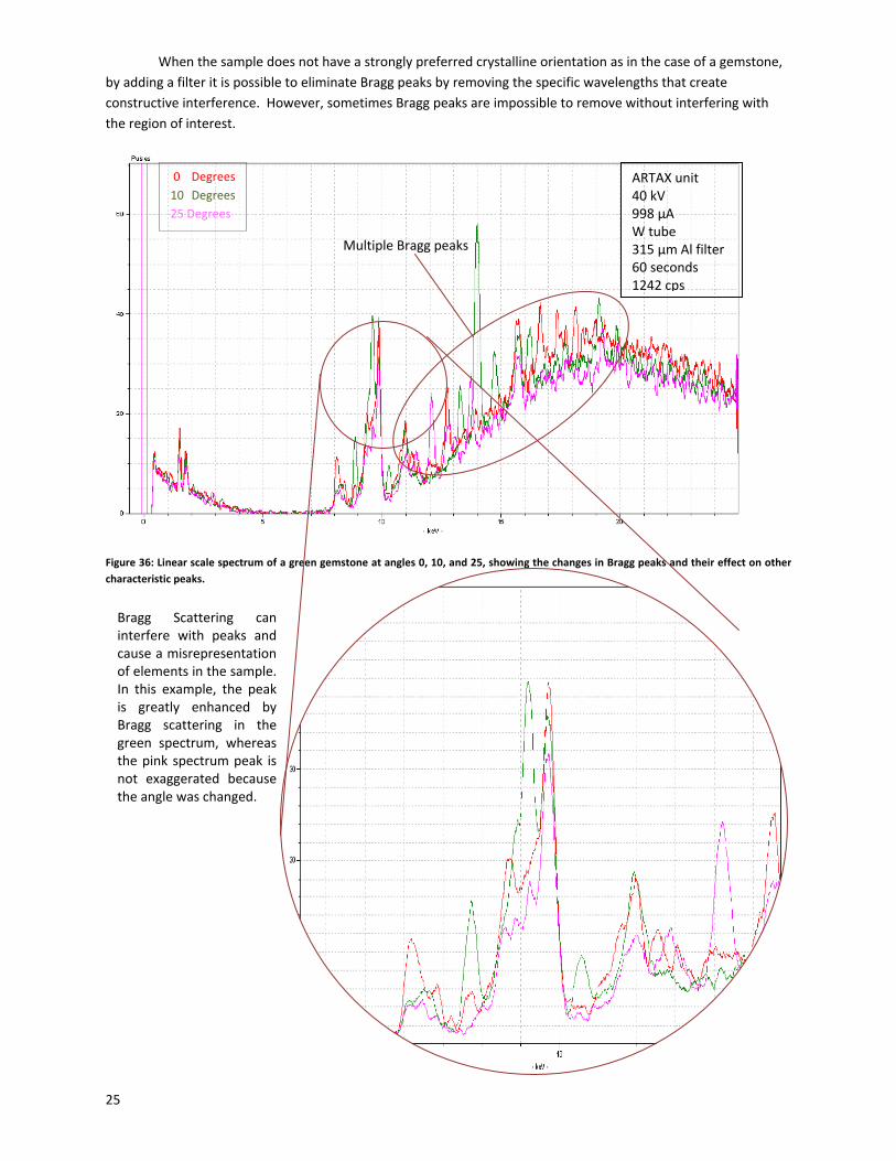
When�the�sample�does�not�have�a�strongly�preferred�crystalline�orientation�as�in�the�case�of�a�gemstone,�by�adding�a�filter�it�is�possible�to�eliminate�Bragg�peaks�by�removing�the�specific�wavelengths�that�create�constructive�interference.��However,�sometimes�Bragg�peaks�are�impossible�to�remove�without�interfering�with�the�region�of�interest.���
�
Figure�36:�Linear�scale�spectrum�of�a�green�gemstone�at�angles�0,�10,�and�25,�showing�the�changes�in�Bragg�peaks�and�their�effect�on�other�characteristic�peaks.�
�
�
�
�
�
�
�
�
�
�
�
�
�
Bragg� Scattering� can�interfere� with� peaks� and�cause�a�misrepresentation�of�elements�in�the�sample.��In� this� example,� the� peak�is� greatly� enhanced� by�Bragg� scattering� in� the�green� spectrum,� whereas�the�pink�spectrum�peak� is�not� exaggerated� because�the�angle�was�changed.��
ARTAX�unit�40�kV�998�ʅA�W�tube�315�ʅm�Al�filter�60�seconds�1242�cps�
�0� Degrees�10� Degrees�25�Degrees�
Multiple�Bragg�peaks
�26
�
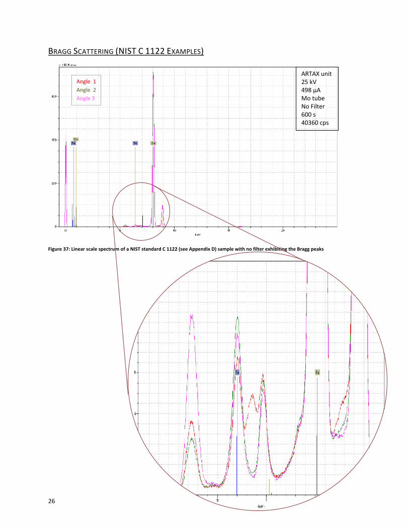
BRAGG�SCATTERING�(NIST�C�1122�EXAMPLES)�
�
Figure�37:�Linear�scale�spectrum�of�a�NIST�standard�C�1122�(see�Appendix�D)�sample�with�no�filter�exhibiting�the�Bragg�peaks��
�
�
�
�
�
�
�
�
�
�
�
�
ARTAX�unit25�kV�498�ʅA�Mo�tube�No�Filter�600�s�40360�cps�
Angle� 1�Angle� 2�Angle�3�
�27
�
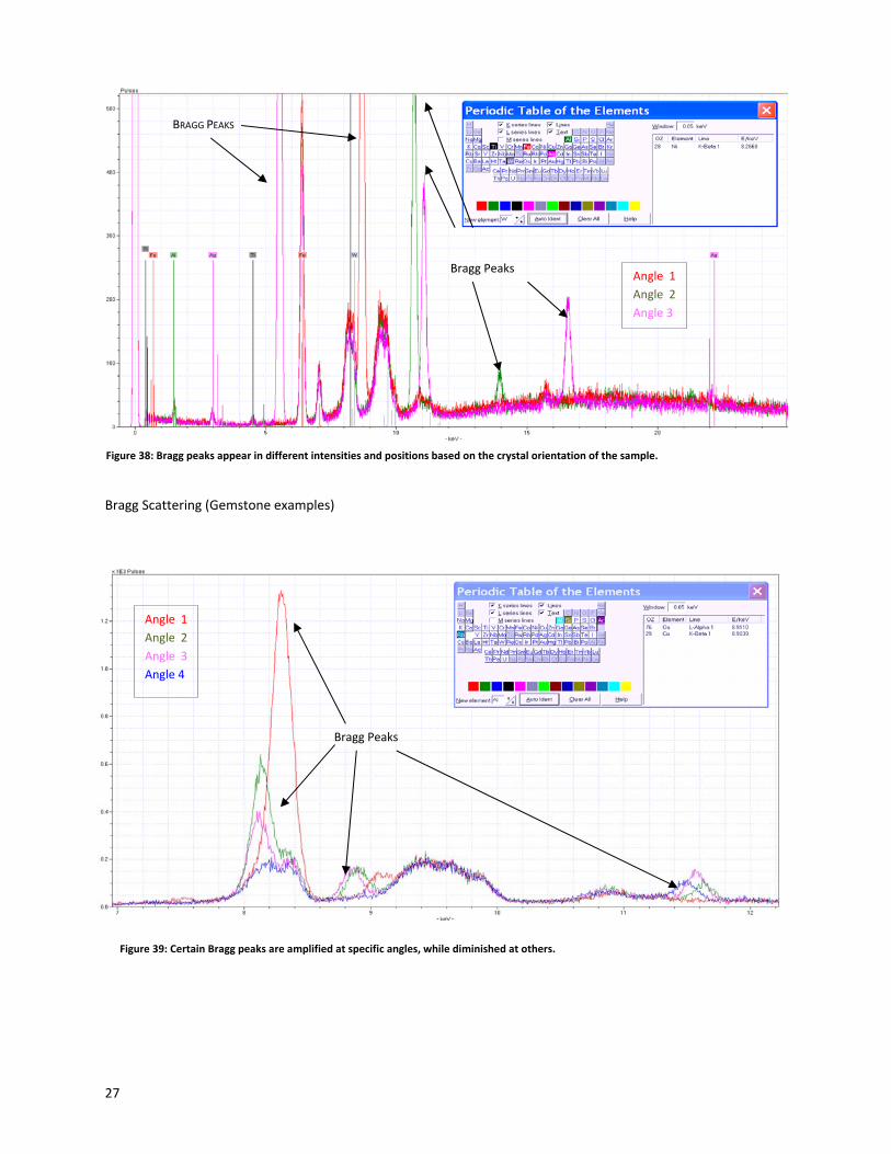
Bragg�Scattering�(Gemstone�examples)�
�
�
��
Bragg�Peaks�
Figure�38:�Bragg�peaks�appear�in�different�intensities�and�positions�based�on�the�crystal�orientation�of�the�sample.�
Figure�39:�Certain�Bragg�peaks�are�amplified�at�specific�angles,�while�diminished�at�others.
Angle� 1�Angle� 2�Angle�3�
Angle� 1�Angle� 2�Angle� 3�Angle�4�
Bragg�Peaks�
BRAGG�PEAKS�
�28
�
�
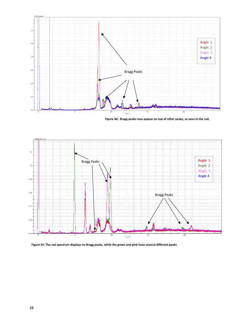
Bragg�Peaks�
Bragg�Peaks� Angle� 1�Angle� 2�Angle� 3�Angle�4�
Figure�41:�The�red�spectrum�displays�no�Bragg�peaks,�while�the�green�and�pink�have�several�different�peaks�
Figure�40:��Bragg�peaks�may�appear�on�top�of�other�peaks,�as�seen�in�the�red.
Angle� 1�Angle� 2�Angle� 3�Angle�4�
Bragg�Peaks�
�29
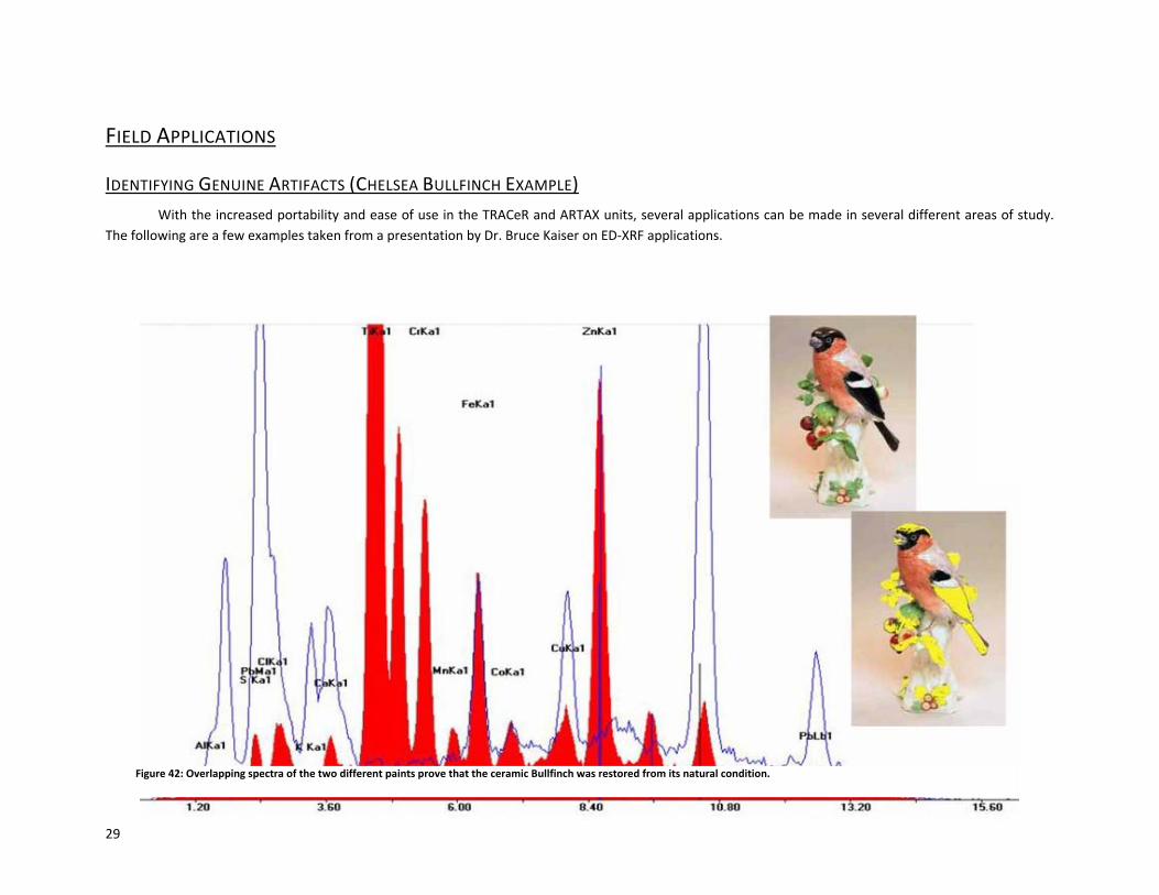
FIELD�APPLICATIONS��
IDENTIFYING�GENUINE�ARTIFACTS�(CHELSEA�BULLFINCH�EXAMPLE)�� With�the�increased�portability�and�ease�of�use�in�the�TRACeR�and�ARTAX�units,�several�applications�can�be�made�in�several�different�areas�of�study.�The�following�are�a�few�examples�taken�from�a�presentation�by�Dr.�Bruce�Kaiser�on�EDͲXRF�applications.���
�
�
Figure�42:�Overlapping�spectra�of�the�two�different�paints�prove�that�the�ceramic�Bullfinch�was�restored�from�its�natural�condition.
�30
IDENTIFYING�TRUE�ORIGINS�(STONEWARE�EXAMPLE)�
�
�
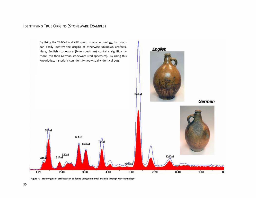
By�Using�the�TRACeR�and�XRF�spectroscopy�technology,�historians�can� easily� identify� the� origins� of� otherwise� unknown� artifacts.��Here,� English� stoneware� (blue� spectrum)� contains� significantly�more�iron�than�German�stoneware�(red�spectrum).��By�using�this�knowledge,�historians�can�identify�two�visually�identical�pots.�
Figure�43:�True�origins�of�artifacts�can�be�found�using�elemental�analysis�through�XRF�technology
�31
�
�
�
�
�
Measuring Chlorine with the Tracer Measurement of Cl is very important as it is often involved in corrosion and degradation of artifacts in marine environments. Or in some cases is a key constituent of pigments or other coatings, or an issue in paper conservation. The following slides first depict how to make up thin film standards to determine the Cl surface content in micro grams per square centimeter. And then how to set the Bruker handheld xrf instrument up to measure levels as low as 10 micro grams per square and shows 2 applications. It should be noted the Cl analysis is very much a SURFACE ANALYSIS when using xrf, as the Cl atom emits only a 2.7 keV x ray. This low an energy x ray is not able to escape the sample unless the atom is very near the surface.
�32
�
�
�
�
�
�
�
�
�
�
�
�
�
�
�
�
�
�
�
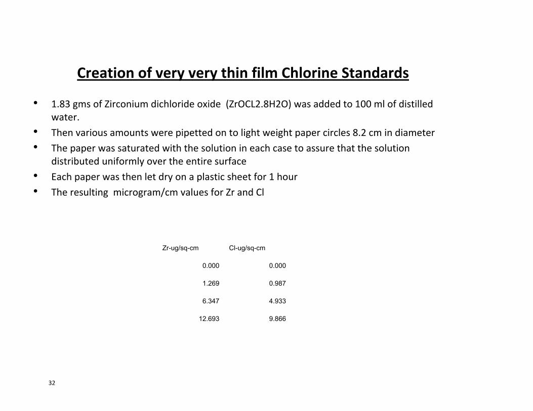
Creation�of�very�very�thin�film�Chlorine�Standards�
• 1.83�gms�of�Zirconium�dichloride�oxide��(ZrOCL2.8H2O)�was�added�to�100�ml�of�distilled�water.�
• Then�various�amounts�were�pipetted�on�to�light�weight�paper�circles�8.2�cm�in�diameter�
• The�paper�was�saturated�with�the�solution�in�each�case�to�assure�that�the�solution�distributed�uniformly�over�the�entire�surface�
• Each�paper�was�then�let�dry�on�a�plastic�sheet�for�1�hour�
• The�resulting��microgram/cm�values�for�Zr�and�Cl��
9.86612.693
4.9336.347
0.9871.269
0.0000.000
Cl-ug/sq-cmZr-ug/sq-cm
�33�
Cl senstivity(ugm/square cm)
50
100
150
200
250
300
350
2 2.2 2.4 2.6 2.8 3 3.2 3.4
keV
# of
x-r
ays
Pure iron0 .0 Cl0.99 Cl4.93 Cl9.87 Cl
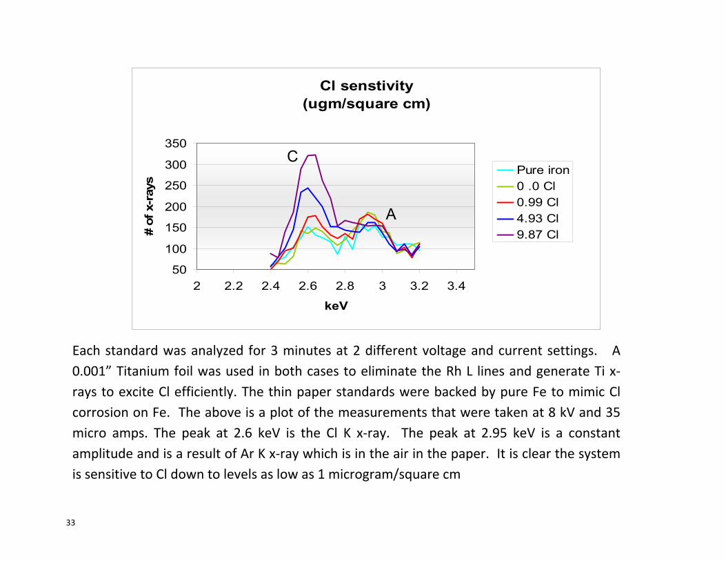
Each�standard�was�analyzed� for�3�minutes�at�2�different�voltage�and�current�settings.� � �A��0.001”�Titanium�foil�was�used� in�both�cases�to�eliminate�the�Rh�L� lines�and�generate�Ti�xͲrays�to�excite�Cl�efficiently.�The�thin�paper�standards�were�backed�by�pure�Fe�to�mimic�Cl�corrosion�on�Fe.��The�above�is�a�plot�of�the�measurements�that�were�taken�at�8�kV�and�35�micro� amps.� The� peak� at� 2.6� keV� is� the� Cl� K� xͲray.� � The� peak� at� 2.95� keV� is� a� constant�amplitude�and�is�a�result�of�Ar�K�xͲray�which�is�in�the�air�in�the�paper.��It�is�clear�the�system�is�sensitive�to�Cl�down�to�levels�as�low�as�1�microgram/square�cm�
C
A
�34
�
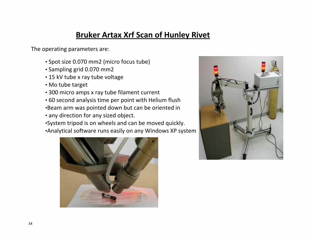
Bruker�Artax�Xrf�Scan�of�Hunley�Rivet
The�operating�parameters�are:
•�Spot�size�0.070�mm2�(micro�focus�tube)�•�Sampling�grid�0.070�mm2�•�15�kV�tube�x�ray�tube�voltage�•�Mo�tube�target�•�300�micro�amps�x�ray�tube�filament�current�•�60�second�analysis�time�per�point�with�Helium�flush�•Beam�arm�was�pointed�down�but�can�be�oriented�in�•�any�direction�for�any�sized�object.��•System�tripod�is�on�wheels�and�can�be�moved�quickly.�•Analytical�software�runs�easily�on�any�Windows�XP�system��
�

�35
�
0.00 0.07 0.14 0.21 0.28 0.35 0.42 0.49 0.56 0.63 0.70 0.77 0.840.00
0.07
0.14
0.21
0.28
0.35
0.42
0.49
0.56
Micrograms/cm2 of Chlorine
mm
mm
Cl Distribution on Rivet Side at Machined Boundary26-28
24-2622-2420-2218-2016-1814-1612-1410-128-106-84-62-40-2
Start scan
Machined
area
un Machined
area
�36
�
�
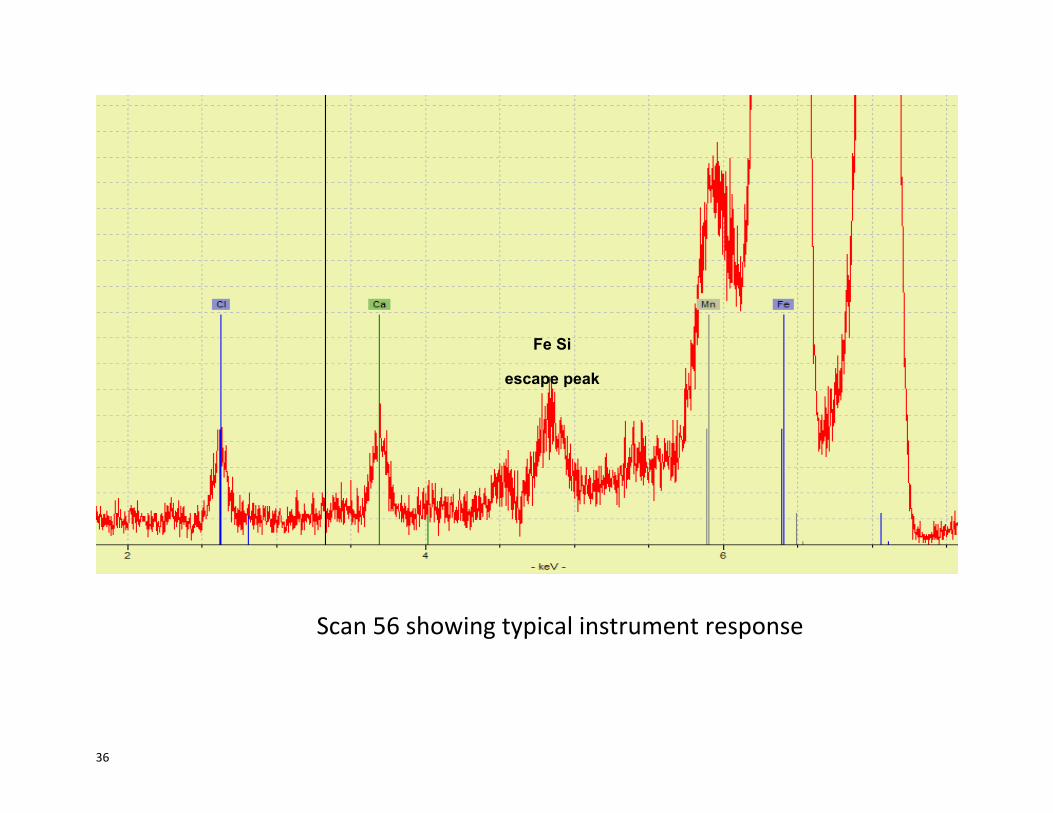
Scan�56�showing�typical�instrument�response
Fe Si
escape peak

�37
�
�
Bruker�TRACeR�Operating�Parameters�
x 40�kV�and�10�micro�amps�
x .006”�Cu,�.001”Ti,�.012”�Al�filters�
x 180�sec�data�acquisition�
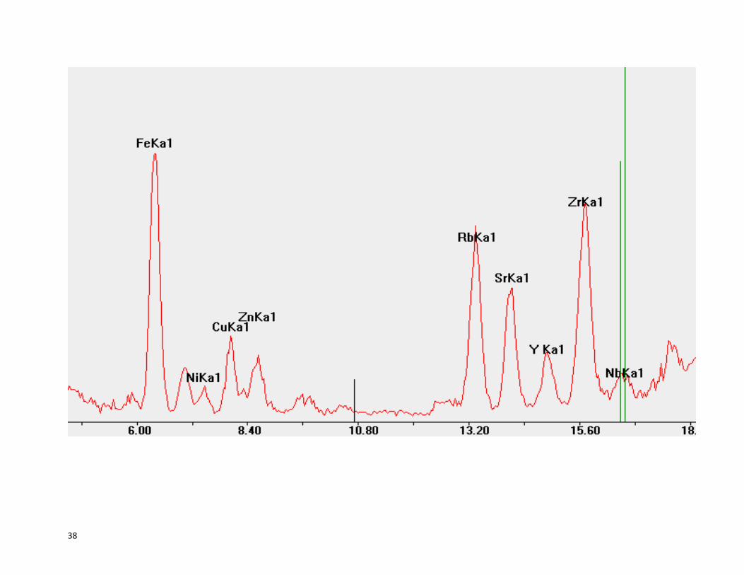
Sourcing�Obsidian�
•�ppm�sensitivity�to�key�elements�
•�Key�technique�to�determine�human�movement���and�activity�
•�Bruker�TRACeR�xrf�systems�found�to�be�very�accurate�for�this�application�
•�The�following�data�is�an�example�of�Tracer�analysis�done�by�Jeff�Speakman�of�the�Smithsonian
�38
�
�
�
�
�

�39
�
�
�
0
1000
2000
3000
4000
5000
6000
5 6 7 8 9 10 11 12 13 14 15 16 17 18 19 20
alcaChivayCRG 0002IxtepequeMLZ 1019Mono Glass MTNOtumbaPico de OrizabaQuispisisaSierra de PachucaUcareoUNL-050_1XMC 020Yellowstone
Fe
Zr
ZCF
Rb Sr Y
Nb Zr
�40
�
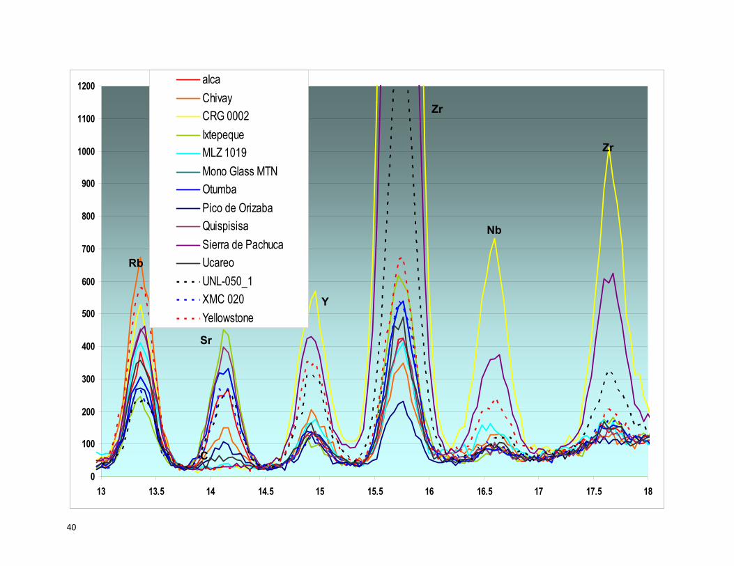
0
100
200
300
400
500
600
700
800
900
1000
1100
1200
13 13.5 14 14.5 15 15.5 16 16.5 17 17.5 18
alcaChivayCRG 0002IxtepequeMLZ 1019Mono Glass MTNOtumbaPico de OrizabaQuispisisaSierra de PachucaUcareoUNL-050_1XMC 020Yellowstone
Zr
C
Rb
Sr
Y
Nb
Zr
�41
�
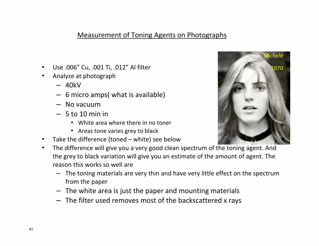
Measurement�of�Toning�Agents�on�Photographs�
• Use�.006”�Cu,�.001�Ti,�.012”�Al�filter��• Analyze�at�photograph�
– 40kV��– 6�micro�amps(�what�is�available)�– No�vacuum�– 5�to�10�min�in�
• White�area�where�there�in�no�toner�• Areas�tone�varies�grey�to�black�
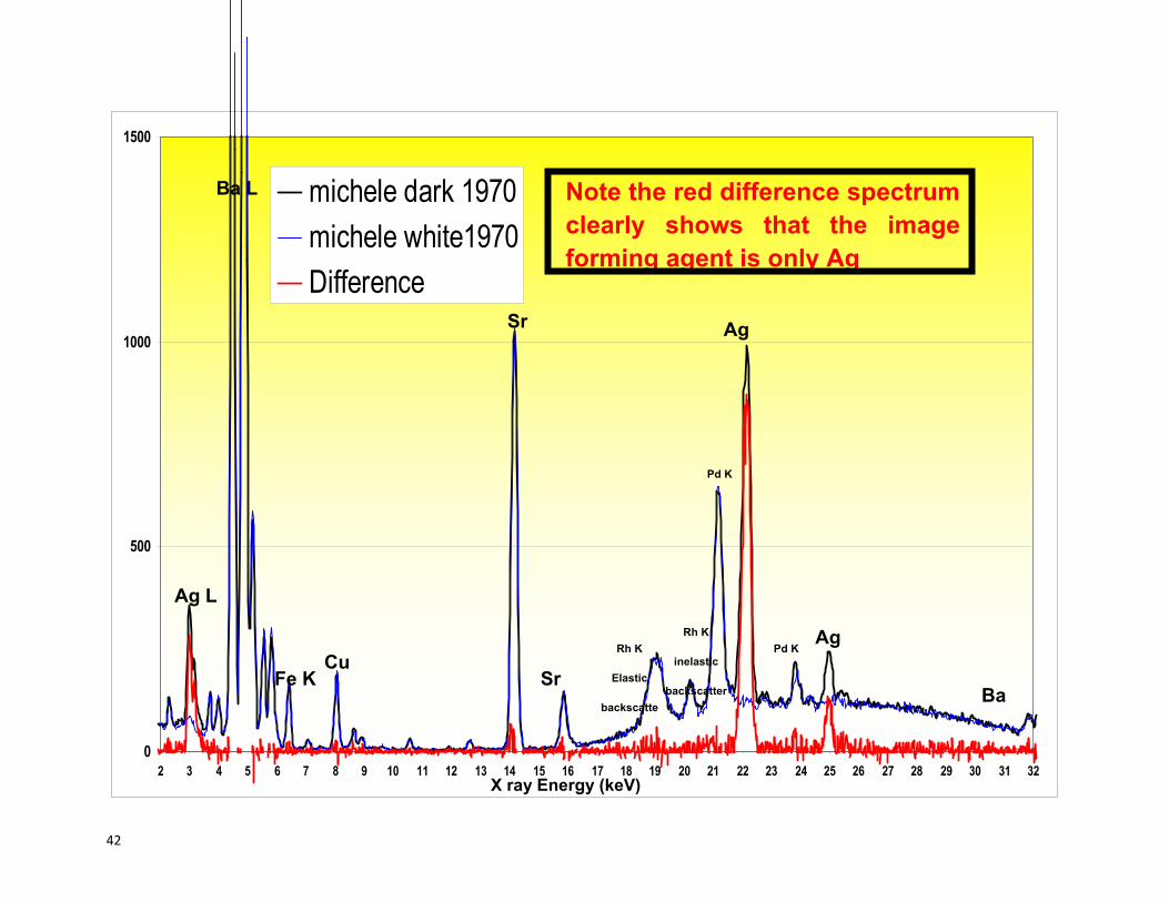
• Take�the�difference�(toned�–�white)�see�below�• The�difference�will�give�you�a�very�good�clean�spectrum�of�the�toning�agent.�And�
the�grey�to�black�variation�will�give�you�an�estimate�of�the�amount�of�agent.�The�reason�this�works�so�well�are��– The�toning�materials�are�very�thin�and�have�very�little�effect�on�the�spectrum�
from�the�paper��– The�white�area�is�just�the�paper�and�mounting�materials�– The�filter�used�removes�most�of�the�backscattered�x�rays�
Michele�
1970
�42
0
500
1000
1500
2 3 4 5 6 7 8 9 10 11 12 13 14 15 16 17 18 19 20 21 22 23 24 25 26 27 28 29 30 31 32
michele dark 1970michele white1970Difference
Ba L
Ba
Ag
Ag L
Ag Rh K
Elastic
backscatte
Pd K
Pd K
Rh K
inelastic
backscatter Sr
Sr
Fe K Cu
Note the red difference spectrum clearly shows that the image forming agent is only Ag
X ray Energy (keV)
�43
APPENDICES�
APPENDIX�A�
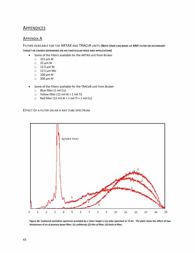
FILTERS�AVAILABLE�FOR�THE�ARTAX�AND�TRACER�UNITS�(NOTE�USER�CAN�MAKE�UP�ANY�FILTER�OR�SECONDARY�
TARGET�HE�CHOSES�DEPENDING�ON�HIS�PARTICULAR�NEED�AND�APPLICATION)�
x Some�of�the�Filters�available�for�the�ARTAX�unit�from�Bruker�o 315�ʅm�Al�o 25�ʅm�Ni�o 12.5�ʅm�Ni�o 12.5�ʅm�Mo�o 100�ʅm�Al�o 200�ʅm�Al�
�x Some�of�the�Filters�available�for�the�TRACeR�unit�from�Bruker�
o Blue�filter�(1�mil�Cu)�o Yellow�filter�(12�mil�Al�+�1�mil�Ti)�o Red�filter�(12�mil�Al�+�1�mil�Ti�+�1�mil�Cu)�
�
EFFECT�OF�A�FILTER�ON�AN�XͲRAY�TUBE�SPECTRUM��
��
Figure�44:�Scattered�excitation�spectrum�provided�by�a�silver�target�xͲray�tube�operated�at�15�kV.��The�plots�show�the�effect�of�twothicknesses�of�an�al�primary�beam�filter:�(1)�unfiltered;�(2)�thin�al�filter;�(3)�thick�al�filter.�
�44
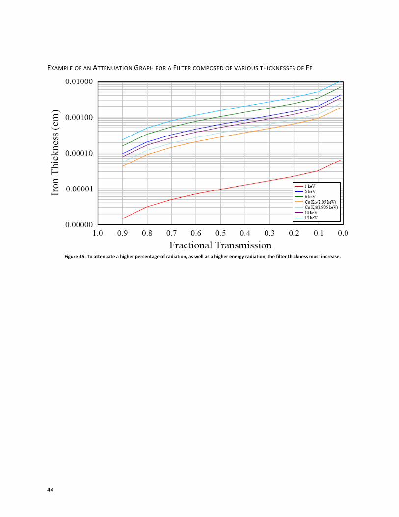
��EXAMPLE�OF�AN�ATTENUATION�GRAPH�FOR�A�FILTER�COMPOSED�OF�VARIOUS�THICKNESSES�OF�FE�
��
Figure�45:�To�attenuate�a�higher�percentage�of�radiation,�as�well�as�a�higher�energy�radiation,�the�filter�thickness�must�increase.��

�45
�
TYPICAL�FILTER,�VOLTAGE�AND�CURRENT�SELECTION�FOR�OPTIMUM�XRF�ELEMENTAL��
GROUP�ANALYSIS�USING�THE�TRACER���
Screening�for�all�Elements�(Lab�Rat�mode):�
1. No�filter�2. 40�kV��3. 3�to�5�micro�amps�(for�non�metallic�samples)�4. 0.6�to�1.4�micro�amps�(for�metallic�samples)�5. Utilize�the�vacuum.�
�These�settings�allow�all�the�x�rays�from�1�keV�to�40�keV�to�reach�the�sample�thus�exciting�all�the�elements�for�Mg�to�Pu.�
To�optimize�for�particular�elemental�groups�one�wants�to�use�filters�and�settings�that�“position”�the�X�ray�energy�impacting�the�sample�just�above�the�absorption�edges�of�the�element(s)�of�interest.�Examples�of�how�to�go�about�this�is�given�below.��Note�as�well�that�the�depth�of�analysis�is�also�very�much�a�function�of�both�the�x�ray�energy�used�to�probe�the�material�and�the�element�that�is�being�excited,�both�are�exponential�functions�dependent�on�the�matrix�of�elements�that�the�material�is�composed.�
�
Figure�46:�This�graph�is�made�to�determine�the�filter�thickness�required�for�optimal�results�in�testing�a�copper�sample.�
�46
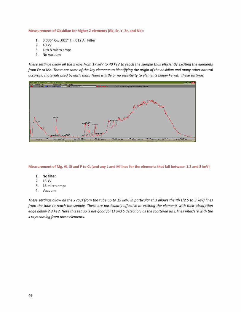
Measurement�of�Obsidian�for�higher�Z�elements�(Rb,�Sr,�Y,�Zr,�and�Nb):�
1. 0.006”�Cu,�.001”�Ti,�.012�Al��Filter�2. 40�kV�3. 4�to�8�micro�amps�4. No�vacuum�
�These�settings�allow�all�the�x�rays�from�17�keV�to�40�keV�to�reach�the�sample�thus�efficiently�exciting�the�elements�from�Fe�to�Mo.�These�are�some�of�the�key�elements�to�identifying�the�origin�of�the�obsidian�and�many�other�natural�occurring�materials�used�by�early�man.�There�is�little�or�no�sensitivity�to�elements�below�Fe�with�these�settings.��
�
�
�
�
�
�
�
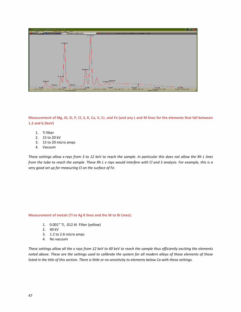
�Measurement�of�Mg,�Al,�Si�and�P�to�Cu(and�any�L�and�M�lines�for�the�elements�that�fall�between�1.2�and�8�keV)�
1. No�filter�2. 15�kV�3. 15�micro�amps�4. Vacuum�
�These�settings�allow�all�the�x�rays�from�the�tube�up�to�15�keV.�In�particular�this�allows�the�Rh�L(2.5�to�3�keV)�lines�from�the�tube�to�reach�the�sample.�These�are�particularly�effective�at�exciting�the�elements�with�their�absorption�edge�below�2.3�keV.�Note�this�set�up�is�not�good�for�Cl�and�S�detection,�as�the�scattered�Rh�L�lines�interfere�with�the�x�rays�coming�from�these�elements.�
�47
�
�
�
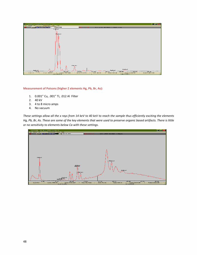
Measurement�of�Mg,�Al,�Si,�P,�Cl,�S,�K,�Ca,�V,�Cr,�and�Fe�(and�any�L�and�M�lines�for�the�elements�that�fall�between�1.2�and�6.5keV)�
1. Ti�filter�2. 15�to�20�kV�3. 15�to�20�micro�amps�4. Vacuum�
�These�settings�allow�xͲrays�from�3�to�12�keV�to�reach�the�sample.� In�particular�this�does�not�allow�the�Rh�L� lines�from�the�tube�to�reach�the�sample.�These�Rh�L�x�rays�would�interfere�with�Cl�and�S�analysis.�For�example,�this�is�a�very�good�set�up�for�measuring�Cl�on�the�surface�of�Fe.�
�
�
�
�
Measurement�of�metals�(Ti�to�Ag�K�lines�and�the�W�to�Bi�Lines):�
1. 0.001”�Ti,�.012�Al��Filter�(yellow)�2. 40�kV�3. 1.2�to�2.6�micro�amps�4. No�vacuum�
�These�settings�allow�all�the�x�rays�from�12�keV�to�40�keV�to�reach�the�sample�thus�efficiently�exciting�the�elements�noted�above.�These�are�the�settings�used�to�calibrate�the�system�for�all�modern�alloys�of�those�elements�of�those�listed�in�the�title�of�this�section.�There�is�little�or�no�sensitivity�to�elements�below�Ca�with�these�settings.�
�48
�
�
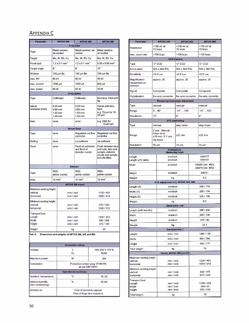
Measurement�of�Poisons�(higher�Z�elements�Hg,�Pb,�Br,�As):�
1. 0.001”�Cu,�.001”�Ti,�.012�Al��Filter�2. 40�kV�3. 4�to�8�micro�amps�4. No�vacuum�
�These�settings�allow�all�the�x�rays�from�14�keV�to�40�keV�to�reach�the�sample�thus�efficiently�exciting�the�elements�Hg,�Pb,�Br,�As.�These�are�some�of�the�key�elements�that�were�used�to�preserve�organic�based�artifacts.�There�is�little�or�no�sensitivity�to�elements�below�Ca�with�these�settings.�
�
�
�
�
�
�
�
�
�
�
�
�

�49
APPENDIX�B��
�
�
�
�
�
�
�
�
�
� �
�
�
�
�
�
�
�
�
�
�
�
�
�
�
�
Figure�47:�Explanation�of�Si�PIN�characteristics
�50
APPENDIX�C�
�51
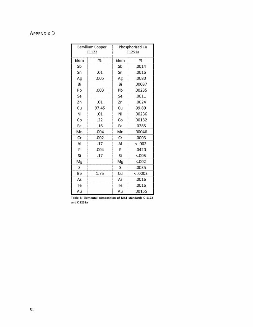
APPENDIX�D��
Beryllium�CopperC1122�
Phosphorized�CuC1251a�
Elem %� Elem %�Sb� � Sb� .0014�Sn� .01� Sn� .0016�Ag� .005� Ag� .0080�Bi� � Bi� .00037�Pb� .003� Pb� .00235�Se� � Se� .0011�Zn� .01� Zn� .0024�Cu� 97.45� Cu� 99.89�Ni� .01� Ni� .00236�Co� .22� Co� .00132�Fe� .16� Fe� .0285�Mn� .004� Mn� .00046�Cr� .002� Cr� .0003�Al� .17� Al� <�.002�P� .004� P� .0420�Si� .17� Si� <.005�Mg� � Mg� <.002�S� � S� .0035�Be� 1.75� Cd� <�.0003�As� � As� .0016�Te� � Te� .0016�Au� � Au� .00155�
Table�8:�Elemental� composition�of�NIST� standards�C�1122�and�C�1251a�
�52
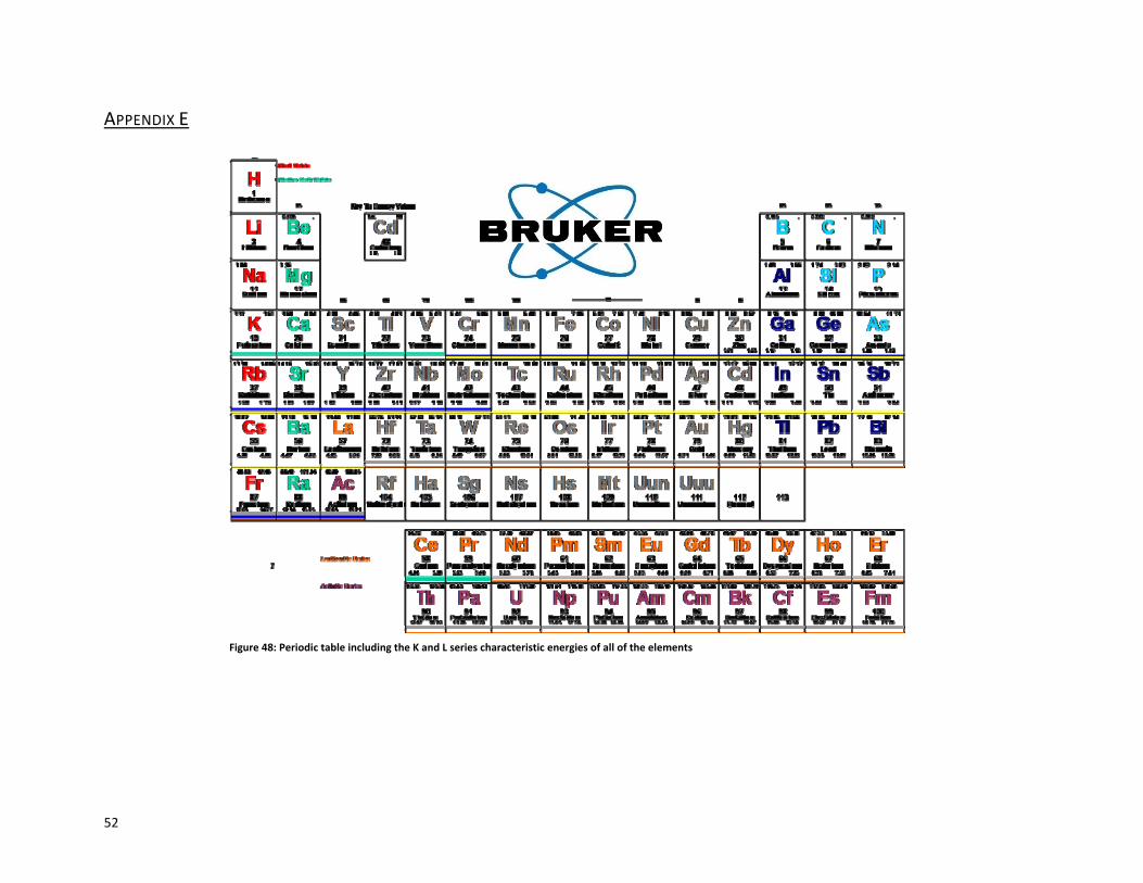
APPENDIX�E
Figure�48:�Periodic�table�including�the�K�and�L�series�characteristic�energies�of�all�of�the�elements�

�53
�