cvp and breakeven analysis

7/30/2019 Cvp and Breakeven Analysis

http://slidepdf.com/reader/full/cvp-and-breakeven-analysis 1/23

CVP AND BREAKEVEN ANALYSIS

Nikhil Ramesh, a software engineer, returned home one evening dejected and utterly

perplexed! He had lost his job that fetched him a package of Rs 75,000 a month. That

morning what happened to him was literally a nightmare. As soon as he reached his

office in the morning he found, to his dismay, that his ID cards did not work, his PC

was disabled, and passwords were disqualified—just about anything, to give the

message across that he is being shown the door. Then came the worst—the pink slip.

Ramesh had been working with an IT company Infitech, the company he got placed

with on the day one of his campus placements. Although still a bachelor Ramesh had

taken a home loan from HDFC for tax planning purposes. The equated monthly

instalment (EMI) on the loan amounts to Rs 12,500 per month. Besides, he had also

taken an auto loan to buy his new Hyundai Santro. The EMI for which comes to Rs

10,000 a month. With the debt servicing obligation of Rs 22,500 a month Ramesh is

broke.

Till last year everything was going fine and smooth. Even middle sized IT companies

such as Infitech were witnessing soaring bottom line. The employees were getting

huge bonuses. Last year only the company announced stock options and Ramesh was

also one of the beneficiaries. The company had been expanding for the past five years

and the growth in manpower was around 35% during this period. The company

shifted its Bangalore operations to bigger premises two years back that it had hired in

view of its expanding human resource base. People started to look at options to cut

down the costs. First step was to lay off the extra workforce so as to bring down the

salary bill along with the other overheads. Next was to cut down the capacity by

shifting to smaller premises as this would bring down the rentals and costs on

maintenance.



It all started with the slowdown in the US IT sector. Cost cutting became the order of

the day, with overheads being axed first. Venture capitalists, unsure of returns, began

dictating terms. Even IT companies with finances in order and new frontier software

to offer found growth rates dipping. All of which meant one thing: lay offs. The less

skilled were the first to go. Freshers are not the only ones to be kicked around. Even

those with supposedly permanent jobs were also at the receiving end.

Ramesh was really dreading as to how should he share this news with his parents who

incidentally were there with him for vacation. But his father had already come to

know of this from his pal, Ravi. The father trying to give him solace said, "Son, it is

not your fault. It is pure economics. Every economy witnesses such business cycles

and they are only a passing phase. You learn from them and move ahead." Ramesh's

response was prompt "Actually both I and my company were sailing on the same

boat. The company in the wake of growing business became overenthusiastic in

expanding its physical and human resources which led to surge in its salary bills and

rentals. Till the time expansion phase was on, all was fine but the moment the projects

started shrinking all went haywire." Adding further, Ramesh said, "The growing

salary bills that were being taken as a measure of growth suddenly became

burdensome fixed costs." The physical expansion started to be seen as overcapacity

causing fixed costs. To reach the breakeven in wake of receding revenues, the finance

The mistake I committed was to create a very high fixed interest obligation oblivious

of the nature of fixed costs. They do not change with the changing seasons.

Source: Adapted with changes from 'Of job-cuts in IT: The lost pride',

http://www.cybermediadice.com/ . Accessed on 18 January 2007.

http://www.cybermediadice.com/

http://www.cybermediadice.com/



INTRODUCTION

Besides ratio analysis, another analytical tool that is comprehensively used in the

decision-making process is cost volume profit (CVP) analysis. Decisions such as—

change in cost and profit for a given level of change in activity level (volume), the

adjustments to be made in costs and/or volume to change the profits by a desired

margin, the required change in costs to enhance the volume, etc., depend upon the

relationship that exists between cost, volume, and profit. The CVP analysis focuses

upon the relationship between these three key parameters of financial decision-

making to arrive at such important business decisions.

Breakeven analysis is the most prominent and widely used technique of CVP analysis.

The concept of breakeven analysis is built around the breakeven point (BEP), which is

a no-profit, no-loss point. Fixed costs are the focus of breakeven analysis as the

coverage of such costs is crucial for the firm to breakeven. Breakeven analysis is used

in profit planning and cost control besides bping useful for several other managerial

decisions.

NATURE AND BEHAVIOUR OF COSTS

Increased business activity (volume) requires increased resources to carry out those

activities, which in turn, increases the activity (volume) requires increased resources

activities, which in turn, increases the associated costs. However, this increase in cost

is not in the same proportion as 11 the increase in the volume. This disproportionate

change in cost is due to the fact that all the costs do not vary with the changing

activity levels. Before proceeding further to discuss CVP and breakeven analysis let

us understand and behaviour vis-a-vis volume.

This the incurred by firms can be divided into two costs and fixed costs. The costs that

vary in direct proportion to the change in the volume are termed as variable costs.



Due to the variation of such costs with the level of volume or production, such costs

are also referred to as product costs. The noteworthy point here is that on variable

costs vary proportionately; but on per unit basis, variable cost remains constant as can

be seen in Table 3-1.

Table 3.1 Variable costs

Volume Cost per Total variable

(No. of units) unit costs

(InRs) (In Rs)

100 1,000 1,00,000

200 1,000 2,00,000

2500 1,000 25,00,000

5000 1,000 50,00,000

7500 1,000 75,00,000

10000 1,000 1,00,00,000

12500 1,000 1,25,00,000

Raw material costs, power and fuel costs, wages paid on the piece wage rate

basis, target-based incentive/commission to salespersons are some of the examples of

variable costs. From the decision-making point of view, variable costs are termed as

controllable because the total variable costs can be changed by altering the level of

production and these costs are within the control of a cost/responsibility centre.

Since variable costs fluctuate automatically with the activity level, they can be

controlled during adverse times. For example, if the sales are down due to decline in

demand the variable costs will come down automatically and will pose no problems

for the management. The behaviour of variable costs vis-a-vis the activity level is

shown in the Figure 3-1.

Fixed costs refer to such components of costs that remain invariant to the

changing activity level. Such costs are alternatively referred to as period costs as they

change with time and not with volume. The examples of fixed costs include rent,

salaries, etc. Total fixed costs remain constant; per unit fixed costs bear an inverse

relationship with the level of activity. It is not that the fixed costs do not change at all



but the change happens only if the level of activity of the firm goes beyond a certain

range, which is known as the relevant range. As the activity level of the firm reaches

the end point of this relevant range, it becomes necessary to expand the capacity.

Capacity expansion causes a sudden spurt

Figure 3.1 Behaviour of variable costs

In the total fixed costs. Till the time the firm operates within the range, these costs

remain fixed. For example, if a firm has a capacity to store 10,000 units of output in

its warehouse then till the time the output reaches the level of 10,000 units the rent for

the warehouse, which is a fixed cost, remains the same. Although it may go up on

account of factors such as inflation and annual increment as per the lease agreement,

it does not increase with an increase in the production level. The moment the output

level of the firm exceeds the level of 10,000 units, the firm will have to hire additional

warehousing facility and this would lead to an increase in rent. Thus in such a

situation, the relevant range within which the fixed costs remain fixed is upto 1-

10,000 units. This behaviour of fixed costs vis-a-vis the volume is demonstrated in

Figure 3-2.



Figure 3-2 Behaviour of fixed costs

Fixed costs are also termed as uncontrollable costs because once they are incurred

they remain fixed at a given level. Changing the level of such fixed costs requires a

major restructuring, which is not within the control of a responsibility centre or a cost

centre. It is a strategic decision that is taken by the top management. For example, to

cut down the salary bill, which is a fixed cost, a decision whether to lay off employees

has to be taken by the top management. Such a decision may have major

repercussions for the firm. Similarly, the decision to change the nature of firm's

operation—to shift from production as a pore activity to distribution as a core

business function may bring down the fixed production costs incurred by the business,

but this again is a strategic business decision that has to be taken by the top

management. Thus by and large, fixed costs are uncontrollable costs. Since they are

constant, fixed costs assume significance in financial decision-making. The

management has to ensure that fixed costs are kept within a manageable limit as they

cannot be reversed easily.

The total fixed costs can be divided into—fixed operating and fixed financing costs.

Fixed operating costs include costs such as rent, salary, and other fixed



administrative, and selling and distribution expenses that are incurred to carry out the

firm's operations. The fixed costs incurred on financing the firm's operations are

termed as fixed financing costs. The two main financing costs are interest and lease

rent. To put it simply. it can be said that all business-related fixed costs except for

interest and lease rentals are fixed operating costs. One may wonder as to how it

matters whether a cost under the category of fixed operating costs or fixed costs!

After all both of them remain fixed. We let you over this issue for a while and take up

the issue a little later i the chapter under the section on operating and financial 1

Besides variable and the fixed costs, there is a 1 of costs termed as semi-variable

costs. These costs are a combination of variable and fixed costs. As can be Figure 3-3

these costs change but not in the direct ] the increase or decrease in the volume.

Although 1 costs are positively correlated with sales

Correlation may

not be necessarily one. If the volume increases by 5% the total amount of semi-

variable costs will increase by less than 5%. These costs are also referred to as mixed

costs, semi-fixed costs, or partly variable costs. Costs incurred on repairs and



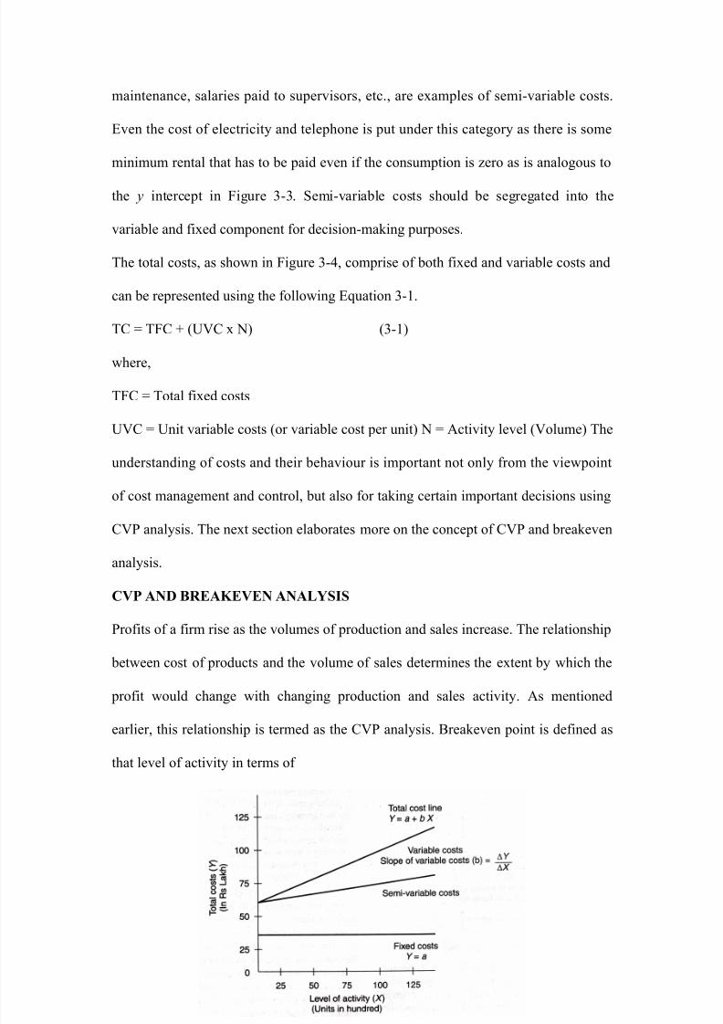
maintenance, salaries paid to supervisors, etc., are examples of semi-variable costs.

Even the cost of electricity and telephone is put under this category as there is some

minimum rental that has to be paid even if the consumption is zero as is analogous to

the y intercept in Figure 3-3. Semi-variable costs should be segregated into the

variable and fixed component for decision-making purposes.

The total costs, as shown in Figure 3-4, comprise of both fixed and variable costs and

can be represented using the following Equation 3-1.

TC = TFC + (UVC x N) (3-1)

where,

TFC = Total fixed costs

UVC = Unit variable costs (or variable cost per unit) N = Activity level (Volume) The

understanding of costs and their behaviour is important not only from the viewpoint

of cost management and control, but also for taking certain important decisions using

CVP analysis. The next section elaborates more on the concept of CVP and breakeven

analysis.

CVP AND BREAKEVEN ANALYSIS

Profits of a firm rise as the volumes of production and sales increase. The relationship

between cost of products and the volume of sales determines the extent by which the

profit would change with changing production and sales activity. As mentioned

earlier, this relationship is termed as the CVP analysis. Breakeven point is defined as

that level of activity in terms of



Revenue or in terms of production levels at which firm recovers all its cost. In other

words, it is a level of no profit or no loss. Operation beyond breakeven point would

result in profit, while operation below it would mean loss for the firm. Breakeven

point is of significance to all stakeholders of the firm. Knowing the breakeven point

for profit-making firms is important as it tells how safe the stakeholders are given the

variability of sales and cost structure emanating from the uncertain environment the

firm operates in. Breakeven point is the most significant techniques in CVP analysis.

Although there are other techniques like profit volume analysis, marginal cost

analysis, key factor analysis etc. in addition to breakeven analysis that aid in CVP

analysis but the BEP is normally used as a sine qua non for the CVP analysis.

To have a clear understanding of breakeven point (BEP) analysis and CVP analysis,

the profit and loss account statement of a firm is analysed. For easier understanding

and illustration, let us take an example of a single product firm, though in the real

world it is rare to find such firm. Ideally firms would like to produce single product to

keep management of the firm simple. However, market conditions, desire for growth,

and prevailing competition force the management to produce more than one product.

Let us assume that a firm named SG Footwear is in the business of producing PVC

shoes. It has installed 10 sophisticated direct injection process (DIP) moulding

machines by importing them from Taiwan. These extremely sophisticated machines

are capable of producing full, single piece PVC cloth and leather shoes. Each machine



has 16 stations producing 8 pairs of shoes in one production cycle lasting for 5

minutes. The capacity of the firm can be estimated as about 7,000 pairs per shift

equivalent to 42 lakh pairs per annum as shown. Capacity = No. of pairs per cycle x

No. of cycles per shift xNo. of machines No. of pairs of shares/shift = 8 x (480/5) X

10

= 7,680 Less: Wastage and set up time approx 8-9% = 680 Annual Capacity =

Capacity/Shift x No. of Shifts/day x No. of Days/annum = 7,000 x 2 x 300 = 42 lakh

pairs of shoes per annum Assuming that the selling price per pair of shoes is Rs 200

the capacity annual revenue of SG Footwear is Rs 8,400 lakh. Capacity revenue

= No. of pairs per shift x Shifts per days

x Days/Annum x Selling Price

= 7,000 x 2 x 300 x 200 = Rs 8,400 lakh

The management of SG Footwear is hopeful of booking the machine to the extent of

60% of capacity utilization as more than 25 lakh pairs of shoes can be sold. Based on

the above target and the cost of raw materials, packing materials and consumables

per pair of shoes including wastages of Rs 105, Rs 6, and Rs 3 per pair, respectively,

the management has prepared a profitability statement as shown in Table 3-2.

Table 3-2 Profitability statement of SG Footwear

Pairs of shoes in lakh

CapacityCapacity Utilization | Nos. of pairs of shoes

42.0060%

25.20

Rs per pair of shoe

Selling Price Raw Material Packing Material Consumables 200.00

105.00

6.00

3.00

Profitablity Basis Rs lakh



Revenue

Raw Material

Packing Material

Consumables

Electricity

WagesRepairs & Maintenance

Salaries

Travelling & Conveyance

Business Promotion

Freight

Selling Commission

Administrative Overheads

at Rs 200 per pair of shoe

atRs 105 per pair of shoe



Rs 4/unit, 100 KW/Machine

20 lakh per monthEstimated

at Rs 25 lakh per month

Estimated

Estimated

at 0.5% of selling price

at 10% of selling price

Estimated

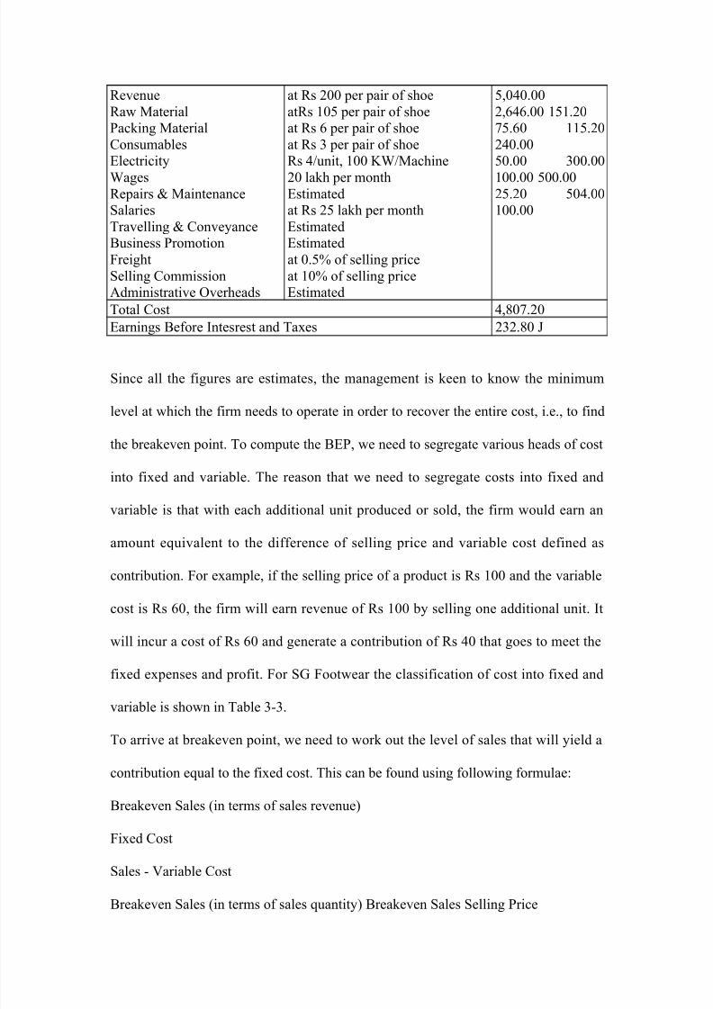
5,040.00

2,646.00 151.20

75.60 115.20

240.00

50.00 300.00

100.00 500.0025.20 504.00

100.00

Total Cost 4,807.20

Earnings Before Intesrest and Taxes 232.80 J

Since all the figures are estimates, the management is keen to know the minimum

level at which the firm needs to operate in order to recover the entire cost, i.e., to find

the breakeven point. To compute the BEP, we need to segregate various heads of cost

into fixed and variable. The reason that we need to segregate costs into fixed and

variable is that with each additional unit produced or sold, the firm would earn an

amount equivalent to the difference of selling price and variable cost defined as

contribution. For example, if the selling price of a product is Rs 100 and the variable

cost is Rs 60, the firm will earn revenue of Rs 100 by selling one additional unit. It

will incur a cost of Rs 60 and generate a contribution of Rs 40 that goes to meet the

fixed expenses and profit. For SG Footwear the classification of cost into fixed and

variable is shown in Table 3-3.

To arrive at breakeven point, we need to work out the level of sales that will yield a

contribution equal to the fixed cost. This can be found using following formulae:

Breakeven Sales (in terms of sales revenue)

Fixed Cost

Sales - Variable Cost

Breakeven Sales (in terms of sales quantity) Breakeven Sales Selling Price



Breakeven Sales (in terms of % capacity utilization)

Breakeven Sales Capacity Sales

Table 3-3 Classification of cost of SG Footwear

Variable Fixed Nature of Cost Cost Profitability Rslakh Cost Rslakh Rslakh

Revenue 1 5.040.00

Raw Materials 2,646.00 Variable 2,646.00 —

Packing Material 151.20 Variable 151.20 —

Consumables 75.60 Variable 75.60 —

Electricity 115.20 Variable 115.20 -

Wages 240.00 Fixed — 240.00

Repairs & Maintenance 50.00 Fixed — 50.00

Salaries 300.00 Fixed — 300.00

Travelling & Conveyance 100.00 Fixed — 100.00

Business Promotion 500.00 Fixed — 500.00

Freight 25.20 Variable 25.20 -

Selling Commission 504.00 Variable 504.00 —

Administrative Overheads 100.00 Fixed — 100.00

Total Cost 4,807.20 3,517.20 11,290.00

The breakeven (sale quantity) can also be computed using the model:

Fixed Costs= --------------------------------

Contribution per unit

Using the above formulae the breakeven point for SG Footwear is computed at sales

of Rs. 4269.50 lakh equivalent to 21.35 lakh pairs of shoes and capacity utilization of

above 51% as shown below.



Although every unit sold covers up the variable costs and also leaves some surplus

(known as contribution), it requires a certain minimum number of units to be sold in

order to recover the total fixed costs incurred. The higher the amount of fixed costs

incurred by the firm, higher is the number of units that it needs to sell in order to

reach the breakeven point and start earning profits. The businesses should make sure

that the amount of fixed costs that they commit to are not too high as it would further

shift the breakeven point. However there are certain businesses such as power

generation, telecom, etc. that have a long gestation period. In such cases, due to the

nature of business it takes a long time for the business to breakeven and start earning

profits. Such businesses should try and stick to the production and delivery schedule

so as to ensure that the breakeven point does not get delayed.



Since marketing and production functions normally their performance and progress in

terms of revenues and quantities respectively knowing the breakeven point in

revenual and quantity helps them to easily correlate activity is above breakeven point.

Various representations of breakeven point are Table 3-4.

Table 3-4 Breakeven point for SG Footwear

(a) In terms of revenue (Rs Lakh) 4269.50

(b) In terms of number of pairs of shoes sold (Lakh) 31.35

(c) In terms of capacity utilization (%) 50.83

A graphical view of breakeven point is presented in 3-5. Observe that as the level of

sales rise the variable also rise linearly and the fixed costs remain constant. V cost and

fixed cost together account for a firm's total cost-Total cost line would be parallel to

the variable cost Sales rise linearly and the breakeven point is the intersection total

cost and sales, where sales total cost. Selling price being the variable cost, the revenue

line rise faster than the cost line. To of the breakeven point is the and to its left is the

loss area. 11 that until the firm reaches the point breakeven it incurs losses. These

losses are due to the fact that the firm has not been able to cover its fixed costs.

Let us look at another related concept—margin of safety— that is important for

decision-making.

Margin of Safety

Breakeven point also helps in establishing the level of risk the firm is facing

depending upon which side of breakeven point and how far from breakeven point the



current level of operations of the firm are. Current level of production and sales in the

close vicinity of the breakeven point represents high risk. In other words, operating at

a sales level close to the breakeven point poses risk for the firm as the margin

available to such firm in case of a downward slide in sale will be low.

The margin of safety can be determined from the distance of current operation from

the breakeven point. It is the difference between the sales at the breakeven point and

the actual sales level. It is calculated as follows: Margin of Safety (% Actual Sales -

Breakeven Sales xlOO Actual Sales It represents the cushion that is available to the

firm in case the sales decline. Given the actual sales fall on the right side of the

breakeven point, higher the difference between actual sales and the breakeven point

greater is the margin of safety.

It indicates that the business would be in position to tide over any temporary setback

in its revenues. If the margin of safety is thin or shows a declining trend it is the cause

of concern for the business as even a slight decline in sales may push the company

below the breakeven (in the loss area).

In the SG footwear's case the margin of safety would be: Margin of Safety (in

absolute terms)

= Actual Sales - Sales at BEP

= 5040 - 4269.50 = Rs 770.50 lakh

Margin of Safety (%) =

5040-4269.50

xlOO

5040 = 15.29% approx.



This implies that if the sales decline by more that 15.29% then only SG footwear will

incur loss in its operations. Till the time the decline in sales is less than 15.29% firm

will manage to remain profitable.

Breakeven analysis, although very useful in decision-making, has been criticized for

its unrealistic assumptions. Let us understand what these assumptions are and what

their limitations are. Margin of safety also assumes importance as a higher margin of

safety would cover up for the limitations of the breakeven analysis.

Assumptions of Breakeven Analysis

In the analysis of breakeven point for SG Footwear, we made some assumptions that

were convenient to present the analysis. Let us understand these assumptions and their

limitations in the case of SG Footwear. These assumptions are:

Constancy of selling price In the analysis, we assumed that the selling price of the

shoes will remain constant at Rs 200 per pair. In practice, this assumption holds good

for a limited range of sales. Normally firms have to decrease the price if drastic

change in the level of sales is contemplated. In other words SG Footwear would have

to decrease the price substantially if it wants to increase the sales say from 21 lakh

pairs to 30 lakh pairs. However, it is possible that it may continue to charge the same

price of Rs 200 for a marginal increase in sales volume from 21 lakh pairs to 22 lakh

pairs. In the graphical presentation, the constancy assumption implies linear

relationship of revenue and the quantity sold.

Constancy of fixed costs and proportionate variability of variable costs For the

purpose of breakeven analysis, costs are clearly segregated into variable and fixed.

Graphically the fixed cost is a horizontal straight line and variable cost is a rising

straight line. In real life situations, as discussed earlier, fixed costs remain constant

only within the relevant range. Beyond that even the fixed costs go up suddenly.



Similarly, the assumption that the variable costs per unit remain constant may also not

hold well in a given business situation. The increase in the prices of inputs and other

variable costs on account of the impact of inflation and other external factors may

affect the contribution and thus the breakeven point arrived at using the breakeven

analysis. Are the costs strictly classifiable into fixed and variable? Strictly speaking

the answer is no. It may be difficult to segregate some of the costs into fixed and

variable components. Although there are techniques to segregate such mixed costs

into variable and fixed components, these techniques are not universal.

Production process remains the same Breakeven analysis assumes that the production

process, technique, etc. do not undergo any change. However, in view of an increased

competitive environment and to maintain/enhance their operating efficiency, firms are

forced to bring in the necessary changes in the production processes and technology.

Many a times such a change is thrust upon by the changing external environment. For

certain businesses, the rate of such a change is very high.

Constant product mix The breakeven analysis assumes that the product mix and the

sales mix remain constant for a multi-product firm. However, in reality both

production mix and sales mix are neither constant nor are they under the control of the

firm. Firms with a view to increase their profits may keep on altering their

production-sales mix. The market forces are equally responsible in deciding the

production-sales mix.

The assumptions of the breakeven analysis mentioned above may not be compatible

with the dynamic environment that the firms are faced with today where there is

nothing constant, be it variable costs per unit, total fixed costs, or the selling price per

unit. Despite the assumptions and their limitations, we feel that these assumptions are

made to highlight the application of the concept and in no way do they dilute the



power of the analytical tool. Further, there is nothing that restricts from relaxing these

assumptions in the light of the prevailing/emerging scenario. For example, if a hike in

the sales price is expected, multiple breakeven points could be computed for the

expected levels of selling prices besides the breakeven point at the prevailing selling

price.

Having discussed the assumptions of breakeven point and their limitations, we now

move on to the computation of breakeven point for a multiproduct firm.

BREAKEVEN POINT: MULTIPLE PRODUCTS

Most firms produce and market multiple products. Breakeven point analysis can be

extended to firms dealing in multiple products with some adjustments by converting

all the products of the firm into a composite. Data requirement for conducting a

breakeven point analysis for a multiple product company is the same as that of single

product firm—selling price, variable cost per unit, and aggregate fixed cost. Besides

this, we need to have the sales-product mix.

Let us understand how to compute the breakeven point for a multi-product firm.

Assume that Label Maker, a firm manufacturing labels, produces three different kinds

of labels namely large, medium, and small. The relevant cost details and the product

mix are given below:

product Selling

Price(Rs/thousa

nd)

Variable

Cost (RsAhousan

d)

Product

Mix

Large

Labels

Medium

Labels

Small

1,000 700

300

500 400 200 20% 30%

50%



Labels

Label Maker has a fixed cost of Rs 72 lakh per month and wants to find the level at

which it must operate in order to breakeven.

The way to calculate the breakeven point in this case is to convert different products

into a single composite product. The above products with the given product mix can

be treated as a composite product 'grand label' consisting of 20% large label, 30%

medium label, and 50% small label with selling price and variable cost as follows:

Selling price of 'grand label'

= 0.20 x 1000 + 0.30 x 700 + 0.50 x 300 = Rs 560

Variable cost of 'grand label'

= 0.20 x 500 + 0.30 x 400 + 0.50 x 200 = Rs 320

Contribution of 'grand label' = Rs 240

To breakeven, Label Maker must produce 30,000 (72,00,000/ 240) grand labels each

month. The breakeven sales would be = Rs 168 lakh (30,000 x 560) per month.

This is equivalent to

Large labels = 20% of 30,000 = 6,000 per month Medium labels = 30% of 30,000 =

9,000 per month

Small labels = 50% of 30,000 = 15,000 per month The limitations of the analysis are

rather obvious. Besides the assumptions made under single product case of constancy

of prices and costs and its nature we additionally assume constancy of product mix. If

the product-mix changes, the conclusions drawn above would be fallacious.

Nevertheless, breakeven point remains a powerful tool for analysis and profit

planning. Its accuracy would be dependent on the validity of assumptions.

OPERATING LEVERAGE



As discussed earlier, total fixed costs can be categorized into fixed operating costs and

fixed financing costs. Now let us understand how these fixed costs affect the risk.

Operating leverage measures the sensitivity of the firm's profits (PBT) to the change

in sales. The degree of operating leverage (DOL) is computed as follows:

DOT = Contribution

Pr ofit Before Tax

A degree of operating leverage of 2 implies that if the firm's sales (represented by

contribution margin) change by 100%, its profits before tax would change by 200%.

A firm with a high proportion of fixed operating costs in its cost structure will have a

high degree of operating leverage. Operating leverage is a measure of both risk and

opportunity. Other things remaining the same, a higher degree of operating leverage

signifies greater opportunity of profits with increasing sales. So in the previous case,

with the sales increasing by 100%, the firm's PBT will increase by 200%.

This high degree of operating leverage also magnifies the operating risk of the firm.

In the situation discussed earlier, the degree of operating leverage of 2 would become

a cause of concern for the firm in times of declining sales as a decline in sales will

precipitate the decline in PBT, which would decline by a rate that is twice the decline

in the sales. Operating leverage can make or break a firm depending upon the way it

is managed. Two firms that are identical in all respects other than their fixed operating

costs will have a different risk-return profile as discussed next.

Assume that Alpha and Beta are two identical firms. The firms are similar in all ways

except for their cost structure. The information for both the firms for the month of

January stood as follows:

Alpha Ltd Beta Ltd

(InRs) (InRs)

Selling price (per unit) 20 20Variable costs (per unit) 8 8



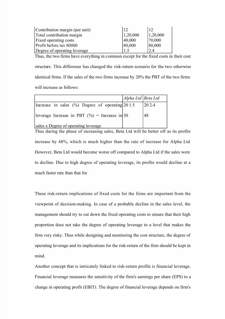
Contribution margin (per unit) 12 12

Total contribution margin 1,20,000 1,20,000

Fixed operating costs 40,000 70,000

Profit before tax 80000 80,000 80,000

Degree of operating leverage 1.5 2.4

Thus, the two firms have everything in common except for the fixed costs in their cost

structure. This difference has changed the risk-return scenario for the two otherwise

identical firms. If the sales of the two firms increase by 20% the PBT of the two firms

will increase as follows:

Alpha Ltd Beta Ltd

Increase in sales (%) Degree of operating

leverage Increase in PBT (%) = Increase in

sales x Degree of operating leverage

20 1.5

30

20 2.4

48

Thus during the phase of increasing sales, Beta Ltd will be better off as its profits

increase by 48%, which is much higher than the rate of increase for Alpha Ltd

However, Beta Ltd would become worse off compared to Alpha Ltd if the sales were

to decline. Due to high degree of operating leverage, its profits would decline at a

much faster rate than that for

These risk-return implications of fixed costs for the firms are important from the

viewpoint of decision-making. In case of a probable decline in the sales level, the

management should try to cut down the fixed operating costs to ensure that their high

proportion does not take the degree of operating leverage to a level that makes the

firm very risky. Thus while designing and monitoring the cost structure, the degree of

operating leverage and its implications for the risk-return of the firm should be kept in

mind.

Another concept that is intricately linked to risk-return profile is financial leverage.

Financial leverage measures the sensitivity of the firm's earnings per share (EPS) to a

change in operating profit (EBIT). The degree of financial leverage depends on firm's



capital structure. Higher the usage of debt financing in its capital structure higher the

fixed financing costs (the interest) and higher will be its degree of financial leverage.

As the degree of operating leverage determines the operating risk of the business,

the degree of financial leverage determines its financial risk. Together they go on to

determine the overall risk of the business. To contain the risk within manageable

limits, a firm should either have a low degree of operating leverage or a low degree of

financial leverage. The possibility of bankruptcy increases if both the degree of

operating leverage and degree of financial leverage are high. Since financial leverage

relates to the capital structure of a firm it has been taken up in detail in the chapter on

capital structure.

DECISIONS USING BREAKEVEN ANALYSIS

The CVP analysis is a very handy tool to understand the relationship that exists

between the elements of financial decision-making—cost, volume, and profit. Some

of these decisions that are facilitated by the CVP analysis are discussed below:

Planning for a Target Level of Profit

All firms work on specific targets of sales, production, and profit. It is desirable to

know the level of sales or production that will generate the required or the target level

of profit. The profit for the firm at breakeven point is zero by definition. If we treat

the desired profit as part of the fixed cost, the breakeven formula can be used to plan

for the target profit level.

Since costs are tax deductible and profit is not, the inclusion of profit in the fixed cost

must be done on pre-tax basis.

With 40% tax (7) a profit before tax (PBT) of Rs 100 will yield Rs 60 {PBT x (1 - T)}

only. The volume required for a target profit of x can be calculated as follows:

XFixed Cost +---------



I-T

Target Sales =--------------------------------- X sales

Sales-variable costs

Target Sales

Target Quantity = ------------------

Selling PlaceSelling Place

Target % capacity utilization = ----------------------

Capacity Sales

The select data from the breakeven analysis of SG Footwear is reproduced in Table 3-

5 below:

Table 3-5 Select breakeven point data: SG Footwear

(Rs lakh)

Capacity Revenue 8400.00

Current level of Sales 5040.00Variable cost 3517.20 (69.79%)

Contribution Margin 1522.80 (30.21%)

Fixed Cost 1290.00

Profit Before Tax 232.80

Assuming a tax rate of 40%, the level of sales SG Footwear needs to achieve to

generate a post tax profit of Rs 500 lakh can be calculated by using Equation 3-2.

x

Fixed Cost + --------1-T

Target Sales = ------------------------x Sales

Sale – Variable Cost

500.00

1290.00 + 0.60

-------------------------- x 5040.00 = Rs 7027.58 lacs

1522.80

cvp and breakeven analysis

Documents