CVEN 5161

Advanced Mechanics of Materials I

Instructor: Kaspar J. Willam

Revised Version of Class Notes

Fall 2003

Chapter 1

Preliminaries

The mathematical tools behind stress and strain are housed in Linear Algebra and Vec-tor and Tensor Analysis in particular. For this reason let us revisit established conceptswhich hopefully provide additional insight into matrix analysis beyond the mere mechanicsof elementary matrix manipulation.

1.1 Vector and Tensor Analysis

(a) Cartesian Description of Vectors:

Forces, displacements, velocities and accelerations are objects F ,u,v,a ∈ <3 whichmay be represented in terms of a set of base vectors and their components. In thefollowing we resort to cartesian coordinates in which the base vectors ei form an or-thonormal set which satisfies

ei · ej = δij ∀ i, j = 1, 2, 3 where [δij] = 1 =

1 0 00 1 00 0 1

(1.1)

where the Kronecker symbol [δij] = 1 designates the unit tensor. Consequently, theforce vector may be expanded in terms of its components and base vectors,

F = F1e1 + F2e2 + F3e3 =3∑i

Fiei → Fiei (1.2)

The last expression is a short hand index notation in which repeated indices infersummation over 1,2,3.

In matrix notation, the inner product may be written in the form,

F = [F1, F2, F3]t

e1

e2

e3

→ [Fi] =

F1

F2

F3

(1.3)

1

where we normally omit the cartesian base vectors and simply represent a vector interms of its components (coordinates).

(b) Scalar Product (Dot Product) of Two Vectors: (F · u)∈ <3

The dot operation generates the scalar:

W = (F · u) = (Fiei) · (ujej) = Fiujδij = Fiui (1.4)

Using matrix notation, the inner product reads F tu = Fiui, where F t stands for a rowvector and u for a column vector. The mechanical interpretation of the scalar productis a work or energy measure with the unit [1 J = 1Nm]. The magnitude of the dotproduct is evaluated according to,

W = |F ||u| cos θ (1.5)

where the absolute values |F | = (F ·F )12 and |u| = (u ·u)

12 are the Euclidean lengths

of the two vectors. The angle between two vectors is defined as

cos θ =(F · u)

|F ||u|(1.6)

The two vectors are orthogonal when θ = ±π2,

(F · u) = 0 if F 6= 0 and u 6= 0 (1.7)

In other terms there is no work done when the force vector is orthogonal to the dis-placement vector.

Note: Actually, the mechanical work is the line integral of the scalar product betweenthe force vector times the displacement rate, W =

∫F · du. Hence the previous

expressions were based on the assumption that the change of work along the integrationpath is constant.

(c) Vector Product (Cross Product) of Two Vectors: (x× y)∈ <3:

The cross product generates the vector z which is orthogonal to the plane spanned bythe two vectors x,y according to the right hand rule:

z = x× y = xiyj(ei × ej) where |z| = |x||y| sin θ (1.8)

In 3-d the determinant scheme is normally used for the numerical evaluation of the crossproduct. Its components may be written in index notation with respect to cartesiancoordinates

zp = εpqrxqyr (1.9)

2

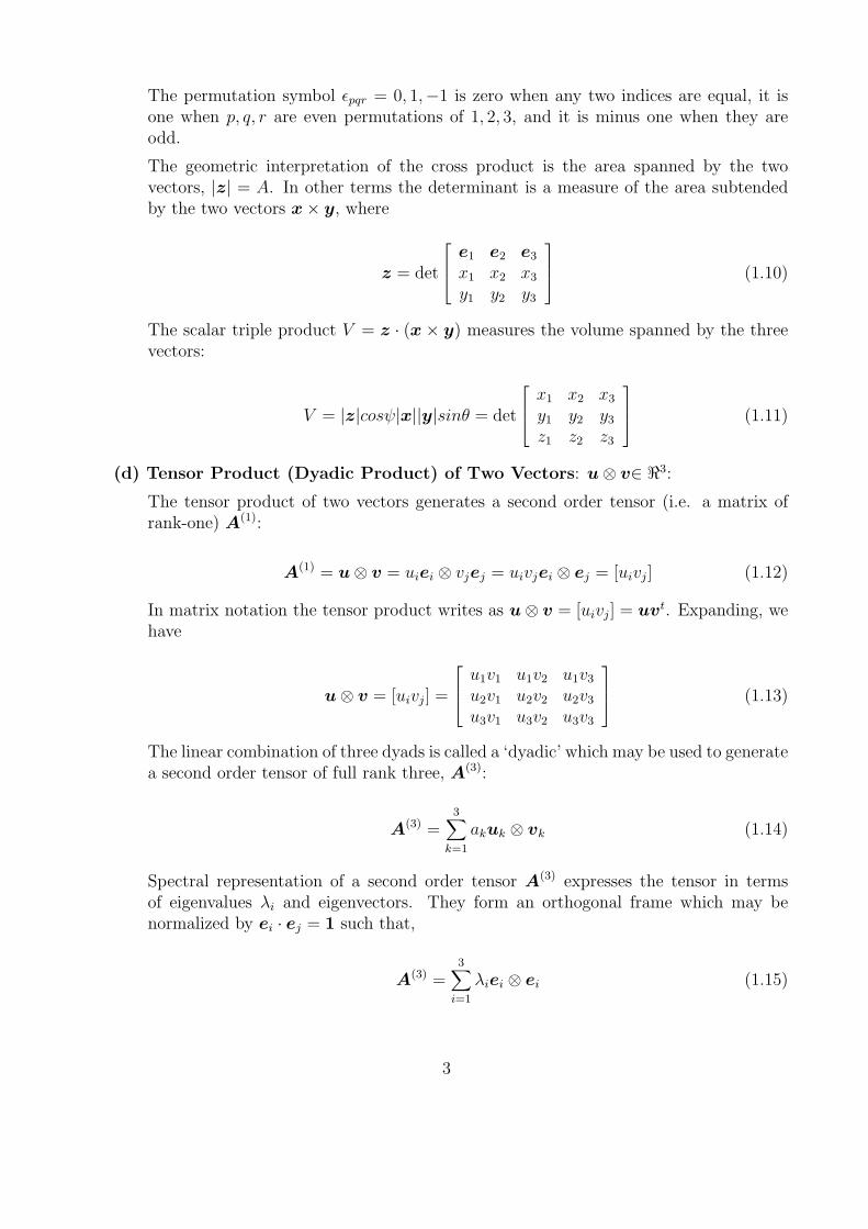
The permutation symbol εpqr = 0, 1,−1 is zero when any two indices are equal, it isone when p, q, r are even permutations of 1, 2, 3, and it is minus one when they areodd.

The geometric interpretation of the cross product is the area spanned by the twovectors, |z| = A. In other terms the determinant is a measure of the area subtendedby the two vectors x× y, where

z = det

e1 e2 e3

x1 x2 x3

y1 y2 y3

(1.10)

The scalar triple product V = z · (x × y) measures the volume spanned by the threevectors:

V = |z|cosψ|x||y|sinθ = det

x1 x2 x3

y1 y2 y3

z1 z2 z3

(1.11)

(d) Tensor Product (Dyadic Product) of Two Vectors: u⊗ v∈ <3:

The tensor product of two vectors generates a second order tensor (i.e. a matrix ofrank-one) A(1):

A(1) = u⊗ v = uiei ⊗ vjej = uivjei ⊗ ej = [uivj] (1.12)

In matrix notation the tensor product writes as u⊗ v = [uivj] = uvt. Expanding, wehave

u⊗ v = [uivj] =

u1v1 u1v2 u1v3

u2v1 u2v2 u2v3

u3v1 u3v2 u3v3

(1.13)

The linear combination of three dyads is called a ‘dyadic’ which may be used to generatea second order tensor of full rank three, A(3):

A(3) =3∑

k=1

akuk ⊗ vk (1.14)

Spectral representation of a second order tensor A(3) expresses the tensor in termsof eigenvalues λi and eigenvectors. They form an orthogonal frame which may benormalized by ei · ej = 1 such that,

A(3) =3∑

i=1

λiei ⊗ ei (1.15)

3

Note: the tensor product increases the order of of the resulting tensor by a factor two.Hence the tensor product of two vectors (two tensors of order one) generates a secondorder tensor, and the tensor product of two second order tensors generates a fourthorder tensor, etc.

(e) Coordinate Transformations:

Transformation of the components of a vector from a proper orthonormal coordinatesystem e1, e2, e3 into another proper orthonormal system E1,E2,E3 involves the op-erator Q of direction cosines. In 3-d we have,

Q = cos(Ei · ej) (1.16)

where the matrix of direction cosines is comprised of,

e1 e2 e3

E1 cos(E1e1) cos(E1e2) cos(E1e3)E2 cos(E2e1) cos(E2e2) cos(E2e3)E3 cos(E3e1) cos(E3e2) cos(E3e3)

(1.17)

The Q-operator forms a proper orthonormal transformation, Q−1 = Qt i.e. it satisfiesthe conditions,

Qt ·Q = 1 and det Q = 1 (1.18)

In the case of 2-d, this transformation results in a plane rotation around the x3-axis,i.e.

Q =

cos θ sin θ 0− sin θ cos θ 0

0 0 1

(1.19)

where θ ≥ 0 for counterclockwise rotations according the right hand rule. Conse-quently, the transformation of the components of the vector F from one coordinatesystem into another,

F = Q · F and inversely F = Qt · F (1.20)

The (3× 3) dyadic forms an array A of nine scalars which follows the transformationrule of second order tensors,

A = Q ·A ·Qt and inversely A = Qt · A ·Q (1.21)

This distinguishes the array A to form a second order tensor.

4

(f) The Stress Tensor:

Considering the second order stress tensor as an example when A = σ then the lineartransformation results in the Cauchy theorem, that mapping of the stress tensor ontothe plane with the normal n results in the traction vector t:

σt · n = t or σjinj = ti (1.22)

This transformation may be viewed as a projection of the stress tensor onto the planewith the normal vector nt = [n1, n2, n3], where

σ =

σ11 σ12 σ13

σ21 σ22 σ23

σ31 σ32 σ33

(1.23)

with the understanding that σ = σt is symmetric in the case of Boltzmann continua.The Cauchy theorem states that the state of stress is defined uniquely in terms of thetraction vectors on three orthogonal planes t1, t2, t3 which form the nine entries in thestress tensor. Given the stress tensor, the traction vector is uniquely defined on anyarbitrary plane with the normal n, the components of which are,

t = σt · n =

σ11n1 + σ21n2 + σ31n3

σ12n1 + σ22n2 + σ32n3

σ13n1 + σ23n2 + σ33n3

(1.24)

The traction vector t may be decomposed into normal and tangential components onthe plane n,

σn = n · t = n · σt · n (1.25)

and(τn)2 = |t|2 − σ2

n = t · t− (n · t)2 (1.26)

which are the normal stress and the tangential stress components on that plane.

(g) Eigenvalues and Eigenvectors:

There exist a nonzero vector np such that the linear transformation σt ·np is a multipleof np. In this case n‖t we talk about principal direction n = np in which the tangentialshear components vanish,

σt · np = λnp (1.27)

The eigenvalue problem is equivalent to stating that

[σt − λ1] · np = 0 (1.28)

5

For a non-trivial solution np 6= 0 the matrix (σt−λ1) must be singular. Consequently,det(σt − λ1) = 0 generates the characteristic polynomial

p(λ) = det(σt − λ1) = λ3 − I1λ2 − I2λ− I3 = 0 (1.29)

where the three principal invariants are,

I1 = trσ = σii = σ1 + σ2 + σ3 (1.30)

I2 =1

2[trσ2 − (trσ)2] =

1

2[σijσij − σ2

ii] = −[σ1σ2 + σ2σ3 + σ3σ1] (1.31)

I3 = det σ = σ1σ2σ3 (1.32)

According to the fundamental theorem of algebra, a polynomial of degree 3 has exactly3 roots, thus each matrix σ ∈ <3 has 3 eigenvalues λ1 = σ1, λ2 = σ2, λ3 = σ3. If apolynomial with real coefficients has some non-real complex zeroes, they must occurin conjugate pairs.

Note: all three eigenvalues are real when the stress tensor σ = σt is symmetric.

Further, det(σt − λ1) = (−1)3 det(λ1 − σt), thus the roots of both characteristicequations are the same.

(i) Similarity Equivalence:

Similarity transformations, i.e. triple products of the form

σ = S−1 · σ · S (1.33)

preserve the spectral properties of σ. In other terms, if σ ∼ σ, then the characteristicpolynomial of σ is the same as that of σ.

p(λ) = det(σ − λ1) = det(S−1 · σ · S − λS−1 · S) = det(σ − λ1) (1.34)

(j) Orthonormal or Unitary Equivalence:

A matrix U ∈ <3 is unitary (real orthogonal) if

U t ·U = 1 and U t = U−1 (1.35)

with det U = 1 for proper orthonormal transformations. Consequently each unitarytransformation is also a similarity transformation, σ ∼ σ, where

σ = U−1 · σ ·U = U t · σ ·U (1.36)

but not vice versa.

Note: Unitary equivalence distinguishes second order tensors from matrices of orderthree, since it preserves the length of the tensor σ in any coordinate system. In otherterms, a zero length tensor in one coordinate system will have zero length in any othercoordinate system.

6

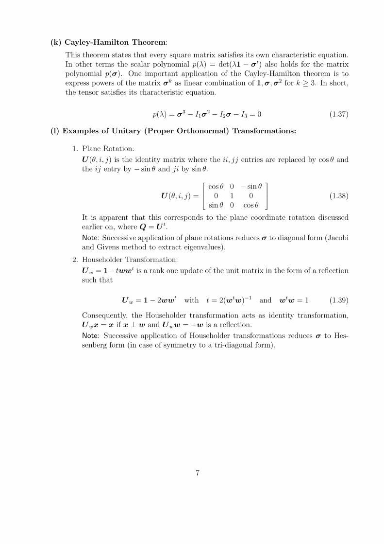
(k) Cayley-Hamilton Theorem:

This theorem states that every square matrix satisfies its own characteristic equation.In other terms the scalar polynomial p(λ) = det(λ1 − σt) also holds for the matrixpolynomial p(σ). One important application of the Cayley-Hamilton theorem is toexpress powers of the matrix σk as linear combination of 1,σ,σ2 for k ≥ 3. In short,the tensor satisfies its characteristic equation.

p(λ) = σ3 − I1σ2 − I2σ − I3 = 0 (1.37)

(l) Examples of Unitary (Proper Orthonormal) Transformations:

1. Plane Rotation:

U (θ, i, j) is the identity matrix where the ii, jj entries are replaced by cos θ andthe ij entry by − sin θ and ji by sin θ.

U (θ, i, j) =

cos θ 0 − sin θ0 1 0

sin θ 0 cos θ

(1.38)

It is apparent that this corresponds to the plane coordinate rotation discussedearlier on, where Q = U t.

Note: Successive application of plane rotations reduces σ to diagonal form (Jacobiand Givens method to extract eigenvalues).

2. Householder Transformation:

Uw = 1− twwt is a rank one update of the unit matrix in the form of a reflectionsuch that

Uw = 1− 2wwt with t = 2(wtw)−1 and wtw = 1 (1.39)

Consequently, the Householder transformation acts as identity transformation,Uwx = x if x ⊥ w and Uww = −w is a reflection.

Note: Successive application of Householder transformations reduces σ to Hes-senberg form (in case of symmetry to a tri-diagonal form).

7

Chapter 2

Differential Equilibrium:

The balance laws of continuum mechanics comprise statements as follows:

1. Balance of Linear Momentum.

2. Balance of Angular Momentum.

3. Balance of Mass.

4. Balance of Energy (First Law of Thermodynamics).

“ Forces” are measured indirectly through their action on deformable solids.Distributed forces include:

• b : body force/unit volume(i. e. density).

• tn : surface traction.

Integrating the distributed forces over part I of the body B defines the resultant force vector

fI =∫BI

b dv +∫

∂BItn da (2.1)

The Cauchy Lemma : states pointwise balance of surface tractions across any surface inthe interior of the body.

tn(x,n) + tn(x,−n) = 0 (2.2)

ortn(x,n) = −tn(x,−n) (2.3)

2.1 The Cauchy Theorem:

The stress tensor is a linear mapping of the stress vector tn onto the normal vector n.

tn = σσσσt(x) · n (2.4)

8

In indicial notation,ti = σji nj (2.5)

Considering elementary tetrahedron:

tn = n1 t1 + n2 t2 + n3 t3 (2.6)

The stress tensor σσσσ is simply composed of the coordinates of stress vectors on three mutuallyorthogonal planes

σσσσ =

σ11 σ12 σ13

σ21 σ22 σ23

σ31 σ32 σ33

(2.7)

In our notation of σij, the first subscript i refers to normal direction of the area element andthe subscript j refers to the direction of the traction.

Considering the equilibrium in x1 direction :∑fx1 = 0.

t1da = σ11n1da+ σ21n2da+ σ31n3da (2.8)

thent1 = σ11n1 + σ21n2 + σ31n3 (2.9)

With the help of the Divergence Theorem we find

∫∂B σji nj da =

∫B σji,j dv (2.10)

The equation of motion by Cauchy states the balance between the body forces and surfacetractions when inertia forces remain negligible:∫

Bbidv +

∫∂Btni da = 0 (2.11)

can be rewritten asσji,j + bi = 0 (2.12)

“Cauchy’s First Theorem” states pointwise equilibrium in the interior of the body.

In the dynamic case, the balance equations generalize to

σji,j + bi =D

Dt(ρxi) (2.13)

9

2.2 Balance of Linear Momentum:

Linear momentum is defined as:i =

∫BIρ u dv (2.14)

Application of Newton’s second law∑

f = m · a to the control volume of the body

D

Dti = f (2.15)

“Dynamic equilibrium” or the balance of linear momentum may be expressed as∫BI

D

Dt(ρu)dv =

∫∂BI

b dv +∫BI

tn da (2.16)

or in terms of ∫BI

(b − D

Dt(ρx))dv +

∫∂B

tn da = 0 (2.17)

2.3 Balance of Angular Momentum

Angular momentum involves

h0 =∫BI

(x× ρu) dv (2.18)

where the pole is assumed to coincide with the origin x0 = 0. The moment of the distributedforces is

m0 =∫B(x× b)dv +

∫∂B

(x× tn) da (2.19)

The balance of angular momentum states

Dh0

Dt= m0 (2.20)

D

Dt

∫B(x× ρu)dv =

∫B

(x× b)dv +∫

∂B(x× tn) da (2.21)

The divergence theorem yields for the last term above∫B[x× (b + div σσσσt − ρu)]dv + 2

∫B(1× σσσσt)dv = 0 (2.22)

Application of the first theorem of Cauchy : b + div σσσσt − ρ DDt

u = 0, we get

1× σσσσt = 0 → σσσσ = σσσσt (2.23)

which states that the stress tensors symmetric, i.e. σσσσt = σσσσ, i.e. the “Boltzmann Postulate”of a symmetric stress tensor.

In index notation :eijkσjk = 0 → σjk = σkj (2.24)

this results inσ23 − σ32 = 0; σ31 − σ13 = 0; σ12 − σ21 = 0 (2.25)

10

2.4 Alternative Stress Measures:

Consider that the force vector is the same on the deformed and undeformed surface areas

f = tn da = σσσσt n da = ΣΣΣΣt N dA (2.26)

then ΣΣΣΣ denotes the “First Piola-Kirchhoff” stress tensor with respect to the undeformedsurface area.

From Nanson’s formula n da = J F−t N dA we get

J σσσσt F−t N dA = ΣΣΣΣt N dA (2.27)

orΣΣΣΣ = J F−1 σσσσ (2.28)

which shows the loss of symmetry of the first Piola-Kirchhoff stress, ΣΣΣΣ 6= ΣΣΣΣt .

The “Second Piola-Kirchoff” stress is defined as

S = ΣΣΣΣ F−t = J F−1 σσσσ F−t (2.29)

orS = F−1 ττττ F−t (2.30)

in which ττττ = J σσσσ denotes the Kirchoff stress. From σσσσ = 1J

F S Ft , we can relate the

Kirchhoff stress to the second Piola-Kirchhoff stress

ττττ = F S Ft (2.31)

Balance of Linear Momentum:

In the current reference configuration

D

Dt(∫Bρ x dv) =

∫B

b dv +∫

∂Btn da (2.32)

in which tn = σσσσt · n. In the initial undeformed reference configuration this reads∫B0

ρ0Dx

DtdV =

∫B0

b0 dV +∫

∂B0

ΣΣΣΣt N dA (2.33)

2.5 Mechanical Stress Power:

Conjugate forms of kinematic and static measures lead to an inner product form of stressand deformation rate. Using the divergence theorem the spatial description of momentumbalance leads to the local statement of differential equilibrium :

div σσσσt + b = ρ DvDt

(2.34)

11

If this equation of motion is scalar multiplied with v and integrated over the entire body,we get ∫

B(div σσσσt) · v dv +

∫B

b · v dv =∫Bρ v · v dv (2.35)

With (div σσσσt) · v = div(σσσσt · v) − σσσσ : d, we get∫B

b · v dv +∫

∂Bt · v da =

∫Bσσσσ : d dv +

D

Dt

∫Bρv.v dv (2.36)

Using the divergence theorem the material description of momentum balance leads to thelocal statement of differential equilibrium :

Div Σt + b0 = ρ0D VDt

(2.37)

If this equation is multiplied with the weighing function v and integrated over the entirebody in the reference configuration, we find∫

B0

(Div ΣΣΣΣt) · v dV +∫B0

b0 · v dV =∫B0

ρ0D

DtV · v dV (2.38)

After analogous calculation to the spatial description we get∫B0

b0 · v dV +∫

∂B0

(Σt ·N) · v dA =∫B0

ΣΣΣΣt : F dV +∫B0

ρ0 V · v dV (2.39)

Stress Power:

Considering ττττ = ρ σσσσ, the inner product of stress and the rate of deformation leads toalternative representations in terms of conjugate values

Wσ =1

ρ0

ττττ : d =1

ρσσσσ : d =

1

ρ0

ΣΣΣΣt : F =1

ρ0

S : EG (2.40)

12

Chapter 3

Kinematics of Continua

Abstract

In this Chapter, the motion and deformation of continua will be reviewed:

• Kinematics of Motion : X,x,u.

• Kinematics of Deformation: F,E, e.

3.1 Kinematics of Motion:

The motion of continua may be described in two ways:

(a) In the Lagrangean description the continuous medium is considered to be comprised ofparticles the motion of which is of primary interest. The Lagrangean coordinates describethe spatial variation of a field variable in terms of the particle position X in the initial ref-erence configuration.

(b) In the Eulerian description the location is of primary interest which is occupied by parti-cles at the time t. The Eulerian coordinates describe the spatial variation of a field variablein terms of the spatial domain x occupied by the continuum.

Usually, Eulerian coordinates are used to study the motion of fluids through a fixed spatialdomain, while Lagrangean coordinates are primarily used to follow the particle motion ofsolids. In sum, every function expressed in Lagrangean coordinates may be transformed intoEulerian coordinates and vice-versa.

• In Lagrangean coordinates, which are known as material coordinates, the initial posi-tion of a particle is used to label the material particle under consideration:

– Lagrange Coordinates : (Material Description)

X = XAeA where A = 1, 2, 3 (3.1)

where eA denote the orthogonal material base vectors.

13

• In Eulerian coordinates, which are known as spatial coordinates, the location is usedto label the material position of a material particle at the time t:

– Euler Coordinates : (Spatial Description)

x = xiei where i = 1, 2, 3 (3.2)

where ei denote the orthogonal spatial base vectors.

The scalar temperature field may be represented by :

– Lagrangean Coordinates : T = T (X, t) - material description.

– Eulerian Coordinates : T = T (x, t) - spatial description.

In Lagrangean coordinates the temperature at every material point is studied, while inEulerian coordinates the temperature at a fixed location which the material occupiesis of primary interest.

During the motion, the deformation gradient is defined as:

F =∂x

∂X⇒ dx = F · dX (3.3)

where X denotes the position of a arbitrary material particle in the (initial) reference con-figuration, and x its position in the current configuration. The determinant detF is knownas the Jacobian of the deformation gradient. Therefore the mapping of the material lineelement dX from the reference into the current configuration is defined by : dxi

dxj

dxk

=

dxi

dXA

dxi

dXB

dxi

dXCdxj

dXA

dxj

dXB

dxj

dXCdxk

dXA

dxk

dXB

dxk

dXC

dXA

dXB

dXC

(3.4)

Restriction: it can be shown that the Jacobian J = detF 6= 0 defines the volume change.

In other terms, for rigid body motions, J = 1 in the absence of deformation. For a uniqueone-to-one defomation map detF 6= 0 must hold.

3.2 Polar Decomposition:

The polar decomposition theorem states that the deformation gradient F may be decomposeduniquely into a positive definite tensor and a proper orthogonal tensor, i.e. the right U orleft V stretch tensor plus the rotation R tensor.

14

1. Right Polar Decomposition: F = R ·Uwhere: detR = 1, Rt ·R = 1, R ·Rt = 1,

Note, U = Ut such that λU > 0 and

U2 = Ut ·Rt ·R ·U = Ft · F (3.5)

2. Left Polar Decomposition: F = V ·Rwhere:

V2 = F · Ft = V ·R ·Rt ·V (3.6)

Note V = Vt such that λV > 0 and λV = λU

The Physical Meaning of U and V is:

• Right Decomposition: dx = R · U · dX, which means that dX is first stretched andthen rotated.

• Left Decomposition: dx = V ·R · dX, which means that dX is first rotated and thenstretched.

If F is non-singular ⇒ detF 6= 0 and positive, then there exists a unique decomposition intoa proper orthogonal tensor R and a positive definite tensor U or V.

3.3 Strain Definition:

In this section alternative strain measures are introduced to define strain.

Extensional Engineering Strain:

In the uniaxial case the engineering strain is simply the length change normalized by theoriginal length:

εeng =∆L

L0

=L− L0

L0

. (3.7)

The triaxial extension of the engineering strain will be dicussed later on in the context ofinfinitesimal deformations.

Extensional Logarithmic Strain [Hencky, 1928]:

In the uniaxial case the logarithmic strain is defined by integrating the stretch rate:

εln =∫ L

L0

d`

`= ln

L

L0

= lnλ where λ =L

L0

. (3.8)

15

The Triaxial extension of the logarithmic strain may be described in two ways:

• Lagrangean format : εεεεUln = lnU, with principal coordinates which are defined by eU

• Eulerian format : εεεεVln = lnV, with principal Coordinates which are defined by eV wherethe two base triads are related by the rotation eV = R · eU .

Spectral Representation :

U =3∑

i=1

λi eiU ⊗ ei

U and εεεεUln =3∑

i=1

(lnλi) eiU ⊗ ei

U (3.9)

V =3∑

i=1

λi eiV ⊗ ei

V and εεεεVln =3∑

i=1

(lnλi) eiV ⊗ ei

V (3.10)

3.3.1 Lagrangean Strain Measures:

If dS is the infinitesimal line element measuring the initial distance of two points, and if dsis the current length of the line element between those two points, then one can define theextensional deformation is defined as:

ds2 − dS2 = dxt · dx− dXt · dX = dXt · [Ft · F− 1] · dX (3.11)

The term in bracket defines the Green strain which is related to the right stretch tensor by:

EG = 12

[Ft · F− 1] = 12

[U2 − 1] (3.12)

In indicial form,

F =∂xi

∂XA

ei ⊗ eA (3.13)

U2 =∂xi

∂XA

· ∂xi

∂XB

(3.14)

EGAB =

1

2(∂xi

∂XA

· ∂xi

∂XB

− δAB) (3.15)

Generalized Lagrangean Strain [Doyle-Erickson 1956]:

The generalized format of Lagrangean strain is defined as:

Em = 1m

[Um − 1] (3.16)

where m is an integer, where

m=0, defines the logarithmic strain:

E0 = lnU (3.17)

16

m=1, defines the Biot strain:E1 = [U− 1] (3.18)

m=2, defines the Green strain:

E2 = 12

[U2 − 1] (3.19)

Using the definition of stretch λ = LL0

, then 1-dim examples of extensional strain measuresinclude :

E0 = lnλ = ln LL0

E1 = λ− 1 = L−L0

L0

E2 = 12

[λ2 − 1] = 12

[L2−L2

0

L20

]

(3.20)

We see that E0 reduces to the logarithmic Hencky strain, E1 to the engineering strain ,and E2 to the Green strain.

Strain-Displacement Relationship

If X and x are the initial and current position vectors of a particle, then the displacementvector defines the relation between X and x as:

x = x(X, t) = u(X, t) + X (3.21)

The deformation gradient is related to the displacement gradient,

∂x

∂X=∂u

∂X+ 1 = H + 1 where

∂u

∂X= H (3.22)

With F = H + 1 the material stretch tensor reads,

U2 = Ft · F = 1 + H + Ht + Ht ·H (3.23)

and the Lagrangean strain-displacement relationship defines the Green strain in terms of:

EG = 12[1 + H + Ht + Ht ·H] (3.24)

3.3.2 Eulerian Strain Measures :

Parallel to the material description, the extensional deformation may be defined in terms ofspatial coordinates,

ds2 − dS2 = dxt · [1− F−t · F−1] · dx (3.25)

The term in the bracket defines the Almansi strain which is related to the left stretch tensorby,

eA = 12

[1− F−t · F−1] = 12

[1− (V2)−1] (3.26)

Generalized Eulerian Strain [Doyle-Erickson 1956]:

17

The generalized Eulerian strain tensor is defined as:

em = 1m

(Vm − 1) (3.27)

where m is an integer.

m=0, defines the spatial format of the logarithmic strain:

e0 = lnV (3.28)

m=-1, defines the spatial format of the Biot strain

e−1 = [1−V−1] (3.29)

m=-2, defines the Almansi strain

e−2 = 12

[1−V−2] (3.30)

using the inverse stretch measure 1λ

= L0

L, then 1-dim examples include:

e0 = −ln 1λ

= ln LLo

e−1 = 1− 1λ

= L−L0

L

e−2 = 12

[1− 1λ2 ] = 1

2[L2−L2

0

L2 ]

(3.31)

We see that in 1-dim e0 coincides with the logarithmic Hencky strain, e1 corresponds to theengineering strain in which the length change is however normalized by the current length,while the Almansi strain e−2 corresponds to the Green strain E2.

Strain-Displacement Relationship

In the spatial description the motion is described by the inverse relation:

u(x, t) = x−X(x, t) (3.32)

The spatial displacement gradient is defined as:

h =∂u

∂x= 1− ∂X

∂x= 1− F−1 (3.33)

orF−1 = 1− h (3.34)

V−2 = F−t · F−1 = 1− h− ht + ht · h (3.35)

Substituting into the expression of the Almansi strain eA renders the Eulerian strain-displacementrelationship in the form,

eA = 12[h + ht − ht · h] (3.36)

18

3.3.3 Infinitesimal Deformations and Rotations:

If the displacement gradient H is very small, then detH << 1 ⇒ det(Ht ·H) ' 0. Thus,

εεεε =1

2[H + Ht] ' 1

2[h + ht] (3.37)

In short, in the case of “Infinitesimal Deformations” the spatial and the material displace-ment gradients coincide,

∂u

∂X∼ ∂u

∂x(3.38)

Additive decomposition into symmetric and skew-symmetric components leads to

H =∂u

∂X=

1

2[H + Ht] +

1

2[H−Ht] (3.39)

where the symmetric part defines the traditional linearized strain tensor

εij =1

2[∂ui

∂Xj

+∂uj

∂Xi

] (3.40)

and where the skew-symmetric part defines the infinitesimal rotation tensor

ωij =1

2[∂ui

∂Xj

− ∂uj

∂Xi

] (3.41)

such that εij = εji and ωij = −ωji.

19

Chapter 4

Elastic Material Models

Linear elasticity is the main staple of material models in solids and structures. The statement‘ut tensio sic vis’ attributed to Robert Hooke (1635-1703) characterizes the behavior ofa linear spring in which the deformations increase proportionally with the applied forcesaccording to the anagram ‘ceiiinossstuv’. The original format of Hooke’s law included thegeometric properties of the wire test specimens, and therefore the spring constant did exhibita pronounced size effect. The definition of the modulus of elasticity E, where

σ = E ε (4.1)

is attributed to Thomas Young (1773-1829). He expressed the proportional materialbehavior through the notion of a normalized force density and a normalized deformationmeasure, though the original formulation also did not entirely eliminate the size effect.The tensorial character of stress was established by Cauchy, who defined the triaxial stateof stress by three traction vectors using the celebrated tetraeder argument of equilibrium.The state of stress is described in terms of Cartesian coordinates by the second order tensor

σ(X, t) =

σ11 σ12 σ13

σ21 σ22 σ23

σ31 σ32 σ33

(4.2)

The conjugate state of strain is a second order tensor with Cartesian coordinates,

ε(X, t) =

ε11 ε12 ε13ε21 ε22 ε23ε31 ε32 ε33

(4.3)

which is normally expressed in terms of the symmetric part of the displacement gradient, ifwe restrict our attention to infinitesimal deformations. In the case of non-polar media wemay confine our attention to stress measures, which are symmetric according to the axiomof L. Boltzmann,

σ = σt or σij = σji (4.4)

and the conjugate strain measures

ε = εt or εij = εji (4.5)

20

where i = 1, 2, 3 and j = 1, 2, 3. As a result, the eigenvalues are real-valued and consti-tute the set of principal stresses and strains with zero shear components in the principaleigen-directions of the second order tensor. In contrast, non-symmetric stress and strainmeasures may exhibit complex conjugate principal values and maximuum normal stress andstrain components in directions with non-zero shear components characteristic for micropolarCosserat continua.Restricting this exposition to symmetric stress and strain tensors they may be cast intovector form using the Voigt notation of crystal physics.

σ(X, t) =[σ11 σ22 σ33 τ12 τ23 τ31

]t(4.6)

andε(X, t) =

[ε11 ε22 ε33 γ12 γ23 γ31

]t(4.7)

where τij = σij, γij = 2εij,∀i 6= j. The vector form of stress and strain will allow us toformulate material models in matrix notation used predominantly in engineering, (some ofthe properties of second order tensors and basic tensor operations are expanded in AppendixI).

4.1 Linear Elastic Material Behavior:

Generalization of the scalar format of Hooke’s law is based on the notion that the triaxialstate of stress is proportional to the triaxial state of strain through the linear transformation,

σ = E : ε or σij = Eijklεkl (4.8)

Considering the symmetry of the stress and strain, the elasticity tensor involves in general36 elastic moduli. This may be further reduced to 21 elastic constants, if we invoke majorsymmetry of the elasticity tensor, i.e.

E = E t or Eijkl = Eklij with Eijkl = Eijlk and Eijkl = Ejikl (4.9)

The task of identifying 21 elastic moduli is simplified if we consider specific classes of sym-metry, whereby orthotropic elasticity involves nine, and transversely anisotropic elasticityfive elastic moduli.

1. Isotropic Linear Elasticity

In the case of isotropy the fourth order elasticity tensor has the most general represen-tation,

E = ao1⊗ 1 + a11⊗1 + a21⊗1 or Eijkl = aoδijδkl + a1δikδjl + a2δilδjk (4.10)

where 1 = [δij] stands for the second order unit tensor. The three parameter expres-sion may be recast in terms of symmetric and skew symmetric fourth order tensorcomponents as

E = ao1⊗ 1 + b1I + b2Iskew (4.11)

21

where the symmetric fourth order unit tensor reads

I =1

2[1⊗1 + 1⊗1] or Iijkl =

1

2[δikδjl + δilδjk] (4.12)

and the skewed symmetric one

Iskew =1

2[1⊗1− 1⊗1] or Iskew

ijkl =1

2[δikδjl − δilδjk] (4.13)

Because of the symmetry of stress and strain the skewed symmetric contribution isinactive, b2 = 0, thus isotropic linear elasticity the material behavior is fully describedby two independent elastic constants. In short, the fourth order material stiffnesstensor reduces to

E = Λ1⊗ 1 + 2GI or Eijkl = Λδijδkl +G[δikδjl + δilδjk] (4.14)

where the two elastic constants Λ, G are named after Gabriel Lame (1795-1870).

Λ =E ν

[1 + ν][1− 2ν](4.15)

denotes the cross modulus, and

G =E

2[1 + ν](4.16)

designates the shear modulus which have a one-to-one relationship with the modulusof elasticity and Poisson’s ratio, E, ν.

In the absence of initial stresses and initial strains due to environmental effects, thelinear elastic relation reduces to

σ = Λ[trε]1 + 2Gε or σij = Λεkkδij + 2Gεij (4.17)

Here the trace operation is the sum of the diagonal entries of the second order tensorcorresponding to double contraction with the identity tensor trε = εkk = 1 : ε.

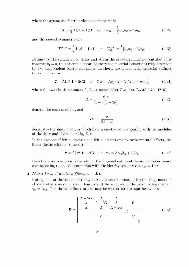
2. Matrix Form of Elastic Stiffness: σ = E ε

Isotropic linear elastic behavior may be cast in matrix format, using the Voigt notationof symmetric stress and strain tensors and the engineering definition of shear strainγij = 2εij. The elastic stiffness matrix may be written for isotropic behavior as,

E =

Λ + 2G Λ ΛΛ Λ + 2G Λ 0Λ Λ Λ + 2G

G0 G

G

(4.18)

22

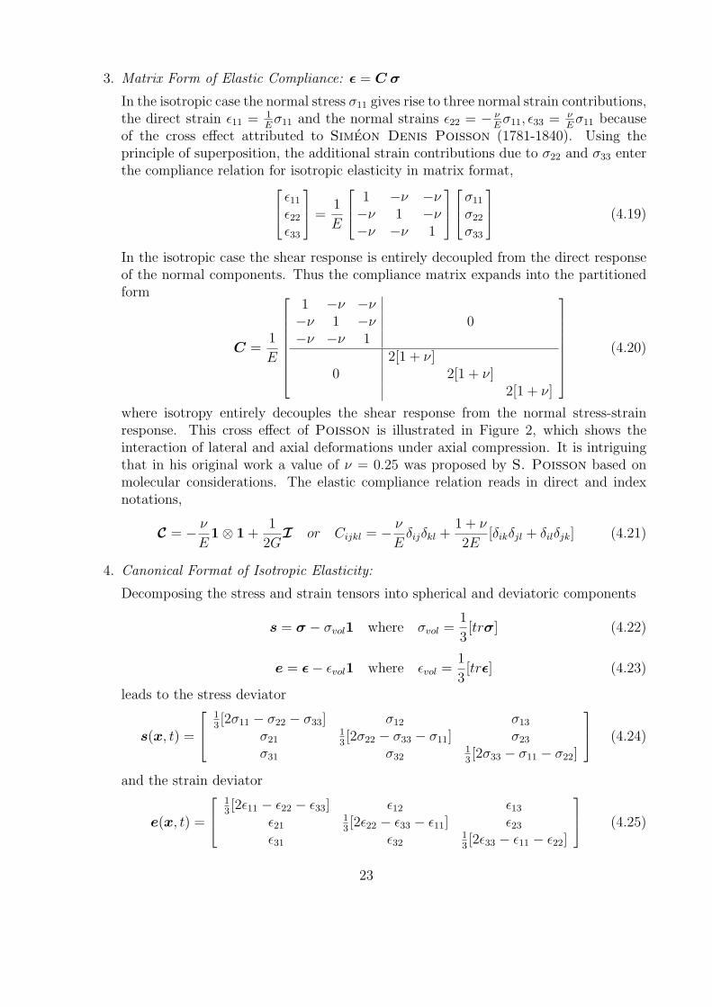
3. Matrix Form of Elastic Compliance: ε = C σ

In the isotropic case the normal stress σ11 gives rise to three normal strain contributions,the direct strain ε11 = 1

Eσ11 and the normal strains ε22 = − ν

Eσ11, ε33 = ν

Eσ11 because

of the cross effect attributed to Simeon Denis Poisson (1781-1840). Using theprinciple of superposition, the additional strain contributions due to σ22 and σ33 enterthe compliance relation for isotropic elasticity in matrix format, ε11

ε22

ε33

=1

E

1 −ν −ν−ν 1 −ν−ν −ν 1

σ11

σ22

σ33

(4.19)

In the isotropic case the shear response is entirely decoupled from the direct responseof the normal components. Thus the compliance matrix expands into the partitionedform

C =1

E

1 −ν −ν−ν 1 −ν 0−ν −ν 1

2[1 + ν]0 2[1 + ν]

2[1 + ν]

(4.20)

where isotropy entirely decouples the shear response from the normal stress-strainresponse. This cross effect of Poisson is illustrated in Figure 2, which shows theinteraction of lateral and axial deformations under axial compression. It is intriguingthat in his original work a value of ν = 0.25 was proposed by S. Poisson based onmolecular considerations. The elastic compliance relation reads in direct and indexnotations,

C = − ν

E1⊗ 1 +

1

2GI or Cijkl = − ν

Eδijδkl +

1 + ν

2E[δikδjl + δilδjk] (4.21)

4. Canonical Format of Isotropic Elasticity:

Decomposing the stress and strain tensors into spherical and deviatoric components

s = σ − σvol1 where σvol =1

3[trσ] (4.22)

e = ε− εvol1 where εvol =1

3[trε] (4.23)

leads to the stress deviator

s(x, t) =

13[2σ11 − σ22 − σ33] σ12 σ13

σ2113[2σ22 − σ33 − σ11] σ23

σ31 σ3213[2σ33 − σ11 − σ22]

(4.24)

and the strain deviator

e(x, t) =

13[2ε11 − ε22 − ε33] ε12 ε13

ε2113[2ε22 − ε33 − ε11] ε23

ε31 ε3213[2ε33 − ε11 − ε22]

(4.25)

23

which have the property trs = 0 and tre = 0. The decomposition decouples thevolumetric from the distortional response, because of the underlying orthogonality ofthe spherical and deviatoric partitions, s : [σvol1] = 0 and e : [εvol1] = 0. Thedecoupled response reduces the elasticity tensor to the scalar form,

σvol = 3Kεvol and s = 2Ge (4.26)

in which the bulk and the shear moduli,

K =E

3[1− 2ν]= Λ +

2

3G and G =

E

2[1 + ν]=

3

2[K − Λ] (4.27)

define the volumetric and the deviatoric material stiffness.

Consequently, the internal strain energy density expands into the canonical form oftwo decoupled contributions

2W = σ : ε = [σvol1] : [εvol1] + s : e = 9Kε2vol + 2Ge : e (4.28)

such that the positive strain energy argument delimits the range of possible values ofPoisson’s ratio to −1 ≤ ν ≤ 0.5

4.1.1 Linear Isotropic Elasticity under Thermal Strain

In the case of isotropic material behavior, with no directional properties, the size of a repre-sentative volume element may change due to thermal effects or shrinkage and swelling, butit will not distort. Consequently, the expansion is purely volumetric, i.e. identical in alldirections. Using direct and index notation, the additive decomposition of strain into elasticand initial volumetric components, ε = εe +εo, leads to the following extension of the elasticcompliance relation:

ε = − ν

E[trσ]1 +

1

2Gσ + εo1 or εij = − ν

Eσkkδij +

1

2Gσij + εoδij (4.29)

where εo = α∆T1 denotes the initial volumetric strain e.g. due to thermal expansion whenthe temperature changes from the reference temperature, ∆T = T −To. The inverse relationreads

σ = Λ[trε]1 + 2Gε− 3εoK1 or σij = Λεkkδij + 2Gεij − 3εoKδij (4.30)

Rewriting this equation in matrix notation we have:σ11

σ22

σ33

=

K + 43G K − 2

3G K − 2

3G

K − 23G K + 4

3G K − 2

3G

K − 23G K − 2

3G K + 4

3G

ε11ε22ε33

− 3Kεo

111

(4.31)

Considering the special case of plane stress, σ33 = 0, the stress-strain relations reduce in thepresence of initial volumetric strains to:[

σ11

σ22

]=

E

1− ν2

[1 νν 1

] [ε11ε22

]− E

1− νεo

[11

](4.32)

where the shear components are not affected by the temperature change in the case ofisotropy.

24

4.1.2 Free Thermal Expansion

Under stress free conditions the thermal expansion εo = α[T − To]1 leads to ε = εo, i.e.

ε11 = α[T − To] (4.33)

ε22 = α[T − To] (4.34)

ε33 = α[T − To] (4.35)

Thus the change of temperature results in free thermal expansion, while the mechanicalstress remains zero under zero confinement, σ = E : εe = 0.

4.1.3 Thermal Stress under Full Kinematic Restraint

In contrast to the unconfined situation above, the thermal expansion is equal and oppositeto the elastic strain εe = −εo under full confinement, when ε = 0. In the case of plane stress,the temperature change ∆T = T − To leads to the thermal stresses

σ11 = − E

1− να[T − To] (4.36)

σ22 = − E

1− να[T − To] (4.37)

25