J Glob Optim (2012) 53:663–681DOI 10.1007/s10898-011-9730-1

Curvature-constrained directional-cost paths in the plane

Alan J. Chang · Marcus Brazil · J. Hyam Rubinstein ·Doreen A. Thomas

Received: 10 September 2010 / Accepted: 17 May 2011 / Published online: 31 May 2011© Springer Science+Business Media, LLC. 2011

Abstract This paper looks at the problem of finding the minimum cost curvature-constrained path between two directed points where the cost at every point along the pathdepends on the instantaneous direction. This generalises the results obtained by Dubins forcurvature-constrained paths of minimum length, commonly referred to as Dubins paths. Weconclude that if the reciprocal of the directional-cost function is strictly polarly convex, thenthe forms of the optimal paths are of the same forms as Dubins paths. If we relax the strict polarconvexity to weak polar convexity, then we show that there exists a Dubins path which isoptimal. The results obtained can be applied to optimising the development of undergroundmine networks, where the paths need to satisfy a curvature constraint and the cost of devel-opment of the tunnel depends on the direction due to the geological characteristics of theground.

Keywords Curvature constraint · Dubins paths · Path optimization · Directional cost ·Anisotropic velocity · Pontryagin’s minimum principle

A. J. Chang (B) · D. A. ThomasDepartment of Mechanical Engineering, The University of Melbourne, Victoria 3010,Australiae-mail: a.chang5@pgrad.unimelb.edu.au

D. A. Thomase-mail: doreen.thomas@unimelb.edu.au

M. BrazilDepartment of Electrical and Electronic Engineering, The University of Melbourne,Victoria 3010, Australiae-mail: brazil@unimelb.edu.au

J. H. RubinsteinDepartment of Mathematics and Statistics, The University of Melbourne,Victoria 3010, Australiae-mail: rubin@ms.unimelb.edu.au

123

664 J Glob Optim (2012) 53:663–681

1 Introduction

The problem studied in this paper is that of finding a minimum cost curvature-constrainedpath between two directed points where the cost at every point along the path depends on theinstantaneous direction. The problem is properly defined later in Sect. 2.3. In short, we wishto solve the problem of:

minE∈Ppq

∫

E

c(α)ds

for some given directional-cost function c(α), where Ppq denotes the set of all curvature-constrained paths between two directed points p and q .

The motivation for studying this problem stems from the issue of directional faulting inthe ground where an underground mine is to be developed. The resulting problem is alsointeresting in its own right. The costs associated with an underground mine tunnel are mostlymade up of development, haulage, and other maintenance costs. The faulting results in regionsof ground where the cost of development (both tunnelling and support) is significantly morein certain directions than others due to a required increase in time and resources to safelytunnel and provide extra support. Haulage and maintenance on the other hand is generallyindependent of the faulting, and simply depends on the length. The formulation we adopt inthis paper is able to handle all of these costs, as the effect of haulage and maintenance wouldbe just adding a constant to the directional-cost function of development.

Variations of the problem of finding the shortest curvature-constrained path between twodirected points introduced by Dubins [5] have been extensively studied in the literature. Awell-known extension is the problem of allowing the path to correspond to a vehicle whichcan move both forwards and backwards in [10]. More relevant extensions include [11] wherethe path crosses weighted regions of different velocity and [8] where the velocity of theairplane is affected by a constant wind. Also, [3] and [12] study the problem of classifyingwhen a particular Dubins path is optimal for a given pair of directed points.

The major tools employed in tackling this problem are adapted from Dubins [5] andBoissonnat [1]. By transforming the minimum weighted length problem into a minimumtime problem, it becomes clear that the reciprocal of the directional-cost function becomesthe object of interest in characterising the forms of optimal paths that have to be considered.We denote this reciprocal as the velocity function, and introduce the concepts of strict-ness and polar convexity. A polarly convex (PC) velocity function means that the triangleinequality holds for cost of paths. This paper focuses on the forms of optimal paths thatresult when we consider PC velocity functions. A strict velocity function is one where wedo not have an interval of directions where the triangle inequality is satisfied by equality.We distinguish between strictly polarly convex (SPC) where the strict triangle inequalityholds, and weakly polarly convex (WPC) where the triangle inequality could be satisfied byequality.

The structure of this paper is as follows. The first step is to apply Pontryagin’s MinimumPrinciple as in [1] to conclude that any optimal path must only consist of maximum curva-ture arcs and straight segments, given any strict velocity function. We then prove some basicproperties of the cost of paths subjected to SPC velocity functions. Applying these propertiesallows us to generalise the results of [5] to conclude that the forms of optimal paths are thesame as Dubins paths, if the velocity function is SPC. Finally, we show that there alwaysexist an optimal path which is a Dubins path, if the velocity function is WPC.

123

J Glob Optim (2012) 53:663–681 665

Empirical studies of the relationship between rock strength and fault orientation relativeto the tunnelling direction such as [6] and [7] demonstrate that there is a relationship betweenthe required support cost and the direction in which the tunnel is developed. As the problemof finding shortest underground mine networks with this additional consideration is not yetsolved, common practice is to use experience and intuition to account for this. Understandingexactly how to solve this problem mathematically will enable the geological information tobe incorporated into existing algorithms such as in [2]. By incorporating directional depen-dency of cost into the algorithms, the resulting output will be much more accurate and helpfulfor the preliminary design of underground mine networks.

During the course of writing this paper, it was brought to our attention that similar workwas being done concurrently by Dolinskaya in [4]. The application in their case was for navalpath planning but is mathematically formulated in similar manner. In their work, they con-sider an anisotropic minimum radius of curvature function, as well as an anisotropic velocityfunction. The motivation and future direction in which their work is being developed isdifferent from our work.

2 Background

We first define what we mean by curvature-constrained paths.

2.1 Curvature-constrained paths

In the following, a, b ∈ R2 and p, q ∈ R

2 × R/2π . Also, C1 (resp. C2) will mean that thefirst (resp. second) derivative exists and is continuous.

A path from a to b is a directed piecewise C1 curve from a to b. We parametrise our pathsby arc-length, E : [0, t f ] → R

2 with E(0) = a and E(t f ) = b. The direction α ∈ R/2πat a differentiable point of a path E(t) is given by the polar angle of the tangent at the pointin the direction of increasing t . At the endpoints, the directions are taken as the respectivelimits of α.

Given a minimum turning circle radius R > 0, a curvature-constrained path between twodirected points p, q is a C1 path that is piecewise C2, where the absolute curvature every-where along the path is bounded by 1/R, and the given directions at the start and end pointscoincide with the directions of p and q respectively. Without loss of generality, we assumethe minimum turning circle radius R = 1 in this entire paper. Let C be a label denoting anarc of maximum curvature of length less than 2π . Let S be a label denoting a straight linesegment.

A CS-path is a curvature-constrained path E : [0, t f ] → R2 such that there exist t0, . . . , tn

such that t0 = 0 and tn = t f , ti−1 < ti for i = 1, . . . , n, where E is not twice differentiableat ti for i = 1, . . . , n, and each subpath Ei : [ti−1, ti ] → R

2 is either a C arc or S seg-ment. The form of such a CS-path is then the sequence of C and S labels in ascending orderof i . The sense of a C can be further specified using the labels L and R for left-turning andright-turning arcs respectively. In the form of a CS-path, any consecutive C arcs must be ofopposite sense due to the condition that the CS-path is differentiable but not twice differen-tiable at the point in between two consecutive labels. This condition also implies that therewill never be consecutive S labels in the form of a CS-path.

Dubins [5] first studied the problem of finding the shortest curvature-constrained pathbetween any two given directed points in R

2 and proved the following theorem.

123

666 J Glob Optim (2012) 53:663–681

Theorem 1 Given any two directed points p, q ∈ R2 × R/2π and a prescribed minimum

radius of curvature R, the shortest curvature-constrained path is a CS-path with one of thefollowing forms.

1. CSC2. CCC3. any degeneracies of the two forms

where C denotes a C arc of length greater than πR

CS-paths of the forms described in Theorem 1 will be referred to as Dubins paths. Note thatthere are at most 6 distinct Dubins paths for any pair p, q because of the different sense ofthe C arcs, but they do not all necessarily exist and degeneracies may occur.

Theorem 1 was later proved again by Boissonnat et al. [1] by formulating it as a con-trol problem and applying Pontryagin’s Minimum Principle. A more detailed version of [1]can be found in [13]. We summarise the key ideas here as we will need to use the controlformulation for one of the main results.

2.2 Control formulation

We summarise the necessary background for applying Pontryagin’s Minimum Principlefrom [9]. Note that we are presenting a simplified version of the principle as that is suf-ficient for this paper. We also present the minimum principle as opposed to the maximumprinciple originally formulated in [9], since it is commonly stated in the minimum principleform in the current literature.

Consider a system of differential equations with prescribed boundary conditions as in (1),where x(t) denotes the states of the system, and the piecewise continuous function u :[0, T ] → U is the control we want to choose, for some convex and compact U . The func-tions f j are continuous in the variables x, u and continuously differentiable with respectto x .

x j = f j (x(t), u(t)), x(0) = xi , x(T ) = x f for j = 1, . . . , n

where x(t) = (x1(t), . . . , xn(t)) and z denotes dz/dt(1)

We restrict ourselves to only considering the controls that satisfy the boundary conditions.Such controls will be referred to as admissible controls. Since we are interested in time opti-mality, the relevant cost function J (u) is of the form shown in (2) below. We aim to find anadmissible control which minimises J , the total time to start from xi and end at x f .

J (u) =T∫

0

dt (2)

To state the minimum principle, we need to introduce another system of equations in theauxiliary variables ψ1, . . . , ψn as follows.

ψ j = −n∑

k=1

∂ f j

∂xkψk for j = 1, . . . , n (3)

Let the Hamiltonian H be defined as follows.

H(ψ, x, u) =n∑

k=1

ψk fk(x, u) (4)

123

J Glob Optim (2012) 53:663–681 667

For fixed ψ, x, H is a function of u. Let M(ψ, x) denote the lower bound of the values of H .

M(ψ, x) = infu∈U

H(ψ, x, u) (5)

We can then state the minimum principle as follows.

Theorem 2 If u(t) is an optimal admissible control, there exists a nonzero continuous vectorfunction ψ(t) satisfying (3), such that ∀t ∈ [0, T ],1. H(ψ(t), x(t), u(t)) = M(ψ(t), x(t)) = constant2. M(ψ(t), x(t)) ≤ 0

2.3 Directional cost

We now introduce directional-cost to curvature-constrained paths. Some basic terms whichwill be used consistently throughout this paper are defined in this section. Let R+ denote theset of all strictly positive real numbers {x ∈ R : x > 0}.

A directional-cost function is a continuous, piecewise C2 function c : R/2π → R+. Thecorresponding velocity function v : R/2π → R+ is given by v(α) = 1/c(α), which is alsocontinuous and piecewise C2. The interpretation of the velocity function in the context ofdirectional-cost is a measure of the distance that can be travelled in the direction α at the costof one unit.

Given a path E and a directional-cost function c,

– the length of E, L(E), is given by L(E) = ∫E ds.

– E is degenerate if it has zero length.– the cost of E, T (E), is given by T (E) = ∫

E c(α)ds

Let Ppq denote the set of all curvature-constrained paths between two directed points pand q . An optimal path from p to q is a path E ∈ {P ∈ Ppq : T (P) ≤ T (Q)∀Q ∈ Ppq}.

Our problem involves identifying an optimal path between given start and end directedpoints, subject to a given velocity function. It can be seen that by the way the problem hasbeen posed, the problem of finding the minimum total cost path is equivalent to a problemof finding the minimum total time for a vehicle to travel from p to q if the velocity of thevehicle depends on the direction it is facing at any point in time. This is the motivation forcalling the reciprocal of the directional-cost function a velocity function.

3 Application of Pontryagin’s minimum principle

In [1], the problem is formulated as a minimum time problem by having a cost function thatis simply the integral of 1 over the path. We could simply modify the cost function to bethe integral of c(α) instead, and indeed this will yield the same result. However, we chooseto formulate the problem differently, keeping the cost function the same, while incorporat-ing the directional-cost by making the velocity of the vehicle v(α). Both these approachesare mathematically identical, but the latter provides additional insight which is helpful formotivating the later sections. We first consider velocity functions that are strict as definedbelow.

Given a velocity function v, let K = vv′′ − 2v′2 − v2 which is defined for almost all α

since v is piecewise C2. Since K (α) = κ(α)(v2 + v′2) 32 where κ(α) is the signed curvature

of the polar function v, the sign of K gives the sign of the curvature of v. In particular, if

123

668 J Glob Optim (2012) 53:663–681

K = 0 on an interval [α1, α2], this corresponds to v being a straight line in polar coordinatesfrom (v(α1), α1) to (v(α2), α2). We discuss the implications of this in Sect. 4.

A velocity function is strict if there are no (non-trivial) intervals [α1, α2] where K (α) =0 ∀α ∈ [α1, α2].Lemma 1 For any given pair of directed points p, q ∈ R

2 × [0, 2π) and strict velocityfunction v, any optimal path is necessarily a CS-path.

Proof First, let us consider the case where v is strict and C2 everywhere. Let the statesx(t), y(t) and α(t) represent the coordinates and direction of the path at time t . Let u(t) bethe control variable that governs the instantaneous curvature at time t . Recall that withoutloss of generality, we let the minimum radius of curvature be 1 and hence, u ∈ [−1, 1]. Letp = (xi , yi , αi ) and q = (x f , y f , α f ). Our problem can then be formulated in the followingmanner.

x = v(α) cos(α), x(0) = xi , x(T ) = x f

y = v(α) sin(α), y(0) = yi , y(T ) = y f

α = v(α)u, α(0) = αi , α(T ) = α f (6)

J (u) = ∫ T0 dt (7)

Letψx , ψy andψα be the corresponding auxiliary variables. From (3) we get the following.

ψx = 0

ψy = 0

ψα = ψxv(α) sin α − ψxv′(α) cosα − ψyv(α) cosα − ψyv

′(α) sin α − v′(α)ψαu (8)

From (4) we get an expression for the Hamiltonian H as follows.

H = ψxv(α) cos(α)+ ψyv(α) sin(α)+ v(α)ψαu (9)

Define λ and φ by λ =√ψ2

x + ψ2y ≥ 0, tan φ = ψy/ψx , φ ∈ [0, 2π) so that ψx =

λ cosφ,ψy = λ sin φ. Observe that ψx and ψy are constant on [0, T ], so it follows that λand φ are also constant on [0, T ]. We can then rewrite H and ψα as follows.

H = λv(α) cos(α − φ)+ v(α)ψαu (10)

ψα = λv(α) sin(α − φ)− λv′(α) cos(α − φ)− v′(α)ψαu (11)

By the minimum principle (Theorem 2), in order for the control u to be optimal, either:

1. ∂H/∂u �= 0 ⇒ u = ±1 so the path is an arc of radius 1; or2. ∂H/∂u = v(α)ψα = 0 ⇒ ψα = 0

We now show that u = 0 is for the second case. Since ψα = 0, we have ψα = 0 as well.Note that λ �= 0 since λ = 0 ⇒ (ψx , ψy, ψα) = (0, 0, 0), which violates the condition thatthis vector must be non-zero. Rearranging (11) then gives the following.

α ={φ + arctan(v′(α)/v(α)) orφ + arctan(v′(α)/v(α))+ π

Differentiating either of the two possibilities for α with respect to t and recalling α =v(α)u gives the following.

u(vv′′ − 2v′2 − v2) = 0 (12)

123

J Glob Optim (2012) 53:663–681 669

Recall that K = vv′′ − 2v′2 − v2 where the sign of K gives the sign of the curvature of v.When K �= 0, it follows that u = 0. Where we are unable to guarantee u = 0 is at some timet∗ when K (α(t∗)) = 0. Since v is strict, for any α∗ where K (α∗) = 0, there exists ε > 0 suchthat K (α) �= 0 ∀α ∈ (α∗ − ε, α∗ + ε) \ {α∗}. If u(t∗) �= 0, α is changing when t = t∗ sinceα = u. Hence, there exists δ > 0 such that for any t ∈ (t∗, t∗ + δ), K (α(t)) �= 0. Hence,u is never non-zero for time intervals of non-zero length. Alternatively, u(t∗) = 0 wouldcorrespond to an S subpath in the direction α(t∗). Hence, any optimal path is a CS-path if vis C2 everywhere and there are only a finite number of points where K = 0.

Suppose that v is piecewise C2 instead of C2 everywhere. It follows that there are only afinite number of directions αi where v(αi ) is not twice differentiable. By applying a similarargument as above for the directions where K = 0, we conclude that any optimal path is aCS-path if v is a strict velocity function.

4 Polarly convex velocity function

In the previous section, we established that any optimal path is a CS-path, given a strictvelocity function v. We are interested in establishing the forms of optimal paths for agiven v. In [5], Dubins paths are established to be optimal through Euclidean geometricarguments. Here, these arguments are no longer available to us due to the nature of the veloc-ity function. However, if we assume that the velocity function v is strictly polarly convex,by which we mean that v is strict and it maps out the boundary of a convex region in R

2

(in polar coordinates), then it can be shown that the strict triangle inequality holds, which issufficient to re-establish the main results of Dubins.

In this section, we show that strict polar convexity of the velocity function implies thatthe forms of optimal curvature-constrained paths are the same as Dubins paths. However,an example is given to show that a shortest curvature-constrained path is not necessarilyan optimal path for a particular choice of start and end directed points, even if the velocityfunction is strictly polarly convex. Furthermore, we show that by relaxing the strict convexityto weak convexity, there still always exists a Dubins path which is an optimal path.

The practical implication of these results is that the optimal path can be constructed bycomputing the cost of the (up to 6) Dubins paths between any two directed points, andselecting the path of lowest cost among the Dubins paths. For the original Dubins problemof constructing the shortest path, there have been works done to exactly determine whichof the Dubins paths are optimal based on the relative positions and orientations of directedpoints, such as in [3] and [12]. Based on their results, the partitioning of the configurationspace is non-trivial, and hence, if we consider the extension to their problem of introducinga polarly convex velocity function, it would be infeasible to obtain an elegant partitioning tothe configuration space in general.

4.1 Polar convexity

A straight path ab is a path from a to b where α is constant along the entire pathand equal to αab. A polygonal path is a path a1 . . . ak+1 made up of k straight pathsa1a2, a2a3, . . . , akak+1.

Given a velocity function v, the velocity set V is the subset of R2 enclosed by the polar

plot of v represented in polar coordinates by Given a velocity function v, the velocity set Vis the subset of R

2 enclosed by the polar plot of v represented in polar coordinates by

123

670 J Glob Optim (2012) 53:663–681

V = {e = (ε(α), α) : ε(α) ∈ [0, v(α)]∀α ∈ [0, 2π)}The velocity set can be interpreted in the context of directional-cost as the set of all pointsthat can be reached by a single straight path from the origin at the cost of no greater than oneunit.

Let conv(S) denote the convex hull of the set S. A velocity function v is

– polarly convex (PC) if V = conv(V ).

– strictly polarly convex (SPC) if it is PC and strict.– weakly polarly convex (WPC) if it is PC but not strict.

– polarly non-convex (PNC) if it is not PC.

Let E2 = (R2, ‖ · ‖e) where ‖ · ‖e is the Euclidean norm. If v is symmetric i.e. v(α) =

v(α + π), the cost of a straight path ab in E2 subject to a PC function v is the same as the

norm of ab in a normed space R2 equipped with a norm ‖ · ‖v that has a unit ball V since

T (ab) = L(ab)/v(αab) = ‖b−a‖v . By relaxing the symmetry property of the normed spacebut retaining the triangle inequality property, it can be seen that the cost of straight paths andpolygonal paths subject to any PC velocity function v satisfies the triangle inequality

T (aeb) ≥ T (ab)

Similarly, the cost of straight paths and polygonal paths subject to an SPC velocity functionsatisfies the strict triangle inequality that is

T (aeb) > T (ab) if e does not lie on ab (13)

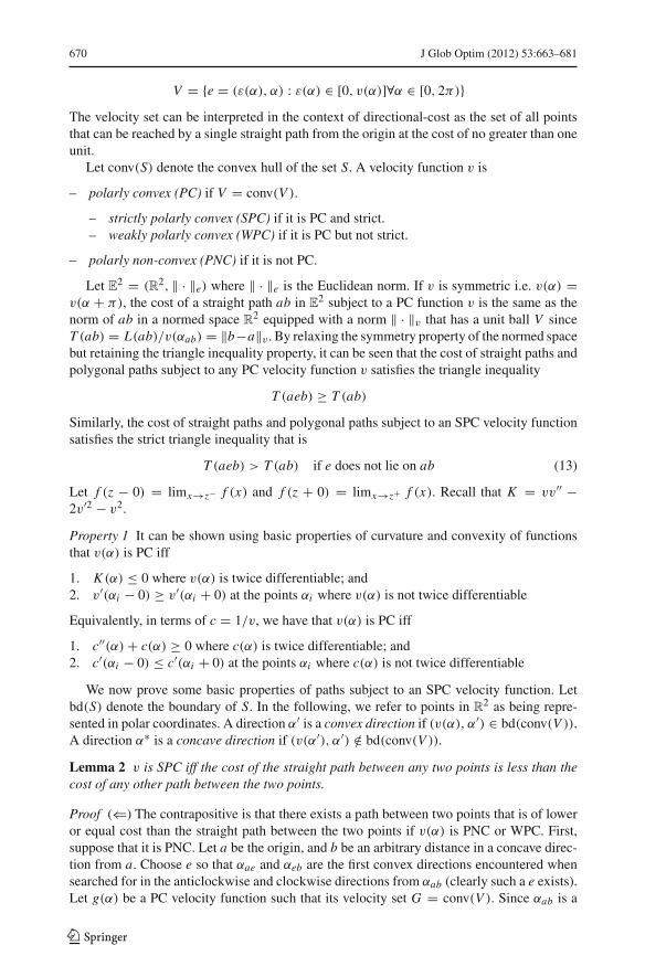
Let f (z − 0) = limx→z− f (x) and f (z + 0) = limx→z+ f (x). Recall that K = vv′′ −2v′2 − v2.

Property 1 It can be shown using basic properties of curvature and convexity of functionsthat v(α) is PC iff

1. K (α) ≤ 0 where v(α) is twice differentiable; and2. v′(αi − 0) ≥ v′(αi + 0) at the points αi where v(α) is not twice differentiable

Equivalently, in terms of c = 1/v, we have that v(α) is PC iff

1. c′′(α)+ c(α) ≥ 0 where c(α) is twice differentiable; and2. c′(αi − 0) ≤ c′(αi + 0) at the points αi where c(α) is not twice differentiable

We now prove some basic properties of paths subject to an SPC velocity function. Letbd(S) denote the boundary of S. In the following, we refer to points in R

2 as being repre-sented in polar coordinates. A direction α′ is a convex direction if (v(α), α′) ∈ bd(conv(V )).A direction α∗ is a concave direction if (v(α′), α′) /∈ bd(conv(V )).

Lemma 2 v is SPC iff the cost of the straight path between any two points is less than thecost of any other path between the two points.

Proof (⇐) The contrapositive is that there exists a path between two points that is of loweror equal cost than the straight path between the two points if v(α) is PNC or WPC. First,suppose that it is PNC. Let a be the origin, and b be an arbitrary distance in a concave direc-tion from a. Choose e so that αae and αeb are the first convex directions encountered whensearched for in the anticlockwise and clockwise directions from αab (clearly such a e exists).Let g(α) be a PC velocity function such that its velocity set G = conv(V ). Since αab is a

123

J Glob Optim (2012) 53:663–681 671

Fig. 1 T (ab) ≤ T (ae2b) ≤ T (ae1e2e3b) ≤ · · · ≤ T (E)

concave direction, g(αae) = v(αae) and g(αeb) = v(αeb) while g(αab) > v(αab). Let Tvand Tg denote the costs of paths subjected to velocity functions v and g respectively. Notethat e was chosen so that Tg(aeb) = Tg(ab), so Tv(aeb) = Tg(aeb) = Tg(ab) < Tv(ab).On the other hand if v(α) is WPC, it follows from its definition that there exists a, b, e wheree does not lie on ab, such that T (aeb) = T (ab).

(⇒) Since v is SPC, the strict triangle inequality (13) holds. Let E(t) be a path with E(0) =a and E(t f ) = b that is not ab. Let e = E(t f /2) so if e lies on ab then T (aeb) = T (ab),otherwise T (aeb) > T (ab). Hence in general, T (aeb) ≥ T (ab). This bisection argumentcan be repeated infinitely on the new straight paths generated to show that T (E) ≥ T (ab).The first few steps of this procedure are illustrated diagrammatically in Fig. 1. The conver-gence of this polygonal path to E(t) is guaranteed by the properties of Euclidean space.Observe that since T (ab) = T (E) can only occur if the inequality is an equality at everystep, that would imply that E = ab which is a contradiction and hence, T (ab) < T (E).

A convex path is a piecewise C2 path that lies on the boundary of its own convex hull. Asupporting line to a convex path at a point e along the convex path, is any supporting lineof the convex hull of the path at e. Given a convex path represented by E : [0, t f ] → R

2,an outer normal ne of a point e = E(te) for some te ∈ (0, 1), is the normal unit vector to asupporting line at e that points away from the convex hull. The outer normal also divides thesupporting line at e into two halves, referred to as being the supporting line on a particularside of the outer normal. Note that the outer normal is not unique if e is not a differentiablepoint. For the following arguments, this will not be an issue, as if there are multiple choicesof ne, picking any one will work.

A path lies on the outer side of a convex path if the path is formed by continuouslydeforming the convex path, without entering the convex hull of the convex path,and is notthe convex path itself. It follows from these definitions that a supporting line at any pointalong a convex path E never intersects the interior of the convex hull of E and must alwaysintersect a path that lies on the outer side of E on both sides of the outer normal at that point.

Lemma 3 v is SPC iff the cost of any path lying on the outer side of a convex path is greaterthan the cost of the convex path.

Proof (⇐) The contrapositive is that there exists a path lying on the outer side of a convexpath that is of lower or equal cost than the convex path if v is PNC or WPC. This followsimmediately by applying the proof of Lemma 2 in the (⇐) direction by taking the straightpath to be the convex path.

(⇒) Let E(t) be a convex path with E(0) = a and E(t f ) = b. Let e = E(t f /2) and G(e)be a supporting line at e. Let E1(t) be a path lying on the outer side of E(t) with E1(0) = aand E1(t f ) = b.

By definition, G(e) does not ever intersect the interior of the convex hull of E , but hasto intersect E1 at least once on each side of ne. Pick an intersection point from each side of

123

672 J Glob Optim (2012) 53:663–681

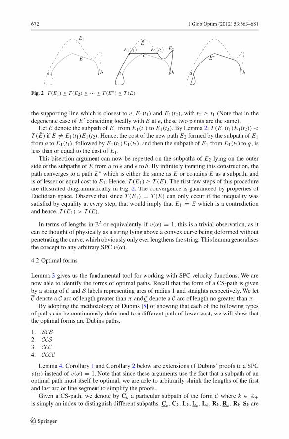
Fig. 2 T (E1) ≥ T (E2) ≥ · · · ≥ T (E∗) ≥ T (E)

the supporting line which is closest to e, E1(t1) and E1(t2), with t2 ≥ t1 (Note that in thedegenerate case of E ′ coinciding locally with E at e, these two points are the same).

Let E denote the subpath of E1 from E1(t1) to E1(t2). By Lemma 2, T (E1(t1)E1(t2)) <T (E) if E �= E1(t1)E1(t2). Hence, the cost of the new path E2 formed by the subpath of E1

from a to E1(t1), followed by E1(t1)E1(t2), and then the subpath of E1 from E1(t2) to q , isless than or equal to the cost of E1.

This bisection argument can now be repeated on the subpaths of E2 lying on the outerside of the subpaths of E from a to e and e to b. By infinitely iterating this construction, thepath converges to a path E∗ which is either the same as E or contains E as a subpath, andis of lesser or equal cost to E1. Hence, T (E1) ≥ T (E). The first few steps of this procedureare illustrated diagrammatically in Fig. 2. The convergence is guaranteed by properties ofEuclidean space. Observe that since T (E1) = T (E) can only occur if the inequality wassatisfied by equality at every step, that would imply that E1 = E which is a contradictionand hence, T (E1) > T (E).

In terms of lengths in E2 or equivalently, if v(α) = 1, this is a trivial observation, as it

can be thought of physically as a string lying above a convex curve being deformed withoutpenetrating the curve, which obviously only ever lengthens the string. This lemma generalisesthe concept to any arbitrary SPC v(α).

4.2 Optimal forms

Lemma 3 gives us the fundamental tool for working with SPC velocity functions. We arenow able to identify the forms of optimal paths. Recall that the form of a CS-path is givenby a string of C and S labels representing arcs of radius 1 and straights respectively. We letC denote a C arc of length greater than π and C denote a C arc of length no greater than π .

By adopting the methodology of Dubins [5] of showing that each of the following typesof paths can be continuously deformed to a different path of lower cost, we will show thatthe optimal forms are Dubins paths.

1. SCS2. CCS3. CCC4. CCCC

Lemma 4, Corollary 1 and Corollary 2 below are extensions of Dubins’ proofs to a SPCv(α) instead of v(α) = 1. Note that since these arguments use the fact that a subpath of anoptimal path must itself be optimal, we are able to arbitrarily shrink the lengths of the firstand last arc or line segment to simplify the proofs.

Given a CS-path, we denote by Ck a particular subpath of the form C where k ∈ Z+is simply an index to distinguish different subpaths. Ck,Ck,Lk,Lk,Lk,Rk,Rk,Rk,Sk are

123

J Glob Optim (2012) 53:663–681 673

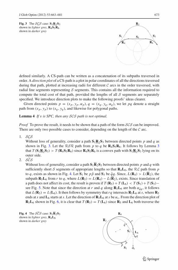
Fig. 3 The SCS case: S1R2S3shown in lighter grey, R4S5R6shown in darker grey

defined similarly. A CS-path can be written as a concatenation of its subpaths traversed inorder. A direction plot of a CS-path is a plot in polar coordinates of all the directions traversedduring that path, plotted at increasing radii for different C arcs in the order traversed, withradial line segments representing S segments. This contains all the information required tocompute the total cost of that path, provided the lengths of all S segments are separatelyspecified. We introduce direction plots to make the following proofs’ ideas clearer.

Given directed points p = (x p, yp, αp), q = (xq , yq , αq), we let pq denote a straightpath from (x p, yp) to (xq , yq), and likewise for polygonal paths.

Lemma 4 If v is SPC, then any SCS path is not optimal.

Proof To prove the result, it needs to be shown that a path of the form SCS can be improved.There are only two possible cases to consider, depending on the length of the C arc.

1. SCSWithout loss of generality, consider a path S1R2S3 between directed points p and q asshown in Fig. 3. Let the RSR path from p to q be R4S5R6. It follows by Lemma 3that T (S1R2S3) > T (R4S5R6) since R4S5R6 is a convex path with S1R2S3 lying on itsouter side.

2. SCSWithout loss of generality, consider a path S1R2S3 between directed points p and q withsufficiently short S segments of appropriate lengths so that R4L6, the RL path from pto q , exists as shown in Fig. 4. Let S1 be p p and S3 be qq . Since, L(R4) > L(R2), thesubpath R5L6 from r to q , where L(R5) = L(R4)− L(R2), exists. Since translation ofa path does not affect its cost, the result is proven if T (R5)+ T (L6) < T (S1)+ T (S3)−see Fig. 5. Note that since the direction at r and q along R5L6 are both αqq , it followsthat L(R5) = L(L6). It then follows by symmetry that rq intersects R5L6 at s, where R5ends at s and L6 starts at s. Let the direction of R5L6 at s be αs . From the direction plot ofR5L6 shown in Fig. 6, it is clear that T (R5) = T (L6) since R5 and L6 both traverse the

Fig. 4 The SCS case: S1R2S3shown in lighter grey, R4L6shown in darker grey

123

674 J Glob Optim (2012) 53:663–681

Fig. 5 The SCS case: Enlargeddiagram with S1S3 shown inlighter grey, R5L6 shown indarker grey

Fig. 6 The SCS case: Directionplot of R5L6 showing R5 and L6traversing the same directions

same set of directions. Let t be the midpoint of qq . By translating S1 so that it now beginsat r , a polygonal path r qq is formed where T (r qq) = 2T (stq) by similar triangles. Byapplying Lemma 3 to the convex arc L6, it follows that T (L6) < T (stq). The result thenfollows since T (R5)+ T (L6) = 2T (L6) < 2T (stq) = T (r qq) = T (S1)+ T (S3).

Corollary 1 If v is SPC, then any CCS path is not optimal.

Proof This result follows from applying similar arguments to those in Lemma 4. If the pathis of the form CCS, the argument for the SCS case can be applied by taking a sufficientlysmall subpath of the CCS path. Otherwise, consider a path L1R2S3 and apply the argumentfor the SCS case, replacing S1 with L1.

Corollary 2 If v is SPC, then any CCC path is not optimal.

Proof This result follows from similar applying arguments to those in Lemma 4 for the SCScase by taking a sufficiently small subpath of the CCC path.

Lemma 5 If v is SPC, then any CCCC path is not optimal.

Proof From Corollary 2, only CCCC cases need to be considered. Without loss of generality,consider LRLR paths from p to q . We will refer to the polygonal path abcd as a validencoding if it corresponds to the centres of the circles corresponding to the arcs of a LRLRpath from p to q traversed in order. Observe that there is no unique LRLR path from pto q , because even though a and d are fixed, the positions of b and c have one degree offreedom. Consider a path E0 = L1R2L3R4 with b = b0 and c = c0 as shown in Fig. 7.

123

J Glob Optim (2012) 53:663–681 675

Fig. 7 E0 = L1R2L3R4 withcorresponding valid encodingab0c0d

By translation, rotation, reflection, and reversing of the path, and corresponding rotation andpossibly reflection of v(α), we can assume that αb0c0 = 0, a = (0, 0), d = (2h, 2k) andαab0 ≥ αc0d .

We first consider the case when αab0 �= αc0d so αab0 > αc0d and look at the effect ofa positive increase on αab. It can be seen that any valid encoding abcd must satisfy theconditions in (14)

cosαab + cosαbc + cosαcd = h

sin αab + sin αbc + sin αcd = k(14)

Since we are interested in how αbc and αcd change as a result of a positive increase in αab,we implicitly differentiate (14) to obtain (15), where dαab > 0.

dαab sin αab + dαbc sin αbc + dαcd sin αcd = 0

dαab cosαab + dαbc cosαbc + dαcd cosαcd = 0(15)

When b = b0, c = c0, (15) yields (16) and (17).

dαab sin αab0 + dαcd sin αc0d = 0

⇒ dαcd = − sin αab0sin αc0d

dαab

(16)

dαab cosαab0 + dαbc + dαcd cosαc0d = 0

⇒ dαab cosαab0 + dαbc − cot αc0d sin αab0 dαab = 0 (17)

⇒ dαbc = sin αab0(cot αc0d − cot αab0)dαab

123

676 J Glob Optim (2012) 53:663–681

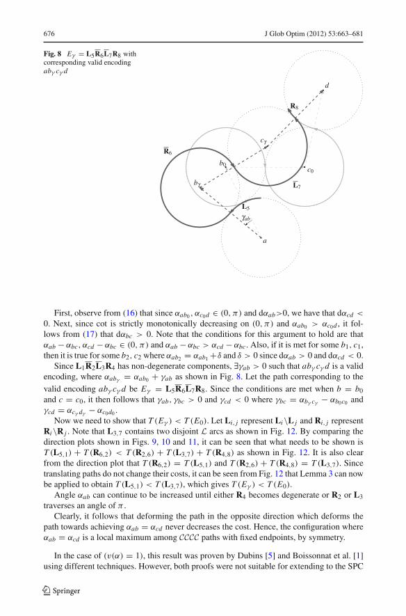
Fig. 8 Eγ = L5R6L7R8 withcorresponding valid encodingabγ cγ d

First, observe from (16) that since αab0 , αc0d ∈ (0, π) and dαab>0, we have that dαcd <

0. Next, since cot is strictly monotonically decreasing on (0, π) and αab0 > αc0d , it fol-lows from (17) that dαbc > 0. Note that the conditions for this argument to hold are thatαab − αbc, αcd − αbc ∈ (0, π) and αab − αbc > αcd − αbc. Also, if it is met for some b1, c1,then it is true for some b2, c2 where αab2 = αab1 +δ and δ > 0 since dαab > 0 and dαcd < 0.

Since L1R2L3R4 has non-degenerate components, ∃γab > 0 such that abγ cγ d is a validencoding, where αabγ = αab0 + γab as shown in Fig. 8. Let the path corresponding to the

valid encoding abγ cγ d be Eγ = L5R6L7R8. Since the conditions are met when b = b0

and c = c0, it then follows that γab, γbc > 0 and γcd < 0 where γbc = αbγ cγ − αb0c0 andγcd = αcγ dγ − αc0d0 .

Now we need to show that T (Eγ ) < T (E0). Let Li, j represent Li\L j and Ri, j representRi\R j . Note that L3,7 contains two disjoint L arcs as shown in Fig. 12. By comparing thedirection plots shown in Figs. 9, 10 and 11, it can be seen that what needs to be shown isT (L5,1) + T (R6,2) < T (R2,6) + T (L3,7) + T (R4,8) as shown in Fig. 12. It is also clearfrom the direction plot that T (R6,2) = T (L5,1) and T (R2,6) + T (R4,8) = T (L3,7). Sincetranslating paths do not change their costs, it can be seen from Fig. 12 that Lemma 3 can nowbe applied to obtain T (L5,1) < T (L3,7), which gives T (Eγ ) < T (E0).

Angle αab can continue to be increased until either R4 becomes degenerate or R2 or L3

traverses an angle of π .Clearly, it follows that deforming the path in the opposite direction which deforms the

path towards achieving αab = αcd never decreases the cost. Hence, the configuration whereαab = αcd is a local maximum among CCCC paths with fixed endpoints, by symmetry.

In the case of (v(α) = 1), this result was proven by Dubins [5] and Boissonnat et al. [1]using different techniques. However, both proofs were not suitable for extending to the SPC

123

J Glob Optim (2012) 53:663–681 677

Fig. 9 Direction plot of E0

Fig. 10 Direction plot of Eγ

Fig. 11 Direction plot of thedifference between E0 and Eγ

v case because there was no easy way to make use of the strict triangle inequality. The proofabove makes use of the strict triangle inequality to extend the result to a general SPC v case.

Finally, putting all of the results together gives the following theorem.

Theorem 3 If v is SPC, then any optimal path is a Dubins path.

We can now apply Theorem 3, to obtain the following result for weakly polarly convex(WPC) functions.

Corollary 3 If v is WPC, then an optimal curvature-constrained directional-cost path canbe found by considering only Dubins paths.

123

678 J Glob Optim (2012) 53:663–681

Fig. 12 Difference between E0 and Eγ

Proof Consider a WPC velocity function v, where c = 1/v. Define a new velocity functionvε = 1/cε by cε = c + ε. Using Property 1, we are able to show that vε is SPC for any ε > 0by using the fact that v is WPC as follows. Clearly c and cε are twice differentiable on thesame intervals of α, and where they are twice differentiable,

c′′ε + cε = c′′ + c + ε ≥ ε > 0

The second condition obviously holds since c′(α) = c′ε(α). This shows that vn is PC and

strict, and hence is SPC. Let T (E) and Tε(E) denote the costs of path E with respect tothe directional-cost functions c and cε respectively. Let p, q be any arbitrary start and enddirected points. Let Dpq denote the set of all Dubins paths from p to q as described in Sect. 2,and recall that Ppq is the set of all curvature-constrained paths from p to q .

Suppose ∃E ∈ Ppq \ Dpq such that T (E) < T (D)∀D ∈ Dpq . Then,

Tε(E) = T (E)+ εL(E)

< T (D), by choosing ε ∈ (0, (T (D)− T (E))/(L(E)))

< Tε(D), ∀D ∈ Dpq

However, Theorem 3 states that there cannot exist such a E since vε is SPC and E /∈ Dpq .Hence, by contradiction, we know that there cannot exist a non-Dubins path which is of lesscost than all other Dubins paths, for any WPC velocity function.

From Theorem 3, it follows that given directed points p, q , the minimum length curva-ture-constrained path and the optimal curvature-constrained directional-cost path are both

123

J Glob Optim (2012) 53:663–681 679

Fig. 13 v(α) as specified in (18)

Fig. 14 L1S2R3 and R4S5L6

Fig. 15 Direction plot ofL1S2R3

Dubins paths if v is SPC. However, Example 1 illustrates that they do not have to be the samepath.

Example 1 Let v(α) be defined as in (18) (shown in Fig. 13).

v(α) =

⎧⎪⎪⎨⎪⎪⎩

49π α

3 + 1, α ∈ [0, 3π

8

]4

9π

( 3π4 − α

)3 + 1, α ∈ ( 3π8 ,

3π4

)1, α ∈ ( 3π

4 , 2π)

(18)

By Property 1, it is easily checked that v(α) is SPC. Let p = (0, 0, π) and q =(−2

√2, 0, 0) be the start and end directed points respectively. The resulting paths L1S2R3

and R4S5L6 are of equal length as shown in Fig. 14. However, the direction plots shownin Figs. 15 and 16 illustrate that they traverse different directions. Hence, T (L1S2R3) <

L(L1S2R3) = L(R4S5L6) = T (R4S5L6). Clearly, there exists ε > 0 such that the shortestcurvature-constrained path from p = (0, ε, π) to q is an RSL path while the optimal pathfrom p to q is an LSR path.

123

680 J Glob Optim (2012) 53:663–681

Fig. 16 Direction plot ofR4S5L6

5 Conclusion

The mathematical problem studied was motivated by the effects of directional faulting ondevelopment cost of underground mine declines. In particular, this meant extending Du-bins [5] result of minimal length paths, to incorporate a directional-cost element. It wasshown that if the velocity function is strictly polarly convex, any optimal path is a Dubinspaths. If the velocity function is polarly convex, then there exists an optimal path which isa Dubins path. The results proved in this paper lay the foundation for future works devel-oping the theory necessary for the design of underground mines taking into considerationanisotropic development and support costs. It has also been seen that it is a useful problemto consider for other practical applications such as naval path planning [4].

From a theoretical viewpoint, this result provides a more general context for the Dubinsresult, in that Dubins paths are actually optimal paths for a much more general problem wherethe velocity depends on the direction, provided that the velocity function is polarly convex.

This paper is the first in a series of papers which will develop the theory necessary to imple-ment an efficient algorithm for constructing optimal underground mine network designs inanisotropic ground conditions. The most immediate question which was not yet addressedin this paper are what the forms of optimal paths are when subject to a polarly non-convexvelocity function. The results of this next step will be presented in a future paper. Anotherextension will be to consider inhomogeneity through geological domains with different direc-tional-cost functions which is related to the problem studied in [11]. In order to constructfeasible paths for underground mine networks, the problem of lifting these planar paths into3-d while satisfying a gradient constraint will need be studied such as in [2].

Acknowledgments This research is supported by a grant from the Australian Research Council.

References

1. Boissonnat, J.D., Cerezo, A., Leblond, J.: Shortest paths of bounded curvature in the plane. J. Intell. Rob.Syst. 11, 5–20 (1994)

2. Brazil, M., Grossman, P.A., Lee, D.H., Rubinstein, J.H., Thomas, D.A., Wormald, N.C.: Decline design inunderground mines using constrained path optimisation. Trans. Inst. Min. Metall. A 117(2), 93–99 (2008)

3. Bui, X.N., Soueres, P., Boissonnat, J.D., Laumond, J.P.: The shortest path synthesis for non-holonomicrobots moving forwards. INRIA, Nice-Sophia-Antipolis, Research Report 2153, (1993)

4. Dolinskaya, I.S.: Optimal path finding in direction, location and time dependent environments. Ph.D.thesis, Industrial and operations engineering, The University of Michigan (2009)

5. Dubins, L.E.: On curves of minimal length with a constraint on average curvature, and with prescribedinitial and terminal positions and tangents. Am. J. Math 79, 497–516 (1957)

123

J Glob Optim (2012) 53:663–681 681

6. Gehring, K., Fuchs, M.: Quantification of rock mass influence on cuttability with roadheaders, 28th ITA(International Tunnelling Association) General assembly and World tunnel congress, Sydney, (2002)

7. Laubscher, D.H.: A geomechanics classification system for the rating of rock mass in mine design. J. S.Atr. Inst. Min. Metal 90(10), 257–273 (1990)

8. McGee, T.G., Spry, S., Hedrick, J.K.: Optimal path planning in a constant wind with a bounded turningrate. In: Proceedings of the AIAA conference on guidance, navigation and control, Ketstone, Colorado(2005)

9. Pontryagin, L.S.: The mathematical theory of optimal processes. vol. 4, Interscience, Translation of aRussian book. (1962)

10. Reeds, J.A., Shepp, L.A.: Optimal paths for a car that goes both forwards and backwards. Pac. J.Math. 145(2), 367–393 (1990)

11. Sanfelice, R.G., Frazzoli, E.: On the optimality of dubins paths across heterogeneous terrain. In: Egerstedt,M., Mishra, B. (eds.) Hybrid Systems: Computation and Control, vol. 4981 pp.457–470. Springer, Hei-delberg (2008)

12. Shkel, A.M., Lumelsky, V.: Classification of the dubins set. Rob. Auton. Syst. 34(4), 179–202 (2001)13. Soueres, P., Laumond, J.P.: Shortest paths synthesis for a car-like robot. IEEE Trans. Automat.

Contr. 41(5), 672–688 (1996)

123