the competition of roughness and curvature in area-constrained polymer...
TRANSCRIPT
THE COMPETITION OF ROUGHNESS AND CURVATURE IN
AREA-CONSTRAINED POLYMER MODELS
RIDDHIPRATIM BASU, SHIRSHENDU GANGULY, AND ALAN HAMMOND
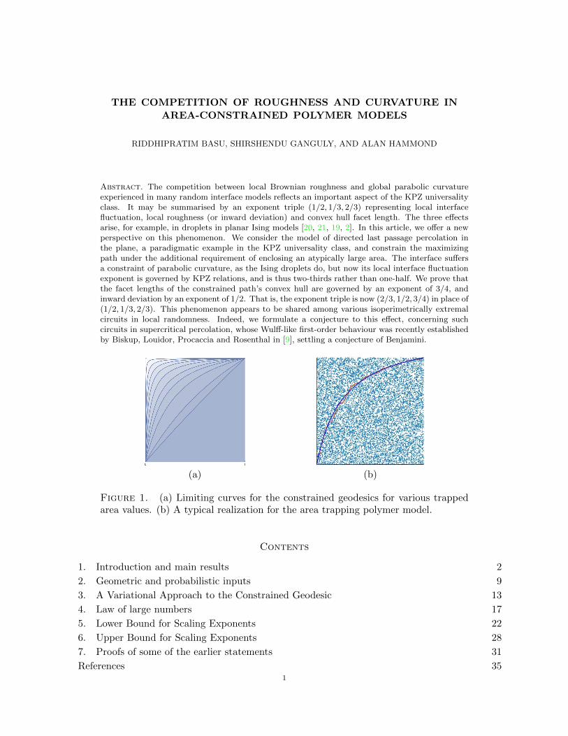
Abstract. The competition between local Brownian roughness and global parabolic curvatureexperienced in many random interface models reflects an important aspect of the KPZ universalityclass. It may be summarised by an exponent triple (1/2, 1/3, 2/3) representing local interfacefluctuation, local roughness (or inward deviation) and convex hull facet length. The three effectsarise, for example, in droplets in planar Ising models [20, 21, 19, 2]. In this article, we offer a newperspective on this phenomenon. We consider the model of directed last passage percolation inthe plane, a paradigmatic example in the KPZ universality class, and constrain the maximizingpath under the additional requirement of enclosing an atypically large area. The interface suffersa constraint of parabolic curvature, as the Ising droplets do, but now its local interface fluctuationexponent is governed by KPZ relations, and is thus two-thirds rather than one-half. We prove thatthe facet lengths of the constrained path’s convex hull are governed by an exponent of 3/4, andinward deviation by an exponent of 1/2. That is, the exponent triple is now (2/3, 1/2, 3/4) in place of(1/2, 1/3, 2/3). This phenomenon appears to be shared among various isoperimetrically extremalcircuits in local randomness. Indeed, we formulate a conjecture to this effect, concerning suchcircuits in supercritical percolation, whose Wulff-like first-order behaviour was recently establishedby Biskup, Louidor, Procaccia and Rosenthal in [9], settling a conjecture of Benjamini.
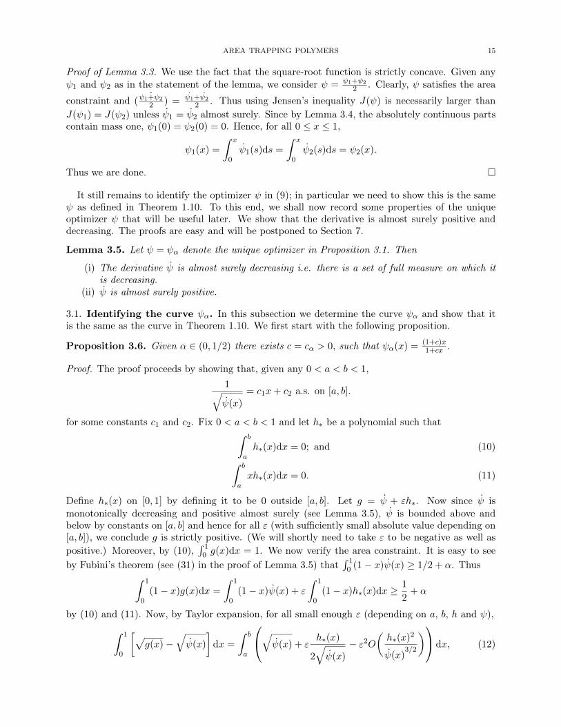
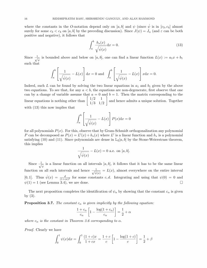
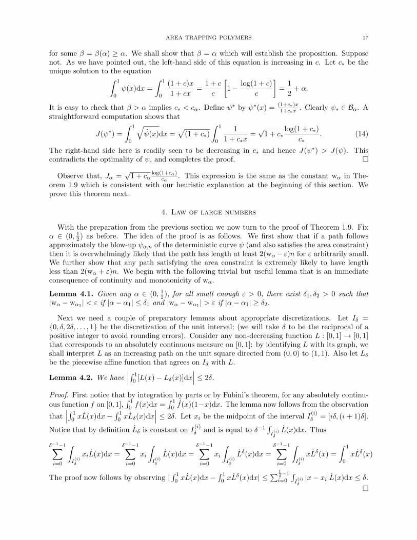
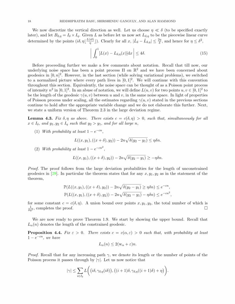
(a) (b)
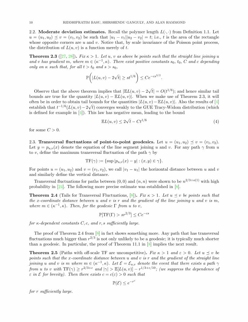
Figure 1. (a) Limiting curves for the constrained geodesics for various trappedarea values. (b) A typical realization for the area trapping polymer model.
Contents
1. Introduction and main results 2
2. Geometric and probabilistic inputs 9
3. A Variational Approach to the Constrained Geodesic 13
4. Law of large numbers 17
5. Lower Bound for Scaling Exponents 22
6. Upper Bound for Scaling Exponents 28
7. Proofs of some of the earlier statements 31
References 351

2 RIDDHIPRATIM BASU, SHIRSHENDU GANGULY, AND ALAN HAMMOND
1. Introduction and main results
The geometric properties of random interfaces are a vast arena of study in rigorous statisticalmechanics. Two important classes of interface models are phase separation models that idealizethe boundary between a droplet of one substance suspended in another, and last passage percola-tion models, where a directed path in independent local randomness maximizes a random weightdetermined by the environment.
One of the best known mathematical examples of phase separation is the two dimensional su-percritical Ising model in a large box with negative boundary condition. Conditioned to have anatypically high number of positive spins in the box, the vertices in the plus phase tend to form adroplet surrounded by a sea of negative spins. The random phase boundary of such a droplet hasbeen the object of intense study. Wulff proposed that the profile of such constrained circuits wouldmacroscopically resemble a dilation of an isoperimetrically optimal curve. This was establishedrigorously in [15] and [23]. Via the FK representation of the Ising model, one observes a similarsituation in the setting of subcritical two dimensional percolation, where the analogous object isthe boundary of the cluster containing the origin after this cluster is conditioned to be atypicallylarge. The Wulff shape captures the macroscopic profile of the circuit in such models, but what offluctuations? Several definitions may be considered that seek to capture fluctuation behaviour onthe part of the circuit, including the deviation in the Hausdorff metric of the convex hull of the cir-cuit from an appropriately scaled Wulff shape. Alternative definitions, more local in nature, servebetter to capture the transition in circuit geometry from local Brownian randomness to a smootherprofile dictated by the constraints of global curvature. In fact, a pair of definitions is natural, oneto capture the longitudinal distance at which the transition takes place, and the second to treat theorthogonal inward deviation of the interface at this transition-scale. To specify the characteristiclongitudinal distance, we may note that the convex hull of the circuit is a polygonal path that iscomposed of planar line segments or facets; we may treat the typical or maximum facet length asa barometer of the transition from the shorter scale of local randomness to the longer scale of cur-vature. Latitudinally, we may note that any point in the circuit has a local roughness, given by itsdistance from the convex hull boundary. The typical or maximum local roughness along the circuitis a latitudinal counterpart to facet length. Alexander [2], and Hammond [20, 21, 19] analysed suchconditioned circuit models and determined that when the area contained in the circuit is of ordern2, so that the circuit has diameter of order n, facet length and local roughness scale as n2/3 andn1/3. A similar situation is witnessed when a parabola x → t−1x2 is subtracted from a two-sidedBrownian motion B : R → R. When t > 0 is large, facets of the motion’s convex hull have lengthΘ(t2/3) and inward deviation Θ(t1/3). This phenomenon is expected to embrace many models inwhich the local structure of the interface is Brownian: another example, which was analysed byFerrari and Spohn [17], is Brownian bridge pinned to zero at −t and t and conditioned to remainabove the semi-circle of radius t centred at the origin.
The second class of random geometric paths we have mentioned are last passage percolation mod-els. These models form part of a huge, Kardar-Parisi-Zhang, class of statistical mechanical modelsin which a path through randomness is selected to be extremal for a natural weight determined bythat randomness. The maximizing paths are often called polymers. The fluctuation behaviour ofa length n polymer with given endpoints may be gauged either in terms of the scale of deviationof its weight from the mean value, or by the scale of deviation of say the polymer’s midpoint fromthe planar line segment that interpolates the polymer’s endpoints. The two deviations are givenby scales n1/3 and n2/3. The scaling has been predicted in the statistical physics literature byKardar, Parisi, and Zhang [25]. The length fluctuation exponent of 1/3 was first proved for planarPoissonian directed last passage percolation, in the seminal work of Baik, Deift and Johansson [4]who also identified the GUE Tracy-Widom scaling limit; the scaling limit of 2/3 for transversaldeviation was proved by Johansson [24]. Since then, this and other integrable models in the same

AREA TRAPPING POLYMERS 3
KPZ universality class have been extensively analysed and detailed information about this modelhas been obtained [27, 28].
It is of much interest to study models that combine phase separation and path minimization(or maximization) in random environment. Consider an environment with local independent ran-domness, and the circuit through that randomness whose weight determined by that randomnessis extremal among those circuits that trap a given area. Studying the random geometry of sucha circuit is a problem of extremal isoperimetry. Taking the randomness to be supercritical perco-lation, Itai Benjamini conjectured the first-order, Wulff-like, behaviour of the boundary of the setin the supercritical percolation cluster attaining the so-called anchored expansion constant. Thiswas proved by [9] by showing that the curve in the limit solves a natural isoperimetric variationalproblem; this has recently been extended to higher dimensions by Gold [18]. Given the role of facetlength and local roughness in capturing the local-random-to-global-curvature transition in circuitgeometry, a natural next task is to seek to understand the scaling exponents of such objects. Thisis our pursuit in this paper. Our choice of model preserves the qualitative features of the problemof interface fluctuation in an isoperimetrically extremal droplet in supercritical percolation and atthe same time ensures that key algebraic aspects of KPZ theory can be harnessed to yield sharpfluctuation estimates.
The particular setting we consider in this paper is planar Poissonian directed last passage per-colation. To impose the required properties, we study this model under a quadratic curvatureconstraint: that is, we force the best path to move away from the straight line and have a qua-dratic curvature on the average. This is done naturally by considering the longest upright path ina Poissonian environment joining (0, 0) and (n, n) which has the additional area trap property thatthe area under the curve is at least (12 + α)n2 for some α ∈ (0, 12). We call this random systemthe Area Trapping Polymer model (though we defer precise definitions to the next section). Notethat from the discussion above it follows that the unconstrained longest path stays close to thediagonal and hence encloses area (12 +o(1))n2. Also postponing precise statements (to Section 1.2),our main results quantify the competition along the contour between a global shape, dictated by aparabola, and local behaviour, guided by KPZ relations. These assertions show that the maximumfacet length of the contour’s least concave majorant scales as n3/4+o(1), while the local roughness,namely inward deviation from the concave majorant, scales as n1/2+o(1).
We also establish a law of large numbers for the length of the optimal path. The proof proceedsby setting up a variational problem, as is natural in such contexts (see [12] and [9]). Perhaps surpris-ingly, however, the problem turns out to have a very explicit solution. The geometric informationabout the limit shape of the constrained polymer is also used as an input in some of the argumentsabout fluctuations. The question of fluctuation in the context of isoperimetrically extremal circuitsin supercritical percolation can be formulated as a first passage percolation analogue of our settingof last passage percolation. Although the first passage percolation model is not exactly solvable,it, too, is believed to be in the KPZ universality class, and the geodesics there are believed to havethe same n2/3 scaling of transversal fluctuation as in our case (see [3] and the references therein).Thus our results suggest that a certain universality is being witnessed and, according to this belief,we formulate a conjecture concerning percolation. We elaborate on this and a number of otherinteresting questions in Section 1.4.
Finally, we discuss briefly the key inputs used in our paper and how it contrasts with theother examples of fluctuation results already mentioned. The results in [20, 21, 19] crucially usedrefined understanding and geometric estimates concerning percolation clusters, while a study ofarea trapping planar Brownian loop [22] used well known estimates for Brownian motion. Exactexpressions involving Brownian motion conditioned to stay above a parabola were the key ingredientin the proofs in [17]. However, in our setting, even though the unconstrained model has integrableproperties, the lack of general geometric understanding as an integrable model is perturbed causes

4 RIDDHIPRATIM BASU, SHIRSHENDU GANGULY, AND ALAN HAMMOND
a big challenge. Nonetheless, we are able to utilize as blackbox estimates certain known factsabout the unconstrained model and their robust variants established recently in [8]. By so doing,we rigorously establish local roughness exponents for the Area Trapping Polymer model. In thisway, this work is an example of the use of integrable probabilistic inputs in obtaining geometricconclusions about settings which lie outside the realm of exact solvability (see [8] for anotherexample of this). We believe a general program of developing such geometric arguments wouldlead to more robust proofs which could work for settings that are non-integrable but are variantsof solvable models.
1.1. Model Definitions. We now recall the planar Poissonian directed last passage percolationmodel.
Let Π be a homogeneous rate one Poisson Point Process (PPP) on the plane. A partial order onR2 is given by (x1, y1) � (x2, y2) if x1 ≤ x2 and y1 ≤ y2. For u � v, a directed path γ from u to vis a piecewise linear path that joins points u = γ0 � γ1 � · · · � γk = v where each γi for i ∈ [k− 1](throughout the article we will adopt the standard notation [n] = {1, 2, . . . , n}) is a point of Π.Define the length of γ, denoted |γ|, to be the number of Π-points on γ.
Definition 1.1. Define the last passage time from u to v, denoted by L(u, v), to be the maximum of|γ| as γ varies over all directed paths from u to v. There may be several maximizing paths betweenu and v, and throughout the paper we will refer to the top most path (it is easy to see that thetop most path is well defined here) among those, as the geodesic between u and v and denote it byγ(u, v).
We will often refer to γ(u, v) as the polymer between u and v. This polymer’s length, or weight,is then |γ(u, v)|.
Next we introduce the area constraint to this classical model.
1.1.1. Area trapped by a path. Consider a path γ between the origin (0, 0) and a point (x, y) in thepositive quadrant. The area trapped by the path γ, denoted by A(γ), is defined to be the area ofthe closed polygon determined by the x-axis, the vertical line segment joining (x, 0) to (x, y), andthe line segments of the path γ. Let γn denote the geodesic between (0, 0) and (n, n). Well-knownfacts about Poissonian LPP readily imply that A(γn) = (12 + o(1))n2 asymptotically almost surely.We constrain the model and consider maximizing paths subject to trapping a much larger area. Tothis end fix α ∈ (0, 12), and let
Lα(n) := max{|γ| : γ path from (0, 0) to (n, n) and A(γ) ≥
(12 + α
)n2}. (1)
It is easily seen that, among the paths that attain this maximum, there is almost surely exactly onethat traps the least area. This path will be called Γα,n. We will write Γn provided that the contextclarifies the value of α in question. We shall call Γn the constrained (or α-constrained) geodesic. Inanalogy with the phase separation example in percolation mentioned in the introduction, it mightseem more natural to consider the family of down right paths joining (n, 0) and (0, n), since all ofthese curves enclose the origin. However, because of the obvious underlying symmetry, and to takeadvantage of standard notational conventions, throughout the sequel we will consider the contourjoining the origin to the point (n, n).
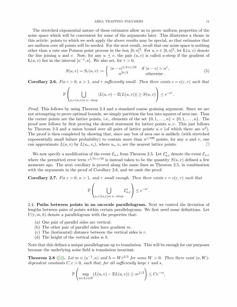
Our main objects of interest are two quantities that measure local regularity of the constrainedgeodesic Γn. The following definitions are illustrated by Figure 2.
Definition 1.2. Let conv(Γα,n) denote the convex hull of the polygon determined by the path Γα,nand the lines y = 0 and x = n. Let Γ∗α,n denote the closure of the polygonal part of the boundaryof conv(Γn) between (0, 0) and (n, n) above the x-axis. Thus Γ∗α,n is the least concave majorant ofΓα,n and is a union of finitely many line segments. These segments will be called facets. Define

AREA TRAPPING POLYMERS 5
maximum facet length of Γn, denoted MFL(Γα,n), to be the maximum Euclidean length of the facets.For x ∈ Γα,n, let d(x,Γ∗α,n) denote the distance from x to Γ∗α,n. This is a natural notion of thelocal roughness at x. Define the maximum local roughness of Γn, denoted MLR(Γn), by
MLR(Γα,n) = sup{x ∈ Γα,n : d(x,Γ∗α,n)}. (2)
In the following subsections we present our main results. We first state our results regarding thefluctuation exponents of Γα,n.
1.2. Scaling exponents for geodesic geometry. The sense in which we capture the exponentsis stronger and easier to state for the lower bounds, and so we begin with them.
Theorem 1.3. Fix α ∈ (0, 12) and ε > 0. Then there exists c = c(α, ε) > 0 such that, for all largeenough n,
P(MFL(Γn) ≥ n3/4−ε) ≥ 1− e−nc .
As we have mentioned, the scaling exponent for transversal fluctuation of point-to-point geodesicin unconstrained Poissonian last passage percolation is known to be 2/3. This fact, alongside thelast theorem, yields the following lower bound on maximum local roughness.
Theorem 1.4. Fix α ∈ (0, 12) and ε > 0. Then there exists c = c(α, ε) > 0 such that for all largeenough n,
P(MLR(Γn) ≥ n1/2−ε) ≥ 1− e−nc .
Regarding the matching upper bound, we prove that, with high probability, there exists a denseset of α ∈ (0, 2−1) for which the maximum length of the facets away from the boundary is bounded
above by n3/4+o(1). To make this precise, fix δ ∈ (0, π/4), and consider a facet in Γα,n with endpointsA and B recorded in clockwise order. Setting O = (n, 0), let θA denote the acute angle that OAmakes with the y-axis and θB, the acute angle that OB makes with the x-axis; see Figure 2.
Definition 1.5. The facet AB is called δ-interior if min(θA, θB) ≥ δ.
Note that the union of the δ-interior facets forms a polygonal path. (The union could be empty,but we will infer later from Theorem 1.10 that this event has an exponentially small probability.)Let A0 and B0 denote the extremities of this union path, and let Γδ,α,n denote the subpath of Γα,nbetween A0 and B0. Define the maximum δ-interior facet length of Γα,n, denoted by MFL(Γδ,α,n),to be the maximum length of the δ-interior facets. Define the δ-interior maximum local roughness,denoted by MLR(Γδ,α,n), by altering (2) in Definition 1.2 so that now the supremum is taken overall x ∈ Γδ,α,n and the distance is measured from the corresponding restricted part of Γ∗α,n).
Definition 1.6. Fix ε > 0. We say α ∈ (0, 12) is (n, ε, δ)-good if MFL(Γδ,α,n) ≤ n3/4+ε.
Here is our upper bound concerning the maximum length of facets.
Theorem 1.7. Fix ε > 0, δ ∈ (0, π/4) and an interval [α1, α2] ⊂ (0, 12). Let In,α1,α2 denote the setof (n, ε, δ)-good α ∈ [α1, α2]. Then there exists c = c(ε, δ, α1, α2) > 0 such that the probability thatIn,α1,α2 6= ∅ is at least 1− e−nc for all large enough n.
Our final principal result concerning exponents asserts that, for α ∈ In,α1,α2 , it is highly likely
that MLR(Γδ,α,n) ≥ n1/2+ε. Thus we obtain, with high probability, an n1/2+ε upper bound forinterior maximum local roughness for a dense, though possibly n-dependent and random, set of α.
Theorem 1.8. In the setting of Theorem 1.7, there exists c > 0, such that the event that thereexists α ∈ In,α1,α2 such that MLR(Γδ,α,n) > n1/2+ε, occurs with probability at most e−n
cfor all
large enough n.

6 RIDDHIPRATIM BASU, SHIRSHENDU GANGULY, AND ALAN HAMMOND
{ {MFL(Γ∗
α)
MLR(Γ∗α)
Γα
Γ∗α
ψα
A
B
δ
δ
θA
θB
θ = n−1/4
n3/4
nn
m ≈ nθ2 = (nθ)2/3 = n1/2
m
(a) (b)
Figure 2. (a) The three different curves correspond to ψα,n,Γα,n,Γ∗α,n. The
dashed lines indicate the δ− interior and hence the facets inside the sector boundedby them, are the δ−interior facets. (b)The scale at which the competition from twosources are equal to each other.
We now state a law of large numbers for Lα(n) and the constrained geodesic. Although the routetaken here of setting up an appropriate variational problem is by now classical [12], we point outthat it was not at all obvious that the solution can be explicitly described. Moreover some of theconsequences of the results in the following section are used as geometric inputs for the fluctuationresults stated before.
1.3. Law of Large Numbers. For the unconstrained model, a straightforward super-additivityargument yields that n−1ELn converges to a limit. The evaluation of the limiting constant isclassical: [30, 26] showed that the limit equals 2 by using Young tableaux combinatorics and theRSK correspondence (see also [1]). However, for the constrained model, the super-additive structureis lost and it is not clear a priori that a law of large numbers for Lα(n) exists. Our first result hereis to establish the law of large numbers for the area trapping polymer model; we are also able toevaluate the limiting constant implicitly as a function of α.
Given α ∈ (0, 1/2), let cα be given implicitly by the following equation:
1 + cαcα
(1− log(1 + cα)
cα
)=
1
2+ α. (3)
One can see that the function f(c) = 1+cc [1− log(1+c)
c ] is strictly increasing1 in c, and converges to
1/2 and 1 at 0 and ∞ respectively. Let wα =√
1 + cαlog(1+cα)
cα.
Theorem 1.9. For any α ∈ (0, 1/2),
ELα(n) = 2wαn+ o(n)
as n→∞.
Notice that wα → 1 as α → 0; hence the above theorem is consistent with the result in theclassical unconstrained case. In the unconstrained model, one also has a law of large numbers forthe geodesic, i.e., it is known that the geodesic is concentrated around the straight line joining
1f ′(c) = (2+c) log(1+c)−2c
c3and d
dc[(2 + c) log(1 + c) − 2c] = log(1 + c) − c
1+c> 0.
AREA TRAPPING POLYMERS 7
(0, 0) and (n, n). More precisely, under the rescaling that takes the n× n square to a unit square,the geodesic converges almost surely in Hausdorff distance to the diagonal of the unit square [12];
(as mentioned before, the precise order of the transversal fluctuations are known to be n2/3 as aconsequence of integrability). Even though we do not have any exactly solvable structure in theconstrained model, we can establish a similar law of large numbers here too asserting that theconstrained geodesic concentrates around a deterministic curve. Moreover, we can identify thelimiting curve in a fairly explicit manner.
Let ψα : [0, 1]→ [0, 1] be defined as ψα(x) = (1+cα)x1+cαx
where cα is as above. Also let ψα,n : [0, n]→[0, n] be the n blow-up of ψα i.e. ψα,n(x) = nψα(x/n). We denote by dist(·, ·) the Hausdorffdistance. The following theorem is our law of large numbers for the constrained geodesic.
Theorem 1.10. For any α ∈ (0, 1/2) and ∆ > 0, there exists c = c(α,∆) such that, for all largeenough n, it is with probability at least 1− e−cn that
dist(Γα,n, ψα,n) ≤ ∆n.
In particular, this theorem states that to first order, the constrained geodesics behave like agiven smooth curve. This result will be useful to us when we study the scaling exponents for localroughness of the constrained geodesic, in particular, when we seek to rule out long and flat facets(see Theorem 2.2).
1.4. Open questions and future directions. Below we list below several interesting questionsfor future research:
(1) The upper bound Theorem 1.7 is weaker than the lower bound Theorem 1.3. Strengtheningthe former is a natural open problem.
(2) By definition, A(Γα,n) ≥ (12 + α)n2. The typical order of A(Γα,n) − (12 + α)n2 remainsunknown.
(3) For α ∈ (0, 1/2), what is the typical deviation of Γα,n from the curve ψα,n? What is theorder of fluctuations of Lα(n)?
(4) In a phase separation problem, [20, 21, 19] determines the polylogarithmic corrections toboth elements of the (2/3, 1/3) (facet length,local roughness) exponent pair. The powersof the logarithm are (1/3, 2/3). Finding such corrections for the Area Trapping Polymermodel would refine the identification of the exponent pair (3/4, 1/2) made in this articleand suggested by the first point.
The first two points will be discussed further in Section 6.2.
Supercritical percolation: We end this section with a conjecture regarding fluctuation expo-nents in the context of supercritical percolation on the nearest neighbour graph on Z2. As we havementioned already, [9] settles a conjecture of Benjamini regarding the limit shape of isoperimetri-cally extremal sets. Formally, for supercritical percolation, with the origin 0 conditioned to be inthe infinite cluster C∞(0), the authors in [9] consider the ‘anchored isoperimetric profile’, i.e., forany r > 0 they discuss the set Br which solves the following isoperimetric problem:
inf
{ |∂B||B| : 0 ∈ B,B ⊂ C∞(0) is connected, |B| ≤ r
}where ∂B denotes the edge boundary of B, restricted to C∞(0) (for more details see [9]). The mainresult in [9] shows the convergence of the set Br as r → ∞, after suitable renormalization, to adeterministic Wulff crystal, in the Hausdorff sense. To go beyond first order behaviour one has tounderstand local geometric properties of the boundary of Br. The extremal circuit broadly has tosatisfy a:
(1) volume condition,
8 RIDDHIPRATIM BASU, SHIRSHENDU GANGULY, AND ALAN HAMMOND
(2) and an extremal isoperimetry condition.
The heuristic now is that the former is a global constraint while the latter is only local. Namely,each local part of the boundary does not feel the volume constraint |Br| ≤ r, and thereby justtries to move through the open edges while trying to minimize the number of open edges that itcuts across, since these are precisely the edges that contribute to |∂Br|. This brings us within therealm of first passage percolation, which is also predicted to lie in the KPZ universality class; (see[3] for more on first passage percolation). Thus, Theorems 1.3, 1.4, 1.7 and 1.8 can be thought ofas rigorous counterparts to the above discussion in the integrable last passage percolation setting.In light of this discussion, these results lead us to conjecture fluctuation exponents for the abovemodel. Next we formulate a precise statement in a slightly simpler setting.
Recall the standard definition of the dual graph of the nearest neighbour lattice on Z2. Given asupercritical bond percolation environment on the edge set of Z2 with density p > pc(Z2) = 1/2,for every positive integer n, consider the set Dn2 of dual circuits (namely simple loops consistingof dual edges) enclosing a connected subset of Z2 of size n2 and containing the origin such thatthe number of primal open edges in the percolation environment that the circuit cuts through isminimized. Thus the above model is an exact analogue of the model considered in this paper, inthe context of first passage percolation in a bond percolation environment. Note, however, thatsuch a circuit is not necessarily unique due to the discrete nature of the problem. We now stateprecisely our conjecture.
Conjecture: Consider bond percolation on the nearest neighbour lattice on Z2 with any super-critical parameter value p > pc(Z2). The random variables
maxD∈Dn2
∣∣∣∣ log(MFL(D))
log n− 3/4
∣∣∣∣ and maxD∈Dn2
∣∣∣∣ log(MLR(D))
log n− 1/2
∣∣∣∣converge to zero in probability as n grows to infinity where for any D ∈ Dn2 , the maximum facetlength MFL(D) and maximum local roughness MLR(D) are defined in the same way as in thispaper by considering the convex hull of the points in D.
We end with the remark that the problem considered in [9] corresponds to a similar first passagepercolation problem where the environment has bounded dependence range and hence should havethe same fluctuation behaviour as the simpler model just described.
1.5. Organization of the rest of the article. In Section 2 we collect some preliminary proba-bilistic results: some for the constrained model and a few for the unconstrained one. The resultsfor the unconstrained model follow from the sharp moderate deviation estimates in [27, 28] andthe consequences established in [8]. In Section 3, we set up and solve the variational problem forthe law of large numbers and the following Section 4 is devoted to the proofs of Theorem 1.9 andTheorem 1.10: the law of large numbers for the length of constrained geodesic and the path itself.We next turn to the proofs of the results on the scaling exponents. In Section 5 we provide proofsof Theorems 1.3 and Theorem 1.4. The proofs of Theorem 1.7 and Theorem 1.8 are completedin Section 6. Proofs of some of the auxiliary results stated and used throughout the article arepostponed to Section 7. Throughout the article we will use various letters to denote universalconstants whose value may change from line to line.
Acknowledgments. The authors thank Marek Biskup, Craig Evans and Ofer Zeitouni for usefuldiscussions. S.G.’s research is supported by a Miller Research Fellowship at UC Berkeley. A.H. issupported by NSF grant DMS-1512908.
AREA TRAPPING POLYMERS 9
2. Geometric and probabilistic inputs
In this section we gather the probabilistic inputs needed for our proof. First we shall recorda few useful facts about the length and geometry of the constrained geodesics that will be usedrepeatedly. The bulk of this section will then recall results about the unconstrained model. Theseresults are all consequences of the basic integrable ingredients obtained by Lowe, Merkl and Rolles[27, 28]. Some of the arguments are fairly standard in the exactly solvable literature, in which casewe provide a sketch the proof or point to the relevant reference. A few of these consequences wereestablished and used recently in [8] and we quote the relevant results here.
We start with some basic facts about the constrained model.
2.1. Some basic results for the Area Trapping Polymer model. We first start with concen-tration for Lα(n). In the absence of integrability, we use standard Poincare inequality techniques
and obtain a concentration at n1/2+o(1) scale.
Theorem 2.1. Fix any α ∈ (0, 1/2). Then there exists a constant C > 0 such that for for all nand all t > 0,
P(|Lα(n)− E(Lα(n))| ≥ t) ≤ Ce−t2/Cn log2(n).
The proof is standard and is postponed until the end of the paper in Section 7.
Our next result rules out flat facets. This is a consequence of Theorem 1.10, which asserts thatit is extremely unlikely that any interior facets (which are those in the bulk) have very shallow orsteep gradient. Even though, we will need a stronger version later (see Theorem 4.6) it is instructiveto state a weaker form of the result now, and give its simple proof.
Theorem 2.2. For any small enough δ > 0 there exists ω > 0 such that, with probability 1− e−cn,all δ−interior facets make an angle with the x−axis which lies in the interval (ω, π/2− ω).
Proof. We start by recalling a simple fact: for two facets of Γ∗α,n with starting points u1, u3 andending points u2, u4 respectively where u1 � u2 � u3 � u4, by convexity of Γ∗α,n, the angle madewith the x−axis by the facet (u1, u2) is larger than the angle made by (u3, u4).
Consider any δ−interior facet (u1, u2), and let u1 = (x, y). Also let L1, L2 be the straight linesjoining the origin to u1 and (n, n) to u2 respectively. Let v1 and v2 be the points of intersection ofL1 and L2 with ψα,n. Theorem 1.10 implies that, for any ε > 0, with probability at least 1− e−cn,the bound
max(|u1 − v1|, |u2 − v2|) ≤ εnholds for all δ-interior facets, simultaneously. Now, by the convexity of Γ∗α,n, the gradient of thefacet (u1, u2) is between the gradient of the lines joining (0, 0) to u1 and (n, n) to u2. Choosing εto be much smaller than δ, we see that the gradient of the facet (u1, u2) plus an error of O(ε) liesbetween the gradients of the line joining the origin and v1, and that joining (n, n) and v2. Thus weare done by choosing ε to be small enough and using the strict convexity of ψα,n; (see Figure 2(a)for illustration). �
We will later need Theorem 4.6, a strengthening of the above result, which is uniform in α. Weturn to state useful results that concern the unconstrained, exactly solvable, model. All of theseare corollaries of the following moderate deviation estimates.
10 RIDDHIPRATIM BASU, SHIRSHENDU GANGULY, AND ALAN HAMMOND
2.2. Moderate deviation estimates. Recall the polymer length L(·, ·) from Definition 1.1. Letu = (u1, u2) � v = (v1, v2) be such that |u1 − v1||u2 − v2| = t; i.e., t is the area of the rectanglewhose opposite corners are u and v. Notice that, by scale invariance of the Poisson point process,the distribution of L(u, v) is a function merely of t.
Theorem 2.3 ([27, 28]). Fix κ > 1. Let u, v as above be points such that the straight line joining uand v has gradient m, where m ∈ (κ−1, κ). There exist positive constants s0, t0, C and c dependingonly on κ such that, for all t > t0 and s > s0,
P(|L(u, v)− 2
√t| ≥ st1/6
)≤ Ce−cs3/2 .
Observe that the above theorem implies that |EL(u, v)− 2√t| = O(t1/6); and hence similar tail
bounds are true for the quantity |L(u, v) − EL(u, v)|. When we make use of Theorem 2.3, it willoften be in order to obtain tail bounds for the quantities |L(u, v)−EL(u, v)|. Also the results of [4]
establish that t−1/6(L(u, v)−2√t) converges weakly to the GUE Tracy-Widom distribution (which
is defined for example in [4]). This law has negative mean, leading to the bound
EL(u, v) ≤ 2√t− Ct1/6 (4)
for some C > 0.
2.3. Transversal fluctuations of point-to-point geodesics. Let u = (u1, u2) � v = (v1, v2).Let y = pu,v(x) denote the equation of the line segment joining u and v. For any path γ from uto v, define the maximum transversal fluctuation of the path γ by
TF(γ) := {sup |pu,v(x)− y| : (x, y) ∈ γ}.For points u = (u1, u2) and v = (v1, v2), we call |v1 − u1| the horizontal distance between u and vand similarly define the vertical distance.
Transversal fluctuations for paths between (0, 0) and (n, n) were shown to be n2/3+o(1) with highprobability in [24]. The following more precise estimate was established in [8].
Theorem 2.4 (Tails for Transversal Fluctuations, [8]). Fix κ > 1. Let u � v be points such thatthe x-coordinate distance between u and v is r and the gradient of the line joining u and v is m,where m ∈ (κ−1, κ). Then, for the geodesic Γ from u to v,
P[TF(Γ) > sr2/3] ≤ Ce−cs
for κ-dependent constants C, c, and r, s sufficiently large.
The proof of Theorem 2.4 from [8] in fact shows something more. Any path that has transversal
fluctuations much bigger than r2/3 is not only unlikely to be a geodesic; it is typically much shorterthan a geodesic. In particular, the proof of Theorem 11.1 in [8] implies the next result.
Theorem 2.5 (Paths with off-scale TF are uncompetitive). Fix κ > 1 and ε > 0. Let u � v bepoints such that the x-coordinate distance between u and v is r and the gradient of the straight linejoining u and v is m where m ∈ (κ−1, κ). Let E = Eu,v denote the event that there exists a path γ
from u to v with TF(γ) ≥ r2/3+ε and |γ| > E[L(u, v)] − r1/3+ε/10; (we suppress the dependence ofε in E for brevity). Then there exists c = c(ε) > 0 such that
P(E) ≤ e−rc
for r sufficiently large.
AREA TRAPPING POLYMERS 11
The stretched exponential nature of these estimates allow us to prove uniform properties of thenoise space which will be convenient for some of the arguments later. This illustrates a theme inthis article: points to which we seek apply the above results may be special, so that estimates thatare uniform over all points will be needed. For the next result, recall that our noise space is nothingother than a rate one Poisson point process in the box [0, n]2. For u, v ∈ [0, n]2, let L(u, v) denotethe line joining u and v. Now, for any u � v, the pair (u, v) is called κ-steep if the gradient ofL(u, v) lies in the interval [κ−1, κ]. We also set, for τ > 0,
S(u, v) = Sτ (u, v) :=
{|u− v|1/3+ε/10 if |u− v| > nτ ,
n2τ/3 otherwise .(5)
Corollary 2.6. Fix ε > 0, κ > 1, and τ sufficiently small. Then there exists c = c(ε, τ) such that
P
⋃u,v:(u,v)is κ−steep
|L(u, v)− E(L(u, v))| ≥ S(u, v)
≤ e−nc .Proof. This follows by using Theorem 2.3 and a standard coarse graining argument. Since we arenot attempting to prove optimal bounds, we simply partition the box into squares of area one. Thusthe corner points are the lattice points, i.e., elements of the set {0, 1, . . . , n} × {0, 1, . . . , n}. Theproof now follows by first proving the desired statement for lattice points u, v. This just followsby Theorem 2.3 and a union bound over all pairs of lattice points u, v (of which there are n2).The proof is then completed by showing that, since any box of area one is unlikely (with stretched
exponentially small failure probability) to contain more than nε/100 points, for any u and v, onecan approximate L(u, v) by L(u∗, v∗), where u∗, v∗ are the nearest lattice points. �
We now specify a modification of the event Eu,v from Theorem 2.5. Let E∗u,v denote the event Eu,vwhere the permitted error term r1/3+ε/10 is instead taken to be the quantity S(u, v) defined a fewmoments ago. The next corollary is proved along the same lines as Theorem 2.5, in combinationwith the arguments in the proof of Corollary 2.6, and we omit the proof.
Corollary 2.7. Fix ε > 0, κ > 1, and τ small enough. Then there exists c = c(ε, τ) such that
P
⋃u,v:|(u,v)is κ−steep
E∗u,v
≤ e−nc .2.4. Paths between points in an on-scale parallelogram. Next we control the deviation oflengths between pairs of points within certain parallelograms. We first need some definitions. LetU(r,m, h) denote a parallelogram with the properties that:
(a) One pair of parallel sides are vertical.(b) The other pair of parallel sides have gradient m.(c) The (horizontal) distance between the vertical sides is r.(d) The height of the vertical sides is h.
Note that this defines a unique parallelogram up to translation. This will be enough for our purposesbecause the underlying noise field is translation invariant.
Theorem 2.8 ([8]). Let m ∈ (κ−1, κ) and h = Wr2/3 for some W > 0. Then there exist (κ,W )-dependent constants C, c > 0, such that, for all sufficiently large r and s,
P
(sup
u∈A,v∈B(L(u, v)− EL(u, v)) ≥ sr1/3
)≤ Ce−cs,

12 RIDDHIPRATIM BASU, SHIRSHENDU GANGULY, AND ALAN HAMMOND
and
P(
infu∈A,v∈B
(L(u, v)− EL(u, v)) ≤ −sr1/3)≤ Ce−cs,
where A and B respectively denote the left third and right third of U(r,m, h).
The next theorem states that, even if the paths are restricted to stay inside the parallelogram,the fluctuation remains on-scale. Let L(u, v;U) denote the length of the longest path from u to vthat does not exit U .
Theorem 2.9 ([8]). Under the assumptions of Theorem 2.8, there exist (κ,W )-dependent constantsC, c > 0 such that, for all sufficiently large r and s,
P(
infu∈A,v∈B
(L(u, v;U)− EL(u, v)) ≤ −sr1/3)≤ Ce−cs1/2
where A and B respectively denote the right third and the left third of U(r,m, h).
2.5. Paths constrained in a thin parallelogram. The next set of results shows that, if a pathis constrained to have much smaller than typical transversal fluctuation, then it must have muchsmaller length than a typical geodesic’s.
Theorem 2.10 (Paths with small TF are uncompetitive). Fix ε > 0. Consider the parallelogram
U = U(r,m, h), where m ∈ (κ−1, κ) and h = r2/3−ε. Let u0 and v0 denote the midpoints of thevertical sides A0 and B0 of U . Then, for some c = c(ε) > 0,
P(L(u0, v0;U) ≥ EL(u0, v0)− r1/3+ε/3
)≤ e−rc
for r sufficiently large.
The proof of Theorem 2.10 follows a strategy, by now well known, that has been used to showGaussian fluctuation of paths constrained to stay in a thin rectangle in [11] in the context of firstpassage percolation. In the context of LPP, the Gaussian fluctuation has recently been shown in[14], and tail bounds are proved in a more general context in the preprint [7]. We now provide asketch of Theorem 2.10’s proof.
Sketch of Proof. Without loss of generality let us assume m = 1. Also, we can replace the paral-lelogram U by the rectangle U ′, one of whose pairs of sides is parallel to the line segment u0v0,with the other pair having midpoints u0 and v0 and length r2/3−ε. Divide the rectangle U ′ into Kequal parts (each of width r
K ) by parallel line segments perpendicular to u0v0. Let Li denote theleft side of the i-th rectangle and let ui be its midpoint. Now let γi be the best path (i.e. withmaximal value of |γ|) between Li and Li+1 that stays within U ′. It follows from Theorem 2.8 that
it is extremely likely that |γi| − L(ui, ui+1) � (K−1r)1/3. It follows that up to an error of order
much smaller than K2/3r1/3 we can approximate L(u0, v0;U′) by
∑i L(ui, ui+1). Now observe that
L(ui, ui+1) are independent and identically distributed with mean 2r/K − C(K−1r)1/3 (here we
use (4)) and standard deviation of the order of (K−1r)1/3. By standard concentration inequali-
ties, one then shows that∑
i L(ui, ui+1) concentrates around 2r −K2/3r1/3 at scale K1/6r1/3. By
choosing K � rε/2 properly one gets the result. �
In the same vein, we have the following corollary.
Corollary 2.11. Fix ε > 0, κ > 1, and τ small enough. Then there exists c = c(ε, τ) such that,with probability at least 1− e−nc,
supu,v:|u−v|≥nτ ,(u,v)is κ−steep
L(u, v, U)− E(L(u, v)) ≤ −|u− v| 13+ε.
AREA TRAPPING POLYMERS 13
2.6. Estimates for One-Sided Geodesics. We end this section by considering geodesics in adifferent constrained model. Baik and Rains [5, 6] considered increasing paths from (0, 0) to (n, n)that lie above the diagonal line joining the points. Recall that L(u, v) denotes the length of thelongest increasing path between points u � v. Let L�(u, v) denote the length of the longest pathbetween u and v restricted to lie above the line joining u and v and, similarly to Definition 1.1,let γ�(u, v) denote the corresponding uppermost one-sided geodesic between u and v. Moreover,let L�(n) denote L�(u, v) in the special case that u = (0, 0) and v = (n, n). Baik and Rains [5, 6]
proved that EL�(n) = 2n+ o(n) and that the fluctuations are again of order n1/3 (although in thiscase the scaling limit is different; it is the GSE Tracy Widom distribution instead of the GUE TracyWidom distribution). We shall need the corresponding moderate deviation estimates, consequencesof Theorem 2.9.
Theorem 2.12. Let u, v be as in the hypothesis of Theorem 2.3. There exist positive constantss0, t0, C and c such that, for all t > t0 and s > s0,
P[|L�(u, v)− 2√t| ≥ st1/6] ≤ Ce−cs1/2 .
Proof. The upper tail result follows from Theorem 2.3 due to L�(u, v) ≤ L(u, v). For the lower tail,we use Theorem 2.9 with the straight line joining u and v being the bottom side of the parallelogramand use the fact that EL(u, v) = 2
√t−Θ(t1/6). �
We need a uniform version of this result. Recall S(u, v) = Sτ (u, v) from (5).
Corollary 2.13. Fix ε > 0, κ > 1, and τ > 0 small enough. Then there exists c = c(ε, τ) suchthat, with probability at least 1− e−nc,
supu,v:(u,v)is η−steep
L�(u, v)− E(L(u, v)) ≥ −S(u, v).
Proofs of Corollaries 2.7 2.11, 2.13 follow from the corresponding theorems for fixed points, inthe same way as Corollary 2.6 follows from Theorem 2.3. We omit the details.
3. A Variational Approach to the Constrained Geodesic
We now move towards proving Theorem 1.9 and Theorem 1.10. Deuschel and Zeitouni [13, 12]studied in detail the hydrodynamic limit of the unconstrained geodesic for inhomogeneous pointprocesses. We follow their strategy broadly and study the limit of the constrained curve by meansof appropriate variational problems. We first explain the idea. Fix α ∈ (0, 12) for the rest of thissection. First let us assume that a limiting continuous curve φ of the constrained geodesics existsafter scaling. This curve φ : [0, 1]→ [0, 1] will be continuous, non-decreasing and surjective. By the
area constraint,∫ 10 φ(s)ds ≥ 1
2 + α. Now heuristically, since in practice there is always a little bitof area excess, one can approximate φ by a piecewise affine function at a scale local enough thateach piece is exempt from the area constraint; and we can then use the law of large numbers for theunconstrained geodesic (see Theorem 2.3) at every local scale and sum over them. This argumentsuggests that the approximating path will have length 2J(φ)n+ o(n) where
J(φ) =
∫ 1
0
√φ(s)ds.
It thus seems that we should maximize J(φ) among all curves φ satisfying the area constraint, andthe maximum will be the constant appearing in the required law of large numbers. We now proceedto make this precise. Let B be the collection of all right-continuous non-decreasing functions from[0, 1] to [0, 1]. Thus B is in bijection with the set of all sub-probability measures on [0, 1]. Now, forany φ ∈ B, by the Lebesgue decomposition theorem we can write
φ = φac + φs (6)
14 RIDDHIPRATIM BASU, SHIRSHENDU GANGULY, AND ALAN HAMMOND
in a unique way as a sum of a pair of sub-probability measures, with φac being the absolutelycontinuous part and φs the singular part (with respect to Lebesgue measure). Note that this
implies φac has a derivative φac almost everywhere2 such that, for any 0 ≤ x ≤ 1, we have∫ x
0φac(s)ds = φac(x)
while φs is almost surely flat and hence has derivative 0 almost surely. Thus φ = φac almost surely.Also define
J(φ) =
∫ 1
0
√φ(s)ds. (7)
Let
Bα =
{φ ∈ B :
∫ 1
0φ(s)ds ≥ 1
2 + α
}. (8)
We shall often omit the subscript α. Finally let
Jα = supφ∈Bα
J(φ). (9)
The first step is to show existence and uniqueness of the solution.
Proposition 3.1. There exists a unique element ψ = ψα ∈ B that attains the supremum in (9).
Note that the function ψ = ψα in Proposition 3.1 will be the same in the statement of Theo-rem 1.10. The existence and uniqueness parts of Proposition 3.1 have separate proofs. We firststate the existence result.
Lemma 3.2. There exists ψ ∈ B that achieves the supremum in (9).
The proof of Lemma 3.2 is technical: it uses a compactness argument on the space of probabilitymeasures following a similar argument from [12]. We postpone the proof until Section 7.
In the next part we show uniqueness.
Lemma 3.3. Suppose ψ1 and ψ2 are in Bα and satisfy J(ψi) = Jα for i = 1, 2. Then ψ1 = ψ2.
The proof of Lemma 3.3 is rather straightforward once we establish the following technical lemmathat rules out the possibility that any of the optimizing functions has a nontrivial singular part.
Lemma 3.4. Let ψ ∈ Bα be such that J(ψ) = Jα. Then ψ corresponds to a probability measurewhich is absolutely continuous with respect to Lebesgue measure.
Here is the basic idea of the proof of this lemma. From the results of [12] it follows that withoutthe area constraint the optimizing curve is the diagonal line, i.e., the preferred gradient for thegraph of the function is one. If the singular part is non-trivial, then the graph of the function ψmay be expected to have a flat piece. Because the gradient of the graph has to be one on averagedue to boundary conditions, it follows that there must be a piece of the graph having gradient awayfrom one. We shall show that one can modify the flat and the steep parts of the curve locally bypieces with more moderate gradient in a way that increases not only the value of the functionalJ but while still satisfying the area constraint; and thereby optimality will be contradicted. Also,clearly in the case that ψ does not have total mass one, one can add to it another function to makeit (or, more precisely of course, to bring it into correspondence with) a probability measure, whilealso increasing the value of J(ψ), and thus contradict maximality in this case also. Thus ψ is alsoa probability measure. The details of the proof are postponed to Section 7.
We can now prove the uniqueness result using Lemma 3.4.
2Throughout the article, for any function f on [0, 1], which is differentiable almost everywhere, we will denote its
derivative by f . Recall that this does not necessarily imply∫ x0f(s)ds = f(x) for all x.
AREA TRAPPING POLYMERS 15
Proof of Lemma 3.3. We use the fact that the square-root function is strictly concave. Given anyψ1 and ψ2 as in the statement of the lemma, we consider ψ = ψ1+ψ2
2 . Clearly, ψ satisfies the area
constraint and˙
(ψ1+ψ2
2 ) = ψ1+ψ2
2 . Thus using Jensen’s inequality J(ψ) is necessarily larger than
J(ψ1) = J(ψ2) unless ψ1 = ψ2 almost surely. Since by Lemma 3.4, the absolutely continuous partscontain mass one, ψ1(0) = ψ2(0) = 0. Hence, for all 0 ≤ x ≤ 1,
ψ1(x) =
∫ x
0ψ1(s)ds =
∫ x
0ψ2(s)ds = ψ2(x).
Thus we are done. �
It still remains to identify the optimizer ψ in (9); in particular we need to show this is the sameψ as defined in Theorem 1.10. To this end, we shall now record some properties of the uniqueoptimizer ψ that will be useful later. We show that the derivative is almost surely positive anddecreasing. The proofs are easy and will be postponed to Section 7.
Lemma 3.5. Let ψ = ψα denote the unique optimizer in Proposition 3.1. Then
(i) The derivative ψ is almost surely decreasing i.e. there is a set of full measure on which itis decreasing.
(ii) ψ is almost surely positive.
3.1. Identifying the curve ψα. In this subsection we determine the curve ψα and show that itis the same as the curve in Theorem 1.10. We first start with the following proposition.
Proposition 3.6. Given α ∈ (0, 1/2) there exists c = cα > 0, such that ψα(x) = (1+c)x1+cx .
Proof. The proof proceeds by showing that, given any 0 < a < b < 1,
1√ψ(x)
= c1x+ c2 a.s. on [a, b].
for some constants c1 and c2. Fix 0 < a < b < 1 and let h∗ be a polynomial such that∫ b
ah∗(x)dx = 0; and (10)∫ b
axh∗(x)dx = 0. (11)
Define h∗(x) on [0, 1] by defining it to be 0 outside [a, b]. Let g = ψ + εh∗. Now since ψ is
monotonically decreasing and positive almost surely (see Lemma 3.5), ψ is bounded above andbelow by constants on [a, b] and hence for all ε (with sufficiently small absolute value depending on[a, b]), we conclude g is strictly positive. (We will shortly need to take ε to be negative as well as
positive.) Moreover, by (10),∫ 10 g(x)dx = 1. We now verify the area constraint. It is easy to see
by Fubini’s theorem (see (31) in the proof of Lemma 3.5) that∫ 10 (1− x)ψ(x) ≥ 1/2 + α. Thus∫ 1
0(1− x)g(x)dx =
∫ 1
0(1− x)ψ(x) + ε
∫ 1
0(1− x)h∗(x)dx ≥ 1
2+ α
by (10) and (11). Now, by Taylor expansion, for all small enough ε (depending on a, b, h and ψ),∫ 1
0
[√g(x)−
√ψ(x)
]dx =
∫ b
a
√ψ(x) + εh∗(x)
2√ψ(x)
− ε2O(h∗(x)2
ψ(x)3/2
) dx, (12)
16 RIDDHIPRATIM BASU, SHIRSHENDU GANGULY, AND ALAN HAMMOND
where the constants in the O-notation depend only on [a, b] and ψ (since ψ is in [c3, c4] almostsurely for some c3 < c4 on [a, b] by the preceding discussion). Since J(ψ) = Jα (and ε can be bothpositive and negative), it follows that ∫ b
a
h∗(x)√ψ(x)
dx = 0. (13)
Since 1√ψ
is bounded above and below on [a, b], one can find a linear function L(x) := a1x + b1
such that ∫ b
a
1√ψ(x)
− L(x)
dx = 0 and
∫ b
a
1√ψ(x)
− L(x)
xdx = 0.
Indeed, such L can be found by solving the two linear equations in a1 and b1 given by the abovetwo equations. To see that, for any a < b, the equations are non-degenerate, first observe that onecan by a change of variable assume that a = 0 and b = 1. Then the matrix corresponding to the
linear equations is nothing other than
[1/2 11/3 1/2
]and hence admits a unique solution. Together
with (13) this now implies that ∫ b
a
1√ψ(x)
− L(x)
P (x)dx = 0
for all polynomials P (x). For this, observe that by Gram-Schmidt orthogonalization any polynomialP can be decomposed as P (x) = L′(x) +h∗(x) where L′ is a linear function and h∗ is a polynomialsatisfying (10) and (11). Since polynomials are dense in L2[a, b] by the Stone-Weierstrass theorem,this implies
1√ψ(x)
− L(x) = 0 a.e. on [a, b].
Since 1√ψ
is a linear function on all intervals [a, b], it follows that it has to be the same linear
function on all such intervals and hence 1√ψ(x)
= L(x), almost everywhere on the entire interval
[0, 1]. Thus ψ(x) = d(1+cx)2
for some constants c, d. Integrating and using that ψ(0) = 0 and
ψ(1) = 1 (see Lemma 3.4), we are done. �
The next proposition completes the identification of ψα by showing that the constant cα is givenby (3).
Proposition 3.7. The constant cα is given implicitly by the following equation:
1 + cαcα
[1− log(1 + cα)
cα
]=
1
2+ α
where cα is the constant in Theorem 3.6 corresponding to α.
Proof. Clearly we have∫ 1
0ψ(x)dx =
∫ 1
0
(1 + c)x
1 + cx=
1 + c
c
[1− log(1 + c)
c
]=
1
2+ β
AREA TRAPPING POLYMERS 17
for some β = β(α) ≥ α. We shall show that β = α which will establish the proposition. Supposenot. As we have pointed out, the left-hand side of this equation is increasing in c. Let c∗ be theunique solution to the equation∫ 1
0ψ(x)dx =
∫ 1
0
(1 + c)x
1 + cx=
1 + c
c
[1− log(1 + c)
c
]=
1
2+ α.
It is easy to check that β > α implies c∗ < cα. Define ψ∗ by ψ∗(x) = (1+c∗)x1+c∗x
. Clearly ψ∗ ∈ Bα. Astraightforward computation shows that
J(ψ∗) =
∫ 1
0
√ψ(x)dx =
√(1 + c∗)
∫ 1
0
1
1 + c∗x=√
1 + c∗log(1 + c∗)
c∗. (14)
The right-hand side here is readily seen to be decreasing in c∗ and hence J(ψ∗) > J(ψ). Thiscontradicts the optimality of ψ, and completes the proof. �
Observe that, Jα =√
1 + cαlog(1+cα)
cα. This expression is the same as the constant wα in The-
orem 1.9 which is consistent with our heuristic explanation at the beginning of this section. Weprove this theorem next.
4. Law of large numbers
With the preparation from the previous section we now turn to the proof of Theorem 1.9. Fixα ∈ (0, 12) as before. The idea of the proof is as follows. We first show that if a path followsapproximately the blow-up ψα,n of the deterministic curve ψ (and also satisfies the area constraint)then it is overwhelmingly likely that the path has length at least 2(wα− ε)n for ε arbitrarily small.We further show that any path satisfying the area constraint is extremely likely to have lengthless than 2(wα + ε)n. We begin with the following trivial but useful lemma that is an immediateconsequence of continuity and monotonicity of wα.
Lemma 4.1. Given any α ∈ (0, 12), for all small enough ε > 0, there exist δ1, δ2 > 0 such that|wα − wα1 | < ε if |α− α1| ≤ δ1 and |wα − wα1 | > ε if |α− α1| ≥ δ2.
Next we need a couple of preparatory lemmas about appropriate discretizations. Let Iδ ={0, δ, 2δ, . . . , 1} be the discretization of the unit interval; (we will take δ to be the reciprocal of apositive integer to avoid rounding errors). Consider any non-decreasing function L : [0, 1] → [0, 1]that corresponds to an absolutely continuous measure on [0, 1]: by identifying L with its graph, weshall interpret L as an increasing path on the unit square directed from (0, 0) to (1, 1). Also let Lδbe the piecewise affine function that agrees on Iδ with L.
Lemma 4.2. We have∣∣∣∫ 1
0 [L(x)− Lδ(x)]dx∣∣∣ ≤ 2δ.
Proof. First notice that by integration by parts or by Fubini’s theorem, for any absolutely continu-
ous function f on [0, 1],∫ 10 f(x)dx =
∫ 10 f(x)(1−x)dx. The lemma now follows from the observation
that∣∣∣∫ 1
0 xL(x)dx−∫ 10 xLδ(x)dx
∣∣∣ ≤ 2δ. Let xi be the midpoint of the interval I(i)δ = [iδ, (i + 1)δ].
Notice that by definition Lδ is constant on I(i)δ and is equal to δ−1
∫I(i)δ
L(x)dx. Thus
δ−1−1∑i=0
∫I(i)δ
xiL(x)dx =
δ−1−1∑i=0
xi
∫I(i)δ
L(x)dx =
δ−1−1∑i=0
xi
∫I(i)δ
Lδ(x)dx =
δ−1−1∑i=0
∫I(i)δ
xLδ(x) =
∫ 1
0xLδ(x)
The proof now follows by observing |∫ 10 xL(x)dx−
∫ 10 xL
δ(x)dx| ≤∑ 1δ−1
i=0
∫I(i)δ
|x− xi|L(x)dx ≤ δ.
�
18 RIDDHIPRATIM BASU, SHIRSHENDU GANGULY, AND ALAN HAMMOND
We now discretize the vertical direction as well. Let us choose η � δ (to be specified exactlylater), and let Bδ,η = Iδ × Iη. Given L as before let us now set Lδ,η to be the piecewise linear curve
determined by the points (iδ, ηbL(iδ)η c). Clearly for all x, |Lδ − Lδ,η| ≤ 2ηδ , and hence for η ≤ δ2,∣∣∣∣ ∫ 1
0[L(x)− Lδ,η(x)]dx
∣∣∣∣ ≤ 4δ. (15)
Before proceeding further we make a few comments about notation. Recall that till now, ourunderlying noise space has been a point process Π on R2 and we have been concerned aboutgeodesics in [0, n]2. However, in the last section (while solving variational problems), we switchedto a normalized picture where every path lives in [0, 1]2. We will continue with this conventionthroughout this section. Equivalently, the noise space can be thought of as a Poisson point processof intensity n2 in [0, 1]2. In an abuse of notation, we will define L(u, v) for two points u, v ∈ [0, 1]2 tobe the length of the geodesic γ(u, v) between u and v, in the same noise space. In light of propertiesof Poisson process under scaling, all the estimates regarding γ(u, v) stated in the previous sectionscontinue to hold after the appropriate variable change and we do not elaborate this further. Next,we state a uniform version of Theorem 2.3 in the large deviation regime.
Lemma 4.3. Fix δ, η as above. There exists c = c(δ, η) > 0, such that, simultaneously for allx ∈ Iδ, and y1, y2 ∈ Iη such that y2 > y1, and for all large n,
(1) With probability at least 1− e−cn,
L((x, y1), ((x+ δ), y2))− 2n√δ(y2 − y1) ≤ ηδn.
(2) With probability at least 1− e−cn2,
L((x, y1), ((x+ δ), y2))− 2n√δ(y2 − y1) ≥ −ηδn.
Proof. The proof follows from the large deviation probabilities for the length of unconstrainedgeodesics in [29]. In particular the theorem states that for any x, y1, y2 as in the statement of thetheorem,
P(L((x, y1), ((x+ δ), y2))− 2n√δ(y2 − y1) ≥ ηδn) ≤ e−cn,
P(L((x, y1), ((x+ δ), y2))− 2n√δ(y2 − y1)− ηδn) ≤ e−cn2
,
for some constant c = c(δ, η). A union bound over points x, y1, y2, the total number of which is1δη2
, completes the proof. �
We are now ready to prove Theorem 1.9. We start by showing the upper bound. Recall thatLα(n) denotes the length of the constrained geodesic.
Proposition 4.4. Fix ε > 0. There exists c = c(α, ε) > 0 such that, with probability at least1− e−cn, we have
Lα(n) ≤ 2(wα + ε)n.
Proof. Recall that for any increasing path γ, we denote its length or the number of points of thePoisson process it passes through by |γ|. Let us now notice that
|γ| ≤∑i∈Iδ
L
((iδ, γδ,η(iδ)
),((i+ 1)δ, γδ,η((i+ 1)δ) + η
)).

AREA TRAPPING POLYMERS 19
Thus by the previous lemma, with probability at least 1− e−cn, we have for all increasing paths γ(from (0, 0) to (1, 1) in the rescaled space)
|γ| ≤∑i∈Iδ
2δ
√γδ,η((i+ 1)δ) + η)− γδ,η(iδ)
δn+ 2ηn,
=∑i∈Iδ
2nδ
√γδ,η +
η
δ+ 2ηn.
An argument involving truncating at γδ,η <√
ηδ shows that, with probability at least 1− e−cn, for
all increasing paths γ, ∑i∈Iδ
nδ
√γδ,η +
η
δ≤ n
∑i
δ√γδ,η +
(ηδ
)1/4O(n).
Thus, for η < δ5, with probability at least 1− e−cn, for all γ,
|γ| ≤ n∫ 1
02√γδ,η(x)dx+O(δn). (16)
Now let γ be an increasing path that traps area at least 1/2 + α (which corresponds to area
(1/2 + α)n2 in the unscaled model). By (15), it follows that∫ 10 γδ,η(x)dx ≥ 1
2 + α − O(δ) and
hence, by continuity of wα, we have∫ 10
√γδ,η(x)dx ≤ (wα + ε/2) by choosing δ sufficiently small.
By choosing δ suitably small, this implies that, with probability at least 1 − e−cn, the bound|γ| ≤ 2(wα + ε)n for such increasing paths γ. This completes the proof of the proposition. �
We now show the corresponding lower bound.
Proposition 4.5. Fix ε > 0. There exists c = c(α, ε) > 0 such that, with probability at least
1− e−cn2, we have
Lα(n) ≥ 2(wα − ε)n.
Proof. The derivation of this lower bound is straightforward: we will take a discretization of ψαand then use the continuity of ψ. Fix ε > 0. Choose θ > 0 and consider ψ∗ = ψα+θ. Then, by
definition,∫ 10 ψ∗(x)dx ≥ 1
2 +α+ θ. Choose θ small enough that wα+θ =∫ 10
√ψ∗(x)dx ≥ wα − ε/2.
By using the continuity of ψ and ψ, we see that, for given ε, there exist sufficiently smallchoices of δ and η such that the piecewise affine function ψ∗,δ,η interpolating between the points
ui := (iδ, ηbψ∗(iδ)η c) satisfies∫ 1
0ψ∗,δ,η(x)dx ≥ 1
2+ α+
θ
2,
∫ 1
0
√ψ∗,δ,η(x)dx ≥ wα −
3ε
4.
Now let γ(i,i+1) be the geodesic between the points ui and ui+1. Let γ be the path obtained by
concatenating the paths γ(i,i+1) for i = 0, . . . , δ−1 − 1. Using Lemma 4.3, it follows that, with
probability at least 1− e−cn2,
|γ| ≥∑i∈Iδ
2nδ
√ψ∗,δ,η − 2nη ≥ 2(wα − ε)n,
where we take η and δ sufficiently small. Now, by Lemma 4.2, we find that∣∣∣∣∫ 1
0γ(x)dx−
∫ 1
0ψ∗,δ,η(x)dx
∣∣∣∣ ≤ 2δ,
20 RIDDHIPRATIM BASU, SHIRSHENDU GANGULY, AND ALAN HAMMOND
since γ and ψ∗,δ,η agree on Iδ. Hence, for δ small enough,∫ 10 γ(x)dx ≥ 1
2 +α. Thus, Lα,n is at leastas large as |γ|. Hence, we are done. �
Proof of Theorem 1.9. Combining Proposition 4.4 and Proposition 4.5, we complete the proof ofTheorem 1.9 by noting that an upper tail bound of the form P(Lα(n) ≥ k) ≤ e−k for all k ≥ 5n2 iseasily obtained by bounding the upper tail of the Poisson-distributed total number of points. �
4.1. Law of large numbers for the geodesic. We now prove Theorem 1.10. The proof is bycontradiction: if dist(Γα, ψα) ≥ ∆, and the noise space is such that the events listed in Lemma 4.3occur, then we would be able to construct an absolutely continuous function h that traps area at
least 1/2 + α and for which∫ 10
√h(x)dx >
∫ 10
√ψα(x)dx. This would contradict the extremality
of ψα. To show the above inequality, we will employ a concavity argument. For notational brevity,let γ = Γα and ψ = ψα. For δ, η > 0, recall the definition of γδ,η from the previous section. Wewill consider the function h = 2−1
(γδ,η + ψ
). Fixing parameters ε, δ and η ≤ δ5, we will restrict
attention to the event A, on which:
(1) |γ| ≤ 2n∫ 10
√γδ,η(x)dx+O(δn),
(2) 2(wα − ε)n ≤ |γ| ≤ 2(wα + ε)n.
By Propositions 4.4 and 4.5, and (16),
P(A) ≥ 1− e−cn. (17)
Observe that Proposition 3.6 implies that ψ is bounded away from zero and infinity on [0, 1]. Thus,
ψ lies in [c1, C2] where 0 < c1 < C2 <∞. Suppose that supx|γ(x)− ψ(x)| ≥ ∆. We now claim that
if δ, η are small enough compared to ∆, then there exists y ∈ [0, 1] such that
|γδ,η(y)− ψ(y)| ≥ ∆
2. (18)
To see this, we choose y ∈ [0, 1] such that |γ(y)−ψ(y)| ≥ ∆. Let y1 ∈ Iδ be such that y1 ≤ y < y1+δ.Now we consider two cases:
(1) If γ(y) ≥ ψ(y) + ∆, then
γδ,η(y1 + δ) ≥ γ(y)− η ≥ ψ(y) + ∆− η ≥ ψ(y1 + δ) + ∆− C2δ, and hence,
γδ,η(y1 + δ) ≥ ψ(y1 + δ) + ∆− C2δ.
These implications, excepting the last, follow by definition. The last implication is due toψ having Lipschitz constant at most C2.
(2) If ψ(y) ≥ γ(y) + ∆, then, similarly,
ψ(y1) ≥ ψ(y)− C2δ ≥ γ(y) + ∆− C2δ ≥ γδ,η(y1) + ∆− C2δ, and hence,
ψ(y1) ≥ γδ,η(y1) + ∆− C2δ.
Thus, by (18), ∫ 1
0|γδ,η(x)− ψ(x)|dx ≥
∣∣∣∣∫ y
0[γδ,η(x)− ψ(x)]dx
∣∣∣∣ ≥ ∆
2.
Also, note that, since both ψ and γδ,η start at (0, 0) and end at (1, 1),∫ 10 γδ,η(x)dx =
∫ 10 ψ(x)dx.
Hence, ∫ 1
0[ψ(x)− γδ,η(x)]1Sdx ≥ ∆/4, (19)
where S denotes {x ∈ [0, 1] : ψ(x) ≥ γδ,η}. Moreover, on S,
γδ,η ≤ ψ ≤ C2 (20)
AREA TRAPPING POLYMERS 21
for some C2 > 1. Observing that h =γδ,η+ψ
2 , we see that the concavity of x → √x implies that√h−√γδ,η+√ψ
2 is non-negative. Furthermore, simple algebra shows that, for all x ∈ S,
√h(x)−
[
√ψ(x) +
√γδ,η(x)]
2=
(
√ψ(x)−
√γδ,η(x))2
4[√h(x) +
[√ψ(x)+
√γδ,η(x)]
2 ]
(20)
≥(
√ψ(x)−
√γδ,η(x))2
8C2, (21)
≥ (ψ(x)− γδ,η(x))2
8C2[
√ψ(x) +
√γδ,η(x)]2
(20)
≥ (ψ(x)− γδ,η(x))2
100C22
.
The proof is now completed by observing that a length gain has been realized:∫ 1
0
√h(x)−[
√ψ(x) +
√γδ,η(x)]
2
dx ≥∫ 1
0
√h(x)−[
√ψ(x) +
√γδ,η(x)]
2
1Sdx
(21)
≥∫ 1
0
(ψ(x)− γδ,η(x))2
100C22
1Sdx
≥ 1
100C22
(∫|(ψ(x)− γδ,η(x)|1Sdx
)2
(19)
≥ 1
2000C22
∆2.
On the eventA, we see, by means of this inequality and the definition ofA, that if supx|γ(x)− ψ(x)| ≥ ∆
holds, then ∫ 1
0
√h(x)dx ≥ [(wα − ε) +
1
C2∆2]
for some constant C that depends only on α. Also, both∫ 10 ψ(x)dx and
∫ 10 γ(x)dx are at least
12 + α by definition, and hence by (15), we have∫ 1
0h(x)dx =
∫ 10 ψ(x)dx+
∫ 10 γδ,η(x)dx
2≥ 1
2+ α− ε/2,
where ε can be made arbitrarily small by choosing δ and hence η small enough. This inferencecontradicts the continuity of wα in α. Hence we are done. �
We now use similar arguments as those employed to prove the law of large numbers in order toestablish a variant of Theorem 2.2 that is also uniform in α. This particular variant will be crucialin the proof of Theorem 1.7.
Theorem 4.6. Fix 0 < α1 < α2 <12 . For any small enough δ > 0, there exist ω > 0 and c > 0
such that, with probability at least 1 − e−cn, all δ-interior facets of Γα,n for α ∈ [α1, α2], make anangle with the x-axis that lies in the interval (ω, π/2− ω).
Proof. Recall that the proof of Theorem 2.2 used Theorem 1.10 and the strict convexity of thefunction ψα. Since ψα is uniformly convex for all α ∈ [α1, α2], this proof will be complete, usingthe same arguments as in the proof of Theorem 2.2, once we prove the following uniform versionof Theorem 1.10: for any ∆ > 0, with probability at least 1− e−cn,
supα∈[α1,α2]
supx|Γα(x)− ψα(x)| ≤ ∆,

22 RIDDHIPRATIM BASU, SHIRSHENDU GANGULY, AND ALAN HAMMOND
where c depends on ∆ and the interval [α1, α2]. We fix an ε to be specified later and discretizethe interval [α1, α2] to obtain the set B = {α1, α1 + ε, α1 + 2ε, . . . , α2}. Fixing parameters ε, δ andη ≤ δ5, again as before we restrict attention to the event A on which, for all α ∈ B,
(1) |Γα| ≤ 2n∫ 10
√Γα,δ,η(x)dx+O(δn);
(2) and 2(wα − ε)n ≤ |Γα| ≤ 2(wα + ε)n.
Similar to (17), by Propositions 4.4 and 4.5, and (16), followed by a union bound, P (A) ≥ 1−e−cn.Now if δ and η are chosen to be sufficiently small depending on ∆, by the previous result [A; easierjust to state the name of the result], Theorem 1.10, and a simple union bound, we obtain
supα∈B
supx|Γα(x)− ψα(x)| ≤ ∆.
The proof will proceed along the same lines as the proof of Theorem 1.10 did. With the aim ofarriving at a contradiction, let α ∈ [α1 + iε, α1 + (i+ 1)ε] be such that
supx|Γα(x)− ψα(x)| > ∆. (22)
Clearly, |Γα1+(i+1)ε| ≤ |Γα| ≤ |Γα1+iε| holds by definition. Since ψβ is a continuous function of βin the supremum norm, we see that, for small enough ε,
supx|Γα(x)− ψα1+iε(x)| ≥ ∆/2.
Now, as we argued in the proof of Theorem 1.10, this implies that
supx|Γα,δ,η(x)− ψα1+iε(x)| ≥ ∆/2. (23)
Note then that|Γα| ≥ |Γα1+(i+1)ε| ≥ 2n(wα1+(i+1)ε − ε) ≥ 2n(wα − ε1),
where ε1 can be made small enough by choosing ε small enough. The first inequality follows bydefinition, and the second by the occurrence of A.
Thus, using (16), we find that ∫ 1
0
√Γα,δ,η(x)dx ≥ wα − ε1.
This along with (23) allows us to apply the concavity argument that appears in the proof of Theorem1.10: by choosing ε, δ, η much smaller than ∆, we thus contradict the continuity of wβ at β = α. �
5. Lower Bound for Scaling Exponents
In this section we provide proofs of the lower bounds on MFL(Γn) and MLR(Γn), i.e., we proveTheorem 1.3 and Theorem 1.4. Most of the work goes into proving the MFL lower bound Theo-rem 1.3, since the lower bound for local roughness is a reasonably easy corollary of Theorem 2.4.Let α ∈ (0, 12) and ε > 0 be fixed for the rest of the section. Let Aε denote the event that
MFL(Γn) ≤ n3/4−ε. We shall show that the event Aε is extremely unlikely. We start with anoverview of the proof. We shall need a geometric definition.
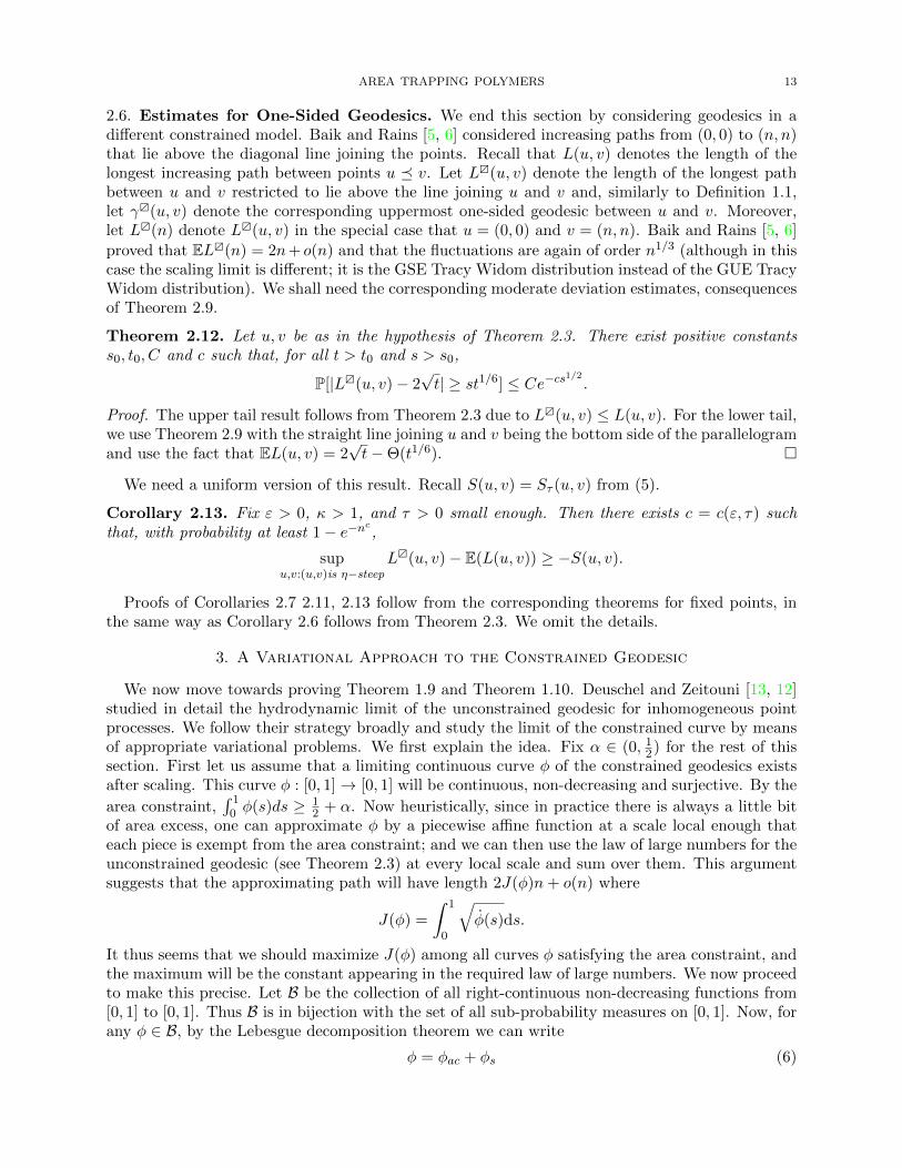
Definition 5.1. Let C > 1, κ > 1 be given constants. A sequence of points u0 � u1 � · · · � uk iscalled a (C, κ)-regular sequence if the following conditions hold.
(i) The union of line segments joining ui to ui+1 for i = 0, 1, . . . , k−1, is the graph of a concavefunction.
(ii) The gradient of all the line segments joining ui to ui+1 is ∈ ( 1κ , κ).
(iii) The distance |uk − u0| between the first and last point in the sequence lies in
( 1Cn
3/4−ε/2, Cn3/4−ε/2).

AREA TRAPPING POLYMERS 23
(iv) The distance between the consecutive points in the sequence is small: |ui − ui+1| ≤ n3/4−ε.(v) Let θ1 and θ2 be the angles that the line segments (u0, u1) and (uk−1, uk) make with the
positive x-axis (clearly θ1 ≥ θ2 by hypothesis). Then θ1 − θ2 ≤ 100C2n−1/4−ε/2.
See Figure 3 for an illustration of this definition.
uk
u0
v
u1
uk−1
n1/2−ε/2
n3/4−
ε{n3/
4−ε/
2
u∗
ukuk−1
u2
u0
Γ
γ
u1
u∗
(a) (b)
Figure 3. (a) A sequence of regular corners u0, u1, . . . , uk. The triangle T isan isosceles triangle formed by vertices u0, uk and u∗ such that the adjacent sideslie above the piecewise linear path passing through the points u0, u1, . . . , uk. Bydefinition of regularity, the triangle T is contained in the parallelogram R formed bythe vertices u0, v0, vk and uk which has vertical height n1/2−ε/2. Observe that theheight of this parallelogram is much smaller than the transversal fluctuation of pathsbetween u0 and uk. (b) On Aε, there is a regular sequence of corners u0, u1, . . . , ukand Γ is the best constrained path. We show that there is an alternative path γbetween u0 and u1 above the triangle T that is extremely likely to be strictly largerin length than the restriction of Γ between u0 and uk. Then the path obtained byreplacing Γ with γ between u0 and uk has a larger length and traps a larger area,thus leading to a contradiction.
Before proceeding, we try to motivate item (v). Consider the least concave majorant of anincreasing path from (0, 0) to (n, n) as described in Definition 1.2. The total change of angle madeby the line segments constituting the concave majorant with the x-axis is roughly the ratio of π/2
and n. So over a distance of around n3/4−ε/2, the change of angle should be roughly n1/4−ε/2. Item(v) asserts that on a regular sequence the change of angle is not much more than this average.
The following basic geometric consequence will be useful.
Lemma 5.2. Let S = {u0, u1, . . . , uk} be a (C, κ)-regular sequence for some C, κ > 1. Let LS denotethe union of line segments joining the consecutive points of S. Let R denote the parallelogram withtwo vertical sides of length n1/2−ε/2 whose bottom side is the line segment joining u0 and uk; seeFigure 3(a). Then there exists a point u∗ in R such that the triangle T formed by the points u0, ukand u∗ is an isosceles triangle (with the sides adjacent to u∗ being of equal length) contained in Rsuch that the two sides of T adjacent to u∗ lie above the piecewise affine curve obtained by joiningthe consecutive points of S.
Proof. Consider the angles ω1 and ω2 made by the line segments (u0, u1) and (uk−1, uk) respectivelywith the line segment (u0, uk). Also, let v be the point of intersection obtained by extending theline segments (u0, u1) and (uk−1, uk). By convexity, the piecewise affine curve obtained by joiningthe points of S lies inside the triangle (u0, uk, v). Moreover, it follows from elementary geometric

24 RIDDHIPRATIM BASU, SHIRSHENDU GANGULY, AND ALAN HAMMOND
arguments that θ1−θ2 = ω1+ω2. Now let us consider the isosceles triangle (u0, uk, u∗) where (u0, uk)forms the base and θ1− θ2 is the value of the two equal angles. Since θ1− θ2 is at least as big as ω1
and ω2, it follows that the triangle (u0, uk, v) is contained inside the triangle (u0, uk, u∗). Moreover,
the latter is clearly contained in a parallelogram of height O(n3/4−ε/2n−1/4−ε/2) where the constant
in the O(·) notation depends on κ. Since for all large enough n, n3/4−ε/2n−1/4−ε/2 � n1/2−ε/2, weare done. �
Let us now record the main steps of the proof of Theorem 1.3. Let Γ denote the constrainedgeodesic. Recall that Γ∗α,n denotes least concave majorant of Γ and is a union of facets as describedin Definition 1.2.
Step 1: We shall fix a (C, κ)-regular sequence S = {u0, u1, . . . , uk}, and consider the bestpath γS from u0 to uk that passes through all the points in the sequence. We shall show thatwith very high probability the length of this path is much smaller than the length of the best pathbetween u0 and uk. The reason that this event is likely is the following: because the lengths of thesegments {ui, ui+1} are much smaller than that of the segment {u0, uk}, it will turn out that thepath γ will have a much smaller transversal fluctuation compared to the typical geodesic betweenu0 and uk. Thus, by Theorem 2.10, it is extremely likely that this path has a much smaller length.
Step 2: Next we will show that there exists a path between u0 and uk that lies above theline segments joining the consecutive points of S and whose length is comparable to that of thegeodesic between u0 and uk. This will follow from the definition of regular sequence together withan application of Lemma 5.2 and Theorem 2.12.
Step 3: Finally, we will show that, on the event Aε, it is overwhelmingly likely that there existsa (C, κ)-regular sequence made out of consecutive corners of Γ∗α,n. Once we establish this, we willarrive at a contradiction: using the first two steps, we will construct a path that traps more areathan does Γ and that also has a greater length.
The next proposition treats the first step.
Proposition 5.3. Let S = {u0, u1, . . . , uk} be a (C, κ)-regular sequence. For i = 0, 1, . . . , k − 1,let γi be the geodesic between ui and ui+1. Let γS denote the concatenation of the paths γi. Thenthere exists c > 0 such that, with probability at least 1− e−nc, we have
|γS | ≤ EL(u0, uk)− n1/4−ε/12.
Proof. Let R′ be the parallelogram with sides parallel to the sides of R such that u0 and uk are themidpoints of the vertical sides of R′; and the height of the vertical sides is 4n1/2−ε/2. For each i,let Ri denote the parallelogram with the following properties:
(1) Ri has one pair of vertical sides and the other pair of sides is parallel to the line segmentjoining ui and ui+1.
(2) The vertical sides have midpoints ui and ui+1.
(3) The height of the vertical sides is n1/2−3ε/5.
It is straightforward to check from Definition 5.1 that all the rectangles Ri are contained in therectangle R′. Now it follows from Theorem 2.5 that, with probability at least 1−e−nc , each geodesicγi is contained in the parallelogram Ri. In particular, on this event,
|γS | ≤ L(u0, uk;R′).
The result now follows using Theorem 2.10 and the assumed lower bound on |u0 − uk|. �
Next we move on to Step 2, in which we show the existence of a “good” path between u0 and uk.
AREA TRAPPING POLYMERS 25
ukuk−1
u2
u0
u1
R′ n3/4−ε/2
Ri
Γ
n1/2−ε/2
n1/2−3ε/5
n3/4−ε
v0
v1
n3/4−ε n1/2−ε}
Γ
γ�(v0, v1)
(a) (b)
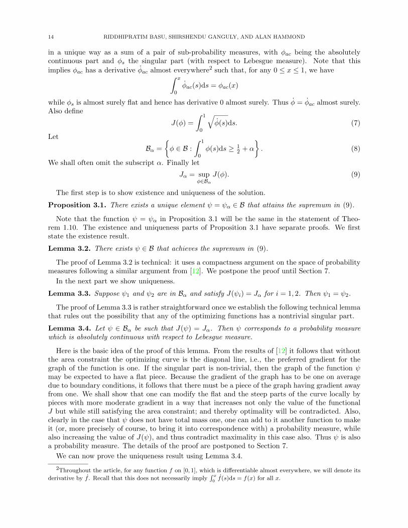
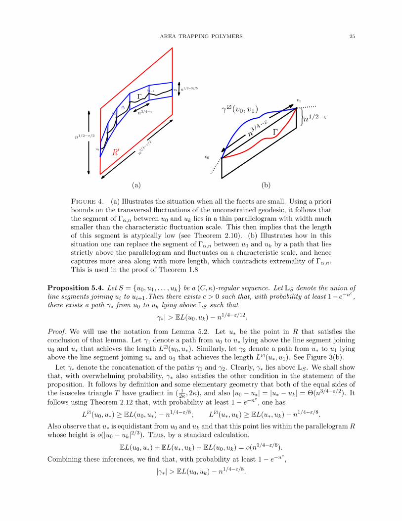
Figure 4. (a) Illustrates the situation when all the facets are small. Using a prioribounds on the transversal fluctuations of the unconstrained geodesic, it follows thatthe segment of Γα,n between u0 and uk lies in a thin parallelogram with width muchsmaller than the characteristic fluctuation scale. This then implies that the lengthof this segment is atypically low (see Theorem 2.10). (b) Illustrates how in thissituation one can replace the segment of Γα,n between u0 and uk by a path that liesstrictly above the parallelogram and fluctuates on a characteristic scale, and hencecaptures more area along with more length, which contradicts extremality of Γα,n.This is used in the proof of Theorem 1.8
Proposition 5.4. Let S = {u0, u1, . . . , uk} be a (C, κ)-regular sequence. Let LS denote the union ofline segments joining ui to ui+1.Then there exists c > 0 such that, with probability at least 1−e−nc,there exists a path γ∗ from u0 to uk lying above LS such that
|γ∗| > EL(u0, uk)− n1/4−ε/12.
Proof. We will use the notation from Lemma 5.2. Let u∗ be the point in R that satisfies theconclusion of that lemma. Let γ1 denote a path from u0 to u∗ lying above the line segment joiningu0 and u∗ that achieves the length L�(u0, u∗). Similarly, let γ2 denote a path from u∗ to u1 lyingabove the line segment joining u∗ and u1 that achieves the length L�(u∗, u1). See Figure 3(b).
Let γ∗ denote the concatenation of the paths γ1 and γ2. Clearly, γ∗ lies above LS . We shall showthat, with overwhelming probability, γ∗ also satisfies the other condition in the statement of theproposition. It follows by definition and some elementary geometry that both of the equal sides ofthe isosceles triangle T have gradient in ( 1
2κ , 2κ), and also |u0 − u∗| = |u∗ − uk| = Θ(n3/4−ε/2). It
follows using Theorem 2.12 that, with probability at least 1− e−nc , one has
L�(u0, u∗) ≥ EL(u0, u∗)− n1/4−ε/8; L�(u∗, uk) ≥ EL(u∗, uk)− n1/4−ε/8.Also observe that u∗ is equidistant from u0 and uk and that this point lies within the parallelogramRwhose height is o(|u0 − uk|2/3). Thus, by a standard calculation,
EL(u0, u∗) + EL(u∗, uk)− EL(u0, uk) = o(n1/4−ε/6).
Combining these inferences, we find that, with probability at least 1− e−nc ,|γ∗| > EL(u0, uk)− n1/4−ε/8.
26 RIDDHIPRATIM BASU, SHIRSHENDU GANGULY, AND ALAN HAMMOND
This completes the proof of the proposition. �
In the final step, we establish that, on Aε, that is if MFL(Γn) is smaller than n3/4−ε, it isextremely likely that there exists a regular sequence whose points are consecutive corners of Γ∗α,n(the least concave majorant of Γα,n). Let Reg(C, κ) denote the event that there exist consecutivecorners u0, u1, . . . , uk of Γ∗α,n such that {u0, u1, . . . , uk} is a (C, κ)-regular sequence.
Proposition 5.5. There exist C, κ such that, except for a sub-event of exponentially small proba-bility, the event Aε is contained in the event Reg(C, κ), i.e.,
P(Aε \ Reg(C, κ)) ≤ e−cn,for some universal constant c > 0.
On Aε, we shall find a regular sequence among interior facets. Before proceeding we state aneasy geometric lemma that will be used. The proof is provided in Section 7.
u
v
ω ω2
ω1
(n, 0)
{
Figure 5. Crude estimates on length of facets which subtend an angle θ at the origin.
For any two points p1, p2 ∈ [0, n]2, denote by θ(p1, p2) the acute angle between the lines joiningthe points p1 and p2 to the point (n, 0), i.e., the bottom right corner of the square (see Figure 5).
Lemma 5.6. There exists θ0, such that with probability at least 1 − e−cn, simultaneously, for allu, v on Γ∗α,n with θ(u, v) ≤ θ0,
|u− v| = Θ(θ(u, v)n).
Proof of Proposition 5.5. Observe that by definition, on Aε, any sequence u0 � u1 � · · · � ukof consecutive corners of Γ∗α,n satisfies condition (i) and (iv) of Definition 5.1. Fix δ > 0. By
Theorem 4.6, we see that it is with a failure probability of at most e−cn that all the δ−interiorfacets have gradient s in the interval (1/κ, κ) for some κ(δ) > 1. For the remainder of the proof,we shall assume that this event occurs. Now we partition all the δ-interior vertices of Γ∗α,n (it iseasy to see they are non-empty on Aε) into consecutive segments
(v1, v2, . . . , vi1), (vi1+1, vi1+2, . . . , vi2), . . . , (24)
(where vi’s are the consecutive corners on Γ∗α,n) such that
θ(vij , vij+1−1) < n−1/4−ε/2 ≤ θ(vij+1, vij+1)
for all j = 0, 1, . . . , where i0 = 1.
We denote the segment (vij , vij+1, . . . , vij+1) by Sj . Thus if S1, S2, . . . , Sm are all such seg-
ments, then m = Θ(n1/4+ε/2). It follows from convexity and the boundedness of the gradients (see
Lemma 5.6 and Figure 5) that |vij − vij+1 | = Θ(n3/4−ε/2). Let ωk denote the angle made by the
AREA TRAPPING POLYMERS 27
line segment (vk, vk+1) with the positive x-axis. Let θj = ωij − ωij+1−1. Notice that, by convexity,θj is nonnegative for all j. Also observe that∑
j
θj ≤π
2.
This together with Markov’s inequality and the fact that the number of Sj ’s is Θ(n1/4+ε/2) implies
that, for some constant C, there exists at least one Sj such that θj ≤ Cn−1/4−ε/2. Setting S =(u0, u1, . . . , uk) to be equal to such a sequence, we see that S satisfies all conditions in Definition 5.1for some C, κ > 1. This completes the proof of the proposition. �
With all this preparation, we are ready to prove Theorem 1.3.
Proof of Theorem 1.3. Let α ∈ (0, 12) and ε > 0 be fixed as before. Let (C, κ) be such that theconclusion of Proposition 5.5 holds. Let S denote the event that there exists a (C, κ)-regularsequence for which at least one of the conclusions in Proposition 5.3 and Proposition 5.4 does nothold. Using the proofs of the said propositions, along with taking a union bound over all pairs ofgrid points obtained by coarse graining [0, n]2 (exactly as Corollary 2.6 followed from Theorem 2.3),that P(S) ≤ e−nc for some c > 0. By Proposition 5.5, it suffices to show that
Aε ∩ Sc ∩ Reg(C, κ) = ∅.By way of contradiction, let us assume that the set is non-empty. Fix a configuration in the setAε ∩ Sc ∩ Reg(C, κ), and consider the least concave majorant Γ∗α,n of the constrained geodesic.On Aε ∩ Reg(C, κ), there exists a (C, κ)-regular sequence S = {u0, u1, . . . , uk} consisting of con-secutive corners of Γ∗α,n. On Sc, there exists a path γ∗ from u0 to uk satisfying the conclusion ofProposition 5.4. Let γ0 denote the restriction of Γ between u0 and uk. Clearly,
|γ0| ≤∑i
L(ui, ui+1).
It follows from Propositions 5.3 and 5.4 that, on Sc, |γ0| < |γ∗|. Also observe that γ0 lies belowthe line segments joining ui to ui+1 whereas γ∗ lies above these segments. Hence the increasingpath Γ′ from (0, 0) to (n, n) that coincides with Γ between (0, 0) and u0 and between uk and (n, n)and coincides with γ∗ between u0 and uk traps at least as much area as does Γ. However, by theabove discussion, |Γ′| > |Γ|. This contradicts the extremality of Γ and completes the proof of thetheorem. �
5.1. Proof of lower bound of MLR. In this subsection we prove Theorem 1.4. That is, we showthat the maximum local roughness of the facets has scaling exponent at least 1
2 . The basic idea of
the proof is to use KPZ scaling to argue that, if there is a facet of length roughly n3/4, then alongthat facet, the local roughness is likely to be at least (n3/4)2/3 = n1/2. We now make this moreprecise.
Fix ε > 0. We have just proved that, with high probability, there exists a facet of length at leastn3/4−ε. In fact, by the proof of Theorem 1.3, more is true. Fix κ � 1. Let Bε = Bn,ε,κ denote
the event that Γ∗α,n (see Definition 1.2) has a facet of length at least n3/4−ε with endpoints v0 andv1 such that the straight line joining v0 and v1 has gradient ∈ (1/κ, κ). The following lemma is aconsequence of the proof of Theorem 1.3.
Lemma 5.7. For all large enough κ (depending on α), P(Bε) ≥ 1−e−nc for all n sufficiently large,where c is a constant depending only on ε and α.
Proof. Note that the proof of Theorem 1.3 in fact showed that there must be a δ-interior facet oflength at least n3/4−ε with sufficiently large probability. Since all the δ-interior facets satisfy thegradient requirement (see Theorem 4.6), we are done. �
28 RIDDHIPRATIM BASU, SHIRSHENDU GANGULY, AND ALAN HAMMOND
Proof of Theorem 1.4. Let Cε denote the event that MLR(Γn) ≤ n1/2−ε. Thus, to prove Theo-rem 1.4, it suffices to show that
P(Cε ∩ Bε) ≤ e−nc.
Let Γ denote the constrained geodesic. On Cε ∩ Bε, let v0 and v1 be corners of Γ∗α,n satisfyingthe conditions in the definition of Bε. Consider the restriction Γ(v0, v1) of Γ between v0 and v1.
As MLR(Γ) ≤ n1/2−ε, it follows that there exists C = C(κ) > 0 such that the restriction of Γ(call it γ) between v0 and v1 is contained in the parallelogram U that has a pair of vertical sides
of height Cn1/2−ε and whose top side is the line segment joining v0 and v1. Now observe that theheight of the parallelogram is much smaller than the on-scale transversal fluctuation of geodesicsbetween v0 and v1, these fluctuations being at least
(n3/4−ε)2/3−ε/100 ≥ n1/2−3ε/4.Thus, Corollary 2.7 implies that the bound
E(L(v0, v1))− |γ| ≥ |v0 − v1|1/3−5ε/9
fails with probability at most e−nc. By Corollary 2.13,
L�(v0, v1)− E(L(v0, v1)) ≥ −|v0 − v1|13+ε/100
except, again, on a set of probability at most e−nc. Consider now the path Γ′ that agrees with Γ
outside the segment (v0, v1) and that between v0 and v1 equals γ�(v0, v1), which recall is a path fromv0 to v1 lying above the line segment that joins these two points and achieves length L�(v0, v1). Wesee then that Γ′ has greater length, and traps as much area as, Γ. This contradicts the assumptionof length maximality for Γ; (similarly to the proof of Theorem 1.3. See Figure 4(b).) �
6. Upper Bound for Scaling Exponents
This section is devoted to the proof of Theorem 1.7. That is, it will be shown here that, fora dense set of α that may depend on n, the maximum facet length of the constrained geodesic isvery likely to be at most n3/4+o(1). Theorem 1.8 will then follow by the KPZ scaling enjoyed bytransversal fluctuations.
We explain the main ideas before giving proofs. Recall Definition 1.6 and the interval [α1, α2] inthe hypothesis of Theorem 1.7. The basic idea is to show, using Corollary 2.13, that if a certainvalue of α is not ‘good’ (recall Definition 1.6), we may perform a “landgrab” operation. Let us
assume that there is a facet (v0, v1) which has length n3/4+ε and has a reasonable gradient boundedaway from zero and infinity. Corollary 2.13 allows us to find a path γ from v0 to v1 which lies abovethe facet (v0, v1) at a characteristic height of (n3/4+ε)2/3 and has characteristic fluctuations. Sincewe can afford to allow some error, we can assume
|γ| ≥ E(L(v0, v1))− (n3/4+ε)1/3+ε/1000 ≥ E(L(v0, v1))− n1/4+2ε/5.
Similarly by Corollary 2.6 we can assume that
|Γ(v0, v1)| ≤ E(L(v0, v1)) + n1/4+2ε/5
where Γ(v0, v1) is the restriction of the constrained geodesic Γ between v0 and v1. Thus the path Γ′
which is obtained from Γ by replacing Γ(v0, v1) by γ traps at least n5/4+5ε/3 more area than does Γ
and loses at most n1/4+2ε/5 in length. Repeating this operation about n3/4−5ε/3 times (a repetitionwhich is possible, provided there is no good α in the interval [α1, α2], one gains an area that isΘ(1) while losing at most O(n1−ε) in length with very high probability. This contradicts the factthat ELα1(n)−ELα2(n) = Θ(n) for α1 < α2 which is an easy consequence of Theorems 1.9 and 2.1along with the observation that wα is strictly decreasing in α. Next we provide the details neededto make the above argument precise.
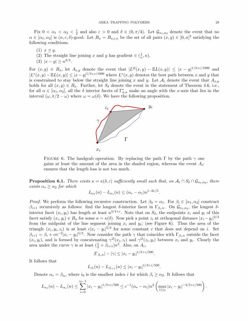
AREA TRAPPING POLYMERS 29
Fix 0 < α1 < α2 <12 and also ε > 0 and δ ∈ (0, π/4). Let Gα1,α2 denote the event that no
α ∈ [α1, α2] is (n, ε, δ)-good. Let Bn = Bn,ε,κ be the set of all pairs (x, y) ∈ [0, n]2 satisfying thefollowing conditions.
(1) x � y.(2) The straight line joining x and y has gradient ∈ ( 1
κ , κ).
(3) |x− y| ≥ n3/4.For (x, y) ∈ Bn, let Ax,y denote the event that |L�(x, y) − EL(x, y)| ≤ |x − y|1/3+ε/1000 and
|L∗(x, y)−EL(x, y)| ≤ |x− y|1/3+ε/1000 where L∗(x, y) denotes the best path between x and y thatis constrained to stay below the straight line joining x and y. Let Aε denote the event that Ax,yholds for all (x, y) ∈ Bn. Further, let Sδ denote the event in the statement of Theorem 4.6, i.e.,for all α ∈ [α1, α2], all the δ interior facets of Γ∗α,n make an angle with the x-axis that lies in theinterval (ω, π/2− ω) where ω = ω(δ). We have the following proposition.
xi
zi yi
Γ
γ
Figure 6. The landgrab operation. By replacing the path Γ by the path γ onegains at least the amount of the area in the shaded region, whereas the event Aε′ensures that the length loss is not too much.
Proposition 6.1. There exists κ = κ(δ, ε) sufficiently small such that, on Aε ∩ Sδ ∩ Gα1,α2, thereexists α∗ ≥ α2 for which
Lα1(n)− Lα∗(n) ≤ (α∗ − α1)n1−6ε/5.
Proof. We perform the following recursive construction. Let β0 = α1. For βi ∈ [α1, α2] constructβi+1 recursively as follows: find the longest δ-interior facet in Γβi,n. On Gα1,α2 , the longest δ-
interior facet (xi, yi) has length at least n3/4+ε. Note that on Sδ, the endpoints xi and yi of this
facet satisfy (xi, yi) ∈ Bn for some κ = κ(δ). Now pick a point zi at orthogonal distance |xi− yi|2/3from the midpoint of the line segment joining xi and yi; (see Figure 6). Thus the area of the
triangle (xi, yi, zi) is at least c|xi − yi|5/3 for some constant c that does not depend on i. Set
βi+1 = βi + cn−2|xi − yi|5/3. Now consider the path γ that coincides with Γβi,n outside the facet(xi, yi), and is formed by concatenating γ�(xi, zi) and γ�(zi, yi) between xi and yi. Clearly thearea under the curve γ is at least (12 + βi+1)n
2. Also, on Aε,
|Γβi,n| − |γ| ≤ |xi − yi|1/3+ε/500.It follows that
Lβi(n)− Lβi+1(n) ≤ |xi − yi|1/3+ε/500.
Denote α∗ = βi0 , where i0 is the smallest index i for which βi ≥ α2. It follows that
Lα1(n)− Lα∗(n) ≤i0−1∑i=0
|xi − yi|1/3+ε/500 ≤ c−1(α∗ − α1)n2
(maxi≤i0|xi − yi|−4/3+ε/500
).

30 RIDDHIPRATIM BASU, SHIRSHENDU GANGULY, AND ALAN HAMMOND
Since |xi − yi| ≥ n3/4+ε for all i, it follows that the final term is at most n−1−4ε/3. This completesthe proof of the proposition. �
We now complete the proof of Theorem 1.7.
Proof of Theorem 1.7. Let κ be large enough that the conclusion of Proposition 6.1 holds. UsingTheorem 4.6 and Corollary 2.11, it follows that, for this choice of κ (and for given α1, α2, δ and ε),one has that, for some constant c > 0,
P[Acε ∪ Scδ ] ≤ e−nc.
Hence, using Proposition 6.1, it suffices to show that
P(Lα1(n)− Lα2(n) ≤ (1/2− α1)n
1−6ε/5)≤ e−nc (25)
for some c > 0. Notice that in the above step we have used the trivial inequality Lα2(n) ≥ Lα∗(n)
for all α∗ ∈ [α2,12). It follows now from Theorem 1.9 that ELα1(n) − ELα2(n) ≥ wα1−wα2
2 n forn sufficiently large. The claimed bound (25) now follows from Theorem 2.1 and the fact thatwα1 − wα2 > 0. This completes the proof. �
6.1. Proof of Theorem 1.8. This derivation is similar to that by which Theorem 1.4 follows fromTheorem 1.3. By Theorem 4.6, for all α ∈ [α1, α2] and all small enough δ, there is a probability atleast 1 − e−cn that all the δ-interior facets of Γ∗α,n are κ-steep for some value of 1 ≤ κ < ∞. Theset of good α′s is a function of the underlying point process and hence is random, but in any case,for any such α that lies in [α1, α2], it holds by definition that all the interior facets of Γ∗α,n have
length at most n3/4+ε. Moreover, by the uniform bounds discussed above, we may suppose thatall the facets are κ-steep. Suppose that the maximum local roughness restricted to the δ-interiorfacets is at least n1/2+ε. Let u and v be the endpoints of the facet that attains this maximum localroughness. Let γ(u, v) be the segment of Γα,n between u and v. By using Corollary 2.7, we seethat, with probability at least 1− e−nc ,
|γ(u, v)| < E(L(u, v))− S(u, v).
On the other hand, by Corollary 2.13 again, we find that, except on an event of probability atmost e−n
c,
L�(u, v) ≥ E(L(u, v)))− S(u, v).
Thus, the path that agrees with Γ from (0, 0) to u and from v to (n, n) and equals the path γ�(u, v)between the points u and v clearly captures at least as much area as does Γα,n and also containsmore points than does Γα,n. This contradicts the extremality of the latter path. �
6.2. Possible extensions and difficulties. We end this section with a few remarks related tothe first two open problems mentioned in Section 1.4. A natural approach to quantifying theproof of Theorem 1.7 is via Proposition 6.1. Namely, one can hope to bound below the density ofthose α ∈ [α1, α2] that are (n, ε) good (where here we ignore the parameter δ for the purpose ofillustration.) This is because using similar arguments to those used in deriving these two results,one can hope to prove the following uniform bound: with high probability the noise space issuch that for all α ∈ [α1, α2] we have Lα(n) − Lα∗(n) ≤ O(`1/3) for α∗ = α + `5/3n−2, where
` = max(MFL(Γα,n), n3/4), and where the O-notation hides poly-logarithmic multiplicative factors(which arise due to the exceptional nature of the facet endpoints that contributes a polynomialentropy factor). Thus, the above implies that the length-to-area gradient in scaled coordinates
(with length measured in units of n and area measured in units of n2) is O( n`4/3
) = O(1) as by
definition ` ≥ n3/4. Also, we know that, for all α which are (n, ε) bad, the gradient is polynomiallysmall (since by the land-grab argument, illustrated in Figure 6, the length loss is much smaller than
AREA TRAPPING POLYMERS 31
the area gain). This coupled with the fact that Lα1 − Lα2 = Θ(n), should then allow to concludethat the density of good α is at least 1
O(1).
Notice that our approach for proving upper bounds relies on the joint coupling of the process forvarious values of α. This is quite different in spirit from the known proofs of similar statements inother contexts such as phase separation [20] where the upper bound was proven for a fixed valueof α. The key ingredient there was an understanding of the excess area fluctuation (see Openquestion (2) in Section 1.4) which then allowed a resampling argument to work. However, since wedo not have such bounds, we have to work across various values of α simultaneously.
A heuristic argument in our setting proving an upper bound of n5/4+o(1) on the excess areatrapped by Γ = Γα, assuming that α is (n, ε/10) good (recall Definition 1.6) can be made as
follows: Suppose that the excess area is more than n5/4+ε. Since, by hypothesis the longest facetlength is at most n3/4+ε/10 , we may find two points x and y on Γ∗α,n such that |x− y| ≈ n3/4+ε/5
and segment of Γ∗α,n between x and y has average curvature (the average distance of the curvefrom the line segment joining x and y is what it should be on for a circle; see Figure 2(b)).Now consider shortcutting Γ between x and y and hence replacing the subpath of Γα,n betweenx and y by the unconstrained geodesic between x and y. This operation will create an area loss(approximately n5/4+3ε/5) which is not enough to violate the area constraint, because the excess
area before the shortcut was at least n5/4+ε. Moreover, the shortcut increases the overall weightand hence contradicts extremality of Γα,n.
7. Proofs of some of the earlier statements
It remains to provide the proofs of Lemmas 3.2, 3.4, 3.5, 5.6 and Theorem 2.1.
7.1. Proof of Lemma 3.2. This subsection follows closely the arguments presented in [12, Section3]. Let φ1, φ2, . . . be a sequence of elements in Bα such that
limnJ(φn) = Jα.
We equip the space of bounded signed measures on [0, 1] with the weak topology generated byC = C[0, 1] (the space of continuous functions on [0, 1]). Since for all n ≥ 1, φn corresponds to asub-probability measure, we may use compactness and pass to a subsequence (denoted again by{n} for convenience), and thus suppose that φn converges to ψ ∈ M, in the weak topology. Thisin particular implies φn(x) converges to ψ(x) almost everywhere (since the convergence happensat all continuity points of ψ, see e.g., [16, Section 3.2] ). Since the φn’s are all bounded by 1 andbelong to Bα, it follows from the bounded convergence theorem that ψ ∈ Bα. Next we will showthat
limnJ(φn) ≤ J(ψ). (26)
Clearly this implies J(ψ) = Jα and hence we would be done. The claim in (26) follows from theupper semicontinuity of J(·) or equivalently the lower semicontinuity of −J(·). To show the latter,one represents −J(·) as an appropriate Legendre transform. To proceed we need some definitions:Clearly (7) extends naturally to all non-negative measures. We extend J to all of M by setting itto be ∞ for all measures which are not non-negative. Moreover, for any f ∈ C, define
Λ(f) =
{∞ if
∫ 10
1|f(s)|ds =∞ or if f ≥ 0 on a set of positive Lebesgue measure.
−14
∫ 10
1f(s)ds otherwise
Now for any φ ∈ B, define Λ∗(φ) = supf∈C[0,1]
[∫ 1
0fdφ− Λ(f)
]. This function is lower semicontinuous,
because whenever f ∈ C[0, 1] and φn is a sequence that converges to φ, the definition of weak
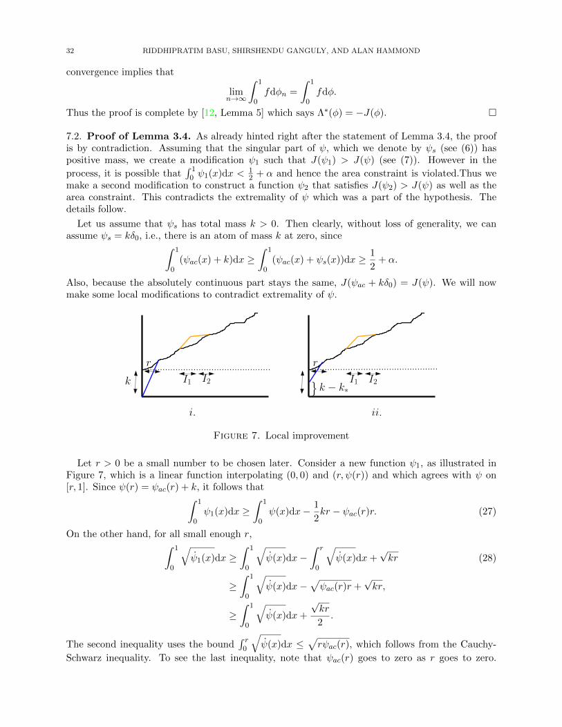
32 RIDDHIPRATIM BASU, SHIRSHENDU GANGULY, AND ALAN HAMMOND
convergence implies that
limn→∞
∫ 1
0fdφn =
∫ 1
0fdφ.
Thus the proof is complete by [12, Lemma 5] which says Λ∗(φ) = −J(φ). �
7.2. Proof of Lemma 3.4. As already hinted right after the statement of Lemma 3.4, the proofis by contradiction. Assuming that the singular part of ψ, which we denote by ψs (see (6)) haspositive mass, we create a modification ψ1 such that J(ψ1) > J(ψ) (see (7)). However in the
process, it is possible that∫ 10 ψ1(x)dx < 1
2 + α and hence the area constraint is violated.Thus wemake a second modification to construct a function ψ2 that satisfies J(ψ2) > J(ψ) as well as thearea constraint. This contradicts the extremality of ψ which was a part of the hypothesis. Thedetails follow.
Let us assume that ψs has total mass k > 0. Then clearly, without loss of generality, we canassume ψs = kδ0, i.e., there is an atom of mass k at zero, since∫ 1
0(ψac(x) + k)dx ≥
∫ 1
0(ψac(x) + ψs(x))dx ≥ 1
2+ α.
Also, because the absolutely continuous part stays the same, J(ψac + kδ0) = J(ψ). We will nowmake some local modifications to contradict extremality of ψ.
k
r
I1 I2
i. ii.
r
I1 I2k − k∗}
Figure 7. Local improvement
Let r > 0 be a small number to be chosen later. Consider a new function ψ1, as illustrated inFigure 7, which is a linear function interpolating (0, 0) and (r, ψ(r)) and which agrees with ψ on[r, 1]. Since ψ(r) = ψac(r) + k, it follows that∫ 1
0ψ1(x)dx ≥
∫ 1
0ψ(x)dx− 1
2kr − ψac(r)r. (27)
On the other hand, for all small enough r,∫ 1
0
√ψ1(x)dx ≥
∫ 1
0
√ψ(x)dx−
∫ r
0
√ψ(x)dx+
√kr (28)
≥∫ 1
0
√ψ(x)dx−
√ψac(r)r +
√kr,
≥∫ 1
0
√ψ(x)dx+
√kr
2.
The second inequality uses the bound∫ r0
√ψ(x)dx ≤
√rψac(r), which follows from the Cauchy-
Schwarz inequality. To see the last inequality, note that ψac(r) goes to zero as r goes to zero.
AREA TRAPPING POLYMERS 33
However, it is easy to see that ∫ 1
0ψ1(x)dx <
∫ 1
0ψ(x)dx.
Thus a priori ψ1 need not be an element of Bα; (see (8)). To ensure that indeed∫ 10 ψ1(x)dx ≥ 1
2 +α,we have to make another modification. Note that already in the proof of Lemma 3.3, we arguedthat, even if ψ is not unique, ψ is unique. Thus there exist cα > 0 and 0 < c1 < c2 depending onlyon α such that the set (ψ)−1[c1, c2] has Lebesgue measure at least cα. (Note that even though theproof of Lemma 3.3 relied on Lemma 3.4, the uniqueness of the density was argued independentlyand hence this is not a circular argument.)
For brevity, let us call the set (ψ)−1[c1, c2] by the name I. We now choose arbitrary disjointsubsets of I ∩ [ε, 1] for some ε > 0, denoted by I1 and I2, both of measure k; (we take theintersection with [ε, 1] to ensure that both the sets are away from 0). Note that this can alwaysbe done if µ(I) > 2k. In case µ(I) ≤ 2k, we can modify ψ1 by taking it to be a linear functioninterpolating (0, k−k∗) and (r, ψ(r)) for some k∗ small enough so that µ(I) > 2k∗; (see Figure 7 ii.Nothing changes in any of the arguments that follow as well as the conclusions and hence we willpretend that k = k∗ throughout the rest of the argument. Let us also choose I1 and I2 such thatsup(I1) < inf(I2), and let ψ2(x) :=
∫ x0 ψ2(y)dy where
ψ2 := ψ1 +r
k1I1 −
r
k1I2 . (29)
We will also choose r < ε. Note that since ψ1 = ψ ≥ c1 on I2, for all small enough r, ψ2 isnon-negative. Also, since the measures of I1 and I2 are the same,∫ 1
0ψ2(x)dx =
∫ 1
0ψ1(x)dx.
We now compute the area under the curve ψ2(·) and see how it differs from that of ψ1(·). Forevery y ∈ [0, 1], we have
ψ2(y)− ψ1(y) =r
k[µ(I1 ∩ [0, y])− µ(I2 ∩ [0, y])].
Thus, ∫ 1
0[ψ2(y)− ψ1(y)]dy =
r
k
∫ 1
0[µ(I1 ∩ [0, y])− µ(I2 ∩ [0, y])]dy, (30)
=r
k
∫ 1
0(1− y)[1I1 − 1I2 ]dy,
≥ rk.
The last inequality follows since, as µ(I1) = µ(I2) = k and sup(I1) < inf(I2), the integral above isat least k2. Thus, the new function ψ2(x) traps at least as much area as does ψ(x) since∫ 1
0ψ2(x)dx−
∫ 1
0ψ(x)dx = [
∫ 1
0ψ2(x)dx−
∫ 1
0ψ1(x)dx] + [
∫ 1
0ψ1(x)dx−
∫ 1
0ψ(x)dx],
≥ rk − rk
2− Cψac(r)r > 0,
for all small enough r, since C > 0 is an universal constant, (the last inequality uses (27)).

34 RIDDHIPRATIM BASU, SHIRSHENDU GANGULY, AND ALAN HAMMOND
Moreover, by Taylor expansion (using (29) and ψ1 ≥ c1 on I1 ∪ I2),∫ 1
0
√ψ2(x)dx−
√ψ1(x)dx ≥
∫I1
√ψ1(x)(
r
2kψ1(x)− C(
r
kψ1(x))2)dx
+
∫I2
√ψ1(x)(− r
2kψ1(x)− C(
r
kψ1(x))2)dx
≥ −C rkk = −Cr.
We use the bound ψ1 > c1 and that µ(I1) = µ(I2) = k crucially in the last inequality, and allthe constants depend only on c1 through the Taylor expansion. Thus, by choosing r � k we have√rk � r, and hence using (28),∫ 1
0
√ψ2(x)dx−
∫ 1
0
√ψ(x)dx =
∫ 1
0
√ψ2(x)dx−
∫ 1
0
√ψ1(x)dx+
∫ 1
0
√ψ2(x)dx−
∫ 1
0
√ψ1(x)dx,
≥ −Cr +√kr − C
√ψac(r)r,
≥√kr/2,
for all small enough r, since C > 0 is an universal constant. Hence, we obtain a contradiction tothe extremality of ψ. �
7.3. Proof of Lemma 3.5. (i) The proof follows by taking the monotone rearrangement and using
uniqueness. Let ψmon be the monotone rearrangement of ψ. Notice that, by Fubini’s theorem,
1
2+ α ≤
∫ 1
0ψ(x)dx =
∫ 1
0ψ(x)(1− x)dx ≤
∫ 1
0(ψ)mon(x)(1− x)dx =
∫ 1
0ψ1(x)dx (31)
where ψ1 = (ψ)mon. Only the second inequality above needs justification and it is a conse-quence of a standard rearrangement inequality. Thus ψ1 satisfies the area constraint. Also clearly∫ 10
√ψ(x)dx =
∫ 10
√ψ1(x)dx as rearrangement keeps integrals unchanged. This contradicts the
uniqueness of ψ unless ψ = ψ1
(ii) Let ψ be zero on a set of positive measure. By the first part of the lemma, this implies thatthere exists a such that ψ(y) is a constant on the interval [a, 1]. Note that it is easy to contradictextremality of ψ if ψ is not one on this interval. In case it is one on this interval, consider thefunction ψ1(x) = 1− ψ−1(1− x) (where ψ−1(1) = a). We claim that∫ 1
0ψ1(y)dy =
∫ 1
0ψ(x)dx, and
∫ 1
0
√ψ1(y)dy =
∫ 1
0
√ψ(x)dx.
The first equality follows by Fubini’s theorem. The second becomes clear after the change of variabley = 1 − φ(x) is made. Now, by uniqueness, ψ1 = ψ, and by Lemma 3.4 ψ has no singular part.However, ψ1 has an atom of mass 1− a at 0 which implies a = 1. �
7.4. Proof of Lemma 5.6. The reader may find it useful to refer to Figure 5. Let ω1 and ω2
be the acute angles that the line segments ((n, 0), u) and ((n, 0), v) make with the x-axis and they-axis. Now, without loss of generality, we can assume 0 ≤ ω1 ≤ π/4; otherwise, we could workwith ω2, since clearly one of the two quantities is at most π/4. Now, as a simple consequence ofTheorem 1.10, we see that, with probability at least 1−e−cn, (n, 0) is at a Θ(n) distance from Γ∗α,n.Also, since ψα is strictly concave, and ω1 ≤ π/4, the line segment (u, v) makes at least an anglec(α) > 0 (depending only on α and not on u and v) with the x-axis. The proof is now completedby considering the triangle ((n, 0), u, v) and simple geometric arguments. We omit the details. �
AREA TRAPPING POLYMERS 35
7.5. Proof of Theorem 2.1. The proof will follow by constructing a suitable martingale andappealing to well known concentration results for martingales. However things are slightly compli-cated by the possibility that the martingale may not have bounded increments. A simple truncationargument will allow us to take the increments to be bounded. Our proof strategy follows closelyarguments in [10]. The proof relies on some coarse graining. We start by introducing some notation.Let
Ai := {(x, y) : i ≤ x+ y < i+ 1}.Also let Bi,j = [i− 1, i)× [j − 1, j). Fix a number k to be specified soon. Recall the point processΠ and the path Γ = Γα,n from Section 1.1.1. Let Γk = Γk,α,n be the increasing path between(0, 0) and (n, n) with the same constraints as Γ along with the additional constraint that thecardinality of the intersection with Ai is less than k, for all i ∈ [0, . . . , 2n − 1]. Let us denote by|Γk| the weight of Γk. Consider the Doob Martingale {E [|Γk| | Fi]}0≤i≤2n−1, along the filtrationFi = {Π ∩ Aj : j ≤ i}. Note that the martingale increments are deterministically bounded by k.The following is a standard consequence of the Azuma-Hoeffding inequality.
Lemma 7.1. P(∣∣|Γk| − E(|Γk|)| ≥ t) ≤ e−
t2
4k2n .
In the remainder of the section, we obtain a bound on∣∣|Γ|− |Γk|∣∣ and thus also on
∣∣E|Γ|−E|Γk|∣∣.
Let Π∗ be the point process obtained from Π by removing points arbitrarily if necessary fromΠ∩Bi,j to make sure that |Π∗ ∩Bij | ≤ k/3 for all 1 ≤ i, j ≤ n. Let Γ∗ := Γα,∗ be the longest pathwith the same constraints as Γα in the environment Π∗.
Lemma 7.2. Deterministically as a consequence of the definitions it follows that |Γk| ≥ |Γ∗|.
Proof. Clearly it suffices to show that Γ∗ intersects none of the Ai’s at more than k points. Theproof is by contradiction: assume that there exists i such that |Γ∗ ∩ Ai| ≥ k + 1. Since the pointson Γ∗ are totally ordered (recall the ordering introduced in Section 1.1), let (x1, y1) and (x2, y2) bethe smallest and largest points in the set Γ∗ ∩Ai. By definition of Ai,
(x2 − x1) + (y2 − y1) ≤ 1, (32)
so that Γ∗ ∩ Ai intersects at most three B′i,js, since the number of different indices it can cross in
each direction is at most one if (32) is to be satisfied. Thus Γ∗ ∩Ai has to intersect at least one ofthe boxes at more than k+1
3 points. This contradicts the definition of Γ∗. �
Thus, it follows that |Γ| − |Γk| ≤ |Γ| − |Γ∗| ≤ C, where C =∑
i,j max(|Πi,j | − k/3, 0) and
Πi,j = Π ∩Bi,j . Taking k = 6 lognlog logn , the proof is now complete in view of the next result.
Lemma 7.3. The random variable C satisfies the following:
(1) P(C ≥ λn1/2 lognlog logn) ≤ 2λ2e−λ
2
(2) E(C) ≤ 1.
This is a simple consequence of the observation that |Πi,j | are independent Poisson variables with
mean one and the following tail bound of a standard Poisson variable X: P (X > r) ≤ e−r log r+r. �
References
[1] David Aldous and Persi Diaconis. Hammersley’s interacting particle process and longest increasing subsequences.Probab. Th. Rel. Fields, 103:199–213, 1995.
[2] Kenneth S Alexander. Cube–root boundary fluctuations for droplets in random cluster models. Communicationsin Mathematical Physics, 224(3):733–781, 2001.
[3] Antonio Auffinger, Michael Damron, and Jack Hanson. 50 years of first passage percolation. arXiv preprintarXiv:1511.03262, 2015.

36 RIDDHIPRATIM BASU, SHIRSHENDU GANGULY, AND ALAN HAMMOND
[4] Jinho Baik, Percy Deift, and Kurt Johansson. On the distribution of the length of the longest increasing subse-quence of random permutations. J. Amer. Math. Soc, 12:1119–1178, 1999.
[5] Jinho Baik and Eric M. Rains. Symmetrized random permutations. In Random Matrix Models and Their Appli-cations, volume 40 of Mathematical Sciences Research Institute Publications, pages 1–19, 2001.
[6] Jinho Baik and Eric M. Rains. Symmetrized random permutations. MSRI volume: Random Matrix Models andTheir Applications(40):1–19, 2001.
[7] Riddhipratim Basu and Alan Hammond. Localization of near geodesics in Brownian Last Passage Percolation.In preparation.
[8] Riddhipratim Basu, Vladas Sidoravicius, and Allan Sly. Last passage percolation with a defect line and thesolution of the Slow Bond Problem. Preprint arXiv 1408.3464.
[9] Marek Biskup, Oren Louidor, Eviatar B Procaccia, and Ron Rosenthal. Isoperimetry in two-dimensional perco-lation. arXiv preprint arXiv:1211.0745, 2012.
[10] Bela Bollobas and Graham Brightwell. The height of a random partial order: concentration of measure. TheAnnals of Applied Probability, pages 1009–1018, 1992.
[11] Sourav Chatterjee and Partha S. Dey. Central limit theorem for first-passage percolation time across thin cylin-ders. Probability Theory and Related Fields, 156(3):613–663, 2013.
[12] Jean-Dominique Deuschel and Ofer Zeitouni. Limiting curves for iid records. The Annals of Probability, pages852–878, 1995.
[13] Jean-Dominique Deuschel and Ofer Zeitouni. On increasing subsequences of iid samples. Combinatorics, Proba-bility and Computing, 8(03):247–263, 1999.
[14] Partha S. Dey, Ron Peled, and Matthew Joseph. Longest increasing path within the critical strip. Preprint.[15] Roland L. Dobrushin, Roman Kotecky, and S Shlosman. Wulff construction: a global shape from local interaction,
volume 104. American Mathematical Society Providence, Rhode Island, 1992.[16] Rick Durrett. Probability: theory and examples. Cambridge university press, 2010.[17] Patrik L Ferrari and Herbert Spohn. Constrained brownian motion: fluctuations away from circular and parabolic
barriers. Annals of probability, pages 1302–1325, 2005.[18] Julian Gold. Isoperimetry in supercritical bond percolation in dimensions three and higher. arXiv preprint
arXiv:1602.05598, 2016.[19] Alan Hammond. Phase separation in random cluster models iii: Circuit regularity. Journal of Statistical Physics,
142(2):229–276, 2011.[20] Alan Hammond. Phase separation in random cluster models i: Uniform upper bounds on local deviation. Com-
munications in Mathematical Physics, 310(2):455–509, 2012.[21] Alan Hammond. Phase separation in random cluster models ii: The droplet at equilibrium, and local deviation
lower bounds. Ann. Probab., 40(3):921–978, 05 2012.[22] Alan Hammond and Yuval Peres. Fluctuation of a planar brownian loop capturing a large area. Transactions of
the American Mathematical Society, 360(12):6197–6230, 2008.[23] Dmitry Ioffe and Roberto H Schonmann. Dobrushin–kotecky–shlosman theorem up to the critical temperature.
Communications in mathematical physics, 199(1):117–167, 1998.[24] Kurt Johansson. Transversal fluctuations for increasing subsequences on the plane. Probability theory and related
fields, 116(4):445–456, 2000.[25] Mehran Kardar, Giorgio Parisi, and Yi-Cheng Zhang. Dynamic scaling of growing interfaces. Phys. Rev. Lett.,
56:889–892, 1986.[26] B.F. Logan and L.A. Shepp. A variational problem for random young tableaux. Advances in Math., 26:206–222,
1977.[27] Matthias Lowe and Franz Merkl. Moderate deviations for longest increasing subsequences: The upper tail.
Comm. Pure Appl. Math., 54:1488–1519, 2001.[28] Matthias Lowe, Franz Merkl, and Silke Rolles. Moderate deviations for longest increasing subsequences: The
lower tail. J. Theor. Probab., 15(4):1031–1047, 2002.[29] Timo Seppalainen. Large deviations for increasing sequences on the plane. Probability Theory and Related Fields,
112(2):221–244, 1998.[30] A.M. Vershik and S.V. Kerov. Asymptotics of the plancherel measure of the symmetric group and the limiting
form of young tables. Soviet Math. Dokl., 18:527–531, 1977. Translation of Dokl. Acad. Nauk. SSSR 233 (1977)1024-1027.

AREA TRAPPING POLYMERS 37
Riddhipratim Basu, Department of Mathematics, Stanford University, Stanford, CA, USA
E-mail address: [email protected]
Shirshendu Ganguly, Department of Statistics, UC Berkeley, Berkeley, CA, USA
E-mail address: [email protected]
Alan Hammond, Departments of Mathematics and Statistics, UC Berkeley, Berkeley, CA, USA
E-mail address: [email protected]