current meter performance in the surf zone - woods hole … · 2010-09-27 · current meter...

OCTOBER 2001 1735E L G A R E T A L .

q 2001 American Meteorological Society

Current Meter Performance in the Surf Zone*

STEVE ELGAR AND BRITT RAUBENHEIMER

Woods Hole Oceanographic Institution, Woods Hole, Massachusetts

R.T. GUZA

Scripps Institution of Oceanography, La Jolla, California

(Manuscript received 2 August 2000, in final form 12 April 2001)

ABSTRACT

Statistics of the nearshore velocity field in the wind–wave frequency band estimated from acoustic Doppler,acoustic travel time, and electromagnetic current meters are similar. Specifically, current meters deployed 25–100 cm above the seafloor in 75–275-cm water depth in conditions that ranged from small-amplitude unbrokenwaves to bores in the inner surf zone produced similar estimates of cross-shore velocity spectra, total horizontaland vertical velocity variance, mean currents, mean wave direction, directional spread, and cross-shore velocityskewness and asymmetry. Estimates of seafloor location made with the acoustic Doppler sensors and collocatedsonar altimeters differed by less than 5 cm. Deviations from linear theory in the observed relationship betweenpressure and velocity fluctuations increased with increasing ratio of wave height to water depth. The observedcovariance between horizontal and vertical orbital velocities also increased with increasing height to depth ratio,consistent with a vertical flux of cross-shore momentum associated with wave dissipation in the surf zone.

1. Introduction

Mean flows and wave-orbital velocities in the surfzone usually have been measured with electromagneticcurrent meters, but recently acoustic Doppler currentmeters also have been used. Although there are manycomparisons of acoustic Doppler sensors with other cur-rent meters in the laboratory (Kraus et al. 1994; Voul-garis and Trowbridge 1998; and references therein) andin deep water (Andersen et al. 1999; Gilboy et al. 2000;and references therein), there are no detailed compari-sons of electromagnetic and acoustic sensors in the surfzone. Here, acoustic Doppler, acoustic travel time, andelectromagnetic current meters are compared for a rangeof nearshore wave conditions.

Previous studies in the surf zone have shown that theobserved relationship between bottom pressure and hor-izontal velocity variance, integrated over the wind–wavefrequency band, is consistent (errors less than 20%) withthe theoretical transfer function of linear wave theory(Guza and Thornton 1980, and references therein).

*Woods Hole Oceanographic Institution Contribution Number10241.

Corresponding author address: Steve Elgar, Applied Ocean Phys-ics and Engineering, Woods Hole Oceanographic Institution, MS 11,Woods Hole, MA 02543.E-mail: [email protected]

However, wavenumbers estimated with arrays of pres-sure gauges deployed in the nearshore and surf zonedeviate from linear theory at frequencies between 2 and3 times the power spectral peak frequency (Herbers etal. 2001, manuscript submitted to J. Phys. Oceanogr.,hereafter HESG). Here, deviations from linear theoryof the complex transfer function between pressure andboth horizontal and vertical velocities are examined asa function of frequency and of the ratio of wave heightto water depth.

The instruments, field deployment, and data acqui-sition are described next (section 2), followed by com-parisons of velocity statistics (section 3a), observationsof nonlinearities (section 3b), and comparisons of es-timates of seafloor elevation made with acoustic Dopp-ler current meters and sonar altimeters (section 3c).

2. Observations

a. Field deployment and data acquisition

Current meters, sonar altimeters, and a pressure gaugewere mounted on two frames deployed in the surf zonenear the Scripps Institution of Oceanography pier, onthe southern California coast. One frame (Fig. 1, topright) contained a Marsh–McBirney biaxial electromag-netic current meter (EMC1) with a 4-cm-diameter spher-ical probe (Aubrey and Trowbridge 1985; Guza et al.1988), 3 SonTek acoustic Doppler OCEAN probes (5-MHz transmitter; Cabrera et al. 1987; Lohrmann et al.

1736 VOLUME 18J O U R N A L O F A T M O S P H E R I C A N D O C E A N I C T E C H N O L O G Y

FIG. 1. (top) Schematic of frames and instruments that were deployed in the surf zone. The frames held one Marsh–McBirney electromagneticcurrent meter (EMC1), four SonTek OCEAN acoustic Doppler current meters mounted downward- (AD2D, AD3D, AD4D, AD5D) looking,and one mounted upward- (AD3U) looking, one MAVS acoustic travel time current meter (ATT1), two sonar altimeters (ALT1, ALT2), anda SETRA pressure gauge (PRES). (bottom) Photograph of the right-hand side frame (top) in the surf zone (courtesy of V. Polonichko).


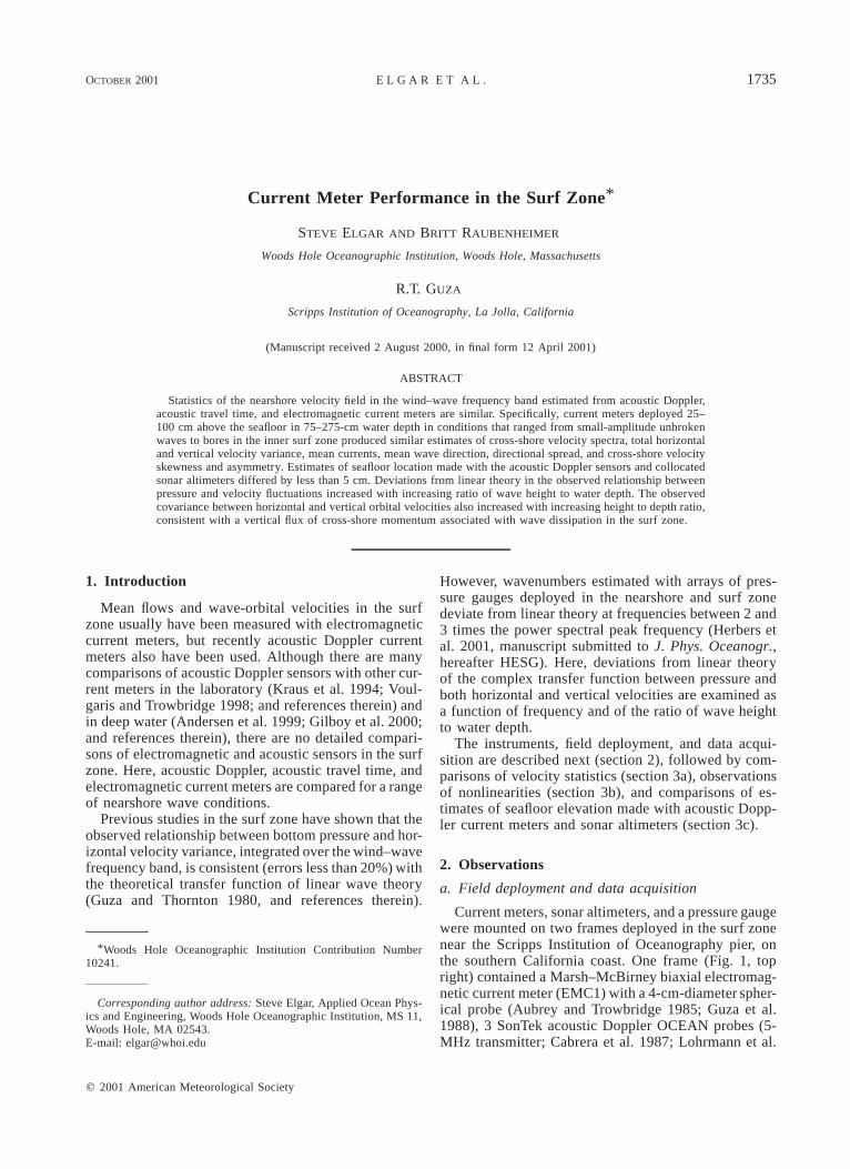
FIG. 2. Cross-shore velocity vs time. (a) Velocity reported by an acoustic Doppler velocimeter (AD4D) sampled at 16 Hz (dotted curve)and after correcting values with low correlations (solid curve). [Hsig 5 80 cm, h 5 160 cm.] (b) Corrected AD4D velocity time series [solidcurve, same as (a)] and the velocity from a collocated electromagnetic current meter (EMC1) sampled at 16 Hz, but with a 2-Hz antialiasingfilter (dotted curve). (c) Velocity time series (2-Hz sample rate) from AD4D (solid curve) and EMC1 (dotted curve) seaward of the surfzone. [Hsig 5 50 cm, h 5 215 cm.]

1994, 1995; Voulgaris and Trowbridge 1998), and asonar altimeter (ALT1; Gallagher et al. 1996). Two ofthe acoustic Doppler sensors (AD2D and AD4D) werepointed down, and one was rotated from upward(AD3U) to downward (AD3D) looking during the de-ployment. A Setra pressure gauge (PRES) was deployedadjacent to a frame leg. A second frame (Fig. 1, topleft) displaced about 5 m alongshore from the first framecontained a downward-looking SonTek acoustic Dopp-ler OCEAN probe (AD5D), a sonar altimeter (ALT2),and a MAVS acoustic travel time current meter (ATT1;Williams et al. 1987). Cables connected the sensors toshore-based data acquisition computers and power sup-plies.

The sensing volumes of EMC1, AD4D, AD3U,ATT1, and AD5D were approximately 75 cm above theseafloor, and the sensing volumes of AD3D and AD2Dwere approximately 40 and 25 cm above the seafloor,respectively (Fig. 1). The sensors were aligned (628)to the frames before deployment, and the frames werealigned (658) with the shoreline by sighting along thecross bars with a handheld compass.

Data were acquired for 3072-s (51.2 min) periodsevery hour for 2 weeks during November 1999. All

samples from both frames were controlled by a commonshore-based clock. The instruments were deployed inwater depths that ranged from 75 to 275 cm owingprimarily to tidal fluctuations. Smaller depth changescaused by erosion and accretion occurred over severaldays (610 cm) and over tidal periods (61 cm). Sig-nificant wave heights (4 times the standard deviation ofsea surface elevation fluctuations) ranged from 37 to132 cm. The deployment location was in the surf zonemost of the time (Fig. 1), and wave heights often werelimited by breaking. The ratio g of significant waveheight (Hsig) to water depth (h) ranged from 0.21 to0.64. The frequency f p of the power spectral primarypeak ranged from 0.055 to 0.160 Hz. Mean wave di-rections ranged from 08 to 158 relative to shore normal.Maximum 51.2-min mean cross-shore (U), alongshore(V), and vertical (W) currents were 20, 40, and 5 cms21, respectively. Instantaneous horizontal velocitiesgreater than 300 cm s21 were observed.

b. Current meters and data reduction

The electromagnetic current meter measures thecross-shore and alongshore velocity in a volume within


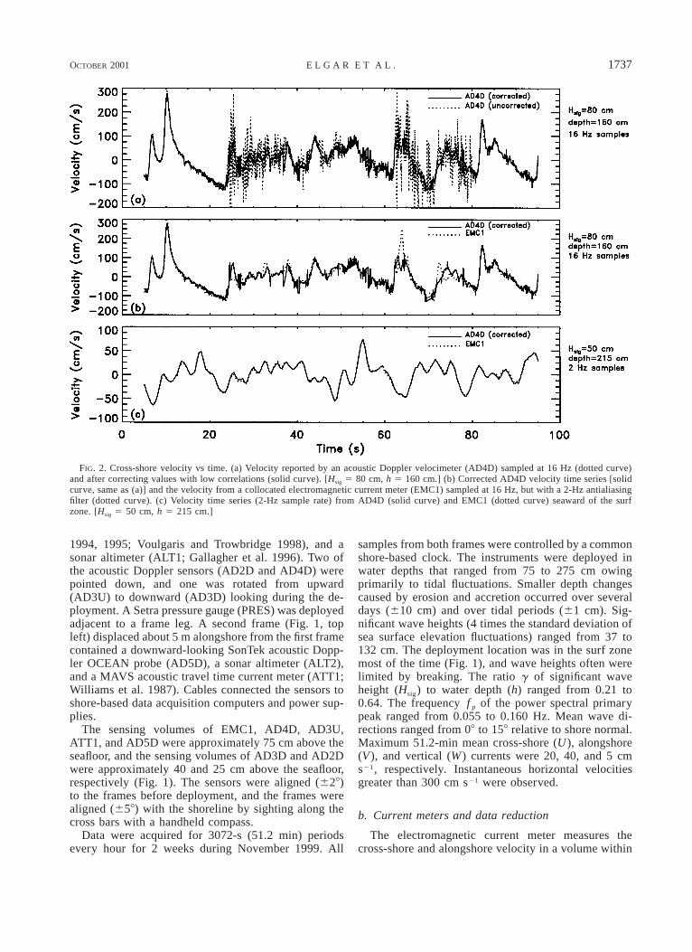
FIG. 3. Energy density of cross-shore velocity vs frequency for upward- (AD3U) and downward- (AD4D, AD5D) looking acoustic Doppler,acoustic travel time (ATT1), and electromagnetic (EMC1) current meters with sample volumes 75 cm above the seafloor. (a) Breaking wavesin the surf zone, Hsig 5 80 cm, h 5 160 cm. The sample rate was 16 Hz. (EMC1 is not shown for frequencies above 1.5 Hz, where a 2-Hz antialiasing filter resulted in reduced energy density levels. ATT1 and AD5D were not operational.) (b) Nonbreaking waves seaward ofthe surf zone, Hsig 5 50 cm, h 5 215 cm. The sample rate was 2 Hz. (ATT1 is not shown for frequencies above 0.3 Hz, where occasionalspikes from a malfunctioning circuit resulted in increased noise levels.) Spectra were estimated from six 512-s time series using a Hanningwindow with 75% overlap. Spectral estimates from five neighboring frequency bands were merged, yielding approximately 60 degrees offreedom and a frequency resolution of 0.01 Hz.

approximately 1 diameter (4 cm) of the spherical probe.Laboratory studies suggest the spherical electromag-netic sensors may be sensitive to free stream turbulenceand wakes behind the probes (Aubrey and Trowbridge1985). However, field studies have shown no evidenceof large distortions owing to the complex flow field,although substantial errors in velocity measurementsmay occur when the sensor is near the free surface orseabed (Guza et al. 1988). Antialiasing filters in theelectromagnetic current meter attenuated EMC1 signallevels above about 1.5 Hz.

The acoustic travel time current meter measures theaverage cross-shore, alongshore, and vertical velocityalong the 10-cm-long acoustic path between two 12-cmdiameter rings separated 7 cm in the vertical. Previousstudies have shown these current meters to be accurate,even at low flow speeds (Williams et al. 1987). Theacoustic travel time sensor (ATT1) had a maximum sam-ple rate of 4 Hz.

Acoustic Doppler current meters transmit short acous-tic pulses that are scattered back by reflectors in thewater within the sample volume. For the parametersused here, the acoustic Doppler current meters measurethe velocity within a cylindrical sample volume ap-

proximately 1.8-cm long and 1.2-cm diameter centeredabout 18 cm from the transducer. Using informationabout the instrument orientation and measurementsalong three beams, the average phase differences be-tween several successive returns are converted intocross-shore, alongshore, and vertical velocities (Lher-mitte and Serafin 1984; Cabrera et al. 1987; Brumleyet al. 1991; Lhermitte and Lemmin 1994; Zedel et al.1996; Voulgaris and Trowbridge 1998; and referencestherein). Bubbles and suspended sediment in the surfzone are strong reflectors, and the signal-to-noise ratioof the backscattered acoustic pulses usually is high. Incontrast, the electromagnetic and acoustic travel timecurrent meters do not require scatterers, and thereforewould work equally well in clear water. The acousticDoppler current meters, the altimeters, and the pressuregauge were sampled at rates ranging from 2 to 16 Hz.

Rapidly moving particles within the sample volumecan result in successive returns from different scatterers,leading to inaccurate velocity estimates (Cabrera et al.1987; Voulgaris and Trowbridge 1998). Furthermore,excessive scatterers (e.g., bubbles) near the sample vol-ume can reflect sidelobe energy resulting in noisy ve-locity estimates. For example, 16-Hz velocity samples


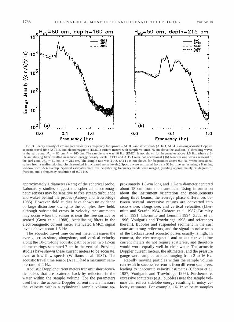
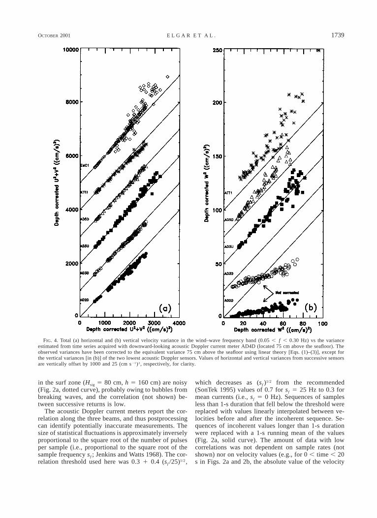
FIG. 4. Total (a) horizontal and (b) vertical velocity variance in the wind–wave frequency band (0.05 , f , 0.30 Hz) vs the varianceestimated from time series acquired with downward-looking acoustic Doppler current meter AD4D (located 75 cm above the seafloor). Theobserved variances have been corrected to the equivalent variance 75 cm above the seafloor using linear theory [Eqs. (1)–(3)], except forthe vertical variances [in (b)] of the two lowest acoustic Doppler sensors. Values of horizontal and vertical variances from successive sensorsare vertically offset by 1000 and 25 (cm s21)2, respectively, for clarity.

in the surf zone (Hsig 5 80 cm, h 5 160 cm) are noisy(Fig. 2a, dotted curve), probably owing to bubbles frombreaking waves, and the correlation (not shown) be-tween successive returns is low.

The acoustic Doppler current meters report the cor-relation along the three beams, and thus postprocessingcan identify potentially inaccurate measurements. Thesize of statistical fluctuations is approximately inverselyproportional to the square root of the number of pulsesper sample (i.e., proportional to the square root of thesample frequency sf ; Jenkins and Watts 1968). The cor-relation threshold used here was 0.3 1 0.4 (sf /25)1/2,

which decreases as (sf )1/2 from the recommended(SonTek 1995) values of 0.7 for sf 5 25 Hz to 0.3 formean currents (i.e., sf 5 0 Hz). Sequences of samplesless than 1-s duration that fell below the threshold werereplaced with values linearly interpolated between ve-locities before and after the incoherent sequence. Se-quences of incoherent values longer than 1-s durationwere replaced with a 1-s running mean of the values(Fig. 2a, solid curve). The amount of data with lowcorrelations was not dependent on sample rates (notshown) nor on velocity values (e.g., for 0 , time , 20s in Figs. 2a and 2b, the absolute value of the velocity


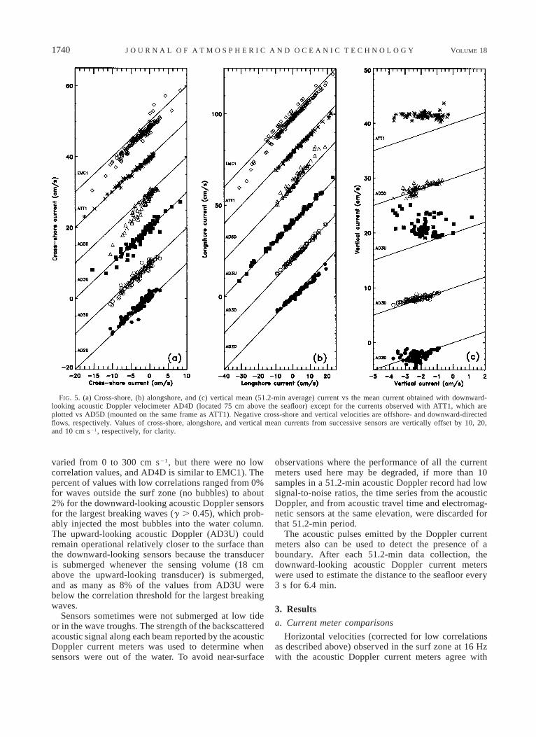
FIG. 5. (a) Cross-shore, (b) alongshore, and (c) vertical mean (51.2-min average) current vs the mean current obtained with downward-looking acoustic Doppler velocimeter AD4D (located 75 cm above the seafloor) except for the currents observed with ATT1, which areplotted vs AD5D (mounted on the same frame as ATT1). Negative cross-shore and vertical velocities are offshore- and downward-directedflows, respectively. Values of cross-shore, alongshore, and vertical mean currents from successive sensors are vertically offset by 10, 20,and 10 cm s21, respectively, for clarity.

varied from 0 to 300 cm s21, but there were no lowcorrelation values, and AD4D is similar to EMC1). Thepercent of values with low correlations ranged from 0%for waves outside the surf zone (no bubbles) to about2% for the downward-looking acoustic Doppler sensorsfor the largest breaking waves (g . 0.45), which prob-ably injected the most bubbles into the water column.The upward-looking acoustic Doppler (AD3U) couldremain operational relatively closer to the surface thanthe downward-looking sensors because the transduceris submerged whenever the sensing volume (18 cmabove the upward-looking transducer) is submerged,and as many as 8% of the values from AD3U werebelow the correlation threshold for the largest breakingwaves.

Sensors sometimes were not submerged at low tideor in the wave troughs. The strength of the backscatteredacoustic signal along each beam reported by the acousticDoppler current meters was used to determine whensensors were out of the water. To avoid near-surface

observations where the performance of all the currentmeters used here may be degraded, if more than 10samples in a 51.2-min acoustic Doppler record had lowsignal-to-noise ratios, the time series from the acousticDoppler, and from acoustic travel time and electromag-netic sensors at the same elevation, were discarded forthat 51.2-min period.

The acoustic pulses emitted by the Doppler currentmeters also can be used to detect the presence of aboundary. After each 51.2-min data collection, thedownward-looking acoustic Doppler current meterswere used to estimate the distance to the seafloor every3 s for 6.4 min.

3. Results

a. Current meter comparisons

Horizontal velocities (corrected for low correlationsas described above) observed in the surf zone at 16 Hzwith the acoustic Doppler current meters agree with


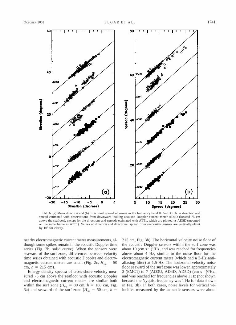
FIG. 6. (a) Mean direction and (b) directional spread of waves in the frequency band 0.05–0.30 Hz vs direction andspread estimated with observations from downward-looking acoustic Doppler current meter AD4D (located 75 cmabove the seafloor), except for the directions and spreads estimated with ATT1, which are plotted vs AD5D (mountedon the same frame as ATT1). Values of direction and directional spread from successive sensors are vertically offsetby 108 for clarity.

nearby electromagnetic current meter measurements, al-though some spikes remain in the acoustic Doppler timeseries (Fig. 2b, solid curve). When the sensors wereseaward of the surf zone, differences between velocitytime series obtained with acoustic Doppler and electro-magnetic current meters are small (Fig. 2c, Hsig 5 50cm, h 5 215 cm).

Energy density spectra of cross-shore velocity mea-sured 75 cm above the seafloor with acoustic Dopplerand electromagnetic current meters are similar bothwithin the surf zone (Hsig 5 80 cm, h 5 160 cm, Fig.3a) and seaward of the surf zone (Hsig 5 50 cm, h 5

215 cm, Fig. 3b). The horizontal velocity noise floor ofthe acoustic Doppler sensors within the surf zone wasabout 10 (cm s21)2/Hz, and was reached for frequenciesabove about 4 Hz, similar to the noise floor for theelectromagnetic current meter (which had a 2-Hz anti-aliasing filter) at 1.5 Hz. The horizontal velocity noisefloor seaward of the surf zone was lower, approximately3 (EMC1) to 7 (AD3U, AD4D, AD5D) (cm s21)2/Hz,and was reached for frequencies above 1 Hz (not shownbecause the Nyquist frequency was 1 Hz for data shownin Fig. 3b). In both cases, noise levels for vertical ve-locities measured by the acoustic sensors were about


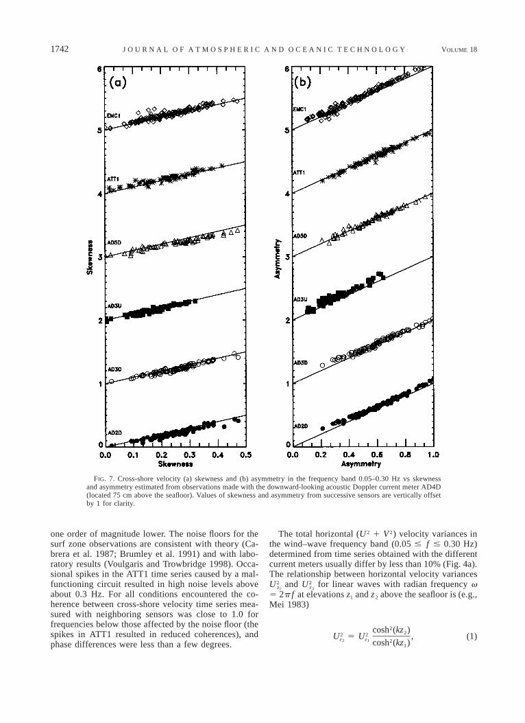
FIG. 7. Cross-shore velocity (a) skewness and (b) asymmetry in the frequency band 0.05–0.30 Hz vs skewnessand asymmetry estimated from observations made with the downward-looking acoustic Doppler current meter AD4D(located 75 cm above the seafloor). Values of skewness and asymmetry from successive sensors are vertically offsetby 1 for clarity.

one order of magnitude lower. The noise floors for thesurf zone observations are consistent with theory (Ca-brera et al. 1987; Brumley et al. 1991) and with labo-ratory results (Voulgaris and Trowbridge 1998). Occa-sional spikes in the ATT1 time series caused by a mal-functioning circuit resulted in high noise levels aboveabout 0.3 Hz. For all conditions encountered the co-herence between cross-shore velocity time series mea-sured with neighboring sensors was close to 1.0 forfrequencies below those affected by the noise floor (thespikes in ATT1 resulted in reduced coherences), andphase differences were less than a few degrees.

The total horizontal (U 2 1 V 2) velocity variances inthe wind–wave frequency band (0.05 # f # 0.30 Hz)determined from time series obtained with the differentcurrent meters usually differ by less than 10% (Fig. 4a).The relationship between horizontal velocity variances

and for linear waves with radian frequency v2 2U Uz z1 2

5 2p f at elevations z1 and z2 above the seafloor is (e.g.,Mei 1983)

2cosh (kz )22 2U 5 U , (1)z z2 1 2cosh (kz )1


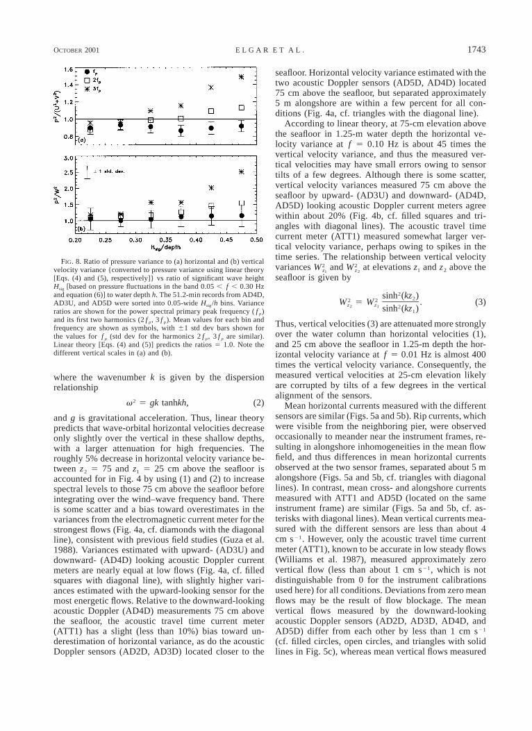
FIG. 8. Ratio of pressure variance to (a) horizontal and (b) verticalvelocity variance {converted to pressure variance using linear theory[Eqs. (4) and (5), respectively]} vs ratio of significant wave heightHsig [based on pressure fluctuations in the band 0.05 , f , 0.30 Hzand equation (6)] to water depth h. The 51.2-min records from AD4D,AD3U, and AD5D were sorted into 0.05-wide Hsig/h bins. Varianceratios are shown for the power spectral primary peak frequency ( f p)and its first two harmonics (2 f p, 3 f p). Mean values for each bin andfrequency are shown as symbols, with 61 std dev bars shown forthe values for f p (std dev for the harmonics 2 f p, 3 f p are similar).Linear theory [Eqs. (4) and (5)] predicts the ratios 5 1.0. Note thedifferent vertical scales in (a) and (b).

where the wavenumber k is given by the dispersionrelationship

2v 5 gk tanhkh, (2)

and g is gravitational acceleration. Thus, linear theorypredicts that wave-orbital horizontal velocities decreaseonly slightly over the vertical in these shallow depths,with a larger attenuation for high frequencies. Theroughly 5% decrease in horizontal velocity variance be-tween z2 5 75 and z1 5 25 cm above the seafloor isaccounted for in Fig. 4 by using (1) and (2) to increasespectral levels to those 75 cm above the seafloor beforeintegrating over the wind–wave frequency band. Thereis some scatter and a bias toward overestimates in thevariances from the electromagnetic current meter for thestrongest flows (Fig. 4a, cf. diamonds with the diagonalline), consistent with previous field studies (Guza et al.1988). Variances estimated with upward- (AD3U) anddownward- (AD4D) looking acoustic Doppler currentmeters are nearly equal at low flows (Fig. 4a, cf. filledsquares with diagonal line), with slightly higher vari-ances estimated with the upward-looking sensor for themost energetic flows. Relative to the downward-lookingacoustic Doppler (AD4D) measurements 75 cm abovethe seafloor, the acoustic travel time current meter(ATT1) has a slight (less than 10%) bias toward un-derestimation of horizontal variance, as do the acousticDoppler sensors (AD2D, AD3D) located closer to the

seafloor. Horizontal velocity variance estimated with thetwo acoustic Doppler sensors (AD5D, AD4D) located75 cm above the seafloor, but separated approximately5 m alongshore are within a few percent for all con-ditions (Fig. 4a, cf. triangles with the diagonal line).

According to linear theory, at 75-cm elevation abovethe seafloor in 1.25-m water depth the horizontal ve-locity variance at f 5 0.10 Hz is about 45 times thevertical velocity variance, and thus the measured ver-tical velocities may have small errors owing to sensortilts of a few degrees. Although there is some scatter,vertical velocity variances measured 75 cm above theseafloor by upward- (AD3U) and downward- (AD4D,AD5D) looking acoustic Doppler current meters agreewithin about 20% (Fig. 4b, cf. filled squares and tri-angles with diagonal lines). The acoustic travel timecurrent meter (ATT1) measured somewhat larger ver-tical velocity variance, perhaps owing to spikes in thetime series. The relationship between vertical velocityvariances and at elevations z1 and z2 above the2 2W Wz z1 2

seafloor is given by

2sinh (kz )22 2W 5 W . (3)z z2 1 2sinh (kz )1

Thus, vertical velocities (3) are attenuated more stronglyover the water column than horizontal velocities (1),and 25 cm above the seafloor in 1.25-m depth the hor-izontal velocity variance at f 5 0.01 Hz is almost 400times the vertical velocity variance. Consequently, themeasured vertical velocities at 25-cm elevation likelyare corrupted by tilts of a few degrees in the verticalalignment of the sensors.

Mean horizontal currents measured with the differentsensors are similar (Figs. 5a and 5b). Rip currents, whichwere visible from the neighboring pier, were observedoccasionally to meander near the instrument frames, re-sulting in alongshore inhomogeneities in the mean flowfield, and thus differences in mean horizontal currentsobserved at the two sensor frames, separated about 5 malongshore (Figs. 5a and 5b, cf. triangles with diagonallines). In contrast, mean cross- and alongshore currentsmeasured with ATT1 and AD5D (located on the sameinstrument frame) are similar (Figs. 5a and 5b, cf. as-terisks with diagonal lines). Mean vertical currents mea-sured with the different sensors are less than about 4cm s21. However, only the acoustic travel time currentmeter (ATT1), known to be accurate in low steady flows(Williams et al. 1987), measured approximately zerovertical flow (less than about 1 cm s21, which is notdistinguishable from 0 for the instrument calibrationsused here) for all conditions. Deviations from zero meanflows may be the result of flow blockage. The meanvertical flows measured by the downward-lookingacoustic Doppler sensors (AD2D, AD3D, AD4D, andAD5D) differ from each other by less than 1 cm s21

(cf. filled circles, open circles, and triangles with solidlines in Fig. 5c), whereas mean vertical flows measured


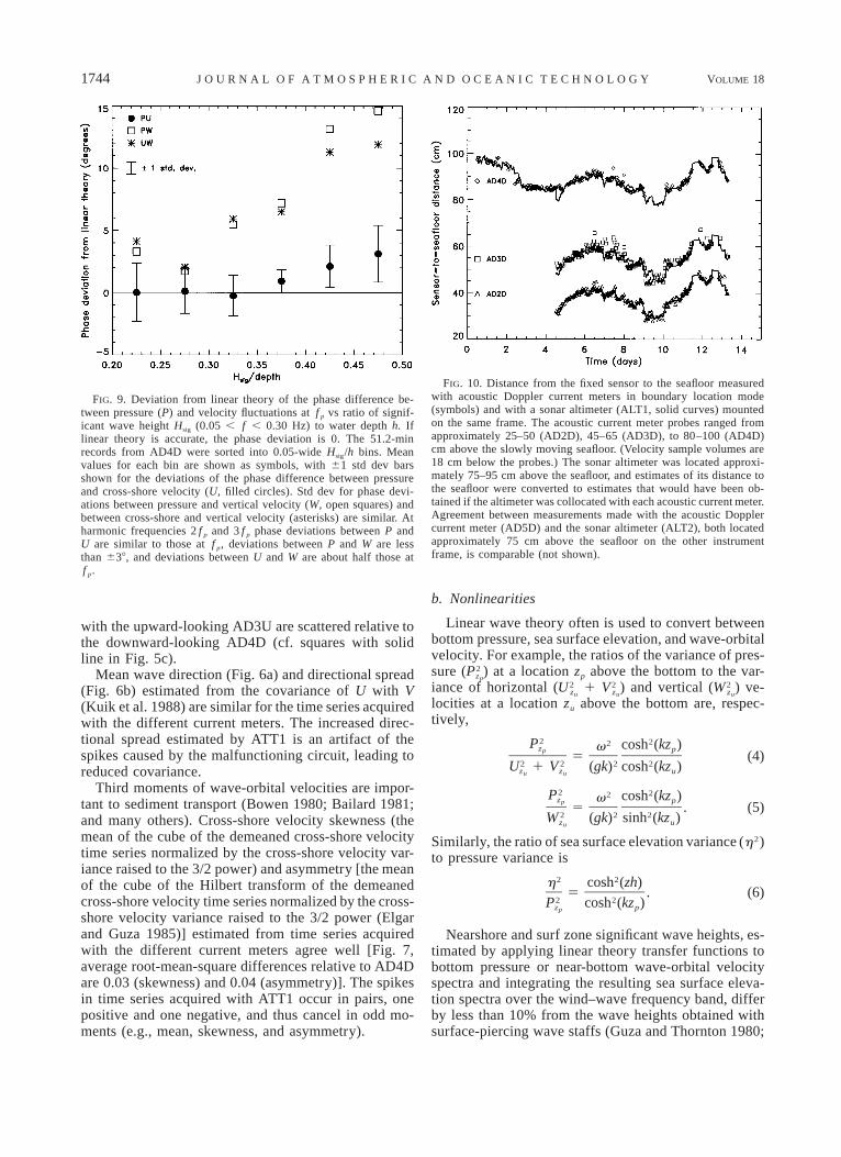
FIG. 9. Deviation from linear theory of the phase difference be-tween pressure (P) and velocity fluctuations at f p vs ratio of signif-icant wave height Hsig (0.05 , f , 0.30 Hz) to water depth h. Iflinear theory is accurate, the phase deviation is 0. The 51.2-minrecords from AD4D were sorted into 0.05-wide Hsig/h bins. Meanvalues for each bin are shown as symbols, with 61 std dev barsshown for the deviations of the phase difference between pressureand cross-shore velocity (U, filled circles). Std dev for phase devi-ations between pressure and vertical velocity (W, open squares) andbetween cross-shore and vertical velocity (asterisks) are similar. Atharmonic frequencies 2 f p and 3 f p phase deviations between P andU are similar to those at f p, deviations between P and W are lessthan 638, and deviations between U and W are about half those atf p.

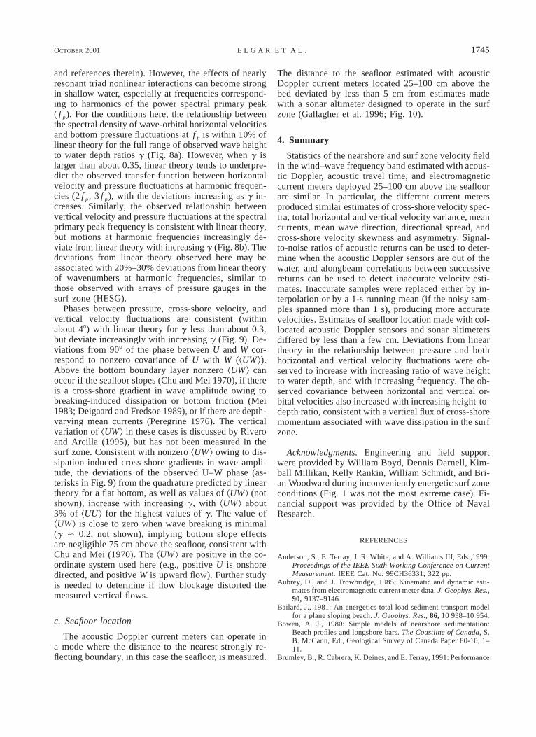
FIG. 10. Distance from the fixed sensor to the seafloor measuredwith acoustic Doppler current meters in boundary location mode(symbols) and with a sonar altimeter (ALT1, solid curves) mountedon the same frame. The acoustic current meter probes ranged fromapproximately 25–50 (AD2D), 45–65 (AD3D), to 80–100 (AD4D)cm above the slowly moving seafloor. (Velocity sample volumes are18 cm below the probes.) The sonar altimeter was located approxi-mately 75–95 cm above the seafloor, and estimates of its distance tothe seafloor were converted to estimates that would have been ob-tained if the altimeter was collocated with each acoustic current meter.Agreement between measurements made with the acoustic Dopplercurrent meter (AD5D) and the sonar altimeter (ALT2), both locatedapproximately 75 cm above the seafloor on the other instrumentframe, is comparable (not shown).

with the upward-looking AD3U are scattered relative tothe downward-looking AD4D (cf. squares with solidline in Fig. 5c).

Mean wave direction (Fig. 6a) and directional spread(Fig. 6b) estimated from the covariance of U with V(Kuik et al. 1988) are similar for the time series acquiredwith the different current meters. The increased direc-tional spread estimated by ATT1 is an artifact of thespikes caused by the malfunctioning circuit, leading toreduced covariance.

Third moments of wave-orbital velocities are impor-tant to sediment transport (Bowen 1980; Bailard 1981;and many others). Cross-shore velocity skewness (themean of the cube of the demeaned cross-shore velocitytime series normalized by the cross-shore velocity var-iance raised to the 3/2 power) and asymmetry [the meanof the cube of the Hilbert transform of the demeanedcross-shore velocity time series normalized by the cross-shore velocity variance raised to the 3/2 power (Elgarand Guza 1985)] estimated from time series acquiredwith the different current meters agree well [Fig. 7,average root-mean-square differences relative to AD4Dare 0.03 (skewness) and 0.04 (asymmetry)]. The spikesin time series acquired with ATT1 occur in pairs, onepositive and one negative, and thus cancel in odd mo-ments (e.g., mean, skewness, and asymmetry).

b. Nonlinearities

Linear wave theory often is used to convert betweenbottom pressure, sea surface elevation, and wave-orbitalvelocity. For example, the ratios of the variance of pres-sure ( ) at a location zp above the bottom to the var-2Pzp

iance of horizontal ( 1 ) and vertical ( ) ve-2 2 2U V Wz z zu u u

locities at a location zu above the bottom are, respec-tively,

2 22P cosh (kz )vz pp5 (4)

2 2 2 2U 1 V (gk) cosh (kz )z z uu u

2 22P cosh (kz )vz pp5 . (5)

2 2 2W (gk) sinh (kz )z uu

Similarly, the ratio of sea surface elevation variance (h2)to pressure variance is

2 2h cosh (zh)5 . (6)

2 2P cosh (kz )z pp

Nearshore and surf zone significant wave heights, es-timated by applying linear theory transfer functions tobottom pressure or near-bottom wave-orbital velocityspectra and integrating the resulting sea surface eleva-tion spectra over the wind–wave frequency band, differby less than 10% from the wave heights obtained withsurface-piercing wave staffs (Guza and Thornton 1980;


and references therein). However, the effects of nearlyresonant triad nonlinear interactions can become strongin shallow water, especially at frequencies correspond-ing to harmonics of the power spectral primary peak( f p). For the conditions here, the relationship betweenthe spectral density of wave-orbital horizontal velocitiesand bottom pressure fluctuations at f p is within 10% oflinear theory for the full range of observed wave heightto water depth ratios g (Fig. 8a). However, when g islarger than about 0.35, linear theory tends to underpre-dict the observed transfer function between horizontalvelocity and pressure fluctuations at harmonic frequen-cies (2 f p, 3 f p), with the deviations increasing as g in-creases. Similarly, the observed relationship betweenvertical velocity and pressure fluctuations at the spectralprimary peak frequency is consistent with linear theory,but motions at harmonic frequencies increasingly de-viate from linear theory with increasing g (Fig. 8b). Thedeviations from linear theory observed here may beassociated with 20%–30% deviations from linear theoryof wavenumbers at harmonic frequencies, similar tothose observed with arrays of pressure gauges in thesurf zone (HESG).

Phases between pressure, cross-shore velocity, andvertical velocity fluctuations are consistent (withinabout 48) with linear theory for g less than about 0.3,but deviate increasingly with increasing g (Fig. 9). De-viations from 908 of the phase between U and W cor-respond to nonzero covariance of U with W (ÛW&).Above the bottom boundary layer nonzero ÛW& canoccur if the seafloor slopes (Chu and Mei 1970), if thereis a cross-shore gradient in wave amplitude owing tobreaking-induced dissipation or bottom friction (Mei1983; Deigaard and Fredsoe 1989), or if there are depth-varying mean currents (Peregrine 1976). The verticalvariation of ÛW& in these cases is discussed by Riveroand Arcilla (1995), but has not been measured in thesurf zone. Consistent with nonzero ÛW& owing to dis-sipation-induced cross-shore gradients in wave ampli-tude, the deviations of the observed U–W phase (as-terisks in Fig. 9) from the quadrature predicted by lineartheory for a flat bottom, as well as values of ÛW& (notshown), increase with increasing g, with ÛW& about3% of ÛU& for the highest values of g. The value ofÛW& is close to zero when wave breaking is minimal(g ø 0.2, not shown), implying bottom slope effectsare negligible 75 cm above the seafloor, consistent withChu and Mei (1970). The ÛW& are positive in the co-ordinate system used here (e.g., positive U is onshoredirected, and positive W is upward flow). Further studyis needed to determine if flow blockage distorted themeasured vertical flows.

c. Seafloor location

The acoustic Doppler current meters can operate ina mode where the distance to the nearest strongly re-flecting boundary, in this case the seafloor, is measured.

The distance to the seafloor estimated with acousticDoppler current meters located 25–100 cm above thebed deviated by less than 5 cm from estimates madewith a sonar altimeter designed to operate in the surfzone (Gallagher et al. 1996; Fig. 10).

4. Summary

Statistics of the nearshore and surf zone velocity fieldin the wind–wave frequency band estimated with acous-tic Doppler, acoustic travel time, and electromagneticcurrent meters deployed 25–100 cm above the seafloorare similar. In particular, the different current metersproduced similar estimates of cross-shore velocity spec-tra, total horizontal and vertical velocity variance, meancurrents, mean wave direction, directional spread, andcross-shore velocity skewness and asymmetry. Signal-to-noise ratios of acoustic returns can be used to deter-mine when the acoustic Doppler sensors are out of thewater, and alongbeam correlations between successivereturns can be used to detect inaccurate velocity esti-mates. Inaccurate samples were replaced either by in-terpolation or by a 1-s running mean (if the noisy sam-ples spanned more than 1 s), producing more accuratevelocities. Estimates of seafloor location made with col-located acoustic Doppler sensors and sonar altimetersdiffered by less than a few cm. Deviations from lineartheory in the relationship between pressure and bothhorizontal and vertical velocity fluctuations were ob-served to increase with increasing ratio of wave heightto water depth, and with increasing frequency. The ob-served covariance between horizontal and vertical or-bital velocities also increased with increasing height-to-depth ratio, consistent with a vertical flux of cross-shoremomentum associated with wave dissipation in the surfzone.

Acknowledgments. Engineering and field supportwere provided by William Boyd, Dennis Darnell, Kim-ball Millikan, Kelly Rankin, William Schmidt, and Bri-an Woodward during inconveniently energetic surf zoneconditions (Fig. 1 was not the most extreme case). Fi-nancial support was provided by the Office of NavalResearch.

REFERENCES

Anderson, S., E. Terray, J. R. White, and A. Williams III, Eds.,1999:Proceedings of the IEEE Sixth Working Conference on CurrentMeasurement. IEEE Cat. No. 99CH36331, 322 pp.

Aubrey, D., and J. Trowbridge, 1985: Kinematic and dynamic esti-mates from electromagnetic current meter data. J. Geophys. Res.,90, 9137–9146.

Bailard, J., 1981: An energetics total load sediment transport modelfor a plane sloping beach. J. Geophys. Res., 86, 10 938–10 954.

Bowen, A. J., 1980: Simple models of nearshore sedimentation:Beach profiles and longshore bars. The Coastline of Canada, S.B. McCann, Ed., Geological Survey of Canada Paper 80-10, 1–11.

Brumley, B., R. Cabrera, K. Deines, and E. Terray, 1991: Performance


of a broad-band acoustic Doppler current profiler. IEEE OceanicEng., 16, 402–503.

Cabrera, R., K. Deines, B. Brumley, and E. Terray, 1987: Develop-ment of a practical coherent acoustic Doppler current profiler.Proc. Oceans ’87, Halifax, NS, Canada, IEEE Oceanic Engi-neering Society, 93–97.

Chu, V., and C. Mei, 1970: On slowly varying Stokes waves. J. FluidMech., 41, 873–887.

Diegaard, R., and J. Fredsoe, 1989: Shear stress distribution in dis-sipative water waves. Coastal Eng., 13, 357–378.

Elgar, S., and R. Guza, 1985: Observations of bispectra of shoalingsurface gravity waves. J. Fluid Mech., 161, 425–448.

Gallagher, E., B. Boyd, S. Elgar, R. Guza, and B. Woodward, 1996:Performance of a sonar altimeter in the nearshore. Mar. Geol.,133, 241–248.

Gilboy, T., T. Dickey, D. Sigurdson, X. Yu, and D. Manov, 2000: Anintercomparison of current measurements using a vector mea-suring current meter, an acoustic Doppler current profiler, and arecently developed acoustic current meter. J. Atmos. OceanicTechnol., 17, 561–574.

Guza, R., and E. Thornton, 1980: Local and shoaled comparisons ofsea surface elevations, pressures, and velocities. J. Geophys.Res., 85, 1524–1530.

——, M. Clifton, and F. Rezvani, 1988: Field intercomparisons ofelectromagnetic current meters. J. Geophys. Res., 93, 9302–9314.

Herbers, T., S. Elgar, N. Sarap, and R. Guza, 2001: Dispersion prop-erties of surface gravity waves in shallow water. J. Phys. Ocean-ogr., submitted.

Jenkins, G., and D. Watts, 1968: Spectral Analysis and Its Applica-tions. Holden-Day, 525 pp.

Kraus, N., A. Lohrmann, and R. Cabrera, 1994: New acoustic meterfor measuring 3D laboratory flows. J. Hydraul. Eng., 120, 406–412.

Kuik, A., G. van Vledder, and L. Holthuijsen, 1988: A method for

routine analysis of pitch-and-roll buoy data. J. Phys. Oceanogr.,18, 1020–1034.

Lhermitte, R., and R. Serafin, 1984: Pulse-to-pulse coherent Dopplersignal processing techniques. J. Atmos. Oceanic Technol., 1,293–308.

——, and U. Lemmin, 1994: Open-channel flow and turbulence mea-surement by high-resolution Doppler sonar. J. Atmos. OceanicTechnol., 11, 1295–1308.

Lohrmann, A., R. Cabrera, and N. Kraus, 1994: Acoustic-Dopplervelocimeter (ADV) for laboratory use. Proc. Conf. on Funda-mentals and Advancements in Hydraulic Measurements and Ex-perimentation, Buffalo, NY, American Society of Civil Engi-neers, 351–365.

——, G. Gelfenbaum, and J. Haines, 1995: Direct measurement ofReynold’s stress with an acoustic Doppler velocimeter. Proc.IEEE Fifth Conf. on Current Measurements, St. Petersburg, FL,IEEE Oceanic Engineering Society, 205–210.

Mei, C., 1983: The Applied Dynamics of Ocean Surface Waves. WileyInterscience, 728 pp.

Pergerine, D., 1976: Interaction of water waves and currents. Adv.Appl. Mech., 16, 9–117.

Rivero, F., and A. Arcilla, 1995: On the vertical distribution of ^uw&.Coastal Eng., 25, 137–152.

SonTek, 1995: ADV operation manual, version 1.0. [Available fromSonTek, 6837 Nancy Ridge Drive, Suite A, San Diego, CA92121.]

Voulgaris, G., and J. Trowbridge, 1998: Evaluation of the acousticDoppler velocimeter (ADV) for turbulence measurements. J. At-mos. Oceanic Technol., 15, 272–289.

Williams, A., J. Tochko, R. Koehler, T. Gross, W. Grand, and C.Dunn, 1987: Measurement of turbulence with an acoustic currentmeter array in the oceanic bottom boundary layer. J. Atmos.Oceanic Technol., 4, 312–327.

Zedel, L., E. Hay, and A. Lohrmann, 1996: Performance of singlebeam pulse-to-pulse coherent Doppler profiler. IEEE J. OceanicEng., 21, 290–299.

current meter performance in the surf zone - woods hole … · 2010-09-27 · current meter...

Documents