University of LjubljanaFaculty of mathematics and physics

Department of physics

Surf Zone Hydrodynamics

Tilen Kusterle

Mentor: prof. dr. Rudolf Podgornik

June 12, 2007

Abstract

This seminar presents a brief introduction into the physics of water waves with emphasison surf zone hydrodynamics. At the beginning, there is an introduction into the terminology,which includes the explanation of origin and types of water waves and how these waves can berepresented and studied. Next, the linear wave theory is explained in somewhat greater details,as it is the most fundamental and the simplest theory with far-reaching results that give aninsight into much more complicated problems of nonlinear wave hydrodynamics. Finally, thespecifics of surf zone waves, their transformations and impact on mean water level are presented.

1

Contents

1 Introduction 3

2 Types of waves in water 3

3 The linear wave theory 43.1 Definition of wave parameters . . . . . . . . . . . . . . . . . . . . . . . . . . . . . . . 43.2 Assumptions and formulation of the linear wave theory . . . . . . . . . . . . . . . . . 43.3 Results of the linear wave theory . . . . . . . . . . . . . . . . . . . . . . . . . . . . . 6

4 Transformation of waves 11

5 Surf zone waves 115.1 Surf zone . . . . . . . . . . . . . . . . . . . . . . . . . . . . . . . . . . . . . . . . . . 115.2 Transformation of waves in the surf zone . . . . . . . . . . . . . . . . . . . . . . . . . 12

5.2.1 Shallow water equations and a simple explanation of wave transformation thatleads to breaking . . . . . . . . . . . . . . . . . . . . . . . . . . . . . . . . . . 12

5.2.2 Breaker type . . . . . . . . . . . . . . . . . . . . . . . . . . . . . . . . . . . . 145.2.3 Breaker index . . . . . . . . . . . . . . . . . . . . . . . . . . . . . . . . . . . . 16

5.3 Wave setup and setdown . . . . . . . . . . . . . . . . . . . . . . . . . . . . . . . . . . 165.4 Wave runup on beaches . . . . . . . . . . . . . . . . . . . . . . . . . . . . . . . . . . 17

6 Conclusion 18

2

1 Introduction

The aim of this seminar is to introduce and explain to some extent the physics behind one of themost common and well-known processes in nature - the motion of water near a shoreline. The sightand pleasant sound of waves breaking near a beach is very familiar to people, however they generallydo not realize what a complicated process it really is.

There are numerous questions that arise, for example: What causes waves on water surface? Howfast do waves travel? How do water particles move at different depths as a consequence of waves?Why do waves grow in height as they approach the shore? Why and how do waves break? These aresome of the questions I would like to answer in my seminar. The hydrodynamics of surf zone wavesas well as many other aspects of coastal engineering are explained in far greater detail in [1], whichserved as a starting point for this seminar.

2 Types of waves in water

There are many different factors that cause waves in a body of water. The most common reason isthe wind, that is the movement of air above water surface. The relative motion of the two fluids - gasand liquid - produces friction that drives the waves. Besides wind waves there are also internal waves(also caused by friction, but in this case between layers of liquid that have different densities dueto stratification of the temperature or the salinity [2], [3]), waves caused by tides, currents, tectonicactivity and movement of objects in water.

For wind waves there are also several factors that determine their size and shape [4]. Thesefactors are wind speed, fetch (distance of open water that the wind has blown over) and length oftime the wind has blown over a given area. Over time three different types of wind waves develop:

• ripples

• seas

• swells

Ripples are capillary waves, which means that the main contribution to the restoring force that allowsthem to propagate is due to surface tension instead of gravity (see comment before equation (8)).Ripples appear on smooth water when the wind blows and cease if the wind stops. The restoring forceof other two types of wind waves is mainly due to gravity (also called gravity waves). Seas are larger-scale, often irregular motions that form under sustained winds and tend to last much longer, evenafter the wind has died. As seas propagate away from their area of origin, they separate accordingto their direction and wavelength. Swells are far more stable in their direction and frequency thanseas since they are formed by stable wind systems such as tropical storms, for instance.

The study and modeling of water waves can be divided into two categories: regular and irregularwaves [1]. The regular waves approach deals mainly with two dimensional waves that are small inamplitude and of sinusoidal or slightly deviant form. Its objective is to provide a detailed under-standing of wave mechanics. Waves of sinusoidal form are explained in terms of linear wave theory,but for waves that deviate from a pure sinusoid the representation requires mathematically morecomplicated nonlinear theories. On the other hand, the irregular waves approach employs statisticaland probabilistic theories for describing the natural time dependent, three dimensional characteristicsof real wave systems. But the problem is so complicated, that even with this approach, simplifica-tions are required. To obtain information about a wave system, a combination of both mentionedapproaches is usually used. For example, information from irregular waves approach can be used to

3

determine the expected range of wave conditions and directional distributions of wave energy in orderto select an individual wave height and period for the problem under study. Then the proceduresfrom regular waves approach can be applied to characterize the kinematics and dynamics that mightbe expected.

3 The linear wave theory

3.1 Definition of wave parameters

At the very beginning it is appropriate to have a look at how a general progressive wave on watersurface can be described. In two dimensions the wave form can be represented by the variablesx (spatial) and t (temporal) or by their combination θ = kx − ωt (phase), where k is the wavenumber and ω the angular or radian frequency. Figure 1 depicts the parameters that define asimple, periodic wave of permanent form propagating over a horizontal bottom. Such a wave maybe completely characterized by the wave height H, wavelength L and water depth d. The highestpoint of the wave is the crest and the lowest is the trough. For linear or small-amplitude waves, theheight of the crest above the still-water level (SWL) and the distance of the trough below the SWLare both equal to the wave amplitude a, therefore we get the relation a = H

2 . The wave period Tis the time interval between the passage of two successive wave crests or troughs at a given pointand the wavelength L is the horizontal distance between two successive wave crests or troughs. Thewave period and the wavelength are related to the angular frequency ω = 2π

T and the wave numberk = 2π

L . Other wave parameters include the phase velocity or wave celerity C = LT = ω

k , the wavesteepness ε = H

L , the relative depth dL and the relative wave height H

d .

Figure 1: Definition of wave parameters [1].

3.2 Assumptions and formulation of the linear wave theory

The linear wave theory is the most elementary wave theory. It is also referred to as the small-amplitude theory and was developed by Airy in 1845. The goal of this section is to present themain assumptions and formulation of this theory. A more detailed argumentation and derivation

4

concerning this theory can be found in one of preceding seminars [5]. The assumptions of the linearwave theory are as follows:

1. The fluid is homogeneous and incompressible (the density ρ is a constant).

2. Surface tension can be neglected.

3. Coriolis effect due to Earth’s rotation can be neglected.

4. Pressure at the free surface is uniform and constant.

5. The fluid is ideal or inviscid (lacks viscosity).

6. A wave does not interact with other water motions and the flow is irrotational so that waterparticles do not rotate (only normal forces are important and shearing forces are negligible).

7. The bottom is a horizontal, fixed and impermeable boundary, which implies that the verticalvelocity at the bed is zero.

8. The wave amplitude is small and the waveform is invariant in time and space.

9. Waves are plane or long-crested (two-dimensional).

These assumptions pose serious limitations to the validity of the theory. For the study of surf zonehydrodynamics the first five assumptions can be considered in a good approximation as valid. That isnot the case for the final assumptions, so the linear wave theory alone can not be used for describingphenomena near a shoreline. It does however, because of its simplicity, offer results that can betaken into consideration when trying to understand clearly more complicated problem of surf zonehydrodynamics.

Because of the above assumptions, the formulation of the small-amplitude theory can be signifi-cantly simplified. The assumption of irrotationality (∇× v = 0) allows the use of a scalar functiontermed the velocity potential Φ, whose gradient at any point in fluid is the velocity vector v. In twodimensions we deal with two coordinates: x (horizontal) and z (vertical). Accordingly the velocitycomponents in x-direction and z-direction are

u =∂Φ∂x

and w =∂Φ∂z

. (1)

Furthermore, the assumption of incompressibility (∇ · v = 0) implies that there is another scalarfunction, the so-called stream function Ψ, defined by equations

u =∂Ψ∂z

and w = −∂Ψ∂x

. (2)

Lines of constant values of the potential function (equipotential lines) and lines of constant valuesof the stream function are mutually perpendicular or orthogonal. The relations

∂Φ∂x

=∂Ψ∂z

and∂Φ∂z

= −∂Ψ∂x

(3)

are termed the Cauchy-Riemann conditions. Both Φ and Ψ satisfy the Laplace equation, whichgoverns the flow of and ideal fluid (inviscid and incompressible fluid)

∂2Φ∂x2

+∂2Φ∂z2

= 0 and∂2Ψ∂x2

+∂2Ψ∂z2

= 0. (4)

5

In order to find the solution of the Laplace equation ∇2Φ = 0 for the velocity potential Φ,boundary conditions must be assigned. The first boundary condition is simply

∂Φ∂z

= 0, for z = −d, (5)

which means that there is no vertical velocity component at the bottom. For the surface, which isof the form η(x, t), there are two conditions. The kinematic condition states that a “fluid particle”at the surface remains there at all times:

ddt

(z − η(x, t)) = 0 ⇔ dη

dt=

∂Φ∂z

, for z = η(x, t). (6)

There is also a dynamical condition at the free surface, which is basically the Bernoulli equation

∂Φ∂t

+12(∇Φ)2 + gη +

p

ρ=

pa

ρ, (7)

where pa is the atmospherical pressure and p the pressure in water at the surface. Because one of theassumptions of linear wave theory is that surface tension can be neglected, it follows p = pa (Surfacetension can be taken into account by writing p− pa = κT , where T is presumably constant surfacetension and κ = ∇ · n the mean curvature of the surface. Here n is the unit normal vector to thesurface, which is pointing upwards. Surface tension only brings an additional term into the velocitypotential, but it does not alter the term due to gravity [6]). Therefore the dynamical condition states

∂Φ∂t

+12(∇Φ)2 + gη = 0, for z = η(x, t). (8)

In agreement with the linear wave theory one can further linearize the boundary conditions (6) and(8) by neglecting quadratic and higher order terms in η and Φ and from there compute the velocitypotential Φ, the solutions for the form of the surface η and the wave celerity. For further details see[6] or [7].

3.3 Results of the linear wave theory

The solution of Laplace equation for velocity potential with the previously stated boundary contitionsis (see [5], [6], [8] )

Φ(x, z, t) =gH

2ω

cosh[k(z + h)]cosh(kh)

sin(kx− ωt). (9)

A simple class of solutions for water surface elevation is of the form of a sinusoidal wave profile,which is in one dimension described by expression (see [6])

η(x, t) = a cos (kx− ωt) =H

2cos

(2πx

L− 2πt

T

)= a cos θ, (10)

where η is the elevation of water surface relative to the SWL and H = 2a is the height of thewave. The equation (10) represents a periodic, sinusoidal, progressive wave traveling in the positivex-direction. The speed at which a sinusoidal wave form propagates is the so-called phase velocity orwave celerity. In time interval of one wave period such a wave advances for one wavelength, thereforeits celerity can be expressed as

C =L

T. (11)

6

From the linear wave theory a general expression relating wave celerity to wavelength and waterdepth can be derived (see [6]):

C =

√gL

2πtanh

(2πd

L

). (12)

This equation is the dispersion relation as one can see that waves with different periods (wavelengths)propagate at different speeds. To be more exact, greater wavelength L means faster propagation.From equations (12) and (11) another expression for wave celerity can be derived

C =gT

2πtanh

(2πd

L

). (13)

In terms of the wave number k and the wave angular frequency ω equation (13) can be written as

C =g

ωtanh(kd). (14)

According to the relative depth criterion dL , water waves are classified as shown in Table 1. In deep

Classification d/L kd tanh(kd)Deep water 1/2 to ∞ π to ∞ ≈ 1Transitional 1/20 to 1/2 π/10 to π tanh(kd)

Shallow water 0 to 1/20 0 to π/10 ≈ kd

Table 1: Classification of water waves according to the relative depth criterion dL [1].

water, the expression tanh(kd) is approximately equal to unity, therefore from equations (12), (13)and (11) the deep water celerity can be written as

C0 =

√gL0

2π=

gT

2π=

L0

T, (15)

where L0 denotes the length of deep water waves. Deep water, as it was defined by the above equation,actually occurs at infinite depth, but tanh(2πd/L) approaches unity at quite small relative depth.For example, for d/L = 0.5 the expression gives tanh(π) ≈ 0.9963. In shallow water (d/L < 1/25),tanh(kd) is approximately equal to kd and therefore equation (12) simplifies to

C =√

gd. (16)

As one can see, wave celerity in shallow water depends only on water depth. In general, the celerityand length of a wind wave are dependent only upon the wave’s period (or frequency) in deep water.But as depth becomes shallower, they depend upon depth and period and finally, in shallow wateronly water depth is relevant.

With the help of (1) velocity components can be calculated from equation (9). They are asfollows:

u =H

2gT

L

cosh[k(z + d)]cosh(kd)

cos(kx− ωt),

w =H

2gT

L

sinh[k(z + d)]cosh(kd)

sin(kx− ωt). (17)

7

Integration of (17) gives fluid particle displacements

ξ = −HgT 2

4πL

cosh[k(z + d)]cosh(kd)

sin(kx− ωt),

ζ =HgT 2

4πL

sinh[k(z + d)]cosh(kd)

cos(kx− ωt), (18)

where ξ is the horizontal displacement and ζ is the veritcal displacement of a water particle from itsmean position. These equations can be further simplified using the relationship(

2π

T

)2

=2πg

Ltanh

(2πd

L

). (19)

Thus,

ξ = −H

2cosh[k(z + d)]

sinh(kd)sin(kx− ωt),

ζ =H

2sinh[k(z + d)]

sinh(kd)cos(kx− ωt). (20)

Rewriting these last equations to

sin2(kx− ωt) =(

2ξ

H

sinh(kd)cosh[k(z + d)]

)2

,

cos2(kx− ωt) =(

2ζ

H

sinh(kd)sinh[k(z + d)]

)2

(21)

and summing them together givesξ2

A2+

ζ2

B2= 1, (22)

where

A =H

2cosh[k(z + d)]

sinh(kd),

B =H

2sinh[k(z + d)]

sinh(kd). (23)

Expression (22) is the equation of an ellipse with a horizontal semi-axis equal to A and a verticalsemi-axis equal to B. Thus, the linear wave theory predicts water particles to move in closed orbits.In deep water (d/L > 0.5), where |d| |z| (d > 0 and z < 0), A and B are equal:

A = B =H

2exp

(2πz

L

), (24)

therefore the water particle orbits are circular. In shallow water (d/L < 1/25) however, A and Bbecome

A =H

2L

2πd, B =

H

2

(1 +

z

d

)(25)

and the orbits are elliptical - the shallower the water, the flatter the ellpise. From equations (20)follows that the amplitude of the water particle displacement decreases exponentially with depth. Inshallow water horizontal particle displacement near the bottom can be large. Orbits of water particle

8

displacements based on linear wave theory are presented in Figure 2. In contrast with the linearwave theory, laboratory measurements have shown [1] that particle orbits are not completely closed,therefore a fluid particle does not return to its initial position after each wave cycle. The differencebetween linear theory and observations is due to the mass transport phenomenon (the linear theorydoes not predict it, but it comes as a consequence of aperiodic terms in the expressions for particledisplacements in nonlinear wave theories, for example Stokes finite-amplitude wave theory).

Figure 2: Fluid particle displacements from mean position for shallow and deep water waves [1]. Inlinear wave theory particles are predicted to move in closed circular (deep water) of elliptical (shallowor transitional water) orbits.

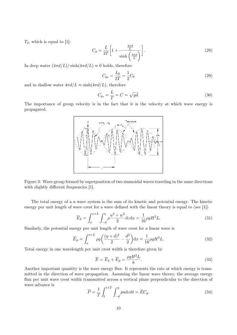
From equation (12) it is obvious that waves with different wavelengths L travel at differentspeeds - they have different phase velocities. The speed of a group of waves comprising of wavesof different wavelengths is termed the group velocity Cg. Waves in deep or transitional water withgravity as the primary restoring force have lesser group velocity than phase velocity. For capillarywaves, propagated primarily under the influence of surface tension, the group velocity may exceed thevelocity of an individual wave [1]. The concept of group velocity can be illustrated by considering thesuperposition of two sinusoidal waves moving in the same direction with slightly different wavelengthsand periods. The equation of water surface is then

η = η1 + η2 =H

2cos

(2πx

L1− 2πt

T1

)+

H

2cos

(2πx

L2− 2πt

T2

). (26)

The resulting form of water surface is shown in Figure 3. The waves appear to be traveling in groupsdescribed by the equation of the envelope

ηenvelope = ±H cos[π

(L2 − L1

L1L2

)x− π

(T2 − T1

T1T2

)t

]. (27)

The group velocity reaches its maximum when L1 approaches L2 and consequently T1 approaches

9

T2, which is equal to [1]:

Cg =L

2T

[1 +

4πdL

sinh(

4πdL

)]. (28)

In deep water (4πd/L)/ sinh(4πd/L) ≈ 0 holds, therefore

Cg0 =L0

2T=

12C0 (29)

and in shallow water 4πd/L ≈ sinh(4πd/L), therefore

Cgs =L

T= C =

√gd. (30)

The importance of group velocity is in the fact that it is the velocity at which wave energy ispropagated.

Figure 3: Wave group formed by superposition of two sinusoidal waves traveling in the same directionswith slightly different frequencies [1].

The total energy of a a wave system is the sum of its kinetic and potential energy. The kineticenergy per unit length of wave crest for a wave defined with the linear theory is equal to (see [1])

Ek =∫ x+L

x

∫ η

−dρu2 + w2

2dzdx =

116

ρgH2L. (31)

Similarly, the potential energy per unit length of wave crest for a linear wave is

Ep =∫ x+L

xρg

((η + d)2

2− d2

2

)dx =

116

ρgH2L. (32)

Total energy in one wavelength per unit crest width is therefore given by

E = Ek + Ep =ρgH2L

8. (33)

Another important quantity is the wave energy flux. It represents the rate at which energy is trans-mitted in the direction of wave propagation. Assuming the linear wave theory, the average energyflux per unit wave crest width transmitted across a vertical plane perpendicular to the direction ofwave advance is

P =1T

∫ t+T

t

∫ η

−dpudzdt = ECg. (34)

10

4 Transformation of waves

In this section the goal is to point out the processes that can affect a wave as it propagates fromdeep into shallow water. These processes are [1]:

1. refraction

2. shoaling

3. diffraction

4. dissipation due to friction

5. dissipation due to percolation

6. breaking

7. additional growth due to the wind

8. wave-current interaction

9. wave-wave interaction

The first three effects are propagation effects and are caused by bottom topography, which influencesthe direction of wave travel and causes wave energy to be concentrated or spread out. Diffraction isalso due to objects that interrupt wave propagation. The next three effects are dissipation effects orsink mechanisms that remove energy from the wave field. The wind is a source mechanism, because itadds energy to the wave field. Wave-current and wave-wave interactions, which result from nonlinearcoupling of wave components, also affect wave propagation and transformation.

Among these processes I would like to point out refraction and shoaling. Take for example amonochromatic (and thereby long-crested) wave propagating across a region in which there is astraight shoreline with all depth contours evenly spaced and parallel to the shoreline. If the waveis not perpendicular to the shore, water depth beneath different parts of the same wave crest isdifferent. Therefore, according to equation (14) and the fact that for the case of monochromaticwaves, wave period remains constant when water depth changes, wave celerity changes along thecrest of the wave. In Figure 4 a part of the wave in shallower water (point A) has smaller celerity asa part in deeper water (point B). As a result of the speed differential along the wave crest, the crestbecomes more parallel to the shore.

5 Surf zone waves

5.1 Surf zone

The surf zone is the region extending from the seaward boundary of wave breaking to the limit ofwave uprush. As waves approach the coast their steepness increases on account of decrease in waterdepth. When a limiting value of the wave steepness is reached, the wave breaks. That happens inwater depth that is approximately equal to the height of the waves. After breaking in the surf zone,the waves (now reduced in height) continue to move in and run up onto the sloping front of the beach,forming an uprush of water called swash. The water then runs back down again as backswash.

Within the surf zone, wave breaking is the dominant hydrodynamic process and it drives nearshore currents and sediment transport. Calculation of surf zone wave transformation is crucialfor understanding and preventing storm damage (flooding and wave damage), calculating shorelineevolution and cross-shore beach profile change and designing of coastal structures.

11

Figure 4: Wave crests approaching a straight shore with parallel depth contours at an angle bendtowards the shore. [1].

5.2 Transformation of waves in the surf zone

The goal of this section is to present and explain incipient wave breaking and the transformation ofwave height through the surf zone. In general, as a wave approaches a beach, water depth decreasesand the wave slows down (evident from equation (12)), although its period (frequency) remains thesame. As a result, it grows taller and changes shape - its crest becomes shorter and steepens, whileits trough lengthens and flattens out [9]. Because wave’s length L decreases and height H increases,there is an increase of steepness H

L . Waves break as they reach a limiting steepness, which is afunction of the relative depth d

L and the beach slope tanβ (where β is the angle between the slopeof the bottom and the horizontal plane).

5.2.1 Shallow water equations and a simple explanation of wave transformation thatleads to breaking

In [9] one can find a detailed derivation and explanation of equations that describe water wave motionin shallow water and on a sloping beach. It is a very extensive topic and detailed argumentationand understanding is beyond the scope of this seminar. However, I would like to point out justa few results that help to understand why waves transform so drastically near a shoreline, whichconsequently leads to breaking.

To obtain the nonlinear shallow water equations one starts similarly as in formulation of the linearwave theory. The flow is also governed by the Laplace equation and the same boundary conditions.It is useful to introduce dimensionless variables

(x∗, y∗) =1L

(x, y), z∗ =z

d, t∗ =

Ct

L, η∗ =

η

a, Φ∗ =

d

aLCΦ, (35)

where C =√

gd is wave celerity in shallow water (16). There are also two fundamental parametersthat characterize the nonlinear shallow water waves:

ε =a

dand δ =

d2

L2. (36)

12

In terms of these variables and parameters shallow water equations are as follows [9]

u∗t∗ + ε(u∗u∗x∗ + v∗u∗y∗) + η∗x∗ = 0,

v∗t∗ + ε(u∗v∗x∗ + v∗v∗y∗) + η∗y∗ = 0,

η∗t∗ + [u∗(1 + εη∗)]x∗ + [v∗(1 + εη∗)]y∗ = 0, (37)

where subscript index represents partial derivative with respect to that variable and u∗ = uC and

v∗ = vC . When ε 1 holds, that means a d, the above system can be linearized. In dimensional

form the linearized system is

ut + gηx = 0,

vt + gηy = 0,

ηt + d(ux + vy) = 0. (38)

By eliminating u and v from these equations one gets

ηtt = C2(ηxx + ηyy) = C2∇2η, (39)

which is a well-known two-dimensional wave equation. It corresponds to the nondispersive shallowwater waves that propagate with a constant velocity C =

√gd.

In case of one-dimensional wave equation ηtt = C2ηxx, the general solution is

η(x, t) = Θ−(x− Ct) + Θ+(x + Ct), (40)

where Θ− and Θ+ are arbitrary functions to be determined by the initial or boundary conditionsand represent waves moving with constant speed C without change of shape along the positive andthe negative directions of x, respectively. The solutions Θ− and Θ+ correspond to the two factorsin the wave equation (

∂

∂t+ C

∂

∂x

)(∂

∂t− C

∂

∂x

)η = 0. (41)

The simplest linear wave equation is therefore ηt + Cηx = 0 with general solution η = Θ−(x− Ct).This equation holds in shallow water (d/L < 1/20) when a d. However, the simplest first-ordernonlinear wave equation has the form

ηt + C(η)ηx = 0, (42)

where C(η) is a given function of η. The above nonlinear wave equation can be used as the firstapproximation to the wave equation when the condition a d is not fulfilled. In order to understandwhy waves break in the surf zone, let us have a look at (42) when −∞ < x < ∞, t > 0 andη(x, t = 0) = f(x). We try to solve this system by the method of characteristics [9]. In order toconstruct continuous solutions, we consider the total derivative dη = ∂η

∂t dt + ∂η∂xdx, where the points

(x, t) lie on a family of curves Γ. The derivative dxdt represents the slope of curve Γ at any point on

it. If we have a look at dηdt = ηt + dx

dt ηx, we see that we are trying to solve

dx

dt= C(η), x(0) = ξ,

dη

dt= 0, η(ξ, 0) = f(ξ), (43)

where C(η) is the slope of a characteristic curve Γ at any point on it and ξ is a chosen initialpoint. Because dη

dt = 0, the value of η does not change along the characteristic curve Γ. Therefore,

13

C(η) on Γ is equal to the value at the initial point ξ, so C(η) = C(f(ξ)) = F (ξ). By integratingthe relation dx

dt = F (ξ) and condition x(0) = ξ, one gets x = tF (ξ) + ξ, which represents thecharacteristic curve that is a straight line whose slope is not a constant, but depends on ξ. Becauseηx = f ′(ξ)ξx = f ′(ξ)

1+tF ′(ξ) and ηt = f ′(ξ)ξt = −F (ξ)f ′(ξ)1+tF ′(ξ) , the system (43) has a unique solution provided

1 + tF ′(ξ) 6= 0 and f and C are C1(R) functions.Let us assume C(η) > 0, so the point (ξ, f(ξ)) moves parallel to the x-axis in the positive

direction. The solution exists if 1 + tF ′(ξ) 6= 0, where t > 0. As we can see, this condition is alwayssatisfied for sufficiently small time t. As 1 + tF ′(ξ) → 0, both ηx and ηt tend to infinity and thesolution develops a singularity (discontinuity). By expressing t from the above condition, we gett = − 1

F ′(ξ) , which is positive if F ′(ξ) = c′(f)f ′(ξ) < 0. If we further assume c′(f) > 0, the precedinginequality implies that f ′(ξ) < 0. Suppose that τ is the time when the solution first develops asingularity for some value of ξ. Then

τ = −(

min−∞<ξ<∞

c′(f)f ′(ξ))−1

> 0. (44)

Figure 5 shows time evolution of a nonlinear solution η(x, t) calculated for a wave profile by themethod of characteristics. Each part of a long, large-amplitude wave on a gently sloping beachpropagates independently with the velocity u + C = u +

√gd, where u is local fluid velocity [9].

Higher parts of such a wave have a greater water velocity in the direction of propagation than lowerparts of the wave, therefore C = C(η) is justified. Consequently, any forward-facing slope steepensuntil the wave breaks. It is worth mentioning that such breaking is typical nonlinear phenomenon.In linear theory breaking does not occur, because all parts of the wave have the same celerity andtherefore the shape of the solution does not change.

Figure 5: Figure depicts time evolution of a nonlinear solution u(x, t) (u(x, t) corresponds to η(x, t)in the text) calculated for a wave profile by the method of characteristics. The characteristics areshown by the dotted lines, with two of them (from x = ξ1 and x = ξ2) intersecting at t > τ [9].

5.2.2 Breaker type

According to the form of waves at breaking they can be classified in four breaker types [1]:

• spilling type,

14

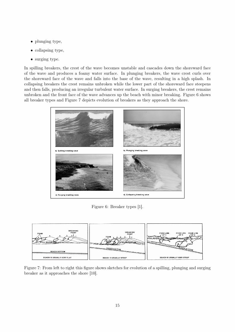
• plunging type,

• collapsing type,

• surging type.

In spilling breakers, the crest of the wave becomes unstable and cascades down the shoreward faceof the wave and produces a foamy water surface. In plunging breakers, the wave crest curls overthe shoreward face of the wave and falls into the base of the wave, resulting in a high splash. Incollapsing breakers the crest remains unbroken while the lower part of the shoreward face steepensand then falls, producing an irregular turbulent water surface. In surging breakers, the crest remainsunbroken and the front face of the wave advances up the beach with minor breaking. Figure 6 showsall breaker types and Figure 7 depicts evolution of breakers as they approach the shore.

Figure 6: Breaker types [1].

Figure 7: From left to right this figure shows sketches for evolution of a spilling, plunging and surgingbreaker as it approaches the shore [10].

15

Breaker type can also be correlated to the surf similarity parameter ξ0, defined as

ξ0 = tan β

(H0

L0

)− 12

, (45)

where H0 and L0 denote the deep water wave height and wavelength. According to the value of thesurf similarity parameter, breaker type on a uniformly sloping beach can be one of the following:

ξ0 > 3.3 surging, collapsing,

0.5 < ξ0 < 3.3 plunging,

ξ0 < 0.5 spilling. (46)

From (45) and (46) can be deduced that spilling breakers occur for steep waves on gently slopingbeaches. On the other hand, surging and collapsing breakers occur for low steepness waves on steepbeaches.

Concerning fluid motion, spilling breakers differ little from unbroken waves, as they generate lessturbulence near the bottom and thus tend to be less effective in suspending sediment than plungingor collapsing breakers. Plunging breakers produce the most intense local fluid motion, because asthey break their crest acts as a free-falling jet that may scour a trough into the bottom.

After categorizing possible wave forms it should be mentioned that the transition between breakertypes is gradual and no strict rules or conditions apply. There are many other factors that affectbreaker type, for example the direction and magnitude of local wind. It has been shown (see [1])that onshore winds cause waves to break in deeper depths and spill, whereas offshore winds causewaves to break in shallower depths and plunge.

5.2.3 Breaker index

Another quantity that can be assigned to surf zone waves is the breaker index, which describesdimensionless breaker height, that is the height Hb of the wave just before it breaks. Incipientbreaking can be defined in several ways. The most common is the point where wave height reachesmaximum, but it can also be the point where the front face of the wave becomes vertical (plungingbreakers) or the point just prior to appearance of foam on the wave crest (spilling breakers). Twocommon indices are the breaker depth index γb = Hb

db, where db is the depth at breaking, and the

breaker height index Ωb = HbH0

. Numerous estimates for values of both indices were derived formtheoretical models and laboratory experiments on solitary and monochromatic waves. Each one ofthese results requires an extensive comment, therefore I believe they are beyond the scope of thisseminar. However, interested reader can find further information in [1].

5.3 Wave setup and setdown

A setup is a rise in the mean water level above the still-water elevation (SWL) of the sea producedby waves breaking on a beach [11]. As one would expect from continuity, there is also a region calledsetdown, where the mean elevation of the sea is depressed. Total water depth is a sum of still-waterdepth d and mean water surface elevation about still-water level η: h = d + η. Sloping mean waterlevel balances the pressure gradient and the gradient of the incoming momentum (Figure 8). Theflux of horizontal incoming momentum across unit area of a vertical plane is equal to

M(x, t) =∫ η

−d(p + ρu2)dz. (47)

16

The following expression represents the cross-shore balance of momentum [12]

∂Sxx

∂x= −ρgd

∂η

∂x, (48)

where Sxx is cross-shore component of radiation stress, defined as the mean value of M(x, t) withrespect to time minus mean flux in the absence of waves, that is

Sxx =∫ η

−d(p + ρu2)dz −

∫ 0

−dp0dz. (49)

Based on the linear wave theory and equation (48), Longuet-Higgins and Stewart (1963) obtainedthe setdown for regular, normally incident waves seaward of the breaker zone [1]:

η = −18

2πH2/L

sinh(4πd/L). (50)

The maximum lowering of water level occours near the break point ηb. In the surf zone, η increasesbetween the break point and the shoreline (Figure 8).

Figure 8: Definition sketch for wave setup [1]. SWL is still-water level and MWL is mean (time-averaged) water level.

5.4 Wave runup on beaches

Wave runup is the maximu elevation of wave uprush above SWL (Figure 9). It is the superpositionof the mean water level (wave setup) and fluctuations about that mean (swash).

Figure 9: Definition of wave runup on beaches. [1].

According to [1] theoretical approaches for calculating runup on beaches are not yet viable.Difficulties inherent in runup prediction include nonlinear wave transformation, wave reflection,beach porosity, roughness and permeability. There were however empirical attempts to determine

17

wave runup as a function of beach slope, incident wave height and wave steepness. For regular wavesthere is, for example, Hunt’s formula for uniform, smooth and impermeable slopes

R

H0= ξ0, for 0.1 < ξ0 < 2.3, (51)

where ξ0 is the surf similarity parameter as defined in (45).

6 Conclusion

Through this seminar I had a chance to get a glimpse of incredible complexity of an everydayphysical phenomena - the surf zone hydrodynamics. As with the rest of hydrodynamics, there arenot many problems that could be dealt with analytically and offer compact results. However, thereare numerous theories and models based on more or less restricting assumptions, that offer someresults, facts and insights into the underlaying processes.

In the end I would like to thank my mentor for providing me with literature and helping mechoose relevant and interesting information among a vast quantity of writings on this subject.

18

References

[1] Coastal Engineering Manual - Part II,http://www.usace.army.mil/publications/eng-manuals/em1110-2-1100/PartII/PartII.htm,page visited 5.13.2007

[2] J. Pedlosky, Waves in the Ocean and Atmosphere (Springer-Velrag, Berlin, Heidelberg, 2003)

[3] H. A. Dijkstra, Nonlinear Physical Oceanography (Kluwer Academic Publishers, 2000)

[4] http://en.wikipedia.org/wiki/Ocean_surface_wave,page visited 5.13.2007

[5] A. Premelč, Simuliranje priobalnih valov z modelom SWAN (Seminar, May 2007)

[6] K. B. Dysthe Lectures given at the summer school on: Water Waves and Ocean Currents (Uni-versity of Bergen, 2004),http://www.math.uio.no/ johng/info/dysthe/Nordfjordeid-versjon.pdf,page visited 5.13.2007

[7] L. D. Landau, E. M. Lifshitz, Fluid Mechanics (Pergamon Books, Ltd., 1987)

[8] J. Lighthill, Waves in Fluids (Cambridge University Press, Cambridge, 1978).

[9] L. Debnath, Nonlinear Water Waves (Academic Press, Inc., 1994)

[10] http://www.marineplanner.com/bowditch/chap-33.pdf,page visited 5.15.2007

[11] http://www.ocean.washington.edu/people/faculty/parsons/OCEAN549B/setup-lect.pdf,page visited 5.13.2007

[12] http://www.ocean.washington.edu/people/faculty/parsons/OCEAN549B/rad-stress-lect.pdf,page visited 5.13.2007

19