currency dependent differences in credit spreads of eur ... annual meetings... · currency...

1

Currency Dependent Differences in Credit Spreads of EUR and

USD Denominated Foreign Currency Government Bonds

Andreas Rathgeber, David Rudolf, Stefan Stöckl

Andreas Rathgeber (Corresponding Author) Department for Human and Economic Sciences UMIT – The Health and Life Sciences University Hall/Tyrol Eduard Wallnöfer-Zentrum 1, 6060 Hall in Tirol, Austria E-Mail: [email protected] David Rudolf Institute for Business Administration - Finance and Banking University of Augsburg Universitätsstraße 12, 86159 Augsburg, Germany E-Mail: [email protected]

Stefan Stöckl FIM Research Centre Department of Information Systems Engineering & Financial Management University of Augsburg Universitätsstraße 12, 86159 Augsburg, Germany E-Mail: [email protected]

2

Abstract

Can the credit spreads of one and the same issuer differ in two different currencies? If so, can

an investor exploit this situation? To answer these questions and to add to the existing

literature, we extend the Jarrow/Turnbull model with a second currency and test these

theoretical results with an extensive empirical study. As a major result we discovered that the

credit spreads, and therefore the cumulated implied default probabilities of nearly all bonds

denominated in USD in comparison to EUR denominated bonds, are significantly higher for

all terms. As the results could largely be explained by the dependence between event of

default and exchange rate, an investor cannot therefore profit from this fact and the findings

of the empirical study lend support to the validity of the paradigm of the efficient market

hypothesis.

JEL classification: G12; G13; G15

Keywords: Credit Spreads; Efficient Market Hypothesis; Foreign Currency Government

Bonds; Implied Default Probabilities; Term Structure of Interest Rates

3

I. INTRODUCTION

Credit spreads represent both the credit risk for a debtor and an opportunity for an investor.

What if an investor can choose between two credit spreads in two different currencies from

the same debtor?

Generally it is a widely held practice to use credit spreads of one issuer to valuate bonds, for

exanple, without taking into account the existence of bonds from the same issuer denominated

in different currencies. But this approach is only correct if we assume that the credit spreads

of one issuer are not correlated with the corresponding currency, i.e. that continuous credit

spreads are equal across all currencies and therefore that risk-neutral implied default

probabilities are also equal.

However, this is only true in a normally distributed framework and an arbitrage-free market in

the specific case of non-correlation between credit spread and risk-free interest rate on the one

hand and between credit spread and exchange rate on the other hand, as shown by

Jankowitsch and Pichler (2005).

There is a large amount of literature that assesses the impact of various factors on credit

spreads and therefore also on the implied default probabilities of sovereign bonds (e.g.,

Edwards, 1986; Cantor and Packer, 1996; Eichengreen and Mody, 1998; Min, 1998; Peter,

2002; Grandes, 2003; Jostova, 2006; Hilscher and Nosbusch, 2007; Pan and Singleton, 2006;

Remolona et al., 2007; Longstaff et al., 2007, amongst many others).

However, the impact of currency denomination on credit spreads has so far received little

attention in literature. Amongst the few to look at this issue, Kamin and von Kleist (1999)

find that credit spreads of emerging market sovereign debt denominated in USD (U.S. Dollar)

were systematically higher in the 90s, which is attributed to comparable higher U.S. treasury

yields. But this is not a satisfactory explanation, as will be shown later.

4

Kercheval et al. (2003) find that corporate credit spread returns of corresponding issuer

clusters, i.e., of clusters containing bonds with identical rating, sector, and currency

denomination, are somewhat uncorrelated across different currencies, whereas credit spread

returns of similar issuer clusters with identical currency denomination are highly correlated.

This effect is also found at a single-issuer level, but only based on a very limited database.

The authors attribute their empirical results to market segmentation. However, the study has,

according to Jankowitsch and Pichler (2005), a few shortcomings. Among other things the

data doesn’t only include foreign currency bonds, so that a potential home bias could arise

within the different clusters.

McBrady (2003) investigates the empirical determinants (in this particular case: default risk,

liquidity premiums and segmented markets) of industrial country sovereign spreads. Among

other things he shows that market segmentation is present even in the biggest and most liquid

bond markets. He argues that investors prefer local currency bonds due to regulatory

constraints for institutional investors like pension funds, local benchmark orientation of funds

and limited access for private investors to swaps, which prevents them from effectively

hedging exchange rate risk.

Jankowitsch and Pichler (2005) also analyze corporate credit spreads across different

currencies. Contrary to Kercheval et al. (2003) they do not compare credit spread returns of

issuer clusters but credit spread curves at a single-issuer level. They find that credit spread

curves at the single-issuer level significantly differ across currencies. Jankowitsch and Pichler

(2005) interpret their findings as rejection of the hypothesis of independence between default

risk and the risk-free interest rate or default risk and exchange rate risk. Again, it is not clear

whether the corporate bonds in the sample are comparable in terms of their seniority and

collateralization.

5

Van Landschoot (2008) systematically compares the determinants of EUR (EUR) and USD

yield spread dynamics in the corporate bond markets. Among other results she finds that the

liquidity risk is higher for USD corporate bonds than for EUR corporate bonds. Her results

also indicate that the credit cycle, as measured by the region-specific default probability,

significantly increases USD yield spreads, whereas these findings are not valid for EUR yield

spreads.

Sener and Kenc (2008) empirically examine the determinants of the same risk across different

currencies and their effects on the valuation of risky debt. Their central result is that only a

small fraction of the spread can be explained by default risk because credit spreads of the

same issuer are not only currency-dependent but further influencing factors, such as a

variation in bankruptcy laws, tax regimes and liquidity conditions in domestic markets, also

play a significant role in the calculation of credit spreads across different credit markets.

The aim of this project is twofold: first, the existing theoretical models were unable to draw a

conclusion on the question of whether the variables default, exchange and interest rate are

dependent on each other. Therefore we show, by means of a Jarrow/Turnbull model extended

with a second currency, that, given a positive correlation between exchange rate - defined as

EUR/USD - and the event of default, the credit spreads in USD should theoretically be higher

than in EUR and vice versa.

Second, the empirical studies that have been published so far partially compare credit spreads

of different issuers or the same issuer with different contractual specifications. They also do

not take into account a potentially existing home bias. Additionally, these surveys do not take

into account the fact that the term structure estimation error might influence the differences in

credit spreads. Above all, due to the drawbacks of the applied theoretical models, the

influence of the correlation structure cannot be measured. We overcome these shortcomings

by choosing a well conditioned data set and by considering appropriate independent variables

6

within the regression analysis in order to examine potential driving factors for different credit

spreads.

The paper is organized as follows: the extension of the theoretical model in section 2 is

followed up by an empirical study in section 3, in which the shortcomings outlined above are

avoided. Finally, section 4 concludes the paper.

II. THEORETICAL ANALYSIS IN PERFECT MARKETS

a. Completion with the help of a forward contingent contract

In the Jarrow/Turnbull-framework applied here we assume two complete and perfect markets,

in two currencies (“Domestic Currency Unit” shortened as DCU and “Foreign Currency Unit”

shortened as FCU), with fixed recovery rates δ and payment of the recovery rates upon bond

maturity. The risky and riskless discount factors can be expressed as a function of the

maturity T and a spot rate s:

( ) ( )T(T)sexpT)(0,B ZT(T)sexpT)(0,ZB FCUFCUDCUDCU ⋅−=⋅−=

( )( ) ( )( )T(T)cs(T)sexpT)(0,RZB T(T)cs(T)sexpT)(0,RZB FCUFCUFCUDCUDCUDCU ⋅−−=⋅−−= (1)

Whereas the credit spread cs is defined as the difference between risky and riskless

continuously compounded interest rates:

( ) ( ).T)(0,T)/RZB(0,ZBlnT1cs(T) T)(0,T)/RZB(0,ZBln

T1cs(T) FCUFCUFCUDCUDCUDCU ==

(2) According to Jarrow and Turnbull (1995) the so defined credit spreads can be expressed in

terms of the recovery rate δ and the implied default probability λ:

( ) ⎟⎟⎠

⎞⎜⎜⎝

⎛+−

=••

• 11δT)(0,λ1ln

T1cs(T)

(3)

7

Because we assume that the recovery rate is constant (and the same in different currencies),

then the credit spread is an injective function of the implied default probability.

Furthermore, two riskless short term interest rate processes can be defined as

( ) ( )∫∫ −=−=TT

0FCUFCU

0DCUDCU dt (t)sexpT)(0,d dt (t)sexpT)(0,d

(4)

Additionally, the process for the discount factor, based on the interest rate difference in two

money market accounts, is defined by short term interest rate difference process

( )∫ +−=T

0FCUDCU dt (t)s(t)sexpT)d(0,

(5)

Because the framework is constructed for a single currency area, we extend the framework to

a second currency area connected via a stochastic exchange rate driven by a single factor.

Both credit risk-free interest rates are stochastic and, in contrast to Jarrow and Turnbull

(1995), might depend on the stochastic interest rate or the default event. Secondly, there is an

exchange rate for transferring one unit of the foreign currency (FCU) in e(0) units of the

domestic currency (DCU) at time 0. Because we can trade zero bonds maturing at T in both

interest rates, the corresponding forward exchange rate is e(0,T).

To achieve a complete market in the correlated setting we implement a FX conditional

forward contract (CFC). However, in this context it is important to add that this is only a

technical construction to complete the markets. With the help of the CFC, differences in

implied default probabilities can be traced back to the value of this contract. The CFC binds

the parties to exchange the currencies under a certain condition. Here the condition is the

survival of the issuer.

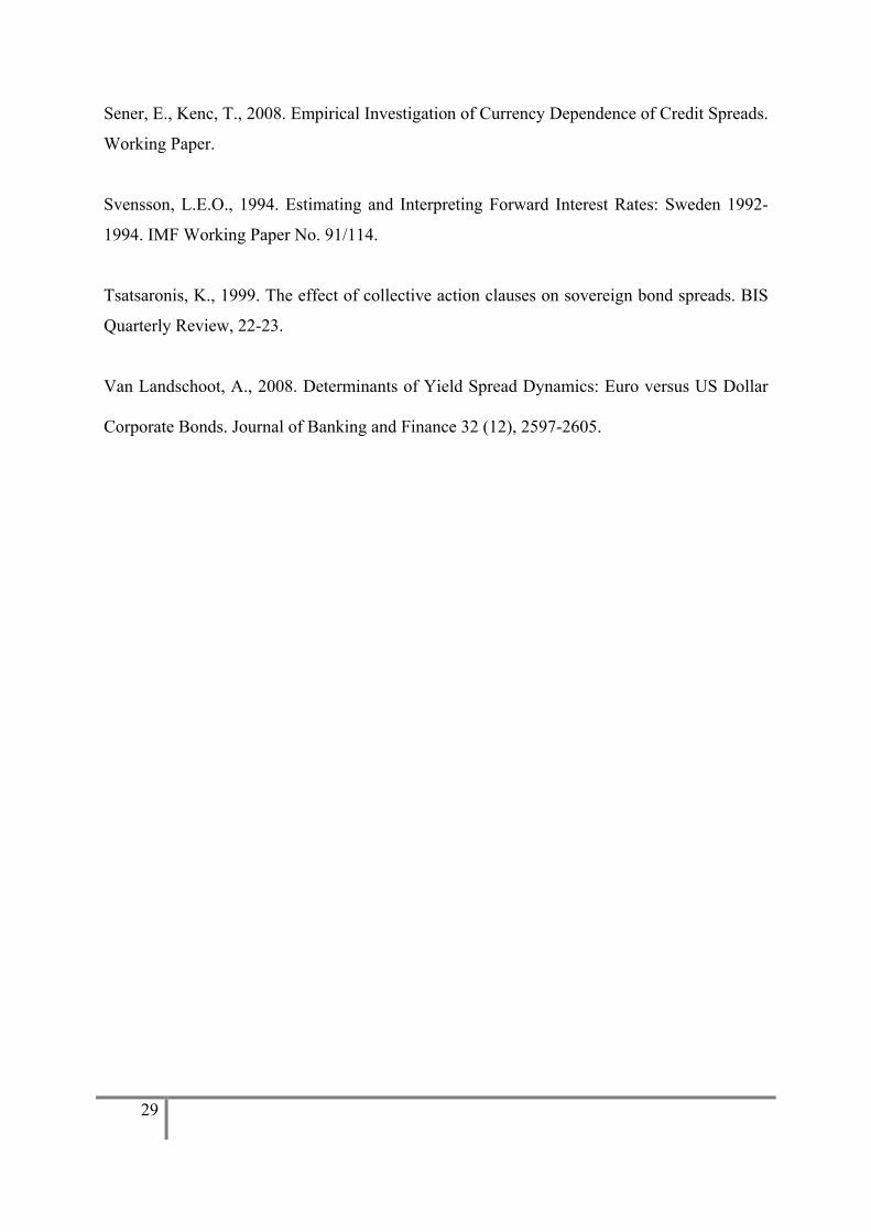
As one can see in Exhibit 1, buying one unit of a risky domestic currency bond maturing in T

RZBDCU(0,T) leads to the same payoffs as the following portfolio: one unit of forward value

8

at T e(0,T) of a risky foreign currency bond at RZBFCU(0,T), the amount of the recovery rate δ

of a FX forward contract and 1-δ of the conditional forward contract. In the case of survival,

the domestic currency bond pays 1 DCU just as the foreign currency bond pays 1 FCU. The

latter can be exchanged at the same rate partly by using the FX forward and partly by using

the CFC. In the default case both bonds pay only the recovery rate in DCU and FCU. Now

only the recovery rate is exchanged using the FX forward. Because the FX forward is by

nature a transaction with no ex ante capital exchange, we can use the value of the CFC to

evaluate eventual pricing differences and driving forces.

b. Value of the Conditional Forward Contract

If the value of the CFC is zero, the arbitrage-free criterion results in

T).(0,RZBT)e(0,

e(0)=T)(0,RZB FCUDCU

Keeping in mind that

e(0)T)(0,ZBT)(0,ZB

T)e(0,DCU

FCU=

this yields

T)(0,RZBT)(0,ZBT)(0,ZB

T)(0,RZB FCUFCU

DCUDCU =

and

.λ=λ⇔T)(0,ZBT)(0,RZB

=T))(0,ZB

T)(0,RZBFCUDCU

FCU

FCU

DCU

DCU

(6)

Consequently, if the value of CFC=0, the default probabilities are the same in both currencies.

Therefore a positive value for CFC coincides with a lower implied default and higher survival

probability in the domestic currency and vice versa. Because the sign of CFC does not

9

change, if we alter the payment style from cash to future-style, we assume for simplification

purposes that the payment style is future–style in the following formulas.

c. Factors affecting the implied default probability

In the next step we analyze the value of CFC if the variables survival of the issuer and/or

exchange rate and/or discount factor, based on the interest rate difference, is stochastically

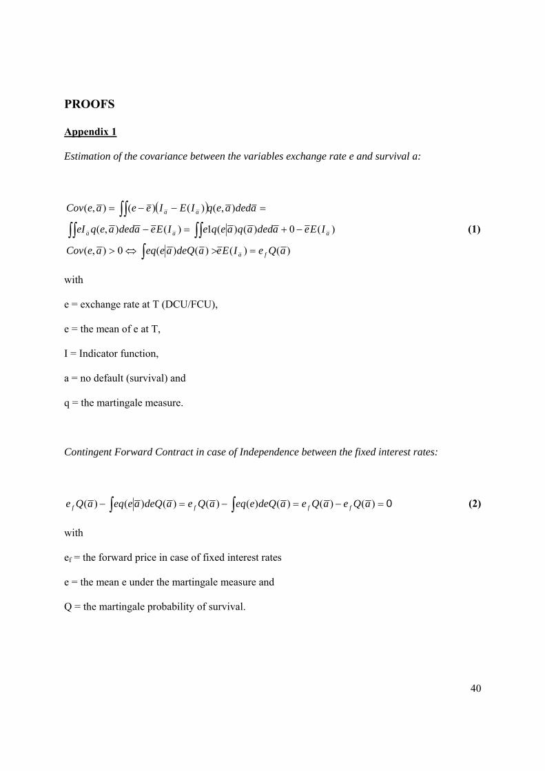
dependent. As is shown in Appendix 1, the value of CFC is always zero if the exchange rate

and the survival are independent and conditionally independent, given the discount factor in

the martingale measure world. At first glance, this result contradicts the result of Jankowitsch

and Pichler (2005), but is explainable because they use a Duffie/Singleton-framework, where

implied probabilities of credit spreads and/or recovery rates are not deterministic in time.

Furthermore, in contrast to Jankowitsch and Pichler (2005), supporting evidence can be

shown if dependence between the exchange rate and survival is presumed. Due to the fact that

the correlation is negative, the exchange rate is low at survival and therefore the value of the

CFC is positive and, finally, the implied default probability λ of RZBFCU exceeds the implied

probability of RZBDCU and vice versa. This is due to the fact that, in the case of survival, a

lower exchange rate (DCU/FCU) is more likely in the martingale measure. Consequently the

investment in the foreign currency bond cuts the possible cash flows of the contingent

position and therefore lowers the value.

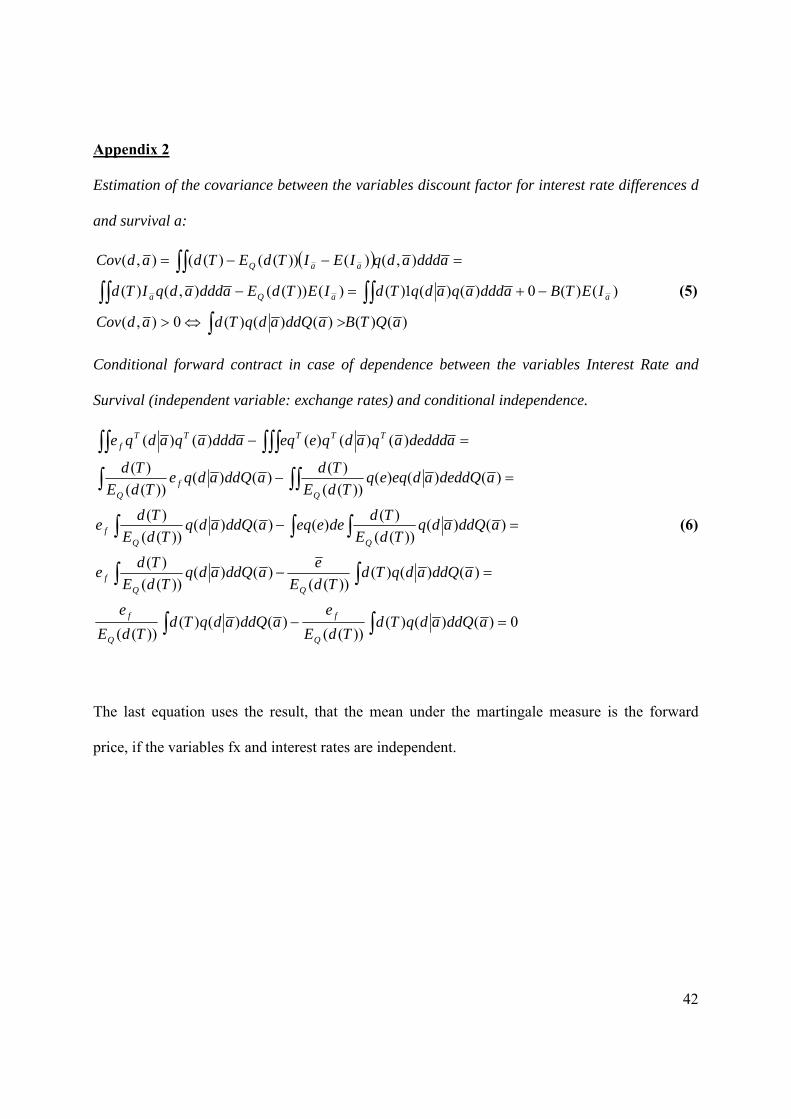
If the value of the CFC is non-zero, a correlated discount factor for the interest rate difference

influences the value of the CFC, even though discount factors for the interest rate difference

and the exchange rate are conditionally independent, given the survival. As shown in

Appendix 2, a positive correlation of the discount factor for the interest rate difference and the

survival leads to a higher absolute value of the CFC and the absolute difference between the

implied probabilities grows bigger. Due to the fact that the discount factor for interest rate

10

differences is strictly positive, the sign of the CFC cannot change and therefore dumping of

the absolute value of CFC through the correlation of discount factors for the interest rate

differences and survival cannot completely equalise the effect resulting from the correlation

of exchange rate and survival (see

EXHIBIT

Exhibit 11).

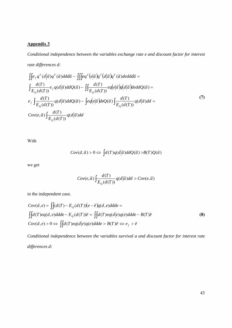
The case can also be considered in which the discount factor for the interest rate difference is

independent and conditionally independent of the survival. Here a positive correlation

between discount factor and exchange rate decreases the signed value of the CFC and vice

versa. Consequently, the value of a positive CFC and of a negative CFC is lowered when the

correlation coefficient is positive. Furthermore, in the case of a positive CFC, the difference in

implied probabilities lowers just as it increases in the case of a negative CFC. According to

Appendix 3, it can be stated that the CFC always reacts the same way as in the independent

case. Even if the correlation of exchange rate and survival and the correlation of discount

factor and survival contradict each other, the sign of the value will not change.

In conclusion, the main driver of the difference in credit spreads and the implied default

probability is the correlation between exchange rate and the event of survival or default. The

correlation between discount factor and exchange rate or the correlation between discount

factor and default can only alter the size of the difference but not the sign (see Exhibits 2

and 3).

These theoretical considerations lead to the first hypothesis to explain the difference between

two credit spreads in two different currencies of the same issuer. Given a positive correlation

11

between exchange rate (defined as EUR/USD) and the event of default, the first hypothesis is

formulated in the following way:

H1: The higher the correlation between the exchange rate and the implied survival

probability, the higher the difference theoretically between the implied default probabilities of

the USD and EUR denominated foreign currency government bonds.

d. Further hypotheses

In addition to correlation, further potential influencing factors related to an imperfect and/or

incomplete market, such as liquidity (H2), coupon rate (H3), collective action clauses (H4)

and a pricing error (H5) were tested.

Amongst many others, Easley et al. (2002), argue that liquidity is priced because investors

maximize expected returns net of transactions (or liquidity) costs. Several studies, including

for example Collin-Dufresne et al. (2001) or Longstaff et al. (2005), conclude that (changes

in) yield spreads and therefore (in) the implied default probabilities are significantly affected

by liquidity risk (e.g., Driessen, 2005; Van Landschoot, 2008; Chen et al., 2007).

As a result of these theoretical reflections the second hypothesis is formulated as follows:

H2: The bigger the differences between the liquidity risks of USD and EUR dominated

government bonds, the bigger the differences between the signed value of the implied default

probabilities of the USD and EUR denominated foreign currency government bonds.

Generally there is one main reason why credit spreads and therefore differences in the implied

default probabilities might be affected by taxes: differences in income tax regimes between

countries or currency areas (e.g., Driessen, 2005; Sener and Kenc, 2008; Van Landschoot,

2008). For such an analysis it would be necessary to know the nationality and the legal status

12

of the bondholders. Consequently the analysis is limited to the perspective of German and

U.S. investors. For German private investors bonds with a low coupon were advantageous

from a tax point of view in the recent past because capital gains were tax-exempt after a one

year holding period, whereas interest income is always taxable. For German companies there

is no difference in taxation. Also capital gains and interest income are taxed differently in the

U.S. for private investors. In the U.S. there is no differentiation between sundry kinds of

income with the result that interest income is assessed using the relevant individual tax rate.

In comparison, capital gains are liable to a tax rate of 15% and, unlike in Germany, there is no

tax-exemption after a one year holding period. Prior to the tax reform of 1986, U.S. sovereign

bonds with high coupons were clearly discriminated (Jordan, 1984; Litzenberger and Rolfo,

1984; Ronn, 1987), whereas this coupon effect could not be found after the reforms (Green

and Odegaard, 1997; Elton and Green, 1998). As bonds with high coupon rates systematically

show higher credit spreads and therefore higher implied default probabilities (Elton et al.,

2004) as a result of tax disadvantages, we use the coupon rate as an explanatory variable to

test the tax effect (Lim et al., 2003). In the case of German investors, higher coupon rates

were a disadvantage in the past from a tax point of view as well. Therefore it is possible that a

(potential) coupon tax effect could explain differences in the implied default probabilities

between government bonds denominated in EUR and USD, and therefore our third hypothesis

is formulated as follows:

H3: Given a coupon tax effect (discrimination of high coupons in both currencies),

government bonds with higher coupon rates feature higher implied default probabilities.

As the real world default probabilities are equal for all the bonds considered from an issuer,

differences in the default risk can only be due to different recovery rates. But this cannot be

attributed to differences in seniority, as all bonds considered from an issuer rank pari passu.

13

Therefore, only different legal procedures in case of default could lead to a different recovery

rate. In fact there are different legal procedures in place because of collective action clauses.

Collective action clauses enable a qualified majority of bondholders to change material

characteristics of the bond, such as principal, coupon rate or maturity. In this case, the higher

credit spreads/implied default probabilities or yields would compensate bondholders for a

lower recovery rate. However, most studies cannot find a significant impact of collective

action clauses on bond yields (e.g., Tsatsaronis, 1999; Dixon and Wall, 2000; Gugiatti and

Richards, 2003; Becker et al., 2003 amongst many others). Our fourth hypothesis is

formulated as follows:

H4: Government bonds which contain more collective action clauses applied to the sample

considered feature higher implied default probabilities.

Generally, a direct comparison of two bonds denominated in EUR and in USD can only be

carried out successfully if the two bonds have the same maturity as well as coupon payments.

Because this rare event is non-existent in the data source, a comparison is achieved, according

for example to Jankowitsch and Pichler (2005) or Sener and Kenc (2008), by the comparison

of the credit spread curves which are estimated from bond prices. The drawback of this

methodology is that it neglects the error in the credit spread estimation process.

To allow for this effect we use the credit spread curve or, equivalently, the implied default

probabilities from USD to calculate the bond prices in EUR and vice versa. We then compare

this price with the price estimated using the implied default probabilities in the opposite

currency. In this way the latter might be influenced by the measurement error in the credit

spread curve estimation. A positive difference between estimated price and market price leads

to a positive difference between the estimated price using the implied default probabilities in

the opposite currency and the former estimated price.

14

H5: The bigger the signed estimation error of the USD and EUR denominated bonds, the

bigger the differences between the signed value of the implied default probabilities of the

USD and EUR denominated foreign currency government bonds and vice versa.

III. DATASET AND METHODS

a. Dataset

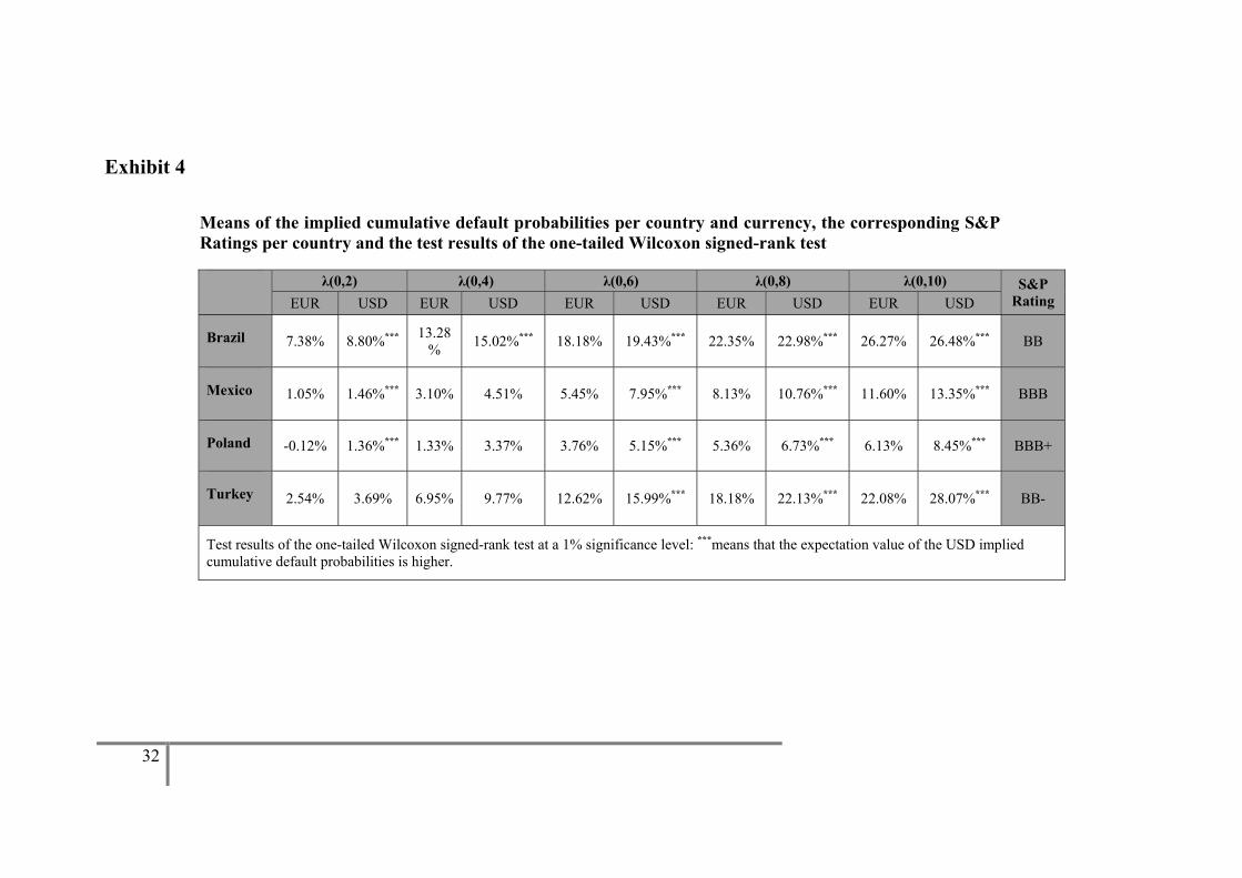
The data sample contains prices for 93 bonds and approximately 11.000 trading days for

sovereign bonds of Brazil, Mexico, Poland, and Turkey, of which 31 are denominated in EUR

and the remainder in USD (see Exhibit 6). The daily prices were downloaded from Thomson

Reuters Datastream and cover the period April 1998 to June 2008. These four countries were

chosen for the analysis because only these countries fulfilled all three necessary criteria

during the analysis period. The first criterion is that all countries had to have at least five

bonds outstanding, both in EUR and USD, because five bonds are necessary to estimate stable

spot rate curves using established methods. The second criterion is that all bonds are foreign

currency bonds due to the potentially different default risk of local currency sovereign bonds.

EUR and USD are the most common foreign currencies in which sovereign bonds are

denominated and have the additional advantage that the yield curve, i.e., the risk-free spot rate

curve, can be estimated very accurately for both currencies. The third criterion is that the

foreign currency rating of all issuers considered was below A on the S&P scale in 2006,

leaving enough room for the occurrence of significant differences in the credit spreads or

implied default probabilities. All bonds have fixed coupon payments once or twice a year and

are redeemed at par. None of the bonds contain embedded options or are redeemable or

callable prior to maturity. All bonds constitute unsubordinated and unsecured debt, i.e., they

rank pari passu, which is assured by a so-called negative pledge in the prospectuses. This

15

ensures that all bonds from an issuer should have, apart from differences specified in section

II d., the same default risk, and that their credit spread can be fully attributed to default risk

because the cash-flows are known ex-ante in the case of no default occurring before maturity.

To estimate the implied default probabilities for each issuer and each currency according to

the reduced-form model of Jarrow and Turnbull (1995), the risky and the risk-free discount

factors have to be estimated.

For the correlation structure analysis a EUR/USD exchange rate was required and the rate

fixed in Frankfurt by the German Central Bank was applied.

b. Estimation of risky and risk-free discount factors

Three estimation methods were applied to estimate the risky discount factors: the method

established by Chambers et al. (1984), the method presented by Nelson and Siegel (1987), and

the Restricted Integro Basis Spline – Method, proposed initially by Rathgeber (2008). As the

Restricted Integro Basis Spline – Method turned out to be superior, both in terms of

estimation quality and consistency of the estimated discount factors, only the discount factors

estimated by this method were used for further analysis.

German sovereign bonds (“Bundesanleihen”) were used to estimate the risk-free EUR spot

rates. The German Central Bank uses the method proposed by Svensson (1994,) which is an

extension of the method of Nelson and Siegel (1987), allowing a more flexible course of the

yield curve to estimate the EUR yield curve. It is important to take into account that the

German Central Bank does not use the exact discount function developed by Svensson (1994)

but a slight modification proposed by Schich (1997), which inconsistently uses discretely,

instead of continuously, compounded interest rates.

For the sake of unity, the Svensson method was also used to estimate the risk-free USD

discount factors. For the estimation, daily prices of 77 treasury bonds and notes were

16

downloaded from Reuters Datascope Select. All bonds have fixed coupon payments twice a

year and are redeemed at par. Before we calculate the implied default probabilities we briefly

discuss the results expected from a theoretical point of view.

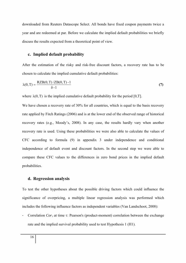
c. Implied default probability

After the estimation of the risky and risk-free discount factors, a recovery rate has to be

chosen to calculate the implied cumulative default probabilities:

1 - δ1 - T) /ZB(0,T)RZB(0,T)λ(0, =

(7)

where T)λ(0, is the implied cumulative default probability for the period [0,T].

We have chosen a recovery rate of 30% for all countries, which is equal to the basis recovery

rate applied by Fitch Ratings (2006) and is at the lower end of the observed range of historical

recovery rates (e.g., Moody’s, 2008). In any case, the results hardly vary when another

recovery rate is used. Using these probabilities we were also able to calculate the values of

CFC according to formula (9) in appendix 3 under independence and conditional

independence of default event and discount factors. In the second step we were able to

compare these CFC values to the differences in zero bond prices in the implied default

probabilities.

d. Regression analysis

To test the other hypotheses about the possible driving factors which could influence the

significance of overpricing, a multiple linear regression analysis was performed which

includes the following influence factors as independent variables (Van Landschoot, 2008):

- Correlation Corτ at time τ: Pearson's (product-moment) correlation between the exchange

rate and the implied survival probability used to test Hypothesis 1 (H1).

17

- Liquidity risk factor Liqτ at time τ: bid ask spread of bonds evaluated by LOT-Measure,

used to test Hypothesis 2 (H2) (Lesmond et al., 1999).

- Coupon rate CR : coupon rate of bonds, used to test Hypothesis 3 (H3).

- Collective Action Clauses CAC: dummy, which is 1 in the case of collective action

clauses, used to test Hypothesis 4 (H4).

- Measurement error errτ at time τ: defined as relative error between the estimated price

and the market price RBτ.

( )

ττ

τDCU,τDCU,τDCU,

T

1=tτDCU,τDCU, τDCU,

ττ

RBRB1-1=

t)(0,λt)(0,ZB(t)CFδ+t)(0,λ-1t)(0,ZB(t)CFRB1-1=err ∑ ⎟⎟

⎠

⎞⎜⎜⎝

⎛⋅⋅⋅⋅⋅

(8)

whereby T is the maturity of the risky bond and CF•(t) are its cash flows, used to test

Hypothesis 5 (H5).

Because the liquidity risk factor and the measurement error may be measured with an error

and is likely to be correlated with the regression residuals, we performed a Hausmann’s

specification test to identify potential correlations. In accordance with Griffith et al. (1993, p.

462) we used the lagged variable as instrumental variable. In case of a significant correlation

we used the instrumental variable as an independent variable.

The dependent variable is the relative pricing difference between the two currencies.

Assuming that the implied default probabilities of the foreign currency are valid in the

domestic currency, the relative price difference, can be expressed as

( ) ⎟⎟⎠

⎞⎜⎜⎝

⎛⋅⋅⋅+⋅⋅−=

=

)t,0(t)(0,ZB(t)CF)t,0(-1t)(0,ZB(t)CFRB

11diff FCU, DCU, DCU,

T

1t FCU, DCU, DCU,∑ ττττττ

ττ λδλ

(9)

Following the methodology of Ehrhardt et al. (1995) or Eom et al. (1998) the regression

equation for each time is given by

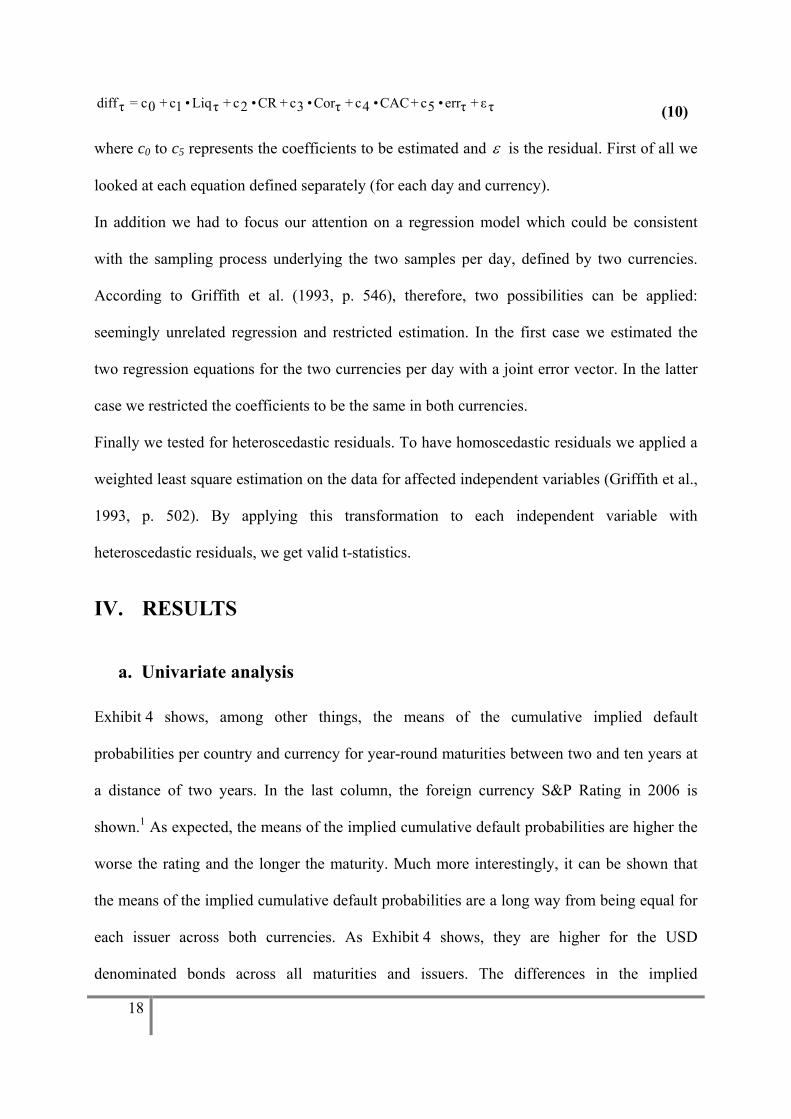
18

τε+τerr•5c+CAC•4c+τCor•3c+CR•2c+τLiq•1c+0c=τdiff (10)

where c0 to c5 represents the coefficients to be estimated and ε is the residual. First of all we

looked at each equation defined separately (for each day and currency).

In addition we had to focus our attention on a regression model which could be consistent

with the sampling process underlying the two samples per day, defined by two currencies.

According to Griffith et al. (1993, p. 546), therefore, two possibilities can be applied:

seemingly unrelated regression and restricted estimation. In the first case we estimated the

two regression equations for the two currencies per day with a joint error vector. In the latter

case we restricted the coefficients to be the same in both currencies.

Finally we tested for heteroscedastic residuals. To have homoscedastic residuals we applied a

weighted least square estimation on the data for affected independent variables (Griffith et al.,

1993, p. 502). By applying this transformation to each independent variable with

heteroscedastic residuals, we get valid t-statistics.

IV. RESULTS

a. Univariate analysis

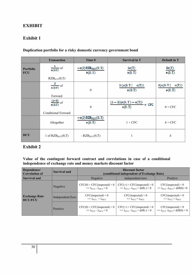
Exhibit 4 shows, among other things, the means of the cumulative implied default

probabilities per country and currency for year-round maturities between two and ten years at

a distance of two years. In the last column, the foreign currency S&P Rating in 2006 is

shown.1 As expected, the means of the implied cumulative default probabilities are higher the

worse the rating and the longer the maturity. Much more interestingly, it can be shown that

the means of the implied cumulative default probabilities are a long way from being equal for

each issuer across both currencies. As Exhibit 4 shows, they are higher for the USD

denominated bonds across all maturities and issuers. The differences in the implied

19

cumulative default probabilities are economically significant: given a risk-free spot rate of

4%, today’s price difference between two zero-coupon bonds with 10-year maturity is

somewhere between 6% and 29% for the four countries, exceeding usual bid-ask-spreads by a

large margin. To establish whether these differences are also statistically significant they were

tested with the help of the Wilcoxon signed-rank test. This test was chosen due to the fact that

it has no requirements relating to the distribution of the differences. For each country and

trading day the difference between the implied cumulative default probabilities was calculated

for year-round maturities ranging from two to ten years at a distance of two years. To test

whether the USD implied cumulative default probabilities are significantly higher than the

results shown the one-tailed versions of the Wilcoxon signed-rank test was applied. Exhibit 4

gives the results in addition to the above mentioned issues (cumulative default probabilities,

S&P Ratings). “H0” means that the null hypothesis of equal expectation values could not be

rejected at a 1% significance level, whereas ”H1” means that the expectation value of the USD

implied cumulative default probabilities is higher. It can be seen that this is true for nearly all

maturities in Brazil, Mexico, Poland, and Turkey, apart from the two and four year maturities.

As shown in one of the previous sections, the implied default probabilities of one issuer are

only equal across different currencies if there is independence between default risk and the

evolution of the risk-free interest rate in the respective currency on the one hand, and between

default risk and the evolution of the exchange rate between the two currencies considered on

the other hand. Therefore, the finding for different credit spreads or implied default

probabilities could be attributed to the fact that the assumption of independence is not correct,

as Jankowitsch and Pichler (2005) interpreted their results. To analyze a possible dependence

between default risk and the evolution of the exchange rate between EUR and USD, the

Pearson's (product-moment) correlation coefficient between the exchange rate of the EUR in

USD and the USD bonds implied default probability was calculated and for the default risk in

20

EUR the correlation between the exchange rate of the USD in EUR and the EUR bonds

implied survival probability as a proxy was calculated.2 Therefore, the assumption was

introduced that the correlation coefficient is the same in the martingale measure as in the real

word measure. The proxy for the default risk serves as the unobservable dichotomy variable.

As estimation time for the coefficients a 2500 day trading window was used.

As can be seen in Exhibit 6, the correlation coefficients are strongly and statistically

significantly positive for the USD and negative for the EUR. The effect is persistent among

different currencies and maturities. Furthermore, it can be said that the longer the maturity,

the higher the correlation coefficients. Due to the fact that the correlation is, with a few

exceptions, monotone in maturity, the maturity can be used as an instrumental variable for

correlation (see part III.d).

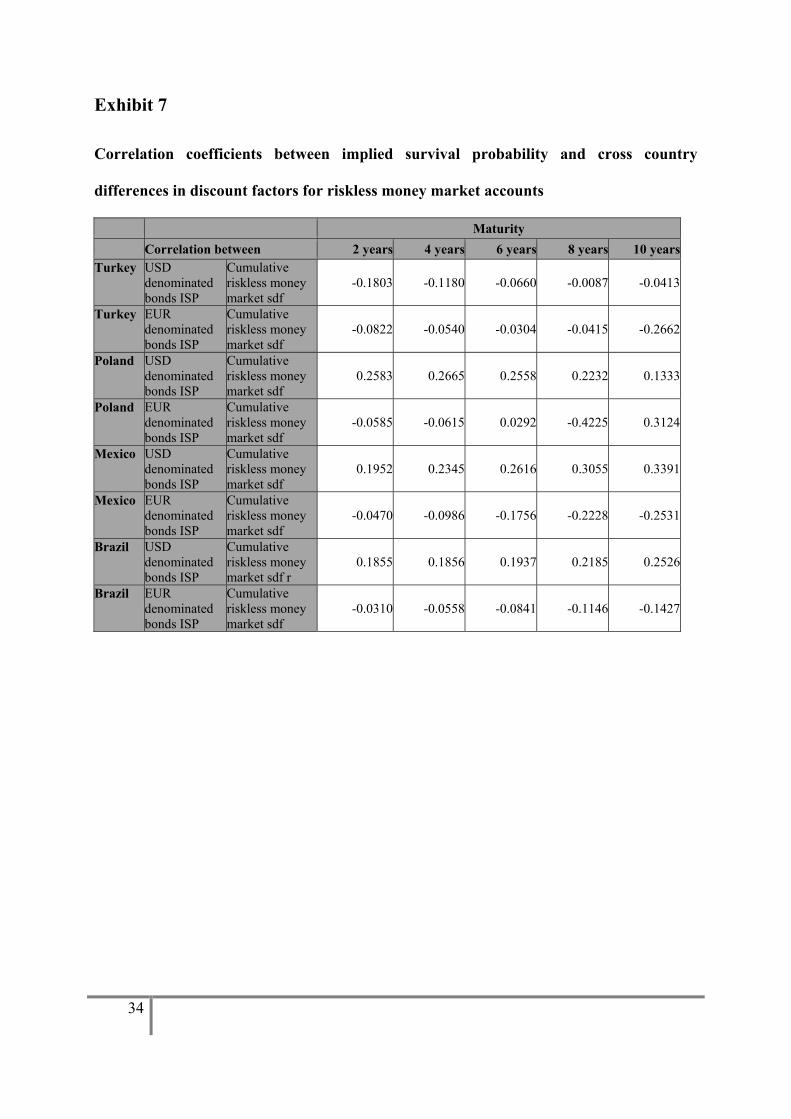
On the other hand, the data indicates a more or less zero correlation between the risk-free

interest rate and the default risk of bonds denominated in the respective currency. As shown

in Exhibit 7, there is no pattern and the correlation coefficients are frequently insignificant.

Therefore an influence is very unlikely. This finding confirms the results found by

Eichengreen and Moody (1998) but contradicts the results of Arora and Cerisola (2000).

Furthermore, the extent of the differences in the implied default probabilities (see Exhibit 4),

as shown in Exhibit 8, can be traced in many cases to the correlation between exchange rate

and implied survival probability with regard to the different countries and maturities. In

addition to this, it is apparent that there is a structural difference on the one hand between the

varying maturities and on the other hand between the respective issuers.

21

b. Multivariate analysis

In the context of the multivariate analysis, one regression equation for each day was

calculated in order to compute an average coefficient for each country and currency and the

amount of significant coefficient at a 1% significance level for each country and currency.

Altogether three different regression models were used:

1. Each currency and each issuer were separately incorporated in the respective

regression equation (“Single Model”).

2. Each issuer, without a distinction relating to currency, was separately entered into the

respective regression equation (“Total Model”).

3. Seemingly unrelated regressions model (“SUR”).

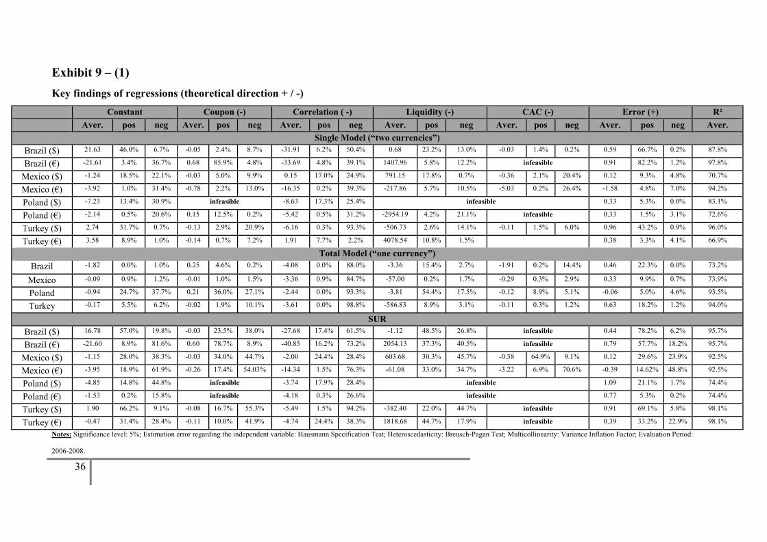
In terms of the findings of the three regression models, the proportion of highly significant

regression coefficients (5% level) as well as the average coefficient are listed in tabular form

in Exhibits 9 – (1-3) and 10 (see also Ehrhardt et al., 1995). The results are corrected for an

eventual estimation error in the dependent variables correlation, liquidity and error. In

addition to that the standard errors are corrected for eventual heteroskedasticity. Lastly we

had to exclude several independent variables in the Polish regression due to multicolliniarity.

First of all there is an indirect positive confirmation of the first hypothesis in that the signed

values of the implied default probabilities in USD are statistically significantly higher than the

implied default probabilities in EUR.

Secondly, the coefficient of the variable correlation in most regressions deviates significantly

from zero. Additionally, the sign of the coefficient coincides with the direction proposed by

hypothesis 1.

22

Liquidity, as an additional possible factor of influence, can only be proved very occasionally,

especially in the context of the SUR in the case of nearly all considered countries. When the

variable is significant its regression coefficient often features the wrong sign.

The results, in terms of the effect of taxes, are ambivalent. The third hypothesis can be

confirmed tendentially for Poland and Turkey by using the total model, but it is very likely

confirmed by the single regression. This might be due to the fact that the coupon effect was

still in existence in the eurozone for a long time. By using the SUR it can be confirmed for

Mexico and Turkey (see Exhibit 9 – (1)).

Furthermore, the purchase of collective action clauses only plays a minor role. Nevertheless,

the fourth hypothesis can be confirmed at a 5% significance level in the case of Poland and

Turkey due to the fact that both Turkish and Polish EUR government bonds contain no

collective action clauses and therefore the dummy variable, by which collective action clauses

as an factor of influence were tested, functions as an indicator variable relating to the

respective currencies.

Moreover, the effect of the term structure estimation error can only be proved in the case of

Brazil and marginally inter alia for Turkey in the context of the SUR. The reason for this is

that for Brazil more government bonds are available and therefore a higher pricing error

results.

To sum up, the most important factor of influence on the different credit spreads and therefore

the implied default probabilities seems to be the correlation between the exchange rate and the

event of default. All other possible factors of influence, which were tested in the context of

this empirical study, are more or less able to explain the empirically established differences

between the implied default probabilities.

23

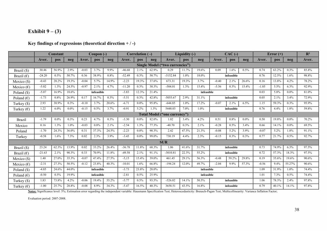
c. Robustness analysis

In order to obtain the robustness of our results several regressions were performed. First of all

we used a shorter evaluation period (2007-2008) and again got the same results (see Exhibit 9

– (3)).

In addition to that we excluded in the regression models the very occasionally significant

variables liquidity and CAC (not reported) and were therefore able to confirm our results.

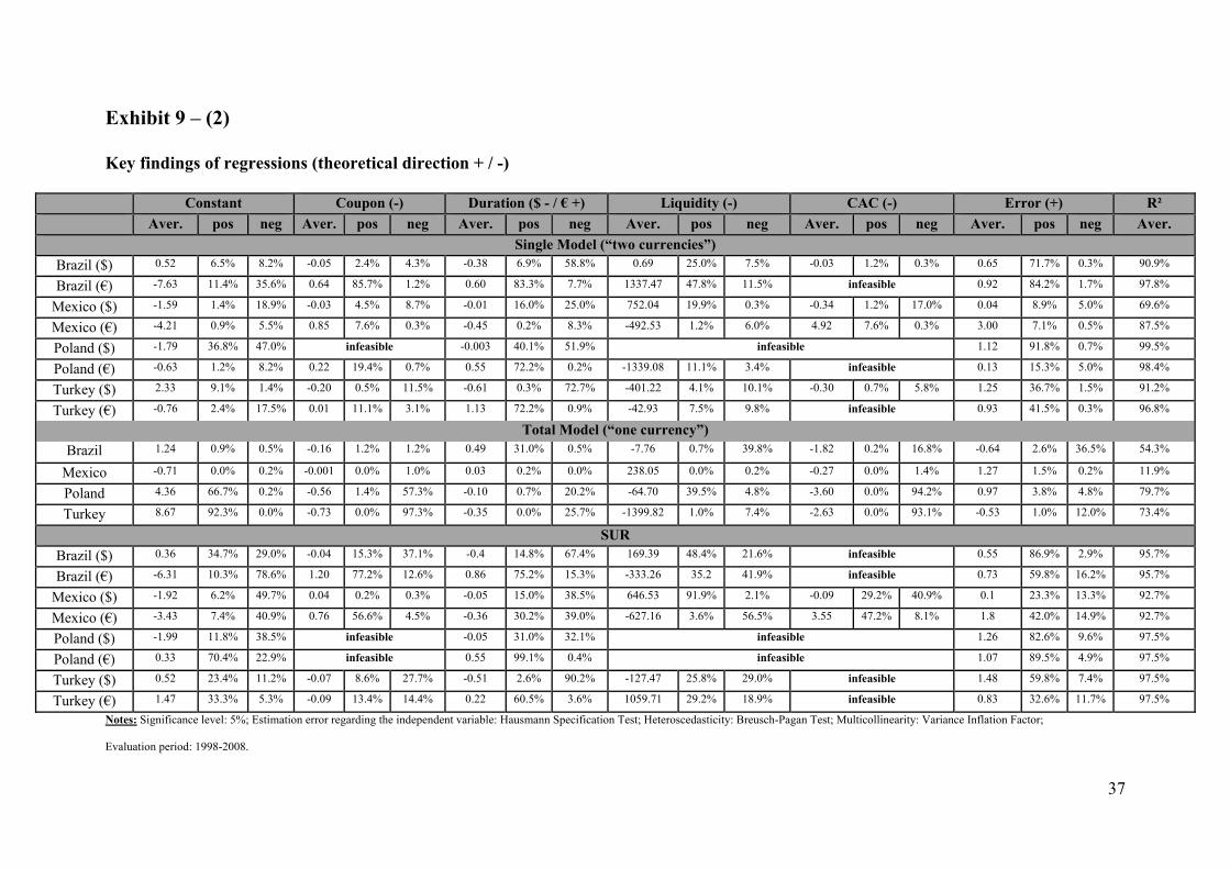
Furthermore, we took the duration of bonds expressed in years as an instrumental variable for

correlation in order to test hypothesis 1 into account, because, as you can see in Exhibit 6, the

correlation coefficient is monotone in maturity and we got approximately the same results

(see Exhibit 9 – (2)). Again the coefficient of the variable duration deviates significantly from

zero in most regressions. The other hypothesis (2-5) can be endorsed at a 5% significance

level in isolated cases. Additionally, we split the data set in two periods: 1998-2003 and 2004-

2008. We ran the regressions separately (not reported) and found the same results.

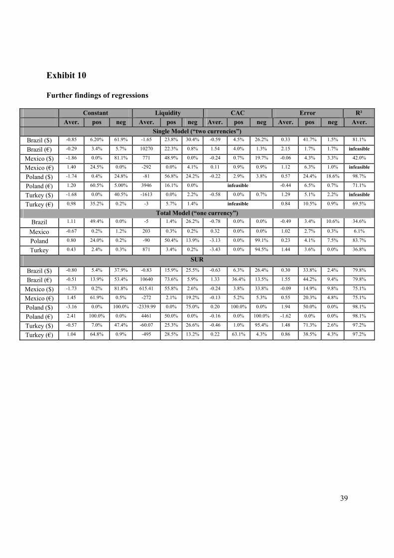
Last but not least the results without consideration the variable correlation do not differ from

the presented results (see Exhibit 10). To sum up, the robustness of our results seems to be

worth.

IV. CONCLUSIONS

To begin with we bridged an existing research gap where existing theoretical models were

unable to draw a conclusion on the question of whether the variables default, exchange and

interest rate are dependent (Jankowitsch and Pichler, 2005). We showed by means of a

Jarrow/Turnbull model that, given a positive correlation between exchange rate and the event

of default, the credit spreads in USD are statistically significantly higher than in EUR and

vice versa. Furthermore, we avoided the existing shortcomings relating to the consideration of

24

contractual specifications and the influence of the term structure estimation error in the

empirical studies published so far (e.g., Kercheval et al., 2003; McBrady, 2003), by taking

different contractual specifications and the influence of the term structure estimation error

into account. Moreover, due to the drawbacks of the applied theoretical models, we took into

account the influence of the correlation structure. It turned out that the influence of the

correlation structure was highly significant (see Exhibit 6).

Additionally, following for example Elton et al. (2001), Driessen (2005), Sener and Kenc

(2008) and Van Landschoot (2008), we found out that other factors of influence are (slightly)

responsible for the different credit spreads. In this context we took the influence of taxes (e.g.,

Elton et al., 2004) and liquidity risk (e.g., Driessen, 2005; Van Landschoot, 2008; Chen et al.,

2007) into account and obtained similar results to those in the literature cited. However, it has

to be added that the effects of liquidity and taxes could only be proved very occasionally.

Furthermore, we initially considered different contractual specifications and the term structure

estimation error, but in fact these two factors only seem to play a minor part.

As a large part of the results could be explained by the dependence between event of default

and exchange rate, the findings of the empirical study lend support to the validity of the

paradigm of the efficient market hypothesis.

For future research it would be interesting to also consider corporate bonds denominated in

different (foreign) currencies from one issuer and to take more contingent factors of influence

into account.

25

References

Arora, V., Cerisola, M., 2000. How Does U.S. Monetary Policy Influence Economic

Conditions in Emerging Markets? IMF Working Paper No. 00/148.

Becker, T., Richards, A., Yunyong, T., 2003. Bond restructuring and moral hazard: are

collective action clauses costly? Journal of International Economics 61 (1), 127-161.

Cantor, R., Packer, F., 1996. Determinants and Impact of Sovereign Credit Ratings. Economic

Policy Review, Federal Reserve Bank of New York 2, 37-53.

Chambers, D.R., Carleton, W.T., Waldman, D.W, 1984. A New Approach to Estimation of

the Term Structure of Interest Rates. Journal of Financial and Quantitative Analysis 19, 233-

252.

Chen, L., Lesmond, D., Wie, J., 2007. Corporate Yield Spreads and Bond Liquidity. Journal

of Finance 62 (1), 119-149.

Collin-Dufresne, P., Goldstein, R. S., Martin, J. S., 2001. The determinants of credit spread

changes. Journal of Finance 56 (6), 2177-2207.

Dixon, L., Wall, D., 2000. Collective action problems and collective action clauses. Financial

Stability Review, Bank of England, 142-151.

Driessen, J., 2005. Is default event risk priced in corporate bonds? Review of Financial

Studies 18, 165-195.

Easley, D., Hvidkjaer, S., O`Hara, M., 2002. Is information risk a determinant of asset

returns. Journal of Finance 57 (5), 2185-2221.

Edwards, S., 1986. The pricing of bonds and bank loans in international markets: An

empirical analysis of developing countries' foreign borrowing. European Economic Review

30 (3), 565-589.

26

Ehrhardt, M.C., Jordan, J.V., Prisman, E.Z., 1995. Tests for tax-clientele and tax-option

effects in U.S. treasury bonds. Journal of Banking and Finance 19 (6), 1055-72.

Eichengreen, B., Mody, A., 1998. What Explains Changing Spreads On Emerging-Market

Debt? Working Paper, The National Bureau of Economic Research.

Elton, E.J., Green, C., 1998. Tax and Liquidity Effects in Pricing Government Bonds. Journal

of Finance 53 (5), 1533-1562.

Elton, E. J., Gruber, M. J., Agrawal, D., Mann, C., 2001. Explaining the rate spread on

corporate bonds. Journal of Finance 56 (1), 247-277.

Elton, E. J., Gruber, M. J., Agrawal, D., Mann, C., 2004. Factors affecting the valuation of

corporate bonds. Journal of Banking and Finance 28 (11), 2747-2767.

Eom, Y.H., Subrahmanyam, M.G., Uno, J., 1998. Coupon Effects and the Pricing of Japanese

Government Bonds: An Empirical Analysis. Journal of Fixed Income 8(2), 69-86

Fitch Ratings, 2006. Introducing the Fitch Vector Default Model Version 3.0. Exposure Draft.

Grandes, M., 2003. Convergence and Divergence of Sovereign Bond Spreads: Theory and

Facts from Latin America. Working Paper, American University of Paris.

Green, R.C., Odegaard, B.A., 1997. Are There Tax Effects in the Relative Pricing of U.S.

Government Bonds? Journal of Finance 52 (2), 609-633.

Griffith, W.,Hill, C., Judge, G., 1993. Learning and Practicing Econometrics, John Wiley &

Sons: New York et al.

Gugiatti, M., Richards, A., 2003. Do Collective Action Clauses Influence Bond Yields? New

Evidence From Emerging Markets. Research Discussion Paper, Reserve Bank of Australia.

27

Hilscher, J., Nosbusch, Y., 2007. Determinants of Sovereign Risk: Macroeconomic

Fundamentals and the Pricing of Sovereign Debt. Working Paper, Brandeis University at

Waltham and London School of Economics.

Jankowitsch, R., Pichler, S., 2005. Currency dependence of corporate credit spreads. Journal

of Risk 8 (1), 1-24.

Jarrow, R.A., Turnbull, S.M., 1995. Pricing Derivatives on Financial Securities Subject to

Credit Risk. Journal of Finance 50 (1), 53-85.

Jordan, J.V., 1984. Tax Effects in Term Structure Estimation. Journal of Finance 39 (2), 393-

406.

Jostova, G., 2006. Predictability in Emerging Sovereign Debt Markets. Journal of Business

79, 527-565.

Kamin, S.B., von Kleist, K., 1999. The Evolution and Determinants of Emerging Market

Credit Spreads in the 1990s. BIS Working Paper No. 68.

Kercheval, A., Goldberg, L., Breger, L., 2003. Modeling Credit Risk: Currency Dependence

in Global Credit Markets. Journal of Portfolio Management, 29 (2), 90-100.

Lesmond, D., Ogden, J., Trzcinka, C., 1999. A New Measure of Total Transactions Costs.

Review of Financial Studies, 12 (5), 1113-1141.

Lim, K.G., Song, F., Warachka, M., 2004. The effect of taxes on the prices of defaultable

debt. Journal of Risk 6 (2), 1-30.

Litzenberger, R.H., Rolfo, J., 1984. An International Study of Tax Effects on Government

Bonds. Journal of Finance 39 (1), 1-22.

Longstaff, F. A., Mithal, S., Neis, E., 2005. Corporate yield spreads: default risk or liquidity?

New evidence from the credit-default swap market. Journal of Finance 60, 2213-2254.

28

Longstaff, F.A., Pan, J., Pedersen, L.H., Singleton, K.J., 2007. How Sovereign is Sovereign

Credit Risk? Working Paper No. 13658, The National Bureau of Economic Research.

McBrady, M.R., 2003. What explains Industrial Country Sovereign Spreads? Working Paper,

University of Virginia.

Min, H.G., 1998. Determinants of Emerging Market Bond Spread: Do Economic

Fundamentals Matter? World Bank Policy Research Working Paper No. 1899.

Moody’s. 2008. Sovereign Default and Recovery Rates, 1983 – 2007. Special Comment.

Nelson, Ch., Siegel, A., 1987. Parsimonious Modeling of Yield Curves. Journal of Business

60 (4), 473-489.

Pan, J., Singleton, K., 2006. Default and Recovery Implicit in the Term Structure of

Sovereign CDS Spreads. Working Paper, The National Bureau of Economic Research.

Peter, M., 2002. Estimating Default Probabilities of Emerging Market Sovereigns: A New

Look at a Not-So-New Literature. Working Paper No. 06/2002, Graduate Institute of

International Studies at Geneva.

Rathgeber, A., 2008. The estimation of discount factors – a theoretical and empirical

contribution to improve the estimation quality of yield curves. Unpublished postdoctoral

thesis, University of Augsburg.

Remolona, E.M., Scatigna, M., Wu, E., 2007. Interpreting sovereign spreads. BIS Quarterly

Review, 27-39.

Ronn, E.I., 1987. A New Linear Programming Approach to Bond Portfolio Management.

Journal of Financial and Quantitative Analysis 22, 439-466.

Schich, S.T., 1997. Estimating the German term structure. Discussion Paper No. 4/97,

German Central Bank Research Group.

29

Sener, E., Kenc, T., 2008. Empirical Investigation of Currency Dependence of Credit Spreads.

Working Paper.

Svensson, L.E.O., 1994. Estimating and Interpreting Forward Interest Rates: Sweden 1992-

1994. IMF Working Paper No. 91/114.

Tsatsaronis, K., 1999. The effect of collective action clauses on sovereign bond spreads. BIS

Quarterly Review, 22-23.

Van Landschoot, A., 2008. Determinants of Yield Spread Dynamics: Euro versus US Dollar

Corporate Bonds. Journal of Banking and Finance 32 (12), 2597-2605.

30

EXHIBIT

Exhibit 1

Duplication portfolio for a risky domestic currency government bond

Transaction Time 0 Survival in T Default in T Portfolio FCU

of

RZBFCU(0,T)

of

Forward

0

of

Conditional Forward

0

0 + CFC

Altogether

1 + CFC δ + CFC

DCU 1 of RZBDCU(0,T) - RZBDCU(0,T) 1 δ

Exhibit 2

Value of the contingent forward contract and correlations in case of a conditional independence of exchange rate and money markets discount factor Dependence/ Correlation of Survival and Discount factor

(conditional independent of Exchange Rate) Survival and Negative independent/zero Positive

Exchange Rate DCU/FCU

Negative CFC(0) > CFC(inspected) > 0 => λFCU - λDCU > 0

CFC(+) > CFC(inspected) > 0 => λFCU - λDCU > diff(-) > 0

CFC(inspected) > 0 => λFCU -λDCU> diff(0) >0

Independent/Zero CFC(inspected) = 0 => λFCU = λDCU

CFC(inspected) = 0 => λFCU = λDCU


Positive CFC(0) < CFC(inspected) < 0 => λFCU - λDCU < 0

CFC(+) < CFC(inspected) < 0 => λFCU - λDCU < diff(-) < 0

CFC(inspected) < 0 => λFCU -λDCU< diff(0) < 0

31

Exhibit 3

Value of the contingent forward contract and correlations in case of a conditional independence of survival and money markets discount factor Dependence/ Correlation of

Exchange rate and

Discount factor (conditional independent of Survival)

Survival and Negative independent/zero Positive

Exchange Rate DCU/FCU

Negative CFC(inspected) > CFC(0) > 0=> λFCU - λDCU > diff(0) > 0

CFC(inspected) < 0 => λFCU - λDCU > diff(+) > 0

CFC(0) > CFC(inspected) > 0 => λFCU -λDCU > 0

independent/ zero




Positive CFC(0) < CFC(inspected) < 0=> λFCU - λDCU < 0

CFC(inspected) < 0 => λFCU - λDCU < diff(-) < 0

CFC(inspected) < CFC(0) < 0 => λFCU -λDCU< diff(0) < 0

32

Exhibit 4

Means of the implied cumulative default probabilities per country and currency, the corresponding S&P Ratings per country and the test results of the one-tailed Wilcoxon signed-rank test

λ(0,2) λ(0,4) λ(0,6) λ(0,8) λ(0,10) S&P Rating EUR USD EUR USD EUR USD EUR USD EUR USD

Brazil 7.38% 8.80%*** 13.28

% 15.02%*** 18.18% 19.43%*** 22.35% 22.98%*** 26.27% 26.48%*** BB

Mexico 1.05% 1.46%*** 3.10% 4.51% 5.45% 7.95%*** 8.13% 10.76%*** 11.60% 13.35%*** BBB

Poland -0.12% 1.36%*** 1.33% 3.37% 3.76% 5.15%*** 5.36% 6.73%*** 6.13% 8.45%*** BBB+

Turkey 2.54% 3.69% 6.95% 9.77% 12.62% 15.99%*** 18.18% 22.13%*** 22.08% 28.07%*** BB-

Test results of the one-tailed Wilcoxon signed-rank test at a 1% significance level: ***means that the expectation value of the USD implied cumulative default probabilities is higher.

33

Exhibit 5

Tabulation of descriptive data for the sample

Brazil Mexico Poland Turkey USD EUR USD EUR USD EUR USD EUR

Number of Bonds 24 6 17 7 5 10 16 8 CAC 10 1 6 3 3 0 10 0

Average Lot-Measure 2.8% 0.31% 0.14% 0.33% 0.79% 0.03% 0.09% 0.06%

Average Coupon (per Country and

Currency) 9.65% 9.81% 7.81% 7.13% 5.93% 4.76% 9.16% 6.48%

Exhibit 6

Correlation coefficients between implied survival probability and exchange rate

Maturity Correlation between 2 years 4 years 6 years 8 years 10 yearsTurkey USD denominated bonds

Implied Survival probability

EUR in USD 0.2858 0.5004 0.6946 0.7699 0.7674

Turkey EUR denominated bonds Implied Survival probability

USD in EUR -0.7235 -0.7236 -0.7126 -0.7294 -0.7800

Poland USD denominated bonds Implied Survival probability

EUR in USD 0.4319 0.4908 0.5550 0.6174 0.6616

Poland EUR denominated bonds Implied Survival probability

USD in EUR -0.6241 -0.7363 -0.7498 -0.6506 -0.5634

Mexico USD denominated bonds Implied Survival probability

EUR in USD 0.2591 0.3167 0.3715 0.4468 0.5256

Mexico EUR denominated bonds Implied Survival probability

USD in EUR -0.3688 -0.4813 -0.5727 -0.5676 -0.5579

Brazil USD denominated bonds Implied Survival probability

EUR in USD 0.6761 0.6929 0.7055 0.7136 0.6911

Brazil EUR denominated bonds Implied Survival probability

USD in EUR -0.4629 -0.5043 -0.5407 -0.5692 -0.5856

34

Exhibit 7

Correlation coefficients between implied survival probability and cross country

differences in discount factors for riskless money market accounts

Maturity Correlation between 2 years 4 years 6 years 8 years 10 yearsTurkey USD

denominated bonds ISP

Cumulative riskless money market sdf

-0.1803 -0.1180 -0.0660 -0.0087 -0.0413

Turkey EUR denominated bonds ISP


-0.0822 -0.0540 -0.0304 -0.0415 -0.2662

Poland USD denominated bonds ISP


0.2583 0.2665 0.2558 0.2232 0.1333

Poland EUR denominated bonds ISP


-0.0585 -0.0615 0.0292 -0.4225 0.3124

Mexico USD denominated bonds ISP


0.1952 0.2345 0.2616 0.3055 0.3391

Mexico EUR denominated bonds ISP


-0.0470 -0.0986 -0.1756 -0.2228 -0.2531

Brazil USD denominated bonds ISP

Cumulative riskless money market sdf r

0.1855 0.1856 0.1937 0.2185 0.2526

Brazil EUR denominated bonds ISP


-0.0310 -0.0558 -0.0841 -0.1146 -0.1427

35

Exhibit 8

Differences in implied default probabilities and value of CFP attributed to correlation

between exchange rate and implied survival probability

Maturity 2 years 4 years 6 years 8 years 10 yearsTurkey Difference in Implied Probability 0.0064 -0.0035 -0.0235 -0.0546 -0.1309

Explainable by indirect estimation of Covariance

63% >100% 71% 44% 22%

Poland Difference in Implied Probability -0.0112 -0.0202 -0.0271 -0.0326 -0.0339

Explainable by direct estimation of Covariance

16% 27% 38% 48% 63%

Mexico Difference in Implied Probability -0.0130 -0.0221 -0.0287 -0.0310 -0.0232


10% 15% 19% 33% 52%

Brazil Difference in Implied Probability -0.0142 -0.0174 -0.0126 -0.0063 -0.0021


53% 66% >100% >100% >100%

36

Exhibit 9 – (1) Key findings of regressions (theoretical direction + / -)

Constant Coupon (-) Correlation ( -) Liquidity (-) CAC (-) Error (+) R² Aver. pos neg Aver. pos neg Aver. pos neg Aver. pos neg Aver. pos neg Aver. pos neg Aver.

Single Model (“two currencies”) Brazil ($) 21.63 46.0% 6.7% -0.05 2.4% 8.7% -31.91 6.2% 50.4% 0.68 23.2% 13.0% -0.03 1.4% 0.2% 0.59 66.7% 0.2% 87.8%

Brazil (€) -21.61 3.4% 36.7% 0.68 85.9% 4.8% -33.69 4.8% 39.1% 1407.96 5.8% 12.2% infeasible 0.91 82.2% 1.2% 97.8%

Mexico ($) -1.24 18.5% 22.1% -0.03 5.0% 9.9% 0.15 17.0% 24.9% 791.15 17.8% 0.7% -0.36 2.1% 20.4% 0.12 9.3% 4.8% 70.7%

Mexico (€) -3.92 1.0% 31.4% -0.78 2.2% 13.0% -16.35 0.2% 39.3% -217.86 5.7% 10.5% -5.03 0.2% 26.4% -1.58 4.8% 7.0% 94.2%

Poland ($) -7.23 13.4% 30.9% infeasible -8.63 17.3% 25.4% infeasible 0.33 5.3% 0.0% 83.1%

Poland (€) -2.14 0.5% 20.6% 0.15 12.5% 0.2% -5.42 0.5% 31.2% -2954.19 4.2% 21.1% infeasible 0.33 1.5% 3.1% 72.6%

Turkey ($) 2.74 31.7% 0.7% -0.13 2.9% 20.9% -6.16 0.3% 93.3% -506.73 2.6% 14.1% -0.11 1.5% 6.0% 0.96 43.2% 0.9% 96.0%

Turkey (€) 3.58 8.9% 1.0% -0.14 0.7% 7.2% 1.91 7.7% 2.2% 4078.54 10.8% 1.5% 0.38 3.3% 4.1% 66.9%

Total Model (“one currency”)

Brazil -1.82 0.0% 1.0% 0.25 4.6% 0.2% -4.08 0.0% 88.0% -3.36 15.4% 2.7% -1.91 0.2% 14.4% 0.46 22.3% 0.0% 73.2%

Mexico -0.09 0.9% 1.2% -0.01 1.0% 1.5% -3.36 0.9% 84.7% -57.00 0.2% 1.7% -0.29 0.3% 2.9% 0.33 9.9% 0.7% 73.9%

Poland -0.94 24.7% 37.7% 0.21 36.0% 27.1% -2.44 0.0% 93.3% -3.81 54.4% 17.5% -0.12 8.9% 5.1% -0.06 5.0% 4.6% 93.5%

Turkey -0.17 5.5% 6.2% -0.02 1.9% 10.1% -3.61 0.0% 98.8% -586.83 8.9% 3.1% -0.11 0.3% 1.2% 0.63 18.2% 1.2% 94.0%

SUR

Brazil ($) 16.78 57.0% 19.8% -0.03 23.5% 38.0% -27.68 17.4% 61.5% -1.12 48.5% 26.8% infeasible 0.44 78.2% 6.2% 95.7%

Brazil (€) -21.60 8.9% 81.6% 0.60 78.7% 8.9% -40.85 16.2% 73.2% 2054.13 37.3% 40.5% infeasible 0.79 57.7% 18.2% 95.7%

Mexico ($) -1.15 28.0% 38.3% -0.03 34.0% 44.7% -2.00 24.4% 28.4% 603.68 30.3% 45.7% -0.38 64.9% 9.1% 0.12 29.6% 23.9% 92.5%

Mexico (€) -3.95 18.9% 61.9% -0.26 17.4% 54.03% -14.34 1.5% 76.3% -61.08 33.0% 34.7% -3.22 6.9% 70.6% -0.39 14.62% 48.8% 92.5%


Poland (€) -1.53 0.2% 15.8% infeasible -4.18 0.3% 26.6% infeasible 0.77 5.3% 0.2% 74.4%

Turkey ($) 1.90 66.2% 9.1% -0.08 16.7% 55.3% -5.49 1.5% 94.2% -382.40 22.0% 44.7% infeasible 0.91 69.1% 5.8% 98.1%

Turkey (€) -0.47 31.4% 28.4% -0.11 10.0% 41.9% -4.74 24.4% 38.3% 1818.68 44.7% 17.9% infeasible 0.39 33.2% 22.9% 98.1%

Notes: Significance level: 5%; Estimation error regarding the independent variable: Hausmann Specification Test; Heteroscedasticity: Breusch-Pagan Test; Multicollinearity: Variance Inflation Factor; Evaluation Period:

2006-2008.

37

Exhibit 9 – (2)

Key findings of regressions (theoretical direction + / -)

Constant Coupon (-) Duration ($ - / € +) Liquidity (-) CAC (-) Error (+) R² Aver. pos neg Aver. pos neg Aver. pos neg Aver. pos neg Aver. pos neg Aver. pos neg Aver.

Single Model (“two currencies”) Brazil ($) 0.52 6.5% 8.2% -0.05 2.4% 4.3% -0.38 6.9% 58.8% 0.69 25.0% 7.5% -0.03 1.2% 0.3% 0.65 71.7% 0.3% 90.9%

Brazil (€) -7.63 11.4% 35.6% 0.64 85.7% 1.2% 0.60 83.3% 7.7% 1337.47 47.8% 11.5% infeasible 0.92 84.2% 1.7% 97.8%

Mexico ($) -1.59 1.4% 18.9% -0.03 4.5% 8.7% -0.01 16.0% 25.0% 752.04 19.9% 0.3% -0.34 1.2% 17.0% 0.04 8.9% 5.0% 69.6%

Mexico (€) -4.21 0.9% 5.5% 0.85 7.6% 0.3% -0.45 0.2% 8.3% -492.53 1.2% 6.0% 4.92 7.6% 0.3% 3.00 7.1% 0.5% 87.5%


Poland (€) -0.63 1.2% 8.2% 0.22 19.4% 0.7% 0.55 72.2% 0.2% -1339.08 11.1% 3.4% infeasible 0.13 15.3% 5.0% 98.4%

Turkey ($) 2.33 9.1% 1.4% -0.20 0.5% 11.5% -0.61 0.3% 72.7% -401.22 4.1% 10.1% -0.30 0.7% 5.8% 1.25 36.7% 1.5% 91.2%

Turkey (€) -0.76 2.4% 17.5% 0.01 11.1% 3.1% 1.13 72.2% 0.9% -42.93 7.5% 9.8% infeasible 0.93 41.5% 0.3% 96.8%


Brazil 1.24 0.9% 0.5% -0.16 1.2% 1.2% 0.49 31.0% 0.5% -7.76 0.7% 39.8% -1.82 0.2% 16.8% -0.64 2.6% 36.5% 54.3%

Mexico -0.71 0.0% 0.2% -0.001 0.0% 1.0% 0.03 0.2% 0.0% 238.05 0.0% 0.2% -0.27 0.0% 1.4% 1.27 1.5% 0.2% 11.9%

Poland 4.36 66.7% 0.2% -0.56 1.4% 57.3% -0.10 0.7% 20.2% -64.70 39.5% 4.8% -3.60 0.0% 94.2% 0.97 3.8% 4.8% 79.7%

Turkey 8.67 92.3% 0.0% -0.73 0.0% 97.3% -0.35 0.0% 25.7% -1399.82 1.0% 7.4% -2.63 0.0% 93.1% -0.53 1.0% 12.0% 73.4%

SUR

Brazil ($) 0.36 34.7% 29.0% -0.04 15.3% 37.1% -0.4 14.8% 67.4% 169.39 48.4% 21.6% infeasible 0.55 86.9% 2.9% 95.7%

Brazil (€) -6.31 10.3% 78.6% 1.20 77.2% 12.6% 0.86 75.2% 15.3% -333.26 35.2 41.9% infeasible 0.73 59.8% 16.2% 95.7%

Mexico ($) -1.92 6.2% 49.7% 0.04 0.2% 0.3% -0.05 15.0% 38.5% 646.53 91.9% 2.1% -0.09 29.2% 40.9% 0.1 23.3% 13.3% 92.7%

Mexico (€) -3.43 7.4% 40.9% 0.76 56.6% 4.5% -0.36 30.2% 39.0% -627.16 3.6% 56.5% 3.55 47.2% 8.1% 1.8 42.0% 14.9% 92.7%


Poland (€) 0.33 70.4% 22.9% infeasible 0.55 99.1% 0.4% infeasible 1.07 89.5% 4.9% 97.5%


Turkey (€) 1.47 33.3% 5.3% -0.09 13.4% 14.4% 0.22 60.5% 3.6% 1059.71 29.2% 18.9% infeasible 0.83 32.6% 11.7% 97.5%

Notes: Significance level: 5%; Estimation error regarding the independent variable: Hausmann Specification Test; Heteroscedasticity: Breusch-Pagan Test; Multicollinearity: Variance Inflation Factor;

Evaluation period: 1998-2008.

38

Exhibit 9 – (3)

Key findings of regressions (theoretical direction + / -)

Constant Coupon (-) Correlation ( -) Liquidity (-) CAC (-) Error (+) R² Aver. pos neg Aver. pos neg Aver. pos neg Aver. pos neg Aver. pos neg Aver. pos neg Aver.

Single Model (“two currencies”) Brazil ($) 30.46 56.9% 2.9% -0.03 3.7% 9.9% -46.68 2.1% 62.9% 0.29 11.7% 19.6% 0.09 1.6% 0.5% 0.74 63.2% 0.3% 85.8%

Brazil (€) -24.20 0.5% 50.7% 0.36 38.9% 0.8% -52.49 0.3% 50.7% -3152.84 1.0% 18.0% infeasible 0.76 12.5% 1.6% 98.8%

Mexico ($) -0.43 28.2% 19.3% -0.04 5.7% 14.9% -2.23 19.3% 37.6% 673.31 19.3% 3.7% -0.40 2.1% 26.6% 0.16 13.8% 4.2% 78.2%

Mexico (€) -5.02 1.3% 24.5% -0.97 2.1% 4.7% -11.20 0.3% 30.3% -504.01 1.3% 15.4% -5.56 0.3% 15.4% -1.85 5.5% 6.3% 92.9%


Poland (€) -1.73 0.8% 26.9% 0.17 16.7% 0.3% -5.51 0.3% 42.8% -5055.67 2.9% 31.1% infeasible 0.05 2.1% 3.4% 72.9%

Turkey ($) 2.93 38.9% 0.3% -0.10 3.7% 20.6% -6.71 0.0% 95.8% -644.85 1.0% 17.2% -0.07 2.1% 6.5% 1.15 59.3% 0.3% 95.9%

Turkey (€) 1.22 6.0% 0.0% -0.15 0.5% 3.7% -0.91 5.2% 1.3% 5448.03 7.0% 1.0% infeasible 0.76 4.4% 1.8% 59.8%


Brazil -1.79 0.0% 0.3% 0.23 4.7% 0.3% -3.30 0.0% 82.0% 1.02 3.4% 4.2% 0.51 0.8% 0.0% 0.50 19.8% 0.0% 70.2%

Mexico 0.16 1.3% 1.0% -0.03 0.8% 2.1% -2.54 1.3% 77.3% -40.70 0.3% 2.1% -0.28 0.5% 3.4% 0.66 14.1% 0.0% 69.5%

Poland -1.70 24.3% 36.0% 0.31 37.3% 24.5% -2.23 0.0% 90.3% 2.42 47.5% 21.3% -0.08 5.2% 3.9% -0.07 5.2% 1.8% 91.1%

Turkey -0.58 1.6% 7.3% 0.02 2.3% 3.9% -3.45 0.0% 99.0% 730.19 4.4% 2.3% -0.15 0.3% 0.3% 0.77 21.7% 0.5% 92.7%

SUR

Brazil ($) 23.24 62.3% 13.9% 0.02 33.2% 26.4% -36.78 11.8% 68.3% 1.06 41.6% 31.7% infeasible 0.73 74.9% 6.3% 97.5%

Brazil (€) -21.63 2.1% 90.3% 0.33 70.9% 11.8% -49.58 2.1% 91.1% -3010.81 22.3% 55.2% infeasible 0.72 57.3% 18.3% 97.5%

Mexico ($) 1.40 27.0% 35.3% -0.07 47.4% 27.5% -5,15 15.4% 39.0% 461.45 29.1% 56.3% -0.48 59.2% 29.8% 0.19 35.6% 19.6% 90.6%

Mexico (€) -2.31 27.3% 50.5% -0.12 23.8% 40.3% -10.01 1.6% 66.8% -194.24 12.0% 49.7% -2.04 9.9% 57.3% -0.56 9.4% 55.27% 90.6%


Poland (€) -0.50 0.5% 19.9% infeasible -2.81 0.5% 25.9% infeasible 1.01 7.3% 0.5% 74.4%


Turkey (€) -1.00 25.7% 28.8% -0.08 8.9% 34.3% -5.47 16.5% 40.3% 3658.51 43.5% 16.8% infeasible 0.79 40.1% 14.1% 97.8%

Notes: Significance level: 5%; Estimation error regarding the independent variable: Hausmann Specification Test; Heteroscedasticity: Breusch-Pagan Test; Multicollinearity: Variance Inflation Factor;

Evaluation period: 2007-2008.

39

Exhibit 10

Further findings of regressions

Constant Liquidity CAC Error R² Aver. pos neg Aver. pos neg Aver. pos neg Aver. pos neg Aver.

Single Model (“two currencies”) Brazil ($) -0.85 6.20% 61.9% -1.65 23.8% 30.4% -0.59 4.5% 26.2% 0.33 41.7% 1.5% 81.1%

Brazil (€) -0.29 3.4% 5.7% 10270 22.3% 0.8% 1.54 4.0% 1.3% 2.15 1.7% 1.7% infeasible

Mexico ($) -1.86 0.0% 81.1% 771 48.9% 0.0% -0.24 0.7% 19.7% -0.06 4.3% 3.3% 42.0%

Mexico (€) 1.40 24.5% 0.0% -292 0.0% 4.1% 0.11 0.9% 0.9% 1.12 6.3% 1.0% infeasible

Poland ($) -1.74 0.4% 24.8% -81 56.8% 24.2% -0.22 2.9% 3.8% 0.57 24.4% 18.6% 98.7%

Poland (€) 1.20 60.5% 5.00% 3946 16.1% 0.0% infeasible -0.44 6.5% 0.7% 71.1%

Turkey ($) -1.68 0.0% 40.5% -1613 0.0% 2.2% -0.58 0.0% 0.7% 1.29 5.1% 2.2% infeasible

Turkey (€) 0,98 35.2% 0.2% -3 5.7% 1.4% infeasible 0.84 10.5% 0.9% 69.5%

Total Model (“one currency”) Brazil 1.11 49.4% 0.0% -5 1.4% 26.2% -0.78 0.0% 0.0% -0.49 3.4% 10.6% 34.6%

Mexico -0.67 0.2% 1.2% 203 0.3% 0.2% 0.32 0.0% 0.0% 1.02 2.7% 0.3% 6.1%

Poland 0.80 24.0% 0.2% -90 50.4% 13.9% -3.13 0.0% 99.1% 0.23 4.1% 7.5% 83.7%

Turkey 0.43 2.4% 0.3% 871 3.4% 0.2% -3.43 0.0% 94.5% 1.44 3.6% 0.0% 36.8%

SUR

Brazil ($) -0.80 5.4% 37.9% -0.83 15.9% 25.5% -0.63 6.3% 26.4% 0.30 33.8% 2.4% 79.8%

Brazil (€) -0.51 13.9% 53.4% 10640 73.6% 5.9% 1.33 36.4% 13.5% 1.55 44.2% 9.4% 79.8%

Mexico ($) -1.73 0.2% 81.8% 615.41 55.8% 2.6% -0.24 3.8% 33.8% -0.09 14.9% 9.8% 75.1%

Mexico (€) 1.45 61.9% 0.5% -272 2.1% 19.2% -0.13 5.2% 5.3% 0.55 20.3% 4.8% 75.1%

Poland ($) -3.16 0.0% 100.0% -2339.99 0.0% 75.0% 0.20 100.0% 0.0% 1.94 50.0% 0.0% 98.1%

Poland (€) 2.41 100.0% 0.0% 4461 50.0% 0.0% -0.16 0.0% 100.0% -1.62 0.0% 0.0% 98.1%

Turkey ($) -0.57 7.0% 47.4% -60.07 25.3% 26.6% -0.46 1.0% 95.4% 1.48 71.3% 2.6% 97.2%

Turkey (€) 1.04 64.8% 0.9% -495 28.5% 13.2% 0.22 63.1% 4.3% 0.86 38.5% 4.3% 97.2%

40

PROOFS

Appendix 1

Estimation of the covariance between the variables exchange rate e and survival a:

( )

)()()()(0),(

)(0)()(1)(),(

),()()(),(

aQeIEeadeQaeeqaeCov

IEeadedaqaeqeIEeadedaeqeI

adedaeqIEIeeaeCov

fa

aaa

aa

=>⇔>

−+=−

=−−=

∫∫∫∫∫

∫∫

(1)

with

e = exchange rate at T (DCU/FCU),

e = the mean of e at T,

I = Indicator function,

a = no default (survival) and

q = the martingale measure.

Contingent Forward Contract in case of Independence between the fixed interest rates:

0=−=−=− ∫∫ )()()()()()()()( aQeaQeadeQeeqaQeadeQaeeqaQe ffff (2)

with

ef = the forward price in case of fixed interest rates

e = the mean e under the martingale measure and

Q = the martingale probability of survival.

41

The price at T of the conditional forward contract in case of dependence between the variables

exchange rate e and survival a:

0),(0)()()( <⇔>− ∫ aeCovadeQaeeqaQe f (3)

Conditional forward contract in case of dependence between the variables exchange rate e and

survival a (Conditional independent interest rates):

00)()()()()()())((

)()(

)()()())((

)()()()()()(

<⇔>−=−

=−=−

∫∫∫

∫∫∫∫∫

CovadeQaeeqaQeadeQaeeqdddqTdE

TdaQe

adddeQaeeqdqTdE

TdaQeadddedaqaeqdeqaQe

fQ

f

Qf

TTTf

(4)

with

qT = the forward measure for time T and

))(()(TdE

TddQdQ

QT = = the Radon-Nikodym-derivative of the martingale measure in relation to the

forward measure.

42

Appendix 2

Estimation of the covariance between the variables discount factor for interest rate differences d

and survival a:

( )

)()()()()(0),(

)()(0)()(1)()())((),()(

),()())(()((),(

aQTBaddQadqTdadCov

IETBadddaqadqTdIETdEadddadqITd

adddadqIEITdETdadCov

aaQa

aaQ

∫∫∫∫∫

∫∫

>⇔>

−+=−

=−−=

(5)

Conditional forward contract in case of dependence between the variables Interest Rate and

Survival (independent variable: exchange rates) and conditional independence.

0)()()())((

)()()())((

)()()())((

)()())((

)(

)()())((

)()()()())((

)(

)()()())((

)()()())((

)(

)()()()()(

=−

=−

=−

=−

=−

∫∫

∫∫

∫∫∫

∫∫∫

∫∫∫∫∫

addQadqTdTdE

eaddQadqTd

TdEe

addQadqTdTdE

eaddQadqTdE

Tde

addQadqTdE

TddeeeqaddQadqTdE

Tde

adeddQadeqeqTdE

TdaQddadqeTdE

Td

adedddaqadqeeqadddaqadqe

Q

f

Q

f

QQf

QQf

Qf

Q

TTTTTf

(6)

The last equation uses the result, that the mean under the martingale measure is the forward

price, if the variables fx and interest rates are independent.

43

Appendix 3

Conditional independence between the variables exchange rate e and discount factor for interest

rate differences d:

( ) ( )

( ) ( )

( )

∫

∫∫∫

∫∫∫

∫∫∫∫∫

=−

=−

=−

ddadqTdE

TdaeCov

ddadqTdE

TdaQdeaeeqaddQadqTdE

Tde

aQdeddadqaeeqTdE

TdaQddadqeTdE

Td

adedddaqadqaeeqadddaqadqe

Q

QQf

Qf

Q

TTTTTf

)())((

)(),(

)())((

)()()()())((

)(

)())((

)()()())((

)(

)()()(

(7)

With

)()()()()(0),( aQTBaddQadqTdadCov ∫ >⇔>

we get

),()())((

)(),( aeCovddadqTdE

TdaeCovQ

>∫

in the independent case.

( )

eeeTBdddeeqedeqTdedCov

eTBdddeeqedeqTdeTdEdddeedeqTd

dddeedqeeTdETdedCov

f

Q

Q

>⇔>⇔>

−=−

=−−=

∫∫∫∫∫∫

∫∫

)()()()(0),(

)()()()())((),()(

),())(()((),(

(8)

Conditional independence between the variables survival a and discount factor for interest rate

differences d:

44

( ) ( )

( ) ( )

( )

( ) ( )( )aeEeaQTB

aedCovaeEeaQ

aQaeETdE

aedCovaQe

aQdeddedqaeeqTdE

TdaQdddqeTdE

Td

adedddaqedqaeeqadddaqdqe

fff

Qf

Qf

Q

TTTTTf

−=⎟⎟⎠

⎞⎜⎜⎝

⎛−−

=⎟⎟⎠

⎞⎜⎜⎝

⎛+−

=−

=−

∫∫∫

∫∫∫∫∫

)()(

),()(

)())((

),()(

)())((

)()()())((

)(

)()()(

(9)

If 0),( <aedCov , the value is increasing.

ENDNOTES

1 The S&P foreign currency rating remained unchanged for all countries through 2006 apart from Brazil where the

rating was upgraded from BB- to BB on February 22.

2 Additionally the Spearman's rank correlation coefficient, which is proposed in the existing literature, was

calculated. Due to the fact that the use of this correlation coefficient revealed approximately to the same results

compared to the use of the Pearson's (product-moment) correlation coefficient, the latter was used for the

calculations.

currency dependent differences in credit spreads of eur ... annual meetings... · currency...

Documents