curl and divergence - math 311, calculus...
TRANSCRIPT
3.33pt

Curl and DivergenceMATH 311, Calculus III
J. Robert Buchanan
Department of Mathematics
Spring Summer 2019
Curl
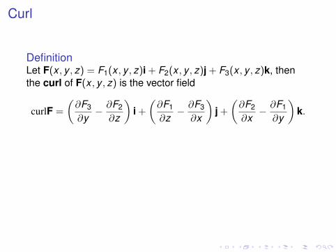
DefinitionLet F(x , y , z) = F1(x , y , z)i + F2(x , y , z)j + F3(x , y , z)k, thenthe curl of F(x , y , z) is the vector field
curlF =
(∂F3
∂y− ∂F2
∂z
)i +
(∂F1
∂z− ∂F3
∂x
)j +
(∂F2
∂x− ∂F1
∂y
)k.
Often the curl is denoted
∇× F =
∣∣∣∣∣∣i j k∂∂x
∂∂y
∂∂z
F1 F2 F3
∣∣∣∣∣∣

Curl
DefinitionLet F(x , y , z) = F1(x , y , z)i + F2(x , y , z)j + F3(x , y , z)k, thenthe curl of F(x , y , z) is the vector field
curlF =
(∂F3
∂y− ∂F2
∂z
)i +
(∂F1
∂z− ∂F3
∂x
)j +
(∂F2
∂x− ∂F1
∂y
)k.
Often the curl is denoted
∇× F =
∣∣∣∣∣∣i j k∂∂x
∂∂y
∂∂z
F1 F2 F3
∣∣∣∣∣∣
Example
Compute the curl of
F(x , y , z) = xzi + xyzj− y2k.
∇× F = 〈−2y − xy , x , yz〉

Example
Compute the curl of
F(x , y , z) = xzi + xyzj− y2k.
∇× F = 〈−2y − xy , x , yz〉

Graphical Interpretation
Suppose F(x , y , z) = 〈x , y ,0〉, then the vector field resembles:
. -1.0 -0.5 0.0 0.5 1.0-1.0-0.50.00.51.0
x
y
∇× F = 〈0,0,0〉
When ∇× F = 0 we say the vector field is irrotational.

Right Hand Rule
Suppose F(x , y , z) = 〈−y , x ,0〉, then the vector fieldresembles:
. -1.0 -0.5 0.0 0.5 1.0-1.0-0.50.00.51.0
x
y
∇× F = 〈0,0,2〉
∇ × F at a point is a vector parallel to the axis of rotation of theflow lines.

Divergence
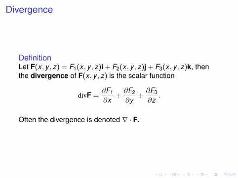
DefinitionLet F(x , y , z) = F1(x , y , z)i + F2(x , y , z)j + F3(x , y , z)k, thenthe divergence of F(x , y , z) is the scalar function
divF =∂F1
∂x+
∂F2
∂y+
∂F3
∂z.
Often the divergence is denoted ∇ · F.
Divergence
DefinitionLet F(x , y , z) = F1(x , y , z)i + F2(x , y , z)j + F3(x , y , z)k, thenthe divergence of F(x , y , z) is the scalar function
divF =∂F1
∂x+
∂F2
∂y+
∂F3
∂z.
Often the divergence is denoted ∇ · F.
Example
Find the divergence of
F(x , y , z) = 〈ex sin y ,ex cos y , z〉
∇ · F = 1

Example
Find the divergence of
F(x , y , z) = 〈ex sin y ,ex cos y , z〉
∇ · F = 1

Graphical Interpretation
Suppose F(x , y , z) = 〈x , y ,0〉, then the vector field resembles:
. -1.0 -0.5 0.0 0.5 1.0-1.0-0.50.00.51.0
x
y
∇ · F = 2
When ∇ · F > 0 at a point we say the point is a source.

Incompressible Flow
Suppose F(x , y , z) = 〈−y , x ,0〉, then the vector fieldresembles:
. -1.0 -0.5 0.0 0.5 1.0-1.0-0.50.00.51.0
x
y
∇ · F = 0
When ∇ · F = 0 we say the vector field is incompressible ordivergence free.
Sink
Suppose F(x , y , z) = 〈−x ,−y ,0〉, then the vector fieldresembles:
. -1.0 -0.5 0.0 0.5 1.0-1.0-0.50.00.51.0
x
y
∇ · F = −2
When ∇ · F < 0 at a point we say the point is a sink.
Divergence, Gradient, and Curl
ExampleSuppose F(x , y , z) is a vector field and f (x , y , z) is a scalarfunction. Determine whether the following are vector fields,scalar functions, or undefined operations.
1. ∇× (∇f )
vector field
2. ∇× (∇ · F)
undefined operation
3. ∇ · (∇f )
scalar function
Divergence, Gradient, and Curl
ExampleSuppose F(x , y , z) is a vector field and f (x , y , z) is a scalarfunction. Determine whether the following are vector fields,scalar functions, or undefined operations.
1. ∇× (∇f ) vector field2. ∇× (∇ · F) undefined operation3. ∇ · (∇f ) scalar function

Remarks
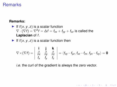
Remarks:I If f (x , y , z) is a scalar function∇ · (∇f ) = ∇2f = ∆f = fxx + fyy + fzz is called theLaplacian of f .
I If f (x , y , z) is a scalar function then
∇×(∇f ) =
∣∣∣∣∣∣i j k∂∂x
∂∂y
∂∂z
fx fy fz
∣∣∣∣∣∣ = 〈fzy−fyz , fxz−fzx , fyx−fxy 〉 = 0
i.e. the curl of the gradient is always the zero vector.
Remarks
Remarks:I If f (x , y , z) is a scalar function∇ · (∇f ) = ∇2f = ∆f = fxx + fyy + fzz is called theLaplacian of f .
I If f (x , y , z) is a scalar function then
∇×(∇f ) =
∣∣∣∣∣∣i j k∂∂x
∂∂y
∂∂z
fx fy fz
∣∣∣∣∣∣ = 〈fzy−fyz , fxz−fzx , fyx−fxy 〉 = 0
i.e. the curl of the gradient is always the zero vector.

Three-dimensional Conservative Vector Fields
TheoremSuppose that F(x , y , z) = 〈F1(x , y , z),F2(x , y , z),F3(x , y , z)〉 isa vector field whose component functions have continuous firstpartial derivatives in an open region D ⊂ R3. If F isconservative then ∇× F = 0.
Note: the converse of this theorem is not true. If ∇× F = 0 itdoes not necessarily mean that F is conservative.

Example (1 of 2)
Determine whether the following vector field is conservative.
F(x , y , z) = 〈xz, xyz,−y2〉
Since ∇× F = 〈−(2 + x)y , x , yz〉 6= 0 then we know F is notconservative.

Example (1 of 2)
Determine whether the following vector field is conservative.
F(x , y , z) = 〈xz, xyz,−y2〉
Since ∇× F = 〈−(2 + x)y , x , yz〉 6= 0 then we know F is notconservative.

Example (2 of 2)
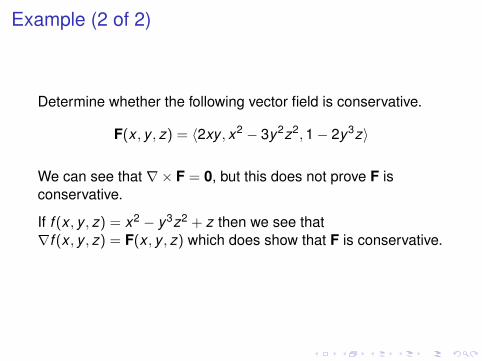
Determine whether the following vector field is conservative.
F(x , y , z) = 〈2xy , x2 − 3y2z2,1− 2y3z〉
We can see that ∇× F = 0, but this does not prove F isconservative.
If f (x , y , z) = x2 − y3z2 + z then we see that∇f (x , y , z) = F(x , y , z) which does show that F is conservative.
Example (2 of 2)
Determine whether the following vector field is conservative.
F(x , y , z) = 〈2xy , x2 − 3y2z2,1− 2y3z〉
We can see that ∇× F = 0, but this does not prove F isconservative.
If f (x , y , z) = x2 − y3z2 + z then we see that∇f (x , y , z) = F(x , y , z) which does show that F is conservative.

Conservative Vector Fields Revisited
TheoremSuppose that F(x , y , z) = 〈F1(x , y , z),F2(x , y , z),F3(x , y , z)〉 isa vector field whose component functions have continuous firstpartial derivatives in all of R3. Then F is conservative if and onlyif ∇× F = 0.
Conservative Vector Fields
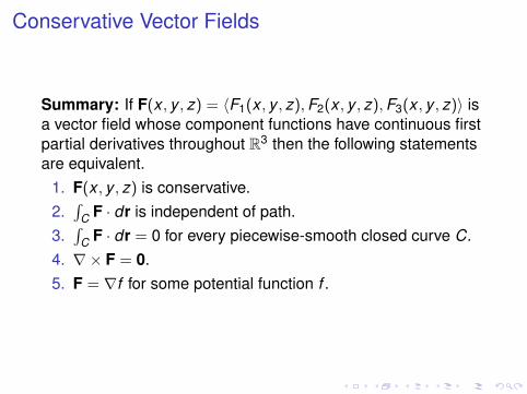
Summary: If F(x , y , z) = 〈F1(x , y , z),F2(x , y , z),F3(x , y , z)〉 isa vector field whose component functions have continuous firstpartial derivatives throughout R3 then the following statementsare equivalent.
1. F(x , y , z) is conservative.2.∫
C F · dr is independent of path.3.∫
C F · dr = 0 for every piecewise-smooth closed curve C.4. ∇× F = 0.5. F = ∇f for some potential function f .

Connection with Green’s Theorem
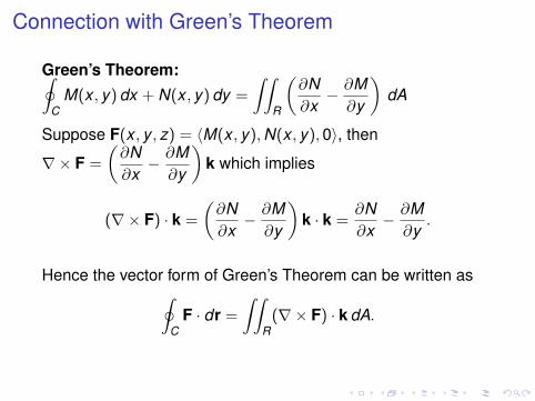
Green’s Theorem:∮C
M(x , y) dx + N(x , y) dy =
∫∫R
(∂N∂x− ∂M
∂y
)dA
Suppose F(x , y , z) = 〈M(x , y),N(x , y),0〉, then
∇× F =
(∂N∂x− ∂M
∂y
)k which implies
(∇× F) · k =
(∂N∂x− ∂M
∂y
)k · k =
∂N∂x− ∂M
∂y.
Hence the vector form of Green’s Theorem can be written as∮C
F · dr =
∫∫R
(∇× F) · k dA.
Connection with Green’s Theorem
Green’s Theorem:∮C
M(x , y) dx + N(x , y) dy =
∫∫R
(∂N∂x− ∂M
∂y
)dA
Suppose F(x , y , z) = 〈M(x , y),N(x , y),0〉, then
∇× F =
(∂N∂x− ∂M
∂y
)k which implies
(∇× F) · k =
(∂N∂x− ∂M
∂y
)k · k =
∂N∂x− ∂M
∂y.
Hence the vector form of Green’s Theorem can be written as∮C
F · dr =
∫∫R
(∇× F) · k dA.
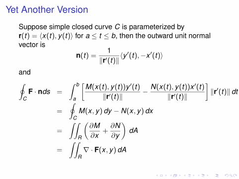
Yet Another Version
Suppose simple closed curve C is parameterized byr(t) = 〈x(t), y(t)〉 for a ≤ t ≤ b, then the outward unit normalvector is
n(t) =1
‖r′(t)‖〈y ′(t),−x ′(t)〉
and∮C
F · nds =
∫ b
a
[M(x(t), y(t))y ′(t)
‖r′(t)‖− N(x(t), y(t))x ′(t)
‖r′(t)‖
]‖r′(t)‖dt
=
∮C
M(x , y) dy − N(x , y) dx
=
∫∫R
(∂M∂x
+∂N∂y
)dA
=
∫∫R∇ · F(x , y) dA
Homework
I Read Section 14.5.I Exercises: 1–59 odd