cultural scene detection using reverse louvain...
TRANSCRIPT

JID:SCICO AID:1690 /FLA [m3G; v 1.126; Prn:6/02/2014; 14:58] P.1 (1-29)
Science of Computer Programming ••• (••••) •••–•••
Contents lists available at ScienceDirect
Science of Computer Programming
www.elsevier.com/locate/scico
Cultural scene detection using reverse Louvain optimization
Mohammad Hamdaqa a,∗, Ladan Tahvildari a, Neil LaChapelle b, Brian Campbell b
a Software Technologies Applied Research (STAR) Group, University of Waterloo, Waterloo, Ontario, Canadab Sceneverse Inc., Kitchener, Ontario, Canada
h i g h l i g h t s
• Formalized an ontology for graphing socio-cultural “scenes” in Meetup data.• Created a k-partite, directed “scene graph” of all data (people, place, topic).• Applied Louvain optimization recursively “in reverse” to partition the graph.• Compared with overlap analysis of three weighted, undirected graphs.• “Reverse Louvain” offered same precision, better recall of scene data.
a r t i c l e i n f o a b s t r a c t
Article history:Received 1 February 2013Received in revised form 31 October 2013Accepted 9 January 2014Available online xxxx
Keywords:Scene ontologyScene graphSocial analyticsCommunity detectionCultural web
This paper proposes a novel approach for discovering cultural scenes in social networkdata. “Cultural scenes” are aggregations of people with overlapping interests, whose looselyinteracting activities from virtuous cycles amplify cultural output (e.g., New York artscene, Silicon Valley startup scene, Seattle indie music scene). They are defined by time,place, topics, people and values. The positive socioeconomic impact of scenes drawspublic and private sector support to them. They could also become the focus for newdigital services that fit their dynamics; but their loose, multidimensional nature makesit hard to determine their boundaries and community structure using standard socialnetwork analysis procedures. In this paper, we: (1) propose an ontology for representingcultural scenes, (2) map a dataset to the ontology, and (3) compare two methods fordetecting scenes in the dataset. The first method takes a hard clustering approach. Wederive three weighted, undirected graphs from three similarity analyses; linking peopleby topics, topics by people, and places by people. We partition each graph using Louvainoptimization, overlap them, and let their inner joint represent core scene elements. Thesecond method introduces a novel soft clustering approach. We create a “scene graph”:a single, unweighted, directed graph including all three node classes (people, places,topics). We devise a new way to apply Louvain optimization to such a graph, and usefiltering and fan-in/out analysis to identify the core. Both methods detect core clusters withprecision, but Method One misses some peripherals. Method Two evinces better recall,advancing our knowledge about how to represent and analyze scenes. We use Louvainoptimization recursively to successfully find small clusters.
© 2014 Elsevier B.V. All rights reserved.
* Corresponding author.E-mail addresses: [email protected] (M. Hamdaqa), [email protected] (L. Tahvildari), [email protected] (N. LaChapelle),
[email protected] (B. Campbell).URLs: http://stargroup.uwaterloo.ca (M. Hamdaqa), http://www.sceneverse.com (N. LaChapelle).
0167-6423/$ – see front matter © 2014 Elsevier B.V. All rights reserved.http://dx.doi.org/10.1016/j.scico.2014.01.006

JID:SCICO AID:1690 /FLA [m3G; v 1.126; Prn:6/02/2014; 14:58] P.2 (1-29)
2 M. Hamdaqa et al. / Science of Computer Programming ••• (••••) •••–•••
1. Introduction
Cultural scenes1 [1–4] emerge whenever a critical mass of people interacts within some shared context (place and time)with overlapping interests on shared topics [5]. Examples include the New York art scene, the Silicon Valley startup scene,the Paris fashion scene, and myriad smaller and less sharply delineated local scenes all over the world.
1.1. Problem: the challenge of scene analysis
People on a scene do not typically all know each other. Connections both within and between clusters can be weakerthan in a friends-based network, as well as less direct. The only connection between two people may be two connectedinterests, participation in similar events, or patronage of a particular business that is a known scene place. This partialmutual anonymity is important for giving scenes the diffuse and pervasive character. It lets the scenes serve as a soft frameof reference for their diverse, differentially committed participants [6,7].
The diffuse nature of scenes does not prevent them from being powerful drivers of economic and cultural value creation.The indie music contributed approximately $379.4 million to the Canadian national economy in 2011, and roughly half ofthat value was generated by smaller players operating at the local scene level [8]. Chicago assessed the impact of its ownlocal indie music scene by determining how much of the $80 million spent on live music tickets in 2004 went to largepop acts listed in the Billboard 100 versus niche and specialized artists listed in the Village Voice Pazz and Jop Critics Poll.Again, the split was close to 50% [9]. When Seattle assessed the economic impact of their own musical scene in 2004,they of course had to refer to one particular grassroots/indie scene repeatedly: the grunge scene, made world famous bybands like Nirvana, Pearl Jam, Soundgarden and Alice in Chains [10]. Small local scenes frequently blow up to become globalphenomena, they can utterly transform local economies in the process.
The positive socioeconomic impact of scenes is strengthened, not weakened by the indirectness of scene networks. Inthis regard, scenes can be described as adventitious networks. The property of adventitiousness in this context means thatmany links are accidental and indirect, but fortuitous2 [11]; producing positive feedback cycles of positive externalities3 [7],like Adam Smith’s invisible hand. People accidentally and unintentionally support and inspire people they will never meetto join the creative community and produce what it values, by virtue of these adventitious links [13].
In order to preserve the adventitious property of scene networks, representations of the community structure and boundariesof scenes need to be inclusive. High recall and larger cluster sizes are more desirable than narrower representations, givenequal or near-equal precision. This is because the scene periphery feeds the core. The participation of less central peopleadventitiously supports the creativity of central people, so losing sight of scene participants seriously compromises a scenerepresentation. However, achieving the necessary degree of recall with precision is difficult, because: (1) scenes are dynamicand evolve over time, (2) scenes are multifaceted, involving multiple interacting dimensions (topics, people, locations, times),and (3) scene interests can be hidden or implicit; in cold stars (i.e., not explicitly ranked or rated [14]), or sparse data.
1.2. Research goal and methods
The goal of this paper is to contrast two approaches to discover scenes in cultural data with a special interest in as-sessing the power and precision of each method for retrieving scene people. The data for our comparison came from thelocation-based social networking service Meetup.4 This online service helps people coordinate real-time, face-to-face gath-erings (“meetups”) on topics of shared interest, and so serves as an acceptable proxy or indicator of scene activity. Ourdataset included all meetups within 25 miles of Waterloo, Ontario, Canada. We devised a scene ontology that we used fororganizing and processing the dataset, and subjected it to the following procedures.
In Method One, we generated three weighted, undirected graphs based on similarity analysis. One graph connectedscene people through shared or similar interests. The second graph represented scene topic similarity based on peopleinterested in those topics. The third graph delineated scene locations based on people using those locations. Each graphwas then partitioned using Louvain modularity optimization [15] to reveal community structure, and then the three graphswere overlapped to reveal scenes. The inner join of the graphs was taken to represent central scene elements. This was arelatively hard clustering approach.
In Method Two, we devised a scene graph; an unweighted, directed graph which combines people, place and topic nodesin a single graph; with people as the source nodes and places and topics as target nodes. We also devised a way of applyingthe Louvain method to this graph, treating it as an undirected graph for modularization, then applying record reconcili-ation to restore node facet information to the partitioned graph for subsequent facet filtering. We could thus determine
1 Related social phenomena include: subcultures (Hebdige, 1979), neo-tribes (Maffesoli, 1996; Cova, 1997; Kozinets, 2001), and genres (Lena & Peterson,2008).
2 Adventitiousness produces serendipity, so adventitious networks would subsume and generate “serendipitous networks”, defined as new connectionsbetween people who find themselves in the same immediate situation.
3 Shank (1994) [12] defines a scene as a runaway creative system: “an overproductive signifying community (in which) far more semiotic information isproduced than can be rationally parsed”.
4 http://www.meetup.com.

JID:SCICO AID:1690 /FLA [m3G; v 1.126; Prn:6/02/2014; 14:58] P.3 (1-29)
M. Hamdaqa et al. / Science of Computer Programming ••• (••••) •••–••• 3
the community structure of scenes in the data; and identify their constituent topics and people. Then, we exploited thestill-available directional information in the graph using fan-in/fan-out analysis to determine centrality. This was a relativelysoft clustering approach.
1.3. Findings and limitations
A key finding of our research is that the limitations of Louvain optimization for identifying small clusters in large datasetscan be overcome when the source domain is hierarchical. Large scenes generally contain sub-scenes. We therefore exploitedthe hierarchical operation of the Louvain method by applying it recursively to find the sub-scenes. That is, we first ap-plied the Louvain method to the whole network to discover the main scenes, and then to those resulting scenes to revealsub-scenes. This enabled the successful detection of community structure at different scales.
Results from the two different methods were evaluated with ground truth data, Jaccard similarity and our own metric of“scene theme” similarity. Both graphing techniques correctly identified the scene cores, but community size was larger withscene graph analysis (Method Two) than it was when similarity graphs were overlapped (Method One). This suggests thatthe softer scene graph analysis technique performed better at delineating the actual scene boundaries in the available data,and better preserved network adventitiousness.
Our scene graph is amenable to many more social network analysis techniques, and the extraction of more insights intoscene structure and dynamics. However, such work lies beyond the scope of this paper.
1.4. Significance of the study
Several original contributions to the literature emerge from our research.
(i) Introducing the unique features of cultural scenes, including the property of adventitiousness, and propose them asnew objects for social network analysis.
(ii) Formalizing our current conceptualization of scene elements in a semantic ontology.(iii) Taking Louvain optimization; a clustering and partitioning technique usually used on bipartite, undirected graphs; and
apply it to a directed k-partite graph. This enables Louvain partitioning of a multidimensional directed network.(iv) Exploiting the hierarchical operation of Louvain optimization to circumvent its difficulty in detecting small clusters in
large networks; applying it to the global network first, then recursively to emergent sub-graphs.(v) Introducing a soft clustering strategy involving a novel “scene graph” and techniques for analyzing it; which together
provide better scene recall than a harder clustering approach, with equal precision.(vi) Creating a “scene theme similarity” metric, in a manner which may turn out to be generalizable to other k-partite
graphs. No use of Louvain optimization that we are aware of applies it in the manner described in our paper.
The reminder of this paper is organized as follows: Section 2 describes related work and gives an overview of Sceneverseplatform. Section 3 presents the scene ontology. Section 4 discusses the graph construction and scene identification methods.Section 5 presents our experimental design. Section 6 evaluates the scene discovery results. A discussion on the results isprovided in Section 7. Finally, conclusions and directions for future work are presented in Section 8.
2. Related work and research context
This section position our work within the existing related work and defines its context.
2.1. Related work
This article presents an empirical study of scene discovery in online socio-cultural network data. This section puts ourwork in context within the substantial literature targeting similar problems.
2.1.1. Community detection in networksA scene is a type of social community (i.e., people community) that shares topics of interest in designated locations
during a period of time. In network and graph theory, a community is defined as a group of nodes that are denselyconnected to one another, but have relatively weak connections with other parts in the network [16]. Partitioning of nodesinto groups and sub-groups is crucial to understand the meaning and behavior of the network. Studying grouping patternsto detect communities has been the focus of many research studies for long time (e.g., Stuart Rice had manually clustereddata to study political groups in the 1920s [17]). Communities have been studied in almost all domains (e.g., social sciences[18–20], bibliometrics [21], anthropology [22], telecommunication [15], biology (i.e., human brain connectome [23])). Forcomprehensive studies on the literature of community detection in networks the reader can refer to Porter et al. [17], orFortunato et al. [16] respectively.
Recently, there has been increasing interest in applying community detection techniques to discover virtual communitiesin online social networks and the cultural web [24–28]. Several techniques and algorithms have been devised to automati-cally detect communities in networks.

JID:SCICO AID:1690 /FLA [m3G; v 1.126; Prn:6/02/2014; 14:58] P.4 (1-29)
4 M. Hamdaqa et al. / Science of Computer Programming ••• (••••) •••–•••
These techniques can be divided into two groups based on the type of the methods used to find the linkage betweenthe network nodes. Communities can be detected using statistical correlation and similarity analysis (e.g., hierarchical clus-tering, k-means), or via graph partitioning [29] (e.g., Girvan Newman algorithm [20], network modularity [15], surprisemaximization [30], k-clique percolation [31]).
Michelle Girvan and Mark Newman proposed using graph clustering for community detection [20]. Since then, the usegraph clustering techniques (i.e., Modularity Analysis) to detect communities became very prevalent. This is because graphclustering and community detection share the same goal; to find clusters of vertices (i.e., modules) on a graph that are morestrongly connected to each other than to the rest of the network. The difference is that while graph clustering techniquesusually require us to specify the number of clusters we want to extract as input to the algorithm, in community detectiontechniques, discovering the number of communities is one of the desired outcomes.
Several studies have compared the performance of different community detection techniques with regard to modularity,performance, memory requirements, scalability and other measures. The work by Papadopoulos et al. [26] is an example ofan up-to-date comprehensive comparison between these techniques within the context of social media networks.
2.1.2. Social graph creationSocial media networks contain multiple edge and vertex types depending on the network’s “focal object” (e.g., people in
Facebook, photos in Flickr), and the way other nodes are connected to it. No single algorithm successfully detects communitystructure in all such networks. Network design significantly determines the techniques that can reveal underlying topology,and understanding this topology is vital for delivering information services to network users.
In Sceneverse, the focal object is the scene itself, so Sceneverse services must be informed by scene graph topology.A scene graph has at least three vertex types, connected through both symmetrical and asymmetrical (directed) relation-ships. However, many community detection techniques only work with simple, undirected graphs, with one or at most twovertex types. They cannot be used to analyze k-partite or hyper-graphs [26]. The Louvain modularity optimization method,used in this paper, shares these limitations. It was originally designed to work with undirected graphs. Arenas et al. [32]developed a technique for applying modularity optimization to directed graphs, while Barber [33] developed a method forapplying it to bipartite graphs [33]. However, both approaches involved transforming the graphs so that modularity opti-mization could then be applied to them.
In contrast, our approach does not require transforming graphs. Instead, we leverage Louvain modularity’s lack of concernwith vertex-type and edge-direction to perform a pure modularity clustering that ignores type and directional data. Then,we use fan-in and fan-out analysis to extract that missing data from each community that the modularity analysis identifies.
To summarize, modularity and graph clustering techniques are usually applied to social networks after reducing thenetwork into a simple form that consists of a maximum of two types of vertices. The price paid for this graph reduction isobviously a loss in information. Consequently, these approaches fail to detect communities in social networks that cohere inmultifaceted ways (i.e., scenes).
2.1.3. Community detection applicationsThere have been several recent works that attempt to derive meaningful clustering using modularity techniques and
graph partitioning. Most of these works deal with single facet graph clustering (i.e., clusters of stopic, people, locations,pictures, etc.). In the domain of folksonomy production [34], Begelman et al. [35] reduced tag proliferation by first designingan inter-tag correlation graph for tags that described the same resources. Then they partitioned this graph using spectralbisection and the modularity function. In related work on folksonomy grooming, Simpson [36], and Papadopoulos et al. [37]applied variations of different partitioning techniques to divide tag graph into modules. Fatemi et al. [38] constructed asocial network graph for the Internet Movies Database (IMDb) based on the reviewers for these movies. Fatemi then usedfour community detection algorithms to analyze the underlying community structure of the network. The study of IMDb isinteresting because users review diverse topics that are interesting to them, hence communities of movies linked by theirreviewers can reveal social interest clusters that cut across categories defined by genre tags.
In a study on friend relationships between social network users, Mislove et al. [39] have crawled public user profilesfrom different social media providers (e.g., YouTube, Orkut, Flickr and LiveJournal). The authors then studied the structureof the resultant networks using graph partitioning techniques. Traud et al. performed a similar study on data collectedfrom Facebook, where they examined the roles of universities in structuring students’ social networks [40]. Many otherstudies have also segmented user clusters based on various similarity factors. This has been extensively explored lately inthe field of content filtering and smart recommendation systems. For example, Tsatsou et al. [41] integrate the results oftag community detection in a personalized ad recommendation system. Pham et al. [42] grouped users into clusters toidentify their neighborhoods, and hence derive better recommendations than those delivered by traditional content filteringalgorithms. García-Crespo et al. used natural language processing and the semantic categorization of opinions to analyzecustomer emotions, in order to assist the development of marketing strategies and product development plans [13].
Perhaps the most relevant work to the approach proposed in this paper is the work done by Zhao et al. [43], usingmultifaceted stepwise clustering. The goal of their work was to find events in social text streams (e.g., blogs). Zhao et al.defined an event as information flow between a group of social actors on a specific topic over a certain time period [43].There are two main differences between the scene concept and Zhao’s event concept. First, a scene is a higher-level conceptwhich includes many events. Scene events are temporal snapshots of a social occasion during a specific time interval on

JID:SCICO AID:1690 /FLA [m3G; v 1.126; Prn:6/02/2014; 14:58] P.5 (1-29)
M. Hamdaqa et al. / Science of Computer Programming ••• (••••) •••–••• 5
the scene timeline. They also have a particular title that connects to the scene’s topical theme (this scene terminology isexplained in the scene ontology section of this paper). The second difference is that the scene concept also has a spatialdimension.
Zhao et al. [43] combined three event dimensions: the temporal, social, and textual content of blog streams, to discoverevents. Their technique involves three phases. In the first phase, they transform social text streams into a graph, then useN-cut method [44] to partition the graph into topics, such that each blog belongs to one topic. In the second phase, a socialgraph is constructed. The topic-based social graph is then partitioned into a sequence of graphs based on the intensity ofinteraction along the temporal dimension. Finally, in the third phase, the social-temporal-topical graphs are divided intofiner-grained events by applying the N-cut graph partitioning method a second time.
All these prior studies deal with undirected, weighted graphs. Only Zhao et al. [43] deals with multifaceted graphs. Noneof these studies explored the partitioning of a directed, multifaceted graph in a single step. None of them leveraged thepower of fan-in and fan-out analysis to further identify the facet types in each cluster as we did in our approach to scenegraph partitioning.
2.2. Research context: the sceneverse platform
This study is part of a collaborative research program supporting the development of the Sceneverse platform.
2.2.1. Sceneverse missionSceneverse, a portmanteau of “scene” and “universe”, aims to support all scenes on a platform optimized for representing
scene dynamics and facilitating scene transactions. Though scenes are natural contexts for economic activity [45,46], scenecommerce can be contentious. To be successful, it must respect the complex interplay of values, politics, ideologies andattitudes that structure scenes [47–50]. For this reason, accurate representations of scenes and scene values are crucial forproviding them with digital services.
On the Sceneverse platform, scene data will be derived from two sources: user-contributed content, and the behavior ofpeople using Sceneverse enabled web and mobile applications. The provision of value-adding services will depend on thefaithful representation and analysis of scenes in this data.
2.2.2. Sceneverse front-end componentsFig. 1 presents an overview of the Sceneverse5 platform. It provides complementary services at two different levels,
front-end and back-end. Front-end services consist of web and mobile applications that serve participants’ needs from thescene center to its margins.
There are different levels of participation in scenes. Active scenes have a small, dense core of avid participants; as wellas “near-satellite” members who participate fairly frequently, and many peripheral “far-satellite” members who participateinfrequently.
For example, the inner core of an art scene would consist of full-time professional artists, the dealers that representthem, the galleries that display their works, the art critics that review it, and the primary patrons who purchase works.It would also include avid amateurs who spend equal amounts of time in these activities, and attend many of the sameevents, but who do so largely on a voluntary, non-cash basis. Near-satellite members would be the friends and contacts ofthis inner core who participate as spectators or dabblers in art-scene-related activities on a consistent basis (their defaultchoice is to participate unless they are busy), but whose main occupations and preoccupations lie elsewhere.
Far-satellite members many not have friends or relatives in the scene core, but maintain an interest in art. They attendexhibitions, buy books and prints, and take classes on an opportunistic and occasional basis, rarely committing to more thanone such activity, and only doing so once in awhile.
Sceneverse-enabled applications help the inner-core find better ways to produce and consume the “cultural capital” ofthe scene. Satellite members enjoy high-recall services that give them easier access to the scene’s core, enhancing theirscene experience. Peripheral participants enjoy high-precision services that help them quickly and efficiently enjoy selectscene activities as they fit their moods and inclinations.
Current Sceneverse front-end applications target avid/core and near-orbiting scene participants. One example Sceneversecurrently offers is an event planning and ticket sales service for people booking concerts on the indie music scene. Scenev-erse is also producing a storytelling application that engages scene participants in social, mobile, augmented reality contentcreation and curation. The application lets participants compose stories describing personal scene experiences, chronicle thebroader history of their scene, discover other peoples’ stories, and indicate their sentiments towards stories. Stories includethose based on Sceneverse Events. The user-contributed content and behavior provides essential information to create whatwe call a user universe. A user universe can be seen as an ego network of a user’s topics of interests, locations, and behaviormonitored in both time and space.
5 www.sceneverse.com.

JID:SCICO AID:1690 /FLA [m3G; v 1.126; Prn:6/02/2014; 14:58] P.6 (1-29)
6 M. Hamdaqa et al. / Science of Computer Programming ••• (••••) •••–•••
Fig. 1. Sceneverse platform architecture.
2.2.3. Sceneverse back-end componentsOn the back-end, the Sceneverse platform aims to offer a cross-service, cross-device, pervasive frame of reference for all
the digitally mediated activities that might support a local scene.The back-end architecture under consideration in this paper consists of three main components; the scene ontology, a
semantic and linguistic engine, and the scene extraction engine. Both of the engines depend on the scene ontology, whichprovides the vocabulary for building semantic queries, rendering scene content, and reasoning about new and existingscenes. For example, the semantic and linguistic engine provides natural language understanding and semantic web linksfor processing and annotating user stories with context-appropriate tags. It also supports dynamic rendering of contentbased on the scene ontology. The extraction engine uses pre-existing web data as well as data gathered from frontendservices to discover scenes. All the algorithms needed to identify and reason about the socio-spatio-topical boundaries ofscenes are either implemented in the semantic/linguistic engine or the scene extraction engine.
These back-end processes support front-end tasks and facilitate the creation and manipulation of scene representations.
3. The scene ontology
The scene ontology developed for this paper furnishes a set of clear concepts with well-defined interrelationships forrepresenting cultural scenes in web data. Such a formal scene ontology is essential for (1) building semantic queries, (2) ren-dering scene content, and (3) reasoning about new and existing scenes. The ontology proposed in this section is mainly usedto consolidate the data collected from different resources and check inconsistencies. It will also be used in our frameworkfor querying the data.
The rationale for scene participation is the scene itself, which is its own ultimate reason for gathering/clustering. Noindividual scene dimension alone can furnish the reason, since adventitious connections can come through all of them. Thisbecomes clear when you ask a core scene participant why they care about the scene. The answer is unlikely to be only onething, or one type of thing, but their cumulative scene experience in its totality. Because the scene is both psychologicallyand sociologically real, it has its own distinct representation in our ontology.

JID:SCICO AID:1690 /FLA [m3G; v 1.126; Prn:6/02/2014; 14:58] P.7 (1-29)
M. Hamdaqa et al. / Science of Computer Programming ••• (••••) •••–••• 7
Fig. 2. A scene ontology excerpt.
3.1. High-level overview
The Scene is constituted by several other ontological concepts, including Topics, People, Locations and Times. In ourcurrent ontology, we split the Time dimension into two categories: Scene Active Period, and Events. The two time conceptsare needed to define temporal boundaries of scenes. Scenes are constituted by many events, which in total sum up to theScene Active Period. This is shown in the UML diagram illustrating the scene ontology in Fig. 3.
While the UML diagram gives a useful schematic overview, the fully formalized ontology exploits RDF and OWL toexplicitly represent the scene facets and their relationship in a way that allows easy discovery, dynamic access, and simplelinkage to other resources on the web.
Ontologies can be either designed from scratch or as an extension of existing ontologies. Extending existing ontologiesis the recommended best practice [51]. An ontology can be extended horizontally or vertically. In horizontal extension, theoriginal ontology is imported and used in the same way (i.e. with the same semantics) as in the domain it was importedform. In contrast, with vertical extension, an ontology is imported and then updated to support the new domain. A good coreontology should be designed to support both horizontal and vertical extension, by maintaining the right balance betweendomain-independent and domain-specific concepts. Getting the balance wrong can restrict further vertical extensions in thefuture.
Our scene ontology was designed by horizontal extension [52] through importing existing ontologies, e.g.: TimeOntology,EventOntology, FOAF, and GeoOntology. It was also designed to be generic enough to support vertical extensibility [53] toother domains.
Fig. 2 shows an excerpt of the Scene ontology. The Scene ontology has been constructed using the Protégé [54] ontologyeditor. When transcribing an OWL ontology to RDF, every statement must be converted into triples. An RDF triple containsa subject, a predicate and an object. A set of such triples is a graph, where the subject is always a node, the predicate isalways an arc and the object is always a node. The OWL scene ontology graph is fully laid out in Appendix A of this paper.Its corresponding RDF triples are given in Appendix B.
Protégé utilizes various Description Logic reasoners (e.g., RACER [55], FaCT++ [56], Pellet [57]) to perform different in-ferencing services (i.e., computing inferred superclasses, determining class consistency). In addition to reasoning, Protégéfacilitates generating the RDFs needed to query the model using the SPARQL protocol and RDF query language [58]. In thispaper, model reconciliation between the ontology and the dataset (i.e., Meetup data) was carried out by mapping the APIschema elements to the ontology concept tree manually, and a script was used to populate the OWL ontology with indi-vidual elements based on the target social network site API. The design of the Sceneverse platform calls for a semantic andlinguistic engine that automatically tags parsed data from users’ stories with concepts belonging to the scene ontology. Theimplementation of such an engine is out of scope for this paper.
3.2. Main scene concepts
The main scene concepts are Topic, People, Locations and Time. Each is expanded and explained in detail below.
Topic: The subject of interest. It can be anything (e.g., person, place, event, topic, thing). A scene is normally described as alist of topics (e.g. the Blues/Jazz scene).

JID:SCICO AID:1690 /FLA [m3G; v 1.126; Prn:6/02/2014; 14:58] P.8 (1-29)
8 M. Hamdaqa et al. / Science of Computer Programming ••• (••••) •••–•••
Fig. 3. The scene ontology.
People (social graph): Scene participants share a reason for gathering, and thus form a membership group, albeit a diffuseone. The network centrality of People derives from their contribution to the Scene and their activity level (active or passive).Types of People include:
(a) Scenester: A Person whose Scene is clearly identified.(b) Scenester Friend: A Person who communicates and collaborates with a Scenester, but does not participate directly in
that Scenester’s Scenes.(c) Multi-Persona Scenester: A Person with multiple persons. A persona is how a Person is known on a particular Scene.
A single-persona Scenester is just a Scenester.(d) Personage: Some person named or mentioned in Scene stories, chronicles or news. May or may not also be a Scenester.(e) Silhouette: An abstraction over Scenesters, persons and Personages. Silhouettes define various categories and types of
People, what they value, how they are valued and how much prestige they have in the scene. The platform’s enginesgenerate Silhouettes for marketing purposes or making recommendations etc. This allows People to be typified whileprotecting their privacy.
(f) Scene Organizer: A Person who sets up Scenes and grants authorizations to new Scenesters.(g) Scene Follower: A Person who follows Scenes, but is not a Scenester or Scenester Friend. A Scene Follower is a passive
presence, whose existence amplifies the Scene’s reputation. However, s/he does not otherwise participate in the Scene.(h) Secluded Scenester: People who are not part of any Scene (e.g., new members in online networks who have insufficient
profile or interest data).
Location: Holds the list of locations (e.g., Uptown Waterloo, University of Waterloo) where Scene events and happeningshave previously occurred. These locations are centralized around the main scene location (e.g., Waterloo)

JID:SCICO AID:1690 /FLA [m3G; v 1.126; Prn:6/02/2014; 14:58] P.9 (1-29)
M. Hamdaqa et al. / Science of Computer Programming ••• (••••) •••–••• 9
Fig. 4. The scene conceptual model.
Time: Captures the temporal aspect of the scene. Processing Time is much harder than processing the other scene dimen-sions. Currently, we manage scene temporality using two main concepts:
(a) Scene Active Period: The period during which People were involved in activities related to the Scene, and Events wereorganized. Conventions for declaring a Scene inactive are needed (e.g., if no Events have occurred in the past two years).
(b) Event: Used to capture a Scene snapshot. An Event has the following properties:• Title: Should be aligned with Scene themes, described by the list of Scene Topics.• Location: Should fall within the perimeter defining the core Scene Location.• Participants: Should be Scene People. Behavioral and social data indicate when someone new should be added to the
list of Scene People.• Time: This value percolates upwards to be used in inferences that determine the Scene Active Period. The timespan
between the first Event Time and the Time of the last Event defines the Scene Active Period.
Capturing the temporal data is one of the main challenges. The elements used to capture the temporal data in ourontology (i.e., Scene Active Period and Event) are discrete and hence, by using the standard methods of publishing structureddata (i.e., RDF) the ontology can be updated with the correct information. Currently, the Sceneverse framework depends onbatch processing to update the data, and the update function runs periodically.
3.3. Passions as associations
Scenes are fundamentally constituted by the collective set of relationships or associations that connect People with theirTopics of interest. In Fig. 4 these associations are represented as Passions connecting a Person to a Topic. Fig. 4 showsthat people can be part of the scene or peripherals. People who are part of the scene directly affect the scene reputationthrough their participation or contribution to the scene. While peripherals only follow the scene; hence, they affect thescene reputation by their collective engagement, not direct contributions. For example in a soccer scene, a soccer playeris part of the scene because s/he directly affects the scene, while the team fans are just followers. Similarly, in the socialnetwork scene people who contribute to the topic by commenting can have direct impact on the scene and hence they arein the core of the scene; whereas, people who just like the topic or silently follow it are peripherals.
Recall that a Topic can be anything. There are topic-people who cannot be real people or Scene People (they maybe fictional, like Harry Potter, or dead/historical, like Socrates). There can also be topic-people who happen to also bereal people, and who may further be Scene People of some type. Similarly, there can be topic-places, topic-events andtopic-periods.
“Passion for” can capture the strength of a Person’s connection to any object of interest. These relationships can beexplicit or implicit, with Time (real-time, not topic-time) and Location working as orthogonal factors (disjoint) that eitherweaken or strengthen these relationships. This is illustrated using concentric circles in the bottom right corner in Fig. 4,where Passion decreases with temporal, spatial or social distance.
4. Graph construction and scene identification methods
Identifying the socio-spatio-topical boundaries of a scene is a non-trivial soft clustering problem. Clustering needs toexploit both the similarities among multiple concepts (i.e., people, topics and locations), and the relationships betweenthese concepts, in order to identify community’s boundaries. In this section, we describe how we collected and preparedour data, and enacted two methods for graphing that data and detecting scene structures and boundaries implicit in it.

JID:SCICO AID:1690 /FLA [m3G; v 1.126; Prn:6/02/2014; 14:58] P.10 (1-29)
10 M. Hamdaqa et al. / Science of Computer Programming ••• (••••) •••–•••
Fig. 5. The scene discovery approach. (For interpretation of the references to color in this figure legend, the reader is referred to the web version of thisarticle.)
4.1. Graph construction overview
Fig. 5 illustrates the entire procedure we followed in our approach to detecting scenes, including both methods of graphgeneration and analysis that we evaluate in our study. Both techniques start with a data preprocessing stage. Method One(Blue) applies similarity analysis to create three undirected weighted graphs (i.e., a contingency matrix); one for topicsassociated by people who are interested in them, on for people associated by interest in similar topics, and one for placesassociated with similar people. Method Two (Red), by contrast, starts right away with the construction of a single scenegraph; a simple directed graph that permits nodes of all three kinds: people, topics and locations.
Following graph construction, clustering is carried out on all of the graphs using network modularity analysis. In MethodOne, the three separate similarity graphs are clustered individually, and then combined by finding the intersection betweenthe clusters. This produced a single graph for comparison with the single graph already generated using Method Two.
After clustering, both resulting graphs are further analyzed and visualized using graph visualization and manipulationsoftware (Gephi) [59]. Finally, the scenes revealed by the procedures are analyzed.
Many social network analysis measures and techniques could have been used to bring out scene facets and rearrangethem around graph centers. However, to keep things concise, this paper will focus mainly on scene discovery, and onlymention centrality analysis techniques very briefly.
4.2. Data collection
Finding relevant cultural data for scene research is a challenging task. Most social networking sites present some, but notall of the needed data, restricting access to it for both business and privacy reasons. For our purposes, the best available datacame from “Meetup.com”; an online social network that helps people organize gatherings at offline local venues to enjoyshared interests. The gatherings are called meetups, and their data points include social, topical, temporal and geographicalinformation. Meetups are not clustered into scenes, but scenes are potentially detectable in this dataset.
Fig. 6 shows the data collection process. A scraper was implemented using Meetup.com’s APIs to collect the data requiredto build scenes. The scraper started with a specific geographical location, and returned all meetups around that location.For each Meetup group returned, the scraper then requested a membership list and the topics that describe the group. Foreach member in that group, the scraper then returned their topics of interest and profile information (i.e., age, residentiallocation), as well as the groups and meetups they belong to. The time the user joined the group, as well as the user’s lastactivity in that group were also retrieved.

JID:SCICO AID:1690 /FLA [m3G; v 1.126; Prn:6/02/2014; 14:58] P.11 (1-29)
M. Hamdaqa et al. / Science of Computer Programming ••• (••••) •••–••• 11
Fig. 6. The data collection process.
4.3. Preprocessing
Several preprocessing steps were needed before the raw data was ready for clustering and analysis:
(a) Topic Dimensionality Reduction: Meetup lets people propose topics in their own terms at both the group purposeand personal interest level, producing a large population of topics with many similar terms that would compromisesimilarity-based clustering. We reduced this dimensionality by combining topics with high syntactic similarity usingtext-clustering techniques.
(b) Outlier Removal: Outliers would negatively impact scene discovery and analysis, so it was important to purge themfrom the dataset and correct skewed data. We used facet filtering to detect abnormalities in the data and removeoutliers.
(c) Formatting for Visualization and Analysis: Further refinements and transformations were needed to make the datacompatible with all the tools we used in our study (e.g., Gephi).
4.4. Graph creation
As explained earlier, two methods were used to create graphs in preparation for the graph modularity partitioning step.Then the partitioning algorithm was applied in the same way to both graph types. We found that the way the graphs werecreated and weights assigned to their edges significantly affected the final partitioning results.
4.4.1. Method One: similarity matrix graphsIn this technique, three similarity matrices were created; one for topics based on their being liked by similar people, one
for people based on their liking of similar topics, and one for location based on persons who were there.To find the topic similarity matrix, the topic-person table was first converted into a coincidence matrix (a.k.a. adjacency
matrix). Each topic was represented as a vector of users who liked it. The algorithm then correlated topic similarities usingcosine similarity as shown in Eq. (1). Cosine similarity is defined as the cosine of the angle between two vectors (x and y)with the value being normalized between zero and one if both x and y are positive.
CosSim(x, y) =∑
i xi yi√∑i x2
i
√∑i y2
i
= x · y
‖x‖‖y‖ (1)
Cosine similarity was selected in this case for two main reasons: First, cosine similarity is proven to be powerful, yet it isthe simplest inner product correlation between two vectors [60]; hence, it will give better performance results. Second,our dataset does not contain any subjective values or ratings. It consists of vectors of only zeros and ones (e.g., zerorepresents the absence of a person on the topic list, whereas one presents their presence). This makes a higher performancecorrelation measure more valuable than a shift invariant one. Furthermore, calculating the cosine correlation can be easilymap-reduced/parallelized. This has major implications for the applicability of our techniques on big data sets.
Cosine similarity was calculated between each pair of topics to generate a similarity matrix. The similarity matrix wasthen converted into a weighted undirected graph with links between nodes (edges) considered only when the weights(similarity measures) were within the upper 97th percentile. In other words, we considered the three nearest neighbors.Fig. 7 shows an example of a similarity matrix and its corresponding graph.
The same steps were repeated to create the people and location similarity matrices. For example, in the case of thepeople graph, each person was represented as a vector of the topics s/he liked. The graphs generated were then exportedfor partitioning and clustering based on the Louvain graph modularity algorithm.

JID:SCICO AID:1690 /FLA [m3G; v 1.126; Prn:6/02/2014; 14:58] P.12 (1-29)
12 M. Hamdaqa et al. / Science of Computer Programming ••• (••••) •••–•••
Fig. 7. A similarity matrix and its corresponding graph.
Fig. 8. Scene graph example.
4.4.2. Method Two: the scene graphIn Method Two, instead of separately clustering people, topics, and locations, we combined them on a single graph:
a scene graph. This gave it the property of being bijective. We also created it as a simple (unweighted) directed graph, withpeople as source nodes and either topics or locations as target nodes. So a directed edge would be created from a personnode to a topic node if that person expressed an interest in it. Similarly, a directed edge would be created between a personand a location if the person was involved in an activity there or a topic situated there.
We hypothesized that the precise relationships between nodes of different facet types might preserve important infor-mation, as would the directedness. Furthermore, generating a single graph would allow us to run a multifaceted similarityanalysis in a single step. However, modularity maximization partitioning uses modularity strength, which depends on thegraph structure to cluster the graph into communities. Hence, all nodes in the graph would be treated as equivalent regard-less of type for purposes of clustering.
Fig. 8 illustrates the scene graph of one person who likes three topics, and participates in activities related to thesetopics in two locations (Kitchener and Waterloo). Note that a scene graph focuses on Scene Locations rather than thepersonal profile location, which reflects the place of residence.
The advantage of having a scene graph is twofold: (1) It enables simple one step multi-facet clustering when combinedwith modularity maximization graph partitioning, (2) since scene graphs are bijective graphs, we can store more informationabout the relationship between scene concepts. In fact, a scene graph inherently models the core relationships of a scene(passions and places). Knowing the direction of the relationships, techniques like fan-in and fan-out analysis can be applied.This enriches knowledge discovery by providing insight about the types of clustered nodes. For example, scene graph parti-tioning can easily reveal who the most influential people in the scene are, where the scene is geographically centered, andwhat the most important topics are on a scene.
Our hypothesis was that this second approach to graph generation might produce better results than the first approach,while tremendously simplifying scene discovery. This would be extremely important for cultural scene computing, sincesocial network data volume can explode quickly on networks with heavy user participation.
4.5. New Louvain graph partitioning techniques
This section shows how Louvain graph partitioning has been utilized and modified for scene detection.
4.5.1. Revealing community structureThe steps listed above generated graphs from “Meetup.com” data, but did not partition them into scenes. Our goal was to
reveal scenes boundaries using network analysis and graph partitioning; discovering community structure and maximizingmodularity by analyzing which nodes were most densely interconnected. Modularity (Q ) maximization approaches partitiongraphs on the principle that a set of nodes are highly likely to be in the same module if they are densely interconnectedas a cluster, relative to their sparser connection to other modules. Many natural networks, informal human networks, or-ganizational networks and system networks in fact exhibit this kind of modular structure, also called community structure.

JID:SCICO AID:1690 /FLA [m3G; v 1.126; Prn:6/02/2014; 14:58] P.13 (1-29)
M. Hamdaqa et al. / Science of Computer Programming ••• (••••) •••–••• 13
Fig. 9. Louvain modularity algorithm [adopted form [15]].
Since scenes are informal human networks, it was reasonable to hypothesize that modularity maximization would revealthe community structure of scenes.
The Louvain method is a well accepted and widely used modularity maximization approach for discovering communitiesin large networks. The main advantage of the Louvain method is that it is very fast (e.g., in one experiment it was ableto analyze 118 million nodes in 152 minutes [15]). It also provides a generally acceptable degree of accuracy. This isextremely important for scene discovery due to the large size of social networks and that fact that data in such networksgrows exponentially over time. However, what makes this approach appealing in our case is that scenes exhibit hierarchicalstructure; super-scenes may include several sub-scenes. This exactly matches how the Louvain method works.
4.5.2. “Reverse” LouvainThe Louvain method is an iterative algorithm with two phases. First, it searches small communities by optimizing mod-
ularity locally. This is done by assigning each node i in the network to a group (module) then calculating the gain inmodularity �Q of merging the node i with each of its neighbor communities C , as shown in Eq. (2). Where
∑in is the sum
of the weights of the links inside C ,∑
tot is the sum of the weights of the links incident to nodes in C , ki is the sum of theweights of the links incident to node i, ki,in is the sum of the weights of the links from i to nodes in C , and m is the sumof the weights of all the links in the network. Based on the results, the node will be added to the module that maximizesnetwork modularity.
�Q =[∑
in + ki,in
2m−
(∑tot +ki
2m
)2]−
[∑in
2m−
(∑tot
2m
)2
−(
ki
2m
)2](2)
The second phase aggregates nodes within the same community to build a new network. The new network nodes arecommunities, which themselves are more densely interconnected than the relatively more sparse connections betweennodes in the new super-community. These steps are repeated until a maximum modularity is achieved as shown in Fig. 9.
In our effort to detect scenes and sub-scenes, we exploited this hierarchy-generation feature by reversing the process.We applied the method to the whole network to discover the main scenes within it. Then we recursively applied it to eachof the identified main scenes to discover sub-scenes within them
4.5.3. Louvain on a simple directed graphThe Louvain method takes an adjacency matrix as input; hence it can be applied to undirected graphs whether or not
they are weighted. In Method One, we applied the Louvain method quite conventionally to our three similarity graphs:weighted undirected graphs that grouped people, or topics, or locations into communities.
We also applied it quite unconventionally to our scene graph, which was an unweighted directed graph. We treated itas if it was an unweighted, undirected graphs for the purposes of grouping the scene graph nodes into communities, whichimmediately revealed scene structure. Then, we applied fan-in and fan-out analysis using directional information to identifytypes of nodes within the discovered scenes.
These unconventional uses of the Louvain modularity maximization algorithm generated necessary results for us, andthey constitute key contributions of our research.

JID:SCICO AID:1690 /FLA [m3G; v 1.126; Prn:6/02/2014; 14:58] P.14 (1-29)
14 M. Hamdaqa et al. / Science of Computer Programming ••• (••••) •••–•••
Fig. 10. The scene center is the inner join of people, topics and locations graphs.
4.6. Scene analysis
Once the graph had been partitioned, and the boundaries of the scene were identified, depending on the type of thegraph, the following techniques were applied to further reveal and analyze scene structure:
(a) Facet Filtering: Facet filtering [61] is a multidimensional technique that uses different data properties to organize in-formation into groups to facilitate its exploration and navigation [62]. In our work, after our two differently producedgraphs were clustered as described above, we exported them and merged them with the original dataset as new labels(facets). Each record was thus described using four additional clustering classes; namely, people clusters, topic clusters,location clusters, and scene clusters (the clusters generated through scene graph partitioning).Facet filtering could then be used to filter the records based on commonalities and mutual exclusions across the differ-ent clusters. This cluster overlapping would help find people who conducted activities in the same places around thesame topics of interest. In other words, it could help identify people, topics and locations that best represented thescene core or center as shown in Fig. 10. Moreover, facet filtering could be used to evaluate the quality of clustering inboth scene graph and similarity based clustering.
(b) Fan-In Analysis: In directed graphs, fan-in analysis is a measure of the number of links that are directed toward a node.In a scene graph, edges connect people to their topics of interest and locations. Accordingly, fan-in analysis can helpidentify the popularity of topics or locations within a scene. This can reveal the main topics that specify a scene, or itssignificant locations.
(c) Fan-Out Analysis: In directed graphs, fan-out analysis is a measure of the number of links that are directed out from anode. In a scene graph, fan-out analysis could help identify the most active people in a scene.
These simple techniques were essential for uncovering the main scene facets for each of the identified partitions. How-ever, many additional network analysis techniques could be usefully applied to these graphs, generating insights that mighthelp investors frame, find and answer questions about cultural scenes. Some of the relevant network measures are discussedin Section 7.
5. Application of the methods and experimental results
In this section, a case study will be used to illustrate how the graph construction and scene identification approach canbe applied on a given dataset.
5.1. Case study description
As explained earlier, the dataset used in this study was crawled from Meetup.com using the process explained in Sec-tion 4.2. The data was collected and reconciled based on shared keys between the different datasets. In total, informationabout 150 groups were collected. The collected groups were all located within 25 miles of Waterloo, Ontario, and distributedbetween 14 urban communities. Out of those 150 groups, 132 groups were open, 1 was closed and 7 had only recently beenapproved. Out of the 132 open groups, only 123 groups were publically accessible. 813 topics within 28 categories wereused to describe these groups with, an average of six topics per group. The total number of members including duplicateswas 13.735 users; since a user can be a member of several groups.
In addition to the main dataset, a subset of the crawled data was created for validation. This subset was studiedthoroughly to make it serviceable as a ground truth for qualitative evaluation of the clustering. Table 1 summarizes theparameters of the two datasets. Table 2 shows example of the crawled data.

JID:SCICO AID:1690 /FLA [m3G; v 1.126; Prn:6/02/2014; 14:58] P.15 (1-29)
M. Hamdaqa et al. / Science of Computer Programming ••• (••••) •••–••• 15
Fig. 11. Clustering with Open Refine.
Table 1The data set summary.
Dataset Location Groups Communities Topics Categories Users
1 Within 25miles fromWaterloo
150 14 813 28 13.735
2 KitchenerandWaterloo
2selected
2 364 23 100
5.2. Data preprocessing and refinement
Several decisions had to be made to prepare the data for analysis. First, groups and users who made their data privatewere filtered out. Then, topical dimensionality was reduced. After that, members with unusually many topics of interestwere removed. Finally, data inconsistencies and special characters were treated.
Data preprocessing and refinement was conducted using Open Refine (previously known as Google Refine). Open Refineis an open source tool for refining messy data, cleaning it up, and transforming it from one format into another [63]. Itfacilitates facet analysis and provides a set of clustering techniques out of the box. It also allows users to review clusteringresults before reflecting them back into the original dataset as shown in Fig. 11.
Two clustering techniques were chosen based on their performance in finding phonetically and syntactically similartopics. The first was a key collision technique based on the Metaphone3 phonetic algorithm [64]. The second was basedon a variation of the k nearest-neighbor algorithm that uses Levenshtein distance [65] to measure the similarity/differencebetween topics (i.e., strings). Combining both clustering techniques reduced the number of topics by an average of 11.5%.
Fig. 11 shows the manual part of the process, in which users are given the choice to accept or reject merging thesuggested similar raws under the same cluster. For example, based on Metaphone3, the algorithm suggests that both thetopics “Entrepreneur” and “Entrepreneurship” should be clustered under the same topic “Entrepreneur”. By accepting thissuggestion, 441 raws will be merged with 310 raws to have a bigger cluster of 751 raws.
After applying facet filtering to the dataset, it became apparent that a few members have very large numbers of topicsof interest (i.e., over 100 topics). A decision was made to exclude those members by removing the top 3% of members withhighest topic counts. We surmised that these members did not have focal interests, but were rather Meetup trackers. Theirpresence in the dataset would have been deleterious to the clustering algorithms. Finally, all trailing spaces, inconsistencies,symbols, and special characters were removed or replaced (e.g., replacing & with AND) in order to avoid errors whiletransforming data from one format into another throughout our multi-step procedures.
5.3. Scene discovery results
After data refinement, the dataset was transformed into the four types of graphs our methods produce (people, topic,location, and scene graphs) based on the two techniques described in Section 4.4. The graphs were then exported to theGephi visualization and analysis platform. Gephi is an open-source interactive visualization and exploration platform fornetworks, complex systems, dynamic and hierarchical graphs. It provides powerful tools that implement several statisticalanalysis, filtering and visualization algorithms that can be applied directly to graphs [59].
Fig. 12 shows a sample of a people similarity matrix and its corresponding people graph. Each node in the graph representsa person; an edge between two people indicates a similarity between them, while the edge weight (thickness) corresponds

JID:S
CIC
OA
ID:1690
/FLA
[m3G
;v1.126;P
rn:6/02/2014;14:58]P.16(1-29)
16M
.Ham
daqaet
al./ScienceofCom
puterProgram
ming•••
(••••)•••–•••
MGroup categoryname
MGroup topics
tech Web_Design
Graphic_DesignWeb_TechnologyInternet_AND_TechnologyWeb_Development
games BoardgamesDungeons_AND_DragonsLive_Action_Role_PlayingShadowrunWar_GamesStar_Wars_RPGD20_GamingWhite_WolfRoleplaying_Games_(RPGs)Strategy_GamesGamingPC_GamingComputer_Gaming
Music DrummerAlternative_HealthMeditationDrum_CircleConsciousnessLive_MusicHand_DrummingMeeting_New_PeopleAfrican_drumming
Table 2Example of the crawled data.
Member Id Topics ID Topics name Member city Membergroups
MGroupscities
MGroupscategory ID
12209746 1044 Event_Planning Waterloo Webdesigners/developers
Waterloo 34
10 290 Spirituality4417 Consciousness
15 478 Holistic_Health15 018 Music
1322 Meditation Gamers Waterloo 11243 Alternative_Health
17 866 Meeting_New_People10 581 Social
2278 Drum_Circle79 103 Healing_Drum_Circle17 570 Drumming21 309 Recreational_Drumming16 733 Hand_Drumming
496 Game_Development
Groovers Kitchener 21

JID:SCICO AID:1690 /FLA [m3G; v 1.126; Prn:6/02/2014; 14:58] P.17 (1-29)
M. Hamdaqa et al. / Science of Computer Programming ••• (••••) •••–••• 17
Fig. 12. People similarity matrix and its corresponding people graph.
Fig. 13. Topics graph after applying Louvain’s modularity.
to the strength of the relationship. Location and topic graphs are similar to the people graph; they consist of one type ofnodes with weights on the edges. The Louvain algorithm was applied to all of the graphs that were based on similaritymatrices (i.e., people, topics, locations). The result of clustering was exported and reconciled with each record in the datasetfor evaluation.
Fig. 13 shows an example where modularity partitioning was applied to a topic graph using dataset 2 and the peoplesimilarity analysis. As shown in the figure, topic graphs express high modularity (i.e., Q = 0.713). Seven communities wereidentified; and within each community the topics were ranked using the degree of connectivity as a metric to show theimportance and centrality of the topics. For example, in Fig. 13, it is clear that the Drum Circle was a centralized topicwithin the main community in dataset 2.
Now, given the fact that this dataset was built using two groups; one of them is the Organic Groove Community Drum-mers, which was mainly a drumming circle meetup. It is apparent that the topic graphs can be effectively be used todiscover communities in cultural web data. However, our goal was to discover scenes, not topical communities. The goalwas to cluster people, location and topics all together. In order to create scenes, the results of clustering topics, locations,and people had to be merged. This was done by overlapping the partitioning results using facet filtering. More about thiswill follow in the evaluation section.
We proceeded as described earlier with applying the Louvain algorithm, unconventionally, to the scene graphs (directedunweighted graphs with different node types) we generated from the dataset. Fig. 14a shows an example of applying theLouvain algorithm on the scene graph generated from dataset 1. 1070 communities were identified. The maximum modular-ity was (Q = 0.469) which can be considered adequate. Out of the 1070 communities identified, 14 communities represent90% of the whole dataset. This is because in large social networks, modularity optimization often fails to detect clusterssmaller than some scale [66]. For this reason, we applied modularity optimization in iterations. However, the preliminaryresults of this clustering strategy were already appealing. For example, when emphasizing fan-in analysis (by using it as a

JID:SCICO AID:1690 /FLA [m3G; v 1.126; Prn:6/02/2014; 14:58] P.18 (1-29)
18 M. Hamdaqa et al. / Science of Computer Programming ••• (••••) •••–•••
Fig. 14. Scene detection and analysis process.

JID:SCICO AID:1690 /FLA [m3G; v 1.126; Prn:6/02/2014; 14:58] P.19 (1-29)
M. Hamdaqa et al. / Science of Computer Programming ••• (••••) •••–••• 19
Table 3A sample of records after reconciliation.
Member ID Topic name People clusteringtopics similarity
Topics clusteringpeople similarity
Scene graphpeople
Scene graphtopics
12209746 Event_Planning P4 T2 SG5 SG512209746 Spirituality P4 T2 SG5 SG212209746 Consciousness P4 T2 SG5 SG512209746 Holistic_Health P4 T2 SG5 SG212209746 Music P4 T2 SG5 SG55230546 Italian_Language P5 T3 SG6 SG65230546 French_Language P5 T3 SG6 SG65230546 Hiking P5 T2 SG6 SG25230546 Walking P5 T2 SG6 SG65230546 Spanish_Language P5 T3 SG6 SG65230546 Dining_Out P5 T4 SG6 SGI5230546 Childfree P5 T3 SG6 SG65230546 Alternative_Health P5 T2 SG6 SG55230546 Meditation P5 T2 SG6 SG55230546 Outdoor_Recreation P5 T2 SG6 SG2
ranking factor to enlarge the node and label size), the main topics and topic groups (e.g., 34 which refers to the technologytopic group) in each scene became visible. (Waterloo Region is known to be a center for the technology scene in Ontario.)This was obvious in the result, which showed technology as the topic category with highest fan-in. The results of clusteringvia this method were also exported and reconciled with the records in the dataset for further analysis and evaluation.
At this juncture, it is important to highlight the concrete advantages of applying the Louvain algorithm in multiple itera-tions to discover sub-scenes. For example in Fig. 14b, the graph in Fig. 14a was filtered to show only the technology scene.The Louvain algorithm was then applied to the technology scene alone, which partitioned it into 9 technological commu-nities with maximum modularity of (Q = 0.456). Fig. 14c shows the relationships between the generated communities. Inthis figure, the bigger is the community, the bigger the size of the node. Fig. 14d focuses on communities 3, 4, and 9, whichrefer to mobile development, technology start-ups and web development, respectively. Note that all these figures presentfan-in analyses, revealing the topical dimension of the scene. Nevertheless, these scenes also include people and locationnodes as shown in Fig. 14e. In which, we zoomed in to show the labels of the different nodes that may not be apparentdue to its low ranking based on fan-in analysis. On the other hand Fig. 14f shows the soft clustering characteristic in scenegraphs. “Entrepreneurship” lies between the technology start-up scene and the business networking scene. Soft clustering isone of the main characteristics of scene graphs that facilitate discovering new scenes.
6. Evaluating the scene discovery results
It is challenging to evaluate the results of scene discovery efforts without any ground truth data. Evaluating clusteringapproaches is known to be difficult if no ground truth data is available. In fact, this is considered an open research problem.This section presents the techniques we used to evaluate our scene clustering results.
After graph partitioning, each node belonged to one cluster. For example, as shown in Table 3, the person with memberID (12209746) belonged to cluster SG5 when the partitioning was done using the scene graph method. The same personbelonged to partition T2 in when we used people graph partitioning, and P2 after topic graph partitioning.
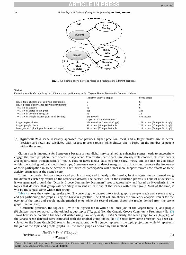
The nodes with their corresponding partitions were then reconciled with the original records information (each record inthe dataset was matched with its corresponding partition). As illustrated in Fig. 15, one record could be distributed acrossdifferent partitions depending on whether the reconciliation was done based on the topic, location, or member ID. Table 3shows a sample of records after reconciliation. The evaluation case considered only topics and people; since the location inthe dataset was the same for all the scenes (i.e., Kitchener/Waterloo).
The outcome of the scene discovery methods were evaluated based on three evaluation criteria; namely, (1) scenerelevancy (i.e., precision, recall, F1-score) and community size (2) Jaccard similarity, and (3) modularity. The following sub-sections explains them in more detail.
6.1. Scene relevance and community size
The ability to discover and retrieve relevant scenes depends on the quality of scene partitioning, which was evaluatedbased on calculating the scene topics (i) precision, (ii) recall, (iii) F1-score. In addition, we assessed (iv) the number ofpeople within the scene (cluster size). The evaluation relied on two hypotheses:
(a) Hypothesis 1: When a scene discovery approach is applied to a dataset that consists of well-defined cultural groups(e.g., Meetup groups), then the minimum number of scenes should be at least equal the number of groups, with eachscene centralized around the topics that describe each group.
JID:SCICO AID:1690 /FLA [m3G; v 1.126; Prn:6/02/2014; 14:58] P.20 (1-29)
20 M. Hamdaqa et al. / Science of Computer Programming ••• (••••) •••–•••
Fig. 15. An example shows how one record is distributed into different partitions.
Table 4Clustering results after applying the different graph partitioning to the “Organic Groove Community Drummers” dataset.
Similarity analysis graphs Scene graph
No. of topic clusters after applying partitioning 6 6No. of people clusters after applying partitioning 6 6Total No. of clusters 12 6Total No. of topics in the graph 225 225Total No. of people in the graph 32 32Total No. of sample records (sum of all fan-ins) 475 records
(a person has multiple topics)475 records
Largest topics cluster 274 records (47 topic & 30 ppl) 172 records (36 topic & 29 ppl)Largest people cluster 99 records (49 topic & 6 ppl) 122 records (47 topic & 11 ppl)Inner join of topics & people (topics ∩ people) 81 records (33 topic & 6 ppl) 111 records (36 topic & 11 ppl)
(b) Hypothesis 2: A scene discovery approach that provides higher precision, recall and a larger cluster size is better.Precision and recall are calculated with respect to scene topics, while cluster size is based on the number of peoplewithin the scene.
Cluster size is important for Sceneverse because a new digital service aimed at enhancing scenes needs to successfullyengage the more peripheral participants in any scene. Core/central participants are already well informed of scene eventsand opportunities through word of mouth, cultural news media, existing online social media and the like. To add valuewithin the existing cultural media landscape, Sceneverse needs to detect marginal participants and increase the frequencyof their participation in scene activities. That increased participation will funnel more support towards the efforts of sceneactivity organizers at the scene’s core.
To find the overlap between topics and people clusters, and to analyze the results; facet analysis was performed usingthe different clustering results on the reconciled dataset. The dataset used in the evaluation process is a subset of dataset 2.It was generated around the “Organic Groove Community Drummers” group. Accordingly, and based on Hypothesis 1, thetopics that describe that group will definitely represent at least one of the scenes within that group. Most of the time, itwill be the largest scene within that group.
Table 4 shows the clustering results after (1) converting the dataset into a topic graph, a people graph and a scene graph,and (2) partitioning the graphs using the Louvain algorithm. The first column shows the similarity analysis results for theoverlap of the topic and people graphs (method one), while the second column shows the results derived from the scenegraph (method two).
To calculate precision, the topics (TP) with the highest fan-in within the inner join of the largest topic (T) and people(P) clusters were compared to the original group topics (TPOriginal) (i.e., the Organic Groove Community Drummers). Eq. (3)shows how scene precision has been calculated using Similarity Analysis (SA). Similarly, the scene graph topics (ΠTP{SG}) ofthe largest scene detected were compared with the original group topics. Eq. (4) shows how scene precision has been cal-culated for the Scene Graph (SG) results. In the equations, the Π symbol represents the topic projection, while � representsthe join of the topic and people graphs, i.e., the scene graph as derived by this method
PrecisionSA = |ΠTP{TG � PG} ∩ {TPOriginal}||{TP }| (3)
Original

JID:SCICO AID:1690 /FLA [m3G; v 1.126; Prn:6/02/2014; 14:58] P.21 (1-29)
M. Hamdaqa et al. / Science of Computer Programming ••• (••••) •••–••• 21
Input: DatasetOutput: Scene-Relevantforall the Records r ∈ Dataset do
if RecordTopic rtp ∈ SceneTopic thenScene-Relevant++;
endend
Algorithm 1: Finding relevant scenes.
Table 5Topics of the Organic Groove Community Drummers.
Original Similarity analysis graphs Scene graph
Alternative health 3 4Meditation 4 6Drum circle 6 11Consciousness 3 3Live music 3 7Social 3 3Music 4 7Hand drumming 5 aDrumming 4 6Meeting new people 4 4African drumming 4 7Recreational drumming 5 5West African drumming 4 9Healing rhythms drum circle 5 5Social 3 3Total number of records with exact topics 60 89
PrecisionSG = |ΠTP{SG} ∩ {TPOriginal}||{TPOriginal}| (4)
Eq. (5) shows the formalism for assessing scene recall. Scene recall was calculated by comparing the number of recordsin the scene (RScene-Retrieved), where a user indicated interest in any topics used to describe the ground truth scene, to thenumber of records in the dataset that refer to the same topics (RScene-Relevant).
Recall = RScene-Retrieved
RScene-Relevant(5)
RScene-Retrieved can be calculated by summing all the fan-in values for all topics that constitute the scene, as shown inEq. (6).
RScene-Retrieved =n∑
i=1
TPi(FanIn) (6)
On the other hand, RScene-Relevant can be found by searching the records for scene-specific topics as shown in the pseudo-code in Algorithm 1.
Table 5 shows the main topics that described the “Organic Groove Community Drummers”. The table also shows thefan-in analysis of these topics in both the scene graph, as well as the inner join of both topic and people similarity graphs.
As shown in Table 6. Both techniques provide 100% precision with respect to the topics that describe the “OrganicGroove Community Drummers” group. However, the scene graph technique provides higher recall with respect to the totalnumber of records returned in which a user indicated an interest in any of the topics used to describe the “Organic GrooveCommunity Drummers” group. However, the scene graph technique recalled more of the total number of records whereusers indicated interest in topics describing the Organic Groove Community Drummers group. Moreover, the size of thescene community in terms of participants identified is much higher using the scene graph technique; almost 92% higher.
Finally, to show the accuracy of the scene graph approach over the similarity analysis graph approach, the harmonicmean of precision and recall, or F1 score, has been calculated. The F1 score takes values between zero and one; the closerthe value to 1 the higher the accuracy of the information retrieval approach. Eq. (7) shows how the F1 score is calculated.The results are shown in Table 6, where the F1 score confirms higher accuracy for the scene graph over the similarityanalysis graph technique.
F 1 = 2 · Precision · Recall
Precision + Recall(7)

JID:SCICO AID:1690 /FLA [m3G; v 1.126; Prn:6/02/2014; 14:58] P.22 (1-29)
22 M. Hamdaqa et al. / Science of Computer Programming ••• (••••) •••–•••
Table 6Precision, recall and scene size results.
Similarity analysis graphs Scene graph
Total number of records with exact 60 89Topics returned total number of records with exact 122 122Topics in the dataset precision (with respect to the original group topics list) 100% 100%Recall 49% 73%F1 measure 65.77% 84.39%Number of people in the scene 6 ppl 11 ppl
Table 7Evaluation results using Jaccard and theme similarity.
Scene Equivalent(T ∩ P)graphspartition
Jaccardsimilarityindex
Themesimilarityindex
TotalNo. oftopics
TotalNo. oftopics(T ∩ P)
TotalNo. ofpeopleSG
TotalNo. ofpeople(T ∩ P)
SG1 T4 ∩ P2 0.547 1.0 40 26 4 2SG2 T2 ∩ P5 0.271 0.6 52 37 8 7SG3 T2 ∩ P1 0.442 0.2 22 40 2 6SG4 T1 ∩ T3 1.0 1.0 26 26 2 2SG5 T2 ∩ P4 0.605 1.0 36 33 11 6SG6 T5 ∩ P1 0.308 0.2 31 32 4 5
6.2. Jaccard similarity for scenes with no ground truth
A similar process that does not require ground truth data was applied to all other clusters (other than the main onewhich was used in the previous analysis). The process began by finding all the inner joins of the different combinations ofpeople and topics graphs partitions. Then, for each partition in the scene graph, similarity was calculated to find the distancebetween each of the inner join sets and the partition. As shown in Eq. (3), the Jaccard Similarity Index was calculated byfinding the size of the intersection between the scene topics (A) and each of the inner join combinations (B) divided by thesize of the union of the two sets. After calculating the Jaccard Similarity Index, it was apparent that more information wasneeded in order to reason scientifically about the results. For this reason, another similarity metric that also uses JaccardSimilarity was used to refine and confirm the results of the first metric.
J (A, B) = |A ∩ B||A ∪ B| (8)
We call this metric scene theme similarity. As indicated by the name, this metric focused on the main scene topics;those shared by many Scene People. Scene theme similarity was calculated by creating a list that consisted of the top fivetopics (highest in fan-in) for each scene and topic people inner join cluster. Then, the themes were compared using JacquardSimilarity.
As shown in Table 7, by combining both Jaccard and theme similarity, better insight into clustering results was attained.For example, if both Jaccard similarity and theme similarity were high (i.e., above 0.5), this was a good indication that thescene discovered had a well-defined boundary. Examples of such scenes were SG1, SG5 and SG4. In this case, the larger thesize of the scene, the better the scene. For example, even though both similarity indices of SG4 were high; it was consideredto be a weak scene, because it was so small (2 people).
On the other hand, when Jaccard and theme similarity were both low, or in cases when theme similarity was higherthan Jaccard similarity, manual data inspection was performed. We adjudged that scene graph partitioning provided morerational results. In the case where theme similarity was higher than Jaccard, the scenes discovered using the inner joinmethod were composite mixed scenes (i.e., contained more than one scene). On the other hand, when both Jaccard andtheme similarity were low, the scene was not clearly identified in the case of the inner join.
For instance, the SG6 theme contained the following topics: Walking, Camping and Kayaking, Backpacking, and BoardGames. The (T5 ∩ P1) theme contained: Board Games, Executive and Business Coaching, Psychology, Yoga, Atheists. Clearlythe topical theme of SG6 is more coherent and makes more sense for clustering as a scene than the one generated usingthe inner join method (T5 ∩ P1).
It is worth mentioning that the results obtained using these metrics is aligned with the results obtained when groundtruth data were available. Both results favor scene graph over the people-topic inner join for scene discovery. Moreover,using either quantitative or qualitative analysis, a good scene still evinced the same properties; a cohesive community,strong central topics and significant numbers of people participating.

JID:SCICO AID:1690 /FLA [m3G; v 1.126; Prn:6/02/2014; 14:58] P.23 (1-29)
M. Hamdaqa et al. / Science of Computer Programming ••• (••••) •••–••• 23
6.3. Modularity metric Q
Modularity is a widely used metric to show how well a network is partitioned. Consequently, modularity was calculatedfor the three graphs generated here. The results of applying the Louvain method to the people, topic, and scene graphs are0.647, 0.713, and 0.469 respectively. Overall modularity was adequate, indicating cohesive communities. The modularity ofboth people and topic graphs separately was higher than that for the scene graph. This result is expected since the moredimensions you add to the graph the less modularity you have. However, it is this characteristic that gives the scene graphits special property as a graph uniquely able to reveal the cultural contours of the scene.
7. Discussions on obtained results
Graphs with a single node type that are created using similarity analysis play important roles in recommendationsystems. Such graphs can achieve high modularity when applying graph partitioning, and hence they delineate coherentpartitions or communities. Unfortunately, communities identified in these graphs fail at representing cultural scenes. This isbecause a scene is a multidimensional concept, in which time, location, topics and people all contribute to define the sceneboundary. A workaround can be devised by first creating a graph for each of the dimensions, then partitioning (clustering)these graphs, and finally finding the inner join of the different partitions. Unsurprisingly, the results of this workaround aredisappointing because of the size of the communities generated. Overlapping the communities is a type of hard clustering.It assists in identifying the scene center, but fails to capture the whole scene. In order to be able to identify the boundariesof the scene efficiently, there is a need for either (1) efficient techniques that can combine different similarity measures, or(2) similarity measures that work the same way with different types of objects.
The scene graph approach was created to address this particular problem. It creates a graph that combines differenttypes of nodes. Then, it uses graph modularity to partition the graph. From the graph partitioning algorithm perspective,all nodes are the same, despite their scene-dimension type. In order to preserve as much information about the node typesin the graph as possible, the scene graph was constructed as a directed graph. Moreover, a record reconciliation process,followed by facet filtering, was used to merge the partitioning results with the original records in order to further analyzethe clustering results.
7.1. The main findings
Scene graph partitioning is a soft clustering technique. That is designed specifically to discover scenes in cultural data. Itis easier faster and more suitable for discovering cultural scenes than single facet graphs and their overlaps. This is shown inthe evaluation experiment on the small Meetup dataset, in which the scene graph method outperformed the method basedon graph similarity and overlap by almost 53% in terms of execution time. The 53% has been obtained by comparing thetime needed for scene detection using the scene graph, and the sum of the time needed to partition and overlap the people,location, and topics graph. Moreover, the quality of the scenes generated using the scene graph method demonstrated muchmore complete and representative scene communities, with almost a 92% larger community size and 18.62% higher accuracy,based on the F1 measure.
7.2. Dependency on Louvain graph partitioning
Both methods proposed in this paper depend on Louvain graph partitioning. In fact, the performance bottleneck for thescene graph approach stems from its dependency on Louvain graph partitioning for community detection. The scene graphcalls the partitioning algorithm recursively; and this has obvious implications for the efficiency and scalability of the parti-tioning algorithm in large datasets. In a recent study, Papadopoulos et al. [26] have compared the performance of existingcommunity detection techniques, and they favored the Louvain method over other methods for large scale graphs such associal networks. This study supports Papadopoulos findings. We compared six different community detection techniques(i.e., Louvain [15], Fast Greedy [67], Leading Eigen Vector [68], Walktrap [69], Label Propagation [70], and Infomap [71]) interms of complexity, performance, modularity and the number, the size and structure of the generated communities. Weapplied the different techniques on the first Meetup dataset used for scene detection (i.e., 10 781 vertices and 61 151 edges).
Table 8 compares the complexity of each of the aforementioned methods. The first column in the table representsthe complexity obtained without any assumptions about the underlying graph, while the second assumes a sparse graph,in which the number of vertices is approximately equal the number of edges. The complexity of community detectionalgorithms is usually expressed in terms of the number of vertices (n), number of edges (m), as well as the depth of thetree (d) when hierarchical methods are used. Complexity gives a good indication of how well the algorithms will performas the dataset size reaches infinity. The results of comparing complexity shows us that the Louvain method is one of thebest candidates in terms of complexity. Other possible candidates include Label Propagation and Infomaps.
Complexity analysis helps us understand the scalability of the algorithm. However, the experimental results better illu-minate the performance of the algorithm with respect to the different dataset types, sizes, and other factors that can impactthe algorithm performance (e.g., memory consumption).
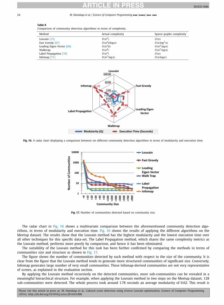
JID:SCICO AID:1690 /FLA [m3G; v 1.126; Prn:6/02/2014; 14:58] P.24 (1-29)
24 M. Hamdaqa et al. / Science of Computer Programming ••• (••••) •••–•••
Table 8Comparison of community detection algorithms in terms of complexity.
Method Actual complexity Sparse graphs complexity
Louvain [15] O (n2) O (n)
Fast Greedy [67] O (n2d logn) O (n log2 n)
Leading Eigen Vector [68] O (n3d) O (n2 logn)
Walktrap O (n4) O (n2 logn)
Label Propagation [70] O (n2) O (n)
Infomap [71] O (n2 logn) O (n logn)
Fig. 16. A radar chart displaying a comparison between six different community detection algorithms in terms of modularity and execution time.
Fig. 17. Number of communities detected based on community size.
The radar chart in Fig. 16 shows a multivariate comparison between the aforementioned community detection algo-rithms, in terms of modularity and execution time. Fig. 16 shows the results of applying the different algorithms on theMeetup dataset. The results show that the Louvain method has the highest modularity and the lowest execution time overall other techniques for this specific data-set. The Label Propagation method, which shares the same complexity metrics asthe Louvain method, performs more poorly by comparison, and hence it has been eliminated.
The suitability of the Louvain method for this task has been further confirmed by comparing the methods in terms ofcommunities size and structure as shown in Fig. 17.
The figure shows the number of communities detected by each method with respect to the size of the community. It isclear from the figure that the Louvain method tends to generate more structured communities of significant size. Conversely,Infomap generates large number of very small communities. These Infomap-derived communities are not very representativeof scenes, as explained in the evaluation section.
By applying the Louvain method recursively on the detected communities, more sub-communities can be revealed in ameaningful hierarchical structure. For example, when applying the Louvain method in two steps on the Meetup dataset, 128sub-communities were detected. The whole process took around 1.78 seconds an average modularity of 0.62. This result is

JID:SCICO AID:1690 /FLA [m3G; v 1.126; Prn:6/02/2014; 14:58] P.25 (1-29)
M. Hamdaqa et al. / Science of Computer Programming ••• (••••) •••–••• 25
comparable to the one achieved by Infomap. However, the communities here are more meaningful and follow a hierarchicalorder that preserves the consistency of topic information.
Moreover the recursive Louvain method outperforms Infomap. It is 3442 times faster on this dataset. The number itselfrapidly scales in a linear relationship with the scale of the graph.
7.3. Analysis techniques
Once scenes have been discovered, and their topics and key people have been identified, a second round of analysis isneeded to rank people within each scene based on centrality. In this paper fan-in and fan-out analysis was used. However,more factors and many additional analytical techniques could be applied to reveal these scene relationships.
For example, factors such as the distance between a person’s place of residence and the scene’s central location, orthe duration in time of a person’s connection to a topic, could significantly affect the assessed strength of the connectionbetween the person and the scene. Several other analytical techniques could also be used; for example:
(i) Centrality: Roughly indicates the social power of a node based on how much the connectivity of a network dependson it (i.e. how disconnected the graph would be if that node were removed). Betweenness, Closeness, and Degree areall centrality measures.
(ii) Betweenness: The extent to which a node lies between other nodes in the network. This takes into account theconnectivity of the node’s neighbors, giving a higher value for nodes which bridge clusters. The measure reflects thenumber of people a person is connected to indirectly through their direct links.
(iii) Closeness: The degree an individual is near all other individuals in a network (directly or indirectly). It indicates thenode’s ability to access information through the grapevine of network members.
(iv) Bridging: A relationship is a bridge if deleting it would cause its endpoints to lie in separate components of a graph.(v) Density: The degree a respondent’s ties know each other, i.e. the proportion of ties among an individual’s group of
contacts. Network-wide or global density is the proportion of ties in a network relative to the total number possible.There can be sparse versus dense networks.
(vi) Ego-effect: The degree an individual’s network reaches out into the network and provides it with novel informationand influence.
(vii) Structural cohesion: The minimum number of members who, if removed from a group, would disconnect the group.
In the context of scene discovery, the output from these social network analysis techniques would have to be combinedand mapped to scene concepts. For example, a combination of fan-out, bridge and centrality analysis might reveal differentontological roles for people within a scene.
The application of these additional social network analysis techniques is out of scope for this paper. A later paper willbe dedicated to discussing their use in the context of scene discovery.
8. Conclusions and future research directions
In this article, we argued the need for a platform dedicated to facilitate engaging its users in socio-cultural activities, andthe need for tools and techniques that can reveal socio-cultural communities in existing datasets. We introduced Sceneverse,a proposed platform for supporting the creation and analysis of an online sociocultural universe. The proposed Sceneverseplatform consists of several components. This paper focused on the concepts, techniques and methods used to implementthe scene extraction engine component. Accordingly, we first created a scene ontology to provide a crisp understanding ofthe scene concept, and to enable building scene representations from the cultural and social data available on the web. Wethen devised an approach for automatic scene discovery in that data.
Scene discovery depends on the ability to cluster similar people, who have similar interests, expressed around similarevents and venues, in certain locations, within a general span of time. This is challenging, since most clustering techniqueswork on single facet, and the scene is a multifaceted concept. To deal with this challenge, two techniques were examined. Inthe first technique, social and cultural data were first converted into three types of single faceted socio-cultural graphs; onefor people, one for topics and one for locations. Each of these graphs were then partitioned into groups based on Louvainmodularity optimization, and the resultant communities were overlapped to create scenes. In the second technique, a scenegraph, which is a multifaceted directed graph, was created. Then it was partitioned directly into scenes using Louvainmodularity optimization.
The two proposed methods were empirically evaluated using data crawled from the cultural and social networkMeetup.com. Preliminary results demonstrate the superiority of the scene graph technique over the overlapping of single-faceted graphs in identifying the scene boundaries. While both techniques were able to detect the scene center in terms ofthe key people, main topics and central locations for a scene, the size of the community in terms of number of people iden-tified was larger with scene graph partitioning. This is because a scene graph partitioning is a softer clustering techniquethan community overlapping.
The scene graph technique proposed in this paper overcomes two of the main drawbacks associated with graph parti-tioning. The first drawback is the information lost when converting a multifaceted dataset into graphs. We overcame this

JID:SCICO AID:1690 /FLA [m3G; v 1.126; Prn:6/02/2014; 14:58] P.26 (1-29)
26 M. Hamdaqa et al. / Science of Computer Programming ••• (••••) •••–•••
problem by preserving relational information in directed graphs, then using fan-in and fan-out analysis to highlight the dif-ferent nodes in each partition. The second drawback is specifically related to modularity optimization techniques, in whichmodularity at a large scale fails to reveal small communities. This problem has been addressed by applying the Louvainalgorithms in iterations. In fact, taking this approach proved ideal for scene discovery, since it organizes scenes in hierar-chical order (scene, sub-scene), which fits the natural social topology of scene. Scene graphs are designed specifically todiscover scenes in cultural data. Scene graph analysis using reverse Louvain optimization is easier, faster and more suitablefor discovering cultural scenes than overlapping single facet graphs.
In addition to our scene discovery procedure, this article also briefly discussed scene analysis techniques. We used fan-in,fan-out and facet filtering to discover important scene graph nodes. Future efforts will focus on investigating other anal-ysis techniques to rank people, topics and locations within each scene (e.g., based on centrality or other social networkanalysis measures). The results will be used in prototypes of the Sceneverse platform to enhance scene experience and toprovide scene participants with better choices. Moreover, the scene discovery approach proposed in this paper is poten-tially generalizable to other domains. Hence, we are planning to apply this technique to other domains where multifacetedrecommenders are needed.
Appendix A. OWL scene ontology graph
Appendix B. Scene ontology triples
Subject Predicate Object
http://www.sceneverse.com/CW/scene/ http://www.w3.org/1999/02/22-rdf-syntax-ns#type http://www.w3.org/2002/07/owl#Ontologyhttp://www.sceneverse.com/CW/scene/ http://www.w3.org/2000/01/rdf-schema#comment “This ontology describes the cultural scene based on Sceneverse Inc. definition”http://www.sceneverse.com/CW/scene/ http://www.w3.org/2002/07/owl#imports http://purl.org/vocab/bio/0.1/http://www.sceneverse.com/CW/scene/ http://www.w3.org/2002/07/owl#imports http://www.isi.edu/~pan/damltime/time-entry.owlhttp://www.sceneverse.com/CW/scene/ http://www.w3.org/2002/07/owl#imports http://xmlns.com/foaf/0.1/http://www.sceneverse.com/CW/scene/associatedWith http://www.w3.org/1999/02/22-rdf-syntax-ns#type http://www.w3.org/2002/07/owl#ObjectPropertyhttp://www.sceneverse.com/CW/scene/associatedWith http://www.w3.org/1999/02/22-rdf-syntax-ns#type http://www.w3.org/2002/07/owl#FunctionalPropertyhttp://www.sceneverse.com/CW/scene/associatedWith http://www.w3.org/2000/01/rdf-schema#subPropertyOf http://www.w3.org/2002/07/owl#topObjectPropertyhttp://www.sceneverse.com/CW/scene/centralizedArround http://www.w3.org/1999/02/22-rdf-syntax-ns#type http://www.w3.org/2002/07/owl#ObjectPropertyhttp://www.sceneverse.com/CW/scene/centralizedArround http://www.w3.org/2000/01/rdf-schema#subPropertyOf http://www.w3.org/2002/07/owl#topObjectProperty
(continued on next page)

JID:SCICO AID:1690 /FLA [m3G; v 1.126; Prn:6/02/2014; 14:58] P.27 (1-29)
M. Hamdaqa et al. / Science of Computer Programming ••• (••••) •••–••• 27
(continued)
Subject Predicate Object
http://www.sceneverse.com/CW/scene/describeScene http://www.w3.org/1999/02/22-rdf-syntax-ns#type http://www.w3.org/2002/07/owl#ObjectPropertyhttp://www.sceneverse.com/CW/scene/hasActivePeriod http://www.w3.org/1999/02/22-rdf-syntax-ns#type http://www.w3.org/2002/07/owl#ObjectPropertyhttp://www.sceneverse.com/CW/scene/hasActivePeriod http://www.w3.org/1999/02/22-rdf-syntax-ns#type http://www.w3.org/2002/07/owl#FunctionalPropertyhttp://www.sceneverse.com/CW/scene/hasActivePeriod http://www.w3.org/2000/01/rdf-schema#domain http://www.sceneverse.com/CW/scene/Scenehttp://www.sceneverse.com/CW/scene/hasActivePeriod http://www.w3.org/2000/01/rdf-schema#range http://www.sceneverse.com/CW/scene/SceneActivePeriodhttp://www.sceneverse.com/CW/scene/hasActivePeriod http://www.w3.org/2002/07/owl#inverseOf http://www.sceneverse.com/CW/scene/associatedWithhttp://www.sceneverse.com/CW/scene/hasEvent http://www.w3.org/1999/02/22-rdf-syntax-ns#type http://www.w3.org/2002/07/owl#ObjectPropertyhttp://www.sceneverse.com/CW/scene/hasEvent http://www.w3.org/2000/01/rdf-schema#domain http://www.sceneverse.com/CW/scene/Scenehttp://www.sceneverse.com/CW/scene/hasEvent http://www.w3.org/2000/01/rdf-schema#range http://www.sceneverse.com/CW/scene/SceneEventhttp://www.sceneverse.com/CW/scene/hasEvent http://www.w3.org/2002/07/owl#inverseOf http://www.sceneverse.com/CW/scene/sceneEventhttp://www.sceneverse.com/CW/scene/hasLocation http://www.w3.org/1999/02/22-rdf-syntax-ns#type http://www.w3.org/2002/07/owl#ObjectPropertyhttp://www.sceneverse.com/CW/scene/hasLocation http://www.w3.org/2000/01/rdf-schema#domain http://www.sceneverse.com/CW/scene/Scenehttp://www.sceneverse.com/CW/scene/hasLocation http://www.w3.org/2000/01/rdf-schema#range http://www.sceneverse.com/CW/scene/SceneLocationhttp://www.sceneverse.com/CW/scene/hasLocation http://www.w3.org/2002/07/owl#inverseOf http://www.sceneverse.com/CW/scene/centralizedArroundhttp://www.sceneverse.com/CW/scene/hasPeople http://www.w3.org/1999/02/22-rdf-syntax-ns#type http://www.w3.org/2002/07/owl#ObjectPropertyhttp://www.sceneverse.com/CW/scene/hasPeople http://www.w3.org/2000/01/rdf-schema#domain http://www.sceneverse.com/CW/scene/Scenehttp://www.sceneverse.com/CW/scene/hasPeople http://www.w3.org/2000/01/rdf-schema#range http://www.sceneverse.com/CW/scene/ScenePersonhttp://www.sceneverse.com/CW/scene/hasPeople http://www.w3.org/2002/07/owl#inverseOf http://www.sceneverse.com/CW/scene/participateInhttp://www.sceneverse.com/CW/scene/hasTopic http://www.w3.org/1999/02/22-rdf-syntax-ns#type http://www.w3.org/2002/07/owl#ObjectPropertyhttp://www.sceneverse.com/CW/scene/hasTopic http://www.w3.org/2000/01/rdf-schema#domain http://www.sceneverse.com/CW/scene/Scenehttp://www.sceneverse.com/CW/scene/hasTopic http://www.w3.org/2000/01/rdf-schema#range http://www.sceneverse.com/CW/scene/SceneTopichttp://www.sceneverse.com/CW/scene/hasTopic http://www.w3.org/2002/07/owl#inverseOf http://www.sceneverse.com/CW/scene/describeScenehttp://www.sceneverse.com/CW/scene/participateIn http://www.w3.org/1999/02/22-rdf-syntax-ns#type http://www.w3.org/2002/07/owl#ObjectPropertyhttp://www.sceneverse.com/CW/scene/sceneEvent http://www.w3.org/1999/02/22-rdf-syntax-ns#type http://www.w3.org/2002/07/owl#ObjectPropertyhttp://www.sceneverse.com/CW/scene/sceneEvent http://www.w3.org/2000/01/rdf-schema#subPropertyOf http://www.w3.org/2002/07/owl#topObjectPropertyhttp://www.w3.org/2002/07/owl#topObjectProperty http://www.w3.org/1999/02/22-rdf-syntax-ns#type http://www.w3.org/2002/07/owl#ObjectPropertyhttp://www.w3.org/2002/07/owl#topObjectProperty http://www.w3.org/1999/02/22-rdf-syntax-ns#type http://www.w3.org/2002/07/owl#TransitivePropertyhttp://www.sceneverse.com/CW/scene/MultiPersonaScenester http://www.w3.org/1999/02/22-rdf-syntax-ns#type http://www.w3.org/2002/07/owl#Classhttp://www.sceneverse.com/CW/scene/MultiPersonaScenester http://www.w3.org/2000/01/rdf-schema#subciassOf http://www.sceneverse.com/CW/scene/ScenePersonhttp://www.sceneverse.com/CW/scene/Personage http://www.w3.org/1999/02/22-rdf-syntax-ns#type http://www.w3.org/2002/07/owl#Classhttp://www.sceneverse.com/CW/scene/Personage http://www.w3.org/2000/01/rdf-schema#subClassOf http://www.sceneverse.com/CW/scene/ScenePersonhttp://www.sceneverse.com/CW/scene/Scene http://www.w3.org/1999/02/22-rdf-syntax-ns#type http://www.w3.org/2002/07/owl#Classhttp://www.sceneverse.com/CW/scene/Scene http://www.w3.org/2000/01/rdf-schema#subClassOf http://www.sceneverse.com/CW/scene/Scenehttp://www.sceneverse.com/CW/scene/SceneActivePeriod http://www.w3.org/1999/02/22-rdf-syntax-ns#type http://www.w3.org/2002/07/owl#Classhttp://www.sceneverse.com/CW/scene/SceneActivePeriod http://www.w3.org/2000/01/rdf-schema#subClassOf http://www.isi.edu/~pan/damltime/time-entry.owl#IntervalThinghttp://www.sceneverse.com/CW/scene/SceneEvent http://www.w3.org/1999/02/22-rdf-syntax-ns#type http://www.w3.org/2002/07/owl#Classhttp://www.sceneverse.com/CW/scene/SceneEvent http://www.w3.org/2000/01/rdf-schema#subClassOf http://linkedevents.org/ontology/Eventhttp://www.sceneverse.com/CW/scene/SceneEvent http://www.w3.org/2000/01/rdf-schema#subClassOf http://purl.org/NET/c4dm/event.owl#Eventhttp://www.sceneverse.com/CW/scene/SceneEvent http://www.w3.org/2000/01/rdf-schema#subClassOf http://purl.org/dc/dcmitype/Eventhttp://www.sceneverse.com/CW/scene/SceneEvent http://www.w3.org/2000/01/rdf-schema#subClassOf http://sw.opency:.org/2009/04/07/concept/en/Eventhttp://www.sceneverse.com/CW/scene/SceneFollower http://www.w3.org/1999/02/22-rdf-syntax-ns#type http://www.w3.org/2002/07/owl#Classhttp://www.sceneverse.com/CW/scene/SceneFollower http://www.w3.org/2000/01/rdf-schema#subClassOf http://www.sceneverse.com/CW/scene/ScenePersonhttp://www.sceneverse.com/CW/scene/SceneLocation http://www.w3.org/1999/02/22-rdf-syntax-ns#type http://www.w3.org/2002/07/owl#Classhttp://www.sceneverse.com/CW/scene/SceneLocation http://www.w3.org/2000/01/rdf-schema#subClassOf http://www.w3.org/2003/01/geo/wgs84_pos#SpatialThinghttp://www.sceneverse.com/CW/scene/SceneOrganizer http://www.w3.org/1999/02/22-rdf-syntax-ns#type http://www.w3.org/2002/07/owl#Classhttp://www.sceneverse.com/CW/scene/SceneOrganizer http://www.w3.org/2000/01/rdf-schema#subClassOf http://www.sceneverse.com/CW/scene/ScenePersonhttp://www.sceneverse.com/CW/scene/ScenePerson http://www.w3.org/1999/02/22-rdf-syntax-ns#type http://www.w3.org/2002/07/owl#Classhttp://www.sceneverse.com/CW/scene/SceneTopic http://www.w3.org/1999/02/22-rdf-syntax-ns#type http://www.w3.org/2002/07/owl#Classhttp://www.sceneverse.com/CW/scene/SceneTopic http://www.w3.org/2000/01/rdf-schema#subClassOf http://www.sceneverse.com/CW/scene/SceneTopichttp://www.sceneverse.com/CW/scene/Scenester http://www.w3.org/1999/02/22-rdf-syntax-ns#type http://www.w3.org/2002/07/owl#Classhttp://www.sceneverse.com/CW/scene/Scenester http://www.w3.org/2000/01/rdf-schema#subClassOf http://www.sceneverse.com/CW/scene/ScenePersonhttp://www.sceneverse.com/CW/scene/ScenesterFriend http://www.w3.org/1999/02/22-rdf-syntax-ns#type http://www.w3.org/2002/07/owl#Classhttp://www.sceneverse.com/CW/scene/ScenesterFriend http://www.w3.org/2000/01/rdf-schema#subClassOf http://www.sceneverse.com/CW/scene/ScenePersonhttp://www.sceneverse.com/CW/scene/SecludedScenester http://www.w3.org/1999/02/22-rdf-syntax-ns#type http://www.w3.org/2002/07/owl#Classhttp://www.sceneverse.com/CW/scene/SecludedScenester http://www.w3.org/2000/01/rdf-schema#subClassOf http://www.sceneverse.com/CW/scene/ScenePersonhttp://www.sceneverse.com/CW/scene/Silhouette http://www.w3.org/1999/02/22-rdf-syntax-ns#type http://www.w3.org/2002/07/owl#Classhttp://www.sceneverse.com/CW/scene/Silhouette http://www.w3.org/2000/01/rdf-schema#subClassOf http://www.sceneverse.com/CW/scene/ScenePersonhttp://www.sceneverse.com/CW/scene/Sponsor http://www.w3.org/1999/02/22-rdf-syntax-ns#type http://www.w3.org/2002/07/owl#Classhttp://www.w3.org/2000/10/swap/pim/contact#Person http://www.w3.org/2000/01/rdf-schema#subClassOf http://xmlns.com/foaf/0.1/Agent
References
[1] D. Hebdige, Subculture: The meaning of style, Crit. Q. 37 (2) (2007) 120–124.[2] M. Maffesoli, The Time of the Tribes: The Decline of Individualism in Mass Society, Theory Cult. Soc., vol. 41, Sage Publications Limited, 1996.[3] B. Cova, Community and consumption: Towards a definition of the “linking value” of product or services, Eur. J. Mark. 31 (3/4) (1997) 297–316.[4] R. Kozinets, Utopian enterprise: Articulating the meanings of Star Trek’s culture of consumption, J. Consum. Res. 28 (1) (2001) 67–88.[5] D. Silver, T. Clark, C. Yanez, Scenes: Social context in an age of contingency, Soc. Forces 88 (5) (2010) 2293–2324.[6] C. Hume, Art of the city: Exhibit shows how relationship with cultural creativity, or lack thereof, can make or break a metropolis, Toronto Star (2001),
online ed.[7] W. Straw, Scenes and sensibilities, Public 22 (23) (2002) 245–257.[8] Nordicity, Sound analysis: An examination of the Canadian independent music industry, Tech. Rep. NGL13-02-15, Canadian Independent Music Asso-
ciation (CIMA), 2013, retrieved from: http://www2.cimamusic.com/wp-content/uploads/2013/07/Sound_Analysis.CIMA_.FINAL_.2013.pdf [last accessed:October 2013].
[9] L. Rothfield, D. Coursey, S. Lee, D. Silver, W. Norris, T. Hotze, et al., Chicago music city: A report on the music industry in Chicago, Tech. Rep.ISBN 0-9747047-3-3, The Chicago Music Commission, 2006, retrieved from: http://74.220.219.62/~natkinne/chicago-music.org/wp-content/uploads/2008/12/chicagomusiccity_fullreport1.pdf [last accessed: October 2013].
[10] W.B. Beyers, A. Bonds, A. Wenzl, P. Sommers, The economic impact of Seattle’s music industry: A report for the city of Seattle’s office of economicdevelopment, Tech. Rep., University of Washington and City of Seattle’s Office of Economic Development, 2004, retrieved from: http://web.williams.edu/Economics/ArtsEcon/Documents/Seattle_Music_StudyFinal.pdf [last accessed: October 2013].
[11] H. Jang, S. Choe, J. Song, Exploring serendipitous social networks: sharing immediate situations among unacquainted individuals, in: The InternationalConference on Human Computer Interaction with Mobile Devices and Services, 2011, pp. 513–516.
[12] B. Shank, Dissonant Identities: The Rock’n’Roll Scene in Austin, Texas, Wesleyan, 2011.[13] Á. García-Crespo, R. Colomo-Palacios, J.M. Gómez-Berbís, B. Ruiz-Mezcua, Semo: A framework for customer social networks analysis based on semantics,
J. Inf. Technol. 25 (2) (2010) 178–188.[14] A. Schein, A. Popescul, L. Ungar, D. Pennock, Methods and metrics for cold-start recommendations, in: The International ACM SIGIR Conference on
Research and Development on Information Retrieval, 2002, pp. 253–260.

JID:SCICO AID:1690 /FLA [m3G; v 1.126; Prn:6/02/2014; 14:58] P.28 (1-29)
28 M. Hamdaqa et al. / Science of Computer Programming ••• (••••) •••–•••
[15] V. Blondel, J.L. Guillaume, R. Lambiotte, E. Lefebvre, Fast unfolding of communities in large networks, J. Stat. Mech. Theory Exp. 1 (10) (2008)1742–1754.
[16] S. Fortunato, Community detection in graphs, Phys. Rep. 486 (3) (2010) 75–174.[17] M. Porter, J. Onnela, P. Mucha, Communities in networks, Not. Am. Math. Soc. 56 (9) (2009) 1082–1097.[18] P. Monge, N. Contractor, Theories of Communication Networks, Oxford University Press, USA, 2003.[19] L. Freeman, The Development of Social Network Analysis: A Study in the Sociology of Science, Empirical Press, 2004.[20] M. Girvan, M. Newman, Community structure in social and biological networks, Proc. Natl. Acad. Sci. USA 99 (12) (2002) 7821–7826.[21] X. Liu, J. Bollen, M. Nelson, H. Van de Sompel, Co-authorship networks in the digital library research community, Inf. Process. Manag. 41 (6) (2005)
1462–1480.[22] C. Kottak, Cultural Anthropology: Appreciating Cultural Diversity, McGraw–Hill, 2011.[23] E. Bullmore, D. Bassett, Brain graphs: Graphical models of the human brain connectome, Annu. Rev. Clin. Psychol. 7 (2011) 113–140.[24] N. Du, B. Wu, X. Pei, B. Wang, L. Xu, Community detection in large-scale social networks, in: The International Workshop on Knowledge Discovery on
the Web and International Workshop on Social Networks Analysis, 2007, pp. 16–25.[25] L. Tang, H. Liu, Community detection and mining in social media, Synth. Lect. Data Min. Knowl. Discov. 2 (1) (2010) 1–137.[26] S. Papadopoulos, Y. Kompatsiaris, A. Vakali, P. Spyridonos, Community detection in social media, Data Min. Knowl. Discov. 24 (3) (2012) 515–554.[27] A. Traud, P. Mucha, M. Porter, Social structure of facebook networks, Phys. A, Stat. Mech. Appl. 391 (16) (2011) 4165–4180.[28] E. Ferrara, Community structure discovery in facebook, Int. J. Soc. Netw. Min. 1 (1) (2012) 67–90.[29] S. Schaeffer, Graph clustering, Comput. Sci. Rev. 1 (1) (2007) 27–64.[30] R. Aldecoa, I. Marín, Deciphering network community structure by surprise, PLoS ONE 6 (9) (2011) 24–95.[31] T. Evans, Clique graphs and overlapping communities, J. Stat. Mech. Theory Exp. 12 (1) (2010) 1–39.[32] A. Arenas, J. Duch, A. Fernández, S. Gómez, Size reduction of complex networks preserving modularity, New J. Phys. 9 (6) (2007) 176–190.[33] M. Barber, Modularity and community detection in bipartite networks, Phys. Rev. E 76 (6) (2007) 1–11.[34] K. Dellschaft, S. Staab, An epistemic dynamic model for tagging systems, in: The ACM Conference on Hypertext and Hypermedia, 2008, pp. 71–80.[35] G. Begelman, P. Keller, F. Smadja, et al., Automated tag clustering: Improving search and exploration in the tag space, in: The Collaborative Web Tagging
Workshop, 2006, pp. 15–33.[36] E. Simpson, Clustering tags in enterprise and web folksonomies, in: The International AAAI Conference on Weblogs and Social Media, 2008,
pp. 222–223.[37] S. Papadopoulos, Y. Kompatsiaris, A. Vakali, A graph-based clustering scheme for identifying related tags in folksonomies, Data Warehous. Knowl.
Discov. 6263 (2010) 65–76.[38] M. Fatemi, L. Tokarchuk, An empirical study on IMDb and its communities based on the network of co-reviewers, in: The Workshop on Measurement,
Privacy, and Mobility, 2012, pp. 1–7.[39] A. Mislove, M. Marcon, K. Gummadi, P. Druschel, B. Bhattacharjee, Measurement and analysis of online social networks, in: The ACM SIGCOMM
Conference on Internet Measurement, 2007, pp. 29–42.[40] A. Traud, E. Kelsic, P. Mucha, M. Porter, Community structure in online collegiate social networks, Am. Phys. Soc. 88 (2009) 1–38.[41] D. Tsatsou, S. Papadopoulos, I. Kompatsiaris, P. Davis, Distributed technologies for personalized advertisement delivery, in: Online Multimedia Adver-
tising: Techniques and Technologies, IGI Global, Hershey, 2011, pp. 233–261.[42] M. Pham, Y. Cao, R. Klamma, M. Jarke, A clustering approach for collaborative filtering recommendation using social network analysis, J. Univers.
Comput. Sci. 17 (4) (2011) 583–604.[43] Q. Zhao, P. Mitra, B. Chen, Temporal and information flow based event detection from social text streams, in: The National Conference on Artificial
Intelligence, vol. 2, 2007, pp. 1501–1506.[44] J. Shi, J. Malik, Normalized cuts and image segmentation, IEEE Trans. Commun. Netw., Pattern Anal. Mach. Intell. 22 (8) (2000) 888–905.[45] D. Silver, D. Miller, Contextualizing the artistic dividend, J. Urban Aff. 2012 (2012).[46] D. Silver, The American scenescape: amenities, scenes and the qualities of local life, Camb. J. Reg., Econ. Soc. 5 (1) (2012) 97–114.[47] O. Císar, M. Koubek, Include ‘em all?: Culture, politics and a local hardcore/punk scene in the Czech Republic, Poetics 40 (1) (2012) 1–21.[48] D. Silver, T. Clark, L. Rothfield, A theory of scenes, Manuscript, University of Chicago, 2007, retrieved from: http://tnc.research.googlepages.com/
atheoryofscenes [accessed January 27, 2013].[49] R. Kozinets, Technology/ideology: How ideological fields influence consumers’ technology narratives, J. Consum. Res. 34 (6) (2008) 865–881.[50] R. Kozinets, J. Handelman, M. Lee, Don’t read this, or, who cares what the hell anti-consumption is, anyways?, Consump. Mark. Cult. 13 (3) (2010)
225–233.[51] M. Samwald, K. Cheung, Experiences with the conversion of senselab databases to RDF/OWL, World Wide Web Consortium (W3C) Interest Group Note,
2008, retrieved from: http://www.w3.org/TR/hcls-senselab/ [accessed October 2013].[52] K. Siorpaes, M. Hepp, myOntology: The marriage of ontology engineering and collective intelligence, in: Bridging the Gap between Semantic Web and
Web 2.0, 2007, pp. 127–138.[53] N. Villegas, H. Müller, The SmarterContext ontology and its application to the smart internet: A smarter commerce case study, in: The Personal Web,
in: Lecture Notes in Computer Science, vol. 7855, 2013, pp. 151–184.[54] H. Knublauch, R.W. Fergerson, N.F. Noy, M.A. Musen, The Protégé OWL plugin: An open development environment for semantic web applications, in:
The Semantic Web, Springer, 2004, pp. 229–243.[55] V. Haarslev, R. Müller, Racer system description, in: Automated Reasoning, 2001, pp. 701–705.[56] D. Tsarkov, I. Horrocks, FaCT++ description logic reasoner: System description, in: Automated Reasoning, 2006, pp. 292–297.[57] E. Sirin, B. Parsia, B.C. Grau, A. Kalyanpur, Y. Katz, Pellet: A practical OWL-DL reasoner, Web Semant. Sci. Serv. Agents World Wide Web 5 (2) (2007)
51–53.[58] B. Quilitz, U. Leser, Querying distributed RDF data sources with SPARQL, in: The Semantic Web: Research and Applications, Springer, 2008, pp. 524–538.[59] M. Bastian, S. Heymann, M. Jacomy, Gephi: An open source software for exploring and manipulating networks, in: The International AAAI Conference
on Weblogs and Social Media, 2009, pp. 361–362.[60] J. Friedman, T. Hastie, R. Tibshirani, The Elements of Statistical Learning: Data Mining, Inference, and Prediction, Springer Ser. Stat., vol. 1, 2001.[61] S. Herring, A faceted classification scheme for computer-mediated discourse, Lang. Internet 4 (1) (2007) 1–37.[62] D. Tunkelang, Faceted search, Synth. Lect. Inf. Concept. Retr. Services 1 (1) (2009) 1–80.[63] H. Ma, Google refine, Tech. Serv. Q. 29 (3) (2012) 242–243, retrieved from: http://code.google.com/p/google-refine/.[64] L. Philips, Hanging on the metaphone, Comput. Lang. 7 (1990) 9–43.[65] S. Lu, K. Fu, A sentence-to-sentence clustering procedure for pattern analysis, IEEE Trans. Syst. Man Cybern. 8 (5) (1978) 381–389.[66] S. Fortunato, M. Barthelemy, Resolution limit in community detection, Proc. Natl. Acad. Sci. USA 104 (1) (2007) 36–41.[67] A. Clauset, M.E. Newman, C. Moore, Finding community structure in very large networks, Phys. Rev. E 70 (6) (2004) 66–72.[68] M.E. Newman, Finding community structure in networks using the eigenvectors of matrices, Phys. Rev. E 74 (3) (2006) 36–46.[69] P. Pons, M. Latapy, Computing communities in large networks using random walks, in: Computer and Information Sciences—ISCIS 2005, 2005,
pp. 284–293.

JID:SCICO AID:1690 /FLA [m3G; v 1.126; Prn:6/02/2014; 14:58] P.29 (1-29)
M. Hamdaqa et al. / Science of Computer Programming ••• (••••) •••–••• 29
[70] U.N. Raghavan, R. Albert, S. Kumara, Near linear time algorithm to detect community structures in large-scale networks, Phys. Rev. E 76 (3) (2007)036–46.
[71] M. Rosvall, C.T. Bergstrom, Maps of random walks on complex networks reveal community structure, Proc. Natl. Acad. Sci. USA 105 (4) (2008)1118–1123.