Contents

1 Introduction 51.1 Special structural design . . . . . . . . . . . . . . . . . . . . . . . . . . . . . . . . 61.2 Classifications . . . . . . . . . . . . . . . . . . . . . . . . . . . . . . . . . . . . . . 81.3 Structural Morphology . . . . . . . . . . . . . . . . . . . . . . . . . . . . . . . . . 91.4 Structural design process . . . . . . . . . . . . . . . . . . . . . . . . . . . . . . . 91.5 Discussion . . . . . . . . . . . . . . . . . . . . . . . . . . . . . . . . . . . . . . . . 9

2 Technology and knowledge 112.1 Geometry . . . . . . . . . . . . . . . . . . . . . . . . . . . . . . . . . . . . . . . . 132.2 Principles of Structural Morphology . . . . . . . . . . . . . . . . . . . . . . . . . 222.3 Analogies between structural engineering, physical models and natural structures 672.4 Physical Modelling . . . . . . . . . . . . . . . . . . . . . . . . . . . . . . . . . . . 672.5 Biomimetics . . . . . . . . . . . . . . . . . . . . . . . . . . . . . . . . . . . . . . . 84

3 Structural concepts 1213.1 Shells and domes . . . . . . . . . . . . . . . . . . . . . . . . . . . . . . . . . . . . 1223.2 Cable-net and membrane structures . . . . . . . . . . . . . . . . . . . . . . . . . 1433.3 Pneumatic structures . . . . . . . . . . . . . . . . . . . . . . . . . . . . . . . . . . 1653.4 Space frames . . . . . . . . . . . . . . . . . . . . . . . . . . . . . . . . . . . . . . 2083.5 Kinetic and adaptable structures . . . . . . . . . . . . . . . . . . . . . . . . . . . 277

4 Advanced computation for Structural Design 2914.1 Theory . . . . . . . . . . . . . . . . . . . . . . . . . . . . . . . . . . . . . . . . . . 2924.2 Form description and generation . . . . . . . . . . . . . . . . . . . . . . . . . . . 2944.3 Descriptive techniques . . . . . . . . . . . . . . . . . . . . . . . . . . . . . . . . . 2944.4 Generative Techniques . . . . . . . . . . . . . . . . . . . . . . . . . . . . . . . . . 2964.5 Form finding . . . . . . . . . . . . . . . . . . . . . . . . . . . . . . . . . . . . . . 3244.6 Structural optimisation . . . . . . . . . . . . . . . . . . . . . . . . . . . . . . . . 331

A Appendices 367A.1 Example projects . . . . . . . . . . . . . . . . . . . . . . . . . . . . . . . . . . . . 367A.2 Papers by Chris Williams . . . . . . . . . . . . . . . . . . . . . . . . . . . . . . . 429

1

2

Preface

This reader belongs to the course ”CT5251: Structural Design - Special Structures” of DelftUniversity of Technology, faculty of Civil Engineering and Geosciences, of the Structural DesignLab. It covers a wide variety of knowledge, technology and examples of the field of specialstructures.

For comments and corrections please contact the editor.

April 2006,J.L. Coenders, Editor (J.L.Coenders@tudelft.nl)

2nd edition

The reader has been updated with new project information, a new section on pneumaticstructures and a new section on shell structures.

April 2007,J.L. Coenders, Editor (J.L.Coenders@tudelft.nl)

3rd edition

The reader has been updated with spelling and other textual corrections.

March 2008,J.L. Coenders, Editor (J.L.Coenders@tudelft.nl)

Acknowledgements

The editor of this reader would like to acknowledge the following persons for their usefulcontributions and work:

Jaap Aanhaanen, Andrew Borgart, Vincent van Dinter, Pim Dumans, Petra van Hennik,dr. Pierre Hoogenboom, Rogier Houtman, dr. Pieter Huybers, Paco Oltheten, Eline Ouwerkerk,Anke Rolvink, Michelle van Roosbroeck, Peter van de Rotten, Roel van de Straat, MatthijsToussaint, prof. Leo Wagemans, dr. Chris Williams.

3

4

Introduction 1Contents

1.1 Special structural design . . . . . . . . . . . . . . . . . . . . . . . . . 6

1.2 Classifications . . . . . . . . . . . . . . . . . . . . . . . . . . . . . . . . 8

1.3 Structural Morphology . . . . . . . . . . . . . . . . . . . . . . . . . . 9

1.4 Structural design process . . . . . . . . . . . . . . . . . . . . . . . . . 9

1.5 Discussion . . . . . . . . . . . . . . . . . . . . . . . . . . . . . . . . . . 9

5

1.1 Special structural design

Special structural design is a wide field of knowledge which includes many structural types,concepts, techniques, methods, etc. The field of ‘special structures’ is not very clearly defined,since:

1. Where does the boundary between ‘regular’ and ‘special’ lie?

2. This boundary shifts with increase in knowledge and experience with the structures.

3. Also terms like ‘non-standard’ do not give a clear definition of what is a ‘standard’ structureand what is a ‘non-standard’ one.

4. Terms like ‘free-form’ and the attempts made by many academics and theorists to finda clear definition for these kinds of structures unfortunately does not result in a clearboundary.

Because the geometrical definition of the structure often is not obvious, definitions tend tobe aimed at the assumed lack of a mathematical definition. However, although special structureshave a complex geometrical definition, they usually are very well-defined, but not recta-linear.So, in this reader no set definition for special structures will be given, except that they requireknowledge, which usually is not directly part of a recta-linear building and a modified designprocess.Structural concepts include among others:

• membrane structures

• pneumatic structures

• adaptive structures

• kinetic structures

• deployable structures

• retractable structures

• shell structures

• blob/free-form structures

• wide span structures

• lightweight structures

• tensegrity structures

• cable-net structures

• grid structures or grid shell structures

• lattice structures

The boundary between special structures and other structural types tends to become morevague, since high-rise structures more and more use the knowledge from this field. Recta-linearstructures more often are mixed with these conventional parts and more often experiments withnew materials are being performed in buildings.Since the field of special structures and the related knowledge is such a wide field, the goal

6

of this reader is to introduce students of a graduate level to this field of knowledge. And toguide them to the vast array of available knowledge in the form of books, proceedings, journals,websites, etc., if they require more knowledge. For more in-depth knowledge on structuralbehaviour, advanced mathematics and advanced computational modelling and analysis, studentsare referred to the available courses around the world which each cover a small bit of in-depthknowledge.

This course collects the knowledge of structural concepts and the special design techniques,methods, etc. required for the design of these structures, such as:

• physical and computational modelling techniques

• mathematical and geometrical description

• parametric and associative design

• manual and computational analysis

• building methods and material

This introduction will continue with explanation of basic terminology, which commonly canbe found in the field of knowledge for special structures (see section 2.2.

1. Structural morphologyStructural morphology is defined as the ‘Genesis of structures’. This definition unfortu-nately includes many things, but often has very much to do with the definition and designof complex regular and irregular structures. It is closely related to geometry for structures.

2. Form findingAlso about the definition of form finding much discussion exists in the world. The authorwould like to make a distinction between:

(a) Classical form finding, which includes the definition of structural shape (form), basedon the ‘form follows force’ principle. People like Antoni Gaudı, Frei Otto and HeinzIsler used this principle to find efficient shapes for their buildings. However, the result-ing shape language remains quite limited to the ‘hanging chains’, inverted membrane’analogy or minimal energy shapes of soap films.

(b) Modern form finding, which seems to include any method and process to come to anappropriate shape in the eyes of the designer. Form finding follows no clear principle todefine the shape, but includes many methods, such as NURBS definition, optimisationmethods and generative methods.

3. Form Finding versus Structural OptimisationForm Finding usually is related to the field of architecture and to finding the shape ofa structure, and more in detail the equilibrium shape of the structure. Form Finding isusually identified with cable-nets, membranes, shells, etc. Heino Engel (Engel 1999) callsthese form-active structures (systems of flexible, non-rigid matter in which the redirectionof forces is effected by particular form design and characteristic form stabilization) orsurface-active structures (systems of flexible, but otherwise rigid planes (=resistant tocompression, tension, shear) in which the redirection of forces is effected by surfaceresistance and particular surface form.

7

4. Form Finding by Werkman (Werkman 2003)Werkman describes form finding as ”an iterative process where the designer determines theconstraints (input) and analyses the results (output), but where he does not influences theprocess (black box) of the shape development itself”. He divides form finding in biomorpheform finding, which researches the morphology of nature (nature is taken as a reference),and the technomorphe, which follows the principles of form of lightweight structures. Herefers to Frei Otto’s principle of ”Form-Force-Mass” and minimal energy structures, or theircomponents.

5. Structural optimisationOptimisation can be defined as the process of searching for the minimum (or maximum)value of a set of criteria, defined by an object function, within a given set of boundaries, of-ten defined by parameters or variables. Structural optimisation deals with the optimisationof structures.

1.2 Classifications

In the field of form finding many different classifications, subdivisions and different terminologiesare used. This is probably based on the many points of view of the research fields where thistechnology has evolved: Architecture, Civil Engineering, Structural Engineering, Building Engi-neering, Mechanical Engineering, Aerospace Engineering, Mathematics, Mechanics, Informatics,etc. etc.

A classification based on four classes can be given:

• Physical modelling and optimisation

• Analytical optimisation

• Numerical and computational optimisation

• Grid generation and configuration processing

Focussed on the definition of geometry (Williams 2000)Chris Williams, University of Bath, UK, looks at form finding and optimisation from a pointof view as a definition method for geometry. A quote from one of his papers: ”Form Find-ing is the process of establishing a structural geometry for a mechanism to carry a particularload” (Williams 2000). When looking from this point of view three categories can be seen:

• Sculptural

• Geometric

• Physical

In sculptural definition of geometry the shape is sculpted by hand and scanned in the computer ordirectly sculpted in the computer. In the geometric approach the form is derived from geometricobjects, which requires a lot of mathematic knowledge. In the physical approach the form comesfrom a physical process. Williams argues that combinations of these methods should be used inprojects to describe the difficult geometry.

8

1.3 Structural Morphology

A lot of discussion has been going over the years. Wester (Wester 1994) describes StructuralMorphology as ”the study of interaction between geometrical form and structural behaviour”.Ramm (Ramm & Bletzinger 1993) descibes it as the ”study of the interaction between form andstructures”. He argues that structural morphology deals with the discipline of forms in general,and that structural optimisation deals with the genesis of optimal forms.Structural Morphology is often associated with regular shapes, such as the Platonic regularshapes. Also irregular shapes built from regular elements can be included. In the past structuralmorphology was researched because of the use of space-trusses, which are closely related tostacking of regular geometrical shapes, such as cubes, piramids, etc. Structural Morphologycan also be seen as part of form finding. By studying the morphology of structural formed byregular shapes, more complex irregular structures can be formed. It could be seen as a formof physical form finding or physical or analytical or numerical generation of shape, dependingon the fact if you build models, use mathematics or use the computer to study the morphology(Coenders 2004)).

By reading ”38 Years of Morphology, an Anthology” (Huybers 2000a), an impression canbe acquired of structural morphology, based on papers of one of the most active people in theworld, in the field of structural morphology, Piet Huybers of the Delft University of Technology.Many resources on structural morphology can also be found in the Structural Morphology Group(SMG) newsletters of the International Association of Shell and Spatial Structures (IASS).

1.4 Structural design process

The structural design process of special structures often differs from that of ‘regular’ structures,due to the often experimental nature of the design which requires inclusion of different steps nextto the ‘regular’ design steps. Changes include:

• Special steps to define a unique definition for the geometry of the structure.

• Special knowledge or use of software for the analysis of these structures.

• Experimental steps to determine the behaviour of the structure, materials or conditions.

• Development of special software tools to help in the design process.

Often computation and computational modelling are required to perform even simple opera-tions. Especially in large structures with many varying elements even the simplest of tasks oftenrequires automation.

1.5 Discussion

Different structures Form finding and structural optimisation are techniques, technologies ordriving-force for design for different structures. It is applied on many structures, especially cable-nets and membranes in the case of form finding and trusses and shells in the case of structuraloptimisation. Often, when looking for information on the subjects of form finding and structuraloptimisation, the author has experienced that people rather elaborate on the final structure ofa design, the details of the structure and only make a quick remark on how the form (shape,topology, sizes, sections, etc.) of the structure was found. It seems the authors are not proud oftheir ingeneous methods, or do not want to share them. There are few books on the subject ofform finding itself and although there are many books on structural optimisation, they all seem

9

to propagate one method or a few methods of solving the problems.Maybe form finding and structural optimisation cannot be seen apart from the structures forwhich they work. Jorg Schlaich (Schlaich 2000), a skillfull engineer of lightweight structuresfor example, does not look at form finding, or optimisation, but at the lightweight structuresresulting from it, as whole. Maybe this approach is a better one.

Structural optimisation usually is more related to the field of mechanics and usually is relatedto a more ’scientific’ approach than form finding. The question here is if more mathematicsmeans more scientific. Structural optimisation has been well-developed for specific purposes inmechanical engineering and civil engineering.Note here that both methods are focussed on the ’form follows force’ (Ramm & Bletzinger 1993)principle, where optimisation in general does not only has to focus on this. Also other criteriacould be used.

Choice of method Rules can not be given for the choice of the ideal method of form findingand structural optimisation. One has to try, research, look at the general characteristics ofmethods and see if they fit the structural problem to solve. Isler (Isler 2000) states ”The choiceof form depends on the task and the importance of statical requirements: Functions and force”.

10

Technology and knowledge 2When designing special structures, special technology and related knowledge is required. Manytechniques have been invented over the ages to create these spectacular structures. Chapter 2will only give an overview and some insight in the technology and knowledge used by architects,engineers and contractors to build these structures.Note that many of the techniques involve knowledge from many other fields of knowledge, suchas mathematics, geometry, model building, mechanics, biology, biomechanics, etc. making itimpossible to cover all these topics in depth. When the reader is interested in further knowledge,please refer to the recommended study material.

Contents2.1 Geometry . . . . . . . . . . . . . . . . . . . . . . . . . . . . . . . . . . 13

2.1.1 Basics . . . . . . . . . . . . . . . . . . . . . . . . . . . . . . . . . . . . 13

2.1.2 Vector mathematics . . . . . . . . . . . . . . . . . . . . . . . . . . . . 14

2.1.3 Curve and surface geometry . . . . . . . . . . . . . . . . . . . . . . . . 15

2.2 Principles of Structural Morphology . . . . . . . . . . . . . . . . . . 22

2.2.1 Structural Morphology . . . . . . . . . . . . . . . . . . . . . . . . . . . 22

2.2.2 Ordering Principles and Tesselations . . . . . . . . . . . . . . . . . . . 27

2.2.3 The polyhedra . . . . . . . . . . . . . . . . . . . . . . . . . . . . . . . 44

2.3 Analogies between structural engineering, physical models and

natural structures . . . . . . . . . . . . . . . . . . . . . . . . . . . . . 67

2.4 Physical Modelling . . . . . . . . . . . . . . . . . . . . . . . . . . . . 67

2.4.1 Catenaries . . . . . . . . . . . . . . . . . . . . . . . . . . . . . . . . . . 71

2.4.2 Hanging Models . . . . . . . . . . . . . . . . . . . . . . . . . . . . . . 72

2.4.3 Soap Film Modeling . . . . . . . . . . . . . . . . . . . . . . . . . . . . 76

2.4.4 High elasticity membranes or fabrics . . . . . . . . . . . . . . . . . . . 82

2.4.5 Wet-cloth models . . . . . . . . . . . . . . . . . . . . . . . . . . . . . . 83

2.5 Biomimetics . . . . . . . . . . . . . . . . . . . . . . . . . . . . . . . . . 84

2.5.1 Types of analogies . . . . . . . . . . . . . . . . . . . . . . . . . . . . . 84

2.5.2 Cellular structures . . . . . . . . . . . . . . . . . . . . . . . . . . . . . 85

2.5.3 Branching and tree structures . . . . . . . . . . . . . . . . . . . . . . . 104

2.5.4 Sea shells and radiolaria . . . . . . . . . . . . . . . . . . . . . . . . . . 117

2.5.5 Biomechanics and muscles . . . . . . . . . . . . . . . . . . . . . . . . . 117

11

Recommended Study Material

Title Author YearNURBS: from projective geometry topractical use

G.E. Farin 1999

The origin of species by means of natu-ral selection

C. Darwin 1891

Handbook of grid generation J.F. Thompson 1999ILEK series Inst. fur Leichtbau Entwerfen und Kon-

struieren-

Applied geometry for computer graph-ics and CAD

D. Marsh 2005

12

2.1 Geometry

Geometry is derived from the greek words ’geos’ and ’metria’, which means ’earth’ and ’measure’.Geometry therefore deals with measuring the earth primarily, which over the centuries hasevolved to the mathematics of measurement of shapes and systems.Geometry contains a wide field of mathematical techniques and applications, from simpleone-dimensional points to higher-dimensional systems and complex manifolds. This section willprovide an overview of characteristic terms and mathematical techniques in the field of geometryfor special structures. Geometry often involves the position of objects while topology refers tothe relationships between the objects.These days geometry for special structures is often close related to the computational descriptionand generation of structures, which will be further covered in Chapter 4.

2.1.1 Basics

The first distinction which has to be made for the description of geometry is the distinction inparametric form and the closed form. Equation 2.1 shows the parametric form of a circle withradius R and Equation 2.2 the closed form. Notice that the parametric form requires additionalinformation, a parameter t, but allows direct calculation of the x and y coordinate, while forthe closed form description first the equation has to be solved. Therefore, in computationaltechniques often the parametric form is preferred over the closed form of description.

x(t) = R cos(t)y(t) = R sin(t)

(2.1)

x2 + y2 = R2 (2.2)

Coordinate systems Another important fact to notice are coordinate systems. A coordinatesystem is a system for specifying points using coordinates measured in some specified way.Coordinates are a set of n variables which fix a geometric object (Mathworld 2008). Differentkinds of coordinate systems exist, which each serve their own purpose and therefore are more orless applicable or useful in various problems.The difference between global and local coordinate systems needs to be noted, especially forcomputational application. Often it is required to translate global to local coordinates and viceversa.

The two most commonly used systems are:

1. Cartesian coordinate systemIf the coordinates are distances measured along perpendicular axes, they are known asCartesian coordinates. Cartesian coordinates are rectilinear two-dimensional or three-dimensional coordinates (and therefore a special case of curvilinear coordinates) whichare also called rectangular coordinates (Mathworld 2008). Often they are expressed as(x,y,z) or in parametric form as (x(t), y(t), z(t)) for curves and (x(u,v), y(u,v), z(u,v)) forsurfaces.

2. Polar coordinate systemThe polar coordinates r (the radial coordinate) and θ (the angular coordinate, often called

13

the polar angle) are defined in terms of Cartesian coordinates by Equation 2.3 and can beinverted with Equation 2.4 (Mathworld 2008).

x = r sin(θ)y = r cos(θ)

(2.3)

r =√

x2 + y2

θ = arctan( yx)

(2.4)

Often related to curves the parameter t is used as a measurement value along the length ofthe curve, scaled between 0 and 1. Zero denotes the beginning of the curve and one the end.Note that this parametric does not always have to be equally scaled over the length of thecurve in cartesian space. In other words, the distance in Cartesian space (x,y,z) between a point

P(t=0.1) and P(t=0.2), to be calculated with√

dx2 + dy2 + dz2, does not have to be equal tothe distance between points P(t=0.4) and P(t=0.5).Similar parameters are used for surfaces, but since surfaces have two directions, also twoparameters are used to describe the surface, often u and v.

2.1.2 Vector mathematics

Vector mathematics deal with vectors, which have been covered extensively in undergraduatemath courses. Refer back to these courses to study the techniques mentioned below.Often these basic vector techniques are used to deal with the generation of structures. Importantoperations are addition and subtraction of vectors, the vector norm, the vector product, thedot-product and the cross product. These techniques are very suitable for the description ofsystems where many linear relationships are present or where projection plays a large role.Knowledge of the basics of vector mathematics is essential for the engineer to describe simplesystems.These techniques are often applied in combination with techniques, such as curve and surfacetechniques, matrix techniques, etc. to simplify certain characteristics of the surfaces or systems,such as tangency and normal vectors.

Basic transformation operations Three often used operations related to vector mathemat-ics are translation, rotation and scaling of a vector.

TranslationTranslation of a vector moves the original vector V to a new vector V’ with the translationdescribed by the translation vector T without changing the direction of the vector. See Equa-tion 2.5.

V′

i = Vi + Ti (2.5)

RotationRotation changes the direction of the vector. Multiplication with the matrix in Equation 2.6 willrotate the vector over an angle teta.

Rθ =

∣

∣

∣

∣

cos θ sin θ− sin θ cos θ

∣

∣

∣

∣

(2.6)

14

ScalingScaling changes the size or length of the vector. The vector is simply multiplied by a scalar s toperform this operation, as can be seen in Equation 2.7.

V′

i = sVi (2.7)

2.1.3 Curve and surface geometry

The geometry of curves and surfaces contains a wide field of techniques. Many techniques areavailable of defining and describing curves and surfaces in many forms.Often used techniques in the field of the definition of architecture and structures are:

1. Geometrical functions

2. NURBS: Non-uniform rational B-Splines

3. Differential geometry

4. Mesh and grid geometry

Below first several general terms will be discussed.

Continuous surface techniques vs. discrete surface techniquesSurfaces (and curves) can be described in a continuous manner or in a discrete manner. Thelatter is often referred to as a mesh, a point grid or a point cloud. Continuous description oftencomes directly from a geometrical function. For this kind of description every point on thecurve or surface can be determined without interpolation techniques, usually simple by fillingin the parameters and computing the xyz-coordinates. With a discrete description only certainpoints on the surface are given. The points in between can only be derived with an interpolationtechnique, leading to facetted surfaces. Advantage of this technique is that often basic vectormathematics or simple transformations can be used to describe the geometry.

Ruled surfacesRuled surfaces are generated by sliding each end of a straight line on their own generating curve,while remaining straight parallel to a prescribed direction or plane. The generated straight lineis not necessarily at right angles to the plane containing the generating director curves.Equation 2.8 shows the parametric description of the general form of the ruled surface.

xi(u, v) = bi(u) + vδi(u) (2.8)

Translational SurfacesSurfaces of translation are generated by sliding a plane curve along another plane curve, whilekeeping the orientation of the sliding curve constant. The latter curve, on which the originalcurve slides, is called the generator of the surface.Translating any spatial curve (generatrix) against another random spatial curve (directrix) willcreate a spatial surface.

Surfaces of revolutionSurfaces of revolution are generated by the rotation of a curve -the meridian- around an axis-the axis of revolution-. The results of revolution-developed surfaces are: conical shells, circulardomes, paraboloids, ellipsoids of revolution, hyperboloids of revolution of one sheet, and others.Equation 2.9 shows the parametric description of the general form of the surface of revolution.

15

x1(u, v) = φ(v) cos(u)x2(u, v) = φ(v) sin(u)

x3(u, v) = ψ(v)(2.9)

Developable vs. non-developable surfacesSurfaces can be developable or non-developable. Developable means that the surface canbe unfolded without cuts or deformation. Mathematically developable surfaces are surfaceswhere the Gaussian curvature is everywhere zero. Non-developable surfaces therefore aredouble-curved.For the description of structures it is important to know if a surface is developable or non-developable, since developable surfaces can be often made of simple plates without deformationor cutting. For the unfolding of non-developable surfaces computational techniques have beencreated, called cutting-pattern generation.

Geometrical functions Curves and surfaces can be derived directly from geometrical func-tions. Often a closed form or parametric form is used. Often simple functions can be used tocreate seemingly very complex geometrical structures.

NURBS: Non-uniform rational B-Splines A special type of a geometrical functiondefinition which is often used for structures, are NURBS. NURBS, ’Non-Uniform RationalB-Splines’, are mathematical representations of n-D geometry that can accurately describe anyshape from a simple 2-D line, circle, arc, or curve to the most complex 3-D organic free-formsurface or solid. Because of their flexibility and accuracy, NURBS models can be used in anyprocess from illustration and animation to manufacturing.Often people tend to believe that NURBS are ’random’ curves, without any mathematicaldescription. As will be shown, these curves have a unique geometrical description. However, itis not a simple one, making projection techniques, mesh techniques, etc. often a more difficultthan with other techniques. On the other hand, NURBS have a very wide field of application,since they are able to model many shapes.

A NURBS curve is defined by four elements: degree, control points, knots and an evaluationrule.

1. DegreeThe degree is a positive whole number. This number is usually 3, but can actually be anypositive whole number. NURBS lines and polylines are usually of degree 1, NURBS circlesare degree 2 (quadratic), and most free-form curves are degree 3 (cubic) or 5 (quintic).

It is possible to increase the degree of a NURBS curve and not change its shape, calleddegree elevation.Generally, it is not possible to reduce a NURBS curve’s degree without changing its shape.

2. Control PointsThe control points are a list of at least (degree+1) points. One of the easiest ways tochange the shape of a NURBS curve is to move its control points.The control points have an associated number called a weight. With a few exceptions,weights are positive numbers. When a curve’s control points all have the same weight(usually 1), the curve is called non-rational, and otherwise the curve is called rational. The

16

R in NURBS stands for rational and indicates that a NURBS curve has the possibility ofbeing rational. In practice, most NURBS curves are non-rational. A few NURBS curves,circles and ellipses being notable examples, are always rational.

3. KnotsThe knots are a list of (degree+N-1) numbers, where N is the number of control points.The number of times a knot value is duplicated is called the knot’s multiplicity. Forexample, for a degree 3 NURBS curve with 11 control points, the list of numbers0,0,0,1,2,2,2,3,7,7,9,9,9 is a satisfactory list of knots. The knot value 0 has multiplicity 3, 1has multiplicity 1, 2 has multiplicity 3, 3 has multiplicity 1, 7 has multiplicity 2, and 9 hasmultiplicity 3. A knot value is said to be a full-multiplicity knot if it is duplicated degreemany times. In the example, the knot values 0, 2, and 9 have full multiplicity. A knotvalue that appears only once is called a simple knot, such as knots 1 and 3 of the example.

Duplicate knot values in the middle of the knot list make a NURBS curve less smooth.At the extreme, a full multiplicity knot in the middle of the knot list means there is aplace on the NURBS curve that can be bent into a sharp kink. For this reason, somedesigners like to add and remove knots and then adjust control points to make curves havesmoother or kinkier shapes. Since the number of knots is equal to (N+degree 1), where Nis the number of control points, adding knots also adds control points and removing knotsremoves control points. Knots can be added without changing the shape of a NURBScurve. In general, removing knots will change the shape of a curve. Knots that are notuniform are called non uniform. The N and U in NURBS stand for non uniform andindicate that the knots in a NURBS curve are permitted to be non-uniform.If a list of knots starts with a full multiplicity knot, is followed by simple knots, terminateswith a full multiplicity knot, and the values are equally spaced, then the knots are calleduniform.

4. Evaluation RuleA curve evaluation rule is a mathematical formula that takes a number and assigns apoint.The NURBS evaluation rule is a formula that involves the degree, control points, andknots. In the formula there are some things called B-spline basis functions. The B and Sin NURBS stand for ’basis spline’.The number the evaluation rule starts with is called a parameter. You can think of theevaluation rule as a black box that eats a parameter and produces a point location. Thedegree, knots, and control points determine how the black box works.

The equation for a B-spline is

s(t) =∑

diNPi (t); di ∈ <3 (2.10)

Differential geometry Differential geometry is officially the study of Riemannian manifolds,but usually this term is used for any type of geometry derived from a base of differentialequations. These techniques are often used for curves and surfaces, and for grid generationtechniques in a structured manner. The field of differential geometry is part of complexmathematics and will not be further covered in this course.Interested readers can refer to Dirk J. Struik’s, Lectures of Classical Differential Geometry

17

(Struik 1950).

It is also possible to generate geometry (and topology) from analytic functions and equa-tions. Various examples of this will be discussed below. Many examples of geometry areavailable, less are known of topology.

Geometry from differential equations and functions Geometry can be generated fromdifferential equations and functions. The Great Courtyard roof of the British museum in Londenis an example of this. What is not well-know is that the shape of the roof has been determinedas a function (Williams 2000) instead of form finding by physical or computational models. Af-terwards some adjustments have been made.Many mathematical books exist on this subject, ”Differential Geometry” (Struik 1950) and ”An-alytical and projective Geometry” (Struik 1953) by Struik are recommended for reading.

Gaudı Many people know Gaudı for his architecture, his learning from nature and of coursehis hanging models, but little people know that Gaudı used mathematical generation techniquesto shape his buildings. In ’The Essential Gaudı’ (i Armengol 2001) Jordi Bonet describes thetree columns of the Sagrada Familia in Barcelona. The columns are generated by a simplemathematical equation (2.11) but create complex shaped columns, which also make sense in astructural manner.

H = n+ n/2 + n/4 + n/8 + n/16 + n/32 + · · · = 2n (2.11)

where n is the number of sides and H the height of a column. The column height and theseries to elevation are determined by the number of sides of each column, or depending fromwhich point one looks, the elevation is determined by the height and the number of sides. Thetwists in the column are produced in the same manner. Figure 2.1 shows the column and itssections.

18

Figure 2.1: Tree column and the sections. Image from (i Armengol 2001).

Figure 2.2: One of the geometry definitions which was found in Gaudı’s buildings. Image from(Zerbst 2002).

19

Figure 2.3: Proposal by Gaudı for a hotel. Image from (Zerbst 2002).

20

Figure 2.4: Parabolic shape in one of Gaudı’s buildings. Image from (Zerbst 2002).

21

Grid and mesh geometry Grid and mesh geometry often involve computation and gen-eration. The computational techniques for grid and mesh geometry generation will be futherdiscussed in Section 4.4.

Formex mathematics Formex mathematics are a special kind of mathematics, developed byNooshin and Disney of the University of Surrey. It is used for the processing of configurations,such as curves, surfaces and all kinds of vector-based configurations. Computational implemen-tations of Formex mathematics are Formian and pyFormex. Formex mathematics will also befurther discussed in Section 4.4.

2.2 Principles of Structural Morphology

2.2.1 Structural Morphology

Morphology; Goethe’s (Goethe, Johann Wolfgang von, 1749-1832) term for the study of formand structure, in its broadest sense, dealing with every aspect of form you can think of. Theseaspects might be physical or abstract, perceptual or symbolic, functional or social, spatial ortemporal. Structural morphology implies: the study of describing and calculation of shapes;the shapes of structures, buildings, or towns, the shapes of cells, crystals, mountains, or livingorganisms, or the arrangements of atoms and stars. The same shape may occur in a varietyof unrelated situations, in various sizes, materials and colors; it may be stationary or moving,rigid or constantly changing. In addition to the physical form, one can look at abstract or non-physical form, the form of ideas or human relationships. Geometry occupies a central place insuch a study which Buckminster Fuller describes as ”explorations in geometry of thinking”. Theneed to explore the different aspects of forms comes from several different motivations; the needto search for alternative ways to define architectural space, to span space, to discover designprinciples in nature, and the need to develop a formal language. In computational sciences, thisaspect is being referred to as shape grammar.To be able to create an optimum structure you have to completely understand the form. Differentgroups did research in this field. These basic forms can also be found in nature.

Structures in Nature As a response to the action of forces nature creates a great diversityof forms from an inventory of basic principles. The form of an object is a diagram of forces(Thompson 1963). There are innumerable examples in nature of forms and structures whichare generated from the combinations of physically as well as chemically different components;snowflakes, soap bubbles, honey combs, etc. Section 2.5 covers more information about thissubject.

Closest packing Closest packing is a structural arrangement of inherent geometric stabilitythat finds expression in the three-dimensional arrangement of polyhedral cells. It can be found inbiological systems as well as in dense arrangement of spherical atoms in the structure of certainmetals. The closest packing develops because nature creates forms and structures according tothe requirements of minimum energy (Thompson 1963).If circles are tightly packed, as dense as possible, and their centers are joined, triangles areformed. When centers of packed hexagons are jointed, an array of triangles also results (seeFigure 2.7. The principle of closest packing is equivalent to that of triangulation. When packingmany circles together, more circles can be placed in a given area with triangular packing. Inthe limit of very many circles, all of a common size, approximately 7 percent more circles maybe placed (Loeb 1966). Figure 2.6 shows some minimal energy packings with figures drawn byconnecting centers. In a three-dimensional array of closest packed equal spheres, each sphere is

22

Figure 2.5: Basic pressure-response diagram showing relationship between the set of pressuresand the form. A change in any of the pressures within the set or in the technology which standsat the interface between pressure and form will alter the diagram and ultimately the form. Imagefrom (Clark 1970).

exactly surrounded by twelve others. The centers of the outer spheres are the 12 vertices of apolyhedron known as the cuboctahedron. Some other examples are shown in Figure 2.8.

Figure 2.6: Comparison of square and triangular packings of equal circles in a given area, withtriangular packing approximately 7 percent more circles may be placed. Image from (Pearce1978).

23

Figure 2.7: Triangulation of two-dimensional closest packed arrays. Changing closest packedcircles into closest packed hexagons. Image from (Pearce 1978).

Figure 2.8: Figures formed by closest packed equal spheres. Image from (Pearce 1978).

24

The Soap Bubble Array as Model Some research with closest packings has been performedby Macior and Matzke (Macior & Matzke 1951) by using soap figures. This soap film behaviorgives an elegant demonstration of minimal principles. Because tension is not the same in everybubble nor pure rhombic dodecahedra neither pure truncated octahedral appear. After observing600 bubbles Matkze found an average of 13.53 faces, for each polyhedron. The majority of thefaces were pentagons.

Figure 2.9: Soap Bubbles. Image from (Pearce 1978).

With soap bubbles the law of closest packing and triangulation can be proposed; ”whencompact arrays of volumetric (morphological) units (cells, bubbles, atoms, etc) are formed byany external, internal or attractive forces, they tend to have the greatest possible numbers ofneighboring units, while equalizing as nearly as possible distances between their centers” (seeFigure 2.9 (Pearce 1978).

Beside the soap bubbles a remarkable series of papers have discussed the cells of variousplants and human fat cells (Lewis 1923), (Marvin 1938), (Matzke 1939). A in general con-sistent behavior is remarked in these diverse groups (realms). The forms of the systems aremanifestations of the least-energy principle. All of the systems tend to conform to the lawof closest packing and triangulation, although there are many other forces at work. Smithstates (Smith 1952): ”It seems that astonishing at first that the cells of things as different as ametal and soap foam can be almost indistinguishable in shape (see Figure 2.10 and 2.11). Onlya crystal growing freely without contact with others can have the highly symmetrical polyhedralshape that is usually thought to typify a crystal.”The soap bubble packing can be taken as the model or type of all systems in which there is aneconomical association of cellular modules.

Closest Packed Unequal Spheres Frank and Kasper (Frank & Kasper 1959) have describedthe structures of complex metal alloys in terms of packing of spheres, in which the allowanceof small variations of sphere diameters permits denser packings than the characteristic twelve-around-one packing of equal spheres.

25

Figure 2.10: Triangulation of planar array of random bubbles viewed form above. Image from(Pearce 1978).

Figure 2.11: Surface of heated aluminum sheet. Image from (Smith 1952).

26

2.2.2 Ordering Principles and Tesselations

Spatial structures can be described in 3-dimensional elements. However, it is convenient tothink of built structures as 0-, 1-, 2- and 3-dimensional structures composed of 0-, 1-, 2- and3-dimensional elements. These four classes of built structures are composed of four elements;vertices, edges, faces and volumes. Example; in space frames the vertices are the nodes, theedges are the struts, the faces are the panels, and the cells are the 3-dimensional modules.

N-Dimensional Tables N-dimensional tables are complex versions of 2-dimensional tables.These higher tables are n-dimensional cubes (n-cubes) which chart all combinations of n inde-pendent variables. These variables could be n different structures, transformations, propertiesor attributes of structures.

N-cubes are determined by an n-star, a star of n distinct non-collinear unit vectors. The totalnumber of combinations to create a polygon equals 2n. N-cubes for cases n= 0,1,2,3,4 can befound in Figure 2.12.

27

Figure 2.12: n-dimension table.28

Figure 2.13: 4-sided polygon. Image from (Lalvani 1991).

29

Polygons Polygons are the simplest structures with a bound region, a face. The number ofvertices and edges are equal here. Polygons are faces of more complex structures like polyhedraplane and space grids, and can be symmetric or irregular, convex or non-convex, have straight orcurved edges, and plane or curved faces. They can transform from one to another by changingtheir angles, lengths, number of sides or curvature.An infinite class of convex polygons corresponding to the sequence of natural numbers exists. Ofthese a special class consists of regular polygons having a plane face, straight and equal edgesand equal contained angles. Curved polygons are produced by curving the edges or the face ofthe polygon. This produces four classes of curved polygons;

1. a plain face with straight edges (00)

2. a plane face with curved edges (10)

3. a curved face with straight edges (01)

4. a curved face with curved edges (11)

The 00 are regular polygons; the other three are classes of non-Euclidean polygons. Herewe are interested in the straight edges for the space frames. There are two cases dependingon whether the straight edges are co-planar or non-planar. When the edges are non-planarinteresting double-curved surfaces can be produced. These include the familiar ”warped” surfacesand the minimal surfaces obtained form soap films. A general method for generating warpedpolygons is by raising/lowering the vertices, mid-faces, or mid-edges in combinations out of thepolygonal lane. Structures 1000, 0100, 0010, 0001 have one point lowered; 1100, 1010, 1001 andtheir complements 0011, 0101, 0110 have two points lowered; their complements 0111, 1011, 1101,1110 have three points lowered; and 0000 and 1111 respectively have none and all points lowered.Warped parallellograms, squares, rectangles and rhombii (See Figure 2.13(a, b, c, d)) can begenerated by a parallel translation of an edge over its two adjacent edges, and quadrilaterals (e,f) require a non-parallel translation.

Zonogons An infinite class of convex polygons with parallel edges, termed zonogons, expandsthe repertoire of polygonal structures. The even sided regular polygons, described before, arepart of the infinite family of zonogons with equal edges. The edge directions of zonogons aredetermined by distinct combinations of i vectors (i=0, 1, 2, 3, 4,...n) from a planar n-star. Zono-gons with equal edges are 2-dimensional projections of n-dimensional regular polygons. Thoughany arbitrary direction for vectors can be chosen, a useful class of modular structures can bederived from the stars of regular polygons. An example is given in figure 2.14 with a 4-star,where the four directions 1, 2, 3 and 4 are determined by an octagon. The combinations of thefour directions produce 16 structures.

Figure 2.14: 4-star. Image from (Lalvani 1991).

30

All zonogons from regular polygonal stars can be tabulated. On the horizontal the starnumbers are given on the vertical the number of different edges (See Figure 2.15).

Figure 2.15: Table with zonogons derived out of regular polygonal stars. Image from (Lalvani1991).

31

Subdivided polygons All polygons can be subdivided in various ways leading to familiesof inter related polygonal compounds. The compound polygons provide basic geometries forsubdividing polygonal space and could be faces of polyhedral structures. Centralized Churchesof the Renaissance and numerous Islamic building used many of these square subdivisions asspace diagrams for their (floor) plans.

Plane Tessellations A plane tessellation is an infinite set of polygons fitting together tocover the whole plane just once, so that every side of each polygon belongs also to one otherpolygon (H.S.M.Coxeter 1963).Plane tessellations are a natural extension of polyhedra, infinite polyhedron, and provide theirlimiting cases. When the sum of angles at every vertex is equal to 360, the surfaces are flat andare known as plane tessellations. The methods of generating polyhedra from the fundamentalregions extend to the derivation of plane tessellations. There are three broad classes of planetessellations: periodic, central and non-periodic. These can be converted into tessellations withcurved polygons, 2-dimensional space frames, or the entire plane could be curved into a curvedsurface. Plane tessellations can be seen as sections or layers of 3-dimensional space structures,or projections of higher-dimensional structures.

Regular Tessellations In modular structural systems such as single or double-layer grids, itnormally is considered advantageous if the number of different member lengths can be limitedand connection angles at the joints standardised. Resulting in regular patterns. This approachcan be rather restrictive as there are only three regular polygons that can be used exclusivelyto completely fill a plane. These are the equilateral triangle with angles of 60, the square withangles of 90 and the hexagon with angles of 120 which all have a minimum of three axes ofsymmetry. Square configurations are described as two-way grids as they have members in onlytwo directions. The grid lines can be parallel to the edges of the grid or set on the diagonal,usually at 45 to the edges. See Figure 2.17 and 2.18.

Plane grids of triangles and hexagons produce three-way grids with members orientatedin three directions. See Figure 2.19 and 2.20. There are only 17 plane symmetries; eighthave triangular-form bases, and nine have four-sided-form bases (Shubnikov & Kopstik 1974),(Buerger 1968).

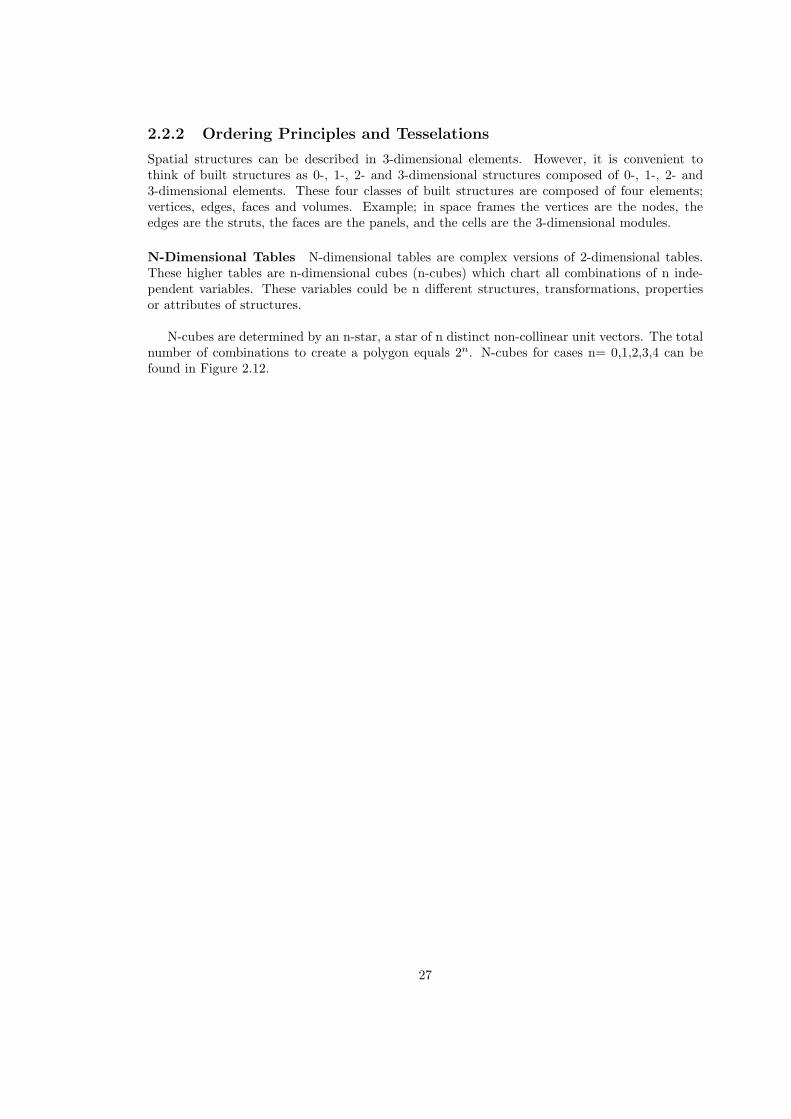
Semi Regular Tessellations A second class of planar partitioning is known as semi regulartessellations. This class requires that all polygons are regular and that all vertices be congruent,but permits the use of more than one type of polygon. There are only eight possible casesof semi regular plane tessellations, which consist of triangles, squares, hexagons, octagons anddodecagons (12 sides). One of these, consisting of triangles and hexagons, can be assembled inright - or left-handed form. Such figures, called enantiomorphs, are mirror images of one another.See Figure 2.21 (8 and 9).

1 hexagons - triangles 60-60-60

2 squares - squares3 octagon/squares - triangles 45-90-45

4 squares/triangles - pentagons (semi-regular)5 squares/triangles - pentagons (semi-regular)6 hexagons/triangles - rhombii7 dodecagons/hexagons/squares - triangles 30-60-90

8 hexagons/triangles - pentagons (semi-regular) left-handed9 hexagons/triangles - pentagons (semi-regular) right-handed10 hexagons/squares/triangles - four-sided-polygons11 dodecagons/triangles - triangles 30-120-30

32

Figure 2.16: Axes of symmetry.

Figure 2.17: Tessellation of flat plane with squares. Image from (Chilton 2000).

33

Figure 2.18: Tessellation of flat plane with rotated squares. Image from (Chilton 2000).

Figure 2.19: Tessellation of flat plane with triangles. Image from (Chilton 2000).

Figure 2.20: Tessellation of flat plane with hexagons. Image from (Chilton 2000).

34

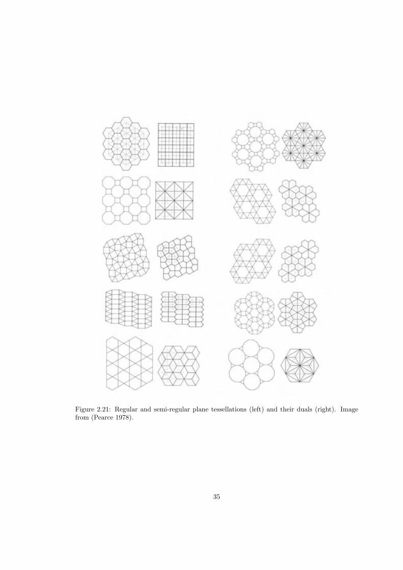
Figure 2.21: Regular and semi-regular plane tessellations (left) and their duals (right). Imagefrom (Pearce 1978).

35

Dual Tessellations The concept of the reciprocal or dual network is important in the closestpacked systems. It is also fundamental to the understanding of the properties of all spatialsystems. A dual network is formed by joining the centers of each polygon to all neighboringpolygons through the shared edges. Only one of the regular and semi regular plane tessellationsis dual to itself; the square grid. Polygonal domains will have always the same number of edgesas there are edges meeting at the vertex it encloses.

Other Tessellations When some of the conditions are relaxed an entirely new range of pos-sibilities emerges. Numerous morphology researches have been performed in the past. Whenvariation in lengths of elements is allowed a lot of other configurations are possible. Most gridconfigurations, however, look far too difficult to use in building practice because of the highnumbers of nodes and different lengths of bars. However, with the modern computer-programsit is quite easy to produce members with many different lengths and nodes without an excessivecost penalty. This is called ’mass customization’; producing huge amounts of unique products.Greg Lynn can be seen as the pioneer in the field of mass customization. His project EmbryologicHouses is an good example of this. The owner can act as a designer of his own house.

In the basic periodic plane tessellations a lot of other tessellation can be produced by placinga vertex in one region which is reflected throughout the plane. Connecting the vertices in theadjacent generates different tessellations.

A lot of different tessellations are shown; Islamic patterns, parallelogram and rectangular,zonogonal, non periodic, non periodic pattern-generation and non-convex polygons (see Figures2.22 and 2.23).

Tessellations with Regular Polygons The entire plane is filled with regular polygons butdo not require that all vertices are surrounded by equal angles. An infinite number of patternsare possible.

Tessellations and Symmetry The rotational symmetry of any figure is determined by count-ing the number of times it repeats or reproduces itself in one revolution about an axis. Onlyfour kinds of rotational symmetry are possible in the uniform subdivision of space: 2-fold, 3-fold,4-fold, 6-fold. A polygon has mirror symmetry when one side is the reflection of the other sideabout a common line which divides the polygons.

Open patterns with regular polygons If not all of the plane have to be filled and notall vertices should be congruent, open patterns emerge. With no need to fill all spaces withpolygons, it is no longer necessary that polygons are used with face angles that can be combinedsummed up to 360 degrees. There still are 360 degree at each vertex but this vertex is not entirelysurrounded by regular polygons.

Compound Tessellations and Islamic patterns Compound tessellations can be derivedfrom the basic tessellations and duals by subdividing the polygons, or through recursive subdi-visions as in polyhedra.

Parallelogram and Rectangular Tessellations Parallelogram and rectangular tessellationsare characterized by four types of centers (axes) of symmetry. Their fundamental regions areparallelograms, rhombii, rectangles or squares.

Triangular Tessellations The three basic forms of the triangles which fill space are the equi-lateral triangle 60-60-60, and the two rightangled triangles 45-90-45 and 30-60-90 (seeFigure 2.24).

36

Figure 2.22: Compound Tessellations and Islamic patterns. Image from (Lalvani 1991).

Zonogonal Tessellations All rhombii and zonogons with i ≤ n can be used as modules togenerate rhombic and zonogonal tessellations. One can use a single rhombii, but combinationsof different rhombii give more variation. See also non-periodic tessellations.

Central Tessellations Central tessellations have a single center of symmetry. The class ofsuch tessellations is infinite.

37

Figure 2.23: Parallelogram and rectangular tessellations and vertex placements. Image from(Lalvani 1991).

Figure 2.24: Triangular tessellations and vertex placements. Image from (Lalvani 1991).

38

Figure 2.25: Zonogonal tessellation. Image from (Lalvani 1991).

39

Figure 2.26: Central tessellations. Image from (Lalvani 1991).

40

Concentric Patterns with regular Pentagons Although the pentagon does not tessellatethe plane, it has the curious property that it generates infinite concentrically repeating openpatterns. Such concentric open patterns have only one axis of rotational symmetry, about thecenter of the central polygon which is the only one which shares all of its edges with otherpentagons. Because the decagon has twice as many sides as a pentagon, their symmetry propertiesare similar. In fact any regular polygon which is not divisible by 2, 3, 4 or 6 will be capableof generating concentric patterns with a center of symmetry. One exception: a regular polygonwhich is divisible by 5 can generate concentric polygons.

Figure 2.27: Concentric repeating patterns with regular pentagons with regular decagons. Imagefrom (Pearce 1978).

Non-periodic Tessellations The rhombii and zonogons have a remarkable property of fillingthe plane non-periodically. Non-periodic tessellations are of recent origin and are characterizedby lack of any translational symmetry.

Figure 2.28: Non-periodic rhombic tessellations and non periodic hexagonal tessellations. Imagefrom (Lalvani 1991).

Non-periodic Pattern-generation The method of deriving plane tessellations by vertexplacement within the fundamental region, or by subdivisions, can be applied to the rhombictessellations.

Tessellation with Non-convex polygons A special class of such polygons having equal edgescan be derived from the difference between two overlapping polygons. This produces crescent-

41

Figure 2.29: Non-periodic Pattern-generation. Image from (Lalvani 1991).

and bow-shaped polygons. It can be separated and their complementary polygons are rhombiiand zonogons. Many other, infinite, tessellations are possible.

42

Figure 2.30: Tessellation with Non-convex polygons. Image from (Lalvani 1991).

43

2.2.3 The polyhedra

Polyhedral forms are bodies in three-dimensional space. They can be used as modules that fitedge-to-edge to produce a large variety of surface structures. When the sum of angles at everyvertex is equal to 360, the surfaces are flat and are known as plane tessellations. When thissum is less than 360, the surfaces have a positive curvature at every vertex and enclose a spaceor volume. Such surfaces are polyhedra (having many faces), though strictly speaking theseare convex polyhedra. Non-convex polyhedra have a sum greater than 360 leading to negativecurvature. Convex polyhedra are composed of V vertices, E edges and F faces related by Euler’sequation V + F = E + 2.

Figure 2.31: Platonic polyhedra as bar and node or pure plate structures. Image from (Chilton2000).

Mathematicians in ancient times, before the Greek civilization, have studied and ascribed spe-cial properties to them. Crithclow (Critchlow 1980) has pointed out that Platonic solids wereknown to the Neolithic culture of northern Britain over a thousand years before Plato (427-347BC). Plato was apparently the first person to attempt a geometrical description of structure innature. He also explored the possibility of developing an inventory of basic shapes which couldbe recombined to form the five regular polyhedra.The most basic of these forms are termed the Regular or Platonic polyhedra and consist of thetetrahedron, hexahedron (cube), octahedron, dodecahedron and iscosahedron. Each of these iscomposed of similar or regular polygons. In other words; the sides of each face are the samelength and each polyhedron has faces of only one polygonal shape. By space grids the latticestructures with bars and nodes are important. However, to understand stability of three di-mensional structures in general, it is advantageous to study the behaviour of simple, regular,polyhedral shapes.Most double layer space truss geometries are based on stable polyhedral forms. When the samepolyhedra will be formed with flat plane surfaces the tetrahedron, cube and dodecahedron foundto be stable. Research has been carried out by Ture Wester at the Royal Academy of Fine Arts,in Copenhagen, into stability and structural duality of polyhedra where bars and nodes wereconnected with plates (see Figure 2.31).

44

Semi-regular Polyhedra There are 13 semi-regular polyhedra, termed ”Archimedean” solids,which use more than one type of regular polygon and which also meet alike at every vertex (seeFigure 2.33). 11 Out of the 13 Archimedean solids are formed by a process called truncation.Truncation is the process of removing all the corners of a polyhedron in a symmetrical fashion.The remaining two Archimedean solids are formed by snubbing the cube and dodecahedron.Snubbing is an interesting process which, roughly speaking, amounts to loosening all faces of apolyhedron and rotating them all slightly in the same direction (clockwise or counterclockwise),creating 2 triangles for each edge and one m-sided polygon for each vertex of degree m. Apolyhedron and its dual have the same snub(s)! If a polyhedron has k edges, its snub has 5kedges, 2k vertices and 3k+2 faces.Note that that neither the pentagon nor decagon appears in the plane tessellations and that thedodecagon, which appears in the plane tessellations, does not appear in any of these polyhedra.

Both Platonic and Archimedean polyhedra have only one vertex-type. Less regular polyhedrahave several vertex-types and can be derived from these by subdividing their faces, by projectionsfrom higher dimensions, or by other methods.

Figure 2.32: Dual regular polyhedra. Image from (Pearce 1978).

Stability To form a stable pin-jointed truss structure composed of nodes interconnected byaxially loaded bars only, a fully triangulated structure must be formed. In a three-dimensionalpin-jointed space frame, it is a necessary condition for stability. Maxwell’s Equation or Foppl’sPrinciple:

n = 3j - 6n = number of bars in the structure.j = number of joints in the structure6 = the minimum number of support reactions.

In almost all cases space frames are based on Platonic polyhedra or Archimedean polyhedraor plate structures. See Figure 2.31. Not fully triangulated structures can be made stable ifsuitable and sufficient additional external supports are provided.

Polyhedra and their duals The dual polyhedron is formed in a manner analogous to thatdescribed for the plane tessellation. However, for polyhedra the reciprocation process is somewhatmore complicated: the point perpendicularly above the center of each face of a given polyhedra

45

Figure 2.33: The 13 Archimedean polyhedra. Image from (Pearce 1978).

is joined with new edges similar points above all neighboring faces such that the new edges thatconnect these points intersect the edges of the original polyhedron, forming the edges of a newdual polyhedron. It is usually true that the respective edges of dual polyhedra perpendicularlybisect each other. Both will have the same number of edges and the inventories of faces andvertices will be exactly reversed. There is only one polyhedron self-dual: the tetrahedron.

46

Figure 2.34: The duals of the 13 Archimedean polyhedra. Image from (Pearce 1978).

47

Prisms and pyramids In addition to the Archimedean figures there are two infinite groupsconsisting of prisms and anti-prisms which correspond to the infinite number of possible polygons.A semi-regular prism is made up of two parallel regular polygons of any number of sides, connectedin equatorial fashion by square faces. The anti-prisms are like prisms except that the equatorialpolygons are equilateral triangles. The cube and the octahedron fall into both categories. Theduals of prisms are called di-pyramids (double pyramids), whose faces are congruent isoscelestriangles. The duals of the anti-prisms are called trapezohedra.

Figure 2.35: Semi-regular prisms (top) and semi-regular anti-prisms. Image from (Pearce 1978).

Convex polyhedra composed of regular polygons Triangulated polyhedra noted specialinterest because of their effectiveness as physical structures. In addition to the five Platonicpolyhedra, there are five others all bounded by equilateral triangles, although it is only in thePlatonic figures that all vertices are equidistant from a center.

Figure 2.36: Dipyramids (top), the duals of prisms (top) Trapezohedra (down), the duals ofantiprisms. Image from (Pearce 1978).

48

Figure 2.37: The convex deltahedra. b: Triangular dipyramid. d: Pentagonal dipyramid. e:12-hedron. f: 14-hedron. g: 16-hedron. Image from (Pearce 1978).

Families in Polyhedra There are four families of polyhedra; the first is an infinite of prismswith general symmetry. The remaining three families correspond to the three regular polyhedraand are the tetrahedral, octahedral and icosahedral families. Each family has polyhedra withmirror-symmetry and rotational symmetry, and regular and semi-regular polyhedra belong tothese four families.

Figure 2.38: Three families of polyhedra: tetrahedral, octahedral and icosahedral, the last twofamilies are here turned into n-stars. Image from (Lalvani 1991).

In the field of polyhedra a lot of research has been done which goes far beyond the goal ofthis reader; for instance curved polyhedra, saddle polyhedra, Kepler-Poinset solids etc.

Simple polyhedra could be combined together in a system to produce a higher-dimensionaltable: a space frame.

49

Zonohedra and Rhombohedra Zonohedra are polyhedra with parallelogram faces and area natural extension of the zonogons described before. A three-dimensional zonotope is called azonohedron. The method of derivation is the same, the one difference being that the n-star isspatial and can be derived from vertex directions to the center of any symmetric or arbitrarypolyhedron. The number of vectors, n, is determined by the number of non-collinear vertices.Zonohedra provide alternative geometries for space structures that define architectural space.The octahedral and icosahedral families (see polyhedra section) each produce seven distinct starswith the following values of n: 3, 4, 6, 12, 12, 12, 24 and 6, 10, 15, 16, 30, 30, 30, 60.

Consider any star of n line segments through one point in space such that no three linesare coplanar. Then there exists a polyhedron, known as a zonohedron, whose faces consist ofn*(n-1) rhombii and whose edges are parallel to the n given lines in sets of 2 ∗ (n − 1) ∗ [i]Furthermore, for every pair of the n lines, there is a pair of opposite faces whose sides lie in thosedirections (Coxeter & R.W.W.Ball 1947). A zonohedron is therefore a polyhedron in which everyface is centrally symmetric (Eppstein 1996).

From the n-stars, zonohedra can be derived from all distinct i-stars (i ≤ n) which determinetheir edge directions. They are the shells of i-cubes (or i-cells), and all its faces are rhombii(i=2). All zonohedra can be decomposed into 3-dimensional building blocks or 3-cells, termedrhombohedra (i=3), which are regular cubes in higher dimensions. Rhombohedra and zonohedraare cells or space fillings. Polyhedra from different symmetry classes generate their own set ofrhombohedra.

50

Figure 2.39: The dodecahedron has 5 rhombohedra from two types of rhombii, 7032’ and 4149’,and the icosidodecahedron has fourteen types of rhombohedral cells from four types of rhombii90, 72, 60, 36. Image from (Lalvani 1991).

Figure 2.40: Vertex placements. Image from (Lalvani 1991).

51

Figure 2.41: Edge combinations. Image from (Lalvani 1991).

Figure 2.42: The fundamental regions of a single rhombohedron, a cube in higher space, areshared. Image from (Lalvani 1991).

52

Figure 2.43: Seven polyhedra of octahedral symmetry corresponding to one cube. Image from(Lalvani 1991).

53

2.2.3.1 Generation of Polyhedra

The method of subdividing polygons can be applied to the faces of polyhedra to generate newpolyhedra. Just like polygons were added to other polygons, polyhedra can be added to otherpolyhedra to generate new polyhedra. There are two possible methods; vertex combinations andedge combinations.

2.2.3.2 Divisions of spherical surfaces

Besides the Recursive Surface Subdivisions there are other divisions possible. When the demandis made that the space frames must consist of (stable) triangles only three polyhedra will do:tetrahedron(4), octahedron(8), icosahedron(20). Other polyhedra must be subdivided in trian-gles, where every summit of the triangles must lay on the defined sphere, before they can beused.

Class I The Platonic polyhedra are subdivided in smaller triangles.

1. Tetrahedron

2. Octahedron (useful horizontal and vertical connections)

3. Icosahedron (easy to split in two parts with even division frequencies)

Figure 2.44: Triangles of frequencies 1 to 4 (top) and minimal triangles. Image from (Lalvani1991).

Regularity of division As can be seen in Figure 2.46 a subdivision there is needed for the curvedpolyhedron-edges. Mostly one of the two following methods is used: (also see Figure 2.47)

• Method I. Equal pieces on a straight line. Projected on the sphere. The subdivision intriangles can be found by connecting the points on the edges of the polyhedra triangle.

• Method II. Equal sizes on a curved line, the centers of the small triangles are used to createfurther subdivision

Both methods use geodesic lines, which is the shortest distance between two points on a curvedsurface.

Recursive Surface SubdivisionsPolygons and polyhedral faces can be subdivided again and again to produce infinite classes offiner subdivisions of a surface. For structures of a fixed size, this produces finer meshes and on

54

Figure 2.45: Division of spherical surfaces Class I Method I. Image from (Lalvani 1991).

Figure 2.46: The tetrahedron, octahedron and icosahedron can be converted into a sphere byusing the minimal triangle. Image from (Knebel & et al. 2002) (Huybers & Ende 1994).

Figure 2.47: Two methods for the subdivision of polyhedron-edges and surfaces. Image from(Huybers & Ende 1994).

the other hand, for elements of a fixed size, larger and larger structures can be produced. Thegeodesic dome of Fuller is an example, and is based on special subdivisions of the triangular facesof a tetrahedron, octahedron or the icosahedron. These subdivisions are described in terms offrequency, the number of times the edge of the polygon, and hence a polyhedron, is subdivided.When the vertices are found by subdivision, a pattern can be made with connection-lines. Alsohere there are two possibilities.

• Triangular pattern; many different triangles needed

• Hexagons and pentagons, 12 in a whole closed sphere, combination of the triangles

The Fuller DomeThe basis of the Fuller dome is either the Iscosahedron or the Dodecahedron. The two polyhedra

55

have to be placed as ”duals” with respect to the centre of the sphere. The corners of the verticesof the icosahedron in the resulting network can be recognized by their pentagonal symmetry andthey correspond with the midpoints of the dodecahedron’s faces. The so-called ”characteristic”triangle is defined by the icosahedron point I2, the dodecahedron point D1 and the icosahedron’sedge midpoint DI-1’ projected on the surface of the sphere (see Figure 2.48). This triangularsurface is the smallest symmetry part of the whole spherical network. It is also called after Fulleras the ”lowest-common-denominator-”or LCD-triangle.It is possible to subdivide the spherical surface in 120 minimal symmetry parts. The actualspecifications of geometric and connectivity properties of the whole network can be reduced tothis minimal triangle.

Figure 2.48: Generation of the Fullerdome. Image from (Knebel & et al. 2002).

In nature many domes can be found. The most expressive is the Bucky ball also called afterBuckminster Fuller: ”Fullerenes”. These Fullerenes are large carbon-cage molecules. By far themost common one is C60 in morphology called the truncated icosahedron.

Fullerenes cages are about 7-15 angstroms in diameter ,which is around a billionth of a meter,or 6-10 times the diameter of a typical atom. On molecule level they are used to create nanotubes.

Another remarkable comparison can be made with the Volvox: a freshwater colonial proto-zoan. Volvox are spherically organized colony of several hundreds to several thousands smallerelements.

56

Figure 2.49: Volvox. Image from (Pearce 1978).

57

Class II An equilateral triangle can be subdivided in 6 by perpendicular lines. The icosahedroncan be divided in 120 equal parts. Rhomboids are formed by connecting these right-angledtriangles. Subdividing these many different divisions can be made.

1. Cubic (regular rhombic)

2. Rhombic dodecahedron

3. Rhombic triacontahedron

Figure 2.50: Class II and III and their subdivisions. Image from (Huybers & Ende 1994).

Figure 2.51: Other basis divisions of spheres. Image from (Huybers & Ende 1994).

Class III A division called ’skew networks’, based on twisted snub solids (see Figure 2.50).

Class IV (see Figure 2.51)

1. Meridians and parallelcircles (’orange peel’)

2. Schwedler

3. Lattice dome

58

2.2.3.3 Space Fillings

Space filling means the combining of similar or complementary bodies in a three-dimensionalpacking continuously repeated, in such a way that there is no unoccupied space. Space fillingsare space structures composed of 3-dimensional modules that fit face-to-face to fill space. Theyare similar to plane tessellations where polygons fit to fill a plane. Rhombohedra, prisms andvarious other polyhedra are units of corresponding space-fillings. Same as in the 2-dimensionalcase there are three different types of fillings; periodic, central and non-periodic. Applications inarchitecture include the use of multi-layered or multi-directional geometries for space frames, or3-dimensional habitats to live in.

Close packings of polyhedra form space-fillings, their edges define space grids. These spacegrids form the basis of architectural space frames. In fact they are the skeleton of the spacestructures.

Dihedral Angle The dihedral angle is the angle formed between the planes of two adjacentpolygons, the angles taken in a plane perpendicular to the common edge. All of the dihedralangles for each of the regular polyhedra are equal. However, of the semi-regular polyhedra,only the cuboctahedron and the icosidodecahedron have equal dihedral angles. There are nineArchimedean figures with two dihedral angels and two which have three. The dihedral angle willbecome quite important as the problem of space fillings is considered (Cundy & A.P.Rollett 1961).

Figure 2.52: Dihedral Angle. Image from (Pearce 1978).

Periodic Space Fillings The cube is the only Platonic polyhedron that will repeat tofill all space. It is the most symmetrical variation on the infinite class of three-dimensionalfigures known as parallelepipeds. The parallelepipeds are prisms whose bases and sides areparallelograms; they are, therefore, six faced polyhedra. The subdivision of space by means ofcongruent parallelepipeds may be characterized in terms of six symmetry classes or systems.These classes form six of the seven crystal systems of crystallography. The seven crystal classesrely upon various combinations of 2-fold, 3-fold, 4-fold and 6-fold or no rotational symmetry.

59

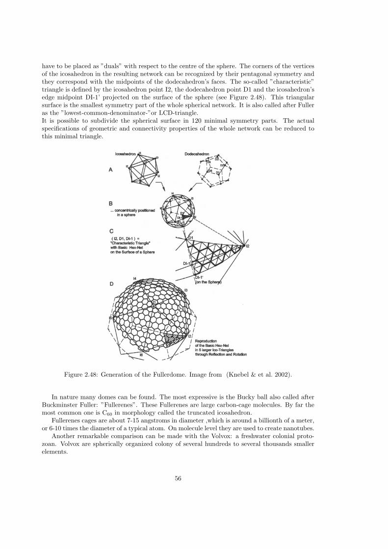
Together they provide a descriptive scheme of space partitioning.As already said the cube is the most symmetrical, it has the greatest number of symmetryaxis. A cube has three axes of 4-fold symmetry, four axes of 3-fold symmetry and six axesof 2-fold symmetry. Ranking by the total number of symmetry axes of each class: (see Figure 2.53

1. Cubic - 13 axes (a)

2. Hexagonal - 7 axes (g)

3. Tetragonal - 5 axes (b)

4. Orthorombic - 3 axes (c)

5. Trigonal - 1 axis (d)

6. Monoclinic - 1 axis (e)

7. Triclinic - no symmetry axis (f)

Figure 2.53: The seven symmetry classes. Image from (Pearce 1978).

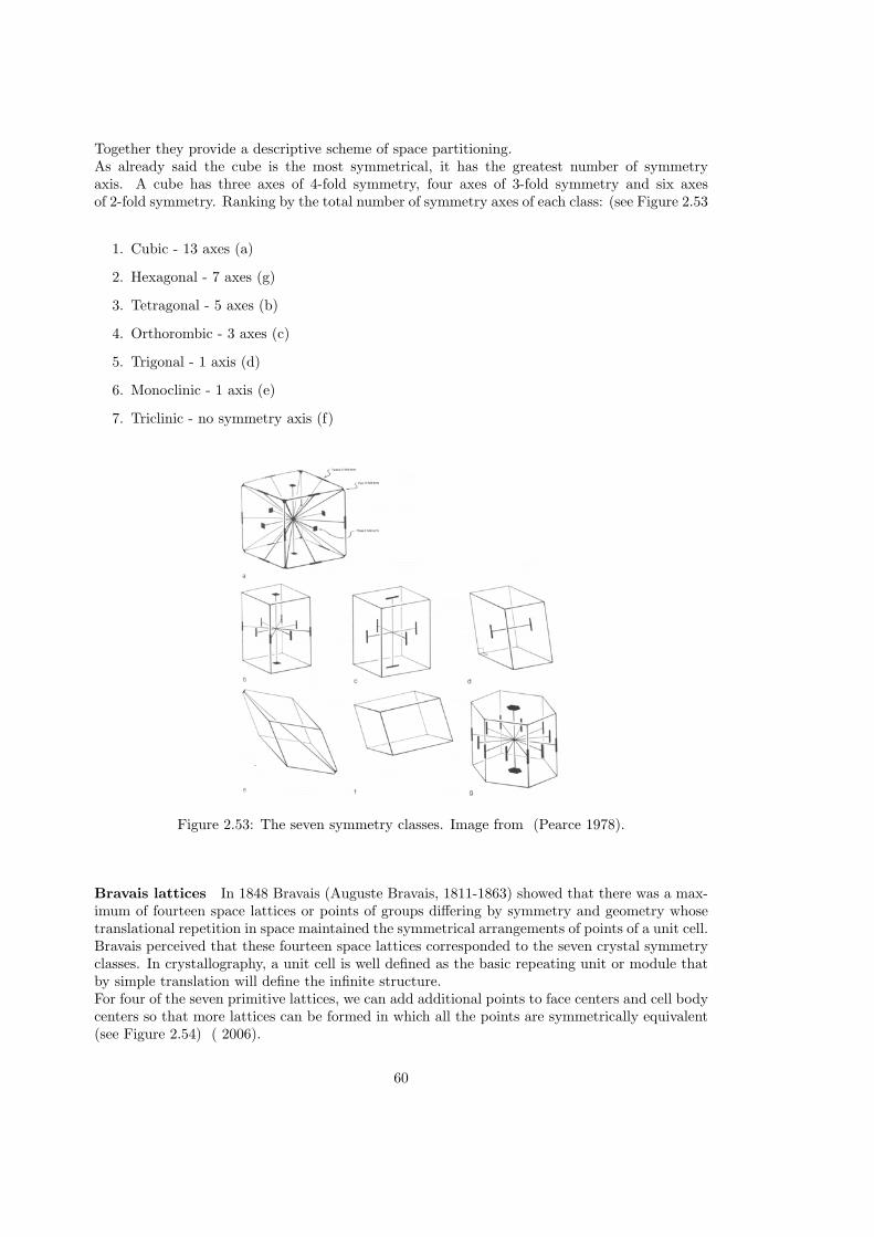
Bravais lattices In 1848 Bravais (Auguste Bravais, 1811-1863) showed that there was a max-imum of fourteen space lattices or points of groups differing by symmetry and geometry whosetranslational repetition in space maintained the symmetrical arrangements of points of a unit cell.Bravais perceived that these fourteen space lattices corresponded to the seven crystal symmetryclasses. In crystallography, a unit cell is well defined as the basic repeating unit or module thatby simple translation will define the infinite structure.For four of the seven primitive lattices, we can add additional points to face centers and cell bodycenters so that more lattices can be formed in which all the points are symmetrically equivalent(see Figure 2.54) ( 2006).

60

• Cubic (3 lattices)

• Tetragonal (2 lattices)

• Orthorhombic (4 lattices)

• Hexagonal (1 lattice)

• Trigonal (1 lattice)

• Monoclinic (2 lattices)

• Triclinic (1 lattice)

Federov (1880) and Schoenflies (1891) determined independently that the 14 Bravais lat-tices maximally generate 230 space groups. For complete descriptions see Chalmers (Chalmers,Holland, Jackson & Williams 1965).

61

Figure 2.54: Bravais lattices. Image from (Pearce 1978).

62

Space Filling Polyhedra Among the Archimedean polyhedra and in the infinite family ofprisms and anti-prisms there are exactly three space fillers: the truncated octahedron, the hexag-onal prism and the triangular prism. Of the thirteen Archimedean duals, only the rhombic do-decahedron will fill all space. Both the rhombic dodecahedron and truncated octahedron havefull cubic symmetry. Symmetry is not the only factor that allows us to discover candidates forspace filling. Another factor is the complementary of adjacent dihedral angles. In a space fillingarray of polyhedra the dihedral angles formed by faces meeting around a common edge must sumto 360. This is equivalent to the requirement of 360 around each vertex of plane tessellation.

Figure 2.55: Space fillings: Triangular prisms, hexagonal prisms, cube, rhombic dodecahedronand the truncated octahedron. Image from (Pearce 1978).

The tetrahedron and octahedron space filling Because the octahedron is the dual of thecube, it has the same symmetry. However, it will not space. Although the symmetry is there, itsdihedral angel of 10928’ makes it impossible for the octahedron to pack with itself to occupy allof space. In combination with the tetrahedral it forms a fully triangulated network, which in turndescribes a space filling array of these polyhedra. In fact it is a face centered cubic (Bravais).Octahedra and tetrahedra will space when packed 1:2. See figure. The result is a space fillingparrellelpiped with six rhombic faces with angels of 120 and 60. The dihedral angel of thetetrahedron is 7032’, which is compatible with the 10928’ dihedral angle of the octahedron.The tetrahedron is less symmetrical than the octahedron (or cube). It has four axes of 3-foldsymmetry and three axes of 2-fold symmetry.

63

Figure 2.56: Tetrahedron-Octahedron space filling. Image from (Pearce 1978).

The icosahedron and dodecahedron space filling The icosahedron and the dodecahedronare dual to each other so they have the same symmetry. The icosahedron is the most symmetricalof all possible polyhedra. It has six 5-fold axes, ten 3-fold axes and fifteen 2-fold axes. The icosa-hedron has twenty equilateral triangular faces. There is no convex polyhedron with more than20 identical regular faces. But both will not fill space. The dihedral angles of the dodecahedronare 11634’ which can not fill a space.

Regular and semi-regular Polyhedra as multiple space fillers Of the Archimedean andPlatonic figures there are altogether nine polyhedra that qualify as candidates for multiple spacefilling systems. In a larger class of semi-regular polyhedra, which includes prisms as well as theArchimedean figures, a look at the semi-regular plane tessellations reveals which of the prismswill qualify for multiple space filling. Triangles, squares, hexagons, octagons and dodecagonsare the polygons that can be combined in various arrangements to form a plane tessellation.This forms the basis for the prisms with square sides. There are eight multiple-prism (from thesemi-regular tessellations) space filling systems.The multiple space fillings can be classified according to how many different types of polyhedrathe system requires. A space filling consisting of one type of polyhedron is called a unary, two -binary, three - ternary, four - quaternary. Systems with more than four types of polyhedra cannot be composed.The first requirement of multiple space filling is that different polyhedra must have matchingparallel faces in common. Of the Platonic and Archimedean figures there are nine polyhedra thatqualify as candidates for multiple space filling systems. There are eleven space filling possibilitiesutilizing these Archimedean and Platonic polyhedra.

Dual Space Filling Following from the definition; if all vertices in a space filling array arecongruent, the dual network will form a unary space filling system composed of a single kind ofpolyhedron. If there is more than one kind of vertex in a space filling structure, its dual spacefilling will be composed of as much different kinds of polyhedra as there are kinds of vertices.The 23 space filling systems consisting of regular and semi-regular polyhedra give 20 unary spacefillings, while three systems have dual space filling systems which are also comprised of regularand semi-regular polyhedra. In total 20 new polyhedra are formed with the dual space filling

64

systems.

Central Space-Fillings Central Space-Fillings have one clear center. However central space-fillings whuch use single rhombohedra give nice forms it is doubtful if they are interesting for(kinetic) space frames.

Figure 2.57: Central space filling with a single rhombohedron, hexacontrahedral star (n=6) withicosahedral symmetry. Image from (Lalvani 1991).

Non Periodic Space-Fillings These fillings work with the non-periodic tessellations andconsist of rhombohedra, zonohedra (and affine polyhedra). It results, just like the tessellations,in rather difficult fillings. A simple example is given in Figure 2.58.

Stellated polyhedra There is a very large class of nonconvex uniform polyhedra. They areloosely referred to as Stellated polyhedra (H.S.M.Coxeter, Longuet-Higgins & Miller 1954).

Loose-Packings Loose packings are a class of orderly structures which cover all space butleave empty spaces in-between. An easy way is to remove cells from the closest packings leavingholes in various places. The space becomes a sponge. Another way to create a loose-packing iswith the polyhedra placement method.

65

Figure 2.58: Non periodic space fillings. Image from (Lalvani 1991).

66

2.3 Analogies between structural engineering, physicalmodels and natural structures

It is useful to discuss analogies in general before covering techniques, such as physical modellingand learning from nature. Analogies are traditionally used in arguments; explaining a specificcase by drawing attention to the similarities with another, mostly better understandableexample.Every analogy between two dissimilar cases have something similar. The more similarities twocases have, the stronger the analogy is. Some people will focus on the dissimilar parts, whileothers focus more on the similar parts. Both ways of dealing with analogies are needed to makeuse of an analogy in a proper way. Find inspiration and stimulation in the parts in which thetwo cases overlap, but keep in mind that it is an analogy, and in that way it is not possible totreat the cases like they are similar. One has to distinguish the similarities and the dissimilarities.

For example; a tree is a beautiful natural structure and in some aspects it can be anuseful inspiration source for man-made structures. The fact that a tree divides the available‘building material’ as optimal as possible over its structure, is an useful principle. On the otherhand; saying that a tree-structure as a whole can function as a good example for a buildingstructure, would be making a doubtful statement. The main function of a tree is collecting asmuch energy as possible. A tree with its branching branches is well adopted to fulfill this task,however which man-made structure has the same purpose? Instead of copying nature we haveto focus on the principles which form the basis of natural structures.

The example of the tree demonstrates the fact that an analogy between two cases isnever valid for 100%. Nevertheless it is interesting to look for analogies between physical models,structures in biology and structural engineering. The potential usefulness of such analogies liesin the way in which our awareness of remarkable and, to us, novel examples of structures inbiology can stimulate our own design imaginations. In short, ‘we are engaged in an exercise of“inter-disciplinary cross-fertilization of ideas”, which seems one of the key characteristic for thedesign of special structures’ (Calladine 1998).

2.4 Physical Modelling

Physical modelling techniques are manual techniques to model certain characteristics ofstructures. ”Physical” refers to the distinction with ”Virtual” or ”Computational”, which aretechniques to model characteristics of structures in computer models and applications.Model building is often viewed upon as ”child’s play” until the architect, engineer or studentsattempts to build his or her first models. Physical modelling is a technique is are easy accessible,but on the other hand different to execute and control properly. Deriving the correct conclusionsfrom physical modelling is an art.This section introduces several of the basic techniques for model building. The best way to learnhow to make and control these techniques is to attempt building these models at home, basedon earlier written down hints and tips, such as in the IL series (published by the Institut furLeichtbau Entwerfen und Konstruieren).

Model building One special technique is model building. With model building the builderstudies the shapes, grids, etc. by making a physical model. An example of this are the foldedpaper models of Huybers (see Figures 2.59 and 2.60) and various other builders (see Figure 2.61).

67

These models can be used for study and formulas can be derived from these models (Huybers &Ende 1994) (Huybers 2000b). Finally entire structures can be studied with these techniques.

Figure 2.59: Models built by Pieter Huybers.

Figure 2.60: A study of stacking regular shapes. Models by Pieter Huybers.

68

Figure 2.61: Some shapes from the field of Structural Morphology.

69

There are many techniques, too many to discuss all and for each structural type or topol-ogy at least one or more techniques often exist. Before a structural engineer starts building amodel, it is a good idea to first research existing techniques, since often model building can bequite complicated when inexperienced. Cattan(Cattan & Reissig 2000) provides an interestingclassification model for built models for structural morphology.

Tekkit is an example of such a model building material, which can be seen in Figure 2.62, forbuilding space trusses.

Figure 2.62: A model in Tekkit.

Another system, which can be seen in Figure 2.63, is the model building material of the Merospace trusses system.

Figure 2.63: Mero model material.

70

2.4.1 Catenaries

The catenary form has been used by famous architects, such as Gaudı, to find the shape oftheir buildings. Because the catenary form follows the tension line for gravity, it is very suitableto design masonry structures when inverted. However, for these masonry structures the deadweight of the brick has to be dominant over other loads, such as the overturning moments andshear-forces of the wind, or unequal loading due to snow for instance. Usually this is the case forthe buildings of architects like Gaudı. The catenary form can be easily derived from mechanics.Figure 2.64 shows the geometry of the catenary.

Figure 2.64: The earliest presentation of a tensile-stressed suspended model describing the load-bearing behaviour of a compressive stressed vaulting structure by Giovanni Poleni (1748), usedto check the stability of the dome of St. Peter’s in Rome. Image from (K. Bach 1988).

As a first step the hanging chain under a equally distributed load can be considered. Thetheoretical shape for a hanging chain under a distributed model is the parabola ().

q = −Hd2w

dx2(2.12)

Equation 2.12 shows the differential equation for a cable under an equally distributed load.When integrated twice, in Equations 2.13 and 2.14, the parabola follows as the shape for anequally distributed shape.

71

dw

dx=

−qHx+ C1 (2.13)

w(x) =−2q

Hx2 + C1x+ C2 (2.14)

From w(0) = 0 and w(L) = 0 follows that:

forw(0)=0 : C2 = 0

w(l)=0 : C1 = 2qlH

(2.15)

w(x) =2q

H(l − x2) (2.16)

However, this model is too simple for the hanging chain hanging under its own weight. Sinceit cannot be assumed that the load is equally distributed, an alteration has to be made to themodel. Equation 2.17 and 2.18 describe the new model.

qx = q0

√

1 + (dy

dx)2 (2.17)

dy

dx=Vx

H=

∫

pxdx

H(2.18)

These can be resolved to Equation 2.19 for the catenary in parametric form.

x(t) = ty(t) = a cosh( ta) (2.19)

Figure 2.65: Funiculars of a semi-circular, a parabola and a catenary arch.

2.4.2 Hanging Models

As stated before Antonio Gaudı used the principle of hanging models intensively. When a hangingmodel is turned upside down a pure compression model arises. Figure 2.65 shows the funicularof a semicircular, a parabola and a catenary arch. The catenary arch is the optimised structurefor the self weight of the structure.

The parabola is the optimised shape for an equally distributed load. Figure 2.130 a showsa hanging model. As a result of its structural principle, the form of a suspended model isself-forming and is capable of transfering its own weight and area load distributed according tothis, solely by means of tension. The grid shell (Figure 2.130b) is the inverse structure of thehanging model and is thus loaded by pure compression. Nevertheless, when unequally distributedloads occur in addition, as is the case with snow or wind loads, the initial coincidence betweenthe structural task and the form is no longer given. The bending stresses and deformationswhich occur result in a form which is less favourable for the transmission of forces - in particular

72

Figure 2.66: Model geometry used to model hanging lines.

with regard to snow loads in the softly curved apex area (Figure 2.130c). The form can be raisedin its apex by adding small weights to the suspended model (Figure 2.130d). The deformationwhich occurs gives the shell a more suitable form for load transmission. The hanging model canalso be adjusted for wind loads (K. Bach 1988).

Gaudı used hanging models to determine the configuration of his buildings. Brick experimentsto determine a slender structure are time-consuming and difficult, where hanging models (cate-naries) show many similarities to brick compression structures, expect that where in catenariestension is the most important force, compression is the most important for brick structures.Both structures also are less good for bending forces, however the dead weight of the masonrycompensates the bending forces for most buildings because of their limited height and/or span.By adjustment and observation Gaudı could make various configurations.

Figure 2.67: Two hanging models by Gaudı. Image from Williams.

Some models which have survived the ages can be seen in Figure 2.67, 2.68 and 2.69. Gaudıcreated the Sagrada Familia, the Guell crypt and several other buildings using these techniques.

73

Figure 2.68: Hanging model by Gaudı. Image from (i Armengol 2001).

Figure 2.69: Hanging models by Gaudı.

74

Hanging chain models Probably the most famous form finding techniques are the hangingchain and hanging net models, made famous by Antoni Gaudı. The hanging chain is a linearelement which finds it equilibrium shape, the catenary line, caused by its own dead weight andgravity. There are many techniques for building these models. Many materials can be usedfor modeling: rope, small chains, large shackeled chains, paperclips, etc. It is possible to hangweights, in the form of simple weights, small sand bags, etc. to simulate the loads on a structure.With pulleys it is possible to simulate loads in the other direction too.Photographing these models and inverting them shows the pressure line for the load, as shownin Figure 2.70 and 2.71. In Section 2.4.1 the mathematical formulation of catenaries is covered.

Figure 2.70: Hanging chain model.

Figure 2.71: Hanging chain model upside down to find the pressure shape.

Hanging net models Hanging net models are very simular to hanging chain models,except that they are three-dimensional nets built from individual linear chains instead oftwo-dimensional chains. Figure 2.72 shows a hanging net model built from paperclips.

Figure 2.72: A hanging paperclip model.

In IL10 (Bach 1974) basic characteristics for hanging nets are given:

75

• The nets are self-forming: they form themselves without external manipulation.

• The nets are unique: they form only one configuration.

• The nets form an equilibrium configuration.

IL10 (Bach 1974) also covers the building of hanging net models and their various purposes:architectonic, form finding models, test models for determining geometry and for determiningforces. The book also covers good model photography and measuring the forces.

2.4.3 Soap Film Modeling

Soap films find the equilibrium shape of a minimal surface between preset (closed) boundaries.The soap film is often made from a special mixture which is stronger than normal dishwashingsoap so that it lasts longer and forms easier. Pustafix is a good soap to use.Many phenomena can be modeled with soap films. Two main directions can be derived: the usefor membrane structures and shells, where usually only the minimal surface between set bound-aries needs to be found and the use for pneumatic structure, where by applying an overpressurein the soapbubble an internal (pneumatic) load is created to drive the forming process. In thismanner not only minimal surfaces can be found.Note that soap film models are very good for studying shapes and finding minimal surfaces, butit is not possible (or hardly possible) to measure forces, stresses, shapes, etc. directly from themodel. Of course, photographing and analysing solves some of those problems.For more indepth theory on the subject of soap film modeling, refer to ”Seifenblasen” (Bach,Burkhardt & Otto 1987) or ”Tensile structures” (Otto 1973). These explain why soap bubblesalways come together with three ’surfaces’ in one ’node’ in a two-dimensional plane and why theangle between it is always 120 degrees. Also more background theory is given about minimalsurfaces and minimum energy shapes, which soap films are.

76

Figure 2.73: Soap bubbles. Image from (Otto 1973).

77

In Figure 2.74 and 2.75 two complex boundaries can be seen with their soap film minimalsurface. The soap film forms the minimal surface between the wireframe.

Figure 2.74: Soap film model.

Figure 2.75: Soap film model.

In Figure 2.76 the analogy between a soap film hypar (hyperbolic paraboloid) and its struc-tural counterpart is shown. The relationship of the shape is clear. The soap film finds the optimal(equilibrium) shape according to which the structure can be build.

78

Figure 2.76: Soap film model. Image from (Bach et al. 1987).

79

For pneumatic structures the soap film is blown in a certain shape possibly with a closed presetboundary. The overpressure in the soap bubble again forms an equilibrium, but not necessarilya minimal surface. The possible shapes for pneumatic structures can be studied in this manner.In Figure 2.77 an example of this can be seen.

Figure 2.77: Soap film model. Image from (Bach et al. 1987).

In Figure 2.78 a soap bubble with increasing overpressure on the inside can be seen in itsdifferent stages.

Figure 2.78: Soap film pneumatic model. Image from (Bach et al. 1987).

80

In Figures 2.79 and 2.80 two examples are given of pneumatic soap films which are createdon an edge. Note that the soap films are not one piece, but consist of various compartments,with the angles explained in the references (see also Section 2.5.2).

Figure 2.79: Soap film pneumatic model.

Figure 2.80: Soap film pneumatic model.

81

2.4.4 High elasticity membranes or fabrics

In Figure 2.81 a panty model is shown, which is an example of a high elasticity membrane (fabric)model. Prestressed panties have an analogy with prestressed membranes. Although the materialand the scale is different, aspects can be studied of the panty model, such as the curvature relatedto the stiffness of the membrane (more curvature usually means more stiffness) by pressing andfeeling the fabric and the forces.

Figure 2.81: Two prestressed pantymodels.

A pneumatic structure can be modeled in more or less the same way as a membrane structurewith the main difference that an overpressure inside the model must ’blow’ the model in acertain direction. Instead of using panty fabric or other fabrics, it is possible to use a highelasticy membrane which is air tight, or lets very little air trough. In this manner it is possibleto simulate the behaviour of the pneumatic structure in a model. Note however that is very hardto scale down the model and the parameters appropriate, and that it might be better to use suchmodels only in shape studies. Figure 2.82 shows an example of a pneumatic model.

Figure 2.82: Picture of the physical pneu model. Image courtesy of P.C. van Hennik.

82

2.4.5 Wet-cloth models

Another technique of making models for membranes and when inverted for shell structures, isthe use of wet cloth. The heavy of moist cloth will approximate the equilibrium shape.Various techniques exist to make inversion of these models possible to structure shells: freezing,plastering, glueing, etc. Heinz Isler made very thin shells in this manner.Figure 2.83 shows an example of a hanging cloth model which was strengthened with plaster.

Figure 2.83: Inverted hanging cloth model, strengthened with plaster. Models by P.C. vanHennik.

83

2.5 Biomimetics

One of the oldest methods of finding form is to learn from nature and imitate its structuralbehavior. Many examples can be given of optimal structures in nature, since nature has itsown optimising law, the Darwinian law of survival of the fittest (Darwin 1859) and evolutionresulting from it. For many ’structures’ in nature gravity is an important load and the structuresare optimised accordingly. Not always is gravity or optimisation the main reason we can learnfrom nature, sometimes the shapes themselves are inspiring for architects and engineers.

A seasoned structural engineer can distinguish many structural principles in nature. With hisknowledge about structural engineering he is able to understand structural principle in nature.It is generally accepted that nature is adopting itself by evolution to its ever changing sur-rounding (Darwin 1859). Not the principles of Evolution and Growth themselves are useful forstructural designers, but the results of these, the optimised natural structures, are. They canfunction as an inspiration for structural design.Although the learning-curve of man-kind is much steeper than that of nature (it may sound a bitstrange to place man-kind opposite to nature, man-kind is of course a product of evolution itself),we can still not compete with the solutions nature found in the struggle to survive. Nachtigallused his own words to express a similar thought (Nachtigall 2001):

Die Natur hat uber Jahrmillionen Erfindung auf Erfindung geturmt. Deshalb erinnert

der Erfinderwettstreit zwichen Mensch und Natur ein wenig an den Wettlauf zwischen

dem Hasen und dem Igel.

Sir D’Arcy Thompson discussed in his work ‘On Growth and Form’ (Thompson 1942) manynatural structures. For example the analogy between the back of a horse, which has to carry theself-weight and the principles of bending of a beam. There are direct similarities between themuscles and bones of animals and the tension and pressure elements of a bridge. On cellularlevel similar analogies exist. The buckling of a microtubule in a cell that is about to divide isessentially the same as the buckling of an elastic bar at a much larger scale (Calladine 1998).For most of the structural engineers the analogy of the back of a horse and a structural beam ismuch clearer that the latter analogy, nevertheless it is possible to find analogies between natureand structural design on different scales.

Famous examples of learning from nature as a form finding technique. Antoni Gaudıis well-known as an architect and structural engineer who learned from nature. Many of hisbuildings show a strong relationship with nature.The Institute for Lightweight Structures of the University of Stuttgart has made many studies ofnature in relationship to structures and building in the period 1970-1990 which are reported invarious books (Bach 1971), (Bach 1973), (Bach 1975). Below some fields of which can be learnedwill be discussed with references to more detailled information.Whalley (Whalley 2000), director of Nicholas Grimshaw & Partners describes the important ofnature for the Eden project and how they have learned from nature to create the shape of thestructure.

2.5.1 Types of analogies

To place the natural structures in their context it seems useful to start with an investigation ofstatical natural structures (deployable structures will not be covered in lecture notes). It shouldbe noted that this section can not and does not offer an exhaustive listing and description of allexisting natural structures.

• Statical natural structures

84

– cellular structures

∗ honey combs

∗ bone structure

– branching and tree structures

∗ tree structures

∗ leaf structures

– skeleton structures

– web structures

– sea shell and radiobria

– biomechanical structures

• Deployable and retractable structures

2.5.2 Cellular structures

In their books Gibson and Ashby and D’Arcy Thompson have covered the subject of cellularstructures, and structures built from cellular or cell-like material, either natural or artifi-cial (Gibson & Ashby 1997) (Thompson 1942).In 1917 D’Arcy Thompson explains, partly in a mathematical manner, the forms of cells, whichare minimal surfaces. He explains minimal surfaces for various forms, cell types and dropletsof water. In another part he extensively explains the clustering of bubbles, minimal energysurfaces and their hexagonal formed minimal shape.

Surface-tension is the leading parameter for the relative orientation of cells. The effect ofthis surface-tension will manifest itself in surfaces minimae areae. The underlying principleof surface-tension is described as follows; The part of the total energy available in a certainsystem, which is ’located’ at the surface, is called the surface energy and is proportional tothe surface of contact between the system and its surrounding substances. Each boundarybetween two substances has its one particular property. The surface energy is also proportionalto this particular property. Equilibrium, which is the condition of minimum potential energyin the system, will accordingly be obtained by the utmost possible reduction of the surfaces incontact (Thompson 1942).With this principle Thompson explains the forming of thin films of oil on water and small dropsof water on tree leaves. Based on an old seventeenth-century theorem, called Lamy’s Theorem:

”if three forces acting at a point be in equilibrium, each force is proportional to the sine

of the angle contained between the directions of the other two.”

P

sinφ=

R

sin ρ=

S

sin ς(2.20)

where P , R and S represent the forces in the partition walls acting on the intersection pointof the working lines of the three forces; φ is the angle between R and S; ρ is the angle betweenP and S and ς is the angle between P and R.Lamy’s Theorem describes a closed (force) triangle. The Cosines Rule is used;

P 2 = R2 + S2 − 2RS cosϕ

R2 = P 2 + S2 − 2PS cosα

85

S2 = P 2 +R2 − 2PR cosβ (2.21)

In Figure 2.84 the used forces and angles are shown.

Figure 2.84: Relation between Lamy’s Theorem and the Cosines Rule.

Because;

− cos(ϕ) = +cos(−ϕ) = +cos(2π − ϕ) (2.22)

and

2π − ϕ = φ (2.23)

Equation 2.21 becomes;

P 2 = R2 + S2 + 2RS cosφ, etc. (2.24)

Equation 2.24 shows clearly that the angle between three equal substances must be 120°. Aslong as there is no difference in external pressure applied. And of course the sum of the threeangles must be 360°.

Figure 2.85: Three situations (a) P = R >> S; (b) P = R and S is a little smaller; (c)P = R = S.

According to Gibson and Asby, a cellular solid is made up of an interconnected network ofsolid struts or plates which the edges and faces of cells. There are several typical structures,

86

such as the two-dimensional honeycomb, the three-dimensional foam with open cells and three-dimensional foam with closed cells (see Figure 2.86).They derived that there are several cell shapes (see Figure 2.87, 2.88 and 2.89).

Figure 2.86: Different types of cellular structures. Image from (Gibson & Ashby 1997).

Figure 2.87: Different types of two-dimensional shapes. Image from (Gibson & Ashby 1997).

87

Figure 2.88: Different types of three-dimensional shapes. Image from (Gibson & Ashby 1997).

Figure 2.89: Different types of grid topologies. Image from (Gibson & Ashby 1997).

88

These cell shapes have to comply with Euler’s Formulas:

F − E + V = 1 (2.25)

for two dimensions

− C + F − E + V = 1 (2.26)

for three dimensions

whereV number of verticesE number of edgesF number of facesC number of cells

Gibson and Asby also derived several formulas for the angles of the edges of the cells.These formulas could be seen as the natural equivalent of optimisation. As nature optimises itscells to a certain equilibrium.

Another interesting property of cell partition, described by Sachs, known as Sachs’s Rule, isthat one cell-wall always tends to set itself at right angles to another cell-wall (Figure 2.93a).This fact can be explained with Equation 2.24; assume for example that R = S >> P andR2 + S2 = 2RS = a Equation 2.24 transform in the following equation;

1 = a+ a cosφ (2.27)

fora⇒ ∞1a− a

aaa

≈ 0 − 1

1= −1 (2.28)

cosφ = −1 ⇒ φ = 180 (2.29)

Sachs’ Rule looks contradictorily with the fact that three substances with the same propertieshave to form angle of 120° with each other. Nevertheless, among plant-tissues it commonlyhappens that one cell-wall has become solid and rigid before another partition-wall impingesupon it (Thompson 1942).Figure 2.90 shows a part of the wing of a dragonfly, the characteristic angles of 90° and 120° areeasy to recognize. Figure 2.91 gives an indication of the distribution of the angles measured ina part of the wing.

89

Figure 2.90: (a) Picture of a part of a dragonfly wing; (b) vector drawing of the venation. Basedon this vector drawing the distribution of the 235 angles of Figure 2.91 is made.

Figure 2.91: (a) Distribution of 235 angles between cell partition walls; (b) Graphical illustrationof the distribution of 235 measured angles between the partition walls of a dragonfly wing. Imagefrom Dumans 2005.

90

Figure 2.92: Introduction of the parameters used for the calculations.

91

The distribution of the angles shows not exactly the expected result. Although a significantpart of the angles fits in the sub-groups of 80–100° (19.6%) and 110–130° (26.8%), the dispersionof the angles is quite big.

Figure 2.93: Detail of the wing of a dragonfly. The characteristic angles 90° and 120° are clearlyvisible.

Figure 2.94: Two wings of a dragonfly, a fore and a hind wing. Both wings look quite similar,although they differ at some points, nevertheless, nature seems to have reasons to form thevenation in this way and it may be assumed that is not a random configuration.

92

Figure 2.95: Fresh and dried leaf of Dieffenbachia. Nature does not always follow the ‘simple’laws and rules made by human beings. In this leave the regular pattern with 180° and 120° whichmay be expected based on Equation 2.24 is missing. Nature has its own, more complex reasonsto form the partition walls the way they are formed.

Figure 2.96: Pattern of soap-partition walls. The characteristic angle of 120°is easy to recognize.Image from (K. Bach 1988).

93

2.5.2.1 Honeycombs

Honeycombs are a special kind of cellular structures, and an inspirational source for many struc-tures. They are usually hexagonal cells made by bees, but there are also man-made examples ofhoneycomb structures.

Figure 2.99 shows a honeycomb structure made by bees. Agreement exists on the fact thatthese structures are optimal structure, but exactly why they are optimal and why bees make themin an optimal way is not agreed on. D’Arcy Thompson (Thompson 1942) elaborates extensivelyon this and on their relationship of various spatial shapes. He also studies the wingshape ofvarious flies, which have cell (or grid) like structures. Also the ILEK refers to dragonfly wings inthe book IL18 (Bach et al. 1987).

Figure 2.97: Dragonfly wing. Image from (Bach et al. 1987).

Figure 2.98: Dragonfly wing. Image from (Bach et al. 1987).

Gibson and Asby (Gibson & Ashby 1997) see honeycombs more in a general sense, astwo-dimensional cellular solids with certain mechanical and biological properties. They coverboth the natural as the arteficial side of honeycomb structures.

When circular sections (e.g. sections of bubbles) are pressed together a regular hexagonalpattern arise. Three partition walls of the same material and loaded, by symmetry, by the sameload touch each other at angles of 120°.

94

From observations of connected bubbles it is known that the ’ends of the cylinder’ become (orbetter; stay) spherical. When, in the case of bee’s cells, to obtain the closest packing, the endsof one layer of cells fits in the ends of a second layer of cells, the spherical ends disappear andtrihedral pyramids appear. One cell-end of the first layer fits in the gap between three cell-endsof the second layer.Many diverse proofs have been given of the minimal character of the bee’s cell (Thompson 1942).A mathematical model of the bee’s cell, used by Maclaurin to proof the optimal form of the bee’scell is given in Figure 2.100.

Figure 2.99: The most famous hexagonal structure; the bee’s cell.

Figure 2.100: Mathematical model of the bee’s cell. Image from (Thompson 1942).

The honey comb structure is often called ‘an optimised natural structure’, but it is importantto mention for which parameter the structure is optimised. There is little doubt that the bee’scell provide the biggest volume-material ratio for a configuration of two layers of compartmentswith an opening to the one or the other side. But is the honey comb so optimal with respect to

95

the transfer of loads?A triangle is the only two-dimensional form which is rigid by itself. All poly angles with morethan three hinges are instable without external support. Thus a honeycomb, which is a hexagonalstructure with six ’potential’ hinges, needs stiffening of the hinges or external support. Thedeformation of the hexagon is presented schematically in Figure 2.101.

Figure 2.101: (a) Schematically representation of the folding of eight hexagons. (b) Foldablebee’s cell structure. Image from ( n.d.).

Part of the stability of the bee’s cells is provided by the semi-fixed joints and partly by externalstiffening elements. The chambers at the border of the honeycomb are not hexagonal. Accordingto Thompson the chambers or cells which constitute the outer layer, retain their original sphericalsurfaces and these still tend to meet the partition-walls connected with them at constant anglesof 120° (Thompson 1942). The form of the cells in the outer layer can be explained by pointingat the principle of occurring angles between partition-walls; the partition-walls will fit the (stiff)boundary at almost right angles (see Figure 2.90). This boundary distortion has a structuralfunction, the distortion prevents the deformation of the hexagonal structure as in Figure 2.101.The partition walls at the boundary of the comb function as a bracing. This model is valid whenwe assume that all connections are pin-joint connections.A more realistic approach, assuming that the joints are semi-fixed is carried out [Mechanics ofHoneycombs (Honeycombs n.d.)]. Figure 2.102 shows the model used for this analysis. It ispossible to calculate the bending moment M , on the angled beam, from which the deflection, d,can be determined.

Figure 2.102: Model for elastic analysis of hexagonal structure.

96

M =Pl sinA

2(2.30)

and;P = σ1(h+ l sinA)b (2.31)

where σ1 represents the stress in the X1 direction and b stands for the depth, out of plane, ofthe honeycomb. P is a point load. It is the resultant of the stress σ1 working over the area(h+ l sinA)b. Substitution of Equation 2.31 into Equation 2.30 gives;

M =σ1(h+ l sinA)bl sinA

2(2.32)

The deflection can be expressed by;

d =Ml2

6EI=σ1(h+ l sinA)bl sinAl2

12Es

(

bt3

12

) (2.33)

The component of deflection in the X1 direction is just d sinA acting over a length l cosA hencethe strain in the X1 direction is;

ε1 =d sinA

l cosA=σ1(h+ l sinA)b.l sinA.l2 sinA

12Es

(

bt3

12

)

l cosA

=

σ1

(

hl

+ sinA

)

l3 sin2A

Est3 cosA(2.34)

Since the modulus of elasticity is the ratio of stress to strain, we can re-arrange the above equationto;

E1

Es

=

(

t

l

)3

.cosA

(

hl

+ sinA

)

. sin2A

(2.35)

where Es is the modulus of elasticity of the solid of which the beam is made and E1 is the modulusof elasticity of the cell in X1 direction. When the honeycomb consists of regular hexagons inwhich h = l and A = 30 then the above equation reduces to;

E1

Es

=4√3

(

t

l

)3

(2.36)

A similar procedure can be followed in the X2 direction and it seems that E1 = E2 and thismeans that a regular hexagonal honeycomb is isotropic. Thus, from structural point of view theorientation of the cells does not matter. The floor of a cell has a V -shape. Figure 2.103 showsa section of two layers of cells. The cells are not placed horizontal but they are placed undera small slope. The combination of the small slope and the V -shape of the cells results in thecollection of the honey in the lowest part.

97

Figure 2.103: Section over two layers of bee’s cells. The small slope results in the collection ofthe honey in the lowest part of the cell.

98

2.5.2.2 Bone and skeleton structures

What can be learned from cancellous or trabecular bones is shown by Gibson (Gibson & Ashby1997). The structure of the bone is closely related to optimal shapes of Michell structures (whichis also explained by Thompson in ”On Growth and Form”(Thompson 1942)). Gibson also showsthat bone has a cellular structure, which grows in such a way that it adapts to the loads it has tosupport (note the resemblance to form finding). The cells will try to strengthen in the directionwhere the load is larger.Also the book IL6 (Bach 1973) covers the adaption of bone-structures to their forces.

Figure 2.104: Bone analogy with Michell structures (see Section 4.6.8). Image from (Thompson1942).

Figure 2.105: Bone structure. Image from (Bach 1973) .

99

Figure 2.106: Bone structure. Image from (Bach 1973) .

Bones form a beautiful example of natural optimisation of material. D’Arcy Thompsondiscussed the cancellous (Thompson 1942) or spongy human bone. He focussed on the tibiaand the femur, the human under and upper leg. The outside bone-cells of the tibia form a solidcylinder. From structural point of view a cylindrical cross-section is quite efficient; torsion stiffand most of the material at the outside to take the bending forces.The ‘head’ of the tibia is some what widened out compared to the middle part of the bone. Thehead is capped with a relative flat plate. Figure 2.107(a) illustrates a very simplified model ofthe human tibia, a cylindrical wall and a flat cover plate. Based on differences in stiffness thedisplacements may be assumed as presented in (b). From a structural point of view it seemslogical to reinforce the part located directly under the flat plat (c).

Figure 2.107: Very simple model of the human tibia (a) The bone can be simplified as a cylinderwith a flat top plate. (b) Without stiffening-elements, the flat plate shows significant deflec-tions. (c) With stiffening-elements, the deflection is much less. The stiffening-elements in bonestructures have strong similarities with Michell structures.

This is exactly what occurs in the bones under pressure like the tibia. The Figure 2.108 showsan x-ray photo of the same head and Figure 2.109 shows an drawing of the head of the femurafter Culmann and Wolff.A fine lattice-work of bone material supports the head of the femur. Similar patterns can be seen

100

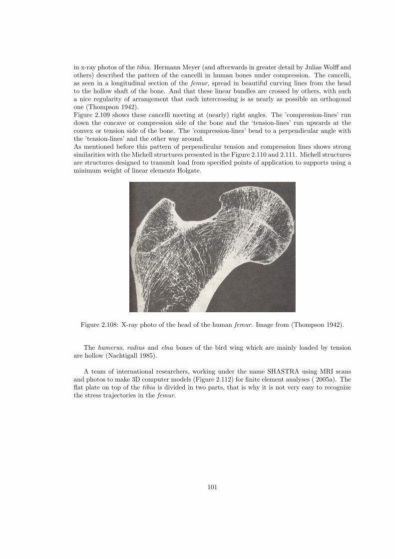
in x-ray photos of the tibia. Hermann Meyer (and afterwards in greater detail by Julias Wolff andothers) described the pattern of the cancelli in human bones under compression. The cancelli,as seen in a longitudinal section of the femur, spread in beautiful curving lines from the headto the hollow shaft of the bone. And that these linear bundles are crossed by others, with sucha nice regularity of arrangement that each intercrossing is as nearly as possible an orthogonalone (Thompson 1942).Figure 2.109 shows these cancelli meeting at (nearly) right angles. The ’compression-lines’ rundown the concave or compression side of the bone and the ‘tension-lines’ run upwards at theconvex or tension side of the bone. The ’compression-lines’ bend to a perpendicular angle withthe ’tension-lines’ and the other way around.As mentioned before this pattern of perpendicular tension and compression lines shows strongsimilarities with the Michell structures presented in the Figure 2.110 and 2.111. Michell structuresare structures designed to transmit load from specified points of application to supports using aminimum weight of linear elements Holgate.

Figure 2.108: X-ray photo of the head of the human femur. Image from (Thompson 1942).

The humerus, radius and elna bones of the bird wing which are mainly loaded by tensionare hollow (Nachtigall 1985).

A team of international researchers, working under the name SHASTRA using MRI scansand photos to make 3D computer models (Figure 2.112) for finite element analyses ( 2005a). Theflat plate on top of the tibia is divided in two parts, that is why it is not very easy to recognizethe stress trajectories in the femur.

101

Figure 2.109: Head of the femur (upper leg). Image from (Thompson 1942).

Figure 2.110: Optimisation of a structure. In every step the required bars are thinner. The mostcomplicated one is called ’Michell structure’. Image from (Beukers & Hinte 2001).

102

Figure 2.111: Michell structures for two different configurations; a cantilever structure and astructure one two supports loaded by a force in the center. Image by (Holgate 1986).

Figure 2.112: 3D model of joint tibia and femur, the flat plate on top of the tibia is clearly visible.Image from ( 2005a).

103

2.5.3 Branching and tree structures

As can be seen in Figures 2.113 and 2.114, also the structure of leaves can be used as an analogyfor structures. Although, the leaf looks to be structural optimal, we’ll have to consider a pointwhich Jorg Schlaich makes: the tree (and the leaves) optimize (grow) themselves to the maximumquantity of sunlight and not necessarily to a good use of force. Copying nature without thinkingis therefore senseless.

Figure 2.113: Leaf structure of the Victoria Amazonica.

Figure 2.114: Hangar structure by Nervi.

Ribs are frequently used in nature to stiffen ‘plates’. For example the wings of butterflies andmoths are a ribbed structures. Their wings are not membranous, rather they are covered withsmall scales1. The ribs which stiffen the scales are clearly visible in Figure 2.115.By adding ribs to a structure the moment of inertia is enlarged, which makes the structurerespond stiffer than without ribs. Furthermore the nerves of leaves may be seen as ribs, givinga leave its stiffness. A well known example of a natural ribbed leave is the Victoria amazonica(Nachtigall 2001).The principle of ribs is widely adopted by architects and structural designers. The beautifulhangars and halls designed by Pier Luigi Nervi (1891–1979) in the end of the thirties are goodexamples of a human ’translation’ of the natural principle of ribbed structures (Figure 2.117).It is broadly assumed that Sir Joseph Paxton, the builder of the Crystal Palace in London(1850–1851) was inspired by the underside of the leaf of the Victoria amazonica.

1http://www.arthropod.net Access-date: 5–2005.

104

Figure 2.115: (a) The ribs of a Boeing airplane show strong similarities with (b) the rib structureof the wings of butterflies at micro-level. Image from (Nachtigall 2001).

Figure 2.116: Underside of the Victoria amazonica, a typical example of a natural rib structure.

105

Figure 2.117: Compilation of pictures of the Palazzetto dello Sport in Roma. Especially thepicture at the right-bottom side shows in a nice way the ribs. They have strong similarities withthe Michell structures which can be found in bones.

106

D’Arcy Thompson (Thompson 1942) explains the growth of trees from a biological and growthpoint of view. A famous example of a structure which imitates trees to bear loads is the SagradaFamilia in Barcelona by Gaudı (i Armengol 2001). Gaudı uses an analogy to trees to create hiscolumns.

Figure 2.118: Oriente railway station, Lisbon, Portugal and departure hall Stuttgarter airport.

Branching structures can be determined by repeated division of mostly linear elements. Theprinciple can be seen at different levels in nature. A tree is an obvious example, but there aremore; electrical discharges in flashes of lightning, division of a river in a delta, cracks in dry mud,dunes in the Sahara Dessert and many others.The branches of a tree inspired some architects and structural designers to develop tree-likestructures. The enclosure of the Oriente railway station in Lisbon, Portugal, by Calatrava andthe departure hall of the Stuttgarter airport by Jorg Schlaich are famous examples of tree-likestructures. In their book The Algorithmic Beauty of Plants, Prusinkiewicz and Lindenmeyerdiscus in a mathematical way the forms of plants. Figure 2.119 shows output from a modelbased on their algorithms (Prusinkiewicz & Lindenmayer 1990).

Mathematical there are only five things which have to be described to draw such figures.

1. the starting point

2. the length of member 0

3. the direction of member 0

4. the angle β

5. the factor R defined as

R =Ln

Ln+1

Figure 2.120 shows the basic idea of the model.With this five parameters it is possible to describe all different regular two-dimensional branch-

ing structures.It is possible to rewrite the algorithms of Prusinkiewicz (Prusinkiewicz & Lindenmayer 1990) insuch a way that they ‘produce’ three-dimensional branching structures. The 3D-representationof the load-bearing structures in Figure 2.121 of the Stuttgarter airport departure hall is not‘produced’ by an algorithm, but by reconstruction of pictures from the structure.

In IL25 (K. Bach 1988) the difference of a branching structure being tensile-stressed anda structure under compression is mentioned. Tensile-stressed structures are optimised systemsfor transmission of tensile forces which have straight connections between the force and thesupport (Figure 2.124b). On the other hand, structures subjected to compressive and bendingstress have branching systems with increasing slenderness (Figure 2.122c and d). Accordingto (K. Bach 1988) the ratio of the length and the thickness is constant;

107

Figure 2.119: Generated branching structures for L0 = 1, n = 10, R = 0.6868 and a changingangle α (95°, 85°, 75°, 65°, 45°, 35°, 25°and 15°).

L1

D1=L2

D2=L3

D3= . . . = constant (2.37)

To demonstrate the structural behaviour of a branching structure like a tree a simple two-

108

Figure 2.120: Explaination of parameters used in model.

Figure 2.121: Three-dimensional representation of branching structure of the Stuttgarter airport.

dimensional model is made. Figure 2.122 shows a symmetrical and regular branching structure(α = 30° and n is 2). The structure is loaded by two different load cases; the first one is a load inthe direction of the structure, as may expected to be a good representation of the natural load,for it is reasonable to assume that a tree grows in a way which is the most favorable to carry theload. The second load case is a pure vertical loading, which represents the load which a tree-likestructure has to carry, when it supports a flat roof, as in the departure hall of Stuttgart.Figure 2.122c and e shows the axial-stresses and the bending stresses resulting from the loads.GSA8.0 is used to calculated these stresses. Based on this model it must be concluded thatEquation 2.37 does not result in the most optimal structure with respect to the axial stresses inthis particulary case (R=0.6868). It is assumed that Equation 2.37 does not ‘produce’ optimalstructures with respect to the axial forces for any value of R, nevertheless it is possible thatEquation 2.37 is valid when R is variable, this is not investigated.

The figures 2.122d and e demonstrate that a tree structure is not optimal for supporting aflat roof.

109

Figure 2.122: Output from GSA8.0 (a) Displacements by point loads in the direction of thestructure; (b) Axial-stresses belonging to the loads of (a); (c) Axial-stresses after the sections arechanged according to formula 2.37; (d) Displacements by point loads in vertical direction; (e)Axial-stresses after the sections are changed according to Equation 2.37.

Figure 2.123: (a) Feasibility study Tree Structures for an exhibition hall, Yale University, USA1960 (Students of Frei Otto during a seminar) (b) Support pillars of a six-angle gridshell in theKings Office, Council of Ministers, Majlis al Shura, Riyadh, Saudi Arabia, 1979 (Rolf Gutbrod,Frei Otto, Buro Happold, Ove Arup and Partners.)

110

Figure 2.124: (a) Tree-like branching structure; (b) tensile-stressed branching structure; (c) undercompression; (d) slenderness increase from top to bottom. Image from (K. Bach 1988).

111

Figure 2.125: Different examples of branching structures found in nature. Image from (K. Bach1988).

112

2.5.3.1 Spider webs

Figure 2.126: A spiderweb.

Figure 2.127: Spider web analogy of a membrane structure. Image from (Bach 1975).

Spider webs are investigated in the past by many researchers. D’Arcy Thompson (Thompson1942) covers spider web’s and their principles of surface tension in his book. The booksIL6 (Bach 1973) and IL8 (Bach 1975) from the Institut fur Leighttragwerke, Stuttgart, dealwith the similarities between spider webs and cable structures. In the book IL6 (Bach 1973)a start is being made with the comparison of the spider webs from nature and cable-net andmembrane structures.This is continued in the book IL8 (Bach 1975) which extensively covers the analogy of spiderwebs with structures. The authors describe the thread material, the elements of a web, the webedges, etc. each time with the relationship to structures. The book also reflects on the biologicalaspects of webbing. Mutoh (Mutoh 2002) describes the use of an analogy of a spiderweb forstructural use.The threads produced by the spider are pure tension elements. The web is fixed at its boundaries,where the tension forces from the web form an equilibrium with the support forces. The web isloaded by its own weight, dew drops, wind loads and the impact of a prey (see Figure 2.128).Not all spiders make webs. They are all capable of producing silk, but the prey-catching tech-nique of web building is not universal. There are many different kind of webs; the ’ordinary’ web

113

Figure 2.128: Dewdrops on the threads of a spider web.

or orb web, the sheet-like webs, tangle webs, triangle webs, and webs that just look like a jumbleof sticky threads ( 2005b).

All webs exist of tension members incapable of taking moment forces, so the principle of puretension in the treads is valid for all different types of web.The angles between the threads explain to the engineer what the ratio between the forces is. Themagnitude of the forces is still unknown but the ratio is fixed.The orb web exist primary of two types of threads; the radial and the spiral threads. A radialthread supports spiral threads. The spiral threads carry blob-like drops. They are made of aviscous liquid (Figure 2.129). The spider uses the sticky blobs to catch its prey.

Figure 2.129: Microscopic photo of a thread of a spider web. The small blobs are made of asticky viscous liquid.

On a damp morning, drops of water may form on the blobs. Sometimes there is one dropper blob; at other times the drops may hang on two blobs each. The weight of the water makesthe threads droop into beautiful shapes (see Figure 2.128). If the blobs are equally spaced andthe drops are of equal weight, the curves of the threads are close to being catenaries ( 2005c)(seeFigure 2.132).

Finally we have to conclude that the shapes of spider webs arise automatically because ofsimple physical principles, without any specific action by the spider. In this respect the websdiffer from the honeycombs of bees, in which the cells are arranged to use smallest possibleamount of wax while retaining enough strength. The bees make hexagonal cells. There is nophysics to make this happen automatically - the bees are “programmed” to do it.

114

Figure 2.130: Grid shells based on hanging models. Image from (K. Bach 1988).

Figure 2.131: Reconstruction of hanging model from Gaudı. Image from (K. Bach 1988).

115

Figure 2.132: Basic geometry of catenary curves. Image from (K. Bach 1988).

Figure 2.133: Spider web and structures based on webs. Image from (K. Bach 1988).

116

2.5.4 Sea shells and radiolaria

Beukers (Beukers & Hinte 2001) and the ILEK (Bach 1990) cover the subject of radiolaria,which are creatures in the depth of the ocean which grow lightweight skeletons. The skeletonsare optimal for their use and shaped in a hexogonal manner, which often points to the fact thathigh stresses have to be transferred (see Figure 2.134).

Figure 2.134: Radiolaria. Image from (Beukers & Hinte 2001).

D’Arcy Thompson (Thompson 1942) describes various shell shapes and skeletons of variouscreatures, such as radiolaria. He shows many examples of structures, which are optimised bygrowth or form the influence of their surroundings and relates them to mathematical theoremsand cellular structures.A special case he covers is the equiangular spiral (an example of this can be seen in Figure 2.135and the mathematical counterpart in Figure 2.136), which is thoroughly researched with math-ematical formulas from various theorems and base shapes, measurements, etc. Here he clearlyshows that nature and mathematics can be very closely related and that although something ismathematically determined, it does not have to be square or triangular. Nature deals with verysimple principles which form very complex shapes.

2.5.5 Biomechanics and muscles

From biomechanics and muscles various aspects for the future might be learned. However, cur-rently in structural engineering only very specific aspects could be learned based on the principlesthat current structures mainly are static and biomechanics mainly is dynamic. However, in me-chanical and aerospace engineering many aspects could be learned from nature.An example of an aspect which could be learned for the near future would be for instancethe combination of muscles and tendons. The muscles provide the raw pulling power and thetendons make the system efficient by storing and delivering energy by acting as a spring sys-tem (Alexander 1992). This might be used in adaptive structures in the future.

117

Figure 2.135: Spiral shell. Image from (Thompson 1942).

Figure 2.136: Spiral analogy of the spiral shell. Image from (Thompson 1942).

118

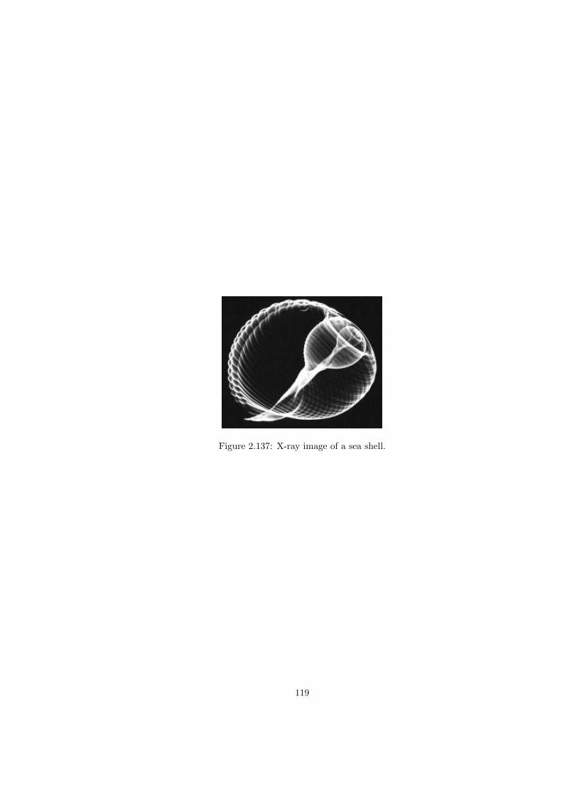
Figure 2.137: X-ray image of a sea shell.

119

120

Structural concepts 3Contents

3.1 Shells and domes . . . . . . . . . . . . . . . . . . . . . . . . . . . . . . 122

3.1.1 Introduction in shell structures . . . . . . . . . . . . . . . . . . . . . . 122

3.1.2 Simplified methods to calculate shell structures . . . . . . . . . . . . . 122

3.1.3 Instability of shell structures . . . . . . . . . . . . . . . . . . . . . . . 133

3.2 Cable-net and membrane structures . . . . . . . . . . . . . . . . . . 143

3.2.1 Introduction . . . . . . . . . . . . . . . . . . . . . . . . . . . . . . . . 143

3.2.2 Evaluation of the computer model . . . . . . . . . . . . . . . . . . . . 143

3.2.3 Cutting Pattern Generation . . . . . . . . . . . . . . . . . . . . . . . . 147

3.2.4 Post Processing the Cutting Patterns . . . . . . . . . . . . . . . . . . 150

3.2.5 Examples . . . . . . . . . . . . . . . . . . . . . . . . . . . . . . . . . . 155

3.3 Pneumatic structures . . . . . . . . . . . . . . . . . . . . . . . . . . . 165

3.3.1 Introduction . . . . . . . . . . . . . . . . . . . . . . . . . . . . . . . . 165

3.3.2 Principles of form . . . . . . . . . . . . . . . . . . . . . . . . . . . . . 170

3.3.3 Materials . . . . . . . . . . . . . . . . . . . . . . . . . . . . . . . . . . 173

3.3.4 Air pressure . . . . . . . . . . . . . . . . . . . . . . . . . . . . . . . . . 179

3.3.5 Making-up of the fabric . . . . . . . . . . . . . . . . . . . . . . . . . . 183

3.3.6 Anchorage . . . . . . . . . . . . . . . . . . . . . . . . . . . . . . . . . . 185

3.3.7 Building physics . . . . . . . . . . . . . . . . . . . . . . . . . . . . . . 187

3.3.8 Regulations . . . . . . . . . . . . . . . . . . . . . . . . . . . . . . . . . 191

3.3.9 Stabilizing the shape . . . . . . . . . . . . . . . . . . . . . . . . . . . . 194

3.4 Space frames . . . . . . . . . . . . . . . . . . . . . . . . . . . . . . . . 208

3.4.1 Space Frames . . . . . . . . . . . . . . . . . . . . . . . . . . . . . . . . 209

3.4.2 Formal definition . . . . . . . . . . . . . . . . . . . . . . . . . . . . . . 217

3.4.3 Single layer systems . . . . . . . . . . . . . . . . . . . . . . . . . . . . 219

3.4.4 Systems with multiple layers. . . . . . . . . . . . . . . . . . . . . . . . 222

3.4.5 Polygons as base element for spatial structures . . . . . . . . . . . . . 223

3.4.6 Parallel rasters . . . . . . . . . . . . . . . . . . . . . . . . . . . . . . . 230

3.4.7 Sphere-shaped truss frames . . . . . . . . . . . . . . . . . . . . . . . . 241

3.4.8 Aspects of construction . . . . . . . . . . . . . . . . . . . . . . . . . . 249

3.4.9 Stability . . . . . . . . . . . . . . . . . . . . . . . . . . . . . . . . . . . 271

3.4.10 Calculation . . . . . . . . . . . . . . . . . . . . . . . . . . . . . . . . . 275

3.5 Kinetic and adaptable structures . . . . . . . . . . . . . . . . . . . . 277

3.5.1 Adaptive structures . . . . . . . . . . . . . . . . . . . . . . . . . . . . 277

121

3.1 Shells and domes

3.1.1 Introduction in shell structures

Recommended Study Material

Title Author YearVormgeving in hout J.H. Pestman

3.1.2 Simplified methods to calculate shell structures

3.1.2.1 The relationship between form and force of curved surfaces: The Rain Flowanalysis

Introduction There is great knowledge of the mechanical behavior of geometrically regularcurved surfaces like most shells structures are formed by (Flugge 1960). This is mainly causedby the fact that these surfaces are relatively easily described by analytical mathematicalfunctions. For describing irregular curved surfaces, like those in Free From Architecture, verylittle analytical mathematical functions exist and therefore it is very hard to derive formulas todescribe their mechanical behavior. One way of dealing with this problem is to calculate thestresses and strains of these irregular curved structures with computer programs based on thefinite element method. However the problem is that you only obtain quantitative informationabout the results (like the magnitude of the forces) but no qualitative information. This does notalways give clear insight into the structural behavior. For example, what is the relation betweenthe shape of the curved surface and the flow of forces. In analytical formulas for regular curvedsurfaces there is a quantitative relation between the magnitude of the forces and the shape of theshell, like the radius. Because of the lack of insight it can be difficult to design irregular curvedsurfaces which have shell-like behavior that is mainly extension forces and little bending moments.

In 2D structures the load and the supports determine the line of thrust of the load. If thesystem line of a structure deviates from the line of thrust of the load it will cause ”corrective”bending moments in the structure. In 3D structures like shells, for example a dome, the line ofthrust of the load can be corrected by the hoop forces so to coincide with the system line of theshell so there are no bending moments in the dome. For a dome where the line of thrust of theload falls outside the system line the hoop forces are compression, and where the line of thrustof the load falls inside of the dome the hoop forces are tension (see Figure 3.1). If we know the”3D line” (surface) of thrust of the load in regards to it’s supports and we combine this with any(irregular) curved surface it is possible to determine the forces in the shell. A way of determiningthe flow of forces of (irregular) curved surfaces is the ”rain flow” analysis of the geometry of thecurved surface.

Presently there is a tendency to integrate design, calculation and production driven by thepossibility to exchange data between CAD-program (Computer Aided Design) and FEM-program(Finite Element Method). This has lead to a wide range of designs for buildings with complexshapes (Free Form Architecture), which sometimes seem to have shell-like behaviour. Shell-likebehaviour consists of mainly extension forces and little bending moments, due to the curvatureof the surface. These buildings are often calculated by first importing the data of the geometryof the shape made by the CAD-program to the FEM-program, where the structural modelis build and calculated. For describing irregular curved sufaces, there are very little simpleanalytical mathematical functions available and therefore it is very hard to derive formulas todescribe their mechanical behaviour. Because of this only quantitative information about theresults (like the magnitude of the forces) but not any qualitative information is obtained. Thisquantitative information doesn’t always give clear insight into the structural behaviour. Thereforeit is convenient to get insight in the mechanical behaviour of (irregular) curved surfaces, without

122

Figure 3.1: Line of thrust of the load (Funicular line) in relation to the Shell surface and thecorrective hoopforces. Image from (Schodek 1998).

use of FEM-program or very complicated analytical formulas.

Analytical and graphical solutions for shell structures Many shell theories have beendeveloped to analyse the mechanical behaviour of shell structures. A well-known theory is themembrane theory for thin shallow shells. In the membrane theory it is assumed that the thick-ness of a shell is far smaller than the overal dimensions. Due to this the flexural rigidity is farsmaller than the extensional rigidity. A thin shell subjected to external applied loads thereforemainly produces membrane forces, which are actually resultants of the in-plane normal and shearstresses that are uniformly distributed across the thickness. In the regions where the membranetheory will not hold, because for example edge disturbances, some (or all) of the bending fieldcomponents are needed to compensate the shortcomings of the membrane field in the disturbedzone. These disturbances have to be described by a more complete analysis, which leads toa bending theory of thin elastic shells. Because of its simplicity the membrane theory gives adirect insight into the structural behaviour and the order of magnitude of the expected responsewithout elaborate computations.There are several ways to make a classification of surfaces: by using the definition of Gaussiancurvature and by using the way the surface is generated. The Gaussian curvature is defined asthe product of the two principal curvatures of a surface in a point. When the Gaussian curvatureis positive both curvatures are pointing in the same direction and the surface is called synclastic.If the Gaussian curvature is negative both curvatures are pointing in another direction and thesurface is called anticlastic. When both the curvatures are zero the surface is flat and is calledzeroclastic. When one curvature is zero the surface is called monoclastic. There are several waysto develop surfaces. The main ways are revolution, translation and ruling. Surfaces of revolutionare generated by the revolution of a plane curve, called the meridional curve, about an axis,called the axis of revolution. Surfaces of translation are generated by sliding a plane curve alonganother plane curve, while keeping the orientation of the sliding curve constant. Ruled surfacesare generated by sliding each end of a straight line on their own generating curve, while remaining

123

the straight line parallel to a prescribed direction or plane. It is also possible to combine severalsurfaces.For several well known shells the mechanical behaviour has been formulated by using the mem-brane theory. The bending moments caused by the edge disturbances can be calculated separatelyand superimposed with the result of the membrane solution. The predominantly load case is mostoften its own weight. For the surfaces of revolution shells subjected to its own weight it is alwayspossible to determine the mechanical behaviour with a graphical solution, to give more insightin the flow of forces. By this graphical method it is easily to construct a polygon of forces. Thispolygon represents the ”corrected” line of thrust, whereby the hoop forces correct the line ofthrust of the load to coincide with the system line of the shell. A nice example of this graphicalmethod is used to calculate the forces in a masonry dome (see Figure 3.2).

Figure 3.2: Graphical determination of the forces in masonry dome due to it’s own weight. Imagefrom (Beranek 1988a)

Rain Flow analysis The next hypothesis for the flow of forces in shell structures has beenthe basis of this method:

Like a rain flow loads will flow along curves with the steepest ascent on the shell surfaceto it’s supports.

These curves can be derived from a gradientplot of a surface, which plots the normal vectorsof the surface in a view from above. These curves are always orthogonal to the vertical contoursof the surface, which are easily to plot. The gradient forces in the vertical sections betweencurves can then be obtained in the same way as with the masonry dome through the verticalequilibrium of forces. The hoop forces have to be in equilibrium with the horizontal forces, whichhave to ensure that the pressure surface (line of thrust of the load) converges with the system(line) surface of the shell. The hypothesis has been formulated from studying the way whichplates transmit their loads. The maximum shear force in a plate is a vector with the magnitudeof the carried load and points in the direction of the flow of the shear force to the supports. Thevector of the maximum shear force can be derived from the gradientplot of the surface whichrepresents the sum of the curvatures because the shear force is the derivative of the sum of thebending moments (M):

124

M = ∆w =d2w

dx2+d2w

dy2(3.1)

As an analogy (the rainflow analogy ((Beranek 1976)) this surface also represents an airinflated membrane, on which the rain flows along curves with the steepest ascent to the supports.In the case for the flow of forces of shells (the hypothesis) the surface of the sum of the curvaturesfor plates or the surface of the air inflated membrane is replaced by the surface of the shell itself.It possible to combine straight edge hypars to get a shell as shown in Figure 3.3. It is assumedthat the separate hypars act as like a single hyppar with diagonal compression and tensionparabola. But according to (Lauletta 1961) however the compression forces are dominate andthe tension froces merely distribute the loads towards the compression trajectories. This gives ina stress distribution (a results of tests) as shown in Figure 3.4, which resembles the contourplotand gradientplot of the flow of forces according to the hypothsis, shown in Figure 3.5.

Figure 3.3: Shell combined of several straight edge hypars.

Figure 3.4: Principal stresses in a shell model combined of several straight edge hypars. Imagefrom (Lauletta 1961)

This hypothesis has been tested on a Free Form design at the Faculty of Architecture(Hanselaar 2003) and comprehends of a shell-like structure for a indoor ski-slope (Figure 3.6).The structure spans in the short direction, so that the long sides are pin fixed. A gradientplotof the surface (Figure 3.7) represents the flow of the forces (loads) according to the hypothe-sis. There a two different kinds of free edges on the short sides. On the left side a raised edgeis visible. Because of this raised edge the loads run away form the edge towards the supportdirection, which leads to a desirable membrane stress distribution. On the other side howeverthe loads run towards the free edge, which then has to transfer the loads towards the supports.This leads to an undesirable situation. In the gradient plot also a couple of drain curves arevisible. Loads from curves leading to these drain curves can be transferred by these drain curveslike membrane forces under certain conditions. However when the curves leading to these drain

125

Figure 3.5: Contourplot and gradientplot of the flow of forces of a shell combined of severalstraight edge hypars.

curves are orthogonal to them large bending moments can be expected. This is visible by thedark bleu color representing large vertical deformations as shown in Figure 4. Looking along acurve large hoop forces can be expected at places where the slope changes rapidly. This is due tothe sudden change of the horizontal force that has to ensure that the pressure surface convergeswith the system surface. These large hoop forces can also result in bending moments.

Figure 3.6: Shell-like structure with contourplot of the vertical displacements determined withan elastic calculation (FEM).

3.1.2.2 The relationship between form and force of curved surfaces: A graphicalsolution

Introduction Because of the geometric complexity of Free Form Architecture it is importantto develop systems which are relatively easy to construct. It is also important to developaccessible methods for designers to understand the principle mechanical and structural behaviorof these complex structures. These methods are complimentary to computer models, like FiniteElement Methods (FEM), which does not always give an insight to the principle mechanicalbehavior of complex structures. Researchers like Frei Otto made physical models for the

126

Figure 3.7: Sketch of gradientplot in top view.

understanding of the mechanical behavior of complex structures. We try to develop analyticand semi-analytic / semi-numerical methods.

The aim of this section (Baecke 2005) is on one hand to extend a graphical method(Beranek 1988b) to derive the section forces in an axisymmetric shell and to be able to studythe mechanical behavior of these types of shells. The graphical method compared with a FEMcalculation gives a very good result. The great advantage of the graphical method is it also givesa good understanding of the mechanical behavior, besides the numeric result.

Graphical solution for shells (Domes) In 2D structures, like arches, the load and thesupports determine the line of thrust of the load. If the centerline (axis) of an arch deviatesform the line of thrust of the load it will cause ”corrective” bending moments in the arch (seeFigure 3.8). In 3D structures like shells, for example a dome, the line of thrust of the load canbe corrected by the hoop forces so to coincide with the axis of the dome surface so there are nobending moments in the dome (see Figure 3.9).

Figure 3.8: Line of thrust of the load (funicular line) in relation the axis of a circular arch.

The stress distribution in domes (in this case a hemispherical dome) is easily verified by meansof a funicular polygon. Two ”orange peels” are regarded as a linear arch (see Figure 3.10). Theloads of the various parts of this arch are easily determined. The shape of the funicular polygonwill not coincide with the centerline (axis) of the arch, unless extra horizontal forces are added.If these horizontal forces need to be directed outwards, they can be produced by tangentialcompressive forces (hoop forces). And if the horizontal forces need to be directed inwards, theycan be produced by tangential tensile forces. Thus a true membrane stress distribution may beexpected in the dome. The above described example (see Figure 3.10) we take into account thatthe deformations of the dome under loading are not constrained. For the stresses and deformation

127

Figure 3.9: Line of thrust of the load (funicular line) in relation to the dome (shell) surface.

is this case see the top two pictures in Figure 3.11 and 3.12. But for most structural uses thebase of a dome will pinned round its hemisphere, thus preventing deformations at its spring dueto loading (bottom two pictures in Figure 3.11 and 3.12). This has as a consequence for thetensile hoop forces at the spring; these will be zero in stead of maximum in the unconstrainedcase.

Figure 3.10: Polygon of forces in dome section.

Graphical solution for a dome with an oculus If we take a section of a (in this case atop part of a) dome with an oculus and determine the forces needed to make global equilibriumwith the loads we need an outward horizontal force in the top and an inward horizontal forcein the spring (see Figure 3.13). A tangential compressive ”ring force” (hoop forces) in the topcan produce the outward horizontal force and a tangential tensile ”ring force” (hoop forces) in

128

Figure 3.11: Hoop forces (NHH) and meridional forces (NRR) in a dome pinned in one pointand on rollers round the hemisphere at its spring (picture above) and a dome pinned round thehemisphere at its spring (picture below).

Figure 3.12: Deformation of a dome pinned in one point and on rollers round the hemisphere atits spring (picture above) and deformation of a dome pinned round the hemisphere at its spring(picture below).

the spring can produce the inward horizontal force in the spring (Figure 3.14). If we comparethis with the hoop forces in a dome without an oculus we can see as a similarity compressionhoop forces in the top and tensile hoop forces at the spring, the difference is that because ofthe oculus the hoop forces will be more concentrated towards the oculus at the edge to forma ”ring force” (Figure 3.15), the numerical result verifiers this (top picture in Figure 3.17). If

129

we again take two ”orange peels” and regard those as a linear arch we can determine the stressdistribution by means of a funicular polygon (Figure 3.16). This graphical result is verified bya numerical calculation (Figure 3.17), the graphical solution gives the correct analysis and thecorrect magnitudes compared to the numerical solution. Because in this case not a hemisphericaldome was taken but only the top part of a dome the support reaction will not only have a verticalresultant (caring the weight) but also a horizontal resultant (Figure 3.18), which would not beneeded for a hemispherical dome, which deformation are unconstrained (Figure 3.10 and toppicture of Figure 3.11).

Figure 3.13: Equilibrium of forces in a section of a dome with an oculus.

Figure 3.14: Hoop (ring) forces in a dome with an oculus.

130

Figure 3.15: Hoop forces (NHH) and meridional Forces (NRR) in a section.

Figure 3.16: Polygon of forces in a section.

131

Figure 3.17: Hoop forces (NHH), above, and meridional forces (NRR), below, numerically calcu-lated.

Figure 3.18: Support reactions.

132

Graphical solution for an axisymmetric ”Donut like” shell It the following case weexamine a axisymmetric shell with a hole, like the dome with an oculus, but in this case thehighest point in the section is not at the inner ring next to the oculus but somewhere betweenthe spring and the inner ring (see Figure 3.19).For the global equilibrium with the loads this means the outward horizontal force will be in thehighest point, which in this case, does not coincide with the inner ring next the hole as it didwith the dome with an oculus, thus creating the greatest arm for equilibrium (see Figure 3.20).As a consequence the tangential compressive ”ring force” (hoop forces) needed to produce theoutward horizontal force is also in the highest point (see Figure 3.21), the graphical solution (seeFigure 3.22) and the numerical calculation verifies this (see Figure 3.23). Another interestingaspect with this example is the type of meridional forces. In the case with the dome and thedome with an oculus the meridional forces are compression, they carry the loads straight downto the supports. In this case the loads first have to be carried up from the inner ring next tothe hole to the highest point, by tensile meridional forces, and from there down to the supportsby compressive meridional forces (bottom picture, Figure 3.21 and Figure 3.24). The graphicalsolution gives the correct analysis, as it does with the dome and the dome with an oculus.Both graphical as numerical solution give a remarkable result in respect to the hoop forces inthe highest point. As pointed out the compressive ”ring forces” are in the highest point, butthe hoop forces on both sides of these compressive ”ring forces” are tensile hoop forces, thisis a result of the equilibrium. This sudden change in hoop force from tension to compressionto tension again has a large impact on the deformations. Hoop forces will cause extensions inthe tangential direction, the compression hoop forces will shorten the rings and the tensile hoopforces will elongate the rings (see Figure 3.27), thus resulting in a sharp dip in the deformations(see Figure 3.25 and 3.26).

Figure 3.19: picture above: dome with an oculus, picture below: axisymmetric ”donut like” shell.

3.1.3 Instability of shell structures

Shells are very efficient in carrying load. However, this efficiency comes at a price. If a shell failsit fails with a bang. There will be no warning and it will collapse faster than we can run.

Ferrybridge. Three reinforced concrete cooling towers collapsed in Ferrybridge UK on Novem-ber 1st 1965 (Fig. 1). Strong winds triggered the successive collapses. All chunks of concretefell inside the towers. There where no fatalities or injuries because there were no workers either

133

Figure 3.20: Equilibrium of forces in a section of an axisymmetric ”donut like” shell.

Figure 3.21: Hoop forces (NHH) and meridional Forces (NRR) in a section.

on or inside the tower at the time. The cooling towers where part of a group of eight at a powerstation. The remaining towers sustained severe structural damage. The towers were 115 m high.

Two factors caused the collapse. The average wind speed over a one minute period, was usedin design whereas, in reality, the structures are susceptible to much shorter gusts. The windloading had been based on experiments using a single isolated tower. The grouping of the towerscreated turbulence on the leeward towers that collapsed.

In-extensional deformation. An in-extensional deformation is a deformation in which onlybending occurs while membrane extension and contraction do not occur. Shells that have zeroGaussian curvature over large areas are susceptible to in-extensional deformation. Since shellsare thin they have very little bending stiffness. Therefore, a shell needs to be designed such thatin-extensional deformations cannot occur. A scaled down physical model of a shell can be usedto study in-extensional deformations that might be possible. Also a finite element program canbe used. The smallest natural frequencies and especially the associated normal modes will showany in-extensional deformations that might be possible.

134

Figure 3.22: Polygon of forces in a section.

Figure 3.23: Hoop forces (NHH) numerically calculated.

Figure 3.24: Meridional forces (NRR) numerically calculated.

Differential equation for shell buckling The structural behaviour of shells including largedisplacements is described by an eight order differential equation (Hoefakker & Blaauwendraad2003)

Et3

12(1 − ν2)∇2∇2∇2∇2∗uz+E∗t∗Γ2∗uz = ∇2∇2pz − nxx∗uz,xx−2∗nxy∗uz,xy−nyy∗uz,yy (3.2)

135

Figure 3.25: Deformations with sharp dip at the hole.

Figure 3.26: Hoop forces (NHH) and meridional forces (NRR) plotted on the deformed surface.

Figure 3.27: The hoop forces will cause extensions in the tangential direction, compression hoopforces will shorten the rings, and tensile hoop forces will elongate the rings, thus resulting in asharp dip of the deformations.

where uz is the displacement perpendicular to the shell surface, pz is the loading perpendicularto the surface. Γ2 and ∇2 are operators.

∇2 = ∂2()∂x2 + ∂2()

∂y2

Γ2 = kx ∗ ∂2()∂y2 − 2 ∗ kxy

∂2()∂x∗∂y

+ ky ∗ ∂2()∂x2

(3.3)

The x and y direction often are not linear but are plotted on the surface of the shell. Thedifferential equation can be solved analytically for elementary shell shapes and elementary loading(Table 3.1.3). E is Young’s modulus, ν is Poisson’s ratio, t is the shell thickness and a is theradius of the middle surface of the shell.

136

Figure 3.28: Three collapsed cooling towers at Ferrybridge.

Yoshimura pattern. The buckling shape of a axially loaded cylinder can be a ”ring pattern”or a ”square pattern” (Figure 3.29). Which one occurs depends on the shell thickness and itsradius. When bucking progresses the ”ring pattern” can transform into the ”square pattern”.When the material starts to deform plastically the shape adopts a ”rhombic pattern”. The latteris called a Yoshimura pattern (Yoshimura 1955) (Figure 3.30. Remarkable about the Yoshimurapattern is that it is in-extensional. Fortunately, large extensions are needed before the Yoshimurapattern is obtained.

Imperfection sensitivity. Experiments on axially compressed cylinders show that the maxi-mum load is much smaller than the critical load (Figure 3.32). This is caused by extreme softeningof a cylinder after buckling. Figure 3.33a shows the behaviour of a perfect cylinder under perfectloading. This result can only be obtained analytically because in reality perfect cylinders donot exist. Figure 3.33b shows that small imperfections cause a large reduction of the maximumload. Imperfections include dents, residual stresses, temperature stresses, inhomogeneities, creep,shrinkage, eccentricity of loading and first order deformations. Not only compressed cylinders butalso bent cylinders and radially compressed domes are very sensitive to imperfections. Hypparsare not sensitive to imperfections.

Experiment. What is the carrying capacity of an axially loaded empty beer can? We modelthe can as an open cylinder. The wall thickness is 0, 08mm the radius is 32, 8mm, Young’s mod-ulus is 2, 1∗105 N/mm and Poisson’s ratio is 0.35. According to Table 3.1.3 the critical loading is:

137

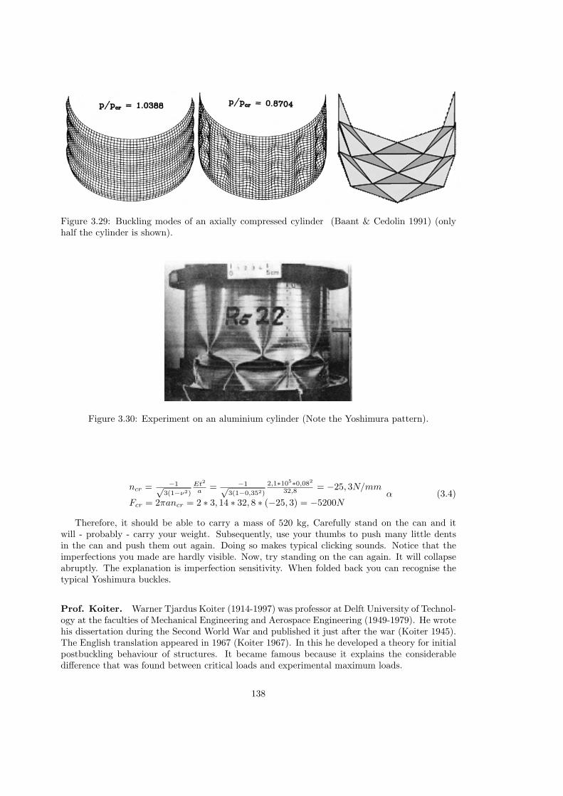
Figure 3.29: Buckling modes of an axially compressed cylinder (Baant & Cedolin 1991) (onlyhalf the cylinder is shown).

Figure 3.30: Experiment on an aluminium cylinder (Note the Yoshimura pattern).

ncr = −1√3(1−ν2)

Et2

a= −1√

3(1−0,352)

2,1∗105∗0,082

32,8 = −25, 3N/mm

Fcr = 2πancr = 2 ∗ 3, 14 ∗ 32, 8 ∗ (−25, 3) = −5200Nα (3.4)

Therefore, it should be able to carry a mass of 520 kg, Carefully stand on the can and itwill - probably - carry your weight. Subsequently, use your thumbs to push many little dentsin the can and push them out again. Doing so makes typical clicking sounds. Notice that theimperfections you made are hardly visible. Now, try standing on the can again. It will collapseabruptly. The explanation is imperfection sensitivity. When folded back you can recognise thetypical Yoshimura buckles.

Prof. Koiter. Warner Tjardus Koiter (1914-1997) was professor at Delft University of Technol-ogy at the faculties of Mechanical Engineering and Aerospace Engineering (1949-1979). He wrotehis dissertation during the Second World War and published it just after the war (Koiter 1945).The English translation appeared in 1967 (Koiter 1967). In this he developed a theory for initialpostbuckling behaviour of structures. It became famous because it explains the considerabledifference that was found between critical loads and experimental maximum loads.

138

Critical loadingpcr[N/m]

Critical membraneforce ncr[N/m]

Imperfectionsensitive

Open cylinder, radially loaded(in-extensional deformation)

14(1−ν2) ∗ Et3

a3−1

4(1−ν2) ∗ Et3

a2 no

Open cylinder, axially loaded −1√3(1−ν2)

∗ Et2

ayes

Open cylinder, torsion loaded 1

3√

2(1−ν2)34

∗ E√

t5

a3 ;

shear force

no

Hyperboloid, axially loaded(cooling tower)

−1√3(1−ν2)

∗ Et2

ayes

Closed cylinder, loaded in all di-rections

2√3(1−ν2)

∗ Et2

a−1√

3(1−ν2)∗ Et2

a;

hoop direction

yes

Sphere 2√3(1−ν2)

∗ Et2

a−1√

3(1−ν2)∗ Et2

ayes

Dome; base radius> 3, 8√at 2√

3(1−ν2)∗ Et2

a−1√

3(1−ν2)∗ Et2

ayes

Hyppar 2√3(1−ν2)

∗ Et2

a−1√

3(1−ν2)∗ Et2

ano

Table 3.1: Critical loading and critical membrane forces for elementary shells.

Figure 3.31: A simple beercan.

Koiter’s laws. The equilibrium of a perfect system can be described by

λ = λcr(1 − c1w − c2w2) (3.5)

Where λ is the load factor, λcr is the critical load factor, w is the amplitude of the deflection,c1 and c2 are constants characterising the given structure. There are three types of post criticalbehaviour (Figure 3.34). Type I behaviour occurs when c1 = 0 and c2 < 0. The structure is notsensitive to imperfections. Type II behaviour occurs when c1 = 0 and c2 > 0 . The structure issensitive to imperfections. The maximum load factor is equal to

139

Figure 3.32: Experimental maximum loads of 172 axially loaded cylinders. (Weingarten et al.1965)

Figure 3.33: Buckling of cylinders for different unevenness size β. (Weingarten et al. 1965)

λmax = λcr(1 − 3(w01

2ρ√c2)

23 ) (3.6)

Where ρ is a coefficient depending on the imperfection shape and w0 is the imperfection ampli-tude. This is called the 2

3 -power law. Type III behaviour occurs when c1 > 0. The structure isvery sensitive to imperfections. The maximum load factor is equal to

λmax = λcr(1 − 2(w0ρc1)12 ) (3.7)

This is called the 12 -power law (Figure 3.35).

Knock down factor. In shell design often the following procedure is used. First the criticalloading is computed by using formulas or a finite element program. Then this loading is reducedby a factor that accounts for imperfection sensitivity. The result needs to be smaller than thedesign loading. This factor is often called ”knock down factor”. It is experimentally determined.For example for reinforced concrete cylindrical shells loaded in bending the following knock downfactor C is used.

C = 1 − 0, 73(1 − e−116

√at ) (3.8)

140

Figure 3.34: Basic types of post buckling behaviour.

Figure 3.35: Maximum load as a function of the imperfection amplitude.

The range in which it is valid is 0, 5 < la< 5 and100 < a

t< 3000 where l is the cylinder

length (Farshad 1992).

Finite element analysis of buckling. Finite element programs can compute critical loadfactors and the associated normal modes. The real critical load is represented by the smallestload factor because a shell will buckle at the first opportunity it gets. If the second smallestbuckling load is very close (say within 2%) to the smallest buckling load we can expect thestructure to be highly sensitive to imperfections. This is because the interaction of bucklingmodes gives a strong softening response after the critical state. For shells that are sensitive toimperfections the maximum load factor might be as small as 1/6 of the critical load factor.

Nonlinear finite element analysis. If a shell is sensitive to imperfections a different kind offinite element analysis is necessary. In this geometrical nonlinear analysis the loading is appliedin small increments for which the displacements are computed. Such analyses should be onlyperformed by experts. It involves equilibrium iterations, path following methods and terminationcriteria. (See the course CT5142 Computational methods in nonlinear solid mechanics). Figure3.36 shows the results of different finite element computations of a simply supported shallowdome.

Design formula. Using the formulas in Table 3.1.3 and the knock down factor in Figure 3.32we can derive a formula for the required thickness of a shell

t =

√

10−n2a

E(3.9)

Where E is Young’s modulus, a is the shell radius in the direction of n1 and n2 is the smallestprincipal membrane force. Note that n2 needs to have a negative value because shells buckleonly due to compression. For hyppars the factor 10 in the formula needs to be replaced by 1.7.

141

Figure 3.36: Shell finite element analysis of a shallow dome (Farshad 1992).

Small shells of reinforced concrete often will be thicker than this formula predicts because thereneeds to be sufficient cover on the reinforcing bars.

142

3.2 Cable-net and membrane structures

Recommended Study Material

Title Author YearEuropean Design Guide for Tensile Sur-face Structures.

B. Forster, M. Mollaert 2004

3.2.1 Introduction

Nowadays membrane structures are produced by using computer software. A model of therequired shape is generated and load analyses are performed. A large benefit of using computersoftware for the analysis of tensile structures is the possibility to determine reaction forces onthe supporting structure in extreme situations. When no computer software is used, these forceshave to be obtained by means of physical modelling. In this case, the scale factor of the physicalmodel causes large deviations in the forces, so a large safety factor needs to be used.Another benefit of using computer software for the realisation of tensile structures is the abilityto generate cutting patterns. These are needed to enable the creation of larger membranes outof small parts. The parts need to have a specific form. When they are assembled, they mustform the required shape. The generation of these patterns can be done precise and convenientby means of computer software.There is one serious drawback of using computer software. It is difficult to get feeling withthe structure. It is represented as a computer model, an estimation of reality. Very often largestructures are visualised at the size of the computer screen, which makes it difficult to understandthe size of the structure. It requires experience and common sense to translate computer datainto useful data for manufacturing.

3.2.2 Evaluation of the computer model

The starting point for the evaluation is the computer model. The model is generated to representthe required shape. During the form finding stage the shape is adapted to the limitations andrequirements of the customer. And the eye of the designer has checked the shape for its aesthetics.Load analyses are performed to get reaction forces and to dimension the supporting structure.The final stage is the translation of the computer model into usable data. However, the modelneeds to be checked on several points:

• What kind of model exist to represent the shape?

• Is this model capable of representing the required shape?

• Is the way of representing the fabric in accordance with the way of the cutting patterngeneration?

What kind of computer models exists? A computer program needs a way to order theinformation about the surface to be described. When a finite element method is used, the surfaceis cut into small pieces and for each piece the forces are calculated. The way of cutting thesurface into pieces is called the discretisation of the surface. The purpose of the discretisationis to make the best approximation of reality possible. A very common way of discretisationof membrane surfaces is to generate a mesh. The mesh is triangulated to be able to makeplanar elements. The mesh is stretched into the right shape. Another way to discretise thesurface is to project a mesh upon the plan view of the surface and cut it with the boundaries.In this way the mesh is not deformed to fit to the boundaries. This approach is used within EASY.

The discretisation of the surface divides the surface into small pieces, the elements. An

143

element can have different properties. It can be, for example, a cable element of a membraneelement. A cable element is a 1-dimensional element. It represents the stiffness of a cable only inthe length direction of the cable. A membrane element is a 2-dimensional element. It representsthe membrane, so it has to take into account the stiffness of an area. When the surface istriangulated, one triangle represents a membrane element and therefore the area of the trianglerepresents the membrane. When the surface is not triangulated, one bar element represents halfthe width towards both sides of the bar to be the membrane.When a radial type of roof is used, a radial mesh is generated. This mesh can againbe stretched into the right shape or projected upon the plan view of the structure and be-ing cut by the boundaries. It is much better to have a radial mesh when a radial structure is used.

Depending on the type of program that is used, a form can be calculated according tothe chosen mesh. There are different approaches. It is possible to generate a minimal surface;this is a surface with the same stresses in all directions. Such a shape is only valid for oneload case. When the loads change, the form should change as well, in order to stay a minimalsurface. But it is regarded as a good starting point for an initial form. Programs based uponthis principle are called dynamic relaxation programs.Another approach is the Force Density approach. This method is based upon linearization ofthe non-linear equation system by introducing a new parameter; the force divided by the lengthof the bar. The non-linear equation system, meant to solve the equilibrium of internal andexternal forces, now suddenly is a linear system which is easy to solve. Therefore very quickform finding is possible. EASY is based upon this system. It is possible to generate a minimalsurface with this approach, it then requires more iterations.Not every shape is suitable to be a minimal surface; especially radial roofs cannot be a minimalsurface. The top of the structure has always higher stresses than the perimeter of the structure.

Does the model represent the required shape? After choosing the model and doing theform finding, the model needs to be evaluated:

1. Does the model look like the required shape?If not, the shape must be adapted by changing the internal stresses in the fabric or changingthe fixed points. This is a matter of aesthetics. With the assistance of a software package,in principle all tools are present to adapt the shape completely to the wishes of the designer.If more elevation or curvature is wanted, it can be adapted, within the restrictions of thestarting points.

2. Are all the necessary parts modelled?For example, if there is a hole in the fabric, is there a hole in the model too. This seemsto be a very obvious remark, but it is very easy to simplify the structure too much. Whenthere is a hole in the fabric, it has great influence upon the stress behaviour of the material.Another aspect is use of ridge and valley cables. Are they attached to the membrane orjust adjacent to the fabric. When the cables are attached to the fabric they will carry apart of the stresses. If not, all the stresses are transported to the tensioning points, whichresults in high stresses.Something that easily can be forgotten, are the links between the fixed points and thefabric. The fabric does not reach to the fixing points exactly, there is always a connectionneeded. This link can cause changes in shape, so it should be modelled. The same holdstrue for the elastically supported fixed points. These points can slightly move and thereforecan influence the shape, which means that they should be modelled as well.Also of large influence upon the stress behaviour of the shape is the width of the meshin proportion to the size of the structure. When the structure is much curved and onlya few elements are used to represent the surface, the elements need to be deformed very

144

much to answer the equilibrium equations. Firstly the shape usually does not answer to theexpected aesthetic qualities and secondly a very high stress surface originates. Thereforealways choose elements in such a manner that they are not deformed too much during formfinding. It may take more form finding runs to find the right mesh.

Can the model be used for cutting pattern generation? One of the most importantpurposes of using computer modelling is the generation of cutting patterns. But the modelmust be useful for the generation of cutting patterns; else it is of no use having such a model.The model represents the membrane and the membrane is materialised with a fabric. A fabricis a woven material. The warp threads are between the loom and the weft threads are wovenin between. The warp threads are tensioned during the weaving process, and the weft threadstherefore pace up and down. When the weft direction is tensioned, it will strain much more thanthe warp direction. So fabric is a non-homogenous material which cannot resist shear forces.Warp and weft threads are orthogonal to each other, so the model must represent this feature ofthe material. The direction of the mesh indicates the direction of the warp and weft direction ofthe fabric. When the form finding is executed, it must be checked whether the cutting patternorientation is according to the mesh orientation.

For the statical analysis, a stiffness is entered, for both warp and weft direction a differ-ent value. Does this stiffness still represent the directions of the threads in the cutting patterns?Usually the mesh is oriented in the direction of the primarily curvature. Then there will occurless shear in the surface. So the cutting pattern orientation will also need to be in the directionof the principle curvature to get the best results when the patterns are assembled. When themodel is not a good base for creating cutting patterns, it must be decided whether the modelwill have to be adapted or not. Adapting the mesh will change the shape, so a new form findingprocedure is started. But when good results are requested, it is better to have a good model tostart from.

Example Following example is a preliminary design for a mobile stage covering. The design ismade by Mick Eekhout (Eekhout 1989). The first attempt to model the preliminary design, isshowed in Figure 3.37.

Figure 3.37: Preliminary design for a mobile stage covering.

There are four lower points, which will be supported by masts and which form the cornerpoints of the stage. The rest of the points are supported by a space frame which is situatedabove the membrane. In principle this form answered the preliminary design requests. Nextphase is to examine this shape to make sure it can be used for generating cutting patterns.

First mandate is to think of the type of modelling that is used. For this particular caseis made use of EASY, which is based upon Force Density form finding, so the found shape is

145

not a minimal surface. Because a cone is used, there is no need to make a minimal surface; itwould give a non-realisable structure. So a model based upon the Force Density approach isappropriate. The mesh used is not too large; it gives a good approximation of the expectedcurvature.

Second mandate is to investigate if the model represents the required shape. The pur-pose of the membrane is to cover a stage. All the necessary parts of the stage can be coveredwith this shape, so that’s OK. The space frame which is situated above the membrane hasenough space to be dimensioned functionally. At the other hand the curvature of the fabricis not very strong so it will result in higher stresses than when there would have been morecurvature. The appearance of the structure is also better. So the modeller is not quite contentwith the shape.Another important question to ask is if all the needed parts are modelled. It seems to be quiteOK, but when thinking about to connect the supporting structure to the lower four points,it occurs that there is something missing. When poles need to be put under the lower pointsand they must be connected to the space frame that is situated above the membrane, it isclear that there should be some holes in the membrane to put the poles through. So there aresome holes missing in the model. Here again the danger of simplification turns up. Becauseonly the membrane is regarded, it is very easy to forget how to connect the membrane to thesupporting structure. Conclusion of investigation the second problem is to change the model.Before starting to change the model, first the third mandate must be checked.

The third mandate is to check if the model can be used for cutting pattern generation.This turned out to be a very important question for this structure. When is looked at theorientation of the mesh, is clear that the cutting patterns for the saddle shaped parts will bealigned horizontally. The cutting patterns of the radial midpart of the roof, will meet the cuttingpatterns of the midpart at right angles. This will create difficulties in manufacturing. Besided,the combination of radial cutting patterns with normal cutting patterns is aesthetically poorand does not seem to fit for this structure. So it seems to be better to change the model to bea structure with all radial parts. It is then also possible to create the holes for the supportingstructure at the lower points.

The model has been changed to have five radial parts. Four of the parts are having alow point as midpoint. One part, the midpart, has a high point as midpoint. The result of thenew model is shown in Figure 3.38. All mandates are checked and it can be concluded that the

Figure 3.38: New model for the mobile stage covering.

146

new model is a much better approximation of the required shape. There is much more curvature,the different area’s flow naturally into each other. The shape is much more satisfactory for theeyes. Also the holes in the membrane are obvious, so no mistakes can be made on their behalf.All the needed parts are modelled. This new model is a good starting point for the generationof cutting patterns.

3.2.3 Cutting Pattern Generation

After the form finding and statical analysis stage, it is needed to translate the found form intorealisable pieces. These pieces are the so-called cutting patterns. It is up to the designer todetermine these pieces. Because the designed form is double curved, it is not possible to flattenthe form into the plane, like can be done for a cube for instance. A cube can be build up from6 equal flat planes. When they are sewn together, the cube originates. The anticlastical shapedmembrane cannot be build up from flat planes. So how to define pieces to be able to assemblethe membrane? Now the features of the material need to be taken into account. Normally arather stretchable type of material is used, compared to the supporting structure. The value ofthe Young’s modulus varies between 400 and 1000 kN/m2 for PVC coated polyester. Comparedto steel, which has a Young’s modulus of 210*106 kN/m2 this is rather small. So it is not toodifficult to deform the membrane a little bit to obtain the requested shape. The way to developcutting patterns for a doubly curved membrane is to introduce deformation. The introductionof deformation is done by a computer program. The extend of the deformation is an indicationof the quality of the program (Houtman 1996).In this Section first the pattern orientation will be discussed. Next the generation of the cuttingpatterns will be discussed.

Cutting pattern orientation The starting point of the cutting pattern orientation is thecomputer model after form finding. The mesh of the computer model models the threads in thefabric. The fabric cannot resist shear forces, so the orientation of the mesh is supposed to bein the direction of the principal curvature. Then there will be very little shear forces. Becausethe mesh is representing the fabric, the patterns must be orientated in such a way that thethreads in the patterns correspond with the mesh orientation. Patterns are cut out of a rollof fabric. Normally the warp threads are orientated along the roll of fabric. The weft threadsare orientated at right angles with the warp direction, so in the width of the roll of the fabric.When the patterns are cut out of the fabric, the warp direction is in the length of the cloth andthe weft direction is in the width of the cloth. So when the cutting patterns are orientated inthe same direction of the mesh, the threads of the fabric will be in the right position to takeup the forces, assuming that the mesh is orientated according to the principal curvature of thestructure.When a radial roof is made use of, normally the mesh should be radial too. The fabric useddoes not have radial threads. But this is approximated by the use of triangular cutting patterns.In conclusion, it can be said that the direction of the mesh is an important directive for theorientation of the cutting patterns.

Another important directive is the number of different areas in the structure. It is notalways possible to model the structure with only one area. One area consists out of a closedpolygon, which represents the edge cables. When two edge cables are adjacent to each other,they are the border between two areas. These cables can have a important contribution increating the required shape, because they have a higher stiffness than the surrounding fabric sothey can take more forces and thus influence the shape. It is also possible to have them just asdummies to indicate the border between two areas. Actually very often a structure is composedout of more areas. For each area separately the cutting patterns must be generated. So each area

147

can have a different orientation of the cutting patterns. This is of course theoretically spoken.The cutting patterns of the different areas must form a consistent unity after orientation. Justthink of what it looks like. Does it create a nice view for the spectators or does it give a ratherconfusing image of the structure. (see Figure 3.39) The seams of the pattern have a large visual

Figure 3.39: The left figure has cutting patterns which meet at right angles. The other figurehas cutting patterns which flow into each other.

effect on the appearance of the structure. They can be used to guide the spectators or tosurprise them. It is up to the designer to create a satisfying outlook of the structure.It is also very important to regard the meeting of the cutting patterns of the different areas.When the pattern of one area meets the patterns of another area at right angles, there is noproblem in theory. The forces can flow from the warp threads of one cloth into the weft threadsof the other cloth. But as soon as there originates another angle, this is not possible anymore.So there needs to be taken some shear forces by the fabric. The threads will rotate and theshape changes unverifiable. In the worst case, wrinkles are the result. So orientating cuttingpatterns is always a matter of trying to get patterns which lie in the length direction of eachother.

Cutting Pattern Generation The starting point for cutting pattern generation is thecomputer model and the ideas of orientation. The model describes the three dimensional surfaceand the cutting patterns are used to approximate this shape by means of flat strips. Becausethe material used can deform easily, this usually gives a very good approximation of the shape.The width of the strip determines the amount of approximation. A very wide strip gives arough estimation of the shape and creates large stress concentrations at the boundaries. This isbecause the deformation is added at the boundaries when the strips are flattened. When a verysmall strip is used, the shape is approximated very precisely. It is a matter of economics which isthe optimal width of a strip. Many small strips mean a lot of work and a lot of waste material.Few wide strips mean less work and less waste material. So before generating the patterns,first must be decided what the minimum required width of the cloths is. This is of course alsodepending on the structure. When it is a curved structure, it will be necessary to use verysmall strips. So for each structure it will be necessary to determine the minimum width for eachseparate structure. The maximum width is determined by the width of the roll in the fabric.Depending on the type of fabric, this varies from 1.8 till 2.5 metres. Also the seam width mustbe taken into account. This must be added to the flattened cloth and decrease the available width.

Next step is to add the lines to the surface of the model to indicate where the patternswill have to originate. These lined are the so called geodesic lines. Geodesic lines are definedas being the shortest distance line over a given surface between two points in space. It is very

148

useful to have a straight line on a curves surface because when the strip is flattened, it willcreate a boundary which is as straight as possible. So the generated patterns are as optimal aspossible.It is also possible to use the mesh to generate cutting patterns. But what then happens is thathighly curved patterns are created, the so called bananas. So it is better to use geodesic lines.Now the problem occurs how to determine the width of the strips upon a curved surface. Thisis a problem which is still not solved. It is just a matter of estimating the number of patternson the basis of the lengths of the borders. The program EASY has a graphical interface to givean indication of the width. But it is just an indication. The whole process of generating cuttingpatterns has to be repeated until all cloths have an acceptable width.It is also necessary to think of the places of the geodesic lines. They form the borders of thecloths, so when the cloths are sewn together, there will originate seams. A seam is a doublelayer of fabric, twice as stiff as the other fabric. Therefore seams ”attract” stresses. So seamscan be used on places where there is little curvature and danger of water sags. They will stiffenthe fabric there, for example in flat corners. So place the geodesic lines deliberately.

When all the needed geodesic lines are placed, they need to be calculated. This dependson the program how to do it. EASY calculates them interactive. When they are calculated thestrips are cut out of the surface on the spot of the geodesic lines. Now there are individualthree dimensional strips. Next stage is to flatten them and to remove the inner mesh so onlyborderlines remain. Now the cutting patterns are ready for post processing.

149

3.2.4 Post Processing the Cutting Patterns

After generation of the cutting patterns, some more things need to be finished. The cuttingpatterns must be checked if they are right or not, stress compensation must be done, the seamlines and the cable pockets must be added. These actions require practical experience and’feeling’ with membrane structures. It can be considered as the most difficult part of the designand realisation of membrane structures. In this section is tried to explain the reasons of theseactions.

Checking the cutting patterns The flattening of the strips is a numerical process and there-fore small deviations in the patterns occur. For example the borders of adjacent strips can havedifferent lengths while they ought to have the same length. Because this occurs often, mostcutting pattern software packages have a module to adjust the border lengths. So the length ofthe borders is changed. It is up to the modeller to check if the adjustment of the border lengths isdone properly. So compare the lengths of the borders before adjustment with the border lengthsafter adjustment. The differences must not be too large. If this is the case, check the differencedgraphically; it is possible that some corners are cut off. It is always possible to adjust that, it isjust that the modeller must be aware of it.Next thing to check is the starting angle that the outer edges of the strips make with the seamline. Calculate or measure the angle of the flattened strip and compare it to the three dimensionalangle of the edge cable with the geodesic line in the model. It is to check if the curvature willoriginate when the patterns are assembled.

Adding stress compensation When the patterns are satisfying, stress compensation can beadded. Stress compensation is done because the found shape in computer modelling is a shapeunder prestress. So actually pieces are cut out of a stressed skin. When the pattern is cut, itshould have to shrink according to the stress that was in the different parts of the pattern. Thisis not the case when the patterns are cut; the lengths of the mesh stay the same. The neededshrinkage must be added by the modeller. The needed shrinkage is called compensation. Theamount of compensation can be derived from the stresses in the computer model. At placeswith high stress there will be needed much compensation. It would be possible to add thecompensation automatically by the computer software. But this is not preferred. Not at allplaces compensation is needed or even desired. Several things need to be taken into account:

• Large forces indicate relatively large stress compensation, small forces indicate relativelysmall compensation.

• When there are small stresses, maybe it is not needed to add stress compensation, becausewith a little bit of displacement the right prestress is reached. This is particularly the casewhen it is an indoor structure. There will be no applied loads, so very little prestress isneeded. Therefore hardly any compensation is needed, when the shape does not demandhigh prestress.

• The fabric used for tensile structures is a synthetic material. It suffers from stress relaxationwhich brings about certain strain of the material. In the course of the years this will resultin unstressed areas. When compensation is added, it must be enough to remain tensionedfor the expected lifetime of the structure. At the other hand areas of the fabric neartensioning points are easy to restress after stress relaxation has occurred. So these are notvery dangerous areas, which do not need special attention. When an area relaxes which isnot easy to restress, this area requests extra attention. Here needs to be done very accuratestress compensation, to prevent the area from going slack.

150

• Preferably both sides of the cutting patterns are curved, and compensation is added toboth sides of the cloths, although it is more easy to have one straight border of a cloth.

• When adding compensation to one part of a cloth, it has to be done for the whole cloth.

• The welding machine has certain welding length. The adjustments made should not be insuch a way that because of a too large welding length the adaptations are lost.

The amount of compensation is depending on the forces in the model. The unstressed lengthof the links can be calculated, but are depending on the Young’s modulus used for the fabricin the computer model. The fabric is a non-linear material. So the stress-strain curve is not astraight line. This is the case for most of the materials, but the problem here is that this curvediffers for every roll of fabric that is produced. Of course there is a tolerance, but this is toolarge for precise working. Stress/strain curves are produced by the manufacturer of the fabric.These curves are always having a ratio for the stress in warp and weft direction, because both ofthe directions have to be measured at the same time. For example 1 to 1, or 1 to 2 , 2 to 1. Butin reality the ratio of stress in warp and weft direction differs largely and can be 1 to 4 or 5 oreven more. So often more information is needed about the material behaviour than is present.Because the material is non-linear, the Young’s modulus is dependent on the stress in thecomputer model. When there is a high stress, the stiffness is lower. The right Young’s modulusneeds to be found in an iterative way. One computer run is made with an initial Young’smodulus, the stresses are checked and another run is made with a Young’s modulus adapted tothe found stresses. When the stresses do not change a lot, the right Young’s modulus is found.Sometimes it is needed to have different Young’s moduli for different areas, when there is a largedifference in stresses. There is always a different Young’s modulus in weft and warp direction.With the right Young’s modulus the unstressed lengths can be calculated, so a value for thecompensation is present.

Compensation is not good at all places. At the border of the membrane for example,where a pocket is made to place a cable. A cable does stretch very little when it is pretensioned.The fabric stretches much more than a cable at the same stress. The cable cannot move inthe pocket because of the friction between pocket and cable, so the fabric is bound to have thesame strain as the cable. Therefore the pockets should have the same length as the cables so nocompensation is allowed.

Example In Figure 3.40 a flattened cloth is showed. The cloth has 2 separate boundaries.At these places compensation is not desired. The material between the boundaries should havecompensation. But the boundaries are having an angle so the compensation is disabled for theseparts. How to do the compensation? What will happen when the borders are stressed? Theymove outwards. So it is possible to add compensation in such a way that the boundaries arerotated a little bit with the rotation point at the top of the cloth and meanwhile the borderskeep the same length.

Adding seam lines and cable pockets When stress compensation is added, the computergenerated cutting patterns are ready. The patterns can be plot out or the coordinates of theborder points can be listed. It is however not very convenient data for the manufacturers.Therefore first the manufacturing process is regarded. Two different cloths must be weldedtogether. This happens by means of a welding machine, which is very large and immobile (seeFigure 3.41). The seams of the adjacent cloths are put under the welding strip, and are welded.The length of the welding strip depends on the curvature of the surface. When there is muchcurvature, the cloths are highly curved too and then only a small length at a time can bewelded. When the manufacturers start welding, they put the ends of the cloths together and

151

Figure 3.40: By means of a dotted line the stress compensation is indicated. It is on a scaledbase. The boundaries should stay at the same length and just rotate a little bit. After stressingthey will rotate into their meant position. Because the opening angle at the bottom point willbecome larger, this needs to be regarded when designing the detailing.

Figure 3.41: A welding machine.

start welding. They put the seams piece by piece together, till the end of the cloths is reached.When there originates an overlap, the welding has not been very good. But because there wasno possibility to check along the way, it was not possible to discover it before the end of clothis reached. So along the seam line points are needed at a certain distance which correspondswith points at the same distance upon the adjacent cloth. Then it is possible to check ifalong the way. When a difference is discovered, it can be adjusted within some marked points.Therefore the assignment is to define points at a fixed distance along the boundaries of the cloths.

152

When the right data is gained to draw the patterns upon the fabric, the question ariseshow to orientate the patterns upon the fabric. When the width of the pattern is somewhat toowide, it is possible to rotate the patterns a little bit to make it fit. Normally only one part ofthe pattern is somewhat too wide, so there is some room to rotate the pattern. Fact is thatbecause of the rotation of the pattern, the orientation of the treads is changing to. This willbe no problem when is taken into account that the threads of adjacent cloths meet at the sameangles at the seam line. So it is best to rotate the patterns in pairs.

Before the cutting patterns are drawn upon the fabric, there must be thought of a seamline and of the pocket manufacturing. First the seam lines:The width of the seam is determined by the required strength of the seam. When a string fabricis used, also a strong seam is needed. Because the seam originates by the welding as the coatingof the fabric, the seam is as string as the coating is attached to the fabric. Therefore a strongerseam is made by using a wider seam. For fabric type 3 normally a seam of 4 centimetres is used.The seam is not added to the data of the pattern. One possibility is to tell the manufacturerwhich side of the pattern needs to get a seam and how wide it should be. It is then addedmanually to the data of the cutting patterns, only at one side.Another method is to add a seam at both sides of the pattern, just by adding a strip to the dataof the cutting patterns. Now at both sides the seam is located. To place the welding marks,another measuring cycle must be done

Also a pocket for the cables must be added. A cable is used to tension the membrane.Therefore it needs to be added to the membrane. Usually is made use of a pocket with the cableinside. This pocket can be added to the cloth in a few ways:

• Lengthen the border of the cloth twice the width of the pocket and fold it back to the borderof the cloth. This is possible when the border is not very curved. When the boundary ishighly curved, the length of the border of the overlap is much smaller than the length ofthe border of the cloth. This can be solved by perpendicular cuts of the pocket, but this isnot elegant (see Figure 3.42).

• Add a rectangular strip to the boundary of the cloth which has a warp and weft directionwhich makes 45 degrees with the border of the cloth. This makes it possible to let thepocket follow the curvature of the border by stretching it a little, which can be done veryeasily because the fabric cannot take any shear forces.

Now all the necessary actions are done to cut out the patterns form the fabric and to weld themtogether. The cutting patterns are ready.

153

Figure 3.42: In the overlap of this pocket is folded back, the border will be much too short.By means of perpendicular cuts it will be possible to solve this problem. It is not a very nicesolution. It is better to use a strip of fabric which has threads which make an angle of 45 degreeswith the boundaries and add it to the cloth. Because of the disability to resist shear forces, it iseasy to deform the strip to make it follow the boundary of the cloth.

154

3.2.5 Examples

A round wood dome structure The first project handles about a round wood dome structure(Huybers 1983). It is meant as an exhibition stand and therefore a covering of the domed spaceis needed. The round wood dome consists out of an antiprisma and half a boll. In the boll partof the dome the membrane is situated (see Figure 3.43). The membrane is generated by meansof the software package EASY.

Figure 3.43: A round wood dome structure generated with EASY.

Modelling the membrane into the computer program The first stage of modelling themembrane is to decide which way of modelling needs to be chosen. At the perimeter there are8 fixed points, and furthermore there are 5 points which can be used to attach the membraneto. It is most easy to model simple saddle shapes between the available points. To get somecurvature in the membrane, there need to be cables between the different areas. A sharply shapedmembrane originates (see Figure 3.44).

Figure 3.44: Modelling the membrane.

Checking the generated computer model At first the type of modelling seemed OK. Therewas very little curvature in the plane, but because of the usage of cables between the different

155

areas, the stresses were not very high. However, the outlook of the structure was not satisfactory.The cables were creating too sharp edges and the little curvature did not give the structure a niceappearance. When thinking of the second checkpoint of Section 3.2.2, another important pointis the missing of the holes in the membrane to connect the cables to the supporting structure.The model needs some adaptation. To do this in the right way, the choice is made to use radialmesh orientation. It then is possible to easily create holes in the membrane and there will occurmuch more curvature.The third checkpoint of Section 3.2.2 handled about the usability of the model to create cuttingpatterns. The first model is consistent for generating cutting patterns, except for the holes inthe membrane

Figure 3.45: Radial pattern orientation.

Figure 3.45 shows a radial patterns orientation. The result is a more curved membrane. Thecables between the different areas are dummies, they do not have a function in determining theshape. The Figure still does not show any holes in the fabric, but when is looked properly, it canbe seen that the centre points of the radial mesh are modelled as being small cones which havea slightly different shape. The model is suitable for generating cutting patterns. The mesh flowsfluidly into each other, and meeting cutting patterns have the same warp and weft orientation.

Orientation of the cutting patterns For orientating the patterns, the plan view of the shapeis considered (see Figure 3.46). It can be seen that the shape consists out of 5 areas. 4 of theareas are identical, only the midpart is different. So only for two parts the cutting patterns needto be generated. The midpart has three axes of symmetry, so only 1/8 of the part needs to begenerated.Because for the modelling is made use of radial meshes, the cutting pattern orientation will be

radial too. At the edges of the areas they will meet each other. Normally it is very useful tohave seam lines in the corners. But in this particular case many parts meet at the corners. It isnot good to have too many parts meet at one place, because it is not possible to weld more thanthree layers of fabric. This must be taken into account when the seam lines are placed.

Generating the cutting patterns The cutting patterns generation program used, is quite aspecial program. It grows a new mesh over the existing surface which is much easier to flatten.The starting and ending line of the growing process is a geodesic. So when the starting line isflattened, it becomes a completely straight line. This is not very desirable, therefore the patternto be generated, is divided into two parts. The dividing line is the starting line for the program.

156

Figure 3.46: Planview of a radial pattern orientation.

So the surface is grown towards two sides. After the pattern parts are flattened, they are sewntogether by the program. A very precisely cutting pattern is obtained.When this program is used, twice as much geodesic lines need to be added to the surface as isneeded for normal cutting programs. The program is called STGEN and is a module of EASY.The following geodesic lines are added to the surface (see Figure 3.47). The lines marked with a

Figure 3.47: Geodesic lines.

grey oval are starting lines for the program. The other lines are cutting lines. The total numberof cloths to be generated is 16, after the generation there will only remain 8 of them. From themidpart is generated, because only three patterns will remain. Now there is a possibility tocheck if the patterns are the same or not.

The geodesic lines are added and calculated. Next stage is the growing of the new sur-face over the existing one. After growing the patterns are far too large. Therefore they are cutwith the cutting geodesics. After cutting they are flattened. Now the rough cutting patterns areready. The patterns are checked whether they are good or not and the different parts are sewntogether. The patterns are shown in Figure 3.48. The starting geodesic lines have disappeared.The result is 8 cutting patterns which are ready for post processing.

157

Figure 3.48: Eight cutting patterns.

158

Postprocessing The purpose of the round wood dome is to function as an exhibition structure,so always for short periods and very often inside. Therefore it is not necessary to do stresscompensation for this membrane. Additional must be mentioned that radial roofs are very easyto stress. By lifting the cone a little bit, there comes an equal pretension in the membrane.And because this membrane is very small, it will be just a little bit of elongation of the materialbefore the right stress is reached. When stress compensation is added, always must be thoughtof the effect of it. What will happen after stress compensation? It must be taken into accountthat the material type used for this roof is Ferrari’s 502. This is a very thin fabric with equalstrain in warp and weft direction. This is because of the special patented weaving techniquesused by the company. When a traditional type of material is used, it will be necessary to dosome compensation, else the weft direction will give too much strain.So the post processing is quickly done for these patterns. A module of EASY is used to findpoints along the border with a minimal distance of 25 centimetres. These points can be used forwelding the parts together.

Entrance Canopy in Helsinki For a new restaurant in Helsinki an entrance canopy is re-quested. It is quite a long building so it is helpful for the visitors when the entrance is indicatedproperly. The building has a very fragile design so the canopy must be very fragile too. Thecanopy is added afterwards to the design so the possible fixing points needed to be indicated afterthe design was ready. The possible membrane resulted in a quite flat design. This was becauseof the restrictions made by the architect. But at the building side was made a mistake in placingthe fixing points. This resulted in a much flatter design as was proposed. As a result of this thefabric had to resist high forces when snow load is present. Therefore the type of fabric used isFerrari’s 1002, which is a very heavy type (see Figure 3.49).

Figure 3.49: Entrance canopy in Helsinki.

Modelling the membrane into the computer program The required shape is a simplesaddle shape, so it is very convenient to use a square mesh to model the shape. The principlecurvature of the shape goes from the fore point to the front point and from one side point to theother side point. So this is the direction that the mesh must have. It can be seen in Figure 3.49that the modelled mesh is according to the principal curvature. What stands out is the very finemesh of the model. This is because of the small size of the membrane and the little curvature.When a larger mesh is used, precious curvature will be lost because the mesh draws a straightline between two points. Less points means less curvature. Therefore such a small mesh is

159

used. It would be nice to introduce some more curvature, but this is not possible because of therestrictions of the architect.

Checking the computer model The first question is if all the necessary parts are modelled.There are no holes in the membrane or cables at the surface missing. The architect wanted acertain distance between the membrane and the mast. In Figure 3.49 can be seen that there is alink between the membrane and the mast. The mast and the ties are also modelled because theties can deform elastically too. The strain of them influences the shape. It therefore is necessaryto model them. So all the necessary parts are modelled. The mesh orientation is according tothe principal curvature so it can be used for cutting pattern generation. It can be concluded thatthe model is OK.

Orientation of the cutting patterns There are two possibilities to orientate the cuttingpatterns. From the fore point to the back point or from one side point to the other side point.Both options follow the principal curvature of the surface so which one to choose. To makethis decision, the extra stiffness of the seam must be taken into account. When the seams areorientated from one side point to the other, the extra stiffness of the seams is not used. Whenthere is snow load, this curvature direction will be relaxed while the other curvature direction willtake the load. Especially in this case it would be very wise to use the extra stiffness because ofthe very flat membrane. So when the seams are orientated from the fore point to the back point,the extra stiffness of the seams is used. When there is applied load, the seam will take more of it.This will prevent the appearance of sags. (see Figure 3.50) Because of the very small membrane,

Figure 3.50: To examine the influence of the seam in the middle, the created cutting patternsare sewn together and re-analyzed under snow load. It can be seen that the middle line takesmuch force under load. The use of the seam line in the middle prevents the occurrence of sags.

only two cloths need to be made and two small corner parts. A seam line is orientated in themiddle in the fabric to make the most of it. The orientation can be seen in Figure 3.51.

Generation of the cutting patterns The cutting patterns are generated with the moduleSTGEN from EASY. So a new surface is grown over the existing surface. For the large cloths thereis made use of starting lines at the middle of the cloths. They are not displayed in Figure 3.49.For the small cloths it was not necessary to use starting lines at the middle, because cloths arenearly flat so the cutting edge would have been flat to. After generation of the patterns the two

160

Figure 3.51: The seam line in the middle of the fabric.

parts of the large cloths are sewn together. They are ready for post processing (see Figure 3.52).

Figure 3.52: Two parts of the large cloths are sewn together.

Post processing The chosen type of fabric makes it unnecessary to use stress compensation.There is an equal stress distribution in the fabric and there are actually only two cloths. Theneeded compensation will be very small which indicates that it will have small effect. The chosentype of fabric does not strain more in weft direction than in warp direction. Also a safety factor10 is used for the fabric so the deformation of it is always in the elastic zone. This is much betterfor the life span of the fabric and it does not give problems with stress relaxation. At the bordersof the cutting patterns new points are defined at an equal distance of 0.5 metres.Atfer the patterns are cut and welded, the angles of the tension points are measured and theconnections to the supporting structure are designed. The installation can be done.

Installation The fabric, mast, anchor plates, cables and connections are transported to thespot. The foundation and fixing points are applied by the primarily contractor, so only theinstallation of the membrane needs to be done. Figure 3.52 shows the building to which themembrane must be attached. The first action is the positioning of the anchor plates upon thefoundation (see Figure 3.53). Then the membrane is transported to the roof of the building,where the installation starts. The membrane is just a very small package which is easily to carryby one person. The fabric is laid down upon a piece of plastic to prevent is from getting dirty.(see Figure 3.54). The fabric is rolled out and the side points are attached to the fixing points(see Figure 3.55). After that the back point is connected to its fixing point. The mast foot isplaced into the anchorage plate. The ties and the membrane are connected to the top of themast. Now the mast is lifted up by means of a winch and man power. The ties are connected tothe anchorage plates while the winch cable is ensuring the stability of the mast during erection

161

(see Figure 3.56). After tensioning the structure, the covering of the mast is removed and theinstallation is ready (see Figure 3.57).

Figure 3.53: The building without the membrane.

Figure 3.54: The anchoring points.

162

Figure 3.55: The membrane.

Figure 3.56: Installing the side points.

Figure 3.57: Erecting the mast.

163

Figure 3.58: The membrane after pretensioning.

164

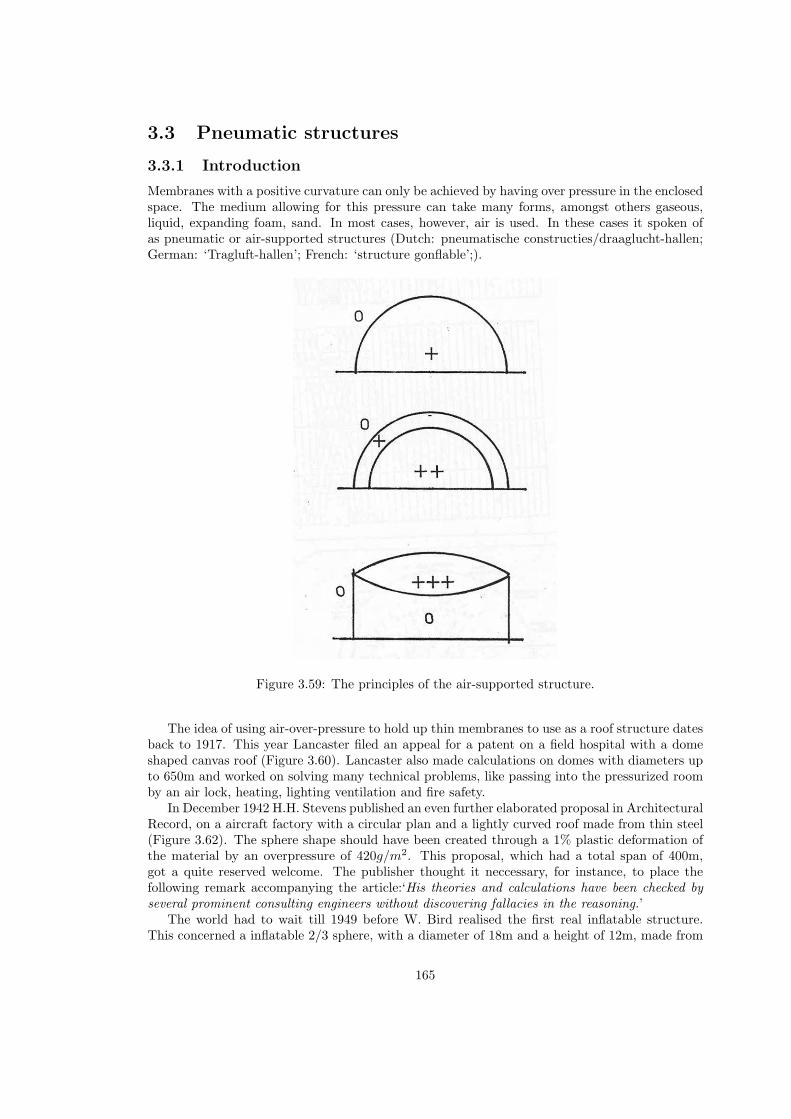
3.3 Pneumatic structures

3.3.1 Introduction

Membranes with a positive curvature can only be achieved by having over pressure in the enclosedspace. The medium allowing for this pressure can take many forms, amongst others gaseous,liquid, expanding foam, sand. In most cases, however, air is used. In these cases it spoken ofas pneumatic or air-supported structures (Dutch: pneumatische constructies/draaglucht-hallen;German: ‘Tragluft-hallen’; French: ‘structure gonflable’;).

Figure 3.59: The principles of the air-supported structure.

The idea of using air-over-pressure to hold up thin membranes to use as a roof structure datesback to 1917. This year Lancaster filed an appeal for a patent on a field hospital with a domeshaped canvas roof (Figure 3.60). Lancaster also made calculations on domes with diameters upto 650m and worked on solving many technical problems, like passing into the pressurized roomby an air lock, heating, lighting ventilation and fire safety.

In December 1942 H.H. Stevens published an even further elaborated proposal in ArchitecturalRecord, on a aircraft factory with a circular plan and a lightly curved roof made from thin steel(Figure 3.62). The sphere shape should have been created through a 1% plastic deformation ofthe material by an overpressure of 420g/m2. This proposal, which had a total span of 400m,got a quite reserved welcome. The publisher thought it neccessary, for instance, to place thefollowing remark accompanying the article:‘His theories and calculations have been checked byseveral prominent consulting engineers without discovering fallacies in the reasoning.’

The world had to wait till 1949 before W. Bird realised the first real inflatable structure.This concerned a inflatable 2/3 sphere, with a diameter of 18m and a height of 12m, made from

165

Figure 3.60: The first designs for an air-supported structure by Lancaster.

a nylon weave, impregnated with rubber (Figure 3.63.Bird’s work meant the needed impulse to an explosive development. Since the construction

of this first pneumatic structure, many daring design have been constructed by companies likeScheldjahl, U.S. Rubber, Goodyear, Irving, Stromeyer, Texair, Krupp, Ogawa, Taiyo Kogyo andmany more. Most of these structures serve as storage depots, exhibition space, swimming poolsor temporary assembly halls creating the possibility of winter production.

One of the largest radomes ever built has a diameter of 70m. It was fabricated by Scheldahland is in use for the so-called Telstar project in Maine. (Figure 3.64)

Cylindershaped halls with a quarter sphere on each end, have been built with lengths up to100m and width to 40m. A wll known example from the early years of the developments, is theexhibition pavilion for the Hannover Messe, built by Krupp. The size was 106 x 35 x 17m andthe total weight was 5,2 tons, while the skin weigh only a mere 1 kg/m2.

Also Japanes companies, like Ogawa Tent Co. Ltd., have come up with interesting and daringapplications of the air support principle. They are involved in most larger projects realized allover the world.

Air-supported structures have a number of clear advantages compared to traditional struc-tures, namely:

• modest investing and transport costs

• light foundations

• demountable

166

Figure 3.61: Patent request by F.W. Lancaster.

• fast warm up

This means it is possible to create a large and cheap covered space within a short timespanand for relatively low cost.

167

Figure 3.62: A design for an aircraft hangar by H.H. Stevens.

Figure 3.63: The first pneumatic dome structure ever built; design by W. Bird (1949).

168

Figure 3.64: The Telstar radome in Maine.

Figure 3.65: An exhibition hall by Krupp in Hannover, shape like a toroid (=part of a cylindricalring).

Figure 3.66: Air-supported halls on a longitudinal base; often applied shapes.

169

3.3.2 Principles of form

Normal force in the meridional direction:

nθ =piR2

2(3.10)

Other direction:

nφ = piR2[1 − r22R1

] (3.11)

Equilibrium equation:

nθ

r1+nφ

R2= pi (3.12)

Where pi is the over-pressure, R1 and R2 are the main radii of curvature. This leads tothe conclusion that the normal force in the circumferential direction becomes negative when2R1 < R2.

Figure 3.67: The common stress distribution in a double curved surface under internal pressure.

For a cylinder is true:

R1 = ∞; nθ =pi

R2; nφ = piR2 (3.13)

For a sphere:

R1 = R2 = R; nθ = nφ =piR2

2(3.14)

170

Figure 3.68: The stress distribution in spherical and cylindrical shaped roof surfaces.

A much used main shape is the cylinder combined with two quarter spheres on both ends.At the connection between the two different parts a discontinuity arises, because the stress inthe longitudinal direction -and with it the elongation- doubles. Nevertheless, this main shape isvery popular, because the cylinder part can be easily made from parallel bands of fabric. Muchmaterial is lossed in cutting and sizing when using double curved shapes.

Figure 3.69: The effect of the shape on the membrane stresses; M = p ∗ r2 .

171

When it is considered to realize an as equally divided stress as possible, the structural shapeis a direct derivative of the circumference of the plan. An equal divided stress occurs whenNx = Ny and Nxy = 0. On the average it is very difficult to analytically define the shape of thean air supported membrane with a random plan. This is why the shape of these structures areusually approached numerically and often also by measuring small scale physical models.

Figure 3.70: Shapes of air-supported surfaces over random plans.

172

3.3.3 Materials

It is thinkable to use isotropic foils, like PVC, saturated polyester, polyaramide, polypropylene,PVF or synthetic rubber, for this type of structures. However, it is usually very hard to createa stable shape due to excessive deformation (low E-modulus) or creep of the material.

This why the most commonly used materials are membranes with a more complicated buildup. To create the desired stiffness and strength weaves are aften chosen. For smaller structuresthis can be made from natural fibres like cotton, the majority is, however, made from linearpolyester fibres (Terlenka Trevira).

In many other cases also nylon or glassfibre weaves are used. The last mentioned mainly inlarge structures. To protect the weave and to create water- and airtightness, the weave is coveredwith a covering layer on both sides. For this layer a number of plastics are suitable. In over 90% ofthe cases in Europe, however, these layer are made from plasticized PVC. This has as advantagethat it is weldable thermally or high frequency. Also synthetic rubbers, like chloorsulfonrubber(Hypalon), polycloridebutadene (Neoprene), ethene-propene rubber and Teflon (PTFE), are usedas a covering material.

On average a covering needs to be at least 0,2mm. This leads to a thickness of PVC-polyestermembranes varying between 0,7mm and 1,2mm. The weight of this membrane is 800-1100kg/mm2. The tensile strength lies between 0,6 and 1,2 kN/cm width.

Averagestrength(kN/5cm)

Internal pres-sure (mm watercolumn)

max. radius

cylinder sphere

3,5 30 23 4650 14 2870 10 20100 7 14150 4,5 9

Table 3.2: Max. radii depending on the material strength and internal pressure.

Natural fibres - Cotton- Linnen

Synthetic fibres - Polyethylene- Polyester- Polyamide- Acrylic- Viscose- Aramide- Extended Chain Polyethylene

Metal fibres - Steel- Stainless Steel- Copper Alloys

Mineral fibres - Glass- Carbon

Table 3.3: Different types of fibre materials

Sometimes a totally different material is used, like thin steelplate. In Halifax in 1979 a designby Carruthers and Wallace was realized, which was a roof structure on a superelliptical plan of

173

Figure 3.71: Stress-strain curves for different types of fibres.

Coating materials - P.V.C.- P.U.- Neoprene- Natural Rubber- Hypalon- P.T.F.E. and F.E.P.- P.V.F.- Silicone Rubber- P.V.D.F.

Table 3.4: Applied coating materials.

82x64m. The membrane was made from 1,5mm thick stainless steel.A super ellipse can be pictured by the following expression:

xv

an

+yn

bn= 1 (3.15)

n can have every positive value. For n = 2 the regular ellipse is found with axis a and b.When n > 2 the circumscribed rectangle is approached. For n = 1 a rhomb is found with straightedges and for values n < 1 a more or less asymptotic shape is found.

When a = 1 and b = E (or Expansion), then equation 3.15 becomes:

xn +yn

En= 1 (3.16)

Yarn Weave Strip Tension (N/mm2) ConstructionWarp (%) Weft(%)

Polyester 1x1 3,000 0 2Polyester 2x2 4,5000 0 0,81Polyester 3x3 9,000 -0,5 3,5Glass 1x1 4,000 +0,5 to -0,5 2,0 to 4,0Glass 1x1 7,000 +0,8 to -0,3 4,0 to 6,0

Table 3.5: Fibre properties

174

Figure 3.72: Often applied types of membrane (costs are not realistic anymore).

Figure 3.73: An example of a high strength membrane build up.

When it is furthermore stated thatx = Rsinφ and y = Rcosφ then the equation can also bewritten as: (also see Figure 3.75)

175

Figure 3.74: The basic shape of an ellipse.

R =E

Ensinnφ+ cosnφ

1n

(3.17)

The most interesting aspect to this structure is the so-called ‘contraction joint’ (see Figure3.78), designed by D.A. Sinoski. In first instance the seam has the shape of an Ω and it isstretched when the roof is inflated. This creates the possibility to construct the roof on a flatsurface, while it gets its final shape during the inflation procedure (up to 38mm watercolumn1).A layer of acoustic and thermal glass wool insulation hangs 30cm underneath the outer plane.

11N/m2 = 1Pa = 0, 102mm water column

176

Figure 3.75: Superellipses with different values for the exponent; in this case a proportion of 1,5between the axis is chosen.

Figure 3.76: Section through the stainless steel roofstructure in Halifax.

177

Figure 3.77: Overview Halifax.

Figure 3.78: Structural lay-out of the air-supported stainless steel roof (82mx64m) with contrac-tion joint.

178

3.3.4 Air pressure

The overpressure needs to be fairly low, because of the very low self weight of the structure. Anoverpressure of 10-30mm watercolumn (0,001-0,003 atm) is sufficient in almost all cases. This isa very small pressure and is comparable to the change of airpressure over an altitude of 8-35m.This means that the same airpressure that needs to be overcome when climbing to the 8th floorof a building is enough to hold up a pneumatic structure. This clearly shows that the differencein airpressure is hardly noticable for persons entering an air-supported structure.

The only precaution that has to be taken is that the inner space has to protected from lossof pressure by an airlock, when entering. In many cases a revolving door is sufficient.

The amount of over-pressure also has some relation with the shape of the structure. Relativelyhigh structures need to be abe to take up large horizontal forces due to windload. In radardomesusually 2/3 or 3/4 spheres are used. To obtain enough shape stability in these cases, the over-pressure has to be increased up to 5- or 10-fold the regularly used pressures.

The sphere-shaped observatory in Bochum, built by Krupp in 1964, has a height of 24,5mand a maximum diameter of 39 m. In this structure an over-pressure of 40-150 mm watercolumnis used.

Force Beaufort vmax[m/s] q0[N/m2] Official description

1 1,5 2 Light air2 3 6 Light breeze3 5,5 19 Gentle breeze4 5,5 19 Moderate breeze5 11 76 Fresh breeze6 14 122 Strong breeze7 17 181 Near gale8 20 250 Gale9 24 360 Strong gale10 28 490 Storm11 32 640 Violent storm12 >32 >640 Hurricane

Table 3.6: Comparison of windspeeds and wind pressures;

In order to maintain the over-pressure, relatively small cold air ventilators are needed, thoughevery air-supported structure has many -however small- airleaks, mainly on seams, at the airlockand at the connection to the ground.

In calculating the use of power, the following rule of thumb is often used: covered area[m2]/200=KW. When a hall with a plan of 800m2 is considered, a power of 800

200 = 4KW isfound.

In such case 2 ventilators of 3KW each would be enough. The second ventilator is thenmainly as a back up if the first on fails. Depending on the needed over-pressure and the useof the enclosed space, extra safety precautions can be taken, like emergency generators. Theair-pressure is by the way always tuned to the current windspeeds, so the skin is never higherstressed than needed.

According to H. Ruhle one should use the following working pressure in calculations:(working pressure: p = pi = pe, so internal over-pressure minus external pressure by loading)

179

Practical values for pi/qw3/4 sphere > 1

> 0, 8 (when large deformations are allowed)

1/2 sphere > 0, 7

1/2 cylinder with 1/4 sphere as ending > 0, 6

For spheres:

1, 5R < h > 1, 05Rp = 0, 85 ∗ q0 = 47mm water column

1, 05R < h > 0, 75Rp = 0, 65 ∗ q0 = 35mm water column

(3.18)

For cylinders and torusses:

p = 0, 55 ∗ q0 = 30mm water column (3.19)

Where q0 is the thrust of the wind; here q0 = 0, 55kN/m2 was used. The actual value of theloading can be calculated from the airspeed. So:

q0 = 5 ∗ ρ(air) ∗ v2, where v in m/sρ(air) = 0, 125

q0 = v2

1,6N/m2

(3.20)

The most important loadcase is: working pressure + wind pressure.

Figure 3.79: Cylinder and sphere.

180

For spheres:1, 5R < h > 1, 05R

nφ = nθ = ∆p∗R2 + q0 ∗R

1, 05R < h > 0, 75R

nφ = nθ = ∆p∗R2 + 0, 75 ∗ (max c) ∗ q0 ∗R

(3.21)

The last equation (3.21) is taken from F. Rudolf. The factor (max c), or shape constant, wasdetermined by G. Beger and E. Macker for a number of values of p/q0.

∆ pq0

1,3 0,65 0,55 0,34 0,27

(max c) 1,05 1,1 1,3 1,6 1,8Cylinders:

nθ = 0, 58(1, 8q0 + ∆p)R (3.22)

Quarter spheres:

nφ = nθ =∆pR

2+ 1, 3q0R (3.23)

Basket handle arches (Dutch: korfbogen): In the cylinder part:

nφ = nθ = 0, 58(1, 8q0 + ∆p)R (3.24)

In the sphere part:nφ = nθ = 0, 8∆pR+ 1, 6 − q0R (3.25)

Figure 3.80: The two hall types, compared in Tables 3.7 & 3.8.

181

Hall no. Plan area Length Width Height Volume Circumference Average needed energym2 m m m m3 m kW/h

1 222 22.52 11.00 5.50 900 57.6 1.652 314 27.24 12.84 6.42 1490 69.1 1.653 423 31.96 14.68 7.34 2290 80.7 2.254 570 38.10 16.50 7.95 3300 95.0 2.255 713 42.82 18.34 9.17 4850 106.6 2.256 872 47.54 20.18 10.09 6520 118.1 3.007 1045 52.24 22.00 11.00 8530 129.6 3.008 1270 58.40 23.84 11.92 11260 144.0 4.109 1553 66.00 25.68 12.84 14870 161.3 4.1010 1823 72.16 27.52 13.76 18720 175.7 5.6011 2114 78.32 29.36 14.68 23190 190.1 5.6012 2425 84.46 31.18 15.59 28260 204.5 8.2513 2758 90.62 33.02 16.51 34070 218.9 11.2514 3112 96.78 34.86 17.43 40620 233.3 11.2515 3539 104.36 36.68 18.34 48650 250.5 11.25

Table 3.7: Needed energy for keeping hall type one from Figure 3.80 pressurized.

Hall no. Plan area Length Width Height Volume Circumference Average needed energym2 m m m m3 m kW/h

1 222 22.52 11.00 5.50 690 67.0 1.652 314 27.24 12.84 6.42 1590 80.2 1.653 423 31.96 14.68 7.34 2440 93.3 2.254 570 38.10 16.50 7.95 3520 109.2 2.255 713 42.82 18.34 9.17 5140 122.3 2.256 872 47.54 20.18 10.09 6910 135.4 3.007 1045 52.24 22.00 11.00 9025 148.5 4.108 1270 58.40 23.84 11.92 11890 164.5 4.109 1553 66.00 25.68 12.84 15650 183.4 5.6010 1823 72.16 27.52 13.76 19690 199.4 8.2511 2114 78.32 29.36 14.68 24360 215.4 8.2512 2425 84.46 31.18 15.59 29670 231.3 11.2513 2758 90.62 33.02 16.51 35740 247.3 11.2514 3112 96.78 34.86 17.43 42580 263.3 11.2515 3539 104.36 36.68 18.34 50940 282.1 11.25

Table 3.8: Needed energy for keeping hall type two from Figure 3.80 pressurized.

182

3.3.5 Making-up of the fabric

Air-supported structures are assembled from strips of weave with a working width of appr.130cm. Cylinders can be made from parallel strips and thus material loss is minimal. In sphere-shaped structures a radial division is normally used. The strips then have to be cut up into longstretched triangles. To diminish material loss as much as possible, and to reduce the numberof strips coming together in the top, a new division is adopted when two strips together havebecome as wide as one strip.

Figure 3.81: Often used patterns in two common shapes.

The connection between the strips is usually made by seams formed in a double overlap.Glueing is also possible, however, the available methods are often do not offer enough weatherresistance. When the surface layers are made from a thermoplastic material, for instance PVC,the connection can also be made by welding. This method is only used for smaller structures,because the connection is only superficial, which means that the weave that provides the strengthis not through-connected.

Figure 3.82: Different possibilities for seams: A. Sowing; B. Gluing or welding; C. Combinations.

Welds are sometimes used to improve the water- and airtightness as well as the weatherproof-

183

ness of the seams, by welding a strip of thermoplastic foil over the sown seam.Material losses:Cylinder: 5-10%Sphere: 20-30%Torus: 10-15%

184

3.3.6 Anchorage

The anchorage has two main functions:

1. Transfer of all membrane forces caused by the over-pressure and wind forces to the under-ground

2. Airtight connection of the skin to the underground

In Figure 3.83 a number of often used anchorage technics is shown. The simplest one is with acircumferential tube filled with sand or water. The size of the anchorage forces in cylinder shapedhalls is mainly defined by the radius R of the structure (when the same maximal over-pressureis considered for all differen sizes of the halls).

In most cases an over-pressure of 30mm water column is sufficient with a wind thrust of0, 95kN/m2 (appr. 140km/h). According to H.J. Schulz (Schulz 1962):

Anchorage force: Z = 0, 7R kN/m (R in m)Vertical component: Zv = 0, 67R kN/mVertical force with R = 5, 5m Zv = 0, 67 ∗ 5, 5 = 3, 7kN/m

When using a sand-filled tube (ρ = 1, 7kg/dm3) and a safety factor 2, a diameter of 75cm isneeded. This means that allready with relatively small radii other systems are needed, to preventbuilding absurd tube dimensions.

The most used system is the one where thread anchors with pull eyes are put into the groundwith a c.t.c distance of approximately 1m. Then a steel tube is pulled through a seam in thestructural skin and through the eyes in the anchors. The seam is off course interrupted at theanchors. A slab of weave is pressed to the ground on the inside of the structure to maintainthe needed over-pressure. When the soilconditions are too poor, it may be necessary to providean extra load, for instance in the form of concrete blocks or a poured foundation. When theanchorage forces increase even further (especially in radomes), the interruptions in the seam areno longer desirable and clamping connections are most often used.

185

Figure 3.83: Some characteristic principles of anchorage.

186

3.3.7 Building physics

3.3.7.1 Indoor climate

The thermal insulation of the very thin skin is of course very small, even though the fairly highthermal conductivity (λ = 0, 10) of the material. The K-value of the material is:

K = 11

αi+ δ

λ+ 1

αe

K = 115+ 0,0008

0,10+ 1

20

= 4Kcal/(m2hK)

(3.26)

For a double layered skin:

K = 10,20+2∗0,008+0,15+0,05

K = 2, 5Kcal/(m2hK)(3.27)

Figure 3.84: The temperature profile for single and double layered skins.

An example:A pneu with a plan of 500m2, a volume of 1800m3, a skin area of 800m2 and ti = +20C, to =

−5C ((Wellesley-Miller 1972).To prevent unnecessary loss of heat, ventilation is only performed once each hour, so n=1.

This frequanzy is off course dependant on the use of the internals pace. When a large ammountof people needs to be present at the same time, nmin should be taken as 40m3 per person. Whenthe loss of air through the airlocks is large, a seperate contribution should be accounted for.

When a 10cm thick concrete floor is considered as a floor structure, then a constant temper-ature of 10C is maintained at 2cm below ground level. The K-value of the in total 2,1m thickfloor layer is 0,47.

For a single skin now holds:

187

Wsingle = (20 + 5) ∗ 1 ∗ 18 −− ∗ 0, 31 + (20 + 5) ∗ 4 ∗ 800 + (20 − 20) ∗ 0, 47 ∗ 500Wsingle = 13.950 + 80.000 + 2.350Wsingel = 96.300Kcal/h

(3.28)

For the double-layered skin:

Wsingle = (20 + 5) ∗ 1 ∗ 18 −− ∗ 0, 31 + (20 + 5) ∗ 2, 5 ∗ 800 + (20 − 20) ∗ 0, 47 ∗ 500Wsingle = 13.950 + 50.000 + 2.350Wsingel = 66.300Kcal/h

(3.29)

This shows that a multiple-layerd skin results in a significant reduce of needed energy whena normal -and for air-supported halls: fairly high- inside temperature needs to be maintained.According to U. Bauer (Bauer 1968) the total heat flow adds up to:

Q = K ∗ F ∗ (t+ 5C (3.30)

Wher F is the total area of the skin and T the desired temperature difference. The extra 5Cis a practical value, considering losses due to airleaks. For an average cylinder hall of 40x18x8mand a demanded temperature difference of 20C a energy consumption of 112.000kcal/h. R.Brylka (Brylka 1970) uses the following rule of thumb:

area of plan[m2]*240 at temperature difference of 20C, so: 100 ∗ 240 = 168.000kcal/h. Thisis clearly on the very safe side.

The forming of condense is a problem especially encountered at swimming pools, becauseof the high internal temperatures and the large evaporation surface. According to Bauer aventilation coefficient of 1,25 per hour is enough to prevent the forming of condense. In extremesituations, like the forementioned swimming halls, this can be achieved by forming gutters, usingthe seam covering strips. By puncturing these in strategic place the possibly formed condensecan be diverted.

Direct solarization can be prevented by using light coloured materials. In the summer, how-ever, the temperature of the outside skin can still accumulate to 55C. Usually, this does notimpose great objections, because the air is refreshed several times each hours. If it still posesproblems, the outside can be cooled by spraying water. In smaller halls -where this problem ismost urgent- also the use of mechanical coolers can be considered.

3.3.7.2 Air locks

To maintain the internal over pressure, the entrances to a air-supported structure need to beprovided with air locks. A number of considerations need to be made in the design of such locks:

• A hole needs to be made in the tensioned outer skin. This can not be done withouttaking precautions: the force from the skin needs to be diverted and brought down to thefoudnation. This is usually done by giving the hole a smoothly run, mostly circular, shapeand leading a cable through the edge seam.

• The entrance itself can be constructed in several manners:

– A simple door opening against the air pressure, so inward.

– A rectangular lock with single or double doors on both sides.

– A revolving door.

188

– Special solutions, like flaps falling over each other or cushion shaped elements.

• The transfer from the outer skin to the lock needs to be made in such a way that theairpressure can be taken in the transfer area, as well as movements are allowed te preventundesired stresses in the skin.

Figure 3.85: Necessary provisions for entering while maintaining the over-pressure.

Figure 3.86: Tensioning around a door.

189

Figure 3.87: Different solutions for an airlock.

190

3.3.8 Regulations

There are no regulations in the Netherlands. A German proposal, dating back to July 1971, onthe design of the ‘Arbeitskreis Tragluftblauten’ of the ‘Fachkommission Bauaufsicht der Argebau’(Argebau 1971), can be summarized as follows:

1. Building permits are provided for a timespan of maximum of 5 years. After 5 years requestscan be made for every time a duration of 3 years.

2. For the calculation the windloading on half cylinders can be schematized by a uniformlydistributed radial suction force of -0,9*the local value of the wind thrust (Figure 3.88). Forthe anchorage a horizontal load of 0,6*wind thrust*height should be considered. A moreacurate calculation, based on the division of the windload of Figure 3.88.4 may be used forhalf cylinders, but has to be used for sphere shaped structures.

3. Snow loading does not have to be considered when it made sure that the inside temperaturenever falls below 12C. If one wants to get permission not to consider snow load anyhow,one should take care that the snow is removed in an early stage. For instance with a cablehangin from the top of the structure. Concentrated loads should always be avoided.

4. The safety on the occurence of folds due to compressive stresses in the skin needs to be:

• For cylinders: V = pi∗rmax nD

= 2, 0

• For spheres: V = pi∗rmax nD

= 1, 2

Where nD is the largest membrane compression force that occurs when the inner pressurepi is left out of consideration.

5. For cylinders holds for the inner pressure, when h/r¡1:

• min pi = 0, 3kN/m2, for h > 8, 00m

• min pi = 0, 2kN/m2, for h < 8, 00m

• min pi = 0, 12kN/m2, for h < 3, 50m and covered area < 200m2

6. The skin material needs to be secured for tearing for at least 5x the maximal tensile stress.The seams need to have a safety factor of 3,5.

7. Air-supported halls, where 11-30 people need to be staying, have to have 2 cold air ven-tilators, each capable of maintaining the overpressure. In halls where over 30 people canreside, the second ventilator needs to be equiped with a self starting engine, non dependendof outside power. In this case also at least two exits need to be available for fire safety. Anair-supported hall is, however, not considered as unsafe regarding fire. They are consideredas very safe structures. In the first place the skin is very light, so collapse is not alwaysdisastrous. Also, the collapse is very slow due to the very low over-pressure, even when theventilators fail or large holes appear. During a fire large holes usually appear locally at thefire, because the materials are often flame stopping. Collapse is furthermore counteractedby the warming up of the internal air, which will expand and initiate a rising motion.(Figure 3.89)

191

Figure 3.88: Loading on circular shaped air-supported halls.

192

Figure 3.89: Time taken to collapse at different door widths.

193

3.3.9 Stabilizing the shape

3.3.9.1 tying down

The shape of the structure can be influenced by tying it down line or point shaped. Frei Otto(Otto, Trostel & Schleyer 1962) gives many possibilities for this. One of the oldest knownapplications is the Brassrail snackbar by V. Lundy, built for the New York World Fair of 1965by Birdair.

Figure 3.90: The principle of stabilisation by tying down.

Lineshaped indentations can be created by spanning cables over the skin (Figure 3.91) or bywalls underneath the skin, like was done in a twin tennishall by Stromeyer.

These cables and walls exert, in most cases, an extra stabilizing effect on the structure,because it becomes less sensitive for asymmetrical or local loading. This creates the possibilityof very large spans, especially when the height is chosen small. In this case the radius for a skinthat has not been tight down will be very large and it will be very sensitive for local disturbances.The tension in the skin will also be very high. This skin stress will be lowered by decreasing theradii. (See Figure 3.69 and (Schippers 1975))

Figure 3.91: The principle of tying down with line shaped ties.

The pattern of these cables on the surface of the roof is most often radial (in circle shapedplans), parallel (in rectangular plans), rectangular or even geodetic (built up from triangles).The most famous example of a rectangular cable pattern is the U.S.A. pavilion on the World Fairin Osaka 1970 (Architectural design: Davis Brody; Structural design: David Geiger), shown inFigure 3.92. The membrane consists of a glassfibre weave with a PVC coating. It has a plan of83x142m, shaped like a super-ellips. In this case exponent n-2,5 was used (Chapter 3.3.3).

Another example is the 135x50m measuring Canadese pavilion for the 1986 Expo in Vancouverby E. Zeidler; the so-called B.C. Place Amphitheatre. Furthermore the Lindsay Park AquaticCentre in Calgary, Canada. This last one has a roof in the shape of a supercircle with a diameterof over 200m. In a supercircle a=b is chosen (also Chapter 3.3.3).

In this structure much attention was payed to the thermal insulation. The roof is built up

194

Figure 3.92: The American pavilion at the Osaka World Fair.

from multiple layers. The outer layer is a glasfibre weave with a PTFE coating. Underneath alayer of 10cm so-called Fibair isolation material is hung and all the way on the inside a dampprooflayer of Tedlar foil is installed. This total layer is still not entirely airtight.

Figure 3.93: The B.C. Place Amphitheatre in Vancouver (top) and the Aquatic centre in Calgary,Canada (bottom).

Research into soap bubbles (mainly based on visual judgement) can provide information aboutthe most appropriate way and shape of the tying down by interior walls. Moreover, studyingthe laws to which conglomerations of two or more soap bubbles apply, gives insight in the originand appearance of inflated foams and some single cell organisms, of which the interior walls arestiffened and are part of the skeleton (Figure 3.94).

The shape of the dividing wall of two soap bubbles follows from:

1RA

+ 1RAB

= 1RB

so: RAB = RA∗RB

RA−RB

(3.31)

When considering two bubbles of the same size the following holds:

RAB = ∞ (3.32)

And when RA = 2RB :

195

Figure 3.94: Soap bubble configurations.

RAB = RA (3.33)

196

3.3.9.2 Double layered structures

The necessity to enter an air-supported structure through an air lock, to prevent the loss ofpressure, is felt like a hindrance in many areas of application. When the skin is made double, theloss of pressure between inside and outside can be made obsolete. When this is done one shouldspeak of an ‘air inflated structure’ rather than an ‘air suppported structure’.

Figure 3.95: Principles of double layered pneumatic structures.

An early example of such a solution is the Boston Arts Centre Theater by Koch, Ross andWeidlinger. Two nylon skins, spanned between a steel circular compression ring with a diameterof 35m, are inflated into a cushion with a thickness in the centre of 6m (Figure 3.96).

When covering a shopping street in Marl Germany, cushions of approximately 30m wide and60m long were used. These were modelled to a more or less flattened shape by a number of tyingcables on both the top and bottomsides, on a c.t.c. distance of 7,5m. The material that was used

197

Figure 3.96: The Boston Arts Centre Theatre by Koch, Ross and Weidlinger.

here was liniar polyester for the weave (Terlenka or Diolen) and PVC for the coating on bothsides. This led to a total weight of the membrane of 850g/m2 and a tearstrength of 4, 15kN/5cmthe thickness of the cushions was approximately 8cm.

In a similar way the engineering company ABT realized a roof in Burger’s Bush in Arnhem.It measured 90x150m and was covered with cushions consiting of three layers of PTFE foil,measuring 3x6m each. This tying down with cables was used to reduce the disadvantage of verythick cushions needed for large spans.

This can also be reached by using internal walls. This was for instance done in the exhibitionhall for the nuclear energie committee of the U.S.A., designed by V. Lundy (Figure 3.99) Thespanning distance for the skin was thus fixed at 1,2m. To be able to give the internal and externalskin a fluent look, it was decided to use over-pressure in the room and choosing a slightly higherover-pressure for the cushions themselves (respectively 38 and 49mm water column). This leadsto the impression of inflated tubes at the free ends of the entrance parts, which are used asportalframes.

Constructing with inflated tubes has been used in many different shapes. For instance theFuji Group pavilion (Osaka, 1970, Figure 3.100) where the architect Yukata Murata used portalframes shaped like giant tubes with a span of around 50m to create an interconnected archedroof.

At the so-called Showboat of the Electric Energy pavilion by the same architect, three portalshaped like tubes, spanning 23m were used as a support for a double membrane spanned inbetween. In these double membranes an under -pressure was created (Figure 3.101). The videopavilion by the ERG Group in Sonsbeek in 1970 was based on a similar principle (Figure 3.102).

198

Figure 3.97: Structural lay out of the covering of a shoppincentre in Marl.

The principle of the tube was not only used for roofstructures. An interesting example is theinflatable bridge, developed by P.S. Bulson for the army engineers. The bridge has a free spanof 6m and can carry the weight of a car. The in this case high tensile forces are taken up byinbedded steel cables, while the compression stress is taken up by timber elements layed in thewidth direction of the bridge (Figure 3.103).

Another important area of application is that of the inflatable barrier (Figure 3.104). Theinternal pressure is provided by water let into the structure. It is possible to get such a dam upto height in a very short matter of time. The oldest example is the so-called ‘Fabridam’, built byImberson in Los Angeles in 1957. In Vezer in France this solution is used to be able to adjust theheight of the dam to the ever changing run-off of the river. This way the effects for the peopleliving in the direct neighbourhood are kept small.

Closer to home an entirely foldable storm surge barrier, proposed by ir. J.C. Buyze, was builtby Vredestein. During normal weather it is stored underneath steel covers and it only is usedwhen the dikes collapse.

Besides by using interior walls, the skins of double-layered inflated structures can be heldtogether by threads. By creating a fine mesh of threads between both layers of skin, a totalflatness of both outer skins kan be achieved. This way pneumatic sandwich panels can be created.

R. Buckminster Fuller, in cooperation with Berger Brothers, developed rubber inflatabledomes, assembled from rhomb- or triangular-shaped panels. The English firm M.L. Aviation

199

Figure 3.98: Structural detail of the covering in Marl.

Figure 3.99: Double layered exhibition hall by V. Lundy.

Co. used to have a standard system in its program, called ‘airmat-shelters’, with which differentcombinations between quarter spheres and half cylinders are possible. It is interesting to notethat hall of 18x9x5m can be pack in a box of 1,5x1,0,5m.

Using airmats fairly large spans can be reached. A pavilion by P. Jutras, for the Expo 1985in Tsukuba, Japan, has a span of 27m with a largest thickness of 4,5m.

200

Figure 3.100: Fuji Group pavilion in Osaka.

201

Figure 3.101: Showboat of the Electric Energy pavilion by Y. Murata.

Figure 3.102: The video-pavilion in Sonsbeek by the ERG-group.

202

Figure 3.103: Inflated bridge structure by P.S. Bulson.

203

Figure 3.104: An inflated dam structure, with water as medium.

Figure 3.105: Principle of the air sandwich.

204

Figure 3.106: Noteworthy pneumatic structures at the Osaka World Fair 1970.

205

3.3.9.3 Rigidising air-supported structures.

As can be concluded from the German proposed regulations, air-supported structures are mainlyregarded as temporary structures. The vulnarability and easily deformable skin are the mostimportant considerations in this regard. It has been tried -not always succesful- to change theseaspects by making the skin rigid, by spraying polyurethane foam or glasfibre polyester onto theskin.

When using polurethane foam it can be chosen to spray it on the inside as well as on theoutside of the structure, because the material has a strong sticking immidiately when expanding.People who have used this technic are G. Gunschel and F. Otto in cooperation with W. Muhlau.

In 1967 the first two test structures with polyurethane foam, constructed by sparying it ontoa PVC air-supported hall, were build in the Netherlands by P.B. Hangelbroek of the InstituutLandbouwbedrijfsgebouwen Wageningen. The PVC foil was held in its right shape by using anet of sisal rope.

Figure 3.107: The principle of rigidising air-supported structures.

Bayer made half-sphere residential units, by spraying polyurethane foam spirally over aninflated model. The spray head was moved up along a meridian arch, while at the same time themodel was turned round a vertical exis. After hardening, the mold was removed. Many hundredsof these structures have been built in Turkey and Guatemala, where they were use as emergencyhousing. In Tilburg a temporary project, the so called ‘Iglonium, arose around 1972, where aseries of the fore-mentioned units were coupled by connecting pieces from the same PU-foam.

Burger Eisenwerke in the same way created a building out of glassfibre polyester, with afootprint of 4x8m and a height of 2,5m, while the material thicknes was a mere 5,5mm. Thehardest thing in glassfibre polyester is the fact that a fairly tough underground is needed to beable to drive out the enclosed air in the laminate.

The character of the inflatable structure changes radically when the stiffening material ishardened out and the over-pressure is released. It can only be concluded that the originalstructure was used merely as a mold to build a totally different structure with a totally differentstructural principle. Now other considerations regarding the structural shape will begin to playan important role.

The use of inflatable structures for mold purposes is also look into in the concrete industry,amongs others by Bini in the Bini-shell principle, by Wallace Neff, by Hangelbroek, Poort andGrabovski for the Airform-procedure for covering silo’s and by the Australian company DomeConstructions. The latter has constructed spheres to up to 80m span, by first spraying a layer ofPU-foam onto the inside of a pneu. After this concrete an reinforcement were added. In the endthe pneu was removed and a watertight coating is applied to the outside in the desired colour.

206

The problem that is encountered usually, is that as a result of the local pouring or sprayingof the concrete many small cracks occur in the end result. This is why the concrete is applied inmany thin layers.

The procedure of making air-supported structures rigid by using foam or glassfibre polyesterhas to take place at the building site. Depending on the climate conditions, this can pose difficultproblems.

207

3.4 Space frames

Recommended Study Material

Title Author YearTitle first entry Author first entry YoP first en-

try

208

3.4.1 Space Frames

A space frame is normally a light weight structure, it is stiff, built out of tension and compressionelements and the nodes are, at least in calculations, working likes hinges. The term spacestructures will be used as a generic term for spatial arrangements, geometric configurations,forms, patterns and structures. The architectural or built space structures have variouscharacteristics which include physical perceptual, functional economic, symbolic, or spatialaspects. The physical aspects deal with weight, size, force, and strength, method of constructionor fabrication, and spatial aspects deal with dimension, topology, geometry and symmetry.The flat shape, of space frames, is used quite often. In space frames a lot of repetition is usedwhich makes it less expensive and easy to build. Different structures and their families transformfrom one to another.

3.4.1.1 Introduction

Designing in three dimensions 1-dimensional space structure (n=1) are organized around a’line’ as in a modular tower or a linear truss. 2-dimensional space structures (n-2) are organizedaround a ’plane’ as in a single- or double-layered space frame. 3-dimensional space structures(n=3) are organized in ’3-dimensional space’ as in a multi-layered or multi-directional spaceframe. N-dimensional space structures must be projected down to 3-and lower dimensions for usto realize them physically. These four classes of built structures are composed of four elements,vertices (nodes), faces (panels), edges (struts), cells (3-dimensional modules).

Most of the time engineers and architects think in terms of planar (2D) structures such asbeams, trusses and portal frames when considering methods of spanning space. However, inmany cases there are advantages to be gained from thinking in three dimensions and applyspatial structures for medium to long spans. Especially when heavy loads points or movingloads are to be supported.

Among architects, engineers and others in the building and construction industry the generalterm ’space frame’ is commonly used to describe three-dimensional structures that may be eitherframes or trusses in the engineering definition of the terms. In fact, practically all ’space frames’are space trusses in the engineering sense. ’Space grid structures’ is an accepted alternativename that encompasses both structural systems. They are systems of inter-connected elements.

A short overview on the development of the space frame In the 19th century severaldomes were designed and built with cast iron elements. August Foppl (1854-1924) is generallyrecognized as one of the first scientists having introduced consequent research work concerning3-D steel trusses. However the first real attempts to design and realize metal space frames areknown to have been made by Alexander Graham Bell (1847-1924). In spite of the fact that instructural engineering the space trusses by Eiffel can be regarded as an assembly of 2-D trusses,the aero plane designs showed explicitly that 2,5-D and 3-D entities had to developed further,because the spatial stability had to be absolute.

• Eiffel tower, Gustave Eiffel (1832-1923)

• First industrial Space Frame, Graham Bell (1847-1922)

• MERO system, Max Meringhausen (1903-1988)

209

• Fuller Sphere, and study on closest packing of spheres, developed the Octet Truss System,Richard Buckminster Fuller (1895-1981)

Figure 3.108: A point load supported by one individual simple truss. Image from (Chilton 2000)

Figure 3.109: Deflection of a system of individual trusses. Image from (Chilton 2000)

210

Figure 3.110: A point load supported space grid of intersecting trusses. Image from (Chilton2000)

Figure 3.111: The deflection of a two-way spanning double-layer grid of intersecting trussesdemonstrating the load distribution advantage. Image from (Chilton 2000)

211

During the 1950s and 1960s, space grid systems were built all over the world as architectsexplored the aesthetic of the modular grid and engineers experimented with jointing systems,materials and configurations. Some people believe that the use of space grids reached its climaxin the 1970s. However, space structures are still being used widely for medium and long spanstructures of innovative form. In the more developed world their use diminishes but in thedeveloping countries there is a huge potential for their widespread use. The materials areexpensive, labour is cheap and simple efficient structures are in demand.

3.4.1.2 The advantages of two way spanning

The principle and benefit of using a two-way spanning structure can be demonstrated as thewoven canvas webbing often used for seats or to support chair hassocks are considered. Ifwebbing strips are used only in one direction, a load applied to one strip will cause it tosag and transfer loads to only two sides of the supporting frame. However, if the webbingstrips are interwoven in two orthogonal directions the loaded strip is partly supported byall others. This reduces the sag of the loaded strip and distributes the applied load evenmore evenly to all sides of the frame. In the second case, each strip does not have to becapable of carrying the full applied load on its own and a lighter structure can be usedfor the supporting frame. Another advantage is that, if one of the webbing strips breaks,the seat as a whole will still support loads. Similar benefits may accrue from the use of two-way spanning structures in architecture and engineering. See Figures 3.108-3.111 (Chilton 2000).

When the span of the structure exceeds about 10 m, the use of beam elements in a single layergrid becomes less economical. And open web trusses or Vierendeel girders may be substitutedfor the solid beams. Connected with a pattern of vertical and/or inclined ’web elements’ betweenthe two plane girders results in a double layer grid. Double layer grids are the most efficient andlightweight structural systems because of their ability to share the task of load carrying throughthe whole structure.

3.4.1.3 Aspect Ratio

The benefit of two-way spanning is the greatest if the ratio of the lengths of strips is around1. The roof will be square in this situation (square bays). It is also possible to modify theload distribution characteristics; by increasing the size of the chord members in the long spandirection.The decision whether to use a three-dimensional space grid or a one-way spanning structure isoften influenced by the plan form of the building and the location of the supporting structure.If support is only possible along two opposing sides of a rectangular building one-way spanningwill almost certainly be more economical. If supports can be provided along all sides it is moredifficult to decide. It depends on several factors, in particular the ratio of the spans in eachdirection; the span aspect ratio. The influence of the span aspect ratio on load distributionwithin a two-way spanning structure is illustrated by a simple point load W applied at theintersection of two orthogonal beams of span L and L. The beams are connected at theirmidpoints (perpendicular) and form in that way a simple single-layer beam grid. The Young’sModulus (E) and second moment of area (I) are the same for both. The relationship betweenthe span aspect ratio (L1/L2) and the loads carried out by each beam W1 and W2 can be foundby the following equations:

Mid-span deflection with hinge and roller support:

212

Span ratio (L2

L1) 1.0 1.2 1.5 2.0 3.0

Beam 1(W1) 0,500W 0,633W 0,771W 0,889W 0,964WBeam 2(W2) 0,500W 0,367W 0,229W 0,111W 0,036W

Table 3.9: Span Ratio. (Chilton 2000) Note: E and I constant, L2 longer span and L1 shorterspan.

δ =1

48

WL3

EI(3.34)

If connected the deflections must be equal. The term 48EI is constant and the equationfollows;

W1(L1)3 = W2(L2)

3 or W1 = W2(L2)

3

(L1)3;

with W1 +W2 = W(3.35)

Figure 3.112: Relationship between span aspect ratio and proportion of the total load carriedout by the longer span beam, L2 of the simple two-beam intersection grid ratio L2/L1, equal to1, 2, 3, 5. Image from (Chilton 2000)

Seen these results it can be concluded that in large space grid structures, a double layer gridis more usual and there are many more intersecting members but the basic principle of usingaspect ratios close to 1.0 still applies. When an economical solution is to be achieved and theaspect ratio is much greater than the 1.0 the possibility of dividing the longer span by introducingintermediate columns should be considered. If a clear span is essential, additional lines of supportin the form of stiff edges or intermediate beams on grid lines may be used to break the structurein approximately square bays. It is also possible to increase the depth of the longer beam andthus the magnitude of its second moment of area I (stiffness). See Figure 3.112.

3.4.1.4 Advantages and disadvantages of space frames

Disadvantages of space frames Space frames have some disadvantages which must be offsetagainst the considerable number of advantages described further on in this section.

213

• Cost The costs can sometimes be high when compared with alternative structural systems.Particularly when space frames are used for relative short spans; spans less than 20 to 30meter can probably be considered as short for most space frames. Choice of grid configu-ration and the depth between the chord layers will affect the economy of the space frame.Prefabricated elements are produced in limited number of standard sizes and depths. Thenodes are the most expensive part of the frame. Reducing the amount of nodes makes theframe more economical and the erection time is shorter.

• Regular Geometry To some eyes the space frames can appear very busy. The regularnature of the geometry is lost and at some viewing angles, the ’lightweight’ structure appearsto be very dense indeed. The upper and lower grid sizes as well as the grid depth have aconsiderable influence on the perceived density of the double layer structure and charismaof the building. On the other hand the space frame can give a nice view on the curves ofthe structure. See Figure 3.113.

Figure 3.113: Regular geometry can gives nice views. Pallafolls sports hall.Image from (Chilton2000)

• Erection time The number and complexity of joints can lead to longer erection timeson site. Designing the grid to contain the most practical minimum number of nodes isgood practice; they are usually the most expensive components. This leads to economy ofmaterial costs and faster erection time.

• Fire protection Most of the times space frames are used at places where normally nominalor no fire resistance is required. However, when necessary it is difficult to achieve econom-ically due the high number and relative large surface area of the space grid elements.

• Load sharing at supports Space frames are called high redundant structures. But alsowith the freedom of placing support are limits; some examples are known of roofs whichcollapsed under snow-loads of 78 − 88kg/m2. In space trusses supported at the bottomnodes there are usually four diagonal web members converging on each support and theseare in compression. Failure of only one of this due accidental damage or buckling underexcessive compression owing to an unforeseen load can lead to the partial or total collapseof the whole structure, as the load originally carried by the failed member transfers to theremaining three in turn causes their failure.

Advantages of space frames Space frames have a considerable number of advantages whichmake them useful as structures.

214

• No bending moments by external forces If loads are directly applied to the nodes thebars within the space frame carry either axial tension or compression forces because spaceframes have hinge connections which can not pass on moments. Bending is only presentdue the self-weight of the bars.

• Installation of services The open nature of the structure allows easy installation ofmechanical and electrical services and air-handling ducts within the structural depth.

• Load sharing The prime advantage of space grid structures is that generally all elementscontribute to the load carrying capacity. This in contrast with planar beams or trusseswhich must be individually capable of carrying any possible concentrated or heavy mov-ing loads. However in space grids such concentrated loads are distributed more evenlythroughout the structures and all supports. The maximum deflections are reduced, lighteror shallower three dimensional structures may be used, which can result in reducing costsof the supporting structures.

• Robustness Failure of one or a limited number of elements, for instance buckling of acompression member under excessive loading, does not necessarily lead to overall or pro-gressive collapse of the structure. Space frames are also called highly redundant structures.The redundancy of space grid structures also assists with their resistance to damage ofspace grid , which allows heat and smoke (in fire) or the force of the blast (in explosion) toescape.

• Modular components and prefabrication Space frames are almost all prefabricatedin the factory. Therefore the product is usually produced with high dimensional accuracy,high quality of surface finishing and generally easily to transport. Without difficulty itcan taken down and reassembled elsewhere. In the past many different systems have beenbrought on the market. The most famous are the MERO system and Space Deck. SeeFigure 3.114 and 3.115.

• Regular geometry and simplicity of erection The use of space grids is the efficiencyof erection for large-span roof structures and especially on sites with limited access. Thewhole roof can be assembled safely at or near ground level and then jacked into its finalposition. Large structures can be assembled out of small elements, on site, with limiteddisruption to other activities.

Figure 3.114: MERO System. Image from http://www.columbia.edu

215

Figure 3.115: Space Deck System. Image from (Nooshin, Space Structures Research Centre,Department of Civil Engineering, University of Surrey, Guildford, UK 1984)

216

• Supporting structures, freedom of placing Within reason, space frames can be sup-ported at any node of the grid and at practically any location in plan. This gives thearchitect considerable freedom in space planning beneath the grid. As mentioned beforesquare bays are preferable. To avoid high forces in one point tree structures are used tolead the forces to the supports.

3.4.2 Formal definition

A space frame (Dutch: ‘ruimtevakwerk’) is a structure, which consists of bars, all connected byhinges. The bars will be purely loaded in axial direction and will not have to take any bendingmoment. Together they need to have such a spatial configuration, in order for a stable systemto be formed. This means that the bars in the structure need to form triangles in two or moredirections.

The term ‘space frame’ is normally used for systems, which have a clear upper and lowerlayer of bars - usually parallel to each other - with in between a network of bars, which keepsthe outer layer in place. Another term used for spaceframes is ‘spacedecks’. These systems haveat least two layers, but sometimes also three or more.

To be complete single-layer systems will be dealt with in short. However, in principle theycan be interpreted as translations of shells. They also have a lot in common with the earliermentioned space frames.

A framework (Dutch:‘staafwerk’) is - according to common opinion - considered a structure,built up from bars which are connected with a certain ammount of bending stiffness.

This stiffness is never infinitely large and can also be different in two perpendiculairdirections. However, this does mean that the bars have to be able to resist the bending momentin the given direction. The bars will be loaded in bending and/or normal force.

The main shape of a framework or a truss system can be:

• flat (slab)

• kinked

• singular curved (barrel vault, cylinder)

• multiply curved (sphere, hyppar)

• combinations (especially cylinder with sphere)

A flat system is in essence always in two or more layers, all others can also be single-layered.

217

Figure 3.116: Different principle shapes of spaceframes

218

3.4.3 Single layer systems

3.4.3.1 Flat;

A single-layer structure will normally not be designed flat. In case of flat structures it shouldbe considered as a combination of beams and columns. In that case the loads are transferedby bending moments; this requires a large construction depth, in order to get a large innermoment-arm.

3.4.3.2 Single folded or curved;

This type of structures is easily made single folded or curved with one type of bar. The jointsmust have at least four or six directions of connection to allow for respectively square ortriangular subdivisions. Dependent of the applied type of division - or pattern - these can be ofone and the same type.

3.4.3.3 Double curved;

To create such structures multiple bartypes are needed. The amount of different types dependson the shape and the chosen method of division. There are also multiple types of joints required.The number of directions of connection usually does not exceed six. The connections of themembers at the joints can be executed as hinges when the bars together form a stable system.This criterium is met if:

s = 3k − 6 (3.36)

where s = number of bars and k = number of joints.

3.4.3.4 Combinations;

Parts of single and double curved surfaces can be joined into one surface. Parts of cylinders arefairly easily combined with parts of spheres. It is for instance also possible to create a crossvault, by combining perpendicular cuts from two equal cylinders, or the opposite shape. Spherescan also be built up from sectors in the shape of cylinderparts.

219

Figure 3.117: Different single layer shapes

220

Figure 3.118: Combinations of single and double curved systems

221

3.4.4 Systems with multiple layers.

3.4.4.1 Double layered

Borrego (Borrego 1967) discerns the following principly different methods:

Direct Grid Two parallel, identical rasters, directly above each other. Upper and lower planeare connected by flat vertical trusses.

Offset Grid Two parallel, identical rasters, in at least one but mostly in two directions shiftedregarding each other in plane, but not rotated. The upper and lower plane are connected bysloping bars.

Figure 3.119: Stacking of octahedrons and tetrahedrons, in which the most often used offset gridappears as horizontal layer

Differential Grid Two parallel, but not-congruous rasters, chosen regarding each other insuch a way that they can work together properly, in combination with the connecting barsbetween upper and lower plane. Furthermore Borrego names the ‘lattice girders’, built up fromprefabricated beam, but these are not essentially different from the first group.

3.4.4.2 Three or more layers

These can be a stacking of multiple flat systems. The direct grids and the offset grids are verysuitable for stacking. In the first case a system of coupled prisma is created, in the other case amore complicated spatial build up is found.

A built up like this can be stretched out into infinity, where the connecting bars meeteach other according to a regular, repeating pattern under carefully defined angles. From thisview parts can be selected which suit the regarded design problem. Vertical parts can for instancebe taken out to create a tower structure, cavities can be made in the outside perimeter, or piecescan be taken of and put on. On a rough base practically every building shape can be approached.

Three-layered trusses are taken into account much more often these days, when dealingwith large spans.

222

3.4.5 Polygons as base element for spatial structures

Spatial frameworks or trusses can in practically all cases be considered as structures in whichthe principal form is based on the so-called Platonic and Archimedic polygons. That is why it isimportant to know their most important characteristics.

The cube, octahedron and tetrahedron are usually the base elements for the well knowntypes of spaceframes.

As shown in (Huybers 1994), every polygon also has an inversed or ‘reciprocal’ shape.The rhombic dodecahedron and rhombic triacontahedron (Dutch: ruitentwaalf- en dertigvlak)are in this context the most important representatives for this group. The direction of the ribsof the rhombic dodecahedron are in a cube and therefore this shape is in certain perspectivessuitable as concept for the geometry and as an alternative for the node-element. The rhombictriacontahedron is - just like the triangular Platonic figures (octahedron and ikosahedron) -often used as concept for sphere divisions. Aside from that, certain structures often calledquasi-crystalline, are based on this shape.

3.4.5.1 Spacefilling stackings of polyhedrons.

Some of these polyhedrons can be put together in larger numbers, into closed spatial packings.This is used in spaceframes. The directions of the ribs, their mutual angles and the positionangle between the planes are therefore interesting data, because these are directly linked to thetrusses based upon them.

Prismatic Systems. In a plane some prisms can be joined into one. In this way direct gridsare formed. With the square, prism or cube a system is made of perpendicularly intersectingtruss beams. The square -or rectangular- faces of prisms must be stiffened to get a stable system.

Cubic Sections In every face of a cube a diagonal can be installed in such a way that althese diagonals together form a tetrahedron. Such braced cubes can be coupled alternatingly-horizontally and vertically- and this way the most often used spatial configuration is derived.The original MERO-system, for instance, is based on this. In this system two lengths of barsexist: length a (cube rib) and length a

√2 (brace). When the ribs of the cubes are taken out,

a system of coupled tetrahedrons is left, with the open spaces in between shaped like octahedrons.

A horizontal cut gives the best known raster, the earlier mentioned offset grid with a rectan-gular pattern in upper an lower plane. A diagonal cut, so alongside a series of triangles, gives theby R. Buckminster Fuller introduced octet-truss, with triangular rasters in upper and lower plane.Grigorievich(IASS 1985) and Mengeringhausen/Eberlein(Mengeringhausen 1975)(Popko 1968)point out the possibilities to realise different sorts of truss systems with a different build up,based on cubic packings.

An orthogonal offset grid according to the cubic system is in fact a layer of upward aimedpyramids with the shape of half an octahedron, of which the tops are connected by the rectangularbar pattern in the upper plane.

Rhombic Dodecahedron Build-up When in the cube, apart from the plane diagonals, alsothe body diagonals are accepted, then the possibility arises to create rhombic dodecahedrons.This means that in this system also edge-endings under 45 degrees become possible. So it willbe easier to work around the corner, for example from roof to wall. The main layout of the truss

223

system can be very similar to the normal cubic system and can therefore also be shaped like anoffset grid of pyramids, but they will now have sideplanes under 45 degrees.In the joints a new direction is introduced, namely arctan( 1√

2) = 35.26. Though there are two

bar lengths needed: a for the horizontals and a√2

for the diagonal ribs.

Other Systems. Apart from the cubic and the rhombic dodecahedron system also some otherconfigurations are known, which can be suitable as principle. There is mainly much interestin the so-called quasi-crystaline build-up. With two types of spatial cells, a thick and a thinone, with rhomb-shaped (Dutch: ‘ruitvormig’) side planes, interesting structures can be built.Depending on the point of view they have a very different appearance.

There is little concrete information available yet. This is also true for the zone-eder-build-up, for which amongst others S. Baer (Baer 1970) and, in the Netherlands, O. Hanegraaff(Hanegraaf & et al. 1975) are conducting a lot of pioneering work. They are trying to furtherexplore the field of the 5-axle symmetry, which is found in the iscohedron and the rhombictriacontahedron Besides some incidental and small scale applications there have not been manypractical developments.

224

Figure 3.120: Two-layered systems

225

Figure 3.121: Cubic rasters with octahedrons, tetrahedrons and cuboctahedrons

Figure 3.122: Spacefilling stacking of a 14-plane

226

Figure 3.123: Typical node element in a cubic system

Figure 3.124: Spatial system of cubes with plane diagonals

227

Figure 3.125: rhombic dodecahedron

Figure 3.126: Spatial view of cubic systems

228

Figure 3.127: Zone-eders

229

3.4.6 Parallel rasters

When space frames are considered, most of the time mainly planar configurations with parallelupper and bottom planes are meant.

3.4.6.1 Often applied shapes

Most popular are the grids which have as many the same bars, so as little different types of bars.These grids are almost always dual, which means that the bottom plane is divided in connectingpolygons (3-,4-,6-, or higher level polygons) and that every joint of the upper plane is centeredabove one of these polygon-planes. This creates a layer of upward aimed pyramids, of which thetops are interconnected.

With the systems, previously indicated as ‘cubic’, in fact only the diagonals from the squarefaces are used. One of the two possible diagonals is chosen in a way that a certain spatial paternis created. All diagonals have the same length and they become the ribs of two of the most oftenused systems.

With the rhombic dodecahedron-systems all ribs of the cubes are used, along with the innerdiagonals. This creates two diagonal lengths: l = 1 and l = 1/2

√2. In this system the shorter

diagonals form the ribs of the pyramids.

3.4.6.2 A cut from a spatial configuration

The chosen cut from the total spatial grid of bars has direct consequences for the characteristicsof the space frame.

Two-way grid A two-way grid can be created by taking orthogonal cuts from both the cubicgrid as the rhombic dodecahedron or rhombic grid. In both cases a system is found consisting ofupward aimed pramids with a height of respectively 1/2a

√2 and 1/2a, in which a is de modular

size of the pyramid base.

Positioning on a plan A two-way grid can be placed on an orthogonal system -or rectangularplan- in two ways. These two variants have a clearly different structural behaviour.

ParallelThe edges of the base of the pyramids are parallel to the edges of the rectangular plan. Thismeans that these are in the longitudinal direction of the span.

DiagonalThe edges of the bases of the pyramids are diagonal. This causes strips to be formed that crossdiagonally. This is especially very advantageous for plans tending towards a square-shape. Thesagging moment will be relatively small, because the span is just 1/2

√2. In the corners it is

even possible to get a change in the direction of the bending moment. When the size of the planis large in the direction of the span, a space frame like this can have weak behaviour, becausethere is little stiffness in the diagonal direction.

230

Figure 3.128: Examples of cubic rasters in possible applications

3.4.6.3 Three-Way grid

With a three-way grid the bars go in three directions in both parallel planes and not in two, aswith the two-way grids, which were treated in the previous paragraphs. It is just another cutfrom the cubic grid. It can also be built up from just one type of bar with a lenght of a

√2. The

height of this grid is 1/3a√

6 and it consists of regular octahedrons and tetrahedrons.An alternative is a grid, which follows the diagonal plane in the cube (See Figure 3.134). Thisconsists of bars with a length of a

√2 and a. It has a height of 1/6a

√6

231

Figure 3.129: Principle of a two-way grid

Figure 3.130: parallel raster

232

Figure 3.131: Two-layered, two-directional diagonal raster233

Figure 3.132: A sphere shaped spaceframe based on a cubic raster

Figure 3.133: A three-way grid with a reduced height

234

Figure 3.134: A three-way grid built from identical bars

235

3.4.6.4 Edge-endings

The sides of a normal offset grid are in an angle with the horizontal plane, which is equal tohalf the dihedral angle (Dutch: ‘standhoek’) of a octahedron: 54.74. With grids based on therhombic dodecahedron this angle is 45. With the three-way type two types of edge angles arefound, one that is equal to the dihedral angle of the tetrahedron, 70.53, and one that is equalto the dihedral angle of the octahedron, 54.74.

This edge-ending can have a cantilever or be drawn back. The terms used for this are:

• Mansard EdgeThe lower plane has the largest size, the roofplane is drawn back. The structure is usuallysupported from the outside.

• Cornice EdgeThe upperplane is larger than the lower plane. When the structure is supported at theoutermost points of the lower plan, the upperplane still protrudes half a triangle.

• Vertical EdgeThe sides can also be finished vertical, for instance to create an easier connection to thefacade. When using a square mesh offset grid, placed parallel regarding the plan, it isneeded to use extra bars with deviating lengths. When such a grid is placed diagonallyonto the plan, vertical edge-endings will automatically occur. With triangular grids thiscan only be realized by adding different dypes of bars. Grids with identicle lower andupper layers, which can be interpreted as collections of vertical prisms, by definition havevertical edge-endings.

3.4.6.5 Modifications

Reduction of the number of bars for economical reasons Not in every case all barsappearing in parallel grids are absolutely necessary. In order to economize, some bars can be leftout, creating a reduced frame. Of course this has to be done with the utmost care and withoutcreating a partially or entirely instable frame.Aside from the usual grids, of which the upper and lower plane are identical but shifted half atriangle in two directions, also alternative combinations can be created in this way. With therectangular square grids we already distinguished the following:

• Fully filled:

– square on square

– diagonal on diagonal

Aside from these for instance the following are known:

• Reduced:

– Square on larger square

– Diagonal on square

– square on diagonal

236

Figure 3.135: Edge-endings of two-layered spaceframes

Supports

• Point support: Underneath a layer or a high point

• spread :By spatial frames widening from bottom to top and support different points at thesame time, thus spreading the loads.

• Linear : The support is made with the edges formed by trusses. The baysize used in verticalsense is most of the times the double height of the truss, so: 2 ∗ 1/2

√2 =

√2.

237

Figure 3.136: Reductions

Discontinuities Creating holes in the frame structure has to be done with care and ofcourse without essential discontinuities in the transfer of forces. In general this will not lead toproblems, due to the large surplus in stiffness of the most used configurations.

Adjusting the dimensions of bars Around discontinuities, above large openings in thewall, with large spans or near the supports, it is often useful to adjust the dimensions of thebars. This has little influence on the visual aspect of the structure, because the geometry doesnot change. Moreover it is possible to look for variaton in wall thickness of the elements andthus keeping the outer dimensions of the tube or bar the same.

Multiple-layered trusses Most trusses -and especially the flat ones- are double-layered.There is, however, a large advantage in stiffness to be achieved by using more than two layers.There are still not many examples of three-layered, let alone multiple-layered, trusses. Thenumber of bars will increase drastically. With three-layered trusses a neutral centre layer isfound and it is often hard to initiate this layer into the division of forces in an economicalway. An advantage is that the lengths of the bars are relatively short, which is very positive inrelation to the buckling-behaviour of the bars when under compression.

238

Figure 3.137: Support types

A start is just to increase the height of the frame in places of high loads. In a shoppingcentre in Rijswijk for example, just the middle part of the structure is built as a three-layeredtruss, to reduce the vertical sag.

Aluminium can also be a reason for applying a three-layered truss, because the E-modulusof aluminum is three times lower than the E-modulus of steel. The maximum deflections andbuckling-stresses will otherwise be reached much sooner.

With very large spans it is also necessary to increase the construction height, without usinglonger bars. Especially hangars for large planes like the Boeing 747 with spans of 80-100m anddoors with almost the same span, need such considerations. Figure 3.139 shows a graduationthesis of J. Poland, with a design for a hangar in India. The basic geometrie can be characterizedas follows: Diagonal to square to diagonal. The inner square is

√2 times as big as the other two

planes, which creates a favourable division of forces.

Research has been performed, especially by Makowsky c.s., which shows that spans up to300m are possible with three-layered grids.

239

Figure 3.138: Design for a three-layered spaceframe with a span of 300m

Figure 3.139: Design of a three-layered structure for a hangar in India, with the cuboctahedronas base element

240

3.4.7 Sphere-shaped truss frames

The sphere is the geometrical place of all points at a given distance to a fixed point. Thisdistance is called the radius of the sphere.

The properties of a sphere are:

• Every cut with a flat plane results in a circle as cutting edge, with a radius which is alwayssmaller than that of the sphere, except when the cut is through the centre of the sphere.These circles are called ‘small circles’.

• If the cut is over the centre of the sphere, the cutting edge is called ‘large circle’.

• A unique large circle is defined by the centrepoint and two points on the outer perimeterof the sphere. Except when these two points are the outer endings of a diameter.

• The shortest distance between two points on a sphere are formed by a piece of the largecircle in between. This shortest path is called a ‘geodesic line’.

Figure 3.140: Large and small circle on a sphere

3.4.7.1 Polyhedron faces

When it is required that a truss is built up from triangles, then just three of the known polyhe-drons fulfills this requirement: the tetrahedron (4), the octahedron (8) and the icosahedron (20).

To make the other polyhedrons suitable for use as a dome structure, it is needed to subdividethe polygons of which they consist, into triangles of which all tops are on the circumscribedsphere. The advantage is then not yet very large. The radius of the sphere can be expressed inthe rib of the equilateral polygons of which the polyhedron consists.

The largest value for this radius that occurs in one of the known polyhedrons is 3.8024. Thismeans that in this case the diameter of a dome shaped like half a sphere is 2 ∗ 3.8 = 7.6 times

241

Figure 3.141: Projection of a triangular division of the circumscribed sphere

the largest riblength. This maximum riblength has a practicle upper boundry, depending onfactors like fabrication techniques, transportability or manageability at the construction site.With a build up of bars also the buckling-length can play a role.

Figure 3.142: First degree subdivisions of polyhedrons

242

Figure 3.143: Orientation on a sphere

z = R cosθx = R sinφ sin θy = R cosφ sin θ

x2 + y2 + z2 = R2

When R = 1 :

sin2φsin2θ + cos2φsin2θ + cos2θ = 1

Distance between the points (x1, y1, z1) and (x2, y2, z2) :

d =√

(x1 − x2)2 + (y1 − y2)2 + (z1 − z2)2

(3.37)

On themselves these polyhedrons have little use for practical application on a larger scale.Unless one should create the polygons of which they consist as flat trusses and then put themtogether into a larger whole.

If it is required to reach larger spans, then the polygons will most of the times be furthersubdivided and the thus found pattern will be projected from the centrepoint onto the sphere.With the by R. Buckminster Fuller introduced principle this is initiated from the three earliermentioned polygons: the tetrahedron, octahedron and icosahedron -with a slight preferencefor the last mentioned- which already consist of triangles. The original triangle will be sub-divided into smaller triangles and the points that are thus found will be projected onto the sphere.

3.4.7.2 Geodesic subdivisions

The subdivision of the surface of the sphere is in principle performed by large circles intersectingat discrete points. There are many possible starting points for this.

243

Methods of division or classes In the further subdivisions the original polyhedron triangleis used as a starting point for this division. Joseph D. Clinton calls this triangle the ‘PrincipalPolyhedral Triangle’ (PPT).

There are three main principles, called ‘classes’, named:

Class I The face is divided into smaller, identical, equilateral triangles. For this the Platonicpolygons, which are built up from triangles, are used as a starting point:

1. Tetrahedron

2. Octahedron (with suitable horizontal and vertical connection faces)

3. icosahedron (easily divided into two pieces with even division frequencies)

Class IIA equilateral triangle can be divided by the isolines of the altitude into six equal, two by twomirrored rectangular triangles. With the icosahedron this gives in total 120 equal parts. Thescan be combined into lozenge-shapes en further subdivided following many different conventions(Kitrick 1990).

When starting with the three Platonic polygons of Class I this gives a series of new possibil-ities:

1. A cube, with the square interpreted as a regular lozenge shape.

2. rhombic dodecahedron

3. rhombic triacontahedron

Class IIIA division called ’Skew networks’ based on twisted snub solids (Dutch: Een volgens de zgn.afgesnoten figuren gedraaide verdeling.)(Tarnai 1987)

other basic divisions

1. meridians and parallel circles (‘orange peel’)

2. Schwedler

3. Lamellas or lattice domes

regularity of the division The further subdivision of the original polyhedronrib is mostlydone according to one of the two following methods:

• Equal parts on a cord (Dutch: ‘koorde’) This method is also called the ‘alternative’. Therib of the original polyhedron is divided into equal parts and after that the found points areprojected from the system’s centre (the origin of the cordinate system) onto the sphere’ssurface.With the subdivisions of the Platonic triangles the points lying in between are found byconnecting according points on the ribs of the polyhedron-triangle. This creates a patternof identical, equilateral, smaller triangles. The intersecting points that are found in thisway can also be projected onto the sphere.

244

• Equal parts on the archIn this method the angle under which the rib is seen from the centre-point, is subdividedinto equal, smaller parts. The result is that the arch on the sphere is subdivided intoequal parts, so equal ribs are created. When connecting lines are drawn on the originalpolyhedron-triangle in the same manner as in the previous case, these no longer intersectexcactly in one point. At every intersecting point small triangles or ‘windows’ appear. Thefurther subdivision is made by projecting the centre points of these ‘windows’ onto thesphere.Though this second method is slightly more complicated, it often is still used because itususally gives a more regular subdivision, which means that the dimensions are closer toeach other. This is shown in Figures 3.146 in which the three Platonic classes and the twomethods are compared.The choice between a division according to the rib or the arch can also be applied for theother classes for the division of heights. In these cases there looked into the connecting linebetween the foot and top of the sphere. For further subdivision it is usually chosen to havean equal division by the sectors.

Connecting pattern When the distribution of the junctions on the sphere’s surface has beendefined by above mentioned methods, the choice concerning the pattern of connectinglines is,within certain boundries, free.

1. Triangular patternA often used pattern is of course a triangular pattern. Though such a pattern can lookvery regular most of the times, still there are often a lot of different triangles involved.The reason for that is made clear in the previous paragraphs.

2. Hexagonal patternTriangles can be combined into hextagonals. A hextagonal can be designed as a stiff panelor as a spatial element.

With domes that do not just consist of a small ‘sphere-cap’ but of a larger part of the sphere-surface, it is theoretically possoble to get a closing pattern out of hextagonals. When -whichis done in most cases- an isokahedronic division is assumed, there will still be places wherepentagonals are needed to close the shape. (twelve with a closed sphere).

245

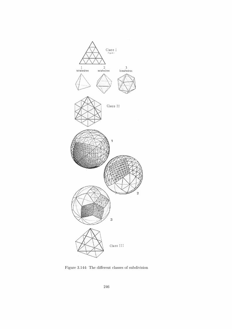
Figure 3.144: The different classes of subdivision

246

Figure 3.145: Some other types of often used sphere subdivisions

Figure 3.146: The two most important methods of subdividing triangular planes

247

Figure 3.147: Different possible connectionpatterns, after the definition of the topological divisionof the points

248

3.4.8 Aspects of construction

3.4.8.1 Prefabrication of larger units

With a number of systems the bar is not the basic element, but are elements preassembled intoa larger, prefabricated element.

Pyramids This element is usually shaped like a pyramid. It does not need to consist of bars,but can also be made partly or entirely from plates. There are multiple examples in steel bar-based pyramids, like Pyramitec, Czaplinski and Space-deck. There have even -some already quitesome time ago- been some experimental projects constructed with concrete bar-based pyramids.H. Caminos, R.P. Burns, P.A. Kurpitz, (Popko 1968). One realized design is a system for theconstruction of halls up to 39 by 39 meters by Mihailesc, Ionescu and Catarich.

Pyramids entirely constructed by plates have been built in aluminium (Makowski) and plastic(Robak, Piano, Huybers). The last type can be found in a porter’s lodge in Delft.

Figure 3.148: Project: Structural Bay System by H. Caminos

Tetrahedrons AluminiumA number of the well-known dome-systems consists of tetrahedrons of which half is made fromfold plate and the two thus created high tops are connected by a crossbar. Interesting examplesof this are domes by the American product TEMCOR (In the Netherlands: Zoetermeer, TheHague, Tilburg, Schiphol).

PlasticsExamples exist of plastic tetrahedrons, mainly in glassfibre reinforced plastic (Wachsmann 1962).These have in general not passed the experimental phase for several reasons, mainly fire safetyand economy-related. A structure like this could be found in Delft on the terrains of the facultyof Civil Engineering and Geo-Sciences, near the Stevin laboratories. This one has actually beenbuilt up from seperate tetrahedrons, interconnected by bolts. In Wollaston, England, there is abuilding of which the roofstructure consists of a number of 15m long V-shaped beams with trian-gular partitions. These were constructed in one part, but have a internal build up of tetrahedrons.

Timber

249

In the system ‘Tetragrid’ by L.C. Booth and B.T. Keay the spaceframes are composed of trian-gular plywood panels and wooden planks.

Figure 3.149: System of prefabricated pyramids

Figure 3.150: Cylindershell of plastic tetrahedrons

Folded lozenge-shapes When two isoscelic triangles are placed with the bases to eachother and are folded a little bit under an angle regarding each other, then half a tetrahe-dron is found. With elements of which the base is large in comparison to the width, it ispossible to create cylindrical spatial structures, which remind of a accordeon. The systemalso behaves like one. When these folds are made in a piece of paper, then it is also pos-sible to entirely flatten them out. This is a transistion shape, which belongs to folding structures.

3.4.8.2 Fabrication and Measurements of Parts

Bars The fabrication of the bars is of course material bound. Roughly three groups can bedistinguished:

250

Figure 3.151: Tetragrid System consisting of muliplex and planks

1. Steel

• Welded connections;Some systems, like the SDC-system, make use of cast or pressed connections to whichthe bars are welded on site.

• Open standard profiles;The transfer of forces is done by shear through the web and/or the flanges, or axialthrough endplates. In the last case it is hard to handle the deformations caused bybending in these plates.

• Rectangular, square or circular tubes;A tube is pinchable in the width direction, which is why it has to be mechanicallyflattened or strengthened by welding enplates on at the tube endings in order to takeflanking force transfer. With axial loads the tube endings are usually provided withwelded or screwed on lump with a hole in the direction of the tube. Du Chateau usescircular tubes in the Spherobat-system, of which the diameter is made smaller towardsthe tube-endings. These will therefore also get a larger wall thickness and there willbe enough material to tap bolt holes (Dutch: ‘draadtappen’).

• Clamp- or claspconnections;

251

Figure 3.152: Antiprismatisch vouwsysteem

The ends of the profile or tube can be provided with special endpieces, which can beclamped together with especially fitting clamp-elements. An example is NODUS.

2. Aluminium

For aluminium in general the same counts as for the steel bars. Because of the threetimes lower E-modulus the bars will mostly have much larger diameters. This can haveconsequences for the production. This material has, however, as special characteristicthat it can be extruded. The cross section can therefor have a very variating profile.This aspect is often used. Du Chateau uses profiles of two concentric tubes, of which themiddle one is connected to the outer tube with longitudinal plates. This is extruded inone cycle, after extrusion the profile is made to the appropriate length and finished. In theendings of the inner tube threads are made to provie for axial connections to the hollowsphere-shaped connections. In the systems Tuball and Schuco extra profiles extrudedin the same way onto the elements, which are meant for the connections of glazing or panels.

3. Timber

There are also some examples in timber. The methods of connection are approximatelythe same as in steel, because mostly steel transistion elements are used between the timbermember and the joint. The joint solution can even be identicle to the steel version. Thereis for instance a version of pieces of MERO-bar, which are pressed into a rectangular timberbeam and fastened with steel dowels. A comparable soution is offered by the ASB-system.In this system a U-shaped steelplate is put into two slots in the head end of square laminated

252

timber beams and fixated with steel pins. The U-shape is made smaller in the direction ofthe pins and has a hole in the narrow crossplate, onto which a sphere shaped connection canbe fixed. In Delft a system for roundwood poles was developed. In this system a steelplateis inserted in a slot in the pole tip and fixed by hollow steel dowels. Through these dowelssteelthreads are pulled and fixed. The plates in the poles are connected by bolts to circularconnector plates with welded on flanges.

Figure 3.153: Spaceframe in rectangular tubes

Figure 3.154: Detail with pinched profiles and eight cornered nodeplates, by W. Beckett

Joints

1. Joints in SteelThese can be shaped as follows:

253

Figure 3.155: Cut over a bar according to the Tuball-plus system

Figure 3.156: Composed cut over a bar, by Schuco

Figure 3.157: Spaceframe in roundwood poles

• Cast spheres or facetted shapes (polyhedrons), usually provided with screw holes withinternal threads. Sizes can be very large, diameters up to 35cm have been used

254

(MERO-stadium in Split). The contactplanes must be carefully made and treated toprovide for a correct system size and can not be fit with a compressable protectivelayer, as for instance a powdercoat-layer. In these joints it must be possible to variatethe direction of the hole under two angles: horizontally and vertically. This demandsprogrammable boring equipment. Especially in Japan these techniques are pretty fardeveloped.

• Cast or pressed hollow spheres. In principle the same counts as for massive spheres.They are easier to deform, so the wall thicknesses should be enough. Usually theyare made in two parts, of which one is a pressed plate. With SDC two shell parts arepressed, which roughly follow the wrapping shape of the connecting bars. Measure-ments are no problem in fabrication, but are in construction. With Unistrut U-shapedprofile-bars are bolted to a cold pressed form, in which also dents are pressed, whichexactly fit into the holes of the bars. This guarantees exact measurements.

• welded tie plates (Dutch: ‘schetsplaten’). When joints are constructed from pieces ofplate, then holes can be predrilled into them. The orientation of the holes is veryimportant, because this defines the c.t.c. distance. That is why this drilling has to bedone with programmable machines or precise boring molds.

2. Joints in aluminium.This material is very suitable for precisioncasting, which enables the production of veryprecise and detailed elements like the jointelements. The material is also easily deformedcold. This characteristic is used in the Triodetic system. The joints in this system are slabshaped and have toothed incisions. The elements are made by extrusion and sawn to discs.The bars fit into the the joints because they are tubes with flattened ends, which have beenequiped with rims corresponding to the toothed incisions. Sometimes these rims have tobe pressed under an angle with the axisdirection, like for instance in diagonal joints.

Figure 3.158: Some examples of facetted nodes

255

Figure 3.159: A Japanese sphere-shaped node

Figure 3.160: A solution with tie plates, with which most common spaceframes can by built

256

Figure 3.161: The triodetic system with aluminium nodes and bars

257

3.4.8.3 Measurements in relation to the detailling.

In structures, built up from a large number of relatively small elements, measurements are veryimportant. Small deviations can accummulate to an intolerable total deviation compared to thedesign. That is why measurements in fabrication have to be controlled very tightly. The influenceof these deviations can be system-bound.

• Welded connectionsIn systems like the SDC-system, tubes are welded between two shell shaped connectingelements. It is clear that there are no high demands for the measurements of the bars. Infact the problem is shifted to the construction site. In construction supports are needed tocreate the total shape. This can be partly neutralized by constructing the structure withtemporary bolts. The welding on site, often under difficult angles and under harsh climateconditions, is a restrictive factor.

• Shear-bolt connection.In joint solutions in which flanking transfer of forces occur, like flanges and tie plates, holetolerances are important. The holes should be made slightly larger than the boltdiameter,because assemblation can be a problem. Normally a minimal tolerance in the order of0,5mm is demanded. This tolerance also depends on the finishing of the bar and the joint.If one of the two is steel, then it will be galvanized and the thickness of this layer needsto be added to the initial tolerance. Usually finishing of the holes and contect surfaces isneeded, because drops and roughness can be formed by the galvanizing, which need to beremoved (of course without damaging the conservative properties). With powdercoatingand painting the same problems arise, though the layer on the contactsurface is much softer.Usually the contactsurfaces are kept blank or another type of finishing is used. The centerto center distance is of course dictating the end measurements in the assemblyphase. Thisdimension can be found within very slim tolerances by using precise boring equipment. Thetotal tolerance of the hole is, however, influencing the total dimension in loaded conditionand can require special care for for instance the displacements.

This can usually be solved by giving the structure a pre-camber, This does imply that thebars on the the bottom side need to be made longer in at least one direction.

• Connection with axially loaded bolts.One should think of the type of joint in which the bar is bolted to a massive or hollow sphere.The spheres are usually cast and therefore relatively rough. The distance of this plane tothe center of the sphere as wel as the length of the bar need to be precisely measured.When these planes are properly finished, a very precise measurements can be achieved.This finishing is, however, not always possible due to the needed surface protection; that iswhy the measurements are sensitive to imperfections in the contactsurfaces. This methodhas as an important advantage, that the bar can be slightly lengthened fairly easily, byusing rings put in between. This can be used to create a pre-camber in the structure.

3.4.8.4 A Connection without seperate joints

In some cases the bars are interconnected without using seperate joints.

1. Connections by dihedral angles (Dutch: ‘standhoeken’) Two different solutions are used:

• In the first case the ends of a tube are provided with welded on attachments withwings, that are placed under the desired angles. These angles are the same as thedihedral angles of the tetrahedron (70.53)and the octahedron (109.47). Examples of

258

Figure 3.162: The positioning of the holes in a node

Figure 3.163: The SDC-system

this are a system by R.B. Fuller and the Pearce-system. The structure of the famousbiosphere is made with a system like this, presumably the last mentioned.

• In another solution an extruded aluminum profile is used with webs and flanges, whichare under these angles over the entire length.

Both methods have an objection; in the heart of the system -where the jointelementsnormally are- no material is found. This can lead to rather large displacements in theconnection, especially when not all directions of connection are taken up. This is definitelythe case in double layer systems and most definitely along the edges.

259

Figure 3.164: A discjoint in a single layer sphereshaped frame

Figure 3.165: The Japanese NS space truss system

2. The ends of the bars are machined;

• Corner elements.The bars are provided with small welded cornerelements, which fit around eachotherlike a wing of a mill and butt (Dutch: ‘stuiken’) along the horizontals. This has beenapplied in a roundwood spacefram in Rotterdam. The corner elements have in thiscase been welded to tie plates, which are put into a slot in the end of the pole andconnected with tubeshaped pins and steel wire.

260

• Flattened bar endingsSomething like that is the case in the RADIAL system. In this system the trusstubesof the sloping diagonal bars are flattened at the endings and put under the requiredangle. These flat pieces are bolted tight in the joining of the horizontals which passeachother with some sort of a half-‘timber’ overlap.

Figure 3.166: Solutions by R.B. Fuller without seperate joints

3.4.8.5 Connection with seperate node elements.

Types of nodes

• Welded:

– Connected directly (For example Kolowski)

– onto a sphere shaped element (Oktaplatte)

– Between arched, pressed plates (SDC)

261

Figure 3.167: A system, developed by TU Delft, with a U-shaped bar-ending

Figure 3.168: The Radial System

– Clamping systems (NODUS)

• Disc-joints (Mero, Triodetic)

• Massive sphereM. Mengeringhausen visualized the cuboctahedron (P10) as a node element. In this ideaall needed connection directions of the ribs and planar diagonals of a cube appear, in total18 directions. This joint is in principle shaped like a cube, chamfered in multiple directionsunder an angel of 45 degrees. With a diagonal on every plane of the cube a tetrahedroncan be formed which entirely consists of equilateral triangles. The MERO-node gives the

262

possibility to not only connect the ribs of the cube, but also the diagonals in the planes.The strange effect then arrises with these nodes, that not only angles of 45 degrees ormultitudes of 45 degrees can be made, but also angles of 60 degrees. Most other systemsare based on the same connection directions. Many examples exist:

– Netherlands: van Thiel Space System

– Japan: Pantadome, Tomoe Unitruss, TM Truss(Taiyo Kogyo), KT Truss.

– USA: Steve Baer (dodekahedron)

– Germany: Mero, Zublin, Krupp, W. Kuhn (mainly rhombic dodecahedron)

• Hollow sphere (Spherobat, Tuball, Alco-dome, Schuco)

• placed (bended or forced plate and/or bar (Unistrut, Power strut)

• Assembled

– From cast elements (Wachsmann)

– Standard half-fabricates

– Tie plates (Octatube, TU-roundwood system, RAI-joint)

This list is probably far from complete. Often a new solution is sought, to avoid payinglicenses needed to use existing systems. The differences with existing systems are therefore oftenvery small and many systems look very similar.

Figure 3.169: A welded joint

263

Figure 3.170: The meeting of different bars in a common spaceframe

Figure 3.171: The Unistrut system

264

Figure 3.172: A composed joint according to a Russian patent

Figure 3.173: Some examples of solutions for single layered spaceframes

265

Figure 3.174: Some special solutions with clamping or slide connections

266

Figure 3.175: Joints with tie plates

267

Figure 3.176: Different massive sphere shaped joints

268

Figure 3.177: A number of hollow sphere shaped joints

269

Used materials There are variants known in almost all known building materials:

• Steel

– Tubes or profiles

• Aluminium

– Tubes or profiles

– Pyramids

• Timber

– Roundwood

– Sawn timber

– Glue-laminated timber

– Multiplex

• Concrete

• Plastics

– Rods (Glassfiber Reinforced epoxy or polyester (GRP))

– Tube (PVC)

– Plates or pyramideshaped elements (GRP)

Figure 3.178: A system with bars of glassfibrepolyester by L. Hollaway

270

3.4.9 Stability

The stability must of course be guaranteed in the usability state as well as in the constructionstate.

3.4.9.1 Usability state

The different aspects which need to be dealt with will be mentioned here with just a shortcomment, because there is mostly not a general solution. These points should be considered asattention points, for which should be taken care in construction.

• Statically determinance or statically under- or overdeterminance

• Buckling of the bars, this is often leading in flat spaceframes. Also care should be takenthat no bar has more than two hinges in longitudinal direction. This is often forgottenwhen dealing with in between connections in the joints themselves.

• Snap-through (Dutch: ‘doorslag’) or too little bending stiffness of single-layered systemswith a too small curvature. To describe this phenomenon a non-lineair calculation is needed.This is an iterative process in which the under loading constantly changing geometry is re-entered into the program until the end situation has been found.

• Buckling (Dutch: ‘uitspatten’) of the nodes because of little stiffness perpendicular tothe plane. This is often repairable. A good example is the Alco-dome of the EindhovenUniversity of Technology. The so-called reductors that are welded to the ends of the barsare only reduced in width-direction, so the bars fit into the joint, but keep their internalheight in the perpendicular direction to the width.

• The rotating out of joints because of too little rotational stiffness in horizontal sense. Inthe tie plate systems, like Octatube, it is needed to always use two bolts in the horizontaldirection to prevent this effect.

271

Figure 3.179: Possible problems with stability

Figure 3.180: Snap through in a single layered domeframe

Figure 3.181: The Varitec system: too many hinges in a bar

272

Figure 3.182: Reductor in a barend; Alcodome sustem of the TU Eindhoven

273

3.4.9.2 Construction state

The situation during construction can be very different from the usablility state.

Possible problems during hoisting:

• Choice of hoisting points, because of cantilevers, which can lead to buckling of lower bars.

• Horizontal reaction force from hoisting cables, when no provisions are used, which can leadto:

– buckling of lower bars

– pinching together of the bottom side of the structure, when the hoisting points connectdiagonally

• tilting of the hoisted structure, when the centre of gravity is not directly below the hoistpoint

Figure 3.183: Failure behaviour of a spaceframe due to buckling of the bars

274

3.4.10 Calculation

3.4.10.1 Approximating calculation by hand

Spaceframes are too complicated to calculate by hand. When there where no computers yet,development in this field was therefore held back. Still it is possible to get a global insight intothe strength and stiffness of the structure, as long as it is simple in essence. Reference is madehere to an adress by Beranek and Hobbelman (Wachsmann 1962), about a calculation methodfor the sketch design. Simple rules for design calculations are given in Merkblatt 10, by theBeratungsstelle fr Stahlverwendung, under chair of H. Witte (1981).

Figure 3.184: The construction of spaceframes

Figure 3.185: Construction of a dome

275

Figure 3.186: An example of a frame generated by FORMEX

276

3.5 Kinetic and adaptable structures

3.5.1 Adaptive structures

Adaptive structures are structures that adapt to their environment according to a certain set ofrules and strategies. Mulder (Mulder 2003) researched some of the conceptual thoughts on theseadaptive structures at the Delft University of Technology in 2003. They can be seen as physicalform finding, since the structure finds its own form by adapting to the environment, not in ascaled-down model, but in a full scale reality. The rules and strategies of the system (physical,computational, man-made, artificial, etc.) are the driving force of the form finding process andthe structure reaching its own structural optimality.

3.5.1.1 Large-Scale Linear Actuators

As already mentioned, a linear actuator can be described by two elements, namely a piston anda mechanism that applies a force to the piston and also controls the motion of the piston. Thisactuator type is the most commonly available and most often used, especially for applicationsdemanding a large force and short response time. This usually implies a high energy demand.Three types of large-scale linear actuators will now be discussed: hydraulic, electromechanical,and electromagnetic systems.

Hydraulic systems create the force by using a hydraulic pressure on the face of a piston headcontained with a cylinder; this is shown in Figure 3.187. Fluid is forced in or out of the cylinderthrough the mechanism to compensate for the piston displacement and to keep up a certainpressure. These systems have the highest force capacity of the linear actuator group, in theorder of meganewtons (depending on the area of the piston).

The force can be described by:

Fc = λ∆Ac (3.38)

where λ is the friction, ∆P is the pressure and Ac is the area of the piston. From Equation 3.38follows that the efficiency of the system is governed by friction. Precise control movementand force can be achieved with an appropriate control system. Protection against overload isprovided by a pressure relief value. When there is a small internal leakage the static load iskept. The disadvantages of this type of system are the requirements for fluid storage systems,complex valves and pumps to regulate the flow and pressure, seals and continuous maintenance.Durability of the seals and the potential for fluid spills are critical issues (Connor 2003).

Electromechanical linear actuators generate the force by moving the piston with a gearmechanism that is driven by an electric motor, i.e. electrical energy is transformed to mechanicalenergy. The motion, and therefore the force, is controlled by altering the power input to themotor. These devices are compact in size, environmentally safe, and economical. Figure 3.189illustrates different sizes of rod-type linear electric actuator systems developed by the com-pany Raco. The thrust (linear force) capacity of these devices goes from 0,5 kN up to 1,2MN (homepage 2005)

277

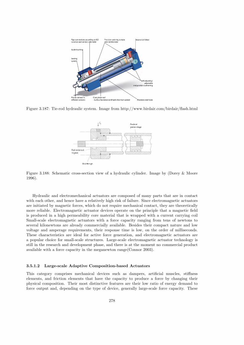
Figure 3.187: Tie-rod hydraulic system. Image from http://www.birdair.com/birdair/flash.html

Figure 3.188: Schematic cross-section view of a hydraulic cylinder. Image by (Dorey & Moore1996).

Hydraulic and electromechanical actuators are composed of many parts that are in contactwith each other, and hence have a relatively high risk of failure. Since electromagnetic actuatorsare initiated by magnetic forces, which do not require mechanical contact, they are theoreticallymore reliable. Electromagnetic actuator devices operate on the principle that a magnetic fieldis produced in a high permeability core material that is wrapped with a current carrying coilSmall-scale electromagnetic actuators with a force capacity ranging from tens of newtons toseveral kilonewtons are already commercially available. Besides their compact nature and lowvoltage and amperage requirements, their response time is low, on the order of milliseconds.These characteristics are ideal for active force generation, and electromagnetic actuators area popular choice for small-scale structures. Large-scale electromagnetic actuator technology isstill in the research and development phase, and there is at the moment no commercial productavailable with a force capacity in the meganewton range(Connor 2003).

3.5.1.2 Large-scale Adaptive Composition-based Actuators

This category comprises mechanical devices such as dampers, artificial muscles, stiffnesselements, and friction elements that have the capacity to produce a force by changing theirphysical composition. Their most distinctive features are their low ratio of energy demand toforce output and, depending on the type of device, generally large-scale force capacity. These

278

Figure 3.189: Different sizes of rod-type electric linear actuators. Image fromhttp://www.racointernational.com

features are very desirable for applications of large-scale civil structures. Adaptive devices thathave a low energy demand and also operate as energy dissipation mechanisms are referred toas semi-active actuators since they behave like passive devices in the sense that they increasethe stability of a structure and require no external energy. A semi-active actuator will neverdestabilize a system even though it has a low energy demand.

Figures 3.190 and 3.191 show the concept of a variable orifice damper. A variable orifice maybe considered as a viscous damper with a variable damping coefficient. Its operation principleconsists in controlling the damping coefficient by adjusting the opening of a valve according tothe force demand specified by the feedback control algorithm. Given that the valve motion isperpendicular to the flow, the force required to alter the valve position is small, and thereforethe energy demand is low; 50 watts of power to operate is a typical amount for such devices (Jr.& Sain 1997).

Artificial muscles At the Vrije Universiteit Brussel (VUB), department of MechanicalEngineering, Multi body Mechanics Research Group, Frank Daerden has recently developed thePleated Pneumatic Artificial Muscle (PPAM), illustrated in Figure 3.192, the successor of thePneumatic Artificial Muscle (PAM) e.g. the McKibben MuscleA pneumatic artificial muscle is in essence, a membrane that will expand radially and contractaxially when generating high pull forces along the longitudinal axis. In other words, pneumaticartificial muscles are contractile devices operated by pressurized air. The muscle is basically

279

Figure 3.190: Schematic of a variable orifice damper. Image from (Jr. & Sain 1997)

Figure 3.191: Variable damping mechanism. Image from http://www.racointernational.com

nothing more than a membrane, which makes it an extremely lightweight actuator.This muscle has a rubber tube which will expand when inflated, while adjacent nettingtransmits tension. Hysteresis (pressure/length course between contracting and relaxing), dueto dry friction between the netting and the rubber tube, makes control of such a device rathercomplicated. Typical of this type of muscles is the need of (reaching) a lower boundary level ofpressure before any action can take place.

The main goal of the new design was to avoid both friction and hysteresis, thus makingcontrol easier while avoiding the lower boundary. This was realized by arranging the membraneinto radially laid out folds that can unfurl free of radial stress when inflated. The membrane’sstiff longitudinal fibres transfer tension. As the pressure rises, the membrane can defold withoutthe occurrence of friction and the muscle’s elongation will not be hindered by material stresses,therefore optimising the contraction. When the artificial muscles are inflated, they swell, shortenand thus generate a contraction force. This means that for the geometry, the developed force(as a function of the length) and the maximum shortening, the bellows gets a ’pumpkin-like’shape when contracting. The (tensile) force depends on the applied pressure and on the muscle’slength, ranging from an extremely high value at maximum length, i.e. zero contraction, to zero

280

at minimum length or maximum contraction. The maximum contraction depends on the initialslenderness (for the mathematical upper boundary case of an infinitely slender bellows, thisslenderness can rise up to 54,3%) (Daerden & Lefeber 2001).

Figure 3.192: Deflated state of the PPAM and inflated state of the PPAM. Image fromwww.vub.ac.be

Each of the characteristics of this type of muscle can be expressed as the product of a scalefactor with a dimensionless function depending only on the contraction and the slenderness. Forthe force for example, it holds:

Ft = pl · f(ε, l

D) (3.39)

with D and l being the initial diameter and length, and the dimensionless contraction(referred to l). The scale factor is expressed by pl2. The following well known relation is alsovalid:

Ft = −p(dVdl

) (3.40)

It unambiguously symbolizes the actuator’s equilibrium length by the determined pressureand the external loading, meaning that the change of the volume over the length is directlydecisive for the developed force (Daerden & Lefeber 2001).

The challenge is to efficiently integrate the muscles in a structure, both visually andstructurally by knowing the possibilities and limitations of these elements.The generated force is highly non-linear and proportional to the applied gauge pressure in themuscle. At a pressure of 300 kPa the force can be as high as 4000 N for a device with an initiallength of 10 cm, weighing only 100 g. It has to be kept in mind that at increasing contraction,the force drastically (non-linearly) drops, as shown in Figure 3.193. So the muscles applied in astructure either supply a large force or make a large displacement possible, but not both.

To have a bi-directional working joint one has to couple two muscles antagonistically. At eachjoint the muscles are attached in a leverage mechanism by pulling rods. The points of attachmentare essential in the design since they determine torque characteristics. Because of the one-way

281

Figure 3.193: Force/contraction curve for PPAM for variable p. Image from (Daerden & Lefeber2001)

force a paired or antagonistic set-up is needed in order to generate a restoring force or movement.

Another type of artificial muscles has been developed by the company Festo. In nature (forexample the human being), biological muscles contract powerfully and relax in a controlledmanner. Festo has tried to implement this principle in an industrial product, resulting in themeanwhile ’standard component’ Fluidic Muscle MAS.The Fluidic Muscle operates in the same way as the previously discussed PPAM, i.e. bymembrane-contraction. The resulting 3-D grid pattern deforms when actuated by compressedair. As internal pressure is increased, an axial pulling force develops to cause the tubular unitto contract, turning it into a linear actuator.

Figure 3.194: Festo Fluidic Muscle. Image from http://www.festo.com/INetDomino

The force capacity of the Fluidic Muscle MAS is comparable to the PPAM (a few kilonew-tons), developed at the VU Brussels by Frank Daerden.

282

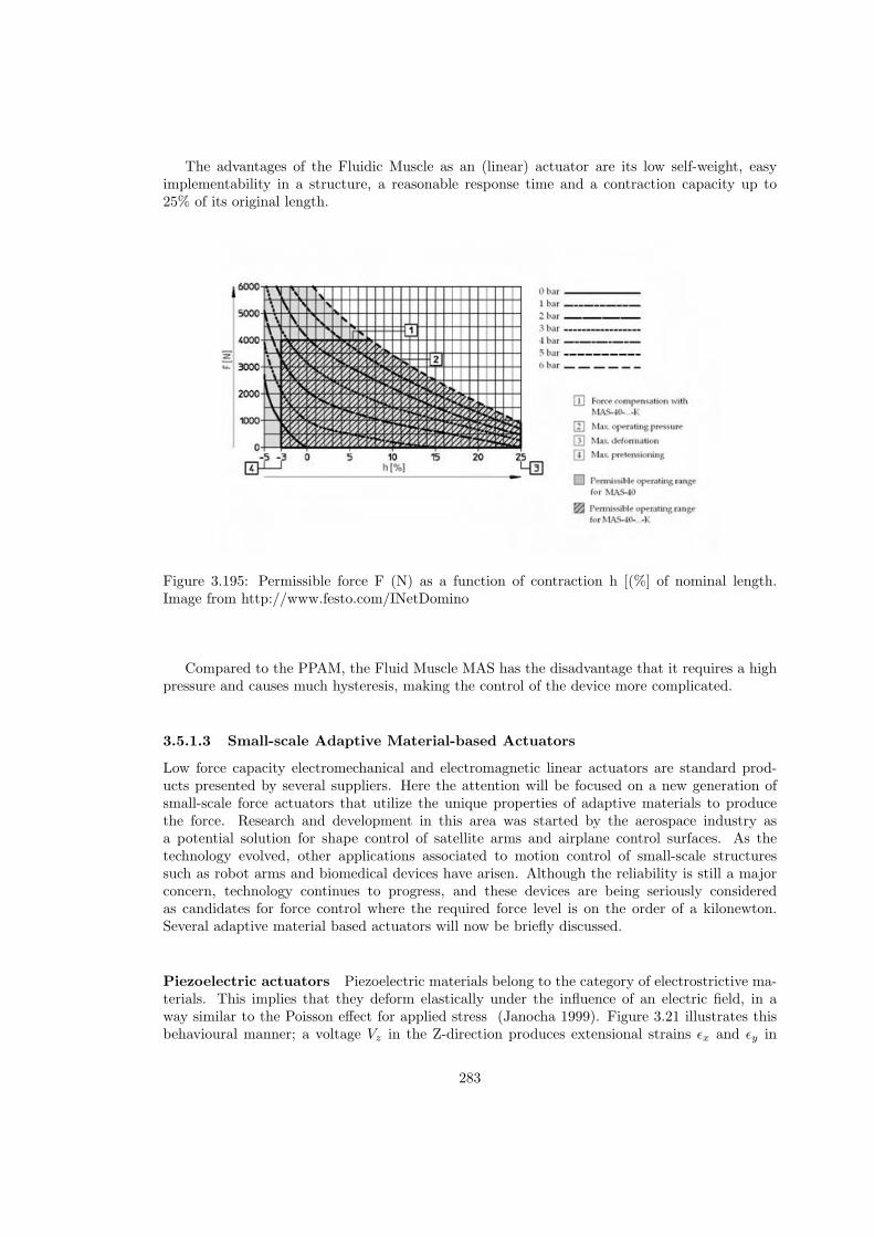
The advantages of the Fluidic Muscle as an (linear) actuator are its low self-weight, easyimplementability in a structure, a reasonable response time and a contraction capacity up to25% of its original length.

Figure 3.195: Permissible force F (N) as a function of contraction h [(%] of nominal length.Image from http://www.festo.com/INetDomino

Compared to the PPAM, the Fluid Muscle MAS has the disadvantage that it requires a highpressure and causes much hysteresis, making the control of the device more complicated.

3.5.1.3 Small-scale Adaptive Material-based Actuators

Low force capacity electromechanical and electromagnetic linear actuators are standard prod-ucts presented by several suppliers. Here the attention will be focused on a new generation ofsmall-scale force actuators that utilize the unique properties of adaptive materials to producethe force. Research and development in this area was started by the aerospace industry asa potential solution for shape control of satellite arms and airplane control surfaces. As thetechnology evolved, other applications associated to motion control of small-scale structuressuch as robot arms and biomedical devices have arisen. Although the reliability is still a majorconcern, technology continues to progress, and these devices are being seriously consideredas candidates for force control where the required force level is on the order of a kilonewton.Several adaptive material based actuators will now be briefly discussed.

Piezoelectric actuators Piezoelectric materials belong to the category of electrostrictive ma-terials. This implies that they deform elastically under the influence of an electric field, in away similar to the Poisson effect for applied stress (Janocha 1999). Figure 3.21 illustrates thisbehavioural manner; a voltage Vz in the Z-direction produces extensional strains εx and εy in

283

the X and Y-directions (Connor 2003). The opposite behavioural characteristic occurs when thematerial is stressed in the X-Y plane, a voltage V

′

z in the Z-direction is generated by σx and σy.Traditionally, piezoelectric actuators have been used as strain sensors. Their use as actuators ismore recent and stimulated mainly by the aerospace industry.

Figure 3.196: Piezoelectric electrical-mechanical interaction. Image from (Connor 2003)

Piezoelectric actuators are fabricated with piezoceramic block-type elements or piezopolymerfilms. Lead zirconate titanate (PZT) is the main piezoceramic composite used for transducerapplications, i.e. sensors and actuators, in the frequency range up to 106 Hz. Artificiallymanufactured polymers on the basis of Polyvinylfluoride (PVDF) is most commonly used inpiezoelectric films (Janocha 1999). As it has a quite low strength, PVDF is used mainly as asensor, particularly for the high frequency range up to 109 Hz. The fundamental principle isthe same for both mentioned materials. The piezoelectric object is attached to a surface whichrestrains it motion. When the object is subjected to a voltage, it inclines to expand imme-diately, and consequently contact forces are produced between the object and the restrainingmedium (Connor 2003).So far, two actuator configurations have been realised. The first model is a conventional linearactuator such as shown in Figure 3.197. Piezoceramic wafers (small thin circular slices of asemi-conducting material) are piled up vertically, fastened, enclosed in a protective housing, andfitted with electrical connectors. These devices can deliver large forces, up to almost 30 kN,with a response time of several milliseconds (Homepage n.d.).

Figure 3.197: Cylindrical piezoceramic linear actuator. Image fromhttp://www.kineticceramics.com

The second configuration has the form of a thin plate, as illustrated in Figure 3.198.Piezoceramic wafers are distributed over the area in a regular pattern. They may also be piledup through the thickness. This type of device is connected to a surface and applies a pair ofself-equilibrating tangential forces to the surface. The peak force depends on the applied voltage

284

and degree of restraint. A force level of 500 N at 200 volts, and millisecond response, are typicalupper limits for current plate-type piezoceramic actuators. Recent developments are concernedwith lowering the voltage requirement (Connor 2003).

Figure 3.198: Plate-type piezoelectric actuator. Image from (Connor 2003).

Shape memory alloys. The shape memory effect (SME) refers to the ability of certain ma-terials to deform at low temperature and then return to their original shape after heating to ahigher temperature. They display the capacity to deform at a low temperature and then returnto their original shape after heating to a higher temperature. Thus behaviour is illustrated inFigure 3.199. The initial straight form is deformed inelastically at room temperature to thetriangular form. When the temperature is raised, the triangular form shifts back to the straightform and remains in that form when the temperature is lowered to room temperature. In thelack of any externally applied force, the transformation from austenite to martensite is duringany subsequent thermal cycling invariant to shape change. This memory effect is caused by aphase transformation from martensite at room temperature to austenite at elevated tempera-ture (F. Ansari & Leung 1997).

Inelastic deformation introduced during the martensite phase is eliminated when the statepasses over to the austenite phase. The phase transitions without applied stress are illustratedin Figure 3.200. As and Af define the temperatures for the start and finish of the transitionfrom martensite to austenite for the case when the material is being heated; the correspondingtemperatures for the cooling case are Ms and Mf . When T is greater than Af , the phase isaustenite but it is possible to change it back to martensite by applying stress. The magnitudeMd is the temperature beyond which austenite cannot be transformed to martensite by stress(i.e., the phase remains austenite for arbitrary applied stress).

Above the transition temperature, shape memory alloys show an exceptional elasticity. Likeclassically elastic materials, a load will cause a shape deformation that disappears during un-loading. The difference is that shape memory alloys may be reversibly elongated or compressedfive to ten times the amount of conventional materials, as illustrated in Figure 3.201. The restor-ing force is nearly independent of the strain. The upper straight line of the superelastic curvecorresponds to the formation of stress induced martensite (SIM) while the lower straight linerepresents the reversion of SIM when the stress is reduced (F. Ansari & Leung 1997).

The stress-strain behaviour is strongly reliant on temperature. Figure 3.202 shows the limitingstress-strain curve for Nitinol, a nickel-titanium alloy.

The last category of the shape memory effect is the two-way effect, illustrated in Figure 3.28.The piece of wire deformed below Mf straightens itself when heated to above Af . But, on beingcooled down to below Mf , the wire changes back to its deformed shape. The wire straightens upon reheating and resumes its deformed shape on cooling. This behaviour repeats itself endlessly.

285

Figure 3.199: One-way shape memory behaviour. Image from (F. Ansari & Leung 1997)

Figure 3.200: Martensitic transformation on cooling and heating. Image from (Connor 2003)

The realization of two-way behaviour implies thermo-mechanical treatment. This usuallyimplicates several transformation cycles. This is achieved by cycling the material under thecombination of stress and temperature.

The two-way shape memory behaviour gives the starting point for force actuation. If atrained shape memory alloy is restrained at low temperature in a way it cannot deform, a force isgenerated when the alloy is heated since it wants to return to its initial undeformed shape. Theactuator does not need any additional (for instance electrical) power supplies, what increases thefail-safety.

Nitinol alloys in the form of small diameter wires (∼ 0.4 mm) are used to assemble a force

286

Figure 3.201: Schematic stress-strain diagram of superelastic behaviour of shape memory alloys.Image from (F. Ansari & Leung 1997)

Figure 3.202: Effect of temperature on stress behaviour of Nitinol. Image from (F. Ansari &Leung 1997)

Figure 3.203: Two-way shape memory behaviour. Image from (F. Ansari & Leung 1997)

actuator. Heating is applied by passing an electric current through the wire. This process limits

287

the response time to seconds versus milliseconds for piezoelectric materials. Another restrictionis the material cost; a usual price is in the order of ¿230/kg (Connor 2003). Most of theapplications of shape memory actuators are for small-sized products thus requiring low capacity,and where cost and response time are not critical issues. Actuated civil structures like bridgesand high-rise buildings with shape memory alloy prestressing tendons can be conceived but therequired technology is still far too expensive (F. Ansari & Leung 1997). Another major topicis the issue of fatigue life. In order for these materials to gain acceptance in main stream civilengineering applications their fatigue performance has to improve considerable.

Controllable fluids Controllable fluids are categorized by their ability to change from a fluidto a semisolid in milliseconds when subjected to an electric or magnetic field. This effect wasidentified by Winslow in 1949. Two materials belonging to this category are electrorheological(ER) and magnetorheological (MR) fluids. In their initial state, they act as viscous fluids. Use ofthe (electric or magnetic) field introduces an additional plastic solid type behaviour mode, andthe response is now a combination of plastic and viscous actions (Janocha 1999).

Figure 3.204: Effect of electric and magnetic fields on stress-strain relationship. Image from(Connor 2003)

Figure 3.204 illustrates this transformation for the situation when the material is idealized asa Bingham solid, which is defined as an ideal plastic solid in parallel with a linear viscous fluid.

The stress-strain relation for a Bingham solid subjected to shear deformation has the form

τ = τysin(γ) + ηγ (3.41)

where τy symbolizes the yield stress and η is the viscosity.Experimental results show that the yield stress increases considerably when the field strength,

f , augments to a limiting value τmax . However, the viscosity is essentially constant. Therefore,it is reasonable to take η equal to a constant, η0 , and consider the material behaviour as acombination of variable Coulomb hysteric damping and constant linear viscous damping. Theequivalent linear material viscosity,ηeq , is reliant on the amplitude and frequency of the sheardeformation. For the case of periodic excitation, ηeq , is given by

ηeq = η0 +4τyπΩγ

(3.42)

where γ is the strain shear amplitude and Ω is the excitation frequency. Devices containingcontrollable fluids can be used either as variable dampers or as semiactive force actuators.Figure 3.205 shows a schematic view of a prototype developed by the Lord Corporation. Themain cylinder accommodates the piston, the MR fluid, and the magnetic circuit. A small electro-magnet is embedded in the piston head and supplied with current that generates the magnetic

288

circuit. A small electromagnet is entrenched in the piston head and supplied with current thatgenerates the magnetic field across the annular orifice. Typical small-scale versions have a forcecapacity of about 3 kN, a millisecond response, and draw about 10 watts of power (Connor 2003).

Figure 3.205: Damper. Image by (Janocha 1999)

Experimental results for quasi-static loading applied to the small scale version are plottedin Figure 3.206. These results show that the Bingham solid idealization is an acceptableapproximation for the actual behaviour, and also that the plastic yield force is restricted bysaturation of the fluid. For this device, saturation arises around 1.5 amps. When utilized as aforce actuator, the amperage is attuned such that, for the observed value of velocity, the desiredforce magnitude is created.

A controllable fluid-type device is more operational than a variable orifice damper since theyield force is the primary component, and this force is independent of velocity. The low externalpower requirements, rapid response, and the potential for large capacity are attractive features.With further development, MR-based actuators should be applicable solutions for large-scalecivil structures.

289

Figure 3.206: Quasi-steady force response for Rheonetics SD-1000-2MR damper. Image from(Connor 2003)

290

Advanced computation for

Structural Design 4Contents

4.1 Theory . . . . . . . . . . . . . . . . . . . . . . . . . . . . . . . . . . . . 292

4.1.1 Special structures . . . . . . . . . . . . . . . . . . . . . . . . . . . . . . 292

4.1.2 Opportunities and challenges . . . . . . . . . . . . . . . . . . . . . . . 292

4.1.3 The structural design process . . . . . . . . . . . . . . . . . . . . . . . 292

4.1.4 Fundamental problems between computation and the structural design

process . . . . . . . . . . . . . . . . . . . . . . . . . . . . . . . . . . . 293

4.2 Form description and generation . . . . . . . . . . . . . . . . . . . . 294

4.3 Descriptive techniques . . . . . . . . . . . . . . . . . . . . . . . . . . 294

4.3.1 Descriptive computational techniques . . . . . . . . . . . . . . . . . . 294

4.4 Generative Techniques . . . . . . . . . . . . . . . . . . . . . . . . . . 296

4.4.1 Generation techniques . . . . . . . . . . . . . . . . . . . . . . . . . . . 296

4.4.2 Mesh techniques . . . . . . . . . . . . . . . . . . . . . . . . . . . . . . 296

4.5 Form finding . . . . . . . . . . . . . . . . . . . . . . . . . . . . . . . . 324

4.5.1 Minimal surfaces . . . . . . . . . . . . . . . . . . . . . . . . . . . . . . 324

4.5.2 Force density method . . . . . . . . . . . . . . . . . . . . . . . . . . . 325

4.5.3 Dynamic relaxation . . . . . . . . . . . . . . . . . . . . . . . . . . . . 327

4.5.4 Shape form finding . . . . . . . . . . . . . . . . . . . . . . . . . . . . . 330

4.5.5 Other form finding methods . . . . . . . . . . . . . . . . . . . . . . . . 330

4.6 Structural optimisation . . . . . . . . . . . . . . . . . . . . . . . . . . 331

4.6.1 Theory of optimisation . . . . . . . . . . . . . . . . . . . . . . . . . . . 331

4.6.2 Classification of optimisation problems . . . . . . . . . . . . . . . . . . 334

4.6.3 Size optimisation . . . . . . . . . . . . . . . . . . . . . . . . . . . . . . 339

4.6.4 Classical optimisation methods . . . . . . . . . . . . . . . . . . . . . . 342

4.6.5 Genetic algorithms . . . . . . . . . . . . . . . . . . . . . . . . . . . . . 346

4.6.6 Simulated annealing . . . . . . . . . . . . . . . . . . . . . . . . . . . . 351

4.6.7 Swarm behaviour and ant colony optimisation . . . . . . . . . . . . . . 352

4.6.8 Michell structures . . . . . . . . . . . . . . . . . . . . . . . . . . . . . 358

4.6.9 Theory of Michell structures . . . . . . . . . . . . . . . . . . . . . . . 362

Recommended Study Material

Title Author YearHandbook for Grid Generation Joe F. Thompson 1999Numerical Recipes in C++ William H. Press, et al. 2001An introduction to genetic algorithms M. Mitchell 1996

291

4.1 Theory

Computational techniques are essential in the modern design of special structures, mainly becausethe advanced geometry of these structures make the design labourious to perform by hand.Computational tools can be used to define, describe, generate, calculate, produce, etc. thesestructures. It can even be said that currently it is almost impossible to perform any seriousdesign step in an efficient manner without computation. However, still many difficulties withcomputation in the structural design of special structures (and in structural design in general)exist.

This chapter will cover the techniques, problems, challenges, opportunities, etc. for thecomputation of special structures, aimed on the structural design. Students will get insight inwhat is available in the world, what the problems and challenges are to solve in the near futureand what the future might bring for the structural engineer.

4.1.1 Special structures

The structural design of special structures is specialistic work, often involving complex mathe-matics for geometry and complex structural behaviour. The techniques related to this are oftennot known to every engineer. Therefore, also the computation for special structures is complex,but also on a niche level, often consisting of custom-build tools. Special structures often involveadvanced geometry, such as double-curvature and advanced definition methods. The mathe-matics of some of these techniques have been discussed in Chapter 2. Often these shapes willhave to be segmented to create some kind of rationality to engineer, produce and assemble thesestructures.

4.1.2 Opportunities and challenges

One of the biggest challenges for the future of structural design is to create integral buildings, oras Ove Arup (the founder of the engineering firm Arup who did many special structures) calledit, Total Architecture, which takes into account many aspects, such as architecture, structure,construction, production, installations, assembly, etc. etc. The related computational challengeis to create software tools which are also integral. Not only because they consider many aspects,but also because they are integrated because they can communicate with eachother.

Another big challenge is to include more automation in the design process, for instance in theform of automated optimisation. This chapter will cover some techniques which currently can beused in some special cases.

4.1.3 The structural design process

It is important to understand the structural design process to understand some of the fundamentalproblems of computation in the structural design process. The structural design process is acomplex process, which involves a lot of playing, variating and exploration by the engineer. Thisrequires a high level of insight and craftsmanship. The design process is unique to any building,any design team and any engineer. This individuality of the design process is hard to capturein computation. The design process is also fast, with an evolutionary, cyclic, iterative nature,requiring good indications early in the design process when the important descisions are beingmade. Many disciplines are involved in the design, so it is a multi-disciplinary process and ateam effort. Many aspects are being considered during the design process which the engineerneeds to weight to an appropriate solution. A lot of the information involves implicit information,inside the head of the engineer, assumptions, codes, etc. while computation often requires veryexplicit information. Another important characteristic of the design process is that it involves atransition from a crude level to a finer, detailed level of information.

292

4.1.4 Fundamental problems between computation and the structuraldesign process

Several fundamental problems can be found between computation and the structural designprocess, which leads to less use of computation than would be possible, purely on a technologicallevel. This list does not attempt to be complete, but ro give an idea what needs to be solved inthe future to get to a situation where computation can be used in a more efficient manner in thestructural design process.

• ConfidenceThe engineer currently often lacks confidence in the techniques which are used in compu-tation. Confidence is important for the engineer, because he is primarily responsible forhis design. Failure or collapse of a structure is a situation which he would like to avoid.Therefore, if he can eliminate some of the risk by using the methods he has insight inand can control, he will do this. This is one of the biggest problems in computation forstructural design.

• InsightThe problem of the lack of insight in the used methods is often referred to as the ’blackbox’ problem, because the engineer does not know what happens in the black box betweeninput and output.

• ControlNext to the lack of insight, is also the lack of control a big issue for the use of computationin the structural design proces. Engineers often do not know how to control advancedmethods in a proper way, because every method, technique or application comes with theirown knowledge, interface, etc.

• ReusabilityA problem of computation is that while it often aims on reusability, still many applications,especially specialistic ones like the ones for special structures, are not very reusable.

• The analysis versus design paradoxAn important issue is the analysis versus design paradox. Much software exists for analysis.However, this software can hardly be used for design work, since design in essence is anotherprocess than analysis and code checking. Hardly any software exists for design purposes,following the principles of the structural design process as discussed above.

• The Swiss-army-knife versus the scalpel paradox Chris Williams, lecturer of the Universityof Bath and engineer at Buro Happold, spoke about this paradox for software. Muchsoftware is able to do many things, like a Swiss-army-knife, but you would not want tooperate a patient with it. While a scalpel makes very precise cuts, but is only fit for onespecific purpose. The same currently still applies to software tools for structural design.

• Software engineeringSoftware engineering is often underestimated by structural engineers. These days build-ing serious software applications requires control over high-level programming languages,knowledge of abstract frameworks, development environments (IDE’s), testing tools, de-ployment tools, versioning tools, continuous building tools, etc. etc. Software engineeringhas become a discipline on its own and to build robust software a team of people is requiredto create this software. However, this does not mean that engineers are unable to buildtheir own tools, since the level of adaptability has shifted from a programming level towardsthe user level by technologies, such as parametric associative design, scripting languages,etc.

293

• Adaptation and customisationBecause tools requires flexibility and individuality of the process, object and engineer, thesetools need to be adaptable and customisable. However, currently very little software forstructural design and engineering purposes is up to this task.

• Interactivity and software integrationInteractivity is a very important aspect for software for structural design, not only interac-tivity with the engineer and the design team, but also between software applications. Thelatter is often called ’software integration’ or ’interoperability’.

4.2 Form description and generation

An important part in the design of building with special design is the description and generationof the buildings as computer models, often because of their complex geometrical nature andbehaviour. Often these buildings consist of complex relationships in the geometrical design of thebuilding. An essential step to design, produce, assemble or construct these building is to providea unique geometrical description for the geometry and topology. As stated, since computationis essential for an efficient design process it is also essential to produce these computer modelswhich relative ease. Since often the computer applications are complex, unaccessible and do notprovide much inside in their behaviour, this is not an easy task.

One of the key differences between a regular design process of a rectangular building and aspecial structure is the step of the form description and generation which comes as an additionalstep within the design. As will become clear by reading this section often even most of theproblems and liberations come from this techniques.

This section provides an insight and overview in the methods used to describe and generateform for special structures. It needs to be noted that these techniques can be used for regularbuildings and structures as well. More complex techniques for generation of building, FormFinding and Structural Optimisation will be covered in Section 4.5. A close relation exists withSection 4.6 on geometry and mathematics.

4.3 Descriptive techniques

4.3.1 Descriptive computational techniques

Description of structures is an important aspect of the design of special structures. Many of themathematical techniques have already been covered in Chapter 2. Purpose of the description ofstructures is providing an unique ’standard’ for drafting, communication, setting out on site, etc.It is important for the coordination between all the disciplines in the design process, structural,architectural, building services, etc. Also for the analsysis of the structure it is important tohave a rigid and accurate definition of the geometry of the structure in the required format bythe analysis tools. Some other purposes include the production, construction and visualisation ofthe design. Visualisation is often important for the presentation of the design to non-professionalparties in the process. Computation for construction is often refered to as Virtual Construction,4D, 5D, xD or nD modelling. These techniques aim on integrating a geometrical definition withdatabases of scheduling, cost, etc. However, for now mainly will be aimed on the geometricaltechniques of description.

4.3.1.1 Description

Various things can be described by the various techniques. On a high level a subdivision canbe made in the geometry (position, measurements) and topology (relationships) of the objects.

294

Another subdivision can be made in the description of the object or the description of theprocess, such as a generation, finding or optimisation process. Also here the distinction betweencontinuous and discrete description exists.

Methods There are different methods of description. There are too many to mention, afew important ones include:

• Mathematical description: Mathematical description has already been covered in Chapter2. Note that this form of description can be combined with other descriptive techniques,or even that often it is necessary to combine these techniques.

• Physical: Physical modelling techniques can be used for the description of objects (andprocesses). However, these can not directly be used in the computer.

• Parametric design: A parametric description derives the geometry (and sometimes topol-ogy) from parameters which can be manipulated by the user. Often this technique is onlyavailable for the generation of geometry.

• Parametric associative or relational design: In parametric associative design not only theparameters can be manipulated by the user, but also the relationships. Often this techniqueis only available for the generation of geometry.

• Constraint solving: In constraint solving only the constraints are defined and the computer’solves’ the geometry. Note that also this method is often only applicable to geometry.

• Object-oriented design: In this method objects are described with a state and a behaviour,rather than only geometry data, such as the variables for points (xyz) and lines (begin andend point numbers).

• Scripting and programming: Scripting and programming can be used to describe and (often)generate the geometry and topology of objects (and structures).

Objects Different objects can be used in the description:

• Points (or point clouds)

• Vectors, lines or curves, such as NURBS

• Planes or surfaces

• Grids and meshes

• Volumes, both regular and irregular

• Volumetric grids and meshes

• Higher dimensional objects

Objects: A computational data structure with a state and a behaviour. Also called Compo-nents or Features. These are used in Object-oriented programming (OOP).Relationships: both mathematical and non-mathematicalProcess: description, generation, finding or optimisation process

295

4.4 Generative Techniques

4.4.1 Generation techniques

Generation techniques are used to generate a structure from a set of parametric objects or a para-metric dataset. Generation is a very powerful technique, because by controling a small amountof parameters a large amount of data elements can be generated, even an entire building designwith all related computational models. While this in theory only requires ’programmers sweat’,generation for structural design is very hard to control by the engineer and several problemsarise in the application of generation, such as the inability to ’solve back’ variables, modify thegeneration process in an efficient way, etc.

Different generation techniques exists, of which parametric design, parametric associativedesign and mesh techniques are the most well known. Often, for free-form structures the engineerneeds to describe a surface, with techniques, such as NURBS (Section 2.1.3), mesh this to a gridfor various purposes, such as structural analysis, etc. and populate this mesh with an amountof (structural) elements. Also a different approach can be chosesn where the engineer describesa generation of the structural elements and modifies the parameters of this generation in such away that the final shape approaches the intended design.

While generation is often only used by specialists, able to write generative software or able tohandle parametric associative modelling software, the basics of generation can already be appliedwith simple tools such as Excel.

4.4.2 Mesh techniques

Many software programs of grid generation techniques have been developed and still are underdevelopment. Grid generation is used in the field of computer fluid dynamics, EMAG, thermaland the environmental discipline in any dimension (surface, volume, etc.).These software programs for structured, unstructured and variational grids have all in commonthe objective to generate an accurate grid over a complex surface, resulting in flat triangles orquadrangulars. The grid that we need to segment a shell surface must generate double curvedelements and not flat elements. Thus, can be postulated that, especially, the node locationsin relation to a certain accuracy of the grid, are of importance for the grid generation on theconcrete shells. Double curved elements with least curvature follow from these node locationson the surface.Figure 4.1 sketches the different node locations generated by a grid, with differing accuracy andelement size.

Figure 4.1: Grid with varying accuracy (and element size) on a certain surface.

The section about the type of grids and their grid generation techniques is divided in threeparts. First the Structured Grids, following by the Unstructured Grids and subsequently theVariational Grids.For the grid generation techniques, the shell is assumed to have no thickness.

296

4.4.2.1 Structured grids

Structured grids are grids where in the most general sense the local organization of the gridpoints and the form of the grid cells do not depend on their position but are defined by a generalrule.Structured grids are in structural engineering the most utilized grid, e.g. in Nervis shells. Themain reasons are the simplicity to generate the grid because these follow often from the designof the shape and the predictable and regular shape of the elements.

The second reason is the easiness to adapt the mesh size, element size and element organiza-tion. Two techniques are often used in the practice, the Block-Structured Grids and StructuredGrid by Analytical Approach. Boundary-Conforming Structured Grids is a third method, oftenused in other engineering disciplines. This method is suitable to generate grids over simplesurfaces.The method of these three grid generation techniques, the field of use and the results areconsidered in the following sections.

Boundary-Conforming Structured Grids

Method An efficient structured grid is one whose generation relies on a mapping concept.The idea is to choose a computational domain Ξn with a simpler geometry than that of thephysical shell shape Xn and then to find a transformation x(ξ)) between these domains whicheliminates the need for a non-uniform mesh when approximating the physical quantities(Haas1962)The corners of the element polygons are formed by the intersection of the coordinate lines, whilethe boundary of Nx is composed of a finite number of line-curves ξi = ξi

0. Consequently, in thiscase the computation region Ξn is a rectangular domain, the boundaries in Rn and the uniformgrid in Ξn is the Cartesian grid. Thus the physical region is represented as a deformation of arectangular domain and the generated grid as a deformed lattice. See Figure 4.2.In practice there will be a trade-off between the difficulty of finding the transformation and thenumber of uniformly spaced points required to find the solution to a given accuracy and elementsize.

Figure 4.2: Boundary-conforming quadrangular & triangular grid.

297

Result A boundary-fitted coordinate grid in the region Xn is commonly generated first onthe boundary of Xn and then successively extended from the boundary to the interior of Xn.This process is analogous to the interpolation of a function from a boundary or to the solutionof a differential boundary value problem. On this base there have been developed three basicgroups of methods of grid generation with the mapping approach;

• Algebraic methods, which use various forms of interpolation or special functions

• Differential methods, based mainly on the solution of elliptic, parabolic and hyperbolicequations in a selected transformed region

• Variational methods, based on optimisation of grid quality properties

For more information about these three methods, refer to the book Grid Generation Methods,by Vladimir Liseikin(Liseikin 1999).In practice, the structured grid generated by mapping approach is today not in this form in use.This is because of the difficulty to find one transformation factor x(ξ), to generate a grid over acomplex 3D shape of the designed structure. for geometrical defined surfaces, the transformationfactor can be found-

Block-Structured Grids Joe F. Thomson, Bharat K. Soni and Nigel P. Weatherill explain inthe Handbook of Grid Generation(Thomson & et al. 1999) the block-structured grid as a spongeanalogy. The best way to visualize the correspondence of a curvilinear grid in the physical fieldwith a logically rectangular grid in the computational field is through the sponge analogy.

Method Consider a rectangular sponge within which an equally spaced Cartesian grid hasbeen drawn. Now wrap the sponge around a circular cylinder and connect the two ends of thesponge together. Clearly the original Cartesian grid in the sponge now has become a curvilineargrid fitted to the cylinder. But the rectangular logical form of the grid lattice is still preservedand a programmer could still operate in the logically un-deformed sponge in constructing the loopand the difference expressions, simply having been given different equations to program.(Maeder& et al. 2004)It is not hard to see, however, that for some boundary shapes the sponge may have to be so greatlydeformed that the curvilinear grid will be so highly skewed and twisted that it is not usable in anumerical solution. The solution to this problem is to use not one, but rather a group of spongesto fill the physical field. Each sponge has its own logically rectangular grid that deforms to acurvilinear grid when the sponge is put in place in the field. The coordinate lines, defining the gridnodes of two adjacent blocks can join smoothly or non-smoothly (Figure 4.3). If the coordinatesdo not join smoothly, which is more efficient for load transferring and element connection, thenduring calculation, the solution values at the nodes of one block must be transferred to those ofthe adjacent block in the neighbouring of their intersection. This is achieved by interpolation.

Results Such a sponge could just as well be around a cylinder of noncircular cross section,regardless of the cross-sectional shape. To carry the analogy further, the sponge could, inprinciple, be wrapped around any shape, or could be expanded and compressed to fill any region(geometrical defined, free-form or form-finding shape), again producing a curvilinear grid fillingthe region and having the same correspondence to a logically rectangular grid.This kind of grid generation is not only suitable for developable surfaces, but also for non-developable surfaces as the sponge can be stretched and squeezed. As a result at certain parts,a nice smooth grid will be generated; however strangely stretched and deformed elements on the

298

Figure 4.3: Types of interface between contiguous blocks; (a) discontinuous, (b & c) nonsmooth,(d) smooth. Image source:

surfaces will also unavoidably be generated.The method could be utilized to generate a grid over all types of morphologies, includinggeometrical defined, free-form and form-finding shapes. The organization of the grid is, like allstructured grids, logical.The roof of the Neckarsulm grid dome is constructed with this block-structured method. HansSchober says (Farin 1999):

‘ The base grid of the structure is manufactured from a quadrangular mesh of slats,square if laid flat on the ground. This plane mesh can be formed in almost any shapeby modifying the original 90 degrees mesh angle. The square becomes rhombi.’

Figure 4.4: Neckarsulm grid dome (left), geometrical principle of the grid shell (middle) & asquare mesh when laid out into a plane (right).

299

Translational Grid Configurations for flat or curved surfaces A number of basicgrid patterns are illustrated in Figure 4.5. The two-way pattern, shown in (a), is the simplestpattern for a flat grid. It consists of two sets of line segments that run parallel to the boundarylines. The diagonal pattern, shown in (b), consists of two parallel sets of line segments that aredisposed obliquely with respect to the boundary lines, forming quadrangulars. Figure 4.5 (c) to(f) show some basic three-way and four-way grid patterns.These grids form triangular elements (Hanisch 1996/1997).However, there are also many other grid patterns that are commonly used. These patterns arenormally derived by removal of some elements from the basic patterns of the figure here above.

Figure 4.5: Six types of basic grid patterns. Image source:

The basic grid patterns of Figure 4.5 are frequently used in practice for complex (double)curved surfaces as geometrical defined, free-form and form-finding surfaces. The grids in thefigure are composed by sliding one, two or three curves, the generatrix, over another curve, thedirectrix.

There can be two approaches perceived with this type of grid configuration. One method isthe translational grids or directrix-generatrix grids. Second method is in fact an extension on theblock-structured grid (Section 4.4.2.1).

Translational Grids The translational surfaces allow a vast amount of shapes for gridshells consisting of quadrangular planar mesh. Translating any spatial curve -one are more-(generatrix) against another random spatial curve (directrix) will create a spatial surfaceconsisting solely of planar quadrangular mesh, as indicated in Figure 4.6 and Figure 4.7. Parallelvectors are the longitudinal and lateral edges of the surface. Subdividing the directrix and thegeneratrix equally results in a grid with constant length and planar mesh.For the prefab elements generated by this methods this means that the elements have the samesize (not the same shape) and the same weight. Varying by size is done by varying the generatrixdistances, sliding over the directrix. This method is in particular suitable to generate a gridconfiguration for geometrical defined surfaces, generated by translation or ruling ‘GeometricalDefined Surfaces’ for the morphology.A drawback of this method and the other structured grid methods- is that the translationalgeneration of grids has no influence on and no optimalisation tools to generate elements withlow double-curvature (what is always easier to manufacture in a mould in concrete).Specifically on this drawback, the unstructured grid techniques come in (Section 4.4.2.2).The Hippo House at the Berlin Zoo (Figure 4.7), the Music Centre Gateshead and many morestructures are designed by this method.

300

Figure 4.6: Translational surface, generated by two curves, directrix and generatrix.

Figure 4.7: Translational surface generated by 1 directrix and 2 generatrixs, the Berlin Zoo HippoHouse.

Quadrangular grid generation by Schlaich and Schober When describing free-formshapes with grids, usually triangular methods are chosen, since they can approximate any shape,always give planar surfaces (when the boundaries are straight lines) and can transfer the shellforces in an efficient manner. However, triangular shapes also have disadvantages. Schlaich Berg-ermann Partner(Schober 2003a, Schober 2002) has developed methods to create quadrangulargrids which guarantee planar surfaces. Advantage of quadrangular grid is that they are moreeconomic than triangular grids, because the glazing is only about half the cost and the joints aremuch easier to fabricate, since only four members come together, instead of six (see Figure 4.8).However, the quadrangular grids have to be braced by cables to transfer shell forces and extrain-plane stability (see Figure 4.9).Both methods are based on the principle that two parallel vectors span a planar surface.

301

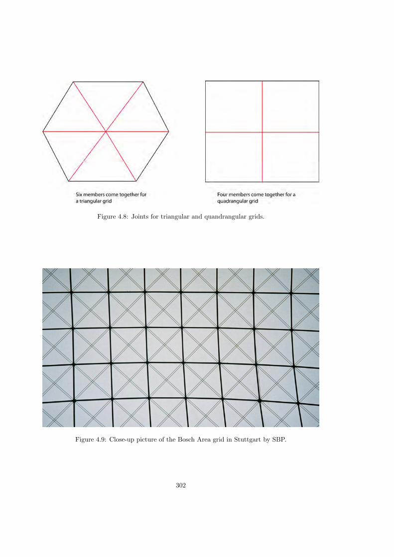
Figure 4.8: Joints for triangular and quandrangular grids.

Figure 4.9: Close-up picture of the Bosch Area grid in Stuttgart by SBP.

302

Figure 4.10: Bosch Area grid in Stuttgart by SBP.

303

Translational surfaces Translational surfaces are based on the principle of translatingsections (or a generatrix) along a describing curve, called the directrix (see Figure 4.11). Manyshapes can be close approximated by this method.

Figure 4.11: Translational Surfaces.

Scale-Trans surfaces Scale-Trans surfaces are based on the principle of scaling thegeneratrices and then translating the sections along the describing curve. This gives even morefreedom of approximation than translational surfaces.

Figure 4.12: Scale-Trans Surfaces

Note that these methods can closely describe many surfaces, but that there are limits to themethods, such as highly curved parts in the directrix cannot be followed. Rotation will have tobe added in that case, which does not always guarantee planar surfaces.

Extension to Block-Structured Grids The second approach is the one when the basegrid of a structure is manufactured from a quadrangular mesh, square if laid flat on the ground.This approach is the same as the block-structured grid (Section 4.4.2.1). In fact, this methodforms an extension to the block-structured grid, because with this technique the grid does nothave to be the 90-degree rectangular grid when laying flat on the ground. The grid could be

304

diagonally, in two ways, three ways or four ways, as sketched in Figure 4.5.The diagonal pattern is utilized to segment the roof of the Orvieto airplane hangar.

Grid Configuration for Dome Shapes Figure 4.13, shows the grid configurations fora dome shape. Five types of grid generation could be distinguished: a Schwedler dome, alamella dome, a diamatic dome, a grid dome and a geodesic dome (Vollers 2001). These gridconfigurations are suitable for all geometrical defined surfaces or parts of surfaces, generated byrotation.A modified form of a ribbed dome (a) is obtained by bracing the quadrilateral panels of thedome. The result is a dome configuration that is referred to as a Schwedler dome. (Named afterthe nineteenth century German engineer J. W. Schwedler who built many domes of this kind)A simple example of a Schwedler dome is shown in (c) and (d). This dome configuration alsoinvolves trimming to avoid overcrowding of the elements at the upper part of the dome. Aribbed dome is generated by the rotation of a curve around an axis and by translation of a ringover the same axis.An example of a lamella dome is shown in (e). A lamella dome has a diagonal pattern andmay involve one or more rings. An example of a trimmed lamella dome with rings is shown in(f). The grid is composed by two curves rotating around an axis. The semi-cupola of the Turinexposition Hall and the Palazzetto dello Sport by Nervi are examples of a lamella dome.The dome configurations shown in (g) and (h) are two examples of a family of domes that arereferred to as diamatic domes. The dome shown in (g) is an example of a basic diamatic formconsisting of triangulated sectors. The pattern of the diamatic dome of (h) is obtained from adenser version of the dome of (g) by removing every other line of elements.The domes shown in (i) and (j) represent two examples of the family of grid domes. A grid domeis obtained by projecting a plane grid pattern, such as the grids in Figure 4.5, onto a curvedsurface.A geodesic dome configuration is shown in (k). A dome of this kind is obtained by mappingpatterns on the faces of a polyhedron and projecting the resulting configuration onto a curvedsurface. The dome of (k) is obtained by mapping a triangulated pattern on five neighbouringfaces of icosahedrons (20-faced regular polyhedron) and projecting the result onto a sphere whichis concentric with the icosahedrons. The geodesic dome of (l) is obtained in a similar mannerwith the initial pattern chosen such that the resulting dome has a honeycomb appearance.For all these grid configurations of a dome it is not possible to point one out, that is betterthan the other. First, because the amount of repetitive elements is in relation to the amountof elements and shape of the structure. For all configurations apply that the elements in onering (horizontally) contains the same shaped elements. Second, the total amount of elementssegmenting the surface, can be varied by adjusting the mesh width, and so the curves distances,generating the mesh/surface. Third, because that the elements do not have to posses a certainshape; The radial grid configuration of the dome could also be used partially; the axis couldlie outside the building, e.g. the Saint Maria Church in Storkow 1 (Figure 4.14). The gridconfiguration is not only applicable to circular ground plans, but also to polygonal ground plans,e.g. the beams of the Noord Holland Pavilion are placed radial. See Figure 4.15. Of course, theelements do not possess the same shape and size all around the surface.

1http://www.sv.vt.edu/classes/ Access-date: 12–2005.

305

Figure 4.13: Grid configurations for dome shapes.

306

Isotope technique A grid generation technique that is derived from the techniques aboveis the isotope technique. With this method a shape is sliced in plural directions (one at least,two or three) by parallel curves, with a certain mutual distance (Rypl 2002). The quadrangularelements formed by these intersecting curves, are the final elements that should be fabricated inprefab concrete. The BMW pavilion Bubble, build for the IAA 99 in Frankfurt, is an exampleof a structure segmented in this way, in three directions. (Figure 4.16)This method has not really any particular advantages; the method does not try to minimize theamount of different element shapes nor do the elements always have a good, optimal shape andsize. This method however, is a suitable method to segment all types of morphologies with astructured and regularly organised grid.Computer programs as Mathcad segment shapes by the isotope technique in two directions.The distance of the segmenting curves can be filled in as a parameter by hand in the program 2.The node locations of the intersecting curves in space are given as x,y,z coordinates in space.Other software programs able to generate structured grids are given in annexure, e.g.BUDMESH2D, ICEM CFD, Truegrid, VGM, i.e.

Figure 4.14: Radial grid, Storkow church.

Figure 4.15: Radial grid of the ’Web Noord Holland.

2www.mathcad.com Access-date: 3–2006.

307

Figure 4.16: Isotope technique, BMW pavilion.

308

4.4.2.2 Unstructured Grids

Many free-form or form-finding designs involve complex regions that are not easily amenableto pure structured grids. Structured grids may lack the required flexibility and robustness forhandling complex surfaces, or the grid cells may become too skewed or twisted. Therefore, theunstructured grid concept is considered as one of the appropriate solutions to the problem ofproducing grids in regions with complex shapes.An unstructured grid has irregularly distributed nodes and their cells are not obliged to havea standard shape. Besides this, the connectivity of neighbouring grid cells is not subject toany restrictions. Thus, unstructured grids provide the most flexible tool for the descriptionof a shapes geometry by a mesh. However, in practice, unstructured grids for architectonicalstructures are not commonly used. It is even so that architects and engineers prefer to adaptthe shape of the design in order to find a translational structured grid(Schober 2003b). If thestructure will be executed in a steel lattice, this choice is understandable when considering theamount and costs of all differing joints to be fabricated. The grid generation techniques forunstructured grids fill in here as these techniques try to find, with certain accuracy, flat elements.But the elements we try to find could be double curved, but should be of least curvature. Thus,the grid generation techniques of unstructured grids help to find the elements with least doublecurvature, concerning a certain accuracy and element size.There are today many techniques available, with all the research activity devoted to automaticgrid generation, for the construction of unstructured grids. However, three approaches arewidely used. They can be described as point insertion methods based on Delaunay triangulation,and Advancing Front Methods and tree-based methods, such as Octree approach. This sectiondescribes the methods.Only the global idea, methods and results concerning the grid generation of complex shellsurfaces, is described as this subject is too wide and complex to be fully described in this reader.

Delaunay Triangulation In general, the Delaunay approach connects neighbouring points,of some previously specified set of nodes in the region of the shell surface, to form tetrahedralcells in such a way that the circumsphere trough the four vertices of a tetrahedral cell doesnot contain any other point. (Figure 4.17) The following subsections discuss the three majortechniques for generating triangles based on the Delaunay criterion; Voronoi Diagram, EdgeFlipping Algorithm and Incremental Bowyer-Watson Algorithm.

Voronoi Diagram The Delaunay triangulation has a dual set of polygons referred to asthe Voronoi Diagram or the Dirichlet Tessellation. The Voronoi Diagram can be constructedfor a random set of points on the surface of a structure. Given a set of points in the plane, theidea is to assign to each point a region of influence in such a way that the regions decomposethe surface of the structure. To describe a specific way to do that, let S element of R2

be a set of n points and define the Voronoi region of p element of S as the set of points xelement of R2 that are at least as close to p as to any other point in S; that is(Edelsbrunner 2001),

Vp = x ∈ R2|||x− p|| ≤ ||x− q|||,∀q ∈ S (4.1)

This definition is illustrated in Figure 4.18The Delaunay triangulation is obtained by drawing each Delaunay edge from one endpoint

straight to the midpoint of the shared Voronoi edge and then straight to the other endpoint.For each triangle formed in this way there is an associated vertex of the Voronoi diagramwhich is at the circum-centre of the three points which form the triangle. Thus each Delaunay

309

Figure 4.17: The circumcircle through 4 vertices does not contain any other point. Image source:

Figure 4.18: Seven points define the same number of Voronoi regions. One of the regions isbounded because the defining point is completely surrounded by the others.

triangle contains a unique vertex of the Voronoi diagram and no other vertex within the Voronoistructure lies within the circle centred at this vertex. Figure 4.19 depicts the Voronoi polygonsand the associated Delaunay triangulation.

It is apparent from the definition of a Voronoi polygon that the degeneracy problems canarise in the triangulation procedure when

• Three points of a potential triangle lie on a straight line

• Four or more points are cyclic

These cases are readily eliminated by rejecting or slightly moving the point which causes thedegeneracy from the original position.More information about the ‘Circles and Power’ and ‘Acyclicity’ can be found in ‘Geometry andTopology for Mesh Generation’ written by Herbert Edelsbrunner(Edelsbrunner 2001).

310

Figure 4.19: Voronoi edges are dotted and the dual Delaunay edges are solid. Image from(Edelsbrunner 2001)

Edge Flipping Algorithm The Edge Flipping Algorithm makes use of the equiangularproperty of the Delaunay-type triangulation, which states that the minimum angle of eachtriangle in the mesh, generated on the shell surface, is maximized(Liseikin 1999).Assuming there is some triangulation of a given set of points, the swapping algorithm transformsit into a Delaunay triangulation by repeatedly swapping the positions of the edges in the meshin accordance with the equiangular property. For this purpose, each pair of triangles whichconstitutes a convex quadrilateral is considered. This quadrilateral produces two of the requiredtriangles when one takes the diagonal which maximizes the minimum of the six interior anglesof the quadrilaterals, as shown in Figure 4.20. Each time an edge swap is performed, thetriangulation becomes more equiangular. The end of the process results in the most equiangulartriangulation.This technique based on the Delaunay criterion re-triangulates a given triangulation in a uniqueway, such that the minimum angle of each triangle in the mesh is maximized. This has theadvantage that the resulting meshes are optimal for the given point distribution, in that they donot usually contain many extremely skewed cells(Baker 1999).

Figure 4.20: The triangulation which maximizes the minimum angle. The dashed line indicatesa possible original triangulation.

311

Incremental Bowyer-Watson Algorithm The incremental technique, introduced byBowyer and Watson in 1981 triangulates a set of points in accordance with the requirementthat the circum-circle through the three vertices of a triangle does not contain any other point,such as mentioned in the previous subsection. The accomplishment of this technique starts froma Delaunay triangulation which is considered as an initial triangulation. The initial triangulationcommonly consists of a square divided into two triangles which contains the given points. Withthis starting Delaunay triangulation, a new grid node is chosen from a given set of points oris found in accordance with some user-specified rule to supply new vertices. Check step (b) inFigure 4.21. In order to define the grid cells which contain this points as a vertex, all the cellswhose circum-circles enclose the inserted points are identified and removed. The union of theremoved cells forms the region which is referred to as the Delaunay or inserting cavity. A newtriangulation is then formed by joining the new point to all boundary vertices of the insertingcavity created by the removal of the identified triangles step (c) in Figure 4.21(Liseikin 1999).

Figure 4.21: Stages of the planar incremental algorithm, three steps. Image from (Liseikin 1999)

Insertion of New Points The nature of the Boyer-Watson algorithm gives rise to aproblem of choosing the position where to insert the new point in the existing mesh, because apoor point distribution can eventually lead to an unsatisfactory triangulation.The new point should be chosen according to some suitable geometrical and physical solution.The geometrical criteria commonly consist in the requirement for the grid to be smooth andfor the cell elements to be of a standard uniform shape and of the necessary size. The physicalcriterion commonly requires the grid cells to be concentrated in the zones of large solutionvariations. With respect to the geometrical criterion of generating uniform cells, the vertices andsegments of the Dirichlet tessellation are promising locations for placing a new point since theyrepresent a geometrical locus which falls, by construction, midway between the triangulationpoints.Thus, in order to control the size and shape of the grid cells, there are commonly consideredtwo different ways in which the new point is inserted. In the first, the new point is chosen at thevertex of the Voronoi polyhedron corresponding to the worst simplex. In the second way, thenew point is inserted into a segment of the Voronoi polyhedron, in a position that guaranteesthe required size of the newly generated simplexes.More information about point insertion strategies can be found in Chapter 11.3.6 in Grid Gen-eration Methods written by Vladimir D. Liseikin(Liseikin 1999) and Chapter 16 in Handbook ofGrid Generation written by Timothy J. Baker(Baker 1999)

Software Many computer programs are developed for Delaunay triangulation3. A fulloverview of meshing software can be found in annexure II of Grid Generation Software forUnstructured Grids, or on the internet; 4

3 http://www.geom.uiuc.edu/software/cglist/ch.html Access-date: 3–2006.4http://www.andrew.cmu.edu/user/sowen/softsurv.html Access-date: 3–2006.

312

Some examples:

• ANSYS

• BAMG

• BL2D

• CADfix

• Geomagic Wrap

• Geopack90

• GMSH

• MEGA

• Mentat

• QHull

Of these programs, Ansys is the most common in use. On the internet site of Ansys thefollowing can be found, considering the grid generation procedure:

’From automatic meshing to highly crafted mesh, ANSYS, Inc. provides the ultimatemeshing solution. ANSYS provides powerful pre- and post-processing tools for meshgeneration from any geometry source, to produce almost any element type, for nearlyany physics, for virtually any application5.’

Other then Delaunay triangulation, Ansys is able to generate a triangular grid by the Advanc-ing Front Technique and a quadrangular grid by Advancing Front Technique or Edge SweepingAlgorithm, Section 4.4.2.2. Except the structural calculation, other features of Ansys which im-proves the program utility for a good grid generation are the capability to adaptivity, refinementand mesh improvement.

Results The advantage of choosing an unstructured grid instead of a structured grid for themeshing of a complex surface is the geometric flexibility and suitability for adaptation inherentto the use of irregularly connected triangular elements. Herewith, the Delaunay triangulation isvery popular in practical applications owing to the following optimality properties:

• Delaunay triangles are nearly equilateral

• The maximum angle is minimised

• The minimum angle is maximised(Liseikin 1999)

Figure 4.22 (left) shows how the Delaunay triangulation is derived from a convex 3D modelby Qhull. Figure 4.22(right) represents a Delaunay triangulation executed with Ansys.

5http://www.andrew.cmu.edu/user/sowen/softsurv.html Access-date: 3–2006.

313

Figure 4.22: Delaunay triangulation with Qhull (left) with Ansys (right).

Advancing Front Technique A widely used algorithm for the design of FE meshes is basedon the Advancing Front Method. The AFM was first published by Peraire et al (Peraire, Peiro& Morgan 1999). for the generation of meshes with triangular elements.

Method The generation problem consists of subdividing an arbitrarily complex domaininto a consistent assembly of elements. The consistency of the generated mesh is guaranteed ifthe generated elements cover the entire domain and the intersection between elements occursonly on common points, sides or triangular faces. The final mesh is constructed in what maybe defined as a bottom-up manner. This means that the process starts by discretizing eachboundary curve in turn. Nodes are placed on the boundary curve components and then adjacentnodes are joined with straight line segments. In the later stages of the generation process, thesesegments will become sides of triangular faces. The length of these segments must therefore, beconsistent with the desired local distribution of mesh size. This operation is repeated for eachboundary curve in turn.The next stage consists of generating planar faces. For each two-dimensional region or surfaceto be discretized, all the sides produced when discretizing its boundary curves are assembledinto the so-called initial front. The relative orientation of the curve components with respect tothe surface must be taken into account in order to give the correct orientation to the sides in theinitial front. This front is used to generate a triangular mesh on the surface. The size and shapeof the generated triangles must be consistent with the local desired size and shape(Farestam &Simpson 1994).Daniel Rypl(Rypl 2002) describes the process of Advancing Front in eleven steps in a moremathematical manner, in an online document.Figure 4.24 presents a flow chart for mesh generation using the Advancing Front Technique.Figure 4.23 demonstrates different stages during the triangulation process by the AdvancingFront Technique.

314

Figure 4.23: The Advancing Front Technique showing different stages during the triangulationprocess.

315

Figure 4.24: Flow chart of the Advancing Front Generation Technique.

316

Software Also for the advancing front technique, around 10 computer programs have beendeveloped. Some programs are only used by a dozen of people; others are more common in use,such as ANSYS, for which is refered to Section 4.4.2.2.Other programs used for structural discipline with the Advancing Front are 6:

• MeGA

• Mentat

• TMG

Figure 4.25 and Figure 4.26 are examples of the Advancing Front Grid Generation Techniquewith Ansys on a chair and a mechanical joint.

Figure 4.25: Model and mesh of a chair.

Figure 4.26: Model and mesh of a mechanical joint.

Results The basic disadvantage of this unstructured grid methodology lies in its incapa-bility to handle multiple regions and multiple material domains. Also the deviation of the meshfrom the original geometry together with a relatively large computational time is considered tobe a drawback(Rypl 2002).

6http://www.andrew.cmu.edu/user/sowen/softsurv.html Access-date: 3–2006.

317

Same as Delaunay, easy parts of the surface are also generated by the Advancing Front Techniquewith result, that the grid of the surface becomes unnecessarily difficult and of different elementssize and shape. This technique is suitable to be used for the complex surfaces in e.g. free-formor form-finding surfaces. Also, the elements with the lowest double curvature are found, just aswith the Delaunay approach.

Octree approach

Method In the Octree approach the region of the shell is first covered by a regularCartesian grid of cubic cells in 3D, or squares in 2D. Then the cubes containing segments of thedomain surface are recursively subdivided in eight cubes until the desired resolution is reached.The cells intersecting the body surfaces are formed into irregular polygonal boundary cells,(Figure 4.27)

Figure 4.27: Example of the Octree approach.

The grid generated by this Octree approach is not considered as the final one, but serves tosimplify the geometry of the final grid, which is commonly composed of tetrahedral cells builtfrom the polygonal cells and the remaining cubes.(Liseikin 1999)The process of meshing the boundary cell is a function of the level of geometric complexitysupported by the mesh generator. In cases where there is only a limited amount of geometriccomplexity allowed per cell, simple templates are possible. When there is no specific limitationon the level of geometric complexity, the process of meshing the boundary octant requires allthe functionality of an automatic mesh generator applied to the local region(Shephard 1999).There are different approaches for the creation of elements in the boundary cells. The first two,create tetrahedral elements. The first of these approaches applies an element removal procedurestarting from a basic cell level boundary representation. The second approach develops a De-launay triangulation based on the mesh vertices of the cell level boundary representation, whichis then followed by an algorithm that insures the resulting surface triangulation is topologicallycompatible and geometrically similar. Since the first two procedures operate strictly accountingfor the intersections of the model and cell boundary entities, they are vulnerable to the small,poorly shaped elements caused by boundary cells touching the model boundary.The third procedure creates tetrahedral elements from a given surface triangulation using anelement removal procedure. The last boundary cell meshing procedure considers the creation ofhexahedral elements to fill the region between the interior cell and the model boundary. Thesetwo procedures create the elements in the regions between the model boundary and interior cellswithout strict adherence to the boundary of the cell. Therefore, they are not susceptible to the

318

creation of poorly shaped elements caused by the boundary cells touching the model boundary.

Software Not too many software programs for Octree grid generation in the structuraldiscipline have been developed. The most common in use is ICEM CFD:

ICEM CFD Engineering, a subsidiary of ANSYS, Inc., develops and markets softwarefor pre- and post-processing of engineering applications such as computational fluiddynamics and structural analysis. Our major products include ICEM CFD, theleading software for 3-D grid generation for CFD and other engineering applications.

Our Direct CAD Interfaces link the parametric geometry creation tools available inCADDS5, CATIA, ICEM Surf, Pro/ENGINEER, SDRC I-DEAS, SolidWorks, andUnigraphics to the grid generation, post-processing, and grid optimisation tools ofICEM CFD. We work closely with these CAD/CAM vendors to ensure that ourDirect CAD Interfaces remain current.

The grid generation tools of ICEM CFD offer the capability to create gridsfrom geometry in multi-block structured, unstructured hexahedral, tetrahedral,hybrid grids consisting of hexahedral, tetrahedral, pyramidal and prismatic cells, aswell as Cartesian grid formats combined with boundary conditions.

The state of the art CFD post-processing and visualization tool, ICEM CFDVisual3, supports solutions in structured, unstructured, steady state, or transientdata and contains powerful features while providing an open scripting system foreasy customization. 7

Results The computer program is relatively easy to use; the user brings the CAD surfacesor STL data that describe the space to be meshed into ICEM CFD Hexa. Then, Hexaautomatically generates a global block around the CAD design. By subdividing this block intosmaller blocks and assigning different materials the user can cut out the desired shape. Toreflect the characteristic features of the geometry to be meshed, the block structure can beinteractively adjusted to the underlying CAD geometry (Shaw 1999).

Figure 4.28: Octree discretization.

7http://www-berkeley.ansys.com Access-date: 12–2005.

319

The unstructured grid generation Octree is a good method to develop a mesh over aformfinding or free-form complex surface. Although, the main drawback of the Octree approachis the inability to match a prescribed boundary surface grid, so the grid on the surface is notconstructed beforehand as desired but is derived from the irregular volume cells that intersectthe surface. Another drawback of this grid is its rapid variation in cell size near the boundary.In addition, since each surface cell is generated by the intersection of a hexahedron with theboundary, problems arise in controlling the variation of the surface cell size and shape.

4.4.2.3 Variational Structured Grids

The mode of variable structured mesh design is required for preserving compatibility betweenthe structured and unstructured parts of the surface. One method is the Hybrid Grid.

Hybrid Grids

Method Promoters of structured schemes highlight the efficiency and accuracy thatis accomplished through the employment of regularly arranged volumes, while promoters ofunstructured schemes emphasize the geometric flexibility and suitability for adaptation inherentto the use of irregularly connected tetrahedral volumes. All advantages of these techniquescan be combined by replacing the use of only one grid generation type by the use of combinedmeshes composed of both structured and unstructured grids. This composed grid generationtype is named a hybrid grid (Shaw 1999).Commonly, a structured grid is generated about each chosen boundary segment. Thesestructured grids are required not to overlap. The remainder of the domain is filled with the cellsof an unstructured grid.These kinds of meshes are widely used for the numerical analysis of boundary value problems inregions with a complex geometry and with a solution of complicated structure, e.g. free-form orform-finding structures.

Figure 4.29: Fragment of a hybrid grid.

Software To generate hybrid grids, a software program which can not only generateunstructured grids, but also structured grids, can be utilised. The software program ICEM CFDis the one commonly in use for the structural discipline (Thompson 1995). This is also used for

320

Figure 4.30: Fragment of a hybrid grid.

the Octree approach of unstructured grids.Another program for the generation of Hybrid Grids is GRIDGEN. The structural part isgenerated by a block-structured grid, while the unstructured part is always generated byDelaunay triangulation.

In the GRIDGEN system of Pointwise (STEINBRENNER/CHAWNER/FOUTS 1990, STEINBRENNER/CHAWNER/ANDERSON 1992, STEIN-BRENNER/CHAWNER 1992, STEINBRENNER/CHAWNER 1993,CHAWNER/STEINBRENNER 1995) the user constructs curves which are inturn used to build the topological surface and volume components. The user thenselects curves as the boundaries of surface grids, and finally surfaces as the boundariesof volume grids (blocks). With this system, grid generation is a user in-the-looptask. The data structure maintains the relationship among the curves, surfaces, andvolumes so that changes can be propagated up or down the hierarchy automatically.The volume grid generation itself is finally done in the batch mode.(Thompson 1995)

Result This combination of grid types not only allows the benefits of structured and un-structured grids to be attained simultaneously, but also allows high grid quality to be achievedthroughout the domain due to the appropriate use of each element type.

4.4.2.4 Configuration processing

Formex mathematics Formex (Nooshin, Space Structures Research Centre, Department ofCivil Engineering, University of Surrey, Guildford, UK 1984, Nooshin & Disney 2002) algebra isa configuration processing mathematic language, which is implemented in a programming lan-guage, Formian(Delft University of Technology 2003) and (School of Engineering 2004). Theconfiguration is an arrangement of parts of the structure. It is mostly used for generating (pro-cessing) regular shapes consisting of one or more-layered grids. The language works with so-calledformices (plural of formex) which form a fundamental operation for the algebra. Very complexshapes can be generated with simple statements, as can be seen in the Formian examples below.This algebra could be seen as an early form of parametric geometry modeling. Simple parameterscontrol complex structures.

321

Perspective view of Figure 4.31

(*) Perspective view (*)

TOP=rinid(7,8,2,2)|[0,0,1;2,0,1]#rinid(8,7,2,2)|[0,0,1;0,2,1];

BOT=rinid(6,7,2,2)|[1,1,0;3,1,0]#rinid(7,6,2,2)|[1,1,0;1,3,0];

WEB=rinid(7,7,2,2)|rosad(1,1)|[0,0,1;1,1,0];

GRID=TOP#BOT# WEB;

use vm(2),vt(2),vh(7,-14,7,7,7,0,7,7,1);

clear; draw GRID;

Figure 4.31: Image made in Formian of the Perpective View. Image fromhttp://www.bk.tudelft.nl/bt/dc/Formian/Formian.html

Lamella dome of Figure 4.32

(*) Lamella dome (*)

ny=12; nz=8; rd=100; a=2; t=50;

e=[1,0,a;1,1,1+a];

f1=rinit(ny,nz,2,2)|rosat(1,1+a)|e;

f2=rinit(ny,2,2,2*nz)|[1,0,a;1,2,a];

f=bs(rd,180/ny,t/(2*nz+a))|(f1#f2);

use &,vt(1),vm(2),vh(10,10,20,0,0,0,0,0,1);

clear; draw f;

Figure 4.32: Image made in Formian of the Lamella dome. Image fromhttp://www.bk.tudelft.nl/bt/dc/Formian/Formian.html

Onion with quadrangular elements of Figure 4.33

322

(*) Onion with quadrangular elements (*)

R=6; (*) 1st radius (*)

Q=10; (*) 2nd radius; conditon: R<Q (*)

M=24; (*) no of elements along U2 (*)

N=20; (*) no of elements along U4 (*)

T=acos|(R/Q);

P=asin|(R/Q); (*) position angle (*)

A=[1,0,1,0;1,0,1,-1;1,1,1,-1;1,1,1,0];

B=rinic(2,4,M,N,1,-1)|A;

C=tran(4,-1*N*P/T)|B;

D=pex|dep(4)|ba(R,360/M,Q,T/N)|C;

use &,vm(2),c(3,8),vh(20*Q,-20*Q,20*Q,0,0,0,0,0,1);

clear; draw D;

Figure 4.33: Image made in Formian of the Onion of quadrangular elements. Image fromhttp://www.bk.tudelft.nl/bt/dc/Formian/Formian.html

Formian can be downloaded on: http://www.surrey.ac.uk/eng/research/masss/ssrc/FMXJLY200.ZIP.Another implementation, pyFormex, can be downloaded on: http://pyformex.berlios.de

323

4.5 Form finding

The techniques intended here are the ’classical Form Finding’ techniques, aimed on the finding ofshapes of structures such as membranes, cable-nets and when inverted, shells. These techniquescan also be applied to other structures to find forms, but then need to be modified. An exampleof this is the British Museum Queen Elisabeth Great Court Roof, where Chris Williams modifiedthe dynamic relaxation method to relax the generated grid for more efficient structural loadbearing behaviour. Classical Form Finding follows the principle of ’Form follows Force’. Theshape of the structure depends on the forces in the structure, but of course the forces also dependon the shape of the structure, leading to complex, non-linear behaviour which cannot be directlydetermined with analytical techniques. These problems have to be solved by an algorithmicapproach. The history of Form Finding is rich, Gaudi, Isler, Candela and Torroja used thephysical alternative in their structures, because computation was not yet available. People likeSchek, Klaus Linkwitz, Frei Otto, Jorg Schlaich and Erik Moncrieff are inventors and users ofthe Force Density method, while people like Mike Barnes, Chris Williams, Ove Arup and TedHappold prefer the Dynamic Relaxation methods.

4.5.1 Minimal surfaces

8 Minimal surfaces are defined as the smallest possible surface area between a given (closed)edge. Minimal surfaces are closely related to many form finding problems. This is caused bythe soap film analogy (Bletzinger n.d.). The problem is considered as if it was a soap film andsince soap films approxiate minimal surfaces, often minimal surfaces are searched for. Minimalsurfaces have some characteristics:

• Area variation is 0:δa = 0

• The mean surface curvature vanishes.

There are 2 approaches to calculating the minimal surface according to the principe of thearea variation is 0. These work from the principle of the starting with a reference surface whichis known, which has to be transformed to an actual surface, which has to be form found.

1. Direct geometrical approach which can be described by (Bletzinger n.d.):

δa =

∫

A

δ(detF )dA =

∫

A

detFF−T : δFdA = 0 (4.2)

whereF deformation gradient

F = ∂x∂X

x(θ1, θ2) is the coordinate on the actual surfaceX(θ1, θ2) is the coordinate on the reference surface

2. Mechanical approach which can be described by (Bletzinger n.d.):

δw = t

∫

a

σ : du,x da = t

∫

A

(F · S) : δFdA = 0 (4.3)

8Bletzinger gives several good mathematical references for minimal surfaces (Bletzinger n.d.)

324

whereσ the Cauchy stress tensorδu,x the derivative of the virtual displacement with respect to the geometry of the actual surfacet thickness of the membraneS second order Piola-Kirchoff stress tensor

This methods works with the principle of virtual work of a stress field, which vanishes whenin equilibrium.

When discretized and linearized form finding methods for cable-nets and membranes can bederived from these formulations, such as the force density method.

4.5.2 Force density method

The Force Density Method is a method to solve the non-linear system of equations of a cable-netstructure by making the system linear. The method can also be used for membrane structuresby discretization of the membrane to cable-net elements. A well-known force density applicationof the form finding, analysis and pattern-cutting of membranes is Easy (Stary 2003) and for anolder application: Grundig, 1986 (Grundig & Bahndorf 1986) (formerly: FASNET). For detailedinformation, refer to Montcrieff (Montcrieff & Grundig 2000).

The force density method is a simplication for cable-net structures of the updated referencestrategy (URS), which is defined by Equation 4.4 according to Bletzinger (Bletzinger n.d.).

K = Ac

∫

L

(Fc ∗ S) : Fuds = Ac

∫

L

1

L(L

l

n

Ac

)1

Lds =

n

l= q (4.4)

whereK stiffness matrixAc Reference surface areaDu Deformation gradient (u is the discretization parameter)

F = lL

Fu = 1L

S second Piola Kirchoff stress (in the reference surface), for minimal surfaces yields:S = L

ln

AcI

n Prescribed tension force in an elementq Force density

This might be a quite complex formulation. A less complex problem illustrates the workingof force density. Consider the problem in Figure 4.34. The three members are number 1,2 and 3.The four nodes are numbered a,b,c and d. Node a and d are supported by a hinged support. Nodeb and c are loaded by a load in the x direction and the y direction. The system of equationsto describe this system is equation 4.7 which can be derived from among others equation 4.5and 4.6.

L1

Xb −Xa

=S1

Sx;1(4.5)

~S1 + ~S2 = ~F1 (4.6)

325

Figure 4.34: Example of a force density problem

(Xb −Xa) S1

L1+ (Xb −Xc)

S2

L2− Fx;b = 0

(Xc −Xb)S2

L2+ (Xc −Xd)

S3

L3− Fx;c = 0

(Yb − Ya) S1

L1+ (Yb − Yc)

S2

L2− Fy;b = 0

(Yc − Yb)S2

L2+ (Yc − Yd)

S3

L3− Fy;c = 0

(4.7)

whereXp x coordinate of point pYp y coordinate of point pSj force in member jLj length of member jFw;p load in the direction of w in point p

Lj =√

(Xend;j −Xbegin;j)2 + (Yend;j − Ybegin;j)2 (4.8)

whereLj length of member jXend;j x coordinate of the node at the end of member jXbegin;j x coordinate of the node at the begin of member jYend;j y coordinate of the node at the end of member jYbegin;j y coordinate of the node at the begin of member j

However, this system cannot be solved since there are 7 unknown variables: four coordinates (Xand Y of b and c) and three forces (S1, S2 and S3). Note that the lengths are be found withequation 4.8, if the coordinates would be known.This problem is solved by the introduction of the preset force density Qj which is defined byequation 4.9. This simplification makes the system of equations linear and solvable, since onlythe four coordinates are unknown now.

Qj =Sj

Lj

(4.9)

whereQj force density in member jSj force in member jLj length of member j

In more complex problems this is used to converge to the equilibrium state of the cable-netor membrane. Important is to understand that the force density is a proportion between the

326

force in a member and the length of a member. When the lengths are held constant and theforces in the edges of the membrane or cable-net and the membrane or cable-net itself are equal,the shape is the same for each force density. However, when made unequal, the curvature ineither the net or the cable-net or membrane itself will increase or decrease, and therefore thesurface area of the cable-net or the membrane, depending on the force density (and the appliedlengths and forces).

Force density method This method which is specifically developed (originally describedby Sheck (Sheck 1974)) for tension structures, uses an analytic technique to linearize theform-finding equation for a tension net. This linearization makes the method independent of thematerial properties of the membrane. Force density ratios (cable force T divided by cable lengthl) need to be specified for each element, and different ratios give different equilibrium shapes.This means, the higher the force density, the shorter the element for a given force. When theforce densities for a node are equal and evenly distributed around the node, a minimal surface(i.e. equilibrium shape) is generated.The method is numerically robust, independent of the initial locations of the nodes, and theequilibrium shape is found easily. The force density solution applied to loads is non-linear, andrequires iteration.

4.5.3 Dynamic relaxation

Dynamic relaxation can be used for finding the shape of net and membrame structures. Re-laxation methods are not really ’form finding methods’ but methods for structural calculationused for form finding purposes. Another well-known method is the solution of a stiffness matrix,either directly or iterative, to determine the equilibrium. However, in some situations, like localinstability, these methods perform less good.Dynamic relaxation is a method which lets the structure relax to a equilibrium situation. On onehand, the velocity of displacement converges to zero and the stiffness of the structure increases.The advantage of this method over matrix methods are that this method does not have to solvematrices, which takes a lot of calculation power, and although it takes more cycles to complete,each cycle takes much less time. Another advantage is the ability to deal with local instability,like wrinkling of the membrane, etc.A couple of examples of software which use this principle are the dynamic relaxation programsby C.J.K. Williams (Williams 2004) and M.R. Barnes (Barnes 1986), the in-house Tensyl soft-ware (Wakefield 1986) by Buro Happold9 and the in-house software of Tensys10.

Dynamic relaxation in detail In this paragraph the procedure of dynamic relaxation willbe explained and illustrated. Dynamic relaxation has an iterative, converging process where inthe end an equilibrium should be reached. The success however depends on various parametersand of course the consistency the structure itself.Each cycle of the process starts with the calculation of the lengths of each member j withEquations 4.10 and 4.11. The first equation calculates the differences in various directions. Aschematic representation of a member can be seen in Figure 4.35.

dxj = xj;end − xj;begin

dyj = yj;end − yj;begin

dzj = zj;end − zj;begin

(4.10)

9Buro Happold, http://www.burohappold.com10Tensys, http://www.tensys.com

327

where

xj;begin x position of the node on the begin of the j-th memberxj;end x position of the node on the end of the j-th member

Figure 4.35: The schematic representation of a member in dynamic relaxation

lj =√

dx2j + dy2

j + dz2j (4.11)

wherelj length of member j

With the Law of Hooke (4.12) the stress σ based on a strain ε can be determined. Whenmultiplied with the section A the tension force Ft can be calculated from the strain (4.13). E isthe modulus of elasticity.

σ = Eε (4.12)

Ft = σA = EAε (4.13)

The strain ε is the difference between the original length and the deformed length divided bythe original length. In Equation 4.14 the tension force is calculated from the lengths.

Ft;j = EAj

lj − Lj

Lj

(4.14)

The force Ft can be decomposed into the various directions to determine the force on eachnode, based on the original load and this extra force (Equation 4.15).

328

Fx;j;begin = Fx;j;begin +dxj

ljFt;j

Fx;j;end = Fx;j;end − dxj

ljFt;j

Fy;j;begin = Fy;j;begin +dyj

ljFt;j

Fy;j;end = Fy;j;end − dyj

ljFt;j

Fz;j;begin = Fz;j;begin +dzj

ljFt;j

Fz;j;end = Fz;j;end − dzj

ljFt;j

(4.15)

The stiffness also changes when the lengths of the members change. This can be seen fromEquation 4.16 where the change of stiffness in each direction is calculated.

∆Sx;j =(

dxj

lj

)2EAj

Lj

∆Sy;j =(

dyj

lj

)2EAj

Lj

∆Sz;j =(

dzj

lj

)2EAj

Lj

(4.16)

From Equations 4.17, 4.18 and 4.19 the new stiffnesses of the system are being determined ineach direction.

Sx;j;begin = Sx;j;begin + ∆Sx;j

Sx;j;end = Sx;j;end + ∆Sx;j(4.17)

Sy;j;begin = Sy;j;begin + ∆Sy;j

Sy;j;end = Sy;j;end + ∆Sy;j(4.18)

Sz;j;begin = Sz;j;begin + ∆Sz;j

Sz;j;end = Sz;j;end + ∆Sz;j(4.19)

Now the stiffness of each node can be determined for each node i in Equation 4.20.

Si = Sx;i + Sy;i + Sz;i (4.20)

In Equation 4.21 the velocities of each node are determined. However, as can be seen fromEquation 4.22, where the node coordinates are adjusted, this velocity is not really a velocity, buta variable stepsize to change the node coordinates with. However, analogy with velocity is goodto keep in mind for understanding the princples.f is a factor which determines the amount of adjustment for the net. c is a convergence factorwhich is 0 or 1, to secure convergence and decreasing speeds. When all speeds summed are largerthan the last cycle, this convergence safety trap goes to 0 and decreases the amount of speed.

Vx;i = c · Vx;i + f · Fx;i

Si

Vy;i = c · Vy;i + f · Fy;i

Si

Vz;i = c · Vz;i + f · Fz;i

Si

(4.21)

xi = xi + Vxi

yi = yi + Vyi

zi = zi + Vzi

(4.22)

329

Figure 4.36: Dynamic relaxation, left the original net structure and right the relaxed structure.Image and software by C.J.K. Williams.

4.5.4 Shape form finding

Using a shape optimisation technique is another method of finding an equilibrium. This op-timisation techniques finds the optimum between force and shape leading to a position wherethe structure is in equilibrium. Also principles of stress averaging can be used to find catenaryshapes.

4.5.5 Other form finding methods

Other methods of Form Finding spring from the computer games industry and non-linear finiteelement analysis. A technique which has been used by Axel Kilian of MIT to create a virtualGaudi hanging model application, is called particle-spring systems. These systems deals withmasses on a spring. Another way of analysing membranes is to use non-linear finite elementsolvers to model and solve the behaviour of the membrane. The membrane is then modelled asmembrane elements, with only in-plane forces.

330

4.6 Structural optimisation

Structural Optimisation deals with the optimisation of structures. Optimisation can be definedas the process to find the minimum (or maximum) of an object-function within a given set ofboundaries or constraints. The object-function describes both the generation process as well asthe evaluation process of the subject of the optimisation. The boundaries or constraints describethe freedom which is given to the algorithm to search the optimum.

4.6.1 Theory of optimisation

Mathematics In this section the basic mathematics of structural optimisation are covered ingeneral form. In other words, not structural engineering problems, but mathematical problemsand methods are described which can be used to solve structural engineering problems.Note again that the purpose of this section is not to be a complete mathematical reference guide,but a general overview over problems and methods. Also should be noted that this section doesnot provide detailed explanation of each method.For more detailed information, its recommended to read ”Numerical Recipes in C++” (Press,Vetterling, Teukolsky & Flannery 2002), ”Structural Optimisation” (Bletzinger 2001), ”Ad-vanced Techniques in the Optimum Design of Structures” (Hernandez 1993) and ”RecentAdvances in Optimal Structural Design” (Burns 2002).

To find a definition of optimisation the following references can be found:

(Kirsch 1993), (Liang 2005) and (Xie & Steven 1997a)

op·ti·mal adj the best or most suitable; extreme; highest; most favourable or most desir-able possible under a restriction expressed or implied

op·ti·mise v the way that something is done or used as effective as possible; trying tomake optimal; trying to reach the extreme; make optimal; get the most out of; use best

op·ti·mum adj the best or most suitable for a particular purpose; the best possible situ-ation; conditions; amount of time etc for something to happen; the best; the highest achievable;the point at which the condition, degree, or amount of something is the most favourable

struc·tur·al adj relating to or having or characterized by structure; affecting or involvedin structure or construction

In the context of a structure subject to multiple loads and support conditions the opti-mal shape is that which best satisfied the constraints, with the degree of satisfaction notnecessarily the same for all the constraints.

General form of an optimisation problem. Equation 4.23. A function is linear if allfunctions f, g and h are linear. If one of these function is non-linear, the optimisation problem isalso non-linear.

331

minimize F (x); x ∈ Rn

such that gi ≤ 0; i = 1, · · · , phj = 0; j = 1, · · · , q

where F (X) =

f1(x)· · ·fn(x)

¯

(4.23)

where

F(x) object functiongi inequality restriction functionshj equality restriction functionsfi(x) i-th object functionx parameters

A special form of this problem are ”variable bound problems” were also the variables x arebounded by a restriction, for instance xi ≤ xi ≤ xi.The space spanned by the possible design variables is called the ”search space”. The spacespanned by the possible design variables, satisfying all constrains, is called the ”feasible domain”.

Below several terms in optimisation will be explained which are important to understandbefore looking at the actual methods of optimisation.

Function approximization versus optimisation A possible classification of solution meth-ods for these optimisation problems is the subdivision in function approximation methods andoptimisation methods.In function approximation methods the algorithm tries to approximate or ’learn’ the object func-tion and of this function the optimum is determined, for instance by determining the derivativesor searching this function. This often involves the optimisation of parameters of the functionwhich models the object function. Neural networks are an example of an algorithm which ’learns’the object function.In optimisation methods the algorithm tries to optimise the object function by searching thesearch space in some manner. The search space is the space spanned by the possible variables,boundaries and constraints.

Discrete versus continuous optimisation Often solution methods for the problem in Equa-tion 4.23 assume continuous functions for f, g and h and the variables x. These methods areoften analytical and are called continuous optimisation.Numerical methods often use a discrete definition of the variables. This is called discrete opti-misation.

Local versus global optimisation One of the main problems of optimisation methods isthe problem of local optima in the object function. The function possesses one or more localoptima which have a derivative of zero, in other words are a top of the hill, or the bottom of avalley, but are not the highest top, or the lowest bottom in the object function, which is calledthe global optimum. Many classical methods have the problem that they get stuck in the localoptima and cannot ‘jump’ out of these optima. Various techniques, such as genetic algorithmsor simulated annealing, have this feature.

332

global and local maxima and minima The feasible region is the set of all solutionsto the problem satisfying all the constraints. The optimal solution for a minimization problemis the solution with the smallest cost value in the feasible region. Similarly, for maximizationproblems, it is the solution with the largest objective function value. The cost function f(x)has a local minimum (also called a relative minimum) at a point x∗ in the feasible set S ifthe function value is the smallest at the point x∗ compared to all other points x in a feasibleneighbourhood N of x∗, that is

f(x∗) ≤ f(x)∀ x(=for all x) in the feasible region.

(4.24)

If strict inequality holds, then x∗ is called the strict or unique global minimum.

Function f(x) has a local minimum at x∗ if this equation holds for all x in a small neigh-bourhood of N of x∗ in the feasible region. Neighbourhood N of the point x∗ is mathematicallydefined as

N = x|x ∈ S with ‖ x− x∗ ‖< δ (4.25)

for some small δ. Geometrically, it is a small feasible region containing the point x∗.

The global and local minima and maxima are shown in Figure 4.37.

Figure 4.37: Global and local maximum and minimum points of a multimodal function.

Discrete versus continuous optimisation Often solution methods for the problem inEquation 4.23 assume continuous functions for f, g and h and the variables x. These methodsare often analytical and are called continuous optimisation.Numerical methods often use a discrete definition of the variables. This is called discreteoptimisation.

Fully stressed design In this strategy no redundancy of stress is allowed. Every elementof the structure has to be stresses to the maximum. When considering a single load-casethis is possible, however one can imagine that this is quite complex when considering more(paradoxical) load-cases.

333

For trusses Equation 4.26 applies (Bletzinger 2001) for convergencing to a fully stressed design.However, it needs to be noted that for statically indetermined structures the correct solutionwill not always be found:

A(k+1)i = max(all loadcases)

[

A(k)i

σ(k)i

σadmissiblei

]

(4.26)

for all members i = 1, · · · , n

whereA

(k)i surface area of the profile section for member i

σ(k)i current stress for member i

k stepnumber

Multi-objective or multi-criteria optimisation Multi-objective or multi-criteria opti-misation are characterized by more than one object-function. An example of this is Equation 4.27.The problem is how to define such a problem that these objectives can be optimised. An ex-ample of this is weighted summation of the objective functions (an example can be seen inEquation 4.28). Bletzinger (Bletzinger 2001) gives some examples of this optimisation.

minimize f(x) =

f1(x)f2(x)· · ·fn(x)

(4.27)

minimize F (x) =n

∑

i=1

wifi (4.28)

wherefi i-th object functionf(x) object function vectorwi weight of the i-th object functionF(x) weighted summation of object functions

4.6.2 Classification of optimisation problems

If an optimisation problem has linear objective and constraint functions, it is called a linear

programming problem. An integer programming problem is a linear programming problem inwhich some or all variables must be non-negative integers. Otherwise, it is called a non-integer

programming problem. The search for an optimal arrangement, grouping, ordering or selectionof discrete objects is called combinatorial optimisation. A problem having a quadratic objectivefunction and linear constraints is called a quadratic programming problem.

It is important to note the following points for the foregoing nonlinear problem model relativeto structural and mechanical system design problems.

1. The model is applicable to all problems with continuous design variables. Multi-objective

and discrete variable problems can also be treated after certain extensions of the model;

2. the functions of the problem are assumed to be twice differentiable. Problems havingnon-differentiable functions can be treated with additional computational effort. Also,

334

gradients of active constraints are assumed to be linearly independent at the optimum;

3. The cost and/or constraint functions may be implicit as well as explicit functions of thedesign variables. That is, their final form in terms of only the design variables may not beknown. The functions, however, can be evaluated using analysis computer programs oncea design is specified;

4. Derivatives of the functions are needed in numerical methods of optimisation. Efficientmethods to calculate them taking advantage of the structure of engineering designproblems have been developed.

Non-linear programming problem A nonlinear programming problem can be representedin the following manner.

Let x represent an n-dimensional design variable vector. Then any design optimisationproblem can be stated as follows: find x to

minimise a cost function f(x)subject toequality constraints: gh(x) = 0, h = 1 to pinequality constraints: gh(x) ≤ 0, h = (p+ 1) to q

xLi ≤ xi ≤ xR

i i = 1 to k

(4.29)

where p is the number of equality constraints and (q-p) is the number of inequalityconstraints. xL

i and xRi are the lower and upper bounds on the design variable xi, and k is

the total number of design variables. This optimisation problem is called a general mixeddiscrete-continuous variable nonlinear optimisation problem. In some situations, there may betwo or more cost functions. This is called a multi-objective optimisation problem.

4.6.2.1 Analytical optimisation

Analytical optimisation usually involves the application of the mathematical methods from sec-tion on structural engineering problems. Usually the calculation is structural and the optimisationpart is a certain mathematical technique. Since every problem brings its own method, there areno real types or categories in this field of optimisation. Also, these technique currently are onlyused for estimates of the final result of more complex calculation methods, since these techniquesonly work when the problem is quite simple and can be solved by analytical techniques. Sincestructural engineering problems usually involve complex search spaces with discrete and contin-uous variables, discrete and continuous object-functions, etc. not many problems can be solvedin an analytic manner.

4.6.2.2 Size, shape and topology optimisation 1

Before the distinction between size, shape and topology optimisation will be made, it must be saidthat there are several understandings of this distinction. Below two of them will be described.

Information taken from: (Bendse 1995), (Bendse 2003), (Coenders 2004), (research group2005) and (Universtat Stuttgart, Institute for Structural Mechanics, Adaptive Finite ElementMethods for fast transient, highly nonlinear processes n.d.)

335

general introduction into shape, size, and topology optimisation Applications ofnumerical methods to truss problems and other discrete models were first described in the earlysixties, but only recently have these challenging large-scale problems attracted renewed interest,especially for producing specialised algorithms.

In the design of the size, shape, and topology of a structure the interest is in the determi-nation of the optimal placement of a given isotropic material in space, which means, it shouldbe determined which points of space should be material points and which points should remainvoid (no material). The geometric representation of a structure is thought of as similar to ablack-white rendering of an image. In discrete form this then corresponds to a black-whiteraster representation of the geometry, with pixels given by the finite element discretisation. So,in its most general setting shape, size and topology optimisation of continuum structures shouldconsist of a determination for every point in space if there is material in that point or not.Alternatively, for a FEM discretisation every element is a potential void or structural member. Inother words, the ground approach is that for an initially chosen layout of nodal points in the trussstructure or in the finite element mesh, the optimum structure connecting the imposed boundaryconditions and external loads is found as a subset of all the elements of the initially chosenset of connections between the truss nodal points or the initially chosen set of finite elements.The positions of nodal points are not used as design variables, meaning that these points are fixed.

Terminology and representation The three principles size, shape, and topology optimisa-tion can be mentioned as one under the common denominator of layout optimisation (Figure 4.38)

Size optimisation The main feature of the size problem is that the domain of the designmodel and variables is known a priori and is fixed throughout the optimisation process.Only the size of certain elements is optimised without changing the shape or topology ofthe structure. Size optimisation is to find the optimal cross-sectional properties of membersin a truss or frame structure or the optimal thickness distribution of a plate structure.It has the goal of maximising the performance of a structure in terms of the weight andoverall stiffness or strength while the equilibrium condition and the design constraints are sat-isfied. The design variable is the cross-sectional area of truss members or the thickness of a plate.

Shape optimisation The goal in shape optimisation, or geometry optimisation, is to find theoptimum geometry of the domain, that is, the shape problem is defined on a domain which isnow the design variable. In shape optimisation, the objective is to find the optimal shape of thedesign domain, which maximises its performance. The shape of the design domain is not fixedbut rather is a design variable. In shape optimisation, only the boundaries of the design domainare changed but not the topology of the domain.

Topology optimisation The purpose of layout optimisation is to find the optimal layoutof a structure within a specified region. The only known quantities in the problem are theapplied loads, the possible support conditions, the volume of the structure to be constructed andpossibly some additional design restrictions such as the location and size of prescribed holes. Inthis problem the physical size and the shape and connectivity of the structure are unknown.

The topology, shape and size of the structure are not represented by standard parametricfunctions but by a set of distributed functions defined on a fixed design domain. These functions

336

Figure 4.38: A representation of the size, shape and topology optimisation method

in turn represent a parameterisation of the rigidity tensor of the continuum and it is thesuitable choice of this parameterisation which leads to the proper design formulations for layoutoptimisation.

The practical use of topology design to date often has been on the level of a creative sparringpartner in the initial phase of a design process. Thus the output of the homogenisation method,as how use of topology optimisation is also called, has been used to identify potential gooddesigns, the completion of the design being based entirely on traditional skills of the designoffice. One effect of the topology method that cannot be underestimated is the efficient testingof the appropriateness of the model of loads and supports. As the topology is very sensitiveto a proper modelling of the load environment, one can immediately discover discrepancies orinaccuracies in this modelling. The results of using the homogenisation method for optimaltopology design tend to favour the use of the sub-optimal microstructures, as these from apractical point of view results in more classically useful structures. In the future it will probablyimplement for example production requirements as constraints that will limit the final design. Itis natural to integrate the material distribution method and the boundary variations approachinto one design tool, employing the topology optimisation techniques as a pre-processor forboundary shape optimisation. The topology is of great importance for the performance of thestructure, and it has turned out that the compliance optimised topologies generated using thehomogenisation method are very good starting points for optimisation concerning several othercriteria such as maximum stress, maximum deflection, etc.

In Figure 4.39 a flow of an integrated design system with topology design and boundary shapedesign modules is given.

4.6.2.3 Size, shape and topology optimisation 2

Form Finding versus Structural optimisation For structural optimisation the subdivisionmade by Ramm (Ramm & Bletzinger 1993) can also be used. Ramm describes structural optimi-sation as: ”Parameters defining the layout of structures and material, the shape, the dimensionsare taken as the unknown primary design variables; we define objectives, equality and inequalityconstraints, bounds for the design parameters and enter the world of mathematical optimisation.In more or less automated iterative process we loop through the three basic modules of structuraloptimisation: geometry, mechanics, mathematics.”He divides this field in four categories which will be covered in the next subsections:

337

Figure 4.39: A flowchart of an integrated design system with topology design and boundaryshape design modules

• Topology optimisation

• Shape optimisation

• Sizing

• Material optimisation

Important is to note that Ramm argues that providing additional information for the designprocess can speed up the optimisation process.

Shape optimisation With shape optimisation the shape of the structures (Ramm (Ramm& Bletzinger 1993): the overall contours of a given structure are adjusted) is the part whichis optimised. The shape is closely related to the geometry of the structure, sometimes it istherefore called geometry optimisation. This type of optimisation is very close to form finding,but shape optimisation can involve more criteria than form finding, where often only the stress

338

is the ‘forming force’. Often shape optimisation involves the simulation of physical equilibriummodels, like soap films or hanging chains and nets.

An example application of shape optimisation is for instance Sphere and Sphere2, developed atthe Delft University of Technology by Nils Addink. The application can optimise the structurefor very simple form finding criteria.

4.6.3 Size optimisation

Size optimisation is called sizing in the subdivision Ramm has made. Size optimisation is theoptimisation of certain sizes of elements in the structure, without really adjusting the shape. Onecould also say that with sizing the initial geometry of the mechanical model is not changed.

Section optimisation A special case of size optimisation is the optimisation of sections orprofiles. In this case the structure consists of certain predefined elements from which can bechosen. The optimisation process seeks the optimum.

Beam optimisation Beam optimisation is the same as section optimisation of beam elementsand probably the simplest form of structural optimisation.

Truss optimisation Truss optimisation is a very old field in structural optimisation, whichdeals with the section optimisation of trusses. Quite old examples of optimisation of 2 and3 member trusses are well known in structural optimisation, since they often can be solvedanalytically or with a simple iterative technique, and thus the computer was not necessary.From these examples much can be learned, even when studying more complex computer models,because often with these simple models great insight in the behaviour of systems can be acquiredand the methods of the computer can be understood.Czyz (Czyz & Lukasiewicz 1994) gives an example of truss optimisation for frequency constraints.Also Burns (Burns 2002) devotes a chapter to truss optimisation, but to the geometry (shape)and topology optimisation of trusses.

Material optimisation Material optimisation is mentioned by Ramm (Ramm & Bletzinger1993) as a field in structural optimisation. Material optimisation is a daily practice for the struc-tural engineer: defining the optimum material properties, such as dimensioning reinforcementbars.

4.6.3.1 Evolutionary structural optimisation (ESO)

A relative new method is the evolutionary structural optimisation (ESO) method. It is asimple concept of slowly removing (or shifting) inefficient material from a structure so that theresulting shape of the structure evolves towards an optimum. The ESO method is based on asimple concept that the step-by-step removal of the inefficient parts from the initial structureleads the structure toward an optimised configuration. There is, however, no consistent rulefor determination of the control parameters needed in the evolutionary process of ESO suchas, what is called, rejection ratios, evolution ratios and tolerance parameters for convergence.Additionally it has to be pointed out that the operations done in the process of the originalESO are only those for removing inefficient parts. It has been found that the evolutionaryoptimisation method can be effectively used for examination of the structural form, espe-cially in the early stages of the design process. The organic form of the structure generated

339

through the usage of the computational morphogenesis scheme has not only a structural ra-tionality but also a fresh appearance not easily acquired only through the usual designing process.

Structural optimisation methods can be enabled to obtain the structural form of whichcharacteristic values are set to be extreme values while the subsidiary conditions imposed on thestress or displacement at specified portion of the structure are satisfied. The civil engineeringindustry has to satisfy all conditions required from the aspects of planning, architecturaldesign, life facilities and other mathematically factors that are hard to prescribe, such associal impact on the human environment. It can be said that all these factors unsuitable formathematical description have been keeping the civil and architectural engineering away fromeffective applications of optimising methods. However, regarding the conditions required fromthe planning or the life facility as the constraint conditions, there can be useful tools for civiland architectural engineering in the structural optimisation field.

4.6.3.2 Extended evolutionary structural optimisation (extended ESO)

Living things (flora and fauna) have been evolving their shapes to survive under variousenvironments they have encountered. They are thought to evolve themselves toward bettershapes by removing unnecessary parts, and, on the other hand, by extending necessary partsas well. Standing at this point of view, the extended evolutionary structural optimisation(extended ESO) method has been proposed, where two ideas are newly introduced

1. shape control scheme by the contour lines for two dimensional problems and the contoursurfaces for three dimensional problems of sensitivity number;

2. bi-directional evolution.

An idea of contour line or contour surface is introduced for the determination of criteria ofthe boundary regions. Additionally, the bi-directional evolution which is the evolution schemewith not only deleting the concerned regions but also increasing them has been also newly intro-duced. Consequently, the proposed scheme makes the ordinary ESO method much more powerful.

In the ordinary ESO method, rejection of the inefficient part of the structure is carriedout referring to the value of rejection ratio, which is given as a definite value in advancefor computation. Consequently, the rejection procedure is performed throughout the wholeevolutionary process of computation based upon that definite initial value and no attention ispaid on the situation of the structure on evolution. In the extended ESO method, utilisationof the contour line is introduced as a new idea for evolutionary process to actively control therejection ratio as well as the portion of evolution. This idea makes it possible to remove theinefficient parts of the structure largely at the early stage of the evolution and to graduallychange the speed of the rejection process according to the actual situation of the evolution.

In the original ESO method, only the rejection procedure has been done and there must bethe necessity of the additional procedure for the structure to keep up the proper evolutionaryprocess. For this purpose, a new approach for the addition in the evolutionary process has beenintroduced. The procedure for addition is composed of two different steps, that is, the first stepfor calculation of the stress values at the cross points of the grid followed by the formation ofthe contour lines and the second step for settlement of the new design domain along the contourline corresponding to the prescribed value.

340

As had been mentioned above, deletions of the portions of the structure as well as additionare realised through usage of the contour lines for the 2-dimensional structures. In a similarmanner, we can extend the way of thought to the evolutions of 3-dimensional structures, wherethe contour of the stress or the other prescribed characteristics values such as deflections, naturalfrequencies, linear buckling loads and so on should be replaced with the contour surface. Figure4.40 shows the evolutional process of the bridge type structures having the road on its upperpart, for the case in which the relative stress of Von Mises is adopted for prescription of thecontour surface, which can be written in the following form

σV onMises =1

2

√

(σx − σy)2 + (σy − σz)2 + 6(τ2xy + τ2

yz + τ2zx) (4.30)

where σx, σy, σz, τxy, τyz, τzx represent the components of the normal stresses and the shearstresses in x-, y-, and z-direction. By using this characteristic value, we can get the mechanicalinformation of the portion of the structure, by which the necessity of deletion or addition canbe judged. It can be observed that in the evolutionary process of the bridge the form changesnot only in the elevation but also in its thickness distribution.

As can be seen from Figure 4.40, the structure continuously changes its form in every pointof itself and it is clear that only 3D approach can realise such characteristics.

Figure 4.40: The elevation and the plan of a bridge structure obtained with the ESO process.

341

4.6.3.3 Performance based optimisation

The principles described above are also dealt with in the performance-based optimisation (PBO)method. Similarly, this method generates an optimal design by gradually removing inefficientmaterial from a structure or adding efficient material to the structure until the performance ofthe structure is maximised. The main features of the PBO technique are its clarity in concepts,simplicity in mathematical formulation, ability to generate the global optimum and easy tounderstand. In PBO design, the weight of a structure is usually selected as the performanceobjective and structural response parameters such as stresses, displacements, overall stiffness andfrequency are treated as performance-based constraints. It is realistic to minimise the weight orcost of a structure subject to geometrical constraints and performance-based constraints, whichinclude stress, displacement, mean compliance, frequency and buckling load constraints. This isbecause performance-based constraints are usually prescribed in the design codes of practice.

4.6.4 Classical optimisation methods

Lagrangian function The Lagrangian function is defined in Equation 4.31 (Bletzinger 2001)which defines the Lagrangian multiplier or Lagrangian parameter λ.

L(x, λ) = f(x) + λg(x) (4.31)

for a problemminimize f(x)such that g(x) ≤ 0

(4.32)

whereL the Langrangian functionx parameterf(x) object functiong(x) restriction functionλ the Langrangian multiplier

For this applies Equation 4.33 and 4.34, which have to be satisfied for the optimum:

dL(x, λ)

dx= 0 (4.33)

dL(x, λ)

dλ= g(x) = 0 (4.34)

Another often used definition is the dual function D(λ) with respect to x, for a given λ:

D(λ) = minxL(x, λ) (4.35)

whereD(λ) dual function of the Langrangian function

Kuhn-Tucker conditions A solution of a general constrained optimisation problem needs tosatisfy the ’Kuhn-Tucker’ conditions. These are often used to check if a found solution is anoptimum:

∂L∂xi

= ∂f∂xi

+∑p

j=1 λj∂gj

∂xi+

∑qj=1 µj

∂hj

∂xi= 0; i = 1, · · · , n

∂L∂λj

= gj(x) = 0; j = 1, · · · , p∂L∂µj

= hj(x) = 0; j = 1, · · · , qλjgj = 0; j = 1, · · · , pλj ≥ 0; j = 1, · · · , p

(4.36)

342

where L(x, λ, µ) = f(x) +∑p

j=1 λjgj(x) +∑q

j=1 µjhj(x) is the Lagrangian and λ and µ thevectors of Lagrangian multipliers of inequality and equality conditions.

Mathematical programming Below various types of mathematical programming, the solu-tion methods for optimisation problems, are listed. Next to this subdivision other subdivisionscould be made, such as constrained versus unconstrained, primal methods (genetic algoritmsalso are part of this category) versus penalty- or barrier methods versus dual methods versusLagrange methods.Penalty- or Barrier methods transform a constrained problem into an unconstrained problem.The methods can also be subdivided based on what kind of data they use: function values only(zero order methods or direct search methods), gradient (gradient or first order methods) orsecond order information (second order of Newton methods) (Bletzinger 2001).

• Linear programmingLinear programming is used for mathematical problems where for Equation 4.23 all functionf, g and h are linear. These problems can be solved in finite iteration steps.

• Non-linear programmingNon-linear programming is used for mathematical problems where for Equation 4.23 oneor more of the functions f, g and h are non-linear.

• Quadratic programmingQuadratic programming are mathematical problems where for Equation 4.23 the functionf is quadratic and the functions g and h are linear. These problems can, like linear pro-gramming be solved in finite iteration steps.

• Dual methods or algorithmsDual methods or algorithms are methods which use the dual function from Equation 4.35to split the procedure of optimisation in a repeated sequence of minimization and maxi-mization problems. Descent methods can be used for each subproblem.

Some other techniques, which will not be further explained are:

• Integer programming (IP)Integer problems are problems where the variable require to take integer values. When thefunctions are linear, the problems is called Integer Linear Programming (ILP).

• Feasible programming

• Penalty programming

• Dynamic programming

• Geometric programming

Line search, 1-D minimization One of the simplest optimisation method class are the linesearch algorithms. These involve searching a line for a minimum.

First-order: Derivative is zero The simplest form of optimisation when the object functionis known, and is differentiable, is to determine the first order derivative of the object functionand calculate for what point the derivative is zero. Both the local and global optima can bedetermined by this

343

Bracketing or interval search A slightly more complex method is bracketing or intervalsearch. The method focusses on closing in the optimum between an upper and lower boundaryand reducing the size of this interval.

Golden section search The Golden section search method is a special kind of intervalsearch where the reduction is the Golden Section: 1

2 (√

5 − 1) ≈ 0.618.

Polynomial interpolation When first order information is available, polynomial interpolationis a good alternative to interval searching. With this method the algorithm interpolates alongthe function, based on the zero-order and first-order information to determine the next point.

Parabolic Interpolation An example of polynomial interpolation is parabolic interpola-tion, where parabolic functions are used for the interpolation

Linear programming methods Two linear programming methods which needs mentioning,because they are wide used, are the Simplex Method and the Branch and Bound Method.

Simplex Method The Simplex Method is a matrix method to solve linear programmingequality problems. By write the equations in a matrix form and solving the matrix with thismethod, the optimum variable can be found. Many kinds of variants to this methods can befound, such as pivoting.

Branch and Bound Method (BBM) The Branch and Bound Method uses a kind oftree-representation to expand the branches of this tree until the constraints are met. Especiallyfor inequality problems, this method has some advantages, such as the abilty to find globaloptima.For more information on this method, refer to Burns (Burns 2002).

Approximation techniques Various approximation techniques are known as optimisationtechniques. A few types are:

• Sequence of linear problems (SLP: Sequential Linear Programming)

• Sequence of quadratic problems (SQP: Sequential Quadratic Programming)

• Convex approximation

• Sequence of linear problems based on intermediate variables

Examples of these methods are:

• Newton-Raphson method

• Quasi-Newton methods

• Neighboorhood search method

Probing all combinations or direct search methods One of the simplest methods classof optimisation are direct search methods. They only use zero-order information, or direct infor-mation. When the gradients can be determined, often these methods are inefficient. However,they are often very general applicable and can be used for almost any search space.

344

Advantages

• When the optimum is possible, it will be found, eventually.

Disadvantages

• Requires a lot of time, maybe even an impossible amount of time.

• Works only in discrete problems.

Grid search Grid search determines for a number of points the values and compares them.The smallest (or highest) function is the first approximation for the optimum and a new grid canbe determined.

Monte Carlo Method A well-known and often used method for this is the Monte CarloMethods, which picks random points, calculates the values of the object-function and comparesthem.

Successive coordinate search This method is also a descent method and searches in eachcoordinate direction. The step size is determined by a line search close to the line minimum.

Hill-climbing methods and direction methods The idea behind descent methods is walk-ing down the hill. This can involve gradient information, which make it a gradient method. Thebest known example is the steepest descent gradient method, which walks downhill along thesteepest gradient. The big disadvantage of these methods is that they are very sensitive to localoptima. Another problem is cycling, where the algorithms keep ’walking’ around the optimum,instead of finding it.

A few examples of these methods are:

• Steepest Ascent Hill-climbing (SAHC)

• Next-Ascent Hill-climbing (NAHC)

• Random Mutation Hill-climbing (RMHC)

• Downhill Simplex MethodThe Downhill Simplex Method uses a reflection of the highest point over the two lowerpoints to determine a new (hopefully lowest) point. In this manner the algorithms walksdownhill.

• Powell’s Quadratic Convergent Method

• Conjugate gradient methods

• Generalized reduced gradient method (GRG)

• Modified feasible direction method

For more detailed information on these methods, refer to Press (Press et al. 2002) and Blet-zinger (Bletzinger n.d.).

345

4.6.5 Genetic algorithms

Genetic algorithms are an optimisation method based on the Darwinian principle of ”Survivalof the Fittest” (Darwin 1859) and mimic the related evolution process. The problem and itsparameters, forming the parametric model, are encoded in a chromosome (DNA-string) whichcan be decoded (grown) to a solution. This chromosome can be part of an individual, a cellor directly part of the population, based on the exact method. The success of the solution isevaluated by a fitness function.By (sexual) reproduction the algorithms evolve the population to a better population. Usuallyreproduction implies crossover (crossing genetic material) and random mutation (mutating thechildren with a very small probability to increase the diversity).Main advantages of this method are that Genetic Algorithms are general applicable, play wellwith large, complex search spaces and can find global optima. Main disadvantages are that theyare slower than specific algorithms, because of their lack of knowledge about the problem.For more information on Genetic Algorithms, read Mitchell (Mitchell 1996), who extensivelycover all aspects of genetic algorithms important to structural optimisation. A sexy fact is thata principle called ‘elitism’ works very well, while this in reality would be the same as cloning.

History and basics

Genetic algorithms In the 60’s genetic algorithms were invented and developed by JohnHolland, which lead to a book in 1975: ”Adaption in Natural and Artificial Systems”. Simultan-ious, Rechenberg developed evolution strategies, a simular idea.Currently the two ideas have been merged in one concept, with genetic algorithms benefittingfrom the performance improvements from evolution strategies.In 1992 John Koza developed the idea of Genetic Programming (GP), which involves evolvingprograms with genetic algorithms.Genetic algorithms are defined as a population-based model that uses selection and recombinationoperators to generate new sample points in a search space (Whitley 2003). Genetic algorithmsare so-called nature-metaphores. They are based on ideas from nature, more specific the conceptof evolution. Why evolution is being used will also be explained further.Other systems which are nature-metaphores are for example neural networks and cellular au-tomata.Genetic algorithms are especially used in so-called NP problems, which stands for nondetermin-istic polynomial problems. This class of problems cannot be easily solved by analytical or simplenumerical methods, since the calculation effort often increases exponentially with the order ofthe problem. However, it is possible to guess the solution and check it in polynomial time. Asub-class of NP-problems which is often mentioned is called NP-hard problems. Usually NP-problems are of the O(2n) order.For example, imagine we have n cities. We want to want to define the shortest route for a sales-man which is travelling between these cities. He wants to visit every city. It is very easy to justtry all combinations, however with the increase of n, the possible combinations increase muchmore. This problem is known as the travelling salesman problem (TSP).

Typical GA process A typical genetic algorithm process looks like the process below.In pseudo-code:

A. Creation of a population of chromosomes.

B. Selection according to their fitness (Evaluation and selection).

C. Breeding by crossover to produce new offspring (Crossover) and

random mutation of new offspring. (Mutation)

346

D. Replacement of the old offspring by the new offspring

(Replacement).

Like in nature, the process always starts with a certain population. This population is beingevaluated, their fitness is being determined and usually based on this fitness the parents areselected. When the parents are selected the breeding starts by recombination, a process in whichcertain genes cross over between parents to the children. After this the children are being mutatedwith a very low probability. When this is done, the old population is replaced by the new one.In this process, hyperplanes in the solutions (the chromosomes) can be identified, which drivethe search process.

The basic idea of the method is to start with a randomly generated set of design alternativesusing the allowable values of each variable. Each design alternative is represented by a uniquefinite length binary string of 0s and 1s for binary coding. This set of designs is called thepopulation in a given generation (iteration) Each design is also assigned a fitness value (usuallythe cost function or the penalty function). From the current population, a set of designsis selected randomly with a bias allocated to more fit members of the population. Randomprocesses are used to generate a new set of designs for the next generation. The size of thepopulation of each generation is kept fixed. Since more fit members of the population are usedto create new designs, the successive generations have a higher probability of having designswith better fitness values. An advantage of this approach is that continuity and differentiabilityof functions are not required, as for the simulated annealing method.

The most common operators that are needed to implement a genetic algorithm are selection,crossover and mutation (Figure 4.41). Some of these operators were inspired by nature and, inthe literature, many versions of these operators can be found. The choice or design of operatorsdepends on the problem and representation scheme employed.

347

Figure 4.41: Flow chart of genetic algorithm.

348

Selection The aim of the selection procedure is to reproduce more copies of individualswhose fitness values are higher than those whose fitness values are low. The selection procedurehas a significant influence on driving the search towards a promising area and finding goodsolutions in a short time. However, the diversity of the population must be maintained to avoidpremature convergence and to reach the global optimal solution.Crossover This operation is considered the one that makes the GA different from otheralgorithms. It is used to create two new individuals (children) from two existing individuals(parents) picked from the current population by the selection procedure. Some commoncrossover operations are one-point crossover, two-point crossover, cycle crossover and uniformcrossover.

one-point crossover

parent 1 1 0 0 0 1 0 0 1 1 1 1parent 2 0 1 1 0 1 1 0 0 0 1 1

new string 1 1 0 0 0 1 1 0 0 0 1 1new string 2 0 1 1 0 1 0 0 1 1 1 1

two-point crossover

parent 1 1 0 1 0 0 0 1 1 0 1 0parent 2 0 1 1 0 1 1 1 1 0 1 1

new string 1 1 0 1 0 1 1 1 1 0 1 0new string 2 0 1 1 0 0 0 1 1 0 1 1

cycle crossover

parent 1 1 2 3 4 5 6 7 8parent 2 a b c d e f g h

new string 1 1 b 3 d e 6 g 8new string 2 a 2 c 4 5 f 7 h

uniform crossoverparent 1 1 0 0 1 0 1 1parent 2 0 1 0 1 1 0 1template 1 1 0 1 0 0 1

new string 1 1 0 0 1 1 0 1new string 2 0 1 0 1 0 1 1

Mutation In this procedure, all individuals in the population are checked bit by bit andthe bit values are randomly reversed according to a specified rate. Unlike crossover, this is amonadic operation. That is, a child string is produced from a single parent string. The mutationoperator forces the algorithm to search new areas. Eventually, it helps the GA avoid prematureconvergence and find the global optimal solution.

mutationold string 1 1 0 0 0 1 0 1 1 1 0new string 1 1 0 0 1 1 0 1 1 1 0

The three steps are repeated for successive generations of the population until no furtherimprovement in the fitness is attainable. The member in this generation with the highest levelof fitness is taken as the optimum design.

349

The crossover rate determines the frequency of the crossover operation. It is useful at thestart of optimisation to discover a promising region. A low crossover frequency decreases thespeed of convergence to such an area. If the frequency is too high, it leads to saturation aroundone solution. The mutation operation is controlled by the mutation rate. A high mutation rateintroduces high diversity in the population and might cause instability. On the other hand, it isusually very difficult for a GA to find a global optimal solution with too low a mutation rate.

The fitness evaluation unit acts as an interface between the GA and the optimisation problem.The GA assesses solutions for their quality according to the information produced by this unitand not by using direct information about their structure. In engineering design problems,functional requirements are specified to the designer who has to produce a structure whichperforms the desired functions within predetermined constraints. The quality of a proposedsolution is usually calculated depending on how well the solution performs the desired functionsand satisfies the given constraints. In the case of a GA, this calculation must be automatic andthe problem is how to devise a procedure which computes the quality of solutions.

Fitness evaluation functions might be complex or simple depending on the optimisationproblem at hand. Where a mathematical equation cannot be formulated for this task, arule-based procedure can be constructed for use as a fitness function or in some cases bothcan be combined. Where some constraints are very important and cannot be violated, thestructures or solutions which do so can be eliminated in advance by appropriately designing therepresentation scheme. Alternatively, the can be given low probabilities by using special penaltyfunctions.

Conventional search techniques, such as hill-climbing, are often incapable of optimisingnon-linear multimodal functions. In such cases, a random search method might be required.However, undirected search techniques are extremely inefficient for large domains. A geneticalgorithm is a directed random search technique, which can find the global optimal solution incomplex multi-dimensional search spaces. A GA is modelled on natural evolution in that theoperators it employs are inspired by the natural evolution process. These operators, known asgenetic operators, manipulate individuals in a population over several generations to improvetheir fitness gradually. Individuals are likened to chromosomes and usually represented as stringsof binary numbers.

GA’s do not use much knowledge about the problem to be optimised and do not deal directlywith the parameters of the problem. They work with codes which represent the parameters.Thus, the first issue in GA application is how to encode the problem under study, i.e. how torepresent the problem parameters. GA’s operate with a population of possible solutions, notonly one possible solution, and the second issue is therefore how to create the initial populationof possible solutions. The third issue in a GA application is how to select or devise a suitableset of genetic operators. Finally, as with other search algorithms, GA’s have to know the qualityof already found solutions to improve them further. Therefore, there is a need for an interfacebetween the problem environment and the GA itself for the GA to have this knowledge. Thedesign of this interface can be regarded as the fourth issue.

At the start of optimisation, a GA requires a group of initial solutions. There are two ways offorming this initial population. The first consists of using randomly produces solutions createdby a random number generator. This method is preferred for problems about which no a prioriknowledge exists or for assessing the performance of an algorithm. The second method employsa priori knowledge about the given optimisation problem. Using this knowledge, a set of require-ments is obtained and solutions which satisfy those requirements are collected to form an initial

350

population. In this case, the GA starts the optimisation with a set of approximately known so-lutions and therefore converges to an optimal solution in less time than with the previous method.

Important control parameters of a simple GA include the population size (number ofindividuals in the population), crossover rate and mutation rate. A large population size meansthe simultaneous handling of many solutions and increases the computation time per iteration.However, since many samples from the search space are used, the probability of convergence toa global optimal solution is higher than when using a small population size.

4.6.6 Simulated annealing

Simulated annealing is an optimisation algorithm which provides a simulated analogy betweenan object function and the free energy of simple thermodynamics systems under the slow de-scendance of temperature. Annealing is a process where a solid is melted in a high temperaturebath until all molecules can move independant of each other and after this it is cooled until allthermal mobility is lost. The molecules are able to rearrange themselves in a low energy state.The free energy of the solid is minized by this.Simulated annealing is an approximation stochastic algorithm which towards the optimal solu-tion. An important feature of this method is called ’accepting’, where the better solutions arealways accepted and the worse solutions sometimes get accepted. This way the algorithm canescape local optima. Like genetic algorithms, simulated annealing also provides a reasonableapproximation of the optimum within a reasonable computation effort.Orta-Rial (Orta-Rial 2000) provides an example of structural optimisation of trusses using sim-ulated annealing.

Simulated annealing is inspired by an analogy between the physical annealing of solids(crystals) and combinatorial optimisation problems. In the physical annealing process a solid isfirst melted and then cooled very slowly, spending a long time at low temperatures, to obtaina perfect lattice structure corresponding to a minimum energy state. Simulated annealingtransfers this process to local search algorithms for combinatorial optimisation problems. It doesso by associating the set of solutions of the problem attached with the states of the physicalsystem, the objective function with the physical energy of the solid, and the optimal solutionswith the minimum energy states. Simulated annealing is a local search strategy which tries toavoid local minima by accepting worse solutions with some probability (Figure 4.42).

In the analogy between a combinatorial optimisation problem and the annealing process,the states of the solid represent feasible solutions of the optimisation problem, the energies ofthe states correspond to the values of the objective function computed at those solutions, theminimum energy state corresponds to the optimal solution to the problem and rapid quenchingcan be viewed as local optimisation.

The algorithm consists of a sequence of iterations. Each iteration consists of randomlychanging the current solution to create a new solution in the neighbourhood of the currentsolution. The neighbourhood is defined by the choice of the generation mechanism. Once anew conclusion is created the corresponding change in the cost function is computed to decidewhether the newly produced solution can be accepted as the current solution. If the changein the cost function is negative the newly produced solution is directly taken as the currentsolution. Otherwise, the current solution is unchanged.

In order to implement the algorithm for a problem, there are four principal choices that mustbe made.

351

Figure 4.42: Flow chart of simulated annealing.

• representation of solutions

• definition of the cost function

• definition of the generation mechanism for the neighbours

• designing a cooling schedule

Solution representation and cost function definitions are as for GAs. Various generationmechanisms could be developed that again could be borrowed from GAs, for example, mutationand inversion. In designing the cooling schedule for a simulated annealing algorithm, fourparameters must be specified. These are an initial temperature, a temperature update rule, thenumber of iterations to be performed at each temperature step and a stopping criterion for thesearch. One example of a cooling schedule is the geometric cooling rule. This rule updates thetemperature by the following formula

Ti+1 = cTi, i = 0, 1, 2, ... (4.37)

where c is a temperature factor which is a constant smaller than, but close to 1.

4.6.7 Swarm behaviour and ant colony optimisation

Swarm behaviour or swarm algorithms are algorithms which use an analogy to the swarmbehaviour of a swarm of birds. The birds always keep their distance from eachother withincertain limits. When they move too far from eachother, they might loose their others, so

352

they move closer and when they move too close, they might collide, so they move furtherfrom each other. The movement of one bird influences every other bird directly or indirectly.This behaviour of one bird already resembles some behaviour of line searching or bracketingalgorithms. When combining a lot of ’birds’ in a three-dimensional or higher dimensional spaceone can imagine that the birds can search this space, especially when a ’bird’ is preprogrammedwith a certain ”always moving” behaviour.

The emergent collective intelligence of groups of simple agents approach emphasisesdistributedness, direct or indirect interactions among relatively simple agents, flexibility, androbustness. Flexibility allows adaptation to changing environments, while robustness endowsthe colony with the ability to function even though some individuals may fail to perform theirtasks. The number of its successful applications is exponentially growing in combinatorialoptimisation, communication networks and robotics. However, it is fair to say that very fewapplications of swarm intelligence have been developed. One of the main reasons for this relativelack of success resides in the fact that swarm-intelligent systems are hard to program, becausethe paths to problem solving are not predefined but emergent in these systems and result frominteractions among individuals and between individuals and their environment as much as fromthe behaviours of the individuals themselves. Therefore, using a swarm-intelligent system tosolve a problem requires a thorough knowledge not only of what individual behaviours mustbe implemented but also of what interactions are needed to produce such or such global behaviour.

The daily problems solved by a colony include finding food, building or extending a nest,efficiently dividing labour among individuals, efficiently feeding the brood, responding to externalchallenges, spreading alarm, etc. Many of these problems have counterparts in engineering andcomputer science. One of the most surprising behavioural patterns exhibited by ants is theability of certain ant species to find what computer scientists call shortest paths and it is thisbehavioural pattern that inspired computer scientists to develop algorithms for the solution ofoptimisation problems. The ant algorithm ant colony optimisation (ACO) is one outcome ofthese research efforts, and targets discrete optimisation problems. In fact, ACO algorithms arethe most successful and widely recognised algorithmic technique based on ant behaviours.

Ant colonies, and more generally social insect societies, are distributed systems that, in spiteof the simplicity of their individuals, present a highly structured social organisation. As a resultof this organisation, ant colonies can accomplish complex tasks that in some cases far exceed theindividual capabilities of a single ant. The field of ant algorithms studies models derived fromthe observation of real ants behaviour, and uses these models as a source of inspiration for thedesign of novel algorithms for the solution of optimisation and distributed control problems. Themain idea is that the self-organising principles which allow the highly coordinated behaviour ofreal ants can be exploited to coordinate populations of artificial agents that collaborate to solvecomputational problems.

Ants coordinate their activities via stigmergy, a form of indirect communication mediatedby modifications of the environment. Indirect interactions are very subtle: two individualsinteract indirectly when one of them modifies the environment and the other responds to thenew environment at a later time. For example, a foraging ant deposits a chemical on the groundwhich increases the probability that other ants will follow the same path. The idea behind antalgorithms is then to use a form of artificial stigmergy to coordinate societies of artificial agents.An important insight of early research on ants behaviour was that most of the communicationamong individuals, or between individuals and the environment, is based on the use of chemicalsproduced by the ants. These chemicals are called pheromones. By sensing pheromone trailsforagers can follow the path to food discovered by other ants. This collective trail-laying and

353

trail-following behaviour whereby an ant is influenced by a chemical trail left by other ants isthe inspiring source of ACO.

To test the autocatalytic or positive feedback process of the self-organising behaviourof the ants three double bridge experimental cases by Deneubourg are executed in1990 (J.L. Deneubourg 1991).

In the first experiment the bridge between the ant nest and a food source consists of twobranches of equal length (Figure 4.43). At the start, ants were free to move between thenest and the food source and the percentage of ants that chose one or the other of the twobranches were observed over time. The outcome was that, although in the initial phase randomchoices occurred, eventually all the ants used the same branch. This result can be explainedas follows. When a trial starts there is no pheromone on the two branches. Hence, the antsdo not have a preference and they select with the same probability any of the branches. Yet,because of random fluctuations, a few more ants will select one branch over the other. Becauseant deposit pheromone while walking, a larger number of ants on a branch results in a largeramount of pheromone on that branch; this larger amount of pheromone in turn stimulatesmore ants to choose that branch again, and so on until finally the ants converge to one single path.

Figure 4.43: First experiment: two branches of equal length between the nest and the foodsource.

In the second experiment the bridge has two branches, with one branch twice as long asthe other branch (Figure 4.44). In this case, in most of the trials, after some time all theants chose to use only the short branch. As in the first experiment, ants leave the nest toexplore the environment and arrive at a decision point where they have to choose one of thetwo branches. Because the two branches initially appear identical to the ants, they chooserandomly. Therefore, it can be expected that, on average, half of the ants choose the shortbranch and the other half the long branch, although stochastic oscillations may occasionallyfavour one branch over the other. However, this experimental setup presents a remarkabledifference with respect to the previous one: because one branch is shorter than the other, theants choosing the short branch are the first to reach the food and to start their return to thenest. But then, when they must make a decision between the short and the long branch, thehigher level of pheromone on the short branch will bias their decision in its favour. Therefore,pheromone starts to accumulate faster on the short branch, which will eventually be used by allthe ants because of the autocatalytic process. Interestingly, it can be observed that, even whenthe long branch is twice as long as the short one, not all the ants use the short branch, but asmall percentage may take the longer one. This may be interpreted as a type of path exploration.

In the third experiment, after convergence over the long branch, the ant colony is offereda new and shorter connection between the nest and the food source (Figure 4.45). This didntaffect the number of ants that was using the long branch; the short branch was only selected

354

Figure 4.44: Second experiment: two branches of different length between the nest and the foodsource.

sporadically. This can be explained by the high pheromone concentration on the long branchand by the slow evaporation of it.

Figure 4.45: Third experiment: with the removal of the obstacles, the model again consists oftwo branches with different length between the nest and the food.

The double bridge experiments show that ant colonies have a built-in optimisation capability.By the use of probabilistic rules based on local information they can find the shortest pathbetween two points in their environment.

The goal is to define algorithms that can be used to solve minimum cost problems oncomplicated graphs, where the minimum cost path (or the shortest path) between source anddestination nodes needs to be determined. Unfortunately, the solving of a complicated graphcan result in the following problem: the ants, while building a solution, may generate loops. Asa consequence of the forward pheromone trail updating mechanism, loops tend to become moreand more attractive and ants can get trapped in them. But even if an ant can escape such loops,the overall pheromone trail distribution becomes such that short paths are no longer favouredand the mechanism that in the simpler double bridge situation made the ant choose the shortestpath with higher probability does not work anymore.

Because this problem is due to forward pheromone trail updating, it might seem that the

355

simplest solution to this problem would be the removal of the forward updating mechanism. Inthis way ants would rely only on backward updating. Still, this is not a solution. If the forwardupdate is removed, the system does not work anymore, not even in the simple case of the doublebridge experiment. Therefore, it is needed to extend the capabilities of the artificial ants in away that, while retaining the most important characteristics of real ants, allows them to solveminimum cost path problems on generic graphs. In particular, artificial ants are given a limitedform of memory in which they can store the partial paths they have followed so far, as well asthe cost of the links they have traversed.

In experiments with foraging ants, it was shown that the pheromone evaporation rate is soslow compared to the time necessary for the ant colony to converge to the short path that, formodelling purposes, it can be neglected. When considering artificial ants things are different.Experimental results show that on very simple graphs, like the ones modelling the double bridgeor the extended double bridge setups, pheromone evaporation is also not necessary. On thecontrary, it improves the algorithms performance in finding good solutions to the minimum costpath problem on more complex graphs.

The experiments with the S-ACO method results in four conclusions

1. The differential path length effect, although important, is not enough to allow the effectivesolution of large optimisation problems;

2. Pheromone updates based on solution quality are important for fast convergence;

3. The larger the number of ants, the better the convergence behaviour of the algorithm,although this comes at the cost of longer simulation times;

4. Pheromone evaporation is important when trying to solve more complex problems

In the model of Deneubourg, the probability of choosing a branch at a certain time dependson the total number of ants that used the branch until that time. It is assumed that the amountof pheromone on a branch is proportional to the number of ants that used the branch to crossthe bridge. With this assumption, pheromone evaporation is not taken into account: this is aplausible assumption, because the experiments typically last of the order of an hour, a time scalethat may not be sufficient for the amount of pheromone to be reduced significantly. Let Ai andBi be the number of ants that have used branches A and B after i ants have used the bridge.The probability PA(PB) that the (i+ 1)th ant chooses branch A(B) is

PA =(k +Ai)

n

(k +Ai)n + (k +Bi)n= 1 − PB (4.38)

This equation quantifies the way in which a higher concentration on branch A gives a higherprobability of choosing branch A, depending on the absolute and relative values of Ai and Bi.The parameter n determines the degree of nonlinearity of the choice function: when n is large,if one branch has only slightly more pheromone than the other, the next ant that passes willhave a high probability of choosing it. The parameter k quantifies the degree of attraction ofan unmarked branch: the greater k, the greater the amount of pheromone to make the choicenon-random. The values of the parameters k and n that give the best fit to the experimentalmeasures are n ≈ 2 and k ≈ 20.

The choice dynamics follows from the equation.

Ai+1 =

Ai + 1 if δ ≤ PA

Ai if δ > PA(4.39)

356

and

Bi+1 =

Bi + 1 if δ > PA

Bi if δ ≤ PA(4.40)

Ai +Bi = i (4.41)

where δ is a random variable uniformly distributed over [0,1].

Six design tasks as guidelines for attacking problems by ACO:

1. represent the problem in the form of sets of components and transitions or by means of aweighted graph, on which ants build solutions;

2. define appropriately the meaning of the pheromone trails, that is, the type of decision theybias. This is a crucial step in the implementation of an ACO algorithm and, often, a gooddefinition of the pheromone trails is not a trivial task and typically requires insight intothe problem to be solved;

3. define appropriately the heuristic preference for each decision that an ant has to takewhile construction a solution, that is, define the heuristic information associated with eachcomponent or transition. Notice that heuristic information is crucial for good performanceif local search algorithms are not available or cannot be applied;

4. if possible, implement an efficient local search algorithm for the problem to be solved, be-cause the results of many ACO applications to NP-hard combinatorial optimisation prob-lems show that the best performance is achieved when coupling ACO with local optimisers;

5. choose a specific ACO algorithm and apply it to the problem being solved, taking theprevious aspects into account;

6. tune the parameters of the ACO algorithm. A good starting point for parameter tuning isto use parameter settings that were found to be good when applying the ACO algorithmto similar problems or to a variety of other problems. An alternative to time-consumingpersonal involvement in the tuning task is to use automatic procedures for parametertuning.

So, in conclusion, the ant colony optimisation approach has turned out to be more thanjust a fun metaphor. Recent developments, which combine the ant colony approach with localsearches and/or other optimisation methods, are promising. What is the basic idea underlyingall ant-based optimisation? It is to use a positive feedback mechanism, based on an analogy withthe trail-laying trail-following behaviour of some species of ants and some other social insects,to reinforce those portions of good solutions that contribute to the quality of these solutions, orto directly reinforce good solutions. A virtual pheromone, used as reinforcement, allows goodsolutions to be kept in memory, from where they can be used to make up better solutions. Ofcourse, one needs to avoid some good, but not very good, solutions becoming reinforced to thepoint where they constrain the search too much, leasing to a premature convergence (stagnation)of the algorithm. To avoid that, a form of negative feedback is implemented through pheromoneevaporation, which includes a time scale into the algorithm. This time scale must not be toolarge, otherwise suboptimal premature convergence behaviour can occur. But it must not be tooshort either, or otherwise no cooperative behaviour can emerge. Cooperative behaviour is theother important concept here: ant colony algorithms make use of the simultaneous explorationof different solutions by a collection of identical ants. Ants that perform well at a given iteration

357

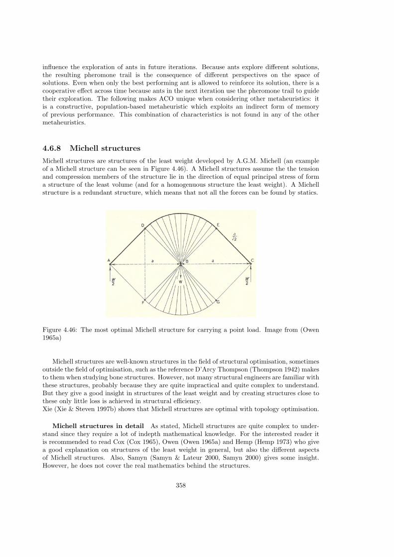
influence the exploration of ants in future iterations. Because ants explore different solutions,the resulting pheromone trail is the consequence of different perspectives on the space ofsolutions. Even when only the best performing ant is allowed to reinforce its solution, there is acooperative effect across time because ants in the next iteration use the pheromone trail to guidetheir exploration. The following makes ACO unique when considering other metaheuristics: itis a constructive, population-based metaheuristic which exploits an indirect form of memoryof previous performance. This combination of characteristics is not found in any of the othermetaheuristics.

4.6.8 Michell structures

Michell structures are structures of the least weight developed by A.G.M. Michell (an exampleof a Michell structure can be seen in Figure 4.46). A Michell structures assume the the tensionand compression members of the structure lie in the direction of equal principal stress of forma structure of the least volume (and for a homogenuous structure the least weight). A Michellstructure is a redundant structure, which means that not all the forces can be found by statics.

Figure 4.46: The most optimal Michell structure for carrying a point load. Image from (Owen1965a)

Michell structures are well-known structures in the field of structural optimisation, sometimesoutside the field of optimisation, such as the reference D’Arcy Thompson (Thompson 1942) makesto them when studying bone structures. However, not many structural engineers are familiar withthese structures, probably because they are quite impractical and quite complex to understand.But they give a good insight in structures of the least weight and by creating structures close tothese only little loss is achieved in structural efficiency.Xie (Xie & Steven 1997b) shows that Michell structures are optimal with topology optimisation.

Michell structures in detail As stated, Michell structures are quite complex to under-stand since they require a lot of indepth mathematical knowledge. For the interested reader itis recommended to read Cox (Cox 1965), Owen (Owen 1965a) and Hemp (Hemp 1973) who givea good explanation on structures of the least weight in general, but also the different aspectsof Michell structures. Also, Samyn (Samyn & Lateur 2000, Samyn 2000) gives some insight.However, he does not cover the real mathematics behind the structures.

358

Figure 4.47: Table of Michell structures. Image from (Owen 1965a)

As stated, Michell structures assume a system of members (line elements) in the direction of theprincipal stresses σε/σT (tension) and −σε/σC (compression). The base of the layout of the fieldof orthogonal. The coordinates of such a system are α and β.

Figure 4.48: Michell strain field. Image from (Owen 1965a)

A line element ds is defined as

ds2 = A2dα2 +B2dβ2 (4.42)

where A and B are positive functions of α and β which describe the field. For these definitionsapplies:

359

∂xA∂α

= cosφ

∂yA∂α

= sinφ

∂xB∂β

= −sinφ

∂yB∂β

= cosφ

(4.43)

where x and y are the two-dimensional cartesian coordinates.Finally can be derived for the assumptions that all functions A and B must satisfy with (for moredetailed explanation, refer to Hemp (Hemp 1973):

(

∂

∂α

) (

∂B

A∂α

)

+

(

∂

∂β

) (

∂A

B∂β

)

= 0 (4.44)

It can also be proved that equation 4.45 must be statisfied for Michell structures.

∂2φ

∂α∂β= 0 (4.45)

When ti is the thickness of each member along the lines, with for the α-lines t1 and the β-linest2, T1 and T2 can be defined as:

T1 = σTBt1T2 = −σCAt2

(4.46)

For the equilibrium then must be satisfied:

∂T1

∂α− T2

∂φ

∂β= 0 (4.47)

and

∂T2

∂β+ T1

∂φ

∂α= 0 (4.48)

These equations are requirements for a solution, and cannot be directly written to one solution.That explains why there are more Michell structures, which satisfy these requirements. Fromnow on an example shall be explained which meets these requirements.

The spoked wheel A well-known example of a Michell structure is a spoked wheel (whichcan be seen in Figure 4.49), which consists of a two-dimensional spokes field in tension and a rimin compression.

For this applies:

α = rβ = θφ = θA = 1B = r

(4.49)

An equilibrium of the forces on a small length Rdθ on the rim requires:

Pθcosdθ

2= Pθ+dθcos

dθ

2(4.50)

360

Figure 4.49: The spoked wheel. Image from (Owen 1965a)

from which can be derived:

Pθ = Pθ+dθ (4.51)

which means that the compressive forces in the rim must be constant.A vertical equilibrium of a small part of the rim requires:

Pθ =W

2(4.52)

A radial equilibrium of the rim requires:

2Pθ · sindθ

2= ft ·R · dθ · tR (4.53)

which can be written to:

tRR =Pθ

ft

=W

2ft

(4.54)

For the equilibrium of the spoke field can be written:

ft · r · dθt = ft(r + dr)dθ(t+ dt) (4.55)

from which can be derived:

dt

t+dr

r= 0 (4.56)

From this can be proven that for the spokefield applies:

Vs =

∫ R

0

∫ π

0

t · rdθdr =W

2ft

· π ·R (4.57)

361

where Vs is the volume of the spokefield.And for the rim applies:

Vr = πRW

2

1

fc

(4.58)

where Vr is the volume of the rim.For the total volume applies:

V = Vs + Vr = WRπ

2

(

1

ft

+1

fc

)

= π

(

WR

f

)

(4.59)

The last only applies when f = fc = ft.

4.6.9 Theory of Michell structures

Figure 4.50: The most efficient Michell structure for carrying a central load w. All members arein tension or compression.

In another example, in The analysis of light structures Owen (Owen 1965b) studies structuresof minimum volume of material as done by Michell.

Owen writes; suppose a typical compression member is designed to work to a mean compres-sive stress fc and a typical tension member to a mean tensile stress ft. If Pc is the compressiveforce in a typical strut, the area Ac of the member will be given by

Acfc = Pc (4.60)

Similarly if Pt is the tensile force in a typical tie, the cross-sectional area At of the tie isgiven by

Atft = Pt (4.61)

However, Owen prefers to represent the force in a typical member jf of a structure by Pjf

and to take this force as positive when it is tensile. Pjf will then be replaced when appropriateby either Pt or Pc, and both Pt and Pc, will be positive values. The x component of the force injf exerted on the joint j will be

362

Pif (xf − xj)

ljf

(4.62)

and the x component that it exerts on the joint f

− Pif (xf − xj)

ljf

(4.63)

By denoting the external loadings acting on the joints j and f in the direction of the axesfor equilibrium, Owen finally comes to a constant which can be written as

km = Σ(xX + yY + zZ) (4.64)

so km is the sum of the products of coordinates and corresponding force components.

When ft for all ties and fc for all struts are constant and when Vt and Vc are respectivelythe volume of the tension and compression members, then

Vtft − Vcfc = km (4.65)

Or in words, the volumes of the tension and compression members (Vt and Vc) multipliedwith respectively the tension and compression stresses should be in equilibrium with the externalloads acting on the structure. The total volume of the whole structure can be written as

V = Vt + VcV = Vt(1 +ft

fc

) − km

fc

V = Vc(1 +fc

ft) +

km

ft

(4.66)

The volume of the joints is ignored.

Owen then states that since the volume of a structure cannot be negative these resultsindicate that when km is positive the structure of least volume, if this exists, will be one whichhas no compression members, i.e. Vc = 0, and the least volume will then be km

ft. On the other

hand, if km is negative, then a structure which has the least volume will be one which has notension members and that this least volume will then be −km

ft. When km vanishes a dilemma

arises because the theoretical least weight may now be zero, corresponding to Vt or Vc zero.This indicates that structures composed entirely of compression or tension members are nolonger possible means of connecting the specified loads. Such structures must then contain acombination of tension and compression members. Owen then uses the concepts of virtual workto give a formula from which it can be observed that a Michell structure will have the least volume.

The simplest Michell strain field which can be imagined is that in which all the strainsare equal in all directions. A member in any direction in this field will be strained the sameamount as any other member. The structure will then be all in compression or all in tension.There is often an infinity of possible minimum structures which will each have the volume

mm

(fcorft), and this is the minimum possible volume of structural material to carry the given

loads. Any geometry of such bars which maintains a specified set of loads in equilibrium is thenas light as any other set of bars or any combination of such bars provided always equilibriumis maintained. Such arrangements of bars can range from mechanisms to highly redundantstructures. So, structures as in Figure 4.51, where all the members work to a tensile stress f ,

363

are now recognisable as minimum structures.

Figure 4.51: A minimum weight structure for concentric loads.

a Michell structure of a centrally loaded simply supported beam

In a plane, if one principal strain at a point is extensional and the other compressive, it isknown that these strains must be at right angles. A simple set of plane curves which can depict astrain field is that of lines radiating from a point and concentric sectors of circles centred on thispoint. In this field, if the radial displacement u at a radial distance r is εr and if the tangentialdisplacement v here is −2εrθ, where θ is the angle between the radius and some given direction,then the radial strain is ∂u

∂r= ε, the tangential strain u

r+ ∂v

r∂θ= −ε, and the shear strains on

radial and tangential planes vanish. These radial and tangential extensional strains are thenprincipal strains and this field is of the kind that Michell postulates.

Analogy with pneumatic structures To give better insight, an analogy with pneumaticstructures can be made.

The same results can be derived from the analogy with pneumatic structures. The rim undercompression is replaced by a pneumatic structure (a membrane, which can only take tensilestresses) and the tensile stress in the spoke field can be replaced with the universal pressure of agas. The spoked wheel can thus be inverted to a pneumatic structure as in Figure 4.53, wherethe radius of the half-circle shaped pneumatic structure is R and the overpressure is p over alength b. The opening angle α is 90, therefore, the tensile forces per length at the supports (Aand B) have only a vertical component, nv = n = pR (n is the support reaction per length) orNv = N = pbR. This formula (also known as the kettle formula) is analogous with Equation 4.67.

364

Figure 4.52: A Michell structure for carrying a central load w on two supports.

t · r = W2ft

≈ N = nbR

witht ≈ br ≈ RW/2 ≈ Nft ≈ p

(4.67)

Figure 4.53: A pneumatic structure analogous to a Michell structure.

Returning to the Michell structure, the thickness of the spoke sheet is thus inverselyproportional to the radius r and independent of the angular position θ. At the central point B,where r = 0, the thickness become infinite. From the practical viewpoint the load W can neverbe absolutely concentrated at B so that this infinity is not really disturbing. It requires moreimagination to accept the idealisation to two dimensions of a spoke sheet of variable thicknesswhich is really a three dimensional structure. Accepting this, a beam structure for carrying

365

a central load has been derived. It consists of (i) a spoke field subjected to constant radialtensile stress, and (ii) a semi-circumferential rim orthogonal to the spoke field and in constantcompression.The members of the structures all lie in the directions of the maximum strains envisaged. Thisis therefore a Michell structure for carrying a central load. The volume of the spoke field is

∫ R

0

∫ π

0

t · rdθ · dr =

∫ R

0

∫ π

0

W

2ft

· dθ · dr =W

2ft

· π ·R (4.68)

and the volume of the rim is

W

2fc

· π ·R (4.69)

366

Appendices AA.1 Example projects

The project descriptions below are not thorough descriptions of the structural design and engi-neering of these structures, but try to provide a tiny view in how the architects and structuralengineers found the form of these structures, illustrated with images of the structures themselves.

A.1.1 Sagrada Familia - Barcelona, Spain (Gaudi)

Recommended Study Material

Title Author YearThe Essential Gaudi J. Bonet 2001

As already explained, Antoni Gaudi is the absolute founding father of form finding with hishanging models. For his most famous building, the Sagrada Familia in Barcelona, Spain, he useda physical hanging chains model, built from wires and tiny sand bags. By adjusting the lengthsof the wires he could find the shape he desired.

Next to this, Gaudi used mathematical principles, like ruled surfaces and surfaces of revolu-tion, to create the geometry for parts of his buildings. Many methods and principles have beendiscovered (i Armengol 2001) in his shapes of the Sagrada Familia

367

Figure A.1: Sagrada Familia in Barcelona, Spain. Image from (Zerbst 2002)

Figure A.2: Sagrada Familia in Barcelona, Spain. Image from (Zerbst 2002)

368

Figure A.3: Sagrada Familia in Barcelona, Spain. Image from (Zerbst 2002)

Figure A.4: Sagrada Familia in Barcelona, Spain. Image from (Zerbst 2002)

369

A.1.2 Multihalle Mannheim - Mannheim, Germany (Frei Otto)

Recommended Study Material

Title Author YearIL13 Frei Otto, et al. 1978

A very famous building in the world of form finding is the Multihalle in Mannheim,Germany, which was researched by Frei Otto and the ILEK (fur Leichtbau Entwerfen undKonstruieren 1978).

Figure A.5: Picture of the physical model of the Multihalle Mannheim. Image from ChrisWilliams

370

Figure A.6: Picture of the Multihalle Mannheim grid.

Figure A.7: Picture of the Multihalle Mannheim grid.

Figure A.8: Picture of the Multihalle Mannheim grid.

371

Figure A.9: Picture of the Multihalle Mannheim grid.

372

A.1.2.1 Background

Every two years a garden exhibition is held in one of the major cities in the Federal Republicof Germany. In 1970 it was decided that this Bundesgartenschau of 1975 was to be held inMannheim (Happold & Liddell 1975). A master plan was developed for the area of Herzogenriedpark, where the festivities would take place. The plan included a large covered space, where avariety of activities could take place. The winning design for this space was the grid shell of FreiOtto and Ove Arup & Partners as structural engineers. Otto, famous for his structures of tensionnets, used hanging models for his designs. Also the Multihalle of Mannheim was designed withhanging models.The complex consists of a multi-purpose hall, where a range of activities can take place, suchas exhibitions, flower shows, entertainment, concerts, theatre, sports activities, etc. In a secondsmaller hall a restaurant is situated. The halls are connected by a covered link. Figure A.10shows an aerial view of the complex.

Figure A.10: Areal view of the Multihalle. Image from Burkhardt et al. 1978

Figure A.11: Inside view of the Multihalle. Image from Burkhardt et al. 1978

373

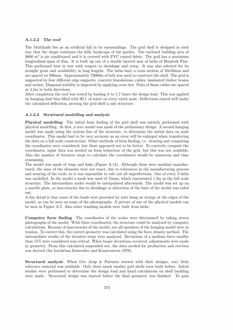
A.1.2.2 The roof

The Multihalle lies as an artificial hill in its surroundings. The grid shell is designed in suchway that the shape continues the hilly landscape of the garden. The enclosed building area of3600 m2 is air conditioned and it is covered with PVC coated fabric. The grid has a maximumlongitudinal span of 85m. It is built up out of a double layered mat of laths of Hemlock Pine.This performed best in test with respect to shrinkage and creep. It was also selected for itsstraight grain and availability in long lengths. The laths have a cross section of 50x50mm andare spaced on 500mm. Approximately 72000m of lath was used to construct the shell. The grid issupported by four different edge supports: concrete foundations, cables, laminated timber beamsand arches. Diagonal stability is improved by applying cross ties. Pairs of 6mm cables are spacedat 4,5m in both directions.After completion the roof was tested by loading it to 1,7 times the design load. This was appliedby hanging dust bins filled with 90 l. of water on every ninth node. Deflections stayed well underthe calculated deflection, proving the grid shell a safe structure.

A.1.2.3 Structural modelling and analysis

Physical modelling The initial form finding of the grid shell was entirely performed withphysical modelling. At first, a wire model was made of the preliminary design. A second hangingmodel was made using the system line of the structure, to determine the initial data on nodecoordinates. This model had to be very accurate as an error will be enlarged when transferringthe data on a full scale construction. Other methods of form finding, i.e. drawing and computingthe coordinates were considered, but these appeared not to be better. To correctly compute thecoordinates, input data was needed on form behaviour of the grid, but this was not available.Also the number of iterative steps to calculate the coordinates would be numerous and timeconsuming.The model was made of rings and links (Figure A.13). Although these were machine manufac-tured, the sizes of the elements were not exact, due to tolerances in the manufacturing processand wearing of the tools, so it was impossible to rule out all imperfections. One of every 3 lathswas modelled. In the model a mesh was used of 15mm, which represented 1,5m in the full scalestructure. The intermediate nodes would be interpolated afterwards. The model was set up ona marble plate, so inaccuracies due to shrinkage or distortion of the base of the model was ruledout.A fun detail is that some of the loads were provided by nuts hung on strings at the edges of themodel, as can be seen on some of the photographs. A picture of one of the physical models canbe seen in Figure A.5. Also other standing models were built from laths.

Computer form finding The coordinates of the nodes were determined by taking stereophotographs of the model. With these coordinated, the structure could be analysed by computercalculations. Because of inaccuracies of the model, not all members of the hanging model were intension. To correct this, the correct geometry was calculated using the force density method. Theintermediate results of the iterative steps were analysed. Deviations of a medium force smallerthan 15% were considered non critical. When larger deviations occurred, adjustments were madein geometry. From this calculated suspended net, the data needed for production and erectionwas derived (fur Leichtbau Entwerfen und Konstruieren 1978).

Structural analysis When Ove Arup & Partners started with their designs, very littlereference material was available. Only three much smaller grid shells were built before. Initialstudies were performed to determine the design load and hand calculations on shell bucklingwere made. Structural design was started before the final geometry was finished. To gain

374

Figure A.12: Hanging model (Burkhardt et al 1978).

Figure A.13: Detail of the model (Burkhardt et al 1978).

knowledge on behaviour of grid shells, tests on a working model of the Essen grid shell wareexecuted. The results showed that lath size had to be increased to enhance buckling resistance,to 100x100mm. This would give problems however with forming the shell, as more force isneeded to bend the laths with a bigger cross section. Also the contract was already let anda lath size of 50x50mm was agreed. Decided was to apply a double layered mat, so bendingflexibility was maintained during construction. After applying shear blocks between the layers,sufficient out of plane bending strength will be provided.Design loading was determined by using wind and snowfall records in the area and by windtunnel testing on a 1:200 scale model. This way, the design could be fully optimized, instead ofjust using normative average loading values. Also tests were carried out on the nodes and toinvestigate stress relaxation of the timber.

To determine a collapse load, tests were executed on a model of the grid shell. To cor-rectly model the full size structure, dimensional analysis was used, which means scaling thefactors that govern the behaviour of the physical system. Perspex members were used to modelthe grid. One model member represented six double layer members on full scale (Figure A.14).

375

The model was tested by hanging 100mm nails on the nodes and dial gauges were used tomeasure the deflections (Figure A.15).The test results were compared with the results of computer calculations. The collapse loaddetermined by the tests was 2,8 kN/m2. The calculations gave a value slightly over 1 kN/m2.This difference occurs because the model does not scale the shear deformation of the full scalestructure. This shear resistance is largely controlled by the individual slip per unit of force ofthe joints. The Perspex model corresponds to a full size structure with a very high value of jointstiffness, thus resulting in a high collapse load.Grundig describes some of the computation, which seems to be an early force density method.

Figure A.14: Test model. Image from Burkhardt et al. 1978

Figure A.15: Tests on the model. Image from Burkhardt et al. 1978

376

A.1.2.4 Connection details

Typical node joint The laths are bolted together in the nodes. To provide slipping of theouter layers during erection, these layers have slotted holes. After erection, shear resistance isneeded, so the bolts are tightened to provide sufficient friction. Testing indicated that tension inthe bolts would decrease in time, due to shrinkage of the timber. To prevent this, spring washersare applied (Figure A.16 and Figure A.18).

Figure A.16: Typical node joint. Image from Burkhardt et al. 1978

Figure A.17: Photo of a typical node joint. Image from www.kunst.uni-stuttgart.de

Joints in the laths The laths are prefabricated into laths up to 40m by finger jointing. Thejoints used was 20mm with a 6mm root, to suit the machines of the factory. Quite a lot of jointsbroke during site handling and erection due to this short connection length. The laths were

377

repaired by nailing 50x25mm lapping pieces to each side. This was also used to lengthen thelaths into the required length.

Boundary connections Four types of edge connections are used in the Multihalle (Fig-ure A.18). Originally, Frei Otto designed all boundaries on columns as cable edges. Cable edgesupports are possible where boundary forces are more or less constant and where the change inangle of the boundary system line at the column is not that large that excessive support reactionsare caused. These conditions were only met at parts of the restaurant. To connect the grid shellto the cable, it is first connected to a plywood board. This board also helps to cope with thedifferences in distributed lath forces and the cable reaction force. At the columns the cables arebrought together (Figure A.19).Where cable supports could not be applied, edge beams are used. 60x500mm laminated timberbeams are connected on either side of the grid. The laths are bolted to these beams. Also wherethe grid is connected to the concrete support, it is first connected to timber beams. The timberbeams are connected to the steel columns with steel plates. These plates are bolted to the beamsand welded to the columns (Figure A.21). The connection itself was simple, but the geometrywas not as for every connection the angles were different. The cutting profile for the plates hadto be determined accurately to provide production drawings. A special computer program waswritten for this task. Also the production drawings for the arches were produced by a speciallywritten computer program.At the valley between the Banana and the Multihalle a laminated timber beam is applied witha circular section. Steel connecters connect the grid to the valley beam (Figure A.20).

Figure A.18: Edge layout. Image from Burkhardt et al. 1978

378

Figure A.19: Cable edge connection. Image from Burkhardt et al. 1978

Figure A.20: Valley beam connection. Image from Burkhardt et al. 1978

379

Figure A.21: Edge column connection. Image from Burkhardt et al. 1978

380

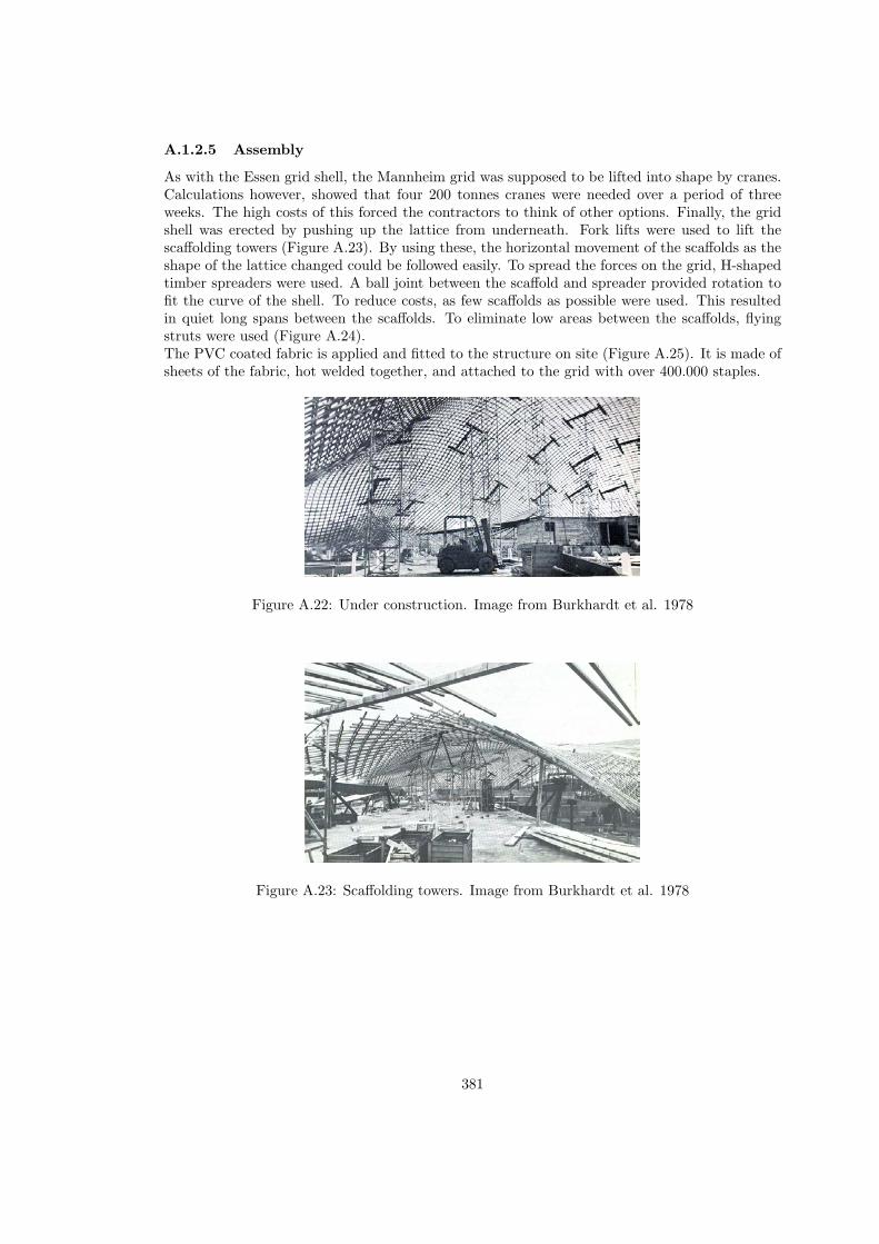
A.1.2.5 Assembly

As with the Essen grid shell, the Mannheim grid was supposed to be lifted into shape by cranes.Calculations however, showed that four 200 tonnes cranes were needed over a period of threeweeks. The high costs of this forced the contractors to think of other options. Finally, the gridshell was erected by pushing up the lattice from underneath. Fork lifts were used to lift thescaffolding towers (Figure A.23). By using these, the horizontal movement of the scaffolds as theshape of the lattice changed could be followed easily. To spread the forces on the grid, H-shapedtimber spreaders were used. A ball joint between the scaffold and spreader provided rotation tofit the curve of the shell. To reduce costs, as few scaffolds as possible were used. This resultedin quiet long spans between the scaffolds. To eliminate low areas between the scaffolds, flyingstruts were used (Figure A.24).The PVC coated fabric is applied and fitted to the structure on site (Figure A.25). It is made ofsheets of the fabric, hot welded together, and attached to the grid with over 400.000 staples.

Figure A.22: Under construction. Image from Burkhardt et al. 1978

Figure A.23: Scaffolding towers. Image from Burkhardt et al. 1978

381

Figure A.24: Intermediate strut. Image from Burkhardt et al. 1978

Figure A.25: Applying the roof skin. Image from Burkhardt et al. 1978

382

Figure A.26: Interior.

383

A.1.3 British Museum - London, United Kingdom (sir Norman Foster)

Recommended Study Material

Title Author YearThe definition of curved geometry forwidespan enclosures. (enclosed in thisreader)

C. Williams 2000

The Analytic and numerical definitionof the geometry of the British museumgreat court roof

C. Williams 2000

The design and manufacture of theBritish museum great court roof

S. Brown and M. Cook 2002

For the Great Court Yard roof of the British Museum in London, UK, by sir Norman Fostera combination of various analytic and numerical methods have been used by Buro Happold andC.J.K. Williams to find the form of the roof.First the shape of the roof was described by a function (Williams 2000) (Equation A.1 to A.4).

z = z1 + z2 + z3 (A.1)

wherez1 = (hcentre − hedge)η + hedge (A.2)

z2α

= (1 − λ)

(35.0 + 10.0ψ) 12 (1 − cos2θ)+

24.02

(

12 (1 − cos2θ)) + sinθ

)

+(7.5 + 12.0ψ)

(

12 (1 − cos2θ) − sinθ

)

− 1.6

− 10.02 (1 + cos2θ) + 10.0

[

12

(

12 (1 − cos2θ) + sinθ

)]2(1.0 − 3.0α)

+2.5[

12

(

12 (1 − cos2θ) − sinθ

)]2 (

ra− 1

)2

(A.3)

z3β

= λ(

3.52 (1 + cos2θ) + 3.0

2 (1 − cos2θ) + 0.3sinθ)

+1.05[

e−µ(1− xb ) + e−µ(1+ x

b )] [

e−µ(1− yc ) + e−µ(1+ y

d )] (A.4)

On this function the grid was projected.Then, a dynamic relaxation procedure was used to relax the grid. Then was executed by removingthe normal direction to the shape from the relaxation procedure. The nodes could only movealong the grid with that procedure.Eventually the limitation of the size of the glass was the restriction and controlling factor forthe shape of the structural grid. This ’form finding’ procedure was executed by running a lot ofprocedures as described above by hand with different parameters for the grid.Brown (Brown & Cook 2002) also describes that spirals were used to define the grid. He furtherdescribes the procedure of the form finding and more details of the structural design.

384

Figure A.27: British museum computer model. Image by Chris Williams.

385

A.1.4 Esplanade theatres - Singapore, China (M. Wilford)

Recommended Study Material

Title Author YearThe geometrical processing of the free-formed envelopes for the Esplande The-atres in Singapore

J. Sanchez Alverez 2002

The envelopes of the arts centre in Sin-gapore

H. Klimke et al. 2002

In Sanchez (Sanchez-Alvarez 2002) and Klimke (Klimke, Sanchez, Vasilu, Stuhler & Kaspar2002) the structural design and the geometrical description of the Esplanade theaters in Singaporeis described. The ’form finding’ is this form was not really done by a form finding method.This project is mentioned because this is sometimes refered to as form finding, but is more ageometrical description with NURBS curves and a mesh (grid) projected on the surfaces. Thiscould also be seen as form finding, when looking from an abstract point of view, because itinvolves the definition of form.

Figure A.28: The Esplanade theatres in Singapore.

386

A.1.5 Downland Grid Shell - Singleton, United Kingdom (E. Cullinan,Buro Happold)

Recommended Study Material

Title Author YearDownland Grid Shell F. Jensen 2000The structural engineering of theDownland Gridshell

R. Harris and O. Kelly 2002

The Downland Grid Shell, at the Weald and Downland Musuem in Sussex, UK, is the roofof the new Archive Store and the Workshop building.

Figure A.29: Physical model of the Downland Grid shell. Image by Frank Jensen.

Figure A.30: Physical model of the Downland Grid shell. Image by Frank Jensen.

387

Figure A.31: Computer model of the Downland Grid shell,. Image by Frank Jensen.

Figure A.32: Physical model of the Downland Grid shell with the computer model projected onthe surface. Image by Frank Jensen.

388

A.1.5.1 Background

The Weald and Downland grid shell, shown in Figure A.33 and Figure A.34 is built at the Wealdand Downland Open Air Museum in Sussex in the UK, and was finished in 2002. This museum hasover 45 historical buildings from South East England, which have been rescued and rebuilt there.The museum needed a new building for study and practice of building conversation, especiallythe timber framing tradition in England. Also a new conservation store for collection items wasneeded. To extend the collection of timber structures into the 21st century, the new buildingshould be an example for modern rural buildings. The result of the combination of skills ofthe architect Edward Cullinan Architects, the engineer Buro Happold and the carpenter, GreenOak Carpentry Company, truly is a display of modern craftsmanship (Harris & Kelly 2002).The basement of the building is sunken into the hillside and houses the conservation store. Theworkshop is situated on the ground floor and is roofed by the grid shell. The roof has the shapeof a triple-bulb hourglass, to mirror the rolling shapes of the West Sussex Downs.

Figure A.33: The Weald & Downland grid shell. Image from www.wealddown.co.uk

Figure A.34: Inside view of the grid shell. Image from www.wealddown.co.uk

389

A.1.5.2 The roof

The triple-bulb hourglass roof is 48m long and between 11-16m wide. It has an internal heightof 7-10m. The roof is clad with Red Cedar boards and polycarbonate glazing. The grid is builtup out of 50x35mm oak laths in four layers, like the grid shell in Mannheim, to provide good outof plane resistance. The laths have a spacing of 500mm in areas with high load, and 1000mm inother areas. Original designs were made with 500mm spacing for the whole structure. Carefulexamination of the forces and stresses by computer analysis lead to increasing of the spacing,which saved construction time and reduced costs significantly. Shear blocks are screwed betweenthe different layers to provide composite action between the layers. To increase stability, diagonalbracing is applied. In the lower parts the bracing laths run in longitudinal direction, at the topin transverse direction. These also provide support for the cladding boards.The cladding consists of polycarbonate glazing, which covers the upper part of the roof, and West-ern Red Cedar boards. This closed part is insulated with a multi-layered composite insulationmaterial (Weald & open air museum 2005).

A.1.5.3 Structural modelling and analysis

Physical modelling Physical modelling involved an important part of the modelling process.It provided a lot of information on form, structure and construction of the shell. Scheme modelsof wire mesh were made to research the form. After this a larger 1:30 model using wood stripswas built. This proved to be very instructive. The geometry of the model was used to determinethe boundary conditions for the computer model. It also served as presentation model (Harris &Kelly 2002).After this an accurate wire mesh model was made, to explore the formation of the shape and todetermine self weight bending. Dimensional analysis was used to correctly model the full scalestructure (Jensen 2000). A boundary template was used to determine if the correct shape wasreached. Also internal scaffolding was modelled to approximate the formation procedure as goodas possible. The wire mesh was loaded by hanging large steel nail on the nodes.Main conclusion of the experiment was that the saddles would not form themselves under deadweight. External forces are needed to reach the final shape. As the lattice becomes more curved,larger forces are needed to stretch the lattice, so the initial lay out of the lattice should be alreadystretched instead of with square angles. In was also concluded that formation of the waists costsa lot of force when first a barrel shape is adopted. Formation of the valleys and tops should beformed simultaneously to prevent breakage of the laths.

Computer form finding Using a modified dynamic relaxation method, the shape of thestructure was determined. Dynamic relaxation is an iterative process that modifies an initialapproximation to the desired shape by monitoring the kinetic energy of the model as it is madeto oscillate. The method is generally used to examine oscillations of a pure catenary shape togenerate a final shape. The W&D grid shell however is not a purely catenery shape. It is notpossible to create the saddles with a hanging chain model. The method had to be modified byincluding the bending stiffness of the laths, to correctly model the shape.

Structural analysis The structure is analysed and designed in accordance with the eurocode 5,using timber grade D30 with a characteristic bending strength of 30N/mm2. Structural analysiswas performed using the elastic analysis software STAAD Pro. Two methods were used. Dynamicrelaxation was used for second order analysis of buckling instability. Using the STAAD model adeflection analysis to compare the deflected shape with the non-linear analysis under the sameload. This proved that under working load the behaviour is elastic, with adequate factor ofsafety against buckling. Detailed stress checks were made using the information provided by the

390

STAAD model.It was also concluded that the shape of the grid enhanced the load bearing capacity. Thewaisting along the building improved the strength and stiffness against asymmetric loads (Harris& Kelly 2002).

A.1.5.4 Timber

Selection A number of species of timber were considered for construction of the grid shell.Based on their properties and the results of a series of tests, oak was selected for the grid. Thisspecies performed best in the structural tests carried out at Bath University, with respect tobending behaviour. It proved to be stiffer than other species and has a considerably higherbending strength. Although it needs more force than other species to be bended it can achieve asmaller bending radius prior to failing. Also it showed a somewhat plastic failure mode, comparedto more brittle timber. Additionally, oak has high natural durability, so no treatment would benecessary. Possible leakages will not lead to decay of the timber (R. Harris, pers. email comm.14 March 2006).Another reason is that, oak is one of the most common used materials in the museum’s collectionof buildings and the species was readily available from sustainable sources in UK. Strangelyenough, eventually the timber was sourced in Normandy, because better timber with a lowerrejection rate was available there.The main disadvantage of oak is that the direction of grain varies significantly, due to the growthcharacteristics. This was overcome by cutting out the defects and joining the pieces together tocreate laths of the required length. Selection was made on the following requirements (Harris &Kelly 2002):

• A maximum slope of grain of 1:10

• No dead knots or live knots. Only small pin knots were allowed, provided that they formedno more than 20% of the width of any face.

• No shakes or splits

• No sapwood (sapwood is not naturally durable and not resistant to infestations)

Lath production Although tests indicated that the shell could be formed using dry oak, greenoak was used. Green timber is easier to bend, thus making the forming process of the shell easier.One disadvantage of oak is its acidity, making it difficult to joint with adhesives. Using greenoak only make this worse, also because of the moisture content of the green timber. After anadhesive was found which is not affected by this acidity and the moisture content, the use of itwas no problem anymore.In total, approximately 6000 linear meters of lath were needed. The average length of individualpieces was 0.6m so 10.000 finger joints were used in the structure. Laths of 6m length weremade off site, using a special machine, to maximize the quality with a minimum wastage. Thefinger joints are hardly visible, so despite the amount the joints have minimal visual impact(Figure A.35).On site the laths were jointed into laths up to 37m long. Here, a scarf joints with a slope of1:7 was used (Figure A.36). The joints were made in a tunnel tent to avoid weather influences.There is an interesting contrast between the two jointing techniques used. Finger jointing wasthe latest technology, while scarf jointing has been used for centuries.The joints performed well during construction. There were approximately 145 breakages duringforming. Almost all broken joints were finger joints. Main causes were (Harris & Kelly 2002):

• Pinching of the lattice on scaffold supports

391

• Tight curvature

• Tension build-up because restriction of the relative slipping between the layers

• Dry joints

Figure A.35: The Weald & Downland grid shell. Image from www.wealddown.co.uk

Figure A.36: Scarf joint. Image from www.wealddown.co.uk

A.1.5.5 Connection details

Typical node joint For the connection between the laths a special connector was designed. Itconsists of three plates, connected with four bolts (Figure A.37). The middle plate has a pin inthe centre, keeping the connection into place. The outer layers can slide freely in their directionduring shaping of the structure. Two of the four bolts can be used to connect the diagonalbracing. The connecter proved to be very successful and has been patented.

Edge connection At the edges the grid shell is connected to the floor of the structure. Thelaths are bolted between two layers of plywood and connected to the floor beams. The floorand floor beams are cut into shape and the first layer of plywood boarding is connected to theglulam floor beams with angle brackets prior to the erection of the roof. Holes are drilled inthe boarding aligned with the holes in the brackets. Figure A.39 shows one of the positions ofthe brackets. After the grid is lowered, blocks are installed on this location to fix the sandwich

392

Figure A.37: Assembly of a typical node joint. Image from www.wealddown.co.uk

structure firmly to the brackets on the inside (Figure A.40). Also the gaps between the layersare filled up with timber where the grid overlaps the boarding to create a solid section four timesthe depth of a lath. The second layer of plywood is attached and the laths and plywood layersare bolted together (Figure A.41). The whole sandwich is bolted to the brackets on the inside tocreate a rigid edge connection.

Figure A.38: Floor and beams are cut into shape. Image from www.wealddown.co.uk

393

Figure A.39: Location of the brackets. Image from www.wealddown.co.uk

Figure A.40: Connection to the edge. Image from www.wealddown.co.uk

394

Figure A.41: Edge detail. Image from www.wealddown.co.uk

Figure A.42: Finished connection. Image from www.wealddown.co.uk

395

A.1.5.6 Assembly

Instead of pushing or lifting up the grid against gravity, the Weald and Downland grid shell waslowered into position. The flat grid of laths was laid out on a special scaffolding system at thelevel of the valleys of the shape. This scaffolding system used adjustable jacks to accurately alterthe heights to form the shape of the grid shell.The mat was laid out at a height of 7m. As concluded from the experiences of physical modelling,the mat was not laid out with 90 angles between the laths. 96 and 84 angles were used and theresulting mat was 47x25m (Kelly, HARRIS & ROWE 2001). The process of lowering the gridwas carefully monitored visually and with the information provided by scaffolding jacks system.The longitudinal centre line was used as a reference line, as this line was not to move transversely.The nodes on this line were painted white, to be able to visually check if the nodes remained ona straight line.The scissoring and sliding of the laths was influenced with straps in plane of the grid. Bytensioning the straps in the desired direction, the scissoring was stimulated. The strappingarrangement was continuously monitored. Failing of the lattice to scissor or of the laths to sliderelatively to each other would lead to breakages so the process was observed carefully.After formation was finished, the valleys resembled the designs very well. The domes howeverappeared to be too low. Also the perimeter nodes around the domes were 300mm too low.Adjustments were made by pushing up the perimeter nodes using small jacks.The formation process was very successful. Observation was seen as the key control of theformation process. Potential problems could be isolated and dealt with continuously by observingthe behaviour of the lattice.

Figure A.43: Flat mat of laths. Image from www.wealddown.co.uk

396

Figure A.44: Start of lowering. Image from www.wealddown.co.uk

Figure A.45: Adjustable jack. Image from www.wealddown.co.uk

397

Figure A.46: Angled jacks. Image from www.wealddown.co.uk

Figure A.47: Halfway down. Image from www.wealddown.co.uk

398

Figure A.48: Completed form. Image from www.wealddown.co.uk

399

A.1.6 Eden Project - Bodelva, United Kingdom (Grimshaw)

Recommended Study Material

Title Author YearThe Eden Project glass houses worldenvironments

A. Whalley 2000

The Eden project (see figure A.49) by Nicolas Grimshaw & Partners (Whalley 2000) hasbeen formed by structural morphology, by geometrical techniques to form a grid from hexagonalelements in the desired shape. Much has been learned from nature’s efficiency, not only asa structural but also an architectural motive, since the structure itself is also close related tonature (it houses many plants).

Figure A.49: Image of the Eden project

400

A.1.7 Groningen Twister - Groningen, The Netherlands (KCAP)

Recommended Study Material

Title Author YearThe Groningen Twister - an experimentin applied generative design.

F. Scheurer 2003

The Groningen Twister is a collaborative project between the design team of Kees Chris-tiaanse Architects & Planners (KCAP) in Rotterdam, an engineering team of Ove Arup &Partners in Amsterdam and the chair for Computer Aided Architectural Design (CAAD) atthe ETH Zurich. The project was initiated in February 2003. The aim of the project wasto develop a CAD-tool which would help the architects of KCAP to solve a complex designtask: Underneath a pedestrian area that links the main station to the city centre of Groningen,there was a need for parking space for approximately 3000 bicycles (Figure A.50). To supportthe concrete slab of the pedestrian level, the desired design called for more than one hundredcolumns of different sizes to be placed in a random pattern, but to be then sized and controlledaccording to structural, functional and aesthetic needs.

Figure A.50: Model view of the Groningen Stadsbalkon. (Scheurer 2003)

To solve this problem, software was developed at the chair for CAAD that simulates a growthprocess for the columns. The distribution of the columns is defined by structural rules, providedby ARUP’s engineers, as well as functional and design rules provided by KCAP’s designers. Theresults are presented to the user as a three dimensional, dynamically evolving model. At anytime during this process the user is able to control the model on the screen interactively. Theuser can control the process in two distinct ways, on the one hand by directly controlling theplacement of single columns, on the other hand by adjusting various parameters that define theproperties of the columns and the environment. The system provides real time feedback, as thecolumn distribution tries to adapt to the changed configuration. This allows the user to testvarious alternative solutions in very short time (Figure A.51).

401

Figure A.51: Screenshot of the Groningen Twister model. (Scheurer 2003)

After a stable and satisfactory condition is achieved, the resulting column locations can beexported for construction documents in various digital file formats (Figure A.52).

Figure A.52: Color coding by kinetic energy. (Scheurer 2003)

The columns represent particles in a swarm system. Each column in the system is an au-tonomous individual, exploring the habitat and reacting to its neighbouring columns. Accordingto the two layers of the habitat, the column model consists of two independent parts. The bottomend can move freely within the ground plane of the model, whereas the top end can move in theplane described by the slab. The actual column position, length and tilt is defined by the connect-ing line. It has to be assured, that the tilt angle stays below the assigned maximum (Figure A.53).

This behaviour is easily described by a spring-mass-system (called particle spring system):punctual masses are connected by a virtual spring that pulls depending on the distances betweenthe masses. In the model each organism is composed of two masses which describe the top andbottom end of the column and a spring in between. The force of this spring is proportional tothe horizontal distance and, since the move of the masses is confined within the two planes ofthe habitat, they are drawn to positions above each other.

402

Figure A.53: The column model with a maximum bearing capacity and tilt. (Scheurer 2003)

The columns are interacting with their adjacent columns as well as with the surroundinghabitat following the same simple principles of attraction and repulsion by virtual springs. Ifthey come to close, the top masses of each column are repelled by the slab outline, the holes,and the areas without cellar. The bottom masses are attracted by the closest bike stand.

To get the desired effect of distributing the columns, they seek to stay at a certain “socialdistance” to each other. This distance is defined by the maximum spanning distance of theslab and the bearing capacities of the respective columns. The bearing capacity of a columndefines a circle around the top end marking the area where column is able to support the slab.Neighbouring columns therefore have to be aligned so that their radii touch or overlap slightly.This is also accomplished by virtual springs that push or pull between their respective top masses.

The specifications of the columns were given by Arup. There are three types of columns withdifferent diameters and bearing capacities. The maximum radius of the column results from thebearing capacity and defines the distance between the columns. The tilt angle of the columnswas limited to 10 degrees so that this factor could be ignored in structural calculations. Alsothe height differences between the ground plane and the slab were not cared for and an averageheight of 3,0 meters was used throughout the habitat. The approximate number of columnsneeded was estimated by Arup based on the maximum radii and the building budget whichwould only allow for a certain number of columns.

By making the columns pressure sensitive and able to change their type, an actual growthprocess was possible. Instead of assigning a column diameter and bearing radius from the be-ginning, the columns are able to adapt to their surroundings by changing their size autonomously.

A column that is too far away from its neighbours detects a low surrounding pressure and

403

starts to grow in discrete steps, matching the column types. If it reaches the largest possiblestate and still has no close neighbours, it splits into two small columns which both startgrowing again. If a column gets to close with its neighbours or the edges of the habitat theresulting pushing increases the pressure and it starts shrinking in just the same way. And ifit reaches the smallest state while the pressure remains high, it finally dies. Thus, by “seed-ing” a single column the whole area of the slab is filling up with columns over time (Figure A.54).

Figure A.54: The relation between the habitats and the ’agents’ en the growth, birth, shrinkageand death of the columns. (Scheurer 2003)

A.1.8 Web of North Holland - Haarlemmermeer/Delft, The Nether-lands (ONL)

.Recommended Study Material

Title Author YearArchitectural design and mass cus-tomization.

S. Boer and K. Oosterhuis 2004

Design conceptionFor the Dutch province of North Holland ONL designed a pavillion for the world horticulturalexhibition ’Floriade’ 2002. Architecturally there is no distinguishable difference between wall,floor or ceiling (Figure A.55).

The design was based on a topological surface that governs the logical aesthetic continuityof the shape. The specific shape of the surface came about in a design process which combinedmilled physical models of the computer model with again computer modelling of adaptationsto the milled models to attain a good space for its program as well as introducing the rigorousstyling requirements of ONL. During this process a clear vision arose of the concave / convexdynamics and the shaping lines, the folding lines that fade in and fade out of the shape. ONLdescribed the styling requirements in a number of shaping rules of the design. It was important

404

Figure A.55: A rendering of the Web of North Holland. Image from (Boer & Oosterhuis 2004).

to describe the design not in mass, but in a number of design rules and guidelines since itsinternal program was still to change. To control the shape and the look of the design a NURBSsurface was created (Figure A.56).

Figure A.56: The NURBS surface of the design. Image from (Boer & Oosterhuis 2004).

Expanding on the conventional paradigm of a construction grid ONL mapped a triangulargrid with the internal integrity of an icosahedron (a 20-faced polyhedron on the NURBS surface.The icosahedron system was chosen for a number of reasons, the main reason being that it is aclosed system, like the design (Figure A.57).

With the pavilion for the Web of North Holland ONL reaffirmed their strong beliefs acquiredby previous projects [Elhorst-Vloedbelt, saltwater pavilion] that one can gain a maximum designfreedom and keep the budget in check by gaining control over a system of similar, but differentelements. A number of techniques can be determined that make this possible:

1. File to Factory: A construction process is greatly simplified by connecting the file createdby the architect to the machine, eliminating intermediate steps that are inefficient - andeven more so - susceptible to errors.

2. Mass customization: An irregular shape can only exist by the grace of irregular elements,therefore control over mass customization greatly increases design freedom.

3. Parameterisation: One Building, One Detail. Ideally, in a mass customized solution more

405

Figure A.57: Mapping of a constructive grid based on a icosahedron. Image from (Boer &Oosterhuis 2004).

parameters can be found than those that account for shape alone. These can be utilized tooptimise the design.

Figure A.58: 3D model of the panels with the construction showing. Image from (Boer &Oosterhuis 2004).

4. Design control hierarchy: In this specific pavilion the shape is described in a single NURBSsurface, essentially all that follows will refer to this surface. A NURBS surface is createdusing NURBS lines, keeping this creation link intact yields control on a higher level, bychanging the line, the surface changes and the entire system changes. Primarily for designersthis notion is paramount.

5. Body Styling: These techniques give the architect / designer full freedom to shape thevolume of the building, to propose styled creases and smooth transitions of creasesdisappearing into the surface of the overall body. ONL has two other projects in theproduction phase that have been designed with the above in mind: the Cockpit buildingand the Acoustic Barrier. The Cockpit building is part of a fluid design of the AcousticBarrier, to accommodate the transition from the one to the other the design controlhierarchy proved to be essential, both projects share the same outlines, but differ inconstruction principle. Construction is based on a streamlined File-to-Factory processdescribed earlier.

406

This pavillion was designed to be open-air, meaning that in essence the construction is openand that rain would essentially fall through it. In respect to cladding this building, things werepretty simple in terms of insulation and waterproofing. However, ONL invested in creating aconstruction that already describes the shape exactly, therefore the cladding must be able tofollow this shape with a minimum of processing. As was stated earlier, ONL wanted to buildthis building only once, with creating a mold, the building is built more than once and half of itis thrown away. Prior to the design of this pavilion ONL conducted a small study of the material’Hylite’, an aluminum laminate produced by the Corus group that consists of aluminum onboth sides and polyethylene in the middle (Figure A.59). It has the look of aluminum, but theflexibility and pliability of a polymer. ONL found this to be a flexible material that will let itselfbe fitted on a triangle of three spatial curves in a form of pseudo double curvedness.

In 2006, the Web was placed in front of the faculty of Architecture, Delft University ofTechnology.

Figure A.59: Specific view to illustrate the effectiveness of the application of the Hylite. Imagefrom (Boer & Oosterhuis 2004).

407

A.1.9 Akutagwa River Side Project - Takatsuki City, Japan

.Recommended Study Material

Title Author YearComputational morphogenesis and itsapplication to structural design.

H. Ohmori et al. 2005

Akutagwa River Side project is the project which brought a practical project to appeal thepotential and possibility of the computational morphogenesis method for the future. It has beenplanned at the site along the shopping arcade which runs from the north front of Takatsuki JRstation in Japan, where a large scale redevelopment of the urban district has been planned toactivate the shopping area by renewing the decrepit shopping area through both introductionof the new buildings as well as renovation of conventional stock of urban district. The presentproject has been designed not only as to be effective as a leading project to the campaign butalso to have an attractive appearance even if it does not have a big mass.

The west and south side wall development diagram of the building after completion (April of2004) is shown in Figure A.60. Figure A.61 shows a rendering of the complete building. As canbe seen from the diagram and the rendering, the west side and south side wall structures havenon-geometrical form which is even that of organisation, which has been generated through theproposed process of computational morphogenesis through usage of the extended ESO method.

Figure A.60: The west and south side wall development diagram of the building. Image from(Ohmori & et al. 2005).

Figure A.62 shows the evolutionary process of the extended ESO method from which we canobserve how the south side wall form has been changed through the process of deletion of theportion with low density of Von Mises’ relative stress as well as the process of addition of thenecessary portion. In the evolutionary process, it has to be noticed that the slabs of each floor

408

Figure A.61: A perspective view of the building in a rendering. Image from (Ohmori & et al.2005).

level are treated not to be deleted through the evolutionary process and so is the east side wall.

In order to ensure and proof that the structure with the form obtained through thecomputational morphogenesis procedure has enough capability, 3D elasto-plastic numericalanalysis is carried out. Figure A.63 shows the deflection state of the whole structure subjectedto the horizontal loads in x-, y-direction and also in the direction at an angle 45 degrees to thex-axis, respectively.

Some photos of the construction site and the inside and the outside view of the building justafter the completion are shown in Figures A.64 up to A.69.

409

Figure A.62: The evolution process of the south wall. Image from (Ohmori & et al. 2005).

Figure A.63: The limit state deflection of the whole structure subjected to horizontal loads inx-, y-direction and under an angle. Image from (Ohmori & et al. 2005).

410

Figure A.64: outside view. Image from (Ohmori & et al. 2005).

Figure A.65: inside view. Image from (Ohmori & et al. 2005).

411

Figure A.66: inside view. Image from (Ohmori & et al. 2005).

Figure A.67: inside view. Image from (Ohmori & et al. 2005).

Figure A.68: outside view. Image from (Ohmori & et al. 2005).

412

Figure A.69: outside view. Image from (Ohmori & et al. 2005).

413

A.1.10 Palazzetto dello Sport - Rome, Italy (P.L. Nervi)

For the Olympics 1960 in Rome, Nervi executed three stadiums; a small Palazzetto dello Sport(Figure A.71, designed with architect A. Vitellozzi, a larger covered Palazzo dello Sport, witharchitect Piancentini and the Stadio Flaminio, a 50.000-seat stadium designed with his sonAntonio.The flute-edged roof shell of the Palazzetto dello Sport is composed of 1620 prefabricated,diamond-shaped sections, joined by poured-in-place concrete that makes their connecting ribs,creating a webbed ceiling network, like a lamella dome. (Figure A.70Nervi employed diamond shaped ferro-cement waffle units (2,5 cm thick) as permanent formworkfor this shell. The ferro-cement waffle units were produced from fine-aggregate concrete andwire reinforcement. They were laid on scaffolding. Then, the reinforcement to the ribs wasplaced in the intermediate spaces. By casting the ribs and pouring a layer of concrete overthe diamond shaped elements the actual load-bearing structure was formed. A compressionring in the centre forms a cupola, providing a central source of natural light. The forces thatflow through these ribs are gathered in prefabricated, triangular sections, which transfer theload to exterior Y-shaped buttresses and vertical supports. The building seats 5000 spectators.The prefabricated elements are put in place in just 30 days as can be seen in Figures A.72 & A.73.

Figure A.70: Internal view of the Palazetto dello Sport; h=21m, d=60m

414

Figure A.71: Palazetto dello Sport

Figure A.72: Placement of the prefabricated elements

Figure A.73: Finishing of the structures, before pouring concrete

415

A.1.11 Sydney Opera House - Sydney, Australia (J. Utzon)

Recommended Study Material

Title Author YearIABSE proceedings IABSE 2006

The beautiful sail-like vaults of the Opera House, designed by Jørn Utzon, were a great succesfor architect and engineer, but also had some disappointments. The shape of the vaults as drawnin the sketches could nor be built, nor be calculated by the engineers. It took years and yearsand a lot of money to find a possible solution to build the vaults in an easy, economic and thepreferred, prefabricated way. Finally the solution was to change the shape of the vaults in sucha way that the curvature of the elements would all be the same. Finally, the vaults and the tilelids are made as concrete, prefabricated elements, which have, due to the chosen shape, the samecurvature. The repetition of the elements was maximized. The process of transition from free-form to spherical geometry, the segmentation process and the realization of the superstructureand the tile lids are described in the following paragraphs.

Figure A.74: Sydney Opera House

A.1.11.1 Morphology; from Free-form to Geometrical Defined

Between 1956 and 1961 analytical work and model tests were directed towards finding a com-prehensive statical solution to the problems posed by Utsons scheme. The first approaches wereaimed at finding a structural solution, one that would both provide stability and retain the roofprofiles as they had been initially conceived: single-skin concrete shells strengthening by theircurves. The ideal shell needed to unify the various surfaces, form a structure that would provestable under all climatic conditions and respond to the requirements for erection and cladding.[12]The geometry of the shells, as presented in the first design book, in 1961, was based on a parabola.The simple concrete skin was, nevertheless, reinforced by the use of internal ribs. The followingyear, this construction principle was modified. The parabolic shells evolved into two thin con-crete membranes, approximately 1,2 m apart, with a web placed between the layers capable oftransmitting shear forces. Tests revealed that the shear forces and the bending moments in thesystem were far higher than had been anticipated and that it is was impossible to calculate theload distribution to the foundations. The engineers continued to explore the geometry and con-struction techniques of the double skin system. The shell profile became circular, then elliptical.The three-dimensional metal structure was transformed so that it could be constructed in a navaldockyard. Uncertainties remained respecting the behaviour of such shell in the instance of violent

416

winds and in the repercussions of vibration on the glazed facades. Again, Utson indicated hisreservations as to their internal appearance and the acoustical problems were far from resolved.The engineers re-examined the two geometries in the light of other construction techniques. InJune 1961, the structural principles were altered radically. From now on, concrete members oftriangular section, fanning out from the base of each shell and joined to a ridge beam describingeither elliptical or circular sections, formed the shells. Complex scaffolding was envisaged for theirconstruction, but the question of the cost of this technique was still insolvable and Utson wasnot really satisfied with any of these proposals (Figure A.75). In the autumn of 1961, the designteam came up with a simple idea that, in a single stroke, resolved all the problems that had beenencountered over some years. He altered the given of the problem by proposing that the surfacesof all the shells should be calculated from one potential sphere. (Figure A.77) The solution hadgreat geometric rigor; an assembly of cast elements would replace the long-contemplated in-situformation of the shells scaffolding would be redundant this would mean that every segment ofthe shell was identical.

Figure A.75: Summary of the roof solutions

A.1.11.2 Segmentation and shape of the superstructure

All the half-shells of the roofs were developed from the quarters of the same theoretical spherewith a radius of 75m. The ribs forming the half-shells gathered together into a fanshaped.The ribs were formed of hollow concrete segments prefabricated on site using the land betweenBotanical Gardens and Sydney Cove, which was to be transformed into an immense casting yard.The section of each rib widened continuously from the base to the summit. At pedestal levelthe rib was a simple T-section becoming, at the ridge beam, an open Y with the two arms thus

417

Figure A.76: Presentation of the spherical solution

formed being braced by a series of crosspieces, also in concrete. See Figures A.77 and A.78.

A.1.11.3 Fabrication of the Rib Segments

The ribs curve in two directions and were cast in plywood lined, double curved steel formwork.The plywood was treated with several layers of fibreglass-bonded resin to give a smooth andprecise finish. Each form could produce five rib segments of 4,6m length, which would be locatedin an equivalent position on the different ribs.

Figure A.77: Y-shaped prefab elements (a) Fan shaped element of the vault (b)

A.1.11.4 Fabrication of the Cladding Elements

Like the vault segments, the tile-lids were prefabricated on site. Spherical geometry again madeseries production possible here there were 18 types of lid. Ultimately, a total of 4253 lids weremade. For the lower parts of the vault certain lids were replicated up to 280 times. The prefabri-cation process was a relatively simple operation that did not require specially qualified personnel.A bronze plate of double curved form, overlaid by a diagonal grid of square aluminium strips,locating and spacing the tiles, formed the base of each mould. The base and side of the mouldwere first cleaned by compressed air; then lubricated. The tiles were sorted by type, rather likeprinting types, and these were then fitted into the framework with their surfaces facing the base.The joints were filled with a layer of heated animal glue, which set on cooling, to prevent groutpenetration onto the surface of the panels. Three layers of precut galvanized steel mesh wereplaced on top of the tiles, separated by small pieces of asbestos cement to allow a sufficient layerof concrete between the mesh and the tile back. Reinforcement in the ribs had been cut, bentand galvanized prior to being fixed into position. (Figure A.79) Three hours after the concretehad been poured and compacted by vibrators the panel was covered by a PVC tent and treatedwith steam to accelerate curing. This eight-hour process took place at night in order to optimize

418

Figure A.78: The prefab vualt during construction

the use of the moulds. In the morning the sides of the moulds were taken off and the lateralpanels were raised with the assistance of a winch, a delicate process, as it was difficult to avoiddamaging the sharp edges of the tiles that bordered each lid. The animal glue, which had meltedduring the steam curing process, left a concave meniscus in the tile joints and this was filled withan epoxy compound. The finished lids were classified according to their final position and thenstored.

Figure A.79: Fabrication of a tile lid

A.1.11.5 Installation of the Prefab Elements

A crane track was installed along the rising axes of each set of vaults to be constructed. Thepedestals for the rib sections were cast in-situ, symmetrically, on either side of the vault axis ontothe steel rods that anchored them to the foundations. Pre-stressing cables fixed on the pedestalsformed a supple pre-structure. Cranes capable of lifting the twelve ton segments up to a height offifty meters were specially supplied and the elements were installed using an ingenious mechanism

419

developed for the scheme; a telescopic arch able to pivot on a base fixed to the pedestals. Asits extrados was able to simulate the interior surface of any arch to be raised, it was possibleto rotate and adjust the length of the cast arms to deal with all possible scenarios. The exactposition of the segments was adjusted by the surveyors from measurements taken by theodoliteand calculated by computer. The segments were then bolted together by hydraulic jacks beforethe anchorage cables were stressed to ensure that they maintained their exact position. SeeFigure A.78. The tile lids had to be applied to the structure as it was erected. Since they followthe same geometry as the arch segments, their width and lateral joints corresponded with theirunderlying ribs. The larger panels weighted up to four ton. Finally, the joints were waterproofedwith lead flashing. See Figure A.80 for the installation of the tile lids on the vaults.

Figure A.80: Tiles lids attached to the ribs segments

420

A.1.12 Luifel Zonnestraal, Hilversum, The Netherlands (H.-J. Henket)

A pavilion on the terrain of the previous sanatorium De Zonnestraal presents the latest develop-ments on the domain of concrete technology and construction techniques; prefab, demountableand high strength concrete elements.

A.1.12.1 Shape of the shed

The basic surface of the shed is 9 by 9m and 3.5m high. The plate is segmented in 4 elements ofidentical properties and size, to make the fabrication, transport and montage easier. The plateis just, thanks to the use of high strength concrete, 2.5cm thick and stiffened by transversal andradial ribs with a thickness of 4cm. The 4 quadrants are connected to each other with bolts,trough stainless steel elements inserted in the concrete during moulding.

A.1.12.2 Composition of the Concrete

The shed roof is constructed with UHPC, Ultra High Performance Concrete, which is, due tothe higher amount of cement and specific additives, 5 times stronger than ordinary concrete.And, also 5 to 10 times more expensive than standard concrete. The four arms of the shed roofare composed of fibre-reinforced UHPC. The fibres have a diameter of 1mm.

Figure A.81: The roof of the shed is 25mm thick and the stiffening ribs are 40mm thick

A.1.12.3 Formwork

The double curved components of the roof are composed with the file-to-factory method; on thebasis of 2D drawings, 3D drawings are composed. The formwork is made out of 2 thick multiplexlaminated plates; where with the aid of the 3D-CAD-file, a grinder turning around 3 axes, drillout the shape of the arms. The components are not treated with a finishing material; this is notnecessary due to the low porosity of the UHPC and the exact fitting of the components.

421

Figure A.82: The roof of the shed rests on a steel column onto which the fibre reinforced UHPCarms are attached.

422

A.1.13 Hessing Cockpit

Figure A.83: Design impression of the Hessing Cockpit by ONL

Architect: ONLContractors and engineers: Meijers Staalbouw, Pilkington Glass, PolynedYear: 2005

Geometry The cockpit building is designed as a prestigious car showroom and garage forthe Hessing Company, displaying Rolls Royces, Bentleys, Lamborghinis, Maseratis and Lotuses.Special about this showroom is that it is integrated in a sound barrier alongside the A2motorway nearby Utrecht. The total project, the ‘Acoustic Barrier’ together with the ‘CockpitBuilding’, has a length of 1500 meters. In the whole combination of barrier and building, linesare continued and curves fluently transform between convex and concave, see Figure A.83. TheCockpit spans in its length 120m, and in its maximum width more than 25m. One of the maindesign rules applied by ONL states that the length of the cockpit has to measure at least 10times its height to guarantee that the cockpit keeps its smooth appearance when passed by at aspeed of 120 km/h. The maximum height of the building is therefore 12 meters. The total floorspace is 6400 m2.

Structure The free formed shape of the cockpit building is only present on the motorway sideof the building. The backside of the cockpit is build of with standard rolled profiles, covered withprofiled steel plates. The other ’leg’ of the three hinged truss is formed by the curved facade onthe A2 motorway side, see Figure A.84.

Inside the building, 3 different levels for the car-showroom are located. These floors areconnecting facades, but they have their own load bearing structure. No significant verticalloads from the floors are transmitted to the curved facade. The connection of the facadesthrough the floors is beneficial for the stability of the facades, outward buckling of thecurved facade is hindered by this coupling. The curved facade structure is build up of (overdimensioned) tubular steel profiles (total steel usage: 1000 tons), see Figure A.85. These

423

Figure A.84: Cross section of Hessing Cockpit

profiles are connected by a standard parametric node detail, in which 4 tubes come together.This way a quadrangular grid is formed. In order to make the grid form retaining, horizontalcoupling profiles are added to divide the quadrangular grid into a triangular grid. On theoutside of the structural steel, profiles are placed for supporting the triangular glazing (2000 m2).

Design and Construction process In the whole structural design process, no structural en-gineering firm has been involved. The structural design and the development of the constructionprocess have been performed by a combination of the architect and the steel contractor. As withthe Web of North Holland, a file to factory production process was used to feed the productionmachinery of the steel supplier with the design specific data. The production principle behindthe steel structure is ‘Mass Customisation’. Production according to the principle of masscustomisation follows a completely different path from the normal ‘Mass Production’ processes.There are no catalogues, the products are produced starting from raw material (which in mostcases still is mass produced) for a specific purpose, to become a unique part on a unique locationin a specific building. The ‘mass produced’ part will not fit anywhere else, it is a unique element.

The point cloud that forms the basis for the 3D model for the Acoustic Barrier andCockpit Building is generated in a parametric way. Only a few parameters describe the totalgeometry of both the barrier and the building. These parameters are based on rules that areinitiated by the architect. Client, contractor and facade supplier were able to alternate theparameters to optimise the design. The parametric lines that define the contours and crosssections are the base for the file to factory process. This geometrical envelope is divided into astructural grid, again by making use of parameters. The values of these parameters are definedin consultation with the steel- and facade supplier. This way the length and weight of theprofiles can be economically optimised by increasing or decreasing the density of the grid. Theintersection points of the geometrical envelope and the structural grid result in a point cloudthat forms the base for the geometry of the main load bearing structure and the facade structure.

To get from a point cloud to a realisable design, several scripts are developed. Thesescripts are developed in such a way that each point of the point cloud (each structural node)can be elaborated iterative. If the geometry of the design changes, calculations, drawings,dimensioning and nodes are again generated by the scripts. In total three scripts were used.

424

Figure A.85: Structure of the Hessing Cockpit

The first two define the geometrical data of an element. The third script, written by the steelsupplier, generates the main load bearing structure. This is an iterative process that createsa detail around each point of the point cloud based on parameters that are supplied by thearchitect and steel supplier. An optimisation routine is built in to realise a grid that is mosteconomical for the combination of steel and glass supplier.

425

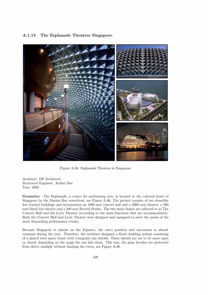
A.1.14 The Esplanade Theatres Singapore

Figure A.86: Esplanade Theatres in Singapore

Architect: DP ArchitectsStructural Engineer: Atelier OneYear: 2002

Geometry The Esplanade, a centre for performing arts, is located in the cultural heart ofSingapore by the Marina Bay waterfront, see Figure A.86. The project consists of two domelikefree formed buildings and incorporates an 1800 seat concert hall and a 2000 seat theatre, a 200seat black box theatre and a 200 seat Recital Studio. The two main domes are referred to as TheConcert Hall and the Lyric Theatre (according to the main functions that are accommodated).Both the Concert Hall and Lyric Theatre were designed and equipped to meet the needs of themost demanding performance events.

Because Singapore is almost on the Equator, the sun’s position and movement is almostconstant during the year. Therefore, the architect designed a fixed cladding system consistingof a glazed steel space frame with triangular sun shields. These shields are set to be more openor closed, depending on the angle the sun hits them. This way, the glass facades are protectedfrom direct sunlight without limiting the views, see Figure A.86.

426

Figure A.87: Double layered Spaceframe for the Free Formed structure

Both the concert hall and theatre are housed in separate spaces. One of the main rea-sons to do this is to be able to comply with the high acoustic requirements for the bothspaces. Therefore, both theatres are also supported by rubber footings to isolate them from thevibrations of nearby subway lines. Around the primary spaces (the actual performance spaces),lobbies and foyers are created by the free formed facade structure. These multi level secondaryspaces are not linked to the free formed facade structure, and therefore are not causing anypoint concentrated loads on the dome like facade structure.

The curvature of the free formed envelope is irregular, but convex on all points of thesurface. In comparison to other free formed buildings, the curvature of the envelope of theEsplanade is less irregular. Because there are no transitions from convex to concave curvature,bending moments in the facade structure are limited. What makes the domes even less irregularis the fact that they are symmetric around their long axis. The dimensions of the Concert Hallare: length 93 meters, width 59 meters, height from the inclined base edge, 26 meters and forthe Lyric theatre: length 102 meters, width 61 meters, height from the inclined base edge, 24meters.

Structure The shape of the domes is designed to fit tightly around the boxes of the ConcertHall and Lyric Theatre. The designed NURBS surfaces were meshed into rhombic grids by thearchitect to get the desired look of the building. The grid that was generated on the surface

427

Figure A.88: Square-On-Diagonal Double Layered grid topology

has a constant mesh length of 1,5 meter. The difference between the two rhombic grids of theshells is the orientation of the meshes. For the Concert Hall, the main polygons run eitheralong or across the base edge of the shell, whereas in the Lyric Theatre these polygons rundiagonally to the base line. As structural solution for the envelopes of the Esplanade Theatres, adouble layered spaceframe was chosen, see Figure A.87. The geometrical topology of the doublelayered grid is known as the square-on-diagonal double layered grid. This type of geometricalarrangement is used when a square on square layout is too dense. Because a high transparencyis desired by the architect, the square-on-diagonal typology is chosen, see Figure A.88. Theexternal grid matches the lines of the basic rhombic grid that was designed by the architect, thenodal points of the internal diagonal grid lie at a constant distance of 90 cm inside the externalgrid. The nodal points of internal grid are acquired by offsetting lines through the midpointsof the external net by 90 cm; the intersections between these offset lines form the nodes of theinternal grid. The underlying grid is acquired by connecting the nodal points diagonally in achessboard layout. The result is a

√2 times as wide grid. To obtain the square-on-diagonal

double layered grid, the nodes of the external grid are connected to the nodes of the internalgrid. The rhombic external grid is split to obtain a triangulated grid. This triangular grid wasrequired for the structural stability as well as for the support of the triangular glass planes.

The by MERO designed steel space trusses are supported at the bottom at each second orthird top chord on concrete edge girders. The upper edges of the space trusses are supportedby the concrete box of the Concert Hall / Lyric Theatre. To stabilise the envelope structure itwas necessary to support the lower and upper edges of the space frames. At the lower edges,the bearing points are fully restraint, at the upper edges, it was necessary to allow for thermalexpansion. At the top, the space frames are rigidly fixed to the non resilient stair towers; otherbearing points are only supported horizontally where this is statically required. The solutionfor the upper bearings had to deliver an unrestrained support and take care of the vibrationinsulation to prevent the transfer of sound from the cladding into the concert and theatreauditorium. A special rubber composite was applied for the upper supports. For the structuralanalysis, besides the dead loads and live loads, wind- and thermal loads were considered.

The designed double layered spaceframe provides high accuracy through machined fabri-cation and can therefore be easily shaped into the designed free form geometry. The topchord members are square hollow sections to allow direct support for the triangular glasspanels, see Figure A.89. The nodes of the top chord members are special bowl type nodes.

428

Figure A.89: Node detail, designed by MERO

To keep the nodes small, special head plates are applied for the square diagonal members,which divide the rhombic configurations into triangles. The space diagonal members andthe bottom chord members are standard MERO round tubes, the nodes are forged spheres.All components were produced at the MERO workshops in Germany. In total, over 32.000line elements and almost 8.500 nodes were necessary to construct the space frames for both domes.

The facade of the Esplanade Theatres is closed by triangular glass panels that are directlysupported by the top chord of the space frame. In theory, only every second of the 10.500glass panels is identical. When a tolerance of 2,5 millimeters is allowed, which can be adjustedin the joints, the number of different panels can be reduced to about 1.500. The panels arefixed to withstand wind suction by means of aluminium discs at the top chord nodes an by twoadditional clamps at each top chord member.

The facades of the Lyric Theatre and the Concert Hall are covered by 4.900 shadingpanels. The design steps for these panels were first to determine the rise of each panel andsecond to optimise the cutting patterns, similar to the glass panels. Result was thirty basiccutting patterns and thirty more special patterns for the edge panels. Panels are made of 4 mmthick aluminium sheets, which are supported at 300 mm above the top chord of the space trusses.

For the construction process a special erection sequence was planned. The domes weredivided into sections that can best be described as vertical orientated strips. The erection wasto follow these sections from top to bottom and proceed to the horizontally adjacent sections.Scaffolding was applied to allow adjustment to the hardly predictable requirements of the threedimensional spaceframe geometry. Spaceframe units of 4,5 meter by 4,5 meter to a maximumof 9 meter were pre assembled on the ground and lifted onto the concrete structure. Afterconnection to the bearings, the erection succeeded with the single members and nodes. Twoindependent groups started erecting on one end of the symmetry line, both constructing towardsthe other end of the symmetry line, keeping each other in balance. The small tolerances inthe fabrication of the nodes and members, together with permanent measurements of the nodepositions, enabled the erected structure to meet the described geometry.

A.2 Papers by Chris Williams

In this paragraph two papers by Dr. Chris Williams, an Engineer, formerly at Arup and later atBuro Happold, and tutor at the University of Bath. Amongst others he was responsible for the

429

structural design of the glass roof of the British Museum. He often uses form finding techniquesto help him with his designs.

430

THE ANALYTIC AND NUMERICAL DEFINITION OF

THE GEOMETRY OF THE BRITISH MUSEUM GREAT

COURT ROOF

Chris J K WilliamsUniversity of Bath, UK

Abstract: The steel and glass British Museum Great Court Roof covers a rectangular area

of 70 by 100 metres containing the 44 metre diameter Reading Room. The paper describes

in detail how the spiralling geometry of the steel members was generated working closely

with the architects, Foster and Partners, and the engineers, Buro Happold A combination

of analytic and numerical methods were developed to satisfy architectural, structural and

glazing constraints. Over 3000 lines of computer code were specially written for the

project, mainly for the geometry definition, but also for structural analysis.

Introduction

Figure 1 is a computer generated image of the original scheme for the roof and this paper

will describe the process of generating the final geometry from this starting point.

Figure 1. Computer generated image of the original scheme

The British Museum Great Court is 73m east-west and 97m north-south. The centre of

the 44m diameter Reading Room is offset 3m to the north of the centre of the Court. The

space in the Court outside the Reading Room was used for temporary book store buildings,

but with the completion of the new British Library at St Pancras the book storage was no

longer required.

2

The new roof over the Court was designed by Foster and Partners, architects, and

Buro Happold, engineers, and was fabricated and erected by Waagner Biro. The roof is

constructed of a triangular grid of steel members welded to node pieces. The members are

boxes welded from plate and are tapered to change depth. The grid is triangulated for

structural stiffness and so that it can be glazed with one flat panel of double glazing for

each triangle of the structural grid.

The roof is supported around the Reading Room and on the rectangular boundary

where it sits on sliding bearings to avoid imposing lateral thrusts on the existing building.

This means that the roof can only push outwards at the corners where it can be resisted by a

tension in the edge beam. Internal tension ties were considered, but rejected on architectural

grounds.

The surface geometry

The shape of the roof is defined by a surface on which the nodes of the steel grid lie. The

height of the surface, z, is a function of x in the easterly direction and y in the northerly

direction. The origin lies on a vertical line through the centre of the Reading Room. The

function is: z = z1 + z2 + z3 where z1 = hcentre - hedge( )h + hedge ,

z2

a= 1 - l( )

35.0 + 10.0y( )1

21 + cos2q( ) +

24.0

2

1

21 - cos 2q( ) + sinq

Ê

ËÁ

ˆ

¯˜

+ 7.5 + 12.0y( )1

21 - cos2q( ) - sinq

Ê

ËÁ

ˆ

¯˜ - 1.6

Ê

Ë

ÁÁÁÁÁ

ˆ

¯

˜˜˜˜

-10.0

21 + cos2q( ) + 10.0

1

2

1

21 - cos2q( ) + sinq

Ê

ËÁ

ˆ

¯˜

È

ÎÍ

˘

˚˙

2

1.0 - 3.0a( )

+2.51

2

1

21 - cos2q( ) - sinq

Ê

ËÁ

ˆ

¯˜

È

ÎÍ

˘

˚˙

2r

a- 1

Ê

ËÁ

ˆ

¯˜

2

and

z3

b= l

3.5

21+ cos2q( ) +

3.0

21- cos 2q( ) + 0.3sinq

Ê

ËÁ

ˆ

¯˜

+1.05 e

-m 1-x

b

Ê

Ë

ÁÁ

ˆ

¯

˜˜

+ e

-m 1+x

b

Ê

Ë

ÁÁ

ˆ

¯

˜˜

Ê

Ë

ÁÁÁ

ˆ

¯

˜˜˜

e

-m 1-y

c

Ê

Ë

ÁÁ

ˆ

¯

˜˜

+ e

-m 1+y

d

Ê

Ë

ÁÁ

ˆ

¯

˜˜

Ê

Ë

ÁÁÁ

ˆ

¯

˜˜˜

.

In these expressions the polar co-ordinates, r = x2+ y

2 and q = cos-1x

r= sin

-1 y

r, and

h =

1-x

b

Ê

ËÁ

ˆ

¯˜ 1 +

x

b

Ê

ËÁ

ˆ

¯˜ 1 -

y

c

Ê

ËÁ

ˆ

¯˜ 1 +

y

d

Ê

ËÁ

ˆ

¯˜

1-ax

rb

Ê

ËÁ

ˆ

¯˜ 1 +

ax

rb

Ê

ËÁ

ˆ

¯˜ 1 -

ay

rc

Ê

ËÁ

ˆ

¯˜ 1 +

ay

rd

Ê

ËÁ

ˆ

¯˜

, y = 1 -x

b

Ê

ËÁ

ˆ

¯˜ 1 +

x

b

Ê

ËÁ

ˆ

¯˜ 1-

y

c

Ê

ËÁ

ˆ

¯˜ 1 +

y

d

Ê

ËÁ

ˆ

¯˜ , a =

r

a- 1

Ê

ËÁ

ˆ

¯˜y and

1-a

rb

=b- x( )

2+ c- y( )

2

b - x( ) c- y( )+

b - x( )2+ d + y( )

2

b - x( ) d + y( )+

b + x( )2+ c- y( )

2

b + x( ) c- y( )+

b + x( )2+ d + y( )

2

b + x( ) d + y( ).

The constants are a = 22.245 , b = 36.625 , c= 46.025, d = 51.125 , l = 0.5, m = 14.0 ,

hcentre = 20.955 and hedge = 19.71 .

3

The functions z1 , z2 and z3 are each built up from its own fundamental function. The

first, shown in figure 2, supplies the correct change in level between the rectangular

boundary and the circular Reading Room. The vertical scale in the figure is chosen

arbitrarily. The original scheme had the roof level arching up along each of the rectangle

edges, and this would have had certain structural advantages, but the final scheme has a

constant height along the edges. The remaining two fundamental functions give z = 0

around the rectangular and circular boundaries.

Figure 2. Level change function, Figure 3. Function with finite curvature at corners

1 -x

b

Ê

ËÁ

ˆ

¯˜ 1 +

x

b

Ê

ËÁ

ˆ

¯˜ 1 -

y

c

Ê

ËÁ

ˆ

¯˜ 1 +

y

d

Ê

ËÁ

ˆ

¯˜

1 -ax

rb

Ê

ËÁ

ˆ

¯˜ 1 +

ax

rb

Ê

ËÁ

ˆ

¯˜ 1 -

ay

rc

Ê

ËÁ

ˆ

¯˜ 1 +

ay

rd

Ê

ËÁ

ˆ

¯˜

r

a- 1

Ê

ËÁ

ˆ

¯˜ 1 -

x

b

Ê

ËÁ

ˆ

¯˜ 1 +

x

b

Ê

ËÁ

ˆ

¯˜ 1 -

y

c

Ê

ËÁ

ˆ

¯˜ 1 +

y

d

Ê

ËÁ

ˆ

¯˜

Figure 4. Function with conical corners

1 -a

r

b - x( )2+ c - y( )

2

b - x( ) c- y( )+

b - x( )2+ d + y( )

2

b - x( ) d + y( )+

b + x( )2+ c- y( )

2

b + x( ) c - y( )+

b + x( )2+ d + y( )

2

b + x( ) d + y( )

Figure 5. Final surface

4

The second fundamental function is shown in figure 3. Both this function and the first

produce a horizontal surface at the corners. This is inevitable unless the curvature tends to

infinity at the corners, like approaching the tip of a cone and this is what happens with the

third fundamental function shown in figure 4.

The issue of the curvature of the corners was important for architectural and structural

reasons and the relative amount of the second and third fundamental functions was chosen

to balance these constraints. The corners were important structurally because of the thrusts

coming down to the corners to be balanced by tensions in the edge beam. The corners are

reinforced locally by external trusses which cannot be seen from inside the Court.

The final shape was obtained by adding a constant times the first fundamental

function to the second and third fundamental functions multiplied by two different

functions of x and y. These extra functions were chosen to satisfy planning, architectural

and structural constraints.

Figure 5 shows the final surface on which the faceting is that of the glazing grid. The

concentration of curvature at the corners can be seen.

The structural grid

The structural grid passed through many stages before arriving at the final form as shown in

the right hand drawing in figure 6. In the early scheme on the left of figure 6 the grid meets

the rectangular boundary in an unsatisfactory way in that some triangles are cut through,

leading to a combination of triangles and quadrilaterals. The central drawing overcomes

this problem, but is still coarse compared to the final form.

The starting point in producing the final grid is shown in figure 7. This is a simple

geometric drawing in which points equally spaced around the Reading Room are joined to

equally spaced points around the rectangular boundary. The radial lines so formed are then

divided into varying numbers of equal segments. The structural grid is produced from this

‘mathematical grid’ by ‘joining the dots’ as seen in the right hand half of figure 7.

Figure 6. Evolution of the structural grid

However this produces discontinuities, particularly on the diagonal directions. These

were removed by ‘relaxing’ the grid to produce figure 8. The relaxation process was as

follows.

5

Figure 7. Starting grid

Figure 9 shows a typical node, i, j of the mathematical grid surrounded by its four

neighbours. If pi, j is the position vector of the typical node at some point during the

relaxation process, then

f i, j = pi-1, j - pi, j( ) + pi+1, j - pi, j( ) + 2 - z( ) pi, j-1 - pi, j( ) + z pi, j+1 - pi, j( )would be the fictitious force applied to the node by ‘strings’ attached to the neighbouring

nodes if the tension coefficients of the strings are 1, 1, 2 - z( ) and z . The tension

coefficient is the tension in a member divided by its length. The purpose of the variable z

will be described later.

Now imagine that the nodes of the mathematical grid are free to slide with no friction

over the surface defining the shape. The force qi, j = fi, j - f i, j •ni, j( )ni, j (where ni, j is the

unit normal to the surface) is the component of f i, j tangential to the surface and therefore

the nodes will slide until all the qi, j = 0 .

The quantity z = 1- 0.004 1.5m - j( ) 1- cos 2q( ) where m = 70 is the value of j on the

Reading Room boundary and q is the polar co-ordinate. This function was chosen so as to

6

control the maximum size of the glass triangles which occur near the centre of the southern

boundary. It was the limitation on glass size which was the controlling factor in choosing

the structural grid.

Figure 8. Relaxed grid

i-1, ji, j-1

i+1, ji, j+1

i, j

Figure 9. Typical grid nodes Figure 10. Elevation of structural grid looking north

The non-linear equations qi, j = 0 were solved by repeated application of the

algorithm dpi, j( )this cycle

= c1qi, j + c2 dpi, j( )the previous cycle

where dpi, j is the movement of

the typical node and the constants c1 and c2 £ 1.0 are chosen to optimise the speed of

convergence. The larger the constants, the faster the convergence, but if they are too high,

7

numerical instability occurs. This process is known as dynamic relaxation and was invented

by Alister Day. The whole mathematical grid was run through 5000 cycles before the

process was judged to have converged. Convergence was speeded by using setting c2 = 0

when the sum of the squares of the dpi, j passed through a maximum.

Figures 10, 11 and 12 show the final structural grid.

Figure 11. Elevation of structural grid looking west

Figure 12. Isometric of structural grid

Figure 13. Outwards deflections due to loading

8

Figure 14. View showing south side collapsed while north remains standing

Structural analysis

A detailed description of the structural analysis of the roof is beyond the scope of this

paper. A specially written computer program was used, together with commercial software.

Figures 13 and 14 show the deflections due to a large vertical load, much larger than

possible on the roof. The spreading of the boundaries can be seen on the plan and on figure

14 it can be seen that the south side has collapsed, hanging in tension, while the north side

still stands.

Figure 15. Day and night views

Conclusion

This paper discusses one aspect of one project and figure 15 contains photographs of the

completed Great Court. Papers by the architects, engineers and builders of this and other

recent projects are contained in Barnes and Dickson (2000).

References

Michael R. Barnes and Michael G.T. Dickson, Thomas Telford, Widespan roof structures,

London 2000

The definition of curved geometry for widespan enclosures

Chris J K Williams

Department of Architecture and Civil Engineering

University of Bath

UK

1 Introduction

If an enclosure is to be constructed of curved lines and surfaces rather than straight

lines and flat planes, the questions arise as to how the geometry is first to be chosen

and then how it can be defined with sufficient accuracy for the structure to be built

and clad.

There are clearly many ways that the geometry can be chosen and defined, but they

fall into three broad categories and the methods used on any one project may fall intomore than one of these categories. The categories are:

Sculptural in which a model is sculpted by hand or a computer model is

constructed that can be deformed interactively.

Geometric in which the form is defined in terms of geometrical objects which

might be simple spheres, cylinders or cones, or much more complicatedobjects which can only be visualised using computers.

Physical in which the shape is controlled by some physical process such as a

soap film or a hanging chain. The physical process may be modelled by an

actual physical model or a mathematical model which may by analytic ornumerical in a computer.

An example of a mixed sculptural and physical approach would be bending a piece of

wire by hand (the sculptural part) and then dipping it into soap solution and

withdrawing it to form a soap film (the physical part).

An example of a mixed geometric and physical approach would be forming a soap

film between two parallel circular rings so that the rings are simple geometric entities.

In this case the soap film forms a catenary of revolution so that one might say that it is

a relatively simple geometric object formed by a physical process.

The methods used for any one project will depend upon many factors. Perhaps the

most important of these is the relative importance of structural, architectural and other

constraints. Another is the experience of the design team in using various techniques,

especially since the technology may have evolved in other disciplines such assculpture, medicine or automobile, aerospace or ship design.

In the following I shall discuss some recent experience using a number of methods to

try and illustrate the possibilities of the three approaches.

2 Sculptural

Traditionally large sculptures or even car bodies were first made as small clay models

or maquettes which were measured and enlarged. Now much of this work is done

using computers employing software written for the automobile and aerospace

industries. Frank O. Gehry & Associates use aerospace software, but the starting pointis still physical models.

Such software is expensive and time is needed to learn how it can be used. Curved

lines are divided up into a series of spline curves which fit together with an

appropriate continuity of orientation and curvature. Curved surfaces are constructed

from curved patches. These patches, developed for Computer Aided Design are very

similar to the finite elements developed for the analysis of shell structures.

Figure 1 Body Zone sculptureArchitect: Branson Coates Architecture

Engineer: Buro Happold

Figures 1 to 5 show the Body Zone in the Millennium Dome. The shape was defined

by the small physical model in the photographs in figure 1. A structural grid was

drawn on the model and this was measured using a standard CAD package from

scanned images of the photographs. This data was used to construct the computer

model shown in figure 2.

Figure 2 First computer modelArchitect: Branson Coates Architecture

Engineer: Buro Happold

Figure 3 Sections through sculptureArchitect: Branson Coates Architecture

Engineer: Buro Happold

Figure 4 Computer model from sectionsArchitect: Branson Coates Architecture

Engineer: Buro Happold

Following this work it was decided to concentrate on defining the figures in terms of

parallel cross-sections. A copy of the physical model was sliced using a saw and the

resulting cross-sections were scanned and 'traced' to produce figure 3. These cross-

sections were joined to produce the three dimensional image shown in figures 4 and 5.

Figure 5 Rendered imageArchitect: Branson Coates Architecture

Engineer: Buro Happold

The software used to produce figures 2, 3 and 4 was specially written for the project.

3 Geometric

The limit of what can be done using geometry is the mathematical knowledge and

imagination of the individual. As an example let us consider Le Corbusier's Modulor1

shown in figure 6b. Modulor is based upon the Fibonacci series, examples of which

are

1, 1, 2, 3, 5, 8, 13, 21,34. . . . .

and

1, 3, 4, 7, 11, 18, 29, 47, . . . .

In both cases each term is the sum of the two preceding terms. Thus if xn is the nth

term,

xn = xn-1 + xn-2 .

Figure 6a Figure 6b Le Corbusier's sketch

Computer image

This equation has the general solution

xn =

lf 2 -1( )f n + l - f 2( )-1( )

n

f n

l -1( ) f 2 +1( )x0

where f =1+ 5

2 is the Golden Section and l =

1

1-x0

x1

. As n gets larger, the ratio of

successive terms becomes closer to f regardless of the starting two terms of the series,

x0 and x1 . Ifx1

x0= f , then l = f

2 and xn = f

nx0 which is the basis of Modulor. The

computer program below was used to produce the dxf file that is plotted in figure 6a,

replicating Modulor.

dxf files are text files which can be read by CAD programs such as AutoCAD,

MicroStation or MiniCAD.

#include <fstream.h>

#include <iostream.h>#include <math.h>

int i,j,k,m,nhalfycles,finish;

float PI,x,y,z,U,V,W,alpha,beta,

A,C,phi;

ofstream Julia("Modulor.dxf");

int main(void)

PI=4.0*atan(1.0);

Julia<<"0\nSECTION\n2\nENTITIES\n";

nhalfycles=18;m=20*nhalfycles;

phi=(1.0+sqrt(5.0))/2.0;C=216.0;

for(j=1;j<=4;j+=1)

if(j==4)finish=90.0;

else finish=60;

for(k=0;k<=finish;k+=3)

A=1.2*cos((PI*k)/180.0);

for(i=0;i<=m;i+=1)

beta=-(1.0*i*nhalfycles)/(2.0*m);

alpha=beta;if(j<=2)alpha-=0.5;

y=C*pow(phi,alpha);

if(j==1||j==3)

x=A*y*fabs(sin(beta*PI));

if(j==2||j==4)

x=A*0.5*y*fabs(sin(2.0*beta*PI));

if(j<=2)x=-x;

x=x/8.0;

z=0.0;

if(i!=0)

Julia<<"0\nLINE\n8\n0\n";

Julia<<"10\n"<<U<<"\n20\n"<<

V<<"\n30\n"<<W<<"\n";

Julia<<"11\n"<<x<<"\n21\n"<<

y<<"\n31\n"<<z<<"\n";

U=x;V=y;W=z;

Julia<<"0\nENDSEC\n0\nEOF\n";

Julia.close();

cout<<"DXF file written\n";

return 0;

Figure 7 Golden section log spiral

Figure 8 Two spirals

The program will run on any computer (Macintosh, PC etc.) with a C++ compiler and

very little work would be required to convert the program to Basic or Fortran.

An unlimited variety of curves and surfaces can be produced by such programs. For

example, figures 7, 8 and 9 were produced using the formulae

x = fa cos2ap

y = fa sin2ap

¸˝˛

,

x = fa cos2ap +f -a cosap

y = fa sin2ap -f -a sinap

¸˝˛

and

x = 1 + r( )fa + 1 - r( )f-a cosap

y = 1- r( )f -a sinap

¸

˝

˛

respectively.

Figure 9 Spirals to lines

Figure 10 Rendered image

In each case a is varied to draw a curve and in the case of figure 9, a different value

of r is used for each curve.

The surface in figure 10 was obtained from the curves in figure 9 by giving each

curve a different value of z.

Figure 11 Bridge study

Figure 12 Bridge study

The bridge studies in figures 11, 12 and 13 were also produced by purely

mathematical methods as was the shell study in figure 14. In each case the whole

object is defined by the just one set of mathematical formula so that there is complete

continuity of all derivatives, orientation, curvature, rate of change of curvature etc.

Figure 13 Bridge study

Figure 14 Shell study for Stuttgart railway stationArchitect: Ingenhoven Overdiek Kahlen und Partner

Consultant Architect: Professor Frei Otto

Engineer: Buro Happold

Figure 15 Millennium Dome Rest Zone - system geometryArchitect: Richard Rogers Partnership

Engineer: Buro Happold

Figure 16 Rest ZoneArchitect: Richard Rogers Partnership

Engineer: Buro Happold

Figures 15 and 16 show the Rest Zone in the Millennium Dome which was produced

by deforming a torus. Again there is complete continuity of all derivatives.

4 Physical

In the membrane theory of shell structures the geometry of the structure and the loads

are assumed to be known and the three membrane stresses - two tensile orcompressive and one shear are unknown.

There are three equations of equilibrium, one in the direction normal to the surface,

sabbab + p = 0 ,

and two in the plane of the surface,

sab:a + p

b= 0 .

The notation here is similar to that in Green and Zerna2. In these equations the

geometry of the shell is determined by the components of the metric tensor, gab , and

of the curvature tensor, bab . The components of load are pa

and p , and the

unknown membrane stress components are s11

, s22

and s21= s

12.

The fact that there are three equilibrium equations and three unknown membrane

stress components means that shells are essentially statically determinate if the overall

shape and boundary supports permit. An inappropriate shape or lack of support may

mean that a shell is a mechanism.

It is not at all obvious which shapes and support conditions lead to mechanisms and

which do not. Spivak3

discusses this issue in purely geometric terms, for example the

Cohn-Vossen theorem states that any complete convex surface with positive Gaussian

curvature is not a mechanism if membrane strains are prevented.

A cooling tower on the ground is not a mechanism, but a spherical shell with a hole in

the top is.

A shell may also be a mechanism if it is made of masonry, so that the principal

membrane stresses must be compressive, or if it is made of fabric in which case theymust be tensile.

A mechanism can carry certain loads if it has the correct shape. In the case of a

masonry structure, the dominant load is the dead load and in the case of a fabric

structure it is prestress upon which wind and snow are added.

Form finding is the process of establishing a structural geometry for a

mechanism to carry a particular load.

Gaudi used hanging models which, when inverted, defined the shape of masonry

arches and vaults for the Colonia Guell and the Sagrada Familia. Professor Frei Otto

pioneered the use of physical models for fabric structures, cable nets and grid shells.

Figure 17 Tree of the FutureArchitect: Mark Fisher Associates

Engineer: Atelier One

Form finding: Lynne Mabon, University of Bath

Now much of this work is done with numerical models, although physical models are

indispensable for initial studies. Form finding a fabric structure with a soap film or

minimal surface is done by setting the membrane stress components

sab

= Tgab

where T is the surface tension. In addition a geodesic co-ordinate system for

generating the cutting the pattern is obtained by imposing the conditions g12 = 0 and

g22 = constant .

An equal mesh net is produced by writing

s12= 0 and g11 = g22 = constant ,

if there is no elastic extension, otherwise g11 and g22 increase with tension. Equal

mesh nets are more difficult to form find than fabric structures due to the adjustmentof cable lengths at the boundary.

Figure 18 Mannheim Bundesgartenschau 1.5m gridArchitect: Mutschler & Partners

Consultant Architect: Atelier Warmbronn (Professor Frei Otto)

Form finding: Büro Linkwitz

Engineer: Ove Arup & Partners (Ted Happold and Ian Liddell)

Figure 19 Mannheim erection

Figure 17 shows one of the equal mesh nets of the Tree of the Future intended for the

Central Show in the Millennium Dome. In this case a computer program was

specially written by Lynne Mabon of Bath University which automatically generated

the boundary data.

Figure 18 shows the hanging chain model for the Mannheim Bundesgartenschau. This

is a computer generated model by Büro Linkwitz, based upon Frei Otto's accuratephysical model. Figures 19 and 20 show the erection and load testing of the shells.

Figure 20 Mannheim load test

Figures 21 and 22 show computer generated models of the Weald and Downland

Museum. In this case the mathematical model had to contain bending stiffness during

form finding, otherwise compressive stresses produced wrinkling.

Figure 21 Weald and Downland MuseumArchitect: Edward Cullinan Architects

Engineer: Buro Happold

Figure 22 Weald and Downland MuseumArchitect: Edward Cullinan Architects Engineer: Buro Happold

5 The British Museum Great Court Roof

Figures 30 is an image of the computer model of the British Museum Great Court

Roof. It was generated by a mixed approach.

Figure 23 British Museum Great Court Roof - first functionArchitect: Foster and Partners

Engineer: Buro Happold

The shape of the surface was defined analytically by weighting and summing

functions based on those shown in figures 23, 24 and 25. The weightings also varied

with position to satisfy architectural, planning, structural and clearance requirements.

Figure 24 British Museum Great Court Roof - second functionArchitect: Foster and Partners

Engineer: Buro Happold

The positions of nodes on the surface were obtained from the starting grid shown in

figure 26. A displacement was calculated for each interior node of this grid to make

its x, y and z co-ordinates the weighted average of the current co-ordinates of the four

surrounding nodes. However, before moving a node, the component of displacement

normal to the surface (see figure 27) was removed so that the node remained on the

surface. This relaxation procedure was repeated thousands of times for the wholestructure until the geometry settled down to that in figure 28.

Figure 25 British Museum Great Court Roof - third functionArchitect: Foster and Partners

Engineer: Buro Happold

The weighting of the surrounding nodes was varied at different points on the surface

to control the distribution of the nodes, in particular in relation to the sizes of the glasspanels.

Figure 27 British Museum Great Court Roof - surface normalsArchitect: Foster and Partners

Engineer: Buro Happold

Figure 26 British Museum Great Court Roof - original gridArchitect: Foster and Partners

Engineer: Buro Happold

The spiraling members were obtained by joining points in the form finding grid as

shown in figure 29 to produce figures 30 and 31.

Figure 28 British Museum Great Court Roof - relaxed gridArchitect: Foster and Partners

Engineer: Buro Happold

Figure 29 British Museum Great Court Roof - steel members on gridArchitect: Foster and Partners

Engineer: Buro Happold

Figure 30 British Museum Great Court Roof - steel membersArchitect: Foster and Partners

Engineer: Buro Happold

Figure 31 British Museum Great Court Roof - steel membersArchitect: Foster and Partners

Engineer: Buro Happold

6 Conclusion

This paper discusses some of the ways in which curved forms can be generated. It is

not possible to say that any one method is the optimum, because there are so many

possibilities and the architectural, structural and environmental constraints will neverbe the same on two projects.

References

1 Le Corbusier, The Modulor, translated by Peter de Francia and Anna Bostock,

Faber and Faber, London 1961.

2 Green, A.E. and Zerna, W., Theoretical elasticity, 2nd

edition, Oxford University

Press, 1968.

3 Spivak, Michael, A comprehensive introduction to differential geometry, volume

5, 2nd

edition, Publish or Perish Inc., Delaware, 1975, 1979.

Bibliography

(2005a). World Wide Web: http://www.ticam.utexas.edu/CCV/projects/shastra/projects/visualization/me-joint-sim.htm.

(2005b). World Wide Web: http://www.beakman.com/beakman/spider/spider.html.

(2005c). World Wide Web: www.brantacan.co.uk.

(2006). World Wide Web: www.phycomp.technion.ac.il.

(n.d.). World Wide Web: http://www.midcoast.com/ bo/CloseFromTop.jpg.

Alexander, R. M. (1992). Op Verkenning in de Biomechanica, Dieren in Beweging (Originaltitle: Exploring biomechanics, Animals in motion), dutch edition (1995) edn, The ScientificAmerican Library (De Wetenschappelijke Bibliotheek).

Argebau (1971). Argebau, richlinien fur de bau und betrieb von tragluftbauten.

Baant, Z. & Cedolin, L. (1991). Stability of Structures, Elastic Inelastic, Fracture and Damagetheories, New York; Oxford University Press.

Bach, K., Burkhardt, B. & Otto, F. (eds) (1987). IL18 Seifenblasen, Forming bubbles, number 18in IL, Institut fur leichte flachentragwerke.

Bach, K. (ed.) (1971). IL3 Biology and Building, part 1, Information of the Lightweight StructuresInstitute (IL), number IL3 in IL, Institut fur Leichtbau Entwerfen und Konstruieren.

Bach, K. (ed.) (1973). IL6 Biology and Building, part 3, Information of the Institute forLightweight Structures (IL), number IL6 in IL, Institut fur Leichtbau Entwerfen und Kon-struieren.

Bach, K. (ed.) (1974). IL10 Grid Shells, Gitterschalen, number IL10 in IL, Institut fur LeichtbauEntwerfen und Konstruieren.

Bach, K. (ed.) (1975). IL 8 Netze in natur und technik, Nets in nature and technics, number IL8in IL, Institut fur Leichtbau Entwerfen und Konstruieren.

Bach, K. (ed.) (1990). IL33 Radiolarien, Radiolaria, number 33 in IL, Institut fur leichte flachen-tragwerke.

Baecke, W. (2005). Het ontwerpen van vouwschalen bestaand uit prefab elementen, Master’sthesis, Delft University of Technology.

Baer, S. (1970). Zome Primer, Albuquerque, Zomeworks Corporation.

Baker, T. J. (1999). Delaunay-Voronoi Methods. Handbook of Grid Generation, online version,CRC Press.

Barnes, M. (1986). Computer-aided design of cable and membrane structures, with applicationsto expo 88 and dqdc, riyadh, in V. Sedlak (ed.), LSA86, Lightweight Structures in Architec-ture, The First International Conference on Lightweight Structures in Architecture, Sydney,Australia, 24-29 August 1986, Proceedings, Volume I, Lightweight Structures in Architec-ture, Unisearch Limited, The University of New South Wales, PO Box I Kensington, NSWAustralia 2033, pp. 254–270.

455

Bauer, U. (1968). Traglufthallen und ihren klimatischen bedingungen, Sport und BaderbautenJanuary: 9–27.

Bendse, M. (1995). Optimization of structural topology, shape, and material, Berlin Heidelberg,Springer-Verlag.

Bendse, M. (2003). Topology optimization - Theory, methods and applications, Berlin Heidelberg,Springer-Verlag.

Beranek, P. W. (1976). Berekening van platen, TU Delft.

Beranek, P. W. (1988a). Understanding of structures, Proceedings of the InternationalUpdatingCourse on Structural Consolidation Stable-Unstable? Structural Consolidation Of AncientBuildings, Center For The Conservation Of Historic Towns And Buildings, Leuven Univer-stity.

Beranek, P. W. (1988b). Understanding of structures, stable-unstable, Leuven University Press .

Beukers, A. & Hinte, E. (2001). Lightness, the inevitable renaissance of minimum energy struc-tures, 3rd edn, 010 publishers, Rotterdam.

Bletzinger, K. (n.d.). Structural optimization lecture papers, Printed.

Bletzinger, P. (2001). Structural optimization, Reader for the Lehrstuhl fur Statik, TechnischeUniversitat Munchen.

Boer, S. & Oosterhuis, K. (2004). Architectural parametric design and mass customization,Proceedings of the 5th European Conference on Product and Process Modelling in the AECIndustry .

Borrego, J. (1967). Space Grid Structures, Cambridge, MIT Press.

Brown, S. & Cook, M. (2002). The design and manufacture of the british museum great courtroof, IABSE Symposium Melbourne, IABSE.

Brylka, R. (1970). Traglufthalle Heute, technische mitteilungen Krupp Werksberichte, Band 28,Krupp.

Buerger, M. (1968). Elementary Crystallography, M.I.T.

Burkhardt, B. e. a. (n.d.). Multihalle Mannheim, Institut fur leichte Flchentragwerke.

Burns, S. (2002). Recent advances in optimal structural design, Reston: American Society ofCivil Engineers.

Calladine, C. (1998). Deployable structures: What can we learn from biological structures, inS. Pellegrino & S. Guest (eds), Proc. IUTUM-IASS Symp. on Deployable Structures: Theoryand Applications, Kluwer Academic Publisher, Dordrecht, pp. 63–75.

Cattan, A. & Reissig, P. (2000). Hard models of manual and visual operation for the generationand reading of spatial forms, in J. Gerrits (ed.), Bridge between civil engeering and archi-tecture, International Association for Shell and Spatial Structures (IASS), Working Groupno. 15 ’Structural Morphology’ (SMG), Delft University of Technology, Delft University ofTechnology, The Netherlands, pp. 42–47. 1st edition.

Chalmers, B., Holland, J., Jackson, K. & Williams, R. (1965). Crystallography, A ProgrammedCourse in three Dimensions, New York: Appleton-Century-Crofts.

456

Chilton, J. (2000). Space Grid Structures, Architectural Press, Oxford.

Clark, R. (1970). KINETIC ARCHITECTURE, New York; van Nostrand einhold Company.

Coenders, J. (2004). Structural form finding, new life through a new definition, World WideWeb, Delft University of Technology. Part of Master’s thesis.

Connor, J. (2003). Introduction to Structural Motion Control, Upper Saddle River, NJ; PrenticHall Pearson Education, Inc.

Cox, H. (1965). The Design of Structures of Least Weight, Pergamon Press Ltd.

Coxeter, H. & R.W.W.Ball (1947). Mathematical Recreations and Essays, New York, Macmillan.

Critchlow, K. (1980). Time Stands Still, G. Fraser.

Cundy, H. & A.P.Rollett (1961). Mathematical Models, London: Clarendon.

Czyz, J. & Lukasiewicz, S. (1994). Optimization of space lattice structures with multimodal fre-quency constraints, in J. Abel, J. Leonard & C. Penalba (eds), Spatial, Lattice and TensionStructures, IASS-ASCE, American Society of Civil Engineering, 345 East 47th Street, NewYork 10017-2398, pp. 419–428.

Daerden, F. & Lefeber, D. (2001). The concept and design of pleated pneumatic artificial muscles,International Journal of Fluid Power 2,3: 41–50.

Darwin, C. (1859). The Origin of Species, Oxford University Press.

Delft University of Technology, F. o. A. (2003). Formian - formex, World Wide Web,http://www.bk.tudelft.nl/bt/dc/Formian/Formian.html.

Dorey, A. & Moore, J. (1996). Advances in actuators, Bristol, UK: Institute of Physics Publishing.

Edelsbrunner, H. (2001). Geometry and Topology for Mesh Generation, Cambridge UniversityPress.

Eekhout, M. (1989). Architecture in Space Structure, 010 Publishers.

Engel, H. (1999). Tragsysteme, Structure Systems, 2nd edn, Verlag Gert Hatje, Senefelderstrasse12, 73760 Ostfildern-Ruit.

Eppstein, D. (1996). Zonohedra and zonotopes, Mathematica in Educ. Res. 5: 15–21.

F. Ansari, A. M. & Leung, C. (eds) (1997). Intelligent Civil Engineering Materials and Structures,New York, American Society of Civil Engineers.

Farestam, S. & Simpson, R. (1994). A framework for advanced front techniques of finite elementmesh generation.

Farin, G. (1999). NURBS, from Projective Geometry to Practical Use., 2nd edn, Natick, Mas-sachusetts; AK Peters.

Farshad, M. (1992). Design and Analysis of Shell Structures, Dordrecht; Kluwer AcademicPublischers.

Festo (2005). Festo homepage, World Wide Web, http://www.festo.com/INetDomino/.

Flugge, W. (1960). Stresses in Shells, Springer Verlag, Berlin.

457

Frank, F. & Kasper, J. (1959). Complex alloy structures regarded as sphere packings. ii. analysesand classification of representative structures., Acta Crystallographica 12: 483–499.

fur Leichtbau Entwerfen und Konstruieren, I. (1978). IL13 Multihalle Mannheim, number IL13in IL, Institut fur Leichtbau Entwerfen und Konstruieren.

Gibson, L. & Ashby, M. (1997). Cellular solids, structure and properties, 2nd edn, CambridgeUniversity Press.

Grundig, L. & Bahndorf, J. (1986). Form finding of a roof structure for a health spa, in V. Sedlak(ed.), LSA86, Lightweight Structures in Architecture, The First International Conference onLightweight Structures in Architecture, Sydney, Australia, 24-29 August 1986, Proceedings,Volume I, Lightweight Structures in Architecture, Unisearch Limited, The University of NewSouth Wales, PO Box I Kensington, NSW Australia 2033, pp. 246–253.

Haas, A. (1962). Design of thin concrete shells, Vol. 1, positive Curvature Index, New York, JohnWiley and Sons.

Hanegraaf, A. & et al. (1975). Primary zonohedra, Preprint 2nd Conference on Space Structures.

Hanisch, F. (1996/1997). B-spline curves, Applet on Internet.http://www.cs.technion.ac.il/ cs234325/homepage/applets/doc/html/etc/appletIndex.html(sept. 2005).

Hanselaar, H. (2003). Snowplace, Master’s thesis, Delft University of Technology.

Happold, E. & Liddell, W. (1975). lattice roof for the mannheim bundesgartenschau, The Struc-tural Engineer 53, no3.

Harris, R. & Kelly, O. (2002). The structural engineering of the downland gridshell, in G. Parke& P. Disney (eds), Space Structures 5, University of Surrey, Guildford, UK, Thomas TelfordPublishing, pp. 161–172.

Hemp, W. (1973). Optimum structures, Oxford University Press.

Hernandez, S. (1993). Advanced Techniques in the Optimum Design of Structures, Vol. 12 of Top-ics in Engineering, Computational Mechanics Publications, Southampton, UK and Boston,USA.

Hoefakker, J. & Blaauwendraad, J. (2003). Theory of Shells, Lecture book, Delft University ofTechnology.

Holgate, A. (1986). The art in structural design, Oxford University Press.

Homepage, K. C. I. (n.d.). World Wide Web, http://www.kineticceramics.com.

homepage, R. I. (2005). World Wide Web, http://www.racointernational.com.

Honeycombs (n.d.). World Wide Web, http://www.mse.mtu.edu/ dr-john/my4150/honey/h1.html.

Houtman, R. (1996). The influence of distorsion introduced by cloth flattening on stress behaviourof tensile structures, Delft University ofTechnology, department of Civil Engineering.

H.S.M.Coxeter, H. (1963). Regular Polytopes, New York: Macmillan.

H.S.M.Coxeter, Longuet-Higgins, M. & Miller, J. (1954). Uniform Polyhedra. PhilosophicalTransactions, Londen: Royal Society.

458

Huybers, D. (2000a). 38 years of morphology, an anthology, Printed for the Delft University ofTechnology.

Huybers, D. & Ende, G. (1994). Prisms and antiprisms, in J. Abel, J. Leonard & C. Penalba (eds),Spatial, Lattice and Tension Structures, IASS-ASCE, American Society of Civil Engineering,345 East 47th Street, New York 10017-2398, pp. 142–151.

Huybers, P. (1983). Een koepelconstructie van rondhout, Delft University of Technology, depart-ment of Civil Engeneering.

Huybers, P. (1994). Draagconstructies Gebouwen Deel 2: Vorm en Functie, Fac. Civiele TechniekTU Delft.

Huybers, P. (2000b). Polyhedriods, in J. Gerrits (ed.), Bridge between civil engeering and archi-tecture, International Association for Shell and Spatial Structures (IASS), Working Groupno. 15 ’Structural Morphology’ (SMG), Delft University of Technology, Delft University ofTechnology, The Netherlands, pp. 100–107. 1st edition.

i Armengol, J. B. (2001). The Essential Gaudi, The geometric modulation of the Church of theSagrada Familia, 2nd edn, ECSA. Translation by Mark Burry.

IASS, W. . (1985). Recommendations for air-supported structures., IASS.

Isler, H. (2000). Creating shell shapes, in J. Gerrits (ed.), Bridge between civil engeering and ar-chitecture, International Association for Shell and Spatial Structures (IASS), Working Groupno. 15 ’Structural Morphology’ (SMG), Delft University of Technology, Delft University ofTechnology, The Netherlands, pp. 108–115. 1st edition.

Janocha, H. (ed.) (1999). Adaptronics and Smart Structures, Berlin, Springer.

Jensen, F. (2000). Downland grid shell, Master’s thesis, University of Bath, UK. Final yeardissertation.

J.L. Deneubourg, e. a. (1991). Swarm-made architecture, Proc. European conference on ArtificialLife.

Jr., B. S. & Sain, M. (1997). Controlling buildings: A new frontier in feedback., IEEE ControlSystems Magazine on Engineering Technology; Special Issue 17 nr. 6: 19–35.

K. Bach, B. B. F. O. (ed.) (1988). IL25, number 25 in IL, Institut fur Leichtbau Entwerfen undKonstruieren.

Kelly, O., HARRIS, R.J.L., D. M. & ROWE, J. (2001). Construction of the downland gridshell,The Structural Engineer 79(17).

Kirsch, U. (1993). Structural optimization - Fundamentals and applications, Berlin Heidelberg,Springer-Verlag.

Kitrick, C. (1990). A unified approach to class i, ii and iii geodesic domes, International Journalof Space Structures 5, nr. 3&4: 223–246.

Klimke, H., Sanchez, J., Vasilu, M., Stuhler, W. & Kaspar, C. (2002). The envelopes of the artscentre in singapore, Space Structures 5, Thomas Telford, London, pp. 795–806.

Knebel, K. & et al. (2002). The structural making ofthe eden domes, Space Structures 5 1: 245–254.

Koiter, W. (1945). Over de Stabiliteit van het Elastisch Evenwicht, Amsterdam; H.J. Paris.

459

Koiter, W. (1967). Nasa technical translation, NASA Technical F10,833.

Lalvani, H. (1991). Morpological Aspects of Space Structures, -. p1-68.

Lauletta, E. (ed.) (1961). Statics Of Hyperbolic Paraboloidical Shells Studied By Means Of Models,Vol. Proceedings of the symposium on shell research.

Lewis, F. (1923). The typical shape of polyhedral cells in vegetable parenchyma and the restora-tion of that shape following cell division, Proceedings of the American Academy of Arts andSciences 58: 527–552.

Liang, Q. (2005). Performance-based optimization of structures - Theory and applications, Oxon,Spon Press.

Liseikin, V. (1999). Grid generation methods, New York, Scientific Computation.

Loeb (1966). The architecture of Crystal, Proportion, Symmetry and Rhythm, Georgy Kepes,New York: Braziller.

Macior, W. & Matzke (1951). An experimental analysis of cell-wall curvatures, and approxi-mations to minimal tetrakaidekahedra in the leaf parenchyma of rhoeo discolor, AmericanJournal of Botany 38: 783–793.

Maeder, U. & et al. (2004). Ceracem, a new high performence concrete: characterisations andapplications, Kassel University press.

Marvin, J. (1938). The shape of compressed lead shot and its relation to cell shape, AmericanJournal of Botany 25: 280–287.

Mathworld (2008). World Wide Web: www.mathworld.com.

Matzke, E. (1939). Volume-shape relationships in lead shot and their bering on cell shapes,American Journal of Botany 26: 288–295.

Membrane, B. T. & Welcome!, L. S. B. H. (2005). Birdair homepage: Welcome!, World WideWeb, http://www.birdair.com/birdair/flash.html.

Mengeringhausen, M. (1975). Komposition im Raum, Band 1, Raumfachwerke aus Staben undKnoten, Wiebaden/Berlijn, Bauverlag GMBH.

Mitchell, M. (1996). An Introduction to Genetic Algorithms, 2nd edn, MITPress.

Montcrieff, E. & Grundig, L. (2000). Computional modelling of lightweight structures: Form-finding , load analysis and cutting pattern generation, Proceedings Symposium VU Brussel,VU Brussel.

Mulder, H. (2003). Adaptive structures, Master’s thesis, Delft University of Technology, DelftUniversity of Technology, NL.

Mutoh, I. (2002). How does a metal cobweb behave?, in G. Parke & P. Disney (eds), SpaceStructures 5, University of Surrey, Guildford, UK, Thomas Telford Publishing, pp. 47–55.

Nachtigall, W. (1985). Warum die Vgel fliegen, Raschen und Rhring.

Nachtigall, W. (2001). Das groe Buch der Bionik; Neue Technologien nach dem Vorbild derNatur, Stuttgart, Deutsche Verslags-Ansalt.

Nooshin, H. & Disney, P. (2002). Formex configuration processing, Reader for the Faculty ofArchitecture, Structural Design Group, Delft University of Technology.

460

Nooshin, Space Structures Research Centre, Department of Civil Engineering, University of Sur-rey, Guildford, UK, H. (1984). Formex Configuration Processing in Structural Engineering,Elsevier Applied Science Publishers.

Ohmori, H. & et al. (2005). Computational morphogenesis and its application to structuraldesign, Proceedings of the international symposium in shell and spatial structures .

Orta-Rial, B. (2000). Optimisation of shape and topology of statically determined trusses underworse loading conditions using simulated annealing, in J. Gerrits (ed.), Bridge between civilengeering and architecture, International Association for Shell and Spatial Structures (IASS),Working Group no. 15 ’Structural Morphology’ (SMG), Delft University of Technology, DelftUniversity of Technology, The Netherlands, pp. 321–328. 1st edition.

Otto, F. (1973). Tensile Structures (Original title: Zugbeanspruchte Konstruktionen), Vol. 1 and2, paperback, english translation edn, MIT Press.

Otto, F., Trostel, R. & Schleyer, F. (1962). Zugbeanspruchte Konstruktionen, dl 1, UlsteinFachverlag, Frankfurt.

Owen, J. (1965a). The Analysis and Design of Light Structures, Edward Arnold (Publishers)Ltd.

Owen, J. (1965b). The analysis and design of light structures., American Elsevier Publ. co.

Pearce, P. (1978). Structure in Nature is a Strategy for Design, Cambridge/Massachusetts; MITPress.

Peraire, J., Peiro, J. & Morgan, K. (1999). Advancing Front Grid Generation. Online version,CRC Press.

Popko, E. (1968). Geodesics, Detroit, University of Detroit Press.

Press, W., Vetterling, W., Teukolsky, S. & Flannery, B. (2002). Numerical Recipes in C++, TheArt of Scientific Computing, 2nd edn, Cambridge University Press.

Prusinkiewicz, P. & Lindenmayer, A. (1990). The Algorithmic Beauty of Plants, New York,Springer-Verslag.

Ramm, E. & Bletzinger, K. (1993). Structural optimization, International Association for Shelland Spatial strucures (IASS) newsletter 112 p. 6.

research group, T. (2005). Topology optimization, World Wide Web, http://www.topopt.dtu.dk/.

Rypl, D. (2002). Grid generation, World Wide Web:http://power2.fsv.cvut.cz/ dr/papers/Thesis.viewed: july 2005.

Samyn, P. (2000). The volume indicators for michell-type structures and telescopic beams, inJ. Gerrits (ed.), Bridge between civil engineering and architecture, Proceedings of the 4thInternational Colloquium on Structural Morphology, August 17-19, 2000, Delft, NL, IASS,Delft University of Technology, pp. 305–308.

Samyn, P. & Lateur, P. (2000). Volume and displacement indicators of isostatic structures thecase of the horizontal isostatic span, vertically loaded, in J. Gerrits (ed.), Bridge between civilengineering and architecture, Proceedings of the 4th International Colloquium on StructuralMorphology, August 17-19, 2000, Delft, NL, IASS, Delft University of Technology, pp. 294–307.

461

Sanchez-Alvarez, J. (2002). The geometrical processing of the free-formed envelopes for theesplanade theatres in singapore, Space Structures 5, Thomas Telford, London, pp. 1025–1035.

Scheurer, F. (2003). The groninger twister - an experiment in applied generative design, Milan,In Generative Art 2003. Proceedings of the 4th International Conference, ed. C. Soddu .

Schippers, J. (1975). Pneumatische constructies, Master’s thesis, Delft University of Technology,faculty of Civil Engineering and GeoSciences.

Schlaich, J. (2000). Lightweight structures, in M. Barnes & U. Michael Dickson, Universityof Bath (eds), Widespan Roof Structures, University of Bath, UK, Thomas Telford Publish-ing, London, UK, Thomas Telford Ltd, 1 Heron Quay, London E14 4JD, UK, pp. 178–188.

Schober, D. (2002). Geometrie-prinzipien fur wirtschaftliche und effiziente schalentragwerke,Bautechnik 79: 16–24.

Schober, D. (2003a). Freeform glass structures, Distributed as a paper copy, Schlaich BergermanPartner.

Schober, H. (2003b). Freeform Glass Structures, Stuttgart, Schlaig, Bergermann und Partner.

Schodek, D. (1998). Structures, Prentice Hall.

School of Engineering, U. o. S. (2004). Formian 2.0, World Wide Web,http://www.surrey.ac.uk/eng/research/ems/ssrc/formian.htm.

Schulz, H. (1962). Die traglufthalle, Technische mitteilungen Krupp March: 133–138.

Shaw, J. (1999). Hybrid Grids. Handbook of grid generation, online version, CRC Press.

Sheck, H. (1974). The force density method for form-finding and computation of general net-works., Computation Methods in Applied Mechanics and Engineering .

Shephard, M. e. a. (1999). Automatic Grid Generation Using Spatially based Trees. Handbook ofGrid Generation, online version., CRC Press.

Shubnikov, A. & Kopstik, V. (1974). Symmetry in Science and Art, Plenum.

Smith, C. (1952). Grain Shapes and Other Metallurgical Applications of Topology,” in MetalInterfaces, Cleveland: American Society of Metals. pages 65-113.

Stary, B. (2003). Technet gmbh, World Wide Web, http://www.technet-gmbh.com.

Struik, D. (1950). Differential Geometry, Addison-Wesley Mathematrics Series, Addison-WesleyPress, inc., USA.

Struik, D. (1953). Analytic and projective geometry, Addison-Wesley Publishing Company, inc.,USA.

Tarnai, T. (1987). Spherical Grid Structures, Budapest; Hungarian Inst. for Building Science.

Thompson, D. (1942). On Growth and Form, Cambridge University Press.

Thompson, D. (1963). Growth and Form, Cambridge University Press.

Thompson, J. (1995). A Reflectionon Grid Generation in the 90’s, Trends Needs and Influences.,NSF Engineering Research Center for Computational Field Simulation.

462

Thomson, J. & et al. (1999). An elementary Introduction, CRC Press.

Universtat Stuttgart, Institute for Structural Mechanics, Adaptive Finite Element Methodsfor fast transient, highly nonlinear processes (n.d.). World Wide Web, http://www.uni-stuttgart.de/ibs/research/adaptive/index.html.

Vollers, K. (2001). Twist and Build creating non-orthogonal architecture, Rotterdam, 010 Pub-lishers.

Wachsmann, K. (1962). Wendepunkt im Bauen, Munchen, Rowohlt Verlag.

Wakefield, D. (1986). Tensyl, the development of an integrated cad system for stressed membranestructures, in V. Sedlak (ed.), LSA86, Lightweight Structures in Architecture, The FirstInternational Conference on Lightweight Structures in Architecture, Sydney, Australia, 24-29 August 1986, Proceedings, Volume I, Lightweight Structures in Architecture, UnisearchLimited, The University of New South Wales, PO Box I Kensington, NSW Australia 2033,pp. 271–278.

Weald & open air museum, D. (2005). World Wide Web:http://www.wealddown.co.uk/downland-gridshell.htm.

Weingarten, V., Morgan, E. & Seide, P. (1965). Elastic stability of thin-walled cylindrical andconical shells under combined internal pressure and axial compression, AIAA Journal 3: 500–505.

Wellesley-Miller, S. (1972). Pneumatische constructies, Documentatie bouwwezen.

Werkman, H. (2003). Een podiumoverkapping voor het openluchttheater in soest, Master’s thesis,Delft University of Technology.

Wester, T. (1994). The nature of structural morphology and some interdisplinary examples,in J. Abel, J. Leonard & C. Penalba (eds), Spatial, Lattice and Tension Structures, IASS-ASCE, American Society of Civil Engineering, 345 East 47th Street, New York 10017-2398,pp. 1000–1009.

Whalley, A. (2000). The eden project glass houses world environments, in M. Barnes &U. Michael Dickson, University of Bath (eds), Widespan Roof Structures, University ofBath, UK, Thomas Telford Publishing, London, UK, Thomas Telford Ltd, 1 Heron Quay,London E14 4JD, UK, pp. 75–84.

Whitley, D. (2003). A genetic algorithm tutorial, World Wide Web,http://www.cse.msu.edu/~cse848/papers/whitleyTutorial.ps. Online article.

Williams, C. (2000). The definition of curved geometry for widespan enclosures, in M. Barnes& M. Dickson (eds), Widespan Roof Structures, University of Bath, UK, Thomas TelfordPublishing, London, UK, Department of Architecture and Civil Engineering, University ofBath, UK.

Williams, C. (2004). Dynamic relaxation c++ programs, World Wide Web,http://www.bath.ac.uk/~abscjkw.

Xie, Y. & Steven, G. (1997a). Evolutionary structural optimization, Londen, Springer-Verlag.

Xie, Y. & Steven, G. (1997b). Evolutionary Structural Optimization, Springer-Verlag BerlinHeidelberg New York.

463

Yoshimura, Y. (1955). On the mechanism of buckling of a circular shell under axial compression,NACA Tech. Note 1390, Sec 7.7.

Zerbst, R. (2002). Antoni Gaudi, The Complete Buildings, Taschen GmbH.

464

List of Figures

2.1 Tree column and the sections. Image from (i Armengol 2001). . . . . . . . . . . 192.2 One of the geometry definitions which was found in Gaudı’s buildings. Image from

(Zerbst 2002). . . . . . . . . . . . . . . . . . . . . . . . . . . . . . . . . . . . . . . 192.3 Proposal by Gaudı for a hotel. Image from (Zerbst 2002). . . . . . . . . . . . . . 202.4 Parabolic shape in one of Gaudı’s buildings. Image from (Zerbst 2002). . . . . . 212.5 Basic pressure-response diagram showing relationship between the set of pressures

and the form. A change in any of the pressures within the set or in the technologywhich stands at the interface between pressure and form will alter the diagramand ultimately the form. Image from (Clark 1970). . . . . . . . . . . . . . . . . 23

2.6 Comparison of square and triangular packings of equal circles in a given area, withtriangular packing approximately 7 percent more circles may be placed. Imagefrom (Pearce 1978). . . . . . . . . . . . . . . . . . . . . . . . . . . . . . . . . . . 23

2.7 Triangulation of two-dimensional closest packed arrays. Changing closest packedcircles into closest packed hexagons. Image from (Pearce 1978). . . . . . . . . . 24

2.8 Figures formed by closest packed equal spheres. Image from (Pearce 1978). . . . 242.9 Soap Bubbles. Image from (Pearce 1978). . . . . . . . . . . . . . . . . . . . . . . 252.10 Triangulation of planar array of random bubbles viewed form above. Image from

(Pearce 1978). . . . . . . . . . . . . . . . . . . . . . . . . . . . . . . . . . . . . . . 262.11 Surface of heated aluminum sheet. Image from (Smith 1952). . . . . . . . . . . . 262.12 n-dimension table. . . . . . . . . . . . . . . . . . . . . . . . . . . . . . . . . . . . 282.13 4-sided polygon. Image from (Lalvani 1991). . . . . . . . . . . . . . . . . . . . . 292.14 4-star. Image from (Lalvani 1991). . . . . . . . . . . . . . . . . . . . . . . . . . . 302.15 Table with zonogons derived out of regular polygonal stars. Image from (Lalvani

1991). . . . . . . . . . . . . . . . . . . . . . . . . . . . . . . . . . . . . . . . . . . 312.16 Axes of symmetry. . . . . . . . . . . . . . . . . . . . . . . . . . . . . . . . . . . . 332.17 Tessellation of flat plane with squares. Image from (Chilton 2000). . . . . . . . . 332.18 Tessellation of flat plane with rotated squares. Image from (Chilton 2000). . . . 342.19 Tessellation of flat plane with triangles. Image from (Chilton 2000). . . . . . . . 342.20 Tessellation of flat plane with hexagons. Image from (Chilton 2000). . . . . . . . 342.21 Regular and semi-regular plane tessellations (left) and their duals (right). Image

from (Pearce 1978). . . . . . . . . . . . . . . . . . . . . . . . . . . . . . . . . . . . 352.22 Compound Tessellations and Islamic patterns. Image from (Lalvani 1991). . . . 372.23 Parallelogram and rectangular tessellations and vertex placements. Image from

(Lalvani 1991). . . . . . . . . . . . . . . . . . . . . . . . . . . . . . . . . . . . . . 382.24 Triangular tessellations and vertex placements. Image from (Lalvani 1991). . . . 382.25 Zonogonal tessellation. Image from (Lalvani 1991). . . . . . . . . . . . . . . . . 392.26 Central tessellations. Image from (Lalvani 1991). . . . . . . . . . . . . . . . . . . 402.27 Concentric repeating patterns with regular pentagons with regular decagons. Im-

age from (Pearce 1978). . . . . . . . . . . . . . . . . . . . . . . . . . . . . . . . . 412.28 Non-periodic rhombic tessellations and non periodic hexagonal tessellations. Im-

age from (Lalvani 1991). . . . . . . . . . . . . . . . . . . . . . . . . . . . . . . . 412.29 Non-periodic Pattern-generation. Image from (Lalvani 1991). . . . . . . . . . . . 422.30 Tessellation with Non-convex polygons. Image from (Lalvani 1991). . . . . . . . 432.31 Platonic polyhedra as bar and node or pure plate structures. Image from (Chilton

2000). . . . . . . . . . . . . . . . . . . . . . . . . . . . . . . . . . . . . . . . . . . 442.32 Dual regular polyhedra. Image from (Pearce 1978). . . . . . . . . . . . . . . . . 452.33 The 13 Archimedean polyhedra. Image from (Pearce 1978). . . . . . . . . . . . . 46

465

2.34 The duals of the 13 Archimedean polyhedra. Image from (Pearce 1978). . . . . . 472.35 Semi-regular prisms (top) and semi-regular anti-prisms. Image from (Pearce 1978). 482.36 Dipyramids (top), the duals of prisms (top) Trapezohedra (down), the duals of

antiprisms. Image from (Pearce 1978). . . . . . . . . . . . . . . . . . . . . . . . 482.37 The convex deltahedra. b: Triangular dipyramid. d: Pentagonal dipyramid. e:

12-hedron. f: 14-hedron. g: 16-hedron. Image from (Pearce 1978). . . . . . . . . 492.38 Three families of polyhedra: tetrahedral, octahedral and icosahedral, the last two

families are here turned into n-stars. Image from (Lalvani 1991). . . . . . . . . . 492.39 The dodecahedron has 5 rhombohedra from two types of rhombii, 7032’ and

4149’, and the icosidodecahedron has fourteen types of rhombohedral cells fromfour types of rhombii 90, 72, 60, 36. Image from (Lalvani 1991). . . . . . . . 51

2.40 Vertex placements. Image from (Lalvani 1991). . . . . . . . . . . . . . . . . . . . 512.41 Edge combinations. Image from (Lalvani 1991). . . . . . . . . . . . . . . . . . . 522.42 The fundamental regions of a single rhombohedron, a cube in higher space, are

shared. Image from (Lalvani 1991). . . . . . . . . . . . . . . . . . . . . . . . . . 522.43 Seven polyhedra of octahedral symmetry corresponding to one cube. Image from

(Lalvani 1991). . . . . . . . . . . . . . . . . . . . . . . . . . . . . . . . . . . . . . 532.44 Triangles of frequencies 1 to 4 (top) and minimal triangles. Image from (Lalvani

1991). . . . . . . . . . . . . . . . . . . . . . . . . . . . . . . . . . . . . . . . . . . 542.45 Division of spherical surfaces Class I Method I. Image from (Lalvani 1991). . . . 552.46 The tetrahedron, octahedron and icosahedron can be converted into a sphere by

using the minimal triangle. Image from (Knebel & et al. 2002) (Huybers &Ende 1994). . . . . . . . . . . . . . . . . . . . . . . . . . . . . . . . . . . . . . . . 55

2.47 Two methods for the subdivision of polyhedron-edges and surfaces. Image from(Huybers & Ende 1994). . . . . . . . . . . . . . . . . . . . . . . . . . . . . . . . . 55

2.48 Generation of the Fullerdome. Image from (Knebel & et al. 2002). . . . . . . . . 562.49 Volvox. Image from (Pearce 1978). . . . . . . . . . . . . . . . . . . . . . . . . . . 572.50 Class II and III and their subdivisions. Image from (Huybers & Ende 1994). . . 582.51 Other basis divisions of spheres. Image from (Huybers & Ende 1994). . . . . . . 582.52 Dihedral Angle. Image from (Pearce 1978). . . . . . . . . . . . . . . . . . . . . . 592.53 The seven symmetry classes. Image from (Pearce 1978). . . . . . . . . . . . . . . 602.54 Bravais lattices. Image from (Pearce 1978). . . . . . . . . . . . . . . . . . . . . . 622.55 Space fillings: Triangular prisms, hexagonal prisms, cube, rhombic dodecahedron

and the truncated octahedron. Image from (Pearce 1978). . . . . . . . . . . . . . 632.56 Tetrahedron-Octahedron space filling. Image from (Pearce 1978). . . . . . . . . 642.57 Central space filling with a single rhombohedron, hexacontrahedral star (n=6)

with icosahedral symmetry. Image from (Lalvani 1991). . . . . . . . . . . . . . . 652.58 Non periodic space fillings. Image from (Lalvani 1991). . . . . . . . . . . . . . . 662.59 Models built by Pieter Huybers. . . . . . . . . . . . . . . . . . . . . . . . . . . . 682.60 A study of stacking regular shapes. Models by Pieter Huybers. . . . . . . . . . . 682.61 Some shapes from the field of Structural Morphology. . . . . . . . . . . . . . . . 692.62 A model in Tekkit. . . . . . . . . . . . . . . . . . . . . . . . . . . . . . . . . . . . 702.63 Mero model material. . . . . . . . . . . . . . . . . . . . . . . . . . . . . . . . . . 702.64 The earliest presentation of a tensile-stressed suspended model describing the load-

bearing behaviour of a compressive stressed vaulting structure by Giovanni Poleni(1748), used to check the stability of the dome of St. Peter’s in Rome. Imagefrom (K. Bach 1988). . . . . . . . . . . . . . . . . . . . . . . . . . . . . . . . . . . 71

2.65 Funiculars of a semi-circular, a parabola and a catenary arch. . . . . . . . . . . . 722.66 Model geometry used to model hanging lines. . . . . . . . . . . . . . . . . . . . . 732.67 Two hanging models by Gaudı. Image from Williams. . . . . . . . . . . . . . . . 732.68 Hanging model by Gaudı. Image from (i Armengol 2001). . . . . . . . . . . . . . 74

466

2.69 Hanging models by Gaudı. . . . . . . . . . . . . . . . . . . . . . . . . . . . . . . . 742.70 Hanging chain model. . . . . . . . . . . . . . . . . . . . . . . . . . . . . . . . . . 752.71 Hanging chain model upside down to find the pressure shape. . . . . . . . . . . . 752.72 A hanging paperclip model. . . . . . . . . . . . . . . . . . . . . . . . . . . . . . . 752.73 Soap bubbles. Image from (Otto 1973). . . . . . . . . . . . . . . . . . . . . . . . 772.74 Soap film model. . . . . . . . . . . . . . . . . . . . . . . . . . . . . . . . . . . . . 782.75 Soap film model. . . . . . . . . . . . . . . . . . . . . . . . . . . . . . . . . . . . . 782.76 Soap film model. Image from (Bach et al. 1987). . . . . . . . . . . . . . . . . . . 792.77 Soap film model. Image from (Bach et al. 1987). . . . . . . . . . . . . . . . . . . 802.78 Soap film pneumatic model. Image from (Bach et al. 1987). . . . . . . . . . . . . 802.79 Soap film pneumatic model. . . . . . . . . . . . . . . . . . . . . . . . . . . . . . . 812.80 Soap film pneumatic model. . . . . . . . . . . . . . . . . . . . . . . . . . . . . . . 812.81 Two prestressed pantymodels. . . . . . . . . . . . . . . . . . . . . . . . . . . . . 822.82 Picture of the physical pneu model. Image courtesy of P.C. van Hennik. . . . . . 822.83 Inverted hanging cloth model, strengthened with plaster. Models by P.C. van

Hennik. . . . . . . . . . . . . . . . . . . . . . . . . . . . . . . . . . . . . . . . . . 832.84 Relation between Lamy’s Theorem and the Cosines Rule. . . . . . . . . . . . . . 862.85 Three situations (a) P = R >> S; (b) P = R and S is a little smaller; (c)

P = R = S. . . . . . . . . . . . . . . . . . . . . . . . . . . . . . . . . . . . . . . . 862.86 Different types of cellular structures. Image from (Gibson & Ashby 1997). . . . 872.87 Different types of two-dimensional shapes. Image from (Gibson & Ashby 1997). 872.88 Different types of three-dimensional shapes. Image from (Gibson & Ashby 1997). 882.89 Different types of grid topologies. Image from (Gibson & Ashby 1997). . . . . . 882.90 (a) Picture of a part of a dragonfly wing; (b) vector drawing of the venation. Based

on this vector drawing the distribution of the 235 angles of Figure 2.91 is made. . 902.91 (a) Distribution of 235 angles between cell partition walls; (b) Graphical illustra-

tion of the distribution of 235 measured angles between the partition walls of adragonfly wing. Image from Dumans 2005. . . . . . . . . . . . . . . . . . . . . . . 90

2.92 Introduction of the parameters used for the calculations. . . . . . . . . . . . . . . 912.93 Detail of the wing of a dragonfly. The characteristic angles 90° and 120° are clearly

visible. . . . . . . . . . . . . . . . . . . . . . . . . . . . . . . . . . . . . . . . . . . 922.94 Two wings of a dragonfly, a fore and a hind wing. Both wings look quite similar,

although they differ at some points, nevertheless, nature seems to have reasonsto form the venation in this way and it may be assumed that is not a randomconfiguration. . . . . . . . . . . . . . . . . . . . . . . . . . . . . . . . . . . . . . . 92

2.95 Fresh and dried leaf of Dieffenbachia. Nature does not always follow the ‘simple’laws and rules made by human beings. In this leave the regular pattern with180° and 120° which may be expected based on Equation 2.24 is missing. Naturehas its own, more complex reasons to form the partition walls the way they areformed. . . . . . . . . . . . . . . . . . . . . . . . . . . . . . . . . . . . . . . . . . 93

2.96 Pattern of soap-partition walls. The characteristic angle of 120°is easy to recognize.Image from (K. Bach 1988). . . . . . . . . . . . . . . . . . . . . . . . . . . . . . . 93

2.97 Dragonfly wing. Image from (Bach et al. 1987). . . . . . . . . . . . . . . . . . . . 942.98 Dragonfly wing. Image from (Bach et al. 1987). . . . . . . . . . . . . . . . . . . 942.99 The most famous hexagonal structure; the bee’s cell. . . . . . . . . . . . . . . . . 952.100Mathematical model of the bee’s cell. Image from (Thompson 1942). . . . . . . . 952.101(a) Schematically representation of the folding of eight hexagons. (b) Foldable

bee’s cell structure. Image from ( n.d.). . . . . . . . . . . . . . . . . . . . . . . . 962.102Model for elastic analysis of hexagonal structure. . . . . . . . . . . . . . . . . . . 962.103Section over two layers of bee’s cells. The small slope results in the collection of

the honey in the lowest part of the cell. . . . . . . . . . . . . . . . . . . . . . . . 98

467

2.104Bone analogy with Michell structures (see Section 4.6.8). Image from (Thompson1942). . . . . . . . . . . . . . . . . . . . . . . . . . . . . . . . . . . . . . . . . . . 99

2.105Bone structure. Image from (Bach 1973) . . . . . . . . . . . . . . . . . . . . . . 992.106Bone structure. Image from (Bach 1973) . . . . . . . . . . . . . . . . . . . . . . 1002.107Very simple model of the human tibia (a) The bone can be simplified as a cylin-

der with a flat top plate. (b) Without stiffening-elements, the flat plate showssignificant deflections. (c) With stiffening-elements, the deflection is much less.The stiffening-elements in bone structures have strong similarities with Michellstructures. . . . . . . . . . . . . . . . . . . . . . . . . . . . . . . . . . . . . . . . . 100

2.108X-ray photo of the head of the human femur. Image from (Thompson 1942). . . 1012.109Head of the femur (upper leg). Image from (Thompson 1942). . . . . . . . . . . 1022.110Optimisation of a structure. In every step the required bars are thinner. The most

complicated one is called ’Michell structure’. Image from (Beukers & Hinte 2001). 1022.111Michell structures for two different configurations; a cantilever structure and a

structure one two supports loaded by a force in the center. Image by (Holgate 1986).1032.1123D model of joint tibia and femur, the flat plate on top of the tibia is clearly

visible. Image from ( 2005a). . . . . . . . . . . . . . . . . . . . . . . . . . . . . 1032.113Leaf structure of the Victoria Amazonica. . . . . . . . . . . . . . . . . . . . . . . 1042.114Hangar structure by Nervi. . . . . . . . . . . . . . . . . . . . . . . . . . . . . . . 1042.115(a) The ribs of a Boeing airplane show strong similarities with (b) the rib structure

of the wings of butterflies at micro-level. Image from (Nachtigall 2001). . . . . . 1052.116Underside of the Victoria amazonica, a typical example of a natural rib structure. 1052.117Compilation of pictures of the Palazzetto dello Sport in Roma. Especially the

picture at the right-bottom side shows in a nice way the ribs. They have strongsimilarities with the Michell structures which can be found in bones. . . . . . . . 106

2.118Oriente railway station, Lisbon, Portugal and departure hall Stuttgarter airport. 1072.119Generated branching structures for L0 = 1, n = 10, R = 0.6868 and a changing

angle α (95°, 85°, 75°, 65°, 45°, 35°, 25°and 15°). . . . . . . . . . . . . . . . . . . 1082.120Explaination of parameters used in model. . . . . . . . . . . . . . . . . . . . . . . 1092.121Three-dimensional representation of branching structure of the Stuttgarter airport. 1092.122Output from GSA8.0 (a) Displacements by point loads in the direction of the struc-

ture; (b) Axial-stresses belonging to the loads of (a); (c) Axial-stresses after thesections are changed according to formula 2.37; (d) Displacements by point loadsin vertical direction; (e) Axial-stresses after the sections are changed according toEquation 2.37. . . . . . . . . . . . . . . . . . . . . . . . . . . . . . . . . . . . . . 110

2.123(a) Feasibility study Tree Structures for an exhibition hall, Yale University, USA1960 (Students of Frei Otto during a seminar) (b) Support pillars of a six-anglegridshell in the Kings Office, Council of Ministers, Majlis al Shura, Riyadh, SaudiArabia, 1979 (Rolf Gutbrod, Frei Otto, Buro Happold, Ove Arup and Partners.) 110

2.124(a) Tree-like branching structure; (b) tensile-stressed branching structure; (c)under compression; (d) slenderness increase from top to bottom. Imagefrom (K. Bach 1988). . . . . . . . . . . . . . . . . . . . . . . . . . . . . . . . . . . 111

2.125Different examples of branching structures found in nature. Image from (K. Bach1988). . . . . . . . . . . . . . . . . . . . . . . . . . . . . . . . . . . . . . . . . . . 112

2.126A spiderweb. . . . . . . . . . . . . . . . . . . . . . . . . . . . . . . . . . . . . . . 1132.127Spider web analogy of a membrane structure. Image from (Bach 1975). . . . . . 1132.128Dewdrops on the threads of a spider web. . . . . . . . . . . . . . . . . . . . . . . 1142.129Microscopic photo of a thread of a spider web. The small blobs are made of a

sticky viscous liquid. . . . . . . . . . . . . . . . . . . . . . . . . . . . . . . . . . . 1142.130Grid shells based on hanging models. Image from (K. Bach 1988). . . . . . . . . 1152.131Reconstruction of hanging model from Gaudı. Image from (K. Bach 1988). . . . 115

468

2.132Basic geometry of catenary curves. Image from (K. Bach 1988). . . . . . . . . . . 1162.133Spider web and structures based on webs. Image from (K. Bach 1988). . . . . . . 1162.134Radiolaria. Image from (Beukers & Hinte 2001). . . . . . . . . . . . . . . . . . . 1172.135Spiral shell. Image from (Thompson 1942). . . . . . . . . . . . . . . . . . . . . . 1182.136Spiral analogy of the spiral shell. Image from (Thompson 1942). . . . . . . . . . 1182.137X-ray image of a sea shell. . . . . . . . . . . . . . . . . . . . . . . . . . . . . . . . 119

3.1 Line of thrust of the load (Funicular line) in relation to the Shell surface and thecorrective hoopforces. Image from (Schodek 1998). . . . . . . . . . . . . . . . . . 123

3.2 Graphical determination of the forces in masonry dome due to it’s own weight.Image from (Beranek 1988a) . . . . . . . . . . . . . . . . . . . . . . . . . . . . . . 124

3.3 Shell combined of several straight edge hypars. . . . . . . . . . . . . . . . . . . . 1253.4 Principal stresses in a shell model combined of several straight edge hypars. Image

from (Lauletta 1961) . . . . . . . . . . . . . . . . . . . . . . . . . . . . . . . . . . 1253.5 Contourplot and gradientplot of the flow of forces of a shell combined of several

straight edge hypars. . . . . . . . . . . . . . . . . . . . . . . . . . . . . . . . . . . 1263.6 Shell-like structure with contourplot of the vertical displacements determined with

an elastic calculation (FEM). . . . . . . . . . . . . . . . . . . . . . . . . . . . . . 1263.7 Sketch of gradientplot in top view. . . . . . . . . . . . . . . . . . . . . . . . . . . 1273.8 Line of thrust of the load (funicular line) in relation the axis of a circular arch. . 1273.9 Line of thrust of the load (funicular line) in relation to the dome (shell) surface. 1283.10 Polygon of forces in dome section. . . . . . . . . . . . . . . . . . . . . . . . . . . 1283.11 Hoop forces (NHH) and meridional forces (NRR) in a dome pinned in one point

and on rollers round the hemisphere at its spring (picture above) and a domepinned round the hemisphere at its spring (picture below). . . . . . . . . . . . . . 129

3.12 Deformation of a dome pinned in one point and on rollers round the hemisphere atits spring (picture above) and deformation of a dome pinned round the hemisphereat its spring (picture below). . . . . . . . . . . . . . . . . . . . . . . . . . . . . . 129

3.13 Equilibrium of forces in a section of a dome with an oculus. . . . . . . . . . . . . 1303.14 Hoop (ring) forces in a dome with an oculus. . . . . . . . . . . . . . . . . . . . . 1303.15 Hoop forces (NHH) and meridional Forces (NRR) in a section. . . . . . . . . . . . 1313.16 Polygon of forces in a section. . . . . . . . . . . . . . . . . . . . . . . . . . . . . . 1313.17 Hoop forces (NHH), above, and meridional forces (NRR), below, numerically cal-

culated. . . . . . . . . . . . . . . . . . . . . . . . . . . . . . . . . . . . . . . . . . 1323.18 Support reactions. . . . . . . . . . . . . . . . . . . . . . . . . . . . . . . . . . . . 1323.19 picture above: dome with an oculus, picture below: axisymmetric ”donut like” shell.1333.20 Equilibrium of forces in a section of an axisymmetric ”donut like” shell. . . . . . 1343.21 Hoop forces (NHH) and meridional Forces (NRR) in a section. . . . . . . . . . . . 1343.22 Polygon of forces in a section. . . . . . . . . . . . . . . . . . . . . . . . . . . . . . 1353.23 Hoop forces (NHH) numerically calculated. . . . . . . . . . . . . . . . . . . . . . 1353.24 Meridional forces (NRR) numerically calculated. . . . . . . . . . . . . . . . . . . . 1353.25 Deformations with sharp dip at the hole. . . . . . . . . . . . . . . . . . . . . . . . 1363.26 Hoop forces (NHH) and meridional forces (NRR) plotted on the deformed surface. 1363.27 The hoop forces will cause extensions in the tangential direction, compression hoop

forces will shorten the rings, and tensile hoop forces will elongate the rings, thusresulting in a sharp dip of the deformations. . . . . . . . . . . . . . . . . . . . . . 136

3.28 Three collapsed cooling towers at Ferrybridge. . . . . . . . . . . . . . . . . . . . . 1373.29 Buckling modes of an axially compressed cylinder (Baant & Cedolin 1991) (only

half the cylinder is shown). . . . . . . . . . . . . . . . . . . . . . . . . . . . . . . 1383.30 Experiment on an aluminium cylinder (Note the Yoshimura pattern). . . . . . . . 1383.31 A simple beercan. . . . . . . . . . . . . . . . . . . . . . . . . . . . . . . . . . . . . 139

469

3.32 Experimental maximum loads of 172 axially loaded cylinders. (Weingarten et al.1965) . . . . . . . . . . . . . . . . . . . . . . . . . . . . . . . . . . . . . . . . . . . 140

3.33 Buckling of cylinders for different unevenness size β. (Weingarten et al. 1965) . . 1403.34 Basic types of post buckling behaviour. . . . . . . . . . . . . . . . . . . . . . . . 1413.35 Maximum load as a function of the imperfection amplitude. . . . . . . . . . . . . 1413.36 Shell finite element analysis of a shallow dome (Farshad 1992). . . . . . . . . . . 1423.37 Preliminary design for a mobile stage covering. . . . . . . . . . . . . . . . . . . . 1453.38 New model for the mobile stage covering. . . . . . . . . . . . . . . . . . . . . . . 1463.39 The left figure has cutting patterns which meet at right angles. The other figure

has cutting patterns which flow into each other. . . . . . . . . . . . . . . . . . . . 1483.40 By means of a dotted line the stress compensation is indicated. It is on a scaled

base. The boundaries should stay at the same length and just rotate a little bit.After stressing they will rotate into their meant position. Because the openingangle at the bottom point will become larger, this needs to be regarded whendesigning the detailing. . . . . . . . . . . . . . . . . . . . . . . . . . . . . . . . . . 152

3.41 A welding machine. . . . . . . . . . . . . . . . . . . . . . . . . . . . . . . . . . . . 1523.42 In the overlap of this pocket is folded back, the border will be much too short.

By means of perpendicular cuts it will be possible to solve this problem. It is nota very nice solution. It is better to use a strip of fabric which has threads whichmake an angle of 45 degrees with the boundaries and add it to the cloth. Becauseof the disability to resist shear forces, it is easy to deform the strip to make itfollow the boundary of the cloth. . . . . . . . . . . . . . . . . . . . . . . . . . . . 154

3.43 A round wood dome structure generated with EASY. . . . . . . . . . . . . . . . . 1553.44 Modelling the membrane. . . . . . . . . . . . . . . . . . . . . . . . . . . . . . . . 1553.45 Radial pattern orientation. . . . . . . . . . . . . . . . . . . . . . . . . . . . . . . 1563.46 Planview of a radial pattern orientation. . . . . . . . . . . . . . . . . . . . . . . . 1573.47 Geodesic lines. . . . . . . . . . . . . . . . . . . . . . . . . . . . . . . . . . . . . . 1573.48 Eight cutting patterns. . . . . . . . . . . . . . . . . . . . . . . . . . . . . . . . . . 1583.49 Entrance canopy in Helsinki. . . . . . . . . . . . . . . . . . . . . . . . . . . . . . 1593.50 To examine the influence of the seam in the middle, the created cutting patterns

are sewn together and re-analyzed under snow load. It can be seen that the middleline takes much force under load. The use of the seam line in the middle preventsthe occurrence of sags. . . . . . . . . . . . . . . . . . . . . . . . . . . . . . . . . . 160

3.51 The seam line in the middle of the fabric. . . . . . . . . . . . . . . . . . . . . . . 1613.52 Two parts of the large cloths are sewn together. . . . . . . . . . . . . . . . . . . . 1613.53 The building without the membrane. . . . . . . . . . . . . . . . . . . . . . . . . . 1623.54 The anchoring points. . . . . . . . . . . . . . . . . . . . . . . . . . . . . . . . . . 1623.55 The membrane. . . . . . . . . . . . . . . . . . . . . . . . . . . . . . . . . . . . . . 1633.56 Installing the side points. . . . . . . . . . . . . . . . . . . . . . . . . . . . . . . . 1633.57 Erecting the mast. . . . . . . . . . . . . . . . . . . . . . . . . . . . . . . . . . . . 1633.58 The membrane after pretensioning. . . . . . . . . . . . . . . . . . . . . . . . . . . 1643.59 The principles of the air-supported structure. . . . . . . . . . . . . . . . . . . . . 1653.60 The first designs for an air-supported structure by Lancaster. . . . . . . . . . . . 1663.61 Patent request by F.W. Lancaster. . . . . . . . . . . . . . . . . . . . . . . . . . . 1673.62 A design for an aircraft hangar by H.H. Stevens. . . . . . . . . . . . . . . . . . . 1683.63 The first pneumatic dome structure ever built; design by W. Bird (1949). . . . . 1683.64 The Telstar radome in Maine. . . . . . . . . . . . . . . . . . . . . . . . . . . . . . 1693.65 An exhibition hall by Krupp in Hannover, shape like a toroid (=part of a cylindrical

ring). . . . . . . . . . . . . . . . . . . . . . . . . . . . . . . . . . . . . . . . . . . . 1693.66 Air-supported halls on a longitudinal base; often applied shapes. . . . . . . . . . 1693.67 The common stress distribution in a double curved surface under internal pressure. 170

470

3.68 The stress distribution in spherical and cylindrical shaped roof surfaces. . . . . . 1713.69 The effect of the shape on the membrane stresses; M = p ∗ r

2 . . . . . . . . . . . . 1713.70 Shapes of air-supported surfaces over random plans. . . . . . . . . . . . . . . . . 1723.71 Stress-strain curves for different types of fibres. . . . . . . . . . . . . . . . . . . . 1743.72 Often applied types of membrane (costs are not realistic anymore). . . . . . . . . 1753.73 An example of a high strength membrane build up. . . . . . . . . . . . . . . . . . 1753.74 The basic shape of an ellipse. . . . . . . . . . . . . . . . . . . . . . . . . . . . . . 1763.75 Superellipses with different values for the exponent; in this case a proportion of

1,5 between the axis is chosen. . . . . . . . . . . . . . . . . . . . . . . . . . . . . 1773.76 Section through the stainless steel roofstructure in Halifax. . . . . . . . . . . . . 1773.77 Overview Halifax. . . . . . . . . . . . . . . . . . . . . . . . . . . . . . . . . . . . . 1783.78 Structural lay-out of the air-supported stainless steel roof (82mx64m) with con-

traction joint. . . . . . . . . . . . . . . . . . . . . . . . . . . . . . . . . . . . . . . 1783.79 Cylinder and sphere. . . . . . . . . . . . . . . . . . . . . . . . . . . . . . . . . . . 1803.80 The two hall types, compared in Tables 3.7 & 3.8. . . . . . . . . . . . . . . . . . 1813.81 Often used patterns in two common shapes. . . . . . . . . . . . . . . . . . . . . . 1833.82 Different possibilities for seams: A. Sowing; B. Gluing or welding; C. Combinations.1833.83 Some characteristic principles of anchorage. . . . . . . . . . . . . . . . . . . . . . 1863.84 The temperature profile for single and double layered skins. . . . . . . . . . . . . 1873.85 Necessary provisions for entering while maintaining the over-pressure. . . . . . . 1893.86 Tensioning around a door. . . . . . . . . . . . . . . . . . . . . . . . . . . . . . . . 1893.87 Different solutions for an airlock. . . . . . . . . . . . . . . . . . . . . . . . . . . . 1903.88 Loading on circular shaped air-supported halls. . . . . . . . . . . . . . . . . . . . 1923.89 Time taken to collapse at different door widths. . . . . . . . . . . . . . . . . . . . 1933.90 The principle of stabilisation by tying down. . . . . . . . . . . . . . . . . . . . . . 1943.91 The principle of tying down with line shaped ties. . . . . . . . . . . . . . . . . . . 1943.92 The American pavilion at the Osaka World Fair. . . . . . . . . . . . . . . . . . . 1953.93 The B.C. Place Amphitheatre in Vancouver (top) and the Aquatic centre in Cal-

gary, Canada (bottom). . . . . . . . . . . . . . . . . . . . . . . . . . . . . . . . . 1953.94 Soap bubble configurations. . . . . . . . . . . . . . . . . . . . . . . . . . . . . . . 1963.95 Principles of double layered pneumatic structures. . . . . . . . . . . . . . . . . . 1973.96 The Boston Arts Centre Theatre by Koch, Ross and Weidlinger. . . . . . . . . . 1983.97 Structural lay out of the covering of a shoppincentre in Marl. . . . . . . . . . . . 1993.98 Structural detail of the covering in Marl. . . . . . . . . . . . . . . . . . . . . . . . 2003.99 Double layered exhibition hall by V. Lundy. . . . . . . . . . . . . . . . . . . . . . 2003.100Fuji Group pavilion in Osaka. . . . . . . . . . . . . . . . . . . . . . . . . . . . . . 2013.101Showboat of the Electric Energy pavilion by Y. Murata. . . . . . . . . . . . . . . 2023.102The video-pavilion in Sonsbeek by the ERG-group. . . . . . . . . . . . . . . . . . 2023.103Inflated bridge structure by P.S. Bulson. . . . . . . . . . . . . . . . . . . . . . . . 2033.104An inflated dam structure, with water as medium. . . . . . . . . . . . . . . . . . 2043.105Principle of the air sandwich. . . . . . . . . . . . . . . . . . . . . . . . . . . . . . 2043.106Noteworthy pneumatic structures at the Osaka World Fair 1970. . . . . . . . . . 2053.107The principle of rigidising air-supported structures. . . . . . . . . . . . . . . . . . 2063.108A point load supported by one individual simple truss. Image from (Chilton 2000) 2103.109Deflection of a system of individual trusses. Image from (Chilton 2000) . . . . . 2103.110A point load supported space grid of intersecting trusses. Image from (Chilton 2000)2113.111The deflection of a two-way spanning double-layer grid of intersecting trusses

demonstrating the load distribution advantage. Image from (Chilton 2000) . . . 2113.112Relationship between span aspect ratio and proportion of the total load carried

out by the longer span beam, L2 of the simple two-beam intersection grid ratioL2/L1, equal to 1, 2, 3, 5. Image from (Chilton 2000) . . . . . . . . . . . . . . . 213

471

3.113Regular geometry can gives nice views. Pallafolls sports hall.Image from (Chilton2000) . . . . . . . . . . . . . . . . . . . . . . . . . . . . . . . . . . . . . . . . . . . 214

3.114MERO System. Image from http://www.columbia.edu . . . . . . . . . . . . . . . 2153.115Space Deck System. Image from (Nooshin, Space Structures Research Centre,

Department of Civil Engineering, University of Surrey, Guildford, UK 1984) . . . 2163.116Different principle shapes of spaceframes . . . . . . . . . . . . . . . . . . . . . . . 2183.117Different single layer shapes . . . . . . . . . . . . . . . . . . . . . . . . . . . . . . 2203.118Combinations of single and double curved systems . . . . . . . . . . . . . . . . . 2213.119Stacking of octahedrons and tetrahedrons, in which the most often used offset grid

appears as horizontal layer . . . . . . . . . . . . . . . . . . . . . . . . . . . . . . . 2223.120Two-layered systems . . . . . . . . . . . . . . . . . . . . . . . . . . . . . . . . . . 2253.121Cubic rasters with octahedrons, tetrahedrons and cuboctahedrons . . . . . . . . 2263.122Spacefilling stacking of a 14-plane . . . . . . . . . . . . . . . . . . . . . . . . . . . 2263.123Typical node element in a cubic system . . . . . . . . . . . . . . . . . . . . . . . 2273.124Spatial system of cubes with plane diagonals . . . . . . . . . . . . . . . . . . . . 2273.125rhombic dodecahedron . . . . . . . . . . . . . . . . . . . . . . . . . . . . . . . . . 2283.126Spatial view of cubic systems . . . . . . . . . . . . . . . . . . . . . . . . . . . . . 2283.127Zone-eders . . . . . . . . . . . . . . . . . . . . . . . . . . . . . . . . . . . . . . . . 2293.128Examples of cubic rasters in possible applications . . . . . . . . . . . . . . . . . . 2313.129Principle of a two-way grid . . . . . . . . . . . . . . . . . . . . . . . . . . . . . . 2323.130parallel raster . . . . . . . . . . . . . . . . . . . . . . . . . . . . . . . . . . . . . . 2323.131Two-layered, two-directional diagonal raster . . . . . . . . . . . . . . . . . . . . . 2333.132A sphere shaped spaceframe based on a cubic raster . . . . . . . . . . . . . . . . 2343.133A three-way grid with a reduced height . . . . . . . . . . . . . . . . . . . . . . . 2343.134A three-way grid built from identical bars . . . . . . . . . . . . . . . . . . . . . . 2353.135Edge-endings of two-layered spaceframes . . . . . . . . . . . . . . . . . . . . . . . 2373.136Reductions . . . . . . . . . . . . . . . . . . . . . . . . . . . . . . . . . . . . . . . 2383.137Support types . . . . . . . . . . . . . . . . . . . . . . . . . . . . . . . . . . . . . . 2393.138Design for a three-layered spaceframe with a span of 300m . . . . . . . . . . . . . 2403.139Design of a three-layered structure for a hangar in India, with the cuboctahedron

as base element . . . . . . . . . . . . . . . . . . . . . . . . . . . . . . . . . . . . . 2403.140Large and small circle on a sphere . . . . . . . . . . . . . . . . . . . . . . . . . . 2413.141Projection of a triangular division of the circumscribed sphere . . . . . . . . . . . 2423.142First degree subdivisions of polyhedrons . . . . . . . . . . . . . . . . . . . . . . . 2423.143Orientation on a sphere . . . . . . . . . . . . . . . . . . . . . . . . . . . . . . . . 2433.144The different classes of subdivision . . . . . . . . . . . . . . . . . . . . . . . . . . 2463.145Some other types of often used sphere subdivisions . . . . . . . . . . . . . . . . . 2473.146The two most important methods of subdividing triangular planes . . . . . . . . 2473.147Different possible connectionpatterns, after the definition of the topological divi-

sion of the points . . . . . . . . . . . . . . . . . . . . . . . . . . . . . . . . . . . . 2483.148Project: Structural Bay System by H. Caminos . . . . . . . . . . . . . . . . . . . 2493.149System of prefabricated pyramids . . . . . . . . . . . . . . . . . . . . . . . . . . . 2503.150Cylindershell of plastic tetrahedrons . . . . . . . . . . . . . . . . . . . . . . . . . 2503.151Tetragrid System consisting of muliplex and planks . . . . . . . . . . . . . . . . . 2513.152Antiprismatisch vouwsysteem . . . . . . . . . . . . . . . . . . . . . . . . . . . . . 2523.153Spaceframe in rectangular tubes . . . . . . . . . . . . . . . . . . . . . . . . . . . 2533.154Detail with pinched profiles and eight cornered nodeplates, by W. Beckett . . . . 2533.155Cut over a bar according to the Tuball-plus system . . . . . . . . . . . . . . . . . 2543.156Composed cut over a bar, by Schuco . . . . . . . . . . . . . . . . . . . . . . . . . 2543.157Spaceframe in roundwood poles . . . . . . . . . . . . . . . . . . . . . . . . . . . . 2543.158Some examples of facetted nodes . . . . . . . . . . . . . . . . . . . . . . . . . . . 255

472

3.159A Japanese sphere-shaped node . . . . . . . . . . . . . . . . . . . . . . . . . . . . 2563.160A solution with tie plates, with which most common spaceframes can by built . . 2563.161The triodetic system with aluminium nodes and bars . . . . . . . . . . . . . . . . 2573.162The positioning of the holes in a node . . . . . . . . . . . . . . . . . . . . . . . . 2593.163The SDC-system . . . . . . . . . . . . . . . . . . . . . . . . . . . . . . . . . . . . 2593.164A discjoint in a single layer sphereshaped frame . . . . . . . . . . . . . . . . . . . 2603.165The Japanese NS space truss system . . . . . . . . . . . . . . . . . . . . . . . . . 2603.166Solutions by R.B. Fuller without seperate joints . . . . . . . . . . . . . . . . . . . 2613.167A system, developed by TU Delft, with a U-shaped bar-ending . . . . . . . . . . 2623.168The Radial System . . . . . . . . . . . . . . . . . . . . . . . . . . . . . . . . . . . 2623.169A welded joint . . . . . . . . . . . . . . . . . . . . . . . . . . . . . . . . . . . . . 2633.170The meeting of different bars in a common spaceframe . . . . . . . . . . . . . . . 2643.171The Unistrut system . . . . . . . . . . . . . . . . . . . . . . . . . . . . . . . . . . 2643.172A composed joint according to a Russian patent . . . . . . . . . . . . . . . . . . 2653.173Some examples of solutions for single layered spaceframes . . . . . . . . . . . . . 2653.174Some special solutions with clamping or slide connections . . . . . . . . . . . . . 2663.175Joints with tie plates . . . . . . . . . . . . . . . . . . . . . . . . . . . . . . . . . . 2673.176Different massive sphere shaped joints . . . . . . . . . . . . . . . . . . . . . . . . 2683.177A number of hollow sphere shaped joints . . . . . . . . . . . . . . . . . . . . . . . 2693.178A system with bars of glassfibrepolyester by L. Hollaway . . . . . . . . . . . . . . 2703.179Possible problems with stability . . . . . . . . . . . . . . . . . . . . . . . . . . . . 2723.180Snap through in a single layered domeframe . . . . . . . . . . . . . . . . . . . . . 2723.181The Varitec system: too many hinges in a bar . . . . . . . . . . . . . . . . . . . . 2723.182Reductor in a barend; Alcodome sustem of the TU Eindhoven . . . . . . . . . . . 2733.183Failure behaviour of a spaceframe due to buckling of the bars . . . . . . . . . . . 2743.184The construction of spaceframes . . . . . . . . . . . . . . . . . . . . . . . . . . . 2753.185Construction of a dome . . . . . . . . . . . . . . . . . . . . . . . . . . . . . . . . 2753.186An example of a frame generated by FORMEX . . . . . . . . . . . . . . . . . . . 2763.187Tie-rod hydraulic system. Image from http://www.birdair.com/birdair/flash.html 2783.188Schematic cross-section view of a hydraulic cylinder. Image by (Dorey & Moore

1996). . . . . . . . . . . . . . . . . . . . . . . . . . . . . . . . . . . . . . . . . . . 2783.189Different sizes of rod-type electric linear actuators. Image from

http://www.racointernational.com . . . . . . . . . . . . . . . . . . . . . . . . . . 2793.190Schematic of a variable orifice damper. Image from (Jr. & Sain 1997) . . . . . . 2803.191Variable damping mechanism. Image from http://www.racointernational.com . . 2803.192Deflated state of the PPAM and inflated state of the PPAM. Image from

www.vub.ac.be . . . . . . . . . . . . . . . . . . . . . . . . . . . . . . . . . . . . . 2813.193Force/contraction curve for PPAM for variable p. Image from (Daerden & Lefeber

2001) . . . . . . . . . . . . . . . . . . . . . . . . . . . . . . . . . . . . . . . . . . . 2823.194Festo Fluidic Muscle. Image from http://www.festo.com/INetDomino . . . . . . 2823.195Permissible force F (N) as a function of contraction h [(%] of nominal length.

Image from http://www.festo.com/INetDomino . . . . . . . . . . . . . . . . . . . 2833.196Piezoelectric electrical-mechanical interaction. Image from (Connor 2003) . . . . 2843.197Cylindrical piezoceramic linear actuator. Image from

http://www.kineticceramics.com . . . . . . . . . . . . . . . . . . . . . . . . . . . 2843.198Plate-type piezoelectric actuator. Image from (Connor 2003). . . . . . . . . . . . 2853.199One-way shape memory behaviour. Image from (F. Ansari & Leung 1997) . . . . 2863.200Martensitic transformation on cooling and heating. Image from (Connor 2003) . 2863.201Schematic stress-strain diagram of superelastic behaviour of shape memory alloys.

Image from (F. Ansari & Leung 1997) . . . . . . . . . . . . . . . . . . . . . . . . 287

473

3.202Effect of temperature on stress behaviour of Nitinol. Image from (F. Ansari &Leung 1997) . . . . . . . . . . . . . . . . . . . . . . . . . . . . . . . . . . . . . . . 287

3.203Two-way shape memory behaviour. Image from (F. Ansari & Leung 1997) . . . . 2873.204Effect of electric and magnetic fields on stress-strain relationship. Image from

(Connor 2003) . . . . . . . . . . . . . . . . . . . . . . . . . . . . . . . . . . . . . 2883.205Damper. Image by (Janocha 1999) . . . . . . . . . . . . . . . . . . . . . . . . . . 2893.206Quasi-steady force response for Rheonetics SD-1000-2MR damper. Image from

(Connor 2003) . . . . . . . . . . . . . . . . . . . . . . . . . . . . . . . . . . . . . 290

4.1 Grid with varying accuracy (and element size) on a certain surface. . . . . . . . . 2964.2 Boundary-conforming quadrangular & triangular grid. . . . . . . . . . . . . . . . 2974.3 Types of interface between contiguous blocks; (a) discontinuous, (b & c) nons-

mooth, (d) smooth. Image source: . . . . . . . . . . . . . . . . . . . . . . . . . . 2994.4 Neckarsulm grid dome (left), geometrical principle of the grid shell (middle) & a

square mesh when laid out into a plane (right). . . . . . . . . . . . . . . . . . . . 2994.5 Six types of basic grid patterns. Image source: . . . . . . . . . . . . . . . . . . . 3004.6 Translational surface, generated by two curves, directrix and generatrix. . . . . . 3014.7 Translational surface generated by 1 directrix and 2 generatrixs, the Berlin Zoo

Hippo House. . . . . . . . . . . . . . . . . . . . . . . . . . . . . . . . . . . . . . 3014.8 Joints for triangular and quandrangular grids. . . . . . . . . . . . . . . . . . . . . 3024.9 Close-up picture of the Bosch Area grid in Stuttgart by SBP. . . . . . . . . . . . 3024.10 Bosch Area grid in Stuttgart by SBP. . . . . . . . . . . . . . . . . . . . . . . . . 3034.11 Translational Surfaces. . . . . . . . . . . . . . . . . . . . . . . . . . . . . . . . . . 3044.12 Scale-Trans Surfaces . . . . . . . . . . . . . . . . . . . . . . . . . . . . . . . . . . 3044.13 Grid configurations for dome shapes. . . . . . . . . . . . . . . . . . . . . . . . . . 3064.14 Radial grid, Storkow church. . . . . . . . . . . . . . . . . . . . . . . . . . . . . . . 3074.15 Radial grid of the ’Web Noord Holland. . . . . . . . . . . . . . . . . . . . . . . . 3074.16 Isotope technique, BMW pavilion. . . . . . . . . . . . . . . . . . . . . . . . . . . 3084.17 The circumcircle through 4 vertices does not contain any other point. Image

source: . . . . . . . . . . . . . . . . . . . . . . . . . . . . . . . . . . . . . . . . . 3104.18 Seven points define the same number of Voronoi regions. One of the regions is

bounded because the defining point is completely surrounded by the others. . . . 3104.19 Voronoi edges are dotted and the dual Delaunay edges are solid. Image from

(Edelsbrunner 2001) . . . . . . . . . . . . . . . . . . . . . . . . . . . . . . . . . . 3114.20 The triangulation which maximizes the minimum angle. The dashed line indicates

a possible original triangulation. . . . . . . . . . . . . . . . . . . . . . . . . . . . 3114.21 Stages of the planar incremental algorithm, three steps. Image from (Liseikin 1999)3124.22 Delaunay triangulation with Qhull (left) with Ansys (right). . . . . . . . . . . . . 3144.23 The Advancing Front Technique showing different stages during the triangulation

process. . . . . . . . . . . . . . . . . . . . . . . . . . . . . . . . . . . . . . . . . . 3154.24 Flow chart of the Advancing Front Generation Technique. . . . . . . . . . . . . . 3164.25 Model and mesh of a chair. . . . . . . . . . . . . . . . . . . . . . . . . . . . . . . 3174.26 Model and mesh of a mechanical joint. . . . . . . . . . . . . . . . . . . . . . . . . 3174.27 Example of the Octree approach. . . . . . . . . . . . . . . . . . . . . . . . . . . . 3184.28 Octree discretization. . . . . . . . . . . . . . . . . . . . . . . . . . . . . . . . . . . 3194.29 Fragment of a hybrid grid. . . . . . . . . . . . . . . . . . . . . . . . . . . . . . . . 3204.30 Fragment of a hybrid grid. . . . . . . . . . . . . . . . . . . . . . . . . . . . . . . . 3214.31 Image made in Formian of the Perpective View. Image from

http://www.bk.tudelft.nl/bt/dc/Formian/Formian.html . . . . . . . . . . . . . . 3224.32 Image made in Formian of the Lamella dome. Image from

http://www.bk.tudelft.nl/bt/dc/Formian/Formian.html . . . . . . . . . . . . . . 322

474

4.33 Image made in Formian of the Onion of quadrangular elements. Image fromhttp://www.bk.tudelft.nl/bt/dc/Formian/Formian.html . . . . . . . . . . . . . . 323

4.34 Example of a force density problem . . . . . . . . . . . . . . . . . . . . . . . . . . 3264.35 The schematic representation of a member in dynamic relaxation . . . . . . . . . 3284.36 Dynamic relaxation, left the original net structure and right the relaxed structure.

Image and software by C.J.K. Williams. . . . . . . . . . . . . . . . . . . . . . . . 3304.37 Global and local maximum and minimum points of a multimodal function. . . . 3334.38 A representation of the size, shape and topology optimisation method . . . . . . 3374.39 A flowchart of an integrated design system with topology design and boundary

shape design modules . . . . . . . . . . . . . . . . . . . . . . . . . . . . . . . . . 3384.40 The elevation and the plan of a bridge structure obtained with the ESO process. 3414.41 Flow chart of genetic algorithm. . . . . . . . . . . . . . . . . . . . . . . . . . . . . 3484.42 Flow chart of simulated annealing. . . . . . . . . . . . . . . . . . . . . . . . . . . 3524.43 First experiment: two branches of equal length between the nest and the food

source. . . . . . . . . . . . . . . . . . . . . . . . . . . . . . . . . . . . . . . . . . . 3544.44 Second experiment: two branches of different length between the nest and the food

source. . . . . . . . . . . . . . . . . . . . . . . . . . . . . . . . . . . . . . . . . . . 3554.45 Third experiment: with the removal of the obstacles, the model again consists of

two branches with different length between the nest and the food. . . . . . . . . 3554.46 The most optimal Michell structure for carrying a point load. Image from (Owen

1965a) . . . . . . . . . . . . . . . . . . . . . . . . . . . . . . . . . . . . . . . . . . 3584.47 Table of Michell structures. Image from (Owen 1965a) . . . . . . . . . . . . . . . 3594.48 Michell strain field. Image from (Owen 1965a) . . . . . . . . . . . . . . . . . . . 3594.49 The spoked wheel. Image from (Owen 1965a) . . . . . . . . . . . . . . . . . . . . 3614.50 The most efficient Michell structure for carrying a central load w. All members

are in tension or compression. . . . . . . . . . . . . . . . . . . . . . . . . . . . . . 3624.51 A minimum weight structure for concentric loads. . . . . . . . . . . . . . . . . . . 3644.52 A Michell structure for carrying a central load w on two supports. . . . . . . . . 3654.53 A pneumatic structure analogous to a Michell structure. . . . . . . . . . . . . . . 365

A.1 Sagrada Familia in Barcelona, Spain. Image from (Zerbst 2002) . . . . . . . . . . 368A.2 Sagrada Familia in Barcelona, Spain. Image from (Zerbst 2002) . . . . . . . . . . 368A.3 Sagrada Familia in Barcelona, Spain. Image from (Zerbst 2002) . . . . . . . . . . 369A.4 Sagrada Familia in Barcelona, Spain. Image from (Zerbst 2002) . . . . . . . . . . 369A.5 Picture of the physical model of the Multihalle Mannheim. Image from Chris

Williams . . . . . . . . . . . . . . . . . . . . . . . . . . . . . . . . . . . . . . . . . 370A.6 Picture of the Multihalle Mannheim grid. . . . . . . . . . . . . . . . . . . . . . . 371A.7 Picture of the Multihalle Mannheim grid. . . . . . . . . . . . . . . . . . . . . . . 371A.8 Picture of the Multihalle Mannheim grid. . . . . . . . . . . . . . . . . . . . . . . 371A.9 Picture of the Multihalle Mannheim grid. . . . . . . . . . . . . . . . . . . . . . . 372A.10 Areal view of the Multihalle. Image from Burkhardt et al. 1978 . . . . . . . . . . 373A.11 Inside view of the Multihalle. Image from Burkhardt et al. 1978 . . . . . . . . . 373A.12 Hanging model (Burkhardt et al 1978). . . . . . . . . . . . . . . . . . . . . . . . . 375A.13 Detail of the model (Burkhardt et al 1978). . . . . . . . . . . . . . . . . . . . . . 375A.14 Test model. Image from Burkhardt et al. 1978 . . . . . . . . . . . . . . . . . . . 376A.15 Tests on the model. Image from Burkhardt et al. 1978 . . . . . . . . . . . . . . . 376A.16 Typical node joint. Image from Burkhardt et al. 1978 . . . . . . . . . . . . . . . 377A.17 Photo of a typical node joint. Image from www.kunst.uni-stuttgart.de . . . . . . 377A.18 Edge layout. Image from Burkhardt et al. 1978 . . . . . . . . . . . . . . . . . . . 378A.19 Cable edge connection. Image from Burkhardt et al. 1978 . . . . . . . . . . . . . 379A.20 Valley beam connection. Image from Burkhardt et al. 1978 . . . . . . . . . . . . 379

475

A.21 Edge column connection. Image from Burkhardt et al. 1978 . . . . . . . . . . . . 380A.22 Under construction. Image from Burkhardt et al. 1978 . . . . . . . . . . . . . . . 381A.23 Scaffolding towers. Image from Burkhardt et al. 1978 . . . . . . . . . . . . . . . 381A.24 Intermediate strut. Image from Burkhardt et al. 1978 . . . . . . . . . . . . . . . 382A.25 Applying the roof skin. Image from Burkhardt et al. 1978 . . . . . . . . . . . . . 382A.26 Interior. . . . . . . . . . . . . . . . . . . . . . . . . . . . . . . . . . . . . . . . . . 383A.27 British museum computer model. Image by Chris Williams. . . . . . . . . . . . . 385A.28 The Esplanade theatres in Singapore. . . . . . . . . . . . . . . . . . . . . . . . . 386A.29 Physical model of the Downland Grid shell. Image by Frank Jensen. . . . . . . . 387A.30 Physical model of the Downland Grid shell. Image by Frank Jensen. . . . . . . . 387A.31 Computer model of the Downland Grid shell,. Image by Frank Jensen. . . . . . . 388A.32 Physical model of the Downland Grid shell with the computer model projected on

the surface. Image by Frank Jensen. . . . . . . . . . . . . . . . . . . . . . . . . . 388A.33 The Weald & Downland grid shell. Image from www.wealddown.co.uk . . . . . . 389A.34 Inside view of the grid shell. Image from www.wealddown.co.uk . . . . . . . . . . 389A.35 The Weald & Downland grid shell. Image from www.wealddown.co.uk . . . . . . 392A.36 Scarf joint. Image from www.wealddown.co.uk . . . . . . . . . . . . . . . . . . . 392A.37 Assembly of a typical node joint. Image from www.wealddown.co.uk . . . . . . . 393A.38 Floor and beams are cut into shape. Image from www.wealddown.co.uk . . . . . 393A.39 Location of the brackets. Image from www.wealddown.co.uk . . . . . . . . . . . . 394A.40 Connection to the edge. Image from www.wealddown.co.uk . . . . . . . . . . . . 394A.41 Edge detail. Image from www.wealddown.co.uk . . . . . . . . . . . . . . . . . . . 395A.42 Finished connection. Image from www.wealddown.co.uk . . . . . . . . . . . . . . 395A.43 Flat mat of laths. Image from www.wealddown.co.uk . . . . . . . . . . . . . . . . 396A.44 Start of lowering. Image from www.wealddown.co.uk . . . . . . . . . . . . . . . . 397A.45 Adjustable jack. Image from www.wealddown.co.uk . . . . . . . . . . . . . . . . 397A.46 Angled jacks. Image from www.wealddown.co.uk . . . . . . . . . . . . . . . . . . 398A.47 Halfway down. Image from www.wealddown.co.uk . . . . . . . . . . . . . . . . . 398A.48 Completed form. Image from www.wealddown.co.uk . . . . . . . . . . . . . . . . 399A.49 Image of the Eden project . . . . . . . . . . . . . . . . . . . . . . . . . . . . . . . 400A.50 Model view of the Groningen Stadsbalkon. (Scheurer 2003) . . . . . . . . . . . . 401A.51 Screenshot of the Groningen Twister model. (Scheurer 2003) . . . . . . . . . . . 402A.52 Color coding by kinetic energy. (Scheurer 2003) . . . . . . . . . . . . . . . . . . . 402A.53 The column model with a maximum bearing capacity and tilt. (Scheurer 2003) . 403A.54 The relation between the habitats and the ’agents’ en the growth, birth, shrinkage

and death of the columns. (Scheurer 2003) . . . . . . . . . . . . . . . . . . . . . . 404A.55 A rendering of the Web of North Holland. Image from (Boer & Oosterhuis 2004). 405A.56 The NURBS surface of the design. Image from (Boer & Oosterhuis 2004). . . . 405A.57 Mapping of a constructive grid based on a icosahedron. Image from (Boer &

Oosterhuis 2004). . . . . . . . . . . . . . . . . . . . . . . . . . . . . . . . . . . . . 406A.58 3D model of the panels with the construction showing. Image from (Boer &

Oosterhuis 2004). . . . . . . . . . . . . . . . . . . . . . . . . . . . . . . . . . . . . 406A.59 Specific view to illustrate the effectiveness of the application of the Hylite. Image

from (Boer & Oosterhuis 2004). . . . . . . . . . . . . . . . . . . . . . . . . . . . 407A.60 The west and south side wall development diagram of the building. Image from

(Ohmori & et al. 2005). . . . . . . . . . . . . . . . . . . . . . . . . . . . . . . . . 408A.61 A perspective view of the building in a rendering. Image from (Ohmori & et al. 2005).409A.62 The evolution process of the south wall. Image from (Ohmori & et al. 2005). . . 410A.63 The limit state deflection of the whole structure subjected to horizontal loads in

x-, y-direction and under an angle. Image from (Ohmori & et al. 2005). . . . . . 410A.64 outside view. Image from (Ohmori & et al. 2005). . . . . . . . . . . . . . . . . . 411

476

A.65 inside view. Image from (Ohmori & et al. 2005). . . . . . . . . . . . . . . . . . . 411A.66 inside view. Image from (Ohmori & et al. 2005). . . . . . . . . . . . . . . . . . . 412A.67 inside view. Image from (Ohmori & et al. 2005). . . . . . . . . . . . . . . . . . . 412A.68 outside view. Image from (Ohmori & et al. 2005). . . . . . . . . . . . . . . . . . 412A.69 outside view. Image from (Ohmori & et al. 2005). . . . . . . . . . . . . . . . . . 413A.70 Internal view of the Palazetto dello Sport; h=21m, d=60m . . . . . . . . . . . . . 414A.71 Palazetto dello Sport . . . . . . . . . . . . . . . . . . . . . . . . . . . . . . . . . . 415A.72 Placement of the prefabricated elements . . . . . . . . . . . . . . . . . . . . . . . 415A.73 Finishing of the structures, before pouring concrete . . . . . . . . . . . . . . . . . 415A.74 Sydney Opera House . . . . . . . . . . . . . . . . . . . . . . . . . . . . . . . . . . 416A.75 Summary of the roof solutions . . . . . . . . . . . . . . . . . . . . . . . . . . . . . 417A.76 Presentation of the spherical solution . . . . . . . . . . . . . . . . . . . . . . . . . 418A.77 Y-shaped prefab elements (a) Fan shaped element of the vault (b) . . . . . . . . 418A.78 The prefab vualt during construction . . . . . . . . . . . . . . . . . . . . . . . . . 419A.79 Fabrication of a tile lid . . . . . . . . . . . . . . . . . . . . . . . . . . . . . . . . . 419A.80 Tiles lids attached to the ribs segments . . . . . . . . . . . . . . . . . . . . . . . . 420A.81 The roof of the shed is 25mm thick and the stiffening ribs are 40mm thick . . . . 421A.82 The roof of the shed rests on a steel column onto which the fibre reinforced UHPC

arms are attached. . . . . . . . . . . . . . . . . . . . . . . . . . . . . . . . . . . . 422A.83 Design impression of the Hessing Cockpit by ONL . . . . . . . . . . . . . . . . . 423A.84 Cross section of Hessing Cockpit . . . . . . . . . . . . . . . . . . . . . . . . . . . 424A.85 Structure of the Hessing Cockpit . . . . . . . . . . . . . . . . . . . . . . . . . . . 425A.86 Esplanade Theatres in Singapore . . . . . . . . . . . . . . . . . . . . . . . . . . . 426A.87 Double layered Spaceframe for the Free Formed structure . . . . . . . . . . . . . 427A.88 Square-On-Diagonal Double Layered grid topology . . . . . . . . . . . . . . . . . 428A.89 Node detail, designed by MERO . . . . . . . . . . . . . . . . . . . . . . . . . . . 429

477

478

List of Tables

3.1 Critical loading and critical membrane forces for elementary shells. . . . . . . . . 1393.2 Max. radii depending on the material strength and internal pressure. . . . . . . . 1733.3 Different types of fibre materials . . . . . . . . . . . . . . . . . . . . . . . . . . . 1733.4 Applied coating materials. . . . . . . . . . . . . . . . . . . . . . . . . . . . . . . . 1743.5 Fibre properties . . . . . . . . . . . . . . . . . . . . . . . . . . . . . . . . . . . . . 1743.6 Comparison of windspeeds and wind pressures; . . . . . . . . . . . . . . . . . . . 1793.7 Needed energy for keeping hall type one from Figure 3.80 pressurized. . . . . . . 1823.8 Needed energy for keeping hall type two from Figure 3.80 pressurized. . . . . . . 1823.9 Span Ratio. (Chilton 2000) Note: E and I constant, L2 longer span and L1 shorter

span. . . . . . . . . . . . . . . . . . . . . . . . . . . . . . . . . . . . . . . . . . . . 213

479