cse 560 reference text - stutz
TRANSCRIPT

CSE 560 Reference Text - Stutz 1 Spring 2009
CSE 560 Reference Text Al Stutz
Version 5.0 The Ohio State University
Introduction......................................................................................................................... 3Chapter 1 Starting CSE 560................................................................................................ 4
Chapter 1.1 Hints on Working on a Team & lab electronic submission ........................ 4Chapter 1.2 Getting an Assignment ................................................................................ 4General:........................................................................................................................... 5System Designer ............................................................................................................. 8Programming Team ........................................................................................................ 8Validation/Certification Team ........................................................................................ 8Maintenance.................................................................................................................... 9Testing Strategies............................................................................................................ 9
Chapter 3: Management Plan for the Proposed Project .................................................... 103.1. Introduction............................................................................................................ 103.2. Team composition.................................................................................................. 103.3. Anticipated issues and resolving differences in the team environment................. 103.4. Team organization and coordination ..................................................................... 103.5. Setting and Measuring Milestones......................................................................... 113.6 General Design Procedure ...................................................................................... 113.7. Conclusion ............................................................................................................. 11
Chapter 4: Assemblers ...................................................................................................... 124.1 General.................................................................................................................... 124.2 Addressing Options................................................................................................. 124.3 Statement of Problem.............................................................................................. 124.4 DATA STRUCTURE ............................................................................................. 134.6 Algorithm................................................................................................................ 184.7 Why 2 Passes? It can be done in ONE! ................................................................. 22
Chapter 5: Linkers/Loaders............................................................................................... 235.1 General Loader Scheme.......................................................................................... 235.2 Subroutine Linkages ............................................................................................... 235.3 Multiple Entry Points.............................................................................................. 245.4 Relocation ............................................................................................................... 245.5 Linker/Loaders in Conjunction with Compilers and Libraries ............................... 245.6 CASES representing Evolution of Linker/Loaders................................................. 245.6.1 Case 1: Initial Case Absolute Loader................................................................... 245.6.2 Case 2: Multiple Programs in the same Language............................................... 245.6.4 Case 4: Source Libraries ...................................................................................... 255.6.5 Case 5: Object Libraries....................................................................................... 255.6.6 Case 6: Load Libraries ......................................................................................... 265.7 Library Concepts..................................................................................................... 265.8 Linker/Loader Optional Features............................................................................ 265.9 Absolute Loader...................................................................................................... 275.10 Compile & Go Loaders......................................................................................... 285.11 Relocating Loaders General.................................................................................. 29

CSE 560 Reference Text - Stutz 2 Spring 2009
5.12 BSS:Relocating Loaders ....................................................................................... 295.13 Direct Linking Loader DLL.................................................................................. 325.14 Address Calculations ............................................................................................ 345.15 Linking/Binding.................................................................................................... 365.16 Dynamic Loading (overlay).................................................................................. 365.17 Dynamic Loading.................................................................................................. 365.18 Dynamic Linking .................................................................................................. 375.19 Design of an Absolute Loader .............................................................................. 375.20 Design of a Direct Linking Loader (IBM main-frame) ........................................ 385.21 Specification of Data Structures ........................................................................... 425.22 Object File............................................................................................................. 425.23 Global External Symbol Table.............................................................................. 425.24 Algorithm.............................................................................................................. 425.25 Summary ............................................................................................................... 445.26 Implementing Your CSE 560 Linker (binder) ...................................................... 45
Reports .............................................................................................................................. 46Documentation.................................................................................................................. 46Chapter 6: Hardware Simulator ........................................................................................ 47

CSE 560 Reference Text - Stutz 3 Spring 2009
Introduction In this set of notes I am trying to provide you with enough information to the class in order to assist you in preparation for the labs and examinations. Students should also you reference materials per the class handout and ones you discover on the web or even in the library. Unfortunately the materials provided here will not answer all your questions. You must be active in meeting with the graders and the instructor. You should actively participate in class and come you’re your questions. I try to run this class like software development project. Teams will bring questions, share conceptual solutions and respect each other. There are many solutions and methodologies to develop solutions for the lab assignments. No one solution is correct. My belief is that you should always develop software with the idea that clean, clear, easily understood, and secure code is far more beneficial for a company than highly efficient code. As computer hardware continues to get faster, we need to be less concerned about efficiency. However this is changing since the solution to obtain faster processors is to create multiple CPU on the same chip. There are other resources for the class on cse.ohio-state.edu/~al Please share any suggestions you have to enhance/improve this handout. Some of the material in this handout was obtained from the Donovan book on Systems programming from 1972.

CSE 560 Reference Text - Stutz 4 Spring 2009
Chapter 1 Starting CSE 560 Chapter 1.1 Hints on Working on a Team & lab electronic submission So this is one of those silly group project courses: Working with a team can be anywhere from fun to awful, depending on your attitude and the attitudes of your teammates. Without knowledge of the work habits or attitudes of your new team members how can you guarantee a successful project and fairness in grading? Everyone must be involved in each aspect of the project (design, standards, documentation, and test planning, coding, and testing.) In order to work on a team you will have to be considerate of your teammates. They are all high school graduates and college juniors or above. In spite of your first impression they are capable intelligent people and deserve respect. Most team problems occur because a member of the team is over committed. This over commitment may be due to school class load, work issues, family issues, etc. It does not necessarily mean that they are lazy or stupid. However, if you feel that a team member is not attempting to contribute to the team, just let me know. We can have some friendly discussions and many times resolve the problem. You should all agree on a common language and a common hardware platform. Unless you are all extremely skilled (or masochistic), you should not use multiple platforms. Planning is the most important thing you can do. One hour spent in a preliminary team meeting saves many individual hours of redundant and possibly incompatible coding. Many students want to do all their planning at the design at the keyboard. In this class procrastination would be a serious mistake. What if I feel that my teammates are not doing their "fair" share?
Contact the grader and/or the instructor. We will have a group meeting or individual meeting to determine exactly what the problem is. The earlier we discover and correct problems the more flexibility we have in making adjustments.
One teammate is a coding "whiz-kid" and has decided to simply do it all.
Contact the grader and/or the instructor. We will have a group meeting or individual meeting to determine exactly what the problem is. The earlier we discover and correct problems the more flexibility we have in making adjustments. The "whiz-kid" that prevents others from working on the lab will have their lab grade reduced.
What if two of your teammates are long time buddies and they do everything together (software wise) and leave you out?
Contact the grader and/or the instructor. We will have a group meeting or individual meeting to determine exactly what the problem is. The earlier we discover and correct problems the more flexibility we have in making an adjustment.
What is differential grading? How can we avoid it?
If the grader and I determine that all team members did not do a fair share of the work, then different grades will be assigned to each team member. If one team member does it all, he/she may get a lower grade than the rest of the team. No one will be happy with the grade. A differential grade may be assigned.
Can I still pass the class without doing anything on the labs?
Absolutely not. Chapter 1.2 Getting an Assignment 1.2.1 Analysis There are several methods used today
1. The Programmer is the analyst 2. The Project Team LEADER is the analyst 3. The company has a totally separate team of analyst that only does analysis
The Primary purpose is to understand the needs of the users and write specifications for the programming team. 1.2.2 System Design Converts these specifications into a "design document." Showing the various modules and what they are to accomplish and which routine calls which. Also important is the identification of all parameters that are to be passed. A list of all the validation tests that should be preformed.

CSE 560 Reference Text - Stutz 5 Spring 2009
1.2.3 Your Assignment Probably a subset of the "design document." It is your responsibility to design, code, test, verify, and PROVE that your module meets the original specifications. The coding should:
1. Meet or Surpass company-coding standards 2. Should be CLEAR STRAIGHT forward coding 3. Should use library functions (don't re-invent SQRT, SIN or any company-supplied functions.) 4. Avoid lots of temporary variables 5. Let the system do some of the dirty work i.e. bit conversion don't write your own. 6. Replace repetitive expressions with a function or subroutine. 7. Use meaningful variable names---follow company standards. 8. Use parenthesis to avoid confusion 9. Use arrays to avoid repetitive sequences. 10. Modularize 11. If doing maintenance: If the code is bad rewrite don't patch it. 12. Use recursive procedures when and only when necessary Test the program module by module FIRST. 13. Give meaningful error messages recover where necessary. Tell what the error is and how to fix it. 14. Don't just find one error and quit -- continue on and find all the errors. 15. Input should be easy to enter. 16. Output should be self-explanatory 17. Never trust any information provided by previous developers. 18. Don't run and gun 19. Don't comment bad code rewrite it.
Efficiency 20. Make it correct before faster 21. Make it fail safe before faster. 22. Make the code clear and clean before faster. 23. Let the compiler do optimization.
Documentation 24. Make comments and code agree. 25. Don't just echo the code in comments.
e.g. ADD 3,AB Add AB to register 3 26. Use meaningful statement labels where possible. 27. Use meaningful procedure names.
Testing the Program 28. Prepare your own test data and figure out the expected results by hand. 29. Ask someone else to prepare a test for and figure out the expected results by hand 30. Test all the input data for plausibility and validity. (e.g. why even bother to calculate the area of a triangle if
one of the sides is < 0). Test the program a boundary values. 31. Never trust any data. Make sure that the input does not exceed the limits of your program [i.e. if you have an
array of 50 elements be sure not to read in more than 50. Report an error if you do read in more than 50]. 32. Test with meaningful real test data.
General: Problems are never fully defined. Once you get a set of specifications, you need to study examine and sketch out issues and concerns. You will need to ask leading questions. While I do not intentionally leave information out, end user specifications rarely match the level of detail required by the programmer. You and your teammates MUST agree to standard coding practices: • Will variables be passed or will you use global variables. • A standard format for variable names. • Variable names that represent a meaning. Names such as: a, x, z, n are not as clear as number_of_cases, location_counter, etc. • You should agree to a maximum module size + 10%. If a module needs to be larger than the group standard, then
break into multiple modules. A good rule is two screens worth including comments. • You will need to agree to how to share files and how to know when a module should be added or a new update
added to the lab. You must designate one team member has having sole responsibility to update the program files. If everyone makes changes then you will have a real mess!
• You should work using the make utility • You should consider writing several UNIX scripts that will change the permissions of files for easy compiling.
You might also want to write a script to facilitate computation via the UNIX make utility. • Use common modules to avoid duplication.

CSE 560 Reference Text - Stutz 6 Spring 2009
What if we have a question? All these options are acceptable and encouraged. Order of operation for maximum success!
1. Email the grader 2. Call the grader 3. Visit the grader during office hours 4. Email instructor 5. Call the instructor
General Things (before you write any code):
1. Have regular meetings where everyone can meet. 2. Keep minutes of discussions. 3. Publish clear assignments and due dates. Send email summaries 4. Think about testing as you design the system. What are the syntax rules? 5. How will you prove that the code truly works?
Design: 1. Layout a top down design. Look for routine modules you will need repetitively: Binary to hex Binary to decimal Decimal to hex Decimal to binary (Could these really be one routine?) Building a table Searching a table (Could these really be one routine?) Etc. 2. Write a "dummy module" for each routine needed. Dummy module--sample written is in pseudo-code.
Check_for_overflow: begin
Procedure Name:Check_for_overflow Description: This routine determines whether the results of the operation would have resulted in an
overflow. In this system the data length is 16 bits so the results range from --8,388,608 to +8,388,607
Calling Sequence (temp_result, flag) Input parameters: temp_result Output parameters: flag Errors Conditions Tested: overflow Error Messages Generated: message ### Original Author: Al Stutz Procedure Creation Date: February 22, 1999 Modification Log: Who when why Al 3/11/93 Forgot to send message to screen
Initialize flag Write: In routine Check_for_overflow Write temp_result, flag end;
Documentation: 1. Draft the user guide BEFORE any code is written.
It is easier to make modifications in this document rather than in the code. 2. Make clear assignments.

CSE 560 Reference Text - Stutz 7 Spring 2009
Designing a Test Plan: Test plans should be logical. For example you should test all valid executions of arithmetic instructions in one test. In another you should test all the shift operations, in another all the branches (jumps). 1. Write down an overall test plan similar to the above statement. 2. Describe what each test proves. 3. For each item being tested, you should determine the outcome by hand before making a run. 4. Never hesitate using extra output (write) statements in your code. They will help you debug and help us in
grading. 5. We provide you with a grading sheet that shows the level of detail that we expect. Be sure to review this and use
it as a guide for your planning. (HINT: We expect everything listed on the grading sheet be tested and then some.) Writing Code: Even it you ignore all other advice; you should not do any coding before you complete the above steps. You must know what needs to be done and the extent of the testing, 1. As routines are written, they should be tested, even in their "dummy form." Once you have "all the routines
identified" (you will miss some), and then start expanding them and step testing as you go. Test changes as you make them rather than all at once!
2. Have someone other than the module author also test it. Testing: All the final testing must be done on the same version of the code. If in one of the tests an error shows up that you subsequently fix, then you must re-run all previous tests. Your one line change could very well impact the results of an earlier run. (I have many examples of where a small change has destroyed people).
1. Use realistic test data 2. Test both extremes 3. Test each function 4. Test each error message

CSE 560 Reference Text - Stutz 8 Spring 2009
Chapter 2: Software Engineering Notes In the 50’ s-60’s-70 the growth in the size/scope/complexity of systems forced serious consideration of a more procedural way to develop software systems. The only working model we had to copy from was an engineering model. These models were equivalent in magnitude to some of the software challenges we were facing. Hence the term "Software Engineering" "Software Engineering" originally was intended to develop a procedural, traceable, adaptable way to determine the needs (analysis), describe the need in people terms (requirements analysis document), specify the needs in "nerd terms" (specifications document), develop the system design (design document). Doing each of these correctly required a variety of extremely dedicated employees. Systems Analyst--Requirements Analysis/Specifications For systems analysis there were two ideas of the skills the people should have: 1. The analyst should not have any programming experience. Programming experience would restrict their design to
be what they thought (knew) a computer could do. 2. The analysis should be an experienced programmer 3. Non-technical people develop the design Requirements--work with end users to find out functionality and interfaces required. Specifications take the requirements and write into one or more programs.
1. Worry about data input/output 2. Data verification 3. Testing the resulting product 4. Verbal based 5. Decision Tables 6. Flow Diagrams
System Designer The System Designer (SD) was normally a high level person within the organization (i.e. paid a lot of money). They had excellent writing skills, leadership ability, etc. The SD would take the specifications and with reference to the requirements-design a programming model that would support the design. Key issues:
• Data input/output--file formats • Defining information from and to the end user • Define the certification of success completion • Define the module structures
Look for general purpose modules to develop Try to find existing routine from other systems to use
(these are already tested) • Ensure programmers follow company standards
Programming Team Collection of staff with a variety of skills: programmers (senior, junior, and entry level) documentation people, testing staff, and management. Validation/Certification Team System Testing was initially basic testing. It wasn't until the late 70's did we try to develop a more formal technique to test and verify programs or systems. One of the main ideas was: could we incorporate testing concepts in the design and code development process. Testing is now close to 50% the total system cost. • Module Testing • Top-down design • Component testing • System testing • Proving the program/system is correct--statistically Then there is "Usability testing" to make sure the end users can effectively use the documentation and the system.

CSE 560 Reference Text - Stutz 9 Spring 2009
Maintenance • Adaptive--make changes do to evolving changes in hardware, operating systems, and requirements • Enhancement--add new features • Corrective--fix errors • Perfective--performance enhancements Testing Strategies Levels of Testing Unit Incremental System Bottom up testing Top down Testing Quality is important as is meeting the deadline.

CSE 560 Reference Text - Stutz 10 Spring 2009
Chapter 3: Management Plan for the Proposed Project 3.1. Introduction This group has proposed to design and to build a hardware simulator for a new architecture, as well as an assembler and relocating linker. These three projects demand a team structure. Individual's skills alone will not guarantee the success of the project since team interaction is necessary. A general plan of organization must link together the team members' work. This plan addresses the issues necessary to manage the team's work and to ensure that the team completes the project efficiently and thoroughly. 3.2. Team composition All programmers will work together on designing and implementing the assembler. The team will then be subdivided. One sub-group will complete the relocating linking loader, while the other will complete the hardware simulator. To avoid misunderstandings in syntax, all of the team members must be competent programmers in the same language. Members of the team must also be available to meet at a common time so that all will receive the same information. Because many alternative methods can enhance the product's quality, some diversity in the team is optimal. However, too many differences will be discouraged. Limiting the time wasted in disagreements is important. 3.3. Anticipated issues and resolving differences in the team environment Individuals likely have different approaches to problem solving. Disagreements are certainly unproductive if allowed to continue, and they threaten the team's unity. However, team members may present their ideas and contribute positive suggestions to the group. When handled in an organized, fair way, differences may actually improve the final product. For this reason, the group should devote a limited amount of meeting time to sharing ideas and receiving feedback from group members. Finally, the group must establish a consensus on the issues. Group members will sign in agreement that they accept the decisions. Each member must gain approval from the team before making any major changes in the team's plan. Team members need a certain amount of freedom to complete their work, but the team's ability to work together is most important because the products must function when all of their components are combined. The team will strive to maintain a respectful, productive environment despite differences. The amount of work from each individual is also an anticipated issue. The team will distribute work as equally as possible among members. The overworked team member as well as the under worked team member may be unproductive. Higher stress may decrease the quality of work. The team will attempt to limit this by dividing the project into manageable tasks and emphasizing the quality of the work more. Team members will also probably have different levels of experience and talents. Therefore, tasks will first be assigned on a volunteer system. The team will try not to assign certain tasks to a member who does not feel able to complete them. This should result in fewer problems later, when members might have realized that they are unable to perform their duties. Team members with problems should report them to the group so that other members may assist in solving the problems. Solving problems is for the good of the team as a whole, and helping other teammates will be encouraged when necessary. However, each team member will still be held responsible for his tasks. Each programmer must contribute a functioning piece in order to successfully build the product. The team coordination plan addresses other issues related to the unified team approach. 3.4. Team organization and coordination Each team member must remember our foci: effective management of time and resources and development of a high-quality product that fulfills its purposes. Each team meeting will include this philosophy while also exploring specific issues in depth. Initial team meetings will discuss the general plans for the project. They will divide the project into manageable stages by a method called top-down programming. This is essential because attempting to solve a large challenge without understanding the steps to succeed is both more difficult for the programmers and requires more time and resources. The general approach also includes setting standard practices to produce consistent, unified work. Since each programmer's tasks are dependent on others' work, this will ensure that all members' works combine into one functioning project. Inconsistencies are potential problems. Design sessions should include specific discussions of data structures and variables being used. The interrelation of tasks also requires that each team member fully understands his specific tasks and is capable of completing them. Recording the assignments of jobs and the content of meetings avoids confusion and allows the team to analyze the effectiveness of each meeting. This will improve the effectiveness of the team's functioning. In addition, each team member will sign and agree to responsibilities. This will provide accountability within the team.

CSE 560 Reference Text - Stutz 11 Spring 2009
3.5. Setting and Measuring Milestones The team will use a checklist of tasks to evaluate general progress. The checklist will be created during the first meetings, when the problem is divided into stages. It will be altered, as new tasks are added and old ones completed. Every team member should have the opportunity to view this information at any time. Every team member should also report his progress at the team meetings. Team members will be responsible for testing their own work before submitting it to the group. If the group finds a problem in the testing of the project as a whole, locating that problem will probably require more time than locating the problem in a small section would require. As the individual members complete their tasks, the group testing will become increasingly important. All of the pieces must function together. When the team divides to work on the hardware simulator and relocating linking loader, interaction between the teams must be established to ensure that all 3 projects perform properly together. Again, all members must focus not only on specific tasks but also on the general goals. Testing of the complete product and then complete system will follow extensive testing of individual components. Testing small pieces at a time isolates the problem to a component. If the individual components function in testing, they may then be tested together. This organized approach to testing will increase the knowledge gained from the testing in the same way that top-down design will increase the efficiency of the design process. In addition, test files of reasonable length should be used so that each file tests only a limited number of errors. This will make error checking easier. 3.6 General Design Procedure Before discussing the detailed design of an assembler, let us examine the general problem of designing software. Listed below are six steps that should be followed by the designer: 1. Specify the problem 2. Write the user documentation 3. Specify data structures (what data and tables are needed) 4. Define format of data structures 5. Specify algorithm 6. Look for modularity (i.e., capability of one program to be subdivided into independent programming units) 7. Repeat 1 through 6 on modules 3.7. Conclusion The nature of team management must be strict enough to maintain group unity, but it must also allow its members some freedom and flexibility to allow their individual talents to contribute to the group effort. This plan brings enough discipline to the team environment that the team will be able to operate optimally. The final key to success is the logical, organized approach to the design and implementation of the project. Because the team environment bonds the technical work of the programmers together, its management is as important to the project as the technical pieces themselves. The combination of the above factors will produce the highest quality products in the most efficient way.

CSE 560 Reference Text - Stutz 12 Spring 2009
Chapter 4: Assemblers An assembler is a program that accepts as input an assembly language program and produces its machine language equivalent along with information for the linker/loader and report for the user. Essentially it transforms code in one language into another.
Function of an assembler
4.1 General Assemblers are nothing more than BIG translators that transform code from one language to another following established syntax rules. In most cases the code is transformed into machine code with information regarding the program, location of internal variables that might be referenced by another program, information regarding local addresses that will need to be updated based on where the operating system assigns the program to memory. These actions are the role of the linker/loader (Chapter 5). 4.2 Addressing Options Absolute addresses – address fields that will not need to be modified by the loader. Relocatable addresses – addresses that will need to be adjusted IFF the loader opts to place this program at a different memory location than the assembler assigned. Externally defined symbols/labels - The assembler does not know the addresses (or values) of these symbols and it is up to the loader to find the programs containing these symbols, load them into memory, and place the addresses of these symbols in the calling program. Indirect Addresses – the address points to a location in memory that contains the target address. Direct Addresses - address of an explicit location in the physical memory. Immediate – The normal address will be used for an immediate value rather than an address. Within the instruction there must be a flag to indicate this. 4.3 Statement of Problem Pretend that we are the “assembler” trying to translate the program in the first column below. We read the START instruction and note that it is pseudo-op (directive) instruction (to the assembler) giving JOHN as the name of this program; the assembler must pass the name of this program to the loader. Intermediate steps on assembling a program SOURCE PROGRAM First Pass Second Pass JOHN START 0 LOAD l,VAL2 0 0001b 1x,???? 1 0001b 1x,C relocatable ADD l,VAL1 4 1000b 1x,???? 4 1000b 1x,10 relocatable STORE l,RES 8 0010b 1x,???? 8 0010b 1x,14 relocatable VAL1 DATA 1*4 C 00000004x C 00000004x absolute VAL2 DATA 1*5 10 00000005x 10 00000005x absolute RES DATA 1*1 14 00000001x 14 00000001x absolute END
Assembler Language Source
Assembler
2 or MORE passes
Object File Machine Language
Databases, source libraries, and table values
Report for The user

CSE 560 Reference Text - Stutz 13 Spring 2009
The program starts by setting the signed load address at 0. Next comes a LOAD instruction: LOAD l,VAL2. We need to make sure it is valid syntax. Look up the bit/hex configuration for the mnemonic in a table (machine operations table) and put the bit configuration for the LOAD (0001b) in the appropriate place in the machine language instruction. Next we need the address of VAL2. At this point, however, we do not know where VAL2 is, so we cannot supply its address. So we move on, we maintain a location counter indicating the relative address of the instruction being processed; this counter is incremented by 4 bytes (length of a LOAD instruction). The next instruction is an ADD instruction. We look up the op-code (1000b), but we do not know the address for VAL1. The same thing happens with the STORE instruction. The DATA instruction is a directive asking the assembler to define some data; for VAL1 we are to produce a '4'. We know that this word will be stored at relative location C, because the location counter now has the value C, having been incremented by the length of each preceding instruction. The first instruction, 4 bytes long (1 word), is at relative address 0. The next two instructions are also 4 bytes long. We say that the symbol "VAL1" has the address C. The next instruction has as a label VAL2 and an associated location counter address 10. The label on RES has an associated address of 14. As the assembler, we can now go back through the program and fill in the missing information in the third column. Because symbols can appear before they are defined, it is convenient to make two passes over the input (as this example shows). The first pass has only to define the symbols, assign addresses, and perform syntax checking; the second pass can then generate the instructions and addresses. (There are one-pass assemblers and multiple-pass assemblers. Their design and implications are discussed later). Specifically the assembler does the following: 1. Calculates the Location Counter (Pass 1) 2. Scans for errors (Pass 1) 3. Generate instructions:
a. Evaluate the mnemonic in the operation field to produce its machine code. (Pass 1) b. Evaluate the sub fields—find the value of each symbol, process literals, and assign addresses. (Pass
1&2) 4. Process pseudo-ops/directives (Pass 1&2) We can group these tasks into two passes or sequential scans over the input; associated with each task are one or more assembler modules. Pass 1: Purpose—define symbols and literals, and determine the Location Counter 1. Syntax scan 2. Determine length of machine instructions (Machine_Operations_Table) 3. Keep track of Location Counter (Location_Counter) 4. Generate Symbol Table with address/value of symbols (Symbol_Table) 5. Remember literals (Literal_Table came be combined with the Symbol_Table) 6. Process some Directives, e.g., EQU, BEGIN/ORIGIN/Start/PGM 7. Build an intermediate version (file or structure) to assist pass 2 8. Generate data for DATA/num, SKIP, and literals (DATA_GEN) Pass 2: Purpose—generate object program 1. Look up addresses of symbols (Symbol_Table) 2. Generate instructions (Machine_Operations_Table) 3. Generate reports for the user 4. Generate the object file destined for the simulator 4.4 DATA STRUCTURE The second step in our design procedure is to establish the databases. Pass 1 databases: 1. Input source program. 2. Location Counter used to keep track of each instruction's location 3. Machine-Operation Table indicates the symbolic mnemonic for each instruction and its length (two, four, or six bytes). 4. Directive/Pseudo-Operation Table indicates the symbolic mnemonic and action to be taken for each pseudo-op in pass 1. 5. Symbol Table used to store each label and its corresponding value. 6. Literal Table used to store each literal encountered and its corresponding assigned location. 7. An exact copy of the input is saved for pass 2. This may be stored in a secondary storage device, such as disk or in a
structure in main memory (small programs such as the CSE 560 programs) (augmented with information that pass 1 discovered).

CSE 560 Reference Text - Stutz 14 Spring 2009
Pass 2 databases: 1. Copy of source program (with pass 1 knowledge). 2. Location Counter. 3. Machine Operation Table, which indicates for each instruction: (a) symbolic mnemonic; (b) length; (c) binary machine op-
code, and (d) format (e.g., RS, RX, and SSI). 4. Directive/Pseudo-Operation Table that indicates for each pseudo- op the symbolic mnemonic and the action to be taken in
pass 2. 5. Symbol Table prepared by pass 1, containing each label and its corresponding value. 6. Base Table, which indicates which registers are currently, specified as base registers by USING pseudo-op and what are the
specified contents of these registers. 7. A workspace, INST, is used to hold each instruction as its various parts (e.g., binary op-code, register fields, length fields,
displacement field) are being assembled together. 8. An output file of assembled instructions in the format needed by the loader.
Assembler Pass 1 Structure Flowchart
Label Present?
Search MOT
MOTGET
f i nd l engthHandl e l i teral s
LI TSTOUpdate LC
END? Go to pass 2
f i nd l engthi f any
Search POT
POTGET
Store l abel
STSTO
Start Pass 1
Get next l i ne
yes
yes
yes
yes
no
no
no
no
i l l egalop- code
A
A

CSE 560 Reference Text - Stutz 15 Spring 2009
PASS 2 OVERVIEW
Start
GetI nstructi on
Search POT
POTGET
Search MOT
MOTGET
Get i nstr, l entype & bi nary
Eval operand
STGET
Assembl e MCi nstructi on
Move to next i nstructi on
END?
Pri nt l i sti ngCreate obj ectf i l e
Process pass 2pseudo- ops
EXI Tyes yes
no
no
no
yes
ERROR

CSE 560 Reference Text - Stutz 16 Spring 2009
4.5 Format of the Databases The third step in our design procedure is to specify the format and content of each of the databases - a task that must be undertaken even before describing the specific algorithm underlying the assembler design. In actuality, the algorithm, database, and formats are all inter-related. Their specification is in practical designs, circular, in that the designer has in mind some features of the format and algorithm he/she plans to use and continues to iterate their design until all cases work. Pass 2 requires a Machine Operation Table containing name, length, binary code, and format; Pass 1 requires only name, format, and length. We could use two separate tables with different formats and contents or use the same table for both passes; the same is true of the Directive/Pseudo Operation Table. By generalizing the table formats, we could combine the tables into one table. For this particular design, we will use separate tables. Once we decide what information belongs in each database, it is necessary to specify the format of each entry. For example, in what format are symbols stored (e.g., left justified, padded with blanks, coded in ASCII) and what are the coding conventions? The Machine-Op Table and Pseudo Op Tables are examples of fixed tables. The contents of these tables are not filled in or altered during the assembly process. Machine-op Table for passes 1 and 2 (not based on this quarters assignment) Mnemonic op-code
Binary op-code
Instruction length
Instruction format
Operand format
ADD 1000 4 bytes RX Register, address(index register) MPY 0101 4 bytes RX Register, address(index register) STORE 0010 4 bytes RX Register, address(index register) LOAD 0001 4 bytes RX Register, address(index register) HALT 1111 4 bytes n/a n/a MVC 1001 6 bytes SSI address(index register), address(index register) Pseudo-op/Directive Table (not based on this quarters assignment) Pseudo-op Directive
Pass 1 Pass 2 Operand Format Code
operand Range low
operand Range high
Size
END Y Y AN2 0 255 0 EQU Y N AN 0 255 0 START or PGM
Y N AN2 0 255 0
NUM Y Y AN-Max -32768 +32767 1 word or 4 bytes
The Symbol Table and Literal Table include for each entry the name and assembly-time address/value fields but also a length field, usage field, and a relative location indicator. The length field indicates the length (in bytes) of the instruction or data to which the symbol is attached. For example, consider COMMA CHAR , F NUM O AD SKIP 1 WORD NUM 3*6 In this example, the symbol COMMA has length 1 byte but requires 1 word (4 bytes); F has length 4 bytes (1 word); AD has length 4 bytes (1 word) WORD has length 4 bytes (1 word) (the multiplier, 3, must be considered in determining length). If a symbol is equivalent (via EQU) to another, its length is made the same as that of the other. The assembler to calculate length codes used with certain SSI-type instructions uses the length field. Symbol Table for pass 1 and pass 2 Symbol Location
Addr/Value (hexadecimal)
Length (hexadecimal) Relocation code
Usage Value if EQU assigns a
constant JOHN 0000 22 (total pgm length) R Label VAL1 000C 4 R Data VAL2 0010 4 R Data RES 0014 4 R Data

CSE 560 Reference Text - Stutz 17 Spring 2009
The relative-location column tells the assembler whether the value of the symbol is absolute (does not change if the program is moved in memory), or relative to the start of the program. If the symbol is defined by equivalence with a constant (e.g., 6) or an absolute symbol, then the symbol is absolute. Otherwise, it is a relative symbol. The relative-location field in the symbol table will have an R in it if the symbol is relative, or an A if the symbol is absolute. In the actual assembler a substantially more complex algorithm is generally used. The following assembly program is used to illustrate the use of the variable tables (symbol table and literal table). We are only concerned with the problem of assembling this program; its specific function is irrelevant. Sample Assembly Source Program (generic code) 1 PRGAM2 Begin 0 2 CLA 3 AC EQU 2 4 INDEX EQU 3 5 TOTAL EQU 4 6 SETUP EQU * 7 SUB INDEX, INDEX ???? 8 LOOP LDX DATA1,INDEX 9 ADD TOTAL 10 ADD =5 11 STO SAVE,INDEX 12 ADD DATA1 13 COMPARE INDEX,=50 14 BNOTEQUAL LOOP 15 LOADREG 1,TOTAL 16 TRA 14 17 SAVE BSS 5 18 DATAAREA EQU * 19 DATA1 DEC….. 25,26,97,101,.............................. (50 numbers) 20 END In keeping with the purpose of pass 1 of an assembler (define symbols and literals), we can create the symbol and literal tables shown below. Symbol Table Symbol Location Address
(hexadecimal) Length (hexadecimal)
Relocation code
Usage Value if EQU assigns a constant
PRGAM2 0 108 R Pgm name AC n/a n/a A EQU value 2 INDEX n/a n/a A EQU value 3 TOTAL n/a n/a A EQU value 4 SETUP 4 4 R EQU Address n/a LOOP 8 4 R Instruction Label n/a SAVE 2C 4 R Data Label n/a DATAAREA 30 4 R EQU Address n/a DATA1 30 C8 R Data Label n/a Literal Table Symbol Location Address
(hexadecimal) Length (hexadecimal)
Relocation code
Usage Value
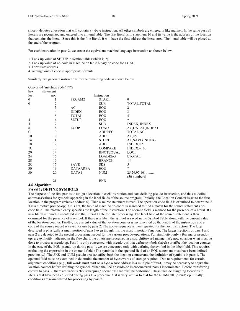
=5 F8 4 R LITERAL 5 =1 FC 4 R LITERAL 1 =50 100 4 R LITERAL 50 We scan the program above keeping a local counter. For each symbol in the label field we make an entry in the symbol table. For the symbol PRGAM2 its value is its relative location. We update the location counter, noting that the each instruction is 4 bytes long. Continuing, we find that the next four symbols are defined by the pseudo-op EQU. These symbols are entered into the symbol to and the associated values given in the argument fields of the EQU statements entered. Note: None of the Pseudo-ops encountered effect location counter since they do not result in any object code.) Thus the location counter has a value 8 when LOOP is encountered. Therefore, LOOP is entered into the symbol table with a value 8. It is a relocatable variable. Its length is 4
CSE 560 Reference Text - Stutz 18 Spring 2009
since it denotes a location that will contain a 4-byte instruction. All other symbols are entered in like manner. In the same pass all literals are recognized and entered into a literal table. The first literal is in statement 10 and its value is the address of the location that contains the literal. Since this is the first literal, it will have the first address the literal area. The literal table will be placed at the end of the program. For each instruction in pass 2, we create the equivalent machine language instruction as shown below. 1. Look up value of SETUP in symbol table (which is 2) 2. Look up value of op-code in machine op table binary op code for LOAD 3. Formulate address 4. Arrange output code in appropriate formula Similarly, we generate instructions for the remaining code as shown below. Generated "machine code" ???? hex statement loc. no. Instruction 0 1 PRGAM2 START 0 0 2 SUB TOTAL,TOTAL - 3 AC EQU 2 - 4 INDEX EQU 3 - 5 TOTAL EQU 4 4 6 SETUP EQU * 4 7 SUB INDEX, INDEX 8 8 LOOP LOAD AC,DATA1(INDEX) C 9 ADDREG TOTAL,AC 10 10 ADD AC,=5 14 11 STORE AC,SAVE(INDEX) 18 12 ADD INDEX,=2 1C 13 COMPARE INDEX,=100 20 14 BNOTEQUAL LOOP 24 15 LOADREG l,TOTAL 28 16 BRANCH 14 2C 17 SAVE SKS 5 30 19 DATAAREA EQU * 30 20 DATA1 NUM 25,26,97,101........... (50 numbers) 21 END 4.6 Algorithm PASS 1: DEFINE SYMBOLS The purpose of the first pass is to assign a location to each instruction and data defining pseudo-instruction, and thus to define addresses/values for symbols appearing in the label fields of the source program. Initially, the Location Counter is set to the first location in the program (relative address 0). Then a source statement is read. The operation-code field is examined to determine if it is a directive pseudo-op; if it is not, the table of machine op-codes is searched to find a match for the source statement's op-code field. The matched entry specifies the length of the instruction. The operand field is scanned for the presence of a literal. If a new literal is found, it is entered into the Literal Table for later processing. The label field of the source statement is then examined for the presence of a symbol. If there is a label, the symbol is saved in the Symbol Table along with the current value of the location counter. Finally, the current value of the location counter is incremented by the length of the instruction and a copy of the source record is saved for use by pass 2. The above sequence is then repeated for the next instruction. The loop described is physically a small portion of pass I even though it is the most important function. The largest sections of pass 1 and pass 2 are devoted to the special processing needed for the various pseudo-operations. For simplicity, only a few major pseudo-ops are explicitly indicated in the flowchart; the others are processed in a straightforward manner. We now consider what must be done to process a pseudo op. Pass 1 is only concerned with pseudo-ops that define symbols (labels) or affect the location counter. In the case of the EQU pseudo-op during pass 1, we are concerned only with defining the symbol in the label field. This requires evaluating the expression in the operand field. (The symbols in the operand field of an EQU statement must have been defined previously.) The SKS and NUM pseudo ops can affect both the location counter and the definition of symbols in pass 1. The operand field must be examined to determine the number of bytes/words of storage required. Due to requirements for certain alignment conditions (e.g., full words must start on a byte whose address is a multiple of two), it may be necessary to adjust the location counter before defining the symbol. When the END pseudo-op is encountered, pass 1 is terminated. Before transferring control to pass 2, there are various "housekeeping" operations that must be performed. These include assigning locations to literals that have been collected during pass 1, a procedure that is very similar to that for the NUM/CHC pseudo op. Finally, conditions are re-initialized for processing by pass 2.

CSE 560 Reference Text - Stutz 19 Spring 2009
Pass 1 Read source file line by line save it in augmented intermediate file (needed for pass 2 report), validate it if symbol check symbol table is it already present? ==> yes==> set error code ==>no==> enter into table enter LC in HEX into table Check instruction does it consume memory ==> yes==> update LC Check Pseudo-op Label? ==> place in symbol table if not already entered Consume memory? ==> yes==> update LC Process as required if END finish up pass 1 check for more records (error) start pass 2 Check syntax of operand field save source line (with added information) for pass 2 appended with LC, op-code, r, s, x, error codes In-between Passes sort symbol table save intermediate source file build general object file information
pass 2: GENERATE CODE After all the symbols have been defined by pass 1, it is possible to finish the assembly by processing each record and determining values for its operation code and its operand field. In addition, pass 2 must structure the generated code into the appropriate format for later processing by the loader, and print an assembly listing containing the original source and the hexadecimal equivalent of the bytes generated. A record is read from the source file left by pass 1. The operation code field is examined to determine if it is a pseudo-op; if it is not, the table of machine op codes (MOT) is searched to find a match for the op-code field. The matching MOT entry specifies the length, binary op-code, and the format type of the instruction. The operand fields of the different instruction format types require somewhat different processing. For the RR-format instructions, each of the two register specification fields is evaluated. This evaluation may be very simple, as in: AR 2,3 [RR Format] MPY 1,EVEN [RX format] MPY 1,EVEN(3) [RX format] or more complex, as in: MPY l,EVEN+EVEN+I MOVE MUD, DIRT [SSI format] MOVE MUD(3),DIRT [SSI format] The two fields are inserted into their respective fields in the RR-instruction. For RX format instructions, the register and index fields are evaluated and processed in the same way as the register specifications for RR-format instructions. The storage address operand is evaluated to generate an Effective Address EA). Only the RR and RX instruction types are explicitly shown in the flow-chart. The other instruction formats are handled similarly. After the instruction has been assembled, it is put into the necessary format for later processing by the loader. Typically, several instructions are placed on a single record. A listing line containing a copy of the source card, its assigned storage location, and its hexadecimal representation is then printed. Finally, the location counter is incremented and processing is continued with the next record. As in pass 1, each of the pseudo-ops calls for special processing. The EQU pseudo-op requires very little processing in pass 2, because symbol definition was completed in pass 1. It is necessary only to print the EQU record as part of the printed listing. The SKS and NUM/CHC pseudo-ops are processed essentially as in pass 1. In pass 2, however, actual code must be generated for the NUM/CHC pseudo-op. Depending upon the data types specified, this involves various conversions (e.g., floating point character to binary representation) and symbol evaluations (e.g., address constants). The END pseudo-op indicates the end of the source program and terminates the assembly. Various "housekeeping" tasks must now be performed." For example, code must be generated for any literals remaining in the Literal Table.

CSE 560 Reference Text - Stutz 20 Spring 2009
Pass 2 Read augmented source file if instruction ==> yes==> instruction use op-code (binary) saved from pass 1 start building binary version of the instruction add r & X field binary convert to hex look up S symbol in symbol/literal table append hex address to end of instruction determine A/R/E...then add A/R/E to end of hex op-code append symbol if E write valid machine code instruction ==> no==> pseudo-op define hex equivalent for CHR, NUM and ADR write valid hex to object file process other pass 2 formatting pseudo ops END finish object file finish output print symbol table Be sure to think about modularization... Look for Modularity We now review our design, looking for functions that can be isolated. Typically, such functions fall into two categories: (1) multi-use and (2) unique. Listed below are some of the functions that may be isolated in the two passes. Look a a common table building/searching, hex integer bit conversions. PASS 1: 1. READ1 Read the next assembly source card. 2. POT_TABLE Search the pass 1 Pseudo-Op Table (POT) for a match with the operation field of the current source
card. 3. MOT_TABLE Search the Machine-Op Table (MOT) for a match with the operation of the current source card. 4. SYM_TABLE Store a label and its associated value into the Symbol Table (ST). If the symbol is already in the
table, return error indication (multiply defined symbol). 5. LIT_TABLE Store a literal into the Literal Table (LT); do not store the same literal twice. 6. WRITE1 Write a copy of the assembly source record on a storage device for use by pass 2. 7 DLENGTH Scan operand field of space consuming pseudo-ops to determine the amount of storage required. 8. EVAL Evaluate an arithmetic expression consisting of constants and symbols (e.g. 6, ALPHA, BETA
+14*GAMMA). 9. STGET Search the Symbol Table (ST) for the entry corresponding to a specific symbol (used by
SYM_TABLE, and EVAL). 10. LIT_LC Assign storage locations to each literal in the literal table (may use DLENGTH). PASS 2 1. READ2 Read the next assembly source record from the file copy. 2. POT_TABLE Same as in pass 1 3. MOT_TABLE Same as in pass 1 (evaluate expressions). 4. EVAL Same as in pass 1 (evaluate expressions). 5. OBJECT Convert generated instruction to object record format; write the record when it is filled with data. 6. PRINT Convert relative location and generated code to character format; print the line along with copy of
the source card. 7. DATAGEN Process the fields of the data-generating pseudo-op to generate object code (uses EVAL). 8. DLENGTH Same as in pass 1. 9. LIT_GEN Generate code for literals (uses DATAGEN). Each of these functions should independently go through the entire design process (problem statement, data basics, algorithm, modularity, etc.). These functions can be implemented as separate external subroutines, as internal subroutines, or as sections of the pass 1 and pass 2 programs. In any case, the ability to tract functions separately makes it much easier to design the structure of the assembler and each of its parts. Thus, rather than viewing the assembler as a single program (of 1,000 to 10,000 source

CSE 560 Reference Text - Stutz 21 Spring 2009
statements), we view it as a coordinated collection of routines each of relatively minor size and complexity. We will not attempt to examine all of these functional routines in detail since they are quite straightforward. There are two particular observations of interest: (1) several of the routines involve the scanning or evaluation of fields (e.g., DLENGTH, EVAL, DATA_GEN); (2) several other routines involve the processing of tables by storing or searching (e.g., POT_TABLE, MOT_TABLE, LIT_TABLE, SYSTO, STGET). Tables: Assemblers rely primarily on Tables. Getting the tables established properly is critical to the development of a straightforward assembler. Most assemblers rely on: Machine Operations table contains all the instructions, binary equivalent, length, and valid instruction format (parsing information). Pseudo-op table that contains all the pseudo-ops length (if necessary), format (parsing information) Symbol Table that contains all program defined labels/variables, length, types (label, numeric, character, address), relative (to start of the program) memory location, and location(s) where used. Literal table (depends on how literal are implemented) which contains all program defined literals, length, type (numeric, character, address), relative (to start of the program) memory location, and location(s) where used. Data Files/Tables name Pass 1 Pass 2 Source reviewed augmented as provided by programmer MOT searched not needed as provided by assembler developer POT searched searched as provided by assembler developer Symbol Table entries made searched format defined by the developers Literal Table entries made searched format defined by the developers Intermediate source created searched Assembler builds this source image plus pass 1 information
CSE 560 Reference Text - Stutz 22 Spring 2009
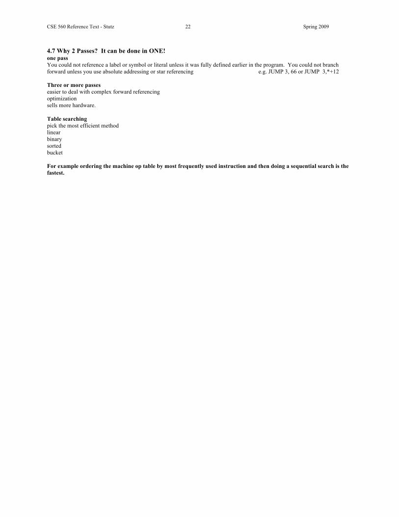
4.7 Why 2 Passes? It can be done in ONE! one pass You could not reference a label or symbol or literal unless it was fully defined earlier in the program. You could not branch forward unless you use absolute addressing or star referencing e.g. JUMP 3, 66 or JUMP 3,*+12 Three or more passes easier to deal with complex forward referencing optimization sells more hardware. Table searching pick the most efficient method linear binary sorted bucket For example ordering the machine op table by most frequently used instruction and then doing a sequential search is the fastest.

CSE 560 Reference Text - Stutz 23 Spring 2009
Chapter 5: Linkers/Loaders The users source programs are usually converted to object program files (machine language) by assemblers and compilers. The linker/loader is a program, which accepts the object program files, integrates the references and performs address adjustments in preparation for these programs to be executed by the computer, and in some cases initiates the execution.
Linker/Loaders -- Why were they Developed?
1. Wanted to increase programmer productivity 2. Independent module compilations 3. Libraries 4. Multi-language program systems 5. Reduced programmer errors 6. Programmers are lazy.... and error prone... They did not like having to code absolute memory addresses into
their code. 7. Operating systems needed to be more in control of memory utilization, to allow more than one user's program
in memory at one time, and wanted to allow the use of libraries. 8. Programmers can’t count
5.1 General Loader Scheme There are various schemes for accomplishing the four functions of a linker/loader It is desirable to introduce the term segment, which is a unit of information that is treated as an entity, be it a program or data. Usually a segment corresponds to a single source procedure, object file, or data segment. In some languages/assemblers it is possible to produce multiple program or data segments in a single source file.
5.2 Subroutine Linkages The problem of subroutine linkage is this: a main program A wishes to transfer to subprogram B. The programmer, in program A, could write a transfer instruction (e g, LINKTO B) to subprogram B. However, the assembler does not know the address of this symbol reference and will declare it as an error (undefined symbol) unless a special mechanism has been provided. The assembler pseudo-op EXTERNAL followed by a list of symbols indicates that the symbols are defined in other programs but referenced in the present program. Correspondingly, if a symbol is defined in one program and referenced in others, we insert it into a symbol list following the pseudo-op ENTRY. In turn, the assembler will inform the loader that other programs may reference these symbols For example, the following sequence of instructions may be simple calling sequence to another program: MAIN START EXTERNAL SUBROUT LINK Reg14, SUBROUT Branch and link to subroutine Reg14 has the return address END The above sequence of instructions first declares SUBROUT as an external variable, that is, a variable referenced but not defined in this program. The load instruction loads the address of that variable into register 15. The LINK instruction branches to the address of SUBROUT, and leaves the address/value of the next instruction in register 14. Programming conventions, are necessary for both the caller and called subprograms to cooperate. Since in our example register 14 contains the address of the return point, we simply need to branch to that address. But before we return we need to be nice and reset the registers back to the values that the calling routine expects.
Loaders must perform four functions: Relocation: Adjust all address dependent locations, such as address constants, to correspond to the
allocated space. Adjusting the addresses of those instructions (or data elements) that require changes if & only if the program is loaded at a different location than the compiler/assembler predicted.
Allocation: Allocate space in memory for the programs. Linking: Resolve symbolic references between object files. Load: The physical operation of placing the code in memory and the signal to start execution
and providing the execution start address.

CSE 560 Reference Text - Stutz 24 Spring 2009
SUBROUT START Backup registers Restore Registers Return to calling program END 5.3 Multiple Entry Points The uses of multiple entry points are: 1. Common coding practice Example: SIN and COS involve basically the same computations and could employ different entry points of
the same routine. 2. Collecting together related routines for convenience 3. Better or convenient access to common data base 5.4 Relocation There is an intentional disconnect between translators and operating systems. As memory systems grew in size and the operating system was truly able to handle multiple user tasks “executing at the same time” there was no need for a solid connection between the translator and the OS. This means that the translator must assume a memory load point. If it disagrees with the next available location, the linker/loader must relocate all the addresses to adapt to the new memory start location. 5.5 Linker/Loaders in Conjunction with Compilers and Libraries The relationship between compilers and linker/loads has evolved over the years. As programmers sought more features compilers were enhanced to provide more information about the module in order to make the linker/loader easier to write and provide additional features. Probably the most important one is the ability to reference libraries of independent code either in source, object, or load format. Typically these procedures were common libraries that were to be shared in across the company. In some cases the procedures were set into a shared address location in memory so that many programs running concurrently could share these memory resident modules. On the next several pages you will see the evolution as as libraries at various levels were added to the compilation/link/load process. 5.6 CASES representing Evolution of Linker/Loaders 5.6.1 Case 1: Initial Case Absolute Loader Absolute Loader Loaded exactly where the assembler assumed the program would be loaded. Memory can only have one active program in memory and it all had to fit! 5.6.2 Case 2: Multiple Programs in the same Language A single program with more than one routine can be UNIFIED to appear to be one program. Without making the programmer determine and set the link addresses. Program(s) could be compiled/assembled and the object file saved so that subsequent executions would not require compilation.
translator
Object file On DISK Loader Memory
translator
Object file On DISK
Linker loader
translator
Object file On DISK
Memory
CSE 560 Reference Text - Stutz 25 Spring 2009
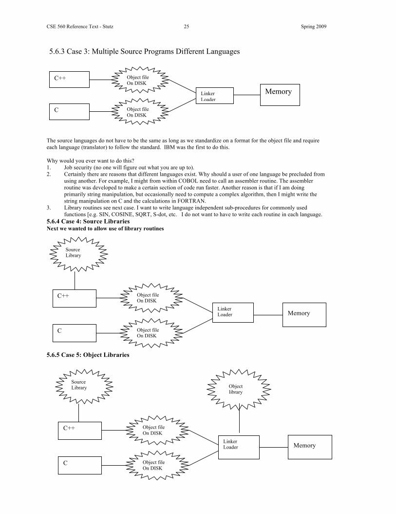
5.6.3 Case 3: Multiple Source Programs Different Languages The source languages do not have to be the same as long as we standardize on a format for the object file and require each language (translator) to follow the standard. IBM was the first to do this. Why would you ever want to do this? 1. Job security (no one will figure out what you are up to). 2. Certainly there are reasons that different languages exist. Why should a user of one language be precluded from
using another. For example, I might from within COBOL need to call an assembler routine. The assembler routine was developed to make a certain section of code run faster. Another reason is that if I am doing primarily string manipulation, but occasionally need to compute a complex algorithm, then I might write the string manipulation on C and the calculations in FORTRAN.
3. Library routines see next case. I want to write language independent sub-procedures for commonly used functions [e.g. SIN, COSINE, SQRT, S-dot, etc. I do not want to have to write each routine in each language.
5.6.4 Case 4: Source Libraries Next we wanted to allow use of library routines 5.6.5 Case 5: Object Libraries
C++
Object file On DISK
Linker Loader
Memory
C
Object file On DISK
C++
Object file On DISK
Linker Loader
C
Object file On DISK
Memory
Source Library
C++
Object file On DISK
Linker Loader
C
Object file On DISK
Memory
Source Library Object
library

CSE 560 Reference Text - Stutz 26 Spring 2009
5.6.6 Case 6: Load Libraries 5.7 Library Concepts The library concept provides computer centers the opportunity to establish standard routines for commonly needed functions or to isolate functions that are constantly under change so that the changes could be done in a single routine. FOR EXAMPLE: Suppose that your company has a corporate database that is constantly evolving in size and number of data-elements. There are 200 programs that need to read the data. Rather than having to modify 200 programs each and every time elements are added. We can simply write a company standard routine to read the database and return the requested elements. Thus only one routine would need to be changed and tested. OK if I can save the object file and avoid constant re-compilations why can't I save some of the work that the loader does. Three of the loader functions are dependent on where in memory the program is assigned [relocation, allocation, and linking]. Loading can be done independent of the other functions. So I can break the loader into a binder (to do the linking) & a module loader to do the other functions. By placing the load module on disk, I no longer have to go through this step of the process. Just like I no longer have to compile each and every time. This saves me time. It may not appear important to you right now to go through all these hoops to save a small amount of time. However in an on-line interactive environment time saved reduces overhead, improves response times [ users are expecting response times of less than 1 second regardless of the complexity], and allows more users to use the system. Finally, if all the source program translators (assemblers and compilers) produce compatible object program file formats and use compatible linkage conventions, it is possible to write subroutines in several different languages since the object files to be processed by the loader will all be in the same "language" (machine language). 5.8 Linker/Loader Optional Features Linkers/Loaders will many times allow users to provide additional information or request particular features. These are typical requested via the command line or through a separate data file. These features include but are not limited to: different reports, overlay designs, dynamic linking, library locations, debugging features etc.
C++
Object file On DISK
Linker Loader
C
Object file On DISK
Memory
Source Library Object
library Load library
Load file
Module Loader

CSE 560 Reference Text - Stutz 27 Spring 2009
5.9 Absolute Loader The simplest type of loader is the absolute loader. The first attempt at a loader! As you will learn loaders have gone through an evolution forward and backwards. Many of the functions of a loader really end up being shared between the translator and the loader. The translator must prepare the data in an easy to use format with all the right data. With this in mind for each loader you need to answer who does the 4 basic functions or how are these functions really shared. Absolute Loader the first real loader was just that a loader. The only real computational function it provided was the loading of the code into memory and starting the execution at the right place. Advantages
1. Simple to implement 2. fast
Disadvantages
1. The programmer must specify to the assembler the address in core where the program is to be loaded. 2. The programmer must remember the address of each subroutine and use that absolute address explicitly in
other subroutines to perform subroutine linkage. 3. May lead to wasted memory since the programmer may not have calculated the memory exactly. 4. May lead to errors (see above). 5. If you must modify your source code and the module length changes, you may have to go through all your
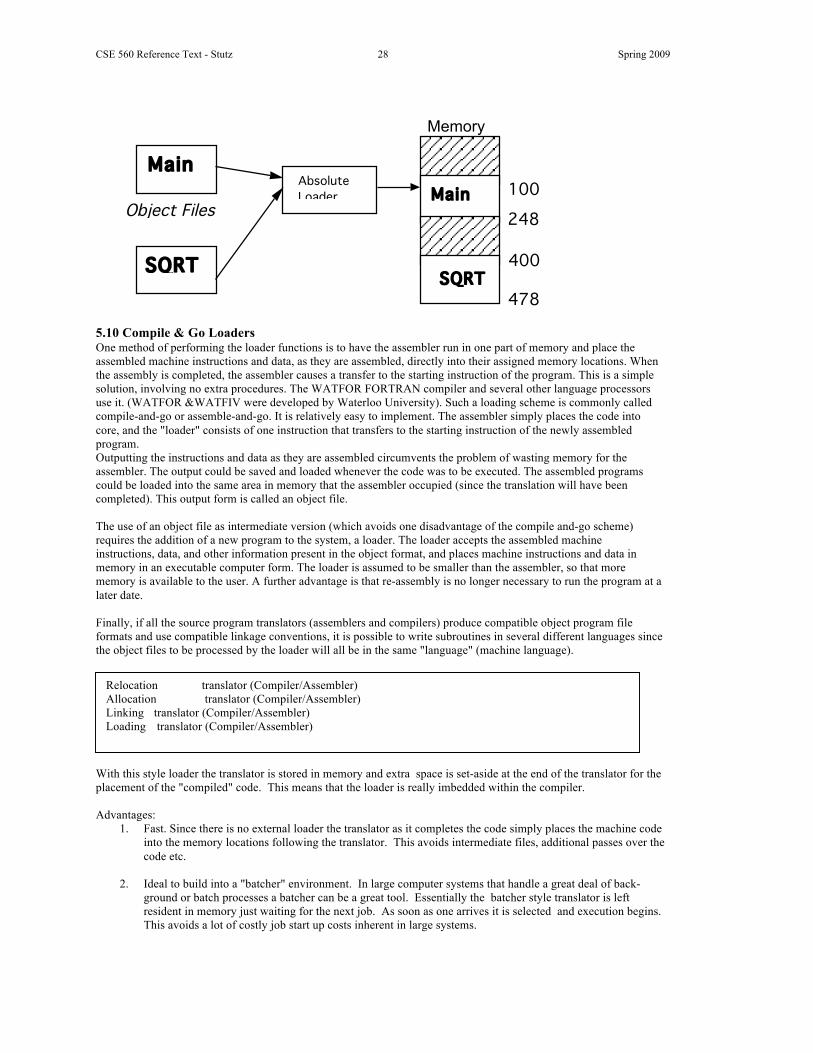
code looking for linkages See the illustration of the operation of an absolute assembler and an absolute loader. The programmer must be careful not to assign two subroutines to the same or overlapping locations The MAIN program is assigned to location 100-247 and the SQRT subroutine is assigned locations 400-477. If changes were made to MAIN that increased its length to more than 300 bytes, the end of MAIN (at 100 + 300 = 400) would overlap the start of SQRT (at 400) It would then be necessary to assign SQRT to a new location by changing its START pseudo-op record and re-assembling it. Furthermore, it would also be necessarily to modify all other subroutines that referred to the address of SQRT. In situations where dozens of subroutines are being used, this manual "shuffling" can get very complex, tedious, and wasteful of core.
Absolute Loader Relocation This is done by the translator but only because the programmer has dictated the actual load
address so the translator uses the numbers provided by the programmer. Allocation Done by the programmer. The programmer must determine the length required by all the
modules and determine whether or not they will all fit. Programmers must also select the actual location in memory that the code will be placed. This leads to errors since programmers are terrible with numbers.
Linking Done by the programmer. If one program calls another or uses an external variable, the
programmer must determine the actual location and "hard-code" the address. This will also lead to errors.
Loading This is done by the LOADER
CSE 560 Reference Text - Stutz 28 Spring 2009
5.10 Compile & Go Loaders One method of performing the loader functions is to have the assembler run in one part of memory and place the assembled machine instructions and data, as they are assembled, directly into their assigned memory locations. When the assembly is completed, the assembler causes a transfer to the starting instruction of the program. This is a simple solution, involving no extra procedures. The WATFOR FORTRAN compiler and several other language processors use it. (WATFOR &WATFIV were developed by Waterloo University). Such a loading scheme is commonly called compile-and-go or assemble-and-go. It is relatively easy to implement. The assembler simply places the code into core, and the "loader" consists of one instruction that transfers to the starting instruction of the newly assembled program. Outputting the instructions and data as they are assembled circumvents the problem of wasting memory for the assembler. The output could be saved and loaded whenever the code was to be executed. The assembled programs could be loaded into the same area in memory that the assembler occupied (since the translation will have been completed). This output form is called an object file.
The use of an object file as intermediate version (which avoids one disadvantage of the compile and-go scheme) requires the addition of a new program to the system, a loader. The loader accepts the assembled machine instructions, data, and other information present in the object format, and places machine instructions and data in memory in an executable computer form. The loader is assumed to be smaller than the assembler, so that more memory is available to the user. A further advantage is that re-assembly is no longer necessary to run the program at a later date. Finally, if all the source program translators (assemblers and compilers) produce compatible object program file formats and use compatible linkage conventions, it is possible to write subroutines in several different languages since the object files to be processed by the loader will all be in the same "language" (machine language).
With this style loader the translator is stored in memory and extra space is set-aside at the end of the translator for the placement of the "compiled" code. This means that the loader is really imbedded within the compiler. Advantages:
1. Fast. Since there is no external loader the translator as it completes the code simply places the machine code into the memory locations following the translator. This avoids intermediate files, additional passes over the code etc.
2. Ideal to build into a "batcher" environment. In large computer systems that handle a great deal of back-
ground or batch processes a batcher can be a great tool. Essentially the batcher style translator is left resident in memory just waiting for the next job. As soon as one arrives it is selected and execution begins. This avoids a lot of costly job start up costs inherent in large systems.
Main
SQRT
Absolute Loader Main
SQRT
Object Files 100
400 248
478
Memory
Relocation translator (Compiler/Assembler) Allocation translator (Compiler/Assembler) Linking translator (Compiler/Assembler) Loading translator (Compiler/Assembler)

CSE 560 Reference Text - Stutz 29 Spring 2009
Disadvantages
1. Must re-compile every time. No way to save an object version or load module. 2. a portion of memory is wasted because the memory occupied by the assembler is unavailable to the object
program. 3. Requires additional memory since the compiler and the code being compiled must both reside in memory. 4. Standard subroutine libraries must be source based rather than object code. 5. It is very difficult to handle multiple segments, especially if the source programs are in different languages
(e.g.,. one subroutine in assembly language and another subroutine in FORTRAN. This last disadvantage makes it very difficult to produce orderly modular programs as discussed in the design of assemblers.
5.11 Relocating Loaders General It wasn't long before management and programmers learned that programmers really couldn't add, so the absolute loader needed to be improved. Relocating loaders took more responsibility for allocation, linking, and relocation. 5.12 BSS:Relocating Loaders Binary Symbolic Subroutine (BSS) Loader was one of the first in about 1956. Before relocating loaders programmers could not easily write modules in different languages. The BSS loaders permit multiple program segments in different languages to be compiled at different times. It required all the translators to produce a common object file format. BSS loaders also allowed the development of independent (and separate) data segments [FORTRAN BLOCK DATA) To avoid possible re-assembling of all subroutines when a single subroutine is changed, and to perform the tasks of allocation and linking for the programmer, the general class of relocating loaders was introduced An example of a relocating loader scheme is that of the Binary Symbolic Subroutine (BSS) loader such as was used in the IBM 7094, IBM 1130, GE 635, and UNIVAC 1108. The BSS loader allows many procedure segments, yet only one data segment (common segment). The assembler assembles each procedure segment independently and passes on to the loader the text and information as to relocation and inter-segment references.
The output of a relocating assembler using a BSS scheme is the object program and information about all other program it references. In addition, there is information (relocation information) as to locations in this program that need to be changed if it is to be loaded in an arbitrary place in memory, i.e. the locations which are dependent on the core allocation. For each source program the assembler outputs a text (machine translation of the program) prefixed by a transfer vector that consists of addresses containing names of the subroutines referenced by the source program For example, if a Square Root Routine (SQRT) was referenced and was the first subroutine called, the first location in the transfer vector could contain the symbolic name SQRT. The statement calling SQRT would be translated into a transfer instruction indicating a branch to the location of the
A
Source Libraries
Memory
User assigned memory
Compiler Compile & go Translator
Program
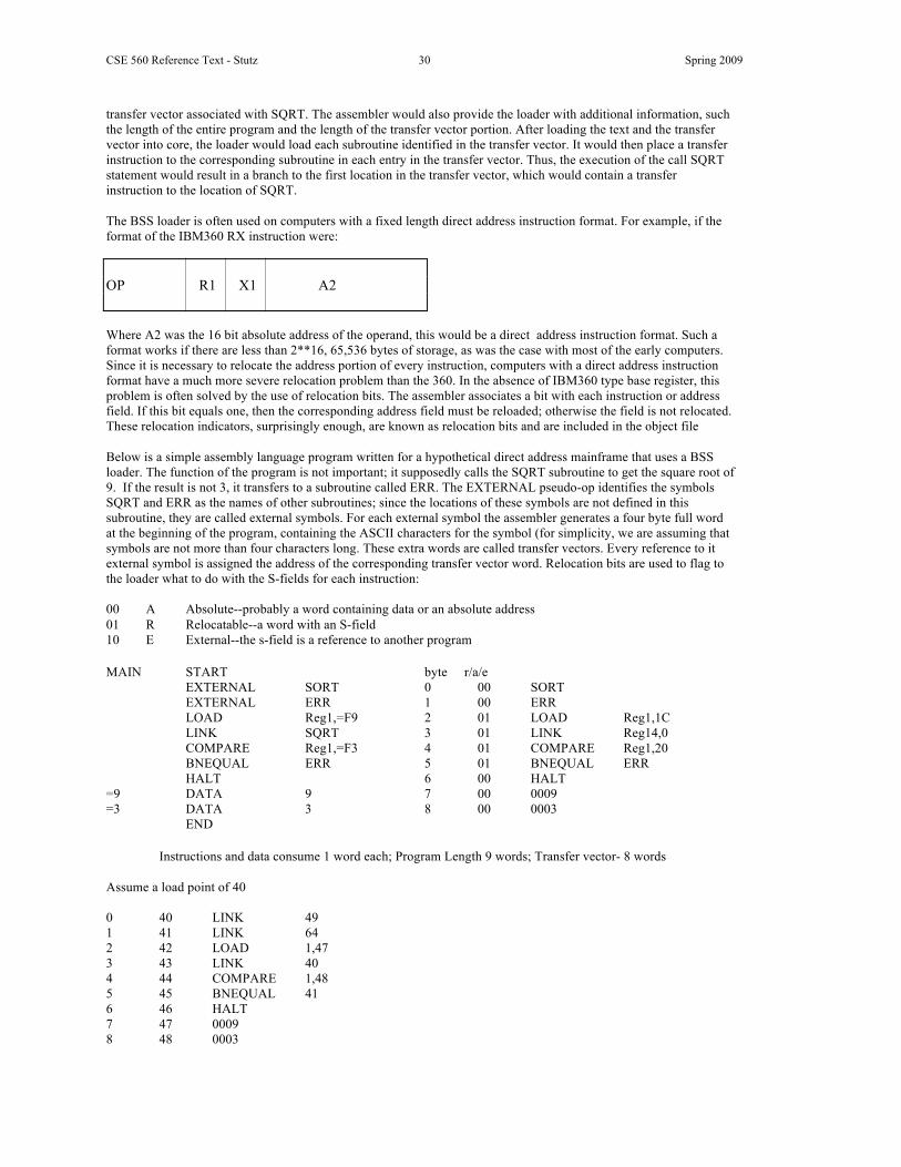
CSE 560 Reference Text - Stutz 30 Spring 2009
transfer vector associated with SQRT. The assembler would also provide the loader with additional information, such the length of the entire program and the length of the transfer vector portion. After loading the text and the transfer vector into core, the loader would load each subroutine identified in the transfer vector. It would then place a transfer instruction to the corresponding subroutine in each entry in the transfer vector. Thus, the execution of the call SQRT statement would result in a branch to the first location in the transfer vector, which would contain a transfer instruction to the location of SQRT. The BSS loader is often used on computers with a fixed length direct address instruction format. For example, if the format of the IBM360 RX instruction were: OP R1 X1 A2 Where A2 was the 16 bit absolute address of the operand, this would be a direct address instruction format. Such a format works if there are less than 2**16, 65,536 bytes of storage, as was the case with most of the early computers. Since it is necessary to relocate the address portion of every instruction, computers with a direct address instruction format have a much more severe relocation problem than the 360. In the absence of IBM360 type base register, this problem is often solved by the use of relocation bits. The assembler associates a bit with each instruction or address field. If this bit equals one, then the corresponding address field must be reloaded; otherwise the field is not relocated. These relocation indicators, surprisingly enough, are known as relocation bits and are included in the object file Below is a simple assembly language program written for a hypothetical direct address mainframe that uses a BSS loader. The function of the program is not important; it supposedly calls the SQRT subroutine to get the square root of 9. If the result is not 3, it transfers to a subroutine called ERR. The EXTERNAL pseudo-op identifies the symbols SQRT and ERR as the names of other subroutines; since the locations of these symbols are not defined in this subroutine, they are called external symbols. For each external symbol the assembler generates a four byte full word at the beginning of the program, containing the ASCII characters for the symbol (for simplicity, we are assuming that symbols are not more than four characters long. These extra words are called transfer vectors. Every reference to it external symbol is assigned the address of the corresponding transfer vector word. Relocation bits are used to flag to the loader what to do with the S-fields for each instruction: 00 A Absolute--probably a word containing data or an absolute address 01 R Relocatable--a word with an S-field 10 E External--the s-field is a reference to another program MAIN START byte r/a/e EXTERNAL SORT 0 00 SORT EXTERNAL ERR 1 00 ERR LOAD Reg1,=F9 2 01 LOAD Reg1,1C LINK SQRT 3 01 LINK Reg14,0 COMPARE Reg1,=F3 4 01 COMPARE Reg1,20 BNEQUAL ERR 5 01 BNEQUAL ERR HALT 6 00 HALT =9 DATA 9 7 00 0009 =3 DATA 3 8 00 0003 END Instructions and data consume 1 word each; Program Length 9 words; Transfer vector- 8 words Assume a load point of 40
0 40 LINK 49 1 41 LINK 64 2 42 LOAD 1,47 3 43 LINK 40 4 44 COMPARE 1,48 5 45 BNEQUAL 41 6 46 HALT 7 47 0009 8 48 0003

CSE 560 Reference Text - Stutz 31 Spring 2009
Based upon the relocation bits, the loader has relocated the address fields to correspond to the allocated address of MAIN, which is loaded at 40. Using the program length information, the loader placed the subroutines SQRT and ERR at the next available location which were 49 and 64, respectively. The transfer vector words were changed to contain branch instructions to the corresponding routines. The four functions of the loader (allocation, linking, relocation, and loading were all performed automatically by the BSS loader. The relocation bits are used to solve the problem of relocation; the transfer vector is used to solve the problem of linking; and the program length information is used to solve the problem of allocation. The disadvantages of the BSS loader scheme.
1. The transfer vector linkage is only useful for transfers, and is not well suited for loading or storing external data (data located in another procedure segment)
2. The transfer vector increases the size of the object program in memory 3. The BSS loader, as described, processes procedure segment but does not facilitate access to data segments
that can be shared. This last shortcoming is overcome in many BSS loaders by allowing one common data segment, often called COMMON. This facility is usually implemented by extending the relocation bits scheme to use 2 bits per half word address field if the bits are 01, the half word is relocated relative to the procedure segment, and if they are 10, it is relocated relative to the address of the single common data segment. If the bits are 00 or 11, the half word is not relocated.
The translator and the loader do LINKING as a joint activity by use of the TRANSFER VECTOR.
TRANSFER Vector (TV). The translator set asides an area at the start of each object file to serve as a TV area. The
purpose of the TV is to isolate linking commands to a specific area. For example consider the following program.
Program A1 .. .. .. .. .. ..
CALL Test
call Testreturn to main pgm
branch to TV entry 1a=b+ca=b+c
BSS Linker/Loader Relocation This is done by flagging each and every word as to what needs to be done. The flagging
is done through relocation bits. Similar to our fifth column. 00 no relocation required 01 relocation [add the load point to this address] 10 External Reference 11 no relocation required Allocation Linker figures out the amount of memory needed for the job and works with the
operating system to determine where the code should be placed in memory. The translator must provide the length of each module....[The loader simply adds up the length of the modules]
Linking Transfer Vector Loading Done by the BSS loader

CSE 560 Reference Text - Stutz 32 Spring 2009
5.13 Direct Linking Loader DLL The most recent linker/loader design. Allows Multiple Modules using multiple languages and data A direct linking loader is a general relocatable loader, and it perhaps the most popular loading scheme presently used. The direct linking loader has the advantage of allowing the programmer multiple procedure segments and multiple data segments and of giving complete freedom in referencing data or instructions combined in other segments. This provides flexible inter-segment referencing and accessing ability, while at the same time allowing independent transactions of programs. A general form for the assembler output with such a loading scheme is patterned after those used in the IBM mainframe. The formats themselves are somewhat arbitrary, the information that the assembler must give to the loader is not. The assembler (translator) must give the loader the following information with each procedure or data segment
1. The length of segment 2. A list of all the symbols in the segment that may be referenced by other segments and their relative location
within the segment (entries) 3. A list of all symbols not defined in the segment but referenced in the segment (external) 4. Information as to where address constants are loaded in the segment and a description of how to revise their
values. The machine code translation of the source program and the relative addresses assigned 5. The TEXT 6. End of Program delimiter
DLL Linker Loader Relocation Loader with help from the translator.. translator provides list of locations needing relocation Allocation Loader with help from the translator – length Linking Loader translator provides list Loading Loader

CSE 560 Reference Text - Stutz 33 Spring 2009
Pass 1 Activities • Scan for start of segments place in symbol table calculate load point • Scan for Entries place in symbol table (header record) • Calculate load points of each program • Validate input • Hex where it is suppose to be HEX • Records in order 1,2.....2,3 • Label Problems • Duplicate Labels • Build Symbol table
Pass 2 Activities • Calculate memory locations for text
o (IPLA + type 2 record addr = memory location) • Scan the text for Externals. look up in GEST (Global External Symbol Table) and get the right address • When finished with all segments set execution start address using the type 3 record from the first program.
GEST Table: What entries are needed? • Program names • Symbols flagged as entry • Relative location • Translator Assigned load point • Linker adjusted load point • Usage
Most DLL have the following record types:
• ESD External Symbol Dictionary o Modules names, Entries, Externals
• TXT Text cards • RLD Relocation and linking Directory
o Additional Adjustments due to external references or address arithmetic • END Delimiter • EOF
Program Relocation Suppose that there are many programs in memory being executed and a new program needs to be placed in memory
Operating system
04 Program A
Program B50
100 Program C
150
But D was assembled assuming the D would be loaded at 4 NOT 150. What do we need to change? Check the relocation indicator if the address needs to be adjusted simply look up the name of the module in the GEST and pick up the load point. Add the load point to each address Binder
Dividing the load process into two pieces where the activities of linking, allocation, and partially relocation are done independent of the loading.
Module Loader does the second piece Final relocation Loading

CSE 560 Reference Text - Stutz 34 Spring 2009
Together these two pieces are sometimes called the LINKAGE EDITOR 5.14 Address Calculations Absolute addr1 - addr 2 both are within the same module Simple Relocatable addr- number The assembler can calculate relative differences addr + number and then the loader simply adds the module load point. Complex Relocatable addr1+addr2-addr3+12 where 1 is module 1 etc... Assembler can do some of the work but the loader may have to adjust the address several times. Typical information from a loader
1. Load Map (all entries points and all labels declared entry) 2. Module total length 3. Execution start address 4. Load address
Below is a simple example using a direct-linking loading scheme. A source program (left hand column) is translated by an assembler in order to produce the object code in the right column. John START ENTRY RESULT EXTERNAL SUM LOAD Reg1,POINTER 0 LOAD 1,9 LINK ASUM 1 Link B STORE Regl,RESULT 2 STORE 1,A HALT 3 HALT TABLE DATA 1,7,9,10,13 4 00000001 5 00000007 6 00000009 7 0000000A 8 0000000D POINTER DATA ADDR(TABLE) 9 00000010 RESULT NUM 0 A 00000000 ASUM DATA ADDR(SUM) B ???? EXTERNAL END The DATA ADDR(TABLE) pseudo-operation instructs the assembler to create a constant with the value of the address of TABLE, and causes this constant to be placed in the location labeled POINTER. At this point the assembler does not know the final absolute address of TABLE since it has no idea where the program is going to be loaded. It knows, however, that the address the 9th word from the beginning of the program. The assembler will put a 1016 in POINTER and inform the loader that the content of location POINTER is incorrect if this program is loaded anywhere except absolute location 0. For instance, if this program were loaded in location 2000, the loader would have to change the contents of POINTER to be a 201016 The DATA ADDR(SUM) pseudo-op, which instructs the assembler to create a constant with the value of the address of the subroutine SUM and cause the constant to be placed in the location labeled ASUM. Since the assembler has no idea where the procedure SUM will be loaded, it cannot generate this constant. Thus, the assembler must provide information to the loader that will cause it to put the real absolute address of SUM at the designated location (ASUM) when the programs are loaded We have named the program JOHN. Hence, JOHN is a symbol that may be referenced externally or "called" by other programs. We also have stated that other programs may reference the symbol RESULT. These facts must be passed on to the loader. The design of the direct linking loading scheme presented is similar to the standard IBM mainframe scheme. The assembler produces four types of records in the object file ESD, TXT, RLD, and END. External Symbol Dictionary (ESD) records combine information about all symbols that are defined in this program but that may be referenced elsewhere, and all symbols referenced in this program but defined elsewhere. The text (TXT) records control the actual object code translated version of the source program. The Relocation and Linkage Directory (RLD) records contain information about those locations in the program whose contents depend on the address at which the program is placed. For such locations the assembler must supply information enabling the loader to correct their

CSE 560 Reference Text - Stutz 35 Spring 2009
contents. The END record indicates the end of the object file and specifies the starting address for execution if the assembled routine is the "main" program. The information that would appear for the preceding program on the ESD, TXT, RLD, and END records is shown. The reference numbers do not actual appear on the records. They are for the benefit of the reader, since each denotes the record number of the original program that resulted in the object file record; e.g., the first RLD record resulted from record number 14 in the original program. Three ESD records are needed for the program JOHN. The first record contains the name of the program JOHN, which may be referenced externally. The "type" mnemonic we have used is SD, which means the symbol has Segment Definition. The relative address of JOHN is O, and the length of the program that JOHN denotes is C16. On the next ESD record appears the symbol RESULT, which is a Local Definition (LD); its relative address is A16. The final ESD record specifies that the symbol SUM is an External Reference (ER). We will read in a later section how the ER symbols are actually used in conjunction with the RLD records. The TXT records contain the actual assembled program. The format and use of the records are similar to those for the absolute loader. The RLD records contain the following information:
1. The location of each constant that needs to be changed due to relocation 2. By what it has to be changed 3. The operation to be performed
ESD records symbol type Address Length JOHN PGM_NAME 0 C words RESULT LOCAL_SYM A 1 word SUM External_sym unknown unknown TXT records Relative location
"object" code
0 LOAD 1,916 1 Link B16 2 STORE 1,A16 3 HALT 4 0000000116 5 0000000716 6 0000000916 7 0000000A16 8 0000000D16 9 0000001016 A 0000000016 B ???????? External RLD record Symbol Flag Length Relative Location JOHN + 1 word 4 bytes 016 JOHN + 1 word 4 bytes 216 JOHN + 1 word 4 bytes 916 SUM + 1 word 4 bytes B16 The first RLD record of the example contains a plus sign denoting that something must be added to the constant; and the symbol field indicating that the value of external symbol JOHN must be added to relative location 016. The relative value of JOHN is 0. When the program is loaded, the loader will determine its absolute value. The second RLD record of our example contains a 2C16, denoting the relative location of a constant that must be changed. The symbol field indicates that the value of the external symbol SUM must be added to relative location B16. Although the assembler does not know the absolute address of SUM, the loader will later be asked to find the correct value. The process of adjusting the address constant of an internal symbol, such as TABLE, is normally called relocation; while the process of applying the contents of an address constant for an external symbol, such as SUM, is normally referred to as linking. Significantly, the RLD record mechanism used for both cases, which explains why they are called relocation and linkage directories records. The reader may wish to compare this technique with the mechanisms used in the BSS relocating loader described earlier.

CSE 560 Reference Text - Stutz 36 Spring 2009
5.15 Linking/Binding There are numerous variations to the previously presented loader schemes. One disadvantage of the direct linking loader is that it is necessary to allocate, relocate, link, and load all of the subroutines each time in order to execute a program. Since there may be tens and often hundreds of subroutines involved, especially when we include utility routines such as SQRT, etc., this loading process can be extremely time consuming. Furthermore, even though the loader program may be smaller than the assembler, it does absorb a considerable amount of space. Dividing the loading process into two separate programs a binder and a module loader can solve these problems. A binder is a program that performs the same functions as the direct linking loader in "binding" subroutines together, but rather than placing the relocated and linked text directly into memory, it outputs the text in a file. This output file is in a format ready to be loaded and is typically called a load module. The module loader merely has to physically load the module into core. The binder essentially performs the functions of allocation, relocation, and linking; the module loader merely performs the function of loading. There are two major classes of binders. The simplest type produces a load module that looks very much like a single absolute loader file. This means that the specific core allocation of the program is performed at the time that the subroutines are bound together. Since this kind of module looks like an actual "snapshot" or "image" of a section of core, it is called a core image module and the corresponding binder is called a core image builder. A more sophisticated binder, called a link editor, can keep track of the relocation. Information that the resulting load module can be further relocated must be contained within the module and thereby loaded anywhere in core. In this case the module loader must perform additional allocation and relocation as well as loading, but it does nothing to worry about the complex problems of linking. In both cases, a program that is to be used repeatedly need only be bound once and then can be loaded whenever required. The memory image builder binder is relatively simple and fast. The linkage editor binder is somewhat more complex but allows a more flexible allocation and loading scheme. 5.16 Dynamic Loading (overlay) When you have limited memory space how can you fit in a program larger than the memory space?
Main Program
Sub A
Sub B
Sub C
Subroutine D
Subroutine
E
I have room for Main A, B, & C or main, D, E but not all of them. I need to examine the structure of the program to see if this segregation makes sense. I must be sure that all globally needed symbols are within the main program or some other common routine. 5.17 Dynamic Loading In each of the previous loader schemes we have assumed that all of the subroutines needed are loaded into core at the same time. If the total amount of core required by all these subroutine exceeds the amount available, as is common with large programs or small computers, there is trouble! There are several hardware techniques, such as paging and segmentation that attempts to solve the problem. Conventional dynamic loading schemes based upon the use of a binder prior to loading. Usually the subroutines of a program are needed at different times for example, pass 1 and pass 2 of an assembler are mutually exclusive. By explicitly recognizing which subroutines calls other subroutines it is possible to produce an overlay structure that identifies mutually exclusive subroutines. Suppose a program consisting of five subprograms (A{20k}, B{20k}, C{30k}, D{10k}, and E{20k}) that require 100K bytes of core. Subprogram A only calls B, D and

CSE 560 Reference Text - Stutz 37 Spring 2009
E; subprogram B only calls C and E; subprogram D only calls E; and subprogram C and E does not call any other routines. Note that procedures B and D are never in used the same time; neither are C and E. If we load only those procedures that are actually to be used at any particular time, the amount of core needed is equal to the longest path of the overlay structure. This happens to be 70K for the example. In order for the overlay structure to work it is necessary for the module loader to load the various procedures as they are needed. There are many binders capable of processing and allocating an overlay structure. The portion of the loader that actually intercepts the "calls" and loads the necessary procedure is called the overlay supervisor or simply the flipper. A major disadvantage of all of the previous loading schemes is that it a subroutine is referenced but never executed (e.g., if the programmer had placed a call statement in the program but this statement was never executed because of a condition that branched around it), the loader would still incur the overhead or linking the subroutine. Furthermore, all of these schemes require the programmer to explicitly name all the procedures that might be called. 5.18 Dynamic Linking In a highly interactive environment we want to reduce delays as much as possible. One way is to only load a module if the logic of the program is such that it is called. Without being called or needed the module never enters the load process. Good for seldom used routines.. Program must help select the candidates just as they do for the Overlay structure. A general type of loading scheme is called dynamic linking. This is a mechanism by which loading and linking of external references are postponed until execution time. The assembler produces text, binding, and relocation information from a source language file. The loader loads only the main program. If the main program should execute a transfer instruction to an external address, or should reference an external variable (that is, a variable that has not been determined in this procedure segment), the loader is called. Only then has the segment containing the external reference loaded. An advantage here is that no overhead is incurred unless the procedure to be called or referenced is actually used. A further advantage is that the system can be dynamically reconfigured. The major drawback to using this type of loading scheme is the considerable overhead and complexity incurred, due to the fact that we have postponed most of the binding process until execution time. 5.19 Design of an Absolute Loader With an absolute loading scheme the programmer and the assembler perform the tasks of location, relocation, and linking. Therefore, it is only necessary for the loader to read records of the object file and move the text on the records into the absolute locations specified by the assembler. There are 2 types of information that the object file must accommodate from the assembler to the loader. First, it must convey the machine instructions that the assembler has created along with the assigned core locations. Second, it must convey the entry point of the program, which is where the loader is to transfer control when all instructions are loaded. The algorithm for an absolute loader is quite simple. The object file for this loader consists of a series of text records terminated by a transfer record Therefore, the loader should read one record at a time, moving the text to the location specified on the record, until the transfer record is reached. At this point the assembled instructions are in core, and it is only necessary to transfer to the entry point specified on the transfer record. A flowchart for this process is illustrated below.
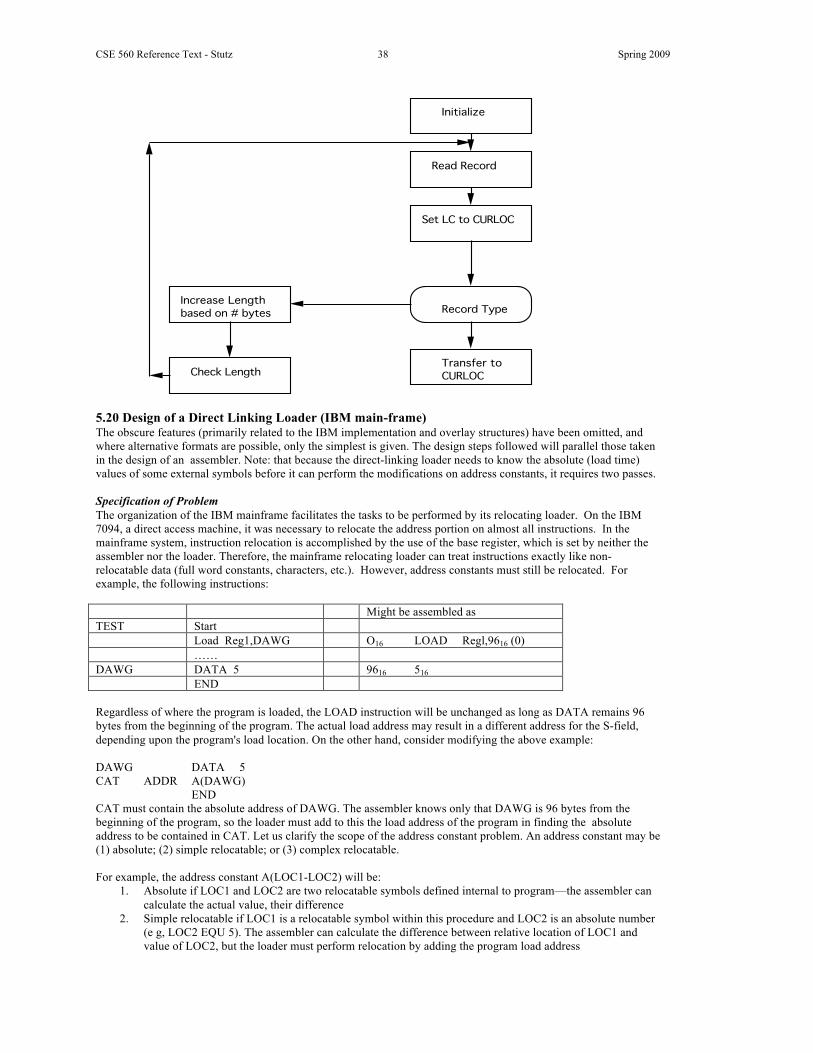
CSE 560 Reference Text - Stutz 38 Spring 2009
Record Type
Transfer toCURLOC
Increase Lengthbased on # bytes
Check Length
Set LC to CURLOC
Read Record
Initialize
5.20 Design of a Direct Linking Loader (IBM main-frame) The obscure features (primarily related to the IBM implementation and overlay structures) have been omitted, and where alternative formats are possible, only the simplest is given. The design steps followed will parallel those taken in the design of an assembler. Note: that because the direct-linking loader needs to know the absolute (load time) values of some external symbols before it can perform the modifications on address constants, it requires two passes. Specification of Problem The organization of the IBM mainframe facilitates the tasks to be performed by its relocating loader. On the IBM 7094, a direct access machine, it was necessary to relocate the address portion on almost all instructions. In the mainframe system, instruction relocation is accomplished by the use of the base register, which is set by neither the assembler nor the loader. Therefore, the mainframe relocating loader can treat instructions exactly like non-relocatable data (full word constants, characters, etc.). However, address constants must still be relocated. For example, the following instructions: Might be assembled as TEST Start Load Reg1,DAWG O16 LOAD Regl,9616 (0) …… DAWG DATA 5 9616 516 END Regardless of where the program is loaded, the LOAD instruction will be unchanged as long as DATA remains 96 bytes from the beginning of the program. The actual load address may result in a different address for the S-field, depending upon the program's load location. On the other hand, consider modifying the above example:
DAWG DATA 5 CAT ADDR A(DAWG) END CAT must contain the absolute address of DAWG. The assembler knows only that DAWG is 96 bytes from the beginning of the program, so the loader must add to this the load address of the program in finding the absolute address to be contained in CAT. Let us clarify the scope of the address constant problem. An address constant may be (1) absolute; (2) simple relocatable; or (3) complex relocatable. For example, the address constant A(LOC1-LOC2) will be:
1. Absolute if LOC1 and LOC2 are two relocatable symbols defined internal to program—the assembler can calculate the actual value, their difference
2. Simple relocatable if LOC1 is a relocatable symbol within this procedure and LOC2 is an absolute number (e g, LOC2 EQU 5). The assembler can calculate the difference between relative location of LOC1 and value of LOC2, but the loader must perform relocation by adding the program load address
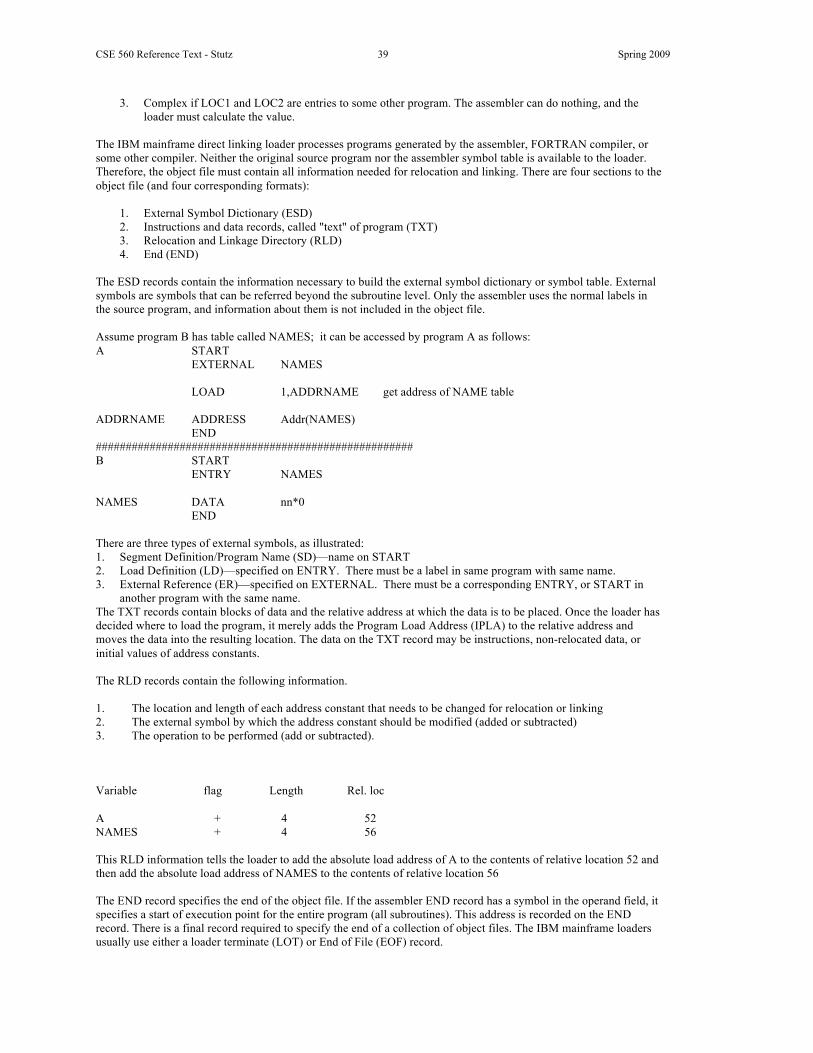
CSE 560 Reference Text - Stutz 39 Spring 2009
3. Complex if LOC1 and LOC2 are entries to some other program. The assembler can do nothing, and the loader must calculate the value.
The IBM mainframe direct linking loader processes programs generated by the assembler, FORTRAN compiler, or some other compiler. Neither the original source program nor the assembler symbol table is available to the loader. Therefore, the object file must contain all information needed for relocation and linking. There are four sections to the object file (and four corresponding formats):
1. External Symbol Dictionary (ESD) 2. Instructions and data records, called "text" of program (TXT) 3. Relocation and Linkage Directory (RLD) 4. End (END)
The ESD records contain the information necessary to build the external symbol dictionary or symbol table. External symbols are symbols that can be referred beyond the subroutine level. Only the assembler uses the normal labels in the source program, and information about them is not included in the object file. Assume program B has table called NAMES; it can be accessed by program A as follows: A START EXTERNAL NAMES LOAD 1,ADDRNAME get address of NAME table ADDRNAME ADDRESS Addr(NAMES) END ##################################################### B START ENTRY NAMES NAMES DATA nn*0 END There are three types of external symbols, as illustrated: 1. Segment Definition/Program Name (SD)—name on START 2. Load Definition (LD)—specified on ENTRY. There must be a label in same program with same name. 3. External Reference (ER)—specified on EXTERNAL. There must be a corresponding ENTRY, or START in
another program with the same name. The TXT records contain blocks of data and the relative address at which the data is to be placed. Once the loader has decided where to load the program, it merely adds the Program Load Address (IPLA) to the relative address and moves the data into the resulting location. The data on the TXT record may be instructions, non-relocated data, or initial values of address constants. The RLD records contain the following information. 1. The location and length of each address constant that needs to be changed for relocation or linking 2. The external symbol by which the address constant should be modified (added or subtracted) 3. The operation to be performed (add or subtracted). Variable flag Length Rel. loc A + 4 52 NAMES + 4 56 This RLD information tells the loader to add the absolute load address of A to the contents of relative location 52 and then add the absolute load address of NAMES to the contents of relative location 56 The END record specifies the end of the object file. If the assembler END record has a symbol in the operand field, it specifies a start of execution point for the entire program (all subroutines). This address is recorded on the END record. There is a final record required to specify the end of a collection of object files. The IBM mainframe loaders usually use either a loader terminate (LOT) or End of File (EOF) record.

CSE 560 Reference Text - Stutz 40 Spring 2009
Subroutine A ESD TXT RLD END Subroutine B ESD TXT RLD END Subroutine C ESD TXT RLD END EOF The simple programs PGA and PGB on the next page illustrate a wide range of relocation and linking situations. The display shows the ESD, TXT, and RLD records produced by the assembler for PGA and PGB, respectively. Finally, we show, the contents of main storage after the programs have been allocated space, relocated, linked, and loaded. You should examine these figures carefully and validate the correctness and reasons for each value. A few specific points in these examples should be noted. Both PGA and PGB contain an address constant of the form A(A2-A1-3). 1 O PGA START 2 ENTRY A1,A2 3 EXTERNAL B1,PGB 4 20 A1 5 30 A2 6 40 ADDR A(A1) 7 44 ADDR A(A2+15) 8 48 ADDR A(A2-A1-3) 9 52 ADDR A(PGB) 10 56 ADDR A(B1+PGB-A1+4) 11 END 12 0 PGB START 13 ENTRY B1 14 EXTERNAL A1,A2 15 16 B1 16 24 ADDR A(A1) 17 28 ADDR A(A2+15) 18 32 ADDR A(A2-A1-3) 19 END You should note that both instances of this address constant (location 152, 200) have the same value. Since both A2 and A1 are symbols internal to PGA, the assembler processing PGA, can compute the entire expression and determine the value of 7. We see that the TXT record for location 48-51 contains the 7 and there are no associated RLD records for address constant. On the other hand, these symbols are external PGB; thus, the assembler, while processing PGB has no means of evaluating the address constant. This is illustrated also. The TXT record for relative location 32-35 contains a -3, the only part of the address constant that can be calculated by the assembler. The last two RLD records tell the loader to add the load address of A2 to location 32-35 and then subtract the load address of A1. When processed by the loader, this address constant in PGB will indeed have the same value as the one in PGA. Since the direct linking loader may encounter external references in an object file which can not be evaluated until a later object file is processed, this type of loader requires two passes. Their functions are very similar to those of the two passes of an assembler. The major functions of pass 1 of a direct linking loader is to allocate and assign each program location in core and create a symbol table filling in the values of the external symbols. The major function of pass 2 is to load the actual program text and perform the relocation modification of any address constants needing to be altered.

CSE 560 Reference Text - Stutz 41 Spring 2009
The first pass allocates and assigns storage locations to all segments and stores the values of an external symbols in a symbol table. The external symbol appears as local definitions on the ESD records of another assembled program. For every external reference symbol there must be a corresponding internal symbol in some other program. The loader inserts the absolute address of all of the external symbols in the symbol table. In the second pass the loader places the text into the assigned locations and performs the relocation task, modify relocatable constants. ESD Records for PGA
Variable Name Type Address Length Reference: to source line
PGA Program Name 0 60 1 A1 Local variable 20 2 A2 Local variable 30 2
PGB External Var 3 B1 External Var 3
TXT Records for PGA
Relative Address Contents What the assembler did Reference to source line 40 20 6 44 45 =30+15 7 48 7 30-20-3 8 52 0 unknown 9 56 -16 -20+4 10
RLD Records for PGA
Relative Address Arithmetic Operator
Variable Name
Length Reference to source line
40 + PGA 4 6 44 + PGA 4 7 52 + PGB 4 9 56 + B1 4 10 56 + PGB 4 10 56 - PGA 4 10
ESD Records for PGB
Variable Name Type address Length Reference: to source line
PGB Program Name 0 36 12 B1 Local Variable 16 N/A 13 A1 External Var unknown N/A 14 A2 External Var unknown N/A 14
TXT Records for PGB
Relative Address Contents What the assembler did Reference to source line
24 0 =0 A1 unknown 16 28 15 =15 A2 unknown 17 32 -3 =-3 A1,A2 unknown 18
RLD Records for PGB
Relative Address Arithmetic Operator
Variable Name
Length Reference to source line
24 + A1 4 16 28 + A2 4 17 32 + A2 4 18 32 - A1 4 18
Main storage after loading programs PGA and PGB PGA loaded at location 104 PGB loaded at location 168.

CSE 560 Reference Text - Stutz 42 Spring 2009
Final memory contents of memory memory address 104 .. .. .. 144 124 6 148 149 7 152 7 8 156 168 9 160 232 10 164 unused 168 load point of PGB .. .. .. 192 124 16 196 149 17 200 7 18 5.21 Specification of Data Structures The next step in our design procedure is to identify the databases required by each pass of the loader. Pass 1 databases:
1. Input object files. 2. A parameter, the Initial Program Load Address (IPLA) supplied by the programmer or the operating system
that specifies the address to load the first segment. 3. A Program Load Address (PLA) counter, used to keep track of each segment's assigned location 4. A table, the Global External Symbol Table (GEST) that is used to store each external symbol and its
corresponding assigned core address 5. A copy of the input to be used later by pass 2. This may be stored on an auxiliary storage device, such as
magnetic tape, disk, or drum, or the original object file may be reread by the loader a second time for pass 2. 6. A printed listing, the load map, that specifies each external symbol and its assigned value.
Pass 2 databases:
1. Copy of object program to be inputted to pass 1 2. The Initial Program Load Address parameter (IPLA) 3. The Program Load Address counter (PLA) 4. The Global External Symbol Table (GEST'), prepared by pass 1, containing each external symbol and its
corresponding absolute address value 5. An array, the Local External Symbol Array (LESA), which is used to establish a correspondence between the
NAMES, used on ESD and RLD records, and the corresponding external symbol's absolute address. 5.22 Object File The object file has been discussed several times; We depict in detail the actual file format that is used by various IBM mainframe direct linking loaders. The specific record format is not crucial, but these figures present a good example of the various techniques used to encode information. 5.23 Global External Symbol Table The Global External Symbol Table (GEST) is used to store the external symbols defined by means of a Segment Definition (SD) or Local Definition (LD) entry on an External Symbol Dictionary (ESD) record. When these symbols are encountered during pass 1, they are assigned an absolute core address; this address is stored, along with the symbol, in the GEST as illustrated. 5.24 Algorithm The following two flowcharts describe an algorithm for a direct linking loader. While the illustrate most of the logical processes involved, these flowcharts are still a simplification of the operations performed in a complex loader. In particular, many special features, such as COMMON segments library processing dynamic loading dynamic linking are not explicitly included.

CSE 560 Reference Text - Stutz 43 Spring 2009
Pass 1 - allocate segments and define symbols The purpose of the first pass assign a location to each segment, and thus to define the values of all external symbol. Since we wish to minimize the amount of core storage required for the total program, we will assign each segment the next table location after the preceding segment. It is necessary for the loader to know where. It can load the first segment. This address the Initial Program Load Address (IPLA), is normally determined by the operating system. In some systems the programmer may specify the IPLA; in either case we will assume that the IPLA is a parameter supplied to the loader. Initially, the Program Load Address (PLA) is set to the Initial Program Load address IPLA. An object record is then read and a copy written for use by pass 2. The record can be one of five types, ESD, TXT, RLD, END, or LDT/EOF. If it is a TXT or RLD record, there is no processing required during pass 1 so the next record is read. An ESD record is processed in different ways depending upon the type of external symbol, SD, LD or ER. If a segment definition ESD record is read, the length field, LENGTH, from the record is temporarily saved in the variable, SLENGTH . The value, VALUE, to be assigned to this symbol is set to the value of the PLA. The symbol and its assigned value are then stored in the GEST; if the symbol already existed in the GEST, there must have been a previous SD or LD ESD with the same name - this is an error. The symbol and its value are printed as part of the load map. A similar process is used for LD symbols; the value to be assigned is set to the current PLA plus the relative address, ADDR, indicated on the ESD record. The ER symbols do not require any processing during pass 1. When an END record is encountered, the program load address is incremented by the length of the segment and saved in SLENGTH, becoming the PLA for the next segment. When the LDT or EOF record is finally read, pass 1 is completed and control transfer to pass 2. Pass 2 load text and relocate/link address constants After all the segments have been assigned locations and the external symbols have been defined by pass 1, it is possible to complete the loading by loading the text and adjusting (relocation or linking) address constants. At the end of pass 2, the loader will transfer control to the loaded program. The following simple rule is often used to determine where to commence execution:
1. If an address is specified on the END record, that address is used as the execution start address. 2. Otherwise, execution will commence at the beginning of the first segment
At the beginning of pass 2 the program load address is initialized as in pass 1, and the execution start address (EXADDR) is set to IPLA. The records are read one by one from the object file left by pass 1. Each of the five types of records is processed differently, as follows: ESD records Each of the ESD record types is processed differently. SD-type ESD The LENGTH of the segment is temporarily saved in the variable SLENGTH. The appropriate entry in the local external symbol array, LESA(ID), is set to the current value of the Program Load Address. LD type ESD The LD-type ESD does not require any processing during pass 2. ER type ESD The Global External Symbol Table (GEST) is searched for match with the ER symbol. If it is not found, the corresponding segment or entry must be missing - this is an error. If the symbol is found in the GEST, its value is extracted and the corresponding Local External Symbol Array entry, LESA(ID), is set equal to it. TXT record When a TXT record is read, the text is copied from the record to the appropriate relocated core location (PLA + ADDR). RLD record The value to be used for relocation and linking is extracted from the load external symbol array as specified). Depending upon the flag setting (plus or minus) the value is either added to or subtracted from the address constant. The actual relocated address of the address constant is computed as the sum of the PLA and the ADDR field specified on the RLD record. END record If an execution start address is specified on the END record, it is saved in the variable EXADDR after being relocated by the PLA. The Program Load Address is incremented by the length of the segment and saved in SLENGTH, becoming the PLA for the next segment. LDT/E0F record The loader transfers control to the loaded program at the address specified by current contents of the execution, address variable (EXADDR)

CSE 560 Reference Text - Stutz 44 Spring 2009
5.25 Summary The four basic functions of a loader are allocation, linking, relocation, and loading. The various type of loader (compile and go, absolute, relocating, direct-linking, dynamic loading and dynamic linking) differ primarily in the manner in which the four basic functions are accomplished a typical direct linking loader requires two passes. The first pass allocates space for the segments and defines the values of the external symbols. The second pass actually loads the text and uses the data in the external symbol table, produced by pass 1, to relocation link the address constant. Although these purposes are quite different, the design of the direct linking loader has many similarities to the design of an assembler. In particular, the use of a symbol table is important in both cases. Loader Summary Table Absolute Compile and
Go Binary Symbolic Subroutine
Direct Linking Loader
Allocation Programmer Compiler or translator
Translator provides data for each routine loader adds them together
Translator provides data for each routine loader adds them together
Relocation Programmer Compiler or translator
Translator flags each word with bits - LDR processes them
Translator provides RLD records - LDR processes them
Linking Programmer Compiler or translator
Translator provides info in Transfer Vector. LDR processes TV
Translator provides info via RLD and ESD records. LDR processes them
Load Programmer Compiler or translator
Loader Loader

CIS 560 Assembler Lecture Notes 45 Spring 2009
5.26 Implementing Your CSE 560 Linker (binder) OK so you have to create a loader. This isn’t so bad you will need to generate 2 passes. You need harvest code from your assembler. In particular, you symbol table tools, conversion routines, validation of labels, etc. So pass 1 does --syntax checking --build symbol table from start, share records Pass 2 --works on the txt and modify records. --generates output file --generates reports to user Loader steps Don’t worry that your assembler is not 100% perfect. All of the assemblers were very good and will be able to generate test files for the loader and the simulator.. Since the assembler only assembles 1 program at a time and one of the purposes of the loader is to take several object files and blend them into a single “bound” module. We need to figure out how to create an input file for the loader that contains one or more object files. Lets take the easy route….So suppose you have several object files that you would like to be linked together. These have been assembled one at a time and generate individual object files. What you need to do is organize all these files into one big file. The “main” routine should be first -- the order of the others should not matter. The loader…… Pass1 Verify syntax and format… Check for correct object file records Verify that hex is hex Verify that the execution start address is in the range of the module Labels are valid syntactically Number of text records is less than or equal to the program length Build a Symbol table with the following columns:
Symbol Program initial load address (only for program name) Assembler computed address Loader re-computed relocated address (only for program name, SDR Share) Length (only for program name) Relocation Adjustment value only for program name Execution start address (only for program name) External Symbols should not appear in the table until they are defined from another program.
All these items come from the Header, Linking, and END records So how will you compute the relocated address. Program Name Formulas:
First Module Ldr_computed_load_address=assembler_computed_load_address Second+modules Ldr_computed_load_address=Previous module (load_point+ length) + This_module(assembler_computed_load_point)
Shared variables Compute an adjustment for each module and store in symbol table along with program name: adjustment=loader_computed_load_address- assembler_computed_load_address Then every variable being shared is relocated by the adjustment. Loader_computed_Variable_address=SDR_reported_address+adjustment [check to make sure this is in the range of the program.]

CIS 560 Assembler Lecture Notes 46 Spring 2009
The adjustment will be used to adjust the address fields flagged by R in the A/R/E field. Pass 2 ---- dealing with the TXT and Modify records and generating a load file Step 1 creates the load file header record. Almost all the information comes from the loader symbol table. You will need the program name, load address, is based off the first module in the symbol table. You will also need the overall program length.— Overall_length=(last module_loader_computed load point)(length of last module)- (load point of the first module) You will also need execution start address. This comes from the first module’s END record. All other execution start addresses are ignored. Step2 deal with TEXT and Modification records First module TXT records -- you need to copy the 4 hex digits representing the instruction/data into a memory location pointed to by the address at the front of the TXT record. So convert the address into integer. Look at the A/R/E flag if A or R then convert the 4 hex digits into an integer and assign it to the array memory. If the flag is M then you need to look at the MOD records. See below dealing with MOD records. Second + module TXT records -- you need to copy the 4 hex digits representing the instruction/data into a memory location pointed to by the relocated address (address at the front of the TXT record+adjustment). Then convert the address into integer. Look at the A/R/E flag if A then convert the 4 hex digits into an integer and assign it to the array memory. If the flag is M then you need to look at the MOD records. See below dealing with MOD records. If the flag is R, then take the last 2 digits (s-field) from the instruction. Convert to integer then add the adjustment *** then verify that it is in the range of first module *** then convert to hex and place in the last 2 digits. Using the revised hex instruction create a C record.. Dealing with Modify records If the flag is E then we need to look at the mod records that follow the TXT record. Using the +/- codes and the label names prepare a mod adjust value. Look the labels up in the loader symbol table pick up the loader_computed address and create the adjustment. Once this is cone take the s-field form the TXT record and add the adjustment. Using the revised hex instruction create a C record. Reports Pass 1 as it encounters syntax errors reports the line in error and the error messages Pass 2 “prints” the loader symbol table and generates a load file destined for the simulator. Documentation We will need to update the assembler documentation to show how to run the loader and list of error messages. We will also need the module descriptions, DED, test plan (with runs). Questions: Why do we have to do all the syntax checking and verification if our perfect assembler generated the input file. You have no protection against someone using an editor to enhance the object file. For example we may turn the debug flag off/on by editing the object file rather than re-compiling. There are many other reasons we will discuss these in class.

CIS 560 Assembler Lecture Notes 47 Spring 2009
Chapter 6: Hardware Simulator When you develop a hardware simulator you have to determine at what level the simulator needs to be developed. For example in the CSE-560 simulator, we will rely on a the higher level language to develop all the arithmetic and other operations. In other simulators, the simulation is done all the way down to the bit level. This would include simulation of the bit adder on the chip itself. For example in the CSE-560 Simulator an add is as simple as: Result=Operand1 + Operand2 Design of the CSE-560 Simulator You can think of the process as a 2-pass system where the first pass will input the output from the linker and the second pass would perform the simulation. Pass 1 Activities: Input Linker output Verify the input syntactically Place the text records into a shared “array”/Structure based on the address Report errors to the user Pass 2 Activities Begin simulation at the location based by the execution start address. Sequentially go through the program Decipher the instruction based on the binary op-code and call that function. Verify that the operation would not cause a fault such as division by zero or overflow If a jump instruction “transfer control” to that memory location Handle any I/O requested by the program Report any errors to the end user. Of course like with all programs you should look for opportunities to develop common routines that can be called from through out the program to solve common issues. For example it makes sense to develop one procedure to test for the overflow condition. Why have a separate method in the add, subtract, multiply, divide, or input procedures in the program. The same is true when increasing the location counter or simulating a jump/branch. You should develop a common routine to handle this function and validate that the result is in the range of the program.