crowdvoting the timing of new product...
TRANSCRIPT

Crowdvoting the Timing of New Product Introduction
Victor Araman∗ Rene Caldentey†
July 2016
Working Paper Olayan School of Business, AUB
Please Dot Not Distribute Without Authors’ Permission
Abstract
Launching new products into the marketplace is a complex and risky endeavor that companies
must continuously undertake. As a result, it is not uncommon to witness major firms discontinuing
a product shortly after its introduction. In this paper, we consider a seller who has the ability to
first test the market and gather demand information before deciding whether or not to launch a new
product. In particular, we consider the case in which the seller sets up an online voting system that
potential customers can use to provide feedback about their willingness to buy the new product. This
voting system has the potential of offering a win-win situation whereby a consumer who votes hopes
to influence the seller’s final assortment, while at the same time these votes and their pace benefit
the seller as they provide valuable information to better forecast demand. We investigate the optimal
design of such a crowdvoting system and its implications on the seller’s commercialization strategy.
1 Introduction
Bringing new products into the marketplace offers great opportunities for companies to generate new
revenue streams and increase sales. However, such endeavors represent a risky bet, and unsuccessful
products are a major liability generating possibly great capital expenditure, early markdowns, serious
goodwill cost, and loss of market share. It is not infrequent to witness major brands preferring to
discontinue a product, shortly after its introduction, rather than taking more risks and incurring higher
draining costs‡. For these reasons, companies seek to test the market’s reaction to a product before the
decision of launching is made. In practice, these market tests can be expensive and difficult to conduct
effectively and probably worth doing only for a few radically new products. However, this reality is now
changing as companies are beginning to see the potential to crowdsource such market testing activities.
Broadly speaking, crowdsourcing is a recent phenomenon used by all kind of companies, from small start-
ups to multinationals and across industries in the private and public sectors to outsource some difficult
tasks, previously impossible, too costly, or inefficient. More specifically,
∗Olayan School of Business, American University of Beirut, Beirut, Lebanon.†Booth School of Business, The University of Chicago.‡Sell Big or Die Fast, New York Times, J. Wortham and V.G. Kopytoff, August 23, 2011

“Simply defined, crowdsourcing represents the act of a company or institution taking a function once
performed by employees and outsourcing it to an undefined (and generally large) network of people in the
form of an open call.” Jeff Howe, 2006.
As an example, a recurrent application of crowdsourcing is when a company publishes (online) specific
needs in order to benefit from a greater selection of suppliers (e.g., Unilever has a list of “Wants” available
on its website for those interested in suggesting a technical solution and becoming a Unilever partner).
However, crowdsourcing is not only a B2B phenomenon but a B2C as well, whereby companies use such
platforms to reach out to consumers and channel their feedback; the so-called “wisdom of the crowd”.
In many cases, crowdsourcing is becoming a primary source of information in the innovation process
(e.g., Fiat Mio project was the result of 17,000 participants submitting more than 11,000 ideas that were
studied and interpreted by Fiat and resulted in the final concept). One way of “sourcing” information
is through the implementation of a crowdvoting system, in which the “crowd” is asked to vote on a
particular point of interest (e.g., in 2011, 1.8 Million people voted to decide what should be the plural of
Prius, Toyota’s flagship hybrid car. In this contest, run on Toyota’s website, 25% voted for Prii which is
now the official term to describe the plural of Prius.)
As the Internet and social network platforms keep growing worldwide, we expect that crowdvoting ini-
tiatives, such as the Fiat Mio project or the Toyota Prii example, becomes standard business practices
in the design and introduction of new products into the marketplace. As a matter of the fact, the list
of companies taking advantage of, or built around crowdvoting systems, is increasing at a fast pace.
For example, in order to better understand customers needs and reduce any supply-demand mismatch,
the French company myfab.com has witnessed a great success with their new furniture business model.
This company offers a set of designs and prototypes on their website. Visitors log in and vote for their
favorite product during a given window of time. At the end of this voting phase, the designs that are
most liked become available for sales in their online boutique. As a result of this model, mismatch costs
are significantly reduced allowing myfab.com to offer highly targeted products at very competitive prices.
Another example is Threadless.com, a site where anyone can design a T-shirt and submit it to a weekly
contest. Viewers vote for their favorite T-shirt and the winning designs are selected for production and
their designers get rewarded.
Motivated by this emerging trend, we investigate the question of how a company can approach the task
of setting up a crowdvoting system to support the process of launching a new product into the market.
Specifically, we focus on two distinguishing features that we believe make these online voting systems
particularly valuable. First, a crowdvoting system acts as a demand forecasting mechanism allowing
companies to assess the market potential of new products before committing the necessary resources
needed for launching them. Second, crowdvoting offers a natural opportunity to pre-sell an item that is
being voted. By pre-selling a new product, the seller (i) creates an incentive for customers to vote, (ii) is
able to price discriminate between voters and regular buyers and generate more revenues and (iii) is able
to build up an “inventory” of pre-orders that hedge the cost and risk of launching the product. In other
words, such a system offers an opportunity to crowdfund (some of) the costs of bringing new products
into the marketplace, which is a feature that is particularly relevant for small firms and entrepreneurs
2

that have limited access to capital markets (e.g., kickstarter.com).
In this paper, we propose a stylized mathematical model to study the design of a crowdvoting system. In
particular, we consider a seller who is contemplating launching a new product and is uncertain about its
market potential. The seller sets up an online system in which website visitors can review the product
description and attributes and, if they like it, can vote (click) on the product without any commitment.
To stimulate this process, the seller sometimes offers a price discount (or coupon) for voters valid if the
product gets commercialized. Before opening up the voting process, the seller has an initial belief on
how successful the product will be. As the votes get casted, the seller learns consumers’ preferences and
updates his belief about market demand. Eventually, the seller stops the voting phase and either discards
the product or launches it and starts a regular selling phase. A critical question in the design of the
system is how long the crowdvoting phase should last. On one hand, the longer the duration the more
accurate the seller’s demand forecast would be. On the other hand, a long voting period can discourage
consumers to vote or to purchase the product if it is eventually launched. In addition, the seller incurs
an opportunity cost by delaying the start of the selling phase.
In practice, most crowdvoting systems use a fixed pre-determined voting period; those with presales set
also a minimum “sales” target to reach by the end of the voting period. However, in an uncertain market
environment this is typically suboptimal. In this paper, we propose instead a stopping time formulation
to determine the optimal duration of the voting process. Our model allows us to quantify the trade-off
between the value of demand information and the financial impact of delaying the product introduction
to accumulate pre-orders. Our formulation also sheds some light on how to price the voting phase to
stimulate effectively this voting process.
We conclude this introduction with a brief discussion that connects our work with some related literature.
First of all, our research contributes to the recent and growing literature on crowdsourcing; see Jeff Howe
(2006) and Surowiecki (2004). From a business perspective, this phenomenon seems to encompass at least
three main functions: evaluating (crowdvoting), donating or funding (crowdfunding) and developing and
designing solutions (crowdcreation). Particularly relevant to us are the first two functions.
Despite the attention that the industry has been giving to crowdsourcing, the academic literature remains
limited. On the crowdcreation end, few studies have shed some light on the benefits of crowdsourcing
in generating new product ideas (see Terwiesch and Xu, 2008 and Huang et al., 2014). In the field
of Operations Research we mention the recent work of Krager et al. (2014) that looks at adaptively
allocating small tasks to workers through crowdsourcing while meeting some reliability target. On the
crowdvoting end, and more relevant to our work, the paper by Marinesi and Girotra (2013) focuses on
measuring the information that is acquired from a customer voting system. Using a two-period game-
theoretical model, they prove among other results that by offering a sufficiently high discount during the
voting phase, crowdvoting systems - used to decide whether to develop the product or not - represent an
effective way to elicit information on customers willingness-to-pay. Our model shares with Marinesi and
Girotra (2013) the same sequence of events as well as how the second period depends on the learning
that occurred in the first one. As opposed to Marinesi and Girotra (2013) we do not consider strategic
consumers; however, we consider a more detailed modelling of the first phase relying on a continuous
time setting with dynamic learning and with the possibility of ending the voting phase at anytime.
3

Finally, crowdfunding has been getting recently a lot of attention not only on the practical level (e.g. kick-
starter.com or indiegogo.com) but also on the academic level. The latter effort is primarily exploratory.
We mention the recent work of Mollick (2014) that looks at the determinant factors of (crowdfunding)
project success and at how reliable these projects end up being. Another recent work is that of Crosetto
and Regner (2014) that analyzes the correlation between the success of a project and the rate at which
the funding has been received during the funding phase. More relevant to our context is the work of
Belleflamme et al. (2014), who also consider a two-period model where founders announce the project or
the product idea and set a target for the funds requested during the first period. If the target is reached
during the first period, investors either get their share in profit or the product itself at a discounted price.
The authors also model the asymmetry of information that exists between the seller and the investor
with respect to the quality of the product. In the crowdfunding literature, demand learning per se is not
explicitly modelled and to the best of our knowledge there is no work that has explicitly analyzed how
to jointly optimize the duration of the fundraising campaign and the funding target.
Probably, the primary role of a crowdvoting phase is to learn the market’s reaction to a potential new
product. On the other hand, the primary role of a crowdfunding phase is to generate the necessary funds
to launch a new product or develop a new project. By introducing the possibility of voters to pre-sell a
product, the voting phase becomes also a funding campaign. Recently, Threadless.com introduced the
possibility for voters to pre-buy their favorite T-shirt; interestingly, they called this feature “funding”.
The main objective of this work is to suggest a model that incorporates some of the main features and
dynamics of crowdvoting and analyze their implications on the profitability of the product; in particular,
we focus on characterizing the optimal duration of the crowdvoting phase. Implicitly, this duration
embodies the trade-off between the value of information acquired from voters and the financial impact
generated by the pre-sales phase.
Our work is also related to the advance-purchase literature. Similarly to a crowdvoting phase, the benefits
from an advance-purchase tactic are primarily: (i) a better forecast of the selling season demand and,
(ii) an opportunity to price discriminate when the consumers have heterogenous valuations. The value
of such strategy is often analyzed through a two-period model where the demand of both periods are
correlated and consumers are strategic (see the early work of Gale and Holmes, 1992, Gale and Holmes,
1993, Dana, 1998 and more recently, that of Tang et al., 1995 and Prasad et al., 2011). By dropping
the strategic consumer piece, Raman and Fisher (1996) and Boyaci and Ozer (2010) are able to add
additional operational complexities and use the early purchase to have a better hold of their production
quantity required for the selling phase. In a multi-product setting, Raman and Fisher (1996) obtain
approximations for production quantities when constrained by a finite capacity. On the other hand,
Boyaci and Ozer (2010) consider a single product with a preselling phase that runs over (finite) multiple
periods. Advanced demand information in the context of inventory management is also a relevant stream
of literature where customers place orders in advance of their needs due to positive leadtimes. Sellers
take this information into account for replenishment purposes (e.g. Gallego and Ozer, 2001).
Some of the main differences between our work and the literature around advance-purchase include the fact
that we model the crowdvoting phase using a continuous time infinite horizon setting that incorporates
dynamically an (active) Bayesian learning of the market size. Our work is also unique in proposing a
4

setting that allows one to analyze the case of pure voting (where no presales occur but only votes are
tracked); in this case, we obtain a full characterization of the payoff. As we rely on active demand
learning, one of the main decision the seller faces in our case is the duration of the voting phase which
is obtained through an optimal stopping problem. Only Boyaci and Ozer (2010) allows for such control
variable in a finite horizon setting. However, in our case the seller not only decides when to end the
crowdvoting phase, but also, whether to discard the product at this point or commercialize it. When
presales are allowed, this important caveat makes the crowdvoting phase looks even more like a funding
phase; if not enough funds are accrued then the product is discarded, otherwise, these funds are used to
support the cash-flows of the selling phase (including when to incur the fixed cost). Similarly, to some of
this research we also look in the Extension section how to adapt our model to take pricing of the voting
phase into account.
On the demand learning side, our model assumes that voters arrive according to a Poisson process with
an unknown rate that the seller estimates using a Bayesian sequential learning approach. There is a
long list of papers that have considered such learning framework; in particular we mention the recent
work on dynamic pricing and incomplete demand information (see Aviv and Pazgal, 2002, Araman and
Caldentey, 2009 and Farias and Van Roy, 2010) who use a similar model for their selling phase, however,
with no presales or voting available.
In terms of methodology and solution techniques, our paper builds on the work of Peskir and Shiryaev
(2000) on Bayesian sequential testing for a Poisson process. Despite the similarities, there are major
differences between Peskir and Shiryaev (2000)’s work and ours. In the former paper, the objective is to
minimize a one-dimension total expected cost that includes the running cost and the cost generated from
a possible type I or type II error at the time when the test stops. In our case, we maximize an infinite
horizon discounted revenues characterized by a piecewise linear function. Moreover, in the pure voting
case, we provide an alternative analysis of the problem using a diffusion approximation. In addition,
in the case with pre-orders (see Section 5) the solution methods in Peskir and Shiryaev (2000) do not
directly apply and we must use a completely different approach.
The rest of the paper is organized as follows. In the next section, we introduce the different components
of the general model and discuss the main assumptions. In Section 3, we consider the special case of the
full information where the seller knows exactly the demand rate. In particular, we depict the financial
value that the voting phase offers to the seller even when demand is fully known. This is then followed in
Section 4 by a detailed analysis of the case where voters do not end up buying the product if and when
launched; we call them impulse voters. We formulate the problem as a set of quasi-variational inequalities
which we solve completely and obtain a closed-form solution of the payoff function. These results are
further simplified by appropriately scaling the problem and solving for a diffusion approximation. As
a result, among others, we obtain a simple relationship for the expected time of the voting phase. In
Section 5, we tackle the general case where demand is unknown and is being learned and voters can
possibly purchase the product if commercialized, that is, some voters are actual buyers. We first highlight
the structural difference between the general case and the special case of impulse voters. We characterize
the optimal payoff and suggest an efficient algorithm to solve it. Moreover, we offer approximations of
the value function and of the policy to adopt that preserve the main properties of the voting system. We
5

numerically show that the approximations perform well. In Section 6, we discuss some extensions to our
model including pricing tactics as well as incorporating the effect of delaying the product introduction
on the voters ‘patience’ to wait and buy it. We conclude in Section 7 and offer some possible directions
for future work.
2 Model Description
We consider a firm, “the seller”, who is planning to introduce a new product into the marketplace. We
assume that the demand for this product is driven by a Poisson process with rate (or market potential)
Λ and that the seller is uncertain about its true value. In particular, he believes that Λ is a random
variable with values in λL, λH with 0 < λL ≤ λH. If Λ = λH then the seller expects the product to be a
commercial success and launching it is an optimal decision. On the other hand, if Λ = λL then demand is
expected to be low and the seller should discard the product (e.g., the fixed costs of launching it exceed
the expected sales profits).
In an attempt to reduce the risks of his decision, the seller sets up an online voting system in which
potential customers (those visiting the seller’s website) can vote, say by clicking on the product, if they
are interested in buying it in the event that it becomes available. For simplicity, we assume that the
retailer only tracks the cumulative number of favorable votes, i.e., the system does not allow unfavorable
voting. (In practice, we could imagine a more sophisticated interface using a more detailed scoring system,
e.g., a 0 to 10 scale, or even allowing for consumer reviews.) This voting phase occurs before the seller
decides to launch the product and has the potential of offering a win-win situation whereby a consumer
who votes hopes to influence the retailer to commercialize the “right” products; and on the other hand,
these votes and their pace provide valuable information that the retailer can use to better forecast the
value of Λ.
A key feature of the system is the actual duration of this voting phase, which we denote by τ . On one
hand, the seller would like to make τ as large as possible to maximize the quality of his demand forecast.
On the other hand, there is the financial cost of extending the voting system and delaying the possible
revenues that will be generated during the selling phase. In addition, a long voting phase can discourage
customers from voting or reduce their likelihood of purchasing when the product is made available. Hence,
the seller’s problem can be viewed as one of balancing the trade-off between exploration and exploitation.
To formalize the seller’s problem, we introduce the following mathematical framework. Let (Ω,F ,P) be
a probability space endowed with a Poisson process N(t) with rate Λ and let F = (Ft)t≥0 be the usual
filtration generated by N . Given this filtration, we define the set T of stopping times with respect to F.
At time t = 0, the seller starts a voting phase during which he records the number of votes (or clicks)
that the product receives. This voting phase continues until a (possibly random) time τ ≥ 0 at which a
decision to introduce or discard the product is made and we restrict τ ∈ T . (A trivial example, which
appears to be one of the most common strategies used in the emerging crowdvoting implementations, is
to set τ = T for some fixed time T .) We note that for t ≤ τ , Nt counts the number of votes that the
product has received up to time t.
6

In terms of demand forecast, we assume that the seller starts the voting phase with a prior belief λ0 = E[Λ].
As time goes by, and the voting process Nt unfolds, the seller updates this prior according to Bayes rule.
It follows that, at time t, the seller’s belief λt := E[Λ|Ft] satisfies:
Lemma 1 (Belief Process) The process (λt,Ft) : t ≥ 0 is a martingale that solves the stochastic
differential equation
dλt = η(λt−)[dNt − λt dt
]where η(λ) :=
(λH − λ) (λ− λL)
λ.
In addition, for a given initial condition λ0 = λ, the value of λt depends on the path of the voting process
Ns : 0 ≤ s ≤ t only through the value of the likelihood ratio L(t, n) := (λH/λL)n exp(−(λH − λL) t)
according to
λt =λL (λH − λ) + λH (λ− λL)L(t,Nt)
λH − λ+ (λ− λL)L(t,Nt).
Proof: All proofs are relegated to the appendix.
The function η(λ) is the size of the jump of the belief process at an arrival epoch (i.e., a measure of the
‘amount’ of learning carried by a vote).
We complete the model description by specifying the objective function. We assume that the seller is a
risk-neutral agent who maximizes the expected discounted value of the cash-flows generated by his retail
business. Note that all these cash-flows happen after τ , since there are no sales or financial transactions
during the voting phase. At time τ , the seller stops the voting process and decides whether or not to
launch the product based on the available information at this time. In the case that the product is
discarded, we assume the seller receives a fixed reward R (possibly zero) which captures the opportunity
cost of his business (see Section 2.1 below for further discussion). On the other hand, if the seller decides
to introduce the product then he incurs a fixed cost K and collects the revenues from sales, which come
from two sources:
i. Revenues from the regular selling phase: If the product is introduced in the market,
customers arriving after τ will be able to purchase the product and the seller will collect these
sales revenues. We aggregate this future stream of revenues in a function GR(Λ), which we assume
depends on the unknown demand rate Λ. In particular, –and for a number of reasons that we
discuss in Section 2.1– we focus on the case in which future payoffs can be expressed as a linear
function of the demand, that is, GR(Λ) := β + δΛ, for two constants β and δ > 0.
ii. Revenues from the voting phase: If the product is set first onto a voting phase, voters, who
by definition have showed interest in the product, would possibly come back and purchase it if
commercialized. They represent the second source of revenues. We denote by Nτ the number of
voters accumulated by τ of which a fraction (but, not necessarily all) purchases the product; it is
useful to think of those revenues as some form of pre-orders or pre-sales that build-up during the
voting phase. We assume that the seller’s expected revenues generated during the voting phase
are collected at time τ and are aggregated in a function GV which we assume is linear in Nτ ,
GV(Nτ ) := φNτ . In Section 2.1, we further motivate this point and discuss specifically how this
7

model encompasses for instance the possibility of offering a price discount (e.g., a coupon) to voters
that decide to purchase the product; in Section 6 we look at additional variants of this model.
Putting all the pieces together, the seller’s payoff at time τ conditional on the value of Λ and the number
of voters Nτ = n is given by
G(Λ, n) := max
R︸︷︷︸discard
, GR(Λ) +GV(n)−K︸ ︷︷ ︸commercialize
. (1)
As a result, the seller’s problem can be described by the following optimization problem:
Π(λ) := supτ∈T
E[e−r τ G(λτ , Nτ )
]subject to dλt = η(λt−)
[dNt − λt dt
]and λ0 = λ, (2)
where r is the seller’s discount factor and Π(λ) is his expected discounted payoff under an optimal
strategy, which is parametrized by his initial (prior) belief λ = E[Λ]. We will tackle the solution of
(2) using dynamic programming and so we find convenient to extend Π(λ) and define the seller’s value
function Π(λ, n), which is the seller’s expected discounted payoff-to-go if he finds himself in a state where
n votes have been already collected and his current belief about the expected value of Λ is λ. In other
words,
Π(λ, n) := supτ∈T
E[e−r τ G(λτ , n+Nτ )
]subject to dλt = η(λt−)
[dNt − λt dt
]and λ0 = λ. (3)
Despite our stylized mathematical formulation, solving the optimal stopping problem (3) presents some
challenges that have limited our ability to provide a simple characterization of Π(λ, n) and an optimal
stopping time τ∗(λ, n). For this reason, we have postponed the analysis of the general case to Section 5.
Before, we first discuss two special cases that help us understand the structure of an optimal solution
and that we also believe are important in their own right. First, in Section 3, we consider the case of
full demand information in which the seller knows in advance the true value of Λ. Then, in Section 4,
we investigate the case in which φ = 0, which we refer to as a pure voting system. We analyze these two
special cases separately because they allow us to isolate and measure the impact of the two main features
of our crowdvoting system, namely,
(a) Financial Component: Under full information, votes carry no demand information and only
impact the firm’s cash-flows in the form of pre-orders at the time of introduction, and
(b) Informational Component: In contrast, in a pure voting system, votes have no direct impact
on the firm’s cash-flows and only affect the seller’s forecast of the actual demand.
In addition to isolating these two effects, the payoffs associated with these extreme cases can also be
used to derive simple upper and lower bounds for the value of Π(λ) in (2). In this regard, the following
properties of Π(λ) will prove useful in deriving these bounds as well as in the analysis in the following
sections.
Proposition 1 The seller’s value function Π(λ, n) is increasing and convex in both λ and n.
8

2.1 Discussion of the Model Assumptions
One aspect of the model that requires further discussion is our assumption that sales revenues are linear
in the demand rate Λ, i.e., GR(Λ) = β + δΛ. On one hand, we can view this assumption as a tractable
first-order linear approximation of a more complex dependence of GR(Λ) on Λ. Alternatively, if we
denote by pR the fixed price set during the selling phase and suppose that (i) the demand process after
introduction is statistically equivalent to the voting process Nt, (ii) the seller is uncapacitated (e.g., has
infinite inventory) and (iii) operates over an infinite horizon, then under these conditions, we have that
GR(Λ) = E[∫ ∞
τe−r (t−τ)pR dNt|Λ
]=pR Λ
r
(see Chapter II in Bremaud, 1980 for details on how to define the stochastic integral above and compute
its expectation). Of the three conditions above, condition (i) is probably the most questionable as one
would expect the behavior of voters to be somehow different (although correlated) to that of actual
buyers. For instance, since voting is essentially “free”, we can expect that people visiting the seller’s
website will be more prone to vote for the product if they like it than to buy it at the price pR. However,
if there is a linear relationship between the demand intensity of buyers after time τ and the arrival rate
of voters prior to τ (e.g., Λbuyers = xΛ for some x > 0) then the linearity of GR(Λ) on Λ would still hold.
Another aspect of the model that needs further motivation is the linearity of the expected sales from
the voting phase i.e., GV(n) = φn. Given a number of votes Nτ accumulated at the end of the voting
phase, it seems reasonable to assume that not every voter ends up buying the product. For instance, a
fraction of those might be impulse buyers that would have bought the product immediately at the time
of voting (if it was available) but would not return to purchase it at the introduction time τ . To capture
this behavior, we assume that with probability θ ∈ [0, 1] a vote will be converted into a sale if the product
is introduced (i.e., a fraction 1 − θ of voters are impulse buyers). So, for instance, if those voters that
decide to purchase the product at introduction are charged the same price pR set during the selling phase
then, conditional on Nτ , the seller’s expected revenues generated during the voting phase and collected
at time τ are given by GV(Nτ ) = pR θ Nτ i.e., φ = pR θ.
The previous discussion touches upon another aspect of our model that is worth commenting on, namely,
the effect of prices on the arrival rates of voters and buyers. In order to keep our formulation as simple and
parsimonious as possible, we have not explicitly modeled this dependence in our base model. However,
we do investigate this connection in Section 6.1; there, we extend our model to the case in which the
intensity of the voting process is given by Λ FV(pV), for some decreasing function FV that captures the
voters’ reservation price distribution where, pV, is the price that the seller offers to voters if they return
to buy the product (if it is commercialized).
Besides affecting the speed of voting, the price pV can also impact the likelihood that a voter will return
to purchase the product, i.e., θ = θ(pV). More generally, one would expect that the likelihood that a
voter returns to buy the product depends not only on the level of discount but also on the amount of
time that the voter must wait. Someone that voted a long time ago is probably less likely to buy the
product than someone who voted close to the introduction time. We report on this variation of the model
in Section 6.2 where we consider the case in which a voter remains interested in buying the product for
a randomly distributed amount of time.
9

Finally, another aspect of the model that deserves some discussion is the parameter R, i.e., the reward
that the seller collects if he ends up discarding the product. This parameter should be interpreted as the
opportunity cost that the seller incurs as he commits his operations (or a portion of it) to the specific
product that he is testing and possibly commercializing. For instance, the retailer can be restricted to
test a limited number of products in a given category at any given time. In this case, the opportunity cost
should be computed on the basis of the (historical) average profit that a product generates in this category.
It is not uncommon, however, to see many online retailers using crowdvoting systems that display a very
large list of products (most of them direct substitutes) at any given time. This is a practice that suggests
a relatively small value of R. For this reason, as part of our analysis, we will consider the special case of
R = 0 and discuss the practical implications for the design of a voting system.
2.2 Notation and Conventions
In order to streamline the presentation, and without loss of generality, we find convenient to introduce a
couple of changes of variables. From the definition of the payoff function G in equation (1) we have that
G(Λ, n)
δ= max
R
δ,β −K + φn
δ+ Λ
.
By appropriately changing the units that we use to measure payoffs, we can normalize δ to be equal to
1. In addition, we set the change of variable β ← β −K so that the payoff function can be rewritten in
the following compact form:
G(Λ, n) = maxR , β + φn+ Λ. (4)
Observe that the parameter β can take negative values. Finally, to avoid trivial cases, we will assume
that
β + λL < R, 0 < λL < λH and r > 0. (5)
If the first inequality does not hold then the option of discarding the product can never be optimal. The
other two conditions on the values of λL, λH and r are self-evident.
3 Full Information
In this section, we analyze the case of full information in which the seller knows the true value of the
demand rate Λ = λ at time t = 0. (We can think of this as a special case of the general model in which
λL = λH = λ.) This is an important benchmark that we will use to quantify the value of a voting system
from a demand learning perspective. At the same time, this full information case is helpful to understand
the financial role played by a voting system. Indeed, as we will see even if there is nothing to learn the
seller might still want to use a voting system because of its impact on his cash-flows at the product’s
introduction time. The full information policy can also be implemented as certainty equivalent type of
heuristic for the case in which Λ is not known.
To get some intuition as to why a voting system is beneficial in this full information case, note that
the seller –by going through a voting phase first and delaying the decision to introduce the product– is
essentially postponing the disbursement of the fixed launching cost and is simultaneously accumulating
10

pre-orders. This “inventory” of voters creates at the time of commercialization an instantaneous boost
in revenues which could be sufficiently large to make the decision of launching the product an optimal
one, even if launching immediately at time t = 0 is not.
We will denote by ΠD(λ) the seller’s expected discounted payoff if Λ = λ. More generally, we will denote
by ΠD(λ, n) the seller’s value function if he has already collected n votes. It follows that ΠD(λ) = ΠD(λ, 0).
The seller’s optimization problem in this full information case is given by
ΠD(λ, n) := supτ∈T
E[e−r τ G(λ, n+Nτ )
],
where Nt is a Poisson process with rate λ. Given the Markovian nature of the problem, we can restrict
our attention to hitting times τm := inft > 0, Nt = m for some nonnegative integer m. Furthermore, it
is not hard to see that in this full information case it is never optimal for the seller to introduce a voting
system and to later decide to discard the product. As a result, we can rewrite the optimization problem
as follows:
ΠD(λ, n) = maxR , max
m∈NE[e−r τm (β + λ+ φ (n+m))
] = max
R , max
m∈N
(λ
r + λ
)m(β + λ+ φ (n+m))
,
where the second equality uses the fact that τm has an Erlang distribution with parameters (m,λ). Let
us define the auxiliary functions
H(λ, n,m) :=
(λ
λ+ r
)m(β + λ+ φ (m+ n)) and m(λ, n) := arg max
m∈N
H(λ, n,m)
.
For fixed λ and n, the function H(λ, n,m) is unimodal in m. As a result, it can be easily proven that
m(λ, n) :=
⌈λ (φ− r)− r β
φ r− n
⌉+
(6)
where dxe is the ceiling function (i.e., the smaller integer greater than or equal to x) and x+ := max0, x.The following result follows.
Proposition 2 Under full information, the seller’s value function is equal to
ΠD(λ, n) = max
R,
(λ
r + λ
)m(λ,n) (β + λ+ φ (n+m(λ, n)
).
Furthermore, the seller uses the voting system until m∗(λ) := m(λ, 0) 11(ΠD(λ) > R) votes are collected
and launches the product only if ΠD(λ, 0) > R.
As we mentioned above, under full information, the value of a voting system is that it gives the seller an
opportunity to postpone the costs of introducing the product while she accumulates pre-orders resulting
from the voting process. However, if m∗(λ) = 0, the voting system does not bring any additional value,
i.e., immediate stopping is optimal. Intuitively, this happens in the extreme and opposite cases in which
the fixed cost of introducing the product is too high or too low compared to the revenues from sales. In
11

the former case the best course of action is to discard the product immediately while in the latter case
the best decision is to launch it immediately without going through a voting phase.
The following is a straightforward corollary of Propositions 1 and 2 that provides necessary and sufficient
conditions that ensure that a product will never be discarded.
Corollary 1 The product will never be discarded if and only if ΠD(λL) > R. For this inequality to hold,
the following condition is necessary λL (φ− r) > r β.
To prove this result, note that by (i) the monotonicity of Π(λ) (see Proposition 1) and (ii) the fact that
λ = λL is an absorbing state for the dynamics of λt (see Lemma 1), we have that Π(λ) ≥ Π(λL) =
ΠD(λL) > R. As a result discarding is never optimal. Furthermore, for ΠD(λL) > R to hold, we must
have m(λL, 0) > 0 which implies the condition λL (φ− r) > r β.
Figure 1 depicts the form of an optimal policy in the (λ, n) space under full information, where n is the
number of votes that the seller has already received. Of course, at time t = 0, the seller has received no
0 0.5 1 1.5 2 2.5 30
10
20
30
40
50
60
70
80
90
Seller’s Optimal Strategy under Full Information
Arrival Rate (λ)
Number of Votes (n)
Stop Voting Processand Discard Product
Stop Voting Processand Launch Product
Continue Voting Process
Figure 1: Data: : β = −5, R = 1, φ = 0.1 and r = 5%.
votes and the implementation of this optimal policy depends exclusively on what is optimal at the level
n = 0 (i.e., the X-axis). For instance, in this example, the voting system will be used only if λ & 2.4.
Otherwise, the product should be discarded immediately. It is worth noting that if R = 0, then the
product will always be commercialized either directly if λ is high enough or after a voting phase that will
be long enough to dilute the fixed costs and accumulate the necessary votes to generate positive payoff.
Proposition 2 is also useful in the design of a voting system. For instance, if the seller decides to use the
voting system then he can announce at time t = 0 that m∗(λ) votes will be collected before launching
the product; making the system more transparent to the customers; (alternatively, he can estimate the
amount of time that the voting system will be open (e.g., in expectation m∗(λ)/λ units of time) and
commit to a fixed duration based on this estimate.). It is interesting to note that the value m(λ, n) can
be either increasing or decreasing in λ depending on whether φ > r or φ < r, respectively. Hence, for
large values of φ the seller will tend to collect more votes before introducing the product as the demand
12

intensity increases. At the same time, the average time m∗(λ)/λ that the voting system will be open, if
it is implemented, is decreasing in λ when β < 0 (i.e., when there is a positive launching cost). †
Let us conclude this section deriving upper and lower bounds for the seller value function Π(λ, n) in (3)
which are based on the function H(λ, n,m) and the full information payoff ΠD(λ, n).
Proposition 3 For all λ ∈ [λL, λH] and n ∈ N, the seller’s expected discounted payoff Π(λ, n) satisfies
Π(λ, n) := maxR , max
m∈NE[H(Λ, n,m)
]≤ Π(λ, n) ≤ E
[ΠD(Λ, n)
]=: Π(λ, n),
where the expectations are taken with respect to Λ with prior E[Λ] = λ.
A few remarks about this result and implications are in order. First of all, it is worth noticing that the
bounds Π(λ, n) and Π(λ, n) are tight in the following cases:
(i) When R is large. Indeed, since the function H(λ, n,m) is increasing in λ, it follows that if R ≥maxm∈NH(λH , n,m) then Π(λ, n) = R. In this case, the optimal action is to stop and discard the
product.
(ii) When Λ is deterministic (i.e. λL = λH). In this case, we trivially have that Π(λ, n) = Π(λ, n) for
all λ ∈ [λL, λH] and n ∈ N.
(iii) When m(λL, n) = m(λH, n) = m∗ > 0 and ΠD(λ, n) > R. Indeed, from equation (6) it follows
that if m(λL, n) = m(λH, n) = m∗ then we must have m(λ, n) = m∗ for all λ ∈ [λL, λH]. As a
result, maxm∈NH(λ, n,m) = H(λ, n,m∗) ≥ H(λL, n,m∗) > R for all λ ∈ [λL.λH] (where the strict
inequality follows from the assumption ΠD(λ, n) > R). It follows that R < maxm∈N E[H(Λ, n,m)] =
E[H(Λ, n,m∗)] = E[ΠD(Λ, n)] and we conclude that Π(λ, n) = Π(λ, n).
A potential drawback of these bounds is the fact that they are based on a model with full information.
As a result, one should not expect that they perform particularly well in capturing the value of demand
learning. Take for instance the extreme case in which φ = 0. In this situation, votes generate no
incremental revenue and so the voting system only provides an opportunity for demand learning. It is
not hard to see that if φ = 0 then m(λ, n) = 0, that is, the voting system will never be used. To handle
this issue, in the following section we explore in detail the case in which φ = 0 and provide a complete
characterization of an optimal solution in this pure voting scenario.
4 Pure Voting System
In this section we discuss the case in which none of the voters arriving in [0, τ ] will return to buy the
product if it is made available. As a result, this voting period becomes a pure demand learning phase
†Although theoretically possible, we expect the case φ > r to be somehow atypical in practice. Indeed, based on our
interpretation of the payoff functions GR(Λ) and GV(n) in Section 2.1 and the scaling of the parameters in Section 2.2, the
(normalized) value of φ is equal to the product of the retail price pR and the likelihood θ that a voter will return to buy
the product divided by the value of δ = pR/r. Hence, under these assumptions we get φ = θ r and since θ ≤ 1 we expect
φ ≤ r. Roughly speaking, these calculations reveal that we could expect φ > r in situations in which the average price paid
by voters is substantially larger than the average retail price charged after introduction.
13

that generates no direct revenues in the form of pre-orders. From a modeling perspective, this scenario
corresponds to the case in which φ = 0 and the seller’s payoff becomes independent of Nτ .
Despite the fact that this pure demand learning model can be viewed as a special case of the general model
with φ ≥ 0, the solution method that we use to solve it differs significantly from the case φ > 0. As we
discuss in Section 5, the case where φ > 0 is reduced to solving a finite horizon stochastic control problem
using backward recursion. On the other hand, the pure voting case, that we tackle in this section, is
formulated as an infinite horizon stochastic control problem whose solution relies on an application of the
functional Picard fixed point Theorem. The value function satisfies a set of quasi-variational inequalities
(QVIs) in the form of a delayed ODE with free boundary conditions. In this regard, our analysis in this
section is related to Peskir and Shiryaev (2000).
With a slight abuse of notation, we redefine in this section G(λ) := G(λ, 0) = maxR, β+λ. In order to
avoid trivial solution we assume in this section that β + λL < R < β + λH, otherwise immediate stopping
would be optimal.
The value function in this pure voting model is given by
Π(λ) = supτ∈T
E[e−r τ G(λτ )
]subject to dλt = η(λt−)
[dNt − λt dt
], λ0 = λ. (7)
In order to solve the stopping problem in (7) we derive optimality conditions in the form of a set of partial
differential inequalities that characterize the optimal stopping time. To develop these ideas, we start by
introducing the notion of quasi-variational inequalities. To this end, let us define the set D of functions
Z(·) given by
D :=Z(λ) : [λL, λH]→ R such that Z(·) is continuous and has right derivative for every λ ∈ [λL, λH)
.
We also define the operator H that applies on functions Z ∈ D as follows
HZ(λ) := λ[Z(λ+ η(λ))− Z(λ)− η(λ) ∂+Z(λ)
]− r Z(λ), (8)
where ∂+Z(λ) := limh↓0(Z(λ+ h)− Z(λ))/h.
Definition 1 (QVI) The function Z(λ) ∈ D satisfies the quasi-variational inequalities for the seller’s
problem (7), if for every λ ∈ [λL, λH),
HZ(λ) ≤ 0
Z(λ)−G(λ) ≥ 0 (9)(Z(λ)−G(λ)
)HZ(λ) = 0.
As we will show, a solution to these QVI conditions partition the interval [λL, λH] into two regions: a
continuation region in which the seller’s optimal strategy is to keep the voting process open and an
intervention region in which stopping the voting period is optimal.
Continuation: C :=λ ∈ [λL, λH] : Z(λ) > G(λ) and HZ(λ) = 0
Intervention: I :=
λ ∈ [λL, λH] : Z(λ) = G(λ) and HZ(λ) ≤ 0
For every solution of the QVI we can associate a control τ ∈ T .
14

Definition 2 Let Z ∈ D be a solution of the QVI in (9). We define the control τ as follows
τ = inft > 0 : Z(λt) = G(λt).
We call it the QVI-control associated to Z.
We are now ready to connect the QVI conditions to the optimization problem in (7) by mean of the
following verification theorem, which provides a set of sufficient conditions for the optimal value function
of the seller’s problem.
Theorem 1 (Verification) Let Z(λ) ∈ D be a solution of the QVI in (9). Then,
Z(λ) ≥ Π(λ) for every λ ∈ [λL, λH].
In addition, if there exists a QVI-control associated to Z then it is optimal and Z(λ) = Π(λ).
According to the previous theorem, we can search for the solution of the seller’s optimization problem
by solving the system of QVI equations in (9), which we can rewrite in the following more compact form
(HJB conditions):
0 = maxG(λ)− Z(λ) , λ
[Z(λ+ η(λ))− Z(λ)− η(λ)Z ′(λ)
]− r Z(λ)
, (10)
with border conditions Z(λH) = G(λH) and Z(λL) = G(λL) since both λ = λH and λ = λL are absorbing
states.
In what follows, we will solve the HJB equation above by taking advantage of the fact that the belief
process λt has only forward jumps, i.e., η(λ) > 0 for all λ ∈ (λL, λH). Our method works in three steps.
First, we postulate that the stopping time τ that solves problem (7) is of the threshold type. That is, we
assume that there exist two thresholds λ, λ ∈ [λL, λH] with λ ≤ λ such that the continuation region is the
interval (λ, λ). Figure 2 depicts an example. We note that without lost of generality we can assume that
G(λ) ≥ R. Otherwise, for any λ in the continuation region G(λ) = R and an optimal strategy would be
to stop immediately. The condition G(λ) ≥ R is equivalent to λ ≥ λ, where λ := R − β. In passing, we
note that the convexity of Π(λ) (see Proposition 1) implies that the difference Π(λ)−G(λ) is maximized
at λ = λ. In other words, the value of using the voting system to learn demand is maximized when the
seller’s belief is equal to λ.
Second, in this continuation region, the HJB condition above leads to the ODE
λ[Z(λ+ η(λ))− Z(λ)− η(λ)Z ′(λ)
]− r Z(λ) = 0, for all λ ∈ (λ, λ). (11)
We solve this ODE and impose value-matching and smooth-pasting conditions to derive the values of λ
and λ. Finally, we use the verification Theorem 1 to prove that the candidate solution Z(λ) that we have
derived is indeed an optimal solution, that is, Z(λ) = Π(λ) for all λ ∈ [λL, λH]. To ease the exposition,
we have relegated most of the technical steps of this program to the appendix and have concentrated on
providing an intuitive description of the methodology.
Given a value of λ in (λ, λH), we first solve the ODE in (11) in (λL, λ). To this end, we use the method
of integrating factors to rewrite it as follows
d
dλ
[(λ− λL)αL
(λH − λ)αHZ(λ)
]=
(λ− λL)αL
(λH − λ)αH
Z(λ+ η(λ))
η(λ), (12)
15

0.25 10
1
Belief: h
G(h)
R
W(h)
Continuation Region (Learning)
λ λ
Figure 2: Value function Π(λ) for β = 0, R = 0.5, λL = 0.25, λH = 1 and r = 5%. The dashed line represents G(λ).
where
αH :=r + λH
λH − λL
and αL :=r + λL
λH − λL
.
Note that (12) is a delayed differential equation since in its right-hand side the function Z is evaluated
at λ+ η(λ). We take advantage of this feature and of the fact that η(λ) > 0 to develop a simple iterative
procedure that solves this ODE in (λL, λ). The following definition will prove useful in our description of
the algorithm.
Definition 3 (Lag Operator) For any λ ∈ [λL, λH] we define the lag operator L(λ) that satisfies
L(λ) + η(L(λ)) = λ.
It is straightforward to show that L(λ) is increasing in λ and satisfies
L(λ) =λL λH
λL + λH − λ.
Furthermore, for any λ0 ∈ [λL, λH), the sequence λn = L(λn−1) converges to λL as n→∞.
Iterative Procedure:
1. Input: Choose λ ∈ (λ, λH).
2. Initialization: Set i = 0, λi = λ, Ii = [λi, λH] and Zi(λ) = G(λ) = β + λ for all λ ∈ Ii. Set i = 1.
3. Computation: Set λi = L(λi−1) and Ii = [λi, λi−1). For all λ ∈ Ii, compute Zi(λ) solving the ODE
d
dλ
[(λ− λL)αL
(λH − λ)αHZ(λ)
]=
(λ− λL)αL
(λH − λ)αH
Z(λ+ η(λ))
η(λ),
with border condition Zi−1(λi−1) = Zi(λi−1).
4. Iteration: Set i← i+ 1 and go to Step 3 and iterate.
16

5. Output: The algorithm produces a function Z(λ; λ) in (λL, λH) parametrized by the value of λ in Step
1 given by Z(λ; λ) = Zi(λ) for λ ∈ Ii, i = 0, 1, . . .
A few remarks about this procedure are in order. First of all, we note that the ODE in Step 3 is a
conventional (i.e., non-delayed) differential equation in Zi(λ). This follows from the fact that the right-
hand depends exclusively on the function Zi−1(λ) in the interval Ii−1, which has been computed in the
previous iteration of the algorithm. One direct implication of this feature is that the algorithm can
be easily implemented using standard numerical methods for ODE. Another important property of the
algorithm is that it produces a function Z(λ; λ) that is continuous in (λL, λH]. This follows from the
border condition in Step 3. Furthermore, because the different pieces Zi(λ), i = 1, 2, . . . solve the same
ODE in Step 3 and the function η(λ) is continuous, one can show that Z(λ, λ) is also differentiable in
the interval (λL, λH] except (possibly) at λ = λ.
The following proposition provides an explicit characterization of the function Z(λ; λ) produced by the
previous algorithm.
Proposition 4 Let λ ∈ (λ, λH) and define a decreasing sequence λii≥−1 such that λ−1 = λH, λ0 = λ
and λi+1 = L(λi) for i ≥ 1. The ODE (12) admits a solution Z(λ; λ), on (λL, λ] parameterized by λ and
given by
Z(λ; λ) = Zi(λ) for all λ ∈ [λi, λi−1], i ≥ 0
where,
Zi(λ) = Ai (λH − λ) +Bi (λ− λL) +(λH − λ)αH
(λ− λL)αL
i−1∑n=0
Ci,n lnn(λH (λ− λL)
λL (λH − λ)
), λ ∈ [λi, λi−1].
The coefficients Ai, Bi and Ci,n : n = 0, . . . , i − 1 satisfy the recursions A0 = (β + λL)/(λH − λL),
B0 = (β + λH)/(λH − λL), C0,0 = 0 and
Ai :=Ai−1 λL
(λH − λL)αL
, Bi :=Bi−1 λH
(λH − λL)αH
, Ci,n =λαH
L
(λH − λL)λαLH
Ci−1,n−1
n, n = 1, 2, . . . , i− 1,
and Ci,0 = Ki, where Ki is a constant of integration that is computed imposing the value-matching
condition Zi(λi−1) = Zi(λi−1), for all i ≥ 1.The function Z(λ; λ) is convex in (λL, λ) and satisfies
Z(λ; λ)→∞ as λ ↓ λL.
The next step in our characterization of the value function Z(λ) is to impose the optimality conditions in
the HJB equation (10) to our candidate solution Z(λ, λ) derived in Proposition 4. Using these conditions,
we will determine the value of λ as well as λ that define the continuation region. To get some intuition
about how we will use these optimality conditions, let us consider Figure 3 which depicts the function
Z(λ; λ) produced by the iterative procedure for three different values of λ ∈ 0.8, 0.826, 0.85. The dashed
line represents G(λ). We note that for λ = 0.826, the function Z(λ; 0.826) achieves its minimum at a
value λ such that Z(λ; 0.826) = G(λ) = R. In what follows, we argue that this property implies that
Z(λ, 0.826) is indeed the value function Π(λ) and that λ = λ.
17

0.25 1
1
Belief: h
G(h)
Z(h,0.85)
Z(h,0.826)
Z(h,0.80)
R
Figure 3: Value of Z(λ; λ) produced by the iterative procedure for four values of λ ∈ 0.8, 0.826, 0.85. For λ = 0.826, the
function Z(λ; λ) satisfies the smooth-pasting condition at λ. The dashed line represents G(λ). Data: β = 0, R = 0.5, λH = 1,
λL = 0.25 and r = 5%.
To this end, let us consider first a value of λ such that the function Z(λ; λ) > G(λ) in the interval (λL, λ).
This is the case of λ = 0.85 in Figure 3. This strict inequality and the HJB equation (10) imply that
Z(λ) = Z(λ; λ) in (λL, λ). But from Proposition 4 we know that Z(λ; λ) increases to∞ as λ ↓ λL and from
Proposition 1 we know that the value function Π(λ) is non-decreasing and converges to G(λL) = R as λ
approaches λL. This contradiction implies that the value of λ must satisfy the condition: Z(λ; λ) ≤ G(λ)
for some λ ∈ (λL, λ), which rules out the value λ = 0.85 in our example.
Consider now a value of λ such that Z(λ; λ) intersects G(λ) at some value λ ≤ λ. (This is the case of
λ = 0.826 and λ = 0.80 in the figure.) Let λ := maxλ ≤ λ : Z(λ; λ) = G(λ). Because of the convexity
of Z(λ; λ), one can show that λ ≤ λ, that is, at λ we have Z(λ; λ) = G(λ) = R. The monotonicity of the
value function and the HJB equation suggest that the only candidate solution in this case is
Z(λ) =
Z(λ; λ) if λ ∈ (λ, λH)
R if λ ∈ [λL, λ].(13)
It is not hard to see that this function Z(λ) satisfies the HJB condition (10) only if the two pieces match
smoothly at λ = λ†. In other words, the derivative of Z(λ, λ) at λ = λ has to be equal to 0. Note
that in Figure 3 Z(λ, 0.826) satisfies this condition (by construction) while Z(λ, 0.80) violates it. To get
some additional intuition about why this smooth-pasting condition is satisfied at optimality, note that the
dynamics of the belief process in equation (7) are such that λt decreases smoothly in between consecutive
arrival epochs of Nt and jumps forward when a voter arrives. This suggests that the value function Z(λ)
should be smooth at the lower threshold λ as this value is reached smoothly from the interior of the
continuation region. Using this smooth-pasting condition, we can pinpoint the value of λ, which in the
†To see this, suppose that the derivate of Z(λ; λ) is strictly positive at λ = λ (e.g., for λ = 0.80 in Figure 3). Then, by
continuity one can show that for the proposed solution Z(λ) in (13), λ,[Z(λ + η(λ)) − Z(λ) − η(λ)Z′(λ)
]− r Z(λ) > 0 in
the interval (λ− ε, λ) for some ε > 0.
18

case of the example in Figure 3 leads to λ = 0.3784.
The following proposition summarizes our previous discussion and provides some additional features of an
optimal solution, e.g., specific conditions on the parameters of the problem that guarantee the existence
of λ satisfiying the required smooth-pasting condition.
Proposition 5
a) Let Z(λ) be the function defined in (13), where Z(λ; λ) is the function computed in Proposition 4 for
some λ ∈ (λ, λH). Furthermore, supposed that λ is such that Z(λ; λ) satisfies the value-matching and
smooth-pasting conditions:
Z(λ; λ) = R and Z ′(λ; λ) = 0,
for some λ < λ. Then, Π(λ) = Z(λ) for all λ ∈ (λL, λH).
b) The existence of λ ∈ (λ, 1) satisfying the conditions above is guaranteed if and only if
(λH − λ) (λ− λL) > Rr. (14)
The following corollary is an important byproduct of the previous proposition. For notational convenience,
let us define
X :=4Rr
(λH − λL)2and q :=
λH − λλH − λL
.
Corollary 2 For any prior λ ∈ [λL, λH], immediate stopping (i.e., no learning) is an optimal strategy if
condition (14) is not satisfied, that is, if (i) X ≥ 1 or (ii)
q ≤ 1
2
(1−√
1−X)
or q ≥ 1
2
(1 +√
1−X).
In this case, Π(λ) = G(λ) for all λ ∈ [λL, λH].
A few words about this result are in order. First of all, to get some intuition about condition (i), we can
view rR as a measure of the opportunity cost of waiting. This cost increase with the discount rate r and
the opportunity cost R. On the other hand, the term λH−λL is a measure of the speed of learning‡. Hence,
condition (i) formalizes the intuition that if the opportunity cost is high and/or the speed of learning is
low, then learning is not profitable. To understand condition (ii), let us recall first that we have assumed
that β+λL < R < β+λH to avoid trivial cases. As a result, we have that q = (G(λH)−G(λL))/(λH−λL).
It follows then that condition (ii) formalizes the idea that if the maximum possible value of learning
(measured by the difference of the payoff function under perfect information G(λH)−G(λL)) is too small
or too large then immediate stopping is optimal.
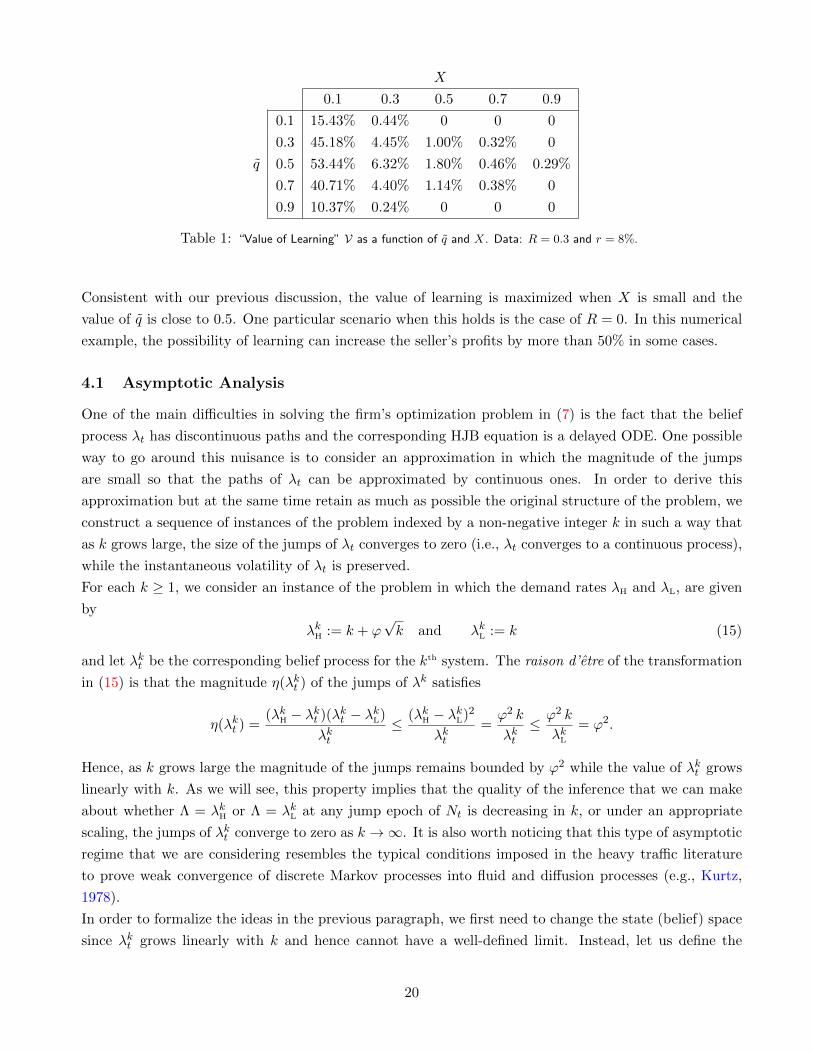
Table 1 summarizes the value of learning as a function of q and X measured as follows
V := supλ∈[λL,λH]
Π(λ)−G(λ)
G(λ)
.
Note that q ∈ (0, 1). Also, from condition (i) in Corollary 2, learning is not valuable if X ≥ 1, i.e., V = 0.
‡To see this, let PH and PL be two probability measures under which Nt is a Poisson process with rate λH and λL,
respectively. Then, the likelihood ratio L = dPH/dPL satisfies
Lt =
(λH
λL
)Nt
exp(−(λH − λL) t),
and so the speed of learning is determined by the difference λH − λL.
19
X
0.1 0.3 0.5 0.7 0.9
0.1 15.43% 0.44% 0 0 0
0.3 45.18% 4.45% 1.00% 0.32% 0
q 0.5 53.44% 6.32% 1.80% 0.46% 0.29%
0.7 40.71% 4.40% 1.14% 0.38% 0
0.9 10.37% 0.24% 0 0 0
Table 1: “Value of Learning” V as a function of q and X. Data: R = 0.3 and r = 8%.
Consistent with our previous discussion, the value of learning is maximized when X is small and the
value of q is close to 0.5. One particular scenario when this holds is the case of R = 0. In this numerical
example, the possibility of learning can increase the seller’s profits by more than 50% in some cases.
4.1 Asymptotic Analysis
One of the main difficulties in solving the firm’s optimization problem in (7) is the fact that the belief
process λt has discontinuous paths and the corresponding HJB equation is a delayed ODE. One possible
way to go around this nuisance is to consider an approximation in which the magnitude of the jumps
are small so that the paths of λt can be approximated by continuous ones. In order to derive this
approximation but at the same time retain as much as possible the original structure of the problem, we
construct a sequence of instances of the problem indexed by a non-negative integer k in such a way that
as k grows large, the size of the jumps of λt converges to zero (i.e., λt converges to a continuous process),
while the instantaneous volatility of λt is preserved.
For each k ≥ 1, we consider an instance of the problem in which the demand rates λH and λL, are given
by
λkH := k + ϕ√k and λkL := k (15)
and let λkt be the corresponding belief process for the kth system. The raison d’etre of the transformation
in (15) is that the magnitude η(λkt ) of the jumps of λk satisfies
η(λkt ) =(λkH − λkt )(λkt − λkL)
λkt≤ (λkH − λkL)2
λkt=ϕ2 k
λkt≤ ϕ2 k
λkL= ϕ2.
Hence, as k grows large the magnitude of the jumps remains bounded by ϕ2 while the value of λkt grows
linearly with k. As we will see, this property implies that the quality of the inference that we can make
about whether Λ = λkH or Λ = λkL at any jump epoch of Nt is decreasing in k, or under an appropriate
scaling, the jumps of λkt converge to zero as k →∞. It is also worth noticing that this type of asymptotic
regime that we are considering resembles the typical conditions imposed in the heavy traffic literature
to prove weak convergence of discrete Markov processes into fluid and diffusion processes (e.g., Kurtz,
1978).
In order to formalize the ideas in the previous paragraph, we first need to change the state (belief) space
since λkt grows linearly with k and hence cannot have a well-defined limit. Instead, let us define the
20

auxiliary belief process qkt := P(Λ = λkL|Ft) = (λkH − λkt )/(λkH − λkL) for the kth system. From Lemma 1, it
follows that qkt satisfies the SDE
dqkt = qkt (1− qkt )(λkH − λkL)
[dt− dNk
t
Λk(qkt )
],
where Nkt is a point process with intensity Λk(qkt ) := λkL q
kt + λkH (1− qkt ).
Proposition 6 Consider a sequence of problems indexed by k for which the arrival rates λkH and λkL are
given by (15). Let qkt = P(Λ = λkL|Ft) be the seller’s belief process that Λ = λkL with qk0 = q0, independent
of k. Then, qkt converges weakly to qt, solution of the SDE
dqt = ϕ qt (1− qt) dWt,
where Wt is a Wiener process.
According to Proposition 6, the scaling in (15) leads to a diffusion approximation for the dynamics of the
auxiliary belief process qt = P(Λ = λL|Ft).
Let us turn now to the seller’s objective function. Given our asymptotic result on qt, we find convenient
to rewrite the seller’s expected payoff in terms of qt rather than λt. Since λt = λL qt + λH (1 − qt), we
set G(q) := maxR, β + λL q + λH (1 − q). As we scale the system with k, we would like the seller’s
optimization problem to remain well-posed, that is, we would like to ensure that the profit function
remains bounded. For this, we must use an appropriate scaling for how the parameters R and β change
with k. We define Rk := R√k and βk = β
√k−k for some fixed constants R and β§. Under this scaling,
we get that
Gk(q) := maxRk , βk + λkL q + λkH (1− q)
=√k max
R , β + ϕ(1− q)
.
We define
G(q) :=Gk(q)√
k= max
R , β + ϕ(1− q)
. (16)
Based on the asymptotic results in Propositions 6 and the asymptotic scaled objective, we can approxi-
mate the firm’s optimization problem as follows
Π(q) = supτ∈T
Eq[e−r τ G(qτ )
](17)
subject to dqt = ϕ qt (1− qt) dWt, q0 = q. (18)
As before the solution is of the threshold type, that is, there exist two constants q and q such that
(ϕ q (1− q))2
2Π′′(q)− rΠ(q) = 0, q < q < q (19)
Π(q) = G(q), q ∈ [0, 1]− (q, q) (20)
Π′(q) = −1 and Π′(q) = 0. (21)
§Note that the condition βk + λkL < Rk < βk + λkH that we need to avoid trivial cases boils down to β < R < β + ϕ.
21

After some manipulations, one can show that a general solution for the ODE in (19) is given by
Π(q) = K0(1− q)A
qA−1+K1
qA
(1− q)A−1, where A :=
1 +√
1 + 8r/ϕ2
2(22)
and K0 and K1 are two constants of integration. The next result follows.
Proposition 7 Let A := (1 +√
1 + 8r/ϕ2)/2. There exist constants q, q ∈ (0, 1), K0 and K1 such that
Π(q) =
β + ϕ (1− q) if 0 ≤ q ≤ q
K0 (1− q)A q1−A +K1 (1− q)1−A qA if q ≤ q ≤ q
R if q ≤ q ≤ 1.
The constants are determined imposing smooth-pasting conditions in (20)-(21) at q and q. The function
Π(q) is twice-continuously differentiable and convex in (0, 1).
To complete our diffusion approximation, we now interpret the results in Proposition 7 in terms of the
original (unscaled) primitive model. For this, we reverse the scaling using the fact that k = λL to get
ϕ =λH − λL√
λL
, R =R√λL
, β =β + λL√
λL
, and Π(λ) =√λL Π(q).
Note that we have used a slight abuse of notation writing Π(λ) for the unscaled approximated value
function. In addition, we must also write the threshold q and q in terms of threshold on the values of λ,
specifically we have
λ = q λL + (1− q)λH and λ = q λL + (1− q)λH.
Putting all the pieces together, we get the following diffusion approximation:
Π(λ) =
β + λ if λ ≤ λ ≤ λH
K0 (λ− λL)A (λH − λ)1−A +K1 (λ− λL)1−A (λH − λ)A if λ ≤ λ ≤ λ
R if λL ≤ λ ≤ λ,
(23)
where the constants λ, λ, K0 and K1 are determined imposing value-matching and smooth-pasting con-
ditions at λ = λ and λ = λ.
Figure 4 depicts an example comparing the value function Π(λ) and the diffusion approximation Π(λ).
We note that Π(λ) satisfies value-matching and smooth-pasting conditions at λ and λ. This is in contrast
to Π(λ) that satisfies these conditions only at λ.
Table 2 summarizes a set of computations experiments that numerically evaluate the quality of the
diffusion approximation. In particular, the values reported in the table correspond to the relative error
E := supλ∈[λL,λH]
|Π(λ)− Π(λ)|
Π(λ)
22

0.35 10.4
1
Belief: h
W(h):Optimal SolutionR
W(h):Diffusion Approximation~
Figure 4: Diffusion approximation: Data: : β = 0, λH = 1, λL = 0.35, R = 0.5 and r = 5%.
ϕ = (λH − λL)/√λL
0.1 0.3 0.5 0.7 0.9
0.1 0.85% 0.86% 2.73% 5.19% 6.61%
0.3 0.36% 0.90% 2.21% 4.11% 5.94%
R 0.5 0.36% 0.69% 0.14% 2.91% 4.43%
0.7 0.12% 0.68% 0.99% 1.54% 2.31%
0.9 0.08% 0.12% 0.36% 0.62% 0.93%
Table 2: Relative error E as a function of R and ϕ. Data: β = 0, λH = 1 and r = 5%.
as a function of R and ϕ. Overall, the results show that the diffusion approximation is very accurate
across a wide range of parameters. As expected, the approximation is particularly good for small values
of ϕ.
Besides providing a simple representation of the value function, the diffusion approximation is also useful
as it allows us to use standard results for one-dimensional diffusion processes (e.g., Section 5.5 in Karatzas
and Shreve, 1991) to analyze its optimal solution. For instance, the following corollary characterizes the
expected duration of the voting phase and the likelihood that a product will be eventually introduced
into the market.
Corollary 3 Let (λ, λ) be the optimal continuation region where λ and λ are given in equation (23). For
any initial condition λ ∈ (λ, λ), let τ∗ := inft > 0 : λt ∈ (λ, λ) and γ∗ := P(λτ∗ = λ |λ0 = λ). Then,
γ∗ =λ− λλ− λ
and E[τ∗] = γ∗ T (λ) + (1− γ∗) T (λ)− T (λ),
where T (λ) is the function
T (λ) :=2
ϕ2
λH + λL − 2λ
λH − λLln
(λH − λλ− λL
).
23

5 Voting System with Preselling
In this section we study the seller’s optimization problem defined in equation (2) for the case in which
φ > 0; that is, in expectation, every vote generates a positive revenue if the product is eventually launched.
Recall that Π(λ, n) is the seller’s value function which is given by
Π(λ, n) = supτ∈T
E[e−r τG(λτ , Nτ ) |λ0 = λ,N0 = n
], for all (λ, n) ∈ (λL, λH)× N. (24)
Our solution method takes full advantage of the fact that the number of votes Nt is a monotonically
increasing process, which is a property that allows us to interpret the two dimensional dynamic program-
ming formulation as a one dimensional finite-horizon stochastic control problem. As a result we are able
to use a recursive method that computes the seller’s value function and characterizes the continuation
and intervention regions. The method is obtained through a backward induction on the value of n; for
this, we first argue that if the number of votes n reaches a sufficiently large value, then it is in the seller’s
best interest to introduce immediately the product in the market and capitalize on the instantaneous
expected revenues φn that these voters generate. We formalize this intuition in the following lemma,
which uses the mapping m(λ) = m(λ, 0) defined in equation (6). (Recall that m(λ) is the optimal number
of votes needed to launch the product in the full information case, i.e., when Λ = λ is known at time 0.)
Lemma 2 Let n be given by
n := max
m
(r(R− λL)
φ− r
),m(λL) ,m(λH)
.
Then, for all states (λ, n) with λL ≤ λ ≤ λH and n ≥ n it is optimal to stop immediately and to launch
the product in the market. In this case, the seller’s value function is equal to
Π(λ, n) = β + λ+ φn, for all n ≥ n.
It is worth noticing that we can use n to (upper) bound the time of the voting campaign. Indeed, the
quantity τn which is the time it takes the voting process to collect n votes, is clearly an upper bound on
the actual voting duration; and for example, the seller can easily compute its expected value,
E[τn] =
(λH − λλH − λL
)n
λL
+
(λ− λL
λH − λL
)n
λH
.
Equipped with the upper bound n , we can compute the value of Π(λ, n) using backward induction in n.
Proposition 8 The value function Π(λ, n) satisfies recursively the optimality equation
Π(λ, n) =(λH − λ)αH
(λ− λL)αLmax
λ1∈(λL,λ]
[∫ λ
λ1
(x− λL)αL
(λH − x)αH
Π(x+ η(x), n+ 1)
η(x)dx+
(λ1 − λL)αL
(λH − λ1)αHG(λ1, n)
], (25)
with boundary condition Π(λ, n) = β + λ+ φn, for all λ ∈ [λL, λH] and n ≥ n.
Using arguments similar to those used in the previous section, one can show that the value function
Π(λ, n) satisfies the HJB equation:
0 = maxG(λ, n)−Π(λ, n) , λ
[Π(λ+ η(λ), n+ 1)−Π(λ, n)− η(λ) ∂+Π(λ, n)
]− rΠ(λ, n)
, (26)
24

with border conditions Π(λH, n) = ΠD(λH, n), Π(λL, n) = ΠD(λL, n), for all n ≥ 0 and Π(λ, n) = β+λ+φn
for all λ ∈ [λL, λH] and n ≥ n (recall the definition of the full information value function ΠD(λ, n) in
Proposition 2).
In contrast to the pure voting case discussed in the previous section, we do not have a closed-form
solution for the value function Π(λ, n) and we must rely on equations (25) or (26) to compute an optimal
solution numerically. As with most dynamic programming equations, part of the challenge in solving (25)
is dealing with inner optimization over λ1. In this regard, the following result greatly simplifies these
numerical calculations.
Proposition 9 For any initial belief λ ∈ (λL,ΛH) and n ≥ 0, let
L∗(λ, n) = argmaxλ1∈(λL,λ]
[∫ λ
λ1
(x− λL)αL
(λH − x)αH
Π(x+ η(x), n+ 1)
η(x)dx+
(λ1 − λL)αL
(λH − λ1)αHG(λ1, n)
], (27)
be the optimal hitting threshold in equation (25). Suppose that for some λ0 and n, L∗(λ0, n) = λ0 < λ0.
Then, L∗(λ, n) = λ0 for all λ ∈ [λ0, λ0].
This result essentially formalizes the intuition that the seller’s only source of information is the one
coming from the jumps of the voting process Nt. Indeed, if no jumps are occuring then the threshold
to stop is fixed independent of the current value of λt. (We omit its proof as it follows directly from
the characterization of Π(λ, n) in Proposition 8.) We note that the mapping L∗(λ, n) fully characterizes
the seller’s optimal strategy. Indeed, the state (λ, n) belongs to the continuation or intervention regions
depending on whether L∗(λ, n) < λ or L∗(λ, n) = λ, respectively.
Figure 5 depicts the seller’s optimal strategy in the (λ, n) space for two instances of the problem that
differs only on the relationship between φ and r. In each panel, the shaded area corresponds to the
intervention region, which is further divided into two subregions: in the top region it is optimal to stop
the voting and launch the product while in the lower region it is optimal to stop and discard the product.
Note that while the lower boundary of the continuation region is decreasing in λ the upper boundary
can be either increasing (left panel) or decreasing (right panel). This seems consistent with the fact that
m(λ) is increasing or decreasing in λ which in turns depends on whether φ > r or φ < r, respectively
(see equation (6)).
5.1 Computational Experiments
In this section we conduct two types of numerical experiments to further investigate the properties and
performance of our proposed voting system. First, we do a sensitivity analysis with respect to the main
parameters of the model. Second, we consider two simple policies which are commonly used in practices
and use them as benchmarks to evaluate the benefits of our proposed solution.
Before moving into the details of these computations, let us summarize some general guidelines that we
have used in the design of our experiments. First of all, we impose the normalization λH = 1. This is
without loss of generality as we can always scale the units of time accordingly. Also, to avoid trivial
cases, we assume that the condition λL + β ≤ R is satisfied (otherwise, discarding the products is never
an optimal decision). We also assume that β ≤ 0, R ≥ 0 and R ≤ β + λH, that is, launching the product
25

1 1.5 20
15
30
Belief (λ)
Number of Votes (n)
Stop Voting and Launch
Continue Voting
Stop Voting and Discard
Case φ > r
Continue Voting
Stop Voting and Launch
Stop Voting and Discard
Case φ < r
1 1.5 20
15
30
Belief (λ)
Number of Votes (n)
Figure 5: Optimal strategy for the instances λL = 1, λH = 2, β = −1, R = 1, r = 5% and φ = 0.065 (left panel) and
φ = 0.035 (right panel). The top dashed line is at the level n = 25 (left panel) and n = 29 (right panel).
is costly, the opportunity cost of discarding the product is nonnegative and a high demand product will
always be launched (even in a pure voting scenario with φ = 0). It follows that R ∈ [0, 1] and β ∈ [−1, 0].
Finally, in an effort to standardize our result across different instances, we measure payoffs relative to
the case without a voting system. Specifically, we focus on the following performance measures:
G := maxλL≤λ≤λH
Π(λ, 0)−G(λ, 0)
G(λ, 0)
and G :=
1
λH − λL
∫ λH
λL
Π(λ, 0)−G(λ, 0)
G(λ, 0)dλ,
which are the maximum and average† relative gains of using a voting system, respectively.
I) Sensitivity Analysis: In what follows, we investigate the sensitivity of G and G with respect to
the two main components embedded in our voting system: (1) informational (demand learning) and (2)
financial (pre-selling revenues). To this end, we define the following quantities:
Opportunity for Learning : L :=λH − λL
λH
and
Opportunity for Pre-Selling : PS :=φ (λH + λL)
2 r R.
Our definition of the opportunity for learning L is motivated by two characteristics of the learning process.
On one hand, L is a normalized –in [0, 1]– measure of the “amount” of uncertainty that the seller faces.
If L is close to zero then there is not much to learn while if L is close to one then there is a significant
difference between the intensities of high and low demand products and the opportunity for learning is
high. On the other hand, L also measures the speed of learning (see foonote (‡) for mode details). Higher
values of L mean that the voting process is more informative and the seller can learn quicker the value
of Λ.†In our numerical experiments we have approximated the integrals by summation over a partition with mesh size ∆λ =
0.001.
26

Let us turn to our second measure, the opportunity for pre-selling value PS. To understand its definition,
note that our goal is to isolate the financial value of pre-selling. For this, we consider a deterministic
model in which the voting process Nt is replaced by a fluid process NFt = Λ t and so the seller’s value
function in (24) becomes
ΠF(λ, n) = max
R , max
t≥0
e−r t
(β + λ+ φ (n+ λ t)
).
Letting t∗ be the optimal solution in the inner maximization, one can show that the option of pre selling
is valuable (i.e., generates enough cash-flows in the form of pre-orders to support launching the product)
ifφλ
r R≥ er t∗ .
Our definition of PS is motivated by the quantity on the left-hand side of this inequality, replacing the
value of λ by the mid-value (λH +λL)/2. Hence, we expect that the voting system to be more (financially)
beneficial to the seller for large values of PS.
Figure 8 plots the values of G (left panel) and G (right panel) as function of the opportunity for learning
L for two scenarios with φ > 0 and φ = 0 (pure voting). Interestingly, the value of the voting system
increases monotonically with L. On one hand, this is expected since a large value of L means that there
is more room for learning. However, on the other hand, a large value of L implies that the seller faces
larger demand risk and the likelihood of discarding the product is higher. This example also reveals that
the gains of using a voting system can be quite significant, as much as 15% even in a pure voting system
with φ = 0.
0.5 0.6 0.7 0.8 0.9 1.00
0.02
0.04
0.06
0.08
0.1
0.12
0.14
0.16
0.18
0.5 0.6 0.7 0.8 0.9 1.00
0.005
0.01
0.015
0.02
0.025
L! L!
G! G!
ϕ = 0.01 ϕ = 0.01
Pure Voting
Pure Voting
Figure 6: Maximum (G) and average (G) relative gains as function of the opportunity for learning L. Data: R = 0.4, β = −0.5
and r = 0.05.
Turning to the sensitivity of the seller’s payoffs with respect to the opportunity to pre-sell, Figure 7
depicts the behavior of maximum and average relative gains as a function of PS. In these computations,
we have varied the value of the opportunity cost R (in the range [0.1, 0.4]) keeping everything else fixed.
27

It is interesting to note that the relative gains associated with the voting system grow rapidly with PSif φ > 0. However, these gains are limited and remain bounded in a pure voting context. In other words,
the seller should pay special attention to identify the type of mechanisms that one can use to induce
voters to become buyers, for instance, by offering price discounts and other benefits.
0 5 10 150
0.5
1
1.5
2
2.5
3
3.5
4
0 5 10 150
0.1
0.2
0.3
0.4
0.5
0.6
0.7
0.8
0.9
PS! PS!
G! G!
ϕ = 0.01 ϕ = 0.01
Pure Voting Pure Voting
Figure 7: Maximum (G) and average (G) relative gains as function of the opportunity for pre-selll PS. Data: λL = 0.5,
β = −0.5 and r = 0.05.
Benchmarks: Let us now compare the performance of our voting system to two alternative policies in
which the seller announces, at time t = 0, either (i) a fixed duration T ∗ ≥ 0 for the voting phase or (ii)
a fixed number of votes M∗ ≥ 0 that will be collected before a launching decision is made. We have
chosen these simple (open-loop) policies as benchmarks because they are popular and commonly used in
practice as they are easy to communicate and implement.
For a given prior λ on the value of Λ, we let ΠT(λ, n) and ΠM(λ, n) be the seller’s expected discounted
payoffs under the two static policies mentioned. From the representation of λt in terms of the likelihood
ratio L(t,Nt) in Lemma 1, we can compute the values of ΠT(λ, n) and ΠM(λ, n) as follows:
ΠT(λ, n) := supT≥0
E
[e−r T max
R , β +
λL (λH − λ) + λH (λ− λL)L(t,NT )
λH − λ+ (λ− λL)L(t,NT )+ φ (n+NT )
]and
ΠM(λ, n) := supm∈N
E
[e−r τm max
R , β +
λL (λH − λ) + λH (λ− λL)L(τm,m)
λH − λ+ (λ− λL)L(τm,m)+ φ (n+m))
],
where τm is the mth epoch of the voting process Nt. Obviously, ΠT(λ, n) and ΠM(λ, n) are lower bounds
for the value function Π(λ, n). To assess the performance of our proposed voting system with respect to
these approximations we compute the worst-case relative errors:
ET := maxλL≤λ≤λH
Π(λ, 0)−ΠT(λ, 0)
Π(λ, 0)
and EM := max
λL≤λ≤λH
Π(λ, 0)−ΠM(λ, 0)
Π(λ, 0)
,
28

as well as the average relative errors:
ET :=1
λH − λL
∫ λH
λL
Π(λ, 0)−ΠT(λ, 0)
Π(λ, 0)dλ and EM :=
1
λH − λL
∫ λH
λL
Π(λ, 0)−ΠM(λ, 0)
Π(λ, 0)dλ.
Fixed Duration
Worst-Case Error: ET
λL
φ 0.2 0.4 0.6 0.8
0.005 3.2% 1.6% 0.5% 0.0%
0.01 3.3% 1.8% 0.7% 0.0%
0.05 8.0% 7.1% 5.1% 1.9%
0.1 13.0% 10.5% 3.5% 2.4%
Fixed Number of Votes
Worst-Case Error: EM
λL
φ 0.2 0.4 0.6 0.8
0.005 4.5% 2.4% 1.0% 0.0%
0.01 5.5% 2.8% 1.5% 0.0%
0.05 17.9% 12.1% 4.1% 0.0%
0.1 26.9% 9.2% 0.2% 0.0%
Average Error: ET
λL
φ 0.2 0.4 0.6 0.8
0.005 0.4% 0.1% 0.0% 0.0%
0.01 0.6% 0.1% 0.0% 0.0%
0.05 2.0% 1.4% 1.0% 1.4%
0.1 3.3% 2.3% 2.1% 1.8%
Average Error: EM
λL
φ 0.2 0.4 0.6 0.8
0.005 0.5% 0.1% 0.0% 0.0%
0.01 0.7% 0.2% 0.0% 0.0%
0.05 3.4% 1.7% 0.1% 0.0%
0.1 5.0% 1.4% 0.0% 0.0%
Table 3: Percentage relative errors ET and EM. Data: R = 0.5, β = −1, λH = 1 and r = 5%.
As we can see from the values of the worst-case errors ET and EM in Table 3, using these static approxima-
tions can lead to substantial suboptimality, in some cases as large as to 27%. (As expected, the average
errors ET and EM are smaller but still significant.) If we compare the two approximations, we also note
that using a fixed duration for the voting process leads to better performance when λL is small but as
λL increases setting a fixed number of votes is a better strategy. In other words, under high demand
uncertainty a voting campaign with fixed duration is preferred to one with a fixed target of votes, and
vice-versa. The fact that a fixed number of votes is better when demand uncertainty is low is somehow
expected since choosing a fixed number of votes is an optimal strategy under full information (see Section
3). Another important observation that emerges from these numerics is that the value of using an optimal
stopping rule to determine the duration of the voting phase (instead of a fixed static policy) increases in
φ, that is, when the opportunities for pre-selling are higher. It follows that when the conversion of voters
into buyers is low a static voting campaign could lead to good performance. However, as the conversion
rate increases the seller has more incentives to use a dynamic stopping rule.
6 Extensions
6.1 Pricing Tactic
Up to this point, we have focused on determining the optimal duration of the voting phase. However, there
is another factor that can have a significant impact on the overall success of a crowdvoting system and
29

that is pricing. In this section, we extend our model to investigate this issue. As we have been discussing
throughout, the performance of a crowdvoting system depends on its capacity to (a) improve the seller’s
demand forecast and (b) generate pre-orders that will translate into sales if and when the product is
launched. These two objectives, however, are not necessarily aligned when it comes to determining a
pricing policy. On one hand, in an effort to speed up the voting and demand learning processes, the
seller would like to offer voters deep price discounts to encourage them to vote. On the other hand, price
discounts will reduce the revenues that these pre-orders will generate. Hence, an optimal pricing tactic
should try to appropriately balance these two conflicting objectives.
To put the previous discussion on a concrete mathematical footing, let us consider the following variation
of our base model. As before, we divide the planning horizon into two phases –voting and selling phases–
and we assume that consumers arrive to the system according to a Poisson process with rate Λ during the
entire planning horizon. In this case, however, we also assume that arriving consumers have a maximum
willingness-to-pay for the product and that their voting and/or purchasing behavior depends on whether
or not the price they see exceeds this threshold. Since it is reasonable to assume that the reservation
price of individuals that arrive during the voting phase is different than the one of those arriving during
the selling phase, we let FV(p) and FR(p) be the cumulative probability distribution of the willingness-to-
pay of voters and buyers, respectively. On the seller side, we assume that he sets a price pV during the
crowdvoting phase (this will be the price that voters will pay at the time the product is launched) and a
price pR during the regular selling phase if this latter phase eventually materializes. As a result, the voting
process is driven by a Poisson process with rate Λ FV(pV), where FV(pV) := 1− FV(pV) is the probability
that an arriving voter clicks at the product at price pV. Similarly, the demand for the product during the
regular selling phase follows a Poisson process with intensity Λ FR(pR), where FR(pR) := 1−FR(pR). From
a practical standpoint, one would expect that pV ≤ pR, that is, that the seller is willing to offer voters a
discount to incentivize them to vote as well as to compensate them for the risk and delay that they face
in getting the product. We will not impose this constraint directly but rather we will investigate how the
optimal prices pV and pR depend on the values of the different parameters of the model, and in particular
on FV and FR.
In this modified setting, the voting process Nt has intensity Λ FV(pV). Hence, the belief process λt =
E[Λ|Ft] satisfies
dλt = η(λt−)[dNt − FV(pV)λt dt
]where η(λ) =
(λH − λ) (λ− λL)
λ.
Based on our discussion in Section 2.1, the seller’s payoff at time τ conditional on the value of λτ = λ
and the number of voters Nτ = n is given by
G(λ, n) = max R , GR(λ) +GV(n)−K = max
R ,
pR FR(pR)
rλ+ θ pV n−K
.
Recall that K > 0 is the fixed cost of launching the product and θ ∈ [0, 1] is the probability that a
voter will return to buy the product if it is eventually put on the marketplace. As a result, the seller’s
30

optimization problem is now given by
Π(λ) = suppV,pR,τ∈T
E[e−r τ max
R ,
pR FR(pR)
rλτ + θ pVNτ −K
]subject to dλt = η(λt−)
[dNt − FV(pV)λt dt
]and λ0 = λ.
Since the dynamics of λt are independent of pR, it follows that the optimal regular price is given by
p∗R := arg maxp FR(p). This result should be intuitively clear, since once the product is introduced on
the market, the seller focuses exclusively on maximizing the instantaneous revenue rate. In other words,
demand learning provides no additional value at this point. Let us set δ∗ := p∗R FR(p∗R)/r.
On the other hand, the dependence of G(Λ, n) on pV is more complex since this price affects both the
revenues at launching as well as the dynamics of λt and Nt. In order to isolate the effect of pV on the
seller’s expected payoff, let us introduce a time change to remove the dependence of the state variable on
pV. Specifically, let us define λ(t) := λ(t/FV(pV)) and N(t) := N(t/FV(pV)). (Note that Nt is a Poisson
process with rate Λ.) Also, by appropriately scaling R, K, θ and Π(λ) by δ∗, we can assume that δ∗ = 1.
With these changes, the seller’s optimization becomes
Π(λ) = suppV,τ∈T
E[exp
(− r
FV(pV)τ
)max
R , λτ + θ pV Nτ −K
](28)
subject to dλt = η(λt−)[dNt − λt dt
]and λ0 = λ.
We note that this formulation is equivalent to our base model with β = −K, φ = θ pV and a modified
discount fact r/FV(pV). So, for a fixed value of pV, with FV(pV) > 0, we can use the solution techniques
that we developed in the previous sections to derive an optimal stopping rule. The optimization in
(28) provides an alternative perspective on the trade-off that the seller faces when choosing pV. On one
hand, a large pV will increase the revenues at introduction θ pV Nτ . On the other hand, increasing pV
will decrease FV(pV), effectively increasing the (modified) discount factor r/FV(pV). The following result
follows directly from (28).
Proposition 10 In a pure voting system, that is when θ = 0, it is optimal to set pV = 0.
In other words, when the voting system is a pure demand learning mechanism and has no direct impact
on the seller’s cash-flows, it is in the seller best interest to stimulate the pace of voting as much as possible
by offering voters deep discounts, which in our model corresponds to setting pV = 0.
Figure 8 plots the optimal value of pV as a function of the conversion rate θ. As we can see, the result
in Proposition 10 extends to a range of values θ. So even if a voter can generate a positive revenue at
introduction, it is better for the seller to prioritize learning speed by giving voters a deep discount. On
the other hand, as θ grows large, the optimal price pV also increases and rapidly converges to the myopic
value p∗V = arg maxp FV(p)
6.2 Impatient Voters
Another aspect of our model that deserves further discussion is voters’ purchasing behavior. Up to this
point, we have assumed that there is a fixed probability θ that a voter returns to buy the product at
31

0.05 0.1 0.15 0.2 0.25 0.3 0.35 0.4 0.45 0.50.1
0.2
0.3
0.4
0.5
0.6
0.7
0.8
e
pv
Figure 8: Optimal crowdvoting prive pV as a function of the conversation θ of voters into buyers. The dashed line is at the
myopic price level p∗V = arg maxp FV(p). Data: R = 0.4, β = −0.5 and r = 0.05, λL = 0.2, λH = 1 and λ = 0.5.
its introduction time. Our motivation behind this formulation is the idea that a fraction 1 − θ of the
voters are impulse buyers that would have bought the product if it would have been available at the time
they voted but they will not return to buy it at a later time. In addition, we have also assumed that
this probability θ is independent of how long non-impulse voters have to wait. It seems reasonable to
expect, however, that these non-impulse buyers have a maximum tolerance on how long they are willing
to wait. To capture this impatience, we assume that each non-impulse customer is willing to wait for
an exponential amount of time with rate α. If the product is not available after this time, the customer
will no longer be interested (i.e., her preferences have changed or she has bought a substitute product
somewhere else).
Let us denote by Sτ the expected number of sales that would be realized if the product is launched at
time τ .
Lemma 3 (Sales from Voters) If the seller introduces the product at time τ ∈ T , then the expected
number of sales at introduction, Sτ satisfies the following stochastic differential equation
dSt = −αSt dt+ θ dNt S0 = 0, 0 ≤ t ≤ τ.
Using this lemma, we can rewrite the seller’s optimization problem in this case with impatient voters as
the following optimal stopping problem:
Π(λ) = supτ∈T
E[e−r τ G(λτ , Sτ )
]subject to dλt = η(λt−)
[dNt − λt dt
], λ0 = λ
dSt = −αSt dt+ θ dNt, S0 = 0,
where G(λ, S) = maxR, β + λ+ pV S with pV the price that a voter will pay to purchase the product.
32

As before, we can tackle the solution to this problem using dynamic programming methods. However,
a key difference between the optimization problem above and the one discussed in Section 5 is that the
corresponding value function Π(λ, S) depends on the state variable S (i.e., expected number of sales
at introduction) as opposed to the number of votes. Because the process St is no longer discrete and
monotonic in time, we can no longer use backward induction as we did in the previous section to solve
the dynamic program. A detailed analysis of this model is beyond the scope of this paper. Instead, we
provide a simple approximation that builds upon our previous results.
To this end, let us denote by Xt the number of non-impulse voters that have arrived in [0, t] and who
are still willing to buy the product (see the proof of Lemma 3 for a precise definition). It follows that
St = E[Xt|Ft]. Note that from the seller’s perspective, Xt evolves as a hidden birth-death process.
Actually, the arrivals of new voters (births) are partially visible since the seller can see the voting process
but cannot differentiate between impulse and non-impulse buyers. On the other hand, the seller cannot
see deaths which correspond to the time epochs at which voters “renege” because their patient limit has
been exceeded. Births occur at a rate θΛ while deaths occur at a rate αXt. From standard birth-death
theory it follows that, conditional on X0 = 0, Xt has a Poisson distribution and
E[Xt|X0 = 0,Λ] =θΛ
α(1− exp(−α t)).
Based on the above, we could approximate Sτ by the constant S := θΛ/α, i.e. by the long-term average
value of Xt. We expect this approximation to be accurate in those situation in which the voting process
is open for a relatively long period of time relative to the rate at which voters renege. Under this
approximation, the seller’s payoff becomes a function of Λ exclusively and is given by
G(Λ) = maxR , β + Λ +
pV θΛ
α
.
As before, if we denote by φ = pV θ we can use the change of variables R := αR/(α + φ) and β :=
αβ/(α+ φ), we can rewrite this payoff as
G(R) =α+ φ
αG(Λ), where G(λ) := maxR , β + Λ.
As a result, and modulo the factor (α+ φ)/α, the seller’s optimization problem is given
Π(λ) := supτ∈T
E[e−r τ maxR , β + Λ
]subject to dλt = η(λt−)
[dNt − λt dt
], λ0 = λ.
The resulting optimization problem is exactly the same as the one we solved under pure voting but
replacing β and R by β and R and so we can directly export all the results in Section 4 to solve this
problem explicitly.
7 Concluding Remarks
In this paper we analyze the value of crowdsourcing in the context of new product introduction. More
specifically, we consider a seller contemplating the possibility of launching a new product into the market.
33

The seller is uncertain on whether the product will be successful or not- if commercialized - and rely on a
voting platform (crowdvoting) to make a more informed decision. The seller makes available the design
online for potential buyers to vote on. As the voting progresses, the seller has to decide when to end
the voting phase and, as a result of the information gathered, whether to discard the product or to
commercialize it. In the case it is commercialized, the seller incurs a fixed cost and collects a stream of
revenues from sales which depend on the market size. If it is discarded, the seller collects a payoff R that
captures the product’s opportunity cost. This voting phase can also be used to generate pre-orders and
hence some positive cash flow at introduction. The voting system plays then two main functions. First
and foremost, it represents a market learning mechanism, whereby the seller would continuously update
his estimate of the market size as votes get casted. Secondly, it represents a funding mechanism whereby,
through the pre-orders generated, the voting phase allows the seller to reduce, at introduction, the impact
of the fixed costs at the expense of a delay in launching the product and thus in the materialization of
the total profits.
In order to dissect the impact of each of these two functions, we study each separately. In Section 3,
we assume that the market demand rate is known, and hence the voting phase is only used to better
manage the product’s cash flow. In this full information case, the optimal policy is, from the start,
to either discard the product or to announce a ‘funding target’ which is given by the number of votes
that need to be collected before the product is launched. This full information policy also represents a
myopic approximation to the general case that we use to generate a lower and an upper bounds that are
particularly tight when the uncertainty is low or the opportunity cost, R is high. Next, in Section 4, we
focus on the pure voting case where visitors do not have the opportunity to pre-order the item. In this
case, the crowdvoting platform is primarily used to learn the market size, which is done through Bayesian
updating. In the pure voting, we obtain an explicit expression of the payoff in closed-form using QVI
machinery. The optimal policy, characterized by the following stopping time
τ = inft ≥ 0 : Π(λt) = G(λt),
is then fully defined and easy to implement. The closed form expression brings also additional advantages;
in particular, an exact measure of the value of learning, Π(λ) − G(λ). Maximum learning is shown to
be obtained when the opportunity cost from running the voting phase is small or when the speed of
learning measured by the difference λH−λL is large. We also determine simple conditions on the problem
parameters’ to assess whether a crowdvoting phase is worthwhile or not. Furthermore, we conduct in this
pure voting setting, an asymptotic analysis by scaling some of the parameters, in particular λH and λL by
n, while keeping their difference in√n and the magnitude of the jumps η, bounded. We prove in this case
that the belief process P(Λ = λL|Ft) converges to a diffusion process. As a result, we convert the scaled
optimization problem at the limit, into a simple second order ODE with smooth border conditions. The
solution to the ODE reveals a simple formulation of the payoff function and an explicit characterization of
the distribution of the optimal stopping time (i.e. the duration of the crowdvoting session), in particular,
of its expected value.
In Section 5, we investigate the general case in which the voting platform is used to presell as well as
to conduct a Bayesian learning on the market size Λ. The seller needs to track in this case both the
updated value of λ and the number of votes over time. Given the complexity of the problem in this
34

general case, we cannot obtain closed form solutions. Nevertheless, we were able to fully characterize
the optimal payoff as a solution of a recursive relationship with given boundary conditions that can be
solved rather easily numerically. We were also able to fully characterize the continuation region, which
is particularly helpful in implementing the optimal policy in practice. Finally, we conducted intensive
numerical experiments and our conclusions were of two folds. First, we identified the parameters to which
the payoff is sensitive to and showed that the value of the voting phase increase with respect to these
parameters. Despite the many parameters defining the model, we reduced our analysis to how sensitive
the payoff is with respect to the opportunity of learning and to that of pre-selling, each embodied by one
well identified quantity. As expected, the value of a crowdvoting platform increases (and becomes quite
sizeable) as the uncertainty on the market size and the opportunity of pre-selling increase. Secondly, we
showed numerically that offering a voting phase for which the duration is set dynamically (as a result of
a sophisticated stopping rule that accounts for both the market learning level and the funds generated
through pre-sales) generates a clear edge compared to those simple (myopic and open loop) policies used
in practice; whether those relying on a fixed deterministic duration or set based on a funding target
(number of votes). Again this edge is sizeable when both the opportunities of learning and preselling
are high. From this analysis we also observe that when the opportunity of learning is small while the
opportunity of preselling is high, a preset number of votes performs well. On the other hand, when the
opportunity of learning is large (i.e. the market uncertainty is high) then a preset number of votes is too
risky and the seller would be better off fixing the duration of the voting phase. The performance of the
latter policy deteriorates as the opportunity of preselling increases.
Finally in Section 6, we discuss two extensions of our model to take into account pricing strategies and
voters patience. In the first one, we introduce the price of the voting phase as a static decision variable
that needs to be set by the seller on top of the duration. For that we show that the earlier model can
easily accommodate this important addition and can leverage on the previous solution techniques. We
numerically explore the impact of the conversion rate (a proxy for the opportunity of preselling) on the
optimal price and observe that the latter is either set to be zero when the conversion rate is very small in
greater support of the informational component; or converging quickly to the value that maximizes the
preselling rate and hence in support of the financial component. This conclusion argues (surprisingly) for
a simple pricing rule despite the complexity of the general model. Next, we consider the case where the
likelihood for every vote to be converted into sales decreases with time and hence, the later the product is
introduced the more revenues from early voters are lost. In many contexts, this is a more natural setting,
whereby the accumulated funds follows a stochastic process that is not necessarily increasing with time.
We again formulate the problem in the general case and suggest to approximate the sales process by its
long-term average average. This approximation reduces the problem to a formulation similar to the pure
voting setting which can be solved in closed form. Finally, this section also shows that the model we are
suggesting in this paper to analyze crowdvoting platforms is flexible enough and can be adapted to include
other relevant factors and additional layers of complexities while keeping a good level of tractability.
This work also identifies many interesting avenues to tackle in future research. One major avenue is that
of incorporating strategic customers that could use voting as a way to increase their overall surplus. In
such game theoretic setting, one important question is whether the seller is better off announcing the
number of votes accumulated at this point or not. Indeed, strategic customers might try to “manipulate”
35

the seller by not voting if the number of votes is already high. But, at the same time a customer
uncertain about her true valuation can see her expected valuation increasing with a high number of
votes. Another avenue is that of multi products, where customers visit the platform and are offered
multiple choices (e.g. T-shirts designs). Their decision to vote or not would not only take their own
valuation into account but also the probability that their favorite choice would be commercialized or not.
Other avenues related to dynamic pricing and inventory management could also be worth exploring as
well.
References
Araman, V., R. Caldentey. 2009. Dynamic pricing for nonperishable products with demand learning.
Oper. Res. 57(5) 1169–1188. 5
Aviv, Y., A. Pazgal. 2002. Pricing of short life-cycle products through active learning. Working Paper,
Olin School of Business, Washington University, St. Louis. 5
Belleflamme, P., T. Lambert, A. Schwienbacher. 2014. Crowdfunding: Tapping the right crowd. Journal
of Business Venturing 29(5) 585–609. 4
Billingsley, P. 1968. Convergence of probability measures. Wiley series in probability and mathematical
statistics, Wiley, New York. 43
Boyaci, T., O. Ozer. 2010. Information acquisition for capacity planning via pricing and advance selling:
When to stop and act? Oper. Res. 58(5) 1328–1349. 4, 5
Bremaud, P. 1980. Point Processes and Queues, Martingale Dynamics. Springer-Verlag, New York, NY.
9
Crosetto, P., T. Regner. 2014. Crowdfunding: Determinants of success and funding dynamics. Jena
Economic Research Papers 8. 4
Dana, J. 1998. Advanced purchase discounts and price discrimination in competitive markets. J. Political
Econom. 106(2) 395–422. 4
Farias, V.F., B. Van Roy. 2010. Dynamic pricing with a prior on market response. Operations Research
58 16–29. 5
Gale, I. L., T.J. Holmes. 1992. The efficiency of advanced-purchase discounts in the presence of aggregate
demand uncertainty. International Journal of Industrial Organization 10(4) 413–437. 4
Gale, I. L., T.J. Holmes. 1993. Advance-purchase discounts and monopoly allocation of capacity. American
Economoc Review 83(1) 135–146. 4
Gallego, G., O. Ozer. 2001. Optimal dynamic pricing of inventories with stochastic demand over finite
horizons. Management Sci. 47(10) 1344–1360. 4
36

Huang, Y., P.V. Singh, Y. Xu. 2014. Crowdsourcing new product ideas under consumer learning. Man-
agement Sci. 60(9) 2138–2159. 3
Jeff Howe. 2006. Crowdsourcing: A definition. URL http://crowdsourcing.typepad.com/cs/2006/
06/crowdsourcing_a.html. 2, 3
Karatzas, I., S.E. Shreve. 1991. Brownian Motion and Stochastic Calculus. Springer-Verlag, New York,
NY. 23
Krager, D.R., S. Oh, D. Shah. 2014. Budget-optimal task allocation for reliable crowdsourcing systems.
Operations Research 62(1) 1–24. 3
Kurtz, T. G. 1978. Strong approximation theorems for density dependent markov chains. Stochastic
Processes and their Applications 6 223–240. 20
Kurtz, T.G., P. Protter. 1991. Weak limit theorems for stochastic integrals and stochastic differential
equations. The Annals of Probability 19(3) 1035–1070. 44
Marinesi, S., K. Girotra. 2013. Information acquisition through customer voting systems. Tech. rep.,
Working Paper, INSEAD. 3
Mollick, E. 2014. The dynamics of crowdfunding: An exporatory study. Journal of Business Venturing
29(1) 1–16. 4
Peskir, G., A.N. Shiryaev. 2000. Sequential testing problems for poisson processes. Ann. Stat. 28 837–859.
5, 14
Prasad, A., K.E Stecke, X. Zao. 2011. Advance selling by a newsvendor retailer 20(1) 1059–1478. 4
Protter, P.E. 2004. Stochastic Integration and Differential Equations. Springer, Germany. 38, 40, 44
Raman, A., M. Fisher. 1996. Reducing the cost of demand uncertainty through accurate response to
early sales. Oper. Res. 44(4) 87–99. 4
Surowiecki, J. 2004. The Wisdom of Crowds. Random House, Inc., New York, NY. 3
Tang, C.S., K. Rajaram, A. Alptekinoglu, J. Ou. 1995. The benefits of advanced booking discount
programs: Model and analysis. Management Sci. 50(4) 465–478. 4
Terwiesch, C., Y. Xu. 2008. Innovation contests, open innovation and multi-agent problem solving.
Management Sci. 54(9) 1529–1543. 3
Whitt, W. 1980. Some useful functions for functional limit theorems. Mathematics of Operations Research
5(1) 67–85. 43
37

Appendix A: Proofs
Proof of Lemma 1: Let us define the auxiliary state variable qt := P(Λ = λL|Ft) with initial condition
q0 = q. Note that λt = λL qt + λH (1 − qt) and qt = (λH − λt)/(λH − λL). Now, using the Poisson
distribution of cumulative votes in [0, t] and Bayes’ rule we get that
qt =q (λL t)
Nt exp(−λL t)/Nt!
q (λL t)Nt exp(−λL t)/Nt! + (1− q) (λH t)Nt exp(−λH t)/Nt!
=q
q + (1− q)(λH/λL)Nt exp(−(λH − λL) t)=
q
q + (1− q)L(t,Nt), (29)
where the first equality follows from the Markov property of the voting process. This proves the second
part of the lemma.
Let us turn now to the first part. Using (29) we can derive the dynamics of the process (qt : t ≥ 0).
To this end, we write qt = f(Yt), where Yt := ln(λH/λL)Nt − (λH − λL) t is an Ft-semimartingale and f
is a twice differentiable and bounded function given by f(n) := qq+(1−q) exp(n) . From Ito’s lemma (e.g.,
Protter, 2004) and the fact that Yt is a finite variation process (which follows from the fact that N(t) is
a pure-jump process), we get
dqt = f ′(Yt−) dYt + f(Yt)− f(Yt−)− f ′(Yt−) ∆Yt.
Taking advantage of the pure-jump nature of Nt, we have dNt = ∆Nt, dYt = ∆Yt − (λH − λL) dt, and
f(Yt)− f(Yt−) = [f(Yt− + ln(λL/λH))− f(Yt−)]dNt, so that
dqt = −f ′(Yt−)(λH − λL) dt+ [f(Yt− + ln(λL/λH))− f(Yt−)] dNt
= (λH − λL)q(1− q) exp(Yt−)
(q + (1− q) exp(Yt−))2dt+
[q
q + (1− q) exp(Yt−)λHλL
− q
q + (1− q) exp(Yt−)
]dNt
= −η(qt−)[dNt − (λLqt− + λH(1− qt−))dt
], where η(qt) :=
qt(1− qt)(λH − λL)
λLqt + λH(1− qt). (30)
Finally, since λt = λL qt + λH (1 − qt), it follows that dλt = −(λH − λL) dqt. Plugging these identities in
(30), the result follows.
Proof of Proposition 1: First of all, to prove the monotonicity of Π(λ, n) on λ and n it suffices to
note that G(λ, n) is increasing in both λ and n and that the belief process λt is pathwise increasing in
the initial value λ0 (see Lemma 1).
To prove the convexity of Π(λ, n) on λ, let us denote by EL and EH the expectation operators conditional
on Λ = λL and Λ = λH, respectively. It follows that
Π(λ, n) = supτ∈T
E[e−r τ G(λτ , n+Nτ )]
= supτ∈T
EL[e−r τ G(λτ , n+Nτ )]P(Λ = λL) + EH[e−r τ G(λτ , n+Nτ )]P(Λ = λH)
= sup
τ∈T
EL[e−r τ G(λτ , n+Nτ )]
(λH − λλH − λL
)+ EH[e−r τ G(λτ , n+Nτ )]
(λ− λL
λH − λL
).
38

Consider a pair of beliefs λ1, λ2 ∈ [λL, λH] and set λ = αλ1 + (1 − α)λ2 for some α ∈ [0, 1]. Then,
convexity of Π(λ) follows from
Π(λ, n) = supτ∈T
EL[e−r τ G(λτ , n+Nτ )]
(λH − λλH − λL
)+ EH[e−r τ G(λτ , n+Nτ )]
(λ− λL
λH − λL
)= sup
τ∈T
α
[EL[e−r τ G(λτ , n+Nτ )]
(λH − λ1
λH − λL
)+ EH[e−r τ G(λτ , n+Nτ )]
(λ1 − λL
λH − λL
)]+
(1− α)
[EL[e−r τ G(λτ , n+Nτ )]
(λH − λ2
λH − λL
)+ EH[e−r τ G(λτ , n+Nτ )]
(λ2 − λL
λH − λL
)]≤ α sup
τ∈T
[EL[e−r τ G(λτ , n+Nτ )]
(λH − λ1
λH − λL
)+ EH[e−r τ G(λτ , n+Nτ )]
(λ1 − λL
λH − λL
)]+
(1− α) supτ∈T
[EL[e−r τ G(λτ , n+Nτ )]
(λH − λ2
λH − λL
)+ EH[e−r τ G(λτ , n+Nτ )]
(λ2 − λL
λH − λL
)]= αΠ(λ1) + (1− α) Π(λ2).
Finally, to prove the convexity of Π(λ, n) on n note that
Π(λ, n+ 1) + Π(λ, n− 1) = supτ∈T
E[e−r τ G(λτ , n+ 1 +Nτ )
]+ supτ∈T
E[e−r τ G(λτ , n− 1 +Nτ )
]≥ sup
τ∈TE[e−r τ
(G(λτ , n+ 1 +Nτ ) +G(λτ , n− 1 +Nτ )
)]≥ 2 sup
τ∈TE[e−r τ G(λτ , n+Nτ )
]= 2 Π(λ, n),
where the second inequality follows from the convexity of G(λ, n) on n.
Proof of Proposition 3: Let us first derive the lower bound. Suppose the seller uses the strategy
of running the voting system until time τm at which the mth vote is collected and then at this time he
launches the product (i.e., the option of discarding is not considered). Since this strategy is feasible and
τm ∈ T we have that
Π(λ, n) ≥ E[e−r τm G(λτm , Nτm)|N0 = n
]≥ E
[e−r τm
(β + λτm + φ (n+m)
)].
In addition, λτm = E[Λ|Fτm ] and so we also have that
Π(λ, n) ≥ E[e−r τm
(β + E[Λ|Fτm ] + φ (n+m)
)]= E
[E[e−r τm
(β + Λ + φ (n+m)
)∣∣∣Fτm]]= E
[e−r τm
(β + Λ + φ (n+m)
)]= E
[E[e−r τm
(β + Λ + φ (n+m)
)∣∣Λ] ]= E
[(Λ
Λ + r
)m (β + Λ + φ (n+m)
)]= E[H(Λ, n,m)].
Taking ‘max’ over m and noticing that Π(λ, n) is trivially greater than R, we conclude that
Π(λ, n) ≥ maxR , max
m≥0E[H(Λ, n,m)
].
39

To derive the upper bound, we use the convexity Π(λ, n) on λ derived in Proposition 1. It follows by
Jensen’s inequality that
Π(λ, n) = Π(E[Λ], n) ≤ E[Π(Λ, n)] = P(Λ = λL) Π(λL, n) + P(Λ = λH) Π(λH, n)
= P(Λ = λL) ΠD(λL, n) + P(Λ = λH) ΠD(λH, n)
= E [ΠD(Λ, n)] .
Note that we have used the identities Π(λL, n) = ΠD(λL, n) and Π(λH, n) = ΠD(λH, n), which follow from
the fact that the states λ = λL and λ = λH are absorbing for the dynamics of λt.
Proof of Theorem 1: Let Z(λ) ∈ D be a function that satisfies the QVI conditions and consider an
arbitrary admissible policy τ ∈ T and let λt be the corresponding trajectory of the belief process starting
at λ0 = λ.
Given the assumptions on Z(·), we can apply integration by part followed by Ito’s lemma (see Protter,
2004) to get that
e−rτ Z(λτ ) = Z(λ) +
∫ τ
0e−r t
(λt [Z(λt + η(λt))− Z(λt)− η(λt) ∂+Z(λt)]− r Z(λt)
)dt
+
∫ τ
0e−r t[Z(λt− + η(λt−))− Z(λt−)] (dNt − λt dt)
= Z(λ) +
∫ τ
0e−r tHZ(λt) dt+
∫ τ
0e−r t
[Z(λt− + η(λt−))− Z(λt−)
]dMt,
where H is the operator defined in (8) and Mt is an Ft-martingale given by
Mt := Nt −∫ t
0λs ds.
Since Z satisfies the QVI in (9), it follows that HZ(λt) ≤ 0 which implies
e−r τ Z(λτ ) ≤ Z(λ0) +
∫ τ
0e−r t
[Z(λt− + η(λt−))− Z(λt−)
]dMt.
Now, note that the term e−r t[Z(λt− + η(λt−)) − Z(λt−)] is a bounded previsible process while Mt is a
martingale and thus the expectation of this last integral is equal to zero. As a result, we get that
E[e−rτ Z(λτ )] ≤ Z(λ).
In addition, from the second QVI condition in Definition 1 we have that Z(λ) ≥ G(λ) and get
Z(λ) ≥ E[e−rτ G(λτ )].
Since this inequality follows for any admissible τ ∈ T , we conclude that
Z(λ) ≥ Π(λ).
To complete the proof, note that all the inequalities above become equalities for the QVI-control associated
to Z(λ).
40

Proof of Proposition 4: For i = 1, we can solve directly (12) since Z0(λ) = β + λ. After some
straightforward calculation we get that
Z1(λ) = K1(λH − λ)αH
(λ− λL)αL+A1 (λH − λ) +B1 (λ− λL) λ ∈ [λ1, λ0], (31)
where K1 is a constant of integration to be determined and
A1 :=λL (β + λL)
αL (λH − λL)2and B1 :=
λH (β + λH)
αH (λH − λL)2.
We can determine the value of K1 as to guarantee continuity of the function Z and so by using the value
matching condition Z0(λ) = Z1(λ)
K1 =(λ− λL)αL
(λH − λ)αH
[β + λ−A1(λH − λ)−B1(λ− λL)
].
Given the solution for Z1(λ) in (31), we can solves for Z2(λ) in λ ∈ [λ2, λ1] integrating the ODE
d
dλ
[(λ− λL)αL
(λH − λ)αHZ2(λ)
]=
(λ− λL)αL
(λH − λ)αH
Z1(λ+ η(λ))
η(λ), λ ∈ [λ2, λ1].
After some tedious but straightforward calculations we get
d
dλ
[(λ− λL)αL
(λH − λ)αHZ2(λ)
]=
d
dλ
[K1 λ
αHL
(λH − λL)λαLH
ln
(λ− λL
λH − λ
)+
A1 λL
(λH − λL)αL
(λ− λL
λH − λ
)αL+
B1 λH
(λH − λL)αH
(λ− λL
λH − λ
)αH]which leads to
Z2(λ) = K2(λH − λ)αH
(λ− λL)αL+A2 (λH − λ) +B2 (λ− λL) + C2
(λH − λ)αH
(λ− λL)αLln
(λ− λL
λH − λ
)λ ∈ [λ2, λ1], (32)
where
A2 :=A1 λL
(λH − λL)αL
, B2 :=B1 λH
(λH − λL)αH
, C2 :=K1 λ
αHL
(λH − λL)λαLH
and K2 is a constant of integration that we find imposing the value matching condition Z1(λ1) = Z2(λ1).
We can see that the first three terms in the representation of Z2(λ) in (32) have the same functional
form as those in the representation of Z1(λ) in (31). Hence, as we iterate this sequential resolution of the
ODE, we will expect a similar pattern repeating on each iteration. That is, we expect Zi(λ) to satisfy
Zi(λ) = Ki(λH − λ)αH
(λ− λL)αL+Ai (λH − λ) +Bi (λ− λL) + C2
(λH − λ)αH
(λ− λL)αLln
(λ− λL
λH − λ
)+ other terms,
where
Ai :=Ai−1 λL
(λH − λL)αL
, Bi :=Bi−1 λH
(λH − λL)αH
, Ci :=Ki−1 λ
αHL
(λH − λL)λαLH
andKi is a constant of integration that we find imposing the value matching condition Zi−1(λi−1) = Zi(λi−1).
In order to find the ‘other terms’ in the representation of Zi(λ) we need to identify how the logarithmic
term in (32) will expand as we keep integrating the ODE for i = 3, 4, . . . . Rather than iterating the ODE
to derive this new term, we will use an “educated guess” to postulate a generic solution for Zi(λ) and
then use induction to verify the prosed solution is indeed the right one. To this end, let us suppose that
Zi(λ) admits the following representation
Zi(λ) = Ai (λH − λ) +Bi (λ− λL) +(λH − λ)αH
(λ− λL)αL
i−1∑n=0
Ci,n lnn(λH (λ− λL)
λL (λH − λ)
), λ ∈ [λi, λi−1], (33)
41

where Ai, Bi and Ci,n are constant to be determined. We use the convention∑−1
k=0 xk = 0 so that
condition (33) holds for i = 0 with A0 = (β + λL)/(λH − λL) and B0 = (β + λH)/(λH − λL).
We will now use the ODE (12) to compute Zi+1(λ) in the domain λ ∈ [λi+1, λi] and we will verify that
it has the desired form given by (33).
First of all, we note that under condition (33) and for λ ∈ [λi+1, λi] we have
(λ− λL)αL
(λH − λ)αH
Zi(λ+ η(λ))
η(λ)= Ai λL
(λ− λL)αL−1
(λH − λ)αH+Bi λH
(λ− λL)αL
(λH − λ)αH+1
+λαH
L
λαLH
1
(λH − λ) (λ− λL)
i−1∑n=0
Ci,n lnn(λH (λ− λL)
λL (λH − λ)
).
Now, combing the fact that αH = αL + 1 and the identities
(λ− λL)α−1
(λH − λ)α+1=
d
dλ
[1
α (λH − λL)
(λ− λL
λH − λ
)α]and
1
(λH − λ) (λ− λL)lnn(λH (λ− λL)
λL (λH − λ)
)=
1
(λH − λL)
d
dλ
[1
n+ 1lnn+1
(λH (λ− λL)
λL (λH − λ)
)]we conclude that
(λ− λL)αL
(λH − λ)αH
Zi(λ+ η(λ))
η(λ)=
d
dλ
[Ai λL
(λH − λL)αL
(λ− λL
λH − λ
)αL
+Bi λH
(λH − λL)αH
(λ− λL
λH − λ
)αH
+λαH
L
(λH − λL)λαLH
i−1∑n=0
Ci,nn+ 1
lnn+1
(λH (λ− λL)
λL (λH − λ)
)].
From this observation, it is not hard to see that the ODE
d
dλ
[(λ− λL)αL
(λH − λ)αHZi+1(λ)
]=
(λ− λL)αL
(λH − λ)αH
Zi(λ+ η(λ))
η(λ), .
has a solution of that is similar in form to that in equation (33), that is,
Zi+1(λ) = Ai+1 (λH − λ) +Bi+1 (λ− λL) +(λH − λ)αH
(λ− λL)αL
i∑n=0
Ci+1,n lnn(λ− λL
λH − λ
), λ ∈ [λi+1, λi],
where the coefficients Ai+1, Bi+1 and Ci+1,n : n = 0, . . . , i satisfy the recursions
Ai+1 :=Ai λL
(λH − λL)αL
, Bi+1 :=Bi λH
(λH − λL)αH
, Ci+1,n =λαH
L
(λH − λL)λαLH
Ci,n−1
n, n = 1, 2, . . . , i,
and Ci+1,0 = Ki+1, where Ki+1 is a constant of integration that is computed imposing the value-matching
Zi+1(λi) = Zi(λi).
Proof of Proposition 5: To prove part (a), it is not hard to show that the function Z(λ) defined in
the proposition satisfies the QVI conditions given in (9) for all λ ∈ (λL, λH) and the border conditions
Z(λL) = G(λL) and Z(λH) = G(λH). As a result, a direct application of the Verification Theorem 1
implies that Π(λ) = Z(λ).
42

The proof of part (b) is based on the convexity of Z(λ; λ) on λ and its continuity on λ. The argument in
this proof can be easily explained using again the three curves Z(λ, λ) depicted in Figure 3. First, note
that if λ is sufficiently high (i.e., λ = 0.85 in the figure) then Z(λ; λ) will not intersect G(λ) in (λL, λ) and
the value-matching condition in part (a) cannot be satisfied. To see this, note that from the ODE (11)
that defines Z(λ; λ) we have that
Z ′(λ; λ) =Z(λ+ η(λ); λ)− Z(λ; λ)
η(λ)− r Z(λ; λ)
(λH − λ)(λ− λL), λ ∈ (λL, λ).
For λ sufficiently high and λ ↑ λ, it is not hard to see that Z ′(λ; λ) < 0. Hence, by the convexity of
Z(λ; λ) on λ, the function Z(λ; λ) is decreasing in (λL, λ) and therefore does not intersect G(λ).
Consider now the case in which λ approaches λ from above. We want to show that Z(λ; λ) will intersect
G(λ) , this is the same as requiring that limλ↑λ Z′(λ; λ) > 0 as λ ↓ λ. Using again the ODE (11), this
condition is equivalent to
(λH − λ) (λ− λL) > Rr.
Recall that λ = R − β. To complete the proof, note that Z(λ; λ) is a solution to the first-order ODE
(11), with border condition Z(λ; λ) = β + λ, which is a continues function of λ. Hence, by the previous
argument it follows that if the previous inequality holds then there must exist a unique λ ∈ (λ, λH) such
that the value-matching and smooth-pasting conditions are satisfied.
Proof of Proposition 6: For the sake of the proof, we denote by Qkt =∫ t
0 (1 − qks )ds and N1(t) the
homogenous Poisson process with unit rate. We write Λk(q) = k + ϕ(1− q)√k. We denote by Nk(t) the
Poisson process with rate∫ t
0 Λk(qks )ds = kt+√k ϕ Qkt and we observe that Nk(t)
d= N1(kt)+N1(
√k ϕ Qkt ).
We wish to prove a FCLT for Nk(t) whereby,
Nk(t)−∫ t
0 Λk(qks )ds√k
d=N1(kt)− kt√
k+
(N1(√k ϕ Qkt )√k
− ϕ Qkt
)⇒Wt
as k → ∞, in the Skorohod topology on D[0,∞) (see Billingsley, 1968). This result follows first by
appealing to the FCLT for a homogenous Poisson process, secondly by recalling that Qkt is stochastically
bounded and arguing that a variant of the SLLN applies forcing the second term in the previous sum to
converge almost surely to zero, and finally by noticing that the limit of the sum converges to the sum of
the limits and that is true in this case because of the continuity (a.s.) of both limits (see Whitt, 1980).
What remains is a careful argument of why the term(N1(√k ϕ Qkt )√k
− ϕ Qkt
)→ 0 a.s.
We recall that Qkt lives in a compact set. Hence, any subsequence of Qkt contains a sub-subsequence
(mn : n ≥ 0) that converges to some limit l ≥ 0. Thus, for any ε > 0, and for n large enough,
∣∣N1(√mn ϕ Q
mnt )
√mn
− ϕ Qmnt∣∣ ≤ ∣∣N1(
√mn ϕ (l + ε))√mn
− l ϕ∣∣+∣∣ϕ (l − Qmnt )
∣∣ ≤ 2 ε.
43

It is not hard to see that this forces any converging subsequence ofN1(√k ϕ Qkt )√k
−ϕ Qkt to converge to zero
almost surely as k → ∞. But, the sequence itself is clearly almost surely bounded, hence we conclude
that it must converge to zero almost surely as k →∞. By noticing that∣∣N1(
√k ϕ Qkt )√k
−ϕ Qkt∣∣ is uniformly
bounded in t by a converging sequence N1(√k ϕ)√k
+ ϕ shows that the convergence of∣∣N1(
√k ϕ Qkt )√k
− ϕ Qkt∣∣
to zero is uniform in t.
Going back to the dynamics of the belief process, we have that
dqkt = −√k(λkH − λkL)
qkt (1− qkt )
Λk(qkt )dY k
t ,
where Y kt = 1√
k
[dNk
t − Λk(qkt )dt]. It is also easily verified that if (qk, Y
k) converges to (q, Y ) in the
Skorohod topology, then(qk,−
√k(λkH − λkL) qk(1−qk)
Λk(qk), Yk)→(q, ϕ q(1 − q), Y ), as k → ∞. Recalling
the FCLT type convergence obtained above and the fact that Nk(t) −∫ t
0 Λk(qks )ds is a well behaving
martingale, we conclude from Proposition 5.1 of Kurtz and Protter (1991) on convergence of sequences
of solutions of stochastic differential equations, that every limit point of the sequence qk(·), satisfies the
following SDE
dqt = ϕ qt (1− qt) dWt.
Hence, any converging subsequence of qk converges to the same limit that is solution to the previous
SDE. Given that the sequence qk is uniformly bounded and take values in the compact [0, 1], we conclude
that the sequence itself qk, converges to q - solution to the SDE.
Proof of Corollary 3: To compute the probability γ∗ = P(τ∗ = q) that the product will be intro-
duced, we use Dynkin’s formula where for some stopping time τq
E[f(qτq)] = f(q) + E[∫ τq
0Gf(qt) dt
], where Gf(q) :=
(ϕ q (1− q))2
2
d2f(q)
dq2,
and G is the infinitesimal generator of the diffusion process qt in equation (18). Consider the identity
function f(q) = q. It follows that Gf(q) = 0 and by Dynkin’s formula E[qτq ] = q. But since τq is the first
exit time of the process qt from the continuation region (q, q) we have that E[qτq ] = γ∗ q + (1− γ∗) q and
the result follows by replacing q and q by their values as a function respectively of λ and λ.
To compute the expectation E[τ∗], we consider a function T (q) such that G(T ) = 1. One can verify that
the function T (q) = 2ϕ2 (2q − 1) ln
(q
1−q
)satisfies this condition. It follows from Dynkin’s formula that
E[T (qτ∗)] = T (q) +E[τ∗]. The result follows directly from this equality when we replace q and q by their
values as a function respectively of λ and λ.
Proof of Lemma 2: First of all, it is easy to see that for all n ≥ n we have G(λ,N) = β+λ+φn ≥ R.
That is, the number of voters is so large that the seller will never discard the product. Hence, the value
function Π(λ, n) satisfies
Π(λ, n) = supτ∈T
E[e−r τ
(β + λτ + φ(n+Nτ )
)|λ0 = λ,N0 = n
].
Now, from Ito’s lemma (see Protter, 2004) we have that
e−r τ (β+λτ+φ(n+Nτ ) = β+λ+φn+
∫ τ
0e−r t
(λt φ−r (β+λt+φ (n+Nt))
)dt+
∫ τ
0e−r t(η(λt−)+φ) dMt,
44

where Mt = Nt−∫ t
0 λs ds is an Ft-martingale. Also, since n ≥ n, one can show that the argument inside
the ‘dt’ integral is non-positive for all λt ∈ [λL, λH]. We conclue that
E[e−r τ (β + λτ + φ(n+Nτ )] ≤ β + λ+ φn
and therefore stopping immediately (i.e., τ = 0) is optimal.
Proof of Proposition 8: Suppose the system is currently in state (λ0, n) and let τ0 be the time until
the next epoch of Nt (i.e., the time until the next vote) assuming the seller keeps the voting system open.
Now, starting from the state (λ0, n), the belief process λt evolves in the time interval [0, τ0) according to
the dynamics
dλt = − (λH − λt) (λt − λL) dt. (34)
Because λt evolves deterministically before τ0, it should be clear that if the seller decides to stop at a
time τ1 < τ0 (i.e., before a new vote) then this choice of τ1 could have been made with the information
available at time t = 0. In other words, at time t = 0, the seller can select a deterministic time τ1 ≥ 0
(possibly infinite) at which to stop if a new voter has not arrived before this time. It follows that
Π(λ0, n) = supτ1≥0
E[e−r (τ1∧τ0)
(G(λτ1 , n) 11(τ1 < τ0) + Π(λτ0 + η(λτ0), n+ 1) 11(τ1 ≥ τ0)
)],
where the expectation is taken over τ0, the epoch of the next vote. It is not hard to see that the probability
distribution of τ0 satisfies
P(τ0 > t) = exp
(−∫ t
0λsds
)=
(λH − λ0
λH − λL
)e−λLt +
(λ0 − λL
λH − λL
)e−λHt.
As a result, we can rewrite the value of Π(λ0, n) as follows
Π(λ0, n) = supτ1≥0
[∫ τ1
0e−r t Π(λt + η(λt), n+ 1)λt P(τ0 > t) dt+ e−r τ1 G(λτ1 , n)P(τ0 > τ1)
].
Furthermore, because of the one-to-one correspondence between t and λt, we can replace the integration
with respect to t by an integration with respect to λ. For this, note that equation (34) implies the
following change of variables
t(λ) =1
(λH − λL)ln
((λH − λ) (λ0 − λL)
(λ− λL) (λH − λ0)
).
With a slight abuse of notation, let us denote λ1 = λτ1 and rewrite the seller optimization problem using
the decision variable λ1 instead of τ1 as follows
Π(λ0, n) = maxλ1∈(λL,λ0]
[∫ λ0
λ1
e−r t(λ) Π(λ+ η(λ), n+ 1)
η(λ)P(τ0 > t(λ)) dλ+ e−r t(λ1)G(λ1, n)P(τ0 > t(λ1))
].
After some manipulations, we get that (recall the definitions of αL and αH in (12))
Π(λ0, n) =(λH − λ0)αH
(λ0 − λL)αLmax
λ1∈(λL,λ0]
[∫ λ0
λ1
(λ− λL)αL
(λH − λ)αH
Π(λ+ η(λ), n+ 1)
η(λ)dλ+
(λ1 − λL)αL
(λH − λ1)αHG(λ1, n)
].
45

Proof of Lemma 3: Let τ1, τ2, . . . , τT be the arrival epochs of Nt, 0 ≤ t ≤ τ with T the total
number of voters (possibly infinite). For voter n with 1 ≤ n ≤ T , we define two random variables νn and ζn
such that νn is a Bernoulli random variable with probability θ of success and ζn is an exponential random
variable with rate α. If νn = 0 then voter n is an impulse buyer which will not be interested in buying
the product later on. On the other hand, conditional on νn = 1, i.e. voter n is non-impulse, ζn measures
the amount of time he will be willing to wait for the product. We assume that νn, ζn, 1 ≤ n ≤ T are
independent random variables.
It follows that the number of sales generated at an introduction time t ≤ τ is equal to
Xt :=
T∑n=1
11(τn ≤ t and νn = 1 and ζn ≥ t− τn
).
As a result, the expected number of sales given Ft is equal to
Nt = E[Xt|Ft] =T∑n=1
11(τn ≤ t) P(νn = 1 and ζn ≥ t− τn) =T∑n=1
11(tn ≤ t) θ e−α (t−τn).
From this expression, it is easy to see that Nt satisfies the SDE in the Lemma. We end this proof by
getting a closed form solution by writing∫ t
0d(eαuNu) = eα tNt = N0 +
∫ t
0eαudNu +
∫ t
0αNue
αudu
= N0 +
∫ t
0eαu(−αNudu+ θdNu) + α
∫ t
0Sue
αudu
= N0 +
∫ t
0θ eαu dNu.
46