cross country correlates for the quality of budget...

Working Draft

Cross Country Correlates for the Quality of Budget Execution: Political Institutions, Fiscal Constraints, and Public Financial Management

Douglas Addison March 2012

Abstract: A new database of budgets and budgetary outcomes is introduced that could prove useful to researchers and practitioners in several areas including political institutions, fiscal economics, and public financial management. An in-depth analysis is provided of cross-country patterns of budgetary deviations. Few countries execute their budgets well. The common-pool problem is evident as expenditures deviate more when total resource deviations increase. This temptation is moderated by mature, programmatic ruling political parties. Pro-cyclical behavior is correlated with inflation. Counter-cyclical behavior is correlated with interest payment obligations and the capacity to manage cashflows. The paper concludes with an agenda for future work.

Working Draft

Cross Country Correlates for the Quality of Budget Execution:

Political Institutions, Fiscal Constraints, and Public Financial Management

Douglas Addison

JEL classification: Keywords:

I. Introduction 1. Government budgets play dual strategic roles. On the one hand, budgets can be and often are used in the pursuit of macroeconomic objectives such as a sustainable public debt burden, strong economic growth, low inflation, or stability in aggregate domestic demand. On the other hand, budgets are a means of controlling the supply and distribution of transfers and services. Deciding who’s demand functions will be satisfied and to what extent is an inherently political process conducted under the prevailing political institutions within a country.1 It is also true that reconciling these strategic supply and demand objectives cannot be easily achieved without good tools, without adequate methods of public financial management (PFM).2 This paper therefore brings together ideas from three professional fields: fiscal economics, institutional politics, and public financial management. Specifically, it examines the quality of budgetary execution and provides tests of potential correlates of budgetary deviations drawn from these three fields. 2. The quality of budgetary execution, meaning the extent to which actual expenditures match intended expenditures (predictability), was selected as the focus of the empirical work because it is a measurable outcome of the combined impact of policy choices, economic shocks, and institutional characteristics. Theoretical concerns aside, there is also a broad consensus within the development community that budgetary predictability facilitates the planning and implementation of programs and projects. For example, Schiavo-Campo (2007) tells us that “In public expenditure management, a lack of predictability of financial resources undermines strategic prioritization and makes it difficult for public officials to plan for the provision of services (and gives them an excellent alibi for nonperformance, to boot). Predictability of government expenditure in the aggregate and in the various sectors is also needed as a signpost to guide the private sector in making its own production, marketing, and investment decisions.” 3. This consensus has found expression in the way that government performance is assessed by aid agencies. The World Bank’s County Performance and Institutional Assessment, used to inform IDA allocations to client governments, includes criteria reflective of budgetary credibility. Specifically, there is an assessment of the quality of budgetary and financial management. This measures the extent to which there is: (a) a comprehensive and credible budget, linked to policy priorities; (b) effective financial management systems to ensure that the budget is implemented as intended in a controlled and predictable way; and (c) timely and accurate accounting and fiscal reporting. The African Development Bank and the Asian Development Bank use similar measures in their own assessments. 4. Similarly, the multi-donor Public Expenditure and Financial Accountability (PEFA) framework, for example, is built around the idea that one of the key critical dimensions of an open and orderly PFM system is budgetary credibility.3 To this end, it includes several indicators to help assess credibility relative to the approved budget. Among these are: i) aggregate expenditure turnout; ii) compositional turnout; iii) revenue turnout; and iv) the management of arrears. The PEFA reports often provide the raw data used to calculate the scores assigned to governments for

1 Aaron Wildavsky (1986) defines budgets as ‘attempts to allocate financial resources through political processes in order to serve differing ways of life. He also notes this is a very complex process. 2 Arigapudi Premchand (2001)asserts that public financial management should be considered in the broader context of macroeconomic policies and the social and economic goals of society. 3 The PEFA Program was founded in December 2001 as a multi-donor partnership between the World Bank, the European Commission, and the UK’s Department for International Development, the Swiss State Secretariat for Economic Affairs, the French Ministry of Foreign Affairs, and the Royal Norwegian Ministry of Foreign Affairs, and the International Monetary Fund.

these and other indicators. The availability of that data motivated the creation of the database described and explored in this paper. 5. To date, the very rich data accumulated through the PEFA reports has not been exploited by many researchers. One exception is De Renzio (2009) who examined correlates of average scores for PEFA indicators 1 through 28, calculated by converting letter scores (D to A) into numeric scores (1 to 4), and omitting scores for indicators D1-D4 which relate to donor performance. His dependent variable therefore includes the impact of three PEFA indicators focused on aggregate expenditure deviations, compositional deviations, and revenue deviations. By using regression analysis, he found that the data did not reject correlations with GDP per capita (positive), population (positive), and to, a smaller extent, aid as a share of gross national income (positive). The data rejected correlations with resource dependency, type of political executive, type of parliamentary system, press freedom and the level of democracy. 6. Given the importance assigned to the quality of budgetary execution, one would expect that there would be a solid literature describing and explaining patterns of budgetary outcomes within and across countries. In fact, as reviewed below, this literature is quite thin. Aggregate budgetary outcomes are described in considerable detail in the fiscal economics literature but almost always in the context of actual spending. Deviations from budgetary targets are rarely explored and, when they are, the topic is usually related to fiscal rules.4 The literature associated with political institutions includes empirical tests of some specific hypotheses regarding the quality of budget execution, notably with regard to deficits and borrowing, but little or nothing is said about budgetary deviations per se. The public financial management literature provides good information about the technical means by which budget execution can be improved but it rarely provides any systematic analysis of what drives budgetary deviations. 7. This paper makes three contributions. First, it introduces a new database of budgets and budgetary outcomes that should prove useful to researchers and practitioners in several areas including fiscal economics, public financial management, institutional economics and, possibly, political economics. The database includes 159 observations from 45 countries over multiple three year time periods with between 9 and 23 budget heads per observation for a total of just over three thousand budget heads. 8. Second, it provides an in-depth analysis of cross-country patterns of budgetary deviations in aggregate and in terms of composition. In so doing, it provides a review of the degree to which a wide range of governments provide the kind of budgetary predictability that Schick and Schiavo-Campo advocate. The analysis here examines the degree to which the level and composition of actual spending match budgetary allocations, e.g. the degree to which actual spending across budget heads deviates from, approved budgetary allocations. In general, it seems that very few countries are able to execute their budgets well. There are widespread errors in forecasting revenues and within-year counter-cyclical financing often fails to fully compensate for revenue deviations. Compositional deviations from budget targets tend to be greater than deviations in total net resources.5 This occurs because over-spending in some heads requires more under-spending in others – and vice versa.

4 See Section VI.B of Kopits (2001) for example. 5 The phrase “total net resources” in this paper refers to the financing counterpart to primary expenditures less external project support from grants and loans. It is therefore equal to revenues less interest and amortization plus grants and loans deposited directly into general treasury accounts, e.g. budget support.

9. Third, a number of hypotheses are proposed and tested that might help explain why some governments execute their budgets well while others do not. These hypotheses can be grouped into three categories: the characteristics of government political institutions, fiscal pressures, and the capacity for public financial management. The analysis is restricted to cross country correlations: nothing can be inferred about causation. Even so, the findings are interesting. The data fail to reject several variables from each of the three categories. The share of a budget that deviates from approved allocations increases when total net resource deviations are increase, although it becomes harder to do so as the number of over-spent ministries increases. The share of a budget accurately spent increases when ruling political parties are mature and independent of personalities. Over-spending is positively correlated with inflation while high interest payment obligations are correlated with counter-cyclical behavior. Counter-cyclical behavior is also correlated with governments that provide cash-flow forecasts to line ministries and regularly monitor the outcome. 10. There are some puzzles as well. It seems that over-spending is correlated with income per capita. An orderly budget process with Cabinet approval of ministry spending ceilings is also correlated with over-spending. These outcomes may be spurious: the independent variables are highly collinear and may suffer from contemporaneous correlation with the error terms to the extent that there are measurement errors, missing variables, or simultaneity bias. 11. The remainder of the paper is organized in the following manner. The new database is introduced and analyzed in Section II. Key elements of the political institutions, fiscal, and PFM literature are reviewed in Section III and used to develop a number of hypotheses. The characteristics of the data used for hypothesis testing are reviewed in Section IV and the implications for an econometric inference testing strategy are discussed in Section V. The test results are discussed in the concluding Section VI along with a proposed agenda for future work by interested researchers.

II. Exploring the Data 12. There has been little published about the distribution of expenditure deviations around the world.6 This makes it challenging to place each situation in context: is the budgetary performance of one government especially good or bad relative to budgetary execution in other countries in similar circumstances? To help improve on our knowledge, this paper examines a database representing 159 observations from 45 national governments from around the world.7 13. The core of the database is constructed from the raw budgetary data used to calculate scores for PEFA indicators PI-1 and PI-2 which focus on expenditure deviations from approved budgetary allocations in level and composition.8 These data exclude project related expenditures

6 Kostopoulos (1999) and Peters (2002) are rare exceptions. Kostopoulos (1999) includes a short description of aggregate budgetary deviations, and sector spending deviations, for several Sub-Saharan African countries. Peters (2002) includes short section describing the magnitude of aggregate deviations (drift) in a handful of Latin American countries as well as an interesting survey of World Bank “public expenditure review” findings on budgetary deviations for spending in health, education, and infrastructure. 7 The PEFA website includes many more countries, allowing for future expansion of the database. Some of the country cases included in the PEFA website were rejected due to lack of published budgetary data, exclusion of domestically funded capital expenditures, less than three years of data, and other problems. 8 It is important to note that many countries approve a budget at the start of a fiscal year and subsequently approve supplemental budgets to make within year corrections. It would be admirable if all budgetary deviations were the consequence of such within year corrections. The fact that such corrections are necessary, however, is indicative of

financed by donors9 and debt service obligations. Additional use of PEFA assessments is made from the raw data used to calculate aggregate deviations in revenues per indicator PI-3. The paper does not make use of the PI-1, 2, and 3 scores themselves. 14. Of the 45 governments represented in the database, 14 are from Sub-Saharan Africa, 5 are from East Asia and the Pacific, 9 are from Europe and Central Asia, 7 are from Latin America and the Caribbean, 3 are from the Middle East and North Africa, 6 are from South Asia and 1 is from a European OECD government.10 Eight of these countries were assessed twice, bringing the total number of country observations to 53. The PEFA assessments include data three years per country, so that the total number of country observations is 159. The years measured depend upon the period of each PEFA assessment and vary from 2002 to 2010. 15. The number of budget categories reported per country observation varies from a low of 9 to a high of 23, with the majority having 20 categories plus a 21rst containing “all other” budget categories. The total number of budget categories in the database is 3,069. In a few cases, these categories are either exact or close matches to the functional (sector) categories described in the IMF (2001) Government Financial Statistics Manual. In most cases, however, these categories are actually ministry “budget heads” that may combine several sectors. This distinction is worth noting because the impact of ministerial accountability on performance can be observed more directly when the spending data refer to ministries rather than functional groups that reflect the combined decisions of more than one minister.11 On the other hand, some of the political economy literature is more oriented around economic categories such as recurrent versus project spending.12 In some cases, pensions are given a single budget line rather than being distributed across ministries or sectors. The data do not, at present, allow one to differentiate between statutory and discretionary spending nor between recurrent and capital spending. (Many governments use a development budget that contains both recurrent and capital expenditures with the latter financed mainly by external donors.)

A. Expenditure Deviations in Levels 16. Budgetary deviations are the result of unanticipated revenue shocks, and simultaneous decisions about compensating measures, desired deviations in aggregate expenditure levels and deviations in expenditure composition. Unanticipated revenues or excessive borrowing could, for example, allow excessive spending in total and by various individual government ministries. It is just as plausible, however, that heavy pressure to spend from some ministries could induce a government to borrow beyond planned limits. This section of the paper therefore provides an exploration of the distribution of deviations in revenues, net financing, and total spending. 17. An algebraic framework is needed. Start by defining the portion of budgetary expenditures under the direct control of the government (E) as primary expenditures less external project support. The counterpart to E, as set out in equation 1 below, must equal total net resources (TNR) which are defined as revenues (R) plus domestic borrowing (B) plus external grants and loans (F)

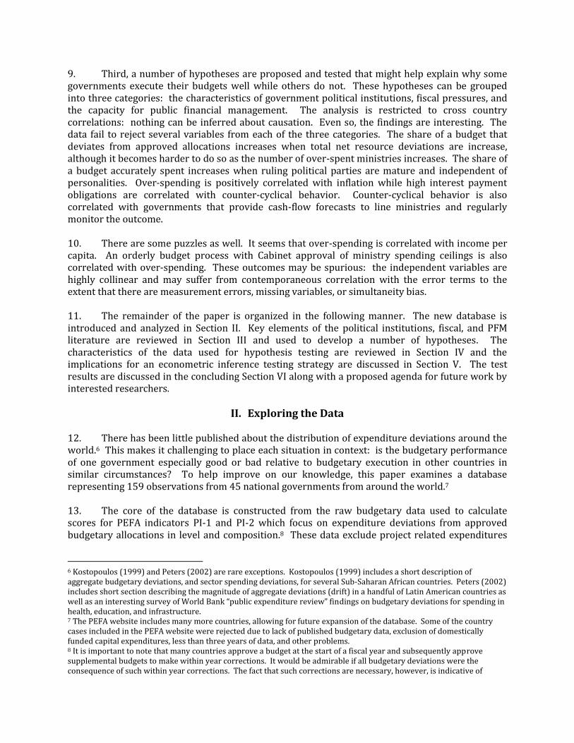
weaknesses in macroeconomic forecasting and in planning as well as the usual unanticipated shocks. The PEFA methodology focuses only on the original budget at the start of each year. 9 These are outside the direct control of the client governments and are difficult for some governments to track. 10 The PEFA website is particularly lacking in reports on developing countries from the Middle East and upper income countries in general. 11 It is common for governments to consolidate or split ministries from year to year. This can confound comparisons over time. 12

Drazen and Eslava (2005) is a good example.

deposited directly into general treasury accounts (e.g. general budget support) less interest (I) and amortization (A). Equation 1 is simply the government’s budget constraint with external project support subtracted from both sides of the equation. (1) E = TNR = R +B + F – I – A This budget constraint can be rewritten as: (2) E = R + NF = TNR where NF refers to net financing. This can be re-written again in terms of the percentage budgetary deviations where superscripts a and b refer to actual outcomes versus budgetary targets. This will be helpful when comparing compositional deviations across countries indexed by i with different sizes of budgets and with different currencies. (3) ei = (Ea,i – Eb,i)/Eb,i = (Ra,i – Rb,i)/Eb,i + (NFa,i – NFb,i)/Eb,i = (TNRa,i – TNRb,i)/Eb,i 18. Figure 1 shows that the distribution of deviations in total expenditures is centered almost on zero and includes a range of observations from a low of -45 percent to a high of 44 percent. Three observations exceed two standard deviations on the negative side of the distribution and another three exceed two standard deviations on the positive side.

FIGURE 1: DEVIATIONS IN TOTAL EXPENDITURES FIGURE 2: DEVIATIONS IN REVENUES

19. By contrast, Figure 2 shows that the majority of revenue deviations were surpluses: 89 of 159 observations were in substantial surplus, meaning they were greater than 5 percent of the budget target, 45 were within +/- 5 percent, and only 25 were less than -5 percent of the target. One possible explanation for this distribution is that many finance ministries deliberately set their targets lower than what they expect, hoping this will help reduce pressure from line ministries to spend or perhaps hoping to reserve some resources for patronage purposes. 20. As Figure 3 shows, there is a clear negative correlation between revenue deviations and deviations in net financing, implying a strong tendency towards within-year counter-cyclical financing. The implementation is far from perfect. In fact, there are many observations where net financing deviations were pro-cyclical (in the upper right and lower left quadrants of Figure 3). The imperfect counter-cyclical tendencies help explain the rather looser positive correlation in Figure 4

0

4

8

12

16

20

-50 -40 -30 -20 -10 0 10 20 30 40 50

Fre

qu

en

cy

0

5

10

15

20

25

30

35

-20 -10 0 10 20 30 40 50 60 70 80 90

Fre

qu

en

cy

between deviations in revenue (as a percent of budgeted expenditures) and deviations in expenditure (also as a share of budgeted expenditures).

FIGURE 3: DEVIATIONS IN REVENUES AND NET FINANCING FIGURE 4: DEVIATIONS IN REVENUES AND EXPENDITURES

B. Expenditure Deviations in Composition

21. In order to get a first glimpse at the compositional data, one can construct a measure of the average absolute compositional deviations within a single budget, |d|. Start by calculating the difference between the approved budgetary allocation for each budget head and the actual spending for that head. These deviations can be expressed as percentages of the approved allocations and will be positive or negative. In order to create a measure of overall ability to deliver an approved budget, the absolute values of the percentage deviations can be averaged across the total number of budget heads. The calculation for each country observation is summarized in equation 4:

(4)

where n is the number of budget heads, E is the expenditure assigned to budget head i, and the a and b subscripts refer to actual and budgeted allocations respectively. 22. There is typically a very wide range of intra-budgetary deviations for any given government and year. This is not surprising: each year brings new macroeconomic shocks and policy changes. For example, the lowest average absolute compositional deviation within the database was 4.5 percent, found in Burundi in 2005. Yet, the absolute value of the intra-budgetary deviations within the Burundi budget ranged from a low of 0.3 percent to a high of 19.8 percent. The worst average absolute compositional deviation was 435 percent, found in Bolivia in 2006. The absolute value of the intra-budgetary deviations in this case ranged from a low of 3.3 percent to a high of 7,673 percent! 23. In addition, the good performers in one year are not necessarily equally as good in the next year. For example, the Burundi average worsened to 24 percent in 2007 and 15 percent in 2007 while Bolivia improved to 135 percent in 2007 and 97 percent in 2008.

-80

-60

-40

-20

0

20

40

60

-20 0 20 40 60 80 100

Deviation in Revenues (%)

Dev

iatio

n in

Net

Fin

anci

ng (

%)

-60

-40

-20

0

20

40

60

-20 0 20 40 60 80 100

Deviation in Revenues (%)

Dev

iatio

n in

Exp

endi

ture

s (%

)

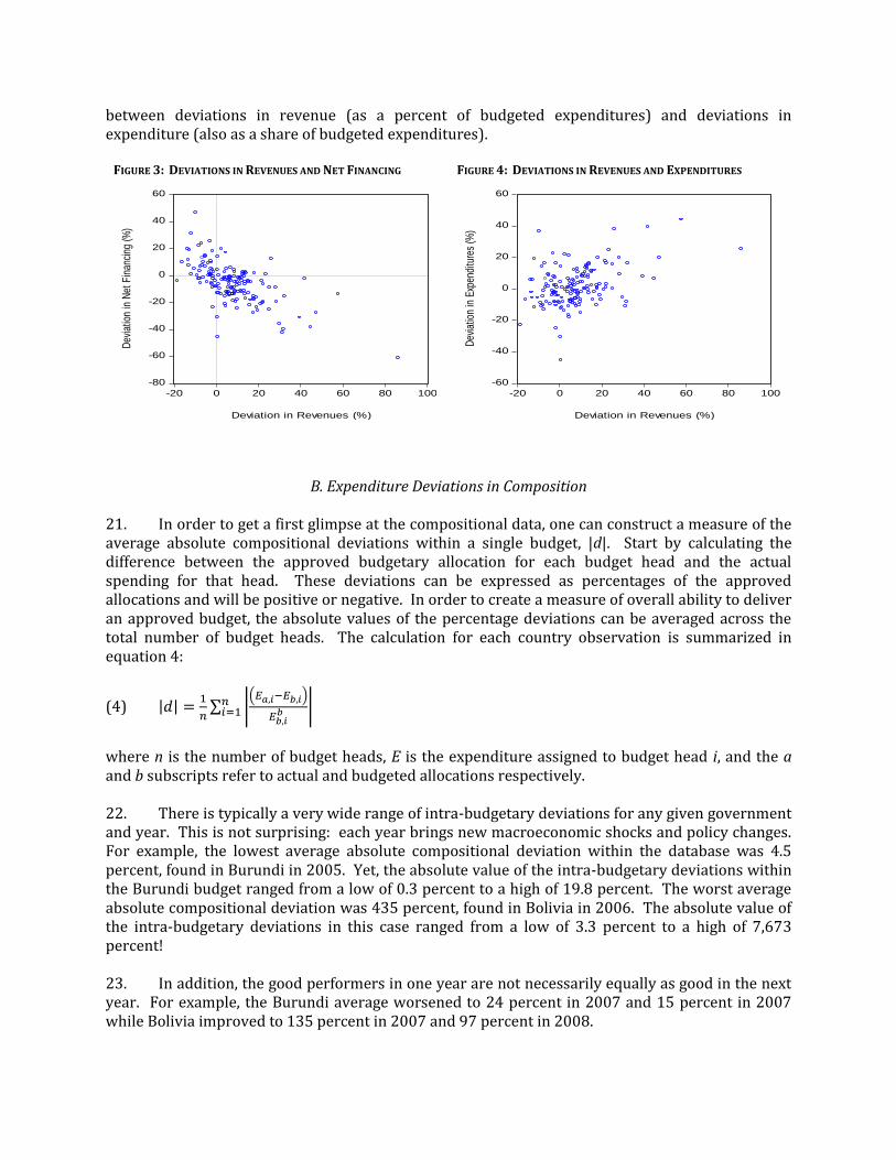
24. The distribution of the average absolute compositional deviation across all 159 observations is shown in the histogram in Figure 5 below. Average deviations between 10 and 20 percent of budgeted allocations were the most frequently found, accounting for 73 out of 159 observations. The median average deviation is 16 percent. The average of the average deviations is 29 percent with a standard deviation of 59 percent. The distribution has quite a long tail: the maximum average deviation in the data set is 557 percent. (The maximum within any given budget head can be far larger, ranging in the database from zero to several thousand percentage points!)

FIGURE 5: DISTRIBUTION OF COMPOSITIONAL DEVIATIONS

C. Compositional Deviations 25. While the measure of absolute compositional deviation clearly illustrates how few countries are able to accurately execute their budgets, it also obscures an interesting puzzle in the data: under-spending and over-spending often occur at the same time within a budget. This is a puzzle because the most obvious reaction to a shortfall in net resources would be to cut all budget heads by the same amount – or at least cut low priority programs. Without more information about extenuating circumstances, increasing spending during a shortfall would seem counterintuitive. Similarly, it would seem odd, at least at first glance, to reduce spending for some budget heads when surplus resources become available. 26. To explore compositional deviations, the data is divided into three groups: over-spent budget heads, under-spent heads, and those accurately spent within ±5 percent of budgeted allocations. These three groups can be viewed from two perspectives: (i) the share of budgetary heads falling into each group; and (ii) the average deviation away from what spending should have been in each group. This is captured in two simple relationships: (5) 1 = fo,i + fu,i + fb,i (6) ei = eo,i + eu,i + eb,i where eu < 0 where f symbolizes the fraction of budget heads in each group, e symbolizes the expenditure deviations within each group, and the subscripts refer to the over-spent group o, the under-spent

0

10

20

30

40

50

60

70

80

0 40 80 120 160 200 240 280 320 360 400 440 480 520 560

Average of Absolute Values of Budget Head Deviations, |d|

Fre

qu

en

cy

group u, and the group spent accurately within ±5 percent of budgeted allocations b. The deviations are expressed as percentages of total budgeted expenditures. Figure 6 shows the distribution of the 6 measures of compositional deviations. They are noticeably skewed and, in the case of eo, eu, and eb, also highly peaked (kurtotic).

FIGURE 6: DISTRIBUTIONS FOR MEASURES OF COMPOSITIONAL DEVIATION

6a. Over-spent group, fo 6b. Under-spent group, fu 6c. Accurately-spent group, fb

6d. Over-spent group, eo 6e. Under-spent group, eu 6f. Accurately-spent group, eb

27. Table 1 provides an example of how the data are generated. The main investment of time for the researcher comes from sorting through those budget heads that are over-spent by more than 5 percent, putting them all into one group, finding the budget heads under-spent by more than 5 percent and putting those in a second group, and assigning the remaining heads to a third group.

TABLE 1—EXAMPLE OF CALCULATIONS FOR BHUTAN, 2005-06

Over-spent group

Under-spent group

Accurately-spent group Total

Budgetary allocations (Ngultrum millions) 682 5,478 3,494 9,654 Actual expenditures (Ngultrum millions) 740 4,815 3,425 8,980 Number of budget heads (count) 1 7 4 12

fo fu fb

Fraction of budget heads (%) 8.3 58.3 33.3 100.0

eo eu ea e

Deviations w.r.t. to total spending (%) 0.6 -6.9 -0.7 -7.0

Deviations w.r.t. to own base (%) 8.5 -12.1 -2.0 -7.0 Source: Bhutan Public Financial Management Accountability Assessment, World Bank Report No. 58444-BT.

28. Substantial portions of many budgets within the data sample were over-spent even when total net resources fell below budgeted amounts and vice-versa, with portions under-spent despite the availability of excess resources. In fact, as shown in Table 2, for 56 instances of excess net resources, there were 557 heads that were over-spent by more than 5 percent while 221 heads under-spent by more than 5 percent. Similarly, for the 49 instances of net resource shortfalls, there were 568 heads that were under-spent by more than 5 percent while 162 heads over-spent by more than 5 percent. There was also simultaneous over- and under-spending even in the 54 cases when resources were close to their targets.

0

5

10

15

20

25

30

0 10 20 30 40 50 60 70 80 90 100

Fre

qu

en

cy

0

5

10

15

20

25

30

0 10 20 30 40 50 60 70 80 90 100

Fre

qu

en

cy

0

5

10

15

20

25

30

35

40

0 10 20 30 40 50 60 70 80 90

Fre

qu

en

cy

0

10

20

30

40

50

60

70

80

0 10 20 30 40 50 60 70 80 90 100

Fre

qu

en

cy

D_OVER

0

10

20

30

40

50

60

70

80

90

-100 -90 -80 -70 -60 -50 -40 -30 -20 -10 0

Fre

qu

en

cy

D_UNDER

0

4

8

12

16

20

24

28

32

-5 -4 -3 -2 -1 0 1 2 3 4 5

Fre

qu

en

cy

D_OK

TABLE 2—DISTRIBUTION OF COMPOSITIONAL DEVIATIONS Net Resource Net Resources Net Resource

Deviation > 5% Totals Deviation < -5% Close to Budget Country Observations 49 54 56 159 Heads Under-spent < -5% Number of Heads 568 313 221 1,102 Average Deviation within Heads -13.1% -4.4% -3.0% -6.6% Heads within ±5% Number of Heads 257 428 261 946 Average Deviation within Heads -0.2% 0.0% 0.2% 0.0% Heads Over-spent > 5% Number of Heads 162 302 557 1,021 Average Deviation within Heads 2.5% 4.5% 17.4% 8.4% Total Number of Heads 987 1,043 1,112 3,142 Average Deviation Net Resources -10.7% 0.1% 14.6% 1.8%

a. Compositional deviations are calculated with respect to total approved expenditures.

29. Compositional deviations tend to be larger than the deviations in total net resources because of the simultaneous over- and under-spending. For example, over-spending some budget heads during a period of an unanticipated resource shortfall necessarily requires that the remaining budget heads be cut beyond what the shortfall would have otherwise required. As shown in Table 2, for the 56 cases of surplus resources, the average deviation in net resources was 14.6 percent while the average deviation within over-spent budget heads was 17.4 percent and the average deviation within under-spent heads was -3.0 percent. For the 49 cases of resource shortfalls, the average deviation in net resources was -10.7 percent while the average deviation within under-spent budget heads was -13.1 percent, and the average deviation in over-spent heads was 2.5 percent. Box 1: Even the best performers are not perfect. South Africa between 2005/06 and 2007/08 was the best performer within the sample. Yet, even in this case, the government managed to keep only 17 of 21 budget heads within 5 percent of approved allocations in 2006/07 when the deviation in net resources was only -0.6 percent. In that year, three heads were under-spent while one was over-spent. In 2005/06, only 14 out of 21 budget heads were within 5 percent of approved allocations when the deviation in net resources was +0.4 percent. Four heads were over-spent and three were under-spent. In 2007/08, only 15 of 21 budget heads were close to approved allocations, four over-spent, and 2 under-spent. Thus, one finds simultaneous under- and over-spending even in the best performing governments.

C. Compositional Deviations and Net Resource Deviations

30. Figure 7 shows how the three budget shares are correlated with percent deviations in net total resources or, equivalently, total spending e. Figure 7a shows that the fraction of budget heads that are over-spent fo increases as net resource deviations increase. The data also show many instances of over-spending when net resource deviations are negative, confirming the data tabulations in Table 2. Figure 7b shows that the fraction of a budget that is under-spent fu decreases with positive net resource deviations. It also shows frequent under-spending despite surplus resources, as noted in Table 2. Figure 7c shows that the share of budget heads spent within ±5 percent of budgeted allocations is highest when net resource deviations are close to zero.

FIGURE 7: SHARE OF BUDGETARY HEADS AS A FUNCTION OF RESOURCE DEVIATIONS

7a. Share of Heads Over-spent, fo 7b. Share of Heads Under-spent, fu 7c. Share of Heads Within-Budget, fb

31. Figures 8a through 8c illustrate how the depth of over- and under-spending varies with deviations in total net resources. Figure 8a is focused on over-spent heads eo while Figure 8b is focused on under-spent heads eu. Both figures should and do display positive slopes: the positive deviations in over-spent heads should increase as resource deviations become more positive while the negative deviations in under-spent heads should become less negative as resource deviations become more positive. Figure 8c shows there is no obvious relationship between the depth of over or under-spending for well spent share of budget heads.

FIGURE 8: PERCENT DEVIATIONS AS A FUNCTION OF RESOURCE DEVIATIONS

8a. Over-spent Group, eo 8b. Under-spent Group, eu 8c. Accurately Spent Group, eb

32. If the apparent linear regularity in the cross country relationships illustrated in Figures 3 and 4 is representative of what happens inside individual countries, then they can be exploited to provide a bit more insight into possible government behaviors. For example, if one assumes fo and fu are linear functions of deviations in net total resources, e, such that: (6a) fo = αo + βo∙e (6b) fu = αu − βu∙e then

0

20

40

60

80

100

-60 -40 -20 0 20 40 60

Resource Deviation, e

0

20

40

60

80

100

-60 -40 -20 0 20 40 60


0

10

20

30

40

50

60

70

80

90

-60 -40 -20 0 20 40 60


0

10

20

30

40

50

-60 -40 -20 0 20 40 60


-50

-40

-30

-20

-10

0

-60 -40 -20 0 20 40 60


-3

-2

-1

0

1

2

-60 -40 -20 0 20 40 60


(6c) fb = 1 – (αu + αo) + (βu – βo)∙e where αo and αu are the intercepts seen in Figures 7a and 7b and βo and βu are the corresponding slopes. Equation 6c encompasses several interesting possibilities regarding what share of budget heads will be well spent. The share accurately spent can be increased by eliminating over-spending during shortfalls in net resources, and by eliminating under-spending when net resources are in surplus, e.g. by setting αo = αu = 0. The share well spent can also be increased by ensuring that the share of under-spent heads is always compensated by an equal share of over-sent heads, e.g. that βu – βo = 0. 33. More interesting, however, is the possibility that the share well spent can increase or decrease as net resource deviations become more positive. The share accurately spent would increase when βu – βo > 0 and decrease when βu – βo < 0. This second case is parallel to, but not the same as, empirical findings by authors such as Talvi and Vegh (2004) who discovered that spending in developing countries is strongly pro-cyclical, particularly in countries with volatile revenues, because it is politically costly to build surpluses rather than spend.13 The difference is that the findings described here refer to within-year tendencies for over- and under-spending whereas the research by Talvi and Vegh and those who followed were exploring behavior in aggregate spending across many years. 34. The main conclusion thus far is that the quality of budget execution is rather poor in most countries. Even in the best performers, it is rare for more than 15 of the 20 largest ministries to spend within 5 percent of their budgeted allocations. Over-spending and under-spending often occur simultaneously. This simultaneity causes compositional deviations to be larger than the deviations in total net resources. Over-spending and under-spending appears to be linearly correlated with net resource deviations on a cross country basis, whether measured as budgetary shares or as percentage deviations from the budget. These observations motivate a number of explanatory hypotheses presented below.

III. Literature Review and Hypotheses 35. At the time this paper was written, the available theoretical and empirical literature from the fields of fiscal economics and political economics has had little to say about why budgetary execution would be stronger in some countries than others. Even so, the literature does include a number of ideas that could be usefully extrapolated to the quality of budgetary execution. By contrast, the public financial management literature offers detailed diagnosis and prescriptions based both on logic and on specific country cases. Several ideas drawn from these three fields are presented below and are used to develop a number of testable hypotheses. These hypotheses will address measures of aggregate expenditure deviations and compositional deviations. 36. There is some useful complementarily in selecting hypotheses from these three fields. Political institutions tend to remain in place for decades while PFM improvements can be achieved within a single decade while fiscal shocks will vary from year to year. Cross-country explanations could benefit from taking each into account.

13 Some authors have speculated that the cyclical bias may be related to government weakness. Roubini and Sachs (1989) for example, found a tendency towards larger deficits in governments characterized by short average tenures and coalition governments with a large number of political parties.

37. In anticipation of the empirical work, the hypotheses presented and tested in this paper will focus only on aggregate expenditure deviations e, and on the fraction of the budget that is over-spent fo, under-spent fu, and accurately spent, fb. The data for percentage deviations eo, eu, and eb is too skewed and kurtotic to be modeled in a straightforward manner. 38. It is assumed here that decisions to deviate from the approved level and composition of expenditures are taken simultaneously and in response to a potentially common set of variables. Compositional deviations were depicted in Section II above as being correlated with deviations in total net resources. Yet the latter are a function of revenue deviations (per Figure 3), macroeconomic constraints and political institutions. In this light, it seems appropriate to work with reduced form equations, where compositional deviations are also a function of revenue deviations, other fiscal constraints, and political institutions. Thus, many of the hypotheses presented here will be oriented around revenue deviations rather than deviations to net total resources. 39. In addition, the potential correlates proposed below could enter into a regression either as part of a linear combination of variables, or through an interaction with revenue deviations, e.g. modifying the slope assigned to revenue deviations. Deviations in total expenditures will be minimized when there is no intercept (positive or negative) and when the slope is made close to zero through counter-cyclical actions. Deviations in fb are equal to 1 – fo - fu. Deviations in fo will be minimized when any positive intercept is reduced to zero and when the positive slope reduced to zero through counter-cyclical behavior. Deviations in fu will be minimized when any positive intercept is reduced to zero and when the negative slope increased to zero.

A. Institutional Theories

40. The data patterns explored in Section II suggest that expenditure deviations are positively correlated with deviations in net total resources. Yet both theory and practice suggest that ensuring a predictable flow of resources through adherence to budgetary targets is the best way to ensure good results in public service delivery. Why would governments choose deviations or allow them to take place? 41. The common-pool problem is often cited as an explanation.14 In the common-pool problem, budgetary resources are spent on the political interests of individual political leaders. Each leader will feel free to pursue their preferred position without much regard for the cost this imposes on society unless there is something counter-balancing the temptation to spend freely. 42. By itself, the common-pool problem does not generate the observed positive correlation between over-spending and unanticipated revenues seen in the data. The logic of the common-pool problem implies that over-spending would occur all the time, even when there are no unanticipated surpluses to spend, so long as political control is weak. The data contradict this: Figures 4, 7 and 8 show many instances of over-spending when deviations in net total resources are zero or close to zero. Moreover, according to common-pool logic, there should be no possibility of under-spending. Yet, the PEFA data show that most governments routinely under-spend at least some budget heads while over-spending others, and usually simultaneously.

14 Weingast, Shepsle, and Johnsen (1981) put the common pool problem at the heart of their model of geographically targeted “pork barrel” projects.

43. Two more assumptions could help explain the data. A useful clue comes from the observation in Section II that most governments appear to under-estimate revenues. If line ministry officials are aware of this under-estimation, and if they can use available information to guess at the degree of under-estimation, then their temptation to over-spend would increase as revenue deviations become more positive although they would also be constrained by various de jure or de facto limits on borrowing. In addition, rather than assuming a government is too weak to stop any over-spending, it might be more realistic to assume a government is strong enough to reduce spending by politically weak ministers in order to compensate for over-spending by others.15 Taking this idea a little further, it is likely that there are increasing costs to over-spending as more and more ministries are forced to under-spend to accommodate over-spending. To test this, a quadratic term can be included.16 The expected correlations are summarized below.

H1: Over-spending will increase as revenue deviations become more positive Aggregate

spending deviation Share of budget

heads over-spent Share of budget

heads under-spent Share of budget heads

accurately spent dR + + − |dR| − dR2 − − + |dR|2 +

44. It will be interesting to observe whether the coefficients for the share of over-spent budget heads are larger than those of the under-spent share of the budget. If they are, this would provide evidence for a within-year version of the pro-cyclical behavior observed by Talvi and Vegh noted above.

45. Common-pool behavior could be shaped in some way by prevailing political institutions. The next several hypotheses focus on this possibility according to the following typology:

autocratic versus anocractic versus autocratic17, and, within the democracies, executives elected by voters versus those elected by parliaments and plurality voting versus proportional voting.

TABLE 3—TYPOLOGY OF POLITICAL INSTITUTIONS

Majoritarian Other Total

Presidential 11 16 27 Autocracy -10 to -6 1 2 3 Anocracy -5 to +5 10 7 17 Democracy +6 to +10 0 7 7 Other a/ 4 5 9 Autocracy -10 to -6 0 0 0 Anocracy -5 to +5 1 0 1 Democracy +6 to +10 3 5 8 Total b/ 15 21 36

a. Non-presidential systems include parliamentary and mixed systems. b. The total is smaller than the sample total of 53 countries because the DPI did not include several small states.

46. Democracy versus Autocracy. Several authors have written on the impact of democracy and autocracy on economic outcomes such as real growth or the composition of spending.18 The focus here, however, is on what might motivate good budget execution. In this regard, the centrality of accountability to voters in democracies can be exploited. Lake and Baum (2001) use an analogy to 15 This pattern could be in evidence continuously and not only in synchronization with political budget cycles. 16 It turns out that the range of data does not extend beyond the turning point of the resulting quadratic equation. Other function forms were tried but did not fit well. 17 Based on Polity2 scores from the Polity IV database provided by Marshall, Jaggers, and Gurr at http://www.systemicpeace.org/polity/polity4.htm. These scores range from -10 for a hereditary monarchy (pure autocracy) to +10 for a consolidated democracy. The empirical tests use the full 21 point scale. 18 See for example and McGuire and Olson (1996) or Deacon (2003).

market theory, arguing the political competition in democracies reduces opportunities for collecting rents at the expense of public good provision. Tonizzo (2008) examines the impact of varying degrees of democracy on government size as a share of GDP. She finds that government size decreases as governments become more democratic, after controlling for income per capita, education, and the share of population over age 65. Most importantly for the discussion here, she finds that this effect is most pronounced through political competition rather than other measures of democratic characteristics such as the mean by which an executive is selected or the existence of checks and balances on executive authority. 47. While none of these authors addressed budgetary deviations directly, it may be possible to extrapolate in that direction. In particular, autocracies might be more likely to over-spend in aggregate even when revenues are on target since they can tolerate the cost of inflationary borrowing more easily than a democracy could. This suggests there should be a negative intercept in the regression equation. The higher degree of accountability in democracies could motivate better budget execution, reducing over-spending and under-spending alike. This could occur directly. It could also occur through an interaction term that softens the correlation between deviations in revenue and deviations in expenditures. There is some support for this idea in the literature: Tornell and Lane (1999) argue that weak governance allows competing groups to exploit the common pool more than proportionately as resources increase (the voracity effect) and that this problem should be reduced in democracies, to the extent that entrenched interests become less powerful and power more diffuse. This leads to the hypotheses in the table below. H2: Democracy will reduce the common-pool problem Aggregate




accurately spent Polity n/a − − Polity + Polity∙dR − − + Polity∙|dR| -

48. Keefer (2011) offers a counter-point: democracy per se may not be as important to good economic development outcomes as the nature of the political parties operating in a country. Those that are programmatic (e.g. those with an identifiable economic agenda) are more likely to get good results, possibly in non-democratic countries as well. Keefer provides two measures for the quality of political parties: one is the faction of parties that are programmatic and the other is the number of years the ruling party has existed less the number of years the current executive has been in office. The latter captures the fact that many countries are ruled by parties that are more oriented around a single personality than an agenda. Thus, a ruling party that was started by one man who has been the executive for the duration of the party would receive a score of zero. By contrast a decades old mature party with leaders in office no more than 8 years at a time would receive a very high score. It is assumed here that programmatic ruling parties would be more likely to minimize compositional deviations. H3: The presence of programmatic parties will reduce the common-pool problem Aggregate




accurately spent Party n/a − − Party + Party∙dR − − + Party∙|dR| -

49. Presidential systems versus parliamentary systems. Presidential systems are found in 32 of 46 country observations. [It is not 53 because small countries are not included in the DPI.] The literature contains two competing hypotheses. One, exemplified by Gerring, Thacker, and Moreno (2005), is that parliamentary systems should exhibit better budgetary execution than presidential

systems because political control is more concentrated, and a wider range of views (within the dominant party or coalition) can be reconciled with lower transaction costs. The other hypothesis, exemplified by Persson, Roland, and Tabellini (1997) is that the presidential system with its separation of powers is likely to display smaller government and less corruption. In particular, the concentration of power found in parliamentary systems tempts abuse and is thus empirically correlated with higher degree of corruption. Cheibub (2006) also finds favor with the presidential system, providing evidence that they generate more smaller budget deficits than parliamentary systems because voters know it is the executive branch that is responsible for budget execution and can vote out the president (or his/her party in congress) if they are not satisfied. He also finds evidence that the relatively weaker performance of parliamentary systems cannot be traced to the costs of maintaining coalition governments as seen in some countries.19 50. These ideas can be applied to budget execution. If presidential systems are more likely to have smaller budget deficits and are less likely to be corrupt, then perhaps they would also display a comparatively better quality of budget execution. To test this hypotheses, a dummy (System) can be employed, based on information taken from the World Bank Database of Political Institutions. The dummy is set to one for presidential systems, so that a zero signifies parliamentary and mixed systems. H4: Presidential systems will reduce the common-pool problem Aggregate




accurately spent System n/a − − System + System∙dR − − + System∙|dR| -

51. Plurality vs proportional elections. There are 21 countries in the sample of 44 for which data are available with plurality (majoritarian, first past the post, winner takes all) elections. Lizzeri and Persico (2001) argue that politicians in majority rule systems have incentives to cater to the preferences of those who can help them to get enough votes to win. They will do so by promising targeted spending. Targeted spending makes less sense in proportional systems because every vote counts. Yet, as Duverger (1954) observed, most plurality systems tend to gravitate towards just two parties while proportional systems tend to have several parties. Proportional systems could therefore require higher spending on side payments and patronage to hold coalitions together. Persson and Tabellini found empirical evidence that countries with plurality elections have smaller expenditures and less corruption. 52. It is not obvious how these two lines of argument would affect the quality of budgetary execution. The approach taken here, without any justifying argument, is to assign a dummy value of 1 to majoritarian systems with the hypothesis that governments with majoritarian systems will display better budget execution. The data are taken from the World Bank Database of Political Institutions. H5: Plurality voting will reduce the common-pool problem Aggregate




accurately spent Plur n/a − − Plur + Plur∙dR − − + Plur∙|dR| -

19 Roubini and Sachs (1989) for example, found a tendency towards larger deficits in governments characterized by short average tenures and coalition governments with a large number of political parties.

53. To close the section on political institutions, it should be noted that the literature contains some reasons to think that the symmetrical hypothesis proposed in H2 above may not be correct. Gavin and Perotti (1997) discovered that public expenditures in OECD countries tended to be pro-cyclical during economic upswings and counter-cyclical during down-swings. Talvi and Vegh (2004) found that spending in developing countries is strongly pro-cyclical because it is politically costly to build surpluses rather than spend. Persson and Tabellini (2000) found something more nuanced: negative income shocks significantly raise spending in parliamentary and proportional systems, while positive income shocks do not lower the spending share. In contrast, positive shocks raise spending in presidential and majoritarian systems while negative shocks have no impact. These effects might be detected by comparing the signs of any significant correlates for under-spending versus over-spending.

B. Fiscal Theories 54. Revenues typically deviate from the fiscal target underlying a budget because of real shocks to the revenue base, inflationary shocks, unanticipated changes in policy, or unanticipated changes in revenue administration. In the section below, various elements of the wide literature on fiscal economics is used to explain why the motivation and ability to compensate for these unanticipated shocks might vary across countries. 55. Unanticipated inflation. Unanticipated price inflation could have two different kinds of impact, depending upon the situation. If the unexpected inflation was very high, then it should motivate under-spending in responsible governments with the power to influence monetary outcomes.20 Yet, a government could also choose to let spending increase enough to maintain its purchasing power, and thus its political and development objectives, if it had the opportunity to do so, e.g. if the inflation rate was low.21 This suggests that the incentive to spend from an unanticipated positive revenue shock would decrease with the inflation rate in the previous year (abstracting from administrative and policy changes). 56. Data on how much price inflation was unanticipated by a government in a given year is not readily available. A few governments publish the expected rate of inflation but many do not. As a proxy, it is assumed here that governments facing unanticipated positive revenue shocks would want to avoid spending from them when inflation was high in the previous year – knowing that inflation tends to have an inertial component. In other words, fiscal policy should be counter-cyclical in nature, leading to the hypotheses below. H6a: Unanticipated inflation will motivate under-spending when prior inflation is high

Aggregate spending deviation

Share of budget heads over-spent

Share of budget heads under-spent

Share of budget heads accurately spent

CPIt-1∙FL∙dR − − + CPIt-1∙FL∙|dR| n.a.

57. Conversely, there is a possibility that unanticipated inflation is the consequence of habitual over-spending. In this case, there would be a positive correlation between inflation (prior or present) and expenditure deviations.

20 Governments using a foreign currency or a fixed exchange rate do not have such powers. The exchange rate regime will be indicated by a dummy variable (FL) assigned a value of 1 for flexible exchange rate systems (including managed floats) and zero otherwise. Data on exchange rate regimes are taken from various issues of the IMF Classification of Exchange Rate Arrangements and Monetary Policy Frameworks. Fixed rates within bands and crawling pegs are included with floating rates since there is scope for monetary policy under these arrangements. 21 In addition, it would be ideal if domestic debt was low, and output was a bit below potential.

H6b: Unanticipated inflation is the consequence of habitual over-spending Aggregate




accurately spent CPIt-1∙FL + + - CPIt-1∙FL n.a.

58. Shocks to Relative Prices. Unanticipated changes in relative prices could cause compositional deviations away from approved budgetary allocations. An unanticipated increase in the international price of oil relative to other costs (non-fuel CPI), such as occurred in 2008, is an obvious example for many countries. Fuel intensive activities would either need to be reduced or, if public service targets are to be maintained, then spending would need to be substantially increased, perhaps at the cost of reducing spending in other activities. This hypothesis will not be tested here due to the author’s lack of information about which countries subsidize fuel prices and which do not. 59. Unanticipated real shocks. Many governments use fiscal policy to counteract the impact of economic recessions and short-term negative real growth. For example, according to the September 2011 IMF Fiscal Monitor, many countries employed a package of spending stimulus measures during the 2009 global recession. In most cases, an unanticipated negative revenue shock can be traced to real reductions in the revenue base (again abstracting from administrative and policy changes) because inflation is rarely negative.22 Thus, if real output is below potential, and if there is an unanticipated negative revenue shock, then government officials should tend to seek extra stimulus through excess spending. As in the case of inflation, however, only a few governments publish expected real GDP and most of the less developed countries cannot track GDP movements within a year. To obtain roughly the same effect, it is assumed here that if output in the prior year was below potential (e.g. a negative gap), and if there was an unanticipated negative revenue shock, then it is likely that government officials will expect current year real output to be below the target used in the fiscal framework underpinning the budget.23 In such circumstances, they may conclude that extra stimulus through higher spending is desirable. This generates the hypothesized relations below.

H7: An unanticipated output gap should motivate over-spending when the prior gap is negative Aggregate




accurately spent GAPt-1 n.a. n.a. n.a. GAPt-1 n.a. GAPt-1∙dR + + − GAPt-1∙|dR| n.a.

60. Debt service. When debt burdens are too high, spending is typically reduced in order to slow the rate of borrowing or generate surpluses. This suggests that when interest obligations are a large share of total spending, a larger share of any unanticipated revenue surpluses should be used to reduce the stock of debt rather than spent on various ministries.24 Conversely, when the interest payment share is very low, governments may be more willing to borrow when revenues are below target. This suggests that high interest payment shares should interact with the slope of the correlation between revenue deviations and total expenditure deviations, making the slope less positive. This would be equally true for the fraction of budget heads over-spent, with the opposite

22 There are only 4 out of 159 examples in the database. Moreover, negative inflation would be dealt with through the interaction term above, driving up spending. 23 Economic output is defined as being below long-run potential when real GDP per capita is below a geometric trend line based on real GDP per capita in the preceding 10 years. The gap is expressed as a percentage deviation from the trend line, with negative percentages signifying output is below potential and positive percentages signifying output is above potential. Output gaps in a given year are highly correlated with output gaps in the preceding year. 24 No portion of an unanticipated surplus may be used for spending in Belgium, as noted by … .

interaction expected for the fraction of the budget under-spent. The impact on the fraction of the budget that is accurately spent should be zero since unanticipated revenue shocks should be diverted to changes in debt stocks rather than spending.

H8a: Unanticipated positive shocks should be saved when the interest obligation share of spending is high Aggregate




accurately spent INTRt-1∙dR − − + INTRt-1∙|dR| n.a.

61. Conversely, there is a possibility that high interest obligations are the consequence of habitual over-spending. In this case, there would be a positive correlation between the share of spending devoted to interest payments and expenditure deviations.

H8b: Unanticipated positive shocks should be saved when the interest obligation share of spending is high Aggregate




accurately spent INTRt-1 + + - INTRt-1 n.a.

62. Income per Capita and Tax Base Stability. De Renzio (2007) found that income per capita is positively correlated with average PEFA scores but did not provide any ideas why this might be so. One possibility is that governments in wealthier countries can pay for better talent and better systems of control than other governments. Another possible explanation comes from Wildavsky (1986) who argued that income per capita could shape the way governments behave. In particular, wealthy countries with stable tax bases would tend to display incremental budgets while the least developed countries with unstable tax bases would be forced to use “repetitive” budgeting, adjusting their expenditures frequently in accord with cash availability.25 Testing Wildavsky’s argument will require a measure of tax base stability in addition to income per capita (GNIPC). The standard deviation in the growth of revenues and grants (RAGSD) will serve here as a proxy for stability of the tax base. On one axis, counter-cyclical policy should be easier to implement as income per capita increases. On the other axis, counter-cyclical policy should become more difficult as the revenue base becomes more volatile. H9: Counter-cyclical policies should be easier as income per capita increases



Share of budget heads under-

spent


ln(GNIPC) n.a. n.a. n.a. ln(GNIPC) + ln(GNIPC)∙dR − − + ln(GNIPC)∙dR n.a.

H10: Counter-cyclical policies should be more difficult as volatility in revenues and grants increases





RAGSD n.a. n.a. n.a. RAGSD − RAGSD∙dR + + − RAGSD∙|dR| n.a.

C. Public Financial Management

63. As noted in the introduction, appropriate techniques of public financial management are needed if a government is to successfully pursue its objectives within prevailing macroeconomic and fiscal constraints. Premchand (1999) offers a good overview of the key topics in what is a

25 Interestingly, Ramey and Ramey ( ) observed, wealthier countries tend to have greater stability in output growth. This correlation is evident in the sample but only at the 15 percent level of signicance.

highly technical field of study and practice.26 These include the roles of the executive and the legislature, policy formulation, budget formulation, budget structures (focus on inputs or programs or outputs?), internal controls (centralized or decentralized, rigid or flexible?), payment systems, accounting and financial reporting, and the importance of external audit to accountability. Von Hagen (2007) makes a parallel point in suggesting that the common-pool problem can be reduced by introducing budgetary rules (there shall be a balanced budget) and procedures (agree on total spending before deciding the composition) backed by centralized mechanisms that impose costs on politicians who do not display adequate restraint.27 64. The PEFA framework provides a means of exploring many of these topics empirically. Several PEFA indicators are nominated below as potential correlated of the quality of budgetary execution. The descriptions of the indicators are generally quoted directly from the PEFA framework without modification. 65. Orderliness and participation in the annual budget process (PI-11). While the Ministry of Finance (MOF) is usually the driver of the annual budget formulation process, effective participation in the budget formulation process by other ministries, departments and agencies (MDAs) as well as the political leadership, impacts the extent to which the budget will reflect macro-economic, fiscal and sector policies. Additionally, the extent to which line ministries have been well consulted should increase their “ownership” of the budget and thus their willingness to implement it accurately. The scoring for orderliness and participation ranges from 1 for poor to 4 for excellent. The criteria include (i) the existence of and adherence to a fixed budget calendar; (ii) the clarity/comprehensiveness of and political involvement in the guidance on the preparation of budget submissions (budget circular or equivalent); and (iii) timely budget approval by the legislature or similarly mandated body. It seems reasonable to expect that the quality of budget execution should increase as PI-11 increases. This should happen directly and through the motivation to conduct counter-cyclical policy. H11: the quality of budget execution should increase as PI-11 increases





PI-11 n.a. − − PI-11 + PI-11∙dR − − + PI-11∙|dR| −

66. Predictability in the availability of funds for commitment of expenditures (PI-16). Effective execution of the budget, in accordance with the work plans, requires that the spending ministries, departments and agencies (MDAs) receive reliable information on availability of funds within which they can commit expenditure for recurrent and capital inputs. This indicator assesses the extent to which the central ministry of finance provides reliable information on the availability of funds to MDAs, that manage administrative (or program) budget heads (or votes) in the central government budget and therefore are the primary recipients of such information from the ministry of finance. The scoring for predictability ranges from 1 for poor to 4 for excellent. The criteria for scoring include: (i) the extent to which cash flows are forecast and monitored; (ii) the reliability and horizon of periodic in-year information to MDAs on ceilings for expenditure commitment; and (iii) the frequency and transparency of adjustments to budget allocations, which are decided above the level of management of MDAs. Hypothesis 12 is that the degree of good budget execution should

26 Books such as Premchand (1984) or Shah (2007) offer deeper guidance. 27 Von Hagen provides a tantalizing example of how Belgium deals with unanticipated revenues or under-spending, requiring that the surplus shall be used only to pay down the national debt.

increase as PI-16 increases. This should happen directly and through the motivation to conduct counter-cyclical policy.

H12: the quality of budget execution should increase as PI-16 increases Aggregate




accurately spent PI-16 n.a. − − PI-16 + PI-16∙dR − − + PI-16∙|dR| −

67. Effectiveness of expenditure controls. A composite variable is constructed from the average of the PEFA indicators for payroll controls (PI-18) and for controls on all other expenditures (PI-20).28 The scores range from 1 for poor controls to 4 for very good controls. In the case of PI-18, the score reflects (i) the Degree of integration and reconciliation between personnel records and payroll data, (ii) the timeliness of changes to personnel records and the payroll; (iii) the effectiveness of internal controls to changes in personnel records and the payroll; and (iv) the existence of payroll audits to identify control weaknesses and/or ghost workers. For all other expenditures, PI-20 measures (i) the effectiveness of expenditure commitment controls; (ii) the comprehensiveness, relevance and understanding of other internal control rules/ procedures; and (iii) the degree of compliance with rules for processing and recording transactions. Hypothesis 13 is that positive expenditure deviations will be reduced as expenditure controls are strengthened. (Expenditure controls cannot force under-spending ministries to spend more.)





accurately spent PI-1820 n.a. − − PI-1820 + PI-1820∙dR − − n.a. PI-1820∙|dR| −

68. Legislative scrutiny of external audit reports (PI-28). The legislature has a key role in exercising scrutiny over the execution of the budget that it approved. This indicator measures (i) the timeliness of examination of audit reports by the legislature (for reports received within the last three years); (ii) the extent of hearings on key findings undertaken by the legislature; and (iii) the issuance of recommended actions by the legislature and implementation by the executive. The score ranges from 1 for weak legislative scrutiny (or the absence of it) to 4 for highly effective scrutiny. The scoring criteria include: (i) the timeliness of examination of audit reports by the legislature (for reports received within the last three years); (ii) the extent of hearings on key findings undertaken by the legislature; and (iii) the issuance of recommended actions by the legislature and implementation by the executive. Hypothesis 14 is that expenditure deviations will

be reduced as legislative scrutiny (accountability) improves. This should happen directly and through the motivation to conduct counter-cyclical policy.





accurately spent PI-28 n.a. − − PI-28 + PI-28∙dR − − + PI-28∙|dR| −

28 The indicator PI-18 was not assessed in the cases of Georgia and Lesotho. For these countries, the average of PI-18 and PI-20 was set to the score from PI-20, knowing that the correlation coefficient for the two variables across the other countries in the sample is 0.The full list of countries included in the full and common samples is found in Annex Table 5.63.

D. Controls 69. Conflict. Several countries in the database were suffering from conflicts during the periods under measurement. Conflict could increase compositional deviations if battle outcomes and battle needs were difficult to predict. To test for any impact, a measure of battle deaths as a share of the population is constructed. H15: The quality of budget execution should worsen as conflict increases.





Battle n.a. + + Battle − Battle∙dR n.a. n.a. n.a. Battle∙|dR| n.a.

70. Population Size. De Renzio (2007) used population as a control variable and proposed that there could be economies of scale in investing in budget systems in larger countries. This would imply that counter-cyclical policies should be easier to implement in countries with larger populations and, in addition, compositional deviations should also be lower in high population countries. H16: The quality of budget execution should increase with population size.





Ln(POP) n.a. − − Ln(POP) + Ln(POP)∙dR − − + Ln(POP)∙|dR| −

71. Government employment. The compositional data are strongly biased towards recurrent spending for most countries which in this sample are mainly poor countries that finance most of their capital investments from external aid. Conversely, rich countries such as Norway tend to have small capital budgets since the private sector takes on a greater role in providing infrastructure and utility services. The personnel bill is often a large part of the recurrent budget and it is normally well protected if only because politicians want to avoid unrest and know it is often difficult to replace skilled workers lost to attrition over poor pay conditions. This protection is achieved through counter-cyclical policies and the avoidance of over-spending on non-wage related activities. Thus it will be useful to control for the effect of large employment bills in the search for correlated of budget execution. The hypothesis is that the quality of budget execution should increase with the share of spending on employment. H17: The quality of budget execution should increase with the share of spending on employment





Empl n.a. − − Empl + Empl∙dR − − + Empl∙|dR| -

IV. Data

72. The empirical tests below will focus on 4 dependent variables, total spending e, the fraction of over-spent budget heads fo, the fraction of under-spent budget heads fu, and the share of accurately spent budget heads fb. The hypotheses advanced in the section above yield 17 potential explanatory variables. These are listed in the table below along with their statistical properties. These are shown twice, once for the full sample and once for a common sample. Not all of the 53 country observations for compositional deviations were accompanied by data for each of the explanatory variables proposed above. In fact, only 36 country observations could be found for

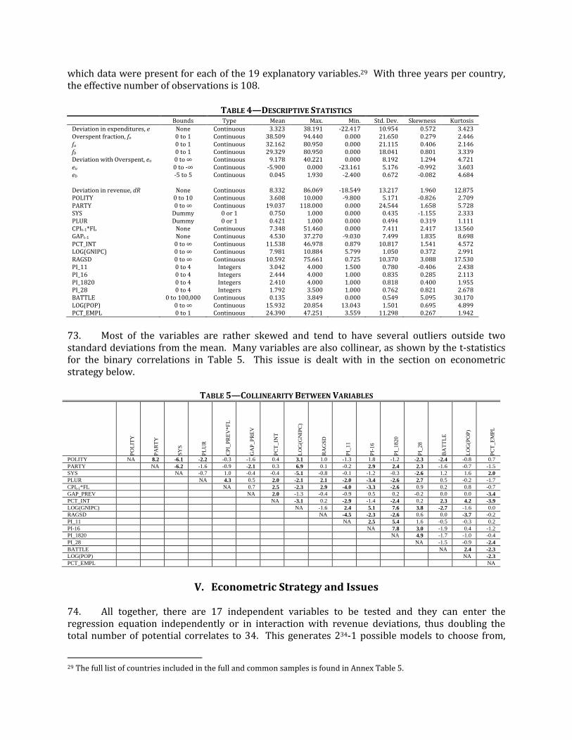
which data were present for each of the 19 explanatory variables.29 With three years per country, the effective number of observations is 108.

TABLE 4—DESCRIPTIVE STATISTICS

Bounds Type Mean Max. Min. Std. Dev. Skewness Kurtosis

Deviation in expenditures, e None Continuous 3.323 38.191 -22.417 10.954 0.572 3.423 Overspent fraction, fo 0 to 1 Continuous 38.509 94.440 0.000 21.650 0.279 2.446 fu 0 to 1 Continuous 32.162 80.950 0.000 21.115 0.406 2.146 fb 0 to 1 Continuous 29.329 80.950 0.000 18.041 0.801 3.339 Deviation with Overspent, eo 0 to ∞ Continuous 9.178 40.221 0.000 8.192 1.294 4.721 eu 0 to -∞ Continuous -5.900 0.000 -23.161 5.176 -0.992 3.603 eb -5 to 5 Continuous 0.045 1.930 -2.400 0.672 -0.082 4.684

Deviation in revenue, dR None Continuous 8.332 86.069 -18.549 13.217 1.960 12.875 POLITY 0 to 10 Continuous 3.608 10.000 -9.800 5.171 -0.826 2.709 PARTY 0 to ∞ Continuous 19.037 118.000 0.000 24.544 1.658 5.728 SYS Dummy 0 or 1 0.750 1.000 0.000 0.435 -1.155 2.333 PLUR Dummy 0 or 1 0.421 1.000 0.000 0.494 0.319 1.111 CPIt-1*FL None Continuous 7.348 51.460 0.000 7.411 2.417 13.560 GAPt-1 None Continuous 4.530 37.270 -9.030 7.499 1.835 8.698 PCT_INT 0 to ∞ Continuous 11.538 46.978 0.879 10.817 1.541 4.572 LOG(GNIPC) 0 to ∞ Continuous 7.981 10.884 5.799 1.050 0.372 2.991 RAGSD 0 to ∞ Continuous 10.592 75.661 0.725 10.370 3.088 17.530 PI_11 0 to 4 Integers 3.042 4.000 1.500 0.780 -0.406 2.438 PI_16 0 to 4 Integers 2.444 4.000 1.000 0.835 0.285 2.113 PI_1820 0 to 4 Integers 2.410 4.000 1.000 0.818 0.400 1.955 PI_28 0 to 4 Integers 1.792 3.500 1.000 0.762 0.821 2.678 BATTLE 0 to 100,000 Continuous 0.135 3.849 0.000 0.549 5.095 30.170 LOG(POP) 0 to ∞ Continuous 15.932 20.854 13.043 1.501 0.695 4.899 PCT_EMPL 0 to 1 Continuous 24.390 47.251 3.559 11.298 0.267 1.942

73. Most of the variables are rather skewed and tend to have several outliers outside two standard deviations from the mean. Many variables are also collinear, as shown by the t-statistics for the binary correlations in Table 5. This issue is dealt with in the section on econometric strategy below.

TABLE 5—COLLINEARITY BETWEEN VARIABLES

PO

LIT

Y

PA

RT

Y

SY

S

PL

UR

CP

I_P

RE

V*

FL

GA

P_P

RE

V

PC

T_IN

T

LO

G(G

NIP

C)

RA

GS

D

PI_

11

PI-

16

PI_

1820

PI_

28

BA

TT

LE

LO

G(P

OP

)

PC

T_E

MP

L

POLITY NA 8.2 -6.1 -2.2 -0.3 -1.6 0.4 3.1 1.0 -1.3 1.8 -1.2 -2.3 -2.4 -0.8 0.7

PARTY

NA -6.2 -1.6 -0.9 -2.1 0.3 6.9 0.1 -0.2 2.9 2.4 2.3 -1.6 -0.7 -1.5

SYS

NA -0.7 1.0 -0.4 -0.4 -5.1 -0.8 -0.1 -1.2 -0.3 -2.6 1.2 1.6 2.0

PLUR

NA 4.3 0.5 2.0 -2.1 2.1 -2.0 -3.4 -2.6 2.7 0.5 -0.2 -1.7

CPIt-1*FL

NA 0.7 2.5 -2.3 2.9 -4.0 -3.3 -2.6 0.9 0.2 0.8 -0.7

GAP_PREV

NA 2.0 -1.3 -0.4 -0.9 0.5 0.2 -0.2 0.0 0.0 -3.4

PCT_INT

NA -3.1 0.2 -2.9 -1.4 -2.4 0.2 2.3 4.2 -3.9

LOG(GNIPC)

NA -1.6 2.4 5.1 7.6 3.8 -2.7 -1.6 0.0

RAGSD

NA -4.5 -2.3 -2.6 0.6 0.0 -3.7 -0.2

PI_11

NA 2.5 5.4 1.6 -0.5 -0.3 0.2

PI-16

NA 7.8 3.0 -1.9 0.4 -1.2

PI_1820

NA 4.9 -1.7 -1.0 -0.4

PI_28

NA -1.5 -0.9 -2.4

BATTLE

NA 2.4 -2.3

LOG(POP)

NA -2.3

PCT_EMPL

NA

V. Econometric Strategy and Issues

74. All together, there are 17 independent variables to be tested and they can enter the regression equation independently or in interaction with revenue deviations, thus doubling the total number of potential correlates to 34. This generates 234-1 possible models to choose from,

29 The full list of countries included in the full and common samples is found in Annex Table 5.

roughly 17.2 billion! Within these, there may be many models where the variables of interest take the expected signs and are significantly different from zero. Unfortunately, due to the frequent collinearity between variables, standard errors will be larger and some variables may be incorrectly rejected. The econometrician will also often observe that a regressor that is positive in one model becomes negative or insignificant in other models. One could also easily miss the fact that an estimated coefficient and its variance are not stable over the majority of models. Worse, one may succumb to temptation and only report the favorable models.

75. In order to expeditiously deal with this challenge, a three step process is employed. The first step is to set out an encompassing regression equation for each of the independent variables, with each equation including all variables from the hypotheses above plus any dummies required to generate a normally distributed error term in order to ensure that hypothesis testing is feasible in a stepwise, general-to-specific procedure. The variable with the highest probability of being rejected as insignificant is removed. The variable with the next highest p-value, given the removal of the first variable, is also removed. Next both of the removed variables are checked for re-inclusion into the model: any variable whose p-value is lower than 5 percent is added back in to the model. Once the addition step has been performed, the next variable is removed. This process is repeated until the largest p-value of the remaining variables is less than 5 percent.30

76. Second, the possibility that some variables are significant only on the strength of various leverage points was tested. This was done by splitting the sample roughly in half and employing the general-to-specific procedure again for each half. Variables that are not significant in both of the smaller samples are dropped, as are those that do not display the same sign. Variables that show large changes in the size of coefficients are retained – though this outcome should serve as a strong cautionary signal that the significance of the variable may not be robust. 77. Third, it is possible for the general to specific approach to miss a key variable or include a variable that may be significant only upon the inclusion of some other variable. In order to get a second opinion on model selection, a technique referred to as Bayesian Averaging of Classical Estimates (BACE) is employed. As explained by Sala-i-Martin (1997) and Doppelhofer et al. (2000), rather than assuming there is a single correct model, as in a simplification search, they assign weights corresponding to a “level of confidence” for each model. This then allows them to calculate a weighted OLS average for each of the potential variables. The only prior assumption required is the expected model size, e.g. out of K variables proposed, perhaps only k would be expected to be significant.31 78. The main statistics generated by BACE for each regressor include the posterior inclusion probability (PIP), the posterior mean coefficient, and the posterior mean standard deviation. The latter two are calculated unconditionally and conditional on inclusion. The PIP indicates the probability that a regressor drawn from set K should be included in a robust model of size k. The posterior means are the weighted averages of all the coefficients and their standard deviations for all models. The posterior means that are conditional upon inclusion use weights based on the assumption that each regressor must be included in any model of size k. For this purpose, the weights are revised to sum to one only for those models containing the regressor. The ratio of the posterior mean coefficients to the posterior mean standard deviations is analogous to the t-statistic.

30 The reported p-value could be higher than 5 percent if White heteroskedasticity-consistent standard errors and covariances are employed after finding heteroskedasticity. 31 Magnus et al (2010) propose an alternative technique that is less computationally demanding. The author did not have access to software using this methodology.

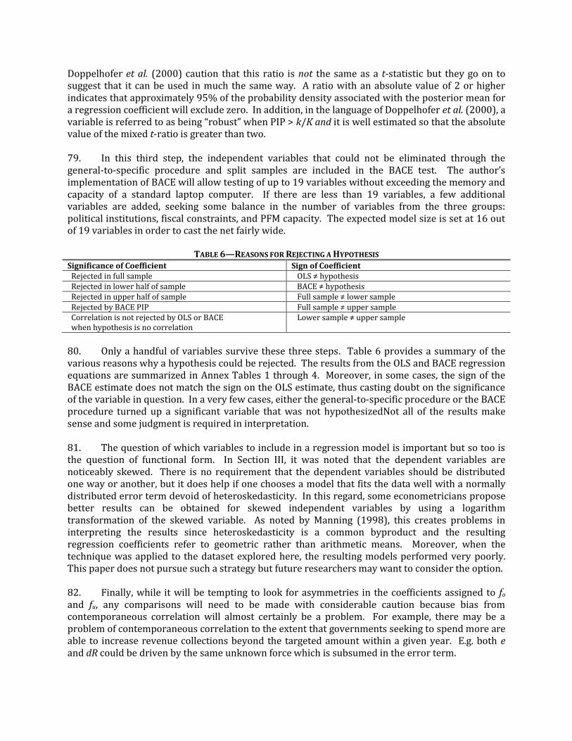
Doppelhofer et al. (2000) caution that this ratio is not the same as a t-statistic but they go on to suggest that it can be used in much the same way. A ratio with an absolute value of 2 or higher indicates that approximately 95% of the probability density associated with the posterior mean for a regression coefficient will exclude zero. In addition, in the language of Doppelhofer et al. (2000), a variable is referred to as being “robust” when PIP > k/K and it is well estimated so that the absolute value of the mixed t-ratio is greater than two. 79. In this third step, the independent variables that could not be eliminated through the general-to-specific procedure and split samples are included in the BACE test. The author’s implementation of BACE will allow testing of up to 19 variables without exceeding the memory and capacity of a standard laptop computer. If there are less than 19 variables, a few additional variables are added, seeking some balance in the number of variables from the three groups: political institutions, fiscal constraints, and PFM capacity. The expected model size is set at 16 out of 19 variables in order to cast the net fairly wide.

TABLE 6—REASONS FOR REJECTING A HYPOTHESIS Significance of Coefficient Sign of Coefficient Rejected in full sample OLS ≠ hypothesis Rejected in lower half of sample BACE ≠ hypothesis Rejected in upper half of sample Full sample ≠ lower sample Rejected by BACE PIP Full sample ≠ upper sample Correlation is not rejected by OLS or BACE when hypothesis is no correlation

Lower sample ≠ upper sample

80. Only a handful of variables survive these three steps. Table 6 provides a summary of the various reasons why a hypothesis could be rejected. The results from the OLS and BACE regression equations are summarized in Annex Tables 1 through 4. Moreover, in some cases, the sign of the BACE estimate does not match the sign on the OLS estimate, thus casting doubt on the significance of the variable in question. In a very few cases, either the general-to-specific procedure or the BACE procedure turned up a significant variable that was not hypothesizedNot all of the results make sense and some judgment is required in interpretation. 81. The question of which variables to include in a regression model is important but so too is the question of functional form. In Section III, it was noted that the dependent variables are noticeably skewed. There is no requirement that the dependent variables should be distributed one way or another, but it does help if one chooses a model that fits the data well with a normally distributed error term devoid of heteroskedasticity. In this regard, some econometricians propose better results can be obtained for skewed independent variables by using a logarithm transformation of the skewed variable. As noted by Manning (1998), this creates problems in interpreting the results since heteroskedasticity is a common byproduct and the resulting regression coefficients refer to geometric rather than arithmetic means. Moreover, when the technique was applied to the dataset explored here, the resulting models performed very poorly. This paper does not pursue such a strategy but future researchers may want to consider the option. 82. Finally, while it will be tempting to look for asymmetries in the coefficients assigned to fo and fu, any comparisons will need to be made with considerable caution because bias from contemporaneous correlation will almost certainly be a problem. For example, there may be a problem of contemporaneous correlation to the extent that governments seeking to spend more are able to increase revenue collections beyond the targeted amount within a given year. E.g. both e and dR could be driven by the same unknown force which is subsumed in the error term.

VI. Test Results and Interpretations 83. The broad conclusion is that there is evidence that several, though far from all, of the proposed hypotheses may be helpful in explaining cross-country patterns of quality in budgetary execution. Tests for the correlates of the over-spent fraction of a budget fo was most successful with 9 of 17 hypotheses not rejected by the three step process outlined above. Only 6 of 17 hypotheses were not rejected for the percentage deviation in total spending, e. Only 3 hypotheses survived in the case of the under-spent fraction of a budget, fu. This may be due to the highly skewed distribution for fu as shown in Figure 6 above. Only 1 hypothesis was not rejected for the fraction of a budget accurately spent, fb. This may be explained by the attempt to model it as if over- and under-spending were symmetrical when there is strong evidence that they are not. 84. It appears that each of the three categories of hypotheses have a role to play. Hypotheses involving fiscal constraints were rejected the least, followed by hypotheses related to political institutions. The impact of public financial management capacity was limited to the degree to which line ministries receive good information about the availability of funds (PI-16). The outcomes are reviewed in more detail below.

A. Political Institutions 85. The modified common-pool hypothesis was not rejected for total expenditure deviations, e, nor for the over-spent fraction of the budget, fo. In addition, the idea that over-spending becomes more difficult as more ministries are over-spent was also not rejected.

86. Only one additional political institutions hypothesis survived. Counter-cyclical policies were used to reduce the degree of over-spending in aggregate and for the share of over-spent budget heads more often in countries with mature programmatic parties (H3) than those with less mature or less programmatic parties. This result was one of the few that is also robust after testing with Bayesian averaging.

TABLE 7—POLITICAL INSTITUTIONS

Deviation in Total

Expenditure , e Fraction

Over-spent, fo Fraction

Under-spent, fu Fraction

Accurately-spent, fb

Hy

po

thes

is

Act

ual

Co

ncl

usi

on

Hy

po

thes

is

Act

ual

Co

ncl

usi

on

Hy

po

thes

is

Act

ual

Co

ncl

usi

on

Hy

po

thes

is

Act

ual

Co

ncl

usi

on

H1 dR + + * + + * − R |dR| − R dR2 − R − − * + R |dR|2 + R H2 POLITY n.a. − R − R POLITY + R POLITY∙dR − R − R + R POLITY∙|dR| − R H3 PARTY n.a. + R − R − R PARTY + + * PARTY∙dR − − * − − * + R PARTY∙|dR| − R H4 SYS n.a. + R − R − R SYS + R SYS∙dR − R − R + R SYS∙|dR| − R H5 PLUR n.a. − R − R PLUR + R PLUR∙dR − R − R + R PLUR∙|dR| − R

An R signifies that the hypothesis was rejected by the 3 step process. A checkmark signifies that a hypothesis was not rejected. Asterisks signify that a coefficient is significant in both OLS and BACE and consistently displays the same sign regardless of sample size. Blanks signify that one or more of these criteria are not met.

87. This outcome is in need of more exploration. On the one hand, Table 5 shows there is strong collinearity between the measure for programmatic parties and the measure for the degree of democracy. It may be that both are measuring the same thing. To sort this out, it would be

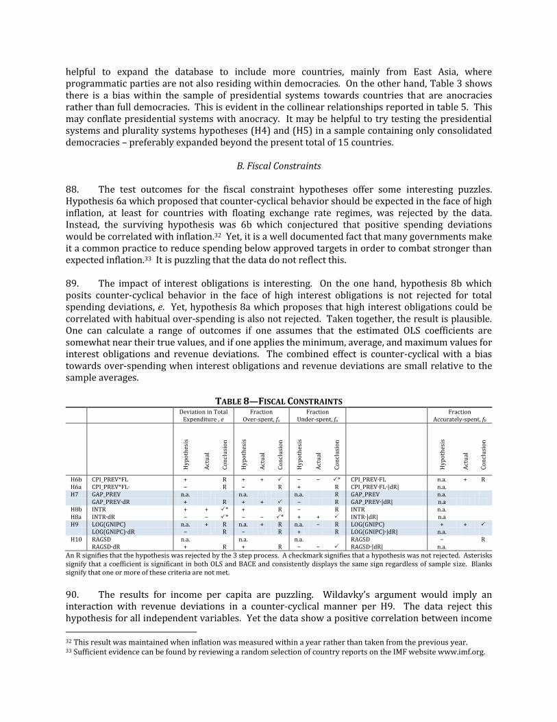
helpful to expand the database to include more countries, mainly from East Asia, where programmatic parties are not also residing within democracies. On the other hand, Table 3 shows there is a bias within the sample of presidential systems towards countries that are anocracies rather than full democracies. This is evident in the collinear relationships reported in table 5. This may conflate presidential systems with anocracy. It may be helpful to try testing the presidential systems and plurality systems hypotheses (H4) and (H5) in a sample containing only consolidated democracies – preferably expanded beyond the present total of 15 countries.

B. Fiscal Constraints 88. The test outcomes for the fiscal constraint hypotheses offer some interesting puzzles. Hypothesis 6a which proposed that counter-cyclical behavior should be expected in the face of high inflation, at least for countries with floating exchange rate regimes, was rejected by the data. Instead, the surviving hypothesis was 6b which conjectured that positive spending deviations would be correlated with inflation.32 Yet, it is a well documented fact that many governments make it a common practice to reduce spending below approved targets in order to combat stronger than expected inflation.33 It is puzzling that the data do not reflect this. 89. The impact of interest obligations is interesting. On the one hand, hypothesis 8b which posits counter-cyclical behavior in the face of high interest obligations is not rejected for total spending deviations, e. Yet, hypothesis 8a which proposes that high interest obligations could be correlated with habitual over-spending is also not rejected. Taken together, the result is plausible. One can calculate a range of outcomes if one assumes that the estimated OLS coefficients are somewhat near their true values, and if one applies the minimum, average, and maximum values for interest obligations and revenue deviations. The combined effect is counter-cyclical with a bias towards over-spending when interest obligations and revenue deviations are small relative to the sample averages.

TABLE 8—FISCAL CONSTRAINTS

Deviation in Total





Hy

po

thes

is

Act

ual

Co

ncl

usi

on

Hy

po

thes

is

Act

ual

Co

ncl

usi

on

Hy

po

thes

is

Act

ual

Co

ncl

usi

on

Hy

po

thes

is

Act

ual

Co

ncl

usi

on

H6b CPI_PREV*FL + R + + − − * CPI_PREV∙FL n.a. + R H6a CPI_PREV*FL∙ − R − R + R CPI_PREV∙FL∙|dR| n.a. H7 GAP_PREV n.a. n.a. n.a. R GAP_PREV n.a. GAP_PREV∙dR + R + + − R GAP_PREV∙|dR| n.a H8b INTR + + * + R − R INTR n.a. H8a INTR∙dR − − * − − * + + INTR∙|dR| n.a H9 LOG(GNIPC) n.a. + R n.a. + R n.a. − R LOG(GNIPC) + + LOG(GNIPC)∙dR − R − R + R LOG(GNIPC)∙|dR| n.a. H10 RAGSD n.a. n.a. n.a. RAGSD − R RAGSD∙dR + R + R − − RAGSD∙|dR| n.a.


90. The results for income per capita are puzzling. Wildavky’s argument would imply an interaction with revenue deviations in a counter-cyclical manner per H9. The data reject this hypothesis for all independent variables. Yet the data show a positive correlation between income

32 This result was maintained when inflation was measured within a year rather than taken from the previous year. 33 Sufficient evidence can be found by reviewing a random selection of country reports on the IMF website www.imf.org.

per capita and deviations in total expenditures, backed by a higher fraction of the budget being over-spent and a smaller share being under-spent. It is difficult to imagine why this should be so. The data do not reject the other half of Wildavsky’s idea, with regard to tax base volatility (H10), but only in the case of the under-spent fraction of the budget, fu.

C. Quality of Public Financial Management 91. Hypothesis 11 that the quality of budgetary execution would improve with an orderly budget process with political buy-in was rejected by the data. To the contrary, a high score for PI-11 is correlated with over-spending. This may be spurious: more work would be needed to confirm whether this outcome is truly robust.

TABLE 9—QUALITY OF PUBLIC FINANCIAL MANAGEMENT

Deviation in Total





Hy

po

thes

is

Act

ual

Co

ncl

usi

on

Hy

po

thes

is

Act

ual

Co

ncl

usi

on

Hy

po

thes

is

Act

ual

Co

ncl

usi

on

Hy

po

thes

is

Act

ual

Co

ncl

usi

on

H11 PI_11 n.a. +* R − +* R − R PI_11 + R PI_11∙dR − R − R + R PI_11∙|dR| − R

H12 PI-16 n.a. − R − R PI-16 + + * PI-16∙dR − − − − * + R PI-16∙|dR| − R

H13 PI_1820 n.a. − R − − PI_1820 + R PI_1820∙dR − R − R n.a. PI_1820∙|dR| − R

H14 PI_28 n.a. −* R − R − R PI_28 + R

PI_28∙dR − R − R + R PI_28∙|dR| − R


92. Hypothesis 12 that counter-cyclical policies would be correlated with good practices in cash-flow forecasting and monitoring was not rejected by the data for total expenditure deviations, e, nor for the over-spent fraction of the budget, fo, nor for the share of the budget accurately spent, fb. The result for the over-spent and accurately-spent fractions are robust in BACE. 93. Hypothesis H13 for expenditure controls is not rejected for the under-spent fraction of the budget, fu. This makes sense only if the over-spent fraction fo decreases or the accurately spent fraction fb increases. Perhaps this would be seen only within countries rather than across countries. 94. The rejection of hypotheses for expenditure controls (PI-1820), in most but not all cases, and for the impact of external audit (PI-28) may seem troubling to some readers. Some comfort can be taken from knowing that, on the one hand, the data are highly collinear. E.g. a country with a high score for PI-16 is very likely to also have a high score for PI-18, PI-20, and PI-28. On the other hand, logic suggests that one of the key reasons to excel along a PI-16 dimension would be to facilitate expenditure control and avoid censure from parliament. 95. In thinking about the outcomes above, an important question to ask is whether PFM capacity might be driven by prevailing political institutions. Do some kinds of political institutions have higher PEFA scores than others? The t-statistics from the bilateral correlations shown in Table 5 provide a partial clue. Two patterns stand out. The variables PI-16, PI-18, PI-20, and PI-28 are all positively and significantly correlated with the presence of mature programmatic political parties. The variables PI-11, PI-16, PI-18, PI-20, and PI-28 are all negatively and significantly correlated with majoritarian voting systems. Yet, regression analysis shows that the political

institutions explain less than 10 percent of the cross-country variation in PEFA scores. This is consistent with de renzio (2009) who found his data rejected correlations between average PEFA scores and resource dependency, type of political executive, type of parliamentary system, press freedom and the level of democracy.

D. Controls 96. Only one hypothesis from the proposed control variables survived the three step testing procedure. The idea that counter-cyclical policy would be easier to implement in high population countries due to a scale effect in PFM systems acquisition (H16) is not rejected by the data for aggregate spending nor for the over-spent fraction of the budget. 97. Population size is also negatively correlated with the under-spent fraction of the budget. This could be a good thing if the over-spent portion of the budget also decreased with population size. It does not. Population size is positively correlated with total expenditure deviations, e, and with the over-spent fraction of the budget, fo. For these two independent variables, e and fo, population size is operating on both the intercept and the slope of the revenue deviations curve. The combined effect is counter-cyclical with a bias towards over-spending that is exacerbated by reductions in the under-spent fraction of the budget. This bias increases with population size. Why this should be so requires a new hypothesis. It may be that social and political pressures to over-spend (and reduce under-spending) increase with population size.

TABLE 10—CONTROLS

Deviation in Total





Hy

po

thes

is

Act

ual

Co

ncl

usi

on

Hy

po

thes

is

Act

ual

Co

ncl

usi

on

Hy

po

thes

is

Act

ual

Co

ncl

usi

on

Hy

po

thes

is

Act

ual

Co

ncl

usi

on

H15 BATTLE n.a. + R + R BATTLE − R BATTLE∙dR n.a. n.a. n.a. BATTLE∙|dR| n.a. + R H16 LOG(POP) n.a. + R − + R − − * LOG(POP) + R LOG(POP)∙dR − R − − + R LOG(POP)∙|dR| − R H17 PCT_EMPL n.a. + R − R − R PCT_EMPL + R PCT_EMPL∙dR − − − R + R PCT_EMPL∙|dR| − R


98. Hypothesis 17 for a counter-cyclical impact from large budget shares devoted to employment was not rejected for total expenditures. The fact that this is not also reflected in the other measures of budgetary deviations may be due to the cross-country nature of the database. Panel data may allow a deeper within country look.

VII. Conclusions

99. This paper introduced and exploited a new database of budgetary execution. It was discovered that very few countries are able to execute their budgets well. There are widespread errors in forecasting revenues and within-year counter-cyclical financing often fails to fully compensate for revenue deviations. Compositional deviations from budget targets tend to be greater than deviations in total net resources. Second, a number of hypotheses to explain the cross-country distribution of budgetary execution quality are inferred from the literature on political institutions, fiscal theory, and public financial management. The data fail to reject correlations with

several variables. The share of a budget that deviates from approved allocations increases when total net resource deviations increase, although it becomes harder to do so as the number of over-spent ministries increases. The share of a budget accurately spent increases when ruling political parties are mature and independent of personalities. Over-spending is positively correlated with inflation while high interest payment obligations are correlated with counter-cyclical behavior. Counter-cyclical behavior is also correlated with governments that provide cash-flow forecasts to line ministries and regularly monitor the outcome. Reductions in the under-spent fraction of a budget are robustly correlated with stronger expenditure controls – implying a corresponding within country reduction in the over-spent fraction of a budget. 100. All of these conclusions should be considered as preliminary. A deepened agenda of work is required to move beyond simple tests of correlation towards testing for specific coefficient values. Highly consistent estimates for the regression coefficients are not within reach due to the impact of numerous outliers and leverage points revealed by the split sample results. A larger sample may help overcome these problems. Many of the variables are collinear, a situation that was only imperfectly dealt with through the application of a general to specific approach and Bayesian model averaging. There are also reasons to expect some of the data are contemporaneously correlated either on account of measurement error, missing variables, or simultaneity bias. This creates bias in the estimated coefficients, so that hypothesis testing is limited here to whether a correlation is significantly different from zero in a positive or negative direction. 101. There are many opportunities for researchers who may want to challenge or expand upon the work begun in this paper. The data sample could be expanded to include more countries, ideally with more representation from high income countries, and with more years per country. This might eventually allow a panel approach to explore within country correlates. This may help resolve some of the incongruities above where an effect seen in one measure of budgetary deviation is not seen in the others. 102. There are a number of econometric challenges that could be addressed. No work has been done yet to test the correlates of the highly skewed percentage deviations ( eo, eu and eb) in the over-spent, under-spent, and accurately-spent portions of each budget. More work is clearly needed in order to sort out issues related to collinearity and contemporaneous correlation. Given the strong probability that the choice of political institutions also determines PFM capacity, simultaneity bias could be a clear source of contemporaneous correlation. 103. It may be possible to expand the list of hypotheses. The list of proposed hypotheses is a first attempt with lots of room for debate and innovation. One obvious possibility is to extend the political economics theory of election cycles to the issue of budgetary deviations. Do election cycles have an impact on aggregate or compositional deviations? If so, under what circumstances? Are some sectors routinely protected more than others? The work by Drazen and Eslava (2005) is intriguing: it provides a behavioral model that points in the right direction. They find that the composition of spending tends to shift away from recurrent spending and towards projects immediately before elections at the local level. Having ordered such a shift, would politicians also push their bureaucracy to ensure the shift is well implemented or would the promise be sufficient so that subsequent budgetary deviations are politically costless? Another possibility is that there may be demographic forces at work. Tonizzo (2008) argued that a large share of the population over 65 years of age would increase the redistributive demand for social services, thereby increasing total expenditures. If this also leads to pressure to spend in excess of budgetary targets, then it would be a useful control variable. It may even help explain the positive correlation

between income and over-spending to the extent that higher income countries tend to have larger shares of senior populations.

Bibliography Cheibub, Jose, 2006., Presidentialism, Electoral Identifiability, and Budget Balances in Democratic Systems, American Political Science Review, Vol. 100, No. 3. Deacon, Robert., 2003, Dictatorship, Democracy, and the Provision of Public Goods, Departmental Working Papers, Department of Economics, UCSB, UC Santa Barbara. de Renzio P., 2009., Taking Stock: What do PEFA Assessments Tell Us About PFM Systems Across Countries?, Working Paper 302, Overseas Development Institute. Duverger, Maurice., 1954., Political Parties: Their Organization and Activity in the Modern State, Wiley, New York. Doppelhofer, G., X. Sala-i-Martin, and R. Miller, 2000. ‘Determinants of Long-run Growth: A Bayesian Averaging of Classical Estimates (BACE) Approach’, Working Paper 7750, Cambridge MA: National Bureau of Economic Research. Drazen, Allan and Marcela Eslava, 2005., Electoral Manipulation via Expenditure Composition: Theory and Evidence, Working Paper 11085, NBER Working Paper Series Gavin M. and R. Perotti (1997), “Fiscal policy in Latin America," NBER Macroeconomics Annual, 12, 11-61. Gerring, John; Strom Thacker, and Carola Moreno, 2005., Are Parliamentary Systems Better?, Comparative Political Studies, Vol. 42, No. 3, 327-359. IMF, 2001., Government Financial Statistics Manual, Washington, DC. IMF, 2011., Fiscal Monitor—Addressing Fiscal Challenges to Reduce Economic Risks, Washington, DC. IMF, various issues, Classification of Exchange Rate Arrangements and Monetary Policy Frameworks, Washington, DC. Lizzeri, Allesando And Nicola Persico, 2001., Why Did The Elites Extend The Suffrage? Democracy and the Scope Of Government, With An Application To Britain’s “Age of Reform,” The Quarterly Journal of Economics, May. Kopits, George, 2001. Fiscal Rules: Useful Policy Framework or Unnecessary Ornament?, IMF Working Paper 01/145. Kostopoulos, Christos, 1999., “Progress in Public Expenditure Management in Africa: Evidence from World Bank Surveys,” Africa Region Working Paper Series – 1. Lake, David and Matthew Baum, 2001., The Invisible Hand of Democracy: Political Control and the Provision of Public Services, Comparative Political Studies, Vol. 34, No. 6, 587-621.

Magnus J., O. Powell, P. Prufer, 2010. A Comparison of Two Model Averaging Techniques with an Application to Growth Empirics, Journal of Econometrics, 154:139-153. Manning, Willard G., 1998. The Logged Dependent variable, Heteroskedasticity, and the Retransformation Problem, Journal of Health Economics, No. 17. Marshall, Monty; Jaggers, Keith; and Ted Gurr, 2010., Polity IV Project, Political Regime Characteristics and Transitions, 1800-2009, Center for International Development and Conflict Management, University of Maryland, College Park, MD. http://www.systemicpeace.org/polity/polity4.htm McGuire, Martin and Mancur Olson, Jr., 1996, The Economics of Autocracy and Majority Rule: The Invisible Hand and the Use of Force, Journal of Economic Literature, Vol. 24, No. 1. Peters, Lucian, 2002. Sound Budget Execution for Poverty Reduction, A Background Paper for the World Bank Institute Program on “Fiscal Policy for Poverty Alleviation” Module on Budget Execution, World Bank, Washington, DC. PEFA Secretariat, 2005. Public Financial Management Performance Measurement Framework, World Bank, Washington, DC. Persson, Torsten, 2002, Do Political Institutions Shape Economic Policy?, Econometrica, Vol. 70, No. 3, 883–905 Persson, T., G. Roland, and G. Tabellini, 1997., Separation of Powers and Political Accountability, Quarterly Journal of Economics, 112, 310–327. Persson, T. and G. Tabellini, 2000., Political Institutions and Economic Policy Outcomes: What Are the Stylized Facts?, Mimeo, Institute for International Economic Studies. Premchand, Agrigapudi, 1984. Government Budgeting and Expenditure Controls: Theory and Practice, International Monetary Fund. Premchand, Agrigapudi, 1999. Public Financial Management: Getting the Basics Right, in Governance, Corruption and Public Financial Management, Asian Development Bank. Premchand, Agrigapudi, 2001. Unfinished Agenda in Public Financial Management, Public

Administration and Public Policy, Vol 91, pages 123-138.

Ramey G. and V. Ramey, 1995., Cross-Country Evidence on the Link between Volatility and Growth, American Economic Review, Vol. 85, No. 5, 1138-1150. Roubini N. and J. Sachs, 1989., Political and Economic Determinants of Budget Deficits in the Industrial Democracies," European Economic Review, 33, 903-938. Sala-i-Martin, X., 1997. ‘I Just Ran 2 Million Regressions’, American Economic Review, 87(2): 178-183.

Schiavo-Campo, Salvatore, 2007., The Budget and It’s Coverage, in Budgeting and Budgetary Institutions, Anwar Shah, editor. The World Bank

Schick, Allen, 1998., A Contemporary Approach to Public Expenditure Management, World Bank Institute. Shah, Anwar, editor, 2007, Budgeting and Budgetary Institutions, The World Bank. Talvi, Ernesto and Carlos Vegh, 2004., Tax Base Variability and Procyclical Policy, Working Paper 7499, National Bureau of Economic Research, Washington, DC. Tonizzo, Martina., 2008, Political Institutions, Size of Government and Redistribution: An Empirical Investigation, Development Studies Institute Working Paper Series, No. 08-89. Tornell, Aaron and Philip Lane, 1999. The Voracity Effect, The American Economic Review, Vol. 89, No. 1 (Mar., 1999), pp. 22-46. Von Hagen, Jurgen, 2007. Budgeting Institutions for Better Fiscal Performance, in Budgeting and Budgetary Institutions, Anwar Shah, editor, The World Bank. Wildavsky, Aaron, 1986., Budgeting: a Comparative Theory of Budgetary Processes, Transaction Publishers, New Jersey.

Weingast, B., Shepsle, K., and C. Johnsen, 1981. The Political Economy of Benefits and Costs: A Neoclassical Approach to Distributive Politics, The Journal of Political Economy, Vol. 89, No. 4, pp. 642-664. World Bank, 1998., Expenditure Management Handbook, Washington, DC.

ANNEX TABLE 1—DEVIATIONS IN TOTAL EXPENDITURES, e

Hypothesis Encompassing Equation Best Survivors

Full Sample Best Survivors

Lower Half of Sample Best Survivors

Upper Half of Sample BACE Results

Variable Expected Conclusion Coefficient Prob. 1/ Coefficient Prob. Coefficient Prob. 1/ Coefficient Prob. 1/ Mixed t-ratio PIP

C

-131.7799 0.0000 -112.9749 0.0000

dR -131.7799 0.0000 -112.9749 0.0000 -171.3157 0.0000 -22.1946 0.0000

dR^2 1.0000 OK 3.4721 0.0498 5.5565 0.0000 3.7065 0.9997 POLITY -1.0000 R -0.5411 0.3315

POLITY∙dR Na -0.0451 0.9199 -0.9313 0.0003 0.8705 0.6954

PARTY -1.0000 R 0.0334 0.3245 -0.0432 0.0199

PARTY∙dR Na 0.1345 0.0985 0.1474 0.0061 0.2856 0.0002 0.1065 0.0016 1.1166 0.7767 SYS -1.0000 OK -0.0122 0.0136 -0.1112 0.0001 -0.0054 0.0015 -3.0710 0.9981

SYS∙dR Na R 5.6646 0.1896 5.8913 0.0074 2.3641 0.9764

PLUR -1.0000 R 0.2519 0.3959 1.0943 0.0000

PLUR∙dR Na -3.7627 0.1484 -10.7777 0.0000

CPI_PREV*FL -1.0000 R 0.2494 0.2317 1.2789 0.0000 CPI_PREV*FL∙dR 1.0000 R 0.3277 0.0710 0.3133 0.0012 1.4082 0.0000 1.0531 0.7557

GAP_PREV -1.0000 R 0.0328 0.0634 0.0556 0.0000 0.0212 0.0469 -0.0697 0.0001 2.7801 0.9893

GAP_PREV∙dR Na 0.0577 0.7545

PCT_INT 1.0000 R 0.0169 0.2963

PCT_INT∙dR 1.0000 OK 0.6566 0.0001 0.5971 0.0000 0.2981 0.0039 4.2874 0.9999 LOG(GNIPC) -1.0000 OK -0.0438 0.0006 -0.0401 0.0000 -3.7126 0.9994

LOG(GNIPC)∙dR Na R 4.4548 0.0059 3.7049 0.0008 6.5781 0.0000 3.6680 0.9992

RAGSD -1.0000 R 0.1120 0.4107

RAGSD∙dR Na 0.1352 0.3046 PI_11 1.0000 R -0.0123 0.1869 -0.0147 0.0002 -0.0119 0.0000 -2.7269 0.9883

PI_11∙dR Na R 8.3753 0.0001 5.0492 0.0000 10.3562 0.0000 6.0669 0.0000 4.6634 1.0000

PI-16 -1.0000 R -0.1086 0.4470 0.2564 0.0068 -0.5418 0.0004

PI-16∙dR Na 1.2562 0.4735

PI_1820 -1.0000 OK -0.3612 0.0288 -0.1839 0.0202 -0.5930 0.0000 -2.0505 0.9540 PI_1820∙dR Na -1.1987 0.6322

PI_28 -1.0000 R -0.0484 0.8149 -0.2777 0.0012 0.8675 0.0000

PI_28∙dR Na R -6.1657 0.0209 -4.2147 0.0002 -10.2598 0.0000 -2.7433 0.0209 -2.3660 0.9722

BATTLE -1.0000 R 0.3739 0.0820 0.2645 0.0237

BATTLE∙dR Na -0.4907 0.8137 6.6914 0.0000 LOG(POP) Na -0.0086 0.9732 -1.2874 0.0000

LOG(POP)∙dR Na R 3.7644 0.0000 3.5232 0.0000 5.8269 0.0000 5.2067 1.0000

PCT_EMPL -1.0000 R -0.1820 0.0085 -0.2390 0.0001 -0.0706 0.0003 0.0924 0.0034 -3.2391 0.9968

PCT_EMPL∙dR Na 0.2178 0.0548 0.2014 0.0253 0.3001 0.0005 0.8583 0.6938 Dummies (None) (None) (One) {Two)

Observations (incl. dummy variables) 108 108 57 51

R-squared 0.6938 0.6282 0.9243 0.9037

Adjusted R-squared 0.5512 0.5628 0.8913 0.8541 S.E. of regression 7.3380 7.2424 3.9846 3.6210

Sum squared resid 3930.7280 4,773.1130 619.2036 432.6798

Log likelihood -347.3456 -357.8310 -148.8629 -126.8893

F-statistic 4.8653 9.6098 28.0222 18.2169

Prob(F-statistic) 0.0000 0.0000 0.0000 0.0000 Normal error term: Jarque-Bera probability 0.7446 0.9107 0.9687 0.6268

Heteroskedasticity Test: White Probability(without cross terms) 0.8826 0.9598 0.8508 0.3448

Omitted Variable Test: RESET Probability (1 term) 0.1564 0.1069 0.7222 0.2595

1. White heteroskedasticity-consistent standard errors & covariance.

ANNEX TABLE 2—Fraction of Budget Heads Over-spent, fo

Hypothesis Encompassing Equation Best Survivors

Full Sample Best Survivors

Lower Half of Sample Best Survivors

Upper Half of Sample BACE Results

Variable Expected Conclusion Coefficient Prob. 1/ Coefficient Prob. 1/ Coefficient Prob. 1/ Coefficient Prob. 1/ Mixed t-ratio PIP

C -175.4823 0.0000 -153.2905 0.0000 -645.9601 0.0000 -127.3264 0.0000

dR 1 OK 6.6377 0.0473 4.5162 0.0010 4.9704 0.0000 2.0634 0.9771

dR^2 -1 OK -1.6031 0.0948 -1.4694 0.0075 -2.3022 0.9639 POLITY -1 R 1.2325 0.1559 -2.6256 0.0145

POLITY∙dR -1 R -0.0515 0.4160 0.2731 0.0043 0.1595 0.0000

PARTY -1 R -0.0123 0.9258 2.0360 0.0000 0.1813 0.0028

PARTY∙dR -1 OK -0.0163 0.0145 -0.0145 0.0003 -0.1240 0.0001 -0.0219 0.0000 -3.4009 0.9977 SYS -1 R 14.6907 0.0423 9.7531 0.0131 80.5508 0.0000 42.7753 0.0000 1.2681 0.7966

SYS∙dR -1 R -0.1263 0.7928 -1.6154 0.0302 -1.1236 0.0007

PLUR -1 R 2.2920 0.6331 -27.0056 0.0000

PLUR∙dR -1 R 0.1014 0.7846 3.0812 0.0000 2.0748 0.0000 0.3190 0.3993

CPIt-1*FL 1 OK 0.5441 0.0176 0.8123 0.0001 2.7483 0.0000 3.5051 0.9982 CPIt-1*FL∙dR -1 R 0.0064 0.8281 -0.0875 0.0030 -0.1579 0.0000

GAP_PREV Na 0.1397 0.6307 -3.3837 0.0000 0.8318 0.0000

GAP_PREV∙dR 1 OK 0.0369 0.1718 0.0531 0.0017 1.6785 0.8918

PCT_INT 1 R 1.0399 0.0001 0.8969 0.0000 -0.5648 0.0000 3.7443 0.9985

PCT_INT∙dR -1 OK -0.0781 0.0004 -0.0618 0.0000 -4.2414 0.9997 LOG(GNIPC) Na R 5.0773 0.0767 7.6469 0.0001 15.3912 0.0000 2.8777 0.9889

LOG(GNIPC)∙dR -1 R 0.1263 0.5801 1.2846 0.0001

RAGSD Na 0.1380 0.5303 -1.0855 0.0006 1.1962 0.0000 0.0642 0.3457

RAGSD∙dR 1 R -0.0117 0.5012 0.1381 0.0001 -0.0535 0.0000 PI_11 -1 R 14.5516 0.0000 13.2498 0.0000 39.1269 0.0000 25.9432 0.0000 5.8555 1.0000

PI_11∙dR -1 R -0.1756 0.5047 -1.0766 0.0007 -0.5909 0.0050

PI-16 -1 R -1.7691 0.5723 36.4268 0.0000 4.2333 0.0058

PI-16∙dR -1 OK -0.5045 0.1105 -0.4001 0.0037 -1.2264 0.0513 -1.5866 0.0000 -2.4228 0.9670

PI_1820 -1 R 1.4164 0.7572 -47.2377 0.0000 PI_1820∙dR -1 R 0.2295 0.6175 2.0858 0.0002 1.1340 0.0000

PI_28 -1 R -10.3347 0.0149 -13.0410 0.0000 24.7211 0.0001 3.1902 0.0440 -3.8653 0.9998

PI_28∙dR -1 R 0.5387 0.1269 0.6936 0.0057 -1.5439 0.0002 1.6427 0.8846

BATTLE 1 R -5.7092 0.1382 -8.1762 0.0015 18.9022 0.0000 15.9115 0.0000 -2.8819 0.9887

BATTLE∙dR Na -0.0834 0.8616 -0.4118 0.0292 LOG(POP) -1 R 6.2391 0.0000 5.3446 0.0000 21.3863 0.0000 3.8369 0.9995

LOG(POP)∙dR -1 OK -0.2785 0.0227 -0.2070 0.0122 -0.3941 0.0000 -1.2825 0.8183

PCT_EMPL -1 R 0.2827 0.1151 0.6117 0.0222 0.4311 0.0008

PCT_EMPL∙dR -1 R -0.0246 0.1124 -0.6703 0.5482 Dummies (Three) (Three) (Five) (Eight)


R-squared 0.7513 0.7069 0.9477 0.9919

Adjusted R-squared 0.6199 0.6436 0.8873 0.9786 S.E. of regression 13.3475 12.9250 7.8590 2.8760

Sum squared resid 12470.9400 14700.9600 1605.8480 157.1604

Log likelihood -409.6927 -418.5763 -176.0226 -101.0646

F-statistic 5.7164 11.1690 15.7025 74.9056





ANNEX TABLE 3—Fraction of Budget Heads Under-spent, fu

Variable

Hypothesis Encompassing Equation

Best Survivors Full Sample

Best Survivors Lower Half of Sample

Best Survivors Upper Half of Sample BACE Results

Expected Conclusion Coefficient Prob. 1/ Coefficient Prob. 1/ Coefficient Prob. 1/ Coefficient Prob. 1/ Mixed t-ratio PIP

C 206.5288 0.0000 189.7654 0.0000 122.9424 0.0000 145.0224 0.0000

dR -1 R -1.7336 0.5538 2.1978 0.0006 8.6898 0.0000 -0.7624 0.6300

dR^2 1 R 2.1715 0.0083 0.9659 0.0000 0.5427 0.5140

POLITY -1 R 0.3741 0.5857 -1.6686 0.0176 POLITY∙dR 1 R 0.0047 0.9234 0.0566 0.0146

PARTY -1 R -0.1662 0.1905 0.0105 0.0019 0.4811 0.0052

PARTY∙dR 1 R 0.0132 0.0458 0.0700 0.0000 0.9756 0.6855

SYS -1 R 13.6894 0.0554 15.0357 0.0002 0.1844 0.3767 SYS∙dR 1 R -0.4942 0.2673 -0.4309 0.0384 2.5276 0.0000 -0.5194 0.5014

PLUR -1 R -6.7040 0.1234 -9.2500 0.0020 -39.6919 0.0000 22.6625 0.0000 0.4777 0.4525

PLUR∙dR 1 R -0.2803 0.3835 2.3660 0.0000

CPIt-1*FL -1 OK -1.0352 0.0001 -0.9394 0.0000 -2.5626 0.0000 -2.2262 0.9631

CPIt-1*FL∙dR 1 R 0.0420 0.0743 0.0418 0.0336 -0.0644 0.0001 0.0848 0.0107 0.5056 0.4802 GAP_PREV Na R -0.6261 0.0464 -0.7394 0.0004 0.7544 0.0365 -2.4501 0.9811

GAP_PREV∙dR -1 R 0.0432 0.1263 0.0590 0.0022 0.8546 0.6383

PCT_INT -1 R -0.2506 0.2761 0.8846 0.0000

PCT_INT∙dR 1 OK 0.0487 0.0057 0.0334 0.0006 1.4847 0.8516

LOG(GNIPC) Na R -11.1317 0.0000 -11.4167 0.0000 -15.4292 0.0000 -3.3162 0.9944 LOG(GNIPC)∙dR 1 R -0.0110 0.9544 -1.1300 0.0000 -0.6375 0.0000

RAGSD Na 0.0254 0.8766 -1.1091 0.0000

RAGSD∙dR -1 OK -0.0099 0.5288 -0.0168 0.0266 -0.5773 0.5369

PI_11 -1 R -6.6186 0.0423 -5.7343 0.0018 -11.1128 0.0000 7.6843 0.0023 -3.6145 0.9981 PI_11∙dR 1 R -0.1110 0.6723

PI-16 -1 R -4.3617 0.1972

PI-16∙dR 1 R 0.3626 0.1830 1.5826 0.0000

PI_1820 -1 OK -4.8564 0.2808 -6.9129 0.0021 -4.5966 0.0378 -0.5320 0.4730

PI_1820∙dR Na -0.0668 0.8483 -1.4029 0.0000 1.2020 0.0000 PI_28 -1 R 16.4760 0.0001 14.1173 0.0000 29.0548 0.0000 9.9325 0.0022 0.9227 0.6772

PI_28∙dR 1 R -0.7206 0.0205 -0.5972 0.0003 -0.6924 0.0059 -0.4975 0.5143

BATTLE 1 R -0.0791 0.9768 -9.4399 0.0000

BATTLE∙dR Na -0.8966 0.0266 -0.9263 0.0012 -1.4125 0.0000 -1.1818 0.7630 LOG(POP) -1 OK -3.7933 0.0005 -3.5789 0.0000 -5.9056 0.0022 -4.2636 0.9999

LOG(POP)∙dR 1 R 0.0687 0.5066

PCT_EMPL -1 R -0.2528 0.1170 1.7772 0.0000

PCT_EMPL∙dR 1 R 0.0178 0.1526 -0.1036 0.0000 0.0307 0.0060

Dummies (Six) (Six) (Four) (Three)


R-squared 0.8188 0.7923 0.9491 0.8984

Adjusted R-squared 0.7107 0.7323 0.9080 0.8507

S.E. of regression 11.3574 10.9252 7.2325 6.8248 Sum squared resid 8642.4230 9906.8430 1621.5990 1583.6590

Log likelihood -389.8899 -397.2632 -176.3008 -159.9754

F-statistic 7.5712 13.1956 23.1028 18.8002





ANNEX TABLE 4—Fraction of Budget Heads Accurately-spent, fb

Variable

Hypothesis Encompassing Equation

Best Survivors Full Sample

Best Survivors Lower Half of Sample

Best Survivors Upper Half of Sample BACE Results

Expected Conclusion Coefficient Prob. 1/ Coefficient Prob. 1/ Coefficient Prob. 1/ Coefficient Prob. 1/ Mixed t-ratio PIP

C Na -26.27205 0.6128

|dR| -1 R 3.823305 0.4534 8.073639 0.0088 -0.226728 0.4806

dR2 1 R 0.800742 0.6784 -2.683976 0.0699 0.496255 0.4738

POLITY 1 R -2.215978 0.0235 -1.531719 0.0000 -2.32522 0.0001 -3.610397 0.9988 POLITY∙|dR| -1 R 0.038763 0.6081 -0.148814 0.0014

PARTY 1 OK 0.263482 0.1384 0.344573 0.0000 0.256135 0.0010 4.642361 1.0000

PARTY∙|dR| -1 R 0.006397 0.5423 0.05437 0.0000

SYS 1 R -19.02954 0.0834 -6.721431 0.0233 -12.5351 0.0229 -1.482169 0.8479 SYS∙|dR| -1 R 0.89234 0.3012

PLUR 1 R -8.114675 0.1789 -5.007874 0.0433 -10.18236 0.0561 -1.257983 0.7881

PLUR∙|dR| -1 R 0.286647 0.5803 -0.777794 0.0738

CPIt-1*FL Na R 0.474216 0.2023 1.379361 0.0117 0.478192 0.4470

CPIt-1*FL∙|dR| Na -0.030078 0.4084 -0.163476 0.0010 GAP_PREV Na 0.486759 0.2506 -0.116724 0.3512

GAP_PREV∙|dR| Na -0.055417 0.1434

PCT_INT Na -0.203542 0.5502 -1.105336 0.0011 0.08221 0.3625

PCT_INT∙|dR| Na R 0.026373 0.3340 0.093309 0.0017 0.299718 0.3926

LOG(GNIPC) 1 OK 5.383008 0.1931 2.015001 0.0159 8.298916 0.0068 0.52124 0.4753 LOG(GNIPC)∙|dR| Na -0.319726 0.3838 -1.107178 0.0042

RAGSD -1 R 0.26829 0.4291 0.949372 0.0356 -0.541375 0.0640 0.281166 0.3838

RAGSD∙|dR| Na -0.014575 0.6152 -0.085714 0.0202 0.056113 0.0040

PI_11 1 R 0.608182 0.8811 4.882899 0.0485 -13.21316 0.0000 PI_11∙|dR| -1 R -0.131997 0.6856

PI-16 1 OK 17.57919 0.0000 14.18519 0.0000 13.37335 0.0003 5.718594 1.0000

PI-16∙|dR| -1 R -0.43599 0.2430 -0.1566 0.0001 0.636937 0.0061 -1.256891 0.8041

PI_1820 1 R -10.71011 0.1246 -5.001448 0.0483 -16.68209 0.0000 12.83997 0.0014 -1.190233 0.7681

PI_1820∙|dR| -1 R 0.72169 0.2133 0.778788 0.0065 PI_28 1 R -4.285615 0.4378 -0.237349 0.3798

PI_28∙|dR| -1 R 0.286335 0.5165

BATTLE -1 R -0.68488 0.9023 9.971589 0.0066

BATTLE∙|dR| Na R 1.398448 0.0441 1.238652 0.0055 3.950227 0.9995 LOG(POP) 1 R 1.372405 0.5863 -2.790085 0.0025 4.506405 0.0000 -0.320481 0.3868

LOG(POP)∙|dR| -1 R -0.230676 0.3434 -0.129844 0.0072

PCT_EMPL 1 R -0.015644 0.9597 -0.478602 0.0030 -0.412199 0.0265 0.360614 0.3993

PCT_EMPL∙|dR| -1 R 0.007709 0.7701

Dummies (None) (None) (None) (One)


R-squared 0.647238 0.583866 0.641726 0.907365

Adjusted R-squared 0.482938 0.550239 0.522301 0.859644

S.E. of regression 12.97242 12.09875 11.29702 7.33904 Sum squared resid 12284.7 14491.6 5360.149 1777.43

Log likelihood -408.8802 -417.8018 -210.3748 -162.9189

F-statistic 3.939368 .. .. ..

Prob(F-statistic) 0 .. .. .. Normal error term: Jarque-Bera probability 0.4912 0.5812 0.3846 0.673




ANNEX 5—QUALITY OF BUDGET EXECUTION

Obs Country

Common

Sample Yr Start Yr End Heads

Deviation in

Revenue, dR

Deviation in

Total

Expenditure, e

Fraction of

Heads Over-

spent, fo

Deviation within

Overspent

Group, eo

Fraction of

Heads Under-

spent, fu

Deviation within

Under-spent

Group, eu

Fraction of -

Heads

Accurately

Spent, fb

Deviation within

Accurately Spent

Group, eb

1 Afghanistan

21-Mar-04 20-Mar-05 21 -8.5449% -10.9706% 42.8571% 6.75473% 42.8571% -17.08648% 14.2857% -0.64%

2 Afghanistan

21-Mar-05 20-Mar-06 21 13.8613% -2.7156% 57.1429% 7.84507% 23.8095% -12.30333% 19.0476% 1.74%

3 Afghanistan

21-Mar-06 20-Mar-07 21 8.7509% -2.2483% 33.3333% 3.35184% 23.8095% -5.68236% 42.8571% 0.08%

4 Armenia Y 1-Jan-05 31-Dec-05 14 3.9997% 6.7138% 35.7143% 7.95167% 7.1429% -0.60995% 57.1429% -0.63%

5 Armenia Y 1-Jan-06 31-Dec-06 14 9.8849% 4.8592% 28.5714% 6.04082% 7.1429% -0.17731% 64.2857% -1.00%

6 Armenia Y 1-Jan-07 31-Dec-07 14 13.5045% 7.3889% 50.0000% 9.05579% 7.1429% -0.13555% 42.8571% -1.53%

7 Belarus Y 1-Jan-05 31-Dec-05 10 15.2949% 10.8258% 80.0000% 11.06418% 0.0000% 0.00000% 20.0000% -0.24%

8 Belarus Y 1-Jan-06 31-Dec-06 10 11.0213% 4.6233% 60.0000% 3.99466% 0.0000% 0.00000% 40.0000% 0.63%

9 Belarus Y 1-Jan-07 31-Dec-07 10 16.5107% 11.9148% 60.0000% 9.98929% 0.0000% 0.00000% 40.0000% 1.93%

10 Benin Y 1-Jan-04 31-Dec-04 21 -7.9199% -9.8251% 23.8095% 4.29754% 71.4286% -13.85392% 4.7619% -0.27%

11 Benin Y 1-Jan-05 31-Dec-05 21 5.6226% -6.5115% 19.0476% 1.79897% 61.9048% -8.74907% 19.0476% 0.44%

12 Benin Y 1-Jan-06 31-Dec-06 21 0.4473% -12.1987% 23.8095% 3.69993% 71.4286% -15.93777% 4.7619% 0.04%

13 Bhutan Y 1-Jul-05 30-Jun-06 12 4.7959% -6.9816% 8.3333% 0.60079% 58.3333% -6.86762% 33.3333% -0.71%

14 Bhutan Y 1-Jul-06 30-Jun-07 12 6.4163% -7.4074% 8.3333% 0.42601% 58.3333% -8.47679% 33.3333% 0.64%

15 Bhutan Y 1-Jul-07 30-Jun-08 12 1.5108% -8.2532% 25.0000% 4.53999% 58.3333% -13.09381% 16.6667% 0.30%

16 Bolivia Y 1-Jan-06 31-Dec-06 21 19.0809% -3.9260% 9.5238% 4.86777% 76.1905% -6.38954% 14.2857% -2.40%

17 Bolivia Y 1-Jan-07 31-Dec-07 21 5.3875% -7.6379% 19.0476% 3.44289% 71.4286% -10.91338% 9.5238% -0.17%

18 Bolivia Y 1-Jan-08 31-Dec-08 21 12.5993% 15.1158% 42.8571% 19.21476% 38.0952% -4.13980% 19.0476% 0.04%

19 Botswana Y 1-Apr-05 31-Mar-06 21 6.1757% -8.6341% 33.3333% 6.12604% 61.9048% -14.71112% 4.7619% -0.05%

20 Botswana Y 1-Apr-06 31-Mar-07 21 7.9175% -10.6730% 9.5238% 0.58502% 76.1905% -11.59809% 14.2857% 0.34%

21 Botswana Y 1-Apr-07 31-Mar-08 21 9.8132% -14.7999% 14.2857% 0.80339% 80.9524% -15.59455% 4.7619% -0.01%

22 Burundi Y 1-Jan-05 31-Dec-05 21 8.7542% -3.1394% 0.0000% 0.00000% 23.8095% -2.97878% 76.1905% -0.16%

23 Burundi Y 1-Jan-06 31-Dec-06 21 -0.5541% -8.2855% 28.5714% 5.78636% 52.3810% -14.07825% 19.0476% 0.01%

24 Burundi Y 1-Jan-07 31-Dec-07 21 -4.5256% -9.1272% 0.0000% 0.00000% 66.6667% -8.63502% 33.3333% -0.49%

25 Cape Verde Y 1-Jan-05 31-Dec-05 20 -6.2617% 3.4440% 30.0000% 5.75037% 45.0000% -2.91693% 25.0000% 0.61%

26 Cape Verde Y 1-Jan-06 31-Dec-06 20 -9.0756% -8.9268% 0.0000% 0.00000% 60.0000% -9.22836% 40.0000% 0.30%

27 Cape Verde Y 1-Jan-07 31-Dec-07 20 16.3554% -1.7562% 15.0000% 1.55709% 40.0000% -1.86373% 45.0000% -1.45%

28 Dominican Republic Y 1-Jan-04 31-Dec-04 20 23.3133% 24.5947% 25.0000% 28.80049% 40.0000% -4.43941% 35.0000% 0.23%

29 Dominican Republic Y 1-Jan-05 31-Dec-05 20 4.4284% 21.4595% 50.0000% 21.83884% 10.0000% -0.30602% 40.0000% -0.07%

30 Dominican Republic Y 1-Jan-06 31-Dec-06 20 -1.3369% 1.3467% 20.0000% 3.73215% 30.0000% -2.72197% 50.0000% 0.34%



33 Dominican Republic Y 1-Jan-09 31-Dec-09 17 -12.0160% 19.5738% 52.9412% 20.57265% 17.6471% -0.82366% 29.4118% -0.18%

34 El Salvadore Y 1-Jan-06 31-Dec-06 21 12.0617% 8.3128% 61.9048% 9.97624% 9.5238% -2.66811% 28.5714% 1.00%



37 Georgia Y 1-Jan-04 31-Dec-04 21 25.1200% 16.1033% 66.6667% 17.81980% 14.2857% -2.00684% 19.0476% 0.29%

38 Georgia Y 1-Jan-05 31-Dec-05 20 32.3112% 16.7825% 55.0000% 26.33503% 25.0000% -9.70677% 20.0000% 0.15%

39 Georgia Y 1-Jan-06 31-Dec-06 21 21.5420% 17.6730% 61.9048% 16.98815% 4.7619% -0.15893% 33.3333% 0.84%

40 Ghana Y 1-Jan-03 31-Dec-03 21 -2.5145% 2.2885% 42.8571% 9.03914% 47.6190% -6.76456% 9.5238% 0.01%

41 Ghana Y 1-Jan-04 31-Dec-04 21 6.7711% 12.4373% 42.8571% 18.64024% 33.3333% -6.67200% 23.8095% 0.47%

42 Ghana Y 1-Jan-05 31-Dec-05 21 -6.2941% -7.9572% 38.0952% 12.42547% 47.6190% -20.59190% 14.2857% 0.21%

43 Ghana Y 1-Jan-06 31-Dec-06 21 -5.2116% 8.5736% 57.1429% 12.95485% 19.0476% -5.14412% 23.8095% 0.76%

44 Ghana Y 1-Jan-07 31-Dec-07 21 -8.3159% 14.1293% 71.4286% 17.23027% 19.0476% -3.12205% 9.5238% 0.02%

45 Ghana Y 1-Jan-08 31-Dec-08 21 25.9725% 38.1913% 76.1905% 40.22083% 14.2857% -2.29987% 9.5238% 0.27%

46 Grenada

1-Jan-06 31-Dec-06 21 -7.1371% 16.4645% 28.5714% 17.85466% 38.0952% -1.51471% 33.3333% 0.12%

47 Grenada

1-Jan-07 31-Dec-07 21 -5.4371% 9.3761% 23.8095% 12.46447% 47.6190% -3.30445% 28.5714% 0.22%

48 Grenada

1-Jan-08 31-Dec-08 21 -1.8000% 16.7615% 33.3333% 20.96600% 47.6190% -3.56123% 19.0476% -0.64%

49 India Y 1-Apr-05 31-Mar-06 23 8.3519% 12.9474% 52.1739% 15.99916% 17.3913% -2.43036% 30.4348% -0.62%

50 India Y 1-Apr-06 31-Mar-07 23 12.1087% 10.6212% 39.1304% 16.26974% 21.7391% -5.55703% 39.1304% -0.09%

51 India Y 1-Apr-07 31-Mar-08 23 -9.7790% 36.9478% 73.9130% 35.99973% 4.3478% -0.01171% 21.7391% 0.96%

52 Jamaica Y 1-Apr-03 31-Mar-04 21 21.8527% 1.3474% 28.5714% 9.98684% 42.8571% -8.70521% 28.5714% 0.07%

53 Jamaica Y 1-Apr-04 31-Mar-05 21 -2.7992% 8.3760% 47.6190% 8.10232% 9.5238% -0.85705% 42.8571% 1.13%

54 Jamaica Y 1-Apr-05 31-Mar-06 21 -12.8114% 5.9163% 52.3810% 6.32364% 9.5238% -0.23070% 38.0952% -0.18%

55 Kosovo

1-Jan-03 31-Dec-03 21 0.3001% -30.2760% 9.5238% 1.40432% 76.1905% -32.10318% 14.2857% 0.42%

56 Kosovo

1-Jan-04 31-Dec-04 21 -1.6795% -24.8395% 4.7619% 0.59000% 71.4286% -25.01826% 23.8095% -0.41%

57 Kosovo

1-Jan-05 31-Dec-05 21 -1.7903% -10.4377% 19.0476% 1.12996% 47.6190% -11.37835% 33.3333% -0.19%

58 Kosovo

1-Jan-06 31-Dec-06 22 9.1547% -10.2080% 4.5455% 1.03260% 68.1818% -10.85706% 27.2727% -0.38%

59 Kosovo

1-Jan-07 31-Dec-07 22 31.2562% -10.8066% 0.0000% 0.00000% 77.2727% -10.79229% 22.7273% -0.01%

60 Kosovo

1-Jan-08 31-Dec-08 22 4.1960% -16.6543% 13.6364% 1.56714% 68.1818% -18.91691% 18.1818% 0.70%

61 Kyrgystan Y 1-Jan-06 31-Dec-06 9 11.1339% 9.7451% 88.8889% 14.21776% 11.1111% -4.47264% 0.0000% 0.00%

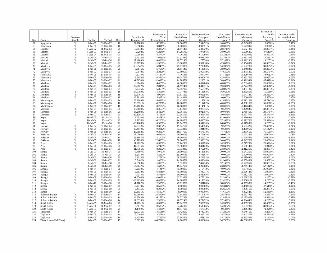
Obs Country

Common


Deviation in

Revenue, dR

Deviation in

Total

Expenditure, e

Fraction of

Heads Over-

spent, fo

Deviation within

Overspent

Group, eo

Fraction of

Heads Under-

spent, fu

Deviation within

Under-spent

Group, eu

Fraction of -

Heads

Accurately

Spent, fb

Deviation within

Accurately Spent

Group, eb



64 Lesotho Y 1-Apr-02 31-Mar-03 21 -3.0943% -2.3352% 28.5714% 6.40729% 28.5714% -8.60219% 42.8571% -0.14%

65 Lesotho Y 1-Apr-03 31-Mar-04 21 7.5204% -6.2246% 14.2857% 1.07686% 38.0952% -6.69068% 47.6190% -0.61%

66 Lesotho Y 1-Apr-04 31-Mar-05 21 -2.0182% -8.3771% 4.7619% 0.17299% 52.3810% -8.09200% 42.8571% -0.46%

67 Malawi Y 1-Jul-04 30-Jun-05 21 9.7322% -7.6935% 33.3333% 4.64829% 52.3810% -12.63220% 14.2857% 0.29%

68 Malawi Y 1-Jul-05 30-Jun-06 21 17.4109% -9.8360% 28.5714% 1.77550% 57.1429% -11.32129% 14.2857% -0.29%

69 Malawi Y 1-Jul-06 30-Jun-07 21 10.2878% -1.3260% 23.8095% 6.36714% 42.8571% -6.95488% 33.3333% -0.74%

70 Maldives

1-Jan-05 31-Dec-05 21 -13.6947% 5.9499% 47.6190% 12.70960% 14.2857% -6.69278% 38.0952% -0.07%

71 Maldives

1-Jan-06 31-Dec-06 21 7.5146% -5.7587% 28.5714% 3.13655% 38.0952% -8.94683% 33.3333% 0.05%

72 Maldives

1-Jan-07 31-Dec-07 21 -7.5049% -13.2128% 23.8095% 6.06878% 47.6190% -19.28158% 28.5714% 0.00%

73 Mauritania

1-Jan-05 31-Dec-05 21 4.5276% -17.7377% 4.7619% 1.60779% 57.1429% -19.60665% 38.0952% 0.26%

74 Mauritania

1-Jan-06 31-Dec-06 21 8.6158% -5.3333% 19.0476% 0.98087% 42.8571% -7.33375% 38.0952% 1.02%

75 Mauritania

1-Jan-07 31-Dec-07 21 -1.5150% -2.0182% 14.2857% 2.28021% 38.0952% -3.99194% 47.6190% -0.31%

76 Moldova

1-Jan-02 31-Dec-02 20 0.3745% 4.4257% 40.0000% 6.09484% 40.0000% -3.20145% 20.0000% 1.53%

77 Moldova

1-Jan-03 31-Dec-03 21 18.8727% 2.8488% 28.5714% 4.43811% 19.0476% -0.72422% 52.3810% -0.87%

78 Moldova

1-Jan-04 31-Dec-04 21 6.7336% 5.3559% 42.8571% 7.56049% 23.8095% -2.43118% 33.3333% 0.23%

79 Moldova Y 1-Jan-05 31-Dec-05 18 14.9759% 11.2556% 77.7778% 13.19563% 16.6667% -1.93385% 5.5556% -0.01%

80 Moldova Y 1-Jan-06 31-Dec-06 18 10.3781% 8.9075% 61.1111% 9.06994% 5.5556% -0.14714% 33.3333% -0.02%

81 Moldova Y 1-Jan-07 31-Dec-07 18 13.9810% 15.8871% 94.4444% 15.54178% 0.0000% 0.00000% 5.5556% 0.35%

82 Montenegro

1-Jan-05 31-Dec-05 14 29.8989% -5.4825% 21.4286% 1.15902% 42.8571% -7.01313% 35.7143% 0.37%

83 Montenegro

1-Jan-06 31-Dec-06 10 20.9531% -0.2796% 10.0000% 2.19402% 40.0000% -1.39815% 50.0000% -1.08%

84 Montenegro

1-Jan-07 31-Dec-07 10 39.4820% 8.2664% 70.0000% 13.14581% 20.0000% -5.47264% 10.0000% 0.59%

85 Morocco Y 1-Jan-05 31-Dec-05 21 10.8159% 8.3593% 57.1429% 10.97075% 9.5238% -2.37984% 33.3333% -0.23%

86 Morocco Y 1-Jan-06 31-Dec-06 21 15.2093% 2.4100% 52.3810% 4.92057% 19.0476% -2.76545% 28.5714% 0.25%

87 Morocco Y 1-Jan-07 31-Dec-07 21 22.1301% 3.1611% 52.3810% 4.40648% 19.0476% -3.05747% 28.5714% 1.81%

88 Nepal

16-Jul-03 15-Jul-04 21 7.7330% -5.8782% 14.2857% 2.42241% 61.9048% -7.89008% 23.8095% -0.41%

89 Nepal

16-Jul-04 15-Jul-05 21 2.7028% -0.2008% 14.2857% 6.63079% 57.1429% -6.57173% 28.5714% -0.26%

90 Nepal

16-Jul-05 15-Jul-06 21 -13.1608% -5.5558% 19.0476% 4.69710% 66.6667% -9.31708% 14.2857% -0.94%

91 Norway Y 1-Jan-04 31-Dec-04 21 17.8332% 0.3837% 19.0476% 0.64694% 9.5238% -1.50742% 71.4286% 1.24%

92 Norway Y 1-Jan-05 31-Dec-05 21 13.4570% -0.2912% 33.3333% 1.24179% 9.5238% -1.43595% 57.1429% -0.10%

93 Norway Y 1-Jan-06 31-Dec-06 21 25.0153% 0.2067% 19.0476% 0.67674% 4.7619% -0.88165% 76.1905% 0.41%

94 Pakistan Y 1-Jul-05 30-Jun-06 10 18.0004% 19.6850% 50.0000% 19.77593% 30.0000% -0.17426% 20.0000% 0.08%

95 Pakistan Y 1-Jul-06 30-Jun-07 10 13.1887% 2.1703% 50.0000% 4.21237% 20.0000% -0.72456% 30.0000% -1.32%

96 Pakistan Y 1-Jul-07 30-Jun-08 10 -3.1196% 22.6833% 50.0000% 22.58317% 30.0000% -1.04370% 20.0000% 1.14%

97 Peru Y 1-Jan-05 31-Dec-05 21 11.9822% 0.3500% 57.1429% 5.31796% 14.2857% -5.77570% 28.5714% 0.81%

98 Peru Y 1-Jan-06 31-Dec-06 21 44.6715% 6.7429% 61.9048% 9.41123% 19.0476% -2.66014% 19.0476% -0.01%

99 Peru Y 1-Jan-07 31-Dec-07 21 31.7365% -8.2292% 33.3333% 2.76290% 23.8095% -11.41226% 42.8571% 0.42%

100 Samoa

1-Jul-03 30-Jun-04 20 -3.4907% -1.0723% 20.0000% 2.18992% 30.0000% -3.64725% 50.0000% 0.38%

101 Samoa

1-Jul-04 30-Jun-05 20 6.2018% 3.2427% 35.0000% 3.54687% 0.0000% 0.00000% 65.0000% -0.30%

102 Samoa

1-Jul-05 30-Jun-06 21 6.9013% 2.7717% 38.0952% 5.75692% 19.0476% -4.01964% 42.8571% 1.03%

103 Samoa

1-Jul-06 30-Jun-07 21 5.5462% 1.8869% 14.2857% 3.88648% 61.9048% -3.05943% 23.8095% 1.06%

104 Samoa

1-Jul-07 30-Jun-08 21 -7.6503% -1.0969% 9.5238% 2.45414% 57.1429% -3.52395% 33.3333% -0.03%

105 Samoa

1-Jul-08 30-Jun-09 21 -5.3647% 1.6284% 19.0476% 3.21868% 23.8095% -1.75714% 57.1429% 0.17%

106 Senegal Y 1-Jan-04 31-Dec-04 20 6.2030% -1.1414% 35.0000% 6.16442% 40.0000% -7.18486% 25.0000% -0.12%

107 Senegal Y 1-Jan-05 31-Dec-05 20 9.9132% -6.8989% 45.0000% 5.34271% 40.0000% -12.02612% 15.0000% -0.22%

108 Senegal Y 1-Jan-06 31-Dec-06 20 4.7373% 5.5439% 50.0000% 12.88089% 40.0000% -7.01271% 10.0000% -0.32%

109 Senegal Y 1-Jan-08 31-Dec-08 21 -1.6500% -4.0426% 33.3333% 8.77815% 52.3810% -12.02871% 14.2857% -0.79%

110 Senegal Y 1-Jan-09 31-Dec-09 21 -16.3130% -6.4270% 14.2857% 9.15339% 71.4286% -15.30851% 14.2857% -0.27%

111 Senegal Y 1-Jan-10 31-Dec-10 21 -1.7102% 2.5950% 47.6190% 7.85188% 38.0952% -4.85538% 14.2857% -0.40%

112 Serbia

1-Jan-07 31-Dec-07 21 -0.2319% -8.5501% 0.0000% 0.00000% 52.3810% -7.45001% 47.6190% -1.10%

113 Serbia

1-Jan-08 31-Dec-08 21 -2.4445% -8.2382% 0.0000% 0.00000% 66.6667% -7.30816% 33.3333% -0.93%

114 Serbia

1-Jan-09 31-Dec-09 21 -10.5031% -5.5607% 0.0000% 0.00000% 47.6190% -4.39252% 52.3810% -1.17%

115 Solomon Islands Y 1-Jan-04 31-Dec-04 14 86.0689% 25.4458% 57.1429% 27.16487% 28.5714% -1.53278% 14.2857% -0.19%

116 Solomon Islands Y 1-Jan-05 31-Dec-05 14 15.7388% -6.2623% 28.5714% 1.41720% 42.8571% -7.18592% 28.5714% -0.49%

117 Solomon Islands Y 1-Jan-06 31-Dec-06 14 17.6320% 2.3280% 28.5714% 6.75452% 57.1429% -4.53464% 14.2857% 0.11%

118 South Africa Y 1-Apr-05 31-Mar-06 21 11.4831% 0.3529% 19.0476% 2.01099% 14.2857% -1.30575% 66.6667% -0.35%

119 South Africa Y 1-Apr-06 31-Mar-07 21 8.2817% -0.6354% 4.7619% 0.68366% 14.2857% -0.65728% 80.9524% -0.66%

120 South Africa Y 1-Apr-07 31-Mar-08 21 1.1480% 1.4230% 19.0476% 1.67042% 9.5238% -0.43642% 71.4286% 0.19%

121 Tajikistan Y 1-Jan-04 31-Dec-04 14 12.9336% 14.5518% 71.4286% 18.74272% 14.2857% -4.54016% 14.2857% 0.35%

122 Tajikistan Y 1-Jan-05 31-Dec-05 14 5.0405% 3.4036% 42.8571% 6.80713% 28.5714% -4.94327% 28.5714% 1.54%

123 Tajikistan Y 1-Jan-06 31-Dec-06 14 8.4354% 7.7230% 57.1429% 11.65113% 35.7143% -3.86152% 7.1429% -0.07%

124 Timor-Leste (Half Year)

1-Jan-07 31-Dec-07 19 0.6023% -44.7840% 0.0000% 0.00000% 94.7368% -44.78056% 5.2632% 0.00%

Obs Country

Common


Deviation in

Revenue, dR

Deviation in

Total

Expenditure, e

Fraction of

Heads Over-

spent, fo

Deviation within

Overspent

Group, eo

Fraction of

Heads Under-

spent, fu

Deviation within

Under-spent

Group, eu

Fraction of -

Heads

Accurately

Spent, fb

Deviation within

Accurately Spent

Group, eb

125 Timor-Leste

1-Jan-08 31-Dec-08 19 41.8400% 39.3187% 73.6842% 39.55537% 5.2632% -0.19755% 21.0526% -0.04%

126 Timor-Leste

1-Jan-09 31-Dec-09 21 -12.0434% -11.1379% 0.0000% 0.00000% 76.1905% -10.51841% 23.8095% -0.62%

127 Tonga

1-Jul-03 30-Jun-04 21 -2.6875% -2.4254% 23.8095% 1.97329% 14.2857% -4.74149% 61.9048% 0.34%

128 Tonga

1-Jul-04 30-Jun-05 21 5.3697% -3.3360% 57.1429% 4.54259% 14.2857% -8.58149% 28.5714% 0.70%

129 Tonga

1-Jul-05 30-Jun-06 21 12.4148% 13.8230% 61.9048% 15.75578% 19.0476% -1.85106% 19.0476% -0.08%

130 Tonga

1-Jul-06 30-Jun-07 21 -2.4033% -1.6142% 19.0476% 2.10919% 42.8571% -2.71899% 38.0952% -1.00%

131 Tonga

1-Jul-07 30-Jun-08 22 5.9171% -0.2618% 40.9091% 6.13405% 13.6364% -6.94195% 45.4545% 0.55%

132 Tonga

1-Jul-08 30-Jun-09 22 -13.4207% -2.0663% 36.3636% 4.81624% 50.0000% -6.45078% 13.6364% -0.43%

133 Trinidad And Tobago Y 1-Oct-04 30-Sep-05 21 28.4483% 9.5236% 42.8571% 11.01186% 23.8095% -0.96621% 33.3333% -0.52%

134 Trinidad And Tobago Y 1-Oct-05 30-Sep-06 21 19.5306% -6.3874% 19.0476% 3.12953% 57.1429% -9.29229% 23.8095% -0.22%

135 Trinidad And Tobago Y 1-Oct-06 30-Sep-07 21 17.7144% 1.1695% 14.2857% 4.30428% 47.6190% -3.24652% 38.0952% 0.11%

136 Tunisia Y 1-Jan-06 31-Dec-06 21 4.0871% 0.8465% 33.3333% 2.93320% 9.5238% -3.06881% 57.1429% 0.98%

137 Tunisia Y 1-Jan-07 31-Dec-07 21 6.3133% 5.7487% 33.3333% 8.62008% 14.2857% -3.27129% 52.3810% 0.40%

138 Tunisia Y 1-Jan-08 31-Dec-08 20 13.5745% 8.8037% 50.0000% 11.26445% 10.0000% -3.35191% 40.0000% 0.89%

139 Vanuatu

1-Jan-03 31-Dec-03 14 -8.0589% -4.7540% 21.4286% 0.52236% 14.2857% -4.55528% 64.2857% -0.72%

140 Vanuatu

1-Jan-04 31-Dec-04 14 3.5766% 1.1915% 14.2857% 1.80661% 21.4286% -1.32593% 64.2857% 0.71%

141 Vanuatu

1-Jan-05 31-Dec-05 14 7.2757% -1.5231% 28.5714% 1.78795% 7.1429% -2.80799% 64.2857% -0.50%

142 Yemen

1-Jan-04 31-Dec-04 21 28.1281% 19.7597% 42.8571% 27.35838% 38.0952% -7.59918% 19.0476% 0.00%

143 Yemen

1-Jan-05 31-Dec-05 21 57.6420% 44.1279% 42.8571% 48.05054% 38.0952% -4.06185% 19.0476% 0.14%

144 Yemen

1-Jan-06 31-Dec-06 21 47.2160% 20.0638% 52.3810% 23.81517% 33.3333% -3.65876% 14.2857% -0.09%

145 Zambia Y 1-Jan-02 31-Dec-02 21 -2.3344% 7.2833% 47.6190% 17.32480% 47.6190% -10.16755% 4.7619% 0.13%

146 Zambia Y 1-Jan-03 31-Dec-03 21 2.4168% 22.1821% 57.1429% 29.00469% 33.3333% -6.65911% 9.5238% -0.16%

147 Zambia Y 1-Jan-04 31-Dec-04 21 1.0517% -11.8215% 23.8095% 8.46918% 47.6190% -20.65293% 28.5714% 0.36%

148 Kenya Y 1-Jul-04 30-Jun-05 21 4.1733% -10.7196% 23.8095% 1.63479% 47.6190% -11.87554% 28.5714% -0.48%

149 Kenya Y 1-Jul-05 30-Jun-06 21 0.9434% -5.5796% 19.0476% 3.73556% 47.6190% -8.22832% 33.3333% -1.09%

150 Kenya Y 1-Jul-06 30-Jun-07 21 -0.6392% -4.1465% 23.8095% 1.33274% 33.3333% -5.66247% 42.8571% 0.18%

151 Uganda Y 1-Jul-05 30-Jun-06 21 3.8661% -1.7755% 28.5714% 5.22461% 33.3333% -5.96724% 38.0952% -1.03%

152 Uganda Y 1-Jul-06 30-Jun-07 21 7.2474% -9.3834% 9.5238% 0.57518% 23.8095% -9.28680% 66.6667% -0.67%

153 Uganda Y 1-Jul-07 30-Jun-08 21 2.1424% -13.5954% 0.0000% 0.00000% 47.6190% -13.14940% 52.3810% -0.45%

154 Sierra Leone Y 1-Jan-04 31-Dec-04 21 5.0791% -7.6400% 23.8095% 2.73947% 47.6190% -10.29866% 28.5714% -0.08%

155 Sierra Leone Y 1-Jan-05 31-Dec-05 21 -3.8348% 5.5014% 42.8571% 7.95179% 28.5714% -2.37876% 28.5714% -0.07%

156 Sierra Leone Y 1-Jan-06 31-Dec-06 21 -6.7430% 1.1190% 28.5714% 6.10008% 38.0952% -6.63365% 33.3333% 1.65%

157 Sierra Leone Y 1-Jan-07 31-Dec-07 21 -18.5484% -22.4171% 9.5238% 0.60841% 71.4286% -23.16063% 19.0476% 0.14%

158 Sierra Leone Y 1-Jan-08 31-Dec-08 21 -3.5767% -3.5404% 19.0476% 5.38999% 57.1429% -8.40263% 23.8095% -0.53%

159 Sierra Leone Y 1-Jan-09 31-Dec-09 21 -6.7996% 6.5959% 42.8571% 10.96191% 28.5714% -4.09679% 28.5714% -0.27%

cross country correlates for the quality of budget...

Documents