credit scoring and the optimization concerning area under ... · 3 credit scoring models - basis...

Credit Scoring and the Optimization concerning Area under the curve

Anne Kraus, Helmut Küchenhoff

Credit Scoring and Credit Control XIII

August 28-30, 2013

1. Credit Scoring and Data description

2. Classical Method: Logistic Regression

3. AUC approach

4. Boosting

5. Conclusion and Outlook

Agenda

Credit Scoring and the optimization concerning AUC 2

3

Credit Scoring models - basis for financial institutions to evaluate the likelihood for credit applicants to default

Decision whether to grant or reject credit to an applicant Data from a German retail bank - specialized on lending consumer credits Fully automated application process of this bank Credit Scoring model as one part of the whole decision Logistic regression as most widely used method for classifying applicants Good interpretability is an important advantage of this method Benchmark newer methods for optimizing the scoring problem

concerning the AUC measure Area under the curve (ROC-curve) as measure of performance for

prediction accuracy AUC as direct optimization criterion

Credit scoring

Credit Scoring and the optimization concerning AUC

4

Data from a German retail bank Large database and long data history Application Scoring – 26 attributes regarding process-related limitations Variables like credit history, existing accounts, personal information such as

age, sex or marital status Excluding non representative data Different definitions for default

• Withdrawal of the credit • Third dunning letter • Time horizon (12 to 30 month) • Basel II

Data description

2008 2010 2009

Developmental period

Observation period


0

10

20

30

40

50

60

70

80

90

100

0 20 40 60 80 100

Tru

e p

osi

tive

rat

e

False positive rate

criterion1 criterion2 criterion3 diagonal

5

ROC-curve , AUC and Gini coefficient Prediciton accuracy AUC Area under the curve

• AUC=area a + area c Gini coefficient

• Gini=area a/(area a + area b)

Gini=2*AUC-1

Measure of performance

area a

area c

area b


0

5

10

15

20

25

20

07

01

20

07

02

20

07

03

20

07

04

20

07

05

20

07

06

20

07

07

20

07

08

20

07

09

20

07

10

20

07

11

20

07

12

20

08

01

20

08

02

20

08

03

20

08

04

20

08

05

20

08

06

20

08

07

20

08

08

20

08

09

20

08

10

20

08

11

20

08

12

Gin

i

month

variable1

criterion1 criterion2 criterion3

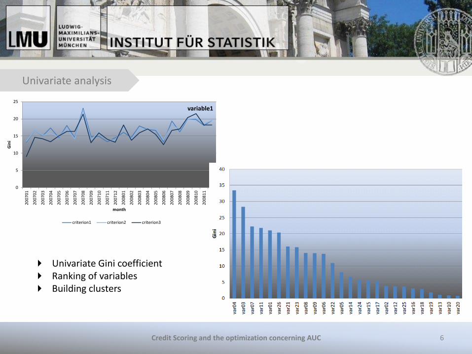
6

Univariate analysis

Univariate Gini coefficient Ranking of variables Building clusters


7

Multivariate analysis

Logistic regression model

• 𝜋𝑖 = 𝑃 𝑌𝑖 = 1 𝑥𝑖) = 𝐺(𝑥𝑖

′𝛽) • 𝐺 𝑡 = 1 + exp −𝑡 -1

Binary outcome variable

• applicant will default (1) • applicant will not default (0)

Maximum Likelihood estimation Test of hundreds of different models AUC as measure of performance (compared to AIC)


8

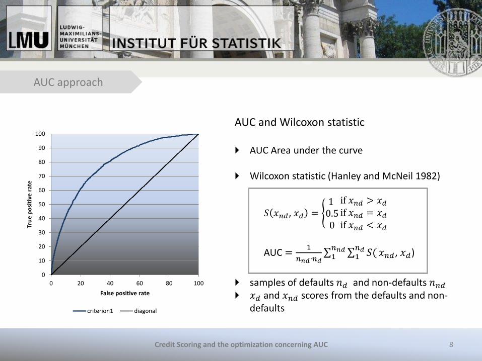
AUC and Wilcoxon statistic AUC Area under the curve

Wilcoxon statistic (Hanley and McNeil 1982)

𝑆 𝑥𝑛𝑑, 𝑥𝑑 = 1 0.50

if 𝑥𝑛𝑑 > 𝑥𝑑

if 𝑥𝑛𝑑 = 𝑥𝑑

if 𝑥𝑛𝑑 < 𝑥𝑑

AUC =1

𝑛𝑛𝑑∙𝑛𝑑 𝑆(

𝑛𝑑1

𝑛𝑛𝑑1 𝑥𝑛𝑑, 𝑥𝑑)

samples of defaults 𝑛𝑑 and non-defaults 𝑛𝑛𝑑 𝑥𝑑 and 𝑥𝑛𝑑 scores from the defaults and non-

defaults

AUC approach

0

10

20

30

40

50

60

70

80

90

100

0 20 40 60 80 100

Tru

e p

osi

tive

rat

e

False positive rate

criterion1 diagonal


9

AUC approach

AUC approach - AUC as direct optimization criterion Logistic regression with Maximum Likelihood Idea of the AUC approach: maximize 𝐴𝑈𝐶 𝛽

AUC 𝛽 =1

𝑛𝑑∙𝑛𝑛𝑑 𝑆(

𝑛𝑛𝑑1

𝑛𝑑1 𝛽𝑇(𝑥𝑑 − 𝑥𝑛𝑑))

𝛽 𝐴𝑈𝐶 = arg𝑚𝑎𝑥𝛽 AUC(β)

= arg𝑚𝑎𝑥𝛽1

𝑛𝑑∙𝑛𝑛𝑑 𝑆(

𝑛𝑛𝑑1

𝑛𝑑1 𝛽𝑇(𝑥𝑑 − 𝑥𝑛𝑑))

𝑥𝑑 and 𝑥𝑛𝑑 scores as vectors of financial indicators 𝛽 vector of coefficient parameters 𝐴𝑈𝐶(𝛽) sum of step functions, non-differentiable with respect to 𝛽 Optimization with Nelder-Mead (1965)


10

AUC approach


Optimality properties of the AUC approach (Pepe, 2006) Exploring linear scores of the form Lβ 𝑥𝑖 = x1 + β2𝑥2 + ⋯+ 𝛽𝑃𝑥𝑃

Neyman-Pearson lemma (1933) Rules based on Lβ 𝑥𝑖 > c are optimal if the score is a monotone increasing function of Lβ 𝑥𝑖

No other classification rule based on 𝑥𝑖 above the ROC curve for Lβ 𝑥𝑖

Assuming that Lβ 𝑥𝑖 has the best ROC curve, Lβ 𝑥𝑖 has the best ROC curve regarding all linear predictors

Find coefficients with the best empirical ROC curve Since the optimal ROC curve has a maximum AUC value, this measure can

be used as objective function to estimate β

Relationship to the maximum rank correlation estimator of Han (1987) Consistency and asymptotically normal distribution (Sherman, 1933)

11

AUC approach


Simulation Study Comparison of the logit model and the AUC approach

Idea: AUC approach outperforms the logit model if link function is not true Simulate data with five different link functions

logit, probit, complementary log log, link1, link2 Three normal distributed explanatory variables and binary response

(n=1000, 𝛽 = (1,0.5,0.3)) 100 simulations Estimation on training data and application to validation data

12

AUC approach


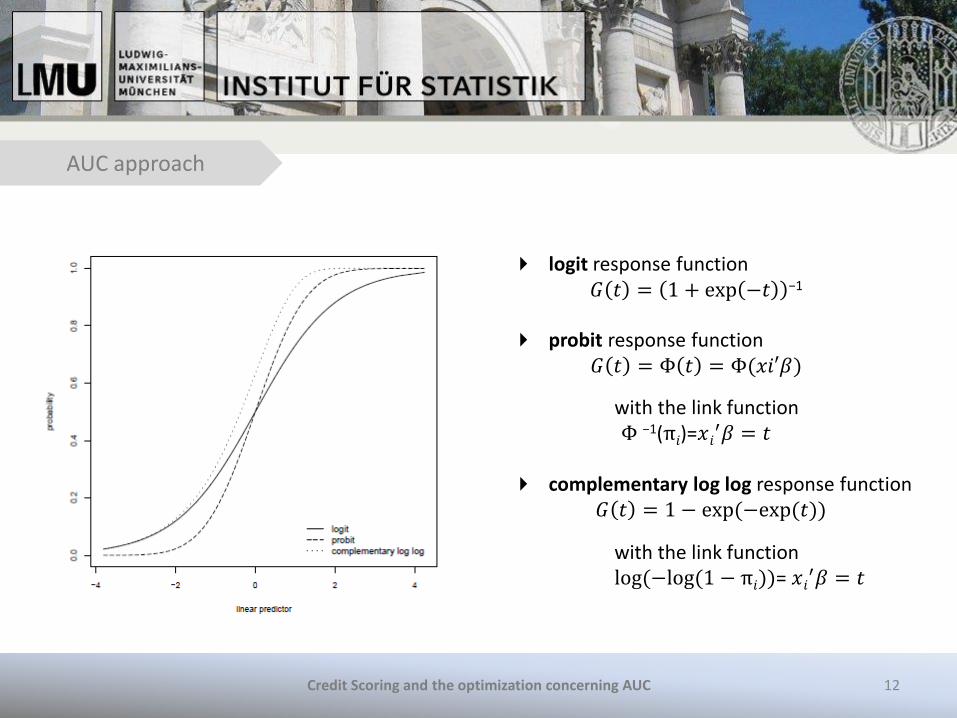
logit response function 𝐺 𝑡 = 1 + exp −𝑡 −1

probit response function

𝐺 𝑡 = Φ 𝑡 = Φ(𝑥𝑖′𝛽)

with the link function Φ −1(π𝑖)=𝑥𝑖

′𝛽 = 𝑡

complementary log log response function 𝐺 𝑡 = 1 − exp (−exp (𝑡))

with the link function log (−log (1 − π𝑖))= 𝑥𝑖

′𝛽 = 𝑡

13

AUC approach


link1 (based on the logit link)

𝐻 𝑡 = 𝐺 𝑡 for 𝑡 ≤ 0𝐺 8 ∗ 𝑡 for 𝑡 > 0

link2 (based on the comp log log link)

Q 𝑡 = 𝐺 0.2 ∗ 𝑡 for 𝑡 ≤ 0𝐺 5 ∗ 𝑡 for 𝑡 > 0

14

AUC approach


Boxplots to compare the coefficients for the logit model (white) and the coefficients for the AUC approach (grey) based on the 100 simulations

15

AUC approach


Results for the simulation study with 100 simulations AUC approach better for link1 and link2

16

AUC approach

50% training sample One coefficient fixed for normalization reasons ML-coefficients basis for the optimization No distribution assumption!


Evaluation on the Credit Scoring data

Aggregation of many „weak“ classifiers in order to achieve a high classification performance Training data with 𝑛 objects and response 𝑦 ∈ +1,−1 Construct a classification rule 𝐹(𝑥) In each step: find an optimal classifier according to the current distribution of weights on the

observation Incorrectly classified observations receive more weight in the next iteration (correctly classified

observations receive less weight) The final model outperforms with high probability in terms of misclassification error rate any

individual classifier

17

Boosting

arbitrary loss function exponential 𝐿 𝑦, 𝑓 = 𝑒−𝑦𝑓 or logistic 𝐿 𝑦, 𝑓 = log (1 + 𝑒−𝑦𝑓) 𝜂 function specifies the type of boosting:

discrete 𝜂 𝑥 = 𝑠𝑖𝑔𝑛(𝑥), real 𝜂 𝑥 = 0.5log (𝑥

1−𝑥) or gentle 𝜂 𝑥 = 𝑥

base learner: classification trees (maxdepth, minsplit)


18

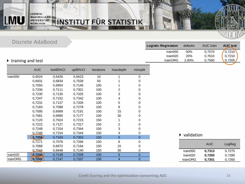
Discrete AdaBoost

training and test

validation


AUC low95%CI up95%CI iterations maxdepth minsplit

train050 0,6524 0,6426 0,6623 10 1 0

0,6931 0,6834 0,7028 50 1 0

0,7050 0,6954 0,7146 100 1 0

0,7206 0,7111 0,7301 100 2 0

0,7230 0,7135 0,7325 100 3 0

0,7247 0,7152 0,7342 100 4 0

0,7231 0,7137 0,7326 100 5 0

0,7183 0,7088 0,7278 100 8 0

0,7095 0,6999 0,7191 100 15 0

0,7081 0,6985 0,7177 100 30 0

0,7120 0,7024 0,7215 150 1 0

0,7222 0,7127 0,7317 150 2 0

0,7249 0,7154 0,7344 150 3 0

0,7249 0,7154 0,7344 150 4 0

0,7258 0,7163 0,7353 150 5 0

0,7171 0,7076 0,7266 150 8 0

0,7068 0,6972 0,7164 150 15 0

0,7044 0,6948 0,7140 150 30 0

train020 0,7244 0,7149 0,7339 150 5 0

trainORG 0,7242 0,7147 0,7337 150 4 0

AUC LogReg

train050 0,7313 0,7275

train020 0,7293 0,7280

trainORG 0,7301 0,7265

Logistic Regression defaults AUC train AUC test

train050 50% 0,7570 0,7210

train020 20% 0,7610 0,7210

trainORG 2,60% 0,7560 0,7205

19

Real AdaBoost

training and test

validation



train050 0,6610 0,6512 0,6708 150 1 0

0,6931 0,6834 0,7027 150 2 0

0,7056 0,6959 0,7152 150 3 0

0,7120 0,7024 0,7216 150 4 0

0,7122 0,7026 0,7218 150 5 0

0,7162 0,7066 0,7257 150 8 0

0,7166 0,7071 0,7262 150 15 0

0,7189 0,7094 0,7284 150 15 10

0,7088 0,6993 0,7184 150 15 100

0,6606 0,6508 0,6704 150 15 500

train020 0,7193 0,7098 0,7288 150 30 0

trainORG 0,7151 0,7056 0,7247 150 8 0

AUC low95%CI up95%CI iterations maxdepth minsplit LogReg

train050 0,7277 0,7146 0,7409 150 15 10 0,7275

train020 0,7233 0,7101 0,7365 150 30 0 0,7280

trainORG 0,7237 0,7105 0,7369 150 8 0 0,7265


train050 50% 0,7570 0,7210

train020 20% 0,7610 0,7210

trainORG 2,60% 0,7560 0,7205

20

Gentle AdaBoost

training and test

validation



train050 0,7251 0,7156 0,7345 150 5 0

train020 0,7275 0,7181 0,7370 150 4 0

trainORG 0,7262 0,7167 0,7357 150 30 0

exponential loss

AUC low95%CI up95%CI iterations maxdepth minsplit LogReg

train050 0,7299 0,7168 0,7431 150 5 0 0,7275

train020 0,7327 0,7196 0,7458 150 4 0 0,7280

trainORG 0,7295 0,7163 0,7426 150 30 0 0,7265


train050 50% 0,7570 0,7210

train020 20% 0,7610 0,7210

trainORG 2,60% 0,7560 0,7205

21

Boosting AUC


Component-wise gradient boosting Covariates are fitted seperately against the gradient Advantage: variable selection during the fitting process Different loss functions lead to a huge variety of different boosting algorithms In order to optimize the AUC – use the AUC as loss function Approximation with sigmoid function for differentiation Different base learners in combination with the AUC loss for the Credit Scoring case

classification trees, linear base learners, smooth effects The results for all three base learners outperform the logit model only in a few cases with many

included covariates In general, the boosting results with AUC loss underachieve compared to the logit model

22

Robust results and good interpretability with logistic regression Slight improvements for the AUC approach by direct AUC optimization Advantage of the AUC approach: no distribution assumption AUC loss behind the expectations Outperforming outcomes with boosting algorithms

Further work with single classification trees, random forests and boosting Interpretability versus prediction accuracy Interesting results and improvements with newer statistical methods and

algorithms from machine learning

Conclusion and Outlook


30.06.2012 Evaluating Consumer Credit Risk 23

BACKUP

24

Classification trees

root node

bad credit

good credit

bad credit good credit

𝑥𝑖 < 𝑐𝑖 𝑥𝑖 ≥ 𝑐𝑖

𝑥𝑗 < 𝑐j

𝑥𝑘 < 𝑐𝑘

𝑥𝑗 ≥ 𝑐𝑗

𝑥𝑘 ≥ 𝑐𝑘

CART-algorithm Breiman et al. (1984) Recursive partitioning Nonparametric approach Principle of impurity reduction Gini Index as impurity measure



Random forest

1. ntree bootstrap samples from the learning sample; ntree parameter for number of trees

2. For each generated bootstrap sample grow a classification tree with following aspects:

• In each node not all predictor variables are used to choose the best split but a special number of randomly selected attributes

• mtry describes this number of randomly preselected splitting variables • Random forests grow unpruned trees

3. For predicting new data aggregation of the prediction from the ntree trees; majority votes

for classification; relative frequency for all trees


Random forest

mean decrease in accuracy

• measure is computed from permuting OOB data

• recording prediction error on the OOB data

• prediction error after permuting each predictor variable

• the difference between the two are averaged over all trees and normalized by the standard deviation of the differences

mean decrease in node impurity

• averaged over all trees: total decrease in node impurities from splitting on the variable

• Gini index for classification

variable importance measures

credit scoring and the optimization concerning area under ... · 3 credit scoring models - basis...

Documents