creation of rainfall areal reduction factors from the basin-averaged rainfall … · ·...
TRANSCRIPT

Creation of Rainfall Areal Reduction Factors from the Basin-Averaged Rainfall Record at
the Lower Mississippi River Forecast Center
W. Scott Lincoln
Katie E. Landry-Guyton
David S. Schlotzhauer
NWS Lower Mississippi River Forecast Center
Corresponding Author:
W. Scott Lincoln

1.0 INTRODUCTION
At the National Weather Service (NWS) Lower Mississippi Forecast Center (LMRFC),
the rainfall archive with the longest period of record is based upon gauge-only data converted to
basin mean areal precipitation (MAP) with the Thiessen Polygon method. This period of record
is over 60 years in length and continues to grow. These data are used for the calibration of
every modeled subbasin in the LMRFC region. Subbasins in the LMRFC area range from
approximately 2.5 mi2 to approximately 2200 mi2.
Starting in 1997, a gridded method was introduced where MAPs were created from bias-
corrected, radar-based estimates (MAPX). This gridded method is anticipated to improve
estimates of basin-averaged rainfall especially where the precipitation is widely varying in time
and space (such as with convection) because the Thiessen polygon method will tend towards
overestimation where storms cross over a gauge location but miss most of the remainder of the
basin, and vice versa. Although generally considered to be more accurate, the MAPX method
has too short of a period of record to be used for effective calibration of hydrologic models at the
LMRFC because of the high variation in rainfall-runoff responses of modeled subbasins.
Because of the differences in the two rainfall estimation techniques and because of the
fact that the hydrologic models are calibrated to the older non-radar method, it is important to
identify potential biases in the rainfall database. Such identification is especially important for
higher-end rainfall events that are causative inputs to a majority of flooding events in the
LMRFC region. One means to check for biases at the higher magnitude end of the MAP dataset
is to perform a frequency analysis in order to compare rainfall amounts from specific average
recurrence intervals (ARIs) to values that would be expected to occur for a basin of that size.
This paper presents the methodology for performing such a comparison and discusses
uncertainties and limitations found during the analysis.
2.0 METHODOLOGY
2.1 Obtaining Precipitation Frequency Data
Providing quantitative precipitation estimates (QPE) or quantitative precipitation
forecasts (QPF) in terms of an ARI is a helpful way of putting values in the context of
climatology for a given location. This concept is already used widely in hydrology to describe a
streamflow crest (such as a “100-year event”) and is also used to convey risk for insurance
purposes (such as the Federal Emergency Management Agency’s [FEMA] 100-year or 1%
floodplain). In addition, this concept is sometimes used to describe rainfall events. Typically this
information is used by engineers to design bridges, culverts, and structures to handle
stormwater, however there have been examples of this information being compared to areas
impacted by flooding (Lincoln W. S., 2014; Lincoln W. S., 2014; Parzybok, 2011).
The Hydrologic Design Studies Center (HDSC) of the NWS has recently undertaken an
effort to update the rainfall frequency data for most states in the continental United States
(CONUS); the results of this effort are presented in both print and digital formats as NOAA Atlas

14 (Perica, et al., 2013). NOAA Atlas 14 contains a series of tables and maps indicating the
estimated rainfall depth that would correspond to a particular ARI. This updated data from NWS
HDSC has an increased number of gauges, a longer period of record from which to calculate
the extreme value distributions, improved output resolution, and output in geographic
information system (GIS) compatible formats (when compared to previous rainfall frequency
analyses). The rainfall frequency data was downloaded in GIS format
(http://hdsc.nws.noaa.gov/hdsc/pfds/pfds_gis.html) for use on this analysis and other projects.
2.2 Converting Point-Based Rainfall Frequency Data to Areal Rainfall Frequency Data
One caveat with using rainfall frequency data is that it is valid only for a given point
location and applicability is lacking for areas. This causes an issue in hydrologic forecasting
because most modeling approaches utilize watersheds with widely varying dimensions and
areally-averaged parameters. To find the corresponding rainfall amount valid for an area at a
given ARI, the use of areal reduction factors (ARFs) is required (Dingman, 1994; Miller,
Frederick, & Tracey, 1973).
One commonly used set of ARFs are the ones published in NOAA Atlas 2 (Miller,
Frederick, & Tracey, 1973). This set of ARFs was intended to be non-specific to any particular
region or ARI, but did vary by storm duration (Figure 1). A review of the scientific literature,
however, found widely varying ARFs (Asquith W. H., 1999; Stanescu, Engineering Hydrology
Chapter 10: Urban Hydrology, 2006). Not only was this variance found to occur across studies,
but sometimes within a single study the ARFs could vary by region, season, and individual ARI
being studied. Because of this uncertainty, ARFs will be discussed in a later section.
Figure 1. Areal reduction factors from NOAA Atlas 2 Figure 14 (Miller, Frederick, & Tracey, 1973).
2.3 Performing Frequency Analysis on LMRFC MAP Data
The gauge-only MAP used at the LMRFC has areal average rainfall for each subbasin
computed on a 6 hour time step is determined using the Thiessen Polygon method. In 2013,
LMRFC completed a depth-duration-frequency analysis on the 6-hour estimates to improve
situational awareness during flood events. The goal was to provide forecasters a list of the
highest MAP values as well as an estimate of values at several ARIs so that current events
could be put into context of past events. At the time of the analysis, data for the January 1950–
December 2012 period was available.
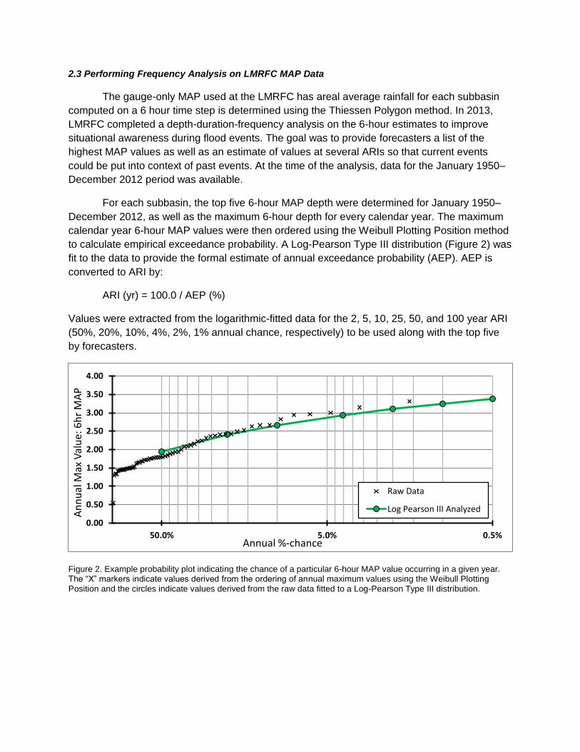
For each subbasin, the top five 6-hour MAP depth were determined for January 1950–
December 2012, as well as the maximum 6-hour depth for every calendar year. The maximum
calendar year 6-hour MAP values were then ordered using the Weibull Plotting Position method
to calculate empirical exceedance probability. A Log-Pearson Type III distribution (Figure 2) was
fit to the data to provide the formal estimate of annual exceedance probability (AEP). AEP is
converted to ARI by:
ARI (yr) = 100.0 / AEP (%)
Values were extracted from the logarithmic-fitted data for the 2, 5, 10, 25, 50, and 100 year ARI
(50%, 20%, 10%, 4%, 2%, 1% annual chance, respectively) to be used along with the top five
by forecasters.
Figure 2. Example probability plot indicating the chance of a particular 6-hour MAP value occurring in a given year. The “X” markers indicate values derived from the ordering of annual maximum values using the Weibull Plotting Position and the circles indicate values derived from the raw data fitted to a Log-Pearson Type III distribution.
0.00
0.50
1.00
1.50
2.00
2.50
3.00
3.50
4.00
0.5%5.0%50.0%
An
nu
al M
ax V
alu
e: 6
hr
MA
P
Annual %-chance
Raw Data
Log Pearson III Analyzed

One issue with the LMRFC MAP frequency analysis data is the bias introduced by fixed-
interval observations. Rainfall recording intervals are tied to an arbitrary time step, for this data it
was a 6-hour timestep. To properly determine the maximum 6-hour rainfall over the course of a
year, the optimal approach would be to use a moving window with an hourly or sub-hourly time
step and aggregate up to 6 hours, otherwise storms that occur near the beginning/end of a 6
hour period will be split in half and bias the statistics lower. This optimal approach is not
applicable to our situation, however, as we estimated ARIs for events of a 6-hour duration and
the available MAP data was also on a 6-hour timestep. Asquith (1998) as well as table 13-10 in
Hydrology for Engineers (1982) provide a fixed interval correction factor for this issue. Because
only one time increment fits within the analyzed duration, the maximum adjustment of 1.13 was
required; data was adjusted by multiplying by this adjustment factor.
2.4 Comparing LMRFC MAP data to NOAA Atlas 14
Next, the spatial averages of the cells for NOAA Atlas 14 grids were computed for the 2,
5, 10, 25, 50, and 100 year ARI for each study basin. A ratio of the LMRFC MAP ARI values to
the NOAA Atlas 14 data was then calculated. To reduce the noise in the data, the data were
averaged within eight (8) separate bins, each with approximately the same number of basins.
For the purposes of this report, these bin-averaged ratios will be referred to as the “LMRFC
MAP ARFs” for this study. It was noted that the LMRFC MAP ARFs generally decrease as ARI
increases. The 2 year (50% annual chance) event was an outlier to this trend (Figure 3; Figure
4), which could be attributed in part to estimation bias of the median maxima (William H.
Asquith, personal communication, November 2015). The fact that the ARFs for a given area
decrease with increasing ARI is likely a manifestation of high rainfall intensities generally being
more spatial restricted as real storms track across the landscape (William H. Asquith, personal
communication, November 2015).
It was expected that when plotted as a function of area, the LMRFC MAP ARFs would
have similar shape to that of other published ARFs. We would expect that very small basins with
an area approaching 0.0 mi2 would have very similar rainfall values to a point location for a
given ARI (ARF of ~1.0) and basins with larger areas should have smaller rainfall values for the
same ARI (ARF < 1.0). This trend was indeed noted in the LMRFC MAP ARFs but it was difficult
to determine which published ARFs would be most applicable to our dataset. The LMRFC MAP
ARFs were compared to the following areal reduction relationships found from our literature
review (Figure 5):
1. The NOAA Atlas 2 relation (Miller, Frederick, & Tracey, 1973).
2. Allen & DeGaetano relation for North Carolina (Allen & DeGaetano, 2005).
3. Fruhling relation (Vladimirescu, 1984). As published in Virtual Campus in Hydrology and
Water Resources’ (VICAIRE’s) online module “Engineering Hydrology” (Stanescu,
Engineering Hydrology Chapter 10: Urban Hydrology, 2006).
4. Leclerc & Schaake relation (Leclerc & Schaake, 1972). As published in VICAIRE’s online
module “Engineering Hydrology” (Stanescu, Engineering Hydrology Chapter 10: Urban
Hydrology, 2006).

5. Stanescu relation (Stanescu, 1995). As published in VICAIRE’s online module
“Engineering Hydrology” (Stanescu, Engineering Hydrology Chapter 10: Urban
Hydrology, 2006).
6. Woolisher & Schwalen relation (Woolisher & Schwalen, 1959). As published in
VICAIRE’s online module “Engineering Hydrology” (Stanescu, Engineering Hydrology
Chapter 10: Urban Hydrology, 2006).
Although the smallest LMRFC basins tended to have the highest variability in ARFs, the
bin average was very similar to ARFs published by Leclerc & Schaake (1972) and Woolisher &
Schwalen (1959). For basins of approximately 100–400 mi2 in size, the LMRFC ARFs generally
paralleled values published previously in NOAA Atlas 2 (1973) and by Allen & DeGaetano
(2005). For basins of approximately 400–2,000 mi2 in size, the LMRFC ARFs generally
paralleled values published by Allen & DeGaetano (2005). The LMRFC MAP ARFs were
virtually incomparable for any basin area to ARFs from the Fruhling relation (Vladimirescu,
1984) nor those published by Stanescu (1995). The Fruhling and Stanescu ARFs both appear
to be substantial departures from the other published ARFs and will thus be no longer
considered for this study.
Figure 3. “LMRFC MAP ARFs” by basin area, plotted separately for each ARI, and also for all ARIs combined.
0.6
0.7
0.8
0.9
1.0
0 200 400 600 800 1000 1200 1400 1600 1800 2000
LMR
FC M
AP
AR
F
Area (mi2)
2 yr
5 yr
10 yr
25 yr
50 yr
100 yr
Avg
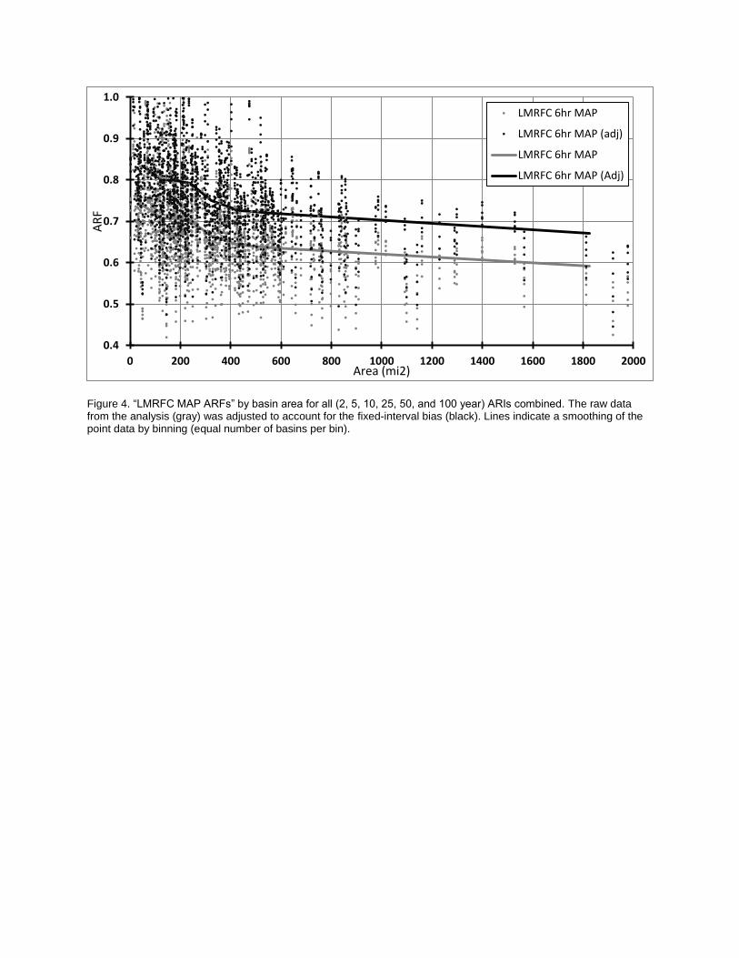
Figure 4. “LMRFC MAP ARFs” by basin area for all (2, 5, 10, 25, 50, and 100 year) ARIs combined. The raw data from the analysis (gray) was adjusted to account for the fixed-interval bias (black). Lines indicate a smoothing of the point data by binning (equal number of basins per bin).
0.4
0.5
0.6
0.7
0.8
0.9
1.0
0 200 400 600 800 1000 1200 1400 1600 1800 2000
AR
F
Area (mi2)
LMRFC 6hr MAP
LMRFC 6hr MAP (adj)
LMRFC 6hr MAP
LMRFC 6hr MAP (Adj)
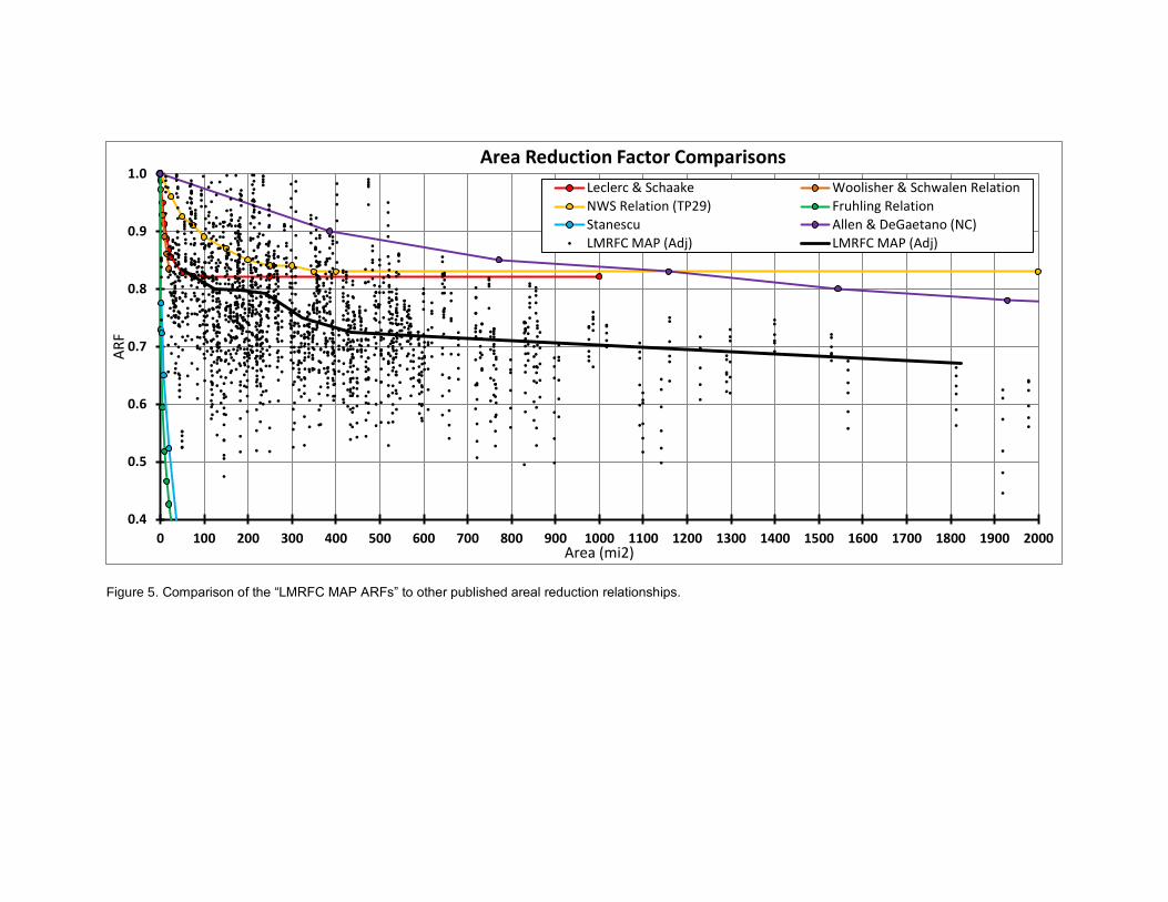
Figure 5. Comparison of the “LMRFC MAP ARFs” to other published areal reduction relationships.
0.4
0.5
0.6
0.7
0.8
0.9
1.0
0 100 200 300 400 500 600 700 800 900 1000 1100 1200 1300 1400 1500 1600 1700 1800 1900 2000
AR
F
Area (mi2)
Area Reduction Factor Comparisons
Leclerc & Schaake Woolisher & Schwalen Relation
NWS Relation (TP29) Fruhling Relation
Stanescu Allen & DeGaetano (NC)
LMRFC MAP (Adj) LMRFC MAP (Adj)

3.0 DISCUSSION & CONCLUSIONS
There are a few different ways to utilize the data created by this analysis. The DDF data
from NOAA Atlas 14 could be used along with a suitable ARF to create the hypothetical
“correct” rainfall amounts for each basin and each ARI. These rainfall amounts could then be
compared to the rainfall amounts produced by the LMRFC MAP frequency analysis to see if any
biases exist, and if so, where along the frequency curve are they found (extreme events, or
more common events). Unfortunately, as seen in section “2.4 Comparing LMRFC MAP data to
NOAA Atlas 14,” published ARFs vary substantially. This makes it quite difficult to determine the
accuracy of the LMRFC MAP data, because proper correction (reduction) for basin area is
required. A “proper correction” might be elusive because a “proper definition” of an ARF is
lacking. There is no one definition that fits all potential applications of ARFs in either synthetic
hydrology (design computations) or rainfall-runoff model calibrations (William H. Asquith,
personal communication, November 2015).
Another way to utilize the data created by this analysis is to take the reduction factors
produced by comparing the LMRFC MAP against the NOAA Atlas 14 data and use them to
produce areal reduction factors based upon our data. Unfortunately, there are many caveats to
this. The frequency analysis performed on the LMRFC 6-hour MAP data was simple. The gauge
network in many parts of the LMRFC area is not as dense as those in published ARF studies,
which will cause basins within a single Thiessen polygon to basically be assigned the rainfall
frequency values of a single point location (the gauge) and not an area. The Log-Pearson Type
III distribution was used in this analysis, but the authors were informed by a peer reviewer that
the Gumbel Distribution may have been more applicable (William H. Asquith, personal
communication, November 2015). This may yield uncertainty that was not quantified.
Regardless of the mentioned issues with this analysis, the output of our analysis is
consistent in some areas with other ARF studies. It has been shown in previous studies that the
ARFs may be different for specific ARIs. In Allen & DeGaetano (2005), a steady decrease in
ARFs was found as the ARI increased, with this difference most notable with larger areas. Our
analysis showed a similar behavior (Figure 3), although the 2 year (50% annual chance) event
was an outlier by being lower than the 5 year (20% annual chance) event. Also, in virtually all
published ARF studies, the ARF trend increases rapidly toward 1.0 as basin sizes decrease to
zero (0). Although the available LMRFC basin sizes and the binned-averaging process make it
difficult to determine the ARF trend for very small basin sizes, we do see a similar trend. We
also evaluated using the median value for each bin rather than the mean based upon a peer
review suggestion; this change yielded negligible differences.
After careful consideration and analysis of our data in context of other published ARFs,
we have decided to present our analysis as an independent, that is alternative, ARF. One
assumption with ARFs is that rainfall ARIs for areas of near 0.0 mi2 should be approximately the
same as for a single point ARI (ARF value of near 1.0). This is not evident in our binning method
because the bin for the smallest areas is an average of ARFs from basins ranging from 2.5 mi2
to 96 mi2 in size. Thus, we have chosen to present two different ARFs based upon our data, one
derived from the binning method (hereafter “Binned Method”) shown previously and another
with a power best-fit regression (hereafter “Regression Method”), the latter of which would have
an ARF value of approximately 1.0 at an area of 0.0 mi2. The Regression Method can be
expressed by:
𝐴𝑅𝐹 = (1.09)( 𝑎 −0.0667)
where 𝑎 is the area and ARF is the areal reduction factor to multiply by the point-based ARI
value. The LMRFC ARFs are shown by Figure 6 and Table 1.
Because of the issues with widely ranging values in different published ARFs and the
simplicity of our analysis, the LMRFC MAP derived ARFs are subject to uncertainty and
attendant questions of applicability. These ARFs may not be suitable for all data types in all
geographic regions. At the present time, the ARFs are likely to be most valid for locations within
the LMRFC forecast area and for areas within the size range of our forecast basins. The authors
recognize that these reduction factors were not derived with as robust of a methodology when
compared to other studies, and should be used with caution.
4.0 ACKNOWLEDGEMENTS
The authors would like to acknowledge William H. Asquith with the United States
Geological Survey Texas Water Science Center for providing helpful guidance and scripts that
aided in the completion of this work.

Figure 6. Areal Reduction Factors derived from the LMRFC MAPs. The Binned Method was derived from bins of equal numbers of subbasins. The Regression Method was derived from a power best-fit regression to the raw data. Table 1. Summary of ARFs derived from the LMRFC MAPs. The Binned Method was derived from bins of equal numbers of subbasins. The Regression Method was derived from a Power best-fit regression to the raw data. Area values correspond to the mid-point of each range of areas in the Binned Method.
Area (mi2) ARF (Binned
Method)
ARF (Regression
Method)
48 0.83 0.84
125 0.80 0.79
181 0.80 0.77
239 0.79 0.76
323 0.75 0.74
435 0.73 0.73
571 0.72 0.71
0.60
0.65
0.70
0.75
0.80
0.85
0.90
0.95
1.00
0 100 200 300 400 500 600 700 800 900 1000 1100 1200 1300 1400 1500 1600 1700 1800 1900
AR
F
Area (mi2)
LMRFC Areal Reduction Factors
LMRFC ARF (Binned Method)
LMRFC ARF (Regression Method)
4.0 WORKS CITED
Allen, R., & DeGaetano, A. (2005). Areal Reduction Factors for Two Eastern United States
Regions with High Rain-Gauge Density. J. Hydrol. Eng., 10(4).
Asquith, W. (1998). Depth-Duration Frequency of Precipitation for Texas. Austin, TX: U.S.
Geological Survey. Retrieved March 2016, from http://pubs.usgs.gov/wri/wri98-
4044/pdf/98-4044.pdf
Asquith, W. H. (1999). Areal-Reduction Factors for the Precipitation of the 1-Day Design Storm
in Texas. Austin, TX: U.S. Geological Survey. Retrieved from
http://pubs.usgs.gov/wri/wri99-4267/pdf/wri99-4267.pdf
Dingman, S. L. (1994). Physical Hydrology. Upper Saddle River, NJ: Simon & Schuster.
Leclerc, G., & Schaake, J. (1972). Derivation of hydrologic frequency curves. Massachusetts
Institute of Technology.
Lincoln, W. S. (2014). Analysis of the 15 June 2013 Isolated Extreme Rainfall Event in
Springfield, Missouri. J. Operational Meteor., 233-245.
doi:http://dx.doi.org/10.15191/nwajom.2014.0219
Lincoln, W. S. (2014). Updated Rainfall Analysis for the May 1995 Southeast Louisiana and
Southern Mississippi Flooding. National Weather Service Technical Paper. Retrieved
from
http://www.srh.noaa.gov/images/lmrfc/tech/Updated_Rainfall_Analysis_1995_05.pdf
Linsley, R., Kohler, M., & Paulhus, J. (1982). Hydrology for Engineers. McGraw-Hill.
Miller, J., Frederick, R., & Tracey, R. (1973). NOAA Atlas 2: Precipitation-Frequency Atlas of the
Western United States. National Weather Service. Silver Spring, MD: NOAA. Retrieved
from
http://www.udfcd.org/downloads/pdf/tech_papers/NOAA_Atlas_2_Precipitation_Frequen
cy_Vol_3_Colorado.pdf
Parzybok, T. W. (2011). Real-time Average Recurrence Interval Rainfall Maps for the U.S. 39th
Annual Conference on Broadcast Meteorology. Oklahoma City, OK: American
Meteorological Society.
Perica, S., Martin, D., Pavlovic, S., Roy, I., Laurent, M. S., Trypaluk, C., . . . Bonnin, G. (2013).
NOAA Atlas 14: Precipitation-Frequency Atlas of the United States (Volume 9). 9. Silver
Spring, MD: NOAA. Retrieved from
http://www.nws.noaa.gov/oh/hdsc/PF_documents/Atlas14_Volume9.pdf
Stanescu, V. (1995). Hidrologie Urbana (Urban Hydrology). Bucharest: Editura Didactica si
Pedagogica.
Stanescu, V. (2006, March). Engineering Hydrology Chapter 10: Urban Hydrology. (L. o.
Ecohydrology, Producer, & Ecole Polytechnique Federale de Lausanne) Retrieved
February 2015, from Virtual Campus in Hydrology and Water Ressources (VICAIRE):
http://echo2.epfl.ch/VICAIRE/mod_1b/chapt_10/main.htm
Vladimirescu, I. (1984). Engineering Hydrology. Bucuresti: Editura Technica.
Woolisher, D., & Schwalen, H. (1959). Frequency Relations for Thunderstorm Rainfall in
Southern Arizona. University of Arizona.