creating musical structure from the temporal dynamics...
TRANSCRIPT

CREATING MUSICAL STRUCTURE FROM THE TEMPORAL DYNAMICS OF SOUNDSCAPES
Ryan Maguire
!"#$%&'$()*&++,-,
!.-.$"+)/'0.10
2343)5"++-"#$,6)5"++
5"6&7,#8)95):;<==
!"#$%!&$
Acoustic signal mixtures from the environment often manifest interesting structural properties. These features can be used to generate musical forms, but access is a problem. Here, Probabilistic Latent Component Analysis (PLCA) has been used to automatically extract independent sources from a mixed signal of environmental sounds. Excitation information corresponding to the temporal evolution of independent acoustic sources in the original environment is extracted. Given this information, we map the temporal dynamics of each independent sound source to a variety of parameters in a musical composition. Thus, the temporal flow of auditory events in an environmental soundscape is used to determine musical structure. After a discussion of PLCA, related composers and music compositions are highlighted. Thereafter, an approach to mapping the temporal dynamics of a given soundscape to a musical setting using source separation techniques is illustrated.
'( )*$%+,-&$)+*
Recent Research in Music Informatics has explored the use of Probabilistic Latent Component Analysis (PLCA) and related techniques to isolate independent components from mixed musical signals [1][6][7]. This has applications in automatic thumbnailing, retrieval, and structural segmentation, as well as music composition [8][11]. Recent compositions have used PLCA to cull specific sonic components from source recordings and then utilized these samples as musical source material [9].
In this paper, we propose using PLCA as a tool to generate musical structure rather than surface material for a composition. Natural soundscapes share traits with musical sound such as repetition, development, persistence, and contrast. Using PLCA to analyse field recordings, one can access the ebb and flow of auditory events in a natural soundscape. The individual sources can then be used to determine the structure of a composition, mapping extracted features to independent synthesizers, instruments, or parameters. In this way, the structure of a natural soundscape can be directly utilized in the creation of musical form.
.( #+-%&/0#/1!%!$)+*
Techniques for source separation from mixed audio include convolutive non-negative matrix factorization (NMF), independent subspace analysis (ISA), Probabilistic Latent Component Analysis (PLCA), and Shift Invariant Probabilistic Latent Component Analysis (SI-PLCA) [1][4][6][7][8][11]. These techniques are well documented in the Music Informatics literature.
Probabilistic Latent Component Analysis is a probabilistic variant of NMF. It decomposes a non-negative matrix V into the product of two multinomial probability distributions, W and H, and a mixing weight, Z. In the auditory domain, V would be a matrix representing the time-frequency content of an audio signal:
!!"#$"#
%":
&$>
'%(%)%
*
(1)
where each column of W can be thought of as a recurrent frequency template and each row of H as the excitations in time of the corresponding basis. Z = diag(z) is a diagonal matrix of mixing weights z and K is the number of bases in W [11]. Each of V, wk , zk, and hk are normalized to sum to 1, as they correspond to probability distributions.
Sparse settings are commonly favoured in the literature. These solutions can be encouraged by imposing constraints using prior distributions, alphaZ and alphaH. A detailed explanation is beyond the scope of this paper, but can be found in [11].
2( 3-#)&!401+)*$#0+50%/5/%/*&/
Several compositions have drawn on PLCA and related techniques for their material. Topel and Casey discuss five compositions which utilize extracted components to articulate characteristics of their source audio at specific moments [9]. For example, Violine (2011), by Spencer Topel decomposed 12 – 90 second audio clips of J.S. Bach's Chaconne in d minor from Partita No. 2 for solo violin into individual notes or pitch classes and then matched extracted components to a live violin signal. Another interesting example is Strange-Charmed (2011), by Michael Casey and Simon Atkinson, which used independent subspace analysis (ISA) to generate an expanded set of sound materials from source sounds such as Geiger counters, insects, and band-pass filters [2][3][4].
The 11th International Conference on Information Sciences, Signal Processing and their Applications: Special Sessions
978-1-4673-0382-8/12/$31.00 ©2012 IEEE 1471

6( #$%-&$-%/05%+30/*7)%+*3/*$!40#+-*,
In this work, we have used PLCA to capture the dynamic flow of independent sound sources in a soundscape and then used this material to control numerous synthesizers, thus generating a musical work with its temporal structure derived from the source soundscape. This differs from previous uses of PLCA and SIPLCA which have focused on using the extracted features directly as audible material for composition. We have instead abstracted the extracted features and used them as a higher level parametric control. Rather than listening to the features themselves, one experiences their presence indirectly.
As a preliminary exercise in this technique, a recording of a mountain soundscape was analysed [5]. The source audio was 2 minutes and 2 seconds long. There are a variety of different bird calls which enter and fade, crescendo and decrescendo independently at different distances, times, and rates. Cicadas also fill the signal with their rhythmic call, more or less noticeable at different times.
In our implementation, standard PLCA with k = 6 was used. This number was an estimate of the number of independent sound sources audible in the recording. This resulted in 6 basis functions w (see Figure 1), each with a distinct correspondent time profile h (see Figure 2). Each w has a distinct frequency profile. This can be considered to be the spectral “signature” of each individual source. Similarly, each corresponding time function h represents when the given spectral profile is most present in the source recording.
Given these unique amplitude-time kernels for each basis, w, we have independently mapped each hk to a different synthesis parameter. In our preliminary implementation, we used each frequency kernel hk to control the amplitude of an independent synthesizer. In this way, the temporal structure of the original components of the soundscape are used to create the temporal structure of a synthesized musical environment.
Amplitudes across 95 frequency bins.
!"#$%#&'()*+&
Figure 2. Bases wk using PLCA with k = 6.
8( &+*&4-#)+*
Previous uses of PLCA in music composition have used the extracted bases as sound material. Here we have used PLCA to extract the temporal structure from a natural soundscape and then used this structure to determine the form of a musical work. This bears some similarity to the idea of cross synthesis with PLCA, wherein the basis functions extracted from one audio signal are combined with the time kernel of a different signal.
Future possibilities include using the extracted temporal information to control other parameters, or alternatively, using this information to generate an acoustic composition or as an input for an algorithmically generated
piece. One might also work with longer sound files so as to utilize processes and changes which occur more gradually in nature. Finally, one might combine this approach with the previous techniques by integrating audio from the soundscape with the structure generated from the same source.
Figure 3. hk using PLCA with k = 6.
%/5/%/*&/#
?>@ Cardoso, Jean-Fran!ois. “Source separation using higher order moments”, Proc. ICASSP-89, pages 2109-2112, 1989.
?3@ Casey, M.A. “Soundspotting: A new kind of process”, The Oxford Handbook of Computer Music, 2009.
?;@ Casey, M.A., and S. Atkinson. Strange-Charmed: MIT EMS@25 CD, Track 9. MIT Media Laboratory, 1999.
?4@ Casey, M.A., and A. Westner. “Separation of mixed audio sources by independent subspace analysis”, Proceedings of the International Computer Music Conference, pages 154-161, 2000.
?=@ Freesound, “050823-suraksan_extract.wav”, Accessed September 29th, 2011, http://www.freesound.org/people/sazman/sounds/7959/
?2@ Smaragdis, P., Bhiksha Raj, and Madhusudana V.S. Shashanka. “Sparse and shift-invariant feature extraction from non-negative data”, ICASSP, pages 2069-2072. IEEE, 2008.
?<@ Smaragdis, P., and Bhiksha Raj. “Shift-Invariant Probabilistic Latent Component Analysis”, MERL Technical Report, TR2007-009.
?A@ Smaragdis, P., B. Raj and M.V. Shashanka “Supervised and semi-supervised separation of sounds from single-channel mixtures”, Proc. 7th Int. Conf. Ind. Compon. Anal. Signal Separation (ICA '07), p.414, 2007.
?B@ Topel, Spencer S., and Michael A. Casey. ''Elementary Sources: Latent Component Analysis for Music Composition'', 12th International Society for Music Information Retrieval Conference, Miami, USA, 2011.
?>:@ Tawaststjerna, Erik; Robert Layton (Translator)(1976-1986). Sibelius. Faber & Faber, Vol. I, 1865-1905, Vol. II, 1904-1914, London.
?>>@ Weiss, Ron J., and Juan Pablo Bello “Identifying repeated patterns in music using sparse convolutive non-negative matrix factorization”, Proc. Int. Conf. Music Inf. Retrieval, pp.420-425, 2005.
1472
Stravinsky's “Full Fadom Five”
Ryan Maguire New England Conservatory of Music
January 2010
Stravinsky's “Full Fadom Five” from Three Songs on William Shakespeare is emblematic of the
composer's idiosyncratic approach to serialism. It is significant for its formal structure, its recurring
motives, and its intervallic content. Standard serial transformations such as inversion, retrograde,
transposition and diminution are used throughout. Despite being a 12-tone work the composer favors
the minor 3rd, perfect 5th, and minor 7th, leading to a distinct semi-diatonic musical language.
Structurally, the piece is divided into three short sections. These divisions follow logically from
the meaning of the text. This structure is apparent in a spectrographic image of the piece.
Full fadom five, thy father lies...
Of his bones are Corrall made; Those are pearles that were his eies,
Nothing of him that doth fade,But doth suffer a Sea-change
into something rich and strange:Sea-Nimphs hourly ring his knell.
Ding dong, ding dongHearke now I heare them;
ding dong bell.

“Full fadom five, thy father lies...” the piece begins. Musically and textually this serves as a
declamation. The piece then moves into an elongated middle section which describes the father's
decaying body in the sea. The last section comes to life with the evocative sounds of the fathers death
knell.
Returning to the first section, the declamation is characterized by fricatives more so than any
other section of the piece. The rhythmic texture is relatively homogeneous- all three instruments
support the voice directly. There is an intervallic motif shared between all four parts. Numbering
intervals chromatically from 0 for the unison to 11 for the major 7 th, the first section is characterized by
the succession of intervals: 5,7,10. I will call this succession motive A. This is repeated twice in a row
in the voice, flute, and clarinet. The viola part has a variation of this. It displays the pattern: 7,5,2,7,5.
Considering 7 and 5 to be interchangeable and 2 to be the inverse of 10, this is a diminished and
inverted presentation of the intervallic motif 5,7,10. Lending credence to this, the five pitches of the
viola part share the exact pitch names with the first five notes of the vocal part, specifically: F, B-flat,
E-flat, D-Flat, A-Flat. While the flute and clarinet play in unison (a significant pairing in that
Stravinsky is essentially treating the wind instruments together as one voice), the voice and viola parts
both present their material at different speeds and with different inflections. Additionally, the winds
begin their presentation a fifth higher than the vocal and viola parts, C5 a fifth above F4. Beginning in
the middle of the text at “thy”, there is an interesting contrary motion displayed between the voice part
and the winds- as one moves up, the other tends to move down. Considering all voices in sum, there are
distinct pitch classes voiced in this introduction: B-flat, C-flat, C, D-flat, E-flat, F, G-flat, and A-flat.
This is significant and as we will see, this pitch set is maintained throughout the piece in the vocal part
with the later addition of G to the set.

As the piece progresses the paring of wind instruments is undone, creating a more varied
texture. Stravinsky introduces a motif which is heard 14 times in this middle section: motive B. The
motif is defined by moving between two adjacent pitches, an interval of 1, on subsequent 16 th notes.
For example, the motif is first heard in the voice on the word Corrall with the pitches: B-flat, C-flat, B-
flat- C-flat.
This motif is actually itself one part of a larger motif which is at play throughout all of the
instruments during the entire middle section. This larger, intervallic motif serves as the primary
generating cell for the entire middle section. It's characteristic interval succession is: 10,7,1,5,1,3. I will
refer to this as motive C. It first appears in the vocal part as well during the text “Of his bones are
Corrall made...”.
Beginning with only the vocal part, this theme is first reversed (3,1,5,1,7,10). Then it's starting
pitch is moved up an octave to E-flat-5 and the original interval succession is voiced in the opposite
direction, in other words the first leap of 10 moves downwards, instead of upwards, and so forth.

Next the reversed (3,1,5,1,7,10) theme is restated, also upside-down. It's final “10” interval
serves as both the end of this motivic statement and the beginning of a restatement of the original
motive, C, in it's original direction, and at it's original pitch location. Following this, as before, the
motive is shifted up an octave and stated upside-down.
When one examines the instrumental parts, motive C appears in even more guises. Stravinsky
begins to play with the equivalence of certain intervals. He substitutes 5 and 7, 3 and 9, and 11 and 1
for each other to create variants of the motif. Here is a list of some of the numerous guises in which
Motive C appears:

When one analyzes every successive interval in the entire piece in each of the four parts some
striking trends appear. For instance, not once does Stravinsky incorporate the tritone, in other words,
the 6 interval. Ultimately this is a 12 tone piece (the clarinet plays all 12 pitches eventually) but the
absence of the tritone gives this piece a distinct character. Of all the parts, the voice part is the most
limited in its intervallic and pitch content. It contains the fewest total number of pitch classes, 9, and
also the least intervallic variety- it contains no 4's, 6's, 8's, 9's, or 11's. One might consider the vocal
part, which is surely the focal point musically, for most listeners, as the distilled base around which the
accompaniment is built. Summing all of the intervals in all of the parts, the interval of 1 is most used,
owing to it's primary role in Motive A, and the repetitive nature of the motive. This interval serves an
ornamental role, embellishing the larger intervals which have a greater effect on the overall harmony of
the piece. Next are the 5, 7, 10, and 3- in that order. This should not be surprising given their
prominence in Motive C. If one considers 5 as the inversion of 7, then these prominent intervals can be
reduced to 3, 7, and 10- a minor seventh chord. Perhaps this explains why the piece, despite using all
twelve tones, maintains the ghost of a familiar tonal character.

Musically, the different intervals play different roles. As stated above, the 1 acts as an
elaboration throughout the piece to add dynamic interest. The 5, 7, and 10 provide the piece with its
leaping quality. The vocal line and all of the instrumental parts tend to leap broadly, sketching out the
musical space in large swaths. This is particularly noteworthy in the clarinet part after the word knell- it
seems to leap about and expand across the musical space painting a broad sound image of a slowly
tolling death knell.
It is here also that the viola introduces it's only vertical sonorities of the piece- with intervals of
1 and 7. This creates a striking moment at the end of the second large section of the piece.
0 1 2 3 4 5 6 7 8 9 10 11
0
10
20
30
40
50
60
VoiceFluteClarinetViola
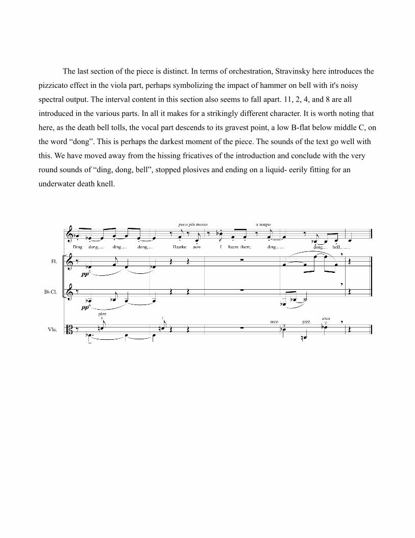
The last section of the piece is distinct. In terms of orchestration, Stravinsky here introduces the
pizzicato effect in the viola part, perhaps symbolizing the impact of hammer on bell with it's noisy
spectral output. The interval content in this section also seems to fall apart. 11, 2, 4, and 8 are all
introduced in the various parts. In all it makes for a strikingly different character. It is worth noting that
here, as the death bell tolls, the vocal part descends to its gravest point, a low B-flat below middle C, on
the word “dong”. This is perhaps the darkest moment of the piece. The sounds of the text go well with
this. We have moved away from the hissing fricatives of the introduction and conclude with the very
round sounds of “ding, dong, bell”, stopped plosives and ending on a liquid- eerily fitting for an
underwater death knell.

Works Consulted:
Cross, Jonathan, ed. The cambridge companion to stravinsky. Cambridge University Press, 2003.
Stravinsky, Igor, and William Shakespeare. Three Songs from William Shakespeare: 1953, for mezzosoprano, flute, clarinet, and viola. Boosey & Hawkes, 1954.
Real-time Rhythmic Pattern Detection from Audio via Template Matching
Ryan MaguireDartmouth College
Digital Musics6242 Hallgarten HallHanover, NH 03755
ABSTRACT
Real-time Rhythmic Pattern Detection from live audio signals is possible using an audio programming environment such as Pure Data, but has been largely neglected. Lower level features such as amplitude, frequency, and tempo are commonly used as data for live processing, however, specific rhythmic pattern detection has not yet attained this same proliferation. We seek to prototype and implement a system for real-time rhythmic pattern detection from a live audio signal via template matching. Our approach is discussed, evaluating several alternative methods of preprocessing to the input audio signal and their effects on obtaining a distance measure between template and input signal. The system is further evaluated for robustness against near matches, and an online rhythmic pattern detector is implemented. Using the results from these tests, an outline for creating a real-time pattern detector in Pure Data is presented and future directions for this project are highlighted.
KeywordsRhythm, Pattern Recognition, Template Matching, Machine Listening
INTRODUCTIONOur goal in this work is to implement real-time rhythmic pattern detection for use in live musical performance, using only audio as input. The motivation for such work is a desire to control and/or interact via machine listening with an audio/visual computer music system. Ultimately our goal is an implementation of real-time rhythmic pattern detection via audio template matching in an environment such as the Pure Data programming language. Making such an object available for a programming language such as Pure Data will add to the repertory of currently available tools for computer listening and analysis in said environment. As a regular matter of course amplitude, frequency, tempo, and timbral information are extracted from live audio input in Pure Data, and this data is utilized in a myriad of ways to drive interaction between a live sound input and the computer. This data can be used to control anything from robotic accompanists to live signal processing. Much of the information currently accessible in Pure Data is
low-level signal information (frequency, amplitude, etc.). Introducing a method for rhythmic pattern detection is a move towards higher-level abstraction, and begins to utilize the kind of perceptually relevant, musical-semantic information that human listeners readily perceive and react to in live music performance and listening.
As a starting point for this project, we have sought to prototype a system which can detect a specified rhythmic pattern when played by the same instrument at roughly the same tempo. We have begun by working with a monophonic signal in a low-noise environment, but would like to eventually scale up to recognize monophonic or polyphonic rhythmic patterns in a variety of sound environments. These are all approachable problems and this work lays a foundation for such future work to build upon.
BACKGROUNDTemplate Matching has been used as a method in machine listening to determine the beat from an audio signal. It has also been used in rhythm detection from MIDI input signals. Other methods have been used to attempt to detect rhythmic patterns from audio, but none of these are currently available in the public domain for use in the Pure Data programing language to be utilized in live performance situations. A previous approach involves the use of Neural Nets to detect rhythmic patterns.
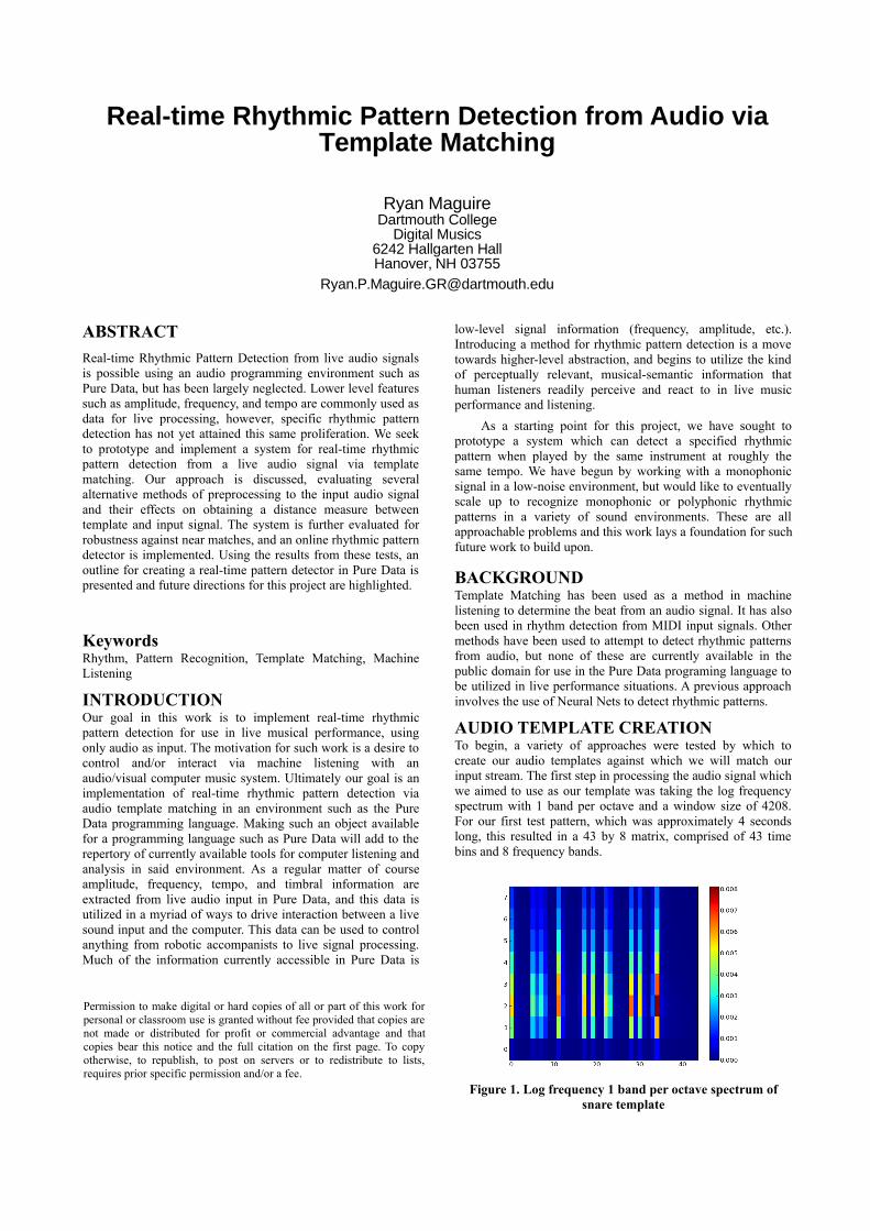
AUDIO TEMPLATE CREATIONTo begin, a variety of approaches were tested by which to create our audio templates against which we will match our input stream. The first step in processing the audio signal which we aimed to use as our template was taking the log frequency spectrum with 1 band per octave and a window size of 4208. For our first test pattern, which was approximately 4 seconds long, this resulted in a 43 by 8 matrix, comprised of 43 time bins and 8 frequency bands.
Figure 1. Log frequency 1 band per octave spectrum of snare template
Permission to make digital or hard copies of all or part of this work for personal or classroom use is granted without fee provided that copies are not made or distributed for profit or commercial advantage and that copies bear this notice and the full citation on the first page. To copy otherwise, to republish, to post on servers or to redistribute to lists, requires prior specific permission and/or a fee.

The next step in our processing was taking the first difference along the time axis in each frequency band. The effect of this is highlighting the changes in amplitude in each band. A large increase in amplitude from one time window to the next, such as is present during the attack of a percussion instrument, for example, would result in a high, positive first difference value. A typical signal decay would result in a small negative first difference value.
Figure 2. First difference of snare template
The third step in our processing was half-wave rectifying the first differentiated signal. By doing this, setting all negative difference values to zero, we eliminate all of the instrumental decays from our signal, and have a signal which could be used fairly easily for onset detection. The positive increases in amplitude in each frequency band have been distilled and amplified.
Figure 3. Half-wave rectification of snare template
In the next phase we attempted to match signals at each of the three steps in our processing method, to see at which step we obtained the most accurate distance measure between different and similar rhythmic patterns.
RHYTMIC PATTERN MATCHINGDuring this phase of our work, we attempted to determine the best representation for our audio signal from which to calculate the distance. To calculate our distance, we used the Pearson's product-moment correlation coefficient to compute Pearson's distance. Alternatively, the Euclidean normed distance could be used. Here, we use the Pearson's product-moment correlation coefficient to compute the Pearson's distance between two matrices, the first representing our rhythm template, and the second the audio segment of equal length which we are testing
as a possible rhythmic match to the first. Then taking the Pearson's distance, which returns a matrix, we take the mean of the values lying along the diagonal, giving us a single number from which to evaluate our “distance”. This distance metric ranges from 0 for an identical match to 2 for the most dissimilar matrices possible.
In this test, we compared four different performances of the same rhythmic pattern played on a snare drum to the first of those four performances, which we took as our template. For each of the 4 possible comparisons (A to A, A to B, A to C, and A to D) we computed the Pearson's distance after either taking the Log Frequency Spectrum, the spectrum plus the first difference, or the spectrum and first difference half-wave rectified, as described in the previous section.
It should be mentioned here that in comparing A to A, we should expect a distance of 0, as A is exactly identical to A. B and C should also be fairly close to our template A, and D should be a little further away as it was dragged a little bit behind the original recording and was not a very accurate performance of the desired rhythmic pattern.
Beginning with our raw audio signals, we take the Log Frequency Spectrum of both, with 1 band per octave and a window size of 4208 samples, with a sample rate of 44100. In our test, we observed that the distance from A for A through D respectively was 0.022, 0.027, 0.056, and 0.033. Several things seem wrong with this distance measure. First, the distance between A and A, while it is the lowest of the four, should truly be zero. Second, D should have the largest distance, not C. These are serious problems and warrant further testing with these features and this distance metric. Until such testing is done, using the 1 band per octave log frequency spectrum representation of our signals to calculate the Pearson's distance can only be viewed as inappropriate for our needs.
Next, we took the first difference of each of our signals in the time domain and used this data to test the distance between the template and the four respective audio signals. The distance we measured between A and A through D respectively were: 0.0, 0.167, 0.152, 0.409. These distance measurements fit very well with our expectation from simply listening to the audio files.
Figure 4. Pearson's distance of template to itself via first difference
The mean distance along the diagonal between A and A should, as it is, be zero, since this is the same signal compared to itself. B and C are both fairly close to A, though not perfectly, exactly the same, so their fairly low scores can be viewed as close matches to the original template. D which was a flawed performance and for our purposes should probably not be viewed as a match, has a higher distance value of 0.409, more than twice the score of B. This is good and we can

imagine setting a threshold between the scores for B and D that would identify those performances closer to B as matches with A and those approaching D as not being matches, as it strayed enough from the original that it could potentially be interpreted as different rhythmic pattern. Overall, using the first difference to calculate the Pearson's distance provides us with distance values that align well with the authors perceptual judgement of the similarity between the different performances.
Figure 5. D vs. A. Note the divergence near the end.
Finally, we attempted to half-wave rectify the data from our previous step before calculating the Pearson's distance. This ran into numerical problems, and we had to add a small amount of noise to the data to get rid of zeros and achieve a more accurate result. Even doing this, however, the Pearson's distances we calculated were large, all above 0.7, and inaccurate. The distance to A of A through D respectively was calculated as: 0.737, 0.747, 0.710, 0.863. D was correctly identified as the most distant of the four, however C was identified as the closest, and A was not given a distance of zero to itself.
Given these results, we have decided to use the first difference representation of our audio signals to calculate the Pearson's product-moment correlation and Pearson's distance, for use in our real-time audio rhythmic pattern detection system.
NEAR-MATCHESThe goal of our rhythm detection system is to identify rhythmic patterns played on a specific instrument, at a specific tempo. Thus, the question of how our system responds to variations in instrumental timbre, tempo, and pattern variations is an important one. Ideally, our system will reject the same pattern played on a different instrument, will reject the same pattern played on the same instrument but at a different tempo, and will reject alternative patterns that do not match our specified template, despite similarities in tempo and identical timbres.
In order to test our system, we first compared the recording of our snare drum test template A to recordings of the same pattern played on a ride cymbal and on a tom-tom. In each case the distance was calculated to be approximately 1.15. You can see that despite the patterns being identical, the differences in timbre accounted for the large distance between our template and these other performances.
The next task was to see how the system would perform when presented with faster and slower performances of the original pattern on the same instrument. In both cases, a large distance was returned, greater than 0.7, demonstrating that the system will not match the same pattern played at a different tempo. This is a desirable quality for our purposes, but one can imagine a situation in which a live performer plays the
specified pattern plus or minus a few beats per minute despite which it might be desirable to identify the performance as a match. In order to make the system robust to such deviations without sacrificing it's tempo stringency, we can resample the input audio selection to slightly stretch and compress the new pattern so that, in the case that a performance of a pattern is accurate, but deviates only slightly in tempo, it will still be identified as a match.
Finally, we tested our system using a similar but distinct rhythmic pattern, to see how the system would respond to a different pattern, despite similarities in tempo and timbre. As hoped, the distance for our alternative pattern was 0.565, significantly higher than the distance scores for accurate performances of the same rhythm.
Figure 6. Snare Template First Difference.
Figure 7. Ride Cymbal First Difference. Note high frequency content.
ONLINE PATTERN DETECTIONAs the next step in our march towards real-time rhythmic pattern detection, we implemented online pattern detection detecting our 4 second long rhythmic template from a longer sound file containing other rhythms at the beginning, the pattern emerging in the middle, and then other rhythms at the end.
To implement this step, we took sub-sections of the longer audio stream file equal in length to the shorter template file, starting at the first window and proceeding through the file one step at a time, taking a 43 window long segment, measuring the distance between the segment and the template, and then incrementing ahead one window and taking a new 43 window
long segment, until reaching the end of the file. Thus, we took segment [0:43], then [1:44], then [2:45], and so on until teaching the last 43 window long segment we could take from the stream file. Calculating the distance between each of these segments and our template was fast and efficient.
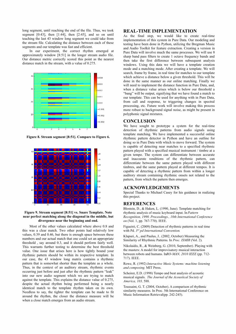
In our experiment, the correct rhythm emerged at approximately window [8:51] in the longer stream audio file. Our distance metric correctly scored this point as the nearest distance match in the stream, with a value of 0.275.
Figure 8. Stream segment [8:51]. Compare to Figure 6.
Figure 9. Stream segment [8:51] vs. Snare Template. Note near perfect matching along the diagonal in the middle, but
divergence near the beginning and end.
Most of the other values calculated where above 0.8 and this was a clear match. Two other points had relatively low values, 0.39 and 0.46, but there is enough space between these numbers and our actual match that one could set an appropriate threshold , say around 0.3, and it should perform fairly well. This warrants further testing to determine the best threshold value. One issue that arises here is how tightly bound your rhythmic pattern should be within its respective template. In our case, the 43 window long matrix contains a rhythmic pattern that is somewhat shorter than the template as a whole. Thus, in the context of an auditory stream, rhythmic events occurring just before and just after the rhythmic pattern “leak” into our new audio segment which we are trying to match against the template. This explains the distance value of 0.275, despite the actual rhythm being performed being a nearly identical match to the template rhythm taken on its own. Needless to say, the tighter the template can be made to fit around the rhythm, the closer the distance measure will be when a close match emerges from an audio stream.
REAL-TIME IMPLEMENTATIONAs the final step, we would like to create real-time implementation of this system in Pure Data. Our modeling and testing have been done in Python, utilizing the Bregman Music and Audio Toolkit for feature extraction. Creating a version in Pure Data will involve much the same processes. We will use 8 sharp band pass filters to create 1 octave frequency bands and then take the first difference between subsequent analysis windows. Using this data we will have a template creation mode and a matching mode. After creating a template. We will search, frame by frame, in real time for matches to our template which achieve a distance below a given threshold. This will be done in the same manner as our online matching. Finally we will need to implement the distance function in Pure Data, and, when a distance value arises which is below our threshold a “bang” will be output, signifying that we have found a match to our template. This can be used for anything with in Pure Data, from call and response, to triggering changes in spectral processing, etc. Future work will involve making this process more robust to background signal noise, as might be present in polyphonic signal mixtures.
CONCLUSIONWe have sought to prototype a system for the real-time detection of rhythmic patterns from audio signals using template matching. We have implemented a successful online rhythmic pattern detector in Python and have an outline for doing so in Pure Data with which to move forward. The system is capable of detecting near matches to a specified rhythmic pattern played with a specified musical instrument / timbre at a given tempo. The system can differentiate between accurate and inaccurate renditions of the rhythmic pattern, can differentiate between the same pattern played with different timbres, and the same pattern played at different tempos. It is capable of detecting a rhythmic pattern from within a longer auditory stream containing rhythmic onsets not related to the pattern, from which the pattern then emerges.
ACKNOWLEDGEMENTSSpecial Thanks to Michael Casey for his guidance in realizing this project.
REFERENCESBlostein, D., & Haken, L. (1990, June). Template matching for rhythmic analysis of music keyboard input. In Pattern Recognition, 1990. Proceedings., 10th International Conference on (Vol. 1, pp. 767-770). IEEE.
Figueiró, C. (2009) Detection of rhythmic patterns in real time with Pd. 3rd pd International Convention.
Klapuri, A., and Paulus, J.. (2002, October) Measuring the Similarity of Rhythmic Patterns. In Proc. ISMIR (Vol. 2).
Nikolaidis, R., & Weinberg, G. (2010, September). Playing with the masters: A model for improvisatory musical interaction between robots and humans. InRO-MAN, 2010 IEEE (pp. 712-717). IEEE.
Rowe, R. (1992) Interactive Music Systems: machine listening and composing. MIT Press.
Scheirer, E.D. (1998) Tempo and beat analysis of acoustic musical signals. The Journal of the Acoustical Society of America, 103, 588.
Toussaint, G. T. (2004, October). A comparison of rhythmic similarity measures. In Proc. 5th International Conference on Music Information Retrieval(pp. 242-245).

Beethoven’s Piano Trio No. 6 in E-flat major, Opus 70 No. 2: First Movement
- Ryan Patrick Maguire -
In the summer and fall of 1808, while away at his summer retreat in Heiligenstadt and,
subsequently, staying with the Countess Marie Erdödy in Vienna, Beethoven composed his Opus 70: a
set of two trios for the piano, violin, and cello.1 These piano trios, numbers five and six, are both
dedicated to Marie Erdödy, with whom he had become close friends.2 They were written just before
Beethoven was given a permanent stipend to stay in Austria and, therefore, at a time of relative
financial vulnerability.3
Trio Number Five in D major, the first of the trios by date of completion and publication
number, is nicknamed the “Ghost” Trio, after the eerie and atmospheric nature of the second of its three
movements.4 The outer movements of the work, marked Allegro vivace e con brio and Presto,
respectively, contrast this mood with a vigorous nature.5
Trio Number Six, in E-Flat major, has four movements. It is one of several works composed
around 1809 by Beethoven in the key of E-Flat major.6 The opening movement enters Poco Sostenuto
in E-Flat major and 4/4 before shifting to an Allegro ma non troppo 6/8 meter. It is a sonata form with a
1 Raptus Association for Music Appreciation. The website cites: Thayer's Life of Beethoven, edited by Elliott Forbes (Princeton NJ: Princeton University Press, 1964), 177-78. I could not obtain the original text.
Barry Cooper, The Beethoven Compendium: A Guide to Beethoven’s Life and Music (London: Thames and Hudson Ltd, 1991), 19.
Emily Anderson, The Letters of Beethoven (London: Macmillan, 1961), 192.2 Raptus Association. The website cites: Cooper, Barry, Beethoven, Master Musician Series, edited by Stanley
Sadie (Oxford: Oxford University Press, 2000), 177-178. I could not obtain the original text.Ludwig Van Beethoven, Trios für Klavier, Violine, und Violoncello, vol. 2, (München: G. Henle Verlag,
1967), pp. 5, 39.3 Barry Cooper, The Beethoven Compendium: A Guide to Beethoven’s Life and Music (London: Thames and
Hudson Ltd, 1991), 19.4 Timothy Noonan, “The Piano Trios of Beethoven,” Master’s Thesis, University of Wisconsin- Milwaukee, 1984,
49. Barry Cooper, The Beethoven Compendium: A Guide to Beethoven’s Life and Music (London: Thames
and Hudson Ltd, 1991), 19.5 Ludwig Van Beethoven, Trios für Klavier, Violine, und Violoncello, vol. 2 (Münich: G. Henle Verlag, 1967), pp.
5-25.6 Raptus. The website cites: William Kinderman, Beethoven (Oxford: Oxford University Press, 1997), 133-5. I was
unable to obtain a copy of the original text. See, however, Opus Numbers 73, 74, and 81a: all in E Flat Major and from within a year or two of 1809.
few minor idiosyncrasies.7 The sprightly second movement, marked Allegretto, is in C major/minor, 2/4
time, and is a double variation form.8 The gently lyrical third movement, marked Allegretto ma non
troppo, is in A-Flat major, ¾ time, and proceeds in an expanded minuet and trio form.9 The Finale,
marked Allegro, brings the return to E-flat major and sonata form, executed in 2/4 time.10
The first movement of Beethoven’s Piano Trio No. 6, Opus 70, No. 2 begins with a slow
introduction which firmly establish the key of the movement as E-flat major.11 The introduction begins
with an inverted arching figure which is passed from cello, to violin, to the upper range of the piano,
and finally to its bass, one measure after the next. This figure is fragmented in the next measure leading
to a measure and a half long trill on g’’ underneath a series of chords- C minor, G minor, E-flat major 7,
and finally A-flat major, with the trill, likewise, stepping up to a-flat’’ as its root. This beautiful
progression leads into an extended stay on the dominant, with a B-Flat pedal in the bass of the piano
under fragments of the opening figure in the strings alternating with flourishes in the right hand of the
piano. An extended scalar run, through the upper register of the piano, works from the dominant to a
cadence on the tonic, E-flat major. The first theme of theme group one is then foreshadowed, and the
introduction closes quietly on the dominant, awaiting the next section with a fermata and a rest.
Beginning in m. 20 and marked Allegro ma non troppo the first theme of the first theme group
is a 4 measure phrase in the tonic (mm. 20-23).12 The phrase is characterized by intervallic leaps
followed by a scalar arch.13 It is first developed by the strings and subsequently picked up in the upper
range of the piano. Having been thus stated twice, various fragments of the theme are used to carry the
7 J. Peter Burkholder, Donald J. Grout, and Claude V. Palisca, A History of Western Music, 7th ed. (New York: W.W. Norton, 2006), 511.
Ludwig Van Beethoven, Trios für Klavier, Violine, und Violoncello, vol. 2 (Münich: G. Henle Verlag, 1967), 39-51.
8 Timothy Noonan, “The Piano Trios of Beethoven,” Master’s Thesis, University of Wisconsin- Milwaukee, 1984, 66.
9 Ibid., 68.10 Ibid., 70.11 Ibid., 62.12 Ludwig Van Beethoven, Trios für Klavier, Violine, und Violoncello, vol. 2 (Münich: G. Henle Verlag, 1967), 40.13 Timothy Noonan, “The Piano Trios of Beethoven,” Master’s Thesis, University of Wisconsin- Milwaukee, 1984,
63.

piece through measure 39, presenting material in at least three distinct manners along the way (mm. 29,
31, and 35).14
In measure 40, a second tonic theme, an ascending fourth followed by a series characterized by
descending thirds lasting 4 measures, is in the cello. The piano and violin then echo this, playing an
octave apart. A flourish of sixteenth-notes seemingly spun from this second theme begins in measure
47. It is passed from the strings to the piano and back, over alternating harmonies of E-flat major and F
minor chords, finally working through a C minor and an F7 chord on the way to a cadence on the
dominant, B-flat major.
Rather than proceeding directly to the second theme group in the dominant as in a traditional
sonata form, the material from the slow introduction is reintroduced in tempo, using longer note values,
in measures 54 and 55. Transposed in E-flat minor, it visits E-flat minor, F diminished, G-flat major, B-
flat minor, and F major harmonies, finally shifting from the F major to a B-flat major chord (mm. 60-
63) in preparation for the second theme group in the dominant.15
Beginning at measure 64, the first theme of the second theme group is played in the upper range
of the piano, preserving the shape of the first theme (mm. 20-23) though highly decorated with runs of
sixteenth notes.16 Following this four measure phrase, a play on m. 64 (compare m. 68 and m. 64) is
passed from the cello, to the violin, and to the piano, over the changing chords B-flat major, E-flat
major, and a B-Flat major 9 (m. 70). A four measure variation leads to a sudden imitative run of 16 th
notes from violin to the cello played forte and lasting two measures. Then back to a re-working of the
preceding variation, now lasting five measures, where-after the imitative runs of 16 th notes, sequencing
from the piano to the strings and there and back again, finally cadence on an F major 7 th chord, the V7
of V (m. 90). Arpeggios on the piano complete the exposition, which is then repeated.17
14 Ludwig Van Beethoven, Trios für Klavier, Violine, und Violoncello, vol. 2 (Münich: G. Henle Verlag, 1967), 40.15 Ludwig Van Beethoven, Trios fur Klavier, Violine, und Violoncello, vol. 2 (Münich: G. Henle Verlag, 1967), 41.16 Timothy Noonan, “The Piano Trios of Beethoven,” Master’s Thesis, University of Wisconsin- Milwaukee, 1984,
64.17 Ibid., 64.

After the repeat, the development begins by continuing the arpeggiated piano figures while
modulating through a variety of new sonorities. Above this, the violin and cello pass a fragment back
and forth based on the beginning of the first theme from the first theme group.18 These figures work
through a variety of harmonies including E and A diminished 7th’s, D-flat major, G-flat major, C major,
and F minor en route to a modulation into the key of A-flat Major at measures 105-6. This modulation
marks the reintroduction of the first theme from theme group two, originally in the dominant, B-flat,
but here down a step. The theme is treated at length from measure 106 through measure 119, being
worked in turn by each of the three instruments in the trio. This developmental section modulates
through several keys including A-flat minor, C-flat major, and E major. Then a fragment of this theme
is developed from measures 120 to 127, moving from E major to E-flat minor and ending on an A-flat
major seventh sonority which leads surprisingly into the recapitulation.
The recapitulation begins with the cello stating the theme in D-flat major before the piano
enters promptly a measure later at m. 128/9 with the theme in the original tonic, E-flat Major. This
recap of theme one is slightly varied from its first appearance in the exposition. The initial statement is
rounded out by octaves in the piano, and the theme's second statement, in the strings, is melodically
varied from the exposition and accompanied by piano arpeggios.19 The strings then play a measure
canonically in sequence, from whence the remainder of the recapitulation proceeds as a standard sonata
recapitulation.20
The coda begins as an extension of the recapitulation at measure 207.21 Building tension
through sequencing the theme over shifting harmonies, it culminates in a long scalar piano cadence
over a D-minor diminished chord, the vii of E-flat Major. This decrescendos into a restatement of the
introduction with only inconsequential deviations from the original scoring, such as a few elaborated
18 E.T.A. Hoffmann, E.T.A. Hoffmann’s Musical Writings: Kreisleriana, The Poet and the Composer, Music Criticism, ed. David Charlton, trans. Martyn Clarke (Cambridge: Cambridge University Press, 1989), 315.
19 Timothy Noonan, “The Piano Trios of Beethoven,” Master’s Thesis, University of Wisconsin- Milwaukee, 1984, 65.
20 Ibid., 65-6.21 Ibid., 66.

harmonies in the piano figuration. After a fermata on the dominant, an allegro piano figure passes from
an F minor to an F-sharp minor, leading up to the B-flat in the upper voice of an E-flat Major chord.
Here an echo of the opening notes of the first theme from the first theme group is repeated and passed
between voices, diminishing slowly from forte to piano and then to pianissimo. Then a pair of piano
arpeggios subtly arch, crescendo, and decrescendo, outlining an E-flat Major chord. Ascending, at the
last, towards a high E-flat in the soprano voice of the piano, Beethoven instead steps back down to a G
on the final note of the movement, reminding us that this is, in fact, only the first of four movements
(mm. 239-241).

Works Consulted:
Anderson, Emily. The Letters of Beethoven. London: Macmillan, 1961.
Arnold, Denis. Beethoven’s Piano Trios. EMI Records, 0542. 1986.
Burkholder, J. Peter, Donald J. Grout, and Claude V. Palisca. A History of Western Music, 7th ed. New York: W.W. Norton, 2006.
Cooper, Barry. The Beethoven Compendium: A Guide to Beethoven’s Life and Music. London: Thames and Hudson Ltd, 1991.
Hoffmann, E.T.A. E.T.A. Hoffmann’s Musical Writings: Kreisleriana, The Poet and the Composer, Music Criticism, ed. David Charlton, trans. Martyn Clarke. Cambridge: Cambridge University Press, 1989.
Kinderman, William. Beethoven’s Compositional Process. Lincoln NE: University of Nebraska Press, 1991.
Noonan, Timothy. “The Piano Trios of Beethoven.” Master’s Thesis, University of Wisconsin-Milwaukee, 1984.
Raptus Association for Music Appreciation. Ludwig Van Beethoven The Magnificent Master. http://www.raptusassociation.org/klavtriop70_e.html. April 17th, 2008.
Tovey, Donald Francis. Beethoven. London: Oxford University Press, 1973.
Editions of Music:
Beethoven, Ludwig Van. Trios fur Klavier, Violine, und Violoncello, vol. 2. Münich: G. Henle Verlag, 1967.