Crawford School of Public Policy

CAMA Centre for Applied Macroeconomic Analysis

Japan’s Oligopolies: Potential Gains from Third Arrow Reforms

CAMA Working Paper 3/2016 January 2016 Akihito Asano Faculty of Liberal Arts, Sophia University Rod Tyers Business School, University of Western Australia Research School of Economic, ANU and Centre for Applied Macroeconomic Analysis (CAMA), ANU

Abstract

Progress has been made in economic reform under the “Abenomics” first (monetary policy) and second (taxation reform) “arrows”. The third, which emphasises structural reforms, has been more politically difficult, thus far yielding mixed results. This paper explores the gains that are possible from the labour market, tax and competition reforms embodied in the third arrow program. Economic rents and industry concentration levels are first identified from Nikkei firm specific data and used to construct an economy-wide model that represents oligopoly behaviour and its regulation explicitly. The analysis finds that modest gains in efficiency are available labour growth and, when it is accompanied by corporate governance reform, the switch between company and consumption taxation. Larger gains are shown to be available from active competition policy and, particularly, from productivity enhancing FDI in services. Central to the results is that a resurgent Japanese economy requires efficiency improvements that raise home rates of return and rebalance its large home and foreign asset portfolio toward home investment and capital growth.

| T H E A U S T R A L I A N N A T I O N A L U N I V E R S I T Y

Keywords Regulation, oligopoly, services, price caps, privatisation, general equilibrium, industrial reform. JEL Classification C68, D43, D58, F41, F47, L13, L43, L51, L80 Address for correspondence: (E) cama.admin@anu.edu.au ISSN 2206-0332

The Centre for Applied Macroeconomic Analysis in the Crawford School of Public Policy has been established to build strong links between professional macroeconomists. It provides a forum for quality macroeconomic research and discussion of policy issues between academia, government and the private sector. The Crawford School of Public Policy is the Australian National University’s public policy school, serving and influencing Australia, Asia and the Pacific through advanced policy research, graduate and executive education, and policy impact. | T H E A U S T R A L I A N N A T I O N A L U N I V E R S I T Y

Japan’s Oligopolies:

Potential Gains from Third Arrow Reforms

Akihito ASANO

Faculty of Liberal Arts Sophia University

Rod TYERS

Business School University of Western Australia, Research School of Economics

Australian National University, and Centre for Applied Macroeconomic Analysis (CAMA)

Crawford School of Government Australian National University

Corresponding author: Rod Tyers Winthrop Professor of Economics UWA Business School M251, Crawley, WA 6009 Australia rod.tyers@uwa.edu.au * The research toward this paper is funded via a grant from the Australia-Japan Foundation and Akihito Asano’s travel to Australia to facilitate the work was funded by a BHP travel grant via the UWA Business School. Thanks are due to ANU Pro Vice Chancellor Jenny Corbett for her partnership in resourcing this project. Thanks for research assistance are due to Shogo Hanashiro, David Sami, Kazuki Tomioka. All technical analysis for the paper is performed using the Gempack modelling software.

1

Japan’s Oligopolies: Potential Gains from Third Arrow Reforms

Abstract Progress has been made in economic reform under the “Abenomics” first (monetary policy) and second (taxation reform) “arrows”. The third, which emphasises structural reforms, has been more politically difficult, thus far yielding mixed results. This paper explores the gains that are possible from the labour market, tax and competition reforms embodied in the third arrow program. Economic rents and industry concentration levels are first identified from Nikkei firm specific data and used to construct an economy-wide model that represents oligopoly behaviour and its regulation explicitly. The analysis finds that modest gains in efficiency are available labour growth and, when it is accompanied by corporate governance reform, the switch between company and consumption taxation. Larger gains are shown to be available from active competition policy and, particularly, from productivity enhancing FDI in services. Central to the results is that a resurgent Japanese economy requires efficiency improvements that raise home rates of return and rebalance its large home and foreign asset portfolio toward home investment and capital growth. 1. Introduction

The recent arrest of Japan’s post-1990s stagnation is commonly attributed to the economic

reforms undertaken during the Abe governments, commonly referred to as “Abenomics”

(IMF 2014a). These comprise three “arrows”, the first referring to expansionary monetary

policy, the second to expansionary fiscal policy and the third to more fundamental,

“structural” reforms of the real economy.1 The final arrow covers reforms to labour markets,

company tax, corporate governance and competition policy.2 Because it includes some

liberalisation of hitherto highly protected sectors like agriculture and electricity, it has been

more politically difficult than the first two and slower to emerge. Yet these structural reforms

are fundamental to a sustainable recovery (IMF 2014b). Indeed, while domestic structural

efficiency is important in any economy, it is particularly significant in Japan because of its

idiosyncratically large asset holdings overseas that can readily be rebalanced into the home

economy in the form of investment that requires no profit repatriation.

Increases to labour force participation and hence labour supply are straight-forward to

analyse, as is reduced company taxation. The effects of both are, arguably, to improve

incentives for Japanese firms to invest at home, thus raising the home capital stock.

Moreover, if new firm entries and the associated recurrent fixed costs are modest and pricing

1 The “three arrows” refer to the Japanese historical reference concerning the ease with which a single arrow can be broken by hand, compared with the resilience of three together. 2 In 2015 additions were made to the “arrows” that took the form of commitments to outcomes, rather than to policy reforms, emphasising overall growth and aged care.

2

is more competitive this will raise production efficiency and increase demand stemming from

both the home market and from exports. Much therefore depends on the efficiency-

generating elements of the third arrow reforms.

It has long been understood that Japan’s services sector has been comparatively inefficient

(Clark 1978, Kay and Clark 2005, Fukao 2010, Jorgenson et al. 2015) and that this stems in

part from strategic behaviour by mandated and structural oligopolies. It is also well

understood that oligopoly pricing can stifle innovation and the Schumpeterian growth process.

Rents therefore arise that favour some in the community while raising costs to others and

fostering an emphasis on strategic behaviour (Aghion et al. 2013, Blanchard and Giavazzi

2003). Even where oligopolies are subject to pricing surveillance and price-cap regulation,

such industries exhibit information asymmetries and regulatory capture (Menezes 2009,

Nepal et al 2014), behaviour which may explain some of the slower growth in Japan during

its “lost decades”. Moreover, corporate governance regulation has, heretofore, been weak in

Japan, allowing high rates of corporate retained earnings (corporate saving) that deny

households the opportunity to allocate capital income, thus supplemented by rents, between

consumption and saving, thus reducing domestic aggregate demand (Aoyagi Ganelli, 2014).

This paper explores the gains that are possible from the third arrow suite of reforms by first

identifying economic rents and industry concentration levels from Nikkei NEEDS firm

specific data and then using an economy-wide model that represents oligopoly behaviour and

price-cap regulation explicitly.3 The analysis estimates the efficiency gains associated with

labour market, taxation and corporate governance reforms and those that remain possible

from allowing free entry and exit, including foreign ownership, while at the same time more

carefully monitoring and regulating the pricing behaviour of “natural” and mandated

monopolies and oligopolies. In doing so it assesses the potential for a period of economic

expansion driven by such reforms that could bring home some of Japan’s foreign held capital

and help see the end of its comparative stagnation. A brief review of Japan’s recent

performance and its economic structure is offered in the section to follow. Section 3 then

describes an empirical analysis of rents and concentration in Japan’s manufacturing and

service industries. The economy-wide model used is presented in Section 4, followed by an

analysis of reform alternatives and their implications for Japanese performance in Section 5.

Conclusions are offered in Section 6.

3 The model is in the spirit of Harris (1984) and a development of more elemental oligopoly models used by Tyers (2005 and 2014). As suggested by Tyers and Corbett (2012), the use of a mode with explicit oligopoly behaviour is complementary to other studies of reforms in the Japanese economy.

3

2. Imperfect Competition and Economic Performance in Japan

There is now little debate over the assertion that competition and its attendant efficiency is an

essential source of successive innovation and hence real growth (Schumpeter 1911, 1942).4

This idea is central to modern research on economic performance (Segerstrom et al. 1990,

Aghion and Howitt 1992, Aghion et al. 2013) yet all economies harbour industries that are

oligopolistic and where sustained rents engender strategic behaviour that detracts from the

kinds of growth-enhancing innovation that are given emphasis by Grossman and Helpman

(2014). In Japan, the lost decades saw aggregate productivity stagnate, with continued very

slow growth in services and a marked slowdown in manufacturing, as indicated in Figure 1.

Yet Japan’s is an advanced, well-ordered, high-saving economy, begging the question as to

why it has not financed sufficient new investment and adopted policies to overcome the

slowdown.

The answers are two-fold. First, Japan’s total saving has been declining in absolute level and

as a share of its GDP throughout the period, as shown in Figure 2. Household saving has

fallen dramatically, due to demographic contraction and associated ageing, with the decline

only partially offset by high levels of retained earnings by corporations, or corporate saving.

Second, Japanese domestic investment has also been declining, leaving persistent current

account surpluses that indicate net investment outflows averaging more than five per cent of

GDP. During the 1980s the then highly productive manufacturing sector invested abroad to

leap trade barriers. Since then, however, high growth in neighbouring China, and the high

average, after-tax rate of return associated with it, has attracted investment by Japan’s iconic

manufacturers. Those firms’ earnings now come primarily from abroad, while the collective

share of foreign output of all Japanese firms has risen to a fifth (IMF 2014a: Figure 2).5 In

association with this there has been a substantial expansion in the proportion of Japanese

wealth that is held abroad. Indeed, the evidence from Figure 3 suggests that, lost decades

notwithstanding, Japan’s rate of accumulating wealth did not slow. Rather, investment was

redirected abroad, slowing output and non-capital income at home.

The large share of Japanese wealth that is held abroad is of particular importance for the

potential level of domestic growth because it means that policy reforms yielding

4 The core idea is “creative destruction”, by which is meant that innovation is induced by competitive forces and that, while any single innovation confers rents in the short run, subsequent competitive innovations “destroy” those rents, maintaining efficiency (Schumpeter 1942: 82-83). 5 The Japanese literature on this outward FDI tends to focus on its effects on employment at home (Yamashita and Fukao 2010 and Kiyota 2014). Yet the key issue for Japan is the location of the new investment and its contribution to domestic output and real wage growth.

4

improvements in home efficiency could induce portfolio rebalancing that would raise

domestic investment, expanding and modernising the domestic capital stock and raising real

wages. Of course it is true that any economy can enjoy an investment response to home

productivity improvements. But, idiosyncratically in Japan’s case, the capital expansion

would be largely domestically owned and so not demand capital income repatriation. This

makes doubly important the intent of third arrow reforms to improve home efficiency.

Indeed, the recent study by Jorgenson et al. (2015) sees competition reforms directed to six

industries that are largely insulated from international competition – real estate, electricity and

gas, construction, other services, finance and insurance, and wholesale and retail trade - as the

“final opportunity for Japan”. They note that these industries have been largely insulated

from domestic competition through government regulation and that major opportunities

remain to improve overall Japanese productivity by fostering more competitive behaviour in

them.

Our approach to estimating the potential for further growth by this means is to model the

whole Japanese economy in a manner that represents both its oligopoly structure and the

potential for changes in its external balance. It is in the spirit of the economy-wide approach

by Blanchard and Giavazzi (2003), who offer an elemental general equilibrium model to

investigate the combined effects of product market and labour market regulation. Their

closed economy model incorporates non-collusive oligopoly in the goods market with rents

being partially distributed via bargaining in the single factor (labour) market. They find that

reducing barriers to entry, including reducing recurrent fixed costs, yields unambiguous

welfare improvements. There is an increase in the number of firms, a higher elasticity of

demand, a lower mark-up and thus lower unemployment and a higher real wage. This

research signals an improvement over prior studies of competition policy through its

characterisation of market structure in an economy-wide context.

As in most open economies, overall economic performance is very sensitive to the relativities

between home production costs and export prices, and hence to the country’s real exchange

rate, a standard definition of which is the common currency ratio of the home and foreign

GDP price levels:

(1) **Y Y

RYY

P Pe EPP

E

= =

,

5

where both the real and nominal exchange rates, eR and E, are expressed according to the

financial convention, so that an appreciation is a rise in value. The Balassa-Samuelson

Hypothesis has this particularly sensitive to the relative and absolute levels of performance of

the tradable (manufacturing) and non-tradable (service) industries (Tyers et al. 2008). It is

also dependent on the direction of external financial flows, with inflows raising demand for

home services, and, because government expenditure focusses on home services, on the

government’s fiscal position.6

Improvements in domestic service productivity of the type Parham (2013) suggests took place

in Australia during its “golden age of microeconomic reform” in the 1990s, therefore have

major overall economic effects by reducing domestic costs relative to prices abroad and hence

by stimulating exports and home investment. This can be seen from the simple Salter

diagram in Figure 4.7 Employing for the sake of the diagram the abstraction that goods and

services are either tradable or not, the effect of productivity constraints due to the exploitation

of oligopoly power is strongest in services, contracting the production possibility function to

the left. Since the price of tradables is constrained by arbitrage through international trade,

this raises the relative price of services, thus appreciating the real exchange rate. Exposing

services to greater competitive forces, through privatisation, competition policy or the

fostering of new entries, reverses this process, thus raising collective welfare as well as

depreciating the real exchange rate. As prices fall toward unit costs there is an allocative

efficiency gain, along with further reduction in those costs due to the capture of scale

economies. It is possible that a considerable share of these potential gains could accrue with

only structural change and without any requirement for associated technical change. In what

follows this underlying behaviour is represented in a more detailed numerical model that

relaxes the extreme dichotomy in tradability.

3. Rents and Concentration in Japanese Manufacturing and Services

The objective here is to characterize the oligopolistic nature of the modern Japanese economy.

We use as our source the Nikkei NEEDS data resource, obtained from FinancialQUEST,

choosing the years 2004 – 2014. The data are drawn from financial statements (profit and

6 The influence of government expenditure has been referred to as the “Froot-Rogoff” effect, following Froot and Rogoff (1995) and, more recently, Galstyan and Lane (2009). Of course, in the short run fiscal expansions can also appreciate real exchange rates by raising home bond yields and drawing foreign investment, thus switching demand into the home economy (Mundell 1963 and Fleming 1962). 7 The diagram is widely used but stems from the classical article, Salter (1959).

6

loss statements and cash flow statements), which are available from the vast majority of listed

firms, and from stock market data on market capitalisation. It covers 2776 firms in 20

sectors. The data are used to derive two sets of information essential to our subsequent

analysis, namely the levels of pure profits (economic rents) enjoyed in each industry and the

corresponding degree of concentration in each. We are also interested to represent the level

of retained earnings (corporate saving) in each industry.

The accounts are first used to derive the levels of gross capital payments after depreciation.

These payments are then sub-divided between interest payments on corporate debt, company

tax, distributed earnings (dividends) and retained earnings. Also drawn from the accounts are

the net and gross levels of outstanding debt. From these it is a simple matter to derive the rate

of corporate saving out of capital income net of company tax and depreciation. As

represented by these data, the implied corporate saving rate averages at about two thirds of

this income. If this corporate behaviour is reflective of all firms it implies that corporate

saving is near a tenth of GDP, an average rate that is above the corresponding levels in other

advanced economies.8

To obtain the pre-tax level of pure profits in each industry we first divide total capital income

after depreciation by the total of the industry’s capitalisation and its net outstanding debt in

the previous year to obtain a gross rate of return. Rents are then indicated by the difference

between this rate of return and that demanded by the market, which we estimate as the interest

rate demanded by the firms’ creditors. This, in turn, is the firm’s annual gross interest

payment divided by its gross debt. The difference between the two rates thus obtained is the

over-market yield. It is shown for 2004 and 2014 in Figures 5 and 6, confirming some

stability through time and across industries, except for the electricity sector, which was

hardest hit by the 3/11 earthquake. We then convert the over-market rate of return into a

share of total capital income (net of depreciation but gross of interest and tax). For the firms

in our sample, this share is quite high, averaging at two thirds. Like corporate saving, if this

proportion is representative of all firms, then total rents are also substantial nationally, rising

8 We suspect this high level of retained earnings reflects idiosyncratic contrasts between Japan’s high rates of company tax, its comparatively weak capital gains tax and the taxation treatment of deceased estates, along with, hitherto, its weak regulation of corporate governance (Aoyagi and Ganelli 2014). The precise links are beyond the scope of this research, though we do experiment with hypothetical interaction between corporate tax and saving rates.

7

through time either side of the GFC with a benchmark level around 13 per cent of GDP

(Figure 7).9

Finally, the Nikkei data allow us to examine industry concentration for the firms in our

sample. Here we report concentration in total sales, the cumulative distributions of which are

summarised in Figure 8. Despite the large size of Japan’s economy, most industries are

dominated by relatively few firms. Apart from the collectives “other manufacturing” and

“recreation”, in which two thirds of the revenue is earned by 58 and 50 firms respectively, the

remaining industries have two thirds of their revenue captured by less than 25 firms. In some

key sectors the concentration is very high. Two thirds of the revenue is earned by six firms or

less in “energy”, “electronics”, “transport equipment”, “textiles”, “electricity”, “gas” and

“telecommunication”. In translating these findings into our economy-wide analysis we are

constrained to make the strong assumption that the listed firms in our sample are

representative of all firms in the Japanese economy.

4. An Oligopoly Model of the Japanese Economy

The model is structured so as to emphasise oligopoly rents and the effects on these of industry

policies of the type presaged by Japan’s “third arrow”. It offers a variety of tax instruments

with which to examine the interaction between corporate and consumption tax rates and its

regulatory armoury extends to privatisation, pricing surveillance and price-cap regulations.

Like that of Balistreri and Markusen (2009), the model separates subnational product

differentiation from that between home and foreign products and, with generally higher

elasticities of substitution between home products than internationally, it yields important

relationships between industry policy, the terms of trade and the real exchange rate.

The links between foreign ownership, trade policy, domestic market structure and technical

changes that have been referred to as “x-efficiency” (Markusen 2004, Markusen and Stahler

2011) are not directly explored in this model, though efficiency gains from increased lengths

of run (scale) in the presence of fixed costs are an important behavioural element. Financial

capital that is either domestically or foreign owned can flow into the economy in the long run

9 The gap between equity yields and interest rates on debt is explained in part by the “equity premium”, which is associated with the fact that debt contracts have a prior claim over liquidated assets and so are less risky. We offer crude estimates of the associated risk premia by industry in Appendix 1 (all appendices are available on request from the authors). These prove to be very much smaller than the yield spreads indicated in Figures 5 and 6, leading us to conclude that the great bulk of the spreads comprise economic rent.

8

but there is no endogenous distinction between foreign and domestic ownership of new

capital at the margin. Unlike prior works of this type, our model embodies an elemental

financial market that motivates cross border financial flows by interest parity and, in long run

closures, changes in the working capital stock.

Importantly for the results obtained, the oligopoly behaviour is embedded within a multi-

sector general equilibrium structure which offers a complete representation of inter-industry

flows. Most oligopolistic (network) services have tended to be comparatively little exported

and primarily used as domestic intermediate inputs. This means that, while distortionary

pricing by oligopolies has modest direct effects (on final product mark-ups) it has very

substantial indirect effects (via mark-ups on intermediates) that build on one another

economy-wide. A key consequence of this is that, when initial mark-ups are large, more

competitive pricing yields effects on overall economic activity that are very much greater than

the neoclassical gains in allocative efficiency from changes in taxes, tariffs or even the terms

of trade. This is most significant in long run closures where improvements in efficiency

encourage enlargement of the capital stock, representing a rebalancing of Japan’s portfolios

away from foreign toward domestic productive assets.10

4.1 Overview of model structure

The scope of the model is detailed in Table 1. Firms in all industries are oligopolistic in their

product pricing behaviour with the degree of price-setting collusion between them represented

by conjectural variations parameters that are set to account for the degree of regulatory

surveillance. Each firm bears fixed capital and labour costs, enabling the representation of

unrealised economies of scale. In making this representation, it is recognised that some

industries are comparatively competitive, generating low pure profits and carrying low fixed

costs. This is represented in the model via parameterisation (larger firm numbers and lower

fixed costs per firm), rather than distinct behavioural assumptions.

Home products in each industry are differentiated by variety via CES nests and output is

Cobb-Douglas in variable factors and intermediate inputs. While firms are oligopolists in

their product markets they have no oligopsony power as purchasers of primary factors or

10 In an application of a more elemental but similar model to Australia, Tyers (2015) shows that, in general equilibrium, widespread distortions due to collusive oligopoly pricing can reduce real GDP by as much as a third in the long run. Large effects from cuts to oligopoly rents stem from the closer association of costs and prices. Since export demand is comparatively elastic, the resulting declines in costs raise the (variable) capital stock and this facilitates expanded export and output volumes. The output changes then yield a further set of efficiency gains, which come from scale effects: longer production runs in the presence of recurrent fixed costs.

9

intermediate inputs.11 A complete system of inter-industry flows is included so as to

represent the dependence of tradable industries on inputs from abroad and from the heavy

manufacturing and services sectors. The economy modelled is “almost small”, implying that

it has no power to influence border prices of its imports but its exports are differentiated from

competing products abroad and hence face finite-elastic demand.12 The main reason that the

“almost small” assumption is so common in national modelling is that countries specialise in

their exports far more than they do in their imports.

The consumer price index is constructed as a composite Cobb-Douglas-CES index of post-

consumption-tax home product and post-tariff import prices, derived from the aggregate

household’s expenditure function. This formulation of the CPI aids in the analysis of welfare

impacts. Because collective utility is also defined as a Cobb-Douglas combination of the

volumes of consumption by generic product, proportional changes in overall economic

welfare correspond with those in CPI-deflated GNP.13

Government expenditures comprise those directly on goods and services and CPI-indexed

transfers to households. Expenditure on goods and services is also via nested CES

preferences and government revenue stems from a tax system that includes both direct

(income) taxes levied separately on labour and capital income and indirect taxes, including

those on consumption, imports and exports.14 A capital goods sector is included which

translates investment expenditure into product and service demands, again using a nested CES

preference structure. The level of total investment expenditure has Q-like behaviour, being

influenced positively by home rates of return on installed capital and negatively by a

11 Imports in each industrial category are seen as homogeneous, differentiated from home products as a group, so that import varietal diversity never changes. Since all home varieties are exported there is no movement on the “extensive margin” of the type that is evident in the models of non-homogeneous export industries by Melitz (2003) and Balistreri et al. (2011). 12 The effective numeraire is the import product bundle. Consumer and GDP price indices are constructed for real aggregations, following the practice in national modelling since Dixon et al. (1982) and Harris (1984). 13 When the utility function is Cobb-Douglas in consumption volumes, the expenditure function is Cobb-Douglas in prices. If the consumer price level, CP , is defined as a Cobb-Douglas index of prices, the equivalent variation in income can be expressed in terms of the proportional change in this index. Thus, following any shock, the income equivalent of the resulting changes to income and prices is:

( )1 0 0 1 1 1 0 11

, ,C

C CC

PW Y Y EV P P Y Y Y YP∆

∆ = − + = − − ,

which can be expressed in proportional change form as:

1 01

0 0 1

1C

C C

C

PY YPW Y P

W Y Y P

∆− −

∆ ∆ ∆ = ≅ − .

This is, approximately, the proportional change in real GNP. 14 Income taxes are approximated by flat rates deduced as the quotient of revenue and the tax base in each case. Capital income tax rates vary by industry in which the income is earned.

10

financing rate obtainable from an open “bond market” in which home and foreign bonds are

differentiated. Savings are sourced from the collective household at a constant rate and from

corporations at industry-specific rates applying to the magnitudes of after tax accounting

profits earned.15 Foreign direct investment and official foreign reserve accumulation are both

represented, to complete the external financial accounts.16

4.2 Short run macroeconomic behaviour

Short run model closures fix productive capital use in all industries but allow investment that

would affect production in the future. Central is the open economy capital market which is

built around the market clearing identity that includes inward and outward private financial

flows. Thus:

(2) ( ) ( ) ( )ˆ ˆ( , ) , , , *, , *,π= + −ce e eD DH Inward R Outward RI r r S Y G FI r r e FI r r e ,

where r is the home real financing rate (bond yield), r* is the real (after foreign tax) yield on

bonds abroad (home and foreign assets being differentiated and so offering different yields), π

is accounting profit and ˆeRe is the expected proportional change in the real exchange rate,

defined in (1). Total domestic saving is the sum of saving by households, corporations and

government: ( ) ( ) ( )D H DH CS S Y S T Gπ= + + − , where DHY is home household disposable

income. The household saving rate is assumed fixed, so that SH = sH YDH. Retained earnings, or

corporate saving, CS , is assumed to remain a fixed proportion of pre-tax accounting profit at

rates that are industry specific, calibrated separately for each industry.

The rate cer is the expected average net rate of return on installed capital, which takes the

following form at the industry level:

(3) Ye K

ce i ii iK

P MPrP

δ= − ,

where KP is the current price of capital goods,17 YeP is the product price level expected to

prevail upon gestation and δ is the rate of depreciation. An average of the sector-specific

rates, ceir , is taken that is weighted by value added in each industry to obtain the economy-

15 For this the Nikkei NEEDS database is again used to determine the allocation by firms of after tax profits as between dividends and retained earnings. 16 Hereafter the capital, financial and official sub-accounts of the balance of payments will be referred to as the “capital account”. 17 This is a composite of the prices of all products acquired for investment.

11

wide level cer . Investment expenditure, I, is then determined relative to its initial value, I0,

by:

(4) 0Vce

K rI P Ir

e

=

.

This relationship is representative of “Q” theory in the sense that the numerator embodies the

present value of assets while the denominator represents current financing costs. It constrains

the investment response to a change in either the rate of return or the financing rate, offering a

reduced form representation of either gestation costs or expectations over short run

consequences of installation for the rate of return. Note that there is no adjustment for the

domestic company tax rate, since it is assumed that all elements of domestic firms’ portfolios

generate income subject to the same tax rate.

In our comparative static analysis inward and outward financial flows are motivated by

changes in the level of an interest parity function that incorporates the difference between the

home and foreign real bond yields and real exchange rate expectations. Two relationships are

used to allow for reversals of the direction of net flow in response to shocks, differences in

policy obstructions as between inward and outward flows and the recognition that outward

flows are portfolio management decisions at home while inward flows are divided between

home and foreign portfolio decisions. Inward flows take the form:

(5) 0 ˆ, 0,

*

FI

Inward

ce eK R

Inward FIr eFI FI

r

eτ e

+= >

where 0InwardFI is the initial inflow level, cer is the average expected rate of return on home

capital, weighted across industries by gross revenue and Kτ is the average tax rate on capital

income, also weighted across industries by gross revenue. Correspondingly, outward flows

are:

(6) 0 ˆ, 0,

*

FO

Outward

eK R

Outward FOr eFI FI

r

eτ e

+= <

where, the more liberal the capital account the larger is the magnitude of the elasticity FOe .

Note that the home yield driving these flows is the interest, or financing, rate r, and not the

expected rate of return on home capital, rce, as in (3). This reflects our assumption that

outward investment is rebalancing away from assets that earn the home yield on average,

12

while inward investment is primarily FDI, which is motivated by longer run expectations

about rates of return.18

The capital market clearing identity (2) then determines the home real interest rate and the

magnitude of the external financial deficit ( Outward Inward DFI FI S I− = − ). This is then equal in

magnitude to the current account surplus [ X M N− + , where N is net factor income from

abroad19]. The model is essentially Walrasian in that shocks originating in saving and

investment, and hence in external flows, cause home (relative to foreign) product prices (and

hence the real exchange rate) to adjust sufficiently to clear home markets and preserve the

balance of payments.20

4.3 Total capital use in the long run

While the home capital stock is fixed in the short run, flows such as those represented in (5)

and (6) cause an eventual change in the level and sectoral distribution of home capital use in

long run closures. Behaviour is then required to determine the level of total home capital use

on the one hand (KT) and the Japanese owned component of it on the other (KD=KT-KF). The

level of KD is significant for Japan since its considerable external holdings, mentioned earlier

do not justify the assumption that it is constant in the long run. Total capital use in the long

run is set to equate a fixed external (after tax) rate of return on capital to home after tax

“market” yields, defined net of pure profits. This ensures that capital moves to equate market

after-tax rates of return at home and abroad while allowing oligopoly behaviour to generate

rents in the home economy.

(7) *K

i i

K

R rPτ δ− = ,

where the home capital rental rate is ( )P K Ti i iR P MP K= , K

iτ is the power of the industry-

specific capital income tax rate. These relationships ensure that reductions to the rate of

capital income taxation see falls in the required pre-tax rate of return demanded domestically

and increases in capital use. The home-owned share of this capital use responds in the long

run as follows:

18 This assumption turns out to be influential in the results obtained, raising the possibility that changes in home efficiency can raise both inflows and outflows at the same time. 19 As modelled, N comprises a fixed net private inflow of income from assets abroad and fixed aid to the government, less endogenous repatriated earnings from foreign-owned physical capital. 20 The parameters in equations (5) and (6) are tabulated in Appendix 4, available on application from the authors.

13

(8) 0

0 0

,1 , 0KDY KDTT

D D KDY KDYT

RGNP KK KRGNP K

e e

e e

= > >

.

This relationship allows long run accumulation of home-owned capital to respond to rises in

real home income as well as to chase returns in the manner of the overall level of capital use.

Of course, changes in KD do not change capital use in the economy but they do change

repatriated capital income and therefore affect the levels of GDP and the real exchange rate.21

4.4 Oligopoly in supply

Firms in each industry supply differentiated products. They carry product-variety-specific

fixed costs and interact on prices. Cobb-Douglas production drives variable costs so that

average variable costs are constant if factor and intermediate product prices do not change but

average total cost declines with output. Firms charge a mark-up over average variable cost

which they choose strategically. Their capacity to push their price beyond their average

variable costs without being undercut by existing competitors then determines the level of any

pure profits and, in the long run, the potential for entry by new firms. Excessive entry is

possible in the sense of Mankiw and Whinston (1986) when shocks favour profitability but

pure profits are constrained by free entry. Production runs contract and average fixed costs

rise.

Each firm in industry i is regarded as producing a unique variety of its product and it faces a

downward-sloping demand curve with elasticity εi (< 0). The optimal mark-up is then:

(9) 111

ii

i

i

pm iv

e

= = ∀+

,

where ip is the firm’s product price, iν is its average variable cost and ie is the elasticity of

demand it faces. Firms choose their optimal price by taking account of the price-setting

behaviour of other firms. A conjectural variations parameter in industry i is then defined as

the influence of any individual firm k, on the price of firm j: i ij ikp pµ = ∂ ∂ .

These parameters are exogenous, reflecting industry-specific free-rider behaviour and the

power of price surveillance by regulatory agencies. The Nash equilibrium case is a non-

collusive differentiated Bertrand oligopoly in which each firm chooses its price, taking the

21 Values for the two elasticities in equation (8) are tabulated in Appendix 4, available on application from the authors.

14

prices of all other firms as given. In this case the conjectural variations parameter µ is zero.

When firms behave as a perfect cartel, it has the value unity. It enters the analysis through the

varietal demand elasticity.22

Critical to the implications of imperfect competition in the model is that the product of each

industry has exposure to five different sources of demand. The elasticity of demand faced by

firms in industry i, εi, is therefore dependent on the elasticities of demand in these five

markets, as well as the shares of the home product in each. They are final demand (F),

investment demand (V), intermediate demand (I), export demand (X) and government demand

(G). For industry i, the elasticity that applies to (9), above, is a composite of the elasticities of

all five sources of demand.

(10) ,F F V V I I X X G G

i i i i i i i i i is s s s s ie e e e e e= + + + + ∀

where jis denotes the volume share of the home product in market i for each source of

demand j. These share parameters are fully endogenous in the model and the elasticities

depend on component elasticities of substitution and the conjectural variations parameters µi.

Thus, the strategic behaviour of firms, and hence the economic cost of oligopolies, is affected

by collusive behaviour on the one hand and the composition of the demands faced by firms on

the other, both of which act through the average elasticity of varietal demand. The collusive

behaviour enters through conjectural variations parameters, µi , and composition through the

demand shares jis . Of course, the capacity firms have to reduce their prices also depends on

the fixed cost burden carried by each industry and hence on firm numbers.

To study the effects of price-cap regulation a Ramsey mark-up, Rim is formulated as:

(11) ,R i ii

i

afcm iνν+

= ∀ ,

where afci is average fixed cost and iν is average variable cost in industry i. Compromise

mark-ups can be simulated by altering the parameter iϕ in an equation for the “chosen” mark-

up:

(12) ( ) ( )1 2C Ri i i i im m m iϕ ϕ= − + − ∀ .

22 A detailed formulation is provided in Appendices 2 and 3, available on request from the authors.

15

Thus, when 1 , Ci i im mϕ = = , thus maximising oligopoly profits, and when

2 , C Ri i im mϕ = = , eliminating pure economic profits altogether.

4.5 The database and its representation of broad economic structure

The economy-wide flow data for the model originates from the GTAP Version 7 global

database for 2007.23 It combines detailed bilateral trade, transport and protection data

characterizing economic linkages among regions, together with individual country national

accounts, government accounts, balance of payments data and input-output tables which

enable the quantification of inter-sectoral flows within and between regions. Factor shares

and input output coefficients from these 2007 data are combined with national accounts and

balance of payments data to construct the complete social accounting matrix. Key structural

elements are evident from Table 2.

Factor shares of value added in each industry are important in interpreting the results. They

are listed in Table 3. These data confirm that factor intensity is highly variable across

industries with several manufacturing industries and the network services very capital

intensive, while low-skill (production) labour dominates in agriculture and textiles24. These

relative intensities drive the distribution of output changes and factor rewards in response to

reform shocks and so are central in explaining heterogeneity across industry effects.

4.6 Calibration of pure profits and oligopoly parameters

The flows represented in the database do not reveal details of intra-sectoral industrial

structure. For this, additional information is required on effective firm numbers, pure profits,

fixed costs and minimum efficient scale for each industry. It is constructed as indicated in

Section 3, with the support of the Nikkei NEEDS Database on listed firms. Integration with

the model database requires, first, pure profits as a share of total revenue in each industry.

This is needed to split capital payments between market and over-market returns. It is also a

starting point for calibrating industry competitive structure. Second, rough estimates are

required of strategically interacting firm numbers in each industry and their corresponding

conjectural variations parameters. Again, the Nikkei data provide numbers and sizes of listed

23 Documentation on the GTAP 7 Data Package may be viewed at: <http://www.gtap.agecon.purdue.edu/databases/>. 24 The skill dichotomy in the database uses the ILO occupational classification, with low-skill indicating production workers and high-skill indicating professionals and para-professionals.

16

firms the concentration of which is suggested in Figure 8. Most Japanese industries are

dominated by a few firms, even if the total numbers are large.25

Third, to complete the formulation of industry demand elasticities, values of elasticities of

substitution between home product varieties on the one hand, and between generic home and

foreign products on the other, are required for each industry. These are initially drawn from

the estimation literature.26 Preliminary industry demand elasticities are then calculated for

each source of demand (final, intermediate, investment, government and export). Initial

shares of the demand facing each industry are then drawn from the database to enable the

calculation of weighted average demand elasticities for each industry. Preliminary mark-up

ratios are deduced from these, via (9). The initial elasticities and mark-up ratios for each

industry are listed in Table 4.27 This completes the initial demand side calibration.

Work on the supply side begins with the application of mark-up ratios to deduce the initial

level of average variable cost in each industry. Then the proportion of pure profits in total

revenue is deducted from the mark-up to arrive at fixed cost revenue shares.28 Total recurrent

fixed cost in each industry then follows. At this point these results are reviewed and, where

conflicting information is available on shares of recurrent fixed costs in total turnover, the

calibration is recommenced with new initial elasticities.29 The initial levels of pure profits,

the shares of fixed and variable costs and industry scale are listed in Table 5.

Importantly for the interpretation of later results, the five sources of demand facing firms in

each industry are not equally elastic. Export and final demand are the most elastic and

intermediate demand the least.30 It is further evident that, where exports dominate demand

firms face larger elasticities and charge smaller mark-ups. Consistent with these observations,

25 The number of “effective” firms is defined more precisely in Appendix 4, which is available on request from the authors. 26 Summaries of this literature are offered by Dimaranan and McDougall (2002) and at http://www.gtap. purdue.edu/databases/. 27 These elasticities appear large in magnitude at first glance because they do not represent the slopes of industry demand curves for generic goods. Rather, they are the elasticities faced by suppliers of individual varieties and are made larger by inter-varietal substitution. 28 Fixed costs take the form of both physical and human capital costs using the rule of thumb (based on estimates by Harris and Cox, 1983) that physical capital has a fixed cost share of 5/6. 29 The actual calibration process is yet more complex than this because the elasticities of intermediate demand depend on intermediate cost shares, which depend on the variable cost share. It is therefore necessary to calibrate iteratively for consistency of elasticities and shares. 30 Export demand is found to be more elastic because of the larger number of substitutable product varieties available abroad while intermediate demand is relatively inelastic because of firms’ reluctance to alter arrangements for intermediate input supply which may depend on location or “just in time” relationships.

17

pure profit shares of total revenue tend to be smaller for export-oriented industries and larger

for the network services.31

4.7 The closures used

In the experiments to be presented both long and short run closures are used. The details of

these are indicated in Table 6. In essence, long run closures have total capital use, and its

distribution between industries, endogenous with foreign capital being supplied elastically at a

common external, after-tax rate of return. Labour supplies are fixed and wages endogenous.

By contrast, short run closures keep total capital use, and its industrial distribution, fixed

while allowing low-skill labour use to vary given an exogenous real wage set at its initial

level. The fiscal policy closure is the same in all experiments, maintaining a constant fiscal

surplus (deficit) throughout. Endogenous changes in revenue are complemented by changes

in government expenditure on goods and services or, when indicated, by changes in the

consumption tax rate.

5. Analysis of Reforms

Three types of analysis are undertaken. The first is labour market expansion of the type that

might be expected from greater female labour force participation or increased immigration.

The second concerns the government’s commitment to reducing capital income tax rates,

which are inefficient in the neoclassical sense because of the high elasticity of capital supply

to the economy. Finally, we investigate reforms to competition policy that are designed to

transform rents into productive economic activity. In each case we examine the short run

effects and, as detailed in Table 6, the effects under two alternative long run closures: fixed

firm numbers (oligopoly) and with free entry and exit.32

5.1 Labour force expansion

Because of uncertainty about the scale of increased participation that might be expected from

changes in labour market policy we illustrate the potential effects by expanding the supply of

both low-skill and high-skill (professional) labour by five per cent. The balance of this shock

across skill levels accords with evidence that a large proportion of potential female

31 Further details as to the database are in Appendix 4, available on request from the authors. 32 We tabulate and discuss the aggregate effects of each reform but, for economy of presentation, we do not detail the effects on individual sectors. These are available in appendices that can be supplied on application to the authors.

18

participants is professionally trained (Steinberg and Nakane 2012; Kinoshita and Guo 2015)

and that it is unlikely that any new immigration will supply less than professionally trained

workers. The results are summarised in Table 7. They show that a rising supply of labour is

expansionary overall, as expected. Less anticipated, however, is the result that the associated

declines in real consumption wages are insignificant. This arises at both lengths of run

because the additional labour raises the expected yield on new investment and so either

expands investment (short run) or the capital stock (long run). These expansions yield an

efficiency dividend, due in the short run and the long run oligopoly case to increased

production scale in both tradable products and less tradable services and in the long run free

entry case to reduced capital rents and more competitive pricing.

Capital owners are substantial gainers in the short run. The investment influx appreciates the

real exchange rate and reduces export competitiveness, contracting the current account

surplus.33 The real skilled wage therefore falls slightly. The welfare of employed low-skill

workers is not impaired, however, though the assumption of a fixed real, low-skill, production

wage (deflated by the GDP price) ensures that only half the additional supply is actually

employed. The long run oligopoly case allows the short run burst of investment to settle and

the working capital stock to enlarge. This is the main source of greater real output and

aggregate welfare. So long as this does not foster new entries, the key effects are substantial

increases in scale and reductions in the fixed cost burden on GDP.

The improved efficiency reduces costs and depreciates the real exchange rate, fostering export

growth and enlarging the current account surplus. Capital returns and rents increase while

worker welfare is reduced only marginally. When free entry is allowed, the increase in rents

is dissipated, though this occurs in part because the new entries raise the recurrent fixed cost

burden but also in part because pricing is more competitive. Because fixed costs are intensive

in both low-skill and high-skill labour, and because the new entries detract little from the real

depreciation, the expansion is almost as large as in the oligopoly case but it secures net

increases in real consumption (CPI deflated) wages for both low-skill and high-skill workers.

5.2 Reduced company tax rates

33 It is notable here that both financial inflows and outflows increase. This stems from the assumptions embodied in (5) and (6). Increased home production raises both household and corporate saving, which reduces the home financing rate. Home portfolios therefore rebalance away from home bonds. The additional labour raises expected returns, however, and this motivates new investment inflows from abroad, combined with the return of some foreign Japanese holdings.

19

The post-concession tax rates on net capital income in our Nikkei sample of listed firms vary

between 30 and 45 per cent of accounting profits after depreciation. These are modelled as

powers (with τK ranging between 1.30 and 1.45) and these powers are reduced across the

board by five per cent. The effects of this shock are summarised in Table 8. Importantly, we

do not assume that the consequence of this is merely a rise in the fiscal deficit or even a

reduction in government expenditure on goods and services. Instead, it is assumed that this

reduction in company tax is paid for by raising the power of the consumption tax rate, so that

there is no change in the fiscal deficit. This tax mix switch causes a widening of the gap

between the consumer and producer price levels, raising the cost of living. The results show

that the power of the consumption tax would need to rise by around eight per cent and this

substantial change necessarily impairs welfare by the measures applied. Of course, partially

offsetting this in the short run is an influx of investment, attracted by higher after-tax returns.

In the long run the capital stock expands because the tax reform ensures that financial

arbitrage yields lower pre-tax rates of return on capital. In all cases there is growth in real

GDP, though the purchasing power of GNP over home consumer goods and services is

reduced, along with real consumption wages of both low-skill and high-skill workers. In all

cases the reduced tax burden and in the long run the greater capital stock sees reduced capital

rental rates and therefore lower production costs, supporting real depreciations that expand

exports. The level of government revenue expands in each case, transfers (pensions) are held

constant relative to the consumer price level, thus raising government expenditure on goods

and services. This suggests scope for fiscal savings to address Japan’s high level of net

government debt.

The effects on efficiency are mixed. In the short run mark-ups rise and scale falls overall

while the level of pre-tax pure profits rises (though by less than real GDP). There is therefore

no efficiency dividend. In the long run oligopoly case the expanded capital stock ensures that

production and “scale” levels rise, reducing average costs, even though pricing is less

competitive in the services sector. With free entry the expansion of firm numbers by a quarter

ensures that pricing is more competitive but fixed costs rise and the real depreciation is more

modest and exports grow less. Pure profits fall significantly as does the overall rate of return

on capital, which is inclusive of pure profits. Home capital owners earn nearer to market

returns on their capital but, in the long run, the larger stock of home capital means higher

capital income. Of course they, along with home workers, pay more for home products after

consumption tax.

20

Although the precise relationship between the tax system and corporate saving in Japan is not

explored here, we examine the possibility that reduced company tax rates might be associated

with direct changes in incentives along with corporate governance reforms (Aoyagi and

Ganelli, 2014) that substantially reduce retained earnings. The effects of this combination are

summarised in Table 9. While the reduced corporate saving inverts Japan’s current account,

in the long run the increased domestic expenditure that results from the rise in household

incomes available for consumption and the smaller household saving rate boosts real output in

most industries and real GDP. The larger increases in output raise additional government

revenue which then demands only modest increases in the consumption tax rate. This means

that labour demand rises while at the same time the cost of living rises only modestly, and so

welfare gains accrue to both low-skill and high-skill workers. Thus, overall, the combination

of taxation and corporate governance reforms offers substantial real growth in Japan’s

economic activity, with reduced corporate saving rates allowing a further boost in output that

extends to real gains to workers.

5.3 Competition policy reforms

Three experiments are offered to illustrate policy approaches to eliminating the considerable

oligopoly rents identified in Section 3. In the first instance we imagine tighter pricing

surveillance. We then consider price cap regulation that reduces the gap between oligopoly

prices and average costs. Finally, since it is widely understood that there is scope for

considerable improvements in productivity in Japan’s services that might be realised as a

consequences of competition policy and the associate foreign investment this sector receives,

we examine the combined effect of price cap regulation and improvement in service sector

efficiency.

Tighter pricing surveillance would be consistent with implementation of trade practices law

designed to limit collusive pricing by firms. The effects of this are indicated by reductions in

the conjectural variations parameter that links pricing by one firm in an oligopoly to pricing

by others. Recall that this parameter varies between zero, representing non-collusive (Nash)

oligopoly and unity, representing cartel behaviour. Here we consider surveillance that

reduces the values of this parameter by 20 per cent across the board. The results are

summarised in Table 10. They show consistent increases in real GDP and the welfare

measures in the short and long runs. Capital owners have reduced pure profits, but real GNP

and real consumption wages all rise. Thus, overall gains are accompanied by some

redistribution of benefits in favour of workers. As with the earlier experiments, the efficiency

21

gains that stem from tighter surveillance raise capital returns and lead to increased investment

and a reduced current account surplus in the short run. In the long run capital stock levels are

larger and the additional efficiency ensures lower real exchange rates and better export

performance, hence expanded current account surpluses. The efficiency gains stem from

more competitive pricing (reduced mark-ups) and increased production scale. In the long run

with free entry sees firms exit, enlarging the scale gains and reducing the collective fixed cost

burden.

A common extension of trade practices law in most advanced economies is price cap

regulation, which fixes prices so as to control the margin between prices and average costs.

In the experiment carried out this is achieved by shocking up the parameter φi in equation (13)

by 20 per cent, thereby reducing the margin of prices over average costs by this proportion.

The results are summarised in Table 11. Their form is similar to the results from tighter

pricing surveillance in that there is more competitive pricing and improved industrial scale,

which collectively raises investment returns and, in turn, encourages investment in the short

run and larger capital stocks in the long run. In the short run the investment surge appreciates

the real exchange rate but, in the long run, the reduced costs depreciate the real exchange rate

and the current account surplus is larger. Here, the shock is not simply to the conjectural

variations parameter (which influences chosen mark-ups) but directly to the price-average

cost margins. The effects for the same proportional shock are therefore larger. Free entry in

the long run offers particularly strong results, aided by the consolidation of production

amongst firm numbers reduced by almost a third, with the most extensive consolidations in

the service industries: telecommunications, finance, business services and recreation.34

5.4 Competition policy reforms combined with FDI driven gains in services efficiency

In a final experiment we examine the implications of combining tighter price cap regulation

with improved technical efficiency in services. This implies that the more competitive

environment, combined with the infusion of new physical capital, encourages improvements

in “x-efficiency” within the services industries. The effects from the 20 per cent reduction in

price-average cost margins and rises in technical efficiency in all the service industries of two

per cent in the short run five per cent in the long run are summarised in Table 12.35 They

show very large expansions in real GDP and in the measures of economic welfare, both in the

34 Industry level results are in Appendix 5, available on application from the authors. 35 These additional productivity shocks are the equivalent of two (short run) and five (long run) per cent increases in total factor productivity coefficients on production functions.

22

short and long runs. Capital owners gain least as returns rise on greater capital volume but

pure profit margins decline. Workers enjoy improvements in real wages by nearly a quarter

in the long run.36 Importantly, the impact of the improvements in services productivity is

larger than that of the forced competitive pricing. Indeed, the comparison of the results in

Tables 11 and 12 suggests the elasticity of real GDP to services productivity has a value of

about two, while the corresponding elasticity for real wages is near three.

6. Conclusion

Third arrow reforms emphasise changes to labour markets, company tax and competition

policy. While they may thus far have yielded mixed results, this analysis shows that they

have the potential to trigger a period of substantial real expansion of the Japanese economy.

Considerable pure profits are shown to be evident across the economy, and most particularly

in the notoriously inefficient services sector. Reforms, simulated using an economy-wide

model that represents oligopoly behaviour, are shown to offer substantial expansion, most

particularly those that address competition policy and that raise productivity in the services

industries.

The expansion of the labour force, either through increased participation by women or

immigration, is shown to be unsurprisingly expansionary overall but efficiency dividends and

new investment cause the expected declines in real consumption wages to be small or non-

existent. The additional labour raises industry scale and therefore efficiency, boosting the

expected yield on home physical capital and encouraging the rebalancing of the collective

portfolio away from Japan’s substantial assets held abroad toward the home economy.

Reducing inefficient capital income taxes and rebalancing the tax system toward more

efficient consumption taxation is also shown to offer improved efficiency, again triggering

rebalancing of Japan’s financial portfolio toward home investment. This stimulates

substantial real growth in Japan’s economic activity and it is shown that real worker incomes

would boosted substantially were the tax reforms combined with changes to corporate

governance requirements so as to reduce the rate of corporate saving.

Enhanced oligopoly pricing surveillance, to reduce collusion amongst large firms, is also

shown to yield consistent increases in real GDP and the welfare measures in the short and

36 The short run results are unrealistic in that the real (GDP price deflated), low-skill wage is held constant in the face of these substantial shocks and low-skill employment is required to expand by 15 per cent.

23

long runs, driven in the long run by domestic capital expansion. These are still larger if

oligopoly pricing is regulated more tightly so as to reduce the price to average cost margin in

all industries. In both cases, capital owners enjoy returns that are expanded by volume

increases but constrained by reduced pure profit rates. Nonetheless, real GNP and real

consumption wages all rise. The efficiency gains stem from the reduced mark-ups and

increased production scale. In the long run firms exit, enlarging the scale gains and reducing

the collective fixed cost burden. As for the other reforms, this attracts new investment and

more extensive capital use. In the short run the investment surge appreciates the real

exchange rate but, in the long run, the reduced costs depreciate the real exchange rate and

raise exports, increasing the current account surplus. Free entry in the long run offers

particularly strong results, aided by the consolidation of production amongst fewer firms, with

the most extensive consolidations in the service industries: telecommunications, finance,

business services and recreation.

A final experiment that assumes expanded investment in services leads to technical efficiency

gains shows that the effects are potentially very large indeed. Indeed, because of the

pervasive use of services as intermediate inputs in all industries, the implied elasticity of real

GDP to services productivity has a value of about two, while the corresponding elasticity for

real wages is near three. Clearly, a key policy priority must be finding ways to improve

services productivity and competitiveness.

References Aghion, P., U. Akcigit and P. Howitt (2013), “What do we learn from Schumpeterian growth

theory?” in P. Aghion and S. Durlauf, Handbook of Economic Growth, Volume II, North-Holland: Elsevier, pp. 515-564.

Aghion, P. and P. Howitt (1992), “A model of growth through creative destruction”, Econometrica, 60: 323-351.

Aoyagi, C. and G. Ganelli (2014), “Unstash the cash! Corporate governance reform in Japan”, IMF Working Paper 14/140, Washington DC, August.

Balistreri, E.J., R.H. Hillberry and T.J. Rutherford (2011), "Structural estimation and solution of international trade models with heterogeneous firms," Journal of International Economics, Elsevier, 83(2): 95-108, March.

Balistreri, E.J. and J.R. Markusen (2009), "Sub-national differentiation and the role of the firm in optimal international pricing”, Economic Modelling, 26(1): 47-62, January.

Blanchard, O. and F. Giavazzi (2003), "Macroeconomic effects of regulation and deregulation in goods and labor markets," The Quarterly Journal of Economics, MIT Press, 118(3): 879-907, August.

24

Beaudry, P. and Portier, F. (2007), ‘When can changes in expectations cause business cycle fluctuations’, Journal of Economic Theory, 135, 458–77.

Clark, G. (1978), “Modern nation preserves outdated attitudes: the key to Japan’s economic ills is to correct the inefficiency of its tertiary industry”, The Japan Times, 23 January.

Kay, C. and T. Clark (2005), Saying Yes to Japan: How Outsiders are Reviving a Trillion Dollar Services Market, New York: Vertical Inc, May.

Coleman, W. (2008), “Gauging economic performance under changing terms of trade: real gross domestic income or real gross domestic product?” Economic Papers, 27(4), 101-116, December.

Cooper, R.J., K.R. McLaren and A.A. Powell (1985), “Short-run macroeconomic closure in applied general equilibrium modelling: experience from ORANI and agenda for further research”, in J. Whalley and J. Piggott (eds), New Developments in Applied General Equilibrium, Cambridge University Press: 411-440.

Dimaranan, B.V. and McDougall, R.A., 2002. Global Trade, Assistance and Production: the GTAP 5 data base, May, Center for Global Trade Analysis, Purdue University, Lafayette.

Dixon, P.B., Parmenter, B.R. and J. Sutton (1978), “Some causes of structural maladjustment in the Australian economy”, Economic Papers, January: 10-26.

Dixon, P.B., Parmenter, B.R., Sutton, J. and Vincent, D.P. (1982), ORANI, a Multi-Sectoral Model of the Australian Economy, North Holland, Amsterdam.

Dixon, P.B. and Rimmer, M.T. (2002), Dynamic General Equilibrium Modelling for Forecasting and Policy: a Practical Guide and Documentation of MONASH, Contributions to Economic Analysis 256, North-Holland Publishing Company; xiv-338.

Dixon, P.B. and Rimmer, M.T. (2004), “The US economy from 1992 to 1998: results from a detailed CGE model”, Economic Record, 80 (Special Issue), September, S13-S23.

Froot, K.A. and K. Rogoff (1995), “Perspectives on PPP and long run real exchange rates”, Chapter 32, G.M. Grossman and K. Rogoff (eds.) Handbook of International Economics Vol III, Amsterdam: Elsevier.

Galstyan, V. and P.R. Lane (2009), “The composition of government spending and the real exchange rate”, Journal of Money, Credit and Banking, 41(6): 1233-1249, September.

Fukao, K., 2010, “Service sector productivity in Japan: the key to future economic growth”, Research Institute of Economy, Trade and Industry, IAA, Discussion Paper 10-P-007, August, 20pp.

Grossman, G.M. and E. Helpman (2014), "Growth, trade, and inequality", NBER Working Papers 20502, Cambridge MA: National Bureau of Economic Research, Inc.

Gunasekera, H.D.B. and R. Tyers (1990), "Imperfect Competition and Returns to Scale in a Newly Industrialising Economy: A General Equilibrium Analysis of Korean Trade Policy", Journal of Development Economics, 34: 223-247.

Harris, R.G. (1984), “Applied general equilibrium analysis of small open economies with scale economies and imperfect competition”, American Economic Review 74: 1016-1032.

25

Harris, R.G. and D. Cox (1983), Trade, Industrial Policy and Canadian Manufacturing, Toronto: Ontario Economic Council.

Harrison, J., J.M. Horridge, M. Jerie and K.R. Pearson (2013), GEMPACK Manual, Centre for Policy Studies, Melbourne, www.monash.edu.au/policy/gpmanual.htm.

Hertel, T.W., (1994), “The ‘pro-competitive effects’ of trade policy reform in a small, open economy”, Journal of International Economics, 36: 391-411.

Horridge, M. (1987), “The long term costs of protection: experimental analysis with different closures of and Australian computable general equilibrium model”, PhD dissertation, University of Melbourne.

IMF (2014a), Japan: 2014 Article IV Consultation Report, International Monetary Fund Country Report 15/236, Washington DC, July.

IMF (2014b), “Japan’s bumpy growth path puts premium on structural reforms”, IMFSurvey Magazine, 31 July.

Ianchovichina, E., J. Binkley and T.W. Hertel (2000), “Procompetitive effects of foreign competition on domestic mark-ups”, Review of International Economics, 8(1): 134-148.

Johansen, Leif (1960). A Multi-Sectoral Study of Economic Growth, North-Holland (2nd enlarged edition 1974).

Jones, R.W. (1971), “The three-factor model in theory, trade and history”, in J. Bhagwati et al. (eds), Trade, Balance of Payments and Growth, Amsterdam: North Holland.

Jorgenson, D.W., K. Nomura and J.D. Samuels (2015), “A half century of trans-Pacific competition: price level indices and productivity gaps for Japanese and U.S. industries, 1955-2012”, RIETI Discussion Paper Series 15-E-054, The Research Institute of Economy, Trade and Industry, Tokyo: http://www.rieti.go.jp/en/.

Kinoshita, Y. and F. Guo (2015), “What can boost female labor force participation in Asia?”, IMF Working Paper 15/56, Washington DC, March.

Kiyota, K. (2014), “Disemployment caused by foreign direct investment? multinationals and Japanese employment”, VOX, Centre for Economic Policy Research, London, 27 November 2014, http://www.voxeu.org/article/disemployment-and-fdi-evidence-japan.

Krueger, A.O. (1977), Growth, Distortions and Patterns of Trade Among Many Countries, Princeton N.J., International Finance Series.

McKinnon, R. and Liu, Z. (2013), Modern Currency Wars: The United States Versus Japan, ADBI Working Paper, October, 437, Asian Development Bank Institute.

Mankiw, M.G. and M.D. Whinston (1986), “Free entry and social efficiency”, RAND Journal of Economics, 17(1): 48-58, Spring.

Markusen, J.R. (2004), Multinational Firms and the Theory of International Trade, Cambridge MA: The MIT Press, January.

Markusen, J.R. and F. Stähler (2011), "Endogenous market structure and foreign market entry," Review of World Economics (Weltwirtschaftliches Archiv), 147(2): 195-215, June.

Melitz, Marc J. (2003), "The Impact of Trade on Intra-Industry Reallocations and Aggregate Industry Productivity," Econometrica, 71(6), 1695-1725.

26

Menezes, F.M. (2009), "Consistent regulation of infrastructure businesses: some economic issues," Economic Papers, 28(1): 2-10, March.

Mundell, R.A., 1963. “Capital mobility and stabilisation policy under fixed and flexible exchange rates”, Canadian Journal of Economics and Political Science, 29: 475-485.

Nepal, R., F.M. Menezes and T. Jamasb (2014), “Network regulation and regulatory institutional reform: revisiting the case of Australia”, School of Economics Discussion Paper 510, University of Queensland, March.

Parham, D. (2013), “Australia’s productivity: past, present and future”, Australian Economic Review, 46(4): 462-472.

Salter, W.E.G. (1959), “Internal and external balance: the role of price and expenditure effects”, Economic Record, 35(71): 226-238.

Schumpeter, J.A. (1911), The Theory of Economic Development: An Inquiry into Profits, Capital, Credit, Interest and the Business Cycle, second publication Harvard University Press 1934, now available from New Jersey: Transaction Publishers, 1983.

______ (1942), Capitalism, Socialism and Democracy, now available from London: Routledge, 1976, 437pp.

Segerstrom, P., Anant, T., and Dinopoulos, E. (1990), "A Schumpeterian model of the product cycle", American Economic Review, 88: 1077-1092.

Sieper, E., (1982), Rationalising Rustic Regulation, Centre for Independent Studies, Sydney.

Steinberg, C. and M. Nakane (2012), “Can women save Japan?”, IMF Working Paper 12/248, Washington DC, October.

Tomioka, K. (2015), “Foreign investment, inequality and stagnation in Japan”, honours thesis, University of Western Australia Business School.

Tyers, R. (2005), “Trade reform and manufacturing pricing behaviour in four archetype Asia-Pacific Economies”, Asian Economic Journal 19(2): 181-203, 2005.

______ (2012), “Japan’s economic stagnation: causes and global implications”, The Economic Record, 88(283): 459-607, December.

______ (2014), “Looking inward for transformative growth”, China Economic Review, 29: 166–184.

______ (2015), “Service oligopolies and Australia’s economy-wide performance”, Australian Economic Review, 48(4): 333-56, December.

Tyers, R. and J. Corbett (2012), “Japan’s Economic Slowdown and its Global Implications: A Review of the Economic Modelling”, Asian-Pacific Economic Literature, 26(2): 1-28, November.

Tyers, R., J. Golley, Y. Bu and I. Bain (2008), “China’s economic growth and its real exchange rate”, China Economic Journal, 1(2): 123 - 145, July.

Yamashita, N. and K. Fukao (2010). "Expansion abroad and jobs at home: evidence from Japanese multinational enterprises," Japan and the World Economy, 22(2), pp 88-97, March.

27

Figure 1: Measured Total Factor Productivity in Japana

a These are indices of Japanese total factor productivity, 2005=100. Sectoral value-added productivity figures are constructed from less aggregated industry data using Törnqvist indices with value added weights. Source: EU KLEMS database (http://www.euklems.net/, March 2008).

Figure 2: Japanese Domestic Saving and Investment as % GDP

Source: International Monetary Fund, World Economic Outlook Database, May 2015

28

Figure 3: The Growth of Japanese Domestic and International Wealtha

a This shows approximations to the values of non-housing wealth held within Japan, in trillion Yen, net of foreign holdings, and total wealth held by Japanese both at home and abroad. It is derived by combining a nominal series for the national capital stock (tangible private assets) with 1) private factor income outflows divided by the Japanese corporate bond yield to indicate foreign holdings in Japan, 2) private factor income inflows divided by the US corporate bond yield, to indicate foreign holdings by Japanese, and 3) official foreign reserves of the Bank of Japan. Source: Tomioka (2015). Figure 4: Oligopoly Constrains Services Productivity and Appreciates the

Real Exchange Rate

T

GDP/pT UMax

PPF A B N pN/pT ↑

29

Figure 5: Rate of Return and Borrowing Rate in 2007

Source: Calculated from the Nikkei NEEDS FinancialQUEST data on listed firms.

Figure 6: Rate of Return and Borrowing Rate in 2014

Source: Calculated from the Nikkei NEEDS FinancialQUEST data on listed firms.

30

Figure 7: Rent and Corporate Saving to GDP Ratio, 2007-2014a

a Corporate saving is displayed as the broken line. Source: Pure profits as a proportion of capital income gross of tax is calculated for the full sample of firms from the Nikkei NEEDS FinancialQUEST data. This proportion is then applied to operating surplus (net of depreciation) from the national accounts for the years shown to obtain total rent, which is then divided by GDP.

Figure 8: Industry Concentration, 2007a

a This shows the proportion of total sales revenue in each industry group that is supplied by the top firm numbers shown on the horizontal axis. Source: Calculated from the Nikkei NEEDS FinancialQUEST data on listed firms.

31

Table 1: Model structure Regions Japan Rest of world Primary factors Natural resources (mineral, energy deposits) Arable land High-skill (professional) labour Low-skill (production) labour Physical capital Sectors 1 Agriculture 2 Fishing 3 Mining and minerals 4 Energy 5 Processed agriculture 6 Electronic equipment 7 Transport equipment 8 Chemicals and rubber 9 Textiles and clothing 10 Metals 11 Other manufactures 12 Electricity 13 Gas 14 Communications 15 Financial services 16 Transport 17 Construction 18 Business services 19 Recreation 20 Other services

Source: Aggregates from the GTAP VII database. Table 2: Economic Structure

Per cent Share of GDPFC

Share of total exports

Export share of output

Net exports over output

1 Agriculture 1.06 0.06 0.34 -22.51 2 Fishing 0.16 0.04 1.77 -16.90 3 Mining and minerals 0.64 1.06 8.88 -18.80 4 Energy 0.07 0.63 2.09 -101.22 5 Processed agriculture 2.71 0.42 0.83 -12.86 6 Electronic equipment 2.18 19.56 32.84 14.61 7 Transport equipment 2.02 22.01 28.45 23.39 8 Chemicals and rubber 2.39 11.17 17.62 6.86 9 Textiles and clothing 0.26 1.32 19.02 -56.41 10 Metals 2.59 6.18 8.72 2.68 11 Other manufactures 4.82 28.08 28.32 13.55 12 Electricity 1.55 0.00 0.00 0.00 13 Gas 0.01 0.00 0.00 -28.68 14 Communications 2.23 0.14 0.48 -0.46 15 Financial services 5.34 0.77 1.25 -1.17 16 Transport 4.44 2.38 3.31 -2.98 17 Construction 6.11 0.97 1.03 0.08 18 Business services 22.21 2.01 0.77 -0.77 19 Recreation 3.59 0.37 0.98 -2.41 20 Other services 35.63 2.83 0.72 -0.34

a GDPFC is GDP at factor cost, which is the sum of value added in each industry. Source: Model database (social accounting matrix), derived from the GTAP global database for 2007.

32

Table 3: Factor Intensities by Industrya

Physical capital

Low-skill labour

High-skill labour

Arable land

Natural resources

1 Agriculture 33.0 47.5 1.6 17.2 0.7 2 Fishing 37.9 18.4 0.3 0.0 43.4 3 Mining and minerals 44.5 33.2 20.4 0.0 1.9 4 Energy 66.7 19.7 11.9 0.0 1.7 5 Processed agriculture 49.6 33.6 16.8 0.0 0.0 6 Electronic equipment 22.6 45.9 31.5 0.0 0.0 7 Transport equipment 22.9 46.6 30.6 0.0 0.0 8 Chemicals and rubber 49.7 31.7 18.6 0.0 0.0 9 Textiles and clothing 14.8 67.8 17.4 0.0 0.0 10 Metals 40.3 37.9 21.8 0.0 0.0 11 Other manufactures 32.1 41.9 25.9 0.0 0.0 12 Electricity 72.5 15.4 12.0 0.0 0.0 13 Gas 57.3 24.9 17.8 0.0 0.0 14 Communications 58.6 23.3 18.1 0.0 0.0 15 Financial services 53.7 27.3 19.0 0.0 0.0 16 Transport 30.3 41.8 27.8 0.0 0.0 17 Construction 14.1 53.0 32.9 0.0 0.0 18 Business services 67.8 17.7 14.4 0.0 0.0 19 Recreation 49.7 29.0 21.3 0.0 0.0 20 Other services 30.7 43.1 26.2 0.0 0.0

a These are factor shares of total value added in each industry, calculated from the database. Shares sum to 100 per cent horizontally. Source: Model database (social accounting matrix), derived from the GTAP Database 2007.

Table 4: Initial Demand Elasticities and Mark-upsa

Final Govt Investment Intermediate Export Average demand elasticity

Industry mark-

ups, %b

1 Agriculture -7.1 -5.4 -4.1 -7.0 -15.0 -7.0 1.17 2 Fishing -7.4 -5.2 -3.6 -6.0 -12.3 -6.4 1.19 3 Mining and minerals -4.7 -4.8 -2.8 -4.0 -15.0 -5.0 1.25 4 Energy -12.0 -6.9 -7.3 -15.0 -15.0 -14.2 1.08 5 Processed agriculture -7.2 -5.2 -3.6 -5.0 -13.7 -6.6 1.18 6 Electronic equipment -10.3 -10.7 -5.3 -6.0 -13.1 -8.8 1.13 7 Transport equipment -15.9 -10.4 -5.3 -9.0 -17.5 -11.7 1.09 8 Chemicals and rubber -9.4 -5.0 -3.8 -5.5 -14.3 -7.3 1.16 9 Textiles and clothing -15.4 -11.9 -5.9 -11.0 -13.4 -11.9 1.09 10 Metals -5.1 -5.0 -3.5 -6.0 -14.9 -6.8 1.17 11 Other manufactures -14.0 -13.9 -6.5 -6.0 -14.3 -8.7 1.13 12 Electricity -2.9 -3.9 -2.2 -3.5 -5.8 -3.3 1.43 13 Gas -2.9 -3.7 -2.2 -3.0 -6.2 -2.9 1.52 14 Communications -3.0 -3.9 -2.2 -3.0 -6.4 -3.0 1.50 15 Financial services -7.0 -7.6 -3.8 -5.0 -9.1 -5.6 1.22 16 Transport -8.0 -8.4 -4.2 -3.0 -10.2 -4.8 1.27 17 Construction -11.1 -9.3 -7.4 -10.0 -11.4 -7.8 1.15 18 Business services -5.9 -4.1 -1.9 -1.5 -8.8 -3.2 1.45 19 Recreation -4.3 -4.7 -2.0 -2.0 -12.4 -4.1 1.32 20 Other services -5.6 -4.8 -2.0 -2.0 -13.6 -4.3 1.30 a All these variables are endogenous in the model. Initial (base) values are provided here. b Industry mark-ups are of producer prices over average variable costs. Source: Elasticities are calculated via the equations in Appendix 2, based on elasticities of substitution defined in Appendix 3. Appendices are available on request from the authors. Those elasticities of substitution, in turn, are calibrated via the iterative approach described in the text with starting values from an established literature that includes surveys cited by Harris and Cox (1984) and Dimaranan and McDougall (2002).

33

Table 5: Calibrated Pure Profit and Cost Shares, and Industry Scale

Per cent of industry turnover Pure profita Fixed costa Variable costa Scaleb 1 Agriculture 13.3 1.0 85.7 100 2 Fishing 12.1 3.5 84.4 72 3 Mining and minerals 14.0 6.0 80.0 40 4 Energy 3.9 3.1 93.0 90 5 Processed agriculture 12.5 2.6 84.8 97 6 Electronic equipment 3.1 8.3 88.6 32 7 Transport equipment 3.5 5.1 91.4 54 8 Chemicals and rubber 9.3 4.4 86.3 59 9 Textiles and clothing 2.3 6.1 91.6 45 10 Metals 8.1 6.7 85.2 38 11 Other manufactures 7.4 4.1 88.5 64 12 Electricity 19.0 10.9 70.1 19 13 Gas 18.0 16.4 65.6 12 14 Communications 24.8 8.6 66.6 23 15 Financial services 14.4 3.3 82.3 74 16 Transport 6.9 14.1 79.0 17 17 Construction 4.4 8.4 87.1 31 18 Business services 27.5 3.4 69.1 62 19 Recreation 20.8 3.5 75.7 65 20 Other services 13.8 9.6 76.7 24

a The final three columns of the table are calibrated. First, elasticities are estimated, from which mark-up ratios are calculated. The pure profit shares of total revenue are then used to deduce the fixed cost residual. b Scale is defined as the ratio (in %) of the gross quantity produced and minimum efficient scale, which in turn, is the level of output where unit fixed cost is 3% of unit variable cost. The 3% is arbitrary and agriculture (farms) have average scale exceeding this, yielding 100%. The results are suggestive of relative scale only. Source: Pure profit proportions are adapted from the Nikkei NEEDS Database through Financial Quest.

Table 6: Closures Used Long run Capital is internationally and sectorally mobile at a fixed external rate of returna

Fiscal policy is constrained to retain constant the 2006-7 deficit Employment fixed, all factor rewards endogenous Oligopoly Fixed numbers of firms, n Endogenous pure profits Free entry and exit Chamberlinian oligopoly: n endogenous, pure profits exogenous Short run Fixed real (GDP price deflated), low-skill wage and endogenous low-skill employment Capital use is fixed and industry-specific, so rates of return differ by industry Fiscal policy is constrained to retain as constant the 2006-7 deficit Oligopoly Fixed numbers of firms, n Endogenous pure profits a The total stock of physical capital varies in the long run and the home-owned share of it depends on corresponding long run changes in domestic real income and the share of wealth that is held abroad, as per equation (9). The home-owned share of domestic capital is important because if affects the level of factor income outflow associated with profit repatriation.

34

Table 7: Aggregate Effects of Labour Market Reformsa

Per cent change

Oligopolyb Free entry/exitb

Short runc Long runc Long runc Low-skill and high-skill labour up 5% Output and factor volumes Real GDP 2.9 5.6 4.2 Capital stock 0.0 4.3 5.4 Low-skill employment 2.4 5.0d 5.0d Government and external Government expendituree /GDP 2.6 4.7 3.1 Current account /GDP -44.4 38.6 21.0 Finance Rate of return gross of taxf 4.3 2.8 -3.0 Home interest rateg -5.2 -3.2 -1.3 Investment expenditure /GDP 4.7 -2.9 -3.2 Inward foreign investment /GDP 97.9 -3.3 -8.6 Outward foreign investment /GDP 33.0 15.6 4.8 Pricing and costs Real exchange rate 0.19 -0.98 -0.73 Number of firms 0.00 0.00 14.7 Average mark-uph, tradables 0.15 -0.14 -0.13 Average mark-uph, services 0.14 0.08 -0.23 Fixed costs /GDP -0.03 -0.16 1.2 Pre-tax pure profits /GDP 2.1 2.9 -3.3 Average industry scalej, tradables 1.7 8.0 -4.3 Average industry scalej, services 3.2 5.2 -6.3 Welfare Real GNP, PC deflated 2.7 5.1 4.0 Real low-skill wage, PC deflated 0.00 -0.39 0.53 Real low-skill wage, PY price deflated -0.01 -0.27 0.59 Real high-skill wage, PC deflated -3.1 -0.51 0.59

a This experiment simply raises the stock of low-skill labour and the stock of high-skill labour by 5%. In the short run all the additional low-skill labour is not necessarily employed since the real (GDP price deflated), low-skill wage is held constant. b “Oligopoly” refers to fixed numbers of firms with unfettered oligopoly pricing. “Free entry/exit” allows firm numbers to adjust while retaining pure (economic) profits at their initial levels (defined relative to foreign prices, after tax). c The long run allows free international mobility of capital at an external after tax rate of return along with full real wage adjustment to clear labour markets. The short run fixes the capital stock in each industry and the real wage of low-skill workers. d These entries represent the exogenous shocks to low-skill labour use. e This is government expenditure on goods and services only. Pensions (transfers) are held constant relative to the CPI. f This is inclusive of pure profits and pre-tax. It is different from the “market rate of return”. g This is the yield on home-issued long term bonds, or the financing rate. h This is the gross-revenue weighted mark-up ratio. j Scale is defined as the ratio (in %) of the gross quantity produced to minimum efficient scale, which in turn, is the level of output where unit fixed cost is 5% of unit variable cost. Here it is an average, weighted by gross revenue. Source: Simulations of the model described in the text.

35

Table 8: Aggregate Effects of Company Tax Reforms a

Per cent change

Oligopolyb Free entry/exitb

Short runc Long runc Long runc Power of capital taxes reduced by 5% Output and factor volumes Real GDP 3.8 4.9 3.8 Capital stock 0.0 3.9 5.2 Low-skill employmentd -0.7 0.0 0.0 Government and external Power of the consumption tax 8.2 7.2 8.7 Government expendituree /GDP -3.3 -3.4 -2.8 Current account /GDP -0.2 83.0 53.7 Finance Rate of return gross of taxf -0.9 -3.0 -10.8 Home interest rateg -10.9 -8.7 -6.2 Investment expenditure /GDP 4.3 -2.9 -4.1 Inward foreign investment /GDP 74.0 -29.6 -36.1 Outward foreign investment /GDP 40.4 21.9 5.0 Pricing and costs Real exchange rate -0.36 -1.25 -0.85 Number of firms 0.00 0.00 26.0 Average mark-uph, tradables 0.06 -0.26 -0.24 Average mark-uph, services 0.40 0.30 -0.17 Fixed costs /GDP -0.10 -0.20 1.59 Pre-tax pure profits /GDP -3.6 -2.8 -12.3 Average industry scalej, tradables 0.9 6.6 -11.2 Average industry scalej, services -1.1 -0.3 -15.5 Welfare Real GNP, PC deflated -4.5 -2.8 -4.8 Real low-skill wage, PC deflated -7.54 -6.01 -6.02 Real low-skill wage, PY price deflated 0.00 0.88 2.20 Real high-skill wage, PC deflated -8.38 -6.08 -5.88

a This experiment reduces the power of company taxes by 5% but maintains government spending by replacing the lost revenue via the consumption tax, the increase in the power of which is here endogenous. b “Oligopoly” refers to fixed numbers of firms with unfettered oligopoly pricing. “Free entry/exit” allows firm numbers to adjust while retaining pure (economic) profits at their initial levels (defined relative to foreign prices, after tax). Because after tax pure profits are held constant, pure profits before tax decline, which is pro-competitive. c The long run allows free international mobility of capital at an external after tax rate of return along with full real wage adjustment to clear labour markets. The short run fixes the capital stock in each industry and the real wage of low-skill workers. d Low skill employment is here endogenous in the short run and fixed in the long run. e This is government expenditure on goods and services only. Pensions (transfers) are held constant relative to the CPI. f This is inclusive of pure profits and pre-tax. It is different from the “market (after tax) rate of return”, which is fixed externally in this long run analysis. g This is the yield on home-issued long term bonds, or the financing rate. h This is the gross-revenue weighted mark-up ratio. j Scale is defined as the ratio (in %) of the gross quantity produced to minimum efficient scale, which in turn, is the level of output where unit fixed cost is 5% of unit variable cost. Here it is an average, weighted by gross revenue. Source: Simulations of the model described in the text.

36

Table 9: Aggregate Effects of Company Tax Reforms Combined with Reduced Corporate Savinga

Per cent change

Oligopolyb Free entry/exitb

Short runc Long runc Long runc Power of capital taxes reduced by 5%, combined a corporate saving rate lower by 50% Output and factor volumes Real GDP 3.1 5.6 4.4 Capital stock 0.0 10.4 11.7 Low-skill employmentd 0.5 0.0 0.0 Government and external Power of the consumption tax 2.2 1.8 3.4 Government expendituree /GDP -7.0 -5.4 -4.4 Current account /GDP -318.8 -99.0 -105.7 Finance Rate of return gross of taxf 1.5 -6.7 -14.8 Home interest rateg -2.2 14.6 18.9 Investment expenditure /GDP 0.2 -20.2 -21.7 Inward foreign investment /GDP 227.6 -45.3 -50.9 Outward foreign investment /GDP -21.9 -70.2 -76.3 Pricing and costs Real exchange rate 4.29 0.07 0.17 Number of firms 0.00 0.00 59.4 Average mark-uph, tradables 0.72 -0.08 -0.09 Average mark-uph, services -0.53 -0.82 -1.38 Fixed costs /GDP 0.56 0.29 2.24 Pre-tax pure profits /GDP -2.4 -3.0 -13.7 Average industry scalej, tradables -10.0 -0.9 -9.4 Average industry scalej, services 3.7 5.5 -16.6 Welfare Real GNP, PC deflated 0.3 3.1 0.8 Real low-skill wage, PC deflated -1.88 2.03 2.10 Real low-skill wage, PY price deflated 0.00 3.80 5.32 Real high-skill wage, PC deflated -1.03 2.23 2.54

a This experiment reduces the power of company taxes by 5% but maintains government spending by replacing the lost revenue via the consumption tax, the increase in the power of which is here endogenous. This change, combined with corporate governance reforms, is assumed to induce a reduction by half in the rate of corporate saving from after tax capital income. b “Oligopoly” refers to fixed numbers of firms with unfettered oligopoly pricing. “Free entry/exit” allows firm numbers to adjust while retaining pure (economic) profits at their initial levels (defined relative to foreign prices, after tax). Because after tax pure profits are held constant, pure profits before tax decline, which is pro-competitive. c The long run allows free international mobility of capital at an external after tax rate of return along with full real wage adjustment to clear labour markets. The short run fixes the capital stock in each industry and the real wage of low-skill workers. d Low skill employment is here endogenous in the short run and fixed in the long run. e This is government expenditure on goods and services only. Pensions (transfers) are held constant relative to the CPI. f This is inclusive of pure profits and pre-tax. It is different from the “market (after tax) rate of return”, which is fixed externally in this long run analysis. g This is the yield on home-issued long term bonds, or the financing rate. h This is the gross-revenue weighted mark-up ratio. j Scale is defined as the ratio (in %) of the gross quantity produced to minimum efficient scale, which in turn, is the level of output where unit fixed cost is 5% of unit variable cost. Here it is an average, weighted by gross revenue. Source: Simulations of the model described in the text.

37

Table 10: Aggregate Effects of Tighter Pricing Surveillancea

Per cent change

Oligopolyb Free entry/exitb

Short runc Long runc Long runc Reduced collusion: conjectural variations parameters reduced by 20%. Output and factor volumes Real GDP 2.8 2.1 2.1 Capital stock 0.0 3.5 2.4 Low-skill employmentd 3.3 0.0 0.0 Government and external Government expendituree /GDP 2.3 1.6 1.8 Current account /GDP -63.5 19.8 21.3 Finance Rate of return gross of taxf 1.2 -3.8 -1.3 Home interest rateg -4.6 0.6 -0.1 Investment expenditure /GDP 5.0 -3.1 -2.4 Inward foreign investment /GDP 106 -24.2 -18.5 Outward foreign investment /GDP 28.6 -4.3 -0.5 Pricing and costs Real exchange rate 0.05 -1.01 -0.82 Number of firms 0.00 0.0 -4.43 Average mark-uph, tradables 0.06 -0.22 -0.21 Average mark-uph, services -1.11 -1.27 -0.91 Fixed costs /GDP 0.28 0.26 -0.20 Pre-tax pure profits /GDP -2.7 -4.0 -1.3 Average industry scalej, tradables 0.8 2.9 2.7 Average industry scalej, services 4.3 3.2 13.5 Welfare Real GNP, PC deflated 2.8 2.2 2.1 Real low-skill wage, PC deflated 0.14 3.7 2.6 Real low-skill wage, PY price deflated 0.0 3.6 2.6 Real high-skill wage, PC deflated 4.4 3.8 2.7

a This experiment simply reduces the conjectural variations parameter (the index of collusion between oligopoly firms) by 20% to reflect tighter surveillance as part of competition policy. In the short run the real low-skill wage is held constant relative to the GDP price level. b “Oligopoly” refers to fixed numbers of firms with unfettered oligopoly pricing. “Free entry/exit” allows firm numbers to adjust while retaining pure (economic) profits at their initial levels (defined relative to foreign prices, after tax). c The long run allows free international mobility of capital at an external after tax rate of return along with full real wage adjustment to clear labour markets. The short run fixes the capital stock in each industry and the real wage of low-skill workers. d Low skill employment is here endogenous in the short run and fixed in the long run. e This is government expenditure on goods and services only. Pensions (transfers) are held constant relative to the CPI. f This is inclusive of pure profits and pre-tax. It is different from the “market rate of return”. g This is the yield on home-issued long term bonds, or the financing rate. h This is the gross-revenue weighted mark-up ratio. j Scale is defined as the ratio (in %) of the gross quantity produced to minimum efficient scale, which in turn, is the level of output where unit fixed cost is 5% of unit variable cost. Here it is an average, weighted by gross revenue. Source: Simulations of the model described in the text.

38

Table 11: Aggregate Effects of Tighter Price Cap Regulationa

Per cent change

Oligopolyb Free entry/exitb

Short runc Long runc Long runc Closure of price-to-average cost gap 20% Output and factor volumes Real GDP 8.2 5.6 7.7 Capital stock 0.0 10.0 9.2 Low-skill employmentd 10.8 0.0 0.0 Government and external Government expendituree /GDP 5.6 -3.8 5.5 Current account /GDP -330 83.0 71.2 Finance Rate of return gross of taxf 3.0 -11.5 -5.0 Home interest rateg -23.1 -1.8 -1.3 Investment expenditure /GDP 27.2 -6.3 -8.6 Inward foreign investment /GDP 810 -56.1 -55.2 Outward foreign investment /GDP 291 7.0 2.0 Pricing and costs Real exchange rate 3.7 -1.6 -1.51 Number of firms 0.00 0.0 -31.4 Average mark-uph, tradables -0.57 -1.8 -1.9 Average mark-uph, services -2.9 -3.3 -3.1 Fixed costs /GDP 1.4 1.0 -0.77 Pre-tax pure profits /GDP -9.1 -13.2 -5.7 Average industry scalej, tradables 1.3 11.9 52.8 Average industry scalej, services 13.4 8.1 34.5 Welfare Real GNP, PC deflated 8.1 5.7 7.3 Real low-skill wage, PC deflated 0.47 11.1 10.2 Real low-skill wage, PY price deflated 0.0 10.9 10.2 Real high-skill wage, PC deflated 14.0 11.2 10.1

a This experiment imposes mark-ups that reduce the initial price-to-average cost gap by 20%.. In the short run the real (GDP price deflated), low-skill wage is held constant. b “Oligopoly” refers to fixed numbers of firms with unfettered oligopoly pricing. “Free entry/exit” allows firm numbers to adjust while retaining pure (economic) profits at their initial levels (defined relative to foreign prices, after tax). c The long run allows free international mobility of capital at an external after tax rate of return along with full real wage adjustment to clear labour markets. The short run fixes the capital stock in each industry and the real wage of low-skill workers. d Low skill employment is here endogenous in the short run and fixed in the long run. e This is government expenditure on goods and services only. Pensions (transfers) are held constant relative to the CPI. f This is inclusive of pure profits and pre-tax. It is different from the “market rate of return”. g This is the yield on home-issued long term bonds, or the financing rate. h This is the gross-revenue weighted mark-up ratio. j Scale is defined as the ratio (in %) of the gross quantity produced to minimum efficient scale, which in turn, is the level of output where unit fixed cost is 5% of unit variable cost. Here it is an average, weighted by gross revenue. Source: Simulations of the model described in the text.

39

Table 12: Aggregate Effects of Tighter Price Cap Regulation Combined with Services Productivity Improvementa

Per cent change

Oligopolyb Free entry/exitb

Short runc Long runc Long runc Closure of the price-to-average cost gap by 20% combined with a services productivity boost of 2% (short run) and 5% (long run) Output and factor volumes Real GDP 14.5 16.6 17.6 Capital stock 0.0 19.1 19.3 Low-skill employmentd 15.9 0.0 0.0 Government and external Government expendituree /GDP 10.4 11.0 12.0 Current account /GDP -637 96.0 107 Finance Rate of return gross of taxf 10.9 -10.4 -8.3 Home interest rateg -40.7 -3.4 -4.2 Investment expenditure /GDP 56.2 -13.8 -14.2 Inward foreign investment /GDP 2673 -59.9 -60.0 Outward foreign investment /GDP 1165 10.6 15.6 Pricing and costs Real exchange rate 9.7 -5.0 -5.2 Number of firms 0.00 0.0 -22.6 Average mark-uph, tradables 0.84 -2.03 -2.1 Average mark-uph, services -2.4 -3.35 -3.3 Fixed costs /GDP 2.6 1.65 1.01 Pre-tax pure profits /GDP -5.5 -12.8 -10.3 Average industry scalej, tradables -3.3 23.0 44.6 Average industry scalej, services 24.3 20.5 29.1 Welfare Real GNP, PC deflated 14.3 16.2 17.0 Real low-skill wage, PC deflated 1.2 23.0 22.9 Real low-skill wage, PY price deflated 0.0 23.1 23.0 Real high-skill wage, PC deflated 21.1 23.2 23.0

a This experiment imposes mark-ups that reduce the initial price-to-average cost gap by 20% while at the same time boosting output productivity by 2% in the short run and 5% in the long run. In the short run the real (GDP price deflated), low-skill wage is held constant. b “Oligopoly” refers to fixed numbers of firms with unfettered oligopoly pricing. “Free entry/exit” allows firm numbers to adjust while retaining pure (economic) profits at their initial levels (defined relative to foreign prices, after tax). c The long run allows free international mobility of capital at an external after tax rate of return along with full real wage adjustment to clear labour markets. The short run fixes the capital stock in each industry and the real wage of low-skill workers. d Low skill employment is here endogenous in the short run and fixed in the long run. e This is government expenditure on goods and services only. Pensions (transfers) are held constant relative to the CPI. f This is inclusive of pure profits and pre-tax. It is different from the “market rate of return”. g This is the yield on home-issued long term bonds, or the financing rate. h This is the gross-revenue weighted mark-up ratio. j Scale is defined as the ratio (in %) of the gross quantity produced to minimum efficient scale, which in turn, is the level of output where unit fixed cost is 5% of unit variable cost. Here it is an average, weighted by gross revenue. Source: Simulations of the model described in the text.

40

1

Appendices to:

Third Arrow Reforms and Japan’s Economic Performance1

A.1: Industry Yield Risk, Spreads and Premia

A complete financial analysis of equity yields in Japanese industries is beyond the scope of

this study. Here we offer some evidence that the yield spreads calculated from the Nikkei

data are larger than risk-driven equity premia. We compare the riskiness across industries of

“whole industry” portfolios, roughly evaluating risk premia in each case. While the focus on

whole industry portfolios causes underestimation of average firm-level risk premia, we offset

this by ignoring variability in debt rates, implying such contracts are risk-free. Yield risk is

derived from our short annual sample (2004-2014), though the small sample includes both the

GFC and the 2011 tsunami, which should enlarge apparent riskiness. We use an Arrow-Pratt

coefficient of relative risk aversion of R=4 and derive the equity premium spread as

(A1.1) 2

E D Er r R s ,

where sE is the standard deviation of equity yields. The results, listed in Table A1.1, show

that, with the single exception of the electronic equipment industry, the yield spreads are very

large by comparison with the risk premia.

A.2: The Model in Detail

This appendix complements the presentation of the model offered in the main text and so the

analytics offered there are not repeated. It emphasises the representation of demand and

production technology in the model and it details the tax system that is built into it. Although

the model simulates only the real economy, an exchange rate is defined in the equations as a

solution device. In one available closure its value adjusts to satisfy a balance of payments

condition, thereby bringing about changes in domestic relative to international prices. Most

often, however, an alternative closure is adopted in which the balance of payments condition

is eliminated from the model and the artificial exchange rate fixed, so that all the adjustments

to shocks are made by the home prices relative to those of imported products, which

constitute the numeraire. The balance of payments condition is still met because it is implied

by the household’s and the government’s budget constraints.

Mark-ups:

Oligopolistic firms operate in differentiated product markets and so each chooses its price,

and hence mark-up, to take advantage of its monopoly over the supply of its own product

variety. Thus, within each industry, each firm faces an elasticity of demand that depends on

the number of other firms and the degree of pricing collusion between firms. Symmetry

within each sector implies a common optimal unregulated mark-up for each firm, as in

equation (9) of the main text.

1 Authors are Akihito Asano (Sophia University) and Rod Tyers (UWA and ANU CAMA).

2

Demand elasticities

These depend on the structure of the model, to be detailed below. They are essential to the

capture of oligopoly behaviour since they determine the size of mark-up ratios, via equations

(9) through (12) in the main text. For final demand the elasticity expression is:

(A2.1) (1 )

11 1 1

Fi

iHF F F F F F

i i i i i i i iF

i i

Pn

n P

,

where F

i is the elasticity of substitution of final demand across home varieties in sector i, F

i

is the home share in final demand for product i, F

i is the elasticity of substitution of final

demand for good i between domestic and foreign countries, in is the number of domestic

firms in industry i, ˆiHP is the CES composite price of all home varieties of product i, and ˆ F

iP

is the CES composite of home and foreign final product prices in the domestic market,

weighted by domestic consumption shares. Equation (A2.1) is derived in A.3, below.

The behaviour of government consumption and the expenditure of the capital goods sector on

home and foreign products are similar, except that the government pays no import duties or

consumption tax and the capital goods sector pays no import duties. Their composite prices

are therefore formulated differently. Their structure is nonetheless the same:

(A2.2) (1 )

11 1 1

ˆ

Gi

iHG G G G G G

i i i i i i i iGi i

Pn

n P

,

(A2.3) (1 )

11 1 1

ˆ

Vi

iHV V V V V V

i i i i i i i iVi i

Pn

n P

.

For the intermediate demand elasticity a similar expression is obtained:

(A2.4) 1

1

1( 1) 1 1

ˆ

Ii

NiHI I I I I I

i ij i ij i ij i i i iIj i i

Ps n

n P

,

where sijI is the share of industry j in the total intermediate demand for input i and ˆ I

iP is the

CES composite of home and foreign intermediate product prices in the domestic market,

weighted by domestic intermediate consumption shares.

For exports it is assumed that home firms face such competition in foreign markets that non-

collusive pricing behaviour is necessitated. The foreign demand elasticity takes the same

form as (A2.1), except that the foreign conjectural variation parameter, X

i , is zero:

(A2.5)

(1 )

11 1 1

ˆ

Xie

iX X X X X X

i i i i i i i iXi i

Pn

n P

3

(1 )

11

ˆ

Xie

iX X X X

i i i i iXi i

P

n P

,

where ˆ e

iP is the CES composite foreign currency price of all exported varieties of product I

and ˆ X

iP is the CES composite of exported and competing foreign final product prices in the

foreign market, weighted by foreign consumption shares. Foreigners differentiate home

exports from corresponding foreign products with elasticity of substitution X

i and home

varieties from one another with elasticity of substitution X

i .

Domestic prices of imported goods:

These are:

(A2.6) * (1 )(1 )w M C

i i ii

pp

e

where w

ip is the exogenous foreign currency price of goods produced in the rest of the world, M

i is the ad valorem tariff rate and C

i is the consumption tax rate on final demand for the

products of industry i.

Domestic prices of home products:

As in equation (9) of the main text, these are marked up over average variable cost. To obtain

average variable cost, note that production is Cobb-Douglas in variable factors and inputs,

with output elasticities αi for capital, βki for factors k and γji for inputs j and that the

subaggregation of imported and domestic inputs is CES. Unit variable costs are therefore

calculated as:

(A2.7) 1 1

ˆ jii ki

K NI

i i k ji

k j

v b r w P i

.

where the scale coefficient bi is calibrated from the SAM, as are all the exponents in the

equation, and ˆ I

jiP is a CES composite of home and imported input prices weighted by the

domestic and imported shares specific to consuming industry i:

(A2.8) 1

(1 )(1 ) 1*ˆ (1 )II Ijj jI

ji ji j ji jP p p

,

where ji is the domestic share of inputs from industry j in use by industry i. Then, domestic

producer prices are simply higher by the mark-up, mi: ,i i ip m v i .

Unit factor and input demands:

A full set of inter-industry flows is characterised in the model. The volumes of each

intermediate demand are derived by solving the firm’s cost minimisation problem with Cobb-

Douglas production in variable factors and inputs. It is assumed that firms have no

4

monopsony power in either factor or input markets. Therefore, the unit factor demands for

capital and other factors are:

(A2.9) ,K i ii

vu i

r

and ,L ki i

ki

k

vu k i

w

,

where k denotes non-capital factors which are natural resources and skilled and unskilled

labour.

The corresponding unit input demands are Leontief input-output coefficients, except that their

values depend on product and input prices. For home-produced and imported inputs from

industry i used in the product of industry j, respectively they are:

(A2.10) *

*(1 )

, ,ˆ ˆ ˆ ˆ

I Ii i

ij j ij ji iij ij ij ijI I I I

ij ij ij ij

v vp pA A i j

P P P P

.

Prices of home product exports in foreign markets:

These are in foreign currency so they depend on the home producer price, the exchange rate,

the export subsidy rate X

is and the foreign import tariff rate, *M

i :

(A2.11) *(1 )

(1 )i

Me i i

i X

p ep i

s

.

Export demand:

Foreigners differentiate home exports from corresponding foreign products with elasticity of

substitution X

i (>0) and home varieties from one another with elasticity of substitution X

i .

This gives the following expression for foreign demand for variety j of home product i:

(A2.12)

0

0ˆ ˆ ˆ

XX X Xii i ie e

iHji i i iij eX X X

i i i i i

pE p pX

n P P P P

,

where i is the calibrated reference share of the home export in total consumption, Ei is a

calibrated constant representing foreign expenditure on exports from industry i, and ˆ X

iP is a

CES composite of the home export price, e

ip , and the foreign product price, w

ip , in the

foreign market, weighted by foreign consumption shares. X

i is a shock that can be applied

under short run conditions to reduce trade elasticities without affecting the database

calibration. It requires the inclusion in the equation of the initial values for the home export

price, 0e

ip , and the composite price of products abroad, 0ˆ X

iP , so that the constant term is re-

calibrated by the shock.

Final demand:

Home consumers differentiate home products from corresponding foreign products with

elasticity of substitution F

i (>0) and home varieties from one another with elasticity of

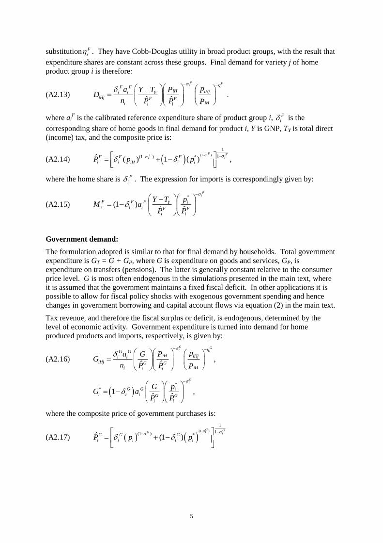
5

substitution F

i . They have Cobb-Douglas utility in broad product groups, with the result that

expenditure shares are constant across these groups. Final demand for variety j of home

product group i is therefore:

(A2.13) ˆ ˆ

F Fi iF F

iH iHji i YiHj F F

iHi i i

pa Y T PD

n P P P

.

where aiF is the calibrated reference expenditure share of product group i, F

i is the

corresponding share of home goods in final demand for product i, Y is GNP, TY is total direct

(income) tax, and the composite price is:

(A2.14) (1 )

1

1(1 ) *ˆ ( ) 1 ( )F FF i

iiF F F

i i iH i iP p p

,

where the home share is F

i . The expression for imports is correspondingly given by:

(A2.15) *

(1 )ˆ ˆ

Fi

F F F iYi i i F F

i i

pY TM a

P P

Government demand:

The formulation adopted is similar to that for final demand by households. Total government

expenditure is GT = G + GP, where G is expenditure on goods and services, GP, is

expenditure on transfers (pensions). The latter is generally constant relative to the consumer

price level. G is most often endogenous in the simulations presented in the main text, where

it is assumed that the government maintains a fixed fiscal deficit. In other applications it is

possible to allow for fiscal policy shocks with exogenous government spending and hence

changes in government borrowing and capital account flows via equation (2) in the main text.

Tax revenue, and therefore the fiscal surplus or deficit, is endogenous, determined by the

level of economic activity. Government expenditure is turned into demand for home

produced products and imports, respectively, is given by:

(A2.16) ˆ ˆ

G Gi iG G

iH iHji iiHj G G

iHi i i

pa G PG

n P P P

,

*

* 1ˆ ˆ

Gi

G G ii i i G G

i i

pGG a

P P

,

where the composite price of government purchases is:

(A2.17) (1 )

1

1(1 ) *ˆ (1 )

G GiG i

iG G G

i i i i iP p p

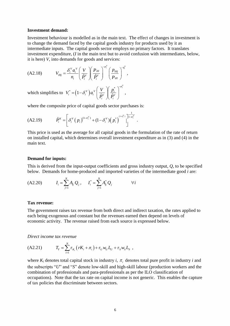
6

Investment demand:

Investment behaviour is modelled as in the main text. The effect of changes in investment is

to change the demand faced by the capital goods industry for products used by it as

intermediate inputs. The capital goods sector employs no primary factors. It translates

investment expenditure, (I in the main text but to avoid confusion with intermediates, below,

it is here) V, into demands for goods and services:

(A2.18) ˆ ˆ

V Vi iV V

iH iHji iiHj V V

iHi i i

pa V PV

n P P P

,

which simplifies to *

* 1ˆ ˆ

Vi

V V ii i i V V

i i

pVV a

P P

,

where the composite price of capital goods sector purchases is:

(A2.19) (1 )

1

1(1 ) *ˆ (1 )

V ViV i

iK V V

i i i i iP p p

.

This price is used as the average for all capital goods in the formulation of the rate of return

on installed capital, which determines overall investment expenditure as in (3) and (4) in the

main text.

Demand for inputs:

This is derived from the input-output coefficients and gross industry output, Q, to be specified

below. Demands for home-produced and imported varieties of the intermediate good i are:

(A2.20) * *

1 1

,N N

i ij j i ij j

j j

I A Q I A Q i

Tax revenue:

The government raises tax revenue from both direct and indirect taxation, the rates applied to

each being exogenous and constant but the revenues earned then depend on levels of

economic activity. The revenue raised from each source is expressed below.

Direct income tax revenue

(A2.21) 1

i

N

Y K i i U U U S S S

i

T rK w L w L

,

where Ki denotes total capital stock in industry i, i denotes total pure profit in industry i and

the subscripts “U” and “S” denote low-skill and high-skill labour (production workers and the

combination of professionals and para-professionals as per the ILO classification of

occupations). Note that the tax rate on capital income is not generic. This enables the capture

of tax policies that discriminate between sectors.

7

Consumption tax revenue

(A2.22) *

1 1

N NC C

C i i i i i i

i i

T p D p M

Import tariff revenue

(A2.23) *

1

( )wN

M iM i i i

i

pT M I

e

Export tax revenue

(A2.24) 1

( )N

X

X i i i

i

T s p X

,

where X

is denotes the net power of the export subsidy rate.

Total tax revenue is then simply a sum of the individual components above.

Pure or economic profits or losses:

These are calculated as revenue derived from mark-ups over unit variable costs, less total

fixed costs. For sector i:

(A2.25) ( ) ( )K S L

i i i i i i S i U ip v Q n r f w f w f i ,

where ni is the number of firms, fiK is the fixed capital requirement per firm, fi

L is the fixed

low-skill labour requirement and fiS is the fixed high-skill labour requirement per firm in

sector i. Net profit in industry i is therefore:

(A2.26) ( ) ( ) 1N K S L K

i i i i i i S i U i ip v Q n r f w f w f i

National income (GNP):

This is the sum of payments to domestically owned factors of production with the home share

of any net profits or losses made, the net income from indirect taxation and the net inflow

from abroad, B, which represents the net income component of the current account and

unrequited transfers.

(A2.27) *

1 1 1

1K N N

D DD k k i Y K T D i

k i iT T

K KBY rK w L T T r K K

K e K

,

where TY is revenue from direct (income) tax. GDP, on the other hand, is a measure of the

income from production in the domestic economy, so it excludes factor payments and other

flows to and from abroad:

(A2.28) 1 1

K N

T k k i Y

k i

GDP rK w L T T

8

Total factor demands:

The model has two capital market closures. In one (the “long run closure”) physical capital is

perfectly mobile abroad at the exogenous world interest rate r. In the other (the “short run

closure”), physical capital stocks are fixed in each industry and industry rates of return are

endogenous. Either way, physical capital is fully employed, with total demand having

variable and fixed components:

(A2.29) 1

NK D K

T i i i i

i

K u Q n f

,

where fiK is the total fixed cost outlaid by industry i. Similarly, the demand for skilled labour

also includes a variable and fixed component. It is:

(A2.30) 1

NL D L

S Si i i i

i

L u Q n f

Finally, demand for all other variable factors (unskilled labour and mineral-energy resources)

is:

(A2.31) 1

2,...,N

L

j ji i

i

L u Q j F

In the short run closure, employment of low-skill labour is endogenous, while either the real,

low-skill, consumption (CPI deflated) or production (GDP price deflated) wage is exogenous,

so that low-skill labour can be unemployed.

A.3: Final Demand Elasticity with Price Interaction

Here the final demand elasticity is derived to illustrate the method by which all the elasticity

expressions of Appendix 2 (A2.1 – A2.4) are arrived at. From (A2.13) the demand equation

for domestic variety j of commodity i is:

(A3.1) ˆ ˆ

F Fi iF F

iH iHji i YiHj F F

iHi i i

pa Y T Pd

n P P P

,

where the composite prices are the average price of generic product i available on the home

market from both home production and imports:

(A3.2) (1 )

1

1(1 ) *ˆ ( ) 1 ( )F FF i

iiF F F

i i iH i iP p p

,

and the average price of home varieties of product i:2

(A3.3)

1

1(1 )

1

1ˆ ( )

Fi

iFi

n

iH iHj

ji

P pn

.

Substitute (A3.2) and (A3.3) into (A3.1) and the full demand equation can be re-written as:

2 In equilibrium, because firms have identical technologies, these prices are equal, though this is not perceived

by firms in setting their prices.

9

(1 )

( )1

1 1(1 ) (1 )*

1

ˆ ˆ

ˆ

1( ) 1 ( ) ( )

F Fi i

F FF Fi ii i

F Fi i

FiF iF Fi

i i

F FiH iHji i Y

iHj F FiHi i i

F FFi i

iHY i iHj

i

nF FF Fi i

Y i iH i i iHj

ji i

pa Y T Pd

n P P P

aY T P P p

n

aY T p p p p

n n

Fi

iHj

Differentiating with respect to iHjp gives:

211 11 *

1

1

1 1 11 1 1 1

1

1

1

Fi

F F FF F F FiF F i i ii i i ii i

nF FiHj F F F F Fi i

Y i iH i i i i iH iHj i iHj iH iHjFjiHj i i i i

F F F F

i i i iY F

ji i i

d aY T p p p p p P P

p n n n

aY T

n n

1111

1 21 2

11

1

F Fi i

FFF F Fi iF Fii i ii i

F FF i ii

FnFi iHjiH iHiiHj iH iH iHj iHj

i iHj iHj iHj

F FF

Fi ii iHY i iHj

i

pp pp p p p P p

n p p p

aY T p P P

n

Fi

Noting that: 1

iHj i

iHh

p j h

p j h

,

and noting further that iHj iHhp p j h , because firms within an industry behave

symmetrically, the expression can be written as:

2( 1) 2( ) 2

12 1 2

11

11

11 1

F F F Fi i i i

FF F F ii i i

F F FF i i ii

F FF

iHj F Fi ii iHY i i iHj

iHj i i

F FF

F Fi iiH iY i i iHj i i

i i

F FF

Fi ii iHY i iHj

i

d aY T P P p

p n n

aY T P p n P

n n

aY T p P P

n

This further simplifies to:

(A3.4)

( 1) ( )

1

1 1

11

11 1

F F F Fi i i i

F F F Fi i i i

F Fi i

FF F

i iHi i iHjF FF

iHj ii ii iHY iHj

iHj i F F FiHi i iHj i i i iHj

i

P P pd na

Y T P P pp n

P p n pn

So that the elasticity of final demand is:

10

1

( 1) ( ) 1 1

1

1 11 1 1

F F F Fi i i i

F F F FF Fi i i ii i

F F F Fi i i i

iHj iHj

iHj iHj

F FFi i

iHY i iHj

i

F F F F F FiH iHi i i iHj i i iHj i i i iHj

i i

iHj

F FF

i ii iHY iHj

i

d p

p d

aY T P P p

n

P P p P p n pn n

p

aY T P P p

n

On the symmetry assumption this simplifies to:

(A3.5) (1 )1

11 1 1

FFii

iHiHjF F F F F F

i i i i i i i iFiHi i

p Pn

n P P

A.4: The Database and the Oligopoly Calibration

This appendix offers discussion of the flow database, or social accounting matrix, for the

model, the calibration of elasticities, fixed cost shares and other industrial organisation

parameters and, finally, the parameters that drive the financial market embedded within it.

A4.1 The flow database

The basic flow database is from the GTAP VII data for 2007. It supplies most of the elements

of the social accounting matrix. It combines detailed bilateral trade, transport and protection

data characterizing economic linkages among regions, together with individual country

national accounts, government accounts, balance of payments data and input-output tables

which enable the quantification of inter-sectoral flows within regions. The first step toward

completing the database is to extract the indirect tax components from trade flows and

consumption payments. This enables the completion of the government revenue row of the

matrix.

The second is to allocate profits after tax, depreciation and “abnormals” between retained

earnings (corporate saving) and dividends. This requires the first call on the Nikkei NEEDS

Database on listed firms. Transfers between government and households, direct tax and

household saving, along with elements of the balance of payments, are then acquired to

enable the completion of rows and columns associated with household and government

incomes and outlays, as well as column entries for saving. Further issues associated with the

flow database are discussed in Section 3 of the main text.

A4.2 The industrial organisation parameters

Turning to the industrial organisation components of the database, no complete set of data on

the structure and conduct of Japan’s agricultural, manufacturing and mining sectors is

publicly available let alone of its service industries. Some relevant data is available

piecemeal, for individual sectors or industries, though this is occasionally at too fine a level of

aggregation for an illustrative economy-wide study such as this. It has therefore been

necessary to extrapolate patterns to some sectors and to make crude assumptions about others.

11

To clarify the assumptions made, this appendix offers an expansion of the summary given in

Section 3 of the text.

First, estimates of pure (over-market) profits are required as shares of revenue in each

industry. This is needed to finalise the flow database but also to calibrate industry

competitive structure. For these data on the profitability of listed public firms from the Nikkei

NEEDS Database. For this comparative static analysis, depreciation and “abnormals” are

considered firm costs and so deducted from gross profits at the outset. After-tax accounting

profit rates imply rates of return that are compared with borrowing rates on corporate debt (as

implied by the corresponding data on debt and debt service) to obtain measures of pure

profits.3

Second, rough estimates of strategically interacting firm numbers in each industry and their

corresponding conjectural variations parameters are required. It is not sufficient simply to

record the number of establishments in each industry, however. Unless industries are

subdivided finely, considerable diversity of firm size and product is embodied in each.

Indeed, within a particular industry classification, many firms supply intermediate inputs to

other firms in the same classification. Prices of the products that emerge from a particular

industry are very likely determined by a small proportion of the firms within it. For estimates

of “strategically interacting” firm numbers in each industry and their corresponding

conjectural variations parameters, the Nikkei NEEDS Database is again used to examine

industry structure in each sector, focussing on the numbers of firms supplying more than 60

per cent of industry capital (market capitalisation plus net debt). The results of this analysis

are displayed in Table A4.1. In the end the values for the “effective” number of firms and the

conjectural variations parameter in each sector are judgemental, taking into account the

numbers of missing private firms and farms and the extent of regulatory surveillance limiting

the full exploitation of oligopoly power.

Third, to complete the formulation of industry demand elasticities, elasticities of substitution

between home product varieties and between generic home and foreign products are required

for each sector. These are drawn from the estimation literature.4 Initial industry demand

elasticities are then calculated for each source of demand (final, investment, intermediate,

government and export), via the equations in Appendices 2 and 3. Initial shares of the

demand facing each industry are then drawn from the database and shown in Table A4.2.

These enable the calculation of weighted average demand elasticities for each industry.

Mark-up ratios are then deduced from these, fixing average variable cost in each sector, via

equation (9). The initial equilibrium average elasticities and mark-up ratios for each sector

are given in Table 4 of the main text. Note that the elasticities appear large in magnitude at

first glance. This is because they do not represent the slopes of industry demand curves for

generic goods. Rather, they are the elasticities faced by suppliers of individual varieties and

are made larger by inter-varietal substitution.

This completes the demand side calibration. It enables us to turn to the calibration of the

supply side, where we begin by using the mark-up ratios to deduce the initial level of average

variable cost in each sector. The proportion pure profits make up of total turnover is deducted

from the mark-up to arrive at fixed cost shares of total turnover.5 Total recurrent fixed cost in

3 This set of approximations is obviously precarious. It considers only listed firms, thus ignoring most of the

farming community in agriculture and the small and family businesses in the services sector, not to mention

large private firms in all sectors and government-owned service firms. 4 Summaries of this literature are offered by Dimaranan and McDougall (2002) and at http://www.gtap.

purdue.edu/databases/.. 5 Fixed costs take the form of both physical and human capital costs using the rule of thumb (based on estimates

by Harris and Cox, 1983) that physical capital has a fixed cost share of 5/6.

12

each sector then follows. The results of this calibration are summarised in the first three

columns of Table 5 in the main text. It is now possible to obtain a sense of the scale of

production.6 Under our assumption of Cobb-Douglas technology in variable factor use,

combined with recurrent fixed costs, if industries could expand indefinitely without changing

unit factor rewards (the partial equilibrium assumption that is relaxed here), average fixed

cost would approach average variable cost asymptotically from above. Following Harris and

Cox (1983) we choose an arbitrary minimum efficient scale (MES) product volume at the

point where average fixed cost would decline to a twentieth of average variable cost. The

implied scale parameters are displayed in the final column of Table 5 in the main text. They

confirm expectations that fixed costs are most prominent in electricity, gas, water,

telecommunications and transport services, due to fixed physical infrastructure and network

maintenance costs. The results also suggest, plausibly, that the sectors closest to their

minimum efficient scale are agriculture, mining, finance and “other services”.

A3.3 The financial parameters

This appendix concerns the parameters associated with Sections 4.2 and 4.3 of the main text.

These describe the determinants of investment, in new home physical capital, the inflow of

financial investment, the outflow of financial investment and the long run growth of domestic

claims over home physical capital. The behaviour is driven by five simple elasticities, values

for which are given in Table A4.3.

A.4 Sectoral Detail from Simulation Results

The quantity of information revealed by model simulations is vast and all cannot be

represented here. Rather than attempt this we offer tabulations of changes in gross output by

industry, corresponding with all the policy simulations undertaken. In interpreting these it is

important to note that the changes in gross output have many determinants. Central are each

industry’s factor proportions (Table 3), which drive separate responses when factor prices

change. Industries supplying tradables are very responsive to changes in the real exchange

rate, which tends to appreciate with investment surges in the short run and to depreciate with

lower capital costs in the long run. Also important are initial levels of pure profits, fixed costs

and conjectural variations parameters. Industries that are highly concentrated and

comparatively collusive clearly face greater change with the onset of competition reforms. It

is notable, however, that such industries can expand in these circumstances, since reduced

costs and prices induce growth in demand. In the short run labour supply can accommodate

expansions and, in the long run, such expansions are accommodated by capital growth.

6 The actual calibration process is more complex than this because the elasticities of intermediate demand

depend on intermediate cost shares, which depend on the variable cost share. It is therefore necessary to

calibrate iteratively for consistency of elasticities and shares.

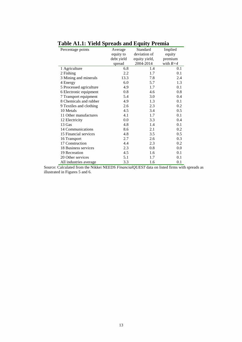
13

Table A1.1: Yield Spreads and Equity Premia

Percentage points Average

equity to

debt yield

spread

Standard

deviation of

equity yield,

2004-2014

Implied

equity

premium

with R=4

1 Agriculture 6.8 1.4 0.1

2 Fishing 2.2 1.7 0.1

3 Mining and minerals 13.3 7.8 2.4

4 Energy 6.0 5.7 1.3

5 Processed agriculture 4.9 1.7 0.1

6 Electronic equipment 0.8 4.6 0.8

7 Transport equipment 5.4 3.0 0.4

8 Chemicals and rubber 4.9 1.3 0.1

9 Textiles and clothing 2.6 2.3 0.2

10 Metals 4.5 3.4 0.5

11 Other manufactures 4.1 1.7 0.1

12 Electricity 0.0 3.3 0.4

13 Gas 4.8 1.4 0.1

14 Communications 8.6 2.1 0.2

15 Financial services 4.8 3.5 0.5

16 Transport 2.7 2.6 0.3

17 Construction 4.4 2.3 0.2

18 Business services 2.3 0.8 0.0

19 Recreation 4.5 1.6 0.1

20 Other services 5.1 1.7 0.1

All industries average 3.3 1.6 0.1

Source: Calculated from the Nikkei NEEDS FinancialQUEST data on listed firms with spreads as

illustrated in Figures 5 and 6.

14

Table A4.1: Effective Firms and Conjectural Variations Listed firms

with 60%

industry

revenue

Listed firms

with 80%

industry

revenue

Effective

firm

numbera

Conjectural

Variations:

0-1b

1 Agriculture na na 50 0.4

2 Fishing 3 3 3 0.3

3 Mining and minerals 2 6 4 0.6

4 Energy 3 4 4 0.5

5 Processed agriculture 9 22 15 0.2

6 Electronic equipment 4 6 5 0.2

7 Transport equipment 4 11 7 0.4

8 Chemicals and rubber 20 45 32 0.1

9 Textiles and clothing 4 10 7 0.2

10 Metals 9 24 15 0.3

11 Other manufactures 43 105 74 0.1

12 Electricity 3 6 5 0.8

13 Gas 2 3 3 0.7

14 Communications 2 4 4 0.7

15 Financial services 7 21 14 0.5

16 Transport 12 24 18 0.4

17 Construction 18 41 29 0.3

18 Business services 5 13 9 0.5

19 Recreation 36 90 63 0.2

20 Other services 11 53 33 0.1

a This index represents the “effective” number of strategically interacting firms in each sector. Firm numbers

exceeding 100 have negligible effect on pricing. It is borne in mind that large numbers of farms and private

firms are omitted from the data on listed firms.

b The conjectural variations parameter ranges between zero (non-collusive oligopoly) and unity (cartel). The

numbers chosen reflect industry concentration and the extent of existing regulatory surveillance.

Sources: Nikkei NEEDS Database of listed Japanese firms.

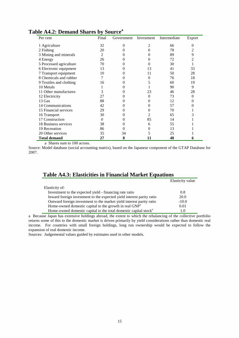
15

Table A4.2: Demand Shares by Sourcea

Per cent Final Government Investment Intermediate Export

1 Agriculture 32 0 2 66 0

2 Fishing 20 0 0 78 2

3 Mining and minerals 2 0 0 89 9

4 Energy 26 0 0 72 2

5 Processed agriculture 70 0 0 30 1

6 Electronic equipment 13 0 13 41 33

7 Transport equipment 10 0 11 50 28

8 Chemicals and rubber 7 0 0 76 18

9 Textiles and clothing 16 0 5 60 19

10 Metals 1 0 1 90 9

11 Other manufactures 3 0 23 46 28

12 Electricity 27 0 0 73 0

13 Gas 88 0 0 12 0

14 Communications 42 0 0 57 0

15 Financial services 29 0 0 70 1

16 Transport 30 0 2 65 3

17 Construction 0 0 85 14 1

18 Business services 38 0 6 55 1

19 Recreation 86 0 0 13 1

20 Other services 35 34 5 25 1

Total demand 27 8 11 48 6

a Shares sum to 100 across.

Source: Model database (social accounting matrix), based on the Japanese component of the GTAP Database for

2007.

Table A4.3: Elasticities in Financial Market Equations Elasticity value

Elasticity of:

Investment to the expected yield - financing rate ratio 0.8

Inward foreign investment to the expected yield interest parity ratio 20.0

Outward foreign investment to the market yield interest parity ratio -10.0

Home-owned domestic capital to the growth in real GNPa 0.01

Home-owned domestic capital to the total domestic capital stocka 1.0

a Because Japan has extensive holdings abroad, the extent to which the rebalancing of the collective portfolio

returns some of this to the domestic market is driven primarily by yield considerations rather than domestic real

income. For countries with small foreign holdings, long run ownership would be expected to follow the

expansion of real domestic income.

Sources: Judgemental values guided by estimates used in other models.

16

Table A5.1: Industry Output Effects of Labour Market and Tax Reforms a

Per cent change

Oligopolyb Free entry/exit

b

Short runc Long run

c Long run

c

Low and high skill labour up 5%

1 Agriculture 1.4 3.9 3.3

2 Fishing 1.0 2.4 2.7

3 Mining and minerals 2.0 11.2 7.0

4 Energy 2.1 4.1 3.7

5 Processed agriculture 1.7 4.0 3.7

6 Electronic equipment 1.3 7.9 5.3

7 Transport equipment 0.9 13.7 8.6

8 Chemicals and rubber 1.2 7.1 4.9

9 Textiles and clothing 1.9 6.3 4.2

10 Metals 2.2 8.8 5.4

11 Other manufactures 2.1 7.3 4.1

12 Electricity 1.8 5.6 4.7

13 Gas 1.8 3.5 4.2

14 Communications 2.2 4.4 4.8

15 Financial services 2.0 4.9 4.3

16 Transport 2.4 4.7 4.0

17 Construction 7.1 3.3 1.4

18 Business services 2.1 4.4 4.4

19 Recreation 1.8 3.6 3.4

20 Other services 3.7 6.6 4.8

Power of company tax down 5%

1 Agriculture -2.9 -1.5 -2.9

2 Fishing -2.6 -1.8 -2.0

3 Mining and minerals 4.1 17.4 13.0

4 Energy -2.5 -0.7 -1.8

5 Processed agriculture -3.9 -2.3 -3.5

6 Electronic equipment 1.2 6.9 2.4

7 Transport equipment 2.1 12.7 3.7

8 Chemicals and rubber 0.5 6.1 2.5

9 Textiles and clothing -0.3 2.2 -1.3

10 Metals 3.2 9.1 3.6

11 Other manufactures 2.0 6.5 1.5

12 Electricity -1.5 2.0 0.4

13 Gas -4.3 -2.8 -3.7

14 Communications -3.0 -1.4 -1.3

15 Financial services -2.0 0.2 -1.0

16 Transport -1.9 -0.2 -1.8

17 Construction 6.6 1.6 -1.0

18 Business services -2.4 -0.7 -1.0

19 Recreation -4.0 -2.8 -3.9

20 Other services -1.5 -0.4 -2.0

a The first experiment simply raises the stock of low-skill labour and the stock of high-skill labour by 5%. In

the short run all the additional low-skill labour is not necessarily employed since the real (GDP price deflated)

low-skill wage is held constant. The second experiment reduces the power of company tax by 5% but holds both

pensions and government expenditure on goods and services constant, raising the power of the consumption tax

to compensate for lost revenue from capital taxation.

b “Oligopoly” refers to fixed numbers of firms with unfettered oligopoly pricing. “Free entry/exit” allows firm

numbers to adjust while retaining pure (economic) profits at their initial levels (defined relative to foreign

prices).

c The long run allows free international mobility of capital at an external after tax rate of return along with full

real wage adjustment to clear labour markets. The short run fixes the capital stock in each industry and the real

(GDP price deflated) wage of low-skill workers.

Source: Simulations of the model described in the text.

17

Table A5.2: Industry Output Effects of Corporate Governance and Pricing

Surveillance Reforms a

Per cent change

Oligopolyb Free entry/exit

b

Short runc Long run

c Long run

c

Power of capital taxes reduced by

5%, combined a corporate saving

rate lower by 50%

1 Agriculture 4.6 8.0 6.2

2 Fishing 4.9 8.6 8.9

3 Mining and minerals -13.1 -7.8 -11.2

4 Energy 6.4 7.4 5.9

5 Processed agriculture 7.5 11.7 10.1

6 Electronic equipment -15.9 -2.4 -6.8

7 Transport equipment -28.8 -6.4 -14.3

8 Chemicals and rubber -9.8 0.9 -1.7

9 Textiles and clothing -5.6 0.6 -2.7

10 Metals -15.2 -6.8 -11.3

11 Other manufactures -12.4 -4.8 -8.5

12 Electricity 1.3 6.9 5.4

13 Gas 10.1 12.9 14.0

14 Communications 6.2 10.3 11.5

15 Financial services 3.6 8.9 7.5

16 Transport 3.7 6.6 4.6

17 Construction 2.7 -13.2 -16.1

18 Business services 5.2 9.4 8.8

19 Recreation 8.7 13.4 11.2

20 Other services 2.3 4.4 2.5

Reduced collusion: conjectural

variations parameters reduced by

20%.

1 Agriculture 2.7 1.4 1.5

2 Fishing 1.8 1.5 1.4

3 Mining and minerals 1.5 6.0 5.4

4 Energy 4.5 3.9 3.5

5 Processed agriculture 2.0 1.5 1.4

6 Electronic equipment 0.0 3.1 3.4

7 Transport equipment -0.8 5.8 7.2

8 Chemicals and rubber 0.6 3.0 3.1

9 Textiles and clothing 2.9 2.0 2.3

10 Metals 0.8 2.4 3.1

11 Other manufactures 0.4 1.2 1.8

12 Electricity 3.2 4.2 3.9

13 Gas 6.4 6.4 4.9

14 Communications 5.1 5.3 4.3

15 Financial services 4.3 5.3 4.4

16 Transport 5.8 5.7 5.2

17 Construction 6.7 -1.1 -0.3

18 Business services 5.0 5.5 4.1

19 Recreation 2.1 1.9 1.7

20 Other services 3.0 1.7 1.9

a This experiment reduces the power of company taxes by 5% but maintains government spending by replacing

the lost revenue via the consumption tax, the increase in the power of which is here endogenous. This change,

combined with corporate governance reforms, is assumed to induce a reduction by half in the rate of corporate

saving from after tax capital income. The second experiment reduces the conjectural variations parameter (the

index of collusion between oligopoly firms) by 20% to reflect tighter surveillance as part of competition policy.

In the short run the real (GDP price deflated), low-skill wage is held constant.

18

b “Oligopoly” refers to fixed numbers of firms with unfettered oligopoly pricing. “Free entry/exit” allows firm

numbers to adjust while retaining pure (economic) profits at their initial levels (defined relative to foreign

prices).

c The long run allows free international mobility of capital at an external after tax rate of return along with full

real wage adjustment to clear labour markets. The short run fixes the capital stock in each industry and the real

(GDP price deflated) wage of low-skill workers.

Source: Simulations of the model described in the text.

19

Table A5.3: Industry Output Effects of Tighter Price Cap Regulation and

Services Productivity Gainsa

Per cent change

Oligopolyb Free entry/exit

b

Short runc Long run

c Long run

c

Closure of price-to-average cost gap

20%

1 Agriculture 11.4 8.3 7.8

2 Fishing 7.9 7.6 7.1

3 Mining and minerals 13.2 34.0 38.4

4 Energy 14.7 12.2 13.6

5 Processed agriculture 9.8 8.7 8.7

6 Electronic equipment -10.4 3.9 8.1

7 Transport equipment -21.9 10.6 19.0

8 Chemicals and rubber 4.0 18.4 22.2

9 Textiles and clothing 2.8 2.0 5.1

10 Metals 8.1 20.3 26.5

11 Other manufactures 1.1 5.7 10.8

12 Electricity 11.6 16.5 18.8

13 Gas 12.4 11.0 10.6

14 Communications 14.6 14.8 14.7

15 Financial services 9.0 10.9 12.0

16 Transport 10.0 8.4 9.9

17 Construction 32.7 -3.0 -0.5

18 Business services 11.9 12.2 12.3

19 Recreation 7.5 7.2 7.6

20 Other services 10.7 6.0 8.8

Closure of the price-to-average cost

gap by 20% combined with a services

productivity boost of 2% (short run)

and 5% (long run)

1 Agriculture 11.3 11.3 11.1

2 Fishing 8.2 10.6 10.2

3 Mining and minerals 21.3 77.1 83.6

4 Energy 22.5 20.1 20.7

5 Processed agriculture 10.5 13.3 13.3

6 Electronic equipment -24.8 14.4 16.2

7 Transport equipment -39.1 22.8 25.2

8 Chemicals and rubber -6.1 32.3 33.1

9 Textiles and clothing -2.4 5.9 7.3

10 Metals 4.1 34.7 36.4

11 Other manufactures -5.3 10.5 13.2

12 Electricity 16.6 35.3 36.7

13 Gas 20.3 27.0 27.5

14 Communications 20.8 30.2 30.6

15 Financial services 10.8 17.7 18.4

16 Transport 16.6 23.2 24.0

17 Construction 69.2 3.2 4.3

18 Business services 17.4 25.3 25.9

19 Recreation 11.1 16.7 17.1

20 Other services 18.7 19.1 20.2

a The first experiment imposes mark-ups that reduce the initial price-to-average cost gap by 20%.. The second

experiment imposes mark-ups that reduce the initial price-to-average cost gap by 20% while at the same time

boosting output productivity by 2% in the short run and 5% in the long run. In the short run the real (GDP price

deflated), low-skill wage is held constant.

b “Oligopoly” refers to fixed numbers of firms with unfettered oligopoly pricing. “Free entry/exit” allows firm

numbers to adjust while retaining pure (economic) profits at their initial levels (defined relative to foreign

prices).

20

c The long run allows free international mobility of capital at an external after tax rate of return along with full

real wage adjustment to clear labour markets. The short run fixes the capital stock in each industry and the real

(GDP price deflated) wage of low-skill workers.

Source: Simulations of the model described in the text.