crash: a block-adaptive-mesh code for radiative shock - deep blue

The Astrophysical Journal Supplement Series, 194:23 (20pp), 2011 June doi:10.1088/0067-0049/194/2/23C© 2011. The American Astronomical Society. All rights reserved. Printed in the U.S.A.

CRASH: A BLOCK-ADAPTIVE-MESH CODE FOR RADIATIVE SHOCKHYDRODYNAMICS—IMPLEMENTATION AND VERIFICATION

B. van der Holst1, G. Toth

1, I. V. Sokolov

1, K. G. Powell

2, J. P. Holloway

3, E. S. Myra

1, Q. Stout

4, M. L. Adams

5,

J. E. Morel5, S. Karni

6, B. Fryxell

1, and R. P. Drake

11 Department of Atmospheric, Oceanic and Space Sciences, University of Michigan, Ann Arbor, MI 48109, USA

2 Department of Aerospace Engineering, University of Michigan, Ann Arbor, MI 48109, USA3 Nuclear Engineering and Radiological Sciences, University of Michigan, Ann Arbor, MI 48109, USA

4 Computer Science and Engineering, University of Michigan, Ann Arbor, MI 48109, USA5 Department of Nuclear Engineering, Texas A&M University, College Station, TX 77843, USA

6 Department of Mathematics, University of Michigan, Ann Arbor, MI 48109, USAReceived 2011 January 26; accepted 2011 March 17; published 2011 May 2

ABSTRACT

We describe the Center for Radiative Shock Hydrodynamics (CRASH) code, a block-adaptive-mesh code formulti-material radiation hydrodynamics. The implementation solves the radiation diffusion model with a gray ormulti-group method and uses a flux-limited diffusion approximation to recover the free-streaming limit. Electronsand ions are allowed to have different temperatures and we include flux-limited electron heat conduction. Theradiation hydrodynamic equations are solved in the Eulerian frame by means of a conservative finite-volumediscretization in either one-, two-, or three-dimensional slab geometry or in two-dimensional cylindrical symmetry.An operator-split method is used to solve these equations in three substeps: (1) an explicit step of a shock-capturinghydrodynamic solver; (2) a linear advection of the radiation in frequency-logarithm space; and (3) an implicitsolution of the stiff radiation diffusion, heat conduction, and energy exchange. We present a suite of verificationtest problems to demonstrate the accuracy and performance of the algorithms. The applications are for astrophysicsand laboratory astrophysics. The CRASH code is an extension of the Block-Adaptive Tree Solarwind Roe UpwindScheme (BATS-R-US) code with a new radiation transfer and heat conduction library and equation-of-state andmulti-group opacity solvers. Both CRASH and BATS-R-US are part of the publicly available Space WeatherModeling Framework.

Key words: hydrodynamics – methods: numerical – radiative transfer

Online-only material: color figures

1. INTRODUCTION

As photons travel through matter, the radiation field experi-ences changes due to net total emission, absorption, and scatter-ing; see, for instance, Mihalas & Mihalas (1984), Pomraming(2005), and Drake (2006). At high enough energy density theradiation heats and accelerates the plasma. At a fundamentallevel, the radiation can be described by the time evolution ofthe spectral radiation intensity Iν(r, t, n, ν), which is the radi-ation energy per unit area, per unit solid angle in the directionof photon propagation n, per unit interval of photon frequencyν, per unit time interval. Several methods have been devel-oped to solve the radiation field in various degrees of physicsfidelity.

In Monte Carlo radiative transfer methods, the radiation isstatistically evaluated. Small photon packets are created withtheir energy and propagation direction statistically selected.The packets are propagated through matter using the radiationtransfer equation (Nayakshin et al. 2009; Maselli et al. 2009;Baek et al. 2009). Characteristic methods use integration alongrays of various lengths to solve for the angular structure of theradiation transport. A recent conservative, causal ray-tracingmethod was developed and combined with a short characteris-tic ray-tracing for the transfer calculations of ionizing radiation(Mellema et al. 2006). Solar surface magneto-convection sim-ulations are increasingly realistic and use a three-dimensional(3D), non-gray, approximate local thermodynamic equilibrium(LTE), radiative transfer for the heating and cooling of plasma.These simulations are typically formulated for four frequency

bins in the radiative transport equation (Vogler et al. 2005; Steinet al. 2007; Martınez-Sykora et al. 2009).

For some applications, simplifications to the radiation transfercan be made by calculating moments of the radiation intensityover the solid angle Ω. The spectral radiation energy and thespectral radiation energy flux are defined by the 0th and 1stmoments as

Eν(r, t, ν) = 1

c

∫4π

Iν(r, t, n, ν)dΩ,

Fν(r, t, ν) =∫

4π

nIν(r, t, n, ν)dΩ. (1)

In addition, the spectral radiation pressure tensor Pν is definedby the second moment

Pν(r, t, ν) = 1

c

∫4π

nnIν(r, t, n, ν)dΩ. (2)

A whole class of radiation transfer models is based on solvingthe corresponding radiation moment equations using a closurerelation between the spectral pressure tensor and the spectralintensity (Mihalas & Mihalas 1984; Pomraming 2005; Drake2006).

A radiation hydrodynamics code based on variable Eddingtontensor (VET) methods (Stone et al. 1992) can still capture theangular structure of the radiation field by relating the spectralradiation pressure tensor to the spectral radiation intensity andthe method is applicable for both the optically thin and thick

1

http://dx.doi.org/10.1088/0067-0049/194/2/23

The Astrophysical Journal Supplement Series, 194:23 (20pp), 2011 June van der Holst et al.

regime. Optically thin versions of the VET method have beenused in the context of cosmological reionization (Petkova &Springel 2009; Gneden et al. 2009). A more complete listof radiation hydrodynamic codes for the transfer of ionizingradiation in the context of astrophysical phenomena can befound in the radiative transfer comparison project (Iliev et al.2009).

Further simplification assumes that the radiation pressure isisotropic and proportional to the radiation energy. This is thediffusion approximation. Several codes have been developedusing this approximation. HYDRA (Marinak 2001) is an ar-bitrary Lagrange Eulerian code for two-dimensional (2D) and3D radiation hydrodynamics. The radiation transfer model isbased upon either flux-limited multi-group or implicit MonteCarlo radiation transport. The Eulerian code RAGE (Gittingset al. 2008) uses a cell-based adaptive mesh refinement (AMR)to achieve resolved radiative hydrodynamic flows. HYADES(Larsen & Lane 1994) solves the radiation hydrodynamic equa-tions on a Lagrangian mesh, while CALE (Barton 1985) can useeither a fixed Eulerian mesh, an embedded Lagrangian mesh,or a partially embedded, partially remapped mesh. Our newlydeveloped radiation hydrodynamic solver uses an Eulerian gridtogether with a block-based AMR strategy.

We limit the discussion of the radiation hydrodynamicsimplementation in CRASH (Center for Radiative Shock Hy-drodynamics) to plasmas in the absence of magnetic fields.Most of the description in this paper can, however, eas-ily be extended to magnetohydrodynamic (MHD) plasmasas well. Indeed, since the CRASH code is essentially theMHD Block-Adaptive Tree Solarwind Roe Upwind Scheme(BATS-R-US) code (Powell et al. 1999; Toth et al. 2011), ex-tended with libraries containing radiation transport, equation-of-state (EOS), and opacity solvers, the implementation for thecoupling between the radiation field and MHD plasmas is readilyavailable. The CRASH code uses the recently developed Block-Adaptive Tree Library (BATL; Toth et al. 2011). Here we willfocus on the radiation implementation. Both the CRASH andBATS-R-US codes are publicly available as part of the SpaceWeather Modeling Framework (SWMF; Toth et al. 2005) or canbe used as stand-alone codes.

In the following, Section 2 introduces the radiation hydrody-namic equations for multi-material plasmas, in a form generalenough to apply at high energy density. Section 3 describesthe numerical algorithms to solve these equations. Section 4presents verification tests for radiation and electron heat con-duction on non-uniform meshes in one-dimensional (1D), 2D,and 3D slab geometry and in axially symmetric (rz) geometry.We also show a full system multi-material radiation hydrody-namic simulation on an adaptively refined mesh and demonstrategood scaling up to 1000 processors. The paper is summarizedin Section 5.

2. EQUATIONS OF RADIATION HYDRODYNAMICS INDENSE PLASMAS

The equations of radiation hydrodynamics describe the timeevolution of both matter and radiation. For the applications thatsupported the work reported here, the code must be able tomodel matter as a high energy density plasma that is in LTE sothat the population of all atomic and ion states can be obtainedfrom statistical physics (see for instance Landau & Lifshitz1980). We allow for multiple materials throughout the spatialdomain of interest, but restrict the analysis to plasma flowsthat are far from relativistic. The materials can be heated to

sufficiently high temperatures so that they can ionize and createfree electrons, introducing the need for a time evolution equationfor the electron energy density. The electrons transfer heat bythermal heat conduction and emit and absorb photon radiation.The radiation model discussed in this paper is non-equilibriumdiffusion, in which the electron and radiation temperature can bedifferent. We approximate the radiation transfer with a gray ormulti-group flux-limited diffusion (FLD). This model is also ofinterest for application to a number of astrophysical problems.

In the following subsections, we will describe the radiativetransfer equations for the evolution of the multi-group radia-tion energy densities (Section 2.1) in the FLD approximation(Section 2.5). The coupling of the radiation field to the twospecies hydrodynamic equations of electrons and ions are dis-cussed in Section 2.2. In Section 2.3, the method for trackingthe different materials is treated, while the lookup tables usedfor of the EOS and opacities are mentioned in Section 2.4.

2.1. Radiation Transport

In this section, we will build up the form of the radiationtransport in the multi-group diffusion approximation that isused for the implementation in the CRASH code. The spectralpressure tensor, Equation (2), is often approximated in the form(Mihalas & Mihalas 1984)

Pν(r, t, ν) = EνTν, (3)

where

Tν(r, t, ν) = 1

2(1 − χν)I +

1

2(3χν − 1)

FνFν

|Fν |2 , (4)

is the spectral Eddington tensor, χν is the Eddington factor, andI is the identity matrix. The second term on the right-hand sideis a dyad constructed from the direction of the spectral radiationflux. The pressure tensor can be used to arrive at a time evolutionequation for the solid angle integrated spectral radiation energy(Buchler 1983)

∂Eν

∂t+ ∇ · (Eνu) − ν

∂

∂ν(Pν : ∇u) = diffusion + emission

− absorption, (5)

which contains the velocity u of the background plasma. Herethe colon denotes the contraction of the two tensors Pν and ∇u.The processes described by the symbolic terms on the right-handside of Equation (5) will be described below.

Setting the Eddington factor χν = 1/3 corresponds to theradiation diffusion model. In this case the radiation is assumedto be effectively isotropic and the spectral radiation pressure canbe described by the scalar

pν = 1

3Eν = (γr − 1)Eν, (6)

where we have introduced the adiabatic index of the radiationfield, which in this case has the relativistic value γr = 4/3.The time evolution for the spectral energy density can then besimplified to

∂Eν

∂t+ ∇ · (Eνu) − (γr − 1)(∇ · u)ν

∂Eν

∂ν= diffusion + emission − absorption. (7)

2


The second and third terms on the left-hand side of Equation (7)express the change in the spectral energy density due to theadvection and compression of the background plasma, whichmoves with the velocity u, as well as the frequency shift dueto compression. In the free-streaming limit where the radiationhardly interacts with the matter, χν approaches 1. In this paper,we will keep χν = 1/3 and at the same time use an FLD for thefree-streaming regime whenever needed (see Section 2.5).

The set of equations for the spectral energy density (7)still consists of an infinite number of equations, one for eachfrequency. A finite set of governing equations to describe theradiation transport in the multi-group diffusion approximationis obtained when we choose a set of frequency groups. Here weenumerate groups with the index, g = 1, . . . , G. The intervalof the photon frequencies, relating to the gth group is denotedas [νg−1/2, νg+1/2]. A discrete set of group energy densities, Eg,is introduced in terms of the integrals of the spectral energydensity of the frequency group interval:

Eg =∫ νg+1/2

νg−1/2

Eνdν. (8)

Now we can integrate Equation (7) to arrive at the desired set ofthe multi-group equations:

∂Eg

∂t+ ∇ · (Egu) + (γr − 1)Eg∇ · u − (γr − 1)(∇ · u)

×∫ νg+1/2

νg−1/2

∂(νEν)

∂νdν

=∫ νg+1/2

νg−1/2

(diffusion + emission − absorption) dν. (9)

The fourth term on the left-hand side is a frequency shift due tothe plasma compression. This term is essentially a conservativeadvection along the frequency axis.

In the context of the multi-group radiation diffusion, adiscussion about the stimulated emission is not less importantthan LTE. Excellent accounts on the stimulated emission exist inthe literature, see for instance Zel’dovich & Raizer (2002). Herewe merely summarize how the stimulated emission modifies theabsorption opacity κa

ν obtained from, e.g., opacity tables. This isimportant when dealing with externally supplied opacity tables,since the CRASH code assumes that the absorption opacities arecorrected. Integrating the total absorption and emission over alldirections and summing up the two polarizations of the photons,the following expression can be derived for the emission andabsorption

emission − absorption = cκaν

′(Bν − Eν), (10)

where the effective absorption coefficient, κaν

′, is introduced toaccount for the correction due to stimulated emission:

κaν

′ = κaν

(1 − exp

[− ε

kBTe

]), (11)

in which ε = hν is the photon energy, kB is the Boltzmann con-stant, and Te is the electron temperature. We also introduced thespectral energy density distribution of the blackbody radiation(the Planckian)

Bν = 8π

h3c3

ε3

exp[ε/(kBTe)] − 1. (12)

The total energy density in the Planck spectrum equals B =∫ ∞0 dνBν = aT 4

e , where a = 8π5k4B/(15h3c3) is the radiation

constant.We use the standard definition of the group Planck mean

opacity κPg and group Rosseland mean opacity κRg (Mihalas &Mihalas 1984)

κPg =∫ νg+1/2

νg−1/2dνκa

ν′Bν

Bg

, κRg =∂Bg

∂Te∫ νg+1/2

νg−1/2dν 1

κtν

∂Bν

∂Te

,

Bg =∫ νg+1/2

νg−1/2

dνBν (13)

in which κtν is the spectral total opacity. The right-hand side of

Equation (9) can now be written as (see for instance Mihalas &Mihalas 1984; Pomraming 2005)

∂Eg

∂t+ ∇ · (Egu) + (γr − 1)Eg∇ · u − (γr − 1)∇ · u

×∫ νg+1/2

νg−1/2

∂(νEν)

∂νdν

= ∇ · (Dg∇Eg) + σg(Bg − Eg), (14)

where Dg = c/(3κRg) is the radiation diffusion coefficient forradiation group g in the diffusion limit. The absorption andemission uses the coefficient σg = cκPg . These group meanopacities are either supplied by lookup tables or by an opacitysolver.

In a single group approximation (gray diffusion), the spectralenergy density is integrated over all photon frequencies and thetotal radiation energy density is obtained by

Er (r, t) =∫ ∞

0Eνdν. (15)

This amounts to summing up all groups Er = ∑g Eg . The gray

radiation diffusion equation can be derived as (see for instanceMihalas & Mihalas 1984; Pomraming 2005; Drake 2006)

∂Er

∂t+∇ · (Eru)+ (γr −1)Er∇ ·u = ∇ · (Dr∇Er )+σr (B −Er ),

(16)where the diffusion coefficient Dr in the diffusion limit is nowdefined by the single group Rosseland mean opacity κR asDr = c/(3κR), and the absorption coefficient σr is defined interms of the single group Planck mean opacity κP as σr = cκP .

2.2. Hydrodynamics

In the CRASH code, a single fluid description is used so thatall of the atomic and ionic species as well as the electrons movewith the same bulk velocity u. The conservation of mass

∂ρ

∂t+ ∇ · (ρu) = 0 (17)

provides the time evolution of the mass density ρ of all thematerials in the simulation. The plasma velocity is obtainedfrom the conservation of momentum

∂ρu∂t

+ ∇ · [ρuu + I (p + pr )] = 0. (18)

The total plasma pressure is the sum of the ion and electronpressures: p = pi + pe. The net force of the radiation on the

3


plasma is given by the gradient of the total radiation pressure−∇pr , where the total radiation pressure is obtained from thegroup radiation energies: pr = (γr − 1)

∑Eg .

In a high density plasma, the electrons are very strongly cou-pled to the ions by collisions. However, for higher temperatures,the electrons and ions get increasingly decoupled. At a shockfront, where ions are preferentially heated by the shock wave,the electrons and ions are no longer in temperature equilibrium.Ion energy is transferred to the electrons by collisions, whilethe electrons in turn radiate energy. We therefore solve separateequations for the ion/atomic internal energy density Ei and theelectron internal energy density Ee:

∂Ei

∂t+ ∇ · (Eiu) + pi∇ · u = σie(Te − Ti), (19)

∂Ee

∂t+ ∇ · (Eeu) + pe∇ · u = ∇ · (Ce∇Te) + σie(Ti − Te)

+G∑

g=1

σg(Eg − Bg). (20)

The coupling coefficient σie = nakB/τie in the collisional en-ergy exchange between the electrons and ions depends on theion–electron relaxation time τie(Te, na,m) and the atomic num-ber density na. Energy transfer depends also on the differencebetween ion temperature Ti and electron temperature Te. InEquation (20), we have included electron thermal heat conduc-tion with conductivity Ce(Te, na,m). Since electrons are thespecies that are responsible for radiation emission and absorp-tion, the energy exchange between the electrons and the radia-tion groups is added to Equation (20).

For the development of the numerical schemes in Section 3,we will use an equation for the conservation of the total energydensity

e = ρu2

2+ Ei + Ee +

G∑g=1

Eg, (21)

instead of the equation for ion internal energy (19). This isespecially important in regions of the computational domainwhere hydrodynamic shocks can occur, so that we can recoverthe correct jump conditions. Conservation of total energy canbe derived from Equations (14) and (17)–(20) as

∂e

∂t+∇ · [(e+p+pr )u] = ∇ · (Ce∇Te)+

G∑g=1

∇ · (Dg∇Eg). (22)

The frequency shift term in Equation (14), due to the plasmacompression, does not show up in the conservation of totalenergy if we use energy conserving boundary conditions at theend points of the frequency domain, i.e., at ν = 0 and ν = ∞ inthe analytical description or at the end points of the numericallytruncated finite domain.

2.3. Level Sets and Material Identification

In many CRASH applications, we need a procedure todistinguish between different materials that may be present.We assume that materials do not mix, but differ from eachother by their properties such as the EOS and opacities. If weuse M different materials, then we can define for each materialm = 1, . . . ,M the level set function dm(r, t) (see for instanceKreiss & Olsson 2005; Olsson et al. 2007; Sussman & Pucket

2000) which is initially set to zero at the material interface,positive inside the material region, and negative outside thematerial region. Generally, we use a smooth and signed distancefunction in the initial state. At later times, the location of materialm is obtained by means of a simple advection equation

∂dm

∂t+ ∇ · (dmu) = dm∇ · u. (23)

For any given point in space and time, we can determine what thematerial is since analytically only one of the level set functionsdm can be positive at any given point. Numerical errors willcreate regions where this is not true in solutions to the discretizedform of Equation (23). Whenever this happens, the materialhaving the largest dm is assigned as the material in that region.This is a simple approximation, and we may explore moresophisticated approaches in the future. The number of materiallevels M is configured at compile time.

2.4. Equation of State and Opacities

We have implemented EOS solvers and a code to calcu-late the frequency-averaged group opacities. This implemen-tation will be reported elsewhere, but it is important to notethat in the EOS and opacity solver, the temperature is as-sumed to be well below relativistic values: T � 105 eV. Anon-relativistic speed of motion is also assumed, which sim-plifies the radiation transport equation and allows neglect ofrelativistic corrections for opacities. In this paper, we will as-sume that all necessary quantities are calculated and stored inlookup tables. Our EOS solver assumes that the corrections as-sociated with ionization, excitation, and Coulomb interactionsof partially ionized ion–electron plasma are all added to theenergy of the electron gas and to the electron pressure. This ispossible since these corrections are controlled by the electrontemperature. The ion internal energy density, ion pressure, andion specific heat in an isochoric process per unit of volume aresimply

pi = nakBTi, Ei = pi

γ − 1, CV i =

(∂Ei

∂Ti

)ρ

= nakB

γ − 1,

(24)which are due to the contributions from ion translationalmotions, for which γ = 5/3.

The relations among electron internal energy density, pres-sure, density, and temperature are known as the EOS. To solvethese relations is usually complex and time consuming. Wetherefore store these relations in invertible lookup tables. Foreach material m, our EOS tables have logarithmic lookup argu-ments (log Te, log na). The list of quantities stored in these tablesis indicated in Table 1. These lookup tables are populated withquantities that are needed for both single- and two-temperaturesimulations. For two-temperature plasma simulations, we needpe, Ee, the electron specific heat CVe, and the electron-speed-of-sound gamma γSe

. For convenience, we add the total pres-sure p = pe + pi , total internal energy density E = Ei + Ee,single-temperature specific heat CV , and the single-temperaturespeed-of-sound gamma γS , which can be used in single-temperature simulations. We use high enough table resolutionsso that it is sufficient to use a bilinear interpolation in the lookuparguments. If pe or Ee (or p and E in single temperature mode)are known upon entry to the lookup instead of Te, we do abinary search in the table to find the appropriate electron tem-perature. The latter works only if the necessary thermodynamic

4


Table 1Quantities Stored in the EOS Tables as aFunction of log Te[eV] and log na[m−3]

Quantity Stored Quantity UnitsTotal pressure p p/na eVTotal internal energy density E E/na eVElectron pressure pe pe/na eVElectron internal energy density Ee Ee/na eVSpecific heat CV CV /(nakB )Electron specific heat CVe CV e/(nakB )Speed of sound gamma γS

Electron speed of sound gamma γSe

Inverse of ion–electron interaction time 1/τie s−1

Electron conductivity Ce J m−1 s−1 K−1

Mean ionization Z

Mean square ionization Z2

Table 2Quantities Stored in the Opacity Tables as aFunction of log ρ[kg m−3] and log Te[eV]

Quantity Symbol UnitsSpecific group Rosseland mean opacities κRg/ρ kg−1 m2

Specific group Planck mean opacities κPg/ρ kg−1 m2

derivatives are sign definite, i.e., the table is invertible. Otherthermodynamic quantities that are needed, but not stored inthese lookup tables, can be derived. For example, the electrondensity can be obtained from the mean ionization ne = naZ.

In addition, we have lookup tables for the averaged multi-group opacities. These tables are either constructed internallyfor a given frequency range, number of groups, and selected ma-terials or externally supplied. For any material m, the logarithmiclookup arguments are (log ρ, log Te). The stored quantities (seeTable 2) are the specific Rosseland mean opacity κRg/ρ and spe-cific Planck mean opacity κPg/ρ for all groups g = 1, . . . ,Gused during a simulation. Planck opacities are assumed to becorrected for stimulated emission, as discussed in Section 2.1.The groups are always assumed to be logarithmically distributedin frequency space.

2.5. Flux-limited Diffusion

Radiation diffusion, if uncorrected, can transport energy tooefficiently in the optically thin free-streaming limit. In thediffusion limit, the radiation diffusion flux for each groupfollows Fick’s law Fg = −Dg∇Eg , where the diffusioncoefficient Dg depends on the Rosseland mean opacity κRg

for the group g via Dg = c/(3κRg). However, this flux ispotentially unbounded. In the optically thin free-streaming limit,the magnitude of the radiation flux can be at most cEg inorder to maintain causality. Various flux limiters exist in theliterature (see, for instance, Minerbo 1978; Lund & Wilson1980; and Levermore & Pomraming 1981) that ensure that thediffusion flux is limited by this free-streaming flux. We haveimplemented the so-called square-root flux limiter to obtain thecorrect propagation speed in the optically thin regime (Morel2000). For this flux limiter, the diffusion coefficient is rewrittenas

Dg = c√(3κRg)2 + |∇Eg |2

E2g

. (25)

In the limit that the radiation length scale LR = Eg/|∇Eg|is large, the diffusive limit is recovered. For a small radiation

length scale, Dg = c|Eg|/|∇Eg| and the radiation propagateswith the speed of light.

Similarly, we have implemented the option to limit theelectron thermal heat flux (see Drake 2006 for more details onelectron flux limiters). The classical Spitzer–Harm formula forthe collisional electron conductivity is proportional to T

5/2e /Z2,

where Z2 is the mean square ionization of the used material.The collisional model is only valid when the temperature scalelength LT = Te/|∇Te| is much larger than the collisionalmean free path of the electrons λmfp. When the temperaturescale length is only a few λmfp or smaller, this descriptionbreaks down. This may for instance happen in laser-irradiatedplasmas. In such a case, one could determine the heat fluxby solving the Fokker–Planck equation for the electrons, butthis is computationally expensive. Instead, we use a simplifiedmodel to limit the electron heat flux. A free-streaming heat fluxcan be defined as the thermal energy density in the plasmatransported at some characteristic thermal velocity: FFS =nekBTevth, where vth = √

kBTe/me. For practical applications,the maximum heat transport is usually only a fraction of thisfree-streaming flux: F = −(f FFS/|∇Te|)∇T e, where f is theso-called flux limiter. This heat flux model is the threshold modeland is also used in other radiation hydrodynamics packages,such as HYADES (Larsen & Lane 1994). The flux-limited heatflux can now be defined as

F = − min

(Ce,

f FFS

|∇Te|)

∇Te. (26)

The flux limiter f is an adjustable input parameter and can betuned to let the simulated results better fit reality.

3. THE NUMERICAL METHOD

In this section, we describe the discretization of the setof multi-material, radiation hydrodynamic equations for thedensity (17), momentum (18), total energy (22), electron internalenergies (20), radiation group energy (14), and material level-set functions (23). The equations are time integrated usingan operator-split method to solve the equations in substeps.Formally, we may write this system as

∂U∂t

= Rhydro(U) + Rfrequency(U) + Rdiffusion(U), (27)

where U is the vector of state variables. We have split theright-hand sides of the equations into three parts and timeadvance the equations with an operator splitting method inthe following order. (1) The right-hand side Rhydro describesthe advection and pressure contributions (Section 3.1). Thispart is essentially the ideal hydrodynamic equations augmentedwith the advection and compression of the radiation energy,the electron internal energy, and the material level sets. (2)The right-hand side Rfrequency is the advection of the radiationfield in frequency space (Section 3.2). (3) The right-hand sideRdiffusion takes care of the diffusion and energy exchange terms,which we will solve with an implicit scheme (Section 3.3). Thischoice of operator splitting is not unique. Instead of splittingthe hydrodynamic advection operator and the extra advanceoperator for the frequency advection, one could attempt todiscretize the frequency advection flux as an extra flux forthe control volume of the four-dimensional (x, y, z, ν) space.However, since the CRASH code is built around the existingBATS-R-US code in 1D, 2D, and 3D, we opted for splittingthe frequency advection from the hydro update. Boundaryconditions are treated in Section 3.4.

5


3.1. Hydro Solve

The first step of the operator splitting is an update of thehydrodynamic equations, including the advection and compres-sion of the radiation energy density, electron internal energydensity, and the level sets. We have implemented two variantsto solve the hydrodynamic equations: using (1) conservationof the total energy (Section 3.1.1) and (2) a non-conservativepressure formulation (Section 3.1.2). We can also combine thetwo discretizations in a hybrid manner within a multi-materialsimulation (Karni 1996).

3.1.1. Conservative

We have implemented several hydrodynamic shock-capturingschemes in the CRASH code: the HLLE scheme (Harten et al.1983; Einfeldt et al. 1991), the Rusanov scheme (Yee 1989),and a Godunov scheme (Godunov 1959) with an exact Riemannsolver. In this section, we will explain how we generalizedthe HLLE scheme for our system of equations that includesradiation, level sets, and an EOS. The other hydrodynamicschemes can be generalized in a similar fashion.

Typical hydrodynamic solvers in the literature assume con-stant γ . Our problem is to generalize the constant γ hydrosolvers for the case of a spatially varying polytropic index, γe,which varies due to ionization, excitation, and Coulomb inter-actions. A method that is applicable to all the aforementioned,constant-γ , hydrodynamic shock-capturing schemes is one ofsplitting the electron internal energy Ee density into the sumof an ideal (translational) energy part pe/(γ − 1) and an extrainternal energy density EX . Similarly, we can define an idealtotal energy density

eI = ρu2

2+

pi + pe

γ − 1+

G∑g=1

Eg, (28)

which is related to the total energy density by e = eI + EX.We time advance pe with the ideal electron pressure equationand EX by a conservative advection equation, and then apply acorrection step as described below.

The time update with the operator Rhydro solves the followingequations:

∂ρ

∂t+ ∇ · (ρu) = 0, (29)

∂ρu∂t

+ ∇ · [ρuu + I (p + pr )] = 0, (30)

∂eI

∂t+ ∇ · [(eI + p + pr )u] = 0, (31)

1

γ − 1

∂pe

∂t+

1

γ − 1∇ · (peu) + pe∇ · u = 0, (32)

∂EX

∂t+ ∇ · [EXu] = 0, (33)

∂Eg

∂t+ ∇ · (Egu) + (γr − 1)Eg∇ · u = 0, (34)

∂dm

∂t+ ∇ · (dmu) − dm∇ · u = 0, (35)

where the frequency advection, diffusion, and energy exchangeterms are omitted in this first operator step. After each time

advance from time tn to time tn+1, we have to correct e, eI , pe,and EX . We denote the uncorrected variables with a superscript∗, then we recover at time level n + 1 the true electron internalenergy En+1

e and the true total energy density en+1 by

En+1e = p∗

e

γ − 1+ E∗

X, (36)

en+1 = e∗I + E∗

X. (37)

Since both eI and EX follow a conservation law, the totalenergy density e is also conserved. The true electron pressure isrecovered from the updated electron internal energy and massdensity by means of the EOS:

pn+1e = pEOS

(ρn+1, En+1

e , m), (38)

where the function pEOS can be either a calculated EOS or anEOS lookup table for material m, determined by the level setfunctions dn+1

m (Section 2.3). The extra internal energy EX isreset as the difference between the true electron internal energyand the ideal electron internal energy for γ = 5/3:

En+1X = En+1

e − pn+1e

γ − 1. (39)

This is positive because the EOS state pEOS satisfies Ee−pe/(γ−1) � 0 at all times. The ideal part of the total energy density attime level n + 1 can now be updated as

en+1I = en+1 − En+1

X . (40)

We have now recovered en+1, eIn+1, pn+1

e , and En+1X at time tn+1.

We time advance the hydrodynamic equations to the timelevel ∗ with a shock-capturing scheme with a constant γ = 5/3.For an ideal EOS, the speed of sound of Equations (29)–(34)can be derived as

cs =√

γ (pi + pe) + γrpr

ρ, (41)

which includes modifications due to the presence of the totalradiation pressure. This speed of sound will be used in the hydroscheme below. Since the CRASH EOS solver always satisfiesEX � 0 and γe � 5/3, the speed of sound for the ideal EOS isalways an upper bound for the true speed of sound.

We use shock-capturing schemes to advance Equations (29)–(35). In the following, we denote the (near) conservativevariables by U = (ρ, ρu, eI , pe, EX,Eg, dm) and let U be gridcell averages in the standard finite volume sense. If we assumefor the moment a 1D grid with spacing Δx, cell center index i,and cell face between cell i and i + 1 identified by half indicesi + 1/2, then we can write the two-stage Runge–Kutta hydroupdate as

Un+1/2i = Un

i − Δt

2Δx

(f n

i+1/2 − f ni−1/2

), (42)

Un+1i = Un

i − Δt

Δx

(f

n+1/2i+1/2 − f

n+1/2i−1/2

), (43)

where f is the numerical flux. In particular, the HLLE flux fequals the physical flux F (UR

i+1/2) when c+s = ui + cs � 0,

6


F (ULi+1/2) when c−

s = ui − cs � 0, and in all other cases it usesthe weighted flux

fi+1/2 = c+s F

(UL

i+1/2

) − c−s F

(UR

i+1/2

)+ c+

s c−s

(UR

i+1/2 − ULi+1/2

)c+s − c−

s

.

(44)Here the left and right cell face states are

ULi+1/2 = Ui +

1

2ΔLUi, (45)

URi+1/2 = Ui+1 − 1

2ΔRUi+1. (46)

We use the generalized Koren limiter and define the limitedslopes as

ΔLUi =minmod

[β(Ui+1 − Ui), β(Ui − Ui−1),

2Ui+1 − Ui − Ui−1

3

],

(47)

ΔRUi =minmod

[β(Ui+1 − Ui), β(Ui − Ui−1),

Ui+1 − Ui − 2Ui−1

3

],

(48)

for the extrapolations from the left and right. This reconstructioncan be third order in smooth regions away from extrema (Koren1993; Toth et al. 2008). The parameter β can be changedbetween 1 and 2, but in simulations with AMR we havebest experience with β = 3/2. We generally apply the slopelimiters on the primitive variables (ρ, u, pi, pe, EX/ρ,Eg, dm),instead of the conservative variables. We apply the slopelimiter on EX/ρ, instead of EX , since EX/ρ is smoother atshocks and across material interfaces. A multi-dimensionalupdate is obtained by adding the fluxes for each direction ina dimensionally unsplit manner.

After each stage of the two step Runge–Kutta, we correctfor the EOS effects via the update procedure outlined inEquations (36)–(40).

3.1.2. Non-conservative Pressure Equations

In regions away from shocks, it is sometimes more importantto preserve pressure balance than to have a shock-capturingscheme that recovers the correct jump conditions. This isespecially important at material interfaces. We therefore haveimplemented the option to solve the hydro part of the pressureequations

∂pi

∂t+ ∇ · (piu) + (γ − 1)pi∇ · u = 0, (49)

∂pe

∂t+ ∇ · (peu) + (γSe − 1)pe∇ · u = 0, (50)

instead of the equations for the total energy (31) and the electroninternal energy (32). As long as the speed-of-sound gamma forthe electrons

γSe= ρ

pe

(∂pe

∂ρ

)Se

(51)

is smaller than γ = 5/3, the numerical scheme is stable.Contrary to the energy conserving scheme, the pressure-basedscheme can directly include the EOS and we no longer needthe time evolution of the extra internal energy density (33).The EOS contribution in the electron-pressure Equation (50) isimplemented as a source term −(γSe − γ )pe∇ · u added to theideal electron pressure equation.

To facilitate using both the shock-capturing properties andthe pressure balance at the material interfaces during CRASHsimulations, we have several criteria to switch between themautomatically. One of the criteria, for instance, uses a detectionof steep pressure gradients as a shock identification. The usercan select the magnitude of the pressure gradient above whichthe scheme switches to the conservative energy equations.

3.2. Frequency Advection

The set of multi-group Equation (14) contains an integralover the group photon frequencies. Performing this integration,the frequency advection update by the Rfrequency operator can bewritten as

∂Eg

∂t−(γr −1)(∇·u)

[νg+1/2Eν(νg+1/2)−νg−1/2Eν(νg−1/2)

] = 0.

(52)These equations, however, still depend on the, as yet, unassignedphoton group frequencies νg and the spectral radiation energydensity Eν . We will now restrict the analysis to a frequency gridthat is uniformly spaced in the frequency logarithm, i.e.,

ln(νg+1/2) − ln(νg−1/2) = Δ(ln ν) = constant. (53)

For a large enough number of frequency groups G, the groupenergy Eg can then be approximated as the product of the photonfrequency, spectral radiation energy Eν , and the logarithmicgroup spacing Δ(ln ν):

Eg =∫ νg+1/2

νg−1/2

Eνdν =∫ ln νg+1/2

ln νg−1/2

Eννd(ln ν) ≈ EννΔ(ln ν).

(54)Using this approximation in Equation (52), we obtain our finalform of the frequency advection

∂Eg

∂t+ uν

Eg+1/2 − Eg−1/2

Δ(ln ν)= 0, (55)

where uν = −(γr − 1)∇ · u is the frequency advection speed.The values Eg±1/2 are to be interpolated from the mesh-centeredvalues Eg toward the group boundaries.

The frequency advection is a conservative linear advectionin the log-frequency coordinate, for which the physical flux isdefined as Fg−1/2 = uνEg−1/2. For the boundary conditions inthe frequency domain we assume zero radiation flux so thatno radiation can leak at the edges of the frequency domain.Equation (55) can be discretized with the one-stage second-order upwind scheme

En+1g = E∗

g − Δtfg+1/2 − fg−1/2

Δ(ln ν), (56)

where time level ∗ is now the state after the hydro update andthe numerical flux is

7


fg−1/2 = uν

[Eg − 1 − C

2Δ(Eg+1 − Eg,Eg − Eg−1)

],

uν � 0,

fg−1/2 = uν

[Eg−1 +

1 − C

2Δ(Eg − Eg−1, Eg−1 − Eg−2)

],

uν � 0, (57)

and we use the superbee limiter (Roe 1986) for the limitedslope Δ. The Courant–Friedrichs–Lewy (CFL) number C =|uν |Δt/Δ(ln ν) depends on the hydrodynamic time step Δt . If Cis larger than 1, the frequency advection is sub-cycled with thenumber of steps equal to the smallest integer value larger thanC.

3.3. Implicit Diffusion and Energy Exchange

The stiff parts of the radio hydrodynamic equations are solvedimplicitly in an operator-split fashion. These stiff parts are theradiation energy diffusion, electron heat conduction, and theenergy exchange between the electrons and each energy groupg and between the electrons and ions. In this section, we willdescribe two implicit schemes that are implemented: (1) solvingall radiation groups, together with electron and ion temperaturesin a coupled manner (Section 3.3.1) and (2) solving each radi-ation group energy and the electron temperature independently(Section 3.3.2). Our strategy for resolution changes is describedin Appendix A, while the modifications for the rz-geometry areexplained in Appendix B.

3.3.1. Coupled Implicit Scheme

Discretizing the diffusion and energy exchange terms ofEquations (19)–(20), and (14) implicitly in time leads to

En+1i − E∗

i

Δt= σ ∗

ie

(T n+1

e − T n+1i

), (58)

En+1e − E∗

e

Δt= σ ∗

ie

(T n+1

i − T n+1e

)+ ∇ · C∗

e ∇T n+1e

+G∑

g=1

σ ∗g

(En+1

g − Bn+1g

), (59)

En+1g − E∗

g

Δt= σ ∗

g

(Bn+1

g − En+1g

)+ ∇ · D∗

g∇En+1g , (60)

where time level ∗ now corresponds to the state after the hydroupdate and the frequency advection. The coupling coefficientsσ ∗

ie and σ ∗g and the diffusion coefficients C∗

e and D∗g are taken

at time level ∗ (frozen coefficients). One can either (1) solvethe coupled system of G + 2 Equations (58)–(60) implicitlyor (2) solve Equation (58) for the ion internal energy En+1

i ,substitute the solution back into Equation (59), and solve theresulting reduced set of G + 1 Equations (59)–(60) implicitly.Here we describe the second scheme, because it is more efficient,especially for a small number of groups, e.g., for gray radiationdiffusion. Note that if we had included ion heat conduction inEquation (60), then we would have to solve the entire coupledsystem of equations.

First, we introduce the ion Planck function Bi = aT 4i as a

new variable similar to the electron Planck function B = aT 4e ,

and replace Ei and Ee with these variables using the chain rule

∂Ei

∂t= ∂Ei

∂Ti

∂Ti

∂Bi

∂Bi

∂t= CV i

4aT 3i

∂Bi

∂t,

∂Ee

∂t= CV e

4aT 3e

∂B

∂t,

(61)where CVi and CVe are the specific heats of the ions and electrons,respectively. Now Equation (58) can be replaced with

Bn+1i = B∗

i + Δtσ ′ie

(Bn+1 − Bn+1

i

), (62)

where

σ ′ie = σ ∗

ie

4aT 3i

CV i

1

a(Te + Ti)(T 2

e + T 2i

) (63)

is again taken at time level ∗. The numerator comes from(T 4

e − T 4i )/(Te − Ti). Equation (62) can be solved for Bn+1

i .This result can be substituted into the electron internal energyEquation (59) to obtain

C ′V e

Δt(Bn+1 − B∗) = σ ′′

ie(B∗i − Bn+1) + ∇ · C ′

e∇Bn+1

+G∑

g=1

σ ∗g

(En+1

g − w∗gB

n+1), (64)

where we have introduced new coefficients at time level ∗:

σ ′′ie = CV i

4aT 3i

σ ′ie

1 + Δtσ ′ie

, C ′e = C∗

e

4aT 3e

, C ′V e = C∗

V e

4aT 3e

. (65)

The Planck weights w∗g = B∗

g/B∗ satisfy∑

g wg = 1. It isconvenient to introduce the changes ΔB = Bn+1 − B∗ andΔEg = En+1

g − E∗g to arrive at

[C ′

V e

Δt+ σ ′′

ie − ∇ · C ′e∇

]ΔB −

G∑g=1

σ ∗g

(ΔEg − w∗

gΔB)

= σ ′′ie

(B∗

i − B∗) + ∇ · C ′e∇B∗ +

G∑g=1

σ ∗g

(E∗

g − w∗gB

∗), (66)

[1

Δt− ∇ · D∗

g∇]

ΔEg − σ ∗g

(w∗

gΔB − ΔEg

)= σ ∗

g

(w∗

gB∗ − E∗

g

)+ ∇ · D∗

g∇E∗g . (67)

This is a coupled system of G + 1 linearized equations forthe changes ΔB and ΔEg . The right-hand sides are all at timelevel *.

A discrete set of equations is obtained by applying thestandard finite volume method to Equations (66) and (67)and partitioning the domain in a set of control volumes Vi,enumerated by a single index i = 1, . . . , I . As an example, thefluxes Fgij associated with the radiation diffusion operator maybe obtained by approximating the gradient of the group energydensity with a simple central difference in the uniform part ofthe mesh:

−∫

Vi

∇ · (Dg∇Eg)dV =∑

j

Fgij =∑

j

SijDgijEgi − Egj

|xi − xj | ,

(68)where the index j enumerates the control volumes which have acommon face with the control volume i, the face area being Sij,and the distance between cell centers is |xi − xj |. Note that we

8


assumed here an orthogonal mesh. Generalization to curvilineargrids can be done as shown in Toth et al. (2008). The diffusioncoefficients at a face are obtained by simple averaging of thecell centered diffusion coefficient: Dgij = (Dgi + Dgj )/2. Thediscretization of the diffusion operator at resolution changes isdescribed in Appendix A.

The linear system (66)–(67) can be written in a more compactform as the linearized implicit backward Euler scheme(

I − Δt∂R∂U

)ΔU = ΔtR(U∗), (69)

where U are the I × (G + 1) state variables B and Eg forall I control volumes and ΔU = Un+1 − U∗. R is definedby the spatially discretized version of the right-hand side ofEquations (66) and (67). The matrix A = I − Δt∂R/∂U is aI × I block matrix consisting of (G+ 1)× (G+ 1) sub-matrices.This matrix A is in general non-symmetric due to the Planckweight w∗

g in the energy exchange between the radiation andelectrons. To solve this system we use Krylov sub-space typeiterative solvers, like GMRES (Saad & Schultz 1986) or Bi-CGSTAB (van der Vorst 1992). To accelerate the convergenceof the iterative scheme, we use a preconditioner. In the currentimplementation of CRASH, we use the Block IncompleteLower-Upper decomposition (BILU) preconditioner, which isapplied for each adaptive mesh refinement block independently.For gray radiation diffusion the Planck weight is one, and thematrix A can be proven to be symmetric positive definite (SPD)for commonly used boundary conditions (see, for example,Edwards 1996). In that case, we can use a preconditionedconjugate gradient (PCG) scheme (see, for instance, Eisenstat1981).

For some verification tests, we can attempt to go second orderin time under the assumption of temporally constant coefficientsusing the Crank–Nicolson scheme

Un+1 − U∗

Δt= (1 − α)R(U∗) + αR(Un+1), (70)

with α = 1/2. The implicit residual can again be linearizedR(Un+1) = R(U∗) + (∂R/∂U)∗ΔU to obtain the linear system ofequations (

I − αΔt∂R∂U

)ΔU = ΔtR(U∗). (71)

We use the same iterative solvers as for the backward Eulerscheme.

Finally, we show how we use the solution ΔB and ΔEg forg = 1, . . . , G from the non-conservative Equations (66) and(67) to advance the solution of the original Equations (58)–(60)and still conserve the total energy. One needs to express thefluxes and energies on the right-hand side in the latter equationsin terms of Bn+1 and En+1

g while still keeping the coefficientsfrozen. After some algebra we obtain

En+1i = E∗

i + Δtσ ′′ie

(Bn+1 − B∗

i

), (72)

En+1e = E∗

e + C ′V e(Bn+1 − B∗), (73)

En+1g = E∗

g + ΔEg. (74)

This update conserves the total energy to round-off error. Notethat at this final stage, taking too large time step may result in

negative ion internal energy En+1i if Bn+1 � B∗

i and negativeelectron internal energy En+1

e if Bn+1 � B∗. If this happens,the advance might be redone with a smaller time step, to limitthe drop in B, or by some other time step control scheme. Ageneralization of the conservative update to the Crank–Nicolsonscheme is also implemented for verification tests with timeconstant coefficients.

For completeness, we mention that in the absence of radiationwe solve during the implicit step for the temperatures Te and Tiinstead of the radiation-energy-like variables aT 4

e and aT 4i . In

that case the corresponding matrix A is always SPD. In principle,the formulation in temperatures can be generalized to radiationas well. In Landau & Lifshitz (1980), a spectral temperatureTν(Eν, ν) is defined, such that the spectral energy density islocally equal to the spectral Planckian energy density at thetemperature Tν : Eν = Bν(Tν, ν). This relationship is a one-to-one map. A group temperature, Tg, can also be introduced asthe discrete analog such that the group energy density can beobtained by

Eg(Tg) =∫ νg+1/2

νg−1/2

Bν(Tg, ν)dν. (75)

Equation (60) can be recast as equation for the group tempera-ture Tg. This introduces the group specific heat of the radiationCg = dEg/dTg . The set of Equations (58)–(60) reformulatedas an implicit backward Euler scheme for the temperaturesTi, Te, and Tg can in a similar way as in Edwards (1996) beproven to be SPD. While this scheme has the advantage of be-ing SPD, the conservative update of the group energy densityEn+1

g = E∗g + C∗

gΔTg might result in negative energy densityEn+1

g for time steps that are too large.

3.3.2. Decoupled Implicit Scheme

The coupled implicit scheme of Section 3.3.1 requires solu-tion of a large system of equations (G + 1 variables per meshcell). The preconditioning of such a system can be computa-tionally expensive and requires overall a lot of memory. Wetherefore also implemented a decoupled implicit scheme thatsolves each equation independently.

For some applications, the electron temperature does notchange much in exchanging energy with the radiation. Thisis typically so if the electrons have a much larger energy densitythan the radiation, so that Te changes little due to interaction withthe radiation in a single time step. In that case, we first solvefor the electron and ion temperatures without the contributionsfrom the radiation-electron energy exchange. Let again timelevel ∗ indicate the state after the hydro update and frequencyadvection, and again freeze C∗

e , D∗g , σ ∗

ie, σ ∗g at time level ∗.

Discretization in time now leads to

En+1i − E∗

i

Δt= σ ∗

ie

(T ∗∗

e − T n+1i

), (76)

E∗∗e − E∗

e

Δt= σ ∗

ie

(T n+1

i − T ∗∗e

)+ ∇ · C∗

e ∇T ∗∗e , (77)

where the time level ∗∗ of Ee indicates that we still have toperform an extra update to time level n + 1 with the radiation-electron energy exchange. Each radiation group energy densityis solved independently using time level ∗ for the electrontemperature in B∗

g :

En+1g − E∗

g

Δt= σ ∗

g

(B∗

g − En+1g

)+ ∇ · D∗

g∇En+1g , (78)

9


where we have exploited the assumption that B∗g is not stiff.

Equations (76)–(78) can be recast in equations for the G + 1independent changes ΔB = B∗∗ − B∗ and ΔEg = En+1

g − E∗g :[

C ′V e

Δt+ σ ′′

ie − ∇ · C ′e∇

]ΔB = σ ′′

ie

(B∗

i − B∗) + ∇ · C ′e∇B∗,

(79)

[1

Δt+ σ ∗

g − ∇ · D∗g∇

]ΔEg = σ ∗

g

(w∗

gB∗ − E∗

g

)+ ∇ · D∗

g∇E∗g .

(80)

where we have used the definitions (61), (63), and (65) of thecoefficients, frozen at time level ∗. Each equation for the changesis in the form of the linearized implicit backward Euler scheme(69) and can be solved independently with iterative solvers likeGMRES and Bi-CGSTAB using a BILU preconditioner. Aslong as the boundary conditions are such that the matrices aresymmetric and positive definite, a PCG method might also beused.

In a manner similar to the coupled implicit scheme, aconservative update for the energy densities can be derived as

En+1g = E∗

g + ΔEg, (81)

En+1i = E∗

i + Δtσ ′′ie

(B∗∗ − B∗

i

), (82)

En+1e = E∗

e +C ′V e(B∗∗ −B∗)+Δt

G∑g=1

σ ∗g

(En+1

g −w∗gB

∗), (83)

which preserves the total energy to round-off errors. The maindifference between the conservative update in the coupled anddecoupled schemes is that here the energy exchange betweenthe radiation and electrons is added afterward as the last term inEquation (83).

This scheme requires less computational time for precon-ditioning and for the Krylov solver than the coupled implicitalgorithm. However, it generally needs more message passingin parallel computations. It is therefore not always guaranteedthat the decoupled scheme is faster. The memory usage is alwayssmaller.

3.4. Boundary Conditions

The CRASH code allows for any user specified type of bound-ary conditions. Several commonly used boundary conditions arereadily available in the main code for convenience, e.g., fixed,extrapolation with zero gradient, periodic, and reflective.

For the radiation field, we have implemented a zero or fixedincoming flux boundary condition that is used instead of the ex-trapolation with zero gradient. This type of boundary conditionis useful if there are no sources of radiation outside the compu-tational domain and we assume that outflowing radiation doesnot return back into the computational domain (zero albedo).Note that simple extrapolation with zero gradient can make theradiation diffusion problem ill-posed. The boundary conditionis derived as follows. Radiation diffusion approximation corre-sponds to a linear-in-angle intensity distribution

Ig = c

4πEg +

3

4πFg · n, (84)

so we can calculate the radiation flux through a boundarysurface. If we define the outward pointing normal vector of the

boundary as nb, the net flux of radiation energy inward throughthis boundary is

F ing = −

∫n·nb<0

nb · nIgdΩ = cEg

4− 1

2nb · Fg, (85)

where the closure (84) is used. In the radiation diffusion model,the flux is written as Fg = −Dg∇Eg , where the diffusioncoefficient Dg is a non-linear function of Eg and ∇Eg in anFLD model. The boundary condition satisfies

Eg +2Dg

cnb · ∇Eg = 4

cF in

g . (86)

For the left boundary in the x-direction, for instance, this can bediscretized as

Eg0 + Eg1

2− 2Dg

c

Eg1 − Eg0

Δx= 4

cF in

g , (87)

where the index 1 corresponds to the last physical cell and 0to the ghost cell. This equation can be solved for the ghost cellvalue. For zero incoming radiation flux boundary conditions weset F in

g = 0.

4. CODE VERIFICATION

To test the CRASH as well as the BATS-R-US and SWMFcodes, we have implemented numerous tests. These tests aresubdivided in two categories: functionality tests and verificationtests. Both test suites are performed automatically and returnpass or fail messages depending on whether or not certainpredefined tolerance criteria are met. This automated testingprocess provides software quality confidence especially whenused in combination with a software version control systemlike Concurrent Versions System to recover previous correctlyperforming code.

The functionality tests are performed nightly on severalcomputer platforms with different compilers and numbers ofprocessors. They consist of unit tests and full system tests.Unit tests are designed to test a particular unit, for example,a linear equation solver. The full system tests, on the otherhand, exercise the code in the way end-users will use it for theirresearch applications. We always try to cover as much code aspossible with these tests so that we can discover bugs and otherunwanted side effects early on.

To test the correctness of the implemented algorithms we havealso constructed a suite of verification tests. This suite is exe-cuted daily on a dedicated parallel computer and runs specificsimulations to quantify against analytic and semi-analytic solu-tions, whenever possible. The CRASH test repository currentlycovers a wide range of tests for hydrodynamics, multi-materialadvection methods, gray and multi-group radiation diffusion,and heat conduction, to mention a few. These are performed totest for grid and/or time convergence, as deemed necessary. Wealso simulate full system laboratory experiment configurationsin various geometries, dimensionalities, and physics fidelities.The results are either validated against laboratory experimentsor simply used to check that the code keeps performing thesesimulations as expected. Once a week, we also perform a paral-lel scalability test on a large parallel computer to verify that thecode does not degrade in performance during further develop-ment of the software.

In the following sub-sections, we highlight some specificverification tests related to the implicit radiation (Section 4.2)

10


0 1 2 3 4 5x (cm)

0

200

400

600

800

1000te

mpe

ratu

re [

eV]

Tmat numerical

Tmat reference

Trad numerical

Trad reference

Figure 1. Material (Tmat) and radiation (Trad) temperature solution of the Su& Olson (1996) non-equilibrium Marshak radiation diffusion problem obtainedwith the CRASH code on a non-uniform grid. The reference temperatures ofthe analytical method of Su & Olson (1996) are shown as lines.

and heat conduction (Section 4.3) solver. These tests cover bothCartesian and rz-geometry, and some of them also involve thehydrodynamic solver. We demonstrate a 3D full system test inSection 4.4 and describe the parallel scalability in Section 4.5.

4.1. Error Assessment

For assessment of the accuracy of the solutions in the testsuites, an appropriate definition of the numerical errors has tobe defined. We use two types of errors to quantify the verificationanalysis. The relative L1 error is defined as

EL1 =N∑

α=1

∑Ii=1 |Uαi − Vαi |∑I

i=1 |Vαi |, (88)

where α = 1, . . . , N indexes the state variables of numericalsolution vector U and the reference solution V, and i = 1, . . . , Iindexes the grid cells of the entire computational domain. Fortest problems with smooth solutions, we will also use the relativemaximum error defined by

EL∞ =N∑

α=1

maxi=1,...,I |Uαi − Vαi |maxi=1,...,I |Vαi | . (89)

Quite often, the reference solution is defined on a grid withhigher resolution than that of the numerical solution. In thatcase, we first coarsen the reference solution to the resolution ofthe numerical solution.

4.2. Radiation Tests

4.2.1. Su–Olson Test

Su & Olson (1996) developed a 1D Marshak wave test, tocheck the accuracy of the scheme and the correctness of theimplementation of the time-dependent non-equilibrium grayradiation diffusion model. In this test, radiation propagatesthrough a cold medium that is initially absent of radiation.The equations are linearized by the choice of the specificheat of the material CV = 4aT 3 as well as by setting theRosseland and Planck opacities to the same uniform and time-independent constant κR = κP = κ . The cold medium is definedon a half-space of the slab geometry 0 � x < ∞. At theboundary on the left, a radiative source is specified, creatingan incident radiation flux of F in = aT 4

in, where Tin = 1 keV.

0.001 0.010Grid resolution

0.0001

0.0010

0.0100

rela

tive

L1

erro

r

2nd order slope

Figure 2. Relative L1 error for the Su–Olson test on a non-uniform grid.

As time progresses, the radiation diffuses through the initiallycold medium and by energy exchange between radiation andmatter, the material temperature rises. In Su & Olson (1996), asemi-analytical solution is derived for the time evolution of theradiation energy and material temperature. We use this solutionfor our verification test.

For convenience, we locate the right boundary at a finitedistance x = 5 cm and impose a zero incoming radiation fluxon that boundary. We decompose the computational domain into6 grid blocks at the base level with 10 cells per block. Betweenx = 5/6 cm and x = 5/3 cm, the domain is refined by onelevel of AMR. During the time evolution, radiation diffuses tothe right through the resolution changes. The system is time-evolved with the implicit radiation diffusion solver by usinga PCG method until the final time 0.02 ns. The solver stepsthrough a series of fixed time steps of 5 × 10−4 ns and we usea Crank–Nicolson approach to achieve second-order accuratetime integration. Note that this is possible because coefficientsof the matrix to be solved are not time-dependent. The computedradiation and material temperatures at the final time are shownin Figure 1 and agree well with the semi-analytical solution.

Figure 2 shows the relative L1 error of the radiation andmaterial temperatures versus increasing grid resolution of thebase level grid. We did not use the semi-analytical solutionas the reference, since it is difficult to get an accurate enoughsolution with the quadrature method as mentioned by Su &Olson (1996). Instead, we use a very high resolution (1920cells) numerical reference solution obtained with the CRASHcode. Four different base level resolutions with 60, 120, 240, and480 cells are used to demonstrate the second-order convergence.The time step is proportional to the cell size Δx.

4.2.2. Lowrie’s Non-equilibrium Radiation Hydrodynamic Solutions

Lowrie & Edwards (2008) designed several shock tube prob-lems for the non-equilibrium gray radiation diffusion coupledto the hydrodynamic equations that can be used for code verifi-cation. These solutions are planar radiative shock waves wherethe material and radiation temperatures are out of equilibriumnear the shock, but are assumed to be in radiative equilibriumfar from the shock. Depending on the Mach number of the pre-shock state, a wide range of shock behavior can occur. For theCRASH test suite, we selected a few of the semi-analytic so-lutions from Lowrie & Edwards (2008). In this section we willdescribe the Mach 1.05 flow with uniform opacities as an exam-ple. Here the shock is smoothed by energy exchange with thediffusive radiation. Another more challenging Mach 5 problemwith non-uniform opacities will be described in Section 4.3.3.

11


0.6050.6100.6150.6200.625

-0.10 -0.05 0.00 0.05 0.10X

-0.010.000.01

Y

-0.10 -0.05 0.00 0.05 0.10X

-0.010.000.01

Y

0.6050.6100.6150.6200.625

-0.10 -0.05 0.00 0.05 0.10X

-0.010.000.01

Y

-0.10 -0.05 0.00 0.05 0.10X

-0.010.000.01

Y

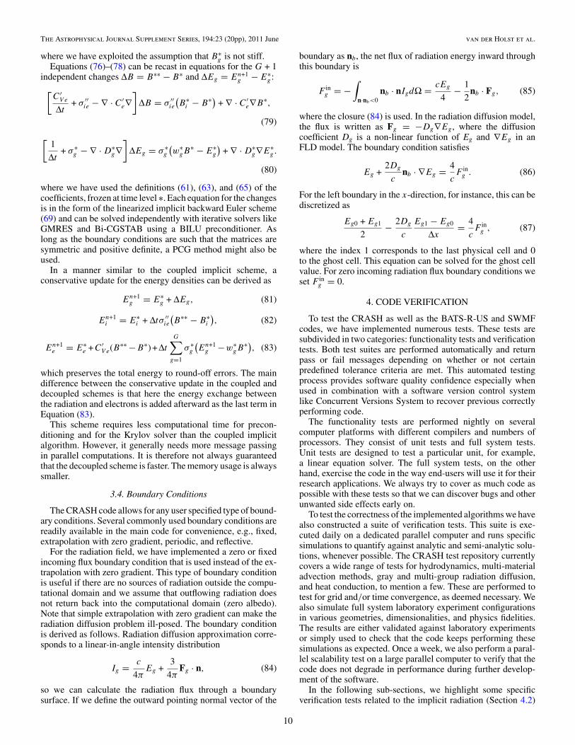
Figure 3. Rotated shock-tube test on a 2D AMR grid based on the Mach number1.05 non-equilibrium gray radiation hydrodynamic test in Lowrie & Edwards(2008). Shown is the radiation temperature in color contour at the initial (toppanel) and final (bottom panel) times. Black crosses indicate cell centers.

(A color version of this figure is available in the online journal.)

The Mach 1.05 test is performed on a 2D non-uniformgrid. The initial condition is taken to be the same as theoriginal steady state reference solution. Since the system ofequations is Galilean invariant, we can add an additional velocity−1.05 so that the velocity on the left boundary is zero whilethe smoothed shock will now move to the left. This newinitial condition as well as the velocity vector are rotated bytan−1(1/2) ≈ 26.◦56. This means that there is a translationalsymmetry in the (−1, 2) direction of the xy-plane as shownin Figure 3. The computational domain is −0.12 < x < 0.12by −0.02 < y < 0.02 decomposed in 3 × 3 grid blocks of24 × 4 cells each. We apply one level of refinement insidethe region −0.04 < x < 0.04 by −0.02/3 < y < 0.02/3.The initial smoothed shock starts at the right boundary of therefined grid and we time-evolve the solution until it reachesthe resolution change on the left as shown in Figure 3. For theboundary conditions in the x-direction, we use zero radiationinflux conditions for the radiation field, while a zero gradient isapplied to the remaining state variables. On the y boundaries,we apply a sheared zero gradient in the (−1, 2) direction for allvariables.

The hydrodynamic equations are time-evolved with theHLLE scheme with a CFL number 0.8. We use the generalizedKoren limiter with β = 3/2 for the slope reconstruction. For theimplicit radiation diffusion solver, we use the GMRES iterativesolver in combination with a BILU preconditioner. The specificheat is time-dependent since it depends on the density, thereforethe implicit scheme is only first-order accurate in time. To enablesecond-order grid convergence for this smooth test problem, wecompensate for this by reducing the CFL number proportionalto the grid cell size, in other words Δt ∝ Δx2, so that second-order accuracy with respect to Δx can be achieved. We increase


0.0001

0.0010

0.0100

rela

tive

L1

erro

r

2nd order slope

conservativenon-conservative

Figure 5. Relative L1 error for the Mach 1.05 non-equilibrium radiationdiffusion test on a non-uniform grid. Both non-conservative and conservativehydrodynamic schemes are tested.

the spatial resolution by each time doubling the number of gridblocks at the base level in both the x- and y-directions.

The convergence of the numerically obtained material andradiation temperatures along the y = 0 cut at the final timet = 0.07 is shown in Figure 4. The solid, dotted, and dashed linescorrespond to the solutions with the 3×3, 6×6, and 12×12 baselevel grid blocks, respectively. The advected semi-analyticalreference solution is shown as a blue line for comparison.

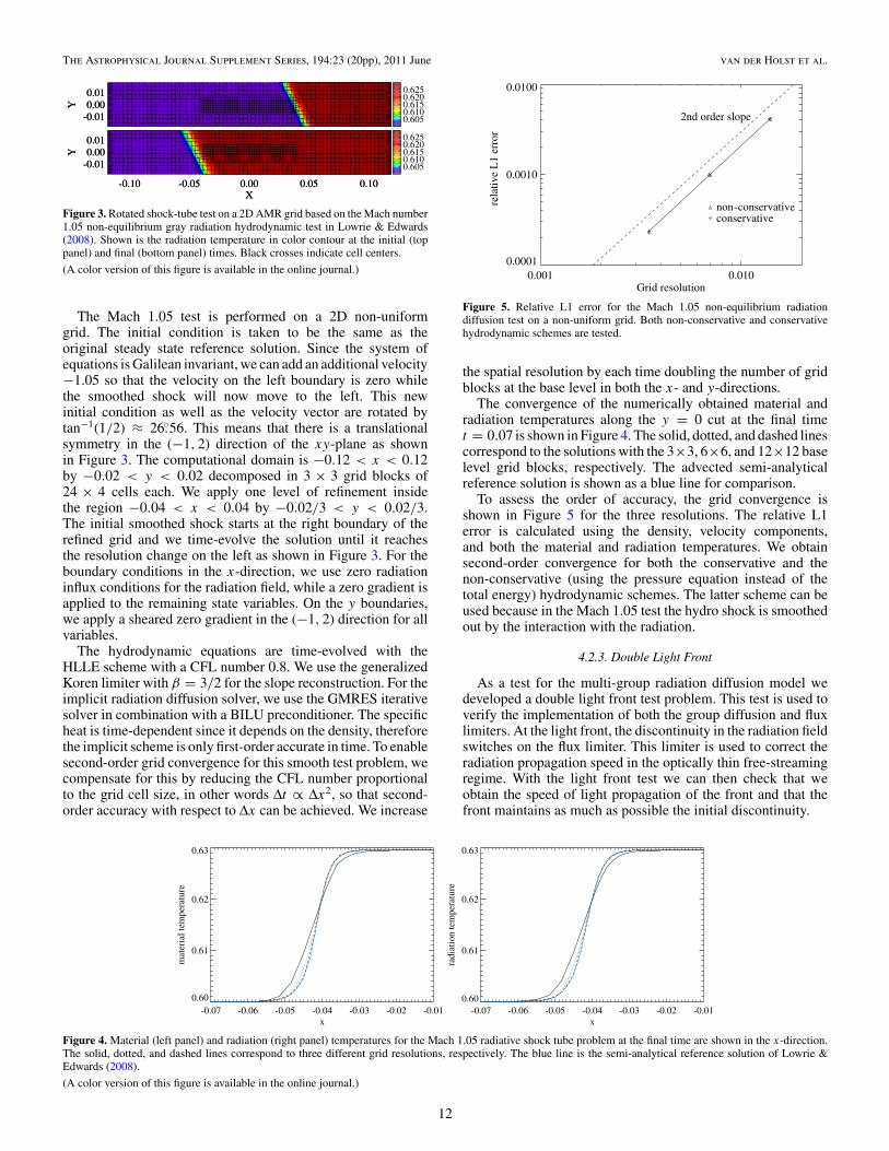
To assess the order of accuracy, the grid convergence isshown in Figure 5 for the three resolutions. The relative L1error is calculated using the density, velocity components,and both the material and radiation temperatures. We obtainsecond-order convergence for both the conservative and thenon-conservative (using the pressure equation instead of thetotal energy) hydrodynamic schemes. The latter scheme can beused because in the Mach 1.05 test the hydro shock is smoothedout by the interaction with the radiation.

4.2.3. Double Light Front

As a test for the multi-group radiation diffusion model wedeveloped a double light front test problem. This test is used toverify the implementation of both the group diffusion and fluxlimiters. At the light front, the discontinuity in the radiation fieldswitches on the flux limiter. This limiter is used to correct theradiation propagation speed in the optically thin free-streamingregime. With the light front test we can then check that weobtain the speed of light propagation of the front and that thefront maintains as much as possible the initial discontinuity.

-0.07 -0.06 -0.05 -0.04 -0.03 -0.02 -0.01x

0.60

0.61

0.62

0.63

mat

eria

l tem

pera

ture

-0.07 -0.06 -0.05 -0.04 -0.03 -0.02 -0.01x

0.60

0.61

0.62

0.63

radi

atio

n te

mpe

ratu

re

Figure 4. Material (left panel) and radiation (right panel) temperatures for the Mach 1.05 radiative shock tube problem at the final time are shown in the x-direction.The solid, dotted, and dashed lines correspond to three different grid resolutions, respectively. The blue line is the semi-analytical reference solution of Lowrie &Edwards (2008).


12


Figure 6. Solutions for the 1D double light front test for four different non-uniform grid resolutions. The radiation energy for group 1 (left panel) enters from the leftboundary, for group 2 (right panel) it enters from the right boundary. The symbols for base resolution 80 show one level of grid refinement for 0.1 < x < 0.2 and0.8 < x < 0.9.

0.001 0.010 0.100Grid resolution

0.01

0.10

rela

tive

L1

erro

r

x-directiony-direction

z-direction

2/3 order slope

Figure 7. Relative L1 error for the double light front test on a non-uniform grid.The test is performed for the x-, y-, and z-directions.

This test is constructed as follows. We use a 1D computationaldomain of the size of 1 m in the x-direction. On this domain, weinitialize the two radiation group energy densities Eg (g = 1, 2)with a very small, positive number to avoid division by zeroin the flux limiter. Also the Rosseland mean opacities are setto a small number corresponding to strong radiation diffusion,while the Planck mean opacities are set to zero correspondingto an optically thin medium. The radiation energy density ofthe first group enters from the left boundary by applying a fixedboundary condition with value one in arbitrary units. On theright boundary this group is extrapolated with zero gradient.Note that these are the proper boundary conditions in the free-streaming limit and not the diffusive flux boundary conditionsdescribed in Section 3.4. The second radiation group entersfrom the right boundary with density 1, and it is extrapolatedwith zero gradient at the left boundary. We time-evolve bothgroups for 0.5 m/c seconds. The analytic solution is then twodiscontinuities that have reached x = 0.5 m, since both frontspropagate with the speed of light c.

The computational domain is non-uniform. In the coarsestresolution, there are 10 grid blocks of 4 cells each at the baselevel. Inside the regions 0.1 < x < 0.2 and 0.8 < x < 0.9, weuse one level of refinement. The total time evolution is dividedinto 400 fixed time steps. We use GMRES for the radiationdiffusion solver in combination with a BILU preconditioner. Forthe grid convergence, we reduce the fixed time step quadraticallywith grid resolution. This time step reduction mimics second-order discretization in time. In Figure 6, the two group energydensities are shown for the base level grid resolutions 40, 80,160, and 320. Clearly, with increasing number of cells, thesolution converges toward the reference discontinuous fronts atx = 0.5.

In Figure 7, the grid convergence is shown for the fourresolutions. The relative L1 error is calculated using both

radiation group energy densities and compared to the analyticalreference solution with the discontinuities at x = 0.5. In Gittingset al. (2008), it was stated that for a second-order differencescheme the convergence rate for a contact discontinuity is 2/3.Indeed, we find this type of convergence rate, due to numericaldiffusion of the discontinuities, for the light front test. We havealso performed the tests in the y- and z-directions to furtherverify the implementation.

4.2.4. Relaxation of Radiation Energy Test

This test is designed to check the relaxation rate betweenmaterial and radiation. The energy exchange between thematerial and radiation groups can be written as

CV

∂T

∂t=

G∑g=1

σg(Eg − Bg), (90)

∂Eg

∂t= σg(Bg − Eg). (91)

For a single radiation group, an analytic expression can befound to describe the relaxation in time. However, for anarbitrary number of groups, a time-dependent analytic solutionis less obvious, except for some rather artificial cases. Herewe assume an extremely large value of the specific heat CVto make analysis more tractable. In this case, the materialtemperature is time-independent, so that Bg is likewise timeindependent. The solution is then Eg = Bg(1− e−σgt ) assumingEg(t = 0) = 0 initially. At time t = 1/σg , the group radiationenergy density is Eg = Bg(1 − 1/e). Note that this test onlyneeds one computational mesh cell in the spatial domain. Weset T = 1 keV and the resulting Planckian spectrum, definedby Bg, is depicted by the dotted line in the left panel ofFigure 8. We use 80 groups logarithmically distributed overthe photon energy domain in the range of 0.1 eV to 20 keV.The computed Eg at time t = 1/σg are shown as + points.For the simulation we used the GMRES iterative solver and theCrank–Nicolson scheme. To assess the error, we repeated thetest with time steps of 1/20, 1/40, and 1/80 of the simulationtime. The second-order convergence rate is demonstrated in theright panel of Figure 8.

4.3. Heat Conduction Tests

4.3.1. Uniform Heat Conduction in rz-geometry

This test is designed to verify the implicit heat conductionsolver in rz-geometry. It tests the time evolution of the temper-ature profile using uniform and time-independent heat conduc-tivity. In rz-geometry, the equation of the electron temperaturefor purely heat conductive plasma follows

CV e

∂Te

∂t= 1

r

∂

∂r

(rCe

∂Te

∂r

)+

∂

∂z

(Ce

∂Te

∂z

). (92)

13


0 5.0•103 1.0•104 1.5•104 2.0•104

photon energy [ev]

0

5.0•10-5

1.0•10-4

1.5•10-4

2.0•10-4

2.5•10-4

Eg [eV]Bg(1-1/e) [eV]Bg [eV]

0.1 1.0time step (arbitrary units)

0.0001

0.0010

0.0100

rela

tive

max

imum

err

or 2nd order slope

Figure 8. Relaxation of radiation energy test for 80 groups. Left panel is for the time-independent spectrum Bg (dotted line) and the group radiation energy solution Egat time 1/σg (+ points) vs. the photon energies after 80 time steps. The analytical reference solution is shown as a solid line. Right panel shows the relative maximumerror for 20, 40, and 80 time steps demonstrating second-order convergence rate.

2.53.03.54.04.55.0

-2 -1 0 1 2X

0.20.40.60.8

R

-2 -1 0 1 2X

0.20.40.60.8

R

2.53.03.54.04.55.0

-2 -1 0 1 2X

0.20.40.60.8

R

-2 -1 0 1 2X

0.20.40.60.8

R

Figure 9. Electron temperature for the uniform heat conduction test on a non-uniform grid in rz-geometry. The top panel shows the electron temperature inthe initial condition while the bottom panel is the electron temperature at thefinal time. The black box indicates the region within which the grid is refinedby one level.


We set the electron specific heat CV e = 1 and assume electronconductivity Ce to be constant. In this case, a solution can bewritten as a product of a Gaussian profile in the z-direction andan elevated Bessel function J0 in the r-direction (Arfken 1985):

Te = Tmin + T01√

4πCete− z2

4Cet J0(br)e−b2Cet , (93)

where b ≈ 3.8317 is the first root of the derivative of J0(r). Weselect the following values for the input parameters: Tmin = 3,T0 = 10, and Ce = 0.1 in dimensionless units.

The computational domain is −3 < z < 3 and 0 < r < 1discretized with 3 × 3 grid blocks of 30 × 30 cells each. In theregion −1 < z < 1 and 1/3 < r < 2/3, we apply one levelof mesh refinement. We impose a symmetry condition for theelectron temperature on the axis. On all other boundaries theelectron temperature is fixed to the time-dependent referencesolution. We time-evolve this heat conduction problem with aPCG method from time t = 1 to the final time at t = 1.5.The Crank–Nicolson approach is used to achieve second-orderaccurate time integration.

The initial and final solutions for the electron temperatureare shown in Figure 9 in color contour in the rz-plane. Theheat conduction has diffused the temperature in time to a moreuniform state. The black line indicates the region in whichthe mesh refinement was applied. The relative maximum errorof the numerically obtained electron temperature versus theanalytical solution is shown in Figure 10. Here we used thenon-uniform grid with base resolutions of 902, 1802, 3602, and7202 cells and set the time step proportional to the cell size todemonstrate a second-order convergence rate.


10-6

10-5

10-4

rela

tive

max

imum

err

or 2nd order slope

Figure 10. Relative maximum error for the uniform heat conduction test on anon-uniform grid in the rz-geometry.

4.3.2. Reinicke–Meyer-ter Vehn Test

The Reinicke & Meyer-ter-Vehn (1991) problem tests boththe hydrodynamic and heat conduction implementations. Thistest generalizes the well-known Sedov–Taylor strong pointexplosion in single-temperature hydrodynamics by includingthe heat conduction. The heat conductivity is parameterized asa non-linear function of the density and material temperature:Ce = ρaT b. We select the spherically symmetric self-similarsolution of Reinicke & Meyer-ter-Vehn (1991) with coefficientsa = −2 and b = 13/2 and the adiabatic index is γ = 5/4. Thissolution produces, similar to the Sedov–Taylor blast-wave, anexpanding shock front through an ambient medium. However,at very high temperatures, thermal heat conduction dominatesthe fluid flows, so that a thermal front precedes the shock front.With the selected parameters, the heat front is always at twicethe distance from the origin of the explosion as is the shockfront.

We perform the test in rz-geometry. The computationaldomain is divided in 200 × 200 cells. The boundary conditionsalong the r and z axes are reflective. The two other boundaries,away from explosion, are prescribed by the self-similar solution.The time evolution is numerically performed as follows. For thehydrodynamics, we use the HLLE scheme with the CFL numberset to 0.8. Since this test is performed on a uniform grid withoutAMR, we can use the generalized Koren limiter with β = 2.This is the same as the original Koren (1993) slope limiter. Theheat conduction is solved implicitly with the PCG method. Thetest is initialized with the spherical self-similar solution with theshock front located at the spherical radius 0.225 and the heat

14


0.0

0.2

0.4

0.6

0.8

1.0de

nsity

0.0

0.2

0.4

0.6

0.8

1.0

tem

pera

ture

0.0 0.2 0.4 0.6 0.8 1.0Radius

0.0

0.2

0.4

0.6

0.8

1.0

radi

al v

eloc

ity

Figure 11. Density (top panel), temperature (middle panel), and radial velocity(bottom panel) along the z = 0 cut for the Reinicke–Meyer-ter Vehn test inrz-geometry. The numerical solution (+ symbols) is at the final time comparedto the self-similar analytical reference solution (solid lines).

front is at 0.45. The simulation is stopped once the shock fronthas reached 0.45 and the heat front is at 0.9.

A 1D slice along the r-axis of the solution at the final time isshown in Figure 11. We normalize the output similar to Reinicke& Meyer-ter-Vehn (1991). The temperature is normalized by thecentral temperature, while the density and radial velocity arenormalized by their values of the post-shock state at the shock.The numerical solution obtained by the CRASH code is shownas + symbols and is close to the self-similar reference solution,shown as solid lines. Note that the temperature is smooth dueto the heat conduction, except for the discontinuous derivativeat the heat front. The wiggle at r = 0.3 in the density andradial velocity is due to the diffusion of the analytical shockdiscontinuity in the initial condition during the first few timesteps. In the left panel of Figure 12, the spherical expansion oftemperature at the final time is shown. Clearly, the Cartesian gridwith the rz-geometry does not significantly distort the sphericalsymmetry of the solution. The spatial distribution of the error in

the temperature is shown in the right panel. The errors are largestat the discontinuities of the shock and heat fronts as expected.

A grid convergence study is performed with resolutions of2002, 4002, and 8002 cells. The relative L1 error in Figure 13is calculated using the density, velocity components, and thematerial temperature. The convergence rate is first-order due tothe shock and heat front.

4.3.3. Heat Conduction Version of Lowrie’s Test

Any of the verification tests for non-equilibrium gray diffu-sion coupled to the single temperature hydrodynamics can bereworked as a test for the hydrodynamic equations for the ionscoupled to the electron pressure equation with electron heat con-duction and energy exchange between the electrons and ions.As an example, we transform one of the non-equilibrium graydiffusion tests of Lowrie & Edwards (2008) to verify the heatconduction implementation.

The electron energy density Equation (20) without the radia-tion interaction can be written as

∂Ee

∂t+ ∇ · [Eeu] + pe∇ · u = ∇ · [Ce∇Te] + σie(Ti − Te), (94)

where the heat conduction and energy exchange terms on theright-hand side depend on the gradients and differences of thetemperatures. The equation for the gray radiation energy density(16) on the other hand depends on the gradients and differencesof energy densities. By defining the radiation temperature Tr byEr = aT 4

r and using the definition of the Planckian B = aT 4e ,

we can rewrite the energy density equation for the radiation as

∂Er

∂t+ ∇ · [Eru] +

1

3Er∇ · u = ∇ · [Dr∇Er ]+ cκP (aT 4 − Er)

= ∇ · [Dr∇Tr ] + cκP (T − Tr ),

(95)

where Dr = Dr4aT 3r and cκP = cκP a(T 2 + T 2

r )(T + Tr )are the new coefficients that appear due to this transformation.Equations (94) and (95) are now of the same form. To translatea gray diffusion test to a heat conduction test, we reinterpretDr as the heat conductivity Ce and cκP as the relaxationcoefficient σie in the ion–electron energy exchange. In addition,the material temperature T and radiation temperature Tr haveto be reinterpreted as the ion temperature Ti and electrontemperature Te, respectively. Note that we also have to relatethe electron pressure and internal energy by pe = Ee/3 similar

0.0

0.2

0.4

0.6

0.8

temperature

0.2 0.4 0.6 0.8

Z

0.2

0.4

0.6

0.8

R

0.00

0.05

0.10

0.15

0.20

0.25

0.30temperature error

0.2 0.4 0.6 0.8

Z

Figure 12. Temperature (left panel) and temperature error compared to the reference solution (right panel) for the Reinicke–Meyer-ter Vehn test in rz-geometry.


15



0.01

0.10

rela

tive

L1

erro

r

1st order slope

Figure 13. Relative L1 error for the Reinicke–Meyer-ter Vehn test in rz-geometry.

to the radiation field corresponding to γe = 4/3, and let theelectron internal energy and electron specific heat depend onthe electron temperature as Ee = aT 4

e and CV e = 4aT 3e ,

respectively.As an example, we transform the Mach 5 non-equilibrium

gray diffusion shock tube problem of Lowrie & Edwards(2008). It uses non-uniform opacities that depend on thedensity and temperature defined by Dr = 0.0175(γ T )7/2/ρand cκP = 106/Dr . The above described procedure is usedto translate this problem to an electron heat conduction testwith energy exchange between the electron and ions. The heatconductivity for this test is Ce = 4aT 3

e 0.0175(γ Ti)7/2/ρ andthe relaxation coefficient between the electron and ions isσie = a(T 2

i + T 2e )(Ti + Te)4aT 3

e 106/Ce.We perform this Mach 5 heat conduction test on a 2D non-

uniform grid. For the initial condition, the 1D semi-analyticalsteady state reference solution of Lowrie & Edwards (2008)is used. There is a Mach 5 pre-shock flow on the left side ofthe tube resulting in an embedded hydro shock as well as asteep thermal front (a look at Figure 14 will help to understandthis shock tube problem). We add an additional velocity ofMach −5 so that the pre-shock velocity is zero and the shockis no longer steady, but instead will move to the left with avelocity −5 (in units in which the pre-shock speed of soundis 1). The problem is rotated counterclockwise on the grid bytan−1(1/2). The translational symmetry is now in the (−1, 2)direction in the xy-plane similar to the Mach 1.05 shock tubeproblem described in Section 4.2.2. The computational domain

is −0.0384 < x < 0.0384 by −0.0048 < y < 0.0048. Insidethe area −0.0128 < x < 0.0128 and −0.0016 < y < 0.0016,we apply one level of refinement. This refinement is set up suchthat both the heat front as well as the shock front propagatethrough the resolution change on the left (from fine to coarse)and right (from coarse to fine), respectively. For the boundaryconditions in the x-direction, we fix the state on the right sidewith the semi-analytical solution, but for the left side we usezero gradient. On the y boundaries, we apply a sheared zerogradient in the (−1, 2) direction.

For the evolution until the final time t = 0.0025, we use theHLLE scheme together with the generalized Koren limiter withβ = 3/2 to solve the hydrodynamic equations. The CFL numberis set to 0.8. The heat conduction and energy exchange betweenelectrons and ions are solved implicitly with the backward Eulerscheme using the GMRES iterative solver in combination witha BILU preconditioner.

In Figure 14, the electron (right panel) and ion (left panel)temperatures are shown at the final time along the x-axis.The semi-analytical reference solution is shown as a blueline, while the numerical solution is shown with + symbolsfor a simulation with 192 × 24 cells at the base level inthe x- and y-directions. The hydro shock is located nearx ≈ 0.0085 and shows up in the ion temperature as a jumpin the temperature, followed directly behind the shock by astrong relaxation due to the energy exchange between the ionsand electrons. The electron temperature stays smooth due tostrong heat conduction. The heat front is seen with a steep footat x ≈ −0.022. This front corresponds to the radiative precursorin the non-equilibirum gray diffusion tests of Lowrie & Edwards(2008). We repeat the test with four different resolutions at thebase level: 192 × 24, 384 × 48, 768 × 96, and 1536 × 192 cellsin the x- and y-directions. The insets in both panels of Figure 14show the four resolutions as solid, dotted, dashed, dash-dottedlines, respectively. In the left panel, the zoom-in shows theconvergence of the ion temperature toward the embedded hydroshock and the temperature relaxation. In the right panel, theblow-up shows the convergence toward the reference precursorfront. Note that no spurious oscillations appear near the shockor near the precursor.

Due to the discontinuity in both the shock and heat precursor,the convergence rate can be at most first-order. Indeed, inFigure 15 the relative L1 error shows first-order accuracy. Theerror is calculated using all the density, velocity components,and both temperatures. Note that the spike in the ion temperature

-0.04 -0.02 0.00 0.02 0.04x

0

1

2

3

4

5

6

ion

tem

pera

ture

heat front

0.007 0.008 0.009 0.0105.0

5.5

6.0

6.5

hydro shock

relaxation

-0.04 -0.02 0.00 0.02 0.04x

0

1

2

3

4

5

6

elec

tron

tem

pera

ture

-0.025 -0.024 -0.023 -0.022 -0.0210.5

1.0

1.5

2.0

Figure 14. Mach 5 shock tube problem of Lowrie & Edwards (2008) transformed to a non-uniform heat conduction and ion–electron collision frequency test androtated on a 2D non-uniform grid. Ion (left panel) and electron (right panel) temperatures at the final time are shown in the x-direction. The blue line is the referencesolution. In the left panel, the grid convergence near the shock is shown in the inset. In the right panel, a blow-up of the grid convergence to the reference heat front isshown.


16



0.001

0.010re

lativ

e L

1 er

ror

1st order slope

Figure 15. Relative L1 error for the Mach 5 non-equilibrium heat conductiontest on a non-uniform grid.

is spatially so small that a huge number of grid cells are neededto get a fully resolved shock and relaxation state.

4.4. Full System Tests

The CRASH test repository contains a range of full systemconfigurations to be used for validation with future laboratoryexperiments. In Figure 16, we show the configuration of a 3Delliptical nozzle through which a fast shock of the order of150 km s−1 will be launched, which is still significantly slowerthan the speed of light. The shock wave is produced by a 1.1 nslaser pulse from the left with 4 kJ of energy irradiating a 20 μmthick beryllium disk, initially located at x = 0. A layer of goldis glued to the plastic tube to protect the outside of the tube fromthe laser-driven shock. The plastic (polyimide) tube is circularfor x < 500 μm with a radius of 600 μm. Beyond x = 750 μmthe tube is made elliptical by flattening the tube in the y-directionby a factor two.

A laser energy deposition library is currently under construc-tion and the implemented will be reported elsewhere. For thispaper, we will instead perform the first part of the simula-tion with the 2D, Lagrangian, radiation hydrodynamics codeHYADES (Larsen & Lane 1994) to time advance the heatingdue to the irradiation by the laser beams and the response ofthe plasma until 1.1 ns. This laser pulse first shocks and thenaccelerates the beryllium to the right. After 1.1 ns, the out-put of HYADES is used as an initial condition of the CRASHcode.

This simulation is performed for a two-temperature, electronand ion, plasma. For the radiation, we use the FLD approxi-mation with 30 groups. The photon energy is in the range of0.1 eV to 20 keV, logarithmically distributed over the groups.

Due to the symmetry in the problem we only simulate onequadrant (y > 0 and z > 0), with reflective boundary con-ditions at y = 0 and z = 0. At all other boundaries we usean extrapolation with zero gradient for the plasma and a zeroincoming flux boundary for the radiation. The domain size is[−150, 3900] × [0, 900] × [0, 900] microns for the x, y, z co-ordinates. The base level grid consists of 120 × 20 × 20 blocksof 4 × 4 × 4 mesh cells. One level of dynamic mesh refine-ment is used at material interfaces and the shock front. Overall,the effective resolution is 960 × 160 × 160 cells and there areapproximately 4.5 million finite volume cells. The hydrody-namic equations are solved with the HLLE scheme with a CFLnumber 0.8 together with the generalized Koren limiter withβ = 3/2. The diffusion and energy exchange of the radiationgroups as well as the heat conduction are solved with the de-coupled implicit scheme using a Bi-CGSTAB iterative solver.The simulation from 1.1 ns to 13 ns physical time took 1 hrand 55 minutes on 480 cores of the FLUX supercomputer at theUniversity of Michigan.

In Figure 17, we show the shock structure at 13 ns. Theaccelerated beryllium compresses the xenon directly to the rightof the interface, which is seen as a high density plasma nearx = 1700 μm in the top right panel of Figure 17. This drives aprimary shock and the velocity jump at x ≈ 1700 μm is seen inthe middle left panel. Behind the shock front, the ions are heatedas depicted from the middle right panel, followed directly behindthe shock by cooling due to the energy exchange between ionsand electrons. Early on, electron heating produces ionizationand emission of radiation, and the radiation in turn heats andionizes the material ahead of the primary shock. The radiationtemperature, as measured by the total radiation energy density,is shown in the bottom left panel. The photons will interactagain with the matter, sometimes after traveling some distance.This is the source of the wall shock seen ahead of the primaryshock (Doss et al. 2009, 2011): photons traveling ahead of theshock interact with the plastic wall, heat it, and in turn drivea shock off the wall into the xenon. The ablation of plasticis depicted in the top left panel as a radially inward movingpolyimide (in green color) near and even ahead of the primaryshock. The compressed xenon due to plastic ablation is seen inthe top right panel as a faint density feature that is ahead of theprimary shock front, between x = 1700 μm and x = 2000 μm.Interaction between the photons and matter is also seen by theradiative precursor to the right of the radiative shock elevatingthe electron temperature ahead of the shock in the bottomright panel. This is due to the strong coupling between theelectrons and radiation field. The reader is referred to Drake et al.(2011) for more details on radiative effects in radiative shocktubes.

0

1

2

3

4Material and AMR levels

0 500 1000 1500 2000X [micron]

200

400

600

800

Z [

mic

ron]

0 500 1000 1500 2000X [micron]

200

400

600

800

Z [

mic

ron]

Material and AMR levels

0

1

2

3


0 500 1000 1500 2000X [micron]

200

400

600

800

Y [

mic

ron]

0 500 1000 1500 2000X [micron]

200

400

600

800

Y [

mic

ron]

Material and AMR levels

Figure 16. Geometry of the 3D elliptic nozzle experiment after 1.1 ns, consisting of 5 materials: beryllium (blue), xenon (black), polyimide (green), gold (yellow),and acrylic (red) in both panels. The radius of the inside of the polyimide tube is 600 μm in the y = 0 plane (left panel). In the z = 0 plane (right panel), the radius ofthe inner tube is 600 μm for x < 500 μm, but shrinks to 300 μm beyond x = 750 μm. The lines represent the mesh refinement at material interfaces and shock fronts.


17


0

1

2

3


200

400

600

800

Y [

mic

ron]

200

400

600

800

Y [

mic

ron]

-20020406080100

X Velocity [km/s]

200

400

600

800

Y [

mic

ron]

-3.0

-2.5

-2.0

-1.5

log Radiation Temperature [keV]

0 500 1000 1500 2000X [micron]

200

400

600

800

Y [

mic

ron]

-3

-2

-1

0

1

log Density [g/cm3]

-4

-3

-2

-1

log Ion Temperature [keV]

-3.5

-3.0

-2.5

-2.0

-1.5

log Electron Temperature [keV]

0 500 1000 1500 2000X [micron]

Figure 17. Simulated radiative shock structure at 13ns in a 3D elliptic nozzle consisting of the five materials indicated in Figure 16. The plots show in the xy-plane incolor contour the variables indicated in the plot title. The primary shock is at x ≈ 1700.


4.5. Parallel Performance

We present parallel scaling studies on the Pleiades supercom-puter at NASA Ames. This computer is an SGI ICE clusterconnected with InfiniBand. Figure 18 shows strong scaling fora problem size that is independent of the number of processors.This 3D simulation is a circular tube version of the full systemtest described in Section 4.4. It uses five materials, 30 radia-tion groups, and separate electron and ion temperatures. Thegrid contains 80 × 8 × 8 blocks of 4 × 4 × 4 cells each at thebase level and in addition two time-dependent refinement levels.There are overall approximately 2.6 million cells in this prob-lem. We use lookup tables for the EOS and opacities, so that thecomputational time for that is negligible. For the hydrodynamicequations, we use the HLLE scheme together with the gener-alized Koren limiter with β = 3/2. The radiation diffusion,electron heat conduction, and energy exchange terms are solvedimplicitly with the decoupled scheme, using the Bi-CGSTABiterative solver. This simulation is performed for 20 time stepsfor the number of cores varying from 128 to 2048, but excludesfile I/O to measure the performance of the implicit solver. Upto 1024 cores, we get good scaling. However, for more cores weobserve saturation in the performance.

5. SUMMARY

We have extended the BATS-R-US code (Powell et al.1999; Toth et al. 2011) with a new radiation transfer andheat conduction library. This new combination, together withthe EOS and multi-group opacity solver, is called the CRASHcode. This code uses the recently developed parallel BATL (Tothet al. 2011) to enable highly resolved radiation hydrodynamicsolutions. The implemented radiation hydrodynamic schemessolve for gray or multi-group radiation diffusion models in theFLD approximation.

In high-energy-density plasmas, the electrons are most of thetime strongly coupled to the ions by collisions. An importantexception is at hydrodynamic shocks, where the ions are heated

100 1000Number of cores

104

105

Num

ber

of c

ell u

pdat

es/s

ec

Figure 18. Strong scaling of the CRASH code, running a 3D CRASH applicationwith five material level sets, electron and ion temperature, 30 radiation groups,and two levels of time-dependent mesh refinement.

by the shock wave and the electrons and ions are out of tempera-ture equilibrium. Since radiative shocks are the main applicationfor CRASH, we have implemented a separate electron pressureequation with the electron thermal heat conduction. For the elec-tron heat conduction, we have added the option of a flux limiterto limit the thermal flux with the free-streaming heat flux.

The multi-material radiation hydrodynamic equations aresolved with an operator-split method that consists of threesubsteps: (1) solving the hydrodynamic equations with standardfinite volume shock-capturing schemes, (2) the linear advectionof the radiation in frequency-logarithm space, and (3) theimplicit solution of the radiation, heat conduction, and energyexchanges. For the implicit solver, standard Krylov solvers areused together with a BILU preconditioner. This preconditionerscales well up to 1000 processors on present-day parallelcomputers. For future work, we may explore for the implicitmulti-group diffusion a multi-level preconditioner to better scalethe radiation solver beyond 1000 processors.

18


2

1a

b

c3

Figure 19. Cell and face centers at the adaptive interface in 2D.

We have presented a suite of verification tests that benchmarkthe performance. These tests verify the correctness and accuracyof our implementation of the gray and multi-group radiationdiffusion algorithm and the heat conduction in 1D, 2D, and 3Dslab and 2D rz geometry. To demonstrate the full capabilityof the implementation, we have presented a 3D multi-materialsimulation of a radiative shock wave propagating through anelliptical nozzle. This configuration will be used in futurevalidation studies.

We caution the reader that another CRASH code has alreadybeen discussed in the literature (Ciardi et al. 2001; Maselli et al.2003, 2009; Pierleoni et al. 2009). This code is used for cos-mological reionization around the first stars using Monte Carloradiative transfer methods. Our code is different and uses multi-group radiation diffusion models in the FLD approximation. Theapplications are for astrophysics and laboratory astrophysics.

The authors express their gratitude to M. J. Grosskopf andE. Rutter for providing HYADES output. Discussions with B.Torralva and C. C. Chou are gratefully acknowledged. Thiswork was funded by the Predictive Sciences Academic AlliancesProgram in DOE/NNSA-ASC via grant DEFC52-08NA28616and by the University of Michigan. The simulations wereperformed on the NASA Advanced Supercomputing systemPleiades.

APPENDIX A

DISCRETIZATION OF THE DIFFUSION OPERATOR ATRESOLUTION CHANGES

In Sections 3.3.1 and 3.3.2, the diffusion operator is dis-cretized on a uniform mesh with a standard finite volume methodin combination with a central difference approximation for thegradient in the flux calculation as in Equation (68). The diffusioncoefficient needed at the face is obtained by simple arithmeticaveraging of the left and right cell center diffusion coefficients.The generalization to resolution changes as in Figure 19 is lessstraightforward. In the following, we denote the fine cell cen-ters by a and b, the coarse cell center by c. The flux densities atresolution changes in the direction orthogonal to the interfaceare denoted by F1 and F2 at the fine faces, and F3 at the coarseface.

In Edwards (1996), a strategy was developed to discretize thediffusion operator on an adaptive mesh in the context of reservoirsimulations. The main ingredients of the method are (1) requirethe continuity of the flux at the resolution change in the strongsense, i.e., F1 = F2 = F3 and (2) discretize the gradient inthe diffusion flux by a one-sided difference. An expression wasfound for the diffusion flux F = −D∇E in which the diffusioncoefficient is replaced by a weighted harmonic average of thecell centered values Da, Db, Dc. In Gittings et al. (2008), it wasargued that this discretization does not properly propagate the

self-similar Marshak waves of the radiation diffusion model,unless the cell centered diffusion coefficients are calculated ona common face temperature.

In the code discussed in this paper, we follow a differentapproach that replaces the harmonic average of the diffusioncoefficient in Edwards (1996) with an arithmetic average andfor the flux densities normal to the resolution change interfacewe obtain

F1 = F2 = F3 = − 2D

3Δx[Ec − (Ea + Eb)/2] , (A1)

where Δx is the fine cell size and the diffusion coefficient at theface is averaged as

D3 = [Dc + (Da + Db)]/3. (A2)

We have demonstrated with verification tests including thosediscussed above that this change produces properly propagatingradiative precursor and shock fronts. Generalizations to 1D and3D are straightforward.

APPENDIX B

rz-GEOMETRY

Incorporating rz-geometry in a finite volume formulation isas follows: the radial cell face area and the cell volume must bemade proportional to the distance r from the symmetry axis. Inaddition, the r component of the momentum Equation (18) ismodified as

∂ρur

∂t+ ∇ · [ρuur + r(p + pr )] = p + pr

r, (B1)

where r is the unit vector in the r-direction and ur = u · r.This correction reflects that the pressure term is a gradient, nota divergence.

REFERENCES

Arfken, G. 1985, Mathematical Methods for Physicists (3rd ed.; San Diego,CA: Academic)

Baek, S., Di Matteo, P., Semelin, B., Combes, F., & Revaz, Y. 2009, A&A, 495,389

Barton, R. T. 1985, in Numerical Astrophysics, ed. J. M. Centrella, J. M.LeBlanc, & R. L. Bowers (Boston, MA: Jones & Bartlett), 482

Buchler, J. R. 1983, J. Quant. Spectrosc. Radiat. Transfer, 30, 395Ciardi, B., Ferrara, A., Marri, S., & Raimondo, G. 2001, MNRAS, 324, 381Doss, F. W., Drake, R. P., & Myra, E. S. 2011, Phys. Plasmas, submittedDoss, F. W., Robey, H. F., Drake, R. P., & Kuranz, C. C. 2009, Phys. Plasmas,

16, 112705Drake, R. P. 2006, High-Energy Density Physics (Berlin: Springer)Drake, R. P., et al. 2011, High Energy Density Physics, in pressEdwards, M. G. 1996, J. Comput. Phys, 126, 356Einfeldt, B., Munz, C. D., Roe, P. L., & Sjogreen, B. 1991, J. Comput. Phys.,

92, 273Eisenstat, S. C. 1981, SIAM J. Sci. Stat. Comput., 2, 1Gittings, M., et al. 2008, Comput. Sci. Discovery, 1, 015005Gnedin, N. Y., Tassis, K., & Kravtsov, A. V. 2009, ApJ, 697, 55Godunov, S. K. 1959, Mat. Sb., 47, 271Harten, A., Lax, P. D., & van Leer, B. 1983, SIAM Rev., 25, 35Iliev, I. T., et al. 2009, MNRAS, 400, 1283Karni, S. 1996, SIAM J. Sci. Comput., 17, 1019Koren, B. 1993, in Numerical Methods for Advection-Diffusion Problems, ed.

C. B. Vreugdenhil & B. Koren (Braunschweig: Vieweg), 117Kreiss, G., & Olsson, E. 2005, J. Comput. Phys., 210, 225Landau, L. D., & Lifshitz, E. M. 1980, Theoretical Physics, Vol. 5. Statistical

Physics, Part 1 (3rd ed.; New York: Pergamon)Larsen, J., & Lane, S. 1994, J. Quant. Spectrosc. Radiat. Transfer, 51, 179Levermore, C. D., & Pomraning, G. C. 1981, ApJ, 248, 321

19

http://dx.doi.org/10.1051/0004-6361:200810757

http://adsabs.harvard.edu/abs/2009A&A...495..389B

http://adsabs.harvard.edu/abs/2009A&A...495..389B

http://dx.doi.org/10.1016/0022-4073(83)90102-4

http://adsabs.harvard.edu/abs/1983JQSRT..30..395B

http://adsabs.harvard.edu/abs/1983JQSRT..30..395B

http://dx.doi.org/10.1046/j.1365-8711.2001.04316.x

http://adsabs.harvard.edu/abs/2001MNRAS.324..381C

http://adsabs.harvard.edu/abs/2001MNRAS.324..381C

http://dx.doi.org/10.1063/1.3259354

http://adsabs.harvard.edu/abs/2009PhPl...16k2705D

http://adsabs.harvard.edu/abs/2009PhPl...16k2705D

http://dx.doi.org/10.1016/j.hedp.2011.03.005

http://dx.doi.org/10.1006/jcph.1996.0143

http://adsabs.harvard.edu/abs/1996JCoPh.126..356E

http://adsabs.harvard.edu/abs/1996JCoPh.126..356E

http://dx.doi.org/10.1016/0021-9991(91)90211-3

http://adsabs.harvard.edu/abs/1991JCoPh..92..273E

http://adsabs.harvard.edu/abs/1991JCoPh..92..273E

http://dx.doi.org/10.1137/0902001

http://dx.doi.org/10.1088/1749-4699/1/1/015005

http://adsabs.harvard.edu/abs/2008CS&D....1a5005G

http://adsabs.harvard.edu/abs/2008CS&D....1a5005G

http://dx.doi.org/10.1088/0004-637X/697/1/55

http://adsabs.harvard.edu/abs/2009ApJ...697...55G

http://adsabs.harvard.edu/abs/2009ApJ...697...55G

http://dx.doi.org/10.1137/1025002

http://dx.doi.org/10.1111/j.1365-2966.2009.15558.x

http://adsabs.harvard.edu/abs/2009MNRAS.400.1283I

http://adsabs.harvard.edu/abs/2009MNRAS.400.1283I

http://dx.doi.org/10.1137/S106482759528003X

http://adsabs.harvard.edu/abs/1993LNP...414..110K

http://dx.doi.org/10.1016/j.jcp.2005.04.007

http://adsabs.harvard.edu/abs/2005JCoPh.210..225O


http://dx.doi.org/10.1016/0022-4073(94)90078-7

http://adsabs.harvard.edu/abs/1994JQSRT..51..179L

http://adsabs.harvard.edu/abs/1994JQSRT..51..179L

http://dx.doi.org/10.1086/159157

http://adsabs.harvard.edu/abs/1981ApJ...248..321L

http://adsabs.harvard.edu/abs/1981ApJ...248..321L


Lowrie, R. B., & Edwards, J. D. 2008, Shock Waves, 18, 129Lund, C. M., & Wilson, J. R. 1980, Lawrence Livermore National Laboratory

Report UCRL-84678Marinak, M. M., Kerbel, G. D., Gentile, N. A., Jones, O., Munro, D., Pollaine,

S., Dittrich, T. R., & Haan, S. W. 2001, Phys. Plasmas, 8, 2275Martınez-Sykora, J., Hansteen, V., De Pontieu, B., & Carlsson, M. 2009, ApJ,

701, 1569Maselli, A., Ferrara, A., & Ciardi, B. 2003, MNRAS, 345, 379Maselli, A., Ferrara, A., & Gallerani, S. 2009, MNRAS, 395, 1925Mellema, G., Iliev, I. T., Alvaraz, M. A., & Shapiro, P. R. 2006, New Astron.,

11, 374Mihalas, D., & Weibel-Mihalas, B. 1984, Foundations of Radiation Hydrody-

namics (New York: Oxford Univ. Press)Minerbo, G. N. 1978, J. Quant. Spectrosc. Radiat. Transfer, 20, 451Morel, J. E. 2000, J. Quant. Spectrosc. Radiat. Transfer, 65, 769Nayakshin, S., Cha, S. H., & Hobbs, A. 2009, MNRAS, 397, 1314Olsson, E., Kreiss, G., & Zahedi, S. 2007, J. Comput. Phys., 225, 785Petkova, M., & Springel, V. 2009, MNRAS, 396, 1383Pierleoni, M., Maselli, A., & Ciardi, B. 2009, MNRAS, 393, 872Pomraming, G. C. 2005, The Equations of Radiation Hydrodynamics (Mineola,

NY: Dover)

Powell, K. G., Roe, P. L., Linde, T. J., Gombosi, T. I., & DeZeeuw, D. L. 1999, J.Comput. Phys., 154, 284

Reinicke, P., & Meyer-ter-Vehn, J. 1991, Phys. Fluids A, 3, 1807Roe, P. L. 1986, Annu. Rev. Fluid Mech., 18, 337Saad, Y., & Schultz, M. H. 1986, SIAM J. Sci. Stat. Comput., 7, 856Stein, R. F., Benson, D., & Nordlund, A. 2007, in ASP Conf. Ser. 369, New

Solar Physics with Solar-B Mission, ed. K. Shibata, S. Nagata, & T. Sakurai(San Francisco, CA: ASP), 87

Stone, J. M., Mihalas, D., & Norman, M. L. 1992, ApJS, 80, 819Su, B., & Olson, G. L. 1996, J. Quant. Spectrosc. Radiat. Transfer, 56,

337Sussman, M., & Puckett, E. G. 2000, J. Comput. Phys., 162, 301Toth, G., Ma, Y., & Gombosi, T. I. 2008, J. Comput. Phys., 227, 6967Toth, G., et al. 2005, J. Geophys. Res., 110, A12226Toth, G., et al. 2011, J. Comput. Phys., in pressvan der Vorst, H. A. 1992, SIAM J. Sci. Stat. Comput., 13, 631Vogler, A., Shelyag, S., Schussler, M., Cattaneo, F., Emonet, T., & Linde, T.

2005, A&A, 429, 335Yee, H. C. 1989, NASA TM-101088Zel’dovich, Ya. B., & Raizer, Yu. P. 2002, Physics of Shock Waves and High-

Temperature Hydrodynamic Phenomena (Mineola, NY: Dover)

20

http://dx.doi.org/10.1007/s00193-008-0143-0

http://adsabs.harvard.edu/abs/2008ShWav..18..129L

http://adsabs.harvard.edu/abs/2008ShWav..18..129L

http://dx.doi.org/10.1063/1.1356740

http://adsabs.harvard.edu/abs/2001PhPl....8.2275M

http://adsabs.harvard.edu/abs/2001PhPl....8.2275M

http://dx.doi.org/10.1088/0004-637X/701/2/1569

http://adsabs.harvard.edu/abs/2009ApJ...701.1569M

http://adsabs.harvard.edu/abs/2009ApJ...701.1569M

http://dx.doi.org/10.1046/j.1365-8711.2003.06979.x

http://adsabs.harvard.edu/abs/2003MNRAS.345..379M

http://adsabs.harvard.edu/abs/2003MNRAS.345..379M

http://dx.doi.org/10.1111/j.1365-2966.2009.14699.x

http://adsabs.harvard.edu/abs/2009MNRAS.395.1925M

http://adsabs.harvard.edu/abs/2009MNRAS.395.1925M

http://dx.doi.org/10.1016/j.newast.2005.09.004

http://adsabs.harvard.edu/abs/2006NewA...11..374M

http://adsabs.harvard.edu/abs/2006NewA...11..374M

http://dx.doi.org/10.1016/0022-4073(78)90024-9

http://adsabs.harvard.edu/abs/1978JQSRT..20..541M


http://dx.doi.org/10.1016/S0022-4073(99)00148-X



http://dx.doi.org/10.1111/j.1365-2966.2009.15091.x

http://adsabs.harvard.edu/abs/2009MNRAS.397.1314N

http://adsabs.harvard.edu/abs/2009MNRAS.397.1314N




http://dx.doi.org/10.1111/j.1365-2966.2009.14843.x

http://adsabs.harvard.edu/abs/2009MNRAS.396.1383P

http://adsabs.harvard.edu/abs/2009MNRAS.396.1383P

http://dx.doi.org/10.1111/j.1365-2966.2008.13874.x

http://adsabs.harvard.edu/abs/2009MNRAS.393..872P

http://adsabs.harvard.edu/abs/2009MNRAS.393..872P



http://adsabs.harvard.edu/abs/1999JCoPh.154..284P

http://adsabs.harvard.edu/abs/1999JCoPh.154..284P

http://dx.doi.org/10.1063/1.857961

http://adsabs.harvard.edu/abs/1991PhFl....3.1807R

http://adsabs.harvard.edu/abs/1991PhFl....3.1807R

http://dx.doi.org/10.1146/annurev.fl.18.010186.002005

http://adsabs.harvard.edu/abs/1986AnRFM..18..337R

http://adsabs.harvard.edu/abs/1986AnRFM..18..337R

http://dx.doi.org/10.1137/0907058

http://adsabs.harvard.edu/abs/2007ASPC..369...87S

http://dx.doi.org/10.1086/191682

http://adsabs.harvard.edu/abs/1992ApJS...80..819S

http://adsabs.harvard.edu/abs/1992ApJS...80..819S

http://dx.doi.org/10.1016/0022-4073(96)84524-9

http://adsabs.harvard.edu/abs/1996JQSRT..56..337S

http://adsabs.harvard.edu/abs/1996JQSRT..56..337S


http://adsabs.harvard.edu/abs/2000JCoPh.162..301S

http://adsabs.harvard.edu/abs/2000JCoPh.162..301S


http://adsabs.harvard.edu/abs/2008JCoPh.227.6967T

http://adsabs.harvard.edu/abs/2008JCoPh.227.6967T

http://dx.doi.org/10.1029/2005JA011126


http://dx.doi.org/10.1137/0913035

http://dx.doi.org/10.1051/0004-6361:20041507

http://adsabs.harvard.edu/abs/2005A&A...429..335V

http://adsabs.harvard.edu/abs/2005A&A...429..335V

crash: a block-adaptive-mesh code for radiative shock - deep blue

Documents