cranfield university naveed ur rahman
TRANSCRIPT
Cranfield University
Naveed ur Rahman
Propulsion and Flight Controls Integration
for the Blended Wing Body Aircraft
School of Engineering
PhD Thesis

Cranfield University
Department of Aerospace Sciences
School of Engineering
PhD Thesis
Academic Year 2008-09
Naveed ur Rahman
Propulsion and Flight Controls Integration
for the Blended Wing Body Aircraft
Supervisor: Dr James F. Whidborne
May 2009
c©Cranfield University 2009. All rights reserved. No part of this publication may
be reproduced without the written permission of the copyright owner.

Abstract
The Blended Wing Body (BWB) aircraft offers a number of aerodynamic perfor-
mance advantages when compared with conventional configurations. However, while
operating at low airspeeds with nominal static margins, the controls on the BWB
aircraft begin to saturate and the dynamic performance gets sluggish. Augmenta-
tion of aerodynamic controls with the propulsion system is therefore considered in
this research. Two aspects were of interest, namely thrust vectoring (TVC) and flap
blowing. An aerodynamic model for the BWB aircraft with blown flap effects was
formulated using empirical and vortex lattice methods and then integrated with a
three spool Trent 500 turbofan engine model. The objectives were to estimate the
effect of vectored thrust and engine bleed on its performance and to ascertain the
corresponding gains in aerodynamic control effectiveness.
To enhance control effectiveness, both internally and external blown flaps were sim-
ulated. For a full span internally blown flap (IBF) arrangement using IPC flow, the
amount of bleed mass flow and consequently the achievable blowing coefficients are
limited. For IBF, the pitch control effectiveness was shown to increase by 18% at low
airspeeds. The associated detoriation in engine performance due to compressor bleed
could be avoided either by bleeding the compressor at an earlier station along its ax-
ial length or matching the engine for permanent bleed extraction. For an externally
blown flap (EBF) arrangement using bypass air, high blowing coefficients are shown
to be achieved at 100% Fan RPM. This results in a 44% increase in pitch control
authority at landing and take-off speeds. The main benefit occurs at take-off, where
both TVC and flap blowing help in achieving early pitch rotation, reducing take-off
field lengths and lift-off speeds considerably. With central flap blowing and a lim-
ited TVC of 10◦, the lift-off range reduces by 48% and lift-off velocity by almost 26%.
For the lateral-directional axis it was shown that both aileron and rudder control
powers can be almost doubled at a blowing coefficient of Cu = 0.2. Increased roll
authority greatly helps in achieving better roll response at low speeds, whereas the
increased rudder power helps in maintaining flight path in presence of asymmetric
thrust or engine failure, otherwise not possible using the conventional winglet rudder.
i

ii

Acknowledgments
I would like to dedicate this thesis to my parents who worked tirelessely throughout
their lives and are still making all efforts to support me and my family in every
possible way. I am here at this stage of my carrier only because of them. It would
be very hard for me to pay them back for what they have done, probably the best
way would be to try and match what they did for us, for our children.
My deepest acknowledgments to my supervisor and mentor Dr. James F. Whid-
borne who guided me throughout my research and made this thesis possible. I
am greatly indebted to him. In addition, it would not be fair not to mention Dr.
Alastair K. Cooke whom I bothered many a times to seek guidance with regards
to flight dynamics and aerodynamic model building. I found his NFLC Jetstream
model very valuable in understanding flight dynamics in an entirely new perspective.
Last but not the least, I would like to thank my wife, Zahra, and my kids, Sarah
and Saad, for their patience, understanding and support during the last three years.
I hope I would be able to give more time to them after my studies.
My time here at Cranfield has been memorable, except for the cold British weather
I have enjoyed every aspect of this country. Once again, I would like to thank, ev-
erybody who helped me finish this work and made this Cranfield experience a most
pleasurable one.
Naveed ur Rahman.
May, 2009
iii

Contents
Abstract i
Acknowledgments iii
Contents v
List of Tables x
List of Figures xii
Abbreviations and Symbols xxi
1 Introduction 1
1.1 Introduction . . . . . . . . . . . . . . . . . . . . . . . . . . . . . . . . 1
1.2 Problem Description . . . . . . . . . . . . . . . . . . . . . . . . . . . 2
1.3 Objectives . . . . . . . . . . . . . . . . . . . . . . . . . . . . . . . . . 2
1.4 Methodology . . . . . . . . . . . . . . . . . . . . . . . . . . . . . . . 4
1.5 Thesis Outline . . . . . . . . . . . . . . . . . . . . . . . . . . . . . . . 5
2 Literature Review 7
2.1 Literature Review - Tailless Aircraft . . . . . . . . . . . . . . . . . . . 7
2.1.1 A Historical Perspective . . . . . . . . . . . . . . . . . . . . . 8
2.1.2 Tailless Aircraft and Longitudinal Stability . . . . . . . . . . . 11
2.1.3 Tailless Aircraft and Lateral-Directional Stability . . . . . . . 17
2.2 A Literature Review on Jet-Flaps . . . . . . . . . . . . . . . . . . . . 22
2.2.1 Past and the Present . . . . . . . . . . . . . . . . . . . . . . 22
v
CONTENTS
2.2.2 Jet-Flaps and Mechanism of High Lift . . . . . . . . . . . . . 23
2.2.3 Achievable Lift Coefficients . . . . . . . . . . . . . . . . . . . 26
2.2.4 Some Blown Flap Arrangements . . . . . . . . . . . . . . . . 27
2.3 A Review on Propulsion/Controls Integration . . . . . . . . . . . . . 28
2.3.1 MD-11 Propulsion Controlled Transport Aircraft . . . . . . . 28
2.3.2 Boeing - Propulsion/Flight Control System . . . . . . . . . . . 30
2.3.3 Propulsion Control for F-15 Aircraft . . . . . . . . . . . . . . 31
2.3.4 Hunting H-126 - Jet Flap Research Aircraft . . . . . . . . . . 33
2.3.5 UAV Flight Control through Circulation Control . . . . . . . . 34
2.3.6 Embedded Wing Propulsion (EWP) . . . . . . . . . . . . . . . 35
2.4 Conclusions - Literature Review . . . . . . . . . . . . . . . . . . . . . 35
3 Identification of Control Problems 37
3.1 Control Authority Analysis . . . . . . . . . . . . . . . . . . . . . . . . 37
3.1.1 Longitudinal Control Power and Trim . . . . . . . . . . . . . . 37
3.1.2 Lateral-Directional Control Power and Trim . . . . . . . . . . 41
3.2 Variation in Dynamic Modes . . . . . . . . . . . . . . . . . . . . . . . 45
3.2.1 Variation in Dynamic Modes - Longitudinal Axis . . . . . . . 46
3.2.2 Varition in Dyanmic Modes - Lateral Directional Axis . . . . . 49
3.3 BWB - Handling Qualities Assessment . . . . . . . . . . . . . . . . . 52
3.3.1 Longitudinal Handling Qualities (BWB) . . . . . . . . . . . . 52
3.3.2 Lateral-Directional Handling Qualities (BWB) . . . . . . . . . 57
3.4 Chapter Summary . . . . . . . . . . . . . . . . . . . . . . . . . . . . 62
4 Transient Engine Model and Effects of Controls Integration 63
4.1 A Hybrid 3 Spool Turbofan Engine Model . . . . . . . . . . . . . . . 66
4.1.1 Engine Stations and State Vector . . . . . . . . . . . . . . . . 66
4.1.2 Calculation of Pressure Derivatives - (Pi) . . . . . . . . . . . . 67
4.1.3 Calculation of Speed Derivatives - (N) . . . . . . . . . . . . . 72
4.1.4 Iterative Solution of Compressor Thermodynamics . . . . . . . 73
4.1.5 Iterative Solution of Turbine Thermodynamics . . . . . . . . . 75
vi
CONTENTS
4.1.6 Matlab Implementation . . . . . . . . . . . . . . . . . . . . . 75
4.2 Model Validation . . . . . . . . . . . . . . . . . . . . . . . . . . . . . 77
4.2.1 Design Point Validation . . . . . . . . . . . . . . . . . . . . . 77
4.2.2 Validation of Engine Transients . . . . . . . . . . . . . . . . . 78
4.3 Thrust Vectoring and Engine Performance . . . . . . . . . . . . . . . 85
4.3.1 Thrust Vectoring and Engine Transients . . . . . . . . . . . . 85
4.3.2 Thrust Vectoring and Steady State Performance . . . . . . . 87
4.4 Effect of Engine Bleed on its Performance . . . . . . . . . . . . . . . 88
4.4.1 Transient Engine Performance with Step Bleed . . . . . . . . . 88
4.4.2 Engine Performance under Steady State Bleed . . . . . . . . . 91
4.5 Chapter - Summary . . . . . . . . . . . . . . . . . . . . . . . . . . . . 93
5 A BWB Model with Blown Flaps 95
5.1 Introduction . . . . . . . . . . . . . . . . . . . . . . . . . . . . . . . . 95
5.2 General Description . . . . . . . . . . . . . . . . . . . . . . . . . . . . 96
5.3 Building the BWB Aircraft Model . . . . . . . . . . . . . . . . . . . . 97
5.3.1 The BWB Planform and Wing Sections . . . . . . . . . . . . . 97
5.3.2 Validation of BWB Airfoil profiles . . . . . . . . . . . . . . . . 99
5.3.3 Wing Forces and Moments . . . . . . . . . . . . . . . . . . . . 102
5.3.4 Vertical Fin Forces and Moments . . . . . . . . . . . . . . . . 113
5.4 Model Validation . . . . . . . . . . . . . . . . . . . . . . . . . . . . . 116
5.4.1 Tornado Results . . . . . . . . . . . . . . . . . . . . . . . . . . 116
5.4.2 Validation of Spanwise Lift and Pitching Moment . . . . . . . 118
5.4.3 Validation of Aero Derivatives w.r.t Air Angles . . . . . . . . 120
5.4.4 Validation of Aero Derivatives w.r.t Body Rates (p, q, r) . . . 123
5.4.5 Validation of Control Derivatives . . . . . . . . . . . . . . . . 124
5.5 Effect of Blown Flaps on Aero Derivatives . . . . . . . . . . . . . . . 126
5.5.1 Effect on Spanwise Lift and Pitch moment . . . . . . . . . . . 126
5.5.2 Lift and Pitch moment (CL, Cm) with Flap Blowing . . . . . . 128
5.5.3 Increase in Roll moment (Cl) with Flap Blowing . . . . . . . . 130
5.5.4 Increase in Yawing moment (Cn) with Flap Blowing . . . . . . 130
5.5.5 Relative Flap Effectiveness . . . . . . . . . . . . . . . . . . . . 131
5.6 Chapter - Summary . . . . . . . . . . . . . . . . . . . . . . . . . . . . 132
vii
CONTENTS
6 Propulsion and Controls Integration 133
6.1 Engine Bleed and Lift/Pitching Moment . . . . . . . . . . . . . . . . 134
6.1.1 Internally Blown Flaps (IBF) - Using IPC Bleed . . . . . . . 134
6.1.2 Externally Blown Flaps (EBF) - Using LPC/Fan Bleed . . . . 150
6.1.3 Engine Matched for Additional Bleed at Design Point . . . . . 154
6.2 Controls Performance with Flap Blowing . . . . . . . . . . . . . . . . 156
6.2.1 Control of Pitch Axis with Blown Flaps . . . . . . . . . . . . . 156
6.2.2 Roll Control and Blown Flaps . . . . . . . . . . . . . . . . . . 157
6.2.3 Directional Control and Blown Flap Rudder . . . . . . . . . . 159
6.3 Controls Performance with Thrust Vectoring . . . . . . . . . . . . . . 162
6.4 Trim Results with Flap Blowing and TVC . . . . . . . . . . . . . . . 166
6.4.1 Trimming with AFC + Fixed TVC . . . . . . . . . . . . . . . 166
6.4.2 Trimming with Blown Flaps . . . . . . . . . . . . . . . . . . . 168
6.5 Chapter Summary . . . . . . . . . . . . . . . . . . . . . . . . . . . . 170
7 Landing and Take-off Performance 173
7.1 General Description . . . . . . . . . . . . . . . . . . . . . . . . . . . 173
7.2 Landing with TVC and Flap Blowing . . . . . . . . . . . . . . . . . 175
7.2.1 Landing with Fixed TVC . . . . . . . . . . . . . . . . . . . . 176
7.2.2 Landing with Fixed TVC + Flap Blowing . . . . . . . . . . . 177
7.3 Take-off Performance . . . . . . . . . . . . . . . . . . . . . . . . . . . 178
7.3.1 Description of Take-off Phases . . . . . . . . . . . . . . . . . . 178
7.3.2 Forces and Moments on BWB During Take-off . . . . . . . . . 179
7.3.3 Nominal Un-Assisted Take-off . . . . . . . . . . . . . . . . . . 180
7.3.4 Take-off Performance with TVC and Flap Blowing . . . . . . 182
7.4 Chapter Summary . . . . . . . . . . . . . . . . . . . . . . . . . . . . 184
8 Conclusions and Further Research 185
8.1 Conclusions . . . . . . . . . . . . . . . . . . . . . . . . . . . . . . . . 185
8.2 Further Research . . . . . . . . . . . . . . . . . . . . . . . . . . . . . 190
8.3 Dissemination of Results . . . . . . . . . . . . . . . . . . . . . . . . . 192
viii
CONTENTS
A BWB Data - Baseline 193
A.1 General Description . . . . . . . . . . . . . . . . . . . . . . . . . . . . 193
A.2 Mass and Inertia Properties . . . . . . . . . . . . . . . . . . . . . . . 194
A.3 Geometric properties . . . . . . . . . . . . . . . . . . . . . . . . . . . 195
A.4 Aerodynamic Properties . . . . . . . . . . . . . . . . . . . . . . . . . 196
A.4.1 Normal Force Coefficient, CZ . . . . . . . . . . . . . . . . . . 196
A.4.2 Axial Force Coefficient, CX . . . . . . . . . . . . . . . . . . . 197
A.4.3 Side Force Coefficient, CY . . . . . . . . . . . . . . . . . . . . 198
A.4.4 Roll Moment Coefficient, Cl . . . . . . . . . . . . . . . . . . . 199
A.4.5 Pitch Moment Coefficient, Cm . . . . . . . . . . . . . . . . . . 199
A.4.6 Yaw Moment Coefficient, Cn . . . . . . . . . . . . . . . . . . . 200
B BWB Linear Model 203
B.1 Dimensional Derivatives . . . . . . . . . . . . . . . . . . . . . . . . . 203
B.1.1 Axial Force (X) Derivatives . . . . . . . . . . . . . . . . . . . 204
B.1.2 Side Force (Y ) Derivatives . . . . . . . . . . . . . . . . . . . . 205
B.1.3 Normal Force (Z) Derivatives . . . . . . . . . . . . . . . . . . 206
B.1.4 Roll Moment (L) derivatives . . . . . . . . . . . . . . . . . . . 207
B.1.5 Pitching moment (M) derivatives . . . . . . . . . . . . . . . . 207
B.1.6 Yawing moment (N) derivatives . . . . . . . . . . . . . . . . . 207
B.2 Linearization Results . . . . . . . . . . . . . . . . . . . . . . . . . . . 208
B.3 Validation of the Linear Airframe Model . . . . . . . . . . . . . . . . 211
B.3.1 Longitudinal Axis . . . . . . . . . . . . . . . . . . . . . . . . . 211
B.3.2 Lateral-Directional Axis . . . . . . . . . . . . . . . . . . . . . 213
C BWB - Flight Control System Design 217
C.1 Control of Longitudinal Axis . . . . . . . . . . . . . . . . . . . . . . . 217
C.1.1 Longitudinal Stability Augmentation . . . . . . . . . . . . . . 217
C.1.2 Control of Airspeed and Altitude . . . . . . . . . . . . . . . . 222
C.2 Control of Lateral-Directional Axis . . . . . . . . . . . . . . . . . . . 224
C.2.1 Lateral-Directional - (SAS) . . . . . . . . . . . . . . . . . . . . 224
C.2.2 Lateral-Directional Gain Schedule . . . . . . . . . . . . . . . . 229
C.2.3 Conclusions . . . . . . . . . . . . . . . . . . . . . . . . . . . . 230
ix
CONTENTS
D Implementation Details - BWB Model with Blown Flaps 231
E Implementation Details - Hybrid Turbofan Model 233
E.1 Components Maps . . . . . . . . . . . . . . . . . . . . . . . . . . . . 234
E.1.1 Compressor Maps . . . . . . . . . . . . . . . . . . . . . . . . . 235
E.1.2 Turbine Maps . . . . . . . . . . . . . . . . . . . . . . . . . . . 236
E.2 Code Listings . . . . . . . . . . . . . . . . . . . . . . . . . . . . . . . 238
E.2.1 Iterative Routine for Compressor Calculations . . . . . . . . . 238
E.2.2 Iterative Routine for Turbine Calculations . . . . . . . . . . . 241
E.2.3 Calculation of Thermodynamic properties of Gas . . . . . . . 244
F Single Spool Turbojet Model and Investigation of Bleed Effects 249
F.1 Introduction . . . . . . . . . . . . . . . . . . . . . . . . . . . . . . . . 249
F.2 The Engine Model . . . . . . . . . . . . . . . . . . . . . . . . . . . . 250
F.2.1 Intake Model . . . . . . . . . . . . . . . . . . . . . . . . . . . 250
F.2.2 The AMT Olympus Compressor Model . . . . . . . . . . . . . 251
F.2.3 The AMT Olympus Combustor Model . . . . . . . . . . . . . 252
F.2.4 The AMT Olympus Turbine Model . . . . . . . . . . . . . . . 253
F.2.5 The AMT Olympus Convergent Nozzle . . . . . . . . . . . . . 254
F.2.6 Evaluation of Pressure Derivatives (P3, P5) . . . . . . . . . . 254
F.2.7 Evaluation of Rotational Acceleration (N) . . . . . . . . . . . 255
F.2.8 RPM Controller . . . . . . . . . . . . . . . . . . . . . . . . . . 256
F.3 AMT Olympus Turbojet Engine . . . . . . . . . . . . . . . . . . . . . 256
F.4 Simulation Description . . . . . . . . . . . . . . . . . . . . . . . . . . 258
F.4.1 Pre-Transient . . . . . . . . . . . . . . . . . . . . . . . . . . . 258
F.4.2 Transient . . . . . . . . . . . . . . . . . . . . . . . . . . . . . 259
F.5 Simulation Results and Validation . . . . . . . . . . . . . . . . . . . . 259
F.5.1 Steady State Results . . . . . . . . . . . . . . . . . . . . . . . 259
F.5.2 Bleed Experimentation . . . . . . . . . . . . . . . . . . . . . . 261
F.5.3 Bleed Simulation and Validation . . . . . . . . . . . . . . . . . 261
F.6 Summary . . . . . . . . . . . . . . . . . . . . . . . . . . . . . . . . . 263
x
List of Tables
3.1 CAP parameters at (V = 200 kts, Alt = 5000 ft, Kn = 0.1) . . . . . 52
3.2 Neil Smith parameters at (V = 200 kts, Alt = 5000 ft, Kn = 0.1) . . 54
3.3 MILSTD 8785C - Lateral-directional requirements . . . . . . . . . . . 57
3.4 Roll rate at first minimum as percentage of roll rate at first peak (k) 60
3.5 Time to reach 30◦ bank angle - SAS engaged . . . . . . . . . . . . . . 60
3.6 Adverse/proverse yaw measurements . . . . . . . . . . . . . . . . . . 61
3.7 Summary of BWB stability and control problems . . . . . . . . . . . 62
4.1 Rolls Trent 500 design point parameters validation . . . . . . . . . . 77
5.1 Section characteristics for the BWB model . . . . . . . . . . . . . . . 97
5.2 Geometrical parameters for the BWB winglet . . . . . . . . . . . . . 113
6.1 Engine/airframe parameters and slot height variation . . . . . . . . . 143
6.2 Engine/airframe parameters and IPC bleed location . . . . . . . . . . 148
6.3 Engine/airframe parameters and airspeed variation . . . . . . . . . . 149
6.4 Engine/airframe parameters at 5000 Fan RPM . . . . . . . . . . . . . 149
6.5 Design point calculations for the Trent 500 . . . . . . . . . . . . . . . 151
6.6 External blown centre-body flap using bypass flow . . . . . . . . . . . 153
6.7 Trent 500 matched for permanent IPC bleed . . . . . . . . . . . . . . 155
6.8 Lateral FCS - Gain schedule . . . . . . . . . . . . . . . . . . . . . . . 160
6.9 Trim results with central flap blowing and TVC . . . . . . . . . . . . 170
7.1 Landing performance with TVC and central flap blowing . . . . . . . 177
7.2 Take-off performance with TVC and central flap blowing . . . . . . . 184
xi
LIST OF TABLES
A.1 BWB mass and inertia properties [7] . . . . . . . . . . . . . . . . . . 195
A.2 BWB geometric properties [7] . . . . . . . . . . . . . . . . . . . . . . 195
A.3 BWB winglet parameters [63] . . . . . . . . . . . . . . . . . . . . . . 196
A.4 Normal force coefficient (CZ) . . . . . . . . . . . . . . . . . . . . . . . 196
A.5 Aerodynamic derivative (CZq) . . . . . . . . . . . . . . . . . . . . . . 196
A.6 Axial force coefficient polynomial parameters . . . . . . . . . . . . . . 198
A.7 Aero derivatives - side force coefficient (CY ) . . . . . . . . . . . . . . 198
A.8 Aero derivative (CYr) . . . . . . . . . . . . . . . . . . . . . . . . . . 199
A.9 Aero derivatives - roll moment coefficient (Cl) . . . . . . . . . . . . . 199
A.10 Roll derivative (Clr) . . . . . . . . . . . . . . . . . . . . . . . . . . . 199
A.11 Aero derivatives - pitch moment coefficient (Cm) . . . . . . . . . . . . 200
A.12 Aero derivatives - yawing moment coefficient (Cn) . . . . . . . . . . . 201
C.1 MILSTD 8785C - short period mode requirements . . . . . . . . . . . 217
C.2 Longitudinal controller gains . . . . . . . . . . . . . . . . . . . . . . 223
D.1 Description of ESDU strip element model subroutines . . . . . . . . . 232
E.1 Description of 3 spool turbofan model subroutines . . . . . . . . . . . 234
F.1 Technical data AMT Olympus . . . . . . . . . . . . . . . . . . . . . . 258
F.2 AMT Olympus engine steady state comparison . . . . . . . . . . . . . 259
F.3 Validation of bleed results - 61% throttle setting . . . . . . . . . . . . 262
xii
List of Figures
2.1 Lt. John W. Dunne in his flying wing . . . . . . . . . . . . . . . . . . 7
2.2 Horten IX . . . . . . . . . . . . . . . . . . . . . . . . . . . . . . . . . 8
2.3 YB-49 at take-off . . . . . . . . . . . . . . . . . . . . . . . . . . . . . 9
2.4 Northrop B2 Spirit . . . . . . . . . . . . . . . . . . . . . . . . . . . . 9
2.5 X-48B undergoing wind tunnel testing at NASA . . . . . . . . . . . . 10
2.6 An artists impression of the Silent Aircraft . . . . . . . . . . . . . . . 10
2.7 Variation of pitching moment with angle of attack . . . . . . . . . . . 11
2.8 Forces and moments on wing and horizontal tail . . . . . . . . . . . . 12
2.9 Trailing edge reflex for tailless airplanes . . . . . . . . . . . . . . . . . 14
2.10 A tailless aircraft in positive sideslip . . . . . . . . . . . . . . . . . . 17
2.11 B-2 split flap rudders deployed on ground . . . . . . . . . . . . . . . . 21
2.12 The jet-flap concept . . . . . . . . . . . . . . . . . . . . . . . . . . . . 22
2.13 Flow control through a trailing edge blown flap . . . . . . . . . . . . 23
2.14 Lift increment vs blowing momentum . . . . . . . . . . . . . . . . . . 24
2.15 Lift coefficients with trailing edge flap blowing . . . . . . . . . . . . . 26
2.16 Internal and external blown flap arrangements . . . . . . . . . . . . . 27
2.17 Mcdonald Douglas MD-11 transport aircraft . . . . . . . . . . . . . . 29
2.18 F-15 aircraft modified for propulsion control . . . . . . . . . . . . . . 31
2.19 Hunting corporation H-126 jet-flap research aircraft . . . . . . . . . . 33
2.20 The EWP concept for an 800 passenger BWB . . . . . . . . . . . . . 35
3.1 Variation in trim alpha with airspeed and CG position . . . . . . . . 38
3.2 Variation in lift coefficient with alpha and elevator deflection . . . . . 39
3.3 Variation in trim elevator with airspeed and CG position . . . . . . . 40
xiii
LIST OF FIGURES
3.4 Variation in trim throttle with airspeed and CG position . . . . . . . 40
3.5 Trim rudder with starboard engine fail . . . . . . . . . . . . . . . . . 42
3.6 Trim aileron with starboard engine fail . . . . . . . . . . . . . . . . . 43
3.7 Trim rudder with starboard engine fail and crosswinds . . . . . . . . 43
3.8 Trim aileron with starboard engine fail and crosswinds . . . . . . . . 44
3.9 A CAD model of baseline BWB configuration with winglet rudders . 44
3.10 Variation in static margin,Kn with xcg position . . . . . . . . . . . . 45
3.11 Variation in Longitudinal Modes with Static margin and Airspeed . . 46
3.12 Short period frequency (ωsp) variation . . . . . . . . . . . . . . . . . . 47
3.13 Short period damping (ζsp) variation . . . . . . . . . . . . . . . . . . 47
3.14 Phugoid frequency (ωph) variation . . . . . . . . . . . . . . . . . . . . 48
3.15 Phugoid damping (ζph) variation . . . . . . . . . . . . . . . . . . . . . 48
3.16 Variation in Lat-Dir Modes with Static margin and Airspeed . . . . . 49
3.17 Roll mode time constant (τr) variation . . . . . . . . . . . . . . . . . 50
3.18 Spiral time constant (τs) variation . . . . . . . . . . . . . . . . . . . . 50
3.19 Dutch roll frequency (ωdr) variation . . . . . . . . . . . . . . . . . . . 51
3.20 Dutch roll damping (ζdr) variation . . . . . . . . . . . . . . . . . . . . 51
3.21 CAP Assessment - Longitudinal response to step elevator . . . . . . . 53
3.22 CAP Assessment - Short period characteristics . . . . . . . . . . . . . 53
3.23 Pilot and aircraft close loop system model . . . . . . . . . . . . . . . 54
3.24 Neil Smith Assessment at [V = 200 kts, Alt = 5000 ft] . . . . . . . . 55
3.25 Neil Smith Assessment at [V = 200, 300 kts, Alt = 0 to 30000 ft] . . 55
3.26 CAP Assessment with SAS . . . . . . . . . . . . . . . . . . . . . . . . 56
3.27 Neil Smith Assessment with SAS . . . . . . . . . . . . . . . . . . . . 56
3.28 Roll rate (p/δa) step response - Open loop . . . . . . . . . . . . . . . 58
3.29 Roll angle (φ/δa) step response - Open loop . . . . . . . . . . . . . . 59
3.30 Comparison - roll rate/angle response with SAS . . . . . . . . . . . . 59
3.31 Roll angle response - SAS engaged . . . . . . . . . . . . . . . . . . . 60
3.32 Adverse yaw due to aileron deflection - SAS engaged . . . . . . . . . 61
xiv
LIST OF FIGURES
4.1 The AMT Olympus single spool turbojet [50] . . . . . . . . . . . . . 64
4.2 Three-spool turbofan schematic . . . . . . . . . . . . . . . . . . . . . 66
4.3 Inter-component volume, V2.1 . . . . . . . . . . . . . . . . . . . . . . 68
4.4 Inter-component volumes, V2.2 and V3 . . . . . . . . . . . . . . . . . . 69
4.5 Inter-component turbine volumes [V4.1, V4.1, V5] . . . . . . . . . . . . . 71
4.6 Thermodynamic conditions for the compressor . . . . . . . . . . . . . 73
4.7 Iterative solution for compressor/turbine thermodynamics. . . . . . . 74
4.8 Thermodynamic conditions for the turbine . . . . . . . . . . . . . . . 75
4.9 Three-spool turbofan hybrid engine model . . . . . . . . . . . . . . . 76
4.10 Percent errors in pressures and temperatures at design point . . . . . 78
4.11 Transient on LPC map with step reduction in fuel . . . . . . . . . . . 79
4.12 Transient on IPC map with step reduction in fuel . . . . . . . . . . . 80
4.13 Transient on HPC map with step reduction in fuel . . . . . . . . . . . 80
4.14 Pressure derivatives with step reduction in fuel . . . . . . . . . . . . . 82
4.15 Thrust Transient with step reduction in fuel . . . . . . . . . . . . . . 83
4.16 Pressure and temperature transient with step reduction in fuel . . . . 83
4.17 Control scheme for constant axial thrust . . . . . . . . . . . . . . . . 85
4.18 Nozzle deflection of +20◦ at constant axial thrust . . . . . . . . . . . 86
4.19 Engine performance with TVC at constant axial thrust . . . . . . . . 87
4.20 Engine performance with 10% IPC bleed at constant axial thrust . . 89
4.21 Engine performance with 10% IPC bleed at constant RPM . . . . . . 90
4.22 Engine performance with bleed at constant axial thrust . . . . . . . . 91
4.23 IP compressor map with IPC bleed at constant axial thrust . . . . . . 92
4.24 HP compressor map with IPC bleed at constant axial thrust . . . . . 92
5.1 Blended wing body tailless aircraft with 15 control surfaces . . . . . . 96
5.2 Wing partitions/sections for the BWB . . . . . . . . . . . . . . . . . 98
5.3 Centre-body : inner and outer wing section profiles [63] . . . . . . . . 99
5.4 Centre-body : sectional lift, drag and pitching moment, Mach = 0.3 . 100
5.5 Inner and outer wing : sectional lift, drag and pitch moment, Mach
= 0.3 . . . . . . . . . . . . . . . . . . . . . . . . . . . . . . . . . . . . 101
xv
LIST OF FIGURES
5.6 BWB strip elements : geometry setup . . . . . . . . . . . . . . . . . 102
5.7 Effective forward velocity : Ue . . . . . . . . . . . . . . . . . . . . . . 103
5.8 Effective vertical velocity: We . . . . . . . . . . . . . . . . . . . . . . 103
5.9 ∂CL/∂δ for a 2D airfoil with flap blowing [15] . . . . . . . . . . . . . 105
5.10 Increase in lift curve slope for a 2D airfoil with flap blowing . . . . . 106
5.11 Twist distribution for BWB planform [63] . . . . . . . . . . . . . . . 107
5.12 Downwash effect on the local flow over an airfoil section of a finite wing107
5.13 Variation in effective to geometric angle of attack across span . . . . 108
5.14 Sectional pitch moment at positive alpha . . . . . . . . . . . . . . . . 110
5.15 Forces and moments on the BWB wing . . . . . . . . . . . . . . . . . 111
5.16 Vertical fin on BWB wing tips . . . . . . . . . . . . . . . . . . . . . . 113
5.17 Factor F as function of Cu for A = 3.73 . . . . . . . . . . . . . . . . . 114
5.18 Tornado results : pressure distribution at V =200 m/s, α = 4◦ . . . . 116
5.19 Tornado results : forces and moments at V =200 m/s, α = 4◦ . . . . 117
5.20 Tornado results : spanwise lift coefficient at V =200 m/s, α = 4◦ . . . 117
5.21 Validation : Spanwise lift coefficient . . . . . . . . . . . . . . . . . . . 118
5.22 Validation : Spanwise lift . . . . . . . . . . . . . . . . . . . . . . . . . 118
5.23 Spanwise pitching moment about CG . . . . . . . . . . . . . . . . . . 119
5.24 Z force coefficient (CZ) . . . . . . . . . . . . . . . . . . . . . . . . . . 120
5.25 Pitching moment coefficient (Cm) with xcg = 29.4 m . . . . . . . . . . 121
5.26 X force coefficient (CX) . . . . . . . . . . . . . . . . . . . . . . . . . 121
5.27 Variation in aerodynamic coefficients with sideslip (β) . . . . . . . . . 122
5.28 Variation in aerodynamic coefficients with body rates (p, q, r) . . . . . 124
5.29 Normal force (CZ) and pitch moment (Cm) variation with δf1 . . . . 125
5.30 Normal force (CZ) and roll moment (Cl) variation with δf3 . . . . . . 125
5.31 Spanwise CL with blown flaps (Cu = 0.05, δf = +20◦) . . . . . . . . . 127
5.32 Spanwise CM with blown flaps (Cu = 0.05, δf = +20◦) . . . . . . . . 127
5.33 Effect of flap blowing (Flaps 1,2,4 and 5) on pitch axis . . . . . . . . 128
5.34 Change in lift and pitching moment with blown flaps . . . . . . . . . 129
5.35 Effect of blowing on Flap 3 (roll axis) . . . . . . . . . . . . . . . . . . 130
xvi
LIST OF FIGURES
5.36 Effect of blowing on rudder (yaw axis) . . . . . . . . . . . . . . . . . 131
5.37 Evaluation of flap effectiveness (∆CL/∆Cm) . . . . . . . . . . . . . . 131
6.1 BWB aircraft with IPC bleed for internally blown flaps . . . . . . . . 135
6.2 Effect of bleed slot height on jet velocity, thrust and mass flow . . . . 136
6.3 Effect of bleed slot height on rotor speeds . . . . . . . . . . . . . . . . 137
6.4 Effect of bleed slot height on compressor delivery pressures . . . . . . 137
6.5 Effect of bleed slot height on station temperatures . . . . . . . . . . . 138
6.6 Transients on LPC map with variation in bleed slot height . . . . . . 139
6.7 Transients on IPC map with variation in bleed slot height . . . . . . 140
6.8 Transients on HPC map with variation in bleed slot height . . . . . . 140
6.9 Effect of bleed slot height on spanwise blowing coefficient . . . . . . . 141
6.10 Effect of bleed slot height on spanwise lift coefficient . . . . . . . . . . 142
6.11 Effect of bleed slot height on spanwise pitch moment coefficient . . . 143
6.12 Effect of IPC bleed location on station pressures . . . . . . . . . . . . 144
6.13 Effect of IPC bleed location on station temperatures . . . . . . . . . 144
6.14 Effect of IPC bleed location on IP compressor . . . . . . . . . . . . . 145
6.15 Effect of IPC bleed location on HP compressor . . . . . . . . . . . . . 146
6.16 Effect of IPC bleed location on blowing momentum coefficient . . . . 146
6.17 Reduction in blowing coefficient as IPC bleed location moved aft . . . 147
6.18 Spanwise pitching moment coefficient and IPC bleed location . . . . . 148
6.19 Flap 1 in a fully blown external flap arrangement . . . . . . . . . . . 150
6.20 Spanwise blowing coefficient - Externally blown centre-body flap . . 151
6.21 Spanwise lift coefficient - Externally blown centre-body flap . . . . . . 152
6.22 Spanwise pitch moment coeff. - Externally blown centre-body flap . . 152
6.23 Thrust at design point for engine matched for IPC bleed . . . . . . . 154
6.24 SFC at design point for engine matched for IPC bleed . . . . . . . . . 155
6.25 Pitch control with externally blown centre-body flaps at 300 kts . . . 156
6.26 Pitch control with externally blown centre-body flaps at 175kts . . . 157
6.27 Roll response at 200 kts with inboard aileron blown at Cu = 0.2 . . . 158
xvii
LIST OF FIGURES
6.28 Time to reach 30◦ bank angle with and without flap blowing . . . . . 158
6.29 Lateral FCS loop structure used for non-linear simulation . . . . . . . 159
6.30 Yaw axis response with flap blowing on rudder at Cu = 0.2 . . . . . . 160
6.31 XY trajectory with and without flap blowing on rudder . . . . . . . . 161
6.32 Trim Nozzle deflections for pure TVC . . . . . . . . . . . . . . . . . 162
6.33 Trim Throttle for pure TVC . . . . . . . . . . . . . . . . . . . . . . . 163
6.34 Pure TVC Mode : Control of pitch attitude at 200 kts, xcg = 29.4 m . 164
6.35 Pure TVC Mode : Trim throttle and nozzle deflection, xcg = 29.4 m . 164
6.36 AFC + TVC Mode (δnoz = δe) : Pitch control at 200 kts, xcg = 29.4 m165
6.37 AFC + TVC Mode (δnoz = δe) : Trim throttle, nozzle deflection . . . 165
6.38 AFC + Fixed TVC (δnoz = 10◦) : Trim angle of attack, xcg = 29.4 m 166
6.39 AFC + Fixed TVC (δnoz = 10◦) : Trim elevator, xcg = 29.4 m . . . . 167
6.40 AFC + Fixed TVC (δnoz = 10◦) : Trim throttle, xcg = 29.4 m . . . . 167
6.41 AFC + Central flap blowing (Cu = 0.2) : Trim angle of attack,
xcg = 29.4 m . . . . . . . . . . . . . . . . . . . . . . . . . . . . . . . . 168
6.42 AFC + Central flap blowing (Cu = 0.2) : Trim elevator, xcg = 29.4 m 169
6.43 AFC + Central flap blowing (Cu = 0.2) : Trim throttle, xcg = 29.4 m 169
7.1 BWB and engine simulation output window . . . . . . . . . . . . . . 174
7.2 Glide slope coupler with an initial lateral offset of -1000m . . . . . . . 175
7.3 Landing at 160kts with fixed TVC = 10◦ . . . . . . . . . . . . . . . . 176
7.4 Landing with TVC = 10◦ + Central flap blowing at Cu = 0.2 . . . . 177
7.5 Take-off phases . . . . . . . . . . . . . . . . . . . . . . . . . . . . . . 178
7.6 Forces and moments on the BWB during take-off . . . . . . . . . . . 179
7.7 Take-off simulations for BWB aircraft, (No TVC or flap blowing) . . 180
7.8 Pitch moment break down about the main landing gear . . . . . . . . 181
7.9 Take-off performance with thrust vectoring . . . . . . . . . . . . . . . 182
7.10 Take-off performance with limited TVC and central flap blowing . . . 183
7.11 Pitch moments with TVC and central flap blowing . . . . . . . . . . 184
A.1 General layout of the BWB aircraft . . . . . . . . . . . . . . . . . . . 193
xviii
LIST OF FIGURES
A.2 Control convention on the BWB aircraft . . . . . . . . . . . . . . . . 194
A.3 Normal force coefficient (CZ) . . . . . . . . . . . . . . . . . . . . . . . 197
A.4 Axial force coefficient (CX) . . . . . . . . . . . . . . . . . . . . . . . . 197
A.5 Side force coefficient (CY ) . . . . . . . . . . . . . . . . . . . . . . . . 198
A.6 Roll moment coefficient (Cl) . . . . . . . . . . . . . . . . . . . . . . . 200
A.7 Pitch moment coefficient (Cm) . . . . . . . . . . . . . . . . . . . . . . 201
B.1 Longitudinal response for +1.0◦ step elevator : Open loop . . . . . . 212
B.2 Lateral-directional response for +1.0◦ step aileron : Open loop . . . . 214
B.3 Lateral-directional response for +1.0◦ step rudder : Open loop . . . . 216
C.1 Longitudinal flight control system architecture . . . . . . . . . . . . . 218
C.2 Effect of angle of attack feedback on short period poles . . . . . . . . 219
C.3 Effect of pitch rate feedback on short period damping . . . . . . . . . 220
C.4 Step response with alpha and pitch rate feedback . . . . . . . . . . . 221
C.5 Gain schedule for longitudinal control . . . . . . . . . . . . . . . . . . 222
C.6 Lateral-directional FCS architecture . . . . . . . . . . . . . . . . . . . 224
C.7 Effect of sideslip feedback on dutch roll poles . . . . . . . . . . . . . . 226
C.8 Effect of yaw rate feedback on lateral dynamics . . . . . . . . . . . . 227
C.9 Yaw rate to rudder (r/δr) impulse response with SAS . . . . . . . . . 227
C.10 Roll angle to aileron (φ/δa) response with yaw SAS . . . . . . . . . . 228
C.11 Roll rate/angle response at 300 knots with and without ARI . . . . . 230
C.12 Gain schedule for lateral-directional control . . . . . . . . . . . . . . . 230
E.1 Low Pressure Compressor (LPC/Fan) map and design point . . . . . 235
E.2 Intermediate Pressure Compressor (IPC) map and design point . . . 235
E.3 High Pressure Compressor (HPC) map and design point . . . . . . . 236
E.4 Low Pressure Turbine (LPT) map and design point . . . . . . . . . . 236
E.5 Intermediate Pressure Turbine (IPT) map and design point . . . . . . 237
E.6 High Pressure Turbine (HPT) map and design point . . . . . . . . . . 237
E.7 HP Compressor calculations and pressure derivatives . . . . . . . . . 240
xix
LIST OF FIGURES
E.8 HP Turbine calculations and pressure derivatives . . . . . . . . . . . 243
F.1 Single spool turbojet schematic with inter-component volumes . . . . 250
F.2 Compressor map for the AMT Olympus engine . . . . . . . . . . . . 251
F.3 Turbine map for the AMT Olympus engine . . . . . . . . . . . . . . 253
F.4 Control volumes on a single spool turbojet . . . . . . . . . . . . . . . 255
F.5 Simulink model for the AMT Olympus turbojet . . . . . . . . . . . . 256
F.6 RPM control system architecture . . . . . . . . . . . . . . . . . . . . 257
F.7 AMT Olympus single spool turbo jet engine [81] . . . . . . . . . . . . 257
F.8 Transients on the AMT Olympus compressor map . . . . . . . . . . . 258
F.9 Validation : Thrust, EGT, fuel and compressor exit pressure . . . . . 260
F.10 Validation : Drop in thrust due to bleed at different throttle settings 262
xx
Abbreviations and symbols
Aircraft Notation
af Lift curve slope for vertical fin
at Lift curve slope for horizontal tail
aw Lift curve slope for wing
b Reference, Wing span
c Mean aerodynamic chord
cf Flap chord
CL Lift coefficient, L/(qS)
CLfLift coefficient of vertical fin
CLtLift coefficient of horizontal tail
CLwLift coefficient of wing
Cl Rolling moment coefficient, l/(qSb)
Clβ Variation of rolling moment coefficient with side slip, (∂Cl/∂β)
Clδa Variation in roll moment coefficient with aileron deflection, (∂Cl/∂δa)
Clδr Variation in roll moment coefficient with rudder deflection, (∂Cl/∂δr)
Clp Variation in roll moment coefficient with roll rate, (∂Cl/∂p)/(b/Vt)
Clr Variation in roll moment coefficient with yaw rate, (∂Cl/∂r)/(b/Vt)
Cm Pitching moment coefficient, M/(qSc)
Cmac Pitching moment coefficient about aerodynamic center
Cm0 Pitching moment at CG for zero total lift
Cmα Variation in pitch moment coefficient with angle of attack, (∂Cm/∂α)
Cmq Pitch damping derivative, (∂Cm/∂q)/(c/Vt)
Cmδe Variation in pitch moment coefficient with elevator deflection, (∂Cm/∂δe)
Cn Yawing moment coefficient, N/(qSb)
Cnβ Variation of yawing moment coefficient with side slip,(∂Cn/∂β)
Cnδa Variation in yawing moment coefficient with aileron deflection, (∂Cn/∂δa)
Cnδr Variation in yawing moment coefficient with rudder deflection, (∂Cn/∂δr)
Cnp Variation in yawing moment coefficient with roll rate, (∂Cn/∂p)/(b/Vt)
Cnr Variation in yawing moment coefficient with yaw rate, (∂Cn/∂r)/(b/Vt)
CY Side force coefficient, Y/(qS)
CY β Variation of side force coefficient with side slip, (∂CY /∂β)
CY δa Variation in side force coefficient with aileron deflection, (∂CY /∂δa)
xxi
Abbreviations and Symbols
CY δr Variation in side force coefficient with rudder deflection, (∂CY /∂δr)
CY p Variation in side force coefficient with roll rate, (∂CY /∂p)/(b/Vt)
CY r Variation in side force coefficient with yaw rate, (∂CY /∂r)/(b/Vt)
Cu Blowing momentum coefficient, (mjetVjet/(qS))
CX Body X aerodynamic force coefficient, (X/(qS))
CxiPolynomial coefficient for CX
CZ Z aerodynamic force coefficient, Z/(qS)
CZα Variation in Z force coefficient with alpha, (∂CZ/∂α)
CZδe Variation in Z force coefficient with elevator, (∂CZ/∂δe)
CZ0 Z force coefficient at zero alpha
CZq Variation in Z force coefficient with pitch rate, (∂CZ/∂q)/(c/Vt)
CZu Variation in Z force coefficient with forward velocity, (∂CZ/∂u)/(c/Vt)
g Acceleration due to gravity, (m/sec2)
Ixx Inertia about X Body axis, (kg.m2)
Iyy Inertia about Y Body axis, (kg.m2)
Izz Inertia about Z Body axis, (kg.m2)
h Altitude
h Non-dimensional distance b/w CG and tip of mean aerodynamic chord
h0 Non-dimensional distance b/w wing AC and tip of mean aerodynamic chord
ht Non-dimensional distance b/w tail AC and tip of mean aerodynamic chord
it Horizontal tail incidence w.r.t to fuselage reference line
Kn Static margin, (h− h0)
l Rolling moment about CG
Lw Lift generated by wing
Lfin Lift generated by vertical fin
Lt Lift generated by horizontal tail
M Mach number
m Aircraft mass, (kg)
Mcg Pitching moment about center of gravity◦
Mu Pitch moment variation with forward velocity, qSc(2Cm − Cmαα)◦
Mw Pitch moment variation with downward velocity, qScCmα◦
M q Pitch moment variation with pitch rate, qScCmq/(Vt/c)◦
M δePitch moment variation with elevator deflection, qScCmδe
N Yaw moment about CG◦
Nv Yaw moment variation with side velocity, qSbCnβ/Vt
◦
Np Yaw moment variation with roll rate, qSbCnp/(Vt/b)
◦
N r Yaw moment variation with yaw rate, qSbCnr/(Vt/b)
◦
N δaYaw moment variation with aileron deflection, qSbCnδa
xxii
Abbreviations and Symbols
◦
N δrYaw moment variation with rudder deflection, qSbCnδr
p Roll rate
pn Position north
pe Position east
q Pitch rate
q Dynamic pressure, (1/2ρVt2)
r Yaw rate
S Wing reference area
Tθ2Time constant of numerator zero of (q/δe) transfer function
Tγ Flight path angle delay
Vt True Airspeed
U, u X body Velocity, perturbation velocity
V, v Y body Velocity, perturbation velocity
W,w Z body Velocity, perturbation velocity
W Aircraft Weight
S Wing reference area
St Tail reference area
Sf Vertical fin reference area
X X body force◦
Xu X force variation with forward velocity, ρUSCX + (qS/U)(2Cx2CZ − Cx1)CZαα◦
Xw X force variation with downward velocity, -(qS/U)[2Cx2CZ − Cx1]CZα
◦
Xq X force variation with pitch rate, −qS[2Cx2CZ − Cx1]CZq
◦
XδeX force variation with elevator deflection, −qS[2Cx2CZ − Cx1]CZδe
Y Y body force◦
Y v Y force variation with side velocity◦
Y p Y force variation with roll rate, qSCYp/(Vt/b)
◦
Y r Y force variation with yaw rate, qSCYr/(Vt/b)
◦
Y δaY force variation with aileron deflection, qSCYδa
◦
Y δrY force variation with rudder deflection, qSCYδr
Z Z body force◦
Zu Z force variation with forward velocity, ρSCZU − (qSCZαα/U)
◦
Zw Z force variation with downward velocity, ρSCZW + (qSCZα/U)
◦
Zq Z force variation with pitch rate,qSCZq/(Vt/c)
◦
ZδeZ force variation with elevator deflection, qSCZδe
L Roll moment about CG◦
Lv Roll moment variation with side velocity, qSbClβ/(Vt)◦
Lp Roll moment variation with roll rate, qSbClp/(Vt/b)
xxiii
Abbreviations and Symbols
◦
Lr Roll moment variation with yaw rate, qSbClr/(Vt/b)◦
LδaRoll moment variation with aileron deflection, qSbClδa
◦
LδrRoll moment variation with rudder deflection, qSbClδr
α Angle of attack
β Angle of side slip
γ Flight path angle
Λ Wing Sweep back angle
ωsp Short period mode natural frequency
ωph Phugoid mode natural frequency
ωD Dutch roll mode natural frequency
τR Roll mode time constant
τS Spiral mode time constant
ǫ Downwash angle on horizontal tail
φ, θ, ψ Aircraft roll, pitch and yaw angles
θn Nozzle pitch deflection angle
ρ Air density
δa Aileron deflection
δe Elevator deflection
δr Rudder deflection
δt Throttle deflection
xxiv
Abbreviations and Symbols
Engine Notation
A9 Core Nozzle exit area
A19 Bypass nozzle exit area
cp Specific heat at constant pressure
gc Proportionality constant, gc = 1 in SI Units
hi Specific enthalpy at ith station, (J.Kg/K)
Is Spool inertia, (kg.m2)
HVfuel Heating value of fuel
mi Mass storage rate at ith volume, (kg/s)
N Shaft rotational speed, RPM
NL Physical, Low pressure compressor shaft rotational speed
NI Physical, Intermediate compressor shaft rotational speed
NH Physical, High pressure compressor shaft rotational speed
N∗
c Corrected, compressor speed, (N/√
Tin/Tstd)
N∗
t Corrected, turbine speed, (N/√Tin)
Pa Ambient pressure
Pi Total pressure at station number i
Pr Pressure ratio
Pd Total pressure in bleed duct
Pstd Standard pressure at sea level
R Gas constant, (J/Kg/K)
Si Entropy at ith station
Td Total temperature in bleed duct
Ti Total temperature at station number i
Tstd Standard temperature at sea Level
TC Core or main nozzle thrust
TB Bypass nozzle thrust
Tx X component of vectored thrust
Tz Z component of vectored thrust
u Engine control vector, [wf , A9]
Vi Inter-component volume of ith station
w Mass flow rate (kg/s)
wa Mass flow rate of air
wf Mass flow rate of fuel
wcl Mass flow rate from LPC/Fan exit
wci Mass flow rate from IPC exit
xxv
Abbreviations and Symbols
wch Mass flow rate from HPC exit
wtl Mass flow rate from LPT exit
wti Mass flow rate from IPT exit
wth Mass flow rate from HPT exit
wLP Mass flow rate at LPC/Fan Entry
wIP Mass flow rate at IPC Entry
wHP Mass flow rate at HPC Entry
w∗
c Corrected mass flow through compressor, (win
√
Tin/Tstd)/(Pin/Pstd)
w∗
t Corrected mass flow through turbine , win
√
Tin/Pin
wcore Main Nozzle exit mass flow rate
wwing Wing Nozzle exit mass flow rate
wbypass Bypass Nozzle exit mass flow rate
X Engine state vector
x/l Non-dimensional bleed location along compressor length, l
ηb Combustor burning efficiency
ηc Compressor isentropic efficiency
ηI Intake efficiency
ηm Mechanical transmission efficiency
ηt Turbine isentropic efficiency
∆h Specific enthalpy change
∆T Temperature change
γ Ratio of specific heats
φHP Fraction of bleed from HPC mass flow rate
φIP Fraction of bleed from IPC mass flow rate
τturb Torque generated by the turbine
τcomp Torque required by the compressor
xxvi
Abbreviations and Symbols
Abbreviations
AC Aerodynamic Center
AFC Aerodynamic Flight Control
BWB Blended Wing Body
CFD Computational Fluid Dynamics
CG Center of Gravity
FCS Flight Control System
PCA Propulsion Controlled Aircraft
EBF Externally Blown Flaps
EGT Exhaust Gas Temperature
HP High Pressure
HPC High Pressure Compressor
HPT High Pressure Turbine
IBF Internally Blown Flaps
IP Intermediate Pressure
IPC Intermediate Pressure Compressor
ICV Inter-component Volume
IPT Intermediate Pressure Turbine
LP Low Pressure
LPC Low Pressure Compressor or Fan
LPT Low Pressure Turbine
TET Turbine Entry Temperature
TVC Thrust Vector Control
xxvii

Chapter 1
Introduction
1.1 Introduction
The flying wing design is a very attractive configuration due to the aerodynamic
performance advantages it offers over its conventional counterpart [1]. However, the
omission of horizontal and vertical stabilizers leads to stability and control authority
issues. Consequently very few tailless aircraft have been designed and flown suc-
cessfully. This is especially true for the civil aerospace sector where the technical
advantages associated with this design are easily outweighed by the requirements
on safety and degradation in handling qualities.
The blended wing body (BWB) is a special kind of tailless aircraft which has gained
renewed interest despite the stability and control deficiencies inherent in its de-
sign [2]. This aircraft has been aimed towards the more challenging civil aerospace
sector with the following benefits in mind.
• Absence of a horizontal stabilizer and a cylindrical fuselage implies lesser wet-
ted area and therefore less drag. From the aerodynamics point of view this
means lesser power required at cruise condition and therefore potentially fewer
engines for the same payload. From an environmental perspective, it means
lesser emissions per passenger or a greener aircraft.
• Low landing speeds are desirable for all types of aircraft. In the blended wing
body concept, the fuselage also produces a significant amount of lift in addition
to the outboard wings. Therefore at low airspeeds it might not be necessary
to use high lift devices which add weight and complexity in the system.
• Another concept that has been gaining interest is to mount the engines above
the Fuselage Reference Line (FRL). The blended fuselage could then act as
1
1 Introduction
a noise shield, reflecting most of the energy away from ground [3]. This has
led to a revolutionary new BWB design developed under the Silent Aircraft
Initiative [4], a joint project between MIT & Cambridge. Although still in its
infancy, it is already considering new control strategies such as thrust vectoring
to provide additional pitch control authority to this aircraft [5].
Despite these benefits, the BWB concept has many technical challenges [6] which
have to be overcome before it becomes a reality.
1.2 Problem Description
Some of the challenges faced by the BWB aircraft designers are,
• Optimization of the planform for attainment of a significantly higher lift to
drag ratio than conventional configurations.
• Structural design of a non-cylindrical pressurized fuselage.
• Provision of adequate control authority over the full flight envelope.
• A low emission, low noise propulsion system.
This particular thesis however will focus just on the stability and control aspects,
the aim being to see if they can be modified/improved by help from the propulsion
system.
1.3 Objectives
The research objectives were grouped as, (i) to quantify the flight control system
performance of a representative BWB aircraft [7] and (ii) to augment it by means
of propulsion and aerodynamic controls integration. This extends the role of the
propulsion system in providing control in addition to provision of thrust. The re-
search methodology was therefore set so as to model both the aerodynamics and the
propulsion system as accurately as possible and achieve optimum stability mar-
gins/handling qualities, without significantly compromising the efficiency of the
propulsion system. In this context, the following candidate concepts for controls
and propulsion system integration were evaluated,
2
1 Introduction
• Use of Jet-Flaps - Conventional trailing edge flaps on the aerodynamic
surfaces are used to generate a force that can be applied about a given axis to
generate a control moment. This provides an efficient mechanism to control the
aircraft in all three axes. With an increase in flap deflection, the flap efficiency
decreases due to boundary layer growth and adverse pressure gradient on the
upper trailing edge of the airfoil. At higher flap deflections, the flow may
eventually separate and the flap efficiency is drastically reduced. If a certain
amount of air from a pressure source such as the engine compressor is blown
onto the upper trailing edge of the airfoil, it re-energizes the boundary layer
and the airfoil has the potential to be used at much larger deflection angles [8].
If the amount of blown air is increased to an extent that the thin film of
jet sheet extends beyond the physical flap limits then the system behaves as
pneumatic or air flap, more commonly called the jet-flap. Englar [9] states
that this concept has the potential of generating lift comparable to that of
the mechanically complex high lift configurations. Since the BWB aircraft has
limited moment arms for both the pitch and yaw axis, a problem of control
authority exists. The jet-flap concept can be applied here, making the flaps
more effective and hence provide better control authority to the aircraft.
• Thrust Vectoring - An alternate option is the use of thrust vectoring by
the limited motion of the jet exhaust of the engine. Thrust vectoring pro-
vides the necessary control force by deflection of the exhaust jet but with a
corresponding loss in net axial thrust.
• Control Allocation - The third concept is that of control allocation which is
based on the proper utilization of control surfaces that span the entire extent
of the trailing edge for the BWB. By means of control allocation it may be
possible to allocate a control surface to more than one axis without knowledge
to the pilot. This would be done automatically by the flight management
system, translating pilot commands to appropriate control surfaces depending
on the flight condition.
• Circulation Control - In the circulation control concept [10], the mechanical
flaps are omitted altogether and the thin jet sheet of air is deflected by means
of a special arrangement from the trailing edge of the airfoil. In this research,
the flapless circulation control concept is not considered as it will be shown
later that controls/propulsion augmentation is necessary only under low speed
flight conditions. Under high speed flight the control force from mechanical
flaps is adequate to control the aircraft in all three axis.
The final solution however may be a hybrid or a combination of the above.
3
1 Introduction
1.4 Methodology
The BWB planform used in this research has been derived from a previous PhD work
by Castro [7] at Cranfield University. This research therefore may be considered
as a continuation of earlier efforts. The BWB aircraft has been the subject of
active research in the industry and academia and therefore an adequate aerodynamic
database exists. The methodology adopted for the implementation of propulsion
and flight control systems integration on this aircraft was analytical and was broken
down into the following aspects.
• Identification of Control Problems - As a first step, it was considered
necessary to ascertain the longitudinal and lateral-directional stability and
control properties for this aircraft. This included, (i) trim and linear analysis
under different flight conditions, (ii) evaluation of handling qualities for all
three axis and (iii) the design of a stability augmentation system. This exer-
cise clearly identified the areas where controls/propulsion integration could be
applied and found useful.
• Turbofan Transient Performance Modeling - Two key elements that
form the building blocks of any propulsion/controls integration concept are
the propulsion system and the airframe. Propulsion system transient perfor-
mance modeling was therefore considered an important aspect of this work.
The requirement was to evaluate the performance of a turbofan engine under
variable bleed conditions, effect/extent of thrust vectoring necessary and inter-
action of aerodynamic controls with engine dynamics. Variable engine bleed
was required to cater for an internally blown flap arrangement whereas thrust
vectoring was considered for pitch control. In the literature, two approaches
have been traditionally considered for transient performance modeling of en-
gine dynamics, namely, (i) an iterative approach and (ii) the inter-component
volume approach. The iterative approach is accurate but not well suited for
real-time applications whereas the inter-component volume approach is sim-
pler to implement, is therefore faster but less accurate. After a detailed assess-
ment of both the methods, a novel hybrid approach was adopted to model a
three spool turbofan engine in a real-time environment. The benefits incurred
were both speed and accuracy. The model was validated against the Cranfield
University’s gas turbine simulation program, TURBOMATCH [11], and the
NASA’s DYNGEN [12] iterative engine simulation code.
• Development of a BWB Model with Blown Flaps - The next logical
step was to develop an aircraft model in which the effects of an internally or
4
1 Introduction
externally blown flaps could be simulated. The BWB planform that has been
considered had variable twist along the span and different sweep back angles
for the inboard and outboard wing sections. In addition, it had an aerody-
namic camber section profile which varied from reflexed camber for the inboard
sections, nearly symmetric for the mid span and super-critical for the outboard
wing. The aerodynamic model for this BWB configuration was developed us-
ing a combination of Engineering Sciences Data Units (ESDUs) and a vortex
lattice code called TORNADO [13]. The model was then validated against a
reference BWB aircraft [7], of similar planform. The effect of blown flaps was
included using the jet-flap theory as initially developed by Spence [14] and
Williams [15] and later on extended/validated by many other researchers.
• Controls and Propulsion Integration - With the propulsion and aero-
dynamic models in place, it was now possible to incorporate the aerodynamic
influence of blown flaps and its effect on engine performance. Slot widths of
appropriate dimensions were allocated above the trailing edge of the flaps and
then a bleed source selected from either the LP, IP or HP compressor stages
of the three spool turbofan. Each of the slots now acted as nozzles to supply a
mass flow at a certain jet velocity. The primary aerodynamics effects were an
increased sectional lift curve slope, CLα, and a greater flap effectiveness. The
blown flap arrangement was also implemented for the vertical fins which was
later found to be crucial for an asymmetric thrust or engine failure condition.
• Integrated Model Evaluation - The propulsion and airframe models were
implemented in a full six degree of freedom non-linear flight simulation. Lat-
eral and longitudinal flight control systems were designed and implemented
to simulate various flight conditions including take-off, approach and landing.
Control modes included, pure thrust vector control (TVC), pure aerodynamic
flight control (AFC) , AFC + TVC and blown flap arrangements at different
blowing momentum coefficients (Cu). The detrimental effect of engine blowing
and thrust vectoring was assessed whereas the advantages gained in aerody-
namics were recorded. These are presented in the results and conclusions
section.
1.5 Thesis Outline
Following this introduction, a detailed literature review is presented in Chapter 2.
The literature review section covers aspects such as the development of tailless
5
1 Introduction
aircraft and their generic stability problems. It also includes a discussion of the jet-
flap concept and mentions of some aircraft that have attempted to use propulsion
and flight control systems integration. Chapter 3 presents in detail the stability,
control and handling qualities aspects of the considered airframe and identifies the
major problem areas. Chapter 4 and 5 cover the hybrid engine and the BWB aircraft
model with blown flaps respectively. Chapter 6 discusses the propulsion and controls
integration aspects of the above models, whereas Chapter 7 presents the results of
various flight conditions with propulsion and controls model integrated in a non-
linear flight simulation environment. Chapter 8 concludes this research, identifies
limitations and sets directions for further research work on the subject.
6
Chapter 2
Literature Review
By virtue of the nature of the research topic involving both tailless aircraft and
propulsion/flight control systems integration, the literature review is sub-divided
into the following sections, (i) tailless aircraft and their stability analysis, (ii) jet-
flaps and their applications and (iii) a brief review of a few propulsion controlled
aircraft that have used either thrust vectoring or jet-flaps or a combination thereof.
2.1 Literature Review - Tailless Aircraft
In this section, tailless aircraft are first considered in general, their historical de-
velopment in the UK, US and Europe along with some of the recent developments.
The longitudinal and lateral-directional aerodynamic properties of the tailless de-
signs are then highlighted to emphasize upon the underlying reasons related to poor
controls and handling qualities performance.
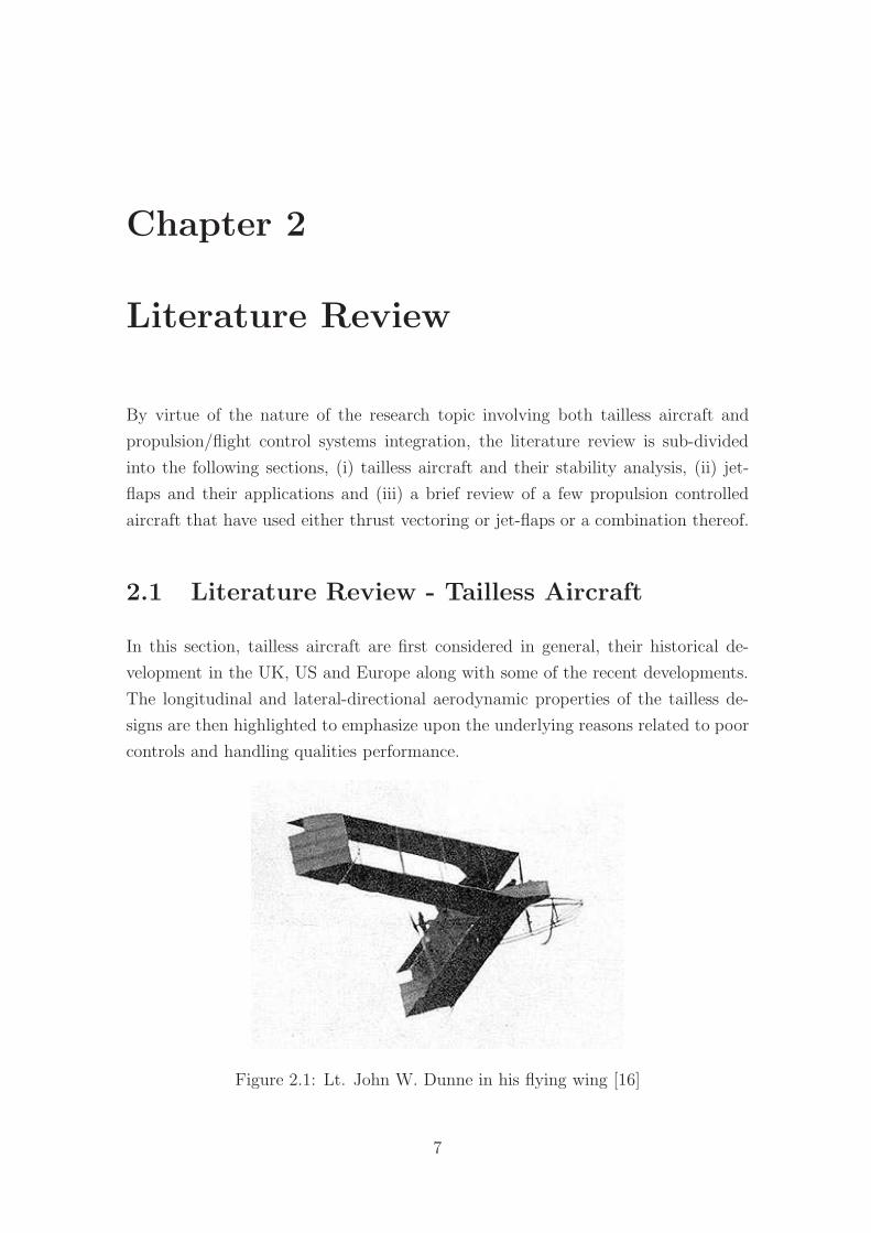
Figure 2.1: Lt. John W. Dunne in his flying wing [16]
7
2 Literature Review
2.1.1 A Historical Perspective
Developments in the UK and Germany - Some of the earliest contributions to
flying wings came from Lt. John W. Dunne [17] of UK between the period 1907-1914.
He started his work from a tailless glider and followed it up by a series of powered
bi-planes. Even at this early stage of development, he had realized the advantage of
wing sweep to increase the effective tail length. He also incorporated wash out or
twist at the wing tips to counteract the premature tip stall characteristics, that are
inherent in swept wing designs. One of his many works is shown in Figure 2.1.
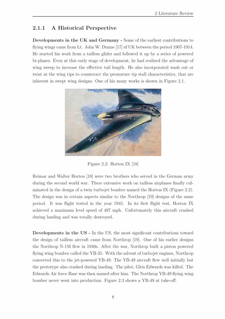
Figure 2.2: Horten IX [18]
Reimar and Walter Horten [18] were two brothers who served in the German army
during the second world war. There extensive work on tailless airplanes finally cul-
minated in the design of a twin turbojet bomber named the Horton IX (Figure 2.2).
The design was in certain aspects similar to the Northrop [19] designs of the same
period. It was flight tested in the year 1945. In its first flight test, Horton IX
achieved a maximum level speed of 497 mph. Unfortunately this aircraft crashed
during landing and was totally destroyed.
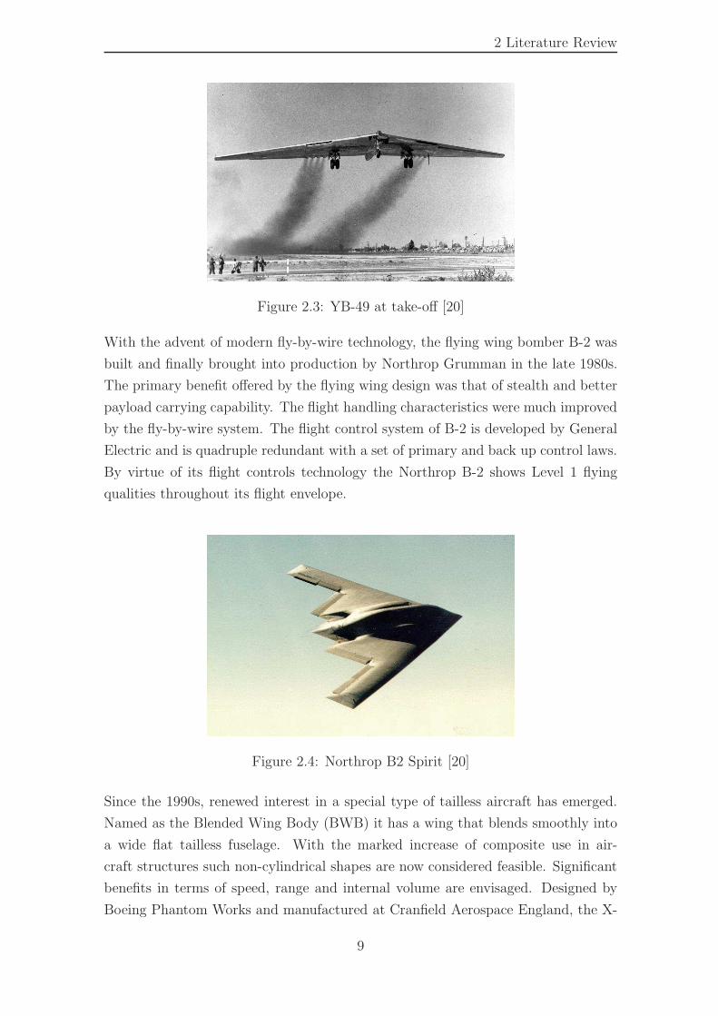
Developments in the US - In the US, the most significant contributions toward
the design of tailless aircraft came from Northrop [19]. One of his earlier designs
the Northrop N-1M flew in 1940s. After the war, Northrop built a piston powered
flying wing bomber called the YB-35. With the advent of turbojet engines, Northrop
converted this to the jet-powered YB-49. The YB-49 aircraft flew well initially but
the prototype also crashed during landing. The pilot, Glen Edwards was killed. The
Edwards Air force Base was then named after him. The Northrop YB-49 flying wing
bomber never went into production. Figure 2.3 shows a YB-49 at take-off.
8
2 Literature Review
Figure 2.3: YB-49 at take-off [20]
With the advent of modern fly-by-wire technology, the flying wing bomber B-2 was
built and finally brought into production by Northrop Grumman in the late 1980s.
The primary benefit offered by the flying wing design was that of stealth and better
payload carrying capability. The flight handling characteristics were much improved
by the fly-by-wire system. The flight control system of B-2 is developed by General
Electric and is quadruple redundant with a set of primary and back up control laws.
By virtue of its flight controls technology the Northrop B-2 shows Level 1 flying
qualities throughout its flight envelope.
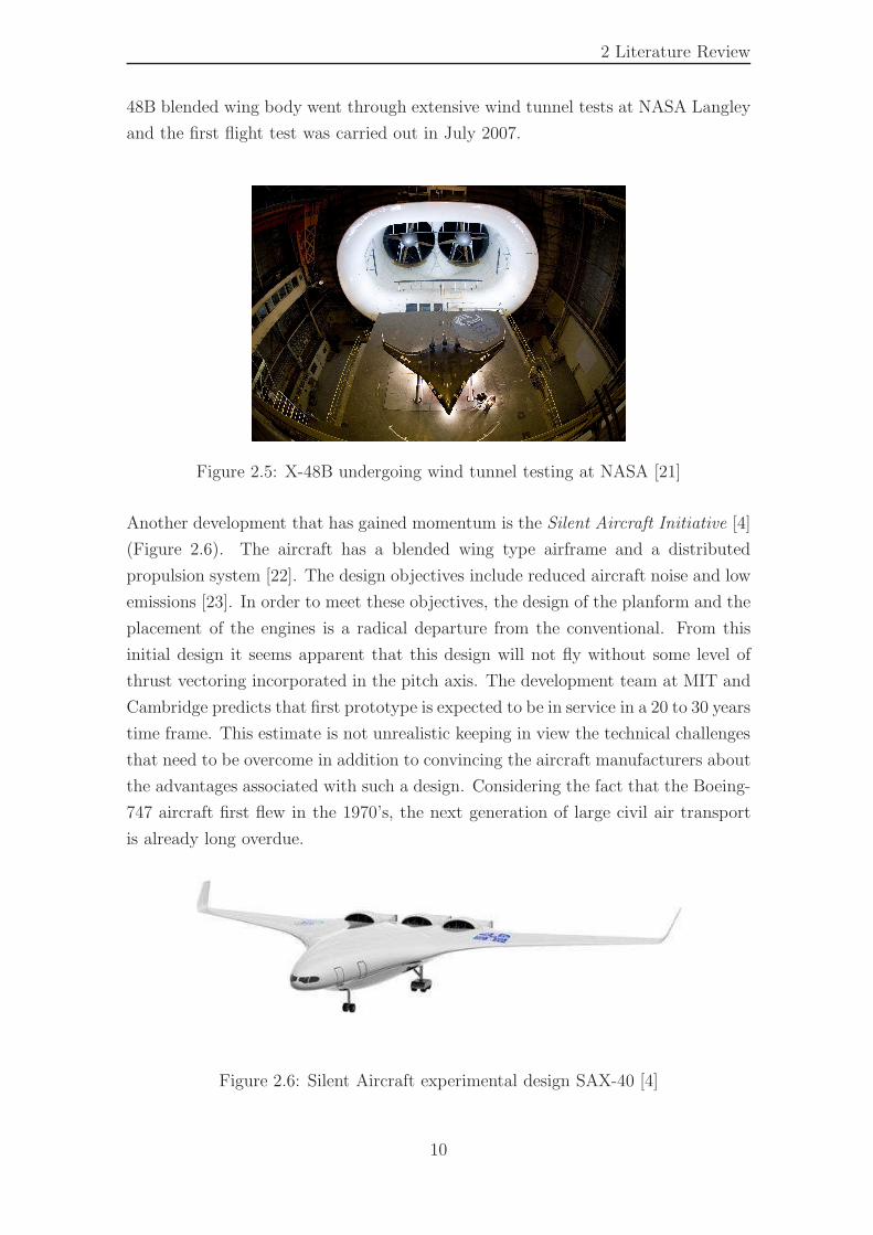
Figure 2.4: Northrop B2 Spirit [20]
Since the 1990s, renewed interest in a special type of tailless aircraft has emerged.
Named as the Blended Wing Body (BWB) it has a wing that blends smoothly into
a wide flat tailless fuselage. With the marked increase of composite use in air-
craft structures such non-cylindrical shapes are now considered feasible. Significant
benefits in terms of speed, range and internal volume are envisaged. Designed by
Boeing Phantom Works and manufactured at Cranfield Aerospace England, the X-
9
2 Literature Review
48B blended wing body went through extensive wind tunnel tests at NASA Langley
and the first flight test was carried out in July 2007.
Figure 2.5: X-48B undergoing wind tunnel testing at NASA [21]
Another development that has gained momentum is the Silent Aircraft Initiative [4]
(Figure 2.6). The aircraft has a blended wing type airframe and a distributed
propulsion system [22]. The design objectives include reduced aircraft noise and low
emissions [23]. In order to meet these objectives, the design of the planform and the
placement of the engines is a radical departure from the conventional. From this
initial design it seems apparent that this design will not fly without some level of
thrust vectoring incorporated in the pitch axis. The development team at MIT and
Cambridge predicts that first prototype is expected to be in service in a 20 to 30 years
time frame. This estimate is not unrealistic keeping in view the technical challenges
that need to be overcome in addition to convincing the aircraft manufacturers about
the advantages associated with such a design. Considering the fact that the Boeing-
747 aircraft first flew in the 1970’s, the next generation of large civil air transport
is already long overdue.
Figure 2.6: Silent Aircraft experimental design SAX-40 [4]
10
2 Literature Review
2.1.2 Tailless Aircraft and Longitudinal Stability
This section presents a review on some of the important longitudinal stability param-
eters as applicable to tailless designs. These include the pitch stiffness parameter,
Cmα , the pitch damping derivative, Cmq and the elevator control power, Cmδe . It
also includes a brief review of the influence of static margin, Kn, and wing sweep,
Λ, on the longitudinal stability of such aircraft.
2.1.2.1 Tailless Aircraft and Static Pitch Stability (Cmα)
A discussion on the underlying equations that govern the longitudinal stability of
tailless designs is considered. An appreciation of this aspect is important as it leads
the aircraft designer to shape the wing so that it provides both lift and control at
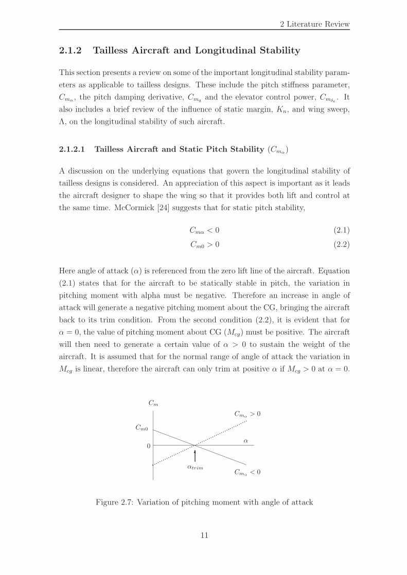
the same time. McCormick [24] suggests that for static pitch stability,
Cmα < 0 (2.1)
Cm0 > 0 (2.2)
Here angle of attack (α) is referenced from the zero lift line of the aircraft. Equation
(2.1) states that for the aircraft to be statically stable in pitch, the variation in
pitching moment with alpha must be negative. Therefore an increase in angle of
attack will generate a negative pitching moment about the CG, bringing the aircraft
back to its trim condition. From the second condition (2.2), it is evident that for
α = 0, the value of pitching moment about CG (Mcg) must be positive. The aircraft
will then need to generate a certain value of α > 0 to sustain the weight of the
aircraft. It is assumed that for the normal range of angle of attack the variation in
Mcg is linear, therefore the aircraft can only trim at positive α if Mcg > 0 at α = 0.
0
Cm
αtrim
6
Cmα> 0
Cm0
..
Cmα< 0
..........
..........
..........
..........
..........
....
α
Figure 2.7: Variation of pitching moment with angle of attack
11
2 Literature Review
In Figure 2.7 the aircraft is in trim at a certain positive value of angle of attack,
where the total pitching moment about the centre of gravity is zero. If the angle
of attack is now slightly increased from its trim value, the pitching moment about
CG varies almost linearly with alpha. For the line marked Cmα < 0, the increment
in pitching moment is negative. Thus a nose down moment is introduced which
for a given elevator setting, δe, brings the aircraft back to αtrim. In contrast, if the
variation of pitching moment marked with line Cmα > 0 is considered, the increment
in pitching moment with angle of attack is positive. This shall further increase the
angle of attack and the aircraft would quickly diverge in the pitch axis.
Wing
Mac
V
it
MO
?
:
6
?
K
?
htc -
� -
(ht − h)c --
Tail
h0c
�
c
hc �
LtLw
-
α
W
1
�
CG
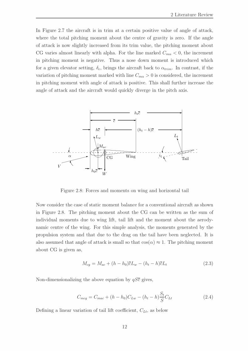
Figure 2.8: Forces and moments on wing and horizontal tail
Now consider the case of static moment balance for a conventional aircraft as shown
in Figure 2.8. The pitching moment about the CG can be written as the sum of
individual moments due to wing lift, tail lift and the moment about the aerody-
namic centre of the wing. For this simple analysis, the moments generated by the
propulsion system and that due to the drag on the tail have been neglected. It is
also assumed that angle of attack is small so that cos(α) ≈ 1. The pitching moment
about CG is given as,
Mcg = Mac + (h− h0)cLw − (ht − h)cLt (2.3)
Non-dimensionalizing the above equation by qSc gives,
Cmcg = Cmac + (h− h0)CLw − (ht − h)StSCLt (2.4)
Defining a linear variation of tail lift coefficient, CLt, as below
12
2 Literature Review
CLt = at[α
(
1 − dǫ
dα
)
− it] (2.5)
where at is the tail plane lift curve slope and the remaining term is the effective angle
of attack seen by the tail. It is less than the wing angle of attack, α, by the wing
down-wash effect, dǫ/dα, and the tail incidence angle, it. The wing lift coefficient
can also be expressed by a linear relationship
CLw = awα (2.6)
where aw is the lift curve slope of the wing. Equation (2.4) can now be written as
Cmcg = Cmac + (h− h0)awα− (ht − h)StSat
[
α
(
1 − dǫ
dα
)
− it
]
(2.7)
Equation (2.7) is the basic relationship for the pitching moment about CG for an
aircraft with a tail. Defining the following,
Cm0 = Cmac + (ht − h)StSatit (2.8)
Cmα = (h− h0)aw − (ht − h)StSat
(
1 − dǫ
dα
)
(2.9)
Equation (2.7) can be re-written as
Cmcg = Cm0 + Cmαα (2.10)
From Equation (2.2) we have argued that for positive pitch stability Cm0 > 0.
Examining Equation (2.8) it can be seen that for a tailed aircraft, Cm0 has two
parts. One due to wing, Cmac, and other due to the fixed incidence of the tail. For
positively cambered airfoils, Cmac is invariant with α and is negative. Overall Cm0
is then made positive by the second term (due to the tail) on the right hand side
of Equation (2.8). The tail setting angle, it, is defined positive downwards and the
distance between the tail aerodynamic centre and the CG, ht−h, is also positive. So
the contribution of the tail towards Cm0 is positive and helps to achieve the desired
condition of Cm0 > 0. For a tailless aircraft, Equation (2.8) reduces to
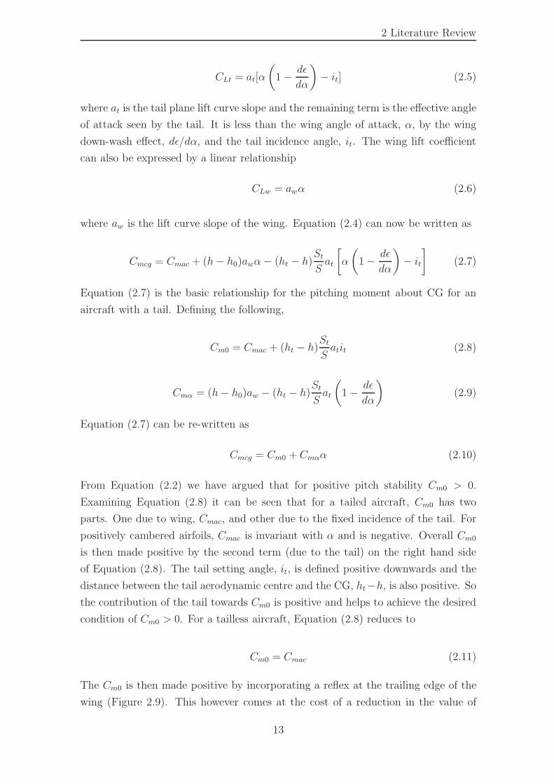
Cm0 = Cmac (2.11)
The Cm0 is then made positive by incorporating a reflex at the trailing edge of the
wing (Figure 2.9). This however comes at the cost of a reduction in the value of
13
2 Literature Review
achievable lift coefficient.
α
CG
6
?
L
W
ReflexRMac3
AC*
V
Figure 2.9: Trailing edge reflex for tailless airplanes
Referring to the expression for Cmα as given by Equation (2.9), it can be seen that it
also has two parts, one given by the wing and the other by the tail. From Equation
(2.1) it is known that for positive pitch stability, Cmα < 0. The second part (due
to the tail) on right hand side of Equation (2.9) provides most of the negative
component of Cmα. The first part (h − h0)aw, which is due to the wing is usually
positive with (h− h0) being positive. This means that the CG can be located aft of
the aerodynamic centre of the wing. For a tailless aircraft however, Equation (2.9)
reduces to
Cmα = (h− h0)aw (2.12)
The only way in which Cmα can now be be made negative is by setting (h−h0) < 0.
That is by locating the CG ahead of the aerodynamic centre of the wing. This
severely restricts the available CG range for tailless aircraft as compared to a con-
ventional configuration.
2.1.2.2 Tailless Aircraft and Pitch Damping (Cmq)
For aircraft with horizontal stabilizers, most of the pitch damping is contributed by
the horizontal stabilizer. However Jones [25] points out that as long as the aircraft
has a positive static margin, a lower value of Cmq associated with tailless airplanes
is not a serious disadvantage. Northrop [19] further explains that although the value
of Cmq is low for tailless airplanes, the short period oscillation is well damped. This
is due to the vertical damping parameter, CZw, that absorbs most of the energy of
oscillation.
14
2 Literature Review
Donlan [26] further suggests that a reduced or a negative static margin for tailless
aircraft may result in an uncontrolled dynamic instability called tumbling. Tum-
bling consists of a continuous pitching rotation about the lateral axis of the airplane.
Conventional control surfaces are almost rendered useless once the tumbling motion
is initiated. Donlan [26] continues to state that to avoid this tumbling dynamic
mode, the centre of gravity of a tailless airplane should never be permitted under
any condition to reach a position behind the aerodynamic centre of the wing. Fre-
maux [27] however argues that a positive static margin is not a guarantee against the
tumbling phenomenon for tailless aircraft. The absence of the horizontal stabilizer
and thus reduced pitch damping, Cmq, is a big drawback in this context.
2.1.2.3 Tailless Aircraft and Elevator Control Power (Cmδe)
The type of longitudinal control usually employed for tailless aircraft consists of
an elevator (or flap) placed at the trailing edge of the wing. For the same static
margin, the elevator of a tailless airplane usually must be deflected considerably
more than that of a conventional airplane to produce the same change in pitching
moment coefficient Cm. Donlan [26] also analyzes the control power required for
take-off conditions. At take-off, the longitudinal control besides supplying a pitching
moment to trim the aircraft, must also be able to provide the additional pitching
moment necessary to counteract:
• Pitching moment of the weight of airplane about the point of ground contact.
• Pitching moment created by friction force on wheels.
It appears likely that if some scheme of enhancing the elevator control power (Cmδe)
is not provided the nose wheel would not lift off, especially for tailless aircrafts with
large static margins.
2.1.2.4 Tailless Aircraft and Static Margin (Kn)
For a tailless aircraft, the static margin is simply the non-dimensional distance
between the aerodynamic centre (AC) of the wing and the CG location. It is positive
if CG is ahead of AC toward nose. The longitudinal control power and dynamic
stability problems severely restrict the CG range for tailless airplanes. Donlan [26]
suggests an ultimate static margin range of 0.02 to 0.08 for such aircraft. Castro [7]
also states that due to the limited control power the positive static margin has to be
limited to lower values than those of conventional aircraft. Northrop [19] however
15
2 Literature Review
argues that an unstable configuration augmented with the power of a digital fly-by-
wire flight control system provides the best design option for a tailless aircraft. The
final range of static margin for any aircraft can however only be ascertained after a
full dynamic and static stability analysis throughout its flight envelope.
2.1.2.5 Effect of Wing Sweep (Λ) on Tailless Aircraft
It was noted by Thorpe [28] that sweep-back gives the wing an effective tail length
and is therefore especially adaptable for tailless airplanes. High lift flaps can then
be placed at the centre of the wing where their lift increments produce only mi-
nor changes in pitching moment about the centre of gravity. Flaps for longitudinal
control can be located near the wing tips to produce the requisite pitching moment
for trim. Furthermore, he adds that sweep-back introduces the undesirable effect of
premature tip stall, which can be avoided by use of wash out or wing twist. This
lowers the angle of attack of the tip section.
Another effective method advocated by Donlan [26] to overcome tip stall was the
use of leading edge slats. He states that if this method is properly implemented,
it could delay tip stall by 10◦. Thorpe [28] further states that use of wing sweep
enhances the elevator control power but introduces a worse problem of tip stall due
to lateral growth of boundary layer over the swept wing. This, if left untreated, may
result in wing drop and loss of control due to lack of flow over the control surface.
Northrop [19] also concludes that sweep back provides probably the best way to
enhance longitudinal control power for tailless designs.
16
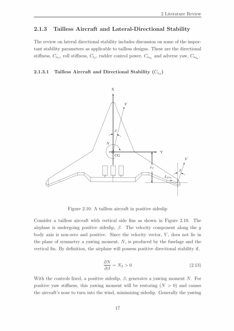
2 Literature Review
2.1.3 Tailless Aircraft and Lateral-Directional Stability
The review on lateral directional stability includes discussion on some of the impor-
tant stability parameters as applicable to tailless designs. These are the directional
stiffness, Cnβ , roll stiffness, Clβ , rudder control power, Cnδr and adverse yaw, Cnδa .
2.1.3.1 Tailless Aircraft and Directional Stability (Cnβ)
6
�
�
X
-
V
VCG
U
N
i:
i:
β
β
6Y
?
xf
iLfin
Figure 2.10: A tailless aircraft in positive sideslip
Consider a tailless aircraft with vertical side fins as shown in Figure 2.10. The
airplane is undergoing positive sideslip, β. The velocity component along the y
body axis is non-zero and positive. Since the velocity vector, V , does not lie in
the plane of symmetry a yawing moment, N , is produced by the fuselage and the
vertical fin. By definition, the airplane will possess positive directional stability if,
∂N
∂β= Nβ > 0 (2.13)
With the controls fixed, a positive sideslip, β, generates a yawing moment N . For
positive yaw stiffness, this yawing moment will be restoring (N > 0) and causes
the aircraft’s nose to turn into the wind, minimizing sideslip. Generally the yawing
17
2 Literature Review
moment from the fuselage is de-stabilizing however the contribution from an aft-
placed vertical fin is stabilizing. This yawing moment may be expressed as
N = qSbCn (2.14)
where Cn is the yawing moment coefficient, S is the reference area, b is the charac-
teristic length and q is the free stream dynamic pressure. The lift from the vertical
fin is
Lfin =1
2ρVt
2SfCLf (2.15)
If the distance of the mean aerodynamic centre of the vertical fin and the centre of
gravity of aircraft is xf , then the yawing moment generated by the fin is
Nf = Lfinxf =1
2ρVt
2SfCLfxf (2.16)
But CLf = af (1− dǫdβ
)β, where af is the vertical fin lift curve slope and dǫ/dβ is the
down wash factor of fuselage and wing on the vertical fin. Therefore (2.15) becomes,
Nf =1
2ρVt
2Sfafxf (1 − dǫ
dβ)β (2.17)
Non-dimensionalizing by qSb and taking partial derivative w.r.t β gives,
Cnβfin =SfS
xfbaf(1 − dǫ
dβ) (2.18)
From the above equation, it is evident that directional stiffness parameter Cnβ is a
function of the vertical fin area Sf and fin moment arm xf . For flying wings it is
usual practice to place the vertical fins at the wing tips. Structurally it becomes
difficult to provide a large fin area using such an arrangement. The fin moment
arm, xf , is also reduced significantly. Directional stability will thus start depending
upon on the contribution from the wing/fuselage combination. This may be diffi-
cult to calculate theoretically but can be measured quite accurately in a wind tunnel.
Donlan [26] in his report has mentioned about the difficulty in achieving the accept-
able values of Cnβ for flying wings. During a series of wind tunnel tests conducted
at NASA Langley it was noted that achievable values of Cnβ are less than one third
to that of airplanes with tails. This poses a significant challenge in achieving the
desired value of weather-cock stability for flying wings.
18
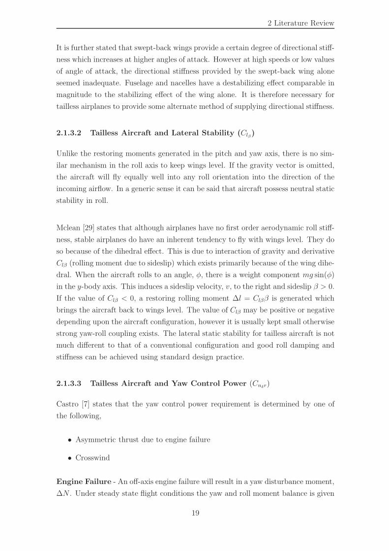
2 Literature Review
It is further stated that swept-back wings provide a certain degree of directional stiff-
ness which increases at higher angles of attack. However at high speeds or low values
of angle of attack, the directional stiffness provided by the swept-back wing alone
seemed inadequate. Fuselage and nacelles have a destabilizing effect comparable in
magnitude to the stabilizing effect of the wing alone. It is therefore necessary for
tailless airplanes to provide some alternate method of supplying directional stiffness.
2.1.3.2 Tailless Aircraft and Lateral Stability (Clβ)
Unlike the restoring moments generated in the pitch and yaw axis, there is no sim-
ilar mechanism in the roll axis to keep wings level. If the gravity vector is omitted,
the aircraft will fly equally well into any roll orientation into the direction of the
incoming airflow. In a generic sense it can be said that aircraft possess neutral static
stability in roll.
Mclean [29] states that although airplanes have no first order aerodynamic roll stiff-
ness, stable airplanes do have an inherent tendency to fly with wings level. They do
so because of the dihedral effect. This is due to interaction of gravity and derivative
Clβ (rolling moment due to sideslip) which exists primarily because of the wing dihe-
dral. When the aircraft rolls to an angle, φ, there is a weight component mg sin(φ)
in the y-body axis. This induces a sideslip velocity, v, to the right and sideslip β > 0.
If the value of Clβ < 0, a restoring rolling moment ∆l = Clββ is generated which
brings the aircraft back to wings level. The value of Clβ may be positive or negative
depending upon the aircraft configuration, however it is usually kept small otherwise
strong yaw-roll coupling exists. The lateral static stability for tailless aircraft is not
much different to that of a conventional configuration and good roll damping and
stiffness can be achieved using standard design practice.
2.1.3.3 Tailless Aircraft and Yaw Control Power (Cnδr)
Castro [7] states that the yaw control power requirement is determined by one of
the following,
• Asymmetric thrust due to engine failure
• Crosswind
Engine Failure - An off-axis engine failure will result in a yaw disturbance moment,
∆N . Under steady state flight conditions the yaw and roll moment balance is given
19

2 Literature Review
as,
∆N = qSb(Cnββ + Cnδaδa+ Cnδrδr) (2.19)
Cl = 0 = Clββ + Clδaδa+ Clδrδr (2.20)
The cross derivatives namely yawing moment due to aileron deflection, Cnδa, (ad-
verse yaw) and rolling moment due to rudder deflection (adverse roll), Clδr, also
appear in the above equations. Assuming zero sideslip (β = 0), the above reduces to
a system of two equations and can be solved analytically for two unknowns (δa, δr).
The rudder deflection will be required to counteract the disturbance in yaw and the
aileron deflection will be required to counteract adverse roll generated by the rudder.
Cross wind - For the cross wind case, the sideslip is not zero and the equations
can be simply re-written as
tan β =v
Vt(2.21)
Cn = 0 = Cnββ + Cnδaδa+ Cnδrδr (2.22)
Cl = 0 = Clββ + Clδaδa+ Clδrδr (2.23)
where v is the wind component in the y-body axis. The net rolling and yawing
moment coefficients are considered zero. The above equations can be solved analyt-
ically for the aileron and rudder deflections required for steady state side slipping
flight.
Castro [7] analyzes four blended wing configurations for assessment of rudder power
under these conditions. For the engine failed case with β = 0 it was found that
the aircraft with maximum control power, Cnδr, required the minimum amount of
rudder deflection to trim the engine moment. This was as expected. However under
cross-wind conditions (β 6= 0) the same aircraft had the maximum deflection re-
quired to trim since directional stiffness, Cnβ, was also large for that aircraft. High
directional stiffness though desirable therefore becomes a problem under severe cross
wind conditions especially at landing.
Various kinds of rudders were tested by Northrop [19] in his early designs. The most
successful design was that of the double split flap drag rudder shown in Figure 2.11.
Split flaps generate yawing moment by the differential drag on the split flaps and
by virtue of their long moment arm (approximately half span) from the centre of
20
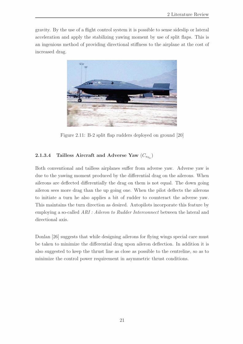
2 Literature Review
gravity. By the use of a flight control system it is possible to sense sideslip or lateral
acceleration and apply the stabilizing yawing moment by use of split flaps. This is
an ingenious method of providing directional stiffness to the airplane at the cost of
increased drag.
Figure 2.11: B-2 split flap rudders deployed on ground [20]
2.1.3.4 Tailless Aircraft and Adverse Yaw (Cnδa )
Both conventional and tailless airplanes suffer from adverse yaw. Adverse yaw is
due to the yawing moment produced by the differential drag on the ailerons. When
ailerons are deflected differentially the drag on them is not equal. The down going
aileron sees more drag than the up going one. When the pilot deflects the ailerons
to initiate a turn he also applies a bit of rudder to counteract the adverse yaw.
This maintains the turn direction as desired. Autopilots incorporate this feature by
employing a so-called ARI : Aileron to Rudder Interconnect between the lateral and
directional axis.
Donlan [26] suggests that while designing ailerons for flying wings special care must
be taken to minimize the differential drag upon aileron deflection. In addition it is
also suggested to keep the thrust line as close as possible to the centreline, so as to
minimize the control power requirement in asymmetric thrust conditions.
21
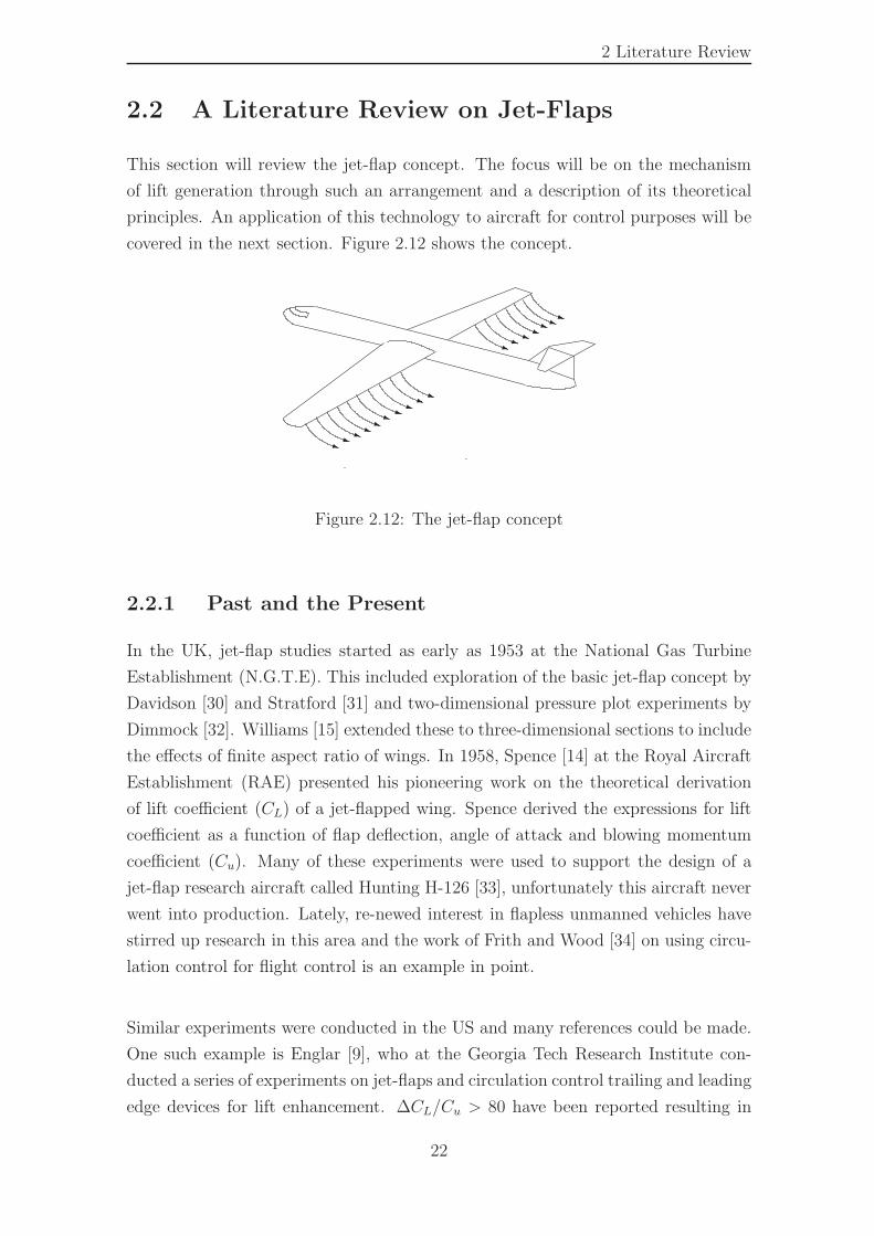
2 Literature Review
2.2 A Literature Review on Jet-Flaps
This section will review the jet-flap concept. The focus will be on the mechanism
of lift generation through such an arrangement and a description of its theoretical
principles. An application of this technology to aircraft for control purposes will be
covered in the next section. Figure 2.12 shows the concept.
qqqqqqq
qqqqqqq
qqq
Figure 2.12: The jet-flap concept
2.2.1 Past and the Present
In the UK, jet-flap studies started as early as 1953 at the National Gas Turbine
Establishment (N.G.T.E). This included exploration of the basic jet-flap concept by
Davidson [30] and Stratford [31] and two-dimensional pressure plot experiments by
Dimmock [32]. Williams [15] extended these to three-dimensional sections to include
the effects of finite aspect ratio of wings. In 1958, Spence [14] at the Royal Aircraft
Establishment (RAE) presented his pioneering work on the theoretical derivation
of lift coefficient (CL) of a jet-flapped wing. Spence derived the expressions for lift
coefficient as a function of flap deflection, angle of attack and blowing momentum
coefficient (Cu). Many of these experiments were used to support the design of a
jet-flap research aircraft called Hunting H-126 [33], unfortunately this aircraft never
went into production. Lately, re-newed interest in flapless unmanned vehicles have
stirred up research in this area and the work of Frith and Wood [34] on using circu-
lation control for flight control is an example in point.
Similar experiments were conducted in the US and many references could be made.
One such example is Englar [9], who at the Georgia Tech Research Institute con-
ducted a series of experiments on jet-flaps and circulation control trailing and leading
edge devices for lift enhancement. ∆CL/Cu > 80 have been reported resulting in
22
2 Literature Review
lift coefficients comparable to or better than most complex mechanical flap systems.
Englar further analyzes the application of these concepts to a representative model
of Boeing 737-100 during take-off and landing. Take-off performance was verified
against a 50 ft obstacle. Using analytical studies it was shown that the take-off
distance could reduced by more than 50% and the landing speed be reduced up to
40% due to blowing from the trailing edge of the airfoil. The bleed mass flow from
the engine was restricted to 5% of the overall fan inflow resulting in a appoximately
5% loss in thrust. For cruise, climb or descent, jet-flaps were not used.
2.2.2 Jet-Flaps and Mechanism of High Lift
Figure 2.13: Flow control through a trailing edge blown flap [8]
There are two fundamental methods to change the lift coefficient of the airfoil. These
are, (i) to adjust the angle of attack of the airfoil relative to the incoming airflow
or (ii) to deflect the trailing edge flap i-e change its geometry. As the angle of
attack is increased or the flaps are deflected to higher values, flow separation sets
in. This occurs either at the wing tip or close to flap hinge. The frictional losses
in the boundary layer causes the flow to loose much of its kinetic energy and in the
presence of adverse pressure gradient it eventually separates. This puts an upper
limit on the achievable lift coefficients [8]. The flow separation can be overcome by
either
• Removing the low energy fluid from boundary layer through suction
• Re-energizing the boundary layer through blowing
23
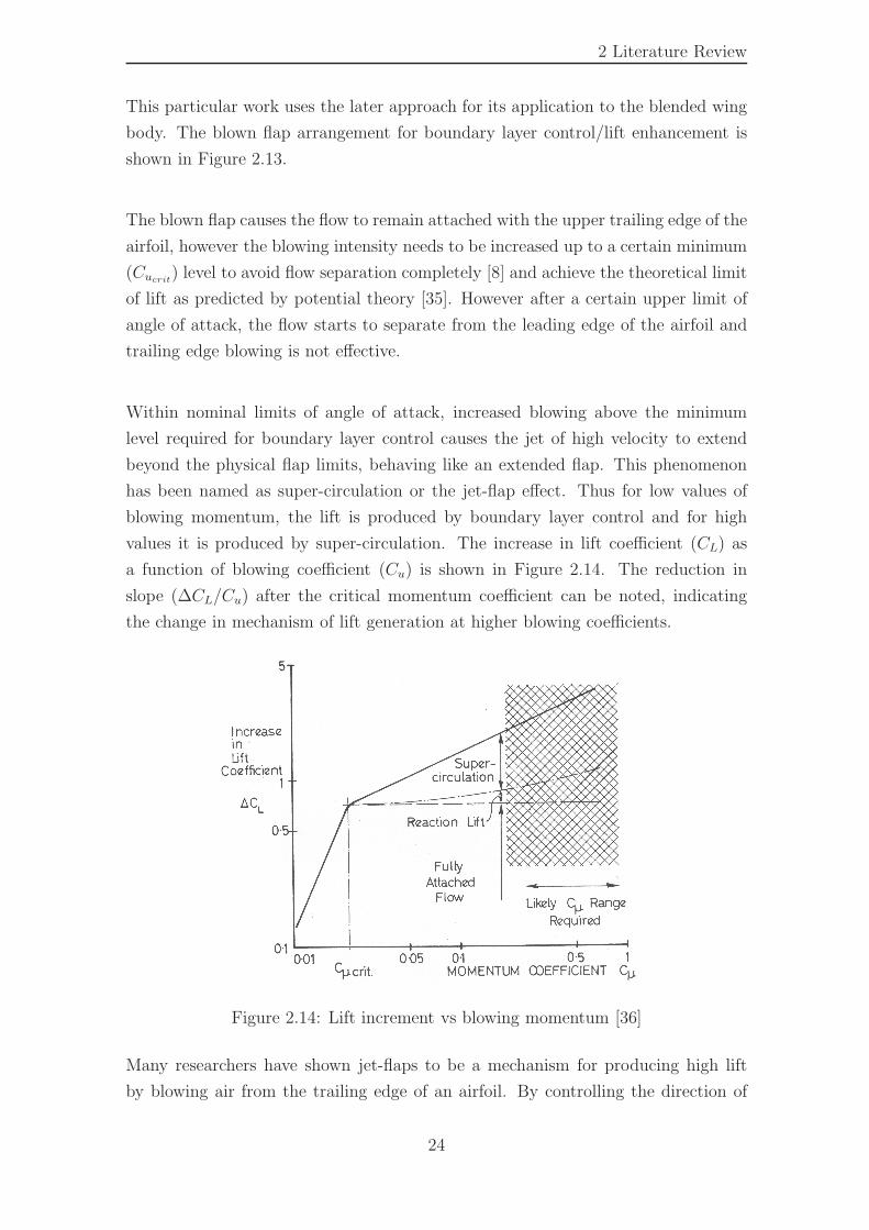
2 Literature Review
This particular work uses the later approach for its application to the blended wing
body. The blown flap arrangement for boundary layer control/lift enhancement is
shown in Figure 2.13.
The blown flap causes the flow to remain attached with the upper trailing edge of the
airfoil, however the blowing intensity needs to be increased up to a certain minimum
(Cucrit) level to avoid flow separation completely [8] and achieve the theoretical limit
of lift as predicted by potential theory [35]. However after a certain upper limit of
angle of attack, the flow starts to separate from the leading edge of the airfoil and
trailing edge blowing is not effective.
Within nominal limits of angle of attack, increased blowing above the minimum
level required for boundary layer control causes the jet of high velocity to extend
beyond the physical flap limits, behaving like an extended flap. This phenomenon
has been named as super-circulation or the jet-flap effect. Thus for low values of
blowing momentum, the lift is produced by boundary layer control and for high
values it is produced by super-circulation. The increase in lift coefficient (CL) as
a function of blowing coefficient (Cu) is shown in Figure 2.14. The reduction in
slope (∆CL/Cu) after the critical momentum coefficient can be noted, indicating
the change in mechanism of lift generation at higher blowing coefficients.
Figure 2.14: Lift increment vs blowing momentum [36]
Many researchers have shown jet-flaps to be a mechanism for producing high lift
by blowing air from the trailing edge of an airfoil. By controlling the direction of
24
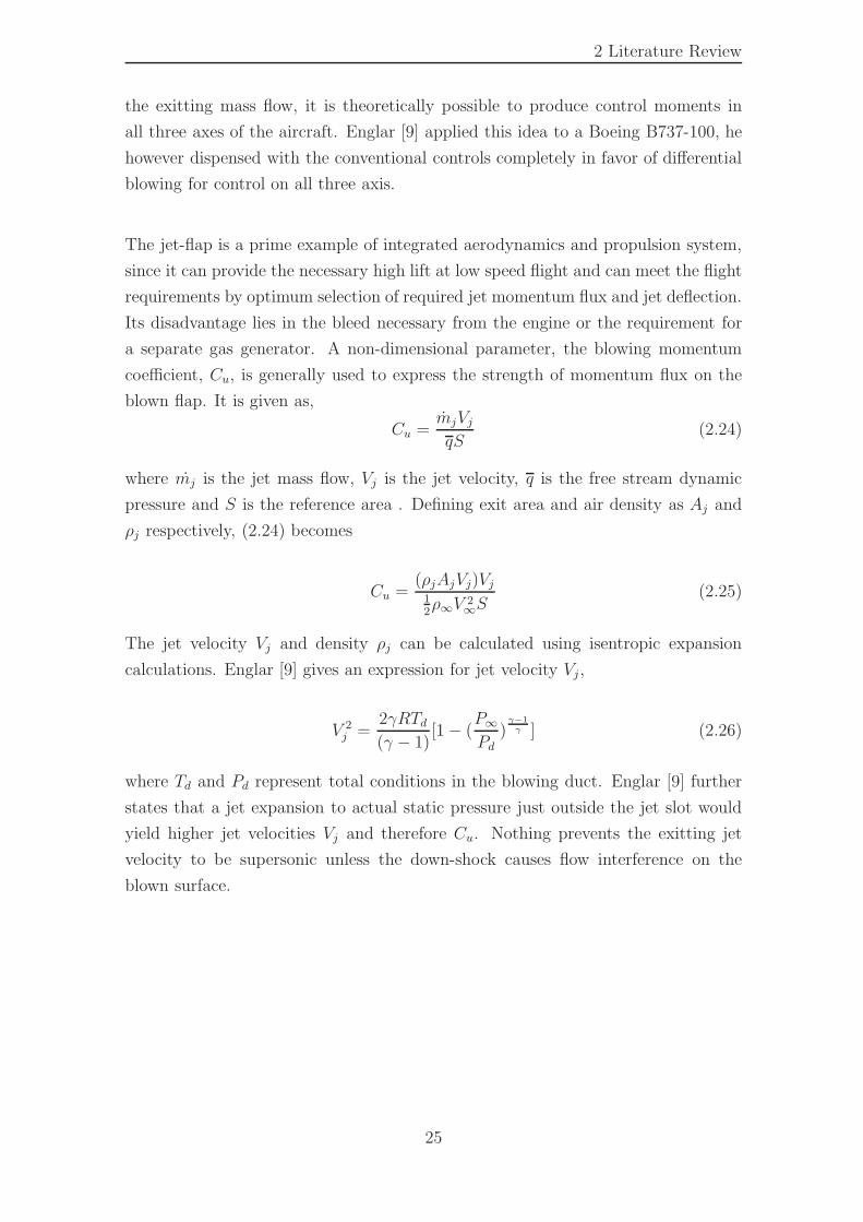
2 Literature Review
the exitting mass flow, it is theoretically possible to produce control moments in
all three axes of the aircraft. Englar [9] applied this idea to a Boeing B737-100, he
however dispensed with the conventional controls completely in favor of differential
blowing for control on all three axis.
The jet-flap is a prime example of integrated aerodynamics and propulsion system,
since it can provide the necessary high lift at low speed flight and can meet the flight
requirements by optimum selection of required jet momentum flux and jet deflection.
Its disadvantage lies in the bleed necessary from the engine or the requirement for
a separate gas generator. A non-dimensional parameter, the blowing momentum
coefficient, Cu, is generally used to express the strength of momentum flux on the
blown flap. It is given as,
Cu =mjVjqS
(2.24)
where mj is the jet mass flow, Vj is the jet velocity, q is the free stream dynamic
pressure and S is the reference area . Defining exit area and air density as Aj and
ρj respectively, (2.24) becomes
Cu =(ρjAjVj)Vj
12ρ∞V 2
∞S
(2.25)
The jet velocity Vj and density ρj can be calculated using isentropic expansion
calculations. Englar [9] gives an expression for jet velocity Vj ,
V 2j =
2γRTd(γ − 1)
[1 − (P∞
Pd)γ−1γ ] (2.26)
where Td and Pd represent total conditions in the blowing duct. Englar [9] further
states that a jet expansion to actual static pressure just outside the jet slot would
yield higher jet velocities Vj and therefore Cu. Nothing prevents the exitting jet
velocity to be supersonic unless the down-shock causes flow interference on the
blown surface.
25
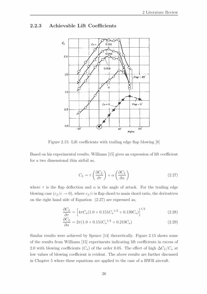
2 Literature Review
2.2.3 Achievable Lift Coefficients
Figure 2.15: Lift coefficients with trailing edge flap blowing [8]
Based on his experimental results, Williams [15] gives an expression of lift coefficient
for a two dimensional thin airfoil as,
CL = τ
(
∂CL∂τ
)
+ α
(
∂CL∂α
)
(2.27)
where τ is the flap deflection and α is the angle of attack. For the trailing edge
blowing case (cf/c→ 0), where cf/c is flap chord to main chord ratio, the derivatives
on the right hand side of Equation (2.27) are expressed as,
∂CL∂τ
=[
4πCu(1.0 + 0.151Cu1/2 + 0.139Cu)
]1/2
(2.28)
∂CL∂α
= 2π(1.0 + 0.151Cu1/2 + 0.219Cu) (2.29)
Similar results were achieved by Spence [14] theoretically. Figure 2.15 shows some
of the results from Williams [15] experiments indicating lift coefficients in excess of
2.0 with blowing coefficients (Cu) of the order 0.05. The effect of high ∆CL/Cu at
low values of blowing coefficient is evident. The above results are further discussed
in Chapter 5 where these equations are applied to the case of a BWB aircraft.
26
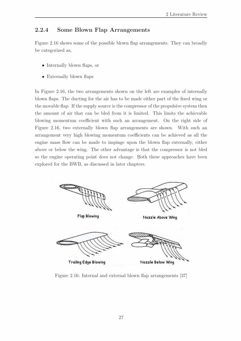
2 Literature Review
2.2.4 Some Blown Flap Arrangements
Figure 2.16 shows some of the possible blown flap arrangements. They can broadly
be categorized as,
• Internally blown flaps, or
• Externally blown flaps
In Figure 2.16, the two arrangements shown on the left are examples of internally
blown flaps. The ducting for the air has to be made either part of the fixed wing or
the movable flap. If the supply source is the compressor of the propulsive system then
the amount of air that can be bled from it is limited. This limits the achievable
blowing momentum coefficient with such an arrangement. On the right side of
Figure 2.16, two externally blown flap arrangements are shown. With such an
arrangement very high blowing momentum coefficients can be achieved as all the
engine mass flow can be made to impinge upon the blown flap externally, either
above or below the wing. The other advantage is that the compressor is not bled
so the engine operating point does not change. Both these approaches have been
explored for the BWB, as discussed in later chapters.
Figure 2.16: Internal and external blown flap arrangements [37]
27
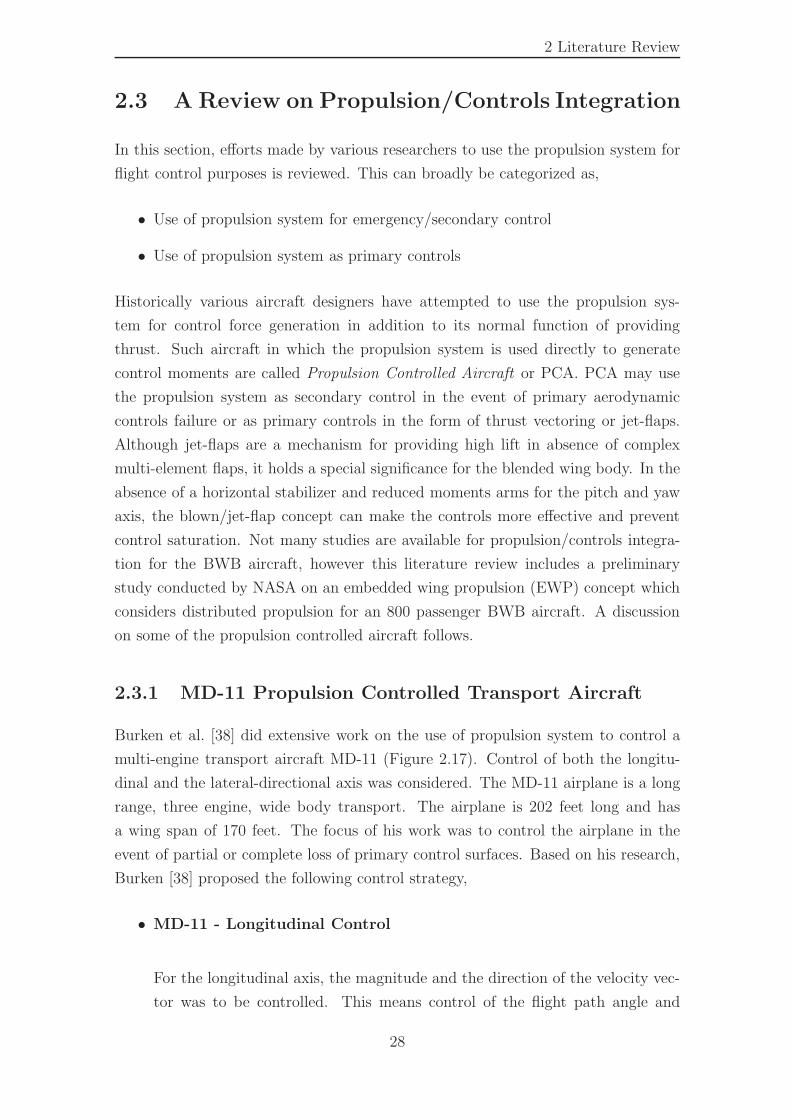
2 Literature Review
2.3 A Review on Propulsion/Controls Integration
In this section, efforts made by various researchers to use the propulsion system for
flight control purposes is reviewed. This can broadly be categorized as,
• Use of propulsion system for emergency/secondary control
• Use of propulsion system as primary controls
Historically various aircraft designers have attempted to use the propulsion sys-
tem for control force generation in addition to its normal function of providing
thrust. Such aircraft in which the propulsion system is used directly to generate
control moments are called Propulsion Controlled Aircraft or PCA. PCA may use
the propulsion system as secondary control in the event of primary aerodynamic
controls failure or as primary controls in the form of thrust vectoring or jet-flaps.
Although jet-flaps are a mechanism for providing high lift in absence of complex
multi-element flaps, it holds a special significance for the blended wing body. In the
absence of a horizontal stabilizer and reduced moments arms for the pitch and yaw
axis, the blown/jet-flap concept can make the controls more effective and prevent
control saturation. Not many studies are available for propulsion/controls integra-
tion for the BWB aircraft, however this literature review includes a preliminary
study conducted by NASA on an embedded wing propulsion (EWP) concept which
considers distributed propulsion for an 800 passenger BWB aircraft. A discussion
on some of the propulsion controlled aircraft follows.
2.3.1 MD-11 Propulsion Controlled Transport Aircraft
Burken et al. [38] did extensive work on the use of propulsion system to control a
multi-engine transport aircraft MD-11 (Figure 2.17). Control of both the longitu-
dinal and the lateral-directional axis was considered. The MD-11 airplane is a long
range, three engine, wide body transport. The airplane is 202 feet long and has
a wing span of 170 feet. The focus of his work was to control the airplane in the
event of partial or complete loss of primary control surfaces. Based on his research,
Burken [38] proposed the following control strategy,
• MD-11 - Longitudinal Control
For the longitudinal axis, the magnitude and the direction of the velocity vec-
tor was to be controlled. This means control of the flight path angle and
28
2 Literature Review
Figure 2.17: Mcdonald Douglas MD-11 transport aircraft [38]
airspeed. Burken [38] allocated individual control tasks to separate engines
available on the aircraft. Collective thrust changes on the wing engines were
used to implement flight path angle control and the tail engine was used to
implement speed control. A flight path error was formed which was passed
through a limited P+I network to generate a pitch angle demand. Pitch angle
and pitch rate feedback was then used to form collective commands for the
left and right engines. The use of pitch angle and pitch rate feedback ensured
adequate phugoid and short period damping. For speed control, Burken [38]
used the tail engine and a conventional auto-throttle speed control system.
• MD-11 - Lateral-directional Control
Lateral-directional control was obtained by using differential throttle inputs
to generate yaw, resulting in roll caused by the dihedral term, Clβ. The pri-
mary parameter to be controlled was aircraft heading. A heading error was
generated, which was used to generate a bank angle demand. Roll angle, roll
and yaw rates were used in the inner loops to control and damp the roll angle.
The differential thrust command was then transmitted to the left and right
wing engines. This was an intelligent way of obtaining roll control by use of
the dihedral effect.
This control strategy was later flight tested on an actual airplane. The aircraft was
successfully landed with the primary control surfaces locked at the neutral position.
29
2 Literature Review
2.3.2 Boeing - Propulsion/Flight Control System
Various studies have been carried out for propulsion and controls integration on
the Boeing aircraft. Two of these are presented here for the Boeing-747 and the
Boeing-737 aircraft respectively.
• Boeing-747 - Thrust Vectoring Control (TVC)
Harefors [39] at the University of Leicester recently conducted a study in col-
laboration with Volvo Aero Corporation on the design of an integrated propul-
sion and flight control system for a Boeing-747 aircraft. Both differential thrust
management and thrust vectoring control (TVC) were considered. The study
concludes that such aircraft can be effectively controlled by use of differential
and collective thrust only. To obtain control in all three axes, thrust vectoring
was implemented along y and z axes of the aircraft. The vectoring angles
(δy, δz) were limited to 45◦ and the slew rate limit on the nozzle actuators was
set at 60◦/s. The thrust components in the x, y and z aircraft axes are given
as
Tx = T cos δy cos δz
Ty = T sin δy cos δz
Tz = T cos δy sin δz
In this study, thrust vectoring was used on all four engines of the Boeing-747
to obtain control moments in three axes. Deflection in the x-z plane generates
a Tz force. This force, when used differentially on outboard engines, is most
effective in producing roll moment. The motion of the nozzle in the x-y plane
produces a Ty force which can be used to generate a yawing moment. The
pitching moment is generated by a contribution from the Tx force and that of
a Tz force due to the collective thrust vectoring in the x-z plane. Harefors [39]
concludes that effective control can be achieved with differential thrust for lat-
eral control and collective thrust for longitudinal control. The flying qualities
however using PCA alone are not as good as those obtained by use of aero-
dynamic control surfaces, but when PCA and TVC are combined, excellent
flying qualities were achieved for the lateral axis. For the longitudinal axis,
the TVC+PCA combination still falls short of the flying qualities achieved by
use of the horizontal stabilizer.
30
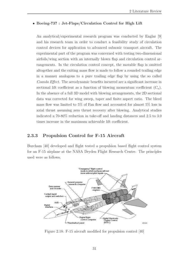
2 Literature Review
• Boeing-737 : Jet-Flaps/Circulation Control for High Lift
An analytical/experimental research program was conducted by Englar [9]
and his research team in order to conduct a feasibility study of circulation
control devices for application to advanced subsonic transport aircraft. The
experimental part of the program was concerned with testing two-dimensional
airfoils/wing section with an internally blown flap and circulation control ar-
rangements. In the circulation control concept, the movable flap is omitted
altogether and the exiting mass flow is made to follow a rounded trailing edge
in a manner analogous to a pure trailing edge flap by using the so called
Coanda Effect. The aerodynamic benefits incurred are a significant increase in
sectional lift coefficient as a function of blowing momentum coefficient (Cu).
In the absence of a full 3D model with blowing arrangements, the 2D sectional
data was corrected for wing sweep, taper and finite aspect ratio. The bleed
mass flow was limited to 5% of Fan flow and accounted for almost 5% loss in
axial thrust assuming zero thrust recovery after blowing. Analytical studies
indicated a 70-80% reduction in take-off and landing distances and 2.5 to 3.0
times increase in the maximum achievable lift coefficient.
2.3.3 Propulsion Control for F-15 Aircraft
Burcham [40] developed and flight tested a propulsion based flight control system
for an F-15 airplane at the NASA Dryden Flight Research Centre. The principles
used were as follows,
Figure 2.18: F-15 aircraft modified for propulsion control [40]
31
2 Literature Review
• Roll Control using Differential Thrust
Differential thrust generates sideslip that through the dihedral effect results
in roll rate. Roll rate is controlled to establish a bank angle that results in
a turn and a change in aircraft heading. Full differential thrust for the F-15
airplane yields a roll rate of approximately 15◦/sec at a speed of 170 kts. With
throttles-only flight control, bank is controlled by yaw and the turns were typ-
ically not coordinated.
• Longitudinal Control using Collective Thrust
Burcham [40] states that a thrust increase will cause an increase in speed that
results in greater lift. With the lift being more than the weight, the flightpath
angle will increase, causing the airplane to climb. If allowed to continue, this
effect will be oscillatory (phugoid mode). The degree of change to the flight-
path angle is proportional to the difference between the initial trim airspeed
and the current airspeed. Hence, the flightpath angle tends to increase as
speed or throttle increases.
If the thrust line is inclined nose up to the flightpath, an increase in thrust will
increase the vertical component of thrust. This increased vertical component
of thrust will cause a direct increase in vertical velocity (that is, rate of climb)
and a resulting increase in flightpath angle. For a given aircraft configuration,
this effect will increase as angle of attack is increased or the speed is lowered.
Burcham [40] states that for the F-15 airplane, the combination of the above
thrust effects is to produce a nose up flightpath angle rate response. This rate
response peaks at approximately 2◦/sec for an increase in throttle for level
flight to intermediate power on both engines at 170 kts.
Burcham [40] concludes that the PCA pitch and roll control provided adequate
up-and-away flight control. In addition, PCA system was used for landings and
was found adequate for safe runway landings in good weather. Pitch control was
sluggish but very stable. Approximately 10 seconds were required to achieve a
commanded flight path change. Bank angle control was positive but lagged inputs
by approximately 3 seconds. On approaches, the pilots spent most of their time
making bank angle corrections.
32
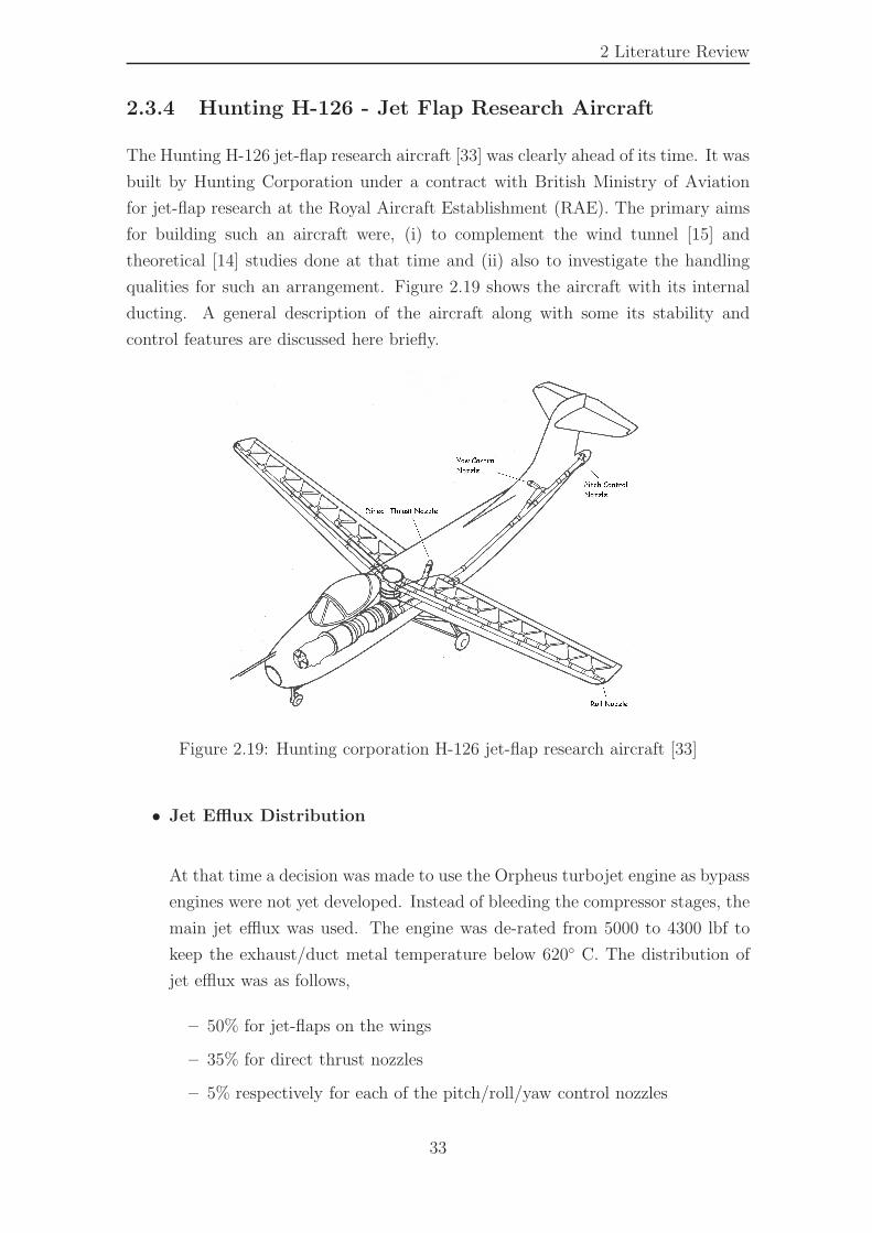
2 Literature Review
2.3.4 Hunting H-126 - Jet Flap Research Aircraft
The Hunting H-126 jet-flap research aircraft [33] was clearly ahead of its time. It was
built by Hunting Corporation under a contract with British Ministry of Aviation
for jet-flap research at the Royal Aircraft Establishment (RAE). The primary aims
for building such an aircraft were, (i) to complement the wind tunnel [15] and
theoretical [14] studies done at that time and (ii) also to investigate the handling
qualities for such an arrangement. Figure 2.19 shows the aircraft with its internal
ducting. A general description of the aircraft along with some its stability and
control features are discussed here briefly.
Figure 2.19: Hunting corporation H-126 jet-flap research aircraft [33]
• Jet Efflux Distribution
At that time a decision was made to use the Orpheus turbojet engine as bypass
engines were not yet developed. Instead of bleeding the compressor stages, the
main jet efflux was used. The engine was de-rated from 5000 to 4300 lbf to
keep the exhaust/duct metal temperature below 620◦ C. The distribution of
jet efflux was as follows,
– 50% for jet-flaps on the wings
– 35% for direct thrust nozzles
– 5% respectively for each of the pitch/roll/yaw control nozzles
33
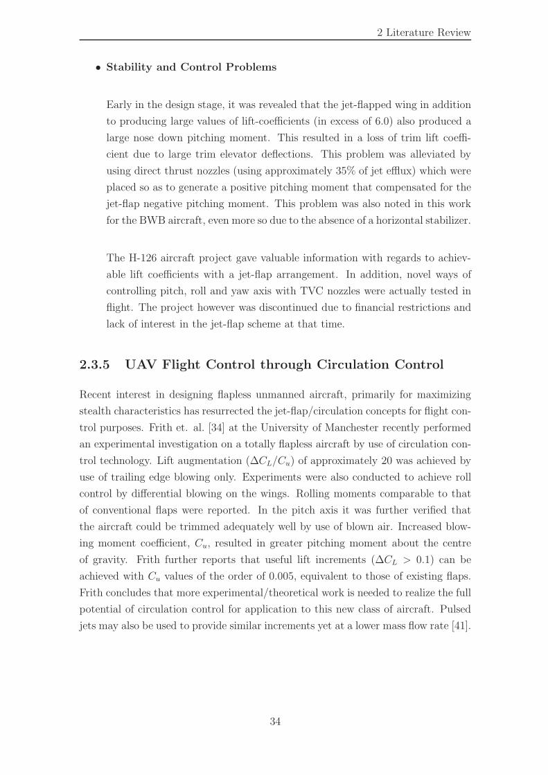
2 Literature Review
• Stability and Control Problems
Early in the design stage, it was revealed that the jet-flapped wing in addition
to producing large values of lift-coefficients (in excess of 6.0) also produced a
large nose down pitching moment. This resulted in a loss of trim lift coeffi-
cient due to large trim elevator deflections. This problem was alleviated by
using direct thrust nozzles (using approximately 35% of jet efflux) which were
placed so as to generate a positive pitching moment that compensated for the
jet-flap negative pitching moment. This problem was also noted in this work
for the BWB aircraft, even more so due to the absence of a horizontal stabilizer.
The H-126 aircraft project gave valuable information with regards to achiev-
able lift coefficients with a jet-flap arrangement. In addition, novel ways of
controlling pitch, roll and yaw axis with TVC nozzles were actually tested in
flight. The project however was discontinued due to financial restrictions and
lack of interest in the jet-flap scheme at that time.
2.3.5 UAV Flight Control through Circulation Control
Recent interest in designing flapless unmanned aircraft, primarily for maximizing
stealth characteristics has resurrected the jet-flap/circulation concepts for flight con-
trol purposes. Frith et. al. [34] at the University of Manchester recently performed
an experimental investigation on a totally flapless aircraft by use of circulation con-
trol technology. Lift augmentation (∆CL/Cu) of approximately 20 was achieved by
use of trailing edge blowing only. Experiments were also conducted to achieve roll
control by differential blowing on the wings. Rolling moments comparable to that
of conventional flaps were reported. In the pitch axis it was further verified that
the aircraft could be trimmed adequately well by use of blown air. Increased blow-
ing moment coefficient, Cu, resulted in greater pitching moment about the centre
of gravity. Frith further reports that useful lift increments (∆CL > 0.1) can be
achieved with Cu values of the order of 0.005, equivalent to those of existing flaps.
Frith concludes that more experimental/theoretical work is needed to realize the full
potential of circulation control for application to this new class of aircraft. Pulsed
jets may also be used to provide similar increments yet at a lower mass flow rate [41].
34
2 Literature Review
2.3.6 Embedded Wing Propulsion (EWP)
This last part of the literature review briefly discusses the distributed propulsion
work done at NASA. The propulsion-airframe integration efforts have culminated
into the so called Embedded Wing Propulsion (EWP) [42] concept. EWP is based
on a blended wing body and utilizes a large number of relatively smaller engines
embedded within the inboard wing structure. The leading edge forms the intake
and the trailing edge as the exit for the engine mass flow. The trailing and the
leading edge could be deflected to achieve high lift coefficients for take-off and land-
ing. Thrust vectoring was also considered for a 2D case using computational fluid
dynamics. The author concludes that EWP concept can be adapted for a variety of
missions with aerodynamics performance advantages. Figure 2.20 shows a notional
concept for the EWP.
Figure 2.20: The EWP concept for an 800 passenger BWB [42]
2.4 Conclusions - Literature Review
The literature review section has discussed at some length the tailless aircraft, jet-
flaps and some propulsion/controls integration concepts. Many more examples could
be given but have been omitted due to space limitations. Important conclusions can
be made from this review,
• Propulsion and flight control systems integration has been done on a number
of aircraft, more so for the conventional configuration. Tailless aircraft in
service are few and those with propulsion and controls integrated even less.
35

2 Literature Review
With emerging new configurations such as the blended wing body, the jet-
flap/blowing concepts for lift generation and flight control has gained renewed
interest.
• Large increments in lift coefficients can be achieved using the jet-flap scheme,
however it is accompanied by a significant nose down pitch moment. This
pitch moment has to be countered without a loss in trim lift coefficient before
the full potential of a blown flap arrangement can be utilized.
• Last but not the least, the supply of compressed air from any engine would
be limited and would result in a loss of thrust depending upon the percent-
age bleed. Any mechanism that utilizes the jet efflux directly without the
use of internal ducting and accompanying pressure losses would be therefore
preferred.
36
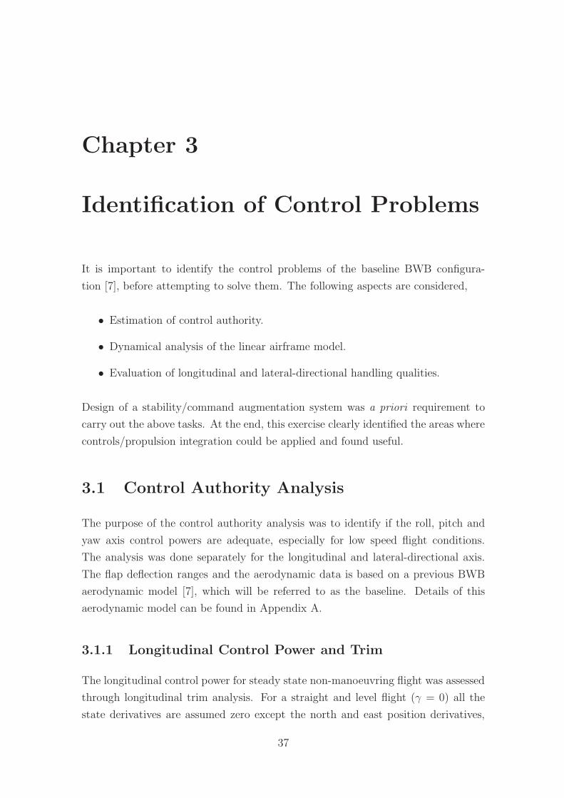
Chapter 3
Identification of Control Problems
It is important to identify the control problems of the baseline BWB configura-
tion [7], before attempting to solve them. The following aspects are considered,
• Estimation of control authority.
• Dynamical analysis of the linear airframe model.
• Evaluation of longitudinal and lateral-directional handling qualities.
Design of a stability/command augmentation system was a priori requirement to
carry out the above tasks. At the end, this exercise clearly identified the areas where
controls/propulsion integration could be applied and found useful.
3.1 Control Authority Analysis
The purpose of the control authority analysis was to identify if the roll, pitch and
yaw axis control powers are adequate, especially for low speed flight conditions.
The analysis was done separately for the longitudinal and lateral-directional axis.
The flap deflection ranges and the aerodynamic data is based on a previous BWB
aerodynamic model [7], which will be referred to as the baseline. Details of this
aerodynamic model can be found in Appendix A.
3.1.1 Longitudinal Control Power and Trim
The longitudinal control power for steady state non-manoeuvring flight was assessed
through longitudinal trim analysis. For a straight and level flight (γ = 0) all the
state derivatives are assumed zero except the north and east position derivatives,
37
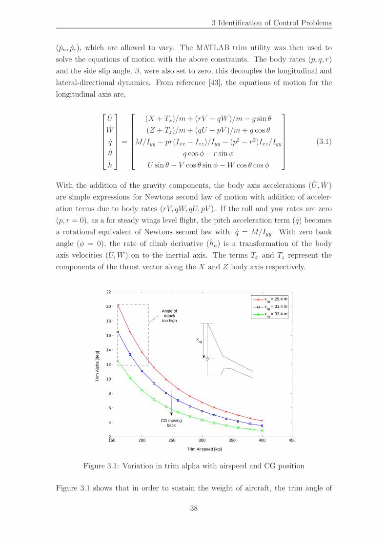
3 Identification of Control Problems
(pn, pe), which are allowed to vary. The MATLAB trim utility was then used to
solve the equations of motion with the above constraints. The body rates (p, q, r)
and the side slip angle, β, were also set to zero, this decouples the longitudinal and
lateral-directional dynamics. From reference [43], the equations of motion for the
longitudinal axis are,
U
W
q
θ
h
=
(X + Tx)/m+ (rV − qW )/m− g sin θ
(Z + Tz)/m+ (qU − pV )/m+ g cos θ
M/Iyy − pr(Ixx − Izz)/Iyy − (p2 − r2)Ixz/Iyy
q cosφ− r sin φ
U sin θ − V cos θ sin φ−W cos θ cosφ
(3.1)
With the addition of the gravity components, the body axis accelerations (U , W )
are simple expressions for Newtons second law of motion with addition of acceler-
ation terms due to body rates (rV, qW, qU, pV ). If the roll and yaw rates are zero
(p, r = 0), as a for steady wings level flight, the pitch acceleration term (q) becomes
a rotational equivalent of Newtons second law with, q = M/Iyy. With zero bank
angle (φ = 0), the rate of climb derivative (hn) is a transformation of the body
axis velocities (U,W ) on to the inertial axis. The terms Tx and Tz represent the
components of the thrust vector along the X and Z body axis respectively.
150 200 250 300 350 400 4502
4
6
8
10
12
14
16
18
20
22
Trim Airspeed [kts]
Trim
Alp
ha [d
eg]
xcg
= 29.4 m
xcg
= 31.4 m
xcg
= 33.4 m
xcg
CG movingback
Angle ofAttack
too high
Figure 3.1: Variation in trim alpha with airspeed and CG position
Figure 3.1 shows that in order to sustain the weight of aircraft, the trim angle of
38
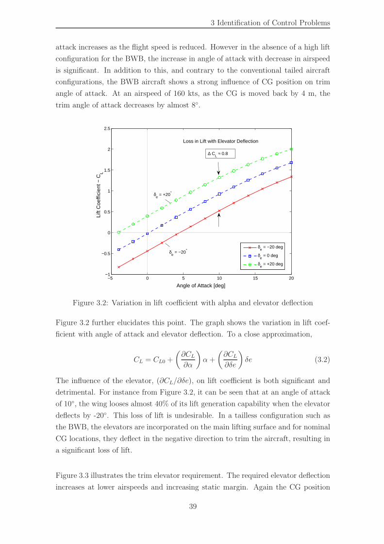
3 Identification of Control Problems
attack increases as the flight speed is reduced. However in the absence of a high lift
configuration for the BWB, the increase in angle of attack with decrease in airspeed
is significant. In addition to this, and contrary to the conventional tailed aircraft
configurations, the BWB aircraft shows a strong influence of CG position on trim
angle of attack. At an airspeed of 160 kts, as the CG is moved back by 4 m, the
trim angle of attack decreases by almost 8◦.
−5 0 5 10 15 20−1
−0.5
0
0.5
1
1.5
2
2.5
Lift
Coe
ffici
ent −
CL
Angle of Attack [deg]
δe = −20 deg
δe = 0 deg
δe = +20 deg
∆ CL ≈ 0.8
Loss in Lift with Elevator Deflection
δe = −20°
δe = +20°
Figure 3.2: Variation in lift coefficient with alpha and elevator deflection
Figure 3.2 further elucidates this point. The graph shows the variation in lift coef-
ficient with angle of attack and elevator deflection. To a close approximation,
CL = CL0 +
(
∂CL∂α
)
α+
(
∂CL∂δe
)
δe (3.2)
The influence of the elevator, (∂CL/∂δe), on lift coefficient is both significant and
detrimental. For instance from Figure 3.2, it can be seen that at an angle of attack
of 10◦, the wing looses almost 40% of its lift generation capability when the elevator
deflects by -20◦. This loss of lift is undesirable. In a tailless configuration such as
the BWB, the elevators are incorporated on the main lifting surface and for nominal
CG locations, they deflect in the negative direction to trim the aircraft, resulting in
a significant loss of lift.
Figure 3.3 illustrates the trim elevator requirement. The required elevator deflection
increases at lower airspeeds and increasing static margin. Again the CG position
39
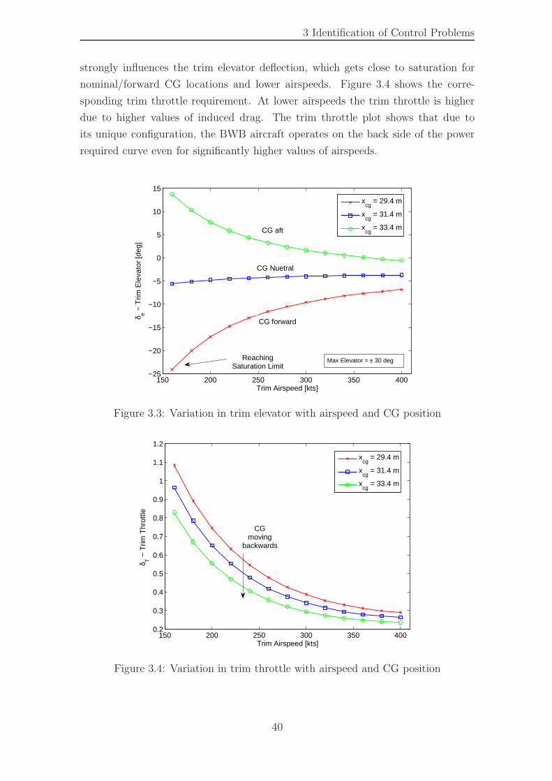
3 Identification of Control Problems
strongly influences the trim elevator deflection, which gets close to saturation for
nominal/forward CG locations and lower airspeeds. Figure 3.4 shows the corre-
sponding trim throttle requirement. At lower airspeeds the trim throttle is higher
due to higher values of induced drag. The trim throttle plot shows that due to
its unique configuration, the BWB aircraft operates on the back side of the power
required curve even for significantly higher values of airspeeds.
150 200 250 300 350 400−25
−20
−15
−10
−5
0
5
10
15
Trim Airspeed [kts]
δ e − T
rim E
leva
tor
[deg
]
xcg
= 29.4 m
xcg
= 31.4 m
xcg
= 33.4 m
ReachingSaturation Limit
CG forward
CG Nuetral
CG aft
Max Elevator = ± 30 deg
Figure 3.3: Variation in trim elevator with airspeed and CG position
150 200 250 300 350 4000.2
0.3
0.4
0.5
0.6
0.7
0.8
0.9
1
1.1
1.2
Trim Airspeed [kts]
δ T −
Trim
Thr
ottle
xcg
= 29.4 m
xcg
= 31.4 m
xcg
= 33.4 m
CGmoving
backwards
Figure 3.4: Variation in trim throttle with airspeed and CG position
40
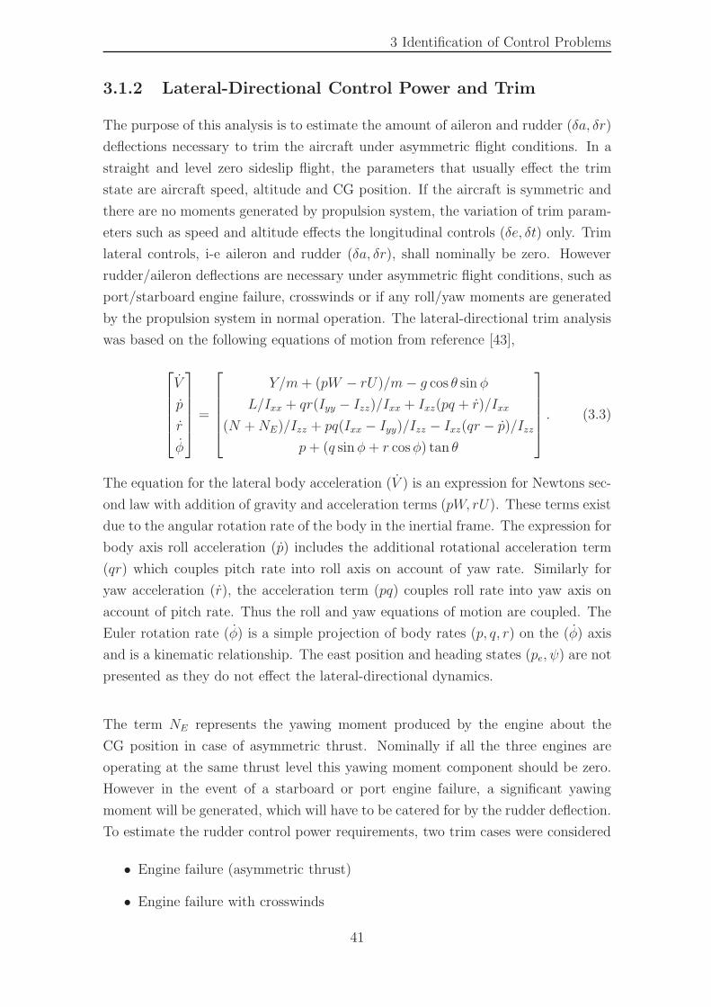
3 Identification of Control Problems
3.1.2 Lateral-Directional Control Power and Trim
The purpose of this analysis is to estimate the amount of aileron and rudder (δa, δr)
deflections necessary to trim the aircraft under asymmetric flight conditions. In a
straight and level zero sideslip flight, the parameters that usually effect the trim
state are aircraft speed, altitude and CG position. If the aircraft is symmetric and
there are no moments generated by propulsion system, the variation of trim param-
eters such as speed and altitude effects the longitudinal controls (δe, δt) only. Trim
lateral controls, i-e aileron and rudder (δa, δr), shall nominally be zero. However
rudder/aileron deflections are necessary under asymmetric flight conditions, such as
port/starboard engine failure, crosswinds or if any roll/yaw moments are generated
by the propulsion system in normal operation. The lateral-directional trim analysis
was based on the following equations of motion from reference [43],
V
p
r
φ
=
Y/m+ (pW − rU)/m− g cos θ sin φ
L/Ixx + qr(Iyy − Izz)/Ixx + Ixz(pq + r)/Ixx
(N +NE)/Izz + pq(Ixx − Iyy)/Izz − Ixz(qr − p)/Izz
p+ (q sinφ+ r cosφ) tan θ
. (3.3)
The equation for the lateral body acceleration (V ) is an expression for Newtons sec-
ond law with addition of gravity and acceleration terms (pW, rU). These terms exist
due to the angular rotation rate of the body in the inertial frame. The expression for
body axis roll acceleration (p) includes the additional rotational acceleration term
(qr) which couples pitch rate into roll axis on account of yaw rate. Similarly for
yaw acceleration (r), the acceleration term (pq) couples roll rate into yaw axis on
account of pitch rate. Thus the roll and yaw equations of motion are coupled. The
Euler rotation rate (φ) is a simple projection of body rates (p, q, r) on the (φ) axis
and is a kinematic relationship. The east position and heading states (pe, ψ) are not
presented as they do not effect the lateral-directional dynamics.
The term NE represents the yawing moment produced by the engine about the
CG position in case of asymmetric thrust. Nominally if all the three engines are
operating at the same thrust level this yawing moment component should be zero.
However in the event of a starboard or port engine failure, a significant yawing
moment will be generated, which will have to be catered for by the rudder deflection.
To estimate the rudder control power requirements, two trim cases were considered
• Engine failure (asymmetric thrust)
• Engine failure with crosswinds
41
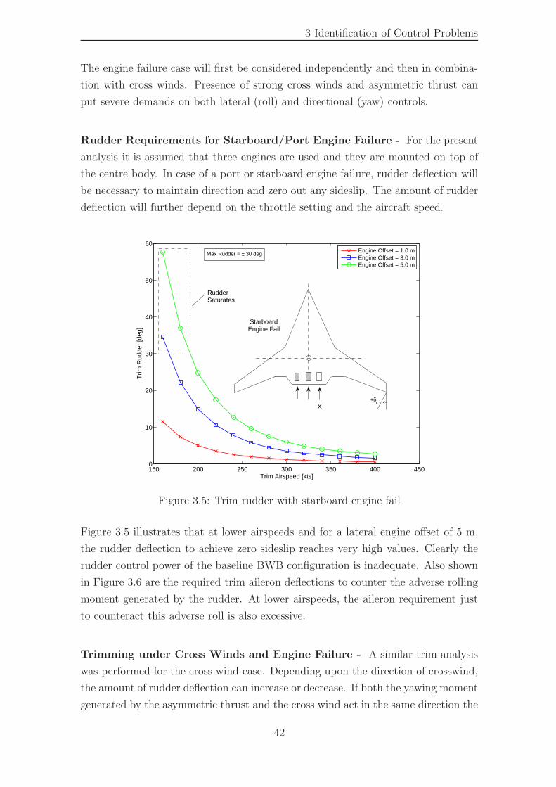
3 Identification of Control Problems
The engine failure case will first be considered independently and then in combina-
tion with cross winds. Presence of strong cross winds and asymmetric thrust can
put severe demands on both lateral (roll) and directional (yaw) controls.
Rudder Requirements for Starboard/Port Engine Failure - For the present
analysis it is assumed that three engines are used and they are mounted on top of
the centre body. In case of a port or starboard engine failure, rudder deflection will
be necessary to maintain direction and zero out any sideslip. The amount of rudder
deflection will further depend on the throttle setting and the aircraft speed.
150 200 250 300 350 400 4500
10
20
30
40
50
60
Trim Airspeed [kts]
Trim
Rud
der
[deg
]
Engine Offset = 1.0 mEngine Offset = 3.0 mEngine Offset = 5.0 m
X
StarboardEngine Fail
+δr
RudderSaturates
Max Rudder = ± 30 deg
Figure 3.5: Trim rudder with starboard engine fail
Figure 3.5 illustrates that at lower airspeeds and for a lateral engine offset of 5 m,
the rudder deflection to achieve zero sideslip reaches very high values. Clearly the
rudder control power of the baseline BWB configuration is inadequate. Also shown
in Figure 3.6 are the required trim aileron deflections to counter the adverse rolling
moment generated by the rudder. At lower airspeeds, the aileron requirement just
to counteract this adverse roll is also excessive.
Trimming under Cross Winds and Engine Failure - A similar trim analysis
was performed for the cross wind case. Depending upon the direction of crosswind,
the amount of rudder deflection can increase or decrease. If both the yawing moment
generated by the asymmetric thrust and the cross wind act in the same direction the
42
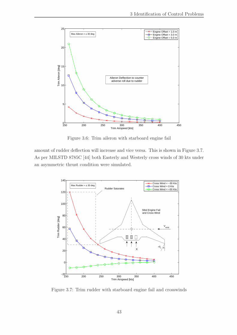
3 Identification of Control Problems
150 200 250 300 350 400 4500
5
10
15
20
25
Trim Airspeed [kts]
Trim
Aile
ron
[deg
]
Engine Offset = 1.0 mEngine Offset = 3.0 mEngine Offset = 5.0 m
Aileron Deflection to counteradverse roll due to rudder
Max Aileron = ± 30 deg
Figure 3.6: Trim aileron with starboard engine fail
amount of rudder deflection will increase and vice versa. This is shown in Figure 3.7.
As per MILSTD 8785C [44] both Easterly and Westerly cross winds of 30 kts under
an asymmetric thrust condition were simulated.
150 200 250 300 350 400 450−20
0
20
40
60
80
100
120
140
Trim Airspeed [kts]
Trim
Rud
der
[deg
]
Trim Rudder Vs Airspeed
Cross Wind = −30 KtsCross Wind = 0 KtsCross Wind = +30 Kts
X
Stbd Engine Failand Cross Wind
+δr
Rudder Saturates
Vwind
Max Rudder = ± 30 deg
Figure 3.7: Trim rudder with starboard engine fail and crosswinds
43
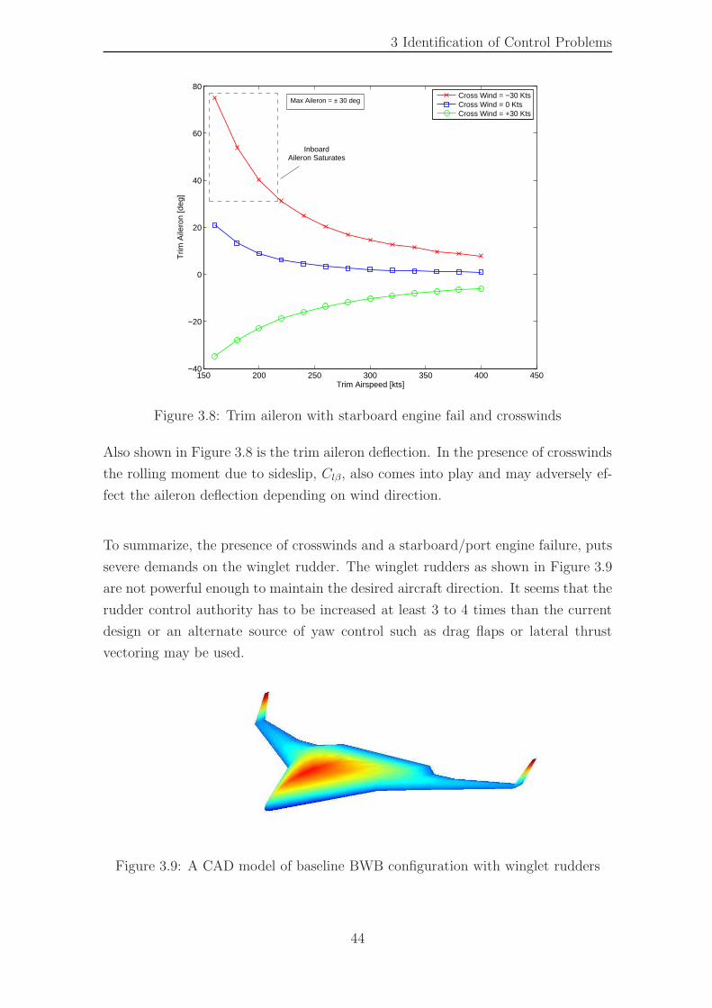
3 Identification of Control Problems
150 200 250 300 350 400 450−40
−20
0
20
40
60
80
Trim Airspeed [kts]
Trim
Aile
ron
[deg
]
Cross Wind = −30 KtsCross Wind = 0 KtsCross Wind = +30 Kts
InboardAileron Saturates
Max Aileron = ± 30 deg
Figure 3.8: Trim aileron with starboard engine fail and crosswinds
Also shown in Figure 3.8 is the trim aileron deflection. In the presence of crosswinds
the rolling moment due to sideslip, Clβ, also comes into play and may adversely ef-
fect the aileron deflection depending on wind direction.
To summarize, the presence of crosswinds and a starboard/port engine failure, puts
severe demands on the winglet rudder. The winglet rudders as shown in Figure 3.9
are not powerful enough to maintain the desired aircraft direction. It seems that the
rudder control authority has to be increased at least 3 to 4 times than the current
design or an alternate source of yaw control such as drag flaps or lateral thrust
vectoring may be used.
Figure 3.9: A CAD model of baseline BWB configuration with winglet rudders
44
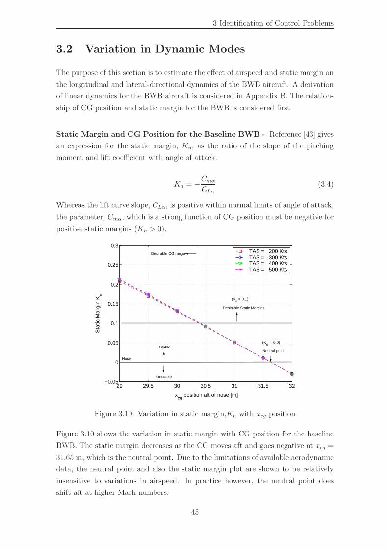
3 Identification of Control Problems
3.2 Variation in Dynamic Modes
The purpose of this section is to estimate the effect of airspeed and static margin on
the longitudinal and lateral-directional dynamics of the BWB aircraft. A derivation
of linear dynamics for the BWB aircraft is considered in Appendix B. The relation-
ship of CG position and static margin for the BWB is considered first.
Static Margin and CG Position for the Baseline BWB - Reference [43] gives
an expression for the static margin, Kn, as the ratio of the slope of the pitching
moment and lift coefficient with angle of attack.
Kn = −CmαCLα
(3.4)
Whereas the lift curve slope, CLα, is positive within normal limits of angle of attack,
the parameter, Cmα, which is a strong function of CG position must be negative for
positive static margins (Kn > 0).
29 29.5 30 30.5 31 31.5 32−0.05
0
0.05
0.1
0.15
0.2
0.25
0.3
Sta
tic M
argi
n K
n
xcg
position aft of nose [m]
TAS = 200 Kts TAS = 300 Kts TAS = 400 Kts TAS = 500 Kts
Desirable Static Margins
Desirable CG range
Stable
Unstable
Neutral point
Nose
(Kn > 0.1)
(Kn = 0.0)
Figure 3.10: Variation in static margin,Kn with xcg position
Figure 3.10 shows the variation in static margin with CG position for the baseline
BWB. The static margin decreases as the CG moves aft and goes negative at xcg =
31.65 m, which is the neutral point. Due to the limitations of available aerodynamic
data, the neutral point and also the static margin plot are shown to be relatively
insensitive to variations in airspeed. In practice however, the neutral point does
shift aft at higher Mach numbers.
45
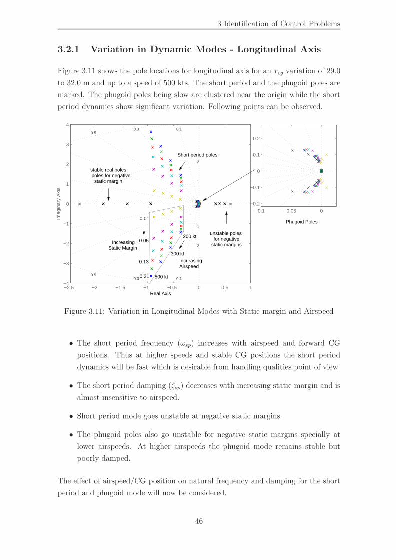
3 Identification of Control Problems
3.2.1 Variation in Dynamic Modes - Longitudinal Axis
Figure 3.11 shows the pole locations for longitudinal axis for an xcg variation of 29.0
to 32.0 m and up to a speed of 500 kts. The short period and the phugoid poles are
marked. The phugoid poles being slow are clustered near the origin while the short
period dynamics show significant variation. Following points can be observed.
−2.5 −2 −1.5 −1 −0.5 0 0.5 1−4
−3
−2
−1
0
1
2
3
4
1
2
4
0.3
1
0.50.1
0.50.3
4
0.1
2
Real Axis
Imag
inar
y A
xis
−0.1 −0.05 0−0.2
−0.1
0
0.1
0.2
IncreasingStatic Margin
IncreasingAirspeed
0.01
0.05
0.13
0.21
200 kt
300 kt
500 kt
Phugoid Poles
unstable poles for negative
static margins
Short period poles
stable real poles poles for negativestatic margin
Figure 3.11: Variation in Longitudinal Modes with Static margin and Airspeed
• The short period frequency (ωsp) increases with airspeed and forward CG
positions. Thus at higher speeds and stable CG positions the short period
dynamics will be fast which is desirable from handling qualities point of view.
• The short period damping (ζsp) decreases with increasing static margin and is
almost insensitive to airspeed.
• Short period mode goes unstable at negative static margins.
• The phugoid poles also go unstable for negative static margins specially at
lower airspeeds. At higher airspeeds the phugoid mode remains stable but
poorly damped.
The effect of airspeed/CG position on natural frequency and damping for the short
period and phugoid mode will now be considered.
46
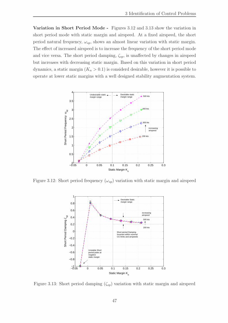
3 Identification of Control Problems
Variation in Short Period Mode - Figures 3.12 and 3.13 show the variation in
short period mode with static margin and airspeed. At a fixed airspeed, the short
period natural frequency, ωsp, shows an almost linear variation with static margin.
The effect of increased airspeed is to increase the frequency of the short period mode
and vice versa. The short period damping, ζsp, is unaffected by changes in airspeed
but increases with decreasing static margin. Based on this variation in short period
dynamics, a static margin (Kn > 0.1) is considerd desirable, however it is possible to
operate at lower static margins with a well designed stability augmentation system.
−0.05 0 0.05 0.1 0.15 0.2 0.25 0.30
0.5
1
1.5
2
2.5
3
3.5
4
Static Margin Kn
n
Sho
rt P
erio
d F
requ
ency
ωsp
200 kts
300 kts
400 kts
500 kts
increasingairspeed
Undesirable staticmargin range
Desirable staticmargin range
Figure 3.12: Short period frequency (ωsp) variation with static margin and airspeed
−0.05 0 0.05 0.1 0.15 0.2 0.25 0.3−1
−0.8
−0.6
−0.4
−0.2
0
0.2
0.4
0.6
0.8
1
Static Margin Kn
Sho
rt P
erio
d D
ampi
ng ζ
sp
Desirable Staticmargin range
Unstable Short period poles at negativestatic margin
200 kts
500 kts
increasing airspeed
Short period DampingInvariant within nominalCG limits and airspeeds
Figure 3.13: Short period damping (ζsp) variation with static margin and airspeed
47
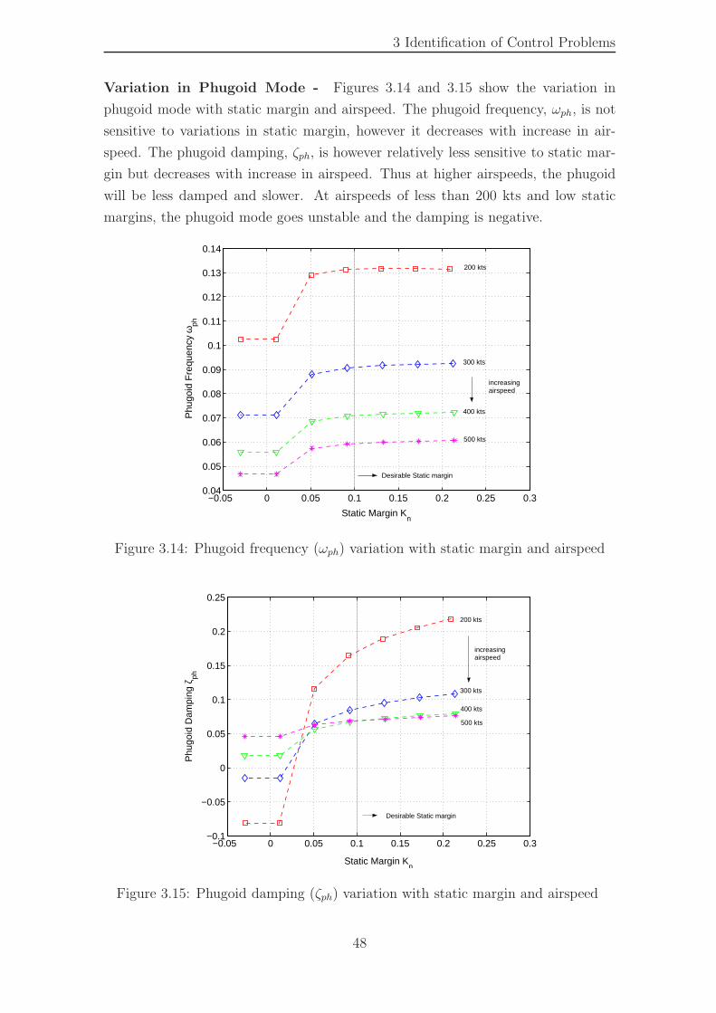
3 Identification of Control Problems
Variation in Phugoid Mode - Figures 3.14 and 3.15 show the variation in
phugoid mode with static margin and airspeed. The phugoid frequency, ωph, is not
sensitive to variations in static margin, however it decreases with increase in air-
speed. The phugoid damping, ζph, is however relatively less sensitive to static mar-
gin but decreases with increase in airspeed. Thus at higher airspeeds, the phugoid
will be less damped and slower. At airspeeds of less than 200 kts and low static
margins, the phugoid mode goes unstable and the damping is negative.
−0.05 0 0.05 0.1 0.15 0.2 0.25 0.30.04
0.05
0.06
0.07
0.08
0.09
0.1
0.11
0.12
0.13
0.14
Static Margin Kn
Phu
goid
Fre
quen
cy ω
ph
200 kts
300 kts
400 kts
500 kts
increasingairspeed
Desirable Static margin
Figure 3.14: Phugoid frequency (ωph) variation with static margin and airspeed
−0.05 0 0.05 0.1 0.15 0.2 0.25 0.3−0.1
−0.05
0
0.05
0.1
0.15
0.2
0.25
Static Margin Kn
Phu
goid
Dam
ping
ζph
Desirable Static margin
200 kts
300 kts
400 kts
500 kts
increasing airspeed
Figure 3.15: Phugoid damping (ζph) variation with static margin and airspeed
48
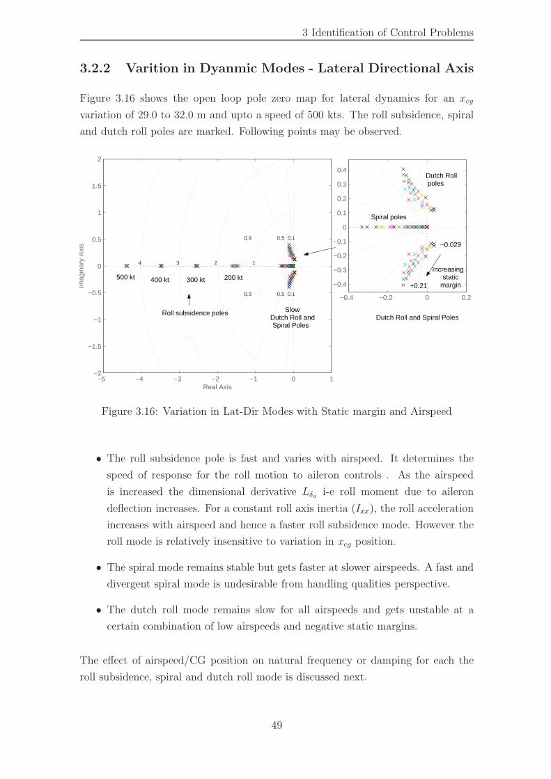
3 Identification of Control Problems
3.2.2 Varition in Dyanmic Modes - Lateral Directional Axis
Figure 3.16 shows the open loop pole zero map for lateral dynamics for an xcg
variation of 29.0 to 32.0 m and upto a speed of 500 kts. The roll subsidence, spiral
and dutch roll poles are marked. Following points may be observed.
−0.4 −0.2 0 0.2
−0.4
−0.3
−0.2
−0.1
0
0.1
0.2
0.3
0.4
−5 −4 −3 −2 −1 0 1−2
−1.5
−1
−0.5
0
0.5
1
1.5
2
234
0.5
0.1
0.1
1
0.9 0.5
0.9
Real Axis
Imag
inar
y A
xis
Roll subsidence poles
200 kt 300 kt 400 kt 500 kt
Spiral poles
Dutch Roll poles
Increasing static
margin
−0.029
+0.21
Dutch Roll and Spiral Poles Slow
Dutch Roll andSpiral Poles
Figure 3.16: Variation in Lat-Dir Modes with Static margin and Airspeed
• The roll subsidence pole is fast and varies with airspeed. It determines the
speed of response for the roll motion to aileron controls . As the airspeed
is increased the dimensional derivative Lδa i-e roll moment due to aileron
deflection increases. For a constant roll axis inertia (Ixx), the roll acceleration
increases with airspeed and hence a faster roll subsidence mode. However the
roll mode is relatively insensitive to variation in xcg position.
• The spiral mode remains stable but gets faster at slower airspeeds. A fast and
divergent spiral mode is undesirable from handling qualities perspective.
• The dutch roll mode remains slow for all airspeeds and gets unstable at a
certain combination of low airspeeds and negative static margins.
The effect of airspeed/CG position on natural frequency or damping for each the
roll subsidence, spiral and dutch roll mode is discussed next.
49
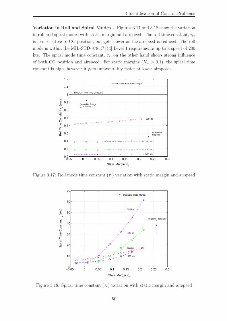
3 Identification of Control Problems
Variation in Roll and Spiral Modes - Figures 3.17 and 3.18 show the variation
in roll and spiral modes with static margin and airspeed. The roll time constant, τr,
is less sensitive to CG position, but gets slower as the airspeed is reduced. The roll
mode is within the MIL-STD-8785C [44] Level 1 requirements up to a speed of 200
kts. The spiral mode time constant, τs, on the other hand shows strong influence
of both CG position and airspeed. For static margins (Kn > 0.1), the spiral time
constant is high, however it gets unfavourably faster at lower airspeeds.
−0.05 0 0.05 0.1 0.15 0.2 0.25 0.30.2
0.3
0.4
0.5
0.6
0.7
0.8
0.9
1
1.1
1.2
Static Margin Kn
Rol
l Tim
e C
onst
ant τ
r (se
c)
200 kts
300 kts
400 kts
500 kts
increasingairspeed
Desirable Static Margin
Level 1− Roll Time Constant
Desirable Range(τ
r < 1.0 sec)
Figure 3.17: Roll mode time constant (τr) variation with static margin and airspeed
−0.05 0 0.05 0.1 0.15 0.2 0.25 0.30
10
20
30
40
50
60
70
Static Margin Kn
Spi
ral T
ime
Con
stan
t τs (
sec) 500 kts
400 kts
200 kts
300 kts
Desirable Static Margin
Higher τs desirable
Figure 3.18: Spiral time constant (τs) variation with static margin and airspeed
50
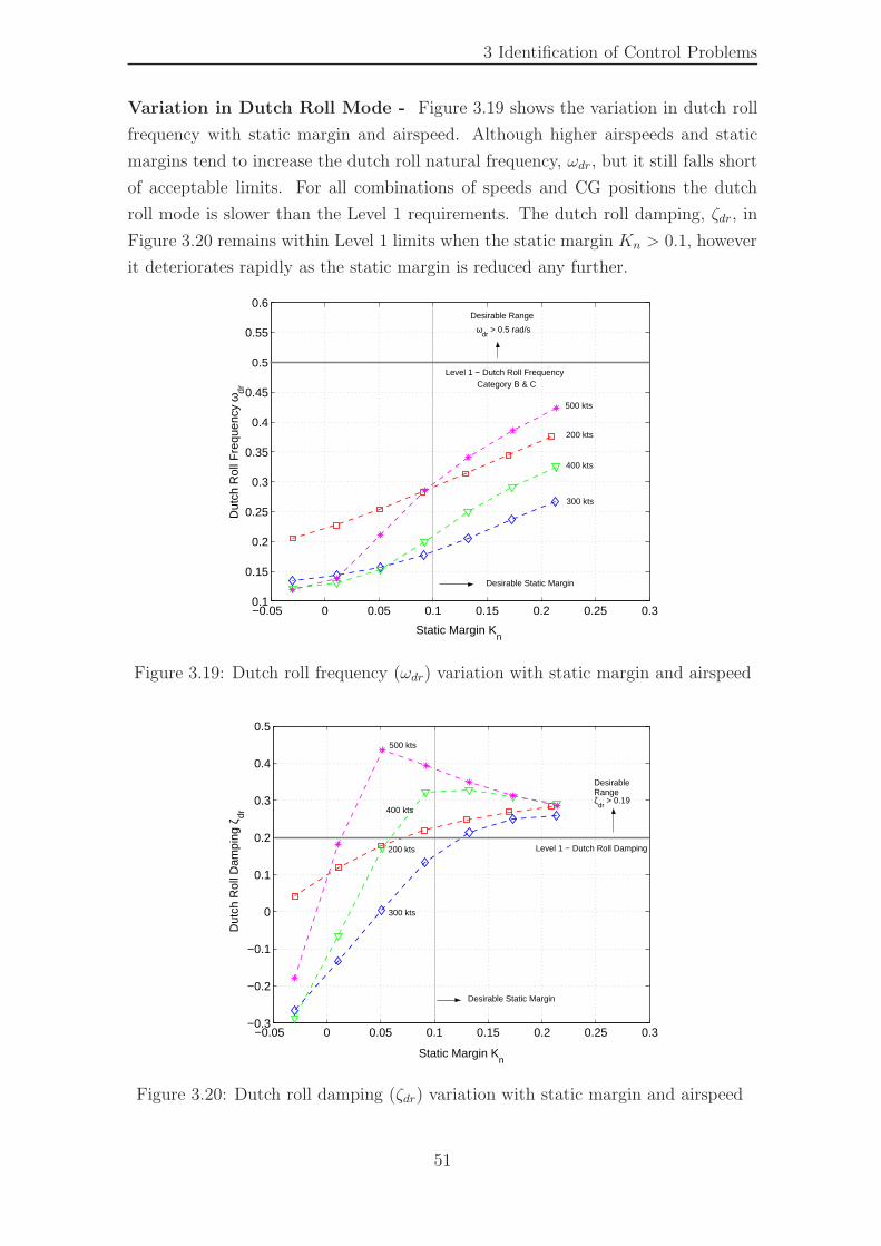
3 Identification of Control Problems
Variation in Dutch Roll Mode - Figure 3.19 shows the variation in dutch roll
frequency with static margin and airspeed. Although higher airspeeds and static
margins tend to increase the dutch roll natural frequency, ωdr, but it still falls short
of acceptable limits. For all combinations of speeds and CG positions the dutch
roll mode is slower than the Level 1 requirements. The dutch roll damping, ζdr, in
Figure 3.20 remains within Level 1 limits when the static margin Kn > 0.1, however
it deteriorates rapidly as the static margin is reduced any further.
−0.05 0 0.05 0.1 0.15 0.2 0.25 0.30.1
0.15
0.2
0.25
0.3
0.35
0.4
0.45
0.5
0.55
0.6
Static Margin Kn
Dut
ch R
oll F
requ
ency
ωdr
Desirable Static Margin
200 kts
300 kts
400 kts
500 kts
Level 1 − Dutch Roll Frequency
ωdr
> 0.5 rad/s
Category B & C
Desirable Range
Figure 3.19: Dutch roll frequency (ωdr) variation with static margin and airspeed
−0.05 0 0.05 0.1 0.15 0.2 0.25 0.3−0.3
−0.2
−0.1
0
0.1
0.2
0.3
0.4
0.5
Static Margin Kn
Dut
ch R
oll D
ampi
ng ζ
dr
Desirable Static Margin
Desirable Rangeζ
dr > 0.19
Level 1 − Dutch Roll Damping 200 kts
300 kts
400 kts
500 kts
Figure 3.20: Dutch roll damping (ζdr) variation with static margin and airspeed
51
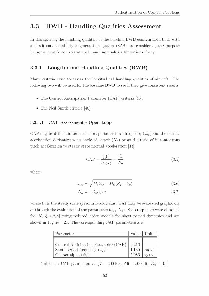
3 Identification of Control Problems
3.3 BWB - Handling Qualities Assessment
In this section, the handling qualities of the baseline BWB configuration both with
and without a stability augmentation system (SAS) are considered, the purpose
being to identify controls related handling qualities limitations if any.
3.3.1 Longitudinal Handling Qualities (BWB)
Many criteria exist to assess the longitudinal handling qualities of aircraft. The
following two will be used for the baseline BWB to see if they give consistent results.
• The Control Anticipation Parameter (CAP) criteria [45].
• The Neil Smith criteria [46].
3.3.1.1 CAP Assessment - Open Loop
CAP may be defined in terms of short period natural frequency (ωsp) and the normal
acceleration derivative w.r.t angle of attack (Nα) or as the ratio of instantaneous
pitch acceleration to steady state normal acceleration [43],
CAP =q(0)
Nz(∞)
=ω2sp
Nα
(3.5)
where
ωsp =√
MqZw −Mw(Zq + Ue) (3.6)
Nα = −ZwUe/g (3.7)
where Ue is the steady state speed in x-body axis. CAP may be evaluated graphically
or through the evaluation of the parameters (ωsp, Nα). Step responses were obtained
for [Nz, q, q, θ, γ] using reduced order models for short period dynamics and are
shown in Figure 3.21. The corresponding CAP parameters are,
Parameter Value Units
Control Anticipation Parameter (CAP) 0.216 -Short period frequency (ωsp) 1.139 rad/sG’s per alpha (Nα) 5.986 g/rad
Table 3.1: CAP parameters at (V = 200 kts, Alt = 5000 ft, Kn = 0.1)
52
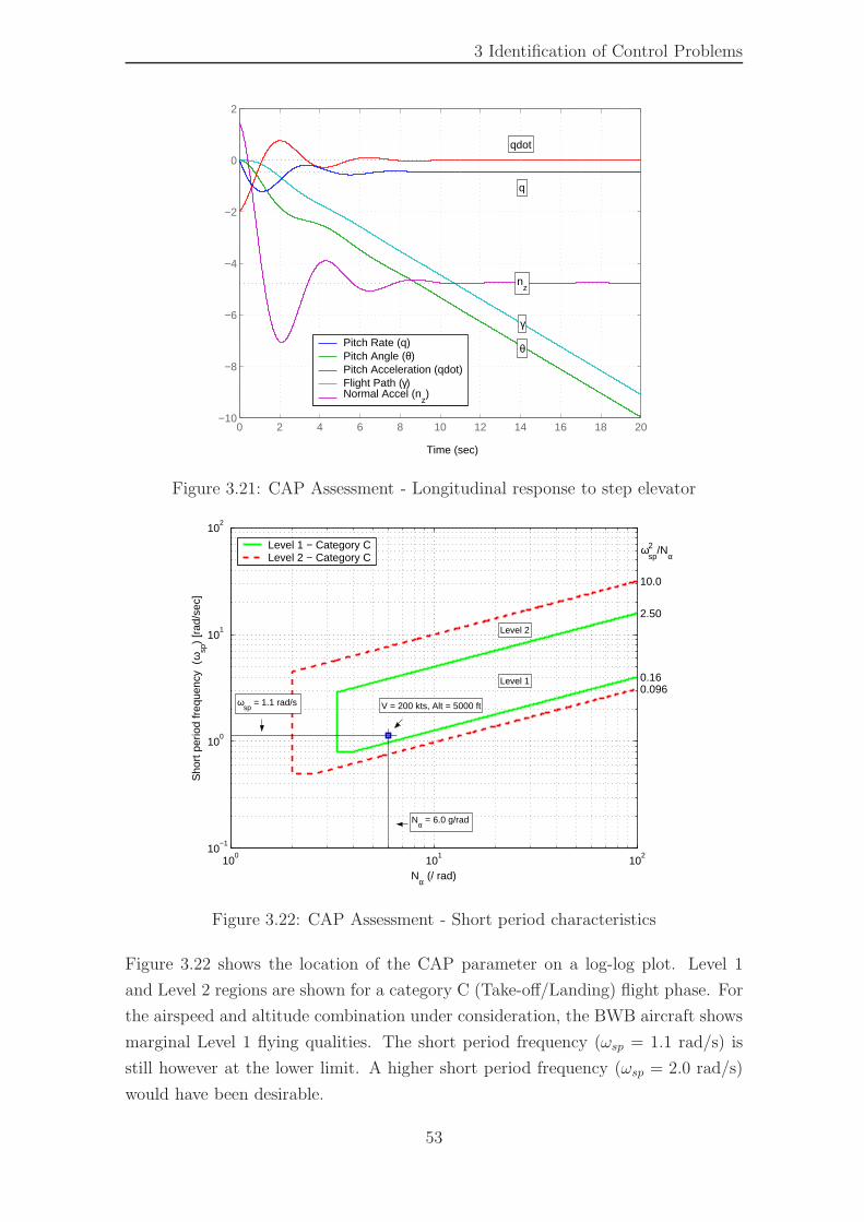
3 Identification of Control Problems
0 2 4 6 8 10 12 14 16 18 20−10
−8
−6
−4
−2
0
2
q
qdot
θ
γ
nz
Pitch Rate (q)Pitch Angle (θ)Pitch Acceleration (qdot)Flight Path (γ)Normal Accel (n
z)
Time (sec)
Figure 3.21: CAP Assessment - Longitudinal response to step elevator
100
101
102
10−1
100
101
102
0.16
2.50
0.096
10.0
Nα (/ rad)
Sho
rt p
erio
d fr
eque
ncy
(ω
sp)
[rad
/sec
]
Level 1 − Category CLevel 2 − Category C
ωsp
= 1.1 rad/s
Level 2
Level 1
Nα = 6.0 g/rad
ωsp2 /N
α
V = 200 kts, Alt = 5000 ft
Figure 3.22: CAP Assessment - Short period characteristics
Figure 3.22 shows the location of the CAP parameter on a log-log plot. Level 1
and Level 2 regions are shown for a category C (Take-off/Landing) flight phase. For
the airspeed and altitude combination under consideration, the BWB aircraft shows
marginal Level 1 flying qualities. The short period frequency (ωsp = 1.1 rad/s) is
still however at the lower limit. A higher short period frequency (ωsp = 2.0 rad/s)
would have been desirable.
53
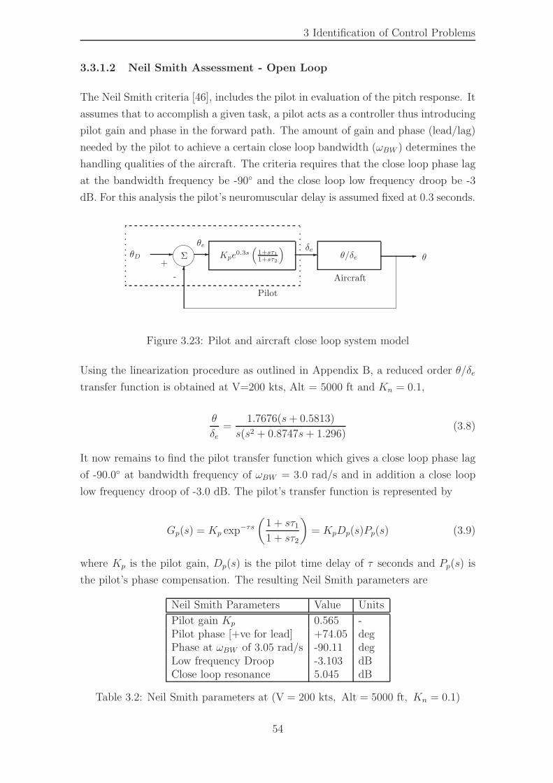
3 Identification of Control Problems
3.3.1.2 Neil Smith Assessment - Open Loop
The Neil Smith criteria [46], includes the pilot in evaluation of the pitch response. It
assumes that to accomplish a given task, a pilot acts as a controller thus introducing
pilot gain and phase in the forward path. The amount of gain and phase (lead/lag)
needed by the pilot to achieve a certain close loop bandwidth (ωBW ) determines the
handling qualities of the aircraft. The criteria requires that the close loop phase lag
at the bandwidth frequency be -90◦ and the close loop low frequency droop be -3
dB. For this analysis the pilot’s neuromuscular delay is assumed fixed at 0.3 seconds.
-θ/δeθD Kpe0.3s
(
1+sτ1
1+sτ2
)
-θ
-θe
Pilot
6
Σ-
Aircraft
δe
+
-
Figure 3.23: Pilot and aircraft close loop system model
Using the linearization procedure as outlined in Appendix B, a reduced order θ/δe
transfer function is obtained at V=200 kts, Alt = 5000 ft and Kn = 0.1,
θ
δe=
1.7676(s+ 0.5813)
s(s2 + 0.8747s+ 1.296)(3.8)
It now remains to find the pilot transfer function which gives a close loop phase lag
of -90.0◦ at bandwidth frequency of ωBW = 3.0 rad/s and in addition a close loop
low frequency droop of -3.0 dB. The pilot’s transfer function is represented by
Gp(s) = Kp exp−τs
(
1 + sτ11 + sτ2
)
= KpDp(s)Pp(s) (3.9)
where Kp is the pilot gain, Dp(s) is the pilot time delay of τ seconds and Pp(s) is
the pilot’s phase compensation. The resulting Neil Smith parameters are
Neil Smith Parameters Value Units
Pilot gain Kp 0.565 -Pilot phase [+ve for lead] +74.05 degPhase at ωBW of 3.05 rad/s -90.11 degLow frequency Droop -3.103 dBClose loop resonance 5.045 dB
Table 3.2: Neil Smith parameters at (V = 200 kts, Alt = 5000 ft, Kn = 0.1)
54
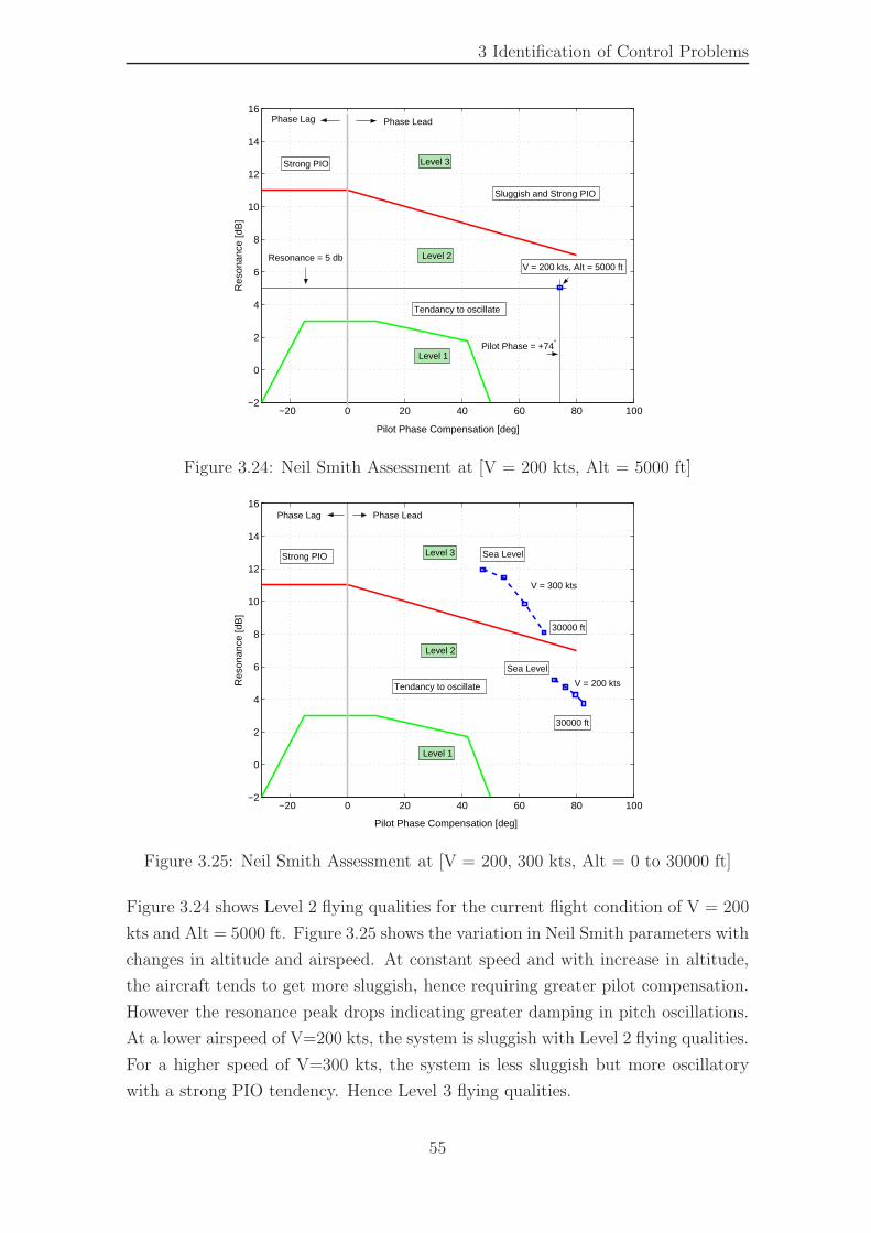
3 Identification of Control Problems
−20 0 20 40 60 80 100−2
0
2
4
6
8
10
12
14
16
Level 1
Level 2
Level 3Strong PIO
Sluggish and Strong PIO
Tendancy to oscillate
Pilot Phase Compensation [deg]
Res
onan
ce [d
B]
Phase Lead Phase Lag
Resonance = 5 db
Pilot Phase = +74°
V = 200 kts, Alt = 5000 ft
Figure 3.24: Neil Smith Assessment at [V = 200 kts, Alt = 5000 ft]
−20 0 20 40 60 80 100−2
0
2
4
6
8
10
12
14
16
Level 1
Level 2
Level 3Strong PIO
Pilot Phase Compensation [deg]
Res
onan
ce [d
B]
30000 ft
Sea Level
30000 ft
Sea Level
Phase Lead Phase Lag
V = 300 kts
V = 200 kts Tendancy to oscillate
Figure 3.25: Neil Smith Assessment at [V = 200, 300 kts, Alt = 0 to 30000 ft]
Figure 3.24 shows Level 2 flying qualities for the current flight condition of V = 200
kts and Alt = 5000 ft. Figure 3.25 shows the variation in Neil Smith parameters with
changes in altitude and airspeed. At constant speed and with increase in altitude,
the aircraft tends to get more sluggish, hence requiring greater pilot compensation.
However the resonance peak drops indicating greater damping in pitch oscillations.
At a lower airspeed of V=200 kts, the system is sluggish with Level 2 flying qualities.
For a higher speed of V=300 kts, the system is less sluggish but more oscillatory
with a strong PIO tendency. Hence Level 3 flying qualities.
55
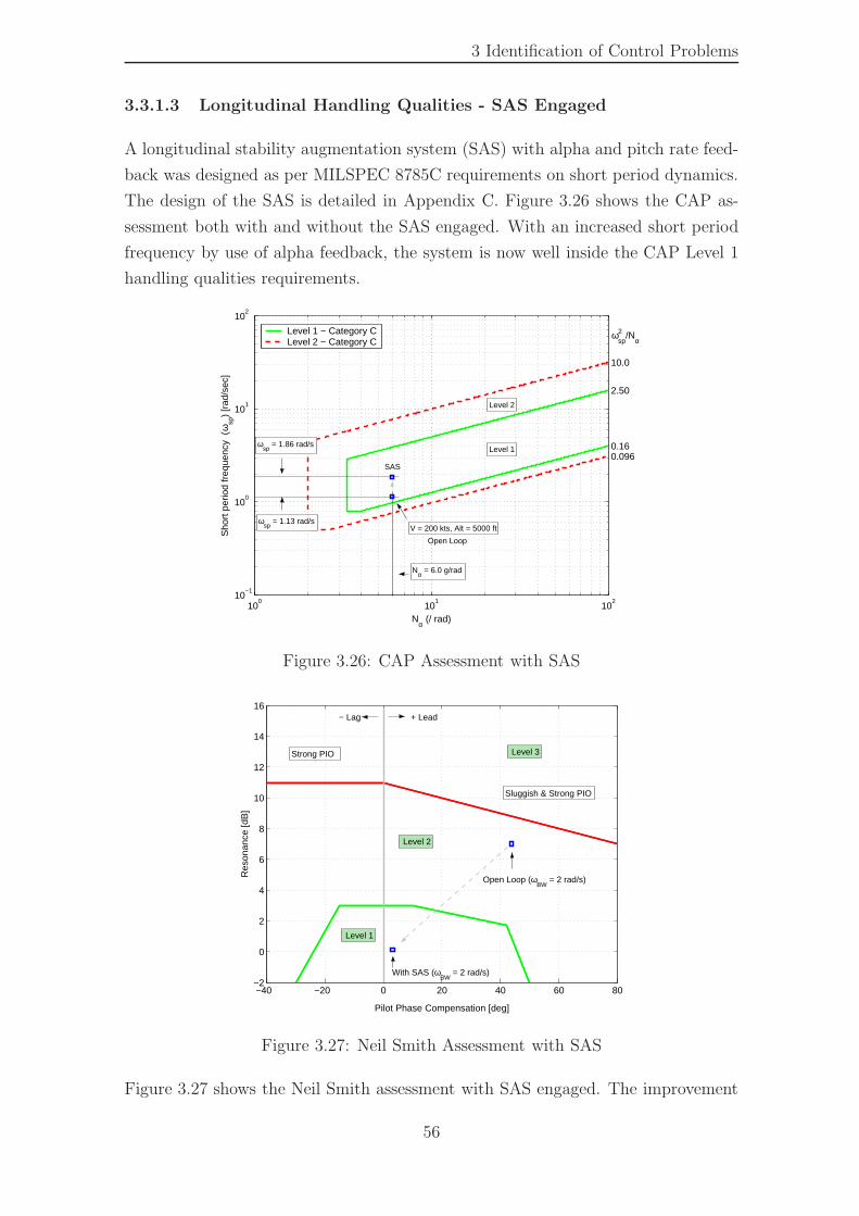
3 Identification of Control Problems
3.3.1.3 Longitudinal Handling Qualities - SAS Engaged
A longitudinal stability augmentation system (SAS) with alpha and pitch rate feed-
back was designed as per MILSPEC 8785C requirements on short period dynamics.
The design of the SAS is detailed in Appendix C. Figure 3.26 shows the CAP as-
sessment both with and without the SAS engaged. With an increased short period
frequency by use of alpha feedback, the system is now well inside the CAP Level 1
handling qualities requirements.
100
101
102
10−1
100
101
102
0.16
2.50
0.096
10.0
Nα (/ rad)
Sho
rt p
erio
d fr
eque
ncy
(ω
sp)
[rad
/sec
]
Level 1 − Category CLevel 2 − Category C
ωsp
= 1.13 rad/s
Level 2
Level 1
Nα = 6.0 g/rad
ωsp2 /N
α
V = 200 kts, Alt = 5000 ft
SAS
ωsp
= 1.86 rad/s
Open Loop
Figure 3.26: CAP Assessment with SAS
−40 −20 0 20 40 60 80−2
0
2
4
6
8
10
12
14
16
Level 1
Level 2
Level 3Strong PIO
Sluggish & Strong PIO
Pilot Phase Compensation [deg]
Res
onan
ce [d
B]
Open Loop (ωBW
= 2 rad/s)
With SAS (ωBW
= 2 rad/s)
+ Lead − Lag
Figure 3.27: Neil Smith Assessment with SAS
Figure 3.27 shows the Neil Smith assessment with SAS engaged. The improvement
56
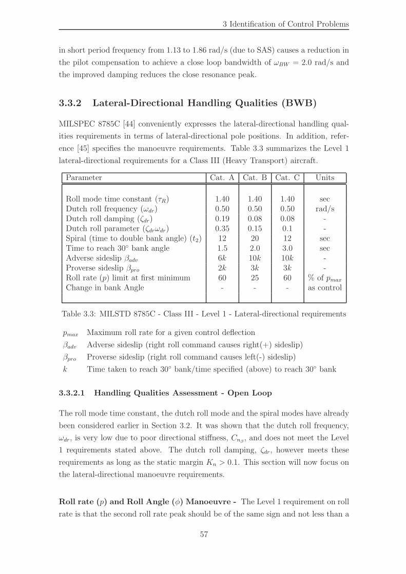
3 Identification of Control Problems
in short period frequency from 1.13 to 1.86 rad/s (due to SAS) causes a reduction in
the pilot compensation to achieve a close loop bandwidth of ωBW = 2.0 rad/s and
the improved damping reduces the close resonance peak.
3.3.2 Lateral-Directional Handling Qualities (BWB)
MILSPEC 8785C [44] conveniently expresses the lateral-directional handling qual-
ities requirements in terms of lateral-directional pole positions. In addition, refer-
ence [45] specifies the manoeuvre requirements. Table 3.3 summarizes the Level 1
lateral-directional requirements for a Class III (Heavy Transport) aircraft.
Parameter Cat. A Cat. B Cat. C Units
Roll mode time constant (τR) 1.40 1.40 1.40 secDutch roll frequency (ωdr) 0.50 0.50 0.50 rad/sDutch roll damping (ζdr) 0.19 0.08 0.08 -Dutch roll parameter (ζdrωdr) 0.35 0.15 0.1 -Spiral (time to double bank angle) (t2) 12 20 12 secTime to reach 30◦ bank angle 1.5 2.0 3.0 secAdverse sideslip βadv 6k 10k 10k -Proverse sideslip βpro 2k 3k 3k -Roll rate (p) limit at first minimum 60 25 60 % of pmaxChange in bank Angle - - - as control
Table 3.3: MILSTD 8785C - Class III - Level 1 - Lateral-directional requirements
pmax Maximum roll rate for a given control deflection
βadv Adverse sideslip (right roll command causes right(+) sideslip)
βpro Proverse sideslip (right roll command causes left(-) sideslip)
k Time taken to reach 30◦ bank/time specified (above) to reach 30◦ bank
3.3.2.1 Handling Qualities Assessment - Open Loop
The roll mode time constant, the dutch roll mode and the spiral modes have already
been considered earlier in Section 3.2. It was shown that the dutch roll frequency,
ωdr, is very low due to poor directional stiffness, Cnβ , and does not meet the Level
1 requirements stated above. The dutch roll damping, ζdr, however meets these
requirements as long as the static margin Kn > 0.1. This section will now focus on
the lateral-directional manoeuvre requirements.
Roll rate (p) and Roll Angle (φ) Manoeuvre - The Level 1 requirement on roll
rate is that the second roll rate peak should be of the same sign and not less than a
57
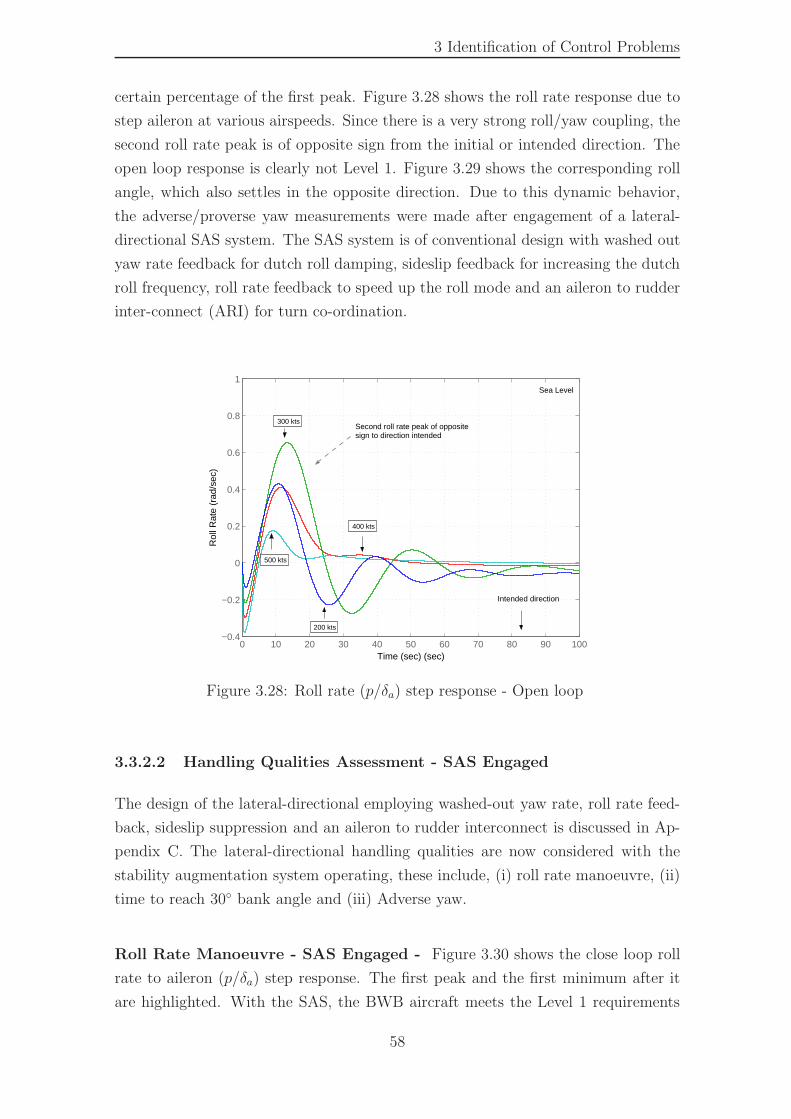
3 Identification of Control Problems
certain percentage of the first peak. Figure 3.28 shows the roll rate response due to
step aileron at various airspeeds. Since there is a very strong roll/yaw coupling, the
second roll rate peak is of opposite sign from the initial or intended direction. The
open loop response is clearly not Level 1. Figure 3.29 shows the corresponding roll
angle, which also settles in the opposite direction. Due to this dynamic behavior,
the adverse/proverse yaw measurements were made after engagement of a lateral-
directional SAS system. The SAS system is of conventional design with washed out
yaw rate feedback for dutch roll damping, sideslip feedback for increasing the dutch
roll frequency, roll rate feedback to speed up the roll mode and an aileron to rudder
inter-connect (ARI) for turn co-ordination.
0 10 20 30 40 50 60 70 80 90 100−0.4
−0.2
0
0.2
0.4
0.6
0.8
1
Time (sec) (sec)
Rol
l Rat
e (r
ad/s
ec)
200 kts
300 kts
400 kts
500 kts
Sea Level
Second roll rate peak of opposite sign to direction intended
Intended direction
Figure 3.28: Roll rate (p/δa) step response - Open loop
3.3.2.2 Handling Qualities Assessment - SAS Engaged
The design of the lateral-directional employing washed-out yaw rate, roll rate feed-
back, sideslip suppression and an aileron to rudder interconnect is discussed in Ap-
pendix C. The lateral-directional handling qualities are now considered with the
stability augmentation system operating, these include, (i) roll rate manoeuvre, (ii)
time to reach 30◦ bank angle and (iii) Adverse yaw.
Roll Rate Manoeuvre - SAS Engaged - Figure 3.30 shows the close loop roll
rate to aileron (p/δa) step response. The first peak and the first minimum after it
are highlighted. With the SAS, the BWB aircraft meets the Level 1 requirements
58
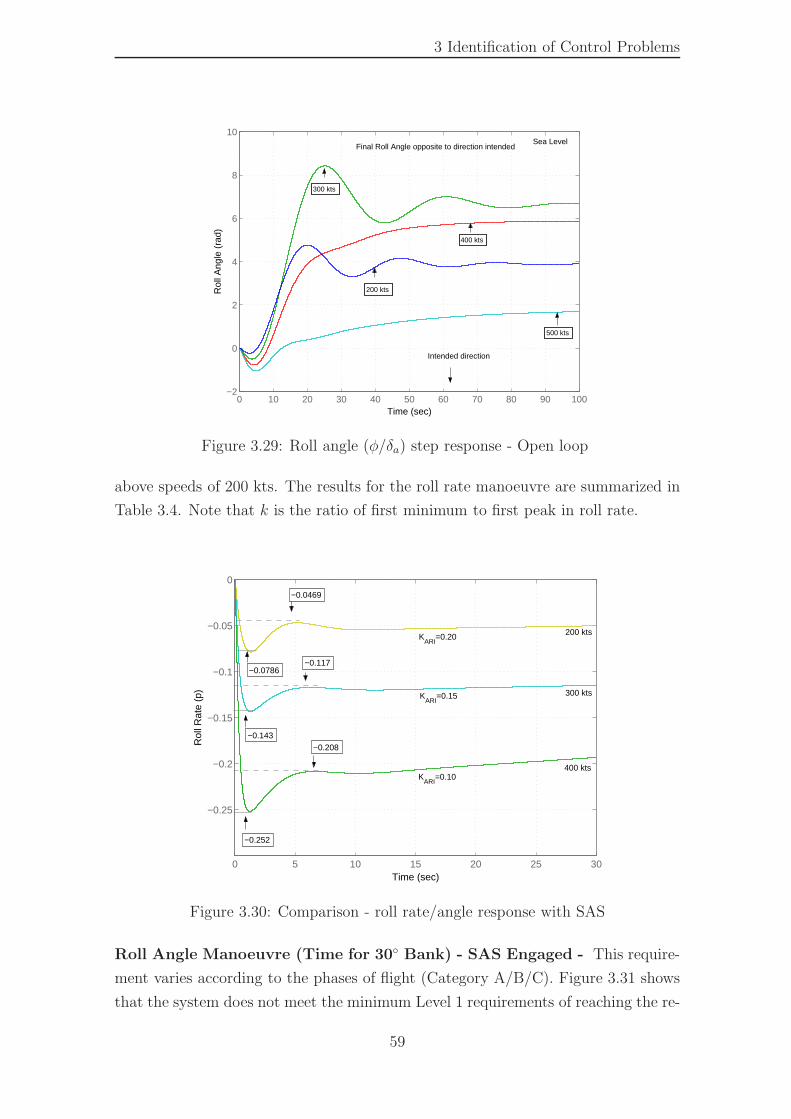
3 Identification of Control Problems
0 10 20 30 40 50 60 70 80 90 100−2
0
2
4
6
8
10
Time (sec)
Rol
l Ang
le (
rad)
200 kts
500 kts
300 kts
400 kts
Sea Level
Intended direction
Final Roll Angle opposite to direction intended
Figure 3.29: Roll angle (φ/δa) step response - Open loop
above speeds of 200 kts. The results for the roll rate manoeuvre are summarized in
Table 3.4. Note that k is the ratio of first minimum to first peak in roll rate.
0 5 10 15 20 25 30
−0.25
−0.2
−0.15
−0.1
−0.05
0
Time (sec)
Rol
l Rat
e (p
)
−0.252
−0.208 −0.143
−0.117 −0.0786
−0.0469
400 kts
300 kts
200 kts
KARI
=0.10
KARI
=0.15
KARI
=0.20
Figure 3.30: Comparison - roll rate/angle response with SAS
Roll Angle Manoeuvre (Time for 30◦ Bank) - SAS Engaged - This require-
ment varies according to the phases of flight (Category A/B/C). Figure 3.31 shows
that the system does not meet the minimum Level 1 requirements of reaching the re-
59
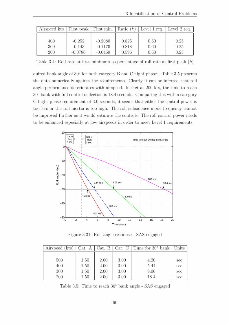
3 Identification of Control Problems
Airspeed kts First peak First min. Ratio (k) Level 1 req. Level 2 req.
400 -0.252 -0.2080 0.825 0.60 0.25300 -0.143 -0.1170 0.818 0.60 0.25200 -0.0786 -0.0469 0.596 0.60 0.25
Table 3.4: Roll rate at first minimum as percentage of roll rate at first peak (k)
quired bank angle of 30◦ for both category B and C flight phases. Table 3.5 presents
the data numerically against the requirements. Clearly it can be inferred that roll
angle performance deteriorates with airspeed. In fact at 200 kts, the time to reach
30◦ bank with full control deflection is 18.4 seconds. Comparing this with a category
C flight phase requirement of 3.0 seconds, it seems that either the control power is
too less or the roll inertia is too high. The roll subsidence mode frequency cannot
be improved further as it would saturate the controls. The roll control power needs
to be enhanced especially at low airspeeds in order to meet Level 1 requirements.
0 2 4 6 8 10 12 14 16 18 20−50
−40
−30
−20
−10
0
10
Time (sec)
Rol
l ang
le (
deg)
Time to reach 30 deg Bank Angle Cat CReq
3 sec
Cat BReq
2 sec
500 kts
400 kts
300 kts
200 kts
18.4 sec 9.06 sec 5.44 sec
4.2 sec
Figure 3.31: Roll angle response - SAS engaged
Airspeed (kts) Cat. A Cat. B Cat. C Time for 30◦ bank Units
500 1.50 2.00 3.00 4.20 sec400 1.50 2.00 3.00 5.44 sec300 1.50 2.00 3.00 9.06 sec200 1.50 2.00 3.00 18.4 sec
Table 3.5: Time to reach 30◦ bank angle - SAS engaged
60
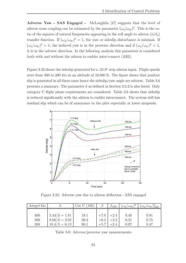
3 Identification of Control Problems
Adverse Yaw - SAS Engaged - McLaughlin [47] suggests that the level of
aileron cross coupling can be estimated by the parameter (ωφ/ωdr)2. This is the ra-
tio of the squares of natural frequencies appearing in the roll angle to aileron (φ/δa)
transfer function. If (ωφ/ωdr)2 = 1, the yaw or sideslip disturbance is minimal. If
(ωφ/ωdr)2 > 1, the induced yaw is in the proverse direction and if (ωφ/ωdr)
2 < 1,
it is in the adverse direction. In the following analysis this parameter is considered
both with and without the aileron to rudder inter-connect (ARI).
Figure 3.32 shows the sideslip generated for a -25.0◦ step aileron input. Flight speeds
were from 400 to 200 kts at an altitude of 10,000 ft. The figure shows that positive
slip is generated in all three cases hence the sideslip/yaw angle are adverse. Table 3.6
presents a summary. The parameter k as defined in Section 3.3.2 is also listed. Only
category C flight phase requirements are considered. Table 3.6 shows that sideslip
is reduced significantly with the aileron to rudder interconnect. The system still has
residual slip which can be of annoyance to the pilot especially at lower airspeeds.
0 5 10 15 20 250
1
2
3
4
5
6
7
8
Time (sec)
Sid
eslip
(de
g)
+7.0 deg
+6.4 deg
+ 5.7 deg
+2.4 deg
+2.2 deg
400 kts
300 kts
200 kts
300 kts
400 kts
200 kts
With ARI
Without ARI
Steady incrementdue to unstableSpiral Mode
Figure 3.32: Adverse yaw due to aileron deflection - SAS engaged
Airspd kts k Cat C (10k) β βARI (ωφ/ωdr)2 (ωφ/ωdr)
2ARI
400 5.44/3 = 1.81 18.1 +7.0 +2.4 0.40 0.81300 9.06/3 = 3.02 30.2 +6.4 +2.2 0.31 0.75200 18.4/3 = 6.13 60.1 +5.7 +2.4 0.07 0.47
Table 3.6: Adverse/proverse yaw measurements
61
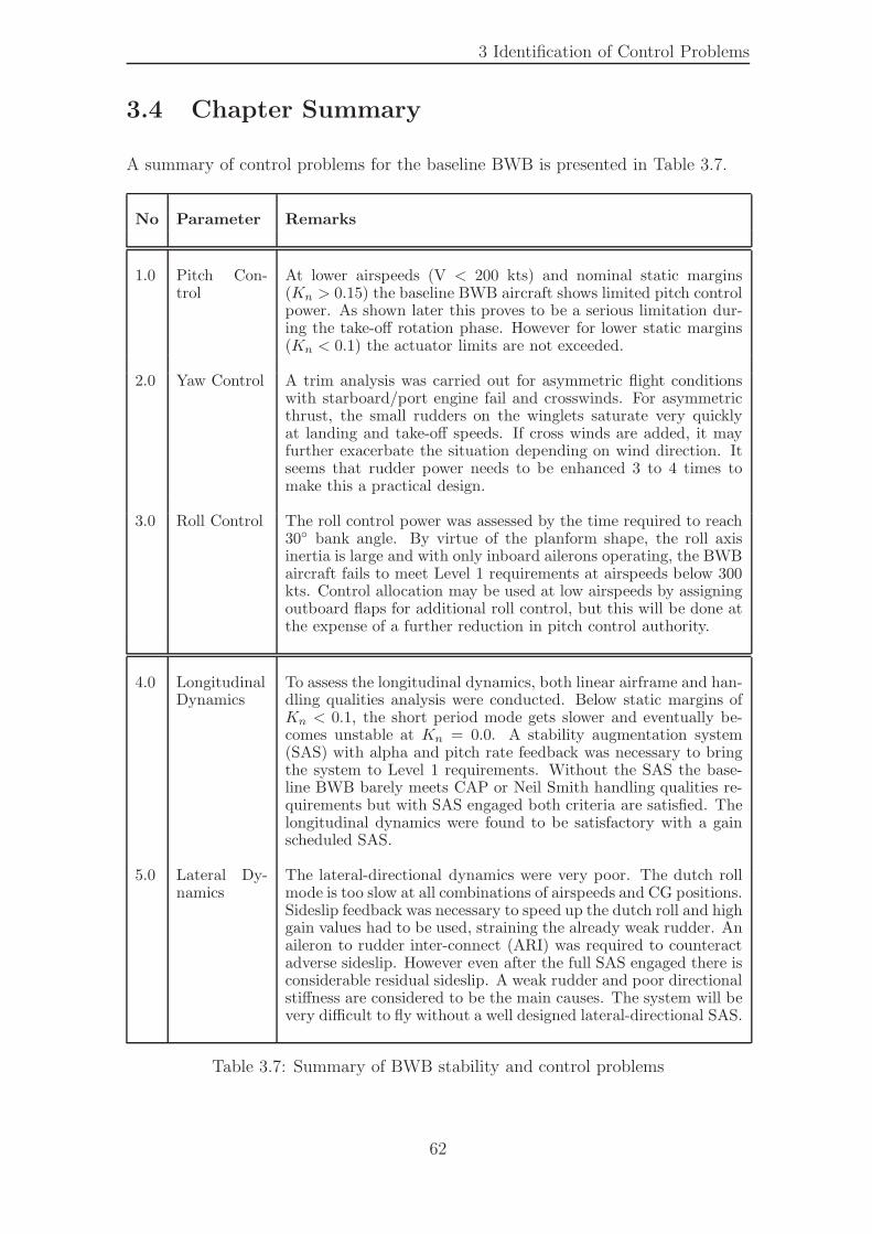
3 Identification of Control Problems
3.4 Chapter Summary
A summary of control problems for the baseline BWB is presented in Table 3.7.
No Parameter Remarks
1.0 Pitch Con-trol
At lower airspeeds (V < 200 kts) and nominal static margins(Kn > 0.15) the baseline BWB aircraft shows limited pitch controlpower. As shown later this proves to be a serious limitation dur-ing the take-off rotation phase. However for lower static margins(Kn < 0.1) the actuator limits are not exceeded.
2.0 Yaw Control A trim analysis was carried out for asymmetric flight conditionswith starboard/port engine fail and crosswinds. For asymmetricthrust, the small rudders on the winglets saturate very quicklyat landing and take-off speeds. If cross winds are added, it mayfurther exacerbate the situation depending on wind direction. Itseems that rudder power needs to be enhanced 3 to 4 times tomake this a practical design.
3.0 Roll Control The roll control power was assessed by the time required to reach30◦ bank angle. By virtue of the planform shape, the roll axisinertia is large and with only inboard ailerons operating, the BWBaircraft fails to meet Level 1 requirements at airspeeds below 300kts. Control allocation may be used at low airspeeds by assigningoutboard flaps for additional roll control, but this will be done atthe expense of a further reduction in pitch control authority.
4.0 LongitudinalDynamics
To assess the longitudinal dynamics, both linear airframe and han-dling qualities analysis were conducted. Below static margins ofKn < 0.1, the short period mode gets slower and eventually be-comes unstable at Kn = 0.0. A stability augmentation system(SAS) with alpha and pitch rate feedback was necessary to bringthe system to Level 1 requirements. Without the SAS the base-line BWB barely meets CAP or Neil Smith handling qualities re-quirements but with SAS engaged both criteria are satisfied. Thelongitudinal dynamics were found to be satisfactory with a gainscheduled SAS.
5.0 Lateral Dy-namics
The lateral-directional dynamics were very poor. The dutch rollmode is too slow at all combinations of airspeeds and CG positions.Sideslip feedback was necessary to speed up the dutch roll and highgain values had to be used, straining the already weak rudder. Anaileron to rudder inter-connect (ARI) was required to counteractadverse sideslip. However even after the full SAS engaged there isconsiderable residual sideslip. A weak rudder and poor directionalstiffness are considered to be the main causes. The system will bevery difficult to fly without a well designed lateral-directional SAS.
Table 3.7: Summary of BWB stability and control problems
62
Chapter 4
Transient Engine Model and
Effects of Controls Integration
In the previous chapter, the BWB aircraft was analyzed from a stability and con-
trols point of view and certain problem areas were identified. In this context, various
control methodologies were highlighted in Chapter 1, where the propulsion system
could be used to augment the control characteristics of the BWB aircraft. These
included, (i) thrust vectoring to supplement the aerodynamic flight controls for the
longitudinal and lateral-directional axis and (ii) the use of blown flaps to improve
flap effectiveness and hence provide better control authority.
Thrust vectoring on its own does not directly affect the engine operating point or the
steady state running line. The loss in axial thrust due to vectored thrust can be re-
claimed by adjustment of throttle position. However in a blown flap arrangement, if
the bleed mass flow is taken from an engine compressor stage, then this disrupts the
mass flow for engine components downstream. The engine operating point shifts and
may adversely affect critical engine parameters such as the turbine entry temperature
(TET), the specific fuel consumption (SFC) and thrust. It is therefore considered
necessary to a have a real-time transient model of the propulsion system that could
be integrated with a BWB aircraft with a blown flap controls arrangement. In this
context this chapter will cover,
• The development of a transient engine model.
• Model validation.
• Engine performance under variable bleed conditions.
• Engine performance under thrust vectoring.
63
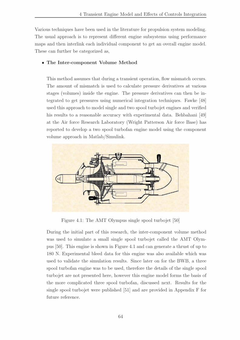
4 Transient Engine Model and Effects of Controls Integration
Various techniques have been used in the literature for propulsion system modeling.
The usual approach is to represent different engine subsystems using performance
maps and then interlink each individual component to get an overall engine model.
These can further be categorized as,
• The Inter-component Volume Method
This method assumes that during a transient operation, flow mismatch occurs.
The amount of mismatch is used to calculate pressure derivatives at various
stages (volumes) inside the engine. The pressure derivatives can then be in-
tegrated to get pressures using numerical integration techniques. Fawke [48]
used this approach to model single and two spool turbojet engines and verified
his results to a reasonable accuracy with experimental data. Behbahani [49]
at the Air force Research Laboratory (Wright Patterson Air force Base) has
reported to develop a two spool turbofan engine model using the component
volume approach in Matlab/Simulink.
Figure 4.1: The AMT Olympus single spool turbojet [50]
During the initial part of this research, the inter-component volume method
was used to simulate a small single spool turbojet called the AMT Olym-
pus [50]. This engine is shown in Figure 4.1 and can generate a thrust of up to
180 N. Experimental bleed data for this engine was also available which was
used to validate the simulation results. Since later on for the BWB, a three
spool turbofan engine was to be used, therefore the details of the single spool
turbojet are not presented here, however this engine model forms the basis of
the more complicated three spool turbofan, discussed next. Results for the
single spool turbojet were published [51] and are provided in Appendix F for
future reference.
64
4 Transient Engine Model and Effects of Controls Integration
• The Iterative Method
This method uses an iterative approach such as the Newton Raphson method [52]
to satisfy or minimize a set of error variables given certain engine parameters
as inputs. The method starts with an initial guess of the engine state vector
and computes error variables that need to satisfy steady state constraints. A
pass through the engine calculations is made and the errors or mismatch across
engine components are calculated. The error values are used to calculate a new
and improved guess for the state vector. The process is repeated till the error
variables are less than a specified tolerance.
Sellers [12] used the iterative approach to model the transient performance
of various engine configurations. An engine simulation program by the name
of DYNGEN was written by Sellers and later updated it by DYGABCD. The
DYGABCD was also capable of producing A,B,C,D matrices (linear model) at
a given engine operating point. Lately, Parker [53] at the NASA’s Glenn Re-
search centre has developed a turbofan engine simulation in Matlab/Simulink.
The program is called MAPSS (Modular Aero Propulsion Simulation Soft-
ware) and is based on an iterative procedure.
The DYNGEN program had transient capability and could simulate a three
spool turbofan with inter-stage bleeds. It was accurate and could easily handle
design point calculations. It was used extensively for the initial assessment of
the three spool turbofan. Its only draw back was that it used an iterative ap-
proach, a three spool turbofan would require nine state variables and as many
iterations to reach a converged solution. Thus it was not suitable for real-time
implementation. On the other hand, the non-iterative inter-component volume
approach when expanded to a three spool turbofan started giving increasing
errors across high pressure engine stages. To solve this problem a hybrid ap-
proach was adopted which combined the two methods thus providing both
speed and accuracy. This approach was applied to the three spool turbofan
and shall form the subject for the rest of this chapter.
65
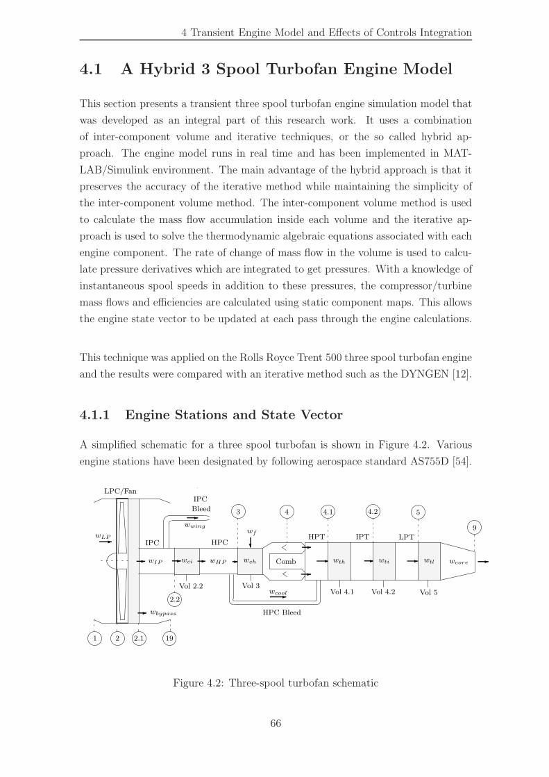
4 Transient Engine Model and Effects of Controls Integration
4.1 A Hybrid 3 Spool Turbofan Engine Model
This section presents a transient three spool turbofan engine simulation model that
was developed as an integral part of this research work. It uses a combination
of inter-component volume and iterative techniques, or the so called hybrid ap-
proach. The engine model runs in real time and has been implemented in MAT-
LAB/Simulink environment. The main advantage of the hybrid approach is that it
preserves the accuracy of the iterative method while maintaining the simplicity of
the inter-component volume method. The inter-component volume method is used
to calculate the mass flow accumulation inside each volume and the iterative ap-
proach is used to solve the thermodynamic algebraic equations associated with each
engine component. The rate of change of mass flow in the volume is used to calcu-
late pressure derivatives which are integrated to get pressures. With a knowledge of
instantaneous spool speeds in addition to these pressures, the compressor/turbine
mass flows and efficiencies are calculated using static component maps. This allows
the engine state vector to be updated at each pass through the engine calculations.
This technique was applied on the Rolls Royce Trent 500 three spool turbofan engine
and the results were compared with an iterative method such as the DYNGEN [12].
4.1.1 Engine Stations and State Vector
A simplified schematic for a three spool turbofan is shown in Figure 4.2. Various
engine stations have been designated by following aerospace standard AS755D [54].
IPCLPC/Fan
- wbypass
IPC-wLP
wci
Bleed
wwing
-
- -wcore-
?
Comb
-
--
HPC
- -
Vol 3Vol 2.2Vol 4.1
wf
wth
-
HPC Bleed
wcool
-wti
HPT
Vol 4.2
IPT LPT
wtl
Vol 5
-wchwIP wHP
4.1 4.2 5
9
4
2.11 2
2.2
3
19
Figure 4.2: Three-spool turbofan schematic
66
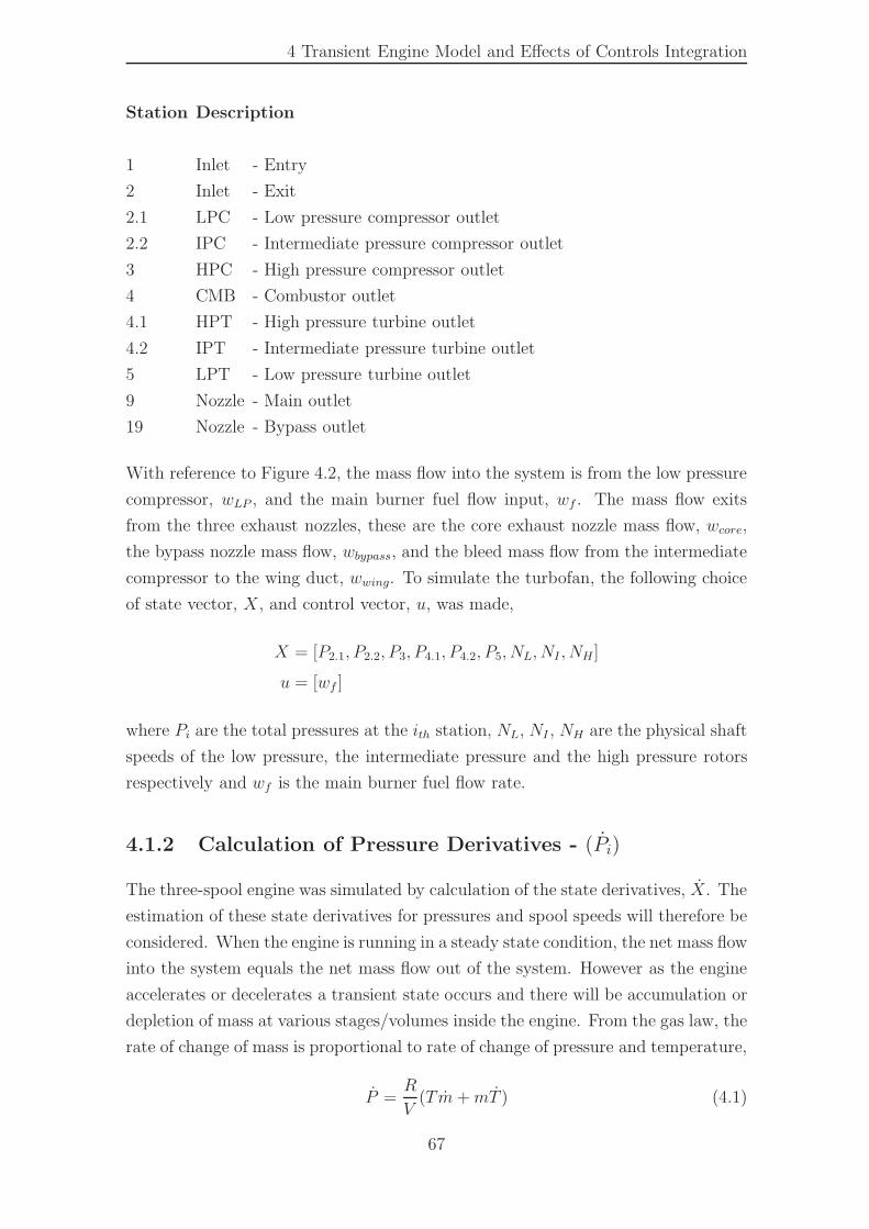
4 Transient Engine Model and Effects of Controls Integration
Station Description
1 Inlet - Entry
2 Inlet - Exit
2.1 LPC - Low pressure compressor outlet
2.2 IPC - Intermediate pressure compressor outlet
3 HPC - High pressure compressor outlet
4 CMB - Combustor outlet
4.1 HPT - High pressure turbine outlet
4.2 IPT - Intermediate pressure turbine outlet
5 LPT - Low pressure turbine outlet
9 Nozzle - Main outlet
19 Nozzle - Bypass outlet
With reference to Figure 4.2, the mass flow into the system is from the low pressure
compressor, wLP , and the main burner fuel flow input, wf . The mass flow exits
from the three exhaust nozzles, these are the core exhaust nozzle mass flow, wcore,
the bypass nozzle mass flow, wbypass, and the bleed mass flow from the intermediate
compressor to the wing duct, wwing. To simulate the turbofan, the following choice
of state vector, X, and control vector, u, was made,
X = [P2.1, P2.2, P3, P4.1, P4.2, P5, NL, NI , NH ]
u = [wf ]
where Pi are the total pressures at the ith station, NL, NI , NH are the physical shaft
speeds of the low pressure, the intermediate pressure and the high pressure rotors
respectively and wf is the main burner fuel flow rate.
4.1.2 Calculation of Pressure Derivatives - (Pi)
The three-spool engine was simulated by calculation of the state derivatives, X. The
estimation of these state derivatives for pressures and spool speeds will therefore be
considered. When the engine is running in a steady state condition, the net mass flow
into the system equals the net mass flow out of the system. However as the engine
accelerates or decelerates a transient state occurs and there will be accumulation or
depletion of mass at various stages/volumes inside the engine. From the gas law, the
rate of change of mass is proportional to rate of change of pressure and temperature,
P =R
V(Tm+mT ) (4.1)
67
4 Transient Engine Model and Effects of Controls Integration
The above equation has two derivatives, the terms mT andmT . Bates and Fawke [48]
have shown that the temperature derivative can be neglected in comparison to the
mass derivative term. Thus to calculate the pressure derivatives, the mass flow
errors inside the control volumes are required. The pressure derivatives are based
on engine component maps as outlined in Appendix E and have been obtained as
follows,
4.1.2.1 Mass Flow Error at LPC/Fan exit - (m2.1)
With reference to Figure 4.4, an inter-component volume, V2.1, is placed at the fan
exit and the entry of the intermediate compressor and the bypass duct. The mass
flow, wcl, entering into this volume is from the low pressure (LP) compressor which
is a function of LPC corrected shaft speed, NLC∗ = NL/
√
T2/Tstd, and fan pressure
ratio, P2.1/P2. With the assumption of zero bleed from the LPC stage we have,
wLP = wcl = f(P2.1
P2
, NLC∗)MAP (4.2)
where wLP is obtained using an LP compressor map given in Appendix E, with LPC
pressure ratio, P2.1/P2, and corrected LPC shaft speed, NLC∗, as inputs.
wbypasswLP
V2.1
Fan/LPC
-
-wcl wIP
m2.1
P2.1, T2.1
P1
P2
IPC-
P2.2, T2.2
-wci
-
Pa
Figure 4.3: Inter-component volume, V2.1, between Fan and IPC/bypass nozzle
The mass flow exiting from the control volume, V2.1, goes into the intermediate
pressure (IP) compressor and the bypass nozzle. The mass flow ingested by the
intermediate compressor, wIP , is a function of the intermediate compressor pressure
ratio, P2.2/P2.1, and the IPC corrected shaft speed, NIC∗ = NI/
√
T2.1/Tstd. A
68
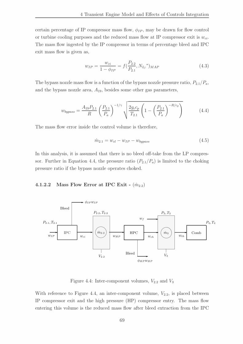
4 Transient Engine Model and Effects of Controls Integration
certain percentage of IP compressor mass flow, φIP , may be drawn for flow control
or turbine cooling purposes and the reduced mass flow at IP compressor exit is wci.
The mass flow ingested by the IP compressor in terms of percentage bleed and IPC
exit mass flow is given as,
wIP =wci
1 − φIP= f(
P2.2
P2.1, NIC
∗)MAP (4.3)
The bypass nozzle mass flow is a function of the bypass nozzle pressure ratio, P2.1/Pa,
and the bypass nozzle area, A19, besides some other gas parameters,
wbypass =A19P2.1
R
(
P2.1
Pa
)
−1/γ
√
√
√
√
2gccpT2.1
(
1 −(
P2.1
Pa
)
−R/cp)
(4.4)
The mass flow error inside the control volume is therefore,
m2.1 = wcl − wIP − wbypass (4.5)
In this analysis, it is assumed that there is no bleed off-take from the LP compres-
sor. Further in Equation 4.4, the pressure ratio (P2.1/Pa) is limited to the choking
pressure ratio if the bypass nozzle operates choked.
4.1.2.2 Mass Flow Error at IPC Exit - (m2.2)
IPCwIP
V2.2
-
Bleed
HPC
- φIPwIP
wci
-wHP
φHPwHP
-
P2.2, T2.2 P3, T3
P2.1, T2.1
-wch
-Bleed
- Combm2.2wth
P4, T4
-wf
m3
V3
Figure 4.4: Inter-component volumes, V2.2 and V3
With reference to Figure 4.4, an inter-component volume, V2.2, is placed between
IP compressor exit and the high pressure (HP) compressor entry. The mass flow
entering this volume is the reduced mass flow after bleed extraction from the IPC
69
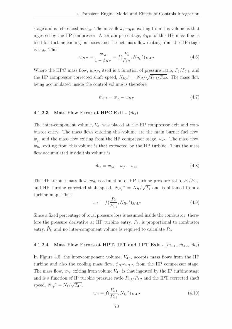
4 Transient Engine Model and Effects of Controls Integration
stage and is referenced as wci. The mass flow, wHP , exiting from this volume is that
ingested by the HP compressor. A certain percentage, φHP , of this HP mass flow is
bled for turbine cooling purposes and the net mass flow exiting from the HP stage
is wch. Thus
wHP =wch
1 − φHP= f(
P3
P2.2, NHC
∗)MAP (4.6)
Where the HPC mass flow, wHP , itself is a function of pressure ratio, P3/P2.2, and
the HP compressor corrected shaft speed, NHC∗ = NH/
√
T2.2/Tstd. The mass flow
being accumulated inside the control volume is therefore
m2.2 = wci − wHP (4.7)
4.1.2.3 Mass Flow Error at HPC Exit - (m3)
The inter-component volume, V3, was placed at the HP compressor exit and com-
bustor entry. The mass flows entering this volume are the main burner fuel flow,
wf , and the mass flow exiting from the HP compressor stage, wch. The mass flow,
wth, exiting from this volume is that extracted by the HP turbine. Thus the mass
flow accumulated inside this volume is
m3 = wch + wf − wth (4.8)
The HP turbine mass flow, wth is a function of HP turbine pressure ratio, P4/P4.1,
and HP turbine corrected shaft speed, NHT∗ = NH/
√T4 and is obtained from a
turbine map. Thus
wth = f(P4
P4.1
, NHT∗)MAP (4.9)
Since a fixed percentage of total pressure loss is assumed inside the combustor, there-
fore the pressure derivative at HP turbine entry, P4, is proportional to combustor
entry, P3, and no inter-component volume is required to calculate P4.
4.1.2.4 Mass Flow Errors at HPT, IPT and LPT Exit - (m4.1, m4.2, m5)
In Figure 4.5, the inter-component volume, V4.1, accepts mass flows from the HP
turbine and also the cooling mass flow, φHPwHP , from the HP compressor stage.
The mass flow, wti, exiting from volume V4.1 is that ingested by the IP turbine stage
and is a function of IP turbine pressure ratio P4.1/P4.2 and the IPT corrected shaft
speed, NIT∗ = NI/
√T4.1.
wti = f(P4.1
P4.2
, NIT∗)MAP (4.10)
70
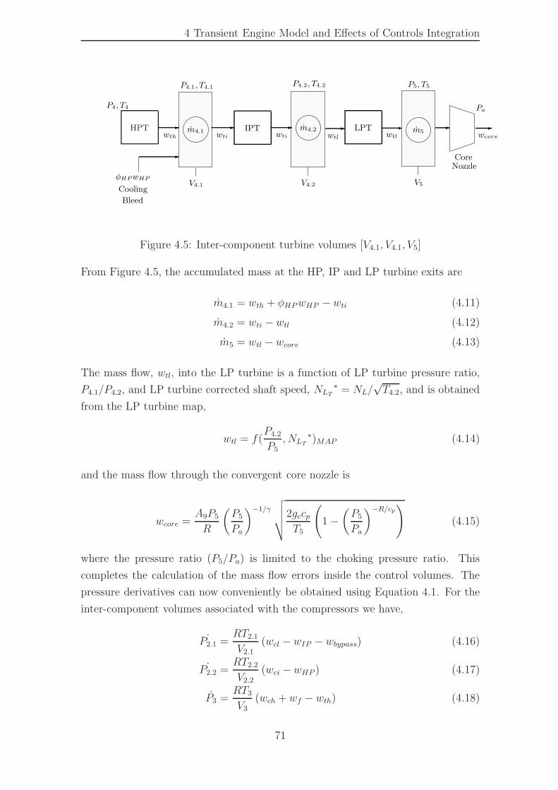
4 Transient Engine Model and Effects of Controls Integration
HPT
P4, T4
V4.1
wti- m4.2
P4.2, T4.2
wti-
wthIPT LPT
-
φHPwHPV4.2 V5
-
P5, T5
m4.1wtl
P4.1, T4.1
Cooling
m5--
wcore-
wtl
CoreNozzle
Pa
-
Bleed
Figure 4.5: Inter-component turbine volumes [V4.1, V4.1, V5]
From Figure 4.5, the accumulated mass at the HP, IP and LP turbine exits are
m4.1 = wth + φHPwHP − wti (4.11)
m4.2 = wti − wtl (4.12)
m5 = wtl − wcore (4.13)
The mass flow, wtl, into the LP turbine is a function of LP turbine pressure ratio,
P4.1/P4.2, and LP turbine corrected shaft speed, NLT∗ = NL/
√T4.2, and is obtained
from the LP turbine map,
wtl = f(P4.2
P5
, NLT∗)MAP (4.14)
and the mass flow through the convergent core nozzle is
wcore =A9P5
R
(
P5
Pa
)
−1/γ
√
√
√
√
2gccpT5
(
1 −(
P5
Pa
)
−R/cp)
(4.15)
where the pressure ratio (P5/Pa) is limited to the choking pressure ratio. This
completes the calculation of the mass flow errors inside the control volumes. The
pressure derivatives can now conveniently be obtained using Equation 4.1. For the
inter-component volumes associated with the compressors we have,
˙P2.1 =RT2.1
V2.1(wcl − wIP − wbypass) (4.16)
˙P2.2 =RT2.2
V2.2(wci − wHP ) (4.17)
P3 =RT3
V3
(wch + wf − wth) (4.18)
71
4 Transient Engine Model and Effects of Controls Integration
and similarly for the volumes associated with the turbines,
˙P4.1 =RT4.1
V4.1(wth + φHPwHP − wti) (4.19)
˙P4.2 =RT4.2
V4.2(wti − wtl) (4.20)
P5 =RT5
V5(wtl − wcore) (4.21)
Now if the initial pressures are known, then from the knowledge of the initial state
vector, X0, the subsequent time history of Pi can be obtained by convenient numer-
ical integration methods.
4.1.3 Calculation of Speed Derivatives - (N)
The remaining derivatives of the state vector i.e. the rotational acceleration deriva-
tives NL, NI , NH can be calculated by estimating the difference in torque generated
by the turbine and that required by the compressor,
N =dN
dt=
(ηmτturb − τcomp)
Is(4.22)
The turbine torque, τturb, or the compressor torque, τcomp, can be expressed in terms
of turbine and compressor work and physical spool speeds. In addition, if there is
a fraction of bleed (φ = wb/wc) taken from a non-dimensional axial location (x/l)
along the compressor, then the torque required by the compressor is
τcomp =60
2πNwccp∆Tc
(
(1 − φ) + φx
l
)
(4.23)
From reference [55], ∆Tc is,
∆Tc =1
ηcT1
(
(
P2
P1
)γ−1γ
− 1
)
(4.24)
Here subscripts 1 and 2, represent inlet and outlet conditions respectively, and do
not relate to the three spool turbofan station designation. The problem with Equa-
tion (4.24) is that it is implicit, and the values of parameters like γ and cp are in
turn dependent upon exit conditions, [T2, P2]. Fixed values of these parameters had
to be assumed. This was later found to introduce significant errors in high pressure
stages. It was therefore decided to solve these equations iteratively using specific
enthalpy, h, rather than total temperature. In terms of enthalpy change, the torques
72
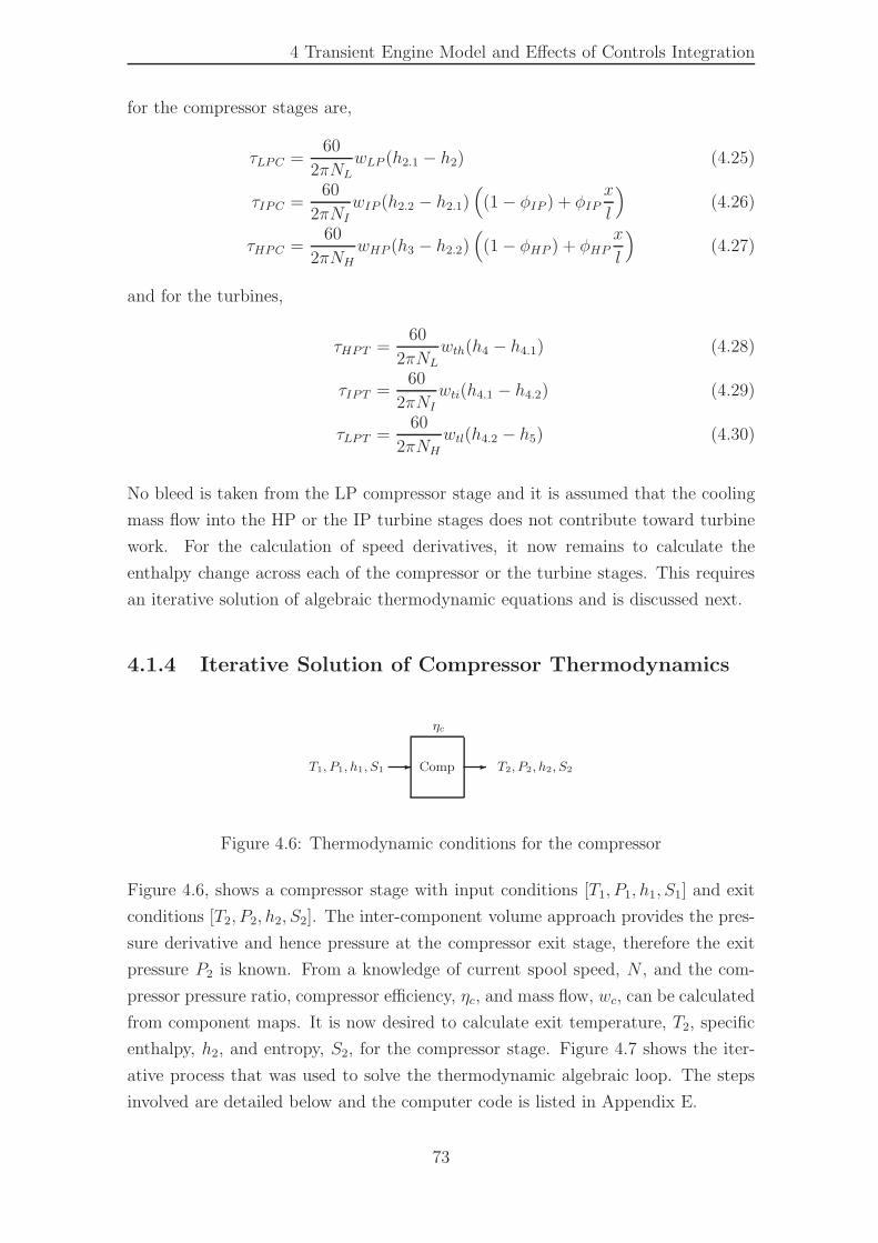
4 Transient Engine Model and Effects of Controls Integration
for the compressor stages are,
τLPC =60
2πNLwLP (h2.1 − h2) (4.25)
τIPC =60
2πNIwIP (h2.2 − h2.1)
(
(1 − φIP ) + φIPx
l
)
(4.26)
τHPC =60
2πNHwHP (h3 − h2.2)
(
(1 − φHP ) + φHPx
l
)
(4.27)
and for the turbines,
τHPT =60
2πNL
wth(h4 − h4.1) (4.28)
τIPT =60
2πNI
wti(h4.1 − h4.2) (4.29)
τLPT =60
2πNH
wtl(h4.2 − h5) (4.30)
No bleed is taken from the LP compressor stage and it is assumed that the cooling
mass flow into the HP or the IP turbine stages does not contribute toward turbine
work. For the calculation of speed derivatives, it now remains to calculate the
enthalpy change across each of the compressor or the turbine stages. This requires
an iterative solution of algebraic thermodynamic equations and is discussed next.
4.1.4 Iterative Solution of Compressor Thermodynamics
Comp- T2, P2, h2, S2-
ηc
T1, P1, h1, S1
Figure 4.6: Thermodynamic conditions for the compressor
Figure 4.6, shows a compressor stage with input conditions [T1, P1, h1, S1] and exit
conditions [T2, P2, h2, S2]. The inter-component volume approach provides the pres-
sure derivative and hence pressure at the compressor exit stage, therefore the exit
pressure P2 is known. From a knowledge of current spool speed, N , and the com-
pressor pressure ratio, compressor efficiency, ηc, and mass flow, wc, can be calculated
from component maps. It is now desired to calculate exit temperature, T2, specific
enthalpy, h2, and entropy, S2, for the compressor stage. Figure 4.7 shows the iter-
ative process that was used to solve the thermodynamic algebraic loop. The steps
involved are detailed below and the computer code is listed in Appendix E.
73
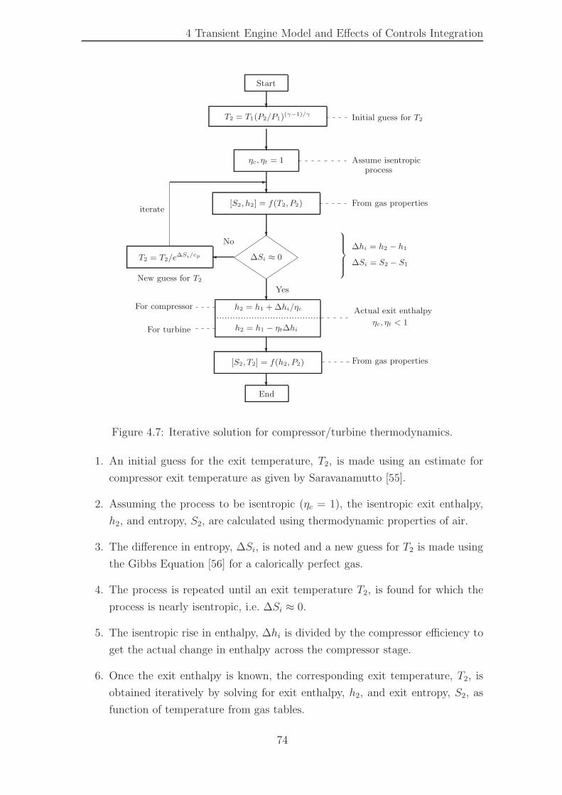
4 Transient Engine Model and Effects of Controls Integration
T2 = T1(P2/P1)(γ−1)/γ
Initial guess for T2
[S2, h2] = f(T2, P2)
ηc, ηt = 1
?
?From gas properties
Assume isentropic
?
process
T2 = T2/e∆Si/cp
-
?
∆Si ≈ 0�
New guess for T2
No
Yes
iterate
Actual exit enthalpy
ηc, ηt < 1
[S2, T2] = f(h2, P2)
?From gas properties
End
?
Start
?
∆hi = h2 − h1
∆Si = S2 − S1
h2 = h1 + ∆hi/ηc
h2 = h1 − ηt∆hi
For compressor
For turbine
........................................
Figure 4.7: Iterative solution for compressor/turbine thermodynamics.
1. An initial guess for the exit temperature, T2, is made using an estimate for
compressor exit temperature as given by Saravanamutto [55].
2. Assuming the process to be isentropic (ηc = 1), the isentropic exit enthalpy,
h2, and entropy, S2, are calculated using thermodynamic properties of air.
3. The difference in entropy, ∆Si, is noted and a new guess for T2 is made using
the Gibbs Equation [56] for a calorically perfect gas.
4. The process is repeated until an exit temperature T2, is found for which the
process is nearly isentropic, i.e. ∆Si ≈ 0.
5. The isentropic rise in enthalpy, ∆hi is divided by the compressor efficiency to
get the actual change in enthalpy across the compressor stage.
6. Once the exit enthalpy is known, the corresponding exit temperature, T2, is
obtained iteratively by solving for exit enthalpy, h2, and exit entropy, S2, as
function of temperature from gas tables.
74
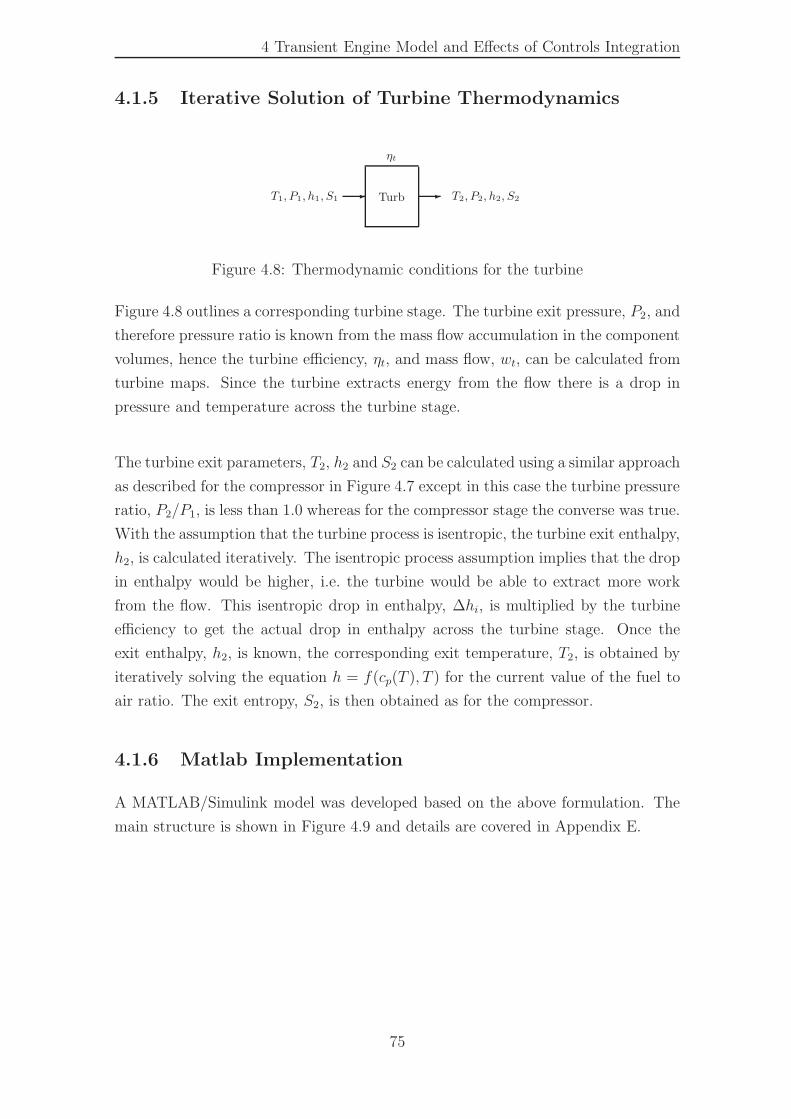
4 Transient Engine Model and Effects of Controls Integration
4.1.5 Iterative Solution of Turbine Thermodynamics
Turb- T2, P2, h2, S2-
ηt
T1, P1, h1, S1
Figure 4.8: Thermodynamic conditions for the turbine
Figure 4.8 outlines a corresponding turbine stage. The turbine exit pressure, P2, and
therefore pressure ratio is known from the mass flow accumulation in the component
volumes, hence the turbine efficiency, ηt, and mass flow, wt, can be calculated from
turbine maps. Since the turbine extracts energy from the flow there is a drop in
pressure and temperature across the turbine stage.
The turbine exit parameters, T2, h2 and S2 can be calculated using a similar approach
as described for the compressor in Figure 4.7 except in this case the turbine pressure
ratio, P2/P1, is less than 1.0 whereas for the compressor stage the converse was true.
With the assumption that the turbine process is isentropic, the turbine exit enthalpy,
h2, is calculated iteratively. The isentropic process assumption implies that the drop
in enthalpy would be higher, i.e. the turbine would be able to extract more work
from the flow. This isentropic drop in enthalpy, ∆hi, is multiplied by the turbine
efficiency to get the actual drop in enthalpy across the turbine stage. Once the
exit enthalpy, h2, is known, the corresponding exit temperature, T2, is obtained by
iteratively solving the equation h = f(cp(T ), T ) for the current value of the fuel to
air ratio. The exit entropy, S2, is then obtained as for the compressor.
4.1.6 Matlab Implementation
A MATLAB/Simulink model was developed based on the above formulation. The
main structure is shown in Figure 4.9 and details are covered in Appendix E.
75
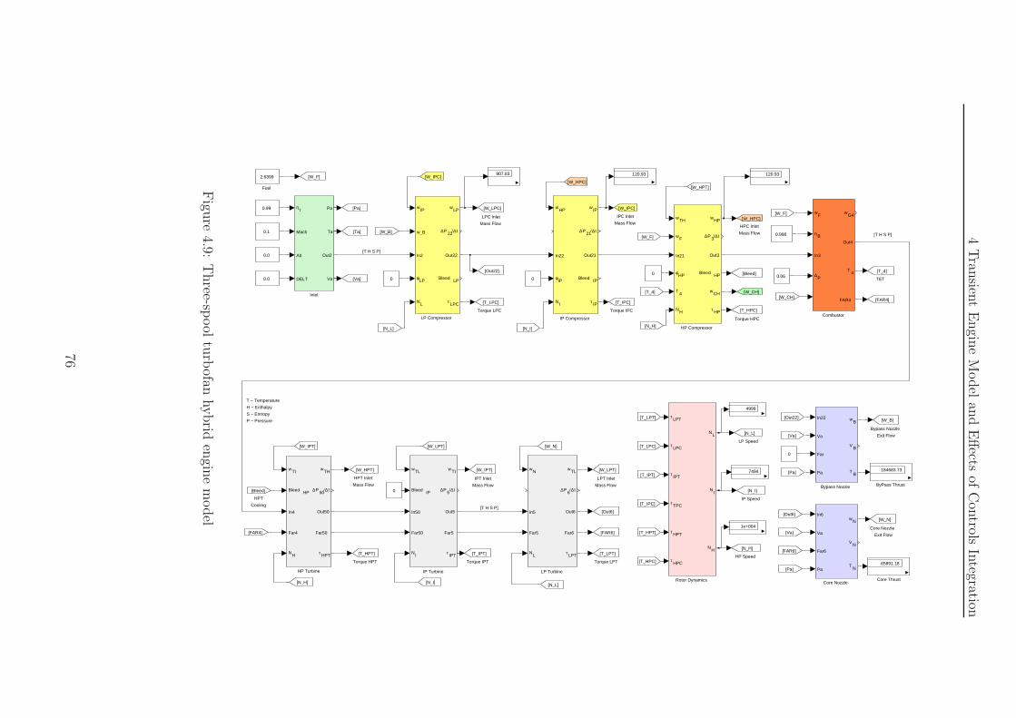
4Tran
sient
Engin
eM
odel
and
Effects
ofC
ontrols
Integration
T − Temperature
H − Enthalpy
S − Entropy
P − Pressure
[T H S P]
[Bleed]
Torque LPT
[T_LPT]
Torque LPC
[T_LPC]
Torque IPT
[T_IPT]
Torque IPC
[T_IPC]
Torque HPT
[T_HPT]
Torque HPC
[T_HPC]
[FAR4]
TET
[T_4]
Rotor Dynamics
τLPT
τLPC
τIPT
τTPC
τHPT
τHPC
NL
NI
NH
[FAR6]
[Out6]
LPT Inlet
Mass Flow
[W_LPT]
[W_F]
LPC Inlet
Mass Flow
[W_LPC]
LP Turbine
wN
In5
Far5
NL
wTL
∆P6/∆ t
Out6
Far6
τLPT
LP Speed
[N_L]
LP Compressor
wIP
w_B
In2
φLP
NL
wLP
∆P22
/∆ t
Out22
BleedLP
τLPC
Inlet
ηI
Mach
Alt
DELT
Pa
Ta
Out2
Va
[Out22]
IPT Inlet
Mass Flow
[W_IPT]
IPC Inlet
Mass Flow
[W_IPC]
IP Turbine
wTL
BleedIP
In50
Far50
NI
wTI
∆P5/∆ t
Out5
Far5
τIPT
IP Speed
[N_I]
IP Compressor
wHP
In22
φIP
NI
wIP
∆P21
/∆ t
Out21
BleedIP
τIP
[Va]
[Ta]
[Pa]
HPT Inlet
Mass Flow
[W_HPT]
[FAR4]
HPT
Cooling
[Bleed]
[W_CH]
HPC Inlet
Mass Flow
[W_HPC]
HP Turbine
wTI
BleedHP
In4
Far4
NH
wTH
∆P50
/∆ t
Out50
Far50
τHPT HP Speed
[N_H]
[Out22]
[Out6]
[W_B]
[W_N][W_LPT][W_IPT]
[W_CH]
[W_F]
[W_HPT]
[W_F]
[T_4]
[Va]
[Va]
[Pa]
[Pa]
[FAR6]
[N_H]
[N_H]
[W_IPC]
[N_I]
[N_I]
[N_L]
[N_L]
[T_HPT]
[T_IPT]
[T_LPT]
[T_HPC]
[T_IPC]
[T_LPC]
[W_HPC]
HP Compressor
wTH
wF
In21
φHP
T4
NH
wHP
∆P3/∆ t
Out3
BleedHP
wCH
τHP
Fuel
2.6399120.93120.93907.83
1e+004
7494
4999
Core Thrust
65891.18
Core Nozzle
Exit Flow
[W_N]
Core Nozzle
In6
Va
Far6
Pa
wN
VN
TN
Combustor
wF
ηB
In3
∆P
wG4
Out4
T4
FAR4
Bypass Nozzle
Exit Flow
[W_B]
Bypass Nozzle
In22
Va
Far
Pa
wB
VB
TB
ByPass Thrust
184683.73
0.998
000
0
0.1
0.0
0.0
0.99
0.06
0
[T H S P]
[T H S P]
Figu
re4.9:
Three-sp
ool
turb
ofanhybrid
engin
em
odel
76
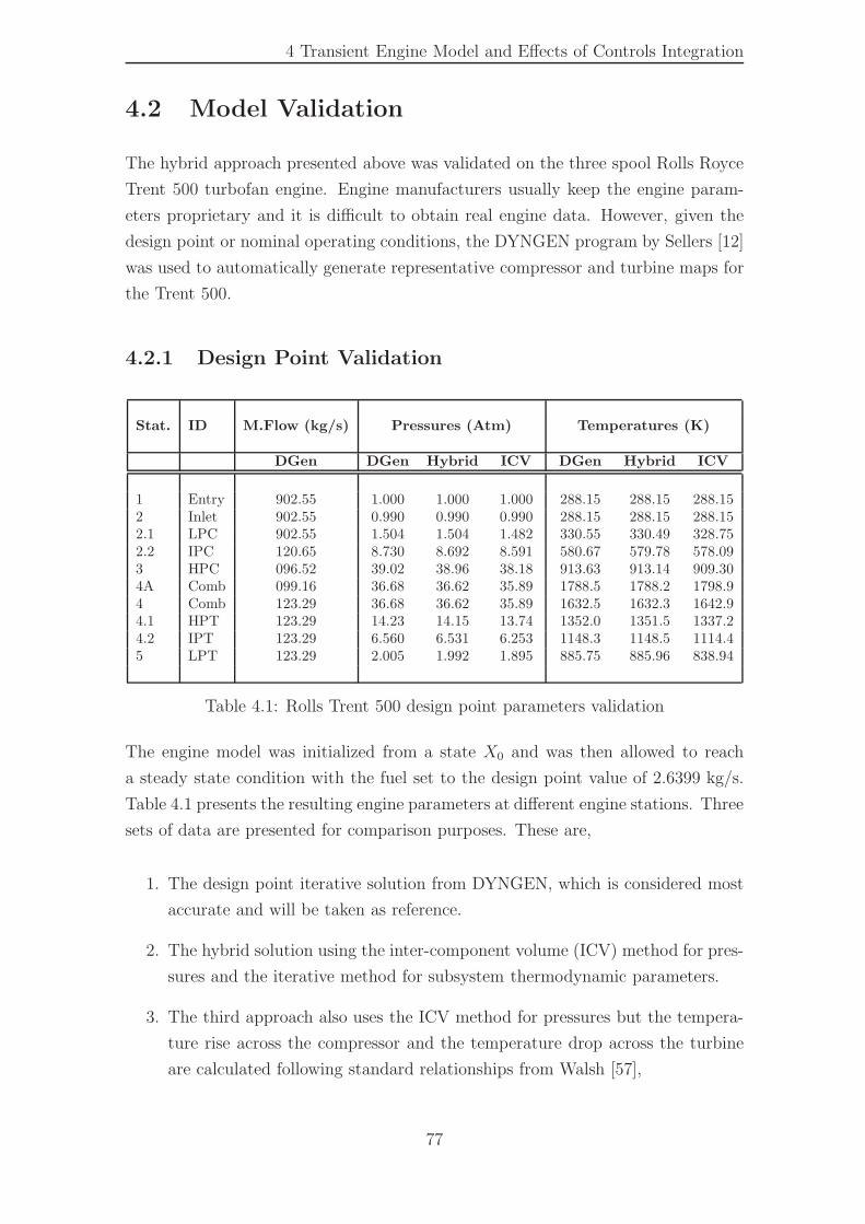
4 Transient Engine Model and Effects of Controls Integration
4.2 Model Validation
The hybrid approach presented above was validated on the three spool Rolls Royce
Trent 500 turbofan engine. Engine manufacturers usually keep the engine param-
eters proprietary and it is difficult to obtain real engine data. However, given the
design point or nominal operating conditions, the DYNGEN program by Sellers [12]
was used to automatically generate representative compressor and turbine maps for
the Trent 500.
4.2.1 Design Point Validation
Stat. ID M.Flow (kg/s) Pressures (Atm) Temperatures (K)
DGen DGen Hybrid ICV DGen Hybrid ICV
1 Entry 902.55 1.000 1.000 1.000 288.15 288.15 288.152 Inlet 902.55 0.990 0.990 0.990 288.15 288.15 288.152.1 LPC 902.55 1.504 1.504 1.482 330.55 330.49 328.752.2 IPC 120.65 8.730 8.692 8.591 580.67 579.78 578.093 HPC 096.52 39.02 38.96 38.18 913.63 913.14 909.304A Comb 099.16 36.68 36.62 35.89 1788.5 1788.2 1798.94 Comb 123.29 36.68 36.62 35.89 1632.5 1632.3 1642.94.1 HPT 123.29 14.23 14.15 13.74 1352.0 1351.5 1337.24.2 IPT 123.29 6.560 6.531 6.253 1148.3 1148.5 1114.45 LPT 123.29 2.005 1.992 1.895 885.75 885.96 838.94
Table 4.1: Rolls Trent 500 design point parameters validation
The engine model was initialized from a state X0 and was then allowed to reach
a steady state condition with the fuel set to the design point value of 2.6399 kg/s.
Table 4.1 presents the resulting engine parameters at different engine stations. Three
sets of data are presented for comparison purposes. These are,
1. The design point iterative solution from DYNGEN, which is considered most
accurate and will be taken as reference.
2. The hybrid solution using the inter-component volume (ICV) method for pres-
sures and the iterative method for subsystem thermodynamic parameters.
3. The third approach also uses the ICV method for pressures but the tempera-
ture rise across the compressor and the temperature drop across the turbine
are calculated following standard relationships from Walsh [57],
77
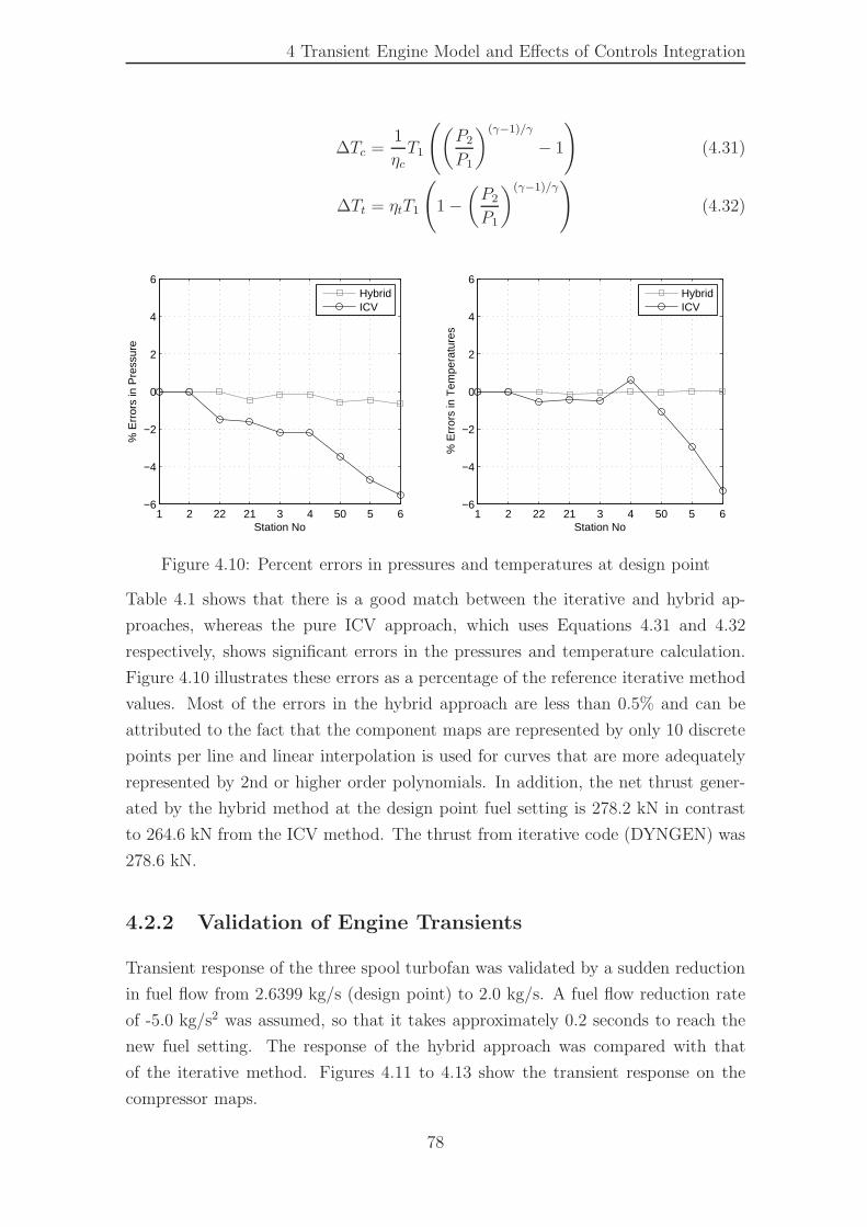
4 Transient Engine Model and Effects of Controls Integration
∆Tc =1
ηcT1
(
(
P2
P1
)(γ−1)/γ
− 1
)
(4.31)
∆Tt = ηtT1
(
1 −(
P2
P1
)(γ−1)/γ)
(4.32)
1 2 22 21 3 4 50 5 6−6
−4
−2
0
2
4
6
Station No
% E
rror
s in
Pre
ssur
e
HybridICV
1 2 22 21 3 4 50 5 6−6
−4
−2
0
2
4
6
Station No
% E
rror
s in
Tem
pera
ture
s
HybridICV
Figure 4.10: Percent errors in pressures and temperatures at design point
Table 4.1 shows that there is a good match between the iterative and hybrid ap-
proaches, whereas the pure ICV approach, which uses Equations 4.31 and 4.32
respectively, shows significant errors in the pressures and temperature calculation.
Figure 4.10 illustrates these errors as a percentage of the reference iterative method
values. Most of the errors in the hybrid approach are less than 0.5% and can be
attributed to the fact that the component maps are represented by only 10 discrete
points per line and linear interpolation is used for curves that are more adequately
represented by 2nd or higher order polynomials. In addition, the net thrust gener-
ated by the hybrid method at the design point fuel setting is 278.2 kN in contrast
to 264.6 kN from the ICV method. The thrust from iterative code (DYNGEN) was
278.6 kN.
4.2.2 Validation of Engine Transients
Transient response of the three spool turbofan was validated by a sudden reduction
in fuel flow from 2.6399 kg/s (design point) to 2.0 kg/s. A fuel flow reduction rate
of -5.0 kg/s2 was assumed, so that it takes approximately 0.2 seconds to reach the
new fuel setting. The response of the hybrid approach was compared with that
of the iterative method. Figures 4.11 to 4.13 show the transient response on the
compressor maps.
78
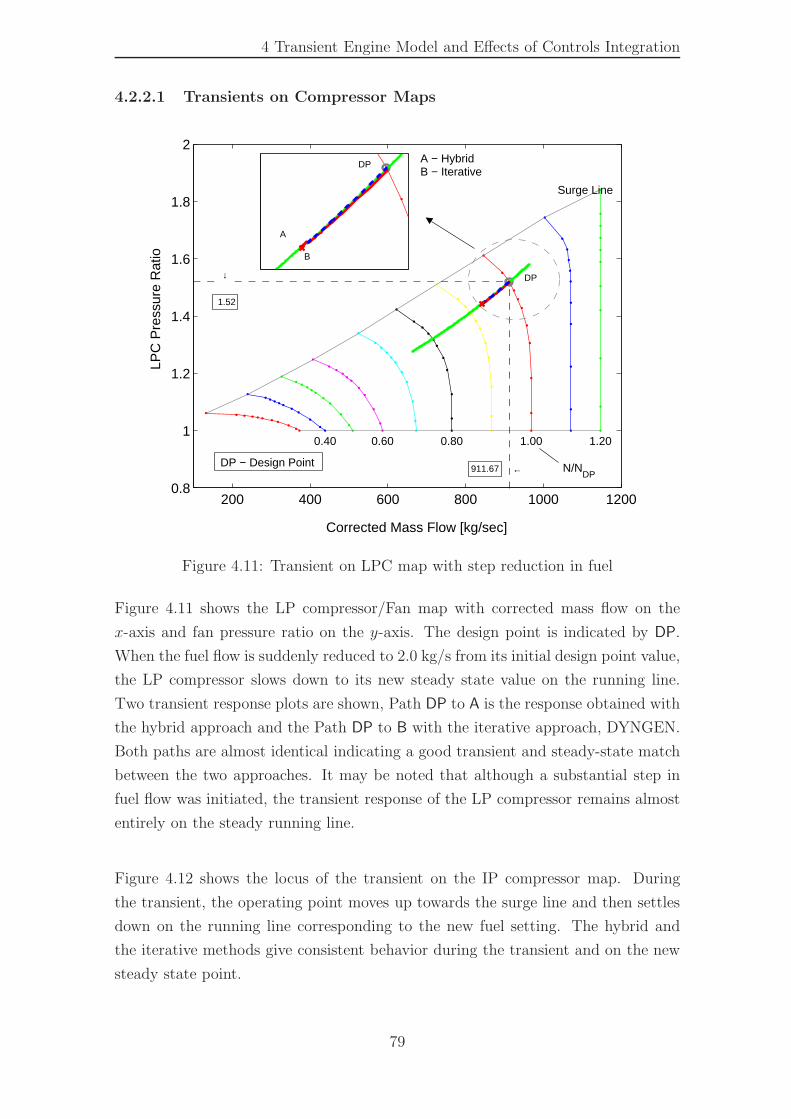
4 Transient Engine Model and Effects of Controls Integration
4.2.2.1 Transients on Compressor Maps
200 400 600 800 1000 12000.8
1
1.2
1.4
1.6
1.8
2
0.40 0.60 0.80 1.00 1.20
Corrected Mass Flow [kg/sec]
LPC
Pre
ssur
e R
atio
1.52
↓
←911.67
DP
A
B
DP
Surge Line
A − HybridB − Iterative
N/NDP
DP − Design Point
Figure 4.11: Transient on LPC map with step reduction in fuel
Figure 4.11 shows the LP compressor/Fan map with corrected mass flow on the
x-axis and fan pressure ratio on the y-axis. The design point is indicated by DP.
When the fuel flow is suddenly reduced to 2.0 kg/s from its initial design point value,
the LP compressor slows down to its new steady state value on the running line.
Two transient response plots are shown, Path DP to A is the response obtained with
the hybrid approach and the Path DP to B with the iterative approach, DYNGEN.
Both paths are almost identical indicating a good transient and steady-state match
between the two approaches. It may be noted that although a substantial step in
fuel flow was initiated, the transient response of the LP compressor remains almost
entirely on the steady running line.
Figure 4.12 shows the locus of the transient on the IP compressor map. During
the transient, the operating point moves up towards the surge line and then settles
down on the running line corresponding to the new fuel setting. The hybrid and
the iterative methods give consistent behavior during the transient and on the new
steady state point.
79
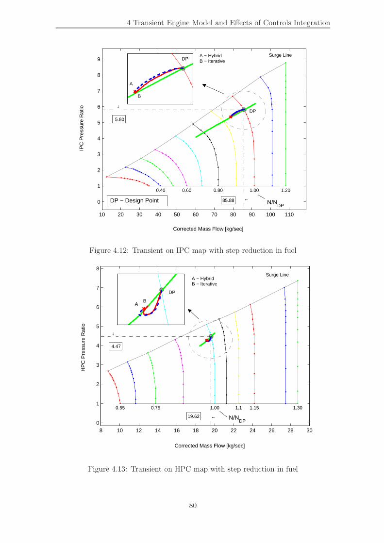
4 Transient Engine Model and Effects of Controls Integration
10 20 30 40 50 60 70 80 90 100 110
0
1
2
3
4
5
6
7
8
9
0.40 0.60 0.80 1.00 1.20
Corrected Mass Flow [kg/sec]
IPC
Pre
ssur
e R
atio
5.80
↓
←85.88
Surge Line
DP
DP
A
B
A − HybridB − Iterative
DP − Design Point N/NDP
Figure 4.12: Transient on IPC map with step reduction in fuel
8 10 12 14 16 18 20 22 24 26 28 300
1
2
3
4
5
6
7
8
0.55 0.75 1.00 1.1 1.15 1.30
Corrected Mass Flow [kg/sec]
HP
C P
ress
ure
Rat
io
4.47
↓
←19.62
AB
DP
A − HybridB − Iterative
Surge Line
N/NDP
Figure 4.13: Transient on HPC map with step reduction in fuel
80
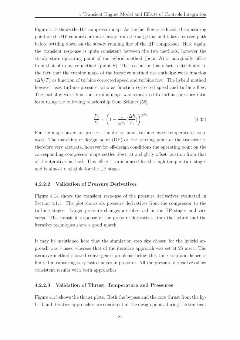
4 Transient Engine Model and Effects of Controls Integration
Figure 4.13 shows the HP compressor map. As the fuel flow is reduced, the operating
point on the HP compressor moves away from the surge line and takes a curved path
before settling down on the steady running line of the HP compressor. Here again,
the transient response is quite consistent between the two methods, however the
steady state operating point of the hybrid method (point A) is marginally offset
from that of iterative method (point B). The reason for this offset is attributed to
the fact that the turbine maps of the iterative method use enthalpy work function
(∆h/T ) as function of turbine corrected speed and turbine flow. The hybrid method
however uses turbine pressure ratio as function corrected speed and turbine flow.
The enthalpy work function turbine maps were converted to turbine pressure ratio
form using the following relationship from Seldner [58],
P2
P1=
(
1 − 1
ηtcp(∆h
T1)
)γγ−1
(4.33)
For the map conversion process, the design point turbine entry temperatures were
used. The matching of design point (DP) or the starting point of the transient is
therefore very accurate, however for off-design conditions the operating point on the
corresponding compressor maps settles down at a slightly offset location from that
of the iterative method. This effect is pronounced for the high temperature stages
and is almost negligible for the LP stages.
4.2.2.2 Validation of Pressure Derivatives
Figure 4.14 shows the transient response of the pressure derivatives evaluated in
Section 4.1.1. The plot shows six pressure derivatives from the compressor to the
turbine stages. Larger pressure changes are observed in the HP stages and vice
versa. The transient response of the pressure derivatives from the hybrid and the
iterative techniques show a good match.
It may be mentioned here that the simulation step size chosen for the hybrid ap-
proach was 5 msec whereas that of the iterative approach was set at 25 msec. The
iterative method showed convergence problems below this time step and hence is
limited in capturing very fast changes in pressure. All the pressure derivatives show
consistent results with both approaches.
4.2.2.3 Validation of Thrust, Temperature and Pressures
Figure 4.15 shows the thrust plots. Both the bypass and the core thrust from the hy-
brid and iterative approaches are consistent at the design point, during the transient
81
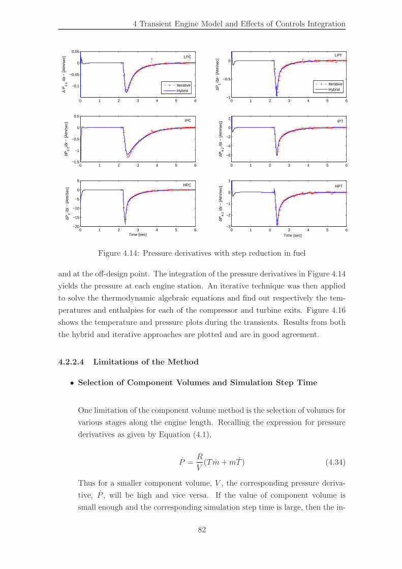
4 Transient Engine Model and Effects of Controls Integration
0 1 2 3 4 5 6
−0.1
−0.05
0
0.05
∆ P
2.1 /∆
t − [A
tm/s
ec]
IterativeHybrid
0 1 2 3 4 5 6−1.5
−1
−0.5
0
0.5
∆P2.
2/∆t −
[Atm
/sec
]
0 1 2 3 4 5 6−20
−15
−10
−5
0
5
∆P3 /∆
t − [A
tm/s
ec]
Time [sec]
0 1 2 3 4 5 6−1
−0.5
0
∆P5 /∆
t− [A
tm/s
ec]
Time [sec]
0 1 2 3 4 5 6
−6
−4
−2
0
2
∆P4.
2 /∆t −
[Atm
/sec
]
IterativeHybrid
0 1 2 3 4 5 6−3
−2
−1
0
1
∆P4.
1 /∆t −
[Atm
/sec
]
LPC
IPC
HPC
LPT
IPT
HPT
Figure 4.14: Pressure derivatives with step reduction in fuel
and at the off-design point. The integration of the pressure derivatives in Figure 4.14
yields the pressure at each engine station. An iterative technique was then applied
to solve the thermodynamic algebraic equations and find out respectively the tem-
peratures and enthalpies for each of the compressor and turbine exits. Figure 4.16
shows the temperature and pressure plots during the transients. Results from both
the hybrid and iterative approaches are plotted and are in good agreement.
4.2.2.4 Limitations of the Method
• Selection of Component Volumes and Simulation Step Time
One limitation of the component volume method is the selection of volumes for
various stages along the engine length. Recalling the expression for pressure
derivatives as given by Equation (4.1),
P =R
V(Tm+mT ) (4.34)
Thus for a smaller component volume, V , the corresponding pressure deriva-
tive, P , will be high and vice versa. If the value of component volume is
small enough and the corresponding simulation step time is large, then the in-
82
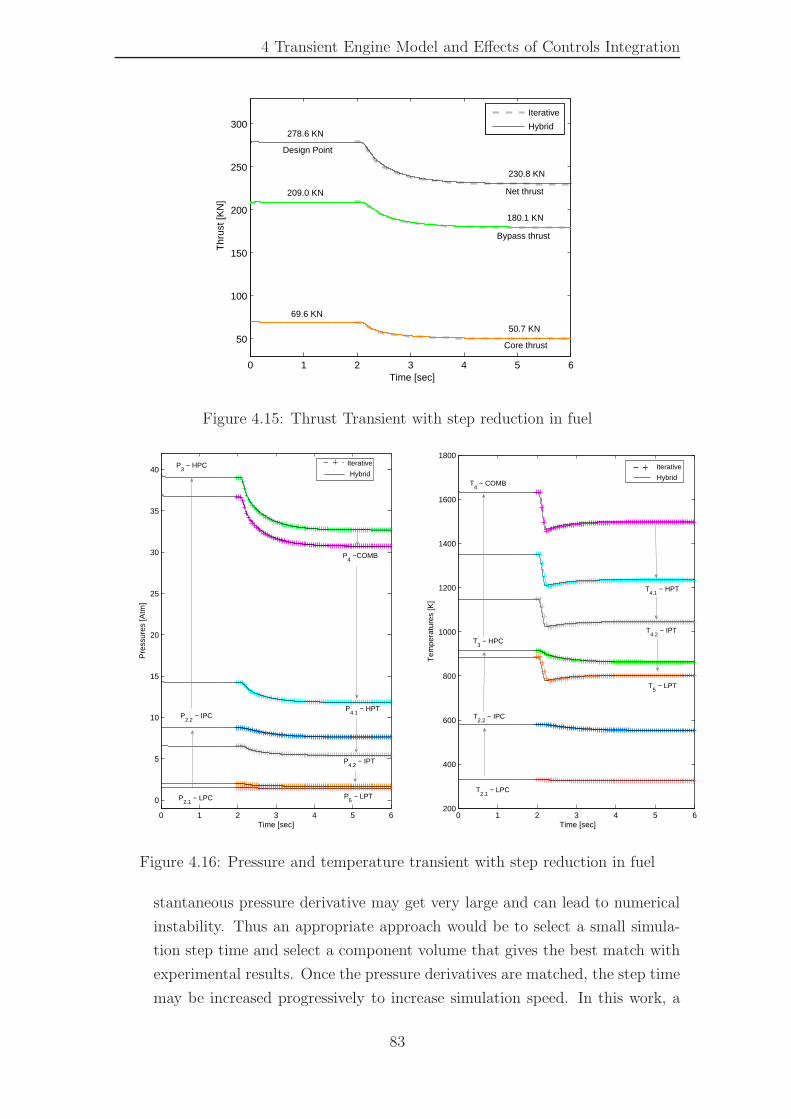
4 Transient Engine Model and Effects of Controls Integration
0 1 2 3 4 5 6
50
100
150
200
250
300
Time [sec]
Thr
ust [
KN
]
Iterative
Hybrid278.6 KN
209.0 KN
69.6 KN
Design Point
Core thrust
Bypass thrust
Net thrust
230.8 KN
180.1 KN
50.7 KN
Figure 4.15: Thrust Transient with step reduction in fuel
0 1 2 3 4 5 6200
400
600
800
1000
1200
1400
1600
1800
Time [sec]
Tem
pera
ture
s [K
]
0 1 2 3 4 5 6
0
5
10
15
20
25
30
35
40
Time [sec]
Pre
ssur
es [A
tm]
P2.1
− LPC P5 − LPT
P2.2
− IPCP
4.1 − HPT
P3 − HPC
P4.2
− IPT
P4 −COMB
Iterative
Hybrid
T2.1
− LPC
T2.2
− IPC
T3 − HPC
T4 − COMB
T4.1
− HPT
T4.2
− IPT
T5 − LPT
Hybrid
Iterative
Figure 4.16: Pressure and temperature transient with step reduction in fuel
stantaneous pressure derivative may get very large and can lead to numerical
instability. Thus an appropriate approach would be to select a small simula-
tion step time and select a component volume that gives the best match with
experimental results. Once the pressure derivatives are matched, the step time
may be increased progressively to increase simulation speed. In this work, a
83

4 Transient Engine Model and Effects of Controls Integration
fixed step Euler numerical integration technique was used, with a step time of
5 msec. The selection of component volumes however affects the transient op-
eration only, the equilibrium or the steady state condition remains un-affected.
• Limitation of Component Maps
Engine components such as the compressor and the turbine may consist of
more than one stages. For example a typical high pressure compressor (HPC)
may have more than eight stages. In this simulation, component interstage dy-
namics were not simulated and single component maps were used to represent
each engine subsystem.
84
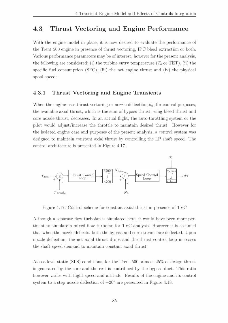
4 Transient Engine Model and Effects of Controls Integration
4.3 Thrust Vectoring and Engine Performance
With the engine model in place, it is now desired to evaluate the performance of
the Trent 500 engine in presence of thrust vectoring, IPC bleed extraction or both.
Various performance parameters may be of interest, however for the present analysis,
the following are considered; (i) the turbine entry temperature (T4 or TET), (ii) the
specific fuel consumption (SFC), (iii) the net engine thrust and (iv) the physical
spool speeds.
4.3.1 Thrust Vectoring and Engine Transients
When the engine uses thrust vectoring or nozzle deflection, θn, for control purposes,
the available axial thrust, which is the sum of bypass thrust, wing bleed thrust and
core nozzle thrust, decreases. In an actual flight, the auto-throttling system or the
pilot would adjust/increase the throttle to maintain desired thrust. However for
the isolated engine case and purposes of the present analysis, a control system was
designed to maintain constant axial thrust by controlling the LP shaft speed. The
control architecture is presented in Figure 4.17.
LoopLoop
5200
4200
-Σ Σ -
6 6
---+
-+
-
Speed Control
wfmax
wfmin
T4
?
- -Tdem
NLdem
T cos θn
wf
NL
Thrust Control
Figure 4.17: Control scheme for constant axial thrust in presence of TVC
Although a separate flow turbofan is simulated here, it would have been more per-
tinent to simulate a mixed flow turbofan for TVC analysis. However it is assumed
that when the nozzle deflects, both the bypass and core streams are deflected. Upon
nozzle deflection, the net axial thrust drops and the thrust control loop increases
the shaft speed demand to maintain constant axial thrust.
At sea level static (SLS) conditions, for the Trent 500, almost 25% of design thrust
is generated by the core and the rest is contribued by the bypass duct. This ratio
however varies with flight speed and altitude. Results of the engine and its control
system to a step nozzle deflection of +20◦ are presented in Figure 4.18.
85
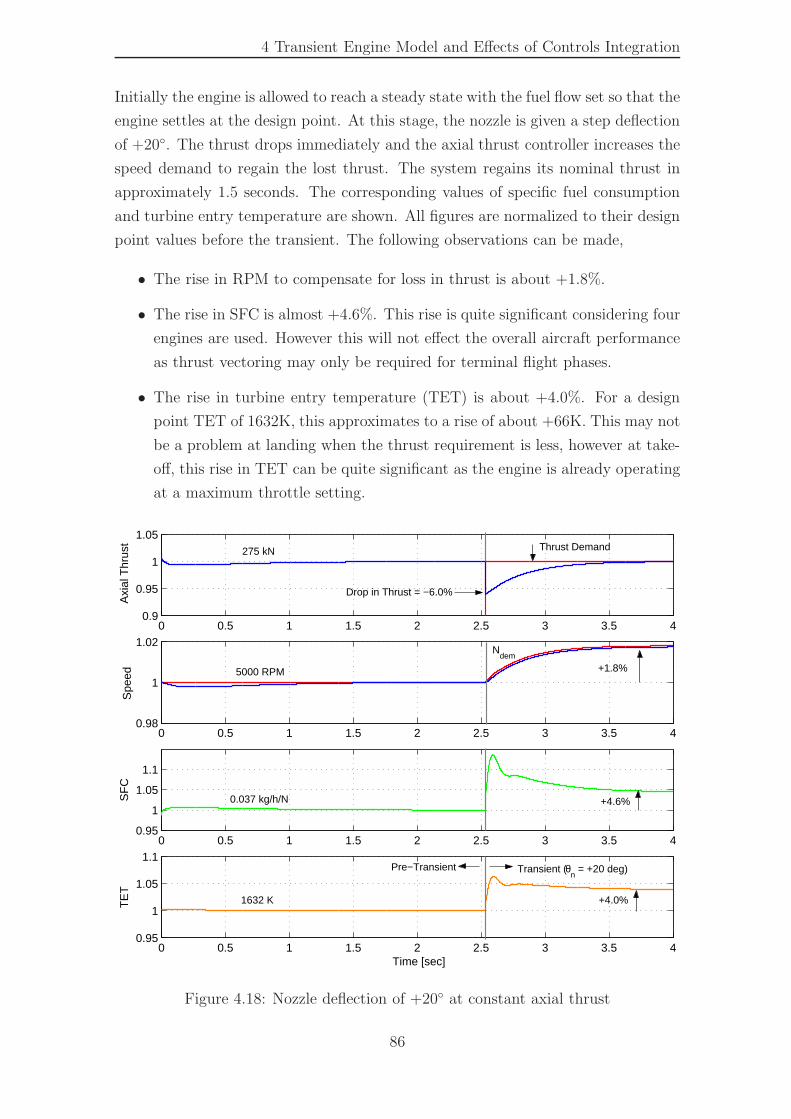
4 Transient Engine Model and Effects of Controls Integration
Initially the engine is allowed to reach a steady state with the fuel flow set so that the
engine settles at the design point. At this stage, the nozzle is given a step deflection
of +20◦. The thrust drops immediately and the axial thrust controller increases the
speed demand to regain the lost thrust. The system regains its nominal thrust in
approximately 1.5 seconds. The corresponding values of specific fuel consumption
and turbine entry temperature are shown. All figures are normalized to their design
point values before the transient. The following observations can be made,
• The rise in RPM to compensate for loss in thrust is about +1.8%.
• The rise in SFC is almost +4.6%. This rise is quite significant considering four
engines are used. However this will not effect the overall aircraft performance
as thrust vectoring may only be required for terminal flight phases.
• The rise in turbine entry temperature (TET) is about +4.0%. For a design
point TET of 1632K, this approximates to a rise of about +66K. This may not
be a problem at landing when the thrust requirement is less, however at take-
off, this rise in TET can be quite significant as the engine is already operating
at a maximum throttle setting.
0 0.5 1 1.5 2 2.5 3 3.5 40.9
0.95
1
1.05
Axi
al T
hrus
t
0 0.5 1 1.5 2 2.5 3 3.5 40.98
1
1.02
Spe
ed
0 0.5 1 1.5 2 2.5 3 3.5 40.95
1
1.05
1.1
SF
C
0 0.5 1 1.5 2 2.5 3 3.5 40.95
1
1.05
1.1
Time [sec]
TE
T
275 kN
Drop in Thrust = −6.0%
Thrust Demand
5000 RPM
0.037 kg/h/N
1632 K +4.0%
+4.6%
+1.8%
Transient (θn = +20 deg) Pre−Transient
Ndem
Figure 4.18: Nozzle deflection of +20◦ at constant axial thrust
86
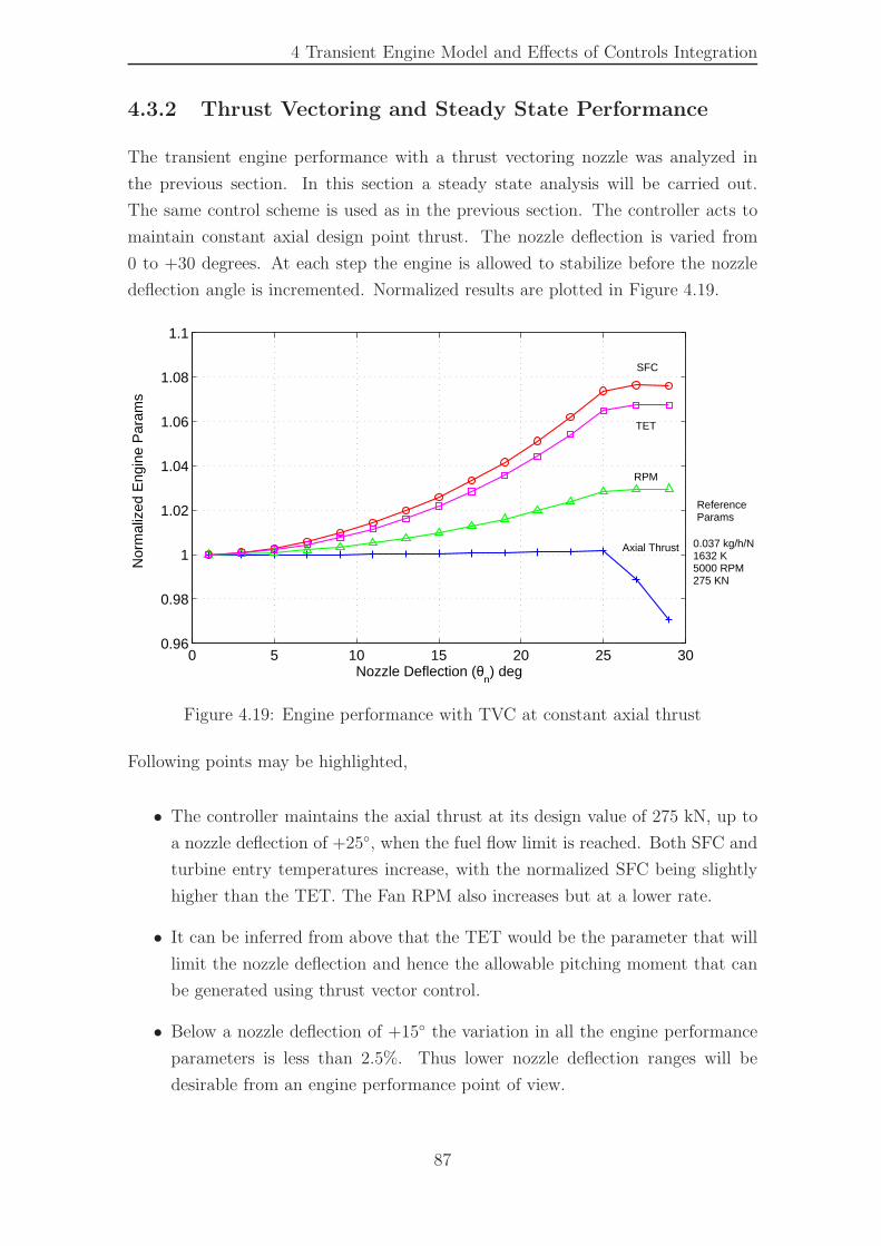
4 Transient Engine Model and Effects of Controls Integration
4.3.2 Thrust Vectoring and Steady State Performance
The transient engine performance with a thrust vectoring nozzle was analyzed in
the previous section. In this section a steady state analysis will be carried out.
The same control scheme is used as in the previous section. The controller acts to
maintain constant axial design point thrust. The nozzle deflection is varied from
0 to +30 degrees. At each step the engine is allowed to stabilize before the nozzle
deflection angle is incremented. Normalized results are plotted in Figure 4.19.
0 5 10 15 20 25 300.96
0.98
1
1.02
1.04
1.06
1.08
1.1
Nozzle Deflection (θn) deg
Nor
mal
ized
Eng
ine
Par
ams
SFC
TET
RPM
Axial Thrust 0.037 kg/h/N1632 K 5000 RPM 275 KN
ReferenceParams
Figure 4.19: Engine performance with TVC at constant axial thrust
Following points may be highlighted,
• The controller maintains the axial thrust at its design value of 275 kN, up to
a nozzle deflection of +25◦, when the fuel flow limit is reached. Both SFC and
turbine entry temperatures increase, with the normalized SFC being slightly
higher than the TET. The Fan RPM also increases but at a lower rate.
• It can be inferred from above that the TET would be the parameter that will
limit the nozzle deflection and hence the allowable pitching moment that can
be generated using thrust vector control.
• Below a nozzle deflection of +15◦ the variation in all the engine performance
parameters is less than 2.5%. Thus lower nozzle deflection ranges will be
desirable from an engine performance point of view.
87
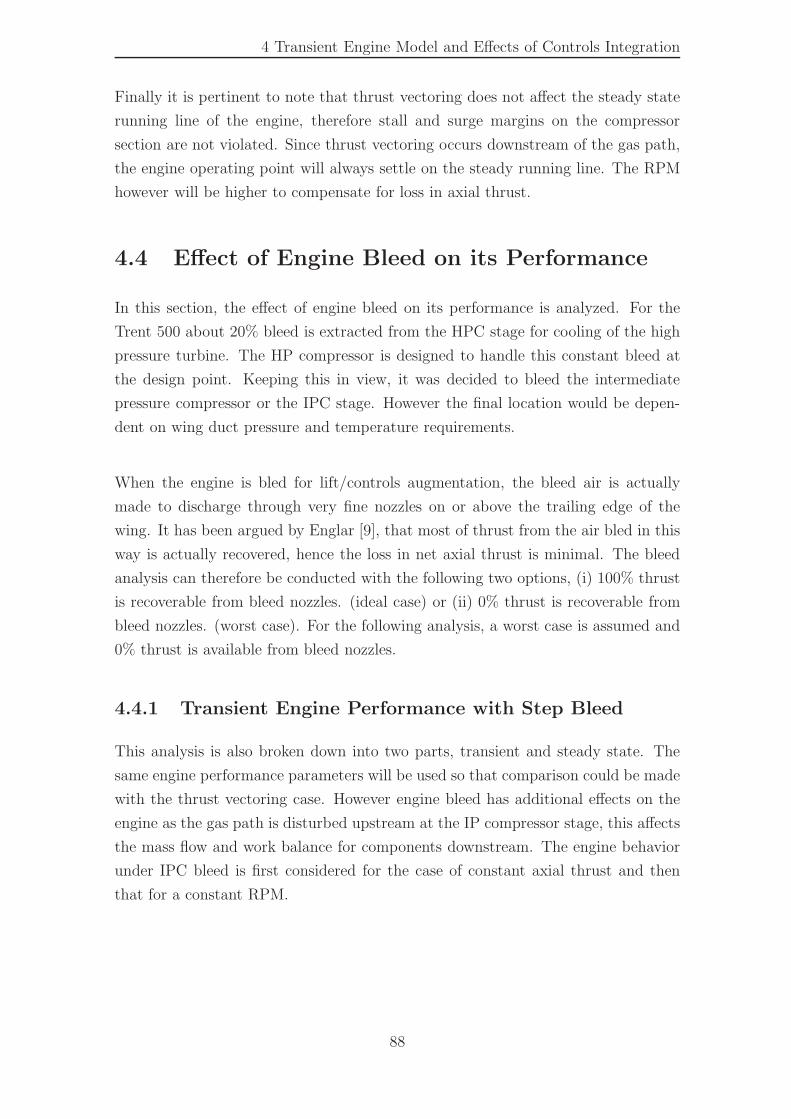
4 Transient Engine Model and Effects of Controls Integration
Finally it is pertinent to note that thrust vectoring does not affect the steady state
running line of the engine, therefore stall and surge margins on the compressor
section are not violated. Since thrust vectoring occurs downstream of the gas path,
the engine operating point will always settle on the steady running line. The RPM
however will be higher to compensate for loss in axial thrust.
4.4 Effect of Engine Bleed on its Performance
In this section, the effect of engine bleed on its performance is analyzed. For the
Trent 500 about 20% bleed is extracted from the HPC stage for cooling of the high
pressure turbine. The HP compressor is designed to handle this constant bleed at
the design point. Keeping this in view, it was decided to bleed the intermediate
pressure compressor or the IPC stage. However the final location would be depen-
dent on wing duct pressure and temperature requirements.
When the engine is bled for lift/controls augmentation, the bleed air is actually
made to discharge through very fine nozzles on or above the trailing edge of the
wing. It has been argued by Englar [9], that most of thrust from the air bled in this
way is actually recovered, hence the loss in net axial thrust is minimal. The bleed
analysis can therefore be conducted with the following two options, (i) 100% thrust
is recoverable from bleed nozzles. (ideal case) or (ii) 0% thrust is recoverable from
bleed nozzles. (worst case). For the following analysis, a worst case is assumed and
0% thrust is available from bleed nozzles.
4.4.1 Transient Engine Performance with Step Bleed
This analysis is also broken down into two parts, transient and steady state. The
same engine performance parameters will be used so that comparison could be made
with the thrust vectoring case. However engine bleed has additional effects on the
engine as the gas path is disturbed upstream at the IP compressor stage, this affects
the mass flow and work balance for components downstream. The engine behavior
under IPC bleed is first considered for the case of constant axial thrust and then
that for a constant RPM.
88
4 Transient Engine Model and Effects of Controls Integration
Engine Transient with Bleed - At Constant Axial Design Thrust
Figure 4.20 shows the results of 10% bleed extraction from the IPC stage. The bleed
is applied as a step with the assumption that zero thrust is contributed by the wing
nozzle. From Figure 4.20, the following can be observed:
• Upon bleed extraction there is an initial drop in axial thrust. The axial thrust
controller subsequently adjusts the RPM demand by +0.55% to maintain the
same level of thrust.
• The SFC increases by +8.0% and the TET by +5.0%.
Since 0% thrust recovery is assumed, the above analysis is conservative. If this con-
straint is relaxed, the rise in fuel consumption and TET to maintain the same level
of thrust will be less. This will be further investigated after establishing the exact
bleed requirements for landing and take-off. Consequently, if the bleed requirements
are high, the contribution of wing nozzle can be a significant portion of the net
thrust generated.
0 0.5 1 1.5 2 2.5 3 3.5 4 4.50.99
1
1.01
Axi
al T
hrus
t
0 0.5 1 1.5 2 2.5 3 3.5 4 4.5
1
1.01
Spe
ed
0 0.5 1 1.5 2 2.5 3 3.5 4 4.5
1
1.1
1.2
SF
C
0 0.5 1 1.5 2 2.5 3 3.5 4 4.50.95
1
1.05
1.1
Time [sec]
TE
T
275 KN
5000 RPM
0.037 kg/h/N
1632 K
Thrust Demand
+0.55%
+8.0%
+5.0%
Ndem
N
Pre Transient
Pre Transient Drop in thrust due to step bleed = −0.6%
RPM rises to maintain axial thrust
Figure 4.20: Engine performance with 10% IPC bleed at constant axial thrust
89
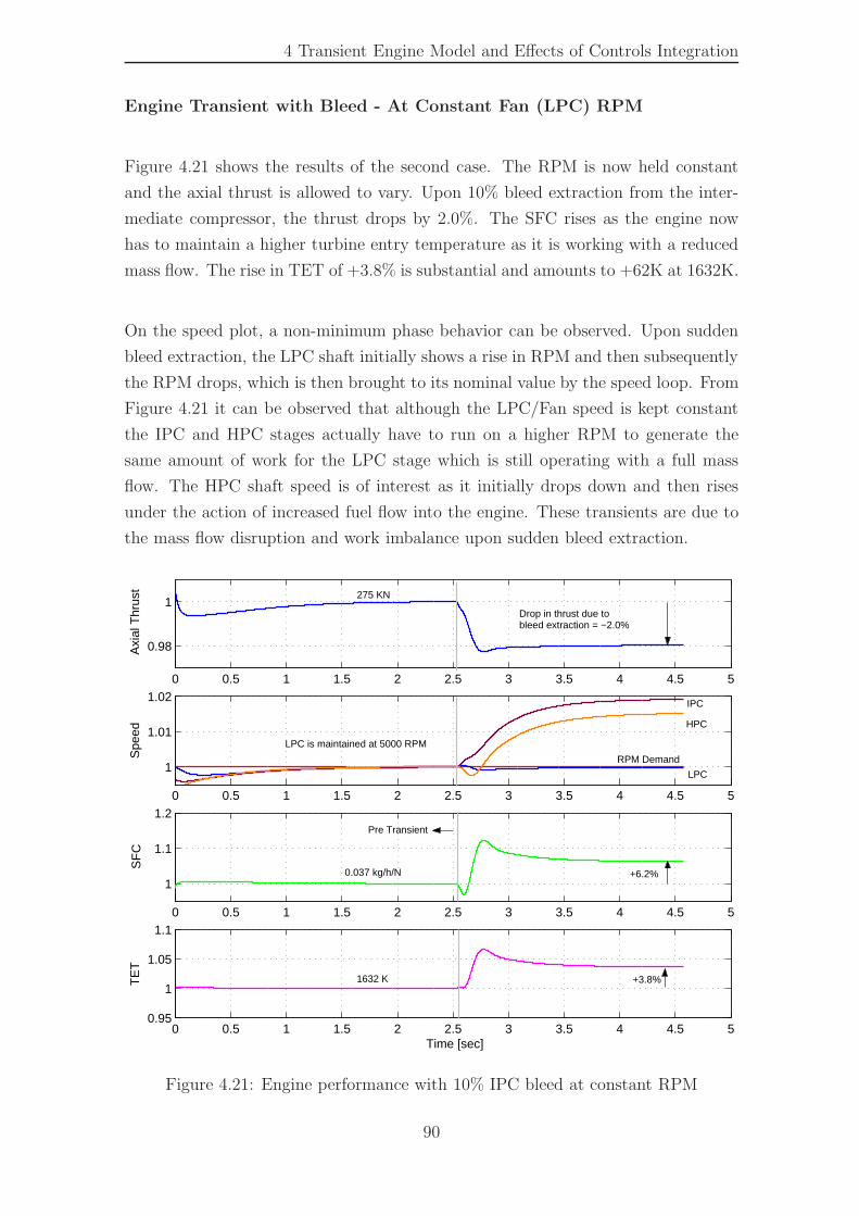
4 Transient Engine Model and Effects of Controls Integration
Engine Transient with Bleed - At Constant Fan (LPC) RPM
Figure 4.21 shows the results of the second case. The RPM is now held constant
and the axial thrust is allowed to vary. Upon 10% bleed extraction from the inter-
mediate compressor, the thrust drops by 2.0%. The SFC rises as the engine now
has to maintain a higher turbine entry temperature as it is working with a reduced
mass flow. The rise in TET of +3.8% is substantial and amounts to +62K at 1632K.
On the speed plot, a non-minimum phase behavior can be observed. Upon sudden
bleed extraction, the LPC shaft initially shows a rise in RPM and then subsequently
the RPM drops, which is then brought to its nominal value by the speed loop. From
Figure 4.21 it can be observed that although the LPC/Fan speed is kept constant
the IPC and HPC stages actually have to run on a higher RPM to generate the
same amount of work for the LPC stage which is still operating with a full mass
flow. The HPC shaft speed is of interest as it initially drops down and then rises
under the action of increased fuel flow into the engine. These transients are due to
the mass flow disruption and work imbalance upon sudden bleed extraction.
0 0.5 1 1.5 2 2.5 3 3.5 4 4.5 5
0.98
1
Axi
al T
hrus
t
0 0.5 1 1.5 2 2.5 3 3.5 4 4.5 5
1
1.01
1.02
Spe
ed
0 0.5 1 1.5 2 2.5 3 3.5 4 4.5 5
1
1.1
1.2
SF
C
0 0.5 1 1.5 2 2.5 3 3.5 4 4.5 50.95
1
1.05
1.1
Time [sec]
TE
T
RPM Demand
Pre Transient
Drop in thrust due to bleed extraction = −2.0%
LPC is maintained at 5000 RPM
+6.2%
+3.8%
275 KN
0.037 kg/h/N
1632 K
LPC
HPC
IPC
Figure 4.21: Engine performance with 10% IPC bleed at constant RPM
90
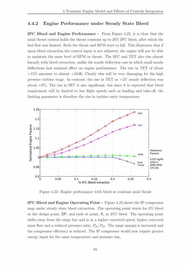
4 Transient Engine Model and Effects of Controls Integration
4.4.2 Engine Performance under Steady State Bleed
IPC Bleed and Engine Performance - From Figure 4.22, it is clear that the
axial thrust control holds the thrust constant up to 20% IPC bleed, after which the
fuel flow was limited. Both the thrust and RPM start to fall. This illustrates that if
upon bleed extraction the control input is not adjusted, the engine will not be able
to maintain the same level of RPM or thrust. The SFC and TET also rise almost
linearly with bleed extraction, unlike the nozzle deflection case in which small nozzle
deflections had minimal effect on engine performance. The rise in TET of about
+15% amounts to almost +244K. Clearly this will be very damaging for the high
pressure turbine stage. In contrast, the rise in TET at +25◦ nozzle deflection was
about +8%. The rise in SFC is also significant, but since it is expected that bleed
requirement will be limited to low flight speeds such as landing and take-off, the
limiting parameter is therefore the rise in turbine entry temperature.
0 0.05 0.1 0.15 0.2 0.25 0.30.9
0.95
1
1.05
1.1
1.15
1.2
1.25
% IPC Bleed extraction
Nor
mal
ized
Eng
ine
Par
ams
SFC
TET
AxialThrust
ReferenceParams
0.037 kg/hN1632 K5000 RPM275 KN
RPM
Figure 4.22: Engine performance with bleed at constant axial thrust
IPC Bleed and Engine Operating Point - Figure 4.23 shows the IP compressor
map under steady state bleed extraction. The operating point starts for 0% bleed
at the design point, DP, and ends at point, X, at 25% bleed. The operating point
shifts away from the surge line and is at a higher corrected speed, higher corrected
mass flow and a reduced pressure ratio, P21/P22. The surge margin is increased and
the compressor efficiency is reduced. The IP compressor would now require greater
energy input for the same temperature and pressure rise.
91
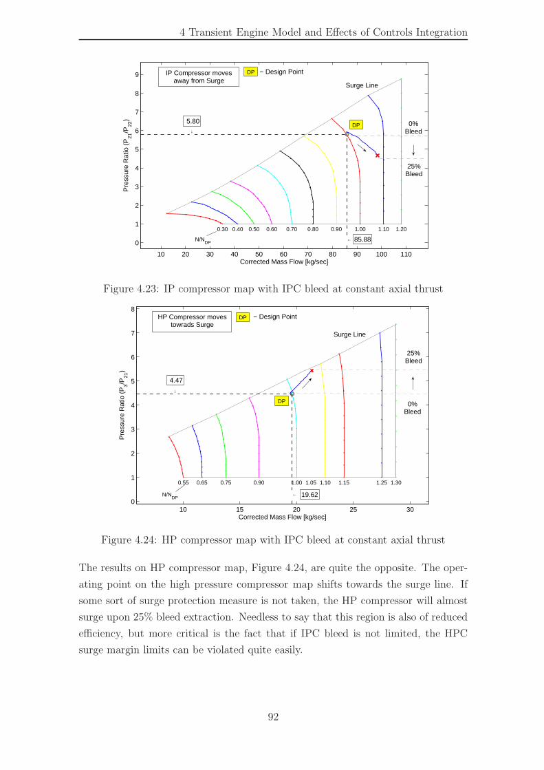
4 Transient Engine Model and Effects of Controls Integration
10 20 30 40 50 60 70 80 90 100 110
0
1
2
3
4
5
6
7
8
9
0.30 0.40 0.50 0.60 0.70 0.80 0.90 1.00 1.10 1.20
Corrected Mass Flow [kg/sec]
Pre
ssur
e R
atio
(P
21/P
22) 5.80
↓
← 85.88
Surge Line
25%Bleed
0%Bleed
IP Compressor movesaway from Surge
DP
DP − Design Point
N/NDP
Figure 4.23: IP compressor map with IPC bleed at constant axial thrust
10 15 20 25 300
1
2
3
4
5
6
7
8
0.55 0.65 0.75 0.90 1.00 1.05 1.10 1.15 1.25 1.30
Corrected Mass Flow [kg/sec]
Pre
ssur
e R
atio
(P
3/P21
)
4.47
↓
← 19.62
Surge Line
HP Compressor movestowrads Surge
25%Bleed
0%Bleed
DP
DP − Design Point
N/NDP
Figure 4.24: HP compressor map with IPC bleed at constant axial thrust
The results on HP compressor map, Figure 4.24, are quite the opposite. The oper-
ating point on the high pressure compressor map shifts towards the surge line. If
some sort of surge protection measure is not taken, the HP compressor will almost
surge upon 25% bleed extraction. Needless to say that this region is also of reduced
efficiency, but more critical is the fact that if IPC bleed is not limited, the HPC
surge margin limits can be violated quite easily.
92
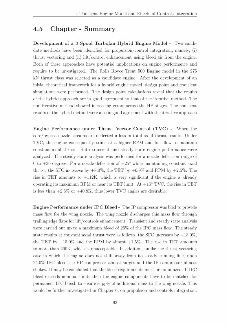
4 Transient Engine Model and Effects of Controls Integration
4.5 Chapter - Summary
Development of a 3 Spool Turbofan Hybrid Engine Model - Two candi-
date methods have been identified for propulsion/control integration, namely, (i)
thrust vectoring and (ii) lift/control enhancement using bleed air from the engine.
Both of these approaches have potential implications on engine performance and
require to be investigated. The Rolls Royce Trent 500 Engine model in the 275
kN thrust class was selected as a candidate engine. After the development of an
initial theoretical framework for a hybrid engine model, design point and transient
simulations were performed. The design point calculations reveal that the results
of the hybrid approach are in good agreement to that of the iterative method. The
non-iterative method showed increasing errors across the HP stages. The transient
results of the hybrid method were also in good agreement with the iterative approach
Engine Performance under Thrust Vector Control (TVC) - When the
core/bypass nozzle streams are deflected a loss in total axial thrust results. Under
TVC, the engine consequently trims at a higher RPM and fuel flow to maintain
constant axial thrust. Both transient and steady state engine performance were
analyzed. The steady state analysis was performed for a nozzle deflection range of
0 to +30 degrees. For a nozzle deflection of +25◦ while maintaining constant axial
thrust, the SFC increases by +8.0%, the TET by +6.9% and RPM by +2.5%. The
rise in TET amounts to +112K, which is very significant if the engine is already
operating its maximum RPM or near its TET limit. At +15◦ TVC, the rise in TET
is less than +2.5% or +40.8K, thus lower TVC angles are desirable.
Engine Performance under IPC Bleed - The IP compressor was bled to provide
mass flow for the wing nozzle. The wing nozzle discharges this mass flow through
trailing edge flaps for lift/controls enhancement. Transient and steady state analysis
were carried out up to a maximum bleed of 25% of the IPC mass flow. The steady
state results at constant axial thrust were as follows, the SFC increases by +18.0%,
the TET by +15.0% and the RPM by almost +1.5%. The rise in TET amounts
to more than 200K, which is unacceptable. In addition, unlike the thrust vectoring
case in which the engine does not shift away from its steady running line, upon
25.0% IPC bleed the HP compressor almost surges and the IP compressor almost
chokes. It may be concluded that the bleed requirements must be minimized. If IPC
bleed exceeds nominal limits then the engine components have to be matched for
permanent IPC bleed, to ensure supply of additional mass to the wing nozzle. This
would be further investigated in Chapter 6, on propulsion and controls integration.
93

4 Transient Engine Model and Effects of Controls Integration
94
Chapter 5
A BWB Model with Blown Flaps
5.1 Introduction
A significant part of this work went into the development and validation of a BWB
aircraft model with blown flaps. This was a difficult task due to the complex nature
of the aerodynamics problem and due to the absence of any previous aerodynamic
data for such a configuration. Various approaches were possible to accomplish this
task, these included, (i) building a three-dimensional wind tunnel model with blown
flap capability and then performing a series of wind tunnel tests; limited time and
resources did not allow such an approach, (ii) to build a CFD model and then try to
estimate the blown flap effects computationally or (iii) to build an analytical aero-
dynamic model based on available databases such as the Engineering Sciences Data
Units (ESDU) and then validate/fine tune this model with panel method codes
and an earlier BWB aerodynamic model [7]. All three approaches were deliber-
ated upon and the third approach was chosen owing to its flexibility in selection of
airfoil/planform parameters and its implementation within the available resources.
This aerodynamic model was subsequently used for trimming analysis and non-linear
flight simulations. The method however is based on estimations, in order to improve
upon its accuracy, CFD and wind tunnel experiments would be necessary.
This chapter explains the development of this aerodynamic model and covers aspects
such as the general description of aircraft, the wing airfoil geometric characteris-
tics/variation along the span, estimation of the wing forces and moments, aerody-
namic contributions due to the vertical fins on wing tips and finally model validation.
The development of this model was greatly facilitated by Cooke’s work on the NFLC
Jetstream [59] and by Amrane’s work on the high performance sailplane [60].
95
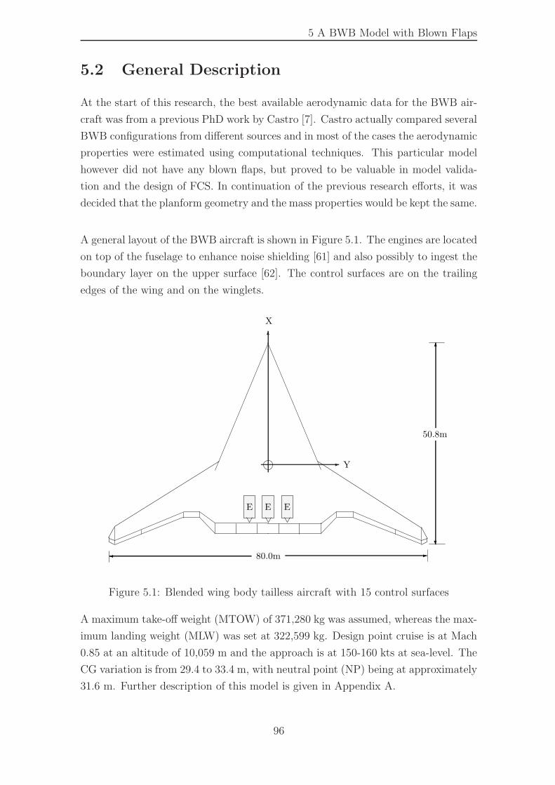
5 A BWB Model with Blown Flaps
5.2 General Description
At the start of this research, the best available aerodynamic data for the BWB air-
craft was from a previous PhD work by Castro [7]. Castro actually compared several
BWB configurations from different sources and in most of the cases the aerodynamic
properties were estimated using computational techniques. This particular model
however did not have any blown flaps, but proved to be valuable in model valida-
tion and the design of FCS. In continuation of the previous research efforts, it was
decided that the planform geometry and the mass properties would be kept the same.
A general layout of the BWB aircraft is shown in Figure 5.1. The engines are located
on top of the fuselage to enhance noise shielding [61] and also possibly to ingest the
boundary layer on the upper surface [62]. The control surfaces are on the trailing
edges of the wing and on the winglets.
6
-
E
X
EE
Y
80.0m -�
6
?
50.8m
Figure 5.1: Blended wing body tailless aircraft with 15 control surfaces
A maximum take-off weight (MTOW) of 371,280 kg was assumed, whereas the max-
imum landing weight (MLW) was set at 322,599 kg. Design point cruise is at Mach
0.85 at an altitude of 10,059 m and the approach is at 150-160 kts at sea-level. The
CG variation is from 29.4 to 33.4 m, with neutral point (NP) being at approximately
31.6 m. Further description of this model is given in Appendix A.
96
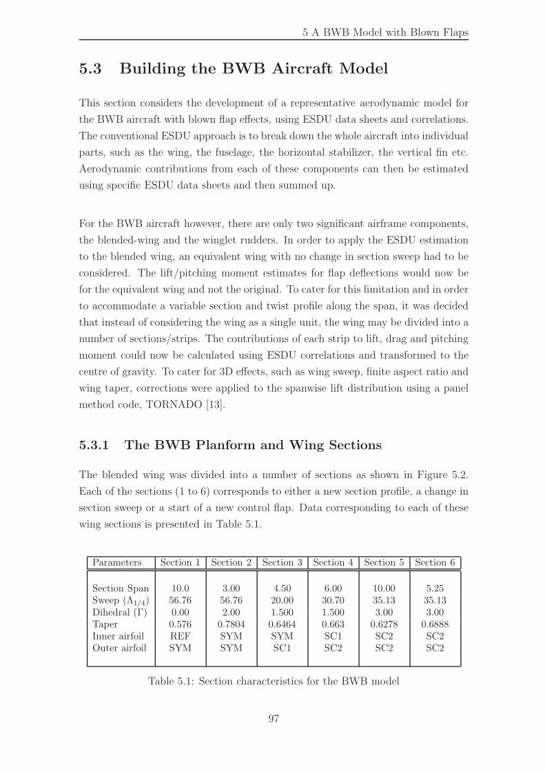
5 A BWB Model with Blown Flaps
5.3 Building the BWB Aircraft Model
This section considers the development of a representative aerodynamic model for
the BWB aircraft with blown flap effects, using ESDU data sheets and correlations.
The conventional ESDU approach is to break down the whole aircraft into individual
parts, such as the wing, the fuselage, the horizontal stabilizer, the vertical fin etc.
Aerodynamic contributions from each of these components can then be estimated
using specific ESDU data sheets and then summed up.
For the BWB aircraft however, there are only two significant airframe components,
the blended-wing and the winglet rudders. In order to apply the ESDU estimation
to the blended wing, an equivalent wing with no change in section sweep had to be
considered. The lift/pitching moment estimates for flap deflections would now be
for the equivalent wing and not the original. To cater for this limitation and in order
to accommodate a variable section and twist profile along the span, it was decided
that instead of considering the wing as a single unit, the wing may be divided into a
number of sections/strips. The contributions of each strip to lift, drag and pitching
moment could now be calculated using ESDU correlations and transformed to the
centre of gravity. To cater for 3D effects, such as wing sweep, finite aspect ratio and
wing taper, corrections were applied to the spanwise lift distribution using a panel
method code, TORNADO [13].
5.3.1 The BWB Planform and Wing Sections
The blended wing was divided into a number of sections as shown in Figure 5.2.
Each of the sections (1 to 6) corresponds to either a new section profile, a change in
section sweep or a start of a new control flap. Data corresponding to each of these
wing sections is presented in Table 5.1.
Parameters Section 1 Section 2 Section 3 Section 4 Section 5 Section 6
Section Span 10.0 3.00 4.50 6.00 10.00 5.25Sweep (Λ1/4) 56.76 56.76 20.00 30.70 35.13 35.13Dihedral (Γ) 0.00 2.00 1.500 1.500 3.00 3.00Taper 0.576 0.7804 0.6464 0.663 0.6278 0.6888Inner airfoil REF SYM SYM SC1 SC2 SC2Outer airfoil SYM SYM SC1 SC2 SC2 SC2
Table 5.1: Section characteristics for the BWB model
97
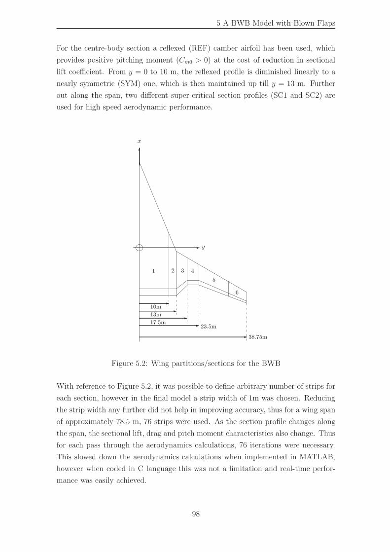
5 A BWB Model with Blown Flaps
For the centre-body section a reflexed (REF) camber airfoil has been used, which
provides positive pitching moment (Cm0 > 0) at the cost of reduction in sectional
lift coefficient. From y = 0 to 10 m, the reflexed profile is diminished linearly to a
nearly symmetric (SYM) one, which is then maintained up till y = 13 m. Further
out along the span, two different super-critical section profiles (SC1 and SC2) are
used for high speed aerodynamic performance.
-
3 4
5
6
2
--
-
-
13m
17.5m
10m
38.75m
-
6
1
x
y
23.5m
Figure 5.2: Wing partitions/sections for the BWB
With reference to Figure 5.2, it was possible to define arbitrary number of strips for
each section, however in the final model a strip width of 1m was chosen. Reducing
the strip width any further did not help in improving accuracy, thus for a wing span
of approximately 78.5 m, 76 strips were used. As the section profile changes along
the span, the sectional lift, drag and pitch moment characteristics also change. Thus
for each pass through the aerodynamics calculations, 76 iterations were necessary.
This slowed down the aerodynamics calculations when implemented in MATLAB,
however when coded in C language this was not a limitation and real-time perfor-
mance was easily achieved.
98
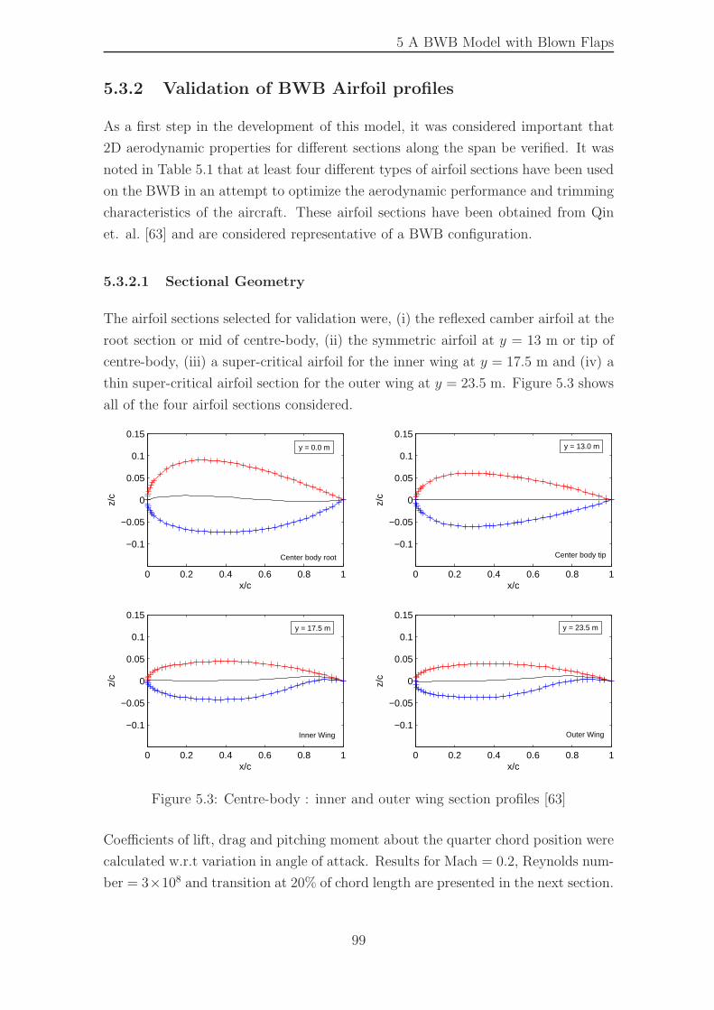
5 A BWB Model with Blown Flaps
5.3.2 Validation of BWB Airfoil profiles
As a first step in the development of this model, it was considered important that
2D aerodynamic properties for different sections along the span be verified. It was
noted in Table 5.1 that at least four different types of airfoil sections have been used
on the BWB in an attempt to optimize the aerodynamic performance and trimming
characteristics of the aircraft. These airfoil sections have been obtained from Qin
et. al. [63] and are considered representative of a BWB configuration.
5.3.2.1 Sectional Geometry
The airfoil sections selected for validation were, (i) the reflexed camber airfoil at the
root section or mid of centre-body, (ii) the symmetric airfoil at y = 13 m or tip of
centre-body, (iii) a super-critical airfoil for the inner wing at y = 17.5 m and (iv) a
thin super-critical airfoil section for the outer wing at y = 23.5 m. Figure 5.3 shows
all of the four airfoil sections considered.
0 0.2 0.4 0.6 0.8 1
−0.1
−0.05
0
0.05
0.1
0.15
z/c
x/c0 0.2 0.4 0.6 0.8 1
−0.1
−0.05
0
0.05
0.1
0.15
z/c
x/c
0 0.2 0.4 0.6 0.8 1
−0.1
−0.05
0
0.05
0.1
0.15
z/c
x/c0 0.2 0.4 0.6 0.8 1
−0.1
−0.05
0
0.05
0.1
0.15
z/c
x/c
y = 0.0 m y = 13.0 m
y = 17.5 m y = 23.5 m
Center body root Center body tip
Inner Wing Outer Wing
Figure 5.3: Centre-body : inner and outer wing section profiles [63]
Coefficients of lift, drag and pitching moment about the quarter chord position were
calculated w.r.t variation in angle of attack. Results for Mach = 0.2, Reynolds num-
ber = 3×10⁸ and transition at 20% of chord length are presented in the next section.
99
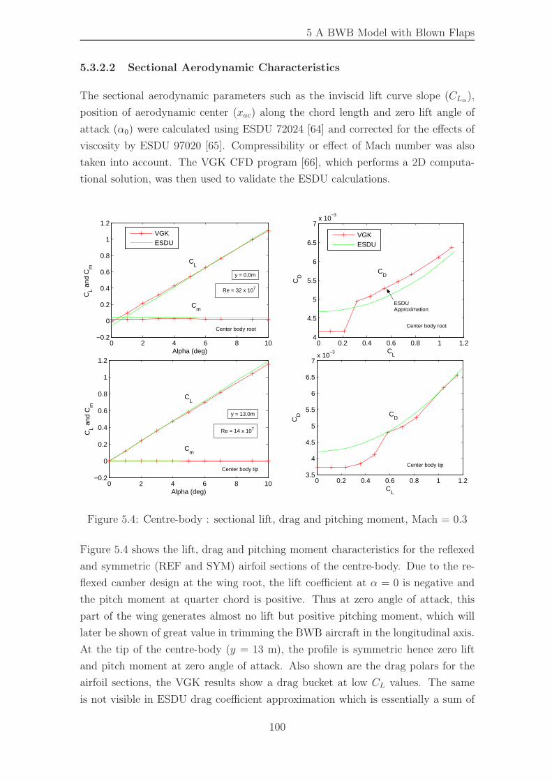
5 A BWB Model with Blown Flaps
5.3.2.2 Sectional Aerodynamic Characteristics
The sectional aerodynamic parameters such as the inviscid lift curve slope (CLα),
position of aerodynamic center (xac) along the chord length and zero lift angle of
attack (α0) were calculated using ESDU 72024 [64] and corrected for the effects of
viscosity by ESDU 97020 [65]. Compressibility or effect of Mach number was also
taken into account. The VGK CFD program [66], which performs a 2D computa-
tional solution, was then used to validate the ESDU calculations.
0 2 4 6 8 10−0.2
0
0.2
0.4
0.6
0.8
1
1.2
Alpha (deg)
CL a
nd C
m
0 0.2 0.4 0.6 0.8 1 1.24
4.5
5
5.5
6
6.5
7x 10
−3
CL
CD
0 2 4 6 8 10−0.2
0
0.2
0.4
0.6
0.8
1
1.2
Alpha (deg)
CL a
nd C
m
0 0.2 0.4 0.6 0.8 1 1.23.5
4
4.5
5
5.5
6
6.5
7x 10
−3
CL
CD
CL
Cm
Cm
CL
Center body root Center body root
Center body tip Center body tip
y = 0.0m
y = 13.0m
CD
CD
ESDU Approximation
VGKESDU
VGKESDU
Re = 32 x 107
Re = 14 x 107
Figure 5.4: Centre-body : sectional lift, drag and pitching moment, Mach = 0.3
Figure 5.4 shows the lift, drag and pitching moment characteristics for the reflexed
and symmetric (REF and SYM) airfoil sections of the centre-body. Due to the re-
flexed camber design at the wing root, the lift coefficient at α = 0 is negative and
the pitch moment at quarter chord is positive. Thus at zero angle of attack, this
part of the wing generates almost no lift but positive pitching moment, which will
later be shown of great value in trimming the BWB aircraft in the longitudinal axis.
At the tip of the centre-body (y = 13 m), the profile is symmetric hence zero lift
and pitch moment at zero angle of attack. Also shown are the drag polars for the
airfoil sections, the VGK results show a drag bucket at low CL values. The same
is not visible in ESDU drag coefficient approximation which is essentially a sum of
100
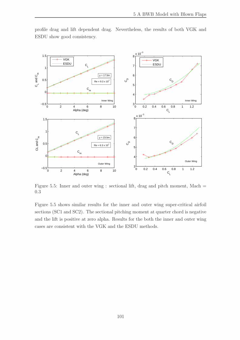
5 A BWB Model with Blown Flaps
profile drag and lift dependent drag. Nevertheless, the results of both VGK and
ESDU show good consistency.
0 2 4 6 8 10−0.5
0
0.5
1
1.5
Alpha (deg)
CL a
nd C
m
0 0.2 0.4 0.6 0.8 1 1.23
4
5
6
7
8x 10
−3
CL
CD
0 2 4 6 8 10−0.5
0
0.5
1
1.5
Alpha (deg)
CL
and
Cm
0 0.2 0.4 0.6 0.8 1 1.23
4
5
6
7
8x 10
−3
CL
CD
CL
CL
Cm
Cm
CD
CD
Inner Wing Inner Wing
Outer Wing Outer Wing
y = 17.5m
y = 23.5m
VGKESDU
VGKESDU
Re = 9.3 x 10⁷
Re = 6.3 x 10⁷
Figure 5.5: Inner and outer wing : sectional lift, drag and pitch moment, Mach =0.3
Figure 5.5 shows similar results for the inner and outer wing super-critical airfoil
sections (SC1 and SC2). The sectional pitching moment at quarter chord is negative
and the lift is positive at zero alpha. Results for the both the inner and outer wing
cases are consistent with the VGK and the ESDU methods.
101
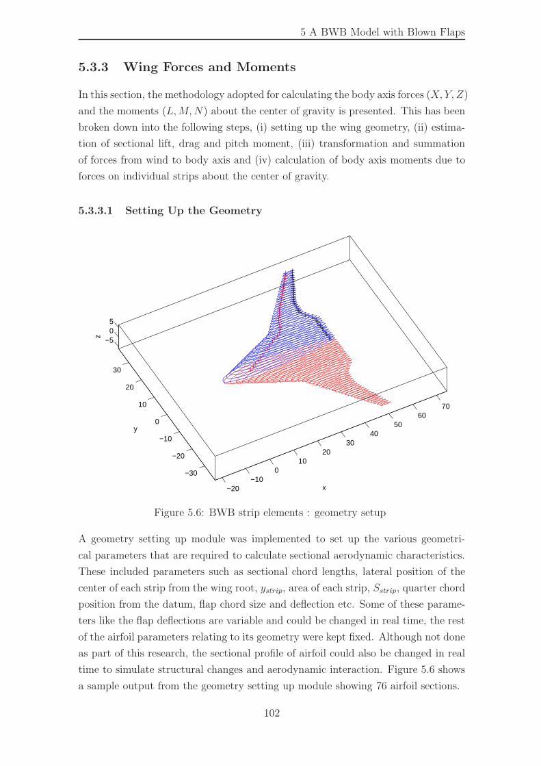
5 A BWB Model with Blown Flaps
5.3.3 Wing Forces and Moments
In this section, the methodology adopted for calculating the body axis forces (X, Y, Z)
and the moments (L,M,N) about the center of gravity is presented. This has been
broken down into the following steps, (i) setting up the wing geometry, (ii) estima-
tion of sectional lift, drag and pitch moment, (iii) transformation and summation
of forces from wind to body axis and (iv) calculation of body axis moments due to
forces on individual strips about the center of gravity.
5.3.3.1 Setting Up the Geometry
−20−10
010
2030
4050
6070
−30
−20
−10
0
10
20
30
−505
x
y
z
Figure 5.6: BWB strip elements : geometry setup
A geometry setting up module was implemented to set up the various geometri-
cal parameters that are required to calculate sectional aerodynamic characteristics.
These included parameters such as sectional chord lengths, lateral position of the
center of each strip from the wing root, ystrip, area of each strip, Sstrip, quarter chord
position from the datum, flap chord size and deflection etc. Some of these parame-
ters like the flap deflections are variable and could be changed in real time, the rest
of the airfoil parameters relating to its geometry were kept fixed. Although not done
as part of this research, the sectional profile of airfoil could also be changed in real
time to simulate structural changes and aerodynamic interaction. Figure 5.6 shows
a sample output from the geometry setting up module showing 76 airfoil sections.
102
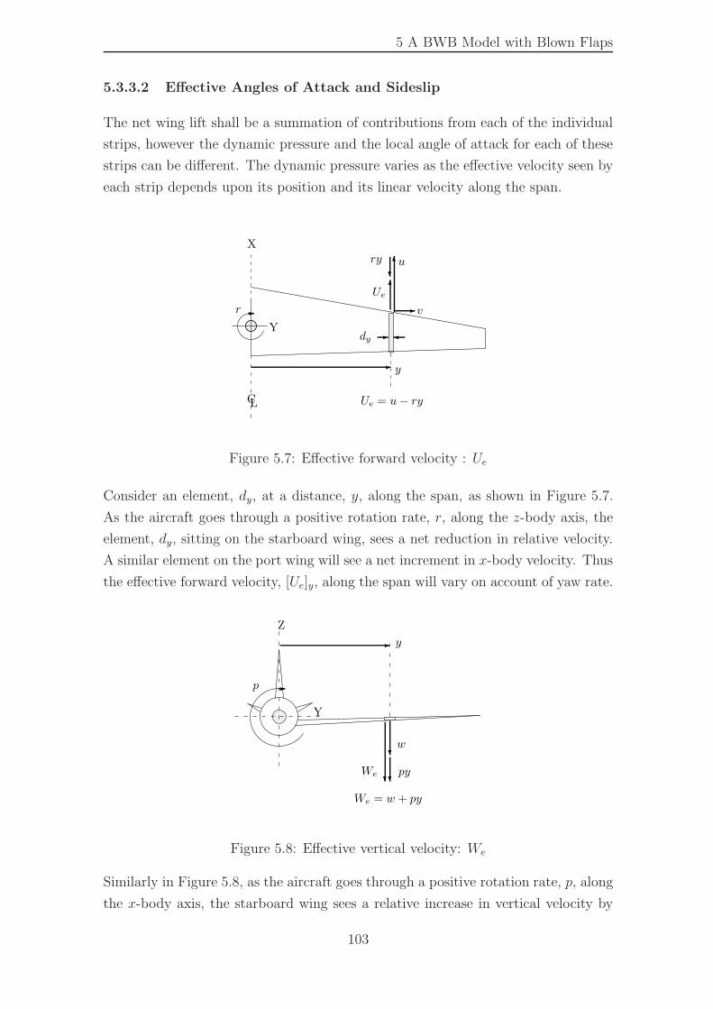
5 A BWB Model with Blown Flaps
5.3.3.2 Effective Angles of Attack and Sideslip
The net wing lift shall be a summation of contributions from each of the individual
strips, however the dynamic pressure and the local angle of attack for each of these
strips can be different. The dynamic pressure varies as the effective velocity seen by
each strip depends upon its position and its linear velocity along the span.
dy
y-
Ue = u − ry
-
X
L
- �
r
Y
C
6
-
6
u
v
ry
Ue
?
Figure 5.7: Effective forward velocity : Ue
Consider an element, dy, at a distance, y, along the span, as shown in Figure 5.7.
As the aircraft goes through a positive rotation rate, r, along the z-body axis, the
element, dy, sitting on the starboard wing, sees a net reduction in relative velocity.
A similar element on the port wing will see a net increment in x-body velocity. Thus
the effective forward velocity, [Ue]y, along the span will vary on account of yaw rate.
?
??
w
pyWe
-
Z
p
We = w + py
-
Y
y
Figure 5.8: Effective vertical velocity: We
Similarly in Figure 5.8, as the aircraft goes through a positive rotation rate, p, along
the x-body axis, the starboard wing sees a relative increase in vertical velocity by
103
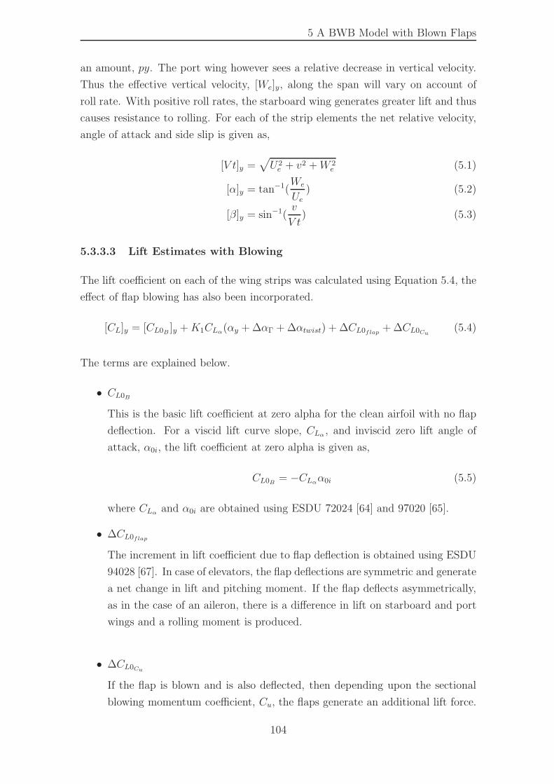
5 A BWB Model with Blown Flaps
an amount, py. The port wing however sees a relative decrease in vertical velocity.
Thus the effective vertical velocity, [We]y, along the span will vary on account of
roll rate. With positive roll rates, the starboard wing generates greater lift and thus
causes resistance to rolling. For each of the strip elements the net relative velocity,
angle of attack and side slip is given as,
[V t]y =√
U2e + v2 +W 2
e (5.1)
[α]y = tan−1(We
Ue) (5.2)
[β]y = sin−1(v
V t) (5.3)
5.3.3.3 Lift Estimates with Blowing
The lift coefficient on each of the wing strips was calculated using Equation 5.4, the
effect of flap blowing has also been incorporated.
[CL]y = [CL0B ]y +K1CLα(αy + ∆αΓ + ∆αtwist) + ∆CL0flap + ∆CL0Cu(5.4)
The terms are explained below.
• CL0B
This is the basic lift coefficient at zero alpha for the clean airfoil with no flap
deflection. For a viscid lift curve slope, CLα , and inviscid zero lift angle of
attack, α0i, the lift coefficient at zero alpha is given as,
CL0B = −CLαα0i (5.5)
where CLα and α0i are obtained using ESDU 72024 [64] and 97020 [65].
• ∆CL0flap
The increment in lift coefficient due to flap deflection is obtained using ESDU
94028 [67]. In case of elevators, the flap deflections are symmetric and generate
a net change in lift and pitching moment. If the flap deflects asymmetrically,
as in the case of an aileron, there is a difference in lift on starboard and port
wings and a rolling moment is produced.
• ∆CL0Cu
If the flap is blown and is also deflected, then depending upon the sectional
blowing momentum coefficient, Cu, the flaps generate an additional lift force.
104
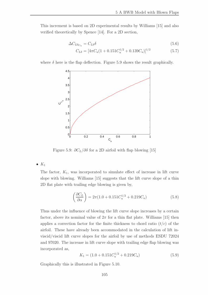
5 A BWB Model with Blown Flaps
This increment is based on 2D experimental results by Williams [15] and also
verified theoretically by Spence [14]. For a 2D section,
∆CL0Cu= CLδδ (5.6)
CLδ = [4πCu(1 + 0.151C1/2u + 0.139Cu)]
1/2 (5.7)
where δ here is the flap deflection. Figure 5.9 shows the result graphically.
0 0.2 0.4 0.6 0.8 10
0.5
1
1.5
2
2.5
3
3.5
4
4.5
Cu
CL δ
Figure 5.9: ∂CL/∂δ for a 2D airfoil with flap blowing [15]
• K1
The factor, K1, was incorporated to simulate effect of increase in lift curve
slope with blowing. Williams [15] suggests that the lift curve slope of a thin
2D flat plate with trailing edge blowing is given by,
(
∂CL∂α
)
= 2π(1.0 + 0.151C1/2u + 0.219Cu) (5.8)
Thus under the influence of blowing the lift curve slope increases by a certain
factor, above its nominal value of 2π for a thin flat plate. Williams [15] then
applies a correction factor for the finite thickness to chord ratio (t/c) of the
airfoil. These have already been accommodated in the calculation of lift in-
viscid/viscid lift curve slopes for the airfoil by use of methods ESDU 72024
and 97020. The increase in lift curve slope with trailing edge flap blowing was
incorporated as,
K1 = (1.0 + 0.151C1/2u + 0.219Cu) (5.9)
Graphically this is illustrated in Figure 5.10.
105
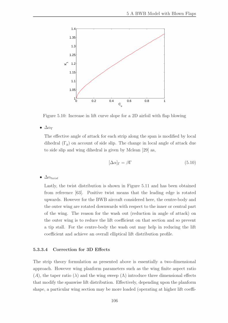
5 A BWB Model with Blown Flaps
0 0.2 0.4 0.6 0.8 11
1.05
1.1
1.15
1.2
1.25
1.3
1.35
1.4
Cu
K1
Figure 5.10: Increase in lift curve slope for a 2D airfoil with flap blowing
• ∆αΓ
The effective angle of attack for each strip along the span is modified by local
dihedral (Γy) on account of side slip. The change in local angle of attack due
to side slip and wing dihedral is given by Mclean [29] as,
[∆α]Γ = βΓ (5.10)
• ∆αtwist
Lastly, the twist distribution is shown in Figure 5.11 and has been obtained
from reference [63]. Positive twist means that the leading edge is rotated
upwards. However for the BWB aircraft considered here, the centre-body and
the outer wing are rotated downwards with respect to the inner or central part
of the wing. The reason for the wash out (reduction in angle of attack) on
the outer wing is to reduce the lift coefficient on that section and so prevent
a tip stall. For the centre-body the wash out may help in reducing the lift
coefficient and achieve an overall elliptical lift distribution profile.
5.3.3.4 Correction for 3D Effects
The strip theory formulation as presented above is essentially a two-dimensional
approach. However wing planform parameters such as the wing finite aspect ratio
(A), the taper ratio (λ) and the wing sweep (Λ) introduce three dimensional effects
that modify the spanwise lift distribution. Effectively, depending upon the planform
shape, a particular wing section may be more loaded (operating at higher lift coeffi-
106
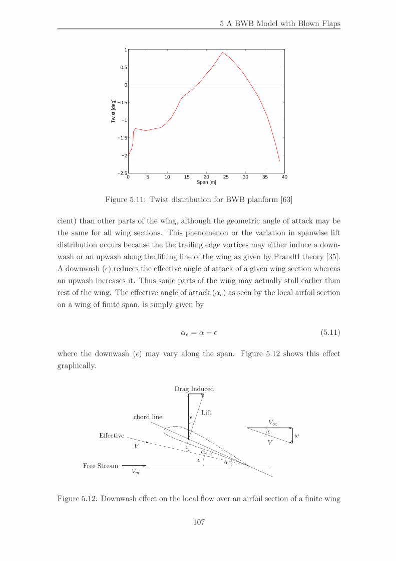
5 A BWB Model with Blown Flaps
0 5 10 15 20 25 30 35 40−2.5
−2
−1.5
−1
−0.5
0
0.5
1
Span [m]
Tw
ist [
deg]
Figure 5.11: Twist distribution for BWB planform [63]
cient) than other parts of the wing, although the geometric angle of attack may be
the same for all wing sections. This phenomenon or the variation in spanwise lift
distribution occurs because the the trailing edge vortices may either induce a down-
wash or an upwash along the lifting line of the wing as given by Prandtl theory [35].
A downwash (ǫ) reduces the effective angle of attack of a given wing section whereas
an upwash increases it. Thus some parts of the wing may actually stall earlier than
rest of the wing. The effective angle of attack (αe) as seen by the local airfoil section
on a wing of finite span, is simply given by
αe = α− ǫ (5.11)
where the downwash (ǫ) may vary along the span. Figure 5.12 shows this effect
graphically.
6-�
Drag Induced
ǫLift
chord line
z
-
αe
αǫ
-
?q
V∞
wǫ
V
V∞
V
Effective
Free Stream
Figure 5.12: Downwash effect on the local flow over an airfoil section of a finite wing
107
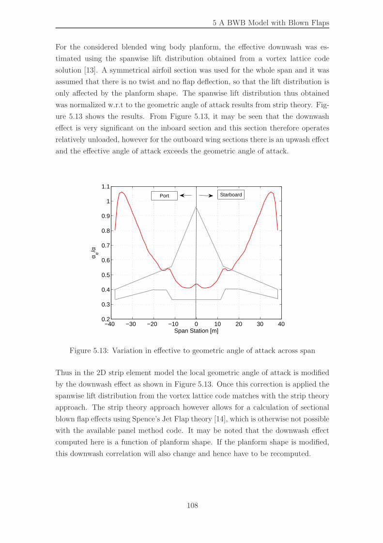
5 A BWB Model with Blown Flaps
For the considered blended wing body planform, the effective downwash was es-
timated using the spanwise lift distribution obtained from a vortex lattice code
solution [13]. A symmetrical airfoil section was used for the whole span and it was
assumed that there is no twist and no flap deflection, so that the lift distribution is
only affected by the planform shape. The spanwise lift distribution thus obtained
was normalized w.r.t to the geometric angle of attack results from strip theory. Fig-
ure 5.13 shows the results. From Figure 5.13, it may be seen that the downwash
effect is very significant on the inboard section and this section therefore operates
relatively unloaded, however for the outboard wing sections there is an upwash effect
and the effective angle of attack exceeds the geometric angle of attack.
−40 −30 −20 −10 0 10 20 30 400.2
0.3
0.4
0.5
0.6
0.7
0.8
0.9
1
1.1
Span Station [m]
α e/α
StarboardPort
Figure 5.13: Variation in effective to geometric angle of attack across span
Thus in the 2D strip element model the local geometric angle of attack is modified
by the downwash effect as shown in Figure 5.13. Once this correction is applied the
spanwise lift distribution from the vortex lattice code matches with the strip theory
approach. The strip theory approach however allows for a calculation of sectional
blown flap effects using Spence’s Jet Flap theory [14], which is otherwise not possible
with the available panel method code. It may be noted that the downwash effect
computed here is a function of planform shape. If the planform shape is modified,
this downwash correlation will also change and hence have to be recomputed.
108
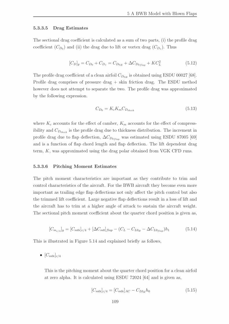
5 A BWB Model with Blown Flaps
5.3.3.5 Drag Estimates
The sectional drag coefficient is calculated as a sum of two parts, (i) the profile drag
coefficient (CD0) and (ii) the drag due to lift or vortex drag (CDv). Thus
[CD]y = CD0 + CDv = CD0B+ ∆CD0flap
+KC2L (5.12)
The profile drag coefficient of a clean airfoil CD0Bis obtained using ESDU 00027 [68].
Profile drag comprises of pressure drag + skin friction drag. The ESDU method
however does not attempt to separate the two. The profile drag was approximated
by the following expression.
CD0 = KcKmCDthick (5.13)
where Kc accounts for the effect of camber, Km accounts for the effect of compress-
ibility and CDthick is the profile drag due to thickness distribution. The increment in
profile drag due to flap deflection, ∆CD0flapwas estimated using ESDU 87005 [69]
and is a function of flap chord length and flap deflection. The lift dependent drag
term, K, was approximated using the drag polar obtained from VGK CFD runs.
5.3.3.6 Pitching Moment Estimates
The pitch moment characteristics are important as they contribute to trim and
control characteristics of the aircraft. For the BWB aircraft they become even more
important as trailing edge flap deflections not only affect the pitch control but also
the trimmed lift coefficient. Large negative flap deflections result in a loss of lift and
the aircraft has to trim at a higher angle of attack to sustain the aircraft weight.
The sectional pitch moment coefficient about the quarter chord position is given as,
[Cmc/4 ]y = [Cm0i]c/4 + [∆Cm0]flap − (CL − CL0B − ∆CL0flap)h1 (5.14)
This is illustrated in Figure 5.14 and explained briefly as follows,
• [Cm0i]c/4
This is the pitching moment about the quarter chord position for a clean airfoil
at zero alpha. It is calculated using ESDU 72024 [64] and is given as,
[Cm0i]c/4 = [Cm0i]AC − CL0Bh0 (5.15)
109
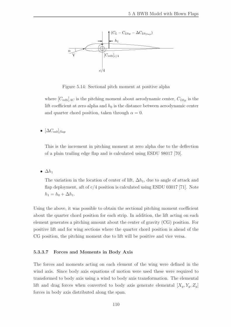
5 A BWB Model with Blown Flaps
c/4
6
1αV
(CL − CL0B− ∆CL0flap
)
- �-
h1
[Cm0i]c/4
Figure 5.14: Sectional pitch moment at positive alpha
where [Cm0i]AC is the pitching moment about aerodynamic center, CL0B is the
lift coefficient at zero alpha and h0 is the distance between aerodynamic center
and quarter chord position, taken through α = 0.
• [∆Cm0]flap
This is the increment in pitching moment at zero alpha due to the deflection
of a plain trailing edge flap and is calculated using ESDU 98017 [70].
• ∆h1
The variation in the location of center of lift, ∆h1, due to angle of attack and
flap deployment, aft of c/4 position is calculated using ESDU 03017 [71]. Note
h1 = h0 + ∆h1.
Using the above, it was possible to obtain the sectional pitching moment coefficient
about the quarter chord position for each strip. In addition, the lift acting on each
element generates a pitching amount about the center of gravity (CG) position. For
positive lift and for wing sections where the quarter chord position is ahead of the
CG position, the pitching moment due to lift will be positive and vice versa.
5.3.3.7 Forces and Moments in Body Axis
The forces and moments acting on each element of the wing were defined in the
wind axis. Since body axis equations of motion were used these were required to
transformed to body axis using a wind to body axis transformation. The elemental
lift and drag forces when converted to body axis generate elemental [Xy, Yy, Zy]
forces in body axis distributed along the span.
110
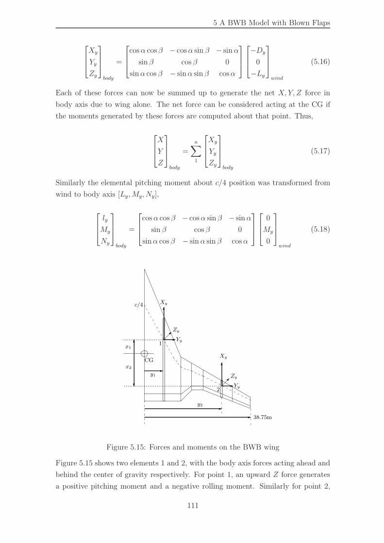
5 A BWB Model with Blown Flaps
Xy
Yy
Zy
body
=
cosα cosβ − cosα sin β − sinα
sin β cos β 0
sinα cos β − sinα sin β cosα
−Dy
0
−Ly
wind
(5.16)
Each of these forces can now be summed up to generate the net X, Y, Z force in
body axis due to wing alone. The net force can be considered acting at the CG if
the moments generated by these forces are computed about that point. Thus,
X
Y
Z
body
=
n∑
1
Xy
Yy
Zy
body
(5.17)
Similarly the elemental pitching moment about c/4 position was transformed from
wind to body axis [Ly,My, Ny],
ly
My
Ny
body
=
cosα cosβ − cosα sin β − sinα
sin β cosβ 0
sinα cosβ − sinα sin β cosα
0
My
0
wind
(5.18)
-
-
c/4
Xy
6
-
- 38.75m
x1
.......................
......................................................
6
?
x2
CG
1
y2
y1
�2
6
Yy
-� Yy
Zy
Xy
Zy
Figure 5.15: Forces and moments on the BWB wing
Figure 5.15 shows two elements 1 and 2, with the body axis forces acting ahead and
behind the center of gravity respectively. For point 1, an upward Z force generates
a positive pitching moment and a negative rolling moment. Similarly for point 2,
111

5 A BWB Model with Blown Flaps
an upward Z force shall generate a negative pitching moment and a negative rolling
moment. The net moments about the CG were calculated as the sum of moments
for each of these strip elements.
Net Roll Moment - For positive span (starboard wing), positive Z force (down),
generates a positive rolling moment about the CG.
lcg =n∑
1
(ly + Zyy) (5.19)
where Ly is the rolling moment acting on a given strip, Zy is the normal force on that
strip and y is the lateral distance of that strip from centerline, positive starboard.
Net Pitch Moment - If xmrp is the distance of the moment reference point or the
CG from the nose datum, being positive aft and xposc/4 the position of quarter chord
position for each given strip, then positive Z force shall generate a nose down or
negative pitch moment if (xmrp − xposc/4) is positive. Thus
Mcg =
n∑
1
(My − Zy(xmrp − xposc/4)) (5.20)
where My is the pitching moment about the quarter chord position for each strip.
Note that in Figure 5.15, the distance (xmrp− xposc/4) is simply referred as x1 or x2,
with x1 > 0 and x2 < 0.
Net Yaw Moment - For a positive span, y, towards right or starboard wing, a
positive X force on the starboard wing will generate a negative yaw moment and
vice versa. Similarly a positive Y force will generate positive yaw moment about
CG if (xmrp − xposc/4) is positive.
Ncg =
n∑
1
(Ny −Xyy + Yy(xmrp − xposc/4)) (5.21)
This completes the calculation of wing forces and moments.
112
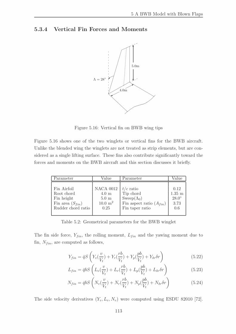
5 A BWB Model with Blown Flaps
5.3.4 Vertical Fin Forces and Moments
4.0m
5.0m
6
?
*
�
.................................
Λ = 28◦
Figure 5.16: Vertical fin on BWB wing tips
Figure 5.16 shows one of the two winglets or vertical fins for the BWB aircraft.
Unlike the blended wing the winglets are not treated as strip elements, but are con-
sidered as a single lifting surface. These fins also contribute significantly toward the
forces and moments on the BWB aircraft and this section discusses it briefly.
Parameter Value Parameter Value
Fin Airfoil NACA 0012 t/c ratio 0.12Root chord 4.0 m Tip chord 1.35 mFin height 5.0 m Sweep(Λ0) 28.0◦
Fin area (Sfin) 10.0 m2 Fin aspect ratio (Afin) 3.73Rudder chord ratio 0.25 Fin taper ratio 0.6
Table 5.2: Geometrical parameters for the BWB winglet
The fin side force, Yfin, the rolling moment, Lfin and the yawing moment due to
fin, Nfin, are computed as follows,
Yfin = qS
(
Yv(v
Vt) + Yr(
rb
Vt) + Yp(
pb
Vt) + Yδrδr
)
(5.22)
Lfin = qbS
(
Lv(v
Vt) + Lr(
rb
Vt) + Lp(
pb
Vt) + Lδrδr
)
(5.23)
Nfin = qbS
(
Nv(v
Vt) +Nr(
rb
Vt) +Np(
pb
Vt) +Nδrδr
)
(5.24)
The side velocity derivatives (Yv, Lv, Nv) were computed using ESDU 82010 [72].
113
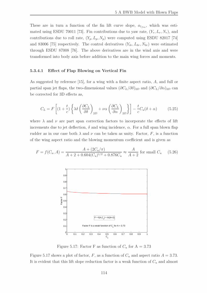
5 A BWB Model with Blown Flaps
These are in turn a function of the fin lift curve slope, a1fin , which was esti-
mated using ESDU 70011 [73]. Fin contributions due to yaw rate, (Yr, Lr, Nr), and
contributions due to roll rate, (Yp, Lp, Np) were computed using ESDU 82017 [74]
and 83006 [75] respectively. The control derivatives (Yδr, Lδr, Nδr) were estimated
through ESDU 87008 [76]. The above derivatives are in the wind axis and were
transformed into body axis before addition to the main wing forces and moments.
5.3.4.1 Effect of Flap Blowing on Vertical Fin
As suggested by reference [15], for a wing with a finite aspect ratio, A, and full or
partial span jet flaps, the two-dimensional values (∂CL/∂δ)2D and (∂CL/∂α)2D can
be corrected for 3D effects as,
CL = F
[
(1 +t
c)
{
λδ
(
∂CL∂δ
)
2D
+ να
(
∂CL∂α
)
2D
}]
− t
cCu(δ + α) (5.25)
where λ and ν are part span correction factors to incorporate the effects of lift
increments due to jet deflection, δ and wing incidence, α. For a full span blown flap
rudder as in our case both λ and ν can be taken as unity. Factor, F , is a function
of the wing aspect ratio and the blowing momentum coefficient and is given as
F = f(Cu, A) =A + (2Cu/π)
A + 2 + 0.604(Cu)1/2 + 0.876Cu≈ A
A + 2for small Cu (5.26)
0 0.1 0.2 0.3 0.4 0.5 0.6 0.7 0.8 0.9 10
0.1
0.2
0.3
0.4
0.5
0.6
0.7
0.8
0.9
1
Cu
Fac
tor
F
F = f(A,Cu) ≈ A/(A+2)
Factor F is a weak function of Cu for A = 3.73
Figure 5.17: Factor F as function of Cu for A = 3.73
Figure 5.17 shows a plot of factor, F , as a function of Cu and aspect ratio A = 3.73.
It is evident that this lift slope reduction factor is a weak function of Cu and almost
114
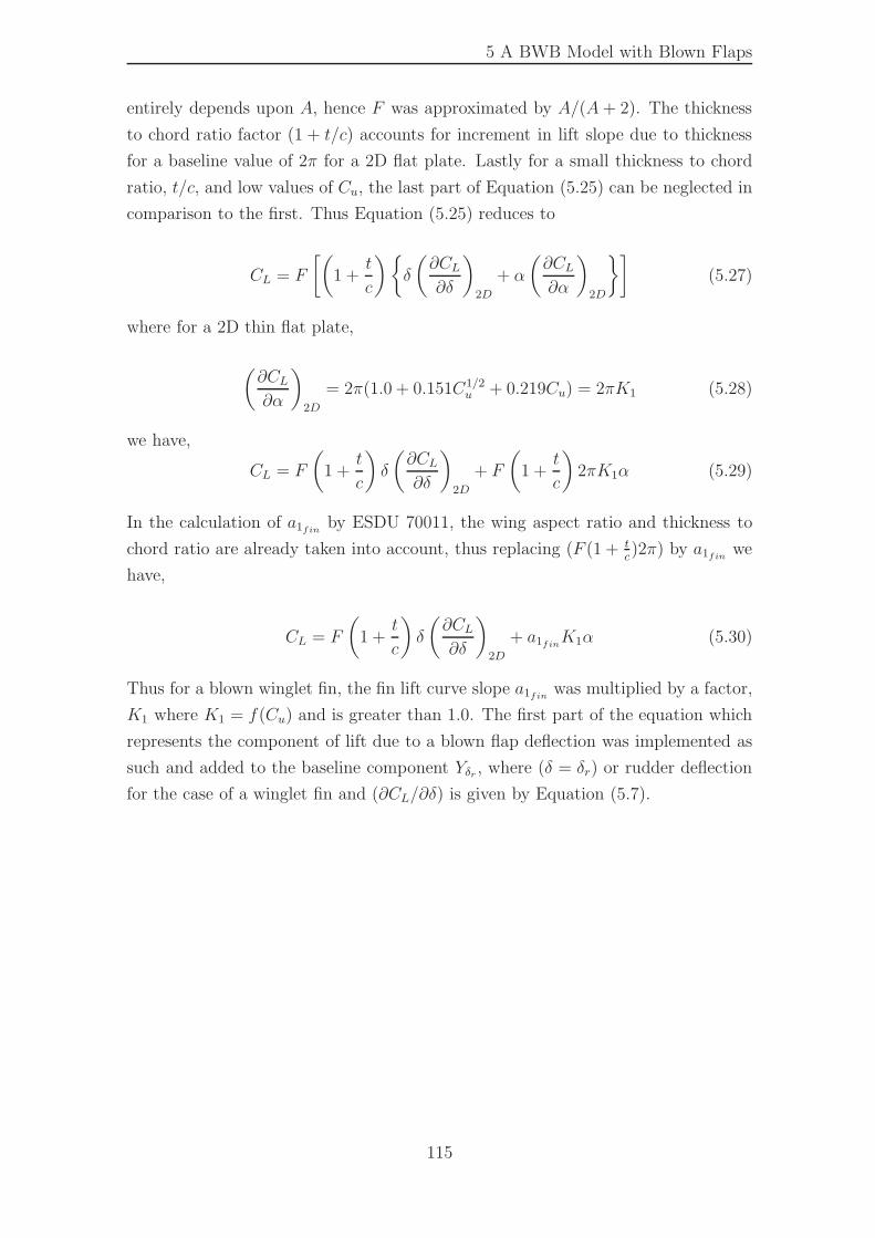
5 A BWB Model with Blown Flaps
entirely depends upon A, hence F was approximated by A/(A+ 2). The thickness
to chord ratio factor (1 + t/c) accounts for increment in lift slope due to thickness
for a baseline value of 2π for a 2D flat plate. Lastly for a small thickness to chord
ratio, t/c, and low values of Cu, the last part of Equation (5.25) can be neglected in
comparison to the first. Thus Equation (5.25) reduces to
CL = F
[(
1 +t
c
){
δ
(
∂CL∂δ
)
2D
+ α
(
∂CL∂α
)
2D
}]
(5.27)
where for a 2D thin flat plate,
(
∂CL∂α
)
2D
= 2π(1.0 + 0.151C1/2u + 0.219Cu) = 2πK1 (5.28)
we have,
CL = F
(
1 +t
c
)
δ
(
∂CL∂δ
)
2D
+ F
(
1 +t
c
)
2πK1α (5.29)
In the calculation of a1fin by ESDU 70011, the wing aspect ratio and thickness to
chord ratio are already taken into account, thus replacing (F (1 + tc)2π) by a1fin we
have,
CL = F
(
1 +t
c
)
δ
(
∂CL∂δ
)
2D
+ a1finK1α (5.30)
Thus for a blown winglet fin, the fin lift curve slope a1fin was multiplied by a factor,
K1 where K1 = f(Cu) and is greater than 1.0. The first part of the equation which
represents the component of lift due to a blown flap deflection was implemented as
such and added to the baseline component Yδr , where (δ = δr) or rudder deflection
for the case of a winglet fin and (∂CL/∂δ) is given by Equation (5.7).
115
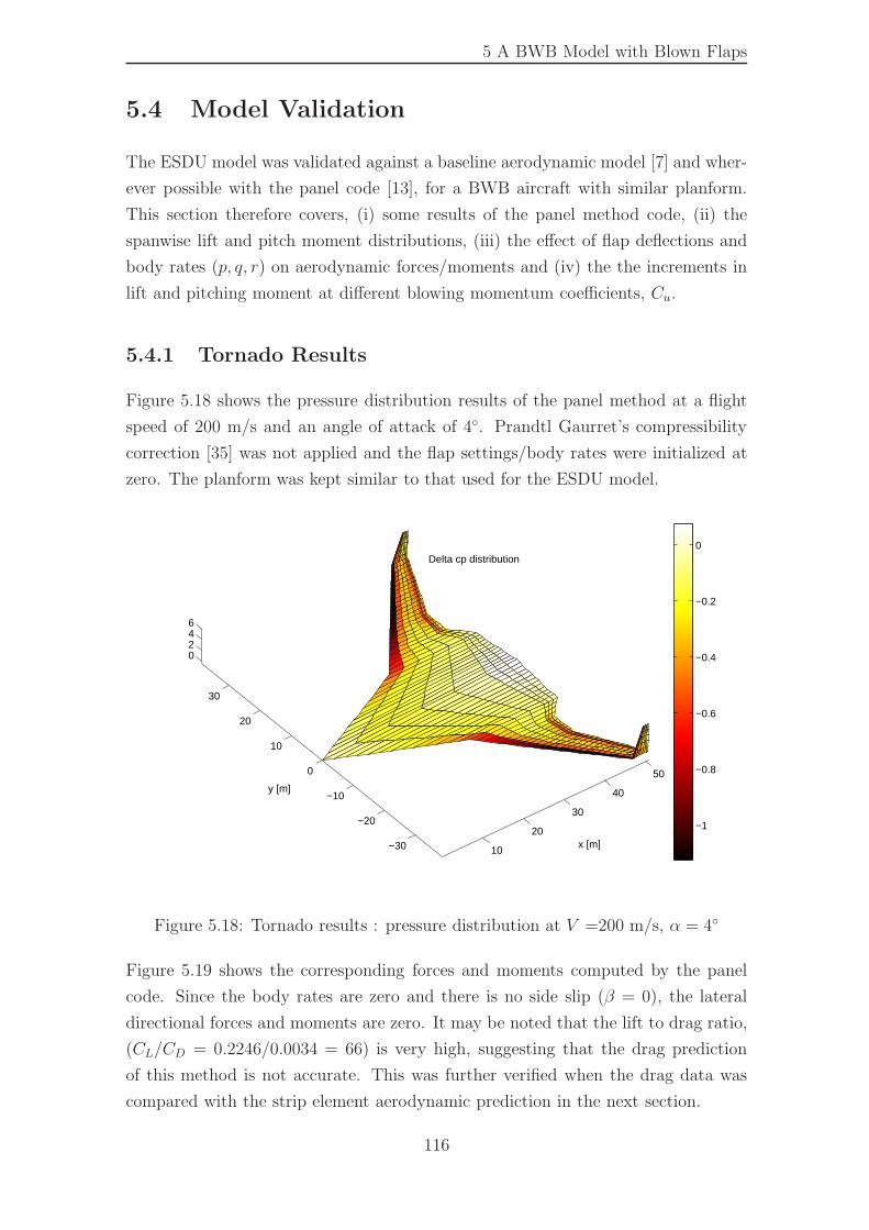
5 A BWB Model with Blown Flaps
5.4 Model Validation
The ESDU model was validated against a baseline aerodynamic model [7] and wher-
ever possible with the panel code [13], for a BWB aircraft with similar planform.
This section therefore covers, (i) some results of the panel method code, (ii) the
spanwise lift and pitch moment distributions, (iii) the effect of flap deflections and
body rates (p, q, r) on aerodynamic forces/moments and (iv) the the increments in
lift and pitching moment at different blowing momentum coefficients, Cu.
5.4.1 Tornado Results
Figure 5.18 shows the pressure distribution results of the panel method at a flight
speed of 200 m/s and an angle of attack of 4◦. Prandtl Gaurret’s compressibility
correction [35] was not applied and the flap settings/body rates were initialized at
zero. The planform was kept similar to that used for the ESDU model.
10
20
30
40
50
−30
−20
−10
0
10
20
30
0246
x [m]
Delta cp distribution
y [m]
−1
−0.8
−0.6
−0.4
−0.2
0
Figure 5.18: Tornado results : pressure distribution at V =200 m/s, α = 4◦
Figure 5.19 shows the corresponding forces and moments computed by the panel
code. Since the body rates are zero and there is no side slip (β = 0), the lateral
directional forces and moments are zero. It may be noted that the lift to drag ratio,
(CL/CD = 0.2246/0.0034 = 66) is very high, suggesting that the drag prediction
of this method is not accurate. This was further verified when the drag data was
compared with the strip element aerodynamic prediction in the next section.
116
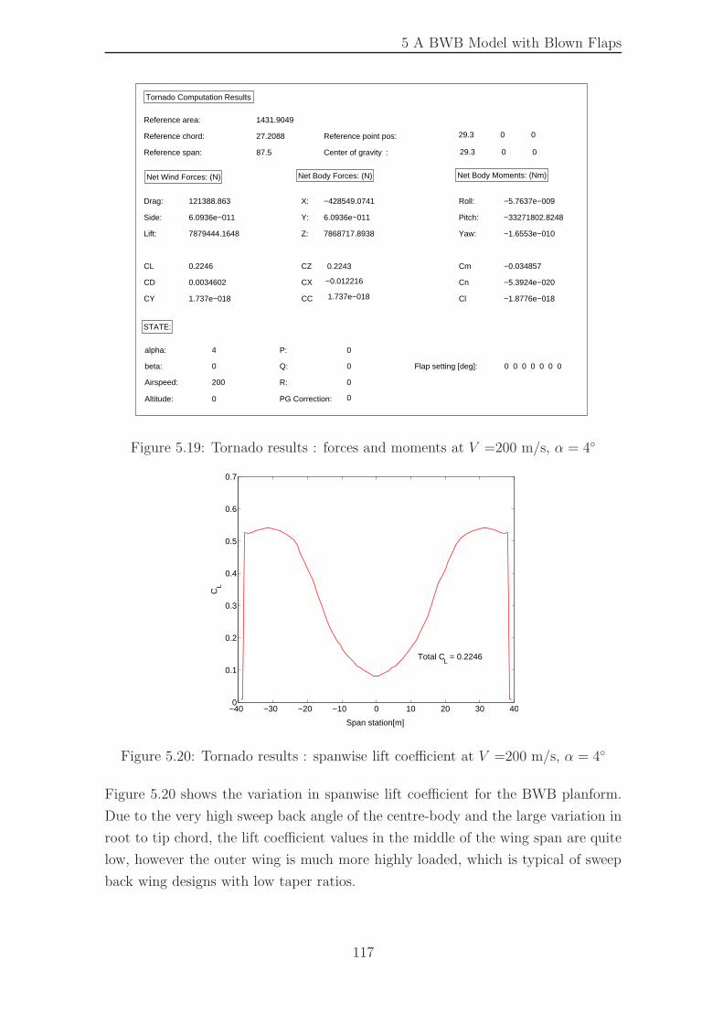
5 A BWB Model with Blown Flaps
Tornado Computation Results
Reference area: 1431.9049
Reference chord: 27.2088
Reference span: 87.5
Reference point pos: 29.3 0 0
Center of gravity : 29.3 0 0
Net Wind Forces: (N)
Drag: 121388.863
Side: 6.0936e−011
Lift: 7879444.1648
Net Body Forces: (N)
X: −428549.0741
Y: 6.0936e−011
Z: 7868717.8938
Net Body Moments: (Nm)
Roll: −5.7637e−009
Pitch: −33271802.8248
Yaw: −1.6553e−010
CL 0.2246
CD 0.0034602
CY 1.737e−018
CZ 0.2243
CX −0.012216
CC 1.737e−018
Cm −0.034857
Cn −5.3924e−020
Cl −1.8776e−018
STATE:
alpha: 4
beta: 0
Airspeed: 200
Altitude: 0
P: 0
Q: 0
R: 0
PG Correction: 0
Flap setting [deg]: 0 0 0 0 0 0 0
Figure 5.19: Tornado results : forces and moments at V =200 m/s, α = 4◦
−40 −30 −20 −10 0 10 20 30 400
0.1
0.2
0.3
0.4
0.5
0.6
0.7
CL
Span station[m]
Total CL = 0.2246
Figure 5.20: Tornado results : spanwise lift coefficient at V =200 m/s, α = 4◦
Figure 5.20 shows the variation in spanwise lift coefficient for the BWB planform.
Due to the very high sweep back angle of the centre-body and the large variation in
root to tip chord, the lift coefficient values in the middle of the wing span are quite
low, however the outer wing is much more highly loaded, which is typical of sweep
back wing designs with low taper ratios.
117
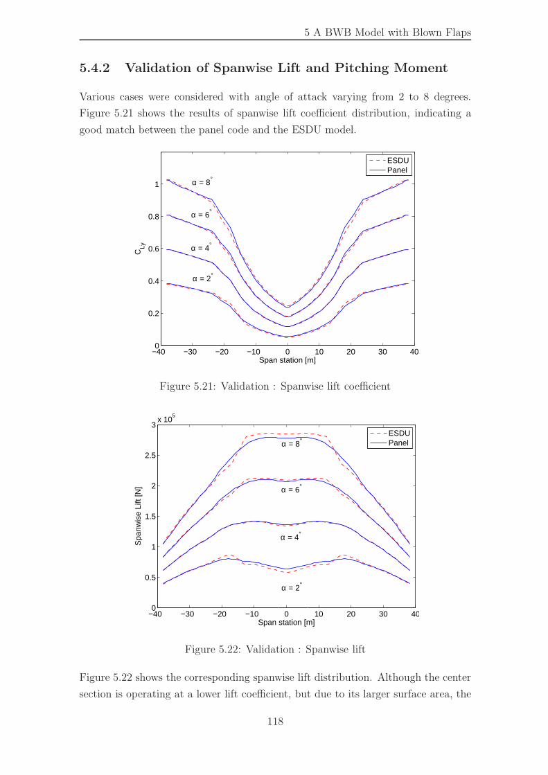
5 A BWB Model with Blown Flaps
5.4.2 Validation of Spanwise Lift and Pitching Moment
Various cases were considered with angle of attack varying from 2 to 8 degrees.
Figure 5.21 shows the results of spanwise lift coefficient distribution, indicating a
good match between the panel code and the ESDU model.
−40 −30 −20 −10 0 10 20 30 400
0.2
0.4
0.6
0.8
1
Span station [m]
CLy
ESDUPanel
α = 2°
α = 4°
α = 6°
α = 8°
Figure 5.21: Validation : Spanwise lift coefficient
−40 −30 −20 −10 0 10 20 30 400
0.5
1
1.5
2
2.5
3x 10
5
Span station [m]
Spa
nwis
e Li
ft [N
]
ESDUPanelα = 8°
α = 6°
α = 4°
α = 2°
Figure 5.22: Validation : Spanwise lift
Figure 5.22 shows the corresponding spanwise lift distribution. Although the center
section is operating at a lower lift coefficient, but due to its larger surface area, the
118
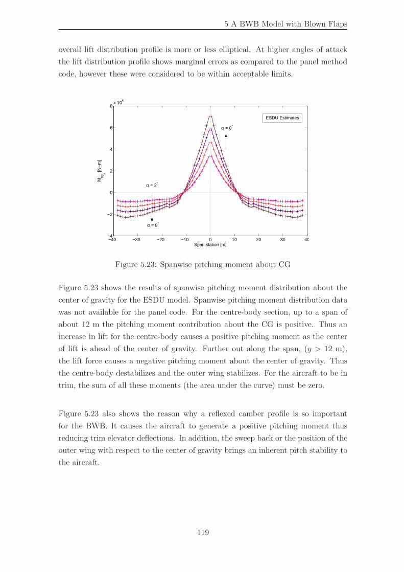
5 A BWB Model with Blown Flaps
overall lift distribution profile is more or less elliptical. At higher angles of attack
the lift distribution profile shows marginal errors as compared to the panel method
code, however these were considered to be within acceptable limits.
−40 −30 −20 −10 0 10 20 30 40−4
−2
0
2
4
6
8x 10
6
Span station [m]
Mcg
y [N−
m]
ESDU Estimates
α = 2°
α = 8°
α = 8°
Figure 5.23: Spanwise pitching moment about CG
Figure 5.23 shows the results of spanwise pitching moment distribution about the
center of gravity for the ESDU model. Spanwise pitching moment distribution data
was not available for the panel code. For the centre-body section, up to a span of
about 12 m the pitching moment contribution about the CG is positive. Thus an
increase in lift for the centre-body causes a positive pitching moment as the center
of lift is ahead of the center of gravity. Further out along the span, (y > 12 m),
the lift force causes a negative pitching moment about the center of gravity. Thus
the centre-body destabilizes and the outer wing stabilizes. For the aircraft to be in
trim, the sum of all these moments (the area under the curve) must be zero.
Figure 5.23 also shows the reason why a reflexed camber profile is so important
for the BWB. It causes the aircraft to generate a positive pitching moment thus
reducing trim elevator deflections. In addition, the sweep back or the position of the
outer wing with respect to the center of gravity brings an inherent pitch stability to
the aircraft.
119

5 A BWB Model with Blown Flaps
5.4.3 Validation of Aero Derivatives w.r.t Air Angles
In this section, the variation in aerodynamic forces and moments with respect to
angle of attack (α) and angle of side slip (β) will be considered. Wherever possible
comparison is made between the baseline, the panel method and the strip element
ESDU models. The baseline aerodynamic model which relies on previous research
work and collection of aerodynamic databases [7] uses the same planform as the
panel method and the strip element models, however the exact airfoil profile and
twist distribution for the baseline model was not available. In the absence of any
other data this was considered to be the best available reference.
5.4.3.1 Variation with Angle of Attack (α)
0 1 2 3 4 5 6−0.6
−0.5
−0.4
−0.3
−0.2
−0.1
0
0.1
Alpha [deg]
CZ
− Z
For
ce C
oeffi
cien
t
ESDU
Panel
Baseline
ESDU
Panel
Baseline
Figure 5.24: Z force coefficient (CZ)
Z Force w.r.t alpha - (CZα) - Figure 5.24 shows the variation in the Z force
coefficient with respect to angle of attack. A body axis notation has been adopted
in which the z-axis points downwards, y-axis towards the starboard wing and x-axis
towards the nose. Two points may be noted in the figure. Firstly, at zero angle of
attack the coefficient, CZ , is almost zero or positive, indicating almost zero or nega-
tive lift at zero angle of attack. The reason for this is the reflexed camber/symmetric
airfoils for the centre-body and inner wing respectively. Secondly, the slopes of the
curve CZα match well. It may be pointed out further that in the baseline model
the compressibility effect was not included, the same has been done for the strip
element and panel codes. When the compressibility effect is added the normal force
coefficient slope increases with Mach number.
120
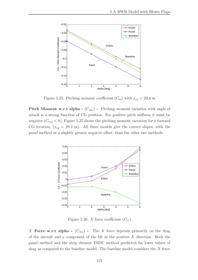
5 A BWB Model with Blown Flaps
0 1 2 3 4 5 6−0.16
−0.14
−0.12
−0.1
−0.08
−0.06
−0.04
−0.02
Alpha [deg]
Cm
− P
itch
Mom
ent C
oeffi
cien
t
ESDU
Baseline
Panel
ESDU
Panel
Baseline
Figure 5.25: Pitching moment coefficient (Cm) with xcg = 29.4 m
Pitch Moment w.r.t alpha - (Cmα) - Pitching moment variation with angle of
attack is a strong function of CG position. For positive pitch stiffness it must be
negative (Cmα < 0). Figure 5.25 shows the pitching moment variation for a forward
CG location, (xcg = 29.4 m). All three models give the correct slopes, with the
panel method at a slightly greater negative offset, than the other two methods.
0 1 2 3 4 5 6−0.04
−0.03
−0.02
−0.01
0
0.01
0.02
0.03
0.04
0.05
Alpha [deg]
CX
− X
For
ce C
oeffi
cien
t
ESDU
Panel
Baseline
ESDU
Panel
Baseline
Figure 5.26: X force coefficient (CX)
X Force w.r.t alpha - (CXα) - The X force depends primarily on the drag
of the aircraft and a component of the lift in the positive X direction. Both the
panel method and the strip element ESDU method predicted far lower values of
drag as compared to the baseline model. The baseline model considers the X force
121
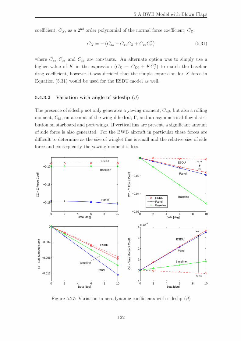
5 A BWB Model with Blown Flaps
coefficient, CX , as a 2nd order polynomial of the normal force coefficient, CZ ,
CX = −(
Cx0 − Cx1CZ + Cx2C2Z
)
(5.31)
where Cx0, Cx1 and Cx2 are constants. An alternate option was to simply use a
higher value of K in the expression (CD = CD0 + KC2L) to match the baseline
drag coefficient, however it was decided that the simple expression for X force in
Equation (5.31) would be used for the ESDU model as well.
5.4.3.2 Variation with angle of sideslip (β)
The presence of sideslip not only generates a yawing moment, Cnβ, but also a rolling
moment, Clβ, on account of the wing dihedral, Γ, and an asymmetrical flow distri-
bution on starboard and port wings. If vertical fins are present, a significant amount
of side force is also generated. For the BWB aircraft in particular these forces are
difficult to determine as the size of winglet fins is small and the relative size of side
force and consequently the yawing moment is less.
0 2 4 6 8 10
−0.19
−0.18
−0.17
Beta [deg]
CZ
− Z
For
ce C
oeff
0 2 4 6 8 10−0.06
−0.04
−0.02
0
Beta [deg]
CY
− Y
For
ce C
oeff
0 2 4 6 8 10
−0.012
−0.008
−0.004
0
Beta [deg]
Cl −
Rol
l Mom
ent C
oeff
0 2 4 6 8 10−1
0
1
2
3
4x 10
−3
Beta [deg]
Cn
− Y
aw M
omen
t Coe
ff
ESDU ESDU
ESDU
ESDU
Panel
Panel
Panel
Panel Baseline
Baseline Baseline
Baseline
Fin
Fin
No Fin
No Fin
ESDUPanelBaseline
Figure 5.27: Variation in aerodynamic coefficients with sideslip (β)
122
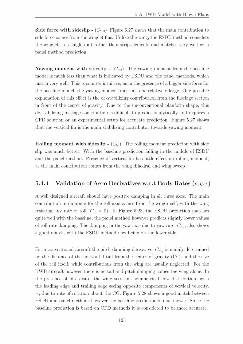
5 A BWB Model with Blown Flaps
Side force with sideslip - (CY β) Figure 5.27 shows that the main contribution to
side force comes from the winglet fins. Unlike the wing, the ESDU method considers
the winglet as a single unit rather than strip elements and matches very well with
panel method prediction.
Yawing moment with sideslip - (Cnβ) The yawing moment from the baseline
model is much less than what is indicated by ESDU and the panel methods, which
match very well. This is counter intuitive, as in the presence of a bigger side force for
the baseline model, the yawing moment must also be relatively large. One possible
explanation of this effect is the de-stabilizing contribution from the fuselage section
in front of the center of gravity. Due to the unconventional planform shape, this
de-stabilizing fuselage contribution is difficult to predict analytically and requires a
CFD solution or an experimental setup for accurate prediction. Figure 5.27 shows
that the vertical fin is the main stabilizing contributor towards yawing moment.
Rolling moment with sideslip - (Clβ) The rolling moment prediction with side
slip was much better. With the baseline prediction falling in the middle of ESDU
and the panel method. Presence of vertical fin has little effect on rolling moment,
as the main contribution comes from the wing dihedral and wing sweep.
5.4.4 Validation of Aero Derivatives w.r.t Body Rates (p, q, r)
A well designed aircraft should have positive damping in all three axes. The main
contribution in damping for the roll axis comes from the wing itself, with the wing
resisting any rate of roll (Clp < 0). In Figure 5.28, the ESDU prediction matches
quite well with the baseline, the panel method however predicts slightly lower values
of roll rate damping. The damping in the yaw axis due to yaw rate, Cnr , also shows
a good match, with the ESDU method now being on the lower side.
For a conventional aircraft the pitch damping derivative, Cmq is mainly determined
by the distance of the horizontal tail from the center of gravity (CG) and the size
of the tail itself, while contributions from the wing are usually neglected. For the
BWB aircraft however there is no tail and pitch damping comes the wing alone. In
the presence of pitch rate, the wing sees an asymmetrical flow distribution, with
the leading edge and trailing edge seeing opposite components of vertical velocity,
w, due to rate of rotation about the CG. Figure 5.28 shows a good match between
ESDU and panel methods however the baseline prediction is much lower. Since the
baseline prediction is based on CFD methods it is considered to be more accurate.
123
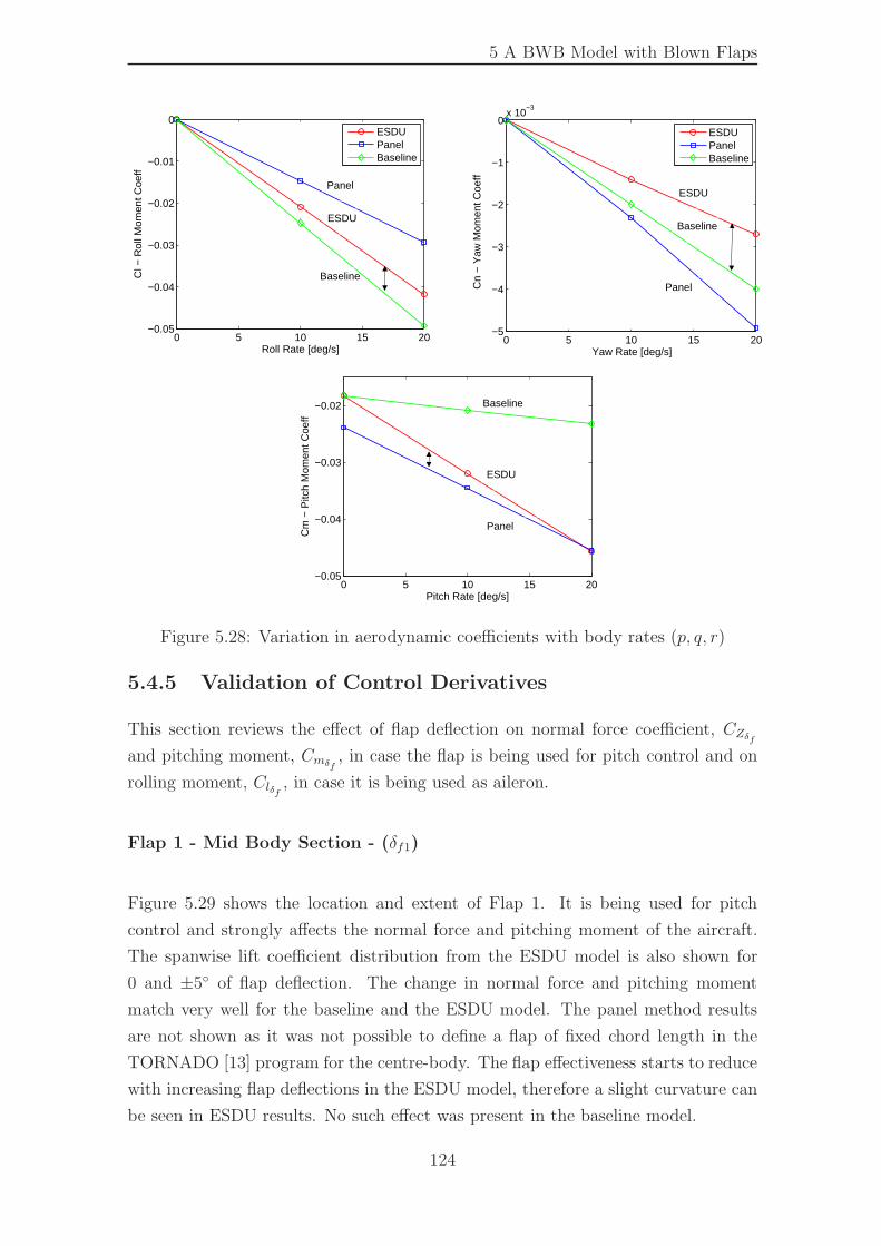
5 A BWB Model with Blown Flaps
0 5 10 15 20−0.05
−0.04
−0.03
−0.02
−0.01
0
Roll Rate [deg/s]
Cl −
Rol
l Mom
ent C
oeff
ESDUPanelBaseline
0 5 10 15 20−5
−4
−3
−2
−1
0x 10
−3
Yaw Rate [deg/s]
Cn
− Y
aw M
omen
t Coe
ff
ESDUPanelBaseline
0 5 10 15 20−0.05
−0.04
−0.03
−0.02
Pitch Rate [deg/s]
Cm
− P
itch
Mom
ent C
oeff
ESDU
Panel
Panel
Panel
Baseline
ESDU
Baseline
ESDU
Baseline
Figure 5.28: Variation in aerodynamic coefficients with body rates (p, q, r)
5.4.5 Validation of Control Derivatives
This section reviews the effect of flap deflection on normal force coefficient, CZδfand pitching moment, Cmδf , in case the flap is being used for pitch control and on
rolling moment, Clδf , in case it is being used as aileron.
Flap 1 - Mid Body Section - (δf1)
Figure 5.29 shows the location and extent of Flap 1. It is being used for pitch
control and strongly affects the normal force and pitching moment of the aircraft.
The spanwise lift coefficient distribution from the ESDU model is also shown for
0 and ±5◦ of flap deflection. The change in normal force and pitching moment
match very well for the baseline and the ESDU model. The panel method results
are not shown as it was not possible to define a flap of fixed chord length in the
TORNADO [13] program for the centre-body. The flap effectiveness starts to reduce
with increasing flap deflections in the ESDU model, therefore a slight curvature can
be seen in ESDU results. No such effect was present in the baseline model.
124
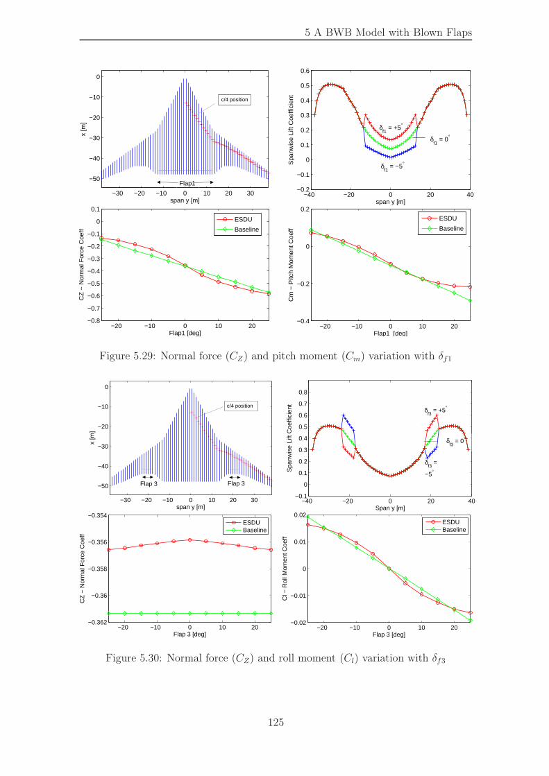
5 A BWB Model with Blown Flaps
−30 −20 −10 0 10 20 30
−50
−40
−30
−20
−10
0
span y [m]
x [m
]
−40 −20 0 20 40−0.2
−0.1
0
0.1
0.2
0.3
0.4
0.5
0.6
span y [m]
Spa
nwis
e Li
ft C
oeffi
cien
t
−20 −10 0 10 20−0.8
−0.7
−0.6
−0.5
−0.4
−0.3
−0.2
−0.1
0
0.1
Flap1 [deg]
CZ
− N
orm
al F
orce
Coe
ff
ESDU
Baseline
−20 −10 0 10 20−0.4
−0.2
0
0.2
Flap1 [deg]
Cm
− P
itch
Mom
ent C
oeff
ESDU
Baseline
Flap1
δf1
= −5°
δf1
= 0°
δf1
= +5°
c/4 position
Figure 5.29: Normal force (CZ) and pitch moment (Cm) variation with δf1
−30 −20 −10 0 10 20 30
−50
−40
−30
−20
−10
0
span y [m]
x [m
]
−40 −20 0 20 40−0.1
0
0.1
0.2
0.3
0.4
0.5
0.6
0.7
0.8
Span y [m]
Spa
nwis
e Li
ft C
oeffi
cien
t
−20 −10 0 10 20−0.362
−0.36
−0.358
−0.356
−0.354
Flap 3 [deg]
CZ
− N
orm
al F
orce
Coe
ff
ESDUBaseline
−20 −10 0 10 20−0.02
−0.01
0
0.01
0.02
Flap 3 [deg]
Cl −
Rol
l Mom
ent C
oeff
ESDUBaseline
Flap 3Flap 3
δf3
=
−5°
δf3
= +5°
δf3
= 0°
c/4 position
Figure 5.30: Normal force (CZ) and roll moment (Cl) variation with δf3
125
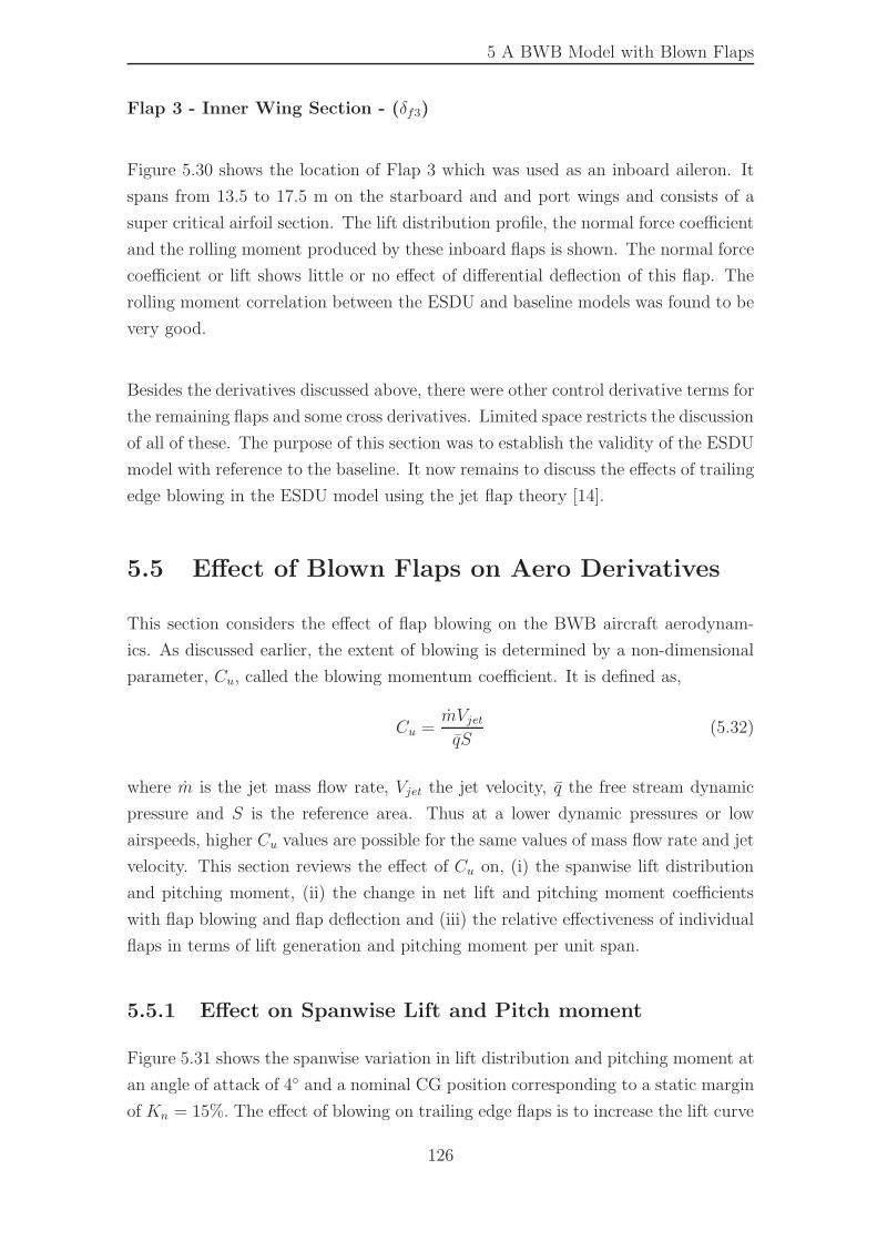
5 A BWB Model with Blown Flaps
Flap 3 - Inner Wing Section - (δf3)
Figure 5.30 shows the location of Flap 3 which was used as an inboard aileron. It
spans from 13.5 to 17.5 m on the starboard and and port wings and consists of a
super critical airfoil section. The lift distribution profile, the normal force coefficient
and the rolling moment produced by these inboard flaps is shown. The normal force
coefficient or lift shows little or no effect of differential deflection of this flap. The
rolling moment correlation between the ESDU and baseline models was found to be
very good.
Besides the derivatives discussed above, there were other control derivative terms for
the remaining flaps and some cross derivatives. Limited space restricts the discussion
of all of these. The purpose of this section was to establish the validity of the ESDU
model with reference to the baseline. It now remains to discuss the effects of trailing
edge blowing in the ESDU model using the jet flap theory [14].
5.5 Effect of Blown Flaps on Aero Derivatives
This section considers the effect of flap blowing on the BWB aircraft aerodynam-
ics. As discussed earlier, the extent of blowing is determined by a non-dimensional
parameter, Cu, called the blowing momentum coefficient. It is defined as,
Cu =mVjetqS
(5.32)
where m is the jet mass flow rate, Vjet the jet velocity, q the free stream dynamic
pressure and S is the reference area. Thus at a lower dynamic pressures or low
airspeeds, higher Cu values are possible for the same values of mass flow rate and jet
velocity. This section reviews the effect of Cu on, (i) the spanwise lift distribution
and pitching moment, (ii) the change in net lift and pitching moment coefficients
with flap blowing and flap deflection and (iii) the relative effectiveness of individual
flaps in terms of lift generation and pitching moment per unit span.
5.5.1 Effect on Spanwise Lift and Pitch moment
Figure 5.31 shows the spanwise variation in lift distribution and pitching moment at
an angle of attack of 4◦ and a nominal CG position corresponding to a static margin
of Kn = 15%. The effect of blowing on trailing edge flaps is to increase the lift curve
126
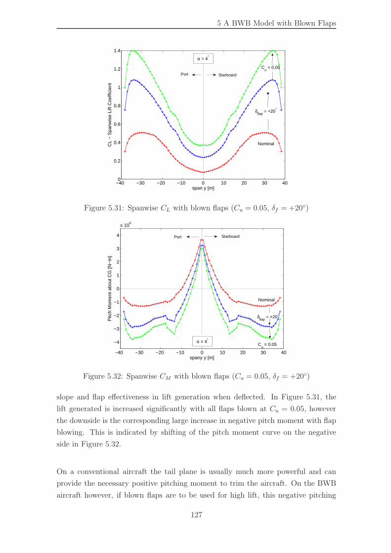
5 A BWB Model with Blown Flaps
−40 −30 −20 −10 0 10 20 30 400
0.2
0.4
0.6
0.8
1
1.2
1.4
span y [m]
CL
− S
panw
ise
Lift
Coe
ffici
ent
δflap
= +20°
Cu = 0.05
Nominal
α = 4°
StarboardPort
Figure 5.31: Spanwise CL with blown flaps (Cu = 0.05, δf = +20◦)
−40 −30 −20 −10 0 10 20 30 40
−4
−3
−2
−1
0
1
2
3
4
x 106
spany y [m]
Pitc
h M
omen
t abo
ut C
G [N
−m
]
Cu = 0.05
δflap
= +20°
Nominal
α = 4°
StarboardPort
Figure 5.32: Spanwise CM with blown flaps (Cu = 0.05, δf = +20◦)
slope and flap effectiveness in lift generation when deflected. In Figure 5.31, the
lift generated is increased significantly with all flaps blown at Cu = 0.05, however
the downside is the corresponding large increase in negative pitch moment with flap
blowing. This is indicated by shifting of the pitch moment curve on the negative
side in Figure 5.32.
On a conventional aircraft the tail plane is usually much more powerful and can
provide the necessary positive pitching moment to trim the aircraft. On the BWB
aircraft however, if blown flaps are to be used for high lift, this negative pitching
127
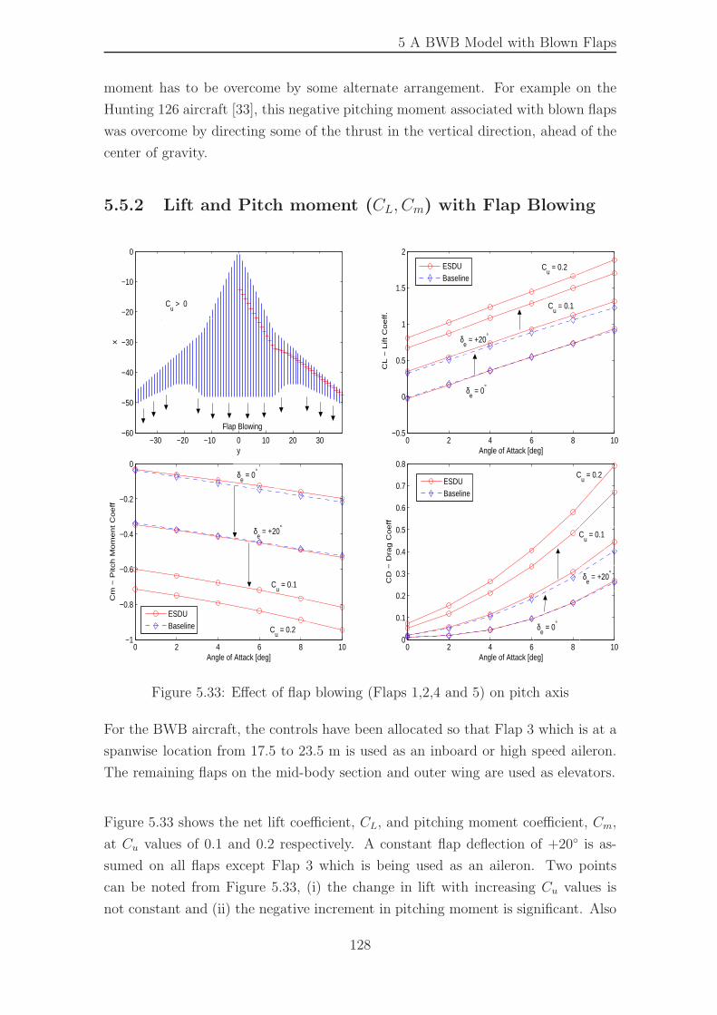
5 A BWB Model with Blown Flaps
moment has to be overcome by some alternate arrangement. For example on the
Hunting 126 aircraft [33], this negative pitching moment associated with blown flaps
was overcome by directing some of the thrust in the vertical direction, ahead of the
center of gravity.
5.5.2 Lift and Pitch moment (CL, Cm) with Flap Blowing
−30 −20 −10 0 10 20 30−60
−50
−40
−30
−20
−10
0
y
x
0 2 4 6 8 10−0.5
0
0.5
1
1.5
2
Angle of Attack [deg]
CL
− L
ift
Co
eff
.
ESDUBaseline
0 2 4 6 8 10−1
−0.8
−0.6
−0.4
−0.2
0
Angle of Attack [deg]
Cm
− P
itch
Mo
me
nt
Co
eff
ESDUBaseline
0 2 4 6 8 100
0.1
0.2
0.3
0.4
0.5
0.6
0.7
0.8
Angle of Attack [deg]
CD
− D
rag
Co
eff
ESDUBaseline
Flap Blowing
Cu > 0
Cu = 0.1
Cu = 0.1
Cu = 0.1
Cu = 0.2
Cu = 0.2
Cu = 0.2
δe = +20°
δe = 0°
δe = 0°
δe = +20°
δe = 0°
δe = +20°
Figure 5.33: Effect of flap blowing (Flaps 1,2,4 and 5) on pitch axis
For the BWB aircraft, the controls have been allocated so that Flap 3 which is at a
spanwise location from 17.5 to 23.5 m is used as an inboard or high speed aileron.
The remaining flaps on the mid-body section and outer wing are used as elevators.
Figure 5.33 shows the net lift coefficient, CL, and pitching moment coefficient, Cm,
at Cu values of 0.1 and 0.2 respectively. A constant flap deflection of +20◦ is as-
sumed on all flaps except Flap 3 which is being used as an aileron. Two points
can be noted from Figure 5.33, (i) the change in lift with increasing Cu values is
not constant and (ii) the negative increment in pitching moment is significant. Also
128
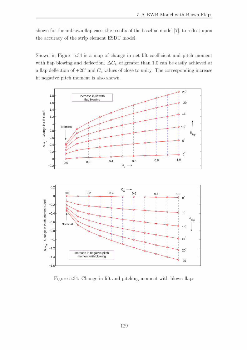
5 A BWB Model with Blown Flaps
shown for the unblown flap case, the results of the baseline model [7], to reflect upon
the accuracy of the strip element ESDU model.
Shown in Figure 5.34 is a map of change in net lift coefficient and pitch moment
with flap blowing and deflection. ∆CL of greater than 1.0 can be easily achieved at
a flap deflection of +20◦ and Cu values of close to unity. The corresponding increase
in negative pitch moment is also shown.
−0.2
0
0.2
0.4
0.6
0.8
1
1.2
1.4
1.6
1.8
∆ C
L − C
hang
e in
Lift
Coe
ff.
Cu
0.0 0.2 0.4 0.6 0.8 1.0
Increase in lift withflap blowing
0°
5°
20°
25°
10°
δflap
15°
Nominal
−1.6
−1.4
−1.2
−1
−0.8
−0.6
−0.4
−0.2
0
0.2
∆ C
m −
Cha
nge
in P
itch
Mom
ent C
oeff
Cu
0.0 0.2 0.4 0.6 0.8
10°
δflap
15°
20°
Increase in negative pitchmoment with blowing
25°
5°
0°1.0
Nominal
Figure 5.34: Change in lift and pitching moment with blown flaps
129
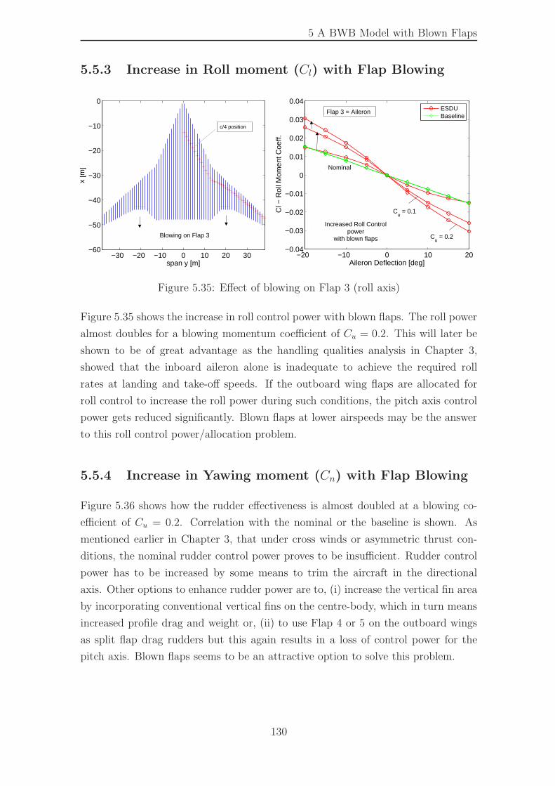
5 A BWB Model with Blown Flaps
5.5.3 Increase in Roll moment (Cl) with Flap Blowing
−30 −20 −10 0 10 20 30−60
−50
−40
−30
−20
−10
0
span y [m]
x [m
]
−20 −10 0 10 20−0.04
−0.03
−0.02
−0.01
0
0.01
0.02
0.03
0.04
Aileron Deflection [deg]
Cl −
Rol
l Mom
ent C
oeff.
ESDUBaseline
Increased Roll Controlpower
with blown flaps
Nominal
Cu = 0.1
Cu = 0.2Blowing on Flap 3
Flap 3 = Aileron
c/4 position
Figure 5.35: Effect of blowing on Flap 3 (roll axis)
Figure 5.35 shows the increase in roll control power with blown flaps. The roll power
almost doubles for a blowing momentum coefficient of Cu = 0.2. This will later be
shown to be of great advantage as the handling qualities analysis in Chapter 3,
showed that the inboard aileron alone is inadequate to achieve the required roll
rates at landing and take-off speeds. If the outboard wing flaps are allocated for
roll control to increase the roll power during such conditions, the pitch axis control
power gets reduced significantly. Blown flaps at lower airspeeds may be the answer
to this roll control power/allocation problem.
5.5.4 Increase in Yawing moment (Cn) with Flap Blowing
Figure 5.36 shows how the rudder effectiveness is almost doubled at a blowing co-
efficient of Cu = 0.2. Correlation with the nominal or the baseline is shown. As
mentioned earlier in Chapter 3, that under cross winds or asymmetric thrust con-
ditions, the nominal rudder control power proves to be insufficient. Rudder control
power has to be increased by some means to trim the aircraft in the directional
axis. Other options to enhance rudder power are to, (i) increase the vertical fin area
by incorporating conventional vertical fins on the centre-body, which in turn means
increased profile drag and weight or, (ii) to use Flap 4 or 5 on the outboard wings
as split flap drag rudders but this again results in a loss of control power for the
pitch axis. Blown flaps seems to be an attractive option to solve this problem.
130
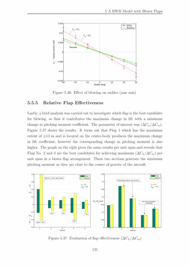
5 A BWB Model with Blown Flaps
−30 −20 −10 0 10 20 30−0.015
−0.01
−0.005
0
0.005
0.01
0.015
Rudder [deg]
Cn −
Yaw
ing
mom
ent c
oeff
ESDUBaseline
Cu = 0.1
Cu = 0.2
Nominal
Figure 5.36: Effect of blowing on rudder (yaw axis)
5.5.5 Relative Flap Effectiveness
Lastly, a brief analysis was carried out to investigate which flap is the best candidate
for blowing, so that it contributes the maximum change in lift with a minimum
change in pitching moment coefficient. The parameter of interest was (∆CL/∆Cm).
Figure 5.37 shows the results. It turns out that Flap 1 which has the maximum
extent of ±13 m and is located on the centre-body produces the maximum change
in lift coefficient, however the corresponding change in pitching moment is also
higher. The graph on the right gives the same results per unit span and reveals that
Flap No. 2 and 3 are the best candidates for achieving maximum (∆CL/∆Cm) per
unit span in a blown flap arrangement. These two sections generate the minimum
pitching moment as they are close to the center of gravity of the aircraft.
1 2 3 4 5−0.3
−0.2
−0.1
0
0.1
0.2
0.3
0.4
Flap No
PlainBlown
1 2 3 4 50
0.05
0.1
0.15
0.2
0.25
0.3
0.35
Flap No
PlainBlown
∆ CL
∆ Cm
∆CL/ ∆C
m/span
These flaps produce max ∆CL/∆C
m
Not Good candidatesfor blowing
Cu = 0.1
δflap
= +20°C
u = 0.1
δflap
= +20°
Max ∆ CL due to span extent
10m
5m
span = 13m
4m 6m
Figure 5.37: Evaluation of flap effectiveness (∆CL/∆Cm)
131
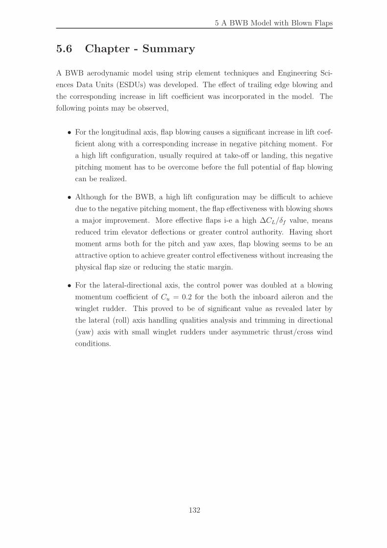
5 A BWB Model with Blown Flaps
5.6 Chapter - Summary
A BWB aerodynamic model using strip element techniques and Engineering Sci-
ences Data Units (ESDUs) was developed. The effect of trailing edge blowing and
the corresponding increase in lift coefficient was incorporated in the model. The
following points may be observed,
• For the longitudinal axis, flap blowing causes a significant increase in lift coef-
ficient along with a corresponding increase in negative pitching moment. For
a high lift configuration, usually required at take-off or landing, this negative
pitching moment has to be overcome before the full potential of flap blowing
can be realized.
• Although for the BWB, a high lift configuration may be difficult to achieve
due to the negative pitching moment, the flap effectiveness with blowing shows
a major improvement. More effective flaps i-e a high ∆CL/δf value, means
reduced trim elevator deflections or greater control authority. Having short
moment arms both for the pitch and yaw axes, flap blowing seems to be an
attractive option to achieve greater control effectiveness without increasing the
physical flap size or reducing the static margin.
• For the lateral-directional axis, the control power was doubled at a blowing
momentum coefficient of Cu = 0.2 for the both the inboard aileron and the
winglet rudder. This proved to be of significant value as revealed later by
the lateral (roll) axis handling qualities analysis and trimming in directional
(yaw) axis with small winglet rudders under asymmetric thrust/cross wind
conditions.
132

Chapter 6
Propulsion and Controls
Integration
In the preceding chapters, a BWB model with blown flaps and a three spool turbofan
engine model were developed. In this chapter some results of the integration of these
two models are presented. The following aspects will be covered,
• Allowable bleed and achievable lift/pitch moment
The questions to be answered here are, (i) what is the most appropriate loca-
tion for bleed off-take, LPC, IPC, HPC or directly from the main exhaust, (ii)
what are the optimum bleed slot heights, (iii) how much bleed can be taken
from a particular arrangement and how much blowing coefficient (Cu) can be
achieved and (iv) what are the increments in lift and pitching moment.
• Controls performance with blowing
A particular value of blowing momentum coefficient would be assumed and
dynamic responses in roll, pitch and yaw axis would be presented. Results
would indicate handling qualities improvements if any.
• Controls performance with thrust vectoring
A comparison of longitudinal control responses for pure aerodynamic flight
control (AFC), thrust vector control (TVC), and AFC + TVC would be made.
• Trim results with flap blowing and thrust vectoring
Trim results with flap blowing and TVC would be presented at different air-
speeds.
133
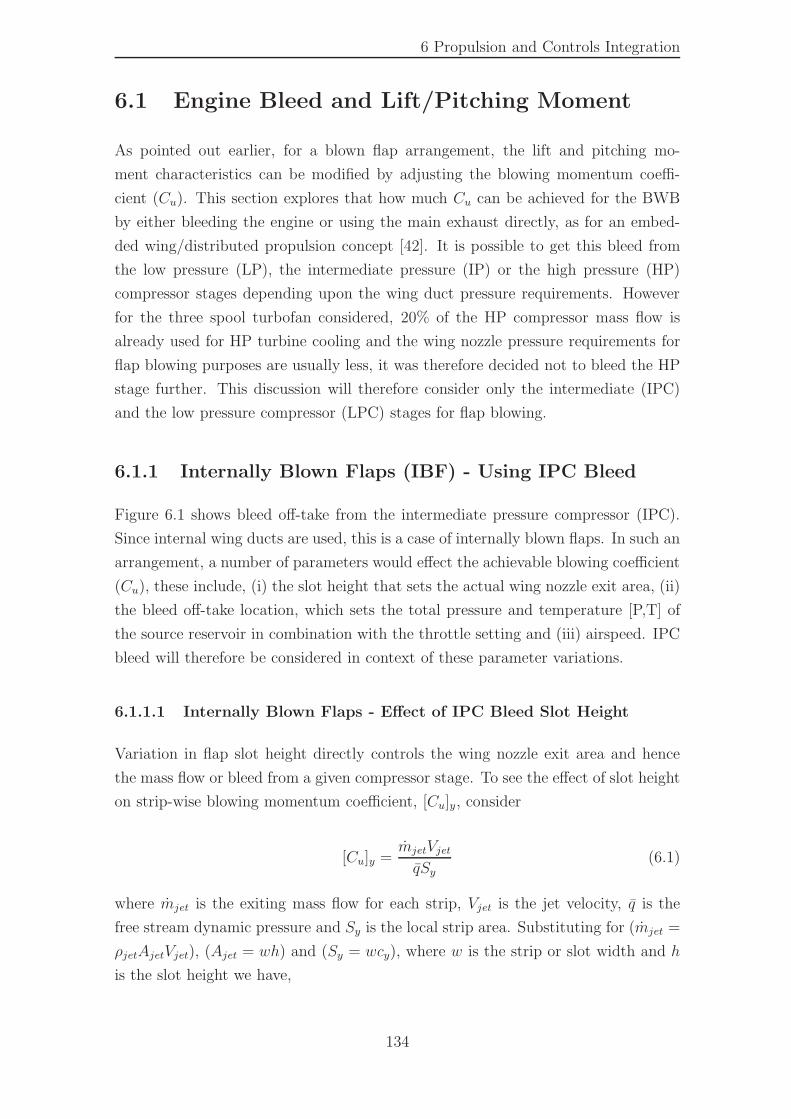
6 Propulsion and Controls Integration
6.1 Engine Bleed and Lift/Pitching Moment
As pointed out earlier, for a blown flap arrangement, the lift and pitching mo-
ment characteristics can be modified by adjusting the blowing momentum coeffi-
cient (Cu). This section explores that how much Cu can be achieved for the BWB
by either bleeding the engine or using the main exhaust directly, as for an embed-
ded wing/distributed propulsion concept [42]. It is possible to get this bleed from
the low pressure (LP), the intermediate pressure (IP) or the high pressure (HP)
compressor stages depending upon the wing duct pressure requirements. However
for the three spool turbofan considered, 20% of the HP compressor mass flow is
already used for HP turbine cooling and the wing nozzle pressure requirements for
flap blowing purposes are usually less, it was therefore decided not to bleed the HP
stage further. This discussion will therefore consider only the intermediate (IPC)
and the low pressure compressor (LPC) stages for flap blowing.
6.1.1 Internally Blown Flaps (IBF) - Using IPC Bleed
Figure 6.1 shows bleed off-take from the intermediate pressure compressor (IPC).
Since internal wing ducts are used, this is a case of internally blown flaps. In such an
arrangement, a number of parameters would effect the achievable blowing coefficient
(Cu), these include, (i) the slot height that sets the actual wing nozzle exit area, (ii)
the bleed off-take location, which sets the total pressure and temperature [P,T] of
the source reservoir in combination with the throttle setting and (iii) airspeed. IPC
bleed will therefore be considered in context of these parameter variations.
6.1.1.1 Internally Blown Flaps - Effect of IPC Bleed Slot Height
Variation in flap slot height directly controls the wing nozzle exit area and hence
the mass flow or bleed from a given compressor stage. To see the effect of slot height
on strip-wise blowing momentum coefficient, [Cu]y, consider
[Cu]y =mjetVjetqSy
(6.1)
where mjet is the exiting mass flow for each strip, Vjet is the jet velocity, q is the
free stream dynamic pressure and Sy is the local strip area. Substituting for (mjet =
ρjetAjetVjet), (Ajet = wh) and (Sy = wcy), where w is the strip or slot width and h
is the slot height we have,
134
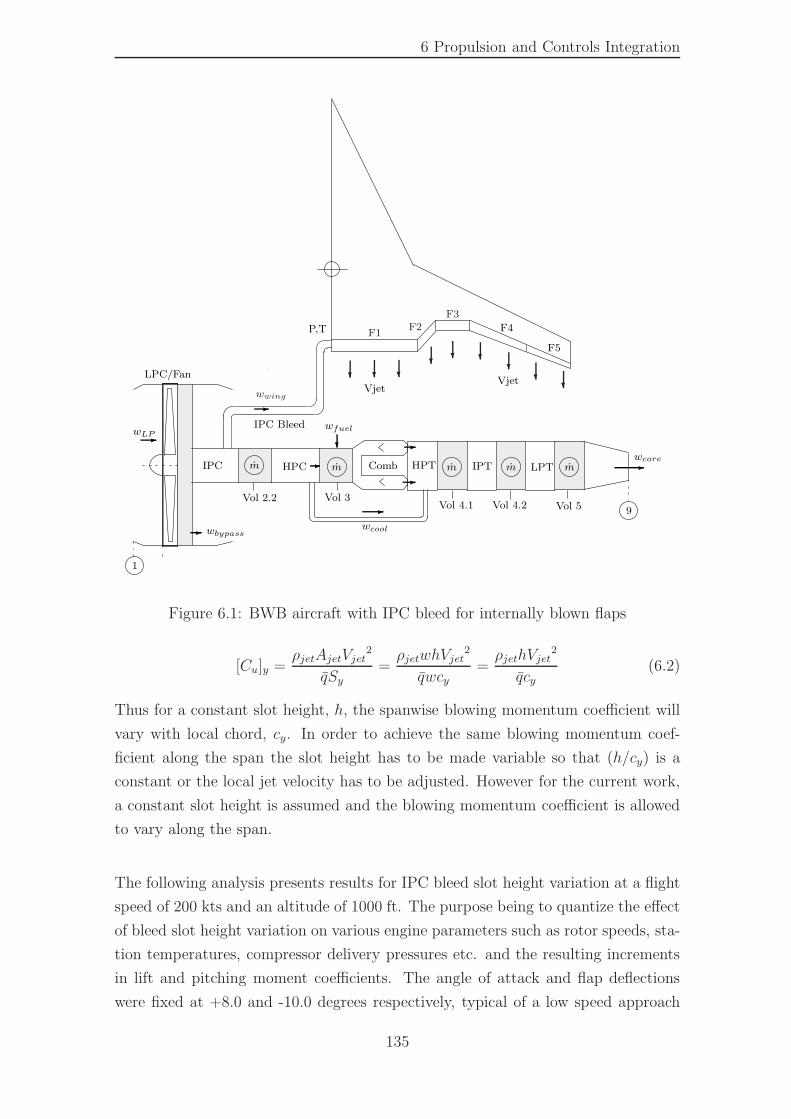
6 Propulsion and Controls Integration
?
wwing
?? ? ?
??
??
F1F2
F3
-
LPC/Fan
- wbypass
LPT
-wLP
F4
-
HPTwcore-IPT
?
Comb
-
HPCIPC
wcool
Vol 3Vol 2.2Vol 4.1
wfuel
-
-
Vol 4.2 Vol 5
F5
9
1
Vjet
P,T
IPC Bleed
m m m m m
Vjet
Figure 6.1: BWB aircraft with IPC bleed for internally blown flaps
[Cu]y =ρjetAjetVjet
2
qSy=ρjetwhVjet
2
qwcy=ρjethVjet
2
qcy(6.2)
Thus for a constant slot height, h, the spanwise blowing momentum coefficient will
vary with local chord, cy. In order to achieve the same blowing momentum coef-
ficient along the span the slot height has to be made variable so that (h/cy) is a
constant or the local jet velocity has to be adjusted. However for the current work,
a constant slot height is assumed and the blowing momentum coefficient is allowed
to vary along the span.
The following analysis presents results for IPC bleed slot height variation at a flight
speed of 200 kts and an altitude of 1000 ft. The purpose being to quantize the effect
of bleed slot height variation on various engine parameters such as rotor speeds, sta-
tion temperatures, compressor delivery pressures etc. and the resulting increments
in lift and pitching moment coefficients. The angle of attack and flap deflections
were fixed at +8.0 and -10.0 degrees respectively, typical of a low speed approach
135
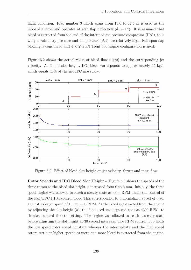
6 Propulsion and Controls Integration
flight condition. Flap number 3 which spans from 13.0 to 17.5 m is used as the
inboard aileron and operates at zero flap deflection (δa = 0◦). It is assumed that
bleed is extracted from the end of the intermediate pressure compressor (IPC), thus
wing nozzle entry pressure and temperature [P,T] are relatively high. Full span flap
blowing is considered and 4 × 275 kN Trent 500 engine configuration is used.
Figure 6.2 shows the actual value of bleed flow (kg/s) and the corresponding jet
velocity. At 3 mm slot height, IPC bleed corresponds to approximately 45 kg/s
which equals 40% of the net IPC mass flow.
0 30 60 90 1200
20
40
60
IPC
Ble
ed (
kg/s
)
0 30 60 90 120100
150
200
250
Net
thru
st (
kN)
0 30 60 90 120350
400
450
Jet V
eloc
ity (
m/s
)
slot = 0 mm slot = 1 mm slot = 2 mm slot = 3 mm
A
B
C
D
≈ 45.4 kg/s
≈ 39% IPCMass flow
Net Thrust almostconstant
at 4300 RPM
High Jet Velocitydue to high IPC exit
[P,T]
Time (secs)
Figure 6.2: Effect of bleed slot height on jet velocity, thrust and mass flow
Rotor Speeds and IPC Bleed Slot Height - Figure 6.3 shows the speeds of the
three rotors as the bleed slot height is increased from 0 to 3 mm. Initially, the three
spool engine was allowed to reach a steady state at 4300 RPM under the control of
the Fan/LPC RPM control loop. This corresponded to a normalized speed of 0.86,
against a design speed of 1.0 at 5000 RPM. As the bleed is extracted from the engine
by adjusting the slot height (h), the fan speed was kept constant at 4300 RPM, to
simulate a fixed throttle setting. The engine was allowed to reach a steady state
before adjusting the slot height at 30 second intervals. The RPM control loop holds
the low speed rotor speed constant whereas the intermediate and the high speed
rotors settle at higher speeds as more and more bleed is extracted from the engine.
136
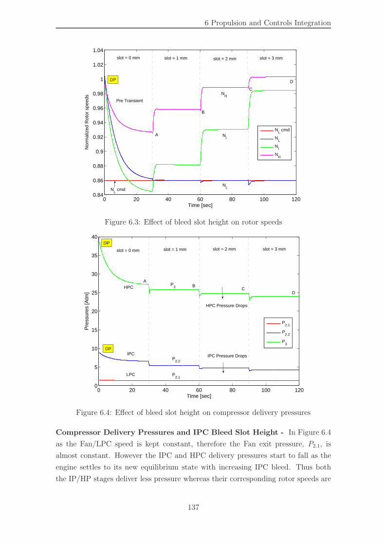
6 Propulsion and Controls Integration
0 20 40 60 80 100 1200.84
0.86
0.88
0.9
0.92
0.94
0.96
0.98
1
1.02
1.04
Time [sec]
Nor
mal
ized
Rot
or s
peed
s
NL cmd
NL
NI
NH
DP
A
B
C
D
slot = 0 mm slot = 1 mm slot = 2 mm slot = 3 mm
Pre Transient
NL
NI
NH
NL cmd
Figure 6.3: Effect of bleed slot height on rotor speeds
0 20 40 60 80 100 1200
5
10
15
20
25
30
35
40
Time [sec]
Pre
ssur
es [A
tm]
P2.1
P2.2
P3
P2.1
P3
P2.2
AB
CD
slot = 1 mmslot = 0 mm slot = 3 mmslot = 2 mm
LPC
DP
IPC Pressure Drops
HPC
HPC Pressure Drops
DP
IPC
Figure 6.4: Effect of bleed slot height on compressor delivery pressures
Compressor Delivery Pressures and IPC Bleed Slot Height - In Figure 6.4
as the Fan/LPC speed is kept constant, therefore the Fan exit pressure, P2.1, is
almost constant. However the IPC and HPC delivery pressures start to fall as the
engine settles to its new equilibrium state with increasing IPC bleed. Thus both
the IP/HP stages deliver less pressure whereas their corresponding rotor speeds are
137
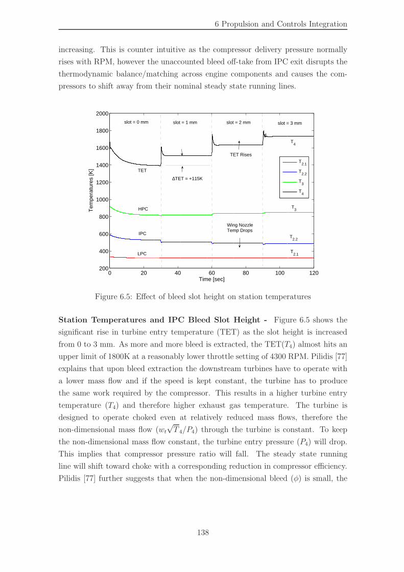
6 Propulsion and Controls Integration
increasing. This is counter intuitive as the compressor delivery pressure normally
rises with RPM, however the unaccounted bleed off-take from IPC exit disrupts the
thermodynamic balance/matching across engine components and causes the com-
pressors to shift away from their nominal steady state running lines.
0 20 40 60 80 100 120200
400
600
800
1000
1200
1400
1600
1800
2000
Time [sec]
Tem
pera
ture
s [K
]
T2.1
T2.2
T3
T4
slot = 0 mm slot = 1 mm slot = 2 mm slot = 3 mm
HPC
IPC
LPC
TET
∆TET = +115K
TET Rises
Wing NozzleTemp Drops
T4
T3
T2.2
T2.1
Figure 6.5: Effect of bleed slot height on station temperatures
Station Temperatures and IPC Bleed Slot Height - Figure 6.5 shows the
significant rise in turbine entry temperature (TET) as the slot height is increased
from 0 to 3 mm. As more and more bleed is extracted, the TET(T4) almost hits an
upper limit of 1800K at a reasonably lower throttle setting of 4300 RPM. Pilidis [77]
explains that upon bleed extraction the downstream turbines have to operate with
a lower mass flow and if the speed is kept constant, the turbine has to produce
the same work required by the compressor. This results in a higher turbine entry
temperature (T4) and therefore higher exhaust gas temperature. The turbine is
designed to operate choked even at relatively reduced mass flows, therefore the
non-dimensional mass flow (wt√T 4/P4) through the turbine is constant. To keep
the non-dimensional mass flow constant, the turbine entry pressure (P4) will drop.
This implies that compressor pressure ratio will fall. The steady state running
line will shift toward choke with a corresponding reduction in compressor efficiency.
Pilidis [77] further suggests that when the non-dimensional bleed (φ) is small, the
138
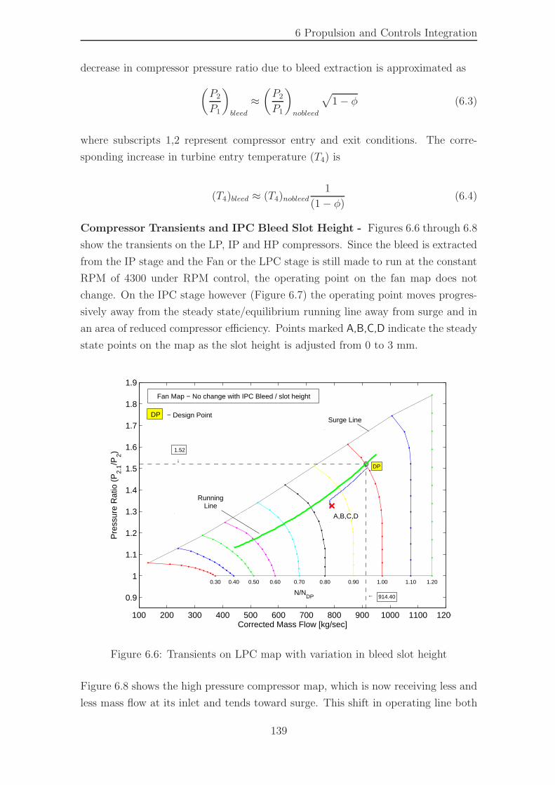
6 Propulsion and Controls Integration
decrease in compressor pressure ratio due to bleed extraction is approximated as
(
P2
P1
)
bleed
≈(
P2
P1
)
nobleed
√
1 − φ (6.3)
where subscripts 1,2 represent compressor entry and exit conditions. The corre-
sponding increase in turbine entry temperature (T4) is
(T4)bleed ≈ (T4)nobleed1
(1 − φ)(6.4)
Compressor Transients and IPC Bleed Slot Height - Figures 6.6 through 6.8
show the transients on the LP, IP and HP compressors. Since the bleed is extracted
from the IP stage and the Fan or the LPC stage is still made to run at the constant
RPM of 4300 under RPM control, the operating point on the fan map does not
change. On the IPC stage however (Figure 6.7) the operating point moves progres-
sively away from the steady state/equilibrium running line away from surge and in
an area of reduced compressor efficiency. Points marked A,B,C,D indicate the steady
state points on the map as the slot height is adjusted from 0 to 3 mm.
100 200 300 400 500 600 700 800 900 1000 1100 1200
0.9
1
1.1
1.2
1.3
1.4
1.5
1.6
1.7
1.8
1.9
0.30 0.40 0.50 0.60 0.70 0.80 0.90 1.00 1.10 1.20
Corrected Mass Flow [kg/sec]
Pre
ssur
e R
atio
(P
2.1/P
2) 1.52
↓
← 914.40
DP
A,B,C,D
Surge Line
RunningLine
Fan Map − No change with IPC Bleed / slot height
N/NDP
DP − Design Point
Figure 6.6: Transients on LPC map with variation in bleed slot height
Figure 6.8 shows the high pressure compressor map, which is now receiving less and
less mass flow at its inlet and tends toward surge. This shift in operating line both
139
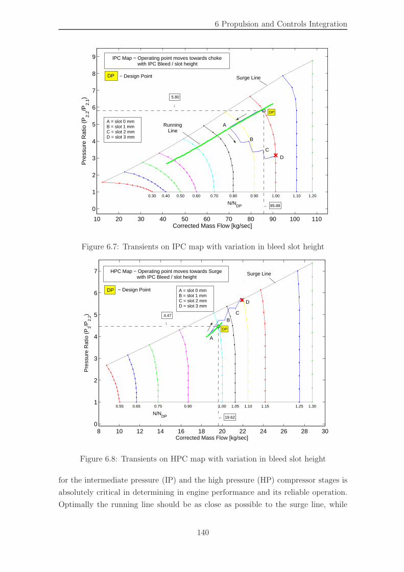
6 Propulsion and Controls Integration
10 20 30 40 50 60 70 80 90 100 110
0
1
2
3
4
5
6
7
8
9
0.30 0.40 0.50 0.60 0.70 0.80 0.90 1.00 1.10 1.20
Corrected Mass Flow [kg/sec]
Pre
ssur
e R
atio
(P
2.2/P
2.1) 5.80
↓
← 85.88
DP
Surge Line
RunningLine
IPC Map − Operating point moves towards choke with IPC Bleed / slot height
B
A
C
D
A = slot 0 mmB = slot 1 mmC = slot 2 mmD = slot 3 mm
DP − Design Point
N/NDP
Figure 6.7: Transients on IPC map with variation in bleed slot height
8 10 12 14 16 18 20 22 24 26 28 300
1
2
3
4
5
6
7
0.55 0.65 0.75 0.90 1.00 1.05 1.10 1.15 1.25 1.30
Corrected Mass Flow [kg/sec]
Pre
ssur
e R
atio
(P
3/P2.
2) 4.47
↓
← 19.62
DP
A
BC
D
Surge Line
A = slot 0 mmB = slot 1 mmC = slot 2 mmD = slot 3 mm
HPC Map − Operating point moves towards Surge with IPC Bleed / slot height
DP − Design Point
N/NDP
Figure 6.8: Transients on HPC map with variation in bleed slot height
for the intermediate pressure (IP) and the high pressure (HP) compressor stages is
absolutely critical in determining in engine performance and its reliable operation.
Optimally the running line should be as close as possible to the surge line, while
140
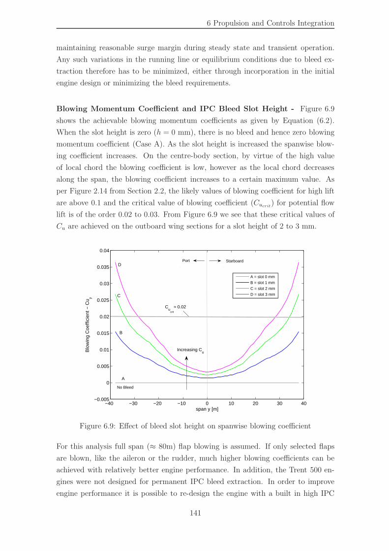
6 Propulsion and Controls Integration
maintaining reasonable surge margin during steady state and transient operation.
Any such variations in the running line or equilibrium conditions due to bleed ex-
traction therefore has to be minimized, either through incorporation in the initial
engine design or minimizing the bleed requirements.
Blowing Momentum Coefficient and IPC Bleed Slot Height - Figure 6.9
shows the achievable blowing momentum coefficients as given by Equation (6.2).
When the slot height is zero (h = 0 mm), there is no bleed and hence zero blowing
momentum coefficient (Case A). As the slot height is increased the spanwise blow-
ing coefficient increases. On the centre-body section, by virtue of the high value
of local chord the blowing coefficient is low, however as the local chord decreases
along the span, the blowing coefficient increases to a certain maximum value. As
per Figure 2.14 from Section 2.2, the likely values of blowing coefficient for high lift
are above 0.1 and the critical value of blowing coefficient (Cucrit) for potential flow
lift is of the order 0.02 to 0.03. From Figure 6.9 we see that these critical values of
Cu are achieved on the outboard wing sections for a slot height of 2 to 3 mm.
−40 −30 −20 −10 0 10 20 30 40−0.005
0
0.005
0.01
0.015
0.02
0.025
0.03
0.035
0.04
span y [m]
Blo
win
g C
oeffi
cien
t − C
u y
A = slot 0 mm
B = slot 1 mm
C = slot 2 mm
D = slot 3 mm
StarboardPort
A
B
C
D
Increasing Cu
No Bleed
Cu
crit
≈ 0.02
Figure 6.9: Effect of bleed slot height on spanwise blowing coefficient
For this analysis full span (≈ 80m) flap blowing is assumed. If only selected flaps
are blown, like the aileron or the rudder, much higher blowing coefficients can be
achieved with relatively better engine performance. In addition, the Trent 500 en-
gines were not designed for permanent IPC bleed extraction. In order to improve
engine performance it is possible to re-design the engine with a built in high IPC
141
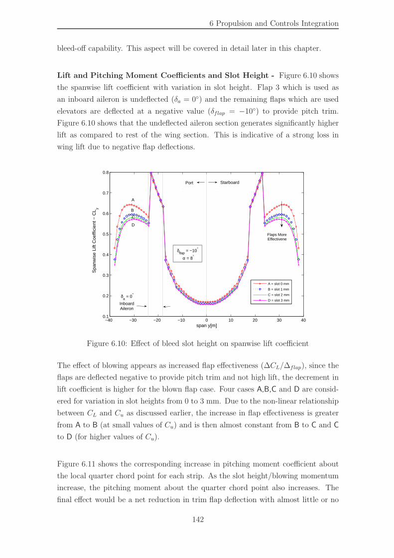
6 Propulsion and Controls Integration
bleed-off capability. This aspect will be covered in detail later in this chapter.
Lift and Pitching Moment Coefficients and Slot Height - Figure 6.10 shows
the spanwise lift coefficient with variation in slot height. Flap 3 which is used as
an inboard aileron is undeflected (δa = 0◦) and the remaining flaps which are used
elevators are deflected at a negative value (δflap = −10◦) to provide pitch trim.
Figure 6.10 shows that the undeflected aileron section generates significantly higher
lift as compared to rest of the wing section. This is indicative of a strong loss in
wing lift due to negative flap deflections.
−40 −30 −20 −10 0 10 20 30 400.1
0.2
0.3
0.4
0.5
0.6
0.7
0.8
span y[m]
Spa
nwis
e Li
ft C
oeffi
cien
t − C
L y
A = slot 0 mm
B = slot 1 mm
C = slot 2 mm
D = slot 3 mm
Port Starboard
A
B
D
C
InboardAileron
δa = 0°
Flaps MoreEffectivene
α = 8°δ
flap = −10°
Figure 6.10: Effect of bleed slot height on spanwise lift coefficient
The effect of blowing appears as increased flap effectiveness (∆CL/∆flap), since the
flaps are deflected negative to provide pitch trim and not high lift, the decrement in
lift coefficient is higher for the blown flap case. Four cases A,B,C and D are consid-
ered for variation in slot heights from 0 to 3 mm. Due to the non-linear relationship
between CL and Cu as discussed earlier, the increase in flap effectiveness is greater
from A to B (at small values of Cu) and is then almost constant from B to C and C
to D (for higher values of Cu).
Figure 6.11 shows the corresponding increase in pitching moment coefficient about
the local quarter chord point for each strip. As the slot height/blowing momentum
increase, the pitching moment about the quarter chord point also increases. The
final effect would be a net reduction in trim flap deflection with almost little or no
142
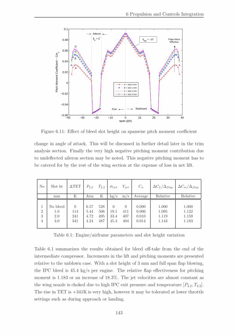
6 Propulsion and Controls Integration
−40 −30 −20 −10 0 10 20 30 40−0.06
−0.04
−0.02
0
0.02
0.04
0.06
0.08
0.1
span y[m]
Pitc
h M
omen
t Coe
ffici
ent −
Cm
y
A = slot 0 mm
B = slot 1 mm
C = slot 2 mm
D = slot 3 mm
A
B
C
D
StarboardPort
Aileron
δa = 0°
Flaps MoreEffective
δflap
= −10°
Figure 6.11: Effect of bleed slot height on spanwise pitch moment coefficient
change in angle of attack. This will be discussed in further detail later in the trim
analysis section. Finally the very high negative pitching moment contribution due
to undeflected aileron section may be noted. This negative pitching moment has to
be catered for by the rest of the wing section at the expense of loss in net lift.
No Slot ht ∆TET P2.2 T2.2 mjet Vjet Cu ∆CL/∆flap ∆Cm/∆flap
mm K Atm K kg/s m/s Average Relative Relative
1 No bleed 0 6.57 528 0 0 0.000 1.000 1.0002 1.0 114 5.44 506 19.1 411 0.006 1.095 1.1223 2.0 241 4.72 495 33.4 407 0.010 1.119 1.1594 3.0 341 4.24 487 45.4 404 0.014 1.143 1.183
Table 6.1: Engine/airframe parameters and slot height variation
Table 6.1 summarizes the results obtained for bleed off-take from the end of the
intermediate compressor. Increments in the lift and pitching moments are presented
relative to the unblown case. With a slot height of 3 mm and full span flap blowing,
the IPC bleed is 45.4 kg/s per engine. The relative flap effectiveness for pitching
moment is 1.183 or an increase of 18.3%. The jet velocities are almost constant as
the wing nozzle is choked due to high IPC exit pressure and temperature [P2.2, T2.2].
The rise in TET is +341K is very high, however it may be tolerated at lower throttle
settings such as during approach or landing.
143
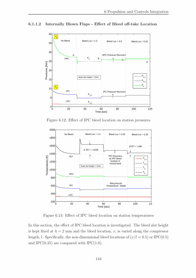
6 Propulsion and Controls Integration
6.1.1.2 Internally Blown Flaps - Effect of Bleed off-take Location
0 20 40 60 80 100 1200
5
10
15
20
25
30
35
40
Time [sec]
Pre
ssur
es [A
tm]
P2.1
P2.2
P3
P2.1
P3
P2.2
A
BC
D
Bleed Loc = 1.0No Bleed Bleed Loc = 0.25Bleed Loc = 0.5
LPC
X0
IPC Pressure Recovers
HPC
HPC Pressure Recovers
X0
IPC
fixed slot height = 2mm
Figure 6.12: Effect of IPC bleed location on station pressures
0 20 40 60 80 100 120200
400
600
800
1000
1200
1400
1600
1800
2000
Time [sec]
Tem
pera
ture
s [K
]
T2.1
T2.2
T3
T4
No Bleed Bleed Loc = 1.0 Bleed Loc = 0.50 Bleed Loc = 0.25
HPC
IPC
LPC
TET
∆TET = +28K
TET Recoversas IPC bleed
location ismoved back
Wing NozzleTemperature Stable
fixed slot height = 2mm
∆ TET = +243K
Figure 6.13: Effect of IPC bleed location on station temperatures
In this section, the effect of IPC bleed location is investigated. The bleed slot height
is kept fixed at h = 2 mm and the bleed location, x, is varied along the compressor
length, l. Specifically, the non-dimensional bleed locations of (x/l = 0.5) or IPC(0.5)
and IPC(0.25) are compared with IPC(1.0).
144
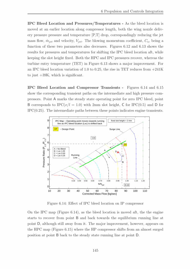
6 Propulsion and Controls Integration
IPC Bleed Location and Pressures/Temperatures - As the bleed location is
moved at an earlier location along compressor length, both the wing nozzle deliv-
ery pressure pressure and temperature [P,T] drop, correspondingly reducing the jet
mass flow, mjet and velocity, Vjet. The blowing momentum coefficient, Cu, being a
function of these two parameters also decreases. Figures 6.12 and 6.13 shows the
results for pressures and temperatures for shifting the IPC bleed location aft, while
keeping the slot height fixed. Both the HPC and IPC pressures recover, whereas the
turbine entry temperature (TET) in Figure 6.13 shows a major improvement. For
an IPC bleed location variation of 1.0 to 0.25, the rise in TET reduces from +241K
to just +39K, which is significant.
IPC Bleed Location and Compressor Transients - Figures 6.14 and 6.15
show the corresponding transient paths on the intermediate and high pressure com-
pressors. Point A marks the steady state operating point for zero IPC bleed, point
B corresponds to IPC(x/l = 1.0) with 2mm slot height, C for IPC(0.5) and D for
IPC(0.25). The intermediate paths between these points indicates engine transients.
10 20 30 40 50 60 70 80 90 100 110
0
1
2
3
4
5
6
7
8
9
0.30 0.40 0.50 0.60 0.70 0.80 0.90 1.00 1.10 1.20
Corrected Mass Flow [kg/sec]
Pre
ssur
e R
atio
(P
2.2/P
2.1) 5.80
↓
← 85.88
DP
Surge Line
RunningLine
IPC Map − Operating point moves towards runningline as IPC bleed location (Loc) is shifted back
B
A
C
DA = No BleedB = Loc 1.00C = Loc 0.50D = Loc 0.25
fixed slot height = 2 mm
DP − Design Point
N/NDP
Figure 6.14: Effect of IPC bleed location on IP compressor
On the IPC map (Figure 6.14), as the bleed location is moved aft, the the engine
starts to recover from point B and back towards the equilibrium running line at
point D, although still away from it. The major improvement, however, appears on
the HPC map (Figure 6.15) where the HP compressor shifts from an almost surged
position at point B back to the steady state running line at point D.
145
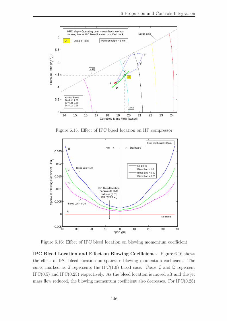
6 Propulsion and Controls Integration
14 15 16 17 18 19 20 21 22 23 243
3.5
4
4.5
5
5.5
6
Corrected Mass Flow [kg/sec]
Pre
ssur
e R
atio
(P
3/P2.
2)
4.47
↓
← 19.62
DP
A
B
C
D
Surge Line
A = No BleedB = Loc 1.00C = Loc 0.50D = Loc 0.25
HPC Map − Operating point moves back towradsrunning line as IPC bleed location is shifted back
fixed slot height = 2 mmDP − Design Point
Figure 6.15: Effect of IPC bleed location on HP compressor
−40 −30 −20 −10 0 10 20 30 40−0.005
0
0.005
0.01
0.015
0.02
0.025
span y[m]
Spa
nwis
e B
low
ing
Coe
ffici
ent −
Cu y
No Bleed
Bleed Loc = 1.0
Bleed Loc = 0.50
Bleed Loc = 0.25
StarboardPort
A
C
B
D
fixed slot height = 2mm
No bleed
Bleed Loc = 1.0
IPC Bleed locationbackwards shiftreduces [P,T]and hence C
u
Bleed Loc = 0.25
Figure 6.16: Effect of IPC bleed location on blowing momentum coefficient
IPC Bleed Location and Effect on Blowing Coefficient - Figure 6.16 shows
the effect of IPC bleed location on spanwise blowing momentum coefficient. The
curve marked as B represents the IPC(1.0) bleed case. Cases C and D represent
IPC(0.5) and IPC(0.25) respectively. As the bleed location is moved aft and the jet
mass flow reduced, the blowing momentum coefficient also decreases. For IPC(0.25)
146
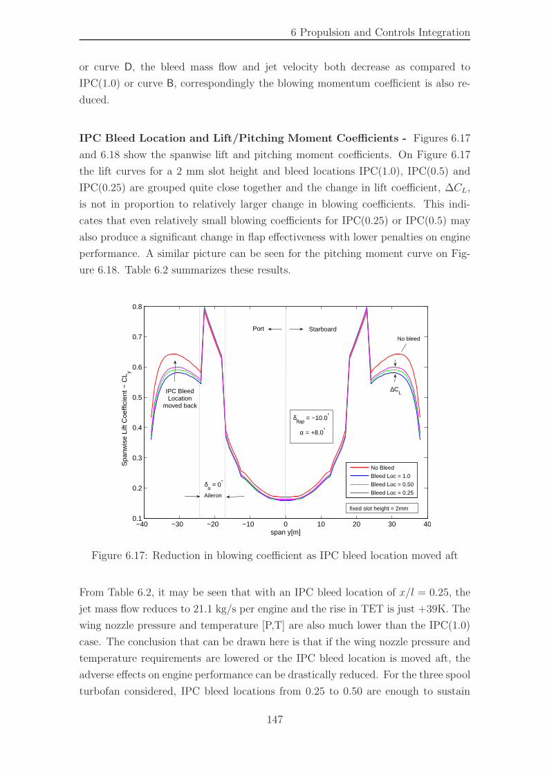
6 Propulsion and Controls Integration
or curve D, the bleed mass flow and jet velocity both decrease as compared to
IPC(1.0) or curve B, correspondingly the blowing momentum coefficient is also re-
duced.
IPC Bleed Location and Lift/Pitching Moment Coefficients - Figures 6.17
and 6.18 show the spanwise lift and pitching moment coefficients. On Figure 6.17
the lift curves for a 2 mm slot height and bleed locations IPC(1.0), IPC(0.5) and
IPC(0.25) are grouped quite close together and the change in lift coefficient, ∆CL,
is not in proportion to relatively larger change in blowing coefficients. This indi-
cates that even relatively small blowing coefficients for IPC(0.25) or IPC(0.5) may
also produce a significant change in flap effectiveness with lower penalties on engine
performance. A similar picture can be seen for the pitching moment curve on Fig-
ure 6.18. Table 6.2 summarizes these results.
−40 −30 −20 −10 0 10 20 30 400.1
0.2
0.3
0.4
0.5
0.6
0.7
0.8
span y[m]
Spa
nwis
e Li
ft C
oeffi
cien
t − C
L y
No Bleed
Bleed Loc = 1.0
Bleed Loc = 0.50
Bleed Loc = 0.25
StarboardPort
δa = 0°
Aileron
δflap
= −10.0°
α = +8.0°
IPC BleedLocation
moved back
fixed slot height = 2mm
No bleed
∆CL
Figure 6.17: Reduction in blowing coefficient as IPC bleed location moved aft
From Table 6.2, it may be seen that with an IPC bleed location of x/l = 0.25, the
jet mass flow reduces to 21.1 kg/s per engine and the rise in TET is just +39K. The
wing nozzle pressure and temperature [P,T] are also much lower than the IPC(1.0)
case. The conclusion that can be drawn here is that if the wing nozzle pressure and
temperature requirements are lowered or the IPC bleed location is moved aft, the
adverse effects on engine performance can be drastically reduced. For the three spool
turbofan considered, IPC bleed locations from 0.25 to 0.50 are enough to sustain
147
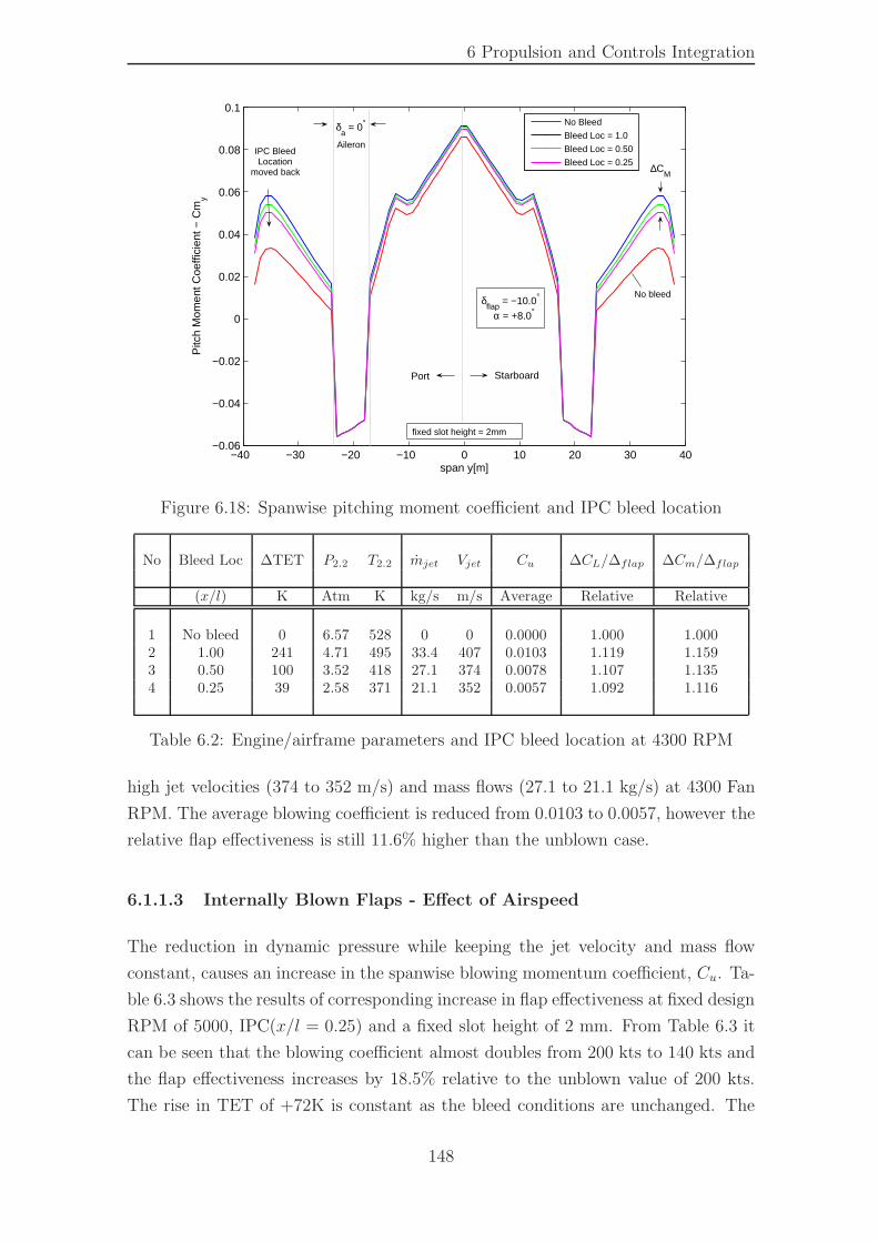
6 Propulsion and Controls Integration
−40 −30 −20 −10 0 10 20 30 40−0.06
−0.04
−0.02
0
0.02
0.04
0.06
0.08
0.1
span y[m]
Pitc
h M
omen
t Coe
ffici
ent −
Cm
y
No Bleed
Bleed Loc = 1.0
Bleed Loc = 0.50
Bleed Loc = 0.25
StarboardPort
No bleed
IPC BleedLocation
moved back
α = +8.0°δ
flap = −10.0°
fixed slot height = 2mm
δa = 0°
Aileron
∆CM
Figure 6.18: Spanwise pitching moment coefficient and IPC bleed location
No Bleed Loc ∆TET P2.2 T2.2 mjet Vjet Cu ∆CL/∆flap ∆Cm/∆flap
(x/l) K Atm K kg/s m/s Average Relative Relative
1 No bleed 0 6.57 528 0 0 0.0000 1.000 1.0002 1.00 241 4.71 495 33.4 407 0.0103 1.119 1.1593 0.50 100 3.52 418 27.1 374 0.0078 1.107 1.1354 0.25 39 2.58 371 21.1 352 0.0057 1.092 1.116
Table 6.2: Engine/airframe parameters and IPC bleed location at 4300 RPM
high jet velocities (374 to 352 m/s) and mass flows (27.1 to 21.1 kg/s) at 4300 Fan
RPM. The average blowing coefficient is reduced from 0.0103 to 0.0057, however the
relative flap effectiveness is still 11.6% higher than the unblown case.
6.1.1.3 Internally Blown Flaps - Effect of Airspeed
The reduction in dynamic pressure while keeping the jet velocity and mass flow
constant, causes an increase in the spanwise blowing momentum coefficient, Cu. Ta-
ble 6.3 shows the results of corresponding increase in flap effectiveness at fixed design
RPM of 5000, IPC(x/l = 0.25) and a fixed slot height of 2 mm. From Table 6.3 it
can be seen that the blowing coefficient almost doubles from 200 kts to 140 kts and
the flap effectiveness increases by 18.5% relative to the unblown value of 200 kts.
The rise in TET of +72K is constant as the bleed conditions are unchanged. The
148
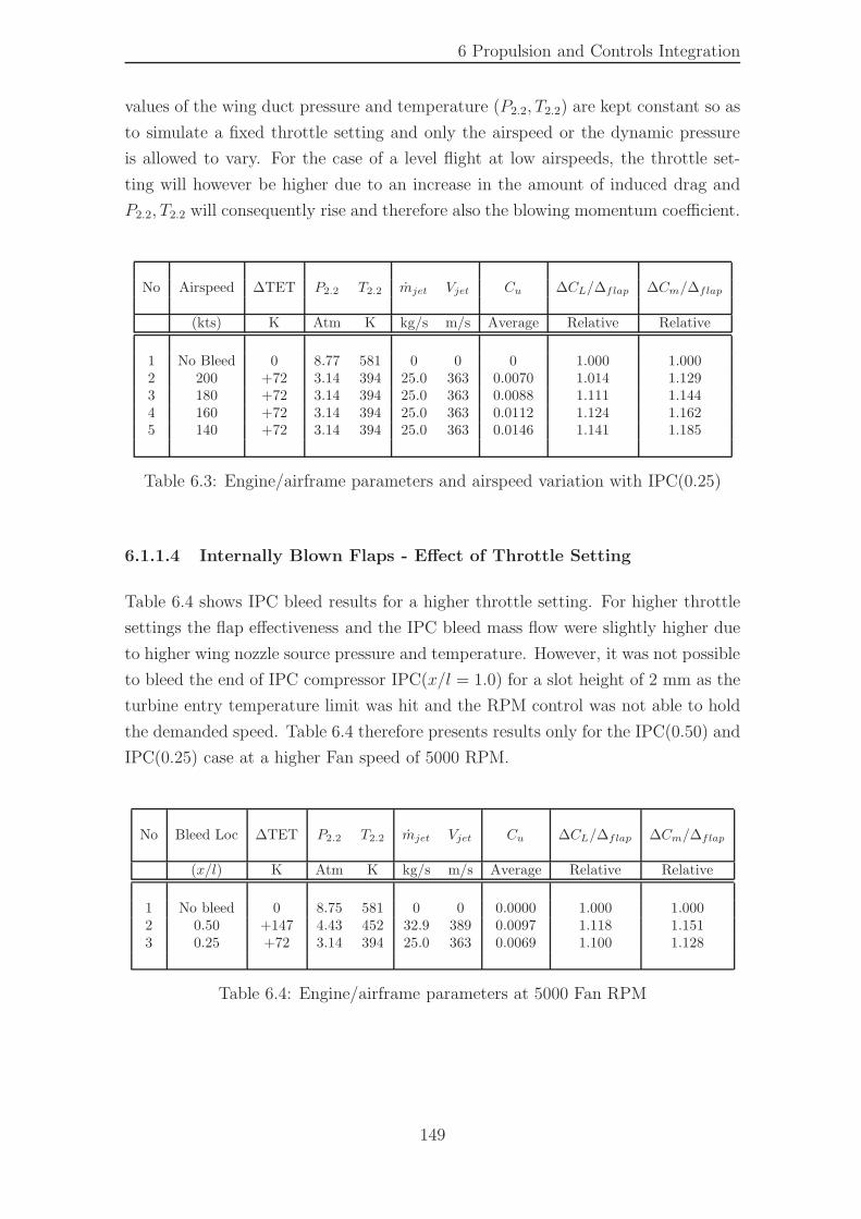
6 Propulsion and Controls Integration
values of the wing duct pressure and temperature (P2.2, T2.2) are kept constant so as
to simulate a fixed throttle setting and only the airspeed or the dynamic pressure
is allowed to vary. For the case of a level flight at low airspeeds, the throttle set-
ting will however be higher due to an increase in the amount of induced drag and
P2.2, T2.2 will consequently rise and therefore also the blowing momentum coefficient.
No Airspeed ∆TET P2.2 T2.2 mjet Vjet Cu ∆CL/∆flap ∆Cm/∆flap
(kts) K Atm K kg/s m/s Average Relative Relative
1 No Bleed 0 8.77 581 0 0 0 1.000 1.0002 200 +72 3.14 394 25.0 363 0.0070 1.014 1.1293 180 +72 3.14 394 25.0 363 0.0088 1.111 1.1444 160 +72 3.14 394 25.0 363 0.0112 1.124 1.1625 140 +72 3.14 394 25.0 363 0.0146 1.141 1.185
Table 6.3: Engine/airframe parameters and airspeed variation with IPC(0.25)
6.1.1.4 Internally Blown Flaps - Effect of Throttle Setting
Table 6.4 shows IPC bleed results for a higher throttle setting. For higher throttle
settings the flap effectiveness and the IPC bleed mass flow were slightly higher due
to higher wing nozzle source pressure and temperature. However, it was not possible
to bleed the end of IPC compressor IPC(x/l = 1.0) for a slot height of 2 mm as the
turbine entry temperature limit was hit and the RPM control was not able to hold
the demanded speed. Table 6.4 therefore presents results only for the IPC(0.50) and
IPC(0.25) case at a higher Fan speed of 5000 RPM.
No Bleed Loc ∆TET P2.2 T2.2 mjet Vjet Cu ∆CL/∆flap ∆Cm/∆flap
(x/l) K Atm K kg/s m/s Average Relative Relative
1 No bleed 0 8.75 581 0 0 0.0000 1.000 1.0002 0.50 +147 4.43 452 32.9 389 0.0097 1.118 1.1513 0.25 +72 3.14 394 25.0 363 0.0069 1.100 1.128
Table 6.4: Engine/airframe parameters at 5000 Fan RPM
149
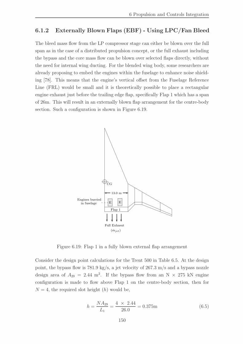
6 Propulsion and Controls Integration
6.1.2 Externally Blown Flaps (EBF) - Using LPC/Fan Bleed
The bleed mass flow from the LP compressor stage can either be blown over the full
span as in the case of a distributed propulsion concept, or the full exhaust including
the bypass and the core mass flow can be blown over selected flaps directly, without
the need for internal wing ducting. For the blended wing body, some researchers are
already proposing to embed the engines within the fuselage to enhance noise shield-
ing [78]. This means that the engine’s vertical offset from the Fuselage Reference
Line (FRL) would be small and it is theoretically possible to place a rectangular
engine exhaust just before the trailing edge flap, specifically Flap 1 which has a span
of 26m. This will result in an externally blown flap arrangement for the centre-body
section. Such a configuration is shown in Figure 6.19.
?
(mjet)
E
? ??
in fuselage
-
E
�
Full Exhasut
Engines burried
Flap 1
CG
13.0 m
Figure 6.19: Flap 1 in a fully blown external flap arrangement
Consider the design point calculations for the Trent 500 in Table 6.5. At the design
point, the bypass flow is 781.9 kg/s, a jet velocity of 267.3 m/s and a bypass nozzle
design area of A29 = 2.44 m2. If the bypass flow from an N × 275 kN engine
configuration is made to flow above Flap 1 on the centre-body section, then for
N = 4, the required slot height (h) would be,
h =NA29
L1
=4 × 2.44
26.0= 0.375m (6.5)
150
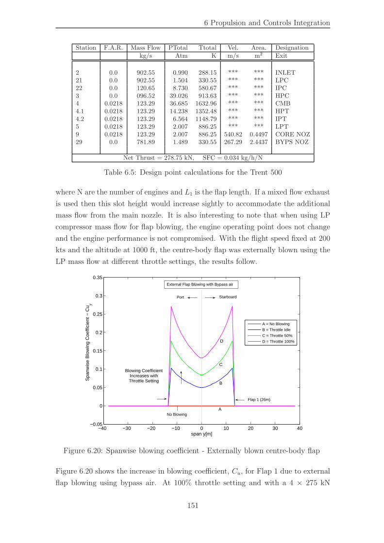
6 Propulsion and Controls Integration
Station F.A.R. Mass Flow PTotal Ttotal Vel. Area. Designationkg/s Atm K m/s m2 Exit
2 0.0 902.55 0.990 288.15 *** *** INLET21 0.0 902.55 1.504 330.55 *** *** LPC22 0.0 120.65 8.730 580.67 *** *** IPC3 0.0 096.52 39.026 913.63 *** *** HPC4 0.0218 123.29 36.685 1632.96 *** *** CMB4.1 0.0218 123.29 14.238 1352.48 *** *** HPT4.2 0.0218 123.29 6.564 1148.79 *** *** IPT5 0.0218 123.29 2.007 886.25 *** *** LPT9 0.0218 123.29 2.007 886.25 540.82 0.4497 CORE NOZ29 0.0 781.89 1.489 330.55 267.29 2.4437 BYPS NOZ
Net Thrust = 278.75 kN, SFC = 0.034 kg/h/N
Table 6.5: Design point calculations for the Trent 500
where N are the number of engines and L1 is the flap length. If a mixed flow exhaust
is used then this slot height would increase sightly to accommodate the additional
mass flow from the main nozzle. It is also interesting to note that when using LP
compressor mass flow for flap blowing, the engine operating point does not change
and the engine performance is not compromised. With the flight speed fixed at 200
kts and the altitude at 1000 ft, the centre-body flap was externally blown using the
LP mass flow at different throttle settings, the results follow.
−40 −30 −20 −10 0 10 20 30 40−0.05
0
0.05
0.1
0.15
0.2
0.25
0.3
0.35
span y[m]
Spa
nwis
e B
low
ing
Coe
ffici
ent −
Cu y
A = No Blowing
B = Throttle Idle
C = Throttle 50%
D = Throttle 100%
A
B
C
D
StarboardPort
No Blowing
Blowing CoefficientIncreases withThrottle Setting
External Flap Blowing with Bypass air
Flap 1 (26m)
Figure 6.20: Spanwise blowing coefficient - Externally blown centre-body flap
Figure 6.20 shows the increase in blowing coefficient, Cu, for Flap 1 due to external
flap blowing using bypass air. At 100% throttle setting and with a 4 × 275 kN
151
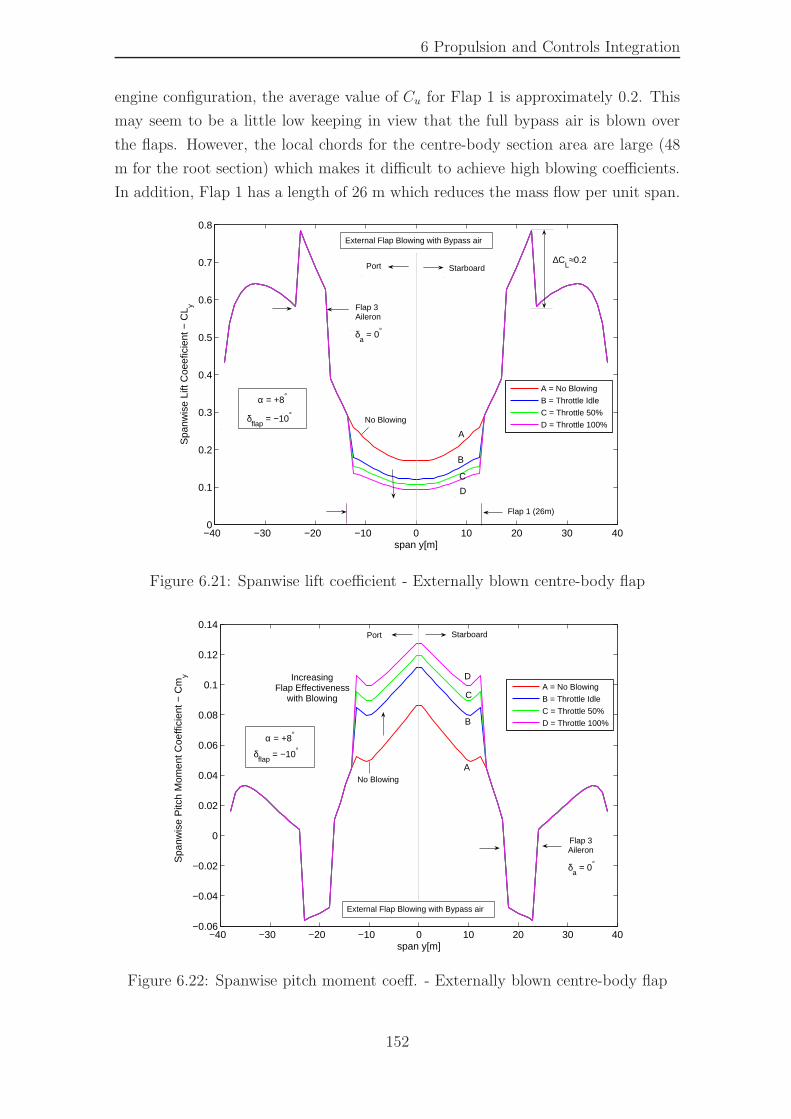
6 Propulsion and Controls Integration
engine configuration, the average value of Cu for Flap 1 is approximately 0.2. This
may seem to be a little low keeping in view that the full bypass air is blown over
the flaps. However, the local chords for the centre-body section area are large (48
m for the root section) which makes it difficult to achieve high blowing coefficients.
In addition, Flap 1 has a length of 26 m which reduces the mass flow per unit span.
−40 −30 −20 −10 0 10 20 30 400
0.1
0.2
0.3
0.4
0.5
0.6
0.7
0.8
span y[m]
Spa
nwis
e Li
ft C
oeef
icie
nt −
CL y
A = No Blowing
B = Throttle Idle
C = Throttle 50%
D = Throttle 100%
External Flap Blowing with Bypass air
StarboardPort
A
B
C
D
α = +8°
δflap
= −10°No Blowing
Flap 1 (26m)
Flap 3Aileron
δa = 0°
∆CL≈0.2
Figure 6.21: Spanwise lift coefficient - Externally blown centre-body flap
−40 −30 −20 −10 0 10 20 30 40−0.06
−0.04
−0.02
0
0.02
0.04
0.06
0.08
0.1
0.12
0.14
span y[m]
Spa
nwis
e P
itch
Mom
ent C
oeffi
cien
t − C
my
A = No Blowing
B = Throttle Idle
C = Throttle 50%
D = Throttle 100%
External Flap Blowing with Bypass air
No BlowingA
B
C
DIncreasingFlap Effectiveness
with Blowing
δflap
= −10°α = +8°
Flap 3Aileron
δa = 0°
StarboardPort
Figure 6.22: Spanwise pitch moment coeff. - Externally blown centre-body flap
152
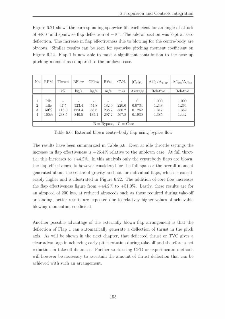
6 Propulsion and Controls Integration
Figure 6.21 shows the corresponding spanwise lift coefficient for an angle of attack
of +8.0◦ and spanwise flap deflection of −10◦. The aileron section was kept at zero
deflection. The increase in flap effectiveness due to blowing for the centre-body are
obvious. Similar results can be seen for spanwise pitching moment coefficient on
Figure 6.22. Flap 1 is now able to make a significant contribution to the nose up
pitching moment as compared to the unblown case.
No RPM Thrust BFlow CFlow BVel. CVel. [Cu]F1 ∆CL/∆flap ∆Cm/∆flap
kN kg/s kg/s m/s m/s Average Relative Relative
1 Idle - - - - - 0 1.000 1.0002 Idle 47.5 523.4 54.8 182.0 220.0 0.0734 1.248 1.2643 50% 116.0 683.4 88.6 238.7 386.2 0.1262 1.317 1.3524 100% 238.5 840.5 135.1 297.2 567.8 0.1930 1.385 1.442
B = Bypass, C = Core
Table 6.6: External blown centre-body flap using bypass flow
The results have been summarized in Table 6.6. Even at idle throttle settings the
increase in flap effectiveness is +26.4% relative to the unblown case. At full throt-
tle, this increases to +44.2%. In this analysis only the centrebody flaps are blown,
the flap effectiveness is however considered for the full span or the overall moment
generated about the centre of gravity and not for individual flaps, which is consid-
erably higher and is illustrated in Figure 6.22. The addition of core flow increases
the flap effectiveness figure from +44.2% to +51.0%. Lastly, these results are for
an airspeed of 200 kts, at reduced airspeeds such as those required during take-off
or landing, better results are expected due to relativey higher values of achievable
blowing momentum coefficient.
Another possible advantage of the externally blown flap arrangement is that the
deflection of Flap 1 can automatically generate a deflection of thrust in the pitch
axis. As will be shown in the next chapter, that deflected thrust or TVC gives a
clear advantage in achieving early pitch rotation during take-off and therefore a net
reduction in take-off distances. Further work using CFD or experimental methods
will however be necessary to ascertain the amount of thrust deflection that can be
achieved with such an arrangement.
153
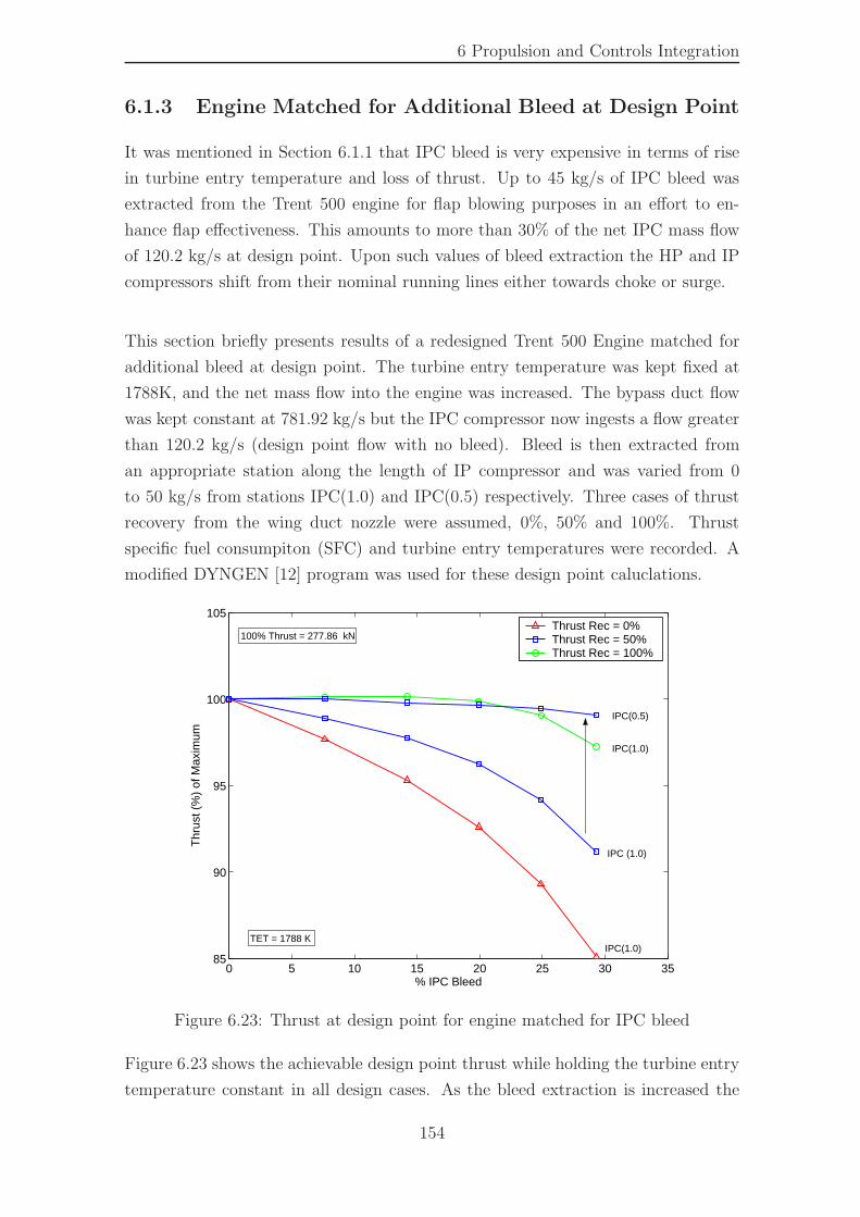
6 Propulsion and Controls Integration
6.1.3 Engine Matched for Additional Bleed at Design Point
It was mentioned in Section 6.1.1 that IPC bleed is very expensive in terms of rise
in turbine entry temperature and loss of thrust. Up to 45 kg/s of IPC bleed was
extracted from the Trent 500 engine for flap blowing purposes in an effort to en-
hance flap effectiveness. This amounts to more than 30% of the net IPC mass flow
of 120.2 kg/s at design point. Upon such values of bleed extraction the HP and IP
compressors shift from their nominal running lines either towards choke or surge.
This section briefly presents results of a redesigned Trent 500 Engine matched for
additional bleed at design point. The turbine entry temperature was kept fixed at
1788K, and the net mass flow into the engine was increased. The bypass duct flow
was kept constant at 781.92 kg/s but the IPC compressor now ingests a flow greater
than 120.2 kg/s (design point flow with no bleed). Bleed is then extracted from
an appropriate station along the length of IP compressor and was varied from 0
to 50 kg/s from stations IPC(1.0) and IPC(0.5) respectively. Three cases of thrust
recovery from the wing duct nozzle were assumed, 0%, 50% and 100%. Thrust
specific fuel consumpiton (SFC) and turbine entry temperatures were recorded. A
modified DYNGEN [12] program was used for these design point caluclations.
0 5 10 15 20 25 30 3585
90
95
100
105
% IPC Bleed
Thr
ust (
%)
of M
axim
um
Thrust Rec = 0% Thrust Rec = 50% Thrust Rec = 100%
IPC (1.0)
IPC(0.5)
IPC(1.0)
IPC(1.0) TET = 1788 K
100% Thrust = 277.86 kN
Figure 6.23: Thrust at design point for engine matched for IPC bleed
Figure 6.23 shows the achievable design point thrust while holding the turbine entry
temperature constant in all design cases. As the bleed extraction is increased the
154
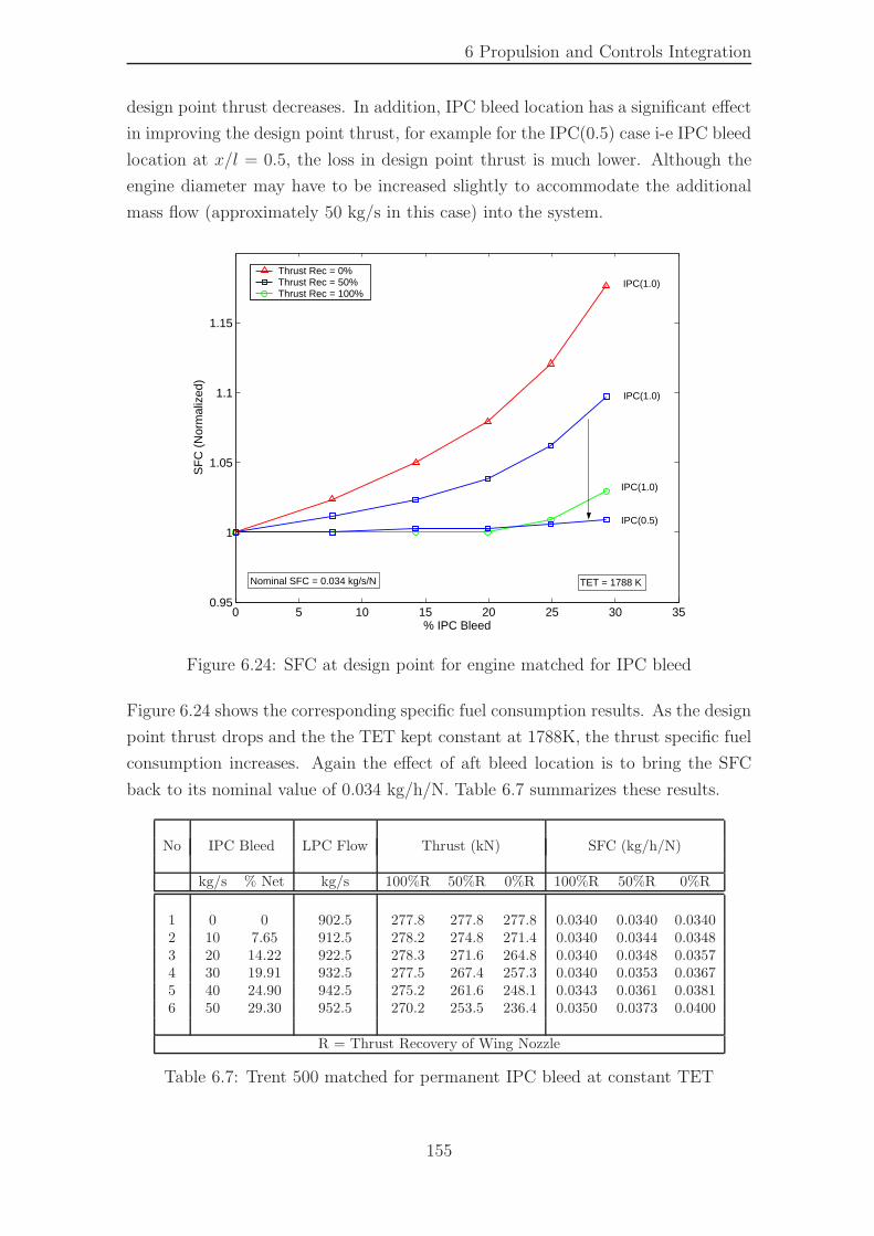
6 Propulsion and Controls Integration
design point thrust decreases. In addition, IPC bleed location has a significant effect
in improving the design point thrust, for example for the IPC(0.5) case i-e IPC bleed
location at x/l = 0.5, the loss in design point thrust is much lower. Although the
engine diameter may have to be increased slightly to accommodate the additional
mass flow (approximately 50 kg/s in this case) into the system.
0 5 10 15 20 25 30 350.95
1
1.05
1.1
1.15
% IPC Bleed
SF
C (
Nor
mal
ized
)
Thrust Rec = 0% Thrust Rec = 50% Thrust Rec = 100%
IPC(1.0)
IPC(0.5)
IPC(1.0)
IPC(1.0)
TET = 1788 K Nominal SFC = 0.034 kg/s/N
Figure 6.24: SFC at design point for engine matched for IPC bleed
Figure 6.24 shows the corresponding specific fuel consumption results. As the design
point thrust drops and the the TET kept constant at 1788K, the thrust specific fuel
consumption increases. Again the effect of aft bleed location is to bring the SFC
back to its nominal value of 0.034 kg/h/N. Table 6.7 summarizes these results.
No IPC Bleed LPC Flow Thrust (kN) SFC (kg/h/N)
kg/s % Net kg/s 100%R 50%R 0%R 100%R 50%R 0%R
1 0 0 902.5 277.8 277.8 277.8 0.0340 0.0340 0.03402 10 7.65 912.5 278.2 274.8 271.4 0.0340 0.0344 0.03483 20 14.22 922.5 278.3 271.6 264.8 0.0340 0.0348 0.03574 30 19.91 932.5 277.5 267.4 257.3 0.0340 0.0353 0.03675 40 24.90 942.5 275.2 261.6 248.1 0.0343 0.0361 0.03816 50 29.30 952.5 270.2 253.5 236.4 0.0350 0.0373 0.0400
R = Thrust Recovery of Wing Nozzle
Table 6.7: Trent 500 matched for permanent IPC bleed at constant TET
155
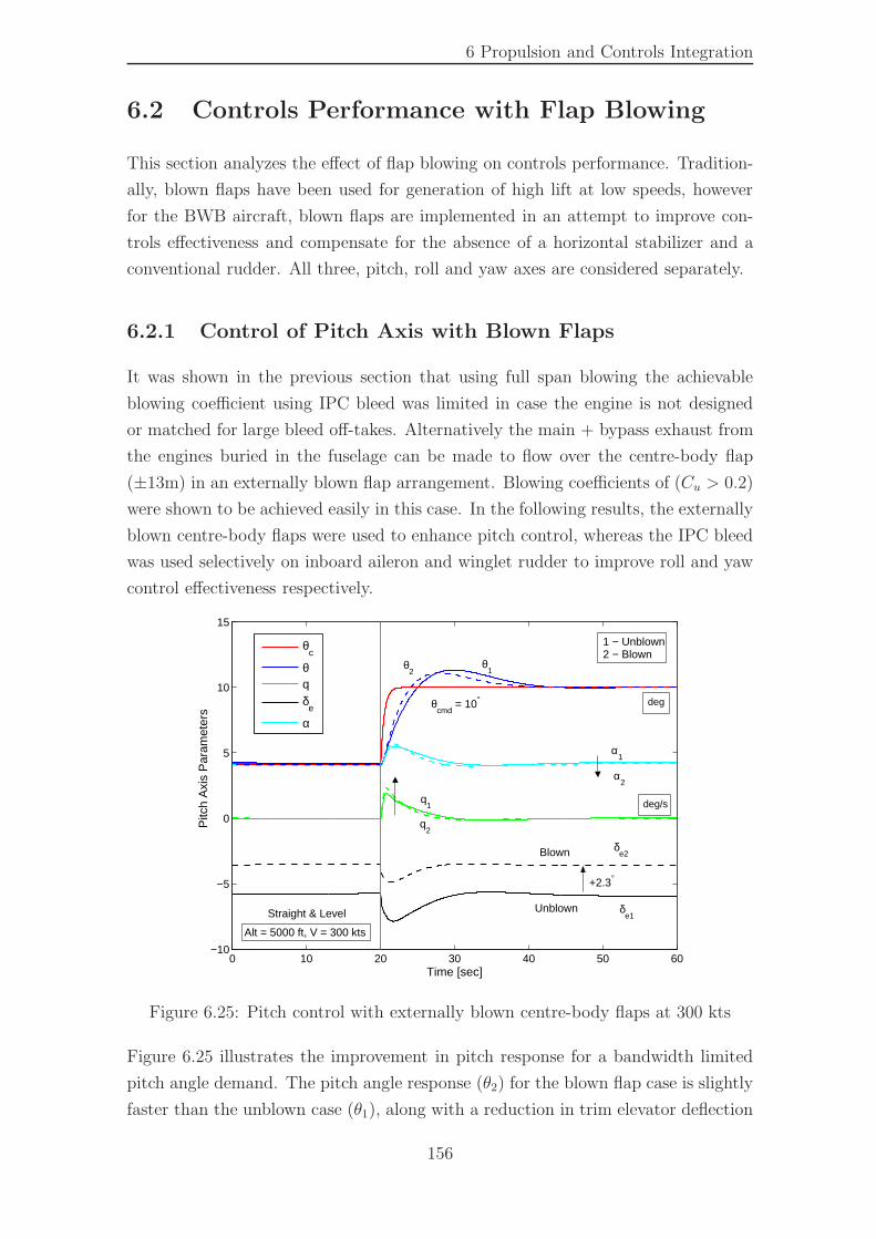
6 Propulsion and Controls Integration
6.2 Controls Performance with Flap Blowing
This section analyzes the effect of flap blowing on controls performance. Tradition-
ally, blown flaps have been used for generation of high lift at low speeds, however
for the BWB aircraft, blown flaps are implemented in an attempt to improve con-
trols effectiveness and compensate for the absence of a horizontal stabilizer and a
conventional rudder. All three, pitch, roll and yaw axes are considered separately.
6.2.1 Control of Pitch Axis with Blown Flaps
It was shown in the previous section that using full span blowing the achievable
blowing coefficient using IPC bleed was limited in case the engine is not designed
or matched for large bleed off-takes. Alternatively the main + bypass exhaust from
the engines buried in the fuselage can be made to flow over the centre-body flap
(±13m) in an externally blown flap arrangement. Blowing coefficients of (Cu > 0.2)
were shown to be achieved easily in this case. In the following results, the externally
blown centre-body flaps were used to enhance pitch control, whereas the IPC bleed
was used selectively on inboard aileron and winglet rudder to improve roll and yaw
control effectiveness respectively.
0 10 20 30 40 50 60−10
−5
0
5
10
15
Time [sec]
Pitc
h A
xis
Par
amet
ers
δe1
δe2
θ1θ
2
α1
q1
Unblown
Blown
Alt = 5000 ft, V = 300 kts
θcmd
= 10°
1 − Unblown 2 − Blown
Straight & Level
α2
q2
+2.3°
θc
θqδ
e
α
deg/s
deg
Figure 6.25: Pitch control with externally blown centre-body flaps at 300 kts
Figure 6.25 illustrates the improvement in pitch response for a bandwidth limited
pitch angle demand. The pitch angle response (θ2) for the blown flap case is slightly
faster than the unblown case (θ1), along with a reduction in trim elevator deflection
156
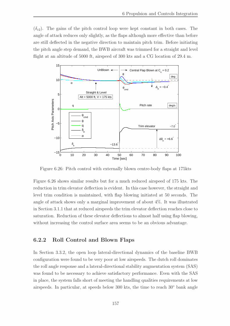
6 Propulsion and Controls Integration
(δe2). The gains of the pitch control loop were kept constant in both cases. The
angle of attack reduces only slightly, as the flaps although more effective than before
are still deflected in the negative direction to maintain pitch trim. Before initiating
the pitch angle step demand, the BWB aircraft was trimmed for a straight and level
flight at an altitude of 5000 ft, airspeed of 300 kts and a CG location of 29.4 m.
0 10 20 30 40 50 60 70 80 90 100−15
−10
−5
0
5
10
15
Time [sec]
Pitc
h A
xis
Par
amet
ers
Central Flap Blown at Cu = 0.2UnBlown
q
θcmd
θ
α
δe
Trim elevator
Pitch rate
Alt = 5000 ft, V = 175 kts
Straight & Level
−13.6°
−7.0°
∆δe = +6.6°
∆α = −0.4°
θcmd
θqδ
e
α
deg/s
deg
Figure 6.26: Pitch control with externally blown centre-body flaps at 175kts
Figure 6.26 shows similar results but for a much reduced airspeed of 175 kts. The
reduction in trim elevator deflection is evident. In this case however, the straight and
level trim condition is maintained, with flap blowing initiated at 50 seconds. The
angle of attack shows only a marginal improvement of about 4%. It was illustrated
in Section 3.1.1 that at reduced airspeeds the trim elevator deflection reaches close to
saturation. Reduction of these elevator deflections to almost half using flap blowing,
without increasing the control surface area seems to be an obvious advantage.
6.2.2 Roll Control and Blown Flaps
In Section 3.3.2, the open loop lateral-directional dynamics of the baseline BWB
configuration were found to be very poor at low airspeeds. The dutch roll dominates
the roll angle response and a lateral-directional stability augmentation system (SAS)
was found to be necessary to achieve satisfactory performance. Even with the SAS
in place, the system falls short of meeting the handling qualities requirements at low
airspeeds. In particular, at speeds below 300 kts, the time to reach 30◦ bank angle
157
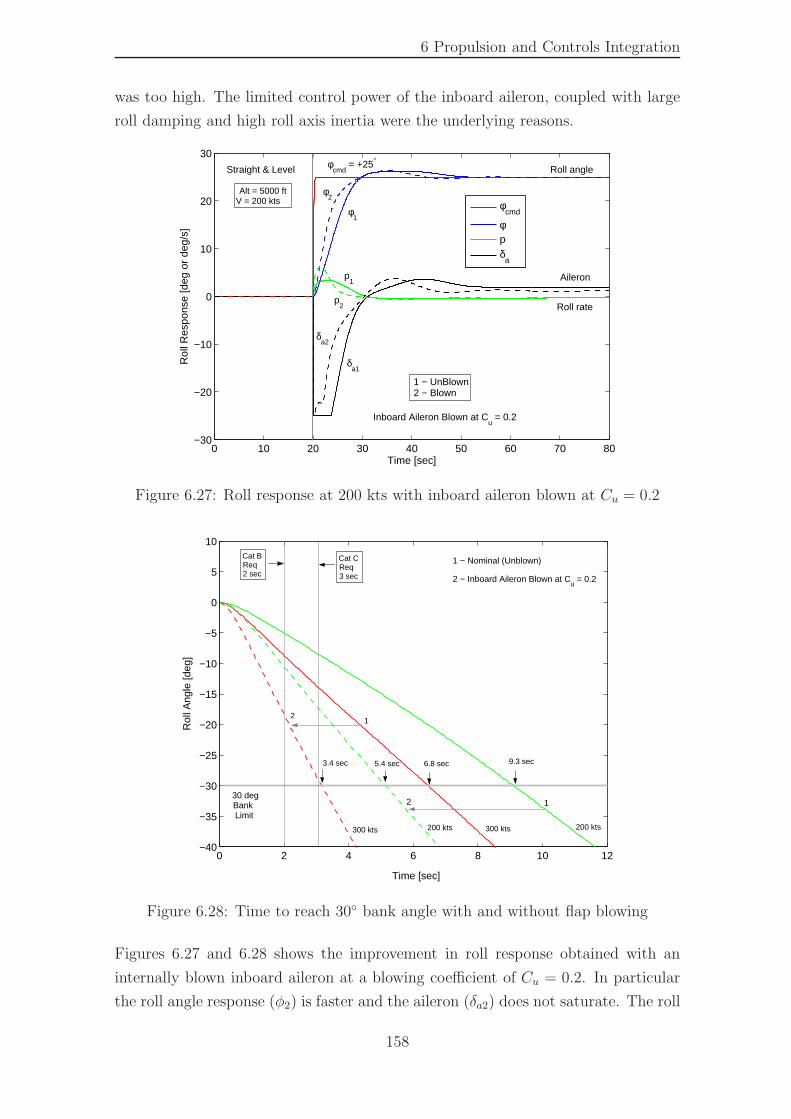
6 Propulsion and Controls Integration
was too high. The limited control power of the inboard aileron, coupled with large
roll damping and high roll axis inertia were the underlying reasons.
0 10 20 30 40 50 60 70 80−30
−20
−10
0
10
20
30
Time [sec]
Rol
l Res
pons
e [d
eg o
r de
g/s]
φ
cmd = +25°
φ1
φ2
p1
p2
δa1
δa2
Straight & Level
Alt = 5000 ft V = 200 kts
1 − UnBlown 2 − Blown
Inboard Aileron Blown at Cu = 0.2
Roll angle
Aileron
Roll rate
φcmd
φpδ
a
Figure 6.27: Roll response at 200 kts with inboard aileron blown at Cu = 0.2
0 2 4 6 8 10 12−40
−35
−30
−25
−20
−15
−10
−5
0
5
10
Time [sec]
Rol
l Ang
le [d
eg]
Cat C Req 3 sec
Cat B Req 2 sec
1 − Nominal (Unblown) 2 − Inboard Aileron Blown at C
u = 0.2
200 kts 200 kts
9.3 sec 6.8 sec 5.4 sec 3.4 sec
300 kts 300 kts
1
1 2
2 30 deg Bank Limit
Figure 6.28: Time to reach 30◦ bank angle with and without flap blowing
Figures 6.27 and 6.28 shows the improvement in roll response obtained with an
internally blown inboard aileron at a blowing coefficient of Cu = 0.2. In particular
the roll angle response (φ2) is faster and the aileron (δa2) does not saturate. The roll
158
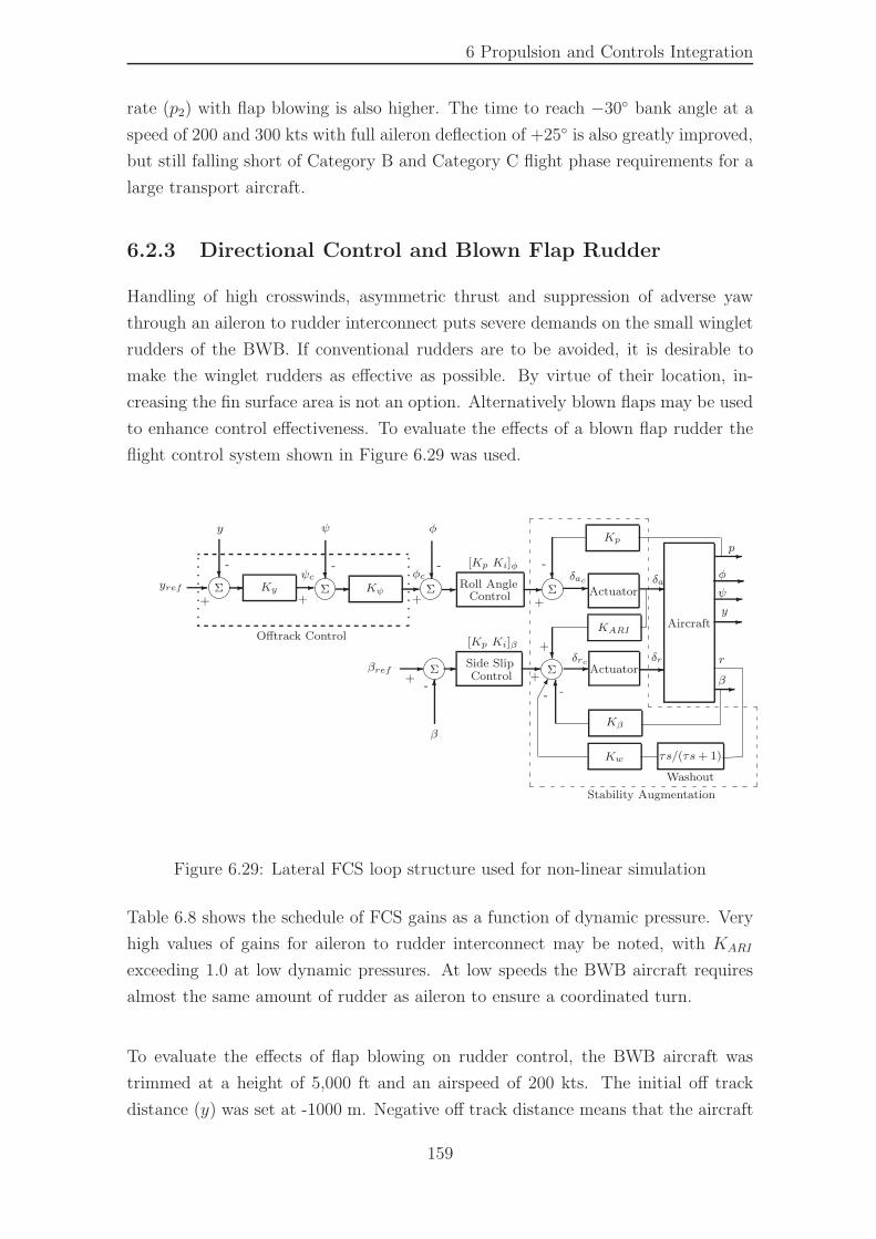
6 Propulsion and Controls Integration
rate (p2) with flap blowing is also higher. The time to reach −30◦ bank angle at a
speed of 200 and 300 kts with full aileron deflection of +25◦ is also greatly improved,
but still falling short of Category B and Category C flight phase requirements for a
large transport aircraft.
6.2.3 Directional Control and Blown Flap Rudder
Handling of high crosswinds, asymmetric thrust and suppression of adverse yaw
through an aileron to rudder interconnect puts severe demands on the small winglet
rudders of the BWB. If conventional rudders are to be avoided, it is desirable to
make the winglet rudders as effective as possible. By virtue of their location, in-
creasing the fin surface area is not an option. Alternatively blown flaps may be used
to enhance control effectiveness. To evaluate the effects of a blown flap rudder the
flight control system shown in Figure 6.29 was used.
Aircraft
β
r
[Kp Ki]φ
-
δrc
-
Actuator -
Actuator -
-
Σ -
-
+βref
�
δrΣ
[Kp Ki]β
Σ
Kβ
Kw
-φc
-
6
τs/(τs+ 1)
φ
KψKy -Σ -Σ -?-
+
ψ
ψc -φ
-ψ
p
Washout
y
δac- δaRoll AngleControl
+
-
-
-?
+
?-
+
Kp
?
+
Stability Augmentation
-
yref
KARI
?+
-Side SlipControl
Σ
6
β
--
-
y
Offtrack Control
-
Figure 6.29: Lateral FCS loop structure used for non-linear simulation
Table 6.8 shows the schedule of FCS gains as a function of dynamic pressure. Very
high values of gains for aileron to rudder interconnect may be noted, with KARI
exceeding 1.0 at low dynamic pressures. At low speeds the BWB aircraft requires
almost the same amount of rudder as aileron to ensure a coordinated turn.
To evaluate the effects of flap blowing on rudder control, the BWB aircraft was
trimmed at a height of 5,000 ft and an airspeed of 200 kts. The initial off track
distance (y) was set at -1000 m. Negative off track distance means that the aircraft
159
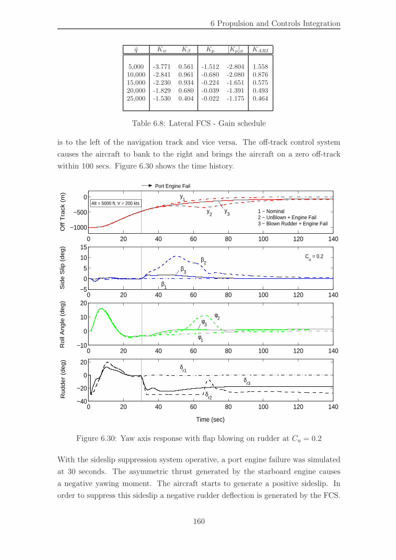
6 Propulsion and Controls Integration
q Kw Kβ Kp [Kp]φ KARI
5,000 -3.771 0.561 -1.512 -2.804 1.55810,000 -2.841 0.961 -0.680 -2.080 0.87615,000 -2.230 0.934 -0.224 -1.651 0.57520,000 -1.829 0.680 -0.039 -1.391 0.49325,000 -1.530 0.404 -0.022 -1.175 0.464
Table 6.8: Lateral FCS - Gain schedule
is to the left of the navigation track and vice versa. The off-track control system
causes the aircraft to bank to the right and brings the aircraft on a zero off-track
within 100 secs. Figure 6.30 shows the time history.
0 20 40 60 80 100 120 140
−1000
−500
0
Off
Tra
ck (
m)
0 20 40 60 80 100 120 140−5
0
5
10
15
Sid
e S
lip (
de
g)
0 20 40 60 80 100 120 140−10
0
10
20
Ro
ll A
ng
le (
de
g)
0 20 40 60 80 100 120 140−40
−20
0
20
Ru
dd
er
(de
g)
Time (sec)
Port Engine Fail
y1
β1
φ1
δr1
y2
β2
φ2
δr2
y3
β3
φ3
δr3
1 − Nominal2 − UnBlown + Engine Fail3 − Blown Rudder + Engine Fail
Cu = 0.2
Alt = 5000 ft, V = 200 kts
Figure 6.30: Yaw axis response with flap blowing on rudder at Cu = 0.2
With the sideslip suppression system operative, a port engine failure was simulated
at 30 seconds. The asymmetric thrust generated by the starboard engine causes
a negative yawing moment. The aircraft starts to generate a positive sideslip. In
order to suppress this sideslip a negative rudder deflection is generated by the FCS.
160
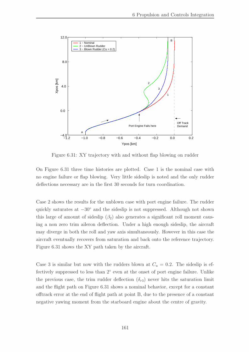
6 Propulsion and Controls Integration
−1.2 −1.0 −0.8 −0.6 −0.4 −0.2 0.0 0.2 −4.0
0.0
4.0
8.0
12.0
Ypos [km]
Xpo
s [k
m]
1 − Nominal2 − UnBlown Rudder3 − Blown Rudder (Cu = 0.2)
Port Engine Fails here
1
2
3
Off TrackDemand
A
B
Figure 6.31: XY trajectory with and without flap blowing on rudder
On Figure 6.31 three time histories are plotted. Case 1 is the nominal case with
no engine failure or flap blowing. Very little sideslip is noted and the only rudder
deflections necessary are in the first 30 seconds for turn coordination.
Case 2 shows the results for the unblown case with port engine failure. The rudder
quickly saturates at −30◦ and the sideslip is not suppressed. Although not shown
this large of amount of sideslip (β2) also generates a significant roll moment caus-
ing a non zero trim aileron deflection. Under a high enough sideslip, the aircraft
may diverge in both the roll and yaw axis simultaneously. However in this case the
aircraft eventually recovers from saturation and back onto the reference trajectory.
Figure 6.31 shows the XY path taken by the aircraft.
Case 3 is similar but now with the rudders blown at Cu = 0.2. The sideslip is ef-
fectively suppressed to less than 2◦ even at the onset of port engine failure. Unlike
the previous case, the trim rudder deflection (δr3) never hits the saturation limit
and the flight path on Figure 6.31 shows a nominal behavior, except for a constant
offtrack error at the end of flight path at point B, due to the presence of a constant
negative yawing moment from the starboard engine about the centre of gravity.
161
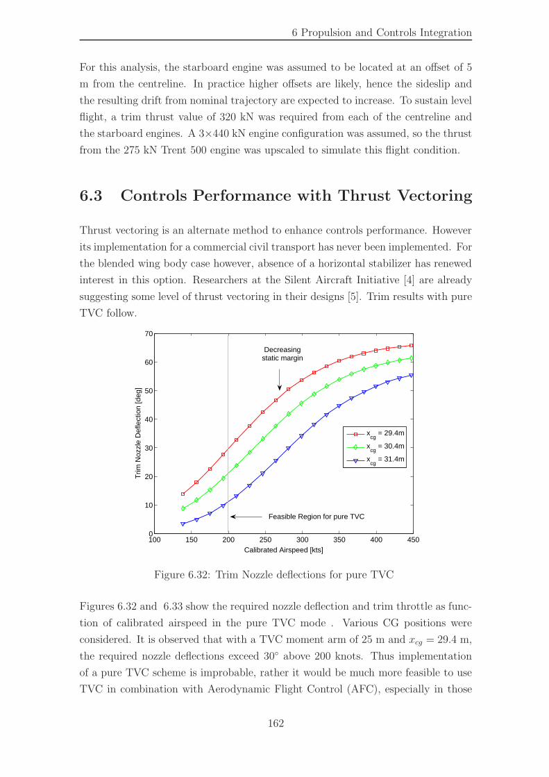
6 Propulsion and Controls Integration
For this analysis, the starboard engine was assumed to be located at an offset of 5
m from the centreline. In practice higher offsets are likely, hence the sideslip and
the resulting drift from nominal trajectory are expected to increase. To sustain level
flight, a trim thrust value of 320 kN was required from each of the centreline and
the starboard engines. A 3×440 kN engine configuration was assumed, so the thrust
from the 275 kN Trent 500 engine was upscaled to simulate this flight condition.
6.3 Controls Performance with Thrust Vectoring
Thrust vectoring is an alternate method to enhance controls performance. However
its implementation for a commercial civil transport has never been implemented. For
the blended wing body case however, absence of a horizontal stabilizer has renewed
interest in this option. Researchers at the Silent Aircraft Initiative [4] are already
suggesting some level of thrust vectoring in their designs [5]. Trim results with pure
TVC follow.
100 150 200 250 300 350 400 4500
10
20
30
40
50
60
70
Calibrated Airspeed [kts]
Trim
Noz
zle
Def
lect
ion
[deg
]
xcg
= 29.4m
xcg
= 30.4m
xcg
= 31.4m
Feasible Region for pure TVC
Decreasingstatic margin
Figure 6.32: Trim Nozzle deflections for pure TVC
Figures 6.32 and 6.33 show the required nozzle deflection and trim throttle as func-
tion of calibrated airspeed in the pure TVC mode . Various CG positions were
considered. It is observed that with a TVC moment arm of 25 m and xcg = 29.4 m,
the required nozzle deflections exceed 30◦ above 200 knots. Thus implementation
of a pure TVC scheme is improbable, rather it would be much more feasible to use
TVC in combination with Aerodynamic Flight Control (AFC), especially in those
162
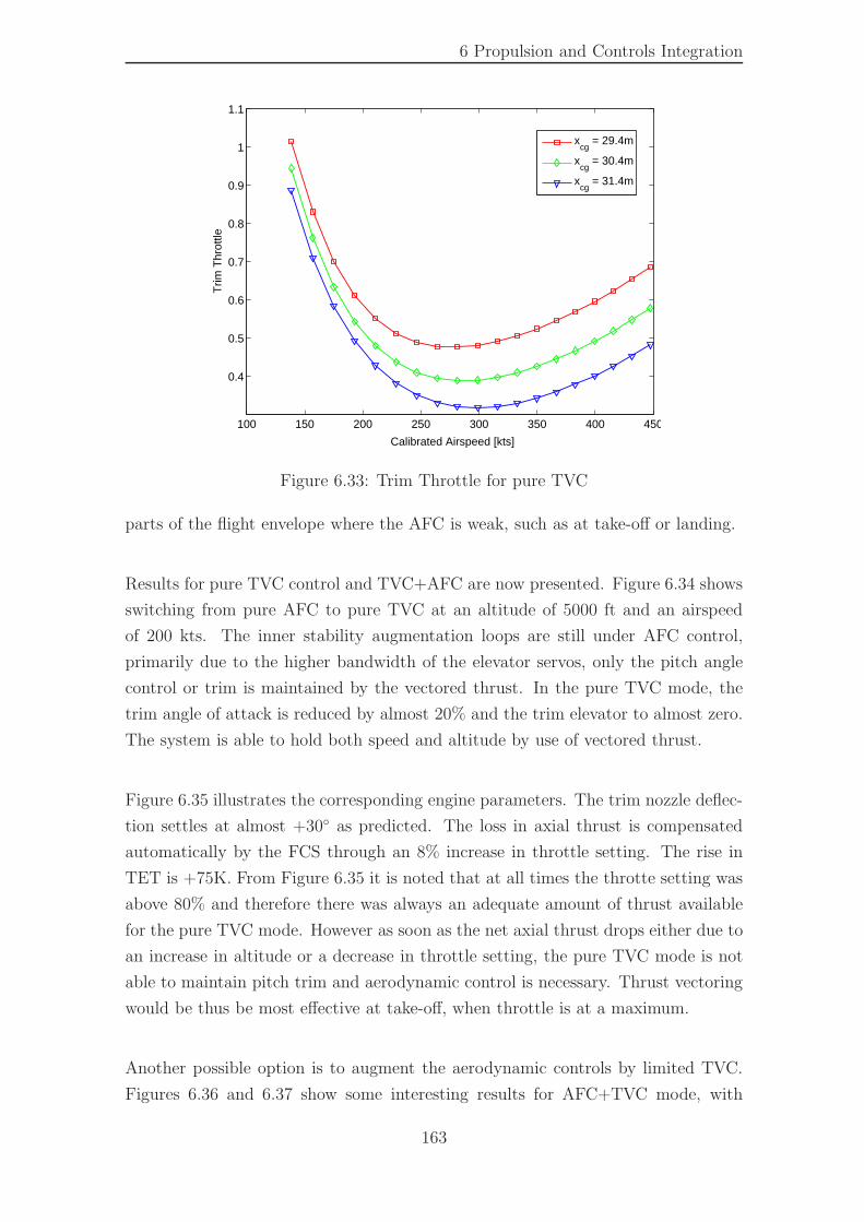
6 Propulsion and Controls Integration
100 150 200 250 300 350 400 450
0.4
0.5
0.6
0.7
0.8
0.9
1
1.1
Calibrated Airspeed [kts]
Trim
Thr
ottle
xcg
= 29.4m
xcg
= 30.4m
xcg
= 31.4m
Figure 6.33: Trim Throttle for pure TVC
parts of the flight envelope where the AFC is weak, such as at take-off or landing.
Results for pure TVC control and TVC+AFC are now presented. Figure 6.34 shows
switching from pure AFC to pure TVC at an altitude of 5000 ft and an airspeed
of 200 kts. The inner stability augmentation loops are still under AFC control,
primarily due to the higher bandwidth of the elevator servos, only the pitch angle
control or trim is maintained by the vectored thrust. In the pure TVC mode, the
trim angle of attack is reduced by almost 20% and the trim elevator to almost zero.
The system is able to hold both speed and altitude by use of vectored thrust.
Figure 6.35 illustrates the corresponding engine parameters. The trim nozzle deflec-
tion settles at almost +30◦ as predicted. The loss in axial thrust is compensated
automatically by the FCS through an 8% increase in throttle setting. The rise in
TET is +75K. From Figure 6.35 it is noted that at all times the throtte setting was
above 80% and therefore there was always an adequate amount of thrust available
for the pure TVC mode. However as soon as the net axial thrust drops either due to
an increase in altitude or a decrease in throttle setting, the pure TVC mode is not
able to maintain pitch trim and aerodynamic control is necessary. Thrust vectoring
would be thus be most effective at take-off, when throttle is at a maximum.
Another possible option is to augment the aerodynamic controls by limited TVC.
Figures 6.36 and 6.37 show some interesting results for AFC+TVC mode, with
163
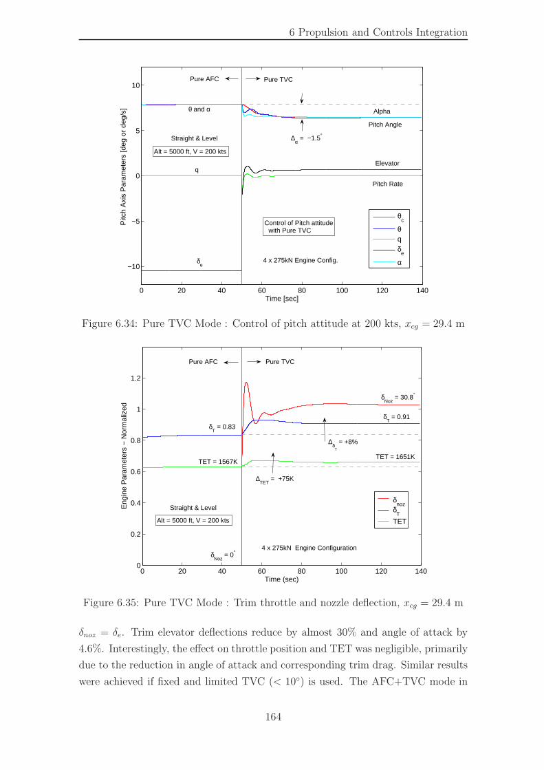
6 Propulsion and Controls Integration
0 20 40 60 80 100 120 140
−10
−5
0
5
10
Time [sec]
Pitc
h A
xis
Par
amet
ers
[deg
or
deg/
s]
Pure TVC Pure AFC
Straight & Level
Alt = 5000 ft, V = 200 kts
Pitch Angle
Pitch Rate
Elevator
θ and α
q
δe
∆α = −1.5°
Control of Pitch attitude with Pure TVC
4 x 275kN Engine Config.
Alpha
θc
θqδ
e
α
Figure 6.34: Pure TVC Mode : Control of pitch attitude at 200 kts, xcg = 29.4 m
0 20 40 60 80 100 120 1400
0.2
0.4
0.6
0.8
1
1.2
Time (sec)
Eng
ine
Par
amet
ers
− N
orm
aliz
ed
δnoz
δT
TET
Pure TVC Pure AFC
TET = 1567K
δT = 0.83
δNoz
= 30.8°
δNoz
= 0°
δT = 0.91
TET = 1651K
∆TET
= +75K
∆δ
T
= +8%
4 x 275kN Engine Configuration
Straight & Level
Alt = 5000 ft, V = 200 kts
Figure 6.35: Pure TVC Mode : Trim throttle and nozzle deflection, xcg = 29.4 m
δnoz = δe. Trim elevator deflections reduce by almost 30% and angle of attack by
4.6%. Interestingly, the effect on throttle position and TET was negligible, primarily
due to the reduction in angle of attack and corresponding trim drag. Similar results
were achieved if fixed and limited TVC (< 10◦) is used. The AFC+TVC mode in
164
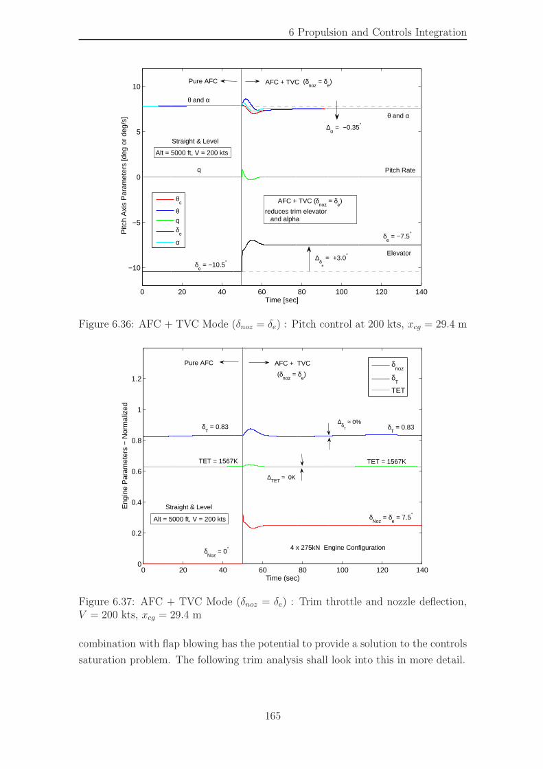
6 Propulsion and Controls Integration
0 20 40 60 80 100 120 140
−10
−5
0
5
10
Time [sec]
Pitc
h A
xis
Par
amet
ers
[deg
or
deg/
s]
θ and α
AFC + TVC Pure AFC
Straight & Level
Alt = 5000 ft, V = 200 kts
Pitch Rate
Elevator
θ and α
q
δe = −10.5°
∆α = −0.35°
AFC + TVC (δnoz
= δe)
reduces trim elevator and alpha
δe = −7.5°
∆δ
e
= +3.0°
(δnoz
= δe)
θc
θqδ
e
α
Figure 6.36: AFC + TVC Mode (δnoz = δe) : Pitch control at 200 kts, xcg = 29.4 m
0 20 40 60 80 100 120 1400
0.2
0.4
0.6
0.8
1
1.2
Time (sec)
Eng
ine
Par
amet
ers
− N
orm
aliz
ed
AFC + TVC Pure AFC
TET = 1567K
δT = 0.83
δNoz
= δe = 7.5°
δNoz
= 0°
δT = 0.83
TET = 1567K
∆TET
≈ 0K
∆δT
≈ 0%
4 x 275kN Engine Configuration
Straight & Level
Alt = 5000 ft, V = 200 kts
(δnoz
= δe)
δnoz
δT
TET
Figure 6.37: AFC + TVC Mode (δnoz = δe) : Trim throttle and nozzle deflection,V = 200 kts, xcg = 29.4 m
combination with flap blowing has the potential to provide a solution to the controls
saturation problem. The following trim analysis shall look into this in more detail.
165
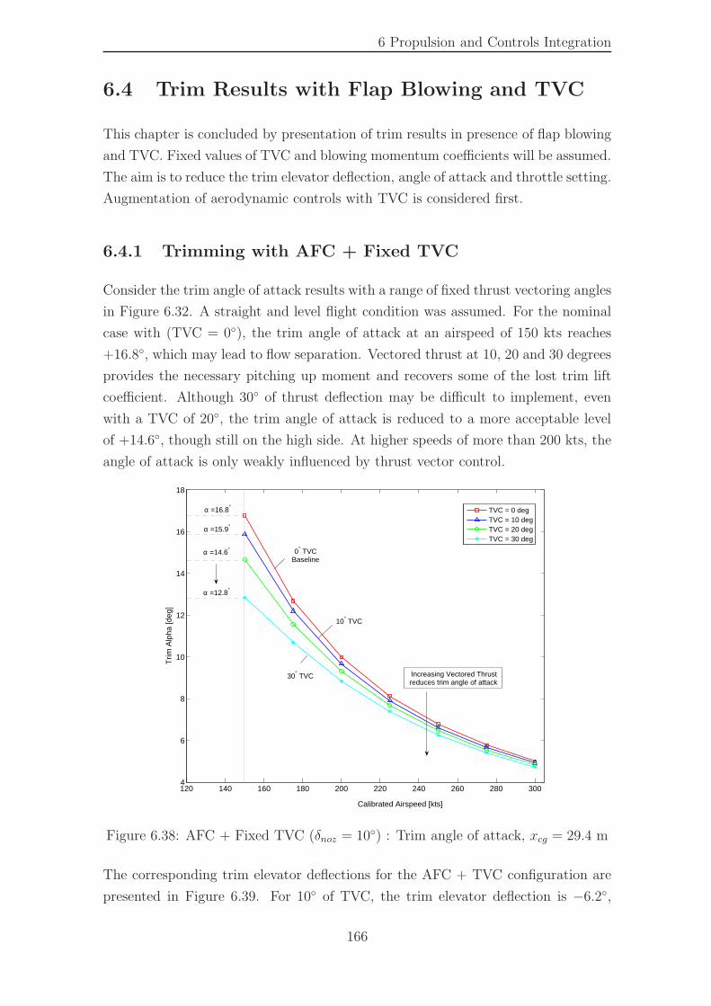
6 Propulsion and Controls Integration
6.4 Trim Results with Flap Blowing and TVC
This chapter is concluded by presentation of trim results in presence of flap blowing
and TVC. Fixed values of TVC and blowing momentum coefficients will be assumed.
The aim is to reduce the trim elevator deflection, angle of attack and throttle setting.
Augmentation of aerodynamic controls with TVC is considered first.
6.4.1 Trimming with AFC + Fixed TVC
Consider the trim angle of attack results with a range of fixed thrust vectoring angles
in Figure 6.32. A straight and level flight condition was assumed. For the nominal
case with (TVC = 0◦), the trim angle of attack at an airspeed of 150 kts reaches
+16.8◦, which may lead to flow separation. Vectored thrust at 10, 20 and 30 degrees
provides the necessary pitching up moment and recovers some of the lost trim lift
coefficient. Although 30◦ of thrust deflection may be difficult to implement, even
with a TVC of 20◦, the trim angle of attack is reduced to a more acceptable level
of +14.6◦, though still on the high side. At higher speeds of more than 200 kts, the
angle of attack is only weakly influenced by thrust vector control.
120 140 160 180 200 220 240 260 280 3004
6
8
10
12
14
16
18
Calibrated Airspeed [kts]
Trim
Alp
ha [d
eg]
TVC = 0 degTVC = 10 degTVC = 20 degTVC = 30 deg
α =16.8°
α =15.9°
α =14.6°
α =12.8°
0° TVCBaseline
10° TVC
30° TVC Increasing Vectored Thrustreduces trim angle of attack
Figure 6.38: AFC + Fixed TVC (δnoz = 10◦) : Trim angle of attack, xcg = 29.4 m
The corresponding trim elevator deflections for the AFC + TVC configuration are
presented in Figure 6.39. For 10◦ of TVC, the trim elevator deflection is −6.2◦,
166
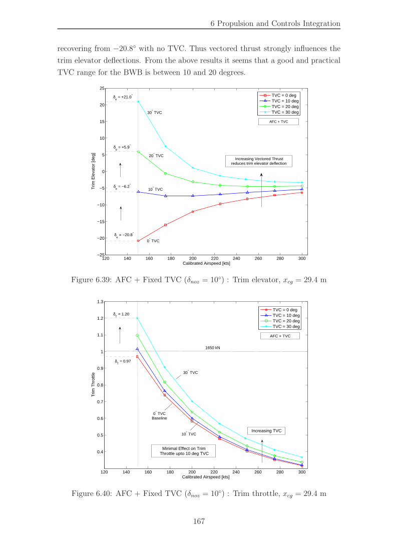
6 Propulsion and Controls Integration
recovering from −20.8◦ with no TVC. Thus vectored thrust strongly influences the
trim elevator deflections. From the above results it seems that a good and practical
TVC range for the BWB is between 10 and 20 degrees.
120 140 160 180 200 220 240 260 280 300−25
−20
−15
−10
−5
0
5
10
15
20
25T
rim E
leva
tor
[deg
]
Calibrated Airspeed [kts]
TVC = 0 degTVC = 10 degTVC = 20 degTVC = 30 deg
δe = −20.8°
δe = −6.2°
δe = +5.9°
δe = +21.0°
Increasing Vectored Thrustreduces trim elevator deflection
0° TVC
10° TVC
20° TVC
30° TVC
AFC + TVC
Figure 6.39: AFC + Fixed TVC (δnoz = 10◦) : Trim elevator, xcg = 29.4 m
120 140 160 180 200 220 240 260 280 300
0.4
0.5
0.6
0.7
0.8
0.9
1
1.1
1.2
1.3
Trim
Thr
ottle
Calibrated Airspeed [kts]
TVC = 0 degTVC = 10 degTVC = 20 degTVC = 30 deg
δT = 1.20
δT = 0.97
1650 kN
30° TVC
0° TVCBaseline
10° TVC
Minimal Effect on Trim Throttle upto 10 deg TVC
Increasing TVC
AFC + TVC
Figure 6.40: AFC + Fixed TVC (δnoz = 10◦) : Trim throttle, xcg = 29.4 m
167
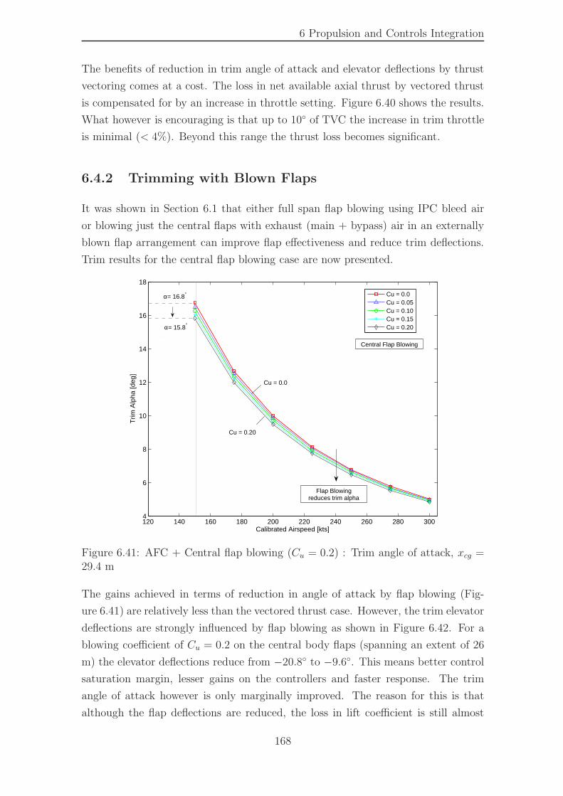
6 Propulsion and Controls Integration
The benefits of reduction in trim angle of attack and elevator deflections by thrust
vectoring comes at a cost. The loss in net available axial thrust by vectored thrust
is compensated for by an increase in throttle setting. Figure 6.40 shows the results.
What however is encouraging is that up to 10◦ of TVC the increase in trim throttle
is minimal (< 4%). Beyond this range the thrust loss becomes significant.
6.4.2 Trimming with Blown Flaps
It was shown in Section 6.1 that either full span flap blowing using IPC bleed air
or blowing just the central flaps with exhaust (main + bypass) air in an externally
blown flap arrangement can improve flap effectiveness and reduce trim deflections.
Trim results for the central flap blowing case are now presented.
120 140 160 180 200 220 240 260 280 3004
6
8
10
12
14
16
18
Calibrated Airspeed [kts]
Trim
Alp
ha [d
eg]
Cu = 0.0Cu = 0.05Cu = 0.10Cu = 0.15Cu = 0.20
α= 16.8°
α= 15.8°
Cu = 0.20
Cu = 0.0
Central Flap Blowing
Flap Blowingreduces trim alpha
Figure 6.41: AFC + Central flap blowing (Cu = 0.2) : Trim angle of attack, xcg =29.4 m
The gains achieved in terms of reduction in angle of attack by flap blowing (Fig-
ure 6.41) are relatively less than the vectored thrust case. However, the trim elevator
deflections are strongly influenced by flap blowing as shown in Figure 6.42. For a
blowing coefficient of Cu = 0.2 on the central body flaps (spanning an extent of 26
m) the elevator deflections reduce from −20.8◦ to −9.6◦. This means better control
saturation margin, lesser gains on the controllers and faster response. The trim
angle of attack however is only marginally improved. The reason for this is that
although the flap deflections are reduced, the loss in lift coefficient is still almost
168
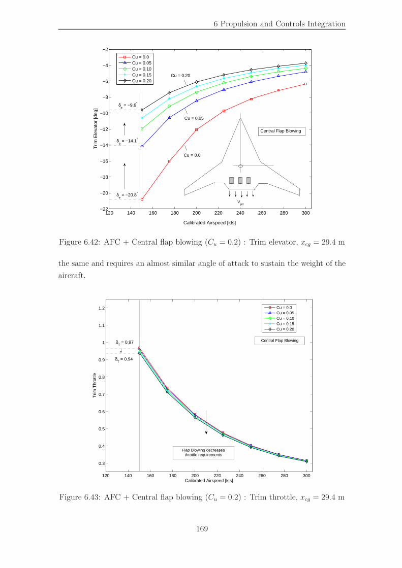
6 Propulsion and Controls Integration
120 140 160 180 200 220 240 260 280 300−22
−20
−18
−16
−14
−12
−10
−8
−6
−4
−2
Trim
Ele
vato
r [d
eg]
Calibrated Airspeed [kts]
Cu = 0.0Cu = 0.05Cu = 0.10Cu = 0.15Cu = 0.20
δe = −20.8°
δe = −14.1°
δe = −9.6°
Cu = 0.0
Cu = 0.05
Cu = 0.20
Central Flap Blowing
Vjet
Figure 6.42: AFC + Central flap blowing (Cu = 0.2) : Trim elevator, xcg = 29.4 m
the same and requires an almost similar angle of attack to sustain the weight of the
aircraft.
120 140 160 180 200 220 240 260 280 300
0.3
0.4
0.5
0.6
0.7
0.8
0.9
1
1.1
1.2
Trim
Thr
ottle
Calibrated Airspeed [kts]
Cu = 0.0Cu = 0.05Cu = 0.10Cu = 0.15Cu = 0.20
δT = 0.97
δT = 0.94
Central Flap Blowing
Flap Blowing decreasesthrottle requirements
Figure 6.43: AFC + Central flap blowing (Cu = 0.2) : Trim throttle, xcg = 29.4 m
169
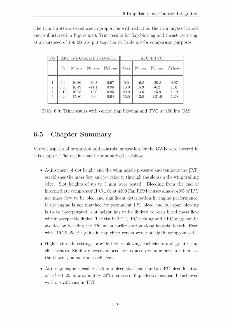
6 Propulsion and Controls Integration
The trim throttle also reduces in proportion with reduction the trim angle of attack
and is illustrated in Figure 6.43. Trim results for flap blowing and thrust vectoring,
at an airspeed of 150 kts are put together in Table 6.9 for comparison purposes.
No AFC with Central Flap Blowing AFC + TVC
Cu [α]trim [δe]trim [δT ]trim δNoz [α]trim [δe]trim [δT ]trim
1 0.0 16.80 -20.8 0.97 0.0 16.8 -20.8 0.972 0.05 16.49 -14.1 0.96 10.0 15.9 -6.2 1.013 0.10 16.25 -12.0 0.95 20.0 14.6 +5.9 1.104 0.20 15.80 -9.6 0.94 30.0 12.8 +21.0 1.20
Table 6.9: Trim results with central flap blowing and TVC at 150 kts CAS
6.5 Chapter Summary
Various aspects of propulsion and controls integration for the BWB were covered in
this chapter. The results may be summarized as follows.
• Adjustment of slot height and the wing nozzle pressure and temperature [P,T]
establishes the mass flow and jet velocity through the slots on the wing trailing
edge. Slot heights of up to 3 mm were tested. Bleeding from the end of
intermediate compressor IPC(1.0) at 4300 Fan RPM causes almost 40% of IPC
net mass flow to be bled and significant deterioation in engine performance.
If the engine is not matched for permanent IPC bleed and full span blowing
is to be incorporated, slot height has to be limited to keep bleed mass flow
within acceptable limits. The rise in TET, IPC choking and HPC surge can be
avoided by bleeding the IPC at an earlier station along its axial length. Even
with IPC(0.25) the gains in flap effectiveness were not highly compromised.
• Higher throttle settings provide higher blowing coefficients and greater flap
effectiveness. Similarly lower airspeeds or reduced dynamic pressures increase
the blowing momentum coefficient.
• At design engine speed, with 2 mm bleed slot height and an IPC bleed location
of x/l = 0.25, approximately 20% increase in flap effectiveness can be achieved
with a +72K rise in TET.
170
6 Propulsion and Controls Integration
• The rise in TET due to IPC bleed can be avoided by bleeding the LPC stage or
matching the engine for permanent IPC bleed. Both these options can provide
much higher blowing coefficients without affecting engine performance.
• Both thrust vectoring and flap blowing have the potential to increase flap
effectiveness. Elevator deflections were shown to be reduced to half with a
central flap blowing coefficient of 0.2. Similar results were achieved for the
aileron and the rudder.
• To keep the blowing duct diameter small, it is suggested that minimal bleed
be taken from the intermediate compressor. To achieve this, only selective
flaps such as aileron and the winglet rudders may be blown at lower airspeeds.
For the longitudinal axis, it is suggested to use external flap blowing directly,
thus not only providing larger blowing coefficients, but also a mechanism to
deflect thrust, thus eliminating the need for special thrust vectoring nozzles.
The amount of thrust deflection that can be actually achieved with such an
arrangement shall however requires further CFD/experimental work, and can
be made part of future research.
171

6 Propulsion and Controls Integration
172
Chapter 7
Landing and Take-off Performance
7.1 General Description
This chapter may be considered as a continuation of the previous chapter on propul-
sion and controls integration, however it considers the longitudinal axis only and
takes a closer look at the landing and take-off phases. The aim is to expand upon
the results obtained earlier and investigate the benefits of thrust vectoring or flap
blowing for these particular low speed flight conditions.
To achieve the above objective, a non-linear six degree of freedom flight simula-
tion was programmed in the C Language in which both the strip element airframe
and the engine models were simulated in real time. Body axis equations of motion
were used for the aircraft and the engine model was implemented using the hy-
brid approach developed earlier. The atmospheric properties were simulated using
the international standard atmospheric (ISA) model. The simulation runs in real
time with 76 strip elements and provides a visual environment to study both air-
craft dynamics and engine responses simultaneously. Blowing coefficients can be user
specified or set by means of adjusting the slot height and specifying a bleed location.
A flight control system (FCS) was also designed that provided control with both
AFC and TVC modes. The design of this FCS is covered in Appendix C. Figure 7.1
shows a snapshot of the simulation showing a graphical representations of the engine
and the aircraft.
173
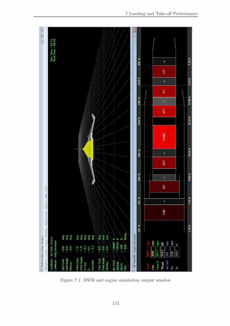
7 Landing and Take-off Performance
Figure 7.1: BWB and engine simulation output window
174
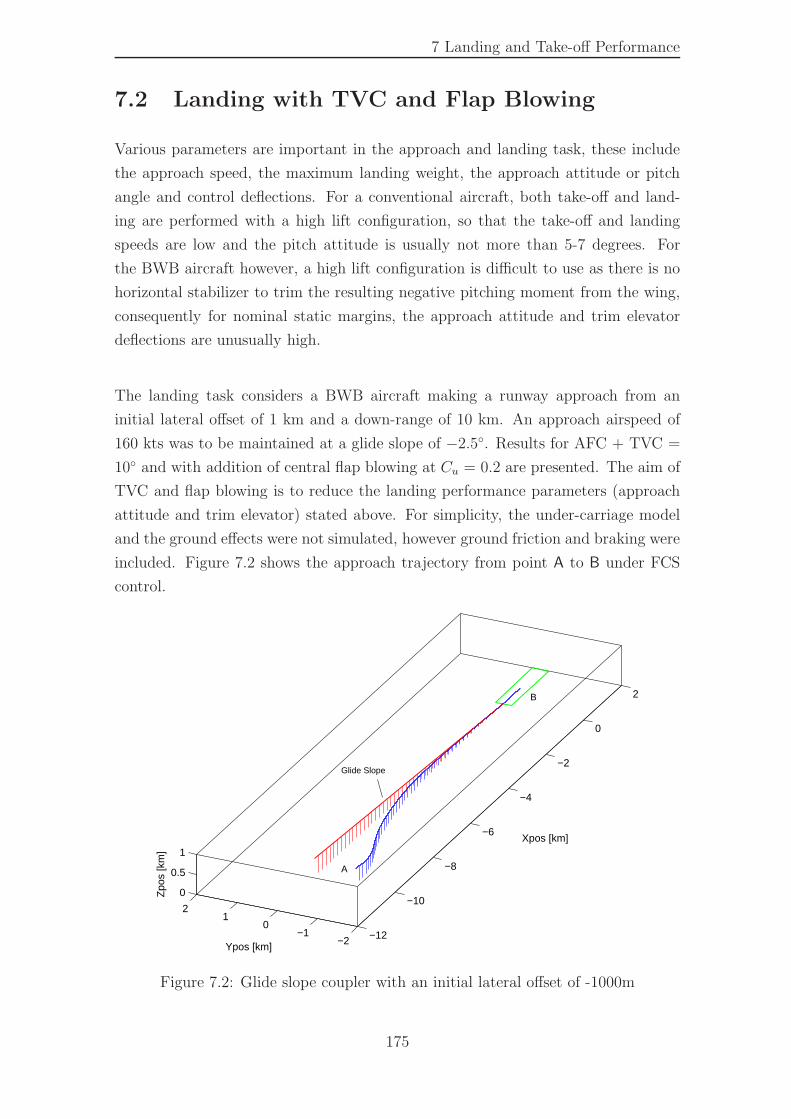
7 Landing and Take-off Performance
7.2 Landing with TVC and Flap Blowing
Various parameters are important in the approach and landing task, these include
the approach speed, the maximum landing weight, the approach attitude or pitch
angle and control deflections. For a conventional aircraft, both take-off and land-
ing are performed with a high lift configuration, so that the take-off and landing
speeds are low and the pitch attitude is usually not more than 5-7 degrees. For
the BWB aircraft however, a high lift configuration is difficult to use as there is no
horizontal stabilizer to trim the resulting negative pitching moment from the wing,
consequently for nominal static margins, the approach attitude and trim elevator
deflections are unusually high.
The landing task considers a BWB aircraft making a runway approach from an
initial lateral offset of 1 km and a down-range of 10 km. An approach airspeed of
160 kts was to be maintained at a glide slope of −2.5◦. Results for AFC + TVC =
10◦ and with addition of central flap blowing at Cu = 0.2 are presented. The aim of
TVC and flap blowing is to reduce the landing performance parameters (approach
attitude and trim elevator) stated above. For simplicity, the under-carriage model
and the ground effects were not simulated, however ground friction and braking were
included. Figure 7.2 shows the approach trajectory from point A to B under FCS
control.
−12
−10
−8
−6
−4
−2
0
2
−2−1
01
2
0
0.5
1Xpos [km]
Ypos [km]
Zpo
s [k
m]
Glide Slope
A
B
Figure 7.2: Glide slope coupler with an initial lateral offset of -1000m
175
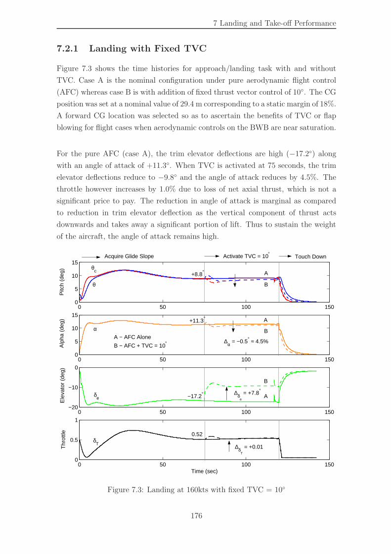
7 Landing and Take-off Performance
7.2.1 Landing with Fixed TVC
Figure 7.3 shows the time histories for approach/landing task with and without
TVC. Case A is the nominal configuration under pure aerodynamic flight control
(AFC) whereas case B is with addition of fixed thrust vector control of 10◦. The CG
position was set at a nominal value of 29.4 m corresponding to a static margin of 18%.
A forward CG location was selected so as to ascertain the benefits of TVC or flap
blowing for flight cases when aerodynamic controls on the BWB are near saturation.
For the pure AFC (case A), the trim elevator deflections are high (−17.2◦) along
with an angle of attack of +11.3◦. When TVC is activated at 75 seconds, the trim
elevator deflections reduce to −9.8◦ and the angle of attack reduces by 4.5%. The
throttle however increases by 1.0% due to loss of net axial thrust, which is not a
significant price to pay. The reduction in angle of attack is marginal as compared
to reduction in trim elevator deflection as the vertical component of thrust acts
downwards and takes away a significant portion of lift. Thus to sustain the weight
of the aircraft, the angle of attack remains high.
0 50 100 1500
5
10
15
Pitc
h (d
eg)
0 50 100 1500
5
10
15
Alp
ha (
deg)
0 50 100 150−20
−10
0
Ele
vato
r (d
eg)
0 50 100 1500
0.5
1
Thr
ottle
Time (sec)
θc
θ
α
δe
δT
Acquire Glide Slope Activate TVC = 10°
A
B
∆δe
= +7.8°
∆δT
= +0.01
A
B
Touch Down
∆α = −0.5° ≈ 4.5%A − AFC Alone
B − AFC + TVC = 10°
A
B
−17.2°
+11.3°
+8.8°
0.52
Figure 7.3: Landing at 160kts with fixed TVC = 10◦
176
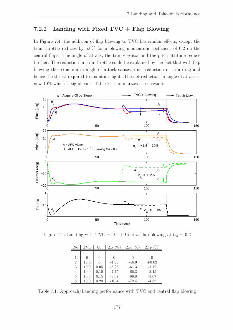
7 Landing and Take-off Performance
7.2.2 Landing with Fixed TVC + Flap Blowing
In Figure 7.4, the addition of flap blowing to TVC has similar effects, except the
trim throttle reduces by 5.0% for a blowing momentum coefficient of 0.2 on the
central flaps. The angle of attack, the trim elevator and the pitch attitude reduce
further. The reduction in trim throttle could be explained by the fact that with flap
blowing the reduction in angle of attack causes a net reduction in trim drag and
hence the thrust required to maintain flight. The net reduction in angle of attack is
now 10% which is significant. Table 7.1 summarizes these results.
0 50 100 1500
5
10
15
Pitc
h (d
eg)
0 50 100 1500
5
10
15
Alp
ha (
deg)
0 50 100 150−20
−10
0
Ele
vato
r (d
eg)
0 50 100 1500
0.5
1
Thr
ottle
Time (sec)
θc
θ
α
δe
δT
Acquire Glide Slope TVC + Blowing
A
B
∆δe
= +12.5°
∆δT
= −0.05
A
B
Touch Down
∆α = −1.4° ≈ 10%A − AFC Alone
B − AFC + TVC = 10° + Blowing Cu = 0.2
A
B
Figure 7.4: Landing with TVC = 10◦ + Central flap blowing at Cu = 0.2
No TVC Cu ∆α (%) ∆δe (%) ∆δT (%)
1 0 0 0 0 02 10.0 0 -4.50 -46.0 +0.623 10.0 0.05 -6.26 -61.3 -1.124 10.0 0.10 -7.75 -66.3 -2.455 10.0 0.15 -9.07 -69.8 -3.676 10.0 0.20 -10.4 -72.4 -4.82
Table 7.1: Approach/Landing performance with TVC and central flap blowing
177
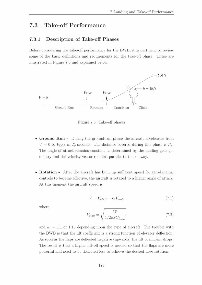
7 Landing and Take-off Performance
7.3 Take-off Performance
7.3.1 Description of Take-off Phases
Before considering the take-off performance for the BWB, it is pertinent to review
some of the basic definitions and requirements for the take-off phase. These are
illustrated in Figure 7.5 and explained below.
h = 500ft
V2 � h = 50ftVLOFVROT
ClimbTransition
? ?V = 0
Ground Run Rotation
Figure 7.5: Take-off phases
• Ground Run - During the ground-run phase the aircraft accelerates from
V = 0 to VLOF in Tg seconds. The distance covered during this phase is Rg.
The angle of attack remains constant as determined by the landing gear ge-
ometry and the velocity vector remains parallel to the runway.
• Rotation - After the aircraft has built up sufficient speed for aerodynamic
controls to become effective, the aircraft is rotated to a higher angle of attack.
At this moment the aircraft speed is
V = VLOF = k1Vstall (7.1)
where
Vstall =
√
W
1/2ρSCLmax(7.2)
and k1 = 1.1 or 1.15 depending upon the type of aircraft. The trouble with
the BWB is that the lift coefficient is a strong function of elevator deflection.
As soon as the flaps are deflected negative (upwards) the lift coefficient drops.
The result is that a higher lift-off speed is needed so that the flaps are more
powerful and need to be deflected less to achieve the desired nose rotation.
178
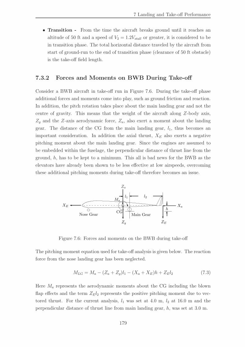
7 Landing and Take-off Performance
• Transition - From the time the aircraft breaks ground until it reaches an
altitude of 50 ft and a speed of V2 = 1.2Vstall or greater, it is considered to be
in transition phase. The total horizontal distance traveled by the aircraft from
start of ground-run to the end of transition phase (clearance of 50 ft obstacle)
is the take-off field length.
7.3.2 Forces and Moments on BWB During Take-off
Consider a BWB aircraft in take-off run in Figure 7.6. During the take-off phase
additional forces and moments come into play, such as ground friction and reaction.
In addition, the pitch rotation takes place about the main landing gear and not the
centre of gravity. This means that the weight of the aircraft along Z-body axis,
Zg and the Z-axis aerodynamic force, Za, also exert a moment about the landing
gear. The distance of the CG from the main landing gear, l1, thus becomes an
important consideration. In addition the axial thrust, XE also exerts a negative
pitching moment about the main landing gear. Since the engines are assumed to
be embedded within the fuselage, the perpendicular distance of thrust line from the
ground, h, has to be kept to a minimum. This all is bad news for the BWB as the
elevators have already been shown to be less effective at low airspeeds, overcoming
these additional pitching moments during take-off therefore becomes an issue.
�
Za
?
� ?XE?
Nose Gear Main Gear
�-
Zg
hXa
6
W
CG
l1Ma
l2
?
-
ZE
Figure 7.6: Forces and moments on the BWB during take-off
The pitching moment equation used for take-off analysis is given below. The reaction
force from the nose landing gear has been neglected.
MLG = Ma − (Za + Zg)l1 − (Xa +XE)h+ ZEl2 (7.3)
Here Ma represents the aerodynamic moments about the CG including the blown
flap effects and the term ZEl2 represents the positive pitching moment due to vec-
tored thrust. For the current analysis, l1 was set at 4.0 m, l2 at 16.0 m and the
perpendicular distance of thrust line from main landing gear, h, was set at 3.0 m.
179
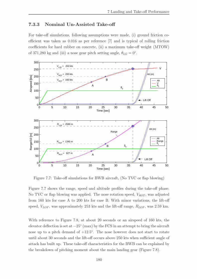
7 Landing and Take-off Performance
7.3.3 Nominal Un-Assisted Take-off
For take-off simulations, following assumptions were made, (i) ground friction co-
efficient was taken as 0.016 as per reference [7] and is typical of rolling friction
coefficients for hard rubber on concrete, (ii) a maximum take-off weight (MTOW)
of 371,280 kg and (iii) a nose gear pitch setting angle, θLG = 0◦.
0 5 10 15 20 25 30 35 40 45 500
50
100
150
200
250
300
Time [sec]
Airs
peed
[kts
]
VLOF
≈ 253 kts
VROT
= 160 kts
VROT
= 200 kts
0 5 10 15 20 25 30 35 40 45 500
50
100
150
200
250
300
Time [sec]
Ran
ge/1
0 [m
]
RROT
= 827 m
RLOF
≈ 2590 m
RROT
= 1345 m
AltVδ
T
AltRangeδ
T
Alt (m)
Alt (m)
δT
δT
A
B
B
A
Lift Off
Lift Off
V
Range
Figure 7.7: Take-off simulations for BWB aircraft, (No TVC or flap blowing)
Figure 7.7 shows the range, speed and altitude profiles during the take-off phase.
No TVC or flap blowing was applied. The nose rotation speed, VROT , was adjusted
from 160 kts for case A to 200 kts for case B. With minor variations, the lift-off
speed, VLOF , was approximately 253 kts and the lift-off range, RLOF , was 2.59 km.
With reference to Figure 7.8, at about 20 seconds or an airspeed of 160 kts, the
elevator deflection is set at −25◦ (max) by the FCS in an attempt to bring the aircraft
nose up to a pitch demand of +12.5◦. The nose however does not start to rotate
until about 30 seconds and the lift-off occurs above 250 kts when sufficient angle of
attack has built up. These take-off characteristics for the BWB can be explained by
the breakdown of pitching moment about the main landing gear (Figure 7.8).
180
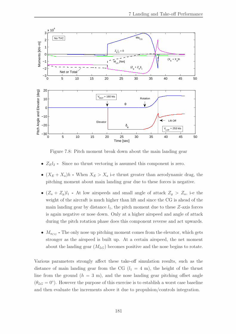
7 Landing and Take-off Performance
0 5 10 15 20 25 30 35 40 45 50−3
−2
−1
0
1
2
3x 10
4
Mom
ents
[kN
−m
]
0 5 10 15 20 25 30 35 40 45 50−30
−20
−10
0
10
20
Time [sec]
Pitc
h A
ngle
and
Ele
vato
r (d
eg)
(XE + X
a)h
MLG
[Net]
(Zg + Z
a)l
1
MaCG
VLOF
= 253 kts
ZEl2 = 0
δe
θ
VROT
= 160 kts
Elevator
No TVC
Rotation
Lift Off
Net or Total
Figure 7.8: Pitch moment break down about the main landing gear
• ZEl2 - Since no thrust vectoring is assumed this component is zero.
• (XE +Xa)h - When XE > Xa i-e thrust greater than aerodynamic drag, the
pitching moment about main landing gear due to these forces is negative.
• (Za + Zg)l1 - At low airspeeds and small angle of attack Zg > Za, i-e the
weight of the aircraft is much higher than lift and since the CG is ahead of the
main landing gear by distance l1, the pitch moment due to these Z-axis forces
is again negative or nose down. Only at a higher airspeed and angle of attack
during the pitch rotation phase does this component reverse and act upwards.
• MaCG - The only nose up pitching moment comes from the elevator, which gets
stronger as the airspeed is built up. At a certain airspeed, the net moment
about the landing gear (MLG) becomes positive and the nose begins to rotate.
Various parameters strongly affect these take-off simulation results, such as the
distance of main landing gear from the CG (l1 = 4 m), the height of the thrust
line from the ground (h = 3 m), and the nose landing gear pitching offset angle
(θLG = 0◦). However the purpose of this exercise is to establish a worst case baseline
and then evaluate the increments above it due to propulsion/controls integration.
181
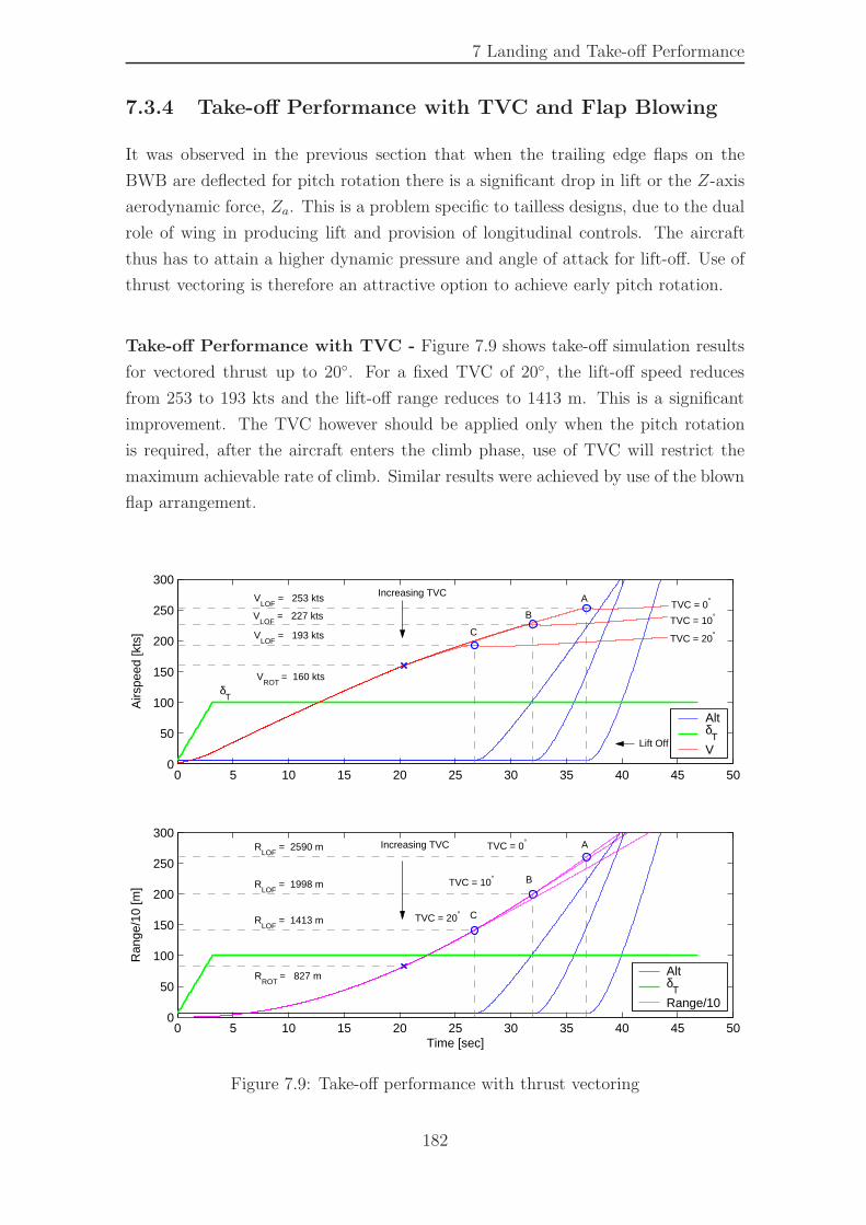
7 Landing and Take-off Performance
7.3.4 Take-off Performance with TVC and Flap Blowing
It was observed in the previous section that when the trailing edge flaps on the
BWB are deflected for pitch rotation there is a significant drop in lift or the Z-axis
aerodynamic force, Za. This is a problem specific to tailless designs, due to the dual
role of wing in producing lift and provision of longitudinal controls. The aircraft
thus has to attain a higher dynamic pressure and angle of attack for lift-off. Use of
thrust vectoring is therefore an attractive option to achieve early pitch rotation.
Take-off Performance with TVC - Figure 7.9 shows take-off simulation results
for vectored thrust up to 20◦. For a fixed TVC of 20◦, the lift-off speed reduces
from 253 to 193 kts and the lift-off range reduces to 1413 m. This is a significant
improvement. The TVC however should be applied only when the pitch rotation
is required, after the aircraft enters the climb phase, use of TVC will restrict the
maximum achievable rate of climb. Similar results were achieved by use of the blown
flap arrangement.
0 5 10 15 20 25 30 35 40 45 500
50
100
150
200
250
300
Airs
peed
[kts
]
VLOF
= 253 kts
VROT
= 160 kts
VLOF
= 227 kts
VLOF
= 193 kts
0 5 10 15 20 25 30 35 40 45 500
50
100
150
200
250
300
Time [sec]
Ran
ge/1
0 [m
]
RLOF
= 2590 m
RROT
= 827 m
RLOF
= 1998 m
RLOF
= 1413 m
Altδ
TV
Altδ
TRange/10
δT
TVC = 10°
TVC = 20°
A
A
B
B
C
C
Lift Off
TVC = 0° Increasing TVC
Increasing TVC
TVC = 20°
TVC = 10°
TVC = 0°
Figure 7.9: Take-off performance with thrust vectoring
182
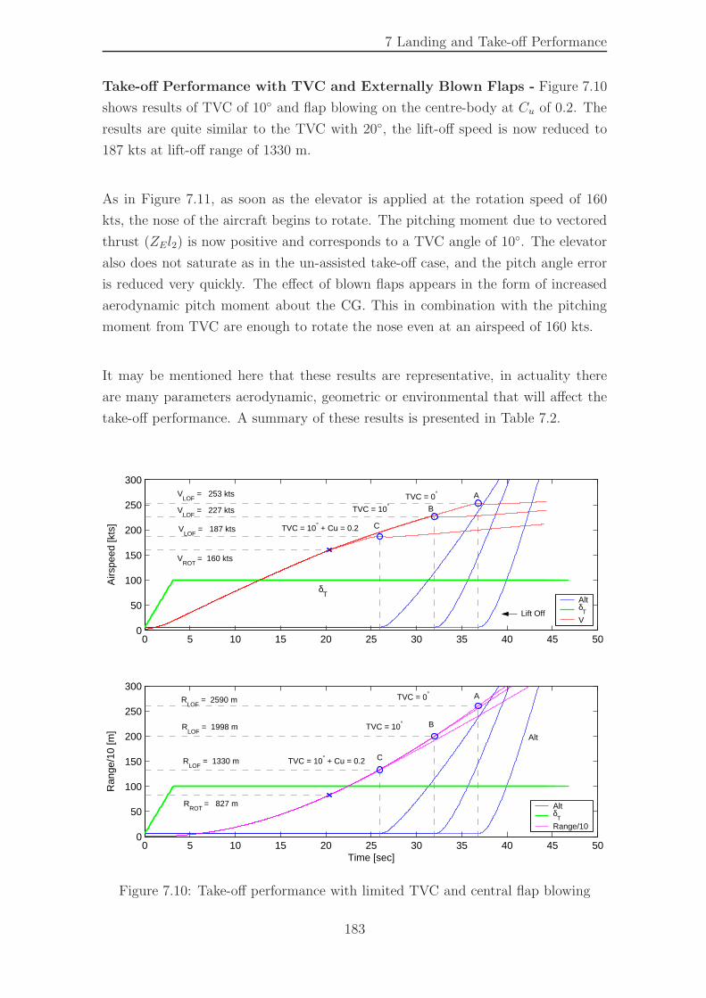
7 Landing and Take-off Performance
Take-off Performance with TVC and Externally Blown Flaps - Figure 7.10
shows results of TVC of 10◦ and flap blowing on the centre-body at Cu of 0.2. The
results are quite similar to the TVC with 20◦, the lift-off speed is now reduced to
187 kts at lift-off range of 1330 m.
As in Figure 7.11, as soon as the elevator is applied at the rotation speed of 160
kts, the nose of the aircraft begins to rotate. The pitching moment due to vectored
thrust (ZEl2) is now positive and corresponds to a TVC angle of 10◦. The elevator
also does not saturate as in the un-assisted take-off case, and the pitch angle error
is reduced very quickly. The effect of blown flaps appears in the form of increased
aerodynamic pitch moment about the CG. This in combination with the pitching
moment from TVC are enough to rotate the nose even at an airspeed of 160 kts.
It may be mentioned here that these results are representative, in actuality there
are many parameters aerodynamic, geometric or environmental that will affect the
take-off performance. A summary of these results is presented in Table 7.2.
0 5 10 15 20 25 30 35 40 45 500
50
100
150
200
250
300
Airs
peed
[kts
]
VLOF
= 253 kts
VROT
= 160 kts
VLOF
= 227 kts
VLOF
= 187 kts
0 5 10 15 20 25 30 35 40 45 500
50
100
150
200
250
300
Time [sec]
Ran
ge/1
0 [m
]
RLOF
= 2590 m
RROT
= 827 m
RLOF
= 1998 m
RLOF
= 1330 m
Altδ
T
V
Altδ
T
Range/10
δT
A
A
B
B
Lift Off
TVC = 10°
TVC = 0°
TVC = 10° + Cu = 0.2 C
TVC = 10° + Cu = 0.2
TVC = 10°
TVC = 0°
C
Alt
Figure 7.10: Take-off performance with limited TVC and central flap blowing
183
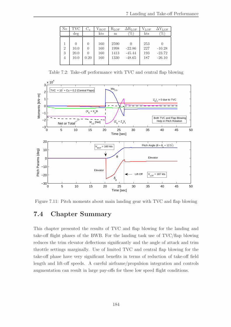
7 Landing and Take-off Performance
No TVC Cu VROT RLOF ∆RLOF VLOF ∆VLOF
deg kts m (%) kts (%)
1 0 0 160 2590 0 253 02 10.0 0 160 1998 -22.86 227 -10.283 20.0 0 160 1413 -45.44 193 -23.724 10.0 0.20 160 1330 -48.65 187 -26.10
Table 7.2: Take-off performance with TVC and central flap blowing
0 5 10 15 20 25 30 35 40 45 50−3
−2
−1
0
1
2
3x 10
4
Mom
ents
[kN
−m
]
Time [sec]
0 5 10 15 20 25 30 35 40 45 50−30
−20
−10
0
10
20
Time [sec]
Pitc
h P
aram
s (d
eg)
(XE + X
a)h
MLG
[Net] (Zg + Z
a)l
1
MaCG
VLOF
= 187 kts
ZEl2 > 0 due to TVC
δe
θ
VROT
= 160 kts
Elevator
TVC = 10° + Cu = 0.2 (Central Flaps)
Lift Off
Pitch Angle (θ = θc = 12.5°)
Elevator
Both TVC and Flap Blowing Help in Pitch Rotation
Net or Total
Figure 7.11: Pitch moments about main landing gear with TVC and flap blowing
7.4 Chapter Summary
This chapter presented the results of TVC and flap blowing for the landing and
take-off flight phases of the BWB. For the landing task use of TVC/flap blowing
reduces the trim elevator deflections significantly and the angle of attack and trim
throttle settings marginally. Use of limited TVC and central flap blowing for the
take-off phase have very significant benefits in terms of reduction of take-off field
length and lift-off speeds. A careful airframe/propulsion integration and controls
augmentation can result in large pay-offs for these low speed flight conditions.
184

Chapter 8
Conclusions and Further Research
This chapter concludes this research work and presents a summary of the main
findings. In addition, it suggests some guidelines for further research on the subject.
8.1 Conclusions
The integration of propulsion and flight control systems for the BWB aircraft is
a multidisciplinary design problem. Excluding structural aspects, it involved at
least three major areas, namely, (i) the propulsion system, (ii) the airframe and
the last but not the least (iii) the flight control system. Thus the basic research
question needed expertise in all these well defined and intricate disciplines. It was
therefore difficult for a single researcher to be able to address all these areas with
equal efficacy, however a humble effort has been made in a limited time frame and
certain conclusions were drawn. These are summarized as follows.
• Control Authority of the Baseline Configuration - Longitudinal trim
analysis reveals that for nominal static margins (Kn > 15%) and low airspeeds
(V < 200 kts), large negative elevator deflections are required to maintain trim
and as a consequence the BWB aircraft looses much of its lift generation capa-
bility. This is contrary to what is desired at take-off and landing speeds when
the required lift coefficient must be high to sustain the weight of the aircraft.
If conventional aerodynamic controls are to be retained it becomes apparent
from longiudinal trim analysis alone that the only efficient way to fly the BWB
aircraft is to fly it either neutrally stable or at a much reduced static margin
(5% < Kn < 10%). A similar analysis for the lateral directional axis shows
that at low dynamic pressures, the small winglet rudders are not sufficient to
maintain direction under an asymmetric thrust flight condition.
185
8 Conclusions and Further Research
These results however do not come as a surprise since the BWB design neither
has a conventional horizontal stabilizer or a vertical fin. A price has to be
payed in order to achieve the promised high speed aerodynamic efficiency. To
conclude, both rudder and elevator control authority augmentation are con-
sidered necessary at landing and take-off speeds.
• Linear Dynamics and Stability Augmentation - Longitudinal linear
analysis suggests that as soon as the static margin gets below 10%, the short
period mode detoriates rapidly. This is contrary to the longitudinal trim re-
quirements where a lower static margin is desirable. In either case, a stability
augmenation system (SAS) using angle of attack and pitch rate feedback was
designed and implemented, ensuring Level 1 flying qualities throughout the
flight enevelope. This flight control system was found to work adequately well
even with the blown flap and thrust vectored arrangements.
The open loop lateral-directional dynamics were very poor, with strong roll/yaw
cross coupling and high values of adverse yaw. The dutch roll mode is very
slow and poorly damped however it was improved using sideslip and yaw rate
feedback but higher gains had to be used due to limited rudder control power.
The adverse yaw problem was also severe, and large values of aileron to rudder
interconnect were required to maintain coordinated turns. In fact at low air-
speeds, the aileron to rudder interconnect gain (KARI) exceeds 1.0, that is the
same amount of rudder deflection as the aileron. Considering its small size,
both the static and dynamic requirements on the winglet rudder are severe.
The roll axis was also found to be sluggish due to the large roll axis inertia.
The inboard ailerons were not able to meet the handling qualities require-
ments at low airspeeds, necessitating the use of control allocation or use of
additional outboard flaps for the roll control below 200 kts. This means a
further reduction in pitch control authority and strengthening of the earlier
argument for using alternate means of control augmentation for the pitch axis.
• Propulsion and Airframe Models with Blown Flap Effects - A hy-
brid three spool turbofan model using a combination of iterative and inter-
component volume techniques was developed. The model provided valuable
insight into the effects on engine performance due to IPC/LPC bleed, re-
quired for flap blowing or due to thrust vectoring, required for pitch controls
186
8 Conclusions and Further Research
augmentation. Subsequently a BWB aerodynamic model using strip element
techniques and Engineering Sciences Data Units (ESDUs) was developed and
validated against the baseline [7]. The effect of trailing edge flap blowing and
the corresponding increase in lift coefficient was incorporated in the model
using the Spence’s jet flap theory [14].
Flap blowing causes a significant increase in flap effectiveness (CLδe ) and there-
fore the pitching moment (Cmδe ) produced by it. For positive flap deflections,
usually required for high lift, the change in lift coefficient (∆CLδe ) is positive
and the pitching moment negative. For negative flap deflections, required for
pitch trim, the converse is true. Flap blowing has traditionally been used to
generate high lift, however the accompanying negative pitching moment is a
problem for the BWB. This negative pitch moment has to be overcome ei-
ther by a provision of an additional control surface such a canard, or through
propulsive means, before the full potential of flap blowing for high lift can
be realized. For the BWB aircraft however, the flaps are deflected negative
to maintain pitch trim, the effect of blown flaps appears as reduction in trim
elevator deflections or greater pitch control power.
The increments in lift and pitching moments were evaluated at various blowing
coefficients, Cu, for full span flap blowing. Even for a conservative Cu of 0.2
at +25 deg flap deflection, the increment in lift coefficient (∆CLδe ) exceeds
1.0, but at the same time is also accompanied by a strong nose down pitch
moment. For the lateral-directional axis the control power was doubled at
Cu = 0.2 for both the inboard aileron and the winglet rudder.
• Allowable Engine Bleed and Achievable Blowing Coefficients - With
the engine and airframe models in place, it was now possible to integrate these
models in a non-linear simulation environment. Allowable engine bleeds, suit-
able bleed locations and the achievable blowing coefficients were the first few
questions to be answered.
1. IPC Bleed - Internal Flap Blowing - Bleeding from the end of inter-
mediate compressor IPC(1.0) with a 3 mm slot height at 4300 Fan RPM
causes almost 40% of IPC net mass flow to be bled and a significant
degradation in engine performance. The resulting blowing coefficients
were just below Cucrit = 0.02−0.03, the minimum momentum to prevent
187
8 Conclusions and Further Research
flow separation. If the engine is not matched for permanent IPC bleed
and full span blowing is to be incorporated, slot height has to be limited
to keep bleed mass flow within acceptable limits. The rise in TET due
to IPC bleed, IP compressor choking and HP compressor surge can be
avoided by bleeding the IPC at an earlier station along its axial length.
Even with an IPC bleed location of x/l = 0.25, the gains in flap effec-
tiveness were not highly compromised. An alternate and more feasible
option is to match the engine for permanent IPC bleed, this however re-
quires freezing the airframe design first to establish bleed requirements.
The airframe and engine designs thus become inter-dependant. Both of
these options can provide much higher blowing coefficients with relatively
lower penalties on engine performance. However to keep the blowing duct
diameters small it is suggested that minimal bleed be taken from the in-
termediate compressor. To achieve this, only selected flaps such as the
aileron or the winglet rudder may be blown at lower airspeeds.
2. LPC Bleed - External Flap Blowing - If the LPC/Fan stage is used
for flap blowing, the Fan exit pressure is generally less and therefore
the jet velocities are low. However there is theoretically no limit on the
amount of mass flow that could be used for flap blowing. A feasible option
is therefore to consider all of the LPC/core mass flow for external flap
blowing for the center body section which has a span of 26 m. Thus all the
mass flow from the engine exhaust impinges upon the center body flaps.
Blowing coefficients in excess of 0.25 were shown to be easily achieved
in this way. For the longitudinal axis or pitch control, it is suggested to
use external flap blowing directly, thus not only providing larger blowing
coefficients, but also a possible mechanism to deflect thrust. The amount
of thrust deflection that can be achieved with such an arrangement shall
however require further CFD/experimental work, and can be made part
of future research.
• Controls Performance with Flap Blowing and TVC Two aspects of
controls augmentation from the propulsion system were considered, namely
thrust vectoring and flap blowing.
1. Thrust Vector Control (TVC) - For nominal static margins, pure
thrust vectoring is able to maintain pitch trim but only under high thrust
conditions. At lower throttle settings, the nozzle deflection exceeds nom-
inal limits. However, thrust vectoring is effective when used in combina-
188
8 Conclusions and Further Research
tion with aerodynamic flight controls (AFC). For the low speed approach
flight condition at 160 kts and with AFC assisted by just 10◦ of fixed
TVC, the trim elevator reduces by 46%, angle of attack by 4.5% and
accompanied by only a marginal increase in trim throttle setting. The
main benefit occurs in the take-off flight condition, where thrust vector-
ing helps in achieving early pitch rotation, thus significantly reducing the
take-off field lengths and the lift-off speeds. For example with 10◦ of
TVC, lift-off range reduces by 22% and lift-off velocity by almost 10%.
2. Flap Blowing - Utilization of blown flaps had similar effects. Blown
flaps were helpful in reducing trim flap deflections during approach and
landing and reducing lift-off distances during take-off runs. For example
addition of central flap blowing at Cu = 0.2, in addition to 10◦ TVC,
reduces the lift-off distance by another 25% and lift-off velocities by a
further 15%. Similarly, at approach speeds, flap blowing makes the flaps
more efffective, resulting in a reduction of trim flap deflections. This is
accompanied by a marginal reduction in angle of attack, which reduces
induced drag and hence in turn the required thrust to sustain flight. For
an approach case at 160 kts, addition of central flap blowing at Cu = 0.2
in addition to 10◦ of TVC, reduces trim elevator deflections by a further
26% and the throttle setting by almost 5%.
To conclude, both flap blowing and thrust vector control have comparable
advantages in provision of additional of pitch, roll and yaw control powers.
For the BWB aircraft in particular when operating with forward CG locations
at low airspeeds, controls begin to saturate and the angle of attack begins to
increase. Provision of propulsion augmentation to the aerodynamic controls at
these low speed flight conditions has potential benefits if implemented properly.
However a multi-disciplinary design approach has to be adopted to make the
overall integration of airframe, flight control system and the propulsion system
successful.
189
8 Conclusions and Further Research
8.2 Further Research
With regards to future work on the subject, following suggestions are made,
• Experimental/CFD Aerodynamic Data - The aerodynamic models de-
veloped in this work used both empirical (ESDUs) and vortex lattice methods
(VLM) to predict lift, drag, pitching moment and other aerodynamic charac-
teristics for the BWB. Effect of blown flaps was added using the well estab-
lished jet-flap theory [14]. This aerodynamic model however must be further
improved using either CFD techniques or experimental methods for aerody-
namic prediction. These methods will provide better aerodynamic estimates
for the blown flap configuration and a more accurate control systems analysis
can be carried out.
Trailing edge flap blowing or distributed propulsion concepts have the poten-
tial of reducing the overall drag by re-energizing the low energy wake from the
trailing edge [42]. In the current work, only lift and pitching moment were of
specific interest and no effort was made to evaluate the reduction in aerody-
namic drag due to trailing edge blowing. Any future work must also address
this important aspect of aircraft design.
It has been reported in this work that externally blown trailing edge flaps on
the center section can provide a possible mechanism of thrust deflection. How
much thrust deflection can practically be achieved with such an arrangement
was however not investigated. If feasible, this may provide a simple and effi-
cient way of vectored thrust for the BWB, which was considered to be valuable
during the take-off and landing phases.
• A Higher Thrust Engine Model - At the start of this research work, the
Trent 500 series engine with a sea-level static thrust of 275 kN was selected.
This was done primarily due to availability of the design point information
for this engine and also due to the fact that the Boeing-747, which is of a
similar weight class uses this engine. However later on, as further analysis was
carried out it was found that at reduced airspeeds, specifically at approach,
the induced drag is very high and a 4×275 = 1100 kN engine configuration is
not enough to maintain the desired flight path. The total thrust was scaled up
to 1650 kN both for take-off and landing analysis. Any future research effort
can expand upon the current propulsion model by updating the compressor
190
8 Conclusions and Further Research
and turbine maps and other associated engine parameters to simulate a higher
thrust engine.
• Structural and Aerodynamic Interaction - The BWB aircraft consid-
ered in this research had a span of approximately 80 m, structures of such
large size are generally not rigid. The aerodynamic model that has been de-
veloped as part of this work considers the aircraft as a rigid structure, however
the strip element approach allows easy integration of any structural changes
under variable aerodynamic loading. This may include wing bending, torsion
or even flutter. Structural/aerodynamic interaction aspects may therefore be
also considered for further research.
• Modifications to the Basic Airframe - Both thrust vectoring and flap
blowing were able to solve the control authority problem, however at lower
airspeeds and high static margins (Kn > 15%) the problem of high angle of
attack remains. A simple an efficient means to solve this problem is to relax
the static margin, which causes significant reduction in both trim angle of at-
tack and elevator deflections. If however, the static margin is to be maintained
as may be desirable for a commercial airliner, an alternate option is to use a
canard arrangement. This has the potential of providing the requisite nose
up pitching moment and reducing the trim angle of attack at low speed flight
conditions. The pros and cons of such a configuration, specifically its effects
on cruise conditions however need to be carefully examined.
The rudder control authority problem for asymmetric thrust conditions was
shown to be improved using a jet flapped rudder. However the size of the rud-
der is still too small and directional stability augmentation gains, specifically
the washout and the aileron to rudder interconnect are too high. If the cruise
drag penalties are not great, it is suggested that conventional twin vertical fins
be incorporated to the basic planform. This will also speed up the dutch roll
by providing natural directional stiffness into the aerodynamic design.
Further research specifically by an aerodynamicist will be required to validate
if the above suggestions are appropriate.
191
8 Conclusions and Further Research
8.3 Dissemination of Results
The findings have been published/presented at the following forums.
Journal Publications
• Rahman, N.U and Whidborne, J.F (2008). A Numerical Investigation into
the Effect of Engine Bleed on Performance of a Single-Spool Turbojet Engine,
Journal of Aerospace Engineering, IMECHE, Vol 222, Part G, pp 939-949.
• Rahman, N.U and Whidborne, J.F (2009). Real-Time Transient Three Spool
Turbofan Engine Simulation: A Hybrid Approach, Journal of Gas Turbines
and Power, ASME, Published Online, 051602-2 / Vol. 131, Sept 2009 .
• Rahman, N.U and Whidborne, J.F (2009). Propulsion and Flight Controls
Integration for the Blended Wing Body Transport Aircraft, Submitted to the
Journal of Aircraft.
Conference Proceedings
• Rahman, N.U and Whidborne, J.F (2008). A Lateral Directional Flight Con-
trol System for the Blended Wing Body Aircraft, Proc, UKACC International
Control Conference, 2008, Manchester, UK.
• Rahman, N.U and Whidborne, J.F (2008). A Longitudinal Flight control
System for the Blended Wing Body Aircraft, Proc, IBCAST International
Bhurban Control Conference, 2009, Islamabad, Pakistan.
• Rahman, N.U and Whidborne, J.F (2008). A Numerical Investigation of En-
gine Bleed on the performance of a Single Spool Turbojet Engine, Proc, IEEE
Controls Conference Imperial College, 2007, London, UK.
192
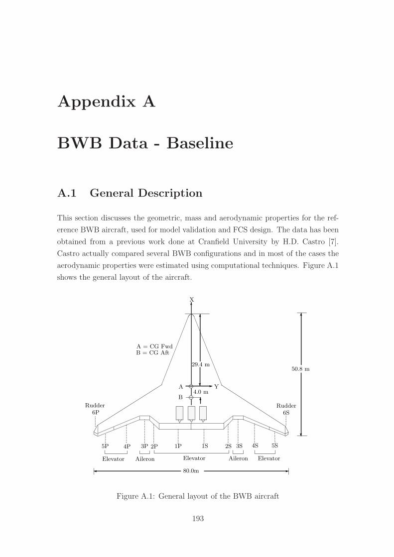
Appendix A
BWB Data - Baseline
A.1 General Description
This section discusses the geometric, mass and aerodynamic properties for the ref-
erence BWB aircraft, used for model validation and FCS design. The data has been
obtained from a previous work done at Cranfield University by H.D. Castro [7].
Castro actually compared several BWB configurations and in most of the cases the
aerodynamic properties were estimated using computational techniques. Figure A.1
shows the general layout of the aircraft.
6
6P
X
6S
-
5P 4P 3P 2P 1P
..........2S
......4S3S 5S
........... ...............
..
..
..
..
..
..
...........
............
...............
.............
........
......
.......
1S
Elevator AileronAileronElevator Elevator
RudderRudder
6
?
50.8 m
80.0m -�
6
Y
29.4 m
?
6
4.0 m
A = CG Fwd
A
B = CG Aft
B
Figure A.1: General layout of the BWB aircraft
193
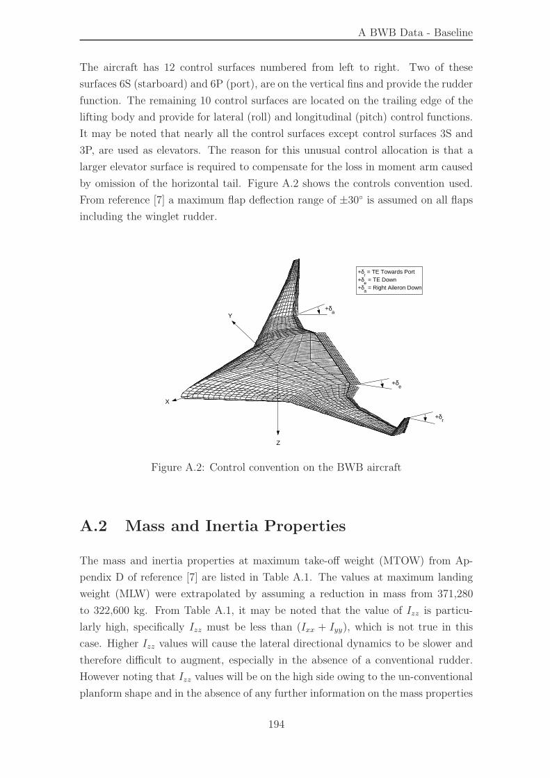
A BWB Data - Baseline
The aircraft has 12 control surfaces numbered from left to right. Two of these
surfaces 6S (starboard) and 6P (port), are on the vertical fins and provide the rudder
function. The remaining 10 control surfaces are located on the trailing edge of the
lifting body and provide for lateral (roll) and longitudinal (pitch) control functions.
It may be noted that nearly all the control surfaces except control surfaces 3S and
3P, are used as elevators. The reason for this unusual control allocation is that a
larger elevator surface is required to compensate for the loss in moment arm caused
by omission of the horizontal tail. Figure A.2 shows the controls convention used.
From reference [7] a maximum flap deflection range of ±30◦ is assumed on all flaps
including the winglet rudder.
+δr
+δe
+δa
X
Y
Z
+δr = TE Towards Port
+δe = TE Down
+δa = Right Aileron Down
Figure A.2: Control convention on the BWB aircraft
A.2 Mass and Inertia Properties
The mass and inertia properties at maximum take-off weight (MTOW) from Ap-
pendix D of reference [7] are listed in Table A.1. The values at maximum landing
weight (MLW) were extrapolated by assuming a reduction in mass from 371,280
to 322,600 kg. From Table A.1, it may be noted that the value of Izz is particu-
larly high, specifically Izz must be less than (Ixx + Iyy), which is not true in this
case. Higher Izz values will cause the lateral directional dynamics to be slower and
therefore difficult to augment, especially in the absence of a conventional rudder.
However noting that Izz values will be on the high side owing to the un-conventional
planform shape and in the absence of any further information on the mass properties
194
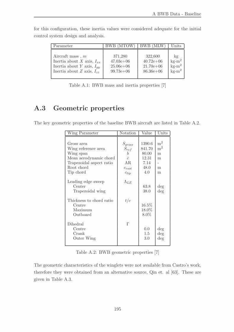
A BWB Data - Baseline
for this configuration, these inertia values were considered adequate for the initial
control system design and analysis.
Parameter BWB (MTOW) BWB (MLW) Units
Aircraft mass , m 371,280 322,600 kgInertia about X axis, Ixx 47.03e+06 40.72e+06 kg-m2
Inertia about Y axis, Iyy 25.06e+06 21.70e+06 kg-m2
Inertia about Z axis, Izz 99.73e+06 86.36e+06 kg-m2
Table A.1: BWB mass and inertia properties [7]
A.3 Geometric properties
The key geometric properties of the baseline BWB aircraft are listed in Table A.2.
Wing Parameter Notation Value Units
Gross area Sgross 1390.6 m2
Wing reference area Sref 841.70 m2
Wing span b 80.00 mMean aerodynamic chord c 12.31 mTrapezoidal aspect ratio AR 7.14 -Root chord croot 48.0 mTip chord ctip 4.0 m
Leading edge sweep ΛLECenter 63.8 degTrapezoidal wing 38.0 deg
Thickness to chord ratio t/cCentre 16.5%Maximum 18.0%Outboard 8.0%
Dihedral ΓCentre 0.0 degCrank 1.5 degOuter Wing 3.0 deg
Table A.2: BWB geometric properties [7]
The geometric characteristics of the winglets were not available from Castro’s work,
therefore they were obtained from an alternative source, Qin et. al [63]. These are
given in Table A.3.
195
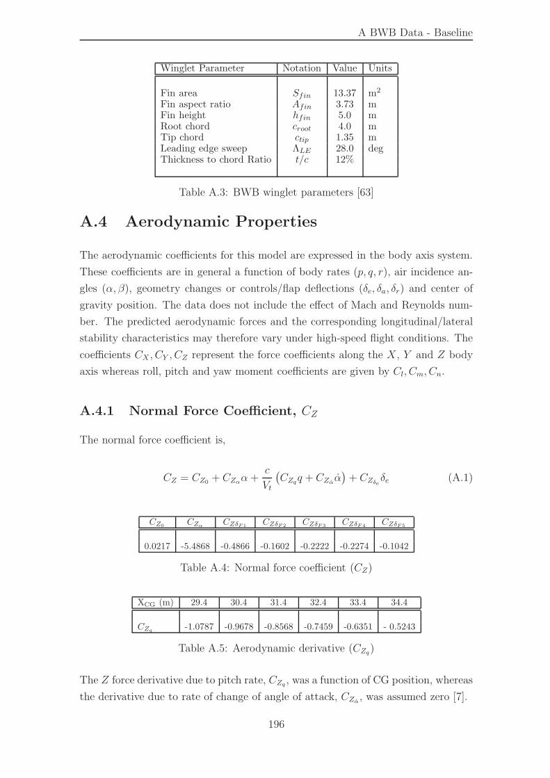
A BWB Data - Baseline
Winglet Parameter Notation Value Units
Fin area Sfin 13.37 m2
Fin aspect ratio Afin 3.73 mFin height hfin 5.0 mRoot chord croot 4.0 mTip chord ctip 1.35 mLeading edge sweep ΛLE 28.0 degThickness to chord Ratio t/c 12%
Table A.3: BWB winglet parameters [63]
A.4 Aerodynamic Properties
The aerodynamic coefficients for this model are expressed in the body axis system.
These coefficients are in general a function of body rates (p, q, r), air incidence an-
gles (α, β), geometry changes or controls/flap deflections (δe, δa, δr) and center of
gravity position. The data does not include the effect of Mach and Reynolds num-
ber. The predicted aerodynamic forces and the corresponding longitudinal/lateral
stability characteristics may therefore vary under high-speed flight conditions. The
coefficients CX , CY , CZ represent the force coefficients along the X, Y and Z body
axis whereas roll, pitch and yaw moment coefficients are given by Cl, Cm, Cn.
A.4.1 Normal Force Coefficient, CZ
The normal force coefficient is,
CZ = CZ0 + CZαα +c
Vt
(
CZqq + CZαα)
+ CZδeδe (A.1)
CZ0CZα
CZδF1CZδF2
CZδF3CZδF 4
CZδF5
0.0217 -5.4868 -0.4866 -0.1602 -0.2222 -0.2274 -0.1042
Table A.4: Normal force coefficient (CZ)
XCG (m) 29.4 30.4 31.4 32.4 33.4 34.4
CZq-1.0787 -0.9678 -0.8568 -0.7459 -0.6351 - 0.5243
Table A.5: Aerodynamic derivative (CZq)
The Z force derivative due to pitch rate, CZq , was a function of CG position, whereas
the derivative due to rate of change of angle of attack, CZα, was assumed zero [7].
196
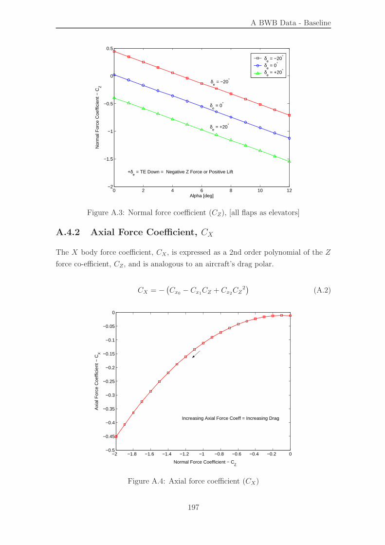
A BWB Data - Baseline
0 2 4 6 8 10 12−2
−1.5
−1
−0.5
0
0.5
Alpha [deg]
Nor
mal
For
ce C
oeffi
cien
t − C
Z
δe = −20°
δe = 0°
δe = +20°
δe = −20°
δe = 0°
δe = +20°
+δe = TE Down = Negative Z Force or Positive Lift
Figure A.3: Normal force coefficient (CZ), [all flaps as elevators]
A.4.2 Axial Force Coefficient, CX
The X body force coefficient, CX , is expressed as a 2nd order polynomial of the Z
force co-efficient, CZ , and is analogous to an aircraft’s drag polar.
CX = −(
Cx0 − Cx1CZ + Cx2CZ2)
(A.2)
−2 −1.8 −1.6 −1.4 −1.2 −1 −0.8 −0.6 −0.4 −0.2 0−0.5
−0.45
−0.4
−0.35
−0.3
−0.25
−0.2
−0.15
−0.1
−0.05
0
Axi
al F
orce
Coe
ffici
ent −
CX
Normal Force Coefficient − CZ
Increasing Axial Force Coeff = Increasing Drag
Figure A.4: Axial force coefficient (CX)
197
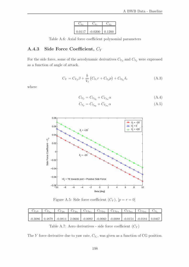
A BWB Data - Baseline
Cx0Cx1
Cx2
0.0117 -0.0200 0.1200
Table A.6: Axial force coefficient polynomial parameters
A.4.3 Side Force Coefficient, CY
For the side force, some of the aerodynamic derivatives CYβ and CYp were expressed
as a function of angle of attack.
CY = CYββ +b
Vt
(
CYrr + CYpp)
+ CYδr δr (A.3)
where
CYβ = CYβ0 + CYβαα (A.4)
CYp = CYp0 + CYpαα (A.5)
−10 −8 −6 −4 −2 0 2 4 6 8 10−0.08
−0.06
−0.04
−0.02
0
0.02
0.04
0.06
0.08
Beta [deg]
Sid
e F
orce
Coe
ffici
ent −
CY
δr = −20°
δr = 0°
δr = +20°
+δr = TE towards port = Positive Side Force
δr = +20°
δr = −20°
Figure A.5: Side force coefficient (CY ), [p = r = 0]
CYβ0 CYβαCY p0
CY pαCY δF1
CY δF2CY δF3
CY δF4CY δF5
CYδr
-0.3086 0.4879 -0.0814 2.0666 -0.0092 -0.0060 -0.0088 -0.0154 -0.0184 0.0467
Table A.7: Aero derivatives - side force coefficient (CY )
The Y force derivative due to yaw rate, CYr , was given as a function of CG position.
198
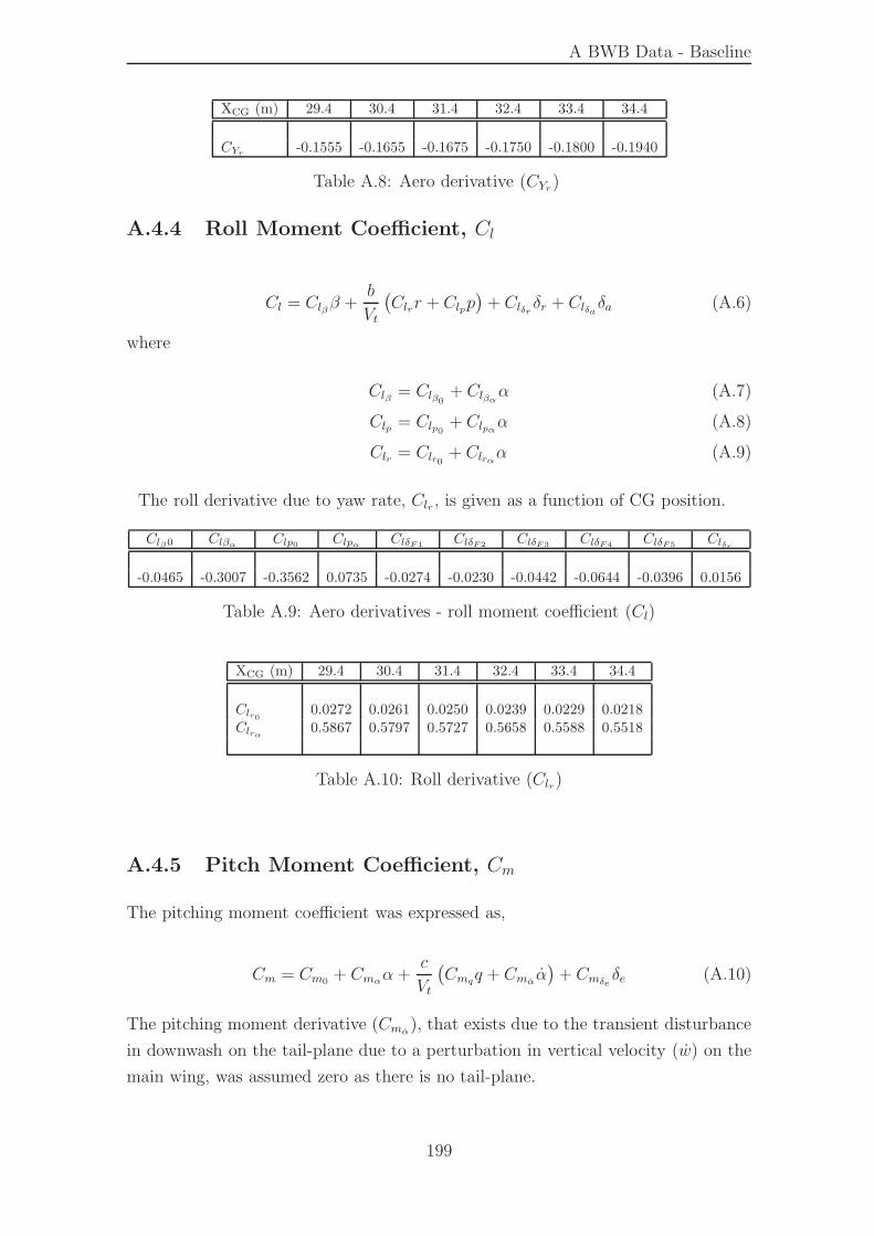
A BWB Data - Baseline
XCG (m) 29.4 30.4 31.4 32.4 33.4 34.4
CYr-0.1555 -0.1655 -0.1675 -0.1750 -0.1800 -0.1940
Table A.8: Aero derivative (CYr)
A.4.4 Roll Moment Coefficient, Cl
Cl = Clββ +b
Vt
(
Clrr + Clpp)
+ Clδr δr + Clδaδa (A.6)
where
Clβ = Clβ0 + Clβαα (A.7)
Clp = Clp0 + Clpαα (A.8)
Clr = Clr0 + Clrαα (A.9)
The roll derivative due to yaw rate, Clr , is given as a function of CG position.
Clβ0 ClβαClp0
ClpαClδF 1
ClδF2ClδF3
ClδF4ClδF5
Clδr
-0.0465 -0.3007 -0.3562 0.0735 -0.0274 -0.0230 -0.0442 -0.0644 -0.0396 0.0156
Table A.9: Aero derivatives - roll moment coefficient (Cl)
XCG (m) 29.4 30.4 31.4 32.4 33.4 34.4
Clr00.0272 0.0261 0.0250 0.0239 0.0229 0.0218
Clrα0.5867 0.5797 0.5727 0.5658 0.5588 0.5518
Table A.10: Roll derivative (Clr)
A.4.5 Pitch Moment Coefficient, Cm
The pitching moment coefficient was expressed as,
Cm = Cm0 + Cmαα +c
Vt
(
Cmqq + Cmαα)
+ Cmδe δe (A.10)
The pitching moment derivative (Cmα), that exists due to the transient disturbance
in downwash on the tail-plane due to a perturbation in vertical velocity (w) on the
main wing, was assumed zero as there is no tail-plane.
199
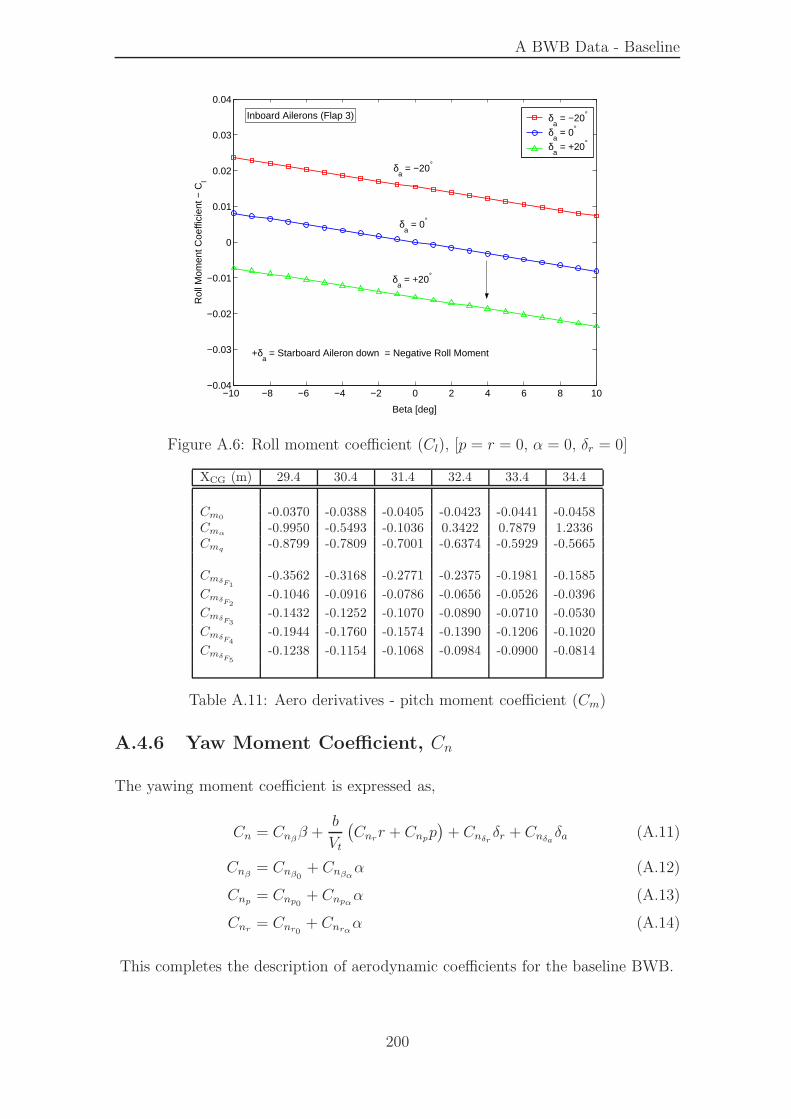
A BWB Data - Baseline
−10 −8 −6 −4 −2 0 2 4 6 8 10−0.04
−0.03
−0.02
−0.01
0
0.01
0.02
0.03
0.04
Beta [deg]
Rol
l Mom
ent C
oeffi
cien
t − C
l
δa = −20°
δa = 0°
δa = +20°
+δa = Starboard Aileron down = Negative Roll Moment
Inboard Ailerons (Flap 3)
δa = −20°
δa = 0°
δa = +20°
Figure A.6: Roll moment coefficient (Cl), [p = r = 0, α = 0, δr = 0]
XCG (m) 29.4 30.4 31.4 32.4 33.4 34.4
Cm0-0.0370 -0.0388 -0.0405 -0.0423 -0.0441 -0.0458
Cmα-0.9950 -0.5493 -0.1036 0.3422 0.7879 1.2336
Cmq-0.8799 -0.7809 -0.7001 -0.6374 -0.5929 -0.5665
CmδF1
-0.3562 -0.3168 -0.2771 -0.2375 -0.1981 -0.1585
CmδF2
-0.1046 -0.0916 -0.0786 -0.0656 -0.0526 -0.0396
CmδF3
-0.1432 -0.1252 -0.1070 -0.0890 -0.0710 -0.0530
CmδF4
-0.1944 -0.1760 -0.1574 -0.1390 -0.1206 -0.1020
CmδF5
-0.1238 -0.1154 -0.1068 -0.0984 -0.0900 -0.0814
Table A.11: Aero derivatives - pitch moment coefficient (Cm)
A.4.6 Yaw Moment Coefficient, Cn
The yawing moment coefficient is expressed as,
Cn = Cnββ +b
Vt
(
Cnrr + Cnpp)
+ Cnδr δr + Cnδaδa (A.11)
Cnβ = Cnβ0 + Cnβαα (A.12)
Cnp = Cnp0 + Cnpαα (A.13)
Cnr = Cnr0 + Cnrαα (A.14)
This completes the description of aerodynamic coefficients for the baseline BWB.
200
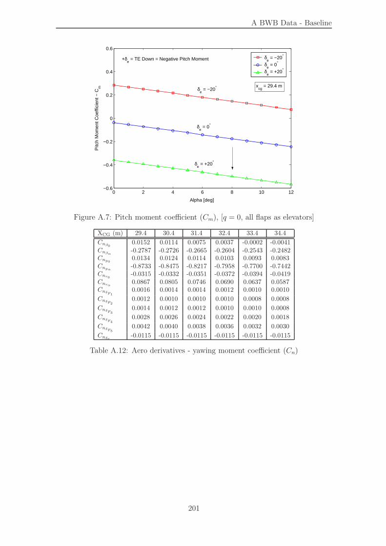
A BWB Data - Baseline
0 2 4 6 8 10 12−0.6
−0.4
−0.2
0
0.2
0.4
0.6
Alpha [deg]
Pitc
h M
omen
t Coe
ffici
ent −
Cm
δe = −20°
δe = 0°
δe = +20°
δe = −20°
δe = 0°
δe = +20°
xcg
= 29.4 m
+δe = TE Down = Negative Pitch Moment
Figure A.7: Pitch moment coefficient (Cm), [q = 0, all flaps as elevators]
XCG (m) 29.4 30.4 31.4 32.4 33.4 34.4
Cnβ00.0152 0.0114 0.0075 0.0037 -0.0002 -0.0041
Cnβα-0.2787 -0.2726 -0.2665 -0.2604 -0.2543 -0.2482
Cnp00.0134 0.0124 0.0114 0.0103 0.0093 0.0083
Cnpα-0.8733 -0.8475 -0.8217 -0.7958 -0.7700 -0.7442
Cnr0-0.0315 -0.0332 -0.0351 -0.0372 -0.0394 -0.0419
Cnrα0.0867 0.0805 0.0746 0.0690 0.0637 0.0587
CnδF1
0.0016 0.0014 0.0014 0.0012 0.0010 0.0010
CnδF2
0.0012 0.0010 0.0010 0.0010 0.0008 0.0008
CnδF3
0.0014 0.0012 0.0012 0.0010 0.0010 0.0008
CnδF4
0.0028 0.0026 0.0024 0.0022 0.0020 0.0018
CnδF5
0.0042 0.0040 0.0038 0.0036 0.0032 0.0030
Cnδr-0.0115 -0.0115 -0.0115 -0.0115 -0.0115 -0.0115
Table A.12: Aero derivatives - yawing moment coefficient (Cn)
201

A BWB Data - Baseline
202

Appendix B
BWB Linear Model
This section develops the linear model for the BWB aircraft. Specifically it covers, (i)
the derivation of dimensional derivatives specific to the BWB, (ii) some linearization
results, (iii) validation of the linear airframe model and (iv) variation in longitudinal
and lateral -directional dynamic modes with CG position and airspeed.
B.1 Dimensional Derivatives
This section discusses the derivation of X and Z force derivatives specific for the
BWB, and is then followed by the derivation of the linear model (A,B,C,D matri-
ces). This linear model is subsequently validated using a non-linear simulation and
the output of MATLAB <linmod.m> linearization utility.
The small perturbation equations of motion from Cooke [43] are reproduced below.
For control system analysis, it is desirable that the longitudinal motion of the aircraft
be uncoupled from the lateral motion. To achieve this decoupling, it is assumed that
the trim angular velocities are zero, (P1 = Q1 = R1 = 0). In addition, zero side slip
velocity (V1 = 0) and steady wings level flight (φ1 = 0) are assumed. The linearized
uncoupled longitudinal equations of motion are,
mu = (◦
Xu +◦
XTu)u+◦
Xww +◦
X ww +◦
Xqq +◦
Xδeδe −mgθ cos θ1 −mqW1 (B.1)
mw = (◦
Zu +◦
ZTu)u+◦
Zww +◦
Zww +◦
Zqq +◦
Zδeδe −mgθ sin θ1 +mqU1 (B.2)
Iyyq = (◦
Mu +◦
MTu)u+ (◦
Mw +◦
MTw)w +◦
M ww +◦
M qq +◦
M δeδe (B.3)
θ = q (B.4)
h = sin θ1u− cos θ1w + (U1 cos θ1 +W1 sin θ1)θ (B.5)
203
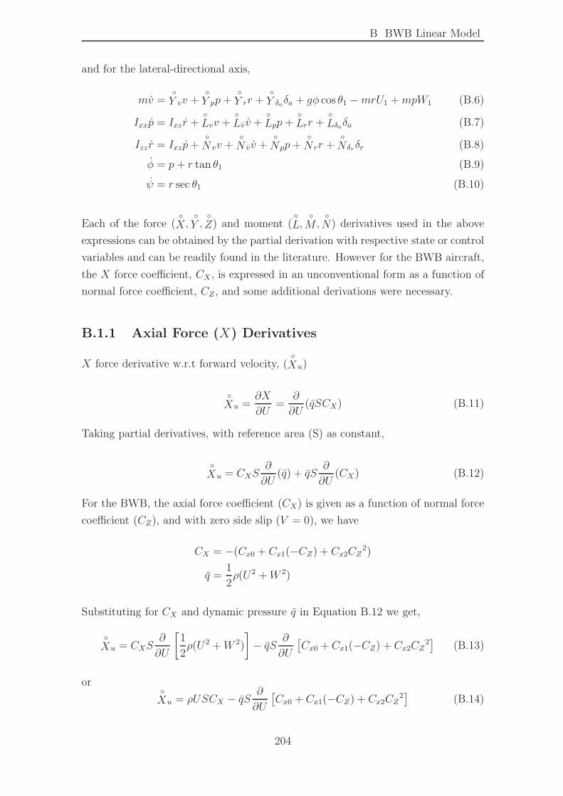
B BWB Linear Model
and for the lateral-directional axis,
mv =◦
Y vv +◦
Y pp+◦
Y rr +◦
Y δaδa + gφ cos θ1 −mrU1 +mpW1 (B.6)
Ixxp = Ixzr +◦
Lvv +◦
Lvv +◦
Lpp +◦
Lrr +◦
Lδaδa (B.7)
Izz r = Ixzp+◦
N vv +◦
N vv +◦
N pp+◦
N rr +◦
N δrδr (B.8)
φ = p+ r tan θ1 (B.9)
ψ = r sec θ1 (B.10)
Each of the force (◦
X,◦
Y ,◦
Z) and moment (◦
L,◦
M,◦
N) derivatives used in the above
expressions can be obtained by the partial derivation with respective state or control
variables and can be readily found in the literature. However for the BWB aircraft,
the X force coefficient, CX , is expressed in an unconventional form as a function of
normal force coefficient, CZ , and some additional derivations were necessary.
B.1.1 Axial Force (X) Derivatives
X force derivative w.r.t forward velocity, (◦
Xu)
◦
Xu =∂X
∂U=
∂
∂U(qSCX) (B.11)
Taking partial derivatives, with reference area (S) as constant,
◦
Xu = CXS∂
∂U(q) + qS
∂
∂U(CX) (B.12)
For the BWB, the axial force coefficient (CX) is given as a function of normal force
coefficient (CZ), and with zero side slip (V = 0), we have
CX = −(Cx0 + Cx1(−CZ) + Cx2CZ2)
q =1
2ρ(U2 +W 2)
Substituting for CX and dynamic pressure q in Equation B.12 we get,
◦
Xu = CXS∂
∂U
[
1
2ρ(U2 +W 2)
]
− qS∂
∂U
[
Cx0 + Cx1(−CZ) + Cx2CZ2]
(B.13)
or◦
Xu = ρUSCX − qS∂
∂U
[
Cx0 + Cx1(−CZ) + Cx2CZ2]
(B.14)
204
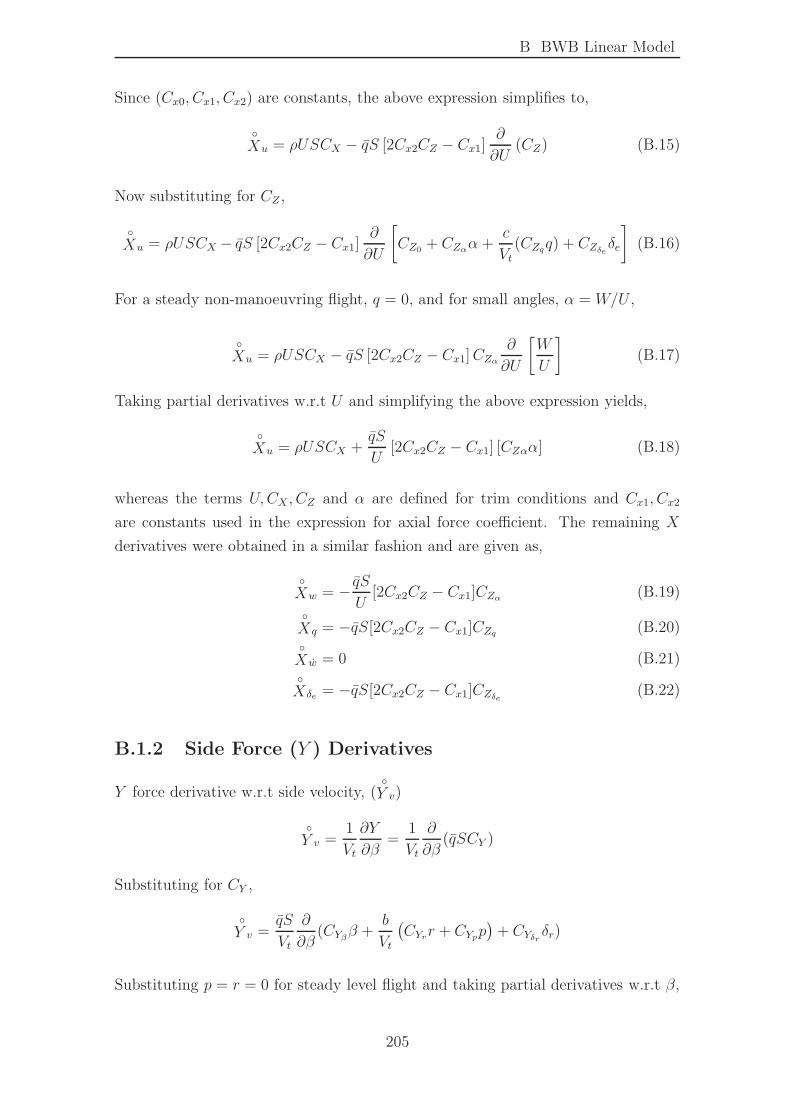
B BWB Linear Model
Since (Cx0, Cx1, Cx2) are constants, the above expression simplifies to,
◦
Xu = ρUSCX − qS [2Cx2CZ − Cx1]∂
∂U(CZ) (B.15)
Now substituting for CZ ,
◦
Xu = ρUSCX − qS [2Cx2CZ − Cx1]∂
∂U
[
CZ0 + CZαα +c
Vt(CZqq) + CZδeδe
]
(B.16)
For a steady non-manoeuvring flight, q = 0, and for small angles, α = W/U ,
◦
Xu = ρUSCX − qS [2Cx2CZ − Cx1]CZα∂
∂U
[
W
U
]
(B.17)
Taking partial derivatives w.r.t U and simplifying the above expression yields,
◦
Xu = ρUSCX +qS
U[2Cx2CZ − Cx1] [CZαα] (B.18)
whereas the terms U,CX , CZ and α are defined for trim conditions and Cx1, Cx2
are constants used in the expression for axial force coefficient. The remaining X
derivatives were obtained in a similar fashion and are given as,
◦
Xw = − qSU
[2Cx2CZ − Cx1]CZα (B.19)
◦
Xq = −qS[2Cx2CZ − Cx1]CZq (B.20)◦
X w = 0 (B.21)◦
Xδe = −qS[2Cx2CZ − Cx1]CZδe (B.22)
B.1.2 Side Force (Y ) Derivatives
Y force derivative w.r.t side velocity, (◦
Y v)
◦
Y v =1
Vt
∂Y
∂β=
1
Vt
∂
∂β(qSCY )
Substituting for CY ,
◦
Y v =qS
Vt
∂
∂β(CYββ +
b
Vt
(
CYrr + CYpp)
+ CYδr δr)
Substituting p = r = 0 for steady level flight and taking partial derivatives w.r.t β,
205
B BWB Linear Model
◦
Y v =qS
VtCYβ (B.23)
The remaining Y force derivatives are given as,
◦
Y r =qSb
VtCYr (B.24)
◦
Y p =qSb
VtCYp (B.25)
◦
Y v = 0 (B.26)◦
Y δa = qSCYδa (B.27)◦
Y δr = qSCYδr (B.28)
B.1.3 Normal Force (Z) Derivatives
Z force derivative w.r.t down velocity, (◦
Zw)
◦
Zw =∂Z
∂W=
∂
∂W(qSCZ)
Taking partial derivatives, with reference area (S) as constant,
◦
Zw = CZS∂
∂W(q) + qS
∂
∂W(CZ) (B.29)
Substituting for CX , and dynamic pressure, q, in Equation B.29 we get,
◦
Zw = CXS∂
∂W
[
1
2ρ(U2 +W 2)
]
− qS∂
∂W
[
CZ0 + CZαα +c
Vt(CZqq) + CZδeδe
]
Replacing α = W/U for small angles and taking partial derivatives we get,
◦
Zw = ρSCZW +qS
U1CZα (B.30)
The remaining Z derivatives are given as,
◦
Zu = ρSCZU − qS
UCZαα (B.31)
◦
Zq = qSCZq/(Vt/c) (B.32)◦
Zw = 0 (B.33)◦
Zδe = qSCZδe (B.34)
Again terms U,W,CZ , α now represent trim conditions.
206
B BWB Linear Model
B.1.4 Roll Moment (L) derivatives
Dimensional derivatives for the rolling moment (L) are expressed as,
◦
Lv =qSb
VtClβ (B.35)
◦
Lp =qSb2
VtClp (B.36)
◦
Lr =qSb2
VtClr (B.37)
◦
Lδa = qSbClδa (B.38)◦
Lδr = qSbClδr (B.39)
B.1.5 Pitching moment (M) derivatives
The pitching moment derivatives are,
◦
Mu = qSc(2Cm − Cmαα) (B.40)◦
Mw = qScCmα (B.41)
◦
M q =qSc2
VtCmq (B.42)
◦
M δe = qScCmδe (B.43)
B.1.6 Yawing moment (N) derivatives
Similarly for the yaw axis we have,
◦
N v =qSb
VtCnβ (B.44)
◦
Np =qSb2
VtCnp (B.45)
◦
N r =qSb2
VtCnr (B.46)
◦
N δa = qSbCnδa (B.47)◦
N δr = qSbCnδr (B.48)
207
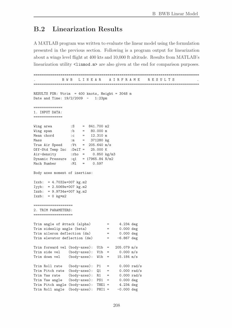
B BWB Linear Model
B.2 Linearization Results
A MATLAB program was written to evaluate the linear model using the formulation
presented in the previous section. Following is a program output for linearization
about a wings level flight at 400 kts and 10,000 ft altitude. Results from MATLAB’s
linearization utility <linmod.m> are also given at the end for comparison purposes.
=================================================================================
. B W B L I N E A R A I R F R A M E R E S U L T S .
=================================================================================
RESULTS FOR: Vtrim = 400 knots, Height = 3048 m
Date and Time: 19/2/2009 - 1:23pm
==============
1. INPUT DATA:
==============
Wing area :S = 841.700 m2
Wing span :b = 80.000 m
Mean chord :c = 12.310 m
Mass :m = 371280 kg
True Air Speed :Vt = 205.640 m/s
Off-Std Temp Inc :DelT = 25.000 K
Air-density :rho = 0.850 kg/m3
Dynamic Pressure :q1 = 17965.84 N/m2
Mach Number :M1 = 0.597
Body axes moment of inertias:
Ixxb: = 4.7032e+007 kg.m2
Iyyb: = 2.5069e+007 kg.m2
Izzb: = 9.9734e+007 kg.m2
Ixzb: = 0 kg*m2
===================
2. TRIM PARAMETERS:
===================
Trim angle of Attack (alpha) = 4.234 deg
Trim sideslip angle (beta) = 0.000 deg
Trim aileron deflection (da) = 0.000 deg
Trim elevator deflection (de) = -6.867 deg
Trim forward vel (body-axes): U1b = 205.079 m/s
Trim side vel (body-axes): V1b = 0.000 m/s
Trim down vel (body-axes): W1b = 15.184 m/s
Trim Roll rate (body-axes): P1 = 0.000 rad/s
Trim Pitch rate (body-axes): Q1 = 0.000 rad/s
Trim Yaw rate (body-axes): R1 = 0.000 rad/s
Trim Yaw angle (body-axes): PS1 = 0.000 deg
Trim Pitch angle (body-axes): THE1 = 4.234 deg
Trim Roll angle (body-axes): PHI1 = -0.000 deg
208
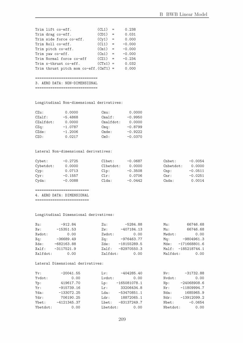
B BWB Linear Model
Trim lift co-eff. (CL1) = 0.238
Trim drag co-eff. (CD1) = 0.031
Trim side force co-eff. (Cy1) = 0.000
Trim Roll co-eff. (Cl1) = -0.000
Trim pitch co-eff. (Cm1) = -0.000
Trim yaw co-eff. (Cn1) = -0.000
Trim Normal force co-eff (CZ1) = -0.234
Trim x-thrust co-eff. (CTx1) = 0.032
Trim thrust pitch mom co-eff.(CmT1) = 0.000
=============================
3. AERO DATA: NON-DIMENSIONAL
=============================
Longitudinal Non-dimensional derivatives:
CZu: 0.0000 Cmu: 0.0000
CZalf: -5.4868 Cmalf: -0.9950
CZalfdot: 0.0000 Cmalfdot: 0.0000
CZq: -1.0787 Cmq: -0.8799
CZde: -1.2006 Cmde: -0.9222
CZ0: 0.0217 Cm0: -0.0370
Lateral Non-dimensional derivatives:
Cybet: -0.2725 Clbet: -0.0687 Cnbet: -0.0054
Cybetdot: 0.0000 Clbetdot: 0.0000 Cnbetdot: 0.0000
Cyp: 0.0713 Clp: -0.3508 Cnp: -0.0511
Cyr: -0.1557 Clr: 0.0706 Cnr: -0.0251
Cyda: -0.0088 Clda: -0.0442 Cnda: 0.0014
=========================
4. AERO DATA: DIMENSIONAL
=========================
Longitudinal Dimensional derivatives:
Xu: -912.84 Zu: -5284.88 Mu: 66746.68
Xw: -15351.53 Zw: -407184.13 Mu: 66746.68
Xwdot: 0.00 Zwdot: 0.00 Mwdot: 0.00
Xq: -36689.49 Zq: -976463.77 Mq: -9804961.3
Xde: -682163.88 Zde: -18155289.5 Mde: -171668801.6
Xalf: -3117521.9 Zalf: -82970550.3 Malf: -185218744.1
Xalfdot: 0.00 Zalfdot: 0.00 Malfdot: 0.00
Lateral Dimensional derivatives:
Yv: -20041.55 Lv: -404285.40 Nv: -31732.88
Yvdot: 0.00 Lvdot: 0.00 Nvdot: 0.00
Yp: 419617.70 Lp: -165081078.1 Np: -24068908.6
Yr: -915739.16 Lr: 33206434.8 Nr: -11809994.7
Yda: -133072.25 Lda: -53470851.1 Nda: 1685965.9
Ydr: 706190.25 Ldr: 18872065.1 Ndr: -13912099.2
Ybet: -4121345.37 Lbet: -83137249.7 Nbet: -0.0654
Ybetdot: 0.00 Lbetdot: 0.00 Nbetdot: 0.00
209
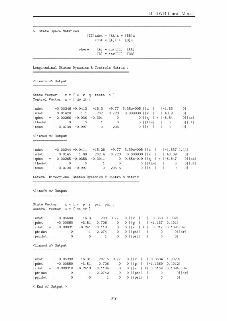
B BWB Linear Model
===============================================================================
5. State Space Matrices
[II]xdot = [AA]x + [BB]u
xdot = [A]x + [B]u
where: [A] = inv[II] [AA]
[B] = inv[II] [BB]
===============================================================================
Longitudinal States Dynamics & Controls Matrix :
================================================
<linafm.m> Output
-----------------
State Vector: x = [ u w q theta h ]
Control Vector: u = [ de dt ]
|udot | |-0.00246 -0.0413 -15.3 -9.77 5.38e-005 ||u | |-1.83 0|
|wdot | |-0.01420 -1.1 202 -0.723 0.000930 ||w | |-48.9 0|
|qdot |= | 0.00266 -0.036 -0.391 0 0 ||q | + |-6.84 0||de|
|thedot| | 0 0 1 0 0 ||the| | 0 0||dt|
|hdot | | 0.0738 -0.997 0 206 0 ||h | | 0 0|
<linmod.m> Output
-----------------
|udot | |-0.00244 -0.0411 -15.28 -9.77 5.39e-005 ||u | |-1.837 4.44|
|wdot | | -0.0145 -1.09 202.4 -0.723 0.000930 ||w | |-48.89 0|
|qdot |= | 0.00265 -0.0358 -0.3911 0 9.65e-019 ||q | + |-6.847 0||de|
|thedot| | 0 0 1 0 0 ||the| | 0 0||dt|
|hdot | | 0.0738 -0.997 0 205.6 0 ||h | | 0 0|
Lateral-Directional States Dynamics & Controls Matrix
=====================================================
<linafm.m> Output
-----------------
State Vector: x = [ v p r psi phi ]
Control Vector: u = [ da dr ]
|uvot | | -0.05400 16.3 -208 9.77 0 ||v | | -0.358 1.902|
|pdot | | -0.00860 -3.51 0.706 0 0 ||p | | -1.137 0.401|
|rdot |= | -0.00031 -0.241 -0.118 0 0 ||r | + | 0.017 -0.139||da|
|phidot| | 0 1 0.074 0 0 ||phi| | 0 0||dr|
|psidot| | 0 0 1 0 0 ||psi| | 0 0|
<linmod.m> Output
-----------------
|uvot | | -0.05398 16.31 -207.5 9.77 0 ||v | |-0.3584 1.9020|
|pdot | | -0.00859 -3.51 0.706 0 0 ||p | |-1.1369 0.4012|
|rdot |= |-0.000318 -0.2413 -0.1184 0 0 ||r | +| 0.0169 -0.1394||da|
|phidot| | 0 1 0.0740 0 0 ||phi| | 0 0||dr|
|psidot| | 0 0 1 0 0 ||psi| | 0 0|
< End of Output >
210
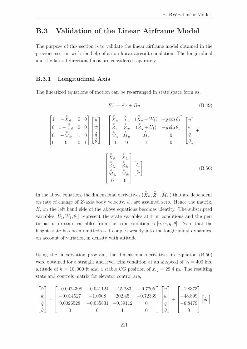
B BWB Linear Model
B.3 Validation of the Linear Airframe Model
The purpose of this section is to validate the linear airframe model obtained in the
previous section with the help of a non-linear aircraft simulation. The longitudinal
and the lateral-directional axis are considered separately.
B.3.1 Longitudinal Axis
The linearized equations of motion can be re-arranged in state space form as,
Ex = Ax+Bu (B.49)
1 −◦
X w 0 0
0 1 −◦
Zw 0 0
0 −◦
M w 1 0
0 0 0 1
u
w
q
θ
=
◦
Xu
◦
Xw (◦
Xq −W1) −g cos θ1◦
Zu
◦
Zw (◦
Zq + U1) −g sin θ1◦
Mu
◦
Mw
◦
M q 0
0 0 1 0
u
w
q
θ
+
◦
Xδe
◦
Xδt◦
Zδe
◦
Zδt◦
M δe
◦
M δt
0 0
[
δe
δt
]
(B.50)
In the above equation, the dimensional derivatives (◦
Xw,◦
Zw,◦
M w) that are dependent
on rate of change of Z-axis body velocity, w, are assumed zero. Hence the matrix,
E, on the left hand side of the above equations becomes identity. The subscripted
variables [U1,W1, θ1] represent the state variables at trim conditions and the per-
turbation in state variables from the trim condition is [u, w, q, θ]. Note that the
height state has been omitted as it couples weakly into the longitudinal dynamics,
on account of variation in density with altitude.
Using the linearization program, the dimensional derivatives in Equation (B.50)
were obtained for a straight and level trim condition at an airspeed of Vt = 400 kts,
altitude of h = 10, 000 ft and a stable CG position of xcg = 29.4 m. The resulting
state and controls matrix for elevator control are,
u
w
q
θ
=
−0.0024398 −0.041124 −15.283 −9.7705
−0.014527 −1.0908 202.45 −0.72339
0.0026528 −0.035831 −0.39112 0
0 0 1 0
u
w
q
θ
+
−1.8373
−48.899
−6.8479
0
[
δe]
211
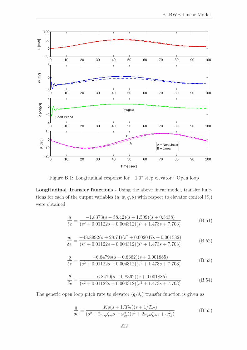
B BWB Linear Model
0 10 20 30 40 50 60 70 80 90 100−50
0
50
100
u [m
/s]
0 10 20 30 40 50 60 70 80 90 100−5
0
5
w [m
/s]
0 10 20 30 40 50 60 70 80 90 100−4
−2
0
2
q [d
eg/s
]
0 10 20 30 40 50 60 70 80 90 100−20
−10
0
10
θ [d
eg]
Time [sec]
A
B
A − Non LinearB − Linear
Short Period
Phugoid
Figure B.1: Longitudinal response for +1.0◦ step elevator : Open loop
Longitudinal Transfer functions - Using the above linear model, transfer func-
tions for each of the output variables (u, w, q, θ) with respect to elevator control (δe)
were obtained.
u
δe=
−1.8373(s− 58.42)(s+ 1.509)(s+ 0.3438)
(s2 + 0.01122s+ 0.004312)(s2 + 1.473s+ 7.703)(B.51)
w
δe=
−48.8992(s+ 28.74)(s2 + 0.002047s+ 0.001582)
(s2 + 0.01122s+ 0.004312)(s2 + 1.473s+ 7.703)(B.52)
q
δe=
−6.8479s(s+ 0.8362)(s+ 0.001885)
(s2 + 0.01122s+ 0.004312)(s2 + 1.473s+ 7.703)(B.53)
θ
δe=
−6.8479(s+ 0.8362)(s+ 0.001885)
(s2 + 0.01122s+ 0.004312)(s2 + 1.473s+ 7.703)(B.54)
The generic open loop pitch rate to elevator (q/δe) transfer function is given as
q
δe=
Ks(s+ 1/Tθ1)(s+ 1/Tθ2)
(s2 + 2ωspζsps+ ω2sp)(s
2 + 2ωphζphs+ ω2ph)
(B.55)
212
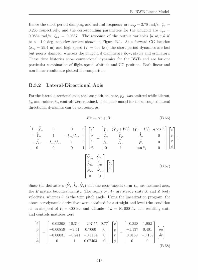
B BWB Linear Model
Hence the short period damping and natural frequency are ωsp = 2.78 rad/s, ζsp =
0.265 respectively, and the corresponding parameters for the phugoid are ωph =
0.0854 rad/s, ζph = 0.0657. The response of the output variables [u, w, q, θ, h]
to a +1.0 deg step elevator are shown in Figure B.1. At a forward CG location
(xcg = 29.4 m) and high speed (V = 400 kts) the short period dynamics are fast
but poorly damped, whereas the phugoid dynamics are slow, stable and oscillatory.
These time histories show conventional dynamics for the BWB and are for one
particular combination of flight speed, altitude and CG position. Both linear and
non-linear results are plotted for comparison.
B.3.2 Lateral-Directional Axis
For the lateral directional axis, the east position state, pE, was omitted while aileron,
δa, and rudder, δr, controls were retained. The linear model for the uncoupled lateral
directional dynamics can be expressed as,
Ex = Ax+Bu (B.56)
1 −◦
Y v 0 0 0
−◦
Lv 1 −Ixz/Ixx 0
−◦
N v −Ixz/Izz 1 0
0 0 0 1
v
p
r
φ
=
◦
Y v (◦
Y p +W1) (◦
Y r − U1) g cos θ1◦
Lv◦
Lp◦
Lr 0◦
Nv
◦
N p
◦
N r 0
0 1 tan θ1 0
v
p
r
φ
+
◦
Y δa
◦
Y δr◦
Lδa◦
Lδr◦
N δa
◦
N δr
0 0
[
δa
δr
]
(B.57)
Since the derivatives (◦
Y v,◦
Lv,◦
N v) and the cross inertia term Ixz are assumed zero,
the E matrix becomes identity. The terms U1,W1 are steady state X and Z body
velocities, whereas θ1 is the trim pitch angle. Using the linearization program, the
above aerodynamic derivatives were obtained for a straight and level trim condition
at an airspeed of Vt = 400 kts and altitude of h = 10, 000 ft. The resulting state
and controls matrices were
v
p
r
φ
=
−0.05398 16.314 −207.55 9.77
−0.00859 −3.51 0.7060 0
−0.00031 −0.241 −0.1184 0
0 1 0.07403 0
v
p
r
φ
+
−0.358 1.902
−1.137 0.401
0.0169 −0.139
0 0
[
δa
δr
]
(B.58)
213
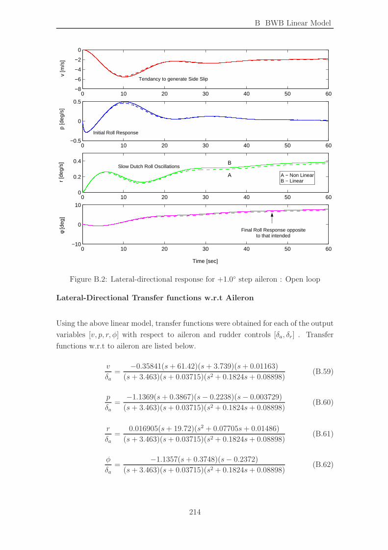
B BWB Linear Model
0 10 20 30 40 50 60−8
−6
−4
−2
0
v [m
/s]
0 10 20 30 40 50 60−0.5
0
0.5
p [d
eg/s
]
0 10 20 30 40 50 600
0.2
0.4
r [d
eg/s
]
0 10 20 30 40 50 60−10
0
10
φ [d
eg]
Time [sec]
Tendancy to generate Side Slip
Initial Roll Response
Slow Dutch Roll Oscillations
A
B
Final Roll Response opposite to that intended
A − Non LinearB − Linear
Figure B.2: Lateral-directional response for +1.0◦ step aileron : Open loop
Lateral-Directional Transfer functions w.r.t Aileron
Using the above linear model, transfer functions were obtained for each of the output
variables [v, p, r, φ] with respect to aileron and rudder controls [δa, δr] . Transfer
functions w.r.t to aileron are listed below.
v
δa=
−0.35841(s+ 61.42)(s+ 3.739)(s+ 0.01163)
(s+ 3.463)(s+ 0.03715)(s2 + 0.1824s+ 0.08898)(B.59)
p
δa=
−1.1369(s+ 0.3867)(s− 0.2238)(s− 0.003729)
(s+ 3.463)(s+ 0.03715)(s2 + 0.1824s+ 0.08898)(B.60)
r
δa=
0.016905(s+ 19.72)(s2 + 0.07705s+ 0.01486)
(s+ 3.463)(s+ 0.03715)(s2 + 0.1824s+ 0.08898)(B.61)
φ
δa=
−1.1357(s+ 0.3748)(s− 0.2372)
(s+ 3.463)(s+ 0.03715)(s2 + 0.1824s+ 0.08898)(B.62)
214
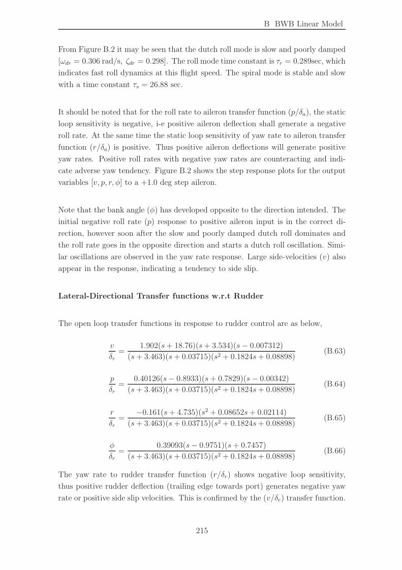
B BWB Linear Model
From Figure B.2 it may be seen that the dutch roll mode is slow and poorly damped
[ωdr = 0.306 rad/s, ζdr = 0.298]. The roll mode time constant is τr = 0.289sec, which
indicates fast roll dynamics at this flight speed. The spiral mode is stable and slow
with a time constant τs = 26.88 sec.
It should be noted that for the roll rate to aileron transfer function (p/δa), the static
loop sensitivity is negative, i-e positive aileron deflection shall generate a negative
roll rate. At the same time the static loop sensitivity of yaw rate to aileron transfer
function (r/δa) is positive. Thus positive aileron deflections will generate positive
yaw rates. Positive roll rates with negative yaw rates are counteracting and indi-
cate adverse yaw tendency. Figure B.2 shows the step response plots for the output
variables [v, p, r, φ] to a +1.0 deg step aileron.
Note that the bank angle (φ) has developed opposite to the direction intended. The
initial negative roll rate (p) response to positive aileron input is in the correct di-
rection, however soon after the slow and poorly damped dutch roll dominates and
the roll rate goes in the opposite direction and starts a dutch roll oscillation. Simi-
lar oscillations are observed in the yaw rate response. Large side-velocities (v) also
appear in the response, indicating a tendency to side slip.
Lateral-Directional Transfer functions w.r.t Rudder
The open loop transfer functions in response to rudder control are as below,
v
δr=
1.902(s+ 18.76)(s+ 3.534)(s− 0.007312)
(s+ 3.463)(s+ 0.03715)(s2 + 0.1824s+ 0.08898)(B.63)
p
δr=
0.40126(s− 0.8933)(s+ 0.7829)(s− 0.00342)
(s+ 3.463)(s+ 0.03715)(s2 + 0.1824s+ 0.08898)(B.64)
r
δr=
−0.161(s+ 4.735)(s2 + 0.08652s+ 0.02114)
(s+ 3.463)(s+ 0.03715)(s2 + 0.1824s+ 0.08898)(B.65)
φ
δr=
0.39093(s− 0.9751)(s+ 0.7457)
(s+ 3.463)(s+ 0.03715)(s2 + 0.1824s+ 0.08898)(B.66)
The yaw rate to rudder transfer function (r/δr) shows negative loop sensitivity,
thus positive rudder deflection (trailing edge towards port) generates negative yaw
rate or positive side slip velocities. This is confirmed by the (v/δr) transfer function.
215
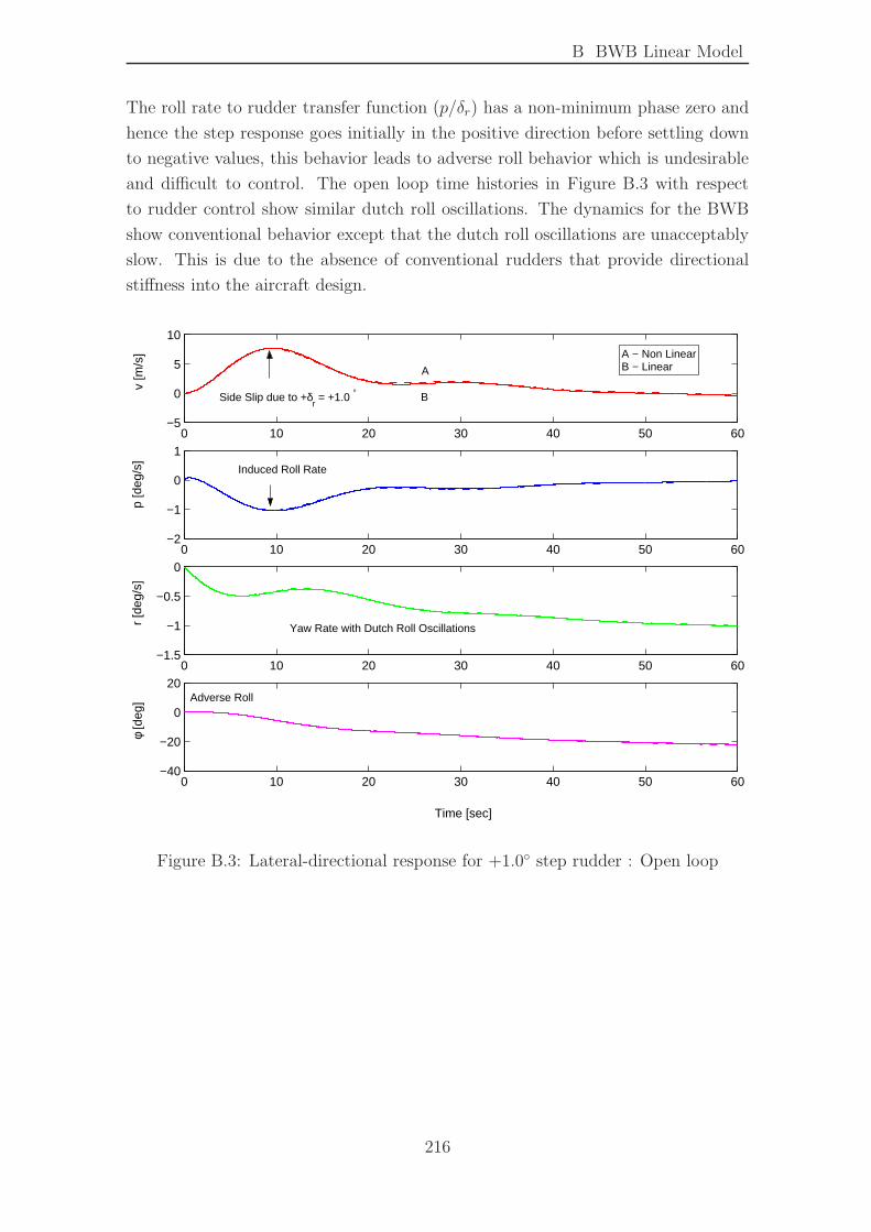
B BWB Linear Model
The roll rate to rudder transfer function (p/δr) has a non-minimum phase zero and
hence the step response goes initially in the positive direction before settling down
to negative values, this behavior leads to adverse roll behavior which is undesirable
and difficult to control. The open loop time histories in Figure B.3 with respect
to rudder control show similar dutch roll oscillations. The dynamics for the BWB
show conventional behavior except that the dutch roll oscillations are unacceptably
slow. This is due to the absence of conventional rudders that provide directional
stiffness into the aircraft design.
0 10 20 30 40 50 60−5
0
5
10
v [m
/s]
0 10 20 30 40 50 60−2
−1
0
1
p [d
eg/s
]
0 10 20 30 40 50 60−1.5
−1
−0.5
0
r [d
eg/s
]
0 10 20 30 40 50 60−40
−20
0
20
φ [d
eg]
A
B
A − Non LinearB − Linear
Yaw Rate with Dutch Roll Oscillations
Side Slip due to +δr = +1.0 °
Induced Roll Rate
Adverse Roll
Time [sec]
Figure B.3: Lateral-directional response for +1.0◦ step rudder : Open loop
216
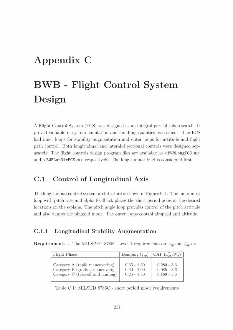
Appendix C
BWB - Flight Control System
Design
A Flight Control System (FCS) was designed as an integral part of this research. It
proved valuable in system simulation and handling qualities assessment. The FCS
had inner loops for stability augmentation and outer loops for attitude and flight
path control. Both longitudinal and lateral-directional controls were designed sep-
arately. The flight controls design program files are available as <BWBLongFCS.m>
and <BWBLatDirFCS.m> respectively. The longitudinal FCS is considered first.
C.1 Control of Longitudinal Axis
The longitudinal control system architecture is shown in Figure C.1. The inner most
loop with pitch rate and alpha feedback places the short period poles at the desired
locations on the s-plane. The pitch angle loop provides control of the pitch attitude
and also damps the phugoid mode. The outer loops control airspeed and altitude.
C.1.1 Longitudinal Stability Augmentation
Requirements - The MILSPEC 8785C Level 1 requirements on ωsp and ζsp are,
Flight Phase Damping (ζsp) CAP (ω2sp/Nα)
Category A (rapid maneuvering) 0.35 - 1.30 0.280 - 3.6Category B (gradual maneuvers) 0.30 - 2.00 0.085 - 3.6Category C (take-off and landing) 0.25 - 1.30 0.160 - 3.6
Table C.1: MILSTD 8785C - short period mode requirements
217
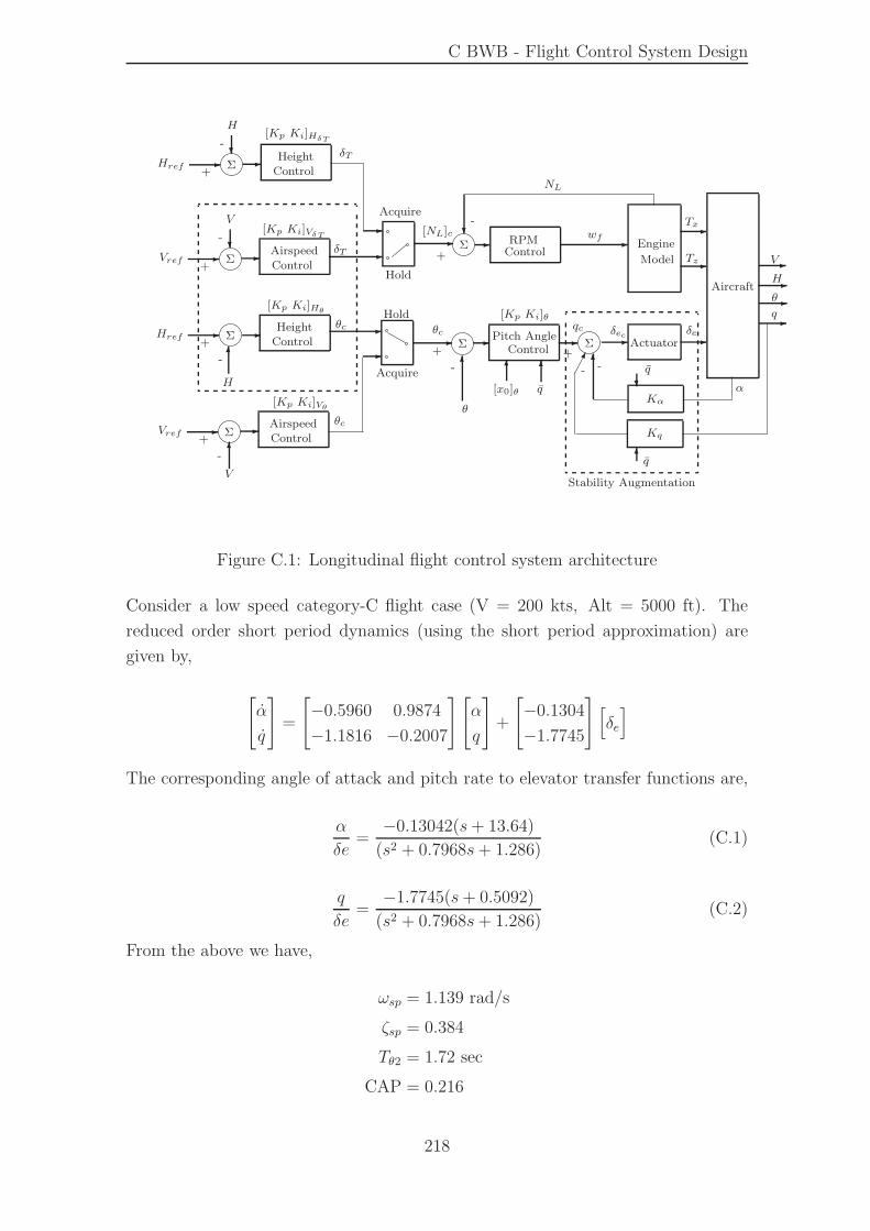
C BWB - Flight Control System Design
[Kp Ki]HδT
[Kp Ki]VδT
Engine
Model
-
-Hold
-wfTx
Tz
[NL]cRPM
ControlΣ -
Aircraft
α
q
?-
NL
-+-
Acquire
-
[Kp Ki]θδec
-
Actuator -
-
+
Hold
Acquire
qc
�
-
6
6
θc
[Kp Ki]Vθ
ΣAirspeedControl
V
-
-+
-
-
H
?-δT
ΣAirspeedControl
V
-
-+-
Vref
Vref
θc
[Kp Ki]Hθ
ΣHeight
Control+
-
δT
-Href
?-
ΣHeight
Control
H
-+-Href
δeΣ
q[x0]θKα
Kq
-
6Σ
-
-
-Pitch AngleControl
θc-
6 66
-
θ
+
-
-
-
θ
H
V
?
6
q
Stability Augmentation
q
Figure C.1: Longitudinal flight control system architecture
Consider a low speed category-C flight case (V = 200 kts, Alt = 5000 ft). The
reduced order short period dynamics (using the short period approximation) are
given by,
[
α
q
]
=
[
−0.5960 0.9874
−1.1816 −0.2007
][
α
q
]
+
[
−0.1304
−1.7745
]
[
δe
]
The corresponding angle of attack and pitch rate to elevator transfer functions are,
α
δe=
−0.13042(s+ 13.64)
(s2 + 0.7968s+ 1.286)(C.1)
q
δe=
−1.7745(s+ 0.5092)
(s2 + 0.7968s+ 1.286)(C.2)
From the above we have,
ωsp = 1.139 rad/s
ζsp = 0.384
Tθ2 = 1.72 sec
CAP = 0.216
218
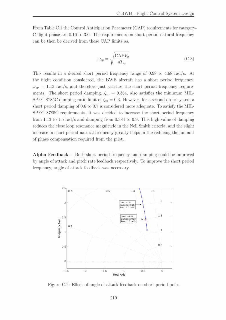
C BWB - Flight Control System Design
From Table C.1 the Control Anticipation Parameter (CAP) requirements for category-
C flight phase are 0.16 to 3.6. The requirements on short period natural frequency
can be then be derived from these CAP limits as,
ωsp =
√
CAPV0
gTθ2(C.3)
This results in a desired short period frequency range of 0.98 to 4.68 rad/s. At
the flight condition considered, the BWB aircraft has a short period frequency,
ωsp = 1.13 rad/s, and therefore just satisfies the short period frequency require-
ments. The short period damping, ζsp = 0.384, also satisfies the minimum MIL-
SPEC 8785C damping ratio limit of ζsp = 0.3. However, for a second order system a
short period damping of 0.6 to 0.7 is considered more adequate. To satisfy the MIL-
SPEC 8785C requirements, it was decided to increase the short period frequency
from 1.13 to 1.5 rad/s and damping from 0.384 to 0.9. This high value of damping
reduces the close loop resonance magnitude in the Neil Smith criteria, and the slight
increase in short period natural frequency greatly helps in the reducing the amount
of phase compensation required from the pilot.
Alpha Feedback - Both short period frequency and damping could be improved
by angle of attack and pitch rate feedback respectively. To improve the short period
frequency, angle of attack feedback was necessary.
−2.5 −2 −1.5 −1 −0.5 0
0
0.5
1
1.5
2
2.5
1.5
1
2
0.30.7 0.1
0.5
0.5
0.9
Real Axis
Imag
inar
y A
xis
Gain : −1.5Damping : 0.25 Freq : 2.0 rad/s
Gain : −0.55Damping : 0.29 Freq : 1.5 rad/s
Figure C.2: Effect of angle of attack feedback on short period poles
219
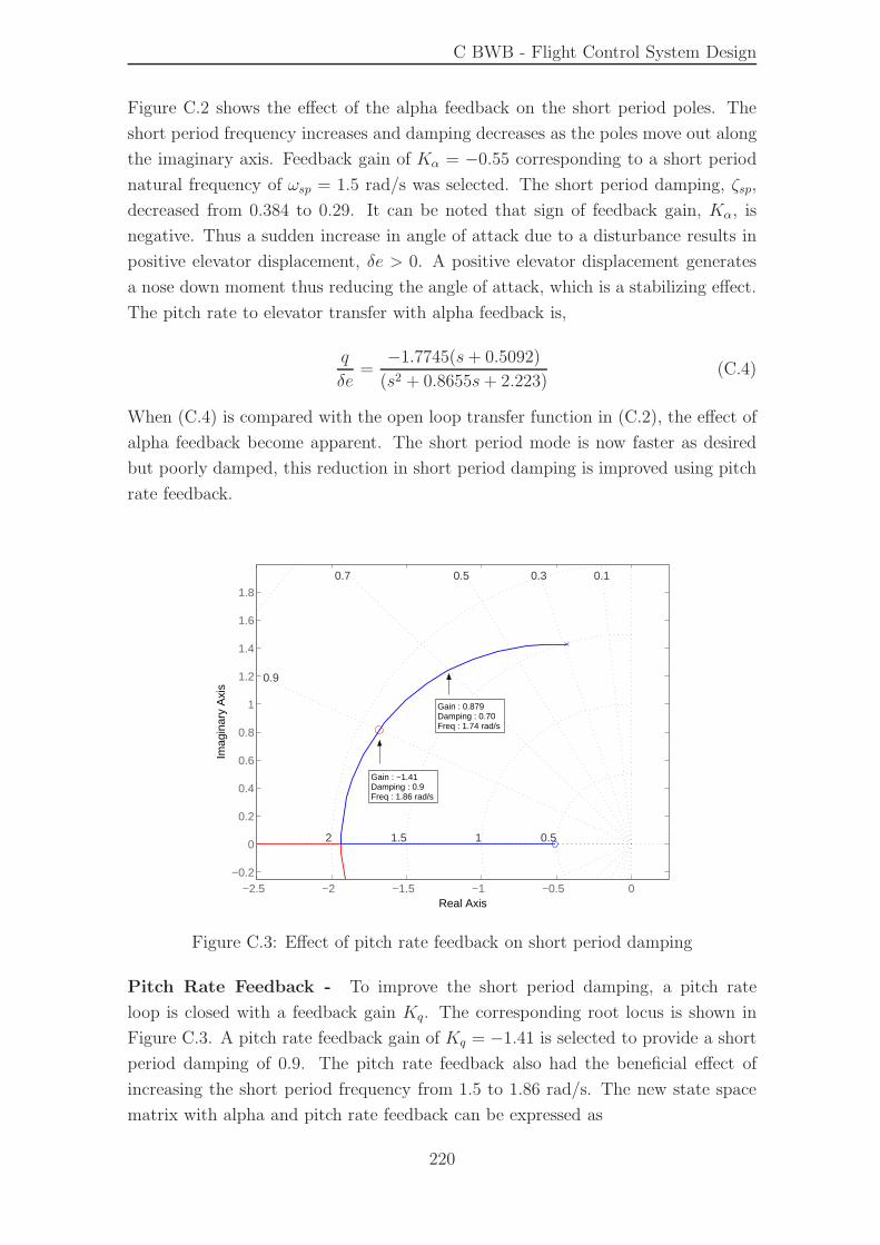
C BWB - Flight Control System Design
Figure C.2 shows the effect of the alpha feedback on the short period poles. The
short period frequency increases and damping decreases as the poles move out along
the imaginary axis. Feedback gain of Kα = −0.55 corresponding to a short period
natural frequency of ωsp = 1.5 rad/s was selected. The short period damping, ζsp,
decreased from 0.384 to 0.29. It can be noted that sign of feedback gain, Kα, is
negative. Thus a sudden increase in angle of attack due to a disturbance results in
positive elevator displacement, δe > 0. A positive elevator displacement generates
a nose down moment thus reducing the angle of attack, which is a stabilizing effect.
The pitch rate to elevator transfer with alpha feedback is,
q
δe=
−1.7745(s+ 0.5092)
(s2 + 0.8655s+ 2.223)(C.4)
When (C.4) is compared with the open loop transfer function in (C.2), the effect of
alpha feedback become apparent. The short period mode is now faster as desired
but poorly damped, this reduction in short period damping is improved using pitch
rate feedback.
−2.5 −2 −1.5 −1 −0.5 0−0.2
0
0.2
0.4
0.6
0.8
1
1.2
1.4
1.6
1.8
1.5 12
0.30.7 0.1
0.5
0.5
0.9
Real Axis
Imag
inar
y A
xis
Gain : −1.41Damping : 0.9Freq : 1.86 rad/s
Gain : 0.879Damping : 0.70Freq : 1.74 rad/s
Figure C.3: Effect of pitch rate feedback on short period damping
Pitch Rate Feedback - To improve the short period damping, a pitch rate
loop is closed with a feedback gain Kq. The corresponding root locus is shown in
Figure C.3. A pitch rate feedback gain of Kq = −1.41 is selected to provide a short
period damping of 0.9. The pitch rate feedback also had the beneficial effect of
increasing the short period frequency from 1.5 to 1.86 rad/s. The new state space
matrix with alpha and pitch rate feedback can be expressed as
220
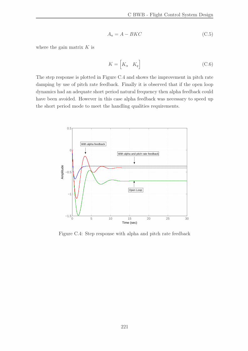
C BWB - Flight Control System Design
An = A− BKC (C.5)
where the gain matrix K is
K =[
Kα Kq
]
(C.6)
The step response is plotted in Figure C.4 and shows the improvement in pitch rate
damping by use of pitch rate feedback. Finally it is observed that if the open loop
dynamics had an adequate short period natural frequency then alpha feedback could
have been avoided. However in this case alpha feedback was necessary to speed up
the short period mode to meet the handling qualities requirements.
0 5 10 15 20 25 30−1.5
−1
−0.5
0
0.5
Time (sec)
Am
plitu
de
Open Loop
With alpha feedback
With alpha and pitch rate feedback
Figure C.4: Step response with alpha and pitch rate feedback
221
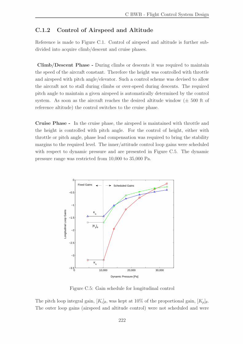
C BWB - Flight Control System Design
C.1.2 Control of Airspeed and Altitude
Reference is made to Figure C.1. Control of airspeed and altitude is further sub-
divided into acquire climb/descent and cruise phases.
Climb/Descent Phase - During climbs or descents it was required to maintain
the speed of the aircraft constant. Therefore the height was controlled with throttle
and airspeed with pitch angle/elevator. Such a control scheme was devised to allow
the aircraft not to stall during climbs or over-speed during descents. The required
pitch angle to maintain a given airspeed is automatically determined by the control
system. As soon as the aircraft reaches the desired altitude window (± 500 ft of
reference altitude) the control switches to the cruise phase.
Cruise Phase - In the cruise phase, the airspeed is maintained with throttle and
the height is controlled with pitch angle. For the control of height, either with
throttle or pitch angle, phase lead compensation was required to bring the stability
margins to the required level. The inner/attitude control loop gains were scheduled
with respect to dynamic pressure and are presented in Figure C.5. The dynamic
pressure range was restricted from 10,000 to 35,000 Pa.
0 10,000 20,000 30,000−3.5
−3
−2.5
−2
−1.5
−1
−0.5
0
Dynamic Pressure [Pa]
Long
itudi
nal L
oop
Gai
ns
[Kp]θ
Kq
Kα
Scheduled GainsFixed Gains
Figure C.5: Gain schedule for longitudinal control
The pitch loop integral gain, [Ki]θ, was kept at 10% of the proportional gain, [Kp]θ.
The outer loop gains (airspeed and altitude control) were not scheduled and were
222
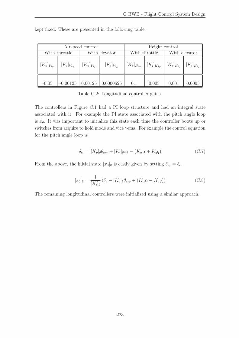
C BWB - Flight Control System Design
kept fixed. These are presented in the following table.
Airspeed control Height controlWith throttle With elevator With throttle With elevator
[Kp]VδT [Ki]VδT [Kp]Vδe [Ki]Vδe [Kp]HδT [Ki]HδT [Kp]Hδe [Ki]Hδe
-0.05 -0.00125 0.00125 0.0000625 0.1 0.005 0.001 0.0005
Table C.2: Longitudinal controller gains
The controllers in Figure C.1 had a PI loop structure and had an integral state
associated with it. For example the PI state associated with the pitch angle loop
is xθ. It was important to initialize this state each time the controller boots up or
switches from acquire to hold mode and vice versa. For example the control equation
for the pitch angle loop is
δec = [Kp]θθerr + [Ki]θxθ − (Kαα+Kqq) (C.7)
From the above, the initial state [x0]θ is easily given by setting δec = δe,
[x0]θ =1
[Ki]θ(δe − [Kp]θθerr + (Kαα +Kqq)) (C.8)
The remaining longitudinal controllers were initialized using a similar approach.
223
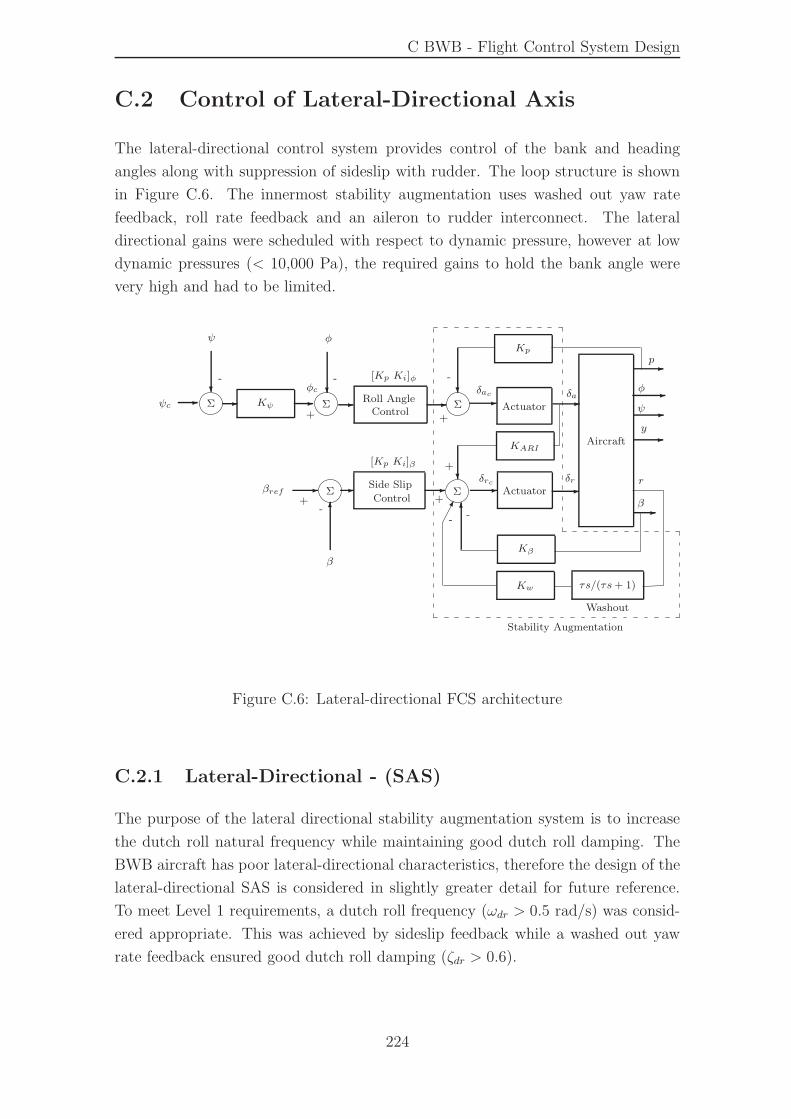
C BWB - Flight Control System Design
C.2 Control of Lateral-Directional Axis
The lateral-directional control system provides control of the bank and heading
angles along with suppression of sideslip with rudder. The loop structure is shown
in Figure C.6. The innermost stability augmentation uses washed out yaw rate
feedback, roll rate feedback and an aileron to rudder interconnect. The lateral
directional gains were scheduled with respect to dynamic pressure, however at low
dynamic pressures (< 10,000 Pa), the required gains to hold the bank angle were
very high and had to be limited.
Aircraft
β
r
[Kp Ki]φ
-
δrc
-
Actuator -
Actuator-
-
Σ -
-
+βref
�
δrΣ
[Kp Ki]β
Σ
Kβ
Kw
-φc
-
6
τs/(τs+ 1)
φ
Kψψc - -Σ -?-
ψ
-φ
-ψ
p
Washout
δac δaRoll AngleControl
+
-
-
-?
+
Kp
?
+
Stability Augmentation
-KARI
?+
-Side Slip
ControlΣ
6
β
-
-
-
y
Figure C.6: Lateral-directional FCS architecture
C.2.1 Lateral-Directional - (SAS)
The purpose of the lateral directional stability augmentation system is to increase
the dutch roll natural frequency while maintaining good dutch roll damping. The
BWB aircraft has poor lateral-directional characteristics, therefore the design of the
lateral-directional SAS is considered in slightly greater detail for future reference.
To meet Level 1 requirements, a dutch roll frequency (ωdr > 0.5 rad/s) was consid-
ered appropriate. This was achieved by sideslip feedback while a washed out yaw
rate feedback ensured good dutch roll damping (ζdr > 0.6).
224
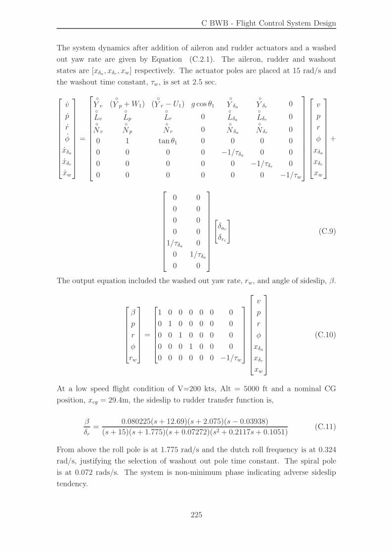
C BWB - Flight Control System Design
The system dynamics after addition of aileron and rudder actuators and a washed
out yaw rate are given by Equation (C.2.1). The aileron, rudder and washout
states are [xδa , xδr , xw] respectively. The actuator poles are placed at 15 rad/s and
the washout time constant, τw, is set at 2.5 sec.
v
p
r
φ
xδaxδrxw
=
◦
Y v (◦
Y p +W1) (◦
Y r − U1) g cos θ1◦
Y δa
◦
Y δr 0◦
Lv◦
Lp◦
Lr 0◦
Lδa◦
Lδr 0◦
N v
◦
N p
◦
N r 0◦
N δa
◦
N δr 0
0 1 tan θ1 0 0 0 0
0 0 0 0 −1/τδa 0 0
0 0 0 0 0 −1/τδr 0
0 0 0 0 0 0 −1/τw
v
p
r
φ
xδaxδrxw
+
0 0
0 0
0 0
0 0
1/τδa 0
0 1/τδa0 0
[
δacδrc
]
(C.9)
The output equation included the washed out yaw rate, rw, and angle of sideslip, β.
β
p
r
φ
rw
=
1 0 0 0 0 0 0
0 1 0 0 0 0 0
0 0 1 0 0 0 0
0 0 0 1 0 0 0
0 0 0 0 0 0 −1/τw
v
p
r
φ
xδaxδrxw
(C.10)
At a low speed flight condition of V=200 kts, Alt = 5000 ft and a nominal CG
position, xcg = 29.4m, the sideslip to rudder transfer function is,
β
δr=
0.080225(s+ 12.69)(s+ 2.075)(s− 0.03938)
(s+ 15)(s+ 1.775)(s+ 0.07272)(s2 + 0.2117s+ 0.1051)(C.11)
From above the roll pole is at 1.775 rad/s and the dutch roll frequency is at 0.324
rad/s, justifying the selection of washout out pole time constant. The spiral pole
is at 0.072 rads/s. The system is non-minimum phase indicating adverse sideslip
tendency.
225
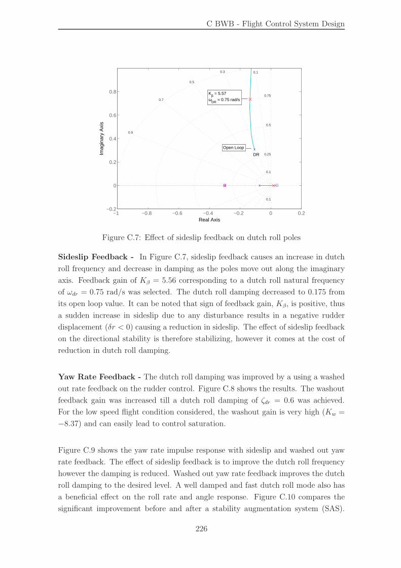
C BWB - Flight Control System Design
−1 −0.8 −0.6 −0.4 −0.2 0 0.2−0.2
0
0.2
0.4
0.6
0.8
0.1
1
0.9
0.5
0.3
0.1
0.70.75
0.5
0.1
0.25
Real Axis
Imag
inar
y A
xis
Kβ = 5.57
ωDR
= 0.75 rad/s
Open Loop
DR
Figure C.7: Effect of sideslip feedback on dutch roll poles
Sideslip Feedback - In Figure C.7, sideslip feedback causes an increase in dutch
roll frequency and decrease in damping as the poles move out along the imaginary
axis. Feedback gain of Kβ = 5.56 corresponding to a dutch roll natural frequency
of ωdr = 0.75 rad/s was selected. The dutch roll damping decreased to 0.175 from
its open loop value. It can be noted that sign of feedback gain, Kβ, is positive, thus
a sudden increase in sideslip due to any disturbance results in a negative rudder
displacement (δr < 0) causing a reduction in sideslip. The effect of sideslip feedback
on the directional stability is therefore stabilizing, however it comes at the cost of
reduction in dutch roll damping.
Yaw Rate Feedback - The dutch roll damping was improved by a using a washed
out rate feedback on the rudder control. Figure C.8 shows the results. The washout
feedback gain was increased till a dutch roll damping of ζdr = 0.6 was achieved.
For the low speed flight condition considered, the washout gain is very high (Kw =
−8.37) and can easily lead to control saturation.
Figure C.9 shows the yaw rate impulse response with sideslip and washed out yaw
rate feedback. The effect of sideslip feedback is to improve the dutch roll frequency
however the damping is reduced. Washed out yaw rate feedback improves the dutch
roll damping to the desired level. A well damped and fast dutch roll mode also has
a beneficial effect on the roll rate and angle response. Figure C.10 compares the
significant improvement before and after a stability augmentation system (SAS).
226
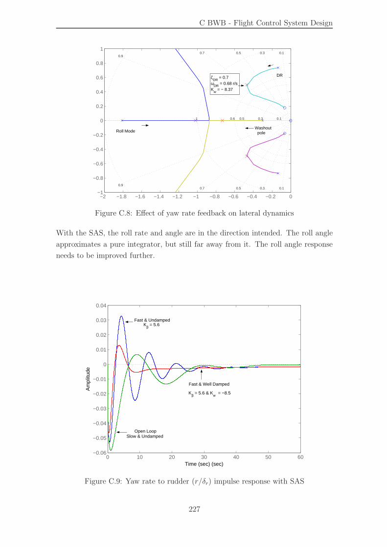
C BWB - Flight Control System Design
−2 −1.8 −1.6 −1.4 −1.2 −1 −0.8 −0.6 −0.4 −0.2 0−1
−0.8
−0.6
−0.4
−0.2
0
0.2
0.4
0.6
0.8
1
2 1
0.7
0.5 0.3 0.1
0.6 0.5
0.1
0.3
0.5
0.1
0.9
0.90.7
0.3
ζDR
= 0.7ω
DR = 0.68 r/s
Kw
= − 8.37
Washoutpole Roll Mode
DR
Figure C.8: Effect of yaw rate feedback on lateral dynamics
With the SAS, the roll rate and angle are in the direction intended. The roll angle
approximates a pure integrator, but still far away from it. The roll angle response
needs to be improved further.
0 10 20 30 40 50 60−0.06
−0.05
−0.04
−0.03
−0.02
−0.01
0
0.01
0.02
0.03
0.04
Time (sec) (sec)
Am
plitu
de
Open LoopSlow & Undamped
Fast & UndampedKβ = 5.6
Fast & Well Damped
Kβ = 5.6 & Kw
= −8.5
Figure C.9: Yaw rate to rudder (r/δr) impulse response with SAS
227
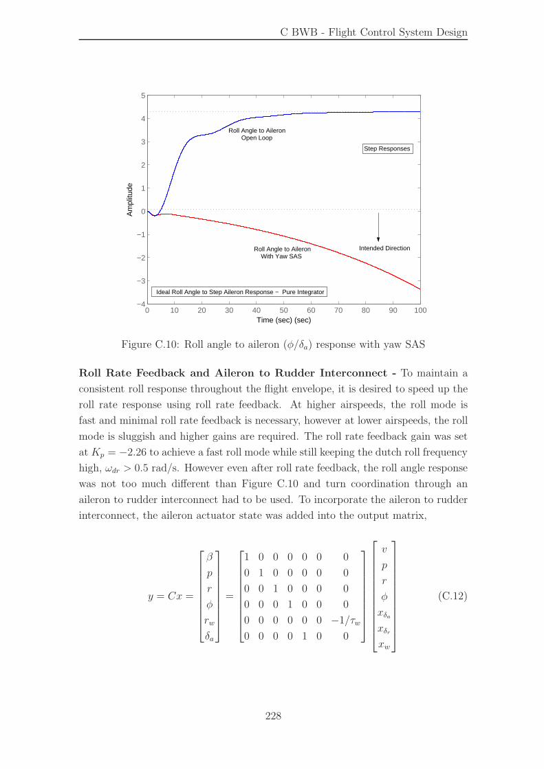
C BWB - Flight Control System Design
0 10 20 30 40 50 60 70 80 90 100−4
−3
−2
−1
0
1
2
3
4
5
Time (sec) (sec)
Am
plitu
deRoll Angle to Aileron
Open Loop
Roll Angle to Aileron With Yaw SAS
Step Responses
Intended Direction
Ideal Roll Angle to Step Aileron Response − Pure Integrator
Figure C.10: Roll angle to aileron (φ/δa) response with yaw SAS
Roll Rate Feedback and Aileron to Rudder Interconnect - To maintain a
consistent roll response throughout the flight envelope, it is desired to speed up the
roll rate response using roll rate feedback. At higher airspeeds, the roll mode is
fast and minimal roll rate feedback is necessary, however at lower airspeeds, the roll
mode is sluggish and higher gains are required. The roll rate feedback gain was set
at Kp = −2.26 to achieve a fast roll mode while still keeping the dutch roll frequency
high, ωdr > 0.5 rad/s. However even after roll rate feedback, the roll angle response
was not too much different than Figure C.10 and turn coordination through an
aileron to rudder interconnect had to be used. To incorporate the aileron to rudder
interconnect, the aileron actuator state was added into the output matrix,
y = Cx =
β
p
r
φ
rw
δa
=
1 0 0 0 0 0 0
0 1 0 0 0 0 0
0 0 1 0 0 0 0
0 0 0 1 0 0 0
0 0 0 0 0 0 −1/τw
0 0 0 0 1 0 0
v
p
r
φ
xδaxδrxw
(C.12)
228
C BWB - Flight Control System Design
The control equation including the aileron to rudder interconnect is
u = −Ky = −[
0 0 Kp 0 0 0
Kβ 0 0 0 Kw −Kari
]
β
p
r
φ
rw
δa
(C.13)
and the system dynamics can now conveniently be expressed as,
Ac = A− BKC (C.14)
Where A and B represent the open loop system dynamics including actuators. The
following close loop roll rate to aileron transfer function was obtained from the above
matrix formulation,
p
δa=
−4.9401(s+ 14.64)(s+ 0.60)(s− 0.018)(s2 + 0.147s+ 0.028)
(s+ 1.57)(s+ 0.722)(s− 0.0156)(s2 + 0.838s+ 0.3574)(s2 + 29.24s+ 219.3)(C.15)
Equation C.15 shows the roll rate to aileron (p/δa) transfer function with an ARI
gain (Kari = 1.0) and roll rate loop engaged. The following can be observed.
• The actuator pole now forms an oscillatory pair, but is fast and well damped.
• The ARI causes the roll subsidence pole to slow down to 1.573 rad/s from its
open loop value of 1.775 rad/s. This also justifies the use of roll rate feedback,
otherwise the roll mode slows down to below Level 1, when ARI is engaged.
• The aileron to rudder interconnect speeds up the dutch roll mode, which is
almost canceled by numerator zeros, hence a less oscillatory roll rate response.
• A slow but unstable spiral is almost canceled by a numerator zero.
The roll response to aileron control for a flight speed of 200 knots is shown in
Figure C.11. The beneficial effect of aileron to rudder interconnect is evident.
C.2.2 Lateral-Directional Gain Schedule
With the lateral directional stability augmentation in place, the bank angle and
heading control loops were formulated using standard methods, however the final
gains actually used in the non-linear simulation had to be reduced/limited to prevent
controls saturation. Figure C.12 presents the gain schedule.
229
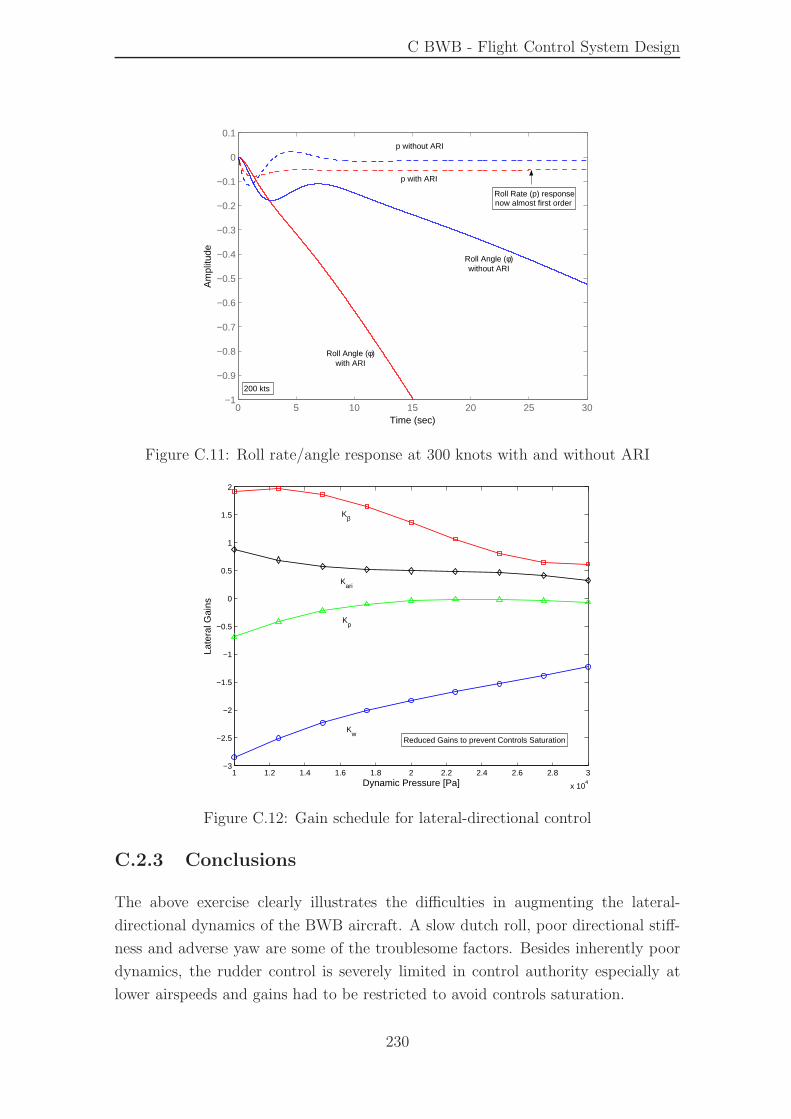
C BWB - Flight Control System Design
0 5 10 15 20 25 30−1
−0.9
−0.8
−0.7
−0.6
−0.5
−0.4
−0.3
−0.2
−0.1
0
0.1
Time (sec)
Am
plitu
de
200 kts
Roll Rate (p) responsenow almost first order
p with ARI
p without ARI
Roll Angle (φ) with ARI
Roll Angle (φ) without ARI
Figure C.11: Roll rate/angle response at 300 knots with and without ARI
1 1.2 1.4 1.6 1.8 2 2.2 2.4 2.6 2.8 3
x 104
−3
−2.5
−2
−1.5
−1
−0.5
0
0.5
1
1.5
2
Dynamic Pressure [Pa]
Late
ral G
ains
Kβ
Kw
Kp
Kari
Reduced Gains to prevent Controls Saturation
Figure C.12: Gain schedule for lateral-directional control
C.2.3 Conclusions
The above exercise clearly illustrates the difficulties in augmenting the lateral-
directional dynamics of the BWB aircraft. A slow dutch roll, poor directional stiff-
ness and adverse yaw are some of the troublesome factors. Besides inherently poor
dynamics, the rudder control is severely limited in control authority especially at
lower airspeeds and gains had to be restricted to avoid controls saturation.
230
Appendix D
Implementation Details - BWB
Model with Blown Flaps
This section briefly describes the ESDU model subroutines written initially in MAT-
LAB for trim and linear analysis and then in C Language for non-linear simulation
implementation. The C language code for the ESDU aerodynamic model has 76
strips and runs in real time along with the hybrid engine model. The development
of this model was greatly facilitated by Cooke’s model of the NFLC Jetstream [59]
which uses the ESDU methods for aerodynamic estimation and by Amrane [60]
which discusses the development of a sail plane model using a strip element ap-
proach. A listing of the subroutines is presented in Table D.1 along with their brief
description.
The user needs to initialize the model by first calling the <init geometry.m> func-
tion, this will load the <geom> structure with appropriate airfoil geometry profile pa-
rameters along the span. If the user requires to make changes to the BWB planform
or airfoil geometry, it will be required to make appropriate changes in this geometry
initialization file. The next step is to call the function, <get aero wing.m>, with
appropriate inputs such as the values of the current state vector, control inputs and
CG position. This function then returns X, Y, Z body forces and moments L,M,N
about the centre of gravity or the moment reference point. In a similar fashion, the
function <get aero fin.m> returns contributions of the vertical fin to these aero-
dynamic forces and moments in body axis. The wing and fin contributions are then
added up to get the net forces and moments in body axis.
Program listings are available in soft form in a CD accompanying this thesis.
231
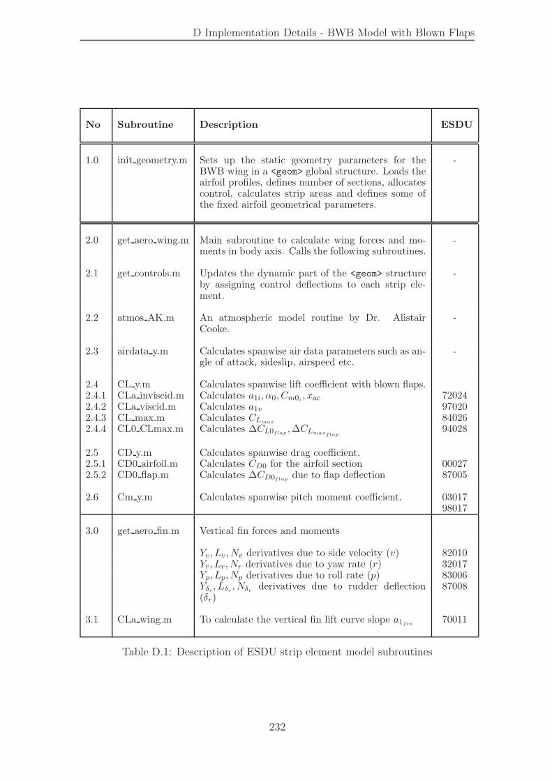
D Implementation Details - BWB Model with Blown Flaps
No Subroutine Description ESDU
1.0 init geometry.m Sets up the static geometry parameters for theBWB wing in a <geom> global structure. Loads theairfoil profiles, defines number of sections, allocatescontrol, calculates strip areas and defines some ofthe fixed airfoil geometrical parameters.
-
2.0 get aero wing.m Main subroutine to calculate wing forces and mo-ments in body axis. Calls the following subroutines.
-
2.1 get controls.m Updates the dynamic part of the <geom> structureby assigning control deflections to each strip ele-ment.
-
2.2 atmos AK.m An atmospheric model routine by Dr. AlistairCooke.
-
2.3 airdata y.m Calculates spanwise air data parameters such as an-gle of attack, sideslip, airspeed etc.
-
2.4 CL y.m Calculates spanwise lift coefficient with blown flaps.2.4.1 CLa inviscid.m Calculates a1i, α0, Cm0i
, xac 720242.4.2 CLa viscid.m Calculates a1v 970202.4.3 CL max.m Calculates CLmax
840262.4.4 CL0 CLmax.m Calculates ∆CL0flap
,∆CLmaxflap94028
2.5 CD y.m Calculates spanwise drag coefficient.2.5.1 CD0 airfoil.m Calculates CD0 for the airfoil section 000272.5.2 CD0 flap.m Calculates ∆CD0flap
due to flap deflection 87005
2.6 Cm y.m Calculates spanwise pitch moment coefficient. 0301798017
3.0 get aero fin.m Vertical fin forces and moments
Yv, Lv, Nv derivatives due to side velocity (v) 82010Yr, Lr, Nr derivatives due to yaw rate (r) 32017Yp, Lp, Np derivatives due to roll rate (p) 83006Yδr
, Lδr, Nδr
derivatives due to rudder deflection(δr)
87008
3.1 CLa wing.m To calculate the vertical fin lift curve slope a1fin70011
Table D.1: Description of ESDU strip element model subroutines
232
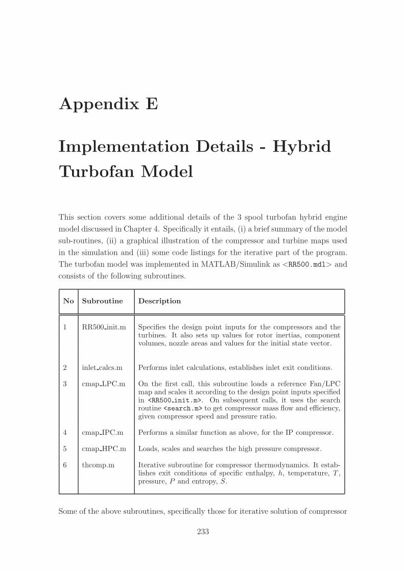
Appendix E
Implementation Details - Hybrid
Turbofan Model
This section covers some additional details of the 3 spool turbofan hybrid engine
model discussed in Chapter 4. Specifically it entails, (i) a brief summary of the model
sub-routines, (ii) a graphical illustration of the compressor and turbine maps used
in the simulation and (iii) some code listings for the iterative part of the program.
The turbofan model was implemented in MATLAB/Simulink as <RR500.mdl> and
consists of the following subroutines.
No Subroutine Description
1 RR500 init.m Specifies the design point inputs for the compressors and theturbines. It also sets up values for rotor inertias, componentvolumes, nozzle areas and values for the initial state vector.
2 inlet calcs.m Performs inlet calculations, establishes inlet exit conditions.
3 cmap LPC.m On the first call, this subroutine loads a reference Fan/LPCmap and scales it according to the design point inputs specifiedin <RR500 init.m>. On subsequent calls, it uses the searchroutine <search.m> to get compressor mass flow and efficiency,given compressor speed and pressure ratio.
4 cmap IPC.m Performs a similar function as above, for the IP compressor.
5 cmap HPC.m Loads, scales and searches the high pressure compressor.
6 thcomp.m Iterative subroutine for compressor thermodynamics. It estab-lishes exit conditions of specific enthalpy, h, temperature, T ,pressure, P and entropy, S.
Some of the above subroutines, specifically those for iterative solution of compressor
233
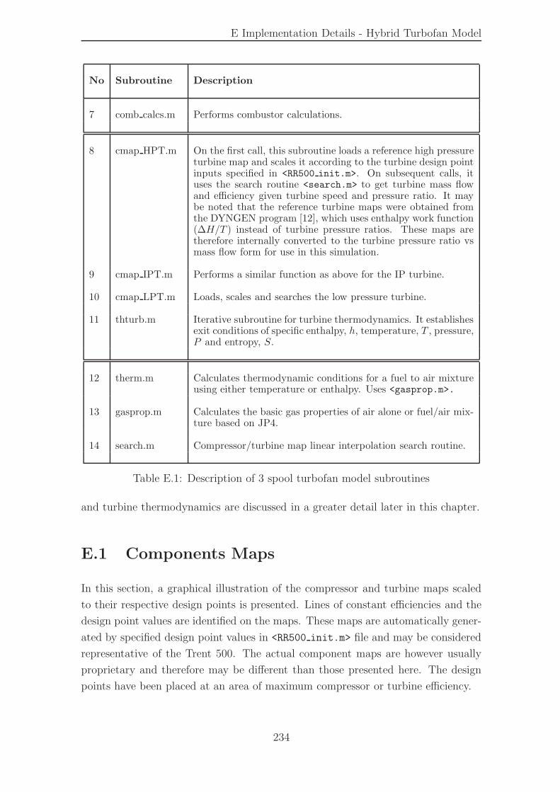
E Implementation Details - Hybrid Turbofan Model
No Subroutine Description
7 comb calcs.m Performs combustor calculations.
8 cmap HPT.m On the first call, this subroutine loads a reference high pressureturbine map and scales it according to the turbine design pointinputs specified in <RR500 init.m>. On subsequent calls, ituses the search routine <search.m> to get turbine mass flowand efficiency given turbine speed and pressure ratio. It maybe noted that the reference turbine maps were obtained fromthe DYNGEN program [12], which uses enthalpy work function(∆H/T ) instead of turbine pressure ratios. These maps aretherefore internally converted to the turbine pressure ratio vsmass flow form for use in this simulation.
9 cmap IPT.m Performs a similar function as above for the IP turbine.
10 cmap LPT.m Loads, scales and searches the low pressure turbine.
11 thturb.m Iterative subroutine for turbine thermodynamics. It establishesexit conditions of specific enthalpy, h, temperature, T , pressure,P and entropy, S.
12 therm.m Calculates thermodynamic conditions for a fuel to air mixtureusing either temperature or enthalpy. Uses <gasprop.m>.
13 gasprop.m Calculates the basic gas properties of air alone or fuel/air mix-ture based on JP4.
14 search.m Compressor/turbine map linear interpolation search routine.
Table E.1: Description of 3 spool turbofan model subroutines
and turbine thermodynamics are discussed in a greater detail later in this chapter.
E.1 Components Maps
In this section, a graphical illustration of the compressor and turbine maps scaled
to their respective design points is presented. Lines of constant efficiencies and the
design point values are identified on the maps. These maps are automatically gener-
ated by specified design point values in <RR500 init.m> file and may be considered
representative of the Trent 500. The actual component maps are however usually
proprietary and therefore may be different than those presented here. The design
points have been placed at an area of maximum compressor or turbine efficiency.
234
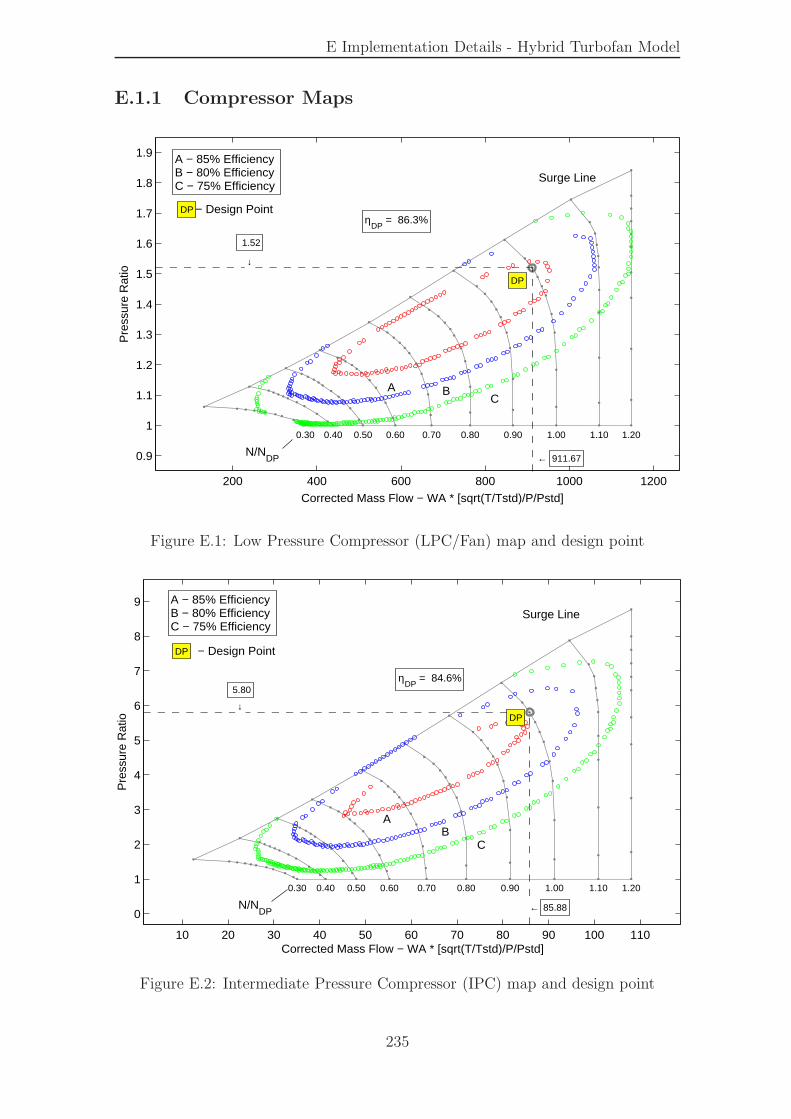
E Implementation Details - Hybrid Turbofan Model
E.1.1 Compressor Maps
200 400 600 800 1000 1200
0.9
1
1.1
1.2
1.3
1.4
1.5
1.6
1.7
1.8
1.9
0.30 0.40 0.50 0.60 0.70 0.80 0.90 1.00 1.10 1.20
Pre
ssur
e R
atio
1.52
↓
← 911.67
DP
DP
A − 85% Efficiency B − 80% Efficiency C − 75% Efficiency
− Design Point
Surge Line
A B C
ηDP
= 86.3%
Corrected Mass Flow − WA * [sqrt(T/Tstd)/P/Pstd]
N/NDP
Figure E.1: Low Pressure Compressor (LPC/Fan) map and design point
10 20 30 40 50 60 70 80 90 100 110
0
1
2
3
4
5
6
7
8
9
0.30 0.40 0.50 0.60 0.70 0.80 0.90 1.00 1.10 1.20
Corrected Mass Flow − WA * [sqrt(T/Tstd)/P/Pstd]
Pre
ssur
e R
atio
5.80
↓
← 85.88
A − 85% Efficiency B − 80% Efficiency C − 75% Efficiency
DP
DP − Design Point
A B
C
Surge Line
ηDP
= 84.6%
N/NDP
Figure E.2: Intermediate Pressure Compressor (IPC) map and design point
235
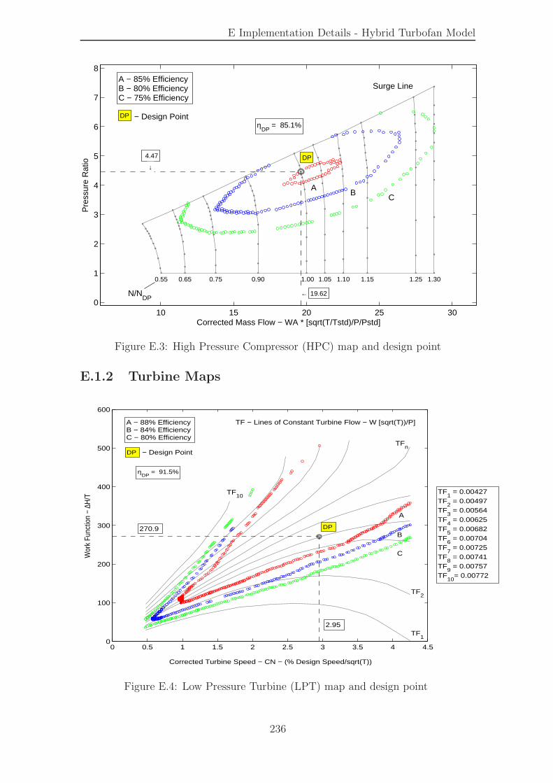
E Implementation Details - Hybrid Turbofan Model
10 15 20 25 300
1
2
3
4
5
6
7
8
0.55 0.65 0.75 0.90 1.00 1.05 1.10 1.15 1.25 1.30
Corrected Mass Flow − WA * [sqrt(T/Tstd)/P/Pstd]
Pre
ssur
e R
atio
4.47
↓
← 19.62
DP
A B
C
A − 85% Efficiency B − 80% Efficiency C − 75% Efficiency
Surge Line
DP − Design Point η
DP = 85.1%
N/NDP
Figure E.3: High Pressure Compressor (HPC) map and design point
E.1.2 Turbine Maps
0 0.5 1 1.5 2 2.5 3 3.5 4 4.50
100
200
300
400
500
600
Corrected Turbine Speed − CN − (% Design Speed/sqrt(T))
Wor
k Fu
nctio
n −
∆H/T
A − 88% Efficiency B − 84% Efficiency C − 80% Efficiency
DP − Design Point
DP
A
B
C
TF1
TF2
TFn
TF10
TF − Lines of Constant Turbine Flow − W [sqrt(T))/P]
270.9
2.95
TF1 = 0.00427
TF2 = 0.00497
TF3 = 0.00564
TF4 = 0.00625
TF5 = 0.00682
TF6 = 0.00704
TF7 = 0.00725
TF8 = 0.00741
TF9 = 0.00757
TF10
= 0.00772
ηDP
= 91.5%
Figure E.4: Low Pressure Turbine (LPT) map and design point
236
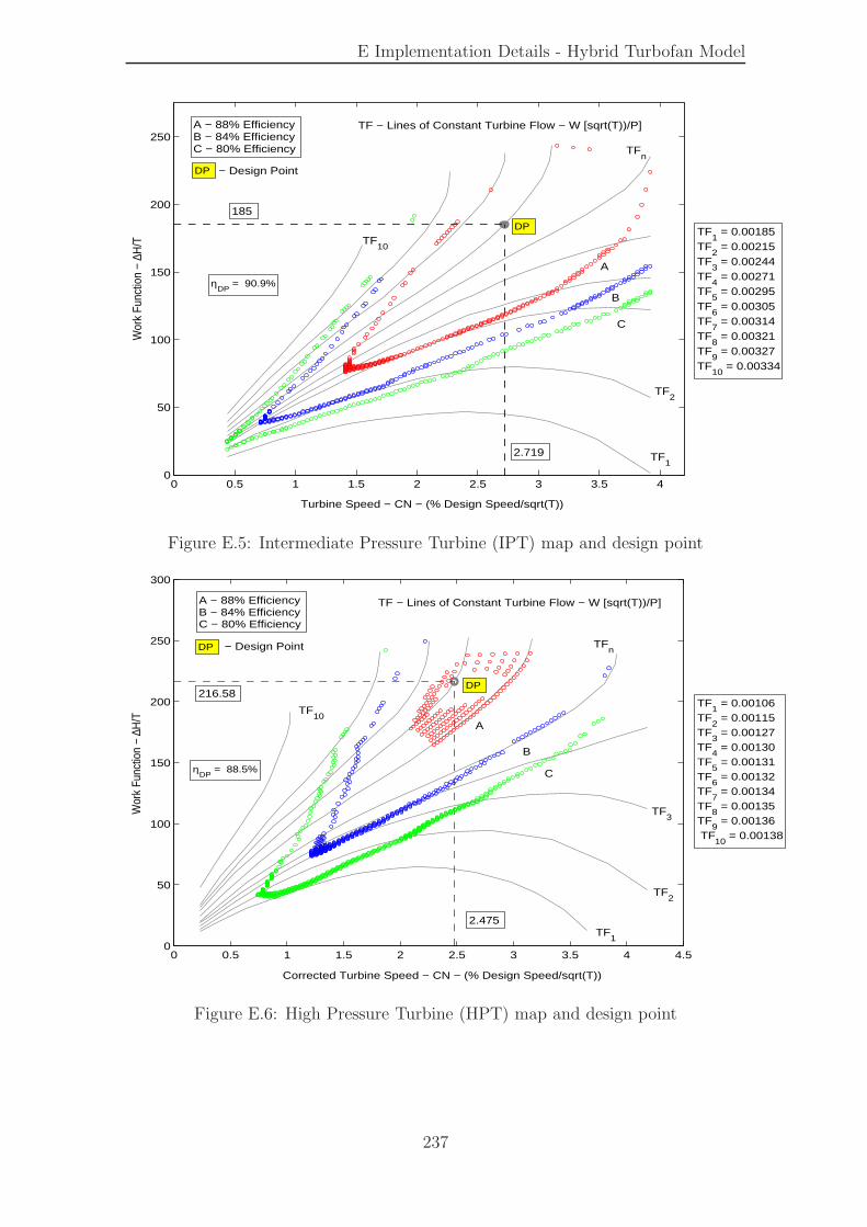
E Implementation Details - Hybrid Turbofan Model
0 0.5 1 1.5 2 2.5 3 3.5 40
50
100
150
200
250
Turbine Speed − CN − (% Design Speed/sqrt(T))
Wor
k Fu
nctio
n −
∆H/T
TF1
TF2
TFn
TF10
A − 88% Efficiency B − 84% Efficiency C − 80% Efficiency
DP
DP − Design Point
2.719
185
A
B
C
TF − Lines of Constant Turbine Flow − W [sqrt(T))/P]
TF1 = 0.00185
TF2 = 0.00215
TF3 = 0.00244
TF4 = 0.00271
TF5 = 0.00295
TF6 = 0.00305
TF7 = 0.00314
TF8 = 0.00321
TF9 = 0.00327
TF10
= 0.00334
ηDP
= 90.9%
Figure E.5: Intermediate Pressure Turbine (IPT) map and design point
0 0.5 1 1.5 2 2.5 3 3.5 4 4.50
50
100
150
200
250
300
Corrected Turbine Speed − CN − (% Design Speed/sqrt(T))
Wor
k Fu
nctio
n −
∆H/T
TF1
TF2
TF3
TFn
TF10
DP
A
B
C
A − 88% Efficiency B − 84% Efficiency C − 80% Efficiency
216.58
2.475
DP − Design Point
TF1 = 0.00106
TF2 = 0.00115
TF3 = 0.00127
TF4 = 0.00130
TF5 = 0.00131
TF6 = 0.00132
TF7 = 0.00134
TF8 = 0.00135
TF9 = 0.00136
TF10
= 0.00138
ηDP
= 88.5%
TF − Lines of Constant Turbine Flow − W [sqrt(T))/P]
Figure E.6: High Pressure Turbine (HPT) map and design point
237
E Implementation Details - Hybrid Turbofan Model
E.2 Code Listings
E.2.1 Iterative Routine for Compressor Calculations
In Chapter 4, a hybrid scheme was adopted for engine simulation, in which the
compressor and turbine thermodynamic conditions are calculated using an iterative
procedure and the pressure derivatives and hence exit pressures using the compo-
nent volume technique. Whereas, other details of the method have been covered
earlier, it was considered important for future reference to list here the subroutines
used for iterative compressor/turbine calculations. The iterative subroutine for the
compressor as listed below is a modified version from the open source reference,
DYNGEN [12]. Figure E.7 shows a Simulink block diagram for the HP compressor
that uses this iterative subroutine to perform stage calculations. The IP and the
LP compressor stages were implemented using a similar procedure.
% =============================================================================
% COMPRESSOR ITERATIVE THERRMODYNAMIC CALCULATIONS .
% =============================================================================
%
% Function Name : [TO,HO,SO,PO] = thcomp(PR,ETA,T,H,S,P,FAR,SI)
% Purpose : Calculates Thermodynamic conditions for the compressor.
%
% Inputs to the program:
%
% PR = Compressor Pressure Ratio [-]
% ETA = Compressor Efficiency [-]
% T = Temperature at Inlet [K]
% H = Specific Enthalpy at Inlet [J/Kg/s]
% S = Entropy at Inlet [J/Kg-C]
% P = Pressure at Compressor Inlet [Pa]
% FAR = Fuel to Air Ratio at Compressor Inlet [-]
%
% Outputs of the program:
%
% TO = Temperature at Compressor Exit [K]
% HO = Specific Enthalpy at Compressor Exit [J/Kg/s]
% SO = Exit Entropy [J/Kg-C]
% PO = Pressure at Compressor Exit [Pa]
%
% Subroutines used :
%
% thermo() : Calculates gas thermodynamic conditions using temperature
% or enthalpy.
%
% Modified From Original reference : DYNGEN[]
% =============================================================================
function [TO,HO,SO,PO] = thcomp(PR,ETA,T,H,S,P,FAR,SI)
CPG = 1048.0; % Specific Heat for Air...[J/Kg/K]
238
E Implementation Details - Hybrid Turbofan Model
% Pressure at Compressor Exit
% ---------------------------
PO = P*PR;
% Initial Guess for Exit Temperature
% ----------------------------------
TP = T * PR^0.28572;
% Step 1. Find Exit Enthalpy (H) iteratively, assuming Process to be Isentropic
% -----------------------------------------------------------------------------
for (I=1:25)
% Thermodynamic gas calculations
% ------------------------------
% Inputs - PO, TP (Actual Exit Pressure , Guessed Exit Temperature)
% Output - SP, HP (Exit Entropy Isentropic , Exit Enthalpy Isentropic)
XX1 = 0.0; % Dummy Input
FLAG = 0; % (0) - Use Temperauture for Gas Thermo Calculations
[SP,YY1,HP,YY2] = therm(PO,XX1,TP,FAR,FLAG);
% Difference in Inlet and Exit Entropy
DELS = SP-S;
% Check convergence (Exit Entropy ~ Inelt Entropy)
if (abs(DELS) <= (0.00005 * S)) break; end
% New Guess for Exit Temperature
TP = TP / exp(DELS/CPG);
if (I==25)
disp(’Error - Iterations exceeded in THCOMP’);
end
end
% Step 2. Now Use Compressor Efficiency to find actual exit Enthalpy (HO)
% ----------------------------------------------------------------------
% Note if ETA = 1.0, then HO = HP and process will be isentropic
HO = H + (HP-H)/ETA;
% Step 3. Use Exit Enthalpy (HO) to Calculate Exit Temperature (TO) and Entropy (SO)
% ----------------------------------------------------------------------------------
% Inputs - PO, HO (Exit Press , Exit Enthalpy after including ETA effect)
% Output - SO, TO (Exit Entropy, Exit Temperature)
FLAG = 1; % (1) - Use Enthalpy for Gas Thermo Calculations
[SO,YY1,YY,TO] = therm(PO,HO,XX1,FAR,FLAG);
% <End of File>
239

EIm
plem
entation
Details
-H
ybrid
Turb
ofanM
odel
Tor_HPC(N−m)
6
w_CH(kg/s)
5
Bleed _HPC(kg/s)
4
Out3
3
P3Dot
2
w_HPC
1
[S3]
[S21]
kg/s1
[W_CH]
kg/s
[W_HPC]
dotP 3
Vol − m^3
V3
Use SI Units
1
SI Units
[P21]
1/2
[H3]
[P3]
P3/P21
N [rad/s]
[H21]
[T3]
[T21]
Integrator
1s
xo
IC − P21
P3_0
HPC Map
NH
T21
P21
P3/P21
Wc
Etac
[Bleed _HPC]
[PR]
[NH_RPM]
[ETAC]
Gas ConstantN−m / (Kg−K)
287 .05
[P21]
[ETAC]
[PR]
[W_HPC]
[W_HPC]
[W_HPC]
[P3]
[W_CH]
[H21]
[T21]
[H3]
[P3]
[W_HPC]
[Bleed _HPC]
[S3]
[H3]
[T3]
[S21]
[H21]
[T21]
[P21]
[NH_RPM]
Display
CompressorCalcs
MATLABFunction
Compressor Torque
2PI/60
(2*pi )/60
1
u
1/P21
1
u
1/N
1
u
(deg K )
[T3]
NH
6
T4
5
Bleed _h
4
In21
3
w_F
2
w_TH
1
Net Mass Flow Ingestedby HP compressor
After Bleed Extraction
Mass Flow Ingestedby HP Turbine
Fuel Flow
Figu
reE
.7:H
PC
ompressor
calculation
san
dpressu
rederivatives
240
E Implementation Details - Hybrid Turbofan Model
E.2.2 Iterative Routine for Turbine Calculations
The turbine calculations were performed using an iterative procedure similar to
compressors, however in this case the input pressure ratio (PR) is less than 1.0,
whereas for the compressor it was greater than 1.0. However, this makes no difference
in the calculations procedure, only the corresponding exit temperatures are less as
the turbine extracts energy from the flow. In addition, the exit enthalpy is calculated
differently than for the compressor stage, specifically if hi is the inlet enthalpy, and
hp is the enthalpy at the turbine exit assuming the process to be isentropic, then
the actual exit enthalpy is
ho = hi − η∆h = hi − η(hp − hi) (E.1)
where η is the turbine efficiency. Thus if η = 1.0, then the exit enthalpy would be
the same as that for an isentropic process and the turbine would be able to extract
greater energy from the flow. A MATLAB/Simulink subsystem that implements the
turbine calculations is shown in Figure E.8 and the code listing is presented below.
% ===============================================================================
% TURBINE ITERATIVE THERRMODYNAMIC CALCULATIONS .
% ===============================================================================
%
% Function Name : [TO,HO,SO,PO] = thturb(PR,ETA,T,H,S,P,FAR)
% Purpose : Calculates Thermodynamic conditions for the turbine.
%
% Inputs to the program:
%
% PR = Turbine Pressure Ratio [-]
% ETA = Turbine Efficiency [-]
% T = Temperature at Inlet [K]
% H = Specific Enthalpy at Inlet [J/Kg/s]
% S = Entropy at Inlet [J/Kg-C]
% P = Pressure at Turbine Inlet [Pa]
% FAR = Fuel to Air Ratio at Turbine Inlet [-]
%
% Outputs of the program:
%
% TO = Temperature at Turbine Exit [K]
% HO = Specific Enthalpy at Turbine Exit [J/Kg/s]
% SO = Exit Entropy [J/Kg-C]
% PO = Pressure at Turbine Exit [Pa]
%
% Subroutines used :
%
% thermo() : Calculates gas thermodynamic conditions using temperature
% or enthalpy.
% ==============================================================================
function [TO,HO,SO,PO] = thturb(PR,ETA,T,H,S,P,FAR)
CPG = 1048.0; % Specific Heat for Air...[J/Kg/K]
241
E Implementation Details - Hybrid Turbofan Model
% Pressure at Compressor Exit
PO = P*PR;
% Initial Guess for Exit Temperature
% ----------------------------------
TP = T * PR^0.28572;
% Step 1. Find Exit Enthalpy (H) iteratively, assuming Process to be Isentropic
% -----------------------------------------------------------------------------
for (I=1:25)
% Thermodynamic gas calculations
% ------------------------------
% Inputs - PO, TP (Actual Exit Pressure , Guessed Exit Temperature)
% Output - SP, HP (Exit Entropy Isentropic , Exit Enthalpy Isentropic)
XX1 = 0.0; % Dummy Input
FLAG = 0; % (0) - Use Temperauture for Gas Thermo Calculations
[SP,YY1,HP,YY2] = therm(PO,XX1,TP,FAR,FLAG);
% Difference in Inlet and Exit Entropy
DELS = SP-S;
% Check convergence (Exit Entropy ~ Inelt Entropy)
if (abs(DELS) <= (0.00005 * S)) break; end
% New Guess for Exit Temperature
TP = TP / exp(DELS/CPG);
if (I==25) disp(’Error - Iterations exceeded in THTURB’); end
end
% Step 2. Now Use Turbine Efficiency to find the new Enthalpy
% -----------------------------------------------------------
DELH_i = H - HP; % isentropic drop in enthalpy
% Note if ETA = 1.0, Then HO = HP and process will be isentropic
HO = H - ETA * DELH_i;
% Step 3. Use Exit Enthalpy (HO) to Calculate Exit Temperature (TO) and Entropy (SO)
% ----------------------------------------------------------------------------------
% Inputs - PO, HO (Exit Press , Exit Enthalpy after including ETA effect)
% Output - SO, TO (Exit Entropy, Exit Temperature)
FLAG = 1; % (1) - Use Enthalpy for Gas Thermo Calculations
[SO,YY1,YY,TO] = therm(PO,HO,XX1,FAR,FLAG);
% <End of File>
242
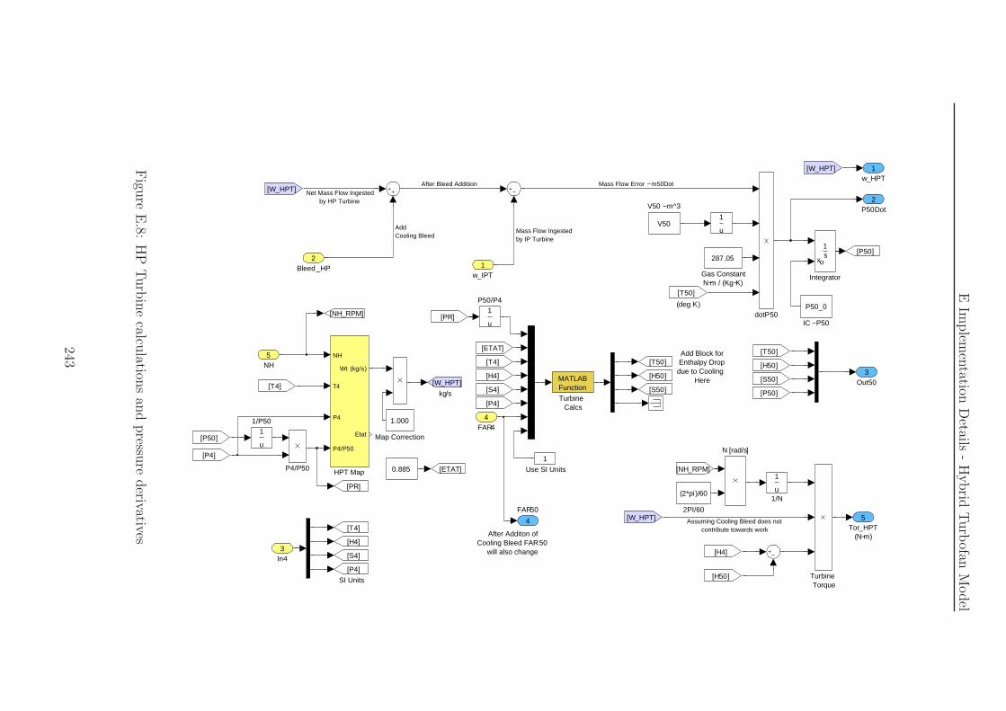
EIm
plem
entation
Details
-H
ybrid
Turb
ofanM
odel
Add Block for Enthalpy Drop due to Cooling
Here
After Additon ofCooling Bleed FAR50
will also change
Tor_HPT(N−m)
5FAR50
4
Out503
P50Dot2
w_HPT1
[S50]
[S4]
kg/s
[W_HPT]
dotP50
V50 − m^3
V50
0.885 Use SI Units
1
Turbine Calcs
MATLABFunction
Turbine Torque
SI Units
[P4]
[H50]
[P50]
[H4]
P50/P41
u
P4/P50
N [rad/s]
Map Correction
1.000
[T50]
[T4]
Integrator
1s
xo
IC − P50
P50_0
HPT Map
NH
T4
P4
P4/P50
Wt (kg/s)
Etat
[PR]
[NH_RPM]
[ETAT]
Gas ConstantN−m / (Kg−K)
287.05
[P4]
[ETAT]
[PR]
[W_HPT]
[W_HPT]
[P4]
[H50]
[T4]
[H4]
[P50]
[W_HPT]
[S50]
[H50]
[T50]
[S4]
[H4]
[T4]
[P50]
[NH_RPM]
2PI/60
(2*pi)/60
1
u
1/P501
u
1/N
1
u
(deg K)
[T50]
NH5
FAR44
In43
Bleed_HP2
w_IPT1
AddCooling Bleed
Net Mass Flow Ingestedby HP Turbine
After Bleed Addition
Assuming Cooling Bleed does notcontribute towards work
Mass Flow Ingestedby IP Turbine
Mass Flow Error − m50Dot
Figu
reE
.8:H
PTurb
ine
calculation
san
dpressu
rederivatives
243
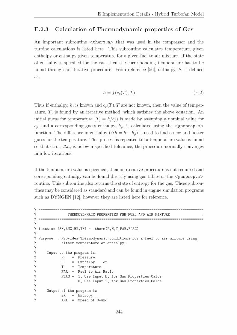
E Implementation Details - Hybrid Turbofan Model
E.2.3 Calculation of Thermodynamic properties of Gas
An important subroutine <therm.m> that was used in the compressor and the
turbine calculations is listed here. This subroutine calculates temperature, given
enthalpy or enthalpy given temperature for a given fuel to air mixture. If the state
of enthalpy is specified for the gas, then the corresponding temperature has to be
found through an iterative procedure. From reference [56], enthalpy, h, is defined
as,
h = f(cp(T ), T ) (E.2)
Thus if enthalpy, h, is known and cp(T ), T are not known, then the value of temper-
ature, T , is found by an iterative method, which satisfies the above equation. An
initial guess for temperature (Tg = h/cp) is made by assuming a nominal value for
cp, and a corresponding guess enthalpy, hg, is calculated using the <gasprop.m>
function. The difference in enthalpy (∆h = h− hg) is used to find a new and better
guess for the temperature. This process is repeated till a temperature value is found
so that error, ∆h, is below a specified tolerance, the procedure normally converges
in a few iterations.
If the temperature value is specified, then an iterative procedure is not required and
corresponding enthalpy can be found directly using gas tables or the <gasprop.m>
routine. This subroutine also returns the state of entropy for the gas. These subrou-
tines may be considered as standard and can be found in engine simulation programs
such as DYNGEN [12], however they are listed here for reference.
% ===============================================================================
% THERMOYDNMAIC PROPERTIES FOR FUEL AND AIR MIXTURE .
% ===============================================================================
%
% function [SX,AMX,HX,TX] = therm(P,H,T,FAR,FLAG)
%
% Purpose : Provides Thermodynamic conditions for a fuel to air mixture using
% either temperature or enthalpy.
%
% Input to the program is:
% P = Pressure
% H = Enthalpy or
% T = Temperature
% FAR = Fuel to Air Ratio
% FLAG = 1, Use Input H, for Gas Properties Calcs
% 0, Use Input T, for Gas Properties Calcs
%
% Output of the program is:
% SX = Entropy
% AMX = Speed of Sound
244
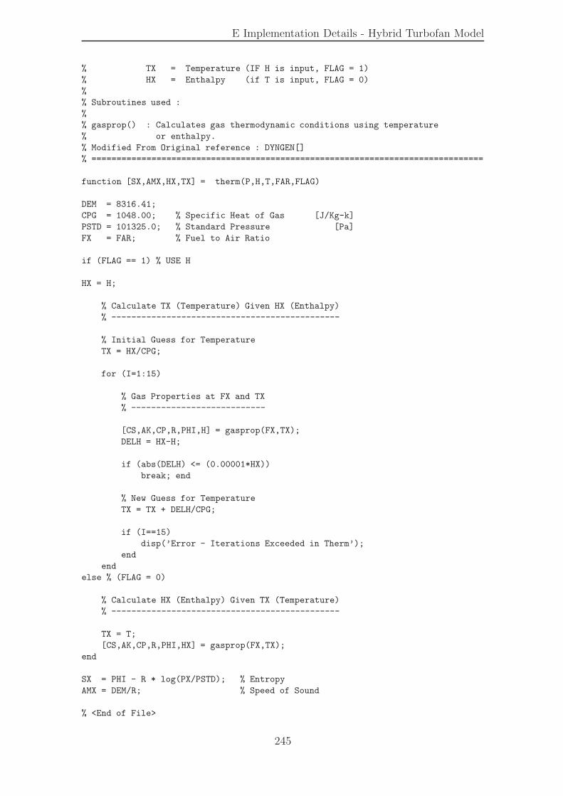
E Implementation Details - Hybrid Turbofan Model
% TX = Temperature (IF H is input, FLAG = 1)
% HX = Enthalpy (if T is input, FLAG = 0)
%
% Subroutines used :
%
% gasprop() : Calculates gas thermodynamic conditions using temperature
% or enthalpy.
% Modified From Original reference : DYNGEN[]
% ===============================================================================
function [SX,AMX,HX,TX] = therm(P,H,T,FAR,FLAG)
DEM = 8316.41;
CPG = 1048.00; % Specific Heat of Gas [J/Kg-k]
PSTD = 101325.0; % Standard Pressure [Pa]
FX = FAR; % Fuel to Air Ratio
if (FLAG == 1) % USE H
HX = H;
% Calculate TX (Temperature) Given HX (Enthalpy)
% ----------------------------------------------
% Initial Guess for Temperature
TX = HX/CPG;
for (I=1:15)
% Gas Properties at FX and TX
% ---------------------------
[CS,AK,CP,R,PHI,H] = gasprop(FX,TX);
DELH = HX-H;
if (abs(DELH) <= (0.00001*HX))
break; end
% New Guess for Temperature
TX = TX + DELH/CPG;
if (I==15)
disp(’Error - Iterations Exceeded in Therm’);
end
end
else % (FLAG = 0)
% Calculate HX (Enthalpy) Given TX (Temperature)
% ----------------------------------------------
TX = T;
[CS,AK,CP,R,PHI,HX] = gasprop(FX,TX);
end
SX = PHI - R * log(PX/PSTD); % Entropy
AMX = DEM/R; % Speed of Sound
% <End of File>
245
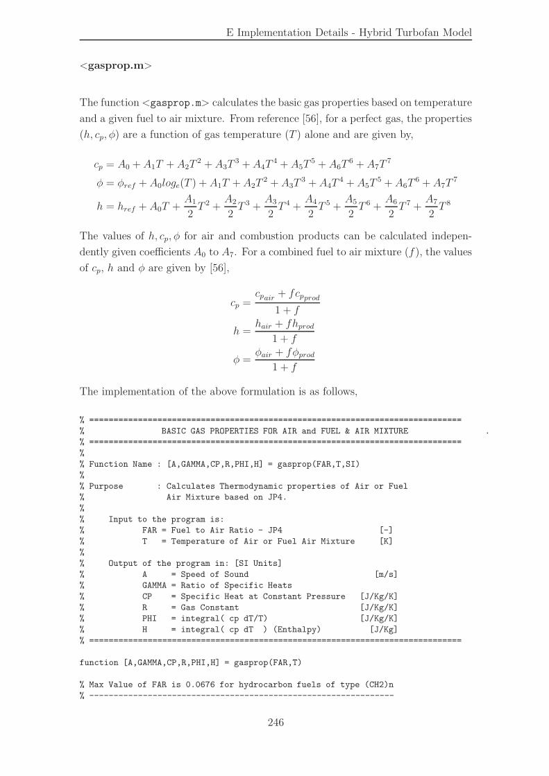
E Implementation Details - Hybrid Turbofan Model
<gasprop.m>
The function <gasprop.m> calculates the basic gas properties based on temperature
and a given fuel to air mixture. From reference [56], for a perfect gas, the properties
(h, cp, φ) are a function of gas temperature (T ) alone and are given by,
cp = A0 + A1T + A2T2 + A3T
3 + A4T4 + A5T
5 + A6T6 + A7T
7
φ = φref + A0loge(T ) + A1T + A2T2 + A3T
3 + A4T4 + A5T
5 + A6T6 + A7T
7
h = href + A0T +A1
2T 2 +
A2
2T 3 +
A3
2T 4 +
A4
2T 5 +
A5
2T 6 +
A6
2T 7 +
A7
2T 8
The values of h, cp, φ for air and combustion products can be calculated indepen-
dently given coefficients A0 to A7. For a combined fuel to air mixture (f), the values
of cp, h and φ are given by [56],
cp =cpair + fcpprod
1 + f
h =hair + fhprod
1 + f
φ =φair + fφprod
1 + f
The implementation of the above formulation is as follows,
% =============================================================================
% BASIC GAS PROPERTIES FOR AIR and FUEL & AIR MIXTURE .
% =============================================================================
%
% Function Name : [A,GAMMA,CP,R,PHI,H] = gasprop(FAR,T,SI)
%
% Purpose : Calculates Thermodynamic properties of Air or Fuel
% Air Mixture based on JP4.
%
% Input to the program is:
% FAR = Fuel to Air Ratio - JP4 [-]
% T = Temperature of Air or Fuel Air Mixture [K]
%
% Output of the program in: [SI Units]
% A = Speed of Sound [m/s]
% GAMMA = Ratio of Specific Heats
% CP = Specific Heat at Constant Pressure [J/Kg/K]
% R = Gas Constant [J/Kg/K]
% PHI = integral( cp dT/T) [J/Kg/K]
% H = integral( cp dT ) (Enthalpy) [J/Kg]
% =============================================================================
function [A,GAMMA,CP,R,PHI,H] = gasprop(FAR,T)
% Max Value of FAR is 0.0676 for hydrocarbon fuels of type (CH2)n
% ---------------------------------------------------------------
246
E Implementation Details - Hybrid Turbofan Model
if (FAR > 0.067623) FAR = 0.067623; end;
% T must be in degree Rankine for Gas tables
% ------------------------------------------
T = T * 9.0/5.0; % Convert to degree Rankine (R)
if (T < 300.0 ) T = 300.0; end;
if (T > 4000.0 ) T = 4000.0; end;
% AIR PATH - INLET AND COMPRESSOR
% -------------------------------
CPA = (((((( 1.0115540E-25 *T - 1.4526770E-21)*T + 7.6215767E-18)*T -...
1.5128259E-14)*T - 6.7178376E-12)*T + 6.5519486E-08)*T -...
5.1536879E-05)*T + 2.5020051E-01;
HEA =((((((( 1.2644425E-26 *T - 2.0752522E-22)*T + 1.2702630E-18)*T -...
3.0256518E-15)*T - 1.6794594E-12)*T + 2.1839826E-08)*T -...
2.5768440E-05)*T + 2.5020051E-01)*T - 1.7558886E+00;
SEA =((((((( 1.4450767E-26 *T - 2.4211288E-22)*T + 1.5243153E-18)*T -...
3.7820648E-15)*T - 2.2392790E-12)*T + 3.2759743E-08)*T -...
5.1576879E-05)*T + 4.5432300E-02) + 2.5020051E-01 *log(T);
% FUEL AIR PATH - PRODUCTS OF COMBUSTION
% --------------------------------------
if (FAR > 0.0)
CPF = (((((( 7.2678710E-25 *T - 1.3335668E-20)*T + 1.0212913E-16)*T -...
4.2051104E-13)*T + 9.9686793E-10)*T - 1.3771901E-06)*T +...
1.2258630E-03)*T + 7.3816638E-02;
HEF =((((((( 9.0848388E-26 *T - 1.9050949E-21)*T + 1.7021525E-17)*T -...
8.4102208E-14)*T + 2.4921698E-10)*T - 4.5906332E-07)*T +...
6.1293150E-04)*T + 7.3816638E-02)*T + 3.0581530E+01;
SEF =((((((( 1.0382670E-25 *T - 2.2226118E-21)*T + 2.0425826E-17)*T -...
1.0512776E-13)*T + 3.3228928E-10)*T - 6.8859505E-07)*T +...
1.2258630E-03)*T + 6.4833980E-01) + 7.3816638E-02 *log(T);
end
CP = (CPA + FAR*CPF)/(1.0+FAR);
H = (HEA + FAR*HEF)/(1.0+FAR);
PHI = (SEA + FAR*SEF)/(1.0+FAR);
R = 1.986375/(28.97 - 0.946186 * FAR); % Gas constant
GAMMA = CP/(CP - R); % Specific Heat Ratio
A = sqrt(GAMMA * R * T * 25031.37); % Speed of Sound [ft/sec]
% Convert to SI Units
% -------------------
CP = CP * 4185.7666; % Specific Heat [J/Kg-K]
PHI = PHI * 4185.7666; % [J/Kg-K]
R = R * 4185.7666; % Gas Constant [J/Kg-K]
H = H * 2325.4259; % Enthalpy [J/Kg]
A = A * 0.3048; % Speed of sound [m/s]
T = T * 5.0/9.0; % Temperature [deg K]
% < End of File>
247

E Implementation Details - Hybrid Turbofan Model
248
Appendix F
Single Spool Turbojet Model and
Investigation of Bleed Effects
During the initial part of this research, a single spool turbojet engine model was
developed to investigate the affects of engine bleed on its performance. Although
later on for the BWB, a three spool turbofan model was used for propulsion and
flight controls integration, the single spool turbojet model proved to be very valuable
in validation of the numerical simulation, as real engine bleed data was available for
this purpose [79]. The single spool turbojet engine model is therefore presented here
for future reference. It is a simpler model than the hybrid engine model discussed
earlier and uses the inter-component volume approach.
F.1 Introduction
This section presents dynamic modeling of a single spool turbojet engine and its
overall performance under variable bleed conditions. The approach followed is to
model various engine subsystems using performance maps and then interlink each
individual component to get an overall engine performance model. Two approaches
were considered, the inter component volume method [48] and the constraint sat-
isfaction iterative method [53]. However the inter-component volume method was
eventually selected due to its real time performance and simplicity. Both open loop
(fuel flow demand defined by user) and closed loop (fuel flow demand set by RPM
control) responses were simulated. The AMT Olympus single spool turbojet en-
gine [50] was selected as a test case. The simulation results were validated with
data from bleed experiments conducted on the AMT Olympus engine at University
of Manchester [79].
249
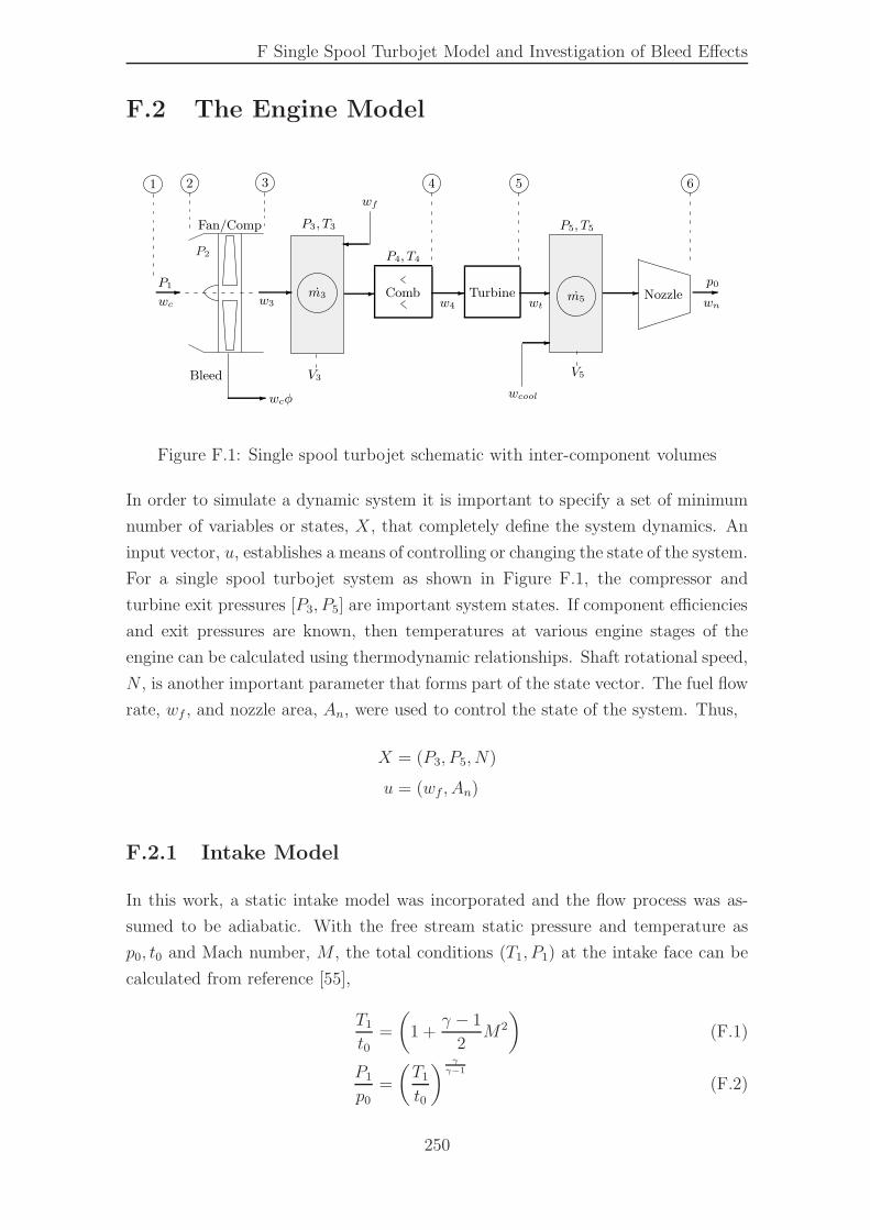
F Single Spool Turbojet Model and Investigation of Bleed Effects
F.2 The Engine Model
P2
- m3
P3, T3
Comb
V3
- Turbine -
�
-- -
P5, T5
w4
Bleed
m5
P1
wc
Fan/Comp
wf
- wcφ
w3
P4, T4
wt
V5
Nozzle -wn
p0
1 2 3 4 5 6
-
wcool
Figure F.1: Single spool turbojet schematic with inter-component volumes
In order to simulate a dynamic system it is important to specify a set of minimum
number of variables or states, X, that completely define the system dynamics. An
input vector, u, establishes a means of controlling or changing the state of the system.
For a single spool turbojet system as shown in Figure F.1, the compressor and
turbine exit pressures [P3, P5] are important system states. If component efficiencies
and exit pressures are known, then temperatures at various engine stages of the
engine can be calculated using thermodynamic relationships. Shaft rotational speed,
N , is another important parameter that forms part of the state vector. The fuel flow
rate, wf , and nozzle area, An, were used to control the state of the system. Thus,
X = (P3, P5, N)
u = (wf , An)
F.2.1 Intake Model
In this work, a static intake model was incorporated and the flow process was as-
sumed to be adiabatic. With the free stream static pressure and temperature as
p0, t0 and Mach number, M , the total conditions (T1, P1) at the intake face can be
calculated from reference [55],
T1
t0=
(
1 +γ − 1
2M2
)
(F.1)
P1
p0
=
(
T1
t0
)γγ−1
(F.2)
250
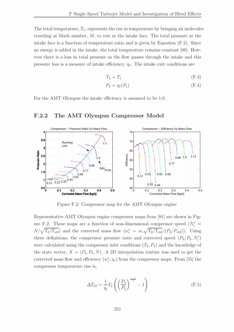
F Single Spool Turbojet Model and Investigation of Bleed Effects
The total temperature, T1, represents the rise in temperature by bringing air molecules
traveling at Mach number, M , to rest at the intake face. The total pressure at the
intake face is a function of temperature ratio and is given by Equation (F.2). Since
no energy is added in the intake, the total temperature remains constant [80]. How-
ever there is a loss in total pressure as the flow passes through the intake and this
pressure loss is a measure of intake efficiency, ηI . The intake exit conditions are
T2 = T1 (F.3)
P2 = ηI(P1) (F.4)
For the AMT Olympus the intake efficiency is assumed to be 1.0.
F.2.2 The AMT Olympus Compressor Model
0 0.1 0.2 0.3 0.4 0.50.5
1
1.5
2
2.5
3
3.5
4
Corrected Mass Flow [kg/s]
Pre
ssur
e R
atio
Compressor − Pressure Ratio Vs Mass Flow
0 0.1 0.2 0.3 0.4 0.545
50
55
60
65
70
75
Corrected Mass Flow [kg/s]
Effi
cien
cyCompressor − Efficiency Vs Mass Flow
0 0.1 0.2 0.3 0.4 0.50.5
1
1.5
2
2.5
3
3.5
4
Corrected Mass Flow [kg/s]
Pre
ssur
e R
atio
0 0.1 0.2 0.3 0.4 0.50.5
1
1.5
2
2.5
3
3.5
4
Corrected Mass Flow [kg/s]
Pre
ssur
e R
atio
0 0.1 0.2 0.3 0.4 0.50.5
1
1.5
2
2.5
3
3.5
4
Corrected Mass Flow [kg/s]
Pre
ssur
e R
atio
0.88
1.0
0.660.77
0.550.44
1.1
0.330.220.11
N/Ndesign
RunningLine
0.110.22
0.33 0.44
0.55 0.66
0.77
0.88 1.0 1.11
Figure F.2: Compressor map for the AMT Olympus engine
Representative AMT Olympus engine compressor maps from [81] are shown in Fig-
ure F.2. These maps are a function of non-dimensional compressor speed (N∗
c =
N/√
T2/Tstd) and the corrected mass flow (w∗
c = wc√
T2/Tstd/(P2/Pstd)). Using
these definitions, the compressor pressure ratio and corrected speed (P3/P2, N∗
c )
were calculated using the compressor inlet conditions (T2, P2) and the knowledge of
the state vector, X = (P3, P5, N). A 2D interpolation routine was used to get the
corrected mass flow and efficiency (w∗
c , ηc) from the compressor maps. From [55] the
compressor temperature rise is,
∆T23 =1
ηcT2
(
(
P3
P2
)γ−1γ
− 1
)
(F.5)
251
F Single Spool Turbojet Model and Investigation of Bleed Effects
therefore the total temperature at the compressor exit is,
T3 = T2 + ∆T23 (F.6)
If a fraction of bleed (φ = wb/wc) is taken from the compressor at a non-dimensional
axial location (x/l) along the compressor, then the exit mass flow is
w3 = wc(1 − φ) (F.7)
and with a bleed location of x/l, the torque required by the compressor is
τcomp =wccp∆T23
Nrad/s
(
(1 − φ) + φx
l
)
(F.8)
The above set of equations was used to calculate compressor exit conditions (w3, T3, P3)
and compressor torque, with inlet exit conditions (T2, P2) and the state vector,
X = (P3, P5, N) as inputs.
F.2.3 The AMT Olympus Combustor Model
The AMT Olympus engine uses an annular type combustion chamber. The amount
of energy imparted to the pressurized air depends upon the fuel to air ratio and the
heating value (HV ) of the fuel. Not all the fuel is burnt and a burner efficiency, ηb,
is associated with the fuel burning process. A typical value for burning efficiency is
0.98. Reference [57] gives an expression for combustor temperature rise,
∆T34 = ηb
(
wfw3
)
HVfuelcp
(F.9)
The combustor exit temperature is therefore
T4 = T3 + ∆T34 (F.10)
and the net mass flow from combustor,
w4 = wf + w3 (F.11)
With a pressure loss, ∆Ploss, the combustor exit pressure will be
P4 = P3(1 − ∆Ploss) (F.12)
This establishes the combustor exit conditions (w4, T4, P4).
252
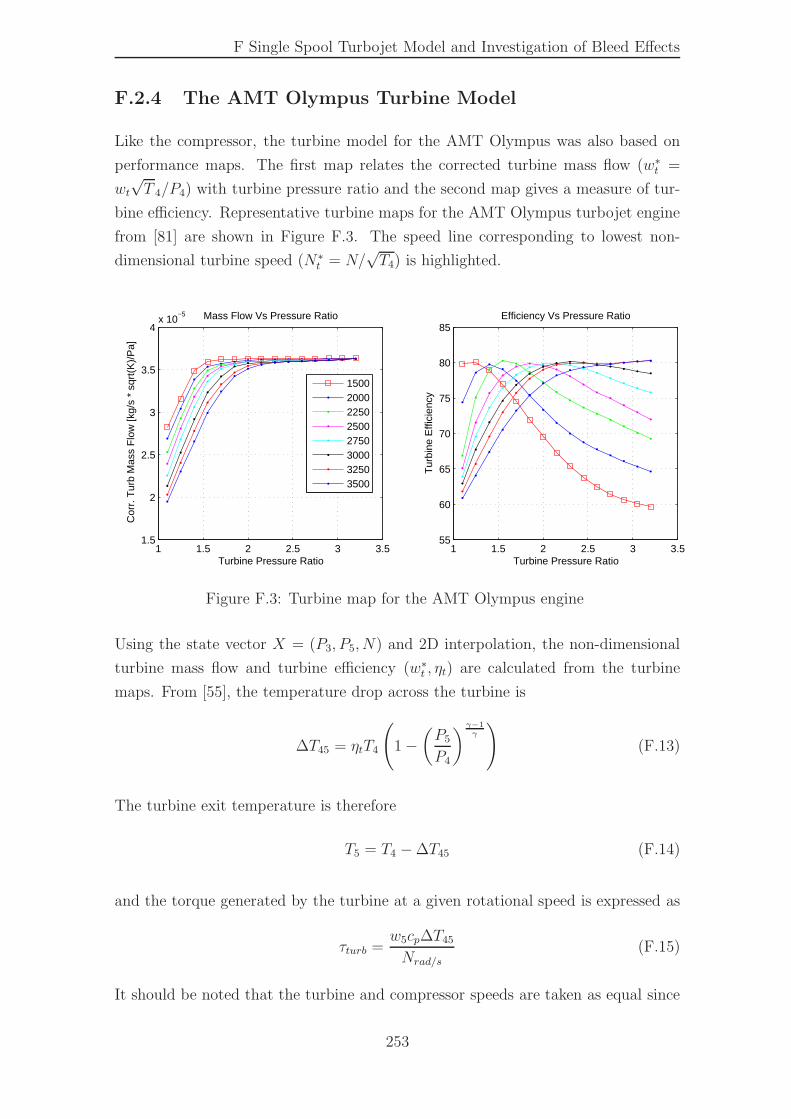
F Single Spool Turbojet Model and Investigation of Bleed Effects
F.2.4 The AMT Olympus Turbine Model
Like the compressor, the turbine model for the AMT Olympus was also based on
performance maps. The first map relates the corrected turbine mass flow (w∗
t =
wt√T 4/P4) with turbine pressure ratio and the second map gives a measure of tur-
bine efficiency. Representative turbine maps for the AMT Olympus turbojet engine
from [81] are shown in Figure F.3. The speed line corresponding to lowest non-
dimensional turbine speed (N∗
t = N/√T4) is highlighted.
1 1.5 2 2.5 3 3.51.5
2
2.5
3
3.5
4x 10
−5
Turbine Pressure Ratio
Cor
r. T
urb
Mas
s F
low
[kg/
s *
sqrt
(K)/
Pa]
Mass Flow Vs Pressure Ratio
15002000225025002750300032503500
1 1.5 2 2.5 3 3.555
60
65
70
75
80
85
Turbine Pressure Ratio
Tur
bine
Effi
cien
cy
Efficiency Vs Pressure Ratio
Figure F.3: Turbine map for the AMT Olympus engine
Using the state vector X = (P3, P5, N) and 2D interpolation, the non-dimensional
turbine mass flow and turbine efficiency (w∗
t , ηt) are calculated from the turbine
maps. From [55], the temperature drop across the turbine is
∆T45 = ηtT4
(
1 −(
P5
P4
)γ−1γ
)
(F.13)
The turbine exit temperature is therefore
T5 = T4 − ∆T45 (F.14)
and the torque generated by the turbine at a given rotational speed is expressed as
τturb =w5cp∆T45
Nrad/s
(F.15)
It should be noted that the turbine and compressor speeds are taken as equal since
253
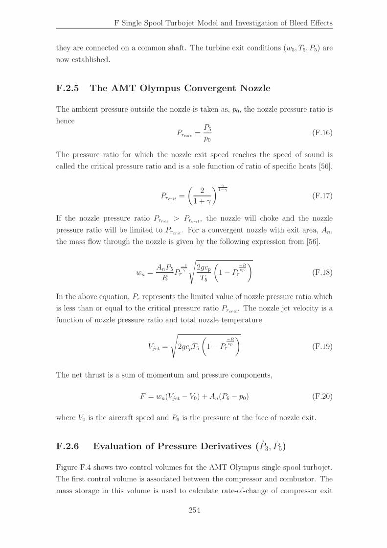
F Single Spool Turbojet Model and Investigation of Bleed Effects
they are connected on a common shaft. The turbine exit conditions (w5, T5, P5) are
now established.
F.2.5 The AMT Olympus Convergent Nozzle
The ambient pressure outside the nozzle is taken as, p0, the nozzle pressure ratio is
hence
Prnoz =P5
p0(F.16)
The pressure ratio for which the nozzle exit speed reaches the speed of sound is
called the critical pressure ratio and is a sole function of ratio of specific heats [56].
Prcrit =
(
2
1 + γ
)γ
1−γ
(F.17)
If the nozzle pressure ratio Prnoz > Prcrit, the nozzle will choke and the nozzle
pressure ratio will be limited to Prcrit . For a convergent nozzle with exit area, An,
the mass flow through the nozzle is given by the following expression from [56].
wn =AnP5
RP
−1γr
√
2gcpT5
(
1 − P−Rcpr
)
(F.18)
In the above equation, Pr represents the limited value of nozzle pressure ratio which
is less than or equal to the critical pressure ratio Prcrit. The nozzle jet velocity is a
function of nozzle pressure ratio and total nozzle temperature.
Vjet =
√
2gcpT5
(
1 − P−Rcpr
)
(F.19)
The net thrust is a sum of momentum and pressure components,
F = wn(Vjet − V0) + An(P6 − p0) (F.20)
where V0 is the aircraft speed and P6 is the pressure at the face of nozzle exit.
F.2.6 Evaluation of Pressure Derivatives (P3, P5)
Figure F.4 shows two control volumes for the AMT Olympus single spool turbojet.
The first control volume is associated between the compressor and combustor. The
mass storage in this volume is used to calculate rate-of-change of compressor exit
254
F Single Spool Turbojet Model and Investigation of Bleed Effects
Control
- -
?
-
Volume
P2
Control
-
Volume
p0
T2
Compressor Combustor Turbine Nozzle
wf
w3 wt wt wnm3 m5
P3 P5
Figure F.4: Control volumes on a single spool turbojet
pressure, P3. The second control volume is between the turbine and nozzle and shall
provide derivative of turbine exit pressure, P5. For the volume associated with the
combustor chamber and the compressor, the rate of accumulation of mass is
m3 = w3 + wf − wt (F.21)
and similarly for the volume between the turbine and the nozzle the rate of change
of mass is
m5 = wt − wn (F.22)
Taking the time derivative of the ideal gas law and neglecting the temperature
derivative term (mT ) as suggested Bates and Fawke [48], gives
P =RT
V(m) (F.23)
which was used to calculate the pressure derivatives (P3, P5) inside each control
volume.
F.2.7 Evaluation of Rotational Acceleration (N)
The rotational acceleration derivative, N , is evaluated by calculating the difference
in torque generated by the turbine and that required by the compressor.
N =dN
dt=
(ηmτturb − τcomp)
Ispool(F.24)
This expression was integrated to get shaft rotational speed as a function of time.
Using the above formulation a dynamic model for the AMT Olympus engine was
implemented in MATLAB/Simulink and is shown in Figure F.5.
255
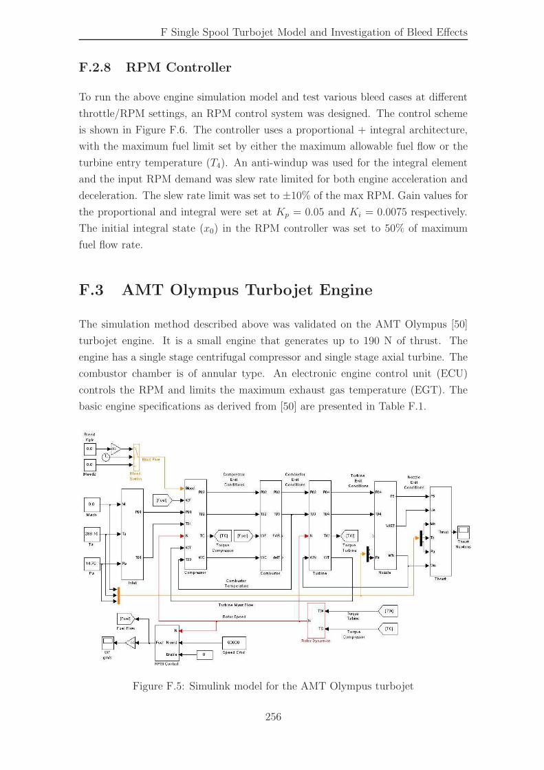
F Single Spool Turbojet Model and Investigation of Bleed Effects
F.2.8 RPM Controller
To run the above engine simulation model and test various bleed cases at different
throttle/RPM settings, an RPM control system was designed. The control scheme
is shown in Figure F.6. The controller uses a proportional + integral architecture,
with the maximum fuel limit set by either the maximum allowable fuel flow or the
turbine entry temperature (T4). An anti-windup was used for the integral element
and the input RPM demand was slew rate limited for both engine acceleration and
deceleration. The slew rate limit was set to ±10% of the max RPM. Gain values for
the proportional and integral were set at Kp = 0.05 and Ki = 0.0075 respectively.
The initial integral state (x0) in the RPM controller was set to 50% of maximum
fuel flow rate.
F.3 AMT Olympus Turbojet Engine
The simulation method described above was validated on the AMT Olympus [50]
turbojet engine. It is a small engine that generates up to 190 N of thrust. The
engine has a single stage centrifugal compressor and single stage axial turbine. The
combustor chamber is of annular type. An electronic engine control unit (ECU)
controls the RPM and limits the maximum exhaust gas temperature (EGT). The
basic engine specifications as derived from [50] are presented in Table F.1.
Figure F.5: Simulink model for the AMT Olympus turbojet
256
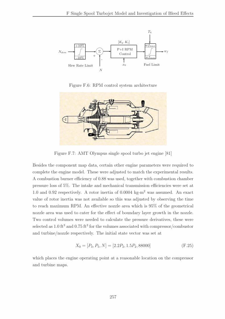
F Single Spool Turbojet Model and Investigation of Bleed Effects
P+I RPM
Control-
+10%
-10%
-Ndem Σ -
Slew Rate Limit
6
Fuel Limit
-
[Kp Ki]
6+
-
x0
wfmax
wfmin
T4
?
- wf
N
Figure F.6: RPM control system architecture
Figure F.7: AMT Olympus single spool turbo jet engine [81]
Besides the component map data, certain other engine parameters were required to
complete the engine model. These were adjusted to match the experimental results.
A combustion burner efficiency of 0.88 was used, together with combustion chamber
pressure loss of 5%. The intake and mechanical transmission efficiencies were set at
1.0 and 0.92 respectively. A rotor inertia of 0.0004 kg-m2 was assumed. An exact
value of rotor inertia was not available so this was adjusted by observing the time
to reach maximum RPM. An effective nozzle area which is 95% of the geometrical
nozzle area was used to cater for the effect of boundary layer growth in the nozzle.
Two control volumes were needed to calculate the pressure derivatives, these were
selected as 1.0 ft3 and 0.75 ft3 for the volumes associated with compressor/combustor
and turbine/nozzle respectively. The initial state vector was set at
X0 = [P3, P5, N ] = [2.2P2, 1.5P2, 88000] (F.25)
which places the engine operating point at a reasonable location on the compressor
and turbine maps.
257
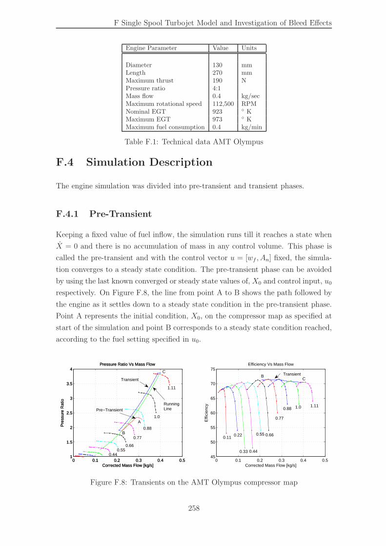
F Single Spool Turbojet Model and Investigation of Bleed Effects
Engine Parameter Value Units
Diameter 130 mmLength 270 mmMaximum thrust 190 NPressure ratio 4:1Mass flow 0.4 kg/secMaximum rotational speed 112,500 RPMNominal EGT 923 ◦ KMaximum EGT 973 ◦ KMaximum fuel consumption 0.4 kg/min
Table F.1: Technical data AMT Olympus
F.4 Simulation Description
The engine simulation was divided into pre-transient and transient phases.
F.4.1 Pre-Transient
Keeping a fixed value of fuel inflow, the simulation runs till it reaches a state when
X = 0 and there is no accumulation of mass in any control volume. This phase is
called the pre-transient and with the control vector u = [wf , An] fixed, the simula-
tion converges to a steady state condition. The pre-transient phase can be avoided
by using the last known converged or steady state values of, X0 and control input, u0
respectively. On Figure F.8, the line from point A to B shows the path followed by
the engine as it settles down to a steady state condition in the pre-transient phase.
Point A represents the initial condition, X0, on the compressor map as specified at
start of the simulation and point B corresponds to a steady state condition reached,
according to the fuel setting specified in u0.
0 0.1 0.2 0.3 0.4 0.51
1.5
2
2.5
3
3.5
4
Corrected Mass Flow [kg/s]
Pre
ssur
e R
atio
Pressure Ratio Vs Mass Flow
0 0.1 0.2 0.3 0.4 0.545
50
55
60
65
70
75
Corrected Mass Flow [kg/s]
Effi
cien
cy
Efficiency Vs Mass Flow
0 0.1 0.2 0.3 0.4 0.51
1.5
2
2.5
3
3.5
4
Corrected Mass Flow [kg/s]
Pre
ssur
e R
atio
Pressure Ratio Vs Mass Flow
A
B
CB
C
1.0
1.11
0.88
0.77
0.44
0.66
0.77
0.66
0.55
1.0 1.11
0.11
0.88
0.55
0.440.33
0.22
TransientTransient
Pre−TransientRunningLine
Figure F.8: Transients on the AMT Olympus compressor map
258
F Single Spool Turbojet Model and Investigation of Bleed Effects
F.4.2 Transient
Once the engine has reached a steady state condition at point B, the control vector
u = [wf , An] consisting of fuel flow rate and nozzle area can be varied to initiate a
transient. During a transient, it takes a finite amount of time for the rotor to spool
up or down but the mass flow and therefore pressure changes inside the engine can
be quite rapid. The effect of a sudden increase in fuel flow is to move the compressor
operating point up along the speed line toward surge. A sudden reduction in fuel flow
causes the reverse action and the compressor operating point moves down toward
the choking point. Path B to C on Figure F.8, shows the transient response of the
AMT Olympus engine to a slew rate limited RPM demand. The transient was run
with RPM control engaged. The engine settles down at point C corresponding to
maximum speed demand of 112,500 RPM.
F.5 Simulation Results and Validation
F.5.1 Steady State Results
The steady state experimental values under zero compressor bleed were compared at
maximum speed with RPM control engaged. Values of fuel flow, thrust, compressor
pressure ratio and mass flow were noted. Table F.2, summarizes the steady state
results at maximum engine RPM.
Engine Parameter Exper. Sim % Error
Maximum Thrust, N 193 189.5 +1.81Pressure ratio 3.55 3.47 +2.25Maximum fuel, gm/sec 9.10 8.85 +2.75EGT at max RPM, ◦ K 1035 970 +6.28
Table F.2: AMT Olympus engine steady state comparison at 112,500 RPM
It is evident from above that there is a good match between the experimental and
the simulated values. The percentage errors are less than 3% for most of the param-
eters except the exhaust gas temperature (EGT) error, which is approx 6%. The
simulation predicts lesser values of exhaust gas temperature at max RPM, however
as will be discussed later, at lower RPM values the EGT correlation was much better.
Figure F.9 presents a correlation between static experimental and simulated engine
thrust as a function of RPM. Besides the engine setting, various environmental
259
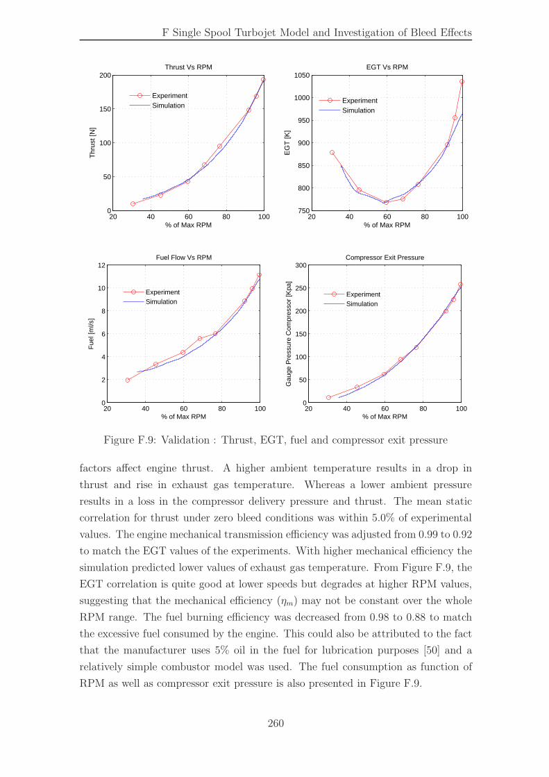
F Single Spool Turbojet Model and Investigation of Bleed Effects
20 40 60 80 1000
50
100
150
200Thrust Vs RPM
% of Max RPM
Thr
ust [
N]
ExperimentSimulation
20 40 60 80 100750
800
850
900
950
1000
1050EGT Vs RPM
% of Max RPM
EG
T [K
]
ExperimentSimulation
20 40 60 80 1000
2
4
6
8
10
12Fuel Flow Vs RPM
% of Max RPM
Fue
l [m
l/s]
ExperimentSimulation
20 40 60 80 1000
50
100
150
200
250
300Compressor Exit Pressure
% of Max RPM
Gau
ge P
ress
ure
Com
pres
sor
[Kpa
]
ExperimentSimulation
Figure F.9: Validation : Thrust, EGT, fuel and compressor exit pressure
factors affect engine thrust. A higher ambient temperature results in a drop in
thrust and rise in exhaust gas temperature. Whereas a lower ambient pressure
results in a loss in the compressor delivery pressure and thrust. The mean static
correlation for thrust under zero bleed conditions was within 5.0% of experimental
values. The engine mechanical transmission efficiency was adjusted from 0.99 to 0.92
to match the EGT values of the experiments. With higher mechanical efficiency the
simulation predicted lower values of exhaust gas temperature. From Figure F.9, the
EGT correlation is quite good at lower speeds but degrades at higher RPM values,
suggesting that the mechanical efficiency (ηm) may not be constant over the whole
RPM range. The fuel burning efficiency was decreased from 0.98 to 0.88 to match
the excessive fuel consumed by the engine. This could also be attributed to the fact
that the manufacturer uses 5% oil in the fuel for lubrication purposes [50] and a
relatively simple combustor model was used. The fuel consumption as function of
RPM as well as compressor exit pressure is also presented in Figure F.9.
260
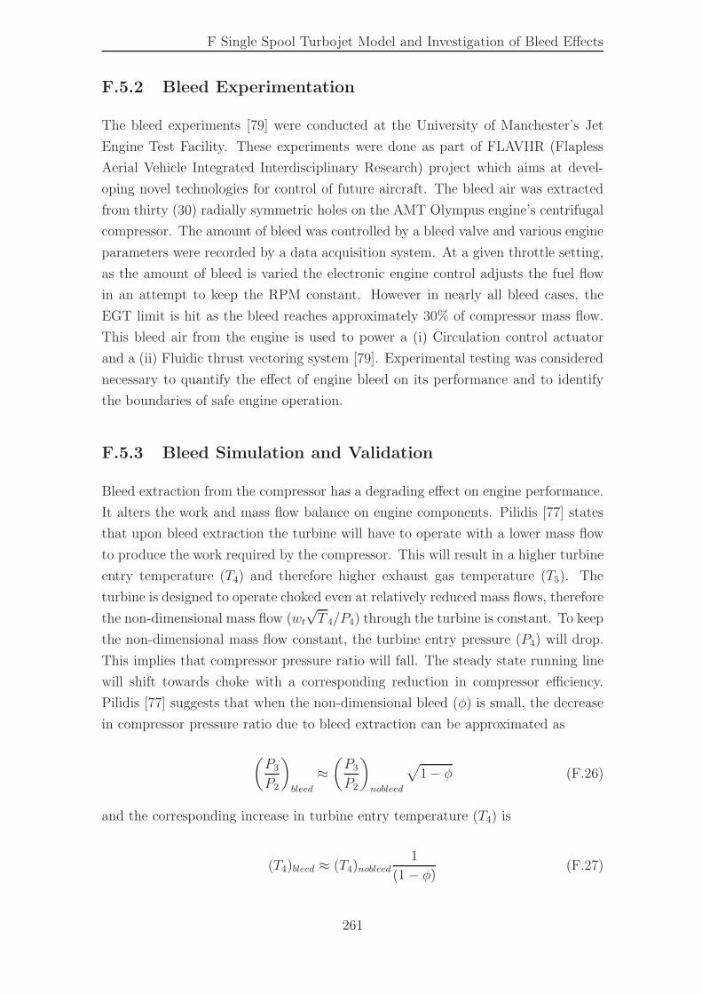
F Single Spool Turbojet Model and Investigation of Bleed Effects
F.5.2 Bleed Experimentation
The bleed experiments [79] were conducted at the University of Manchester’s Jet
Engine Test Facility. These experiments were done as part of FLAVIIR (Flapless
Aerial Vehicle Integrated Interdisciplinary Research) project which aims at devel-
oping novel technologies for control of future aircraft. The bleed air was extracted
from thirty (30) radially symmetric holes on the AMT Olympus engine’s centrifugal
compressor. The amount of bleed was controlled by a bleed valve and various engine
parameters were recorded by a data acquisition system. At a given throttle setting,
as the amount of bleed is varied the electronic engine control adjusts the fuel flow
in an attempt to keep the RPM constant. However in nearly all bleed cases, the
EGT limit is hit as the bleed reaches approximately 30% of compressor mass flow.
This bleed air from the engine is used to power a (i) Circulation control actuator
and a (ii) Fluidic thrust vectoring system [79]. Experimental testing was considered
necessary to quantify the effect of engine bleed on its performance and to identify
the boundaries of safe engine operation.
F.5.3 Bleed Simulation and Validation
Bleed extraction from the compressor has a degrading effect on engine performance.
It alters the work and mass flow balance on engine components. Pilidis [77] states
that upon bleed extraction the turbine will have to operate with a lower mass flow
to produce the work required by the compressor. This will result in a higher turbine
entry temperature (T4) and therefore higher exhaust gas temperature (T5). The
turbine is designed to operate choked even at relatively reduced mass flows, therefore
the non-dimensional mass flow (wt√T 4/P4) through the turbine is constant. To keep
the non-dimensional mass flow constant, the turbine entry pressure (P4) will drop.
This implies that compressor pressure ratio will fall. The steady state running line
will shift towards choke with a corresponding reduction in compressor efficiency.
Pilidis [77] suggests that when the non-dimensional bleed (φ) is small, the decrease
in compressor pressure ratio due to bleed extraction can be approximated as
(
P3
P2
)
bleed
≈(
P3
P2
)
nobleed
√
1 − φ (F.26)
and the corresponding increase in turbine entry temperature (T4) is
(T4)bleed ≈ (T4)nobleed1
(1 − φ)(F.27)
261
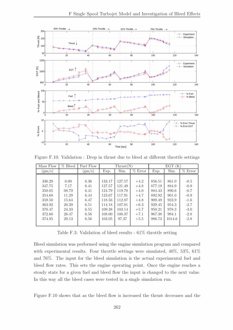
F Single Spool Turbojet Model and Investigation of Bleed Effects
0 20 40 60 80 100 120 14050
100
150
200
Th
rust
[N
]
ExperimentSimulation
0 20 40 60 80 100 120 140800
1000
1200
EG
T [
K]
ExperimentSimulation
0 20 40 60 80 100 120 1400
50
100
% F
ue
l an
d B
lee
d
% Fuel% Bleed
0 20 40 60 80 100 120 140−10
0
10
% E
rro
rs
% Error Thrust% Error EGT
Time [sec]
40% Throttle 53% Throttle 76% Throttle61% Throttle
Thrust
EGT
Bleed
Fuel
Figure F.10: Validation : Drop in thrust due to bleed at different throttle settings
Mass Flow % Bleed Fuel Flow Thrust(N) EGT (K)(gm/s) (gm/s) Exp. Sim. % Error Exp. Sim. % Error
336.29 0.00 6.36 133.17 127.57 +4.2 856.51 861.0 -0.5347.75 7.17 6.41 127.57 121.49 +4.8 877.19 884.9 -0.9350.05 08.79 6.41 124.79 119.78 +4.0 884.43 890.6 -0.7354.68 11.29 6.44 123.67 117.91 +4.7 892.92 901.0 -0.9359.50 15.64 6.47 118.56 112.87 +4.8 909.49 923.9 -1.6363.92 20.39 6.51 114.18 107.01 +6.3 929.45 954.3 -2.7370.47 24.33 6.55 109.38 103.14 +5.7 950.21 978.3 -3.0372.60 26.47 6.56 108.00 100.37 +7.1 967.38 994.1 -2.8374.95 29.13 6.56 103.05 97.37 +5.5 986.73 1014.6 -2.8
Table F.3: Validation of bleed results - 61% throttle setting
Bleed simulation was performed using the engine simulation program and compared
with experimental results. Four throttle settings were simulated, 40%, 53%, 61%
and 76%. The input for the bleed simulation is the actual experimental fuel and
bleed flow rates. This sets the engine operating point. Once the engine reaches a
steady state for a given fuel and bleed flow the input is changed to the next value.
In this way all the bleed cases were tested in a single simulation run.
Figure F.10 shows that as the bleed flow is increased the thrust decreases and the
262
F Single Spool Turbojet Model and Investigation of Bleed Effects
EGT increases. Even at lower throttle settings as the bleed flow is increased, the
EGT hits the upper limit. At this point the fuel or bleed flow cannot be increased
further. Hence there is an upper limit on the amount of bleed that can be extracted
at any given throttle setting or engine RPM. The percentage errors for thrust and
exhaust gas temperature are within 5-10% of experimental values. This variation is
expected since the compressor characteristics change with the amount of bleed flow,
and only steady state compressor maps under no bleed conditions were used for the
simulation. It may also be noted that as the engine bleed is increased the electronic
Engine Control Unit (ECU) tries to adjust the corresponding drop in speed by
increasing the value of fuel flow. Each step in the fuel flow setting corresponds to
a different value of throttle setting. Table F.3 summarizes the experimental and
simulated results for the 61% throttle case.
F.6 Summary
A gas turbine simulation program was written in MATLAB/Simulink and perfor-
mance was compared with experimental values. The results were accurate to within
5.0% for the nominal or zero bleed case and within 10.0% for excessive bleed cases.
The increase in error upon bleed extraction can be attributed to two factors. Firstly,
the location where the bleed is extracted affects the amount of work required by the
compressor and this may also vary non-linearly for the radial compressor of the
AMT Olympus engine. Secondly, the bleed extraction itself may adversely influence
the performance of the compressor and the compressor characteristics may change.
Further work will be required to more accurately model the compressor map with
bleed extraction and improve upon the accuracy of the overall simulation. The com-
pressor/turbine maps were obtained from [81] and the experimental data from [79].
Although both sources refer to the same AMT Olympus engine, the possibility of
statistical variation between the available component maps and the actual engine
under test exists. It is possible to further adjust the component efficiencies in order
to match the experimental results, however this was not considered further. The
simulation method runs in real time and therefore can easily be integrated with
aircraft and active flow control simulation codes.
263

F Single Spool Turbojet Model and Investigation of Bleed Effects
264
Bibliography
[1] R. Leibeck. Design of blended wing body subsonic transport. Journal of Air-
craft, Vol 41, pp. 10-25, 2004.
[2] A. Diedrich, J. Hileman, D. Tan, K. Wilcox, and Z. Spakovsky. Multidisci-
plinary design and optimization of the silent aircraft. In 44th AIAA Aerospace
Sciences Meeting and Exhibit, Nevada, AIAA Paper 2006-1323, 2006.
[3] A. Agarwal and A. Dowling. A ray tracing approach to calculate acoustic
shielding by the silent airframe. In 44th AIAA Aerospace Sciences Meeting and
Exhibit, Nevada, AIAA Paper 2006-2618, 2006.
[4] M.A. Sargeant, J.I. Hileman, S. Spakovszky, and M. Drela. Airframe design for
silent aircraft. In 45th AIAA Aerospace Sciences Meeting and Exhibit, Nevada,
AIAA Paper 2007-0453, 2007.
[5] J.I. Hileman, T.R. Reynolds, E. de la Rosa Blanco, and T. Law. Development
of approach procedures for silent aircraft. In 45th AIAA Aerospace Sciences
Meeting and Exhibit, Nevada, AIAA Paper 2007-0456, 2007.
[6] E. de la Rosa Blanca, C. Hall, and D. Crichton. Challenges in silent aircraft
engine design. In 45th AIAA Aerospace Sciences Meeting and Exhibit, Nevada,
AIAA Paper 2007-0454, 2007.
[7] H.V. Castro. Flying and Handling Qualities of a Fly by Wire Blended Wing
Body Civil Transport Aircraft. PhD thesis, Cranfield University, Cranfield UK,
2003.
[8] J.V. Decken. Aerodynamics of pneumatic high lift devices. In AGARD Lecture
Series, AGARD-LS-43, April, 1970.
[9] R.J. Englar. Development of circulation control technology for application to
advanced subsonic transport aircraft. Journal of Aircraft, Vol 31, pp. 1160-1177,
1994.
265
BIBLIOGRAPHY
[10] G.S Jones. Pneumatic flap performance for a two dimensional circulation con-
trol airfoil. In Applications of Circulation Control Technology, Progress in Aero-
nautics and Astronautics, AIAA, Vol 214, 2005.
[11] Department of Power and Propulsion, Cranfield University, UK. Cranfield Uni-
versity Design and Off Design Engine Simulation Code, TURBOMATCH.
[12] J.F. Sellers and C.J. Daniele. DYNGEN a program for calculation of steady
state and transient performance of turbojet and turbofan engines, NASA TN-
D7901. Technical report, NASA, 1975.
[13] Department of Aeronautics, KTH, Sweden. User’s Guide, Reference Manual,
TORNADO 1.0.
[14] D.A. Spence. The lift coefficient of a thin jet-flapped wing. Proceedings of the
Royal Society of London, Vol 251, pp. 407-425, 1959.
[15] J. Williams and A.J. Alexander. Some exploratory jet flap experiments. Aero.
Quarterly, Vol 8, pp. 21-30, 1957.
[16] www.cite.monash.edu.au.
[17] B. Casey. Flying qualities and control of a blended wing body transport aircraft.
Master’s thesis, Cranfield University, Cranfield UK, 2005.
[18] www.secondworldwarhistory.com.
[19] J.K. Northrop. The development of all wing aircraft. Journal of the Royal
Aeronautical Society, Vol 51, pp. 481-510, 1941.
[20] northrop.host.sk.
[21] Aerospace America, October 2006 Issue. pp 28-33.
[22] C.A. Hall and D. Crichton. Engine and installation configurations for silent
aircraft. In ISABE 2005-1164, 2005.
[23] D. Crichton, E. de la Rosa Blanco, T. Law, and J.I. Hileman. Design and
operation for ultra low noise at take-off. In 45th AIAA Aerospace Sciences
Meeting and Exhibit, Nevada, AIAA Paper 2007-0451, 2007.
[24] B.W. McCormick. Aerodynamics, Aeronautics and Flight Mechanics. John
Wiley, New York, 1995.
[25] R.T. Jones. Notes on the stability and control of tailless airplanes NACA Report
837. Technical report, NACA, 1941.
266
BIBLIOGRAPHY
[26] C.J. Donlan. An interim report on the stability and control of tailless airplanes,
NACA Report No 796. Technical report, NACA, 1944.
[27] C.M. Fremaux. Effect of geometry static stability and mass distribution on the
tumbling characteristics of generic flying wing models. In Proceedings of the
AIAA Atmospheric Flight Mechanics Conference, AIAA-93-3615, 1993.
[28] A.W. Thorpe. Note on longitudinal stability and trim of tailless aircraft, RAE-
TN-AERO 1021. Technical report, Royal Aircraft Establishment, 1942.
[29] D.D. Mclean. Automatic Flight Control Systems. Prentice Hall International,
1990.
[30] I.M. Davidson. The jet flap. Journal of the Royal Aeronautical Society, Vol 60,
pp. 25-50, January, 1956.
[31] B.S. Stratford. Early thoughts on the jet flaps. Aero. Quarterly, Vol 7, pp,
85-105, 1956.
[32] N.A. Dimmock. Some early jet-flap experiments. Aero. Quarterly, Vol 8, pp.
331-345, 1957.
[33] K.D. Harris. The Hunting H-126 jet flap research aircraft. In AGARD Lecture
Series, AGARD-LS-43, April, 1970.
[34] S.P. Frith and N.J. Wood. The use of circulation control for flight control. In
Proceedings of the NASA’s Circulation Control Workshop, 2004.
[35] J.D. Anderson. Fundamentals of Aerodynamics. McGraw Hill, 2001.
[36] J.A. Hooper. Lift augmentation devices and their effect on the engine. In
AGARD Lecture Series, AGARD-LS-43, April, 1970.
[37] J.M. Williams, S.F.J. Butler, and M.N. Wood. The aerodynamics of jet flaps.
In 2nd International Congress of Aeronautical Sciences, Zurich, Sept, 1960.
[38] J.J. Burken. Longitudinal emergency control system using thrust modulation
demonstrated on the MD-11 airplane. In 32nd Joint Propulsion Conference,
AIAA 93-3062, 1996.
[39] M. Harefors and D.G. Bates. Integrated propulsion based flight control system
design for civil transport aircraft. In Proceedings of the 2002 IEEE International
Conference on Control Applications, 2002.
267
BIBLIOGRAPHY
[40] F.W. Burcham. Development and flight evaluation of an emergency digital flight
control system using only engine thrust on an F-15 airplane NASA-TP-3627.
Technical report, NASA, 1996.
[41] G.S. Jones and R.J. Englar. Advances in pneumatic controlled high lift systems
through pulsed blowing. In 21st AIAA Applied Aerodynamics Conference, June,
2003.
[42] D.H. Kim and D.J. Saunders. Embedded wing propulsion conceptual study,
NASA TM-2003-212696. Technical report, Glenn Research Center, 2003.
[43] M.V. Cook. Flight dynamics principles. Arnold publishers, 1997.
[44] MIL-F-8785C. Military specification, flying qualities of piloted airplanes. Tech-
nical report, USAF, 1980.
[45] ESDU 94028. A background to the handling qualities of aircraft. Technical
report, ESDU International, London, 1992.
[46] T.P Neal and R.J. Smith. A flying qualities criterion for the design of fighter
flight control systems. Journal of Aircraft, Vol 8, 1971.
[47] M.D. McLaughlin and J.B. Whitten. Pilot evaluation of dynamic stability
characteristic of a supersonic transport in cruising flight using a fixed base
simulator. Technical report, Langley Research Center, 1964.
[48] A.J. Fawke. Digital Computer simulation of Gas Turbine Dynamic Behavior.
PhD thesis, University of Bristol, Bristol UK, 1970.
[49] A. Behbahani. Modeling diagnostics and prognostics of a two spool turbofan
engine. In Proceedings of the 41st AIAA/ASME/SAE/ASEE Joint Propulsion
Conference and Exhibit, AIAA 2005-4344, 2005.
[50] Advanced Micro Turbines (AMT) Netherlands. AMT Olympus Engine User’s
Manual Serial No 112171.
[51] N.U. Rahman and J.F. Whidborne. A numerical investigation into the effect
of engine bleed on performance of a single-spool turbojet engine. Journal of
Aerospace Engineering, Vol 222, IMECHE Part G, pp. 939-949, 2008.
[52] E.T. Whittaker and G. Robinson. The Calculus of Observations: A Treatise
on Numerical Mathematics. Dover publishers, New York: Dover, 4th ed., 1967.
268
BIBLIOGRAPHY
[53] K. Parker and T.H. Guo. Development of turbofan engine simulation in a
graphical simulation environment NASA-TM-2003-212543. Technical report,
NASA, 2003.
[54] AS755D. Aircraft propulsion system performance station designation and
nomenclature, aerospace standard AS755D. Technical report, SAE, 20 Aug
2004.
[55] H.I.H. Saravanamuttoo, G.F.C. Rogers, and H. Cohen. Gas Turbine Theory.
Longman, 1996.
[56] J.D. Mattingly. Elements of Gas Turbine Propulsion. McGraw Hill, 1996.
[57] P.P. Walsh and P. Fletcher. Gas Turbine Performance. Blackwell publishing,
1999.
[58] K. Seldner. Generalized simulation technique for turbojet engine system anal-
ysis, NASA-TND-6610. Technical report, NASA, 1972.
[59] A.K. Cooke. Simulation model of NFLC Jetstream 31. Technical report, Cran-
field University, Reports CU/COA-2006/0402, 2006.
[60] A.R. Amrane. Flight dynamics model of a high performance sailplane. Master’s
thesis, Cranfield University, Cranfield UK, 2005.
[61] Z. Spakovszky, D. Pilczer, and A. Manneville. Preliminary evaluation of noise
reduction approaches for a functionally silent aircraft. AIAA Journal, Vol 43,
No.3, pp. 836-840, 2006.
[62] A.P. Plas, V. Madani, M.A. Sargant, E.M. Greitzer, C.A. Hall, and T.P. Hynes.
Performance of a boundary layer ingestion propulsion system. In 45th AIAA
Aerospace Sciences Meeting and Exhibit, Nevada, AIAA Paper 2007-0450, 2007.
[63] N. Qin and A. Vavalle. Aerodynamic considerations on blended wing body
aircraft. Progress in Aerospace Sciences, Vol 40, pp. 321-343, 2004.
[64] ESDU 72024. Aerodynamic characteristics of aerofoils in compressible inviscid
airflow at sub-critical mach numbers. Technical report, ESDU International,
London, With Amendments A to D, January 1999.
[65] ESDU 97020. Slope of aerofoil lift curve for subsonic two dimensional flow.
Technical report, ESDU International, London, Issued, September, 1997.
269
BIBLIOGRAPHY
[66] ESDU 96028. VGK method for two dimensional aerofoil sections part 1, princi-
ples and results. Technical report, ESDU International, London, With Amend-
ments A and B, April 2004.
[67] ESDU 94028. Increments in aerofoil lift coefficient at zero angle of attack and in
maximum lift coefficient due to deployment of plain trailing-edge flap, with or
without high lift devices at low speeds. Technical report, ESDU International,
London, Issued, December 1994.
[68] ESDU 00027. Aerofoil profile drag for mach numbers below the drag rise con-
dition. Technical report, ESDU International, London, With Amendments A,
January 2006.
[69] ESDU 87005. Increment in aerofoil profile drag coefficient due to deployment
of a single slotted flap. Technical report, ESDU International, London, With
Amendments A to D, November 2008.
[70] ESDU 98017. Aerofoil and wing and pitching moment coefficient at zero angle
of attack due to deployment of trailing edge plain flaps at low speeds. Technical
report, ESDU International, London, With Amendment A, August 2003.
[71] ESDU 03017. Pitching moment curve for wing with leading edge and trailing
edge high lift devices deployed at low speeds. Technical report, ESDU Interna-
tional, London, With Amendment A, August 2007.
[72] ESDU 82010. Contribution of fin to side-force, yawing moment and rolling
moment derivatives due to side slip, (Yv)f ,(Nv)f , (Lv)f in presence of body,
wing and tail plane. Technical report, ESDU International, London, With
Amendment A to C, April 1993.
[73] ESDU 70011. Lift curve slope and aerodynamic center position of wings in
inviscid subsonic flow. Technical report, ESDU International, London, With
Amendments A to I, 1996.
[74] ESDU 82017. Contribution of fin to side-force, yawing moment and rolling
moment derivatives due to rate of yaw, (Yr)f ,(Nr)f , (Lr)f . Technical report,
ESDU International, London, With Amendment A, 1983.
[75] ESDU 83006. Contribution of fin to side-force, yawing moment and rolling
moment derivatives due to rate of roll, (Yp)f ,(Np)f , (Lp)f in presence of body,
wing and tail plane. Technical report, ESDU International, London, With
Amendment A, 1985.
270
BIBLIOGRAPHY
[76] ESDU 87008. Rudder side-force, yawing moment and rolling moment control
derivatives at low airspeeds, Yδr ,Nδr , Lδr . Technical report, ESDU International,
London, With Amendment A to G, April 1994.
[77] P. Pilidis and J.R. Palmer. Gas turbine theory and performance. MSc Thermal
Power Course Notes, 2006.
[78] A.H. Cesare and C. Daniel. Engine design studies for silent aircraft. Journal
of Turbomachinery, Vol 129, pp. 479-487, July 2007.
[79] W.J. Crowther, K. Gill, P. Wilde, and R. Gueroult. Development of an in-
tegrated propulsion and pneumatic power supply system for flapless uavs.
In AIAA Aviation Technology, Integration and Operations Conference, AIAA
2007-7726, Belfast UK, 18-20 Sept, 2007.
[80] R.L. Daughtery, B. Joseph, and E.J. Franzini. Fluid Mechanics with Engineer-
ing Applications. McGrawHill, 1997.
[81] M. Lichtsinder and Y. Levy. Jet engine model for control and real time simula-
tions. Journal of Engineering for Gas Turbine and Power, Vol 128, pp. 745-753,
2006.
271