Copyright Warning & Restrictions

The copyright law of the United States (Title 17, UnitedStates Code) governs the making of photocopies or other

reproductions of copyrighted material.

Under certain conditions specified in the law, libraries andarchives are authorized to furnish a photocopy or other

reproduction. One of these specified conditions is that thephotocopy or reproduction is not to be “used for any

purpose other than private study, scholarship, or research.”If a, user makes a request for, or later uses, a photocopy orreproduction for purposes in excess of “fair use” that user

may be liable for copyright infringement,

This institution reserves the right to refuse to accept acopying order if, in its judgment, fulfillment of the order

would involve violation of copyright law.

Please Note: The author retains the copyright while theNew Jersey Institute of Technology reserves the right to

distribute this thesis or dissertation

Printing note: If you do not wish to print this page, then select“Pages from: first page # to: last page #” on the print dialog screen

The Van Houten library has removed some ofthe personal information and all signatures fromthe approval page and biographical sketches oftheses and dissertations in order to protect theidentity of NJIT graduates and faculty.

ABSTRACT

SELF SIMILAR FLOWS IN FINITE OR INFINITE TWO DIMENSIONALGEOMETRIES

byLeonardo Xavier Espín Estevez

This study is concerned with several problems related to self-similar flows in pulsating

channels. Exact or similarity solutions of the Navier-Stokes equations are of practical and

theoretical importance in fluid mechanics. The assumption of self-similarity of the solu-

tions is a very attractive one from both a theoretical and a practical point of view. It allows

us to greatly simplify the Navier-Stokes equations into a single nonlinear one-dimensional

partial differential equation (or ordinary differential equation in the case of steady flow)

whose solutions are also exact solutions of the Navier-Stokes equations in the sense that

no approximations are required in order to calculate them. One common characteristic to

all applications of self-similar flows in real problems is that they involve fluid domains

with large aspect ratios. Self-similar flows are admissible solutions of the Navier-Stokes

equations in unbounded domains, and in applications it is assumed that the effects of the

boundary conditions at the edge of the domain will have only a local effect and that a self-

similar solution will be valid in most of the fluid domain. However, it has been shown that

some similarity flows exist only under a very restricted set of conditions which need to

be inferred from numerical simulations. Our main interest is to study several self-similar

solutions related to flows in oscillating channels and to investigate the hypothesis that these

solutions are reasonable approximations to Navier-Stokes flows in long, slender but finite

domains.

SELF SIMILAR FLOWS IN FINITE OR INFINITE TWO DIMENSIONALGEOMETRIES

byLeonardo Xavier Espín Estevez

A DissertationSubmitted to the Faculty of

New Jersey Institute of Technology andRutgers, The State University of New Jersey - Newark

in Partial Fulfillment of the Requirements for the Degree ofDoctor of Philosophy in Mathematical Sciences

Department of Mathematical Sciences, NJITDepartment of Mathematics and Computer Science, Rutgers-Newark

May 2009

Copyright © 2009 by Leonardo Xavier Espín EstevezALL RIGHTS RESERVED

APPROVAL PAGE

SELF SIMILAR FLOWS IN FINITE OR INFINITE TWO DIMENSIONALGEOMETRIES

Leonardo Xavier Espín Estevez

Dr. Demetrios Papageorgiou, Dissertation Advisor DateProfessor of Mathematics, NJIT

Dr. Linda J. Cummings, Committee Member DateAssociate Professor of Mathematics, NJIT

Dr. Peter G. Petropoulos Committee Member DateAssociate Professor of Mathematics, NJIT

Dr. David Rumschitzki, Committee Member DateProfessor of Chemical Engineering, City College of New York

Dr. Michael Siegel, Committee Member DateProfessor of Mathematics, NJIT

BIOGRAPHICAL SKETCH

Author: Leonardo Xavier Espín Estevez

Degree: Doctor of Philosophy

Date: May 2009

Undergraduate and Graduate Education:

• Doctor of Philosophy in Mathematical Sciences,New Jersey Institute of Technology, Newark, New Jersey, 2009

• Master of Science in Applied Mathematics,New Jersey Institute of Technology, Newark, New Jersey, 2008

• Master of Science in Applied Mathematics,National Institute of Pure and Applied Mathematics, Rio de Janeiro, Brazil, 2003

• Bachelor of Science in Mathematics,Escuela Politécnica Nacional, Ecuador, 2001

Major: Mathematical Sciences

iv

Dedicado a Gabriela y a mis padres Xavier y Ximena. Es gracias a ustedes que he podidollegar hasta aquí.

Dedicated to Gabriela and my parents Xavier and Ximena. It is because of you that I havebeen able to reach this point.

ACKNOWLEDGMENT

I want to thank professor Demetrios Papagergiou for his invaluable advice, his patience and

for his sincere interest in me and my development as a scientist. I have learned from him

that part of being a good scientist is also being a good communicator, and I have to say that

it is very difficult to become one. I want to thank professors Michel Siegel, Linda Cum-

mings, Peter Petropoulos and David Rumschitzki for being my thesis committee members

and also for their patience, particularly those who read the first draft of this document two

years ago. I want to thank the entire department of mathematical sciences and specially

professors Gregory Kriegsmann, Louis Tao, Robert Miura, Wooyoung Choi and Sheldon

Wang for their help during my time at the department. I would also like to thank Professor

Andre Nachbin from IMPA, who gave me the idea of coming to NJIT. Finally I want to

thank Jeff Grundy and the excellent department of International Students of NJIT which is,

precisely, one of the good things about being an international student here at NJIT.

vi

TABLE OF CONTENTS

Chapter Page

1 INTRODUCTION 1

2 CHANNEL FLOWS DRIVEN BY ACCELERATING SURFACE VELOCITY 5

2.1 Introduction 5

2.2 Mathematical Formulation 6

2.3 Numerical Methods 9

2.4 Results 11

2.4.1 Unsteady Solutions 15

2.4.2 Decelerating Wall Flows, E < 0 18

2.4.3 Linear Stability of the Similarity Solution f 21

2.5 Conclusions 26

3 CHANNEL FLOWS DRIVEN BY VERTICALLY OSCILLATING WALLS . . 29

3.1 Vertical Oscillations 29

3.2 Dynamics of the Horizontal Flow u0 32

3.2.1 Stagnation Point Flow 33

3.2.2 Solution for Small Reynolds Number 34

3.3 Bifurcations of the Horizontal Flow u0 at Higher Values of R 35

3.4 A Squeezing, Stretching Channel 40

3.5 The Effects of Wall Stretching 43

3.6 Oscillating Flows in Finite Domains 46

4 SOLUTE TRANSPORT IN PULSATING CHANNELS 53

4.1 Governing Equations 54

vii

TABLE OF CONTENTS

(Continued)

Chapter Page

4.2 Solution Valid in the Small Amplitude Oscillations—Large Péclet Number

Limit 60

4.3 Numerical Solution and Results 65

4.4 Computations Beyond the Range of Asymptotic Validity: Effects of Oscil-

lation Amplitude and Peelet Number 68

4.5 Conclusions and Future Work 71

APPENDIX A NAVIER—STOKES SOLVER 74

APPENDIX B NUMERICAL SCHEME FOR SOLVING THE SOLUTE TRANS-

PORT PROBLEM 81

APPENDIX C NUMERICAL SCHEME FOR CALCULATING u0 86

REFERENCES 88

viii

LIST OF TABLES

Table Page

2.1 Approximate period of time dependent type (II) solutions and periods of self-similar solution for increasing values of the Reynolds number. Staffed valueswere reported in (Watson et al. 1990). 20

ix

LIST OF FIGURES

Figure Page

2.1 Schematic diagram for the flow in a long, slender channel with acceleratingwalls. 6

2.2 Velocity profiles at the channel edge x = 1 for several values of the Reynoldsnumber 11

2.3 Pressure gradients dPIdx(x, 0) computed when R = 100 12

2.4 Velocity profiles computed when R = 100 13

2.5 Pressure gradients aP /∂x(x, 0) in the case R = 200 15

2.6 Type (II) velocity profiles in the case R = 200 16

2.7 Pressure gradients at the channel center line at different values of the Reynoldsnumber 17

2.8 Vertical velocity profiles at x = 0.004 (solid line) and x= 0.93359 (dash-dotline) at two different times: t = 1949.968 and t = 4261.556 in the case R = 370 18

2.9 Kinetic energy of the Navier-Stokes solution as a function of time 18

2.10 Kinetic energy of the Navier-Stokes solution as function of time 19

2.11 Pressure gradients at the channel center line computed from type (II) solutionsat different values of the Reynolds number 20

2.12 Streamlines and pressure gradient at the channel center line computed fromtype (II) solutions in the case R = 57 21

2.13 Streamlines computed in the case R = 70 at time t = 1014.761 21

2.14 Eigenvalues corresponding to the asymmetric branch of the exact solution f.. 25

2.15 Velocity profiles u(x, y = 1/2) at different times, in the case R = 357 25

2.16 Function E(t) computed from solutions at different values of the Reynoldsnumber 26

LIST OF FIGURES(Continued)

Figure Page

2.17 Function E(t) computed from solutions at different values of the Reynoldsnumber 27

3.1 Geometry of the problem. 30

3.2 Bifurcation diagram for the flow u0 35

3.3 Values of /(R) for A = 0.35. 37

3.4 Velocity profiles in the case A = 0.35 and R = 10 (R < R3 ) 37

3.5 Velocity profiles in the case A = 0.35 and R = 70 (R, < R < Re ) 38

3.6 Velocity profiles in the case A = 0.35 and R = 80 (R, < R) . 38

3.7 Signal s(t) for A = 0.35 and (a) R = 77, (b) R = 78 39

3.8 Floquet exponent as a function of R. A = 0.35. 40

3.9 Geometry of the problem. 40

3.10 Velocity signal V0(t) in the cases Ai = A2 = 0.4, q0 = 0 and (a) R = 130, (b)R = 135. 44

3.11 Velocity maxima as function of R in the case Al = A2 = 0.4, q0 = 0 44

3.12 Spectrum of the velocity signal V0(t) in the case Al = A2 = 0.4, R = 154, q0 = 0. 45

3.13 Velocity maxima as function of time and Poincaré map for the case Al = A2 =

0.4, R = 154, q0 = 0 46

3.14 Velocity profiles ugh η)/ξi and velocity signals 2 x u(1/2,0,t) in the caseA = 0.45 and R = 10 49

3.15 Streamlines of the Navier-Stokes flow and kinetic energy in the case A = 0.45and R -= 10 50

3.16 Kinetic energy and velocity signal u(1/2, 0, t) in the case A = 0.45 and R 30 51

3.17 Kinetic energy and velocity signal u(1/2, 0, t) in the case A = 0.1 and R = 150 52

3.18 Kinetic energy of the Navier-stokes solution and self-similar flow at time t =15.0997x. Quantities computed in the case A = 0.65 and R = 4 52

xi

LIST OF FIGURES(Continued)

Figure Page

4.1 Definition sketch of the solute transport problem. 56

4.2 ξ -average of the channel and wall solute concentrations for several values ofK. (ε = 0.01, R = 1, = 1000, A, = 20, = 0.01). 64

4.3 Solute concentration in the channel, ζ(ξ) 66

4.4 Solute concentration in the medium at the interface, 0177=1(ξ) 67

4.5 Solute concentration in the channel, C, versus 67

4.6 Solute concentration in the medium at the interface, 01, 7 =1, versus ξ for severalvalues of the wall permeability p 68

4.7 (N) as a function of the Reynolds number for small oscillation amplitudes,A < 0 2 69

4.8 (N) as a function of the Reynolds number for several values of A. The secondplot is an enlargement of the first plot 70

4.9 (N) as a function of the Reynolds number when 0.3 < A < 0 . 4 . 70

4.10 (N) calculated at the upper and lower wall-fluid interfaces in the case (A = 0.4).The second plot is an enlargement of the first plot. 71

A.1 The staggered grid for the discretization of the Navier-Stokes equations 75

A.2 Log-log plot of error for increasing grid sizes. The slope of the curve is —2.0005 77

B.1 Log-log plot of the error as a function of the number of discretization points.(a) accuracy of the scheme in the channel region, (b) accuracy in the tissueregion. 85

xii

CHAPTER 1

INTRODUCTION

The incompressible Navier-Stokes equations govern the motion of viscous fluids and in a

two dimensional Cartesian coordinate system take the following form:

where u and v denote the horizontal and vertical components of the velocity field of the

fluid and p is the pressure. These three unknowns depend on the spatial variables x, y

and time t. The parameters p and p, represent the density and the viscosity of the fluid

respectively. The Navier-Stokes equations result from applying the Transport Theorem to

the integral form of the equations of balance of momentum and incompressibility of the

fluid (see Chorin and Marsden (1992)). This study is concerned with several problems

related to self-similar flows in pulsating channels, that is we are interested in a particular

class of solutions of equations (1.1)-(1.3) for channel geometries.

Exact or similarity solutions of the Navier-Stokes equations are of practical and

theoretical importance in fluid mechanics. In addition to direct physical applications, they

serve as benchmarks for the validity of complex numerical codes. Many basic flows stud-

ied in the field of fluid dynamics are of exact or similarity form: Poiseuille flow in a pipe,

stagnation-point flows, rotating-disk flows are some examples (for a recent and extensive

review of exact solutions of the Navier-Stokes equations the reader is referred to the mono-

graph by Drazin and Riley (2006)). The assumption of self-similarity of the solutions is

a very attractive one from both a theoretical and a practical point of view. It allows us to

greatly simplify the equations of motion (1.1)-(1.3) into a single nonlinear one-dimensional

1

2

partial differential equation (or ordinary differential equation in the case of steady flow)

whose solutions are also exact solutions of the Navier-Stokes equations in the sense that no

approximations are required in order to calculate them.

Self-similar flows have been widely used in applications. A few of them, which are

related to this study are: a model of gas transport in the airways of the lung (Hydon and

Pedley 1993), a model for oxygen transport in transmyocardial revascularization channels

or tubes (Waters 2001), (Waters 2003), a model of blood flow in coronary arteries (Secomb

1978) and flows in porous channels or tubes (Brady 1984). One common characteristic to

all applications of self-similar flows in real problems is that they involve fluid domains with

large aspect ratios. Self-similar flows are admissible solutions of the Navier-Stokes equa-

tions in unbounded domains, and in all the applications mentioned it is typically assumed

that the effects of the boundary conditions at the edge of the domain will have only a local

effect and that a self-similar solution will be valid in most of the fluid domain. However,

it has been shown that some similarity flows exist only under a very restricted set of con-

ditions which need to be inferred from numerical simulations (see for example Brady and

Acrivos (1982a), Brady (1984), Hewitt and Hazel (2007)). Our main interest is to study

several self-similar solutions related to flows in oscillating channels and to investigate the

hypothesis that these solutions are reasonable approximations to Navier-Stokes flows in

long, slender but finite domains.

In Chapter 2, we compare channel flows driven by accelerating (and decelerating)

surface velocity in finite, slender channels with the self-similar solution which exist in in-

finite channels. There is a direct connection between channel flows driven by decelerating

surface velocity and channel flows driven by vertically oscillating walls since the former

arises from the latter in a distinct high-frequency small amplitude limit identified and ana-

lyzed by Hall and Papageorgiou (1999).

Chapter 3 is concerned with flows driven by pulsating channels. Secomb (1978),

studied the flow driven by a two-dimensional infinite channel whose parallel walls oscillate

3

vertically in a prescribed way. He considered the limiting cases of low and high-frequency

wall oscillations, and also the case of small amplitude wall oscillations for arbitrary fre-

quency. Hall and Papageorgiou (1999) studied a closely related problem and presented

results for arbitrary oscillation frequencies and amplitudes. They found that the dynamics

of the flow depend on two non-dimensional parameters: the dimensionless amplitude of

the wall oscillation, A, and the Reynolds number of the flow, R (see Section 3.2.1 for a

summary of the main results concerning this flow). In Section 3.2, we study a secondary

flow which results by superimposing a pressure gradient to the flow driven by vertically

oscillating walls described in Section 3.2.1. We find that the dynamics of the secondary

flow are very different from that of the pulsating flow. In particular, we find that for any

value of the oscillation amplitude a bifurcation occurs at a critical Reynolds number above

which the flow transitions from a time-periodic state to solutions that grow exponentially in

time. In contrast with the pulsating flow, a symmetry breaking bifurcation may or may not

occur, depending on the value of the oscillation amplitude. In Section 3.4 we generalize

the similarity flow driven by vertically oscillating walls by allowing the channel walls to

move laterally as well. This flow is related to an application in passive solute transport

and diffusion in an oscillating channel which is studied in Chapter 4. In Section 3.6 we

compare the similarity flow of Section 3.4 with flows admitted in finite, truncated domains

computed by solving the Navier-Stokes equations numerically.

In Chapter 4 we study a model for oxygen transport in revascularization channels

which utilizes a self-similar solution as a model flow for the fluid inside the channel.

The transmyocardial laser revascularisation procedure is a surgical technique consisting

of drilling long narrow tunnels in certain parts of the heart with the purpose of bringing

oxygenated blood to the heart muscle. Waters (2001) used asymptotic techniques to deter-

mine the effects of the fluid flow on the delivery of solute to the walls of a two dimensional

pulsating channel by deriving an asymptotic solution in the double limit of small amplitude

oscillations and large Péclet number. We perform a numerical study of the model proposed

4

by Waters (2001) for a broader range of the non-dimensional parameters. Specifically,

we study how the approximation is affected when the amplitude of the wall oscillation

increases and we find an approximate range for which the asymptotic approximation and

the numerical approximation give comparable results. We conclude by outlining possible

extensions of this study and describe future research directions.

CHAPTER 2

CHANNEL FLOWS DRIVEN BY ACCELERATING SURFACE VELOCITY

2.1 Introduction

In this Chapter we compare the numerically computed solutions of Navier-Stokes flow in

a channel of finite length, driven by the accelerating surface velocity of the channel walls

(which we call 'accelerating wall' driven flow), with the self-similar solution admitted

by the respective problem in an infinitely long channel. We are interested in studying

how the similarity solution is captured as a Navier-Stokes flow in a truncated domain, and

how the rich bifurcation structure of this class of self-similar solutions is affected by a

truncated domain (for example it has been shown that these similarity flows can produce

complex dynamics including chaotic behavior that follows a Feigenbaum period-doubling

scenario at order one values of the driving parameters, see Hall and Papageorgiou (1999),

Feigenbaum (1981)). In addition we formulate and solve linear stability problems of the

self-similar solutions to general perturbations in order to explain any discrepancies between

computed and self-similar solutions. Previous work (e.g. Brady (1984), Brady and Acrivos

(1981), Brady and Acrivos (1982a)) has shown that similarity flows may not describe a

realizable flow accurately, even if only localized regions of the domain of the problem

are considered. Also, the recent work by Hewitt and Hazel (2007) has shown that non-

linear perturbations at the edge of the finite domain can significantly alter the bifurcation

structure of a similarity flow, as well as the bifurcated solutions. As we will show, similarity

flows could become linearly unstable, rendering the self-similar solution irrelevant in finite

channels after a critical value of the Reynolds number is crossed.

In Section 2.2 we introduce the equations of the problem, the scalings and con-

ventions we utilize through this Chapter. In Section 2.3 we give a brief description of the

code we use to compute our numerical solutions and in Section 2.4 we present our results.

5

6

Section 2.5 is left for a discussion and conclusions.

2.2 Mathematical Formulation

Consider a rectangular channel of semi-width a and length 2L filled with a viscous in-

compressible fluid of density p and viscosity 4u. The top and bottom walls move with the

following velocity parallel to the x-axis

where E is a constant with units of inverse time. In equation (2.1) and in the rest of this

Chapter, we use a Cartesian coordinate system (x, y) with the origin placed at the center

of the channel so that the walls are given by y = ±a, and the channel ends are at x = +L.

The corresponding velocity field is denoted by u = (u, v). Since the velocity due to the

accelerating wall is symmetric about the plane x = 0, it is sufficient to solve in the region

x> 0 with symmetric boundary conditions imposed at x= 0. At the edge x = L the fluid

is allowed to enter and leave the channel and the boundary conditions to be imposed there

are discussed in detail later. We emphasize that the edge boundary conditions are central to

our study since they affect the flow in the whole domain and in particular dictate whether a

similarity solution emerges or not - see later. A schematic of the flow geometry is provided

in figure 2.1.

Figure 2.1 Schematic diagram for the flow in a long, slender channel with acceleratingwalls.

7

The length of the channel, L, and its semi-width a provide a natural way for defining

dimensionless variables for this problem. Accordingly we set

which leads to the nondimensional Navier-Stokes equations (after dropping the primes)

where R pEa²/µ is the Reynolds number for the flow, and the reciprocal of the aspect

ratio of the channel is e = all— The boundary conditions (2.1) at the symmetry plane x= 0

and at the walls y = ±1 become

The boundary conditions at the scaled channel end x = 1 are left unspecified until Section

2.3 where they are required for the calculation of numerical solutions. In the case of nega-

tive acceleration, the only change is in the boundary conditions u(x, 1) = u(x, —1) = —x. By

simplicity and for historical reasons (see Watson et al. (1990), Brady and Acrivos (1981)),

we will refer to this case as negative Reynolds number flow.

The problem (2.2)-(2.4) is exact and is solved numerically later. In the limiting

case when e —f 0 (or equivalently when L +00, i.e. the geometry becomes infinite), the

equations admit a similarity solution of the form

8

that arises from the stream function ψ(x,y, t) = xf (y, t) for the flow. The function f (y, t)

satisfies the equation

subject to the no-slip boundary conditions at the walls

The constant pressure coefficient J3 and the pressure p0 (y) appearing in (2.6) can be calcu-

lated from the equations of motion (2.2)-(2.4) once f (y, t) has been determined.

Our objective is to study the relation between the similarity solution f with the

Navier-Stokes flow described by (2.2)-(2.5) in the case e > 0. Even though any value of

E can be taken in a direct numerical simulation, it is appropriate to consider small values

of E corresponding to long channels. There are two reasons for this: first, we want the

channel to be sufficiently long so that different conditions at x 1 (recall that in unscaled

terms the channel length is 1/e) have sufficient distance to adjust to the exact similarity

solution (2.6); second, a long channel enables us to also study via our full simulation, the

spatial stability of the exact solutions at different values of the flow parameters. Both of

these are addressed fully in what follows. Brady and Acrivos (1982a) studied the related

problems of a symmetric flow (about the x-axis) in a closed channel or tube, driven by the

accelerating walls of an asymptotically infinite channel or tube. They found that below a

critical value of the Reynolds number, small perturbations to the similarity velocity profiles

at the channel edge will decay to zero and consequently the similarity solution would be

a good approximation to the flow in a range 0 < x < x0 < 1 which depends on R. Above

this critical value, the perturbations at the edge propagate to the interior of the channel and

affect the solution in the whole domain, fundamentally altering its nature. In our case, the

channel is of finite extent and we do not impose symmetry along the channel center-line

(y = 0) since, as seen by Watson et al. (1990), the asymmetric branch of the similarity

9

solution f presents a richer bifurcation structure than the symmetric branch at moderately

large values of the Reynolds number, and is also more strongly attracting since it is stable

at the higher Reynolds numbers.

2.3 Numerical Methods

In order to compare the exact solution described by (2.7)-(2.8) with the flow in a long,

finite channel with aspect ratio 0 < e << 1, we set e = 1/100 (corresponding to a channel

100 times longer than wide) and solve equations (2.2)-(2.4) subject to boundary conditions

(2.5) plus conditions at the channel edge at x = 1. We consider two different cases: outflow

conditions

and inflow conditions which consist of prescribing the exact self-similar solution at the

edge

Conditions of type (I) are non-linear perturbations of the self-similar flow which allow us

to compare the behavior of this flow with the findings reported by Hewitt and Hazel (2007)

in a different problem of the flow between two counter rotating disks. As in the present

case, that flow admits self-similar solutions of stagnation point type when the disks are of

infinite radius.

Type (I) conditions require that the total velocity does not change in the direction

normal to the end of the channel. Conservation of mass is automatically satisfied for type

(II) conditions, and for type (I) conditions it implies that v(x = 1,y, t) = 0, which is imposed

accordingly. We solve equations (2.2)-(2.5) numerically with a finite differences scheme

based on the projection method of Chorin that is described in the book by Griebel et al.

10

(1998). We describe our numerical method in detail in Appendix A. Unless stated oth-

erwise, the initial condition for the Navier-Stokes computations is taken to be a quiescent

state throughout the channel and marching is used to reach the most attracting states of

the initial-boundary value problem. Such initializations are appropriate when making com-

parisons between the steady branches of the similarity equations and their Navier-Stokes

analogues. For our computations involving unsteady time-periodic branches, we integrate

the self-similar system (2.7)-(2.8) to large enough times so that transients die away (in

many cases this requires integrations larger than 1000 time units), and the self-similar so-

lutions obtained supply the initial conditions in the whole channel, for the Navier-Stokes

computation. Beyond this initialization, the two systems (self-similar and Navier-Stokes)

are solved in conjunction because they couple through the end conditions at x = 1.

We use two different methods to solve the similarity equations (2.7)-(2.8). The

first one consists of solving the steady version of equation (2.7) in order to obtain solution

branches that may not be stable. This nonlinear boundary value problem was solved with

MATLAB's bvp4c solver. For values of R larger than approximately 355, where the exact

solution f becomes time dependent due to a Hopf-bifurcation, we use a time-dependent,

finite differences code based on the algorithm described by Hall and Papageorgiou (1999)

(as pointed out in the introduction, the problem studied in (Hall and Papageorgiou 1999)

and the one described by equations (2.7)-(2.8) are closely related and the numerical method

utilized in that paper can be easily modified to solve (2.7)-(2.8)). The unsteady code is

capable of calculating the most attracting stable solution since it is based on the solution

of an initial value problem. Solutions which are symmetric or non-symmetric about the

x-axis are computed throughout in order to make full comparisons with the Navier-Stokes

solutions.

11

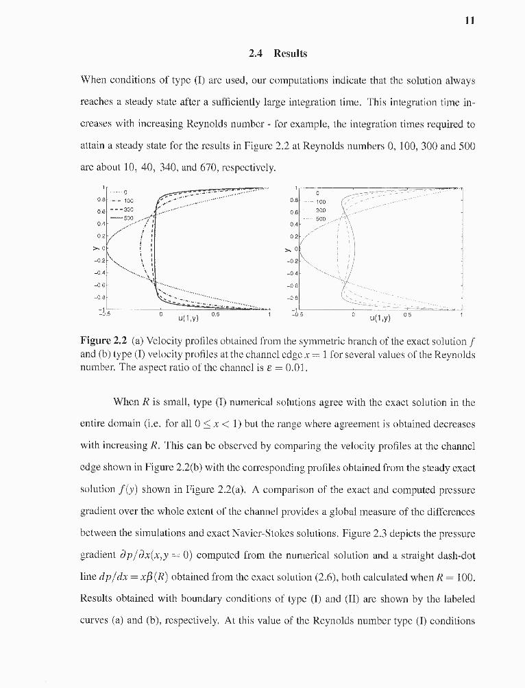
2.4 Results

When conditions of type (I) are used, our computations indicate that the solution always

reaches a steady state after a sufficiently large integration time. This integration time in-

creases with increasing Reynolds number - for example, the integration times required to

attain a steady state for the results in Figure 2.2 at Reynolds numbers 0, 100, 300 and 500

are about 10, 40, 340, and 670, respectively.

Figure 2.2 (a) Velocity profiles obtained from the symmetric branch of the exact solution fand (b) type (I) velocity profiles at the channel edge x= 1 for several values of the Reynoldsnumber. The aspect ratio of the channel is e = 0.01.

When R is small, type (I) numerical solutions agree with the exact solution in the

entire domain (i.e. for all 0 < x < 1) but the range where agreement is obtained decreases

with increasing R. This can be observed by comparing the velocity profiles at the channel

edge shown in Figure 2.2(b) with the corresponding profiles obtained from the steady exact

solution f (y) shown in Figure 2.2(a). A comparison of the exact and computed pressure

gradient over the whole extent of the channel provides a global measure of the differences

between the simulations and exact Navier-Stokes solutions. Figure 2.3 depicts the pressure

gradient ap/ ax(x,y = 0) computed from the numerical solution and a straight dash-dot

line dp/dx=xP(R) obtained from the exact solution (2.6), both calculated when R = 100.

Results obtained with boundary conditions of type (I) and (II) are shown by the labeled

curves (a) and (b), respectively. At this value of the Reynolds number type (I) conditions

12

support a region near x= 0 where the Navier-Stokes flow coincides with the exact solution,

while for type (II) conditions the region of almost perfect agreement is over 70% of the

channel length. To emphasize this agreement we use the velocity profiles computed from

the Navier-Stokes code at different values of x = xi, say, and construct the exact solution

analogues using the self-similar forms (2.6). More precisely we construct the velocity

profiles v(xi,y) and u(xi,y)/xi for several values of xi in the range of agreement, 0 < x <

0.19141 for type (I) conditions and 0 < x < 0.91797 for type (II) conditions as indicated

by the results of Figure 2.3. The results are shown collectively in Figure 2.4 with the top

panels corresponding to type (II) conditions and the bottom ones to type (I) conditions. As

shown, both computed solutions are self-similar and identical in the regions described in

the Figure. We note that there are approximately 250 profiles superimposed in the type (II)

top panels, and about 50 profiles in the lower type (I) panels. For completeness we also

superimpose the exact solutions given by (2.6) at R = 100 indicating that the Navier-Stokes

equations in a finite domain produce this exact solution.

Figure 2.3 Pressure gradients a P/ ax(x, 0) for (a) type (I) numerical solution and (b) type(II) solution, computed when R = 100. The dashed straight line was computed from thesimilarity solution (2.6). The aspect ratio of the channel is E = 0.01.

The remaining fraction of the domain where the flow adapts to the self-similar pro-

file can be significantly reduced in the case of type (II) solutions, by increasing the number

of discretization points. Considering the corresponding increase in computation time we

13

only use the resolution necessary to correctly resolve each case presented in time and space.

As reported by Hewitt and Hazel (2007) and also by Brady and Acrivos (1982a), in cases

of self-similar flows in finite domains where type (II) conditions were subject to non-linear

perturbations, the length of this 'adaptation region' has been seen to be independent of the

type of perturbation used and also independent of the aspect ratio in terms of the scaled

variables. We refer the reader to their papers for details about their results.

Figure 2.4 Velocity profiles corresponding to (a) type (II) edge conditions in the range0.035156 < x < 0.91797, (b) type (I) conditions in the range 0.035156 < x < 0.19141computed when R = 100. The aspect ratio of the channel is e = 0.01.

An important difference between the flow driven by accelerating walls and the flow

driven by counter rotating disks studied by Hewitt and Hazel (2007) is that for moderately

large values of the Reynolds number, although symmetry is not imposed, type (I) flows

remain symmetric and are significantly different from the corresponding similarity flows.

This can be seen in in Figure 2.2 where reversed flow at the center-line y 0 appears when

R = 300 and 500. In the latter case the reversed flow is present in the whole channel,

and the velocity profiles are similar to the one shown in the Figure, all the way down to

x = 0. Consequently, at these values of the Reynolds number the symmetric similarity

solution does not constitute a good qualitative predictor of the flow. In the case of counter

14

rotating disks it was reported by Hewitt and Hazel (2007) that different edge conditions

could significantly alter the location of the mid-plane symmetry-breaking bifurcation, but

such bifurcation was always present. Nevertheless, our results for type (I) conditions appear

to confirm the conclusion presented by Hewitt and Hazel (2007) that the symmetric branch

of the similarity solution is a good predictor of the flow in a vicinity of x = 0 for moderate

values of the Reynolds number (meaning in the present context R 200), independently of

the boundary conditions used at the edge of the domain.

We now turn our attention to type (II) flows and their bifurcations. As found by

Watson et al. (1990), when symmetry is not enforced at the channel center-line, the sim-

ilarity solution has a symmetry breaking bifurcation at the critical value R = 132.75849

where two stable asymmetric solutions appear (each of them can be obtained by reflection

about y 0 from the other). Then, at the value R = 355.5738 the flow Hopf bifurcates and

a stable, unsteady and time-periodic solution appears. The period of the unsteady solution

increases with R, and it nearly doubles when R = 400. Eventually, when R = 1200 there is

evidence of chaotic behavior; see (Watson et al. 1990).

In order to investigate how these features of the exact solution are replicated by

our numerical solution, we performed computations with type (II) boundary conditions at

the channel edge. The profiles required for imposing type (II) conditions were computed

in two ways: a stable asymmetric branch of the exact solution is found by time-marching

the unsteady code described in Section 2.3. Other steady solution branches are efficiently

calculated with MATLAB's bvp4c solver for boundary value problems as mentioned earlier

by using continuation methods in the Reynolds number R.

Both branches of the similarity solution, symmetric and asymmetric, are recovered

by our Navier-Stokes code. In Figure 2.5 we show the pressure gradient ap/ ax(x,y = 0)

computed from the numerical solution for type (I) and type (II) edge conditions, for the

symmetric and asymmetric branches. As pointed out previously, the deviation from the

line /3x at the edge decreases when more discretization points are used. Further inside the

15

Figure 2.5 Pressure gradients aP/ ax(x, 0) for (a) type (I) solution and (b)-(c) type (II)solutions in the case R = 200. The type (II) edge condition for (b) came from the symmetricbranch of the similarity solution and the edge condition for (c) came from an asymmetricbranch. Dash-dot lines were obtained from the similarity solution f in the respective cases.The aspect ratio of the channel is E 0.01.

channel, as the fluid moves away from the edge the solution decays to the similarity solution

as evidenced by the results of Figure 2.6 where profiles v(xi,y) and u(xi,y)/xi for values

of xi between 0 and x = 0.9179 are superimposed with the exact solution velocity profiles.

Similar results are obtained for larger values of R. As an example, in Figure 2.7 we show

pressure gradients corresponding to the asymmetric branch of f, for several values of the

Reynolds number in the regime R> 345.

2.4.1 Unsteady Solutions

When R = 355.5738 the asymmetric steady branch of (2.7) Hopf bifurcates and a time

periodic solution arises. We can impose time dependent type (II) conditions by solving

(2.7) numerically as explained in Section 2.3 and then coupling this solution to our Navier-

Stokes solver.

When the Reynolds number is 370 the time dependent exact solution has an approx-

imate period of 199. As can be observed in Figure 2.8 where velocity profiles near x 0

and x 1 are compared at two instants of time, the exact solution changes slowly over time

16

Figure 2.6 Type (II) velocity profiles corresponding to (a) symmetric branch of the exactsolution, (b) asymmetric branch for 0.074219 < x < 0.91797 in the case R = 200. Theaspect ratio of the channel is e = 0.01.

and this allows the numerical solution to adapt to the time dependent conditions at the edge.

This slow time variation turns out to be fundamental for the stability of the flow as will be

explained in the next paragraphs. Due to the proximity with the location of the Hopf bifur-

cation, the self-similar solution requires a long time to converge to a periodic state. This

explains the relatively large variation between the profiles near x = 1 and x = 0 at the time

= 1949.968. When R = 500 the agreement between the Navier-Stokes solution and the

self-similar solution has improved within the same range of time as can be seen in Figure

2.9. In the right panel of Figure 2.9 we show the velocity signals u(x = 1/2,y = 0, t), with a

solid line, and fy (y = 0,t)/2 with a dash-dot line. The lag between the two curves indicates

the time that it takes the information prescribed as type (II) edge condition to reach the

middle of the channel.

As the Reynolds number increases, the lag that occurs between type (II) conditions

and the velocities at the interior of the channel destabilizes the self-similar flow. When

u(1/2, 0, t) reaches a minimum, the acceleration changes sign and as seen in Figure 2.10

the change of sign for fyt (0,t) occurs at a later time, producing small oscillations. At the

17

Figure 2.7 Pressure gradients at the channel center line computed from type (II) solutionsat different values of the Reynolds number. The dash-dot lines were obtained from theexact solution of the asymmetric branch in the respective cases. The aspect ratio of thechannel is E = 0.01.

top, left panel we can see a 34% increase in the total kinetic energy of the flow, occurring

after fyt has changed sign. When R = 900, the flow is no longer periodic, although the

Navier-Stokes solution coincides with the self-similar solution during periods of time when

the kinetic energy of both solutions is smaller. When the kinetic energy is the smallest, the

self-similar solution is symmetric or nearly symmetric. This is an attracting mode, which

stabilizes the Navier-Stokes solution, in a similar way to what is shown in Figure 2.8, where

profiles at time t = 4261.556 are nearly symmetric throughout the channel. This results in

a return of the Navier-Stokes flow to a 'initial' symmetric state which is then forced by a

periodic type (II) condition producing identical oscillations. This cycle is repeated resulting

in a Navier-Stokes flow which is periodic but not self-similar, as in the cases R = 600, 700

and 800 (approximate periods are reported in Table 2.1). Increasing the Reynolds number

further results in global instability of the self-similar flow, with oscillations persisting in

time and propagating over the whole domain as in Figure 2.13. See the linear stability

analysis of Section 2.4.3 for details about the stability of the different branches of the exact

solution.

18

Figure 2.8 Vertical velocity profiles at x= 0.004 (solid line) and x= 0.93359 (dash-dotline) at two different times: t = 1949.968 and t = 4261.556 in the case R = 370. The arrowshows the direction of increasing time. The right hand plot shows the kinetic energy ofthe solution (solid line) as a function of time. The dash-dot line is the energy of the exactsolution. The aspect ratio of the channel is e = 0.01

Figure 2.9 In the left panel we show a plot of the kinetic energy of the Navier-Stokessolution (solid line) as a function of time. The dash-dot line is the energy of the exactsolution. At the right panel we show velocity signals u(x = 1/2,y = 0, t) (solid line) andfy (y = 0,t)/2 (dash-dot line). All quantities where computed in the case R = 500. Thechannel aspect ratio is E = 0.01

2.4.2 Decelerating Wall Flows, E < 0

In the case of decelerating walls, the similarity solution f is an odd function of y for values

of R less than the critical value 17.30715 where there is a symmetry breaking bifurcation.

The asymmetric solutions which appear from this bifurcation are time independent until

they Hopf-bifurcate at the critical value R = 55.77. As found by Watson et al. (1990),

increasing the Reynolds number further results in a period doubling cascade with evidence

of chaos at the value R ti 78.7.

We proceed with our computations as we did in the case E > 0 by using type (II)

19

Figure 2.10 In the left panels we show plots of the kinetic energy of the Navier-Stokessolution (solid line) as function of time. The dash-dot lines are the energy of the exactsolution. At the right panels we show velocity signals u(x = 1/2,y 0, t) (solid line) andfy (y = 0,t)/2 (dash-dot line) computed when (a) R = 600 and (b) R = 700. The channelaspect ratio is E = 0.01

conditions which were obtained from the steady asymmetric branch of f. In Figure 2.11

we show pressure gradients ap/ x(x,y = 0) computed when R = 15, 45 and 57. The

similarity solution is recovered in the whole channel in the case R = 15, but only away

from the channel ends for the other two cases, since a collision region forms near x = 0. In

this region of the channel the flow is not of similarity form as can be seen in Figures 2.11

and 2.12.

Further investigation of the formation of these collision regions have led us to con-

clude that both steady branches of the exact solution f, symmetric and asymmetric, are

unstable to spatial perturbations in the negative Reynolds number case, when R is larger

than a critical number R0 ti 33. Below this value, perturbations to type II conditions will

grow as the fluid travels down the channel resulting in the collision regions observed around

x = 0. When the Reynolds number is large a sufficient amount of fast moving fluid enter-

20

Table 2.1: Approximate period of time dependent type (II) solutions and periods of self-similar solution for increasing values of the Reynolds number. Starred values were reportedin (Watson et al. 1990).

Figure 2.11 Pressure gradients at the channel center line computed from type (II) solutionsat different values of the Reynolds number. The dash-dot lines were obtained from theexact solution in the respective cases. At the right we show an enlargement of the region0 < x < 0.3. The aspect ratio of the channel is e = 0.01

ing the channel collides with the decelerated fluid in the region near x = 0 destroying the

self-similarity of the solution in this region and affecting the solution in the entire domain.

This was confirmed by the linear stability analysis performed in Section 2.4.3. Also, as

illustrated by Figure 2.12, where the channel has an aspect ratio of 1/50, and Figure 2.11

where the aspect ratio is 1/100, the collision region occupies the same proportion of the

domain in terms of the scaled variables.

The development of collision regions when R 33, together with rapidly oscil-

lating edge conditions when the exact solution Hopf bifurcates at R > 55.77 results in the

21

Figure 2.12 Streamlines and pressure gradient at the channel center line computed fromtype (II) solutions in the case R 57. The dash-dot line was obtained from the exactsolution. The aspect ratio of the channel is E 0.02

instability of time dependent self-similar flows. As described in Section 2.4.1 rapidly os-

cillating type (II) conditions can destabilize the flow, producing wave-like structures with

length scales of the same order of magnitude of the aspect ratio of the channel, like the

ones shown in Figure 2.13. We note that these structures are implicitly neglected when

a self-similar solution is assumed to be valid or when scalings where terms of the form

εa/ax are assumed to be small.

Figure 2.13 Streamlines computed in the case R = 70 at time t = 1014.761. A timedependent type (II) condition was imposed at x = 1. The plot at the right is a enlargementof the region 0.9 < x < 1. The aspect ratio of the channel is e = 0.01

2.4.3 Linear Stability of the Similarity Solution f

The fact that we recover type (II) solutions corresponding to stable and unstable branches

of the exact solution in the positive Reynolds number case suggest that these branches are

22

stable for the Navier-Stokes equations. In order to investigate this possibility and also to

understand the development of collision regions for Reynolds number below the critical

value R0 —33, we performed a linear stability analysis for small perturbations about the

exact solution f: if we look for solutions of equations (2.2)-(2.5) of the form

and we linearize for small (ũ, v , p ) , we obtain the following equations for the perturbations:

subject to conditions

The functions (up , vp ) correspond to perturbations of type (II) conditions at the channel

edge which allow us to take into account small perturbations to the profiles used as type

(II) conditions at the edge of the domain. The restrictions that up and vp have to satisfy are

23

up (+1) = vp (±1) = 0, and mass conservation in the form

The spatial stability analysis performed by Durlofsky and Brady (1984) provides

a useful starting point for our analysis. They studied the evolution of perturbations of the

stream function x f (y) of the form xλg(y). This type of perturbation corresponds to the

particular case = (xλ g',—λxλ-1g ). In the E -> 0 limit of equations (2.12)-(2.14)

perturbations of this form result in the eigenvalue problem

where y is an unknown parameter. An eigenvalue A, > 1 implies that perturbations of flows

with fluid moving towards zero are stable, and eigenvalues 2 < I imply that perturbations of

flows with fluid moving towards infinity are stable. It was reported by Durlofsky and Brady

(1984) that the symmetric branch of f has only positive eigenvalues for 0 < R < 11, both

positive (larger than one) and negative eigenvalues for R > 11 and only negative eigenvalues

for negative Reynolds number. They presented two interpretations to these results. In the

first one the flow is unstable for all Reynolds numbers since both the accelerating and

decelerating wall driven flows have fluid moving towards x = +00 as well as fluid moving

towards x = 0. In the second interpretation a distinction is made between fluid in the

boundary layers adjacent to the walls which form at larger values of R, and the fluid in the

24

core which moves in the opposite direction. Under this interpretation the flow is stable for

all Reynolds numbers. This ambiguity does not exist in finite channels where perturbations

at x = L can only travel to the interior of the channel.

The eigenvalue problem (2.17)-(2.18) can be solved with MATLAB's bvp4c pack-

age. For a given value of A, and the corresponding eigenfunction g, we define the initial

conditions for (as)

which are consistent with the boundary conditions, and we use (up , vp ) = (g' ,-λg) as type

(II) conditions at the edge. In Figure 2.14 we show the eigenvalues that we calculated and

used in the stability computations shown in Figure 2.15 and the left panel of Figure 2.16.

These eigenvalues were obtained by solving equations (2.17)-(2.18) with f in to the asym-

metric branch of the exact solution. Since these eigenvalues are negative, we would expect

this branch to be spatially unstable to perturbations of the form (as) = (xλg'—λxλ-¹g)

in a finite channel. We will see below that this is not the case. For studying the linear

stability of the negative Reynolds number flows we simply construct up , vp and the initial

state using polynomials that satisfy the boundary conditions and conservations of mass.

In Figure 2.15 we show the evolution of velocity profiles ũ(x, y = 1/2, t) for in-

creasing values of t. These profiles were computed with the initial conditions and edge

conditions described in the lines above, with g computed for the asymmetric steady branch

of f when R = 357. The arrows show the direction of the evolution of the profiles. We

can clearly see in this Figure that the perturbations introduced at the edge decrease towards

zero as the fluid moves away from the edge.

In order to study the evolution of the perturbations in the whole channel we define

Figure 2.14 Eigenvalues corresponding to the asymmetric branch of the exact solution f.

Figure 2.15 Velocity profiles ũ(x,y = 1/2) at different times, in the case R = 357. Thearrow shows the direction of increasing time. The aspect ratio of the channel is E = 0.01.

the integral

Stable solutions will be characterized by a decreasing E(t) while unstable solutions will

have increasing E(t). In Figure 2.16 we show the time evolution of E(t) for perturbations

computed at different values of R. This result shows that the asymmetric steady branch of

f in the positive Reynolds number case is stable for equations (2.2)-(2.5) in agreement with

what was observed in the direct simulations in the respective cases. The final value of E(t)

is a positive number because of the non-null perturbations (a— v.,) at the channel edge.

26

Figure 2.16 Function E(t) computed from solutions at different values of the Reynoldsnumber. Curves in the left panel were computed using solutions of the steady, asymmet-ric branch and curves in the right panel were computed with time dependent self-similarsolutions. The channel aspect ratio is e = 0.01.

Similar computations can be performed with the symmetric steady branch of f and

they show that this branch is stable as well. The resulting Figure has similar characteristics

to Figure 2.16 above, and we do not show it here. For completeness, we show stability

computations for the time-dependent branch of the similarity solution in the right panel of

the same Figure.

In the case of negative Reynolds number we set (up ,vp )= (y3 — y, 0) as edge con-

ditions and we define a initial state by scaling up with x between 0 and 1. In Figure 2.17 we

show the time evolution of E(t) computed for the values of the Reynolds number shown.

As expected from the simulations of Figure 2.11, the case R= —15 is stable to spatial per-

turbations and the cases R = —45 and R = —57 are unstable to spatial perturbations. A

log-log plot of the same quantities showed that E(t) is growing exponentially in the latter

two cases. Similar computations performed with the symmetric branch of the self-similar

solution show that this solutions are linearly unstable as well, as shown in Figure 2.17.

2.5 Conclusions

We have computed flows in two dimensional channels of finite length L driven by accel-

erating walls (positive Reynolds number) or by decelerating walls (referred to as negative

27

Figure 2.17 Function E(t) computed with solutions of the asymmetric branch (left panel)and the symmetric branch (right panel) of the similarity solution at different values of theReynolds number. The channel aspect ratio is E = 0.01.

Reynolds number). The equivalent problems in infinitely long channels admit self similar

solutions that can be recovered in a region at the interior of the finite channel which de-

pends on the boundary conditions imposed at the channel end at x = L. If the boundary

condition does not coincide with the exact solution at x L, the length of the region where

the exact solution is recovered decreases with increasing Reynolds number.

For flows driven by accelerating walls, as the Reynolds number increases the self

similar solution has a symmetry breaking bifurcation at the value R = 132.75849 and a

Hopf bifurcation at the value R = 355.5738. We showed that stable and unstable steady

branches of the self-similar solution are recovered as stable Navier-Stokes flows for values

as large as R = 500. The stable, time dependent self-similar solutions that exist for values

larger than R = 355.5738 are recovered as well. The slow time evolution of these time

dependent solutions allows the flow to adjust to the changing conditions at the edge of the

domain. We note, however, that time dependent solutions can be recovered only if the time

dependent exact solution is imposed as boundary condition at x = L. If instead, a steady

Dirichlet condition is used the flow at the interior of the channel will adjust to this steady

condition.

For flows driven by decelerating walls we showed that the self similar solution

becomes unstable to spatial perturbations at a critical value R —33. For values of the

28

Reynolds number less than this critical value, the flow develops a collision region at x = 0

and within this region the flow is not of self similar form. Time dependent self similar

solutions are not found in a finite channel with decelerating walls.

CHAPTER 3

CHANNEL FLOWS DRIVEN BY VERTICALLY OSCILLATING WALLS

In this Chapter, we study flows in infinite or finite two-dimensional channels which are

driven by vertical oscillations of their rigid walls. The movement of the walls is prescribed

via some periodic function of time, and the symmetry of the domain with respect to one of

the spatial variables will allow us to look for self-similar solutions that satisfy a simplified

problem, typically a single non-linear partial differential equation. When a finite channel is

considered, we will integrate the Navier-Stokes equations numerically, without assuming a

special form of the solutions.

3.1 Vertical Oscillations

In this Section we consider flows in a channel whose walls move in the following way: the

position of the upper wall is y = a(t) and the position of the lower wall is y = —a(t), as

shown in Figure 3.1. The oscillation is given by the function

(3.1)

We non-dimensionalize the equations of motion (1.1)-(1.3) as follows:

where 0) = kw°, k is a non-dimensional frequency. The non-dimensional equations of

29

Figure 3.1 Geometry of the problem.

motion are (dropping all primes)

where R = p ω0a²0) I µ is the Reynolds number for this flow. Equation (3.1) becomes

Accordingly, the no-slip boundary conditions take the form

The system (3.2)-(3.4) together with boundary conditions (3.5) is characterized by

two parameters, the Reynolds number R, and the dimensionless oscillation amplitude A.

Note that k can be removed from the problem by rescaling time and redefining R. In what

follows k = 2 so that the forcing a(t) is Jr periodic. This choice also allows us to compare

our results with the ones reported by Hall and Papageorgiou (1999).

Secomb (1978) proposed a solution to equations (3.2)-(3.4) which has the following

30

form:

31

(3.6)

(3.7)

(3.8)

where u0, u1, p0, pi, p2 and the vertical velocity v are functions of t and y alone. This

form of the solution results from assuming that the vertical velocity v is independent of

x, which is a reasonable simplification in an infinite domain. It follows that u must be

linear in x as a consequence of equation (3.4) and that p must be quadratic in x by equation

(3.2). It is convenient to 'fix' the walls of the channel by introducing the variable /I = y I a.

By substituting equations (3.6)-(3.8) into the equations of motion (3.2)-(3.4) and grouping

terms with the same power of x, we obtain the following equations in terms of the new

variable n:

Equations (3.10)-(3.11) for u1, v and p2 can be solved independently of equation

(3.9) for u0 and pi. As a consequence of equation (3.12), we can define a stream function

for u1 and v, and reduce the system (3.10)-(3.12) to a single partial differential equation;

see Section 3.2.1. Once the equation for the stream function is solved we can compute /92

and p0 from equations (3.10) and (3.11) respectively. The unknown pi is only restricted by

32

equation (3.13) and the remaining, linear equation (3.9) for the longitudinal flow u0 can be

solved if the pressure gradient pi is prescribed. In Section 3.2 we study the flow u0 in the

case when pi (t) is constant.

3.2 Dynamics of the Horizontal Flow u0

In this Section we study the dynamics of the horizontal flow u0, which is governed by

equation (3.9). For simplicity we consider the case when the pressure gradient p1(t) is

constant and 0(1). Equation (3.12) implies that there is a scalar function 'I' = xf ern t)which satisfies

(see Spivak (Spivak 1965)). Thus, by rescaling equation (3.9) with the constant pi and

replacing u1 and v with the expressions above we obtain (dropping the primes of all the

rescaled quantities)

A brief description of the main results regarding f is given in Section 3.2.1 below. In

Section 3.2.2 we discuss the properties of the flow u0 valid in the small Reynolds number

regime and in Section 3.3 we discuss the bifurcations of (3.17) which occur at higher values

of R.

33

3.2.1 Stagnation Point Flow

By differentiating equation (3.10) with respect to η and replacing u1 and v with expressions

(3.15) and (3.16) we obtain the one-dimensional partial differential equation

which is subject to boundary conditions

This equation has been studied in detail by Hall and Papageorgiou (1999). For any

fixed value of the oscillation amplitude A, the flow is synchronous with the wall oscillation

a(t) and symmetric about 77 = 0 for small values of the Reynolds number. If R increases

there is a symmetry breaking bifurcation, and if R is increased further the flow becomes

chaotic. The chaotic state is the result of a period doubling cascade or a quasi-periodic

flow, depending on the value of A. Also, it is important to mention that the flow driven by

decelerating walls studied in Chapter 2 appears as a core flow driven by the steady forcing

generated by the wall layers in the small oscillation amplitude — large Reynolds number

limit of the flow f . For details about these results, see (Hall and Papageorgiou 1999).

34

3.2.2 Solution for Small Reynolds Number

When R is small, we can solve equations (3.9)-(3.14) by using a regular asymptotic expan-

sion of the unknowns in powers of R. Let

We can eliminate the pressure term from equation (3.10) by differentiating it with respect

to n. Then by equation (3.12), we find that the leading order terms in the expansion for u1

and v that satisfy the boundary conditions (3.14) are

These are seen to be a squeeze flow and a Poiseuille flow. To find the leading order term in

the expansion for u0 we assume that the prescribed pressure gradient p i is constant. As a

consequence of the homogeneous boundary conditions the first term in the expansion, /c00,

is zero. The first non-null term in the expansion is u01:

If we keep calculating the higher order terms in the expansion for u0 we find that all of

them are even polynomials in the variable n.

35

3.3 Bifurcations of the Horizontal Flow u0 at Higher Values of R

For 0(1) values of the Reynolds number, we solve equation (3.17) numerically. The details

of the numerical scheme we employ are given in Appendix C. In the present case

(3.24)

and, as discussed in the previous Section, the pressure driven flow u0 is symmetric around

= 0, as well as periodic with the same period as a(t) for small values of the Reynolds

number. As described previously, the background flow f loses symmetry at a bifurcation

value of R which is a function of A. It is natural to expect a similar behavior for u0 as it

depends explicitly on f. However, the set of bifurcations of u0 is surprisingly complex as

evidenced by Figure 3.2:

Figure 3.2 Bifurcation diagram for the flow u0.

The dash-dot line in Figure 3.2 indicates the location, in the parameter space A-

R, where the symmetry breaking bifurcation of f occurs (values taken from (Hall and

Papageorgiou 1999)). The dotted line shows the location of symmetry breaking bifurcation

of u0 and the solid line shows the location of the change of stability of u0. In the region

36

`below' the solid line the flow is time periodic and in the region 'above' the solid line the

flow is growing exponentially in time. Likewise, above the dotted line u0 is asymmetric and

below it, u0 is an even function of n . Points in the doted line are labeled Rs , the meaning

of the other symbols in Figure 3.2 and a detailed characterization of the different states of

the flow are given in Section 3.3.

In order to quantify a symmetry breaking bifurcation we consider the function ηu²0,

which is an odd function of 77 provided that u0 is symmetric around η = 0. The integral

indicates any change in the symmetry properties of u0; for example, I is zero as long as u0

remains even. It is understood that t0 is large enough so that any transients in the solution

disappear and a periodic state is attained, for example we took t0 = 700x. At time t = 0

we set u0 = 0 and march forward in time until a periodic state is reached. Note that we

have normalized the value of the integral in order to control its size. For small values of R

and for any value of A the value of /(R, A) is zero, as expected. The solution is bounded

and time-periodic of period 7c. As R increases the amplitude of the oscillations is also

found to increase. This behavior remains unaltered for a range of values of R until a critical

value Rs is reached, above which the solution is no longer symmetric. This can be seen in

Figure 3.3, where we show /(R, A = 0.35). At Rs 20 there is a pitchfork bifurcation to

a solution with I 0. Solutions in the other stable branch can be computed by reflection

about n = 0 combined with standard continuation techniques in the Reynolds number. As

can be seen in Figure 3.2, u0 losses symmetry at values of R which are much smaller than

the corresponding values for f.

In the region 0.473 < A < 0.556 three bifurcations occur. For any fixed A within

this region the flow changes it stability properties when R crosses the solid line shown in

Figure 3.2. For example, when A = 0.5, if R < 12 (labeled as Re), the flow is stable, if

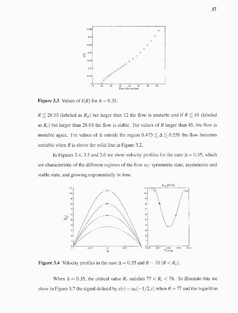
Figure 3.3 Values of I (R) for A = 0.35.

R < 28.03 (labeled as Rd) but larger than 12 the flow is unstable and if R < 45 (labeled

as Rc) but larger than 28.03 the flow is stable. For values of R larger than 45, the flow is

unstable again. For values of A outside the region 0.473 < A < 0.556 the flow becomes

unstable when R is above the solid line in Figure 3.2.

In Figures 3.4, 3.5 and 3.6 we show velocity profiles for the case A = 0.35, which

are characteristic of the different regimes of the flow u0: symmetric state, asymmetric and

stable state, and growing exponentially in time.

Figure 3.4 Velocity profiles in the case A = 0.35 and R = 10 (R < Re ).

When A = 0.35, the critical value R, satisfies 77 < R, < 78. To illustrate this we

show in Figure 3.7 the signal defined by s(t) = u0 (-1/2, t) when R = 77 and the logarithm

Figure 3.5 Velocity profiles in the case A = 0.35 and R = 70 (Rs < R < Re).

38

Figure 3.6 Velocity profiles in the case A = 0.35 and R = 80 (Rc < R).

of the corresponding signal in the case R = 78 which demonstrates the exponential growth

of the function s(t):

Floquet theory provides a basis in which the changes of stability of the pressure

driven flow u0 that occur at the values Rc and Rd can be understood. Equation (3.23),

which governs u0, is linear and we can decompose this flow in two parts, one that is driven

by the pressure gradient p1 and another one that is driven by the oscillations of the wall

alone:

39

Figure 3.7 Signal s(t) for A = 0.35 and (a) R = 77, (b) R = 78. The white lines result fromthe linear interpolation of the signal and the logarithm of the signal, respectively.

with û satisfying the equation

and boundary conditions û(±1, t) = 0. For the values of R considered, all the coefficients

in the linear partial differential equation (3.27) remain time periodic. Formally, we expect

that û can be written in the form

For any fixed the value µ (n) can be estimated from the signal s(t) = û(ηt), once

the initial boundary value problem for û is solved (we use an arbitrary, non-zero initial

condition). In this context, the bifurcations that occur at R = R, correspond to a transcritical

bifurcation. As µ crosses from the negative real axis to the positive real axis (we found

numerically that ,u is real) an exchange of stability of the equilibrium of equation (3.27)

occurs. In the case of Rd, ,Li crosses from the positive real axis to the negative real axis.

In the region 'above' the solid line shown in Figure 3.2, the Floquet exponent is

positive and a monotonically increasing function of R, as can be seen for example, in Figure

3.8 for the particular case A = 0.35. We carried out calculations for values of R as large as

a thousand, for several value of A, and we did not find any further changes in this behavior

40

Figure 3.8 Floquet exponent as a function of R. A = 0.35.

of the flow u0.

3.4 A Squeezing, Stretching Channel

In this Section we consider a stagnation point flow which describes a more general problem

that the one studied in Section 3.1. However, as we will see, this self-similar flow is still

governed by equation (3.18) subject to modified boundary conditions.

Figure 3.9 Geometry of the problem.

Consider a channel whose walls oscillate in the following way: the position of the

walls is y = ±a(t) and x = b(t)x, where z = x(0) is the initial horizontal position of the

41

wall. The functions a and b are given by a = a0a' and b = a0bi where

The non-dimensional constants 0 < 6,1,6,2 < 1 are the oscillation amplitudes and q0 is a

phase shift. As in the previous example, it is convenient to change to a frame of reference

where the channel walls are fixed. Accordingly we non-dimensionalize the Navier-Stokes

equations (1.1)-(1.3) in the following way

Then the non-dimensional equations are (dropping all the primes)

where again R = p 041 /µ. The non-slip boundary conditions in this case are

with a, b given by (3.28)-(3.29), primes removed.

We can modify the ansatz (3.6)-(3.8) to take into account the horizontal oscillations

42

by making the following modifications:

where the unknowns U, V, P and P0 are independent of g. Note that we have not included

the terms that correspond to u0 and p1 in the previous problem, because we are not in-

terested in considering the effects of a driving horizontal pressure gradient, at least at this

stage. This effect can be included in a straightforward way by including u0 and p1 in the

ansatz. The minus sign in front of (3.35) was included for convenience, as it was done with

equation (3.16).

We substitute these equations into (3.30)-(3.32), and replace U =Vil la in the mo-

mentum equation (3.30) to find that V satisfies

subject to boundary conditions

where a = 1 + O1 sin(t), b = 1 + A2 sin(t + q0). Is now clear from equation (3.39) that as

the amplitude of the horizontal oscillations go to zero we recover the flow (3.18)-(3.20).

In the following Section we briefly discuss some of the characteristics of the self-

similar flow defined by V, with special emphasis on the states that occur at moderate os-

cillation amplitudes (A1 = 02 < 0.4) and moderately large values of the Reynolds number

(R < 150). This flow is part of a model for oxygen transport and diffusion, which we study

43

in Chapter 4 and the regime that we just described is important for that application of this

flow. As described in (Hall and Papageorgiou 1999), flows governed by equation (3.37)

support very complex dynamics and have rich sets of bifurcations and bifurcated states

(see Section 3.2.1). It is outside the scope of the present study to provide a comprehen-

sive classification of such states; we will only show particular examples of cases in the

four-dimensional parameter space Ai — A2 - q0 — R and we will describe a very interest-

ing effect of the phase parameter q0 which can completely "laminarize" flows which are

otherwise chaotic, for example.

3.5 The Effects of Wall Stretching

We find numerically that for small values of the Reynolds number and any value of the

oscillation amplitudes the flow is synchronous with the wall motion. This behavior is

characteristic for these types of flows, and an example is the flow (3.18)-(3.20) which is

recovered in the A2 = 0 limit.

First we consider the case A1 = A2 = 0.4, q0 = 0 and we track the changes that

occur to the flow as R grows. As described in Section 3.3, a quantity like the integral

defined in equation (3.25) can be used to characterize a symmetry breaking bifurcation

which in the present case occurs at the value R P.: 39. In order to analyze the dynamics of

the flow at larger values of R, we construct a time signal by V0(t) = V(-1/2, t). When

the flow is synchronous with the wall motion this signal is a 2π-periodic function of time,

all its maxima are equal and separated by a period of 27r. If we denote the maxima of

the signal by {Mi} and the times when a maximum Mi is attained by ti, it follows that in

this case these points satisfy Mi+ 1 = Mi and ti+1 ti = 27r, i = 1, 2, .... We can use these

values to construct a Poincaré return map by plotting the points (Mi,Mi+1), i = 1,2, ....

Clearly, the return map of a 27r periodic signal consists of a single point. When a period

doubling bifurcation occurs, the maxima of the signal lie in two straight lines with its points

satisfying Mi+2 = Mt, 4+2 - ti = 47r, i = 1, 2, ... and the return map consists of two points

44

(see Figure 3.10 for an example). Subsequent period doubling bifurcations appear in the

maxima plots as an increasing number of straight lines (4, 8 etc). If a signal is quasi-

periodic its return map will appear as a filled curve or several of these continuous looking

lines. The appearance of foldings and self-similarity in the return map are indicators of

chaotic flow. More details about these methods and their use in studying time series can be

obtained from Bergé et al. (1984) and examples of the use of velocity signals in classifying

flow dynamics are presented in (Hall and Papageorgiou 1999) and (Blyth et al. 2003).

Figure 3.10 Velocity signal V0(t) in the cases Ai = 02 = 0.4, q0 = 0 and (a) R = 130, (b)R = 135.

Figure 3.11 Velocity maxima as function of R in the case Al = 02 = 0.4, q0 = 0.

In Figure 3.11 we show the maxima of the signal V0(t) versus R; we estimate the

45

maxima of the signal by doing a quadratic polynomial interpolation when a change in

monotonicity of the curve V0 (t) is detected. Initially the flow is 27r periodic in time and

this behavior remains unaltered until the value R ~ 131. At this value a period doubling

bifurcation to a 47r periodic signal occurs. The signals remain 4π-periodic for a range of

values, until R ~ 151 is attained, when a new period doubling occurs. The signal remains

87r periodic until the value R ~ 154 where the maxima of V0(t) appear not to follow a

distinguished pattern anymore (see Figure 3.13). Foldings in the return map and a dense

spectrum (see Figure 3.12) are indicators of a chaotic flow. The same behavior is charac-

teristic for the signals obtained at larger values of R (the largest value of R for which we

did computations is R = 360).

Figure 3.12 Spectrum of the velocity signal V0(t) in the case Ai = 6.2 = 0.4, R = 154,q0 = 0.

Until now we have not considered the effect of the phase q0 on the solutions. So far

the most interesting effect that we observed is that of "stabilization" or "laminarization"of

the flow by setting the wall oscillations completely out of phase. By setting q0 = 7r/2 and

keeping all the other parameters unchanged, we observed that any flow changed to a basic

2π-periodic state. We confirmed this in many different cases including some where chaotic

states were found for the in-phase oscillating walls. A connection between a given state

occurring with in-phase oscillations and the return to the basic 2π-periodic state via small

46

Figure 3.13 Velocity maxima as function of time and Poincaré map for the case Al == 0.4, R = 154, q0 = 0. Enlargements of the regions near A and B are shown in (a), (b),

respectively.

increments in the phase parameter from 0 to g/2 could be the part of a future investigation.

3.6 Oscillating Flows in Finite Domains

In this Section we address the question of how the self-similar flows that we have studied

in this Chapter behave when the fluid domain is truncated to a channel of finite length. We

know from the literature (Hewitt and Hazel (2007), Brady and Acrivos (1982a)) and by the

results of Section 2.3 concerning type (I) boundary conditions that non-linear modifications

to a self-similar solution at the edge of a finite domain will result in an adaptation region

which grows in length with increasing Reynolds number, and within this region the flow

looses self-similarity. Eventually, when R is large enough, the adaptation region occupies

the whole domain. For steady flows, this happens at moderately large values of R. We an-

47

ticipate that the unsteadiness of flows driven by oscillatory walls will affect the stability of

any self-similar solution at smaller values of the Reynolds number. As observed in Section

2.4, in the case of flows driven by accelerating walls, unsteady branches become linearly

unstable at some finite albeit large value of R. In this Section we concentrate in finding

approximate ranges of values of R(d) for which the self-similar solution is recovered as

a Navier-stokes flow, when we impose self-similar profiles as Dirichlet conditions at the

edge of the domain (what we called type (II) conditions in Section 2.3).

The oscillating channel of this Section has finite length b(t) = b0b/ and half width

a(t) = a0a' where a' and b' are time-periodic functions. We use a viscous scaling and

non-dimensionalize the dependent and independent variables as follows

which results in the following dimensionless equations (primes dropped)

where R = pωa²0/µ, as in Section 3.4. We will be mostly computing flows in slender

channels, satisfying 5 = a0/b0 << 1. We need a set of four boundary conditions to complete

the system. For compatibility with stagnation point similarity flows we impose symmetry

at a = 0

48

The no-slip boundary conditions at the top and bottom walls are

At the channel entrance at = 1 we impose the Dirichlet condition

where V satisfies equation (3.37) subject to (3.39). Conditions (3.46)-(3.47) correspond

to what we called type (II) conditions in Section 2.3. The numerical method described in

that Section can be modified to solve equations (3.41)-(3.47). The problem for V is solved

numerically with the solver described in (Hall and Papageorgiou 1999) and the flow V

is coupled to the modified Navier-Stokes solver of Section 2.3 through equations (3.46)-

(3.47).

Considering that all the stagnation point self-similar flows of this Chapter are gov-

erned by the same basic equation (3.18), and that cases corresponding to different forcings

at the walls can be obtained via elementary transformations, we consider only the case of

vertically oscillating channels:

and we adjust the boundary conditions for the Navier-Stokes flow accordingly. Also, it is

important to note that we have abundant knowledge about the self-similar solution driven

by oscillations (3.48)-(3.49) thanks to the detailed study of Hall and Papageorgiou (1999).

For all the computations performed in this Section we set the aspect ratio of the channel to

be 5 = 0.01.

49

First we analyze the case A = 0.45 in some detail. For this value of the ampli-

tude, as R increases the flow V has a symmetry breaking bifurcation at the value R ti 44.

In Figure 3.14 we show approximately 150 superimposed Navier-Stokes velocity profiles

u( ξi,η)/ξi, with 4 i in the interval [0.035156 0.58203] at time t = 65.4096. These pro-

files were computed in the case A = 0.45 and R = 10. The dash-dot line represents the

self-similar profile imposed as type (II) condition at 4 = 1. In the right panel we show ve-

locity signals s(t) = u(1/2,0,t)/(1/2) computed in the same case A = 0.45, R = 10 from

the Navier-Stokes (solid) and self-similar (dash-dot) flows, Since the self-similar solution

prescribed at the edge of the domain changes with time, this information has to travel to

the interior producing a delay which is shown in Figure 3.14 as a discrepancy between

the interior self-similar profiles and the self-similar solution. As can be seen from the sig-

nals, the discrepancy shown in the left panel is nearly the worst case, and for about half of

each period both flows are indistinguishable. In the left panel of Figure 3.15 we show the

streamlines of the Navier-Stokes flow computed at time t = 65.4096 to show the smooth

transition between the interior self-similar profiles and the type (II) condition imposed at

g = 1.

Figure 3.14 Velocity profiles u(ξi,η)/ξi, in the range 0.035156 < i < 0.58203 at timet = 20.82057r in the case A = 0.45 and R = 10. The dash-dot line is the self-similar type(II) condition imposed at 4 = 1. In the right panel we show the corresponding velocitysignals 2 x u(1/2, 0, t). Solid line, Navier-stokes computations. Dash-dot line, self-similarsolution. The aspect ratio of the channel is 8 = 0.01.

To illustrate the time evolution of the solutions in the entire domain we show the

50

kinetic energies of the Navier-stokes flow (solid line) and self-similar solution (dash-dot

line) in the right panel of Figure 3.15. The Navier-Stokes solution is indistinguishable

from the self-similar solution during most of each period and the time ranges where there

are discrepancies between the two curves correspond to the times where the velocity signal

of Figure 3.14 is near its maxima and minima, i.e. the acceleration changes sign.

Figure 3.15 Streamlines of the Navier-Stokes flow at time t = 20.8205g computed in thecase A = 0.45 and R = 10. At the right panel we show the kinetic energy of the Navier-stokes solution (solid line) and self-similar flow (dash-dot line) in the same case. The aspectratio of the channel is 5 = 0.01.

Increasing the value of the Reynolds number —which corresponds to increasing the

frequency of the oscillations of the walls in the present case— results in the destabilization

of the self-similar Navier-Stokes flow, as can be seen in Figure 3.16. The kinetic energy

curve shows oscillations with secondary frequencies additional to the driving frequency

of the walls. These are the result of wave-like spatial structures which have length scales

smaller than the length of the channel (see Figure 3.18 for an example). This situation is

completely analogous to the case of flow driven by accelerating or decelerating walls (see

Section 2.4.2, Figures 2.10 and 2.13).

Our simulations indicate that changes in the value of the oscillation amplitude A

greatly affect the location, in terms of the Reynolds number, where the self-similar Navier-

Stokes flow losses stability. In Figure 3.17 we show the time evolution of the kinetic energy

and velocity signal u(1 / 2,0,t) for the Navier-Stokes flow (solid lines) and self-similar flow

(dash-dot lines) in the case A = 0.1 and R = 150. As these results show, when the amplitude

51

Figure 3.16 Time evolution of the kinetic energy (left panel) and velocity signal u(1/2, 0, t)in the case A = 0.45 and R = 30. Solid line, Navier-stokes computations. Dash-dot line,self-similar solution. The aspect ratio of the channel is 5 = 0.01.

of the oscillations is small, the self-similar solution is recovered in a truncated channel even

at moderately large values of R. This result is important for applications such as the model

for oxygen transport and delivery that we study in Chapter 4, where it is assumed that a

self-similar flow is a valid approximation in the regime of small amplitude oscillations and

small Reynolds number.

When A = 0.25 our results indicate that the self-similar Navier-Stokes flow is re-

covered for values of R as large as a hundred. However, for relatively large values of the

oscillation amplitude, the self-similar Navier-Stokes flow losses stability at much smaller

values of R. In Figure 3.18 we show the kinetic energy and streamlines computed in the

case A = 0.65 and R = 4 which indicate that although the Navier-Stokes flow is self-similar

during a considerable portion of the period, it is no longer stable.

We note that for all the values of the oscillation amplitude considered, the values of

the Reynolds number where we performed computations were considerably smaller that the

corresponding value of the first, symmetry breaking bifurcation of the self-similar solution

V.

52

Figure 3.17 Time evolution of the kinetic energy (left panel) and velocity signal u(1/2, 0, t)in the case A = 0.1 and R = 150. Solid line, Navier-stokes computations. Dash-dot line,self-similar solution. The aspect ratio of the channel is 5 = 0.01.

Figure 3.18 Kinetic energy of the Navier-stokes solution (solid line) and self-similar flow(dash-dot line). At the right panel we show the stream function of the Navier-Stokes flowat time t = 15.09977r. All quantities were computed in the case A = 0.65 and R = 4. Theaspect ratio of the channel is 5 = 0.01.

CHAPTER 4

SOLUTE TRANSPORT IN PULSATING CHANNELS

In this Chapter we study a two dimensional model for oxygen transport in an idealized

channel, which was proposed by S. Waters (2001), Waters (2003) in an attempt to inves-

tigate how blood flow modifies oxygen delivery to the walls of laser induced revascular-

ization vessels. These tubes are drilled in the heart muscle as part of a surgical procedure

intended as a means for increasing the delivery of oxygenated blood to certain parts of the

heart. As described in Waters (2001), the main purpose of that study is to gain a qualita-

tive understanding of the basic physical mechanisms involved in the solute transport and

consumption inside these channels. This is achieved by constructing an asymptotic solu-

tion to a simplified version of the model, which consists of a stagnation point type flow

for an oscillating channel geometry, coupled with an advection diffusion equation for the

solute (oxygen) in the channel. The medium that surrounds the channel adsorbs the solute,

a process which is modeled through a diffusion equation that incorporates uptake of solute

in order to account for the oxygen consumption by the muscle tissue. The solute concen-

tration at the walls couples with the flow inside the channel through a chemical reaction

boundary condition at the channel-wall interface.

Our main objective is to evaluate quantitatively the solute uptake dynamics as a

function of the time periodic or aperiodic flows that derive from the self-similar Navier-

Stokes solutions studied in previous chapters. As a consequence of this quantitative study,

we will be able to determine a range of values of the parameters of the problem for which

the asymptotic solutions of Waters (2001) provides a good approximation for the computed

solutions.

In Section 4.1 we present the governing equations and the boundary conditions for

this problem. In Section 4.2 we review the asymptotic solution valid in the double limit of

small amplitude oscillations and large Péclet number derived in Waters (2001). In sections

53

54

4.3 and 4.4, we present our numerical results and finally in Section 4.5 we discuss several

extensions and modifications of the model.

4.1 Governing Equations

We model the blood as being a homogeneous, incompressible Newtonian fluid, the oxygen

in the blood as a passive solute and the muscle tissue as an homogeneous medium that ab-

sorbs oxygen at a constant rate. Since the tissue is mainly composed of water, the diffusion

coefficient in the channel and in the walls are taken to be equal and the transfer of oxygen

from the fluid to the walls is assumed to be controlled only by a permeability parameter.

At the open end of the channel we assume that there is fluid with constant solute concen-

tration C0. The blood fills an oscillating channel of finite length b(t) = b0b / and half width

a(t) = a0a' where a' and b' are given by formulas (3.28)-(3.29), i.e.

We use the characteristic length and width of the channel b0, a0 to measure horizontal

and vertical distances. Accordingly we non-dimensionalize the dependent and independent

variables as follows

The non-dimensional equations of motion for the fluid inside of the channel take the form

(primes dropped)

55

We make the assumption that the channel is slender, satisfying 8 = a0/b0 << 1. Under this

condition we assume that the velocity field inside of the channel is well approximated by

the self-similar solution (3.34)-(3.36), and given that we do not calculate the velocity field

outside the channel, we assume that the velocity field is given by equations (3.34)-(3.36)

everywhere in the channel, including the entrance at ξ = 1. This hypothesis was examined

in Section 3.6 for the case of vertically oscillating flows, and it was shown to be adequate

for small oscillation amplitudes and moderate values of the Reynolds number.

Let C = C0C be the concentration of solute in the fluid inside the channel and

6 = C00' the concentration of solute in the surrounding tissue. C satisfies the advection

diffusion equation

where u is the velocity field of the fluid inside the channel and D is the diffusion coefficient

of the fluid. 8 satisfies the reaction diffusion equation

The term QO represents the consumption of solute in the tissue.

The non-dimensional concentration equations are (dropping all primes)

where À, = QaFil D is the ratio of consumption timescale to diffusion timescale in the sur-

rounding medium and Pe = coa6ID is the Péclet number. In terms of the Reynolds num-

ber, Pe = RCY where 6 = v/D is the Schmidt number, and v is the kinematic viscosity of

56

the fluid. According to (Waters 2001), the diffusivity of oxygen in the blood is of order

of magnitude D ti 10-9m²s-¹ , the wall permeability coefficient /3 ~ 10 -6ms-¹ , the fre-

quency CO ti 2πs -¹ , the kinematic viscosity of blood v 10 -6m² s-¹ , the rate of oxygen

consumption Q 10- 3 s-¹ , the width of the channel ao 10 -3m and the length of the chan-

nel b0 ~ 10-²m. These values result in the following typical values for the dimensionless

parameters: a = 1000, Pe = 1000, À, ~ 0.2 and 8 = 0.05.

In Figure 4.1 we show a definition sketch for the problem, together with the bound-

ary conditions required for computing a numerical solution. In the remaining paragraphs

of this Section we discuss each boundary condition as well as some alternatives.

Figure 4.1 Definition sketch of the solute transport problem.

A homogeneous Neumann boundary condition at = 0 is compatible with the stag-

nation point flow in the channel:

57

and we assume that far away from the fluid-wall interface the wall concentration decays to

zero,

At the fluid-solid interface oxygen is absorbed from the fluid into the permeable walls. This

effect can be thought of as an irreversible chemical reaction and can be described with the

equation:

which indicates that the rate at which this transference occurs is proportional to the differ-

ence of concentrations between the two media. The parameter /3 measures the permeability

of the wall. If we require also the solute flux to be continuous at the interface, after non-

dimensionalization , the interfacial boundary condition takes the form

The non-dimensional parameter K = D/βa0 is the ratio of the timescales of uptake to dif-

fusion as we will see below, and is of order one in applications. If we denote the tissue

concentration at the upper interface e (g, 1, t) by 0i , according to Purnama (1995) and Bod-

dington and Clifford (1983), the concentration of solute at the interface between a liquid

and a solid which reacts with the solute present in the liquid is given by the two equations

below:

where θi satisfies

58

The first term on the right hand side of (4.9) represents the solute adsorbed from the fluid

and the second term represents the solute leaving the tissue; the coefficients in front of the

two terms are equal since in this model the channel walls represent heart muscle which

is mainly composed by water, as is the fluid in the channel. For more details about these

boundary conditions for flows in reacting media see Purnama (1995) and Boddington and

Clifford (1983).

We will see in Section 4.2 that in the asymptotic limit of small S the longitudinal

diffusion is neglected. This results in effectively ignoring solute diffusion at the wall ends,

and as a consequence a boundary condition for 0 (1, η,t) is not necessary. On the other

hand we need a boundary condition for 0 (1, η,t) in order to do numerical computations.

We impose a homogeneous Neumann condition which implies that there is no change of

properties of 0 at the wall ends. We find numerically that this boundary condition gives

results that are in good agreement with the asymptotic solution derived in Section 4.2.

As an alternative we have also used a homogeneous Dirichlet condition, for matching the

outer wall concentration. Such a boundary condition introduces a layer near the wall ends

at = 1 which can be resolved by taking enough discretization points, even though the

effect is artificial.

In order to set the boundary condition for the channel concentration C at the channel

entrance ξ = 1, we need to consider the relative size of the advective terms with respect

to the diffusive terms in the equation for the solute flux at the channel entrance. When

the advective terms are dominant, to leading order the equation for C is hyperbolic, and

can in principle be solved by the method of characteristics. As the walls of the channel

move laterally apart, fluid is sucked into the channel, and assuming that mixing outside

the channel occurs rapidly enough, we also assume that fluid with solute at concentration

C0 will enter the channel. As the walls contract fluid is expelled and the solute leaving the

channel will depend on the concentration of the solute upstream. In other words we assume

that the solute flux at the channel end

59

where n E N and the time origin is chosen so that the horizontal velocity term in the channel

entrance is u(1, η, t0) < 0 in (4.11) and u(1, ,to) > 0 in (4.12). This boundary condition

is of Danckwerts type and is appropriate for slowly varying flows; see Hydon and Pedley

(1993), Smith (1988) and Danckwerts (1953).

As an alternative to (4.11)-(4.12) the Dirichlet boundary condition

was used by Waters (2001), since the resulting problem is more tractable from an analyt-

ical point of view. This boundary condition implies that the time—average of the solute

flux (4.10) depends only on the diffusive term, as follows from taking C(1, r , t) 1 and

replacing u by the horizontal similarity flow bξ U of Section 3.4. It follows from equations

(3.34)-(3.39) that the first term in (4.10) will depend only on the values of the vertical sim-

ilarity flow V at the boundaries and the periodic function a(t), thus the time average of this

quantity is zero.

Numerical simulations of this problem are performed in Section 4.3 and both bound-

ary conditions are implemented and compared. Also a comparison of the numerical and

asymptotic results of Section 4.2 is presented in sections 4.3 and 4.4.

60

4.2 Solution Valid in the Small Amplitude Oscillations-Large Péclet Number Limit

An asymptotic solution valid in the double limit of small amplitude oscillations-large

Péclet number was derived by Waters (2001). In this Section we re-derive this approximate

solution because a good understanding of it is important when boundary conditions are

chosen for the truncated domain used in numerical computations, and also because we are

interested in comparing this asymptotic solution with our numerical solution.

When the amplitude of the oscillations of the channel is small, Ai = 02 = E << 1,

we expand the velocity field U, V in powers of E as follows:

and similarly for U. The term c.c stands for complex conjugate. Because of the small

amplitude we expect that the leading order velocity field will have the same frequency as

the channel oscillations. The second order terms are decomposed as shown to balance the

terms that appear as result of the nonlinear terms in equation (3.37). This includes the

steady streaming term V [20]

The term V[11 ] is computed straightforwardly from equations (3.37)-(3.39):

61

Bars denote complex conjugates. We look for solutions of the concentration equations

(4.1)-(4.2) in the form:

If we ignore the 0(S2) terms and expand equations (4.1)-(4.2) in powers of e we find that

at leading order

To obtain the governing equation for ζ we substitute the expression for C[ 111 above and

computing the time—average of the equation for 0(e2 ) terms over a period

v [11] ) + c.c.. The asterisk denotes complex conjugate. The steady streaming Péclet number

p = ε²Pe is defined based on the form of the expansion for the velocity field and allows

us to obtain the meaningful balance shown in equation (4.21); the transverse diffusive term

would dominate otherwise.

In a similar way the governing equation for 0 can be derived from the equation for

62

0(e2 ) terms in the expansion of 0, by replacing the identity for 0[ 111 which results from

the 0(e) equation and by taking a time-average over a period:

The solution for /I > 1 is given

The unknown A depends on (6° and is found from the interfacial boundary condition. For

< —1 the solution has the sign inside the exponential reversed.

Equation (4.21) can further simplified by assuming that e << p << 1. If p is small,

the transverse diffusive term in equation (4.21) is dominant and it tends to equilibrate the

concentration of solute across the channel, allowing us to seek an approximation in powers

of /3 as shown below. The assumption e << p <1 is compatible with the previous expan-

sions, and it only restricts the value of the Péclet number to the range E -1 < Pe <<

We expand as follows

where by definition f means f0¹ fdη i.e. we are decomposing ζ in its η-average plus

small fluctuations (by definition W( 1 ) contains all powers of 13). Note that we only consider

positive values of q in this expansion since for small oscillation amplitudes and small

Reynolds numbers the flow is symmetric about Ti = 0. By expanding all terms in equation

(4.21) in powers of /3 we get

63

which at leading order is

By integrating equation (4.25) with respect to n between 0 and 1 we get

With the help of Maple one can show that the η-average of U is zero, which implies

that the first term in (4.25) is gone after the averaging. If we expand all the terms in the

interfacial boundary condition (4.6)-(4.7) in powers of /3, it follows from equation (4.23)

that at leading order

is assumed to be 0(/3). Thus the governing equation for

If y << 1, the leading order solution for equation (4.29) which satisfies the boundary

condition (4.13) is `e = 1, which means that in the asymptotically small solute uptake

regime the solution for an impermeable channel is recovered. As is readily seen from the

definition of y

the limit y 1 corresponds to either X << 1, x = 0(1); or κ >> 1, X = 0(1), which are

respectively, small solute consumption in the channel walls, and small wall permeability. In

Figure 4.2 we show the -average of the numerical solution of the concentration equations

(4.1)-(4.2) subject to the boundary conditions described in Section 4.1, for several values

64

of the wall permeability parameter K. As K gets larger the numerical solution approaches

the solution in the asymptotically small solute uptake regime. Due to the small values of 1.3

and the average of g2 , K has to be very large in order to compensate for these two factors.

Figure 4.2 -average of the channel and wall solute concentrations for several values ofK. (e = 0.01, R =1, = 1000, 2L, = 20, 8 = 0.01).

In the large wall permeability regime, which corresponds to y>> 1, (e= 0 except at

small distances from the channel entrance. We can analyze this region by introducing the

stretched variable z = 77(1— to find that the solution satisfying (e(0) = 1, 4e(0.0) = 0 is

(z) = exp(—z). In terms of the original variables this solution is

(4.30)

From equation (4.6), it follows that the leading order solution for the concentration in the

surrounding tissue region is

The asymptotic solution (4.30) is not valid at distances 0(/3) from the channel en-

trance. In this region the horizontal advective term in equation (4.21) is comparable to the

65

otherwise dominant diffusive term. This implies that y must satisfy 13 « r ½ 1 as seen

from the definition of the stretched variable z.

In the present regime, the advective term in the solute flux at the channel entrance

dominates the diffusive term since the ratio of the characteristic steady advection to lon-

gitudinal diffusion in this region is 0(p/8 2 ). Thus, the boundary condition of choice for

the channel entrance should be (4.11)-(4.12). Comparisons between the results obtained

by using the `advective' boundary condition and the 'diffusive' one (equation (4.13)) are

shown in the next Section.

4.3 Numerical Solution and Results

We discretize equations (4.1)-(4.2) with a Peaceman-Rachford ADI scheme. Spatial dis-

cretizations are done in a uniform grid and all spatial derivatives are approximated with

centered differences with the exception of the advective terms which are approximated

with upwind first order finite differences. In order to compare the numerical results with

the asymptotic solution derived in Section 4.2 we use the boundary condition (4.13) at the

channel entrance, but we also present computations were the boundary condition (4.11)-

(4.12) was employed. We indicate which boundary condition was used in each case. It

is expected from the asymptotic solution (4.31) that the concentration in the surrounding

media will decay very fast away from the fluid-tissue interface at 77 = ±1. Accordingly we

truncate the domain for calculations in the vertical direction from n = —3 to n = +3 and

we impose a homogeneous Dirichlet condition at these boundaries. We find that these con-

ditions produce results that are consistent with the asymptotic computations of the previous

Section. A detailed description of the numerical scheme is given in Appendix B.

As explained in Section 4.1, the typical values for the non-dimensional parameters

in this problem are c = 1000, Pe = 1000, K 0.5 and A, ~ 0.2. In all the numerical

calculations we set 5 = 0.01, which is appropriate given that a value 5 = 0.05 results from

the typical radius and length of a revascularization channel. The amplitude is fixed at the

value A = 0.01.

66

Figure 4.3 Solute concentration in the channel, (ξ) for several values of the soluteconsumption Q. (o- = 1000, 1C = 0.5, R = 4). The curves labeled with A.S were obtainedwith the asymptotic solution (4.30).

As follows from formula (4.30), `e depends on the consumption rate Q through

and for any value of 4, ("decreases as Q increases. We were able to reproduce this

dependency as can be seen in the plots of `e versus 4 of Figure 4.3. The solution in

the large wall permeability regime of these computations is zero everywhere except at

small distances from the channel entrance. Considering that the study presented in Waters

(2001) is essentially a qualitative one and that several parameters and boundary conditions

should be adjusted to provide a better fit between numerical and asymptotic solutions, we

consider the agreement between the numerical and asymptotic solutions shown in Figure

4.3 satisfactory for our purposes.

In Figure 4.4 we show the solute concentration of the tissue at the wall-fluid inter-

face ΘIη=1, as a function of 4 for several values of the wall permeability p. O depends

on f3 through the dimensionless parameter K. As can be seen from equation (4.31), away

from the channel entrance 0 decreases as the wall permeability at the interface increases.

Co is proportional to , which decreases with increasing /3, as the solute passes more easily

through the interface to be consumed in the surrounding tissue. The situation is reversed

near the channel entrance where the availability of solute from outside the channel is not

0. 1

Figure 4.4 Solute concentration in the medium at the interface, 01 17 _1(4 ) for several valuesof the wall permeability p (g = 1000, A, = 20, R = 4). The curves labeled with A.S wereobtained with the asymptotic solution (4.30).

a limitation. Away from the interface the solute concentration decays exponentially at an

approximate rate of 2, 1 /2 as follows from formula (4.31).

67

Figure 4.5 Solute concentration in the channel, C, versus 4. Dash-dotted line obtainedwith scheme implementing the boundary condition (4.11)-(4.12). (0' = 1000, K = 0.5,

= 20, R = 4)

We computed concentrations for several values of the consumption rate Q using

boundary conditions (4.11)-(4.12) instead of boundary condition (4.13) at the channel en-

trance. For the sake of clarity we only present two curves for (ξ) in Figure 4.5 each one

of them obtained with a boundary condition indicated by the corresponding label: either

68

Figure 4.6 Solute concentration in the medium at the interface, 0 11 /7 _1, versus 4 for severalvalues of the wall permeability P. This results were produced with the advective boundarycondition version of the scheme (a = 1000, A, = 20, R = 4).

the `advective' boundary condition given by equations (4.11)-(4.12) or the 'diffusive' one

given by equation (4.13). As shown in Figure 4.5, (e( = 1) is no longer 1 because the

`advective' condition does not require the concentration to be identically 1 at the channel

entrance. The qualitative agreement between the time averaged concentrations indicates

that the choice of equation (4.13) as boundary condition produces reasonable results for

the given values of the governing parameters. In Figure 4.6 we show the wall concentra-

tion at the interface obtained when we repeated the calculations using boundary condition

(4.11)-(4.12). The behavior of 0( , = 1) as a function of J3 is qualitatively the same

as observed in our previous computations for O using the 'diffusive' boundary condition

(4.13).

4.4 Computations Beyond the Range of Asymptotic Validity: Effects of Oscillation

Amplitude and Péclet Number

The asymptotic solution (4.30)-(4.31) is valid in the double limit of small oscillation am-

plitude and large Péclet number. A natural question that arises in the present study is how

the delivery of solute is influenced by the value of the oscillation amplitude. We address

69

this question by studying the evolution of the Nusselt number that we define as follows:

This quantity is a measure of the amount of solute that leaves the channel through the

interface at y = a(t). (N) is a function of X , x , a, R and A, the amplitude of vertical

and horizontal oscillations which here is taken to be equal. The Nusselt number for the

interface at y = —a(t) is defined in a similar way and we compare both quantities when the

Reynolds number is larger than approximately 39, and the flow (3.37) has lost symmetry

about 77 = 0. Since the dependency of the solute concentration on X and K is well explained

by the asymptotic formulas obtained in the previous Section, we keep these two parameters

and a fixed and we compute (N) as a function of the Reynolds number and A. For all the

calculations presented in this Section we set A, = 20, K = 0.5, a = 1, so that Pe R.

Figure 4.7 (N) as a function of the Reynolds number for small oscillation amplitudes,A < 0.2.

In Figure 4.7 we present several curves of (N) as a function of R for amplitude

values A < 0.2 obtained by integrating the equations for the concentrations numerically.

The starred curves were obtained by using the explicit formulas for the asymptotic velocity

presented in Section 4.2, and the un-starred curves were obtained by solving equations

(3.37)-(3.39) numerically. As we can see in the Figure, when A = 0.1 the asymptotic and

numerical computations are indistinguishable for a sizable range of Reynolds numbers (this

is true also for smaller values of A). However, for the relatively small value A = 0.2 the

70

region where the asymptotic formulas for the velocity produce reasonable results is much

smaller. This behavior is maintained and the region of agreement shrinks with increasing

A.

Figure 4.8 (N) as a function of the Reynolds number for several values of A. The secondplot is an enlargement of the first plot.

Figure 4.9 (N) as a function of the Reynolds number when 0.3 < A < 0.4.

For A = 0.4 the effects of the nonlinear velocity field are evident as can be seen

in the results of Figure 4.8. At this value of the oscillation amplitude the Nusselt number

is no longer a monotonic function of R. The curve has local maxima and local minima,

and the first local maximum is attained at relatively small values of R. In Figure 4.9 we

plotted additional (N)-R curves in the range of 0.3 < A < 0.4 to show the transition between

monotonic and non-monotonic behavior better. As seen in Chapter 3, at sufficiently large

values of the Reynolds number the flow V loses symmetry around 77 = 0 due to a symmetry

71

breaking bifurcation. In Figure 4.10 we show the Nusselt number calculated at the lower

and upper interfaces in the case A = 0.4. In this case the symmetry breaking bifurcation

takes place at a value R 39 and for values of R above 60 the difference between the

amount of solute leaving through the upper and lower walls is considerable. Considering

the values of the oscillation amplitude and Reynolds numbers for the results presented in

Figures 4.8 through 4.10, together with the results presented in Section 3.6 for a vertically

oscillating channel, we conclude that for values of 0 greater than 0.2, numerical simulations

should be carried out without assuming that the flow at the interior of the channel is of self-

similar form.

Figure 4.10 (N) calculated at the upper and lower wall-fluid interfaces in the case (A =0.4). The second plot is an enlargement of the first plot.

4.5 Conclusions and Future Work

The numerical results of Section 3.6, show that for small values of the oscillation ampli-

tude (in the case of vertically oscillating walls this means A 0.2) a self-similar flow is a

very robust model for the flow driven by the movements of the walls. On the other hand,

in applications where results for 0(1) values of the Reynolds number and larger values of

the oscillation amplitude are of interest, it is necessary to solve the Navier-Stokes equa-

tions directly without assuming that a self-similar solution will produce reasonable results.

Accordingly, it would be necessary to recalculate the results shown in Figures 4.8 through

4.10, by coupling equations (3.30)-(3.32) to the concentration equations (4.1)-(4.2) directly,

72

without assuming a special form for the velocity field and the pressure.

The asymptotic solution of Section 4.2 gives us a basic understanding of how the

concentration of solute depends on the governing parameters of the model. Equipped with

this knowledge we can now pursue studying more sophisticated models numerically. An

obvious extension would be coupling the solution to the equations of motion of Section

3.6 (in the case of non-zero lateral oscillation amplitude) with the concentration equation

(4.1) directly without assuming that the flow is of self similar form. As seen in Section 3.6,

for relatively large values of the oscillation amplitude, the difference between the Navier-

Stokes flow and self-similar solution can be significant even at order one values of the

Reynolds number. Also in cases of smaller oscillation amplitudes, the discrepancy between

the imposed self-similar solution at the channel entrance and the flow at the interior of the

channel might produce changes in the solute concentration near the channel entrance that

have to be investigated.

For simplicity, we assumed in equation (4.2) that the solute consumption term was

linear. This assumption is reasonable when the wall concentration is small. It would be

more realistic to take into account the effect of cell saturation by modifying the solute

consumption term to

where a is a constant. When 0 is large this term is nearly constant equal to —Q, and

corresponds to consumption in a saturated state (see Murray (2003a), page 7 and Murray

(2003b), page 263).

A related problem of self-similar oscillatory flow in a cylindrical tube was studied

by Blyth, Hall and Papageorgiou (Blyth et al. 2003). In that paper, it was found that with

the exception of the behavior at small Reynolds numbers the dynamics of the axisymmetric

flow differs considerably from the dynamics of the two-dimensional case. As in the chan-

nel flow, the dynamics depend on R and d, and for any value of the oscillation amplitude a

Hopf bifurcation takes place as R increases. They also found that, in a sharp contrast with

73

the channel case, for values A < 0.2 and values A > 0.45 chaotic behavior is not observed.

These differences for self-similar flows between channel geometries and axisymmetric ge-

ometries, together with the asymptotic study of O'dea and Waters (2006) of solute transport

and uptake in twisting tubes, motivate future extensions of the work of Sections 3.6 and 4.3

to the axisymmetric case.

where

(A.1)

(A.2)

(A.3)

APPENDIX A

NAVIER—STOKES SOLVER

The time discretization uses a forward Euler scheme treating the pressure terms implic-

itly while the viscous and convective terms are explicit (see (A.4)-(A.5) below). Stability

is maintained by adapting the time-step so that a CFL condition is satisfied (see Griebel

et al. (1998), Tome and McKee (1994)). The incompressibility equation is used to derive a

Poisson equation for the pressure at time tn+1 which has the form

Once pn+¹ has been computed the velocity field is updated according to the equations

below

(A.4)

(A.5)

Spatial derivatives are discretized on a uniform staggered grid in the following way:

the pressure is evaluated in the middle of the discretization cells, u at the midpoints of the

vertical edges of the cells (the x-momentum equation (A.4) is discretized at the same points)

and v is evaluated at the midpoints of the horizontal cell edges (the y-momentum equation

(A.5) is also discretized at these points), see Figure A.1.

74

75

Figure A.1 The staggered grid for the discretization of the Navier-Stokes equations.

All the spatial derivatives are approximated with centered differences with the ex-

ception of the nonlinear advective terms in equations (A.4) and (A.5) which are approxi-

mated by using an average of centered differences and upwind differences to obtain a higher

order, stable discretization. Fictitious points are introduced outside the computational do-

main in order to maintain second order accuracy for the boundary conditions. A numerical

boundary condition is required for solving the Poisson equation (A.1) and is found as fol-

lows: let h (n1 , n2) be the unit normal vector to the boundary of the domain n at (x,y).

Then from equations (A.4) and (A.5)

thus

Noting that homogeneous Neumann boundary conditions are compatible with the equations

76

of motion as can be seen from the equations above, we conclude that the discretization of

equation (A.1) using homogeneous Neumann boundary conditions, produces a singular

linear system with a matrix that has a block TST (Toeplitz, symmetric and tridiagonal)

structure. As explained by Griebel et al. (1998) this singular system can be replaced by an

approximate non-singular system which results from replacing the homogeneous Neumann

conditions with the approximate Dirichlet conditions

This numerical scheme can be validated by comparing the numerical solution with the

Beltrami flow:

which is an exact solution of the Navier-Stokes equations in a [0 2r] x [0 7r] square (see Sec-

tion 4.6 of the Book by Drazin and Riley (2006) for a description of Beltrami flows). The

pressure term satisfies homogeneous Neumann conditions at the boundary of the square

[0 7r] x [0 g], and our extensive numerical experiments show that the errors introduced

by the change from Neumann to Dirichlet conditions are small enough that do not com-

promise the second order spatial accuracy of the scheme. In Figure A.2 below, we plotted

the error defined as the Frobenius norm of the difference between the exact velocity field

shown in equations (A.8)-(A.10) and the numerical solution computed by imposing initial

and boundary conditions according to the same Beltrami flow. Since the pressure (A.10)

is unique up to a constant, it is not possible to compare the exact and numerical pressures

77

Figure A.2 Log-log plot of error for increasing grid sizes. The slope of the curve is—2.0005.

directly. Several direct comparisons for computed pressure gradients have been shown in

Chapter 2, see for example Figures 2.11 and 2.7.

Typical grid sizes for all the computations reported in this document range from

256 x 256 to 1024 x 1024 uniform meshes. Several accuracy tests were performed to con-

firm that there was little change in the reported results when the resolution is increased.

Most runs are therefore performed with a 256 x 256 grid. The stability condition described

by Griebel et al. (1998) and Tome and McKee (1994) is satisfied by computing the velocity

maximum at each iteration and defining the time-step accordingly:

where the first two inequalities are the CFL condition for this scheme. The resulting time-

step can be uniformly adjusted by multiplying it with a parameter which is less than one.

Typical values of this parameter are 0.5, 0.1 and 0.01, the latter used only with the most

rapidly oscillating flows.

Equation (A.1) is solved efficiently with a Fast Fourier Transform based fast Pois-

son solver (Hockney's method). For simplicity, we describe our Poisson solver considering

a very simple case:

with homogeneous Dirichlet conditions. We can organize the unknowns by columns:

78

and similarly with the right hand side of the equation. The resulting linear system is AP = R,

where A has the following block form

The matrix B is Toeplitz, symmetric and tri-diagonal, and in consequence its eigenvalues

and eigenvectors are known. The Lemma 10.5, from Iserles (2008) page 198, states: let T

be ad x d TST matrix

79

then the eigenvalues of T are

with corresponding orthogonal eigenvectors q1 , where

As corollaries, the matrix of eigenvectors Q [q1 qd] is orthogonal and symmetric.

Also the set of d x d TST matrices is commutative with respect to multiplication (see

Iserles (2008) for the proofs). These properties of TST matrices allow us to simultaneously

diagonalize the block form of the system AP = R, resulting in the block diagonal system

where A is the diagonal matrix of eigenvalues of B, QRi and Pi = QYi, i 1, . ,iM.

These matrix products can be computed very efficiently by using the Fast Fourier Trans-

form. The components of the eigenvector qj can be written in terms of complex exponen-

tials:

and as a consequence the product of any vector z with the matrix of eigenvectors Q can be

computed as the inverse Fourier Transform of a vector z of dimension 2jM + 1 formed by

80

padding z with zeros:

This Poisson solver was also validated independently, by comparing the numerical solution

with eigenfunctions of the Laplace operator in a rectangle.

APPENDIX B

NUMERICAL SCHEME FOR SOLVING THE SOLUTE TRANSPORT

PROBLEM

We now describe the numerical method used for solving concentration equations (4.1)-

(4.2). We discretize the time variable in the following way: to = n&, where At = 2π/M.

We discretize the interval 0 < 4 < 1 by defining a regular grid of the form

We discretize the interval —3 < < 3 by defining a regular grid which consists of three

sections:

We will see below that the advantage of using this grid is that the boundary condition (4.6)-

(4.7) will not alter the tri-diagonal structure of the matrix resulting from the discretization

of the concentration equations. We use the notation Dkξfijnto mean the central difference

approximation of the k-th order ξ-derivative of f at n = ηi, ξ = ξ; and t = tn . The same

81

82

symbol, with a bar over it will mean a forward difference approximation and the symbol

with a bar under it will mean a backward difference approximation.

We first explain the discretization of the problem for the tissue concentration, and

then we explain the differences for the discretization of the channel concentration. The

tissue concentration equation (4.2) is

By denoting the coefficient in front of 04 by and defining the quantities a+ = max{α, 0}

and a- = min{ a, 0} for any real number a, we can write the first order upwind finite dif-

ference approximation of the advective term ξb/bθξ as

We discretize the tissue concentration equation (B.1) with a two-step ADI scheme as fol-

lows: during the first step of the calculation for each i we take the i-th row of the matrix of

unknowns S and we solve for the vector of unknowns sip = (Sp2,...,spN+1) at time tn+1 /2 .

The discrete form of equation (B.1) is

where is the first order upwind finite difference approximation of the advective terms

in (B.1). For each i, equation (B.2) holds for j = 1,...,N. Together with the homogeneous

Neumann boundary conditions at ξ 0 and 4 = 1 this results in N equations for the un-

known vector Spn+¹/² = (42, ...,SpN+1) at time tn+1/2 given information at time The

system can be written in matrix form as follows

83

where the operator 22 comes from the terms defined at time 4, in equation (B.2) which do

not come from 21 θijn The matrix A is time dependent, tri-diagonal and diagonally dom-

inant. We solve the system (B.3) by an LU factorization with recursive back substitution.

When N + 3 < p < 2N+4, the changes that come from the channel concentration equation

(4.1), which is

are that the coefficients in front of the advective terms are different from those in (B.1) and

there is no A, term. Thus, the matrix B which results from the discretization of (B.1) has the

same properties of A.

The second step of the ADI scheme consists of the following: for each q, 2 <

q < N + 1, we take the qth-column of S and solve for the vector of unknowns Sq =

(52,, • . • ,S3N+5 a ) at time tn+1 . The discrete form of (B.1) is now

All the non-diffusive terms have not been included in this step since they were included in

equation (B.2). The discrete form of the interfacial boundary conditions (4.6)-(4.7) is

at n = 1. Equation (B.5) holds for 2 < q < N + 1, 2 < p < N + 1 and 2N + 6 < p <

3N + 5. In the second step of this numerical scheme the discrete form of (B.4) has the

same form of (B.5), thus equations (B.6)-(B.7) together with (B.5) and the homogeneous

Dirichlet conditions at n = ±3, result in 3N+ 4 equations for the unknown vector 4+1/2 =

84

(S2q , , S3N+5 q) at time tn+1 given information at time tn+1/2. The matrix A resulting

from writing the system in matrix form is also time dependent, tri-diagonal and diagonally

dominant.

Due to the difficulty of finding a test solution for the problem given by equations

(4.1)-(4.2) and boundary conditions (4.4), (4.3), (4.6), (4.7) and (4.13), we validate the

code in the following way: we separate the domain of the problem in three parts, two cor-

responding to the tissue wall and one corresponding to the channel. In this way we can

compare the numerical solution with an eigenfunction which satisfies one of the decou-

pled concentration equations in one of the three regions, satisfying appropriate boundary

conditions.

If dl = A2 = 0 the concentration equations (4.1)-(4.2) are reduced to

Accordingly we set initial and boundary conditions in the numerical scheme by employing

the eigenfunctions

85

valid on the region 0 < 4 < 1, -0. < < —1.

Next we calculate the solution to (B.8) numerically and we compare it to the

eigen-function fi for increasing values of the number of discretization points. Here we use the

same number of points for the and T1 variables. A similar comparison is performed be-

tween the solution to (B.9) and f2 in the region 0 < 4 < 1, 1 < < 3. We can see a Log-log

plot of the errors in Figure B.1. Both numerical solution are first order accurate.

Figure B.1 Log-log plot of the error as a function of the number of discretization points.(a) accuracy of the scheme in the channel region, (b) accuracy in the tissue region.

The accuracy of the numerical scheme is calculate in the results of Figure B.1 which

show logarithmic plots of the errors between the exact and computed solution versus the

mesh size. The first order accuracy of the algorithm is confirmed by these results.

APPENDIX C

NUMERICAL SCHEME FOR CALCULATING u0

We discretize the time variable in the following way: tn = wit, where At = 2π/M. We

discretize the interval —1 < rl < 1 by defining a regular grid of the form

We use the notation D; fin to mean the central difference approximation of the k-th order

η-derivative of f at η pi and t = tn.

A suitable numerical scheme for solving the inhomogeneous linear equation

is the Crank-Nicholson scheme. Accordingly we discretize the equation as follows:

where

Equation (C.2) holds for i = 1, ,N. The homogeneous Dirichlet conditions for u0 provide

the equations u00n = u0nN+1, thus there are N equations for the unknown vector P+ 1 =

(u07+1 , , u0Nn+1) at time tn+1 given information at time tn . The system can be written in

matrix form as follows

where A is a tri-diagonal time dependent matrix. We solve the system (C.3) by an LU

86

87

factorization with recursive back substitution. Here we assume that a numerical approxi-

mation of the background flow f has been calculated at the discrete points fin,i=1,...,N.

Details of a numerical scheme for calculating f can be found in (Hall and Papageorgiou

1999).

REFERENCES

Ablowitz, M. J. and Fokas, A. S. (2003), Complex Variables, Cambridge University Press.

Aris, R. (1956), 'On the dispersion of a solute in a fluid flowing through a tube', Proceed-ings of the Royal Society of London 235.

Batchelor, G. K. (2002), An Introduction to Fluid Dynamics, Cambridge University Press.

Benzi, R., Biferale, L., Sbragaglia, M., Succi, S. and Toschi, F. (2006), `Mesoscopic mod-elling of heterogeneous boundary conditions for microchannel flows', Journal ofFluid Mechanics 548.

Berg, P., Pomeau, Y. and Vidal, C. (1984), Order Within Chaos, Towards a DeterministicApproach to Turbulence., Wiley-Interscience.

Birkhoff, G. (1983), 'Numerical fluid dynamics', SIAM Review 25.

Blyth, M. G., Hall, P. and Papageorgiou, D. T. (2003), 'Chaotic flows in pulsating cylindri-cal tubes: a class of exact navier-stokes solutions', J. Fluid Mech. 481.

Boddington, T. and Clifford, A. A. (1983), 'The dispersion of a reactive species (atomichydrogen) in a flowing gas', Proc. R. Soc. Lond. .

Bracewell, R. N. (2000), The Fourier Transform and Its Applications, third edn, McGraw-Hill.

Brady, J. F. (1984), 'Flow development in a porous channel and tube', Physics of Fluids27.

Brady, J. F. and Acrivos, A. (1981), 'Steady flow in a channel or tube with an acceleratingsurface velocity. an exact solution to the navier-stokes equations with reverse flow',Journal of Fluid Mechanics 112.

Brady, J. F. and Acrivos, A. (1982a), 'Closed-cavity laminar flows at moderate reynoldsnumbers', Journal of Fluid Mechanics 115.

Brady, J. F. and Acrivos, A. (1982b), 'Closed-cavity laminar flows at moderate reynoldsnumbers', J. Fluid Mech. .

Bundy, R. D. and Weissberg, H. L. (1970), 'Experimental study of fully developed laminarflow in a porous pipe with wall injection', Physics of Fluids 13.

Carlsson, M., Cain, P., Holmqvist, C., Stahlberg, F., Lundback, S. and Arheden, H. (2004),`Total heart volume variation throughout the cardiac cycle in humans', Am. H. Phys-iol. Heart Circ. Physiol. 287.

Childress, S. and Dudley, R. (2004), 'Transition from ciliary to flapping mode in a swim-ming mollusc: Flapping flight as a bifurcation in re w ', Journal of Fluid Mechanics498.

88

89

Choi, C. H. and Kim, C. J. (2006), 'Large slip of aqueous liquid flow over a nanoengineeredsuperhydrophobic surface', Phys. Rev. Lett. 96.

Chorin, A. and Marsden, J. (1992), A Mathematical Introduction to Fluid Mechanics,Springer-Verlag.

Cottin-Bizonne, C., Jean-Louis Banat, L. B. and Charlaix, E. (2003), 'Low-friction flowsof liquid at nanopatterned interfaces', Nature Materials 2.

Cottin-Bizonne, C., Jurine, S., Baudry, J., Crassous, J., Restagno, F. and Charlaix, E.(2002), Nanorheology: An investigation of the boundary conditions at hydropho-bic and hydrophilic interfaces', European Physical Journal E 9.

Cox, S. M. (1991), 'Two-dimensional flow of a viscous fluid in a channel with porouswalls', Journal of Fluid Mechanics 227.

Crawford, J. D. (1991), 'Introduction to bifurcation theory', Reviews of Modern Physics63.

Danckwerts, P. V. (1953), 'Continuous flow systems: Distributions of residence times.',Chem. Eng. Sci. 1.

Davies, J., Maynes, D., Webb, B. W. and Woolford, B. (2006), 'Laminar flow in a mi-crochannel with superhydrophobic walls exhibiting transverse ribs', Physics of Flu-ids 18.

Drazin, P. and Riley, N. (2006), The Navier-Stokes Equations, A Classification of Flowsand Exact Solutions, Cambridge University Press.

Durlofsky, L. and Brady, J. F. (1984), 'The spatial stability of a class of similarity solutions',Physics of Fluids 27.

Dyke, M. V. (1965), Perturbation Methods in Fluid Mechanics, Academic Press.

Erdelyi, A. (1956), Asymptotic Expansions, Dover Publications, INC.

Feigenbaum, M. (1981), 'Some formalism and predictions of the period-doubling onset ofchaos', North-Holland Mathematics Studies 61.

Feigenbaum, M. J. (1980), 'The transition to aperiodic behavior in turbulent systems',Communications in Mathematical Physics 77.

Ferro, S. and Gnavi, G. (1999), 'Spatial stability of similarity solutions for viscous flows inchannels with porous walls', Physics of Fluids 12.

Franklin, J. N. (2000), Matrix Theory, Dover Publications, INC.

Golub, G. H., Huang, L. C., Simon, H. and Tang, W.-P. (1998), 'A fast poisson solver forthe finite difference solution of the incompressible navier-stokes equations', SIAMJournal of Scientific Computing 19.

90

Griebel, M., Dornseifer, T. and Neunhoeffer, T. (1998), Numerical Simulations in FluidDynamics: A Practical Introduction, SIAM.

Hall, P. and Papageorgiou, D. (1999), 'The onset of chaos in a class of navier-stokes solu-tions', J. Fluid Mech. 393.

Heil, M. and Hazel, A. L. (2003), 'Mass transfer from a finite strip near an oscillating stag-nation point - implications for atherogenesis', Journal of Engineering Mathematics47.

Heil, M. and Waters, S. L. (2006), 'Transverse flows in rapidly oscillating elastic cylindricalshells', Journal of Fluid Mechanics 547.

Hendy, S. C. and Lund, N. J. (2007), 'Effective slip boundary conditions for flows overnanoscale chemical heterogeneities', Physical Review E 76.

Hewitt, R. E. and Hazel, A. L. (2007), `Midplane-symmetry breaking in the flow betweentwo counter-rotating disks', J. Eng. Math 57.

Holmes, M. H. (1995), Introduction to Perturbation Methods, Springer-Verlag.

Horvath, K. A., Smith, W. J., Laurence, R. G., Schoen, F. J., Appleyard, R. F. and Cohn,L. H. (1995), 'Recovery and viability of an acute myocardial infarct after trans-myocardial laser revascularization', Journal of the American College of Cardiology25.

Huang, L. C. (1996), 'On boundary treatment for the numerical solution of the incompress-ible navier-stokes equations with finite difference methods', Journal of Computa-tional Mathematics 14.

Hydon, P. E. and Pedley, T. J. (1993), 'Axial dispersion in a channel with oscillating walls',J. Fluid Mech. 249.

Iserles, A. (2008), A First Course in the Numerical Analysis of Differential Equations,second edn, Cambridge University Press.

John, F. (1986), Partial Differential Equations, Springer-Verlag.

Kincaid, D. and Cheney, W. (1996), Numerical analysis, Brooks/Cole.

King, J. R. and Cox, S. M. (2005), 'Self-similar "stagnation point" boundary layer flowswith suction or injection', Studies in Applied Mathematics 115.

Kunert, C. and Harting, J. (2007), 'Roughness induced boundary slip in microchannelflows', Physical Review Letters 99.

Lagerstrom, P. (1988), Matched Asymptotic Expansions: Ideas and Techniques, Springer-Verlag.

91

Lauga, E. and Stone, H. A. (2003), 'Effective slip in pressure-driven stokes flow', Journalof Fluid Mechanics 489.

Lima, E. L. (1999), Curso de Análise Vol. 2, CNPq, Brasil.

Lin, C. C. and Segel, L. A. (1974), Mathematics Applied to Deterministic Problems in theNatural Sciences, Macmillan Publishing Co.

Mackenzie, J. A. (2004), On the conditioning of an upwind finite-difference approximationof a convection-diffusion boundary value problem on an adaptive grid, Technicalreport, Department of Mathematics University of Strathclyde.

Majda, A. J. and Bertozzi, A. L. (2002), Voracity and Incompressible Flow, CambridgeUniversity Press.

Maynes, D., Jeffs, K., Woolford, B. and Webb, B. W. (2007), 'Laminar flow in a mi-crochannel with hydrophobic surface patterned microribs oriented parallel to theflow direction', Physics of Fluids 19.

Moffatt, H. K. (1963), 'Viscous and resistive eddies near a sharp corner', Journal of FluidMechanics 18.

Moffatt, H. K. (1964), 'Viscous eddies near a sharp corner', Archives of Mechanics 16.

Murray, J. D. (2003a), Mathematical Biology I: An Introduction, third edn, Springer.

Murray, J. D. (2003b), Mathematical Biology II: Spatial Models and Biomedical Applica-tions, third edn, Springer.

Ockendon, H. and Ockendon, J. R. (1995), Viscous Flow, Cambridge University Press.

O'dea, R. D. and Waters, S. L. (2006), 'Flow and solute uptake in a twisting tube', Journalof Fluid Mechanics 562.

Perko, L. (2001), Differential Equations and Dynamical Systems, Springer.

Philip, J. R. (1972), 'Flows satisfying mixed no-slip and no-shear conditions', Journal ofApplied Mathematics and Physics 23.

Priezjev, N. V., Darhuber, A. A. and Troian, S. M. (2005), 'Slip behavior in liquid films onsurfaces of patterned wettability: Comparison between continuum and moleculardynamics simulations', Physical Review E 71.

Purnama, A. (1995), 'The dispersion of chemically active solutes in parallel flow', J. FluidMech. .

Rudin, W. (1970), Real and Complex Analysis, McGraw-Hill.

Ruith, M. R., Chen, P. and Meiburg, E. (2004), 'Development of boundary conditions fordirect numerical simulations of three-dimensional vortex breakdown phenomena insemi-infinite domains', Computers & Fluids 33.

92

Sbragaglia, M., Benzi, R., Biferale, L., Succi, S. and Toschi, F. (2006), 'Surface roughness-hydrophobicity coupling in microchannel and nanochannel flows', Physical ReviewLetters 97.

Sbragaglia, M. and Prosperetti, A. (2007), 'A note on the effective slip properties for mi-crochannel flows with ultrahydrophobic surfaces', Physics of Fluids 19.

Secomb, T. W. (1978), 'Flow in a channel with pulsating walls', J. Fluid Mech. 88.

Smith, R. (1988), 'Entry and exit conditions for flow reactors.', IMA J. Applied M. 41.

Spivak, M. (1965), Calculus on Manifolds, Harper Collins.

Strikwerda, J. C. (2004), Finite Difference Schemes and Partial Differential Equations,SIAM.

Thomas, J. W. (1995), Numerical Partial Differential Equations, Finite Difference Meth-ods, Springer.

Tome, M. F. and McKee, S. (1994), `Gensmac: A computational marker and cell methodfor free surface flows in general domains', Journal of Computational Fhysics 110.

Trefethen, L. N. (2000), Spectral Methods in Matlab, SIAM.

Waters, S. L. (2001), 'Solute uptake through the walls of a pulsating channel', J. FluidMech. 433.

Waters, S. L. (2003), 'A mathematical model for the laser treatment of heart disease', J.Biomech 37.

Watson, E. B. B., Banks, W. H. H., Zaturska, M. B. and Drazin, P. G. (1990), 'On transi-tion to chaos in two-dimensional channel flow symmetrically driven by acceleratingwalls', Journal of Fluid Mechanics 212.

Ybert, C., Barentin, C., Cottin-Bizonne, C., Joseph, P. and Bocquet, L. (2007), 'Achievinglarge slip with superhydrophobic surfaces: Scaling laws for generic geometries',Physics of Fluids 19.

Young, W. R. and Jones, S. (1991), 'Shear dispersion', Physics of Fluids 3.

Zauderer, E. (1998), Partial Differential Equations of Applied Mathematics, Wiley-Interscience.