course number h8974a chemstation revision 01.xx nt...
TRANSCRIPT

Agilent 7500 Inductively Coupled Plasma
Mass Spectrometry Course Number H8974A
ChemStation Revision 01.XX NT Operating System
Student Manual
Revision 1
Gas Chromatography
Liquid Chromatography
Mass Spectrometry
Capillary Electrophoresis
Data Systems


Manual Part Number H8974-90000
Printed in the USA January, 2001
Agilent 7500 Inductively Coupled Plasma
Mass Spectrometry Course Number H8974A
ChemStation Revision 01.XX NT Operating System
Student Manual
Revision 1

ii
Notice
The information contained in this document is subject to change without notice.
Agilent Technologies makes no warranty of any kind with regard to this material, including but not limited to the implied warranties of merchantability and fitness for a particular purpose.
Agilent Technologies shall not be liable for errors contained herein or for incidental, or consequential damages in connection with the furnishing, performance, or use of this material.
No part of this document may be photocopied or reproduced, or translated to another program language without the prior written consent of Agilent Technologies, Inc.
Agilent Technologies, Inc 11575 Great Oaks Way Suite 100, MS 304B Alpharetta, GA 30319
2000 by Agilent Technologies, Inc.
All rights reserved
Printed in the United States of America

iii
Table Of Contents
INTRODUCTION: ELEMENTAL ANALYSIS..........................................................................1
ATOMIC SPECTROMETRY ..............................................................................................................2 ATOMIC MASS AND WEIGHT.........................................................................................................3 ISOTOPES AND ISOBARS ................................................................................................................4 ANALYTICAL TECHNIQUES FOR ELEMENTAL ANALYSIS ...............................................................5 ELEMENTAL ANALYSIS: FAAS.....................................................................................................6 ELEMENTAL ANALYSIS: GFAAS..................................................................................................7 ELEMENTAL ANALYSIS: ICP-OES................................................................................................8 ELEMENTAL ANALYSIS: ICP-MS..................................................................................................9 COMPARISON OF ELEMENTAL TECHNIQUES................................................................................10 GRAPHICAL COMPARISON OF ELEMENTAL TECHNIQUES ............................................................11 COMPARISON OF THE COMPLEXITY OF MULTI-ELEMENTAL TECHNIQUES...................................12 USERS/APPLICATIONS OF ICP-MS ..............................................................................................13 MULTI-ELEMENTAL ANALYSIS OF METALS ................................................................................14
INTRODUCTION: INDUCTIVELY COUPLED PLASMA MASS SPECTROMETRY .....15
WHAT IS ICP-MS? ......................................................................................................................16 ADVANTAGES OF ICP-MS ..........................................................................................................17 AGILENT TECHNOLOGIES AND ICP-MS ......................................................................................18 PROCESSES IN ICP-MS................................................................................................................19 OVERVIEW OF AGILENT 7500 FEATURES....................................................................................20 SCHEMATIC DIAGRAM OF AGILENT 7500A .................................................................................21 SCHEMATIC DIAGRAM OF AGILENT 7500S..................................................................................23 ISIS FOR APPLICATION FLEXIBILITY...........................................................................................24 SAMPLE INTRODUCTION..............................................................................................................25 AGILENT 7500 SAMPLE INTRODUCTION......................................................................................26 AUTOSAMPLERS..........................................................................................................................27 TYPICAL NEBULIZER...................................................................................................................28 SPECIALIZED SAMPLE INTRODUCTION SYSTEMS.........................................................................29 TYPICAL SPRAY CHAMBER – DOUBLE PASS ...............................................................................30 DROPLET DISTRIBUTION WITH AND WITHOUT SPRAY CHAMBER...............................................31 NEW DESIGN AGILENT ICP TORCH BOX ....................................................................................32 INDUCTIVELY COUPLED PLASMA MASS SPECTROMETRY ...........................................................33 INDUCTIVELY COUPLED PLASMA MASS SPECTROMETRY (CONTINUED) .....................................34 WHY ARGON?.............................................................................................................................35 DISTRIBUTION OF IONS IN THE PLASMA ......................................................................................36 SAMPLE IONIZATION IN THE PLASMA..........................................................................................37 FULL MASS CONTROL OF ALL GAS FLOWS.................................................................................38 INTERFACE..................................................................................................................................39 AGILENT 7500 ION LENS SYSTEM...............................................................................................40 DISTRIBUTION OF IONS AND ELECTRONS AROUND THE INTERFACE............................................41 ION ENERGY DISTRIBUTION IN THE INTERFACE ..........................................................................42 THE ELECTROSTATIC LENSES .....................................................................................................43 WHY “OFF-AXIS”?......................................................................................................................44 LOW TRANSMISSION PHOTON STOP SYSTEM ..............................................................................45 AGILENT HIGH TRANSMISSION OFF-AXIS SYSTEM .....................................................................46 ION FOCUSING – NEW OMEGA II LENS .......................................................................................47 FLAT RESPONSE CURVE – HIGH SENSITIVITY AT ALL MASSES...................................................48 AGILENT 7500 QUADRUPOLE .....................................................................................................49

iv
RESOLUTION AND ABUNDANCE SENSITIVITY..............................................................................50 NEW SIMULTANEOUS DUAL MODE DETECTOR & HIGH SPEED LOG AMPLIFIER – TRUE 9 ORDER
DYNAMIC RANGE........................................................................................................................51 THE DETECTOR ...........................................................................................................................52
INTERFERENCES IN ICP-MS ..................................................................................................53
INTERFERENCES IN ICP-MS........................................................................................................54 MASS SPECTROSCOPIC INTERFERENCES......................................................................................55 ISOBARIC INTERFERENCES ..........................................................................................................56 POLYATOMIC INTERFERENCES ....................................................................................................57 MASS SPECTROSCOPIC INTERFERENCES......................................................................................58 OPTIMIZING TO MINIMIZE INTERFERENCE FORMATION IN THE PLASMA [1]................................59 OPTIMIZING TO MINIMIZE INTERFERENCE FORMATION IN THE PLASMA [2]................................60 OPTIMIZING TO MINIMIZE INTERFERENCE FORMATION IN THE PLASMA [3]................................61 EFFECT OF PLASMA TEMPERATURE ON DEGREE OF IONIZATION.................................................62 EFFICIENT AEROSOL DECOMPOSITION ........................................................................................63 OXIDES AND DOUBLY CHARGED IONS ........................................................................................64 DEALING WITH MASS SPECTROSCOPIC INTERFERENCES .............................................................65 INTERFERENCE EQUATIONS ........................................................................................................66 AS INTERFERENCE CORRECTION.................................................................................................67 INTERFERENCE CORRECTION EQUATIONS - AGILENT 7500.........................................................68 NON-SPECTROSCOPIC INTERFERENCES .......................................................................................69 EFFECT OF HIGH DISSOLVED SOLIDS ..........................................................................................70 FIRST IONIZATION POTENTIAL ....................................................................................................71 IONIZATION EFFICIENCY .............................................................................................................72 SIGNAL SUPPRESSION .................................................................................................................73 MATRIX EFFECTS – ON LOW MASS ANALYTE ............................................................................74 MATRIX EFFECTS – ON MEDIUM MASS ANALYTE......................................................................75 MATRIX EFFECTS – ON HIGH MASS ANALYTE ...........................................................................76 SPACE CHARGE INTERFACE AND LENS REGION ..........................................................................77 IONIZATION SUPPRESSION PLASMA REGION ...............................................................................78 WHAT CAN BE DONE ABOUT MATRIX EFFECTS.........................................................................79
TUNING THE AGILENT 7500...................................................................................................81
WHY TUNE THE ICP-MS?...........................................................................................................82 TUNING PROCEDURE OVERVIEW.................................................................................................83 AGILENT 7500 ICP-MS MANUAL TUNE CHECKLIST [1].............................................................84 AGILENT 7500 ICP-MS MANUAL TUNE CHECKLIST [2].............................................................85 AUTOTUNE SCREEN ....................................................................................................................86 AUTOTUNING OF ICP TORCH POSITION AND NEW TARGET TUNE ..............................................87 FEATURES OF AUTOTUNE (1) ......................................................................................................88 FEATURES OF AUTOTUNE (2) ......................................................................................................89 CHOOSING THE AUTOTUNE MODE ..............................................................................................90 BASICS OF THE SOFT EXTRACTION MODE...................................................................................91 COMPARISON OF EXTRACTION MODES SETTINGS .......................................................................92 AUTOTUNE - TARGET SETTING ...................................................................................................93 TARGET SETTING - RANGE SETTING ...........................................................................................94 SENSITIVITY TUNING ..................................................................................................................95 PEAK SHAPE AND RESOLUTION...................................................................................................96 ABUNDANCE SENSITIVITY ..........................................................................................................97 QUADRUPOLE MASS FILTER - SCAN LINE...................................................................................98 DETECTION LIMITS IN NORMAL MODE .......................................................................................99 DETECTION LIMITS IN SOFT EXTRACTION MODE......................................................................100 LOW BECS IN SOFT EXTRACTION MODE ..................................................................................101 PULSE/ANALOG (P/A) TUNING .................................................................................................102

v
MAINTENANCE OF THE AGILENT 7500............................................................................103
MAINTENANCE SCHEDULE........................................................................................................104 RUNNING TIME MAINTENANCE SCREEN ...................................................................................105 EARLY MAINTENANCE FEEDBACK (EMF) ................................................................................106 NORMAL MAINTENANCE OF THE SAMPLE INTRODUCTION SYSTEM ..........................................107 OVERNIGHT CLEANING OF THE SAMPLE INTRODUCTION SYSTEM.............................................108 SAMPLE INTRODUCTION MAINTENANCE...................................................................................109 NEBULIZER CONNECTIONS........................................................................................................110 MAINTENANCE OF A BABINGTON NEBULIZER...........................................................................111 TORCH MAINTENANCE..............................................................................................................112 INTERFACE MAINTENANCE .......................................................................................................113 MAINTENANCE OF THE CONES ..................................................................................................114 EXTRACTION LENSES MAINTENANCE .......................................................................................115 EXTRACTION LENSES................................................................................................................116 CLEANING OF THE EINZEL LENS AND OMEGA LENS ASSEMBLY ...............................................117 INSTRUMENT SHUTDOWN .........................................................................................................118 REMOVAL OF THE EINZEL LENS - OMEGA LENS ASSEMBLY .....................................................119 EXPANDED VIEW OF EINZEL LENS - OMEGA LENS ASSEMBLY .................................................120 PLATE BIAS LENS......................................................................................................................121 PENNING GAUGE.......................................................................................................................122 ROTARY PUMP MAINTENANCE .................................................................................................123 CHANGING ROTARY PUMP OIL .................................................................................................124 MAINTENANCE LOGBOOK SETTING ..........................................................................................125 MAINTENANCE LOGBOOK.........................................................................................................126 SAMPLE INTRODUCTION MAINTENANCE...................................................................................127 AIR FILTERS MAINTENANCE .....................................................................................................128 INSTRUMENT START-UP ............................................................................................................129
INTERNAL STANDARDIZATION IN ICP-MS.....................................................................131
THE ROLE OF INTERNAL STANDARDS .......................................................................................132 HOW THE INTERNAL STANDARDS WORK - 1 .............................................................................133 HOW THE INTERNAL STANDARDS WORK - 2 .............................................................................134 CHOICE OF THE INTERNAL STANDARD ......................................................................................135 CONCENTRATION OF INTERNAL STANDARDS ............................................................................136 ON-LINE ADDITION OF INTERNAL STANDARDS .........................................................................137
SAMPLE PREPARATION TECHNIQUES FOR ICP-MS....................................................139
CONTAMINATION ......................................................................................................................140 TYPES OF CONTAMINATION ......................................................................................................141 CHALLENGES OF TRACE ANALYSIS...........................................................................................142 WHEN A CONTAMINATION CAN OCCUR....................................................................................143 REAGENTS.................................................................................................................................144 WATER - MILLIPORE.................................................................................................................145 NITRIC ACID .............................................................................................................................146 SELECTED METHODS OF SAMPLE PREPARATION.......................................................................147 COMMONLY USED REAGENTS (1) .............................................................................................148 COMMONLY USED REAGENTS (2) .............................................................................................149 COMMONLY USED REAGENTS (3) .............................................................................................150
SEMI-QUANTITATIVE ANALYSIS OF SAMPLES.............................................................151
SEMI-QUANTITATIVE ANALYSIS................................................................................................152 WHAT IS SEMI-QUANTITATIVE ANALYSIS? ...............................................................................153 DATA ACQUISITION ..................................................................................................................154 METHOD SET-UP FOR SEMI-QUANTITATIVE ANALYSIS .............................................................155 PARAMETERS SELECTION - SPECTRUM ACQUISITION................................................................156

vi
PARAMETERS SELECTION - SELECTION OF MASSES ..................................................................157 MORE ACQUISITION PARAMETERS............................................................................................158 REPORT GENERATION ...............................................................................................................159 SEMI-QUANT PARAMETERS.......................................................................................................160 SEMI-QUANTITATIVE DATA ANALYSIS .....................................................................................161 EDITING PARAMETERS ..............................................................................................................162 DAILY UPDATE OF THE SEMI-QUANT PARAMETERS .................................................................163 INTERNAL STANDARD CORRECTION FOR OFF-LINE INTERNAL STANDARD ADDITION ..............164 INTERNAL STANDARD CORRECTION FOR ON-LINE INTERNAL STANDARD ADDITION................165 EXAMPLE OF SEMI-QUANT REPORT [1].....................................................................................166 EXAMPLE OF SEMI-QUANT REPORT [2].....................................................................................167 GENERATING A SEMI-QUANT REPORT.......................................................................................168 MANUAL VERIFICATION OF THE DATA .....................................................................................169
QUANTITATIVE ANALYSIS OF SAMPLES ........................................................................171
WHAT IS QUANTITATIVE ANALYSIS? ........................................................................................172 METHOD SET-UP FOR QUANTITATIVE ANALYSIS ......................................................................173 STEP ONE: EDITING THE AMU SELECT FILE ............................................................................174 EDITING A METHOD FOR QUANTITATIVE ANALYSIS .................................................................175 METHOD INFORMATION ............................................................................................................176 ACQUISITION MODES ................................................................................................................177 ACQUISITION PARAMETERS - MULTITUNE METHOD .................................................................179 PERIODIC TABLE .......................................................................................................................180 MASS TABLE.............................................................................................................................181 PERISTALTIC PUMP PROGRAM ..................................................................................................182 RAW DATA CORRECTIONS ........................................................................................................183 CONFIGURE REPORTS................................................................................................................184 CALIBRATION............................................................................................................................185 CALIBRATION TABLE ................................................................................................................186 SAVE THE CALIBRATION AND THE METHOD .............................................................................187 QUANTITATIVE DATA ANALYSIS ..............................................................................................188 STANDARD DATA FILES ............................................................................................................189 CALIBRATION CURVES..............................................................................................................190 EXAMPLES OF THE CALIBRATION CURVES FOR “EXCLUDED” ...................................................191
SIMPLE SEQUENCING (INTELLIGENT SEQUENCING DISABLED) ...........................193
SEQUENCING.............................................................................................................................194 ASX-500 VIAL POSITION NOMENCLATURE..............................................................................195 SEQUENCING.............................................................................................................................196 SAMPLE LOG TABLE - SEQUENCE FLOW AND PERIODIC BLOCK ...............................................197 SAMPLE LOG TABLE .................................................................................................................198 SPECIAL FEATURES - KEYWORDS .............................................................................................199 RUNNING A SEQUENCE..............................................................................................................200 CHAINED SEQUENCE .................................................................................................................201 CHAINED SEQUENCE .................................................................................................................202
METHOD OF STANDARD ADDITIONS (MSA)...................................................................203
EXTERNAL CALIBRATION..........................................................................................................204 PROS AND CONS OF EXTERNAL CALIBRATION ..........................................................................205 METHOD OF STANDARD ADDITION (MSA) ...............................................................................206 PROS AND CONS OF METHOD OF STANDARD ADDITIONS..........................................................207 DETERMINATION OF URANIUM IN URINE BY MSA....................................................................208 CONVERTING FROM MSA TO EXTERNAL CALIBRATION ...........................................................209 MATRIX-MATCHED URANIUM IN URINE EXTERNAL CALIBRATION...........................................210
OFF-LINE DATA ANALYSIS AND SEQUENCE REPROCESSING .................................211

vii
OFF-LINE DATA ANALYSIS .......................................................................................................212 PROCEDURE FOR OFF-LINE DATA ANALYSIS ............................................................................213 OFF-LINE CALIBRATION REVIEW OF CURRENTLY RUNNING METHOD......................................214 USING DOLIST FOR OFF-LINE DATA REPROCESSING.................................................................215 HOW TO USE DOLIST ................................................................................................................216 SELECTING FILES USING DOLIST ..............................................................................................217 SEQUENCE - REPROCESSING DATA BATCH ...............................................................................218 SEQUENCE REPROCESSING........................................................................................................219
CUSTOM REPORTS AND DATABASES...............................................................................221
WHAT YOU WILL LEARN..........................................................................................................222 CUSTOM REPORTS AND DATABASES.........................................................................................223 CREATING AND EDITING A REPORT TEMPLATE.........................................................................224 CUSTOM REPORTS - REPORT WIZARD.......................................................................................225 CUSTOM REPORTS - DRAG AND DROP (1) .................................................................................227 CUSTOM REPORTS - DRAG AND DROP (2) .................................................................................228 FORMATTING CUSTOM REPORTS...............................................................................................229 CUSTOM REPORTS - PRINTING SET-UP ......................................................................................230 CUSTOM REPORTS - SAVING THE TEMPLATE ............................................................................231 PRINTING CUSTOM REPORTS - INTERACTIVELY ........................................................................232 PRINTING CUSTOM REPORTS - PRINTING MULTIPLE FILES [1]..................................................233 PRINTING CUSTOM REPORTS - PRINTING MULTIPLE FILES [2]..................................................234 DATABASES ..............................................................................................................................235 DATABASE WIZARD..................................................................................................................236 DATABASE - DRAG AND DROP..................................................................................................237 DATABASE - FORMATTING........................................................................................................238 DATABASE - CHARTS ................................................................................................................239 GLOBAL CHART OPTIONS .........................................................................................................240 DATABASE - SAVING.................................................................................................................242 UPDATING THE DATABASE - INTERACTIVELY ...........................................................................243 UPDATE THE DATABASE - MULTIPLE FILES [1].........................................................................244 UPDATE THE DATABASE - MULTIPLE FILES [2].........................................................................245
ISOTOPE RATIO MEASUREMENTS....................................................................................247
EDITING A METHOD FOR QUANTITATIVE ANALYSIS .................................................................248 ACQUISITION MODES ................................................................................................................249 ACQUISITION PARAMETERS FOR ISOTOPIC RATIO MEASUREMENTS..........................................251 REPORT SELECTION ..................................................................................................................252 SETTING PARAMETERS FOR ISOTOPIC RATIOS...........................................................................253 EXAMPLE OF THE ISOTOPIC RATIO REPORT ..............................................................................254
AGILENT ICP-MS CHEMSTATION AND WINDOWS OVERVIEW ...............................255
THE WINDOWS INTERFACE .......................................................................................................256 WINDOWS MENUS.....................................................................................................................257 USEFUL WINDOWS TIPS ............................................................................................................258 MAINTAINING THE COMPUTER SYSTEM....................................................................................259 WINDOWS NT EXPLORER - ENHANCED FILE MANAGEMENT....................................................260 DIRECTORY STRUCTURE OF THE AGILENT CHEMSTATION........................................................261 FILE NAMING ............................................................................................................................262 CHEMSTATION FILE EXTENSIONS .............................................................................................263
AN OVERVIEW OF ICP-MS ENVIRONMENTAL APPLICATIONS ...............................265
OPTIMIZING AGILENT 7500 FOR ENVIRONMENTAL SAMPLES ANALYSIS ..................................266 ENVIRONMENTAL TUNING ........................................................................................................267 THREE GOALS OF ENVIRONMENTAL TUNING............................................................................269 TUNING FLOW CHART...............................................................................................................271

viii
RECOMMENDATIONS ON INTERFERENCE EQUATIONS ...............................................................272 MORE INTERFERENCE CORRECTIONS........................................................................................274 CALIBRATION STANDARDS .......................................................................................................276 LINEAR RANGE DETERMINATION..............................................................................................277 INTERFERENCE CHECK SAMPLES ..............................................................................................278 TROUBLESHOOTING ENVIRONMENTAL APPLICATIONS [1] ........................................................279 TROUBLESHOOTING ENVIRONMENTAL APPLICATIONS [2] ........................................................281 TROUBLESHOOTING ENVIRONMENTAL APPLICATIONS [3] ........................................................283 TROUBLESHOOTING ENVIRONMENTAL APPLICATIONS [4] ........................................................285
SEMICONDUCTOR APPLICATIONS OF ICP-MS AND ADVANTAGES OF AGILENT 7500S SYSTEM...........................................................................................................................287
CHEMICALS AND MATERIALS USED IN SEMICONDUCTOR INDUSTRY........................................288 METALS ANALYSIS IN THE SEMICONDUCTOR INDUSTRY - CUSTOMER GROUPS AND
REQUIREMENTS.........................................................................................................................289 SHIELDTORCH INTERFACE ........................................................................................................290 SHIELDTORCH INTERFACE ........................................................................................................291 NORMAL AND “COOL” PLASMAS ..............................................................................................292 SHIELD TORCH “COOL PLASMA” ..............................................................................................293 SHIELD TORCH INSTALLATION..................................................................................................294 COOL PLASMA TUNING.............................................................................................................295 ADVANTAGES OF COOL PLASMA AT HIGHER POWER (900 - 1100 W) ......................................296 ADVANTAGES OF COOL PLASMA AT LOWER POWER (700-800 W) ...........................................297 DETECTION LIMITS STUDY [1] ..................................................................................................298 DETECTION LIMITS STUDY [2] ..................................................................................................299 AUTOMATIC SWITCHING BETWEEN NORMAL AND COOL PLASMA............................................300
INTELLIGENT SEQUENCE TRAINING TEXT...................................................................301
WHAT IS INTELLIGENT SEQUENCE? ..........................................................................................302 TYPICAL ANALYTICAL FLOW....................................................................................................303 USING INTELLIGENT SEQUENCING ............................................................................................304 SETTING UP A QC CONFIGURATION..........................................................................................319
LABORATORY 1: AGILENT 7500 CONFIGURATION, STARTUP AND TUNING.......327
CONFIGURATION .......................................................................................................................328 STARTUP AND TUNING..............................................................................................................329 AGILENT 7500 STARTUP CHECKLIST ........................................................................................330 SHUTDOWN CHECKLIST ............................................................................................................331
LABORATORY 2: AGILENT 7500 ROUTINE MAINTENANCE ......................................333
GENERAL ..................................................................................................................................334 SAMPLE INTRODUCTION............................................................................................................335 INTERFACE................................................................................................................................336 NEBULIZER, SPRAY CHAMBER AND TORCH...............................................................................337 RE-IGNITE THE PLASMA AND CHECK THE TUNE .........................................................................338
LABORATORY 3: SEMI-QUANTITATIVE ANALYSIS .....................................................339
SEMI-QUANTITATIVE ANALYSIS ...............................................................................................340
LABORATORY 4: QUANTITATIVE ANALYSIS OF UNKNOWN SAMPLE..................341
QUANTITATIVE ANALYSIS ........................................................................................................342
APPENDIX 1 – GENERAL INFORMATION.........................................................................343
PROFESSIONAL ORGANIZATIONS...............................................................................................344 JOURNALS .................................................................................................................................345 SELECTED WEB SITES (1)..........................................................................................................346

ix
SELECTED WEB SITES (2)..........................................................................................................347
APPENDIX 2 – FLOW CHATS ................................................................................................349
MANUAL TUNE TROUBLESHOOTING FLOWCHART [1]...............................................................350 MANUAL TUNE TROUBLESHOOTING FLOWCHART [2]...............................................................351
APPENDIX 3 – DEALING WITH POLYATOMICS .............................................................353
THE PROBLEM...........................................................................................................................354 STRATEGY #1: (HIGH POWER) COOL PLASMA ANALYSIS .........................................................355 COMMERCIALIZATION OF COOL PLASMA ANALYSIS.................................................................356 SCHEMATIC OF AGILENT SHIELDTORCH ...................................................................................357 NOT ALL COOL PLASMAS* ARE THE SAME! [1] .......................................................................358 NOT ALL COOL PLASMAS* ARE THE SAME! [2] .......................................................................359 FE IN 31% H2O2 - 5 PPT SPIKE RECOVERY...............................................................................360 SHIELDTORCH TECHNOLOGY ELIMINATES INTERFERENCES BEFORE THEY FORM! ..................361 CAN HEAVY MATRICES BE ANALYZED? ...................................................................................362 CR IN UNDILUTED METHANOL..................................................................................................363 EXAMPLE OF HEAVY MATRIX ANALYSIS..................................................................................364 CALIBRATION FOR 56FE IN 1000 PPM PT...................................................................................365 CALIBRATION FOR 66ZN IN 1000 PPM PT ..................................................................................366 DETERMINATION OF SE BY HIGH POWER COOL PLASMA ..........................................................367 SPECTRUM OF 10 PPB SE AND BLANK .......................................................................................368 CALIBRATION FOR 80SE............................................................................................................369 DETECTION LIMITS FOR SE BY COOL PLASMA ..........................................................................370 CURRENT RESEARCH DEVELOPMENTS USING THE SHIELDTORCH............................................371 AS CALIBRATION IN 10% HCL .................................................................................................372 LOW LEVEL P CALIBRATION.....................................................................................................373 LOW LEVEL S CALIBRATION.....................................................................................................374 LOW LEVEL SI CALIBRATION....................................................................................................375 STRATEGY #2: RESOLVE THE INTERFERENCES..........................................................................376 LIMITATIONS OF HR-ICP-MS...................................................................................................377 RESOLUTION VS. SENSITIVITY ..................................................................................................378 OTHER FACTS ABOUT HR-ICP-MS [1].....................................................................................379 OTHER FACTS ABOUT HR-ICP-MS [2].....................................................................................380 OTHER FACTS ABOUT HR-ICP-MS [3].....................................................................................381 STRATEGY #3: DISSOCIATE INTERFERENCES WITHIN THE SPECTROMETER .............................382 PRINCIPLE OF COLLISION TECHNOLOGY ...................................................................................383 SELECTING A GAS PHASE REAGENT..........................................................................................384 OPTIMIZING THE GAS PHASE REAGENT ....................................................................................385 SIDE REACTIONS ARE INEVITABLE!!.........................................................................................386 SIDE REACTIONS CREATE NEW INTERFERENCES ......................................................................387 HYDROCARBONS ARE PARTICULARLY PRONE TO COMPLEX CHEMISTRIES EVEN AT TRACE
LEVELS .....................................................................................................................................388 EFFECTS OF SAMPLE MATRIX ...................................................................................................389 STRATEGIES TO OVERCOME THE PROBLEM OF SIDE REACTIONS ..............................................390 LIMITATION OF SCANNING THE ANALYZER QUAD ....................................................................391 COLLISION CELLS CAN CREATE INTERFERENCES .....................................................................392 IN SUMMARY ............................................................................................................................393

x

Introduction: Elemental Analysis

Introduction: Elemental Analysis Atomic Spectrometry
2
Atomic Spectrometry
Atomic Spectrometry
-
-GroundState
ExcitedState
-
- -
-
-
Light of specific characteristic wavelength is absorbed by promoting an electron to a higher energy level (excitation)Light absorption is proportional toelemental concentration
Light of specific wavelengthfrom Hollow Cathode Lamp (HCL)
High energy (light and heat) promotes an electron to a higher energy level (excitation). Electron falls back and emits light at characteristic wavelengthLight emission is proportional toelemental concentration
High energy (light and heat) ejects electron from shell (ionization). Result is free electron and atom with positive charge (Ion)Ions are extracted and measured directly in mass spectrometer
Light and heat energy from high intensity source (plasma)
Light and heat energy from high intensity source (flame or plasma)
Atomic Absorption
Atomic Emission
Mass Spectrometry
Figure 1

Introduction: Elemental Analysis Atomic Mass and Weight
3
Atomic Mass and Weight
Atomic Mass and Weight
1840 Electrons
+ --
-
-
--
-- --
---
-
--
-- - -
- -
--- --1 Proton
1 Neutron
+
1 Proton
+ +- -Electron
Proton
Neutron
Nucleus
Electron shell or cloud
Atomic number of an element is the number of Protons in its nucleus
An atom has an equal number of Protons (1 +ve charge) and electrons (1 -ve charge) and so is electrically neutral.
Figure 2

Introduction: Elemental Analysis Isotopes and Isobars
4
Isotopes and Isobars
Isotopes and Isobars
Isotopes: Atomic number (number of protons) is the same, but number of neutrons is different (e.g. Pb204 & Pb 208)Chemical characteristics are same, but physical properties are different.
Isotopes: Atomic number (number of protons) is the same, but number of neutrons is different (e.g. Pb204 & Pb 208)Chemical characteristics are same, but physical properties are different.
IsotopesIsotopes
Isobars: Atomic number is different, but atomic weight is almost identical so species appear at same mass (e.g. Pb204 & Hg204)Chemical characteristics are different, but physical properties are similar.
Isobars: Atomic number is different, but atomic weight is almost identical so species appear at same mass (e.g. Pb204 & Hg204)Chemical characteristics are different, but physical properties are similar.
IsobarsIsobars
Figure 3

Introduction: Elemental Analysis Analytical Techniques for Elemental Analysis
5
Analytical Techniques for Elemental Analysis
Analytical Techniques for Elemental Analysis
FAAS - Flame Atomic Absorption SpectrometryGFAAS - Graphite Furnace Atomic Absorption Spectrometry ICP-OES - Inductively Coupled Plasma Optical Emission Spectrometry = Inductively Coupled Plasma Atomic Emission Spectrometry (ICP-AES)ICP-MS - Inductively Coupled Plasma Mass Spectrometry
Figure 4

Introduction: Elemental Analysis Elemental Analysis: FAAS
6
Elemental Analysis: FAAS
Elemental Analysis: FAAS
Advantages:InexpensiveRapid for few selected elementsLimited use for organic solvents
DisadvantagesPoor sensitivity (high detection limits)Single element determination at-the-timeRequires large amount of sampleNarrow linear range
Figure 5

Introduction: Elemental Analysis Elemental Analysis: GFAAS
7
Elemental Analysis: GFAAS
Elemental Analysis: GFAAS
Advantages:Relatively inexpensiveRequires small sample volumeExcellent sensitivity (low detection limits)
DisadvantagesSingle element determination at-the-timeHigh operating costs (consumables)Very narrow linear rangeCumbersome and time-consuming techniqueNot suited for organic solventsRequires matrix modifiers
Figure 6
Introduction: Elemental Analysis Elemental Analysis: ICP-OES
8
Elemental Analysis: ICP-OES
Elemental Analysis: ICP-OES
Advantages:Good general-purpose techniqueGood dynamic rangeAccommodates organic solventsMulti-elemental technique
DisadvantagesCost of the instrumentLimits of detectionSample volume requirementsSpectral interferences for unknown/complicated matrices
Figure 7

Introduction: Elemental Analysis Elemental Analysis: ICP-MS
9
Elemental Analysis: ICP-MS
Elemental Analysis: ICP-MS
Advantages:Requires small amount of sampleExcellent dynamic rangeAccommodates organic solventsMulti-elemental techniqueIsotope differentiation and determinationScanning (semi-quant) capabilitiesSuperior limits of detectionLimited and well defined interferences
DisadvantagesCost of the instrument
Figure 8

Introduction: Elemental Analysis Comparison of Elemental Techniques
10
Comparison of Elemental Techniques
Comparison of Elemental Techniques
Sequential Simultaneous
Criteria1 GFAAS ICP-OES ICP-OES ICP-MS
Detection Limits ppt ppb ppb ppq-ppt
Linear Range 2-3 4-6 4-6 9*
Interferences Moderate Many Many Few
Speed Slow Slow Fast Fast
Elemental Coverage Poor Good Good Excellent
Multi-element No Yes Yes Yes
Simultaneous No No Yes Yes
Sample Size uL mL mL uL or mL
Capital Cost $ $ $$ $$
Operating Cost $$$ $$ $$ $
Figure 9

Introduction: Elemental Analysis Graphical Comparison of Elemental Techniques
11
Graphical Comparison of Elemental Techniques
ICP OES
sens
itiv
ity
number of analyses
low
high
highlow
GFAA
ICP-OESFlame AA
ICP-MS
Graphical Comparison of Elemental Techniques
Figure 10

Introduction: Elemental Analysis Comparison of the Complexity of Multi-elemental Techniques
12
Comparison of the Complexity of Multi-elemental Techniques
Comparison of the Complexity of Multielemental Techniques
# emission lines # (natural) isotopesalkali metals
lithium 30 2cesium 645 1
alkali earthsmagnesium 173 3calcium 662 6
transition metalschromium 2277 4iron 4757 4cerium 5755 4
Figure 11

Introduction: Elemental Analysis Users/Applications of ICP-MS
13
Users/Applications of ICP-MS
Users/Applications of ICP-MS
• Environmental• Semiconductor• Nuclear• Clinical/Pharmaceutical• Petrochemical• Geological• Forensic• Academia
Figure 12

Introduction: Elemental Analysis Multi-elemental Analysis of Metals
14
Multi-elemental Analysis of Metals
Multi-elemental Analysis of Metals
Archival
SampleDigestion
HgPreparation CVAAS
Analysis
ICP-OESAnalysis
GFAASAnalysis
Data Compilation
& Review
DataReportingSample
Logging
GFAAS, ICP-OES & CVAA
ArchivalSampleDigestion
ICP-MSAnalysis
Data Review& Reporting
SampleLogging
ICP-MS
Figure 13

Introduction: Inductively Coupled Plasma Mass Spectrometry

Introduction: Inductively Coupled Plasma Mass Spectrometry What is ICP-MS?
16
What is ICP-MS?
What is ICP-MS?
● Inorganic (elemental) analysis technique.
● ICP - Inductively Coupled Plasma high temperature ion source
● MS - Mass Spectrometer– quadrupole scanning spectrometer– mass range from 7 to 250 amu (Li to U...)– separates all elements in rapid sequential scan– ions measured using dual mode detector
➨ ppt to ppm levels➨ isotopic information available
Figure 14

Introduction: Inductively Coupled Plasma Mass Spectrometry Advantages of ICP-MS
17
Advantages of ICP-MS
Advantages of ICP-MS
• Trace and ultratrace measurement of >70 elements - from Li to U– Agilent 7500 can measure from <1ppt to >500ppm (9 orders linear range)
• Spectral simplicity– Every element (except In) has an isotope which is free from direct overlap
• Speed of multi-element analysis– Typical multi-element acquisition in 1-2 min (~4 min including rinse)
• Flexibility to optimize for specific applications– Automated set-up and autotuning give improved ease of use
• Fast semi-quantitative analysis - accurate data without calibration– measurement is based on comparison of relative isotope sensitivity
• Isotope ratio measurements– nuclear, geological, environmental and nutrition studies
Figure 15

Introduction: Inductively Coupled Plasma Mass Spectrometry Agilent Technologies and ICP-MS
18
Agilent Technologies and ICP-MS
Agilent Technologies and ICP-MS
1987 - PMS 100 - first computer controlled ICP-MS1988 - PMS 200 - 2nd generation ICP-MS1990 - PMS 2000 - featuring Omega lens system - lowest random
background in ICP-QMS1992 - ShieldTorch interface developed - interferences
fundamentally reduced for the first time in ICP-QMS -enables analysis of K, Ca, Fe by ICP-QMS
1994 - HP 4500 introduced - World's first benchtop system1998 - Over 500 systems installed1999 - HP 4500 Series 100, 200, 300 introduced2000 - Agilent 7500 series. 7500a, 7500i and 7500s - the next
generation in ICP-MS instrumentation
Figure 16

Introduction: Inductively Coupled Plasma Mass Spectrometry Processes in ICP-MS
19
Processes in ICP-MS
Processes in ICP-MS
Nebulization Desolvation Vaporization Atomization Ionization
Molecule Atom Ion
Aerosol
Particle
Absorption process
Emission process
Nebulization
Desolvation
Vaporization
Atomization
Ionization
Mass analyzer
solid sample
liquid sample
Figure 17

Introduction: Inductively Coupled Plasma Mass Spectrometry Overview of Agilent 7500 Features
20
Overview of Agilent 7500 Features
Overview of Agilent 7500 Features
Open architecture sample introduction system for ease of access and connectivity
Peltier cooled spray chamber for superior stability, low oxide interferences and analysis of organics
Low pulsation peristaltic pump located close to the nebulizer for rapid sample introduction & washout Maintenance-free solid state RF
generator. 27.12MHz frequency generates highest temperature plasma for reduced matrix effects
Durable stainless steel chassis. Benchtop design minimizes the need for laboratory space
4 (or 5) mass flow controllers for improved signal stability and analysis of organics
Simultaneous dual mode detector with high speed amplifier providing 9 orders of dynamic range
True hyperbolic profile solid molybdenum quadrupole operating at 3.0MHz, providing excellent peak shape and abundance sensitivty
Omega II off axis lens system providing superior ion transmission and exceptionally low backgrounds
Exclusive ShieldTorch technology for unrivaled sensitivity and elimination of Ar -based interferences
Computer controlled torch positioning in 3 planes with Autotune for effortless, consistent torch alignment after maintenance
Figure 18

Introduction: Inductively Coupled Plasma Mass Spectrometry Schematic Diagram of Agilent 7500a
21
Schematic Diagram of Agilent 7500a
Schematic Diagram of Agilent 7500a
Fast Simultaneous Dual Mode Detector
Turbo pump
Sample
Hyperbolic Rod Quadrupole
Robust Interface
Omega II Off Axis Lens
Peltier Cooled Spray Chamber
PeriPump
Novel High Capacity Vacuum System Design
Turbo pump
Figure 19
• Sample solution is pumped into the nebulizer. The sample stream is nebulized with argon gas and forms an aerosol of fine droplets.
• The argon gas carries the finest droplets through the turns of the spray chamber and into the plasma where the sample is atomized and ionized.
• Ions are extracted from the atmospheric pressure plasma into the high vacuum region of the mass analyzer via the interface. The interface consists of two water-cooled orifices called cones.
• A three-stage vacuum system provides pressures of 1 Torr between the cones, 10-4 Torr in the lens chamber and 10-6 Torr in the analyzer chamber.
• The ion lens system focuses ions into the analyzer. Light is excluded from the analyzer and detector regions by the Omega lens, which reduces background noise.
• The quadrupole mass filter allows only ions of a specific mass to charge ratio to pass through to the detector at any point in time.

Introduction: Inductively Coupled Plasma Mass Spectrometry Schematic Diagram of Agilent 7500a
22
• The EM detector measures the ion signal at each mass and stores it in the MCA. Data is expressed as counts per second, which is directly proportional to the concentration of the element at that mass.

Introduction: Inductively Coupled Plasma Mass Spectrometry Schematic Diagram of Agilent 7500s
23
Schematic Diagram of Agilent 7500s
Schematic Diagram of Agilent 7500s
Fast Simultaneous Dual Mode Detector
Turbopump
Sample
Hyperbolic Rod Quadrupole
Robust Interface
Omega II Off Axis Lens
Peltier Cooled Spray Chamber
PeriPump
Valves Turbopump
Novel High Capacity Vacuum System Design
Figure 20

Introduction: Inductively Coupled Plasma Mass Spectrometry ISIS for Application Flexibility
24
ISIS for Application Flexibility
ISIS for Application Flexibility
Figure 21

Introduction: Inductively Coupled Plasma Mass Spectrometry Sample Introduction
25
Sample Introduction
Sample Introduction
ICP TorchPlasma Gas
Auxiliary Gas
Carrier Gas
RF Coil
Plasma
Peltier Cooled Spray Chamber
Sample
PeristalticPumps
Internal Standard/Diluent
Blend Gas
Nebulizer
Figure 22
The ease of removal of our torch is a big point:
• 1 minute with Agilent
• 5 minutes with VG
• 10 – 15 minutes with PE
Especially with gloved hands, as in a cleanroom.
We are the only company to offer Pt injector torches. This is in response to demand from Japanese semiconductor users. All other vendors use Al2O3 or sapphire, which give high Al background.
Also, we are the only ones to use a polypropylene spray chamber:
• VG use Teflon (poor wetting - bad stability and washout)
• PE use Ryton, which is impure - high Ba, etc. from filler, and also it is not resistant to H2O4

Introduction: Inductively Coupled Plasma Mass Spectrometry Agilent 7500 Sample Introduction
26
Agilent 7500 Sample Introduction
Agilent 7500 Sample Introduction
Externally mounted spray chamber with new Peltier cooling system
New, low-pulsation 3-channel sample introduction pump -close-coupled to spray chamber to reduce uptake time and dead volume
Open sample area protected with sealed polymer tray - easy access to sample intro components and connection of external devices -�laser ablation�LC�GC�CE
Figure 23

Introduction: Inductively Coupled Plasma Mass Spectrometry Autosamplers
27
Autosamplers
Autosamplers
ASX -500
ASX -100
Figure 24

Introduction: Inductively Coupled Plasma Mass Spectrometry Typical Nebulizer
28
Typical Nebulizer
Typical Nebulizer
Ar gas outlet
High solids Nebulizer(Babbington design)
High solids Nebulizer(Babbington design)
Sample in
Sample out
Argon in
Argon in
Sample in
Concentric NebulizerConcentric Nebulizer
Fine capillary -prone to blockages
Sam ple in
Pt/Rh capillary
Argon in
Cross-flow NebulizerCross-flow Nebulizer
Figure 25

Introduction: Inductively Coupled Plasma Mass Spectrometry Specialized Sample Introduction Systems
29
Specialized Sample Introduction Systems
Specialized Sample Introduction Systems
Inert sample kit with uniquepolypropylene spray chamber
Organic analysis kit includingexclusive oxygen inletconnector for safe addition ofoxygen for organics analysis
Exclusive Agilent Micro FlowNebulizer for trouble-free analysisof microvolume samples
Widest range of ICP torchesincluding exclusive platinuminjector torch for HFand unique photoresist torch forphotoresist matrices
Figure 26

Introduction: Inductively Coupled Plasma Mass Spectrometry Typical Spray Chamber – Double Pass
30
Typical Spray Chamber – Double Pass
Typical Spray Chamber - Double Pass Scott-Type
Sample drain
Small Droplets to ICP
Nebulizer(High solids type)Sample solution
Ar carrier gas
Aerosol
Large Droplets to Waste
Figure 27

Introduction: Inductively Coupled Plasma Mass Spectrometry Droplet Distribution With and Without Spray Chamber
31
Droplet Distribution With and Without Spray Chamber
Droplet Distribution With and Without Spray Chamber
With Spray Chamber
2 3 4 5 6 7 8 9 10 110
5
10
15
20
25
30
Particle Size ( um)
(%)No Spray Chamber
8 14 20 26 32 38 44 50 56 62 68 74 800
10
20
30
40
50
Particle Size ( um )
(%)
Figure 28

Introduction: Inductively Coupled Plasma Mass Spectrometry New Design Agilent ICP Torch Box
32
New Design Agilent ICP Torch Box
New Design Agilent ICP Torch Box
New torchbox position control stepper motors (x-, y- and z-adjustment) are fast and precise.
Quick release torch mounting allows for easy torch removal and replacement for cleaning.
Plasma compartment is separated from the main cabinet, and plasma gases vented separately direct to the exhaust duct.
Figure 29

Introduction: Inductively Coupled Plasma Mass Spectrometry Inductively Coupled Plasma Mass Spectrometry
33
Inductively Coupled Plasma Mass Spectrometry
Inductively Coupled Plasma Mass Spectrometry
Coolant orPlasma Gas
Auxiliary Gas
Carrier orInjector orNebulizer Gas
RF Load CoilRadio Frequency voltage induces rapid oscillation of Ar ions and electrons -> HEAT (~10,000 K)
Sample aerosol is carriedthrough center of plasma-> dried, dissociated,
atomized, ionized~6500 K.
Quartz "torch" madeof concentric tubes
Figure 30

Introduction: Inductively Coupled Plasma Mass Spectrometry Inductively Coupled Plasma Mass Spectrometry (continued)
34
Inductively Coupled Plasma Mass Spectrometry (continued)
Inductively Coupled Plasma Mass Spectrometry
● Plasma is electrical discharge, not chemical flameÎ Ar gas usedÎ plasma at atmospheric pressure -> very high temperature
Î(a low pressure plasma is a fluorescent lamp)Î plasma is generated through inductive coupling of free electrons with
rapidly oscillating magnetic field (27 MHz)Î Energy is transferred collisionally to argon molecules Î plasma is contained in gas flow in a quartz tube (torch)Î sample aerosol is carried through the center of the plasmaÎ proximity to 10,000 C plasma causes dissociation, atomization and
ionizationÎ ions are extracted into the spectrometer
Figure 31

Introduction: Inductively Coupled Plasma Mass Spectrometry Why Argon?
35
Why Argon?
Why Argon?
● Ar is inert● Ar is relatively inexpensive!● Ar is easily obtained at very high purity
Most importantly -● Ar has a 1st ionization potential of 15.75 electron volts (eV)
– higher than the 1st ionization potential of most other elements (except He, F, Ne) and
– lower than the 2nd ionization potential of most other elements (except Ca, Sr, Ba,etc)
● Since the plasma ionization environment is defined by the Ar, most analyte elements are efficiently singly charged
Figure 32

Introduction: Inductively Coupled Plasma Mass Spectrometry Distribution of Ions in the Plasma
36
Distribution of Ions in the Plasma
Distribution of Ions in the Plasma
-8 -6 -4 -2 0 2 4 6 80
20
40
60
80
100
Distance from the center (mm)
Rel
ativ
e Io
n in
tens
ity
Ar
Co
(%)
Normal PlasmaSampling Depth
Cool PlasmaSampling Depth
036
96
9
3
mm 5 10 15 20 25 30
mm
Load coil
Distance from the work coil
Figure 33

Introduction: Inductively Coupled Plasma Mass Spectrometry Sample Ionization in the Plasma
37
Sample Ionization in the Plasma
Sample Ionization in the Plasma
+
Hottest part of plasma ~ 8000K
Particles are decomposed and dissociated
Highest M+ population should correspond to lowest polyatomic population
By sample cone, analytes present as M+ ions
Aerosol is DriedAtoms are formed and then ionized
Residence time is a few milliseconds
Figure 34

Introduction: Inductively Coupled Plasma Mass Spectrometry Full Mass Control of All Gas Flows
38
Full Mass Control of All Gas Flows
Full Mass Control of All Gas Flows
• 4500 Series - 2 MFCs - nebulizer and blend (make-up)– blend gas is required for optimum ShieldTorch analysis, or for organics analysis
• 7500a, 7500i - 4 MFCs - plasma, auxiliary, nebulizer, blend• 7500s - 5 MFCs - plasma, auxiliary, nebulizer, blend, option
Nebulizer gas flow is an important parameter to tune for optimizing signal - separate control of nebulizer gas and total injector flow (by varying make-up gas) is essential for optimum performanceMass flow control (MFC) has the benefits of
superior stability - better short and long term signal precisionmore reproducible set-up and optimizationelectronic control via the PC
Figure 35

Introduction: Inductively Coupled Plasma Mass Spectrometry Interface
39
Interface
Interface
■ Sampling cone■ Skimmer cone
Allows introduction of ions into the vacuum chamberMaterial : Nickel
Platinum
Plasma1 torr
To pumps
Sampler Cone1 mm orifice
Skimmer Cone0.4 mm orifice
Interface1.0 E-02 torr
Mass Spectrometer1.0 E-05 torr
Figure 36

Introduction: Inductively Coupled Plasma Mass Spectrometry Agilent 7500 Ion Lens System
40
Agilent 7500 Ion Lens System
Agilent 7500 Ion Lens System
Serves to focus ions coming from the skimmer into the mass filter. Rejects neutral atoms and minimizes the passage of any photons from ICP.■ Extraction - Extract and accelerate ions from the plasma■ Einzel - Collimate and focus ion beam■ Omega - Bend ion beam to eliminate photons and neutrals■ QP focus - Refocus ion beam
10 -2 Torr 10 -5 Torr
QP- Focus(+) (-)
(-) (+)
Figure 37

Introduction: Inductively Coupled Plasma Mass Spectrometry Distribution of Ions and Electrons Around the Interface
41
Distribution of Ions and Electrons Around the Interface
Distribution of Ions and Electrons Around the Interface
Ar+
e
Ar
ArAr Ar
Sheath
eee
e
Ar
Ar
Ar
Ar+ Ar+
Ar+Ar+
Neutral Plasmaequal numbers of electrons and positive ions at high temp
Cooler Interfacedoes not support ion stabilityneutral Ar sheath forms acting as acondensor preventing the plasma from grounding on the cones
Figure 38

Introduction: Inductively Coupled Plasma Mass Spectrometry Ion Energy Distribution in the Interface
42
Ion Energy Distribution in the Interface
Ion Energy Distribution in the Interface
• Ion lenses are optimized for a particular range of ion energies (potential + kinetic). Low mass ions have lower kinetic energy.
• Cooling the plasma increases the thickness of the sheath, increasing the plasma potential and the energy of the ions.– Shifts the energy distribution
profile to the right -increasing low mass sensitivity.
Li
Y
Tl
Ion energySe
nsit
ivit
y
Ion lens setting
HighLow
Figure 39

Introduction: Inductively Coupled Plasma Mass Spectrometry The Electrostatic Lenses
43
The Electrostatic Lenses
The Electrostatic Lenses
● Ions, photons and neutrals all enter the spectrometer through the interface
➨ the detector is sensitive to photons/neutrals, as well as ions● Ions are charged particles
➨ can be deflected using electric fields ● Photons travel in straight lines● If ions can be deflected off-axis, they will be separated from non-
charged species (photons/neutrals)➨ must ensure that mass bias is not introduced when ions are deflected
Figure 40

Introduction: Inductively Coupled Plasma Mass Spectrometry Why “Off-Axis”?
44
Why “Off-Axis”?
Why “Off-Axis”?
● Detector must be screened from Plasma– Plasma is an intense source of photons and neutrals– Electron Multiplier is photon/neutral sensitive
● Common approach is to place a metal disc in the light path– "Photon Stop"– "Shadow Stop"
● BUT -With the "Photon Stop" or "Shadow Stop" ions must be defocused around the disc and then re-focused on the other side– This is very inefficient and will introduce mass bias
Figure 41

Introduction: Inductively Coupled Plasma Mass Spectrometry Low Transmission Photon Stop System
45
Low Transmission Photon Stop System
Low Transmission Photon Stop System
Low transmission - higher sample uptake, large interface orifices and small torch injector must be used to compensate. Higher matrix loading on the system - more frequent ion lens cleaning, and faster degradation of interface rotary pump oil
Ions re-focused after photon stop,causing mass bias - loss of low mass ions
Simple ion lens - inefficient focusing - must use voltage scan on lens to reduce loss of low mass ions
Higher sample uptake rate (0.7-1.0mL/min), small injector tube (2mm), lower temp plasma (40MHz), fixed sample depth & large cone orifices (1.1/0.9mm) - inefficient matrix deposition
Ions must be defocused around photon stop - loss of ion transmission. Matrix deposition on photon stop and lens, causing drift
Figure 42

Introduction: Inductively Coupled Plasma Mass Spectrometry Agilent High Transmission Off-Axis System
46
Agilent High Transmission Off-Axis System
Agilent High Transmission Off-Axis System
High transmission - sensitivity maintained with less sample loading on system -lower sample uptake, small interface orifices and larger diameter torch injector. Results in much less frequent ion lens cleaning and extended interface rotary pump oil lifetime.
Lower sample uptake rate (0.3mL/min), larger injector tube (2.5mm), higher temp plasma (27MHz), variable sample depth & small cone orifices (1.0/0.4mm) - efficient matrix deposition
Dual extraction lenses prevent loss of low mass ion on exit from interface. Also serve to protect main ion lenses by trapping sample matrix.
Compound ion lens -efficient focusing, high transmission across the mass range
Photons and neutrals removed -ions are deflected off axis into quadrupole with minimal mass bias
Figure 43

Introduction: Inductively Coupled Plasma Mass Spectrometry Ion Focusing – New Omega II Lens
47
Ion Focusing – New Omega II Lens
Ion Focusing - New Omega II lens
Ions enter here
The second part is the Omega II. This is where the ions are sent “off axis”
First 3 lenses are called an “Einzel” lens. These focus the ions
Integrated 1 piece design for easy cleaning (when required)
No wires to attach, makes replacement fast and easy
Gives very high sensitivity and low background performance
Figure 44

Introduction: Inductively Coupled Plasma Mass Spectrometry Flat Response Curve – High Sensitivity at All Masses
48
Flat Response Curve – High Sensitivity at All Masses
Flat Response Curve - High Sensitivity at All Masses
70
0
10
20
30
40
50
60
0 50 100 150 200 250
Mass
Mcp
s/pp
m
Figure 45
Photon stop systems suffer from significant mass bias against low masses due to space charge effects.

Introduction: Inductively Coupled Plasma Mass Spectrometry Agilent 7500 Quadrupole
49
Agilent 7500 Quadrupole
Agilent 7500 Quadrupole
82 84 86 88 90 92 94 96 98 100
10
100
1000
1.0E4
1.0E5
1.0E6
1.0E7
[1] Spectrum No.1 [ 70.409 sec]:YCS8.D# [CPS] [Log]
m/z->
Very low contributions to adjacent masses
Log scale plot of 1ppm Y solution showing excellent peak shape and abundance sensitivity- note no tailing at low or high mass
TRUE hyperbolic rods - precision ground from solid Molybdenum.Novel digitally synthesized 3.0MHz RF generator - produce excellent transmission, peak shape and abundance sensitivity
Figure 46

Introduction: Inductively Coupled Plasma Mass Spectrometry Resolution and Abundance Sensitivity
50
Resolution and Abundance Sensitivity
Resolution and Abundance Sensitivity
Peak Width (amu)at 10% Peak Heighttypically 0.65 - 0.75)
Resolution
PeakHeight
Peak Width (amu) at 50% Peak Height(typically 0.5 - 0.6)
MM - 1 M + 1
Abundance Sensitivity
M - 1
10% Peak Height
Good AbundanceSensitivity.No contributionto neighboring peaks
Poor AbundanceSensitivity.Peak tails intoneighboring peaks
M
Abundance Sensitivity is ratio of peak height M to M-1 & M+1
Figure 47

Introduction: Inductively Coupled Plasma Mass Spectrometry NEW Simultaneous Dual Mode Detector & High Speed Log Amplifier
– True 9 Order Dynamic Range
51
NEW Simultaneous Dual Mode Detector & High Speed Log Amplifier – True 9 Order Dynamic Range
NEW Simultaneous Dual Mode Detector & High Speed Log Amplifier - True 9 Order Dynamic Range
New true simultaneous detector - with extended 9 order dynamic range - largest in ICP-MS!
Agilent’s unique new detection circuit means acquisition speed is not compromised when analyzing in analog mode
Pulse counting mode - min dwell time - 100usecAnalog mode - min dwell time - 100usec!
Transient signals such as those from a laser ablation pulse or chromatography can be measured over a wide dynamic range
Figure 48

Introduction: Inductively Coupled Plasma Mass Spectrometry The Detector
52
The Detector
The Detector
● Electron multiplier➨discrete dynode detector (ETP)
■ each dynode gives "cascade" of electrons■ -> signal is multiplied
Amp
Dynode
ElectronsIonM+
e-e-
M+
Figure 49

Interferences in ICP-MS

Interferences in ICP-MS Interferences in ICP-MS
54
Interferences in ICP-MS
Interferences in ICP-MS
� Mass Spectroscopic Interferencesy Inability to resolve same nominal masses
� Non-spectroscopic Interferences� Result from sample matrix
Figure 50

Interferences in ICP-MS Mass Spectroscopic Interferences
55
Mass Spectroscopic Interferences
Mass Spectroscopic Interferences
z Isobaricz Polyatomic
z Argidesz Oxidesz Other (i.e. Chlorides, Hydrides, etc.)
z Doubly-charged
Figure 51

Interferences in ICP-MS Isobaric Interferences
56
Isobaric Interferences
Isobaric Interferences
Isotopes AMU % AbundanceV 50 0.25Ti 50 5.4Cr 50 4.35
Zr 96 2.8Ru 96 16.68Mo 96 5.52
Ba 138 71.7La 138 0.09Ce 138 0.25
Figure 52

Interferences in ICP-MS Polyatomic Interferences
57
Polyatomic Interferences
Polyatomic Interferences
Interferent m/z Overlaps withN2
+ 28 SiNO+ 30 SiO2
+ 3234
SS
Ar+ 40 CaAr0+ 56 FeAr2
+ 807876
SeSeSe
Figure 53

Interferences in ICP-MS Mass Spectroscopic Interferences
58
Mass Spectroscopic Interferences
Mass Spectroscopic Interferences
� Choose an isotope free of interferences¾ 137Ba instead of 138 Ba
� Optimize instrument to minimize interference¾ Oxides, Doubly-charged ions
� ShieldTorch¾ Reduces polyatomic ions with high ionization potential¾ Removes ArO¾ Removes ArH
Figure 54
Interferences in ICP-MS Optimizing to Minimize Interference Formation in the Plasma [1]
59
Optimizing to Minimize Interference Formation in the Plasma [1]
Optimizing to Minimize Interference Formation in the Plasma [1]
Minimize ‘matrix’ loadinglow sample uptake ratereduce water loading
cooled spray chamberdesolvation
Maximize residence time in plasmamaximum sampling depthlarge diameter torch injector for lower aerosol velocity
Figure 55

Interferences in ICP-MS Optimizing to Minimize Interference Formation in the Plasma [2]
60
Optimizing to Minimize Interference Formation in the Plasma [2]
Optimizing to Minimize Interference Formation in the Plasma [2]
Maximize available energy for ionizationhigh forward powerreduce sample and carrier floweliminate/reduce matrix easily ionizable elements where practicaldilute if necessary
Figure 56

Interferences in ICP-MS Optimizing to Minimize Interference Formation in the Plasma [3]
61
Optimizing to Minimize Interference Formation in the Plasma [3]
Optimizing to Minimize Interference Formation in the Plasma [3]
+
Particles are decomposed and dissociated
By sample cone, analytes present as M+ ions
Aerosol is Dried
Atoms are formed and then ionized
Residence time is on the order of milliseconds. It is essential to optimize plasma energy input ensure sample matrix breakdown!
Figure 57

Interferences in ICP-MS Effect of Plasma Temperature on Degree of Ionization
62
Effect of Plasma Temperature on Degree of Ionization
Effect of Plasma Temperature on Degree of Ionization
0%10%20%30%40%50%60%70%80%90%
100%
0 5 10 15
Ionization potential
deg
ree
of
ion
izta
ion
5000 K
6000 K
7000 K
8000 K
Figure 58
Interferences in ICP-MS Efficient Aerosol Decomposition
63
Efficient Aerosol Decomposition
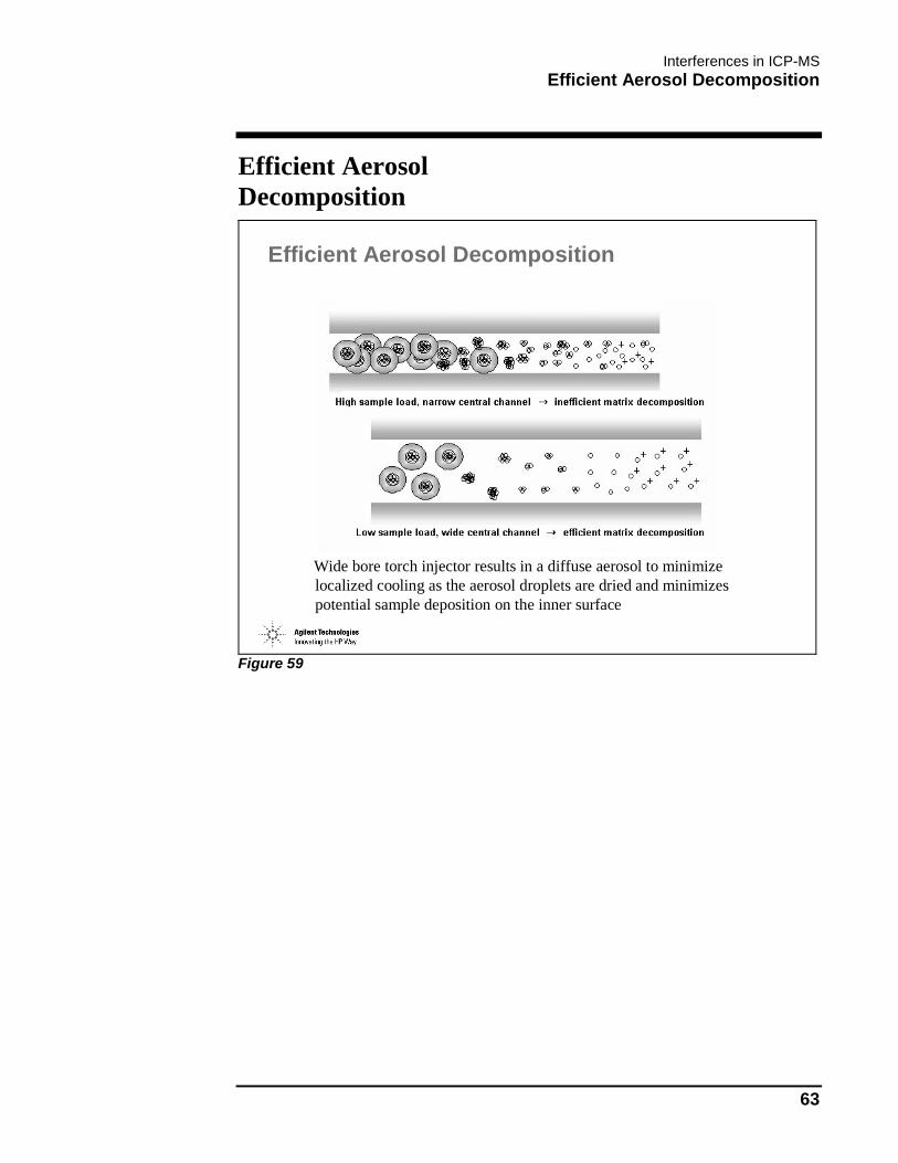
Efficient Aerosol Decomposition
Wide bore torch injector results in a diffuse aerosol to minimize localized cooling as the aerosol droplets are dried and minimizes potential sample deposition on the inner surface
Figure 59

Interferences in ICP-MS Oxides and Doubly Charged Ions
64
Oxides and Doubly Charged Ions
Oxides and Doubly Charged Ions
0
1
2
3
4
5
6
-5 0 5 10 15 20
Temp. (degreeC)
Rat
io (
%) Ce2+
Ba2+CeO
BaO
Figure 60

Interferences in ICP-MS Dealing with Mass Spectroscopic Interferences
65
Dealing with Mass Spectroscopic Interferences
Dealing with Mass Spectroscopic Interferences
� Matrix Elimination� Chelation� Chromatography � ETV� Desolvation
y membrane
y thermal
� Interference correction equations
Figure 61

Interferences in ICP-MS Interference Equations
66
Interference Equations
Interference Equations
Mathematical equations used to minimize the effect of elemental,doubly-charged and polyatomic isobaric interferences in ICP-MS analysis.
Isobaric204 Hg on 204 Pb
Polyatomic75ArCl on 75As
Doubly charged ions88Sr++ on 44 Ca
Figure 62
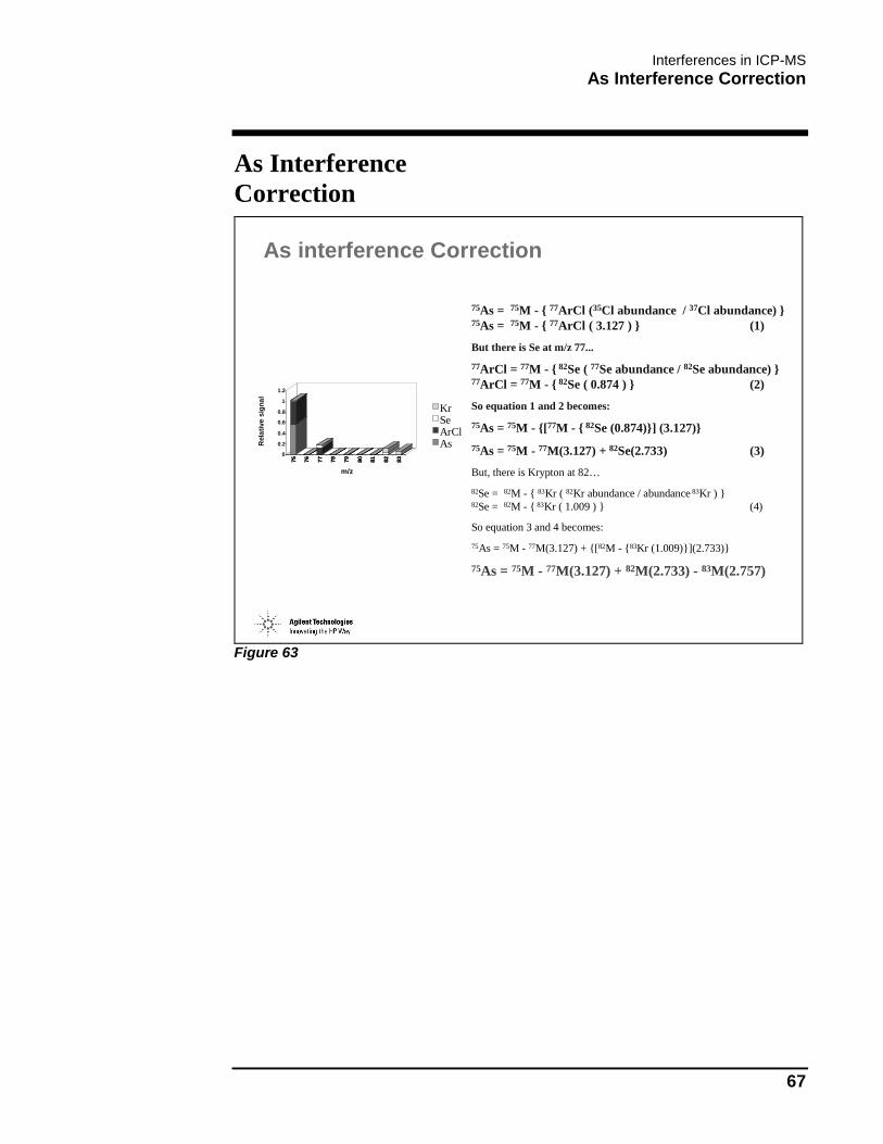
Interferences in ICP-MS As Interference Correction
67
As Interference Correction
As interference Correction
75As = 75M - { 77ArCl (35Cl abundance / 37Cl abundance) }75As = 75M - { 77ArCl ( 3.127 ) } (1)
But there is Se at m/z 77...
77ArCl = 77M - { 82Se ( 77Se abundance / 82Se abundance) }77ArCl = 77M - { 82Se ( 0.874 ) } (2)
So equation 1 and 2 becomes:
75As = 75M - {[77M - { 82Se (0.874)}] (3.127)}
75As = 75M - 77M(3.127) + 82Se(2.733) (3)
But, there is Krypton at 82…
82Se = 82M - { 83Kr ( 82Kr abundance / abundance 83Kr ) }82Se = 82M - { 83Kr ( 1.009 ) } (4)
So equation 3 and 4 becomes:
75As = 75M - 77M(3.127) + {[82M - {83Kr (1.009)}](2.733)}
75As = 75M - 77M(3.127) + 82M(2.733) - 83M(2.757)
75 76 77 78 79 80 81 82 83
0
0.2
0.4
0.6
0.8
1
1.2
Rel
ativ
e si
gna
l
75 76 77 78 79 80 81 82 83
m/z
KrSeArClAs
Figure 63

Interferences in ICP-MS Interference Correction Equations - Agilent 7500
68
Interference Correction Equations - Agilent 7500
Interference Correction Equations - Agilent 7500
Figure 64
Interference equations are edited from Top >> Methods >> Edit Interference Equation… or from Edit Entire Method.
Equations must be simplified and terms combined before entering them into the Edit Interference Equation dialog box.
The actual values are stored within the method folder as ‘correct.icp’, a text file which can be directly edited if desired.

Interferences in ICP-MS Non-Spectroscopic Interferences
69
Non-Spectroscopic Interferences
Non-Spectroscopic Interferences
■ Total Dissolved Solids■ High Mass Elements
� High mass elements affect the signal of low mass element. (Space Charge)
■ Easily Ionized Elements� Limited ionization energy is consumed by easily ionized
elements such as Na and K.
Result from sample matrix
Figure 65

Interferences in ICP-MS Effect of High Dissolved Solids
70
Effect of High Dissolved Solids
Effect of High Dissolved Solids
� Signal suppression
� Deposits on sampler and skimmer cones
� Deposits on ion optics
Figure 66

Interferences in ICP-MS First Ionization Potential
71
First Ionization Potential
First Ionization Potential
First ionization potential
0 10 20 30 40 50 60 70 80 900
5
10
15
20
25
Atomic number
Ioni
sati
on p
oten
tial
(eV)
Ar 15.75eV
He 24.58eV
Li
Be
B
C
Ba
Mg
Al
Si
PS
Cl
K
Ca
ScV
Ti
Cr
Mn
Zn
Ga
GeCu
Fe
Ni
CoAs
Se
Br
Rb
Sr
YZr
Nb
Mo
Tc
Ru
Rh
Pd
Ag
Cd
In
Sn
SbTe
I
Xe
CsNa
LanthanidesHf
TaW
Re
OsIr
Pt
AuHg
Tl
Pb
Bi
Po
Rn
Ra
Ac
N
F
Kr
He
O
Ne
Ar
Figure 67

Interferences in ICP-MS Ionization Efficiency
72
Ionization Efficiency
Ionization Efficiency
0 10 20 30 40 50 60 70 80 900
20
40
60
80
100
Ioni
zati
on e
ffic
ienc
y (%
)
Li
Be
B
C
BaMg
Al
Si
P
S
Cl
K
Ca
ScV
Ti
Cr
Mn
Zn
Ga
GeCu
FeNi
Co
As
Se
Br
Rb
Sr
Y
Zr
Nb
MoTc
Ru
Rh
Pd
Ag
Cd
InSn
Sb
Te
I
Xe
CsNaLanthanides
Hf
TaW
Re
Os
Ir
Pt
Au
Hg
Tl Pb
Bi
Po
Rn
RaAc
N F KrHe
ONe Ar
Figure 68
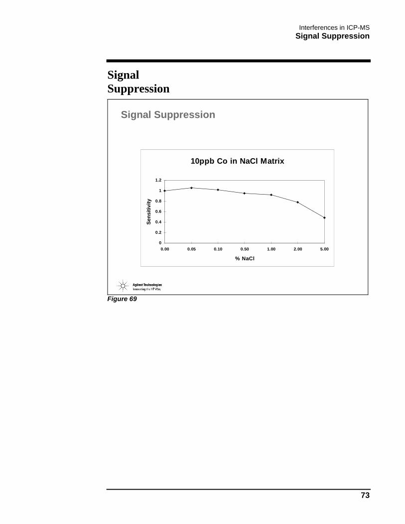
Interferences in ICP-MS Signal Suppression
73
Signal Suppression
Signal Suppression
10ppb Co in NaCl Matrix
0
0.2
0.4
0.6
0.8
1
1.2
0.00 0.05 0.10 0.50 1.00 2.00 5.00
% NaCl
Sen
siti
vity
Figure 69

Interferences in ICP-MS Matrix Effects – On Low Mass Analyte
74
Matrix Effects – On Low Mass Analyte
Matrix Effects - on Low Mass Analyte
Lithium 7
0
0.5
1
0 50 100 150 200 250
Mass of Matrix Element
Sig
nal Low eV
High eVCs
AuCdZn
RbNa
B
UTl
Molar Ratio of Matrix Element to Analyte = 1000:1
Figure 70

Interferences in ICP-MS Matrix Effects – On Medium Mass Analyte
75
Matrix Effects – On Medium Mass Analyte
Matrix Effects - on Medium Mass Analyte
Rhodium 103
0
0.5
1
0 50 100 150 200 250
Mass of Matrix Element
Sign
al Low eV
High eVCs
Au
CdZn
RbNa
B
UTl
Molar Ratio of Matrix Element to Analyte = 1000:1
Figure 71

Interferences in ICP-MS Matrix Effects – On High Mass Analyte
76
Matrix Effects – On High Mass Analyte
Matrix Effects - on High Mass Analyte
Thorium 232
0
0.5
1
0 50 100 150 200 250
Mass of Matrix Element
Sign
al Low eV
High eV
Cs
AuCdZn
RbNa
B
U
Tl
Molar Ratio of Matrix Element to Analyte = 1000:1
Figure 72

Interferences in ICP-MS Space Charge Interface and Lens Region
77
Space Charge Interface and Lens Region
Space ChargeInterface and Lens Region
+++
++
++
++ +
+
+
+
++
++
+
+
++
+
+
+++
Figure 73
After Extraction Lenses, Ion beam is predominantly positive charged.
Strong repulsive forces exist within the ion beam which affect low mass ions much more than high mass ions tending to disperse the low mass portion of the ion beam. Uncontrolled, space charge results in loss of low mass sensitivity, especially in the presence of high mass matrix. Complex, multi-element ion optics can compensate for this effect.

Interferences in ICP-MS Ionization Suppression Plasma Region
78
Ionization Suppression Plasma Region
Ionization SuppressionPlasma Region
---
- --- -
-
-----
Zn
Zn
Na+
Na+
Na+
Na+Na+Na+
Na+Na+
Na+ Na+Na+
Zn
Zn
-
-- -
--
-
-
- -
-
Na Na+ + e-
Zn+ + e- Zn
Figure 74

Interferences in ICP-MS What Can Be Done About Matrix Effects
79
What Can Be Done About Matrix Effects
What Can Be Done About Matrix Effects
� Dilution of Sample� Internal Standardization� Standard Additions� Matrix Elimination
y Chromatographyy ETVy Membrane desolvation
Figure 75

Interferences in ICP-MS What Can Be Done About Matrix Effects
80

Tuning the Agilent 7500

Tuning the Agilent 7500 Why Tune the ICP-MS?
82
Why Tune the ICP-MS?
Why Tune the ICP-MS?
■ Optimize Sensitivityy Maximize Signaly Minimize Noise
■ Verify Correct Mass Calibration■ Verify Correct Ion Ratio Response■ Minimize Interferences
y Oxidesy Doubly-Charged Ionsy Argides
Figure 76

Tuning the Agilent 7500 Tuning Procedure Overview
83
Tuning Procedure Overview
Tuning Procedure Overview
■ Tune Plasma Parameters RF Power Gas Flows Peristaltic Pump Flow Torch Position
■ Tune Ion Optics Extraction and Ion focusing lenses Omega Lenses
■ Tune Quadrupole Mass Analyzer Optimum Mass Resolution and Response Correct Mass Assignments
■ Tune Detector Optimum Sensitivity Optimum Dual Mode (Pulse and Analog) linearity
■ Save Tune Conditions■ Generate Tune Report
Figure 77

Tuning the Agilent 7500 Agilent 7500 ICP-MS Manual Tune Checklist [1]
84
Agilent 7500 ICP-MS Manual Tune Checklist [1]
Agilent 7500 ICP-MS Manual Tune Checklist [1]
See “Manually Tuning the HP-4500 ICP-MS” for detailed instructions
I. Verify Hardware■ vacuum, gas pressures and flows, peri-pump tubes and connections, error log■ examine cones with magnifier
II. Verify Plasma Parameters■ Aspirate tune solution #1, Warm up for 15-30 min■ Check sensitivity, and precision■ Fine tune carrier and/or blend gas flows for maximum signal, minimum RSDs (high
Li RSDs are usually related to worn or damaged cones)■ Verify torch position and run torch position autotune if in doubt■ Check oxides (<0.8% is fine). If high: 1. Decrease carrier and/or blend gas flow. 2.
Decrease peri-pump flow. 3. Increase sampling depth. 4. Increase RF power
III. Ion Lenses■ Adjust Ion lenses for maximum (or desired) signal and minimum noise and RSDs in this
order : Extract 1 and Extract 2 simultaneously (maintain ~ 50 V difference) Einzel 2 Omega Bias, Omega + and Omega - in that order QP focus if necessary
Figure 78

Tuning the Agilent 7500 Agilent 7500 ICP-MS Manual Tune Checklist [2]
85
Agilent 7500 ICP-MS Manual Tune Checklist [2]
Agilent 7500 ICP-MS Manual Tune Checklist [2]
IV. Quadrupole Parameters■ Select Resolution/Axis■ Observe peak shapes, optimize by increasing Plate Bias and Pole Bias together if
necessary■ Adjust peak widths (0.7-0.75 AMU at 10%) if necessary with AMU offset for low mass
and AMU gain for mid- and high-mass■ Adjust mass calibration (nominal mass +/- 0.05 AMU) with Mass Offset for low mass and
Mass Gain for mid and high mass
V. Detector Parameters■ Automatically: Select SetEM from Tune menu■ Run P/A factor Autotune from Tune while aspirating 100 ppb standard
VI. Save Tune and Print Tune Report
Figure 79

Tuning the Agilent 7500 Autotune Screen
86
Autotune Screen
Autotune Screen
Figure 80
Full Autotune should normally only be used when manually tuning the instrument is unsuccessful. Most adjustments can be made more easily and quickly manually. Exceptions are Torch Position, SetEM, Axis and Resolution, and PA factor setting.
Setting realistic tune targets will increase the probability of a successful autotune and speed up the process.
Setting appropriate and relatively narrow parameter ranges will result in faster and more consistent autotunes

Tuning the Agilent 7500 Autotuning of ICP Torch Position and New Target Tune
87
Autotuning of ICP Torch Position and New Target Tune
Autotuning of ICP Torch Position and New Target Tune
• Autotuning is used for consistent optimization, against a pre-defined set of tuning criteria (sensitivity, background, oxides, etc.)
• ICP torch position is critical for obtaining best sensitivity and lowest molecular interferences - manual ICP torch adjustment is imprecise and highly dependent on operator skill and experience.Can also be VERY time consuming.
• Target tune - user can specify the required sensitivity - even at different parts of the mass range. Target tune gives the novice user the expertise of an ICP-MS expert!
• Not limited to pre-defined suite of tune elements.
Figure 81

Tuning the Agilent 7500 Features of Autotune (1)
88
Features of Autotune (1)
Features of Autotune (1)
z CustomizingÖ Tune mass selectionÖ Target tune set up for sensitivities, etc.(*)Ö Tune parameter range set up, fixed tune parameter set up, etc. (*)
z SpeedÖQuick Mode OptionÖ Fix parameter set up (*)ÖQuick measurement
z VisualizingÖ Real time display of the Indicator
(*) These items were realized in the Agilent 4500, but enforced in the Agilent 7500
Figure 82

Tuning the Agilent 7500 Features of Autotune (2)
89
Features of Autotune (2)
Features of Autotune (2)
• Multiple Functions and Abilities¾ 4 tuning modes
♦ Extraction,♦ Soft Extraction,♦ Cool Plasma♦ Hot ShieldTorch
¾ Target Tune¾ RSD Option¾ Saving function of Autotune’s target set up file¾ Skip function¾ Intelligence of Autotune sequence
Figure 83

Tuning the Agilent 7500 Choosing the Autotune Mode
90
Choosing the Autotune Mode
Choosing the Autotune Mode
Figure 84

Tuning the Agilent 7500 Basics of the Soft Extraction Mode
91
Basics of the Soft Extraction Mode
Basics of the Soft Extraction Mode
• Extraction: Charge Separation between the skimmer and the 1st extraction lens• Soft Extraction: Charge Separation between the 1st extraction lens and the 2nd
extraction lens
Extraction
Plasma
Skimmer
1st Extraction Lens
2nd Extraction Lens
Soft Extraction
Plasma
Skimmer
1st Extraction Lens
2nd Extraction Lens
Figure 85

Tuning the Agilent 7500 Comparison of Extraction Modes Settings
92
Comparison of Extraction Modes Settings
Cool Hot Cool HotShieldTorch
Li: 20000(Co: 1000)Y : ---Tl: 300BKG: < 1cpsCeO: >>>
Li: 200
Y : 700Tl: 300BKG: <20cpsCeO: 30%
-------Li: 6
Y : 300Tl: 200BKG: < 1cpsCeO: 8%
Non-ShieldTorch ----------
Li: 15
Y : 30Tl: 15BKG: < 5cpsCeO: 0.5 %
-------- ----------
Extraction Mode Soft Extraction Mode
Typical Sensitivity for Each Mode By Agilent 7500s (Mcps/ppm)
Comparison of Extraction Modes Settings
Figure 86

Tuning the Agilent 7500 Autotune - Target Setting
93
Autotune - Target Setting
Autotune - Target Setting
Figure 87

Tuning the Agilent 7500 Target Setting - Range Setting
94
Target Setting - Range Setting
Target Setting - Range Setting
Figure 88

Tuning the Agilent 7500 Sensitivity Tuning
95
Sensitivity Tuning
Sensitivity Tuning
Figure 89

Tuning the Agilent 7500 Peak Shape and Resolution
96
Peak Shape and Resolution
Peak Shape and Resolution
Increasing the Resolution(narrower peaks) affectsthe low mass side more.
Peak height is reducedand peak center shifts tohigh mass side.
Quadrupole peakstail slightly to thelow mass side
Figure 90

Tuning the Agilent 7500 Abundance Sensitivity
97
Abundance Sensitivity
Abundance Sensitivity
82 84 86 88 90 92
10
100
1000
1.0E4
1.0E5
1.0E6
1.0E7
Spectrum.1 [10.409 sec]:YCS8.D#[CPS][Log]
m/z->
�good
m/z->
82 84 86 88 90 92
10
100
1000
1.0E4
1.0E5
1.0E6
1.0E7
Spectrum.2 [10.409 sec]:YCS9.D#[CPS][Log]
m/z->
�bad
Figure 91

Tuning the Agilent 7500 Quadrupole Mass Filter - Scan Line
98
Quadrupole Mass Filter - Scan Line
Quadrupole Mass Filter - Scan Line
Mass Resolution dependent on:RF frequencyLength of quadrupoleIon speed
Resolution ∝ f2 L2 / V
f : FrequencyL: Length of Q-pole v: Speed of ion
Li
Y
Tl513 V
3056 V
U
V
Figure 92

Tuning the Agilent 7500 Detection Limits in Normal Mode
99
Detection Limits in Normal Mode
Detection Limits in Normal Mode
Unit : ng/L(ppt)Li551
Be2.80.9
3 sigma Integration Time :3sec.
B1193
C500082000
N O F Ne
Na100730
Mg40110
Upper Value : Detection Limit Lower Value : BEC
Al1064
Si700
16000
P5005200
S300044000
Cl600038000
Ar
K300034000
Ca130014000
Sc10
120
Ti29
V38
Cr1565
Mn230
Fe900
19000
Co1
3.2
Ni419
Cu315
Zn22260
Ga3
6.2
Ge16
As835
Se80460
Br600
2300
Kr
Rb0.83.4
Sr12
Y0.20.2
Zr0.30.3
Nb0.20.2
Mo0.50.5
Tc Ru0.80.8
Rh7
100
Pd12
Ag0.71.4
Cd0.71.7
In0.10.2
Sn0.62
Sb0.71
Te77
I70230
Xe
Cs0.52.7
Ba2.53.5
* Hf304
Ta0.080.1
W0.30.5
Re0.30.3
Os Ir0.20.2
Pt18310
Au0.82.3
Hg1.61.2
Tl1
1.8
Pb16
Bi0.20.3
Po At Rn
Ra **
* La0.10.1
Ce0.10.1
Pr0.080.09
Nd1
0.6
Pm Sm0.70.7
Eu0.10.1
Gd0.40.5
Tb0.30.9
Dy0.30.4
Ho0.080.09
Er0.30.2
Tm0.070.09
Yb0.20.3
Lu91
** Ac Th0.20.2
Pa U0.60.8
Np Pu Am Cm Bk Cf Es Fm Md No Lr
Figure 93
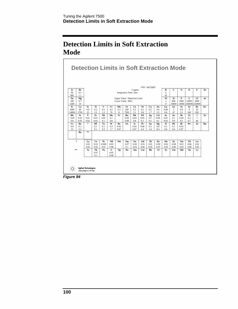
Tuning the Agilent 7500 Detection Limits in Soft Extraction Mode
100
Detection Limits in Soft Extraction Mode
Detection Limits in Soft Extraction Mode
Unit : ng/L(ppt)Li66800
Be0.51.1
3 sigma Integration Time :3sec.
B656
C N O F Ne
Na2002200
Mg0.710
Upper Value : Detection Limit Lower Value : BEC
Al217
Si800
19000
P100013000
S10000100000
Cl3000
120000
Ar
K200014000
Ca90
2700
Sc0.923
Ti0.53.5
V0.11.2
Cr4.274
Mn0.38
Fe200
7500
Co0.23.1
Ni0.10.8
Cu0.21.7
Zn0.62.5
Ga0.080.8
Ge5
47
As0.45.2
Se8
160
Br20830
Kr
Rb 0.050.8
Sr0.020.03
Y0.010.02
Zr0.010.02
Nb0.020.1
Mo0.10.8
Tc Ru0.040.08
Rh0.040.8
Pd0.050.1
Ag0.10.2
Cd0.040.1
In0.010.02
Sn0.10.9
Sb0.040.2
Te0.30.7
I140
Xe
Cs0.823
Ba0.10.2
* Hf0.10.1
Ta0.10.3
W0.31.7
Re0.050.07
Os Ir0.050.07
Pt0.080.4
Au0.31.4
Hg0.88.4
Tl0.20.8
Pb0.10.4
Bi0.030.07
Po At Rn
Ra **
* La0.010.02
Ce0.010.02
Pr0.0080.01
Nd0.030.08
Pm Sm0.070.1
Eu0.020.03
Gd0.030.06
Tb0.010.05
Dy0.090.07
Ho0.020.02
Er0.080.06
Tm0.010.02
Yb0.060.08
Lu0.020.02
** Ac Th0.070.1
Pa U0.050.08
Np Pu Am Cm Bk Cf Es Fm Md No Lr
Figure 94

Tuning the Agilent 7500 Low BECs in Soft Extraction Mode
101
Low BECs in Soft Extraction Mode
Low BECs in Soft Extraction Mode
Background Equivalent Concentration (ppt)
Elements Soft-extraction Extraction
Li 4 800
Na 190 2200
Y 0.005 0.01
Ce 0.004 0.02
Th 0.005 0.1
Figure 95

Tuning the Agilent 7500 Pulse/Analog (P/A) Tuning
102
Pulse/Analog (P/A) Tuning
Pulse/Analog (P/A) Tuning
Figure 96

Maintenance of the Agilent 7500

Maintenance of the Agilent 7500 Maintenance Schedule
104
Maintenance Schedule
Maintenance Schedule
• Daily– Lab conditions, Argon, drain, peristaltic pump tubing, cones
• When Needed– Cones, nebulizer, peristaltic pump tubing, torch, water filter,
electron multiplier
• Weekly– tuning solution preparation, torch, spray chamber, nebulizer,
carrier gas line, cooling system
• Monthly– check rotary pump, oil mist filter, check extraction lens
• 6 months– clean lenses, change rotary pump oil, replace gas tubing
• Yearly– replace o-rings, clean penning gauge, check/replace mist filter
Figure 97

Maintenance of the Agilent 7500 Running Time Maintenance Screen
105
Running Time Maintenance Screen
Running Time Maintenance Screen
Figure 98

Maintenance of the Agilent 7500 Early Maintenance Feedback (EMF)
106
Early Maintenance Feedback (EMF)
Early Maintenance Feedback (EMF)
EMF monitors the operating hours of all major system components andproactively informs the user when:�maintenance is required�consumable items should be replaced
Users can define their own maintenance schedule
Figure 99

Maintenance of the Agilent 7500 Normal Maintenance of the Sample Introduction System
107
Normal Maintenance of the Sample Introduction System
Normal Maintenance of the Sample Introduction System
Non-Glassware Components- Sample tubing- Peristaltic pump tubing 1. Soak in 1% to 5% nitric acid (5 min.)- Babington nebulizer 2. Clean in ultrasonic bath (5 min.)- Crossflow nebulizer 3. Rinse with DI water- Nebulizer end caps- O-rings
Glassware-Concentric nebulizer- Spray chamber 1. Soak in 1% to 5% nitric acid (5 min.)
or sonicate in 10% Citranox
- Ball joint connector 2. Rinse with DI water- Torch
Figure 100

Maintenance of the Agilent 7500 Overnight Cleaning of the Sample Introduction System
108
Overnight Cleaning of the Sample Introduction System
Overnight Cleaning of the Sample Introduction System
For severely contaminated glassware and non-glassware components
Procedure1. Soak in 5% nitric acid overnight or boil in 10%
Citranox® for 1 hour, rinse in 5% nitric acid2. Rinse with DI water
Figure 101

Maintenance of the Agilent 7500 Sample Introduction Maintenance
109
Sample Introduction Maintenance
Sample Introduction Maintenance
Top Cover
Sample Transfer Line
Ball Joint Clamp
Spray Chamber
Nebulizer and End Cap
Spray Chamber Chiller
Figure 102

Maintenance of the Agilent 7500 Nebulizer Connections
110
Nebulizer Connections
Nebulizer Connections
Crossflow Nebulizer
Babington Nebulizer
Concentric Nebulizer
Sample Uptake
Sample Uptake
Sample Uptake
Carrier Gas
Carrier Gas
Carrier Gas
Blend Gas
Blend Gas
Blend Gas
Figure 103
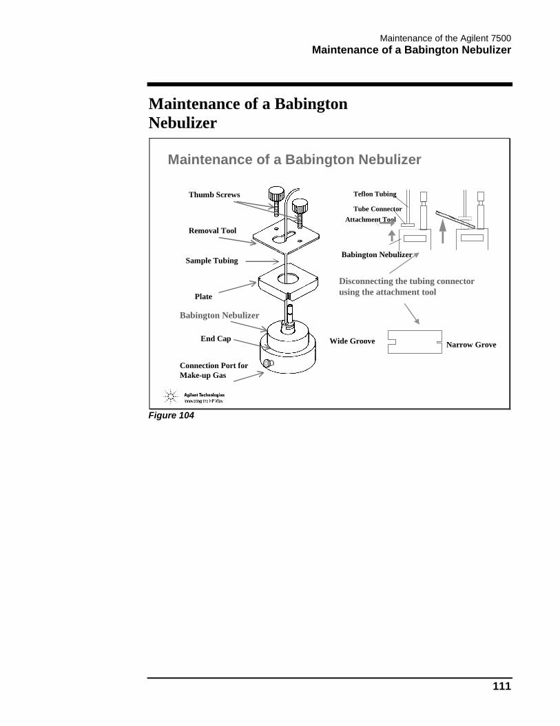
Maintenance of the Agilent 7500 Maintenance of a Babington Nebulizer
111
Maintenance of a Babington Nebulizer
Maintenance of a Babington Nebulizer
Tube Connector
Babington Nebulizer
Attachment Tool
Teflon Tubing
Wide Groove Narrow Grove
Disconnecting the tubing connectorusing the attachment tool
End Cap
Thumb Screws
Sample Tubing
Removal Tool
Plate
Babington Nebulizer
Connection Port forMake-up Gas
Figure 104

Maintenance of the Agilent 7500 Torch Maintenance
112
Torch Maintenance
Torch Maintenance
Torch
Plasma Gas
Auxiliary Gas
Torch Mounting Assembly
Figure 105

Maintenance of the Agilent 7500 Interface Maintenance
113
Interface Maintenance
Interface Maintenance
Routine MaintenanceComponents
- Sampling cone - Skimmer cone
Procedure1. Soak in 1-5% nitric acid (<10 min.)2. Rinse with DI water
Removing Severe DepositsComponents
- Sampling cone - Skimmer cone
Procedure1. Polish with waterproof abrasive paper
- be careful not to damage the orifice2. Rinse with DI water
Figure 106

Maintenance of the Agilent 7500 Maintenance of the Cones
114
Maintenance of the Cones
Maintenance of the Cones
Removal of the Sampling Cone
Removal of the Skimmer Cone
Figure 107

Maintenance of the Agilent 7500 Extraction Lenses Maintenance
115
Extraction Lenses Maintenance
Extraction Lenses Maintenance
● Remove skimmer base from vacuum manifold● Disassemble extraction lenses, screws and spacers● Polish extraction lenses with waterproof abrasive paper● Wash extraction lenses in DI water● Sonicate lenses, spacers and screws in DI water for 5 minutes● Sonicate lenses, spacers and screws in acetone for 5 minutes● Reassemble lenses, spacers and screws on skimmer base● Install skimmer base on vacuum manifold
Figure 108

Maintenance of the Agilent 7500 Extraction Lenses
116
Extraction Lenses
Extraction Lenses
Skimmer Base
Extraction Lens 1
Extraction Lens 2
Screw 2
Spacer 1
Spacer 2
Spacer 1
Screw 1
Figure 109

Maintenance of the Agilent 7500 Cleaning of the Einzel Lens and Omega Lens Assembly
117
Cleaning of the Einzel Lens and Omega Lens Assembly
Cleaning of the Einzel Lens and Omega Lens Assembly
● Disassemble lenses, remove screws and spacers● Polish each lens, lens orifice and the curved surfaces of the Omega lenses using waterproof abrasive paper● Wash lenses in DI water● Sonicate lenses, spacers and screws in DI water for 5 minutes● Sonicate lenses, spacers and screws in acetone or alcohol for 5 minutes● Reassemble and install the lens assemblies and install them in the vacuum manifold● Replace top cover and vent nut and restart system.
Figure 110

Maintenance of the Agilent 7500 Instrument Shutdown
118
Instrument Shutdown
Instrument Shutdown
Shutdown
Standby
Figure 111
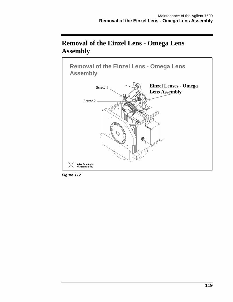
Maintenance of the Agilent 7500 Removal of the Einzel Lens - Omega Lens Assembly
119
Removal of the Einzel Lens - Omega Lens Assembly
Removal of the Einzel Lens - Omega Lens Assembly
Einzel Lenses - Omega Lens Assembly
Screw 1
Screw 2
Figure 112

Maintenance of the Agilent 7500 Expanded View of Einzel Lens - Omega Lens Assembly
120
Expanded View of Einzel Lens - Omega Lens Assembly
Expanded View of Einzel Lens - Omega Lens Assembly
Omega Bias (back)Omega (+)
Spacer 2Omega Contact
Screw 3
Omega Bias (front)Base Plate
Spacer 3
Einzel 3
Einzel 2Einzel 1
Screw 1
Omega (-)
Spacer 1
Spacer 1
Spacer 1
Screw 2
Spacer 1
Spacer 1
Spacer 1
Spacer 1
Shaft
QP Focus (back)QP Focus (front)
Spacer 1
Figure 113

Maintenance of the Agilent 7500 Plate Bias Lens
121
Plate Bias Lens
Plate Bias Lens
QP Focus Guide
Screw 1
Plate Bias Lens
Figure 114

Maintenance of the Agilent 7500 Penning Gauge
122
Penning Gauge
Penning Gauge
1. Magnet Housing2. Collar3. Anode Assembly4. O-ring5. Body Tube6. Cathode Plate7. Cathode Tube8. Circlip
Figure 115

Maintenance of the Agilent 7500 Rotary Pump Maintenance
123
Rotary Pump Maintenance
Rotary Pump Maintenance
● Put system in Shutdown mode (Turn vacuum off)● Turn off pump circuit breakers on front panel● Remove oil inlet cap on top of pump● Remove oil drain plug using a flat blade screwdriver and allow oil to drain into a waste container● Replace oil drain plug and add new oil through the oil inlet until the oil level window is 80% full● Replace oil inlet cap, turn on pump breakers on front panel, and start system (Turn vacuum on)
Figure 116

Maintenance of the Agilent 7500 Changing Rotary Pump Oil
124
Changing Rotary Pump Oil
Changing Rotary Pump Oil
Figure 117
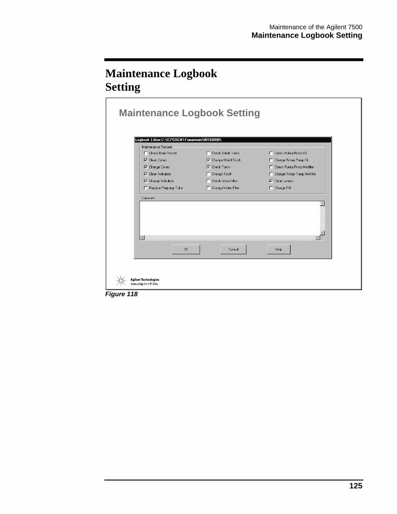
Maintenance of the Agilent 7500 Maintenance Logbook Setting
125
Maintenance Logbook Setting
Maintenance Logbook Setting
Figure 118

Maintenance of the Agilent 7500 Maintenance Logbook
126
Maintenance Logbook
Maintenance Logbook
Figure 119

Maintenance of the Agilent 7500 Sample Introduction Maintenance
127
Sample Introduction Maintenance
Sample Introduction Maintenance
Figure 120

Maintenance of the Agilent 7500 Air Filters Maintenance
128
Air Filters Maintenance
Air Filters Maintenance
■ Remove air filters from the instrument
■ Remove dust from the filters using a vacuum cleaner
■ Wash filters with water if necessary and allow to dry
■ Return filters to the instrument
Figure 121

Maintenance of the Agilent 7500 Instrument Start-up
129
Instrument Start-up
Instrument Start-up
Shutdown
Standby
Analysis
Figure 122

Maintenance of the Agilent 7500 Instrument Start-up
130

Internal Standardization in ICP-MS

Internal Standardization in ICP-MS The Role of Internal Standards
132
The Role of Internal Standards
The Role of Internal Standards
Correct for variations in response due to:Matrix Effects
Transport effectsNebulization effectsIonization effectsSpace-charge effects
Instrument Drift
Figure 123

Internal Standardization in ICP-MS How the Internal Standards Work - 1
133
How the Internal Standards Work - 1
How the Internal Standards Work - 1
• Added to each sample, standard and blank at identical concentration
• System therefore expects identical response from ISTDs in each solution
• Ratio of measured ISTD response to expected ISTD response is used to correct the response of the non-internal standard elements accordingly.
Figure 124

Internal Standardization in ICP-MS How the Internal Standards Work - 2
134
How the Internal Standards Work - 2
How the Internal Standards Work - 2
■ In all cases where potential matrix suppression exists, the use of internal standards is necessary.■ The calibration curve is plotted using the ratio of the analyte signal to IS signal (i.e. ax/isx), thereby canceling the effect of matrix suppression.■ Each analyte in the sample will then be quantitated using the ratio of the IS and the analyte in the sample.
Figure 125

Internal Standardization in ICP-MS Choice of the Internal Standard
135
Choice of the Internal Standard
Choice of the Internal Standard
It is assumed that the IS elements behave in the same way that the analytes do in the plasma when using this correction. Therefore, selecting the appropriate IS element is very important.
These are the things to take into consideration:■ The element is not contained in the sample solution.■ The mass number is close to that of the analyte.■ The ionization potential is similar to that of the analyte.■ Chemical characteristics
The ionization potential matching is extremely important for analytes with high ionization potentials.
Elements that are commonly used as IS are:6Li, Sc, Ge, Y, Rh, In, Tb, Ho, Bi
Figure 126

Internal Standardization in ICP-MS Concentration of Internal Standards
136
Concentration of Internal Standards
Concentration of Internal Standards
The IS elements can be added to the sample in 2 ways:
■ On-line addition by peristaltic pump■ Spike in each standard and sample
In either case, it is recommended to add IS in concentration levels around mid-calibration range (exact concentration is application-specific)
For environmental applications 50 ppb concentration is usually applied.For on-line IS addition use 1 ppm IS stock solution, and use the peristaltic pumps as recommended.
Figure 127

Internal Standardization in ICP-MS On-line Addition of Internal Standards
137
On-line Addition of Internal Standards
On-line Addition of Internal Standards
■ On-line Addition
The IS solution is introduced by a narrow tubing (f = 0.19 mm), and is mixed with the sample at the Y connector. The dilution factor of the IS by the sample is about 1/20. Therefore, a 1 ppm solution in 5 % HNO3 would yield approximately 50 ppb in the sample. At least 5 % HNO3 is needed to avoid absorption of elements to the tubing, as absorption is more severe using narrow tubing.
Figure 128

Internal Standardization in ICP-MS On-line Addition of Internal Standards
138

Sample Preparation Techniques for ICP-MS

Sample Preparation Techniques for ICP-MS Contamination
140
Contamination
Contamination
■ "Contamination is the introduction of any component which affects the numerical value finally attributed to a constituent
relative to the amount present prior to sampling" ■ Types of contamination:
–positive–negative–pseudocontamination
D.E. Robertson "Ultrapurity, Methods and Techniques",M. Zeif and R. Speights, Eds., Marcel Dekker, NY, 1972
Figure 129

Sample Preparation Techniques for ICP-MS Types of Contamination
141
Types of Contamination
Types of Contamination
Positive contamination - results in additive errors. Caused by ➤impurities in reagents➤lab environment➤desorption from container walls
Negative contamination - results in subtractive errors. Caused by ➤losses in handling➤adsorption to container walls
Pseudocontamination - results in either positive or negative errors. Caused by
➤irreproducibility of experimental conditions
Figure 130

Sample Preparation Techniques for ICP-MS Challenges of Trace Analysis
142
Challenges of Trace Analysis
Challenges of Trace Analysis
Analyst
Environment
Sample
Standards
Methodology
Reagents
Figure 131

Sample Preparation Techniques for ICP-MS When a Contamination Can Occur
143
When a Contamination Can Occur
When a Contamination Can Occur
■ Sample collection– collection techniques– collection devices
■ Sample storage– prevention of positive contamination– prevention of negative contamination
■ Sample preparation– reagents– lab environment– apparatus
■ Sample measurement– instrument sample introduction system– standards
Figure 132

Sample Preparation Techniques for ICP-MS Reagents
144
Reagents
Reagents
■ Water■ Nitric acid■ Hydrochloric acid■ Sulfuric acid■ Hydrofluoric acid■ Other inorganic acids■ Hydrogen peroxide■ Alkaline solutions■ Organic solvents
Figure 133
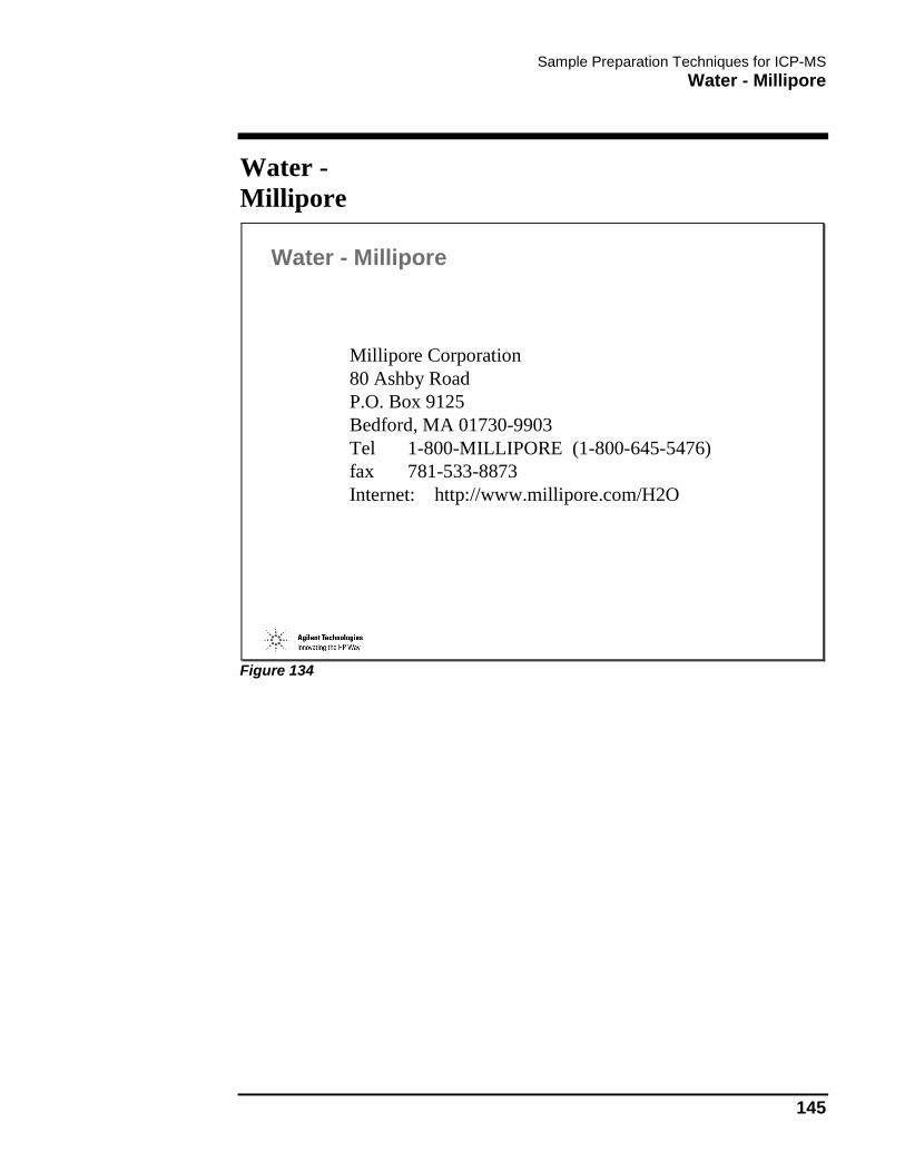
Sample Preparation Techniques for ICP-MS Water - Millipore
145
Water - Millipore
Water - Millipore
Millipore Corporation80 Ashby RoadP.O. Box 9125Bedford, MA 01730-9903Tel 1-800-MILLIPORE (1-800-645-5476)fax 781-533-8873Internet: http://www.millipore.com/H2O
Figure 134

Sample Preparation Techniques for ICP-MS Nitric Acid
146
Nitric Acid
Nitric AcidFrom Fisher Scientific (1-800-766-7000)
“TraceMetal” - for environmental analysis -500 mL in glass, catalog # A509-500, Certificate of Lot Analysis included with each shipment
“Optima” - for semiconductor and clinical applications -catalog # A467-250, 250 mL in Teflon™,catalog # A467-500, 500 mL in Teflon™,Certificate of Lot Analysis included with each bottle
from Mallinkrodt-Baker (1-800-444-0880)
“INSTRA-ANALYZED” (equivalent of “TraceMetal”), 500 mL in poly coated glass, catalog # 9598-00
“ULTREX II” (equivalent of “Optima”)500 mL in Teflon™, catalog # 6901-05
Figure 135

Sample Preparation Techniques for ICP-MS Selected Methods of Sample Preparation
147
Selected Methods of Sample Preparation
Selected Methods of Sample Preparation
� Dilution� Preconcentration� Filtration� Acidification� Digestion
Ö Open vessel digestionÖ Closed vessel digestionÖ Microwave digestion
➱ Fusion➱ Matrix separation
➱ Chromatography➱ Electrothermal Vaporization
Figure 136

Sample Preparation Techniques for ICP-MS Commonly Used Reagents (1)
148
Commonly Used Reagents (1)
Commonly Used Reagents (1)
Nitric Acid (HNO3)Used to dissolve a variety of materials such as metals, alloys, biological samples.Available in very high purity form.Most preferable acid for ICP-MS work, as polyatomic ions are not increased.
Hydrochloric Acid (HCl)Used commonly for sample digestion.Generates Cl derived polyatomic ions.Can be evaporated to dryness and reconstituted in HNO3.
Hydrofluoric Acid (HF)Used to dissolve silica-based materials and geological samples.HF attacks glass, therefore the inert sample introduction system must be used.Teflon containers are often used.Extreme health hazard.
Figure 137

Sample Preparation Techniques for ICP-MS Commonly Used Reagents (2)
149
Commonly Used Reagents (2)
Commonly Used Reagents (2)
Hydrogen Peroxide (H2O2)Strong oxidizing agent used with other acids for digestion.Useful for ICP-MS work, as backgrounds are similar to water (H2O).
Sulfuric Acid (H2SO4)Oxidizing agent used with other acids for digestion.Causes numerous polyatomic ion interferences.Difficult to decompose in plasma due to high boiling point and viscosity.Deteriorates Ni and Cu interface material.Not recommended for use if it can be avoided.
Phosphoric Acid (H3PO4)Used to buffer other acids.Causes numerous polyatomic ion interferences.Difficult to decompose in plasma due to high boiling point and viscosity.Deteriorates Ni interface material.Should be avoided.
Figure 138

Sample Preparation Techniques for ICP-MS Commonly Used Reagents (3)
150
Commonly Used Reagents (3)
Commonly Used Reagents (3)
Perchloric Acid (HClO4)Strong oxidizing agent used with other acids for digestion of organic materials.Generates Cl derived polyatomic ions.More difficult to evaporate than HCl.Not recommended for use if it can be avoided.Handle with care as many solid perchlorates are explosive.
Aqua Regia (1 part conc. HNO3 + 3 parts conc. HCl)
Used for metal digestion, especially precious metals.Generates Cl derived polyatomic ions.Cl matrix can be removed by evaporation.
Figure 139

Semi-quantitative Analysis of Samples

Semi-quantitative Analysis of Samples Semi-quantitative Analysis
152
Semi-quantitative Analysis
Semi-quantitative Analysis
• What is Semi-quantitative Analysis• Setting Semi-quantitative acquisition parameters• Analyzing the samples• Semi-quantitative data analysis
Figure 140

Semi-quantitative Analysis of Samples What is Semi-quantitative Analysis?
153
What is Semi-quantitative Analysis?
What is Semi-quantitative Analysis?
� Is an analytical procedure used to calculate concentrations of all elements present in an unknown sample
� Is useful as a screen prior to Quantitative Analysisy concentration ranges of analytesy selection of internal standards
� Does not require an external calibration � Is generally accurate to +/- 30% or better on completely
unknown samples
Figure 141

Semi-quantitative Analysis of Samples Data Acquisition
154
Data Acquisition
Data Acquisition
Figure 142

Semi-quantitative Analysis of Samples Method Set-up for Semi-quantitative Analysis
155
Method Set-up for Semi-quantitative Analysis
Method Set-up for Semi-quantitative Analysis
Do not check
To write comments & record updates
Figure 143

Semi-quantitative Analysis of Samples Parameters Selection - Spectrum Acquisition
156
Parameters Selection - Spectrum Acquisition
Parameters Selection - Spectrum Acquisition
[1] Select Semi-Quant peak pattern,0.1 s/point, 1 repetition
[2] SelectMass Scale
Figure 144

Semi-quantitative Analysis of Samples Parameters Selection - Selection of Masses
157
Parameters Selection - Selection of Masses
Parameters Selection - Selection of Masses
[1]Select mass ranges
[2] Exclude unlike, impossible, and interfered with masses
Figure 145

Semi-quantitative Analysis of Samples More Acquisition Parameters
158
More Acquisition Parameters
More Acquisition parameters
Do not check
When background is subtracted, and the internal standards are used, exclude up to 4 masses from subtraction (IS masses)
If checked, use the browse button to select the appropriate file
Figure 146

Semi-quantitative Analysis of Samples Report Generation
159
Report Generation
Report Generation
Select a report
Figure 147
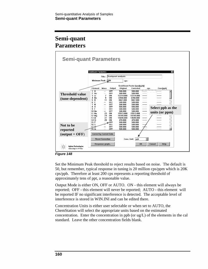
Semi-quantitative Analysis of Samples Semi-quant Parameters
160
Semi-quant Parameters
Semi-quant Parameters
Threshold value (tune-dependent)
Not to be reported(output = OFF)
Select ppb as the units (or ppm)
Figure 148
Set the Minimum Peak threshold to reject results based on noise. The default is 50, but remember, typical response in tuning is 20 million cps/ppm which is 20K cps/ppb. Therefore at least 200 cps represents a reporting threshold of approximately tens of ppt, a reasonable value.
Output Mode is either ON, OFF or AUTO. ON - this element will always be reported; OFF - this element will never be reported; AUTO - this element will be reported IF no significant interference is detected. The acceptable level of interference is stored in WIN.INI and can be edited there.
Concentration Units is either user selectable or when set to AUTO, the ChemStation will select the appropriate units based on the estimated concentration. Enter the concentration in ppb (or ug/L) of the elements in the cal standard. Leave the other concentration fields blank.

Semi-quantitative Analysis of Samples Semi-quantitative Data Analysis
161
Semi-quantitative Data Analysis
Semi-quantitative Data Analysis
Figure 149
Semiquant analysis can be used to estimate the concentration of any element for which a precise measurement can be made by ICP-MS (> 70 elements).
Typically, semiquantitation is accurate to within +/- 30 percent on completely unknown samples. However, semiquantitation is subject to the same interferences as quantitation. Possible interferences due to oxides, hydrides, argides, dimers and doubly-charged ions are checked and flagged on the report. Interference correction equations can be used to minimize these effects where applicable. The use of internal standards can help correct for matrix differences. Blank subtraction can be used to eliminate contributions from laboratory reagents and sample preparation.
The ChemStation comes configured with default SemiQuant response factors. These factors are based on relative ionization potentials and numbers of isotopes for each element. These factors can be updated to reflect the tune state of the HP-4500 by analyzing a calibration mix. At least 3 elements should be used, though more is better. The ChemStation will then interpolate between analyzed masses to update all SemiQuant response factors.
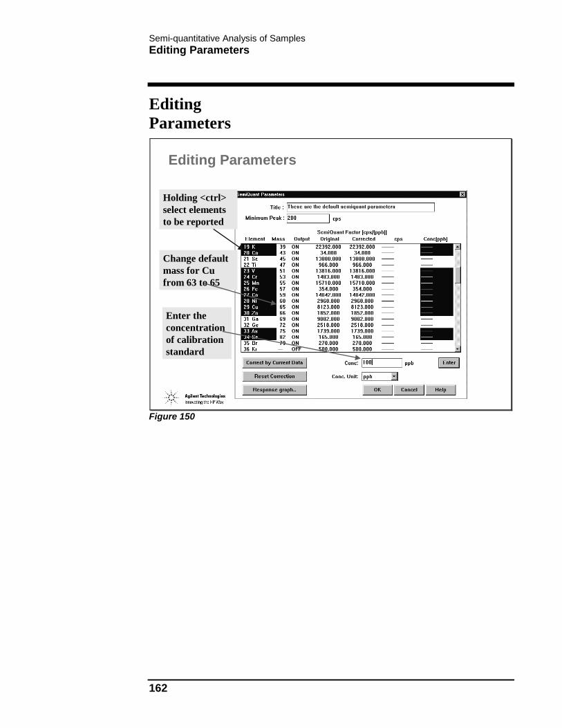
Semi-quantitative Analysis of Samples Editing Parameters
162
Editing Parameters
Editing Parameters
Holding <ctrl> select elements to be reported
Change default mass for Cu from 63 to 65
Enter the concentration of calibration standard
Figure 150

Semi-quantitative Analysis of Samples Daily Update of the Semi-Quant Parameters
163
Daily Update of the Semi-Quant Parameters
Daily Update of the Semi-Quant Parameters
Load a previously acquired file and select “Correct by Current Data”
Figure 151
Correct by Current Data recalculates all semi-quant response factors by first dividing the supplied concentrations by the responses for those elements. Other, non-calibrated element response factors are estimated by interpolation.

Semi-quantitative Analysis of Samples Internal Standard Correction for Off-line Internal Standard Addition
164
Internal Standard Correction for Off-line Internal Standard Addition
Internal Standard Correction for Off-line Internal Standard Addition
IS concentration
Off-line additionActivating internal standard correction
Selecting internal standard
Figure 152
Internal Standardization is recommended since it corrects for changes in instrument sensitivity due to matrix and other effects.
To configure internal standard correction:
Data Analysis >> SemiQuant >> Internal Standard Correction…
Internal standard correction can be applied in two modes:
‘Normal Mode’ assumes that internal standards are added to the samples only and no ISTD reference data file is required. This can be used for analyses such as Laser Ablation, where a matrix element is used as the internal standard. The ISTD factor is calculated from the supplied ISTD concentration and the ISTD response. Up to four internal standard elements can be selected.

Semi-quantitative Analysis of Samples Internal Standard Correction for On-line Internal Standard Addition
165
Internal Standard Correction for On-line Internal Standard Addition
Internal Standard Correction for On-line Internal Standard Addition
On-line addition
Selecting internal standard
Activating internal standard correction
Figure 153
‘Auto Add Mode’ assumes that the online internal standard addition configuration is used. In this case, the exact concentration of the ISTD elements need not be known since an ISTD reference file used. Only the internal standard masses need be selected. In this case, the only requirement is that the ISTD concentration in all samples be identical to the ISTD reference file.
The ISTD reference file can be either a blank or a calibration standard containing online added internal standards.

Semi-quantitative Analysis of Samples Example of Semi-Quant Report [1]
166
Example of Semi-Quant Report [1]
Example of Semi-Quant Report [1]
For signal >200cps (threshold), the concentration of the analyte is reported
For signal <200cps (threshold), a threshold concentration (corresponding to 200 cps) is report
Figure 154

Semi-quantitative Analysis of Samples Example of Semi-Quant Report [2]
167
Example of Semi-Quant Report [2]
Example of Semi-Quant Report [2]
Software indicates possible interferences
Figure 155

Semi-quantitative Analysis of Samples Generating a Semi-quant Report
168
Generating a Semi-quant Report
Generating a Semi-quant Report
Î Automatically as part of Run Method or Run SequenceÎ Manually from Data AnalysisÎ SemiQuant also allows Custom Reports and Custom DatabasesÎ Use of DoList for multiple reports
Figure 156

Semi-quantitative Analysis of Samples Manual Verification of the Data
169
Manual Verification of the Data
Manual Verification of the Data
Figure 157

Semi-quantitative Analysis of Samples Manual Verification of the Data
170

Quantitative Analysis of Samples

Quantitative Analysis of Samples What is Quantitative Analysis?
172
What is Quantitative Analysis?
What is Quantitative Analysis?
Quantitative Analysis:
■ An analytical procedure used to calculate concentrations of specific elements in unknown samples
■ Uses calibration curves based on the response of one or more levels of standards to calculate unknown concentrations
■ Allows the use of internal standards to correct for instrument drift and matrix differences between standards and samples
Figure 158

Quantitative Analysis of Samples Method Set-up for Quantitative Analysis
173
Method Set-up for Quantitative Analysis
Method Set-up for Quantitative Analysis
Steps in Setting up a Quantitative Analysis:
■ Editing the AMU Select file, if necessary ■ Interference correction equations■ Spectrum acquisition parameters■ Peripump program■ Calibration table■ Acquiring calibration standards and updating the calibration table■ Analyzing unknown samples
Figure 159

Quantitative Analysis of Samples Step One: Editing the AMU Select File
174
Step One: Editing the AMU Select File
Step One: Editing the AMU Select File
From Top >> AcquireData >> Edit AMU Select File (amu)...
Figure 160
The AMU select file is the database from which default isotopes are selected when elements are selected from the Periodic Table in Edit Entire Method.
Multiple AMU select files can be created for different applications. For example AMU select files can be created which automatically select the EPA specified isotopes when running EPA methods. AMU select files can also be created for specific matrices in order to avoid known isobaric or polyatomic interferences.
The element needs to have at least one isotope selected, in order to be accessible in the method setting. If needed, select isotopes for P, and Si.

Quantitative Analysis of Samples Editing a Method for Quantitative Analysis
175
Editing a Method for Quantitative Analysis
Editing a Method for Quantitative Analysis
QC Parameters will only be available if Intelligent Sequencing is enabled
Select ‘Edit Entire Method’
Figure 161

Quantitative Analysis of Samples Method Information
176
Method Information
Method Information
Figure 162

Quantitative Analysis of Samples Acquisition Modes
177
Acquisition Modes
Acquisition Modes
Figure 163
Spectrum mode is the most common acquisition mode for standard applications:
• Quant
• Semiquant
Time Resolved Analysis (TRA) and Time Program (more sophisticated than TRA) are used when a transient signal is measured:
• Electrothermal Vaporization (ETV)
• Laser Ablation (LA)
• Discrete Sampling Analysis (using ISIS)
• Chromatographic analysis (LC, GC, IC, CE)
Isotope Analysis mode is used when additional precision is needed for isotope ratio measurements. It is similar to spectrum mode, but with 10X higher sampling frequency.

Quantitative Analysis of Samples Acquisition Modes
178
Multitune mode is used when during a single acquisition more than one tuning parameters are needed to accomplish the optimum performance.

Quantitative Analysis of Samples Acquisition Parameters - Multitune Method
179
Acquisition Parameters - Multitune Method
Acquisition Parameters - Multitune Method
Figure 164

Quantitative Analysis of Samples Periodic Table
180
Periodic Table
Periodic Table
Figure 165

Quantitative Analysis of Samples Mass Table
181
Mass Table
Mass Table
Figure 166

Quantitative Analysis of Samples Peristaltic Pump Program
182
Peristaltic Pump Program
Peristaltic Pump Program
Maximum Speed should not exceed 0.30 rps with online ISTDs addition
Typical Stabilization Time is 50-60 sec
Probe Rinse should be very short (~1 sec)
Rinse time is sample/matrix dependent (30-90 sec)
Figure 167
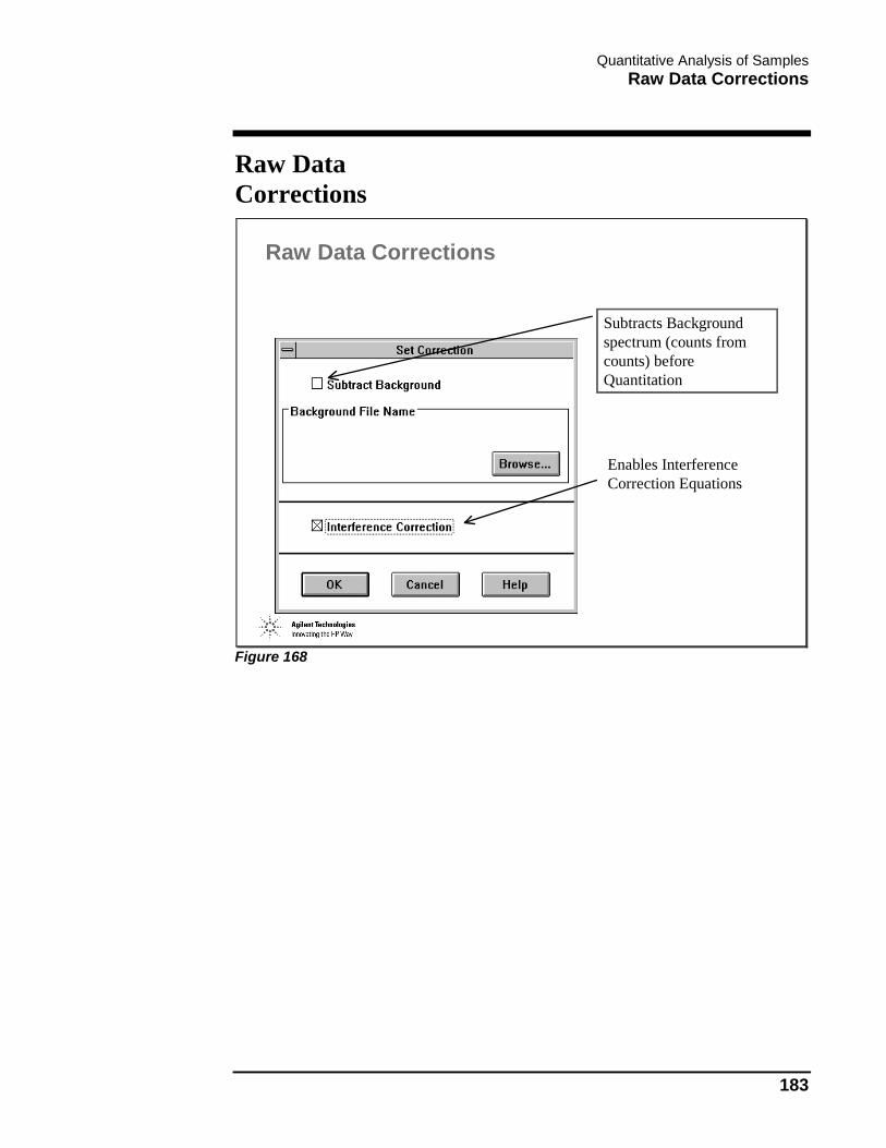
Quantitative Analysis of Samples Raw Data Corrections
183
Raw Data Corrections
Raw Data Corrections
Subtracts Background spectrum (counts from counts) before Quantitation
Enables Interference Correction Equations
Figure 168

Quantitative Analysis of Samples Configure Reports
184
Configure Reports
Configure Reports
Enabled with Intelligent Sequencing
Figure 169

Quantitative Analysis of Samples Calibration
185
Calibration
Calibration
• Now independent of the method• Multiple methods can share the same calibration• Current calibration is displayed on the TOP and Data Analysis title bar
• Link between calibration and method is established when method is saved
Figure 170

Quantitative Analysis of Samples Calibration Table
186
Calibration Table
Calibration Table
Figure 171
Shortcuts:
• Double click any column selects entire column.
• Fill Across is useful for copying Internal Standard Concentrations to all levels.
• Multiple entries can be selected using <Ctrl> plus left click or Shift plus left click.
• Min. Conc. is the lower reporting limit, to disable it replace it with ‘---’, often the reporting limits are entered here.

Quantitative Analysis of Samples Save the Calibration and the Method
187
Save the Calibration and the Method
Save the Calibration and the Method
Figure 172

Quantitative Analysis of Samples Quantitative Data Analysis
188
Quantitative Data Analysis
Quantitative Data Analysis
Figure 173

Quantitative Analysis of Samples Standard Data Files
189
Standard Data Files
Standard Data Files
Figure 174
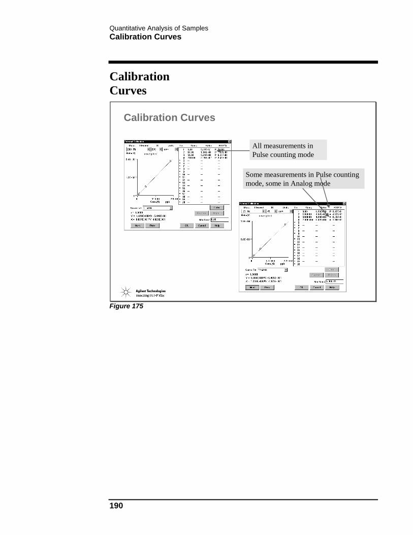
Quantitative Analysis of Samples Calibration Curves
190
Calibration Curves
Calibration Curves
All measurements in Pulse counting mode
Some measurements in Pulse counting mode, some in Analog mode
Figure 175

Quantitative Analysis of Samples Examples of the Calibration Curves for “Excluded”
191
Examples of the Calibration Curves for “Excluded”
Examples of the Calibration Curves for “Excluded”
Mass used for correction - real element
Internal Standard
Mass used for correction
Figure 176

Quantitative Analysis of Samples Examples of the Calibration Curves for “Excluded”
192

Simple Sequencing (Intelligent Sequencing Disabled)

Simple Sequencing (Intelligent Sequencing Disabled) Sequencing
194
Sequencing
Sequencing
Î Associates a list of samples with ALS positions and analytical methodsÎ Allows unattended analysis of multiple samples using multiple acquisition and reporting methods including all calibration updates.Î Designed to be used with an Autosampler (ASX-500 or ASX-100), can be used in a manual modeÎ Allows automatic shutdown upon completion of the sequence
Figure 177

Simple Sequencing (Intelligent Sequencing Disabled) ASX-500 Vial Position Nomenclature
195
ASX-500 Vial Position Nomenclature
ASX-500 Vial Position Nomenclature
Large bottles (tuning solution, rinse solutions, blank)
Example of 21-40-40-40 configuration
Vial 1304 = rack 1, column 3, raw 04 (two digits)
Figure 178

Simple Sequencing (Intelligent Sequencing Disabled) Sequencing
196
Sequencing
Sequencing
Î NT ChemStation Sequencing is Spreadsheet basedÎ Allows shortcuts such as
Îcut, Îcopy, Îpaste, Îrepeat, Îfill down
Î Allows sample list to be inserted from other applications byÎimporting .csv fileÎcopy and paste from other application
Figure 179

Simple Sequencing (Intelligent Sequencing Disabled) Sample Log Table - Sequence Flow and Periodic Block
197
Sample Log Table - Sequence Flow and Periodic Block
Sample Log Table - Sequence Flow and Periodic Block
Figure 180
Sequencing is Modular, each functional part of the sequence is created as a separate block such as calibration block, sample block etc. This is used more fully by Intelligent Sequencing.

Simple Sequencing (Intelligent Sequencing Disabled) Sample Log Table
198
Sample Log Table
Sample Log Table
Shortcut options box
Sequence block selection menu
Figure 181
Right Click selects shortcut options box.
Left Click or Double Click selects options for Type, Method, Dil/Lvl, Action on Failure (Intelligent Sequencing Only), and Skip.
Vial positions increment correctly by reading ALS rack configuration when using fill down.
Any numeric characters in Sample Name, Data File Name, or Comment Fields will be incremented by using fill down.
To avoid auto-incrementation, use copy and paste instead of fill down.
“List Method-Cal” displays the complete path for the method on each sequence line with it’s associated calibration file.

Simple Sequencing (Intelligent Sequencing Disabled) Special Features - Keywords
199
Special Features - Keywords
Special Features - Keywords
Command - a macro programMethpath - specifies a method path (different than the normal ICPCHEM pathway)Overwrit - overwrites a data file without asking for confirmationPause - pauses a sequenceLotsep - separates sample batches (used mostly in intelligent sequencingStdToExt - converts MSA calibration to external calibrationStandby - puts the instrument in Standby mode
Figure 182
Keywords are enabled by selecting ‘Keyword’ Under ‘Type’ and then selecting the desired keyword in the Method Column.
If Keyword Command is selected, the Command or Runstring is entered in the ‘Sample’ Column.
For Example to incorporate the shutdown macro into a Sample Log Table:
Keyword Command Tune “Macro `shutdown’, go”

Simple Sequencing (Intelligent Sequencing Disabled) Running a Sequence
200
Running a Sequence
Running a Sequence
Data batch directory
Figure 183
Upon selecting Run Sequence, a data batch directory is automatically created in the form YYMDDHHx.b, where:
• YY is 2 digit year
• M is month, A=Jan, B=Feb etc
• DD is day HH is hour (24 hour clock)
• x is a letter from a to z for the sequence number within a given hour.
This can be appended, deleted, or modified as needed.

Simple Sequencing (Intelligent Sequencing Disabled) Chained Sequence
201
Chained Sequence
Chained Sequence
Î Allows Multiple Sequences to be Run in SeriesÎ Allows Different Tune Conditions to be Used for Each Sequence
Îfor example Hot and Cool PlasmaÎhigh and low sensitivity etc.
Tunes to be used in a chained sequence must be created (verified) prior to running the sequence
Figure 184

Simple Sequencing (Intelligent Sequencing Disabled) Chained Sequence
202
Chained Sequence
Chained Sequence
Figure 185

Method of Standard Additions (MSA)

Method of Standard Additions (MSA) External Calibration
204
External Calibration
External Calibration
● All Standards are prepared in one matrix● A calibration curve is generated by plotting the intensity vs.
concentration● Sample concentration is calculated using the slope of the
calibration curve● Internal standards are used to correct for matrix-related
signal changes➨ IS can be added on-line
Figure 186

Method of Standard Additions (MSA) Pros and Cons of External Calibration
205
Pros and Cons of External Calibration
Pros and Cons of External Calibration
ProsMinimal sample preparationGood accuracy for simple matrices
ConsIS additions increases contamination potentialLimited with difficult matrices (Photoresist)It doesn't work well with cool plasma
Figure 187

Method of Standard Additions (MSA) Method of Standard Addition (MSA)
206
Method of Standard Addition (MSA)
Method of Standard Addition (MSA)
● Standards are prepared in the sample matrix● A calibration curve is generated by plotting the
intensity vs. spiked concentration● Sample concentration is calculated by extrapolating
to the Y intercept● Calibration can be converted into an external to run
subsequent samples of the same matrix.
Figure 188

Method of Standard Additions (MSA) Pros and Cons of Method of Standard Additions
207
Pros and Cons of Method of Standard Additions
Pros and Cons of Method of Standard Additions
ProsMethod of choice for ultra-trace levelsGood accuracy for all matricesNo need for internal standards
Compensate for differences in sample nebulization and transport efficiency
ConsDifferent calibrations for each matrixAll signal is accounted for
can't distinguish between true signal or backgroundBEC for Ca, Fe and K can be affected
Figure 189

Method of Standard Additions (MSA) Determination of Uranium in Urine by MSA
208
Determination of Uranium in Urine by MSA
Determination of Uranium in Urine by MSA
Reported concentration
Figure 190

Method of Standard Additions (MSA) Converting from MSA to External Calibration
209
Converting from MSA to External Calibration
Converting from MSA to External Calibration
Figure 191

Method of Standard Additions (MSA) Matrix-matched Uranium in Urine External Calibration
210
Matrix-matched Uranium in Urine External Calibration
Matrix-matched Uranium in Urine External Calibration
Note corrected concentrations
Figure 192

Off-line Data Analysis and Sequence Reprocessing

Off-line Data Analysis and Sequence Reprocessing Off-line Data Analysis
212
Off-line Data Analysis
Off-line Data Analysis
Î Reviews calibration and data for currently running sequenceÎ Edits currently running data analysis methodÎ Saves modifications to currently running data analysis method (if needed)Î Reprocesses data for currently running sequenceÎ Reviews/Reprocesses previously acquired data
Figure 193
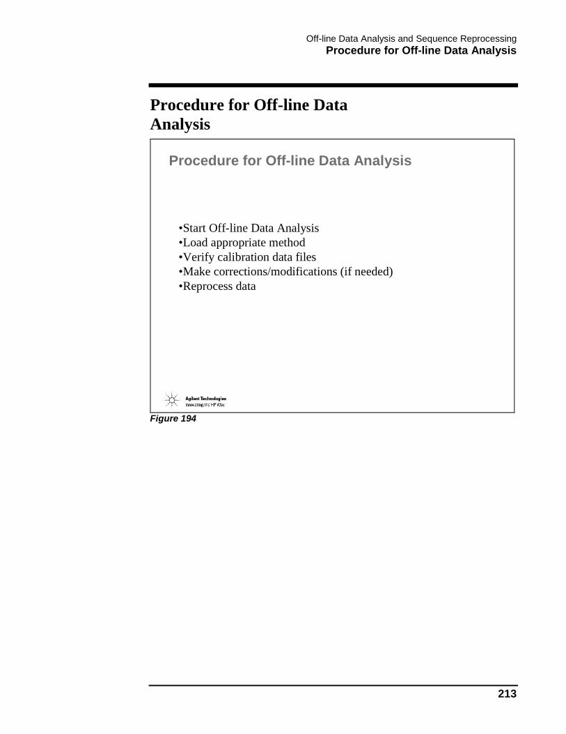
Off-line Data Analysis and Sequence Reprocessing Procedure for Off-line Data Analysis
213
Procedure for Off-line Data Analysis
Procedure for Off-line Data Analysis
•Start Off-line Data Analysis•Load appropriate method•Verify calibration data files•Make corrections/modifications (if needed)•Reprocess data
Figure 194

Off-line Data Analysis and Sequence Reprocessing Off-line Calibration Review of Currently Running Method
214
Off-line Calibration Review of Currently Running Method
Off-line Calibration Review of Currently Running Method
Review calibration graphs:examine linearity, RSDs, intercepts, internal standard reproducibility etc.make any corrections or changes
Select Method >> Save to Online
This procedure updates currently running method
Figure 195

Off-line Data Analysis and Sequence Reprocessing Using DoList for Off-line Data Reprocessing
215
Using DoList for Off-line Data Reprocessing
Using DoList for Off-line Data Reprocessing
Dolist automatically reprocesses a batch or list of data files according to the options selected using to the currently loaded method and calibration.
DoList does NOT update the method or calibration
Figure 196
Dolist always uses the currently loaded method, not necessarily the method originally used to acquire the data.
Dolist does not load the method from disk or resave the method to disk when finished. Therefore, it is possible to make temporary changes to the method for reprocessing only (such as different report destination etc.) and not save the changes permanently to the disk.

Off-line Data Analysis and Sequence Reprocessing How to Use DoList
216
How to Use DoList
How to Use DoList
Data Analysis >> Tools >> Configure DoListData Analysis >> Tools >> DoList
Figure 197

Off-line Data Analysis and Sequence Reprocessing Selecting Files Using DoList
217
Selecting Files Using DoList
Selecting Files Using DoList
Figure 198

Off-line Data Analysis and Sequence Reprocessing Sequence - Reprocessing Data Batch
218
Sequence - Reprocessing Data Batch
Sequence - Reprocessing Data Batch
Used to reprocess entire (or partial) sequenceDoes
Load methods from disk as specifiedUpdate calibrations in order acquiredRecalculate (Requant) data and regenerate reportsSave updated calibrations to disk
Figure 199
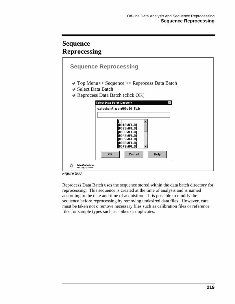
Off-line Data Analysis and Sequence Reprocessing Sequence Reprocessing
219
Sequence Reprocessing
Sequence Reprocessing
Î Top Menu>> Sequence >> Reprocess Data BatchÎ Select Data BatchÎ Reprocess Data Batch (click OK)
Figure 200
Reprocess Data Batch uses the sequence stored within the data batch directory for reprocessing. This sequence is created at the time of analysis and is named according to the date and time of acquisition. It is possible to modify the sequence before reprocessing by removing undesired data files. However, care must be taken not o remove necessary files such as calibration files or reference files for sample types such as spikes or duplicates.

Off-line Data Analysis and Sequence Reprocessing Sequence Reprocessing
220

Custom Reports and Databases

Custom Reports and Databases What You Will Learn
222
What You Will Learn
What You Will Learn
• How to create a template and generate reports• how to create a database and update it
Figure 201
This section will introduce you to the Custom Reports package included in the Agilent 7500 Series ChemStation Software.
Custom Reports is a windows application with three basic functions:
� spreadsheet
� database
� charts
Spreadsheet functions allow to easily design a report template and produce a report for a single sample.
Custom databases contain information from many samples.
Charting of the database is useful for trend analysis and/or monitoring QA/QC samples.
A ChemStation method can have one report template and/or one database assigned for FullQuant analysis and one report template and/or one database assigned for SemiQuant analysis.

Custom Reports and Databases Custom Reports and Databases
223
Custom Reports and Databases
Custom Reports and Databases
• Based on Visual Basic runtime program• When installed, creates \icpchem\custrpt directory• Also creates \icpchem\1\rpttmp• Accessible through FullQuant and SemiQuant menus• Custom report templates are *.fqt or *.sqt files• Custom report databases are *.fqd or *.sqd files
Figure 202
The objective of Custom reports is to provide an interface between the quantitative features of the Agilent 7500 Series ChemStation and the Visual Basic Custom Reports. The link between the two programs is provided through a feature of the Windows environment known as Dynamic Data Exchange (DDE). This link allows easy transfer of information from one program to another.

Custom Reports and Databases Creating and Editing a Report Template
224
Creating and Editing a Report Template
Creating and Editing a Report Template
• Create new report template• Edit the current report template• Specify new report template
Figure 203
Selecting the “New …” menu item from the Template menu will bring up the Custom Report / Database Wizard.

Custom Reports and Databases Custom Reports - Report Wizard
225
Custom Reports - Report Wizard
Custom Reports - Report Wizard
• Select a Report Contents section from the list on the right.• Select an item from the Possible Items for Report list on the left.• Click the Add button.• Repeat until all items and sections are added.• Click OK.
Figure 204
The Report Wizard dialog box is used to build a report template with up to two sections. The header section contains general information about the sample. The All Elements section contains element specific information arranged into tables.
A plus sign next to an item indicates there are sub-items available. Double-click on the plus sign to open the sub-item listing. The plus sign becomes a minus sign. Double-click on the minus sign to close the sub-item listing.
Spectral graphics as well as calibration curves can be added to a custom report template. Graphics can NOT be added to a database.
The Graphic section of the possible report items has two main subsections: Draw Spectrum and Graph of Each Element. Items from the Graphics section can only be added to the Header section of the Report Contents. The items from the Graph of Each Element can be added to either section of the report.
The order of the graphics in the Report Contents listbox of the Report Wizard determines the position in the report for the graphics. The text items are always

Custom Reports and Databases Custom Reports - Report Wizard
226
drawn together and cannot be interspersed with the graphics through the Report Wizard.
Press the Ctrl key and click the graphics to resize or reposition the graphics.

Custom Reports and Databases Custom Reports - Drag and Drop (1)
227
Custom Reports - Drag and Drop (1)
Custom Reports - Drag and Drop (1)
Figure 205

Custom Reports and Databases Custom Reports - Drag and Drop (2)
228
Custom Reports - Drag and Drop (2)
Custom Reports - Drag and Drop (2)
• Accessed by selecting View / Edit Box or clicking Edit Box button of the toolbar.• Select an item and drag it to any cell on the spreadsheet.• Use the Next button or select from the list to view other elements.• The current value for the highlighted item is displayed.
Figure 206
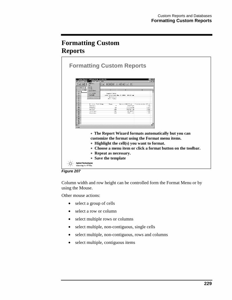
Custom Reports and Databases Formatting Custom Reports
229
Formatting Custom Reports
Formatting Custom Reports
• The Report Wizard formats automatically but you can customize the format using the Format menu items.• Highlight the cell(s) you want to format.• Choose a menu item or click a format button on the toolbar.• Repeat as necessary.• Save the template
Figure 207
Column width and row height can be controlled form the Format Menu or by using the Mouse.
Other mouse actions:
• select a group of cells
• select a row or column
• select multiple rows or columns
• select multiple, non-contiguous, single cells
• select multiple, non-contiguous, rows and columns
• select multiple, contiguous items

Custom Reports and Databases Custom Reports - Printing Set-up
230
Custom Reports - Printing Set-up
Custom Reports - Printing Set-up
• Controls how pages are printed.• Controls paper size.
Figure 208
The following “Print Options”are available:
• Grid Lines - lets you print grid lines (otherwise they are visible on the screen only)
• Black &White - prints color in black and white on a color printer
If selected, “fit to Page(s) scales the document to print a document to print on a single or on the number of pages specified in Pages Wide, Page High.
Scale sets the percentage to reduce or enlarge the document when printed.

Custom Reports and Databases Custom Reports - Saving the Template
231
Custom Reports - Saving the Template
Custom Reports - Saving the Template
• Select File / Save or File / Save As• Default file name is <method name.fqt>; choose this or enter alternate file name and click OK.
• Click Yes to link the template with the current method
Figure 209
For the report template name, any legal DOS name is OK.
The default file name will have the same prefix as the currently loaded method. Notice that all report templates end with either FQT or SQT extension.
After saving the report template the “Link With Method Dialog Box” will appear.

Custom Reports and Databases Printing Custom Reports - Interactively
232
Printing Custom Reports - Interactively
Printing Custom Reports - Interactively
• Load a data file.• Select FullQuant / Print Custom Report.
Figure 210
A custom report may be interactively printed at any time using a two step process.
• First, load the data file.
• Second, select FullQuant / Print Custom Report.
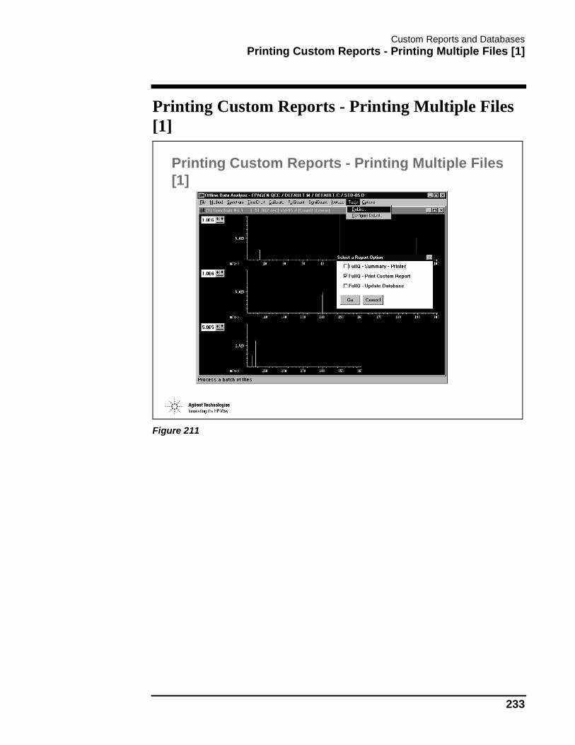
Custom Reports and Databases Printing Custom Reports - Printing Multiple Files [1]
233
Printing Custom Reports - Printing Multiple Files [1]
Printing Custom Reports - Printing Multiple Files [1]
Figure 211

Custom Reports and Databases Printing Custom Reports - Printing Multiple Files [2]
234
Printing Custom Reports - Printing Multiple Files [2]
Printing Custom Reports - Printing Multiple Files [2]
Selected data files will be listed in this box.
Select files to be processed
Figure 212
Select files from the Data File listing:
• multiple continuous
• multiple discontinuous
• a single file can be removed from the “Files Selected for Processing” by double clicking on it.
Click Add to insert those names into the “Files Selected for” Section of the panel.
Click the Process button.

Custom Reports and Databases Databases
235
Databases
Databases
• Create new database• Edit the current database and/or create charts• Specify new database
Figure 213
Selecting the “New…” menu item from the Template menu will bring up the Custom Report / Database Wizard.

Custom Reports and Databases Database Wizard
236
Database Wizard
Database Wizard
• Select a Database section from the list of the right.• Select an item from the Possible Items for Database list on the left.• Click the Add button.• Repeat until all items and sections are added.• Click OK.
Figure 214
Clicking the Add button will add the selected item to the Database Content list on the right.
Clicking the Remove button will remove the selected item from the Database Content list.
Graphics can NOT be added to a database

Custom Reports and Databases Database - Drag and Drop
237
Database - Drag and Drop
Database - Drag and Drop
Figure 215
• Accessed by selecting View / Edit Box or clicking Edit Box button of the toolbar.
• Select an item and drag it to any cell in row 3.
• Use the Next button or select from the list to view other elements.
• The current value for the highlighted item is displayed.
Be aware that if you are editing a database, you can only put items from the Edit Box into row 3. This row contains all the information that you want to keep for each data file.
“Next” accesses the next element in the quantitation results. Elements can also be selected by using the element selection box.
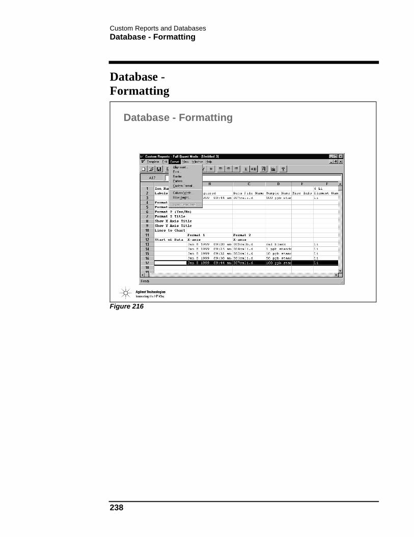
Custom Reports and Databases Database - Formatting
238
Database - Formatting
Database - Formatting
Figure 216

Custom Reports and Databases Database - Charts
239
Database - Charts
Database - Charts
• The Database Wizard formats automatically but you can customize the format using the Chart Options.• Save the database.
Figure 217
“X-Axis” lets you choose which items to chart on the X-Axis. Column B and C of the database determine the X-Axis items. The default item for Column B is Date Acquired and for Column C is Data File Name.
“Y-Axis” lets you choose which items to chart on the Y-Axis. Only numerical values (such as mass or counts) can be used for the Y-Axis.
The Print Option lets you print the current chart or print all charts in the database.

Custom Reports and Databases Global Chart Options
240
Global Chart Options
Global Chart Options
Figure 218
By default, all rows in database are charted. If you enter a number N (other than 0) in the “Data Points from End to Chart” field, then only the last N rows will be charted. This feature is useful when you have added many rows to your database, but are only interested in the last N files. You can override this value for a single chart using the Individual Charts Options dialog box.
Automatic Scaling - The software will automatically choose a range which allows all of the data to be seen. The data is shown in absolute units. The range chosen can be slightly larger than the actual data range.
Manual Scale - The manual scale allows you to control exactly what the scale on the Y axis will be.
Normalize to Maximum - This scale allows you to chart the data as a percentage of the maximum value (set to be 100%).
Set the First Data Point to - This scale allows you to chart all points as a percentage of the first row of data.

Custom Reports and Databases Global Chart Options
241
You can draw up to four control/limits lines on a chart. These lines can be relative to the Mean or to the first value charted.
You can draw the percentage lines or Standard Deviation lines

Custom Reports and Databases Database - Saving
242
Database - Saving
Database - Saving
• Select File / Save or File / Save As• Default file name is <method name.fqd>; choose this or enter alternate file name and click OK.
• Click Yes to link the template with the current method
Figure 219

Custom Reports and Databases Updating the Database - Interactively
243
Updating the Database - Interactively
Updating the Database - Interactively
• Load a data file.• Select FullQuant / Update Database.
Figure 220

Custom Reports and Databases Update the Database - Multiple Files [1]
244
Update the Database - Multiple Files [1]
Update the Database - Multiple Files [1]
Figure 221

Custom Reports and Databases Update the Database - Multiple Files [2]
245
Update the Database - Multiple Files [2]
Update the Database - Multiple Files [2]
Selected data files will be listed in this box.
• Select Tools, DoList...• Select FullQ -- Update Database• Select files to be processed
Figure 222

Custom Reports and Databases Update the Database - Multiple Files [2]
246

Isotope Ratio Measurements

Isotope Ratio Measurements Editing a Method for Quantitative Analysis
248
Editing a Method for Quantitative Analysis
Editing a Method for Quantitative Analysis
QC Parameters will only be available if Intelligent Sequencing is enabled
Select ‘Edit Entire Method’
Figure 223

Isotope Ratio Measurements Acquisition Modes
249
Acquisition Modes
Acquisition Modes
Figure 224
Spectrum mode is the most common acquisition mode for standard applications.
• Quant
• Semiquant
Time Resolved Analysis (TRA) and Time Program (more sophisticated than TRA) are used when a transient signal is measured.
• Electrothermal Vaporization (ETV)
• Laser Ablation (LA)
• Discrete Sampling Analysis (using ISIS)
• Chromatographic analysis (LC, GC, IC, CE)
Isotope Analysis mode is used when additional precision is needed for isotope ratio measurements. It is similar to spectrum mode, but with 10X higher sampling frequency.

Isotope Ratio Measurements Acquisition Modes
250
Multitune mode is used when during a single acquisition more than one tuning parameters are needed to accomplish the optimum performance.

Isotope Ratio Measurements Acquisition Parameters for Isotopic Ratio Measurements
251
Acquisition Parameters for Isotopic Ratio Measurements
Acquisition Parameters for Isotopic Ratio Measurements
Longer acquisition time for less abundant isotope
Usually 5 or 10 repetitions
Figure 225

Isotope Ratio Measurements Report Selection
252
Report Selection
Report Selection
Figure 226

Isotope Ratio Measurements Setting Parameters for Isotopic Ratios
253
Setting Parameters for Isotopic Ratios
Setting Parameters for Isotopic Ratios
Figure 227

Isotope Ratio Measurements Example of the Isotopic Ratio Report
254
Example of the Isotopic Ratio Report
Example of the Isotopic Ratio Report
Figure 228

Agilent ICP-MS ChemStation and Windows Overview

Agilent ICP-MS ChemStation and Windows Overview The Windows Interface
256
The Windows Interface
The Windows Interface
Folder to temporarily hold files, folders, or objects which have been deleted.
Access to disk drives and folders
Start button to open programs
Task Bar
Figure 229
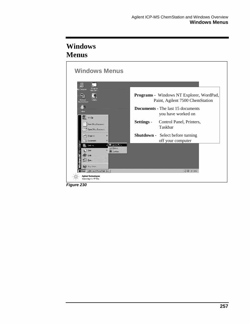
Agilent ICP-MS ChemStation and Windows Overview Windows Menus
257
Windows Menus
Windows Menus
Programs - Windows NT Explorer, WordPad, Paint, Agilent 7500 ChemStation
Documents - The last 15 documentsyou have worked on
Settings - Control Panel, Printers, Taskbar
Shutdown - Select before turningoff your computer
Figure 230

Agilent ICP-MS ChemStation and Windows Overview Useful Windows Tips
258
Useful Windows Tips
Useful Windows Tips
●Add Programs to the first-level menu instead of cascading through menus.●Create Shortcuts by dragging a document to the desktop with a right-click of the mouse button.●Change the desktop properties with a right-click of the mouse button.●Use Ctrl-Alt-Del to end a task that is not responding.
Figure 231

Agilent ICP-MS ChemStation and Windows Overview Maintaining the Computer System
259
Maintaining the Computer System
Maintaining the Computer System
• Delete temporary files on a regular basis
• Use Checkdisk to check for errors on the disk
• Defragment the hard drive using a WinNT utility
• Use Virus detection software
• Create a Windows NT Emergency Repair disk
Figure 232

Agilent ICP-MS ChemStation and Windows Overview Windows NT Explorer - Enhanced File Management
260
Windows NT Explorer - Enhanced File Management
Windows NT Explorer - Enhanced File Management
Click on + sign to open sublevels in the left pane.
Click on the item to display the contents in the right pane as folders.
Figure 233

Agilent ICP-MS ChemStation and Windows Overview Directory Structure of the Agilent ChemStation
261
Directory Structure of the Agilent ChemStation
Directory Structure of the Agilent ChemStation
Std-10.d
D:
Siclnt Icpchem
1
Data
Std-05.d
7500 Methods Qcmode Rpttemp
Custrpt Database Icpexe Icpsetup
Winnt
Icpdemo.d
Calib Chnseq Sequence
Figure 234

Agilent ICP-MS ChemStation and Windows Overview File Naming
262
File Naming
File Naming
Files have the form:<filename>. <extension><up to 8 characters> . <up to 3 characters>Period Separator
Forbidden characters for filenames:. / \ : <space> []| + ; , ? = * < >
Figure 235
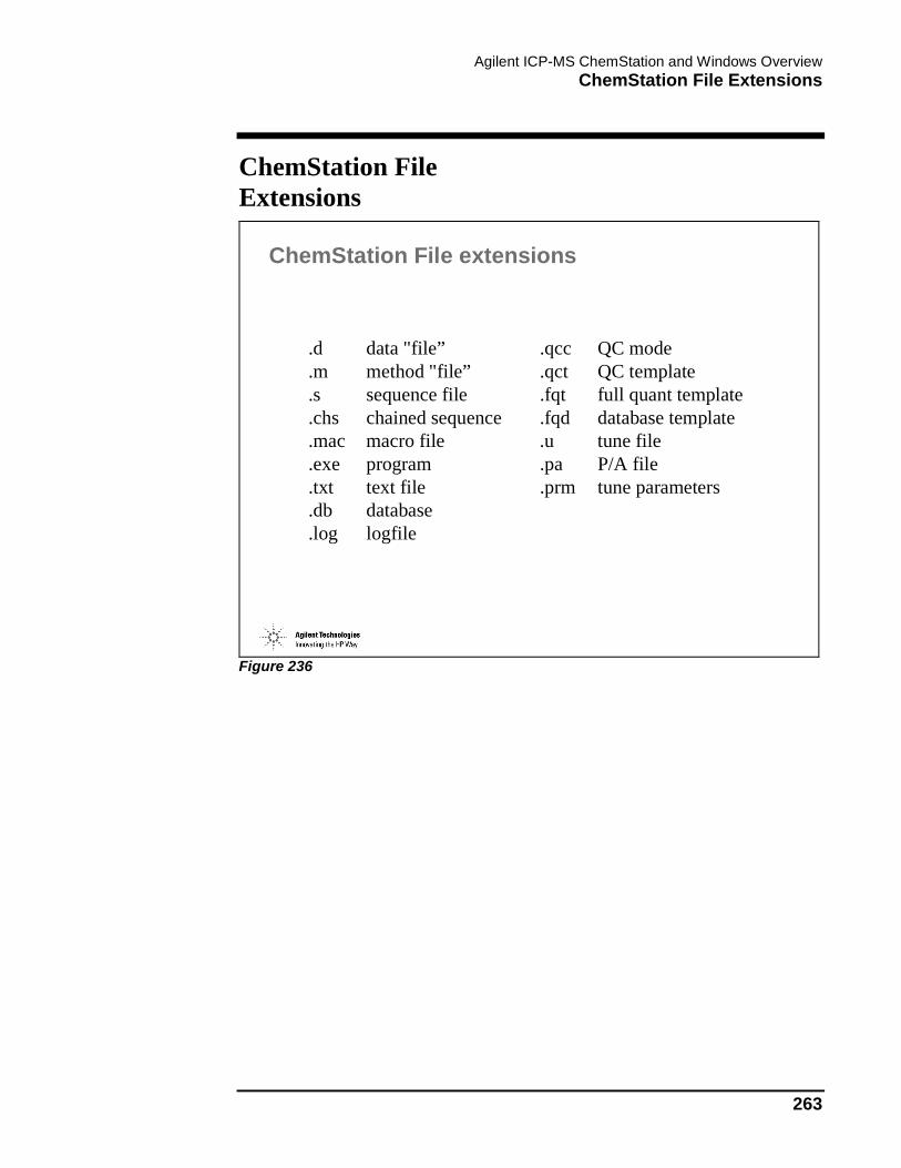
Agilent ICP-MS ChemStation and Windows Overview ChemStation File Extensions
263
ChemStation File Extensions
ChemStation File extensions
.d data "file” .qcc QC mode
.m method "file” .qct QC template
.s sequence file .fqt full quant template
.chs chained sequence .fqd database template
.mac macro file .u tune file
.exe program .pa P/A file
.txt text file .prm tune parameters
.db database
.log logfile
Figure 236

Agilent ICP-MS ChemStation and Windows Overview ChemStation File Extensions
264

An Overview of ICP-MS Environmental Applications

An Overview of ICP-MS Environmental Applications Optimizing Agilent 7500 for Environmental Samples Analysis
266
Optimizing Agilent 7500 for Environmental Samples Analysis
Optimizing Agilent 7500 for Environmental Samples Analysis
ÎTuningMatch instrument dynamic range to analyte concentration range
ÎDetune sensitivity, especially low massÎDilute samples as necessary (off-line or auto-dilute with ISIS)
ÎMinimize Effects of Sample MatrixÎ High RF powerÎ Longer sampling depth ==> longer residence timeÎ Appropriate use/selection of internal standardsÎ Appropriate selection of isotopes
Figure 237

An Overview of ICP-MS Environmental Applications Environmental Tuning
267
Environmental Tuning
Environmental Tuning
Three Steps:Initial Setup and Hardware CheckoutOptimize Physical & Plasma ParametersDetune Sensitivity via Ion Lenses
Figure 238
Initial setup/hardware checkout
When any maintenance is executed, it is important to verify that the instrument can meet specifications for sensitivity, precision, mass calibration, oxides and all other parameters. This will verify that the hardware is operating correctly.
Physical/Plasma Parameters
Since typical environmental samples can contain relatively high matrix, it is important to make tuning adjustments that improve the decomposition of the matrix, such as increasing the plasma temperature or increasing the residence time of the sample in the plasma.
Detune Sensitivity via ion lenses
Typical compositions of environmental samples include higher concentrations of low mass elements such as Na, K, Ca and Mg, and lower concentrations of mid and high mass elements such as Se and Hg.

An Overview of ICP-MS Environmental Applications Environmental Tuning
268
To analyze all the elements at the same time, detuning the low mass only can be an effective technique. However, care must be taken in this process if analysis of Be is required.
Tips
Conditioning of the interface is recommended to improve signal stability, after cleaning the cones or extraction lenses. For conditioning, run tap water through the system for 1/2 hour during tune before finalizing tune conditions and prior to calibration and sample analysis.

An Overview of ICP-MS Environmental Applications Three Goals of Environmental Tuning
269
Three Goals of Environmental Tuning
Three Goals of Environmental Tuning
Optimize aerosol formationMaximize analyte exposure to plasma temperatureMinimize matrix exposure to mass spectrometer components
Figure 239
Increasing sampling depth increases the sample residence time in the plasma. The effect is to allow more time for decomposition (atomization and ionization) of the analyte elements. Each nebulizer has optimal values for carrier gas flow rate and sample flow rate. In general, higher carrier gas flow rates create higher carrier gas pressures thereby generating finer droplets, which lead to better instrument sensitivity. However, excessive carrier gas flows cool the plasma, decreasing the sensitivity and increasing the ratios of oxides and doubly-charged ions significantly. Excessively high carrier gas flows cool the plasma which increases low mass (e.g. Li) sensitivity and noise to a non-acceptable level. Lithium signal should not exceed Yttrium signal in a well tuned system.
Oxides are almost completely controlled by the interaction of four parameters, spray chamber temperature, sample depth, carrier gas flow and peri-pump flow. Since we have chosen to maximize sample depth for other reasons and spray chamber temp should normally be set to 2 C. we must control oxides with carrier gas flow and peri-pump flow. The goal here is to maximize the efficiency of the particular nebulizer being used (smallest droplet size and size distribution), without increasing either flow to the point of over-cooling the plasma.

An Overview of ICP-MS Environmental Applications Three Goals of Environmental Tuning
270
Decreasing the negative voltage on the two extract lenses decreases the number of ions drawn into the mass analyzer. This decreases the sensitivity of the instrument. It also decreases the ion load on the rest of the mass analyzer which minimizes the need to clean the other lenses and components. It is important that the correct voltage gradient between the two lenses be maintained. As such, Ext1 should be set and then Ext2 fine tuned to give the best results. If large changes in Ext1 voltage have little to no effect on sensitivity, this is an indication that the extract lenses need to be cleaned.

An Overview of ICP-MS Environmental Applications Tuning Flow Chart
271
Tuning Flow Chart
Tuning Flow Chart
Tuning the Agilent 7500 ICP-MSfor Environmental Applications
Set RF Power
1350-1500 Watts(monitor reflected power
and adjust if necessary withRF Matching
Adjust Sampling Depth8-9 mm (1)
Set Peri-pump0.08-0.1 RPS
Set Carrier Gas Flow
1.15-1.2 L/min.Monitor oxides; it shouldnot exceed 0.5% (2)
Initial SetupNew Instrument or after Major System
Maintenance
Initially, all tune parametersshould be set according tothe recommended values
on table 1 (shaded)
Then...begin the process ofenvironmental tuning
Oxides < 0.5 %Li counts > 5000
(int. time = 0.1 sec)
Yes
No
1. Decrease carrier (orblend) gas flow2. Increase or decreaseperi-pump flow (3)
Run “Set_EM!”from the Tune Menuto adjust all detector
parameters
"
Initial targets: Li > 8kY > 12 kTl > 8 k
all RSDs < 10%oxides < 1%
FAIL
Run Torch PositionAutotune
FAIL
Check Axis/ResolutionPeak widths0.75 at 10 % +/-0.05mass calib.:nominal mass +/- 0.05
FAIL
Set Ext1 and 2at low voltage, especially Ext2, which improves stability below -35V.(4)
pass
pass
pass
Tune Einzel 1/3, and 2Typical values are -60Vand 14V, respectively.
.
Achieve Goals
No
Achieve Goals
No
Increase both Omega +and QP Focus. Typicalvalues are 6 V and 9V,respectively.Adjustments of theselenses improve signalstability
DO NOT ADJUST:
Any AMU settingsAny Axis settingsDiscriminatorEM voltageLast DynodeP/A factors
Initial Setup/Hardware Checkout
Physical/Plasma Parameters
Detune Sensitivity via ion lenses --- target: low mass sensitivity is reduced in sensitivity by 10xcompared to mid and high mass.
See Appendix 4
Figure 240

An Overview of ICP-MS Environmental Applications Recommendations on Interference Equations
272
Recommendations on Interference Equations
Recommendations on Interference Equations
Generally Use Equations Specified in EPA Method 200.8
May require slight adjustment based on measured values
Figure 241
Arsenic
Since there are lots of polyatomic ions are generated around the mass, it is very difficult to apply universal equation.
When the contribution of 82Kr is considered, the equation should be changed as follows:
As(75) = (1.000)(75C) - (3.127)(77C) + (2.736)(82C) - (2.760)(83C)
However, an unknown peak sometimes appears at mass 83. BrH is also generated at mass 82. As a result, the contribution of Kr is overcorrected, and As might show a negative result.
Selenium
Generally, the use of 82 rather than 77 or 78 is recommended. 77 is interfered with by 40Ar37Cl, and 78 is interfered with by 38Ar40Ar dimer. The 82 isotope needs to be corrected for the possible presence of 82Kr in the Argon gas supply using the following equation.

An Overview of ICP-MS Environmental Applications Recommendations on Interference Equations
273
Se(82) = M(82) - 11.6/11.5 * Kr(83)
= M(82) - 1.0087 * Kr(83)
However, as described the above, the unknown peak might appear at mass 83, thereby a portion of the signal at mass 83 is used practically. An example is as follows:
Se(82) = M(82) - 0.6 * Kr(83)
The monitoring of mass 77 and 78 is also recommended just in case.

An Overview of ICP-MS Environmental Applications More Interference Corrections
274
More Interference Corrections
More Interference Corrections
Some correction factors are based on formation of doubly charged species or oxides rather than on isotope ratios and need to be updated periodically.
• Iron-54• Ca-44
Figure 242
Vanadium
The interference correction might not be useful. Because it is almost redundant (1% NaCl gives about 1ppb ClO equivalent) and can lead to problems when high Cr is present.
Iron
The use of 54 rather than 56 or 57 is recommended. Since mass 54 is interfered with ArN, the concentration of HNO3 should be the same. If the concentration of HNO3 cannot be controlled, the following equation would be useful:
Fe(54) = M(54) - ratio of 54/15 * M(15)
In this case, a blank solution must be analyzed at first, and mass 15 and 54 should be measured. The ratio of 54/15 will be calculated, and this ratio will be entered into the equation.
CaN is unlikely to give an interference at 200 ppm Ca carbonate.
Calcium

An Overview of ICP-MS Environmental Applications More Interference Corrections
275
Ca is normally included at very high concentration; therefore, there is no interference on it.
However, when the mixed standard solution which contains the same concentration of Ca and Sr, the apparent Ca44 will be almost double if the system was calibrated in the absence of Sr. The same problem occurs with Ca43. In this case, the following equation is useful:
Ca(44) = M(44) - ratio of Sr2+/Sr+ * M(88)
Sr solution must be analyzed at first to get the ratio of Sr2+/Sr+.

An Overview of ICP-MS Environmental Applications Calibration Standards
276
Calibration Standards
Calibration Standards
Calibrate no higher than necessary Minimize memory effects and the detector wear
• typical ranges for ‘trace elements’: 0, 1, 10, 100 ppb• major elements such as Na, K, Ca, Mg, Fe: 0, 100, 1000, 10,000 ppb• Hg: 0, 0.1, 0.5, 1, 5 ppb
Major and trace elements are available in a single solution with their concentration in 100:1 ratios, respectivelyMercury supplied in a separate solutionAddition of 100 ppb gold to ALL solutions required for mercury determination
Figure 243

An Overview of ICP-MS Environmental Applications Linear Range Determination
277
Linear Range Determination
Linear Range Determination
‘Practical Linear Range’Reasonable upper range of analyte concentrations after sample dilution to avoid excessive carryover after running LRS
Typically:z ~1 ppm for most elements, z 10-50 ppm for ‘minerals’,z < 500 ppb for Ag, Mo, Sb, Tl, Pb and other memory prone elements, z < 20 ppb for Hg!
Much lower than actual Instrument Linear Range
Figure 244
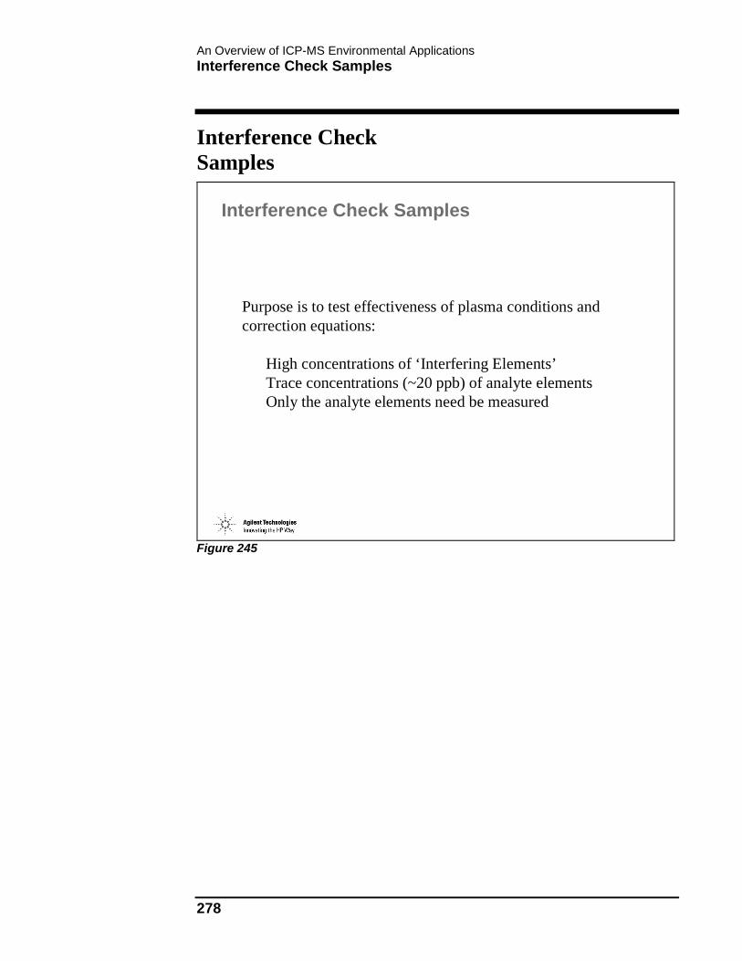
An Overview of ICP-MS Environmental Applications Interference Check Samples
278
Interference Check Samples
Interference Check Samples
Purpose is to test effectiveness of plasma conditions and correction equations:
High concentrations of ‘Interfering Elements’Trace concentrations (~20 ppb) of analyte elementsOnly the analyte elements need be measured
Figure 245

An Overview of ICP-MS Environmental Applications Troubleshooting Environmental Applications [1]
279
Troubleshooting Environmental Applications [1]
Troubleshooting Environmental Applications [1]
High Tune % RSDs
Non-linear Calibrations
High Analysis % RSDs
Poor Agreement Between Calibration and ICV
Figure 246
High RSDs During Tune
Incorrectly tuned plasma parameters such as carrier gas or blend gas flow, peri-pump speed or sample depth.
Dirty cones
Worn peri-pump tubing. Incorrect shoe pressure on peri-pump. Should be just tight enough to insure a smooth flow of sample (aspirate a bubble and watch its progress through the line).
Non-Linear Calibrations
ICP-MS is a linear technique. Pulse mode calibrations should always be linear, if not, suspect standard preparation errors or possible incompatibilities among elements in multi-element standards.
Non-linearity between pulse and analog mode indicates incorrectly set P/A factors or possible worn out detector.
High %RSDs During Analysis

An Overview of ICP-MS Environmental Applications Troubleshooting Environmental Applications [1]
280
Insufficient uptake, rinse-out or stabilization time. Use ‘Edit Average File’ > ‘Tabulate’ to examine individual replicates for upward or downward trends.
Insufficient signal counts.
May be also be caused by worn peri-pump tubing or bubbles in either the sample uptake or internal standard uptake tubing. Check the connections at the ISTD addition “Y” and replace the peri-pump tubing.

An Overview of ICP-MS Environmental Applications Troubleshooting Environmental Applications [2]
281
Troubleshooting Environmental Applications [2]
Troubleshooting Environmental Applications [2]
Poor Analyte Recovery in Spiked Samples for Selected Analytes
Carry-over or Memory Effects for Certain Elements
Figure 247
Poor recovery for selected analytes in spikes.
Several conditions can cause poor recovery of certain analytes in spiked samples. Ag is especially insoluble in the presence of even trace levels of Cl-
, therefore the use of HCl should be avoided whenever possible. Several elements (Zn, As, Se, Cd) have relatively high first ionization potentials and may not be as effectively ionized in samples with high concentrations of easily-ionizable elements such as Na and K. Diluting the sample if possible, or selecting an alternative internal standard with a higher ionization potential may help. Possible alternative internal standards include Ge, Te, and Au.
Carryover or memory interference.
Several elements are prone to memory effects for various reasons. Ag, Mo and Tl tend to stick to surfaces in the sample introduction system and slowly rinse into subsequent samples. Keeping the sample introduction system (sample tubing, peri pump tubing, nebulizer, spray chamber, torch and cones) clean will help minimize carry-over. Also, rinsing between samples with relatively high acid concentration rinse blanks (ca. 5% HNO3) will help. If

An Overview of ICP-MS Environmental Applications Troubleshooting Environmental Applications [2]
282
possible, avoid introducing samples or standards with concentrations of these elements above a few hundred ppb. Use of the Babington nebulizer should also reduce carryover of these elements. Li, when analyzed for extended periods of time or in very high concentrations tends to accumulate on the back sides of the interface cones. Cleaning the cones will usually reduce Li background and carryover. Volatile elements, or elements with volatile hydrides such as Hg and Sb can also carryover due to off-gassing from droplets on the spray chamber walls. Steps to reduce the volatility of these species are helpful.

An Overview of ICP-MS Environmental Applications Troubleshooting Environmental Applications [3]
283
Troubleshooting Environmental Applications [3]
Troubleshooting Environmental Applications [3]
Calibration Drift Over Time
Poor Internal Standard Recoveries in Certain Samples
Figure 248
Calibration Drift over time.
Insure that the instrument is adequately warmed up before initial calibration (warm-up, while scanning in tune for 15 minutes).
Insure that laboratory temperature does not vary by more than 3 degrees C. per hour.
Check cones for signs of sample deposits which may be affecting the size and shape of the cone orifices. Clean if necessary.
Check peri-pump tubing for signs of excessive wear or flattening.
Run SetEM. An electron multiplier which is near the end of its useful life may be changing in response over short periods of time. If running SetEM significantly changes the EM voltage from day to day, the EM should be replaced.
Poor internal standard recoveries in samples.

An Overview of ICP-MS Environmental Applications Troubleshooting Environmental Applications [3]
284
Reduction in internal standard signal is usually caused by high matrix concentration in samples (especially Na, and K). Dilute the samples. It may also be desirable to tune the instrument with a matrix matched tune solution containing appropriate levels of the matrix elements to minimize the effect of any matrix induced suppression of ionization.

An Overview of ICP-MS Environmental Applications Troubleshooting Environmental Applications [4]
285
Troubleshooting Environmental Applications [4]
Troubleshooting Environmental Applications [4]
High Relative Standard Deviations (%RSDs) in SamplesStandards
High %RSDs in Tune
Figure 249
High relative standard deviations (RSDs) for analyte or internal standard elements during sample analysis.
Usually caused by insufficient sample uptake or stabilization time. May be also be caused by worn peri-pump tubing or bubbles in either the sample uptake or internal standard uptake tubing. Check the connections at the ISTD addition “Y” and replace the peri-pump tubing. Shoe pressure on the peri-pump should be just tight enough to insure a smooth flow of sample (aspirate a bubble and watch its progress through the line).
High RSDs during tune.
Incorrectly tuned plasma parameters such as carrier gas or blend gas flow, peri-pump speed or sample depth.
Dirty cones.Worn peri-pump tubing.
Incorrect shoe pressure on peri-pump. Should be just tight enough to insure a smooth flow of sample (aspirate a bubble and watch its progress through the line).

An Overview of ICP-MS Environmental Applications Troubleshooting Environmental Applications [4]
286
Omega lens settings can also affect tune precision as can parameters which affect mass peak shape such as plate and pole bias.

Semiconductor Applications of ICP-MS and Advantages of Agilent 7500s System

Semiconductor Applications of ICP-MS and Advantages of Agilent 7500s System Chemicals and Materials Used in Semiconductor Industry
288
Chemicals and Materials Used in Semiconductor Industry
Chemicals and Materials Used in Semiconductor Industry
IPA
WashingCleaning
HCl
TMAH
H2SO4
HNO3
H2O2 Methanol
Si, GaAsWafer substrate
SiH4, TEOS, NF3, N2Gases
Photoresists - Lithography
HFEtching
Pure Metals - Sputter Targets
Figure 250
BPSG = boron phosphorus silicon glass used for doping.
TEOS = tetra ethoxy silane (used for depositing SiO2 layers.
TMAH = tetra methyl ammonium hydroxide.
Multielement analysis and ultra low detection limits have made ICP-MS the technique of choice for the determination of metallic impurities in the industry.

Semiconductor Applications of ICP-MS and Advantages of Agilent 7500s System Metals Analysis in the Semiconductor Industry - Customer Groups
and Requirements
289
Metals Analysis in the Semiconductor Industry - Customer Groups and Requirements
Metals Analysis in the Semiconductor Industry -Customer Groups and Requirements
● Chemical manufacturers➨ need for QC analysis of products
■ inorganic chemicals■ organic chemicals
● Wafer manufacturers➨ characterize bulk polysilicon➨ monitor contamination control in wet stations➨ analysis of chemicals and various mixes➨ wafer surface characterization
● Device manufacturers➨ monitor contamination control in wet stations
■ analysis of chemicals and various mixes■ photoresist\stripper analysis
Figure 251

Semiconductor Applications of ICP-MS and Advantages of Agilent 7500s System ShieldTorch Interface
290
ShieldTorch Interface
ShieldTorch Interface
● Developed by HP/Yokogawa in 1992➨ led to widespread use of "cool" plasmas
● Prevents secondary discharge in the ICP-MS interface➨ virtually eliminates many polyatomic interferences➨ Shield plate design assures complete discharge removal
● Enables the determination of Fe, Ca and K at low ppt levels➨ 3 orders of magnitude improvement in detection limits
● Improved DLs for most other SEMI elements➨ dramatically reduced interface background
■ sub-ppt DLs for Na● Operates at higher power levels - up to 1100W
➨ other systems must be operated at 500-600W● No consumables
➨ Shield plate lasts indefinitely - never has to be removed
Figure 252
The Agilent 7500 has no loss in sensitivity when switching to cool plasma - Other instruments lose up to 95% of their sensitivity for all Transition metals.
Other Instruments have to run at 600W to reduce ArO - Agilent 7500 can run at 1100W, which means higher sensitivity, lower oxides, and lower matrix effects, and also analyze As, Se.

Semiconductor Applications of ICP-MS and Advantages of Agilent 7500s System ShieldTorch Interface
291
ShieldTorch Interface
ShieldTorch Interface
Figure 253

Semiconductor Applications of ICP-MS and Advantages of Agilent 7500s System Normal and “Cool” Plasmas
292
Normal and “Cool” Plasmas
Normal and “cool” Plasmas
Cool Plasma
Forward Power at 900WSampling Depth at 13mmCarrier Gas Flow at 1.7lpm
Normal Plasma
Forward Power at 1300WSampling Depth at 7mmCarrier Gas Flow at 1.2lpm
Figure 254
Shield Plate removes potential difference between plasma and interface, so no polyatomic ions form behind the sample cone. Cool central channel of plasma gives low Ar and Ar-based ion populations. Shield Plate can be used at high powers.
High temperature gives good ionization and matrix tolerance, but high population of Ar and Ar-based polyatomic species form in the plasma and behind the sample cone, due to potential difference between plasma and interface.

Semiconductor Applications of ICP-MS and Advantages of Agilent 7500s System Shield Torch “Cool Plasma”
293
Shield Torch “Cool Plasma”
Shield Torch “Cool Plasma”
No polyatomic ion formation
No secondarydischarge
No Shield PlatePseudo Cool Plasma achieved using alternative load coil geometry
Potential difference between plasmaand interface gives pinch discharge.Plasma must be operated at600W to remove polyatomics.
Poorly Grounded Shield Plate
Figure 255

Semiconductor Applications of ICP-MS and Advantages of Agilent 7500s System Shield Torch Installation
294
Shield Torch Installation
Shield Torch Installation
The coil should not be exposed to the torch (plasma)
The shield should not be exposed to the coil
CoilBonnet
Shield
The shield should cover the coil and the bonnet should cover the shield
Figure 256

Semiconductor Applications of ICP-MS and Advantages of Agilent 7500s System Cool Plasma Tuning
295
Cool Plasma Tuning
Cool Plasma Tuning
● Reduce RF Power to 900W● Increase blend gas to 0.5L/min● Increase sampling depth to 13mm● Minimize the ArO using x,y torch position● Minimize the ArH using the sampling depth● Optimize using the blend gas
Figure 257

Semiconductor Applications of ICP-MS and Advantages of Agilent 7500s System Advantages of Cool Plasma at Higher Power (900 - 1100 W)
296
Advantages of Cool Plasma at Higher Power (900 - 1100 W)
Advantages of Cool Plasma at Higher Power (900 - 1100 W)
● No loss of sensitivity compared to normal plasma conditions➨ Li - 150 Mcps/ppm➨ Fe - 40 Mcps/ppm
● Higher ionizing power - greatly expanded analyte range➨ many analytical requirements can be performed in one run
● Ability to analyze high matrix samples➨ organics, including Photoresists➨ H3PO4
➨ Si matrices●Meet/exceed HR-ICP-MS performance with new applications
➨ ppt determination of As and V in 5% HCl ➨ low ppt determination of Cr, Mg in organics
Figure 258

Semiconductor Applications of ICP-MS and Advantages of Agilent 7500s System Advantages of Cool Plasma at Lower Power (700-800 W)
297
Advantages of Cool Plasma at Lower Power (700-800 W)
Advantages of Cool Plasma at Lower Power (700-800 W)
● Minimal loss of sensitivity compared to "hotter" plasma conditions➨ Li -100 Mcps/ppm➨ Fe - 20 Mcps/ppm
● Greatly improves the BEC for Ca, Fe and K➨ Specially for the analysis of DI Water, H2O2, and diluted acids
Figure 259
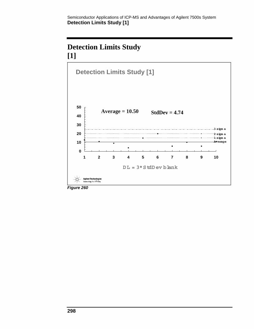
Semiconductor Applications of ICP-MS and Advantages of Agilent 7500s System Detection Limits Study [1]
298
Detection Limits Study [1]
Detection Limits Study [1]
0
10
20
30
40
50
1 2 3 4 5 6 7 8 9 10
3 sigm a
2 sigm a1 sigm aAverage
Average = 10.50 StdDev = 4.74
DL = 3*StdDev blank
Figure 260

Semiconductor Applications of ICP-MS and Advantages of Agilent 7500s System Detection Limits Study [2]
299
Detection Limits Study [2]
Detection Limits Study [2]
0
10
20
30
40
50
0 5 10
Co ncen tra tion
Inte
ns
ity
(X2,Y2)
(X1,Y1)
Figure 261

Semiconductor Applications of ICP-MS and Advantages of Agilent 7500s System Automatic Switching Between Normal and Cool Plasma
300
Automatic Switching Between Normal and Cool Plasma
Automatic Switching Between Normal and Cool Plasma
Chained Sequencing allows the user to run a set of samples under one set of conditions such as cool plasma, then automatically switch the conditions and rerun the same samples under hot plasma.
Multitune Mode allows the user to run the same sample under multiple sets of conditions, automatically switching from one mode to another and then moving to the next sample
Figure 262

Intelligent Sequence Training Text

Intelligent Sequence Training Text What is Intelligent Sequence?
302
What is Intelligent Sequence?
Intelligent Sequence is designed to dramatically improve sample throughput and reporting accuracy while decreasing the time spent by the operator and data reviewer. Intelligent Sequence automates a variety of QA/QC control procedures as well as all the EPA-mandated quality control procedures (EPA Methods 200.8, 6020 and 6020-CLP) from analysis through reporting.
Features
Intelligent sequence has several unique features.
Smart Sequencing
Intelligent Sequence recognizes all EPA designated QA/QC sample types and, when used with an autosampler, allows automatic, unattended analysis of batches of samples with all necessary calibrations, checks and controls. During sequencing, sample results are evaluated for pass/fail against a user-editable database of QC criteria. If a QC parameter is out of range, sequencing automatically performs a user-selectable action to attempt to remedy the problem. All sample results and QC actions are logged and a QC exception report is created.
QC Reporting
During sequencing, sample-type specific reports are generated and stored for all runs. A QC summary report is also generated. This report can be viewed at any time during or after the sequence. The summary report includes, in an easily reviewed format, a list of samples run and any QC failures which may have occurred. All batch or Sample Delivery Group relevant data are automatically stored together in system-generated “batch directories” for convenient archival and retrieval.
Tune Compliance Checking
A simple, graphical user interface allows user selectable tune compliance criteria to be stored with each method. Evaluating a tune sample can be automatic or manual via a simple pull-down menu item.

Intelligent Sequence Training Text Typical Analytical Flow
303
Typical Analytical Flow
1) Select appropriate QC configuration Configuration >> QC Mode
2) Load ICP-MS method Methods >> Load
3) Edit method and QC parameters Methods >> Edit Entire Method
• Method Information
• Interference Equation
• Acquisition
• Data Analysis
� Report… Select QC report
� Calibration Table… Select Load Mass from Current Acq. in New
• QC Parameters
� QC Database
4) Set unreported elements Methods >> Set Unreported Elements
5) Save the method and calibration Methods >> Save
• Verify QC Method
6) Load the tuning method Methods >> Load
7) Edit method and QC parameters Methods >> Edit Entire Method
• Method Information
• Acquisition
• Data Analysis
� Report… Select QC report
• QC Parameters
• QC Tune Criteria
8) Save the method and calibration Methods >> Save
9) Edit the sample log table Sequence >> Edit Sample Log Table
10) Simulate the sequence Sequence >> Simulate Sequence
11) Save the sequence Sequence >> Save
12) Run the sequence Sequence >> Run

Intelligent Sequence Training Text Using Intelligent Sequencing
304
Using Intelligent Sequencing
QC Configuration
To use Intelligent Sequencing, the appropriate QC configuration must be selected in Configuration.
The following QC modes are provided as default.
• EPA2008.QCC --- intelligent functions defined by EPA Method 200.8.
• EPA6020.QCC --- intelligent functions defined by EPA Method 6020.
• EPA6020C.QCC --- intelligent functions defined by EPA Method 6020 CLP.
• EPAGEN.QCC --- Intelligent functions designed to meet both EPA 200.8 and 6020 requirements
• GENERAL.QCC --- Intelligent sequencing disabled (no expected values or failure actions defined)
When selecting GENERAL.QCC, the sequencing mode is changed to the general sequencing mode. When selecting other QC modes, the sequencing mode is changed to intelligent sequencing mode.

Intelligent Sequence Training Text Using Intelligent Sequencing
305
For more information about sample types included in each QC mode, see Appendix of “AGILENT 7500 ChemStation Intelligent Sequence Manual”.
ICP-MS Method
When intelligent sequencing mode is selected, additional menus become available in the Methods menu.
• Edit QC Database… Enables editing of QC related items on a sample type basis such as high limit values, low limit values and error action.
• Edit QC Tune Criteria… Enables editing of tune compliance criteria such as sensitivity, mass resolution and %RSD.
• Verify QC Method… Checks the QC database and QC tune criteria for configuration errors.
• QC Information… Indicates the QC mode name which was used to make the current method.
• Set Unreported Elements… Allows the user to select the elements which are not to be reported on QC custom reports.
Default Methods Provided

Intelligent Sequence Training Text Using Intelligent Sequencing
306
EPA Method 200.8 6020 CLP Remark
QC Mode (.qcc) 200_8 6020 6020CLP
Method (.m) EPA20_8 EPA6020 EPACLP For QC Database
Tuning Method (.m) TN200-8 TN6020 TNCLP For QC Tune Criteria
Edit Entire Method
Use Edit Entire Method to make a complete method including QC parameters.
• Method Information… Same settings as general use.
• Interference Equation… Same settings as general use.
• Acquisition… Same settings as general use.

Intelligent Sequence Training Text Using Intelligent Sequencing
307
• Data Analysis… Same except Select Reports.
• QC Parameters… New menu
(A) QC Database
(B) QC Tune Criteria
Select “QC Report”, and then “Recalculate then Print”

Intelligent Sequence Training Text Using Intelligent Sequencing
308
(A) QC Database
For information about how to read comparative expressions (definition of criteria), see “Setting Up a Method” of “AGILENT 7500 ChemStation Intelligent Sequence Manual”.
<Error Actions supported>
• NextSmpl… Next sample
• Abort… Abort the run
Comparative expressions defined in QC configuration
Elements referred from cal curve
Off(x) is marked for the elements for which Excluded is selected as a curve fit in cal, or used for interference correction
Click here
Sample type opened currently
Expected Value and Low & High Limits
Error Actions and #Allowed Failures
QC Database settings are saved in cal file

Intelligent Sequence Training Text Using Intelligent Sequencing
309
• Blk (Abort) – NextSmpl… Run the blank block then continue (Abort if all of the samples in the blank block fail).
• Blk (Cont.) – NextSmpl… Run the blank block then continue (Continue even if all of the samples in the blank block fail)
• Blk (Abort) – SameSmpl… Run the blank block and re-run same sample (Abort if all of the samples in the blank block fail).
• Blk (Cont.) – SameSmpl… Run the blank block and re-run same sample (Continue even if all of the samples in the blank block fail).
• Cal – SameSmpl… Recalibrate and re-run same sample.
• Cal – AllSmpls… Recalibrate and re-run all samples since last CCV block.
• NextLot… Run next lot of samples
• Run User Macro… Run the user macro which must be placed under the method currently running, and named “QCUSER.MAC”.
<How proceed Criteria>
Up to four criteria for each sample type (except ISTD).
Area for 1st step Criteria 1
Area for 1st step Criteria 2
Area for 2nd step Criteria 1
Area for 2nd step Criteria 2

Intelligent Sequence Training Text Using Intelligent Sequencing
310
Normally just one Criteria (1st step Criteria 1), or two Criteria (1st step Criteria 1 & 2nd step Criteria 1, or 1st step Criteria 1&1st step Criteria 2) is used.
<Examples>
• 1st step Criteria 1
“Check whether the analytical concentrations of certified reference material (CRM) are 90-110% of the certified values (expected values).” 1st step Criteria 1 Low limit: CRM conc >= 0.9 x CRM expected values High limit: CRM conc =< 1.1 x CRM expected values
• 1st step Criteria 1 & 2nd step Criteria 1
1st step, Criteria 1
Fail
Pass
Error action set for
1st step Criteria 1
1st step, Criteria 2
Fail
Pass
Error action set for
1st step Criteria 2
Check to select flag
FILTER
2nd step, Criteria 1
Fail
Pass
Error action set for
2nd step Criteria 1
2nd step, Criteria 2
Fail
Pass
Error action set for
2nd step Criteria 2
Check to select flag
Next sample

Intelligent Sequence Training Text Using Intelligent Sequencing
311
“Check whether the analytical concentrations of CRM are 90-110% of the certified values for elements whose counts are equal or more than 1000 cps” 1st step Criteria 1 Low limit: CRM cps >= 1000 High limit: none 2nd step Criteria 1 Low limit: CRM conc >= 0.9 x CRM expected values High limit: CRM conc =< 1.1 x CRM expected values
• 1st step Criteria 1 & 1st step Criteria 2
“Check whether the analytical concentrations of certified reference material (CRM) are 85-115% of the certified values. If not, recalibrate and then analyze again. Also check whether concentrations are 90-110% of the certified values. If not, have a error flag on a report.” 1st step Criteria 1 Low limit: CRM conc >= 0.85 x CRM expected values High limit: CRM conc =< 1.15 x CRM expected values 1st step Criteria 2 Low limit: CRM conc >= 0.9 x CRM expected values High limit: CRM conc =< 1.1 x CRM expected values

Intelligent Sequence Training Text Using Intelligent Sequencing
312
(B) QC Tune Criteria
*1: “Ref” appears in the Mode list when Response Ratio check is enabled. *2: “Bkg” appears in the Mode list when Max Bkg Count check is enabled.
Masses set in data acq parameters
QC Tune Criteria settings are saved in method file
Set “Ref” for Response Ratio check *1
Fixed to 1 for Resp Ratio Low&High Limits
Set “Bkg” for Bkg check *2
Only Max. Bkg Count is effective
Intelligent Sequence Training Text Using Intelligent Sequencing
313
Notes on Setting a Method
• Use Auto Configuration first, when there are more Off (x) elements other than the elements for which Excluded is selected as a curve fit in the calibration table and the elements with parentheses. When Auto Configuration is used, all Off column settings are always reinitialized.
• In the event of a simultaneous QC failure and ISTD failure, the action on QC failure will take precedence.
• The error action for third failure is set in QC configuration on a sample type basis.
• Set equal or more number of acquired elements for #Allowed QC Failure when the Second Step is used. Otherwise, the First Step does not work as a filter, and QC check won’t go to the Second Step.
• Expected values for Reference part (right side of comparative expressions) always refer to the values set in the First Step Criteria 1. Expected values for Measured part (left side of comparative expressions) refer to the values set in each criteria.
• Use Set Unreported Elements, when there are elements which are not to be reported on QC custom reports.
Before Saving the Method
• Use Verify QC Method to check whether there is any error on settings. (Click this in Method Save Options when method is saved.)
Setting Up a Sequence
Structure of Sample Log Table
Sample Log Table is arranged in subroutines or “Blocks”.
The Sample Log Table is composed of four kinds of sheets as follows:
• Sequence Flow sheet
• Periodic Block sheet
• Individual Block sheet
• Whole List sheet

Intelligent Sequence Training Text Using Intelligent Sequencing
314
Notes on Setting Each Sheet
<Periodic Block>
The upper block setting has priority when there is a conflict with multiple blocks.
<Individual Block>
Analyzed every 10 samples
Periodic Block
Analyzed every 8 hours (480
Individual Block – CALIB Block
Whole List
Main flow TUNE Block
CALIB Block
SMPL Block
TERM Block
Keywords which separate each block are automativcally attached

Intelligent Sequence Training Text Using Intelligent Sequencing
315
• Blanks which are analyzed when the error actions “Blk…….” are taken should be set in BLANK Block.
• Samples which are analyzed when the sequence is aborted should be set in ERRTERM Block.
• When ISTD check is set, the CalBlk should be set at first except Tune since the ISTD counts from the CalBlk are used to establish the reference values.
• When recovery, dilution or duplication check is set, a reference sample type should be set prior to recovery, dilution or duplication sample.
Before Running the Sequence
• Use Simulate Sequence to check whether there is any error on settings.
Running a Sequence
Note on Running a Sequence
• Insure the same QC configuration as the one used when the methods and sequence to be executed were made.
• After editing the sample log table (online) during sequence run, close the table immediately. The sequence is paused while the sample log table is opened.
The methods & calibrations used, actual sample log table and sequence logs as well as all the data in one sequence are saved in this directory.

Intelligent Sequence Training Text Using Intelligent Sequencing
316
• If the data analysis parameters, QC Database or QC Tune Criteria in the method currently used needs to be changed instantly, load the method using Offline Data Analysis, and change it. The modified method can be saved to online using Offline Data Analysis >> Method >> Save to Online.
Sequence Reprocessing of Data
Two ways for batch reprocessing of data:
A. Reprocessing Data Batch Directory
B. Running a Sequence with Reprocessing Only
(A) Reprocess Data Batch Directory
<Files to be selected and used>
icpchem\1\ data\ 98k1109a.b\ 001tune.d
002calb.d
050smpl.d
meth1.m (copied automatically)
meth1.c (copied automatically)
result.s (actual sequence*)
methods\ meth1.m (original)
calib\ meth1.c (original)
• The name for actual sequence is always result.s.
(B) Running a Sequence with Reprocessing Only
<Files to be selected and used>
Data files
1. Select data batch directory to be reprocessed in Reprocess Data Batch Directory
Used for data reprocessing

Intelligent Sequence Training Text Using Intelligent Sequencing
317
icpchem\1\ data\ 98k1109a.b\ 001tune.d
002calb.d
050smpl.d
meth1.m (copied automatically)
meth1.c (copied automatically)
result.s (actual sequence*)
methods\ meth1.m (original)
calib\ meth1.c (original)
* The name for actual sequence is always result.s.
Notes on Reprocessing Data
• Insure the correct method and calibration file are selected when changing parameters for reprocessing; change the copied method and calibration in the data batch directory when using Reprocess Data Batch Directory, and change the original method and calibration when running the sequence with reprocessing only.
• The header information updated using Data Analysis >> File >> Edit Header is not reflected when using batch reprocessing (both ways). Change the Sample Log Table of result.s if needed. However, the
Data files
Used for data reprocessing
3. Select data batch directory to be reprocessed in Start Sequence Dialog Box
1. Load this sequence
2. Insure the path for currently loaded method is the same as the one used for data reprocessing

Intelligent Sequence Training Text Using Intelligent Sequencing
318
header information to be printed out is not changed until the header information is updated using Data Analysis >> File >> Edit Header.

Intelligent Sequence Training Text Setting Up a QC Configuration
319
Setting Up a QC Configuration
QC configuration defines the QC sample type set which contains…
• Sample type name
• Data name suffix
• QC report template
• Type category
• QC Item name to be used for ISTD check
• Error counting way
• Action on 3rd failure
• Comparative expressions
• Error flags for QC report
The Changes in QC Configuration must be implemented with CAUTION as it affects the settings in the QC Database, QC Tune Criteria, or Sample Log Table directly.

Intelligent Sequence Training Text Setting Up a QC Configuration
320
Configuring QC Items

Intelligent Sequence Training Text Setting Up a QC Configuration
321
How to Create or Change a QC Item
Select “New” to make new
Select “Delete” to delete the QC Item currently opened CAUTION: once deleted, it cannot be recovered
Select “List” to load QC Item to be changed
Screen for selected QC Item is opened

Intelligent Sequence Training Text Setting Up a QC Configuration
322
Special Screens
Only QC Itembecomes effective
Screen is completely changed

Intelligent Sequence Training Text Setting Up a QC Configuration
323
Notes on Setting QC Items
• Preservation of the original QC mode files is recommended.
• Once a QC Item is deleted, it will change the setting of related items in the QC Database, QC Tune Criteria, or Sample Log Table even when the same QC Item in the QC mode is restored.
• Also, once a Category of a QC Item is changed, it will change the setting of related items in the QC Database, QC Configuration, or Sample Log Table even when the same Category for the QC Item is restored.
• Basically the AGILENT 7500 ChemStation does a mass defect correction. Therefore, Adopt exact mass should be OFF if not necessary.

Intelligent Sequence Training Text Setting Up a QC Configuration
324
Creating a QC Report Template
When Report File is not selected
When Report File is selected
Select QC Item whose category is Tune to edit QC report template for Tune sample
Select items under an adequate place
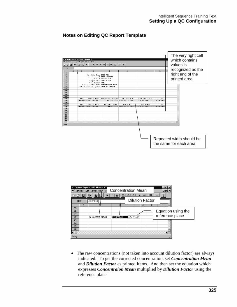
Intelligent Sequence Training Text Setting Up a QC Configuration
325
Notes on Editing QC Report Template
• The raw concentrations (not taken into account dilution factor) are always indicated. To get the corrected concentration, set Concentration Mean and Dilution Factor as printed Items. And then set the equation which expresses Concentraion Mean multiplied by Dilution Factor using the reference place.
Repeated width should be the same for each area
The very right cell which contains values is recognized as the right end of the printed area
Concentration Mean
Dilution Factor
Equation using the reference place

Intelligent Sequence Training Text Setting Up a QC Configuration
326
• There is no function to select the printed area. When there is a column you don’t want to print out, select the column, and then select Format >> Column Width >> Hide.
• When adding graph (spectrum) on a Tune type template, the repeat setting cannot be applied. Individual setting is required.

Laboratory 1: Agilent 7500 Configuration, Startup and Tuning
Reference:
• Agilent 7500 ChemStation Operators Manual
• Agilent 7500 Customer Training Class, Module 4
• Agilent 7500 Customer Training Class, Appendix 2

Laboratory 1: Agilent 7500 Configuration, Startup and Tuning Configuration
328
Configuration
1) Close ChemStation if open and open ‘Configuration’ under Agilent 7500 Program Group
2) Check: Offline Instrument – NOT CHECKED
3) Check: Remote Start – Don’t Use except for synchronization with external sampling devices
4) Check: Sample Introduction as appropriate including peristaltic pump and autosampler
5) Check: EM Protection – select Auto setting of integration time in analog mode
6) Check: QC Mode – GENERAL.QCC
7) Save and Exit

Laboratory 1: Agilent 7500 Configuration, Startup and Tuning Startup and Tuning
329
Startup and Tuning
1) Review Startup Checklist
2) Initiate Plasma and Warm-up Instrument Position ALS in distilled water Go to Tune Select Tune >> PeriPump program for Autotune, review the values here Select Sensitivity and Start (Allow instrument to scan for 10-15 minutes to warm up the quadrupole) Place the ALS probe in position 3 (10 ppb tune solution, Li, Y, Ce, Tl) (Allow time for uptake, 1-2 min)
3) Select Sensitivity >> Start Watch for awhile Select File >> Print, (keep this for reference as your starting point)
4) Select Tune >> Autotune… Select Torch Position, Sensitivity, Resolution/Axis and Tune Report Run Autotune (watch what happens) Compare the new tune report with the original one which you printed
5) Load “poor_s.u” (This has been deliberately mis-tuned for poor sensitivity) Using the ChemStation Manual, Student Manual and Tune Flowcharts, fix this tune
6) Load “high-ox.u” Try to reduce the oxides in this tune
7) Ask the instructor to “Fix” the system so that it generates high %RSDs. Fix this!
8) Save your best tune as best.u
9) Place the internal standard solution on line
10) Under Acq. Parms select masses 6, 140 and 209 (what are these elements and where do they come from, e.g. why would we be interested in monitoring them?)
11) Allow time for ISTD uptake and monitor the ISTD counts and %RSDs, do they make sense?
12) Discuss your results with the instructor.

Laboratory 1: Agilent 7500 Configuration, Startup and Tuning Agilent 7500 Startup Checklist
330
Agilent 7500 Startup Checklist
CHILLER
ARGON
PERIPUMP TUBES CLAMPED
INTERNAL STANDARD MIX
Out for tune
In for analysis
TUNE SOLUTION FULL
BLANK RINSE SOLUTION FULL
DRAIN RESERVOIRS NOT FULL
ALS RINSE PORT RESERVOIR OK
SHIELD IN or OUT (application dependent)
PLASMA ON

Laboratory 1: Agilent 7500 Configuration, Startup and Tuning Shutdown Checklist
331
Shutdown Checklist
ALS IN RINSE SOLUTION, WAIT 1 MINUTE
PLASMA OFF
PERIPUMP TUBES UNCLAMPED
CHILLER

Laboratory 1: Agilent 7500 Configuration, Startup and Tuning Shutdown Checklist
332
(l)Poor Sensitivity
(ll)Poor Precision
(high RSDs)
(III)High Oxides and/or
doubly-charged ions
Check PhysicalParameters:
Sample Uptake rate(bubble)
Nebul izat ion(-visually)
(-sodium bul let)
Torch Posi t ion(x,y visually)
Cone or i f ices
Torch Posi t ion(7-8 mm)
Opt imize SampleDepth and X-Y posi t ion
Sensit ivi tyImproved?
N o
Yes
Check mass ax is andresolut ion. Peaks?
Yes
Set:Carrier Gas: 1.2 - 1.5Peripump : .1 - .15Ext. 1: -150 to -180Ext. 2: -75 to -100Omega Bias : -40Omega (+) : opt imizebetween 0 and 10 VQP Focus : optimizebetween -10 and 10
N o
Veri fy contents of tunesolut ion
Run SetEM
Sensit ivi tyO K ?
Yes
N o
RSDs OK?
Oxides/DoublyCharged OK?
Yes
N o
N o
Go to (II)
GO to (I I I)
Save Tune Fi leYes
Adjust peri-pumpshoe pressure
(decrease t i l l no signal,then slowly increase
just enough for stablesignal)
Adjust carr ier gas f low(carr ier + blend gas <=1.4 - 1.5 ml/min) very
slowly
Fine tune Extractlenses and Omega
lenses
Clean or replace cones
Decrease carr ier /blendgas f low
Increase Sample depth
Decrease per i -pumpflow
Save Tune Fi le
H P 4 5 0 0 I C P - M SM a n u a l T u n e
Troubleshoot ingF lowchar t
�

Laboratory 2: Agilent 7500 Routine Maintenance
Reference:
• Agilent 7500 Administration and Maintenance Manual
• Agilent 7500 Customer Training Class – Module 5
• Maintenance Log Table

Laboratory 2: Agilent 7500 Routine Maintenance General
334
General
1) Remove and examine air filters
2) Examine level and color of oil in Rough Pumps
3) Check all fluids, belts and hoses (just kidding)
4) Check for corrosion and wipe down cabinet as necessary with damp cloth
Laboratory 2: Agilent 7500 Routine Maintenance Sample Introduction
335
Sample Introduction
Remove:
• Peri-pump tubes
• Nebulizer
• Spray Chamber
• Torch
Clean or replace as necessary (refer to maintenance manual)

Laboratory 2: Agilent 7500 Routine Maintenance Interface
336
Interface
1) Remove Sampler and Skimmer Cones and Extraction Lens assembly
2) Sonicate cones in 10% Citranox with occasional careful wiping until visibly clean (10-30 minutes)
3) Rinse cones with water, then DI water, blow dry and set aside.
4) Disassemble extract lens assembly, examine lenses and insulators for discoloration.
5) Sonicate in 10% Citranox and rinse thoroughly as above. Do not sonicate the insulators unless obviously discolored as they take longer to dry.
6) Reassemble and reinstall extraction lenses and interface cones

Laboratory 2: Agilent 7500 Routine Maintenance Nebulizer, Spray chamber and Torch
337
Nebulizer, Spray chamber and Torch
1) Babbington and Crossflow nebulizers can be sonicated in either dilute Citranox or, 5-10% nitric acid as needed. Babbington nebulizers can be unclogged (argon line) with a tiny GC syringe cleaning wire if needed. Rinse well after cleaning.
2) GLASSWARE SHOULD NOT BE SONICATED! However, torches and spray chambers can be boiled in hot 10% Citranox and then rinsed well. This greatly improves the wetability of the spray chamber. Soaking in strong (10-50%) nitric acid solution overnight may also be necessary for extremely dirty or contaminated glassware.
3) Remove the glassware, examine carefully and replace. Be sure all gas and spray chamber drain connections are leak free.

Laboratory 2: Agilent 7500 Routine Maintenance Re-ignite the plasma and check the tune
338
Re-ignite the plasma and check the tune

Laboratory 3: Semi-Quantitative Analysis
Reference:
• Agilent 7500 ChemStation Operators Manual
• Agilent 7500 Customer Training Class Manual, Module 08

Laboratory 3: Semi-Quantitative Analysis Semi-Quantitative Analysis
340
Semi-Quantitative Analysis
1) From Top Level, load default.m
2) Select ‘Edit Entire Method’
3) Edit all method sections to create a semiquant method for unknown sample screening
Do not waste time acquiring nonsense elements such as inert gasses, air, carbon, halogens etc. Also exclude the transuranic elements.
4) Use 0.1 second integration for all elements
5) Use 60 second uptake, 5 second optional rinse, and 60 second stabilization.
6) Do not configure the use of internal standards, since we will be using this method to screen for the presence if internal standard elements in the unknown sample.
7) Examine your tune report and estimate the semiquant response factor threshold (Minimum Peak in cps) necessary to exclude results lower than ~0.1 ppb from the report.
8) Save the method as a unique name.
9) Analyze a blank and a 10 ppb (or 100 ppb) multielement calibration standard with your method.
10) Using the blank and 10 ppb (or 100 ppb) standard, enable blank subtraction and reset the semiquant response factors.
11) Analyze the unknown sample to screen for the presence of the internal standard elements, as well as the presence and approximate concentrations of other analyte elements. This information will be used to develop a quantitative method for analysis of the unknown sample(s).
12) Compare the results with the certified values.
Are semiquant results subject to interferences?
Can they be corrected?
Laboratory 4: Quantitative Analysis of Unknown Sample
Reference:
• Agilent 7500 ChemStation Operators Manual
• Agilent 7500 Customer Training Class, Module 09
• HP/Agilent Standard Operating Procedure, EPA Method 200.8

Laboratory 4: Quantitative Analysis of Unknown Sample Quantitative Analysis
342
Quantitative Analysis
1) Using your SemiQuant results for the Unknown sample and the EPA 200.8 SOP as guidelines, build a quantitative method for analysis of Ag, Al, As, Ba, Be, Cd, Co, Cr, Cu, Mn, Mo, Ni, Pb, Sb, Se, Tl, V and Zn.
2) Include at least two calibration levels plus a blank for each element. If the element is likely to trigger analog mode, include a calibration point which will also be acquired in analog mode. (Why is this?) Multi-element calibration standards will be available in 1; 10; 100; 500; 1,000 ppb concentrations.
3) Build a simple sequence to update your calibration and analyze your unknown sample at two dilutions.
4) Compare your results with the certified values.
5) Discuss your results with the instructor.
Hints:
Always run at least 2 calibration blanks at the beginning of a sequence to insure adequate flush-out of previously run samples.
Always run a blank after the high calibration standard and before any samples to detect possible memory effects.
Always analyze a blank and mid-point calibration as samples at the end of a sequence and every 10 samples to verify that the system is under control.

Appendix 1 – General Information

Appendix 1 – General Information Professional Organizations
344
Professional Organizations
Professional Organizations
★American Chemical Society (ACS) (800) 227-5558http://www,acs.org
★Environmental Protection Agency (EPA) http://www.epa.gov★American Association of Clinical Chemists (AACC) (800) 892-1400★American Board of Clinical Chemistry, Inc.(ABCC) (202) 835-8727★American Society of Clinical Pathologists (ASCP) (312) 738-1336 x.158★Clinical Laboratory Management Association (CLMA) (610) 647-8970★College of American Pathologists (CAP) (800) 323-4040★National Committee for Clinical Laboratory Standards (NCCLS) (610) 688-0100★Society for Applied spectroscopy (301)694-8122★SEMI International Standards (650) 964-5111
http://www.semi.org
Figure 263

Appendix 1 – General Information Journals
345
Journals
Journals
■ Analytical Chemistry■ Journal of Analytical Atomic Spectrometry (JAAS)■ Applied Spectroscopy (free with SAS membership)■ Spectroscopy (free)■ Spectrochimica Acta, Part B■ Analyst■ American Lab (free)■ American Clinical Lab (free)
Figure 264

Appendix 1 – General Information Selected Web Sites (1)
346
Selected Web Sites (1)
Selected Web Sites (1)
• Agilent Technologieshttp://www.agilent.com
• Sample Preparation (Duquesne University)http://www.sampleprep.duq.edu/sampleprep/
• Eastern Analytical Symposiumhttp://www.eas.org/
• FACSShttp://facss.org/info.html
• Pittconhttp://www.pittcon.org/
• NIST Standard reference Program
Figure 265

Appendix 1 – General Information Selected Web Sites (2)
347
Selected Web Sites (2)
Selected Web Sites (2)
• Spex cataloghttp://www.spexcsp.com/crmmain/cat_f.htm
• Spectronhttp://www.vcnet.com/spectron/
• Inorganic Ventureshttp://www.ivstandards.com/
• Michael Cheatcham’s Instrument pageshttp://www.geochemistry.syr.edu/cheatham/InstrPages.html
• Plasmachem-L BBhttp://www.geochemistry.syr.edu/cheatham/icpmsins.html
• US Pharmacopeiahttp://www.usp.org/
Figure 266

Appendix 1 – General Information Selected Web Sites (2)
348

Appendix 2 – Flow Chats

Appendix 2 – Flow Chats Manual Tune Troubleshooting Flowchart [1]
350
Manual Tune Troubleshooting Flowchart [1]
OK?
Instrument Maintenance
No
Oxides andDoubly
Charge?
Startup
Sensitivity?Torch Position Too Low
Omega Lens
Extraction 1, 2
Carrier Gas Flow
Sample Uptake
OK?
OK?
OK?
OK?Precision ?
In Spec.No
No
No
No
In Spec.
Sample Uptake
Carrier Gas Flow
Extraction 1, 2
Einzel 2
Instrument Maintenance
OK?
OK?
OK?
OK?
No
No
No
No
Poor
10 minutes warm-up
Resolution / Axis
Sample Depth
OK?
Carrier Gas Flow
OK?
Pump Speed
OK?
Save Tune File
Print Tune Report.Ready for Analysis
High
No
No
In Spec.
Agilent 7500 ICP-MSManual Tune
TroubleshootingFlowchart
Yes
Yes
Yes
Yes
Yes
Yes
Yes
InstrumentMaintenance
No
Yes
Yes
Yes
Yes
Yes
Set EM Voltage
Set P/A Factor
Figure 267

Appendix 2 – Flow Chats Manual Tune Troubleshooting Flowchart [2]
351
Manual Tune Troubleshooting Flowchart [2]
(l)Poor Sensitivity
(ll)Poor Precision
(high RSDs)
(III)High Oxides and/or
doubly-charged ions
C heck Physical Parameters:
Sample Uptake rate (bubble)
Nebulization(-visually)
(-sodium bul let)
Torch Position(x,y visually)
Cone orifices
Torch Position(7 -8 mm)
Optimize SampleDepth and X-Y
position
SensitivityImproved?
No
Yes
Check mass axisand resolution.
Peaks?
Yes
Set:Carrier Gas : 1.2 - 1.5Peripump : 0.1 - 0.15Ext. 1: -150 to -180Ext. 2: -75 to -100Omega Bias : -40Omega (+) : opt imize between 0 and 10 VQP Focus : opt imize between -10 and 10
No
Verify contents oftune solution
Run SetEM
SensitivityOK?
Yes
No
RSDs OK?
Oxides/DoublyCharged OK?
Yes
No
No
Go to (II)
GO to (III)
Save Tune FileYes
Adjust peri-pump shoepressure
(decrease t i l l no signal, thenslowly increase just enough
for stable signal)
Adjust carrier gas flow(carr ier + blend gas <= 1.4 -
1.5 ml/min) very slowly
Fine tune Extract lensesand Omega lenses
Clean or replace cones
Decrease carrier/blendgas flow
Increase Sampledepth
Decrease peri-pumpflow
Save Tune File
Agi lent 7500I C P - M S
M a n u a l T u n eTroubleshoot ing
Flowchar tΗ
Figure 268

Appendix 2 – Flow Chats Manual Tune Troubleshooting Flowchart [2]
352

Appendix 3 – Dealing with Polyatomics

Appendix 3 – Dealing with Polyatomics The Problem
354
The Problem
The Problem...
Bulk argon from the plasma can combine with entrained atmospheric gases and matrix constituents to form argon polyatomic ions.The resulting polyatomic ions can overlap analyte masses of interest compromising detection limitsCommon examples are:
ArO+ interferes with 56FeArH+ interferes with 39KAr+ interferes with 40CaArCl+ interferes with 75As
Figure 269

Appendix 3 – Dealing with Polyatomics Strategy #1: (High Power) Cool Plasma Analysis
355
Strategy #1: (High Power) Cool Plasma Analysis
Strategy #1: (High Power) Cool Plasma Analysis
• Technique first reported in 1988*:• Reduction of ArH+ interference on Ca simply by modifying ICP operating conditions
• lower plasma power• increased carrier gas flow• longer sampling depth
* Jaing, Houk, and Stevens, Anal. Chem., 1988, 60, 1217
Figure 270

Appendix 3 – Dealing with Polyatomics Commercialization of Cool Plasma Analysis
356
Commercialization of Cool Plasma Analysis
Commercialization of Cool Plasma Analysis
• Developed commercially by HP/Yokogawa in 1992*•featuring patented ShieldTorch Interface
• Cool plasma ICP-MS (using the Agilent ShieldTorch) now the method of choice for ultratrace metals analysis in the semiconductor industry• Over 100 HP 4500's and Agilent 7500’s performing routine cool plasma analysis in the semiconductor industry replacing GFAA, ETV-ICP-MS, HR-ICP-MS
* Sakata K et al., Spectrochim. Acta, 1994, 49B, 1027
Figure 271
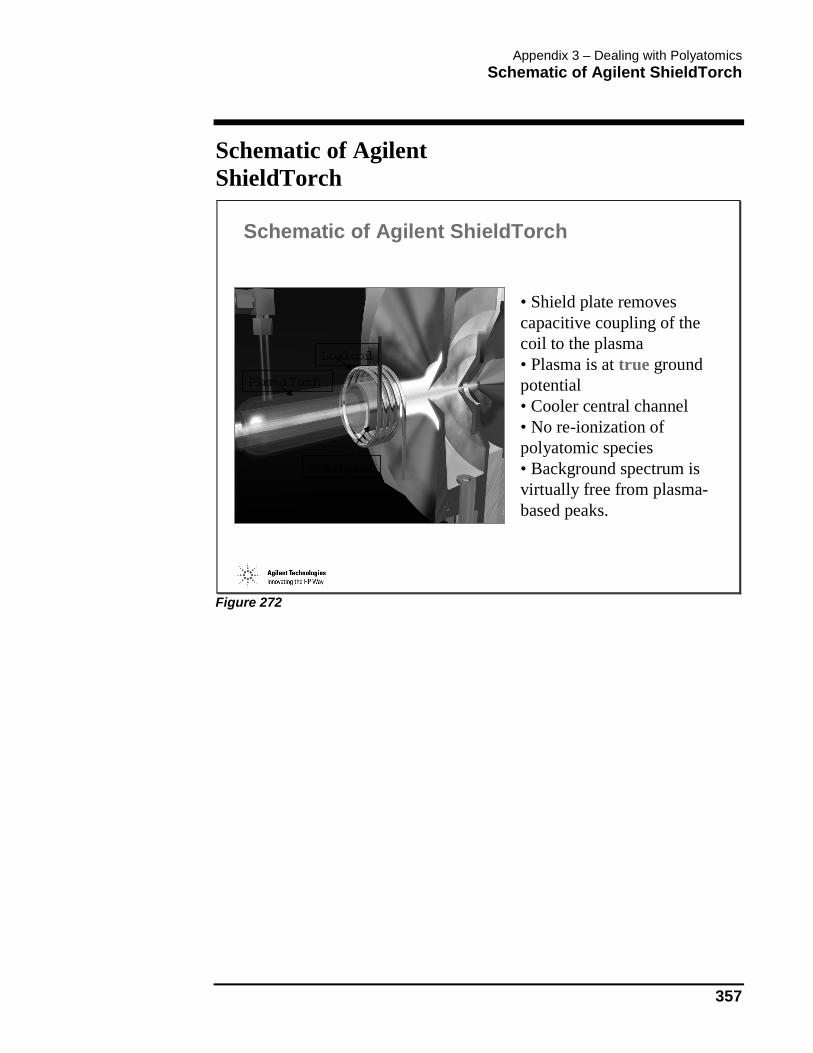
Appendix 3 – Dealing with Polyatomics Schematic of Agilent ShieldTorch
357
Schematic of Agilent ShieldTorch
Schematic of Agilent ShieldTorch
Load coil
Shield plate
Plasma Torch
• Shield plate removescapacitive coupling of the coil to the plasma• Plasma is at true ground potential• Cooler central channel • No re-ionization of polyatomic species• Background spectrum is virtually free from plasma-based peaks.
Figure 272

Appendix 3 – Dealing with Polyatomics Not All Cool Plasmas* Are the Same! [1]
358
Not All Cool Plasmas* Are the Same! [1]
Not All Cool Plasmas* Are the Same! [1]
• The ShieldTorch interface is unique to Agilent• Reduces interferences such as ArH, Ar, ArO, C2, ArC to low ppt levels, enabling sub-ppt level DLs for K, Ca, Fe etc• The key feature of the ShieldTorch is that it can achieve this at 900-1000W forward power
• other systems can only remove interferences at 600-650W -interfering peaks reappear at higher power settings• operating at 650W gives rise to severe matrix effects, and reduced analyte range
* Analysis at 600-650W is often referred to as cold plasma analysis
Figure 273

Appendix 3 – Dealing with Polyatomics Not All Cool Plasmas* Are the Same! [2]
359
Not All Cool Plasmas* Are the Same! [2]
Not All Cool Plasmas* Are the Same! [2]
• Advantages of operation at 900 W - 1000 W (High Power Cool Plasma)
• minimal matrix effects - similar to normal plasma operation (1200-1300W)• higher ionizing power - wider analyte range - including even Zn and B• complete sample matrix decomposition - greatly reduced possibility of interface and spectrometer contamination
Figure 274

Appendix 3 – Dealing with Polyatomics Fe in 31% H2O2 - 5 ppt Spike Recovery
360
Fe in 31% H2O2 - 5 ppt Spike Recovery
Fe in 31% H2O2 - 5 ppt Spike Recovery
Excellent linearity even at 5ppt using high power cool plasma
DL - 0.3ppt in the H2O2 matrix
No collision cell or HR-ICP-MS data reported to date showing Fe linearity at 5ppt
Figure 275

Appendix 3 – Dealing with Polyatomics ShieldTorch Technology Eliminates Interferences Before They Form!
361
ShieldTorch Technology Eliminates Interferences Before They Form!
ShieldTorch Technology Eliminates Interferences Before They Form!
?
Collision Cell
Shield Torch Technology
= Analyte
Figure 276

Appendix 3 – Dealing with Polyatomics Can Heavy Matrices be Analyzed?
362
Can Heavy Matrices be Analyzed?
Can Heavy Matrices be Analyzed?
Example Organics analysis •Until now, carbon-based interferences have prevented the trace analysis of Mg and Cr in organic samples•C2 interferes with Mg 24, 25, 26•ArC interferences with Cr 52, 53
Îhigh power cool plasma (900W) removes these intereferencesdown to single figure ppt levelÎAND is stable in all types of undiluted organic sample, including xylene, toluene and NMP
Figure 277

Appendix 3 – Dealing with Polyatomics Cr in Undiluted Methanol
363
Cr in Undiluted Methanol
Cr in Undiluted Methanol
Excellent linearity at ppt level demonstrates removal of ArCinterference using ShieldTorch system
The concentration of Cr in the sample is calculated at 7 ppt
Figure 278

Appendix 3 – Dealing with Polyatomics Example of Heavy Matrix Analysis
364
Example of Heavy Matrix Analysis
Example of Heavy Matrix Analysis
Example Analysis of trace impurities in Metal AlloysLevels required have traditionally been 10’s ppm or % in the solid, but requirements for lower level characterization are increasing
1000x dilution typically used for ICP-MS, soÎ1ppm in solid requires measurement of 1ppb in solutionÎeasily achieved for most elements by ICP-MS, except K, Ca, FeÎrobust high power cool plasma could be used
Figure 279

Appendix 3 – Dealing with Polyatomics Calibration for 56Fe in 1000 ppm Pt
365
Calibration for 56Fe in 1000 ppm Pt
Calibration for 56Fe in 1000 ppm Pt
High power cool plasma (900W)
Fe at mass 56 in matrix of 1000ppm Pt
Standard Addition calibration at 50, 100, 200 and 500ppt
Figure 280

Appendix 3 – Dealing with Polyatomics Calibration for 66Zn in 1000 ppm Pt
366
Calibration for 66Zn in 1000 ppm Pt
Calibration for 66Zn in 1000 ppm Pt
High power cool plasma (900W)
Zn at mass 66 in matrix of 1000ppm Pt.
Standard Addition calibration at 50, 100, 200 and 500ppt
Zn cannot be measured at 600W
Figure 281

Appendix 3 – Dealing with Polyatomics Determination of Se by High Power Cool Plasma
367
Determination of Se by High Power Cool Plasma
Determination of Se by High Power Cool Plasma
Agilent 7500 Operating ParametersShieldTorch interfaceHigher forward power (1000W)Higher gas flows
1.2 Lpm carrier gas0.8 Lpm blend gas
Ar2 ionization minimized, but plasma has power to ionize Se
Figure 282

Appendix 3 – Dealing with Polyatomics Spectrum of 10 ppb Se and Blank
368
Spectrum of 10 ppb Se and Blank
Spectrum of 10 ppb Se and Blank
Figure 283

Appendix 3 – Dealing with Polyatomics Calibration for 80Se
369
Calibration for 80Se
Calibration for 80Se
• Se at 0, 1, 2, 5 and 10ppb
• No blank subtraction
• No interference correction
• No internal standard
• Precision and linearity good
Figure 284

Appendix 3 – Dealing with Polyatomics Detection Limits for Se by Cool Plasma
370
Detection Limits for Se by Cool Plasma
Detection Limits for Se by Cool Plasma
M ass Blk Blk SD 1ppb 1ppb-Blk 3s DL (ppt)
76 121 8.91 786 665 40.23
77 1796 57.43 2234 438 393.05
78 33 6.04 375 342 52.93
80 113 7.63 478 365 62.72
82 211 13.48 873 662 61.06
Detection Limits (3 sigma, n=10) in 4% HClNote - Integration times varied for different isotopes
Figure 285

Appendix 3 – Dealing with Polyatomics Current Research Developments Using the ShieldTorch
371
Current Research Developments Using the ShieldTorch
Current Research Developments Using the ShieldTorch
• Trace elements in organics• Se isotope ratios• Trace As in chloride matrices• Trace analysis of "difficult" ICP-MS elements
– e.g. S, Si, P • Removal of isobaric interferences (not possible by
collision cells or HR-ICP-MS)– removal of Hg from Pb at mass 204– removal of Zr from Sr at mass 90
Figure 286
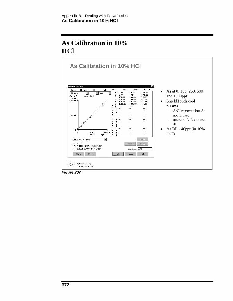
Appendix 3 – Dealing with Polyatomics As Calibration in 10% HCl
372
As Calibration in 10% HCl
As Calibration in 10% HCl
• As at 0, 100, 250, 500 and 1000ppt
• ShieldTorch cool plasma– ArCl removed but As
not ionised – measure AsO at mass
91• As DL - 40ppt (in 10%
HCl)
Figure 287

Appendix 3 – Dealing with Polyatomics Low Level P Calibration
373
Low Level P Calibration
Low Level P Calibration
• P at 0, 5, 10, 20 ppb• ShieldTorch cool
plasma– measure PO at mass
47• P DL - 30ppt
Figure 288

Appendix 3 – Dealing with Polyatomics Low Level S Calibration
374
Low Level S Calibration
Low Level S Calibration
• S at 0, 5, 10, 20 ppb• ShieldTorch cool
plasma– measure SO at
mass 48• S DL - 0.6 ppb
Figure 289

Appendix 3 – Dealing with Polyatomics Low Level Si Calibration
375
Low Level Si Calibration
Low Level Si Calibration
• Si at 0, 5, 10, 20 ppb• ShieldTorch cool
plasma– measure SiO at
mass 44 • Si DL - 1.2 ppb
Figure 290

Appendix 3 – Dealing with Polyatomics Strategy #2: Resolve the Interferences
376
Strategy #2: Resolve the Interferences
Strategy #2: Resolve the Interferences
High resolution ICP-MS can be used to separate the analyte andinterferent peakIncrease mass resolution and separate the analyte and interferentpeaks, then make the measurement
Figure 291

Appendix 3 – Dealing with Polyatomics Limitations of HR-ICP-MS
377
Limitations of HR-ICP-MS
Limitations of HR-ICP-MS
• As in optical spectrometry, there is a trade off between resolution and sensitivity– increasing resolution reduces transmission– the net result is an inability to determine the analyte at trace
levels.• A resolution of up to 7500 is required for some
interferences– at 7500R, signal transmission is only 1% of that at unit mass
resolution (300R)
Figure 292

Appendix 3 – Dealing with Polyatomics Resolution vs. Sensitivity
378
Resolution vs. Sensitivity
Resolution vs, Sensitivity
Sens
itiv
ity
Res
olut
ion
Incr
ease
d R
eso
Red
uced
Se
nsit
ivit
y
Figure 293

Appendix 3 – Dealing with Polyatomics Other Facts About HR-ICP-MS [1]
379
Other Facts About HR-ICP-MS [1]
Other Facts About HR-ICP-MS [1]
• Abundance sensitivity (tailing) is much worse in a magnetic sector than a quadrupole– if the analyte peak is adjacent
to a large interferent peak, eg 39K next to 40Ar, the tail from the Ar overwhelms the K signal
– in these cases, increasing the resolution does not help
Mass
Inte
nsit
y
40Ar
39K
Figure 294

Appendix 3 – Dealing with Polyatomics Other Facts About HR-ICP-MS [2]
380
Other Facts About HR-ICP-MS [2]
Other Facts About HR-ICP-MS [2]
• Mass calibration is critical to obtaining accurate analytical results, however, it is a time consuming process for HR-ICP-MS instruments– resolution is defined by changing slit widths, and these require
calibration/characterization– since the peak is so narrow at high resolution, the peak
maximum cannot be reproducibly located– the analyser must be scanned across the whole peak, which
decreases S/N significantly
Figure 295

Appendix 3 – Dealing with Polyatomics Other Facts About HR-ICP-MS [3]
381
Other Facts About HR-ICP-MS [3]
Other Facts About HR-ICP-MS [3]
• High resolution instruments cost >$350k
• Not perceived to be appropriate for routine analysis
• Require a higher level of operator skill than ICP-QMS
Figure 296

Appendix 3 – Dealing with Polyatomics Strategy #3: Dissociate Interferences Within the Spectrometer
382
Strategy #3: Dissociate Interferences Within the Spectrometer
Strategy #3: Dissociate Interferences Within the Spectrometer
• Utilize collision/dynamic reaction cell technology• Insert a collision cell/dynamic reaction cell within the
spectrometer between the main ion lens and quadrupole analyser
• Control gas phase chemistry within the collision cell to dissociate polyatomic ions thereby eliminating the interferences
Figure 297

Appendix 3 – Dealing with Polyatomics Principle of Collision Technology
383
Principle of Collision Technology
Principle of Collision Technology
Photon Stop
Gas inlet/outlet
Collision Cell
Multipole Ion Guide
Analyser Quadrupole
For Analyte and Interferent ions occurring at the same nominal mass:I nterferent + Reaction Gas IR New Mass
A nalyte + Reaction Gas No Reaction; Analyte at Same Mass
Figure 298

Appendix 3 – Dealing with Polyatomics Selecting a Gas Phase Reagent
384
Selecting a Gas Phase Reagent
Selecting a Gas Phase Reagent
• The ideal reagent should:– have high reactivity with the interferent ion– result in 100% conversion of the interferent ion into
its constituent products– result in a final product that is stable
• Unfortunately, no single gas has been found to be applicable for a complete multielement analysis
• Collision cell chemistries must be tailored for each individual element and sample matrix
Figure 299

Appendix 3 – Dealing with Polyatomics Optimizing the Gas Phase Reagent
385
Optimizing the Gas Phase Reagent
Optimizing the Gas Phase Reagent
• Often, more than one reaction gas is required to analyse a series of different elements
• The need to fill the collision cell with gas for the analysis and then vent the cell and refill with another gas, and re-measure the sample significantly increases analysis time
• Not only must the type of gas used be optimized, but the flow rate of gas through the cell must also be optimized for best S/N
• Few elements optimize using the same type of gas at the same flow rate. Therefore, compromise conditions must be used
Figure 300

Appendix 3 – Dealing with Polyatomics Side Reactions Are Inevitable!!
386
Side Reactions Are Inevitable!!
Side Reactions are Inevitable!!
• Side reactions i.e. unexpected reactions of the collision gas with other matrix components, have always been reported when using this technology
• For example, when using NH3 as a collision gas when Ni is present in the sample:
Reaction Product� Ni+ + NH3 Ni(NH3)+
� Ni+ + Ni(NH3)+ Ni(NH3) 2+
� Ni+ + Ni(NH3) 2+ Ni(NH3) 3+
� Ni+ + Ni(NH3) 3+ Ni(NH3) 4+
Figure 301

Appendix 3 – Dealing with Polyatomics Side Reactions Create New Interferences
387
Side Reactions Create New Interferences
Side Reactions Create New Interferences
Product Interferes withNi(NH3)+ 75As, 77SeNi(NH3) 2+ 92Zr, 92Mo, 94Zr, 94Mo, 95Mo, 96Zr,
96Mo, 96Ru, 98Mo, 98RuNi(NH3) 3+ 109Ag, 111Cd, 112Cd, 112Sn, 113Cd,
113In, 115In, 115SnNi(NH3) 4+ 126Te, 128Te, 130Te, 130Ba, 132Ba
Figure 302

Appendix 3 – Dealing with Polyatomics Hydrocarbons Are Particularly Prone To Complex Chemistries Even at Trace Levels
388
Hydrocarbons Are Particularly Prone To Complex Chemistries Even at Trace Levels
Hydrocarbons Are Particularly Prone To Complex Chemistries Even at Trace Levels
Even for simple hydrocarbons:
Ar+ + CH4 CH3+ + Ar + H +
Ar+ + CH3+ CH2
+ + Ar + H2
Ar+ + CH2+ CH+ + Ar + H3
+
Figure 303

Appendix 3 – Dealing with Polyatomics Effects of Sample Matrix
389
Effects of Sample Matrix
Effects of Sample Matrix
• “Multipole Ion Optics In ICP-MS”, Jonathan Batey, 25th Annual Conference of the Federation of Analytical Chemistry and Spectroscopy Societies, Paper #661.
• Aspirated 400ppm Ca into a collision cell device• Ca could be measured at 40Ca, however, strong peaks were
observed throughout the mass spectrum due to CaOH+ and other Ca molecular ions
• Conclusion - collisions cells were not appropriate for samples containing significant matrix components
Figure 304

Appendix 3 – Dealing with Polyatomics Strategies to Overcome the Problem of Side Reactions
390
Strategies to Overcome the Problem of Side Reactions
Strategies to Overcome the Problem of Side Reactions
• The collision cell quad can be scanned in concert with the analyser quad*– enables the collision cell quad to act like a notch filter– can prevent side reaction ions from entering the analyser quad
* Tanner S.D., Baranov V.I., At. Spectroscopy, 20 (2) 3-4/99
Figure 305

Appendix 3 – Dealing with Polyatomics Limitation of Scanning the Analyzer Quad
391
Limitation of Scanning the Analyzer Quad
Limitation of Scanning the Analyzer Quad
• When the collision cell quad becomes contaminated with sample matrix, it will charge up, and be unable to follow the scan speed of the analyser quad
• Analyte transmission will fall dramatically• Quadrupoles are difficult to clean• Correct realignment is critical to achieve maximum
transmission
Figure 306

Appendix 3 – Dealing with Polyatomics Collision Cells Can Create Interferences
392
Collision Cells Can Create Interferences
Collision Cells Can Create Interferences Through...
• Interferring ions combining with the reaction gas to shift to a new mass– This mass cannot always be anticipated due to ion clustering
• Reaction gas combining with analytes and matrix components not previously interferred with
• Reaction gas combining with ultra-trace contaminants in the cell
• The presence of any type of matrix significantly complicates data interpretation
Figure 307

Appendix 3 – Dealing with Polyatomics In Summary
393
In Summary
In Summary...
• High resolution ICP-MS can resolve the interferences, but is not easy to use, and in complex matrices, poor abundance sensitivity gives rise to severe spectral overlaps
• Collision cells must use different gases/gas mixtures and gas flow rates to meet all analyte requirements
• Collision cells not only reduce targeted interferences but create new unpredictable molecular ion clusters in every individual matrix
• For almost all applications, high power cool plasma has superior performance
Figure 308

Appendix 3 – Dealing with Polyatomics In Summary
394

