coupling strategy of hvac system · pdf fileperform more sophisticated energy saving control....

COUPLING STRATEGY OF HVAC SYSTEM SIMULATION AND CFDPART 2: STUDY ON MIXING ENERGY LOSS IN AN AIR-CONDITIONED ROOM

Satoru Iizuka1, Mina Sasaki1, Gyuyoung Yoon2, Masaya Okumiya1,Junya Kondo3, and Yuka Sakai4

1Nagoya University, Nagoya, Japan2Nagoya City University, Nagoya, Japan3Kajima Corporation, Tokyo, Japan4Toyama City Hall, Toyama, Japan

ABSTRACTA coupled analysis of heating, ventilation and air-conditioning (HVAC) system simulation tool andcomputational fluid dynamics (CFD) model wascarried out to assess the mixing energy loss in an air-conditioned room where heating and cooling operatein the perimeter and interior zones simultaneously.To evaluate the mixing energy loss, we conductedtwo simulations;; one was the case with airflowmixing between the perimeter and interior zones andthe other was the case without airflow mixingbetween the zones. By comparing the required coilloads between the two cases, the mixing energy losswas estimated. The accuracy of the coupled analysiswas assessed by comparing its results with thosefrom an experiment conducted by Ito (1988).

INTRODUCTIONIn recent years, effective energy management andenergy saving strategies are essential in the contextof the issue of global warming. In office buildings,for instance, further improvement in the efficiency ofair-conditioning system is required in order toachieve high energy saving.To examine the performance of air-conditioningsystem, various simulation tools (e.g., Life CycleEnergy Management (LCEM) tool, HVACSIM+,TRNSYS, DeST, EnergyPlus) have been developed.The system simulations performed with those toolsare usually carried out under the assumption ofcomplete mixing in the target room. However,without the consideration of spatial and temporaldistributions of indoor environment, it is difficult toperform more sophisticated energy saving control.Coupled analysis of HVAC system simulation andCFD is a promising strategy to overcome the aboveproblem. CFD is considered to be a powerful tool foranalyzing airflow and thermal environments,therefore detailed information of flow field and airtemperature can be obtained. As reviewed in anotherpaper for this conference (Yoon et al., 2011), severalintensive studies on coupled analysis of HVACsystem simulation and CFD have been conducted(e.g., Lam et al., 2001;; Zhai et al., 2003, 2005, 2006;;Iida et al., 2008).

In this study, coupled simulations of a HVAC systemsimulation tool and a CFD model were carried out toassess the mixing energy loss in an air-conditionedroom where heating and cooling operate in theperimeter and interior zones simultaneously. Themixing energy loss is defined as the differencebetween the sum of the net heating/cooling load andthat of the actual heating/cooling energy supplied tothe room.To evaluate the mixing energy loss, we conductedtwo simulations;; one was the case with airflowmixing between the perimeter and interior zones andthe other was the case without airflow mixingbetween the zones. By comparing the required coilloads between the two cases, the mixing energy losswas estimated.Furthermore, the effects of the reference points oftemperature in the perimeter and interior zones on themixing energy loss were investigated. The accuracyof the coupled analysis was assessed by comparingits results with those from an experiment conductedby Ito (1988).

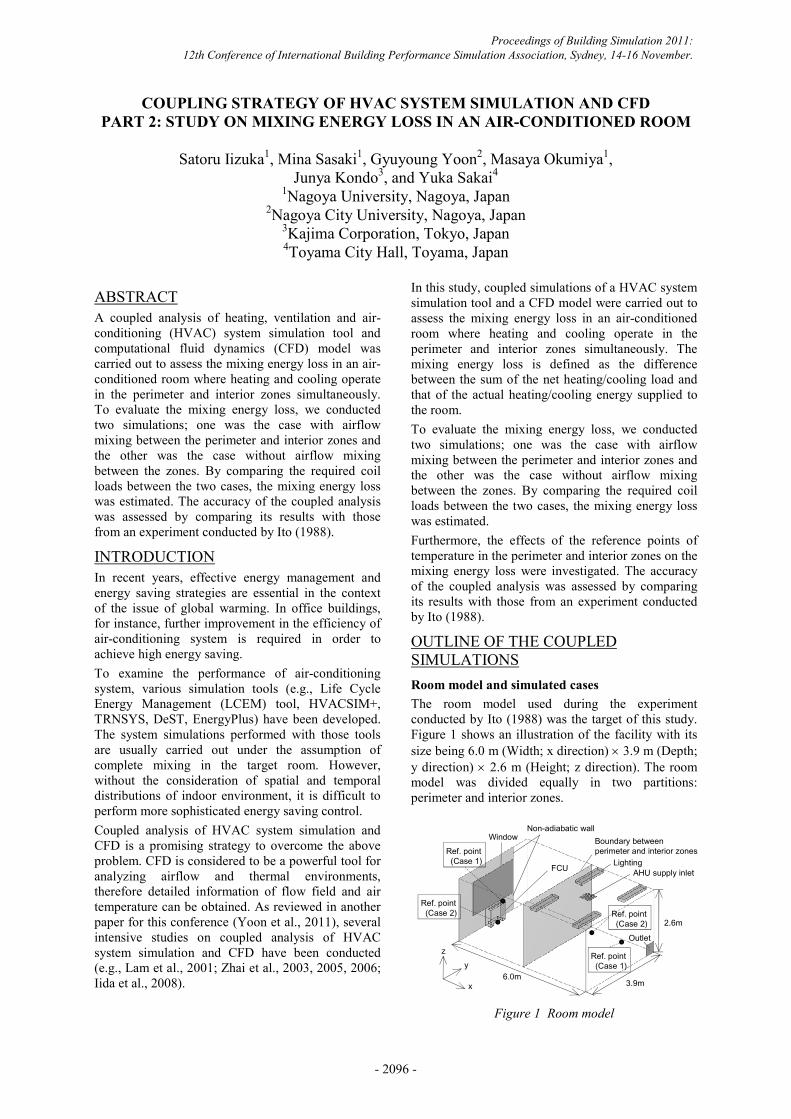
OUTLINE OF THE COUPLEDSIMULATIONSRoom model and simulated casesThe room model used during the experimentconducted by Ito (1988) was the target of this study.Figure 1 shows an illustration of the facility with itssize being 6.0 m (Width;; x direction) 3.9 m (Depth;;y direction) 2.6 m (Height;; z direction). The roommodel was divided equally in two partitions:perimeter and interior zones.

[

\]

PP

P

$+8 VXSSO\ LQOHW/LJKWLQJ

:LQGRZ

2XWOHW

)&8

1RQDGLDEDWLF ZDOO%RXQGDU\ EHWZHHQSHULPHWHU DQG LQWHULRU ]RQHV5HI SRLQW

&DVH

5HI SRLQW&DVH 5HI SRLQW

&DVH

5HI SRLQW&DVH

Figure 1 Room model

Proceedings of Building Simulation 2011: 12th Conference of International Building Performance Simulation Association, Sydney, 14-16 November.

- 2096 -

A fan coil unit (FCU) was installed on the floor ofthe perimeter zone for heating, while a supply inletfrom an air handling unit (AHU) was mounted on theceiling of the interior zone for cooling. The supplyair volumes of FCU and AHU were constant (FCU:320 m3/h, AHU: 325 m3/h). The lighting in theinterior zone was considered as the only internal heatsource (320 W).All walls were adiabatic except the window and itssurrounding wall in the perimeter zone, making it theonly place where heat transfer occurs. The airtemperature outside the window and its surroundingwall was set at 5 °C.The setting temperature in both perimeter and interiorzones was 19 °C. The reference points of temperature,as shown in Figure 1, were different for the two testcases (Cases 1 and 2). In Case 1, the reference pointsin the perimeter and interior zones were located nearthe supply inlet of FCU and at the center of the wallwith an exhaust outlet, respectively, while in Case 2,the reference points in the perimeter and interiorzones were set at the suction opening of FCU and atthe center of the interior zone, respectively.In the experiment conducted by Ito (1988), for bothCases 1 and 2, additional tests with a vinyl-sheetpartition at the boundary between the perimeter andinterior zones were carried out. The mixing energyloss in the experiment was estimated by comparingthe required coil loads between the cases with andwithout the vinyl-sheet partition.In the coupled simulations conducted in this study,we performed additional simulations with a “virtual”adiabatic wall at the boundary between the perimeterand interior zones. Like the estimation in theexperiment, we assessed the mixing energy loss inthe room model by comparing the required coil loadsbetween the cases with and without the virtualadiabatic wall.

HVAC system simulationThe HVAC system simulations were performedusing LCEM tool ver.3.02 developed under thesupervision of the Ministry of Land, Infrastructure,Transport and Tourism (MLIT) of Japan. Table 1shows the specifications of FCU (perimeter zone)and AHU (interior zone) determined based on theresults of heat load calculations.

Table 1 Specifications of FCU and AHU

FCU (PERIMETER ZONE)Supply air volume : 320 m3/hHot water volume : 5.0 l/minHot water temperature : 55-50 CHeating capacity : 3.2 kWAHU (INTERIOR ZONE)Supply air volume : 325 m3/hChilled water volume : 3.6 l/minChilled water temperature : 7-12 CCooling capacity : 1.3 kW

CFDThe airflow and thermal simulations in the roommodel (cf. Figure 1) were conducted using acommercial CFD software, STREAM ver.8. Theanalysis conditions are shown in Table 2. We usedthe standard k- model as the turbulence model. Thetotal number of the grid points was 70,848. In bothCases 1 and 2, the value of the wall coordinate at thefirst grid point adjacent to the wall was around 20-50.

Table 2 CFD analysis conditions

Grid points 64 (x) × 41 (y) × 27 (z) = 70,848Scheme forconvectionterms

1st-order upwind scheme for allgoverning equations

Turbulencemodel

Standard k- model

Inlet boundarycondition

FCU (PERIMETER ZONE)Velocity : 320 m3/hTemp. : PID control (22-26 C)Humidity : Results from HVAC

system simulationk : 1.07×10-2 m2/s2

: 4.68×10-3 m2/s3

AHU (INTERIOR ZONE)Velocity : 325 m3/hTemp. : PID control (14-18 C)Humidity : Results from HVAC

system simulationk : 2.98×10-3 m2/s2

: 4.56×10-4 m2/s3

Outlet boundarycondition

Zero-gradient conditions for allvariables

Wall boundarycondition

Velocity : Logarithmic lawTemp. : Overall heat transfer

coefficients for windowand its surroundingwall were 3.33 W/m2Kand 0.50 W/m2K,respectively. For otherwalls, adiabaticconditions were used.

Humidity : Impermeableconditions withoutcondensation

Heat generation Lighting (interior zone): 320 W

Coupling of HVAC system simulation and CFDThe detailed information on the coupling method ofHVAC system simulation (LCEM tool) and CFD(STREAM) is described in another paper for thisconference (Yoon et al., 2011).In the coupled simulations conducted here, for bothFCU and AHU, the air temperature and humidity atthe exhaust outlet calculated by the CFD simulationwere imposed to the HVAC system simulation. Thehumidity at the supply inlet obtained with the HVACsystem simulation was given to the CFD simulationas boundary conditions. The temperature at the


- 2097 -

supply inlet was provided by a PID control. Thoseprocesses were performed every 30 seconds.

RESULTS AND DISCUSSIONThe following results obtained with the coupledsimulations were those at 6000 seconds from the startof the simulations. The indoor environment at thattime was considered as a statistically steady state.

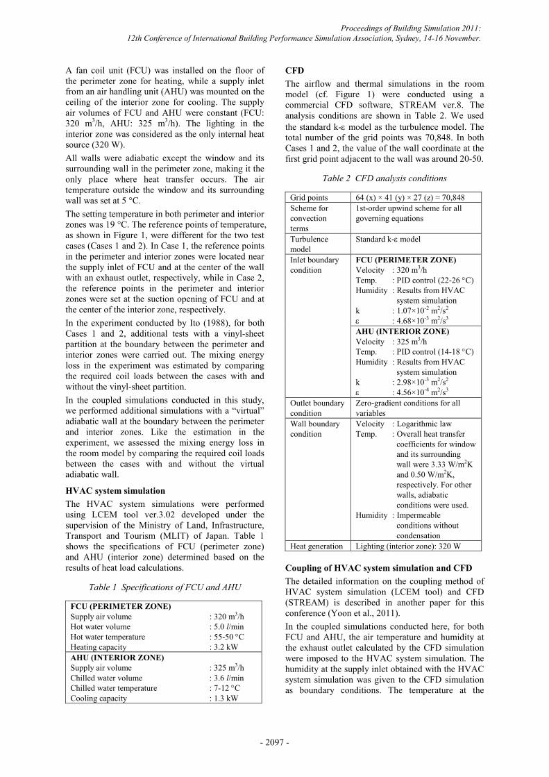
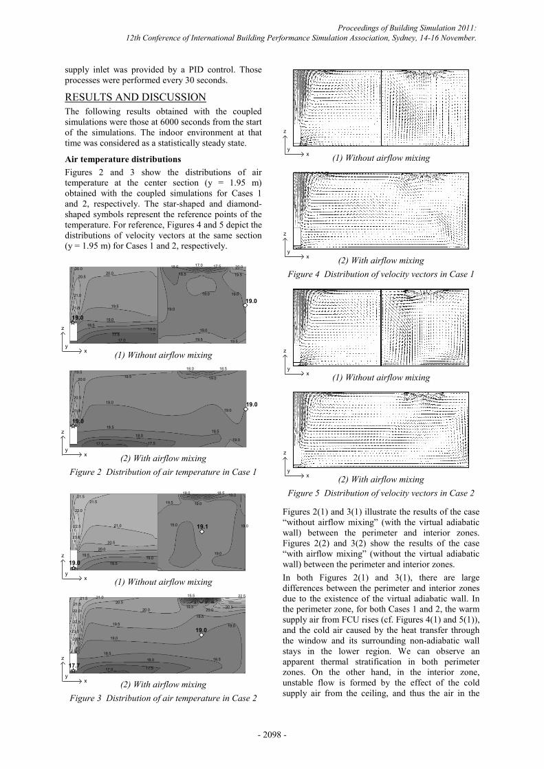
Air temperature distributionsFigures 2 and 3 show the distributions of airtemperature at the center section (y = 1.95 m)obtained with the coupled simulations for Cases 1and 2, respectively. The star-shaped and diamond-shaped symbols represent the reference points of thetemperature. For reference, Figures 4 and 5 depict thedistributions of velocity vectors at the same section(y = 1.95 m) for Cases 1 and 2, respectively.

19.0

19.0

20.0

19.5

19.018.5

18.017.5

20.0

20.5

21.0

21.5

18.5

19.0

19.0

19.5 19.5

19.0 19.0

19.5

20.018.0 17.517.0

17.0

(1) Without airflow mixing

19.0

19.0

19.0

19.0

19.0

18.518.5

18.0

17.517.0

19.0

18.518.0

19.519.5

20.0

20.5

21.0

(2) With airflow mixing

Figure 2 Distribution of air temperature in Case 1

20.5

19.1

19.0

21.0

21.521.5

22.0

22.5

23.0

19.519.0

20.0

18.5

19.0

19.0

19.019.5

19.0

19.018.518.0


19.0

17.7

20.0

20.521.021.5

21.5

22.0

22.5

23.0

23.5

19.5

19.5

19.0

18.5

18.0

17.517.0

18.5

19.0

20.020.5

22.5

19.5

15.5


Figure 3 Distribution of air temperature in Case 2



Figure 4 Distribution of velocity vectors in Case 1



Figure 5 Distribution of velocity vectors in Case 2

Figures 2(1) and 3(1) illustrate the results of the case“without airflow mixing” (with the virtual adiabaticwall) between the perimeter and interior zones.Figures 2(2) and 3(2) show the results of the case“with airflow mixing” (without the virtual adiabaticwall) between the perimeter and interior zones.In both Figures 2(1) and 3(1), there are largedifferences between the perimeter and interior zonesdue to the existence of the virtual adiabatic wall. Inthe perimeter zone, for both Cases 1 and 2, the warmsupply air from FCU rises (cf. Figures 4(1) and 5(1)),and the cold air caused by the heat transfer throughthe window and its surrounding non-adiabatic wallstays in the lower region. We can observe anapparent thermal stratification in both perimeterzones. On the other hand, in the interior zone,unstable flow is formed by the effect of the coldsupply air from the ceiling, and thus the air in the

z

xy

z

xy

z

xy

z

xy

z

xy

z

xy

z

xy

z

xy


- 2098 -

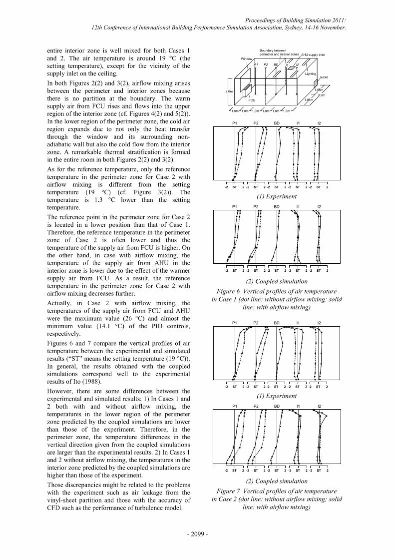
entire interior zone is well mixed for both Cases 1and 2. The air temperature is around 19 °C (thesetting temperature), except for the vicinity of thesupply inlet on the ceiling.In both Figures 2(2) and 3(2), airflow mixing arisesbetween the perimeter and interior zones becausethere is no partition at the boundary. The warmsupply air from FCU rises and flows into the upperregion of the interior zone (cf. Figures 4(2) and 5(2)).In the lower region of the perimeter zone, the cold airregion expands due to not only the heat transferthrough the window and its surrounding non-adiabatic wall but also the cold flow from the interiorzone. A remarkable thermal stratification is formedin the entire room in both Figures 2(2) and 3(2).As for the reference temperature, only the referencetemperature in the perimeter zone for Case 2 withairflow mixing is different from the settingtemperature (19 °C) (cf. Figure 3(2)). Thetemperature is 1.3 °C lower than the settingtemperature.The reference point in the perimeter zone for Case 2is located in a lower position than that of Case 1.Therefore, the reference temperature in the perimeterzone of Case 2 is often lower and thus thetemperature of the supply air from FCU is higher. Onthe other hand, in case with airflow mixing, thetemperature of the supply air from AHU in theinterior zone is lower due to the effect of the warmersupply air from FCU. As a result, the referencetemperature in the perimeter zone for Case 2 withairflow mixing decreases further.Actually, in Case 2 with airflow mixing, thetemperatures of the supply air from FCU and AHUwere the maximum value (26 °C) and almost theminimum value (14.1 °C) of the PID controls,respectively.Figures 6 and 7 compare the vertical profiles of airtemperature between the experimental and simulatedresults (“ST” means the setting temperature (19 °C)).In general, the results obtained with the coupledsimulations correspond well to the experimentalresults of Ito (1988).However, there are some differences between theexperimental and simulated results;; 1) In Cases 1 and2 both with and without airflow mixing, thetemperatures in the lower region of the perimeterzone predicted by the coupled simulations are lowerthan those of the experiment. Therefore, in theperimeter zone, the temperature differences in thevertical direction given from the coupled simulationsare larger than the experimental results. 2) In Cases 1and 2 without airflow mixing, the temperatures in theinterior zone predicted by the coupled simulations arehigher than those of the experiment.Those discrepancies might be related to the problemswith the experiment such as air leakage from thevinyl-sheet partition and those with the accuracy ofCFD such as the performance of turbulence model.

3 3 %' ,

)&8

,

P

P

PP

%RXQGDU\ EHWZHHQSHULPHWHU DQG LQWHULRU ]RQHV $+8 VXSSO\ LQOHW

:LQGRZ

/LJKWLQJRXWOHW

P P P P P P

(1) Experiment

(2) Coupled simulation

Figure 6 Vertical profiles of air temperature

in Case 1 (dot line: without airflow mixing;; solid

line: with airflow mixing)

(1) Experiment

(2) Coupled simulation

Figure 7 Vertical profiles of air temperature



P1 P2 BD I1 I2

ST 2-2 ST 2-2 ST 2-2ST 2-2ST 2-2

P1 P2 BD I1 I2

ST 2-2 ST 2-2 ST 2-2ST 2-2ST 2-2

P1 P2 BD I1 I2

ST 2-2 ST 2-2 ST 2-2ST 2-2ST 2-2

P1 P2 BD I1 I2

ST 2-2 ST 2-2 ST 2-2ST 2-2ST 2-2


- 2099 -

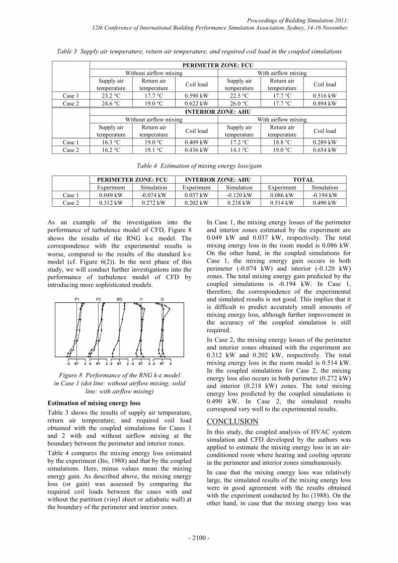
Table 3 Supply air temperature, return air temperature, and required coil load in the coupled simulations

PERIMETER ZONE: FCUWithout airflow mixing With airflow mixing

Supply airtemperature

Return airtemperature Coil load Supply air

temperatureReturn airtemperature Coil load

Case 1 23.2 °C 17.7 °C 0.590 kW 22.5 °C 17.7 °C 0.516 kWCase 2 24.6 °C 19.0 °C 0.622 kW 26.0 °C 17.7 °C 0.894 kW

INTERIOR ZONE: AHUWithout airflow mixing With airflow mixing

Supply airtemperature

Return airtemperature Coil load Supply air

temperatureReturn airtemperature Coil load

Case 1 16.3 °C 19.0 °C 0.409 kW 17.2 °C 18.8 °C 0.289 kWCase 2 16.2 °C 19.1 °C 0.436 kW 14.1 °C 19.0 °C 0.654 kW

Table 4 Estimation of mixing energy loss/gain

PERIMETER ZONE: FCU INTERIOR ZONE: AHU TOTALExperiment Simulation Experiment Simulation Experiment Simulation

Case 1 0.049 kW -0.074 kW 0.037 kW -0.120 kW 0.086 kW -0.194 kWCase 2 0.312 kW 0.272 kW 0.202 kW 0.218 kW 0.514 kW 0.490 kW

As an example of the investigation into theperformance of turbulence model of CFD, Figure 8shows the results of the RNG k- model. Thecorrespondence with the experimental results isworse, compared to the results of the standard k-model (cf. Figure 6(2)). In the next phase of thisstudy, we will conduct further investigations into theperformance of turbulence model of CFD byintroducing more sophisticated models.

Figure 8 Performance of the RNG k- model



Estimation of mixing energy lossTable 3 shows the results of supply air temperature,return air temperature, and required coil loadobtained with the coupled simulations for Cases 1and 2 with and without airflow mixing at theboundary between the perimeter and interior zones.Table 4 compares the mixing energy loss estimatedby the experiment (Ito, 1988) and that by the coupledsimulations. Here, minus values mean the mixingenergy gain. As described above, the mixing energyloss (or gain) was assessed by comparing therequired coil loads between the cases with andwithout the partition (vinyl sheet or adiabatic wall) atthe boundary of the perimeter and interior zones.

In Case 1, the mixing energy losses of the perimeterand interior zones estimated by the experiment are0.049 kW and 0.037 kW, respectively. The totalmixing energy loss in the room model is 0.086 kW.On the other hand, in the coupled simulations forCase 1, the mixing energy gain occurs in bothperimeter (-0.074 kW) and interior (-0.120 kW)zones. The total mixing energy gain predicted by thecoupled simulations is -0.194 kW. In Case 1,therefore, the correspondence of the experimentaland simulated results is not good. This implies that itis difficult to predict accurately small amounts ofmixing energy loss, although further improvement inthe accuracy of the coupled simulation is stillrequired.In Case 2, the mixing energy losses of the perimeterand interior zones obtained with the experiment are0.312 kW and 0.202 kW, respectively. The totalmixing energy loss in the room model is 0.514 kW.In the coupled simulations for Case 2, the mixingenergy loss also occurs in both perimeter (0.272 kW)and interior (0.218 kW) zones. The total mixingenergy loss predicted by the coupled simulations is0.490 kW. In Case 2, the simulated resultscorrespond very well to the experimental results.

CONCLUSIONIn this study, the coupled analysis of HVAC systemsimulation and CFD developed by the authors wasapplied to estimate the mixing energy loss in an air-conditioned room where heating and cooling operatein the perimeter and interior zones simultaneously.In case that the mixing energy loss was relativelylarge, the simulated results of the mixing energy losswere in good agreement with the results obtainedwith the experiment conducted by Ito (1988). On theother hand, in case that the mixing energy loss was

P1 P2 BD I1 I2P1 P2 BD I1 I2

ST 2-2 ST 2-2 ST 2-2ST 2-2ST 2-2


- 2100 -

relatively small, the correspondence of theexperimental and simulated results was not good.Although further improvement in the accuracy is stillrequired, such coupled simulations are very useful toanalyze indoor environment and to perform effectiveenergy management and energy saving in air-conditioned rooms where complete mixing cannot beassumed.

ACKNOWLEDGEMENTThe present work was supported by the EnvironmentResearch and Technology Development Fund(Principal investigator: Prof. Takayuki Morikawa,Nagoya University).

REFERENCESIida, R., Shiraishi, Y., Sagara, N. 2008. Study on

control and diagnosis of HVAC systems for anoffice space, Part 3, Case studies for coupledsimulation of CFD analysis and HVACSIM+(J),Summaries of technical papers of AnnualMeeting Architectural Institute of Japan, D-2,1379-1380 (in Japanese).

Ito, N. 1988. Ph.D. Thesis, Nagoya University.Lam, J.C., Chan, A.L.S. 2001. CFD analysis and

energy simulation of a gymnasium, Building andEnvironment, 36, 351-358.

Yoon, G., Kondo, J., Sakai, Y., Watanabe, T., Iizuka,S., Okumiya, M. 2011. Coupling strategy ofHVAC system simulation and CFD, Part 1,Study on air conditioning system using OA floorin design phase, Submitted to BuildingSimulation 2011.

Zhai, Z., Chen, Q. 2003. Solution characters ofiterative coupling between energy simulation andCFD programs, Energy and Building, 35, 493-505.

Zhai, Z., Chen, Q. 2005. Performance of coupledbuilding energy and CFD simulations, Energyand Buildings, 37, 333-344.

Zhai, Z., Chen, Q. 2006. Sensitivity analysis andapplication guides for integrated building energyand CFD simulation, Energy and Buildings, 38,1060-1068.


- 2101 -

coupling strategy of hvac system · pdf fileperform more sophisticated energy saving control....

Documents