Nonlinear DynDOI 10.1007/s11071-014-1567-y

ORIGINAL PAPER

Coupled axial-torsional dynamics in rotary drillingwith state-dependent delay: stability and control

Xianbo Liu · Nicholas Vlajic · Xinhua Long ·Guang Meng · Balakumar Balachandran

Received: 4 February 2013 / Accepted: 30 June 2014© Springer Science+Business Media Dordrecht 2014

Abstract Nonlinear motions of a rotary drillingmechanism are considered, and a two degree-of-freedom model is developed to study the coupled axial-torsional dynamics of this system. In the model devel-opment, state-dependent time delay and nonlinearitiesthat arise due to dry friction and loss of contact are con-sidered. Stability analysis is carried out by using a semi-discretization scheme, and the results are presentedin terms of stability volumes in the three-dimensionalparameter space of spin speed, cutting depth, and acutting coefficient. These stability volume plots canserve as a guide for choosing parameters for rotarydrilling operations. A control strategy based on stateand delayed-state feedback is presented with the goalof enlargening the stability region, and the effective-

X. Liu · X. Long · G. MengState Key Laboratory of Mechanical System and Vibration,School of Mechanical Engineering, Shanghai Jiao TongUniversity, Shanghai 200240, Chinae-mail:liuxianbo@sjtu.edu.cn

X. Longe-mail:xhlong@sjtu.edu.cn

G. Menge-mail:gmeng@sjtu.edu.cn

N. Vlajic · B. Balachandran (B)Department of Mechanical Engineering, University ofMaryland, College Park, MD 20742, USAe-mail:balab@umd.edu

N. Vlajice-mail:vlajic@umd.edu

ness of this strategy to suppress stick-slip oscillationsis illustrated.

Keywords Drill string · State-dependent time delay ·Stability analysis · Semi-discretization method ·Stick-slip vibrations · Vibration control

1 Introduction

Drill strings are a main component of rotary drillingsystems, which are used to drill deep boreholes for theexploration of oil and natural gas. As illustrated in Fig.1, a typical drill string system consists of a drill bit, thedrill collars, and the drill pipes. The drill bit, which islocated at the bottom of the wellbore, is used to breakup rock formations, while the drill collars are used toapply weight to the drill bit. The combination of thedrill bit and the drill collar illustrated in Fig. 1 is alsoreferred to as the bottom-hole-assembly (BHA). For adetailed description on the drill-string system, one canrefer to the books such as the one by Bommer [1]. Thedrilling system is prone to destructive vibrations andexpensive drill-bit failures due to the high structuralflexibility and nonlinear bit-rock forces. Field mea-surements [2,3] show that the rotary speed range ofdrill bit extends from zero up to twice that of the spin-ning speed of the top motor. This self-exited torsionalvibration is also referred to as stick-slip vibration.In order to further understand the underlying mech-anisms of stick-slip vibrations in drill strings, models

123

X. Liu et al.

Fig. 1 Representative drill-string system

with one degree of freedom, two degrees of freedom,and eight degrees of freedom have been proposed [4–7]. Different friction models have been used by sev-eral authors to study bit-rock interactions and relatedstick-slip effects [4,6,8]. Due to bit-rock cutting, time-delay effects are also considered to be another causeof destructive drill-string vibrations. Time-dependentand state-dependent delay effects have been reportedand studied in manufacturing operations, for exam-ple, the studies of Long, Balachandran, and Mann [9]and Insperger, Stépán, and co-workers [10,11]. Simi-lar to the regenerative effects [12–14] encountered inmetal cutting operations, Richard, Germay and Detour-nay [15,16] proposed time-delay effects in a nonlinearmodel of the drill-string system. They also show thatthe time delay is a root cause of self-excited vibra-tions for both axial and torsional motions and that thetime delay in the drilling process is a state-dependentquantity. After linearization, they were able to uncouplethe torsional and axial vibrations, and study the systemdynamics and stability using the approximation con-sisting of two identical third-order differential equa-tions. In the efforts of Besselink, Wouw and Nijmeijer[17], a modified model for axial and torsional vibrationsis presented based on the state-dependent time-delaymodel presented in earlier work [15]. In the modifiedmodel construction, axial stiffness and axial damping

are taken into consideration but torsional damping isignored. It is noted that Besselink et al. [17] and Richardet al. [16] also examined the uncoupled axial and tor-sional case by exploiting different time scales in thesystem. In the current work, torsion damping is takeninto account in the proposed delay system model and acompletely coupled axial-torsional case is consideredby the authors. The stability of this system incorporat-ing state-dependent delay can be determined.

In order to attenuate undesirable vibrations of a drillstring, different active control methods have been stud-ied [4,18–25]. Jansen and van den Steen [19] useda feedback controller to extend the working rangethrough a vibration-free zone constructed based on asimple torsion pendulum model. Tucker and Wang [20]presented a control approach using feedback throughthe drive torque input to control torsional slip-stickoscillations due to nonlinear friction. Karkoub et al.[25] also studied control of torsional oscillations, andin their control scheme, genetic algorithms were used.Recently, de Bruin et al. [24] proposed a state-feedbackcontroller based on a Popov-like criterion. They intro-duced a model that included set-valued nonlinearitiesand used both simulations and experiments to showthe effectiveness of the scheme for controlling torsionalvibrations. While in these prior studies, there has been afocus on the control of torsional vibrations and nonlin-earities that originate from the chosen friction model,axial vibrations and time delay effects, which are oneof the primary causes of stick-slip vibrations, have notbeen considered.

A goal of the current work is to determine the rangeof stability for the coupled axial-torsional motions inthe presence of state-dependent delay as well as toinvestigate the effectiveness of a feedback controller tosuppress stick-slip vibrations. The remaining sectionsof this article have been put together as follows. Build-ing on earlier efforts [15,17], in Sect. 2, an enhancedmodel for the drill string to study both axial and tor-sional vibrations is proposed. In Sect. 3, nondimen-sional parameters are introduced and the system islinearized about a nominal operating point accordingto the procedure outlined in references [16,17]. Fol-lowing that, a stability analysis is carried out usinga semi-discretization method [26,27] and the stabilityvolume is constructed in a multi-parameter space. InSect. 4, control schemes with choices of optimal feed-back gains are presented and the enlargement of thestability regions in the controlled system is studied. As

123

Coupled axial-torsional dynamics in rotary drilling

a demonstration of the effectiveness of the controller,elimination of nonlinear stick-slip oscillations in thecoupled axial-torsional system is considered. Finally,concluding remarks are provided.

2 Modeling of drill-string motions, bit-rockinteractions, and delay effects

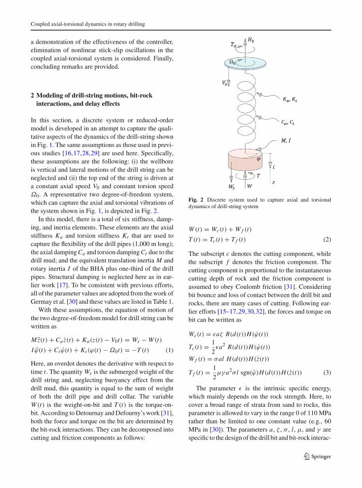
In this section, a discrete system or reduced-ordermodel is developed in an attempt to capture the quali-tative aspects of the dynamics of the drill-string shownin Fig. 1. The same assumptions as those used in previ-ous studies [16,17,28,29] are used here. Specifically,these assumptions are the following: (i) the wellboreis vertical and lateral motions of the drill string can beneglected and (ii) the top end of the string is driven ata constant axial speed V0 and constant torsion speedΩ0. A representative two degree-of-freedom system,which can capture the axial and torsional vibrations ofthe system shown in Fig. 1, is depicted in Fig. 2.

In this model, there is a total of six stiffness, damp-ing, and inertia elements. These elements are the axialstiffness Ka and torsion stiffness Kt that are used tocapture the flexibility of the drill pipes (1,000 m long);the axial damping Ca and torsion damping Ct due to thedrill mud; and the equivalent translation inertia M androtary inertia I of the BHA plus one-third of the drillpipes. Structural damping is neglected here as in ear-lier work [17]. To be consistent with previous efforts,all of the parameter values are adopted from the work ofGermay et al. [30] and these values are listed in Table 1.

With these assumptions, the equation of motion ofthe two degree-of-freedom model for drill string can bewritten as

Mz(t)+ Caz(t)+ Ka(z(t)− V0t) = Ws − W (t)

I ϕ(t)+ Ct ϕ(t)+ Kt (ϕ(t)−Ω0t) = −T (t) (1)

Here, an overdot denotes the derivative with respect totime t . The quantity Ws is the submerged weight of thedrill string and, neglecting buoyancy effect from thedrill mud, this quantity is equal to the sum of weightof both the drill pipe and drill collar. The variableW (t) is the weight-on-bit and T (t) is the torque-on-bit. According to Detournay and Defourny’s work [31],both the force and torque on the bit are determined bythe bit-rock interactions. They can be decomposed intocutting and friction components as follows:

Fig. 2 Discrete system used to capture axial and torsionaldynamics of drill-string system

W (t) = Wc(t)+ W f (t)

T (t) = Tc(t)+ T f (t) (2)

The subscript c denotes the cutting component, whilethe subscript f denotes the friction component. Thecutting component is proportional to the instantaneouscutting depth of rock and the friction component isassumed to obey Coulomb friction [31]. Consideringbit bounce and loss of contact between the drill bit androcks, there are many cases of cutting. Following ear-lier efforts [15–17,29,30,32], the forces and torque onbit can be written as

Wc(t) = εaζ R(d(t))H(ϕ(t))

Tc(t) = 1

2εa2 R(d(t))H(ϕ(t))

W f (t) = σal H(d(t))H(z(t))

T f (t) = 1

2μγ a2σ l sgn(ϕ)H(d(t))H(z(t)) (3)

The parameter ε is the intrinsic specific energy,which mainly depends on the rock strength. Here, tocover a broad range of strata from sand to rocks, thisparameter is allowed to vary in the range 0 of 110 MParather than be limited to one constant value (e.g., 60MPa in [30]). The parameters a, ζ , σ , l, μ, and γ arespecific to the design of the drill bit and bit-rock interac-

123

X. Liu et al.

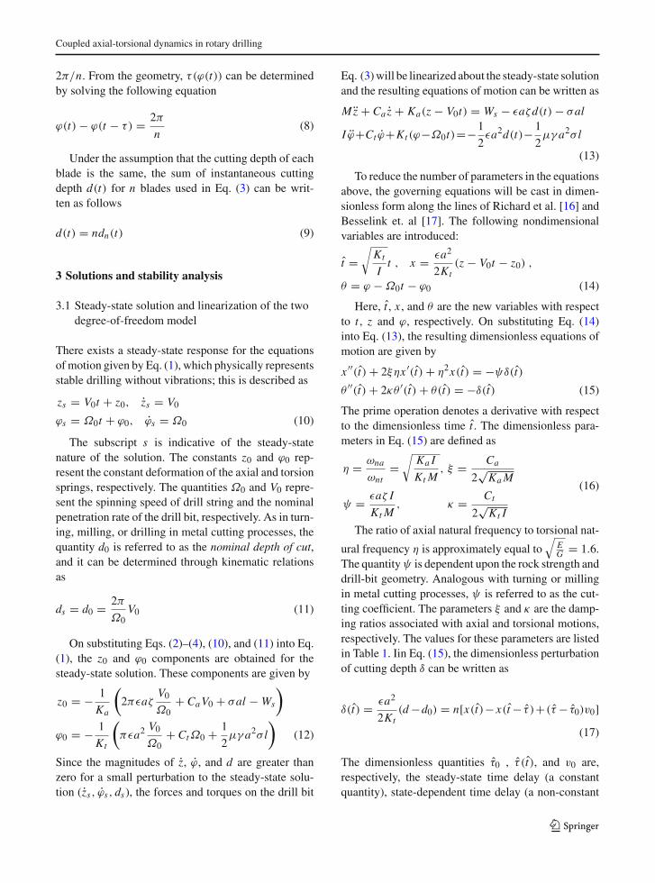
Table 1 Differentparameters and quanitities[30]

Quantities Symbol Value Units

Discrete mass M 3.4e4 kg

Discrete rotary inertia I 116 kg m2

Axial stiffness Ka 7.0e5 N/m

Torsion stiffness Kt 938 Nm/rad

Axial damping Ca 1.56e4 N s/m

Torsion damping Ct 32.9 N s m/rad

Intrinsic specific energy of rock ε 0–110 MPa

Contact strength σ 60 MPa

Radius of drill bit a 108 mm

Wearflat length of drill bit l 1.2 mm

Cutter face inclination ζ 0.6 –

Frictional coefficient for rock-bit interaction μ 0.6 –

Geometry parameter of drill bit γ 1 –

Number of blades on drill bit n 4 –

Ratio of axial to torsion natural frequencies η 1.6 –

Axial damping ratio ξ 0–0.05 –

Torsion damping ratio κ 0–0.05 –

Dimensionless cutting coefficient ψ 0–26.0 –

Dimensionless angular driving speed ω0 0–25.0 –

Dimensionless nominal depth of cut δ0 0–25.0 –

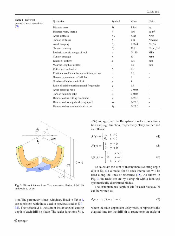
Fig. 3 Bit-rock interactions: Two successive blades of drill bitand rocks to be cut

tion. The parameter values, which are listed in Table 1,are consistent with those used in previous studies [30–32]. The variable d is the sum of instantaneous cuttingdepth of each drill-bit blade. The scalar functions R(·),

H(·) and sgn(·) are the Ramp function, Heaviside func-tion and Sign function, respectively. They are definedas follows:

R(y) ={

y, y ≥ 00, y < 0

(4)

H(y) ={

1, y ≥ 00, y < 0

(5)

sgn(y) =⎧⎨⎩

1, y > 00, y = 0−1, y < 0

(6)

To calculate the sum of instantaneous cutting depthd(t) in Eq. (3), a model for bit-rock interaction will beused along the lines of reference [15]. As shown inFig. 3, the rocks are cut by a drag bit with n identicalsymmetrically distributed blades.

The instantaneous depth of cut for each blade dn(t)can be written as

dn(t) = z(t)− z(t − τ) (7)

where the state-dependent delay τ(ϕ(t)) represents theelapsed time for the drill bit to rotate over an angle of

123

Coupled axial-torsional dynamics in rotary drilling

2π/n. From the geometry, τ(ϕ(t)) can be determinedby solving the following equation

ϕ(t)− ϕ(t − τ) = 2π

n(8)

Under the assumption that the cutting depth of eachblade is the same, the sum of instantaneous cuttingdepth d(t) for n blades used in Eq. (3) can be writ-ten as follows

d(t) = ndn(t) (9)

3 Solutions and stability analysis

3.1 Steady-state solution and linearization of the twodegree-of-freedom model

There exists a steady-state response for the equationsof motion given by Eq. (1), which physically representsstable drilling without vibrations; this is described as

zs = V0t + z0, zs = V0

ϕs = Ω0t + ϕ0, ϕs = Ω0 (10)

The subscript s is indicative of the steady-statenature of the solution. The constants z0 and ϕ0 rep-resent the constant deformation of the axial and torsionsprings, respectively. The quantities Ω0 and V0 repre-sent the spinning speed of drill string and the nominalpenetration rate of the drill bit, respectively. As in turn-ing, milling, or drilling in metal cutting processes, thequantity d0 is referred to as the nominal depth of cut,and it can be determined through kinematic relationsas

ds = d0 = 2π

Ω0V0 (11)

On substituting Eqs. (2)–(4), (10), and (11) into Eq.(1), the z0 and ϕ0 components are obtained for thesteady-state solution. These components are given by

z0 = − 1

Ka

(2πεaζ

V0

Ω0+ Ca V0 + σal − Ws

)

ϕ0 = − 1

Kt

(πεa2 V0

Ω0+ CtΩ0 + 1

2μγ a2σ l

)(12)

Since the magnitudes of z, ϕ, and d are greater thanzero for a small perturbation to the steady-state solu-tion (zs, ϕs, ds), the forces and torques on the drill bit

Eq. (3) will be linearized about the steady-state solutionand the resulting equations of motion can be written as

Mz + Caz + Ka(z − V0t) = Ws − εaζd(t)− σal

I ϕ+Ct ϕ+Kt (ϕ−Ω0t)=−1

2εa2d(t)− 1

2μγ a2σ l

(13)

To reduce the number of parameters in the equationsabove, the governing equations will be cast in dimen-sionless form along the lines of Richard et al. [16] andBesselink et. al [17]. The following nondimensionalvariables are introduced:

t =√

Kt

It , x = εa2

2Kt(z − V0t − z0) ,

θ = ϕ −Ω0t − ϕ0 (14)

Here, t , x , and θ are the new variables with respectto t , z and ϕ, respectively. On substituting Eq. (14)into Eq. (13), the resulting dimensionless equations ofmotion are given by

x ′′(t)+ 2ξηx ′(t)+ η2x(t) = −ψδ(t)θ ′′(t)+ 2κθ ′(t)+ θ(t) = −δ(t) (15)

The prime operation denotes a derivative with respectto the dimensionless time t . The dimensionless para-meters in Eq. (15) are defined as

η = ωna

ωnt=

√Ka I

Kt M, ξ = Ca

2√

Ka M

ψ = εaζ I

Kt M, κ = Ct

2√

Kt I

(16)

The ratio of axial natural frequency to torsional nat-

ural frequency η is approximately equal to√

EG = 1.6.

The quantityψ is dependent upon the rock strength anddrill-bit geometry. Analogous with turning or millingin metal cutting processes, ψ is referred to as the cut-ting coefficient. The parameters ξ and κ are the damp-ing ratios associated with axial and torsional motions,respectively. The values for these parameters are listedin Table 1. Iin Eq. (15), the dimensionless perturbationof cutting depth δ can be written as

δ(t) = εa2

2Kt(d −d0) = n[x(t)− x(t − τ )+ (τ− τ0)v0]

(17)

The dimensionless quantities τ0 , τ (t), and v0 are,respectively, the steady-state time delay (a constantquantity), state-dependent time delay (a non-constant

123

X. Liu et al.

quantity), and axial penetration rate (a constant quan-tity), and they are given by

τ0 = 2π

nω0, ω0 =

√I

KtΩ0

τ =√

Kt

I(τ − 2π

nΩ0) , v0 = εa2

2Kt

√I

KtV0

(18)

where ω0 is the dimensionless angular driving speed.Furthermore, τ is the nondimensional perturbed formof the state-dependent delay τ . Upon substituting Eqs.(14) and (18) into Eq. (8), the result is

θ(t)− θ(t − τ )+ (τ − τ0)ω0 = 0 (19)

After substituting Eqs. (17) and (19) into Eq. (15)and eliminating (τ − τ0), the authors obtain

x ′′(t)+ 2ξηx ′(t)+ η2x(t)=−ψn[x(t)− x(t − τ (t))]−ψnδ0[θ(t)− θ(t − τ (t))]

θ ′′(t)+ 2κθ ′(t)+ θ(t) = −n[x(t)− x(t − τ (t))]+ nδ0[θ(t)− θ(t − τ (t))] (20)

where the dimensionless nominal depth of cut δ0 isdefined as

δ0 = v0

ω0= εa2

2Kt

V0

Ω0= εa2

4πKtd0 (21)

The dimensionless equations of motion Eq. (20) arecoupled by the forces on bit through the state-dependentdelay which originates from the term (τ − τ0)v0 in Eq.(17). Equation (20) is nonlinear and can not be analyt-ically solved since τ is the solution of Eq. (19). Basedon the works of Insperger et al. [11] and Besselink etal. [17], the state-dependent delay in Eq. (20) can belinearized by neglecting the perturbation component oftime delay; that is, τ (t) ≡ τ0. The resulting linearizedequations of motion are of the form

x ′′(t)+ 2ξηx ′(t)+ η2x(t) = −ψn[x(t)− x(t − τ0)]−ψnδ0[θ(t)− θ(t − τ0)]

θ ′′(t)+ 2κθ ′(t)+ θ(t) = −n[x(t)− x(t − τ0)]+ nδ0[θ(t)− θ(t − τ0)] (22)

Equations (22) represent a linear system of delay-differential equations (DDEs) with a constant delay τ0.In this system, the axial and torsional dynamics are cou-pled by an additional term [θ(t)− θ(t − τ0)], which isdependent on the state-dependent delay. The equationsof system dynamics shown here (i.e. Eq. 22) have the

same form as those obtained in earlier work [10,11] onturning dynamics, wherein the two coupled equationshave the same natural frequency (i.e., η ≡ 1). Com-paring the current study with a previous one [17], it isnoted that here torsion damping is taken into accountand the stability of the coupled axial-torsion system isanalyzed unlike the previous study.

3.2 Use of semi-discretization method fordetermining stability

The semi-discretization method, which is well knownin computational fluid mechanics, was first presentedby Insperger and Stépán [26,27] for time-delay sys-tems. This semi-numerical method can be used to studythe stability of solutions of DDEs with parametric exci-tation terms. It has been widely used for making sta-bility predications in milling processes. Due to the rel-atively small number of parameters, the stability of thetwo degree-of-freedom system (22) can be solved ana-lytically along the lines of prior work [11]. However,here, the semi-discretization method will be used todetermine the system stability since determining theanalytic form proposed in reference [11] is not feasibleafter the feedback control scheme is implemented inlater sections of this paper. For a general overview ofthe semi-discretization method, the reader is referredto the book by Insperger and Stépán [33].

To use semi-discretization method, Eq. (22) needsto be written in matrix form as

X = A1 X (t)+ A2 X (t − τ0) (23)

where the state variables are assembled into a vectoras

X (t) =

⎛⎜⎜⎝

x(t)x(t)θ(t)θ(t)

⎞⎟⎟⎠ (24)

and the coefficient matrices A1 and A2 are given by

A1 =

⎛⎜⎜⎝

0 1 0 0−η2 − nψ −2ξη nψδ0 0

0 0 0 1−n 0 −1 + nδ0 −2κ

⎞⎟⎟⎠ (25)

A2 =

⎛⎜⎜⎝

0 0 0 0nψ 0 − nψδ0 0

0 0 0 0n 0 −nδ0 0

⎞⎟⎟⎠ (26)

123

Coupled axial-torsional dynamics in rotary drilling

In order to discretize the delay, the time interval divi-sion [ti , ti+1] of length Δ t is constructed in the follow-ing manner

Δ t = τ0

m + 0.5(27)

where m is a integer. Then, a discrete map can bedefined as

yi+1 = Dyi (28)

where the subscript i corresponds to the time t = iΔ t .The vector yi has dimension 2m+4 and its componentsare structured as

yi = (xi , xi , ϕi , ϕi , xi−1 , ϕi−1 , . . .

. . . , ϕi−m+1 , xi−m , ϕi−m)T (29)

wherein the superscript (·)T has been used to denotethe transpose operation. The coefficient matrix D is a(2m +4) dimensional square matrix, which is given by

D =

⎛⎜⎜⎜⎜⎜⎜⎜⎜⎜⎜⎜⎜⎜⎝

P0 · · · 0

R0 · · · 00 · · · 00 · · · 0

1 0 0 0 0 · · · 0 0 00 0 1 0 0 · · · 0 0 00 0 0 0 1 · · · 0 0 0...............

. . ..........

0 0 0 0 0 · · · 1 0 0

⎞⎟⎟⎟⎟⎟⎟⎟⎟⎟⎟⎟⎟⎟⎠

(30)

Here, the P and R matrices are 4×4 and 4×2 matrices,respectively. They can be determined as

P = eA1 Δ t , R = (P − I )A−11 A2 (31)

where the quantity eA1Δ t is the matrix exponential ofA1Δ t . The superscript -1 is used to denote a matrixinversion operation, and the matrix I is the identitymatrix.

The stability of solutions of the discrete map (28)depends on the coefficient matrix D. The system isstable if all of the eigenvalues of D are located withinthe unit circle on the complex plane [34]. Alternatively,the system is stable if the spectral radius of matrix D isless than one and this stability condition can be writtenas

ρ(D) = 2m+4maxi=1

( |λi | ) < 1 (32)

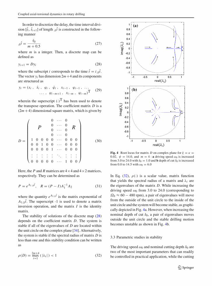
Fig. 4 Root locus for matrix D on complex plane for ξ = κ =0.02, ψ = 14.0, and m = 4 : a driving speed ω0 is increasedfrom 3.0 to 24.0 with δ0 = 1.0 and b depth of cut δ0 is increasedfrom 0.0 to 14.5 with ω0 = 6.0

In Eq. (32), ρ(·) is a scalar value, matrix functionthat yields the spectral radius of a matrix and λi arethe eigenvalues of the matrix D. While increasing thedriving speed ω0 from 3.0 to 24.0 (corresponding toΩ0 ≈ 60 − 480 rpm), a pair of eigenvalues will movefrom the outside of the unit circle to the inside of theunit circle and the system will become stable, as graphi-cally depicted in Fig. 4a. However, when increasing thenominal depth of cut δ0, a pair of eigenvalues movesoutside the unit circle and the stable drilling motionbecomes unstable as shown in Fig. 4b.

3.3 Parametric studies in stability

The driving speed ω0 and nominal cutting depth δ0 aretwo of the most important parameters that can readilybe controlled in practical application, while the cutting

123

X. Liu et al.

Fig. 5 Stability volume fordrilling operations inω0 − ψ − δ0 parameterspace for ξ = κ =0.02, ω0 = 0.5 − 24.0, andψ = 0.1 − 26.0. Thesurface shade correspondsto the nominal depth ofstable cutting

Fig. 6 Cross-sections ofstability volume of Fig. 5 fordifferent cutting coefficientsψ and ξ = κ = 0.02

coefficient ψ varies as the drill bit reaches differentstrata, such as sand or rock. For further parametric stud-ies, a stability volume is obtained numerically using thelinearized model in the three-dimensional ω0 −ψ − δ0

space and the obtained result is shown in Fig. 5. To clar-ify, the region of stability in the volume refers to pointswhere the solution limt→∞ ||X (t)|| = 0. For the lin-ear system, points outside the volume correspond to anunbounded solution; that is, limt→∞ ||X (t)|| = ∞. Itis noted that under certain circumstances the unstablepoints in the linear system may correspond to long-timeresponses in the form of periodic and quasi-periodicmotions of the nonlinear system, as shown in earlierstudies [15–17]. The shaded volume, which takes theshape of an irregular triangular prism, is the stabilityvolume. This region has different characteristics fromthe stability chart of Insperger et al. [11]. Parameter

values corresponding to a point inside the volume willlead to stable drilling (i.e., Eqs. (10)–(12)), while para-meter values corresponding to a point outside the vol-ume will lead to unstable drilling and something thatshould be avoided in practice. As illustrated in Fig. 5,with an increase in the cutting coefficient ψ from 0.1to 26.0, the stable nominal depth of cut increases. Itis also noted that there is no stable region, when ω0 issmaller than a critical value.

Cross-sections of the stability volume of Fig. 5 fordifferent values of the cutting coefficient ψ are shownin Fig. 6, where the shaded areas correspond to stableregions. As ψ is increased, the left boundary movestoward the right while the top boundary moves up andthe total area of the stable region is enlarged. How-ever, as ψ is increased, the minimum threshold valueof the drive speed ω0 needed to ensure stability is also

123

Coupled axial-torsional dynamics in rotary drilling

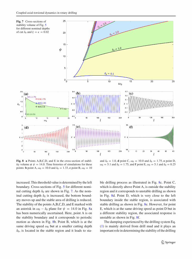
Fig. 7 Cross-sections ofstability volume of Fig. 5for different nominal depthsof cut δ0 and ξ = κ = 0.02

Fig. 8 a Points A,B,C,D, and E in the cross-section of stabil-ity volume at ψ = 14.0. Time histories of simulations for thesepoints: b point A, ω0 = 10.0 and δ0 = 1.33, c point B, ω0 = 10

and δ0 = 1.0, d point C, ω0 = 10.0 and δ0 = 1.75, e point D,ω0 = 5.1 and δ0 = 1.75, and f point E, ω0 = 5.1 and δ0 = 0.25

increased. This threshold value is determined by the leftboundary. Cross-sections of Fig. 5 for different nomi-nal cutting depth δ0 are shown in Fig. 7. As the nom-inal cutting depth δ0 is increased, the bottom bound-ary moves up and the stable area of drilling is reduced.The stability of the points A,B,C,D, and E marked withan asterisk in ω0 − δ0 plane for ψ = 14.0 in Fig. 8ahas been numerically ascertained. Here, point A is onthe stability boundary and it corresponds to periodicmotion as shown in Fig. 8b. Point B, which is at thesame driving speed ω0 but at a smaller cutting depthδ0, is located in the stable region and it leads to sta-

ble drilling process as illustrated in Fig. 8c. Point C,which is directly above Point A, is outside the stabilityregion and it corresponds to unstable drilling as shownin Fig. 8d. Point D, which is very close to the leftboundary inside the stable region, is associated withstable drilling as shown in Fig. 8e. However, for pointE, which is at the same driving speed as point D but ina different stability region, the associated response isunstable as shown in Fig. 8f.

The damping experienced by the drilling system Eq.(1) is mainly derived from drill mud and it plays animportant role in determining the stability of the drilling

123

X. Liu et al.

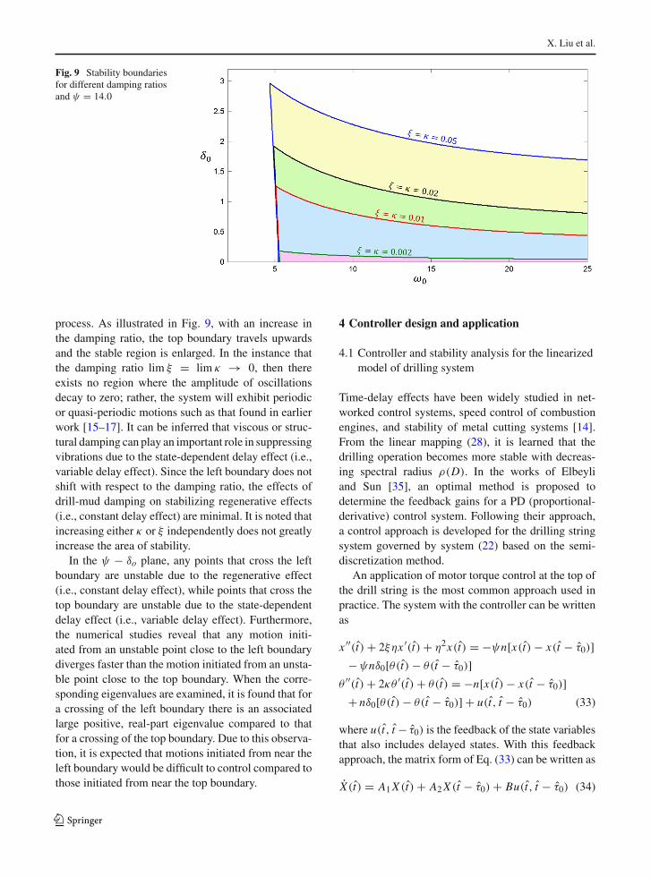
Fig. 9 Stability boundariesfor different damping ratiosand ψ = 14.0

process. As illustrated in Fig. 9, with an increase inthe damping ratio, the top boundary travels upwardsand the stable region is enlarged. In the instance thatthe damping ratio lim ξ = lim κ → 0, then thereexists no region where the amplitude of oscillationsdecay to zero; rather, the system will exhibit periodicor quasi-periodic motions such as that found in earlierwork [15–17]. It can be inferred that viscous or struc-tural damping can play an important role in suppressingvibrations due to the state-dependent delay effect (i.e.,variable delay effect). Since the left boundary does notshift with respect to the damping ratio, the effects ofdrill-mud damping on stabilizing regenerative effects(i.e., constant delay effect) are minimal. It is noted thatincreasing either κ or ξ independently does not greatlyincrease the area of stability.

In the ψ − δo plane, any points that cross the leftboundary are unstable due to the regenerative effect(i.e., constant delay effect), while points that cross thetop boundary are unstable due to the state-dependentdelay effect (i.e., variable delay effect). Furthermore,the numerical studies reveal that any motion initi-ated from an unstable point close to the left boundarydiverges faster than the motion initiated from an unsta-ble point close to the top boundary. When the corre-sponding eigenvalues are examined, it is found that fora crossing of the left boundary there is an associatedlarge positive, real-part eigenvalue compared to thatfor a crossing of the top boundary. Due to this observa-tion, it is expected that motions initiated from near theleft boundary would be difficult to control compared tothose initiated from near the top boundary.

4 Controller design and application

4.1 Controller and stability analysis for the linearizedmodel of drilling system

Time-delay effects have been widely studied in net-worked control systems, speed control of combustionengines, and stability of metal cutting systems [14].From the linear mapping (28), it is learned that thedrilling operation becomes more stable with decreas-ing spectral radius ρ(D). In the works of Elbeyliand Sun [35], an optimal method is proposed todetermine the feedback gains for a PD (proportional-derivative) control system. Following their approach,a control approach is developed for the drilling stringsystem governed by system (22) based on the semi-discretization method.

An application of motor torque control at the top ofthe drill string is the most common approach used inpractice. The system with the controller can be writtenas

x ′′(t)+ 2ξηx ′(t)+ η2x(t) = −ψn[x(t)− x(t − τ0)]−ψnδ0[θ(t)− θ(t − τ0)]

θ ′′(t)+ 2κθ ′(t)+ θ(t) = −n[x(t)− x(t − τ0)]+ nδ0[θ(t)− θ(t − τ0)] + u(t, t − τ0) (33)

where u(t, t − τ0) is the feedback of the state variablesthat also includes delayed states. With this feedbackapproach, the matrix form of Eq. (33) can be written as

X(t) = A1 X (t)+ A2 X (t − τ0)+ Bu(t, t − τ0) (34)

123

Coupled axial-torsional dynamics in rotary drilling

Fig. 10 Block diagram for the time-delay system with control.The elements in the dashed rectangle represent the uncontrolledor original time-delay system governed by system (22) or (23)

where B is the input matrix and is given by

B = (0 0 0 1

)T(35)

The block diagram for the controlled system is illus-trated in Fig. 10. The elements within the red-dashedrectangle correspond to the original system and thematrixes A1, A2, and vector X are given in Eqs. (23) to(26). For a typical drill string, the torque on top can bemonitored and a measure of the torsion vibrations canbe obtained indirectly from the torque or directly froma down-hole measurement [3]. Therefore, the outputmeasurement Y of the system can be written as

Y (t) = C X (t) (36)

In Eq. (36), C is the observability matrix and hastwo possible forms as follows:

Case 1: C = (0 0 1 0

),Case 2: C =

(0 0 1 00 0 0 1

)

(37)

Here, the authors study two control cases of the sys-tem. For the Case 1 system, there is physically one mea-surement, namely, the θ measurement, and for the Case2 system, the measurements include both θ and θ . Feed-back control is carried out for both of these observercases. The feedback control law is constructed as

u = K1Y (t)+ K2Y (t − τ0) (38)

where K1 and K2 are the feedback gains for thestates and the delayed states, respectively. They aredefined as

Case 1:

{K1 = pK2 = q

, Case 2:

{K1 = (p1 p2)

K2 = (q1 q2)(39)

The control law Eq. (38) includes feedback of boththe current output and the delayed output. The effectsof this delayed feedback approach is investigated later.On substituting Eqs. (36)–(39) into Eq. (34), the matrixform of the system takes the form

X = (A1 + BK1C) X (t)+ (A2 + BK2C) X (t − τ0)

(40)

As carried out with Eq. (23), the stability of solu-tions of the system with control Eq. (40) can be deter-mined by using the semi-discretization method follow-ing Eqs. (23)–(32). The feedback gains K1 and K2 areunknowns that will be determined through an optimiza-tion procedure. The stability of the system (40) dependson the spectral radius of matrix D which is a functionof K1 and K2 in the controlled system. This conditionfor stability can be written as

ρ(D(K1, K2)) < 1 (41)

The system is more stable with decreasing ρ(D(K1, K2)), and the feedback gains K1 and K2 are foundthrough the following optimization procedure:

{minimize: ρ(D(K1, K2))

subject to: K1, K2 ∈ [Bnd1,Bnd2] (42)

The terms Bnd1 and Bnd2 are the bounds that aredetermined by the actuator or amplifier limitations andconstraints. Here, the following boundaries are used tolimit the feedback gains for the optimization method

Case 1: p, q ∈ [−10, 10] ,Case 2:

{p1, q1 ∈ [−10, 10]p2, q2 ∈ [−5, 5] (43)

As shown in Fig. 11, by using the same parameters asthose used to carry out the simulations for the unstablemotion shown in Fig. 8d, a curved surface is obtainedby sweeping through the feedback gains. For Case 1,the corresponding equations from Eqs. (37) and (39) areused, and the minimum value on the surface is foundto be min[ρ(D(K1, K2))] = ρ(D(−5.17, 5.06)) =0.979 < 1. From this figure, one can also concludethat the unstable drilling in Fig. 8d can be stablizedby applying the feedback control proposed above, forwhich the optimal feedback gains for the considereddrilling parameters are found to be K1 = −5.17 and

123

X. Liu et al.

Fig. 11 Surface of thespectral radius versusfeedback gainsρ(D(K1, K2)) for Case 1:K1 = p, K2 = q,ξ = κ = 0.02, ψ = 14.0,ω0 = 10, and δ0 = 1.75.Here, the shading on thesurface corresponds to thevalue of spectral radius ρ

Fig. 12 Stabilityboundaries for differentcontrol cases anduncontrolled cases forξ = κ = 0.02 and ψ = 14.0

K2 = 5.06. For Case 2, there are four feedback gainsthat need to be optimized and the variable space is nolonger a surface but a four-dimensional hyper-plane.The MATLAB Optimization Toolbox is used to carryout multivariate optimization.

Further analysis is carried out to study the stabil-ity of drilling operations for the two different controlcases and the results are shown Fig. 12. To obtain theseresults, the authors used the Matlab Optimization Tool-box to solve the control design problem given by Eq.(42). For Case 1 with K2 ≡ 0, which correspondsto only feedback of the current torsion position with-out the delay term in Eq. (38), the stability region isenlarged by 8.2 times compared to the original stabil-ity area without control (ω0 from 0 to 25). Addition-ally, the controller moves the top boundary upward toδ0 = 8.7 but has no effect on the left boundary, whichis difficult to control since that boundary is governedby the regenerative effect as mentioned in Sect. 3.2. By

using Case 1 with two feedback gains for both torsionposition and the delayed torsion position, the stabilityregion is enlarged by the movement of both the topboundary and left boundary and the stability area is17.6 times that for the original system. Here, the leftboundary is changed because of the delay feedback.For Case 2 with four feedback gains corresponding toθ(t), θ (t), θ(t − τ0), and θ (t − τ0), the top boundaryis pushed upward since the feedback of θ is equivalentto the addition of torsion damping.

Time histories for the response associated with pointF (ω0 = 10, δ0 = 12) in Fig. 12 are provided in Fig.13 for three different control schemes. All of the dif-ferent simulations have been started at the same initialcondition, which is the equilibrium position (x(t) =0 and θ(t) = 0, for t ≤ 0) with unit initial axial speedand unit angular speed (i.e., x ′(0) = 1, θ ′(0) = 1). Asshown in Fig. 13a, the response of the system withoutcontrol (u ≡ 0) is unstable and quickly blows up. With

123

Coupled axial-torsional dynamics in rotary drilling

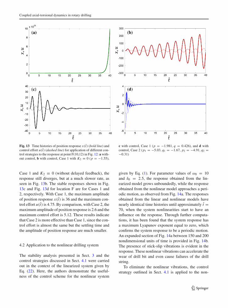
Fig. 13 Time histories of position response x(t) (bold line) andcontrol effort u(t) (dashed line) for application of different con-trol strategies to the response at point F(10,12) in Fig. 12: a with-out control, b with control, Case 1 with K2 ≡ 0 (p = −1.55),

c with control, Case 1 (p = −1.981, q = 0.426), and d withcontrol, Case 2 (p1 = −5.03, q1 = −1.67, p2 = −4.91, q2 =−0.31)

Case 1 and K2 ≡ 0 (without delayed feedback), theresponse still diverges, but at a much slower rate, asseen in Fig. 13b. The stable responses shown in Fig.13c and Fig. 13d for location F are for Cases 1 and2, respectively. With Case 1, the maximum amplitudeof position response x(t) is 36 and the maximum con-trol effort u(t) is 4.75. By comparison, with Case 2, themaximum amplitude of position response is 2.6 and themaximum control effort is 5.12. These results indicatethat Case 2 is more effective than Case 1, since the con-trol effort is almost the same but the settling time andthe amplitude of position response are much smaller.

4.2 Application to the nonlinear drilling system

The stability analysis presented in Sect. 3 and thecontrol strategies discussed in Sect. 4.1 were carriedout in the context of the linearized system given byEq. (22). Here, the authors demonstrate the useful-ness of the control scheme for the nonlinear system

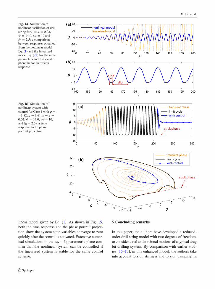
given by Eq. (1). For parameter values of ω0 = 10and δ0 = 2.5, the response obtained from the lin-earized model grows unboundedly, while the responseobtained from the nonlinear model approaches a peri-odic motion, as observed from Fig. 14a. The responsesobtained from the linear and nonlinear models havenearly identical time histories until approximately t =70, when the system nonlinearities start to have aninfluence on the response. Through further computa-tions, it has been found that the system response hasa maximum Lyapunov exponent equal to zero, whichconfirms the system response to be a periodic motion.An expanded section of Fig. 14a between 150 and 200nondimensional units of time is provided in Fig. 14b.The presence of stick-slip vibrations is evident in theresponse. These nonlinear vibrations can accelerate thewear of drill bit and even cause failures of the drillstring.

To eliminate the nonlinear vibrations, the controlstrategy outlined in Sect. 4.1 is applied to the non-

123

X. Liu et al.

Fig. 14 Simulation ofnonlinear oscillation of drillstring for ξ = κ = 0.02,ψ = 14.0, ω0 = 10 andδ0 = 2.5: a comparisonbetween responses obtainedfrom the nonlinear modelEq. (1) and the linearizedmodel Eq. (22) for the sameparameters and b stick-slipphenomenon in torsionresponse

Fig. 15 Simulation ofnonlinear system withcontrol for Case 1 with p =−3.82, q = 3.61, ξ = κ =0.02, ψ = 14.0, ω0 = 10,and δ0 = 2.5): a timeresponse and b phaseportrait projection

linear model given by Eq. (1). As shown in Fig. 15,both the time response and the phase portrait projec-tion show the system state variables converge to zeroquickly after the control is activated. Extensive numer-ical simulations in the ω0 − δ0 parametric plane con-firm that the nonlinear system can be controlled ifthe linearized system is stable for the same controlscheme.

5 Concluding remarks

In this paper, the authors have developed a reduced-order drill string model with two degrees of freedom,to consider axial and torsional motions of a typical dragbit drilling system. By comparison with earlier stud-ies [15–17], in this enhanced model, the authors takeinto account torsion stiffness and torsion damping. In

123

Coupled axial-torsional dynamics in rotary drilling

addition, they treat a nonlinear system with dry friction,loss of contact, and state-dependent time delay.

Studies conducted with these models help theauthors gain important insights into the stability ofmotions and the role played by different parameters andthe delay effects. Stability analyses has been presentedfor the linearized model using the semi-discretizationmethod in the parameter space spanned by the drivespeed ω0, the cutting coefficient ψ , and the nominaldepth of cut δ0. The stability volume is an irregular tri-angular prism and motions initiated at any point insidethis stability volume lead to stable drilling responses.Through the studies, it is found that the left boundaryof the stability diagram is influenced by the regenera-tive effects (i.e., constant delay effects), while the topboundary is influenced by the effect due to the state-dependent delay (i.e., the effect due to variation of thedelay). An examination of the sensitivity of the sta-bility boundaries with respect to different parametersindicates that damping of the drilling system will onlyaffects the top boundary in the stability chart but hasvirtually no effect on the left boundary. This pointsto the difficulty in extending the stable region to lowdriving speeds.

Control strategies are also presented in this paperby using optimal feedback gains [35] and an approachthat makes use of semi-discretization. Feedback thatis proportional to the states and the delayed states arealso introduced. With this feedback control, it is shownthat the stability region for the controlled system with-out delayed feedback is enlarged by only shifting thepreviously mentioned top boundary, while the stabilityregion is enlarged by shifting of both the top bound-ary and the left boundary in the controlled system withdelayed feedback. By applying optimal feedback gains,the stability region is shown to greatly enlarged. Toshow the effectiveness of the control strategy for a non-linear drilling model, numerical studies are carried outfor a system which exhibits nonlinear stick-slip vibra-tions in the uncontrolled case. The simulations showthat the stability characteristics of the nonlinear systemare consistent with those observed for the linearizedsystem and that the proposed control strategy is feasi-ble for the nonlinear system.

Although the stability analysis and control strategypresented in this study were pursued in the context of atwo degree-of-freedom model, their effectiveness canbe demonstrated through studies with higher degree-of-freedom systems such as those obtained through

finite-element modeling. Future work under consider-ation includes examination of similar control strate-gies with higher degree-of-freedom systems obtainedthrough finite-element constructions and experimentalvalidation.

Acknowledgments The authors from Shanghai Jiao Tong Uni-versity gratefully acknowledge the support received through 973Grant No. 2011CB706803 and No. 2014CB04660.

References

1. Bommer, P.: A Primer of Oilwell Drilling. The Universityof Texas at Austin, Austin (2008)

2. Dufeyte, M.-P., Henneuse, H., Elf, A.: Detection and mon-itoring of the slip-stick motion: field experiments. In:SPE/IADC Drilling Conference, pp. 429–438, 11–14 March1991

3. Pavone, D. R., Desplans, J. P.: Application of high samplingrate downhole measurements for analysis and cure of stick-slip in drilling, pp. 335–345. Number SPE 28324. (1994)

4. Navarro-Lopez, E. M., Suarez, R.: Practical approach tomodelling and controlling stick-slip oscillations in oilwelldrillstrings. In: Control Applications, 2004. Proceedings ofthe 2004 IEEE International Conference on, vol. 2, pp. 1454–1460, Sept 2004

5. Brett, J.F.: The genesis of bit-induced torsional drillstringvibrations. SPE Drill. Eng. 7(3), 168–174 (1992)

6. Mihajlovic, N., van Veggel, A.A., van de Wouw, N., Nijmei-jer, H.: Analysis of friction-induced limit cycling in an exper-imental drill-string system. ASME J. Dyn. Syst. Meas. Con-trol 126(4), 709–720 (2004)

7. Liu, X., Vlajic, N., Long, X., Meng, G., Balachandran, B.:Nonlinear motions of a flexible rotor with a drill bit: stick-slip and delay effects. Nonlinear Dyn. 72(1–2), 61–77 (2013)

8. Liao, C.-M., Balachandran, B., Karkoub, M., Abdel-Magid,Y.L.: Drill-string dynamics: reduced-order models andexperimental studies. ASME J. Vib. Acoust. 133(4), 041008(2011)

9. Long, X.H., Balachandran, B., Mann, B.: Dynamics ofmilling processes with variable time delays. Nonlinear Dyn.47, 49–63 (2007)

10. Insperger, T., Stépán, G., Hartung, F., Turi, J.: Statedependent regenerative delay in milling processes. ASMEIDETC/CIE 2005, (DETC2005-85282), 2005 (2005)

11. Insperger, T., Stépán, G., Turi, J.: State-dependent delay inregenerative turning processes. Nonlinear Dyn. 47, 275–283(2007)

12. Stépán, G.: Modelling nonlinear regenerative effects inmetal cutting. Philos. Trans. R. Soc. Lond. Ser. A Math.Phys. Eng. Sci. 359(1781), 739–757 (2001)

13. Balachandran, B.: Nonlinear dynamics of milling processes.Philos. Trans. R. Soc. Lond. Ser. A Math. Phys. Eng. Sci.359(1781), 793–819 (2001)

14. Balachandran, B., Kalmar-Nagy, T., Gilsinn, D.E.: DelayDifferential Equations: Recent Advances and New Direc-tions. Springer, New York (2009)

123

X. Liu et al.

15. Richard, T., Germay, C., Detournay, E.: Self-excited stick-slip oscillations of drill bits. Comptes Rendus Mcanique332(8), 619–626 (2004)

16. Richard, T., Germay, C., Detournay, E.: A simplified modelto explore the root cause of stickslip vibrations in drillingsystems with drag bits. J. Sound Vib. 305(3), 432–456 (2007)

17. Besselink, B., van de Wouw, N., Nijmeijer, H.: A semi-analytical study of stick-slip oscillations in drilling systems.ASME J. Comput. Nonlinear Dyn. 6(2), 021006 (2011)

18. Aldred, W. D., Sheppard, M. C.: Anadrill. Drillstring vibra-tions: A new generation mechanism and control strategies.In: SPE Annual Technical Conference and Exhibition, pp.353–453, 4–7 Oct 1992

19. Jansen, J.D., van den Steen, L.: Active damping of self-excited torsional vibrations in oil well drillstrings. J. SoundVib. 179(4), 647–668 (1995)

20. Tucker, W.R., Wang, C.: An integrated model for drill-stringdynamics. J. Sound Vib. 224(1), 123–165 (1999)

21. Kreuzer, E., Struck, H.: Active damping of spatio-temporaldynamics of drill-strings. In: IUTAM Symposium onChaotic Dynamics and Control of Systems and Processesin Mechanics 122, 407–417 (2005)

22. Yigit, A.S., Christoforou, A.P.: Stick-slip and bit-bounceinteraction in oil-well drillstrings. ASME J. Energy Resour.Technol. 128(4), 268–274 (2006)

23. Khulief, Y.A., Al-Sulaiman, F.A., Bashmal, S.: Vibrationanalysis of drillstrings with self-excited stickslip oscilla-tions. J. Sound Vib. 299(3), 540–558 (2007)

24. de Bruin, J.C.A., Doris, A., van de Wouw, N., Heemels,W.P.M.H., Nijmeijer, H.: Control of mechanical motion sys-tems with non-collocation of actuation and friction: a popovcriterion approach for input-to-state stability and set-valuednonlinearities. Automatica 45(2), 405–415 (2009)

25. Karkoub, M., Abdel-Magid, Y.L., Balachandran, B.: Drill-string torsional vibration suppression using ga optimizedcontrollers. J. Can. Pet. Technol. 48(12), 1–7 (2009)

26. Insperger, T., Stépán, G.: Semi-discretization method fordelayed systems. Int. J. Numer. Method. Eng. 55(5), 503–518 (2002)

27. Insperger, T., Stépán, G.: Updated semi-discretizationmethod for periodic delay-differential equations with dis-crete delay. Int. J. Numer. Method. Eng. 61(1), 117–141(2004)

28. Liu, X., Vlajic, N., Long, X., Meng, G., Balachandran, B.:Multiple regenerative effects in cutting process and nonlin-ear oscillations. Int. J. Dyn. Control 2(1), 86–101 (2014)

29. Germay, C., van de Wouw, N., Nijmeijer, H., Sepulchre,R.: Nonlinear drillstring dynamics analysis. SIAM J. Appl.Dyn. Syst. 8(2), 527–553 (2009)

30. Germay, C., Denol, V., Detournay, E.: Multiple mode analy-sis of the self-excited vibrations of rotary drilling systems.J. Sound Vib. 325(12), 362–381 (2009)

31. Detournay, E., Defourny, P.: A phenomenological model forthe drilling action of drag bits. Int. J. Rock Mech. Min. Sci.Geomech. Abstr. 29(1), 13–23 (1992)

32. Detournay, E., Richard, T., Shepherd, M.: Drilling responseof drag bits: theory and experiment. Int. J. Rock Mech. Min.Sci. 45(8), 1347–1360 (2008)

33. Insperger, T., Stépán, G.: Semi-Discretization for Time-Delay Systems: Stability and Engineering Applications, vol.178. Springer, New York (2011)

34. Nayfeh, A.H., Balachandran, B.: Applied NonlinearDynamics: Analytical, Computational, and ExperimentalMethods. WILEY-VCH Verlag GmbH, Weinheim (1995)

35. Elbeyli, O., Sun, J.Q.: On the semi-discretization method forfeedback control design of linear systems with time delay.J. Sound Vib. 273(12), 429–440 (2004)

123