coulomb explosion and intense-field photodissociation of ... · for studying molecules in intense...
TRANSCRIPT
Coulomb Explosion andIntense-Field Photodissociation of
Ion-Beam H+2 and D+
2
Domagoj Pavicic
Munchen 2004

Coulomb Explosion andIntense-Field Photodissociation of
Ion-Beam H+2 and D+
2
Domagoj Pavicic
Dissertation
an der LMU
der Ludwig–Maximilians–Universitat
Munchen
vorgelegt von
Domagoj Pavicic
aus Zagreb, Kroatien
Munchen, den 11. Marz 2004

Erstgutachter: Prof. Dr. T. W. Hansch
Zweitgutachter: Prof. Dr. H. W. Schrotter
Tag der mundlichen Prufung: 27.4.2004

To my parents,
my brother
and
Helena

Abstract
As the simplest molecule in nature, the hydrogen molecular ion provides a unique systemfor studying molecules in intense laser fields. In this thesis, the Coulomb explosion andphotodissociation channel of H+
2 and D+2 have been investigated with 790-nm, sub-100-
fs laser pulses by employing a high-resolution photofragment imaging technique. Unlikemost experiments, where neutral molecules were used as a target, in this work molecularions were prepared by an electric discharge, providing well-defined starting conditions andallowing experiments at lower intensities.
At intensities close to the threshold for Coulomb explosion (<1014 W/cm2), we ob-served a peak structure in the Coulomb explosion kinetic energy spectra in both H+
2 andD+
2 . We show that the observed peaks can be attributed to the different dissociation en-ergies of vibrationally excited molecules. Furthermore, this preservation of the vibrationalstructure during the Coulomb explosion suggests ionization at one well-defined critical in-ternuclear distance. Moreover, when using pulses with durations of 200–500 fs, we foundthree Coulomb explosion kinetic energy groups with different angular distributions in bothmolecular ions. The groups in D+
2 at a pulse duration of 350 fs and an intensity of 1×10¹⁴
W/cm2 strongly suggest critical internuclear distances of 8, 11 and 15 a.u.In the one-photon photodissociation study of D+
2 at intensities below 2×10¹⁴ W/cm2, weobtained vibrationally resolved fragment velocity distributions. With increasing intensity,we observed the effects of bond softening – narrowing of the angular distributions andvibrational level shifting. These effects were also found in H+
2 and are in agreement withthe model of light-induced potentials. In addition, in the kinetic energy spectra of D+
2 ,we found the smaller widths of the vibrational peaks, which we interpret as being due tothe longer lifetimes of the vibrational states of D+
2 against photodissociation. Moreover,we observed fragments with near-zero kinetic energies with broad angular distributions,indicating dissociation through a vibrational trapping mechanism. In the two-photon bondsoftening process (above-threshold dissociation) of H+
2 , we identified fragments from thesingle vibrational level v = 3. At higher intensities, lower-energy fragments with increasingalignment were observed, suggesting dissociation of the levels v < 3 through the barrierlowering mechanism.
These results provide a basis for quantum mechanical simulations that could lead to abetter understanding of the molecular dynamics in intense fields.

viii Abstract
Zusammenfassung
Das elementarste Molekul in der Natur, das Wasserstoff-Molekulion, stellt ein einzigartigesSystem fur die Untersuchung von Molekulen in intensiven Laserfeldern dar. In dieser Dis-sertation wurden die Coulomb-Explosion und die Photodissoziation des H+
2 und D+2 mit
790-nm, sub-100-fs Laserpulsen unter Verwendung einer hochauflosenden PhotofragmentAbbildungstechnik untersucht. Im Gegensatz zu den meisten Experimenten, in denen neu-trale Molekule als Ausgangsmolekule benutzt wurden, wurden in dieser Arbeit die Molekuli-onen durch eine elektrische Gasentladung erzeugt, was zu wohldefinierten Ausgangsbedin-gungen fuhrte und Experimente mit relativ niedrigen Laserintensitaten ermoglichte.
Bei Intensitaten nahe der Schwelle der Coulomb-Explosion (<1014 W/cm2), beobachtenwir eine Peak-Struktur in den kinetischen Energiespektren der Fragmente der Coulomb-Explosion sowohl bei H+
2 als auch bei D+2 . Wir stellen fest, dass die beobachteten Peaks
den unterschiedlichen Dissoziationsenergien der vibrationsangeregten Molekule zugeordnetwerden konnen. Die Erhaltung der Vibrationsstruktur bei der Coulomb-Explosion deutetdarauf hin, dass die Ionisation bei einem scharfen kritischen internuklearen Abstand statt-findet. Als wir Laserpulse mit einer Dauer von 200–500 fs verwendeten, entdeckten wirdrei Coulomb-Explosions Zentren in den kinetischen Energiespektren mit unterschiedlichenWinkelverteilungen bei beiden molekularen Isotopomeren. So entsprechen die Gruppenbei D+
2 bei einer Pulsdauer von 350 fs und einer Intensitat von 1× 10¹⁴ W/cm2 kritischeninternuklearen Abstanden von 8, 11 und 15 a.u.
Bei der Untersuchung der 1-Photonen Photodissoziation des D+2 beobachten wir bei
einer Intensitat unterhalb 2× 10¹⁴ W/cm2 vibrationsaufgeloste Geschwindigkeitsverteilun-gen der Fragmente. Mit zunehmender Intensitat beobachten wir auch Effekte des bondsoftenings – Einengung der Winkelverteilung und Verschiebung der Vibrationsniveaus.Diese Effekte wurden auch schon vorher bei H+
2 beobachtet und finden ihre Erklarungin dem Modell der lichtinduzierten Potenziale. Insbesondere finden wir in den kinetis-chen Energiespektren von D+
2 kleinere Breiten der Vibrationspeaks, deren Ursache langereLebensdauern der Vibrationszustande von D+
2 bei der Photodissoziation sein sollten. Indem Prozess des 2-Photonen bond softenings von H+
2 identifizieren wir Fragmente deseinzelnen Vibrationsniveaus v = 3. Bei hoheren Intensitaten wurden niederenergetischeFragmente mit zunehmender Ausrichtung in Polarisationsrichtung beobachtet, die auf Dis-sozation durch eine Barriereabsenkung hinweisen.
Diese experimentellen Ergebnisse konnen durch quantenmechanische Rechnungen simuliertwerden, die zu einem besseren Verstandnis der Molekulardynamik in intensiven Laser-feldern fuhren werden.

x Zusammenfassung
Contents
Abstract vii
Zusammenfassung ix
1 Introduction 1
2 H+2 in intense laser fields 5
2.1 Photodissociation in intense laser fields . . . . . . . . . . . . . . . . . . . . 52.1.1 Theoretical approaches . . . . . . . . . . . . . . . . . . . . . . . . . 52.1.2 Floquet picture . . . . . . . . . . . . . . . . . . . . . . . . . . . . . 72.1.3 Bond softening, trapping and above-threshold dissociation . . . . . 122.1.4 Molecular alignment . . . . . . . . . . . . . . . . . . . . . . . . . . 13
2.2 Strong-field ionization and Coulomb explosion . . . . . . . . . . . . . . . . 132.2.1 Photoionization mechanisms . . . . . . . . . . . . . . . . . . . . . . 132.2.2 Semiclassical model of enhanced ionization . . . . . . . . . . . . . . 162.2.3 Charge-resonant enhanced ionization (CREI) . . . . . . . . . . . . . 17
3 Experimental 193.1 Ion beam apparatus . . . . . . . . . . . . . . . . . . . . . . . . . . . . . . . 19
3.1.1 Ion source . . . . . . . . . . . . . . . . . . . . . . . . . . . . . . . . 203.1.2 Mass selection . . . . . . . . . . . . . . . . . . . . . . . . . . . . . . 223.1.3 Ion optics . . . . . . . . . . . . . . . . . . . . . . . . . . . . . . . . 223.1.4 Ion current . . . . . . . . . . . . . . . . . . . . . . . . . . . . . . . 243.1.5 Detection system . . . . . . . . . . . . . . . . . . . . . . . . . . . . 253.1.6 Data acquisition . . . . . . . . . . . . . . . . . . . . . . . . . . . . . 263.1.7 Collimation of the ion beam . . . . . . . . . . . . . . . . . . . . . . 283.1.8 Vacuum system . . . . . . . . . . . . . . . . . . . . . . . . . . . . . 30
3.2 Imaging of fragments . . . . . . . . . . . . . . . . . . . . . . . . . . . . . . 303.2.1 Principle of fragment imaging . . . . . . . . . . . . . . . . . . . . . 313.2.2 Inverse Abel transform . . . . . . . . . . . . . . . . . . . . . . . . . 333.2.3 Comparison of inversion algorithms . . . . . . . . . . . . . . . . . . 333.2.4 Velocity and energy resolution . . . . . . . . . . . . . . . . . . . . . 35
3.3 Femtosecond laser system . . . . . . . . . . . . . . . . . . . . . . . . . . . 37
xii Contents
3.3.1 Laser setup . . . . . . . . . . . . . . . . . . . . . . . . . . . . . . . 373.3.2 Beam and pulse characterization . . . . . . . . . . . . . . . . . . . 403.3.3 Laser intensity . . . . . . . . . . . . . . . . . . . . . . . . . . . . . 45
3.4 Intensity distribution in the interaction region . . . . . . . . . . . . . . . . 453.4.1 Interaction volume . . . . . . . . . . . . . . . . . . . . . . . . . . . 453.4.2 Contribution of the intensity shells to the measured signal . . . . . 48
4 Photodissociation of the deuterium molecular ion 514.1 Vibrationally resolved velocity distributions . . . . . . . . . . . . . . . . . 514.2 Kinetic energy distributions of the fragments . . . . . . . . . . . . . . . . . 534.3 Angular distributions of the fragments . . . . . . . . . . . . . . . . . . . . 58
4.3.1 One-photon bond softening . . . . . . . . . . . . . . . . . . . . . . 584.3.2 Vibrational trapping and two-photon bond softening . . . . . . . . 61
4.4 Comparison with measurements on H+2 at lower intensities . . . . . . . . . 64
5 Photodissociation of the hydrogen molecular ion 695.1 Fragment velocity and kinetic energy distributions . . . . . . . . . . . . . . 695.2 Angular distributions of the fragments: alignment . . . . . . . . . . . . . . 77
5.2.1 Dependence on the peak laser intensity . . . . . . . . . . . . . . . . 775.2.2 Angular distributions of the one- and net two-photon processes . . . 78
5.3 Fragment yields of the one- and the net two-photon process . . . . . . . . . 81
6 Coulomb explosion 856.1 Measurements with sub-100-fs pulses . . . . . . . . . . . . . . . . . . . . . 86
6.1.1 Mechanism of Coulomb explosion . . . . . . . . . . . . . . . . . . . 866.1.2 Coulomb explosion at near-threshold intensities . . . . . . . . . . . 91
6.2 Measurements with pulses of longer durations . . . . . . . . . . . . . . . . 996.3 Fragment yield of the Coulomb explosion channel . . . . . . . . . . . . . . 105
7 Conclusion and perspectives 107
A Unit conversion 109
B Molecular data on H+2 and D+
2 111B.1 Constants . . . . . . . . . . . . . . . . . . . . . . . . . . . . . . . . . . . . 111B.2 Energies and populations of vibrational levels . . . . . . . . . . . . . . . . 111
List of symbols and acronyms 115
Bibliography 117
Acknowledgments 127
Chapter 1
Introduction
Over the past century, understanding of interaction of light with matter has been one ofthe central themes of research in physics. Early investigations of emission and absorptionspectra of atoms and molecules have already provided a wealth of knowledge about theirelectronic structure. With the availability of coherent and monochromatic laser radiationand development of high-resolution laser spectroscopy techniques, our knowledge of thestructure of atoms and molecules has been revolutionized.
Moreover, the advent and continued development of pulsed lasers also made it possi-ble to investigate ultrafast dynamical processes in different systems, ranging from smallmolecules to complex biological systems. Using the pump-probe technique with ultrashortlaser pulses, one can monitor molecular motion (such as vibrations, or making and break-ing of molecular bonds) occurring on the femtosecond timescale (1 femtosecond = 10−15
s). This concept has led to the birth of femtochemistry, for which the 1999 Nobel Prize inchemistry was awarded to Ahmed Zewail [1].
Recent progress in ultrafast optics has made available laser pulses as short as a fewfemtoseconds in the visible spectral range [2]. Since such pulse durations are limited bythe oscillation period of the electromagnetic field in the pulse, generation of shorter pulsesrequires coherent sources of higher-frequency radiation. High-order harmonics of the fun-damental laser radiation generated in noble gas atoms can provide coherent radiation inthe extreme ultraviolet (XUV) and soft x-ray range (e.g., [3]). Recently, such radiationhas been successfully used for generating trains of pulses with durations in the attosecondrange (1 attosecond = 10−18 s) [4, 5]. Single, isolated attosecond pulses [6] have alreadybeen applied to time-resolved spectroscopy of atomic inner-shell electrons [7]. Simultane-ously, theoretical and experimental efforts have been made to characterize the duration ofattosecond XUV pulses [8–12].
Few-cycle pulses in the optical range have also provided evidence that laser-matterinteraction is sensitive to the phase of the oscillating laser electric field with respect to thepulse envelope [13]. Nowadays, intense few-cycles pulses with stabilized carrier-envelopephase can readily be generated [14] and the phase can be accurately determined [15]. Thispermits directed emission and steering of the electron wave packets on the sub-femtosecondtimescale.
2 1. Introduction
In addition to short pulse durations, femtosecond laser pulses are characterized by highpeak intensities. At present, laboratory-scale lasers can deliver pulses shorter than 10 fswith peak powers in the terawatt (1 terawatt = 1012 W) range at a kilohertz repetitionrate [16]. By focusing such pulses it is possible to investigate a variety of intense-fieldphenomena in atoms, molecules, clusters, plasmas and solid materials occurring in theintensity range of 1013 − 1018 W/cm2 (e.g., [3, 17, 18]).
Most of the attention to strong field-matter interaction has been concentrated on atoms.At an intensity of about 1016 W/cm2, the laser electric field strength becomes of the samemagnitude as the field binding a 1s electron in a hydrogen atom (known as atomic unit ofelectric field, 5×10⁹ V/cm). At these and already at lower intensities, light-atom interactionis so strong that normal perturbative approaches break down, leading to novel phenomenacollectively termed as multiphoton processes. These processes include above-thresholdionization (ATI) — absorption of more photons than the minimum number required forionization [19], non-sequential or direct double ionization — simultaneous emission of moreelectrons [20, 21] and high harmonic generation [22, 23].
In addition to the effects observed in atoms, molecules in strong fields exhibit newphenomena associated with additional vibrational and rotational degrees of freedom. In1990, Bucksbaum et al found that the molecular bond is softened by strong laser fields,resulting in photodissociation of the molecules in strongly bound vibrational states [24].The same study also revealed that molecules can absorb more photons than necessary fordissociation, which, by analogy with ATI, is termed above-threshold dissociation (ATD)[25]. The theoretically predicted effects of bond hardening or trapping in the potentialsinduced by the laser fields [26] were recently observed [27, 28]. Alignment of molecules bystrong laser fields has also been extensively studied [29–32].
Besides photodissociation, ionization dynamics of molecules in strong laser fields hasattracted great interest. Early experiments showed that the kinetic energies of the chargednuclear fragments formed after ionization are significantly smaller than had been expected,assuming that ionization and Coulomb repulsion occur at the equilibrium internuclearseparation [33]. The solution was offered by several models [34–36], predicting that thisCoulomb explosion takes place at large internuclear separations through charge-resonanceenhanced ionization (CREI) [36]. This model found high ionization rates at particular,so-called critical, internuclear separations. Despite the numerous experiments carried out,there has hitherto been no clear evidence of the existence of critical distances.
Much attention has been focused on the role of re-collision of the ionized electron withthe parent ion [37]. Recent experiments have shown that non-sequential double ionizationin atoms and molecules is caused by such re-scattered electrons [21, 38]. As a consequence,Coulomb explosion protons with high kinetic energies are produced [39, 40]. The correlationbetween nuclear and re-colliding electron wave packets was successfully exploited to probemolecular dynamics with attosecond resolution [41].
The simplest molecule in nature is the hydrogen molecular ion, consisting of two pro-tons bound by an electron. As a model system, H+
2 is of fundamental importance forunderstanding the physics of molecules as well as atomic clusters in intense laser fields.Though the dissociation and ionization dynamics of H+
2 have been extensively studied the-
3
oretically (e.g., [26, 42]), there is only limited experimental insight into them. Because ofthe difficulties involved in preparing H+
2 , nearly all experiments to date have used H2 andits isotopic variant D2 as primary target [42]. The molecular ions have thus been producedby ionizing the neutral molecules by the same laser pulse as used for molecular ion–laserinteraction. The interplay between the first ionization step and the later ionization anddissociation dynamics of H+
2 has hindered clear interpretation of the experimental results[26]. Moreover, the phenomena occurring at intensities below 1014 W/cm2 were not ac-cessible owing to the relatively high intensities required for ionization of H2. Intense-fieldeffects in H+
2 have been investigated only in two recent experiments employing fast ionbeams [28, 43].
The photofragment velocity distributions of Sandig et al [28] neatly demonstrated theeffects of strong fields for molecules in single vibrational levels. Molecular bond softeningwas manifested in the appearance of fragments from lower-lying vibrational states withincreasing intensity, their alignment along the laser polarization axis and shifting towardslower kinetic energies with respect to the weak-field case. This experiment was, however,limited to study of the photodissociation process at relatively moderate intensities belowabout 1014 W/cm2.
In this thesis, intense-field photodissociation and Coulomb explosion of H+2 and D+
2 arestudied. The main objective of this work is to investigate the Coulomb explosion channelin H+
2 with the aim of elucidating the question of the existence of critical distances inenhanced ionization. Molecular ions in fast beams were used [28], allowing investigationat intensities close to the threshold for this process. A high-resolution fragment imagingmethod was employed, yielding direct information about both the kinetic energy and an-gular distribution of the photofragments. Furthermore, the photodissociation channel inH+
2 is studied at intensities above 1014 W/cm2 in order to investigate the mechanisms ofone- and two-photon bond softening.
Finally, photodissociation of D+2 is investigated at the intermediate intensity range with
the intention of obtaining vibrationally resolved velocity distributions of the fragments.Together with measurements on H+
2 at similar intensities [28], such an experiment canprovide valuable insights into the role of isotope effects in photodissociation. This part ofthe study is also motivated by recent theoretical simulations of the experimental results onH+
2 [44, 45]. Similar calculations on D+2 would add to our understanding of the dynamics
of single vibrational levels in strong laser fields. The third isotopic variant, HD+, has alsobeen studied, these results being presented in the framework of the diploma thesis of Kiess[46].
The thesis is organized as follows. Chapter 2 gives the theoretical background forinterpretation of the results. In Chapter 3, various aspects of the experiment are discussed.Chapter 4 presents the study of photodissociation of D+
2 at the intermediate intensities.In Chapter 5, photodissociation of H+
2 at higher intensities is investigated. In Chapter6, the Coulomb explosion channel in H+
2 and D+2 is explored. Finally, in Chapter 7, the
conclusion and perspectives for future work are given.

4 1. Introduction
Chapter 2
H+2 in intense laser fields
This chapter presents the theoretical background that provides a basis for understanding ofthe experimental results. Section 2.1 deals with the mechanism of photodissociation of H+
2
in intense laser fields. First, a definition of a strong field is given and different theoreticalapproaches used to describe H+
2 in intense fields are discussed. Here, a picture of molecular“dressed” states is presented, which leads to an intuitive description of the light-moleculesystem in terms of light-induced potential curves. Predicted effects such as molecularbond softening, vibrational trapping and above-threshold dissociation will be described,as well as geometric and dynamic alignment. At laser intensities beyond 1014 W/cm2,the dissociation process is increasingly accompanied by molecular ionization followed byCoulomb explosion of the nuclei. This mechanism of fragmentation is discussed in Section2.2. First, a simple semiclassical model of ionization is given, which can explain the kineticenergies of the fragments that were observed in experiments. The results of quantummechanical calculations predicting ionization at particular, so-called critical internucleardistances are presented in the last section.
2.1 Photodissociation in intense laser fields
2.1.1 Theoretical approaches
The interaction of laser radiation with the simplest molecular system H+2 can be described
within different frameworks. Some extensive reviews of theoretical methods describingH+
2 in intense laser fields can be found in references [47, 42, 26]. Most of the approachesare valid only in a certain range of parameters characterizing the radiation field, such asintensity, wavelength and pulse duration. In this section, different regimes specified bythese parameters will be discussed.
At low intensities the interaction can be described by using perturbation theory. Inthis regime the dissociation rate is proportional to laser intensity, what is known as Fermi’sgolden rule (e.g., [48]). At higher laser intensities, multiphoton processes take place, result-ing in various nonlinear effects. These intensity regimes can be characterized with the Rabi
6 2. H+2 in intense laser fields
frequency ωR (see, e.g., [49, 47]), which measures the strength of the radiative coupling:
�ωR [cm−1] = E0 · d = 1.17 × 10⁻³√
I[W/cm2] d [a.u.] , (2.1)
I =1
2cε0E
20 . (2.2)
Here d is the transition dipole moment in atomic units (a.u.) and E0 is the amplitudeof the electric field E(t) = E0 cos(ωt), which is related to intensity I via Eq. (2.2). Theclassification between strong- and weak-coupling regime can be specified by comparing theRabi frequency with the frequency of the nuclear vibrational motion, ωv.
In the case of H+2 , the radiation couples the two lowest electronic states: the attractive
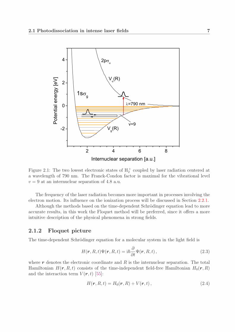
ground state 1sσg and the repulsive first excited state 2pσu. These states are illustratedin Fig. 2.1 with potential curves Vg(R) and Vu(R), where R denotes the internuclearseparation. Energetically higher states will not be considered here since they lie morethan 11 eV higher in energy, which is much larger than the photon energy of 1.6 eVcorresponding to the wavelength of 790 nm, which was used in the experiment. The twolowest states are resonantly coupled at an internuclear distance of 4.8 a.u. If the Rabitransition frequency is small compared to the vibrational frequency ωv, the probability ofthe molecule to absorb a photon during the time spent near the resonance will be low.On the other hand, in the case of ωR � ωv, the molecule will very probably absorb aphoton from the radiation field when it approaches the resonance. The Franck-Condonfactor for this transition is largest for the vibrational level v = 9, since the outer turningpoint almost coincides with the resonant internuclear separation. The vibrational energy�ωv of this level is approximately 1200 cm−1 (∼0.3 eV) 1, with the vibrational period of 29fs (Section 4.2). The Rabi frequency approaches the vibrational frequency at an intensityof 1011 W/cm2, for which �ωR is about 800 cm−1 (according to Eq. (2.1) using the dipolemoment d = 2.3 a.u. [50]). Thus, at intensities I > 1011 W/cm2, the perturbation theoryis no longer applicable and different approaches must be used. When only a few states arecoupled by radiation, as in H+
2 , a useful description can be obtained applying the Floquetor molecular “dressed” state formalisms [51, 47], which describe the molecule-light systemin terms of new light-induced molecular potentials [52–54].
Considering the duration of laser pulses, the methods can be divided into time-depen-dent and time-independent ones. For laser pulses long on the timescale of the molecularvibrational motion and the dissociation process, which is on the order of 10 fs, the evolu-tion of the system can be considered as adiabatic. In this case, time-independent methods,such as the Floquet approach, may be employed. For ultrashort pulses in the femtosecondregime, the laser intensity varies on the timescale of molecular motion, and hence time-dependent methods must be used. Most of the calculations nowadays use wave packetpropagation methods based on direct integration of the time-dependent Schrodinger equa-tion.
1Traditionally, the energies E of states are expressed in units of wave numbers according to the relationE/(hc) = 1/λ. In this work energies will be given in electronvolts (1 eV = 8065.5 cm−1).
2.1 Photodissociation in intense laser fields 7
Figure 2.1: The two lowest electronic states of H+2 coupled by laser radiation centered at
a wavelength of 790 nm. The Franck-Condon factor is maximal for the vibrational levelv = 9 at an internuclear separation of 4.8 a.u.
The frequency of the laser radiation becomes more important in processes involving theelectron motion. Its influence on the ionization process will be discussed in Section 2.2.1.
Although the methods based on the time-dependent Schrodinger equation lead to moreaccurate results, in this work the Floquet method will be preferred, since it offers a moreintuitive description of the physical phenomena in strong fields.
2.1.2 Floquet picture
The time-dependent Schrodinger equation for a molecular system in the light field is
H(r, R, t)Ψ(r, R, t) = i�∂
∂tΨ(r, R, t) , (2.3)
where r denotes the electronic coordinate and R is the internuclear separation. The totalHamiltonian H(r, R, t) consists of the time-independent field-free Hamiltonian H0(r, R)and the interaction term V (r, t) [55]:
H(r, R, t) = H0(r, R) + V (r, t) , (2.4)
8 2. H+2 in intense laser fields
H0(r, R) = TR + Hel(r, R) , (2.5)
where TR is the nuclear kinetic energy operator and Hel is the electronic Hamiltonian.For a linearly polarized monochromatic electric field E(t) = ezE0 cos(ωt) the interac-
tion in the dipole approximation is equal to
V (r, t) = −er · E(t) =eE0z
2
(eiωt + e−iωt
)= V− eiωt + V+ e−iωt , (2.6)
where er is the dipole moment. Here it was assumed that the molecule is perfectly alignedwith the laser electric field.
Since the only time dependence comes from the interaction term V (r, t), the totalHamiltonian is periodic in time H(t) = H(t + T ) with the period T = 2π/ω. According tothe Floquet theorem [55, 56], the solutions can then be written in the form
Ψ(r, R, t) = eiEt/�F (r, R, t) , (2.7)
where E is called quasi-energy. The function F (r, R, t) is periodic with period T , thus itcan be expanded in the Fourier series
F (r, R, t) =n=+∞∑n=−∞
e−inωtFn(r, R) . (2.8)
Using Eqs. (2.7) and (2.8), the wave function now reads
Ψ(r, R, t) = eiEt/�
n=+∞∑n=−∞
e−inωtFn(r, R) . (2.9)
Inserting the Floquet Ansatz (2.9) into the Schrodinger equation (2.3), and using Eqs.(2.4) and (2.6), the time-dependent Schrodinger equation is transformed into a set of time-independent differential equations, in which neighbouring Fourier components are coupled:
[E + n�ω − H0(r, R)] Fn(r, R) = V+ Fn−1(r, R) + V− Fn+1(r, R) . (2.10)
The wave functions Fn(r, R) are solutions of the field-free Hamiltonian H0, which arenow “dressed” with the phase factors e−inωt. For the fixed nuclei (TR = 0), the field-free Hamiltonian is equal to the electronic Hamiltonian. Hence, for H+
2 the functionsFn(r, R) are the wave functions Φg(r, R) and Φu(r, R) of the electronic states 1sσg and2pσu, respectively:
Hel(r, R)|Φg,n(r, R)〉 = Vg(R)|Φg,n(r, R)〉Hel(r, R)|Φu,m(r, R)〉 = Vu(R)|Φu,m(r, R)〉 . (2.11)
From Eq. (2.9) it is clear that identical solutions exist for quasi-energies E, E±�ω, E±2�ω,etc. The field-free solutions Fn(r, R), that is Φg(r, R) and Φu(r, R), can be interpreted

2.1 Photodissociation in intense laser fields 9
as being “dressed” with n photons of the radiation field and are labelled in Eq. (2.11)with indices n. Such dressed states are illustrated in Fig. 2.2(a) and are called adiabaticpotential curves. With this interpretation, V+ in Eq. (2.10) is responsible for one-photonabsorption and V− for emission of one photon. Since only the states of different symmetrycan be coupled, i.e., g ↔ u, the neighbouring functions with indices n and n ± 1 in Eq.(2.10) must correspond to different electronic states, as shown in Fig. 2.2(a). Taking thisinto account, Eq. (2.10) becomes
[E + n�ω − Vg(R)] |Φg,n(r, R)〉 = V+|Φu,n−1(r, R)〉 + V−|Φu,n+1(r, R)〉[E + (n + 1)�ω − Vu(R)] |Φu,n+1(r, R)〉 = V+|Φg,n(r, R)〉 + V−|Φg,n+2(r, R)〉 . (2.12)
Light-induced potential curves
The infinite set of differential equations (2.12) can be written as a matrix and the quasi-energies are then obtained by diagonalizing the matrix
......
......
· · · Vgu(R) 0 0 0 · · ·· · · Vu(R) − (n − 1)�ω Vgu(R) 0 0 · · ·· · · Vgu(R) Vg(R) − n�ω Vgu(R) 0 · · ·· · · 0 Vgu(R) Vu(R) − (n + 1)�ω Vgu(R) · · ·· · · 0 0 Vgu(R) Vg(R) − (n + 2)�ω · · ·· · · 0 0 0 Vgu(R) · · ·
......
......
(2.13)
, where
Vug(R) = Vgu(R) ≡ 〈2pσu|V±|1sσg〉 =E0
2〈2pσu|ez|1sσg〉 =
�ωR
2. (2.14)
In practical calculations matrix (2.13) must be truncated to a finite one. The smallestmatrix consists of a single 2 × 2 Floquet block. The eigenvalues are in this case obtainedby solving the equation ∣∣∣∣Vg(R) − E Vgu(R)
Vgu(R) Vu(R) − �ω − E
∣∣∣∣ = 0 , (2.15)
where for simplicity the photon number n in Eq. (2.13) was set to zero. The results areso-called adiabatic potential curves E−(R) and E+(R):
E±(R) =Vg(R) + Vu(R) − �ω
2± 1
2
√[Vg(R) + �ω − Vu(R)]2 + (�ωR)2 . (2.16)
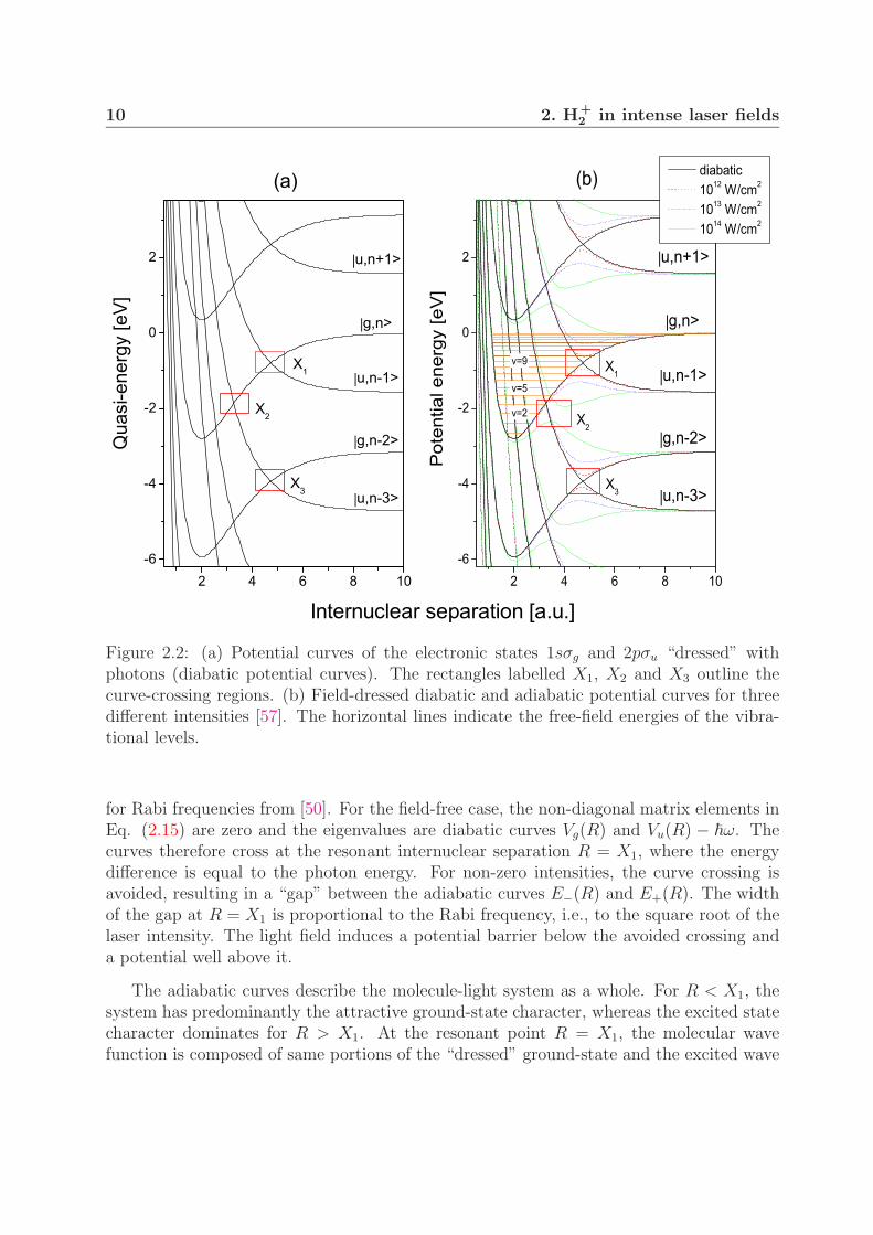
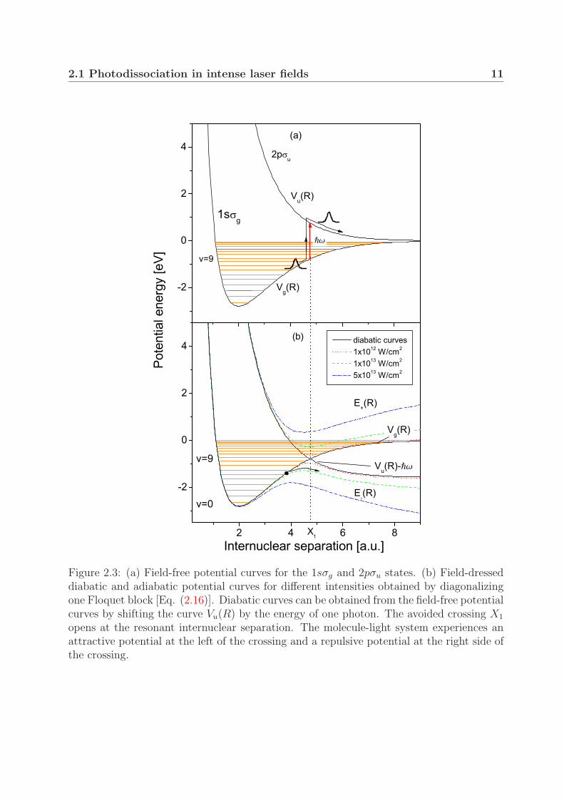
Figure 2.3(b) shows the adiabatic curves calculated from Eq. (2.16) for different intensities.The data for unperturbed curves can be found in [58] and dipole transition moments needed
10 2. H+2 in intense laser fields
|
|
|
|
|
|
|
|
|
|
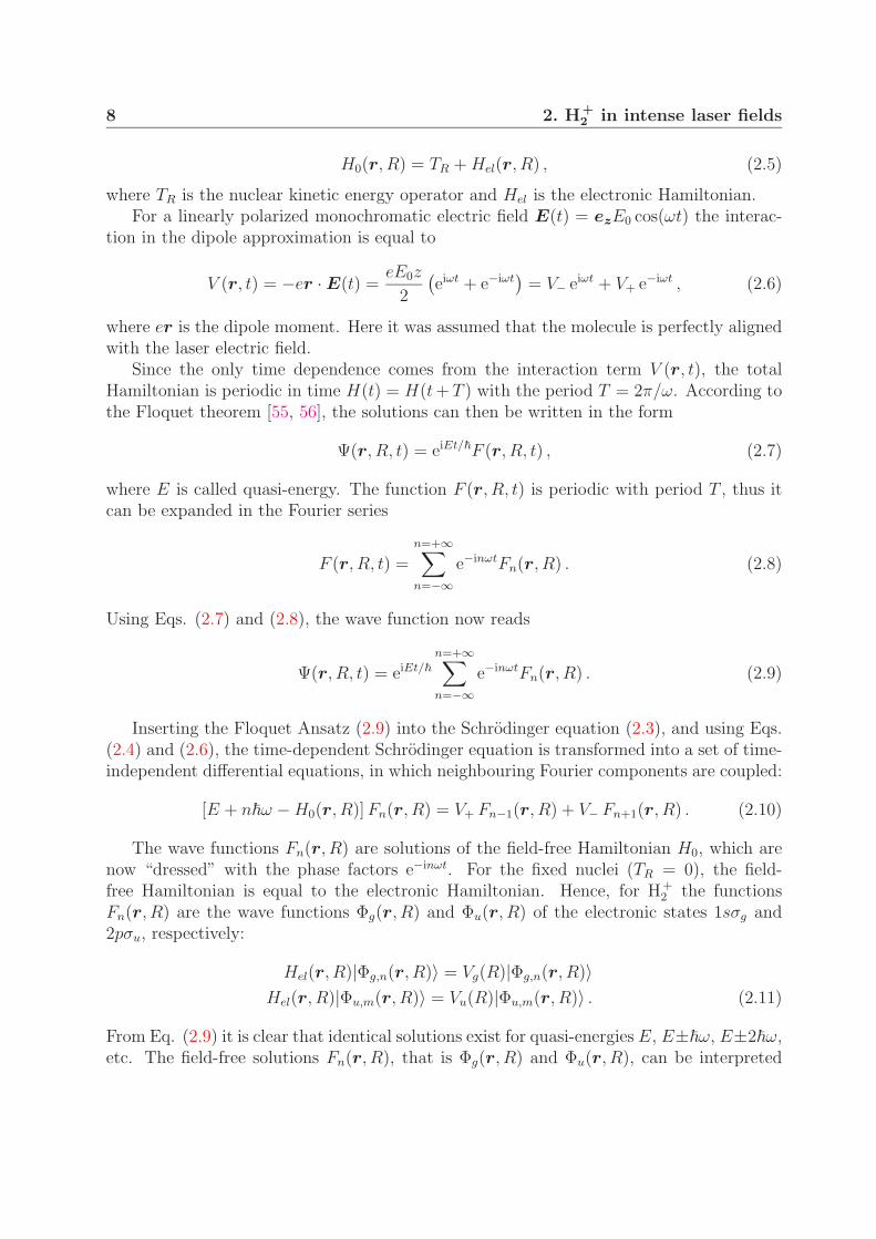
Figure 2.2: (a) Potential curves of the electronic states 1sσg and 2pσu “dressed” withphotons (diabatic potential curves). The rectangles labelled X1, X2 and X3 outline thecurve-crossing regions. (b) Field-dressed diabatic and adiabatic potential curves for threedifferent intensities [57]. The horizontal lines indicate the free-field energies of the vibra-tional levels.
for Rabi frequencies from [50]. For the field-free case, the non-diagonal matrix elements inEq. (2.15) are zero and the eigenvalues are diabatic curves Vg(R) and Vu(R) − �ω. Thecurves therefore cross at the resonant internuclear separation R = X1, where the energydifference is equal to the photon energy. For non-zero intensities, the curve crossing isavoided, resulting in a “gap” between the adiabatic curves E−(R) and E+(R). The widthof the gap at R = X1 is proportional to the Rabi frequency, i.e., to the square root of thelaser intensity. The light field induces a potential barrier below the avoided crossing anda potential well above it.
The adiabatic curves describe the molecule-light system as a whole. For R < X1, thesystem has predominantly the attractive ground-state character, whereas the excited statecharacter dominates for R > X1. At the resonant point R = X1, the molecular wavefunction is composed of same portions of the “dressed” ground-state and the excited wave
2.1 Photodissociation in intense laser fields 11
Figure 2.3: (a) Field-free potential curves for the 1sσg and 2pσu states. (b) Field-dresseddiabatic and adiabatic potential curves for different intensities obtained by diagonalizingone Floquet block [Eq. (2.16)]. Diabatic curves can be obtained from the field-free potentialcurves by shifting the curve Vu(R) by the energy of one photon. The avoided crossing X1
opens at the resonant internuclear separation. The molecule-light system experiences anattractive potential at the left of the crossing and a repulsive potential at the right side ofthe crossing.
12 2. H+2 in intense laser fields
functions, i.e., [59]
Ψ(r, R) =1√2
[Φg,n(r, R) + Φu,n−1(r, R)] .
Here almost the entire electronic charge oscillates between the protons. This is known ascharge-resonance [60] and will be discussed in Section 2.2.3.
The interpretation of the adiabatic curves can be illustrated using the example of anuclear wave packet moving on the curve Vg(R) and approaching the point X1 from theleft, as discussed earlier in Fig. 2.1. In the representation for weak fields [Fig. 2.3(a)], themolecule absorbs one photon and ends up on the repulsive curve Vu(R). In the adiabaticpicture [Fig. 2.3(b)], this process is described as follows. If the protons move slowlyapart, the electron-field system (illustrated now by a black dot) follows the lower adiabaticcurve E−(R). As the internuclear separation reaches the point X1, the attractive potentialchanges to a repulsive one. Consequently, the molecule photodissociates, while the fieldloses one photon being absorbed by the molecule.
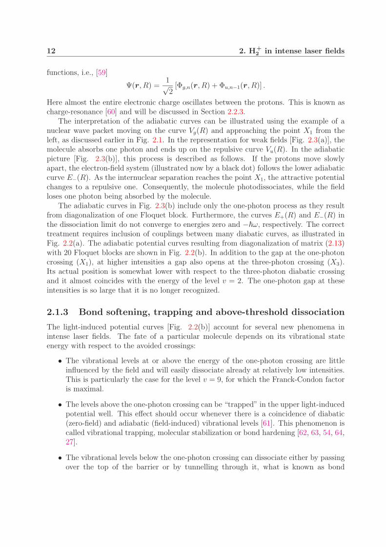
The adiabatic curves in Fig. 2.3(b) include only the one-photon process as they resultfrom diagonalization of one Floquet block. Furthermore, the curves E+(R) and E−(R) inthe dissociation limit do not converge to energies zero and −�ω, respectively. The correcttreatment requires inclusion of couplings between many diabatic curves, as illustrated inFig. 2.2(a). The adiabatic potential curves resulting from diagonalization of matrix (2.13)with 20 Floquet blocks are shown in Fig. 2.2(b). In addition to the gap at the one-photoncrossing (X1), at higher intensities a gap also opens at the three-photon crossing (X3).Its actual position is somewhat lower with respect to the three-photon diabatic crossingand it almost coincides with the energy of the level v = 2. The one-photon gap at theseintensities is so large that it is no longer recognized.
2.1.3 Bond softening, trapping and above-threshold dissociation
The light-induced potential curves [Fig. 2.2(b)] account for several new phenomena inintense laser fields. The fate of a particular molecule depends on its vibrational stateenergy with respect to the avoided crossings:
• The vibrational levels at or above the energy of the one-photon crossing are littleinfluenced by the field and will easily dissociate already at relatively low intensities.This is particularly the case for the level v = 9, for which the Franck-Condon factoris maximal.
• The levels above the one-photon crossing can be “trapped” in the upper light-inducedpotential well. This effect should occur whenever there is a coincidence of diabatic(zero-field) and adiabatic (field-induced) vibrational levels [61]. This phenomenon iscalled vibrational trapping, molecular stabilization or bond hardening [62, 63, 54, 64,27].
• The vibrational levels below the one-photon crossing can dissociate either by passingover the top of the barrier or by tunnelling through it, what is known as bond
2.2 Strong-field ionization and Coulomb explosion 13
softening [24, 65, 66, 54]. The photodissociation probability for these levels increasesnonlinearly with intensity. The lowest vibrational level for which dissociation viaone-photon is energetically allowed is v = 5, as can be seen in Fig. 2.2(b).
• The vibrational levels at or below the three-photon crossing X2 can dissociate byabsorption of three photons. A molecule in one of these levels follows the lowerbranch of the adiabatic curve |u, n− 3〉. It encounters then the avoided crossing X3,where it emits one photon and ends up adiabatically in the state |g, n−2〉. The totalresult of the three-photon absorption followed by one-photon emission is a net two-photon absorption. Since more photons were absorbed than it was necessary, thisprocess is often called above-threshold dissociation (ATD) [25, 65] or two-photonbond softening.
2.1.4 Molecular alignment
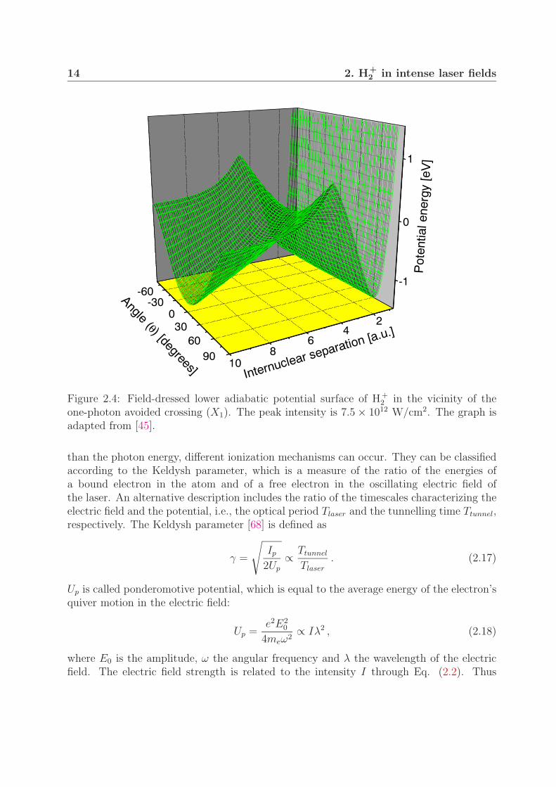
The adiabatic potential curves displayed in Fig. 2.2 were calculated for the electric fieldparallel to the molecular internuclear axis. In most of the experiments, however, the molec-ular orientation is isotropic. The photodissociation dynamics of molecules at an angle θwith respect to the laser polarization axis can be described with the aid of three-dimensionaladiabatic potential surfaces [65, 30]. Figure 2.4 shows a lower adiabatic potential surfacein the vicinity of the one-photon avoided crossing at an intensity of 7.5 × 10¹² W/cm2.
At smaller internuclear separations, which corresponds to a shorter timescale, the dy-namics of the molecules in the vibrational levels below the avoided crossing will be deter-mined by the light-induced potential barrier. The potential barrier is lowest for moleculesparallel to the electric field (θ = 0◦), whereas its height increases with larger angles.Correspondingly, the dissociation probability decreases with the increasing angle, leadingto angular distributions of the fragments peaked along the laser polarization axis. Thisalignment process is usually termed as geometric alignment, since it is mainly determinedby the angular dependence of the photodissociation probability. However, it can also beconsidered dynamically in terms of a wave packet skirting around the hardly penetrablepotential barrier around θ = 90◦ [67, 30]. Classically, the electric field exerts a torque onthe laser-induced molecular dipole moment. On a longer timescale, i.e., at larger inter-nuclear separations, the wave packet evolving on the lower potential surface will tend toend up in the potential valley centered at θ = 0◦, resulting in dynamic alignment of thedissociating molecule.
2.2 Strong-field ionization and Coulomb explosion
2.2.1 Photoionization mechanisms
When an atom or a molecule absorbs a photon of energy hν exceeding the ionizationpotential Ip, it is ionized and the excess energy is carried away by the electron in the formof translational kinetic energy. In the case that the ionization potential is much greater
14 2. H+2 in intense laser fields
24
68
10
-60-30
030
6090
-1
0
1
Pot
entia
l ene
rgy
[eV
]
Internuclear separation [a.u.]
Angle (θ) [degrees]
Figure 2.4: Field-dressed lower adiabatic potential surface of H+2 in the vicinity of the
one-photon avoided crossing (X1). The peak intensity is 7.5 × 10¹² W/cm2. The graph isadapted from [45].
than the photon energy, different ionization mechanisms can occur. They can be classifiedaccording to the Keldysh parameter, which is a measure of the ratio of the energies ofa bound electron in the atom and of a free electron in the oscillating electric field ofthe laser. An alternative description includes the ratio of the timescales characterizing theelectric field and the potential, i.e., the optical period Tlaser and the tunnelling time Ttunnel,respectively. The Keldysh parameter [68] is defined as
γ =
√Ip
2Up
∝ Ttunnel
Tlaser
. (2.17)
Up is called ponderomotive potential, which is equal to the average energy of the electron’squiver motion in the electric field:
Up =e2E2
0
4meω2∝ Iλ2 , (2.18)
where E0 is the amplitude, ω the angular frequency and λ the wavelength of the electricfield. The electric field strength is related to the intensity I through Eq. (2.2). Thus
2.2 Strong-field ionization and Coulomb explosion 15
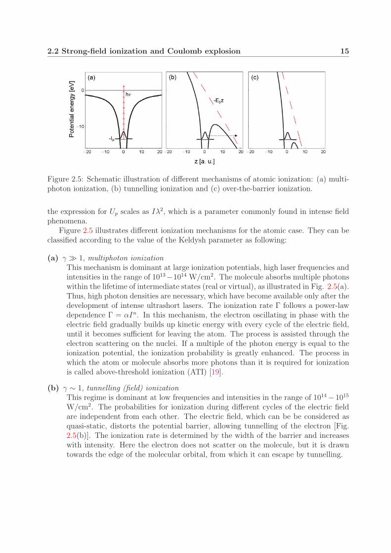
Figure 2.5: Schematic illustration of different mechanisms of atomic ionization: (a) multi-photon ionization, (b) tunnelling ionization and (c) over-the-barrier ionization.
the expression for Up scales as Iλ2, which is a parameter commonly found in intense fieldphenomena.
Figure 2.5 illustrates different ionization mechanisms for the atomic case. They can beclassified according to the value of the Keldysh parameter as following:
(a) γ � 1, multiphoton ionizationThis mechanism is dominant at large ionization potentials, high laser frequencies andintensities in the range of 1013−1014 W/cm2. The molecule absorbs multiple photonswithin the lifetime of intermediate states (real or virtual), as illustrated in Fig. 2.5(a).Thus, high photon densities are necessary, which have become available only after thedevelopment of intense ultrashort lasers. The ionization rate Γ follows a power-lawdependence Γ = αIn. In this mechanism, the electron oscillating in phase with theelectric field gradually builds up kinetic energy with every cycle of the electric field,until it becomes sufficient for leaving the atom. The process is assisted through theelectron scattering on the nuclei. If a multiple of the photon energy is equal to theionization potential, the ionization probability is greatly enhanced. The process inwhich the atom or molecule absorbs more photons than it is required for ionizationis called above-threshold ionization (ATI) [19].
(b) γ ∼ 1, tunnelling (field) ionizationThis regime is dominant at low frequencies and intensities in the range of 1014 − 1015
W/cm2. The probabilities for ionization during different cycles of the electric fieldare independent from each other. The electric field, which can be be considered asquasi-static, distorts the potential barrier, allowing tunnelling of the electron [Fig.2.5(b)]. The ionization rate is determined by the width of the barrier and increaseswith intensity. Here the electron does not scatter on the molecule, but it is drawntowards the edge of the molecular orbital, from which it can escape by tunnelling.
16 2. H+2 in intense laser fields
(c) γ 1, over-the-barrier ionizationThis is the limiting case of field ionization where the barrier is lowered by the stronglaser field (intensity >1015 W/cm2) to such an extent that the electron can pass overthe top of the barrier without tunnelling [Fig. 2.5(c)]. In this regime the ionizationprobability approaches unity within one laser cycle [69].
The classification of the ionization mechanisms described above is not strict and theionization processes often fall in an intermediate regime where the process is described bya combination of the ionization mechanisms.
In the case of the hydrogen molecular ion, the ionization potential depends on theinternuclear separation R [70, 71]
Ip ∼ Ip (H atom) + 1/R . (2.19)
Here all the quantities are in atomic units. The ionization potential of the hydrogen atomis Ip (H atom) = 0.5 a.u. For the internuclear separation R = 10 a.u., where the ionizationrate is enhanced (Section 2.2.3), the ionization potential is Ip ∼ 0.6 a.u. (∼16 eV). Withλ = 790 nm (hν ∼ 1.6 eV) and I = 1014 W/cm2, the Keldysh parameter [Eq. (2.17)] isγ ∼ 1.2. Thus the molecular ionization is best described by the electron tunnelling.
2.2.2 Semiclassical model of enhanced ionization
In the case of H+2 , the ionization process results in formation of two protons starting to
repel each other by Coulomb force. During this process, which is known as Coulombexplosion, each of the protons gains the half of the Coulomb energy ECE = 1/(2R) (inatomic units), where R is the internuclear separation at the moment of ionization. Themeasured kinetic energies of the Coulomb explosion protons of 1–4 eV (e.g., [64]) areconsiderably smaller than the energy of about 7 eV that is expected if ionization wouldtake place at the equilibrium internuclear separation Req ∼ 2 a.u. This discrepancy canbe explained by a semiclassical model of the electron in the electrostatic potential of twoprotons and the constant electric field [34, 35]:
V (z,R,E0) = − 1√(z − R/2)2
− 1√(z + R/2)2
− E0z . (2.20)
Figure 2.6 illustrates the potential defined by Eq. (2.20) for four different internuclearseparations R. The horizontal lines mark the position of the two lowest electronic states insuch a potential. These are Stark shifted and their separation is E0R at large R. For smallinternuclear separations, the electron can oscillate freely between the nuclei [Fig. 2.6(a)].The probability for ionization is here similar to that of the hydrogen atom due to the broadouter potential barrier. As the internuclear separation increases, the inner barrier startsto rise, impeding the charge transfer between the wells [Fig. 2.6(b)]. The probability fortunnelling through the inner barrier during a half of an optical cycle decreases and the elec-tron becomes localized at one proton. This localization of the electron is a crucial element
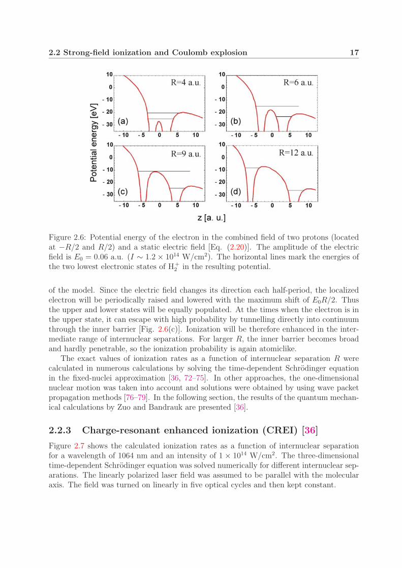
2.2 Strong-field ionization and Coulomb explosion 17
Figure 2.6: Potential energy of the electron in the combined field of two protons (locatedat −R/2 and R/2) and a static electric field [Eq. (2.20)]. The amplitude of the electricfield is E0 = 0.06 a.u. (I ∼ 1.2 × 10¹⁴ W/cm2). The horizontal lines mark the energies ofthe two lowest electronic states of H+
2 in the resulting potential.
of the model. Since the electric field changes its direction each half-period, the localizedelectron will be periodically raised and lowered with the maximum shift of E0R/2. Thusthe upper and lower states will be equally populated. At the times when the electron is inthe upper state, it can escape with high probability by tunnelling directly into continuumthrough the inner barrier [Fig. 2.6(c)]. Ionization will be therefore enhanced in the inter-mediate range of internuclear separations. For larger R, the inner barrier becomes broadand hardly penetrable, so the ionization probability is again atomiclike.
The exact values of ionization rates as a function of internuclear separation R werecalculated in numerous calculations by solving the time-dependent Schrodinger equationin the fixed-nuclei approximation [36, 72–75]. In other approaches, the one-dimensionalnuclear motion was taken into account and solutions were obtained by using wave packetpropagation methods [76–79]. In the following section, the results of the quantum mechan-ical calculations by Zuo and Bandrauk are presented [36].
2.2.3 Charge-resonant enhanced ionization (CREI) [36]
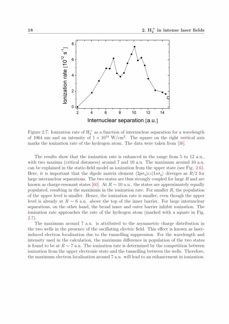
Figure 2.7 shows the calculated ionization rates as a function of internuclear separationfor a wavelength of 1064 nm and an intensity of 1 × 10¹⁴ W/cm2. The three-dimensionaltime-dependent Schrodinger equation was solved numerically for different internuclear sep-arations. The linearly polarized laser field was assumed to be parallel with the molecularaxis. The field was turned on linearly in five optical cycles and then kept constant.
18 2. H+2 in intense laser fields
Figure 2.7: Ionization rate of H+2 as a function of internuclear separation for a wavelength
of 1064 nm and an intensity of 1 × 10¹⁴ W/cm2. The square on the right vertical axismarks the ionization rate of the hydrogen atom. The data were taken from [36].
The results show that the ionization rate is enhanced in the range from 5 to 12 a.u.,with two maxima (critical distances) around 7 and 10 a.u. The maximum around 10 a.u.can be explained in the static-field model as ionization from the upper state (see Fig. 2.6).Here, it is important that the dipole matrix element 〈2pσu|ez|1sσg〉 diverges as R/2 forlarge internuclear separations. The two states are thus strongly coupled for large R and areknown as charge-resonant states [60]. At R ∼ 10 a.u., the states are approximately equallypopulated, resulting in the maximum in the ionization rate. For smaller R, the populationof the upper level is smaller. Hence, the ionization rate is smaller, even though the upperlevel is already at R ∼ 6 a.u. above the top of the inner barrier. For large internuclearseparations, on the other hand, the broad inner and outer barrier inhibit ionization. Theionization rate approaches the rate of the hydrogen atom (marked with a square in Fig.2.7).
The maximum around 7 a.u. is attributed to the asymmetric charge distribution inthe two wells in the presence of the oscillating electric field. This effect is known as laser-induced electron localization due to the tunnelling suppression. For the wavelength andintensity used in the calculation, the maximum difference in population of the two statesis found to be at R ∼ 7 a.u. The ionization rate is determined by the competition betweenionization from the upper electronic state and the tunnelling between the wells. Therefore,the maximum electron localization around 7 a.u. will lead to an enhancement in ionization.
Chapter 3
Experimental
The two intense-field fragmentation mechanisms discussed in the previous chapter — pho-todissociation
H+2 + nhν → H + H+ (3.1)
and ionization followed by Coulomb explosion
H+2 + n′hν → H+ + H+ + e− (3.2)
were investigated by measuring the velocity distributions of the nuclear fragments. Themolecular ions were investigated in fast, mass-selected and well collimated ion beams. Theions were exposed to intense ultrashort pulses produced in an amplified femtosecond lasersystem. The velocity distribution of the nuclear fragments from both channels were imagedon a position sensitive detector.
The ion beam apparatus and the detection system are described in detail in Section3.1. In Section 3.2 the method of fragment imaging is explained and procedures of retriev-ing the original three-dimensional (3D) velocity distribution from the experimental imagesare described. The femtosecond laser system and the characterization of laser pulses arepresented in Section 3.3. The intensity distribution in the interaction region and its impli-cation for measured data is the topic of Section 3.4.
3.1 Ion beam apparatus
The ion beam apparatus used in this work was in previous experiments first applied byFigger et al for the investigation of the emission spectra of rare gas hydrides (HeH, ArH,etc.) and triatomic hydrogen molecules (H3, D3, H2D and D2H) [80–82]. An upgrade ofthe apparatus for the purposes of fragment imaging was carried out by Wunderlich et al,who investigated light-induced potential curves in Ar+
2 [59, 83–85]. In the study of H+2 in
intense laser fields, Sandig et al improved the ion beam collimation, which enabled themto resolve fragments from single vibrational levels [28, 86].
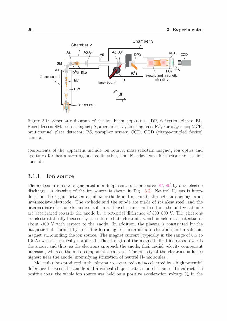
A schematic of the ion beam apparatus is presented in Fig. 3.1. The apparatus consistsof three vacuum chambers, which are each pumped by a turbomolecular pump. The main
20 3. Experimental
ion source
SM
laser beam
MCP
electric and magneticshielding
FC1Chamber 1
Chamber 3Chamber 2
EL1
EL2
DP1
DP2
A4 A7
FC2 PS
DP3
L1
CCD
x
zy
A1
A2 A3A5
A6
Figure 3.1: Schematic diagram of the ion beam apparatus. DP, deflection plates; EL,Einzel lenses; SM, sector magnet; A, apertures; L1, focusing lens; FC, Faraday cups; MCP,multichannel plate detector; PS, phosphor screen; CCD, CCD (charge-coupled device)camera.
components of the apparatus include ion source, mass-selection magnet, ion optics andapertures for beam steering and collimation, and Faraday cups for measuring the ioncurrent.
3.1.1 Ion source
The molecular ions were generated in a duoplasmatron ion source [87, 80] by a dc electricdischarge. A drawing of the ion source is shown in Fig. 3.2. Neutral H2 gas is intro-duced in the region between a hollow cathode and an anode through an opening in anintermediate electrode. The cathode and the anode are made of stainless steel, and theintermediate electrode is made of soft iron. The electrons emitted from the hollow cathodeare accelerated towards the anode by a potential difference of 300–600 V. The electronsare electrostatically focused by the intermediate electrode, which is held on a potential ofabout -100 V with respect to the anode. In addition, the plasma is constricted by themagnetic field formed by both the ferromagnetic intermediate electrode and a solenoidmagnet surrounding the ion source. The magnet current (typically in the range of 0.5 to1.5 A) was electronically stabilized. The strength of the magnetic field increases towardsthe anode, and thus, as the electrons approach the anode, their radial velocity componentincreases, whereas the axial component decreases. The density of the electrons is hencehighest near the anode, intensifying ionization of neutral H2 molecules.
Molecular ions produced in the plasma are extracted and accelerated by a high potentialdifference between the anode and a conical shaped extraction electrode. To extract thepositive ions, the whole ion source was held on a positive acceleration voltage Ua in the

3.1 Ion beam apparatus 21
� � � � �� � � � � � � �
� � � � � � � � � � � � �� � � � � � � � � � � � � �
� � � � � � � � � � � � � � � � � � � � � �� � � � � � �
� � � � � � � � � � � � �
Figure 3.2: Drawing of the duoplasmatron ion source. Neutral gas introduced in the ionsource through the inlet tube is ionized by electrons emitted from the hollow cathode.The produced plasma is confined by the electric field of the intermediate electrode anda nonuniform magnetic field of the intermediate electrode and a solenoid magnet. Theelectrodes are insulated by intermediate ceramic rings (not shown in the figure).
range of 3–12 kV, whereas the rest of the apparatus was grounded. The extracted currentof ions is roughly proportional to the area of the anode aperture. Although the extractedcurrent could be greatly enhanced with anodes with apertures of 300 and 400 µm indiameter, only a small portion could be collimated. Sufficient and more stable current wasachieved using an anode with an aperture of 200 µm. The extracted current was typicallyaround 100 µA and could be varied by adjusting the current of the solenoid magnet.The electrodes in the ion source deteriorate with time due to their high temperature andelectron sputtering. This usually manifested itself in an increased discharge voltage andan unstable extracted current. In this case the hollow cathode was replaced and theintermediate electrode and anode were thoroughly cleaned.
To ensure a constant flow of H2 gas into the ion source, a two-stage pressure regulator1
was installed on a gas container. A fine regulation of the flow was achieved by means of adosing valve2. To ignite the discharge, the pressure in the ion source is increased to about100 Pa for a few seconds. Then it is gradually decreased to a value slightly above thethreshold at which the discharge extinguishes (about 10 Pa). Usually about half an hourafter ignition is needed for stable ion source operation. The pressure in the ion source wasindirectly monitored by measuring the pressure in Chamber 1.
The main formation process of H+2 in the ion source is electron impact ionization of
H2 [88]. For the ion source temperature of about 100◦ C [80], the thermal energy kT ismuch smaller than the vibrational separation, and thus only the ground vibrational levelv = 0 of H2 is populated. In different types of ion sources it was found that the vibrationalpopulation of H+
2 is well described by the Franck-Condon factors between the vibrationallevels of H+
2 in the 1sσg state and the ground vibrational level of H2 in the electronic ground
1Messer Griesheim, Spectron FE 622Balzers, EVN 116
22 3. Experimental
state [89–91]. The vibrational population of H+2 and D+
2 obtained by von Busch et al foran electron bombardment-type ion source is listed in Appendix B. A similar vibrationaldistribution was also reported for a monoplasmatron ion source, which is similar to the ionsource used in our experiment [92].
The rotational temperature of the vibrational ground state of H2 is approximately200 K [86], yielding a Maxwell-Boltzmann distribution of the rotational population withmaximum for the rotational quantum number J = 0 [93]. In the ionization process, therotational quantum number does not undergo large changes, and thus H+
2 is formed in therotational ground state. The smallest allowed change ∆J = ±2 occurs with a much lowerprobability [90].
3.1.2 Mass selection
After extraction from the ion source, molecular ions are directed into a sector magnet3
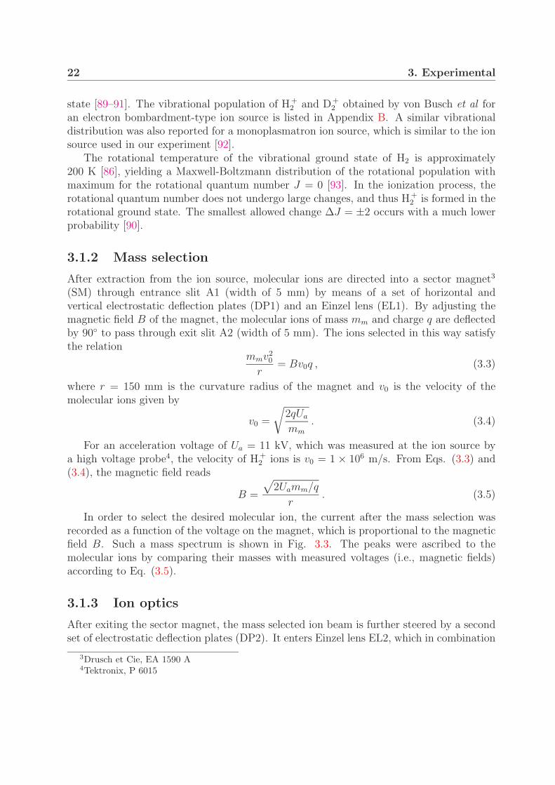
(SM) through entrance slit A1 (width of 5 mm) by means of a set of horizontal andvertical electrostatic deflection plates (DP1) and an Einzel lens (EL1). By adjusting themagnetic field B of the magnet, the molecular ions of mass mm and charge q are deflectedby 90◦ to pass through exit slit A2 (width of 5 mm). The ions selected in this way satisfythe relation
mmv20
r= Bv0q , (3.3)
where r = 150 mm is the curvature radius of the magnet and v0 is the velocity of themolecular ions given by
v0 =
√2qUa
mm
. (3.4)
For an acceleration voltage of Ua = 11 kV, which was measured at the ion source bya high voltage probe4, the velocity of H+
2 ions is v0 = 1 × 10⁶ m/s. From Eqs. (3.3) and(3.4), the magnetic field reads
B =
√2Uamm/q
r. (3.5)
In order to select the desired molecular ion, the current after the mass selection wasrecorded as a function of the voltage on the magnet, which is proportional to the magneticfield B. Such a mass spectrum is shown in Fig. 3.3. The peaks were ascribed to themolecular ions by comparing their masses with measured voltages (i.e., magnetic fields)according to Eq. (3.5).
3.1.3 Ion optics
After exiting the sector magnet, the mass selected ion beam is further steered by a secondset of electrostatic deflection plates (DP2). It enters Einzel lens EL2, which in combination
3Drusch et Cie, EA 1590 A4Tektronix, P 6015

3.1 Ion beam apparatus 23
Figure 3.3: Ion current measured at apertures A3 and A4 as a function of the voltage (i.e.,magnetic field) on the sector magnet. The ions result from ionization and recombinationprocesses in a H2 plasma. The acceleration voltage was Ua = 12 kV.
with Einzel lens EL1 serves as an electrostatic telescope that collimates and maximizes theflux of the ion beam. The voltages applied to the Einzel lenses were U1 ∼ 8 kV andU2 ∼ −12 kV. The beam divergence is restricted by apertures A4 and A7 separated by adistance a of 53 cm.
The apertures were composed of two mutually perpendicular slits5 of different widths.Since a better velocity resolution was needed along the laser polarization axis (z axis),narrower slits were used for collimation along this axis (see Fig. 3.1). In different experi-ments, the widths of the slits along the z axis were h4 = 75 − 200 µm and h7 = 25 − 50µm for apertures A4 and A7, respectively (as shown in Fig. 3.6). Such small values of h7
were also important to reduce intensity variations in the interaction region, as it will bediscussed in Section 3.4. Sufficient intensity of the ion current was provided by using slitsof widths of 200–300 µm along the laser propagation axis (y axis).
For strongest ion currents and optimal beam collimation, the alignment of the aperturesis crucial. For this purpose a helium-neon (HeNe) laser was used, whose propagation axisis first fixed with slit A2 at one end and the center of the multichannel plate (MCP)detector at the other end. After that, a movable Faraday cup in front of the MCP detector(FC2) is adjusted to cover the HeNe beam. After the axis of the HeNe beam is fixed,the attenuated femtosecond laser beam is focused at right angle on it. At this point,the focal position is adjusted only roughly by observing the position of the laser-inducedbreakdown in air. Overlap of the two beams is provided by a 50 µm pinhole placed under45◦ with respect to the both beams. First, the transmission of the HeNe beam through
5Melles Griot
24 3. Experimental
the pinhole is maximized by positioning the pinhole along the y and z axes by means of atranslational stage and a mechanical feedthrough, respectively. After that, the femtosecondbeam is passed through the pinhole by adjusting the x and y position of the focusinglens. After positioning the crossing aperture, aperture A7 and then aperture A4 is alignedby maximizing the signal on a photodiode placed behind the apertures. The proceduredescribed assured that the laser beam will cross the ion beam passing through aperturesA4 and A7. The precise adjustment of the overlap of the ion and laser beams along allthree axes is done by maximizing the detected fragment signal before each measurement.
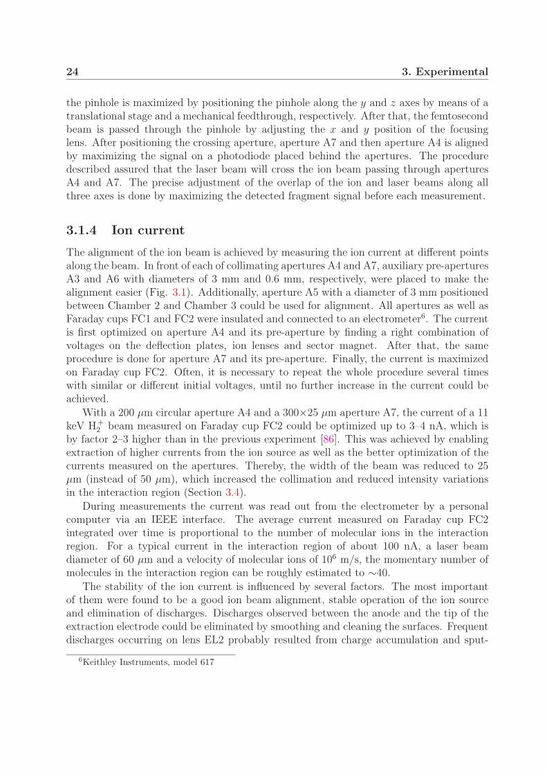
3.1.4 Ion current
The alignment of the ion beam is achieved by measuring the ion current at different pointsalong the beam. In front of each of collimating apertures A4 and A7, auxiliary pre-aperturesA3 and A6 with diameters of 3 mm and 0.6 mm, respectively, were placed to make thealignment easier (Fig. 3.1). Additionally, aperture A5 with a diameter of 3 mm positionedbetween Chamber 2 and Chamber 3 could be used for alignment. All apertures as well asFaraday cups FC1 and FC2 were insulated and connected to an electrometer6. The currentis first optimized on aperture A4 and its pre-aperture by finding a right combination ofvoltages on the deflection plates, ion lenses and sector magnet. After that, the sameprocedure is done for aperture A7 and its pre-aperture. Finally, the current is maximizedon Faraday cup FC2. Often, it is necessary to repeat the whole procedure several timeswith similar or different initial voltages, until no further increase in the current could beachieved.
With a 200 µm circular aperture A4 and a 300×25 µm aperture A7, the current of a 11keV H+
2 beam measured on Faraday cup FC2 could be optimized up to 3–4 nA, which isby factor 2–3 higher than in the previous experiment [86]. This was achieved by enablingextraction of higher currents from the ion source as well as the better optimization of thecurrents measured on the apertures. Thereby, the width of the beam was reduced to 25µm (instead of 50 µm), which increased the collimation and reduced intensity variationsin the interaction region (Section 3.4).
During measurements the current was read out from the electrometer by a personalcomputer via an IEEE interface. The average current measured on Faraday cup FC2integrated over time is proportional to the number of molecular ions in the interactionregion. For a typical current in the interaction region of about 100 nA, a laser beamdiameter of 60 µm and a velocity of molecular ions of 106 m/s, the momentary number ofmolecules in the interaction region can be roughly estimated to ∼40.
The stability of the ion current is influenced by several factors. The most importantof them were found to be a good ion beam alignment, stable operation of the ion sourceand elimination of discharges. Discharges observed between the anode and the tip of theextraction electrode could be eliminated by smoothing and cleaning the surfaces. Frequentdischarges occurring on lens EL2 probably resulted from charge accumulation and sput-
6Keithley Instruments, model 617
3.1 Ion beam apparatus 25
tering on the ceramic holder rings caused by the ion beam. The problem was solved byconstructing a new lens with an additional aperture added at its entrance. Also cleansurfaces and better evacuation through additional openings were beneficial. In addition, anew design provided easier alignment of the lens axes [46].
The horizontal deflection plates DP3, placed after the molecule-laser interaction region,could be used to deflect the ion beam and positive fragments into Faraday cup FC1 (seealso Fig. 3.5). In this way the remaining neutral fragments could be separately detectedon the MCP detector. For detection of both charged and neutral fragments, no voltagewas applied to deflection plates DP3. In order to protect the detector and to measurethe current, Faraday cup FC2 was placed into the beam in front of the detector. This,however, prevented the detection of fragments with small deflections off the ion beam axis.To minimize this effect, a Faraday cup with a diameter of 4 mm was constructed, whichprovided a secure capture of fast molecular ions.
The deflection plates DP3 were enclosed in a metal housing to restrict the electric fieldsto the region inside the housing. The path of the fragments between deflection plates DP3and the detector was shielded against electric and magnetic stray fields using a coppercylinder and two concentric cylindrical sheets of a high-permeability metal [59].
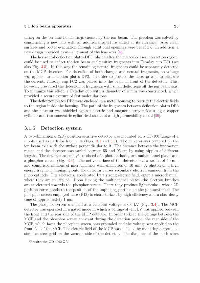
3.1.5 Detection system
A two-dimensional (2D) position sensitive detector was mounted on a CF-100 flange of anipple used as path for fragments (Figs. 3.1 and 3.5). The detector was centered on theion beam axis with the surface perpendicular to it. The distance between the interactionregion and the detector was varied between 55 and 95 cm by using nipples of differentlengths. The detector assembly7 consisted of a photocathode, two multichannel plates anda phosphor screen (Fig. 3.4). The active surface of the detector had a radius of 40 mmand comprised millions of microchannels with diameters of 10 µm. A photon or a highenergy fragment impinging onto the detector causes secondary electron emission from thephotocathode. The electrons, accelerated by a strong electric field, enter a microchannel,where they are multiplied. Upon leaving the multichannel plates, the electron bunchesare accelerated towards the phosphor screen. There they produce light flashes, whose 2Dposition corresponds to the position of the impinging particle on the photocathode. Thephosphor screen employed here (P43) is characterized by high efficiency and a slow decaytime of approximately 1 ms.
The phosphor screen was held at a constant voltage of 6.0 kV (Fig. 3.4). The MCPdetector was operated in a gated mode in which a voltage of -1.4 kV was applied betweenthe front and the rear side of the MCP detector. In order to keep the voltage between theMCP and the phosphor screen constant during the detection period, the rear side of theMCP, which faces the phosphor screen, was grounded and the voltage was applied to thefront side of the MCP. The electric field of the MCP was shielded by mounting a groundedstainless steel grid on the vacuum side of the detector. The diameter of the mesh wires
7Proxitronic, OD 4062 Z-V
26 3. Experimental
� � � � � � � � � � � � � � � � � � � � � � �
� � � � � � � � � � � �
� � � � � � � �
� ! � " �
� � �
� � � � � �
� � � # � � " �� � " �
� � � �
� � �
Figure 3.4: Schematic of the two-stage multichannel plate detector with the typical oper-ating voltages.
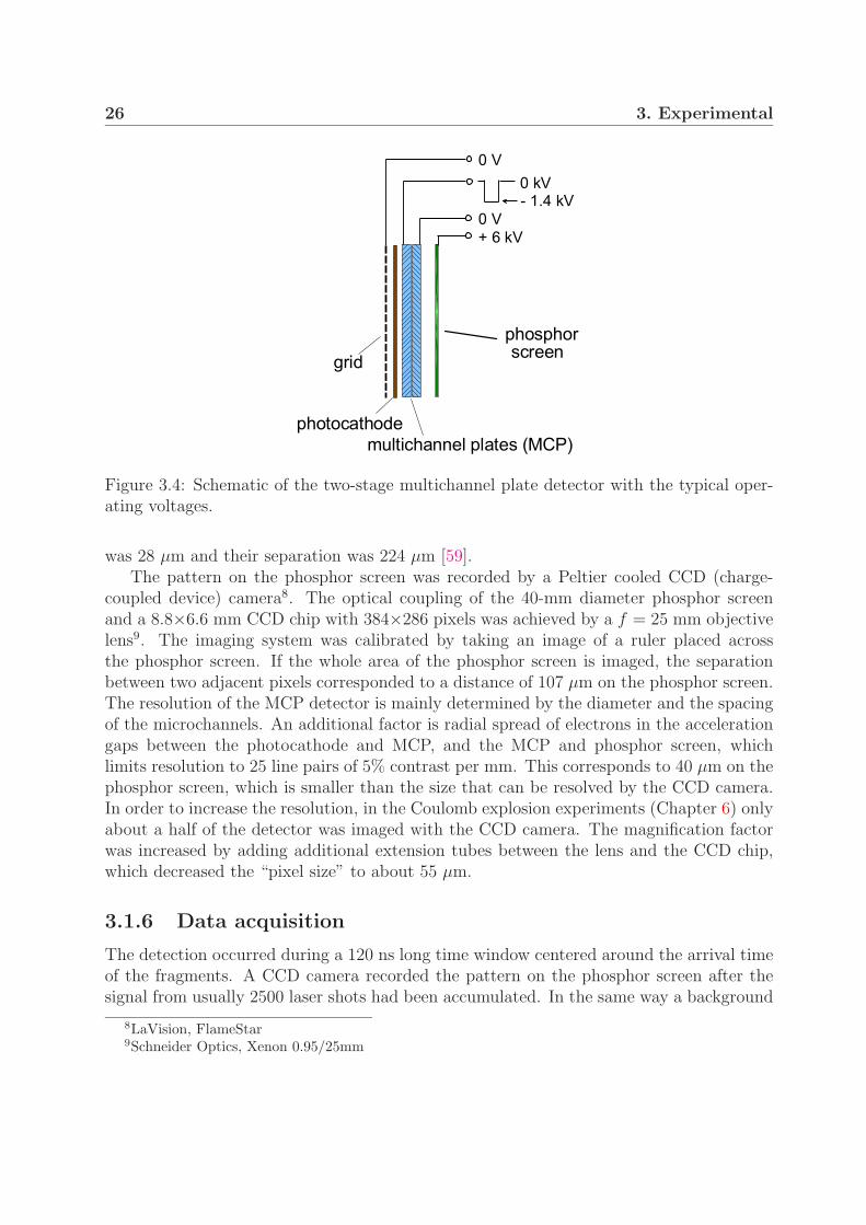
was 28 µm and their separation was 224 µm [59].The pattern on the phosphor screen was recorded by a Peltier cooled CCD (charge-
coupled device) camera8. The optical coupling of the 40-mm diameter phosphor screenand a 8.8×6.6 mm CCD chip with 384×286 pixels was achieved by a f = 25 mm objectivelens9. The imaging system was calibrated by taking an image of a ruler placed acrossthe phosphor screen. If the whole area of the phosphor screen is imaged, the separationbetween two adjacent pixels corresponded to a distance of 107 µm on the phosphor screen.The resolution of the MCP detector is mainly determined by the diameter and the spacingof the microchannels. An additional factor is radial spread of electrons in the accelerationgaps between the photocathode and MCP, and the MCP and phosphor screen, whichlimits resolution to 25 line pairs of 5% contrast per mm. This corresponds to 40 µm on thephosphor screen, which is smaller than the size that can be resolved by the CCD camera.In order to increase the resolution, in the Coulomb explosion experiments (Chapter 6) onlyabout a half of the detector was imaged with the CCD camera. The magnification factorwas increased by adding additional extension tubes between the lens and the CCD chip,which decreased the “pixel size” to about 55 µm.
3.1.6 Data acquisition
The detection occurred during a 120 ns long time window centered around the arrival timeof the fragments. A CCD camera recorded the pattern on the phosphor screen after thesignal from usually 2500 laser shots had been accumulated. In the same way a background
8LaVision, FlameStar9Schneider Optics, Xenon 0.95/25mm
3.1 Ion beam apparatus 27
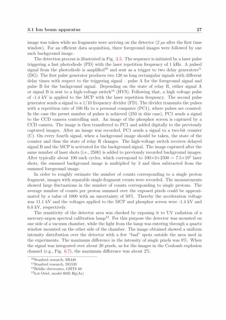
image was taken while no fragments were arriving on the detector (2 µs after the first timewindow). For an efficient data acquisition, three foreground images were followed by onesuch background image.
The detection process is illustrated in Fig. 3.5. The sequence is initiated by a laser pulsetriggering a fast photodiode (PD) with the laser repetition frequency of 1 kHz. A pulsedsignal from the photodiode is amplified10 and sent as a trigger to two delay generators11
(DG). The first pulse generator produces two 120 ns long rectangular signals with differentdelay times with respect to the triggering signal – pulse A for the foreground signal andpulse B for the background signal. Depending on the state of relay R, either signal Aor signal B is sent to a high-voltage switch12 (HVS). Following that, a high voltage pulseof -1.4 kV is applied to the MCP with the laser repetition frequency. The second pulsegenerator sends a signal to a 1/10 frequency divider (FD). The divider transmits the pulseswith a repetition rate of 100 Hz to a personal computer (PC1), where pulses are counted.In the case the preset number of pulses is achieved (250 in this case), PC1 sends a signalto the CCD camera controlling unit. An image of the phosphor screen is captured by aCCD camera. The image is then transferred to PC1 and added digitally to the previouslycaptured images. After an image was recorded, PC1 sends a signal to a two-bit counter(C). On every fourth signal, when a background image should be taken, the state of thecounter and thus the state of relay R changes. The high-voltage switch receives delayedsignal B and the MCP is activated for the background signal. The image captured after thesame number of laser shots (i.e., 2500) is added to previously recorded background images.After typically about 100 such cycles, which correspond to 100×3×2500 = 7.5×10⁵ lasershots, the summed background image is multiplied by 3 and then subtracted from thesummed foreground image.
In order to roughly estimate the number of counts corresponding to a single protonfragment, images with separable single-fragment events were recorded. The measurementsshowed large fluctuations in the number of counts corresponding to single protons. Theaverage number of counts per proton summed over the exposed pixels could be approxi-mated by a value of 1000 with an uncertainty of 50%. Thereby the acceleration voltagewas 11.1 kV and the voltages applied to the MCP and phosphor screen were -1.4 kV and6.0 kV, respectively.
The sensitivity of the detector area was checked by exposing it to UV radiation of amercury-argon spectral calibration lamp13. For this purpose the detector was mounted onone side of a vacuum chamber, while the light from the lamp was entering through a quartzwindow mounted on the other side of the chamber. The image obtained showed a uniformintensity distribution over the detector with a few “bad” spots outside the area used inthe experiments. The maximum difference in the intensity of single pixels was 8%. Whenthe signal was integrated over about 20 pixels, as for the images in the Coulomb explosionchannel (e.g., Fig. 6.7), the maximum difference was about 2%.
10Stanford research, SR44011Stanford research, DG53512Behlke electronics, GHTS 6013Lot-Oriel, model 6035 Hg(Ar)
28 3. Experimental
CCD
DP3
Chamber 3
PSMCP
FC2FC1
W1
EM
fragments
PD
R
PC1
PC2
CDG
FD 1/10
HVSSA
PSU
CU
laserbeam
G
ionbeam
B
A
Figure 3.5: Schematic of Chamber 3 and the components used in the detection. W1,window; PD, photodiode; SA, signal amplifier; DG, delay generator; FD, frequency divider;R, relay; HVS, high-voltage switch; C, 2-bit counter; PC, personal computer; CU, CCDcontrol unit; PSU, Peltier stabilization unit; EM, electrometer; DP, deflection plates; FC,Faraday cup; G, grid; MCP, multichannel plate detector; PS, phosphor screen.
3.1.7 Collimation of the ion beam
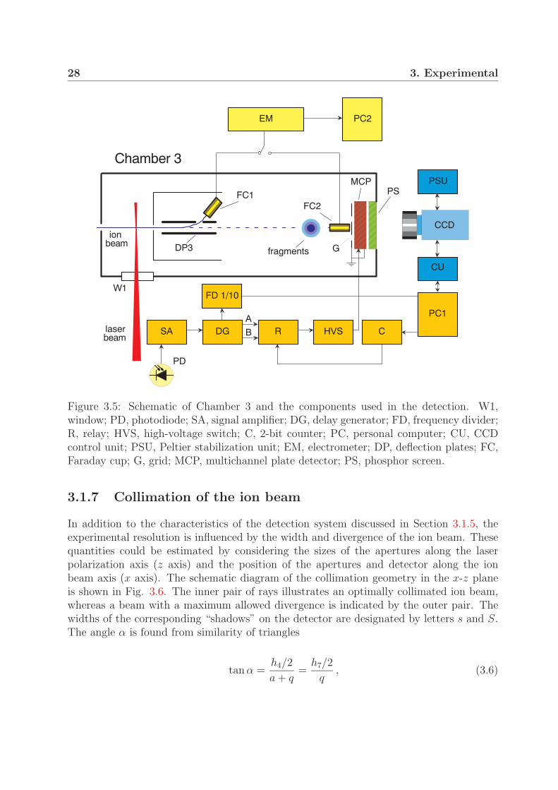
In addition to the characteristics of the detection system discussed in Section 3.1.5, theexperimental resolution is influenced by the width and divergence of the ion beam. Thesequantities could be estimated by considering the sizes of the apertures along the laserpolarization axis (z axis) and the position of the apertures and detector along the ionbeam axis (x axis). The schematic diagram of the collimation geometry in the x-z planeis shown in Fig. 3.6. The inner pair of rays illustrates an optimally collimated ion beam,whereas a beam with a maximum allowed divergence is indicated by the outer pair. Thewidths of the corresponding “shadows” on the detector are designated by letters s and S.The angle α is found from similarity of triangles
tan α =h4/2
a + q=
h7/2
q, (3.6)
3.1 Ion beam apparatus 29
A4 A7MCP
2α 2β
a b
h4h7
qp
Ss
x
z
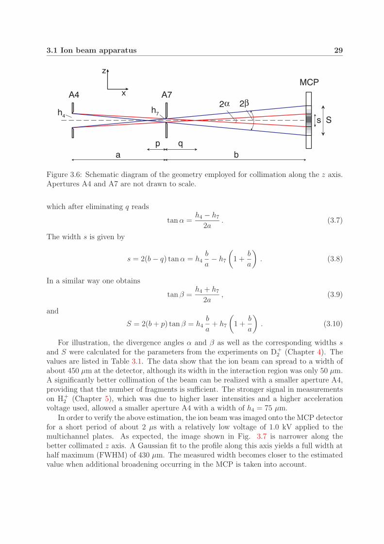
Figure 3.6: Schematic diagram of the geometry employed for collimation along the z axis.Apertures A4 and A7 are not drawn to scale.
which after eliminating q reads
tan α =h4 − h7
2a. (3.7)
The width s is given by
s = 2(b − q) tan α = h4b
a− h7
(1 +
b
a
). (3.8)
In a similar way one obtains
tan β =h4 + h7
2a, (3.9)
and
S = 2(b + p) tan β = h4b
a+ h7
(1 +
b
a
). (3.10)
For illustration, the divergence angles α and β as well as the corresponding widths sand S were calculated for the parameters from the experiments on D+
2 (Chapter 4). Thevalues are listed in Table 3.1. The data show that the ion beam can spread to a width ofabout 450 µm at the detector, although its width in the interaction region was only 50 µm.A significantly better collimation of the beam can be realized with a smaller aperture A4,providing that the number of fragments is sufficient. The stronger signal in measurementson H+
2 (Chapter 5), which was due to higher laser intensities and a higher accelerationvoltage used, allowed a smaller aperture A4 with a width of h4 = 75 µm.
In order to verify the above estimation, the ion beam was imaged onto the MCP detectorfor a short period of about 2 µs with a relatively low voltage of 1.0 kV applied to themultichannel plates. As expected, the image shown in Fig. 3.7 is narrower along thebetter collimated z axis. A Gaussian fit to the profile along this axis yields a full width athalf maximum (FWHM) of 430 µm. The measured width becomes closer to the estimatedvalue when additional broadening occurring in the MCP is taken into account.

30 3. Experimental
Table 3.1: The divergence angles and widths of the ion beam at the detectorcalculated for the parameters from the D+
2 measurements (Chapter 4).
a [cm] b [cm] h4 [µm] h7 [µm] α [mrad] β [mrad] s [µm] S [µm]
53 85 200 50 0.14 0.24 190 450
3.1.8 Vacuum system
The three vacuum chambers were pumped by separate turbomolecular pumps backed byrotary pumps. The differential pumping and small apertures between the chambers assurethat a relatively high pressure in the ion source region is reduced stepwise towards the de-tection region. The pumping speeds of the turbomolecular pumps and the typical pressuresin the chambers are given in Table 3.2. A vacuum of ∼ 2×10⁻⁸ mbar in the interaction anddetection region was achieved by installing a 700 l/s turbomolecular pump. Bayard-Alpertionization gauges14 were used to measure the pressures in the vacuum chambers and Piranithermal conductivity gauges15 for the pressures between each rotary and turbomolecularpump. Gate valves between the chambers enabled their separate venting with nitrogen.In order to suppress vibrations, the rotary pumps were placed on damping rubber blocksand bellows were attached to massive metal blocks.
Table 3.2: Pumping speeds of turbomolecular pumps and typical pressuresin the vacuum chambers.
vacuum chamber Chamber 1 Chamber 2 Chamber 3
pumping speed for N2 [l/s] 345a 500b 680c
pressure [mbar] 2 × 10⁻⁵ 2 × 10⁻⁶ 2 × 10⁻⁸
a Leybold, Turbovac 360b Pfeiffer, TPU 510c Leybold, Turbovac TW 700
3.2 Imaging of fragments
Imaging the fragment velocity distribution can provide information on both the kineticenergy and the angular distributions of fragments. The principle of this technique isexplained in the first subsection. Next, methods of retrieving the original 3D velocity
14Leybold, Ionivac IE 41415Leybold, Thermovac TM 21

3.2 Imaging of fragments 31
y [p
ixel
s]
170 180 1900
20
40
60
80
100
0 20 40 60 80 100
160
150
140
z [pixels]
Figure 3.7: The ion beam profile obtained by imaging the beam on the MCP detector. Avoltage of 1.0 kV was applied to the MCP detector for a total period of about 2 µs. Thedata in the horizontal and vertical profiles were interpolated and then fitted by a Gaussiandistribution. The FWHMs of the z- and y-profiles are 430 and 570 µm, respectively (“pixelsize” is 107 µm). The widths of the apertures were h4 = 200 µm and h7 = 25 µm.
distribution are described and their results are compared on an example of an experimentalimage. Finally, the upper limit on the velocity and kinetic energy resolution is estimated.
3.2.1 Principle of fragment imaging
The principle of imaging is illustrated in Fig. 3.8(a). At time t = 0, molecular ions inthe beam interact with a vertically polarized laser pulse, resulting in fragmentation viaphotodissociation or Coulomb explosion. For the case of homonuclear molecules H+
2 andD+
2 , the energy E gained during the process is equally shared between the fragments. Fromthe conservation of momenta, it follows that the fragments recoil in opposite directionsalong the molecular axis with velocities v =
√E/m, where m is the mass of the fragment.
The monoenergetic fragments are thus found on the surface of a sphere that expands whiletravelling towards the detector. In the case of fragments with different kinetic energies,their spatial distribution will comprise nested spheres of different radii, thus reflectingthe 3D velocity distribution of the fragments. The density of the fragments on a sphere isgenerally not isotropic because of the angular dependence of the fragmentation probability.

32 3. Experimental
$
%
&
$
� �
� �
� �
'
� � � � � � � � � � � � � � � ( �) � � � � � � & � � � � � � � � � � � �
* ( � � � � + � � � � � � � � , � � � �� ) � � � � � � & � � � � � � � � � � � �
� � ) � � � � � �� � � � � � � � �
� � � � � � � � � � � � � � � � � � � � � � � � �
� � � � � � � �
� � � � � � � � � �
� ( � , � � � � � � �� � � � � � � � � � �
� &
$
$ - $ �
$ - $ �
* ( � � � � � � � � � �
� � �
� &
, � &
� �
Figure 3.8: Schematic overview of the fragment imaging. (a) Monoenergetic fragmentscreated after molecule-laser interaction are distributed on the surface of an expandingsphere. The density of the fragments on the sphere (indicated by different colours) reflectsthe fragment 3D velocity distribution. The sphere is projected onto the plane of the MCPdetector, yielding a 2D projection of the 3D velocity distribution of the fragments. (b) Acut through the 3D velocity distribution containing the symmetry axis is obtained from theexperimental image by means of an inversion algorithm. Here the experimental image wassimulated by the projection of a cos2 θ distribution (θ is the polar angle). (c) Cuts throughthe experimental and inverted images at z = z0. The distribution f(y) is the projection ofa slice distribution s(r) onto the y axis (see Fig. 3.9). Here s(r) was reconstructed fromthe simulated 2D projection.

3.2 Imaging of fragments 33
Since this probability depends only on the relative angle between the molecular and laserpolarization axis, the distribution of the fragments will be cylindrically symmetric withrespect to the laser polarization axis. After the time t ∼ L/v0, where L is the distancebetween the interaction region and the detector, the sphere is projected onto the plane ofthe detector. The resulting experimental image (usually called “raw” image) presents a2D projection of the 3D velocity distribution of the fragments.
3.2.2 Inverse Abel transform
The original 3D velocity distribution of fragments can be recovered from its projection,provided the detector plane contains an axis of symmetry. From Fig. 3.8(a) it can be seenthat each slice through the 3D velocity distribution perpendicular to the symmetry axisis projected onto one horizontal line of the experimental image. Thus, the 2D inversionproblem can be reduced to a 1D problem by inverting each line separately. Figure 3.9 showsthe projection of a slice at z = z0 onto the y axis of the detection plane. The distribution ofthe slice is described by a function s(x, y), which is for the case of monoenergetic fragmentsnon-zero on the circle only. The distribution f(y) is obtained from
f(y) =
∫ ∞
−∞s(x, y) dx = 2
∫ ∞
0
s(x, y) dx . (3.11)
Using the substitution r2 = x2 + y2, Eq. (3.11) becomes
f(y) = 2
∫ ∞
y
s(r)r dr√r2 − y2
. (3.12)
The right side of Eq. (3.12) is known as the Abel transform of the function s(r), and hences(r) can be retrieved using its inverse Abel transform [94]
s(r) = − 1
π
∫ ∞
r
df(y)/dy√y2 − r2
dy . (3.13)
By evaluating Eq. (3.13) line by line, the functions s(r) are calculated for all slices.The inverted image is then built up of horizontal lines displaying s(r) for different valuesof z. In Fig. 3.8(b), the experimental image was simulated by the projection of a cos2 θdistribution (θ is the polar angle). The image was inverted using the algorithm of Vrakking,which is described in the next section. The inverted image is a cut through the 3D velocitydistribution containing the symmetry axis. The original 3D distribution illustrated by thesphere in Fig. 3.8 can be obtained by rotating the inverted image along the symmetry axis.The plots in Fig. 3.8(c) show the distributions s(r) and f(y) as cuts through the invertedand experimental images at z = z0.
3.2.3 Comparison of inversion algorithms
The inverse Abel transform described in the previous section is in practice difficult tosolve because of the singularity in the integral at the lower limit, and because the deriva-tive tends to magnify noise. In order to obtain reliable inverted images with a low noise,

34 3. Experimental
s(x,y)=s(r)
xr
f(y)
y
Abel transform
inverse Abel transform
Figure 3.9: The Abel projection of a slice through the 3D velocity distribution at z = z0
onto the y axis. The distribution s(r) on the slice can be retrieved from the projecteddistribution f(y) using the inverse Abel transform.
three inversion procedures have been tested on an example of an experimental image [Fig.3.10(a)]. In comparison with the model example in Fig. 3.8, where all fragments have thesame kinetic energy, in the experimental image Fig. 3.10(a) the fragments with differentkinetic energies were recorded, corresponding to molecules in different vibrational levels.In the inverted images Figs. 3.10(b)-(d), the “rings” associated with the single vibrationallevels are more clearly resolved. Moreover, the contribution of the narrowly distributedfragments at lower velocities is more pronounced. In the experimental image, these frag-ments are overshadowed by the higher-energetic fragments distributed on larger radii onthe same slice, and are thus projected at the same position on the detector.
Until recently, the most commonly used procedure for calculating the inverse Abeltransform [Eq. (3.13)] was the Fourier-Hankel technique [95]. The method is based ona representation of the inverse Abel transform by the Hankel transform of the Fouriertransform of the projection. Although the problems associated with noise are reducedusing this representation, reconstructed images are particularly noisy around the symmetryaxis. The image shown in Fig. 3.10(b) was reconstructed using the Fourier-Hankel methodprovided by the AbelWin package [96].
Recently, several methods with better performances have been developed [99], of whichthe best results are obtained by BASEX (basis-set expansion Abel transform) method [97]and the iterative procedure of Vrakking [98]. The BASEX method is based on expandingthe projected image in a basis set of functions that are Abel transforms of known func-tions. The original 3D velocity distribution can be reconstructed as a linear combinationof these functions, with the same expansion coefficients as the projection. The iterativemethod of Vrakking exploits the similarity between the original 3D angular and velocitydistribution, and the projected 2D angular and radial distributions. Based on that, a trial3D velocity distribution is assumed, from which a 2D projection is calculated. The dif-ferences between the calculated projection and the experimental image are used to apply
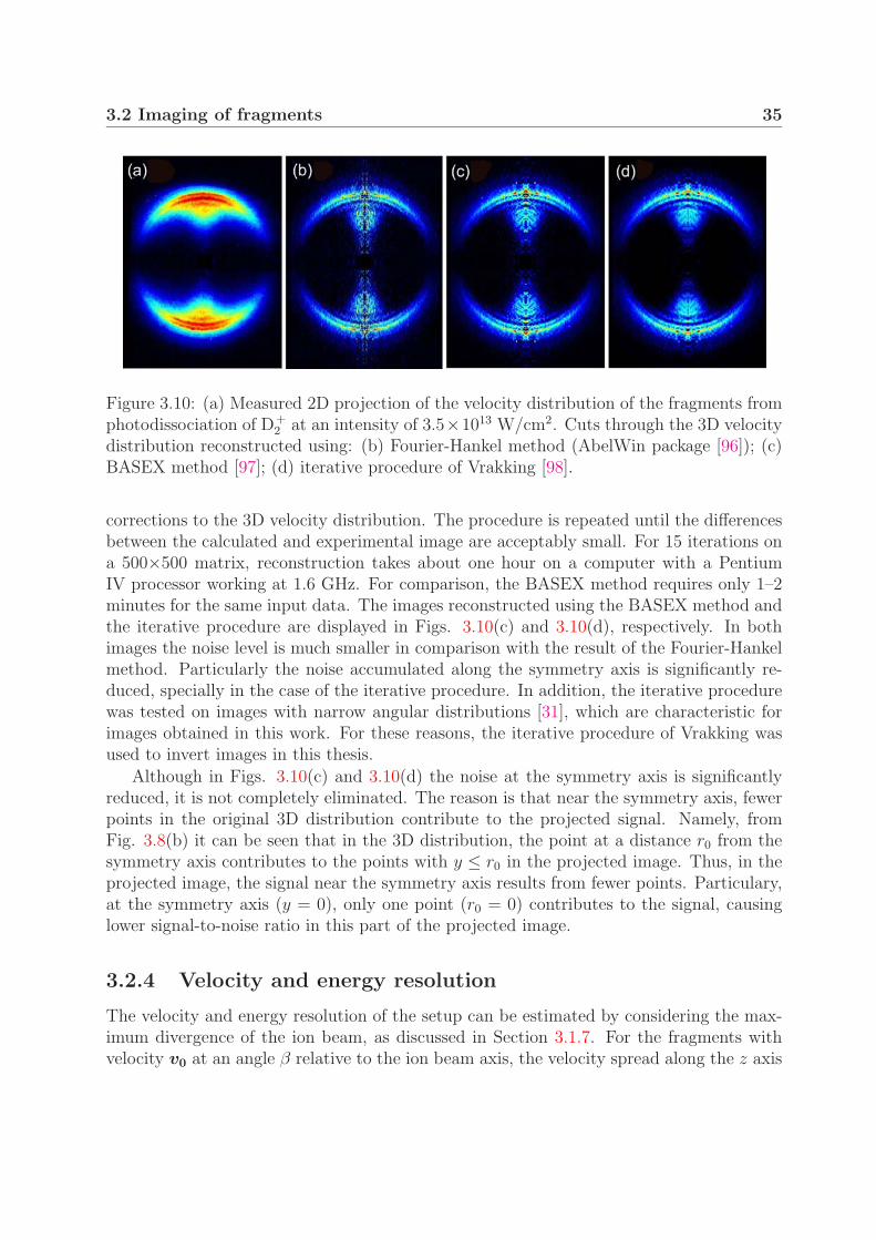
3.2 Imaging of fragments 35
Figure 3.10: (a) Measured 2D projection of the velocity distribution of the fragments fromphotodissociation of D+
2 at an intensity of 3.5×10¹³ W/cm2. Cuts through the 3D velocitydistribution reconstructed using: (b) Fourier-Hankel method (AbelWin package [96]); (c)BASEX method [97]; (d) iterative procedure of Vrakking [98].
corrections to the 3D velocity distribution. The procedure is repeated until the differencesbetween the calculated and experimental image are acceptably small. For 15 iterations ona 500×500 matrix, reconstruction takes about one hour on a computer with a PentiumIV processor working at 1.6 GHz. For comparison, the BASEX method requires only 1–2minutes for the same input data. The images reconstructed using the BASEX method andthe iterative procedure are displayed in Figs. 3.10(c) and 3.10(d), respectively. In bothimages the noise level is much smaller in comparison with the result of the Fourier-Hankelmethod. Particularly the noise accumulated along the symmetry axis is significantly re-duced, specially in the case of the iterative procedure. In addition, the iterative procedurewas tested on images with narrow angular distributions [31], which are characteristic forimages obtained in this work. For these reasons, the iterative procedure of Vrakking wasused to invert images in this thesis.
Although in Figs. 3.10(c) and 3.10(d) the noise at the symmetry axis is significantlyreduced, it is not completely eliminated. The reason is that near the symmetry axis, fewerpoints in the original 3D distribution contribute to the projected signal. Namely, fromFig. 3.8(b) it can be seen that in the 3D distribution, the point at a distance r0 from thesymmetry axis contributes to the points with y ≤ r0 in the projected image. Thus, in theprojected image, the signal near the symmetry axis results from fewer points. Particulary,at the symmetry axis (y = 0), only one point (r0 = 0) contributes to the signal, causinglower signal-to-noise ratio in this part of the projected image.
3.2.4 Velocity and energy resolution
The velocity and energy resolution of the setup can be estimated by considering the max-imum divergence of the ion beam, as discussed in Section 3.1.7. For the fragments withvelocity v0 at an angle β relative to the ion beam axis, the velocity spread along the z axis
36 3. Experimental
is given byδv = 2v0 sin β . (3.14)
Here the velocity of the fragments was approximated by the velocity of the ion beam v0
[Eq. (3.4)]. The fragments ejected with velocities v along the laser polarization axis (zaxis) will be displaced by
D = vt , (3.15)
where t ∼ L/v0 is the time between the interaction and detection. The maximum velocitythat can be observed on a detector of a radius r is equal to
vmax =r
t=
r
L
√2qUa
mm
. (3.16)
The imaged velocity range can be increased with a faster ion beam or by decreasing thedistance L between the interaction region and the MCP detector. In order to achieve abetter resolution of the imaging system, the measured velocity range should be imagedon the largest possible area of the MCP detector. For small velocity spreads, one shoulduse lower acceleration voltages [Eq. (3.14)]. Some experimental parameters describingthe imaged velocity range and the velocity spread are listed in Table 3.3. In the D+
2
measurements (Chapter 4), only fragments from the dissociation channel were recorded,and thus the maximum fragment energy that could be detected was set to about 1.0 eV.On the other hand, in the case of measurements on H+
2 (Chapter 5), fragments withenergies above 4 eV from the Coulomb explosion channel were imaged. The energy rangewas increased by using a higher acceleration voltage. In addition, a larger area of thedetector was used by displacing the zero-velocity point from the detector center. Thehigher fragment signal here also allowed better collimation, which yielded a relative velocityresolution δv/vmax of 8 × 10⁻³.
Table 3.3: Parameters used in the measurements on D+2 (Chapter 4) and H+
2 (Chapter 5)determining the velocity range and the velocity spread of the fragments.
ion Ua [kV] v0 [m/s] L [cm] t [µs] vmax [m/s] Emax [eV] β [mrad] δv [m/s]
D+2 3.1 3.8 × 10⁵ 80 2.1 9.7 × 10³ 0.98 0.24 180
H+2 11.1 1.0 × 10⁶ 95 0.9 2.9 × 10⁴ 4.3 0.12 240
The relative energy resolution of the fragments is given by
δE
Emax
=2vδv + (δv)2
vmax2
. (3.17)
In the case of D+2 , this quantity varies between 4× 10⁻⁴ at the center and 4× 10⁻² at the
edges of the detector, which corresponds to an energy resolution δE of 0.3 meV and 36
3.3 Femtosecond laser system 37
meV, respectively. In the case of H+2 , the energy resolution at the maximum energy of 4.3
eV was 73 meV.In the preceding discussion, the velocity spread of the molecular ions along the ion
beam axis was not taken into account. The energy spread of the ions extracted from aduoplasmatron ion source is less than 10 eV [100]. In the case of D+
2 , this corresponds to ahalf-width of the velocity distribution of ∆v0 ∼ 1.5× 10⁴ m/s, i.e., ∆v0/v0 ∼ 0.04. Due toa spread of the time of flight of ∆t ∼ 90 ns, the fragments would have a maximum energyspread (FWHM) of 190 meV. In the experiment, the energy spread in the ion sourceis somewhat lower and momentum selection by sector magnet SM and the collimatingapertures further narrows the velocity spread. The given value thus presents the upperlimit on the width of the kinetic energy distribution of fragments. In the photodissociationspectra of D+
2 , peaks separated by 60 meV were clearly resolved.
3.3 Femtosecond laser system
In this section, the femtosecond laser system and methods of characterizing laser pulsesare described. The peak laser intensity is defined in terms of the measured pulse energy,pulse duration and beam diameter in the interaction region.
3.3.1 Laser setup
Ultrashort laser pulses were produced and amplified in a commercial chirped pulse am-plification (CPA) laser system. Figure 3.11 shows the layout of the system. The systemcomprises a femtosecond oscillator, a pump laser for the oscillator, a chirped pulse amplifierand a pump laser for the amplifier.
Femtosecond oscillator
A diode-pumped Nd:YVO4 solid-state laser16 was used as the pump laser for the oscillator.Continuous wave radiation at a wavelength of 532 nm is produced by intra-cavity frequencydoubling of the fundamental frequency in a LBO crystal. The femtosecond pulses aregenerated in a Ti:Sapphire oscillator17 utilizing the Kerr lens mode-locking principle [101].The mode locking could be achieved by enabling an intra-cavity acousto-optical modulatoron startup. Two prism pairs serve to compensate for the positive group velocity dispersionintroduced by the optical components in the cavity. The central wavelength is tunablein the range from 720 to 850 nm by a movable slit inserted in a part of the beam wherethe spectral components are spatially separated by means of a prism. The spectral widthcould be adjusted by varying the slit width. For the best performance of the amplifier,the central wavelength was set to 791 nm with a spectral width of 14.5 nm (FWHM). Thespectrum was measured by coupling a part of the beam to a fiber via an Ulbricht sphere
16Spectra Physics, Millennia V17Spectra Physics, Tsunami
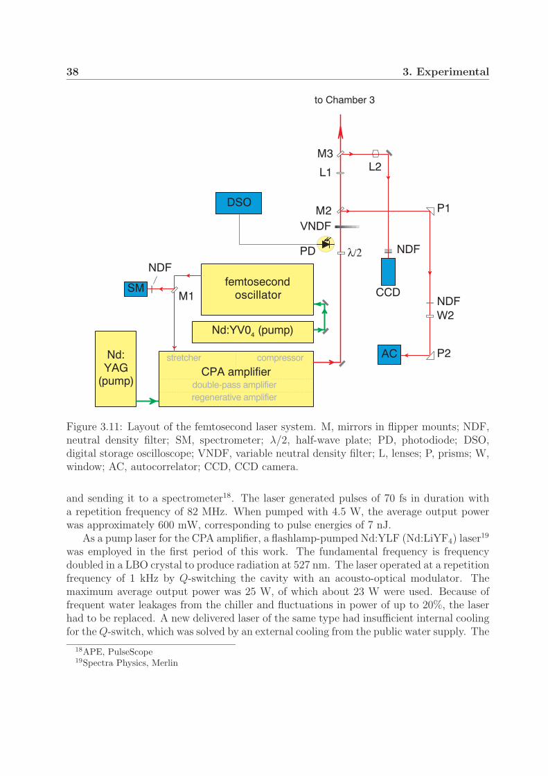
38 3. Experimental
femtosecondoscillator
Nd:YV04 (pump)
Nd:YAG
(pump)
λ/2
regenerative amplifierdouble-pass amplifier
stretcher compressor
CPA amplifier
AC
CCDSM
to Chamber 3
VNDF
NDF
NDFW2
L1
M2
M3L2
P1
P2
M1
NDF
DSO
PD
Figure 3.11: Layout of the femtosecond laser system. M, mirrors in flipper mounts; NDF,neutral density filter; SM, spectrometer; λ/2, half-wave plate; PD, photodiode; DSO,digital storage oscilloscope; VNDF, variable neutral density filter; L, lenses; P, prisms; W,window; AC, autocorrelator; CCD, CCD camera.
and sending it to a spectrometer18. The laser generated pulses of 70 fs in duration witha repetition frequency of 82 MHz. When pumped with 4.5 W, the average output powerwas approximately 600 mW, corresponding to pulse energies of 7 nJ.
As a pump laser for the CPA amplifier, a flashlamp-pumped Nd:YLF (Nd:LiYF4) laser19
was employed in the first period of this work. The fundamental frequency is frequencydoubled in a LBO crystal to produce radiation at 527 nm. The laser operated at a repetitionfrequency of 1 kHz by Q-switching the cavity with an acousto-optical modulator. Themaximum average output power was 25 W, of which about 23 W were used. Because offrequent water leakages from the chiller and fluctuations in power of up to 20%, the laserhad to be replaced. A new delivered laser of the same type had insufficient internal coolingfor the Q-switch, which was solved by an external cooling from the public water supply. The
18APE, PulseScope19Spectra Physics, Merlin
3.3 Femtosecond laser system 39
cavity for the flashlamps was extremely noisy and caused large pulse-to-pulse fluctuations.Besides that, the Q-switch was often damaged and had to be replaced several times. Theproblems were solved after replacing the pump laser by a diode-pumped Nd:LiYF4 laser20.This laser operates at the same wavelength and repetition frequency as its predecessor. Themaximum average output power at 1 kHz is specified to 20 W, but up to 24 W were used.The advantages of diode-pumping over pumping with flashlamps is a better pulse energyand beam pointing stability, a better beam profile, a smaller electric energy consumption,easier handling and longer lifetimes of diodes compared to flashlamps.
Chirped pulse amplifier
The amplification of the pulses from the oscillator (“seed” pulses) employs the chirped pulseamplification technique [102]. To keep the peak intensity of the pulses during amplificationbelow the damage threshold and to avoid nonlinear effects, a seed pulse is first temporallystretched by a factor of up to 104. The energy of such a stretched pulse is enhanced in anamplification process. Finally, the pulse is recompressed to near its original duration.
In the pulse stretching process, different spectral components in the pulse are firstspatially separated by a stretcher grating. The “blue” components are passed through alonger optical path then the “red” ones. Therefore the “blue” part of the spectrum isdelayed with respect to the “red” one. Such a pulse is said to be positively chirped, i.e., itsfrequency increases from the leading to the trailing edge of the pulse. In a similar manner,pulse compression is achieved. This time a negative velocity dispersion is introduced, i.e.,the “red” components have a longer optical path than the “blue” ones, so that the positivegroup velocity dispersion of the stretcher and optical components is compensated.
The maximum spectral width of the pulses that could be stretched and compressedwas limited to 11 nm by the length of the gratings. To amplify shorter pulses havinglarger spectral widths, while maintaining the maximum angular dispersion, the stretcherand compressor gratings with a larger constant should be used. After replacing the originalgratings with 1200 grooves/mm by ones with 1800 grooves/mm21, shorter pulses with aspectral width of typically 14 nm could be stretched, amplified and compressed.
After being stretched, a seed pulse enters the cavity of the regenerative amplifier. Thereit is amplified by traversing through a Ti:Sapphire crystal pumped by 10 W from theNd:YLF laser. Since the pump laser delivers pulses with a repetition frequency of 1 kHz,only a small portion of the seed pulses are amplified. After 15 round trips through thecavity, the pulse energy reaches saturation. The pulse is switched out through a thin filmpolarizer after its polarization is changed by means of a Pockels cell. A second stage of theamplification takes place in a double-pass amplifier. Here the pulse passes twice through aTi:Sapphire crystal pumped by 12.5 W from the Nd:YLF laser. Typically, a pulse energy ofabout 1.6 mJ at the output of the regenerative amplifier was increased to 2.3 mJ after thefirst pass and 3.2 mJ after the second pass in the double-pass amplifier. After compression,the output pulses had an energy of 2.3 mJ and a duration of about 80 fs (FWHM). For
20Spectra Physics, Evolution-3021Spectrogon, PC 1800

40 3. Experimental
comparison, in the previous setup utilizing the Nd:YAG laser as the pump laser and theoriginal stretcher and compressor gratings, the laser delivered pulses with an energy of 1.2mJ and a duration of 130 fs.
3.3.2 Beam and pulse characterization
After leaving the amplifier, the horizontally polarized laser beam first passed through a half-wave plate, which rotated the polarization to vertical. As discussed in Section 3.2.2, verticalpolarization is needed for the purposes of fragment imaging. To adjust the polarization, aGlan polarizer is inserted into the beam and rotated in such a way that the propagationaxis of the reflected beam was precisely horizontal. This is achieved by measuring theheight of the beam spot on a wall. For such orientation, the Glan polarizer transmits thehorizontal component of the laser polarization. By minimizing the transmitted power, theorientation of the λ/2 plate for the required vertically polarized light is achieved.
The height of the laser beam was matched to the height of the ion beam by meansof two mirrors. The focusing is achieved with an achromatic doublet22, which optimallyconcentrates the pulse energy in space and time by eliminating two effects occurring insinglet lenses: (i) different temporal delays of different spatial components of the beam,and (ii) focusing of different spectral components at different points on the optical axis[103]. A focal length of f = 300 mm provided a focused beam diameter sufficiently smallfor achieving peak intensities above 1 × 10¹⁵ W/cm2. The lens was mounted on a xyz-translation stage providing a precise alignment of the overlap of the ion and laser beams.
The pulse energy could be varied with a circular variable neutral density filter23. Fora stronger attenuation, metallic and absorptive neutral density filters of different opticaldensities were used. The use of a combination of a λ/2 plate and a Glan polarizer wasabandoned because of both the energy losses and a relatively large group velocity disper-sion in the polarizer glass. The pulse energy was measured with a powermeter24 placedbehind the variable neutral density filter. The actual pulse energy inside the chamber was9% smaller due to the losses on the mirrors, focusing lens and window on the vacuumchamber. Pulse-to-pulse energy fluctuations were monitored with a high-speed silicon de-tector25 connected to a digital storage oscilloscope26. For this purpose, the peak values of1000 pulses were taken and statistically analysed. The standard deviation of such a samplewas 1–2 % of the mean value.
The autocorrelation and the beam profile could be easily measured by redirecting thebeam to an autocorrelator27 or a CCD camera using mirrors in flipper mounts28 (M2 andM3 in Fig. 3.11).
22Melles Griot23CVI Laser24Coherent, Labmaster with head LM325Thorlabs, DET21026LeCroy, Wavepro 96027APE, PulseCheck28New Focus, model 9891
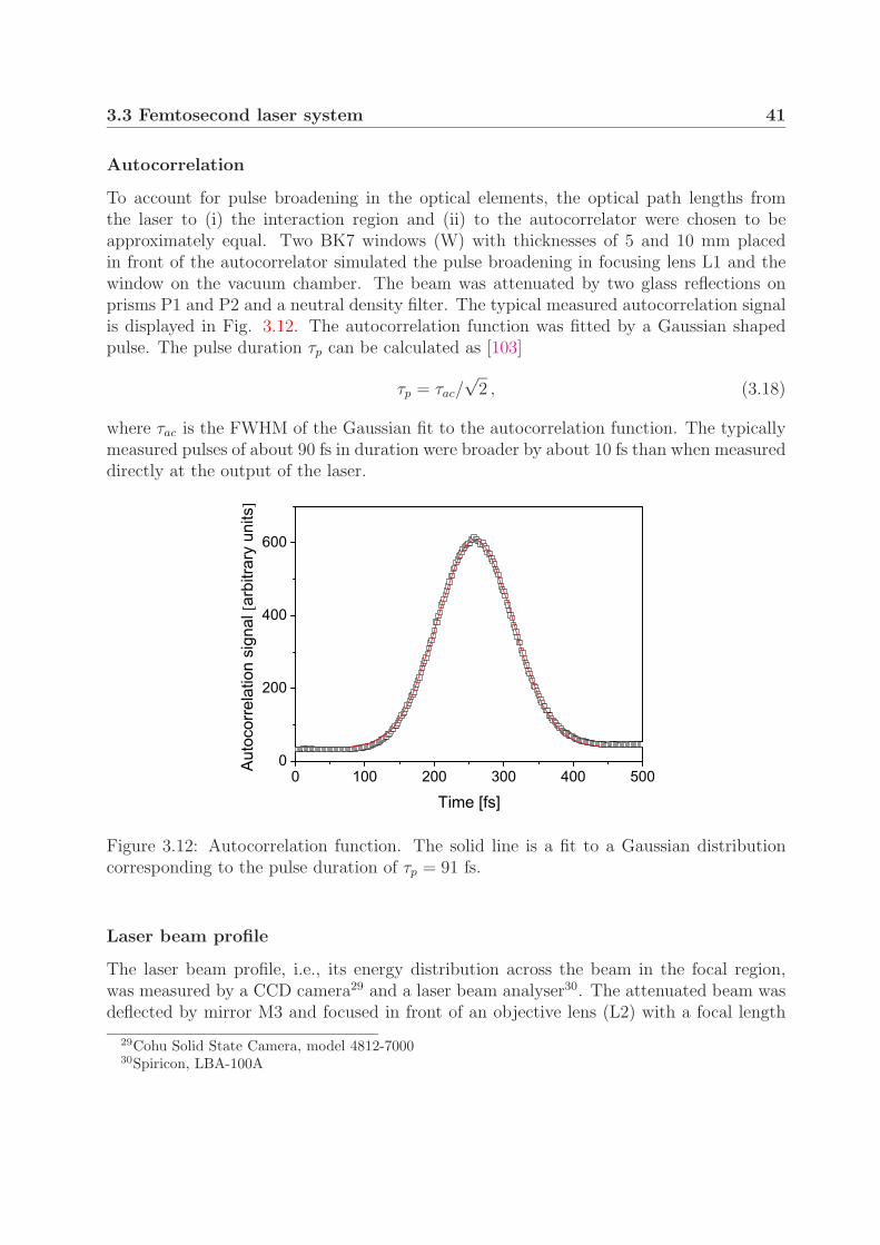
3.3 Femtosecond laser system 41
Autocorrelation
To account for pulse broadening in the optical elements, the optical path lengths fromthe laser to (i) the interaction region and (ii) to the autocorrelator were chosen to beapproximately equal. Two BK7 windows (W) with thicknesses of 5 and 10 mm placedin front of the autocorrelator simulated the pulse broadening in focusing lens L1 and thewindow on the vacuum chamber. The beam was attenuated by two glass reflections onprisms P1 and P2 and a neutral density filter. The typical measured autocorrelation signalis displayed in Fig. 3.12. The autocorrelation function was fitted by a Gaussian shapedpulse. The pulse duration τp can be calculated as [103]
τp = τac/√
2 , (3.18)
where τac is the FWHM of the Gaussian fit to the autocorrelation function. The typicallymeasured pulses of about 90 fs in duration were broader by about 10 fs than when measureddirectly at the output of the laser.
Figure 3.12: Autocorrelation function. The solid line is a fit to a Gaussian distributioncorresponding to the pulse duration of τp = 91 fs.
Laser beam profile
The laser beam profile, i.e., its energy distribution across the beam in the focal region,was measured by a CCD camera29 and a laser beam analyser30. The attenuated beam wasdeflected by mirror M3 and focused in front of an objective lens (L2) with a focal length
29Cohu Solid State Camera, model 4812-700030Spiricon, LBA-100A
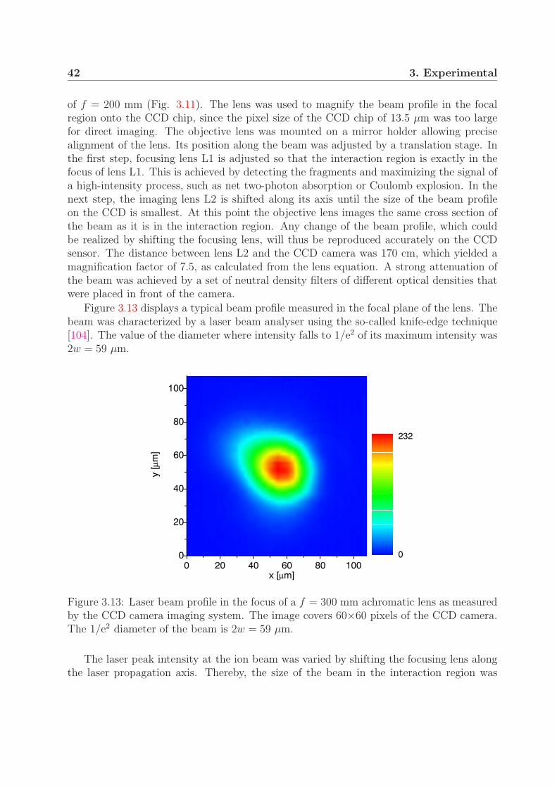
42 3. Experimental
of f = 200 mm (Fig. 3.11). The lens was used to magnify the beam profile in the focalregion onto the CCD chip, since the pixel size of the CCD chip of 13.5 µm was too largefor direct imaging. The objective lens was mounted on a mirror holder allowing precisealignment of the lens. Its position along the beam was adjusted by a translation stage. Inthe first step, focusing lens L1 is adjusted so that the interaction region is exactly in thefocus of lens L1. This is achieved by detecting the fragments and maximizing the signal ofa high-intensity process, such as net two-photon absorption or Coulomb explosion. In thenext step, the imaging lens L2 is shifted along its axis until the size of the beam profileon the CCD is smallest. At this point the objective lens images the same cross section ofthe beam as it is in the interaction region. Any change of the beam profile, which couldbe realized by shifting the focusing lens, will thus be reproduced accurately on the CCDsensor. The distance between lens L2 and the CCD camera was 170 cm, which yielded amagnification factor of 7.5, as calculated from the lens equation. A strong attenuation ofthe beam was achieved by a set of neutral density filters of different optical densities thatwere placed in front of the camera.
Figure 3.13 displays a typical beam profile measured in the focal plane of the lens. Thebeam was characterized by a laser beam analyser using the so-called knife-edge technique[104]. The value of the diameter where intensity falls to 1/e2 of its maximum intensity was2w = 59 µm.
100
80
60
40
20
00 20 40 60 80 100
y [µ
m]
x [µm]
0
44
89
133
178
222232232
0
Figure 3.13: Laser beam profile in the focus of a f = 300 mm achromatic lens as measuredby the CCD camera imaging system. The image covers 60×60 pixels of the CCD camera.The 1/e2 diameter of the beam is 2w = 59 µm.
The laser peak intensity at the ion beam was varied by shifting the focusing lens alongthe laser propagation axis. Thereby, the size of the beam in the interaction region was
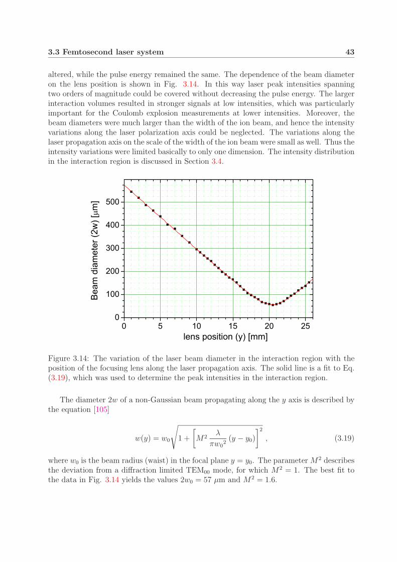
3.3 Femtosecond laser system 43
altered, while the pulse energy remained the same. The dependence of the beam diameteron the lens position is shown in Fig. 3.14. In this way laser peak intensities spanningtwo orders of magnitude could be covered without decreasing the pulse energy. The largerinteraction volumes resulted in stronger signals at low intensities, which was particularlyimportant for the Coulomb explosion measurements at lower intensities. Moreover, thebeam diameters were much larger than the width of the ion beam, and hence the intensityvariations along the laser polarization axis could be neglected. The variations along thelaser propagation axis on the scale of the width of the ion beam were small as well. Thus theintensity variations were limited basically to only one dimension. The intensity distributionin the interaction region is discussed in Section 3.4.
Figure 3.14: The variation of the laser beam diameter in the interaction region with theposition of the focusing lens along the laser propagation axis. The solid line is a fit to Eq.(3.19), which was used to determine the peak intensities in the interaction region.
The diameter 2w of a non-Gaussian beam propagating along the y axis is described bythe equation [105]
w(y) = w0
√1 +
[M2
λ
πw02
(y − y0)
]2
, (3.19)
where w0 is the beam radius (waist) in the focal plane y = y0. The parameter M2 describesthe deviation from a diffraction limited TEM00 mode, for which M2 = 1. The best fit tothe data in Fig. 3.14 yields the values 2w0 = 57 µm and M2 = 1.6.
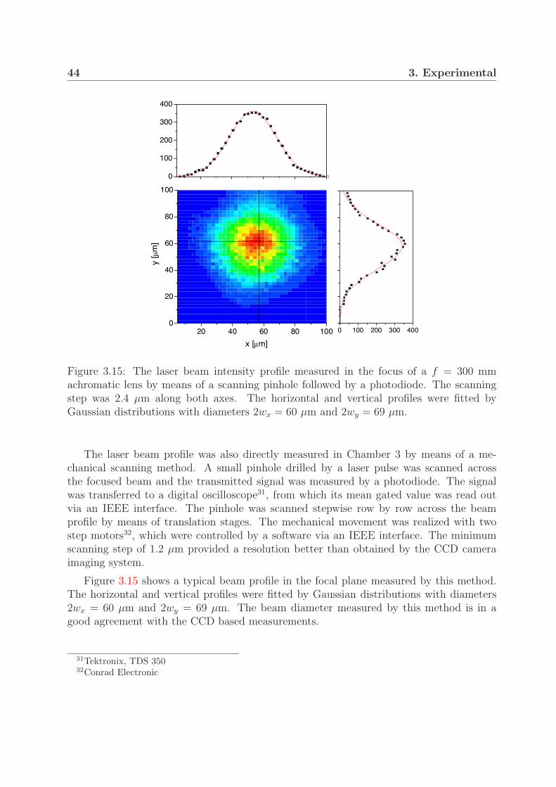
44 3. Experimental
0 100 200 300 400
0
100
200
300
400
20 40 60 80 1000
20
40
60
80
100
x [µm]
y [µ
m]
Figure 3.15: The laser beam intensity profile measured in the focus of a f = 300 mmachromatic lens by means of a scanning pinhole followed by a photodiode. The scanningstep was 2.4 µm along both axes. The horizontal and vertical profiles were fitted byGaussian distributions with diameters 2wx = 60 µm and 2wy = 69 µm.
The laser beam profile was also directly measured in Chamber 3 by means of a me-chanical scanning method. A small pinhole drilled by a laser pulse was scanned acrossthe focused beam and the transmitted signal was measured by a photodiode. The signalwas transferred to a digital oscilloscope31, from which its mean gated value was read outvia an IEEE interface. The pinhole was scanned stepwise row by row across the beamprofile by means of translation stages. The mechanical movement was realized with twostep motors32, which were controlled by a software via an IEEE interface. The minimumscanning step of 1.2 µm provided a resolution better than obtained by the CCD cameraimaging system.
Figure 3.15 shows a typical beam profile in the focal plane measured by this method.The horizontal and vertical profiles were fitted by Gaussian distributions with diameters2wx = 60 µm and 2wy = 69 µm. The beam diameter measured by this method is in agood agreement with the CCD based measurements.
31Tektronix, TDS 35032Conrad Electronic
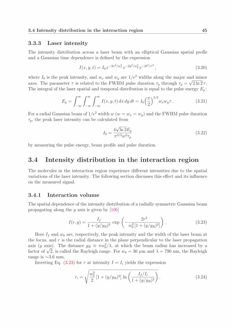
3.4 Intensity distribution in the interaction region 45
3.3.3 Laser intensity
The intensity distribution across a laser beam with an elliptical Gaussian spatial profleand a Gaussian time dependence is defined by the expression
I(x, y, t) = I0 e−2x2/w2x e−2y2/w2
y e−2t2/τ2
, (3.20)
where I0 is the peak intensity, and wx and wy are 1/e2 widths along the major and minor
axes. The parameter τ is related to the FWHM pulse duration τp through τp =√
2 ln 2 τ .The integral of the laser spatial and temporal distribution is equal to the pulse energy Ep :
Ep =
∫ ∞
−∞
∫ ∞
−∞
∫ ∞
−∞I(x, y, t) dx dy dt = I0
(π
2
)3/2
wxwyτ . (3.21)
For a radial Gaussian beam of 1/e2 width w (w = wx = wy) and the FWHM pulse durationτp, the peak laser intensity can be calculated from
I0 =4√
ln 2Ep
π3/2w2τp
(3.22)
by measuring the pulse energy, beam profile and pulse duration.
3.4 Intensity distribution in the interaction region
The molecules in the interaction region experience different intensities due to the spatialvariations of the laser intensity. The following section discusses this effect and its influenceon the measured signal.
3.4.1 Interaction volume
The spatial dependence of the intensity distribution of a radially symmetric Gaussian beampropagating along the y axis is given by [106]
I(r, y) =If
1 + (y/yR)2exp
(− 2r2
w20 [1 + (y/yR)2]
). (3.23)
Here If and w0 are, respectively, the peak intensity and the width of the laser beam atthe focus, and r is the radial distance in the plane perpendicular to the laser propagationaxis (y axis). The distance yR ≡ πw2
0/λ, at which the beam radius has increased by afactor of
√2, is called the Rayleigh range. For w0 = 30 µm and λ = 790 nm, the Rayleigh
range is ∼3.6 mm.Inverting Eq. (3.23) for r at intensity I = Ii yields the expression
ri =
√w2
0
2[1 + (y/yR)2] ln
(If/Ii
1 + (y/yR)2
). (3.24)
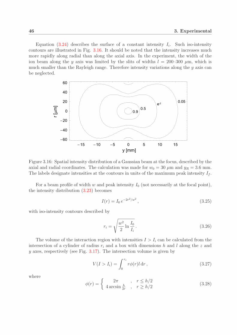
46 3. Experimental
Equation (3.24) describes the surface of a constant intensity Ii. Such iso-intensitycontours are illustrated in Fig. 3.16. It should be noted that the intensity increases muchmore rapidly along radial than along the axial axis. In the experiment, the width of theion beam along the y axis was limited by the slits of widths l = 200–300 µm, which ismuch smaller than the Rayleigh range. Therefore intensity variations along the y axis canbe neglected.
� � � � � � � � � � � � � �
� ! �
� � �
� * �
�
* �
� �
! �
& � . � � /
��. ��/
� # 0� # �
� � *� # � �
Figure 3.16: Spatial intensity distribution of a Gaussian beam at the focus, described by theaxial and radial coordinates. The calculation was made for w0 = 30 µm and yR = 3.6 mm.The labels designate intensities at the contours in units of the maximum peak intensity If .
For a beam profile of width w and peak intensity I0 (not necessarily at the focal point),the intensity distribution (3.23) becomes
I(r) = I0 e−2r2/w2
, (3.25)
with iso-intensity contours described by
ri =
√w2
2ln
I0
Ii
. (3.26)
The volume of the interaction region with intensities I > Ii can be calculated from theintersection of a cylinder of radius ri and a box with dimensions h and l along the z andy axes, respectively (see Fig. 3.17). The intersection volume is given by
V (I > Ii) =
∫ ri
0
rφ(r)l dr , (3.27)
where
φ(r) =
{2π , r ≤ h/2
4 arcsin h2r
, r ≥ h/2(3.28)
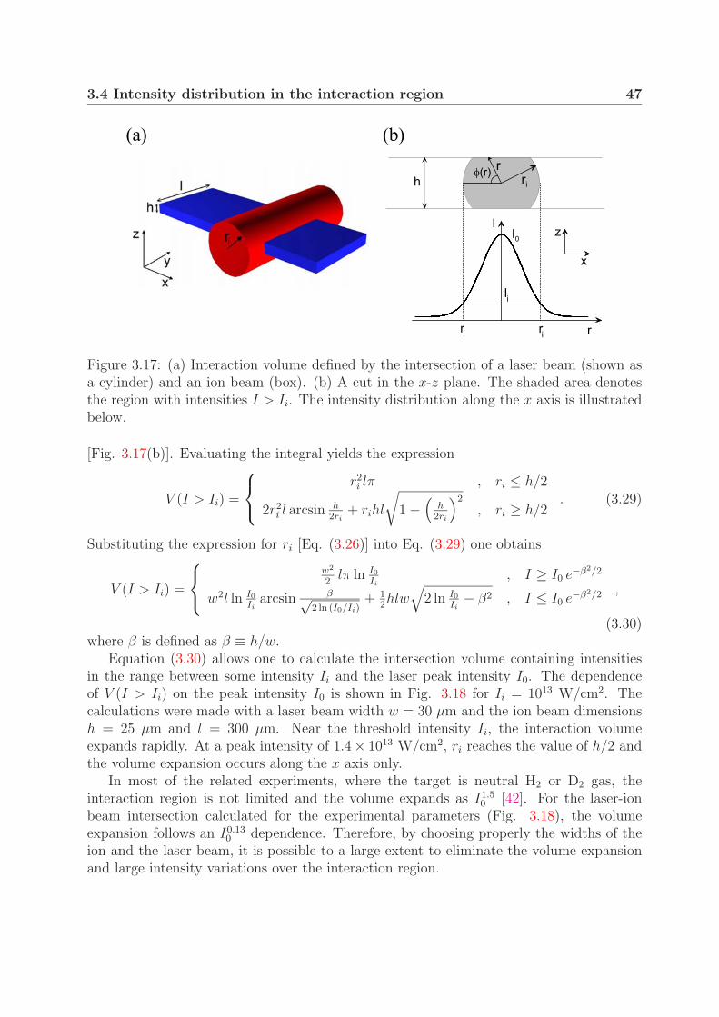
3.4 Intensity distribution in the interaction region 47
� � �
���
��
1�
1
�� � �
� � � � � �
1 �
%
$
Figure 3.17: (a) Interaction volume defined by the intersection of a laser beam (shown asa cylinder) and an ion beam (box). (b) A cut in the x-z plane. The shaded area denotesthe region with intensities I > Ii. The intensity distribution along the x axis is illustratedbelow.
[Fig. 3.17(b)]. Evaluating the integral yields the expression
V (I > Ii) =
r2i lπ , ri ≤ h/2
2r2i l arcsin h
2ri+ rihl
√1 −
(h
2ri
)2
, ri ≥ h/2. (3.29)
Substituting the expression for ri [Eq. (3.26)] into Eq. (3.29) one obtains
V (I > Ii) =
w2
2lπ ln I0
Ii, I ≥ I0 e−β2/2
w2l ln I0Ii
arcsin β√2 ln (I0/Ii)
+ 12hlw
√2 ln I0
Ii− β2 , I ≤ I0 e−β2/2 ,
(3.30)where β is defined as β ≡ h/w.
Equation (3.30) allows one to calculate the intersection volume containing intensitiesin the range between some intensity Ii and the laser peak intensity I0. The dependenceof V (I > Ii) on the peak intensity I0 is shown in Fig. 3.18 for Ii = 1013 W/cm2. Thecalculations were made with a laser beam width w = 30 µm and the ion beam dimensionsh = 25 µm and l = 300 µm. Near the threshold intensity Ii, the interaction volumeexpands rapidly. At a peak intensity of 1.4× 10¹³ W/cm2, ri reaches the value of h/2 andthe volume expansion occurs along the x axis only.
In most of the related experiments, where the target is neutral H2 or D2 gas, theinteraction region is not limited and the volume expands as I1.5
0 [42]. For the laser-ionbeam intersection calculated for the experimental parameters (Fig. 3.18), the volumeexpansion follows an I0.13
0 dependence. Therefore, by choosing properly the widths of theion and the laser beam, it is possible to a large extent to eliminate the volume expansionand large intensity variations over the interaction region.
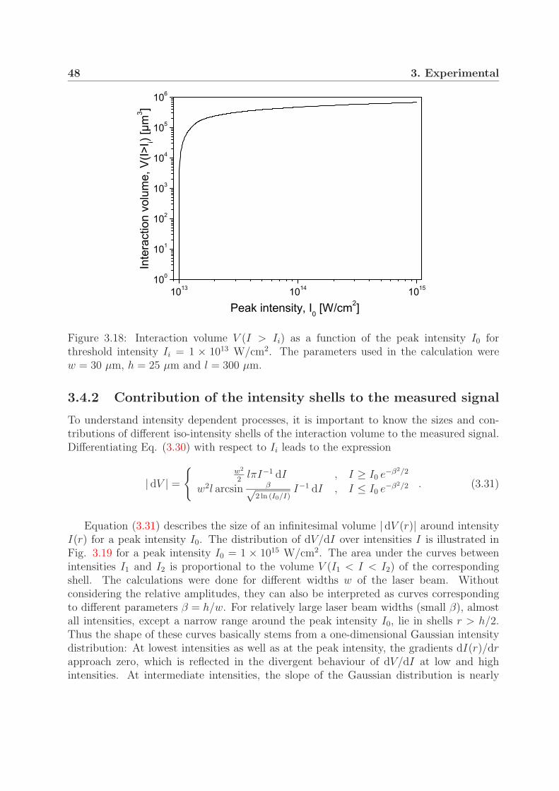
48 3. Experimental
Figure 3.18: Interaction volume V (I > Ii) as a function of the peak intensity I0 forthreshold intensity Ii = 1 × 10¹³ W/cm2. The parameters used in the calculation werew = 30 µm, h = 25 µm and l = 300 µm.
3.4.2 Contribution of the intensity shells to the measured signal
To understand intensity dependent processes, it is important to know the sizes and con-tributions of different iso-intensity shells of the interaction volume to the measured signal.Differentiating Eq. (3.30) with respect to Ii leads to the expression
| dV | =
{w2
2lπI−1 dI , I ≥ I0 e−β2/2
w2l arcsin β√2 ln (I0/I)
I−1 dI , I ≤ I0 e−β2/2 . (3.31)
Equation (3.31) describes the size of an infinitesimal volume | dV (r)| around intensityI(r) for a peak intensity I0. The distribution of dV/dI over intensities I is illustrated inFig. 3.19 for a peak intensity I0 = 1 × 10¹⁵ W/cm2. The area under the curves betweenintensities I1 and I2 is proportional to the volume V (I1 < I < I2) of the correspondingshell. The calculations were done for different widths w of the laser beam. Withoutconsidering the relative amplitudes, they can also be interpreted as curves correspondingto different parameters β = h/w. For relatively large laser beam widths (small β), almostall intensities, except a narrow range around the peak intensity I0, lie in shells r > h/2.Thus the shape of these curves basically stems from a one-dimensional Gaussian intensitydistribution: At lowest intensities as well as at the peak intensity, the gradients dI(r)/drapproach zero, which is reflected in the divergent behaviour of dV/dI at low and highintensities. At intermediate intensities, the slope of the Gaussian distribution is nearly
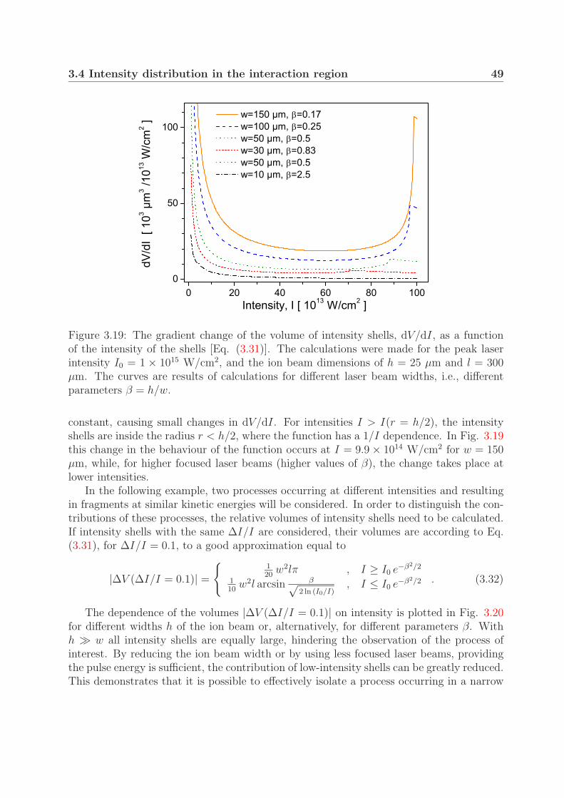
3.4 Intensity distribution in the interaction region 49
Figure 3.19: The gradient change of the volume of intensity shells, dV/dI, as a functionof the intensity of the shells [Eq. (3.31)]. The calculations were made for the peak laserintensity I0 = 1 × 10¹⁵ W/cm2, and the ion beam dimensions of h = 25 µm and l = 300µm. The curves are results of calculations for different laser beam widths, i.e., differentparameters β = h/w.
constant, causing small changes in dV/dI. For intensities I > I(r = h/2), the intensityshells are inside the radius r < h/2, where the function has a 1/I dependence. In Fig. 3.19this change in the behaviour of the function occurs at I = 9.9 × 10¹⁴ W/cm2 for w = 150µm, while, for higher focused laser beams (higher values of β), the change takes place atlower intensities.
In the following example, two processes occurring at different intensities and resultingin fragments at similar kinetic energies will be considered. In order to distinguish the con-tributions of these processes, the relative volumes of intensity shells need to be calculated.If intensity shells with the same ∆I/I are considered, their volumes are according to Eq.(3.31), for ∆I/I = 0.1, to a good approximation equal to
|∆V (∆I/I = 0.1)| =
{120
w2lπ , I ≥ I0 e−β2/2
110
w2l arcsin β√2 ln (I0/I)
, I ≤ I0 e−β2/2 . (3.32)
The dependence of the volumes |∆V (∆I/I = 0.1)| on intensity is plotted in Fig. 3.20for different widths h of the ion beam or, alternatively, for different parameters β. Withh � w all intensity shells are equally large, hindering the observation of the process ofinterest. By reducing the ion beam width or by using less focused laser beams, providingthe pulse energy is sufficient, the contribution of low-intensity shells can be greatly reduced.This demonstrates that it is possible to effectively isolate a process occurring in a narrow

50 3. Experimental
Figure 3.20: Volume of iso-intensity shells with ∆I/I = 0.1 as a function of intensitiesin the interaction region. (a) ion beam of width l = 300 µm and different widths h [Eq.(3.32)]; (b) no constraints on the interaction volume [Eq. (3.33)]. The laser peak intensityand beam width are I0 = 1 × 10¹⁵ W/cm2 and w = 30 µm, respectively.
range of intensities near the peak intensity. This result is important for studies of processesnear the threshold, such as Coulomb explosion, which will be discussed in Section 6.1.2
For comparison, without constraints on the interaction region, the volumes of iso-intensity shells are now given by [42]
|∆V (∆I/I = 0.1)| =π
30w2
0 yR (2I + I0)(I0 − I)12 I− 3
2 . (3.33)
The size of the volume of the intensity shells in this case is shown in Fig. 3.20(b). Thevolume of low-intensity shells is here several orders of magnitude larger than the volumeof interest.

Chapter 4
Photodissociation of the deuteriummolecular ion
This chapter presents measurements on photodissociation of D+2 in femtosecond laser fields
of intensities up to 1.5× 10¹⁴ W/cm2. Section 4.1 discusses the energies of the vibrationallevels of the electronic ground state of D+
2 and presents experimental images resolving thefragments from single vibrational levels. In Section 4.2, the kinetic energy distributions ofthe fragments for different peak intensities are presented and discussed. Particularly, thebond softening effects: the shifting of the peaks to lower kinetic energies (level shifting)and broadening of the peaks with increasing laser intensity are analysed and discussed.The alignment of the fragments is investigated in Section 4.3. Besides the one-photonbond softening process, the angular distributions suggest the mechanisms of vibrationaltrapping and two-photon bond softening (above-threshold dissociation) to occur at highestintensities. In Section 4.4, the kinetic energy distributions of D+
2 fragments are comparedto those of H+
2 measured by Sandig et al under similar experimental conditions [28].
4.1 Vibrationally resolved velocity distributions
In comparison with H+2 , the vibrational levels of the heavier isotopic variant D+
2 are char-acterized by smaller spacings between adjacent levels. The diagram in Fig. 4.1 illustratesthe positions of the vibrational levels of the electronic ground state 1sσg of H+
2 and D+2 .
The potential of the binding ground state of H+2 and D+
2 can be described by ananharmonic oscillator, with the energies of the vibrational levels given by [93]
E(v) = ωe
(v +
1
2
)− ωexe
(v +
1
2
)2
+ ... v = 0, 1, 2, ... (4.1)
Here ωe is the fundamental frequency in the harmonic approximation and ωexe is theanharmonicity constant. Both constants are expressed in units of cm−1 and their valuesfor H+
2 and D+2 are listed in Appendix B. Due to the anharmonicity, the spacing between
successive vibrational levels decreases for higher vibrational levels. The average spacing
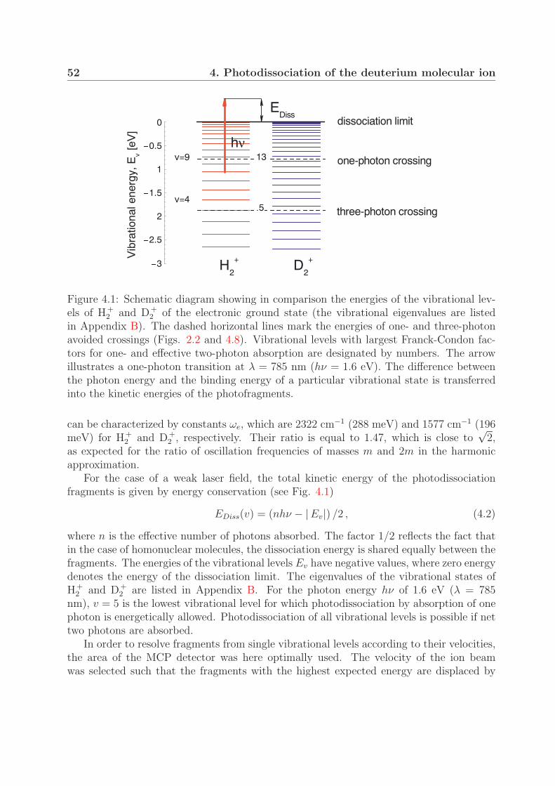
52 4. Photodissociation of the deuterium molecular ion
v=3
v=0-3
-2.5
-2
-1.5
-1
-0.5
0
D2
+H2
+Vib
ratio
nal e
nerg
y, E
v [eV
]
one-photon crossing
three-photon crossing
dissociation limitE
Diss
hν
5
13v=9
v=4
Figure 4.1: Schematic diagram showing in comparison the energies of the vibrational lev-els of H+
2 and D+2 of the electronic ground state (the vibrational eigenvalues are listed
in Appendix B). The dashed horizontal lines mark the energies of one- and three-photonavoided crossings (Figs. 2.2 and 4.8). Vibrational levels with largest Franck-Condon fac-tors for one- and effective two-photon absorption are designated by numbers. The arrowillustrates a one-photon transition at λ = 785 nm (hν = 1.6 eV). The difference betweenthe photon energy and the binding energy of a particular vibrational state is transferredinto the kinetic energies of the photofragments.
can be characterized by constants ωe, which are 2322 cm−1 (288 meV) and 1577 cm−1 (196meV) for H+
2 and D+2 , respectively. Their ratio is equal to 1.47, which is close to
√2,
as expected for the ratio of oscillation frequencies of masses m and 2m in the harmonicapproximation.
For the case of a weak laser field, the total kinetic energy of the photodissociationfragments is given by energy conservation (see Fig. 4.1)
EDiss(v) = (nhν − |Ev|) /2 , (4.2)
where n is the effective number of photons absorbed. The factor 1/2 reflects the fact thatin the case of homonuclear molecules, the dissociation energy is shared equally between thefragments. The energies of the vibrational levels Ev have negative values, where zero energydenotes the energy of the dissociation limit. The eigenvalues of the vibrational states ofH+
2 and D+2 are listed in Appendix B. For the photon energy hν of 1.6 eV (λ = 785
nm), v = 5 is the lowest vibrational level for which photodissociation by absorption of onephoton is energetically allowed. Photodissociation of all vibrational levels is possible if nettwo photons are absorbed.
In order to resolve fragments from single vibrational levels according to their velocities,the area of the MCP detector was here optimally used. The velocity of the ion beamwas selected such that the fragments with the highest expected energy are displaced by
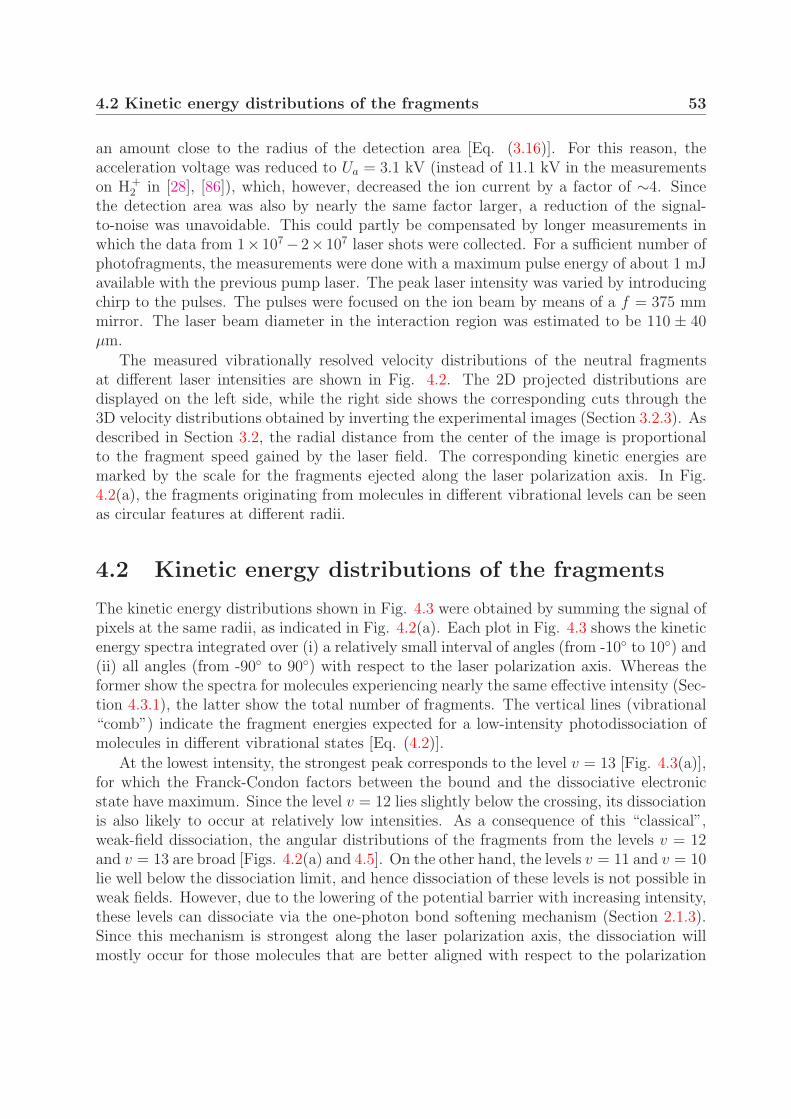
4.2 Kinetic energy distributions of the fragments 53
an amount close to the radius of the detection area [Eq. (3.16)]. For this reason, theacceleration voltage was reduced to Ua = 3.1 kV (instead of 11.1 kV in the measurementson H+
2 in [28], [86]), which, however, decreased the ion current by a factor of ∼4. Sincethe detection area was also by nearly the same factor larger, a reduction of the signal-to-noise was unavoidable. This could partly be compensated by longer measurements inwhich the data from 1× 10⁷ − 2× 10⁷ laser shots were collected. For a sufficient number ofphotofragments, the measurements were done with a maximum pulse energy of about 1 mJavailable with the previous pump laser. The peak laser intensity was varied by introducingchirp to the pulses. The pulses were focused on the ion beam by means of a f = 375 mmmirror. The laser beam diameter in the interaction region was estimated to be 110 ± 40µm.
The measured vibrationally resolved velocity distributions of the neutral fragmentsat different laser intensities are shown in Fig. 4.2. The 2D projected distributions aredisplayed on the left side, while the right side shows the corresponding cuts through the3D velocity distributions obtained by inverting the experimental images (Section 3.2.3). Asdescribed in Section 3.2, the radial distance from the center of the image is proportionalto the fragment speed gained by the laser field. The corresponding kinetic energies aremarked by the scale for the fragments ejected along the laser polarization axis. In Fig.4.2(a), the fragments originating from molecules in different vibrational levels can be seenas circular features at different radii.
4.2 Kinetic energy distributions of the fragments
The kinetic energy distributions shown in Fig. 4.3 were obtained by summing the signal ofpixels at the same radii, as indicated in Fig. 4.2(a). Each plot in Fig. 4.3 shows the kineticenergy spectra integrated over (i) a relatively small interval of angles (from -10◦ to 10◦) and(ii) all angles (from -90◦ to 90◦) with respect to the laser polarization axis. Whereas theformer show the spectra for molecules experiencing nearly the same effective intensity (Sec-tion 4.3.1), the latter show the total number of fragments. The vertical lines (vibrational“comb”) indicate the fragment energies expected for a low-intensity photodissociation ofmolecules in different vibrational states [Eq. (4.2)].
At the lowest intensity, the strongest peak corresponds to the level v = 13 [Fig. 4.3(a)],for which the Franck-Condon factors between the bound and the dissociative electronicstate have maximum. Since the level v = 12 lies slightly below the crossing, its dissociationis also likely to occur at relatively low intensities. As a consequence of this “classical”,weak-field dissociation, the angular distributions of the fragments from the levels v = 12and v = 13 are broad [Figs. 4.2(a) and 4.5]. On the other hand, the levels v = 11 and v = 10lie well below the dissociation limit, and hence dissociation of these levels is not possible inweak fields. However, due to the lowering of the potential barrier with increasing intensity,these levels can dissociate via the one-photon bond softening mechanism (Section 2.1.3).Since this mechanism is strongest along the laser polarization axis, the dissociation willmostly occur for those molecules that are better aligned with respect to the polarization
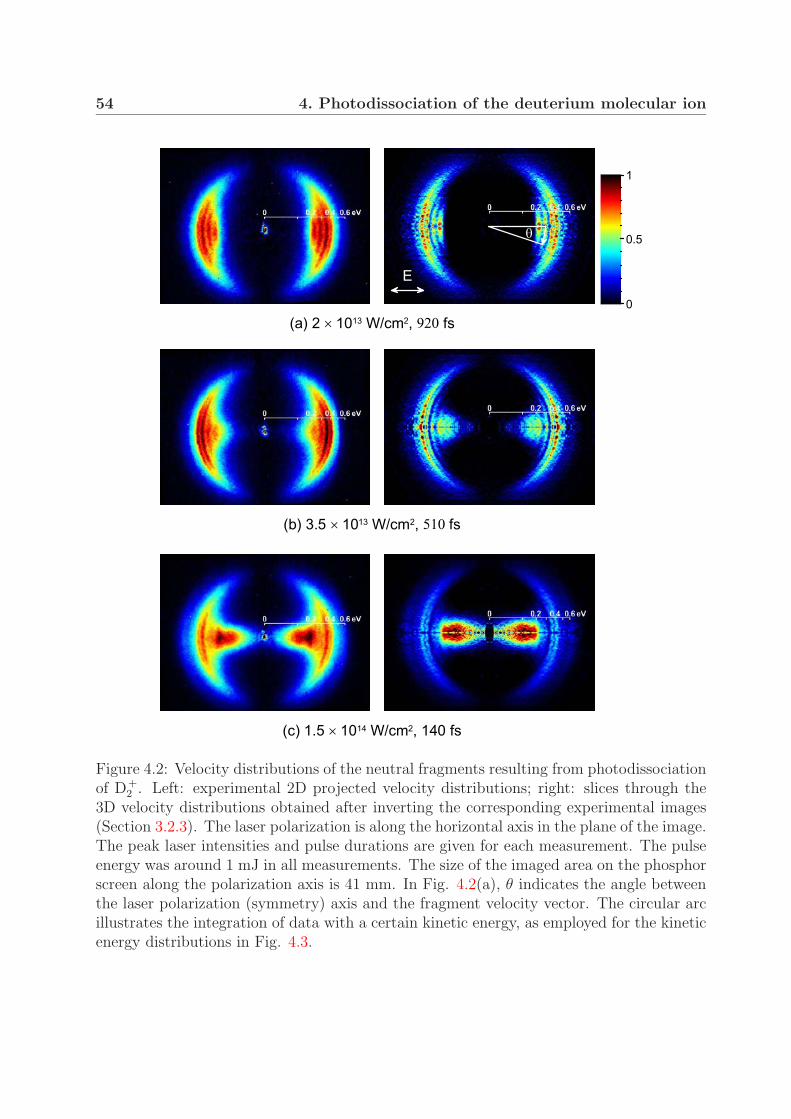
54 4. Photodissociation of the deuterium molecular ion
� � � * � � � � � � �� 2 3 � � * 4 � � � � � , �
� � � � # � � � � � � � �� 2 3 � � * 4 � � � � , �
� � � � # � � � � � � � �� 2 3 � � * 4 � � � � � , �
'
�
� # �
�
Figure 4.2: Velocity distributions of the neutral fragments resulting from photodissociationof D+
2 . Left: experimental 2D projected velocity distributions; right: slices through the3D velocity distributions obtained after inverting the corresponding experimental images(Section 3.2.3). The laser polarization is along the horizontal axis in the plane of the image.The peak laser intensities and pulse durations are given for each measurement. The pulseenergy was around 1 mJ in all measurements. The size of the imaged area on the phosphorscreen along the polarization axis is 41 mm. In Fig. 4.2(a), θ indicates the angle betweenthe laser polarization (symmetry) axis and the fragment velocity vector. The circular arcillustrates the integration of data with a certain kinetic energy, as employed for the kineticenergy distributions in Fig. 4.3.

4.2 Kinetic energy distributions of the fragments 55
Figure 4.3: Kinetic energy distributions of the fragments for the measurements in Fig. 4.2.The distributions were obtained by integrating the inverted velocity distributions over (i)10◦ (from -10◦ to 10◦) and (ii) all angles (from -90◦ to 90◦) around the laser polarizationaxis. The peak laser intensities and pulse durations are (a) 2 × 10¹³ W/cm2, 920 fs; (b)3.5 × 10¹³ W/cm2, 500 fs; (c) 1.5 × 10¹⁴ W/cm2, 140 fs.
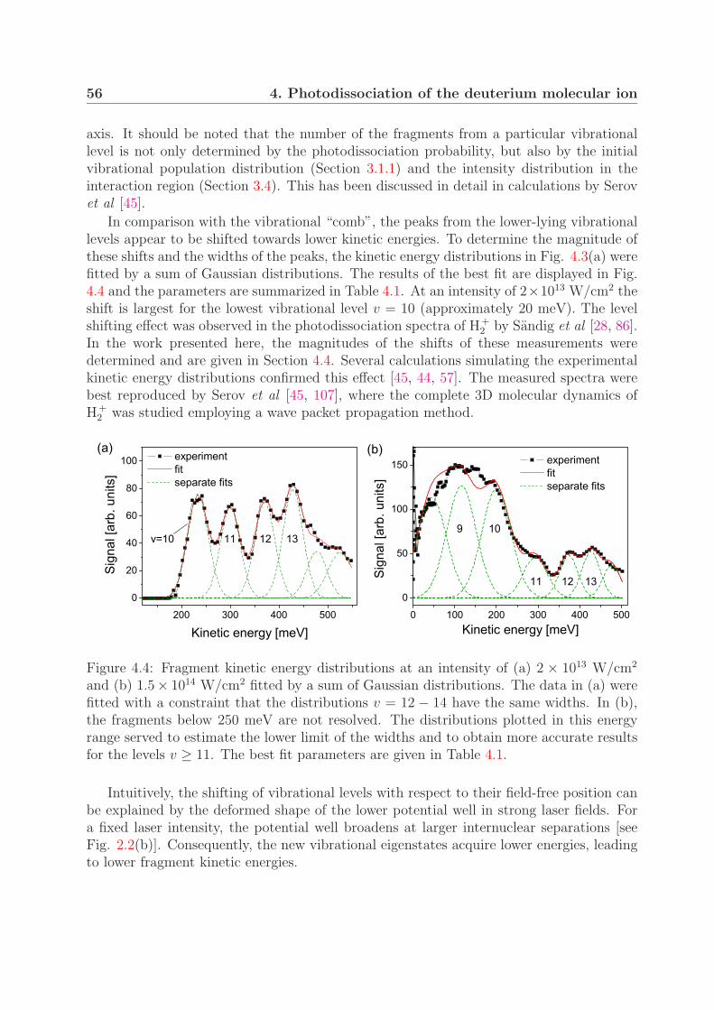
56 4. Photodissociation of the deuterium molecular ion
axis. It should be noted that the number of the fragments from a particular vibrationallevel is not only determined by the photodissociation probability, but also by the initialvibrational population distribution (Section 3.1.1) and the intensity distribution in theinteraction region (Section 3.4). This has been discussed in detail in calculations by Serovet al [45].
In comparison with the vibrational “comb”, the peaks from the lower-lying vibrationallevels appear to be shifted towards lower kinetic energies. To determine the magnitude ofthese shifts and the widths of the peaks, the kinetic energy distributions in Fig. 4.3(a) werefitted by a sum of Gaussian distributions. The results of the best fit are displayed in Fig.4.4 and the parameters are summarized in Table 4.1. At an intensity of 2×10¹³ W/cm2 theshift is largest for the lowest vibrational level v = 10 (approximately 20 meV). The levelshifting effect was observed in the photodissociation spectra of H+
2 by Sandig et al [28, 86].In the work presented here, the magnitudes of the shifts of these measurements weredetermined and are given in Section 4.4. Several calculations simulating the experimentalkinetic energy distributions confirmed this effect [45, 44, 57]. The measured spectra werebest reproduced by Serov et al [45, 107], where the complete 3D molecular dynamics ofH+
2 was studied employing a wave packet propagation method.
Figure 4.4: Fragment kinetic energy distributions at an intensity of (a) 2 × 10¹³ W/cm2
and (b) 1.5× 10¹⁴ W/cm2 fitted by a sum of Gaussian distributions. The data in (a) werefitted with a constraint that the distributions v = 12 − 14 have the same widths. In (b),the fragments below 250 meV are not resolved. The distributions plotted in this energyrange served to estimate the lower limit of the widths and to obtain more accurate resultsfor the levels v ≥ 11. The best fit parameters are given in Table 4.1.
Intuitively, the shifting of vibrational levels with respect to their field-free position canbe explained by the deformed shape of the lower potential well in strong laser fields. Fora fixed laser intensity, the potential well broadens at larger internuclear separations [seeFig. 2.2(b)]. Consequently, the new vibrational eigenstates acquire lower energies, leadingto lower fragment kinetic energies.
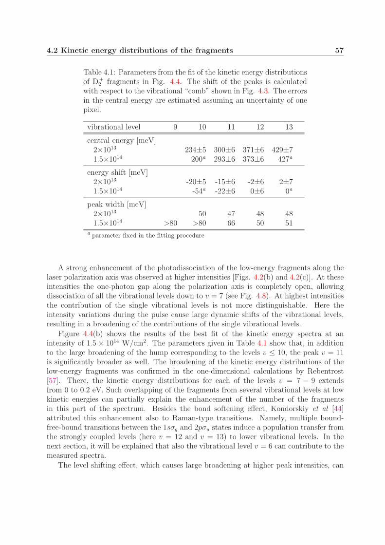
4.2 Kinetic energy distributions of the fragments 57
Table 4.1: Parameters from the fit of the kinetic energy distributionsof D+
2 fragments in Fig. 4.4. The shift of the peaks is calculatedwith respect to the vibrational “comb” shown in Fig. 4.3. The errorsin the central energy are estimated assuming an uncertainty of onepixel.
vibrational level 9 10 11 12 13
central energy [meV]2×10¹³ 234±5 300±6 371±6 429±71.5×10¹⁴ 200a 293±6 373±6 427a
energy shift [meV]2×10¹³ -20±5 -15±6 -2±6 2±71.5×10¹⁴ -54a -22±6 0±6 0a
peak width [meV]2×10¹³ 50 47 48 481.5×10¹⁴ >80 >80 66 50 51
a parameter fixed in the fitting procedure
A strong enhancement of the photodissociation of the low-energy fragments along thelaser polarization axis was observed at higher intensities [Figs. 4.2(b) and 4.2(c)]. At theseintensities the one-photon gap along the polarization axis is completely open, allowingdissociation of all the vibrational levels down to v = 7 (see Fig. 4.8). At highest intensitiesthe contribution of the single vibrational levels is not more distinguishable. Here theintensity variations during the pulse cause large dynamic shifts of the vibrational levels,resulting in a broadening of the contributions of the single vibrational levels.
Figure 4.4(b) shows the results of the best fit of the kinetic energy spectra at anintensity of 1.5 × 10¹⁴ W/cm2. The parameters given in Table 4.1 show that, in additionto the large broadening of the hump corresponding to the levels v ≤ 10, the peak v = 11is significantly broader as well. The broadening of the kinetic energy distributions of thelow-energy fragments was confirmed in the one-dimensional calculations by Rebentrost[57]. There, the kinetic energy distributions for each of the levels v = 7 − 9 extendsfrom 0 to 0.2 eV. Such overlapping of the fragments from several vibrational levels at lowkinetic energies can partially explain the enhancement of the number of the fragmentsin this part of the spectrum. Besides the bond softening effect, Kondorskiy et al [44]attributed this enhancement also to Raman-type transitions. Namely, multiple bound-free-bound transitions between the 1sσg and 2pσu states induce a population transfer fromthe strongly coupled levels (here v = 12 and v = 13) to lower vibrational levels. In thenext section, it will be explained that also the vibrational level v = 6 can contribute to themeasured spectra.
The level shifting effect, which causes large broadening at higher peak intensities, can
58 4. Photodissociation of the deuterium molecular ion
be neglected at lower intensities1. In addition to the experimental width, the peak widthis here determined by the following factors:
• The finite lifetime of the vibrational states. Nuclear wave packets spend a finitetime in the binding ground state before the molecule dissociates. The uncertainty inenergy is related to the lifetime τ through the Heisenberg relation
∆E · τ ∼ � . (4.3)
At the intensities used, the Rabi frequency [Eq. (2.1)] is much higher than thevibrational frequency, and thus the lifetime τ is on the order of magnitude of theoscillation period T = 1/ν. Here ν is the oscillation frequency of a vibrational statev given by [93]
ν(v) = (Ev+1/2 − Ev−1/2)/h . (4.4)
After extrapolating the energies of the vibrational levels, one obtains T = 33 fsfor the oscillation period of the vibrational state v = 10 of D+
2 . From Eq. (4.3),this corresponds to an uncertainty in energy per fragment of ∼10 meV. For thebond softening fragments at higher peak intensities, the lifetime and level shiftingcontributions to the resulting broadening cannot be disentangled.
• The rotational population distribution. The energies of rotational levels in the rigid-rotor approximation are given by [93]
E(J) = BJ(J + 1), (4.5)
where J is the rotational quantum number and B is the rotational constant. Forthe ground electronic state and D+
2 , B = 15.016 cm−1 (∼1.9 meV) [108]. With anassumption that the rotational states J = 0−2 of each vibrational level are occupied(Section 3.1.1), its contribution to the widths of the vibrational peaks in the kineticenergy spectra is ∼6 meV.
• The laser spectral width. For the one-photon absorption process, the laser bandwidth∆λ results in a spread of fragment kinetic energies [Eq. (4.2)]
∆EDiss =1
2h∆ν =
1
2hc
∆λ
λ2. (4.6)
For λ = 785 nm and ∆λ = 12.5 nm, ∆EDiss is about 13 meV.
4.3 Angular distributions of the fragments
4.3.1 One-photon bond softening
Figure 4.5 shows the angular distributions of the fragments from different vibrational levels,as extracted from the inverted image in Fig. 4.2(a). The broadest angular distribution
1This also includes the dissociation of the levels lying at or above the one-photon crossing, whichdissociate already on the rising edge of the pulse
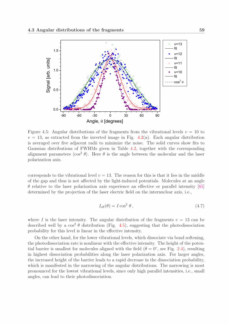
4.3 Angular distributions of the fragments 59
Figure 4.5: Angular distributions of the fragments from the vibrational levels v = 10 tov = 13, as extracted from the inverted image in Fig. 4.2(a). Each angular distributionis averaged over five adjacent radii to minimize the noise. The solid curves show fits toGaussian distributions of FWHMs given in Table 4.2, together with the correspondingalignment parameters 〈cos2 θ〉. Here θ is the angle between the molecular and the laserpolarization axis.
corresponds to the vibrational level v = 13. The reason for this is that it lies in the middleof the gap and thus is not affected by the light-induced potentials. Molecules at an angleθ relative to the laser polarization axis experience an effective or parallel intensity [65]determined by the projection of the laser electric field on the internuclear axis, i.e.,
Ieff(θ) = I cos2 θ , (4.7)
where I is the laser intensity. The angular distribution of the fragments v = 13 can bedescribed well by a cos2 θ distribution (Fig. 4.5), suggesting that the photodissociationprobability for this level is linear in the effective intensity.
On the other hand, for the lower vibrational levels, which dissociate via bond softening,the photodissociation rate is nonlinear with the effective intensity. The height of the poten-tial barrier is smallest for molecules aligned with the field (θ = 0◦, see Fig. 2.4), resultingin highest dissociation probabilities along the laser polarization axis. For larger angles,the increased height of the barrier leads to a rapid decrease in the dissociation probability,which is manifested in the narrowing of the angular distributions. The narrowing is mostpronounced for the lowest vibrational levels, since only high parallel intensities, i.e., smallangles, can lead to their photodissociation.
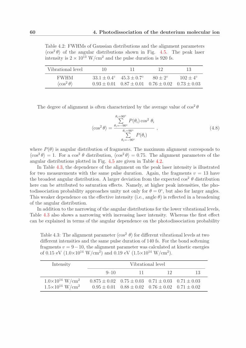
60 4. Photodissociation of the deuterium molecular ion
Table 4.2: FWHMs of Gaussian distributions and the alignment parameters〈cos2 θ〉 of the angular distributions shown in Fig. 4.5. The peak laserintensity is 2 × 10¹³ W/cm2 and the pulse duration is 920 fs.
Vibrational level 10 11 12 13
FWHM 33.1 ± 0.4◦ 45.3 ± 0.7◦ 80 ± 2◦ 102 ± 4◦
〈cos2 θ〉 0.93 ± 0.01 0.87 ± 0.01 0.76 ± 0.02 0.73 ± 0.03
The degree of alignment is often characterized by the average value of cos2 θ
〈cos2 θ〉 =
θi=90◦∑θi=−90◦
P (θi) cos2 θi
θi=90◦∑θi=−90◦
P (θi)
, (4.8)
where P (θ) is angular distribution of fragments. The maximum alignment corresponds to〈cos2 θ〉 = 1. For a cos2 θ distribution, 〈cos2 θ〉 = 0.75. The alignment parameters of theangular distributions plotted in Fig. 4.5 are given in Table 4.2.
In Table 4.3, the dependence of the alignment on the peak laser intensity is illustratedfor two measurements with the same pulse duration. Again, the fragments v = 13 havethe broadest angular distribution. A larger deviation from the expected cos2 θ distributionhere can be attributed to saturation effects. Namely, at higher peak intensities, the pho-todissociation probability approaches unity not only for θ = 0◦, but also for larger angles.This weaker dependence on the effective intensity (i.e., angle θ) is reflected in a broadeningof the angular distribution.
In addition to the narrowing of the angular distributions for the lower vibrational levels,Table 4.3 also shows a narrowing with increasing laser intensity. Whereas the first effectcan be explained in terms of the angular dependence on the photodissociation probability
Table 4.3: The alignment parameter 〈cos2 θ〉 for different vibrational levels at twodifferent intensities and the same pulse duration of 140 fs. For the bond softeningfragments v = 9−10, the alignment parameter was calculated at kinetic energiesof 0.15 eV (1.0×10¹⁴ W/cm2) and 0.19 eV (1.5×10¹⁴ W/cm2).
Intensity Vibrational level
9–10 11 12 13
1.0×10¹⁴ W/cm2 0.875 ± 0.02 0.75 ± 0.03 0.71 ± 0.03 0.71 ± 0.031.5×1014 W/cm2 0.95 ± 0.01 0.88 ± 0.02 0.76 ± 0.02 0.71 ± 0.02
4.3 Angular distributions of the fragments 61
(i.e., geometric alignment), the latter is an indication of dynamic alignment (Section 2.1.4).Classically, higher intensities correspond to higher torques exerted on molecules. In thepicture of light-induced potential curves, this corresponds to a deeper potential valley alongθ = 0◦ in the lower adiabatic potential surface (Fig. 2.4). In both pictures, the result isan alignment of molecules with the laser field.
4.3.2 Vibrational trapping and two-photon bond softening
In order to analyse processes at the highest intensity (I = 1.5× 10¹⁴ W/cm2), the invertedvelocity distribution in Fig. 4.2(c) was transformed to display the angle θ as a functionof the fragment kinetic energy. Thereby, the data along each radius were normalized tounity. The obtained image shown in Fig. 4.6 exhibits two striking features: (i) broadeningof the angular distribution at kinetic energies below 0.15 eV (see also Fig. 4.7), and (ii)its narrowing at kinetic energies above 0.6 eV. Both the features can be explained by anopening of the three-photon gap.
In the previous sections, the appearance of the fragments with low kinetic energies andnarrow angular distributions was explained in terms of bond softening. This mechanism,however, cannot account for the broadening of the angular distributions of the low-energyfragments, as shown in Fig. 4.7. Although the widening of the one-photon gap for angles| θ| > 0◦ could explain this broadening, it would necessarily lead to a broadening of theangular distributions of the upper vibrational levels as well, which is in contrast to theobservations in Figs. 4.6 and 4.7.
The observed broadening can be explained by the effect of vibrational trapping in light-induced potential wells. As explained in Section 2.1.4, in the vicinity of the three-photonavoided crossing X2, the molecules will most probably follow the lower adiabatic curve|u, n − 3〉 (Fig. 4.8). However, for the vibrational levels above the crossing (particularlyv = 6), there is a probability of trapping in the potential well created above the three-photon gap [26]. This effect was experimentally observed in H+
2 by Frasinski et al using792 nm laser pulses of variable pulse lengths [27]. According to their explanation, themolecule first crosses the three-photon gap diabatically on the leading edge of the pulse.From the Landau-Zener formula [65], the probability for a diabatic transition is highest atlow intensities because the width of the gap is rather small. After entering the potentialwell above the gap, the nuclear wave packet loses kinetic energy, turns back and arrivesagain at the gap. At this time the gap is much wider, and hence the probability of thediabatic crossing is small. The wave packet is now trapped in the potential well. As theintensity on the trailing edge of the laser pulse decreases, the shape of the upper adiabaticcurve changes from concave to convex (see Fig. 4.8). Consequently, a portion of the nuclearwave packet is lifted up and finally ends up in the |u, n − 1〉 state by effectively absorbingone photon.
The angular distribution of molecules dissociating via this scenario would be broadenedfor two reasons. (i) The distance between the adiabatic potential curves is smallest at lowest(effective) intensities, i.e., for θ close to 90◦. Consequently, the probability for a diabatictransition is highest for these angles (there is no coupling for θ = 90◦). (ii) The potential

62 4. Photodissociation of the deuterium molecular ion
0
0.5
1
Figure 4.6: Number of fragments as a function of the angle θ and fragment speed (i.e.,radius), as extracted from the inverted data in Fig. 4.2(c) (peak intensity of 1.5 × 10¹⁴
W/cm2). The data on the same radius were normalized to unity. The noise in the dataresults from the inversion procedure and the normalization of these data.
Figure 4.7: Angular distributions from Fig. 4.6 at kinetic energies of 0.025 eV and 0.18eV (radii of 30 and 80 in Fig. 4.6). Each angular distribution comprises data at fiveadjacent radii. The solid lines show fits to Gaussian distributions with FWHMs of 56± 3◦
and 29.5± 0.2◦. The corresponding 〈cos2 θ〉 parameters are 0.84± 0.04 and 0.954± 0.006,respectively.
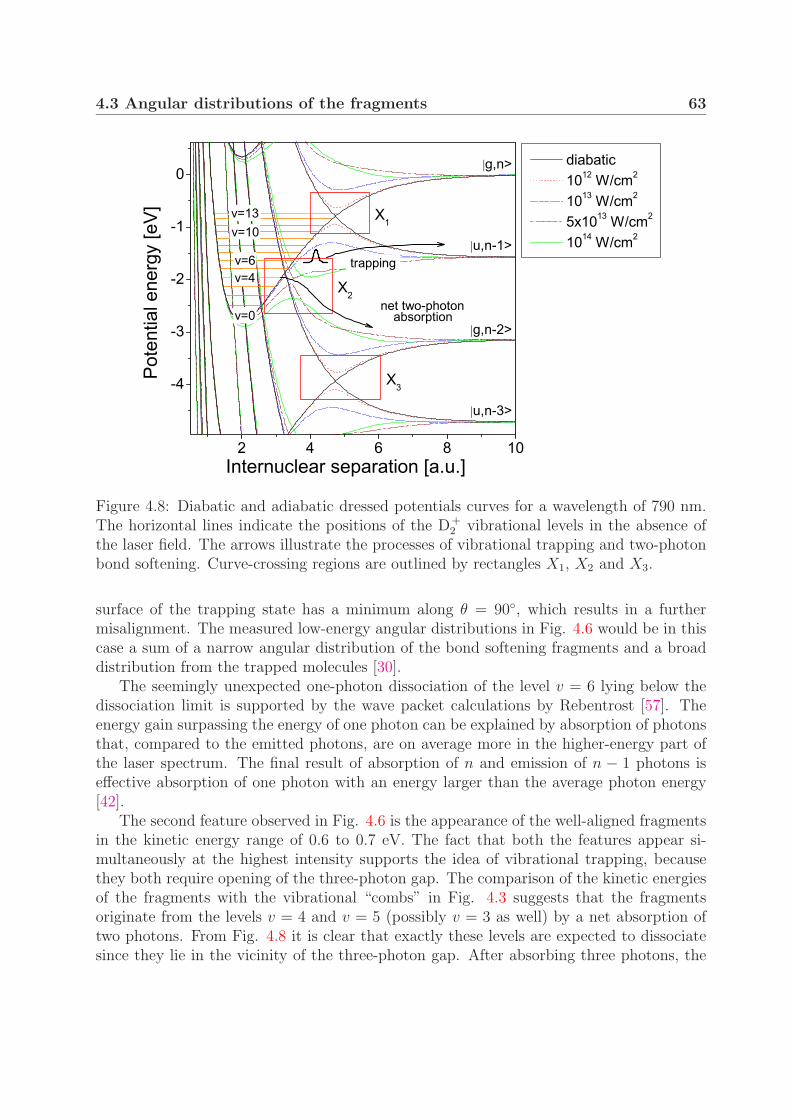
4.3 Angular distributions of the fragments 63
Figure 4.8: Diabatic and adiabatic dressed potentials curves for a wavelength of 790 nm.The horizontal lines indicate the positions of the D+
2 vibrational levels in the absence ofthe laser field. The arrows illustrate the processes of vibrational trapping and two-photonbond softening. Curve-crossing regions are outlined by rectangles X1, X2 and X3.
surface of the trapping state has a minimum along θ = 90◦, which results in a furthermisalignment. The measured low-energy angular distributions in Fig. 4.6 would be in thiscase a sum of a narrow angular distribution of the bond softening fragments and a broaddistribution from the trapped molecules [30].
The seemingly unexpected one-photon dissociation of the level v = 6 lying below thedissociation limit is supported by the wave packet calculations by Rebentrost [57]. Theenergy gain surpassing the energy of one photon can be explained by absorption of photonsthat, compared to the emitted photons, are on average more in the higher-energy part ofthe laser spectrum. The final result of absorption of n and emission of n − 1 photons iseffective absorption of one photon with an energy larger than the average photon energy[42].
The second feature observed in Fig. 4.6 is the appearance of the well-aligned fragmentsin the kinetic energy range of 0.6 to 0.7 eV. The fact that both the features appear si-multaneously at the highest intensity supports the idea of vibrational trapping, becausethey both require opening of the three-photon gap. The comparison of the kinetic energiesof the fragments with the vibrational “combs” in Fig. 4.3 suggests that the fragmentsoriginate from the levels v = 4 and v = 5 (possibly v = 3 as well) by a net absorption oftwo photons. From Fig. 4.8 it is clear that exactly these levels are expected to dissociatesince they lie in the vicinity of the three-photon gap. After absorbing three photons, the
64 4. Photodissociation of the deuterium molecular ion
molecules follow the |u, n−3〉 state and emit one photon at the crossing X2. Consequently,they end up in the |g, n − 2〉 state, reflecting the effective absorption of two photons. Thenarrow angular distribution in Fig. 4.6 is a consequence of the bond softening mechanism,i.e., the angle-dependent width of the three-photon gap.
4.4 Comparison with measurements on H+2 at lower
intensities
H+2 was studied under similar experimental conditions earlier in this group [86]. In order to
compare the 3D velocity distributions and kinetic energy spectra of the two isotopic vari-ants, the experimental images of Ref. [28] were inverted here. Figure 4.9 shows projectedand inverted velocity distributions of the neutral fragments resulting from photodissocia-tion of H+
2 at a wavelength of 785 nm. The pulse energy is 1.0 mJ in both measurementsand the pulse durations are 575 and 135 fs, corresponding to the peak intensities of 3.5×10¹³
and 1.5 × 10¹⁴ W/cm2, respectively [28]. The calculated intensities may differ from thatgiven in the D+
2 measurements because of the uncertainty related to the different focusedbeam diameters in these measurements.
Figure 4.10 shows the kinetic energy distributions of the fragments extracted from theinverted images as discussed in Section 4.2. In distinction from D+
2 , in H+2 the peaks
corresponding to single vibrational levels are more widely spaced, allowing to extend thevibrationally resolved study of bond softening to the lowest dissociating vibrational lev-els. The central energy and the widths of the peaks were determined by fits to Gaussiandistributions as shown in Fig. 4.11. The results of the best fits are given in Table 4.4.
In comparison with D+2 (Table 4.1), the level shifting of the corresponding vibrational
levels of H+2 is of a similar magnitude. This is to be expected, since level shifting is
determined by the shape of the light-induced potential curves, which are the same in bothcases.
In distinction from D+2 , the widths of the peaks of H+
2 are significantly broader. Thissuggests that the widths are primarily determined by the lifetimes of the vibrational states.In strong fields, the nearly resonant vibrational levels (v = 9 in H+
2 and v = 13 in D+2 )
dissociate with a high probability every time the molecule approaches the outer turningpoint, i.e., the lifetime is comparable to the vibrational period. Since the oscillation periodis shorter for H+
2 [see Eq. (4.4)], according to the uncertainty principle [Eq. (4.3)], thespread of its fragment energies would be larger. At lower intensities, at which the peaksare best resolved, the widths of the v = 9 peak in H+
2 and v = 13 peak in D+2 are 68 meV
and 48 meV, respectively. Their ratio of 1.4 is surprisingly close to the inverse ratio oftheir oscillation periods.
It is interesting to note that at an intensity of 3.5× 10¹³ W/cm2 the width of the bondsoftening level v = 6 is smaller than that of the level v = 7 in Fig. 4.10(a). The smallernumber of the fragments from the level v = 6 is a consequence of a lower photodissociationprobability. The corresponding longer lifetime of this level would result in a smaller energy
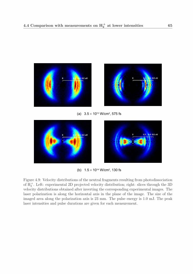
4.4 Comparison with measurements on H+2 at lower intensities 65
� � � � � � # � � � � � � � � � 2 3 � � * 4 � � 5 � � , �
� � � � � � # � � � � � � � � � 2 3 � � * 4 � � � � � , �
Figure 4.9: Velocity distributions of the neutral fragments resulting from photodissociationof H+
2 . Left: experimental 2D projected velocity distribution; right: slices through the 3Dvelocity distributions obtained after inverting the corresponding experimental images. Thelaser polarization is along the horizontal axis in the plane of the image. The size of theimaged area along the polarization axis is 23 mm. The pulse energy is 1.0 mJ. The peaklaser intensities and pulse durations are given for each measurement.
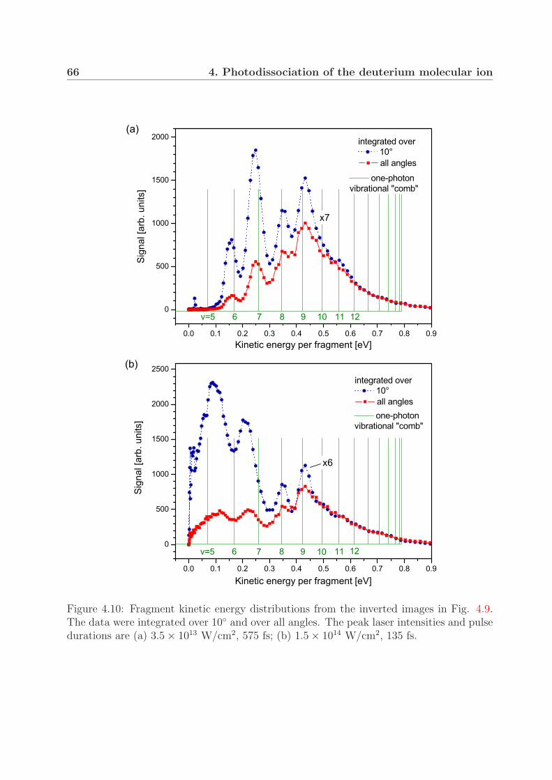
66 4. Photodissociation of the deuterium molecular ion
Figure 4.10: Fragment kinetic energy distributions from the inverted images in Fig. 4.9.The data were integrated over 10◦ and over all angles. The peak laser intensities and pulsedurations are (a) 3.5 × 10¹³ W/cm2, 575 fs; (b) 1.5 × 10¹⁴ W/cm2, 135 fs.
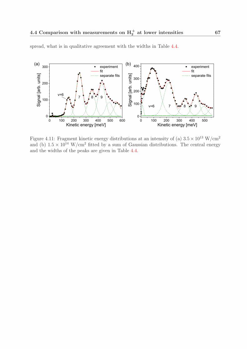
4.4 Comparison with measurements on H+2 at lower intensities 67
spread, what is in qualitative agreement with the widths in Table 4.4.
Figure 4.11: Fragment kinetic energy distributions at an intensity of (a) 3.5× 10¹³ W/cm2
and (b) 1.5 × 10¹⁴ W/cm2 fitted by a sum of Gaussian distributions. The central energyand the widths of the peaks are given in Table 4.4.
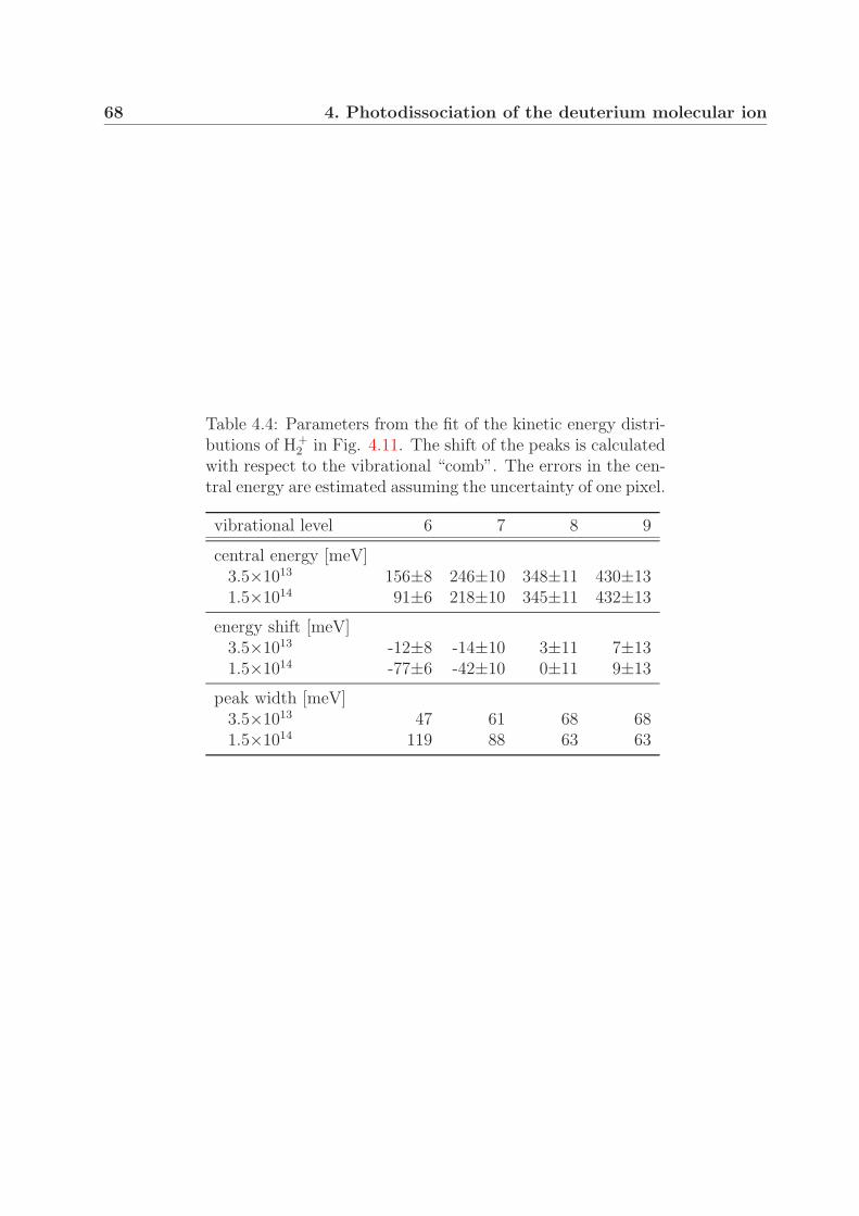
68 4. Photodissociation of the deuterium molecular ion
Table 4.4: Parameters from the fit of the kinetic energy distri-butions of H+
2 in Fig. 4.11. The shift of the peaks is calculatedwith respect to the vibrational “comb”. The errors in the cen-tral energy are estimated assuming the uncertainty of one pixel.
vibrational level 6 7 8 9
central energy [meV]3.5×10¹³ 156±8 246±10 348±11 430±131.5×10¹⁴ 91±6 218±10 345±11 432±13
energy shift [meV]3.5×10¹³ -12±8 -14±10 3±11 7±131.5×10¹⁴ -77±6 -42±10 0±11 9±13
peak width [meV]3.5×10¹³ 47 61 68 681.5×10¹⁴ 119 88 63 63

Chapter 5
Photodissociation of the hydrogenmolecular ion
The investigation of the strong-field photodissociation presented in the previous chapteris in this chapter extended to higher laser intensities. By using shorter pulses, largerpulse energies and stronger focusing, the peak laser intensities above 1× 10¹⁵ W/cm2 wereachieved, allowing to investigate the two-photon bond softening process and Coulombexplosion. The photodissociation and Coulomb explosion channels were studied simulta-neously by detecting both the charged and neutral fragments. In this chapter, results ofthe photodissociation of H+
2 are discussed.In Section 5.1, the velocity distributions of the fragments are shown in a series of images
recorded at different peak intensities. The distributions are analysed by discussing thefragment kinetic energy and angular distributions. Attention is also given to the intensitydistribution in the interaction region. In Section 5.2, the dependence of the alignment onthe peak intensity is discussed for fragments at different kinetic energies. Furthermore, thewidths of the angular distributions of the fragments from the different vibrational levelsare compared. In Section 5.3, the dependence of the fragment yield of the one- (1ω) andnet two- (2ω) photon process on the peak intensity is investigated.
5.1 Velocity and kinetic energy distributions of the
fragments
Figure 5.1 shows an example of the velocity distribution measured at a peak intensity ofabout 1 × 10¹⁵ W/cm2. The circular feature at energies below 0.9 eV corresponds to theneutral (H) and charged (H+) fragments from the photodissociation channel. In addition,the protons from the Coulomb explosion channel can be seen at energies in the rangefrom about 1 to 4 eV. These fragments were identified as Coulomb explosion protons in aseparate measurement in which no fragments were observed when only neutral fragmentswere detected.
Since the experimental images are symmetric with respect to the vertical axis at zero
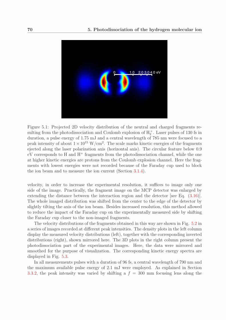
70 5. Photodissociation of the hydrogen molecular ion
0 1.0 2.0 3.0 4.0 eV
Figure 5.1: Projected 2D velocity distribution of the neutral and charged fragments re-sulting from the photodissociation and Coulomb explosion of H+
2 . Laser pulses of 130 fs induration, a pulse energy of 1.75 mJ and a central wavelength of 785 nm were focused to apeak intensity of about 1×10¹⁵ W/cm2. The scale marks kinetic energies of the fragmentsejected along the laser polarization axis (horizontal axis). The circular feature below 0.9eV corresponds to H and H+ fragments from the photodissociation channel, while the oneat higher kinetic energies are protons from the Coulomb explosion channel. Here the frag-ments with lowest energies were not recorded because of the Faraday cup used to blockthe ion beam and to measure the ion current (Section 3.1.4).
velocity, in order to increase the experimental resolution, it suffices to image only oneside of the image. Practically, the fragment image on the MCP detector was enlarged byextending the distance between the interaction region and the detector [see Eq. (3.16)].The whole imaged distribution was shifted from the center to the edge of the detector byslightly tilting the axis of the ion beam. Besides increased resolution, this method allowedto reduce the impact of the Faraday cup on the experimentally measured side by shiftingthe Faraday cup closer to the non-imaged fragments.
The velocity distributions of the fragments obtained in this way are shown in Fig. 5.2 ina series of images recorded at different peak intensities. The density plots in the left columndisplay the measured velocity distributions (left), together with the corresponding inverteddistributions (right), shown mirrored here. The 3D plots in the right column present thephotodissociation part of the experimental images. Here, the data were mirrored andsmoothed for the purpose of visualization. The corresponding kinetic energy spectra aredisplayed in Fig. 5.3.
In all measurements pulses with a duration of 96 fs, a central wavelength of 790 nm andthe maximum available pulse energy of 2.1 mJ were employed. As explained in Section3.3.2, the peak intensity was varied by shifting a f = 300 mm focusing lens along the
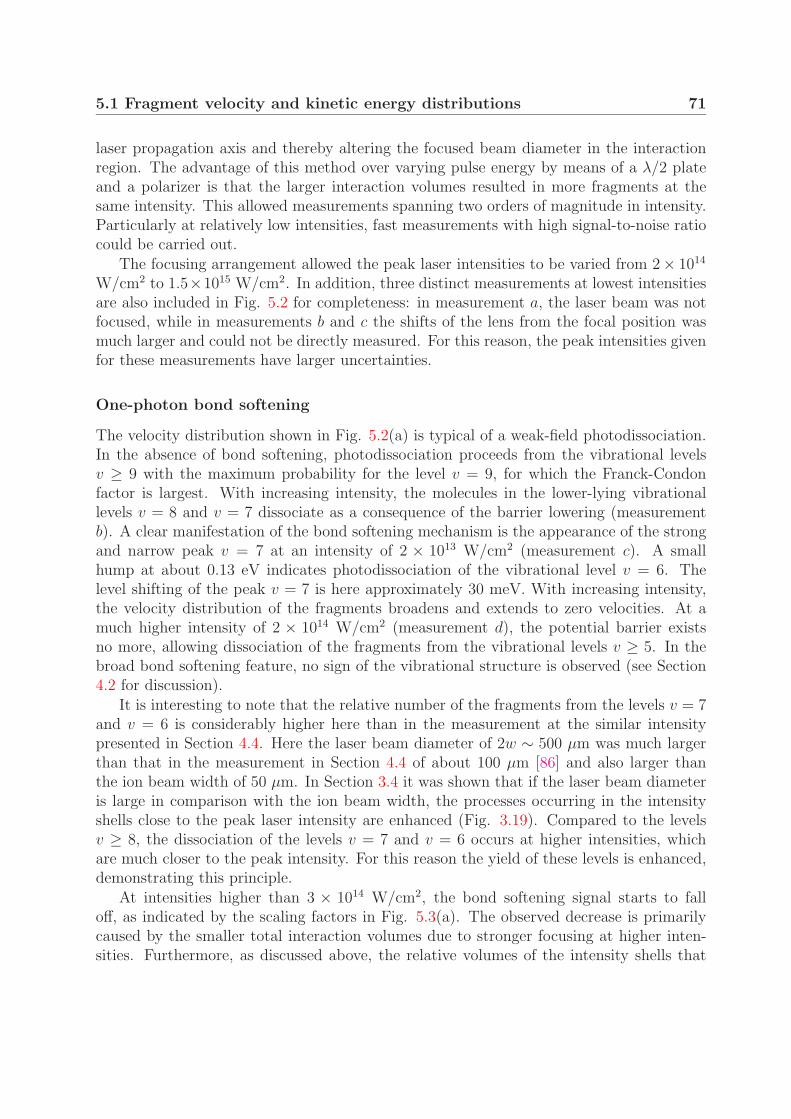
5.1 Fragment velocity and kinetic energy distributions 71
laser propagation axis and thereby altering the focused beam diameter in the interactionregion. The advantage of this method over varying pulse energy by means of a λ/2 plateand a polarizer is that the larger interaction volumes resulted in more fragments at thesame intensity. This allowed measurements spanning two orders of magnitude in intensity.Particularly at relatively low intensities, fast measurements with high signal-to-noise ratiocould be carried out.
The focusing arrangement allowed the peak laser intensities to be varied from 2× 10¹⁴
W/cm2 to 1.5×10¹⁵ W/cm2. In addition, three distinct measurements at lowest intensitiesare also included in Fig. 5.2 for completeness: in measurement a, the laser beam was notfocused, while in measurements b and c the shifts of the lens from the focal position wasmuch larger and could not be directly measured. For this reason, the peak intensities givenfor these measurements have larger uncertainties.
One-photon bond softening
The velocity distribution shown in Fig. 5.2(a) is typical of a weak-field photodissociation.In the absence of bond softening, photodissociation proceeds from the vibrational levelsv ≥ 9 with the maximum probability for the level v = 9, for which the Franck-Condonfactor is largest. With increasing intensity, the molecules in the lower-lying vibrationallevels v = 8 and v = 7 dissociate as a consequence of the barrier lowering (measurementb). A clear manifestation of the bond softening mechanism is the appearance of the strongand narrow peak v = 7 at an intensity of 2 × 10¹³ W/cm2 (measurement c). A smallhump at about 0.13 eV indicates photodissociation of the vibrational level v = 6. Thelevel shifting of the peak v = 7 is here approximately 30 meV. With increasing intensity,the velocity distribution of the fragments broadens and extends to zero velocities. At amuch higher intensity of 2 × 10¹⁴ W/cm2 (measurement d), the potential barrier existsno more, allowing dissociation of the fragments from the vibrational levels v ≥ 5. In thebroad bond softening feature, no sign of the vibrational structure is observed (see Section4.2 for discussion).
It is interesting to note that the relative number of the fragments from the levels v = 7and v = 6 is considerably higher here than in the measurement at the similar intensitypresented in Section 4.4. Here the laser beam diameter of 2w ∼ 500 µm was much largerthan that in the measurement in Section 4.4 of about 100 µm [86] and also larger thanthe ion beam width of 50 µm. In Section 3.4 it was shown that if the laser beam diameteris large in comparison with the ion beam width, the processes occurring in the intensityshells close to the peak laser intensity are enhanced (Fig. 3.19). Compared to the levelsv ≥ 8, the dissociation of the levels v = 7 and v = 6 occurs at higher intensities, whichare much closer to the peak intensity. For this reason the yield of these levels is enhanced,demonstrating this principle.
At intensities higher than 3 × 10¹⁴ W/cm2, the bond softening signal starts to falloff, as indicated by the scaling factors in Fig. 5.3(a). The observed decrease is primarilycaused by the smaller total interaction volumes due to stronger focusing at higher inten-sities. Furthermore, as discussed above, the relative volumes of the intensity shells that

72 5. Photodissociation of the hydrogen molecular ion
0 % � �� *
* % � �� �
� % � �2 3 � � *
� �
� �
� �
� �
) - 0
) - 6
) - 5
) - 0
'
� � � � � � � � � ) � � � � �
Figure 5.2: Velocity distributions of the fragments resulting from photodissociation andCoulomb explosion of H+
2 at different peak intensities. Left column: the experimentallymeasured velocity distributions (left), together with the corresponding inverted distribu-tions (right), shown as “mirror pairs” for the purpose of comparison. The inserted scalemarks kinetic energies of the fragments ejected along the laser polarization axis (horizontalaxis). The horizontal size of the imaged area is 27 mm. Right column: 3D plots presentingthe photodissociation part of the measured data. For the purpose of visualization, themeasured side was mirrored and the data were smoothed using a Gaussian filter. Eachimage is normalized to its maximum signal. The concentric circles mark kinetic energieswith a step width of 0.1 eV. The ticks on the outer circle mark angles with respect to thelaser polarization axis. The pulse energy is 2.1 mJ and the pulse duration is 96 fs in allmeasurements.

5.1 Fragment velocity and kinetic energy distributions 73
� % � �� �
� % � �� �
5 % � �� �
� �
� ,
� �
� �
) - �
� * �
) - 0
) - 6
) - �
* % � �� �
� �
) - 0 ) - 6 ) - 5
) - 0
) - 6
) � 5
) � 5
) � 5
) - 0
) - 6
) � 5 � � � � ) � � � � * � �
) - 6 � 0 � � � �
) - �
� * �
Figure 5.2 (continued): Velocity distributions of the fragments resulting from photodisso-ciation and Coulomb explosion of H+
2 at different peak intensities.

74 5. Photodissociation of the hydrogen molecular ion
� # � % � �� �
� # � % � �� �
� # � % � �� �
� "
� +
� �
0 % � �� �
� �
) � � � � * � �
) - 6 � 0 � � � � ) � 5 � � � �
) � � � � * � �
) - 6 � 0 � � � � ) � 5 � � � �
) � � � � * � �
) - 6 � 0 � � � � ) � 5 � � � �
) � � � � * � �
) - 6 � 0 � � � � ) � 5 � � � �
Figure 5.2 (continued): Velocity distributions of the fragments resulting from photodisso-ciation and Coulomb explosion of H+
2 at different peak intensities.
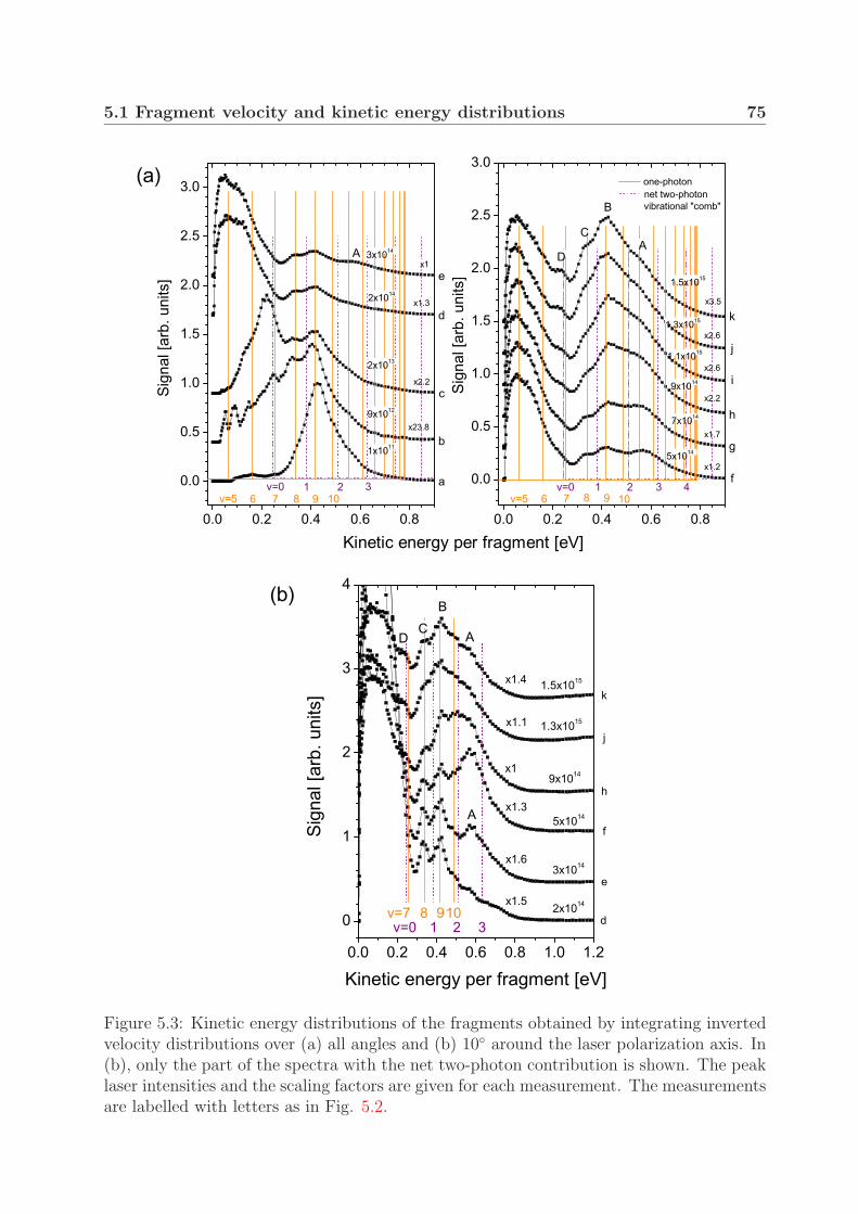
5.1 Fragment velocity and kinetic energy distributions 75
Figure 5.3: Kinetic energy distributions of the fragments obtained by integrating invertedvelocity distributions over (a) all angles and (b) 10◦ around the laser polarization axis. In(b), only the part of the spectra with the net two-photon contribution is shown. The peaklaser intensities and the scaling factors are given for each measurement. The measurementsare labelled with letters as in Fig. 5.2.
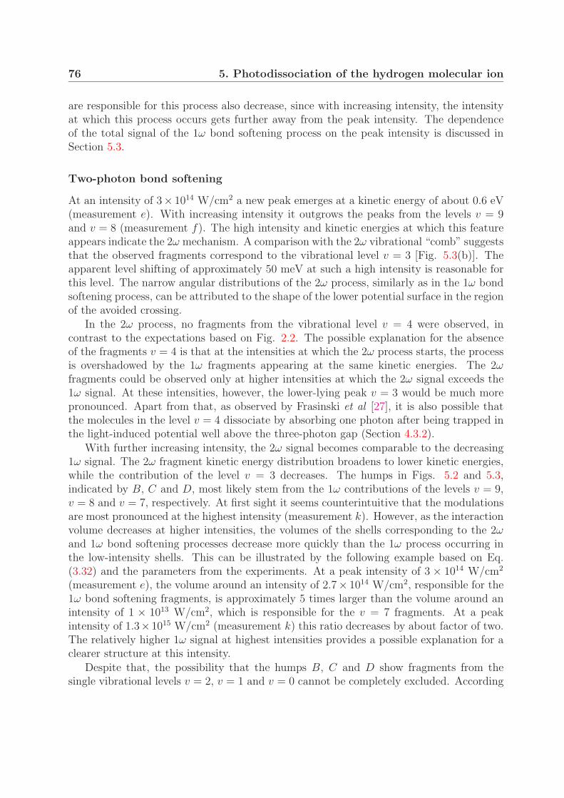
76 5. Photodissociation of the hydrogen molecular ion
are responsible for this process also decrease, since with increasing intensity, the intensityat which this process occurs gets further away from the peak intensity. The dependenceof the total signal of the 1ω bond softening process on the peak intensity is discussed inSection 5.3.
Two-photon bond softening
At an intensity of 3× 10¹⁴ W/cm2 a new peak emerges at a kinetic energy of about 0.6 eV(measurement e). With increasing intensity it outgrows the peaks from the levels v = 9and v = 8 (measurement f). The high intensity and kinetic energies at which this featureappears indicate the 2ω mechanism. A comparison with the 2ω vibrational “comb” suggeststhat the observed fragments correspond to the vibrational level v = 3 [Fig. 5.3(b)]. Theapparent level shifting of approximately 50 meV at such a high intensity is reasonable forthis level. The narrow angular distributions of the 2ω process, similarly as in the 1ω bondsoftening process, can be attributed to the shape of the lower potential surface in the regionof the avoided crossing.
In the 2ω process, no fragments from the vibrational level v = 4 were observed, incontrast to the expectations based on Fig. 2.2. The possible explanation for the absenceof the fragments v = 4 is that at the intensities at which the 2ω process starts, the processis overshadowed by the 1ω fragments appearing at the same kinetic energies. The 2ωfragments could be observed only at higher intensities at which the 2ω signal exceeds the1ω signal. At these intensities, however, the lower-lying peak v = 3 would be much morepronounced. Apart from that, as observed by Frasinski et al [27], it is also possible thatthe molecules in the level v = 4 dissociate by absorbing one photon after being trapped inthe light-induced potential well above the three-photon gap (Section 4.3.2).
With further increasing intensity, the 2ω signal becomes comparable to the decreasing1ω signal. The 2ω fragment kinetic energy distribution broadens to lower kinetic energies,while the contribution of the level v = 3 decreases. The humps in Figs. 5.2 and 5.3,indicated by B, C and D, most likely stem from the 1ω contributions of the levels v = 9,v = 8 and v = 7, respectively. At first sight it seems counterintuitive that the modulationsare most pronounced at the highest intensity (measurement k). However, as the interactionvolume decreases at higher intensities, the volumes of the shells corresponding to the 2ωand 1ω bond softening processes decrease more quickly than the 1ω process occurring inthe low-intensity shells. This can be illustrated by the following example based on Eq.(3.32) and the parameters from the experiments. At a peak intensity of 3 × 10¹⁴ W/cm2
(measurement e), the volume around an intensity of 2.7× 10¹⁴ W/cm2, responsible for the1ω bond softening fragments, is approximately 5 times larger than the volume around anintensity of 1 × 10¹³ W/cm2, which is responsible for the v = 7 fragments. At a peakintensity of 1.3×10¹⁵ W/cm2 (measurement k) this ratio decreases by about factor of two.The relatively higher 1ω signal at highest intensities provides a possible explanation for aclearer structure at this intensity.
Despite that, the possibility that the humps B, C and D show fragments from thesingle vibrational levels v = 2, v = 1 and v = 0 cannot be completely excluded. According
5.2 Angular distributions of the fragments: alignment 77
to the 2ω vibrational “comb”, the fragments from these levels can be expected at similarkinetic energies, providing that they are level shifted to lower kinetic energies, as observedin the 1ω bond softening process. According to the spectra, the magnitude of level shiftingwould be smaller for the lower vibrational levels, as it is expected from the static pictureof vibrational levels in the light-induced electronic state. Although the contribution of thesingle vibration levels in the 2ω signal is not clear, the angular distributions indicate thatthe lower-energy 2ω fragments can be attributed to the lower vibrational levels (discussedin the following section).
5.2 Angular distributions of the fragments: alignment
5.2.1 Dependence on the peak laser intensity
From the velocity distributions presented in Fig. 5.2, it is clear that the angular distribu-tions of the fragments depend on their kinetic energy as well as on the peak laser intensity.In Fig. 5.4, these dependencies are quantified with the alignment parameter 〈cos2 θ〉 [Eq.(4.8)] for the angular distributions of the inverted images in Fig. 5.2.
At intensities up to 2×10¹³ W/cm2, as expected, the lower-lying vibrational levels v = 8and particularly v = 7 show higher degrees of alignment. With increasing intensity, thefragments become increasingly more aligned, which indicates dynamic alignment. Theseresults are in agreement with the observations in the D+
2 measurements, which are discussedin Section 4.3.1.
At a much higher intensity of 1.6 × 10¹⁴ W/cm2, significantly lower alignment param-eters were measured at the same kinetic energies. The degradation of the alignment withincreasing intensity suggests saturation effects as a cause (Section 4.3.1). For the lower-lying vibrational levels, corresponding to the data at 0.13 eV and 0.23 eV, the degradationextends to peak intensities of 6 × 10¹⁴ W/cm2 or higher. For these levels, namely, higherparallel intensities are needed for dissociation, and thus saturation occurs later in Fig.5.4. On the other hand, the angular distributions of the levels v = 8 and v = 9 are notinfluenced by the intensity variations. For the level v = 9, the alignment parameter is 0.74,which is close to that of a cos2 θ distribution.
A rapid increase in alignment with intensity was observed for the fragments at 0.58 eVstarting from an intensity of 3 × 10¹⁴ W/cm2. From Figs. 5.2(e) and 5.3(e) it can be seenthat the narrowing is due to the appearance of the 2ω peak v = 3. The measured angulardistribution is a sum of a broad distribution of the fragments v = 11 − 12 and a narrowerdistribution of the fragments v = 3. Since the contribution of the 2ω process increases muchmore rapidly with intensity, the total angular distribution narrows. The rise in alignmentis also observed at lower kinetic energies. However, there it occurs at increasingly higherpeak intensities, suggesting that these fragments originate from the lower vibrational levelsdue to the barrier lowering. At sufficiently high intensities, a degradation of alignment isobserved for the data at 0.41 and 0.31 eV. This can be attributed to the apparent largercontribution of the 1ω fragments from the levels v = 9 and v = 8.
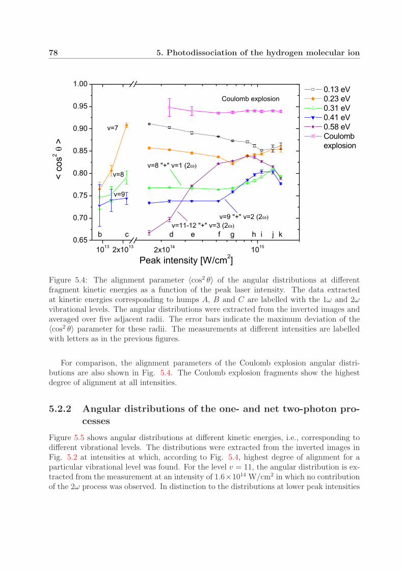
78 5. Photodissociation of the hydrogen molecular ion
Figure 5.4: The alignment parameter 〈cos2 θ〉 of the angular distributions at differentfragment kinetic energies as a function of the peak laser intensity. The data extractedat kinetic energies corresponding to humps A, B and C are labelled with the 1ω and 2ωvibrational levels. The angular distributions were extracted from the inverted images andaveraged over five adjacent radii. The error bars indicate the maximum deviation of the〈cos2 θ〉 parameter for these radii. The measurements at different intensities are labelledwith letters as in the previous figures.
For comparison, the alignment parameters of the Coulomb explosion angular distri-butions are also shown in Fig. 5.4. The Coulomb explosion fragments show the highestdegree of alignment at all intensities.
5.2.2 Angular distributions of the one- and net two-photon pro-cesses
Figure 5.5 shows angular distributions at different kinetic energies, i.e., corresponding todifferent vibrational levels. The distributions were extracted from the inverted images inFig. 5.2 at intensities at which, according to Fig. 5.4, highest degree of alignment for aparticular vibrational level was found. For the level v = 11, the angular distribution is ex-tracted from the measurement at an intensity of 1.6×10¹⁴ W/cm2 in which no contributionof the 2ω process was observed. In distinction to the distributions at lower peak intensities
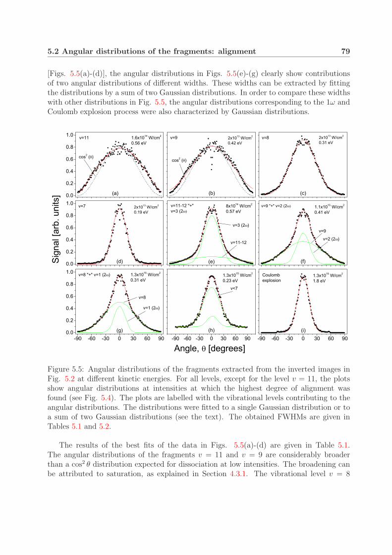
5.2 Angular distributions of the fragments: alignment 79
[Figs. 5.5(a)-(d)], the angular distributions in Figs. 5.5(e)-(g) clearly show contributionsof two angular distributions of different widths. These widths can be extracted by fittingthe distributions by a sum of two Gaussian distributions. In order to compare these widthswith other distributions in Fig. 5.5, the angular distributions corresponding to the 1ω andCoulomb explosion process were also characterized by Gaussian distributions.
Figure 5.5: Angular distributions of the fragments extracted from the inverted images inFig. 5.2 at different kinetic energies. For all levels, except for the level v = 11, the plotsshow angular distributions at intensities at which the highest degree of alignment wasfound (see Fig. 5.4). The plots are labelled with the vibrational levels contributing to theangular distributions. The distributions were fitted to a single Gaussian distribution or toa sum of two Gaussian distributions (see the text). The obtained FWHMs are given inTables 5.1 and 5.2.
The results of the best fits of the data in Figs. 5.5(a)-(d) are given in Table 5.1.The angular distributions of the fragments v = 11 and v = 9 are considerably broaderthan a cos2 θ distribution expected for dissociation at low intensities. The broadening canbe attributed to saturation, as explained in Section 4.3.1. The vibrational level v = 8
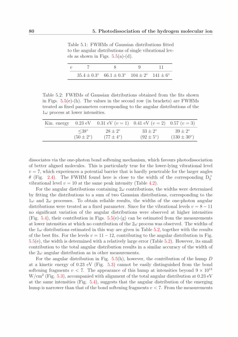
80 5. Photodissociation of the hydrogen molecular ion
Table 5.1: FWHMs of Gaussian distributions fittedto the angular distributions of single vibrational lev-els as shown in Figs. 5.5(a)-(d).
v 7 8 9 11
35.4 ± 0.3◦ 66.1 ± 0.3◦ 104 ± 2◦ 141 ± 6◦
Table 5.2: FWHMs of Gaussian distributions obtained from the fits shownin Figs. 5.5(e)-(h). The values in the second row (in brackets) are FWHMstreated as fixed parameters corresponding to the angular distributions of the1ω process at lower intensities.
Kin. energy 0.23 eV 0.31 eV (v = 1) 0.41 eV (v = 2) 0.57 (v = 3)
≤38◦ 28 ± 2◦ 33 ± 2◦ 39 ± 2◦
(50 ± 2◦) (77 ± 4◦) (92 ± 5◦) (130 ± 30◦)
dissociates via the one-photon bond softening mechanism, which favours photodissociationof better aligned molecules. This is particularly true for the lower-lying vibrational levelv = 7, which experiences a potential barrier that is hardly penetrable for the larger anglesθ (Fig. 2.4). The FWHM found here is close to the width of the corresponding D+
2
vibrational level v = 10 at the same peak intensity (Table 4.2).
For the angular distributions containing 2ω contributions, the widths were determinedby fitting the distributions to a sum of two Gaussian distributions, corresponding to the1ω and 2ω processes. To obtain reliable results, the widths of the one-photon angulardistributions were treated as a fixed parameter. Since for the vibrational levels v = 8− 11no significant variation of the angular distributions were observed at higher intensities(Fig. 5.4), their contribution in Figs. 5.5(e)-(g) can be estimated from the measurementsat lower intensities at which no contribution of the 2ω process was observed. The widths ofthe 1ω distributions estimated in this way are given in Table 5.2, together with the resultsof the best fits. For the levels v = 11− 12, contributing to the angular distribution in Fig.5.5(e), the width is determined with a relatively large error (Table 5.2). However, its smallcontribution to the total angular distribution results in a similar accuracy of the width ofthe 2ω angular distribution as in other measurements.
For the angular distribution in Fig. 5.5(h), however, the contribution of the hump Dat a kinetic energy of 0.23 eV (Fig. 5.3) cannot be easily distinguished from the bondsoftening fragments v < 7. The appearance of this hump at intensities beyond 9 × 10¹⁴
W/cm2 (Fig. 5.3), accompanied with alignment of the total angular distribution at 0.23 eVat the same intensities (Fig. 5.4), suggests that the angular distribution of the emerginghump is narrower than that of the bond softening fragments v < 7. From the measurements
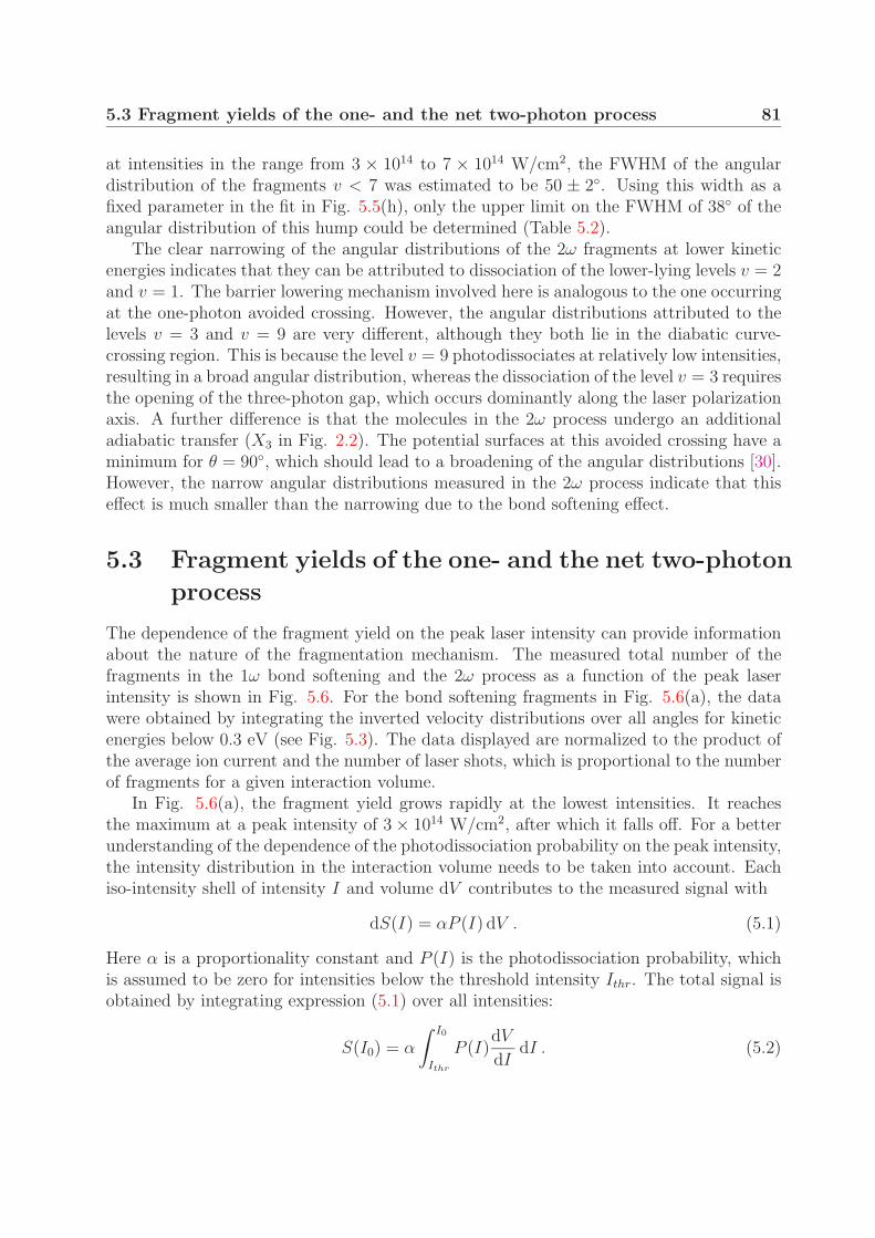
5.3 Fragment yields of the one- and the net two-photon process 81
at intensities in the range from 3 × 10¹⁴ to 7 × 10¹⁴ W/cm2, the FWHM of the angulardistribution of the fragments v < 7 was estimated to be 50 ± 2◦. Using this width as afixed parameter in the fit in Fig. 5.5(h), only the upper limit on the FWHM of 38◦ of theangular distribution of this hump could be determined (Table 5.2).
The clear narrowing of the angular distributions of the 2ω fragments at lower kineticenergies indicates that they can be attributed to dissociation of the lower-lying levels v = 2and v = 1. The barrier lowering mechanism involved here is analogous to the one occurringat the one-photon avoided crossing. However, the angular distributions attributed to thelevels v = 3 and v = 9 are very different, although they both lie in the diabatic curve-crossing region. This is because the level v = 9 photodissociates at relatively low intensities,resulting in a broad angular distribution, whereas the dissociation of the level v = 3 requiresthe opening of the three-photon gap, which occurs dominantly along the laser polarizationaxis. A further difference is that the molecules in the 2ω process undergo an additionaladiabatic transfer (X3 in Fig. 2.2). The potential surfaces at this avoided crossing have aminimum for θ = 90◦, which should lead to a broadening of the angular distributions [30].However, the narrow angular distributions measured in the 2ω process indicate that thiseffect is much smaller than the narrowing due to the bond softening effect.
5.3 Fragment yields of the one- and the net two-photon
process
The dependence of the fragment yield on the peak laser intensity can provide informationabout the nature of the fragmentation mechanism. The measured total number of thefragments in the 1ω bond softening and the 2ω process as a function of the peak laserintensity is shown in Fig. 5.6. For the bond softening fragments in Fig. 5.6(a), the datawere obtained by integrating the inverted velocity distributions over all angles for kineticenergies below 0.3 eV (see Fig. 5.3). The data displayed are normalized to the product ofthe average ion current and the number of laser shots, which is proportional to the numberof fragments for a given interaction volume.
In Fig. 5.6(a), the fragment yield grows rapidly at the lowest intensities. It reachesthe maximum at a peak intensity of 3 × 10¹⁴ W/cm2, after which it falls off. For a betterunderstanding of the dependence of the photodissociation probability on the peak intensity,the intensity distribution in the interaction volume needs to be taken into account. Eachiso-intensity shell of intensity I and volume dV contributes to the measured signal with
dS(I) = αP (I) dV . (5.1)
Here α is a proportionality constant and P (I) is the photodissociation probability, whichis assumed to be zero for intensities below the threshold intensity Ithr. The total signal isobtained by integrating expression (5.1) over all intensities:
S(I0) = α
∫ I0
Ithr
P (I)dV
dIdI . (5.2)
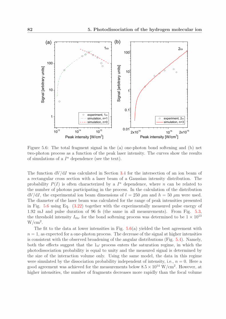
82 5. Photodissociation of the hydrogen molecular ion
Figure 5.6: The total fragment signal in the (a) one-photon bond softening and (b) nettwo-photon process as a function of the peak laser intensity. The curves show the resultsof simulations of a In dependence (see the text).
The function dV/dI was calculated in Section 3.4 for the intersection of an ion beam ofa rectangular cross section with a laser beam of a Gaussian intensity distribution. Theprobability P (I) is often characterized by a In dependence, where n can be related tothe number of photons participating in the process. In the calculation of the distributiondV/dI, the experimental ion beam dimensions of l = 250 µm and h = 50 µm were used.The diameter of the laser beam was calculated for the range of peak intensities presentedin Fig. 5.6 using Eq. (3.22) together with the experimentally measured pulse energy of1.92 mJ and pulse duration of 96 fs (the same in all measurements). From Fig. 5.3,the threshold intensity Ithr for the bond softening process was determined to be 1 × 10¹³
W/cm2.
The fit to the data at lower intensities in Fig. 5.6(a) yielded the best agreement withn = 1, as expected for a one-photon process. The decrease of the signal at higher intensitiesis consistent with the observed broadening of the angular distributions (Fig. 5.4). Namely,both the effects suggest that the 1ω process enters the saturation regime, in which thephotodissociation probability is equal to unity and the measured signal is determined bythe size of the interaction volume only. Using the same model, the data in this regimewere simulated by the dissociation probability independent of intensity, i.e., n = 0. Here agood agreement was achieved for the measurements below 8.5× 10¹⁴ W/cm2. However, athigher intensities, the number of fragments decreases more rapidly than the focal volume
5.3 Fragment yields of the one- and the net two-photon process 83
(n = 0 curve), indicating that the 1ω process is additionally depleted through ionizationinto the Coulomb explosion channel.
The major advantage of the velocity imaging method is that it allows to disentanglethe contributions of fragments through their angular distributions. Utilizing this property,the signal of the 2ω process was extracted from the inverted velocity images. Here the2ω process was treated as a whole since the kinetic energy distributions do not allow todetermine the contributions of single vibrational levels. Therefore, the angular distribu-tions in the kinetic energy range from 0.3 to 0.8 eV were summed and the total angulardistribution was fitted by a sum of two Gaussian distributions, as described in Sec 5.2. Thearea under the Gaussian distribution corresponding to the 2ω process served as a measureof the signal of this process. The data obtained in this way are plotted in Fig. 5.6(b) as afunction of the peak laser intensity.
The best comparison of the results with the model was achieved with a I3 dependence.The obtained result reflects the initial three-photon absorption process. The effect of thesubsequent one-photon re-emission seems to be much smaller, which can be attributed tosaturation of the one-photon process at these intensities. A larger discrepancy betweenthe data and the I3 dependence is found at highest intensities. The smaller slope indicatesthat the 2ω process enters the saturation regime. Besides that, at such high intensities asignificant fraction of the dissociating molecular ions ends up in the Coulomb explosionchannel.
In a recent experiment starting from neutral H2, Gibson et al [109] also found an I3
power law dependence of the 2ω process. On the contrary, in the only related ion beamexperiment, Williams et al [43] have observed a linear n = 1 dependence, which theyattributed to the specific nature of H+
2 . The results presented here cast doubt on thevalidity of these speculations.

84 5. Photodissociation of the hydrogen molecular ion
Chapter 6
Coulomb explosion
This chapter presents a study of the Coulomb explosion (CE) process aimed at findingevidence of the existence of critical distances in the ionization of H+
2 . The predictedmaxima in the ionization rate at particular internuclear separations should be reflected inthe kinetic energies of the CE fragments (Section 2.2.2). To meet the requirements forhigher energy resolution, stronger signal and smaller intensity variations in the interactionregion, the following changes in the setup were made:
• Ion beam collimation was improved by using apertures A4 and A7 with widths alongthe laser polarization axis of 200 µm and 25 µm, respectively. The narrower secondslit also decreased the spatial variations of the laser intensity in the interaction region,as discussed in Section 3.4. At the same time the current of the molecular ions wasincreased (Section 3.1.4).
• As explained in Section 5.1, the size of the fragment velocity distribution on the MCPdetector was enlarged by extending the distance between the interaction region andthe detector. In order to detect energetically higher CE fragments, the center of thevelocity distribution was shifted to the edge of the detector by slightly inclining theaxis of the ion beam.
• The magnification of the CCD camera was increased so that one pixel correspondedto a size of 55 µm on the detector (instead of 107 µm as in the previous chapters).The higher magnification allowed the CE channel and only part of the dissociationchannel to be imaged (see Fig. 6.1).
Section 6.1 deals with measurements using pulses with a duration below 100 fs. First,projected velocity distributions of the CE fragments at different intensities are shownand discussed. Results at near-threshold intensities in H+
2 and D+2 are then presented.
The peaks observed in the kinetic energy spectra are interpreted in a subsequent model.Next, an experiment with elliptically polarized light is described, which was conducted toeliminate a possible alternative explanation for the measured spectra. In Section 6.2, theCE process was investigated using pulses of longer durations, revealing separate groups in
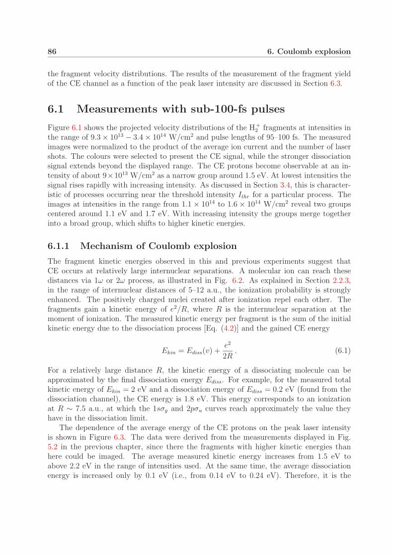
86 6. Coulomb explosion
the fragment velocity distributions. The results of the measurement of the fragment yieldof the CE channel as a function of the peak laser intensity are discussed in Section 6.3.
6.1 Measurements with sub-100-fs pulses
Figure 6.1 shows the projected velocity distributions of the H+2 fragments at intensities in
the range of 9.3 × 10¹³ − 3.4 × 10¹⁴ W/cm2 and pulse lengths of 95–100 fs. The measuredimages were normalized to the product of the average ion current and the number of lasershots. The colours were selected to present the CE signal, while the stronger dissociationsignal extends beyond the displayed range. The CE protons become observable at an in-tensity of about 9×10¹³ W/cm2 as a narrow group around 1.5 eV. At lowest intensities thesignal rises rapidly with increasing intensity. As discussed in Section 3.4, this is character-istic of processes occurring near the threshold intensity Ithr for a particular process. Theimages at intensities in the range from 1.1 × 10¹⁴ to 1.6 × 10¹⁴ W/cm2 reveal two groupscentered around 1.1 eV and 1.7 eV. With increasing intensity the groups merge togetherinto a broad group, which shifts to higher kinetic energies.
6.1.1 Mechanism of Coulomb explosion
The fragment kinetic energies observed in this and previous experiments suggest thatCE occurs at relatively large internuclear separations. A molecular ion can reach thesedistances via 1ω or 2ω process, as illustrated in Fig. 6.2. As explained in Section 2.2.3,in the range of internuclear distances of 5–12 a.u., the ionization probability is stronglyenhanced. The positively charged nuclei created after ionization repel each other. Thefragments gain a kinetic energy of e2/R, where R is the internuclear separation at themoment of ionization. The measured kinetic energy per fragment is the sum of the initialkinetic energy due to the dissociation process [Eq. (4.2)] and the gained CE energy
Ekin = Ediss(v) +e2
2R. (6.1)
For a relatively large distance R, the kinetic energy of a dissociating molecule can beapproximated by the final dissociation energy Ediss. For example, for the measured totalkinetic energy of Ekin = 2 eV and a dissociation energy of Ediss = 0.2 eV (found from thedissociation channel), the CE energy is 1.8 eV. This energy corresponds to an ionizationat R ∼ 7.5 a.u., at which the 1sσg and 2pσu curves reach approximately the value theyhave in the dissociation limit.
The dependence of the average energy of the CE protons on the peak laser intensityis shown in Figure 6.3. The data were derived from the measurements displayed in Fig.5.2 in the previous chapter, since there the fragments with higher kinetic energies thanhere could be imaged. The average measured kinetic energy increases from 1.5 eV toabove 2.2 eV in the range of intensities used. At the same time, the average dissociationenergy is increased only by 0.1 eV (i.e., from 0.14 eV to 0.24 eV). Therefore, it is the
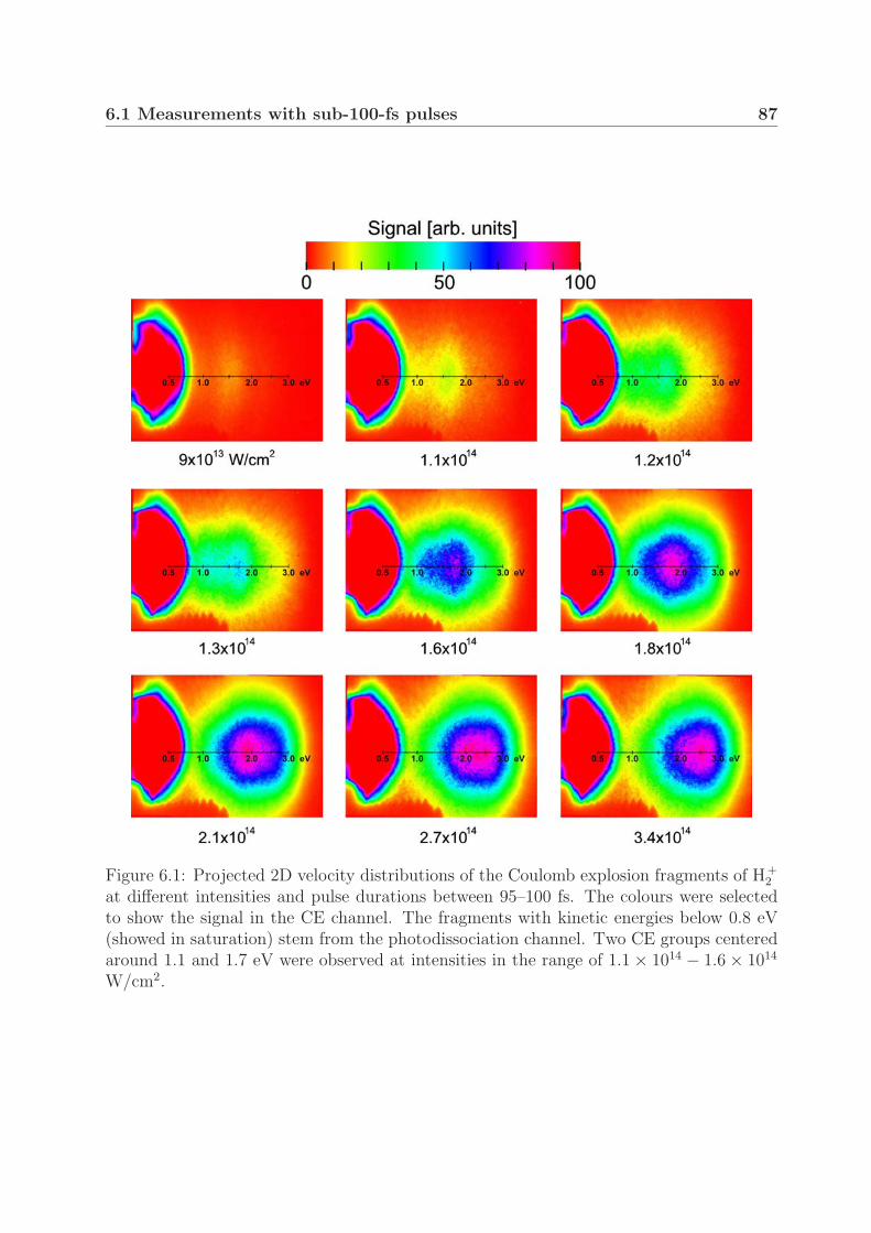
6.1 Measurements with sub-100-fs pulses 87
Figure 6.1: Projected 2D velocity distributions of the Coulomb explosion fragments of H+2
at different intensities and pulse durations between 95–100 fs. The colours were selectedto show the signal in the CE channel. The fragments with kinetic energies below 0.8 eV(showed in saturation) stem from the photodissociation channel. Two CE groups centeredaround 1.1 and 1.7 eV were observed at intensities in the range of 1.1 × 10¹⁴ − 1.6 × 10¹⁴
W/cm2.
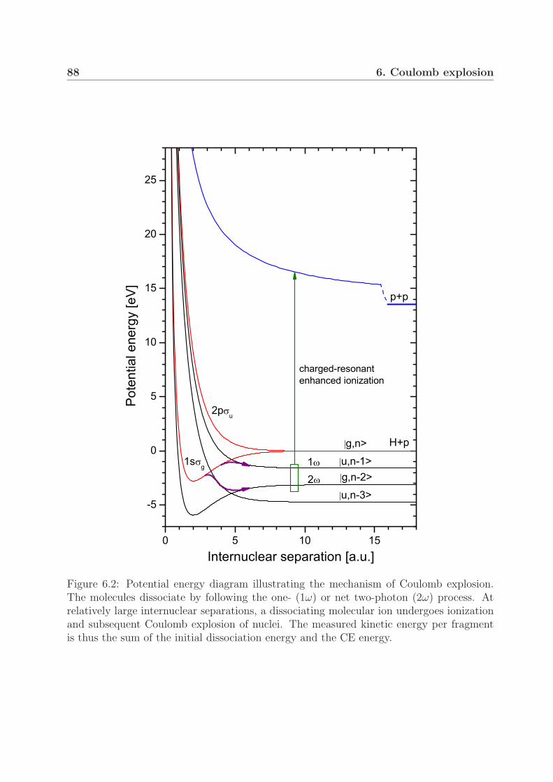
88 6. Coulomb explosion
Figure 6.2: Potential energy diagram illustrating the mechanism of Coulomb explosion.The molecules dissociate by following the one- (1ω) or net two-photon (2ω) process. Atrelatively large internuclear separations, a dissociating molecular ion undergoes ionizationand subsequent Coulomb explosion of nuclei. The measured kinetic energy per fragmentis thus the sum of the initial dissociation energy and the CE energy.
6.1 Measurements with sub-100-fs pulses 89
Figure 6.3: Average kinetic energy of the Coulomb explosion protons as a function of thepeak laser intensity. The data were derived from the kinetic energy spectra obtained byintegrating the inverted velocity distributions in Fig. 5.2 over all angles. The axis on theright side marks the corresponding internuclear separations at which the ionization occurs.
ionization occurring at shorter internuclear separations, rather than the change in theinitial kinetic energy, that is responsible for the higher fragment energies. The reason isthat with increasing peak intensity, the threshold intensity Ithr is reached earlier, i.e., atsmaller internuclear separations. However, this effect is somewhat diminished since Ithr
also increases with decreasing R.
In the interpretation of the images, the spatial intensity distribution must also beconsidered. At intensities near the threshold, the measured signal comes from a narrowintensity range between the threshold intensity and the peak intensity, as illustrated in Fig.6.4. At higher peak intensities, the spectra also include contributions measured at lowerpeak intensities, thus broadening the kinetic energy distributions. At highest intensitiesin Fig. 6.3, a more rapid increase of the average kinetic energy was observed. Roughlyspeaking, the new intensity shells created in the center of the intensity distribution areresponsible for the higher kinetic energies. This can be visualized if the spectra measuredat successive intensities are subtracted from each other, as shown in Fig. 6.5. Obviously,the intensity range from 1.3 × 10¹⁵ to 1.5 × 10¹⁵ W/cm2 is responsible for a narrowerdistribution centered around 2.6 eV, corresponding to an ionization at R ∼ 6 a.u.
The two groups observed in Fig. 6.1 suggest that ionization occurs at two different

90 6. Coulomb explosion
Figure 6.4: Gaussian distributions illustrating one-dimensional spatial intensity distribu-tion for the measurements at highest intensities in Fig. 6.3. The areas under the distri-butions are the same, corresponding to the same pulse energy, whereas their widths aresmaller for higher peak intensities. Only intensities above the threshold intensity Ithr fora particular process contribute to the measured signal.
internuclear separations. An alternative explanation could be that the groups originatefrom different initial kinetic energies of molecules following the 1ω and 2ω dissociationpaths. However, the difference between the average kinetic energies of the fragments inthese processes of less than 0.5 eV is smaller than the one in the two CE groups (see Fig.5.3). Furthermore, since in the dissociation channel the 1ω process is much stronger thanthe 2ω process at intensities below 2× 10¹⁴ W/cm2, basically only one group, rather thanobserved two groups, would be seen in the CE channel.
Angular distributions of the fragments
The alignment of the CE fragments as a function of the laser peak intensity was alreadypresented in Chapter 5 together with the data from the dissociation channel (see Fig.5.4). With the alignment parameter 〈cos2 θ〉 ∼ 0.94, the CE fragments are at all intensitiessignificantly more aligned than the fragments in the dissociation channel. A typical angulardistribution of the CE fragments was shown in Fig. 5.5(i). The data were fitted by aGaussian distribution with a FWHM of 29◦. Angular distributions of similar widths werefound in the experiments starting with H2 [29].
Since the CE fragments result from ionization of dissociating molecules, both the align-ment due to the dissociation process and the angular dependence of the ionization prob-ability will contribute to their angular distributions. A major reason for a higher degreeof alignment of the CE fragments is a strong angular dependence of the ionization prob-ability (geometric alignment). Posthumus et al have shown that the threshold intensity
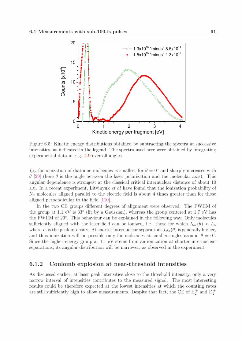
6.1 Measurements with sub-100-fs pulses 91
Figure 6.5: Kinetic energy distributions obtained by subtracting the spectra at successiveintensities, as indicated in the legend. The spectra used here were obtained by integratingexperimental data in Fig. 4.9 over all angles.
Ithr for ionization of diatomic molecules is smallest for θ = 0◦ and sharply increases withθ [29] (here θ is the angle between the laser polarization and the molecular axis). Thisangular dependence is strongest at the classical critical internuclear distance of about 10a.u. In a recent experiment, Litvinyuk et al have found that the ionization probability ofN2 molecules aligned parallel to the electric field is about 4 times greater than for thosealigned perpendicular to the field [110].
In the two CE groups different degrees of alignment were observed. The FWHM ofthe group at 1.1 eV is 33◦ (fit by a Gaussian), whereas the group centered at 1.7 eV hasthe FWHM of 29◦. This behaviour can be explained in the following way. Only moleculessufficiently aligned with the laser field can be ionized, i.e., those for which Ithr(θ) < I0,where I0 is the peak intensity. At shorter internuclear separations Ithr(θ) is generally higher,and thus ionization will be possible only for molecules at smaller angles around θ = 0◦.Since the higher energy group at 1.1 eV stems from an ionization at shorter internuclearseparations, its angular distribution will be narrower, as observed in the experiment.
6.1.2 Coulomb explosion at near-threshold intensities
As discussed earlier, at laser peak intensities close to the threshold intensity, only a verynarrow interval of intensities contributes to the measured signal. The most interestingresults could be therefore expected at the lowest intensities at which the counting ratesare still sufficiently high to allow measurements. Despite that fact, the CE of H+
2 and D+2
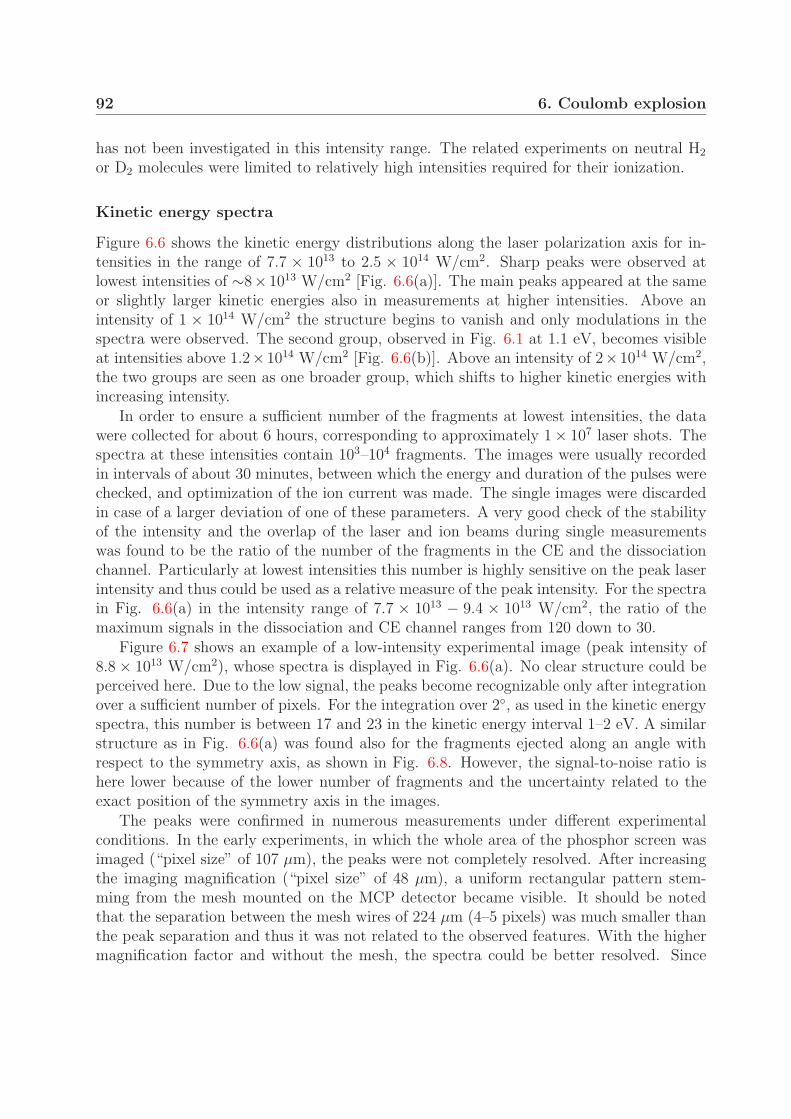
92 6. Coulomb explosion
has not been investigated in this intensity range. The related experiments on neutral H2
or D2 molecules were limited to relatively high intensities required for their ionization.
Kinetic energy spectra
Figure 6.6 shows the kinetic energy distributions along the laser polarization axis for in-tensities in the range of 7.7 × 10¹³ to 2.5 × 10¹⁴ W/cm2. Sharp peaks were observed atlowest intensities of ∼8× 10¹³ W/cm2 [Fig. 6.6(a)]. The main peaks appeared at the sameor slightly larger kinetic energies also in measurements at higher intensities. Above anintensity of 1 × 10¹⁴ W/cm2 the structure begins to vanish and only modulations in thespectra were observed. The second group, observed in Fig. 6.1 at 1.1 eV, becomes visibleat intensities above 1.2×10¹⁴ W/cm2 [Fig. 6.6(b)]. Above an intensity of 2×10¹⁴ W/cm2,the two groups are seen as one broader group, which shifts to higher kinetic energies withincreasing intensity.
In order to ensure a sufficient number of the fragments at lowest intensities, the datawere collected for about 6 hours, corresponding to approximately 1× 10⁷ laser shots. Thespectra at these intensities contain 103–104 fragments. The images were usually recordedin intervals of about 30 minutes, between which the energy and duration of the pulses werechecked, and optimization of the ion current was made. The single images were discardedin case of a larger deviation of one of these parameters. A very good check of the stabilityof the intensity and the overlap of the laser and ion beams during single measurementswas found to be the ratio of the number of the fragments in the CE and the dissociationchannel. Particularly at lowest intensities this number is highly sensitive on the peak laserintensity and thus could be used as a relative measure of the peak intensity. For the spectrain Fig. 6.6(a) in the intensity range of 7.7 × 10¹³ − 9.4 × 10¹³ W/cm2, the ratio of themaximum signals in the dissociation and CE channel ranges from 120 down to 30.
Figure 6.7 shows an example of a low-intensity experimental image (peak intensity of8.8 × 1013 W/cm2), whose spectra is displayed in Fig. 6.6(a). No clear structure could beperceived here. Due to the low signal, the peaks become recognizable only after integrationover a sufficient number of pixels. For the integration over 2◦, as used in the kinetic energyspectra, this number is between 17 and 23 in the kinetic energy interval 1–2 eV. A similarstructure as in Fig. 6.6(a) was found also for the fragments ejected along an angle withrespect to the symmetry axis, as shown in Fig. 6.8. However, the signal-to-noise ratio ishere lower because of the lower number of fragments and the uncertainty related to theexact position of the symmetry axis in the images.
The peaks were confirmed in numerous measurements under different experimentalconditions. In the early experiments, in which the whole area of the phosphor screen wasimaged (“pixel size” of 107 µm), the peaks were not completely resolved. After increasingthe imaging magnification (“pixel size” of 48 µm), a uniform rectangular pattern stem-ming from the mesh mounted on the MCP detector became visible. It should be notedthat the separation between the mesh wires of 224 µm (4–5 pixels) was much smaller thanthe peak separation and thus it was not related to the observed features. With the highermagnification factor and without the mesh, the spectra could be better resolved. Since
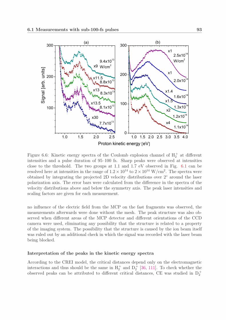
6.1 Measurements with sub-100-fs pulses 93
Figure 6.6: Kinetic energy spectra of the Coulomb explosion channel of H+2 at different
intensities and a pulse duration of 95–100 fs. Sharp peaks were observed at intensitiesclose to the threshold. The two groups at 1.1 and 1.7 eV observed in Fig. 6.1 can beresolved here at intensities in the range of 1.2× 10¹⁴ to 2× 10¹⁴ W/cm2. The spectra wereobtained by integrating the projected 2D velocity distributions over 2◦ around the laserpolarization axis. The error bars were calculated from the difference in the spectra of thevelocity distributions above and below the symmetry axis. The peak laser intensities andscaling factors are given for each measurement.
no influence of the electric field from the MCP on the fast fragments was observed, themeasurements afterwards were done without the mesh. The peak structure was also ob-served when different areas of the MCP detector and different orientations of the CCDcamera were used, eliminating any possibility that the structure is related to a propertyof the imaging system. The possibility that the structure is caused by the ion beam itselfwas ruled out by an additional check in which the signal was recorded with the laser beambeing blocked.
Interpretation of the peaks in the kinetic energy spectra
According to the CREI model, the critical distances depend only on the electromagneticinteractions and thus should be the same in H+
2 and D+2 [36, 111]. To check whether the
observed peaks can be attributed to different critical distances, CE was studied in D+2

94 6. Coulomb explosion
Figure 6.7: Projected 2D velocity distribution of the protons in the Coulomb explosionchannel of H+
2 at an intensity of 8.8 × 10¹³ W/cm2. The integration range for the spectrain Fig. 6.6 is indicated by the lines at an angle of 2◦ with the symmetry axis. The circulararcs mark the position of the main peaks between the kinetic energies of 1.3 and 1.6 eV inFig. 6.6(a).
Figure 6.8: Kinetic energy spectra as in Fig. 6.6(a), but with the integration performedover angles in the range of 2–4◦ both above and below the symmetry axis.
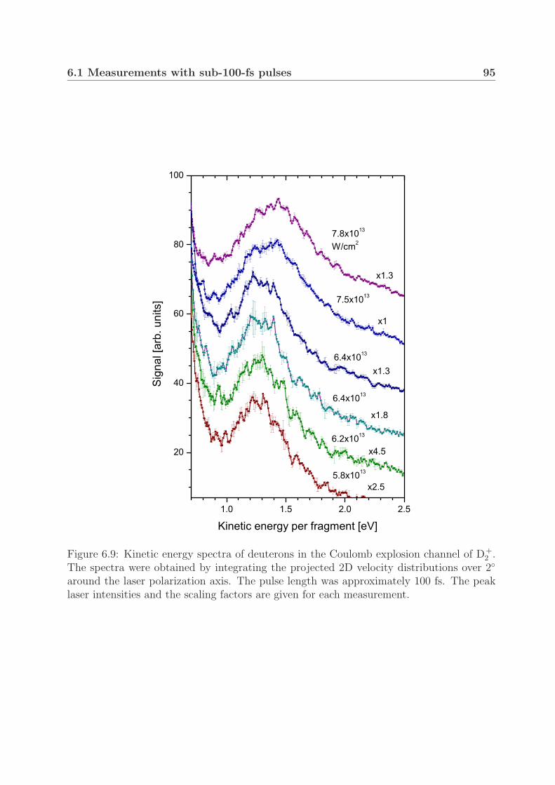
6.1 Measurements with sub-100-fs pulses 95
Figure 6.9: Kinetic energy spectra of deuterons in the Coulomb explosion channel of D+2 .
The spectra were obtained by integrating the projected 2D velocity distributions over 2◦
around the laser polarization axis. The pulse length was approximately 100 fs. The peaklaser intensities and the scaling factors are given for each measurement.
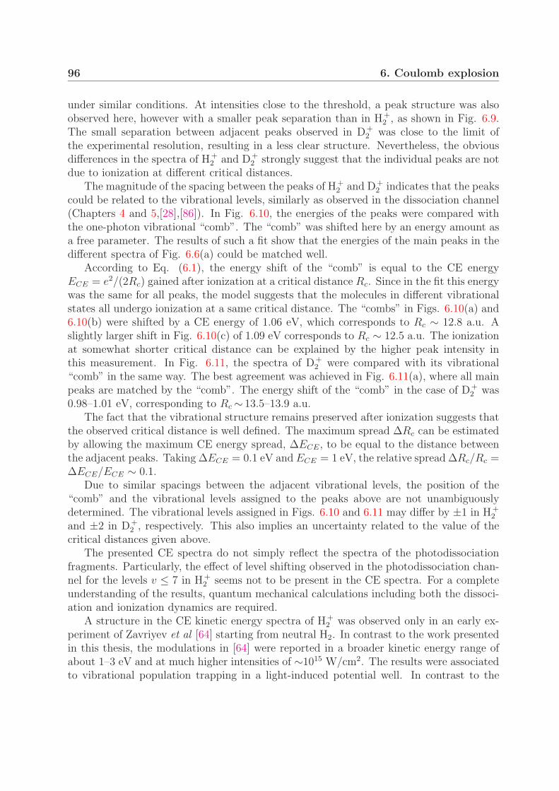
96 6. Coulomb explosion
under similar conditions. At intensities close to the threshold, a peak structure was alsoobserved here, however with a smaller peak separation than in H+
2 , as shown in Fig. 6.9.The small separation between adjacent peaks observed in D+
2 was close to the limit ofthe experimental resolution, resulting in a less clear structure. Nevertheless, the obviousdifferences in the spectra of H+
2 and D+2 strongly suggest that the individual peaks are not
due to ionization at different critical distances.The magnitude of the spacing between the peaks of H+
2 and D+2 indicates that the peaks
could be related to the vibrational levels, similarly as observed in the dissociation channel(Chapters 4 and 5,[28],[86]). In Fig. 6.10, the energies of the peaks were compared withthe one-photon vibrational “comb”. The “comb” was shifted here by an energy amount asa free parameter. The results of such a fit show that the energies of the main peaks in thedifferent spectra of Fig. 6.6(a) could be matched well.
According to Eq. (6.1), the energy shift of the “comb” is equal to the CE energyECE = e2/(2Rc) gained after ionization at a critical distance Rc. Since in the fit this energywas the same for all peaks, the model suggests that the molecules in different vibrationalstates all undergo ionization at a same critical distance. The “combs” in Figs. 6.10(a) and6.10(b) were shifted by a CE energy of 1.06 eV, which corresponds to Rc ∼ 12.8 a.u. Aslightly larger shift in Fig. 6.10(c) of 1.09 eV corresponds to Rc ∼ 12.5 a.u. The ionizationat somewhat shorter critical distance can be explained by the higher peak intensity inthis measurement. In Fig. 6.11, the spectra of D+
2 were compared with its vibrational“comb” in the same way. The best agreement was achieved in Fig. 6.11(a), where all mainpeaks are matched by the “comb”. The energy shift of the “comb” in the case of D+
2 was0.98–1.01 eV, corresponding to Rc ∼ 13.5–13.9 a.u.
The fact that the vibrational structure remains preserved after ionization suggests thatthe observed critical distance is well defined. The maximum spread ∆Rc can be estimatedby allowing the maximum CE energy spread, ∆ECE, to be equal to the distance betweenthe adjacent peaks. Taking ∆ECE = 0.1 eV and ECE = 1 eV, the relative spread ∆Rc/Rc =∆ECE/ECE ∼ 0.1.
Due to similar spacings between the adjacent vibrational levels, the position of the“comb” and the vibrational levels assigned to the peaks above are not unambiguouslydetermined. The vibrational levels assigned in Figs. 6.10 and 6.11 may differ by ±1 in H+
2
and ±2 in D+2 , respectively. This also implies an uncertainty related to the value of the
critical distances given above.The presented CE spectra do not simply reflect the spectra of the photodissociation
fragments. Particularly, the effect of level shifting observed in the photodissociation chan-nel for the levels v ≤ 7 in H+
2 seems not to be present in the CE spectra. For a completeunderstanding of the results, quantum mechanical calculations including both the dissoci-ation and ionization dynamics are required.
A structure in the CE kinetic energy spectra of H+2 was observed only in an early ex-
periment of Zavriyev et al [64] starting from neutral H2. In contrast to the work presentedin this thesis, the modulations in [64] were reported in a broader kinetic energy range ofabout 1–3 eV and at much higher intensities of ∼1015 W/cm2. The results were associatedto vibrational population trapping in a light-induced potential well. In contrast to the
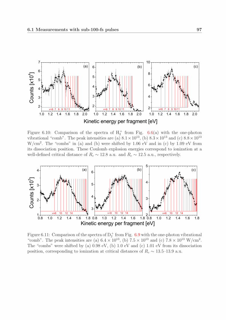
6.1 Measurements with sub-100-fs pulses 97
Figure 6.10: Comparison of the spectra of H+2 from Fig. 6.6(a) with the one-photon
vibrational “comb”. The peak intensities are (a) 8.1×10¹³, (b) 8.3×10¹³ and (c) 8.8×10¹³
W/cm2. The “combs” in (a) and (b) were shifted by 1.06 eV and in (c) by 1.09 eV fromits dissociation position. These Coulomb explosion energies correspond to ionization at awell-defined critical distance of Rc ∼ 12.8 a.u. and Rc ∼ 12.5 a.u., respectively.
Figure 6.11: Comparison of the spectra of D+2 from Fig. 6.9 with the one-photon vibrational
“comb”. The peak intensities are (a) 6.4 × 10¹³, (b) 7.5 × 10¹³ and (c) 7.8 × 10¹³ W/cm2.The “combs” were shifted by (a) 0.98 eV, (b) 1.0 eV and (c) 1.01 eV from its dissociationposition, corresponding to ionization at critical distances of Rc ∼ 13.5–13.9 a.u.

98 6. Coulomb explosion
mechanism of enhanced ionization, later confirmed to be responsible for CE [112], the au-thors proposed that the trapped molecules undergo multiphoton ionization at the differentturning points, giving rise to fragments of different kinetic energies. This interpretationsuffered from several difficulties, one of which is that the population trapping is very un-likely to occur at such high intensities. In the succeeding experiments, no structure in theCE spectra could be observed.
Measurements with elliptically polarized light
An alternative interpretation of the structure observed in the CE spectra could be providedby the role of the ionized electron. From the processes of above-threshold ionization andhigh harmonic generation, it is known that the ionized electron can return to the ioniccore, following the change of the direction of the laser electric field [37]. One can imaginethat the electron could screen the positive charge of a nucleus during the time spent in itsvicinity, thereby weakening the Coulomb repulsion of the fragments. The kinetic energies ofsuch fragments would be shifted to lower values, resulting in maxima at lower and minimaat higher energies than expected. The process could be repeated in the next optical cycles,producing modulations in the spectra.
The return of the electron to a nucleus can be hindered if a small ellipticity is introducedto the laser field. The elliptically polarized field can generally be written as
E(t) = E0 [ex ε cos(ωt) + ez sin(ωt)] , (6.2)
where ε is a parameter characterizing the ellipticity of the electric field. The ellipticitywas introduced to the laser beam by a combination of a zero-order half-wave and a zero-order quarter-wave plate1. First, the optical axis of the λ/2 plate was set to producevertically polarized light. This was done by passing the beam through a properly adjustedGlan polarizer and measuring the power of the reflected beam. After that, the λ/4 platewas placed behind the λ/2 plate and, by maximizing the vertically polarized component,the optical axis of the quarter-wave plate was set parallel to the optical axis of the λ/2plate. An ellipticity was then introduced by rotating the optical axis of the λ/2 plate by asmall angle. The parameter ε was calculated by measuring the power of the vertically andhorizontally polarized components, Pz and Px, respectively:
ε =
√Px
Pz
. (6.3)
Figure 6.12 shows kinetic energy spectrum of the CE protons measured at ε = 0.29.A structure similar to those observed with linearly polarized light can be perceived. Forthe relatively high elipticity used, the return of the electron is not possible, and hence itsimpact on the CE spectra can be excluded. It should be noted that the spectrum measuredhere is distorted, since the laser polarization was not strictly vertical, as required by theimaging method employed.
1Halle
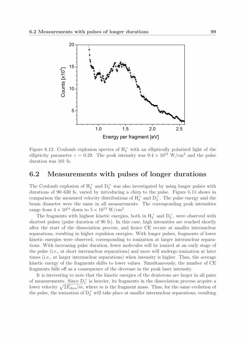
6.2 Measurements with pulses of longer durations 99
Figure 6.12: Coulomb explosion spectra of H+2 with an elliptically polarized light of the
ellipticity parameter ε = 0.29. The peak intensity was 9.4 × 10¹³ W/cm2 and the pulseduration was 101 fs.
6.2 Measurements with pulses of longer durations
The Coulomb explosion of H+2 and D+
2 was also investigated by using longer pulses withdurations of 90–630 fs, varied by introducing a chirp to the pulse. Figure 6.13 shows incomparison the measured velocity distributions of H+
2 and D+2 . The pulse energy and the
beam diameter were the same in all measurements. The corresponding peak intensitiesrange from 4 × 10¹⁴ down to 5 × 10¹³ W/cm2.
The fragments with highest kinetic energies, both in H+2 and D+
2 , were observed withshortest pulses (pulse duration of 90 fs). In this case, high intensities are reached shortlyafter the start of the dissociation process, and hence CE occurs at smaller internuclearseparations, resulting in higher repulsion energies. With longer pulses, fragments of lowerkinetic energies were observed, corresponding to ionization at larger internuclear separa-tions. With increasing pulse duration, fewer molecules will be ionized at an early stage ofthe pulse (i.e., at short internuclear separations) and more will undergo ionization at latertimes (i.e., at larger internuclear separations) when intensity is higher. Thus, the averagekinetic energy of the fragments shifts to lower values. Simultaneously, the number of CEfragments falls off as a consequence of the decrease in the peak laser intensity.
It is interesting to note that the kinetic energies of the deuterons are larger in all pairsof measurements. Since D+
2 is heavier, its fragments in the dissociation process acquire alower velocity
√2Ediss/m, where m is the fragment mass. Thus, for the same evolution of
the pulse, the ionization of D+2 will take place at smaller internuclear separations, resulting
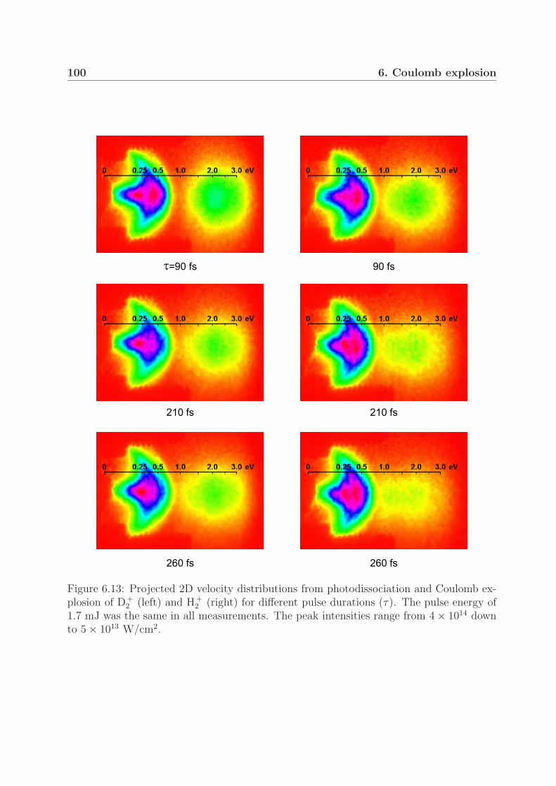
100 6. Coulomb explosion
* ! � � , �
0 � � , �
* � � � , �
* ! � � , �
* � � � , �
- 0 � � , ��
Figure 6.13: Projected 2D velocity distributions from photodissociation and Coulomb ex-plosion of D+
2 (left) and H+2 (right) for different pulse durations (τ). The pulse energy of
1.7 mJ was the same in all measurements. The peak intensities range from 4 × 10¹⁴ downto 5 × 10¹³ W/cm2.
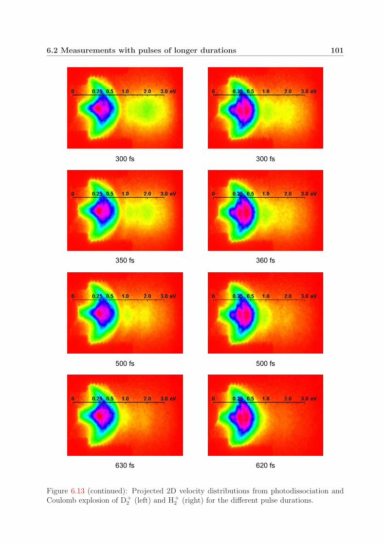
6.2 Measurements with pulses of longer durations 101
! * � � , �
� ! � � , �
� � � � , �
� � � � , �
! � � � , �
� � � � , �
� � � � , �
� � � � , �
Figure 6.13 (continued): Projected 2D velocity distributions from photodissociation andCoulomb explosion of D+
2 (left) and H+2 (right) for the different pulse durations.

102 6. Coulomb explosion
Figure 6.14: Dependence of the average Coulomb explosion energy on the pulse durationfor H+
2 and D+2 (see Fig. 6.13). In the intermediate range of the pulse durations, the ratio
of the durations for D+2 and H+
2 at the same average kinetic energies is approximately 1.4.This is in agreement with the value expected from the ratio of the masses of the molecularions. In the derivation of the average Coulomb explosion energies, the average dissociationenergies were subtracted from the measured average kinetic energies.
in higher kinetic energies. By comparing the images of D+2 and H+
2 in Fig. 6.13 it can beseen that the molecular ions display the same features, which, however, in D+
2 appear atlarger pulse durations. This suggests that the observed features have their origin in thecritical distances, as these are the same for H+
2 and D+2 .
Figure 6.14 shows the dependence of the average CE energies calculated from Fig.6.13 on the pulse duration. Indeed, the ratio of the pulse durations at which the averageCE energy is the same in both molecular ions is approximately 1.4 for intermediate pulsedurations, which is in agreement with the inverse ratio of their velocities. For shorter pulsesthe discrepancy is larger, whereas for large pulse durations the CE fragments overlap withthe fragments from the dissociation channel.
The most interesting observation was made for pulse durations of 350–500 fs in D+2
and ∼300 fs in H+2 . In these measurements, three main CE groups are clearly seen. The
kinetic energy spectrum of the CE deuterons at a pulse duration of 350 fs is shown in Fig.6.15(a). The same signal as a function of the internuclear separation is displayed in Fig.6.15(b). The transformation was made using Eq. (6.1) and 〈Ediss〉 = 0.31 eV, as calculatedfrom the data in the dissociation channel. The main groups centered at 1.2, 1.5 and 2.1eV correspond to critical distances of 15, 11 and 8 a.u., respectively. The two smallest ofthem are close to the critical distances of 7 and 10 a.u. predicted by the CREI model [36].
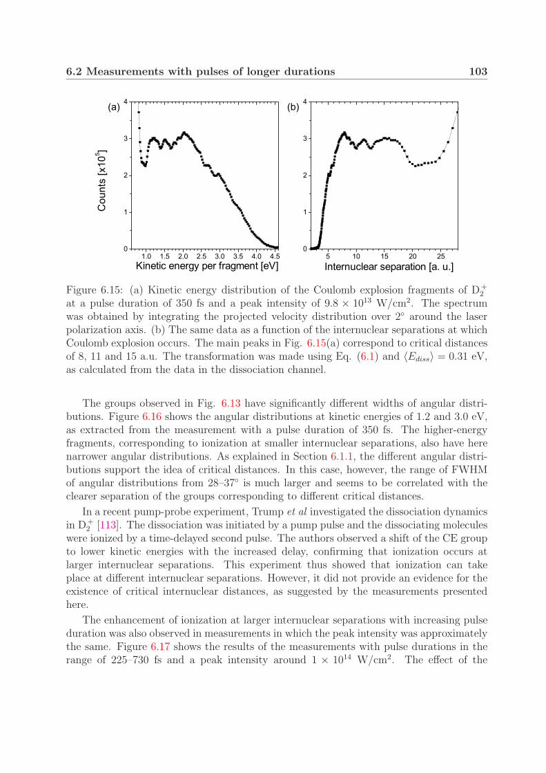
6.2 Measurements with pulses of longer durations 103
Figure 6.15: (a) Kinetic energy distribution of the Coulomb explosion fragments of D+2
at a pulse duration of 350 fs and a peak intensity of 9.8 × 10¹³ W/cm2. The spectrumwas obtained by integrating the projected velocity distribution over 2◦ around the laserpolarization axis. (b) The same data as a function of the internuclear separations at whichCoulomb explosion occurs. The main peaks in Fig. 6.15(a) correspond to critical distancesof 8, 11 and 15 a.u. The transformation was made using Eq. (6.1) and 〈Ediss〉 = 0.31 eV,as calculated from the data in the dissociation channel.
The groups observed in Fig. 6.13 have significantly different widths of angular distri-butions. Figure 6.16 shows the angular distributions at kinetic energies of 1.2 and 3.0 eV,as extracted from the measurement with a pulse duration of 350 fs. The higher-energyfragments, corresponding to ionization at smaller internuclear separations, also have herenarrower angular distributions. As explained in Section 6.1.1, the different angular distri-butions support the idea of critical distances. In this case, however, the range of FWHMof angular distributions from 28–37◦ is much larger and seems to be correlated with theclearer separation of the groups corresponding to different critical distances.
In a recent pump-probe experiment, Trump et al investigated the dissociation dynamicsin D+
2 [113]. The dissociation was initiated by a pump pulse and the dissociating moleculeswere ionized by a time-delayed second pulse. The authors observed a shift of the CE groupto lower kinetic energies with the increased delay, confirming that ionization occurs atlarger internuclear separations. This experiment thus showed that ionization can takeplace at different internuclear separations. However, it did not provide an evidence for theexistence of critical internuclear distances, as suggested by the measurements presentedhere.
The enhancement of ionization at larger internuclear separations with increasing pulseduration was also observed in measurements in which the peak intensity was approximatelythe same. Figure 6.17 shows the results of the measurements with pulse durations in therange of 225–730 fs and a peak intensity around 1 × 10¹⁴ W/cm2. The effect of the
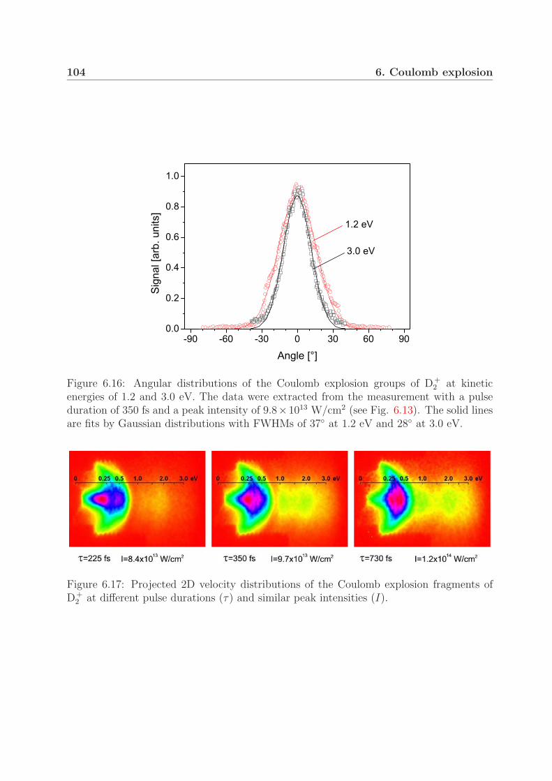
104 6. Coulomb explosion
Figure 6.16: Angular distributions of the Coulomb explosion groups of D+2 at kinetic
energies of 1.2 and 3.0 eV. The data were extracted from the measurement with a pulseduration of 350 fs and a peak intensity of 9.8×10¹³ W/cm2 (see Fig. 6.13). The solid linesare fits by Gaussian distributions with FWHMs of 37◦ at 1.2 eV and 28◦ at 3.0 eV.
Figure 6.17: Projected 2D velocity distributions of the Coulomb explosion fragments ofD+
2 at different pulse durations (τ) and similar peak intensities (I).

6.3 Fragment yield of the Coulomb explosion channel 105
longer pulse lengths on the peak intensities was compensated with smaller laser beamdiameters in the interaction region. The action of longer pulses on molecules is clearlyseen on fragments in the dissociation channel. At the shortest pulse duration, the mostof the molecules dissociate via the high-intensity 1ω and 2ω bond softening mechanisms.With increasing pulse duration more molecules dissociate already at lower intensities onthe rising edge of the pulse. By the time the peak of the pulse is reached, only a smallportion of the molecules will remain undissociated, and consequently the bond softeningpeaks disappear. On the other hand, CE is favoured by the long “time-window” in whichintensity is high. In this case, the large number of molecules arriving at different times canundergo ionization in a broader range of internuclear separations. The increased durationof the laser field will enable ionization at larger internuclear separations, resulting in theCE fragments with lower kinetic energies.
6.3 Fragment yield of the Coulomb explosion channel
The dependence of the total number of counts in the CE channel on the peak laser intensityis displayed in Fig. 6.18. At intensities below 2×10¹⁴ W/cm2, the CE signal exhibits a steeprise with peak intensity. By taking into account the volume expansion and the intensitydependence of the process (Section 5.3), it was found that the data can be described wellby a I3 power dependence. Since the ionization potential is much larger than the photonenergy, the magnitude of n found here is not related to the number of photons absorbed. Forexample, at R = 8 a.u., ionization potential is Ip ∼ 17 eV [Eq. (2.19)], which correspondsto an energy of about 11 photons of λ = 790 nm. This is also expected from the predictionsbased on the value of the Keldysh parameter, which states that ionization should take placein the tunnelling regime (Section 2.2.1).
The fact that the same parameter n is found in the CE and the dissociation process [seeFig. 5.6(b)] suggests that the ionization process follows the dissociation and is possiblylimited by it. At higher peak intensities, the yield of the CE process, similarly as the yieldin the 2ω dissociation process, shows a larger deviation from an I3 power law. However,the comparison with the model for n = 0 suggests that the process has not saturated. Likethe results of the dissociation channel (Section 5.3), the dependence found here is also inagreement with the recent findings in H2 by Gibson et al [109] and contrary to the resultsof the ion beam experiment by Williams et al [43].
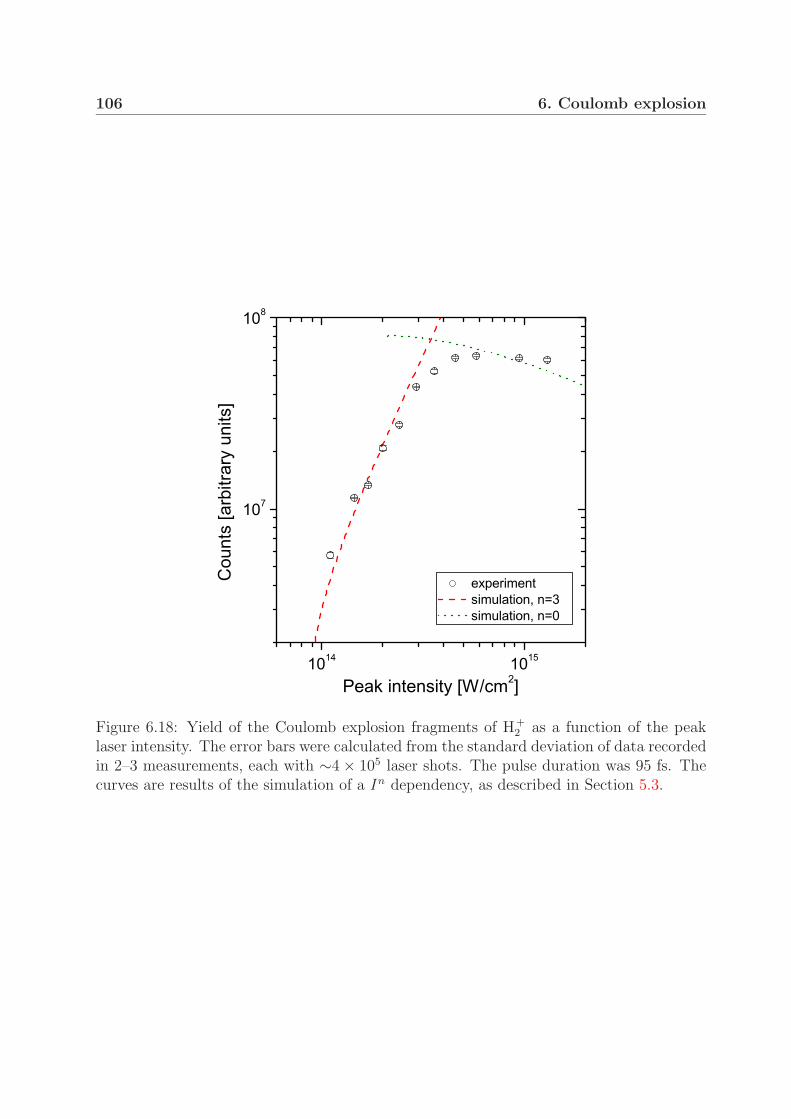
106 6. Coulomb explosion
Figure 6.18: Yield of the Coulomb explosion fragments of H+2 as a function of the peak
laser intensity. The error bars were calculated from the standard deviation of data recordedin 2–3 measurements, each with ∼4 × 10⁵ laser shots. The pulse duration was 95 fs. Thecurves are results of the simulation of a In dependency, as described in Section 5.3.

Chapter 7
Conclusion and perspectives
Photodissociation of D+2 and photodissociation and Coulomb explosion of H+
2 at inten-sities ≥1014 W/cm2 have been investigated for the first time with high resolution. Todate, experiments on H+
2 and D+2 in intense laser fields have been conducted almost exclu-
sively on neutral molecules as targets. The additional ionization process involved not onlycomplicated interpretation of the results, but also hindered investigation of intense-fieldphenomena at lower intensities. Here, fast and collimated beams of H+
2 and D+2 molecular
ions have been used in combination with a photofragment imaging method. The setup pro-vided comparatively small intensity variations in the interaction region and high-resolutionimaging of the three-dimensional velocity distribution of the photofragments.
To elucidate the role of isotope effects in the photodissociation process, D+2 has been
studied under experimental conditions similar to those in the H+2 study of Sandig et al [28]
(Chapter 4). Fragments from the single vibrational levels have been resolved in the velocitydistributions. Their kinetic energy and angular distributions can be interpreted with themodel of light-induced potentials. In comparison with the kinetic energy spectra of H+
2
in [28], here smaller widths of the peaks have been found, suggesting that the measuredwidths reflect the lifetimes of the vibrational states in the perturbed ground electronicstate. Moreover, fragments with near-zero kinetic energies and broad angular distributionshave been observed. They indicate the mechanism of trapping, for which there has hithertobeen little experimental evidence.
In net two-photon photodissociation of H+2 (Chapter 5), the single vibrational level
v = 3 has been identified. With increasing peak intensity, fragments with lower kinetic en-ergies and narrower angular distributions have been observed, which suggests the potentialbarrier-lowering mechanism for the initial three-photon absorption.
The measured velocity distributions of the fragments in the one- and net two-photonphotodissociation processes of D+
2 and H+2 , as well as those of HD+ presented in [46, 114],
provide the basis for theoretical calculations. Simulations based on the three-dimensionaltime-dependent Schrodinger equation, including full nuclear motion and intensity distribu-tion in the interaction region, as done by Serov et al [45], will lead to a better understandingof the photodissociation dynamics of molecules in intense fields.
The main objective of this thesis was to explore the Coulomb explosion channel of
108 7. Conclusion and perspectives
H+2 . The most interesting aspect of this phenomenon is the prediction that ionization is
enhanced at particular critical internuclear distances [34–36]. Up to now, however, suchdistances have not been experimentally observed.
The major contribution of this work consists in presenting the evidence of the existenceof critical internuclear distances of enhanced ionization (Chapter 6). For the first time,a clear structure has been found in kinetic energy distributions of Coulomb explosionprotons. The peaks observed at intensities close to the threshold have been attributedto H+
2 molecules in different vibrational states, ionized at a well-defined critical distanceof about 13 a.u. Furthermore, additional Coulomb explosion velocity-groups have beenobserved at higher intensities and particularly with pulses of longer durations. Theirdifferent kinetic energies and angular distributions strongly suggest ionization at threecritical distances.
The Coulomb explosion data provide a benchmark for theoretical calculations, whichare necessary for a complete understanding of the results. As suggested by the observedstructure, present calculation methods should be extended to incorporate both the dis-sociation and ionization dynamics. In future experiments, it would be interesting to usemolecules prepared in certain vibrational states to unambiguously assign the Coulomb ex-plosion peaks to vibrational quanta. A significant technical improvement leading to clearerspectra would be to use lasers with higher repetition rates, as well as to simultaneouslydetect the fragments from single molecular ions [115].
This work demonstrates that using H+2 in ion beams offers exciting possibilities for
fundamental explorations. As a one-electron system, H+2 is an ideal system for Coulomb
explosion imaging [116, 117]. By ionizing the molecular ion with few-cycle pulses, thevibrational wave function is instantaneously projected onto the Coulomb potential curve.The initial wave function can be reconstructed from the proton kinetic energy distribution.In this way, not only can the molecular structure be directly imaged, but also the temporalevolution of this structure can be followed by employing the pump-probe technique.
Another interesting topic for future research is investigation of the photoelectron ATIspectra of H+
2 . These spectra are produced at critical internuclear distances and recentlythey were theoretically calculated [118]. Moreover, the electron momenta can be imagedin coincidence with the momenta of nuclear fragments [119]. Such a kinematically com-plete experiment, like the one recently carried out on H2 [120], would provide a betterunderstanding of the interplay between nuclear and electronic dynamics for different frag-mentation channels of H+
2 . Furthermore, it would be interesting to investigate diffractionof the electrons from the two nuclei. According to simulations [121], the electron velocitydistribution should exhibit an interference pattern, from which information about the crit-ical internuclear distances could be inferred. Like Coulomb explosion imaging, this methodcould open up the possibility of dynamic imaging of the H+
2 nuclear wave function.
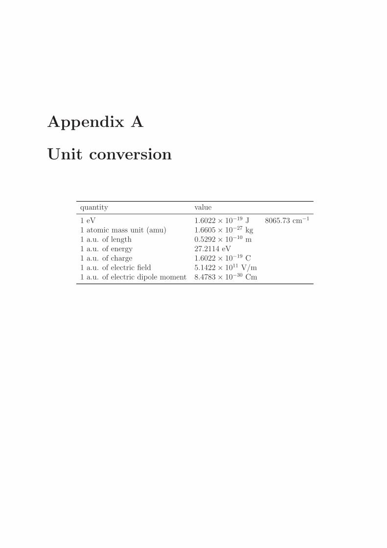
Appendix A
Unit conversion
quantity value
1 eV 1.6022 × 10⁻¹⁹ J 8065.73 cm−1
1 atomic mass unit (amu) 1.6605 × 10⁻²⁷ kg1 a.u. of length 0.5292 × 10⁻¹⁰ m1 a.u. of energy 27.2114 eV1 a.u. of charge 1.6022 × 10⁻¹⁹ C1 a.u. of electric field 5.1422 × 10¹¹ V/m1 a.u. of electric dipole moment 8.4783 × 10⁻³⁰ Cm

110 A. Unit conversion
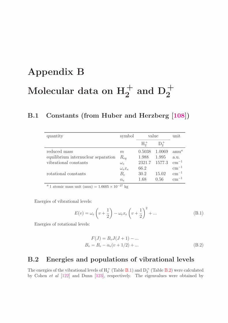
Appendix B
Molecular data on H+2 and D+
2
B.1 Constants (from Huber and Herzberg [108])
quantity symbol value unit
H+2 D+
2
reduced mass m 0.5038 1.0069 amua
equilibrium internuclear separation Req 1.988 1.995 a.u.vibrational constants ωe 2321.7 1577.3 cm−1
ωexe 66.2 cm−1
rotational constants Be 30.2 15.02 cm−1
αe 1.68 0.56 cm−1
a 1 atomic mass unit (amu) = 1.6605 × 10⁻²⁷ kg
Energies of vibrational levels:
E(v) = ωe
(v +
1
2
)− ωexe
(v +
1
2
)2
+ ... (B.1)
Energies of rotational levels:
F (J) = BvJ(J + 1) − ...
Bv = Be − αe(v + 1/2) + ... (B.2)
B.2 Energies and populations of vibrational levels
The energies of the vibrational levels of H+2 (Table B.1) and D+
2 (Table B.2) were calculatedby Cohen et al [122] and Dunn [123], respectively. The eigenvalues were obtained by
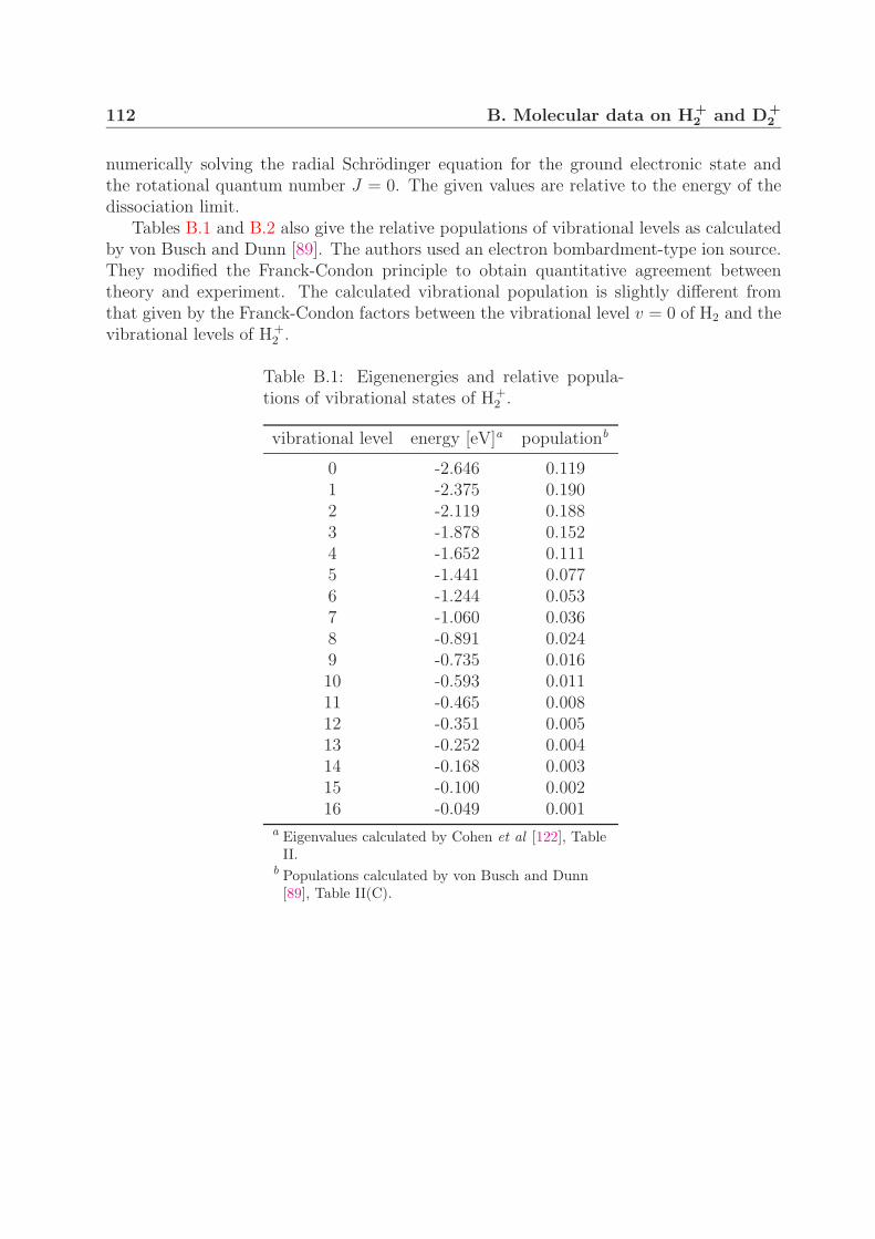
112 B. Molecular data on H+2 and D+
2
numerically solving the radial Schrodinger equation for the ground electronic state andthe rotational quantum number J = 0. The given values are relative to the energy of thedissociation limit.
Tables B.1 and B.2 also give the relative populations of vibrational levels as calculatedby von Busch and Dunn [89]. The authors used an electron bombardment-type ion source.They modified the Franck-Condon principle to obtain quantitative agreement betweentheory and experiment. The calculated vibrational population is slightly different fromthat given by the Franck-Condon factors between the vibrational level v = 0 of H2 and thevibrational levels of H+
2 .
Table B.1: Eigenenergies and relative popula-tions of vibrational states of H+
2 .
vibrational level energy [eV]a populationb
0 -2.646 0.1191 -2.375 0.1902 -2.119 0.1883 -1.878 0.1524 -1.652 0.1115 -1.441 0.0776 -1.244 0.0537 -1.060 0.0368 -0.891 0.0249 -0.735 0.01610 -0.593 0.01111 -0.465 0.00812 -0.351 0.00513 -0.252 0.00414 -0.168 0.00315 -0.100 0.00216 -0.049 0.001
a Eigenvalues calculated by Cohen et al [122], TableII.
b Populations calculated by von Busch and Dunn[89], Table II(C).
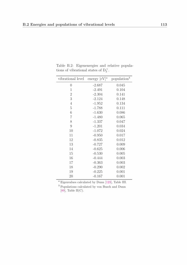
B.2 Energies and populations of vibrational levels 113
Table B.2: Eigenenergies and relative popula-tions of vibrational states of D+
2 .
vibrational level energy [eV]a populationb
0 -2.687 0.0451 -2.491 0.1042 -2.304 0.1413 -2.124 0.1484 -1.952 0.1345 -1.788 0.1116 -1.630 0.0867 -1.480 0.0658 -1.337 0.0479 -1.201 0.03410 -1.072 0.02411 -0.950 0.01712 -0.835 0.01213 -0.727 0.00914 -0.625 0.00615 -0.530 0.00516 -0.444 0.00317 -0.363 0.00318 -0.290 0.00219 -0.225 0.00120 -0.167 0.001
a Eigenvalues calculated by Dunn [123], Table III.b Populations calculated by von Busch and Dunn
[89], Table II(C).

114 B. Molecular data on H+2 and D+
2
List of symbols and acronyms
γ Keldysh parameterε ellipticity of the laser fieldε0 electric permittivity of free spaceθ angle between the molecular internuclear and
the laser polarization axisλ wavelength of the laser fieldν frequency of the laser fieldτ pulse durationω angular frequency of the laser fieldωR Rabi frequency1ω one-photon dissociation2ω net two-photon dissociation2D two-dimensional3D three-dimensionalATI above-threshold ionizationATD above-threshold dissociationB magnetic fieldc speed of light in vacuumCCD charge-coupled deviceCE Coulomb explosionCPA chirped pulse amplificationCREI charge-resonant enhanced ionizationd diameter of the laser beam (FWHM)d transition dipole momente electron chargeE energyE electric fieldE0 amplitude of the electric fieldECE Coulomb explosion energyEdiss dissociation energy
116 List of symbols and acronyms
Ekin kinetic energyEp pulse energyf focal lengthFWHM full width at half maximumh Planck’s constant, aperture width along the
laser polarization axis� reduced Planck’s constant (h/2π)I intensity, peak intensityI0 peak intensityIf peak intensity at the focusIi intensity of an iso-intensity shellIp ionization potentialIthr threshold intensityJ rotational quantum numberl aperture width along the laser propagation
axisL distance between the interaction region and
the MCP detectorm massme electron massmm molecular massMCP multichannel platen number of photons, exponent in In
q ion charger radial coordinate, curvature radius of the sec-
tor magnetR internuclear separationRc critical internuclear distanceReq equilibrium internuclear separationt time between the moment of interaction and
detectionUa acceleration voltageUp ponderomotive potentialv vibrational quantum numberv0 velocity of ions in the ion beamV interaction volume, potentialw laser beam radius (1/e2 half-width)w0 laser beam radius in the focal plane (waist,
1/e2 half-width)x spatial coordinate along the ion beam axisy spatial coordinate along the laser propaga-
tion axisyR Rayleigh rangez spatial coordinate along the laser polariza-
tion axis
Bibliography
[1] A. H. Zewail. Femtochemistry: Atomic-scale dynamics of the chemical bond. J.Phys. Chem. A, 104(24):5660–5694, 2000.
[2] T. Brabec and F. Krausz. Intense few-cycle laser fields: Frontiers of nonlinear optics.Rev. Mod. Phys., 72(2):545–591, 2000.
[3] C. J. Joachain, M. Dorr, and N. Kylstra. High intensity laser-atom physics. Adv. At.Mol. Opt. Phy., 42:225–286, 2000.
[4] N. A. Papadogiannis, B. Witzel, C. Kalpouzos, and D. Charalambidis. Observationof attosecond light localization in higher order harmonic generation. Phys. Rev. Lett.,83(21):4289–4292, 1999.
[5] P. M. Paul, E. S. Toma, P. Breger, G. Mullot, F. Auge, P. Balcou, H. G. Muller,and P. Agostini. Observation of a train of attosecond pulses from high harmonicgeneration. Science, 292(5522):1689–1692, 2001.
[6] M. Hentschel, R. Kienberger, C. Spielmann, G. A. Reider, N. Milosevic, T. Brabec,P. Corkum, U. Heinzmann, M. Drescher, and F. Krausz. Attosecond metrology.Nature, 414(6863):509–513, 2001.
[7] M. Drescher, M. Hentschel, R. Kienberger, M. Uiberacker, V. Yakovlev, A. Scrinizi,T. Westerwalbesloh, U. Kleineberg, U. Heinzmann, and F. Krausz. Time-resolvedatomic inner-shell spectroscopy. Nature, 419(6909):803–807, 2002.
[8] A. Scrinzi, M. Geissler, and T. Brabec. Attosecond cross correlation technique. Phys.Rev. Lett., 86(3):412–415, 2001.
[9] J. Itatani, F. Quere, G. L. Yudin, M. Y. Ivanov, F. Krausz, and P. B. Corkum.Attosecond streak camera. Phys. Rev. Lett., 88(17), 2002.
[10] S. A. Aseyev, Y. Ni, L. J. Frasinski, H. G. Muller, and M. J. J. Vrakking. Attosecondangle-resolved photoelectron spectroscopy. Phys. Rev. Lett., 91(22), 2003.
[11] P. Tzallas, D. Charalambidis, N. A. Papadogiannis, K. Witte, and G. D. Tsakiris.Direct observation of attosecond light bunching. Nature, 426(6964):267–271, 2003.
118 BIBLIOGRAPHY
[12] R. Kienberger, E. Goulielmakis, M. Uiberacker, A. Baltuska, V. Yakovlev, F. Bam-mer, A. Scrinizi, Th. Westerwalbesloh, U. Kleineberg, U. Heinzmann, M. Drescher,and F. Krausz. Atomic transient recorder. Nature, 427:817–821, 2004.
[13] G. G. Paulus, F. Grasbon, H. Walther, P. Villoresi, M. Nisoli, S. Stagira, E. Priori,and S. De Silvestri. Absolute-phase phenomena in photoionization with few-cyclelaser pulses. Nature, 414(6860):182–184, 2001.
[14] A. Baltuska, T. Udem, M. Uiberacker, M. Hentschel, E. Goulielmakis, C. Gohle,R. Holzwarth, V. S. Yakoviev, A. Scrinzi, T. W. Hansch, and F. Krausz. Attosecondcontrol of electronic processes by intense light fields. Nature, 421(6923):611–615,2003.
[15] G. G. Paulus, F. Lindner, H. Walther, A. Baltuska, E. Goulielmakis, M. Lezius, andF. Krausz. Measurement of the phase of few-cycle laser pulses. Phys. Rev. Lett., 91(25), 2003.
[16] J. Seres, A. Muller, E. Seres, K. O’Keeffe, M. Lenner, R. F. Herzog, D. Kaplan,C. Spielmann, and F. Krausz. Sub-10-fs, terawatt-scale Ti:sapphire laser system.Opt. Lett., 28(19):1832–1834, 2003.
[17] D. Batani, C. J. Joachain, S. Martellucci, and A. N. Chester, editors. Atoms, Solidsand Plasmas in Super-Intense Laser-Fields. Kluwer Academic/Plenum Publishers,New York, 2001.
[18] J. H. Posthumus and J. F. McCann. Molecules and Clusters in Intense Laser Fields.Cambridge University Press, Cambridge, 2001.
[19] P. Agostini, F. Fabre, G. Mainfray, G. Petite, and N. K. Rahman. Free-free tran-sitions following six-photon ionization of xenon atoms. Phys. Rev. Lett., 42(17):1127–1130, 1979.
[20] D. N. Fittinghoff, P. R. Bolton, B. Chang, and K. C. Kulander. Observation ofnonsequential double ionization of helium with optical tunneling. Phys. Rev. Lett.,69(18):2642–2645, 1992.
[21] T. Weber, H. Giessen, M. Weckenbrock, G. Urbasch, A. Staudte, L. Spielberger,O. Jagutzki, V. Mergel, M. Vollmar, and R. Dorner. Correlated electron emission inmultiphoton double ionization. Nature, 405(6787):658–661, 2000.
[22] A. McPherson, G. Gibson, H. Jara, U. Johann, T. S. Luk, I. A. McIntyre, K. Boyer,and C. K. Rhodes. Studies of multiphoton production of vacuum-ultraviolet radiationin the rare gases. J. Opt. Soc. Am. B: Opt. Phys., 4(4):595–601, 1987.
[23] M. Ferray, A. L’Huillier, X. F. Li, L. A. Lompre, G. Mainfray, and C. Manus.Multiple-harmonic conversion of 1064 nm radiation in rare gases. J. Phys. B: At.Mol. Opt. Phys., 21(3):L31–L35, 1988.
BIBLIOGRAPHY 119
[24] P. H. Bucksbaum, A. Zavriyev, H. G. Muller, and D. W. Schumacher. Softening ofthe H+
2 molecular bond in intense laser fields. Phys. Rev. Lett., 64(16):1883–1886,1990.
[25] A. Giusti-Suzor, X. He, O. Atabek, and F. H. Mies. Above-threshold dissociation ofH+
2 in intense laser fields. Phys. Rev. Lett., 64(5):515–518, 1990.
[26] A. Giusti-Suzor, F. H. Mies, L. F. DiMauro, E. Charron, and B. Yang. Dynamics ofH+
2 in intense laser fields. J. Phys. B: At. Mol. Opt. Phys., 28(3):309–339, 1995.
[27] L. J. Frasinski, J. H. Posthumus, J. Plumridge, K. Codling, P. F. Taday, and A. J.Langley. Manipulation of bond hardening in H+
2 by chirping of intense femtosecondlaser pulses. Phys. Rev. Lett., 83(18):3625–3628, 1999.
[28] K. Sandig, H. Figger, and T. W. Hansch. Dissociation dynamics of H+2 in intense
laser fields: Investigation of photofragments from single vibrational levels. Phys. Rev.Lett., 85(23):4876–4879, 2000.
[29] J. H. Posthumus, J. Plumridge, M. K. Thomas, K. Codling, L. J. Frasinski, A. J. Lan-gley, and P. F. Taday. Dynamic and geometric laser-induced alignment of moleculesin intense laser fields. J. Phys. B: At. Mol. Opt. Phys., 31(13):L553–L562, 1998.
[30] R. Numico, A. Keller, and O. Atabek. Intense-laser-induced alignment in angularlyresolved photofragment distributions of H+
2 . Phys. Rev. A, 60(1):406–413, 1999.
[31] F. Rosca-Pruna, E. Springate, H. L. Offerhaus, M. Krishnamurthy, N. Farid,C. Nicole, and M. J. J. Vrakking. Spatial alignment of diatomic molecules in in-tense laser fields: I. Experimental results. J. Phys. B: At. Mol. Opt. Phys., 34(23):4919–4938, 2001.
[32] H. Stapelfeldt and T. Seideman. Colloquium: Aligning molecules with strong laserpulses. Rev. Mod. Phys., 75(2):543–557, 2003.
[33] M. Schmidt, D. Normand, and C. Cornaggia. Laser-induced trapping of chlorinemolecules with picosecond and femtosecond pulses. Phys. Rev. A, 50(6):5037–5045,1994.
[34] T. Seideman, M. Y. Ivanov, and P. B. Corkum. Role of electron localization inintense-field molecular ionization. Phys. Rev. Lett., 75(15):2819–2822, 1995.
[35] J. H. Posthumus, L. J. Frasinski, A. J. Giles, and K. Codling. Dissociative ionizationof molecules in intense laser fields: a method of predicting ion kinetic energies andappearance intensities. J. Phys. B: At. Mol. Opt. Phys., 28(10):L349–L353, 1995.
[36] T. Zuo and A. D. Bandrauk. Charge-resonance-enhanced ionization of diatomicmolecular-ions by intense lasers. Phys. Rev. A, 52(4):R2511–R2514, 1995.

120 BIBLIOGRAPHY
[37] P. B. Corkum. Plasma perspective on strong-field multiphoton ionization. Phys. Rev.Lett., 71(13):1994–1997, 1993.
[38] H. Niikura, F. Legare, R. Hasbani, A. D. Bandrauk, M. Y. Ivanov, D. M. Villeneuve,and P. B. Corkum. Sub-laser-cycle electron pulses for probing molecular dynamics.Nature, 417(6892):917–922, 2002.
[39] C. Trump, H. Rottke, and W. Sandner. Strong-field photoionization of vibrationalground-state H+
2 and D+2 molecules. Phys. Rev. A, 60(5):3924–3928, 1999.
[40] A. Staudte, C. L. Cocke, A. H. Prior, A. Belkacem, C. Ray, H. W. Chong, T. E.Glover, R. W. Schoenlein, and U. Saalmann. Observation of a nearly isotropic, high-energy Coulomb explosion group in the fragmentation of D2 by short laser pulses.Phys. Rev. A, 65(2):020703, 2002.
[41] H. Niikura, F. Legare, R. Hasbani, M. Y. Ivanov, D. M. Villeneuve, and P. B.Corkum. Probing molecular dynamics with attosecond resolution using correlatedwave packet pairs. Nature, 421(6925):826–829, 2003.
[42] J. H. Posthumus and J. F. McCann. Diatomic molecules in intense laser fields. InJ. H. Posthumus, editor, Molecules and Clusters in Intense Laser Fields, pages 27–83.Cambridge University Press, Cambridge, 2001.
[43] I. D. Williams, P. McKenna, B. Srigengan, I. M. G. Johnston, W. A. Bryan, J. H.Sanderson, A. El-Zein, T. R. J. Goodworth, W. R. Newell, P. F. Taday, and A. J.Langley. Fast-beam study of H+
2 ions in an intense femtosecond laser field. J. Phys.B: At. Mol. Opt. Phys., 33(14):2743–2752, 2000.
[44] A. Kondorskiy and H. Nakamura. Photodissociation of H+2 and HD+ in an intense
laser field. Phys. Rev. A, 66(5):053412, 2002.
[45] V. N. Serov, A. Keller, O. Atabek, and N. Billy. Quantitative theory-versus-experiment comparison for the intense laser dissociation of H+
2 . Phys. Rev. A, 68(5):053401, 2003.
[46] A. Kiess. Elementare Molekule in intensiven ultrakurzen Laserlichtpulsen - Exper-imentale Untersuchung an HD+. Diploma thesis, Ludwig-Maximilians-UniversitatMunchen, 2003.
[47] A. D. Bandrauk, editor. Molecules in Laser Fields. Marcel Dekker, Inc., New York,1994.
[48] L. D. Landau and E. M. Lifshits. Quantum Mechanics: Non-Relativistic Theory.Pergamon Press, Oxford; New York, 1977.
[49] M. H. Mittleman. Introduction to the Theory of Laser-Atom Interactions. PlenumPress, New York, 1993.
BIBLIOGRAPHY 121
[50] D. R. Bates. The oscillator strength of H+2 , 1sσ − 2pσ. J. Chem. Phys., 19(9):
1122–1124, 1951.
[51] C. Cohen-Tannoudji, J. Dupont-Roc, and G. Grynberg. Atom-Photon Interactions:Basic Processes and Applications. Wiley, New York, 1992.
[52] N. M. Kroll and K. M. Watson. Inelastic atom-atom scattering within an intenselaser beam. Phys. Rev. A, 13(3):1018–1033, 1976.
[53] A. M. F. Lau. Radiative-dressed molecules: Ab initio theory and single/multiphotondissociation with electronic transitions. Phys. Rev. A, 16(4):1535–1542, 1977.
[54] A. D. Bandrauk and M. L. Sink. Photodissociation in intense laser fields: Predisso-ciation analogy. J. Chem. Phys., 74(2):1110–1117, 1981.
[55] S. I. Chu. Floquet theory and complex quasivibrational energy formalism for intensefield molecular photodissociation. J. Chem. Phys., 75(5):2215–2221, 1981.
[56] J. H. Shirley. Solution of the Schrodinger equation with a Hamiltonian periodic intime. Phys. Rev., 138(4B):B979–B987, 1965.
[57] F. Rebentrost. Private communication.
[58] T. E. Sharp. Potential-energy curves for molecular hydrogen and its ions. AtomicData, 2:119–169, 1971.
[59] C. Wunderlich. Licht-induzierte molekulare Struktur. PhD thesis, Ludwig-Maximilians-Universitat Munchen, 1995.
[60] R. S. Mulliken. Intensities of electronic transitions in molecular spectra. II. charge-transfer spectra. J. Chem. Phys., 7:20–34, 1939.
[61] E. E. Aubanel, J. M. Gauthier, and A. D. Bandrauk. Molecular stabilization andangular distribution in photodissociation of H+
2 in intense laser fields. Phys. Rev. A,48(3):2145–2152, 1993.
[62] A. Giusti-Suzor and F. H. Mies. Vibrational trapping and suppression of dissociationin intense laser fields. Phys. Rev. Lett., 68(26):3869–3872, 1992.
[63] G. H. Yao and S. I. Chu. Laser-induced molecular stabilization and trapping andchemical bond hardening in intense laser fields. Chem. Phys. Lett., 197(4-5):413–418,1992.
[64] A. Zavriyev, P. H. Bucksbaum, J. Squier, and F. Saline. Light-induced vibrationalstructure in H+
2 and D+2 in intense laser fields. Phys. Rev. Lett., 70(8):1077–1080,
1993.
122 BIBLIOGRAPHY
[65] A. Zavriyev, P. H. Bucksbaum, H. G. Muller, and D. W. Schumacher. Ionization anddissociation of H2 in intense laser fields at 1.064 µm, 532 nm, and 355 nm. Phys.Rev. A, 42(9):5500–5513, 1990.
[66] G. Jolicard and O. Atabek. Above-threshold-dissociation dynamics of H+2 with short
intense laser pulses. Phys. Rev. A, 46(9):5845–5855, 1992.
[67] R. Numico, A. Keller, and O. Atabek. Laser-induced molecular alignment in disso-ciation dynamics. Phys. Rev. A, 52(2):1298–1309, 1995.
[68] L. V. Keldysh. Ionization in the field of a strong electromagnetic wave. Sov. Phys.-JETP, 20:1018, 1965.
[69] D. Bauer and P. Mulser. Exact held ionization rates in the barrier-suppression regimefrom numerical time-dependent Schrodinger-equation calculations. Phys. Rev. A, 59(1):569–577, 1999.
[70] T. Zuo and A. D. Bandrauk. Harmonic generation by the H+2 molecular ion in intense
laser fields. Phys. Rev. A, 48(5):3837–3844, 1993.
[71] H. T. Yu, T. Zuo, and A. D. Bandrauk. Intense field ionization of molecules withultra-short laser pulses—enhanced ionization and barrier-suppression effects. J. Phys.B: At. Mol. Opt. Phys., 31(7):1533–1551, 1998.
[72] S. Chelkowski, T. Zuo, O. Atabek, and A. D. Bandrauk. Dissociation, ionization,and Coulomb explosion of H+
2 in an intense laser field by numerical integration ofthe time-dependent Schrodinger equation. Phys. Rev. A, 52(4):2977–2983, 1995.
[73] M. Plummer and J. F. McCann. Field-ionization rates of the hydrogen molecularion. J. Phys. B: At. Mol. Opt. Phys., 29(20):4625–4640, 1996.
[74] L. B. Madsen, M. Plummer, and J. F. McCann. Multiphoton ionization of H+2 by
intense light: A comparison of Floquet and wave-packet results. Phys. Rev. A, 58(1):456–465, 1998.
[75] D. Dundas. Efficient grid treatment of the ionization dynamics of laser-driven H+2 .
Phys. Rev. A, 65(2), 2002.
[76] S. Chelkowski, A. Conjusteau, T. Zuo, and A. D. Bandrauk. Dissociative ionizationof H+
2 in an intense laser field: Charge-resonance-enhanced ionization, Coulombexplosion, and harmonic generation at 600 nm. Phys. Rev. A, 54(4):3235–3244,1996.
[77] S. Chelkowski, C. Foisy, and A. D. Bandrauk. Electron-nuclear dynamics of multipho-ton H+
2 dissociative ionization in intense laser fields. Phys. Rev. A, 57(2):1176–1185,1998.
BIBLIOGRAPHY 123
[78] T. D. G. Walsh, F. A. Ilkov, S. L. Chin, F. Chateauneuf, T. T. Nguyen-Dang,S. Chelkowski, A. D. Bandrauk, and O. Atabek. Laser-induced processes during theCoulomb explosion of H2 in a Ti-sapphire laser pulse. Phys. Rev. A, 58(5):3922–3933,1998.
[79] B. Feuerstein and U. Thumm. Fragmentation of H+2 in strong 800-nm laser pulses:
Initial-vibrational-state dependence. Phys. Rev. A, 67(4), 2003.
[80] W. Ketterle. Spektroskopie an Heliumhydrid und am dreiatomigen Wasserstoff-molekul. PhD thesis, Ludwig-Maximilians-Universitat Munchen, 1986.
[81] C. Wunderlich, V. Betz, R. Bruckmeier, and H. Figger. Lifetime measurements onArH and ArD. J. Chem. Phys., 98(12):9362–9371, 1993.
[82] R. Bruckmeier, C. Wunderlich, and H. Figger. New experimental insight into theground state potential surface of triatomic hydrogen. Phys. Rev. Lett., 72(16):2550–2553, 1994.
[83] C. Wunderlich, H. Figger, and T. W. Hansch. Ar+2 molecules in intense laser fields.
Chem. Phys. Lett., 256(1-2):43–50, 1996.
[84] C. Wunderlich, E. Kobler, H. Figger, and T. W. Hansch. Light-induced molecularpotentials. Phys. Rev. Lett., 78(12):2333–2336, 1997.
[85] C. Wunderlich, H. Figger, and T. W. Hansch. Tunneling through light-inducedmolecular potentials in Ar+
2 . Phys. Rev. A, 62(2):023401, 2000.
[86] K. Sandig. H+2 in intensiven Lichtfeldern. PhD thesis, Ludwig-Maximilians-
Universitat Munchen, 2000.
[87] H. Liebl and W.W. Harrison. Study of an iodine discharge in a duoplasmatron (ionsource). Int. J. Mass spectrom., 22(3-4):237–246, 1976.
[88] H. Zhang. Ion Sources. Science Press, Beijing, 1999.
[89] F. von Busch and G. H. Dunn. Photodissociation of H+2 and D+
2 : Experiment. Phys.Rev. A, 5(4):1726–1743, 1972.
[90] W. Koot, W. J. van der Zande, and D. P. de Bruijn. Rotational distribution of H+2
ions produced by 90 eV electron impact. Chem. Phys., 115(2):297–305, 1987.
[91] H. Helm and P. C. Cosby. Photodissociation measurement of rovibrational energiesand populations of molecules in fast beams. J. Chem. Phys., 86(12):6813–6822, 1987.
[92] N.P.F.B. van Asselt, J. G. Maas, and J. Los. Laser induced photodissociation of H+2
and D+2 ions. Chem. Phys., 5(3):429–438, 1974.
124 BIBLIOGRAPHY
[93] J. I. Steinfeld. Molecules and Radiation: An Introduction to Modern Molecular Spec-troscopy. MIT Press, Cambridge, Mass., 2. edition edition, 1985.
[94] R. N. Bracewell. The Fourier Transform and Its Applications. McGraw Hill, Boston,2000.
[95] L. M. Smith and D. R. Keefer. Abel inversion using transform techniques. J. Quant.Spectrosc. Radiat. Transf., 39(5):367–373, 1988.
[96] K. van Niekerk and A. Eppink. Abelflex512, 1996.
[97] V. Dribinski, A. Ossadtchi, V. A. Mandelshtam, and H. Reisler. Reconstructionof Abel-transformable images: The Gaussian basis-set expansion Abel transformmethod. Rev. Sci. Instrum., 73(7):2634–2642, 2002.
[98] M. J. J. Vrakking. An iterative procedure for the inversion of two-dimensionalion/photoelectron imaging experiments. Rev. Sci. Instrum., 72(11):4084–4089, 2001.
[99] A. G. Suits and R. E. Continetti. Imaging in Chemical Dynamics. American ChemicalSociety, Washington, D.C., 2001.
[100] M. von Ardenne. Elektronenphysik, Ubermikroskopie, Ionenphysik. Deutscher Verlagder Wissenschaften, Berlin, 1962.
[101] D. E. Spence, P. N. Kean, and W. Sibbett. 60-fsec pulse generation from a self-mode-locked Ti:sapphire laser. Opt. Lett., 16(1):42–44, 1991.
[102] D. Strickland and G. Mourou. Compression of amplified chirped optical pulses. Opt.Commun., 56(3):219–221, 1985.
[103] J. C. Diels and W. Rudolph. Ultrashort Laser Pulse Phenomena: Fundamentals,Techniques, and Applications on a Femtosecond Time Scale. Academic Press, SanDiego, 1996.
[104] A. E. Siegman, M. W. Sasnett, and T. F. Johnston. Choice of clip levels for beamwidth measurements using knife-edge techniques. IEEE J. Quantum Electron., 27(4):1098–1104, 1991.
[105] W. T. Silfvast. Laser Fundamentals. Cambridge University Press, New York, 1996.
[106] A. E. Siegman. Lasers. University Science Books, Mill Valley, California, 1986.
[107] V. Serov. Photodissociation dynamics in laser fields: Quantitative interpretationof experimental data on NO2 and H+
2 . PhD thesis, Universite Paris XI, U.F.R.Scientifique d’Orsay and St. Petersburg State University, 2003.
[108] K.P. Huber and G. Herzberg. Constants of Diatomic Molecules, volume Vol.4. VanNostrand Reinhold, New York, 1979.
BIBLIOGRAPHY 125
[109] G. N. Gibson, M. Li, C. Guo, and J. Neira. Strong-field dissociation and ionizationof H+
2 using ultrashort laser pulses. Phys. Rev. Lett., 79(11):2022–2025, 1997.
[110] I. V. Litvinyuk, K. F. Lee, P. W. Dooley, D. M. Rayner, D. M. Villeneuve, and P. B.Corkum. Alignment-dependent strong field ionization of molecules. Phys. Rev. Lett.,90(23), 2003.
[111] S. Chelkowski. Private communication, 2001.
[112] E. Constant, H. Stapelfeldt, and P. B. Corkum. Observation of enhanced ionizationof molecular ions in intense laser fields. Phys. Rev. Lett., 76(22):4140–4143, 1996.
[113] C. Trump, H. Rottke, and W. Sandner. Multiphoton ionization of dissociating D+2
molecules. Phys. Rev. A, 59(4):2858–2863, 1999.
[114] A. Kiess, D. Pavicic, T. W. Hansch, and H. Figger. Manuscript in preparation.
[115] H. Hasegawa, A. Hishikawa, and K. Yamanouchi. Coincidence imaging of Coulombexplosion of CS2 in intense laser fields. Chem. Phys. Lett., 349(1-2):57–63, 2001.
[116] H. Stapelfeldt, E. Constant, and P. B. Corkum. Wave packet structure and dynamicsmeasured by Coulomb explosion. Phys. Rev. Lett., 74(19):3780–3783, 1995.
[117] S. Chelkowski, P. B. Corkum, and A. D. Bandrauk. Femtosecond Coulomb explosionimaging of vibrational wave functions. Phys. Rev. Lett., 82(17):3416–3419, 1999.
[118] A. D. Bandrauk, S. Chelkowski, and I. Kawata. Molecular above-threshold-ionizationspectra: The effect of moving nuclei. Phys. Rev. A, 67(1):013407, 2003.
[119] J. Ullrich, R. Moshammer, R. Dorner, O. Jagutzki, V. Mergel, H. Schmidt-Bocking,and L. Spielberger. Recoil-ion momentum spectroscopy. J. Phys. B: At. Mol. Opt.Phys., 30(13):2917–2974, 1997.
[120] H. Rottke, C. Trump, M. Wittmann, G. Korn, W. Sandner, R. Moshammer, A. Dorn,C. D. Schroter, D. Fischer, J. R. C. Lopez-Urrutia, P. Neumayer, J. Deipenwisch,C. Hohr, B. Feuerstein, and J. Ullrich. Coincident fragment detection in strong fieldphotoionization and dissociation of H2. Phys. Rev. Lett., 89(1):013001, 2002.
[121] T. Zuo, A. D. Bandrauk, and P. B. Corkum. Laser-induced electron diffraction: anew tool for probing ultrafast molecular dynamics. Chem. Phys. Lett., 259(3-4):313–320, 1996.
[122] S. Cohen, J. R. Hiskes, and R. J. Riddell. Vibrational states of the hydrogen molecularion. Phys. Rev., 119(3):1025–1027, 1960.
[123] G. H. Dunn. Franck-Condon factors for ionization of H2 and D2. J. Chem. Phys., 44(7):2592–2594, 1966.

126 BIBLIOGRAPHY
Acknowledgments
This research was conducted at Max Planck Institute of Quantum Optics in Garching. Iwould like to thank all those who have helped me to complete this work in every possibleway.
First of all, I want to express my gratitude to Prof. Dr. Theodor W. Hansch for affordingme the opportunity of pursuing my Ph.D. thesis in his group. I am indebted to him forgenerously providing funds for this work and for giving me the chance to present my resultsat various conferences. His ingenuity, enthusiasm and extreme kindness will always be inmy memory. I am truly honoured that I could work in his outstanding group.
I am grateful to my advisor, Dr. Hartmut Figger, for inviting me to work on this interestingproject. I thank him for his invaluable support, continuous encouragement and everlastingoptimism. His friendly suggestions were helpful in many ways during my stay in Germany.I appreciate his ideas and criticism, from which I have learned a lot. His reviews andsuggestions for improving the manuscript of this thesis are gratefully acknowledged.
I am deeply indebted to my predecessor, Dr. Karsten Sandig, for introducing me to theexperimental setup and for being very helpful at the beginning of my work. Karsten hastaught me a lot about the femtosecond system and the ion beam apparatus, without whichit would be difficult to imagine the ensuing work. I thank him for his kindness and foranswering my many questions, also after he had left our group.
I thank Andreas Kiess for his friendly help and assistance in the experiments, numeroustechnical improvements and many helpful comments and discussions. It was gratifying tolearn from him and have the chance to explain to him what I know. Most of all, I thankhim for the pleasant time I had working with him.
I am deeply indebted to Wolfgang Simon and Karl Linner for their skilful technical as-sistance and their willingness to help me in every situation. They always understood myneeds and gave their best to find excellent solutions in the shortest time, which oftenseemed impossible. My gratitude also goes to Helmut Bruckner for his help concerningelectronics, for the devices he lent me and for a great deal of advice. I thank them forgreatly improving the experiment and safety in the lab.
A special word of thanks goes to Dr. Frank Rebentrost, who performed many invaluablecalculations for me. I wish to thank him for his numerous explanations and illuminatingdiscussions.
I thank Dr. Osman Atabek and Dr. Vassili Serov from CNRS, Orsay for very good
128 Acknowledgments
cooperation. Their calculations, insightful explanations and fruitful discussions were mostbeneficial.
I am deeply indebted to Dr. Marc Vrakking for providing me with his inversion algorithmand helping me with its implementation. Thanks also go to Prof. Dr. Peter Rakitzis andDr. Vladimir Dribinski for offering me their inversion programs and support.
I am grateful to Prof. Dr. Gerhard G. Paulus for his kind explanations, suggestions andfor lending me some optical elements.
I am indebted to Hans-Jurgen Hechler and Friedrich Staudt from Spectra Physics for theirtechnical support, help and advice concerning the laser system.
Thanks to Dr. Astrid Muller for her kind help and some very useful tips regarding thelaser system.
I am grateful to Maximilian Herrmann for proofreading this thesis and making invaluablesuggestions.
I would like to thank Birgit Henrich for being my roommate, for her nice company and forhelping me with German.
I am extremely thankful to our secretary, Rosemarie Lechner, for her kindness, continuoushelp and for taking care of many important matters. I specially thank her for her engage-ment with my accommodation. My thanks to Gabriele Gschwendtner for always being sokind and extremely helpful in making appointments.
I also warmly thank all those nice people at MPQ who helped me in one way or another.
I would like to thank all the colleagues in our group: Peter Fendel, Sebastian Fray,Christoph Gohle, Birgit Henrich, Dr. Ronald Holzwarth, Dr. Nikolai Kolachevsky, PhilippKubina, Dr. Thomas Udem, Dr. Jochen Walz and Marcus Zimmermann. This also in-cludes former and visiting members: Christina Alvarez-Diez, Dr. Francesco Cataliotti,Giovanni Cennini, Dr. Kjeld Eikema, Marc Fischer, Dr. Xiaoming Gao, Dr. SavelyKarshenboim, Matthias Konig, Dr. Michael Mei, Dr. Sile Nic Chormaic, Dr. MarkusNiering, Claudia Nießl, Dr. Anette Pahl, Dr. Randolf Pohl, Dr. Jorg Reichert, Dr.Reinard Scheunemann, Andreas Voigt and Prof. Dr. Martin Weitz. With all of them Ihad a very pleasant time at MPQ and particularly at our seminars at Ringberg Castle.I thank them for their kindness, help and support, including the part of our group atLudwig-Maximilians University, Munich.
It is my great pleasure to thank my Croatian friends in Munich: Tanja Bizjak, Nils Paar,Hrvoje Skenderovic, Bojan Pecnik and Petar Mimica for all the experiences we have shared.I thank them for their precious support and a connection with my home. Special thanksto Hrvoje for his pleasant company at MPQ and his precious help.
I am deeply grateful to my parents, Marijana and Mile, and brother Danijel for their greatcare, everlasting support and love. I thank them for believing in me and for everythingthey have done for me during my stay in Germany. Warm thanks also go to my relativesand friends for their interest and support.

Acknowledgments 129
Finally, I would like to give my special thanks to Helena for coming into my life, andmaking it a really happy one. I wish I could thank her enough for her endless love andkindness, and for her all optimism, encouraging support and patience.

130 Acknowledgments
Curriculum Vitae
Domagoj Pavicic
4/10/1975 Born in Zagreb, Croatia
09/1982 – 06/1990 Elementary school in Zagreb, Croatia
09/1990 – 06/1994 High school, XV. gimnazija in Zagreb, Croatia
10/1994 – 11/1999 Study of physics at the University of Zagreb, Faculty of Sci-ence, Zagreb, Croatia
04/1999 – 11/1999 Diploma work at the Institute of Physics, Zagreb, Croatia,group of Dr. G. PichlerThesis title: “Modulation Spectroscopy of Neon Plasma”Thesis advisor: Prof. Dr. D. Veza
01/2000 – 03/2004 Ph.D. work at Max Planck Institute of Quantum Optics inGarching, Germany, group of Prof. Dr. T. W. HanschThesis title: “Coulomb Explosion and Intense-Field Photo-dissociation of Ion-Beam H+
2 and D+2 ”
Thesis advisors: Dr. H. Figger and Prof. Dr. T. W. Hansch