IFPRI Discussion Paper 00801

September 2008

Cotton-Textile-Apparel Sectors of India

Situations and Challenges Faced

Jatinder S. Bedi

Caesar B. Cororaton

Markets, Trade and Institutions Division

INTERNATIONAL FOOD POLICY RESEARCH INSTITUTE The International Food Policy Research Institute (IFPRI) was established in 1975. IFPRI is one of 15 agricultural research centers that receive principal funding from governments, private foundations, and international and regional organizations, most of which are members of the Consultative Group on International Agricultural Research (CGIAR).

FINANCIAL CONTRIBUTORS AND PARTNERS IFPRI’s research, capacity strengthening, and communications work is made possible by its financial contributors and partners. IFPRI receives its principal funding from governments, private foundations, and international and regional organizations, most of which are members of the Consultative Group on International Agricultural Research (CGIAR). IFPRI gratefully acknowledges the generous unrestricted funding from Australia, Canada, China, Finland, France, Germany, India, Ireland, Italy, Japan, Netherlands, Norway, South Africa, Sweden, Switzerland, United Kingdom, United States, and World Bank.

AUTHORS Jatinder S. Bedi, National Council of Applied Economic Research (NCAER) Agro-based Industry Specialist/Fellow jsbedi@ncaer.org Caesar B. Cororaton, Virginia Polytechnic Institute and State University Research Fellow, Institute for Society, Culture, and Environment, and Research Collaborator, International Food Policy Research Institute ccaesar@vt.edu

Notices 1 Effective January 2007, the Discussion Paper series within each division and the Director General’s Office of IFPRI were merged into one IFPRI–wide Discussion Paper series. The new series begins with number 00689, reflecting the prior publication of 688 discussion papers within the dispersed series. The earlier series are available on IFPRI’s website at www.ifpri.org/pubs/otherpubs.htm#dp. 2 IFPRI Discussion Papers contain preliminary material and research results. They have not been subject to formal external reviews managed by IFPRI’s Publications Review Committee but have been reviewed by at least one internal and/or external reviewer. They are circulated in order to stimulate discussion and critical comment.

Copyright 2008 International Food Policy Research Institute. All rights reserved. Chapters of this material may be reproduced for personal and not-for-profit use without the express written permission of but with acknowledgment to IFPRI. To reproduce the material contained herein for profit or commercial use requires express written permission. To obtain permission, contact the Communications Division at ifpri-copyright@cgiar.org.

iii

Contents

Acknowledgments vii 

Abstract viii 

Abbreviations and Acronyms ix 

1. Introduction and Overview Caesar B. Cororaton 1 

References 5 

2. Global Cotton and Textile Markets Caesar B. Cororaton 6 

References 19 

3. The Cotton Sector of India and the Impact of Global Prices on Rural Poverty Jatinder S. Bedi 20 

References 45 

4. Sectoral Analysis of India’s Textiles and Clothing Sectors Jatinder S. Bedi 47 

Endnotes 84 

References 87 

iv

List of Tables

2.1. World cotton supply and use 6

2.2. Major sources of world cotton production (% share) 7 2.3. Harvested area and yield 8 2.4. Major exporters of cotton (% share) 8 2.5. Major users of cotton (% share) 9 2.6. Major importer of cotton (% share) 10 2.7. Direct government assistance to cotton producers, 1997–1998 to 2002–2003 (millions US$) 13 2.8. Government assistance to U.S. cotton producers, 1995–1996 to 2002–2003 (millions US$) 13 2.9. World prices of cotton, cotton yarn, and cotton fabric 14 2.10. Textile exports of selected economies 16 2.11. Clothing exports of selected economies 16 3.1. Official poverty estimates for India (head-count ratio), 1973–1974 to 2004–2005 21 3.2. Annual average prices of Index A cottons in international markets 23 3.3. Domestic cotton prices and comparison to international prices 25 3.4. Farm gate price levels and relationship to support prices, selected varieties 27 3.5. Overview of cotton and other farmer households in India 29 3.6. Cotton farmers reporting different economic activities by size class 29 3.7. State level samples and estimates of cotton farmers 30 3.8. Estimates of cotton production, area, and yield by state 31 3.9. Cotton area, production, and yields by landholding categories 32 3.10. Use of inputs among cotton farmers by landholdings 32 3.11. Economic analysis of cotton cultivation by landholdings 32 3.12. Economic analysis of cotton production by state 34 3.13. Use of inputs among cotton farmers by state 34 3.14. Cost of production, value of output, and profit (Rs/ha) 36 3.15. Regional characteristics of cotton production 37 3.16. Sources of income for cotton farmers by region and landholdings 38 3.17. Poverty among farmers by region and landholdings 39 3.18. Poverty head count at different levels of rise in price of cotton 42 3.19. Poverty gap at different levels of rise in price of cotton 42

v

3.20. Poverty gap squared at different levels of rise in price of cotton 43 4.1. Modernization in Indian textiles and clothing industry: Segment-wise Progress under

TUFS, as of June 31, 2006,provisional (Rs billion) 50 4.2. International cost comparison 51 4.3. Costs of various factors in different countries 52 4.4. Operative requirements for various stages of processing in textiles during 2006 53 4.5. Textiles and clothing industry, all fibers. 54 4.6. Cotton and synthetic textiles and clothing industry 55 4.7. Number of cotton and synthetic textiles and clothing units 56 4.8. Number of employees in cotton and synthetic textiles and clothing units 56 4.9. Value added in cotton and synthetic textiles and clothing units 57 4.10. Value of output in cotton and synthetic textiles and clothing units 57 4.11. Estimates of annual emoluments in cotton and synthetic textiles and clothing units 58 4.12. Various reasons for operating below the production frontier 62 4.13. Productivity of working equivalent spindles 63 4.14. Age composition of spindles and comparison of spindles installed with modern equivalent 65 4.15. Productivity growth of working spindles (% per annum) 66 4.16. Total fabric production (million square meters) 67 4.17. Conversion rates of fabrics from yarn 68 4.18. Estimates of production and consumption of hand-loom cotton fabrics and extent of cotton

hank yarn diversion to the power-loom sector 69 4.19. Estimates of production of fabrics 71 4.20. Varietywise and sectorwise consumption of cotton and synthetic fabrics 73 4.21. Value of output estimates of cotton and synthetic textiles and clothing sector (billion Rs at

2000–2001 prices) 74 4.22. Value of output, value added, and employment estimates in cotton and synthetic textiles and

clothing sector 76 4.23. Comparison of production and consumption of total fabrics and garments estimates

(in Rs billion) 78 4.24. Average trade margins and extent of wholesaler and retailers (average trade margin, %) 78 4.25. Demand forecasts 80 4.26. Total fabrics and fiber equivalent requirements for domestic and export markets 82  

vi

List of Figures

2.1. Export-to-production trade ratio (%) 7 2.2. Nominal cotton price: COTLOOK A and B indices and U.S. price 11 2.3. Cotton vs. polyester fibers 12 2.4. World prices of cotton, cotton yarn, and cotton fabric 15

vii

ACKNOWLEDGMENTS

This discussion paper presents results from one of three main outputs of a research project entitled “Pakistan-India: Cotton Trade Policy and Poverty Study,” undertaken by the International Food Policy Research Institute (IFPRI) and its collaborators from October 2005 to June 2007. The study was supported by the Agriculture and Rural Development Sector Unit, South Asia Region, of the World Bank. We thank Paul Dorosh, the bank’s project manager and a keen and experienced analyst of South Asia’s economies, for his encouragement and support throughout the study. We also thank Dr. Sohail Malik, president of Innovative Development Strategies, Ltd., Islamabad, Pakistan, for his support and facilitation of the investigators’ efforts. We thank Dr. Munir Ahmad of the Pakistan Agriculture Research Council (PARC) and Rizwana Siddiqui of the Pakistan Institute for Development Economics (PIDE) for facilitating the computable general equilibrium (CGE) training workshops, which were held in Islamabad in March and July 2006 as a related activity of the project. Support from the National Center for Applied Economic Research (NCAER), New Delhi, which facilitated the research on the cotton-textile-apparel sectors of India, is also gratefully acknowledged and we thank Aloke Kar for comments and Raj Kumar for research assistance. Finally, we thank Shirley Raymundo, administrative coordinator at IFPRI, for her assistance in preparing this report.

The two other main reports from this project are a corresponding discussion paper focused on Pakistan’s cotton-textile-apparel industries and a research report that evaluates the intersectoral linkages and their effects on rural and urban poverty in Pakistan within the framework of a CGE model. The results of one or more of this project’s components have been presented at two professional meetings (American Agricultural Economics Association, July 2006; Pakistan Society of Development Economists, December 2006); at several policy outreach and discussion meetings with industry, academic, and government representatives in Pakistan (Islamabad Club, Islamabad, December 2006; Punjab Ministry of Commerce, Lahore, December 2006); at IFPRI seminars (Washington, DC, USA, January and April 2007; New Delhi, India, April 2007), NCAER (2007), the World Bank (September 2007), and the University of Guelph, Ontario, Canada (June 2008); at the Conference on Rural Development and Poverty, hosted by PIDE in Islamabad (April 2007); at the World Bank Workshop on Effects of Agricultural Price Distortions on Growth, Income Distribution, and Poverty, in West Lafayette, Indiana, USA (June 2007); at a conference of the Poverty Reduction, Equity, and Growth Network (PEGnet), in Berlin, Germany (September 2007); and at an NCAER-IFPRI conference in New Delhi, India (July 2008). We thank participants at these presentations and meetings for their helpful suggestions and comments.

viii

ABSTRACT

Cotton, textiles, and apparel are critical agricultural and industrial sectors in India. This study provides descriptions of these sectors and examines the key developments emerging domestically and internationally that affect the challenges and opportunities the sectors face. More than four million farm households produce cotton in India, and about one-quarter of output is produced by marginal and small farms. Although production has expanded—most recently with the introduction of Bt (Bacillus thuringiensis) cotton—domestic prices dropped sharply in the late 1990s, in parallel to world cotton prices. Using partial equilibrium simulations, we estimate that a price movement of the magnitude that occurred has a significant effect on levels of poverty among cotton-producing households.

The fiber-to-fabric production chain, from cotton processing through apparel, employs more than 12 million workers in India and provides 16 percent of export earnings. Except for the spinning industry, these sectors are dominated by small, fragmented, and nonintegrated units, which adversely affect their competitiveness. Recent policy reforms have induced some technological improvements. In terms of future prospects for the Indian processing, textile, and apparel industries, our analysis emphasizes three dimensions of reform—the need for further investments in human resource development to improve industry productivity and reduce poverty among workers in these sectors, the emergence of modern domestic retail marketing chains, and the potentially vibrant prospects for the industry that arise from a growing domestic fabric demand and new opportunities in world markets if appropriate policies and investments are undertaken.

Keywords: cotton, textiles, apparel, rural poverty, subsidies, industry policy, world markets

ix

ABBREVIATIONS AND ACRONYMS

AIFI All India Financial Institutions AITRA Ahmedabad Textile and Industry Research Association ASI Annual Survey of India CITI Confederation of Indian Textile Industry CRISIL Credit Rating and Industrial Statistics Information Limited DCSSI Development Commissioner, Small Scale Industries DGCI&S Directorate General of Commercial Intelligence and Statistics DMW Directory Manufacturing Establishments DR Drum Roller E.U. European Union FDI Foreign Direct Investment GVP&M Gross Value of Plant and Machinery ICMF Indian Cotton Mills’ Federation IDBI Industrial Development Bank of India IFCI Industrial Finance Corporation of India IFPRI International Food Policy Research Institute IIT Indian Institutes of Technology ITMF International Textile Manufacturer’s Federation IO Input-Output MFA Multi-Fiber Agreement MM Mini Missions MODVAT Modified Value Added Tax MSMED Micro, Small, and Medium Enterprises Development NAS National Accounts Statistics NCF National Commission on Farmers NCUTE Nodal Centre for Upgradation of Textile Education NDME Non-Directory Manufacturing Establishments NGOs Nongovernmental Organizations NIC National Industrial Classification NID Textile Institute and National Institute of Design NIFT National Institute of Fashion and Technology NPF National Policy for Farmers NSSO National Sample Survey Organisation NTP National Textile Policy OAME Own Account Manufacturing Enterprise PLI Primary Lending Institutions R&D Research and Development SIDBI Small Industrial Development Bank of India SITRA South Indian Textile Research Association SR Saw Roller SSI Small Scale Industry TEXPROCIL Textile Export Promotion Council TMC Technology Mission on Cotton TUFS Technology Up-gradation Fund Scheme U.S. United States WTO World Trade Organization

1

1. INTRODUCTION AND OVERVIEW

Caesar B. Cororaton

Cotton, cotton-related products, textiles, and apparel are important commodities that make up critical agricultural and industrial sectors in Pakistan and India. A number of key developments are emerging domestically and globally that will potentially have profound effects on the cotton-textile-apparel sectors of the two economies. The industries face the challenge of remaining competitive in the context of the elimination of the Multi-Fiber Agreement (MFA) quotas on textile and apparel trade under the World Trade Organization (WTO), the emergence of China as a huge textile and apparel exporter, and new and potential intraregional trade agreements. Implementation of the final WTO ruling against U.S. cotton subsidies, a new U.S. farm bill in 2008, and a possible agreement to multilaterally reduce cotton subsidies and tariffs across the related textile and apparel sectors in the Doha Round of WTO negotiations may also affect the cotton and cotton-related processing industries of Pakistan and India.

This discussion paper presents results from one of three main outputs of a research project on the cotton-related sectors of these two countries undertaken by the International Food Policy Research Institute (IFPRI) from October 2005 to June 2007.1 In the context of the issues cited above, the study’s overall goals were to assess the intersectoral linkages among production, consumption, and trade from raw cotton through final apparel and to evaluate the effects of changes in domestic policies and world trade opportunities in these products on the related agricultural and industrial sectors and on rural poverty in both countries. The principal objectives of the study were as follows:

• To analyze the marketing and producer support policies related to cotton, cotton yarn, textile, and apparel production and trade in Pakistan and India, including an assessment of the structure and levels of income of cotton farmers, the cost structure and flows in the cotton and processed cotton product markets, a detailed description of the cotton/textile trade, pricing and marketing policies since 1990, and a calculation of protection coefficients

• To analyze the effects of changes in world cotton and textile prices and trade opportunities on poverty among farmers, landowners, agricultural and industrial laborers, and other households after assessing the responses of domestic farm-level and industry prices in Pakistan and India to changes in world price levels, Our assessment of the effect of cotton/textile trade policy on poverty rests on two complementary

approaches. First, using available household data for each country, we characterize different types of rural households and their dependence on cotton production and cotton-related employment. We then evaluate the impact of lower cotton prices on rural poverty among cotton-producing households by using partial equilibrium (single-equation) simulations for Pakistan and India. This provides an analysis of both short-run (supply fixed) and long-run (supply price responsive) direct effects of changes in cotton prices.

Second, for Pakistan, the partial equilibrium poverty assessment is complemented by a more comprehensive computable general equilibrium (CGE) analysis, which explicitly models the economic responses of producers to the price incentives they face and the consequent intersectoral effects on production and household incomes and consumption. The CGE model captures interindustry linkages, particularly vertical product linkages in cotton production and procurement, yarn, and textile and clothing production. This model builds on a recently completed social accounting matrix (SAM) constructed by Paul Dorosh, M. K. Niazi, and Hina Nazli (2004). There has recently been substantial progress in the integration of household information with CGE model simulations, and we incorporate these innovations into our analysis to assess disaggregated effects on poverty from the policy simulations.

This discussion paper addresses the first project objective by presenting a description of the characteristics of India’s cotton-textile-apparel sectors and the challenges these sectors face. The second

1 The project was “Pakistan-India: Cotton Trade Policy and Poverty Study” (EW-P091261-ESW-TF055329), supported by the Agriculture and Rural Development Sector Unit, South Asia Region, World Bank.

2

objective is addressed by presenting the partial equilibrium analysis of the effects of price changes on rural poverty in India. A companion discussion paper provides similar analysis for Pakistan (Cororaton et al. 2008). A third report presents the CGE analysis of the project (Cororaton and Orden 2008).

Since 1990, Pakistan and India have undertaken substantial reforms in their cotton and textile industries, increasing the role of the private sector. A careful review of the effectiveness of these reforms for India is provided in the two main chapters of this discussion paper. The industry structure was examined at various stages of production, processing, and marketing by a review of recent industry literature and by analysis of industry trends using secondary data. Additional insights were obtained through focused interviews of major industry players. These discussions and interviews focused on sector-specific issues in the factor markets, the product and export markets, the policy environment and future prospects, existing constraints facing the industries, and likely challenges and opportunities in the near future. Original simulations are presented assessing the effects of cotton prices on poverty among cotton-producing households. The remainder of this introduction and overview summarizes the analysis from each chapter.

Chapter 2 provides an overview of world markets in cotton, textiles, and apparel as a context for the country-level analysis. Global cotton production has doubled since the early 1980s and, since 1990, has increased by about 20 percent, primarily due to yield growth. Acreage, though varying annually, shows little trend growth. The United States, China, and India are the dominant cotton-producing countries, accounting for nearly 65 percent of world production. Since 1970, cotton production in India and Pakistan has increased at a faster-than-world-average pace; as a result, their shares of total cotton output have increased over the past 35 years, with Pakistan now providing about 9 percent of world output and India about 20 percent. In India, the implementation of the Bt cotton program in 2002 increased cotton production by 106 percent from 2002 to 2006. Exports of cotton are dominated by the United States, Brazil, Africa, and Australia. Like China, which now imports about one-fifth of the world’s total cotton traded, both Pakistan and India have declined as cotton exporters, and in some years, they are net cotton importers, as their domestic spinning and textile industries have expanded.

Cotton prices—and specifically the effects on world prices of the subsidy and trade policies of developed countries—have been controversial in the Doha Round of WTO negotiations. Chapter 2 also traces the movement of world cotton prices, noting their decline in the late 1990s from relatively high levels in the middle of the decade. It reviews a set of studies that estimated the impact of subsidies in driving prices lower than they would otherwise be. These effects are put in the context of other short- and long-run supply-and-demand forces affecting the cotton market. Although cotton has lost market share to synthetic fibers since the early 1990s, relative prices do not appear to be the main driving force behind this shift.

To complete the overview, Chapter 2 briefly examines trends in world textile and clothing markets. The value of the textile trade doubled between 1990 and 2005 to more than $200 billion, with an average annual growth rate of 3.9 percent. The European Union, the United States, and China are both large importers and large exporters of textiles, with China a large net exporter, the United States a net importer, and the European Union having nearly balanced trade. Pakistan and India are large net exporters of textiles with very limited imports. The European Union, the United States, and Japan are the three largest clothing importers, and the European Union, China, and Turkey are the largest exporters. Pakistan exports about $3.5 billion of clothing (about half the value of its textile exports), and India more than $8 billion (about equal to its textile exports). For Pakistan, the cotton and related processed goods sectors account for more than 60 percent of its foreign exchange merchandise earnings, whereas for India, they account for about 15 percent. Among other important exporters of textiles or clothing are Korea, Indonesia, Mexico, Bangladesh, Romania, Thailand, Sri Lanka, Malaysia, and the Philippines.

In Chapter 3 Jatinder Bedi describes the cotton-producing sector of India and evaluates the effects of world cotton prices on poverty among cotton-producing households. The chapter begins with a brief review of recent developments in India’s rural and urban poverty. Official poverty rates for 2004–2005 were reported to be 28.7 percent for rural areas and 25.9 percent for urban areas, which are lower than

3

earlier surveys, except for those from 1999–2000. Difficulties in the cotton sector, despite rapid growth of production in recent years, are also described.

The chapter evaluates the movements of international and domestic cotton prices. Indian cotton is grouped with the Index A cottons internationally, the prices of which fell sharply in the late 1990s. Average world price in U.S. dollars declined by 38 percent from a three-year average centered on their peak year of 1994–1995 to a three-year average centered on the lowest price year of 2001–2002. In nominal terms, prices in Indian rupees declined less due to nominal depreciation, but this was offset by inflation with little real depreciation. Consequently, the corresponding three-year averages of real prices in rupees also declined by nearly 33 percent. More recently, the rupee has appreciated in real terms against the dollar, dampening the partial recovery of cotton prices in India. Similar to Pakistan, farm gate prices have exceeded government support prices since 1990. Domestic prices have moved fairly closely with international parity prices, in general exceeding the export parity levels but remaining lower than the import parity levels, which implies that domestic cotton production provides relatively low-cost raw materials to the domestic processing sectors.

India’s cotton-producing sector is described in depth in the chapter. Of the nearly 90 million farm households in India, more than 4 million are cotton producers with production concentrated in nine principal cotton-producing states in three regions: central, north, and south. Of the cotton farmers, nearly half operate farms classified as marginal (less than 1 hectare) or small (1–2 hectares), but these percentages are lower than for other farmers. The marginal and small cotton farmers produce about one-quarter of the total cotton output, with evidence that they use inputs more intensively than optimally so that their efficiency is less than for the semi-medium farms (2–4 hectares). Cotton accounts for less than 20 percent of the incomes of marginal cotton farmers and about one-quarter of the incomes of small cotton farmers, with about 80 percent of their incomes coming from all farming activities and 20 percent from wages. Poverty rates among marginal and small cotton farm households are estimated to be only around 15 percent nationally, which is about half of the poverty rate among all farm households.

The national poverty rate among cotton-producing households is estimated to be 12.8 percent, with the highest poverty levels among the nine main cotton-producing states in Madhya Pradesh and Andhra Pradesh. Partial equilibrium simulation analysis is undertaken to assess the effect of higher cotton prices on poverty among producing households. This analysis suggests that a 30 percent increase, which would match the extent to which real prices fell in the late 1990s, would bring the poverty rate down to around 2 percent nationally and to less than 10 percent in all of the nine main cotton-producing states. Thus, higher cotton prices have a substantial effect on poverty among cotton-producing households in India. But the dependence of these households on income from cotton production and the head count of poverty among these households are lower than is found for Pakistan in our related study.

In Chapter 4 Jatinder Bedi provides an overview of the fiber-to-fabric-to-retail market chain in India, where the industry is estimated to provide employment to more than 12 million workers, 11.5 percent of manufacturing value added, and 16.5 percent of total export earnings in 2004–2005. The chapter begins with a synopsis of the reforms that are affecting the industry, the industry’s strengths, and the challenges it faces. Except for the spinning sector, the industry in India is dominated by small, fragmented, nonintegrated units, which Bedi attributes to various taxes, labor, and other regulatory policies that have favored small-scale, labor-intensive enterprises and discriminated against large-scale, capital-intensive firms. Of the total industry employment, 81.5 percent is in marginal and small firms. This industry structure, Bedi argues, has negatively affected the competitiveness of the textile and clothing industry. Policy reforms starting in the 1990s, including the “de-reservation” of garment production to only the small-scale sector in 2000, development of export zones, and labor market reforms—together with provision of investment support under a Technology Upgradation Fund Scheme since 1999—have induced recent technological development. The Indian industry also has strengths arising from a relatively low-cost raw material base across diverse fibers, relatively low labor costs, and a well-developed network of research, development, design, and testing institutes.

In the raw cotton marketing and ginning sector, most units are small, with problems of contamination, outdated technology, lack of cleaning machinery, failure to use best management

4

practices, and lack of implementation of adequate grades and standards. This contrasts with the spinning industry, which is dominated by medium and large units producing more than 90 percent of the output and total value added. Drawing on his earlier studies, Bedi discusses the efficiency of the spinning sector. During an early period of policy reform (1983–1990), increased demand led to better utilization of existing spindles and reduced idle capacity. In a second phase (1990–2005), investment in new spindles increased; as a result, the efficiency of the industry improved relative to the productivity level attainable with the most recent technology.

The textile industry is diverse and multifaceted, with a relative paucity of reliable data to fully characterize its production and input use. Bedi estimates that official statistics consistently overestimate output levels, though by differing amounts; although the composition of yarns produced has evolved, the official estimation procedures have not fully taken this into account. For 2005–2006, Bedi estimates output at 44 million square meters, compared to the official estimate of nearly 49 million. Changes in textile policy from physical controls toward market-oriented incentives have also prompted changes in the types of units producing fabrics. The hand-loom sector declined continuously, from 25 percent of output in 1983 to less than 5 percent in 2005, whereas during that same period, the power-loom sector share increased from 44 percent to nearly 75 percent. Production of synthetic fabrics has grown at almost twice the rate of cotton fabrics.

In terms of future prospects for the Indian cotton, textile, and apparel industries, Chapter 4 emphasizes three dimensions. First, Bedi calls for further investments in human resource development, in particular better efforts to integrate displaced skilled weavers from the hand-loom sector into productive employment and more coordination among the various training institutes. Second, he highlights the changing patterns of domestic demand and the emergence of more complex, modern retail marketing chains. He notes that the household consumption share of total fabrics has been quite variable, with a recent increase arising from the growth of retail markets and a rising share of consumption going to ready-made garments. Finally, Bedi estimates the prospects for fabric demand through 2015–2016. Taking population growth into account and assuming relatively strong economic growth, modest changes in real prices of synthetic fibers, and modest increase in the relative price of cotton, Bedi finds that total domestic fabric demand will likely increase between 5 and 9 percent annually, with the share of cotton declining from 55 percent in 2005–2006 to less than 40 percent in 2015–2016. He argues that the end of the MFA opens new opportunities for India in export markets, provided the industry can address key challenges, including its relatively low utilization of synthetic fibers. In total, from the domestic and export markets, Bedi predicts that a vibrant growth path for the industry is possible.

5

REFERENCES

Cororaton, C., and D. Orden. 2008. Pakistan’s cotton and textile economy: Intersectoral linkages and effects on rural and urban poverty. Research report, International Food Policy Research Institute, Washington, DC. forthcoming

Cororaton, C., A. Salam, Z. Altaf, and D. Orden. 2008. Cotton-textile-apparel sectors of Pakistan: Situation and challenges faced. Discussion paper, International Food Policy Research Institute, Washington, DC.

Dorosh, P., M. K. Niazi, and Hina Nazli. 2004. A social accounting matrix for Pakistan, 2001–2002: Methodology and results. Background research paper, Pakistan Rural Factor Markets Study, South Asia Rural Development Unit of the World Bank, Washington, DC.

6

2. GLOBAL COTTON AND TEXTILE MARKETS

Caesar B. Cororaton

2.1. Introduction To provide a basis for the chapters that follow, this chapter provides a review of world cotton, textile, and apparel markets, with some specific focus on India. In Chapter 2.2, broad trends in production, consumption, trade, and prices in the international market for cotton are described, and some factors are highlighted as determinants of the movements in the international price of cotton. Chapter 2.3 examines trends in textile and clothing trade since 1990.

2.2. Global Cotton Markets

2.2.1. Trends in Production, Consumption, and Trade

The total global area devoted to cotton production hardly changed from 1965 to 2004, with an average growth of 0.1 percent (Table 2.1). However, productivity in terms of yield (kilogram per hectare) improved by an average of 1.8 percent. Thus, the average output growth of 1.9 percent was largely due to the improvement in yield.

International trade is a major component of the cotton market. However, although exports and imports of cotton grew relatively faster (average rates of 2.5 and 2.4 percent, respectively) than production and consumption (average rates of 1.9 and 2 percent, respectively) from 1965 to 2006, the export-to-production ratio has exhibited a declining trend since the mid-1970s, when it reached a peak of nearly 50 percent (Figure 2.1).

Table 2.1. World cotton supply and use

Supply Use Year Harvested Beginning Ending

Beginning Area Yield Stocks Production Imports Consumption Exports Stocks 1-Aug (mil. ha) (kg/ha) (million 480-lb bales) 1965 33.3 372.5 29.0 56.9 17.4 53.8 17.0 32.6 1970 31.8 380.5 22.4 55.6 24.6 57.1 23.6 21.8 1975 29.9 393.4 33.4 54.0 26.1 61.6 26.0 25.9 1980 32.4 426.3 21.2 63.4 27.3 65.0 26.3 20.6 1985 31.6 552.5 42.1 80.2 28.7 75.3 28.1 47.6 1990 33.2 572.2 25.0 87.1 30.4 85.5 29.6 27.4 1995 36.0 567.2 31.9 93.7 27.4 85.8 27.4 39.9 2000 32.0 604.0 49.2 88.9 27.3 92.2 26.4 46.8 2001 33.7 637.4 46.8 98.8 29.9 94.3 29.0 52.1 2002 30.4 631.0 52.1 88.3 30.6 98.3 30.3 42.3 2003 32.1 646.0 45.4 95.3 34.8 98.1 33.2 44.3 2004 35.8 742.9 44.3 122.1 34.6 108.7 35.0 57.4 2005 34.9 734.5 57.4 117.7 45.9 116.0 44.5 60.4 2006 34.7 765.1 60.4 121.9 — 123.3 — —

Ave. growth1 0.1 1.8 1.8 1.9 2.5 2.0 2.4 1.6 Source: Cotton and Wool Situation and Outlook Yearbook Note: 1. 1965–2006 geometric growth, %; 1965–2005 for imports, exports, and ending stocks; mil. ha: million hectares; lb: pounds; kg: kilogram

7

Figure 2.1. Export-to-production trade ratio (%)

0

10

20

30

40

50

60

Source: Cotton and Wool Situation and Outlook Yearbook, Economic Research Service, USDA

The largest producer of cotton is China, which captures about one-quarter of world production (Table 2.2). Historically, the United States has long been the second major producer of cotton; however, in the past two years, it has been surpassed by India. Over the past 35 years, the average growth of cotton production in India has been 4.6 percent. However, since 2000, cotton production in India has been growing rapidly at 11.6 percent. The surge in cotton production in India is mainly due to the introduction of Bt (Bacillus thuringiensis) cotton in 2002.2 On the other hand, over past 35 years the average cotton production growth in Pakistan was 3.7 percent. This relatively high growth has enabled Pakistan to double its share in the overall world production of cotton. At present, it is the fourth major producer.

Table 2.2. Major sources of world cotton production (% share)

Soviet Period Average China United States India Pakistan Brazil Union1 Turkey Others

1970–1974 17.3 19.4 8.5 4.8 4.6 18.4 3.9 23.1 1975–1979 16.8 19.4 9.3 4.1 4.0 20.4 3.8 22.2 1980–1984 25.7 16.9 9.6 4.9 4.5 16.0 3.4 18.9 1985–1989 23.1 16.5 10.7 8.0 4.3 15.6 3.3 18.7 1990–1994 24.3 19.9 11.8 8.6 3.0 11.7 3.3 17.4 1995–1999 22.4 19.2 14.4 8.4 2.4 8.0 4.2 21.1 2000–2003 24.1 19.6 13.4 8.8 4.8 7.2 4.1 17.9

2004 25.4 19.0 15.6 9.1 4.8 6.6 3.4 16.1 2005 25.1 20.3 16.2 8.6 4.0 7.1 3.0 15.7 20062 29.1 17.7 17.9 8.1 5.7 6.7 3.2 11.5 20073 29.7 15.8 19.7 8.2 5.9 6.9 2.8 11.0

Ave. growth4 3.3 1.7 4.6 3.7 2.6 -0.7 1.6 0.1 Source: Cotton and Wool Situation and Outlook Yearbook Note: 1. Includes former Soviet Union republics; 2. estimates; 3. forecast; 4. 1970–2007 geometric growth of volume production

2 Bt cotton contains a gene, derived from soil bacteria (Bacillus thuringiensis), that protects the cotton crop against bollworm

by producing a special protein. The bollworms feeding on Bt cotton leaves become sleepy and lethargic, causing less damage to the crop plants.

8

The data on harvested area and yield for the four major cotton producers are presented in Table 2.3. Except for the variability around a flat trend, there is not much change in area in either China or the United States, but there are some noticeable increases in India and Pakistan. The yield in China and the United States is higher than the world average and lower in India and Pakistan, though some catching up has occurred. From 1970 to 2006, whereas the improvement in world yield is 76 percent, the improvement in China is 149 percent, in India 193 percent, and in Pakistan 101 percent. The improvement in yield for the United States over this same period is 66 percent.

Table 2.3. Harvested area and yield

World China United States India Pakistan

Harvested area

(mil. ha)

Harvested Area

(mil. ha)

Harvested area

(mil. ha)

Harvested area

(mil. ha)

Harvested area

(mil. ha)

Period Yield

(kg/ha) Yield

(kg/ha) Yield

(kg/ha) Yield

(kg/ha) Yield

(kg/ha) Average 1970–1974 32.9 400.2 5.0 458.6 4.9 526.8 7.6 147.1 1.9 330.5 1975–1979 31.8 409.4 4.8 450.7 4.7 540.3 7.7 158.2 1.9 280.6 1980–1984 32.3 476.1 5.8 680.4 4.4 594.0 7.8 190.5 2.2 342.7 1985–1989 31.4 548.4 5.0 797.0 4.1 701.1 7.1 257.0 2.5 548.3 1990–1994 32.7 570.3 5.9 773.5 5.0 741.3 7.6 287.6 2.8 594.2 1995–1999 33.7 580.1 4.6 966.3 5.4 706.9 9.0 311.2 3.0 568.9 2000–2001 32.9 621.7 4.4 1095.7 5.4 750.9 8.7 292.1 3.0 601.0 2002–2006 33.6 704.1 5.4 1141.4 5.2 875.0 8.4 431.3 3.1 665.9

Ave. 1970–2006 532.1 771.1 673.7 256.7 479.9

Ave. growth1 76.0 148.9 66.1 193.1 101.5

Source: Cotton and Wool Situation and Outlook Yearbook Note: Mil. ha: million hectares; kg: kilogram; 1.Between two subperiods: 1970-1974 and 2002-2006, %

The major source of world cotton exports is the United States (Table 2.4). From the average of 17.8 percent in 1970–1974, its share increased to 36 percent in 2000–2003. In 2004, the share improved to 41.2 percent but declined slightly to 39.4 percent in 2007. The former Soviet Union used to capture a large part of cotton exports in the 1970s, but its share has dropped significantly, especially in the first half of the 2000s. Exports from the African region have improved through the years, as they have with Australia, except in some recent years. Cotton exports from China, India, and Pakistan are relatively limited, though there is substantial annual variability in their exports.

Table 2.4. Major exporters of cotton (% share)

Period Average China United States India Pakistan Brazil

Soviet Union1 Africa2 Australia Others

1970–1974 0.5 17.8 0.6 2.9 3.7 37.3 2.4 0.1 34.7 1975–1979 0.4 21.1 0.7 1.7 0.6 41.3 2.9 0.4 30.9 1980–1984 1.4 23.6 1.4 4.2 1.3 38.4 3.5 1.8 24.5 1985–1989 7.0 18.4 1.6 8.7 1.5 34.5 5.7 3.7 18.9 1990–1994 2.3 25.9 1.8 3.6 0.8 32.6 8.0 6.0 19.0 1995–1999 1.9 25.0 1.7 1.7 0.1 22.9 13.0 9.8 23.9 2000–2003 1.5 36.0 0.7 1.0 2.0 17.6 12.6 10.2 18.3

2004 0.1 41.2 1.9 1.6 4.4 17.0 11.8 5.7 16.3 2005 0.1 39.4 7.8 0.6 4.4 16.3 10.0 6.5 14.9 20063 0.2 34.6 13.5 0.7 3.5 18.3 10.1 5.7 13.5 20074 0.1 39.4 12.2 0.6 6.8 16.8 7.4 3.5 13.1

Note: 1. Former Soviet Union; 2. Includes Benin, Burkina Faso, Cameroon, Chad, Ivory Coast, Mali, Niger, Senegal, Togo, and Central African Republic; 3. Estimates; 4. Forecast

9

Consumption of cotton is determined largely by the size of the textile industries. China, being the world’s leading producer of textile, is also the major user of cotton. At present, it consumes more than one-third of world production (Table 2.5). India and Pakistan have increasingly become major users of cotton as well, due to their relatively larger textile industries.

Table 2.5. Major users of cotton (% share)

Period Average China United States India Pakistan Brazil

Soviet Union1 Turkey Others

1970–1974 19 13 9 4 3 15 2 37 1975–1979 20 11 9 3 4 14 2 37 1980–1984 24 8 9 3 4 12 2 36 1985–1989 24 9 10 4 4 11 3 35 1990–1994 24 12 11 8 4 7 4 31 1995–1999 23 12 15 8 4 3 6 29 2000–2004 30 8 14 9 4 4 6 25 2000–2003 29 19 14 9 4 4 6 14

2004 35 19 14 10 4 3 7 8 2005 39 20 14 10 4 3 6 4 20062 41 15 15 10 4 3 6 8 20073 43 16 15 10 3 3 6 5

Source: Cotton and Wool Situation and Outlook Yearbook Note: 1. Former Soviet Union; 2. Estimates, 3.Forecast

In years when cotton production in China does not meet domestic consumption, the country relies on importation. Cotton imports to China were significant in the middle of the 1990s and in the first half of the present decade (Table 2.6). Cotton imports in the former Soviet Union, E.U.-25, and Japan dropped steadily over time, while they increased in Indonesia and Thailand. Cotton imports into both India and Pakistan have increased in the past 10 years.

10

Table 2.6. Major importer of cotton (% share)

Source: Cotton and Wool Situation and Outlook Yearbook Note: 1. Former Soviet Union

Period Soviet South Average China United States India Pakistan Brazil Union1 Russia E.U.-25 Japan Indonesia Korea Thailand Taiwan Others

1970–1974 4.4 0.2 1.6 0.0 0.0 28.2 0.0 28.6 14.2 0.9 2.4 1.1 2.8 15.7 1975–1979 6.7 0.1 0.8 0.0 0.0 27.9 0.0 25.2 11.9 1.4 3.8 1.5 3.7 17.1 1980–1984 5.7 0.1 0.0 0.2 0.1 25.6 0.0 25.7 12.4 2.0 3.8 1.7 4.2 18.5 1985–1989 2.1 0.0 0.2 0.0 1.1 25.0 10.8 25.1 10.7 3.2 3.2 3.4 5.5 9.8 1990–1994 6.0 0.0 0.7 0.7 4.5 15.7 11.7 21.2 8.0 6.6 3.5 5.4 4.6 11.3 1995–1999 6.2 1.0 1.7 1.4 6.5 6.0 4.2 19.8 5.0 7.8 3.7 5.2 4.9 26.5 2000–2002 4.2 0.1 5.9 2.6 1.6 7.0 5.8 15.0 3.7 8.3 3.5 6.1 4.3 31.9

2003 25.3 0.1 2.3 5.2 1.6 5.0 4.2 9.5 2.2 6.2 3.7 4.8 2.9 27.0 2004 18.5 0.1 3.0 5.1 0.6 4.9 4.2 9.3 2.4 6.4 3.9 6.6 3.9 31.4 2005 42.0 0.1 0.9 3.5 0.7 4.0 3.1 5.3 1.4 4.8 2.2 4.1 2.5 25.5 2006 26.8 0.0 1.0 5.8 1.3 4.8 3.6 5.4 1.5 5.6 2.7 4.9 2.9 33.4

11

2.2.2. Trends in International Cotton Prices

Three indicators of international cotton prices—COTLOOK A and COTLOOK B indices3 and U.S. prices—are presented in Figure 2.2. Together, these indices move generally in the same direction. COTLOOK A index is generally higher than COTLOOK B index, while the U.S. price is either below or above the two indices.

Figure 2.2. Nominal cotton price: COTLOOK A and B indices and U.S. price

-

20

40

60

80

100

120

US

cent

s per

pou

nd

COTLOOK A Index US price COTLOOK B Index

Source: International Cotton Advisory Committee

Source: Cotton and Wool Situation and Outlook Yearbook (number converted from 480-pound bale to metric tons)

There is a high degree of variability in the international price of cotton. Although an increasing trend in nominal prices occurred from the second half of the 1960s through the 1970s, there was no clear direction in the 1980s. The early 1990s saw a sharp hike in cotton prices until 1994, then a significant drop was observed in the second half of the 1990s until 2001. During these years, international cotton prices (A and B indices) fell nearly 60 percent, whereas U.S. cotton prices fell by 40 percent. Wide swings in cotton prices have continued since 2002. After a recovery in 2002 and 2003, prices dropped in 2004. However, the past three years saw improvement in cotton prices.

2.2.3. Some Factors Influencing Movements in International Cotton Prices

Short-term fluctuations in the international price of cotton are affected by various factors, such as expectations, production, and inventories. For example, in China, natural calamities, coupled with a significant drop in stocks, resulted in a sharp increase in prices in 2003. In 2004, lower-than-expected consumption and the expected bumper crop resulted in a decline in domestic prices (Cotton Commodity Notes 2006).

Over the long term, international prices of cotton are affected by improvements in yield due to improved inputs, such as expanded use of irrigation, fertilizers, and chemicals. Other technological developments that reduce cost of production, such as the introduction of genetically modified varieties,

3 COTLOOK A Index is the average of the 5 lowest quotations of 16 styles of cotton (middling 1-3/32”) traded in North

European ports from the following origins: Australia, Brazil, China, Francophone Africa, Greece, India, Mexico, Pakistan, Paraguay, Spain, Syria, Tanzania, Turkey, the United States, and Uzbekistan. COTLOOK B Index is the average of the 3 lowest quotations of eight styles of coarser grades of cotton from Argentina, Brazil, China, India, Pakistan, Turkey, the United States, and Uzbekistan.

12

also affect prices. Other influences on international prices include competition from substitute fibers and trade-distorting policy shifts in major cotton-producing and exporting countries.

One recent development in cotton production is the focus on cost reduction through the less-intensive use of chemicals (Baffes 2004). Contributing to this development has been the introduction of genetically modified seed technology. The technological developments of the 1990s that resulted in the introduction of Bt cotton present potential for reducing cost and thereby for increasing profitability. The leading cotton-producing countries that have introduced this technology include China, India, and Mexico in the Northern Hemisphere, and Argentina, Australia, and South Africa in the Southern. Brazil, Indonesia, Israel, Pakistan, and Turkey are presently in the trial stage. However, the largest user of Bt cotton is the United States, where it is estimated that 70 percent of the cotton area was sown with genetically modified varieties in the 2003–2004 season. In Australia, 44 percent of its cotton area was sown to such varieties in the 2002–2003 season. In China, more than 20 million hectares were planted with such varieties in 2002. Indeed, the introduction of this technology is significant. At present, it is estimated that 22 percent of the world’s cotton planting is now in genetically modified varieties, up from 2 percent in 1996–1997 (Baffes 2004).

Synthetic fibers such as rayon and polyester are substitutes for cotton fibers. Since the early 1990s, there have been major structural shifts in the share of cotton and polyester fibers (Figure 2.3). In the 1980s, cotton and polyester shares were each around 50 percent. However, from 1992 onward, the share of polyester improved to about 60 percent, whereas that of cotton dropped to about 40 percent. The synthetic-cotton price ratio does not appear to be the main factor behind the shift in consumption. Over the past two decades, the prices of the two have generally moved in the same direction. One of the most likely reasons behind the shift is the durability of polyester-based (or polyester mixed with cotton) clothing as compared with pure cotton-based clothing.

Figure 2.3. Cotton vs. polyester fibers

0

5

10

15

20

25

30

35

0

10

20

30

40

50

60

70

80

Price

ratio

: Pol

yeste

r/Cot

ton

Shar

e of C

otto

n and

Synt

hetic

Share of cotton Share of polyester Price ratio: polyester/cottonSource: International Cotton Advisory Committee

Source: Cotton and Wool Situation and Outlook Yearbook (Number converted from 480-pound bales to metric tons)

In the early 1990s, Townsend and Guitchounts (1994) estimated that about two-thirds of cotton was produced in countries that implement some form of trade-distorting government policies, such as taxes and subsidies. Recently, the International Cotton Advisory Committee (ICAC) found that eight countries—Brazil, China, Egypt, Greece, Mexico, Spain, Turkey, and the United States—provided direct support to cotton production (Table 2.7). By far, the largest direct government assistance to cotton producers is in the United States, reaching nearly $4 billion in 2001–2002. Government support in the United States comes in various policy instruments (Table 2.8).

13

Table 2.7. Direct government assistance to cotton producers, 1997–1998 to 2002–2003 (millions US$)

Country 1997–1998 1998–1999 1999–2000 2000–2001 2001–2002 2002–2003 United States 1,163 1,946 3,432 2,148 3,964 2,620 China 2,013 2,648 1,534 1,900 1,196 750 Greece 659 660 596 537 735 718 Spain 211 204 199 179 245 239 Turkey — 220 199 106 59 57 Brazil 29 52 44 44 10 0 Mexico 13 15 28 23 18 7 Egypt 290 — 20 14 23 33 Source: Quoted from Baffes (2004); original sources are ICAC 2002 and 2003, USDA Note: — Not available

Table 2.8. Government assistance to U.S. cotton producers, 1995–1996 to 2002–2003 (millions US$)

Policy Instruments 1995–1996

1996–1997

1997–1998

1998–1999

1999–2000

2000–2001

2001–2002

2002–2003

Coupled payments 3 — 28 535 1,613 563 2,507 248 PFC/DP — 599 597 637 614 575 474 914 Emergency/CCP — — — 316 613 524 1,264 Insurance 180 157 148 151 170 162 236 194 Step-2 34 3 390 308 422 236 196 — Total 217 759 1,163 1,947 3,432 2,149 3,937 2,620 Source: Quoted from Baffes (2004); original sources are USDA (assistance) and ICAC (production) Note: PFC: production flexibility contracts; DP: direct payments; CCP: countercyclical payments; — Not available

A number of studies have attempted to quantify the impact of government support on world prices and production, particularly focusing on the 1994–2002 period in which prices dropped sharply. Orden and associates (2006) and the Food and Agriculture Organization (FAO 2004) surveyed those studies and found that, in general, elimination of the subsidies will likely improve international prices of cotton. However, the magnitude of the impact depends on the method used, such as CGE model, partial equilibrium model, or econometric estimates of supply response.

To cite some conclusions from individual studies, the estimates of the Overseas Development Institute (Gillson et al. 2004) indicated that if the cotton market were to be liberalized, production in the United States and the European Union would fall, whereas world prices of cotton would increase between 18 and 28 percent. This, in turn, would increase export earnings of all developing countries by $610 million. West and Central African countries could gain between $94 million and $355 million in earnings from cotton production. ICAC (2003) found that the removal of subsidies would have resulted in lower production in concerned countries and would therefore have increased world prices of cotton by 21 percent in 2000–2001 and 73 percent in 2001-2002. Goreaux (2003) indicated that export earnings of West and Central Africa were reduced by $250 million because of cotton support policies. The removal of subsidies is estimated to increase world prices of cotton by 18 percent. Reeves et al. (2001) found that the removal of production and export subsidies by the United States and the European Union could lead to a 20 percent reduction in U.S. cotton production and a 50 percent fall in U.S. cotton exports. This, in turn, could increase prices by 10.7 percent from the observed benchmark. Likewise, a study carried out by Australia’s Centre for International Economics (2002) [indicated that the removal of subsidies would increase world cotton prices by 10.7 percent. Sumner (2003) found that if there had not been U.S. subsidies on cotton in 1999–2002, world cotton prices would have been higher by 13 percent. At the lower end of estimates, Tokarick (2003) found that multilateral trade liberalization across cotton and other agricultural markets would improve cotton prices by only 2.8 percent, whereas Poonyth et al. (2004) found that the improvement in cotton prices would range between 3.1 and 4.8 percent.

14

From these studies, the impact of trade-distorting policies in major producing and exporting countries on world cotton prices is significant, with many estimates in the range of 10 to 20 percent. This increase would have far-reaching effects on rural farm households, especially in cotton-producing developing countries, as FAO (2001) estimates indicate that as many as 100 million rural households may have been directly or indirectly involved in cotton production.

2.3. Prices of Cotton Yarn and Cotton Fabric Cotton is processed into yarn and then fabric. This process is also heavily traded internationally. Unlike the COTLOOK A and B indices, however, there are no similar, readily available price indices for cotton yarn and cotton fabric. To provide an idea of how world prices of cotton yarn and fabric move with the world prices of cotton, we derived the traded-price indices of these cotton products using data from the United Nations (UN) Commodity Trade Statistics. We selected major world exporters of cotton yarn and tracked their data on value and quantity traded from 1990 to 2005. Similarly, we tracked the data on value and quantity traded of cotton fabric of major exporters. We computed price series for these products and have expressed them, including the COTLOOK B, with index 2000 = 100 in Table 2.9. For 1990–2005, the coefficient of variation of COTLOOK B is 22.9 percent, whereas cotton yarn is 13 percent and cotton fabric 7.7 percent. Figure 2.4 also shows that COTLOOK B is more volatile compared with cotton yarn and cotton fabric prices.

Table 2.9. World prices of cotton, cotton yarn, and cotton fabric

COTLOOK B Cotton Yarn /1/ Cotton Fabric /2/ 1990 144.9 100.8 125.8 1991 108.9 104.3 124.3 1992 100.0 116.6 111.7 1993 125.3 106.4 99.8 1994 171.9 123.4 107.0 1995 150.9 136.8 121.7 1996 139.4 125.8 124.2 1997 132.2 116.9 115.0 1998 101.1 111.7 113.3 1999 92.3 105.1 106.9 2000 100.0 100.0 100.0 2001 72.5 89.5 100.2 2002 97.6 83.8 116.0 2003 124.1 97.5 111.1 2004 95.3 101.9 118.4 2005 95.3 94.9 116.9 Mean 115.7 107.2 113.3

St. dev. 26.5 14.0 8.7 C.V. % 22.9 13.0 7.7

1994–2001 Change (%) –57.8 –27.4 –6.4

Ratio /3/ 0.47 0.23 Sources: United Nations Commodity Trade Statistics and International Cotton Advisory Committee Note: /1/ Cotton yarn: SITC REV 3 = 6,513 (Countries: China-Hong Kong-Special Administrative Region [SAR], China, India, Pakistan, United States, and Italy); /2/ Cotton fabric, woven: SITC REV 3 = 652 (Countries: China-Hong Kong-SAR, China, India, Pakistan, United States, Italy, Germany, Japan, France, Rep. of Korea, Belgium, Netherlands, and United Kingdom);/3/ For cotton yarn: change in the price of cotton yarn over change in COTLOOK B; for cotton fabric: change in the price of cotton fabric over change in the price of cotton yarn; SITC REV 3: Standard International Trade Classification Revision 3; C.V.: coefficient of variation; St. Dev.: standard deviation

15

Figure 2.4. World prices of cotton, cotton yarn, and cotton fabric

0.0

20.0

40.0

60.0

80.0

100.0

120.0

140.0

160.0

180.0

200.0

1990 1991 1992 1993 1994 1995 1996 1997 1998 1999 2000 2001 2002 2003 2004 2005

COTLOOK-B

Cotton Yarn - 6513

Cotton Fabric - 652

From 1994 to 2001, there was a drop in COTLOOK B of 57.8 percent. From 1994 to 2001, there was a drop in the price of cotton of 27.4 percent. However, from 1995 to 2002, the drop in the price of cotton yarn was relatively higher at 38.8 percent. The drop in the price of cotton fabric was not as dramatic—a decrease of 6.4 percent from 1994 to 2001 and of 19.4 percent from the peak textile prices in 1996. Using these reduced-form relationships, the elasticity between COTLOOK B and the price of cotton yarn was 0.47 in 1994–2001; for that same period, the elasticity between the price of cotton yarn and the price of cotton fabric was 0.23.

2.4. Global Trends in Markets for Textile and Clothing 2.4.1. World Markets

This subchapter presents trends in the world markets for textiles and clothing, the position of India in these markets, and some information on India’s world exports of textiles and sources of its imports.

In 2005, the size of the world market for textiles was $203 billion (Table 2.10). It has grown strongly in the past 15 years. In the 1990s, the average annual growth of the market was about 5 percent. In 2003 and 2004, its annual growth was more than 10 percent, slowing in 2005 to 3.9 percent.

16

Table 2.10. Textile exports of selected economies

1990 2000 2003 2004 2005 World (billion US$) 104.4 157.1 173.7 195.4 203.0

(ave. annual growth, %) — 5.1 10.6 12.5 3.9 % World

E.U.-25 — 35.9 37.4 37.0 33.5 Intra-exports — 24.9 25.2 24.5 21.9 Extra-exports — 14.7 9.7 7.4 11.6

China 6.9 10.3 15.5 17.1 20.2 Hong Kong 7.9 8.6 7.5 7.3 6.8

Re-exports 5.8 7.8 7.1 7.0 6.5 USA 4.8 7.0 6.3 6.1 6.1 Rep. of Korea 5.8 8.1 6.2 5.5 5.1 Taipei, China 5.9 7.6 5.4 5.1 4.8 India 2.1 3.8 3.9 3.6 3.9 Pakistan 2.6 2.9 3.5 3.1 3.5 Turkey 1.4 2.3 3.0 3.3 3.5 Japan 5.6 4.5 3.7 3.7 3.4 Indonesia 1.2 2.2 1.7 1.6 1.7

Source: International Trade Statistics (2006) Note: Textile: SITC REV 3 = 65; SITC REV 3 is Standard International Trade Classification Revision 3.

The European Union captures one-third of the total world export of textiles, mainly through intra-E.U. trade. Its textile trade with the rest of the world accounts for less than 12 percent of the total. China has a rapidly growing share in the world textile market. In 1990, China accounted for 6.9 percent of the world export of textiles. By 2000, its exports had surged such that it had a share of 20.2 percent of the world market. The shares of the other major textile producers are generally stable, implying falling shares for diverse other countries. Hong Kong’s share, which is mostly due to re-exporting, was about 7 percent from 2000 to 2005, with about the same level for the United States. In 2005, the share of India was about 4 percent and of Pakistan 3.5 percent.

Table 2.11 presents the structure of the world market for clothing. In 2005, the total world exports of clothing amounted to $275.6 billion, somewhat larger than the world market for textiles. The world market for clothing is growing strongly, with an average growth of 8.3 percent in the 1990s, rising to 17.6 percent in 2003 and 11.4 percent in 2004, and then slowing to 6.4 percent in 2005.

As with the world market structure for textiles, the European Union has the largest share in the world market for clothing—again, this is mostly intra-E.U. trade. There is remarkable growth in China’s exports of clothing, with its share of the world market increasing from 8.9 percent in 1990 to 26.9 percent in 2005. India’s share is stable at about 3 percent. The share of Pakistan is also stable at about 1 percent.

17

Table 2.11. Clothing exports of selected economies

1990 2000 2003 2004 2005 World (billion US$) 108.1 197.8 232.6 259.1 275.6

(ave. annual growth, %) 8.3 17.6 11.4 6.4 % of World

E.U.-25 — 26.9 29.4 29.7 29.2 Intra-exports — 20.1 22.0 2.2 20.9 Extra-exports — 6.8 7.4 7.4 8.2

China 8.9 18.2 22.4 23.9 26.9 Hong Kong-China 14.2 12.2 10.1 9.7 9.9

Re-export 5.7 7.2 6.4 6.5 7.3 Turkey 3.1 3.3 4.3 4.3 4.3 India 2.3 3.1 2.8 2.6 3.0 Mexico 0.5 4.4 3.2 2.9 2.6 Bangladesh 0.6 2.0 2.1 2.2 2.3 Indonesia 1.5 2.4 1.8 1.7 1.9 United States 2.4 4.4 2.4 2.0 1.8 Romania 0.3 1.2 1.7 1.8 1.7 Thailand 2.6 1.9 1.6 1.5 1.5 Pakistan 0.9 1.1 1.2 1.2 1.3 Sri Lanka 0.6 1.4 1.1 1.1 1.0 Rep. of Korea 7.3 2.5 1.6 1.3 0.9 Malaysia 1.2 1.1 0.9 0.9 0.9 Philippines 1.6 1.3 1.0 0.8 0.8

Source: International Trade Statistics (2006) Note: Clothing: SITC REV 3 = 84; SITC REV 3: Standard International Trade Classification Revision 3.

2.4.2. Liberalization of International Trade in Textiles and Clothing

During the past 30 years, there have been three major shifts in the rules that govern the international trade of textiles and clothing. From 1974 to 1994, the rules set in the Multi-Fiber Agreement (MFA) provided the parameters for bilateral negotiations of how quotas on textile and clothing trade were determined. Under the MFA, discriminatory quotas were allowed in areas where the increase in imports had the potential to cause domestic market disruptions. The European Union, Austria, Canada, Finland, Norway, and the United States applied quotas exclusively to exports from developing country.

With the advent of the World Trade Organization (WTO) in 1995, the MFA was replaced by the WTO Agreement on Textiles and Clothing (ATC), which was designed to provide a transitional phase between the MFA and the full integration of the textile and clothing industry into the multilateral trading system. Under the ATC, Canada, the European Union, Norway, and the United States retained some quota restrictions until January 1, 2005, when the quotas on textile and clothing trade were lifted and replaced by tariffs only.

Before the quotas were lifted, a number of studies estimated the potential effects of liberalized international trade of textiles and clothing. Nordias (2004), for example, argued that China and India would come to dominate world trade. The share of China alone was predicted to reach more than 50 percent during the post-ATC period. Tables 2.10 and 2.11 indicate the rapid increase in the world share of China in both textiles and clothing. The world share of India has not shown significant enlargement thus far. However, with the surge in cotton production due to the implementation of the Bt cotton program and the ongoing policy reforms in India’s textiles and apparel sectors, India’s share in the world market will likely improve in the near future.

Martin (2004) argued that the international markets for clothing and garments will be more price responsive with the abolition of the quota. This abolition would present opportunities to suppliers with high productivity, whereas suppliers that lose competitiveness can expect to suffer losses in market shares. Thus, “raising productivity—either by improving the efficiency of the production process or the

18

range and the quality of the products produced—is key to reaping the benefit from the abolition of the MFA.”(Martin, 2004, p ii).

2.5. Conclusion There are major developments in the world markets for cotton, textiles, and apparel. The increase in world production of cotton was largely due to the improvement in yield as a result of improved inputs, such as expanded use of irrigation, fertilizers, chemicals, and the introduction of Bt cotton. The leading cotton-producing countries that have introduced the Bt cotton technology include China, India, and Mexico in the Northern Hemisphere, and Argentina, Australia, and South Africa in the Southern. There has been a notable expansion in cotton production in India since the implementation of its Bt cotton program in 2002.

Although recently there are improvements in world cotton prices, prices have historically been fluctuating wildly around a generally declining trend. Various studies have indicated that declining world cotton prices are not favorable to poor cotton-exporting countries. Several factors affect world cotton prices, including improvement in productivity, increase in the use of synthetic fibers, and subsidies from governments of developed countries.

The world market for textiles and clothing is huge and has been growing strongly. Recently, the market has been dominated by China, though the European Union’s world market share is also substantial. As part of world trade liberalization, the MFA was dismantled at the start of 2005. This change has made the world market for textiles and clothing more price responsive and competitive, presenting new opportunities for supplies with high productivity. Suppliers that lose competitiveness can expect to suffer losses in market shares.

19

REFERENCES

Aksoy, M. A., and J. C. Beghin, eds. 2004. Global agricultural trade and developing countries. Washington, DC: The World Bank.

Baffes, John. 2004. Cotton: Market setting, policies, and issues. World Bank Policy Research Working Paper 3218. Washington, DC: The World Bank.

Centre for International Economics. 2002. Trade distortions and cotton markets: Implications for Australia cotton producers. Report prepared for the Cotton Research and Development Corporation, Canberra, Australia.

Cotton Commodity Notes. Accessed at http://www.fao.org/es/ESC/en/20953/22215/highlight_28507en_p.html.

Cotton and Wool Situation and Outlook Yearbook. Market and Trade

Economics Division, Economic Research Service, U.S. Department of Agriculture. Accessed at http://usda.mannlib.cornell.edu/MannUsda/viewDocumentInfo.do?documentID=1228

Food and Agriculture Organization (FAO). 2004. Cotton: Impact of support policies on developing countries, a guide to contemporary analysis. Trade Policy Brief 1. Rome: FAO.

Gillson, Ian, C. Poulton, K. Balcombe, and S. Page. 2004. Understanding the impact of cotton subsidies on developing countries. London: Overseas Development Institute.

Goreaux, Louis. 2003. “Prejudice caused by industrialized countries subsidies to cotton sector in Western and Central Africa” (background document to the submission made by Benin, Burkina Faso, Chad, and Mali to the World Trade Organization).

International Cotton Advisory Committee (ICAC). 2003. Production and trade policies affecting the cotton industry. Washington, DC: ICAC.

International Trade Statistics. 2006. Accessed at http://www.intracen.org/tradstat/sitc3-3d/INDEX.HTM

Martin, W. 2004. “Textile and clothing policy note: Implications for Pakistan of abolishing textile and clothing export quotas” (manuscript). The World Bank.

Nordias, H. 2004. The global textile and clothing industry post the agreements of textiles and clothing. Discussion Paper 5, World Trade Organization, Geneva, Switzerland.

Orden, David, Abdul Salam, Reno Dewina, Hina Nazli, and Nicholas Minot. 2006.The impact of global cotton and wheat markets on rural poverty in Pakistan. Final project report prepared for the Pakistan Poverty Assessment Update, Asian Development Bank, Islamabad Resident Mission.

Poonyth, D., A. Sarris, R. Sharma, and S. Shui. 2004. The impact of domestic and trade policies on the world cotton market. Research Working Paper 8, FAO Commodity and Trade Policy, Rome, Italy.

Reeves, G., D. Vincent, and D. Quirke. 2001. Trade distortion and cotton market: implications for Australian cotton producers. Report commissioned by the Cotton Research and Development Corporation, Canberra, Australia.

Sumner, D. A. 2003. The impact of U.S. cotton subsidies on cotton prices and quantities: Simulation analysis for WTO disputes. Background paper prepared for the Brazil WTO Case.

Tokarick, Stephen. 2003. Measuring the impact of distortions in agricultural trade in partial and general equilibrium. Working Paper 03/110, International Monetary Fund, Washington, DC.

Townsend, T. and A. Gutichounts. 1994. “A Survey of Income and Price Support Programs.” Beltwide Cotton Conferences, Proceedings, Cotton Economics and Marketing Conference, National Cotton Council, Memphis, TN.

20

3. THE COTTON SECTOR OF INDIA AND THE IMPACT OF GLOBAL PRICES ON RURAL POVERTY

Jatinder S. Bedi4

3.1. Introduction The objective of this chapter is to assess the effects of world cotton prices on poverty among India’s cotton-producing households. The analysis is provided in four broad chapters. Chapter 3.2 provides an overview of poverty rates in India. Chapter 3.3 presents an assessment of the levels of domestic cotton prices relative to world levels for 1990–1991 to 2005–2006 in nominal and real terms; it also provides a brief analysis of what has happened subsequently. Chapter 3.4 describes India’s cotton-producing sector, including breakdowns among marginal, small, semi-medium, medium, and large farms in terms of output and input use, Bt cotton and production growth, and source of income and levels of poverty in different regions. This appraisal is based on the National Sample Survey Organisation (NSSO) 59th round of data on the Situation Assessment Survey of Farmers (2003). Chapter 3.5 provides the simulation analysis of the effects of cotton prices on poverty among cotton farmers nationally and in the nine main cotton-producing states of India. Summary and conclusions are presented in Chapter 3.6.

3.2. Concept and Official Estimates of Poverty in India This chapter provides a discussion of the poverty line for India as well as estimates of the national levels of rural and urban poverty and the decline of those levels from 1973–1974 to 2004–2005. A poverty line is the income required for a minimum consumption level of food, clothing, shelter, transport, health care, and other necessary items.5

In 1979, the Task Force on Projections of Minimum Needs and Effective Consumption Demand defined the poverty line as the per capita consumption expenditure level at which the average daily calorie requirement were met on the basis of the all-India consumption basket using 1973–1974 data from the National Sample Survey (NSS) 28th round. The task force used the age/sex/activity-specific calorie allowances recommended by the Nutrition Expert Group to estimate the average daily per capita requirement for rural and urban areas (2,400 kilocalories in rural areas and 2,100 kilocalories in urban areas), using their respective population structures as projected for 1982–1983. Thus, to the extent the data permitted, the age, sex, and occupational differentials in the population’s daily calorie requirement were captured in the average norms.

The poverty line thus defined for 1973–1974 had been, until recently, updated over time for changes in price levels using the price deflator implicit in the constant- and current-price estimates of private final consumption expenditure (PFCE) of the National Accounts Statistics (NAS). In 1993, the Expert Group on Proportion and Number of Poor found this procedure unacceptable and recommended exclusive use of NSSO-based distributions of population by level of consumption expenditure for estimating the head-count ratio. At present, following the group’s recommendations, separate deflators are used for rural and urban areas of different states. The state-specific consumer price index of selected commodity groups for agricultural laborers was used as the price deflator for the rural areas, whereas state-specific retail price movement of consumer price index was used for industrial workers for urban areas. Deflator-related issues aside, the acceptability of the measure of India’s incidence of poverty now

4 I am grateful to Caesar Cororaton and David Orden of the International Food Policy Research Institute (IFPRI) for their

valuable suggestions, inputs, and editorial changes to this chapter and Chapter 4. I am also thankful to Aloke Kar, who went through the chapters and made useful changes. I am also grateful to my research assistant, Raj Kumar.

5 See Bedi and Ramachandran (forthcoming) for discussion of broader measures of poverty and their relation to the income measure.

21

depends exclusively on the quality of the basic data collected by the NSSO from a large sample of households by canvassing, using fairly detailed schedules of enquiry (Kulshreshtha and Kar 2005).

The data to measure the incidence of poverty for subsequent periods are available from both annual and quinquennial surveys of household consumption expenditures. The latter provides the most reliable estimates, especially at the state level. The officially estimated incidence of rural poverty in all of India indicates that rural poverty declined from 56.4 percent in 1973–1974 to 37.3 percent in 1993–1994 and further to 28.7 percent in 2004–2005 (Table 3.1).6

Table 3.1. Official poverty estimates for India (head-count ratio), 1973–1974 to 2004–2005

Year

All India (percent of households) Rural Urban Combined

1973–1974 56.44 49.01 54.88 1977–1978 53.07 45.24 51.22

1983 45.65 40.79 44.48 1987–1988 39.09 38.20 38.85 1993–1994 37.27 32.36 35.97 1999–2000 27.00 23.40 26.10 2004–2005 28.70 25.90 27.90

Source: Ministry of Agriculture (2005) Note: The official data for year 1999–2000 is not comparable with 2004–2005 data due to a change in methodology, but the 2004–2005 data is comparable with the 1993–1994 data.

A number of structural factors contribute to rural poverty in India; thus, faster growth through economic reforms is not always accompanied by a faster rate of poverty reduction. Indian farmers are, in many cases, in a bad economic situation, and some are committing suicide, despite the fact that the agriculture sector grew by 6.0 percent during 2005–2006 and 2.7 percent during 2006–2007. Suri (2006) pointed out that although agriculture distress is not a new phenomenon in India, farmer suicides are, especially among seed cotton (kapas) growers. This is happening despite the fact that the cotton yield per hectare increased after 2002–2003, especially after the introduction of Bt cotton and other measures introduced in the centrally sponsored scheme of the Technology Mission on Cotton (TMC).7

The explanations for agricultural distress and for high growth not being accompanied by reductions in poverty are multidimensional and need to be explored. The difficulties for the poor population always accumulate under the various structural adjustment processes. One explanation could be the mismatch between the opportunities available due to economic reforms and the skills of the poorest workers. Poverty can be reduced if growth increases productive employment potential (quantity and quality), a situation that is lacking in India. The lack of integration of the working poor into the economic process explains the lukewarm response of poverty reduction to growth. The impact of domestic prices being linked to international markets, especially at a time when developed countries are providing subsidies and the rupee is appreciating in real terms, are other possible explanations for the low impact on poverty of overall economic growth, particularly for the cotton-producing households that are the focus of this study. The adoption of high-yield varieties of cotton with high-input costs makes the survival of the poor population more difficult during bad years, when crop failures occur after input costs have already been incurred. This problem is exacerbated by the existence of many varieties of seeds, with cotton

6 There is a substantial literature examining the compatibility of the various estimates in Table 3.1. For example, see Sen

(2000), Sen and Himanshu (2004), Himanshu.(2007) and Dev and Ravi (2007). 7 The centrally sponsored scheme of the Technology Mission on Cotton (TMC), comprising four mini missions and

operational since 2000–2001 in all of India’s 13 cotton-growing states, seeks to address various issues—namely, research, extension and development for production, development of market infrastructure/yards, and modernization of ginning/pressing factories.

22

growers, especially those operating small and marginal holdings, lacking knowledge about the seeds they buy or any means to verify the characteristics of those seeds.

3.3. The Transmission of World Prices to Farm-Level Prices in India Developing countries, such as India, are slowly adopting market-oriented polices and lowering or withdrawing various supports, while subsidies in developed countries, particularly for cotton, have persisted at high rates. This chapter examines recent movements in international and domestic cotton prices and the transmission of world price movements to domestic prices in India.

3.3.1. International Prices

The COTLOOK A Index represents the prevailing price at which cotton is being offered in the international market. It is an average of the cheapest five quotations from a selection (at present numbering 19) of the principal upland cottons traded internationally. Taking the average of the five cheapest quotations is a tried and tested means of identifying those which are the most competitive and are therefore likely to be traded in the most volume. This practice is a proxy for weighting, which is impractical due to the absence of timely data by which weights could be calculated. Changes in the selection are made solely to reflect shifts in the cottons most frequently traded and occasionally added to or withdrawn from the, following the provision of appropriate notice, as the quality and availability of cotton from the various countries change. The base quality of the index is “Middling1-3/32" and is calculated by taking a simple average of the day’s cheapest five Far Eastern quotations. The COTLOOK indices are calculated from the prices at which cotton is offered to the industrial consumers—that is, the spinning and textile mills. Offering prices are monitored each business day in the United Kingdom and are published together with the day’s indices at about 2:30 p.m. United Kingdom time.8 The COTLOOK indices are acknowledged by the trading fraternity, governments, and international organizations, such as United Nations Conference on Trade and Development (UNCTAD) and ICAC, as accurate measures of the fluctuation of international raw cotton values. Several cotton-producing countries incorporate the indices, or elements thereof, into national farm legislation.

In view of various technical considerations and characteristics important in determining its quality, Indian cotton is grouped with COTLOOK Index A cottons. The world price of Index A cottons declined in U.S. dollars from a peak of $94.30 per 100 pound in 1994–1995 to a trough of $41.80 in 2001–2002; it then partly rebounded to $57.04 in 2005–2006, as shown in Table 3.2. The price decrease from its peak to trough was 55.67 percent in nominal terms. The decline of the three-year averages centered on these peak and trough years is less, but are still 38.24 percent and 35.55 percent in nominal and real terms, respectively.

8 In a similar manner, B Index (introduced in 1972) of quotations for cottons typically used for spinning coarse count yarns

is also compiled. It is calculated as a simple average of the day’s cheapest three quotations for the nine growths in the selection.

23

Table 3.2. Annual average prices of Index A cottons in international markets

Average Price of Index A Cotton

Rupee Exchange Rate

International Prices in Rupees

Overall

Ag/NonAg Terms of Trade

(Real price uses

10-country index)

Nominal

Real

Nominal

Real Rs per 100 lb

Nominal Real Rs per US$

Rs per US$

US$/100

lb US$/100

lb

Adjusted for Domestic Inflation

Adjusted for 10-

Country Basis

Adjusted for Domestic Inflation

Adjusted for 10-

Country Basis

Triennium Ending

1990–1991 82.90 100.28 17.943 47.521 53.557 1,487 3,939 4,440 — 1991–1992 63.05 62.87 24.474 56.989 44.144 1,543 3,593 2,783 — 1992–1993 57.70 52.06 30.649 64.845 39.942 1,768 3,741 2,305 101.9 1993–1994 70.60 64.55 31.366 61.247 40.479 2,214 4,324 2,858 105.6 1994–1995 94.30 90.59 31.399 54.451 42.533 2,961 5,135 4,011 103.9 1995–1996 85.60 79.03 33.450 53.714 40.875 2,863 4,598 3,499 103.6 1996–1997 78.55 74.77 35.500 54.497 42.142 2,789 4,281 3,310 106.6 1997–1998 72.20 72.55 37.165 54.647 44.488 2,683 3,945 3,212 105.3 1998–1999 58.90 56.74 42.071 58.387 42.649 2,478 3,439 2,512 103.1 1999–2000 52.80 50.89 43.333 58.235 42.675 2,288 3,075 2,253 105.6 2000–2001 57.20 55.79 45.684 57.293 43.182 2,613 3,277 2,470 105.2 2001–2002 41.80 41.78 47.692 57.735 44.256 1,994 2,413 1,850 102.7 2002–2003 55.70 53.36 48.395 56.654 42.413 2,696 3,156 2,362 100.9 2003–2004 69.25 66.35 45.952 51.011 42.417 3,182 3,532 2,937 102.6 2004–2005 53.50 51.18 44.932 46.843 42.357 2,404 2,506 2,266 103.6 2005–2006 57.04 57.04 44.273 44.273 44.273 2,525 2,525 2,525 102.5 Sources: International Cotton Advisory Committee, Cotton World Statistics, Cotton Outlook, various issues; COTLOOK A Index website; terms of trade data from Ministry of Agriculture (2005). Note 1: Index A is the average of the cheapest five quotations from a selection (currently numbering 19) of the following principal upland cottons traded internationally for year 2005–2006: Memphis/Eastern, California/Arizona, Memphis/Orleans/Texas, Tanzania Type 1 SG, Turkish S. Eastern Std 1 RG, Indian H-4/MECH-1/BUNNY, Uzbekistan, Paraguayan, Pakistan 1503, Ivory Coast BEMA, Burkina Faso RUDY, Benin Bela, Mali Katy, Greek, Australian, Mexican, Syrian, Brazilian, Chinese 328. Note 2: The 10-country basis is an export-weighted index with weights based on the direction of India’s exports during 1992–1997. The United States, Japan, the United Kingdom, Germany, and France are included in a 5-country index and Netherlands, Italy, Belgium, Switzerland, and Australia are included, in addition, in the 10-country index. Note 3: Exchange rates are annual monthly averages. From March 1992 to February 1993, a dual exchange rate system was prevalent, in which the official rate was fixed by the Reserve Bank of India (RBI) and the market rate was determined in the interbank market for the U.S. dollar. Data in the table before 1992–1993 is based on the official exchange rate; from 1992–1993 onward it is based on the Foreign Exchange Dealers Association of India. Note 4: Terms of Trade is an index price for received agriculture goods compared with consumption goods by farmers (rural households) and intermediate goods and capital goods required by the agriculture sector.

The decline in Index A cotton prices converted to nominal rupees using the U.S. dollar exchange rate is from Rs 2,961 per 100 pounds in 1994–1995 to Rs 1,994 in 2001–2002, a decrease of 32.67 percent. This is less than the price decline in dollars because of the nominal depreciation of the rupee. The rupee depreciated in nominal terms from 1994–1995 to 2001–2002 by 51.89 percent. However, when adjusted for domestic inflation, the rupee depreciated by only 6.03 percent; when adjusted for a 10-country index real exchange rate (see notes to Table 3.2), it decreased by only 4.05 percent. The exchange rate adjusted by the 10-country real index is important in making a comparison of international

24

competitiveness, whereas the real price in rupees impacts the viability and incomes of raw-cotton-producing farmers. The real price of Index A cotton, expressed in 2005–2006 rupees, decreased from Rs 5,135 per 100 pounds in 1994–1995 to 2,413 per 100 pounds in 2001–2002, a decline of 53.0 percent. Thus, although considerable depreciation took place in nominal terms from 1994–1995 to 2001–2002, the depreciation in real terms (whichever way we look at it) took place at a very slow pace during the same period. The decline in real price in rupees is very close to the decline of the nominal or real U.S. dollar price, as relative inflation in India offset the nominal changes. The decline from the three-year averages centered on these peak and trough years is less: only 9.08 percent in nominal terms, but still 32.7 percent in real terms.

More recently, since 2002–2003, the rupee has been appreciating relative to the dollar in nominal terms (8.5 percent by 2005–2006); thus, world prices expressed in nominal rupees have not increased as much as world prices in U.S. dollars since 2001–2002. This fact has been significant, as appreciation in real terms when compensated by domestic inflation (ignoring dollar inflation) was 23.3 percent from 2001–2002 to 2005–2006, and this trend continued in the first month of 2007–2008. This trend has caused problems for domestic producers, who are not able to bring prices up as much as occurs in dollar terms (the dollar price of cotton was about 36.4 percent higher in 2005–2006 than in 2001–2002, but the rupee price increased by only 26.6 percent in nominal terms and by only 4.6 percent in real terms, taking inflation in India into account). In the absence of appreciation of the rupee against the dollar, the domestic farmers would have felt more relief due to reversal in the decline in cotton prices in dollars after 2001–2002. Apart from these problems, in India, the terms of trade have continuously been showing signs of reversal against the agriculture sector since 1996–1997, as indicated in the last column of Table 3.2, which shows the movement of the general index of agricultural to nonagricultural prices. The only saving grace has been that the competition from abroad did not increase more steeply after 2001–2002, as the real rupee exchange rate adjusted for the 10-country index shows only a marginal rise of 0.04 percent. The result is that the real cotton price in India has increased almost as much as international prices in dollars adjusted on a 10-country basis.

3.3.2. Domestic Prices

Table 3.3 shows the nominal government support and farm gate and harvest season market prices of seed cotton from 1990–1991 to 2005–2006.9 Nominal support prices were revised upward, at least slightly, in all years during this period. Farm gate prices have been substantially higher than support prices in all years, both in aggregate and for specific varieties (as shown in Table 3.5 for 1996–1997 to 2006–2007).10 The average annual growth rate of nominal seed cotton prices at the farm gate was 6.1 percent, compared with the average annual increase of 6.7 percent in the Wholesale Price Index (WPI) and 6.5 percent in the

9 Domestic prices are generally given in terms of rupees per quintal (i.e., per 40 kg); they were converted to prices per 100

pounds in Table 3.3 by multiplying by the ratio 45.3592/40. 10 Cotton production and trade have been subject to a number of policy initiatives and government interventions in the past.

Over time, however, direct government interventions in the cotton sector have largely been phased out. The cotton support price is still announced by the government but has mostly been below market prices for each crop year, and production, processing, marketing, and trade-related activities for cotton are market driven. The seed cotton (kapas) is sold in regulated markets (i.e., the market yards of the Agricultural Produce Market Committees) in various cotton-growing states; the cotton farmers bring in their product for sale, which is conducted either through open auction or by tender system to the bidders. The buyers include government agencies like Cotton Council International, Nafed, Maharashtra Federation, private textile mills, cooperative mills, and private ginners or traders. Whoever bids the highest price has the right to purchase the kapas of a particular cart or trolley. However, the farmers can refuse to sell the kapas, even to the highest bidder. The kapas purchased in market yards operated under the Agricultural Produce Marketing Committee (APMC) Model rules is transported to ginning and processing (G&P) factories, where they are processed; fully pressed lint bales are stored in the warehouses. Some levies on kapas include market fees, cess, and other local taxes, which are borne by the buyer; the farmers get the net price exclusive of all such taxes. In certain states, the kapas is sold through commission agents; in such cases, the commission payable on such sale, which varies from 1 percent to 2.5 percent, is also borne by the buyer. This system of sale of kapas is almost uniform in all the cotton-growing states. All the prospective bidders have to participate and buy kapas through open auction/tender system. The restrictions on imports and exports of cotton have also been removed over time.

25

consumer price index (CPI). Correspondingly, the real value of support prices has declined slightly since 1990–1991.

Table 3.3. Domestic cotton prices and comparison to international prices

Nominal Support

Price (weighted

index)

Farm Gate Prices (weighted)

Market Prices (weighted)

Domestic Market Prices Compared with Export Parity

Domestic Market Prices Compared with Import Parity

Nominal

Real

Nominal

Real

Export Parity(83.24 % of international

price)

Ratio Market/Parity

(%)

Import Parity (104.26% of international

price)

Ratio Market/Parity

(%) 1990–1991 773 1,113 2,949 1,436 3,803 1,238 115.98 1,551 92.59 1991–1992 865 1,368 3,185 1,764 4,108 1,284 137.33 1,609 109.63 1992–1993 999 1,163 2,461 1,500 3,173 1,472 101.90 1,844 81.34 1993–1994 1,117 1,858 3,628 2,396 4,679 1,843 129.98 2,309 103.77 1994–1995 1,253 2,339 4,056 3,017 5,231 2,465 122.41 3,087 97.73 1995–1996 1,417 2,642 4,243 3,408 5,472 2,383 142.99 2,985 114.17 1996–1997 1,450 1,961 3,011 2,529 3,883 2,321 108.95 2,907 87.00 1997–1998 1,593 2,394 3,519 2,911 4,280 2,234 130.33 2,798 104.04 1998–1999 1,715 2,227 3,091 2,674 3,711 2,063 129.64 2,584 103.48 1999–2000 1,845 2,128 2,860 2,650 3,561 1,905 139.14 2,385 111.11 2000–2001 1,899 2,412 3,025 2,897 3,634 2,175 133.19 2,724 106.35 2001–2002 1,944 2,049 2,480 2,342 2,836 1,659 141.13 2,078 112.70 2002–2003 1,948 2,515 2,944 2,905 3,401 2,244 129.47 2,810 103.38 2003–2004 2,002 2,820 3,131 3,138 3,484 2,649 118.47 3,318 94.58 2004–2005 2,044 2,372 2,473 2,503 2,609 2,001 125.09 2,506 99.88 2005–2006 2,053 2,698 2,698 2,852 2,852 2,102 135.67 2,620 108.85 Sources: Textile Commissioner’s Office, Mumbai, and the Cotton Corporation of India Limited, Mumbai, India; East India Cotton Association, Mumbai. Note: All prices are rupees per 100 pounds.

Market prices were higher than the farm gate price of cotton in all years. The nominal market price of cotton trended upward from 1990–1991 through 1995–1996. This upward movement in domestic market price reflected rising international prices, domestic inflation exceeding international (dollar) levels, and the nominal depreciation of the rupee against the dollar. The nominal price of cotton in the domestic market during the reference period was also marked by large fluctuations. The overall mean value of the nominal domestic cotton market price for the period under review was Rs 2,023, with a coefficient of variation of 66.55 percent. The fluctuations in the domestic cotton price picked up further after 1995–1996, with nominal weighted market prices ranging between Rs 3,408 and Rs 2,801. The overall mean value of the nominal domestic price of cotton for 1995–1996 to 2005–2006 was Rs 2,801, with a coefficient of variation of 34.40 percent.

The domestic market prices of cotton can also be compared to the world prices implied by the export and import parity prices (border prices) of cotton lint. As estimated from the prices of Index A cottons, the import and export parity prices of seed cotton also vary considerably. Taking various freight, insurance, port, and marketing costs into consideration, the export parity price was estimated to be 83.24 percent of the quoted COTLOOK A price offered in international markets. Applying this same percentage as an approximation for all years, the average value of export parity prices comes to Rs 2,002 between 1990–1991 and 2005–2006, with a coefficient of variation of 80.01 percent. Similarly, the import parity

26

price of cotton in India was estimated to be 104.26 percent of the Index A prices in 2004–2005. Again, applying this adjustment as an approximation for all years, the average import parity price during this period comes to Rs 2,507.

Comparing the export parity prices with the corresponding domestic market prices of cotton shows that exports of cotton from India have become largely noncompetitive in other markets, as not once out of 16 years was the domestic price lower than the international price. Thus, the nominal protection coefficient on an export basis (i.e., the ratio between domestic and export parity prices) was greater than 1 in all 16 years. Import parity prices are calculated to be about 25 percent higher than export parity prices, as described earlier. A comparison of domestic prices with import parity prices indicates that the price of imported cotton was sometimes higher than the domestic price, though the gap has narrowed somewhat over time. The coefficient of nominal protection, estimated using the import parity price, was less than 1 in 6 out of 16 years. Together, the export and import parity comparisons mean that Indian raw cotton was not available for exports at competitive price for most of the years and that imports from other countries for some years were not competitive compared with domestically produced cotton. However, the situation is undergoing change, as the difference in price of imported cotton and domestically produced cotton is narrowing, and the quality of cotton imported is generally better. This quality difference is important, for it explains why J34 cotton from India fetches higher net export prices (adjusted for boarding, insurance, and other charges) as compared with the price for the same varieties in the domestic market. The difference is higher than can be explained by any taxes on exports of cotton.

Whereas nominal domestic prices track international parity prices relatively closely, the real price of cotton (adjusted for domestic inflation) more directly depicts the price levels affecting the purchasing power and economic well-being of cotton farmers. Real farm gate and market prices of cotton in India are shown in Table 3.4. The real market cotton price in India dropped by 48.2 percent from 1995–1996 to 2001–2002, similar to the decline in world prices in U.S. dollars (which was 53.88 percent from 1994–1995 to 2001–2002, as adjusted for a 10-country inflation index). At the farm gate level, real prices in India fell by 41.5 percent during this period. For the three-year period centered on these years, the average of real market prices fell by 31.8 percent and of farm gate prices by 25.3 percent.

The real market price of seed cotton also fluctuated widely during the period under review. For 6 out of 15 yearly changes from 1990–1991 to 2005–2006, the real value of market prices was less than it had been the preceding year. Furthermore, in 9 of those years, including all years since 1998–1999, the purchasing power of seed cotton was less than it had been in 1990–1991. The nominal price and its real value were highest in the 1995–1996 crop season. Within these swings of the real-value market price of seed cotton, there is a trend decline of 2.76 percent per annum during the reference period.

To summarize what has happened during the entire period of 1990–1991 to 2005–2006, the nominal price of Index A cotton in U.S. dollars increased by 13.75 percent from 1990–1991 to 1994–1995. The net impact of this increase in international prices, coupled with depreciation of the rupee by 74.99 percent, meant a 99.1 percent rise in the price of international cotton in nominal rupees. The period saw considerable growth in cotton lint production in India, increasing from 11.7 million bales in 1990–1991 to 17.8 million bales by 1996–1997. The growth in production continued even after 1994–1995 as international prices initially started declining at a very slow rate and as domestic prices peaked in 1995–1996. The lagged price is a crucial value affecting farmers’ decisions regarding allocation of land among crops.

27

Table 3.4. Farm gate price levels and relationship to support prices, selected varieties

Short Staple Medium Staple Superior Medium Superior Long

Bengal Desi

J34/ Bikaneri Narma

F414/H777/J34 Raj

H4/ MECH Sanker-6

Gujarat

Weight, lbs 12.89 11.74 40.41 17.48 17.48 Farm

Gate to Support Price (%)

Support Price

Farm Gate to Support Price (%)

Support Price

Support Price

Farm Gate to Support Price (%)

Support Price

Farm Gate to Support Price (%)

Support Price

Farm Gate to Support Price (%)

Support Price

1996–1997 112.6 1,162 147.3 13,215 — 132.0 1,463 132.7 1,565 130.4 1,605

1997–1998 162.4 1,162 152.4 1,486 — 143.9 1,622 134.7 1,735 100.0 1,775 1998–1999 161.3 1,219 139.0 1,633 — 123.8 1,752 122.2 1,871 167.7 1,894 1999–2000 120.2 1,332 115.6 1,786 — 108.3 1,871 106.7 2,013 164.3 2,035 2000–2001 115.8 1,378 123.9 — 1,843 121.1 1,928 118.7 2,070 165.8 2,087 2001–2002 140.8 1,417 108.0 — 1,899 100.0 1,984 100.7 2,126 115.3 2,087 2002–2003 142.9 1,417 128.1 — 1,899 123.8 1,984 112.0 2,126 128.4 2,109 2003–2004 146.1 1,457 145.4 — 1,956 137.1 2,041 132.7 2,183 123.1 2,166 2004–2005 123.5 1,486 104.5 — 1,996 108.4 2,081 103.3 2,223 121.8 2,223 2005–2006 128.6 1,486 112.4 — 1,996 108.3 2,081 103.3 2,245 118.9 2,251

2006–2007 1,497 — 2,007 — 2,081 — 2,257 — 2,274 Source: Textile Commissioner’s Office, Mumbai, and the Cotton Corporation of India Limited, Mumbai, India; East India Cotton Association, Mumbai. Note: All prices are in rupees per 100 pounds.

The subsequent decline in world nominal and real cotton prices put similar downward pressure on real prices in rupees, which, in turn, put a severe constraint on farmers. During this period, farmers’ incomes were curtailed and the domestic cotton prices in markets, and hence farm gate prices, declined from 1995–1996 to 2001–2002. The period 1996–1997 to 2002–2003 saw a considerable decline in cotton lint production, which decreased from 17.8 million bales to 13.6 million bales.

A reversal of international prices of cotton after 2000–2001 caused the A Index in U.S. dollar terms to increase by 36.46 percent by 2005–2006. The rupee also appreciated against the dollar from 2001–2002 to 2005–2006. The net impact of the rise in international prices, coupled with appreciation of the rupee, was an increase of 26.6 percent in international cotton prices as expressed in rupees. The international price in rupees adjusted by domestic inflation increased by 4.6 percent only. This, however, was a period when production increased considerably due to the introduction of Bt cotton, which resulted in a considerable rise in yields. Cotton lint production grew from 13.6 million bales in 2002–2003 to 17.9 million bales in 2003–2004 and further to 24.4 million bales in 2004–2005. The increased output during those periods was mainly due to yields increasing from 301.6 kilograms per hectare to 398.8 kilograms per hectare to 467.5 kilograms per hectare, respectively.

Identifying the effects of prices on cotton income and poverty is an empirical issue of importance to policymakers, who need to understand the causes of rising rural poverty levels. For example, what are the consequences of a sustained price decline in real terms? Since this decline is passed through the domestic prices, a decline in world prices of the magnitude observed from the mid-1990s through 2001–2002 had a deleterious effect on the incomes of cotton-producing households in India. This decline contributed to rising poverty in cotton-producing areas. The effect of cotton prices on poverty is separate from the effects of fluctuating yields and production that result from weather and other factors.

28

3.3.3. Developments Since 2005

To update the above analysis, the production of cotton further increased from 24.4 million bales in 2005–2006 to 31.0 million bales in 2007–2008. The international price rose from US$56 per 100 pounds to US$74 per 100 pounds during the same period. The domestic farm gate weighted price increased from Rs 2,698 per 100 pounds in 2005–2006 to Rs 2,651 in 2006–2007 and further to Rs 2,907 in 2007–2008. There are indications that returns per hectare of cotton farmers during the past five year have almost tripled due to both the rise in yield and in the price of cotton. As discussed below, this increase was due to the introduction of Bt cotton, which led to lower costs of inputs. Yields during 2007–2008 more than doubled to 392 kilograms per hectare. The area under cotton production also increased from a low of 7.60 million hectares in 2003–2004 to 9.53 million hectares in 2007–2008.

3.4. India’s Cotton Sector India now ranks second after China among the world’s raw-cotton-producing countries. Raw cotton is India’s largest cash crop, second only to paddy rice and wheat in terms of area sown. This chapter reviews the country’s cotton sector.

In India, the distribution of farmland is unequal, with a large number of households operating on marginal holdings for their livelihoods. The link of poverty to land distribution is demonstrated by the fact that farmers operating marginal landholdings account for 65.5 percent of the farm households and have the highest incidence of poverty (NSSO 2003). The poverty incidence among marginal farmers’ households is 29.11 percent, and this accounts for 76.7 percent of the total farm households falling below the poverty line. Thus, landholding is one of the more important factors in explaining the levels of poverty in India. Overall, about 490 million people live in farm households in India.

3.4.1. Overview of Cotton Production

On average, the total area under cotton has hovered around 8.8 million hectares, accounting for about 4.6 percent of the total gross cropped area annually (CSO, Statistical Abstract, 2003, India). Cotton’s share in the value of output from major crops comes to 3.85 percent (NAS, CSO, 2006). Textiles is the largest industry in India and a major source of employment in manufacturing. The textile industry depends on domestic cotton production for its supply of raw material. Cotton and textile products account for 15.8 percent of the country’s foreign exchange earned from merchandise goods during 2005–2006 (Confederation of Indian Textiles Industry, Annual Report, 2005–2006). A valuable by-product of cotton farming is cottonseed, which helps reduce India’s dependence on imports of edible oils and provides feed for livestock and dairy animals. Cotton harvesting is a labor-intensive activity; thus, the cotton sector’s performance is crucial not only for the growth and development of agriculture and the success of rural poverty alleviation efforts but also for robust growth of the overall economy.

Data from the 2003 NSSO Situation Assessment Survey indicated that 4.06 million farmers, of the total estimated 83.3 million nationally, were cotton growers. These farmers are classified into five groups, according to size of landholdings. Marginal farmers are those operating with less than 1 hectare in landholding, small are those with 1–2 hectares, semi-medium have 2–4 hectares, medium have 4–10 hectares, and large have more than 10 hectares of land.

Annual data on production and area under cotton—and thus yield per hectare—are available from the Directorate of Economics and Statistics, Ministry of Agriculture. The directorate’s coverage is better than the NSSO’s survey rounds. However, the directorate provides information only on a limited number of variables. Thus, this chapter mainly relies on data from the NSSO 59th round on Situation Assessment Survey of Farmers to characterize households producing cotton.

The 59th round of the NSSO survey covered 45,707 sample farmer households, including 1,832 cotton farmer households. The survey was undertaken from January to December 2003. Each household in the sample was interviewed twice during the year—once during January to August to collect data on the 2002 Kharif season and the other during September to December of that year for data on the Rabi

29

season. In each visit to a sample household, data on value and quantity of agricultural inputs and on value and quantity of production were collected separately for each crop. It is important to keep in mind that there are some limitations of this survey data.11

Based on the sample results concerning seed cotton (kapas) production, it is estimated that 4.88 percent of the total number of farmers in the country grow cotton (Table 3.5). Nationally, the proportion of cotton farmers operating marginal-sized farms of less than 1 hectare constitute 22.88 percent of the total cotton farmers, as compared with 63.52 percent of all farmers. This explains the low share (1.76 percent) of cotton farmers within the marginal category. For the other farm sizes, the share of cotton farmers is higher compared with the national average: 6.66 percent for small, 12.28 percent for semimedium, 18.34 percent for medium, and 18.10 percent for large landholdings. The share of cotton farmers in medium and large landholdings are similar and are high compared with the overall national average.

Table 3.5. Overview of cotton and other farmer households in India

Farm Size Sample All Sample Cotton

Estimated Number of Farmers

Estimated Number of Cotton Farmers

Share of Cotton Farmers in Total

Area under Cotton

Number Number

(in thousands) Percent Hectares

(in thousands) Marginal 29,179 547 52,901 930 1.76 399.1 Small 8,539 383 15,994 1,065 6.66 893.7 Semi-medium 4,912 429 9,359 1,150 12.28 1,440.9 Medium 2,692 406 4,248 779 18.34 1,833.2 Large 385 67 780 141 18.10 820.7 All Sizes 45,707 1,832 83,281 4,066 4.88 5,387.5 Source: Derived from farmer household data from NSSO (2003).

In terms of various income sources, essentially all cotton farmers also grow other crops, as shown in Table 3.6. About 60 percent raise at least some livestock, but fewer than 40 percent report wage earnings and fewer than 10 percent report other nonfarm income.

Table 3.6. Cotton farmers reporting different economic activities by size class

Number of Farmers in Economic Activities Farm Size Cotton

Farming Only

Cotton and Other

Cultivation

Livestock

Nonfarm

Wages Marginal 2 545 243 53 351 Small 1 382 210 34 153 Semi-medium 0 429 292 39 110 Medium 0 406 298 36 77 Large 0 67 55 5 6 All sizes 3 1,829 1,098 167 697 Source: Derived from farmer household data from NSSO (2003).

11 To improve data quality, in addition to systematic cleaning of the data by NSSO, changes were made to a total of 97

sample entries for this analysis by looking at various characteristics of the households. In a few cases, the output values were too low, while the input use was high. There is a possibility of crop failure, but the consumption statistics and the statewise crop production data (available from directorate of Cotton Development, Kipas Vikas Nideshalay, Department of Agriculture and Co-operation, Ministry of Agriculture) did not support this conclusion. Several such entries were corrected. Similarly, production was underestimated in a few other cases, and yield and price data were not in order in a few others. Details on these adjustments are available from the author.

30

In terms of regional distribution, the sample covered all states. Among the states, Maharashtra, Andhra Pradesh, Gujarat, Madhya Pradesh, and Rajasthan are the top five cotton-producing areas, with 84.4 percent of the country’s total cotton farm households (Table 3.7). Among these five states, the share of cotton farmers as compared with total farm households constitutes 12.24 percent. In Maharashtra, cotton farmers constitute as much as 25.12 percent of the total farm households. After these top five states, the next four important cotton-growing states are Haryana, Karnataka, Punjab and Tamil Nadu, where cotton farmers constitute about 5 percent of the total farm households—not much higher than the national average. In fact, in Karnataka and Tamil Nadu, the share of cotton farmers in total farm households is lower than the national average. Yet, these nine major cotton-growing states constitute 98.78 percent of the total cotton-growing farmers in the country, and the share of cotton farm households constitute 10.1 percent of the total farm households in these nine states. Thus cotton growing is an important activity in these states.

Table 3.7. State level samples and estimates of cotton farmers

State

Sample Estimate Number of

(in thousands) Share of Cotton

Farmers of Total, %

Estimated Area under Cotton All Farmers

Cotton Farmers All Farmers

Cotton Farmers

Hectares

(in thousands) Punjab 624 87 1,041 126 12.10 236.5 Haryana 609 104 1,341 190 14.18 253.0 Rajasthan 2,282 156 4,962 302 6.08 334.2 Uttar Pradesh 5,902 4 15,911 15 0.09 5.0 Mizoram 498 12 78 1 1.95 0.055 Tripura 962 2 226 1 0.67 0.444 West Bengal 3,588 10 6,549 12 0.18 4.5 Orissa 1,886 3 4,205 16 0.38 5.5 Madhya Pradesh 2,353 176 6,098 368 6.04 373.1 Gujarat 1,030 170 3,333 547 16.42 1,320.4 Maharashtra 3,021 719 6,359 1,597 25.12 1,976.9 Andhra Pradesh 2,807 251 5,412 616 11.40 610.7 Karnataka 1,910 75 3,984 173 4.34 217.2 Kerala 2,028 6 2,133 4 0.19 5.3 Tamil Nadu 2,026 57 3,269 95 2.92 44.8 Other States 14,864 37 29,102 50 0.17 20.7 All India 45,707 1,832 83,281 4,066 4.88 5,387.5 Source: Derived from farmer household data from NSSO (2003).

In the NSSO survey, the statewise sample size is sometimes too small to draw meaningful state-level conclusions. Even when statewise sample size is larger, the sample within a landholding category may be too small for reasonable analysis. Thus, disaggregated analysis should be limited to only those states and size holdings for which sample size is sufficient.

To highlight some of the differences that arise among data sources, Table 3.8 compares several results derived from household data of the 59th round of the NSSO survey with data from the Directorate of Economics and Statistics, Ministry of Agriculture. The NSSO survey consistently suggests smaller levels of area but higher average yields than does the data from the directorate. The implied levels of output (area times yield) between these two data sources did not differ as much.

31

Table 3.8. Estimates of cotton production, area, and yield by state

NSSO Situation Assessment Survey Directorate of Economics and Statistics

State Cotton

Farmers

Share of Total

Farmers

Area under Cotton Production

Per Farm Household Area under

Cotton

Average Area

Possessed per Farmer

Average Gross Crop

Area per Farmer

Cotton Lint

Yield

Area under Cotton Production

Cotton Lint Yield

Number (in

thousands) Percent

Hectares (in

thousands)

Million bales (170

Kg/bale) Hectares Hectares Hectares

Kg/ha

Hectares (in

thousands)

Million Bales (170

Kg/bale)

Kg/ha

Punjab 126 12.10 236.5 0.46 1.877 2.50 4.61 334.1 450 1.08 408.0 Haryana 190 14.18 253.0 0.38 1.330 1.88 2.98 258.6 520 1.04 340.0 Rajasthan 302 6.08 334.2 0.38 1.107 2.52 2.45 191.8 390 0.25 109.0 Madhya Pradesh 368 6.04 373.1

0.89 1.013 2.14 2.68

404.9

560

0.39

118.4

Gujarat 547 16.42 1,320.4 1.58 2.413 1.75 2.18 203.5 1,630 1.68 175.2 Maharashtra 1,597 25.12 1,976.9 3.01 1.238 1.93 2.10 258.8 2,800 2.6 157.9 Andhra Pradesh 617 11.40 610.7

0.89 0.990 1.46 1.56

247.0

800

1.09

231.6

Karnataka 173 4.34 217.2 0.28 1.255 1.66 2.10 216.1 390 0.33 143.8 Tamil Nadu 95 2.92 44.8 0.05 0.470 1.05 1.21 177.1 80 0.08 170.0 Other States 50 0.17 20.7 0.08 0.418 0.84 1.12 656.9 50 0.08 272.0 All India 4,066 4.88 5,387.5 8.00 1.325 1.29 1.59 252.3 7670 8.62 191.1 Source: Derived from farmer household data from NSSO (2003) and Ministry of Agriculture (2005).

Further analysis of cotton farmers by landholdings is presented in Table 3.9. Based on the NSSO data, the distribution of cotton-producing households among various size landholding categories is somewhat even (19–28 percent of the total cotton farmers in each category), except in the case of large landholdings, which have a share of around 3.5 percent. Farmers with marginal landholdings produce only about 8 percent of total cotton output, small farms about 16 percent, semi-medium about 28 percent; medium about 35 percent, and large farms about 13 percent.

According to the data in Table 3.9, the average area of cotton per farmer almost doubles when moving from one size holding to the next larger size. This also holds for gross cropped area (GCA) per farm. The cotton yield is highest among the marginal farmers and lowest among the large farmers, which suggests that the small farmers are able to utilize the land in a more efficient manner even in today’s world of fast-changing technological progress. These farmers are also able to use the land more intensively. Table 3.10 provides additional information on input use by farms based on landholdings.

On efficiency issues, the analysis reported in Table 3.11 indicates that the input-output ratio is lowest and returns per hectare are highest among semi-medium holdings. Thus, the input uses are most efficient at this farm size. The small farmers use inputs more intensively than optimally required; it is difficult to closely monitor the large holdings due to their scale and multiple family interests of wealthy family members, as well as costs due to hired laborers. The total receipt of semi-medium holdings per hectare is second highest after marginal holdings, though returns per hectare are highest for the former. The returns per hectare for marginal holdings are second lowest after large holdings. The returns for marginal holdings may be even lower than reported if one takes into account the implicit wages to family laborers and other underreported expenses, such as transport charges paid in kind. However, the smaller the farm, the more intensively crops are grown, and thus the returns per hectare of cotton farmers from all the crops are highest per hectare of total land among the small holdings.

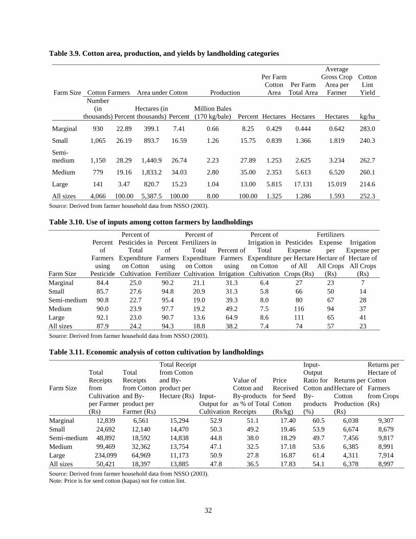
32

Table 3.9. Cotton area, production, and yields by landholding categories

Farm Size Cotton Farmers Area under Cotton Production

Per FarmCotton Area

Per Farm Total Area

Average Gross Crop

Area per Farmer

Cotton Lint

Yield

Number (in

thousands) PercentHectares (in thousands) Percent

Million Bales (170 kg/bale)

Percent Hectares Hectares Hectares

kg/ha

Marginal 930 22.89 399.1 7.41 0.66 8.25 0.429 0.444 0.642 283.0

Small 1,065 26.19 893.7 16.59 1.26 15.75 0.839 1.366 1.819 240.3

Semi-medium 1,150 28.29 1,440.9 26.74 2.23 27.89 1.253 2.625 3.234

262.7

Medium 779 19.16 1,833.2 34.03 2.80 35.00 2.353 5.613 6.520 260.1

Large 141 3.47 820.7 15.23 1.04 13.00 5.815 17.131 15.019 214.6

All sizes 4,066 100.00 5,387.5 100.00 8.00 100.00 1.325 1.286 1.593 252.3 Source: Derived from farmer household data from NSSO (2003).

Table 3.10. Use of inputs among cotton farmers by landholdings

Farm Size

Percent of

Farmers using

Pesticide

Percent of Pesticides in

Total Expenditure on Cotton

Cultivation

Percent of

Farmers using

Fertilizer

Percent of Fertilizers in

Total Expenditure on Cotton

Cultivation

Percent of Farmers

using Irrigation

Percent of Irrigation in

Total Expenditure on Cotton

Cultivation

Pesticides Expense

per Hectare of All

Crops (Rs)

FertilizersExpense

per Hectare of All Crops

(Rs)

Irrigation Expense per Hectare of All Crops

(Rs) Marginal 84.4 25.0 90.2 21.1 31.3 6.4 27 23 7 Small 85.7 27.6 94.8 20.9 31.3 5.8 66 50 14 Semi-medium 90.8 22.7 95.4 19.0 39.3 8.0 80 67 28 Medium 90.0 23.9 97.7 19.2 49.2 7.5 116 94 37 Large 92.1 23.0 90.7 13.6 64.9 8.6 111 65 41 All sizes 87.9 24.2 94.3 18.8 38.2 7.4 74 57 23 Source: Derived from farmer household data from NSSO (2003).

Table 3.11. Economic analysis of cotton cultivation by landholdings

Farm Size

Total Receipts from Cultivation per Farmer (Rs)

Total Receipts from Cotton and By-product per Farmer (Rs)

Total Receipt from Cotton and By-product per Hectare (Rs) Input-

Output for Cultivation

Value of Cotton and By-products as % of Total Receipts

Price Received for Seed Cotton (Rs/kg)

Input-Output Ratio for Cotton and By-products (%)

Returns per Hectare of Cotton Production (Rs)

Returns per Hectare of Cotton Farmers from Crops (Rs)

Marginal 12,839 6,561 15,294 52.9 51.1 17.40 60.5 6,038 9,307 Small 24,692 12,140 14,470 50.3 49.2 19.46 53.9 6,674 8,679 Semi-medium 48,892 18,592 14,838 44.8 38.0 18.29 49.7 7,456 9,817 Medium 99,469 32,362 13,754 47.1 32.5 17.18 53.6 6,385 8,991 Large 234,099 64,969 11,173 50.9 27.8 16.87 61.4 4,311 7,914 All sizes 50,421 18,397 13,885 47.8 36.5 17.83 54.1 6,378 8,997 Source: Derived from farmer household data from NSSO (2003). Note: Price is for seed cotton (kapas) not for cotton lint.

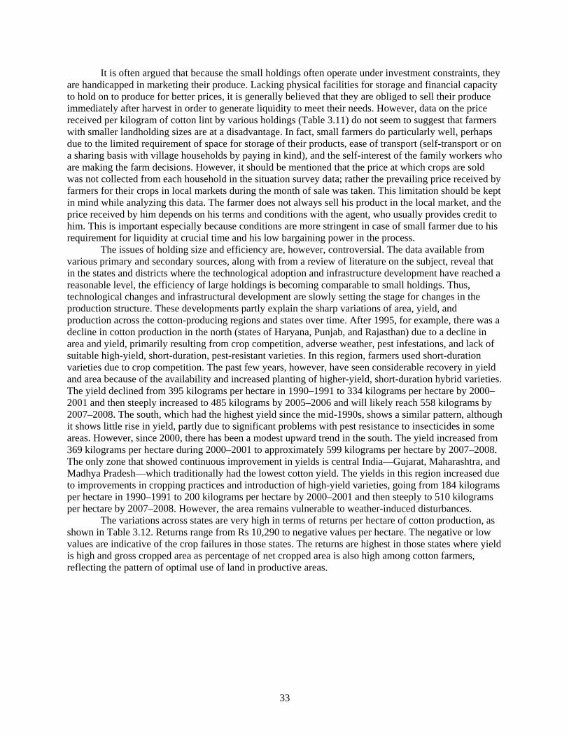
33

It is often argued that because the small holdings often operate under investment constraints, they are handicapped in marketing their produce. Lacking physical facilities for storage and financial capacity to hold on to produce for better prices, it is generally believed that they are obliged to sell their produce immediately after harvest in order to generate liquidity to meet their needs. However, data on the price received per kilogram of cotton lint by various holdings (Table 3.11) do not seem to suggest that farmers with smaller landholding sizes are at a disadvantage. In fact, small farmers do particularly well, perhaps due to the limited requirement of space for storage of their products, ease of transport (self-transport or on a sharing basis with village households by paying in kind), and the self-interest of the family workers who are making the farm decisions. However, it should be mentioned that the price at which crops are sold was not collected from each household in the situation survey data; rather the prevailing price received by farmers for their crops in local markets during the month of sale was taken. This limitation should be kept in mind while analyzing this data. The farmer does not always sell his product in the local market, and the price received by him depends on his terms and conditions with the agent, who usually provides credit to him. This is important especially because conditions are more stringent in case of small farmer due to his requirement for liquidity at crucial time and his low bargaining power in the process.

The issues of holding size and efficiency are, however, controversial. The data available from various primary and secondary sources, along with from a review of literature on the subject, reveal that in the states and districts where the technological adoption and infrastructure development have reached a reasonable level, the efficiency of large holdings is becoming comparable to small holdings. Thus, technological changes and infrastructural development are slowly setting the stage for changes in the production structure. These developments partly explain the sharp variations of area, yield, and production across the cotton-producing regions and states over time. After 1995, for example, there was a decline in cotton production in the north (states of Haryana, Punjab, and Rajasthan) due to a decline in area and yield, primarily resulting from crop competition, adverse weather, pest infestations, and lack of suitable high-yield, short-duration, pest-resistant varieties. In this region, farmers used short-duration varieties due to crop competition. The past few years, however, have seen considerable recovery in yield and area because of the availability and increased planting of higher-yield, short-duration hybrid varieties. The yield declined from 395 kilograms per hectare in 1990–1991 to 334 kilograms per hectare by 2000–2001 and then steeply increased to 485 kilograms by 2005–2006 and will likely reach 558 kilograms by 2007–2008. The south, which had the highest yield since the mid-1990s, shows a similar pattern, although it shows little rise in yield, partly due to significant problems with pest resistance to insecticides in some areas. However, since 2000, there has been a modest upward trend in the south. The yield increased from 369 kilograms per hectare during 2000–2001 to approximately 599 kilograms per hectare by 2007–2008. The only zone that showed continuous improvement in yields is central India—Gujarat, Maharashtra, and Madhya Pradesh—which traditionally had the lowest cotton yield. The yields in this region increased due to improvements in cropping practices and introduction of high-yield varieties, going from 184 kilograms per hectare in 1990–1991 to 200 kilograms per hectare by 2000–2001 and then steeply to 510 kilograms per hectare by 2007–2008. However, the area remains vulnerable to weather-induced disturbances.

The variations across states are very high in terms of returns per hectare of cotton production, as shown in Table 3.12. Returns range from Rs 10,290 to negative values per hectare. The negative or low values are indicative of the crop failures in those states. The returns are highest in those states where yield is high and gross cropped area as percentage of net cropped area is also high among cotton farmers, reflecting the pattern of optimal use of land in productive areas.

34

Table 3.12. Economic analysis of cotton production by state

State Total

Receipts from Cultivation per Farmer

(Rs)

Total Receipts

from Cotton and By-

products per Farmer

(Rs)

Input-Output for

Cultivation

Value of Cotton and

By-products Produced as % of Total Receipts

Price Received for Seed Cotton (Rs/kg)

Input-Output Ratio for

Cotton and By-products

(%)

Returns per Hectare of

Cotton Production

(Rs) Punjab 165,239 40,915 41.3 24.8 20.62 52.8 10,290Haryana 91,945 20,689 43.8 22.5 19.29 58.5 6,454Rajasthan 66,881 11,356 53.3 17.0 16.84 100.1 –6Madhya Pradesh 50,348 21,892 38.2 43.5 17.25 38.9 13,213Gujarat 62,670 30,233 52.4 48.2 20.19 54.6 5,695Maharashtra 40,403 16,495 44.8 40.8 16.69 46.2 7,167Andhra Pradesh 27,400 12,716 64.0 46.4 17.03 74.9 3,225Karnataka 58,941 16,184 48.4 27.5 19.19 44.7 7,135Tamil Nadu 10,695 4,045 81.7 37.8 15.87 89.8 874Other States 20,231 5,882 47.5 29.1 6.77 58.5 5,839All India 50,421 18,397 47.8 36.5 17.83 54.1 6,378

Source: Derived from farmer household data from NSSO (2003). Note: Price is for seed cotton (kapas) not for cotton lint.

The states that have a dominant share of semi-medium holdings are also doing better in terms of returns. The yields and returns, however, are highly correlated, whereas the relationship between yield and input use may vary due to such uncertainties as crop failure. Similarly, input use, although it increases yields, is not always optimally used. Table 3.13 provides additional information on input use by cotton farms by state.

Table 3.13. Use of inputs among cotton farmers by state

State

Percent of Farmers

using Pesticide

Percent of Pesticides in

Total Expenditure on

Cotton Cultivation

Percent of

Farmers using

Fertilizer

Percent of Fertilizers in

Total Expenditure on Cotton

Cultivation

Percent of Farmers

using Irrigation

Percent of Irrigation in

Total Expenditure on Cotton

Cultivation

Pesticides Expense per Hectare of All Crops

(Rs)

FertilizersExpense

per Hectare of All Crops

(Rs)

Irrigation Expense

per Hectare of All Crops (Rs)

Cotton Lint

Yield(kg/ha)

Punjab 99.9 41.4 100.0 12.0 89.9 7.9 235 68 45 334.1Haryana 87.1 30.9 93.2 11.8 94.4 15.0 178 68 86 258.6Rajasthan 76.4 31.5 98.7 11.9 67.6 17.7 89 34 50 191.8Madhya Pradesh 87.0 24.0 88.1 23.2 49.6 9.7 46 45 19

404.9

Gujarat 89.8 19.5 94.1 14.9 52.9 11.4 242 186 142 203.5Maharashtra 87.5 16.9 97.9 24.7 21.3 2.4 154 225 22 258.8Andhra Pradesh 95.1 34.1 87.2 19.2 27.3 2.2 237 134 15

247.0

Karnataka 89.1 18.1 97.6 24.2 8.3 2.0 27 36 3 216.1Tamil Nadu 75.3 10.8 82.0 20.7 32.6 8.0 10 18 7 177.1Other states 59.2 11.3 93.7 20.9 57.0 10.2 1 1 1 656.9All India 87.9 24.2 94.3 18.8 38.2 7.4 74 57 23 252.3Source: Derived from farmer household data from NSSO (2003). Note: Cotton lint yield is based on dividing yield of seed cotton by 3.

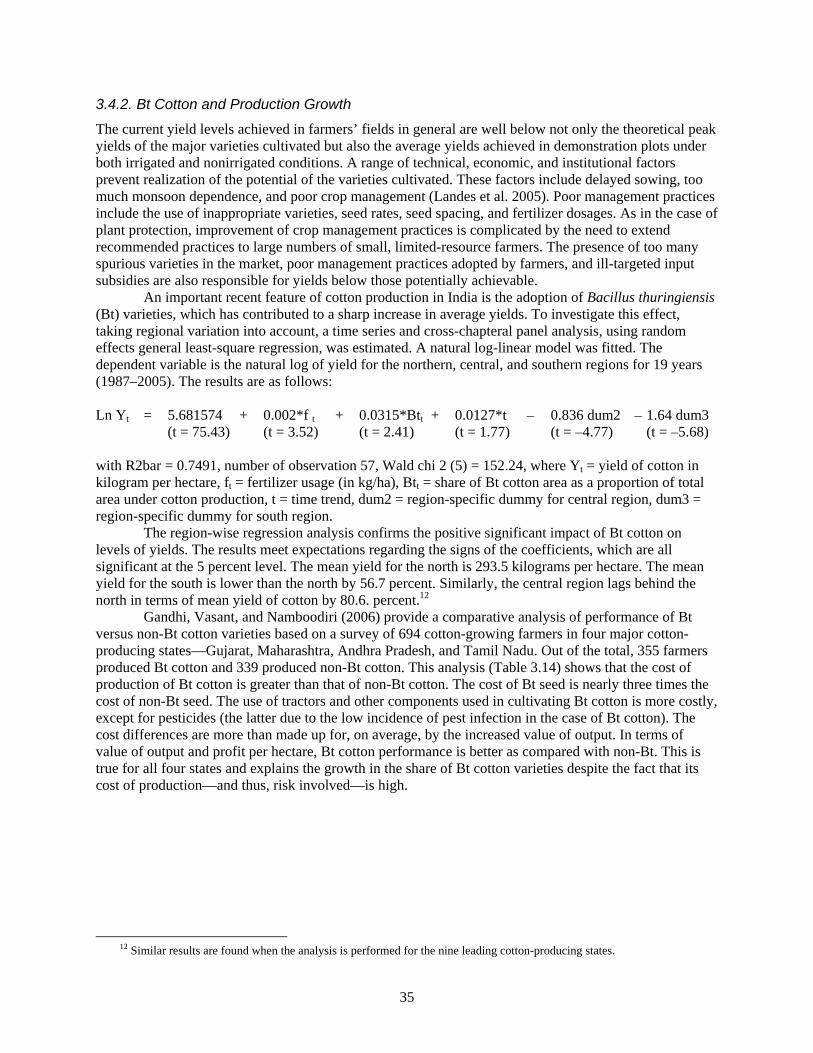
35

3.4.2. Bt Cotton and Production Growth

The current yield levels achieved in farmers’ fields in general are well below not only the theoretical peak yields of the major varieties cultivated but also the average yields achieved in demonstration plots under both irrigated and nonirrigated conditions. A range of technical, economic, and institutional factors prevent realization of the potential of the varieties cultivated. These factors include delayed sowing, too much monsoon dependence, and poor crop management (Landes et al. 2005). Poor management practices include the use of inappropriate varieties, seed rates, seed spacing, and fertilizer dosages. As in the case of plant protection, improvement of crop management practices is complicated by the need to extend recommended practices to large numbers of small, limited-resource farmers. The presence of too many spurious varieties in the market, poor management practices adopted by farmers, and ill-targeted input subsidies are also responsible for yields below those potentially achievable.

An important recent feature of cotton production in India is the adoption of Bacillus thuringiensis (Bt) varieties, which has contributed to a sharp increase in average yields. To investigate this effect, taking regional variation into account, a time series and cross-chapteral panel analysis, using random effects general least-square regression, was estimated. A natural log-linear model was fitted. The dependent variable is the natural log of yield for the northern, central, and southern regions for 19 years (1987–2005). The results are as follows: Ln Yt = 5.681574 + 0.002*f t + 0.0315*Btt + 0.0127*t – 0.836 dum2 – 1.64 dum3 (t = 75.43) (t = 3.52) (t = 2.41) (t = 1.77) (t = –4.77) (t = –5.68) with R2bar = 0.7491, number of observation 57, Wald chi 2 (5) = 152.24, where Yt = yield of cotton in kilogram per hectare, ft = fertilizer usage (in kg/ha), Btt = share of Bt cotton area as a proportion of total area under cotton production, t = time trend, dum2 = region-specific dummy for central region, dum3 = region-specific dummy for south region.

The region-wise regression analysis confirms the positive significant impact of Bt cotton on levels of yields. The results meet expectations regarding the signs of the coefficients, which are all significant at the 5 percent level. The mean yield for the north is 293.5 kilograms per hectare. The mean yield for the south is lower than the north by 56.7 percent. Similarly, the central region lags behind the north in terms of mean yield of cotton by 80.6. percent.12

Gandhi, Vasant, and Namboodiri (2006) provide a comparative analysis of performance of Bt versus non-Bt cotton varieties based on a survey of 694 cotton-growing farmers in four major cotton-producing states—Gujarat, Maharashtra, Andhra Pradesh, and Tamil Nadu. Out of the total, 355 farmers produced Bt cotton and 339 produced non-Bt cotton. This analysis (Table 3.14) shows that the cost of production of Bt cotton is greater than that of non-Bt cotton. The cost of Bt seed is nearly three times the cost of non-Bt seed. The use of tractors and other components used in cultivating Bt cotton is more costly, except for pesticides (the latter due to the low incidence of pest infection in the case of Bt cotton). The cost differences are more than made up for, on average, by the increased value of output. In terms of value of output and profit per hectare, Bt cotton performance is better as compared with non-Bt. This is true for all four states and explains the growth in the share of Bt cotton varieties despite the fact that its cost of production—and thus, risk involved—is high.

12 Similar results are found when the analysis is performed for the nine leading cotton-producing states.

36

Table 3.14. Cost of production, value of output, and profit (Rs/ha)

Gujarat Maharashtra Andhra Pradesh Tamil Nadu Production Activities Bt Non-Bt Bt Non-Bt Bt Non-Bt Bt Non-Bt Human Labor 10,784 9,317 11,754 9,150 9,818 8,249 9,089 7,714Bullock 2,655 2,568 1,913 2,125 2,062 2,024 0 0Tractor 970 737 1,016 748 1,705 1,648 2,373 1,734Farm Yard Manure 1,395 1,424 0 0 2,103 2,000 2,228 1,325Fertilizer 3,254 3,014 7,116 4,086 4,804 4,078 2,922 3,740Seed 3,111 1,314 3,857 1,319 3,313 1,213 3,977 1,180Pesticides 2,586 3,153 3,242 4,120 7,806 10,878 1,909 4,195Irrigation 4,497 4,179 1,136 474 319 163 55 60Other Operational Costs 332 122 Marketing Cost 626 580 1,314 1,181 210 192 487 312Total Cost 29,878 26,287 31,679 23,207 32,139 30,444 23,040 20,260Value of Output 61,943 44,531 54,313 37,524 50,970 35,870 38,282 26,032Profit 32,065 18,244 22,634 14,317 18,831 5,426 15,242 5,772Source: Gandhi and Namboodiri (2006)

The most important reason for the better performance of Bt cotton is its resistance to pests, particularly bollworms. Gandhi and Namboodiri show that yield and profitability are enhanced under both irrigated and nonirrigated conditions and that the average size of farms growing Bt cotton is not much larger than for those growing non-Bt cotton.

A relevant question in light of these positive implications is why the suicide rates among farmers in cotton-producing states have significantly increased after the introduction of Bt cotton, which has been a noted and important social issue. One possible explanation is the high cost of Bt cotton production compared with non-Bt cotton. There is a higher cost of seed incurred early in the year that is lost if the crop fails. In addition, the institutional credit for these farmers is inadequate, and thus farmers have to resort to costly borrowing. Because only 35 percent of the cotton area is irrigated, the impact of weather-induced disturbances is more pronounced in terms of large fluctuations in the average yield for non-irrigated. Thus, farmers growing Bt cotton can get trapped into debt more easily than can others.

In general, the market support prices (MSPs) for cotton have had little influence on producer prices, because market prices are typically well above the MSPs. This is unlike wheat and rice, where MSPs in the principal surplus areas have significantly influenced market prices. The MSPs set for wheat and rice can directly affect the area allocated to cotton by influencing relative returns to growers. It also affects the portion of the growing season that farmers are willing to devote to cotton production and hence the duration of the varieties cultivated and the time available for picking before planting the next crop.

These factors, in addition to poor seed quality in the presence of spurious seeds, compound the problems faced by farmers producing cotton. The presence of too many spurious varieties and suitability of soil are factors responsible for variations in performance. Roughly 100–130 cotton varieties developed in the public and private sectors are now cultivated in India. Only about one-third of the cotton area in India is sown with certified seed that is assured variety purity and germination. Commercially available seeds are often of poor quality, with sale of uncertified, substandard, and second-generation (F2) hybrid seeds not uncommon. The presence of spurious Bt cottonseeds in large varieties has caused several problems, in part because all of these varieties are not suitable for various agronomic conditions. A study by the Central Institute for Cotton Research (CICR) indicated that the average cotton farmer in the central and south regions of India plants three to four varieties on farms that average about 2 hectares. This practice greatly complicates crop and seed management. In addition, the cost of input increases for Bt varieties as compared with non-Bt varieties.

37

All of the above factors contributed to the high input cost and high dependence of farmers on borrowings, despite the improvement in productivity through the introduction of Bt cotton. These factors put small farmers in a bind, especially during bad weather seasons. Pressure from these factors may also have caused the high incidence of suicide among farmers. Thus easy availability of credit and crop insurance are measures that could tremendously benefit cotton-growing farmers.

3.4.3. Regional Analysis of Income Sources of Cotton Farmers by Landholdings

State-level analysis cannot be pushed too far for various-sized holdings, because the sample size is too small even in a few important states; thus, such analysis would not provide reliable results. Therefore, this chapter presents an income analysis for cotton farmers by size distribution based on three major cotton-growing regions—namely, north, central, and south. The states included in each region are only the major cotton-producing states and not those states that have small shares of cotton production. States that are not major cotton producers are classified in an aggregate “Other” group, whatever their location.

A few descriptive statistics for the regions are shown in Table 3.15. The number of cotton farmers is at a maximum in the central region, south comes a distant second, and north third. The share in terms of area and cotton lint production is even higher for the central region. Among the main cotton-growing regions, the yields are similar. The yield per hectare is calculated to be much higher in the aggregate other region, but this outlier is suspect due to a very small sample size of cotton farmers among these widely diversified states, where cotton farmers account for only 1.2 percent of the total farm households.

Table 3.15. Regional characteristics of cotton production

Zone

Sample Number

Farms (mln.)

Cotton Farmers (mln.)

Percent of all

Cotton Farmers

Area (mln. ha)

Gross Crop Area(mln. ha)

Area of

Cotton (mln. ha)

Area per

Cotton Farmer

(ha)

Percent of

Total Cotton Area

Cotton Lint Production (mln. bales)

Percent of Cotton

Production

Cotton Lint

Yield(kg/ha)

All Cotton North 3,515 347 7.3 0.6 15.2 17.6 20.9 0.8 1.33 15.3 1.2 15.3 253Central 6,404 1,065 15.8 2.5 61.8 31.2 36.9 3.7 1.46 68.1 5.5 68.5 254South 6,743 383 12.7 0.9 21.8 18.0 20.8 0.9 0.99 16.2 1.2 15.1 236Other 14,864 37 29.1 0.0 1.2 24.3 32.5 0.0 0.42 0.4 0.1 1.0 657All India 45,707 1,832 83.3 4.1 100.0 107.1 132.7 5.4 1.33 100.0 8.0 100.0 252Source: Derived from farmer household data from NSSO (2003). Note: mln: million

A detailed assessment of sources of cotton farmers’ income by landholdings and region is presented in Table 3.16. This type of assessment was not possible at the state level. The pattern in each region is similar to the all India category. The marginal farmers devote only a portion of their land to cotton production after taking care of their basic food consumption needs, which these farmers produce on their own land in order to maintain self-sufficiency and food security. The small, semi-medium, and medium landholdings try to diversify their land use to avoid concentrated risk, while at the same time devoting at least a reasonable economic size of land to a cash crop, such as raw cotton, to exploit scale economies. They try to do this to the extent feasible for the size landholding they have and the technology being adopted for that size holding. The large landholdings try to take advantage of both economies of scale while also trying to avoid production and marketing management complications by focusing on only a few crops. This phenomenon is similar in all the regions, as shown in Table 3.16.

38

Table 3.16. Sources of income for cotton farmers by region and landholdings

Income of Cotton Farmers from Different Sources (excluding remittances) Sources of Income (percent of total) Sample Size

of Cotton Farmers

Size of Holdings

Cotton Farming

Other Cultivation

All Cultivation Activities

Livestock All Farming Activities Nonfarm Wages All

Activities

All India 547 Marginal 18.84 56.41 75.25 1.80 77.04 2.06 20.90 100.00 383 Small 27.99 45.54 73.53 4.32 77.84 2.05 20.11 100.00 429 Semi-medium 24.47 55.83 80.30 0.61 80.92 1.93 17.15 100.00 406 Medium 20.75 58.61 79.36 3.36 82.72 2.91 14.37 100.00 67 Large 31.03 72.13 103.16 –15.83 87.33 0.92 11.75 100.00

1832 All 22.89 54.56 77.45 1.99 79.44 2.17 18.39 100.00 North Zone

67 Marginal 13.30 68.01 81.31 –5.13 76.18 4.89 18.93 100.00 69 Small 20.70 63.59 84.29 4.07 88.36 2.16 9.48 100.00 95 Semi-medium 2.82 49.86 52.67 4.07 56.74 5.36 37.90 100.00 93 Medium –80.51 –16.86 –97.37 –75.49 –172.85 6.41 66.44 –100.00 23 Large 16.23 36.23 52.46 47.89 100.35 0.00 –0.35 100.00

347 All 8.03 70.21 78.24 –12.03 66.21 5.58 28.22 100.00 Central Zone

259 Marginal 22.14 56.27 78.41 3.83 82.25 0.51 17.24 100.00 166 Small 27.60 42.12 69.72 5.57 75.29 1.90 22.82 100.00 207 Semi-medium 25.27 56.28 81.55 0.50 82.04 1.89 16.06 100.00 228 Medium 22.45 59.37 81.81 5.35 87.17 2.42 10.42 100.00 29 Large 27.01 63.55 90.56 –1.47 89.09 0.80 10.11 100.00

889 All 24.30 54.29 78.59 3.61 82.20 1.60 16.20 100.00 South Zone

154 Marginal 13.43 51.45 64.87 1.22 66.10 4.56 29.34 100.00 97 Small 31.94 49.12 81.06 0.91 81.98 2.47 15.56 100.00 86 Semi-medium 31.43 57.12 88.55 –0.27 88.28 0.36 11.36 100.00 40 Medium 25.69 44.77 70.45 5.86 76.32 5.78 17.90 100.00 6 Large 33.69 68.65 102.34 –2.34 100.00 0.00 0.00 100.00

383 All 24.40 51.34 75.73 1.24 76.97 3.16 19.87 100.00 Other

67 Marginal 4.44 15.92 20.37 –0.01 20.36 3.46 76.18 100.00 51 Small –5.58 22.11 16.53 –4.79 11.74 0.00 88.26 100.00 41 Semi-medium 7.34 4.79 12.13 –14.78 –2.65 0.00 102.65 100.00 45 Medium –0.07 –0.07 –0.15 3.00 2.85 0.00 97.15 100.00 9 Large — — — — — — — —

213 All 2.92 11.57 14.48 –0.12 14.36 2.24 83.39 100.00 Source: Derived from Farmer Household data from NSSO (2003). Note: Net crop income is assumed to include all commodities, including by-products, less crop production costs (i.e., seeds, fertilizer, pesticides, utilities, taxes, transportation, hired labor, and others) and payments to landlords. Net livestock income is calculated as the value of sales of all types of animals and by-products, as well as household consumption of meat, less expenditures on livestock production and purchases. Wages include both cash and in-kind earnings.

The table also shows the various sources of income for cotton farmers, with cotton production accounting for about one-fifth to one-fourth of the income. Other cultivation accounts for nearly half of farmers’ total income. Nonfarm wages are nearly as important as earnings from cotton production, but

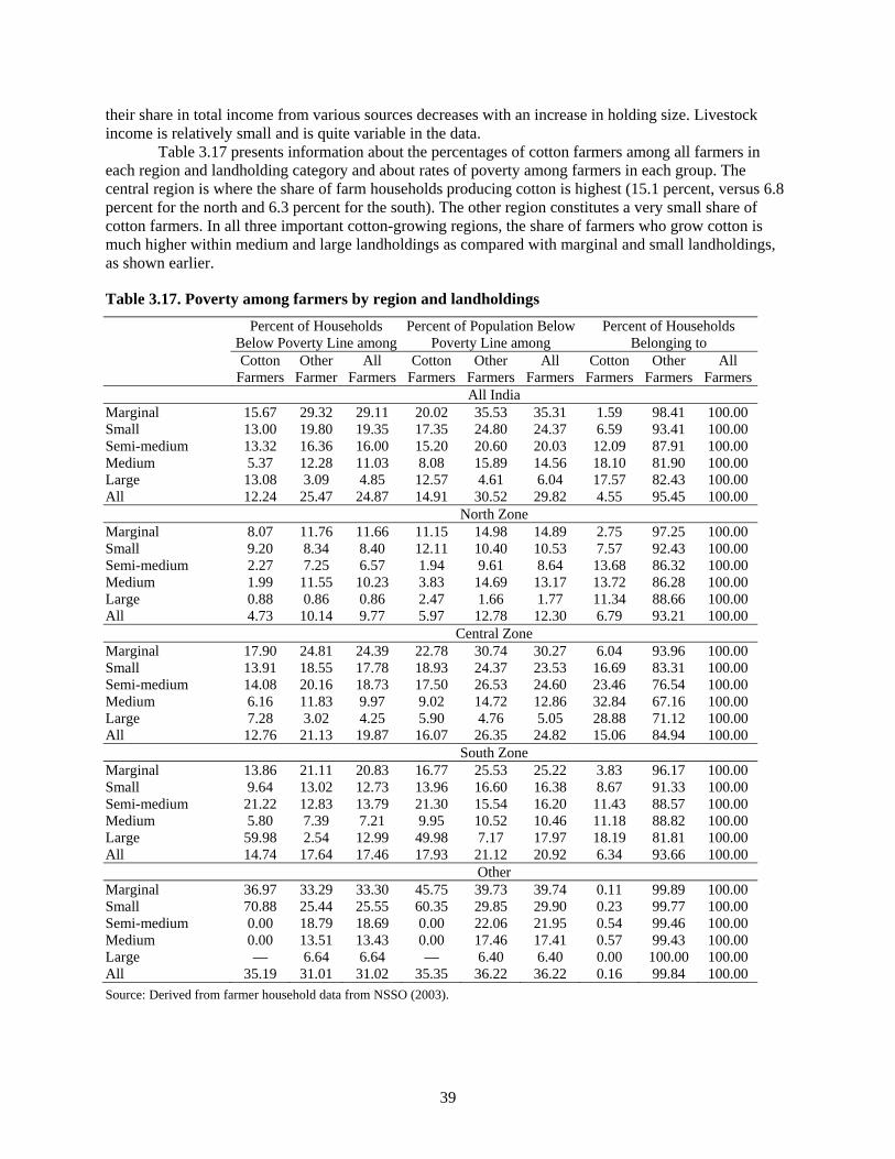
39

their share in total income from various sources decreases with an increase in holding size. Livestock income is relatively small and is quite variable in the data.

Table 3.17 presents information about the percentages of cotton farmers among all farmers in each region and landholding category and about rates of poverty among farmers in each group. The central region is where the share of farm households producing cotton is highest (15.1 percent, versus 6.8 percent for the north and 6.3 percent for the south). The other region constitutes a very small share of cotton farmers. In all three important cotton-growing regions, the share of farmers who grow cotton is much higher within medium and large landholdings as compared with marginal and small landholdings, as shown earlier.

Table 3.17. Poverty among farmers by region and landholdings

Percent of Households Below Poverty Line among

Percent of Population Below Poverty Line among

Percent of Households Belonging to

Cotton Farmers

Other Farmer

All Farmers

Cotton Farmers

Other Farmers

All Farmers

Cotton Farmers

Other Farmers

All Farmers

All India Marginal 15.67 29.32 29.11 20.02 35.53 35.31 1.59 98.41 100.00 Small 13.00 19.80 19.35 17.35 24.80 24.37 6.59 93.41 100.00 Semi-medium 13.32 16.36 16.00 15.20 20.60 20.03 12.09 87.91 100.00 Medium 5.37 12.28 11.03 8.08 15.89 14.56 18.10 81.90 100.00 Large 13.08 3.09 4.85 12.57 4.61 6.04 17.57 82.43 100.00 All 12.24 25.47 24.87 14.91 30.52 29.82 4.55 95.45 100.00 North Zone Marginal 8.07 11.76 11.66 11.15 14.98 14.89 2.75 97.25 100.00 Small 9.20 8.34 8.40 12.11 10.40 10.53 7.57 92.43 100.00 Semi-medium 2.27 7.25 6.57 1.94 9.61 8.64 13.68 86.32 100.00 Medium 1.99 11.55 10.23 3.83 14.69 13.17 13.72 86.28 100.00 Large 0.88 0.86 0.86 2.47 1.66 1.77 11.34 88.66 100.00 All 4.73 10.14 9.77 5.97 12.78 12.30 6.79 93.21 100.00

Central Zone Marginal 17.90 24.81 24.39 22.78 30.74 30.27 6.04 93.96 100.00 Small 13.91 18.55 17.78 18.93 24.37 23.53 16.69 83.31 100.00 Semi-medium 14.08 20.16 18.73 17.50 26.53 24.60 23.46 76.54 100.00 Medium 6.16 11.83 9.97 9.02 14.72 12.86 32.84 67.16 100.00 Large 7.28 3.02 4.25 5.90 4.76 5.05 28.88 71.12 100.00 All 12.76 21.13 19.87 16.07 26.35 24.82 15.06 84.94 100.00

South Zone Marginal 13.86 21.11 20.83 16.77 25.53 25.22 3.83 96.17 100.00 Small 9.64 13.02 12.73 13.96 16.60 16.38 8.67 91.33 100.00 Semi-medium 21.22 12.83 13.79 21.30 15.54 16.20 11.43 88.57 100.00 Medium 5.80 7.39 7.21 9.95 10.52 10.46 11.18 88.82 100.00 Large 59.98 2.54 12.99 49.98 7.17 17.97 18.19 81.81 100.00 All 14.74 17.64 17.46 17.93 21.12 20.92 6.34 93.66 100.00

Other Marginal 36.97 33.29 33.30 45.75 39.73 39.74 0.11 99.89 100.00 Small 70.88 25.44 25.55 60.35 29.85 29.90 0.23 99.77 100.00 Semi-medium 0.00 18.79 18.69 0.00 22.06 21.95 0.54 99.46 100.00 Medium 0.00 13.51 13.43 0.00 17.46 17.41 0.57 99.43 100.00 Large — 6.64 6.64 — 6.40 6.40 0.00 100.00 100.00 All 35.19 31.01 31.02 35.35 36.22 36.22 0.16 99.84 100.00 Source: Derived from farmer household data from NSSO (2003).

40

In terms of measuring poverty, in addition to the data on agricultural production, data on household consumption expenditures were also collected for moving reference periods of “preceding 30 days” and “last 365 days” in the NSSO 59th round. Thus, whereas crop production data were for 2002–2003, the consumption data are mainly for 2003. In principle, use of consumption data from this survey is expected to produce better estimates of the household distribution by consumption expenditure than is the NSSO consumption expenditure surveys conducted in other years. In the regular consumption expenditure surveys of the NSSO, each sample household is interviewed only once for collecting data on household consumption expenditure. In principle, this procedure is valid—because the interviews of sample households are spread evenly over the survey period, the estimates of averages and aggregates are free from seasonal bias. Nevertheless, because observation on the consumption expenditure of a sample household is restricted to 30 days of the survey period, the estimates of household distribution by consumption expenditure obtained from the regular surveys are expected to be affected by seasonal variation in consumption and thus have a wider spread than the actual household distribution by average monthly consumption expenditure. The data on consumption expenditure for two disjoint periods for each sample household in the 59th round are expected to better represent the distribution of households by consumption expenditure. Needless to say, the poverty estimates based on data of two periods, as derived in this analysis, are not exactly comparable with results derived from other NSSO consumption data. The criteria used to estimate poverty are similar to official criteria, but the source and measurement of consumption during the year is different.13

The most important finding from the household survey is that the poverty among cotton-growing farmers is lower compared with other farmers in all sizes of landholdings except large landholdings; this is true in all regions, as shown in Table 3.17. The percentage of cotton households below the poverty line averages only 12.24 percent for all of India, as compared with 25.47 percent of other farmer households below the poverty line. Among the main cotton-producing regions, poverty levels among cotton farmers are generally lower compared with poverty levels among other farmers, except in the south (14.74 percent compared with 17.64 percent for the south). Poverty rates decline as the size of landholdings increases for both cotton farmers and other farmers.

We have more frequently used the concept of households rather than population because the survey is undertaken for the entire household and whatever is true about the household is also relevant for the individual members of the household. However, there seems to be a problem in data regarding large landholdings in the south. The percentage of households below poverty line suddenly increased from 5.80 percent in medium landholdings of the region to 59.98 percent for large landholdings. The discrepancy is caused by too small a sample size—just six households. Hence, this result should be interpreted as an outlier.

A third observation is that poverty among the three major cotton-growing regions is low compared with overall India, as a lot of the poorest states are not falling into the main cotton-growing regions. Poverty levels among farmers are much higher than the national average in the “other” region, which comprises several states spread across all parts of the country, but the share of cotton farmers is small in this diverse region.

13 Bhalla (2006) worked out poverty estimates for all farmer household (not just cotton farmers) using the same data but

taking into consideration consumption only at one point rather than at two points as in this analysis. Bhalla compared the incidence of poverty among farmers with the incidence of poverty of the rural population, using NSS thin-sample household consumption survey data for 2003–2004. He broadly concluded that the poverty among farmer households by the head-count ratio is higher compared with nonfarmer households in rural areas. He critically pointed out that the policymakers should take note of the serious state of affairs in the farming sector and take remedial measures with a view to improving the economic condition of farmers. Among the states, the lowest incidence of poverty among farmer households was in Jammu, Kashmir, and Punjab. Other states where incidence of poverty was low were Himachal Pradesh, Andhra Pradesh, Kerala, and Haryana. Except for Andhra Pradesh, these are relatively small states in terms of population. On the other hand, Orissa, Bihar, Uttar Pradesh, and Madhya Pradesh are the states with the highest incidence of poverty with large populations.

41

3.5. Direct Effects of Cotton Prices on Household Incomes and Poverty The final objective of this chapter is to measure the linkages between global cotton prices and rural poverty in India. For this assessment, a simulation analysis is utilized based on the studies of the impact of lower cotton prices on rural poverty performed by Minot and Daniels (2005) for Benin and Orden et al. (2006) for Pakistan (see the related discussion paper). In particular, the direct effects of changes in cotton price on incomes and poverty among cotton-producing households are assessed, assuming no change in production levels (fixed supply [FS]). The direct effects of incomes and poverty among these households are also assessed, allowing for a supply response (SR) by farmers. For the latter case, for cotton farmers who own their land, per capita income derived from a price change can be calculated as follows:

⎥⎥⎦

⎤

⎢⎢⎣

⎡⎟⎟⎠

⎞⎜⎜⎝

⎛εΔ+Δ=Δ

c

cic

2ccci

ii P

Q)P(

21)PQ(

H1y

where Δyi is the change in per capita income of household i due to a change in the price of cotton; Qci is the quantity of cotton sold by household i; ∆Pc is the change in the real price of cotton; Hi is the number of members in household i; εc is the general equilibrium supply elasticity of cotton; and Pc is the price of cotton. The second term in the brackets is zero when there is no supply response; however, it is positive regardless of whether the price change is positive or negative when there is supply response, implying that the supply-response effect of a price change is more positive (or less negative) than the fixed-supply effect. If production alternatives are limited, the two effects will be similar. The elasticity of supply has to be estimated or assumed based on available studies.

3.5.1. Simulated Direct Effects of Cotton Price on Incomes and Poverty

The simulations incorporated a range of increases in the farm level price of seed cotton. To evaluate whether a household was in poverty, the study compared the household’s annual per capita consumption expenditure with a per capita poverty line based on the official definition per person per month. Additional income resulting from an increase in cotton prices is assumed to be utilized to increase household consumption. Initial levels of poverty among cotton-producing households and the poverty rates with 10 percent to 40 percent increases in cotton price for the nine major cotton-producing states are shown in Table 3.18.

In the simulations analysis, every 10 percent increase in the price of cotton raises an average cotton-producing household’s income and hence decreases poverty, assuming fixed levels of production. A modest supply elasticity of 0.3 is assumed for supply response simulations (a 10 percent increase in price raises output by 3 percent, with additional costs of production also incurred). The supply response leads to slightly higher gains in household income for any given increase in cotton price.

Based on an analysis of the 2002–2003 farmer household data, 0 percent of the cotton-producing households in Punjab and Gujarat were estimated to initially have per capita expenditures below the poverty line, with 2.28 percent in Haryana, 13.02 percent in Rajasthan, 27.82 percent in Madhya Pradesh, 13.66 percent in Maharashtra, 15.77 percent in Andhra Pradesh, 3.68 percent in Karnataka, 28.08 percent in Tamil Nadu, and 12.78 percent in India overall.

42

Table 3.18. Poverty head count at different levels of rise in price of cotton

State

Initial Poverty Level

Poverty Level Resulting from Increase of Cotton Prices of

Model 10% 20% 30% 40% Punjab FS 0 0 0 0 0

SR 0 0 0 0 Haryana FS 2.28 0 0 0 0

SR 0 0 0 0 Rajasthan FS 13.02 9.03 5.88 5.88 3.59

SR 9.03 5.88 3.59 3.59 Madhya Pradesh FS 27.82 11.76 6.11 4.75 3.07

SR 11.76 6.11 4.6 3.07 Gujarat FS 0 0 0 0 0

SR 0 0 0 0 0 Maharashtra FS 13.66 3.25 2.14 0.88 0.41

SR 3.25 2.12 0.88 0.41 Andhra Pradesh FS 15.77 3.65 1.51 0.58 0.58

SR 3.65 1.51 0.58 0.58 Karnataka FS 3.68 0 0 0 0

SR 0 0 0 0 Tamil Nadu FS 28.08 16.94 11.67 9.26 9.26

SR 16.94 11.67 9.26 9.26 All India FS 12.78 4.35 2.73 1.88 1.37

SR 4.35 2.72 1.7 1.35 Source: Author’s calculations based on data from the Household Situation Assessment Survey of Farmers, NSSO (2003). Note: FS: fixed supply; SR: supply response 2

A 30 percent increase in real cotton prices—such as would offset the decline in real domestic prices that occurred in the late 1990s—is estimated to reduce the rate of poverty among cotton-producing households to 0 percent in Haryana and Karnataka, 5.88 percent in Rajasthan, 4.75 percent in Madhya Pradesh, 0.88 percent in Maharashtra, 0.58 percent in Andhra Pradesh, 9.26 percent in Tamil Nadu, and 1.88 percent in all India for the fixed supply response. The declines would be slightly higher if there were a supply response. Overall, cotton prices have quite an effect on rural poverty among cotton-producing households. Tables 3.19 and 3.20 present the results for the poverty gap and poverty gap squared (poverty intensity) under the fixed supply assumption.

Table 3.19. Poverty gap at different levels of rise in price of cotton State Model Initial Poverty

Level Poverty Gap Resulting from Increase of

Cotton Prices of 10% 20% 30% 40% Punjab FS 0 0 0 0 0 Rajasthan FS 2.61 2.49 2 2 1.47 Madhya Pradesh FS 9.26 7.38 5.46 4.91 3.36 Gujarat FS 0 0 0 0 0 Maharashtra FS 3.03 1.41 1.02 0.49 0.19 Andhra Pradesh FS 2.88 0.55 0.36 0.04 0.04 Karnataka FS 0.06 0 0 0 0 Tamil Nadu FS 11.36 9.72 9.39 7.43 7.43 All India FS 3.2 1.96 1.56 1.2 0.9 Source: Author’s calculations based on data from the Household Situation Assessment Survey of Farmers, NSSO (2003). Note: FS: fixed supply

43

Table 3.20. Poverty gap squared at different levels of rise in price of cotton

State Model Initial Poverty Level

Poverty Gap Squared Resulting from Increase of Cotton Prices of

10% 20% 30% 40% Haryana FS 0.03 0 0 0 0 Rajasthan FS 0.91 0.9 0.82 0.82 0.7 Madhya Pradesh FS 10.7 9.9 9.15 8.9 4.02 Gujarat FS 0 0 0 0 0 Maharashtra FS 1.08 0.67 0.51 0.29 0.09 Andhra Pradesh FS 0.99 0.21 0.12 0 0 Karnataka FS 0 0 0 0 0 Tamil Nadu FS 10.78 10.46 10.44 8.44 8.44 All India FS 2.04 1.68 1.53 1.35 0.82 Source: Author’s calculations based on data from the Household Situation Assessment Survey of Farmers, NSSO (2003). Note: FS: fixed supply

3.5.2. Effects of Farm Household Poverty on Regional Poverty Levels

The broader impact on poverty of direct reductions in poverty among cotton farmers depends on the area of geographic aggregation. In states where cotton is a major crop, the impact would be relatively larger. At the national level, however, the share of cotton farmers is less than 5 percent of the total farm households.

The impact of a rise in cotton prices on poverty reduction is not confined to the cotton farmers only but affects rural workers as well. Data from the Employment and Unemployment Survey, NSSO, 55th Round (1999–2000) indicate that there exist 2.87 million cotton-growing workers apart from own paid or family workers. Using the cost of production data from the Agriculture Cost and Price Commission one can determine that there is a direct relationship between wages and prices or overall cost of cotton production within and across various states. However, it is difficult to quantify this impact from the data available; hence it is not possible to establish how much the different price rises in cotton would affect employment and wages and hence poverty of labor.

The major group directly affected by cotton prices, and thus the most important for poverty reduction, consists of workers hired to pick cotton. In India, as in Pakistan, cotton is picked by hand. This fairly labor-intensive practice is a source of employment and supplementary income for farm as well as nonfarm households in rural areas. This work engages a substantial number of women and children in the cotton-growing regions during harvest.

3.6. Summary and Conclusions This chapter has examined world cotton prices, their transmission to domestic prices in India, and the effects of cotton prices on poverty among cotton-producing households. World cotton markets exhibit substantial annual price variability, and world prices fell sharply in the late 1990s. Plausible estimates suggest that subsidies and trade barriers worldwide have pushed world prices down by 10–20 percent compared with values they would have without these interventions (see Chapter 2). For India, domestic cotton prices implied by export and import international prices of cotton lint are calculated. Indian domestic cotton prices are found to closely track their export parity values. The three-year centered average of cotton market real prices in India was calculated as 31.8 percent lower for 2001–2002 than for 1995–1996.

Evaluation of the importance of cotton to the incomes of households is based on the NSSO Situation Assessment Survey for 2002–2003. The study distinguished between various sizes of landholdings, and results are reported separately for the major cotton-producing states. Among the results

44

reported, the study finds that cotton income accounted, on average, for 22.89 percent of the total income of households producing cotton in India in 2002–2003.

Poverty levels among cotton-producing households were found to be 12.24 percent for 2003 at the national level, which is lower than the poverty rate of 25.47 among other farmers. Among the nine primary cotton-producing states, poverty rates among cotton farmers were highest in Tamil Nadu and Madhya Pradesh.

Simulation analysis was undertaken to evaluate the effects of cotton prices on poverty. A simulated increase of low cotton prices in 2002–2003 toward the higher levels of earlier years moved a substantial number of cotton farmers out of poverty. The study examined changes of 10–40 percent, with the discussion focused on a cotton price increase of 30 percent, which is the extent that real prices of cotton fell in India in the late 1990s.

A 30 percent increase in real cotton prices—such as would offset the decline in real domestic prices that occurred in the late 1990s—is estimated to reduce the rate of poverty among cotton-producing households to between 0 and 10 percent in all states and to an average of only 1.88 percent for all India. Thus, cotton prices have quite an effect on poverty among cotton-producing households.

Finally, it is quite important to recognize that the direct effects of cotton prices on rural poverty that are assessed in this study are only a partial measure of the effects that changes in cotton prices could have on the Indian economy. Two aspects merit consideration and need to be addressed in further analysis. First, in geographic districts such as the cotton-producing regions, a substantial drop in income among cotton-producing households would be expected to have multiplier effects within the region on incomes of businesses, hired labor, and others. Second, and quite important at the national level, is that higher cotton prices raise the cost of a key input into the textile and apparel sectors, which provide a large proportion of Indian industrial employment and merchandise exports. To the extent that cotton prices increased worldwide, India would not necessarily be disadvantaged compared with other producers of cotton-based textile and apparel products. However, all of these industries could be less competitive with products produced from synthetic fibers. To evaluate these effects requires a general equilibrium model of the Indian economy in which effects of higher input costs on the textile industry can be assessed, as well as an understanding of the substitutability of different textile fibers in international markets into which India exports.

Thus, there remains a great deal of analysis to be undertaken to fully assess the effects of world cotton prices on the Indian economy. This study provides one important component by evaluating, at a disaggregated household level, the effects of changes in cotton prices on poverty among farmers.

45

REFERENCES

Bedi, Jatinder S. 2002a. Discrepancies in official estimates of production and employment in various sectors of textiles and clothing sector. The Journal of Income and Wealth 24(1 and 2)

———. 2002b. Economic reforms and textile industry: Performance and prospects. Delhi, India: Common Wealth Publisher.

———. 2004a. “Report for the Sub Group on Prospects for Growth, Employment, and Investment in Indian Food Processing Industry. Investment Credit and Technical Support to Promote Employment in Food Processing Sector, a report sponsored by the Ministry of Food Processing Industries.

———. 2004b. Indian small scale industry: A review, its broader concept and performance. Working Paper 2/2003, Institute of Applied Manpower Research, New Delhi.

Bedi, Jatinder S. and Banerjee, Purnendu, K. 2007. “Discrepancies and Validation of data of Various Segments of Indian Manufacturing Sector: Factory Sector & Non-Factory Sector and Small, Medium & Large Scale Manufacturing Sector.” Economic and Political Weekly, March.

Bedi, Jatinder S., and H. Ramachandran. Forthcoming. Human Development Index for Rural AP. Working Paper, National Council for Applied Economic Research (NCAER), New Delhi, India.

Bhalla, G. S. 2006. Condition of Indian peasantry. New Delhi, India: National Book Trust.

———. 2007. Indian agriculture since independence. New Delhi, India: National Book Trust.

Cotton Advisory Board, various issues, Ministry of Textiles.

Central Institute for Cotton Research (CICR), Indian Council of Agricultural Research, Nagpur, India.

Central Statistical Organisation, Statistical Abstract, India, (CSO). 2003, Ministry of Statistics and Programe Implementation, Government of India, New Delhi.

———. 2006. National Accounts Statistics.

Confederation of Indian Textiles Industry, Annual Report, Various Issues, New Delhi. India.

Dev, S Mahendra and C. Ravi. 2007. “Poverty and Inequality: All-India and States, 1983-2005.” Economic and Political Weekly, February 10th.

Directorate of Cotton Development (Kipas Vikas Nideshalay, Mumbai), Department of Agriculture and Co-operation, Ministry of Agriculture.

Fertiliser Association of India, Fertiliser Statistics, Various issues, New Delhi. India

Gandhi, Vasant P., and N. V. Namboodiri. 2006. Adoption and economics of Bt cotton on India. Working Paper 2006-09-04, Indian Institute of Management, Ahmedabad, India.

Government of India.2004-05. Expenditure Budget 2004-05, Vol I of Central Government. Ministry of Finance, New Delhi, India

———. Various issues. Economic survey. Economic Division, Ministry of Finance.

Himanshu. 2007. “Recent Trends in Poverty and Inequality: Some Preliminary Results.” Economic and Political Weekly, February 10.

International Cotton Advisory Committee, Cotton: World Statistics, various issues, Washington D.C., USA

Kulshreshtha, A. C., and Aloke Kar. 2005. Estimates of food consumption expenditure from household surveys and national accounts. In Data and Dogma: The Great Poverty Debate in India, eds. Angus Deaton and Valerie Kozel. India: Macmillan.

Kumar, Vishnu, Aloke Kar, and Sanjay. 2007. Service Producing Manufacturing Units and their Impact on Sectoral GDP, Economic and Political Weekly, September 15-21, 2007, Volume 42, Number 37 pp 3776.

46

Landes, M., S. MacDonald, S. K. Singh, and T. Vollrath. 2005. Growth prospects for India’s cotton and textile industries. CWS-05d-01, Economic Research Service, U.S. Department of Agriculture.

Ministry of Agriculture. 2005. Agriculture statistics at glance. Directorate of Economics and Statistics, Government of India, New Delhi.

———. Various issues. Cotton Advisory Board, India.

Minot, N., and L. Daniels. 2005. Impact of global cotton markets on rural poverty in Benin. Agricultural Economics 33 (suppl.): 453–466.

Mishra, Srijit. 2006. Farmers’ suicides in Maharashtra. Economic and Political Weekly, April 22.

Narasimha, P., and K. C. Suri. 2006. Dimension of agrarian distress in Andhra Pradesh. Economic and Political Weekly, April 22.

Narayanamoorthy, A., and S. S. Kalamkar. 2006. Is Bt cotton cultivation economically viable for Indian farmers? An empirical analysis. Economic and Political Weekly, June 30.

National Commission on Farmers. 2006. National policy for farmers, Ministry of Agriculture, New Delhi. Government of India

National Sample Survey Organization (NSSO). 2005. Consumer expenditure for 2004–05. 61st Round Survey.

———.2003. Situation assessment survey of farmers. 59th Round Survey

———.1997. Small trading units in India. 53rd Round, January–December.

Rajaram, N. 1999. Politics and cotton co-operatives in central Gujarat. Economic and Political Weekly, July 24–30.

Report of the Expert Group on Estimation of Proportion and Number of Poor, Planning Commission. 1993. Government of India, New Delhi, 1993.

———Toward Faster and More Inclusive Growth: An Approach to the 11th Five Year Plan. 2006. Planning Commission, New Delhi, India.

Orden, David, Abdul Salam, Reno Dewina, Hina Nazli, and Nicholas Minot. 2006. The impact of global cotton and wheat markets on rural poverty in Pakistan. Pakistan Poverty Assessment Update, TA-4139-PAK, Final Report, Asian Development Bank.

Sen, Abhijit. 1996. Economic reforms, employment, and poverty: Trends and options. Economic and Political Weekly, September.

———. 2000. Estimates of consumer expenditure and its distribution: Statistical priorities after NSSO 55th Round. Economic and Political Weekly, December 16–22.

Sen, A.and Himanshu. 2004. “Poverty and Inequality in India– I & II.” Economic and Political Weekly, September 25.

Suman, S., and R. Shakeelur. 2004. Bt-Cotton: Fields swamped with illegal variants. Economic and Political Weekly, June 26.

Suri, K C. 2006. Political economy of agrarian distress. Economic and Political Weekly, April 22.

Tamhene, V.K. 2005. “Labour issues in Textiles”, Textile Times. Confederation of Indian Textile Industry, New Delhi.

Textile Committee. Various issues. Consumer purchase of textiles, non-household sectors. Ministry of Textiles, Mumbai.

47

4. SECTORAL ANALYSIS OF INDIA’S TEXTILES AND CLOTHING SECTORS

Jatinder S. Bedi

4.1. Introduction The textiles industry is an important sector of the Indian economy, accounting for 1.9 percent of gross domestic product (GDP), 11.5 percent of the manufacturing value added in 2004–2005 (National Accounts Statistics, NAS, CSO, 2006), and 16.5 percent of total export earnings (DGCI&S, 2006-2007, Ministry of Commerce). Furthermore, it provides employment, directly and indirectly, to millions of skilled and semiskilled workers. From the Annual Survey of Industry data, 2000-2001 on the factory sector and the National Sample Survey Organisation (NSSO) data, 2000-2001 on the nonfactory sector, it is estimated that the textiles and clothing industries engaged total direct employment of 12.4 million in 2000–2001. Because expenditures on clothing account for more than 4.7 percent of total private consumption expenditures (NAS 2006), the textiles and clothing industry is important for consumers as well.14

The objective of this chapter is to analyze the market and producer support policies in the textiles industry from the perspective of (1) the structural changes in the industry, especially in the cotton and synthetic textile supply and demand at various stages of production; (2) the emergence of retail marketing; and (3) the importance of human resource development for the future of the textiles and clothing sector.

The study covers the period from the 1980s to the present. Specifically, this chapter examines the state of cotton ginning, the spinning industry, and the pattern of fabric production and consumption by looking at exports, domestic consumption, value added, output, and direct and indirect employment. It presents estimates regarding the size of various segments of the industry, such as the hand loom, the power loom, and the mill sector at different production scales (small, medium, and large) in light of the market and production support policies that benefited the small-scale sector as well as of the ongoing reform process. Furthermore, the study discusses future implications of present and ongoing investment-intensive modernization in the textiles and clothing industries, as well as several other structural changes in production, marketing (particularly retail marketing), and human resource development.

4.2. Policy Reforms Unlike the other major textile-producing countries, India’s textiles industry is largely dominated by small-scale and nonintegrated spinning, weaving, cloth finishing, and apparel enterprises. Furthermore, many stages in textile production employ outdated technology. Spinning is the only sector that is dominated by large units and that has been able to undergo significant modernization since the 1990s. The main factors behind this modernization include lowering of custom duties and other restrictions on imports of machinery and equipment and lowering of restrictions on imports and exports of raw cotton and yarn. However, the weaving sector lags behind, as it has not been able to improve its scale from small to medium and large scale. There is practically no technological progress in the weaving segment of the industry.

This unique structure—in which the spinning sector is modern with machines that are considered among the best in world while the other segments consist of small, fragmented, non-integrated units—is the result of various tax, labor, and other regulatory policies that have favored small-scale, labor-intensive enterprises and discriminated against large-scale, capital-intensive firms. For example, the mill sector was required to produce a certain percentage of yarn in hank form for use in the hand-loom sector. The mill sector was exempt from excise duty. Large-scale firms were prevented from going into garment and hosiery production for the domestic market. It was also common practice to exclusively reserve the

14 Based on NSSO (1999-2000), 55th round, data on consumer household, textiles and clothing accounted for 6.1 percent of

total household expenses in 1999–2000.

48

production of some product lines, such as towels, for small-scale firms. Furthermore, licensing systems prevented free competition. High custom duties and restrictions on imports and exports of various value-added textile products continued, along with other forms of marketing distortions that discouraged the free flow of trade. All of these distortions created major obstacles not only to competition but also to the realization of economies of scale in a number of production lines and to technological development.

The technological imbalance between the large-scale, modern spinning sector and the small-scale weaving sector created production inefficiencies and therefore negatively affected the competitiveness of the entire textiles and clothing industry. The production of fabric in smaller lots by small garment units spread all over the country was not very conducive to the mill sector, especially to units operating with modern technology, such as air-jet or shuttleless looms with very high speed. The relatively high share of the mill sector in exports is explained by the fact that production is concentrated in heavy fabrics, for which there is a demand in larger lots in the international market. There is also demand for larger lots in the mills that produce denims for exports or superfine varieties.

These policy distortions started back in the 1980s and continued into the 1990s. However, they have been slowly removed through ongoing reform processes. The policy shifts may explain the current improvement in competition in the domestic and the international markets. The shifts have also resulted in significant gains in technical efficiency and improvement in international competitiveness, particularly in the spinning sector.

The major policy reforms in the various stages of the value chain started in 2000. For example, the most important feature of the National Textile Policy (NTP), announced on November 2, 2000, was the “de-reservation” of garment production for the small-scale sector. It is well established that the earlier reservation of the garment sector for the small-scale sector was the key factor behind the failure to create an environment conducive to the modernization of the weaving and garments sectors. Thus, the de-reservation significantly reduced this constraint. Other major reforms that have occurred since 2000 include (1) the removal of restrictions in loom capacity, (2) the use of automatic looms, and (3) the elimination of regulations that allowed only small-scale firms to produce garments and hosiery. However, taxation on goods made from synthetic fibers remains high relative to cotton goods, despite the series of cuts implemented.

The de-reservation of the garment industry from fiber to the garment stage and the introduction of a uniform modified value-added tax (MODVAT) has prevented the negative impact of the escalating duty on various stages of the value added. The escalating duty on value addition was a major factor in discouraging investment in large dyeing, fabrics, and garments units. As a result of this escalating duty, units were split into smaller units to evade duties and to take advantage of excise benefits. This affected the quality of output produced in fabrics, dyeing, and garments. The poor processing quality especially affected the synthetic sector, for which relatively better dyeing facilities are required. However, the economic reform process of bringing better compliance at all stages of production, especially when excise exemptions were curtailed, tried to improve competition.

Other major reforms are inducing technological development in the value-added stages of processing, including (1) development of export zones and technology parks to encourage economies of scale through government support by exempting firms from labor regulations and providing them with concessions on land purchases, credit, and taxes; (2) removal of foreign direct investment constraints;15

(3) reforms in labor regulations that allow splitting of units into several smaller units to avoid complications in laying off workers and in availing tax incentives;16 (4) launching the Technology Upgradation Fund Scheme (TUFS)17 to encourage technological improvement through incentives such as

15 The total inflow of foreign direct investment (FDI) in all sectors improves in response to the economic reforms, but FDI

remains small relative to domestic investment. Moreover, since 1991, the textiles sector has accounted for only about 1 percent of FDI inflows to India (Economic Survey, Government of India 2004).

16 Indian labor policies are cited by several Indian companies as the principal constraint on firm size, industry investment, and international competitiveness. This labor reform benefits particularly those units operating in export zones.

17 First implemented in January 1999 to March 31, 2004, and subsequently extended through March 31, 2007 (i.e., until the end of 10th Five-Year Plan). This open-ended scheme depends on the capacity of the industry to absorb funds in bankable and

49

the 5 percent interest reimbursement of the normal interest charged by lending agencies; (5) sponsorship of various Technology Missions on Cotton (TMC),18 which seek to address the issues of integrating the different aspects of cotton, such as research, extension and development for production, development of market infrastructure/yards, and modernization of ginning/pressing factories, respectively, through mini missions (MMs) I, II, III, and IV (National Policy for Farmers [NPF], National Commission on Farmers [NCF], 2006).

The change in the domestic policy environment, along with phasing out the global Multi-Fiber Agreement (MFA) under the World Trade Organization (WTO), created tremendous opportunities for the textiles and apparel sectors in India. The textiles industry, in turn, responded by adopting major modernization plans in almost all stages of processing and segments, although the level of productivity is still much lower than the potential level. This modernization has resulted in the growth of the industry in both the domestic and the export markets since the mid-1990s. However, industry growth slowed down after 2000. Furthermore, the recent appreciation of the rupee is slowly eroding some of the gains (see Chapter 3 for further discussion of the effects of changes in the exchange rate).

4.3. The Strengths of the Indian Textiles and Clothing Industry India has a comparative advantage in the textiles and apparel sectors because of its excellent multifiber raw material base, with a wide range of count composition; a well-developed network of research and development (R&D), design, and testing institutes; and a surplus labor force. India is the second-largest producer of cotton (23 percent share of the world market), the largest producer of jute (63 percent), the fifth-largest producer of synthetic fiber/yarn (6.5 percent), the second-largest producer of cellulosic (13.5 percent), and among the top nine producers of wool (2 percent).

All varieties of cotton (short, medium, medium-long, and extra-long staple) are grown in India all over India. The leading nine states are Gujarat (with a 35.5 percent share of the country’s cotton production in 2007–2008), Maharashtra (19.4 percent), Andhra Pradesh (13.9 percent), Punjab (7.7 percent), Madhya Pradesh (6.8 percent), Haryana (5.2 percent), Rajasthan (2.9 percent), Karnataka (2.6 percent), and Tamil Nadu (1.6 percent).

The spinning industry in India is the second most modern industry in the world after China. Moreover, further improvement in the competitiveness of the Indian textiles industry has resulted from the slowdown in the textiles industry in developed countries, with the phase out of the MFA and the reimposition of quotas on China by the United States and the European Union; several fiscal reforms; the launching of TUFS and the government’s plan to set up 30 textile parks (only two of which belong to the synthetic textile); and the sudden surge in the modernization processes in the past few years. The increase in investment is reflected in the Credit Rating and Industrial Statistics Information Limited (CRISIL, 2006), which is a vision document of 2006. Using data on machinery, production, imports, and exports, CRISIL estimated that investments of Rs 429.8 billion took place in the four financial years of 2003–2006. Chatterjee (2006) put the estimates at Rs 425.8 billion (Table 4.1).19

technoeconomic-feasible proposals. There is no cap on funding. However, machinery with technology levels lower than specified are not permitted for funding under the scheme.

18 This comprised four mini missions in all 13 cotton-growing states beginning 2000–2001. 19 There was a steep increase in investment as observed from the data for April 1999 to March 2008 as compared with the

evidence presented in Table 4.1. The number of applications received was 17,542, and the project cost was Rs 1,292.6 billion, out of which 17,410 applications were for Rs 1,246.3 billion. The TUFS amount would be Rs 511.2 billion. So far, the amount disbursed has been Rs 400.5 billion to 17,257 applicants.

50

Table 4.1. Modernization in Indian textiles and clothing industry: Segment-wise Progress under TUFS, as of June 31, 2006,provisional (Rs billion)

Sanctioned Dispersed

Industry Segment Applications Project Cost/1/ Amount

% Share Applications Amount

% Share

Composite upgradation 340 105.7 42.5 22.6 300 31.4 26.2 Garment manufacturing 336 17.0 12.0 6.4 276 5.0 4.1 Knitting 663 22.2 7.5 4.0 574 5.1 4.2 Made-up manufacturing 48 7.2 2.2 1.2 38 1.3 1.1 Processing 668 59.5 22.0 11.7 565 14.3 12.0 Spinning 874 125.8 63.4 33.7 736 41.2 34.3 Technical textiles,

including nonwoven 48 9.6 4.0 2.1 43 1.4 1.2 Weaving 821 52.4 21.1 11.2 679 10.7 8.9 Others 1,507 26.4 13.3 7.1 1,361 9.6 8.0 All segments 5,305 425.8 188.1 100.0 4,572 119.9 100.0

Sources: CRISIL and data Chatterjee (2006). Note: /1/. Project cost would include equity (nonloan amount), loan for non-TUFS eligible investment

The data indicate that investment started to take place in all stages of processing after the introduction of TUFS. The analysis of investment patterns also suggests that larger units will likely play a dominant role in future industry growth. The incentive of 5 percent interest subsidies on modernization in TUFS further reinforces this investment pattern toward larger units, which did not take place until 2001. The CRISIL study also found that more than 25 percent of new investment was taking place in approximately 300 old firms. Furthermore, the phenomenon of growth through international acquisition, alliances, and joint ventures has also been gaining ground in recent years.

Moreover, the labor-intensive made-ups and garment industries have witnessed vibrant growth and have the capability of meeting the quality requirements of the global market place. The recent modernization process could set the stage for such growth. All of this points to an immense potential for the Indian textiles industry. This industry is also well poised to take advantage of the quota-free regime. The data from the International Textile Manufacturer’s Federation (ITMF) in Table 4.2 shows the competitiveness of India’s textiles and clothing industries in most products as compared with most of the countries for which ITMF collects data. India is very competitive in both open-end and ring yarn. The availability of raw material at a relatively low cost is one of the crucial factors behind this competitiveness. However, the manufacturing cost is relatively high because the costs of capital and power are significantly higher in India compared with China. The same is true in the case of woven fabrics and knitted yarn and fabrics. However, these data do not include the cost of production in Pakistan, which is one of India’s key competitors. The three main competitors in the textiles and clothing industry that will emerge in the long run are China, India, and Pakistan. A case study by the Gherzi Eastern Limited showed that China currently has the advantage over India, and therefore India needs to be competitive against China on the key cost drivers. However, the Gherzi study also indicated that India’s labor cost is very close to China’s, although higher than other countries including Pakistan’s (Table 4.3).

51

Table 4.2. International cost comparison

Cost Cost Index (Italy = 100) Brazil China India Italy Korea Turkey USA Brazil China India Italy Korea Turkey USA Total costs of ring yarn (US$/kg yarn) 2.61 2.76 2.45 3.59 2.68 2.85 2.86 73 77 68 100 75 79 80 Total cost of open-end yarn (US$/kg yarn) 2.31 2.51 2.17 2.75 2.35 2.48 2.30 84 91 79 100 85 90 84 Manufacturing costs of ring/open-end yarn weaving (US$/yd fabric) 0.2 0.22 0.24 0.47 0.29 0.24 0.34 43 47 51 100 62 51 72 Total costs of woven ring yarn fabric (US$/yd fabric) 0.652 0.691 0.663 1.1 0.754 0.74 0.84 59 63 60 100 69 67 77 Total costs of woven open-end yarn fabric (US$/yd fabric) 0.6 0.647 0.614 0.953 0.696 0.68 0.75 63 68 64 100 73 71 78 Manufacturing costs of ring yarn knitting (US$/yd fabric) 0.14 0.08 0.12 0.24 0.12 0.12 0.19 58 33 50 100 50 50 79 Total costs of knitted ring yarn fabric (US$/yd fabric) 1.208 1.209 1.118 1.706 1.222 1.29 1.37 71 71 66 100 72 75 80 Manufacturing costs of open-end yarn knitting (US$/yd fabric) 0.07 0.04 0.06 0.12 0.06 0.06 0.10 58 33 50 100 50 50 83 Total costs of knitted open-end yarn fabric (US$/yd fabric) 0.557 0.57 0.517 0.7 0.588 0.59 0.58 80 81 74 100 84 84 83

Sources: International Textile Manufacturing Federation, ITMF, International Production cost Comparison,2003 & Compendium of International Textile Statistics, 2004 published by the Office of the Textile Commissioner, Mumbai.

52

Table 4.3. Costs of various factors in different countries

India Bangladesh Indonesia Egypt China Pakistan Vietnam Costs of Various Factors in Different Countries, 2006: Currency conversion rate against $US Rs 45 Tk 71.8 Rp 9275 EGP LE 6.02 Cny 7.98 Rs 60.2 Vnd 16708 Clean cost of cotton to produce per kg of yarn - 60/2 Combed Ring Yarn on Cones for Weaving /1/ 214 251 251 246 251 251 251 Raw water cost (US cents per cubic meter)/2/ 14*&46** Ground water#, Ground water#, 0.23 42 18.2 24 Cost power (US cents/kwh) Average 10 5 6.3 4 8.5 6.1 6.5 Source of power Grid Captive Grid Grid Grid Grid Grid Cost-steam fuel (US cents/kg of steam) 1.1 0.8 1 1 2 2 1.6 Fuel Coal Gas Furnace oil Furnace oil Coal Furnace oil Furnace oil Cost-labor wages, including all benefits (US cents per hour) Average/3/ 62 27 52 60 57 39 29 Costs of Various Factors in Different Countries, October 2001–March 2002: India Bangladesh Indonesia Sri Lanka China Pakistan

Interest rate/4/ LIBOR3.0% + 2.5-3-

0% LIBOR3.0% +

2.5% LIBOR3.0% +

2.5% LIBOR3.0%

+ 3% 6% 5.60% Rate of interest on foreign-currency long-term loan 11–14% 14–16% 16–18% 16–18% 5.50% 13–14% Rate of interest on local currency 6–9% 14–16% 16–18% 16–18% 3% 13–14% Rate for technology upgradation 10.34 or 50%:TUFS 10% 10% 5–6.66% 10% 10% Rate of depreciation for textile machinery 2-4% 2.95% 11.48% 10% About 0% 4.70% Inflation rate, yearly average 7–9% 11–13% 4–6% 6–8% 5.5 8–9% Preshipment credit up to 180 days LIBOR + Max.1% LIBOR + 2.5% LIBOR + 2.5% LIBOR + 3% LIBOR + 2% LIBOR + 2% Postshipment credit LIBOR + Max.1% LIBOR + 2.5% LIBOR + 2.5% LIBOR + 3% 6% LIBOR + 2% Preshipment in local currency up to 180 days Max. PLR-1.5% 10% 18% 18–20% 5.50% 13.50% Postshipment in local currency Max. PLR-1.5% 10% 18% 18–20% 5.50% 13.50%

Source: Gherzi Eastern Limited (2002 & 2006) Notes 1: Raw material cost for yarn is lowest in the case of India based on Gherzi 2006 data. 2: For Raw water cost in case of India: * for borewell cost is 14 US cents per cubic meter and ** for Industrial Development Corporation 46 US cents per cubic meter, for Bangladesh and Indonesia # ground water is used and thus only treatment cost. 3: India’s per hour wages are in line with some of the reference countries. 4: China’s low-interest rates for technology upgradation are accelerating its investments in the textiles sector. For other countries The London Interbank Offered Rate (LIBOR) is the world's most widely used benchmark for short-term interest rates. It's important because it is the rate at which the world's most preferred borrowers are able to borrow money. It is also the rate upon which rates for less preferred borrowers are based. For example, a multinational corporation with a very good credit rating may be able to borrow money for one year at LIBOR plus four or five points.

53

Thus, it is imperative to press further on modernization, which was lacking until recently both in the textiles and clothing industry and in the power sector. Moreover, the huge investment taking place in all sectors after the introduction of TUFS will likely bring down the cost of operative requirements in various stages of textile production (Table 4.4). Once completed, this change will certainly improve India’s competitiveness. However, the appreciation of the rupee is slowly eroding some of the gains in competitiveness.

Table 4.4. Operative requirements for various stages of processing in textiles during 2006

India Bangladesh Indonesia Egypt China Pakistan Vietnam Cotton Yarn - 60/2 Combed Ring Yarn on Cones for Weaving

Yarn realization (%) 70.1 70.1 70.1 69.9 70.1 70.1 70.1 Power (kwh) consumed per kg 11.8 11.8 11.7 11.8 12.8 11.8 11.8 Labor minutes per kg 27.1 36.0 35.5 35.8 35.6 35.7 35.8

Grey cotton sheeting fabric, 20/1 K x 20/1 K/60 x 60, 63" grey width

Power (kwh) consumed per meter 1.02 1.02 1.02 1.03 0.81 1.02 1.02 Operative minutes per meter 2.4 3.3 3.1 3.2 3.2 3.1 3.3

Grey cotton shirting poplin fabric, 40/1 C x 40/1 C/132 x 72, 63" grey width

Power (kwh) consumed per meter 1.20 1.20 1.19 1.20 0.95 1.20 1.20 Operative minutes per meter 4.4 5.8 5.7 5.7 5.7 5.7 5.6

Bed Sheet-bleached, 20/1 K x 20/1 K, 60 x 60, 224 cm x 244 cm

Power (kwh) consumed per meter 0.30 0.30 0.30 0.30 0.24 0.31 0.29 Operative minutes per meter 1.5 2.0 1.8 1.9 1.9 1.8 1.9

Source: Gherzi Eastern Limited (2002 & 2006)

Recent data on textiles and clothing product exports to the United States from various countries and other indicators show that China is finding it increasingly difficult to be competitive—its costs are rising due to increased wages, shortage of power, high power tariff rates and, increasing pressure on the industry to comply with pollution control norms. All of this, in addition to appreciation of the Chinese yuan, has put pressure on China’s textile and clothing industry. This recent development is in contrast to the kind of growth it witnessed earlier and may reflect a turning point. Bangladesh and Vietnam, on the other hand, are able to increase their garment exports to the United States by using high-quality imported fabrics from China. India still needs to improve its quality of fabrics, but a modernization process, as well as depreciation of the rupee in terms of the dollar after March, 2008, has improved India’s competitiveness to some extent.

4.4. Structure of the Ginning, Spinning, Textiles, and Clothing Industries in India This chapter attempts to estimate the size and scale of the industry using unitwise data for the

factory and nonfactory sectors from the Annual Survey of Industry (ASI) and National Statistical Survey Organization (NSSO) for 2000–2001 and information from other sources. Endnote 4.1 at the end of this chapter describes the steps used in arriving at the estimates. The results derived using unit-level data indicate that approximately 5.25 million textile and clothing units existed in India in 2000–2001 (Table 4.5). Approximately 99.9 percent of these units (96.1 percent labeled marginal and 3.8 percent labeled small in the table) operate with gross value of plant and machinery (GVP&M) less than or equal to Rs 10 million. In fact, the share of own account manufacturing enterprise (OAME) units is very high (85.7 percent). This information gives a broad picture of the state of the textiles and clothing industry in India.

54

Table 4.5. Textiles and clothing industry, all fibers

DME and Units with GVP&M Marginal Units Small Medium Large Total OAME NDME Total <= Rs 10 mil. Rs 10–40 mil. > Rs 40 mil. Units 4,496,059 545,483 5,041,542 201,175 1,829 1,624 5,246,170 Employees 7,222,218 1,756,788 8,979,006 469,365 236,567 772,820 12,389,248 Value added 70,156 40,930 111,086 110,389 23,962 125,832 371,269 Output 100,966 85,666 186,633 2,400,855 139,332 614,418 1,409,748 Estimated total emoluments to workers 575 16,088 16,663 50,608 10,893 45,056 123,220 Cotton and Synthetic Share in All Fibers (% share) Units 85.7 10.4 96.1 3.8 0.0 0.0 100 Employees 58.3 14.2 72.5 3.8 1.9 6.2 100 Value added 18.9 11.0 29.9 29.7 6.5 33.9 100 Output 7.2 6.1 13.2 170.3 9.9 43.6 100 Estimated total emoluments to workers 0.5 13.1 13.5 41.1 8.8 36.6 100

Source: Unit-level data of Annual Survey of Industry (ASI; 2000-2001) and National Statistical Survey Organization (NSSO) data on unorganized manufacturing sector (2000-2001) Note:1.Uunits and employees in numbers and the rest in million rupees 2. GVP&M = gross value of plant and machinery; DME = Directory of Manufacturing Establishments; NDME = Non-Directory of Manufacturing Establishments; OAME = Own Account Manufacturing Enterprises 3. Marginal units are those employing fewer than six workers; small units are those units employing six or more workers and investment in GVP&M less than or equal to Rs 10 million at 1997–1998 prices; medium units are those employing GVP&M Rs 10–40 million at 1997–1998 prices; large units are those employing GVP&M > Rs 40 million at 1997–1998 prices. 4. Fixed capital data are obtained by adding fixed capital for the factory sector and market value of capital formation in the unorganized sector.

55

The importance of textiles and clothing industry in terms of employment is evident from the fact that this sector supports the livelihood of 12.39 million employees in the ginning, spinning, weaving, made-ups, and garment industries.20 Of these direct employees, 81.5 percent are at marginal and small units.21 Apart from direct employment, the textiles and clothing industry provides employment in agriculture, petrochemicals, transport, and other sectors.

The manufacturing sector data for the overall textiles and clothing sector indicate that the share of output of the large scale units (with GVP&M greater than Rs 40 million) is 43.6 percent, whereas the share of the value added is 33.9 percent. For the overall textiles and clothing sector, including all fibers, the value of output is Rs 1,409.7 billion, and the value added is Rs 371 billion. The output estimate derived from the aggregate of firm-level data on output needs to be treated with caution because of double counting at various intermediary chains of some units. However, this is not the case for the other variables, including the value added.

The separation of estimates according to various fibers at each stage of production is also important, with the main focus on cotton and synthetic. For 2000–2001, the estimates of the value added from the above data source were Rs 288 billion for these fibers, which is 77.6 percent of the total for textiles and clothing products produced from all fibers (Table 4.6). Using a different method, Bedi (2002a) derived the value added at Rs 225 billion for cotton and synthetic products.

Table 4.6. Cotton and synthetic textiles and clothing industry

DME and Units with GVP&M Marginal Units Small Medium Large Total

OAME NDME Total <= Rs 10

mil. Rs 10–40 mil.

> Rs 40 mil.

Units 2,884,538 325,981 3,210,519 190,053 1,651 1,408 3,403,632 Employees 4,775,261 1,106,146 5,881,407 1,863,245 190,562 533,230 8,468,444 Value added 49,271 30,861 80,131 84,759 20,572 102,527 287,990 Output 68,700 72,774 141,473 389,057 124,403 530,479 1,185,413 Estimated total emoluments to workers 468 12,391 12,858 35,888 8,495 31,336 88,577 Cotton and Synthetic Share in All Fibers (%) Units 64.2 59.8 63.7 94.5 90.3 86.7 64.9 Employees 66.1 63.0 65.5 397.0 80.6 69.0 68.4 Value added 70.2 75.4 72.1 76.8 85.9 81.5 77.6 Output 68.0 85.0 75.8 16.2 89.3 86.3 84.1 Estimated total emoluments to workers 81.4 77.0 77.2 70.9 78.0 69.5 71.9

Source: Unit-level data of ASI (2000-2001) and NSSO data on unorganized manufacturing sector (2000-2001). Note: Units and employees in numbers and the rest in million rupees

The next set of tables (Tables 4.7 through 4.11) show the structure of specific products within the cotton and synthetic textiles and clothing industry using the National Industrial Classification 1998 (NIC 1998) at the five-digit level of classification. These products are in various stages of production: ginning, spinning (yarn), weaving (fabrics), made-ups, and garments. The tables include data on units, employees, value added, output, and emoluments to employees. Each stage is discussed in the following subchapters.

20 Bedi (2002a) estimated that 10.49 million people were employed in the cotton and synthetic textiles and clothing industry

(excluding the ginning sector) in 1999–2000. These estimates do not include silk, wool, or jute and hence could be supported by the ASI and NSSO data on the unorganized manufacturing sector. Bedi’s estimate of the main and casual worker employment in cotton and synthetic textile and clothing industry is 12.87 million.

21 See Endnote 4.1 at the end of the chapter for further discussion.

56

Table 4.7. Number of cotton and synthetic textiles and clothing units

Units in Number Share in Total Cotton and Synthetic (%) Marginal Small Medium Large Total Marginal Small Medium Large Total Cotton ginning, cleaning, and baling 6,320 181 1 — 6,502 0.2 0.1 0.1 — 0.2 Cotton and synthetic spinning 82,835 4,006 628 906 88,375 2.6 2.5 38.0 64.3 2.6 Cotton and synthetic weaving 596,711 60,770 202 145 657,828 18.6 38.3 12.2 10.3 19.3 Cotton and synthetic finishing 50,577 6,704 377 176 57,834 1.6 4.2 22.8 12.5 1.7 Cotton and synthetic made-ups 716,288 42,142 163 112 762,804 22.3 26.6 9.9 8.0 22.4 Cotton and synthetic garments 1,757,788 44,936 280 69 1,830,289 54.8 28.3 16.9 4.9 53.8 Cotton and synthetic, total 3,210,519 158,739 1,651 1,408 3,403,632 100.0 100.0 100.0 100.0 100.0 Share of cotton and synthetic units in all fiber units 64 79 90 87 65 All fibers 5,041,542 201,175 1,829 1,624 5,246,170

Source: Unit-level data of ASI (2000-2001) and NSSO data on unorganized manufacturing sector (2000-2001).

Table 4.8. Number of employees in cotton and synthetic textiles and clothing units

Employees Share in Total Cotton and Synthetic (%) Marginal Small Medium Large Total Marginal Small Medium Large Total Cotton ginning, cleaning, and baling 10,193 4,611 529 — 15,333 0.2 0.2 0.3 0.0 0.2 Cotton and synthetic spinning 126,234 92,514 66,123 360,864 645,735 2.1 4.9 34.7 67.7 7.6 Cotton and synthetic weaving 1,493,846 627,825 21,815 83,165 2,226,651 25.4 33.6 11.4 15.6 26.3 Cotton and synthetic finishing 111,812 108,230 47,226 52,652 319,920 1.9 5.8 24.8 9.9 3.8 Cotton and synthetic made-ups 1,453,579 478,286 16,807 17,019 1,941,234 24.7 25.6 8.8 3.2 22.9 Cotton and synthetic garments 2,685,743 558,135 38,062 19,529 3,319,571 45.7 29.9 20.0 3.7 39.2 Cotton and synthetic, total 5,881,407 1,869,600 190,562 533,230 8,468,444 100.0 100.0 100.0 100.0 100.0 Share of cotton and synthetic units in all fiber units 66 78 81 69 68 All fibers 8,979,006 2,400,855 236,567 772,820 12,389,248

Source: Unit-level data of ASI (2000-2001) and NSSO data on unorganized manufacturing sector (2000-2001).

57

Table 4.9. Value added in cotton and synthetic textiles and clothing units

Value Added (Rs million) Share in Total Cotton and Synthetic (%) Marginal Small Medium Large Total Marginal Small Medium Large Total Cotton ginning, cleaning, and baling 125 93 17 — 236 0.2 0.1 0.1 0 0.1Cotton and synthetic spinning 643 5,333 5,564 71,595 83,135 0.8 5.9 27 69.8 28.9 Cotton and synthetic weaving 17,369 20,846 2,529 15,227 55,972 21.7 23 12.3 14.9 19.4 Cotton and synthetic finishing 1,465 6,869 5,096 6,645 20,075 1.8 7.6 24.8 6.5 7 Cotton and synthetic made-ups 16,907 23,320 2,344 5,877 46,582 21.1 25.7 11.4 5.7 16.2 Cotton and synthetic garments 43,622 34,366 5,021 3,183 81,990 54.4 37.8 24.4 3.1 28.5 Cotton and synthetic, total 80,131 90,828 20,572 102,527 287,990 100 100 100 100 100 Share of cotton and synthetic units in all fiber units 72 82 86 82 78 All fibers 111,086 110,389 23,962 125,832 371,269

Source: Unit-level data of ASI (2000-2001) and NSSO data on unorganized manufacturing sector (2000-2001).

Table 4.10. Value of output in cotton and synthetic textiles and clothing units

Value of Output (Rs million) Share in Total Cotton and Synthetic (%) Marginal Small Medium Large Total Marginal Small Medium Large Total

Cotton ginning, cleaning, and baling 230 354 39 — 624 0.2 0.1 0.0 0.0 0.1 Cotton and synthetic spinning 1,110 44,134 49,899 364,276 459,420 0.8 11.0 40.1 68.7 38.8 Cotton and synthetic weaving 37,721 79,070 15,604 86,984 219,379 26.7 19.7 12.5 16.4 18.5 Cotton and synthetic finishing 8,160 37,353 24,348 35,757 105,617 5.8 9.3 19.6 6.7 8.9 Cotton and synthetic made-ups 29,869 108,734 11,895 25,863 170,695 21.1 27.0 9.6 4.9 14.4 Cotton and synthetic garments 64,384 132,384 22,619 17,598 229,678 45.5 32.9 18.2 3.3 19.4 Cotton and synthetic, total 141,473 402,030 124,403 530,479 1,185,413 100.0 100.0 100.0 100.0 100.0 Share of cotton and synthetic units in all fiber units 76 86 89 86 84 All fibers 186,633 469,365 139,332 614,418 1,409,748

Source: Unit-level data of ASI (2000-2001) and NSSO data on unorganized manufacturing sector (2000-2001).

58

Table 4.11. Estimates of annual emoluments in cotton and synthetic textiles and clothing units

Estimated Total Annual Emoluments to Workers (Rs

million) Share in Total Cotton and Synthetic (%) Marginal Small Medium Large Total Marginal Small Medium Large Total

Cotton ginning, cleaning, and baling 14 50 21 — 86 0.1 0.1 0.2 0.0 0.1 Cotton and synthetic spinning 55 2,489 3,109 20,065 25,719 0.4 6.1 36.6 64.0 29.0 Cotton and synthetic weaving 3,324 12,124 1,160 6,041 22,649 25.8 29.8 13.7 19.3 25.6 Cotton and synthetic finishing 210 3,063 2,066 3,266 8,605 1.6 7.5 24.3 10.4 9.7 Cotton and synthetic made-ups 2,192 9,394 678 1,007 11,558 17.0 23.1 8.0 3.2 13.0 Cotton and synthetic garments 7,063 13,534 1,461 956 19,960 54.9 33.3 17.2 3.1 22.5 Cotton and synthetic, total 12,858 40,654 8,495 31,336 88,577 100.0 100.0 100.0 100.0 100.0 Share of cotton and synthetic units in all fiber units 77 80 78 70 72 All fibers 16,663 50,608 10,893 45,056 123,220

Source: Unit-level data of ASI (2000-2001) and NSSO data on unorganized manufacturing sector (2000-2001).

59

4.4.1. The Cotton Ginning Sector

Based on 2000–2001 data from the ASI and the NSSO, the total number of ginning, cleaning, and bailing units is estimated at 6,502. Most of these units belong to the OAME segment. Table 4.7 shows that only one unit in the ginning industry is medium scale and none are large scale. The share of the value added of the medium- and large-scale sectors accounts for only 7.3 percent of the total value added, which indicates the importance of the small-scale sector in the ginning industry.

India’s cotton ginning industry has the advantage in raw materials because it has the full range of staple lengths of cotton. Its handpicked cotton is considered superior to mechanically harvested cotton. However, Indian cotton has major problems of contamination with other fibers and foreign matters, which often consist of admixtures of multiple varieties of different fiber characteristics. However, Indian cotton, which has had the reputation of being one of the most contaminated in the world, has recently shown improvement in quality of ginned cotton. The industry has witnessed improvement in infrastructure, modern machinery, work practices, and training of personnel between 1993–1994 and 2001–2002. In spite of the positive developments in the industry, however, several areas still need urgent attention by the government and other organizations involved in the sector’s growth process, including the following:

1. Infrastructure. One issue identified in the Census of Cotton Ginning and Processing Factories in India for 2001–2002 (Textile Committee 2004) is the prevalence of poor roads (kuchcha) within the factory premises. As much as 87 percent of the factories have kuchcha roads, which result in contamination of cotton. The other issue is improper storage facilities for lint, of which 40 percent is on open ground. The TMC emphasizes the benefits of storing lint in pala houses or closed godown that have about 4,000 square feet of pucca floor with inner walls plastered up to 10 feet height.

2. Technology. The TMC emphasizes the acquisition of modern technology machines for precleaning, lint cleaning, pneumatic/mechanical conveyor systems, and/or at least three saw gins. This is in addition to presses with built-in trampler systems with lint slides and a pusher mechanism for direct feeding into the box. There has been some improvement in each of these areas, though there is still a long way to go. Some of the crucial concerns include the following:

a. A 2001 survey by the International Textile Manufacturer’s Federation (ITMF) indicates that 5 of the world’s 10 most contaminated traded cotton types come from India. Similarly, a study based on the Census of Cotton Ginning and Processing Factories in India for 2001–2002 (Textile Committee 2004) reveals that about half of the industry does not preclean raw cotton (kapas). Furthermore, the study finds that 46 percent of the precleaning stage is contaminated. Hence the industry needs to be sensitized to the benefits of precleaning operations for better realization of yarn with improved technology. At present, 514 lint cleaning units exist and are capable of cleaning lint for better spinning and yarn quality, which, in turn, leads to better-quality fabric. The factories, therefore, should be encouraged to induct lint cleaners into the industry to help keep the industry ahead in the global competition.

b. The movement of kapas to gins and lint to the press through automatic conveyance systems is an effective method that prevents contamination. The mechanization process also reduces the cost of production. The census shows that in about 85 percent of the cases, kapas is transferred manually to gins, and about 71 percent of lint conveyance to press is made by manual methods. These practices increase the contamination of cotton and thus need to be replaced with an upgraded automatic conveyance system.

c. The census finds that the ginning and pressing sectors have replaced a large number of saw roller (SR) gins with drum roller (DR) gins. However, about 10 percent of factories still use SR gins where many of the activities, such as the feeding of kapas and the transfer of ginned cotton to press, is manually operated. The productivity of SR gins is very low and therefore not viable in the long run. Therefore, the SR gins should be replaced with DR gins with auto-feeder mechanisms. This will significantly improve productivity and quality and can increase efficiency in the spinning process.

60

d. It is observed that 37 percent of the units hold fewer than 24 (but more than 12) DR gins with or without auto feeders. These ginners operate for reasonable periods in the year and are amenable to modernization to at least 24 gins with auto-feeder technology. It is necessary that such ginners should be the target for modernization by the TMC.

e. The census identified 244 units (8 percent) that have more than 24 gins. These ginners are almost modern. The units, being relatively big and modern, should be targeted for implementation of the ISO 9000 quality management system, as this will help standardize best management practices.

f. The census revealed a very old vintage of bale press that uses outdated technology. The pressing is also done through manual trampling method (about 90 percent The TMC recommends new presses with auto-trampling mechanism and lint slide and pusher mechanisms. The manual trampling adds contamination in the stage of processing. Therefore, entrepreneurs should be encouraged to replace old ones with the latest bale press system with auto tramplers.

3. Best Management Practices and Training. The objective of reducing the level of contamination can be achieved not only through introduction of modern technology but also through adoption of best management practices. The census has revealed that only 7 percent of the ginning and pressing units provide uniforms to their workforces. Another 4.4 percent of ginning and pressing units are reported to have provided headgear to the workforce. Uniforms and headgear are essential TMC norms that minimize contamination due to hair, torn synthetic sari pieces, and so on. Efforts should be made to create awareness among workers, and provision should be made for uniforms and headgear. In addition, it is estimated that more than two-thirds of the workforce (mechanics/fitters) is not trained. Formal training is needed, including preinduction and on-the-job exposure to new, modern work practices that will equip workers with new tools and knowledge leading to better efficiency.

In addition to the ginning issues cited above, improvements in quality may require better farm seed management; improved technology of handling, transportation, and ginning; investments in market infrastructure; and investments in marketing systems to provide price premiums that reflect the costs of supplying quality cotton. All of this would require implementation of grades and standards for domestic cotton and improvements in marketing. The cotton-classing scheme could be made effective by analyzing cotton samples from different areas with a view to frame National Grade standards of different growths of cotton. For example, the north region tends to produce mostly short- and medium-staple varieties, the south region mostly long and extra-long staples, and the central region a range of medium- and long-staple varieties (Textile Committee 2004). Furthermore, there should be personnel training programs related to cotton grading sponsored by government, semi- or quasi-government organizations, and cooperative institutions. The recently introduced TMC has helped reduce the contamination in India cotton to a considerable extent, but it is still has long a way to go.

4.4.2. The Spinning Sector

There are 88,375 million spinning units in the country. The total number of large units is 906 million, while the combined share of large and medium units is 1,534 million (Table 4.7). Note that although there are many small-scale spinning units, these units are unaccounted for in the ICMF data because their contribution to value addition is very small. The medium- and large-scale units dominate the sector in terms of value added and the value of output. Their share of the value added is 92.8 percent of the sector’s total value added (Table 4.9), whereas their share of the value of output in the sector is 90.2 percent (Table 4.10). These units also employ 66.1 percent of the total labor engaged in the spinning sector (Table 4.8).

The next analysis is to determine the technological progress in the spinning sector. The analysis is conducted by comparing the resources used (spindles at 100 percent capacity utilisation) with the minimum resources needed of the latest technology (2005-2006 model) to produce the same amount and type and count composition of spun yarn which was actually produced. This technique implicitly adjusts

61

for difference in production per spindle caused due to change in count composition, type of yarn etc. By comparing results at 100 per cent utilisation, the comparison basically measures the relative productivity per working spindle as compared with the productivity per modern spindle (2005-2006 model) due to technological differences. Evaluating the ratio over time, keeping the technology in the denominator constant, helps explain the change in productivity over time due to technological change in the numenator, which is caused due to the change in composition of working spindles over a period of time. For detailed discussion of the analysis used, see Endnote 4.2 at the end of the chapter.

Based on this analysis, the excess spindles used as a percent of installed spindles due to the existing technological gap compared with the latest available in 2005 increased from 19.98 percent in 1983 to 24.37 percent in 1990. It then decreased to 14.74 percent in 1996 (Table 4.12).22

The two reform periods—1983–1990 and 1990–2005—have different characteristics. In the first phase, there was an increase in demand due to the opening up of yarn to export, which led to better utilization of existing spindles and to the decline in the share of idle spindles. However, investment was not sufficient to support the rise in demand, as indicated by the number of active spindles that increased by 4.35 million from 1983 to 1988. In this period, new spindles installed increased by only 2.18 million. Thus, the technological gap between the working spindles and the spindles of the 2005-2006 technology widened in 1983–1988, which explains the use of excess spindles from 19.98 percent in 1983 to 24.37 percent in 1990. On the other hand, the capacity utilization of working spindles did not change much—from 79.72 percent in 1983 to 80.71 percent in 1990 (Table 4.13). This lack of change was due to the inclusion of several spindles among working spindles at reasonable capacity utilisation that either were not working earlier or were working at very low utilization, creating duality in technology in the spinning industry. Modern spindles of the latest technology were increasingly installed and were able to perform at high levels of capacity utilization. Old spindles also increasingly came into operation to fill the excessive demand gap, though their capacity utilization was not as high compared with the modern spindles. This explains why capacity utilization of working spindles was only 80 percent during this period.

22The count-range-wise data in the succeeding year are not available separately for the non-Small Scale Industrial (SSI)

spinning units. Thus, the analysis after 1996 is only possible by including the SSI sector data. Overlapping analysis for the year 1996 is possible because data are available for both sets (excluding and including SSI sector). Thus, the two results derived for 1996 were used to make comparisons for the period before 1996 and after 1996, using 1996 as the reference.

62

Table 4.12. Various reasons for operating below the production frontier

Spindles Equivalent Installed /1/

Minimum Modern Spindles Equivalent Required of 2005–2006 Technology

Total Excess Spindle

Excess Due to Closure

Excess Due to Partial Closure or Idle Spindles

Excess Use Due to Closure, Including

Partial/Idle

Excess Use Due to Loss of Working

Hours Excess Use Due to Technological Gap

Million Million % of Installed Spindles

1 2 3

= (1-2)*100/1 4 5 6 = 4 + 5 7 8 = 3 – 6 – 7 1983 23.44 8.63 63.17 28.68 — 28.68 14.51 19.98 1988 26.61 11.02 58.59 12.78 8.04 20.82 14.28 23.49 1989 26.79 11.12 58.51 13.55 8.36 21.91 13.81 22.79 1990 26.98 11.96 55.65 12.00 4.60 16.60 14.68 24.37 1991 27.76 11.67 57.97 11.49 8.50 19.99 14.09 23.89 1992 28.71 12.02 58.14 13.38 12.99 26.37 12.23 19.54 1993 28.97 13.01 55.11 12.32 12.22 24.54 12.50 18.07

1994 30.17 12.88 57.30 11.92 16.22 28.14 10.87 18.29 1995 32.20 14.94 53.61 12.58 16.01 28.59 9.97 15.05 1996 32.99 15.39 53.33 14.70 13.78 28.48 10.11 14.74

1996 /2/ 35.97 15.33 57.38 16.77 13.78 30.55 9.72 17.10 1997 /2/ 37.09 16.06 56.71 16.81 13.80 30.61 9.71 16.38 2005 /2/ 40.07 19.78 50.63 28.09 6.08 34.17 7.24 9.22

Source: Derived from Ministry of Textiles, various issues, Compendium of Textile Statistics, Office of the Textile Commissioner, International Textile Manufacturing Federation (TMF) data. Note: /1/ Spindles installed are considered at the end of the year (i.e., March 31). These spindles are equivalent. This is calculated using one rotor equal to five spindles estimate. /2/ Includes small-scale spinning units, the share of which increased in the 1990s with the increasing installation of displaced spindles from large units. The modernization in large units in the 1990s led to increasing displacement of old spindles. The count-range-wise data for the period after 1996–1997 is not available for non-SSI sector separately and hence analysis after that year is only possible by including SSI sector. These are thus not exactly comparable with earlier data.

63

Table 4.13. Productivity of working equivalent spindles

Modern Spindle Required at 100%

Capacity Utilization Spindle Active

Utilization of

Working Spindles

Spindle Worked/1/ Mln (at 100%

utilization) Total Spun Yarn

Modern Spindles of Productivity of

2005–2006 Technology

Compared with the Working

Productivity of Spindles Working

Compared with Modern

Index of Productivity of

Working Spindles

million million million kg % % 1 2 3 4 = (2 * 3/100) 5 6 = (5/1)/(5/4) 7 = (5/4)/(5/1) 8 1983 8.63 16.70 79.72 13.32 1,309 154.27 64.82 100.00 1988 11.02 21.10 82.30 17.27 1,588 157.58 63.46 97.90 1989 11.12 20.90 82.36 17.22 1,652 154.80 64.60 99.66 1990 11.96 22.50 80.71 18.54 1,824 151.84 65.86 101.60 1991 11.67 22.20 82.40 18.30 1,805 156.75 63.80 98.42 1992 12.02 21.10 83.67 17.62 1,895 146.87 68.09 105.03 1993 13.01 21.90 83.44 18.24 2,067 140.46 71.20 109.83 1994 12.88 21.70 84.87 18.40 2,084 142.99 69.94 107.89 1995 14.94 23.00 86.08 19.78 2,379 132.52 75.46 116.41 1996 15.39 23.60 86.10 20.26 2,694 132.03 75.74 116.84

1996* 17.04 25.00 86.00 21.48 2,794 126.17 79.26 122.27 1997* 17.84 25.70 86.00 22.13 2,973 123.89 80.72 124.52 2005* 21.99 26.40 89.00 23.48 3,458 106.85 93.59 144.38 Source: Author's calculations. Note: 1. Spindle required: 21.99 million spindles at 100 percent utilization means 24.3 million spindles at 90 percent utilization, which could be considered as optimal utilization in normal circumstances. The capacity utilization of working spindles was actually 89 percent during 2005, which is less by 1 percent compared with optimally achievable utilization under normal circumstances. At 89 percent utilization, the modern spindles required would have been 24.71 million. The actual spindles working are 26.4 million at 89 percent utilization due to the technological gap. Thus the productivity of working spindles compared with modern spindles at 2005 technology is estimated at 93.59 percent.

64

In the second phase, the cut in the excise and custom duties on textile products led to a further rise in demand. However, investment in spindles increased substantially during this period due to the high cuts in custom duties on capital goods. The rise in the number of modern spindles exceeded the demand, and hence old spindles increasingly became obsolete. From 1986 to 1996, India witnessed one of the highest investments in new spindles due to availability of machinery at competitive prices. This resulted in improved productivity of the spinning sector. However, there are still old spindles (42 to 46 years in 1996), and most of them fall under the government sector and they are hardly operational and are awaiting closure.

The investment in spindles remained high after 1996, but it was lower compared with the earlier period. It increased again after 2000 due to major policy reforms in the textiles sector. Large investment in modern spindles during the second phase of the reforms tended to narrow the technological gap between working and modern spindles of the latest-available technology. The modernization process led to a decline in excess spindles used over the minimum required with 2005 technology from 24.37 percent in 1990 to 14.74 percent of installed spindles in 1996. If SSI spindles are included in this analysis, excess spindles declined from 17.10 percent in 1996 to 9.22 percent in 2005.

Although the utilization of working spindles improved due to the modernization process, the percentage of idle spindles in relation to installed spindles increased from 16.60 percent in 1990 to 28.48 percent in 1996. If SSI spinning units are included, the percentage of idle spindles increases from 30.55 percent in 1996 to 34.17 percent in 2005. However, this led to better utilization of working spindles, which improved from 80.71 percent in 1990 to 86.10 percent in 1996 (86 percent if SSI units are included) and further to 89 percent in 2005 (Table 4.13).

The production per spindle changes, after controlling for change in count and fibre composition, with modernization and greatly depends on the age structure of spindles. The ITMF data on shipment to India are crosschecked against the data on availability of spindles in the country. The availability of spindles each year is calculated by adding production to net imports of spindles (ring frames). Recent data on production and imports of spindles are available from the Federation of Indian Textile Engineering Industry (FITE) statistics. The ITMF data are preferred because they have been available continuously since 1974. By comparing the ITMF data on the total number of spindles shipped with the Textile Commissioner’s data on net capacity expansion since 1974, it is possible to estimate the replacement ratios over time. These ratios, together with the data on spindles installed since 1950, are used to estimate the spindles shipped from 1951 to 2005–2006. The data in Table 4.14 show that the modernization process in the spinning industry has stepped up due to the economic reforms introduced in the 1990s, as is evident in the agewise new spindles shipped over time.

The ratio of total working spindles at 100 percent utilization to the minimum number of spindles required of latest technology to spin the yarn being produced from various fibers tells the relative productivity of modern spindles to working spindles. The inverse of this ratio implies the rise in productivity of working spindles due to technological improvement. The productivity index due to technological change improved from 101.60 in 1990 to 116.84 in 1996. If SSI units are included, it improves further to 122.27 percent in 1990 and then to 144.38 percent in 1996. This increase indicates that the gap between the actual and the optimum achievable frontier has been declining over time due to technological improvement.

Table 4.14 shows that the modernization process in the spinning industry has stepped up due to the economic reforms introduced in the 1990s However, there are a few existing spindles that are have not been updated and that are hardly functional. These spindles are awaiting closures by the government. It is estimated (Table 4.13) that the modern spindles required at 100 percent utilization to produce the given count composition of yarn in 2005–2006 is 21.99 million. The capacity utilization in 2005–2006 was 89 percent. This means that the requirement for the modern spindles was 24.71 million. Table 4.13 indicates that there were 26.4 million actual active spindles. The extra requirement was due to technological difference. Most of these operational spindles must be of the age composition of less than 30 years (or installed after 1976). There were 27.08 million of them. Thus, the liberalization policy has affected the working environment in the spinning industry in various ways, and most of the working spindles now seem to be fewer than 30 years old.

65

Table 4.14. Age composition of spindles and comparison of spindles installed with modern equivalent

Age of Spindles Equivalent Installed

(million)

Age-wise Spindles

Equivalent Shipped (million)

Total Cumulative

Shipped (million)

Productivity Index of the Shipped Spindles for Each

Age Group Assuming Index for 2005 Technology

Spindles at 100

Average Weighted Productivity Index Assuming Index

for 2005 Technology Spindles at 100

Spindles Installed during Period

Spindles Equivalent to 2005 Technology

(million)

1 2 3 4 = {Sum

[(1*3)/100]}/2 5 6 = 2 * 4

0–9 8.26 8.26 99.00 99.0 1996–1997 to 2005–

2006 8.18

> 9–15 years old 8.54 16.80 96.10 97.5 1991–1992 to 1996–

1997 16.38

> 15–20 years old 3.26 20.06 93.00 96.8 1986–1987 to 1990–

1991 19.42

> 20–25 years old 3.81 23.87 88.90 95.5 1981–1982 to 1985–

1986 22.81 > 25–30 years old 3.21 27.08 84.20 94.2 1976 to 1980–1981 25.51 > 30–35 years old 0.83 27.91 78.70 93.7 1971 to 1975 26.16 > 35–40 years old 2.02 29.93 72.80 92.3 1966 to 1970 27.63 > 40–45 years old 2.64 32.57 66.60 90.2 1961 to 1965 29.39 > 45–50 years old 1.73 34.30 60.20 88.7 1955 to 1960 30.43 > 50–55 years old 1.17 35.47 53.80 87.6 1950–1951 to 1954 31.06

> 55 years old 4.60 40.07 Older than 1950–1951 Source: Author’s calculations Note: 1. In December 2003, 33 spinning mills and 57 composite mills that had become nonexistent were deleted from the records. The 90 mills had a capacity of 2.44 million spindles, 468 rotors, 29,089 looms, 16 knitting machines, and 91,651 workers on roll. 2. In 2005–2006, 10 spinning mills and 17 composite mills that had become nonexistent were deleted from the records. The 27 mills had a capacity of 0.86 million spindles, 192 rotors, and 11,572 looms. 3. At 89 percent utilization, the modern spindles required would have been 24.61 million that are estimated to be less than 30 years old. The active actual spindles were 26.4 million. The spindles estimated to be less than 30 years of age composition and installed after 1976 are 27.08 million. 4. It is assumed that the spindles that were introduced in the market in 2005 were producing at around 0.5 percent per annum higher as compared with spindles introduced after 1996. Those installed in 1991–1996 were 0.7 higher compared with spindles introduced before the 1990s.

66

The average productivity growth for the entire period is 2.06 percent per annum (Table 4.15), though there are variations within the period. The growth in productivity for 1983 to 1990 was 0.23 percent. This growth improved to 2.37 percent during 1990–2005. This second phase could further be divided into two subperiods: 1990–1996 and 1996–2005. The slowdown in modernization is reflected in the decline in productivity growth after 1996 to 1.86 percent in the second subperiod.

Table 4.15. Productivity growth of working spindles (% per annum)

Period 1983–2005 1983–1990 1990–2005 1990–1996 1996–2005

Growth 2.06 0.23 2.37 3.13 1.86

Source: Author’s calculations Note: The data after year 1996 include small-scale spinning units, the share of which increased in the 1990s with the increasing installation of displaced spindles from large units. The modernization in large units in the 1990s led to higher displacement of old spindles, and therefore to expansion of the small-scale sector. Thus point-to-point compound growth rates are more relevant in the absence of detailed data for yearly changes on capacity utilized, spun yarn produced, closures, and partial closures for both small and large spinning units, especially after 1990. In that sense, the data for large spinning units is 1983 and 1990 and for both small and large units in 1996 and 2005 are comparable, as there were not many small spinning units before 1990.

Table 4.13 indicates that the combined productivity index for the cumulative spindles installed during the past 30 years is estimated at 94.2 percent compared with the modern spindles of 2005 technology. This is marginally higher than the actual productivity index for working spindles estimated at 93.6 percent. Thus, most operational spindles appear to be of age less than 30 years old, though a few working spindles much older than that have very low productivity, bringing down the overall productivity index of working spindles. Because modern spindles are utilized more optimally compared with older ones, the productivity index is not affected very much.23 Most spindles older than 30 years neither are in working condition nor are working most of the year; thus they are awaiting clearance for closures.

4.4.3. The Textile and Clothing Sector

Several studies examine the changes in the structure of India’s textiles and clothing industry. However, the exact state of the industry’s structure is not transparent because of nonavailability of reliable data on the unorganized sectors, such as power loom, hand loom, and garment industry. For example, the Textile Commissioner’s estimates of fabric production in hand loom, power loom, and hosiery derived on the basis of delivery of yarn to various sectors and official conversion rates do not add up to the consumption estimates, which are derived by adding the Textile Committee’s data on domestic consumption (household and nonhousehold sector) to data on net exports from the Textile Export Promotion Council / Directorate General of Commercial Intelligence and Statistics (TEXPROCIL/DGCI&S). The reason lies in the conversion rates of fabrics from yarn, which are not derived scientifically. The problem is compounded because a significant portion of hank yarn gets diverted to gain excise benefits or because cone yarn is wrongfully declared as hank yarn by mills to avoid the required obligations. Thus, an attempt is made to provide another set of estimates of the production of fabrics by carefully working out count-range-wise conversion rates in a scientific manner. See Endnote 4.3 at the end of the chapter for a detailed discussion of the method applied

The estimated conversion rates are then applied to the sectorwise count-range-wise yarn consumption to compute the total quantum of fabric production (Table 4.16). Based on this method, the estimate derived is 43,392 million square meters versus the 2005–2006 official estimate of 48,808 million square meters. It is observed that data in government’s statistics have consistently overestimated total production except for in the initial year of 1983. Furthermore, the margin of error increased in the 1990s, reaching 22.5 percent in 1996–1997 but coming down since then to 12.5 percent in 2005–2006. Most of the difference can be attributed to the 100 percent cotton fabrics, the production of which has always been overestimated in official statistics. The extent of overestimation of cotton fabrics was 8.6 percent in 1983–1984, 27.3 percent in 1991–1992, 41.3 percent in 1999–2000, and 31.1 percent in 2005–2006.

23 These assumptions may not always be true but are as close to reality in that some of the efficiently operated units work

95–97 percent of their capacity installed.

67

Table 4.16. Total fabric production (million square meters)

Count Range 1983 1990–1991

1991–1992

1992–1993

1993–1994

1994–1995

1995–1996

1996–1997

1997–1998

1998–1999

1999–2000

2000–2001

2001–2002

2002–2003

2003–2004

2004–2005

2005–2006

961 1,152 1,364 1,333 1,532 2,349 2,641 2,624 2,849 2,966 3,052 2,723 2,659 2,793 3,099 11–20 2,309 2,337 2,654 2,749 3,127 3,122 3,412 3,392 3,532 3,648 3,488 3,471 3,271 3,632 4,022 21–30 3,172 3,411 3,900 4,178 5,102 5,303 6,125 6,364 7,368 7,795 7,868 8,370 8,350 8,623 9,113 31–40 5,122 5,674 6,002 5,759 6,355 6,620 6,813 6,037 6,323 7,036 7,105 7,467 7,255 7,973 8,479 40–60 4,317 5,133 5,732 6,010 7,086 6,713 8,528 8,971 9,178 9,897 10,543 11,861 12,110 12,401 13,148 60–80 2,368 2,279 2,722 2,519 3,453 2,626 2,830 2,553 2,482 3,026 3,166 3,212 3,222 3,690 4,337 > 80 1,802 1,765 2,072 2,057 2,189 2,057 1,985 1,921 1,671 1,728 1,759 1,900 1,984 2,117 2,342 Total 13,658 20,361 20,050 21,751 24,446 24,605 28,844 28,791 32,336 31,861 33,404 36,096 36,981 39,004 38,852 41,229 44,540 Fabric weight 100.2 94.8 95.3 95.7 95.3 95.0 93.7 100.7 98.8 98.1 98.6 95.6 94.2 92.1 90.9 91.2 88.7 Conversion rate 10.3 10.7 10.6 10.5 10.7 10.7 10.8 10.1 10.5 10.6 10.4 10.4 10.5 10.7 10.8 10.8 11.1 After adjustments 13,989 20,481 19,846 21,226 24,220 24,546 28,123 28,002 32,715 31,997 32,461 33,913 35,114 35,573 36,428 38,703 43,392 Source: Author’s calculations

68

Based on the present method, the weighted conversion rate for a given fiber changes due to the composition share of count yarns used to produce fabrics that are not accounted for in the official statistics. Government estimates apply conversion rates that have not been changed or adjusted in the past 20 years. Moreover, the share of the various sectors also affects the weighted conversion rates, because the mill sector weighs dense fabrics compared with the power-loom sector and power loom compared with the hand-loom sector. All of this has been taken into account in the present method. Table 4.17 compares the conversion rates of the government with the conversion rates derived in the present method.

Table 4.17. Conversion rates of fabrics from yarn

Official Conversion Rates

Derived Conversion Rates Based on

Count-Range-Wise Analysis Meters per kilogram (square meters per kilogram)

Before 1980s

After 1980s After 1980s 1983 1991 2005

1. Cotton yarn 10 10.75 12.4 8.89 9.07 9.73 2. Blended tarn 8 11.1 12.9 11.97 11.74 11.59 a. 100% noncotton yarn 9.06 11.1 12.9 9.65 10.43 14.45 b. Filament yarn

(i) Celluosic (viscose) 9.06 13 16 11.65 11.65 11.15 (ii) Synthetic 14

Nylon 25 31 34.54 34.54 36.71 Polyester 13 14.5 14.05* 14.05 12.02

Sources: 1. Ministry of Textile (1989); 2. Ministry of Textiles (1996), p. 44. Official conversion rates remained unchanged since 1980. Note: * I applied the same conversion rates as for year 1991 because count-range-wise data for year 1983 for filament were not available.

4.4.4. Diversion of Hank Yarn

The sectorwise production of fabrics is then compared with the sectorwise estimates of consumption. All of the information described herein was used to derive varietywise estimates of fabric production and its consumption in each sector. The sectorwise data on domestic household consumption of various varieties are available from the Textile Committee Annual Household Survey in meters and pieces. The conversion rates on piece and meter length equivalent to square meters for household consumption were obtained from the garment export entitlement policy, the textile export entitlement policy, and experts’ opinions. Similar data on exports and imports are available from the Monthly Statistics of the Foreign Trade of India of DGCI&S; similarly, varietywise conversion rates were used. The data on varietywise consumption in the nonhousehold sector until year 1993 are available from Textile Committee reports and were similarly converted equivalent to square meters. Once estimates of household consumption, nonhousehold consumption, and export were worked out until year 1993, it was found that the total consumption added together was very close to production for each year.

The information on nonhousehold sector consumption after year 1993 was updated using the opinion of experts from the industry and the Textile Committee.24 Information available from the unitwise ASI and NSSO manufacturing data for various products in 2000–2001indicates the quantum and value of varieties of overall fabrics produced in the country. However, due to some differences in definitional

24 Bedi (2000) assumed that for the nonhousehold sector, the varieties consumed in household and nonhousehold sectors are

similar. However, this cannot be true, because the consumption of textiles and clothing products in hotels, hospitals, and offices, including military and police personnel, cannot be assumed to be of the same varieties as in the case of households. This is especially true as the consumption of cloth in the nonhousehold segment for hotels and hospital industry is rising and that of military and polices personnel is declining.

69

criteria used in the two sets of data, the adjustments are based on varietywise estimates of production available from unitwise ASI and NSSO data for 2000–2001.25

The comparison of the sectorwise data clearly indicates that until the early 1990s, the hand-loom sector was able to consume more hank yarn than was produced. The removal of several restrictions for expansion and modernization in the weaving capacity and the withdrawal of supports for the hand-loom sector were responsible for the decline in the hand-loom sector’s share. The sector, which was consuming 45 percent more of what was produced in hank form in 1983 and 23.5 percent more in 1991–1992, started consuming 55 percent less in 2000–2001 and 38.3 percent less in 2005–2006 (Table 4.18), as compared with what was produced under the required obligation imposed on the mill sector to produce a certain percentage yarn in hank form. The consumption of hank yarn was 38.3 percent less than what the mills were producing, even with the reduction in the required obligation from 50 to 40 percent. This means that hank yarn was being produced far more in excess than it was being consumed, yet the prevailing market prices for hank and cone yarns do not seem to indicate this. Hank yarn prices were, in fact, marginally higher for most of the varieties, indicating that cone yarn is wrongfully declared as hank yarn in order to meet the required obligations imposed on the mill sector.

Table 4.18. Estimates of production and consumption of hand-loom cotton fabrics and extent of cotton hank yarn diversion to the power-loom sector

Consumption (exports plus

domestic)

Production Derived from Hank Yarn Delivery

Difference between

Production and Consumption

Hank Yarn

Delivery Hank Yarn

Requirement Diversion of Hank Yarn

Million square meters Million

kilograms Million

kilograms % of

Production 1983 3,692 2,546 (1,146) 286 414 (129) (45)

1988–1989 4,027 2,890 (1,137) 315 439 (124) (39) 1989–1990 2,813 2,790 (23) 310 313 (3) (1) 1990–1991 2,848 3,012 164 342 323 19 5 1991–1992 3,475 2,813 (662) 328 405 (77) (24) 1992–1993 2,308 3,206 898 377 271 106 28 1993–1994 2,821 3,535 714 422 337 85 20 1994–1995 2,539 3,664 1,125 438 304 134 31 1995–1996 2,623 4,342 1,719 504 304 200 40 1996–1997 2,541 3,799 1,258 519 347 172 33 1997–1998 2,912 3,921 1,009 540 401 139 26 1998–1999 2,131 3,443 1,312 473 293 180 38 1999–2000 2,179 3,688 1,509 514 304 210 41 2000–2001 1,733 3,854 2,121 530 238 292 55 2001–2002 2,114 3,927 1,813 540 291 249 46 2002–2003 2,134 3,079 945 411 285 126 31 2003–2004 2,154 2,758 604 364 284 80 22 2004–2005 2,190 2,921 731 386 289 97 25 2005–2006 1,978 3,207 1,229 422 260 162 38

Source: Derived by the author from Ministry of Textiles, various issues, Compendium of Textile Statistics, Office of the Textile Commissioner, Textile Committee and TEXPROCIL data. Note: Figures in parentheses are negative values

25 There are some problems inherent in ASI and NSSO data, and thus the estimates derived from ASI and NSSO data are not exactly comparable with the other sets of data. This is because, as per National Industrial Classification (NIC) used in the identification of the sector, a unit is classified in only one category, depending upon its dominance of production; therefore, whatever is produced in that unit, its entire output is put under one NIC classification. Adjustments are therefore made to account for these factors.

70

Due to the lack of data on sectorwise domestic consumption of synthetic fabrics in the household and nonhousehold sectors, Bedi (2002a) assumed that diversion of hank yarn to the power-loom sector was the same for synthetic and cotton yarn. However, the Textile Committee started gathering data on household consumption of handloom fabrics (cotton and synthetic) in 2002–2003. Based on the committee’s information, the extent of total hank yarn (cotton and synthetic) diversion to power-loom sectors is estimated to be 234.5 million kilograms.

4.4.5. Estimates of Production of Fabrics by Power Looms versus Mills

The changes in the textile policy regime from physical controls, financial incentives, and discretionary mechanism to market-oriented incentives have resulted in structural changes in fabric production. The share of the power-loom sector in the total production of fabrics has been steadily increasing from 44.1 percent in 1983 to 61.6 percent in 1991–1992 and to 72.6 percent in 2005–2006 (Table 4.19). On the other hand, the share of the mill sector has been declining continuously, from 27.4 percent in 1983 to 10.5 percent in 1991–1992 and to 3.4 percent in 2004–2005. These changes can be attributed to the development wherein larger units are now starting to emerge as independent weaving units, even if—as per definition—they fall under the power-loom sector rather than under the mill sector (composite mills).

The share of the hand-loom sector in total fabric production declined sharply from 23.5 percent in 1983 to 16.1 percent in 1991–1992 and further to 7.3 percent in 2005–2006. The importance of the hosiery sector is continuously rising, accounting for a 16.2 percent share in total fabric production in 2005–2006. The government’s market and production support programs for the hand-loom sector, including the organization of exhibitions and fairs, the setting up of Urban Hats, and the establishment of marketing complexes and publicity and awareness, are neither sufficient nor implemented in true spirit to put hand-loom production at a higher level.

4.4.6. Shift of Fibers Used in Fabrics

Fiberwise analysis shows that the share of the 100 percent cotton fabrics in total Indian fabric production has declined from 66.7 percent in 1983 to 60.5 percent in 1990–1991 and further to 41.4 percent in 2005–2006 (Table 4.19). The fiberwise analysis also shows that in 2005–2006, out of the total 15.71 percent blended, 4.79 percent is cotton blended and 32.4 percent filament. The production of cotton fabrics grew by 3.02 percent per annum (compared with the government estimate of 1.7 percent per annum) and synthetic fabrics by 5.28 percent per annum (compared with 4.1 percent in the official data). The reason for this difference is primarily due to the shift in fabrics count composition in the 1990s from coarse counts to fine count, which is not captured by the official conversion rates. The share of fabrics in the coarser count range (0–30s) increased from 32.1 percent in 1991–1992 to its peak at 41.2 percent in 1999–2000. It then declined to 36.4 percent in 2005–2006. The share of medium-count range (31–60s) remained more or less the same at 47 percent. The share of fabrics in the finer-count range (greater than 60s) decreased from 20.8 percent to its lowest of 12.4 percent in 1999–2000. It then increased to 15.0 percent in 2005–2006 (Table 4.16).

71

Table 4.19. Estimates of production of fabrics

Fiber Production of Fabrics

(million square meters) % Share of Cotton and Synthetic

Cotton and Synthetic Cotton Only Total Mill Power Loom Hand Loom Hosiery % share of Cotton only

Derived Official Derived Official Derived Official Derived Official Derived Official Derived Official Derived Official Derived Official 1983 13,989 13,137 9,331 10,130 100.0 100.0 25.8 27.4 44.1 — 23.5 0.0 6.6 — 66.7 77.1 1988–1989 18,242 20,018 11,296 13,658 100.0 100.0 15.9 14.5 57.0 54.8 18.3 19.9 8.8 10.7 61.9 68.2 1989–1990 18,457 20,598 11,394 13,936 100.0 100.0 14.4 12.9 58.6 56.5 17.3 19.1 9.6 11.5 61.7 67.7 1990–1991 20,481 22,928 12,390 15,431 100.0 100.0 12.6 11.3 61.3 58.2 16.4 18.7 9.7 11.8 60.5 67.3 1991–1992 19,846 22,588 11,507 14,647 100.0 100.0 12.0 10.5 61.6 58.7 16.1 18.3 10.4 12.5 58.0 64.8 1992–1993 21,226 25,045 12,575 16,343 100.0 100.0 9.4 8.0 62.6 58.5 16.9 20.8 11.1 12.7 59.2 65.3 1993–1994 24,220 27,472 13,551 17,790 100.0 100.0 8.2 7.2 64.3 58.2 16.4 21.3 11.1 13.2 55.9 64.8 1994–1995 24,546 28,175 12,918 17,019 100.0 100.0 9.3 8.1 62.7 57.7 17.0 21.9 11.0 13.3 52.6 60.4 1995–1996 28,123 31,460 15,203 18,900 100.0 100.0 7.2 6.4 61.9 54.7 17.7 22.9 13.2 16.0 54.1 60.1 1996–1997 28,002 34,298 14,068 19,841 100.0 100.0 7.0 5.7 63.0 56.4 15.9 21.7 14.1 16.1 50.2 57.8 1997–1998 32,715 36,896 14,089 19,992 100.0 100.0 6.0 5.3 66.8 56.8 13.9 20.6 13.4 17.3 43.1 54.2 1998–1999 31,997 35,543 12,688 17,948 100.0 100.0 5.6 5.0 68.7 58.2 12.6 19.1 13.0 17.7 39.7 50.5 1999–2000 32,461 38,627 13,267 18,989 100.0 100.0 5.3 4.4 68.4 60.0 13.3 19.0 13.0 16.5 40.9 49.2 2000–2001 33,913 39,675 13,958 19,718 100.0 100.0 4.9 4.2 68.6 60.0 13.3 18.9 13.2 16.9 41.2 49.7 2001–2002 35,114 41,390 14,025 19,769 100.0 100.0 4.4 3.7 69.5 60.9 12.9 18.3 13.3 17.1 39.9 47.8 2002–2003 35,573 41,311 14,164 19,300 100.0 100.0 4.2 3.6 70.6 62.8 10.3 14.5 14.9 19.1 39.8 46.7 2003–2004 36,428 41,721 13,412 18,040 100.0 100.0 3.9 3.4 72.5 64.6 9.3 13.2 14.3 18.8 36.8 43.2 2004–2005 38,703 44,685 15,431 20,655 100.0 100.0 3.9 3.4 70.9 63.4 9.1 12.8 16.0 20.4 39.9 46.2 2005–2006 43,392 48,808 17,965 23,558 100.0 100.0 3.8 3.4 72.6 62.7 7.3 1F2.5 16.2 21.3 41.4 48.3

Source: Official data taken from Indian Cotton Mills’ Federation (2004); other figures are as derived by the author.

72

4.4.7. Varietywise Estimates of Textiles and Garment Production and Consumption

Estimates of textiles and garment production and consumption derived from various sources, as discussed earlier, are given in Table 4.20. The share of ready-made garments increased from 12.6 percent in 1983 to 19.6 percent in 1990–1991 and then to 22.5 percent in 2000–2001, before rising steeply to 24.0 percent in 2005–2006. The share of piece length declined continuously during the period when ready-made garments increased. The decline in the share of garments in piece length until 2000–2001 is due to the shift from traditional cloth, such as dhotis, to other types of garments. The shift in favor of garments in piece length after 2000–2001 is due to the rise in consumption of sari’s by working women. The share of knitted products and household varieties increased until the mid-1990s and then declined marginally due to the steep growth in other varieties.

Using the output values from unitwise ASI and NSSO data and quantum of various varieties of fabrics, the unit prices were worked out and were adjusted for the misspecification of the varieties. Once the adjustments were incorporated for per unit prices for 2000–2001, the estimates of value of output at 2000–2001 prices over time were obtained, as shown in Table 4.21 using data from Table 4.20 on varietywise estimates of production of fabrics.

4.4.8. Changes within Segments of Consumption Demand

The consumption pattern has also undergone major changes over time. The share of household consumption in total fabrics available in the domestic and export markets (production plus imports) was estimated at 75.3 percent in 1983 but declined to 47.9 percent in 1995–1996. It then increased to 61.4 percent in 2003–2004 and then declined to 56.1 percent in 2005–2006. This fluctuation indicates a major change in the consumption pattern among Indian households. Although the share of exports was stable at around 20 percent after the 1990s, there was a sharp rise in household consumption that could be explained by the growth of retail markets for textiles and clothing. Furthermore, there was a decline in the share of nonhousehold consumption. These factors, along with the changes in the retail market mechanism, indicate the rise in the growth of an organized retail market.

73

Table 4.20. Varietywise and sectorwise consumption of cotton and synthetic fabrics

Varieties of Fabrics Consumed

(% share) Consumption in Various Sectors

(% share)

Year

Fabrics Available (production +

imports in million square meters)

Garment in Piece Length

Piece Length

Household Variety

Ready-made Garments

Knitted Products

Total

Household Consumption

Nonhousehold Consumption

Exports

1983 14,004 37.4 27.1 16.0 12.6 6.9 100.0 75.3 6.9 17.8 1988–1989 18,353 29.7 22.1 22.3 17.5 8.3 100.0 60.5 11.4 28.1 1989–1990 18,538 29.0 23.1 21.4 17.6 8.8 100.0 60.6 14.2 25.3 1990–1991 20,548 25.0 21.8 25.0 19.6 8.6 100.0 53.2 15.1 31.7 1991–1992 19,933 28.3 21.9 21.3 18.6 9.8 100.0 58.8 18.1 23.1 1992–1993 21,324 28.4 21.3 21.9 18.7 9.8 100.0 57.3 18.8 23.9 1993–1994 24,509 26.4 20.6 23.7 19.4 9.8 100.0 54.9 19.3 25.8 1994–1995 24,756 24.2 21.1 24.6 19.8 10.3 100.0 52.0 21.9 26.1 1995–1996 28,337 21.0 19.3 27.2 21.6 10.9 100.0 47.9 20.2 31.9 1996–1997 28,193 20.4 20.0 26.1 21.4 12.1 100.0 49.0 22.6 28.4 1997–1998 32,947 20.6 19.2 26.4 22.2 11.6 100.0 50.6 20.7 28.7 1998–1999 32,212 23.6 20.2 23.9 20.0 12.3 100.0 53.3 23.2 23.5 1999–2000 32,694 24.7 20.6 22.5 19.7 12.4 100.0 57.1 24.2 18.7 2000–2001 34,163 26.6 20.2 21.2 22.5 9.5 100.0 58.8 22.9 18.2 2001–2002 36,115 25.5 20.2 20.5 24.7 9.0 100.0 59.2 18.2 22.6 2002–2003 37,637 26.0 18.9 22.8 22.5 9.9 100.0 58.9 22.5 18.6 2003–2004 38,045 26.3 15.7 28.4 18.5 11.1 100.0 61.4 23.5 15.0 2004–2005 40,423 25.8 14.8 23.8 24.7 10.9 100.0 60.1 22.5 17.4 2005–2006 45,338 24.0 13.9 26.2 25.5 10.4 100.0 56.1 19.8 24.0

Source: Derived by the author using data from Ministry of Textiles, various issues, Compendium of Textile Statistics, Office of the Textile Commissioner, ICMF (2004), Textile Committee, various issues, TEXPROCIL data, various issues and DGCI&S, Ministry of Commerce (various issues). Note: P = provisional

74

Table 4.21. Value of output estimates of cotton and synthetic textiles and clothing sector (billion Rs at 2000–2001 prices)

Year Finished Fabrics Fabrics

Household Variety

Ready-made

Garments Knitted Products

Total Fabrics and Garments

Total after Adjusting for

Underestimation Stitching Charges

Total Fabrics

and Clothing

Yarn Exports

Total Textiles

and Clothing

1983 107.5 79.1 50.6 49.6 17.5 304.3 334.8 32.0 366.7 0.9 367.6 1988–1989 111.9 84.3 92.7 90.5 27.9 407.3 448.0 39.9 487.9 5.8 493.7 1989–1990 110.4 89.2 89.7 91.9 29.8 411.0 452.1 39.0 491.1 9.4 500.5 1990–1991 105.3 93.4 116.1 113.4 32.1 460.3 506.3 42.8 549.1 12.4 561.5 1991–1992 115.8 91.0 96.1 104.1 35.7 442.8 487.1 40.0 527.1 18.6 545.7 1992–1993 124.3 94.5 105.4 111.9 38.0 474.1 521.5 42.4 563.9 20.1 584.0 1993–1994 132.9 105.2 131.6 133.8 43.6 547.2 601.9 48.5 650.4 26.2 676.6 1994–1995 122.7 108.7 137.8 137.9 46.6 553.6 609.0 47.4 656.4 35.4 691.8 1995–1996 121.9 114.0 174.0 172.4 56.3 638.6 702.5 55.4 757.9 41.9 799.8 1996–1997 118.0 117.3 166.6 169.4 62.1 633.5 696.9 53.5 750.4 68.7 819.1 1997–1998 139.3 131.9 196.8 205.6 69.3 742.9 817.2 64.0 881.3 74.0 955.3 1998–1999 155.8 135.3 173.9 181.4 72.4 718.8 790.7 60.6 851.4 74.2 925.6 1999–2000 165.8 140.2 166.5 181.4 74.0 727.9 800.7 60.8 861.5 88.6 950.1 2000–2001 185.2 143.0 169.9 203.5 56.5 758.1 833.9 64.5 898.4 74.1 972.5 2001–2002 188.6 153.2 180.6 232.9 60.0 815.3 896.8 72.4 969.2 63.9 1,033.1 2002–2003 200.4 146.7 178.5 259.7 67.2 852.6 937.8 71.5 1,009.3 77.8 1,087.1 2003–2004 205.2 122.5 218.0 234.9 75.8 856.5 942.1 71.3 1,013.4 74.1 1,087.5 2004–2005 214.1 124.5 217.6 280.5 80.3 917.0 1,008.7 76.8 1,085.5 66.7 1,152.2

2005–2006 (p) 223.5 130.9 268.4 325.5 85.8 1,034.1 1,137.5 81.7 1,219.3 74.8 1,294.1 Source: Derived by the author using data from Ministry of Textiles, various issues, Compendium of Textile Statistics, Office of the Textile Commissioner, ICMF (2004), Textile Committee, various issues, TEXPROCIL data, various issues and DGCI&S, Ministry of Commerce (various issues).

75

4.4.9. Human Resource Development and Further Evidence on Employment

Significant shifts in the industry may require major readjustments in human resource development policies so that those skilled workers displaced during the adjustment process may be reabsorbed into productive employment. The problem at present, however, is that policy planners in India have not been able to successfully develop and install a meaningful mechanism that can utilize productive skilled weavers displaced from the hand-loom sector to productive employment in the power-loom and mill sectors. These skilled hand-loom weavers are major assets in the industry, but only if they can be utilized in the production of the sophisticated products that are in demand for domestic and export markets in hand looms or even in power looms and mills. However, labor laws are often distorted and misused by both employers and employees to serve their own interests.

The 2000 National Textile Policy emphasizes that the government should support programs that address the industry’s professional personnel needs. Institutions, such as the National Institute of Fashion and Technology (NIFT), the Nodal Centre for Upgradation of Textile Education (NCUTE), and the Textile Institute and National Institute of Design (NID), need to cooperate among themselves in order to develop and implement useful and appropriate human resource programs. The expertise from technical institutes like the Indian Institutes of Technology (IIT) also needs to be tapped, and efforts are required to reduce the serious gap, both in terms of volume and course contents, between the training needs of the different segments of the textiles industry and the training provided by the existing training institutions. Information technology should also be an integral part of human resource development effort, as specified in National Textile Policy (2000). Nongovernmental organizations (NGOs) and government-funded institutions also have important roles to play, as they can assist in bridging the gap in the establishment of marketing, training, and other related infrastructure. These organizations are also crucial in pushing for the compliance of various rules and regulations on labor and employment.

The 2004–2005 TEXPROCIL Annual Report indicated that the direct employment generation presently in textile industry is estimated at 29 million; in the apparel industry, it is 6 million people.26 These numbers exceed those reported in other sources, where employment in the entire industry is broken down into 4.49 million in the textile sector and 3.32 in the garments sector (see Table 4.8). In the case of textiles, the hand-loom sector employment accounts for 3.06 million, the power loom for 1.21 million, and the mill sector 0.24 million. In the case of fabrics alone, the employment in cotton and synthetic fabrics accounts for 2.23 million, out of which 1.49 million is in the hand-loom sector, 0.63 in the power-loom sector, and about 0.105 million in the mill sector.

Given the huge gap between estimates presented in the TEXPROCIL report and those derived using the ASI and the NSSO data, an alternative method was applied. This alternate method utilized the coefficient of employment per square meter of fabrics based on the 1986 technology as derived in Bedi (2002a) for the various sectors and then applied it to the estimates of sectorwise production of fabrics in square meters.27 Using this method, it was estimated that in 2000–2001, employment was 9.35 million workers in the textiles sector, as compared with the 8.45 million (7.807 million in fabrics, processing, made-ups, and garments and 0.646 million in spinning) derived from the ASI and NSSO data (see Table 4.8 for comparison with numbers close to these). The employment estimates generated in 2000–2001 using the coefficient based on the 1986 survey data are on the higher side in this comparison but are much below the estimates presented in the TEXPROCIL report.

If the estimates derived using both methodologies are comparable, then it implies that the 1986 technology was requiring more workers, as compared with the 2000–2001 technology, to produce the amount of textile goods in various sectors in 2000–2001. The employment estimates derived for the textiles industry using the second method are approximately 1.11 times the estimates derived using the

26 The TEXPROCIL Annual Report (2004–2005) brought out analysis on the profile of the Indian cotton textile industry in

which it was highlighted that the present contribution of the textile industry to GDP is about 4 percent. This sector provides direct employment to more than 35 million people and is the second-largest employment provider in India after agriculture.

27 The coefficient of employment per unit of fabrics derived in this study was based on Mazumdar’s (1991) data for the various sectors. For the hand-loom sector, the estimates in Mazumdar were based on the per unit requirements of main and casual workers on the basis of data available from Mahapatrao’s (1986) survey conducted for the Orissa hand-loom weavers.

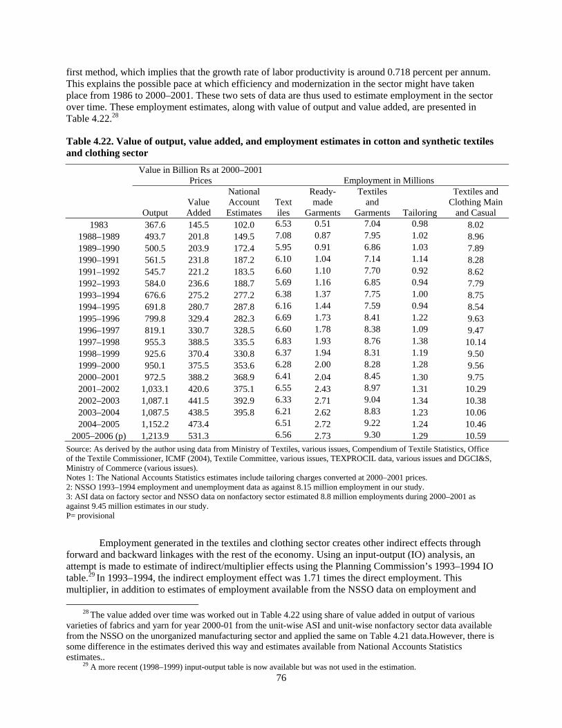
76

first method, which implies that the growth rate of labor productivity is around 0.718 percent per annum. This explains the possible pace at which efficiency and modernization in the sector might have taken place from 1986 to 2000–2001. These two sets of data are thus used to estimate employment in the sector over time. These employment estimates, along with value of output and value added, are presented in Table 4.22.28

Table 4.22. Value of output, value added, and employment estimates in cotton and synthetic textiles and clothing sector

Value in Billion Rs at 2000–2001

Prices Employment in Millions

Output Value Added

National Account Estimates

Textiles

Ready-made

Garments

Textiles and

Garments Tailoring

Textiles and Clothing Main

and Casual 1983 367.6 145.5 102.0 6.53 0.51 7.04 0.98 8.02

1988–1989 493.7 201.8 149.5 7.08 0.87 7.95 1.02 8.96 1989–1990 500.5 203.9 172.4 5.95 0.91 6.86 1.03 7.89 1990–1991 561.5 231.8 187.2 6.10 1.04 7.14 1.14 8.28 1991–1992 545.7 221.2 183.5 6.60 1.10 7.70 0.92 8.62 1992–1993 584.0 236.6 188.7 5.69 1.16 6.85 0.94 7.79 1993–1994 676.6 275.2 277.2 6.38 1.37 7.75 1.00 8.75 1994–1995 691.8 280.7 287.8 6.16 1.44 7.59 0.94 8.54 1995–1996 799.8 329.4 282.3 6.69 1.73 8.41 1.22 9.63 1996–1997 819.1 330.7 328.5 6.60 1.78 8.38 1.09 9.47 1997–1998 955.3 388.5 335.5 6.83 1.93 8.76 1.38 10.14 1998–1999 925.6 370.4 330.8 6.37 1.94 8.31 1.19 9.50 1999–2000 950.1 375.5 353.6 6.28 2.00 8.28 1.28 9.56 2000–2001 972.5 388.2 368.9 6.41 2.04 8.45 1.30 9.75 2001–2002 1,033.1 420.6 375.1 6.55 2.43 8.97 1.31 10.29 2002–2003 1,087.1 441.5 392.9 6.33 2.71 9.04 1.34 10.38 2003–2004 1,087.5 438.5 395.8 6.21 2.62 8.83 1.23 10.06 2004–2005 1,152.2 473.4 6.51 2.72 9.22 1.24 10.46

2005–2006 (p) 1,213.9 531.3 6.56 2.73 9.30 1.29 10.59 Source: As derived by the author using data from Ministry of Textiles, various issues, Compendium of Textile Statistics, Office of the Textile Commissioner, ICMF (2004), Textile Committee, various issues, TEXPROCIL data, various issues and DGCI&S, Ministry of Commerce (various issues). Notes 1: The National Accounts Statistics estimates include tailoring charges converted at 2000–2001 prices. 2: NSSO 1993–1994 employment and unemployment data as against 8.15 million employment in our study. 3: ASI data on factory sector and NSSO data on nonfactory sector estimated 8.8 million employments during 2000–2001 as against 9.45 million estimates in our study. P= provisional

Employment generated in the textiles and clothing sector creates other indirect effects through forward and backward linkages with the rest of the economy. Using an input-output (IO) analysis, an attempt is made to estimate of indirect/multiplier effects using the Planning Commission’s 1993–1994 IO table.29 In 1993–1994, the indirect employment effect was 1.71 times the direct employment. This multiplier, in addition to estimates of employment available from the NSSO data on employment and

28 The value added over time was worked out in Table 4.22 using share of value added in output of various varieties of fabrics and yarn for year 2000-01 from the unit-wise ASI and unit-wise nonfactory sector data available from the NSSO on the unorganized manufacturing sector and applied the same on Table 4.21 data.However, there is some difference in the estimates derived this way and estimates available from National Accounts Statistics estimates..

29 A more recent (1998–1999) input-output table is now available but was not used in the estimation.

77

unemployment for 1994–1995, was used to derive the total direct and indirect employment generation in the textiles and clothing sector, which was estimated at 32.4 million in 1994–1995. However, the multiplier of the coefficient derived using the 1993–1994 IO may have changed due to two reasons that may generate opposing effects. First, technological progress in the textiles and clothing sector has taken place at a faster pace as compared with sectors creating the backward and forward linkage related to the textiles and clothing industry. Second, the shift in fiber composition from cotton to synthetic fiber has resulted in a rise in the capital intensity of the raw material sector. Thus, we tried to assess the direct and indirect employment generation in the textiles and clothing sector using unitwise data from the NSSO 55th Round for 1999–2000. Based on this data set, it is estimated that the textile and clothing industry had direct employment of 10.5 million in 1999–2000. From the same data set, it is also derived that employment in sheep rearing and shorn wool production, sericulture, and cotton was 7.7 million, and in wholesale and retail of textiles and garment products, it was 3 million. Thus, the total direct and indirect employment in the farm and retail sectors was estimated at 21.2 million for 1999–2000, which indicates that the multiplier coefficient is far lower than the indirect multiplier of 1.71. The indirect employment estimate of 10.7 million, however, does not include employment generated in the transport and other indirect services required in the textiles and clothing sector. Thus, if these costs are also included (which are difficult to estimate) in the multiplier for 1999–2000, the multiplier coefficient may only be marginally lower compared with the 1.71 estimated for 1993–1994 using the IO data.

4.5. Apparel Retailing in India The large size of the Indian market for clothing reflects its huge population base and rising incomes. In 2005, the amount of spending on textiles and clothing items by the household sector was estimated at Rs 1,435 billion (US$32.5 billion). This amount does not include tailoring charges, however, which are around 7.4 percent of the retail value of cloth on the basis of the average varieties of cloth consumed. If this cost is included, the total household sector spending on textiles and clothing items is estimated at Rs 1,541 billion (US$34.9 billion), which is 21.6 percent of the total consumption of households. The total retail value of cloth for household and nonhousehold sectors, excluding stitching charges, is estimated at Rs 2,087 billion (US$47.2 billion); including tailoring charges, it is Rs 2,242 billion (US$50.7 billion).30

The total value of retail sales in 2005 was estimated at Rs 2,998 billion,31 including domestic consumption and Rs 756 billion in exports. Exports constituted 25 percent, household expenses 67 percent, and nonhousehold expenses 8 percent of the total retail sale value of cloths, plus stitching charges, in 2005–2006.

Consistent with these aggregates, Table 4.23 indicates that the average margin on textile and clothing products was 109 percent in 1999, 126 percent in 2003, 139 percent in 2005, and 127 percent in 2005. The high margins may be due to the long chain of wholesalers and retailers involved from the production stage to the final consumer stage. The comparison of production and consumption estimates, along with the NSSO data on per unit margin for wholesaler and retailer in Table 4.24, indicates that on average, two wholesalers and two retailers, along with duties, could add up to a margin that is close to 100 percent. The margin for two wholesalers and four retailers will add up to 122.74 percent for cotton textile products and 106.72 percent for garments. The per unit margin is increasing over time due to the emergence of sophisticated high-cost sale retailers.

30 Among other estimates, in the national accounts, expenditures on clothing account for 4.7 percent total private

consumption expenditure. IMAGES KSA TECHNOPAK estimated the size of retailing at Rs 930 billion (2003–2004), which is a low estimate. Textile Outlook International estimated the clothing needs of household and nonhousehold sector at Rs 620 billion (US$12.8 billion), another lower estimate.

31 The expenditure on clothing of all fibers, including floor covering, handicraft items, and coir, was estimated at Rs 3,091 billion in 2005.

78

Table 4.23. Comparison of production and consumption of total fabrics and garments estimates (in Rs billion)

Consumption Expenditure in Margin (%)

Year Household

Sector

Nonhousehold

Sector

Exports of Fabrics

and Garments

Total Fabrics

and Garments

Production: Total

Fabrics and Garments

Value of Consumption/Production

Value of Consumption/Pr

oduction 1999 908.7 366.7 399.4 1,674.8 800.7 209.17 109.17 2003 1,179.7 455.1 490.9 2,125.7 942.1 225.63 125.63 2004 1,337.9 598.3 473.3 2,409.5 1,008.7 238.87 138.87 2005 1,435.1 641.8 506.1 2,583.0 1,137.5 227.08 127.08

Source: As derived by the author using data from Ministry of Textiles, various issues, Compendium of Textile Statistics, Office of the Textile Commissioner, ICMF (2004), Textile Committee, various issues, TEXPROCIL data, various issues and DGCI&S, Ministry of Commerce (various issues).

Table 4.24. Average trade margins and extent of wholesaler and retailers (average trade margin, %)

Commodity Group

Wholesaler Trade

Margin

Retailer Trade

Margin

One Wholesaler

and One Retailer

Two Wholesalers and

Two Retailers

Two Wholesalers

and Four Retailers

Cotton textiles 9.40 16.80 27.78 63.28 122.74 Other textiles 10.00 17.60 29.36 67.34 131.43 Hosiery goods 13.30 17.40 33.01 76.93 143.86 Ready-made garments 13.20 12.70 27.58 62.76 106.72

Source: NSS (1997): Small Trading Units in India: NSS 53rd Round: January-December 1997.

It appears that on average, there may be two wholesalers and two retailers involved. First there is the wholesale dealer, who purchases fabrics from the factory and sells them to various wholesalers throughout the main cities across the country. The wholesaler in the main city sells the fabrics to larger retailers spread across various medium and large cities and to a few customers. These large retailers sell to the retailers that are scattered across the country in various small and large cities. Apart from selling to the customers, these retailers also sell to a large number of retailers in villages. Considering all of this and taking into account that the wholesaler’s and retailer’s margins do not include various costs such as labor, transport, rent, and the like, one can see that costs could easily build up, especially considering that on average there are two wholesalers and two retailers.

It is estimated that clothing expenditures expanded by 10 percent annually in nominal terms and 6.55 percent in real terms from 1990–1991 to 2005–2006. Because the importance of tailoring is still high among Indian consumers, a large number of shops concentrate on selling textiles rather than clothing. Data from the NSSO Employment and Unemployment Survey (1999) confirms this. It is estimated that the retail sale of textile products employed 1.87 million persons in 1999–2000, compared with the 0.78 million employed in garment retailing. According to NSSO data, small units dominated most of the retail market in this segment. Out of the total 2.65 million workers employed in the retail textiles and clothing segment in 1999–2000, 65.9 percent were either self-employed or family-owned workers. Regular employees accounted for only 1.4 percent, and casual workers the remaining 32.7 percent.

4.6. Growth Potential of the Indian Textiles and Clothing Industry At present, the world clothing market is dominated by buyer-driven commodity chains (Gereffi 2000, www.fiber2fashion.com, 2004). Large retailers and branded marketers play pivotal roles along global supply chains by setting up decentralized production networks linked to developing countries and by

79

coordinating the range of activities involved in clothing design, production, and marketing. Many of these firms are interested in creating large-scale operations located in a few countries. So far, China has been the supplier of choice as the industry adjusts to the post-MFA environment. However, international firms are also increasingly interested in India as a source of supply, to reduce risk through diversification and because of the growing perception of India as a competitive clothing supplier with domestic sources of fabric. Interest in India has intensified due to the removal of MFA quota constraints. Large global retailers, such as Wal-Mart, JCPenney, The Gap, Ikea (Sweden), Cades (France), and OTTO (Germany), as well as branded marketers, such as Calvin Klein, Lacoste, and Sara Lee, are attracted to India because of its potential to provide one-stop shopping. Wal-Mart has expressed willingness to buy goods worth US$7–US$10 billion from India over the next two years, provided local companies assure quality products, make timely delivery, and offer competitive prices (www.fiber2fashion.com, 2004). JCPenney also plans to make India an important sourcing hub for apparel, recently expressing willingness to buy $2 billion worth of products annually (www.fiber2fashion.com, 2004).

An attempt has been made to look at the future growth potential of the Indian textiles and clothing industry until 2015–2016. In this exercise, it is assumed that the economy would continue to grow at a high rate and that the WTO would not allow any restrictive practices in international trade. Moreover, it is expected that the Indian government would be able to act in a manner so as to facilitate the sector’s growth. The segmentwise growth prospects are discussed in the following chapters.

4.6.1. Domestic Demand

In the domestic market, high economic growth beginning in the early 1990s, together with declining real prices of yarns and textiles, stimulated the growth in demand for textile products, particularly those blended with synthetic fibers. Real prices of cotton yarns and textiles have declined since the mid-1990s, mainly due to lower prices of raw cotton. However, there has also been a steep decline in prices of synthetic fibers and yarns by about 10 percent annually in real terms since 1990. The decline in the price of synthetic products was driven by lower international prices of raw materials, as well as by reduced tariffs and excise rates in India.

To quantify the future domestic demand prospects, we estimated single-equation demand functions for cotton and synthetics.32 The following assumptions were also made: (1) a change in the wholesale price of synthetic products of between –10 and +20 percent per year, (2) an increase in the relative price of cotton to synthetic of between 10 and 40 percent, (3) GDP average growth of 8 to 10 percent, and (4) population growth of 1.7 percent per year. Under these assumptions, the per capita consumption of fiber will increase from 32.9 square meters (3.60 kilograms) to a range of 56.9 to 75.4 square meters (5.34 to 7.22 kilograms), as shown in Table 4.25. The share of cotton fiber will decline from 54.9 percent in 2005–2006 to a range of 35.2 to 38.0 percent in 2015–2016. This share will be below the international average standard. In terms of fabrics, the share of cotton fabrics in total per capita consumption will decline from 29.9 per cent to a range of 12.2 to 17.3 percent in 2015–2016. The total demand of fabrics will grow from 36,342 million square meters in 2005–2006 to a range of 74,159 and 98,205 million square meters. This demand will translate to a growth range between 5.77 and 9 percent per annum from 2005–2006 to 2015–2016.

32 The equations are: Cottqt = - 1.237*RPt + 0.3643*PCGDPt + 0.2049 *et-1 r2bar = 0.8998 DW = 1.97208 (t=-9.322) (t=2.746) (t=3.655) where Cottqt is per capita households demand of cotton textiles and clothing in quantity; RPt is relative wholesale price of

cotton/price of man-made products; PCGPt is per capita gross domestic product; and et-1 is one year lag error term. Manq* t = - 0.2260* MANP*t + 0.7509*PCGDPt r2bar = 0.9772 DW = 1.90 (t=2.43) (t=2.746) where Manq t is per capita households demand of synthetic textiles and clothing in quantity; MANPt is wholesale price of

synthetic products; PCGDPt is per capita gross domestic product; and et is error term. This equation is transformed using ρ to solve the problem of autocorrelation in the initial model. Manq* t = Manq t - ρManq t, MANP*t = MANPt - ρMANPt, PCGDP*t = PCGDPt - ρPCGDPt, μt = εt - ρεt and B0=γ-ργ.

80

Table 4.25. Demand forecasts

Per Capita Consumption

(square meters) Cotton Fabrics

Synthetic Fabrics Total

Cotton Fiber

Synthetic Fiber/

Filament Total

Cotton Fiber Share

Cotton Synthetic Total Million square meters Million kilograms (kg) Year 2005–2006 9.9 23.1 32.9 10,867 25,475 36,342 2,184 1,792 3,975 54.9 2015-16: Scenario A: with following four alternatives:

Alternative I: increase in relative prices of cotton: 10%

10.8 51.6 62.4 14,143 67,291 81,434 3,195 4,719 7,914 40.4

Alternative II: increase in relative prices of cotton: 20%

9.8 50.8 60.6 12,766 66,269 79,035 2,944 4,647 7,591 38.8

Alternative III: increase in relative prices of cotton: 30%

8.7 50.0 58.8 11,388 65,248 76,636 2,693 4,576 7,269 37.0

Alternative IV: increase in relative prices of cotton: 40%

7.7 49.3 56.9 10,011 64,226 74,237 2,442 4,504 6,946 35.2

Year 2005–2006

9.9 23.1 32.9 10,867 25,475 36,342 2,184 1,792 3,975 54.9 2015-16: Scenario B: with following four alternatives:

Alternative I: increase in relative prices of cotton: 10%

11.7 63.7 75.4 15,311 83,007 98,318 3,569 5,821 9,390 38.0

Alternative II: increase in relative prices of cotton: 20%

10.7 62.9 73.6 13,934 81,985 95,919 3,318 5,750 9,068 36.6

Alternative III: increase in relative prices of cotton: 30%

9.6 62.1 71.7 12,556 80,964 93,520 3,067 5,678 8,745 35.1

Alternative IV: increase in relative prices of cotton: 40%

8.6 61.3 69.9 11,179 79,942 91,121 2,816 5,606 8,422 33.4

Source: Author’s calculations Note: Scenario A: GDP growth of 8% per year; population growth of 1.686%, and four scenarios of increase in relative prices of cotton: 10%, 20%, 30%, and 40% until 2015–2016. Scenario: B: GDP growth of 10% per year, population growth of 1.686%, and four scenarios of increase in relative prices of cotton: 10%, 20%, 30%, and 40% until 2015–2016.

81

4.6.2. Export Potential

Exports of textiles and clothing, which stagnated after 2000, surged by 25 percent in 2005–2006. This may be due to the impact of the phase out of the MFA and the reimposition of restrictions on China’s exports into the U.S. and E.U. markets. These developments present major opportunities for potentially large suppliers such as India to gain additional share in the global market for textile and clothing products. However, for India to gain from these opportunities, several issues have to be addressed: (1) the low supply of synthetic products and the lack of availability of quality fabrics to the garments industry; and (2) the need to rationalize the structure of custom duties on synthetic fiber/filament to make it competitive.

In 2005–2006, cotton fabrics equivalent exports were estimated at 7,105 million square meters and synthetic fabrics at 1,889 million square meters. At present, synthetic fabrics equivalent exports account for 21 percent of the total Indian cotton and synthetic fabrics equivalent exports. Thus exports of synthetic products have a major potential for growth. It is estimated that exports of synthetic fabrics will grow at a rate of 17 percent per annum, whereas cotton will only grow at 6.7 percent. At this rate, the share of synthetic in total fabrics equivalent export will increase to 40 percent by 2015–2016. According to CRISIL (2006), world trade in value terms will grow from $479 billion to $700 billion by 2012 and to $824 billion by 2015–2016—a growth of 5.57 percent per annum. In quantity terms, the expected growth in world trade will be 3.5 percent per annum. It is estimated that India’s export share in the world market will be around 7.2 percent in quantity terms by year 2015–2016—this is from the present level of 4.0 percent. This translates to about US$59 billion of export value by 2015–2016, or about 15.5 percent per annum growth in nominal dollar terms. The exports of cotton fabrics equivalent may reach 13,641 million square meters, whereas synthetic fabrics may reach 9,080 million square meters. The total fabrics equivalent exports will grow from 8,994 million square meters to 22,721 million square meters by 2015–2016—a growth rate of 9.7 percent per annum..

In sum, the total domestic and export demand for cotton fabrics will grow from 17,972 million square meters in 2005–2006 to a range of 23,601 to 28,875 million square meters in 2015–2016 (Table 4.26). This translates to a per annum growth of between 2.8 percent and 4.9 percent. The potentials for growth in synthetic fabrics are much higher—in the range of 10.4 to 12.9 percent per annum. Therefore, the demand for synthetic fabrics will increase from 27,364 million square meters to a range of 73,279 to 92,051 million square meters. The total demand for fabrics (cotton and synthetic) may be in the range of 96,880 to 120,926 million square meters from the present level of 45,336 million square meters, or a growth range of between 7.9 percent and 10.3 percent per annum. The demand for raw cotton will increase from 23.1 million kilograms to a range of 35.2 to 41.9 million kilograms. This means that the raw cotton fiber requirement in textiles and clothing products will grow to a range of 4.30 percent to 6.12 percent per annum from 2005–2006 to 2015–2016.

82

Table 4.26. Total fabrics and fiber equivalent requirements for domestic and export markets

Fabrics

(million square meters) Fiber

(million kilograms) Raw Cotton Requirement

Year Cotton Synthetic Total

Share of Cotton

(%) Cotton Synthetic Total

Share of Cotton

(%) Million bales

% Growth p.a.

2005–2006 17,972 27,364 45,336 39.6 3,929 2,251 6,180 63.6 23.1 Scenario A: with following four alternatives until 2015–2016

2015–2016 27,784 76,371 104,155 26.7 6,733 7,237 13,970 48.2 39.6 5.53 2015–2016 26,407 75,349 101,756 26.0 6,482 7,165 13,647 47.5 38.1 5.13 2015–2016 25,029 74,328 99,357 25.2 6,231 7,093 13,324 46.8 36.7 4.72 2015–2016 23,652 73,306 96,958 24.4 5,980 7,022 13,002 46.0 35.2 4.29

Scenario B: with following four alternatives until 2015–2016 2005–2006 17,972 27,364 45,336 39.6 3,929 2,251 6,180 63.6 23.1 2015–2016 28,952 92,087 121,039 23.9 7,107 8,339 15,446 46.0 41.8 6.11 2015–2016 27,575 91,065 118,640 23.2 6,856 8,267 15,124 45.3 40.3 5.73 2015–2016 26,197 90,044 116,241 22.5 6,605 8,195 14,801 44.6 38.9 5.33 2015–2016 24,820 89,022 113,842 21.8 6,355 8,124 14,478 43.9 37.4 4.92

Source: Author’s calculations Note:p.a.: per annum. Scenario A: GDP growth of 8% per annum and scenarios of increase in relative prices of cotton by 10%, 20%, 30%, and 40% until 2015–2016. Scenario B: GDP Growth of 10% per annum and scenarios of increase in relative prices of cotton by 10%, 20%, 30%, and 40% until 2015–2016.

4.7. Summary and Conclusions This chapter has provided an overview of the fiber-to-fabric-to retail market chain in India, where the industry was estimated to have provided employment to more than 12 million workers, 11.5 percent of manufacturing value added, and 16.5 percent of total export earnings in 2004–2005. Except for the spinning sector, the industry in India is dominated by small, fragmented, nonintegrated units. This fact is attributable to various tax, labor, and other regulatory policies that have favored small-scale, labor-intensive enterprises and have discriminated against large-scale, capital-intensive firms. Of the total industry employment, 81.5 percent is in marginal and small firms. This industry structure has negatively affected the competitiveness of the textiles and clothing industry. Policy reforms starting in the 1990s, including the de-reservation of garment production to only the small-scale sector in 2000 and development of export zones and labor market reforms—together with provision of investment support under a Technology Upgradation Fund Scheme since 1999—have induced recent technological developments. The Indian industry also has strengths arising from a relatively low-cost raw material base across diverse fibers, relatively low labor costs, and a well-developed network of research, development, design, and testing institutes.

In the raw cotton marketing and ginning sector, most units are small, with problems of contamination, outdated technology, lack of cleaning machinery, failure to use best management practices, and lack of implementation of adequate grades and standards. This contrasts with the spinning industry, which is dominated by medium and large units producing more than 90 percent of the output and total value added. During an early period of policy reform (1983–1990), increased demand led to better utilization of existing spindles and reduced idle capacity. In a second phase (1990–2005), investment in new spindles increased, and, as a result, the efficiency of the industry improved relative to the productivity level attainable with the most recent technology.

The textile industry is diverse and multifaceted, with a relative paucity of reliable data to fully characterize its production and input use. Official statistics are estimated to consistently overestimate output levels, those these are by differing amounts. The composition of yarns produced has evolved, but

83

this information has not been fully taken into account in the official estimation procedures. For 2005–2006, it was estimated that output was 44 million square meters, compared with the official estimate of nearly 49 million. Changes in textile policy from physical controls toward market-oriented incentives have also prompted changes in the types of units producing fabrics. The hand-loom sector declined continuously from one-quarter to less than 5 percent of output from 1983 to 2005, whereas the power-loom sector’s share increased from 44 percent to nearly 75 percent during that same period. Production of synthetic fabrics has also grown at almost twice the rate of cotton fabrics.

In terms of future prospects for the Indian cotton, textile, and apparel industries, the chapter emphasizes three dimensions. First, it calls for further investments in human resource development, particularly better efforts to integrate displaced skilled weavers from the hand-loom sector into productive employment as well as more coordination among the various training institutes. Second, it highlights the changing patterns of domestic demand and the emergence of more complex, modern retail marketing chains. Finally, the prospects for fabric demand through 2015–2016 are assessed as being potentially quite robust. Taking population growth into account and assuming relatively strong economic growth, modest changes in real prices of synthetic fibers, and modest increases in the relative price of cotton, total domestic fabric demand will likely increase between 5 and 9 percent annually, with the share of cotton declining from 55 percent in 2005–2006 to less than 40 percent in 2015–2016. The end of the MFA opens new opportunities for India in export markets, provided the industry can address key challenges, including its relatively low utilization of synthetic fibers. In total, from the domestic and export markets, one can predict that a vibrant growth path for the industry is possible.

84

ENDNOTES

Endnote 4.1. The data on the registered factory sector are taken from ASI, while the data on the nonfactory sector are from the NSSO survey on unorganized manufacturing sector. The latest data on the unorganized manufacturing sector is available for 2000–2001. This is used together with the data on the organized manufacturing sector or the factory sector for the same year. The factory sector consists of units of organized manufacturing sector (10 or more workers with power or 20 or more workers without power).1 All remaining manufacturing units fall into the unorganized sector. The NSSO surveys on the unorganized manufacturing sector are area frame-based and exclude all the manufacturing units covered in the ASI. Detailed information on the unorganized manufacturing sector is available through the follow-up enterprise surveys by the NSSO on unorganized manufacturing covering own account enterprises (OAEs), non-directory manufacturing establishments (NDMEs), and directory manufacturing establishments (DMEs). An OAE unit is operated without any hired worker employed on a fairly regular basis. If such an enterprise is engaged in manufacturing and/or repairing activities, it is called OAME. On the other hand, NDME is a manufacturing unit with fewer than six workers (household and hired workers taken together) of which at least one is a hired worker employed on a fairly regular basis. DME units fall under the unorganized sector with six or more employees with at least one of those being a hired worker employed on a fairly regular basis.

The classification of units into organized and unorganized sectors and the further break-up of the unorganized sector into OAME, NDME, and DME could be useful in finding the scale of operation, but the problem is that it cannot be linked with the official definition of small-scale industry (SSI). On the other hand, classification based on the official definition of the small-scale sector would not be able to distinguish the hand-loom from the power-loom sector, nor does the National Industrial classification 1998 (NIC 98) go into that kind of detail of processing activities. Thus, an attempt is made to divide the manufacturing sector in such a way as to capture the importance of the various sectors while at the same time linking it with gross value of plant and machinery2 by classifying into the followings categories: (1) marginal units, which include OAME and NDME units; (2) small units, which include DME and units with a GVP&M of less than or equal to Rs 10 million in 1997–1998 prices of the organized sector; (3) medium units, which include units with GVP&M of more than Rs 10 million to Rs 40 million in 1997–1998 prices of the organized sector; (4) large units, which include units with a GVP&M limit of more than Rs 40 million of the organized sector in 1997–1998 prices.3

For the weaving sector, the further classification of units into the following could be more useful for analysis: The OAME units in the case of weaving are likely to represent most of the hand-loom sector units. The NDME and DME units of the unorganized sector and units with fewer than Rs 10 million investments in 1997–1998 prices in gross value of plant and machinery4 are most likely to represent the

1 Specifically, the ASI surveys units from a list prepared by amalgamating (1) all factories registered under chapters 2m (i) and 2m (ii) of the 1948 Factories Act (i.e., factories employing 10 or more workers and using power, or 20 or more workers but not using power on any day of the preceding 12 months); (2) All bidi and cigar manufacturing establishments registered under the 1966 Bidi and Cigar Workers (Condition of Employment) Act and employing 10 or more workers using power or 20 or more workers without using power.

2 The units are reclassified using various definitions and investment criteria from the combined list of units prepared by amalgamating unitwise ASI and NSSO data on the unorganized sector.

3 The GVP&M values are expressed in 1997–1998 prices because this was the year when the limit for SSI was first raised to Rs 30 million from Rs 6 million. It was lowered to Rs 10 million in 1999–2000 because benefits of concessions meant for smaller units were being enjoyed by the larger units. The limit for SSI was not revised again until the Micro, Small, and Medium Enterprises Development (MSMED) Act 2006 was introduced. Under MSMED, micro enterprises are presently defined with investment in GVP&M up to Rs 0.25 million, small between Rs 0.25 million and Rs 50 million, and medium between Rs 50 and 100 million. The remaining units with GVP&M more than Rs 100 million are defined as large. Note that units with more than Rs 40 million GVP&M limit would be Rs 50 millions in 2000–2001 prices, the year for which these data are being analysed. Thus, the criteria adopted in this study have relevance in the context of MSMED as well.

4 Bedi (2007) found only a few units in the unorganized sector exceed the limit on GVP&M of more than Rs 10 million.

85

power-loom sector. Therefore this is the basis on which the analysis for these sectors has been undertaken.

Endnote 4.2. The minimum required spindles using 2005 technology at 100 percent utilization, which are required for the actual quantum of production of various count composition and fibers of spun yarn, are estimated for each year. For the 2005 technology, the production per spindle for a given count (e.g., 40s) is available from South Indian Textile Research Association (SITRA). For other counts and fibers, the ratios of comparative production per spindles compared with 40s are used from the SITRA norms.5 These norms were established based on a sample survey of various mills over time; despite the fact that technological changes have taken place over time, these ratios remained constant. This means that relative productivity remained the same for various count composition and fibers of spun yarn for various ages of spindles.6

To derive the minimum requirement of spindles at a given technology, a detailed knowledge of the various varieties of yarn being produced (fiber composition, count composition, carded and combed share, etc.) is required. The required spindles at 2005 technology for various years is estimated by adding the number of spindles required to produce the quantum of spun yarn of various varieties, fibers, and counts. The percentage of excess installed spindles compared with the minimum required at the latest technology available to produce a given count composition of spun yarn is estimated for each year. The comparison is then made by removing the gap due to closures of units or low utilization. If the gap due to technological difference compared with modern technology declines over time, it implies that there is technological development taking place. The inverse of excess use of spindles over time due to the technological gap is attributed to the change in productivity of working spindles. Similar analysis for labor can be undertaken based on SITRA norms for labor.

Endnote 4.3. An attempt is made to provide another set of estimates of fabric production by carefully working out count-range-wise conversion rates in a scientific manner. This requires information about (1) the nature of yarn—that is, fiber composition (cotton, blended, or synthetic) and mode of production (spun or filament), and so forth; (2) the count of yarn (i.e., its fineness or coarseness and ply of count); and (3) reed and pick of fabrics (cloth)—that is, the closeness of the weave. The count-range-wise conversion rates derived taking these three factors into account are applied to the count-range-wise yarn consumption of various fibers (sectorwise) to estimate the production of fabrics.

For working out the conversion rates of fabrics for various count ranges and varieties, the data on varietywise parameters are used. These data are available from the Ahmedabad Textile and Industry Research Association (AITRA, 1984), the 15th comprehensive study (second part) on interfirm comparison. The AITRA report has published details on various parameters, such as reeds, picks, and ply, for various fabrics produced in 33 mills. The data in the ATIRA report are collected through

Furthermore, a major share of the organized sector units is within the GVP&M limit of less than Rs 10 million.

5 The production norms could also be estimated using the following formula, which shows that production per spindle depends on the count of yarn produced as well as on the variety of yarn produced in a given technology. This formula was developed by experts in SITRA and is used only for the counts in which the norms are not available. SP = [(Spindle speed * 1000 * E)/{[(C)^1.5]*(44.4)*(3.14)*Tm}], where SP is production per spindle at various counts; spindle speed depends on the technology of spindle; E is efficiency, which depends on the time required to change sliver (efficiency varies from 82 percent to 95 percent and is better the higher the count); C is count; Tm = TPI * (Count)^(–0.5), where TPI stands for twist per inch. Thus, Tm depends on the variety of yarn and the count of yarn. The carded and combed share differs in various varieties of yarn such as hosiery, woven cone yarn, and woven hank yarn. It further depends on whether the yarn is meant for direct or indirect export or for domestic purposes.

6 SITRA (1993) and other SITRA publications on norms for spinning mills and norms for productivity

86

questionnaires. Based on this, the weight of fabrics for each variety is computed using a developed formula.7

The weight of fabrics is the inverse of the conversion rate from yarn to fabrics. This determines the quantity of fabric that can be produced per kilogram of yarn. However, the weighted conversion rate has to be estimated, which is done for each count range rather than for the entire range in order to take into account the changing composition of count ranges over time. The weightage of each variety is given according to the number of varieties produced from a particular count, the percentage of that count of yarn consumed for weaving, and the share of that count of yarn in total yarn used for weaving in its count range. This means yarn consumed for each count for weaving is distributed among major varieties produced from that count to estimate the count-range-wise weighted conversion rates. Yarn consumed for each count is estimated using various data sources. Data on the count-range-wise yarn produced in the mill sector have been available since 1983. Sectorwise and countwise consumption is available for the year 1983. For the other years, total delivery to various sectors is available. South India Mills Association (1996) data were used to estimate the countwise share within count ranges.8

Once the count-range-wise conversion rates for cotton fabrics are estimated for the mill sector, it can be used to compute the relative weight of fabrics made from various fibers and sectors in cases where the count used and variety of fabrics produced are of similar type. Bedi (2002) gave a detailed explanation of the difference in relative weight of similar types of fabrics due to the use of different fibers of spun yarn.

7 The formula is that weight of woven fabric in grams/square meter is equal to (Reeds x 39.37 x 1.06 x 1000) + (Picks x 39.37 x 1.09 x 1000) -------------------------------------- ----------------------------------------- (1690 x S2/Ply) (1690 x S1/Ply) where S1 and S2 are counts of yarn used for fabric products; S1 is warp count and S2 weft count. Warps are put first and are

kept loose in length. Wefts are put later widthwise. The number of ends per inch of weft length is called reeds. The number of warp ends per inch of weft length is called picks. The wefts require more yarn per square meter (1.09) than warp (1.06).

8 Some adjustments have been made in the SIMA data to incorporate a few important counts of yarn that were not produced in 1996 by SIMA mills. For these counts, the share within the count range is taken from other reports. Because there are only few counts that are dominantly produced within the count range irrespective of whether it is domestically used or exported or based on various regions, the results derived on the basis of regional reports will not cause too much deviation from the results. This seems true, as the results derived by using TEXPROCIL and AIFCOSPIN data do not differ much. The count ranges specified for yarn do not change much over the period of time, and hence the same conversion rates could be applied for a specific count range over the period of time.

87

REFERENCES

Ahmedabad Textile Industry Research Association and Ahmedabad Institute of Management Association. 1984. Inter-firm comparison of costs, productivity, and damage (composite mills). July to September, Ahmedabad, India

Annual Survey of Industries (ASI), 2000-01. Ministry of Statistics and Programme Implementation, Central Statistical Organisation (CSO), Kolkata, India

Apparel Export Promotion Council (AEPC), various issues, Handbook of export statistics, Ministry of Textiles, Govt. of India, New Delhi.

Association of Man Made Fibre Industry of India, Various reports, Mumbai, India.

Association of Synthetic Fibre Industry, Handook of Statistics on Man-Made Synthetic Fibre/Yarn Industry, Part-I, Mumbai, India.

Ahmedabad Textile Industry Research Association (ATIRA), Bombay Textile Research Association (BTRA), Northern India Textile Research Association (NITRA), South India Textile Research Association (SITRA). 1991. Norms for the textile industry.India.

Bedi, Jatinder S. 2000. Economic liberalisation and changes in the structure of the Indian textile industry. Thesis submitted to Jawaharlal Nehru University, Center for Economic Studies and Planning.

———. 2002a. Discrepancies in official estimates of production and employment in various sectors of textiles and clothing sector. Journal of Income and Wealth 24(1 and 2), January-December, pp 95-116.

———. 2002b. Economic reforms and textile industry: Performance and prospects. Delhi, India: Common Wealth Publisher.

———. 2003. Production productivity and technological change in Indian spinning sector. Indian Economic Review XXXVIII(2): 205–233.

Bedi, Jatinder S. and Banerjee, Purnendu K.2007. “Discrepancies and Validation of data of Various Segments of Indian Manufacturing Sector: Factory Sector & Non-Factory Sector and Small, Medium & Large Scale Manufacturing Sector.” Economic and Political Weekly, March.

Central Statistical Organisation, Economic Census. 2005. Ministry of Planning and

Programme Implementation Programme Implementation. Government of India. New Delhi. India.

———.National Accounts Statistics, 2006. Ministry of Planning and

Programme Implementation Programme Implementation. Government of India. New Delhi. India.

———.National Industrial Classification, All Economic Activities, 2006. Ministry of Planning and

Programme Implementation Programme Implementation. Government of India. New Delhi. India.

Chatterjee, C. 2006. Textile times, February-March, New Delhi: CITI.

CRISIL report in Vision for Indian Textiles and Clothing Industry, 2007–2012, Confederation of Indian Textile Industry document, 2006.

Cotton Textile Export Promotion Council. various issues. Handbook of export statistics. Bombay, India

Directorate General of Commercial Intelligence and Statistics(DGCI&S),various issues, Foreign Trade Statistics, Ministry of Commerce, Kolkata, India

Directorate of Cotton Development (Kipas Vikas Nideshalay, Mumbai), Department of Agriculture and Co-operation, Ministry of Agriculture. India.

East India Cotton Association, Mumbai, India

Economic Survey, 2004-05, 2005-06, 2006-07, 2007-08, Government of India, Ministry of Finance, Economic Division, New Delhi.

88

Federation of Indian Textile Engineering Industry (FITE), various issues, Mumbai.

Gherzi Eastern Limited. 2002 & 2006. Cost Benchmarking Study: India viz a viz Bangladesh, Indonesia, China, Sri Lanka, and Pakistan. Mumbai, India.

Government of India. 1985. National textile policy. New Delhi: Lok Sabha Secretariat.

———. 2000. National textile policy. New Delhi: Lok Sabha Secretariat.

Indian Cotton Mills’ Federation. 2004. Handbook of statistics on cotton textile industry. New Delhi: Author.

International Textile Manufacturing Federation(ITMF), various issues, Werner International Inc. Management Consultants. Brussels, Belgium.

Jain, L. C. 1983. Handlooms face liquidation—Powerlooms mock at Yojana Bhavan. Economic and Political Weekly I, August 27.

Indian Cotton Mills’ Federation. various issues. Handbook of statistics on cotton textile industry, New Delhi: Author.

KSA Technopak, 2005, India Retail Report, India.

KSA Technopak. KSA Consumer Outlook 2005. KSA Technopak, Guragaon. India.

Mazumdar, D. 1984. The issue of small versus large in the Indian textile industry. Working Paper 645, World Bank, Washington, DC.

———. 1991. Import-substituting industrialisation and protection of the small-scale: The Indian experience in the textile industry. World Development 19(9).

Ministry of Agriculture. 2005. Agriculture statistics at glance. Directorate of Economics and Statistics, Government of India, New Delhi.

———. Various issues. Cotton Advisory Board, India.

Ministry of Finance. Various issues. Economic survey. Economic Division.

Ministry of Textile. 1989. Report of the Working Group on Textile Industry for the Eighth Five-Year Plan, Government of India, New Delhi..

———. 2005. Annual report, 2005-2006, Government of India New Delhi.

———. Various issues. Compendium of textile statistics. Mumbai, India: Office of the Textile Commissioner.

Misra, Sanjiv. 1993. India’s textile sector: A policy analysis. Delhi: Sage Publications.

Modak, S. 2006. FABINDIA weaving customers’ dreams. Economic and Political Weekly, August 5.

National Industrial Classification (NIC). 1998. India

———. National Sample Survey (NSS), Central Statistical Organisation, quinquennial rounds i.e. 43rd, 50th, 55th and 61st round for the period 1987-88, 1993-94, 1999-2000 and 2004-05, consumer expenditure surveys, Ministry of Statistics and Programme Implementation, Government of India New Delhi.

———. 1999. Employment and Unemployment. 55th Round Survey. Ministry of Statistics and Programme Implementation, New Delhi, Government of India.

———.2000-01,Unorganised Manufacturing Sector in India 2000-01, 56th Round, Ministry of Statistics and Programme Implementation, New Delhi, Government of India.

National Sample Survey Organization (NSS0). 1997. Small trading units in India. 53rd Round, January–December.

Navsharn, S., and M. K. Sapra. 2003. Economic liberalisation and informality: Case study from garment sector. Textile Policy, November.

Sastry, D. U. 1984. The cotton mill industry in India. Delhi: Oxford University Press.

Sen, A., ‘Estimates of Consumer Expenditure and Its Distribution: Statistical Priorities after NSS 55th Round’, Economic and Political Weekly, December 16-22.

89

———.and Himanshu. 2004. “Poverty and Inequality in India– I & II.” Economic and Political Weekly, September 25.

South India Mills Association. Various issues. Coimbatore, India.

South India Textile Research Association. Various issues. Coimbatore, India.

Suri, K. C. 2006. Political economy of agrarian distress. Economic and Political Weekly, April 22.

Synthetic and Rayon Textile Exports Promotion Council, Man Made Fibers Textiles Exports Statistics, 2006-07.Mumbai, India.

Tamhene, V. K. 2005. Labour issues in textiles. Textile Times.

The TEXPROCIL, The Cotton Textile Export Promotion Council. Various issues. Mumbai, India. Available at: www.texprocil.org/contact.htm.

The TEXPROCIL, The Cotton Textile Export Promotion Council, Annual Report (2004–2005). Mumbai, India.

Textile Committee. 2001-02. Cotton ginning and pressing factories in India: A techno-economic study 2001–02 (73–76), Mumbai, India

———. Various issues. Market for textile and clothing. Market Research Wing, Ministry of Textiles, Mumbai, India

———. Various issues. Consumer purchase of textiles, non-household sectors. Ministry of Textiles, Mumbai, India.

Uday, Sekhar. 2004. Apparel retailing in India: Opportunities for foreign firms. Textile Outlook International, May–June.

UNCTAD. 1999. Quantifying the benefits obtained by developing countries from the generalized system of preferences. UNCTAD/ITCD/TSB/Misc.52, 7 October, Geneva, Switzerland

Verrer, Raoul. 1996. Competitiveness the International Challenge. Werner International Inc., Management Consultants. International Textile Manufacturing Federation (ITMF), Annual Conference, September 25. Washington DC

World Bank. 2005. World Development Report 2005. Oxford University Press, New Delhi

World Trade Organization. International Trade Statistics, Various Issues. Geneva. Available at: www.statistics@wto.org.

RECENT IFPRI DISCUSSION PAPERS

For earlier discussion papers, please go to www.ifpri.org/pubs/pubs.htm#dp. All discussion papers can be downloaded free of charge.

800. Cotton-textile-apparel sectors of Pakistan: Situations and challenges faced. Caesar B. Cororaton, Abdul Salam, Zafar Altaf, and David Orden, 2008.

799. Race to the top and race to the bottom: Tax competition in rural China. Yi Yao and Ziaobo Zhang, 2008.

798. Analyzing the determinants of farmers’ choice of adaptation methods and perceptions of climate change in the Nile Basin of Ethiopia. Temesgen Deressa, R.M. Hassan, Tekie Alemu, Mahmud Yesuf, Claudia Ringler, 2008

797. Economic transformation in theory and practice: What are the messages for Africa? Clemens Breisinger and Xinshen Diao, 2008.

796. Biosafety at the crossroads: An analysis of South Africa’s marketing and trade policies for genetically modified products. Guillaume P. Gruère and Debdatta Sengupta, 2008.

795. Publish or patent? Knowledge dissemination in agricultural biotechnology. An Michiels and Bonwoo Koo, 2008. 794. Agricultural growth and investment options for poverty reduction in Malawi. Samuel Benin, James Thurlow, Xinshen

Diao, Christen McCool, Franklin Simtowe, 2008. 793. China: Shadow WTO agricultural domestic support notifications. Fuzhi Cheng, 2008.

792. India: Shadow WTO agricultural domestic support notifications. Munisamy Gopinath, 2008.

791. Agricultural growth and investment options for poverty reduction in Zambia. James Thurlow, Samuel Benin, Xinshen Diao, Henrietta Kalinda, and Thomson Kalinda, 2008.

790. Agricultural growth and investment options for poverty reduction in Uganda. Samuel Benin, James Thurlow, Xinshen Diao, Allen Kebba, Nelson Ofwono, 2008.

789. Agricultural public spending in Nigeria. Tewodaj Mogues, Michael Morris, Lev Freinkman, Abimbola Adubi, and Simeon Ehui; with Chinedum Nwoko, Olufemi Taiwo, Caroline Nege, Patrick Okonji, and Louis Chete, 2008.

788. Choosing sensitive agricultural products in trade negotiations. Sébastien Jean, David Laborde, and Will Martin, 2008.

787. An Updated Look at the Recovery of Agricultural Productivity in Sub-Saharan Africa. Alejandro Nin Pratt and Bingxin Yu. 2008

786. Migration, Poverty, and Inequality: Evidence from Burkina Faso. F.S. Wouterse. 2008

785. Insecticide use on vegetables in Ghana: Would GM seed benefit farmers? Daniela Horna, Melinda Smale, Ramatu Al-Hassan, José Falck-Zepeda, and Samuel E. Timpo, 2008.

784. Agriculture for development in Ghana: New opportunities and challenges. Clemens Breisinger, Xinshen Diao, James Thurlow, and Ramatu M. Al-Hassan, 2008.

783. Understanding the investment and abandonment behavior of poor households: An empirical investigation. Ruth Vargas Hill, 2008.

782. Access to irrigation and the escape from poverty: Evidence from Northern Mali. Andrew Dillon, 2008.

781. Structural changes in the Philippine pig industry and their environmental implications. Maria Angeles O. Catelo, Clare A. Narrod, and Marites M. Tiongco, 2008.

780. Evaluating alternative policy responses to higher world food prices: The case of increasing rice prices in Madagascar. David Coady, Paul Dorosh, and Bart Minten, 2008.

779. Contract farming of swine in Southeast Asia as a response to changing market demand for quality and safety in pork. Marites Tiongco, Maria Angeles Catelo, and Ma. Lucila Lapar, 2008.

778. On-site and off-site long-term economic impacts of soil fertility management practices: The case of maize-based cropping systems in Kenya. Ephraim Nkonya, Patrick Gicheru, Johannes Woelcke, Barrack Okoba, Daniel Kilambya, and Louis N. Gachimbi, 2008

777. Development under conditions of inequality and distrust: Social cohesion in Latin America. Marco Ferroni, Mercedes Mateo, Mark Payne, 2008.

INTERNATIONAL FOOD POLICY RESEARCH INSTITUTE

www.ifpri.org

IFPRI HEADQUARTERS

2033 K Street, NW Washington, DC 20006-1002 USA Tel.: +1-202-862-5600 Fax: +1-202-467-4439 Email: ifpri@cgiar.org

IFPRI ADDIS ABABA

P. O. Box 5689 Addis Ababa, Ethiopia Tel.: +251 11 6463215 Fax: +251 11 6462927 Email: ifpri-addisababa@cgiar.org

IFPRI NEW DELHI

CG Block, NASC Complex, PUSA New Delhi 110-012 India Tel.: 91 11 2584-6565 Fax: 91 11 2584-8008 / 2584-6572 Email: ifpri-newdelhi@cgiar.org