cost estimation chapter 7: single variable linear regression · chapter 7: single variable linear...

ICEAA 2016 Bristol – TRN 05

Cost Estimation

Chapter 7:Single Variable Linear Regression

Gregory K. Mislick, LtCol, USMC (Ret)Department of Operations Research

Naval Postgraduate School

y

• Regression Analysis is used to describe a statistical relationship between variables

• Specifically, it is the process of estimating the “best fit” parameters of a specified function that relates a dependent variable to one or more independent variables (including uncertainty)

Definition of Regression

Data Regressiony = xy = a + b x

x x

y

6 - 2


Basic Statistics vs. RegressionExample #1

6 - 3

• Consider the following data set of the cost of 15 homes that are for sale in a particular town, in the column to the right:

Home # Price ($)

1 300,000

2 400,000

3 350,000

4 800,000

5 450,000

6 250,000

7 225,000

8 450,000

9 550,000

10 400,000

11 220,000

12 350,000

13 365,000

14 600,000

15 750,000

Basic Statistics vs. RegressionExample #1 (cont)

• From Chapter 5, we learned how to find the Descriptive Statistics from this data set. Results are shown:

• Questions: What if you wanted to buy a house that was specifically 1,200 square feet in size? Or 2,000 sq ft?

• You cannot determine the cost for any house size from this data set! 6 - 4

Descriptive Statistics

Mean 430666.6667

Standard Error 45651.02269

Median 400000

Mode 400000

Standard Deviation 176805.6506

Sample Variance 31260238095

Kurtosis 0.194942263

Skewness 0.92371377

Range 580000

Minimum 220000

Maximum 800000

Sum 6460000

Count 15



• Here is where Regression Analysis can help greatly.

• What was missing from the previous data set was the size of each home with its associated cost.

• Note the new data set to the right now showing the size of each home along with its cost.

6 - 5

Home# Price($) Square Feet

1 300,000 1400

2 400,000 1800

3 350,000 1600

4 800,000 2200

5 450,000 1800

6 250,000 1200

7 225,000 1200

8 450,000 1900

9 550,000 2000

10 400,000 1700

11 220,000 1000

12 350,000 1450

13 365,000 1400

14 600,000 1950

15 750,000 2100


• With Cost as the Dependent variable, and Square Feet as the Independent (or explanatory) variable, we calculate the following regression results:

Cost = -$311,221.87 + $450.539 * # Square Feet

• We can now answer the Questions from Slide #4:

• Predictions: 1200 sq ft = $229,424.93

• 2,000 sq ft home = $589,856.13 6 - 6

SUMMARY OUTPUT

Regression Statistics

Multiple R 0.919362365 Cost vs Square Feet

R Square 0.845227157

Adjusted R Square 0.833321554


Observations 15

ANOVA

df SS MS F Significance F

Regression 1 3.69908E+11 3.69908E+11 70.99406372 1.26178E‐06

Residual 13 67735302725 5210407902

Total 14 4.37643E+11

Coefficients Standard Error t Stat P‐value Lower 95%

Intercept ‐311221.8767 90000.56578 ‐3.45799911 0.004242478 ‐505656.2781

Square Feet 450.5396012 53.47144891 8.425797513 1.26178E‐06 335.021559


Basic Statistics vs. RegressionExample #1: Conclusions

• You are now able to come up with a “prediction” for any given house size due to the regression equation:

= -311,221.87 + 450.539 * Xor in words,

Cost = -$311,221.87 + $450.539 * # Square Feet

• Clearly, this is much more helpful and more informative than just using descriptive statistics.

• Note: Regression is not ALWAYS better than the Descriptive Statistics. If the R-squared is very low, and Standard Error is high, the basic statistics may be preferable to the regression.

6 - 7

Y

6 - 8

In A Linear Regression Model

• Cost is the dependent (or unknown) variable; generally denoted by the symbol Y.

• The system’s physical or performance characteristics form the model’s known, or independent, variables which are generally denoted by the symbol X.

• The linear regression model takes the following form:

Yi = b0 + b1Xi + ei

where b0 (the Y intercept) and b1 (the slope of the regression line) are the unknown regression parameters and ei is a random error term.


• If the dependent variable is a cost, the regression equation is often referred to as a Cost Estimating Relationship, or CER– The independent variable in a CER is often called a cost

driver. A CER may have one or multiple cost drivers:

Regression Analysis in Cost Estimating

CostCost Driver (multiple)

Power Cable Linear Feet

Power

CostCost Driver

(single)

Aircraft Design # of Drawings

Software Lines of Code

Power Cable Linear Feet

Po

wer

C

able

Co

st

Linear Ft

Examples of cost drivers:

Example with multiple (2) cost drivers:

CER

CER

6 - 9

Three Primary Symbols in Regression

You will see these on the next slide and continually throughout the regression chapters:

• Yi = any of the data points in your data set, and there are “i” of them

• = Y(hat) = the estimate or “prediction” of Y provided by the regression equation

• = Y(bar) = the mean or average of all “i” cost data points

6 - 10

Y

Y


6 - 11

• We desire a model of the form:

• This model is estimated on the basis of historical data as:

• In words: “Actual Cost” = “Estimated Cost” + “Error of Estimation”

Linear Regression Model

iid and ,),0(~

where2

10

xi

iii

Ne

exbby

xbbyx 10ˆ

y

x

b0Slope = b1

yx

Y

X

Y = b0 + b1X

b0

X1

X2

X3

“The True Purpose of What Regression is Trying to Accomplish”

6 - 12

minimum)ˆ(

residualsˆ)(2

10

yy

yyxbbye

i

iiii

The slope and intercept (b1 and b0) are chosen such that the sum of the squared residuals is minimized (Least Squares Best Fit). You are trying to minimize the difference between the actual cost (Yi) and your predicted cost ( ). Solving for the Error of Estimation, we get:

Y


6 - 13

Least Squares Best Fit (LSBF)

• To find the values of b0 and b1 that minimizes one may refer to the “Normal Equations.”

• With two equations and two unknowns, we can solve for b0and b1.

2)ˆ( yyi

2

10

10

XbXbXY

XbnbY

XbYn

Xb

n

Yb

XnX

YXnXY

n

XX

n

YXXY

XX

YYXXb

110

2222

21 )()(

)()(

6 - 14

Example #1 Revisited

• Let’s re-analyze the cost of the 15 homes for sale in the Example #1 data set.

• After computation, we found that the average sale price of all the homes in your data set was $430,666.67. Thus,

= $430,666.67• Then you developed an estimating relationship between

home price and its size in square feet using LSBF regression:

= -$311,221.87 + $450.539 * X• Now you want to estimate the home price of a 2,000 square

foot home:= -311,221.87 + 450.539 * X= -311,221.87 + (450.539 * 2,000)= $589,856.13

Y

Y

Y


6 - 15

Example #1 Conclusions

• What do these numbers mean?• $430,666.67 is the estimate of the average sale

price of all homes in that data set.• $589,856.13 is the estimate for a home in the

data set that has a size of 2,000 sq ft.

• We use regression to try to get a better “prediction” than just using the mean.

• Key Point: If the statistics for the regression are not very good, you can always go back and use the mean. A good regression means you prefer the regression equation as an estimator, instead of using the mean.

6 - 16

Another Example

• Recall the radio data in Ch 5 used on the mean and standard deviation. Now let’s look at the relationship between the average unit production costs and their associated weight:

System FY97$K Weight (lbs)1 22.2 902 17.3 1613 11.8 404 9.6 1085 8.8 826 7.6 1357 6.8 598 3.2 689 1.7 25

10 1.6 24

Historic TransmogrifierAverage Unit Production Cost

0

5

10

15

20

25

0 50 100 150 200

Weight (lbs)

FY

97$K


6 - 17

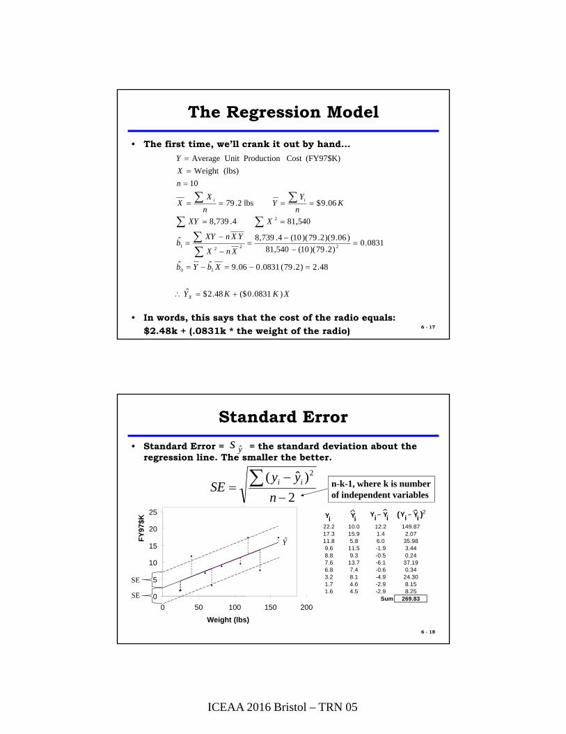
The Regression Model

• The first time, we’ll crank it out by hand...

• In words, this says that the cost of the radio equals: $2.48k + (.0831k * the weight of the radio)

XKKY

XbYb

XnX

YXnXYb

XXY

Kn

YY

n

XX

n

X

Y

X

ii

)0831.0($48.2$ˆ

48.2)2.79(0831.006.9ˆˆ

0831.0)2.79)(10(540,81

)06.9)(2.79)(10(4.739,8ˆ

540,814.739,8

06.9$lbs 2.79

10

(lbs)Weight

(FY97$K)Cost Production Unit Average

10

2221

2

6 - 18

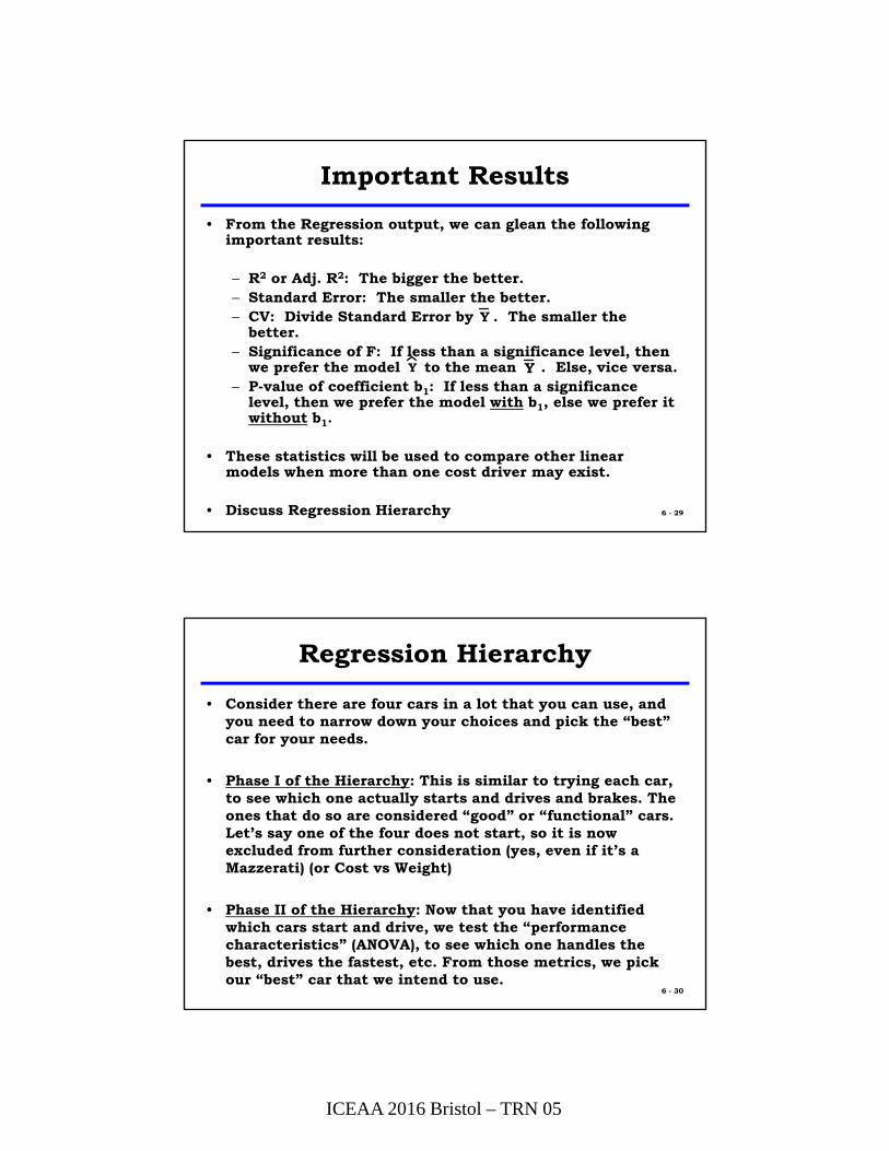
Standard Error

• Standard Error = = the standard deviation about the regression line. The smaller the better.

ys ˆ

2

)ˆ( 2

n

yySE ii n-k-1, where k is number

of independent variables

0

5

10

15

20

25

0 50 100 150 200

Weight (lbs)

FY

97$K

Y

22.2 10.0 12.2 149.8717.3 15.9 1.4 2.0711.8 5.8 6.0 35.989.6 11.5 -1.9 3.448.8 9.3 -0.5 0.247.6 13.7 -6.1 37.196.8 7.4 -0.6 0.343.2 8.1 -4.9 24.301.7 4.6 -2.9 8.151.6 4.5 -2.9 8.25

Sum 269.83

Yi YiYiYi YiYi( )2

SE

SE


6 - 19

Standard Error

• For the radio data, the standard error is $5.8K.• This means that on “average” when predicting the cost of

future systems we will be off by +/- $5.8K in one standard error.

Kn

yySE ii 8.5$

8

83.269

2

)ˆ( 2

0

5

10

15

20

25

0 50 100 150 200

Weight (lbs)

FY

97$K

Y

SE

SE

Standard Error vs Standard Deviation: Similar Concept, but……..

When working with Basic Statistics, you use

Standard Deviation

When performing a regression, you now use

Standard Error

6- 20

0

5

10

15

20

25

0 50 100 150 200

Weight (lbs)

FY

97$K

Y

SE

SE

)($4.449

8.399110

7.559.677.1721

)(

2

22

K

n

yys i


6 - 21

Coefficient of Variation

• Coefficient of Variation (CV):

• This says that on “average”, we’ll be off by 64% when predicting the cost of future systems. The smaller the better. In Ch5, CV was 73% with the same data, so using the regression is slightly better than just using univariate statistics.

%6406.9$

8.5$

K

K

Y

SECV

6 - 22

Analysis of Variance

• Analysis of Variance (ANOVA)

SSRSSESST

YYSSR

YYSSE

YYSST

i

ii

i

2

2

2

)ˆ(Regression Squares of Sum

)ˆ(Errors Squared of Sum

)(Squares of Sum Total

0

5

10

15

20

25

0 50 100 150 200

Weight (lbs)

FY

97$K

ii YY ˆ

YYi ˆYYi

Y

Y

Regressionby explainedVariation

Variation dUnexplaine

Variation Total

SSR

SSE

SST

df SS MS = SS/df F = MSR/MSESignificance F P(b1=b2=0)

SSR 1 130.00 130 (MSR) 3.85 0.0852SSE 8 269.83 33.7 (MSE)SST 9 399.82


6 - 23

Coefficient of Determination

• Coefficient of Determination (R2) represents the percentage of total variation explained by the regression model. The larger the better (as close to 1.0 as you can)

• Since R2 always increases when independent variables are added, Adj. R2 helps to adjust for the number of independent variables. This is necessary when comparing regression models with an unequal number of independent variables (i.e., one independent variable vs. two)

%5.323252.08.399

8.2691

8.399

130

1Variation Total

Variation Explained

2

2

R

SST

SSE

SST

SSRR

%1.242408.0

98.399

88.269

1

1

)1(12

n

SSTkn

SSER adj

6- 24

The F-Statistic

• The F statistic tells us whether the full model, , is preferred to the mean, .

• Say we want to test the strength of the relationship between our model and Y at the = 0.1 significance level...

YY

85.3

88.2691

130:statisticTest

)ˆ(prefer valid)is model (The false is :

)(prefer invalid) is model (The 0:

0

10

E

R

a

k

dfSSE

dfSSR

MSE

MSRF

YHH

YH

= 0.10

(1-) = 0.90

0

FC = 3.46

3.85

From F Table, Pg. 7-50with 1 numerator and 8 denominator d.o.f.

• Since 3.85 falls within the rejection region, we reject H0 and say the full model is better than the mean as a predictor of cost.


6 - 25

The t-statistic

• This statistic tests the marginal contribution of the independent variable on the reduction of the unexplained variation.

• In other words, it tests the strength of the relationship between Y and X (or between Cost and Weight) by testing the strength of the coefficient b1.

• The t-statistic is used to test the hypothesis that X and Y (or Cost and Weight) are NOT related at a given level of significance.

• If the test indicates that that X and Y are related, then we say we prefer the model with b1 to the model without b1, which is the desired result. xbbyx 10ˆ

6 - 26

The t statistic

97.1

16.1378.5

0831.0

)(

:statisticTest

)ht with weigmodel(prefer related) are weight and(Cost 0:

)eight without wmodel(prefer weight) torelatednot is(Cost 0:

2

1111

1

10

11

1

XXSE

b

s

b

s

bt

H

H

bb

a

1 = 0

• Say we wish to test b1 at the = 0.20 significance level. Refer to a T-Table with 8 degrees of freedom...

-1.397 1.397 1.97

/2 = 0.10/2 = 0.10

(1 - ) = 0.80 • Since our test statistic, 1.97, falls within the rejection region, we reject H0and conclude that we prefer the model withb1 to the model without b1.

0


F-Stats and T-Stats Summary

• There will always be only one F-stat in a regression, regardless of how many independent variables there are.

• There will always be one t-stat for each independent variable.

• Thus, in a single variable regression, there will be exactly one F-stat and one t-stat, and the F and t-stats will be virtually identical in value.

• In a two (three) variable regression, there will again be only one F-stat, and there will be exactly two (three) t-stats, one for each independent variable.

6 - 27

6 - 28

There’s an Easier Way...

• Linear Regression Results (Microsoft Excel):

Regression Statistics

Multiple R 0.5702

R Square 0.3251



Observations 10

ANOVA

df SS MS F Significance F

Regression 1 130.00 130.00 3.85 0.0852

Residual 8 269.83 33.73

Total 9 399.82

Coeffic ients Standard Error t Stat P-value Lower 95% Upper 95%

Intercept 2.477 3.823 0.648 0.535 -6.340 11.293

W eight (lbs) 0.083 0.042 1.963 0.085 -0.015 0.181

• Now the information we need is seen at a glance.


6 - 29

Important Results

• From the Regression output, we can glean the following important results:

– R2 or Adj. R2: The bigger the better.– Standard Error: The smaller the better.– CV: Divide Standard Error by . The smaller the

better.– Significance of F: If less than a significance level, then

we prefer the model to the mean . Else, vice versa.– P-value of coefficient b1: If less than a significance

level, then we prefer the model with b1, else we prefer it without b1.

• These statistics will be used to compare other linear models when more than one cost driver may exist.

• Discuss Regression Hierarchy

Y

YY

Regression Hierarchy

• Consider there are four cars in a lot that you can use, and you need to narrow down your choices and pick the “best” car for your needs.

• Phase I of the Hierarchy: This is similar to trying each car, to see which one actually starts and drives and brakes. The ones that do so are considered “good” or “functional” cars. Let’s say one of the four does not start, so it is now excluded from further consideration (yes, even if it’s a Mazzerati) (or Cost vs Weight)

• Phase II of the Hierarchy: Now that you have identified which cars start and drive, we test the “performance characteristics” (ANOVA), to see which one handles the best, drives the fastest, etc. From those metrics, we pick our “best” car that we intend to use.

6 - 30


A Note About Regression

• Ensure that when making a prediction using a regression equation, that the input of the independent variable (say Weight) is within the range of the data. If the smallest value for Weight was 100 lbs, and the largest value was 500 lbs, ensure that what you are trying to predict falls within the range of 100-500 lbs.

• Two Examples:– You are predicting the cost of a house based on square

feet, with historical square foot data values of between 1000 to 3000 sq ft. What if predicting the cost of a 3200 sq ft house?

– You are predicting the cost of an aircraft with maximum speeds of between 500 knots and Mach 2. What if predicting the cost of an aircraft with a max speed of Mach 2.3?

6 - 31

6 - 32

Treatment of Outliers

• In general, an outlier is a residual that falls greater than 2from or .

• The standard residual is

• Recall that since 95% of the population falls within 2 of the mean, then in any given data set, we would expect 5% of the observations to be outliers.

• In general, do not throw them out unless they do not belong in your population.

Y Y

Y

i

X

ii

s

YYor

s

XXor

SE

YY ˆ


6 - 33

Outliers with respect to X

• All data should come from the same population. You should analyze your observations to ensure this is so.

• Observations that are so different that they do not qualify as a legitimate member of your independent variable population are called outliers with respect to the independent variable, X.

• To identify outliers with respect to X, simply calculate and SX. Those observations that fall greater than two standard deviations from are likely candidates.

• You expect 5% of your observations to be outliers, therefore the fact that some of your observations are outliers is not necessarily a problem. You are simply identifying observations that warrant a closer investigation.

X

X

6 - 34

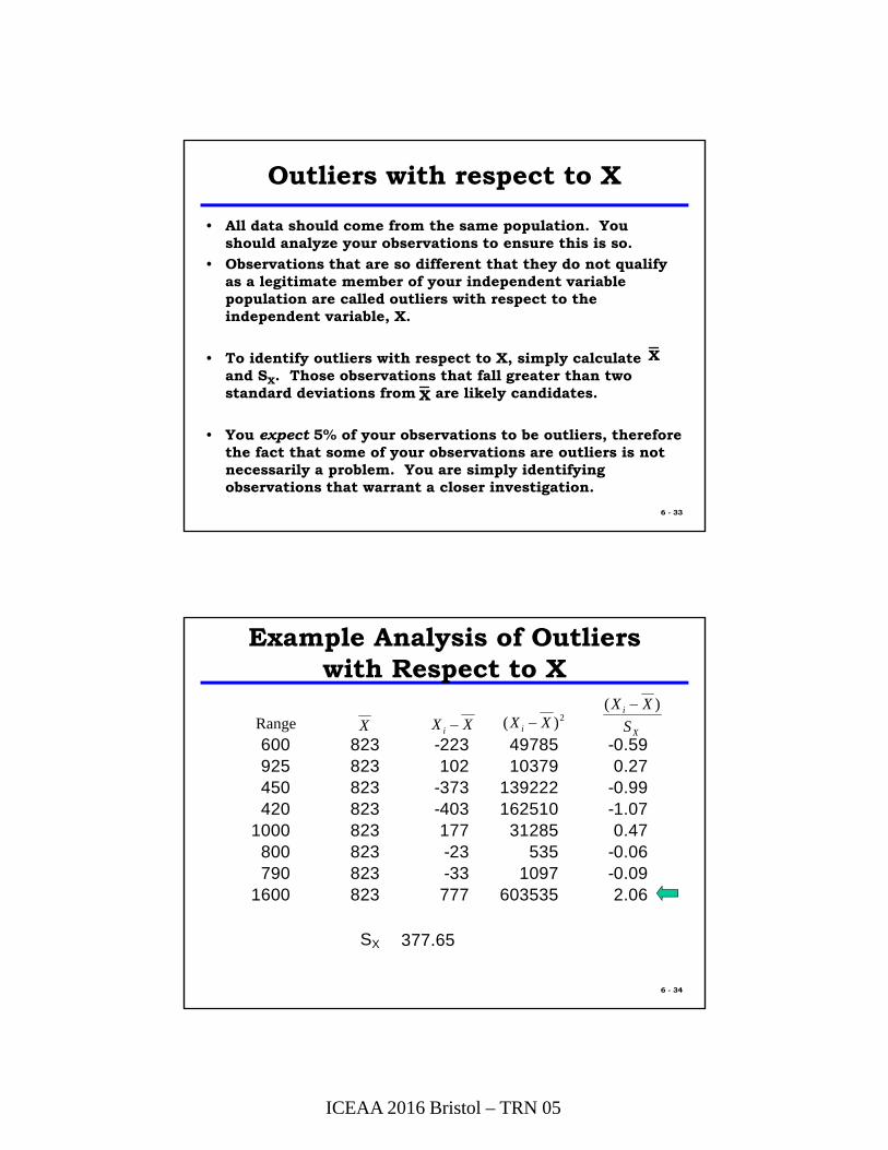
Example Analysis of Outliers with Respect to X

600 823 -223 49785 -0.59925 823 102 10379 0.27450 823 -373 139222 -0.99420 823 -403 162510 -1.07

1000 823 177 31285 0.47800 823 -23 535 -0.06790 823 -33 1097 -0.09

1600 823 777 603535 2.06

SX 377.65

Range X XXi 2)( XXi X

i

S

XX )(


6 - 35

Outliers with Respect to Y

• There are two types of outliers with respect to the dependent variable:– Those with respect to Y itself.– Those with respect to the regression model, .

• Outliers with respect to Y itself are treated in the same way as those with respect to X.

• Outliers with respect to are of particular concern, because those represent observations our model does not predict well.

• Outliers with respect to are identified by comparing the residuals to the standard error of the estimate (SE). This is referred to as the “standardized residual.”

• Outliers are those with residuals greater than ±2 std errors.

Y

Y

Y

Errors Standard of # )ˆ(

SE

YYi

6 - 36

Remedial Measures

• Remember: the fact that you have outliers in your data set is not necessarily indicative of a problem. The trick is to determine WHY an observation is an outlier.

• Possible reasons why an observation is an outlier.– Random Error: No problem– Not a member of the same population: If so, you want to

delete this observation from your data set.– You’ve omitted one or more other cost drivers.– Your model is improperly specified.– The data point was improperly measured (it’s just plain

wrong).– Unusual event (war, natural disaster).– Requires normalization.


6 - 37

Remedial Measures

• Your first reaction should not be to throw out the data point!

• Assuming the observation belongs in the sample, some options are:

– Dampen or lessen the impact of the observation through a transformation of the dependent and or independent variables.

– Develop two or more regression equations (one with and one without the outlier)

• Outliers should be treated as useful information.

Residual Analysis

• So what if you do a regression, and you find that the f-stats are high, the t-stats are high, R-squared’s are low, and Std Errors and CV’s are high? Not a good regression!

• Perhaps you are trying to fit a straight line to data that is not linear.

• How to tell? Plot the original data and see if it is linear or not.

• You can also check the residual plots.

6 - 38


6 - 39

Model Diagnostics

• If the fitted model is appropriate for the data, there will be no pattern apparent in the plot of the residuals versus Xi,

, etc. – Residuals spread uniformly across the range of X-axis

values

iY

0

ei

Xi

6 - 40

Model Diagnostics

• If the fitted model is not appropriate, a relationship between the X-axis values and the ei values will be apparent.

0

ei

Xi

0

ei

t0

ei

iY

0

ei

Xi

Nonnormal Distribution

}

} CurvilinearRelation

Heteroscedasticity

InfluentialRelation


6 - 41

• Data transformations should be tried when residual analysis indicates a non-linear trend:

X= 1/X X= 1/Y X= log X Y= ln Y Y= log Y

– CER are often non-linear when the independent variable is a performance parameter:

Y = aX b

log Y = log a + b log X Y= a + bX» log-linear transformation allows use of linear

regression» predicted values for Y are in “log dollars” which must

be converted back to dollars

Non-Linear Models

6 - 42

Other Concerns

• When the regression results are illogical (i.e., cost varies inversely with a physical or performance parameter), omission of one or more important variables may have occurred or the variables being used may be interrelated

– Does not necessarily invalidate a linear model

– Additional analysis of the model is necessary to determine if additional independent variables should be incorporated or if consolidation/elimination of existing variables is required


6 - 43

Assumptions of OLS

(1) Fixed X– Can obtain many random samples, each with the same X values but different Yi values due to different ei values

(2) Errors have mean of 0– E[ei] = 0

(3) Errors have constant variance (homoscedasticity)– Var[ei] = 2 for all I

(4) Errors are uncorrelated– Cov[ei,ej] = 0 for all i j

(5) Errors are normally distributed– ei ~ N(0, 2)


Estimating Skills Training In Methods Approaches Techniques & Analysis EST.i.MAT-A x

xxx

x

Multivariate Linear Regression andNon-Linear Regression

ICEAA 2016 International Training Symposium

Bristol, 17th to 20th October 2016

Alan R Jones

Estimata LimitedPromoting TRACEability in Estimating

Least Squares Non-Linear Regression

2


Simple Non-Linear Regression

3

Many Cost Estimating Relationships are not Linear

• When we plot cost data against a cost driver, it is often appears to be a curve• For example:

• Projecting curves is not as “Straight Forward” as is it for Straight Line Relationships

• This is where Logarithms often come to the rescue, where we express a number as the power to which a base value must be raised to get that number

• Why such glum faces? Does it bring back bad memories of school?

• A Learning Curve relationship curves down sharply from top-left to bottom-right

• Escalation (normally) causes cost to curve up from the bottom left to the top-right

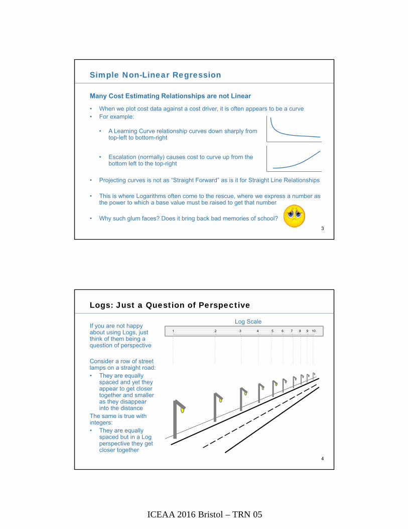
Logs: Just a Question of Perspective

4

1 2 3 4 5 6 7 8 9 10If you are not happy about using Logs, just think of them being a question of perspective

Consider a row of street lamps on a straight road:• They are equally

spaced and yet they appear to get closer together and smaller as they disappear into the distance

The same is true with integers:• They are equally

spaced but in a Log perspective they get closer together

Log Scale


Logs: Just a Question of a Different Perspective

5

In essence, relative to the Arithmetic Mean of the data (simple average):• Logs stretch the relative difference between equally spaced smaller values• and compress the relative difference between equally spaced larger values

Consider, the integers from 1 to 10, their average is 5.5

1 2 3 4 5 6 7 8 9 10

1 2 3 4 5 6 7 8 9 10

Mean

Scale CompressedS c a l e S t r e t c h e d

In certain circumstances we can use this property to unbend curves, giving us a straight line

Compress Scale

Stretch Scale

Mean

Linear Transformations: Summary

6

LinearFunction

y = m x + c

LogarithmicFunction

y = m log(x) + c

PowerFunction

log(y) = m log(x) + c

ExponentialFunction

log(y) = m x + c

Linear x Logarithmic x

Line

ar y

Loga

rithm

ic y

y-A

xis

Sca

le

x-Axis Scale

Why is this important?

If by plotting any of the combinations of:

x or Log(x)

against

y or Log(y)

we get a straight line, then we can perform a linear regression on the

transformed dataCurves and their transformations can have positive or negative gradients

There are three groups of functions that allow us to transform a relationship into a linear form


Linear Transformations

Logarithmic

y = a + b ln x

Exponential

y = a e b x

ln y = ln a + b x

Power

y = a x b

ln y = ln a + b ln x

Adapted from

7

X

ln Y

X

Y

ln X

Y

X

ln Y

X

Y

X

Y

X

Y

X

YX

Y

ln X

ln Y

ln X

ln Y

ln X

ln Y

ModelUnit Space Log Space

b < 0

b > 0

b < 0

b > 0

b > 1

b < 0 b < 0

b > 1

0 < b < 10 < b < 1

It doesn’t matter if we take Natural Logs (LN) or Common

Logs (base 10) or any other base

Function Types – A Word of Caution

8

We can use Logarithmic Transformation to convert many curved relationships into linear ones However, there are occasions when they should not be used …

Time is sometimes used as a secondary measure or indicator of technology, or project maturity:

We can take the Log of Elapsed Time,but we should NEVER take the Log of a Date!It presupposes that we know when time began … ask Stephen Hawkings

We can use a Binary Switch in Multi-variate Regression to signify whether a cost driver or cost element driver is active (1) or inactive (0)

NEVER take the Log of a Binary Switch!Log(0) implodes – it can’t be doneTaking the Log of any Numerical Categorical Variable (zero or not) is highly questionable from a logic perspective

Creates a #NUM! errorin Microsoft Excel


Adapted from

9

Determining the Appropriate Regression Model

• A scatter plot should always be performed first to determine what kind of model should be tested, if any at all:– Specifying the wrong function for a model can lead to an incorrect interpretation

of the results

0

5

10

15

20

0 5 10 15 20

0

5

10

15

20

0 5 10 15 20

0

5

10

15

20

0 5 10 15 20

0

5

10

15

20

0 5 10 15 20

Linear

Non-linearConstant

Data

Choosing the Appropriate Function Type

• Plot the data in Microsoft Excel with standard linear axes

• Right-click on the data. Select “Add Trendline…”

• Select the “Linear” option (default)

• Select “Display R-Squared Value on Chart”– Note the R-Squared Value

– Note the scatter pattern

• Change the Trendline Option, noting the changes in the R-Squared Value and scatter pattern of each:1. Exponential … only if all the y-values are positive

2. Logarithmic … only if all the x-values are positive

3. Power … only if all the x-values and y-values are positive

(We can’t take the Log of a non-positive number)

• As a general rule we are looking for the highest R-Squared Value and an “even” scatter around the Trendline (Homoscedastic) 10


Non-linear Regression Function Summary

• Before we can perform our Regression we must transform the data based on the Function Type

• Logarithmic => take the log of the x data

• Exponential => take the log of the y data

• Power => take the log of both x and y

Note: Other functions can be used to transform data (e.g., x, sin x, etc.) but logarithms are the most common

• Of these, Power Functions are the most common (e.g. Learning Curves, Cost/Weight CERs)

• Time-based relationships might be Exponential Functions (e.g. escalation)

• Logarithmic Functions are less common in practice (but never say “never”)

• We perform the Regression on the Transformed Data, and transform the output back to “real world” space afterwards

Adapted from:

It doesn’t matter which base of Logs we use LOG10 or LN, so long as we are consistent whentransforming back

LOG10 => Transform by raising 10 to the power of the OutputLN Transform by raising “e” to the power of the Output

11

R² = 0.8184

£4,000

£5,000

£6,000

£7,000

£8,000

£9,000

£10,000

£11,000

£12,000

- 20 40 60 80 100

Cos

t

Weight

Exponential Function

R² = 0.8301

£4,000

£5,000

£6,000

£7,000

£8,000

£9,000

£10,000

£11,000

£12,000

- 20 40 60 80 100

Cos

t

Weight

Power Function

R² = 0.8228

£4,000

£5,000

£6,000

£7,000

£8,000

£9,000

£10,000

£11,000

£12,000

- 20 40 60 80 100

Cos

t

Weight

Linear Function

R² = 0.7766

£4,000

£5,000

£6,000

£7,000

£8,000

£9,000

£10,000

£11,000

£12,000

- 20 40 60 80 100

Cos

t

Weight

Logarithmic Function

Example of Non-Linear Regression

12

Cost £ Weight Kg5123 106527 216388 349253 427722 59

9182 638348 71

10702 8511092 97

Plot the data as a scatter diagram and try each function type Trendline in turn

Look for the best (highest) R2

In this case the Power Function appears to be marginally better than the Linear or Exponential Functions

Linear Scale Log Scale


Lin

ea

r S

cale

Lo

g S

cale

Lin

ea

r S

cale

Lo

g S

cale


R² = 0.8184

£4,000

£5,000

£6,000

£7,000

£8,000

£9,000

£10,000

£11,000

£12,000

- 20 40 60 80 100

Cos

t

Weight


R² = 0.8301

£4,000

£5,000

£6,000

£7,000

£8,000

£9,000

£10,000

£11,000

£12,000

- 20 40 60 80 100

Cos

t

Weight

Power Function

R² = 0.8228

£4,000

£5,000

£6,000

£7,000

£8,000

£9,000

£10,000

£11,000

£12,000

- 20 40 60 80 100

Cos

t

Weight

Linear Function

R² = 0.7766

£4,000

£5,000

£6,000

£7,000

£8,000

£9,000

£10,000

£11,000

£12,000

- 20 40 60 80 100

Cos

t

Weight


R² = 0.8184

£4,000

£5,000

£6,000

£7,000

£8,000

£9,000

£10,000

£11,000

£12,000

- 20 40 60 80 100

Cos

t

Weight


R² = 0.8301

£4,000

£5,000

£6,000

£7,000

£8,000

£9,000

£10,000

£11,000

£12,000

- 20 40 60 80 100

Cos

t

Weight

Power Function

R² = 0.8228

£4,000

£5,000

£6,000

£7,000

£8,000

£9,000

£10,000

£11,000

£12,000

- 20 40 60 80 100

Cos

t

Weight

Linear Function

R² = 0.7766

£4,000

£5,000

£6,000

£7,000

£8,000

£9,000

£10,000

£11,000

£12,000

- 20 40 60 80 100

Cos

t

Weight



13

Cost £ Weight Kg5123 106527 216388 349253 427722 59

9182 638348 71

10702 8511092 97

One criterion for “Best Fit” was that the line passed through the Arithmetic Mean of the data

The “Best Fit” now passes through the Arithmetic Mean of the Transformed Data – equivalent to the Geometric Mean of the untransformed raw data Linear Scale Log Scale


Lin

ea

r S

cale

Lo

g S

cale

Lin

ea

r S

cale

Lo

g S

cale


14

Cost £ Weight Kg5123 106527 216388 349253 427722 59

9182 638348 71

10702 8511092 97

Regression

Log Cost £ Log Wgt

3.7095 1.0000

3.8147 1.3222

3.8054 1.5315

3.9663 1.62323.8877 1.7709

3.9629 1.79933.9216 1.8513

4.0295 1.92944.0450 1.9868

SUMMARY OUTPUT

Regression StatisticsMultiple R 0.907072211

R Square 0.822779996


Standard Error 906.6035088Observations 9

ANOVA

df SS MS F Significance FRegression 1 26711840.55 26711840.55 32.49892701 0.000734755Residual 7 5753509.455 821929.9221Total 8 32465350

Coefficients Standard Error t Stat P-value Lower 95% Upper 95%Intercept 4896.171288 662.8970207 7.386020958 0.000151211 3328.668916 6463.673659Weight Kg 62.80385562 11.0167069 5.700783017 0.000734755 36.7534833 88.85422794

SUMMARY OUTPUT

Regression StatisticsMultiple R 0.911100819

R Square 0.830104702



ANOVA

df SS MS F Significance FRegression 1 0.082237376 0.082237376 34.20184657 0.000631733Residual 7 0.016831303 0.002404472Total 8 0.099068679

Coefficients Standard Error t Stat P-value Lower 95% Upper 95%Intercept 3.381360755 0.090973005 37.16883662 2.65273E-09 3.166243781 3.596477728Log Wgt 0.317954346 0.054367578 5.848234483 0.000631733 0.189395452 0.44651324

Log Transform

Regression

Model is significant by all measures. R-Square, F and t Statistics have all increased, and the Standard Error and CV have decreased.

Model is significant by all measures: R-Square, F and t Statistics are all high, and the CV is low.

CV = 11%

CV = 1.3%

But is it a better model?


StatLinear Model

Power - Fit Space

Power - Unit Space

How to Calculate

SSE 5753509.5 0.017 6339427.3

R2 0.823 0.830 0.805

Adj R2 0.797 0.806 0.777

SEE 906.6 0.049 951.6

CV 11.0% 1.3% 11.5%

Adapted from:

15

Unit-Space Goodness of Fit Comparison

These differences are not overwhelming, but the routine serves as a reference for comparison of more complicated, multivariate models across types.In this case the Linear Model is the better option

Warning: It is unusual for a power or exponential model to have better statistics in unit space than in fit space; generally the unit space conversion

causes these stats to worsen

n

iiii YYeSUMSQ

1

2ˆ

kn

nR

1

111 2

i

i

yDEVSQ

eSUMSQ

SST

SSE 11

kn

SSE

1

21 aY R

Y

s

Y

SSE df

-adj

uste

dno

tdf

-adj

uste

d

Just as we wouldn’t compare linear measurements in different scales (imperial v metric) so too we cannot compare between Linear and Log Scales

Least Squares Multivariate Linear Regression

16


Least Squares Multivariate Linear Regression

17

How does it differ from Simple Linear Regression?

• Simple Linear Regression allows the “best fit” straight line to be determined through a set of data points. It assumes that the value of the dependent variable (e.g. y) varies directly to a change in the independent variable (e.g. x)

• Multi-Variate Linear Regression allows the dependent variable (y) to vary in portion to changes in more than one independent variable (e.g. x1, x2, x3 etc)

• Just as one dependent and one independent variable defines a straight line, the addition of a second independent variable defines a 2-D plane

• The addition of third independent variable defines a 3-D surface

• The addition of other independent variables … is impossible to illustrate with a physical analogy but can be done

General Equation• Multi-Variate Linear Regression allows us to find solutions of the form:

y = m1 x1 + m2 xc + … + mn xn + c

Least Squares Multi-Variate Linear Regression

18

When should we consider Multi-Variate linear regression techniques?

When we suspect that the value of dependent variable (e.g. cost or effort) is dependent on the value of more than one other cost driver variable

+ Actual data is characterised by variations:

– some of which are a consequence of a change in the value of other cost driver variables

– others are due to errors of a more random or unpredictable nature

+ When you need to interpolate or extrapolate to a later or earlier value in the sequence or for a different combination of cost driver variable values

When are regression techniques not appropriate?

When you have less data than variables (too many cost drivers, too little data)

When you suspect that the data is from different populations but you do not have any differentiating term or factor (“apples and oranges”)


y x1 ŷ SUMMARY OUTPUTCost £ Weight Kg Model £ Error £5123 10 5,524.21 -401.21 Regression Statistics6527 21 6,215.05 311.95 Multiple R 0.9070722116388 34 7,031.50 -643.50 R Square 0.8227799969253 42 7,533.93 1719.07 Adjusted R Square 0.7974628537722 59 8,601.60 -879.60 Standard Error 906.60350889182 63 8,852.81 329.19 Observations 98348 71 9,355.25 -1007.2510702 85 10,234.50 467.50 ANOVA11092 97 10,988.15 103.85 df SS MS F Significance F

Regression 1 26711840.55 26711840.55 32.49892701 0.000734755Average 8259.667 53.556 8259.667 0.00 Residual 7 5753509.455 821929.9221

Total 8 32465350CV 11.0%

Coefficients Standard Error t Stat P-value Lower 95% Upper 95%Intercept 4896.171288 662.8970207 7.386020958 0.000151211 3328.668916 6463.673659Weight Kg 62.80385562 11.0167069 5.700783017 0.000734755 36.7534833 88.85422794

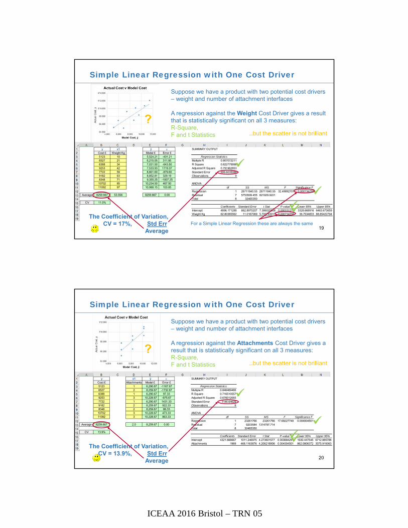
Simple Linear Regression with One Cost Driver

19

Suppose we have a product with two potential cost drivers – weight and number of attachment interfaces

A regression against the Weight Cost Driver gives a result that is statistically significant on all 3 measures:R-Square,F and t Statistics

The Coefficient of Variation,

CV = 17%, Std Err.Average

?…but the scatter is not brilliant

For a Simple Linear Regression these are always the same

y x1 ŷ SUMMARY OUTPUTCost £ Attachments Model £ Error £5123 1 6,290.67 -1167.67 Regression Statistics6527 2 8,259.67 -1732.67 Multiple R 0.8464694666388 1 6,290.67 97.33 R Square 0.7165105579253 3 10,228.67 -975.67 Adjusted R Square 0.6760120657722 1 6,290.67 1431.33 Standard Error 1146.646299182 2 8,259.67 922.33 Observations 98348 2 8,259.67 88.3310702 3 10,228.67 473.33 ANOVA11092 3 10,228.67 863.33 df SS MS F Significance F

Regression 1 23261766 23261766 17.69227749 0.004004501Average 8259.667 2.0 8,259.67 0.00 Residual 7 9203584 1314797.714

Total 8 32465350CV 13.9%

Coefficients Standard Error t Stat P-value Lower 95% Upper 95%Intercept 4321.666667 1011.246975 4.273601577 0.003684291 1930.447545 6712.885788Attachments 1969 468.1163876 4.206218906 0.004004501 862.0806372 3075.919363

Simple Linear Regression with One Cost Driver

20

Suppose we have a product with two potential cost drivers – weight and number of attachment interfaces

A regression against the Attachments Cost Driver gives a result that is statistically significant on all 3 measures:R-Square,F and t Statistics

The Coefficient of Variation,

CV = 13.9%, Std Err.Average

?…but the scatter is not brilliant


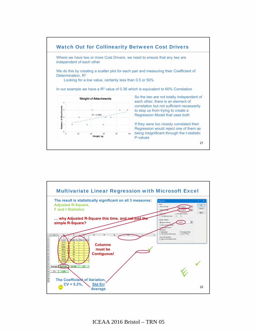
Watch Out for Collinearity Between Cost Drivers

21

Where we have two or more Cost Drivers, we need to ensure that any two are independent of each other

We do this by creating a scatter plot for each pair and measuring their Coefficient of Determination, R2

Looking for a low value, certainly less than 0.5 or 50%

In our example we have a R2 value of 0.36 which is equivalent to 60% Correlation

So the two are not totally independent of each other; there is an element of correlation but not sufficient necessarily to stop us from trying to create a Regression Model that uses both

If they were too closely correlated then Regression would reject one of them as being insignificant through the t-statistic P-values

Multivariate Linear Regression with Microsoft Excel

22

The result is statistically significant on all 3 measures:Adjusted R-Square,F and t Statistics

… why Adjusted R-Square this time, and not just the simple R-Square?

The Coefficient of Variation, CV = 5.2%, Std Err.

Average

Columns must be

Contiguous!


Adjusted R-Square

23

Why do we need to use Adjusted R-Square, and what is it?

• Suppose we believe that weight is the primary cost driver

• But we are unhappy with the residual variation in that simple relationship as we believe that there is at least one secondary driver at work.

• If we add another variable to the mix, Least Squares Regression will attempt to fit any additional variable to the residual error

… but in the process it will even sacrifice some of the best fit relationship already lined up for the primary driver in order to minimise the total error or residual

• The Regression routine will always find the Least Squares Best Fit – even where the relationship is tenuous

• Regression just a dumb calculation – no artificial intelligence involved

… the estimator/analyst has to provide that.

• Every time we add a variable we reduce the degrees of freedom for the Fit Criteria by one

• Adjusted R-Square is a statistic that compensates for this reduction

R2 and Adjusted R2

R2 or R-Square expresses the percentage of total variation in the data that can be explained by the model

Adjusted R2, or R2a, makes an adjustment to the Unexplained Variation to account of

the degrees of freedom within the model (n - 1 - k)

• Can be used to compare coefficients of determination between models with different numbers of variables, k

• Can be used as justification for including near-significant variables in models if those variable improve the model’s performance

Adapted from

24

Penalty (> 1)

SST = SSR + SSE


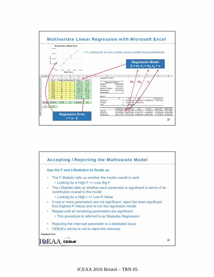
Multivariate Linear Regression with Microsoft Excel

25

Regression Modelŷ = m1 x1 + m2 x2 + c

m1 c m2

Regression Error = y - ŷ

<<< Looking for an even scatter across model (homoscedasticity)

Accepting / Rejecting the Multivarate Model

26

Use the F and t-Statistics to Guide us

• The F-Statistic tells us whether the model overall is valid

• Looking for a High F => Low Sig-F

• The t-Statistic tells us whether each parameter is significant in terms of its contribution overall to the model

• Looking for a High t => Low P-Value

• If one or more parameters are not significant, reject the least significant first (highest P-Value) and re-run the regression model

• Repeat until all remaining parameters are significant

• This procedure is referred to as Stepwise Regression

• Rejecting the Intercept parameter is a debatable issue

• CEBoK’s advice is not to reject the intercept

Adapted from


Multivariate Models Using Linear TransformationSelecting the Best Model

27

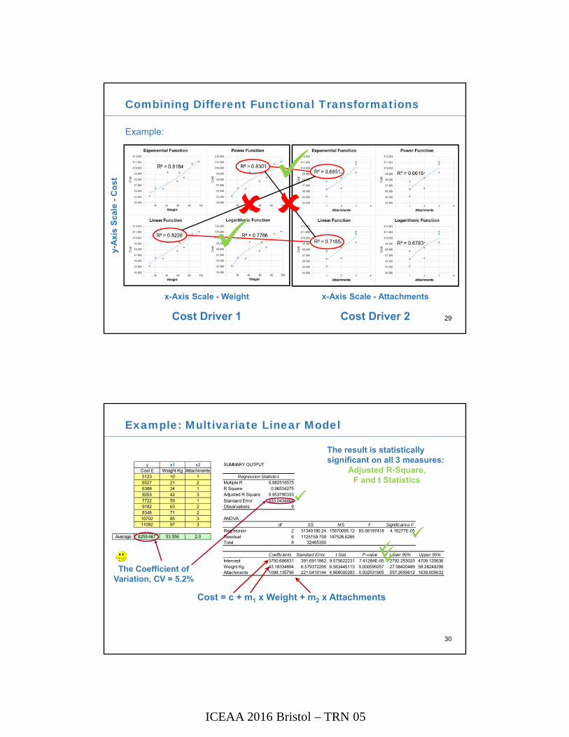
Combining Different Functional Transformations

28

The function type of the dependent (y) variable dictates which Function Types we can combine

LinearFunction

y = m x + c

LogarithmicFunction

y = m log(x) + c

PowerFunction

log(y) = m log(x) + c

ExponentialFunction

log(y) = m x + c

Linear x Logarithmic x

Line

ar y

Loga

rithm

ic y

y-A

xis

Sca

le

x-Axis Scale

We can combine Exponential and Power Functions

We can combine Linear and Logarithmic Functions

We cannot combine Linear and Exponential

or Logarithmic and Power Functions


x-Axis Scale - Attachments

Cost Driver 2

y-A

xis

Sca

le -

Co

st

x-Axis Scale - Weight

Cost Driver 1

Combining Different Functional Transformations

29

Example:

Example: Multivariate Linear Model

30

y x1 x2Cost £ Weight Kg Attachments5123 10 16527 21 26388 34 19253 42 37722 59 19182 63 28348 71 210702 85 311092 97 3

Average 8259.667 53.556 2.0

SUMMARY OUTPUT

Regression StatisticsMultiple R 0.982518575R Square 0.96534275Adjusted R Square 0.953790333


ANOVA

df SS MS F Significance FRegression 2 31340190.24 15670095.12 83.56197418 4.16277E-05Residual 6 1125159.759 187526.6265Total 8 32465350

Coefficients Standard Error t Stat P-value Lower 95% Upper 95%Intercept 3750.686831 391.6911862 9.575622231 7.41284E-05 2792.253025 4709.120636Weight Kg 43.18334894 6.579372295 6.563445113 0.000599257 27.08420489 59.28249298Attachments 1098.135796 221.0418144 4.968000283 0.002531905 557.2659612 1639.005632

Cost = c + m1 x Weight + m2 x Attachments

The result is statistically significant on all 3 measures:

Adjusted R-Square,F and t Statistics

The Coefficient of Variation, CV = 5.2%


Example: Multivariate Transformed Non-linear Model

31

y x1 x2Log Cost £ Log Wgt Attachments

3.7095 1.0000 13.8147 1.3222 23.8054 1.5315 13.9663 1.6232 33.8877 1.7709 13.9629 1.7993 23.9216 1.8513 24.0295 1.9294 34.0450 1.9868 3

Average 3.905 1.646 2.000

SUMMARY OUTPUT

Regression StatisticsMultiple R 0.988416994R Square 0.976968154Adjusted R Square 0.969290872


ANOVAdf SS MS F Significance F

Regression 2 0.096786945 0.048393472 127.2544294 1.22176E-05Residual 6 0.002281735 0.000380289Total 8 0.099068679

Coefficients Standard Error t Stat P-value Lower 95% Upper 95%Intercept 3.411275705 0.036501084 93.45683358 1.01124E-10 3.321960771 3.500590639Log Wgt 0.227564971 0.026096771 8.720043179 0.000125755 0.163708473 0.29142147Attachments 0.059435938 0.009609062 6.18540461 0.000821697 0.03592341 0.082948467

Log(Cost) = c + m1 x Log(Weight) + m2 x Attachments

The result is statistically significant on all 3 measures:

Adjusted R-Square,F and t Statistics

The Coefficient of Variation, CV = 0.5%

=> Cost = 10(c+m2 x Attachments) x Weightm1

StatLinear Model

Power – ExpFit Space

Power – ExpUnit Space

How to Calculate

SSE 1125159.8 0.002 797338.5

R2 0.965 0.977 0.975

Adj R2 0.954 0.969 0.967

SEE 433.0 0.020 364.5

CV 5.2% 0.5% 4.4%

Which is the Better Model?

Adapted from:

32

The Non-linear Model is the better model in this case ... Based on the Sum of Squares Error (SSE) in Unit Space

…but also all other measures in Unit Space

n

iiii YYeSUMSQ

1

2ˆ

kn

nR

1

111 2

i

i

yDEVSQ

eSUMSQ

SST

SSE 11

kn

SSE

1

21 aY R

Y

s

Y

SSE df

-adj

uste

dno

tdf

-adj

uste

dUnit-Space Goodness of Fit Comparison:


Adapted from

33

Steps for Selecting the “Best Model”

• Reject all non-significant models first– Where the F statistic is not significant

• Strip out all non-useful variables and made the model “minimal”– Variables that do not incrementally contribute to goodness of fit, overall

model significance, (adjusted) variation explained, etc– Use t-Statistic and Adjusted R-Squre

• Select “within functional type” e.g. Linear or Power, based on:– Use R2 for Simple Linear Regression (Ordinary Least Squares)– When comparing multivariate regression models, select based on

Adjusted R2, which compensates for the number of independent variables

• Select “across functional type”, Linear v Power, based on:– Sum of Squares Error (SSE) across Single Variable Models– Standard Error Estimate (SEE) for Multivariate models

Unit III - Module 8

34

Selecting “Within Type”

• Start with only significant, “minimal” models

• In choosing among “models of a similar form”, R2 is the criterion

e.g. linear models with other linear models

e.g., power models with other power models

Tip: If a model has a lower R2, but has variables that are more useful for decision makers, retain these, and

consider using them for CAIV trades and the like

R2 = 0.95 R2 = 0.79 R2 = 0.90

Weight

Co

st

Co

st

Co

st

PowerSurface Area

R2 = 0.80 R2 = 0.96A

A B

B

C

Co

st

Co

st

Length Speed

Select the model with the

highest R2

Select the model with the

highest R2


Unit III - Module 8

35

Selecting “Across Type”

• Start with only significant, “minimal” models

• In choosing among “models of a different form”:

– the SSE in unit space is the criterion

– SEE if degrees of freedom change;

– CV if dependent variables changes)

• “Models of a different form” means that you will compare:

– e.g., linear models with non-linear models

– e.g., power models with logarithmic models

• We must compute the SSE by:

– Computing Ŷ in unit space for each data point

– Subtracting each Ŷ from its corresponding actual Y value

– Sum the squared values, this is the SSE

Warning: We cannot use R2 to compare models of different forms because the R2 from the regression is computed on the transformed data, and thus is distorted by the transformation

Unit III - Module 8

36

Option 2. Linear ModelOption 1. Power Model

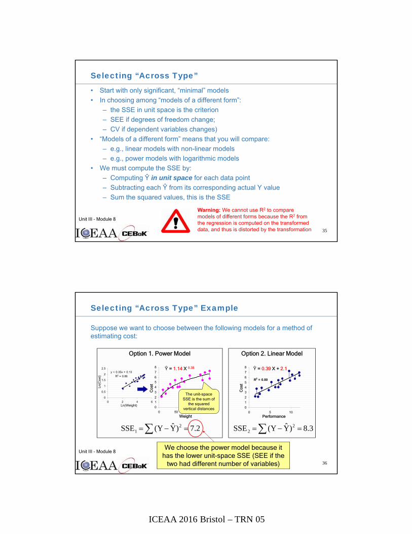
Suppose we want to choose between the following models for a method of estimating cost:

Selecting “Across Type” Example

We choose the power model because it has the lower unit-space SSE (SEE if the

two had different number of variables)

y = 0.35x + 0.13

R2 = 0.86

0

0.5

1

1.5

2

2.5

0 2 4 6

0

1

2

3

4

5

6

7

8

0 50 100 150

Ŷ = 1.14 X 0.35

2.7)YY( SSE 21

The unit-space SSE is the sum of

the squared vertical distances

Co

st

Weight

3.8)YY( SSE 22

Co

st

Performance

Ln(C

ost)

Ln(Weight)

R2 = 0.80

0

1

2

3

4

5

6

7

8

0 5 10

Ŷ = 0.39 X + 2.1


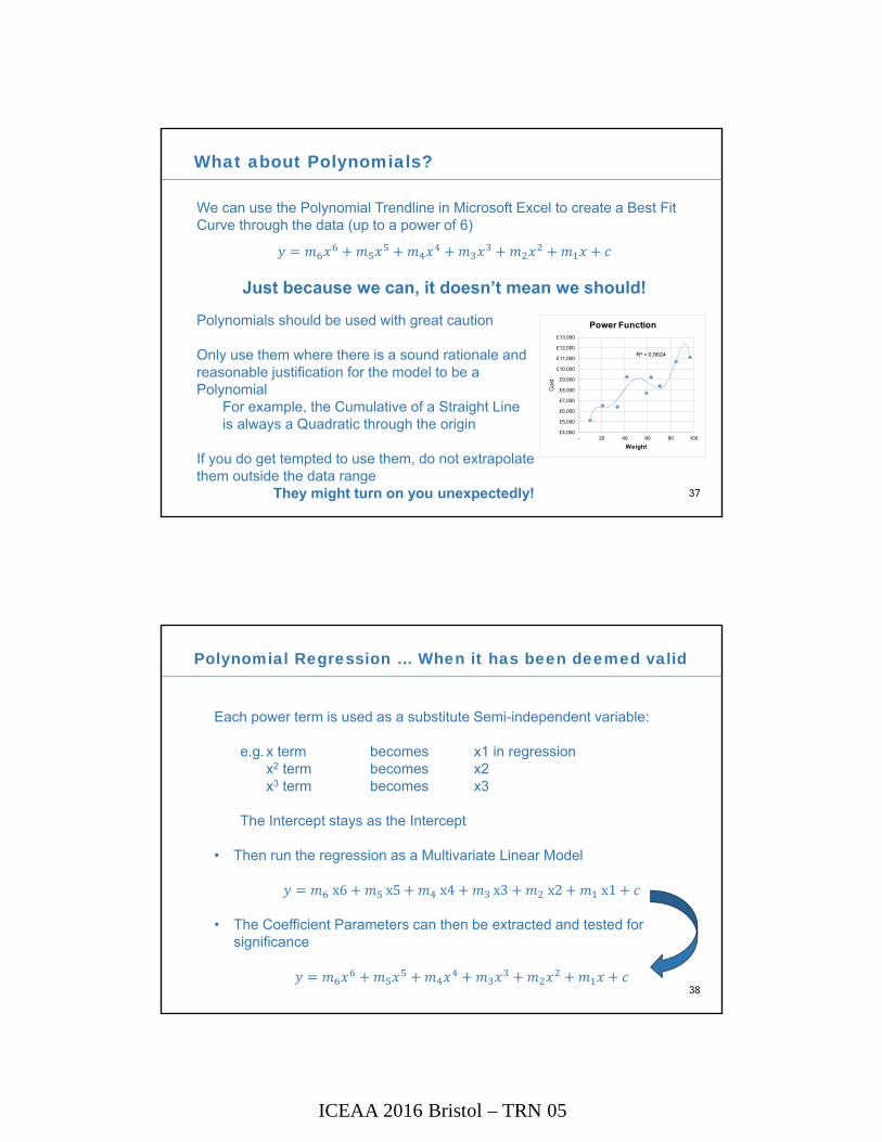
What about Polynomials?

37

We can use the Polynomial Trendline in Microsoft Excel to create a Best Fit Curve through the data (up to a power of 6)

Just because we can, it doesn’t mean we should!

Polynomials should be used with great caution

Only use them where there is a sound rationale and reasonable justification for the model to be a Polynomial

For example, the Cumulative of a Straight Line is always a Quadratic through the origin

If you do get tempted to use them, do not extrapolate them outside the data range

They might turn on you unexpectedly!

R² = 0.9024

£4,000

£5,000

£6,000

£7,000

£8,000

£9,000

£10,000

£11,000

£12,000

£13,000

- 20 40 60 80 100

Cos

t

Weight

Power Function

Polynomial Regression … When it has been deemed valid

38

Each power term is used as a substitute Semi-independent variable:

e.g.x term becomes x1 in regressionx2 term becomes x2x3 term becomes x3

The Intercept stays as the Intercept

• Then run the regression as a Multivariate Linear Model

x6 x5 x4 x3 x2 x1

• The Coefficient Parameters can then be extracted and tested for significance


Multivariate Linear Regression and Non-Linear Regression

Any more questions?

39

cost estimation chapter 7: single variable linear regression · chapter 7: single variable linear...

Documents