correspondence problems in computer vision
TRANSCRIPT

Mathematische BildverarbeitungsgruppeFakultat fur Mathematik und Informatik
Universitat des Saarlandes, 66041 Saarbrucken
Dissertationzur Erlangung des Grades des Doktors der Naturwissenschaften
der Naturwissenschaftlich-Technischen Fakultatender Universitat des Saarlandes
Correspondence Problems in Computer Vision
Novel Models, Numerics, and Applications
vorgelegt von
Henning Lars Zimmer
Saarbrucken, 2011

Tag des Kolloquiums: 10.02.2012
Dekan: Prof. Dr. Holger Hermanns
Prufungsausschuss:Ausschussvorsitzender: Prof. Dr. Hans-Peter SeidelGutachter: Prof. Dr. Joachim Weickert (1. Gutachter)
Prof. Dr. Daniel Cremers (2. Gutachter)Protokollfuhrer: Dr. Andres Bruhn

Mathematical Image Analysis GroupFaculty of Mathematics and Computer Science
Saarland University, 66041 Saarbrucken, Germany
Thesisfor obtaining the degree of a doctor of the natural sciences
of the natural-technical faculties of the Saarland University
Correspondence Problems in Computer Vision
Novel Models, Numerics, and Applications
byHenning Lars Zimmer
Thesis Advisor: Prof. Dr. Joachim Weickert
Referees: Prof. Dr. Joachim Weickert, Prof. Dr. Daniel Cremers
Saarbrucken, Germany, 2011

Copyright c© by Henning Lars Zimmer 2011. All rights reserved. No part of thiswork may be reproduced or transmitted in any form or by any means, electronic ormechanical, including photography, recording, or any information storage or retrievalsystem, without permission in writing from the author. An explicit permission is given toSaarland University to reproduce up to 100 copies of this work and to publish it online.The author confirms that the electronic version is equal to the printed version. It iscurrently available at http://www.mia.uni-saarland.de/zimmer/phd-thesis.pdf.

Eidesstattliche Versicherung
Hiermit versichere ich an Eides statt, dass ich die vorliegende Arbeit selbststandig undohne Benutzung anderer als der angegebenen Hilfsmittel angefertigt habe. Die ausanderen Quellen oder indirekt ubernommenen Daten und Konzepte sind unter Angabeder Quelle gekennzeichnet. Die Arbeit wurde bisher weder im In- noch im Auslandin gleicher oder ahnlicher Form in einem Verfahren zur Erlangung eines akademischenGrades vorgelegt.
Saarbrucken, 10.02.2012
Henning Lars Zimmer


To My Grandfather Heinrich Zimmer


Short Abstract
Correspondence problems like optic flow belong to the fundamental problems in com-puter vision. Here, one aims at finding correspondences between the pixels in two (ormore) images. The correspondences are described by a displacement vector field that isoften found by minimising an energy (cost) function. In this thesis, we present severalcontributions to the energy-based solution of correspondence problems: (i) We startby developing a robust data term with a high degree of invariance under illuminationchanges. Then, we design an anisotropic smoothness term that works complementaryto the data term, thereby avoiding undesirable interference. Additionally, we propose asimple method for determining the optimal balance between the two terms. (ii) Whendiscretising image derivatives that occur in our continuous models, we show that adapt-ing one-sided upwind discretisations from the field of hyperbolic differential equationscan be beneficial. To ensure a fast solution of the nonlinear system of equations thatarises when minimising the energy, we use the recent fast explicit diffusion (FED) solverin an explicit gradient descent scheme. (iii) Finally, we present a novel application ofmodern optic flow methods where we align exposure series used in high dynamic range(HDR) imaging. Furthermore, we show how the alignment information can be used ina joint super-resolution and HDR method.
i

Kurzzusammenfassung
Korrespondenzprobleme wie der optische Fluß, gehoren zu den fundamentalen Prob-lemen im Bereich des maschinellen Sehens (Computer Vision). Hierbei ist das Ziel,Korrespondenzen zwischen den Pixeln in zwei (oder mehreren) Bildern zu finden. DieKorrespondenzen werden durch ein Verschiebungsvektorfeld beschrieben, welches oftdurch Minimierung einer Energiefunktion (Kostenfunktion) gefunden wird. In dieserArbeit stellen wir mehrere Beitrage zur energiebasierten Losung von Korresponden-zproblemen vor: (i) Wir beginnen mit der Entwicklung eines robusten Datenterms, derein hohes Maß an Invarianz unter Beleuchtungsanderungen aufweißt. Danach entwick-eln wir einen anisotropen Glattheitsterm, der komplementar zu dem Datenterm wirktund deshalb keine unerwunschten Interferenzen erzeugt. Zusatzlich schlagen wir eineeinfache Methode vor, die es erlaubt die optimale Balance zwischen den beiden Ter-men zu bestimmen. (ii) Im Zuge der Diskretisierung von Bildableitungen, die in unserenkontinuierlichen Modellen auftauchen, zeigen wir dass es hilfreich sein kann, einseit-ige upwind Diskretisierungen aus dem Bereich hyperbolischer Differentialgleichungenzu ubernehmen. Um eine schnelle Losung des nichtlinearen Gleichungssystems, dassbei der Minimierung der Energie auftaucht, zu gewahrleisten, nutzen wir den kurzlichvorgestellten fast explicit diffusion (FED) Loser im Rahmen eines expliziten Gradien-tenabstiegsschemas. (iii) Schließlich stellen wir eine neue Anwendung von modernenoptischen Flußmethoden vor, bei der Belichtungsreihen fur high dynamic range (HDR)Bildgebung registriert werden. Außerdem zeigen wir, wie diese Registrierungsinforma-tion in einer kombinierten super-resolution und HDR Methode genutzt werden kann.
ii

Abstract
Solving correspondence problems is a fundamental task in computer vision which oc-curs in various applications such as optic flow estimation, 3D reconstruction or imagealignment. For estimating the displacement field that describes the correspondencesbetween the pixels in two images, energy-based approaches that minimise a certain costfunction have proven most successful. In this thesis we show that despite three decadesof research on correspondence problems, there is still room for significant improvementsand novel ideas:
(i) Concerning the design of the energy, we develop a novel, robust data term thatoffers a high degree of invariance w.r.t. various kinds of illumination changes. We thenpropose an anisotropic smoothness term that works complementary to the data termand only smooths in directions where the data term gives no information. The proposedsmoothness term further combines ideas from image- as well as flow-driven strategies,which allows to obtain sharp flow boundaries without oversegmentation problems. Fi-nally, we present a simple, yet well-performing strategy for determining the optimalbalance between the data and the smoothness term.
(ii) For discretising image derivatives that occur in our continuous models, we pro-pose an alternative to the common central finite difference approximations. By adaptingideas from the solution of hyperbolic differential equations, we use correctly oriented,one-sided upwind differences that may lead to improved results.
The minimisation of the energy functionals comes down to solving nonlinear systemsof equations. For a fast solution, we adapt the recently proposed fast explicit diffusion(FED) scheme that combines small (stable) and large (unstable) time step sizes in an ex-plicit gradient descent scheme. Due to its simple nature, this scheme allows an efficientimplementation on modern graphics hardware (GPUs) which gives highly accurate dis-placement fields in the fraction of a second and furthermore enables an implementationon a modern smartphone.
(iii) We present a novel application of modern optic flow approaches in the field ofcomputational photography. By a careful modification of the data term, we are ableto align exposure series that are used in the context of high dynamic range (HDR)imaging. Due to the estimated dense displacement fields, handling severe camera shakeand moving objects becomes possible with our method. By exploiting the subpixelprecision of the displacement fields, we can additionally enhance the spatial resolutionof the result in an energy-based, joint super-resolution and HDR approach. For thelatter, we propose a novel anisotropic smoothness term that gives much more appealingresults compared to previous strategies.
iii

Zusammenfassung
Die Losung von Korrespondenzproblemen ist eine fundamentale Aufgabe im Bereichdes maschinellen Sehens (Computer Vision), die in vielen Anwendungen wie z.B. demoptischen Fluß, bei 3D Rekonstruktionen und bei der Bildregistrierung auftaucht. Umdas Verschiebungsvektorfeld, welches die Korrespondenzen zwischen den Pixeln in zweiBildern beschreibt, zu schatzen, haben sich energiebasierte Verfahren, die eine bestimmteKostenfunktion minimieren als am erfolgreichsten herausgestellt. In dieser Arbeit zeigenwir, dass es trotz drei Jahrzehnten Forschung im Bereich von Korrespondenzproblemennoch immer Raum fur signifikante Verbesserungen und neue Ideen gibt:
(i) Bei dem Entwurf der Energie entwickeln wir einen neuen, robusten Datenterm,welcher ein hohes Maß and Invarianz unter verschiedenen Arten von Beleuchtungsanderun-gen aufweißt. Danach schlagen wir einen anisotropen Glattheitsterm vor, der komple-mentar zu dem Datenterm arbeitet und nur in Richtungen glattet, in denen der Daten-term keine Information liefert. Weiterhin kombiniert der vorgeschlagene GlattheitstermIdeen von bild- sowie fluß-getriebenen Strategien, was scharfe Flußkanten erlaubt, ohnejedoch unter Ubersegmentierung zu leiden. Schließlich stellen wir eine einfache undtrotzdem gut funktionierende Strategie zur Bestimmung der optimalen Balance zwis-chen Daten- und Glattheitsterm vor.
(ii) Zur Diskretisierung von Bildableitungen, die in unseren kontinuierlichen Mod-ellen auftauchen, schlagen wir eine Alternative zu den ublichen, zentralen Finite–Diffe-renzen Approximationen vor. Wir ubernehmen Ideen aus dem Bereich der Losung vonhyperbolischen Differentialgleichungen und nutzen korrekt orientierte, einseitige upwindDifferenzen, was zur Verbesserung der Ergebnisse fuhren kann.
Die Minimierung der Energiefunktionale reduziert sich auf die Losung nichtlinearerGleichungssysteme. Um eine schnelle Losung zu gewahrleisten, nutzen wir das kurzlichvorgestellte fast explicit diffusion (FED) Schema, welches kleine (stabile) und große(instabile) Zeitschrittweiten in einem expliziten Gradientenabstiegsschema kombiniert.Aufgrund seiner einfachen Natur erlaubt dieses Schema eine effiziente Implementierungauf moderner Grafikhardware (GPUs), welche hoch genaue Verschiebungsfelder im Bruch-teil einer Sekunde errechnet. Außerdem erlaubt dieses Schema eine Implementierung aufeinem modernen Smartphone.
(iii) Wir stellen eine neue Anwendung moderner optischer Flußverfahren im Bere-ich der computergestutzten Fotografie (Computational Photography) vor. Durch einesorgsame Modifizierung des Datenterms sind wir in der Lage, Belichtungsreihen zu reg-istrieren, die im Bereich der high dynamic range (HDR) Bildgebung verwendet werden.Wegen der geschatzten dichten Verschiebungsfelder kommt unsere Methode auch mitheftigem Verwackeln und sich bewegenden Objekte zurecht. Indem wir die subpixelGenauigkeit der Verschiebungsfelder ausnutzen, sind wir zusatzlich in der Lage, dieraumliche Auflosung der Bilder in einem energiebasierten, gemeinsamen super-resolu-tion und HDR Ansatz zu erhohen. Bei letzterem schlagen wir einen neuen, anisotropenGlattheitsterm vor, welcher deutlich ansprechendere Ergebnisse als vorhergehende Strate-gien liefert.
iv

Acknowledgements
There are many people that I have to thank because without them, this work wouldhave never been possible.
First of all, I would like to thank Prof. Dr. Joachim Weickert for accepting meas a Ph.D. student, supervising my work, and also for sparking my interest in thefascinating field of image processing and computer vision. I am also very grateful toProf. Dr. Daniel Cremers who agreed to be my second reviewer. I also wish to expressmy gratitude to all current and former members of our group for providing a niceworking atmosphere and for being much more than just colleagues. Especially, I haveto thank Andres Bruhn for the countless hours that he invested in our projects, forhis inspiring ideas and his fruitful comments. Similarly, I wish to thank all personsthat I was granted to work with on joint projects. Those are Levi Valgaerts, MichaelBreuß, Pascal Gwosdek, Oliver Demetz, Sven Grewenig, Andreas Luxenburger, andSebastian Volz from our group, as well as Hans-Peter Seidel, Bodo Rosenhahn, AgustınSalgado, Carsten Stoll and Christian Theobalt from other groups. Furthermore, I amvery grateful to the International Max Planck Research School for Computer Science(IMPRS-CS) for funding me by a three-year scholarship.
I also have to thank my friends and family for their continuous support. Especiallymy parents and grandparents helped me more than words can express. I am also verygrateful to Nadine Moegelin for everything she did for me during our relationship. Lastbut not least, I want to thank our dog Daisy that eased writing up this thesis by sleepingand snoring next to me.
v

vi

Contents
1 Introduction 11.1 Correspondence Problems . . . . . . . . . . . . . . . . . . . . . . . . . . 11.2 Solution of Correspondence Problems . . . . . . . . . . . . . . . . . . . . 61.3 Our Contributions . . . . . . . . . . . . . . . . . . . . . . . . . . . . . . 111.4 Organisation . . . . . . . . . . . . . . . . . . . . . . . . . . . . . . . . . . 14
2 Related Work 172.1 Modelling . . . . . . . . . . . . . . . . . . . . . . . . . . . . . . . . . . . 172.2 Energy Minimisation . . . . . . . . . . . . . . . . . . . . . . . . . . . . . 222.3 Applications . . . . . . . . . . . . . . . . . . . . . . . . . . . . . . . . . . 23
3 Preliminaries 273.1 Images . . . . . . . . . . . . . . . . . . . . . . . . . . . . . . . . . . . . . 273.2 Flow Fields . . . . . . . . . . . . . . . . . . . . . . . . . . . . . . . . . . 283.3 Derivatives . . . . . . . . . . . . . . . . . . . . . . . . . . . . . . . . . . . 303.4 Discretisation . . . . . . . . . . . . . . . . . . . . . . . . . . . . . . . . . 30
4 Modelling 334.1 Variational Optic Flow . . . . . . . . . . . . . . . . . . . . . . . . . . . . 334.2 Data Term . . . . . . . . . . . . . . . . . . . . . . . . . . . . . . . . . . . 344.3 Smoothness Term . . . . . . . . . . . . . . . . . . . . . . . . . . . . . . . 464.4 Automatic Selection of the Smoothness Weight . . . . . . . . . . . . . . . 724.5 Prediction Prior . . . . . . . . . . . . . . . . . . . . . . . . . . . . . . . . 78
5 Numerics 835.1 Discretisation . . . . . . . . . . . . . . . . . . . . . . . . . . . . . . . . . 835.2 Upwind Discretisation of Image Derivatives . . . . . . . . . . . . . . . . . 875.3 Solving the Euler-Lagrange Equations . . . . . . . . . . . . . . . . . . . . 1035.4 Experiments . . . . . . . . . . . . . . . . . . . . . . . . . . . . . . . . . . 114
6 Applications 1176.1 HDR Imaging . . . . . . . . . . . . . . . . . . . . . . . . . . . . . . . . . 1176.2 Aligning Exposure Series for HDR Imaging . . . . . . . . . . . . . . . . . 122
vii

CONTENTS
6.3 Joint Super-Resolution and HDR (SR-HDR) Reconstruction . . . . . . . 136
7 Summary and Future Work 1497.1 Summary . . . . . . . . . . . . . . . . . . . . . . . . . . . . . . . . . . . 1497.2 Future Work . . . . . . . . . . . . . . . . . . . . . . . . . . . . . . . . . . 151
A Proofs 155
Own Publications 161
Bibliography 163
viii
Chapter 1
Introduction
Per aspera ad astra.
Latin saying (“to the stars through difficulties”)
Classic image processing tasks focus on enhancing or analysing a single image, e.g.removing noise or segmenting the image into meaningful regions. Obviously, by consid-ering several images of the same scene, one should be able to do more. For example, onecan combine images taken with different exposure times to create an image that showsdetails in very dark as well as very bright regions, which is known as high dynamicrange (HDR) imaging. Another example is motion estimation which is naturally onlypossible if one considers a whole image sequence, i.e. a video stream. Similarly, 3D re-constructions from images also require several images to overcome the depth ambiguitythat arises when projecting the 3D world onto 2D images.
If we now want to use such a multi-image methods, the most important step isto determine which pixels correspond to the same scene object, more specifically weneed to establish correspondences between the pixels in the given images. The lattertask is referred to as a correspondence problem which is a classic problem in computervision research. In this thesis, we will present contributions to all aspects of research oncorrespondence problems: Appropriate models, efficient solvers, numerical realisationand novel applications.
In the remainder of this chapter we first discuss the basics of correspondence prob-lems. We define the task to be solved, show examples where correspondence problemsoccur and briefly discuss different solution strategies. Moreover, we give an outlook onthe contributions that will be presented later on.
1.1 Correspondence Problems
The basic task of correspondence problems is the following: Consider two images thatroughly depict the same scene, e.g. two subsequent frames of an image sequence or two
1
CHAPTER 1. INTRODUCTION
images taken from slightly different viewpoints. For each pixel in the first image, wethen aim to find its corresponding pixel in the second image. The obtained correspon-dences are usually described by a displacement vector field where each vector pointsfrom a pixel in the first image to its corresponding location in the second image. Con-sequently, the displacement vector field is the unknown to be determined when solvinga correspondence problem.
Let us now present some popular examples where correspondence problems arise inthe fields of image processing and computer vision. Thereby, we define the specific taskthat has to be solved and also give examples for application areas.
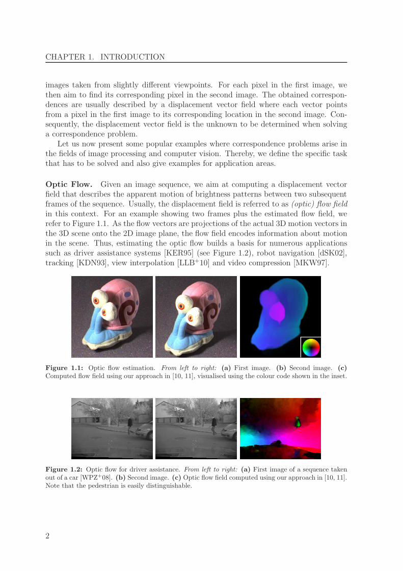
Optic Flow. Given an image sequence, we aim at computing a displacement vectorfield that describes the apparent motion of brightness patterns between two subsequentframes of the sequence. Usually, the displacement field is referred to as (optic) flow fieldin this context. For an example showing two frames plus the estimated flow field, werefer to Figure 1.1. As the flow vectors are projections of the actual 3D motion vectors inthe 3D scene onto the 2D image plane, the flow field encodes information about motionin the scene. Thus, estimating the optic flow builds a basis for numerous applicationssuch as driver assistance systems [KER95] (see Figure 1.2), robot navigation [dSK02],tracking [KDN93], view interpolation [LLB+10] and video compression [MKW97].
Figure 1.1: Optic flow estimation. From left to right: (a) First image. (b) Second image. (c)Computed flow field using our approach in [10, 11], visualised using the colour code shown in the inset.
Figure 1.2: Optic flow for driver assistance. From left to right: (a) First image of a sequence takenout of a car [WPZ+08]. (b) Second image. (c) Optic flow field computed using our approach in [10, 11].Note that the pedestrian is easily distinguishable.
2

1.1. CORRESPONDENCE PROBLEMS
Stereo. In the classic binocular case we are given two images of the same scene thatwere captured from two different viewpoints. The magnitude of the displacements be-tween pixels in these two images is called disparity and is directly related to the depthof the corresponding scene points. Consequently, disparity estimation is an importantstep for 3D reconstructions [FLP01, HZ00]. An example for a basic 3D reconstructionfrom two images is shown in Figure 1.3.
If one knows the relative pose of the two cameras, one can restrict the search forcorrespondences to a single line in the second image. This line is usually referred to asthe epipolar line [FLP01, HZ00]. In the simplest scenario where the two cameras areorthoparallel to each other (or if the images have been rectified), all epipolar lines arehorizontal. Thus, the stereo problem in the orthoparallel case can be interpreted as anoptic flow problem where the vertical displacement component is equal to zero, whicheases the search for correspondences. However, to obtain favourable 3D reconstructions,a large baseline distance between the two cameras is mandatory. This results in displace-ments that are much larger than in the optic flow case and renders stereo reconstructiona challenging task.
Figure 1.3: Stereo matching. From left to right: (a) Left image of the Portal scene, available athttp://cmp.felk.cvut.cz/~cechj/GCS/stereo-images/Portal/. (b) Right image. (c) Disparityestimated with our approach in [8]. (d) Corresponding reconstruction (visualising the estimated dis-parities as heightfield).
Scene Flow. We argued that the optic flow field only describes a projection of theactual 3D motion vectors onto the 2D image plane. If one aims at recovering the full 3Ddisplacement field, called scene flow, one needs to estimate both, the 3D geometry ofthe scene and the correspondences of 3D points between subsequent frames. Thus, sceneflow computation can be seen as solving a stereo problem together with an optic flowproblem which in turn requires to consider binocular image sequences, where a stereopair is available at each time instant [PAT96].
Estimating the scene flow is for sure more complex than optic flow or stereo alone.However, the additional information can be of great help for applications like driver
3

CHAPTER 1. INTRODUCTION
assistance [WRV+08, WMR+09] as well as motion capture [5],[VBR+05], see Figure 1.4.
time t
time t+1
left right
Figure 1.4: Scene flow computation. Left: (a)–(d) Four input images (two stereo pairs at time t andt+1). Right: (e) Reconstruction and scene flow computed with our method from [5].
Image Alignment. Photographic multi-shot techniques [GG09] fuse several imagesof the same scene to obtain an image with increased quality. A popular example for sucha technique is high dynamic range (HDR) imaging [RWPD05] where one tries to tacklethe problem that the dynamic range 1 of real world scenes exceeds the dynamic rangeof image sensors by orders of magnitude. Thus, images obtained by standard camerasoften suffer from under- and oversaturated regions in dark and bright regions, respec-tively. By fusing the information from a series of images taken with varying exposuretimes, a HDR image can be computed that captures details in both, dark and bright re-gions. Further multi-shot techniques include super-resolution [PPK03], extended depthof field [ADA+04], flash/no-flash photography [PSA+04] and image stitching [Sze06].
A major problem is that multi-shot techniques often combine the information at thesame pixel location in all the input images. Consequently, the fusion algorithms relyon perfectly aligned images without any displacements between them. However, thisassumption is hardly met under real world conditions where moving objects and camerashake may cause severe displacements. In such cases, one has to compute the displace-ments between the input images to align them prior to processing. As the captured scenemay be moving, image alignment can be seen as an optic flow problem. However, classi-cal matching assumptions, e.g. assuming that corresponding pixels have similar colour,may not hold due to the different acquisitions of the input images. In HDR imaging,
1The dynamic range denotes the ratio between the darkest and the brightest scene point.
4

1.1. CORRESPONDENCE PROBLEMS
for example, all images were taken with a different exposure time. Nevertheless, wecould show in [9] that a carefully adapted optic flow method is able to robustly alignHDR input, see Figure 1.5 where we compare HDR images computed from a freehandexposure series with and without prior alignment.
Figure 1.5: Freehand HDR imaging. Left column: (a)–(c) Three images of a freehand exposureseries. Right: (d) Computed HDR reconstruction with and without alignment [9]. The float-valuedHDR data is visualised by applying the tone mapping operator from [FLW02].
Medical Image Registration. A common problem in medical imaging is the regis-tration of images that depict the same part of the body, but were captured with differentimaging techniques. An example can be the registration of a magnetic resonance imaging(MRI) template to an ultrasound (US) reference image [FM08], see Figure 1.6. Similarto alignment problems discussed above, also here common matching assumption will faildue to the different capturing techniques. Note that we will not present specific contri-butions to the field of medical image registration in this thesis. However, we decided tokeep this example for completeness reasons.
Particle Image Velocimetry (PIV). The basic task of PIV methods is to analyseimage sequences that depict the flow of small tracer particles that were placed into afluid [RWWK07]. The information encoded in the optic flow field of such sequenceshelps researchers in areas like fluid mechanics, aerodynamics, or meteorology to validatesimulations or to do forecasts.
Basically, PIV can be seen as an optic flow problem. However, the estimated flowfields must obey physical laws like incompressibility, which need to be incorporated inthe model; see e.g. [RSS07]. Additionally, large displacements of small particles andoccurring complex motion patterns like vortices pose further challenges. An example of
5

CHAPTER 1. INTRODUCTION
Figure 1.6: Medical image registration of MRI and US data [FM08]. From left to right: (a) MRItemplate of a part of a human liver. (b) Zoom into marked region in (a). (c) US reference image. (d)Registration of (b) onto (c).
a flow field with strong vortices is shown in Figure 1.7. As for medical image registration,we discuss PIV methods solely for completeness reasons in this chapter.
Figure 1.7: PIV example [RSS07]. From left to right: (a) One of the input images (passive scalarimage). (b) Estimated flow field with colour-coded vorticity.
1.1.1 Our Focus
The preceding list of examples for correspondence problems shows that these problemsoccur in a several important and interesting research areas. One further realises thatoptic flow is a rather general setting for correspondence problems as it does not imposetoo many constraints on the displacement field. For example, optic flow subsumes stereowhere the displacements have to lie on the epipolar lines. Due its generality, we decidedto mainly focus on optic flow in this thesis. At some points, however, we will also showhow to adapt the presented concepts to stereo in the orthoparallel case.
1.2 Solution of Correspondence Problems
Before presenting an overview of our contributions, let us discuss basic solution strategiesfor correspondence problems. First of all, we wish to note that solving correspondence
6

1.2. SOLUTION OF CORRESPONDENCE PROBLEMS
problems is challenging task as they belong to the class of inverse problems. In this sense,given an image and a displacement field, one can easily compute the second image byshifting the pixels of the first image in accordance to the displacement. However, solvingthe inverse problem, i.e. recovering the displacements from two given images, is hardand unfortunately this is exactly the task in correspondence problems.
The fundamental strategy for solving correspondence problems is to impose con-stancy assumptions on image properties. A first idea can be to assume that the imageintensities do not change under their displacement. This is known as the brightnessconstancy assumption [HS81, LK81]. However, for a pixel in the first image, there areprobably several pixels in the second image that have the same or a similar intensity,especially in flat image regions. Even worse, the pixel with the most similar intensitymay not be necessarily the correct match, as we have to take into account image noiseor illumination changes. To overcome this ambiguity, several approaches have beenproposed that can be roughly classified into the two classes:
1. Local approaches determine the displacement for each pixel individually by findinga pixel in the second image that minimises some matching cost. For a successfulresolving of the ambiguities, this cost should be as discriminative as possible. Anexample can be to match whole regions around pixels.
2. Global approaches do not only consider a matching score when assigning a dis-placement to a pixel, but also take into account the displacements of neighbouringpixels. A common strategy to achieve this goal is to assume that neighbouringpixels have similar displacements, i.e. assuming that the overall displacement fieldis smooth.
Let us now shortly discuss and compare local and global approaches.
1.2.1 Local Approaches
Block Matching. One of the simplest possibilities to overcome ambiguities is to com-pare whole patches around pixels instead of just a single pixel. Such techniques arereferred to as block matching approaches; see [MPG85], for example. These methodsperform an exhaustive search (maybe limited by a predefined maximal displacementlimit) and match pixels that give the smallest distance between their patches. In thiscontext, several distance metrics have been proposed, like the sum of squared distances(SSD) or the sum of absolute distances (SAD), which is more robust to outliers. Ad-ditionally, correlation based metrics such as normalised cross correlation (NCC) arepopular as they are invariant under global linear illumination changes.
Regardless of the distance metric used, block matching approaches are known toproduce noisy displacement fields that additionally suffer from block-like artefacts. Fur-thermore, the exhaustive search results in very long runtimes for larger search ranges.
7

CHAPTER 1. INTRODUCTION
Feature Matching. To improve the quality of block matching methods, one can tryto only match image regions that are most discriminative. A typical choice for suchfeatures (also called interest points), are corners which are used within the well-knownSIFT (Scale Invariant Feature Transform) method by Lowe [Low99, Low04]. Here, aunit feature vector is computed from the corner neighbourhood. In contrast to imagepatches used in basic block matching approaches, the SIFT feature vectors are invariantto image scale and rotation, and are robust under affine distortions (noise, change inviewpoint or illumination). Furthermore, the number of interest points is usually muchsmaller than the number of pixels, making the matching more efficient compared toblock matching approaches.
Despite of this desirable properties, feature matching approaches suffer from onefundamental problem: One cannot find an interest point at each pixel and thus theresulting displacement fields are sparse. To obtain dense fields, a postprocessing byinterpolation has to be performed, which is again challenging and often does not yieldfavourable results.
Local Energy-based Approaches. One of the first local optic flow methods wasproposed by Lucas and Kanade [LK81, BM04]. The basic idea of their approach isto impose brightness constancy and additionally assuming that the displacements areconstant within a small neighbourhood around each pixel. These assumptions can beexpressed in a local energy that penalises deviations of the brightness constancy as-sumption within the considered neighbourhood in a quadratic way, leading to a leastsquares fit. The minimisation of the local energy then comes down to solving a 2 × 2linear system of equations, which can be efficiently solved by standard methods, e.g. byapplying Cramer’s rule. An affine extension of the Lucas/Kanade method goes back tothe work of Shi and Tomasi [ST94]. Here, it is assumed that the flow within a neighbour-hood can be described by an affine function, i.e. by 6 parameters. Thus, such methodsare also called parametric methods. A spatiotemporal extension of the Lucas/Kanademethod with additional estimation of the temporal component of the flow field was laterproposed by Bigun et al. [BGW91]. This method can be more robust, but requires tosolve an eigenvalue problem with a 3× 3 matrix.
One major issue of the discussed local energy-based methods is that the assumptionof a locally constant displacement is often violated in reality, e.g. at motion discontinu-ities, leading to block-like artefacts in the displacement fields. Furthermore, dependingon the local image structure, the equation system or eigenvalue problem may not havea unique solution. This happens for example in flat image regions and again results insparse displacement fields.
1.2.2 Global Approaches
Approaches that yield dense displacement fields by construction are energy-based meth-ods that find the displacement field by minimising a suitable global energy formula-tion. The latter usually consists of two terms: a data term and a smoothness term.
8

1.2. SOLUTION OF CORRESPONDENCE PROBLEMS
The data term models constancy assumptions on image features, it may for examplepenalise deviations from the brightness constancy assumption. The smoothness termpenalises fluctuations in the displacement field, thereby regularising the result whichallows to tackle problems with non-unique matches or outliers. The relative weightbetween the two terms is typically steered by a smoothness parameter. Although thefirst global energy-based method was already proposed in 1981 in the seminal work ofHorn and Schunck [HS81], such methods became increasingly popular in recent years.This is mainly due to their potential for giving highly accurate results, which is wit-nessed by top ranking results at the Middlebury optic flow benchmark [BSL+10]. Inaddition to the high accuracy and the dense displacement fields, energy-based ap-proaches are additionally attractive as they are based on transparent mathematicalmodels and allow for an efficient solution. Concerning the latter, sequential multi-grid solvers [BWKS06, KKR07], parallel implementations on modern graphics hardware(GPU) [3] and [WPZ+08, ZPB07], or even parallel multigrid schemes [GT08] renderedrealtime computations of dense flow fields possible.
Within global energy-based methods, one can distinguish discrete methods that min-imise a discrete energy function, and continuous variational approaches and that min-imise a continuous energy functional. We now present the two approaches in moredetail.
Discrete Approaches
Starting from a probabilistic model, the displacement estimation is often formulated interms of optimising a Markov Random Field (MRF), which comes down to minimisinga discrete energy function. The minimisation can be realised by graph cuts [BVZ01,Coo08], dynamic programming [LY09] or similar strategies. Examples for discrete ap-proaches can be found in [BA96, Coo08, LY09, MP98, MB87, SRB10, SRLB08, SSB10].
Variational Approaches
Especially in the context of optic flow estimation, variational approaches are very pop-ular; see e.g. [10, 11] and [AELS99, ADK99, BBPW04, Coh93, HS81, NE86, NBK08,Sch94, WCPB09, WPZ+08, WS01a, WPB10, WTP+09, XCJ08, XJM10, ZPB07].
The minimisation of the continuous energy functionals can be performed by dif-ferent strategies, such as primal-dual approaches, e.g., [WCPB09, WPZ+08, WPB10,WTP+09, XJM10, ZPB07], or by solving the corresponding Euler-Lagrange equations.The latter can be considered as the most widely used technique for solving variationaloptic flow problems and is for example used in [10, 11] and [AELS99, ADK99, BBPW04,Coh93, HS81, NE86, NBK08, Sch94, WS01a]. As we will also follow this strategy in theremainder of this thesis, let us further detail on it.
The Euler-Lagrange Framework. The calculus of variations [Els62] states that aminimiser of the variational energy formulation necessarily has to fulfil the corresponding
9

CHAPTER 1. INTRODUCTION
Euler-Lagrange equations. Provided that the energy is strictly convex, the solution ofthe Euler-Lagrange equations then gives the globally optimal flow field. The Euler-Lagrange equations describe a system of coupled partial differential equations of elliptictype. After discretisation, a linear or nonlinear system of equations arises, depending onthe design of the energy. In the nonlinear case, time-lagged nonlinearity methods, alsoknown as the Kacanov–Galerkin method [FKN73], can help to reformulate the nonlinearproblem as a series of linear ones. To finally solve the linear systems, one exploits thesparsity of the system matrix which allows to use iterative solvers, e.g., the Jacobi,Gauss-Seidel, or SOR method [You03].
An alternative solution strategy is to consider the elliptic problem as the steady stateof a parabolic problem, i.e. where time tends to infinity. In this context, explicit schemescan be used that result in an iterative procedure that updates the solution starting froma given initialisation until a convergence criterion is met. The advantages of explicitschemes is that they are easy to deduce from the energy and very easy to implement.However, to ensure stability very small time step sizes must be chosen s.t. a large numberof iterations are needed until convergence, resulting in poor computational performance.This problem can be alleviated by leveraging the simple structure of explicit schemes forparallel implementations on modern graphics hardware, which can lead to a speed upin the order of magnitudes. An alternative approach can be to resort to semi-implicitgradient descent schemes. Here, arbitrary time step sizes can be used, but one needs tosolve a system of equations at each time step, as in the elliptic case discussed above.
The Warping Strategy for Handling Large Displacements. Let us give a final,but very important remark on variational approaches. To make the minimisation ofvariational approaches tractable, one mostly performs a linearisation of the data con-straints. This proceeding is, however, only valid under the assumption of either smalldisplacements in the sequence or for very smooth images. However, if the temporal sam-pling of the image sequence is too coarse, or in the stereo context where a large baselinedistance is required to obtain a reasonable depth resolution, large displacements areunavoidable. Additionally, the smoothness of the given images is beyond our control.
A common remedy to this problem is to use a coarse-to-fine multiscale technique,often referred to as warping strategy; see e.g. [AWS00, Ana89, BA96, BBPW04, MP98,WTK87]. A first class of methods [Ana89, BA96, BBPW04, MP98] tackles the problemsof large displacements by downsampling the image sequence in a pyramid-like structure.On a small (coarse) levels, the displacements become small enough to be estimated by alinearised approach. These displacements are then used as initialisation for the next finerlevel which is achieved by compensating the images for the already estimated motion,which is known as warping. This procedure is then continued down the pyramid untilthe finest level is reached. A second class of methods [AWS00, WTK87] proceeds in asimilar coarse-to-fine manner, but tackles the problem by smoothing the images via aGaussian blurring. This results in a scale-space representation (e.g. [Lin94]) instead ofthe multiscale pyramid used in the first class of methods.
10

1.3. OUR CONTRIBUTIONS
1.3 Our Contributions
Despite the long history of research on correspondence problems that led to thousandsof papers, we will show that significant progress is still possible. As stated before, ourcontributions will mainly focus on optic flow, where we stick to global energy-based(variational) approaches due to their accuracy and the possibility for efficient solutions.In the remainder of this thesis, we will present contributions to the complete pipeline ofcorrespondence problems research: Modelling, solution, numerical realisation as well asapplications. In the following we briefly summarise the individual contributions.
1.3.1 Modelling
We present both novel ideas for the data term and for the smoothness term.
Data Term. In [10, 11], we revisited a normalisation of the data constraints [LV98,SAH91, SC06] and adapted it to modern data terms. This proceeding helps to prevent anundesirable overweighting of the data term at large image gradients. This is undesirableas large gradients may be caused by unreliable structures like noise or occlusions.
Also in [10, 11], we used a Hue-Saturation-Value (HSV) colour representation insteadof the standard RGB colour space. The benefits of the HSV representation are a highdegree of photometric invariance w.r.t. illumination changes in the scene. However,each channel exhibits a distinct degree of invariance, and a high degree of invarianceis attended by a loss of details. To account for this, we proposed a separate robustpenalisation of each channel, which for each location downweights the influence of theless reliable channels.
Smoothness Term. Widely-used data terms such as the one resulting from the lin-earised brightness constancy assumption only constrain the flow in one direction, whichwe call data constraint direction. In the orthogonal direction, the data term gives noinformation. Motivated by this basic fact, we developed in [10, 11] a novel anisotropiccomplementary smoothness term that enforces smoothness mainly orthogonal to the dataconstraint direction. This allows to fill-in missing information orthogonal to the dataconstraint direction, while avoiding undesirable interference between data and smooth-ness term. Analysing the smoothing behaviour of our complementary smoothness term,it further turns out that it can be characterised as being joint image- and flow-driven:The direction of smoothing is adapted to image structures, whereas the smoothingstrength depends on the flow contrast. This gives sharp flow edges and remedies over-segmentation problems of purely image-driven methods. Our smoothness term can beused in the spatial domain [11], as well as in the spatio-temporal domain [10], wheresmoothness of subsequent flow fields is additionally assumed.
Additionally, we found that slight modifications in the definition of our complemen-tary smoothness term allow to represent a large variety of existing smoothness terms.
11

CHAPTER 1. INTRODUCTION
This motivated us to present a taxonomy of smoothness terms [10] in a unified notationthat eases their analysis and comparison.
Finally we consider smoothness terms for stereo. For most of the optic flow smooth-ness term, it is straightforward to adapt them to the stereo case. However, for theanisotropic flow-driven regulariser of Weickert and Schnorr [WS01a] this is not the case:In [8], we showed that adapting the regulariser from [WS01a] to the stereo case resultsin an isotropic behaviour. To complete the taxonomy of stereo smoothness terms withan anisotropic disparity-driven smoothness term, we proposed in [8] to refrain from anenergy formulation and to model a smoothness term directly on the level of the under-lying Euler-Lagrange equations. This allows to use the structure tensor [FG87] of thedisparity field for steering the direction of smoothing, yielding the desired anisotropicbehaviour.
Automatic Selection of the Smoothness Weight. A central problem when usingglobal energy-based methods is to find an appropriate balance between the data andthe smoothness term, which comes down to find and optimal smoothness weight forthe image sequence under consideration. To avoid a tedious manual adjustment of thesmoothness weight, we proposed in [10] a very simple but surprisingly well-performingmethod for estimating the smoothness weight. Our method bases on the assumptionthat the flow field obtained by an optimal smoothness weight allows for the best possibleprediction of the next frames in the image sequence. This novel concept we name optimalprediction principle (OPP), which allows to select the optimal smoothness weight asthe one corresponding to the flow field with the best prediction quality. To judge thelatter, we evaluate the data constraints between the first and the third frame of thesequence. Under mild assumptions (constant speed, linear trajectory of objects) thiscan be realised by simply doubling the flow vectors. Due to its simplicity, our methodis easy to implement for all variational optic flow approaches, but nevertheless producesfavourable results.
Using the described parameter selection in combination with our complementarysmoothness term yields a variational optic flow approach with an optimal complementarybehaviour plus an optimal balance between the data and the smoothness term. Theresulting method thus harmonises its three components (data term, smoothness term,smoothness weight) and motivated the name optic flow in harmony (OFH ) method [10].
Other Terms. Small objects that undergo large displacements are a major problemfor warping strategies. As these small objects vanish at coarse levels, but their motionis too large for an estimation at finer levels, warping methods fail in estimating thedisplacement of small objects with large displacements. We proposed a simple possibilityto overcome this problem in [5]: We first use a block matching or a SIFT matchingtechnique to obtain a sparse displacement field. As block matching or SIFT matchingapproaches work on the full image resolution, they can capture the displacements ofsmall objects with large displacements. The obtained sparse matches are then used as
12
1.3. OUR CONTRIBUTIONS
an additional prior in a warping-based variational optic flow approach. This finally givesdense displacement fields that can capture large displacements of small objects.
1.3.2 Numerics
Implementing continuous variational models requires to discretise the images, the dis-placement fields, as well as occurring derivatives of both. In [1, 7], we showed that asophisticated discretisation of the image derivatives can help to improve the quality ofthe results. As appropriately oriented one-sided (upwind) discretisations perform well atdiscontinuities and symmetric (central) discretisations are more appropriate in smoothregions, we came up with an adaptive scheme that blends the two discretisations basedon a smoothness measure. This approach is inspired from well-established discretisationsof hyperbolic partial differential equations; see [LeV92, LeV02], for example.
We use the briefly mentioned Euler-Lagrange framework (see Section 1.2.2) for min-imising the energy functionals that are presented in this thesis. For solving the Euler-Lagrange equations, we use two strategies: (i) For an efficient solution on sequentialCPU architectures, we use an elliptic strategy which requires to solve a nonlinear sys-tem of equations. To speed up the solution of the equation system, we use the nonlinearmultigrid scheme proposed by Bruhn et al. [BWKS06]. (ii) Exploiting the possibilityfor massively parallel computing on modern graphics hardware (GPUs), we developedin [3] a method that achieves a speedup of more than one order of magnitude comparedto multigrid schemes on a CPU. This allows to solve our highly accurate complemen-tary optic flow model [10, 11] in near-realtime on sequences with 640 × 480 pixels. Toachieve this high performance, we had to come up with a solution strategy that canefficiently be parallelised on GPUs. As this is difficult for multigrid schemes, we decidedto resort to a parabolic gradient descent strategy which allows us to use the recentlyproposed fast explicit diffusion (FED) scheme [GWB10]. The latter is an explicit solverwith varying time step sizes, where some time steps can significantly exceed the stabil-ity limit of classical explicit schemes. If a series of time step sizes is carefully chosen,the whole is still unconditionally stable. Due to the simple structure of the underlyingexplicit solver, FED can easily and efficiently be implemented in parallel, e.g. by usingthe NVidia CUDA framework [NVI10]. To obtain high performance despite the largeamounts of data involved in the computation, we pay particular attention to an efficientuse of on-chip memory to reduce transfers from and to global memory. To further boostthe performance, we apply a coarse-to-fine strategy.
This strategy not only allows very fast solutions on GPUs, but also enabled us toimplement basic optic flow methods on a modern smartphone [4].
1.3.3 Applications
Our final contributions concern novel applications of optic flow methods in the field ofcomputational photography.
13

CHAPTER 1. INTRODUCTION
Aligning Exposure Series for HDR Imaging. In Figure 1.5, we have seen that amajor obstacle for the practical applicability of HDR imaging techniques is that theyassume the input images to be perfectly aligned. In [9] we showed how to adapt a mod-ern energy-based optic flow approach to cope with the brightness changes in the givenexposure series. This allows for a robust and accurate estimation of dense displacementfields between the input images and yields an alignment method that outperforms ex-isting strategies in challenging real world scenarios. Additionally, our approach neitherrequires a preceding camera calibration nor knowledge of the exposure times and canbe efficiently implemented on CPU and GPU architectures.
Joint Super-Resolution and HDR Reconstruction. As our HDR alignment ap-proach yields dense displacement fields with subpixel precision, they can be used forincreasing the spatial resolution of the result. To this end, one can adapt concepts fromsuper-resolution approaches [EF97, FREM04, MPSC09, TH84] where an image with in-creased spatial resolution is obtained by combining the information from several imagesthat exhibit some degree of subpixel displacement between each other. This basicallyallows to fuse different discrete samplings of the same continuous scene. In [9] we pro-posed the first energy-based joint super-resolution and high dynamic range (SR-HDR)approach that uses a robust data term in combination with an anisotropic smoothnessterm. As we could show, our model gives more appealing results than existing techniquessuch as [GG06, CPK09].
1.4 Organisation
The rest of this thesis is organised as follows:
• Chapter 2 reviews existing prior work that was influential for our contributions.
• The brief Chapter 3 introduces basic definitions concerning the mathematical mod-elling of images and flow fields.
• We then start presenting our contributions in Chapter 4 by discussing novel modelsfor the data term (Section 4.2) and the smoothness term (Section 4.3). In the samechapter, we also show how to select the optimal smoothness weight (Section 4.4)and present a way to handle large displacements of small objects (Section 4.5).
• The first part of Chapter 5 (Section 5.1) presents the numerical approximation ofimage derivatives and flow derivatives that occur in the Euler-Lagrange equations.In Section 5.2 we then focus on a novel adaptive upwind scheme inspired from thenumerical solution of hyperbolic partial differential equations.
The second part (Section 5.3) first presents the warping strategy to handle largedisplacements and then describes different solution strategies in the elliptic caseas well as in the parabolic case. For the latter, we propose an efficient strategy
14

1.4. ORGANISATION
based on the fast explicit diffusion (FED) solver that is implemented on parallelgraphics hardware (GPU) as well as on a modern smartphone.
• In Chapter 6 we first show how to apply modern optic flow methods to the task ofaligning exposure series for freehand HDR imaging, see Section 6.2. As the flowfields are of subpixel precision, they can additionally serve as input for a jointsuper-resolution and HDR (SR-HDR) method, which we describe in Section 6.3.
• We conclude in Chapter 7 by a summary of the presented work and an outlook topossible future research topics.
• In the Appendix A we show proofs of theorems that occur throughout the thesis.
15

CHAPTER 1. INTRODUCTION
16

Chapter 2
Related Work
Wer nicht von dreitausend JahrenSich weiß Rechenschaft zu geben,Bleib im Dunkeln unerfahren,Mag von Tag zu Tage leben.
Johann Wolfgang von Goethe
This chapter gives an overview of methods and approaches that were influential for ourcontributions. In accordance to the focus of this thesis, we mainly review developmentsin energy-based (variational) optic flow estimation. At some points, however, we alsogive remarks on stereo.
We will discuss models for the data term and the smoothness term, present solutionstrategies and also tackle the numerical approximation of derivatives. Finally, we alsodiscuss applications in HDR imaging.
2.1 Modelling
2.1.1 Data Term
In their seminal work, Horn and Schunck [HS81] proposed a data term that penalisesdeviations from the brightness constancy assumption in a quadratic way. While thisstrategy facilitates the minimisation of the energy, it gives too much influence to out-liers that may be caused by noise or occlusions. As a remedy, ideas from the field ofrobust statistics [Hub81] have been adapted which led to robust, subquadratic penaliserfunctions that reduce the influence of outliers [BA96, BBPW04, MP98].
Apart from noise or occlusions, also illumination changes can complicate a reliableflow estimation. To specifically tackle global additive illumination changes, it was pro-posed to impose higher order constancy assumptions in the data term [PBB+06]. Inthis context, especially the constancy of the spatial image gradient has proven useful
17
CHAPTER 2. RELATED WORK
[BBPW04, Sch94, TP84]. As higher order constancy assumptions may be combinedwith the classical brightness constancy assumption, Bruhn and Weickert [BW05] pro-posed to apply the robust penaliser function separately to each constraint. This givesadvantages in cases where a single constancy assumption produces an outlier. Recently,Xu et al. [XJM10] went a step further and proposed estimate a binary map that lo-cally selects between imposing either brightness or gradient constancy. An alternativeto higher-order constancy assumptions can be to preprocess the images by a structure-texture decomposition [WPZ+08].
Apart from an additive part, realistic scenarios also encompass multiplicative illu-mination changes [vG04]. If colour image sequences are available, this issue can betackled by normalising the colour channels [GB97], or by using alternative colour spaceswith photometric invariances [GB97, MBW07, vG04]. If one is restricted to greyscalesequences, using log-derivatives [MBW07] is possible.
Apart from the discussed efforts that aimed at enhancing the robustness of the dataterm, favourable effects have also been reported when normalising the data term [LV98,SC06, SAH91]. This prevents an overweighting of the data term at large image gradientlocations which can be problematic as large gradients may be caused by unreliablestructures like noise or occlusions.
Remarks on Stereo. Sparked by the variational optic flow approach of Horn andSchunck [HS81], researchers also investigated variational stereo approaches [ADSW00,PTK85, RD96]. It is thus not surprising that also the discussed ideas for robust dataterms like subquadratic penaliser functions as well as higher-order constancy assump-tions have been incorporated in recent variational stereo approaches [BAS07, SBW05].
2.1.2 Smoothness Term
Again, first ideas go back to Horn and Schunck [HS81] who proposed a smoothnessterm that penalises the magnitude of the flow gradients in a quadratic fashion. Thisresults in a homogeneous regularisation that does not respect any flow discontinuities.Since different objects may move in different directions or with different velocities, it is,however, desirable to permit discontinuities in the flow field.
Image-driven Smoothness Terms. This goal can be achieved by using image-drivenregularisers that take into account image discontinuities. An isotropic model was pro-posed by Alvarez et al. [AELS99] where a scalar-valued weight function reduces theregularisation at image edges. An anisotropic counterpart that also exploits the direc-tional information of image discontinuities goes back to Nagel and Enkelmann [NE86].Their method regularises the flow field along image edges but not across them. A the-oretical analysis as well as small modifications of the Nagel and Enkelmann regulariserwere later proposed by Schnorr [Sch93].
18

2.1. MODELLING
The major problem of image-driven strategies is oversegmentation: As not everyimage edge coincides with a flow edge, image-driven methods are prone to give overseg-mentation artefacts in textured image regions.
Flow-driven Smoothness Terms. To avoid oversegmentation problems, flow-drivenregularisers have been proposed that respect discontinuities of the evolving flow field andare therefore not misled by image textures. In the isotropic setting this comes downto the use of robust, nonquadratic penalisers which are closely related to line processes[BZ87]. For energy-based optic flow methods, such a strategy was used e.g. by Shul-man and Herve [SH89], and by Schnorr [Sch94]. Later, Weickert and Schnorr [WS01a]presented an anisotropic extension.
However, also flow-driven regularisers do not always give satisfactory results, asthey suffer from delocalised and less sharp flow edges compared to their image-drivencounterparts.
Joint Image- and Flow-driven Smoothness Terms. Comparing the propertiesof image- and flow-driven strategies, the idea arises to combine the advantages ofboth worlds. A first attempt in this direction can be found in the work of Alvarezet al. [AELS99] where an isotropic flow-driven regulariser is used in combination witha scalar-valued weight function that decreases the regularisation at image edges. Thisregulariser still reduces the smoothing at every image edge, and is also prone to over-segmentation problems. A similar strategy (with similar shortcomings) was proposedby Werlberger et al. [WTP+09]. They modified the anisotropic image-driven method ofNagel and Enkelmann [NE86] by reducing the amount of smoothing orthogonal to im-age boundaries by a scalar-valued weight function and additionally apply a nonquadraticpenaliser function.
The first successful combination of image- and flow-driven strategies can be found inthe discrete method of Sun et al. [SRLB08]. There, the authors developed an anisotropicregulariser based on directional flow derivatives that are steered by image structures.This allows to adapt the smoothing direction to the direction of image structures whereasthe smoothing strength depends on the flow contrast. We call such a strategy image- andflow-driven regularisation as it combines the benefits of image- and flow-driven methods:sharp flow edges without oversegmentation problems.
Non-Local Smoothness Terms. Recently, non-local smoothing strategies [Yar85]have been introduced to the optic flow community by the works of Sun et al. [SRB10]as well as Werlberger et al. [WPB10]. In these approaches, it is assumed that the flowvector at a certain pixel is similar to the vectors in a (possibly large) spatial neigh-bourhood. Adapting ideas proposed by Yoon and Kweon [YK06], the similarity to theneighbours is weighted by a bilateral weight that depends on the spatial as well as on thecolour value distance of the pixels. Due to the color value distance, these strategies canbe classified as image-driven approaches and are thus also prone to oversegmentation
19

CHAPTER 2. RELATED WORK
problems. However, comparing non-local strategies to the previously discussed smooth-ness terms is somewhat difficult: Whereas non-local methods explicitly model similarityin a certain neighbourhood, the previous smoothness terms operate on flow derivativesthat only consider their direct neighbours. Nevertheless, the latter strategies model aglobally smooth flow field as each pixel communicates with each other pixel through itsneighbours.
Spatio-temporal Smoothness Terms. The so far discussed smoothness terms onlyassume smoothness of the flow field in the spatial domain. As image sequences may con-sist of more than two frames, yielding more than one flow field, it makes sense to also as-sume temporal smoothness of the flow fields. In a discrete setting, such spatio-temporalsmoothness terms go back to Murray and Buxton [MB87]. For variational approaches,an image-driven spatio-temporal smoothness terms was proposed by Nagel [Nag90] anda flow-driven counterpart was later presented by Weickert and Schnorr [WS01b]. Theflow-driven spatio-temporal smoothness term from [WS01b] was later successfully usedin the method of Brox et al. [BBPW04] as well as in the approach of Bruhn and Weick-ert [BW05].
Remarks on Stereo. Equivalent regularisation strategies have also been studiedfor variational stereo. An isotropic image-driven regulariser was used by Kim andSohn [KS03], whereas an anisotropic version was already earlier proposed by Man-souri et al. [MMK98]. Recent variational stereo approaches mostly rely on an isotropicdisparity-driven regularisers [BAS07, SBW05] to remedy oversegmentation problems.An anisotropic disparity-driven regulariser has been missing so far.
2.1.3 Automatic Selection of the Smoothness Weight
It is well-known that an appropriate choice of the smoothness weight, that determinesthe balance between the data and the smoothness term, is mandatory for obtainingfavourable results. Nevertheless, there has been remarkably little research on methodsthat automatically estimate the optimal smoothness weight or other model parameters.
Concerning an optimal selection of the smoothness weight for variational optic flowapproaches, Ng and Solo [NS97] proposed an error measure which can be estimated fromthe image sequence and the flow estimate only. Using this measure, a brute-force searchfor the smoothness weight that gives the smallest error is performed. Computing theproposed error measure is, however, computationally expensive, especially for robustdata terms. The experiments in [NS97] were hence restricted to the basic method ofHorn and Schunck [HS81]. In a Bayesian framework, a parameter selection approach thatcan also handle robust data terms was presented by Krajsek and Mester [KM07]. Thismethod jointly estimates the flow and the model parameters, where the latter encompassthe smoothness weight and also the relative weight of different data terms. This method
20
2.1. MODELLING
does not require a brute-force search, but the minimisation of the objective function isnevertheless complicated and only feasible if certain approximations are performed.
2.1.4 Other Terms
In some situations, it can make sense to add further terms to the energy formulation,e.g. if other prior information is available.
One example for such an additional prior can be found in the work of Brox and Ma-lik [BM11] where the authors tackled the problem that variational optic flow methodsusually cannot estimate large displacements of small objects. The reason for this is thatat a coarse level of the warping pyramid, these small objects vanish, whereas at a finelevel their displacement is too large to be estimated. To overcome this limitation, theauthors in [BM11] propose to first apply a region-based descriptor matching approach.This gives a set of sparse hypotheses for point correspondences that can, however, cap-ture also large displacements of small objects. Then, a traditional optic flow approach[BBPW04] is guided by these hypotheses to finally obtain a dense flow field that alsocaptures large displacements of small objects. To guide the variational approach, aprior is added that penalises deviations of the sought flow field from the given, sparsehypotheses.
In the context of incorporating feature matching in optic flow approaches, one shouldalso mention the SIFT flow method [LYT+08]. Here, the authors construct a SIFTfeature vector [Low99, Low04] for each pixel and impose constancy of the SIFT vectorsin the data term of a discrete energy formulation. Although the resulting flow fieldssuffer from significant artefacts, the invariances of the SIFT vectors allow to matchimages that only roughly depict the same scene, e.g. two images from a database. Thishas not been possible with classical optic flow methods.
Finally, we wish to note that there exist also other strategies for handling largedisplacements in variational optic flow. Steinbrucker et al. [SPC09b] use a quadratic re-laxation scheme to minimises an energy that does not perform a linearisation in the dataterm. To make this feasible, the minimisation w.r.t. data and smoothness term is decou-pled by introducing an auxiliary variable. For the data term, this allows to perform abrute-force search for the best match on the full image resolution. This renders warpingsuperfluous and enables the approach to estimate arbitrary large displacements at theexpense of being computationally very expensive. Additionally, the simple brute-forcesearch allows to use complicated data terms as the minimisation only requires to evaluatethe data term for the different solutions. This feature was exploited in [SPC09a], wheredata terms that match whole patches based on the L1-norm or normalised cross corre-lation (NCC) are proposed and compared. The benefits of the patch-based matchingseem, however, limited and further increase the computational burden.
21
CHAPTER 2. RELATED WORK
2.2 Energy Minimisation
There exist different possibilities for minimising the energy functionals of variationaloptic flow approaches.
2.2.1 The Euler-Lagrange Framework
The probably most widely used strategy is to solve the corresponding Euler-Lagrangeequations, which constitute a system of coupled partial differential equations (PDE) ofelliptic type. For solving the latter different techniques can be applied.
Numerics. A first step toward solving the Euler-Lagrange equations is to discretisethem, which mainly comes down to sampling the images and the flow fields on somegrid. However, we also need to discretise occurring derivatives of the images and the flowfield. Choosing an appropriate derivative approximation offers some degree of freedom,but this issue has hardly been studied in the context of correspondence problems. If thediscretisation is discussed at all, most approaches [BAS07, BBPW04] use “standard”central finite difference approximations, see [MM94]. Alternatively, some methods like[Coh93] use a finite element method [Joh87]. However, more advanced approximationschemes have been considered for a long time in variational image restoration meth-ods [MO99, ROF92].
After discretising the PDE one ends up with a large linear or nonlinear systemsof equations. Exploiting the sparsity of the system matrix, iterative solvers like theGauss-Seidel method (used for example in [AWS00, HS81, NBK08]) or the more efficientSOR method (used for example in [BBPW04]) can be be applied. A further speed upcan be achieved by using highly efficient multigrid schemes [BWKS06, GvV96, Gla84,GT08, KKR07, KR03]. Here, Bruhn et al. [BWKS06] came up with a bidirectionalfull multigrid scheme that is applicable for a variety of different models and achievesrealtime performance for image sequences of size 160 × 120 pixels. To obtain realtimeperformance also for larger image sizes, El Kalmoun et al. [KKR07] proposed a parallelmultigrid method on a CPU cluster. A similar approach goes back to Grossauer andThoman [GT08] who parallelised a multigrid scheme on a GPU. However, both parallelimplementations could only be realised for basic optic flow models so far.
An alternative is to consider the elliptic problem as the steady state of a parabolicPDE where the evolution time tends to infinity. In this context, explicit schemes (usedfor example in [AELS99]) can be used which are attractive due to their simple implemen-tation that avoids solving large and possible nonlinear systems of equations. However,explicit schemes are only stable if the used time step size is rather small which rendersthem computationally burdensome. An alternative is offered by semi-implicit schemesthat allow arbitrary time step sizes, but again require to solve a system of equations atevery time step.
22

2.3. APPLICATIONS
2.2.2 Primal-Dual Approaches
An alternative to the Euler-Lagrange framework that has become increasingly popularin the last years are primal-dual approaches. For optic flow computations, they were firstproposed by Zach et al. [ZPB07] and were from then on used in a number of methods,see e.g. [WCPB09, WPZ+08, WPB10, WTP+09, XJM10].
The basic idea of primal-dual methods is to introduce an auxiliary variable to de-couple the minimisation w.r.t. the data and the smoothness term. For the data term,one ends up with a simple thresholding step. For the smoothness term, a projected gra-dient descent algorithm similar to the algorithm of Chambolle [Cha04] can be used. Asthe latter was originally proposed for total variation (TV) regularised denoising prob-lems, most of the first primal-dual approaches [WCPB09, WPZ+08, ZPB07] use the TVnorm as subquadratic penaliser in the smoothness term. Applying the same penaliserin the data term (to achieve robustness under outliers) leads to an L1 penalisation.Such methods are thus also referred to as TV-L1 methods. As discussed above for theEuler-Lagrange framework, also here one needs to discretise occurring derivatives of theimages and the flow field.
As the thresholding as well as the gradient descent step can be efficiently implementedin parallel on a GPU, primal-dual approaches are able to achieve realtime performanceeven for modern optic flow models and images of size 512×512 pixels [WPZ+08]. Apartfrom these attractive features, primal-dual approaches suffer from two major problems:(i) The number of data terms that allow to derive a corresponding thresholding step israther limited, e.g. using higher-order constancy assumptions has not been realised sofar. (ii) Adapting the gradient descent algorithm to the smoothness terms different froma TV penaliser can be difficult, especially for anisotropic regularisers, see [WTP+09].
Remarks on Stereo. As in the optic flow case, variational stereo approaches can beminimised using the Euler-Lagrange framework [BAS07, SBW05], as well as primal-dualstrategies [PSG+08].
2.3 Applications
Aligning Exposure Series for HDR Imaging. A simple and fast approach foraligning exposure series is to estimate one global transformation per image pair. Inits seminal work, Ward [War03] describes this transformation by a pure translation,whereas later extensions use a translation plus a rotation [Gro06, JLW08]. To cope withthe brightness changes due to the varying exposures, the aforementioned approachesconsider mean threshold bitmaps (MTB) obtained by a thresholding at the median ofall pixel values. Using a pyramid of these images, the global displacement can thenbe computed by simple shift and difference operations at each pyramid level. Altoughglobal strategies are thus very efficient, they fail in the presence of independently movingobjects or for complex camera motions, such as zooming and tiling.
23

CHAPTER 2. RELATED WORK
Similar restrictions apply to the method in [TM07] where a homography is com-puted from SIFT [Low04] feature matches that are invariant under the brightnesschanges. Such a strategy is implemented in the align image stack algorithm of theHugin toolkit (http://hugin.sourceforge.net). However, homography-based ap-proaches are known to fail for moving objects or camera motions different from a purerotation.
To describe arbitrary camera motions and to handle moving objects in the scene,dense methods are needed that allow to estimate a different displacement vector for eachpixel in the image. This can be achieved by multi-step methods such as the global-localalignment strategies [KUWS03, JO08] that first perform some global alignment andthen refine it using the classical local optic flow approach of Lucas and Kanade [LK81].As optic flow approaches usually assume a similar intensity at corresponding pixels,these approaches first need to transfer the pixel values to the irradiance domain. This,however, requires a preceding calibration step to estimate the camera response function.Another problem is that local optic flow approaches cannot estimate a displacementin flat image regions (aperture problem) and give blocky artefacts as they assume aconstant (or parametric) displacement within a local neighbourhood.
A more advanced multi-step method was proposed in [ST04]. This approach firstcomputes sparse correspondences by matching feature points and then computes a densedisplacement field using weighted linear regression. This result is further refined byapplying a local optic flow method [LK81]. A key aspect in this method is to estimateweights that allow to detect and discard mismatches. To deal with the brightness changesin exposure series, a normalisation is proposed that gives a partial invariance to theexposure changes without using the response function.
There also exist dense methods that do not need to apply several processing steps.Menzel and Guthe [MG07] propose a hierarchical matching of patches that is based oncross-correlation to ensure robustness under the brightness changes. As no smoothnessassumption on the displacements is imposed, this method is prone to give noisy displace-ment fields, leading to artefacts in the alignment. The only approach that imposes anexplicit smoothness assumption on the displacements can be found in [KP04]. Here, astereo method based on zero-mean normalised cross-correlation is used. This, however,is only possible for static scenes without moving objects and additionally requires a pairof cameras with known epipolar geometry.
Joint Super-Resolution and HDR (SR-HDR) Reconstruction. One majorchallenge for SR-HDR approaches is an accurate displacement estimation with sub-pixel precision. Thus, some methods rely on special camera hardware to facilitate thedisplacement estimation: While the methods in [NN05, HTO07] use multisampled im-ages where the pixels on the image sensor are differently exposed, Nakai et al. [NYUS08]influence the displacements by a controlled shift of the image sensor.
Evidently, it is more convenient to use standard cameras and to take an exposureseries with varying viewpoints. This strategy is applied in [RMVS07] where the images
24

2.3. APPLICATIONS
are aligned using a frequency domain approach that estimates a global translation androtation, as in [Gro06, JLW08]. The SR-HDR result is then computed by simply interpo-lating the irradiances of the aligned images. More powerful are approaches that find theSR-HDR image by minimising an energy formulation [GG06, CPK09]. In these worksit is also shown that a joint SR-HDR reconstruction is not only more elegant, but alsogives better results than a sequential approach. Concerning the required displacementestimation, Choi et al. [CPK09] assume the displacements to be given and Gunturk andGevrekci [GG06] estimate the displacements using a homography-based approach as in[TM07]. The main problem of existing energy-based methods is that they use a priorthat enforces the result to be close to a mean image obtained by averaging the irradiancesof the aligned input images. Although this prior stabilises the minimisation, it does notallow to fill in missing information and to smooth the resulting image. However, ourexperiments in Section 6.3.4 will show that an appropriate filling in of information andsmoothing of the result is required to obtain favourable reconstructions.
Finally, we wish to mention the SR-HDR approach of Schubert et al. [SSM09]. Dif-ferent from our goal (a high quality reconstruction), their focus lies on efficiency. Tothis end, they fuse a separately captured HDR exposure set (2 images, short and longexposure) and a SR series (several images, constant exposure, varying viewpoints).
25

CHAPTER 2. RELATED WORK
26

Chapter 3
Preliminaries
As far as the propositions of mathematics refer toreality, they are not certain; and as far as they arecertain, they do not refer to reality.
Albert Einstein
Before starting with the main part of this thesis, let us briefly present basic conceptsthat we will use in the remainder.
3.1 Images
We model images and consequently also image sequences and flow fields as functions.In the optic flow case, we denote the given image sequence by
f(x) : Ω× [0, T ] → R , (3.1)
where x := (x, y, t)⊤. In the latter, (x, y)⊤ ∈ Ω describes the location within a rectan-gular image domain Ω ⊂ R
2 and t ∈ [0, T ] denotes time. The co-domain of f (given byR) denotes the image intensities (greyvalues). Further note that we write vectors like x
and also matrices in a bold font.
3.1.1 Colour Images
We will also consider colour images that consist of several (mostly three) colour channels.An example are colour images encoded in the popular RGB colour space. To denotethe three channels of RGB image sequences in a convenient manner we use the notationf = (f 1, f 2, f 3)⊤.
27

CHAPTER 3. PRELIMINARIES
3.1.2 Presmoothing
We further assume that f has been presmoothed by a frame-wise spatial Gaussianconvolution. Let one frame of the given image sequence be denoted as f0(x, y). Then,the presmoothed version of this frame is obtained as
f(x, y) = (Kσ ∗ f0)(x, y) , (3.2)
where Kσ denotes a Gaussian of standard deviation σ:
Kσ(x, y) :=1
2πσ2exp
(−√x2 + y2
2σ2
), (3.3)
and ∗ is the convolution operator defined as
(Kσ ∗ f)(x, y) :=∫
Ω
Kσ(x, y) f(x− x, y − y) dx dy . (3.4)
This presmoothing step helps to reduce the influence of noise and additionally makesthe image sequence infinitely many times differentiable, i.e. f ∈ C∞. Further notethat a spatio-temporal presmoothing of the whole image sequence is also possible by astraightforward extension of the above. We will use such a presmoothing strategy in thecontext of spatio-temporal optic flow methods in Section 4.3.4.
3.2 Flow Fields
The sought optic flow field that describes the displacement vector field between twoframes at time t and t + 1 will be denoted by
u(x) := (u(x), v(x))⊤ : Ω× [0, T ] → R2 . (3.5)
To ease notation, we introduce the abbreviation w := (u, v, 1)⊤. Here, we (as in theremainder of this thesis) skipped the argument x of the flow field to shorten notation.
Remarks on Stereo We will also consider stereo matching problems in the orthopar-allel stereo case. Here, the disparity d is given by the magnitude of the horizontaldisplacement, i.e. d = |u| and the vertical displacement is equal to zero, i.e. v = 0.
3.2.1 Error Measures
For synthetic or lab-made sequences, a ground truth flow field is often available. Forthe task of measuring the quality of the estimated flow w compared to the ground truthwT , different error measures have been proposed.
28

3.2. FLOW FIELDS
A popular error measure is the average angular error (AAE ) [BFB94] defined as
AAE(w,wT ) :=1
|Ω|
∫
Ω
arccos
(w⊤wT
|w||wT |
)dx dy , (3.6)
where |Ω| denotes the area of the image domain and |w| :=√u2 + v2 + 1 is the Euclidean
norm of the flow vector. Note that the AAE considers the average angle between twospatio-temporal flow vectors. Thus, if the estimated vector is a multiple of the truevector, the angle is not equal to zero, as often assumed incorrectly.
An alternative error measure is given by the average endpoint error (AEE ) [BSL+10]defined as
AEE(u,uT ) :=1
|Ω|
∫
Ω
|u− uT | dx dy , (3.7)
Remarks on Stereo. In the stereo context, the most popular error measure is thebad pixel error (BPE ) [SS02]. It gives the percentage of points that deviate more thana threshold δ from the ground truth uT . This can be expressed as
BPE(u, uT ) :=100
|Ω|
∫
Ω
Gδ(|u(x, y)− uT (x, y)|) dx dy , (3.8)
where Gδ(s) = 1 if s > δ, and 0 else. As proposed in [SS02], we set δ = 1.
3.2.2 Visualisation
For visualising dense flow fields, a colour code is a probably better choice comparedto arrow plots. In the colour code that we will use throughout this thesis, the hueencodes the direction and the brightness encodes the magnitude of the flow vectors, seeFigure 3.1.
Figure 3.1: Colour code used to visualise flow fields.
29
CHAPTER 3. PRELIMINARIES
3.3 Derivatives
We will often consider derivatives of the functions that describe images and flow fields.The reason for this is that the derivatives give important information about edges andthe overall smoothness of the images and flow fields.
As the functions we consider usually depend on more than one variable, we willmostly deal with partial derivatives. The partial derivative of a function f(x, y) w.r.t.the variable x will be denoted by one of the following notations
∂
∂xf =: ∂xf =: fx . (3.9)
With this, we can define the spatial gradient of a function f(x, y) as
∇2f :=
(fxfy
), (3.10)
and similarly we define the spatio-temporal gradient of f(x, y, t) as
∇3f :=
fxfyft
. (3.11)
In the stereo context, we will use the gradient operator ∇xt defined for a functionf(x, y, t) as
∇xtf :=
(fxft
). (3.12)
Given a normalised vector s = (s1, s2)⊤ with |s| = 1, we define the directional derivative
of f(x, y) in s-direction as
fs := s⊤∇2f = s1 fx + s2 fy . (3.13)
We will also use the divergence expression which for a vector-valued function(u(x, y), v(x, y))⊤ is defined as
div
(uv
):= ux + vy . (3.14)
3.4 Discretisation
Most of our models will be formulated in a continuous manner, but digital images aresampled and thus of a discrete nature. Consequently, we will have to discretise the imagesequence as well as the flow field at some point in our implementation. We achieve thisby sampling the functions on a spatio-temporal discrete pixel grid.
30
3.4. DISCRETISATION
Let us illustrate this proceeding on the example of the image sequence f(x, y, t).We first define spatial grid sizes h1 and h2 that represent the grid spacing in x- andy-direction, respectively. Furthermore, let h3 denote the spacing in time direction. Withthis we obtain the discretisation
f(xi, yj, tk) ≈ fki,j , (3.15)
where xi := (i− 12) h1, yj := (j − 1
2) h2 and tk := k h3. In the remainder, we will mostly
consider two frames fki,j and f
k+1i,j of an image sequence, entailing h3 = 1. The resulting
number of pixels in x- and y-direction will be denoted by nx and ny, respectively.We will also have to discrete the continuous concept of derivatives. To this end, we
will use finite difference approximations, see [MM94]. As an example, the x-derivativeof the image sequence f can be approximated by the central difference expression
∂xf(xi, yj, tk) =: fx(xi, yj, tk) ≈ fki+1,j − fk
i−1,j
2h1. (3.16)
A detailed discussion on appropriate finite difference approximations will be given inChapter 5.
31

CHAPTER 3. PRELIMINARIES
32

Chapter 4
Modelling
Essentially, all models are wrong, but some are useful.
George E. P. Box and Norman R. Draper
This chapter presents our contributions to the modelling of variational optic flow ap-proaches which have been published in [5, 8, 10, 11]. The main part of the chapterconsiders models for the data and the smoothness term. Here, we review classicalapproaches and show that our contributions can be derived as logical extensions andcombinations of existing concepts. Additionally, we discuss how to automatically selectan optimal smoothness weight, present an additional prior term and also give remarkson stereo in the orthoparallel case.
4.1 Variational Optic Flow
We will rely on variational approaches for computing the optic flow. These methodsfind the flow field (u, v)⊤ as minimiser of a global energy functional of the general form
E(u, v) =
∫
Ω
(M(u, v) + α V (∇2u,∇2v)
)dx dy . (4.1)
Here, the termM(u, v) denotes the data term that models how well the flow field explainsthe given image sequence f . Weighted by α > 0, the term V (∇2u,∇2v) represents thesmoothness term that models the assumption of a smooth flow field by penalising largeflow gradients.
Note that the energy (4.1) refers to the spatial case where one aims at computing asingle flow field between two frames at time t and t+1. The more general spatio-temporalcase that uses all frames in the sequence will be discussed in Section 4.3.4.
For minimising the energy (4.1) we use the Euler-Lagrange framework. In accordanceto the calculus of variations [Els62], a minimiser (u, v) of the energy (4.1) necessarily
33

CHAPTER 4. MODELLING
has to fulfil the associated Euler-Lagrange equations given by
∂uM − α div
(∂ux
V∂uy
V
)= 0 , (4.2)
∂vM − α div
(∂vxV∂vyV
)= 0 , (4.3)
with homogeneous Neumann boundary conditions. Given that the energy functionalis strictly convex, the solution of the Euler-Lagrange equations yields be the globalminimum of the energy, which is identical to the “optimal“ flow field w.r.t. the imposedmodel assumptions.
4.1.1 Remarks on Stereo
For stereo, we will consider an orthoparallel camera setup which results in purely hor-izontal displacements u. To be able to use a similar notation as before, we considerthe left image fℓ of a stereo pair as a frame of an image sequence at time t, i.e.fℓ(x, y) ≡ f(x, y, t). Consequently, the right image fr is then associated with timet+1, i.e. fr(x, y) ≡ f(x, y, t+ 1). With this, we can define an energy functional for theorthoparallel stereo case as
E(u) =
∫
Ω
(M(u) + αV (∇2u)
)dx dy , (4.4)
where we note that the data and smoothness term term now only depend on the dis-placement u and its gradient ∇2u, respectively. For this energy functional, we onlyobtain a single Euler-Lagrange equation given by
∂uM − α div
(∂ux
V∂uy
V
)= 0 . (4.5)
4.2 Data Term
Following our work in [10, 11], we will in the following systematically derive a sophis-ticated data term that is highly robust w.r.t. several degradations that often impede areliable optic flow estimation.
A Basic Data Term. The starting point for our first data term is the classical bright-ness constancy assumption [HS81]. It states that image intensities remain constantunder their displacement, which for a greyscale image sequence f can be formalised as
f(x+w) = f(x) . (4.6)
34

4.2. DATA TERM
When attempting to minimise an energy functional that incorporates the constraint(4.6) in its data term, one encounters the problem that the unknown flow field w occursimplicitly in the argument of the function f . As a remedy, one can perform a Taylorlinearisation: Assuming that the image sequence is smooth and that the displacementsare small, a first-order Taylor expansion
f(x+w) ≈ f(x) + fx(x) u+ fy(x) v + ft(x) , (4.7)
gives a sufficiently accurate approximation. Plugging (4.7) into (4.6), rearranging theterms and dropping the argument (x) one ends up with the well-known linearised opticflow constraint (OFC )
0 = fx u+ fy v + ft = (∇3f)⊤ w . (4.8)
Performing a quadratic penalisation of the constraint (4.8), we obtain our first dataterm
M1(u, v) =((∇3f)
⊤ w)2
= w⊤(∇3f(∇3f)
⊤)w =: w⊤J0w , (4.9)
where we define the tensor
J0 := ∇3f (∇3f)⊤ . (4.10)
Note that the single equation given by the OFC (4.8) involves two unknowns u and v.It is thus not sufficient to compute a unique solution, which is known as the apertureproblem [BPT88]. Nevertheless, assuming that the image gradient does not vanish, i.e.|∇2f | 6= 0, the OFC allows to compute the flow component orthogonal to image edges,the so-called normal flow. It is defined as
wn :=(u⊤
n , 1)⊤
:=
(− ft|∇2f |
(∇2f)⊤
|∇2f |, 1
)⊤
. (4.11)
Normalisation. Our experiments in Section 4.2.2 will show that a normalisation ofthe data term can be beneficial [LV98, SC06, SAH91]. To understand why this is the
35

CHAPTER 4. MODELLING
case, let us we rewrite the basic data term M1 from (4.9) as
M1(u, v) =((∇3f)
⊤w)2
=((∇2f)
⊤u+ ft)2
=
[|∇2f |
((∇2f)
⊤u
|∇2f |+
ft|∇2f |
)]2
= |∇2f |2[(∇2f)
⊤
|∇2f |
(u+
ft∇2f
|∇2f |2)]2
(4.11)= |∇2f |2
((∇2f)
⊤
|∇2f |(u− un)
)2
=: |∇2f |2 d2 . (4.12)
The introduced term d constitutes a projection of the difference between the estimatedflow u and the normal flow un in the direction of the image gradient ∇2f . In a geometricinterpretation, the term d thus describes the distance from u to the line l in the uv-spacethat is given by
v = −fxfyu− ft
fy, (4.13)
which is a simple rewriting of the OFC (4.8). This shows that all flow vectors that lieon the line l will perfectly fulfil the OFC. Note that the normal flow un is actually theshortest vector that lies on this line. A sketch of this geometric interpretation of thedata constraints is shown in Figure 4.1.
A logical consequence from our geometric interpretation is that one should penalisethe distance d in a data term M2(u, v) = d 2. The data term M1, however, weighs thisdistance by the squared spatial image gradient, asM1(u, v) = |∇2f |2 d 2, see (4.12). Thisresults in a stronger enforcement of the data constraint at high gradient locations. Suchan overweighting may be inappropriate as large gradients can be caused by unreliablestructures, such as noise or occlusions.
As a remedy, we can normalise the data term M1 by multiplying it with a factor[LV98, SAH91]
θ0 :=1
|∇2f |2 + ζ2, (4.14)
where the regularisation parameter ζ > 0 avoids division by zero. Additionally, itreduces the influence of small gradients which are significantly smaller than ζ2, e.g.noise in flat regions. Nevertheless, the normalisation is not influenced for large gradients.Thus, it may pay off to choose a larger value of ζ in the presence of noise. A normalised
36

4.2. DATA TERM
d
l
un
∇2f
|∇2f |
u
Figure 4.1: Geometric interpretation of the rewritten data term. (4.12)
version of M1 can then be written as
M2(u, v) = w⊤J0w , (4.15)
using the normalised tensor
J0 := θ0 J0 = θ0(∇3f (∇3f)
⊤). (4.16)
Gradient Constancy Assumption. The brightness constancy assumption is vio-lated as soon as the illumination conditions in the scene change. A simple (and thusmaybe not too realistic) assumption can be that the scene undergoes a global additiveillumination change. To render the data term robust under such kinds of illuminationchanges, the gradient constancy assumption has been proposed [BBPW04, Sch94, TP84].It states that image gradients remain constant under their displacement, i.e.
∇2f(x+w) = ∇2f(x) . (4.17)
Performing a similar Taylor linearisation as before gives the linearised gradient constancyassumption
(∇3fx)⊤ w = 0 , and (∇3fy)
⊤ w = 0 . (4.18)
Combining both the brightness and the gradient constancy assumption in a quadraticway yields the data term
M3(u, v) = w⊤J w , (4.19)
where the tensor J can be written in the motion tensor notation [BWKS06] that allowsto combine the two constancy assumptions in a joint tensor
J := J0 + γ Jxy
:= J0 + γ (Jx + Jy)
:= ∇3f (∇3f)⊤ + γ
(∇3fx (∇3fx)
⊤ +∇3fy (∇3fy)⊤), (4.20)
37

CHAPTER 4. MODELLING
where the weighting parameter γ > 0 steers the influence of the gradient constancyassumption.
To normalise M3, we replace the motion tensor J by its normalised counterpart
J := J0 + γ Jxy
:= J0 + γ(Jx + Jy
)
:= θ0 J0 + γ (θx Jx + θy Jy)
:= θ0(∇3f (∇3f)
⊤)+ γ
(θx(∇3fx (∇3fx)
⊤)+θy
(∇3fy (∇3fy)
⊤))
, (4.21)
where the two additional normalisation factors are defined as
θx :=1
|∇2fx|2 + ζ2, and θy :=
1
|∇2fy|2 + ζ2. (4.22)
The normalised data term M4 is then given by
M4(u, v) = w⊤J w . (4.23)
Before we continue, let us remark that although the assumption of a global additiveillumination change maybe not very realistic, experiments show that imposing gradientconstancy nevertheless improves the results in most real world scenarios.
Colour Image Sequences. In a next step we extend our data term to multi-channelsequences f = (f 1, f 2, f 3). If one uses the standard RGB colour space, the threechannels represent the red, green and blue channel, respectively. We couple the threecolour channels in the joint motion tensor
JC
:=3∑
c=1
Jc
:=3∑
c=1
[J
c
0 + γ Jc
xy
]
:=
3∑
c=1
[J
c
0 + γ(J
i
x + Jc
y
)]
:=
3∑
c=1
[θc0
(∇3f
c (∇3fc)⊤)
(4.24)
+ γ(θcx
(∇3f
cx (∇3f
cx)
⊤)+ θcy
(∇3f
cy
(∇3f
cy
)⊤))],
with normalisation factors θc for each colour channel f c. The corresponding data termreads as
M5(u, v) = w⊤JCw . (4.25)
38

4.2. DATA TERM
Photometric Invariant Colour Spaces. It is generally agreed that realistic illumi-nation models mainly encompass a multiplicative influence [vG04]. Consequently, solelyimposing gradient constancy which is only invariant under additive illumination changesmight not be sufficient. Following Golland and Bruckstein [GB97], this problem can betackled by using the Hue Saturation Value (HSV ) colour space. The hue channel isinvariant under global and local multiplicative illumination changes, as well as underlocal additive changes. The saturation channel is invariant under global multiplicativeillumination changes, and the value channel exhibits no invariances.
Taking the different levels of invariances into account, Mileva et al. [MBW07] pro-posed to only use the hue channel for optic flow computation as it is the most invariantchannel. We will additionally use the saturation and value channel, because they con-tain information that is not present in the hue channel. As an example, consider theHSV decomposition of the Rubberwhale image from the Middlebury database [BSL+10]shown in Figure 4.2. As it turns out, the shadow at the left of the wheel (shown inthe inset) is not visible in the hue and the saturation channel, but appears in the valuechannel. Nevertheless, especially the hue channel discards a lot of information, as canbe observed for the striped cloth. This information is, on the other hand, available inthe value channel.
(a) Image (b) Hue channel
(c) Saturation channel (d) Value channel
Figure 4.2: Example for an HSV decomposition. First row, from left to right: (a) Colour image withzoom in shadow region left of the wheel. (b) Same for hue channel (visualised with full saturation andvalue). Second row, from left to right: (c) Saturation channel. (d) Value channel.
39
CHAPTER 4. MODELLING
Adequate Treatment of the Hue Channel. One problem when using the HSV colourspace is that the hue channel f 1 describes an angle in a colour circle, i.e. f 1∈ [0, 360).The hue channel is hence not differentiable at the interface between 0 and 360. Inpractise this leads to the following problem: A large change in the angle, e.g. from 5
to 355, leads to large derivative but corresponds to a small change in hue, only.A possible remedy is to consider the unit vector (cos f 1, sin f 1)⊤ corresponding to
the angle f 1. This results in treating the hue channel as two (coupled) channels, whichare both differentiable. Practically, a change in angle is in this case expressed as thedistance between the corresponding unit vectors, which does not suffer from the beforementioned problem.
If we apply this strategy to a normalised motion tensor corresponding to the bright-ness constancy assumption, one obtains
J10 := θ10
(∇3 cos f
1(∇3 cos f
1)⊤
+ ∇3 sin f1(∇3 sin f
1)⊤)
, (4.26)
where the normalisation factor is defined as
θ10 :=1
|∇2 cos f 1|2 + |∇2 sin f 1|2 + ζ2. (4.27)
Note that in the differentiable parts of the hue channel, the motion tensor (4.26) isequivalent to our earlier definition, as
∇3 cos f1(∇3 cos f
1)⊤+∇3 sin f
1(∇3 sin f
1)⊤
= sin2f 1
(∇3f
1(∇3f
1)⊤)
+ cos2f 1
(∇3f
1(∇3f
1)⊤)
=(sin2f 1 + cos2f 1
)(∇3f
1(∇3f
1)⊤)
= ∇3f1(∇3f
1)⊤
, (4.28)
where ∇3 denotes the gradient in the differentiable parts of the hue channel. The tensorJ
1xy for the gradient constancy assumption is adapted accordingly:
J1xy := θ1x
(∇3 cos f
1x
(∇3 cos f
1x
)⊤+∇3 sin f
1x
(∇3 sin f
1x
)⊤)(4.29)
+ θ1y
(∇3 cos f
1y
(∇3 cos f
1y
)⊤+∇3 sin f
1y
(∇3 sin f
1y
)⊤),
with the normalisation factors
θ1x :=1
|∇2 cos f 1x |2 + |∇2 sin f 1
x |2 + ζ2, (4.30)
and
θ1y :=1∣∣∇2 cos f 1
y
∣∣2 +∣∣∇2 sin f 1
y
∣∣2 + ζ2. (4.31)
40

4.2. DATA TERM
Robust Penalisers. To provide robustness of the data term against outliers (possiblycaused by noise or occlusions), Black and Anandan [BA96] proposed to refrain from aquadratic penalisation as it gives too much influence to outliers. Instead they use asubquadratic penaliser function ΨM(s2), where s2 denotes the quadratic data term.Using such a robust penaliser within our data term yields
M6(u, v) = ΨM
(w⊤J
Cw). (4.32)
Good results are reported by Brox et al. [BBPW04] for the subquadratic penaliserΨM(s2) :=
√s2 + ε2, that uses a small regularisation parameter ε > 0.
Bruhn and Weickert [BW05] later proposed a separate penalisation of the brightnessand the gradient constancy assumption, which is advantageous in cases where only oneassumption produces an outlier, but not the other. Incorporating this strategy into ourapproach gives the data term
M7(u, v) = ΨM
(w⊤J
C0 w
)+ γ ΨM
(w⊤J
Cxy w
), (4.33)
where the separate motion tensors are defined as
JC0 :=
3∑
c=1
Jc
0 , and JCxy :=
3∑
c=1
Jc
xy . (4.34)
We will go a step further by proposing a separate robust penalisation of each channelin the HSV colour space. This is justified by the distinct information content of each ofthe three channels, see Figure 4.2. The separate robust penalisation then allows to onlyconsider the most reliable channel at each location, and to reduce the influence of theless reliable channels.
Final Data Term. Incorporating the separate robust penalisation into M7 brings usto our final data term
M(u, v) =3∑
c=1
ΨM
(w⊤J
c
0 w)+ γ
(3∑
c=1
ΨM
(w⊤J
c
xy w))
, (4.35)
where the motion tensors J 1 are adapted to the HSV colour representation as describedbefore on page 40. Note that our final data term is (i) normalised, (ii) combines thebrightness and gradient constancy assumption, and (iii) uses the HSV colour space with(iv) a separate robust penalisation of all channels.
41
CHAPTER 4. MODELLING
Contribution to the Euler-Lagrange Equations. The contributions of our finaldata term (4.35) to the Euler-Lagrange equations (4.2) and (4.3) are given by
∂uM =
3∑
c=1
(Ψ′
M
(w⊤J
c
0w)·([
Jc
0
]1,1u+
[J
c
0
]1,2v +
[J
c
0
]1,3
))(4.36)
+ γ
(3∑
c=1
(Ψ′
M
(w⊤J
c
xy w)·([
Jc
xy
]1,1u+
[J
c
xy
]1,2v +
[J
c
xy
]1,3
))),
∂vM =
3∑
c=1
(Ψ′
M
(w⊤J
c
0w)·([
Jc
0
]1,2u+
[J
c
0
]2,2v +
[J
c
0
]2,3
))(4.37)
+ γ
(3∑
c=1
(Ψ′
M
(w⊤J
c
xy w)·([
Jc
xy
]1,2u+
[J
c
xy
]2,2v +
[J
c
xy
]2,3
))),
where [J ]m,n denotes the entry in rowm and column n of the matrix J , and Ψ′M(s2) is the
derivative of ΨM(s2) w.r.t. its argument. For our proposed penaliser ΨM(s2) =√s2 + ε2
one for example obtains Ψ′M(s2) = 1 / (2
√s2 + ε2).
Analysing the terms (4.36) and (4.37), we can analyse the effect of the separate robustpenalisation of the HSV channels: If a specific channel violates the imposed constancyassumption at a certain location, the corresponding argument of the decreasing functionΨ′
M will be large, which reduces the influence of this channel. Other channels that satisfythe constancy assumption then have a dominating influence on the solution.
4.2.1 Remarks
Let us finish this section by some remarks on the presented concepts.
A Note on Photometric Invariances. Using a photometric invariant colour rep-resentation (like our proposed HSV colour space) renders the estimation of the opticflow invariant under lighting artefacts like shadows. Is this, however, desirable? If oneis interested in recovering the optic flow in its original definition where it describes theapparent motion of brightness patterns between two images [Hor86], such an invarianceis undesirable as it hinders the estimation of apparent motion that is due to lightingchanges. Estimating these motions can, on the other hand, also be of great importance,e.g. for frame interpolation applications.
Nevertheless, photometric invariances are often desirable. This is the case if oneaims at recovering the actual motion of objects in the scene, i.e. the projection of the3D motion field (scene flow) onto the 2D image plane. An example for such a scenarioare driver assistance systems, that should not be misled by moving shadows.
42

4.2. DATA TERM
Issues with an HSV colour representation. Apart from its (mostly) desirable pho-tometric invariances, the HSV colour representation may also pose problems. One suchproblem is that greyscales are not distinguishable in the hue and the saturation channel.An example for this problem is given in Figure 4.3 that shows the HSV decompositionof the logo of the Hamburger Sportverein (a German football club, interestingly alsocalled HSV). Apparently, the black and white areas in the centre are indistinguishablein the hue as well as the saturation channel. In the hue channel, the angle correspondingto a greyscale is even not defined. For visualisation purposes, we assign an angle of 0,corresponding to a red hue.
(a) Image (b) Hue (c) Saturation (d) Value
Figure 4.3: Problems of an HSV decomposition. From left to right: (a) Colour image depictingthe logo of the Hamburger Sportverein (htp://www.hsv.de). (b) Hue channel, visualised with fullsaturation and value. (c) Saturation channel. (d) Value channel.
A RGB Variant of our Data Term. We have seen that in some situations, anHSV colour representation may not be suitable. As a remedy, we propose to resortto a standard RGB colour representation. In this case, however, a separate robustpenalisation of each colour channel makes no sense as none of the RGB channels exhibitsphotometric invariances. Consequently, we only separately apply the robust penaliserfunction to the brightness and the gradient constancy assumption, as in the data termM7 from (4.33).
Linearisation versus Large Displacements. In order to make the minimisationof the resulting energy functional feasible, we performed a linearisation of the dataconstraints. This proceeding is, however, only valid under the assumption of small dis-placements in the sequence or for very smooth image data. However, those assumptionsare often violated under real world conditions, e.g. when the frame rate of the cameraused to record an image sequence is too low. A popular strategy for handling largedisplacements is to use a coarse-to-fine multiscale warping approach, as for examplein [AWS00, Ana89, BA96, BBPW04, MP98, WTK87]. At a coarse (downsampled orsmoothed) version of the image sequence, the displacements become small enough to beestimated by a linearised approach. The obtained coarse solution then serves as initial-isation for the next finer level, resulting in an incremental estimation of the final flowestimate.
43

CHAPTER 4. MODELLING
To simplify the presentation of our ideas, we stick to linearised data terms. InSection 5.3.1 we will detail on how to incorporate our models into a warping scheme tohandle large displacements correctly.
Data Terms for Stereo. Transferring the presented concepts to stereo in the or-thoparallel case is straightforward. Recall that in the orthoparallel case, one only ex-periences horizontal displacements u. Thus, to transfer our optic flow data terms toorthoparallel stereo, we only have to set the vertical flow component to zero, i.e. v = 0.For the brightness constancy assumption this yields
f(x+u, y, t+1) = f(x, y, t) . (4.38)
Performing a linearisation and a quadratic penalisation, one ends up with the data term
(fx u+ ft)2 =
((∇xtf)
⊤
(u1
))2
= (u, 1)(∇xtf (∇xtf)
⊤)(
u1
). (4.39)
As analogue to the the basic motion tensor J0 from (4.10), we can now define a basicstereo tensor as
JStereo0 := ∇xtf(∇xtf)⊤ . (4.40)
Comparing the stereo data term to its to its optic flow counterpart, we realise that thegradient operator ∇3 was replaced by ∇xt and the flow field w was replaced by thevector (u, 1)⊤. Performing these two modifications, all of the above concepts can betransferred from optic flow to orthoparallel stereo.
Normalisation. The normalisation factors for stereo are obtained from their opticflow counterparts by dropping the contributions of fy. The normalisation factor for thebrightness constancy part consequently reads as
1
f 2x + ζ2
. (4.41)
Note that this factor makes sense because of the following rewriting
(fx u+ ft)2 =
(fx
(u+
ftfx
))2
= f 2x
(u+
ftfx
)2
=: f 2x (u− un)
2 , (4.42)
where un := −(ft/fx) is the stereo counterpart of the normal flow, as it solves the lin-earised constraint (4.39). We see that also in the stereo context, a quadratic penalisationof the brightness constancy assumption implicitly results in an undesirable weightingwith f 2
x . As a remedy, one can normalise the data term by multiplication with the factorfrom (4.41).
4.2.2 Experiments
We now present some experiments that prove the merits of our data term design. Forthe smoothness term, we use our novel complementary regulariser that will be presentedin Section 4.3.2.
44

4.2. DATA TERM
Benefits of Normalisation and the HSV Colour Space. We proposed two maininnovations in the data term: constraint normalisation and using an HSV colour repre-sentation. In our first experiment, we thus compare our method against variants of itwhere we (i) do not perform data term normalisation, and (ii) where we use the RGBinstead of the HSV colour space. Recall that in the latter case, we only separatelyrobustify the brightness and the gradient constancy assumption, as a separate robusti-fication of the RGB channels makes no sense. In Figure 4.4 we show the results for theSnail sequence that we have created. Note that it is a rather challenging sequence dueto severe shadows and large displacements up to 25 pixels.
When comparing the results to our final result in Figure 4.4 (f), the following draw-backs of the modified versions become obvious: Without data term normalisation (Fig-ure 4.4 (d)), unpleasant artefacts at image edges arise, even when using a large smooth-ness weight α. This is explained by the fact that without normalisation, the data termis overweighted at these locations and thus noise and occlusions lead to artefacts. Whenrelying on the RGB colour space (Figure 4.4 (e)), a phantom motion in the shadowregion at the right border is estimated.
Effect of the Separate Robust Penalisation. This experiment illustrates the de-sirable effect of our separate robust penalisation of the HSV channels. Using the Rub-berwhale sequence from the Middlebury database [BSL+10], we show in Figure 4.5 thedata term weights Ψ′
M(w⊤Jc
0w) for the brightness constancy assumption on the hue,the saturation and the value channel (c=1, .., 3). Here, brighter pixels correspond to alarger weight and we only show a zoom for better visibility.
As we can see, the weight of the value channel is reduced in the shadow regions (leftof the wheel, of the orange toy and of the clam). This is desirable as the value channelis not invariant under shadows, see Figure 4.2.
A CLG Variant of Our Method. Our next experiment is concerned with a CLGvariant [BWS05] of our data term. In this case we perform (as for the regularisationtensor) a Gaussian convolution of the motion tensor entries. Formally, we thus replacethe motion tensor J
c
0 by Kρ ∗ J c
0 and Jc
xy by Kρ ∗ J c
xy. From this it also becomes clearthat for ρ = 0 we fall back to our original model. Consequently, a CLG variant of ourmethod refers to a setting with ρ > 0 that led to the best results.
First, we compare our method against a CLG variant for some Middlebury sequences,see Table 4.1. We find that the CLG variant always leads to worse results and concludethat for the considered test sequences, this modification seems not to be useful, i.e.setting ρ = 0 seems most appropriate. However, a CLG variant of can actually beuseful in the presence of severe noise in the image sequence. To prove this, we comparein Table 4.2 the performance of our method to its CLG counterpart on noisy versions ofthe Yosemite sequence. As it turns out, the CLG variant improves the results at largenoise scales, but deteriorates the quality for low noise scenarios. This also explains theexperienced behaviour on the Middlebury data sets, which hardly suffer from noise.
45

CHAPTER 4. MODELLING
(a) First frame (b) Zoom into (a) (c) Zoom into second frame
(d) No normalisation (e) RGB colour space (f) Proposed method
Figure 4.4: Results on the Snail sequence with different variants of our data term. First row, fromleft to right: (a) First frame. (b) Zoom into marked region of first frame. (c) Same for second frame.Second row, from left to right: (d) Flow field in marked region, without normalisation (α = 5000.0). (e)Same for RGB colour space (α = 300.0). (f) Same for proposed method that uses HSV colour space andnormalisation (α = 2000.0). All results used the fixed parameters σ = 0.5, γ = 20.0, ρ = 4.0, η = 0.95.
4.3 Smoothness Term
This section first reviews existing smoothness terms that were influential for the designof our complementary regulariser [10, 11]. After presenting the latter and its extensionto the spatio-temporal domain, we finally also discuss comparable smoothness terms forstereo.
4.3.1 A General Framework for Smoothness Terms
To ease notation and comparison of all discussed regularisers, we rewrite them in a novelframework [10] that unifies their notation and eases their comparison.
Preliminaries for our General Framework. Let us first some basic concepts thatwill be used in our general framework.
46
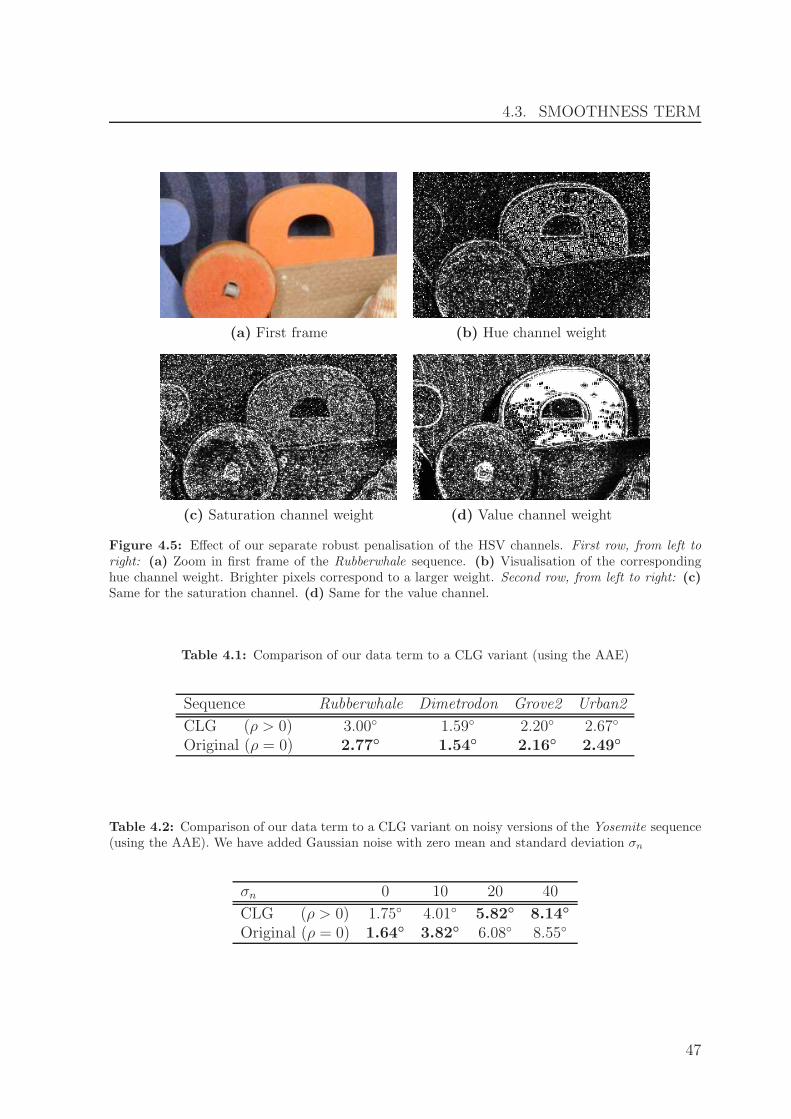
4.3. SMOOTHNESS TERM
(a) First frame (b) Hue channel weight
(c) Saturation channel weight (d) Value channel weight
Figure 4.5: Effect of our separate robust penalisation of the HSV channels. First row, from left toright: (a) Zoom in first frame of the Rubberwhale sequence. (b) Visualisation of the correspondinghue channel weight. Brighter pixels correspond to a larger weight. Second row, from left to right: (c)Same for the saturation channel. (d) Same for the value channel.
Table 4.1: Comparison of our data term to a CLG variant (using the AAE)
Sequence Rubberwhale Dimetrodon Grove2 Urban2
CLG (ρ > 0) 3.00 1.59 2.20 2.67
Original (ρ = 0) 2.77 1.54 2.16 2.49
Table 4.2: Comparison of our data term to a CLG variant on noisy versions of the Yosemite sequence(using the AAE). We have added Gaussian noise with zero mean and standard deviation σn
σn 0 10 20 40
CLG (ρ > 0) 1.75 4.01 5.82 8.14
Original (ρ = 0) 1.64 3.82 6.08 8.55
47

CHAPTER 4. MODELLING
Image-driven regularisers take into account image structures. To analyse the latter,one can consider the structure tensor [FG87]
Sρ := Kρ ∗[∇2f (∇2f)
⊤]=:
2∑
i=1
µi si s⊤i , (4.43)
with an integration scale ρ > 0. The structure tensor is a symmetric, positive semi-definite 2 × 2 matrix that possesses two orthonormal eigenvectors s1 and s2 with cor-responding eigenvalues µ1 and µ2, where w.l.o.g. µ1 ≥ µ2 ≥ 0. Directional informationof image structures is encoded in the eigenvectors: The vector s1 points across imagestructures, whereas the vector s2 points along them. The corresponding eigenvalues µ1
and µ2 describe the contrast along these directions.In the case ρ = 0, i.e. without considering neighbourhood information, one obtains
s01 =∇2f
|∇2f |, and s02 =
(∇2f)⊥
|∇2f |, (4.44)
where (∇2f)⊥ := (−fy, fx)⊤ denotes the vector orthogonal to ∇2f . The corresponding
eigenvalues in this case are µ01 = |∇2f |2 and µ0
2 = 0. For ρ = 0 we also have that|∇2f |2 = tr S0, with tr denoting the trace operator. Consequently, a large value oftr S0 indicates the presence of an image edge.
Most regularisers impose smoothness of the flow field by penalising the magnitudeof the flow gradients. As s1 and s2 constitute an orthonormal basis, we can rewrite the(squared) magnitude of the flow gradients as
|∇2u|2 = u2x + u2y = u2s1 + u2s2 , (4.45)
|∇2v|2 = v2x + v2y = v2s1 + v2s2 , (4.46)
using directional derivatives in s1- and s2-direction.To analyse the smoothing behaviour of the presented regularisers we will consider the
corresponding Euler-Lagrange equations (4.2) and (4.3). For all regularisers discussedhere, the Euler-Lagrange equations can be written in the form
∂uM − α div (D∇2u) = 0 , (4.47)
∂vM − α div (D∇2v) = 0 , (4.48)
with a diffusion tensor D that steers the smoothing of the flow components u and v.Specifically, the eigenvectors of D give the smoothing direction, whereas the correspond-ing eigenvalues determine the magnitude of the smoothing. Thus, the eigenstructure ofthe diffusion tensor determines the smoothing behaviour of the corresponding regu-lariser. For analysing the eigenstructure, we consider the eigendecomposition
D =
2∑
i=1
mi did⊤i , (4.49)
where d1 and d2 are the eigenvectors of D with corresponding eigenvalues m1 ≥ m2 ≥ 0.
48
4.3. SMOOTHNESS TERM
Homogeneous Regularisation. The first and most basic idea for a regulariser invariational optic flow estimation goes back to Horn and Schunck [HS81]. They proposeda homogeneous regulariser which we rewrite in our framework as
VH(∇2u,∇2v) := |∇2u|2 + |∇2v|2
= u2s1 + u2s2 + v2s1 + v2s2 . (4.50)
The corresponding diffusion tensor and its eigendecomposition are given by
DH = I :=
(1 00 1
)
= 1 · exe⊤x + 1 · eye
⊤y , (4.51)
where ex := (1, 0)⊤ and ey := (0, 1)⊤ denote the unit vectors in x- and y-direction, re-spectively. It becomes obvious that this regulariser performs a homogeneous smoothingwith the full strength of 1 at each location. Thus, it will blur important flow edges.
Image-Driven Regularisation. To obtain sharp flow edges, image-driven methodslike [AELS99, NE86] reduce the smoothing at image edges, which manifest themselvesby large values of |∇2f |2.
An isotropic image-driven regulariser was proposed by Alvarez et al. [AELS99] andcan be written as
VII(∇2u,∇2v) := g(|∇2f |2
) (|∇2u|2 + |∇2v|2
)
= g(tr S0)(u2s1 + u2s2 + v2s1 + v2s2
), (4.52)
where g is a decreasing, strictly positive weight function. Considering the eigendecom-position of the corresponding diffusion tensor
DII = g(trS0) I
= g(trS0) · exe⊤x + g(trS0) · eye
⊤y , (4.53)
it turns out that the weight function allows to decrease the smoothing in accordance tothe strength of image edges. However, the smoothing in x- as well as in y-direction isequally reduced.
To additionally steer the direction of smoothing and more importantly, to allow fora different strength of smoothing in different directions, anisotropic strategies have beenproposed. The anisotropic image-driven regulariser of Nagel and Enkelmann [NE86]prevents smoothing of the flow field across image boundaries but encourages smoothingalong them. This is achieved by the regulariser
VAI(∇2u,∇2v) := (∇2u)⊤P (∇2f) ∇2u + (∇2v)
⊤ P (∇2f) ∇2v , (4.54)
49

CHAPTER 4. MODELLING
where P (∇2f) denotes a regularised projection matrix perpendicular to the image gra-dient ∇2f , i.e. along image edges. The projection matrix is defined as
P (∇2f) :=1
|∇2f |2 + 2κ2
((∇2f)
⊥ (∇2f)⊥⊤
+ κ2I), (4.55)
with a regularisation parameter κ > 0. In our framework, the regulariser of Nagel andEnkelmann can be written as
VAI(∇2u,∇2v) =κ2
tr S0 + 2κ2
(u2s01
+ v2s01
)+
tr S0 + κ2
tr S0 + 2κ2
(u2s02
+ v2s02
). (4.56)
The correctness of the rewriting (4.56) is shown in the Appendix A and is based on theobservations that s01 and s02 are the eigenvectors of P , and that the factors in front of(u2
s01
+v2s01
) and (u2s02
+v2s02
) are the corresponding eigenvalues. The diffusion tensor for this
regulariser is identical to the projection matrix, which leads to the eigendecomposition
DAI = P (∇2f)
=κ2
tr S0 + 2κ2s01(s01)⊤
+tr S0 + κ2
tr S0 + 2κ2s02(s02)⊤
. (4.57)
Let us consider the limiting case where the regularisation parameter tends to zero, i.e.κ→0. The regulariser then becomes
VAI(∇2u,∇2v) = u2s02
+ v2s02
, (4.58)
and the eigendecomposition of the diffusion tensor simplifies to
DAI = s02(s02)⊤
. (4.59)
In this limit, we thus obtain a smoothing of the flow field solely in s02-direction, i.e. alongimage edges. In the definition of the normal flow (4.11) we have seen that a data termthat models the brightness constancy assumption constraints the flow only orthogonalto image edges. In the limiting case, the regulariser of Nagel and Enkelmann canhence be interpreted as a first complementary smoothness term that fills in informationorthogonal to the data constraint direction. This complementarity has been emphasisedby Schnorr [Sch93], who contributed a theoretical analysis as well as modifications ofthe original Nagel and Enkelmann functional.
As not every image edge necessarily corresponds to a flow edge, image-driven strate-gies are prone to give oversegmentation artefacts, especially in textured image regions.
Flow-Driven Regularisation. To remedy the oversegmentation problem, it makessense to adapt the smoothing process to the flow edges instead of the image edges.
50

4.3. SMOOTHNESS TERM
In the isotropic setting, Shulman and Herve [SH89] as well as Schnorr [Sch94] pro-posed to use rotationally invariant, subquadratic penaliser functions ΨV , resulting in
VIF(∇2u,∇2v) := ΨV
(|∇2u|2 + |∇2v|2
)
= ΨV
(u2s1 + u2s2 + v2s1 + v2s2
). (4.60)
The associated diffusion tensor is given by
DIF = Ψ′V
(u2s1+ u2s2+ v2s1+ v2s2
)I
= Ψ′V
(u2s1+ u2s2+ v2s1+ v2s2
)· exe
⊤x (4.61)
+Ψ′V
(u2s1+ u2s2+ v2s1+ v2s2
)· eye
⊤y .
The eigenstructure of this diffusion tensor is very similar to the one in the isotropicimage-driven setting, see (4.53). However, in the flow-driven case, the derivative Ψ′ ofthe penaliser function serves as decreasing weight function that reduces the smoothingof the flow field. The weighting thus depends on the contrast of the evolving flow field,and not anymore on image edges.
The underlying diffusion processes on the flow field are given by ut = div (DIF∇2u)and vt = div (DIF∇2v), respectively, which can be characterised as nonlinear isotropicdiffusion processes. In order to introduce total variation (TV ) regularisation [ROF92]to the optic flow case, Cohen [Coh93] used the convex penaliser
ΨV (s2) :=
√s2 + ε2 , (4.62)
with the diffusivity
Ψ′V (s
2) =1
2√s2 + ε2
≈ 1
2 |s| . (4.63)
using a small regularisation parameter ε > 0. Another possible choice is the non-convexPerona-Malik regulariser (Lorentzian) [BA96, PM90] given by
ΨV (s2) := λ2 log
(1 +
s2
λ2
), (4.64)
that results in Perona-Malik diffusion [PM90] with the diffusivity
Ψ′V (s
2) =1
1 + s2
λ2
, (4.65)
with a contrast parameter λ > 0.
An extension of flow-driven strategies to the anisotropic setting was presented byWeickert and Schnorr [WS01a]. They proposed the regulariser
VAF(∇2u,∇2v) := tr ΨV
(∇2u (∇2u)
⊤ +∇2v (∇2v)⊤), (4.66)
51
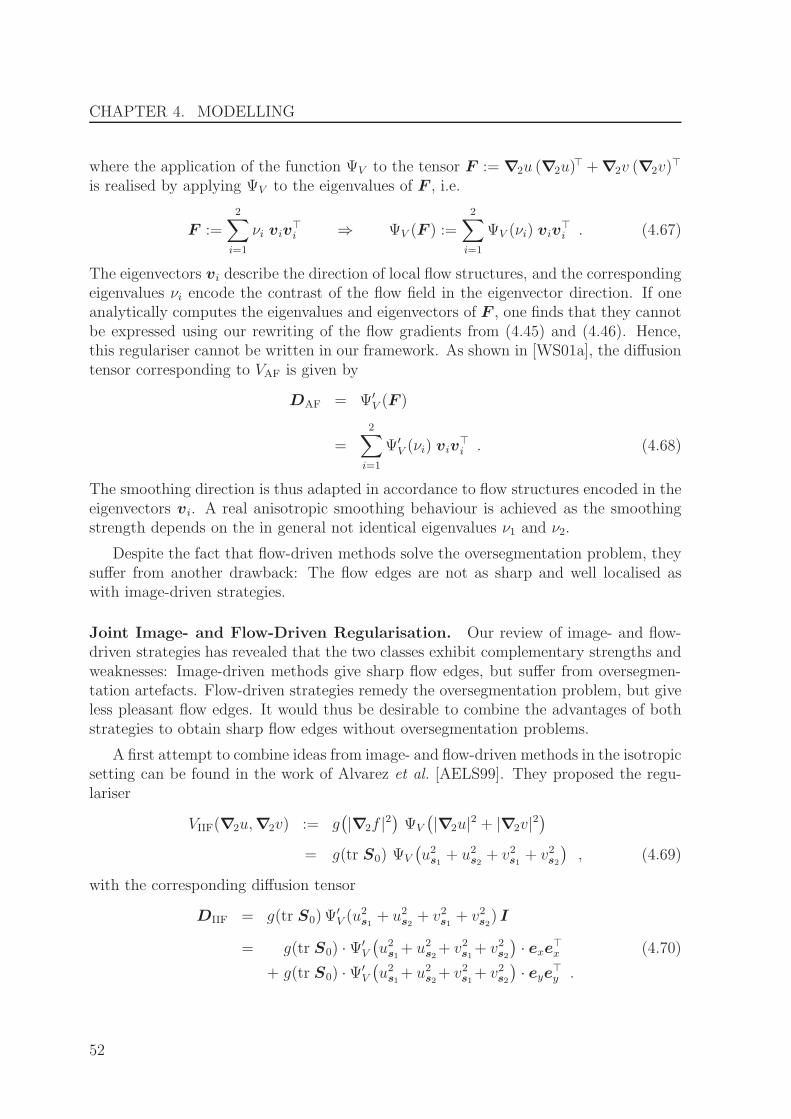
CHAPTER 4. MODELLING
where the application of the function ΨV to the tensor F := ∇2u (∇2u)⊤ +∇2v (∇2v)
⊤
is realised by applying ΨV to the eigenvalues of F , i.e.
F :=2∑
i=1
νi viv⊤i ⇒ ΨV (F ) :=
2∑
i=1
ΨV (νi) viv⊤i . (4.67)
The eigenvectors vi describe the direction of local flow structures, and the correspondingeigenvalues νi encode the contrast of the flow field in the eigenvector direction. If oneanalytically computes the eigenvalues and eigenvectors of F , one finds that they cannotbe expressed using our rewriting of the flow gradients from (4.45) and (4.46). Hence,this regulariser cannot be written in our framework. As shown in [WS01a], the diffusiontensor corresponding to VAF is given by
DAF = Ψ′V (F )
=2∑
i=1
Ψ′V (νi) viv
⊤i . (4.68)
The smoothing direction is thus adapted in accordance to flow structures encoded in theeigenvectors vi. A real anisotropic smoothing behaviour is achieved as the smoothingstrength depends on the in general not identical eigenvalues ν1 and ν2.
Despite the fact that flow-driven methods solve the oversegmentation problem, theysuffer from another drawback: The flow edges are not as sharp and well localised aswith image-driven strategies.
Joint Image- and Flow-Driven Regularisation. Our review of image- and flow-driven strategies has revealed that the two classes exhibit complementary strengths andweaknesses: Image-driven methods give sharp flow edges, but suffer from oversegmen-tation artefacts. Flow-driven strategies remedy the oversegmentation problem, but giveless pleasant flow edges. It would thus be desirable to combine the advantages of bothstrategies to obtain sharp flow edges without oversegmentation problems.
A first attempt to combine ideas from image- and flow-driven methods in the isotropicsetting can be found in the work of Alvarez et al. [AELS99]. They proposed the regu-lariser
VIIF(∇2u,∇2v) := g(|∇2f |2
)ΨV
(|∇2u|2 + |∇2v|2
)
= g(tr S0) ΨV
(u2s1 + u2s2 + v2s1 + v2s2
), (4.69)
with the corresponding diffusion tensor
DIIF = g(tr S0) Ψ′V (u
2s1+ u2s2 + v2s1 + v2s2) I
= g(tr S0) ·Ψ′V
(u2s1+ u2s2+ v2s1+ v2s2
)· exe
⊤x (4.70)
+ g(tr S0) ·Ψ′V
(u2s1+ u2s2+ v2s1+ v2s2
)· eye
⊤y .
52

4.3. SMOOTHNESS TERM
As one can see, the smoothing is still reduced at every image edge via the decreasingfunction g(tr S0). Thus, one obtains similar oversegmentation artefacts as purely image-driven methods, and the proposed strategy fails to combine the advantages of image-and flow-driven strategies.
In the work of Werlberger at al. [WTP+09], a subquadratic penaliser function isused within an anisotropic image-driven regulariser, thereby combining concepts fromanisotropic image-driven and isotropic flow-driven methods. The corresponding regu-lariser is given by
VAIF1(∇2u,∇2v) := ΨV
((∇2u)
⊤Q(∇2f) ∇2u
)+ΨV
((∇2v)
⊤Q(∇2f) ∇2v
), (4.71)
with the tensor
Q(∇2f) := g(|∇2f |β
) ∇2f
|∇2f |(∇2f)
⊤
|∇2f |+
(∇2f)⊥
|∇2f |(∇2f)
⊥⊤
|∇2f |. (4.72)
Similar to the rewriting of the Nagel and Enkelmann regulariser, we can express theregulariser from (4.71) in our general framework as
VAIF1(∇2u,∇2v) := ΨV
(g(tr S0) u
2s01
+ u2s02
)+ΨV
(g(tr S0) v
2s01
+ v2s02
), (4.73)
where we set β = 2. For this regulariser, we obtain two different diffusion tensors, onefor each of the Euler-Lagrange equations. For p ∈ u, v, they read as
DpAIF1
= Ψ′V
(g(tr S0) p
2s01
+ p2s02
)Q(∇2f) (4.74)
= Ψ′V
(g(tr S0) p
2s01
+ p2s02
)g(tr S0) s
01
(s01)⊤
(4.75)
+Ψ′V
(g(tr S0) p
2s01
+ p2s02
)s02(s02)⊤
.
As it turns out, the anisotropy of this regulariser is solely determined by the functiong(tr S0), which only depends on the image gradient. As seen for flow-driven methods, itis, however, necessary to reduce the smoothing strength w.r.t. flow gradients to overcomeoversegmentation problems. Thus, also this regulariser does not allow to combine theadvantages of image- and flow driven methods.
The first method that actually allows to combine the advantages of image- and flow-driven methods goes back to the discrete approach of Sun et al. [SRLB08]. A continuousversion of their regulariser can be written as
VAIF2(∇2u,∇2v) := ΨV
(u2s1)+ΨV
(v2s1)+ΨV
(u2s2)+ΨV
(v2s2). (4.76)
Note that in contrast to earlier approaches [NE86, WTP+09] who considered (∇2f)⊥/|∇2f |
to obtain directional information of image structures, the eigenvectors si of the structure
53
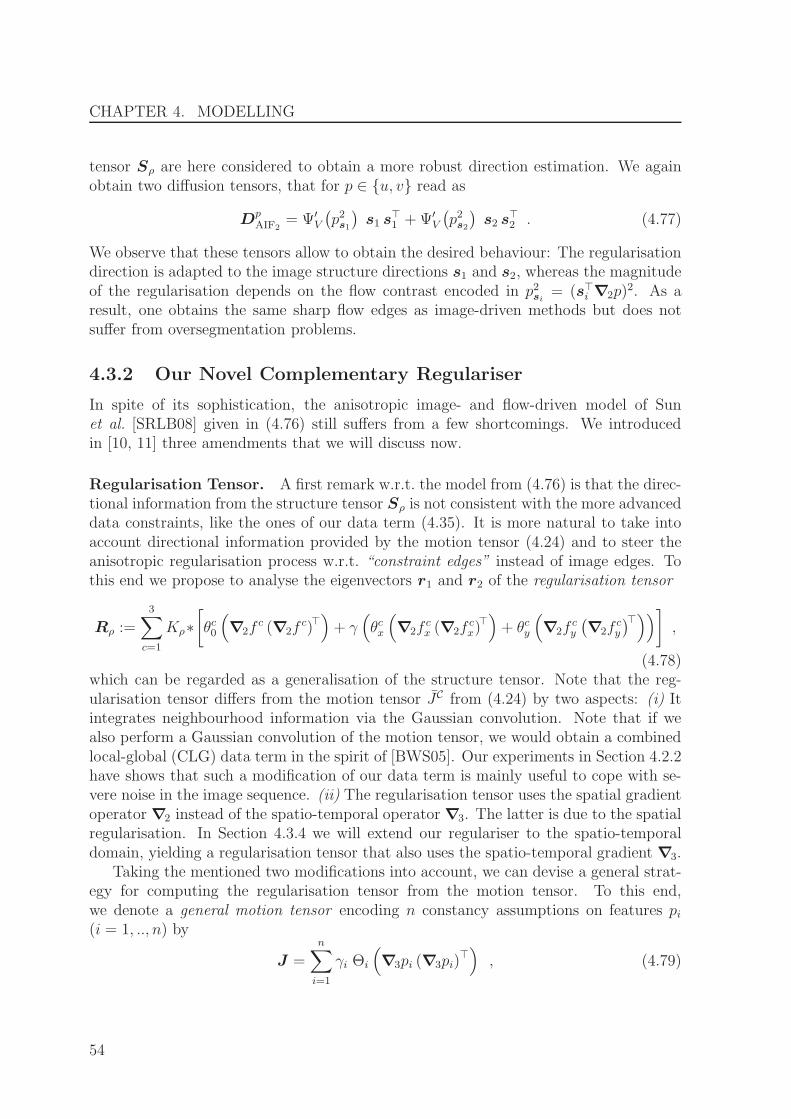
CHAPTER 4. MODELLING
tensor Sρ are here considered to obtain a more robust direction estimation. We againobtain two diffusion tensors, that for p ∈ u, v read as
DpAIF2
= Ψ′V
(p2s1)s1 s
⊤1 +Ψ′
V
(p2s2)s2 s
⊤2 . (4.77)
We observe that these tensors allow to obtain the desired behaviour: The regularisationdirection is adapted to the image structure directions s1 and s2, whereas the magnitudeof the regularisation depends on the flow contrast encoded in p2si = (s⊤i ∇2p)
2. As aresult, one obtains the same sharp flow edges as image-driven methods but does notsuffer from oversegmentation problems.
4.3.2 Our Novel Complementary Regulariser
In spite of its sophistication, the anisotropic image- and flow-driven model of Sunet al. [SRLB08] given in (4.76) still suffers from a few shortcomings. We introducedin [10, 11] three amendments that we will discuss now.
Regularisation Tensor. A first remark w.r.t. the model from (4.76) is that the direc-tional information from the structure tensor Sρ is not consistent with the more advanceddata constraints, like the ones of our data term (4.35). It is more natural to take intoaccount directional information provided by the motion tensor (4.24) and to steer theanisotropic regularisation process w.r.t. “constraint edges” instead of image edges. Tothis end we propose to analyse the eigenvectors r1 and r2 of the regularisation tensor
Rρ :=3∑
c=1
Kρ∗[θc0
(∇2f
c (∇2fc)⊤)+ γ
(θcx
(∇2f
cx (∇2f
cx)
⊤)+ θcy
(∇2f
cy
(∇2f
cy
)⊤))],
(4.78)which can be regarded as a generalisation of the structure tensor. Note that the reg-ularisation tensor differs from the motion tensor JC from (4.24) by two aspects: (i) Itintegrates neighbourhood information via the Gaussian convolution. Note that if wealso perform a Gaussian convolution of the motion tensor, we would obtain a combinedlocal-global (CLG) data term in the spirit of [BWS05]. Our experiments in Section 4.2.2have shows that such a modification of our data term is mainly useful to cope with se-vere noise in the image sequence. (ii) The regularisation tensor uses the spatial gradientoperator ∇2 instead of the spatio-temporal operator ∇3. The latter is due to the spatialregularisation. In Section 4.3.4 we will extend our regulariser to the spatio-temporaldomain, yielding a regularisation tensor that also uses the spatio-temporal gradient ∇3.
Taking the mentioned two modifications into account, we can devise a general strat-egy for computing the regularisation tensor from the motion tensor. To this end,we denote a general motion tensor encoding n constancy assumptions on features pi(i = 1, .., n) by
J =n∑
i=1
γi Θi
(∇3pi (∇3pi)
⊤), (4.79)
54

4.3. SMOOTHNESS TERM
where γi > 0 are weighting factors and Θi denotes normalisation factors that are equal to1 if we do not perform normalisation. The general regularisation tensor correspondingto the general motion tensor (4.79) then reads as
Rρ = Kρ∗[
n∑
i=1
γi Θi
(∇2pi (∇2pi)
⊤)]
. (4.80)
Rotational Invariance. The smoothness term VAIF2from (4.76) lacks the desirable
property of rotational invariance because the directional derivatives of u and v in theeigenvector directions are penalised separately. We propose to jointly penalise the di-rectional derivatives, yielding
VAIF−Rρ−RI(∇2u,∇2v) := ΨV
(u2r1
+ v2r1
)+ΨV
(u2r2
+ v2r2
), (4.81)
where we also used the eigenvectors r1 and r2 of the regularisation tensor.
Single Robust Penalisation. The above regulariser VAIF−Rρ−RI performs a twofoldrobust penalisation in both eigenvector directions. However, we have seen that thedata term mainly constraints the flow in the direction of the largest eigenvalue of theregularisation tensor, i.e. in r1-direction. We hence propose a single robust penalisationin r1-direction. In the orthogonal r2-direction, we opt for a quadratic penalisationyielding a strong filling-in effect of missing information. Incorporating the single robustpenalisation finally yields our complementary regulariser [10, 11]
VCR(∇2u,∇2v) := ΨV
(u2r1+ v2r1
)+ u2r2
+ v2r2. (4.82)
For the penaliser function ΨV , we propose the to use the Lorentzian as defined in (4.64).For our complementary regulariser, we obtain a single, joint diffusion tensor given by
DCR = Ψ′V
(u2r1+ v2r1
)· r1r
⊤1 + 1 · r2r
⊤2 , (4.83)
with Ψ′V as given in (4.65). The derivation of this diffusion tensor is presented in
Appendix A.
Discussion. To understand the advantages of our complementary regulariser com-pared to the closest existing regulariser (4.76), we compare our joint diffusion tensorfrom (4.83) to its counterparts in (4.77). In this way, the following innovations becomeapparent: (i) The smoothing direction is adapted to constraint edges instead of imageedges, as the eigenvectors of the regularisation tensor r1 and r2 are used instead of theeigenvectors of the structure tensor. (ii) We achieve rotational invariance by couplingthe two flow components in the argument of Ψ′
V . (iii) We only reduce the smoothingacross constraint edges, i.e. in r1-direction. Along them, always a strong diffusion withstrength 1 is performed, resembling edge-enhancing anisotropic diffusion [Wei96].
55
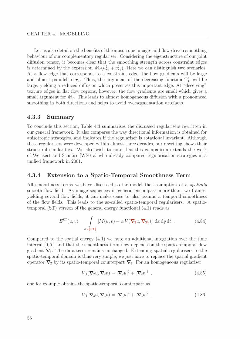
CHAPTER 4. MODELLING
Let us also detail on the benefits of the anisotropic image- and flow-driven smoothingbehaviour of our complementary regulariser. Considering the eigenstructure of our jointdiffusion tensor, it becomes clear that the smoothing strength across constraint edgesis determined by the expression Ψ′
V (u2r1
+ v2r1). Here we can distinguish two scenarios:
At a flow edge that corresponds to a constraint edge, the flow gradients will be largeand almost parallel to r1. Thus, the argument of the decreasing function Ψ′
V will belarge, yielding a reduced diffusion which preserves this important edge. At “deceiving”texture edges in flat flow regions, however, the flow gradients are small which gives asmall argument for Ψ′
V . This leads to almost homogeneous diffusion with a pronouncedsmoothing in both directions and helps to avoid oversegmentation artefacts.
4.3.3 Summary
To conclude this section, Table 4.3 summarises the discussed regularisers rewritten inour general framework. It also compares the way directional information is obtained foranisotropic strategies, and indicates if the regulariser is rotational invariant. Althoughthese regularisers were developed within almost three decades, our rewriting shows theirstructural similarities. We also wish to note that this comparison extends the workof Weickert and Schnorr [WS01a] who already compared regularisation strategies in aunified framework in 2001.
4.3.4 Extension to a Spatio-Temporal Smoothness Term
All smoothness terms we have discussed so far model the assumption of a spatiallysmooth flow field. As image sequences in general encompass more than two frames,yielding several flow fields, it can make sense to also assume a temporal smoothnessof the flow fields. This leads to the so-called spatio-temporal regularisers. A spatio-temporal (ST) version of the general energy functional (4.1) reads as
EST(u, v) =
∫
Ω×[0,T ]
[M(u, v) + α V (∇3u,∇3v)] dx dy dt . (4.84)
Compared to the spatial energy (4.1) we note an additional integration over the timeinterval [0, T ] and that the smoothness term now depends on the spatio-temporal flowgradient ∇3. The data term remains unchanged. Extending spatial regularisers to thespatio-temporal domain is thus very simple, we just have to replace the spatial gradientoperator ∇2 by its spatio-temporal counterpart ∇3. For an homogeneous regulariser
VH(∇2u,∇2v) = |∇2u|2 + |∇2v|2 , (4.85)
one for example obtains the spatio-temporal counterpart as
VH(∇3u,∇3v) = |∇3u|2 + |∇3v|2 . (4.86)
56

4.3.SMOOTHNESSTERM
Table 4.3: Comparison of regularisation strategies. The vectors si and ri denote the eigenvectors of the structure tensor Sρ from (4.43) andthe vectors regularisation tensor Rρ from (4.78), respectively. The next to last column names the tensor that is analysed to obtain directionalinformation for anisotropic strategies, and the last column indicates if the corresponding regulariser is rotational invariant
Strategy Regulariser V Directional RotationalAdaptation Invariance
Homogeneous [HS81] u2s1+ u2s2+ v2s1+ v2s2 — X
Isotropic image-driven [AELS99] g(tr S0)(u2s1+ u2s2+ v2s1+ v2s2
)— X
Anisotropic image-driven [NE86] u2s02
+ v2s02
, for κ→0 S0 X
Isotropic flow-driven [SH89] ΨV
(u2s1+ u2s2+ v2s1+ v2s2
)— X
Isotropic image- and flow-driven [AELS99] g(tr S0) ΨV
(u2s1+ u2s2+ v2s1+ v2s2
)— X
Anisotropic image and flow-driven ΨV
(g(tr S0) u
2s01
+ u2s02
)S0 —
[WTP+09] +ΨV
(g(tr S0) v
2s01
+ v2s02
)
Anisotropic image and flow-driven ΨV
(u2s1)+ ΨV
(v2s1)+ΨV
(u2s2)+ΨV
(v2s2)
Sρ —[SRLB08]
Anisotropic complementary ΨV
(u2r1+ v2r1
)+ u2r2+ v2r2
Rρ X
image- and flow-driven [10, 11]
57

CHAPTER 4. MODELLING
For our complementary regulariser from (4.82), we first have to define the spatio-temporal regularisation tensor
RST
ρ :=3∑
c=1
[θc0
(∇3f
c (∇3fc)⊤)
(4.87)
+ γ(θcx
(∇3f
cx (∇3f
cx)
⊤)+ θcy
(∇3f
cy
(∇3f
cy
)⊤))]
= Kρ ∗ JC. (4.88)
For ρ = 0 it is identical to the motion tensor JCfrom (4.24). Note in this context that
the Gaussian convolution with Kρ is now performed in the spatio-temporal domain,which also holds for the presmoothing of the image sequence. The spatio-temporalregularisation tensor is a 3 × 3 matrix that possesses three orthonormal eigenvectorsr1, r2 and r3. With their help, we define the spatio-temporal complementary regulariser
VCR(∇3u,∇3v) := ΨV
(u2r1
+ v2r1
)+ u2r2
+ v2r2+ u2r3 + v2r3
, (4.89)
with its spatio-temporal diffusion tensor
DSTCR = Ψ′
V
(u2r1 + v2r1
)r1 r
⊤1 + r2 r
⊤2 + r3 r
⊤3 . (4.90)
4.3.5 Experiments
In the following experiments, we compare the discussed regularisation strategies.
Comparison with Other Regularisers. In Figure 4.6, we again use our Snail se-quence to compare our complementary regulariser from (4.82) with other regularisers:(i) A basic homogeneous regulariser [HS81]. (ii) The anisotropic image-driven reg-ulariser of Nagel and Enkelmann [NE86]. (iii) The popular TV regulariser; see (4.60)and (4.62). (iv) The anisotropic image and flow-driven regulariser from [SRLB08], whichbuilt the basis of our complementary regulariser. Here, we use a rotationally invariantformulation that can be obtained from (4.81) by replacing the eigenvectors ri of theregularisation tensor by the eigenvectors si of the structure tensor. As data term, weuse our final data term from (4.35).
Let us compare the obtained results: A homogeneous regularisation (Figure 4.6 (d))clearly gives a oversmoothed result. Using an image-driven strategy (Figure 4.6 (e))gives relatively sharp edges, but suffers from oversegmentation. Note that the latterleads to the cloud-like artefacts because of the strongly textured background. With aflow-driven TV regulariser (Figure 4.6 (f)), we obtain blurred and badly localised flowedges. Using the image-and flow-driven regulariser from [SRLB08] (Figure 4.6 (g)), theflow edges are already more appealing, but unpleasant staircasing artefacts deterioratethe result. This can be explained by the twofold robust penalisation that is performed inthis regulariser. Our result is depicted in Figure 4.6 (h) and obviously gives an appealingflow field without severe degradations.
58
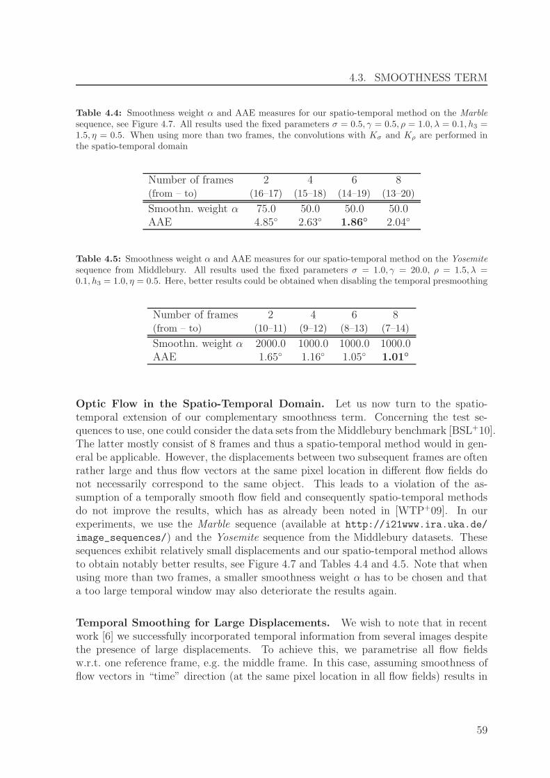
4.3. SMOOTHNESS TERM
Table 4.4: Smoothness weight α and AAE measures for our spatio-temporal method on the Marblesequence, see Figure 4.7. All results used the fixed parameters σ = 0.5, γ = 0.5, ρ = 1.0, λ = 0.1, h3 =1.5, η = 0.5. When using more than two frames, the convolutions with Kσ and Kρ are performed inthe spatio-temporal domain
Number of frames 2 4 6 8(from – to) (16–17) (15–18) (14–19) (13–20)
Smoothn. weight α 75.0 50.0 50.0 50.0AAE 4.85 2.63 1.86 2.04
Table 4.5: Smoothness weight α and AAE measures for our spatio-temporal method on the Yosemitesequence from Middlebury. All results used the fixed parameters σ = 1.0, γ = 20.0, ρ = 1.5, λ =0.1, h3 = 1.0, η = 0.5. Here, better results could be obtained when disabling the temporal presmoothing
Number of frames 2 4 6 8(from – to) (10–11) (9–12) (8–13) (7–14)
Smoothn. weight α 2000.0 1000.0 1000.0 1000.0AAE 1.65 1.16 1.05 1.01
Optic Flow in the Spatio-Temporal Domain. Let us now turn to the spatio-temporal extension of our complementary smoothness term. Concerning the test se-quences to use, one could consider the data sets from the Middlebury benchmark [BSL+10].The latter mostly consist of 8 frames and thus a spatio-temporal method would in gen-eral be applicable. However, the displacements between two subsequent frames are oftenrather large and thus flow vectors at the same pixel location in different flow fields donot necessarily correspond to the same object. This leads to a violation of the as-sumption of a temporally smooth flow field and consequently spatio-temporal methodsdo not improve the results, which has as already been noted in [WTP+09]. In ourexperiments, we use the Marble sequence (available at http://i21www.ira.uka.de/
image_sequences/) and the Yosemite sequence from the Middlebury datasets. Thesesequences exhibit relatively small displacements and our spatio-temporal method allowsto obtain notably better results, see Figure 4.7 and Tables 4.4 and 4.5. Note that whenusing more than two frames, a smaller smoothness weight α has to be chosen and thata too large temporal window may also deteriorate the results again.
Temporal Smoothing for Large Displacements. We wish to note that in recentwork [6] we successfully incorporated temporal information from several images despitethe presence of large displacements. To achieve this, we parametrise all flow fieldsw.r.t. one reference frame, e.g. the middle frame. In this case, assuming smoothness offlow vectors in “time” direction (at the same pixel location in all flow fields) results in
59
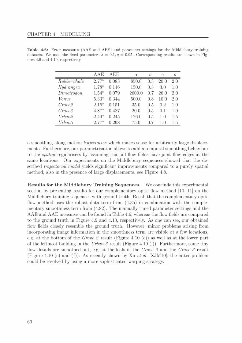
CHAPTER 4. MODELLING
Table 4.6: Error measures (AAE and AEE) and parameter settings for the Middlebury trainingdatasets. We used the fixed parameters λ = 0.1, η = 0.95. Corresponding results are shown in Fig-ures 4.9 and 4.10, respectively
AAE AEE α σ γ ρ
Rubberwhale 2.77 0.083 850.0 0.3 20.0 2.0Hydrangea 1.78 0.146 150.0 0.3 3.0 1.0Dimetrodon 1.54 0.079 2600.0 0.7 26.0 2.0Venus 5.33 0.344 500.0 0.8 10.0 2.0Grove2 2.16 0.151 35.0 0.5 0.2 1.0Grove3 4.87 0.487 20.0 0.5 0.1 1.0Urban2 2.49 0.245 126.0 0.5 1.0 1.5Urban3 2.77 0.298 75.0 0.7 1.0 1.5
a smoothing along motion trajectories which makes sense for arbitrarily large displace-ments. Furthermore, our parametrisation allows to add a temporal smoothing behaviourto the spatial regularisers by assuming that all flow fields have joint flow edges at thesame locations. Our experiments on the Middlebury sequences showed that the de-scribed trajectorial model yields significant improvements compared to a purely spatialmethod, also in the presence of large displacements, see Figure 4.8.
Results for the Middlebury Training Sequences. We conclude this experimentalsection by presenting results for our complementary optic flow method [10, 11] on theMiddlebury training sequences with ground truth. Recall that the complementary opticflow method uses the robust data term from (4.35) in combination with the comple-mentary smoothness term from (4.82). The manually tuned parameter settings and theAAE and AAE measures can be found in Table 4.6, whereas the flow fields are comparedto the ground truth in Figure 4.9 and 4.10, respectively. As one can see, our obtainedflow fields closely resemble the ground truth. However, minor problems arising fromincorporating image information in the smoothness term are visible at a few locations,e.g. at the bottom of the Grove 2 result (Figure 4.10 (c)) as well as at the lower partof the leftmost building in the Urban 3 result (Figure 4.10 (l)). Furthermore, some tinyflow details are smoothed out, e.g. at the leafs in the Grove 2 and the Grove 3 result(Figure 4.10 (c) and (f)). As recently shown by Xu et al. [XJM10], the latter problemcould be resolved by using a more sophisticated warping strategy.
60

4.3. SMOOTHNESS TERM
(a) First frame (b) Zoom into (a) (c) Zoom into second frame
(d) Homogeneous (e) Anisotropic image-driven (f) Isotropic flow-driven
(g) Anisotropic image- (h) Anisotropic
and flow-driven complementary
Figure 4.6: Results for our Snail sequence with different smoothness terms. First row, from left toright: (a) First frame. (b) Zoom in marked region of first frame. (c) Same for second frame. Secondrow, from left to right: (d) Flow field in marked region, with homogeneous regularisation [HS81](α = 200.0). (e) Same for anisotropic image-driven regularisation [NE86] (α = 500.0, κ = 0.1). (f)Same for isotropic flow-driven TV regularisation [Sch94, SH89] (α = 50.0, ε = 0.001). Third row, fromleft to right: (g) Same for anisotropic image- and flow-driven regularisation [SRLB08] (α = 2000.0, ρ =4.0, λ = 0.1). (h) Same for our anisotropic complementary regulariser [10, 11] (α = 2000.0, ρ = 4.0, λ =0.1). All results used the fixed parameters σ = 0.5, γ = 20.0, η = 0.95.
61

CHAPTER 4. MODELLING
(a) Reference frame (b) Ground truth (c) Flow (2 frames)
(d) Flow (4 frames) (e) Flow (6 frames) (f) Flow (8 frames)
Figure 4.7: Results for the Marble sequence with our spatio-temporal method. First row, from leftto right: (a) Reference frame (frame 16). (b) Ground truth (white pixels mark locations where noground truth is available). (c) Result using 2 frames (16–17). Second row, from left to right: (d) Samefor 4 frames (15–18). (e) Same for 6 frames (14–19). (f) Same for 8 frames (13–20).
62
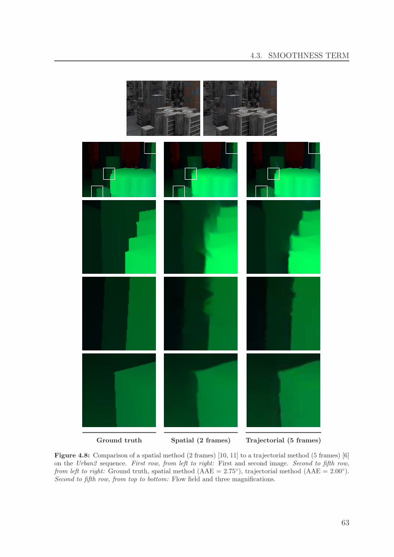
4.3. SMOOTHNESS TERM
Ground truth Spatial (2 frames) Trajectorial (5 frames)
Figure 4.8: Comparison of a spatial method (2 frames) [10, 11] to a trajectorial method (5 frames) [6]on the Urban2 sequence. First row, from left to right: First and second image. Second to fifth row,from left to right: Ground truth, spatial method (AAE = 2.75), trajectorial method (AAE = 2.00).Second to fifth row, from top to bottom: Flow field and three magnifications.
63

CHAPTER 4. MODELLING
Reference frame Ground truth Our result
Figure 4.9: Results for our complementary optic flow method [10, 11] on the Middlebury trainingsequences with ground truth. First column: Reference frame. Second column: Ground truth (whitepixels mark locations where no ground truth is given). Third column: Result with our method. Fromtop to bottom: Rubberwhale, Dimetrodon, Hydrangea and Venus sequence.
64

4.3. SMOOTHNESS TERM
Reference frame Ground truth Our result
Figure 4.10: Results for our complementary optic flow method [10, 11] on the Middlebury trainingsequences with ground truth. First column: Reference frame. Second column: Ground truth (whitepixels mark locations where no ground truth is given). Third column: Result with our method. Fromtop to bottom: Grove2, Grove3, Urban2 and Urban3 sequence.
65

CHAPTER 4. MODELLING
4.3.6 Smoothness Terms for Stereo
In the variational stereo context, similar regularisation strategies as for optic flow havebeen proposed, which we will review in this subsection. Recall that in the consideredorthoparallel case, we will only experience horizontal displacements u.
Image-driven Regularisation. In the isotropic setting, an image-driven regulariserwas proposed by Kim and Sohn [KS03]. It can be written as
VII(∇2u) := g(|∇2f |2
)|∇2u|2
= g(tr S0)(u2s1 + u2s2
), (4.91)
and leads to the same diffusion tensor as in (4.53).
Anisotropic image-driven smoothness terms for stereo became popular through theworks of Mansouri et al. [MMK98] and Alvarez et al. [ADSW02]. They proposed regu-larisers of the form
VAI(∇2u) = ΨV
(∇2u
⊤P (∇2f) ∇2u), (4.92)
with a projection matrix P similar as in the Nagel and Enkelmann regulariser (4.55).
Disparity-driven Regularisation. As seen for flow-driven optic flow regularisers,disparity-driven strategies allow to remedy oversegmentation problems. Isotropic image-driven strategies were introduced to the stereo community by Slesareva et al. [SBW05]and Ben-Ari and Sochen [BAS07]. They used the regulariser
VID(∇2u) := ΨV
(|∇2u|2
)
= ΨV
(u2s1+ u2s2
), (4.93)
leading to the diffusion tensor
DID = Ψ′V
(u2s1+ u2s2
)I
= Ψ′V
(u2s1+ u2s2
)· exe
⊤x +Ψ′
V
(u2s1+ u2s2
)· eye
⊤y . (4.94)
Completing the Taxonomy of Stereo Regularisers
So far, all presented stereo regularisers could be obtained in a straightforward mannerfrom their optic flow counterparts. Let us also try this for an anisotropic disparity-driven regulariser by adapting the anisotropic flow-driven regulariser of Weickert andSchnorr [WS01a] from (4.66). A stereo counterpart can be written as
VAD(∇2u) := tr ΨV
(∇2u (∇2u)
⊤), (4.95)
66

4.3. SMOOTHNESS TERM
with the diffusion tensor
DAD = Ψ′V
(∇2u (∇2u)
⊤)
=:2∑
i=1
Ψ′V (νi) viv
⊤i . (4.96)
In the optic flow case, the tensor in the argument of ΨV was given by ∇2u (∇2u)⊤ +
∇2v (∇2v)⊤, resulting in a coupling of the two flow components. As a consequence, the
desired anisotropic behaviour can be ensured as the eigenvectors of the tensor are ingeneral not parallel to the gradients of both flow components.
In the stereo case, however, the resulting tensor ∇2u (∇2u)⊤ is equal to the structure
tensor of the disparity with a zero integration scale. As we have seen in (4.44) and thefollowing, the eigenstructure of this tensor is trivial. In above notation, it can be writtenas ν1 = |∇2u|2, ν2 = 0 and
v1 =∇2u
|∇2u|, and v2 =
∇2u⊥
|∇2u|. (4.97)
With this, let us rewrite the diffusion part of the corresponding Euler-Lagrange equation:
div (DAD ∇2u) = div(Ψ′
V
(∇2u (∇2u)
⊤)∇2u
)(4.98)
= div
((2∑
i=1
Ψ′V (νi) viv
⊤i
)∇2u
)(4.99)
= div
((Ψ′
V (|∇2u|2)|∇2u|2
∇2u∇2u⊤ (4.100)
+Ψ′
V (0)
|∇2u|2∇2u
⊥(∇2u⊥)⊤
)∇2u
)
(∗)= div
(Ψ′
V (|∇2u|2)|∇2u|2
|∇2u|2∇2u+ 0
)(4.101)
= div(Ψ′
V (|∇2u|2)∇2u)
(4.102)
= div(Ψ′
V (u2s1+ u2s2)∇2u
)= div (DID ∇2u) , (4.103)
where (∗) makes use of the facts that ∇2u⊤∇2u = |∇2u|2 and (∇2u
⊥)⊤∇2u = 0. As itturns out, adapting the anisotropic flow-driven regulariser (4.66) to the stereo contextresults in an isotropic disparity-driven behaviour as for the regulariser (4.93) with thediffusion tensor (4.94).
67

CHAPTER 4. MODELLING
Towards Anisotropic Disparity-driven Regularisation. To model an anisotropicdisparity-driven smoothing process for stereo we follow our work in [8]: We refrain fromdesigning a regulariser VAD and directly model the diffusion tensor DAD.
In order to obtain a truly anisotropic behaviour we adapted ideas from edge en-hancing anisotropic diffusion (EED) filtering [Wei94]. Specifically, we consider a stereovariant of the structure tensor (4.43), given by
Sρ (∇2uσ) := Kρ ∗(∇2uσ∇2u
⊤σ
), (4.104)
where uσ := Kσ ∗ u denotes a Gaussian smoothed version of the disparity u. Com-pared to the previously considered tensor ∇2u∇2u
⊤, we observe two innovations: (i)The disparity u is regularised by the Gaussian convolution with standard deviation σ,and (ii) neighbourhood information is integrated by convolving the tensor entries with aGaussian kernel of standard deviation ρ. Note that regularisation of the unknown u byGaussian convolution with noise scale σ was first proposed in the context of nonlineardiffusion to reduce staircaising artefacts and problems with noise [CLMC92]. Despitethe fact that ∇2uσ is a useful edge detector, the problem still remains that it is sen-sitive under noise for small σ, while an increased σ can lead to undesired cancellationeffects. This can be overcome by an additional convolution of the tensor entries withthe integration scale ρ.
Our modified structure tensor Sρ(∇2uσ) is a symmetric, positive semi-definite matrixwith two orthonormal eigenvectors s1 and s2 which give the directions of the localdisparity structure. The corresponding eigenvalues µ1 ≥ µ2 ≥ 0, give the averagecontrast along these directions. Consequently, we propose to use the following diffusiontensor which takes into account the structural information contained in Sρ(∇2uσ):
DAD := Ψ′V (Sρ (∇2uσ)) =
2∑
i=1
Ψ′V (µi) si s
⊤i . (4.105)
For the diffusivity Ψ′V we propose to use the Perona-Malik diffusivity from (4.65) as it
is known to make backward diffusion possible and thereby enhance edges even more.Let us now show that our method indeed exhibits the described anisotropic be-
haviour:
• In flat disparity regions:µ1 ≈ µ2 ≈ 0 ⇒ Ψ′
V (µ1) ≈ 1, Ψ′V (µ2) ≈ 1.
This leads to a homogeneous smoothing in both directions.
• At a straight disparity edge in s2-direction:µ1 ≫ µ2 ≈ 0 ⇒ Ψ′
V (µ1) ≈ 0, Ψ′V (µ2) ≈ 1.
This leads to an anisotropic smoothing in edge direction, but not across.
• At disparity corners:µ1 ≥ µ2 ≫ 0 ⇒ Ψ′
V (µ1) ≈ 0, Ψ′V (µ2) ≈ 0.
This prevents smoothing.
68

4.3. SMOOTHNESS TERM
Complementary Regularisation for Stereo. Adapting our complementary regu-lariser from (4.82) to the stereo case can be done in a straightforward manner.
Although the stereo tensor (4.39) uses the gradient operator ∇xt, the regularisationtensor for stereo is identical to the optic flow regularisation tensor Rρ from (4.78). Thischoice can be justified as also in the stereo case we want to use directional informationfrom the spatial domain, i.e., from the x- and y-direction, and not from the x- andt-direction. The complementary regulariser for stereo is defined as
VCR(∇2u) = ΨV
(u2r1
)+ u2r2 , (4.106)
with the diffusion tensor
DCR = Ψ′V
(u2r1)· r1r
⊤1 + 1 · r2r
⊤2 . (4.107)
4.3.7 Experiments
Similar to our experiment for the optic flow case in Section 4.3.5, Figure 4.6, we nowwant to compare the performance of the presented stereo regularisers. As test imagepair, we chose the popular Tsukuba pair (available at http://bj.middlebury.edu/
~schar/stereo/data/tsukuba/). In Figure 4.11 we show the disparity maps obtainedwhen using a stereo version of our robust data term (4.35) in combination with differentregularisation strategies. Table 4.7 additionally summarises the parameter settings andthe BPE error measures.
Comparing the results, similar observations as in the optic flow case can be made.A homogeneous regularisation as in [HS81] (Figure 4.11 (d)) gives oversmoothed result.With an anisotropic image-driven regulariser [ADSW02, MMK98] (Figure 4.11 (e)), thedisparity edges become sharper, but oversegmentation artefacts deteriorate the result.As an example, consider the artefact arising at the left of the lamp. A disparity-drivenTV regulariser [BAS07, SBW05] (Figure 4.11 (f)) remedies oversegmentation problems,but clearly gives delocalised disparity edges. Using our anisotropic disparity-driven reg-ulariser [8] (Figure 4.11 (g)) gives more appealing disparity edges due to the smoothingalong edges. To obtain even sharper edges, one can use the image- and disparity-drivenregulariser by adapting the smoothness term from [SRLB08] (Figure 4.11 (h)). However,this regulariser gives unpleasantly jagged disparity edges. When using the stereo variant(4.106) of our complementary regulariser [10, 11] (Figure 4.11 (i)), we obtain sharp andwell-localised disparity edges.
The above observations are further supported by the bad pixel error (BPE) measuresresulting from the different regularisation strategies, see Table 4.7. Finally, we wish tonote that all image-driven strategies (Figure 4.11 (e),(h),(i)) perform especially wellin the occluded areas, which are shown in Figure 4.11 (c). This observation can beexplained as follows: Occlusions are outliers in the data term, as no matching basedon data constancy assumptions is possible in occluded regions. Consequently, a robustdata term will disable its influence and the smoothness has to fill-in the disparity there.
69

CHAPTER 4. MODELLING
Table 4.7: Error measures (BPE) and parameter settings for the Tsukuba pair, see Figure 4.11. Allresults used the fixed parameters σ = 0.5, γ = 5.0, η = 0.95
Regulariser BPE Parameters
Homogeneous [HS81] 11.73 α = 50.0
Anisotropic image-driven [ADSW02, MMK98] 10.14 α = 200.0, κ = 0.1
Isotropic disparity-driven [BAS07, SBW05] 8.57 α = 10.0, ε = 0.001
Anisotropic 8.23 α = 150.0, σ = 1.0,disparity-driven [8] ρ = 2.0, λ = 0.1
Anisotropic 8.12 α = 275.0, ρ = 1.5,image- and disparity-driven [SRLB08] λ = 0.1
Anisotropic complementary 7.12 α = 260.0, ρ = 1.5,image- and disparity-driven [10, 11] λ = 0.1
For the filling-in, it is crucial to consider image instead of disparity information, becausethe disparity estimate is less reliable at occlusions. Thus, image-driven strategies haveadvantages.
70

4.3. SMOOTHNESS TERM
(a) Left image (b) Ground truth (c) Ground truth occlusions
(d) Homogeneous (e) Anisotropic image-driven (f) Isotropic disparity-driven
(g) Anisotropic (h) Anisotropic image- (i) Anisotropic
disparity-driven and disparity-driven complementary
Figure 4.11: Results for the Tsukuba pair with different smoothness terms. First row, from left toright: (a) Left image. (b) Ground truth disparity. (c) Ground truth occlusions. Second row, fromleft to right: (d) Disparity map with homogeneous regularisation [HS81]. (e) Same for anisotropicimage-driven regularisation [MMK98, ADSW02] (f) Same for isotropic disparity-driven TV regulari-sation [SBW05, BAS07]. Third row, from left to right: (g) Same for our anisotropic disparity-drivenregularisation [8]. (h) Same for anisotropic image- and disparity-driven regularisation [SRLB08]. (i)Same for our anisotropic complementary regulariser [10, 11].
71

CHAPTER 4. MODELLING
4.4 Automatic Selection of the Smoothness Weight
To achieve favourable results, an appropriate selection of the model parameters ismandatory. Especially for the smoothness weight α that determines the balance be-tween the data and the smoothness term, an appropriate choice is crucial: Too smallvalues lead to noisy flow fields whereas too large values lead to an over-smoothing. Anautomatic selection of the smoothness weight is thus not only convenient, but especiallyimportant in real world applications of optic flow such as robot navigation or driverassistance. Also in less time-critical applications like video re-timing, an automatic se-lection of model parameters for sure eases the use and boost the acceptance of opticflow-based approaches.
Note that in the mentioned real world scenarios, no ground truth flow is known ingeneral. If this would be the case, a parameter selection would be very simple: Onecould just select the parameters that give the flow field with the smallest deviation fromthe ground truth.
4.4.1 A Novel Concept
Our parameter selection approach uses an error measure that allows to judge the qualityof a flow field without knowing the ground truth. This error measure is based on a novelconcept, the optimal prediction principle (OPP) that we introduced in [10]. The OPPstates that the flow field obtained with an optimal smoothness weight allows for the bestprediction of the next frames in the image sequence. This makes sense as a too smallsmoothness weight would lead to an overfit to the first two frames and consequentlyresult in a bad prediction of further frames. For too large smoothness weights, the flowfields would be too smooth and thus also lead to a bad prediction.
Following the OPP, our error measure needs to judge the quality of the predictionachieved with a given flow field. To this end, we evaluate the imposed data constraintsbetween the first and the third frame of the image sequence, resulting in an averagedata constancy error (ADCE ) measure. To compute this measure, we assume thatthe motion of the scene objects is of more or less constant speed and that it describeslinear trajectories within the considered three frames. Under these assumptions, wesimply double the flow vectors to evaluate the data constraints between the first andthe third frame. Due to the favourable performance of our parameter selection methodthat is demonstrated in Section 4.4.3, we conjecture that the made assumptions holdfor common test sequences. In accordance to this strategy, we can define the ADCE
72

4.4. AUTOMATIC SELECTION OF THE SMOOTHNESS WEIGHT
between frame 1 and 3 as
ADCE1,3(wα) :=1
|Ω|
∫
Ω
[3∑
c=1
ΨM
(θc0 (f
c(x+2wα)−f c(x))2)
(4.108)
+ γ
(3∑
c=1
ΨM
(θcx (f
cx(x+2wα)−f c
x(x))2
+ θcy(f cy(x+2wα)−f c
y(x))2))]
dx dy ,
where wα denotes the flow field obtained with a smoothness weight α. The inte-grand of above expression is (apart from the doubled flow field) a variant of our fi-nal data term (4.35) where no linearisation of the constancy assumptions has beenperformed. To evaluate the images at subpixel locations f i(x+2wα) we use Coonspatches based on bicubic interpolation [Coo67]. Note that when using the HSV colourspace, the normalisation factors Θ1 of the hue channel have to be computed as in(4.27). Also the difference expression for the hue channel have to be computed ac-cordingly. For example, the expression |f 1(x+2w)− f 1(x)|2 has to be replaced by|(cos f 1)(x+2w)− (cos f 1)(x)|2 + |(sin f 1)(x+2w)− (sin f 1)(x)|2.
Determining the Best Parameter. In general, the relation between α and theADCE is not convex, which excludes the use of gradient descent-like approaches forfinding the optimal value of α w.r.t. our error measure.
Similar to the approach in [NS97] we propose a brute-force method that first com-putes the error measures for a “sufficiently large” set of flow fields obtained with differentvalues of α. Then, we select the very α that gave the smallest error. To reduce the num-ber values to test for α, we propose to start from a given, standard value α0. Thisvalue is incremented/decremented nα times by multiplying/dividing it with a steppingfactor a > 1, yielding in total 2nα+1 tests. This strategy results in testing more valuesclose to α0 and, more importantly, less very small or very large values that hardly givereasonable results.
4.4.2 Scale Selection in the Optic Flow Scale Space
In a recent work [2] we investigated the scale space behaviour of variational optic flowmethods, the optic flow scale space. Intuitively, it is clear that our smoothness parameterα serves a similar role as the scale parameter in classic image scale spaces (see e.g.[Lin94]) as larger values of α lead to smoother, i.e. simplified flow fields. In our work, wereformulated the classic Horn and Schunck energy functional in a signal regularisation-like manner by rewriting the data term as a similarity term to the normal flow. To makethis possible, we need to penalise deviations from the normal flow in a spatially varying,
73
CHAPTER 4. MODELLING
matrix weighted norm. If we apply an explicit scheme to solve the corresponding Euler-Lagrange equations (see Section 5.3.4 for more details), we end up with a diffusion-likeevolution that starts from the normal flow and builds up the optic flow scale space.
It is clear that in the optic flow case, there exists one distinct scale α that corre-sponds to the flow field of highest accuracy. To select this optimal scale, which is animportant issue for any scale space, see e.g. [MN03], we utilised our optimal predictionprinciple. The big advantage in the context of the optic flow scale space is that theexplicit evolution gives a flow field after each iteration, i.e. after k iterations a flow fieldcorresponding to the smoothness weight α = k · τ is available, where τ denotes the timestep size of the explicit scheme. Thus, one can easily compute the average data con-stancy error (ADCE) after each iteration and finally select the scale with the smallestADCE as the optimal scale.
4.4.3 Experiments
Performance of our Proposed Error Measure. We first show that our proposeddata constancy error between frame 1 and 3 (ADCE1,3, see (4.108)) is a good approxi-mation of the popular average angular error (AAE) measure. To this end, we comparethe two error measures for the Grove2 sequence in Figure 4.12 (a) and (b). Additionally,we also show results obtained with a simpler error measure that evaluates the data con-stancy assumptions between the first and second frame (ADCE1,2), see Figure 4.12 (c).
It becomes obvious that our proposed error measure (Figure 4.12 (b)) indeed ex-hibits a shape very close to the angular error shown in Figure 4.12 (a). As our errormeasure reflects the quality of the prediction with the given flow field, our result fur-ther substantiates the validity of the proposed OPP. Furthermore, we see that a simpleerror measure that uses only frame one and two (Figure 4.12 (c)) gives unusable resultsas it favours way too small values of the smoothness weight. This behaviour could beexpected as the constancy assumptions are imposed between frame one and two in thedata term and thus they are best fulfilled when the influence of the smoothness term,which is steered by the smoothness weight, becomes small.
Benefits of an Automatic Parameter Selection. Next, we want show that ourautomatic parameter selection works well for a large variety of different test sequences.To this end we apply our method to the Middlebury data sets [BSL+10]. Note thatwe cannot give results for the Dimetrodon and Venus sequence here, as those onlyencompasses two frames and thus our ADCE1,3 measure cannot be computed.
In Table 4.8, we summarise the AAE when (i) setting the smoothness weight α to afixed value (α = α0 = 400.0), (ii) using our automatic parameter selection method, and(iii) selecting the (w.r.t. the AAE) optimal value of α under the tested proposals. As wecan see, estimating the smoothness weight with our proposed method allows to improvethe results compared to a fixed value of α in almost all cases. The only exception isthe Grove 3 sequence where the fixed value of α accidentally coincides with the optimal
74

4.4. AUTOMATIC SELECTION OF THE SMOOTHNESS WEIGHT
2
3
4
5
6
7
0 1000 2000 3000 4000
AA
E
α
80
85
90
95
100
0 1000 2000 3000 4000
AD
CE
1,3
α
70
71
72
73
74
75
0 1000 2000 3000 4000
AD
CE
1,2
α
Figure 4.12: Automatic selection of the smoothness weight α for the Grove2 sequence. From left toright: (a) Angular error (AAE) for 51 values of α, computed from α0 = 400.0 and using a steppingfactor a = 1.1. The remaining parameters were set fixed to σ = 0.5, γ = 20.0, ρ = 4.0, η = 0.95.The dotted line marks the minimum of the graph. (b) Same for the proposed data constancy error(ADCE1,3). (c) Same for a simple data constancy error (ADCE1,2).
value. Compared to the results achieved with an optimal value of α, our results are onaverage 3% and at most 10% worse than the optimal result. When actually comparingthe value of α chosen by our method to the optimal value, it turns out that we oftenchoose a value that seems way too small. Nevertheless, the AAE of the correspondingflow field is still close to the optimum and our method thus fulfils its purpose.
We wish to note that a favourable performance of the proposed parameter selection ofcourse depends on the validity of our assumptions (constant speed and linear trajectoriesof objects). For all considered test sequences these assumptions were obviously valid. Inorder to show the limitations of our method, we applied our approach again to the samesequences, but replaced the third frame by a copy of the second one. This violates theassumption of a constant speed and leads to a severe impairment of results that reachup to 30%.
Comparison to State-of-the-Art Methods. In order to evaluate the performanceof an optic flow method compared to the state-of-the-art, one can submit the resultsto the popular Middlebury benchmark [BSL+10]. The results that we submitted wereobtained with our optic flow in harmony (OFH) method [10] that uses our robust dataterm from (4.35) in combination with the complementary smoothness term from (4.82).The optimal value of the smoothness weight α is determined by our proposed methodbased on the OPP.
We found that for the provided benchmark sequences, using an HSV colour repre-sentation is not as beneficial as seen in our experiment from Figure 4.4 on page 46. Asthe Middlebury sequences hardly suffer from difficult illumination conditions, we cannotprofit from the photometric invariances of the HSV colour space. On the other hand,some sequences even pose problems in their HSV representation. As an example, con-sider the results for the the Teddy sequence in the first row of Figure 4.13. Here we seethat the small white triangle beneath the chimney causes unpleasant artefacts in theflow field. This results from the problem that greyscales do not have a unique represen-
75

CHAPTER 4. MODELLING
Table 4.8: Results (AAE) for some Middlebury sequences when (i) fixing the smoothness weight(α = 400.0), (ii) estimating α with our proposed method, and (iii) with the optimal value of α
Sequence Fixed α Estimated α Optimal α
Rubberwhale 3.43 3.00 3.00
α = 400.0 644.2 943.2
Hydrangea 1.96 1.94 1.86
α = 400.0 440.0 943.2
Grove2 2.59 2.43 2.43
α = 400.0 532.4 779.5
Grove3 5.50 5.62 5.50
α = 400.0 532.4 400.0
Urban2 3.22 2.84 2.66
α = 400.0 532.4 1255.4
Urban3 3.44 3.37 3.35
α = 400.0 484.0 644.2
Yosemite 2.56 1.89 1.71
α = 400.0 1037.5 2224.0
Marble 5.73 5.05 4.94
α = 400.0 1838.0 3581.7
76
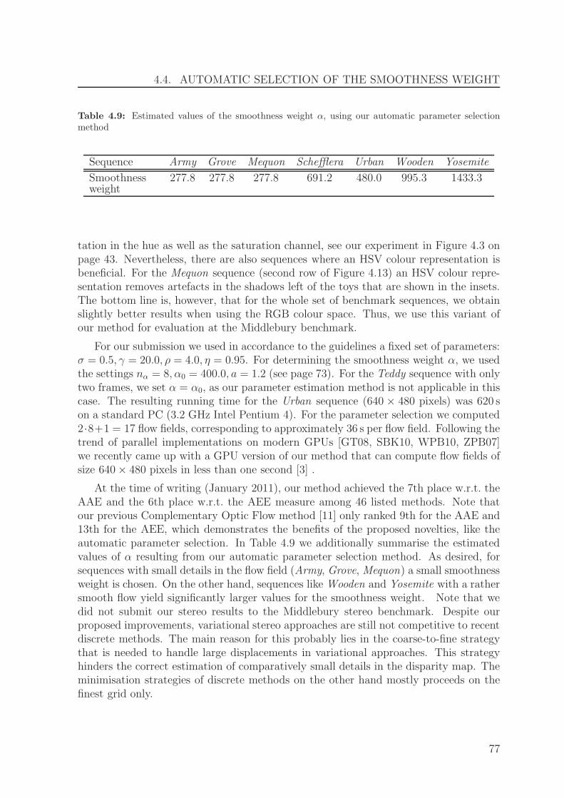
4.4. AUTOMATIC SELECTION OF THE SMOOTHNESS WEIGHT
Table 4.9: Estimated values of the smoothness weight α, using our automatic parameter selectionmethod
Sequence Army Grove Mequon Schefflera Urban Wooden Yosemite
Smoothness 277.8 277.8 277.8 691.2 480.0 995.3 1433.3weight
tation in the hue as well as the saturation channel, see our experiment in Figure 4.3 onpage 43. Nevertheless, there are also sequences where an HSV colour representation isbeneficial. For the Mequon sequence (second row of Figure 4.13) an HSV colour repre-sentation removes artefacts in the shadows left of the toys that are shown in the insets.The bottom line is, however, that for the whole set of benchmark sequences, we obtainslightly better results when using the RGB colour space. Thus, we use this variant ofour method for evaluation at the Middlebury benchmark.
For our submission we used in accordance to the guidelines a fixed set of parameters:σ = 0.5, γ = 20.0, ρ = 4.0, η = 0.95. For determining the smoothness weight α, we usedthe settings nα = 8, α0 = 400.0, a = 1.2 (see page 73). For the Teddy sequence with onlytwo frames, we set α = α0, as our parameter estimation method is not applicable in thiscase. The resulting running time for the Urban sequence (640 × 480 pixels) was 620 son a standard PC (3.2 GHz Intel Pentium 4). For the parameter selection we computed2·8+1 = 17 flow fields, corresponding to approximately 36 s per flow field. Following thetrend of parallel implementations on modern GPUs [GT08, SBK10, WPB10, ZPB07]we recently came up with a GPU version of our method that can compute flow fields ofsize 640× 480 pixels in less than one second [3] .
At the time of writing (January 2011), our method achieved the 7th place w.r.t. theAAE and the 6th place w.r.t. the AEE measure among 46 listed methods. Note thatour previous Complementary Optic Flow method [11] only ranked 9th for the AAE and13th for the AEE, which demonstrates the benefits of the proposed novelties, like theautomatic parameter selection. In Table 4.9 we additionally summarise the estimatedvalues of α resulting from our automatic parameter selection method. As desired, forsequences with small details in the flow field (Army, Grove, Mequon) a small smoothnessweight is chosen. On the other hand, sequences like Wooden and Yosemite with a rathersmooth flow yield significantly larger values for the smoothness weight. Note that wedid not submit our stereo results to the Middlebury stereo benchmark. Despite ourproposed improvements, variational stereo approaches are still not competitive to recentdiscrete methods. The main reason for this probably lies in the coarse-to-fine strategythat is needed to handle large displacements in variational approaches. This strategyhinders the correct estimation of comparatively small details in the disparity map. Theminimisation strategies of discrete methods on the other hand mostly proceeds on thefinest grid only.
77

CHAPTER 4. MODELLING
HSV colour space RGB colour space
Figure 4.13: Comparison of results obtained with HSV or RGB colour representation. From left toright: Reference frame. Result with HSV colour space. Result with RGB colour space. From top tobottom: Teddy sequence (HSV ⇒ AAE = 3.94, RGB ⇒ AAE = 2.64). Mequon sequence (HSV ⇒AAE = 2.28, RGB ⇒ AAE = 2.84).
4.5 Prediction Prior
By construction, optic flow methods using a coarse-to-fine warping scheme cannot esti-mate large displacements of small objects. More precisely, the displacement of an objectmust not be larger than the object itself. However, such large displacements may occurdue to fast motion, low frame rate of the camera, or large baseline distances in the stereocontext. For our scene flow method in [5] we had to cope with the latter problem. Asa remedy, we followed the ideas in [BM11] and added a prediction prior to our usualenergy functional. This prior models the knowledge of an initial guess (a “prediction”)of the flow field we aim to compute, e.g. the prior could be the result from some othermatching strategy that does not suffer from the afore mentioned problems. To incor-porate this prior knowledge into our model we add a third term to the general energyfunctional (4.1), which results in the modified energy functional [BM11]
E(u, v) =
∫
Ω
(M(u, v) + αV (∇2u,∇2v) + β P (u, v)
)dx dy , (4.109)
where P (u, v) denotes the prediction prior, and the weight β > 0 steers its influence onthe overall flow estimation. An obvious idea to define the P is
P (u, v) = ΨP
((u−u)2+(v−v)2
), (4.110)
78

4.5. PREDICTION PRIOR
where (u, v)⊤ denotes the given predictor flow field. For the robust penaliser function wepropose to use ΨP (s
2) =√s2 + ε2, which helps to cope with outliers (wrong estimates)
in the predictor.In some cases, e.g. when using SIFT matches [Low99, Low04] as a predictor, we
are not given a prediction at any point of the image domain. To account for this, wemultiply the prediction prior P with a mask cP (x) that is equal to one if we are givena prediction at the point x ∈ Ω and is else equal to zero. Incorporating the mask in(4.109) gives the energy
E(u, v) =
∫
Ω
(M(u, v) + αV (∇2u,∇2v) + β cP P (u, v)
)dx dy . (4.111)
The corresponding Euler-Lagrange equations for energy (4.111) when using the priorfrom (4.110) are given by
∂uM − α div
(∂ux
V∂uy
V
)+ β cP Ψ′
P
((u−u)2+(v−v)2
)(u−u) = 0 , (4.112)
∂vM − α div
(∂vxV∂vyV
)+ β cP Ψ′
P
((u−u)2+(v−v)2
)(v−v) = 0 . (4.113)
4.5.1 Experiments
We now show experiments that illustrate the benefits of a prediction prior. For our firstexperiment we consider two frames of the Beanbag sequence shown in the top row ofFigure 4.14. Note the rightmost ball undergoes a large displacement to the top, which isindeed larger than its own size. Consequently, optic flow approaches relying on warpingcannot capture this displacement, as can be observed in Figure 4.14 (c). On the otherhand, even a simple block matching approach, see Figure 4.14 (d), can estimate thedisplacement as this technique does not require to work on coarse representations ofthe images. Using the block matching result as a predictor within a warping-basedoptic flow approach then finally allows to obtain a smooth flow field that can capturethe displacement of the right ball, as witnessed in Figure 4.14 (e). A small remainingproblem is that some of the artefacts in the upper right corner are still present in thefinal result.
In our second experiment, we consider a synthetic sequence that we created in thecontext of our work on scene flow from uncalibrated cameras [5]. The scene depictsa textured sphere which is situated in front of a likewise textured background. InFigure 4.15 (a) and (b) we show the left and right image of the corresponding stereopair at time t. Note that we do not have an orthoparallel camera setup in this case,which means that the displacements are not purely horizontal. This can easily be seen atthe ground truth displacement in Figure 4.15 (c). For estimating the displacements, wefirst try to apply our Complementary optic flow approach [10, 11]. As the displacementsof the small-scale textures are rather large (about 30 pixels), the resulting displacement
79

CHAPTER 4. MODELLING
(a) First image (b) Second image
(c) Complementary OF (d) Block matching (NCC) (e) Complementary OF
+ prediction (NCC)
Figure 4.14: Results for the Beanbag sequence. First row, from left to right: (a) First image. (b)Second image. Second row, from left to right: (c) Flow field obtained with our Complementary OpticFlow approach [10, 11] (α = 200.0, σ = 0.3, γ = 10.0, ρ = 1.0, η = 0.95). (d) Same for a simple blockmatching approach (normalised cross correlation (NCC), 9 × 9 blocks). (e) Same for our Comple-mentary Optic Flow approach with additional prediction prior using previous block matching result(α=800.0, β=20.0).
estimation fails, see Figure 4.15 (d). Due to the dominant texture, the present sequenceis on the other hand well-suited for feature matching approaches like SIFT [Low99,Low04], which find a large number of matches that are shown in Figure 4.15 (e). Thesecorrespondences were computed using the binary available under http://www.cs.ubc.ca/~lowe/keypoints/. Incorporating the sparse correspondences as a prediction prior,a favourable estimation of the displacements can be achieved, see Figure 4.15 (f).
80

4.5. PREDICTION PRIOR
(a) Left image (b) Right image (c) Ground truth
(d) Complementary OF (e) SIFT matches (f) Complementary OF
+ prediction (SIFT)
Figure 4.15: Results for the general sphere sequence [5]. First row, from left to right: (a) Leftimage. (b) Right image. (c) Ground truth (white pixels mark locations where no ground truth isavailable). Second row, from left to right: (d) Flow field obtained with our Complementary Optic Flowapproach [10, 11] (α = 100.0, σ = 0.9, γ = 0.3, ρ = 1.0, η = 0.95 ⇒ AAE = 77.78). (e) Sparse SIFTmatches [Low99, Low04] (matching threshold=0.6). (f) Flow field obtained with our ComplementaryOptic Flow approach with additional prediction prior using previous SIFT matches (α=10.0, β=4.0⇒ AAE = 5.13).
81

CHAPTER 4. MODELLING
82

Chapter 5
Numerics
All the mathematical sciences are founded on relationsbetween physical laws and laws of numbers, so that theaim of exact science is to reduce the problems of natureto the determination of quantities by operations withnumbers.
James C. Maxwell
This chapter encompasses two major parts. We first discuss the numerical approxima-tion of derivatives that occur in our continuous models from the previous section. Tothis end, we make use of the popular concept of finite differences, see e.g. [MM94]. Forthe discretisation of image derivatives, we additionally present a novel finding from ourwork in [1, 7]. Here, we showed that an appropriate discretisation strategy borrowedfrom the theory of hyperbolic differential equations can have a tangible influence on thequality of results.
The second part is mainly concerned with reviewing strategies for the solution of theEuler-Lagrange equations, including the embedding in a coarse-to-fine warping frame-work for handling large displacements. As an illustrative example, we consider theEuler-Lagrange equations arising in our complementary optic flow approach [10, 11].Additionally, we present two novel contributions from our side: (i) A fast solver thatis based on a parallel implementation of a fast explicit diffusion (FED) [GWB10] gra-dient descent scheme on modern graphics hardware [3]. (ii) An implementation of theprevious solver on a modern smart phone [4].
5.1 Discretisation
Implementing the continuous variational models that we have discussed in the previouschapter requires to discretise the images and the flow field as well as their derivatives.
83

CHAPTER 5. NUMERICS
The discretisation of the images was already presented in Section 3.4 and the discretisa-tion of the flow fields follows in complete accordance. The discretisation of derivativesis more involved and will be described in the following.
5.1.1 Discretising Derivatives by Finite Differences
In this thesis, we use the concept of finite difference approximations for discretisingderivatives. As an example, consider the approximation of the x-derivative of an imagef(x, y). To this end, finite differences offer three basic choices: forward, backward andcentral differences, which are defined as
D+x f
ki,j :=
1
h1
(fki+1,j − fk
i,j
), D+
x fk+1i,j :=
1
h1
(fk+1i+1,j − fk+1
i,j
), (5.1)
D−x f
ki,j :=
1
h1
(fki,j − fk
i−1,j
), D−
x fk+1i,j :=
1
h1
(fk+1i,j − fk+1
i−1,j
), (5.2)
D0xf
ki,j :=
1
2h1
(fki+1,j − fk
i−1,j
), D0
xfk+1i,j :=
1
2h1
(fk+1i+1,j − fk+1
i−1,j
), (5.3)
where h1 denotes the grid size in x-direction and the finite difference operators D+,D− and D0 denote forward, backward and central differences, respectively. Further notethat these expressions can be computed at the time level k and k+1. The correspondingdifferences for the y-derivative are obtained by simply switching the roles of i and j inabove equations. The approximation error of the one-sided differences (forward andbackward) is in O(h), where h ∈ h1, h2. Their central counterparts only involvean error of O(h2), which, together with the unbiased stencil orientation, explains whycentral differences are a popular “standard” choice in image processing applications.
In order to increase the accuracy, one may use averaged differences that take intoaccount differences from both time levels k and k+1. One possibility is to use averagedcentral differences that for the x-derivative are defined as
D0xf
k+ 1
2
i,j :=1
2
(D0
xfki,j +D0
xfk+1i,j
)
=1
4h1
(fki+1,j − fk
i−1,j + fk+1i+1,j − fk+1
i−1,j
). (5.4)
In the remainder of this chapter, such a central difference approximation will be referredto as a “standard” derivative approximation.
Note that averaging the two signals at time k and k + 1 only makes sense if thedisplacements between the signals are small, in fact smaller than one pixel. Only if thisprecondition is satisfied, our averaging takes into account information originating fromthe same points in space. In our case, the multiscale warping approach (see Section 5.3.1)results in displacements in the desired range.
A means to further reduce the approximation error is to use approximations offourth-order that involve more pixels than just the two direct neighbours of the pixel
84

5.1. DISCRETISATION
under consideration. An averaged fourth-order approximation of the x-derivative is forexample defined as
D00x f
k+ 1
2
i,j :=1
2
(D00
x fki,j +D00
x fk+1i,j
)
:=1
24h1
(−fk
i+2,j + 8fki+1,j − 8fk
i−1,j + fki−2,j (5.5)
−fk+1i+2,j + 8fk+1
i+1,j − 8fk+1i−1,j + fk+1
i−2,j
).
Discretisation of Flow Derivatives
Having presented the basics of finite difference approximations on the examples of imagederivatives, we can turn to the discretisation of the flow derivatives.
Discretising Spatial and Temporal Flow Derivatives. When using flow-drivenor image- and flow-driven regularisers, the spatial flow derivatives ux, uy and vx, vy willoccur in the diffusion tensor D. For discretising the flow derivatives, we use a centraldifference approximation of second order. For example, discretising the derivative ux isdone via
ux ≈ D0xui,j =
1
2h1(ui+1,j − ui−1,j) . (5.6)
For spatio-temporal regularisers discussed in Section 4.3.4, we also need to discretisetemporal flow derivatives ut and vt. To this end, we use the approximation
ut ≈ 1
h3
(uk+1i,j − uki,j
), and vt ≈ 1
h3
(vk+1i,j − vki,j
), (5.7)
respectively. Here, it makes sense to adapt the value of h3 to the given image sequenceto allow for an appropriate scaling of the temporal direction compared to the spatialdirections [WS01b].
Discretising the Divergence Expression. Considering the Euler-Lagrange equa-tions (5.56) and (5.57) shows that we need to discretise divergence expression of theform div(D∇2u). Denoting the tensor entries by
D :=
(a bb c
), (5.8)
we can write the divergence expression as
div (D∇2u) = div
(aux + buybux + cuy
)(5.9)
= ∂x(aux) + ∂x(buy) + ∂y(bux) + ∂y(cuy) . (5.10)
85

CHAPTER 5. NUMERICS
The pure x- and y-terms (∂x(aux) and ∂y(cuy)) are discretised by using forward differ-ences inside the bracket and backward differences for the outer derivative, i.e.
∂x(aux) ≈ D−x
(ai+1,j + ai,j
2
ui+1,j − ui,jh1
)(5.11)
≈ ai+1,j + ai,j2h21
(ui+1,j − ui,j) − ai,j + ai−1,j
2h21(ui,j − ui−1,j) , (5.12)
and correspondingly
∂y(cuy) ≈ ci,j+1 + ci,j2h22
(ui,j+1 − ui,j) − ci,j + ci,j−1
2h22(ui,j − ui,j−1) . (5.13)
For the mixed terms ∂x(buy) and ∂y(bux), we can use a standard approximation bycentral differences, resulting in
∂x(buy) ≈ D0x
(bi,j
ui,j+1 − ui,j−1
2h2
)(5.14)
≈ bi+1,j
4h1h2(ui+1,j+1 − ui+1,j−1)−
bi−1,j
4h1h2(ui−1,j+1 − ui−1,j−1) , (5.15)
and correspondingly
∂y(bux) ≈ bi,j+1
4h1h2(ui+1,j+1 − ui−1,j+1)−
bi,j−1
4h1h2(ui+1,j−1 − ui−1,j−1) . (5.16)
This shows that the divergence expression can be discretised as a weighted sum ofdifferences
div (D ∇2u) ≈∑
i,j∈Ni,j
[w]i,j
([u]i,j − [u]i,j
), (5.17)
where Ni,j denotes the set of pixels in the 8-neighbourhood of the pixel (i, j) and theweights [w]i,j are defined as
[w]i−1,j =ai−1,j + ai,j
2 h21, [w]i+1,j =
ai+1,j + ai,j2 h21
, (5.18)
[w]i,j−1 =ci,j+1 + ci,j
2 h22, [w]i,j+1 =
ci,j−1 + ci,j2 h22
, (5.19)
[w]i−1,j−1 =−bi−1,j − bi,j+1
4 h1h2, [w]i+1,j−1 =
bi+1,j + bi,j+1
4 h1h2, (5.20)
[w]i−1,j+1 =bi−1,j + bi,j−1
4 h1h2, [w]i+1,j+1 =
−bi+1,j + bi,j−1
4 h1h2. (5.21)
86

5.2. UPWIND DISCRETISATION OF IMAGE DERIVATIVES
In order to obtain sharper results, we follow [Wei98] and modify above weights inaccordance to the non-negative stencil proposed in [Wei98], chapter 3.4. This gives theweights
[w]i−1,j =ai−1,j + ai,j
2 h21− |bi−1,j |+ |bi,j|
2 h1h2, (5.22)
[w]i+1,j =ai+1,j + ai,j
2 h21− |bi+1,j |+ |bi,j|
2 h1h2, (5.23)
[w]i,j−1 =ci,j+1 + ci,j
2 h22− |bi,j+1|+ |bi,j |
2 h1h2, (5.24)
[w]i,j+1 =ci,j−1 + ci,j
2 h22− |bi,j−1|+ |bi,j |
2 h1h2, (5.25)
[w]i−1,j−1 =|bi−1,j+1| − bi−1,j+1 + |bi,j| − bi,j
4 h1h2, (5.26)
[w]i+1,j−1 =|bi+1,j+1|+ bi+1,j+1 + |bi,j |+ bi,j
4 h1h2, (5.27)
[w]i−1,j+1 =|bi−1,j−1|+ bi−1,j−1 + |bi,j |+ bi,j
4 h1h2, (5.28)
[w]i+1,j+1 =|bi+1,j−1| − bi+1,j−1 + |bi,j| − bi,j
4 h1h2. (5.29)
5.2 Upwind Discretisation of Image Derivatives
All experiments presented so far used the central difference approximation (5.5) fordiscretising occurring image derivatives. The only exception is the computation of theregularisation tensor (4.78). Here, we do not average the differences, but only use theimage at time level k to consider directional information from the reference image, only.
However, our investigations in [1, 7] showed that using correctly oriented one-sideddifferences can tangibly improve the results compared to central difference approxima-tions. In the context of hyperbolic partial differential equations (HDEs) this fact iswell-known and used in the popular upwind schemes. The major advantage of upwinddiscretisations is that they prevent oscillations at edges as they belong to the class ofso-called monotone schemes that satisfy a discrete maximum-minimum principle. Inthis class, upwind schemes are known to be the most accurate schemes.
5.2.1 A 1D Example
To illustrate the influence of the applied finite difference operator, we use a simple 1Dexample. Here, we consider a 1D signal sequence f(x, t) where x ∈ Ω1 denotes the
87

CHAPTER 5. NUMERICS
position in the interval Ω1 ⊂ R. To compute the unknown displacement function u(x)we minimise the energy functional
E(u) =
∫
Ω1
((fx u+ ft)
2 + αu2x
)dx , (5.30)
which is identical to a 1D version of the Horn and Schunck model [HS81]. Equivalentlyto the brightness constancy assumption, the data term imposes a constancy on the signalvalues. In the smoothness term, we penalise the 1D pendant of the gradient magnitude,given by the x-derivative of the displacement function. Both term use a basic quadraticpenalisation. The Euler-Lagrange equation corresponding to the energy (5.30) reads
f 2x u+ fxft − α uxx = 0 . (5.31)
Let us now present a 1D experiment that shows the importance of an appropriatechoice for the finite difference approximation of fx. Consider the two frames of a signalsequence in Figure 5.1 (a). Here, the signal is displaced by exactly one position to theright in its middle part and stays unchanged otherwise. This is illustrated in the groundtruth displacement shown in Figure 5.1 (b). Note that this example comprises smoothas well as discontinuous signal and displacement regions which make it rather indicative.
We further wish to note that our example also exhibits the so-called occlusion prob-lem. This arises if a foreground object is shifted and occludes parts of the background.Thus, one cannot find any correspondence for the regions that are only visible in the firstframe and then become occluded in the second frame. In our example this happens atPoint 9. Therefore, any computed displacements u will be corrupted at this occlusion.However, while we comment in this way on the expected computational results, theocclusion problem is not a topic in the focus of our work. In practical computations, theocclusion problem is dealt with separately; see e.g. [BBH03] and the references therein.
In Figure 5.1 (c)–(e) we depict the computed displacements using various finite dif-ference discretisations for the signal derivative fx. The displacements were obtained asthe solution of a linear system of equations that arises from the discrete Euler-Lagrangeequation (5.31). As the corresponding system matrix is tridiagonal, the Thomas algo-rithm [Tho49] can be used as a simple and efficient solver. In our experiment, we set thesmoothness weight to the small value of α = 10−4 in order to clearly show the influenceof the discretisation of the signal derivative that occurs in the data term.
Comparing the resulting displacements in Figure 5.1 (c)–(e), the effect of the dif-ferent derivative approximations become obvious: Central differences only perform wellin the smooth signal regions, i.e. at the left and right boundaries. At discontinuitiesthey produce severe oscillations. One-sided differences perform either favourably or failtotally. Obviously, the correct orientation matters here. When using correctly orientedone-sided differences, the displacement almost coincides with the ground truth, exceptat one point. As indicated above, this is not a fault of the method, but is caused bythe occlusion at the jump in the displacement. Note that as the displacement of an
88

5.2. UPWIND DISCRETISATION OF IMAGE DERIVATIVES
occluded point is in general undefined, we set the ground truth at occlusions to thevalue of its right neighbour. The observed behaviour in our experiment is in accordancewith the theory of numerical methods for HDEs [LeV92, LeV02]. There, so called up-wind schemes are a widely used concept for the discretisation of transport equations,where the term upwind refers to correctly oriented one-sided differences. The correctorientation of an upwind stencil in our case is opposite to the displacement direction;see our experiment.
In the hyperbolic theory, central difference approximations as in (5.5) are knownto lead to oscillations. They can even be unconditionally unstable, as for exampleshown in [Tor99]. The reason why they are still a common choice in correspondenceproblems is that here only one time step is performed, and thus the instability is “only”observable in terms of oscillations near strong gradients. Note that there exist stablecentral discretisations like the monotone Lax-Friedrichs and the Lax-Wendroff scheme,see [LeV02]. However, the Lax-Friedrichs scheme is the most dissipative one, it actuallyinvolves the most possible blurring of all monotone schemes. The Lax-Wendroff schemeis not monotone (it is second-order accurate) and is known to generate oscillations asby the Gibbs phenomenon. Finally, let us remark that the stability of explicit schemesfor HDEs involves a condition on the time step size called CFL condition, see [LeV02,Tor99]. This CFL condition can be translated into the assumption, that in one time step,information can only be translated up to one pixel. Therefore, the CFL condition forHDEs is related to the assumption of small displacements in correspondence problems.As discussed earlier, the CFL condition is always satisfied because we use a multiscalewarping approach that results in displacements in the range of one pixel at all pyramidlevels.
Relation to HDEs. Interpreting the data constancy assumption fx u + ft = 0 asa PDE for the temporal evolution of f leads to a transport process in the form of ahyperbolic colour equation, see [LeV02]. The name of this equation is derived from aspecific application in fluid dynamics where coloured tracer particles are given into aflowing fluid in order to visualise the flow lines. The PDE governing the transport ofthe particle density of the tracer is the colour equation. It is often assumed that thefluid moves always in the same way, i.e. the velocity of the fluid is in a steady state.Therefore, the velocity function of the colour is varying in space (as the displacement uin correspondence problems does), but not in time.
As we can observe, the colour equation determines the evolution of f at hand of agiven displacement field u. In hyperbolic problems, the roles of known and unknownare thus switched compared to correspondence problems. We will show, however, thatthe same discretisation principles apply in both cases. A last remark is that the colourequation is a PDE given in the framework of an initial value problem or an initial-boundary value problem. In our setting, the initial state f(x, t) is evolved in time. Therole of the other given state f(x, t+1) will be (i) to determine the displacement directionand (ii) to provide data for accurate discretisations.
89

CHAPTER 5. NUMERICS
0
5
10
15
20
25
30
0 2 4 6 8 10 12-0.5
0
0.5
1
1.5
0 2 4 6 8 10 12
(a) Signal at k and k+1 (b) Ground truth displacement
-1
0
1
2
3
4
5
6
7
8
0 2 4 6 8 10 12
-20
-15
-10
-5
0
5
0 2 4 6 8 10 12-1
0
1
2
3
4
5
6
7
8
0 2 4 6 8 10 12
(c) Central differences (d) Forward differences (e) Backward differences
Figure 5.1: Comparison of different derivative approximations on a simple 1D example. Top row,from left to right: (a) Signal at time k (solid) and k + 1 (dotted). (b) Ground truth displacement.Bottom row, from left to right: (c) Displacement computed using standard central differences averagedbetween time level k and k+1 (solid), compared to the ground truth (dotted). (d) Same for one-sidedforward differences. (e) Same for one-sided backward differences.
5.2.2 A Novel Adaptive Upwind Scheme
As we have seen, the one-sided, low-order upwind differences perform well at signaldiscontinuities. However, in smooth regions the higher order of accuracy of centraldifferences will give a better resolution of the displacement function. Hence, a naturalidea is to combine the two types of schemes by using high-order central approximationin smooth signal parts and upwinding at discontinuities.
This idea has been successfully used for the construction of so-called high-resolutionmethods [LeV02, Tor99] for HDEs. They use a nonlinear blending of low- and high-orderapproximations, steered by a smoothness measure. In the classic framework for HDEs,the blending is performed by a limiter function that can be constructed to result in thetotal variation stability of the high-resolution (HR) scheme. This construction resultsin a non-uniform order but effectively in a discretisation of high quality, which explainsthe naming of HR methods. The adaptation of this methodology to our variationalframework results in an adaptive high-resolution-type (HRT ) discretisation scheme forcorrespondence problems. This scheme was subject of our papers [1, 7] and will bepresented in the following.
Before proceeding with the scheme description, let us give some comments on simi-larities and differences of our method to the classic HR schemes, as we will not apply anoff-the-shelf-approach. While it is very useful to consider the hyperbolic colour equation
90

5.2. UPWIND DISCRETISATION OF IMAGE DERIVATIVES
as a distinct important part to be re-interpreted and discretised, the final aim is tocompute the displacement u. Especially, while a non-oscillatory resolution of edges in uis obviously important as seen by the experiment in Figure 5.1, we do not have to spendtoo much attention to structural properties of a discretisation, e.g. its total variationstability. This would only be important for a long-time integration of f , while in ourcase f is already given and only two time levels k and k + 1 need to be considered.
Measuring Smoothness. First we discuss how to determine the smooth and discon-tinuous regions of a signal which will be needed for steering the blending of the twoconsidered schemes. To this end, we introduce a smoothness measure
Θi :=∣∣D−
x fki −D+
x fki
∣∣+∣∣D−
x fk+1i −D+
x fk+1i
∣∣ , (5.32)
that is close to 0 in smooth regions where backward and forward differences are almostidentical, and large at discontinuities of the signal. Here, one of the differences to anusual setup of high-resolution methods for HDEs becomes obvious: In correspondenceproblems one already has the final state of the evolving signal f at hand, and so we canbase our smoothness measure on both time levels k and k + 1. By using the multiscalewarping approach, such a combination of data from different frames will not result intaking data from entirely different locations as the displacements at each level of thewarping pyramid are in the range of one pixel.
Determining the Upwind Directions. Next we need to determine the appropriateupwind directions for discretising the derivative fx. This is not straightforward, sincethe upwind direction depends on the direction of the displacement field, and this isexactly the unknown we aim to compute.
As a remedy, we propose to compute a predictor solution u whose sign determinesthe upwind direction. This predictor is computed using the high-order standard ap-proximation fH
x of the derivative fx. It is given by the averaged central differenceapproximation (
fHx
)i:= D0
xfk+ 1
2
i . (5.33)
In order to avoid oscillations as seen in our previous experiment, we use a comparativelylarge smoothness weight for this computation (α = 1). If we later consider the extensionof our scheme to optic flow, we can use the same value of α for computing the predictoras well as the final solution, as common choices of α are large enough in general.
With the help of the predictor solution u, the low-order upwind approximation fLx
of fx is defined as
(fLx
)i:=
D−x f
ki , if ui > 0 ,
D+x f
ki , if ui < 0 ,
(fHx )i , if ui = 0 .
(5.34)
Revisiting our experiment in Figure 5.1, one confirms that this definition agrees with theresults obtained there. Note that we compute in (5.34) the upwind stencils employing
91
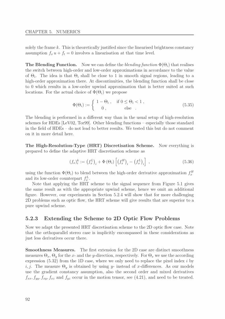
CHAPTER 5. NUMERICS
solely the frame k. This is theoretically justified since the linearised brightness constancyassumption fx u+ ft = 0 involves a linearisation at that time level.
The Blending Function. Now we can define the blending function Φ(Θi) that realisesthe switch between high-order and low-order approximations in accordance to the valueof Θi. The idea is that Θi shall be close to 1 in smooth signal regions, leading to ahigh-order approximation there. At discontinuities, the blending function shall be closeto 0 which results in a low-order upwind approximation that is better suited at suchlocations. For the actual choice of Φ(Θi) we propose
Φ(Θi) :=
1−Θi , if 0 ≤ Θi < 1 ,
0 , else .(5.35)
The blending is performed in a different way than in the usual setup of high-resolutionschemes for HDEs [LeV02, Tor99]. Other blending functions – especially those standardin the field of HDEs – do not lead to better results. We tested this but do not commenton it in more detail here.
The High-Resolution-Type (HRT) Discretisation Scheme. Now everything isprepared to define the adaptive HRT discretisation scheme as
(fx)ki :=
(fLx
)i+ Φ(Θi)
[(fHx
)i−(fLx
)i
], (5.36)
using the function Φ(Θi) to blend between the high-order derivative approximation fHx
and its low-order counterpart fLx .
Note that applying the HRT scheme to the signal sequence from Figure 5.1 givesthe same result as with the appropriate upwind scheme, hence we omit an additionalfigure. However, our experiments in Section 5.2.4 will show that for more challenging2D problems such as optic flow, the HRT scheme will give results that are superior to apure upwind scheme.
5.2.3 Extending the Scheme to 2D Optic Flow Problems
Now we adapt the presented HRT discretisation scheme to the 2D optic flow case. Notethat the orthoparallel stereo case is implicitly encompassed in these considerations asjust less derivatives occur there.
Smoothness Measures. The first extension for the 2D case are distinct smoothnessmeasures Θx, Θy for the x- and the y-direction, respectively. For Θx we use the accordingexpression (5.32) from the 1D case, where we only need to replace the pixel index i byi, j. The measure Θy is obtained by using y- instead of x-differences. As our modelsuse the gradient constancy assumption, also the second order and mixed derivativesfxx, fyy, fxy, fxz and fyz occur in the motion tensor, see (4.21), and need to be treated.
92

5.2. UPWIND DISCRETISATION OF IMAGE DERIVATIVES
Thus, we also need to define a smoothness measure for the mixed xy-direction. Giventhe smoothness measures Θx and Θy, we define the mixed expression as Θxy := Θx+Θy.
Second Order Derivative Approximations. More involved are the high-order andthe (one-sided) low-order approximations of the second order derivatives.
High-Order: The high-order approximations of fxx and fyy are defined as
fxx ≈ D−x
(D+
x fi,j)
=1
h21(fi+1,j − 2fi,j + fi−1,j) , (5.37)
and
fyy ≈ D−y
(D+
y fi,j)
=1
h22(fi,j+1 − 2fi,j + f1,j−1) , (5.38)
respectively. The mixed derivative fxy = ∂yfx is approximated in the finite differencecase as
fxy ≈ D0y
(D0
xfki,j
)(5.39)
= D0y
(1
2h1
(fki+1,j − fk
i−1,j
))(5.40)
=1
4h1h2
(fki+1,j+1 − fk
i−1,j+1 −(fki+1,j−1 − fk
i−1,j−1
)). (5.41)
An averaged version taking into account both time levels is then obtained via
fxy ≈ 1
2
(D0
y
(D0
xfki,j
)+ D0
y
(D0
xfk+1i,j
))(5.42)
=1
8h1h2
(fki+1,j+1 − fk
i−1,j+1 −(fki+1,j−1 − fk
i−1,j−1
)(5.43)
+fk+1i+1,j+1 − fk+1
i−1,j+1 −(fk+1i+1,j−1 − fk+1
i−1,j−1
)).
Similarly, we approximate fxt by
fxt ≈ D+t
(D0
xfki,j
)
=1
2h1
(fk+1i+1,j−fk+1
i−1,j−(fki+1,j−fk
i−1,j)), (5.44)
where D+t f
ki,j := fk+1
i,j − fki,j realises a temporal difference operator. Analogously we
proceed for fyt, yielding
fyt ≈ 1
2h2
(fk+1i,j+1−fk+1
i,j−1−(fki,j+1−fk
i,j−1)), (5.45)
93

CHAPTER 5. NUMERICS
Low-order: In the low-order upwind case, the sign of the predictor (u, v)⊤ indicateswhich one-sided difference should be used: We consider u for x-derivatives and v fory-derivatives, respectively. For approximating fxx we make use of the correspondingupwind difference for fx:
u > 0 : fxx ≈ D−x
(D−
x fki,j
)=
1
h21
(fki,j − 2fk
i−1,j + fki−2,j
), (5.46)
u < 0 : fxx ≈ D+x
(D+
x fki,j
)=
1
h21
(fki+2,j − 2fk
i+1,j − fki,j
). (5.47)
In case u = 0, we use the corresponding high-order approximation described before. Forfyy, we proceed accordingly, taking into account the predictor v:
v > 0 : fyy ≈ D−y
(D−
y fki,j
)=
1
h22
(fki,j − 2fk
i,j−1 + fki,j−2
), (5.48)
v < 0 : fyy ≈ D+y
(D+
y fki,j
)=
1
h22
(fki,j+2 − 2fk
i,j+1 − fki,j
). (5.49)
Concerning the mixed derivative fxy we have to use the two predictors u and v. If apredictor is equal to zero, we use the corresponding high-order approximation, and ifit is non-zero, its sign determines which one-sided upwind approximation to use. Thisleads to the case distinction summarised in Table 5.1. If u = 0 and v = 0 holds, weagain use the high-order approximation of fxy.
For fxt we use the same approach as presented above in the high-order case but justuse one-sided upwind differences for approximating fx. This gives
u > 0 : fxt ≈ D+t
(D−
x fki,j
)=
1
h1
(fk+1i,j − fk+1
i−1,j − (fki,j − fk
i−1,j)), (5.50)
u < 0 : fxt ≈ D+t
(D+
x fki,j
)=
1
h1
(fk+1i+1,j − fk+1
i,j − (fki+1,j − fk
i,j)). (5.51)
Accordingly we proceed for fyt, resulting in
v > 0 : fyt ≈ D+t
(D−
y fki,j
)=
1
h2
(fk+1i,j − fk+1
i,j−1 − (fki,j − fk
i,j−1)), (5.52)
v < 0 : fyt ≈ D+t
(D+
y fki,j
)=
1
h2
(fk+1i,j+1 − fk+1
i,j − (fki,j+1 − fk
i,j)). (5.53)
5.2.4 Experiments
We now present experiments that illustrate the benefits of the proposed HRT scheme.In order to clearly see the influence of the numerics, we start by a considering simple,basic optic flow model and then turn to more advanced, state-of-the-art models.
94

5.2. UPWIND DISCRETISATION OF IMAGE DERIVATIVES
Table 5.1: Upwind-type (one-sided) discretisations of the mixed derivative fxy
Case Discretisation of fxy
u = 0 , v > 0 12h1h2
(fki+1,j − fk
i−1,j − (fki+1,j−1 − fk
i−1,j−1))
u = 0 , v < 0 12h1h2
(fki+1,j+1 − fk
i−1,j+1 − (fki+1,j − fk
i−1,j))
u > 0 , v = 0 12h1h2
(fki,j+1 − fk
i−1,j+1 − (fki,j−1 − fk
i−1,j−1))
u < 0 , v = 0 12h1h2
(fki+1,j+1 − fk
i,j+1 − (fki+1,j−1 − fk
i,j−1))
u > 0 , v > 0 1h1h2
(fki,j − fk
i−1,j − (fki,j−1 − fk
i−1,j−1))
u > 0 , v < 0 1h1h2
(fki,j+1 − fk
i−1,j+1 − (fki,j − fk
i−1,j))
u < 0 , v > 0 1h1h2
(fki+1,j − fk
i,j − (fki+1,j−1 − fk
i,j−1))
u < 0 , v < 0 1h1h2
(fki+1,j+1 − fk
i,j+1 − (fki+1,j − fk
i,j))
Horn and Schunck Model
Our first experiments are conducted with one of the most simple variational optic flowmodels, the one proposed in the seminal work of Horn and Schunck [HS81]. The corre-sponding energy functional models the brightness constancy assumption in the data termand uses a homogeneous regulariser in the smoothness term. In the original formulationonly greyscale images are considered, leading to the energy
E(u, v) =
∫
Ω
(w⊤J0w + α
(|∇2u|2 + |∇2v|2
))dx dy , (5.54)
using the motion tensor notation introduced in Section 4.2.At first we consider a simple synthetic sequence we have created, see Figure 5.2. The
sequence depicts a rectangle that is displaced by one pixel to the right and one pixel tothe bottom, as shown in the ground truth flow field in Figure 5.2 (c). In the same figurewe also compare the results obtained with two different derivative approximations: (i)A standard scheme using central derivative approximations of second order, and (ii) ourproposed adaptive HRT scheme. Additionally, we show two error maps that visualisethe AAE and where brighter pixels correspond to larger errors. To ease comparisonof these maps, we visualise in Figure 5.2 (d) the difference of the error maps. Here,green encodes improvements of the HRT scheme over the standard scheme and red
95

CHAPTER 5. NUMERICS
Table 5.2: Error measures (AAE) for several sequences using the method of Horn and Schunck. Wecompare a standard derivative approximation to our proposed adaptive HRT scheme.
Rectangle Marble Yosemite Street
Standard 31.93 9.11 10.72 9.38
HRT 28.40 8.50 9.53 9.00
encodes impairments. The brightness of the pixels corresponds to the magnitude ofthe difference. Inspecting the error maps and their difference, the expected benefits ofthe HRT scheme become obvious: Especially at the lower and right boundary of therectangle, i.e. at regions with large image discontinuities, the HRT scheme reduces theerror. This observation is validated by the AAE measures given in Table 5.2.
This table also lists the AAE for more complex sequences, like the Marble, theYosemite without clouds, and the Street sequence. The latter is available at http://
of-eval.sourceforge.net. For these sequences, a comparison of error maps resultingfrom a standard derivative approximation and our adaptive scheme is shown in Fig-ure 5.3. It turns out that the HRT scheme allows to decrease the errors in regions withstrong discontinuities. For Marble this is the case at the ground floor, for Yosemite wesee an improvement at the lower left boundary, and for Street the error decreases at theleaves of the tree.
Finally, we wish to evaluate if the upwind directions were correctly estimated usingthe predictor solution. To this end, Figure 5.4 visualises the errors by greyscale mapswhere black pixels mark locations with correct upwind direction, i.e. the sign of thepredictor solution equals the sign of the ground truth flow in this locations. The greypixels mark locations with an error in the direction estimation. The brightness of thepixels corresponds to the magnitude of the ground truth flow at this location. The latteris motivated by the observation that errors in the upwind direction estimation are on theone hand hardly avoidable, but also less harmful, if the flow is very small. Inspecting theerror maps in Figure 5.4, we verify that the computed predictor allows for a very reliableestimation of the correct upwind directions. Note that we do not show an error mapfor our previous experiment in Figure 5.2 as the error is zero there. For the upcomingexperiments, we also refrain from showing error maps for the upwind direction as thisis difficult when using a multiscale warping framework (see Section 5.3.1) where flowincrements are computed at each level.
96

5.2. UPWIND DISCRETISATION OF IMAGE DERIVATIVES
(a) First frame (b) Second frame (c) Ground truth (d) Difference between
(g) and (h)
(e) Standard scheme (f) HRT scheme (g) Error map of (e) (h) Error map of (f)
Figure 5.2: Results for the method of Horn and Schunck on our Rectangle sequence. We comparea standard derivative approximation to our adaptive HRT scheme. First row, from left to right: (a)First frame. (b) Second frame. (c) Ground truth. (d) Difference of the error maps in (g) and (h).Green marks improvements, red impairments of our HRT scheme compared to the standard scheme.Second row, from left to right: (e) Flow field with a standard derivative approximation. (f) Same withour adaptive HRT scheme. (g) Error map for (e). (h) Error map for (f).
97

CHAPTER 5. NUMERICS
First frame Error (standard) Error (HRT) Difference
Figure 5.3: Results for the method of Horn and Schunck. We compare a standard derivative approx-imation to our proposed adaptive HRT scheme. From top to bottom: Marble, Yosemite without cloudsand Street sequence. From left to right: First frame, error map with a standard derivative approxima-tion, same for our adaptive HRT scheme, difference of the two error maps. Green marks improvements,red impairments of our HRT scheme compared to the standard scheme.
Figure 5.4: Error in the estimated upwind directions for the sequences shown in Figure 5.3. Blackpixels mark correct direction. Grey pixels mark errors, where the brightness encodes to the magnitudeof the ground truth flow at the corresponding location. From left to right: (a) Marble, (b) Yosemitewithout clouds, (c) Street sequence.
98

5.2. UPWIND DISCRETISATION OF IMAGE DERIVATIVES
Table 5.3: Error measures (AAE) for several Middlebury sequences using the method of Brox et al..We compare a standard derivative approximation scheme to a pure upwind scheme (Φ(Θi) = 0), andour proposed adaptive HRT scheme.
Rubber- Hydrangea Dime- Grove2 Grove3 Urban2 Urban3 Venuswhale trodon
Standard 3.69 2.18 1.94 2.49 6.17 2.84 5.71 4.79
Upwind 4.87 2.39 3.06 3.13 6.75 3.77 4.58 4.58
HRT 3.55 2.16 1.88 2.46 6.21 2.74 4.11 4.45
Brox et al. Model
In order to show results with a more advanced mode,l we conducted some experimentsusing our HRT scheme within the method of Brox et al. [BBPW04]. Here, compared tothe model of Horn and Schunck [HS81], the data term additionally imposes the gradientconstancy assumption and a subquadratic L1 penalisation is performed. As smoothnessterm, an isotropic flow-driven TV regulariser is used, leading to the energy
E(u, v) =
∫
Ω
(ΨM
(w⊤(J0 + γ Jxy) w
)+ α ΨV
(|∇2u|2 + |∇2v|2
))dx dy , (5.55)
with ΨM(s2) = ΨV (s2) =
√s2 + ε2 and again using the motion tensor notation from
Section 4.2. The minimisation of this energy is embedded in a coarse-to-fine multiscalewarping approach to handle large displacements, see Section 5.3.1.
Due to the more advanced model we can now consider more challenging test data,like the Middlebury sequences that we have also used in the previous chapter. In Fig-ure 5.5, we show results on the Urban3 sequence. As we can see, also for the methodof Brox et al., the HRT scheme allows to improve the results at locations with strongdiscontinuities (marked in the images). In this context, we also refer to Figure 5.6 wherewe show a plot of the gradient magnitude to support the latter observation. The quali-tative improvement is confirmed by the corresponding AAE measures in Table 5.3. Thistable also lists other Middlebury sequences and gives errors for a pure upwind schemeusing first-order, one-sided differences. Such a scheme can easily obtained from our HRTscheme (5.36) by setting Φ(Θi) = 0. Analysing the results in Table 5.3 shows: (i) For7 out of the 8 test sequences, the HRT scheme improves the quality over the standardscheme. Only for Grove 3, the standard scheme is slightly better. (ii) For the consideredchallenging sequences, the blending between high-order and low-order approximations ofthe HRT scheme gives significantly better results than a pure upwind scheme. Note thatfor some sequences, e.g. Dimetrodon, the upwind scheme produces significantly worseresults. This occurs in the presence of large smooth areas in the images. There, centralderivative approximations are best suited and thus an upwind scheme that uses the lessappropriate first-order approximation leads to bad results.
99

CHAPTER 5. NUMERICS
(a) Reference frame (b) Flow (standard) (c) Flow (HRT)
(d) Ground truth (e) Error (standard) (f) Error (HRT)
Figure 5.5: Results for the method of Brox et al. on the Urban3 sequence. We compare a standardderivative approximation to our proposed adaptive HRT scheme. First row, from left to right: (a)Reference frame. (b) Flow field with a standard derivative approximation. (c) Same with our adaptiveHRT scheme. Second row, from left to right: (d) Ground truth flow. (e) Error map with a stan-dard derivative approximation. (f) Same with our adaptive HRT scheme. Boxes indicate regions ofsignificantly better results with the HRT scheme.
Figure 5.6: Plot of the gradient magnitude for the Urban3 sequence. From left to right: (a) Referenceframe. (b) Corresponding gradient magnitude, scaled to the range from 0 to 255. The boxes indicateregions where the HRT scheme performs significantly better than the standard approach, see Figure5.5. We observe that these are regions with strong gradients.
100

5.2. UPWIND DISCRETISATION OF IMAGE DERIVATIVES
Table 5.4: Error measures (AAE) for several Middlebury sequences using our Complementary OpticFlow method. We compare a standard derivative approximation scheme to a pure upwind scheme(Φ(Θi) = 0), and our proposed adaptive HRT scheme.
Rubber- Hydrangea Dime- Grove2 Grove3 Urban2 Urban3 Venuswhale trodon
Standard 3.47 2.30 1.84 2.54 5.34 2.74 3.09 5.26
Upwind 4.40 2.45 2.87 3.02 5.72 4.23 3.25 5.24
HRT 3.28 2.27 1.87 2.51 5.34 2.75 2.96 5.41
Complementary Optic Flow Model
We conclude our experiments on derivative approximations by applying the HRT schemewithin our Complementary Optic Flow model [10, 11] that has been presented in theprevious chapter.
In Figure 5.7, we compare results for the Rubberwhale sequence obtained with theHRT scheme to results with a standard central derivative approximation of second order.Note that we usually used central differences of fourth order for this model, but as thehigh-order approximations in our HRT scheme are of second order, comparing to fourth-order approximations would not be fair. To illustrate the improvements of our HRTscheme, we again give error maps visualising the AAE and show a colour-coded mapvisualising the differences in error. Considering the difference map, we see that our HRTscheme improves the result especially at the edges in the flow field. This improvementbecomes also visible in the corresponding AAE measures that are given in Table 5.4,which also lists results for other Middlebury sequences and further encompasses resultsobtained with a pure upwind scheme. Comparing the error measures, it turns out thatthe HRT scheme allows to improve the results for 4 out of the 8 sequences, in 2 cases theresults are almost identical, and for the remaining 2 sequences, the results of our HRTscheme are slightly worse. Compared to the upwind scheme, the HRT scheme againgives considerably better results.
Discussion
We wish to stress one important conclusion that we can draw from comparing the resultsof above experiments. Obviously, the advanced numerics of our HRT scheme gives amuch stronger improvement in terms of quality when applied within basic models, e.g.in the Horn and Schunck model [HS81]. It seems that the more sophisticated the contin-uous models become, the less influential is an appropriate numerical approximation ofderivatives, as shown in the results with our Complementary Optic Flow model [10, 11].
101
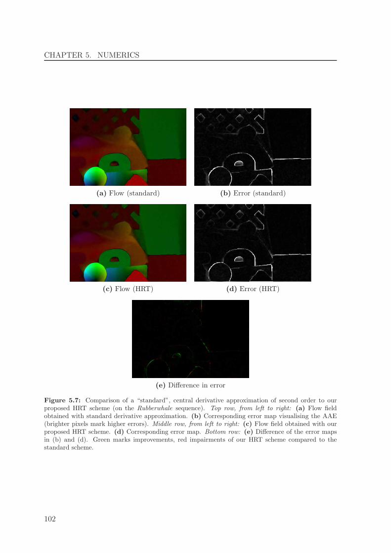
CHAPTER 5. NUMERICS
(a) Flow (standard) (b) Error (standard)
(c) Flow (HRT) (d) Error (HRT)
(e) Difference in error
Figure 5.7: Comparison of a “standard”, central derivative approximation of second order to ourproposed HRT scheme (on the Rubberwhale sequence). Top row, from left to right: (a) Flow fieldobtained with standard derivative approximation. (b) Corresponding error map visualising the AAE(brighter pixels mark higher errors). Middle row, from left to right: (c) Flow field obtained with ourproposed HRT scheme. (d) Corresponding error map. Bottom row: (e) Difference of the error mapsin (b) and (d). Green marks improvements, red impairments of our HRT scheme compared to thestandard scheme.
102

5.3. SOLVING THE EULER-LAGRANGE EQUATIONS
5.3 Solving the Euler-Lagrange Equations
After our detailed discussion on discretisation aspects, we now consider the actual solu-tion of the Euler-Lagrange equations. We start by presenting the coarse-to-fine warpingstrategy that is used for handling large displacements and which leads to modified Euler-Lagrange equations. Then we discuss various solvers for the modified equations.
5.3.1 Handling Large Displacements – Warping
The derivation of the optic flow constraint (4.8) by means of a Taylor linearisation isonly valid under the assumption of either small displacements in the image sequence orfor very smooth image data. However, if the temporal sampling of the sequence is toocoarse, the precondition of small displacements is violated and a linearised approach willfail. To overcome this problem, a popular strategy [Ana89, BA96, BBPW04, MP98] is touse a coarse-to-fine multiscale warping strategy that uses downsampled images: At eachwarping level ℓ, the flow field is split into (uℓ, vℓ, 1)⊤+ (δuℓ, δvℓ, 0)⊤, where (uℓ, vℓ, 1)⊤=:wℓ denotes the already computed solution from coarser levels and (δuℓ, δvℓ, 0)⊤ is theunknown flow increment to be computed at the current level. As the increments aresmall, they can be computed by our discussed linearised approach. As soon as theincrements are computed, the flow at the next finer level ℓ+1 is then obtained by addingthe two quantities, i.e. (uℓ+1, vℓ+1, 1)⊤ := (uℓ, vℓ, 1)⊤ + (δuℓ, δvℓ, 0)⊤. This proceeding iscontinued until the finest level (original resolution) is reached.
To illustrate how above strategy works in practise we apply it to our complemen-tary optic flow model [10, 11] that is obtained by using our final data term (4.35) incombination with our complementary regulariser (4.82). The resulting Euler-Lagrangeequations that need to be solved to obtain the increment (δuℓ, δvℓ, 0)⊤ then read as
0 =
3∑
c=1
Ψ′M
((δwℓ
)⊤(J
c0
)ℓδwℓ
)·([(
Jc0
)ℓ]1,1
δuℓ +[(J
c0
)ℓ]1,2
δvℓ +[(J
c0
)ℓ]1,3
)(5.56)
+ γ
(3∑
c=1
Ψ′M
((δwℓ
)⊤(J
cxy
)ℓδwℓ
)·([(
Jcxy
)ℓ]1,1
δuℓ +[(Jcxy
)ℓ]1,2
δvℓ +[(J
cxy
)ℓ]1,3
))
−α div
(Dℓ
CR∇2
(uℓ + δuℓ
)),
0 =
3∑
c=1
Ψ′M
((δwℓ
)⊤(J
c0
)ℓδwℓ
)·([(
Jc0
)ℓ]1,2
δuℓ +[(J
c0
)ℓ]2,2
δvℓ +[(J
c0
)ℓ]2,3
)(5.57)
+ γ
(3∑
c=1
Ψ′M
((δwℓ
)⊤(J
cxy
)ℓδwℓ
)·([(
Jcxy
)ℓ]1,2
δuℓ +[(Jcxy
)ℓ]2,2
δvℓ +[(J
cxy
)ℓ]2,3
))
−α div
(Dℓ
CR∇2
(vℓ + δvℓ
)),
103

CHAPTER 5. NUMERICS
where we defined δwℓ := (δuℓ, δvℓ, 1)⊤ to ease notation. Further note that the warpedimage sequence f(x+wℓ) is used in the computation of the motion tensors J ℓ and thediffusion tensor
DℓCR :=
(rℓ1|rℓ
2
)( Ψ′V
((uℓ+ δuℓ)2
rℓ1
+ (vℓ+ δvℓ)2rℓ1
)0
0 1
)((rℓ1
)⊤(rℓ2
)⊤
). (5.58)
The vectors rℓ1 and rℓ
2 are the eigenvectors of the regularisation tensor Rℓρ which also
needs to be computed from the warped image sequence f(x+wℓ).We want to stress that Brox et al. [BBPW04] showed that the presented warping
scheme is a mathematically consistent strategy for minimising an energy functional witha data term where no linearisation is performed. Such a version of our final data term(4.35) is given by
M(u, v) =3∑
c=1
ΨM
(θc0 (f
c(x+w)−f c(x))2)
(5.59)
+ γ
(3∑
c=1
ΨM
(θcx (f
cx(x+w)−f c
x(x))2 + θcy
(f cy(x+w)−f c
y(x))2))
.
As large displacements occur in most real world image sequences, all results shown inthis thesis have been computed using the presented warping scheme.
Implementation Details
To evaluate the images at the warped subpixel locations f(x+wℓ) we again use Coonspatches based on bicubic interpolation [Coo67].
To obtain a coarse representation of our problem, we downsample the image sequenceby a factor η ∈ [0.5, 1). In order to prevent aliasing problems, we apply a low-pass filterto the images prior to downsampling [SW49, Uns00]. The latter is realised by a Gaussianconvolution with standard deviation
√2/(4η). The actual downsampling is then realised
by an area-based resampling strategy [BWF+05] that operates on the smoothed images.In most cases, the aliasing artefacts will not significantly deteriorate the flow estimation,which can be attributed to the robust data term. However, for the Urban sequencefrom the official Middlebury benchmark[BSL+10], anti-aliasing is crucial for obtainingreasonable results, see Figure 5.8. As it turns out, the large displacement of the buildingin the lower left corner can only be estimated when using anti-aliasing. We explain thisby the high frequent stripe pattern on the facade of the building.
In order to warp the image sequence at the next finer grid, we need to upsample thealready computed flow field. This is again done by area-based resampling.
Adapting the Smoothness Weight to the Warping Level. The influence of thedata term usually becomes smaller at coarser levels of our multiscale framework. This
104
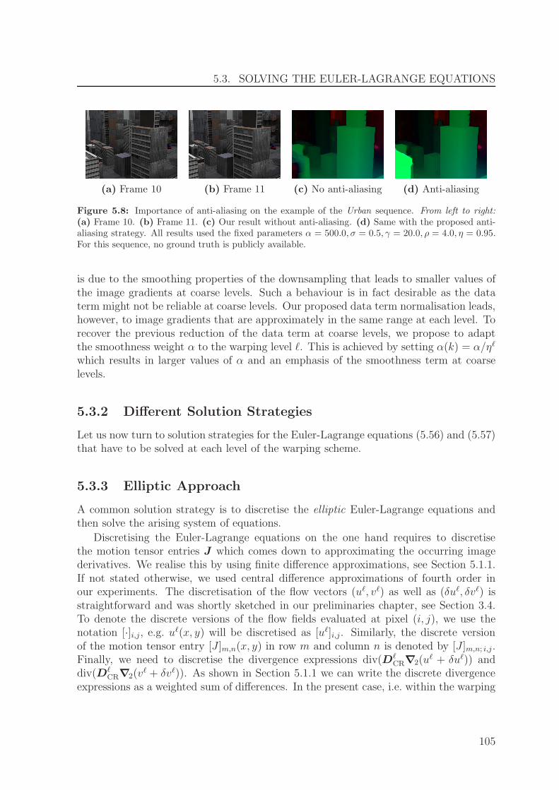
5.3. SOLVING THE EULER-LAGRANGE EQUATIONS
(a) Frame 10 (b) Frame 11 (c) No anti-aliasing (d) Anti-aliasing
Figure 5.8: Importance of anti-aliasing on the example of the Urban sequence. From left to right:(a) Frame 10. (b) Frame 11. (c) Our result without anti-aliasing. (d) Same with the proposed anti-aliasing strategy. All results used the fixed parameters α = 500.0, σ = 0.5, γ = 20.0, ρ = 4.0, η = 0.95.For this sequence, no ground truth is publicly available.
is due to the smoothing properties of the downsampling that leads to smaller values ofthe image gradients at coarse levels. Such a behaviour is in fact desirable as the dataterm might not be reliable at coarse levels. Our proposed data term normalisation leads,however, to image gradients that are approximately in the same range at each level. Torecover the previous reduction of the data term at coarse levels, we propose to adaptthe smoothness weight α to the warping level ℓ. This is achieved by setting α(k) = α/ηℓ
which results in larger values of α and an emphasis of the smoothness term at coarselevels.
5.3.2 Different Solution Strategies
Let us now turn to solution strategies for the Euler-Lagrange equations (5.56) and (5.57)that have to be solved at each level of the warping scheme.
5.3.3 Elliptic Approach
A common solution strategy is to discretise the elliptic Euler-Lagrange equations andthen solve the arising system of equations.
Discretising the Euler-Lagrange equations on the one hand requires to discretisethe motion tensor entries J which comes down to approximating the occurring imagederivatives. We realise this by using finite difference approximations, see Section 5.1.1.If not stated otherwise, we used central difference approximations of fourth order inour experiments. The discretisation of the flow vectors (uℓ, vℓ) as well as (δuℓ, δvℓ) isstraightforward and was shortly sketched in our preliminaries chapter, see Section 3.4.To denote the discrete versions of the flow fields evaluated at pixel (i, j), we use thenotation [·]i,j, e.g. uℓ(x, y) will be discretised as [uℓ]i,j. Similarly, the discrete versionof the motion tensor entry [J ]m,n(x, y) in row m and column n is denoted by [J ]m,n; i,j.Finally, we need to discretise the divergence expressions div(Dℓ
CR∇2(uℓ + δuℓ)) and
div(DℓCR∇2(v
ℓ + δvℓ)). As shown in Section 5.1.1 we can write the discrete divergenceexpressions as a weighted sum of differences. In the present case, i.e. within the warping
105

CHAPTER 5. NUMERICS
framework, we get
div
(Dℓ
CR ∇2
(uℓ+δuℓ
))≈∑
i,j∈Ni,j
[w]ℓi,j
([δuℓ]i,j−[δuℓ]i,j
+[uℓ]i,j−[uℓ]i,j
),(5.60)
div
(Dℓ
CR ∇2
(vℓ+δvℓ
))≈∑
i,j∈Ni,j
[w]ℓi,j
([δvℓ]i,j−[δvℓ]i,j
+[vℓ]i,j−[vℓ]i,j
), (5.61)
where the weights [w]ℓi,j now need to be computed with the current flow estimate (uℓ +
δuℓ, vℓ + δvℓ) as well as with the warped image sequence f(x+wℓ).With this notation, a discrete version of the Euler-Lagrange equations (5.56) and
(5.57) reads as
0 =
3∑
c=1
Ψ′M
([δwℓ
]⊤i,j
[(J
c
0
)ℓ]i,j
[δwℓ
]i,j
)(5.62)
·([(
Jc
0
)ℓ]1,1; i,j
[δuℓ]i,j
+[(J
c
0
)ℓ]1,2; i,j
[δvℓ]i,j
+[(J
c
0
)ℓ]1,3; i,j
)
+ γ
(3∑
c=1
Ψ′M
([δwℓ
]⊤i,j
[(J
c
xy
)ℓ]i,j
[δwℓ
]i,j
)
·([(
Jc
xy
)ℓ]1,1; i,j
[δuℓ]i,j
+[(J
c
xy
)ℓ]1,2 ,i,j
[δvℓ]i,j
+[(J
c
xy
)ℓ]1,3; i,j
))
−α∑
i,j∈Ni,j
[w]ℓi,j
([δuℓ]i,j
−[δuℓ]i,j
+[uℓ]i,j
−[uℓ]i,j
),
0 =3∑
c=1
Ψ′M
([δwℓ
]⊤i,j
[(J
c
0
)ℓ]i,j
[δwℓ
]i,j
)(5.63)
·([(
Jc
0
)ℓ]1,2; i,j
[δuℓ]i,j
+[(J
c
0
)ℓ]2,2; i,j
[δvℓ]i,j
+[(J
c
0
)ℓ]2,3; i,j
)
+ γ
(3∑
c=1
Ψ′M
([δwℓ
]⊤i,j
[(J
c
xy
)ℓ]i,j
[δwℓ
]i,j
)
·([(
Jc
xy
)ℓ]1,2; i,j
[δuℓ]i,j
+[(J
c
xy
)ℓ]2,2 ,i,j
[δvℓ]i,j
+[(J
c
xy
)ℓ]2,3; i,j
))
−α∑
i,j∈Ni,j
[w]ℓi,j
([δvℓ]i,j
−[δvℓ]i,j
+[vℓ]i,j
−[vℓ]i,j
).
Solving the discretised Euler-Lagrange equations (5.62) and (5.63) for the unknownsδuℓ and δvℓ comes down to solving a large nonlinear system of equations. Note that
106

5.3. SOLVING THE EULER-LAGRANGE EQUATIONS
large here means that for an image sequences with a resolution of 1 Megapixel, storingthe system matrix would require several Terabyte of memory. Thus, a direct solution isintractable and one has to resort to an iterative solver, such as the Jacobi, Gauss-Seidelor SOR solver [You03]. Let us briefly explain how to apply such iterative solvers to ourproblem.
The first observation is that the mentioned iterative solvers can only handle linearsystems of equations, but our discretised Euler-Lagrange equations (5.62) and (5.63)lead to nonlinear systems as the unknowns δuℓ and δvℓ occur in the argument of the Ψ′
M
function and implicitly also in the weights [w]ℓi,j
that are computed from the diffusion
tensor DℓCR. A common remedy to this problem is to embed the solution of the nonlinear
system into a series of linear systems that can be solved by the discussed methods. Thisstrategy is known as time-lagged nonlinearity, or Kacanov–Galerkin method [FKN73].To obtain the linear systems, we evaluate the nonlinear terms with a current solutionof the flow field (initially we use a zero solution) and after some iterations of the linearsolver, we recompute the nonlinearities with the updated solution. Then the iterativesolver is again applied to the updated linear system. These steps are iterated in twonested loops (the outer loop updates the nonlinearities, the inner loop updates thesolution by some solver iterations) until some stopping criterion, usually a maximalnumber of inner and outer iterations, is met.
Let us briefly sketch how the discussed iterative solvers for the linear systems work.We consider a general linear equation system given as
Au = b , (5.64)
whereA ∈ R2N×2N denotes the block-diagonal system matrix (with N := nx·ny denoting
the number of pixels), u ∈ R2N is the unknown flow field, and the right-hand side is
denoted by b ∈ R2N . As the matrix A is positive definite for non-constant image
sequences, the solution of the system is given by
u = A−1 b , (5.65)
which requires to compute the inverse A−1 of the system matrix. This, however, is ingeneral a difficult and time-consuming task.
The basic idea of iterative solvers is to find an efficient way to compute an approxi-mation of this inverse. A first step towards this goal is the decomposition of the systemmatrix into A = A1 +A2. With this, we can rewrite (5.64) as
A1 u+A2 u = b . (5.66)
This in turn enables us to come up with the fixed point iteration
A1 uk+1 = b−A2 u
k , (5.67)
where k denotes the iteration index, i.e. uk is the already computed solution and uk+1
is the unknown result of the next iteration. Next, we rewrite equation (5.67) as
uk+1 = A−11 (b−A2 u
k) , (5.68)
107

CHAPTER 5. NUMERICS
where A−11 should be a reasonable and efficient to compute approximation of A−1.
A frequent approach for an efficient approximation of A−1 bases on the decompo-sition A = Ad − Al − Au, where Ad denotes the diagonal part, Al the strictly lowertriangular part and Au the strictly upper triangular part of A. A popular solver re-lying on this decomposition is the Gauss-Seidel method, which is similar to the Jacobimethod, but more efficient. The Gauss-Seidel method defines A1 = Ad−Al, which is atriangular matrix and is hence easy to invert. Consequently, A2 = −Au, as we imposedthat A = A1 + A2 = Ad − Al − Au. Using these decomposition in the fixed pointscheme (5.68) yields
uk+1 = (Ad −Al)−1(b+Auu
k) . (5.69)
For our Euler-Lagrange equations (5.62) and (5.63), this results in the followingGauss-Seidel iteration step
[δuℓ]k+1
i,j=
[∑
c,a
(γ(a)
[Ψ′
M
(J
c
a
)]ℓ,ki,j
([(J
c
a
)ℓ]1,3; i,j
+[(J
c
a
)ℓ]1,2; i,j
[δvℓ]ki,j
))(5.70)
−α
(∑
i,j∈N−
i,j
[w]ℓ,k
i,j
([δuℓ]k+1
i,j+[uℓ]i,j
)+
∑
i,j∈N+
i,j
[w]ℓ,k
i,j
([δuℓ]ki,j
+[uℓ]i,j
))]
·[α [w]
ℓ,k
i,j −(∑
c,a
(γ(a)
[Ψ′
M
(J
c
a
)]ℓ,ki,j
[(J
c
a
)ℓ]1,1; i,j
))]−1
,
[δvℓ]k+1
i,j=
[∑
c,a
(γ(a)
[Ψ′
M
(J
c
a
)]ℓ,ki,j
([(J
c
a
)ℓ]2,3; i,j
+[(J
c
a
)ℓ]1,2; i,j
[δuℓ]ki,j
))(5.71)
−α
(∑
i,j∈N−
i,j
[w]ℓ,k
i,j
([δvℓ]k+1
i,j+[vℓ]i,j
)+
∑
i,j∈N+
i,j
[w]ℓ,k
i,j
([δvℓ]ki,j
+[vℓ]i,j
))]
·[α [w]
ℓ,k
i,j −(∑
c,a
(γ(a)
[Ψ′
M
(J
c
a
)]ℓ,ki,j
[(J
c
a
)ℓ]2,2; i,j
))]−1
,
where we initialise the iterations with zero, i.e. δuℓ,0 = 0 and δvℓ,0 = 0 and the weights[w]ℓ,k are now computed from a diffusion tensor Dℓ,k
CR that is obtained with the currentflow estimate wℓ + δwℓ,k. Note that we furthermore introduced the following abbrevia-tions to ease notation: The sum
∑
c,a
:=3∑
c=1
∑
a∈0,xy
, (5.72)
sums over the image channels c and the two constancy assumptions a ∈ 0, xy, where 0denotes the brightness constancy assumption and xy the gradient constancy assumption.The parameter γ(a) is defined as γ(0) := 1 and γ(xy) := γ. To denote the derivative ofthe penaliser in the data term, we define
[Ψ′
M
(J
c
a
)]ℓ,ki,j
:= Ψ′M
([δwℓ
]ki,j
⊤ [(J
c
a
)ℓ]i,j
[δwℓ
]ki,j
). (5.73)
108

5.3. SOLVING THE EULER-LAGRANGE EQUATIONS
Finally, N−i,j and N+
i,j denote the already processed and the still to be processed neigh-bours of (i, j), respectively.
A popular strategy for speeding up the presented Gauss-Seidel scheme is to performan overrelaxation as in the SOR (Successive Overrelaxation) method. The basic idea ofthe latter method is to extrapolate the result of one Gauss-Seidel step. If we denote byuk+1
GS the result of a Gauss-Seidel iteration, then the SOR scheme reads as
uk+1 = (1− ω)uk + ω uk+1GS = uk + ω
(uk+1
GS − uk), (5.74)
with an overrelaxation parameter ω ∈ [0, 2). For ω = 1 one falls back to the Gauss-Seidel scheme. We propose to set ω = 1.95 which gives good results and allows for aspeedup of two orders of magnitude compared to the original Gauss-Seidel scheme.
A further speed up can be achieved when updating the nonlinearities [Ψ′M(J
c
a)]ℓ,ki,j
and [w]ℓ,ki,j
not after every iteration, but keeping them fixed for some iterations. This
is implemented using two nested loops, as described in the context of the time-laggednonlinearity method (see page 107).
Multigrid Solver
A further speed up compared to the SOR solver can be achieved by using highly efficientmultigrid solvers, see e.g. [Bra77, BWKS06, Hac85, KKR07, Ter86]. For the experimentsin this thesis, we used the full multigrid solver of Bruhn et al. [BWKS06], unless statedotherwise.
Full multigrid schemes combine ideas from unidirectional and bidirectional multigridmethods. The basic strategy of unidirectional methods is to start the iterative solutionwith a good initialisation to reduce the required number of iterations. To obtain thisinitialisation, the problem is transferred to a smaller (coarser) pixel grid and solved there,which should be relatively fast. The coarse solution is then interpolated and serves asinitialisation on the next finer grid. Consequently, unidirectional methods belong tothe class of coarse-to-fine strategies. In contrast to unidirectional schemes, bidirectionalstrategies do not only go from coarse to fine levels, but also revisit coarser levels toobtain correction steps. This is motivated by the fact that iterative solvers eliminatehigh frequency errors relatively fast, but require a very large number of iterations untillow-frequent errors vanish. However, the low frequencies occur as high frequencies oncoarser grids. There, one then computes the error (not the solution) that was stillpresent in the fine grid solution and then corrects the fine grid solution for the estimatederror.
For our experiments, we use a Gauß-Seidel type solver with alternating line relax-ation [BWKS06] to solve the problems arising at each grid level. Please also note thatan in-detail explanation of sophisticated multigrid schemes would by far exceed thescope of this thesis. For a comprehensive overview on multigrid methods for optic flowcomputation, we refer the interested reader to [Bru06].
109

CHAPTER 5. NUMERICS
5.3.4 Parabolic Approach
An alternative to the previously discussed elliptic approach is to apply a gradient descentscheme on the Euler-Lagrange equations. This comes down to solving a system of twocoupled diffusion-reaction equations of parabolic type. The latter can be derived fromthe Euler-Lagrange equations (5.56) and (5.57) and read as
∂θ δuℓ = div
(Dℓ
CR∇2
(uℓ + δuℓ
))(5.75)
− 1
α
[3∑
c=1
Ψ′M
((δwℓ
)⊤(J
c0
)ℓδwℓ
)·([(
Jc0
)ℓ]1,1δuℓ+
[(J
c0
)ℓ]1,2δvℓ+
[(J
c0
)ℓ]1,3
)
+ γ
(3∑
c=1
Ψ′M
((δwℓ
)⊤(J
cxy
)ℓδwℓ
)·([(
Jcxy
)ℓ]1,1δuℓ+
[(J
cxy
)ℓ]1,2δvℓ+
[(Jcxy
)ℓ]1,3
))],
∂θ δvℓ = div
(Dℓ
CR∇2
(vℓ + δvℓ
))(5.76)
− 1
α
[3∑
c=1
Ψ′M
((δwℓ
)⊤(J
c0
)ℓδwℓ
)·([(
Jc0
)ℓ]1,2δuℓ+
[(J
c0
)ℓ]2,2δvℓ+
[(J
c0
)ℓ]2,3
)
+ γ
(3∑
c=1
Ψ′M
((δwℓ
)⊤(J
cxy
)ℓδwℓ
)·([(
Jcxy
)ℓ]1,2δuℓ+
[(J
cxy
)ℓ]2,2δvℓ+
[(Jcxy
)ℓ]2,3
))],
where ∂θ δuℓ and ∂θ δv
ℓ denote derivatives in a numerical time direction. To derive abovediffusion reaction equations (5.75) and (5.76) from the Euler-Lagrange equations (5.56)and (5.57), we proceeded in two steps: First we replace the zeros on the left-hand side bythe numerical time derivatives, which makes sense as in the steady state (θ → ∞), thenumerical time derivatives tends to zero. Then, we switch the signs on the right-handside of the Euler-Lagrange equations to obtain a gradient descent behaviour.
To solve the diffusion-reaction equations (5.75) and (5.76), it is common to useiterative schemes. The latter compute the sought flow increment δwℓ starting from aninitialisation δwℓ,0 := (δuℓ,0, δvℓ,0, 1)⊤. As before, we initialise the iterations with zero.The result of the next iteration δwℓ,k+1 := (δuℓ,k+1, δvℓ,k+1, 1)⊤ is then computed fromthe previous result δwℓ,k := (δuℓ,k, δvℓ,k, 1)⊤. The iterations are stopped as soon as astopping criterion is met, e.g. when the difference between the results of two subsequentiterations drops below a given threshold. If this is the case we can consider the schemeto have reached the desired steady state where ∂θ δu
ℓ ≈ 0 and ∂θ δvℓ ≈ 0.
Stabilised Explicit Scheme. In order to obtain an iterative scheme, we first discre-tise the numerical time derivatives by the forward differences
∂θ δuℓ ≈ δuℓ,k+1 − δuℓ,k
τ, and ∂θ δv
ℓ ≈ δvℓ,k+1 − δvℓ,k
τ, (5.77)
where τ denotes the numerical time step size.
110

5.3. SOLVING THE EULER-LAGRANGE EQUATIONS
The simplest form of an iterative scheme is then given by an explicit scheme thatuses the old value at iteration k for all occurrences of the unknowns at the right-handside. To stabilise such a scheme, one can use the new value at iteration k + 1 in thereaction part. This gives the following stabilised explicit scheme (where we mark thestabilisation in red):
δuℓ,k+1 − δuℓ,k
τ=
∑
i,j∈Ni,j
[w]ℓ,k
i,j
([δuℓ,k
]i,j
−[δuℓ,k
]i,j
+[uℓ]i,j
−[uℓ]i,j
)(5.78)
− 1
α
[3∑
c=1
Ψ′M
((δwℓ,k
)⊤(J
c
0
)ℓδwℓ,k
)·([(
Jc
0
)ℓ]1,1δuℓ,k+1+
[(J
c
0
)ℓ]1,2δvℓ,k+
[(J
c
0
)ℓ]1,3
)
+ γ
(3∑
c=1
Ψ′M
((δwℓ,k
)⊤(J
c
xy
)ℓδwℓ,k
)·([(
Jc
xy
)ℓ]1,1δuℓ,k+1+
[(J
c
xy
)ℓ]1,2δvℓ,k+
[(J
c
xy
)ℓ]1,3
))],
δvℓ,k+1 − δvℓ,k
τ=
∑
i,j∈Ni,j
[w]ℓ,k
i,j
([δvℓ,k
]i,j
−[δvℓ,k
]i,j
+[vℓ]i,j
−[vℓ]i,j
)(5.79)
− 1
α
[3∑
c=1
Ψ′M
((δwℓ,k
)⊤(J
c
0
)ℓδwℓ,k
)·([(
Jc
0
)ℓ]1,2δuℓ,k+
[(J
c
0
)ℓ]2,2δvℓ,k+1+
[(J
c
0
)ℓ]2,3
)
+ γ
(3∑
c=1
Ψ′M
((δwℓ,k
)⊤(J
c
xy
)ℓδwℓ,k
)·([(
Jc
xy
)ℓ]1,2δuℓ,k+
[(J
c
xy
)ℓ]2,2δvℓ,k+1+
[(J
c
xy
)ℓ]2,3
))],
Solving these equations for the unknowns δuℓ,k+1 and δvℓ,k+1 is straightforward and givesthe desired iterative scheme to be implemented.
Obviously, explicit schemes are appealing because they are very easy to deduce and toimplement: In contrast to the previously described elliptic approach, it is not necessaryto solve a large nonlinear system of equations, but an iterative solution scheme candirectly be deduced. However, there is also a price to pay: The stability of explicitschemes can only be guaranteed when using rather small time step sizes τ . This resultsin a poor performance as many iterations are required to reach the desired steady state.In the considered 2D case, the time step limit τ
limis given by
τlim
=1
mmax
(2h21
+ 2h22
) , (5.80)
where we recall that h1 and h2 denote the grid size in x- and y-direction, respectively.By mmax we denote the maximum of the larger eigenvalue over all diffusion tensorsD
ℓ,kCR. Considering (5.80) we realise that large eigenvalues of the diffusion tensors will
decrease the time step size limit even further. When using our complementary smooth-ness term (4.82), the eigenvalues of the resulting diffusion tensor D
ℓ,kCR are given by 1
and Ψ′V (s
2), respectively. As we use the Perona-Malik penaliser, we have Ψ′V (s
2) ≤ 1,see (4.65), and consequently mmax ≤ 1. In this sense, our complementary regulariser iswell-suited for an explicit scheme.
111
CHAPTER 5. NUMERICS
Scheme Step Sizes for 1000 Iterations Stopping Time
Explicit = 500.00
FED = 166 833.33
Figure 5.9: Comparing the stopping time of a standard explicit scheme after 1000 iterations to acorresponding FED cycle. The resulting speed-up factor is 334. Note that this example considers the1D case where the step size limit is 0.5 for an explicit scheme. Illustration: P. Gwosdek.
5.3.5 A Fast Explicit Solver
Our discussion on explicit schemes show that it is desirable to modify an explicit schemes.t. larger time steps can be used and thus fewer iterations are needed until a steadystate is reached. This would combine the easy implementation of explicit schemes withthe efficiency of the sophisticated solvers for elliptic approaches. This goal was recentlyachieved by Grewenig et al. [GWB10]. They presented a Fast Explicit Diffusion (FED)scheme, an explicit scheme that uses some extremely large time steps to ensure a fastconvergence. As could be shown, the combination of large (unstable) and small (stable)time steps within one cycle allows to guarantee unconditional stability of the completeapproach. An illustrated example for an FED cycle compared to a standard explicitscheme is shown in Figure 5.9. Hence, FED schemes outperform elliptic schemes interms of efficiency and are additionally much easier to implement, especially on massivelyparallel architectures like GPUs.
In our paper [3], we showed that although FED schemes were originally developedfor solving diffusion problems, they can easily be adapted for solving the Euler-Lagrangeequations of variational optic flow approaches. An intuitive reason for this is that theEuler-Lagrange equations actually are of diffusion-reaction type. We apply the FEDscheme within our modified explicit scheme from (5.78) and (5.79) by replacing thepreviously fixed time step size τ by a varying FED step size τk which is computedas [GWB10]
τk = τlim
· 1
2 cos2(π 2k+1
4n+2
) , (5.81)
where n denotes the number of iterations in the current cycle.
Remarks. The result of FED iterations only makes sense at the end of a cycle, wherethe unstable time steps have been compensated by stable ones. We thus can onlyupdate the nonlinearities in the weights and the penaliser function Ψ′
M only if a cycleis completed and not in between a cycle.
112
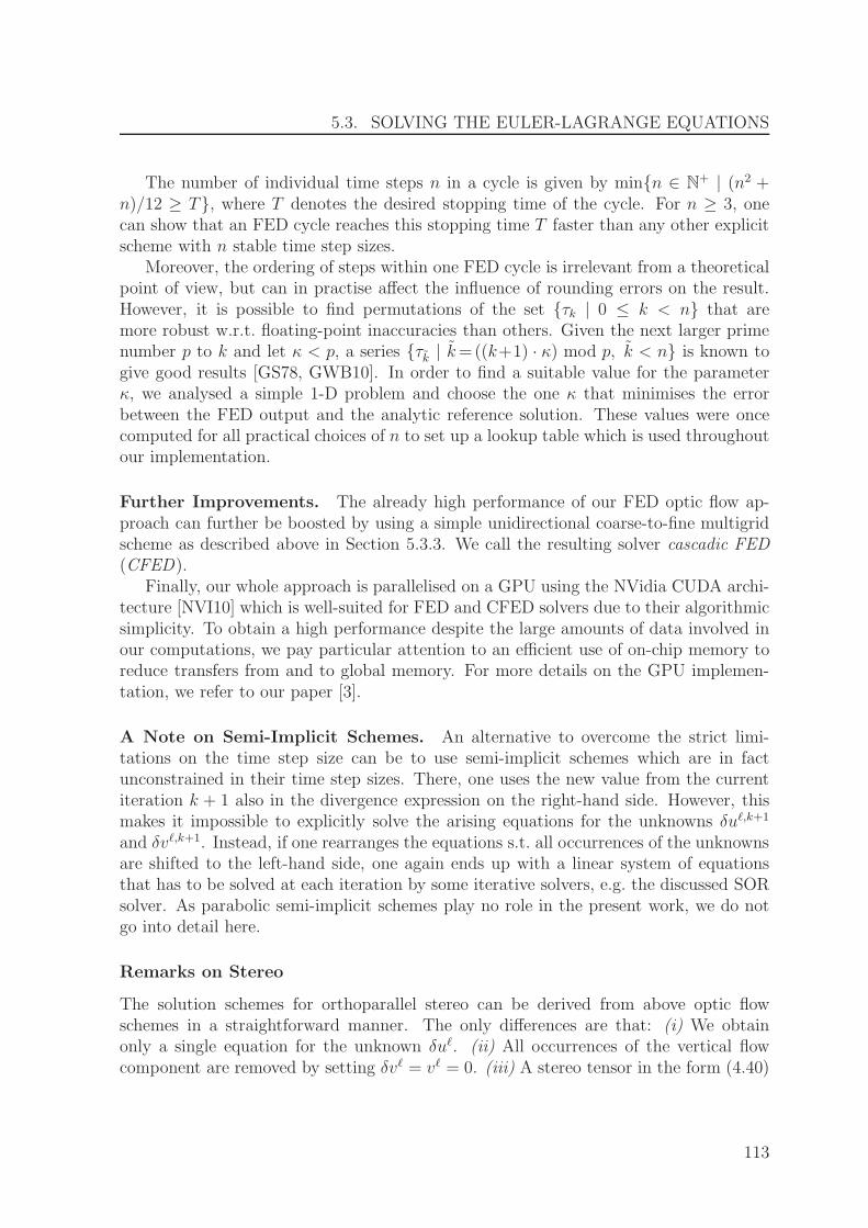
5.3. SOLVING THE EULER-LAGRANGE EQUATIONS
The number of individual time steps n in a cycle is given by minn ∈ N+ | (n2 +
n)/12 ≥ T, where T denotes the desired stopping time of the cycle. For n ≥ 3, onecan show that an FED cycle reaches this stopping time T faster than any other explicitscheme with n stable time step sizes.
Moreover, the ordering of steps within one FED cycle is irrelevant from a theoreticalpoint of view, but can in practise affect the influence of rounding errors on the result.However, it is possible to find permutations of the set τk | 0 ≤ k < n that aremore robust w.r.t. floating-point inaccuracies than others. Given the next larger primenumber p to k and let κ < p, a series τk | k=((k+1) · κ) mod p, k < n is known togive good results [GS78, GWB10]. In order to find a suitable value for the parameterκ, we analysed a simple 1-D problem and choose the one κ that minimises the errorbetween the FED output and the analytic reference solution. These values were oncecomputed for all practical choices of n to set up a lookup table which is used throughoutour implementation.
Further Improvements. The already high performance of our FED optic flow ap-proach can further be boosted by using a simple unidirectional coarse-to-fine multigridscheme as described above in Section 5.3.3. We call the resulting solver cascadic FED(CFED).
Finally, our whole approach is parallelised on a GPU using the NVidia CUDA archi-tecture [NVI10] which is well-suited for FED and CFED solvers due to their algorithmicsimplicity. To obtain a high performance despite the large amounts of data involved inour computations, we pay particular attention to an efficient use of on-chip memory toreduce transfers from and to global memory. For more details on the GPU implemen-tation, we refer to our paper [3].
A Note on Semi-Implicit Schemes. An alternative to overcome the strict limi-tations on the time step size can be to use semi-implicit schemes which are in factunconstrained in their time step sizes. There, one uses the new value from the currentiteration k + 1 also in the divergence expression on the right-hand side. However, thismakes it impossible to explicitly solve the arising equations for the unknowns δuℓ,k+1
and δvℓ,k+1. Instead, if one rearranges the equations s.t. all occurrences of the unknownsare shifted to the left-hand side, one again ends up with a linear system of equationsthat has to be solved at each iteration by some iterative solvers, e.g. the discussed SORsolver. As parabolic semi-implicit schemes play no role in the present work, we do notgo into detail here.
Remarks on Stereo
The solution schemes for orthoparallel stereo can be derived from above optic flowschemes in a straightforward manner. The only differences are that: (i) We obtainonly a single equation for the unknown δuℓ. (ii) All occurrences of the vertical flowcomponent are removed by setting δvℓ = vℓ = 0. (iii) A stereo tensor in the form (4.40)
113

CHAPTER 5. NUMERICS
is used instead of the motion tensors. Here, one should keep in mind that the entry 1, 1of the stereo and motion tensor are identical, but the entry 1, 2 of the stereo tensor isequivalent to the entry 1, 3 of the motion tensor, and the entry 2, 2 of the stereo tensoris equivalent to the entry 3, 3 of the motion tensor.
5.4 Experiments
The following experiments compare efficient CPU and GPU implementations and alsoshow some results that could be obtained on a modern smartphone.
5.4.1 Multigrid on CPU versus CFED on GPU
We start by comparing CPU and GPU implementations. On the CPU side, we usethe full multigrid solver of Bruhn et al. [BWKS06], whereas a parallel CUDA imple-mentation of our cascadic fast explicit diffusion (CFED) solver [3] is used on a GPUarchitecture. We compare the two solvers on the Middlebury training data sets and useour complementary optic flow method [10, 11]. In contrast to the original formulation,we refrain from an HSV colour representation and resort to the standard RGB colourspace out of simplicity and efficiency reasons. Additionally, we restrict the number ofwarping levels to 40 for the Urban 2, Urban 3 and the Venus sequence, and to 10 forthe remaining sequences.
Considering the results shown in Table 5.5 and Figure 5.10, it turns out that ourGPU algorithm allows to obtain speedup factors of up to 55. The quality of resultscan be considered to be comparable to the CPU implementation, where some degreeof impairment had to be accepted for preserving the possibility of an efficient parallelimplementation. We furthermore want to note that due to a better GPU occupancy, thespeed up factors are even higher for larger image sizes. This is illustrated in Figure 5.11where we plotted the runtimes for images of size ratio 4:3 for different image sizes. Aswe can see, our method scales linearly for image sizes larger than 0.5 Megapixel. Below,the efficiency is reduced.
5.4.2 Results on a Mobile Phone
The simple structure of an explicit scheme in combination with the fast CFED solverdoes not only enable implementation on powerful GPUs, but also on mobile platforms,like modern smartphones. As a proof of concept, we showed in [4] that it is possi-ble to implement basic variational optic flow methods like the method of Horn andSchunck [HS81] and the CLG method [BWS05] on an Android smartphone. For smalltest images of size 316× 252 we achieved interactive runtimes of about 10 seconds, seeFigure 5.12.
114
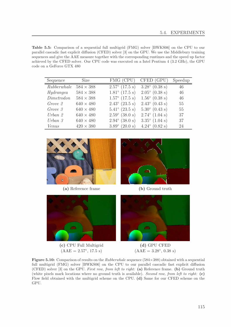
5.4. EXPERIMENTS
Table 5.5: Comparison of a sequential full multigrid (FMG) solver [BWKS06] on the CPU to ourparallel cascadic fast explicit diffusion (CFED) solver [3] on the GPU. We use the Middlebury trainingsequences and give the AAE measure together with the corresponding runtimes and the speed up factorachieved by the CFED solver. Our CPU code was executed on a Intel Pentium 4 (3.2 GHz), the GPUcode on a GeForce GTX 480
Sequence Size FMG (CPU) CFED (GPU) Speedup
Rubberwhale 584× 388 2.57 (17.5 s) 3.28 (0.38 s) 46Hydrangea 584× 388 1.81 (17.5 s) 2.05 (0.38 s) 46Dimetrodon 584× 388 1.57 (17.5 s) 1.56 (0.38 s) 46Grove 2 640× 480 2.43 (23.5 s) 2.43 (0.43 s) 55Grove 3 640× 480 5.41 (23.5 s) 5.30 (0.43 s) 55Urban 2 640× 480 2.59 (38.0 s) 2.74 (1.04 s) 37Urban 3 640× 480 2.94 (38.0 s) 3.35 (1.04 s) 37Venus 420× 380 3.89 (20.0 s) 4.24 (0.82 s) 24
(a) Reference frame (b) Ground truth
(c) CPU Full Multigrid (d) GPU CFED
(AAE = 2.57, 17.5 s) (AAE = 3.28, 0.38 s)
Figure 5.10: Comparison of results on the Rubberwhale sequence (584×388) obtained with a sequentialfull multigrid (FMG) solver [BWKS06] on the CPU to our parallel cascadic fast explicit diffusion(CFED) solver [3] on the GPU. First row, from left to right: (a) Reference frame. (b) Ground truth(white pixels mark locations where no ground truth is available). Second row, from left to right: (c)Flow field obtained with the multigrid scheme on the CPU. (d) Same for our CFED scheme on theGPU.
115
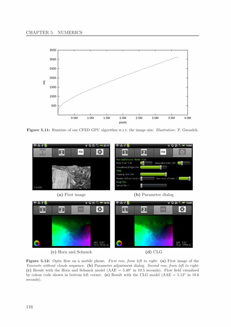
CHAPTER 5. NUMERICS
500
1000
1500
2000
2500
3000
3500
0.5M 1.0M 1.5M 2.0M 2.5M 3.0M 3.5M 4.0M
ms
pixels
Figure 5.11: Runtime of our CFED GPU algorithm w.r.t. the image size. Illustration: P. Gwosdek.
(a) First image (b) Parameter dialog
(c) Horn and Schunck (d) CLG
Figure 5.12: Optic flow on a mobile phone. First row, from left to right: (a) First image of theYosemite without clouds sequence. (b) Parameter adjustment dialog. Second row, from left to right:(c) Result with the Horn and Schunck model (AAE = 5.49 in 10.5 seconds). Flow field visualisedby colour code shown in bottom left corner. (e) Result with the CLG model (AAE = 5.12 in 10.6seconds).
116

Chapter 6
Applications
Il n’existe pas de sciences appliquees, mais seulement desapplications de la science.
Louis Pasteur
In Chapter 1, we pointed out that various applications in the fields of computer visionand image processing require to solve correspondence problems. One example is shown inthe following where we consider a problem from the field of computational photography:the alignment of exposure series for HDR imaging [DM97, MP95, RWPD05, RBS99].This comes down to estimating the displacements in the exposure series, which we realiseby a modified variational optic flow approach that we presented in [9].
In the same work we leveraged the subpixel precision of the resulting flow fields tocombine concepts from super-resolution (SR) methods [PPK03] and HDR imaging ina joint super-resolution and HDR (SR-HDR) technique that computes an image withenhanced dynamic range and spatial resolution.
6.1 HDR Imaging
Before presenting our alignment strategy, we first want to briefly discuss the basics ofHDR imaging.
6.1.1 Why Do We Need HDR Imaging?
We usually model images as continuous functions that map from the image domainΩ ⊂ R
2 to the co-domain R. However, digital images are inherently discrete, they areactually discrete samples of the continuous world. In Section 3.4 we discussed how theimage domain Ω can be discretised. Let us for now still assume that the image domainΩ is continuous and focus on the co-domain.
117

CHAPTER 6. APPLICATIONS
Typical image formats such as JPEG, PNG or PPM reserve 1 byte, i.e. 8 bits ofstorage per pixel and colour channel, resulting in 256 different values for each channel.This means that the image co-domain of each channel is in fact sampled (quantised) andcan be represented by the discrete set 0, .., 255. The dynamic range –the ratio betweensmallest and largest value that can be expressed– thus spans two orders of magnitude inthe discussed case. This range also correspond to the actual dynamic range of commondisplay devices (LCD and CRT displays) as well as print media. However, the dynamicrange of real world scenes is orders of magnitude larger: Outdoor scenes may exhibit adynamic range of up to 5 orders of magnitude between shadows and highlights, or evenmore when a light source, e.g. the sun, is directly visible. This leads to the obviousproblem that today’s low dynamic range (LDR) images that have been taken withstandard cameras either suffer from under-saturation (black pixels) in dark regions orfrom over-saturation (white pixels) in bright regions.
Note that many digital SLR cameras allow to take images in a RAW format thatstores the measured data without further quantisation and allows for up to 14 bits perpixel. However, the resulting dynamic range still only spans 4 orders of magnitude whichis still insufficient in difficult scenarios, as discussed above.
6.1.2 The Basics of HDR Imaging
A popular way to overcome the described problem is to consider a set of images takenwith varying exposure times, a so-called exposure series 1. In this way, despite usinga LDR sensor, the dark parts of the scene can be captured in the long exposures andthe bright parts in the short exposures, respectively. By fusing the information from acomplete exposure series, HDR imaging techniques [DM97, MP95, RWPD05, RBS99]compute a single image with increased dynamic range. More precisely, the resultingimage should ideally describe the actual scene radiances and thus capture the full dy-namic range of the scene. This is of course only possible if the exposure series covers asufficiently large number of exposures. To get an idea how the radiances can be com-puted from the exposure series, we briefly subsume in the following the HDR imagingtechnique of Robertson et al. [RBS99].
Notation and Observation Model. Assume we have taken an exposure series con-sisting of ne images fk : Ω → 0, .., 255 for k = 1, .., ne. The corresponding exposuretimes we denote by tk ∈ R
+. Our goal is now to compute a radiance map r : Ω → R+
from the given exposure series.The basic observation model for HDR imaging relates the measured image intensities
fk and corresponding exposure times tk to the unknown radiances r via
fk(x, y) = φ(tk r(x, y)
), (6.1)
1Also called Wyckoff set in honour of Charles Wyckoff who already in the 1930s combined differentlyexposed film layers to extend the dynamic range of photographic films.
118

6.1. HDR IMAGING
0
50
100
150
200
250
-2 -1 0 1
Pix
el v
alue
s: f k
Log exposure: log10(tk r)
0
2
4
6
8
-1.7 -1.6 -1.5 -1.4 -1.3
Pix
el v
alue
s: f k
Log exposure: log10(tk r)
Figure 6.1: Estimated response curve for our Nikon D90 DSLR camera. It was obtained using thecalibration method described in [RBS99]. We only visualise the response for the red colour channel,as it is very similar to the ones of the two other channels. From left to right: (a) Response curve(logarithmically scaled). (b) Close-up view.
for k = 1, .., ne and where φ : R+ → 0, .., 255 denotes the camera response function,or camera response curve. The latter describes how the amount of light arriving atthe image sensor (given by tk r and referred to as exposure) is mapped to a pixel valuefk. The response function can be estimated from an exposure series by a calibrationprocedure as for example described in [DM97, RBS99]. This has to be done only oncefor a specific camera and we are thus justified in assuming that the response function isknown when computing the radiances.
Considering colour images, one usually assumes the same observation model for eachcolour channel, but with a distinct response function for each channel.
A Note on Camera Response Functions. Let us take a look at a typical responsefunctions for digital cameras. In Figure 6.1 we show the response curve for a standardDSLR camera (Nikon D90). This camera was also used for capturing the images usedin our experiments that will be shown in Sections 6.2.4 and 6.3.4.
Due to the discrete nature of digital cameras, the response curve is in fact a piecewiseconstant function, which means that always a whole interval of radiances is mapped toone pixel value, see Figure 6.1 (b). The size of these intervals depends on the slope of theresponse function. If the response function is steep, only a small interval of radiancesmaps to one pixel value, which is desirable. In flat regions, however, larger intervalsof radiances map to the same pixel value, which reduces the reliability of the radiancecomputation there. If we reconsider the response function in Figure 6.1 (a), we realisethat the function is rather steep in the middle range and becomes flat when approachingits extremes, 0 and 255. According to our previous argumentation, one should thusreduce the influence of rather dark and bright pixels from the radiance computation.This can easily be achieved by using a weighting function ω : 0, .., 255 → [0, 1] in thefinal radiance computation.
In the literature, several weighting functions have been studied, see [GAW+10] fora comprehensive overview. For our experiments, we use the Gaussian-like weighting
119

CHAPTER 6. APPLICATIONS
0
0.2
0.4
0.6
0.8
1
0 50 100 150 200 250W
eigh
t ωk
Pixel values fk
Figure 6.2: Gaussian-like weighting function.
function proposed in [RBS99]. It is given by
ω(fk(x, y)
)=: ωk(x, y) := exp
(−s ·
(fk(x, y)− 127.5
)2
(127.5)2
), (6.2)
with a scale parameter s. A plot of this function for s = 8 is shown in Figure 6.2.Furthermore, it makes sense to set ω = 0 if the weight would become smaller than athreshold value, say 0.001. This completely disables the influence of less reliable pixels.Note in this context that the weight for fully saturated pixels (fk = 255) should anywaybe equal to zero, i.e. ω(255) = 0. The reason for this is that the radiance informationfrom saturated pixels is completely unreliable as any radiance above a certain thresholdwill result in a pixel value of 255.
Computing the Radiances. The sought radiances r are found by minimising anenergy formulation. It solely consists of a data term that penalises deviations from theobservation model (6.1) and is weighted by the discussed weight function ω. To derivethe data term, let us first rewrite the observation model as
fk(x, y) = φ(tk r(x, y)
)
⇒ φ−1(fk(x, y)
)= tk r(x, y)
⇔ φ−1(fk(x, y)
)− tk r(x, y) = 0 , (6.3)
for k = 1, .., ne and where φ−1 denotes the inverse of the camera response function. Fornotational convenience we further define Ik(x, y) := φ−1(fk(x, y)). Using this notationand performing a quadratic penalisation of (6.3) together with the weighting yields theenergy
E(r) =
∫
Ω
(ne∑
k=1
ωk(x, y)(Ik(x, y)− tk r(x, y)
)2)
dx dy . (6.4)
120
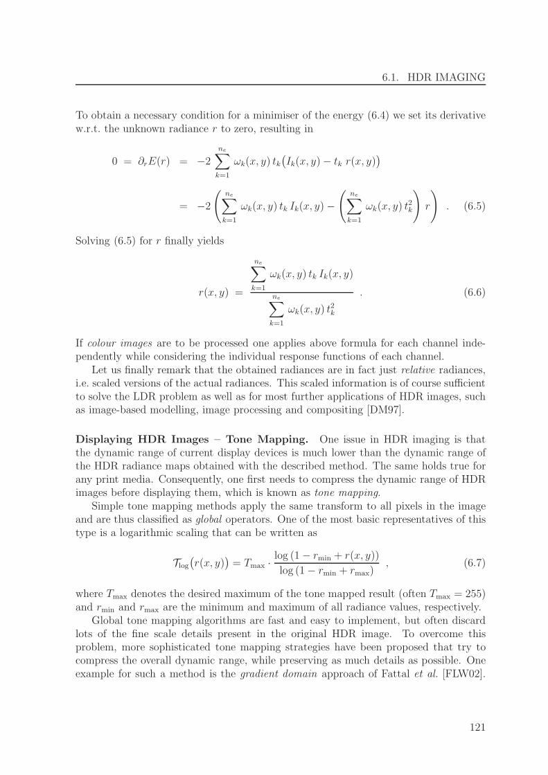
6.1. HDR IMAGING
To obtain a necessary condition for a minimiser of the energy (6.4) we set its derivativew.r.t. the unknown radiance r to zero, resulting in
0 = ∂rE(r) = −2
ne∑
k=1
ωk(x, y) tk(Ik(x, y)− tk r(x, y)
)
= −2
(ne∑
k=1
ωk(x, y) tk Ik(x, y)−(
ne∑
k=1
ωk(x, y) t2k
)r
). (6.5)
Solving (6.5) for r finally yields
r(x, y) =
ne∑
k=1
ωk(x, y) tk Ik(x, y)
ne∑
k=1
ωk(x, y) t2k
. (6.6)
If colour images are to be processed one applies above formula for each channel inde-pendently while considering the individual response functions of each channel.
Let us finally remark that the obtained radiances are in fact just relative radiances,i.e. scaled versions of the actual radiances. This scaled information is of course sufficientto solve the LDR problem as well as for most further applications of HDR images, suchas image-based modelling, image processing and compositing [DM97].
Displaying HDR Images – Tone Mapping. One issue in HDR imaging is thatthe dynamic range of current display devices is much lower than the dynamic range ofthe HDR radiance maps obtained with the described method. The same holds true forany print media. Consequently, one first needs to compress the dynamic range of HDRimages before displaying them, which is known as tone mapping.
Simple tone mapping methods apply the same transform to all pixels in the imageand are thus classified as global operators. One of the most basic representatives of thistype is a logarithmic scaling that can be written as
Tlog
(r(x, y)
)= Tmax ·
log (1− rmin + r(x, y))
log (1− rmin + rmax), (6.7)
where Tmax denotes the desired maximum of the tone mapped result (often Tmax = 255)and rmin and rmax are the minimum and maximum of all radiance values, respectively.
Global tone mapping algorithms are fast and easy to implement, but often discardlots of the fine scale details present in the original HDR image. To overcome thisproblem, more sophisticated tone mapping strategies have been proposed that try tocompress the overall dynamic range, while preserving as much details as possible. Oneexample for such a method is the gradient domain approach of Fattal et al. [FLW02].
121

CHAPTER 6. APPLICATIONS
Here, the gradients of the radiance map are considered and a scaling function is ap-plied that compresses large gradients (reduces the dynamic range), while boosting smallgradients (preserving fine details). The tone mapped result is then obtained by inte-grating the modified gradient field by solving the Poisson equation. We used this tonemapping operator from [FLW02] for displaying all HDR results shown in this thesis.Specifically, we use the implementation of the pfstools package [MKMS07] (http://pfstools.sourceforge.net) with the parameters α = 1.0, β = 0.95, s = 0.8. Pleasedo not confuse this parameters with the correspondent parameters in this thesis. Afterthe tone mapping, we additionally perform a gamma correction with γ = 2.0.
Note that a comprehensive survey on other tone mapping techniques would exceedthe scope of this work and we refer the interested reader to [RWPD05].
6.2 Aligning Exposure Series for HDR Imaging
Taking a closer look at equation (6.6) reveals that the HDR result at a certain positionis obtained by computing a weighted average over the radiances computed from the ex-posure series at this very location. Such a strategy naturally requires perfectly alignedimages without displacements between them. This assumption is, however, hardly ful-filled in real world scenarios due to moving objects (persons, clouds, etc.) or camerashake.
In [9] we tackled this problem by adapting a modern optic flow technique to esti-mate the displacements in the exposure series. This approach seems promising due tothe robustness, high accuracy and efficiency of recent optic flow methods, which wasalso demonstrated in the previous chapters of this thesis. Note that as soon as thedisplacements are known, one can align the exposure series by compensating the imagesfor the displacements.
6.2.1 Variational Optic Flow on Exposure Series
Assume we are given an exposure series fk : Ω → R for k=1, . . . , ne. Our goal is now toestimate the displacements uk := (uk, vk)
⊤ between a reference image fr and the imagesfk. Note that for k = r, we have uk = 0, of course. Some methods, e.g. [MG07] definethe reference image fr as the one with the highest entropy. Assuming that the exposureseries is ordered w.r.t. exposure times, the image with the highest entropy will mostlybe the middle image in the series. We are thus justified in defining r := ⌈m/2⌉, where⌈·⌉ denotes the ceiling function. The latter is defined as ⌈x⌉ = minn ∈ Z | n ≥ x.
To use the notation we have introduced for optic flow, we can use the same idea asin the stereo case and embed fk and fr in an image sequence. This results in fr(x, y) ≡f(x, y, t) and fk(x, y) ≡ f(x, y, t+1). This allows to compute the sought displacement
122
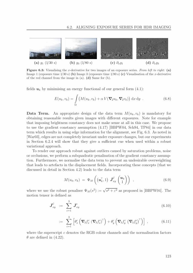
6.2. ALIGNING EXPOSURE SERIES FOR HDR IMAGING
(a) g1 (1/30 s) (b) g3 (1/80 s) (c) ∂xg1 (d) ∂xg3
Figure 6.3: Visualising the x-derivative for two images of an exposure series. From left to right: (a)Image 1 (exposure time 1/30 s) (b) Image 3 (exposure time 1/80 s) (c) Visualisation of the x-derivativeof the red channel from the image in (a). (d) Same for (b).
fields uk by minimising an energy functional of our general form (4.1):
E(uk, vk) =
∫
Ω
(M(uk, vk) + α V (∇2uk,∇2vk)
)dx dy . (6.8)
Data Term. An appropriate design of the data term M(uk, vk) is mandatory forobtaining reasonable results given images with different exposures. Note for examplethat imposing brightness constancy does not make sense at all in this case. We proposeto use the gradient constancy assumption (4.17) [BBPW04, Sch94, TP84] in our dataterm which results in using edge information for the alignment, see Fig. 6.3. As noted in[War03], edges are not completely invariant under exposure changes, but our experimentsin Section 6.2.4 will show that they give a sufficient cue when used within a robustvariational approach.
To render our approach robust against outliers caused by saturation problems, noiseor occlusions, we perform a subquadratic penalisation of the gradient constancy assump-tion. Furthermore, we normalise the data term to prevent an undesirable overweightingthat leads to artefacts in the displacement fields. Incorporating these concepts (that wediscussed in detail in Section 4.2) leads to the data term
M(uk, vk) = ΨM
((u⊤
k , 1)J
Cxy
(uk
1
)), (6.9)
where we use the robust penaliser ΨM(s2) :=√s2 + ε2 as proposed in [BBPW04]. The
motion tensor is defined as
JCxy :=
3∑
c=1
Jc
xy (6.10)
:=3∑
c=1
[θcx
(∇3f
cx (∇3f
cx)
⊤)+ θcy
(∇3f
cy
(∇3f
cy
)⊤)], (6.11)
where the superscript c denotes the RGB colour channels and the normalisation factorsθ are defined in (4.22).
123

CHAPTER 6. APPLICATIONS
In preliminary experiments, we also investigated data terms that impose constancyof the radiances to obtain invariance under exposure changes. This, however, requires apreceding camera calibration step and knowledge of the exposure times as the radiancesare computed via applying the inverse camera response function to the pixel values andthen dividing by the exposure time. Since the radiances make no sense in saturatedregions, and due to possible errors in the calibration, working in the radiance domainalone produced unsatisfactory results. By additionally imposing constancy of the ra-diance gradients we could improve the results. However, we could not obtain betterresults than with our proposed approach, which is simpler and more efficient as it omitscalibration and radiance computations. Note that due to the latter, our approach alsoallows to align image sets for exposure fusion [MKR09] where no camera response curveor exposure times are given.
Also note that using a HSV colour representation as proposed in Section 4.2 doesnot make sense for exposure series. Despite the fact that the exposure changes aremultiplicative and that the hue as well as the saturation channel are invariant undersuch changes, the nonlinearity introduced by the camera response function φ causesproblems. Thus, one would first need to apply the inverse response function which isundesirable, as discussed above.
Smoothness Term. Concerning the smoothness term, we opt for an isotropic flow-driven regulariser [Sch94, SH89]
V (∇2uk,∇2vk) = ΨV
(|∇2 uk|2 + |∇2 vk|2
), (6.12)
using the regularised total variation (TV) penaliser [ROF92] given by ΨV (s2) =
√s2 + ε2.
This discontinuity-preserving smoothness term allows for sharp edges in the flow field,which is important for a favourable alignment, see our experiment in Figure 6.8. Wealso experimented with more advanced smoothness terms, like our complementary regu-lariser [10, 11], but they could not improve the results, as will be shown in the experimentin Figure 6.9.
We further wish to note that the smoothness term plays a very important role inHDR alignment tasks: Flat image regions are omnipresent in exposure series due toover- and undersaturation problems. In this regions, however, the data term does notgive any information and the smoothness term has to fill in the flow field there.
124

6.2. ALIGNING EXPOSURE SERIES FOR HDR IMAGING
6.2.2 Energy Minimisation
As before, we minimise the energy by solving the associated Euler-Lagrange equationswhich read as
3∑
c=1
(Ψ′
M
((u⊤
k , 1)J
Cxy
(uk
1
))·([
Jc
xy
]1,1uk +
[J
c
xy
]1,2vk +
[J
c
xy
]1,3
))(6.13)
−α div(Ψ′
V
(|∇2 uk|2 + |∇2 vk|2
)∇2uk
)= 0 ,
3∑
c=1
(Ψ′
M
((u⊤
k , 1)J
Cxy
(uk
1
))·([
Jc
xy
]1,2uk +
[J
c
xy
]2,2vk +
[J
c
xy
]2,3
))(6.14)
−α div(Ψ′
V
(|∇2 uk|2 + |∇2 vk|2
)∇2vk
)= 0 .
In order to handle large displacements (which often occur in HDR imaging due tosignificant camera shake or fast moving objects), we embed the solution of the Euler-Lagrange equations in the warping framework described in Section 5.3.1. For an efficientsolution of the problem at each warping level, we propose two strategies, based on theavailable hardware architecture: On a sequential CPU architecture, we use the fullmultigrid solver of Bruhn et al. [BWKS06], which we briefly discussed in Section 5.3.3.For parallel GPU architectures, we use the cascadic FED solver from our paper [3],which is described in Section 5.3.5.
One problem with applying the FED scheme for solving above Euler-Lagrange equa-tions is the following: When using a TV penaliser in the smoothness term, the eigen-values of the diffusion tensor are given by
Ψ′V (s
2) =1
2√s2 + ε2
≤ 1
2ε=: λmax . (6.15)
For a standard choice of ε = 0.001 the maximal eigenvalue mmax is thus equal to 500,which significantly restricts the stability limit of an explicit solver, see (5.80). As aconsequence, the time steps that can be chosen by the FED scheme are tangibly smaller.
Fortunately, there is a simple remedy to this problem by using the Charbonnierpenaliser function [CBFAB94] which is defined as
ΨV (s2) = 2 ε2
√1 +
s2
ε2, (6.16)
in the data and the smoothness term. As one can easily show, see Appendix A, theresulting energy is up to a constant factor equal to our proposed energy that usesthe subquadratic function ΨV (s
2) =√s2 + ε2 in the data and smoothness term. The
minimum of both energies is thus the same, yielding the same solution. On the otherhand, the derivative of the Charbonnier function is given by
Ψ′V (s
2) =1√
1 + s2
ε2
≤ 1 , (6.17)
125

CHAPTER 6. APPLICATIONS
Figure 6.4: A freehand exposure series for HDR imaging. Note that severe displacements due tomoving clouds and camera shake. From left to right: (a) Image 1 of the exposure series. (b) Image 2.(c) Image 3 (reference image). (d) Image 4. (e) Image 5.
which results in mmax = 1 and allows for a favourable performance of the FED scheme.
6.2.3 Actual Alignment
Having estimated the displacements (uk, vk)⊤, we can align the exposure series by per-
forming a simple motion compensation. This comes down to replacing each imagefk(x, y) by
f alignk (x, y) := fk(x+uk, y+vk) . (6.18)
6.2.4 Experiments
Comparison to Other Alignment Approaches. In a first experiment, we compareour proposed optic flow-based HDR alignment method to several competing methods.To this end, a real world exposure series was taken freehand using a standard DSLRcamera (Nikon D90). The series consists of 5 images taken with exposure times between1/250 to 1/30 seconds and the image size was rescaled to 512×340 pixels. Some imagesof the series are depicted in the first row of Figure 6.4 where we want to point out thatthe series suffers from severe displacements due to camera shake and moving clouds.
After aligning the images with the different approaches, we compute HDR recon-structions following the approach in [RBS99] that we have also briefly reviewed before.To improve the reconstruction quality, we incorporate information on the camera re-sponse curve, which we estimated beforehand by the method also described in [RBS99].Implementations of the before mentioned algorithms can be found in the pfstools pack-age [MKMS07] (http://pfstools.sourceforge.net).
126

6.2. ALIGNING EXPOSURE SERIES FOR HDR IMAGING
Let us now compare our proposed method to some other alignment strategies. Theseare (i) the global method of Ward [War03], (ii) the align image stack algorithm fromthe Hugin toolkit which implements a homography-based approach as in [TM07], (iii) avariant of our method without data term normalisation, and (iv) the hierarchical blockmatching technique of Menzel and Guthe [MG07].
In Figure 6.5 (b) we show the result obtained with the global alignment strategyfrom [War03], where the black border marks pixels warped outside the image domain.A corresponding zoom is shown in Figure 6.6 (b). It becomes clear that the estimatedglobal translation completely fails in describing the complex displacements between theexposures. We also tried to apply a local optic flow approach [LK81] to the globallyaligned images after transferring them to the radiance domain. We found that such aglobal-local strategy as in [KUWS03] leads to unusable results due to the poor globalalignment. Also the align image stack algorithm, see Figure 6.5 (c) and Figure 6.6 (c),fails to correctly align the images. Obviously, the homography computed from featurematches is not expressive enough to describe the displacements in the exposure series.
In Figure 6.5 (d) we show the result of our method, but without using data termnormalisation. Especially when considering the zoom shown in Figure 6.6 (d), andcomparing it to our final result in Figure 6.6 (f), we realise that the proposed normal-isation allows to resolve any problems with unpleasant artefacts that arise due to anoverweighting of the data term at image edges. This is further substantiated by theflow fields shown in Figure 6.7 (a) and (b). Of course, a larger smoothness weight αwould also resolve this problem, but creates an oversmoothed displacement field thatcannot capture the discontinuity between the buildings and the clouds any more, seeFigure 6.7 (c).
The results obtained with the approach of Menzel and Guthe [MG07] are shown inFigure 6.5 (e). Altough the overall result looks satisfying, the zoom in Figure 6.6 (e)reveals that the hierarchical block matching technique yields unpleasant artefacts at theroof of the house since it does not impose smoothness assumptions on the displacementfield.
Our final result in Figure 6.5 (f) and Figure 6.6 (f) shows a favourable HDR recon-struction without any disturbing artefacts. This becomes possible due to the robust andaccurate displacement estimation of our proposed approach. The latter is demonstratedin Figure 6.8 that visualises all computed flow fields. As one can see, the motion of theclouds and the shift of the buildings due to camera shake are nicely discriminated in thefirst three rows. For the image in the last row, estimating the motion of the clouds isdifficult, but also unimportant, because the cloud region is oversaturated and thus notconsidered in the HDR reconstruction, anyway.
Runtimes. Aligning the whole exposure series from Figure 6.4 that consists of 5 im-ages with 512× 340 pixels each took 75 seconds using our CPU version (full multigridsolver) with unoptimised C code on a 3.2 GHz Intel Pentium 4. An optimised parallelimplementation of a cascadic FED solver on a GeForce GTX 480 reduced the runtime
127
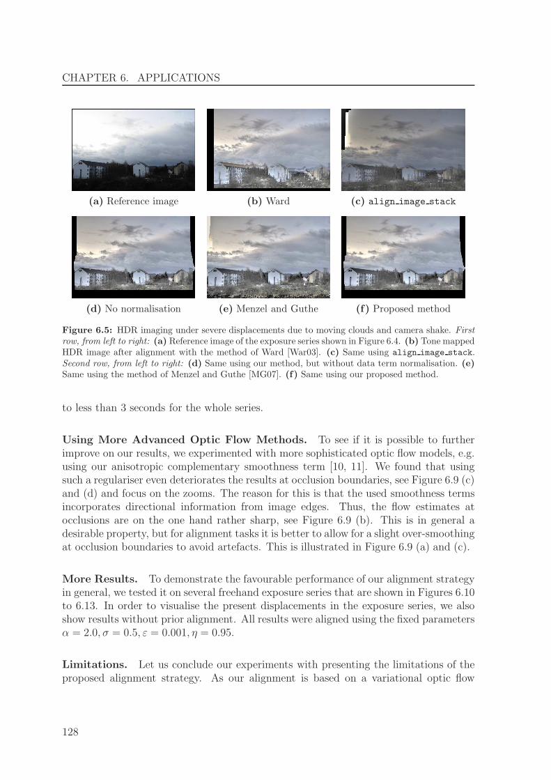
CHAPTER 6. APPLICATIONS
(a) Reference image (b) Ward (c) align image stack
(d) No normalisation (e) Menzel and Guthe (f) Proposed method
Figure 6.5: HDR imaging under severe displacements due to moving clouds and camera shake. Firstrow, from left to right: (a) Reference image of the exposure series shown in Figure 6.4. (b) Tone mappedHDR image after alignment with the method of Ward [War03]. (c) Same using align image stack.Second row, from left to right: (d) Same using our method, but without data term normalisation. (e)Same using the method of Menzel and Guthe [MG07]. (f) Same using our proposed method.
to less than 3 seconds for the whole series.
Using More Advanced Optic Flow Methods. To see if it is possible to furtherimprove on our results, we experimented with more sophisticated optic flow models, e.g.using our anisotropic complementary smoothness term [10, 11]. We found that usingsuch a regulariser even deteriorates the results at occlusion boundaries, see Figure 6.9 (c)and (d) and focus on the zooms. The reason for this is that the used smoothness termsincorporates directional information from image edges. Thus, the flow estimates atocclusions are on the one hand rather sharp, see Figure 6.9 (b). This is in general adesirable property, but for alignment tasks it is better to allow for a slight over-smoothingat occlusion boundaries to avoid artefacts. This is illustrated in Figure 6.9 (a) and (c).
More Results. To demonstrate the favourable performance of our alignment strategyin general, we tested it on several freehand exposure series that are shown in Figures 6.10to 6.13. In order to visualise the present displacements in the exposure series, we alsoshow results without prior alignment. All results were aligned using the fixed parametersα = 2.0, σ = 0.5, ε = 0.001, η = 0.95.
Limitations. Let us conclude our experiments with presenting the limitations of theproposed alignment strategy. As our alignment is based on a variational optic flow
128

6.2. ALIGNING EXPOSURE SERIES FOR HDR IMAGING
(a) Reference image (b) Ward (c) align image stack
(d) No normalisation (e) Menzel and Guthe (f) Proposed method
Figure 6.6: Zoom in the results from Figure 6.5. First row, from left to right: (a) Reference imageof the exposure series shown in Figure 6.4. (b) Tone mapped HDR image after alignment with themethod of Ward [War03]. (c) Same using align image stack. Second row, from left to right: (d)Same using our method, but without data term normalisation. (e) Same using the method of Menzeland Guthe [MG07]. (f) Same using our proposed method.
(a) Normalisation (b) No normalisation (c) No normalisation
(α = 2.0) (α = 2.0) (α = 2.5)
Figure 6.7: Comparing flow fields obtained with and without data term normalisation. From leftto right: (a) Flow field from image 3 (reference) to image 1 of our exposure series from Figure 6.4,computed with normalisation and α = 2.0. (b) Same, but without normalisation and α = 2.0. (c) Nonormalisation and α = 2.5. For all results, we used the fixed parameters σ = 0.5, η = 0.95.
129

CHAPTER 6. APPLICATIONS
gr gk (uk, vk)
Figure 6.8: Flow fields computed on the exposure series from Figure 6.4. First row, from left toright: (a)–(c) Image 1. Image 3. Flow field from image 3 to image 1. Second row, from left to right:(d)–(f) Same for image 2 and 3. Third row, from left to right: (g)–(i) Same for image 4 and 3. Fourthrow, from left to right: (j)–(l) Same for image 5 and 3. For all results, we used the fixed parametersα = 2.0, σ = 0.5, ε = 0.001, η = 0.95.
130
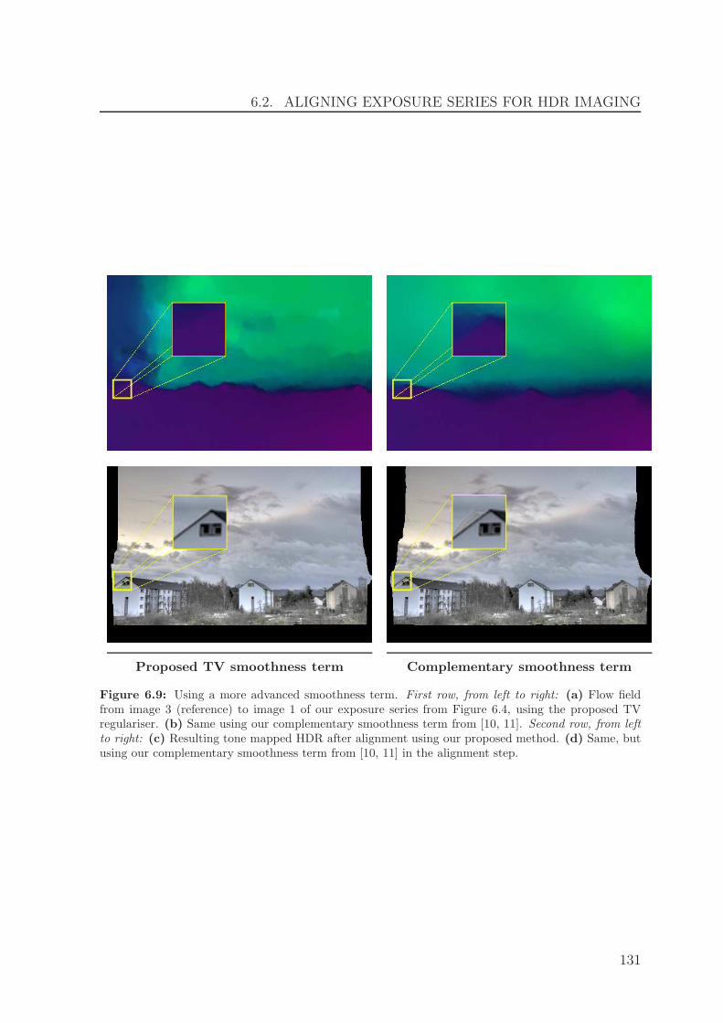
6.2. ALIGNING EXPOSURE SERIES FOR HDR IMAGING
Proposed TV smoothness term Complementary smoothness term
Figure 6.9: Using a more advanced smoothness term. First row, from left to right: (a) Flow fieldfrom image 3 (reference) to image 1 of our exposure series from Figure 6.4, using the proposed TVregulariser. (b) Same using our complementary smoothness term from [10, 11]. Second row, from leftto right: (c) Resulting tone mapped HDR after alignment using our proposed method. (d) Same, butusing our complementary smoothness term from [10, 11] in the alignment step.
131

CHAPTER 6. APPLICATIONS
Figure 6.10: Freehand HDR imaging of a window in the cathedral Notre Dame de Paris. First row,from left to right: (a)–(c) Image 2, 4 and 6 of the exposure series (7 images, 1072×712 pixels, exposuretimes between 1/200 and 2 seconds. Second row, from left to right: (c) Resulting tone mapped HDRimage without alignment. (d) Same using our proposed alignment method.
approach, we naturally have to use a coarse-to-fine warping strategy to handle largedisplacements in the exposure series, see Section 5.3.1. However, we have argued inSection 4.5 that techniques relying on a warping strategy cannot estimate large dis-placements of small objects. This problem can for example occur if persons or carsmove relatively fast while the exposure series is taken. In such cases, our alignmentstrategy will fail to estimate the motion of these objects, which leads to unpleasantartefacts in the resulting HDR image, see Figure 6.14 and focus on the zooms in (d) and(e).
132

6.2. ALIGNING EXPOSURE SERIES FOR HDR IMAGING
Figure 6.11: Freehand HDR imaging of the Max-Planck Institute for Informatics in Saarbrucken.First row, from left to right: (a)–(c) Image 1, 3 and 5 of the exposure series (5 images, 490 × 620pixels, exposure times between 1/800 and 1/50 seconds. Second row, from left to right: (c) Resultingtone mapped HDR image without alignment. (d) Same using our proposed alignment method.
133

CHAPTER 6. APPLICATIONS
Figure 6.12: Freehand HDR imaging of an indoor scene (Lantern). First row, from left to right:(a)–(c) Image 1, 3 and 5 of the exposure series (5 images, 1268× 854 pixels, exposure times between1/320 and 1/6 seconds. Second row, from left to right: (c) Resulting tone mapped HDR image withoutalignment. (d) Same using our proposed alignment method.
Figure 6.13: Freehand HDR imaging of another indoor scene (Room). First row, from left to right:(a)–(c) Image 1, 2 and 3 of the exposure series (3 images, 1024× 680 pixels, exposure times between1/60 and 0.3 seconds. Second row, from left to right: (c) Resulting tone mapped HDR image withoutalignment. (d) Same using our proposed alignment method.
134

6.2. ALIGNING EXPOSURE SERIES FOR HDR IMAGING
(a) Image 1 (b) Image 2 (c) Image 4
(d) Aligned HDR result (e) Zoom in region 1 in (d)
(f) Zoom in region 2 in (d)
Figure 6.14: Limitations of our method (freehand HDR imaging of the Eiffel tower in Paris). Firstrow, from left to right: (a)–(c) Image 1, 2 and 4 of the exposure series (4 images, 1072× 712 pixels,exposure times between 1/4000 and 1/320 seconds. Second row, from left to right: (d) Resulting tonemapped HDR image using our proposed alignment method. (e) Zoom in region 1 marked in (d). Thirdrow: (f) Zoom in region 2 marked in (d).
135

CHAPTER 6. APPLICATIONS
6.3 Joint Super-Resolution and HDR (SR-HDR) Re-
construction
Super-resolution (SR) techniques such as [EF97, FREM04, MPSC09, PPK03, TH84]combine the information from several low-resolution (LR) images of the same scene tocompute an image with increased spatial resolution. Note that although megapixel imagesensors are widely available nowadays, spatial resolution enhancement is still crucial inapplications such as surveillance [ZZSL10] or medical imaging [Gre09], where tiny detailscan be of great importance. Furthermore, cameras in mobile phones still suffer from alimited spatial resolution. The prerequisites for a successful SR reconstruction are: (i)Some amount of subpixel displacement between the LR input images. Note that if thereare no or only integer displacements, all images somehow contain redundant informationand no resolution enhancement is possible 2. (ii) The images should suffer from aliasing,i.e. they have been sampled below the Nyquist frequency [SW49, Uns00]. In this waythe LR images contain valuable high-frequency information that helps to recover the SRresult [VSVV06].
The displacement fields resulting from our previously described HDR alignmentstrategy (Section 6.2) are by construction of subpixel precision. If one additionallyassures that the exposure series suffers from aliasing –e.g. if one uses a camera witha limited resolution like in a mobile phone– we meet all requirements for a SR recon-struction. This motivated our work in [9] where we exploited the displacements in afreehand exposure series in a joint super-resolution and HDR (SR-HDR) approach simi-lar to [CPK09, GG06, HTO07, NYUS08, NN05, RMVS07, SSM09]. This allows to turnthe usually perturbing displacements in the exposure series into an advantage: We cannot only enhance the dynamic range, but also the spatial resolution of the reconstructedimage. In this context, we also want to point out that SR and HDR imaging nicely com-plement each other: While SR methods increase the resolution of the image domain,HDR techniques increase the resolution of the image co-domain, i.e. the dynamic range.
6.3.1 Super-Resolution Basics
Before we describe our joint SR-HDR approach, we want to briefly review the basicconcepts of SR reconstruction. For a more extensive survey, we refer the interestedreader to [PPK03].
Notation and Observation Model. Assume we are given a set of LR input imagesfk : Ωdisc → 0, .., 255 for k = 1, .., ne and where Ωdisc := 1, .., nx × 1, .., ny denotesthe discrete representation of the image domain Ω. Note that we now model the imagesin a completely discrete manner as the SR problem stems from the discretisation anddoes not exist in a continuous model. Our goal is now to compute a SR image F :
2Combing a sequence of images with no or only integer displacements would, however, allow toobtain a denoised result by simply averaging the noisy images.
136

6.3. JOINT SUPER-RESOLUTION AND HDR (SR-HDR) RECONSTRUCTION
ΩSRdisc → 0, .., 255, where ΩSR
disc := 1, .., z · nx × 1, .., z · ny denotes the discrete SRimage domain and z ∈ R is the corresponding SR zoom factor, so usually z > 1.
The standard observation model for SR imaging (as for example used in [EF97]) canbe written as
SBWk F = fk , (6.19)
for k = 1, .., ne. It models the assumption that the LR images fk are obtained from theunknown SR image F by a backward warping (Wk), blurring (B) and a downsampling(S).
The warping Wk describes the displacements (uk, vk)⊤ between the images, which
need to be estimated beforehand. This could for example be done by applying somekind of optic flow algorithm. As the warping operator acts on the SR image F , thedisplacements have to be transferred to the SR grid. To perform this upsampling, weuse an area-based resampling strategy as proposed in [BWF+05]. Note that in the SRcase, the displacements are computed from the images fk to a reference image fr. Forthe HDR alignment in Section 6.2, they were computed in the opposite direction.
The blurring operator B performs a Gaussian convolution with standard deviationσSR. In accordance to the sampling theorem [SW49, Uns00], we set σSR = z ·
√2/4. For
simplicity, we follow Mitzel et al. [MPSC09] and assume the same blurring for all inputimages. For implementing the downsampling operator S, we also adapt the strategy in[MPSC09] and use a simple nearest-neighbour interpolation strategy.
If colour images are given, it is usually assumed that the observation model holdsfor each of the colour channels independently.
Energy-based Super-Resolution Reconstruction. There are different basic strate-gies for computing the SR image from the LR input images. The survey in [PPK03]classifies SR techniques into non-uniform interpolation approaches, frequency domainapproaches and energy-based approaches. We will consider the latter class that findsthe SR image F by minimising an energy function of the form
E(F ) =∑
(i,j)∈ΩSR
disc
[MSR(F ) + ϑ VSR(∇2F )
], (6.20)
where ∇2F denotes a discrete version of the gradient operator in this case. Here, and forour further considerations on SR and joint SR-HDR reconstruction, we will intentionallymisuse concepts borrowed from continuous models to facilitate notation.
The term MSR denotes the data term that penalises deviations from the observationmodel (6.19). Using a quadratic penalisation and considering colour images one endsup with
MSR(F ) =ne∑
k=1
3∑
c=1
(SBWk Fc − f c
k)2 , (6.21)
where c denotes the colour channels. Note that for greyscale images this summationover the channels can be omitted.
137
CHAPTER 6. APPLICATIONS
In general, SR reconstruction is an ill-posed problem, which means that we cannotdetermine an unique solution from the data term alone. This is due to a usually in-sufficient number of available LR images. To overcome this problem, energy-based SRapproaches additionally use a smoothness term SSR that models the assumption of asmooth SR result. As in the optic flow case, it thus allows to fill in the solution inregions where the data alone (the input images) do not provide sufficient information.The degree of smoothness is determined by a regularisation parameter ϑ > 0. A basic,homogeneous regulariser is thus given by
VSR(∇2F ) =
3∑
c=1
|∇2Fc|2 . (6.22)
Energy Minimisation. A necessary condition for a minimiser of the energy (6.20) isgiven by
0 = ∂F c E =n∑
k=1
(W⊤
kBS⊤(SBWk F
c − f ck
))− ϑ F c . (6.23)
Concerning the occurring transposed operators, we implementW⊤k by a forward warping,
B = B⊤ for Gaussian blurring [MPSC09], and S⊤ results in upsampling. To solve theequation (6.23), we follow the approach in [MPSC09] and apply an explicit gradientdescent scheme that reads as
[F c](ℓ+1) − [F c](ℓ)
τ=
n∑
k=1
(W⊤
kBS⊤(f ck − SBWk [F
c](ℓ)))
+ ϑ [F c](ℓ) . (6.24)
Solving for the unknown at the new time level l + 1 then gives the iterative scheme
[F c](ℓ+1) = [F c](ℓ) + τ
[n∑
k=1
(W⊤
kBS⊤(f ck − SBWk [F
c](ℓ)))
+ ϑ [F c](ℓ)
], (6.25)
where [F c](ℓ) denotes the result at iteration ℓ and the parameter τ serves as a numericaltime step size. For stability reasons it is set to the small value of τ = 0.01 in accordanceto [MPSC09].
Some Results and Model Extensions. Let us have a look at results obtained withthe described, basic SR approach. In Figure 6.15 (a) we show one frame of an imagesequence depicting a car. Obviously, the resolution of the used camera was very low andwe cannot recognise any details, as for example the license plate, which is shown in thezoom in Figure 6.15 (d). Considering the SR result in Figure 6.15 (b) and (e), a drasticimprovement becomes visible. However, the SR result looks rather blurry, which canbe explained as follows: The quadratic data term is rather sensitive to outliers causedby noise, occlusions or misregistrations. This means that a relatively large smoothness
138

6.3. JOINT SUPER-RESOLUTION AND HDR (SR-HDR) RECONSTRUCTION
weight ϑ has to be chosen, which in turn blurs the result due to the homogeneoussmoothing of the result.
These problems can be diminished by following Mitzel et al. [MPSC09] who proposedto use a subquadratic data term (L1-norm) in combination with a TV regulariser. Thisresults in the energy
E(F ) =∑
(i,j)∈ΩSR
disc
[ne∑
k=1
ΨM
(3∑
c=1
(SBWk Fc − f c
k)2
)+ ϑ ΨV
(3∑
c=1
|∇2Fc|2)]
, (6.26)
with ΨM(s2) = ΨV (s2) =
√s2 + ε2. With above modifications, the corresponding gra-
dient descent scheme is given by
[F c](ℓ+1) = [F c](ℓ) (6.27)
+ τ
[n∑
k=1
(W⊤
kBS⊤ Ψ′
M
(3∑
c=1
(SBWk [F
c](ℓ) − f ck
)2)(
f ck − SBWk [F
c](ℓ)))
+ϑ div
(Ψ′
V
(3∑
c=1
∣∣∇2[Fc](ℓ)∣∣2)∇2[F
c](ℓ)
)].
When considering the corresponding results in Figure 6.15 (c) and (f), we see that theimproved model allows to obtain a much sharper reconstruction, which makes it easierto recognise the license plate.
6.3.2 A Novel Joint Super-Resolution and HDR (SR-HDR)Model
In the following we show how to extend the presented energy-based SR approach (6.26)to a novel joint super-resolution and HDR (SR-HDR) method that we presented in [9].
We assume to be given a freehand exposure series fk : Ωdisc → 0, .., 255 for k =1, .., ne with corresponding exposure times tk. Furthermore, a zoom factor z has to bespecified and we assume that the displacements between the images of the exposureseries has been estimated. The latter is realised by applying our method described inSection 6.2. From these inputs, we compute a SR-HDR reconstruction, i.e. a super-resolved radiance map R : ΩSR
disc → R+.
Energy Formulation
We compute the SR-HDR image R by minimising a suitable energy function of thegeneral form [CPK09, GG06]
E(R) =∑
(i,j)∈ΩSR
disc
[M(R) + ϑ V (∇2R)
], (6.28)
with a smoothness weight ϑ > 0.
139
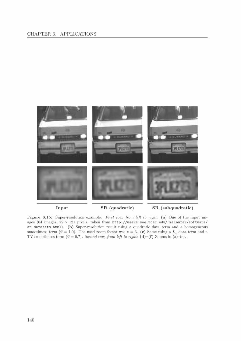
CHAPTER 6. APPLICATIONS
Input SR (quadratic) SR (subquadratic)
Figure 6.15: Super-resolution example. First row, from left to right: (a) One of the input im-ages (64 images, 72 × 121 pixels, taken from http://users.soe.ucsc.edu/~milanfar/software/
sr-datasets.html). (b) Super-resolution result using a quadratic data term and a homogeneoussmoothness term (ϑ = 1.0). The used zoom factor was z = 3. (c) Same using a L1 data term and aTV smoothness term (ϑ = 0.7). Second row, from left to right: (d)–(f) Zooms in (a)–(c).
140
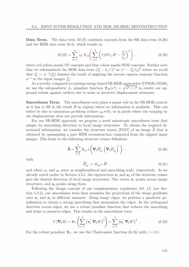
6.3. JOINT SUPER-RESOLUTION AND HDR (SR-HDR) RECONSTRUCTION
Data Term. The data term M(R) combines concepts from the SR data term (6.26)and the HDR data term (6.4), which results in
M(R) =
ne∑
k=1
ωk ΨM
(3∑
c=1
(SBWk R
c − Icktk
)2)
, (6.29)
where red colour marks SR concepts and blue colour marks HDR concepts. Further notethat we reformulated the HDR data term (Ick − tk r
c)2 as (rc − Ick/tk)2 where we recall
that Ick := φ−1(f ck) denotes the result of applying the inverse camera response function
φ−1 to the input images f ck .
As a novelty compared to existing energy-based SR-HDR approaches [CPK09, GG06],we use the subquadratic L1 penaliser function ΨM(s2) =
√s2 + ε2 to render our ap-
proach robust against outliers due to noise or incorrect displacement estimates.
Smoothness Term. The smoothness term plays a major role in the SR-HDR contextas it has to fill in the result R in regions where no information is available. This caneither be due to saturation problems (where ωk≈0), or in pixels where the warping bythe displacements does not provide information.
For our SR-HDR approach, we propose a novel anisotropic smoothness term thatadapts its smoothing direction to local image structures. To obtain the required di-rectional information, we consider the structure tensor [FG87] of an image R that isobtained by upsampling a pure HDR reconstruction computed from the aligned inputimages. This leads to the following structure tensor definition:
S =
3∑
c=1
Kρ1∗(∇2R
cρ2
(∇2R
cρ2
)⊤), (6.30)
withRc
ρ2:= Kρ2∗ Rc , (6.31)
and where ρ1 and ρ2 serve as neighbourhood and smoothing scale, respectively. As wealready noted earlier in Section 4.3.1, the eigenvectors s1 and s2 of the structure tensorgive the desired direction of local image structures: The vector s1 points across imagestructures, and s2 points along them.
Following the design concept of our complementary regulariser [10, 11] (see Sec-tion 4.3.2), our smoothness term then penalises the projections of the image gradientsonto s1 and s2 in different manners: Along image edges, we perform a quadratic pe-nalisation to obtain a strong smoothing that pronounces the edges. In the orthogonaldirection across edges, we use a robust penaliser function that reduces the smoothingand helps to preserve edges. This results in the smoothness term
V (∇2R) = ΨV
(3∑
c=1
(s⊤1 ∇2R
c)2)
+
3∑
c=1
(s⊤2 ∇2R
c)2
. (6.32)
For the robust penaliser ΨV , we use the Charbonnier function (6.16) with ε = 0.1.
141

CHAPTER 6. APPLICATIONS
6.3.3 Energy Minimisation
We compute the SR-HDR image R by minimising the energy (6.28). To this end, weuse a semi-implicit gradient descent scheme given by
[Rc](ℓ+1)− [Rc](ℓ)
τ= (6.33)
ne∑
k=1
(W⊤
kBS⊤ωk Ψ
′M
(3∑
c=1
(SBWk [R
c](ℓ) − Icktk
)2)(
Icktk
− SBWk [Rc](ℓ)))
+ϑ div
(D(s1,s2,∇2R
(ℓ))∇2[R
c](ℓ,ℓ+1)),
The occurring diffusion tensor D is given by
D(s1,s2,∇2R
(ℓ))= Ψ′
V
(3∑
c=1
(s⊤1 ∇2[R
c](ℓ))2)s1s
⊤1 + s2s
⊤2 . (6.34)
Further note that term∇2[Rc](ℓ,ℓ+1) occurring in (6.33) has two indices in the superscript.
By this, we denote that when discretising the divergence expression, the old value atiteration l is used for the neighbouring pixels, whereas the new result at iteration l + 1is used for the central pixel. The gradient descent scheme (6.33) can thus be rewrittenas
[Rc](ℓ+1)i,j − [Rc]
(ℓ)i,j
τ= [mc]
(ℓ)i,j + ϑ
∑
i,j∈Ni,j
[w]i,j
([Rc]
(ℓ)
i,j− [Rc]
(ℓ+1)i,j
) , (6.35)
using the abbreviation
[mc](ℓ)i,j := (6.36)
ne∑
k=1
(W⊤
kBS⊤[ωk]i,j Ψ
′M
(3∑
c=1
(SBWk [R
c](ℓ)i,j −
[Ick]i,jtk
)2)( [Ick]i,jtk
− SBWk [Rc](ℓ)
)),
and where the weights [w]i,j can be derived from the diffusion tensor (6.34) as described
in Section 5.1.1. Solving (6.35) for the unknown update [Rc](ℓ+1) results in the finaliterative scheme given by
[Rc](ℓ+1)i,j =
[Rc](ℓ)i,j + τ
[mc]
(ℓ)i,j + ϑ
∑
i,j∈Ni,j
[w]i,j [Rc](ℓ)i,j
1 + ϑ∑
i,j∈Ni,j
[w]i,j. (6.37)
142
6.3. JOINT SUPER-RESOLUTION AND HDR (SR-HDR) RECONSTRUCTION
Concerning the numerical time step size, we experimentally found that setting τ = 0.5is feasible, which is more than one order of magnitude larger than the step size used inthe explicit scheme (6.25) which was taken from [MPSC09]. We further note that dueto the complicated structure of the data term (6.29), more efficient solution strategiesas in the optic flow case (see Section 5.3.2) are difficult to realise here.
6.3.4 Experiments
For our first experiments, we took a freehand, real world exposure series consisting of9 images with a resolution of 268× 178 pixels and with exposure times between 1/800and 1/8 seconds. Some of the input images are shown in the first row of Figure 6.16. Aszoom factor we set z = 2 for all our experiments. To estimate the displacements betweenthe images of the exposure series, we use our technique described before in Section 6.2.The model parameters were set to α = 2.0, σ = 0.5, η = 0.7. If not stated otherwise,these parameters are also used for the other SR-HDR experiments in this section.
Our SR-HDR Method versus Pure HDR and Existing Approaches. In a firstexperiment (see Figure 6.16) we show two benefits of our proposed SR-HDR method:(i) We illustrate that our obtained SR-HDR reconstruction shown in Figure 6.16 (h)gives a remarkable improvement over a pure HDR reconstruction (Figure 6.16 (d)).Especially when comparing the corresponding zooms in Figure 6.16 (e) and (i) we seethat our SR-HDR result gives a much less pixelated result. (ii) We also want to showthat our proposed model (L1-data term with anisotropic smoothness term) gives muchmore appealing results compared to existing energy-based SR-HDR approaches [CPK09,GG06] that use a quadratic data term and a mean prior. Recall that the latter enforcesthe result to be close to a mean image that is obtained by averaging the radiancescomputed from all input images. Although this prior stabilises the minimisation, it doesnot allow to fill in missing information and to smooth the resulting image. Consequently,the result of such a method (see Figure 6.16 (f) and (g)) hardly improves over a pureHDR reconstruction and is inferior to our result.
Runtimes. As we have noted before, it is much more difficult to come up with anefficient numerical solver for our SR-HDR approach. By using a semi-implicit scheme,we could improve the performance by more than one order of magnitude, as it nowbecomes possible to use a time step size of 0.5 instead of the 0.01 which was reportedfor an explicit scheme in [MPSC09]. However, computing the final SR-HDR result forthe exposure series from Figure 6.16 still takes about half an hour on a standard PC(3.2 GHz Intel Pentium 4).
Different Data and Smoothness Terms. Our next experiment compares the influ-ence of using different data and smoothness terms in energy-based SR-HDR approaches.
143

CHAPTER 6. APPLICATIONS
(a) Image 1 (b) Image 5 (c) Image 9
(d) Pure HDR (e) Zoom in (d)
(f) SR-HDR (mean prior) (g) Zoom in (f)
(h) SR-HDR (proposed) (i) Zoom in (h)
Figure 6.16: Joint SR-HDR reconstruction on a real world exposure series. First row, from left toright: (a) – (c) Images 1, 5 and 9. Second row, from left to right: (d) Upsampled HDR reconstruction.(e) Zoom in (d). Third row, from left to right: (f) SR-HDR result of [CPK09, GG06] (quadratic dataterm, mean prior, ϑ=5.0, τ =0.1, 25 iterations). (g) Zoom in (f). Fourth row, from left to right: (h)Result of proposed method (ϑ=0.3, s=8, ρ1=0.4, ρ2=0.2, τ=0.5, 1000 iterations). (i) Zoom in (h).
144

6.3. JOINT SUPER-RESOLUTION AND HDR (SR-HDR) RECONSTRUCTION
As input images, we use the same exposure series as before in Figure 6.16. In Fig-ure 6.17 (d) and (e) we show the result when using a quadratic data and smoothnessterm. As the quadratic data term is not robust against outliers we have to use a rela-tively large smoothness weight ϑ to avoid unpleasant artefacts. Consequently, the resultlooks rather blurry and lacks detail as the quadratic regulariser leads to a homogeneousdiffusion of the image. When using a robust L1 data term in combination with a TVsmoothness term as proposed for pure SR by Mitzel et al. [MPSC09], the results lookalready much sharper, see Figure 6.17 (f) and (g). However, the edges in the image arerather jagged, which becomes obvious at the planks in the zoom in Figure 6.17 (g). Re-placing the TV regulariser by our proposed anisotropic smoothness term (Figure 6.17 (h)and (i)) allows to obtain a much better reconstruction of edges due to the pronouncedsmoothing in edge direction. The reduced smoothing in the orthogonal direction allowsto preserve fine details, as can be seen at the plant in the zoom in Figure 6.17 (i).
More Results. To conclude our experimental section, we compare our SR-HDR re-sults against pure HDR reconstructions for further real world exposure series. The ex-posure series together with the corresponding results are shown in Figures 6.18 to 6.20.In our opinion, the SR-HDR results always look more appealing compared to a pureHDR reconstruction. As fixed parameters we set s = 8, τ = 0.5 and performed 1000iterations. The only remaining tuning parameter is the smoothness weight ϑ. Its valuesare given in the captions of the respective figures.
The astute reader may also notice that the black border for the HDR and SR-HDRresults are different. This is explained by the fact that in the SR-HDR context, thedisplacements are computed in the opposite direction compared to HDR alignment, asnoted before.
145
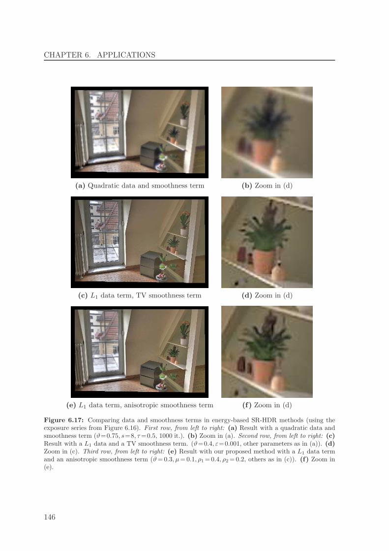
CHAPTER 6. APPLICATIONS
(a) Quadratic data and smoothness term (b) Zoom in (d)
(c) L1 data term, TV smoothness term (d) Zoom in (d)
(e) L1 data term, anisotropic smoothness term (f) Zoom in (d)
Figure 6.17: Comparing data and smoothness terms in energy-based SR-HDR methods (using theexposure series from Figure 6.16). First row, from left to right: (a) Result with a quadratic data andsmoothness term (ϑ=0.75, s=8, τ=0.5, 1000 it.). (b) Zoom in (a). Second row, from left to right: (c)Result with a L1 data and a TV smoothness term. (ϑ=0.4, ε=0.001, other parameters as in (a)). (d)Zoom in (c). Third row, from left to right: (e) Result with our proposed method with a L1 data termand an anisotropic smoothness term (ϑ=0.3, µ=0.1, ρ1=0.4, ρ2=0.2, others as in (c)). (f) Zoom in(e).
146

6.3. JOINT SUPER-RESOLUTION AND HDR (SR-HDR) RECONSTRUCTION
Pure HDR Joint SR-HDR
Figure 6.18: Comparing a pure HDR to a joint SR-HDR result on an indoor scene. First row,from left to right: (a) – (d) Images 1, 3, 6 and 8 of the exposure series (8 images, 268 × 178 pixels,exposure times between 1/200 and and 1/8 seconds.) Second row, from left to right: (d) HDR resultafter aligning the exposure series with our proposed technique. (e) SR-HDR result using our proposedapproach. (same alignment, ϑ = 0.6).
Pure HDR Joint SR-HDR
Figure 6.19: Comparing a pure HDR to a joint SR-HDR result on a lab-made scene. First row, fromleft to right: (a) – (d) Images 2, 5, 7 and 11 of the exposure series (12 images, 257 × 171 pixels,exposure times between 1/2500 and and 1/4 seconds.) Second row, from left to right: (d) HDR resultafter aligning the exposure series with our proposed technique. (e) SR-HDR result using our proposedapproach. (same alignment, ϑ = 0.4).
147
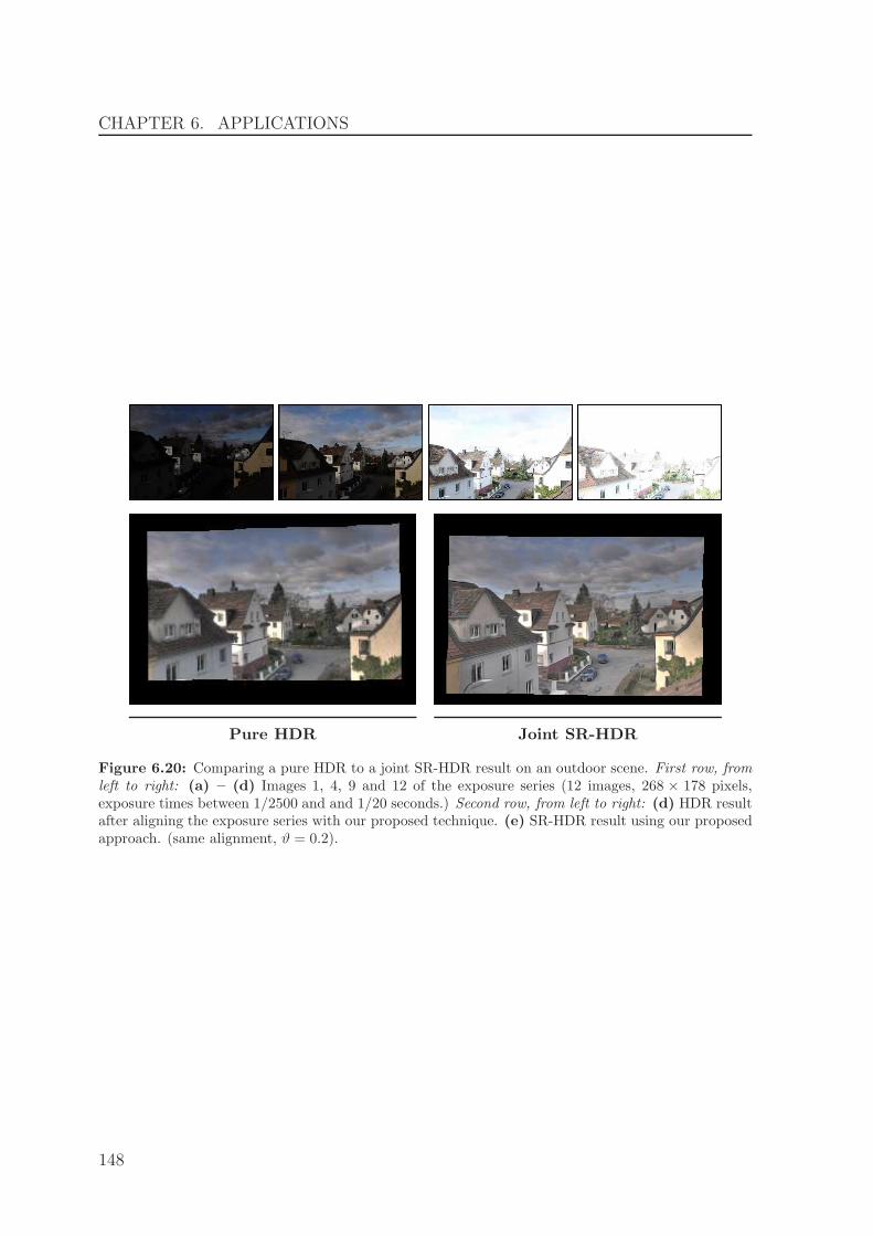
CHAPTER 6. APPLICATIONS
Pure HDR Joint SR-HDR
Figure 6.20: Comparing a pure HDR to a joint SR-HDR result on an outdoor scene. First row, fromleft to right: (a) – (d) Images 1, 4, 9 and 12 of the exposure series (12 images, 268 × 178 pixels,exposure times between 1/2500 and and 1/20 seconds.) Second row, from left to right: (d) HDR resultafter aligning the exposure series with our proposed technique. (e) SR-HDR result using our proposedapproach. (same alignment, ϑ = 0.2).
148

Chapter 7
Summary and Future Work
Nothing shocks me. I’m a scientist.
from the motion picture“Indiana Jones and the Temple of Doom”
7.1 Summary
In the previous chapters we presented contributions to various areas of research oncorrespondence problems. Thereby, we mainly focused on optic flow as a representativeand rather general example. At some points we also discussed the more specific stereomatching problem. Moreover, we only considered energy-based (variational) approachesthat find the optic flow field as minimiser of a suitable energy formulation. In recentyears these strategies have shown to give the most accurate results, and also efficientsolvers have been proposed.
Modelling
Data Term. In Chapter 4 we started by reviewing previous ideas for the design ofrobust data terms, such as subquadratic penaliser functions and higher order constancyassumptions. These concepts were combined into a novel robust data term that offersa high degree of invariance under illumination changes by considering a HSV colourrepresentation and applying robust penaliser functions to each channel separately. Inorder to avoid an undesirable overweighting of the data term at large image gradientlocations, we incorporated the idea of data term normalisation [LV98, SC06, SAH91]into our data term, thereby utilising this concept for modern data terms.
Smoothness Term. After discussing the data term, we turned to the design of anappropriate smoothness term. This resulted in a complementary smoothness term that
149

CHAPTER 7. SUMMARY AND FUTURE WORK
adapts its anisotropic smoothing directions to the imposed data constraints: In thedirection where the data terms provides information, we reduce the smoothing, but optfor a strong smoothing in the orthogonal direction where the data constraints do notprovide information. Moreover, our smoothness term can be classified as being jointimage- and flow-driven as it adapts the direction of smoothing to image edges, whereasthe amount of smoothing depends on the flow contrast. This allows to obtain sharpflow edges as known from image-driven methods, but remedies their oversegmentationproblems. Finally, we presented a general framework that introduces a common notationof several existing as well as our novel smoothness term and thus eases their comparison.
We also discussed smoothness terms for variational stereo approaches where e com-pleted the taxonomy by presenting the first disparity-driven regularisation strategy.
Parameter Selection. Having adapted the smoothness term and the data term, whatremains is to appropriately balance the two terms, i.e. determine the optimal value ofthe smoothness weight for the considered image sequence. To this end, we introduced anovel concept that we call optimal prediction principle (OPP). It states that an optimalflow field (obtained by using an optimal smoothness weight) allows for the best possibleprediction of the next images in the sequence. Assuming constant speed and lineartrajectories of objects, we judge the prediction quality by evaluating the data constraintsbetween the first and the third frame using the doubled flow. Our parameter selectionapproach then simply computes flow fields for several values of the smoothness weightand selects the weight corresponding to the flow field with the best prediction quality.
Combining this parameter selection with our complementary smoothness term yieldsa variational approach where all components (data term, smoothness term and smooth-ness weight) are in harmony, motivating the name optic flow in harmony method.
Other Terms. We also briefly investigated an additional predictor term in the energythat incorporates prior knowledge by enforcing the resulting flow field to be close toa given, predictor flow field, e.g. a (possibly sparse) predictor flow field obtained by afeature matching technique. Altough these methods give in general worse results thanvariational methods, they do not require a coarse-to-fine warping strategy to handle largedisplacements and can thus capture small flow details. As the latter are problematic forvariational methods, a feature matching predictor can help to remedy these problems.
Numerics
For minimising the proposed energy functionals we deduce and solve the associatedEuler-Lagrange equations. Discretising the Euler-Lagrange equations requires to ap-proximate occurring derivatives, which is mostly done by symmetric (central) finitedifference approximations. We could show that using correctly-oriented, one-sided dif-ferences may lead to improved results which constitutes a novel finding for the computervision community. However, such upwind discretisations are a classic concepts for thesolution of hyperbolic partial differential equations. Following further ideas from this
150

7.2. FUTURE WORK
context, we also showed that combining one-sided and central differences based on asmoothness measure leads to even better results. Here, we could draw an interestingconclusion from our extensive experiments: The more sophisticated the continuous mod-els become, the less influential is an appropriate numerical approximation of derivative.Nevertheless, all results illustrated the importance of an appropriate numerical approx-imation of derivatives to some extent and eventually showed that advanced numericsmight be an alternative to sophisticated models.
After discretisation, the Euler-Lagrange equations constitute a nonlinear system ofequations. For an efficient solution of the latter, we used two strategies, depending on theunderlying hardware architecture: On the CPU, we used the full multigrid solver pro-posed in [BWKS06]. To exploit the possibilities of modern graphics hardware (GPUs),we implemented an explicit gradient descent scheme that was speeded up by a coarse-to-fine computation and using variable fast explicit diffusion (FED) [GWB10] time stepsizes. Due to its simple nature, we could easily implement our solver on a parallel GPUarchitecture using the NVidia CUDA framework and achieved speedup factors of upto 55 compared to the multigrid scheme on the CPU. Additionally, we could port thissimple solver to a modern smartphone which allowed us to implement basic optic flowmethods with an interactive performance [4].
Applications
As an example of a novel application area for modern optic flow methods we consideredhigh dynamic range (HDR) imaging. Here, a set of images taken with varying expo-sure times (exposure series) is fused to compute an image with increased dynamic range,which allows to capture that details in dark as well as bright regions. However, the prac-tical applicability of HDR techniques is limited as they assume that the exposure seriesis perfectly aligned, which is often violated due to camera shake or moving objects. Bycarefully modifying a modern optic flow approach, we managed to robustly estimate thedisplacements and thus to align even challenging real world exposure series. The mainmodification was to only impose gradient constancy in the data term as the commonbrightness constancy assumption will not hold due to the varying exposure times.
Exploiting the subpixel precision of the estimated displacement fields, we combinedideas from super-resolution and HDR techniques into an energy-based joint super-resolution and HDR (SR-HDR) approach that computes an image with increased spatialresolution and dynamic range. In this context, we introduced sophisticated regularisa-tion strategies in the SR-HDR context, which we could show to be a key aspect forobtaining visually appealing results.
7.2 Future Work
Our contributions have shown that despite three decades of research on correspondenceproblems, significant improvements in the accuracy as well as in the efficiency are still
151

CHAPTER 7. SUMMARY AND FUTURE WORK
possible. Moreover, growing new research areas such as computational photography giverise to interesting novel applications for correspondence problems. Having this in mind,there are several future directions that seem promising to be explored.
Data Term
We proposed to use an HSV colour representation to obtain robustness under difficultillumination conditions. We would thus like to investigate the usefulness of alternativecolour spaces, e.g. HSL, YUV, or CIELAB. Moreover, we still did not consider extremedistortions in the images, like heavy noise or strong compression artefacts caused bycommon image and video codecs like JPEG or MPEG.
Smoothness Term
Our experiments have shown that joint image- and flow-driven regularisers like ourcomplementary smoothness term mostly remedy oversegmentation problems. However,we found that small artefacts might still be visible in some sequences; see our remarks inSection 4.3.5. We are thus interested in analysing and resolving these remaining issues.Concerning extensions of our smoothness term, we would like to see if the incorporationof recent non-local regularisation ideas [SRB10, WPB10] allows to further improve theperformance of our smoothness term.
Parameter Selection
For our proposed parameter selection approach based on the optimal prediction principle(OPP), we plan to investigate several points:
(i) We would like to improve the efficiency, for example by finding a modificationthat yields similar results but requires to compute less flow fields during the estimationprocess. (ii) It also seems very interesting to apply our approach in cases where onlytwo images are available. This would also remedy the problems with non-constant speedof objects that we have mentioned in Section 4.4.3. (iii) Two interesting extensions ofour method could be to apply the parameter estimation on every level of the warpingscheme, or for subsequent image pairs in an image sequence, respectively. In both cases,we hope that our method could profit from an initialisation with the previous results,i.e. from the previous warping level or from the previous image pair, respectively. (iv)Finally, a deeper theoretical underpinning of the optimal prediction principle may givefurther ideas for improvements and extensions. For example, we hope to explain whyour method seems to underestimate the smoothness weight in general while still givingfavourable results in terms of quality measures.
Joint Super-Resolution and HDR (SR-HDR) Reconstruction
The major limitation of our SR-HDR approach is that its optic flow-based alignmentstep cannot handle large displacements of small objects in the given exposures series.
152
7.2. FUTURE WORK
This leads to unpleasant artefacts in the reconstruction (see Figure 6.14) and is causedby the coarse-to-fine warping strategy. One possible solution to this issue could thus beto incorporate a feature-matching prior as discussed in Section 4.5. Alternatively, if wedo not want, or if we are not able to correct the flow estimate, applying an anti-ghostingtechnique [KAR06] will reduce the disturbing artefacts.
Furthermore, a joint estimation of displacements and SR-HDR reconstruction seemsinteresting. However, it is questionable if the more difficult minimisation of such a modelpays off in terms of quality. As a starting point, we refer to the SR method in [EM09]where a joint estimation of displacements and super-resolved image has been proposed.
An Alternative Modelling and Minimisation Framework
We used the Euler-Lagrange framework for minimising our continuous energy function-als. While this framework allows to minimise rather general energies in an efficient way,it may still restrict the design of the energy terms. For example, non-differentiable pe-naliser functions like the Potts model [Pot52] cannot be used although this might beuseful for obtaining extremely sharp discontinuities. Furthermore, although the appliedcoarse-to-fine warping strategy often allows to compute a good local minimum of theenergy, there is no guarantee on how well the desired global minimum is approximated.
These problems can be alleviated by formulating the correspondence problem as amulti-label problem where each pixel is assigned two labels from a discrete set of labelsto represent the two components of the displacement vector. A globally optimal solutionof such multi-label problems can be computed using graph cut optimisation in a discretesetting [BVZ01]. In a continuous setting, e.g. [PSG+08], one transforms the probleminto a continuous convex problem, computes the global minimum and then projects thecontinuous solution back onto the discrete label space. Until recently, these solvers fea-tured a high computational complexity and an immense memory consumption, whichrendered them practically unusable for large label spaces like the ones typically encoun-tered in optic flow. However, recently discrete [SKH08] as well continuous solvers [GC10]for multi-label problems have been proposed that approximate a globally optimal so-lution while drastically reducing the computational complexity as well as the memoryrequirements. As the approximation is fairly close to the global optimum (less than 5%in [GC10]), adapting these methods to our framework may not only give more freedomin modelling, but in the long run also a further boost in quality and efficiency.
Further Ideas
We have shown that a carefully modified optic flow method is well-suited for aligningexposure series in the context of HDR imaging. Building on this finding, we wouldlike to see if modern optic flow approaches can also help to align the input images forother multi-shot techniques such as extended depth of field (focus stacking) [ADA+04],flash/no-flash photography [PSA+04], image stitching [Sze06] or day and night fu-sion [RIY05]. However, it is not obvious how the optic flow approaches have to be
153

CHAPTER 7. SUMMARY AND FUTURE WORK
adapted to the specific tasks.Building on our first work in [4], we are interested in porting more of our algorithms to
modern smartphones (like the iPhone 4 or Android phones). Nowadays, these platformsoffer reasonable built-in cameras, a remarkable computational power and also flexibleprogramming environments that support native programming languages like C/C++.This opens the door for interesting mobile image processing and computer vision appli-cations that can additionally profit from features like broadband internet access, GPSpositioning and gyroscopic sensors that can be found in almost every modern smart-phone.
154

Appendix A
Proofs
A.1 Reformulation of the Nagel and Enkelmann Regulariser
We want to show the correctness of our reformulation of the Nagel and Enkelmannregulariser from (4.56):
VAI(∇2u,∇2v) = (∇2u)⊤P (∇2f) ∇2u + (∇2v)
⊤P (∇2f) ∇2v
=κ2
tr S0 + 2κ2
(u2s0
1
+ v2s01
)+
tr S0 + κ2
tr S0 + 2κ2
(u2s0
2
+ v2s02
), (A.1)
We proceed in two steps: First, we show that p1 := s01 = ∇2f/|∇2f | and p2 := s02 =∇2f
⊥/|∇2f | are the eigenvectors of the matrix P as defined in (4.55). The correspondingeigenvalues that we denote by q1 and q2 shall be given by the factors in front of (u2
s01
+v2s01
)
and (u2s02
+ v2s02
), respectively. To show that p1 is an eigenvector of P with corresponding
eigenvalue q1, it suffices to prove that P p1 = q1 p1:
P p1 =1
|∇2f |2 + 2κ2
(∇2f
⊥(∇2f
⊥)⊤
+ κ2I)
∇2f
|∇2f |(A.2)
=1
|∇2f |2 + 2κ2
(∇2f
⊥(∇2f
⊥)⊤
∇2f
|∇2f |+
κ2
|∇2f |∇2f
)(A.3)
(∗)=
κ2
|∇2f |2 + 2κ2∇2f
|∇2f |(A.4)
=κ2
|∇2f |2 + 2κ2s01 = q1 p1 , (A.5)
155

APPENDIX A. PROOFS
where (∗) holds as(∇2f
⊥)⊤
∇2f = 0. For the second eigenvector and eigenvalue, oneobtains
P p2 =1
|∇2f |2 + 2κ2
(∇2f
⊥(∇2f
⊥)⊤
+ κ2I)∇2f
⊥
|∇2f |(A.6)
=1
|∇2f |2 + 2κ2
(∇2f
⊥(∇2f
⊥)⊤
∇2f⊥
|∇2f |+
κ2
|∇2f |∇2f
⊥
)(A.7)
(∗)=
1
|∇2f |2 + 2κ2
(∇2f
⊥|∇2f |+κ2
|∇2f |∇2f
⊥
)(A.8)
=1
|∇2f |2 + 2κ2
(∇2f
⊥|∇2f |2 + κ2∇2f⊥
|∇2f |
)(A.9)
=1
|∇2f |2 + 2κ2
(∇2f
⊥ (|∇2f |2 + κ2)
|∇2f |
)(A.10)
=|∇2f |2 + κ2
|∇2f |2 + 2κ2∇2f
⊥
|∇2f |(A.11)
=|∇2f |2 + κ2
|∇2f |2 + 2κ2s02 = q2 p2 , (A.12)
where (∗) holds as(∇2f
⊥)⊤
∇2f⊥ = |∇2f |2.
What remains to show is the validity of the following equation:
∇2u⊤P ∇2u+∇2v
⊤P ∇2v = q1(up21+ vp2
1) + q2(up2
2+ vp2
2) . (A.13)
The proof is a straightforward rewriting, which we exemplify for the u-part:
∇2u⊤P ∇2u = ∇2u
⊤(q1 p1p
⊤1 + q2 p2p
⊤2
)∇2u (A.14)
= q1(∇2u
⊤p1p⊤1 ∇2u
)+ q2
(∇2u
⊤p2p⊤2 ∇2u
)(A.15)
= q1(p⊤1 ∇2u
)2+ q2
(p⊤2 ∇2u
)2(A.16)
= q1u2p1
+ q2u2p2
. (A.17)
Equivalently one obtains for the v-part
∇2v⊤P ∇2v = q1v
2p1
+ q2v2p2
. (A.18)
Combining u- and v-part finally shows the correctness of (A.13):
∇2u⊤P ∇2u+∇2v
⊤P ∇2v = q1u2p1
+ q2u2p2
+ q1v2p1
+ q2v2p2
(A.19)
= q1
(u2p1
+ v2p1
)+ q2
(u2p2
+ v2p2
). (A.20)
156
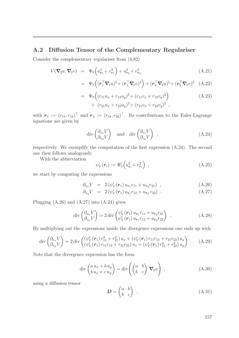
A.2 Diffusion Tensor of the Complementary Regulariser
Consider the complementary regulariser from (4.82)
V (∇2u,∇2v) = ΨV
(u2r1+ v2r1
)+ u2r2
+ v2r2(A.21)
= ΨV
((r⊤
1 ∇2u)2+ (r⊤
1 ∇2v)2)+ (r⊤
2 ∇2u)2+ (r⊤
2 ∇2v)2 (A.22)
= ΨV
((r11ux + r12uy)
2+ (r11vx + r12vy)2)
(A.23)
+ (r21ux + r22uy)2+ (r21vx + r22vy)
2 ,
with r1 := (r11, r12)⊤ and r2 := (r21, r22)
⊤. Its contributions to the Euler-Lagrangeequations are given by
div
(∂ux
V∂uy
V
)and div
(∂vxV∂vyV
), (A.24)
respectively. We exemplify the computation of the first expression (A.24). The secondone then follows analogously.
With the abbreviationψ′V (ri) := Ψ′
V
(u2ri
+ v2ri
), (A.25)
we start by computing the expressions
∂uxV = 2 (ψ′
V (r1) ur1r11 + ur2r21) , (A.26)
∂uyV = 2 (ψ′
V (r1) ur1r12 + ur2r22) . (A.27)
Plugging (A.26) and (A.27) into (A.24) gives
div
(∂ux
V∂uy
V
)= 2div
(ψ′V (r1) ur1r11 + ur2
r21ψ′V (r1) ur1r12 + ur2
r22
). (A.28)
By multiplying out the expressions inside the divergence expressions one ends up with
div
(∂ux
V∂uy
V
)= 2div
((ψ′
V (r1) r211 + r221)ux + (ψ′
V (r1) r11r12 + r21r22)uy(ψ′
V (r1) r11r12 + r21r22) ux + (ψ′V (r1) r
212 + r222)uy
). (A.29)
Note that the divergence expression has the form
div
(a ux + b uyb ux + c uy
)= div
((a bb c
)∇2u
), (A.30)
using a diffusion tensor
D =
(a bb c
). (A.31)
157

APPENDIX A. PROOFS
Hence we can write equation (A.29) in diffusion tensor notation as
div
(∂ux
V∂uy
V
)= 2div (D ∇2u) , (A.32)
with the diffusion tensor
D :=
(ψ′V (r1) · r211 + 1 · r221 ψ′
V (r1) · r11r12 + 1 · r21r22ψ′V (r1) · r11r12 + 1 · r21r22 ψ′
V (r1) · r212 + 1 · r222
). (A.33)
We multiplied the second term of each sum by a factor of 1 to clarify that the eigenvaluesof D are ψ′
V (r1) and 1, respectively. The corresponding eigenvectors are r1 and r2. Wethus can rewrite the tensor D as
D =
(r11 r21r12 r22
)(ψ′V (r1)·r11 ψ′
V (r1)·r121·r21 1·r22
)
= (r1 | r2)
(ψ′V (r1) 00 1
) (r⊤1
r⊤2
). (A.34)
This shows that D is identical to DCR from (4.83), as it can be written as
D = ψ′V(r1) r1 r
⊤1 + r2 r
⊤2 = Ψ′
V
(u2r1 + v2r1
)· r1 r
⊤1 + 1 · r2 r
⊤2 . (A.35)
A.3 Equivalence between Two Energy Functionals
Consider the two energy functionals
E1 =
∫
Ω
(√m2 + ε2 + α
√v2 + ε2
)dx dy , (A.36)
E2 =
∫
Ω
(2ε2√
1 +m2
ε2+ α 2ε2
√1 +
v2
ε2
)dx dy , (A.37)
where m2 denotes some quadratic data term and v2 some quadratic smoothness term,respectively. Note that both energies use the same penaliser in the data and smooth-ness term. The energy E1 uses subquadratic penaliser Ψ(s2) =
√s2 + ε2 that leads to
modified L1 penalisation in the data term and to TV regularisation in the smoothnessterm. The energy E2 uses the Charbonnier function in both terms.
We now wish to prove that E2 is (up to a constant factor) equivalent to E1. This inturn shows that minimising both energies leads to the same solution. Let us denote the
158

integrand of E2 by F2. The latter, we rewrite as
F2 = 2ε2√1 +
m2
ε2+ α 2ε2
√1 +
v2
ε2(A.38)
= 2ε2
(√1 +
m2
ε2+ α
√1 +
v2
ε2
)(A.39)
= 2ε2
(√ε2 +m2
ε2+ α
√ε2 + v2
ε2
)(A.40)
= 2ε2(1
ε
√m2 + ε2 + α
1
ε
√v2 + ε2
)(A.41)
= 2ε(√
m2 + ε2 + α√v2 + ε2
). (A.42)
This shows that E2 = 2εE1 and concludes our proof.
159

APPENDIX A. PROOFS
160

Own Publications
[1] M. Breuß, H. Zimmer, and J. Weickert. Can variational models for correspondenceproblems benefit from upwind discretisations? Journal of Mathematical Imagingand Vision, 39(3):230–244, 2011.
[2] O. Demetz, J. Weickert, A. Bruhn, and H. Zimmer. Optic flow scale space. InA. M. Bruckstein et al., editor, Scale Space and Variational Methods in ComputerVision (SSVM), volume 6667 of Lecture Notes in Computer Science, pages 713–724.Springer, Berlin, 2011.
[3] P. Gwosdek, H. Zimmer, S. Grewenig, A. Bruhn, and J. Weickert. A highly efficientGPU implementation for variational optic flow based on the Euler-Lagrange frame-work. In Proc. 2010 ECCV Workshop on Computer Vision with GPUs, Heraklion,Greece, Sept. 2010. Web page: http://www.mia.uni-saarland.de/Research/
ComplOF-GPU/.
[4] A. Luxenburger, H. Zimmer, P. Gwosdek, and J. Weickert. Fast PDE-based im-age analysis in your pocket. In A. M. Bruckstein et al., editor, Scale Space andVariational Methods in Computer Vision (SSVM), volume 6667 of Lecture Notesin Computer Science, pages 544–555. Springer, Berlin, 2011.
[5] L. Valgaerts, A. Bruhn, H. Zimmer, J. Weickert, C. Stoll, and C. Theobalt. Jointestimation of motion, structure and geometry from stereo sequences. In ComputerVision – ECCV 2010, volume 6314 of Lecture Notes in Computer Science, pages568–581. Springer, Berlin, 2010. Web page: http://www.mia.uni-saarland.de/valgaerts/eccv10/sceneflow/.
[6] S. Volz, A. Bruhn, L. Valgaerts, and H. Zimmer. Modeling temporal coherencefor optical flow. In Proc. Thirteenth International Conference on Computer Vision(ICCV), Barcelona, Spain, Nov. 2011. IEEE Computer Society Press.
[7] H. Zimmer, M. Breuß, J. Weickert, and H.-P. Seidel. Hyperbolic numerics forvariational approaches to correspondence problems. In X.-C. Tai et al., editor,Scale Space and Variational Methods in Computer Vision (SSVM), volume 5567 ofLecture Notes in Computer Science, pages 636–647. Springer, Berlin, 2009.
161

OWN PUBLICATIONS
[8] H. Zimmer, A. Bruhn, L. Valgaerts, M. Breuß, J. Weickert, B. Rosenhahn, andH.-P. Seidel. PDE-based anisotropic disparity-driven stereo vision. In O. Deussen,D. Keim, and D. Saupe, editors, Proceedings of Vision, Modeling, and Visualization(VMV), pages 263–272. AKA Heidelberg, Oct. 2008.
[9] H. Zimmer, A. Bruhn, and J. Weickert. Freehand HDR imaging of moving sceneswith simultaneous resolution enhancement. Computer Graphics Forum (Proceed-ings of Eurographics), 30(2):405–414, Apr. 2011. Web page: http://www.mia.
uni-saarland.de/Research/SR-HDR/.
[10] H. Zimmer, A. Bruhn, and J. Weickert. Optic flow in harmony. InternationalJournal of Computer Vision, 93(3):368–388, Apr. 2011.
[11] H. Zimmer, A. Bruhn, J. Weickert, L. Valgaerts, A. Salgado, B. Rosenhahn, andH.-P. Seidel. Complementary optic flow. In D. Cremers, Y. Boykov, A. Blake,and F. R. Schmidt, editors, Energy Minimization Methods in Computer Visionand Pattern Recognition (EMMCVPR), volume 5681 of Lecture Notes in ComputerScience, pages 207–220. Springer, Berlin, 2009.
162

Bibliography
[ADA+04] A. Agarwala, M. Dontcheva, M. Agrawala, S. Drucker, A. Colburn, B. Cur-less, D. Salesin, and M. Cohen. Interactive digital photomontage. In Proc.ACM SIGGRAPH, pages 294–302, 2004.
[ADK99] G. Aubert, R. Deriche, and P. Kornprobst. Computing optical flow viavariational techniques. SIAM Journal on Applied Mathematics, 60(1):156–182, 1999.
[ADSW00] L. Alvarez, R. Deriche, J. Sanchez, and J. Weickert. Dense disparity mapestimation respecting image derivatives: a PDE and scale-space based ap-proach. In Proc. IAPR Workshop on Machine Vision, pages 423–427,Tokyo, Japan, November 2000.
[ADSW02] L. Alvarez, R. Deriche, J. Sanchez, and J. Weickert. Dense disparity mapestimation respecting image derivatives: a PDE and scale-space basedapproach. Journal of Visual Communication and Image Representation,13(1/2):3–21, 2002.
[AELS99] L. Alvarez, J. Escların, M. Lefebure, and J. Sanchez. A PDE model forcomputing the optical flow. In Proc. XVI Congreso de Ecuaciones Difer-enciales y Aplicaciones, pages 1349–1356, Las Palmas de Gran Canaria,Spain, September 1999.
[Ana89] P. Anandan. A computational framework and an algorithm for the measure-ment of visual motion. International Journal of Computer Vision, 2:283–310, 1989.
[AWS00] L. Alvarez, J. Weickert, and J. Sanchez. Reliable estimation of dense opticalflow fields with large displacements. International Journal of ComputerVision, 39(1):41–56, August 2000.
[BA96] M. J. Black and P. Anandan. The robust estimation of multiple motions:parametric and piecewise smooth flow fields. Computer Vision and ImageUnderstanding, 63(1):75–104, January 1996.
163

BIBLIOGRAPHY
[BAS07] R. Ben-Ari and N.A. Sochen. Variational stereo vision with sharp discon-tinuities and occlusion handling. In Proc. 2007 IEEE International Con-ference on Computer Vision, Rio de Janeiro, Brazil, October 2007. IEEEComputer Society Press.
[BBH03] M.Z. Brown, D. Burschka, and G.D. Hager. Advances in computationalstereo. IEEE Transactions on Pattern Analysis and Machine Intelligence,25(8):993–1008, August 2003.
[BBPW04] T. Brox, A. Bruhn, N. Papenberg, and J. Weickert. High accuracy opticalflow estimation based on a theory for warping. In T. Pajdla and J. Matas,editors, Computer Vision – ECCV 2004, Part IV, volume 3024 of LectureNotes in Computer Science, pages 25–36. Springer, Berlin, 2004.
[BFB94] J. L. Barron, D. J. Fleet, and S. S. Beauchemin. Performance of opticalflow techniques. International Journal of Computer Vision, 12(1):43–77,February 1994.
[BGW91] J. Bigun, G. H. Granlund, and J. Wiklund. Multidimensional orientationestimation with applications to texture analysis and optical flow. IEEETransactions on Pattern Analysis and Machine Intelligence, 13(8):775–790,August 1991.
[BM04] S. Baker and I. Matthews. Lucas-Kanade 20 years on: A unifying frame-work. International Journal of Computer Vision, 56(1):221–255, 2004.
[BM11] T. Brox and J. Malik. Large displacement optical flow: Descriptor matchingin variational motion estimation. IEEE Transactions on Pattern Analysisand Machine Intelligence, 23(3):500–513, March 2011.
[BPT88] M. Bertero, T. A. Poggio, and V. Torre. Ill-posed problems in early vision.Proceedings of the IEEE, 76(8):869–889, August 1988.
[Bra77] A. Brandt. Multi-level adaptive solutions to boundary-value problems.Mathematics of Computation, 31(138):333–390, April 1977.
[Bru06] A. Bruhn. Variational Optic Flow Computation: Accurate Modelling andEfficient Numerics. PhD thesis, Department of Mathematics and ComputerScience, Saarland University, Saarbrucken, Germany, July 2006.
[BSL+10] S. Baker, D. Scharstein, J. P. Lewis, S. Roth, M. J. Black, and R. Szeliski.A database and evaluation methodology for optical flow. InternationalJournal of Computer Vision, 92(1):1–31, September 2010. Web page:http://vision.middlebury.edu/flow/.
164

BIBLIOGRAPHY
[BVZ01] Y. Boykov, O. Veksler, and R. Zabih. Fast approximate energy minimiza-tion via graph cuts. IEEE Transactions on Pattern Analysis and MachineIntelligence, 23(11):1222–1239, November 2001.
[BW05] A. Bruhn and J. Weickert. Towards ultimate motion estimation: Combininghighest accuracy with real-time performance. In Proc. Tenth InternationalConference on Computer Vision, volume 1, pages 749–755, Beijing, China,October 2005. IEEE Computer Society Press.
[BWF+05] A. Bruhn, J. Weickert, C. Feddern, T. Kohlberger, and C. Schnorr. Varia-tional optical flow computation in real-time. IEEE Transactions on ImageProcessing, 14(5):608–615, May 2005.
[BWKS06] A. Bruhn, J. Weickert, T. Kohlberger, and C. Schnorr. A multigrid platformfor real-time motion computation with discontinuity-preserving variationalmethods. International Journal of Computer Vision, 70(3):257–277, De-cember 2006.
[BWS05] A. Bruhn, J. Weickert, and C. Schnorr. Lucas/Kanade meetsHorn/Schunck: Combining local and global optic flow methods. Inter-national Journal of Computer Vision, 61(3):211–231, 2005.
[BZ87] A. Blake and A. Zisserman. Visual Reconstruction. MIT Press, Cambridge,MA, 1987.
[CBFAB94] P. Charbonnier, L. Blanc-Feraud, G. Aubert, and M. Barlaud. Two deter-ministic half-quadratic regularization algorithms for computed imaging. InProc. 1994 IEEE International Conference on Image Processing, volume 2,pages 168–172, Austin, TX, November 1994. IEEE Computer Society Press.
[Cha04] A. Chambolle. An algorithm for total variation minimization and applica-tions. Journal of Mathematical Imaging and Vision, 20(1–2):89–97, 2004.
[CLMC92] F. Catte, P.-L. Lions, J.-M. Morel, and T. Coll. Image selective smoothingand edge detection by nonlinear diffusion. SIAM Journal on NumericalAnalysis, 32:1895–1909, 1992.
[Coh93] I. Cohen. Nonlinear variational method for optical flow computation. InProc. Eighth Scandinavian Conference on Image Analysis, volume 1, pages523–530, Tromsø, Norway, May 1993.
[Coo67] S. A. Coons. Surfaces for computer aided design of space forms. Techni-cal Report MIT/LCS/TR-41, Massachusetts Institute of Technology, Cam-bridge, MA, June 1967.
165
BIBLIOGRAPHY
[Coo08] T. Cooke. Two applications of graph-cuts to image processing. In Proc. In-ternational Conference on Digital Image Computing: Techniques and Ap-plications, DICTA 2008, pages 498–504, Canberra, Australia, December2008. IEEE Computer Society.
[CPK09] J. Choi, M.K. Park, and M.G. Kang. High dynamic range image recon-struction with spatial resolution enhancement. The Computer Journal,52(1):114–125, 2009.
[DM97] P.E. Debevec and J. Malik. Recovering high dynamic range radiance mapsfrom photographs. In Proc. ACM SIGGRAPH, pages 369–378, 1997.
[dSK02] G.N. de Souza and A.C. Kak. Vision for mobile robot navigation: A sur-vey. IEEE Transactions on Pattern Analysis and Machine Intelligence,24(2):237–267, 2002.
[EF97] M. Elad and A. Feuer. Restoration of a single superresolution image fromseveral blurred, noisy, and undersampled measured images. IEEE Trans-actions on Image Processing, 6(12):1646–1658, December 1997.
[Els62] L. E. Elsgolc. Calculus of Variations. Pergamon, London, England, 1962.
[EM09] M. Ebrahimi and A.L. Martel. A PDE approach to coupled super-resolutionwith non-parametric motion. In D. Cremers, Y. Boykov, A. Blake, andF. R. Schmidt, editors, Energy Minimization Methods in Computer Visionand Pattern Recognition (EMMCVPR), volume 5681 of Lecture Notes inComputer Science, pages 112–125. Springer, Berlin, 2009.
[FG87] W. Forstner and E. Gulch. A fast operator for detection and precise locationof distinct points, corners and centres of circular features. In Proc. ISPRSIntercommission Conference on Fast Processing of Photogrammetric Data,pages 281–305, Interlaken, Switzerland, June 1987.
[FKN73] S. Fucik, A. Kratochvil, and J. Necas. Kacanov–Galerkin method. Com-mentationes Mathematicae Universitatis Carolinae, 14(4):651–659, 1973.
[FLP01] O. Faugeras, Q.-T. Luong, and T. Papadopoulo. The Geometry of MultipleImages. MIT Press, Cambridge, MA, 2001.
[FLW02] R. Fattal, D. Lischinski, and M. Werman. Gradient domain high dynamicrange compression. In Proc. ACM SIGGRAPH, pages 249–256, 2002.
[FM08] B. Fischer and J. Modersitzki. Ill-posed medicine – an introduction toimage registration. Problems, 24(3):1–19, 2008.
166

BIBLIOGRAPHY
[FREM04] S. Farsiu, D. Robinson, M. Elad, and P. Milanfar. Fast and robust multi-frame super-resolution. IEEE Transactions on Pattern Analysis and Ma-chine Intelligence, 13(10):1327–1344, October 2004.
[GAW+10] M. Granados, B. Ajdin, M. Wand, C. Theobalt, H.-P. Seidel, and H.P.A.Lensch. Optimal hdr reconstruction with linear digital cameras. InProc. 2010 IEEE Computer Society Conference on Computer Vision andPattern Recognition, volume 1, pages 215–222, an Francisco, CA, USA,June 2010. IEEE Computer Society Press.
[GB97] P. Golland and A. M. Bruckstein. Motion from color. Computer Visionand Image Understanding, 68(3):346–362, December 1997.
[GC10] B. Goldluecke and D. Cremers. Convex relaxation for multilabel problemswith product label spaces. In Computer Vision – ECCV 2010, volume 6315of Lecture Notes in Computer Science, pages 225–238. Springer, Berlin,2010.
[GG06] B.K. Gunturk and M. Gevrekci. High-resolution image reconstructionfrom multiple differently exposed images. IEEE Signal Processing Letters,13(4):197–200, 2006.
[GG09] J. Gulbins and R. Gulbins. Photographic Multishot Techniques. RockyNook, Santa Barbara, CA, USA, 2009.
[Gla84] F. Glazer. Multilevel relaxation in low-level computer vision. In A. Rosen-feld, editor, Multiresolution Image Processing and Analysis, pages 312–330.Springer, Berlin, 1984.
[Gre09] H. Greenspan. Super-resolution in medical imaging. The Computer Journal,52(1):43–63, 2009.
[Gro06] T. Grosch. Fast and robust high dynamic range image generation withcamera and object movement. In L. Kobbelt, T. Kuhlen, T. Aach, andR. Westermann, editors, Proceedings of Vision, Modeling, and Visualization(VMV) 2006, pages 277–284. AKA Heidelberg, 2006.
[GS78] W. Gentzsch and A. Schluter. Uber ein Einschrittverfahren mit zyklis-cher Schrittweitenanderung zur Losung parabolischer Differentialgleichun-gen. Zeitschrift fur angewandte Mathematik und Mechanik, 58:T415–T416,1978.
[GT08] H. Grossauer and P. Thoman. GPU-based multigrid: Real-time perfor-mance in high resolution nonlinear image processing. In A. Gasteratos,M. Vincze, and J. K. Tsotsos, editors, Computer Vision Systems, volume5008 of Lecture Notes in Computer Science, pages 141–150. Springer, Berlin,2008.
167

BIBLIOGRAPHY
[GvV96] S. Ghosal and P. C. Vanek. Scalable algorithm for discontinuous opticalflow estimation. IEEE Transactions on Pattern Analysis and Machine In-telligence, 18(2):181–194, February 1996.
[GWB10] S. Grewenig, J. Weickert, and A. Bruhn. From box filtering to fast explicitdiffusion. In M. Goesele, S. Roth, A. Kuijper, B. Schiele, and K. Schindler,editors, Pattern Recognition, volume 6376 of Lecture Notes in ComputerScience, pages 533–542. Springer, Berlin, 2010.
[Hac85] W. Hackbusch. Multigrid Methods and Applications. Springer, New York,1985.
[Hor86] B. K. P. Horn. Robot Vision. MIT Press, Cambridge, MA, 1986.
[HS81] B. Horn and B. Schunck. Determining optical flow. Artificial Intelligence,17:185–203, 1981.
[HTO07] H.B. Haraldsson, M. Tanaka, and M. Okutomi. Reconstruction of a highdynamic range and high resolution image from a multisampled image se-quence. In Proc. 14th International Conference on Image Analysis andProcessing (ICIAP), pages 303–310, Modena, Italy, September 2007.
[Hub81] P. J. Huber. Robust Statistics. Wiley, New York, 1981.
[HZ00] R. Hartley and A. Zisserman. Multiple View Geometry in Computer Vision.Cambridge University Press, Cambridge, UK, 2000.
[JLW08] K. Jacobs, C. Loscos, and G. Ward. Automatic high-dynamic range imagegeneration for dynamic scenes. IEEE Computer Graphics and Applications,28:84–93, 2008.
[JO08] T. Jinno and M. Okuda. Motion blur free HDR image acquisition usingmultiple exposures. In Proc. 2008 IEEE International Conference on ImageProcessing, pages 1304–1307, San Diego, CA, USA, October 2008.
[Joh87] C. Johnson. Numerical Solution of Partial Differential Equations by theFinite Element Method. Studentlitteratur, Lund, 1987.
[KAR06] E.A. Khan, A.O. Akyuz, and E. Reinhard. Ghost removal in high dynamicrange images. In Proc. 2006 IEEE International Conference on Image Pro-cessing, pages 2005–2008, Atlanta, USA, August 2006.
[KDN93] D. Koller, K. Daniilidis, and H.H. Nagel. Model-based object tracking inmonocular image sequences of road traffic scenes. International Journal ofComputer Vision, 10(3):257–281, 1993.
168

BIBLIOGRAPHY
[KER95] W. Kruger, W. Enkelman, and S. Rossle. Real-time estimation and trackingof optical flow vectors for obstacle detection. In Proc. IEEE ComputerSociety Intelligent Vehicles ’95 Symposium, pages 204–209, Detroit, MI,USA, September 1995. IEEE Computer Society.
[KKR07] E.M. Kalmoun, H. Kostler, and U. Rude. 3D optical flow computationusing a parallel variational multigrid scheme with application to cardiacC-arm CT motion. Image and Vision Computing, 25(9):1482–1494, 2007.
[KM07] K. Krajsek and R. Mester. Bayesian model selection for optical flow esti-mation. In F. A. Hamprecht, C. Schnorr, and B. Jahne, editors, PatternRecognition, volume 4713 of Lecture Notes in Computer Science, pages 142–151. Springer, Berlin, 2007.
[KP04] S.J. Kim and M. Pollefeys. Radiometric alignment of image sequences. InProc. 2004 IEEE Computer Society Conference on Computer Vision andPattern Recognition, volume 1, pages 645–651, Washington, DC, June 2004.IEEE Computer Society Press.
[KR03] E.M. Kalmoun and U. Rude. A variational multigrid method for computingthe optical flow. In T. Ertl, B. Girod, G. Greiner, H. Niemann, H.-P. Seidel,E. Steinbach, and R. Westermann, editors, Proceedings of Vision, Modeling,and Visualization (VMV), pages 577–584. Akademische VerlagsgesellschaftBerlin, 2003.
[KS03] H. Kim and K. Sohn. Hierarchical disparity estimation with energy-basedregularization. In Proc. 2003 IEEE International Conference on ImageProcessing, volume 1, pages 373–376, Barcelona, Spain, September 2003.
[KUWS03] S.B. Kang, M. Uyttendaele, S. Winder, and R. Szeliski. High dynamicrange video. In Proc. ACM SIGGRAPH, pages 319–325, 2003.
[LeV92] R. J. LeVeque. Numerical Methods for Conservation Laws. Birkhauser,Basel, 1992.
[LeV02] R. J. LeVeque. Finite Volume Methods for Hyperbolic Problems. CambridgeUniversity Press, Cambridge, UK, 2002.
[Lin94] T. Lindeberg. Scale-Space Theory in Computer Vision. Kluwer, Boston,1994.
[LK81] B. Lucas and T. Kanade. An iterative image registration technique with anapplication to stereo vision. In Proc. Seventh International Joint Confer-ence on Artificial Intelligence, pages 674–679, Vancouver, Canada, August1981.
169
BIBLIOGRAPHY
[LLB+10] C. Lipski, C. Linz, K. Berger, A. Sellent, and M. Magnor. Virtual VideoCamera: Image-based viewpoint navigation through space and time. Com-puter Graphics Forum, 29(8):2555–2568, 2010.
[Low99] D.G. Lowe. Object recognition from local scale-invariant features. InProc. Seventh International Conference on Computer Vision, pages 1150–1157, Corfu, Greece, September 1999.
[Low04] D.G. Lowe. Distinctive image features from scale-invariant keypoints. In-ternational Journal of Computer Vision, 60(2):91–110, 2004.
[LV98] S.-H. Lai and B. C. Vemuri. Reliable and efficient computation of opticalflow. International Journal of Computer Vision, 29(2):87–105, October1998.
[LY09] C. Lei and Y. H. Yang. Optical flow estimation on coarse-to-fine region-treesusing discrete optimization. In Proc. 2009 IEEE International Conferenceon Computer Vision, Kyoto, Japan, October 2009. IEEE Computer SocietyPress.
[LYT+08] C. Liu, J. Yuen, A. Torralba, J. Sivic, and W. T. Freeman. SIFT flow:Dense correspondence across different scenes. In D. Forsyth, P. Torr, andA. Zisserman, editors, Computer Vision – ECCV 2008, Part III, volume5304 of Lecture Notes in Computer Science, pages 28–42, Berlin, 2008.Springer.
[MB87] D. W. Murray and B. F. Buxton. Scene segmentation from visual motionusing global optimization. IEEE Transactions on Pattern Analysis andMachine Intelligence, 9(2):220–228, March 1987.
[MBW07] Y. Mileva, A. Bruhn, and J. Weickert. Illumination-robust variational op-tical flow with photometric invariants. In F. A. Hamprecht, C. Schnorr,and B. Jahne, editors, Pattern Recognition, volume 4713 of Lecture Notesin Computer Science, pages 152–162. Springer, Berlin, 2007.
[MG07] N. Menzel and M. Guthe. Freehand HDR photography with motion com-pensation. In H.P.A. Lensch, B. Rosenhahn, H.-P. Seidel, P. Slusallek, andJ. Weickert, editors, Proceedings of Vision, Modeling, and Visualization(VMV), pages 127–134. AKA Heidelberg, 2007.
[MKMS07] R. Mantiuk, G. Krawczyk, R. Mantiuk, and H.-P. Seidel. High dynamicrange imaging pipeline: Perception-motivated representation of visual con-tent. In B.E. Rogowitz, T.N. Pappas, and S.J. Daly, editors, Human Visionand Electronic Imaging XII, volume 6492 of Proceedings of SPIE, San Jose,USA, February 2007. SPIE.
170

BIBLIOGRAPHY
[MKR09] T. Mertens, J. Kautz, and F. Van Reeth. Exposure fusion: A simple andpractical alternative to high dynamic range photography. Computer Graph-ics Forum, 28(1):161–171, 2009.
[MKW97] P. Moulin, R. Krishnamurth, and J.W. Woods. Multiscale modeling andestimation of motion fields for video coding. IEEE Transactions on PatternAnalysis and Machine Intelligence, 6(12):1606–1620, 1997.
[MM94] K. W. Morton and L. M. Mayers. Numerical Solution of Partial DifferentialEquations. Cambridge University Press, Cambridge, UK, 1994.
[MMK98] A.-R. Mansouri, A. Mitiche, and J. Konrad. Selective image diffusion: ap-plication to disparity estimation. In Proc. 1998 IEEE International Confer-ence on Image Processing, volume 3, pages 284–288, Chicago, IL, October1998.
[MN03] P. Mrazek and M. Navara. Selection of optimal stopping time for nonlineardiffusion filtering. International Journal of Computer Vision, 52(2/3):189–203, 2003. stopping time.
[MO99] A. Marquina and S. Osher. Explicit algorithms for a new time dependentmodel based on level set motion for nonlinear deblurring and noise removal.SIAM Journal on Scientific Computing, 22(2):387–405, 1999.
[MP95] S. Mann and R.W. Picard. On being ‘undigital’ with digital cameras:Extending dynamic range by combining differently exposed pictures. InProc. 48th IS&T Annual Conference, pages 442–448, Washington DC, USA,May 1995.
[MP98] E. Memin and P. Perez. A multigrid approach for hierarchical motionestimation. In Proc. Sixth International Conference on Computer Vision,pages 933–938, Bombay, India, January 1998. Narosa Publishing House.
[MPG85] H.G. Musmann, P. Pirsch, and H.J. Grallet. Advances in picture coding.Proceedings of the IEEE, 73(4):523–547, 1985.
[MPSC09] D. Mitzel, T. Pock, T. Schoenemann, and D. Cremers. Video super res-olution using duality based TV-L1 optical flow. In J. Denzler, G. Notni,and H. Suße, editors, Pattern Recognition, volume 5748 of Lecture Notes inComputer Science, pages 432–441. Springer, Berlin, 2009.
[Nag90] H.-H. Nagel. Extending the ’oriented smoothness constraint’ into thetemporal domain and the estimation of derivatives of optical flow. InO. Faugeras, editor, Computer Vision – ECCV ’90, volume 427 of LectureNotes in Computer Science, pages 139–148. Springer, Berlin, 1990.
171

BIBLIOGRAPHY
[NBK08] T. Nir, A. M. Bruckstein, and R. Kimmel. Over-parameterized variationaloptical flow. International Journal of Computer Vision, 76(2):205–216,2008.
[NE86] H.-H. Nagel and W. Enkelmann. An investigation of smoothness constraintsfor the estimation of displacement vector fields from image sequences. IEEETransactions on Pattern Analysis and Machine Intelligence, 8:565–593,1986.
[NN05] S.G. Narasimhan and S.K. Nayar. Enhancing resolution along multipleimaging dimensions using assorted pixels. IEEE Transactions on PatternAnalysis and Machine Intelligence, 27(4):518–530, 2005.
[NS97] L. Ng and V. Solo. A data-driven method for choosing smoothing parame-ters in optical flow problems. In Proc. 1997 IEEE International Conferenceon Image Processing, volume 3, pages 360–363, Los Alamitos, CA, USA,1997. IEEE Computer Society.
[NVI10] NVIDIA Corporation. NVIDIA CUDA Programming Guide, 3rd edition,February 2010. http://developer.download.nvidia.com/compute/
cuda/3_0/toolkit/docs/NVIDIA_CUDA_ProgrammingGuide.pdf.
[NYUS08] H. Nakai, S. Yamamoto, Y. Ueda, and Y. Shigeyama. High resolution andhigh dynamic range image reconstruction from differently exposed images.In G. Bebis and et al., editors, Advances in Visual Computing, volume 5359of Lecture Notes in Computer Science, pages 713–722. Springer, Berlin,2008.
[PAT96] I. Patras, N. Alvertos, and G. Tziritas. Joint disparity and motion fieldestimation in steroscopic image sequences. In Proc. 13th International Con-ference on Pattern Recognition, volume 1, pages 359–362, Vienna, Austria,August 1996.
[PBB+06] N. Papenberg, A. Bruhn, T. Brox, S. Didas, and J. Weickert. Highly accu-rate optic flow computation with theoretically justified warping. Interna-tional Journal of Computer Vision, 67(2):141–158, April 2006.
[PM90] P. Perona and J. Malik. Scale space and edge detection using anisotropic dif-fusion. IEEE Transactions on Pattern Analysis and Machine Intelligence,12:629–639, 1990.
[Pot52] R.B. Potts. Some generalized order-disorder transformations. Proceedingsof the Cambridge Philosophical Society, 48:106–109, 1952.
[PPK03] S. Park, M. Park, and M. Kang. Super-resolution image reconstruction: atechnical overview. IEEE Signal Processing Magazine, 20:21–36, 2003.
172

BIBLIOGRAPHY
[PSA+04] G. Petschnigg, R. Szeliski, M. Agrawala, M. Cohen, H. Hoppe, andK. Toyama. Digital photography with flash and no-flash image pairs. InProc. ACM SIGGRAPH, pages 664–672, 2004.
[PSG+08] T. Pock, T. Schoenemann, G. Graber, H. Bischof, and D. Cremers. A con-vex formulation of continuous multi-label problems. In D. Forsyth, P. Torr,and A. Zisserman, editors, Computer Vision – ECCV 2008, Part III, vol-ume 5304 of Lecture Notes in Computer Science, pages 792–805. Springer,Berlin, 2008.
[PTK85] T. Poggio, V. Torre, and C. Koch. Computational vision and regularizationtheory. Nature, 317:314–319, September 1985.
[RBS99] M.A. Robertson, S. Borman, and R.L. Stevenson. Dynamic range improve-ment through multiple exposures. In Proc. Sixth International Conferenceon Image Processing, volume III, pages 159–163, Kobe, Japan, October1999.
[RD96] L. Robert and R. Deriche. Dense depth map reconstruction: A minimiza-tion and regularization approach which preserves discontinuities. In B. Bux-ton and R. Cipolla, editors, Computer Vision – ECCV ’96, volume 1064 ofLecture Notes in Computer Science, pages 439–451. Springer, Berlin, 1996.
[RIY05] R. Raskar, A. Ilie, and J. Yu. Image fusion for context enhancement andvideo surrealism. In Proc. ACM SIGGRAPH Courses, pages 85–93, 2005.
[RMVS07] A.A. Rad, L. Meylan, P. Vandewalle, and S. Susstrunk. Multidimensionalimage enhancement from a set of unregistered differently exposed images. InProc. IS&T/SPIE Electronic Imaging: Computational Imaging V, volume6498, 2007.
[ROF92] L. I. Rudin, S. Osher, and E. Fatemi. Nonlinear total variation based noiseremoval algorithms. Physica D, 60:259–268, 1992.
[RSS07] P. Ruhnau, A. Stahl, and C. Schnorr. Variational estimation of experimen-tal fluids flows with physics-based spatio-temporal regularization. Measure-ment Science and Technology, 18:755–763, 2007.
[RWPD05] E. Reinhard, G. Ward, S. Pattanaik, and P. Debevec. High Dynamic RangeImaging: Acquisition, Display, and Image-Based Lighting. Morgan Kauf-mann Publishers, 2005.
[RWWK07] M. Raffel, C.E. Willert, S.T. Wereley, and J. Kompenhans. Particle ImageVelocimetry: A Practical Guide. Springer, Berlin, second edition, 2007.
173

BIBLIOGRAPHY
[SAH91] E. P. Simoncelli, E. H. Adelson, and D. J. Heeger. Probability distribu-tions of optical flow. In Proc. 1991 IEEE Computer Society Conference onComputer Vision and Pattern Recognition, pages 310–315, Maui, HI, June1991. IEEE Computer Society Press.
[SBK10] N. Sundaram, T. Brox, and K. Keutzer. Dense point trajectories by GPU-accelerated large displacement optical flow. In Computer Vision – ECCV2010, volume 6311 of Lecture Notes in Computer Science, pages 438–451.Springer, Berlin, 2010. number I.
[SBW05] N. Slesareva, A. Bruhn, and J. Weickert. Optic flow goes stereo: A varia-tional method for estimating discontinuity-preserving dense disparity maps.In W. Kropatsch, R. Sablatnig, and A. Hanbury, editors, Pattern Recog-nition, volume 3663 of Lecture Notes in Computer Science, pages 33–40.Springer, Berlin, 2005.
[SC06] T. Schoenemann and D. Cremers. Near real-time motion segmentationusing graph cuts. In K. Franke, K.-R. Muller, B. Nickolay, and R. Schafer,editors, Pattern Recognition, volume 4174 of Lecture Notes in ComputerScience, pages 455–464. Springer, Berlin, 2006.
[Sch93] C. Schnorr. On functionals with greyvalue-controlled smoothness termsfor determining optical flow. IEEE Transactions on Pattern Analysis andMachine Intelligence, 15(10):1074–1079, 1993.
[Sch94] C. Schnorr. Segmentation of visual motion by minimizing convex non-quadratic functionals. In Proc. Twelfth International Conference on PatternRecognition, volume A, pages 661–663, Jerusalem, Israel, October 1994.IEEE Computer Society Press.
[SH89] D. Shulman and J. Herve. Regularization of discontinuous flow fields. InProc. Workshop on Visual Motion, pages 81–86, Irvine, CA, March 1989.IEEE Computer Society Press.
[SKH08] A. Shekhovtsov, I. Kovtun, and V. Hlavac. Efficient MRF deformationmodel for non-rigid image matching. Computer Vision and Image Under-standing, 112:91–99, October 2008.
[SPC09a] F. Steinbrucker, T. Pock, and D. Cremers. Advanced data terms forvariational optic flow estimation. In M.A. Magnor, B. Rosenhahn, andH. Theisel, editors, Proceedings of the Vision, Modeling, and VisualizationWorkshop (VMV), pages 155–164. DNB, November 2009.
[SPC09b] F. Steinbrucker, T. Pock, and D. Cremers. Large displacement optical flowcomputation without warping. In Proc. Twelfth International Conferenceon Computer Vision, Kyoto, October 2009. IEEE Computer Society Press.
174

BIBLIOGRAPHY
[SRB10] D. Sun, S. Roth, and M. J. Black. Secrets of optical flow estimation andtheir principles. In Proc. 2010 IEEE Computer Society Conference on Com-puter Vision and Pattern Recognition, San Francisco, CA, June 2010. IEEEComputer Society Press.
[SRLB08] D. Sun, S. Roth, J. P. Lewis, and M. J. Black. Learning optical flow. InD. Forsyth, P. Torr, and A. Zisserman, editors, Computer Vision – ECCV2008, Part III, volume 5304 of Lecture Notes in Computer Science, pages83–97. Springer, Berlin, 2008.
[SS02] D. Scharstein and R. Szeliski. A taxonomy and evaluation of dense two-frame stereo correspondence algorithms. International Journal of ComputerVision, 47(1-3):7–42, 2002.
[SSB10] D. Sun, E. Sudderth, and M. J. Black. Layered image motion with explicitocclusions, temporal consistency, and depth ordering. In J. Lafferty, C. K. I.Williams, J. Shawe-Taylor, R.S. Zemel, and A. Culotta, editors, Advancesin Neural Information Processing Systems, volume 23, pages 2226–2234.MIT Press, 2010.
[SSM09] F. Schubert, K. Schertler, and K. Mikolajczyk. A hands-on approach tohigh-dynamic-range and superresolution fusion. In Proc. 2009 IEEE Work-shop on Applications of Computer Vision (WACV), Snowbird, Utah, De-cember 2009. IEEE Computer Society Press.
[ST94] J. Shi and C. Tomasi. Good features to track. In Proc. 1994 IEEE ComputerSociety Conference on Computer Vision and Pattern Recognition, pages593–600, Seattle, WA, USA, June 1994. IEEE Computer Society Press.
[ST04] P. Sand and S.J. Teller. Video matching. In Proc. ACM SIGGRAPH, pages592–599, 2004.
[SW49] C. E. Shannon and W. Weaver. The Mathematical Theory of Communica-tion. University of Illinois Press, Urbana, 1949.
[Sze06] R. Szeliski. Image alignment and stitching: a tutorial. Foundations andTrends in Computer Graphics and Vision, 2(1):1–104, 2006.
[Ter86] D. Terzopoulos. Image analysis using multigrid relaxation. IEEE Transac-tions on Pattern Analysis and Machine Intelligence, 8(2):129–139, March1986.
[TH84] R. Tsai and T. Huang. Multiframe image restoration and registration.Advances in Computer Vision and Image Processing, 1(2):317–339, 1984.
175

BIBLIOGRAPHY
[Tho49] L. H. Thomas. Elliptic problems in linear difference equations over a net-work. Technical report, Watson Scientific Computing Laboratory, ColumbiaUniversity, New York, NJ, 1949.
[TM07] A. Tomaszewska and R. Mantiuk. Image registration for multi-exposurehigh dynamic range image acquisition. In Proc. International Conference inCentral Europe on Computer Graphics, Visualization and Computer Vision(WSCG), pages 49–56, Plzen-Bory, CZ, January 2007.
[Tor99] E. F. Toro. Riemann Solvers and Numerical Methods for Fluid Dynamics:A Practical Introduction. Springer, Berlin, second edition, 1999.
[TP84] O. Tretiak and L. Pastor. Velocity estimation from image sequences withsecond order differential operators. In Proc. Seventh International Confer-ence on Pattern Recognition, pages 16–19, Montreal, Canada, July 1984.
[Uns00] M. Unser. Sampling–50 years after Shannon. Proceedings of the IEEE,88(4):569–587, April 2000.
[VBR+05] S. Vedula, S. Baker, P. Rander, R.T. Collins, and T. Kanade. Three-dimensional scene flow. IEEE Transactions on Pattern Analysis and Ma-chine Intelligence, 27(3):475–480, March 2005.
[vG04] J. van de Weijer and T. Gevers. Robust optical flow from photometricinvariants. In Proc. 2004 IEEE International Conference on Image Pro-cessing, volume 3, pages 1835–1838, Singapore, October 2004. IEEE SignalProcessing Society.
[VSVV06] P. Vandewalle, L. Sbaiz, J. Vandewalle, and M. Vetterli. Aliasing is good foryou: Joint registration and reconstruction for super-resolution. TechnicalReport LCAV-2006-001, School of Computer and Communication Sciences,Ecole Polytechnique Federale de Lausanne (EPFL), Switzerland, 2006.
[War03] G. Ward. Fast, robust image registration for compositing high dynamicrange photographs from hand-held exposures. Journal of Graphics, GPU,and Game Tools, 8(2):17–30, 2003.
[WCPB09] A. Wedel, D. Cremers, T. Pock, and H. Bischof. Structure- and motion-adaptive regularization for high accuracy optic flow. In Proc. 2009 IEEE In-ternational Conference on Computer Vision, Kyoto, Japan, October 2009.IEEE Computer Society Press.
[Wei94] J. Weickert. Scale-space properties of nonlinear diffusion filtering with adiffusion tensor. Technical Report 110, Laboratory of Technomathematics,University of Kaiserslautern, Germany, October 1994.
176

BIBLIOGRAPHY
[Wei96] J. Weickert. Theoretical foundations of anisotropic diffusion in image pro-cessing. Computing Supplement, 11:221–236, 1996.
[Wei98] J. Weickert. Anisotropic Diffusion in Image Processing. Teubner, Stuttgart,1998.
[WMR+09] A. Wedel, A. Meißner, C. Rabe, U. Franke, and D. Cremers. Detectionand segmentation of independently moving objects from dense scene flow.In D. Cremers, Y. Boykov, A. Blake, and F. R. Schmidt, editors, En-ergy Minimization Methods in Computer Vision and Pattern Recognition– EMMCVPR, volume 5681 of Lecture Notes in Computer Science, pages14–27. Springer, Berlin, 2009.
[WPB10] M. Werlberger, T. Pock, and H. Bischof. Motion estimation with non-local total variation regularization. In Proc. 2010 IEEE Computer SocietyConference on Computer Vision and Pattern Recognition, San Francisco,CA, June 2010. IEEE Computer Society Press.
[WPZ+08] A. Wedel, T. Pock, C. Zach, H. Bischof, and D. Cremers. An improvedalgorithm for TV-L1 optical flow computation. In D. Cremers, B. Rosen-hahn, A. L. Yuille, and F. R. Schmidt, editors, Statistical and GeometricalApproaches to Visual Motion Analysis, volume 5604 of Lecture Notes inComputer Science, pages 23–45. Springer, Berlin, September 2008.
[WRV+08] A. Wedel, C. Rabe, T. Vaudrey, T. Brox, U. Franke, and D. Cremers.Efficient dense scene flow from sparse or dense stereo data. In D. Forsyth,P. Torr, and A. Zisserman, editors, Computer Vision – ECCV 2008, volume5302 of Lecture Notes in Computer Science, pages 739–751. Springer, Berlin,2008.
[WS01a] J. Weickert and C. Schnorr. A theoretical framework for convex regulariz-ers in PDE-based computation of image motion. International Journal ofComputer Vision, 45(3):245–264, December 2001.
[WS01b] J. Weickert and C. Schnorr. Variational optic flow computation with aspatio-temporal smoothness constraint. Journal of Mathematical Imagingand Vision, 14(3):245–255, May 2001.
[WTK87] A. Witkin, D. Terzopoulos, and M. Kass. Signal matching through scalespace. International Journal of Computer Vision, 1(2):133–144, 1987.
[WTP+09] M. Werlberger, W. Trobin, T. Pock, A. Wedel, D. Cremers, and H. Bischof.Anisotropic Huber-L1 optical flow. In Proc. 20th British Machine VisionConference, London, UK, September 2009. British Machine Vision Associ-ation.
177

BIBLIOGRAPHY
[XCJ08] L. Xu, J. Chen, and J. Jia. A segmentation based variational model foraccurate optical flow estimation. In D. Forsyth, P. Torr, and A. Zisserman,editors, Computer Vision – ECCV 2008, Part I, volume 5302 of LectureNotes in Computer Science, pages 671–684. Springer, Berlin, 2008.
[XJM10] L. Xu, J. Jia, and Y. Matsushita. Motion detail preserving optical flow es-timation. In Proc. 2010 IEEE Computer Society Conference on ComputerVision and Pattern Recognition, San Francisco, CA, June 2010. IEEE Com-puter Society Press.
[Yar85] L. P. Yaroslavsky. Digital Picture Processing: An Introduction. Springer,Berlin, 1985.
[YK06] K.-J. Yoon and I.-S. Kweon. Adaptive support-weight approach for cor-respondence search. IEEE Transactions on Pattern Analysis and MachineIntelligence, 28(4):650–656, 2006.
[You03] D. M. Young. Iterative Solution of Large Linear Systems. Dover, New York,2003.
[ZPB07] C. Zach, T. Pock, and H. Bischof. A duality based approach for realtimeTV-L1 optical flow. In F.A. Hamprecht, C. Schnorr, and B. Jahne, editors,Pattern Recognition, volume 4713 of Lecture Notes in Computer Science,pages 214–223. Springer, Berlin, 2007.
[ZZSL10] L. Zhang, H. Zhang, H. Shen, and P. Li. A super-resolution reconstruc-tion algorithm for surveillance images. Signal Processing, 90(3):848–859,February 2010.
178