Lectures 8, 9 & 10. Multiple Regression Analysis In which you learn how to apply the principles and tests outlined in earlier lectures to more realistic models involving more than 1 explanatory variable and apply new tests to situations relevant to multiple regression analysis

In most cases unlikely can explain all of behaviour in the dependent variable by a single explanatory variable. Most problems require 2 or more right hand side variables to capture behaviour adequately. Consider generalising initially to case of two explanatory variables: Suppose for example that

uoolingYearsofschAgewage +++= 210 βββ ie wages thought to increase with age and also increase with number of years of schooling The interpretation of the coefficients now corresponds to the ceteris paribus (other things equal) assumption often made in economic theory, since the presence of schooling now “nets out” the influence on age –rather than relying on its influence through the residuals as in 2 variable model - so the estimated coefficient on age can be considered as holding schooling constant Given the ols prediction

oolingYearsofschAgewage^

2

^

1

^

0

^βββ ++=

follows that change in the wage

oolingYearsofschAgewage Δ+Δ=Δ^

2

^

1

^ββ

and the effect on the wage when schooling is held fixed implies that

ΔYearsofschooling=0 So that in this case

Agewage Δ=Δ^

1

^β and hence

^

1

^/ β=ΔΔ Agewage

Hence multiple OLS regression coefficients are said to be equivalent to partial derivatives holding the effect of the other variables fixed (ie set to zero change)

tonsschoolingctonsallotherXc AgeWage

XY

tantan1 ∂∂

⇒∂∂

The derivation of OLS coefficients is much as before. The idea remains to choose the coefficients that minimise the sum of squared residuals In the example above there are 2 explanatory variables so

∑∑ −−−== 2

22

^

11

^

0

^2^)( iiii XXYuRSS βββ

First we expand RSS as shown, and then we use the first order conditions for minimising it.

2

3

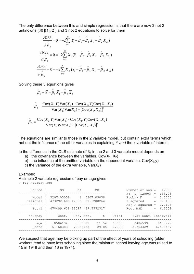
The only difference between this and simple regression is that there are now 3 not 2 unknowns (β0 β1 β2 ) and 3 not 2 equations to solve for them

)(20 22

^

11

^

10

^

0

^ ii

N

ii XXYRSS βββ

β∂

∂−−−−== ∑

=

)(20 22

^

11

^

10

^

1

1

^ ii

N

iii XXYXRSS βββ

β∂

∂−−−== ∑

=

−

)(20 22

^

11

^

10

^

2

2

^ ii

N

iii XXYXRSS βββ

β∂

∂−−−== ∑

=

−

Solving these 3 equations gives

22

^

11

^

0

^XXY βββ −−=

[ ]22121

212211

^

),(Cov))Var(Var),(Cov),(Cov-)()Var(Cov

XX(XXXXYXX,YX

−=β

[ ]22121

211122

^

),(Cov))Var(Var),(Cov),(Cov-)()Var(Cov

XX(XXXXYXX,YX

−=β

The equations are similar to those in the 2 variable model, but contain extra terms which net out the influence of the other variables in explaining Y and the x variable of interest ie the difference in the OLS estimate of β1 in the 2 and 3 variable model depends on

a) the covariance between the variables, Cov(X1, X2) b) the influence of the omitted variable on the dependent variable, Cov(X2,y) c) the variance of the extra variable, Var(X2)

Example: A simple 2 variable regression of pay on age gives . reg hourpay age Source | SS df MS Number of obs = 12098 -------------+------------------------------ F( 1, 12096) = 133.08 Model | 5207.03058 1 5207.03058 Prob > F = 0.0000 Residual | 473292.608 12096 39.1280264 R-squared = 0.0109 -------------+------------------------------ Adj R-squared = 0.0108 Total | 478499.638 12097 39.5552317 Root MSE = 6.2552 ------------------------------------------------------------------------------ hourpay | Coef. Std. Err. t P>|t| [95% Conf. Interval] -------------+---------------------------------------------------------------- age | .0586134 .005081 11.54 0.000 .0486539 .0685729 _cons | 6.168383 .2066433 29.85 0.000 5.763329 6.573437 ------------------------------------------------------------------------------ We suspect that age may be picking up part of the effect of years of schooling (older workers tend to have less schooling since the minimum school leaving age was raised to 15 in 1948 and then 16 in 1974).

4

5

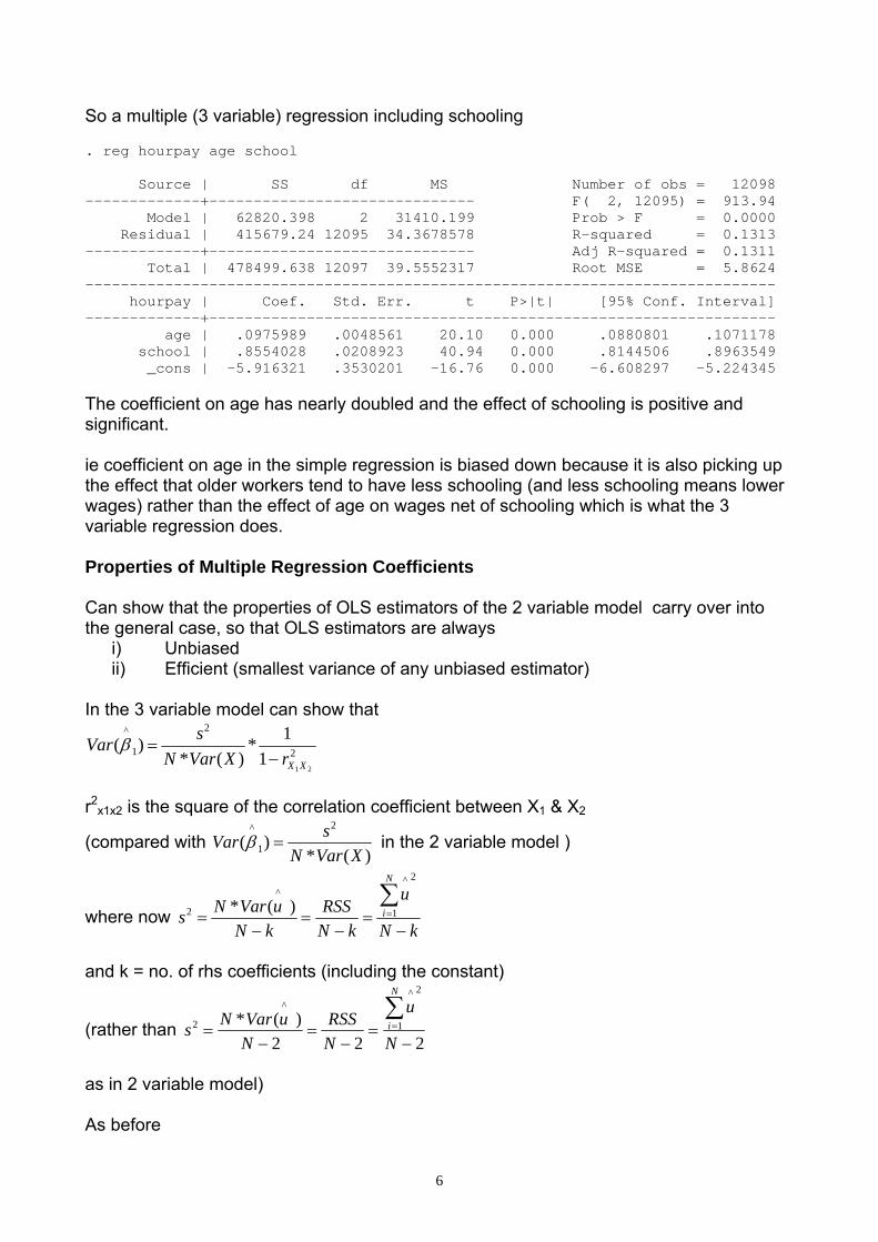
So a multiple (3 variable) regression including schooling . reg hourpay age school Source | SS df MS Number of obs = 12098 -------------+------------------------------ F( 2, 12095) = 913.94 Model | 62820.398 2 31410.199 Prob > F = 0.0000 Residual | 415679.24 12095 34.3678578 R-squared = 0.1313 -------------+------------------------------ Adj R-squared = 0.1311 Total | 478499.638 12097 39.5552317 Root MSE = 5.8624 ------------------------------------------------------------------------------ hourpay | Coef. Std. Err. t P>|t| [95% Conf. Interval] -------------+---------------------------------------------------------------- age | .0975989 .0048561 20.10 0.000 .0880801 .1071178 school | .8554028 .0208923 40.94 0.000 .8144506 .8963549 _cons | -5.916321 .3530201 -16.76 0.000 -6.608297 -5.224345 The coefficient on age has nearly doubled and the effect of schooling is positive and significant. ie coefficient on age in the simple regression is biased down because it is also picking up the effect that older workers tend to have less schooling (and less schooling means lower wages) rather than the effect of age on wages net of schooling which is what the 3 variable regression does. Properties of Multiple Regression Coefficients Can show that the properties of OLS estimators of the 2 variable model carry over into the general case, so that OLS estimators are always

i) Unbiased ii) Efficient (smallest variance of any unbiased estimator)

In the 3 variable model can show that

2

2

1

^

211

1*)(*

)(XXrXVarN

sVar−

=β

r2

x1x2 is the square of the correlation coefficient between X1 & X2

(compared with )(*

)(2

1

^

XVarNsVar =β in the 2 variable model )

where now kN

u

kNRSS

kNuVarNs

N

i

−=

−=

−=

∑=1

2^^

2 )(*

and k = no. of rhs coefficients (including the constant)

(rather than 222

)(* 1

2^^

2

−=

−=

−=

∑=

N

u

NRSS

NuVarNs

N

i

as in 2 variable model) As before

6

7

1) an increase in the residual variance, s2 2) a fall in sample size N

will make the OLS estimates of the effects of the X variables less precise Now in addition

3) an increased correlation between X1 & X2

will also make the OLS estimates of the effects of the X variables less precise (can’t distinguish between the contribution of the individual variables if correlation is high) The consequences of this high correlation is called multicolinearity and the symptoms are that

1) while OLS estimates remain unbiased 2) the standard errors are much larger than would be in the absence of

multicolinearity

and since ).(. 1

^

0

11

^^

β

ββ

est −=

the estimated t values will be smaller than otherwise. You may therefore conclude that variables are statistically insignificant (from zero) when not (ie Type II error) In practice nearly all estimation suffers from multicolinearity since unlikely that the correlation between variables is zero, (if it is the variables are said to be orthogonal). The issue then becomes how serious a problem is it.

Detection: 1) Low t values and high R2 2) The estimates may be sensitive to addition or subtraction of a small number of

observations 3) Look at the simple correlation coefficients between any 2 variables. A correlation

coefficient >0.8 usually says there are problems. Or if the correlation between any two right hand side variables is greater than the correlation between that of each with the dependent variable

Problem: In cases when there are many right hand side variables this strategy may not pick up group as opposed to pairwise correlations.

In this case run an auxiliary regression of any one of the right hand side variables on all the other X variables

X1 = δ0 + δ2X2 + δ3X3 + … δkXk + u

and look at the R2 from this regression. An R2 > 0.8 suggests problems

8

9

Solutions: Unfortunately the only sensible thing to do when faced with multicolinearity is either to

1) Get more data – (since an increase in N will reduce the standard errors) 2)Get more (uncorrelated) variables – since this should reduce the residual variance s2 and offset the multicolinearity effect.

If this fails then quite often the only solution is to drop one of the original correlated variables. The issue cannot be answered given the available data.

Example: Multicolinearity Often in time series data when there are few observations (annual data is often all there is available) variables display common trends and so are highly correlated. This means it is difficult to discern individual effects of the RHS variables. Suppose you regress consumption on a time trend, (a trend is just a variable that increases by one for each year of the data) . reg cons trend Source | SS df MS Number of obs = 45 ---------+------------------------------ F( 1, 43) = 960.81 Model | 4.5380e+11 1 4.5380e+11 Prob > F = 0.0000 Residual | 2.0309e+10 43 472306243 R-squared = 0.9572 ---------+------------------------------ Adj R-squared = 0.9562 Total | 4.7411e+11 44 1.0775e+10 Root MSE = 21733 ------------------------------------------------------------------------------ cons | Coef. Std. Err. t P>|t| [95% Conf. Interval] ---------+-------------------------------------------------------------------- trend | 7732.329 249.4543 30.997 0.000 7229.257 8235.402 _cons | 129380.1 6588.931 19.636 0.000 116092.2 142667.9 ------------------------------------------------------------------------------ This appears highly significant and economically important. However a 3 variable regression of consumption on the trend and income gives . reg cons trend income Source | SS df MS Number of obs = 45 ---------+------------------------------ F( 2, 42) = 2919.99 Model | 4.7072e+11 2 2.3536e+11 Prob > F = 0.0000 Residual | 3.3853e+09 42 80603294.8 R-squared = 0.9929 ---------+------------------------------ Adj R-squared = 0.9925 Total | 4.7411e+11 44 1.0775e+10 Root MSE = 8977.9 ------------------------------------------------------------------------------ cons | Coef. Std. Err. t P>|t| [95% Conf. Interval] ---------+-------------------------------------------------------------------- trend | -140.4874 553.0085 -0.254 0.801 -1256.504 975.5288 income | .9333721 .0644142 14.490 0.000 .8033789 1.063365 _cons | 11579.25 8573.289 1.351 0.184 -5722.351 28880.84 ------------------------------------------------------------------------------ The trend variable is now insignificant, the standard error on the estimate has increased massively and the sign of the coefficient is negative. This does not look sensible.

10

11

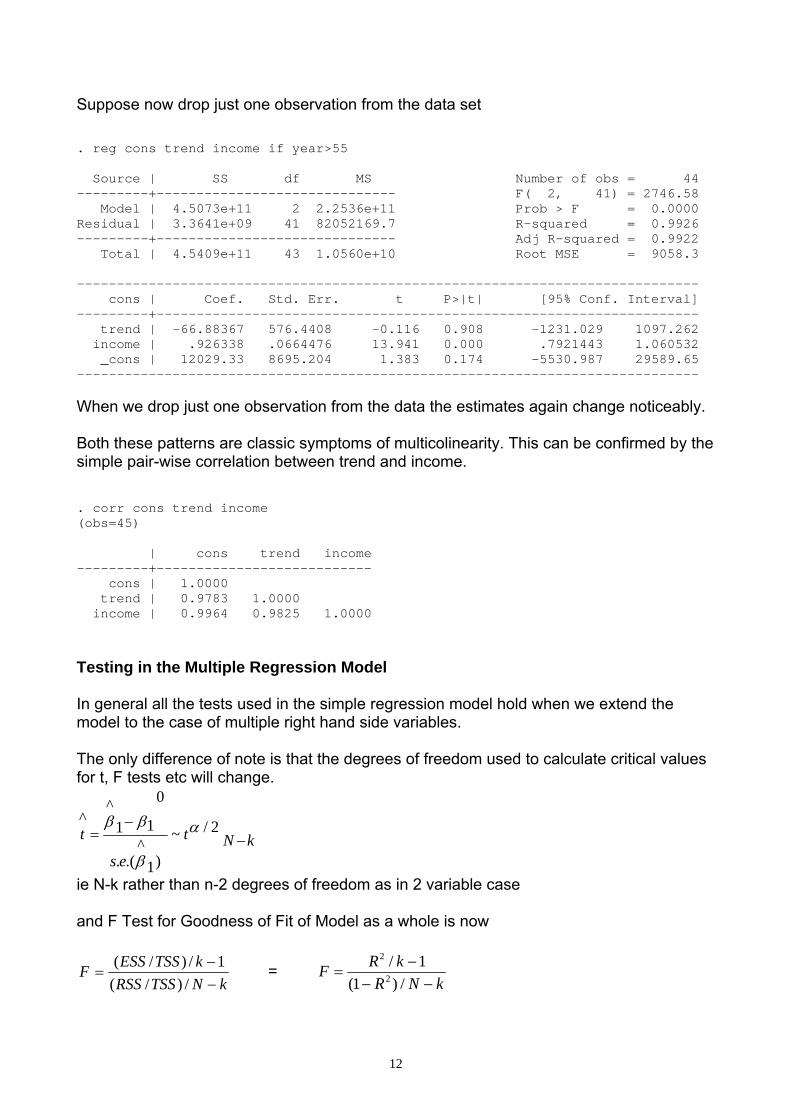
Suppose now drop just one observation from the data set . reg cons trend income if year>55 Source | SS df MS Number of obs = 44 ---------+------------------------------ F( 2, 41) = 2746.58 Model | 4.5073e+11 2 2.2536e+11 Prob > F = 0.0000 Residual | 3.3641e+09 41 82052169.7 R-squared = 0.9926 ---------+------------------------------ Adj R-squared = 0.9922 Total | 4.5409e+11 43 1.0560e+10 Root MSE = 9058.3 ------------------------------------------------------------------------------ cons | Coef. Std. Err. t P>|t| [95% Conf. Interval] ---------+-------------------------------------------------------------------- trend | -66.88367 576.4408 -0.116 0.908 -1231.029 1097.262 income | .926338 .0664476 13.941 0.000 .7921443 1.060532 _cons | 12029.33 8695.204 1.383 0.174 -5530.987 29589.65 ------------------------------------------------------------------------------ When we drop just one observation from the data the estimates again change noticeably. Both these patterns are classic symptoms of multicolinearity. This can be confirmed by the simple pair-wise correlation between trend and income. . corr cons trend income (obs=45) | cons trend income ---------+--------------------------- cons | 1.0000 trend | 0.9783 1.0000 income | 0.9964 0.9825 1.0000 Testing in the Multiple Regression Model In general all the tests used in the simple regression model hold when we extend the model to the case of multiple right hand side variables. The only difference of note is that the degrees of freedom used to calculate critical values for t, F tests etc will change.

kNt

es

t −−

= 2/~

)1^

.(.

0

11^

^ α

β

ββ

ie N-k rather than n-2 degrees of freedom as in 2 variable case and F Test for Goodness of Fit of Model as a whole is now

kNTSSRSSkTSSESSF−−

=/)/(

1/)/( = kNR

kRF−−

−=

/)1(1/

2

2

12

13

ie k-1 and N-k rather than 2-1 and n-2 degrees of freedom as in 2 variable case (k = no. of rhs coefficients including the constant) The R2 use in this calculation is the same as before as is its interpretation as the square of the correlation coefficient between predicted and actual value The Adjusted R2

One problem with using the R2 in a multiple regression is (can show) that the R2 (and the ESS) will never fall when add regressors. (this is because OLS minimises the RSS so whenever a variable is dropped the RSS will always increase because the size of the residual increases) - If so may be tempted to add as many variables as regressors in order to increase the fit of the model. - Problem (notes on multicolinearity show) that this will increase the chance of introducing correlation between rhs variables which will inflate the estimated standard errors and run this risk of type II error. Useful therefore to also report the adjusted R2

kNNR

NTSSkNRSSR

−−

−−=−−

−=1)21(1

1//1

2_

which contains an adjustment factor so that while RSS never ↑ (and usually falls) when new variables added (and the ESS will never ↓ ) there is a penalty to adding new variables because N-k ↓ (so moving in the opposite direction to the effect of adding more variables on RSS) Can show that adjusted R2 will only increase if the t value on the new variable > 1 (in absolute value)

useful (alternative) rule for deciding whether to keep a variable in a regression. - If it raises the adjusted R2 keep it in

Since can’t interpret the adjusted R2 as the as the square of the correlation coefficient between predicted and actual value useful to report both in a multiple regression. Indeed the F test of goodness of fit uses the R2 not adjusted R2 )

14

15

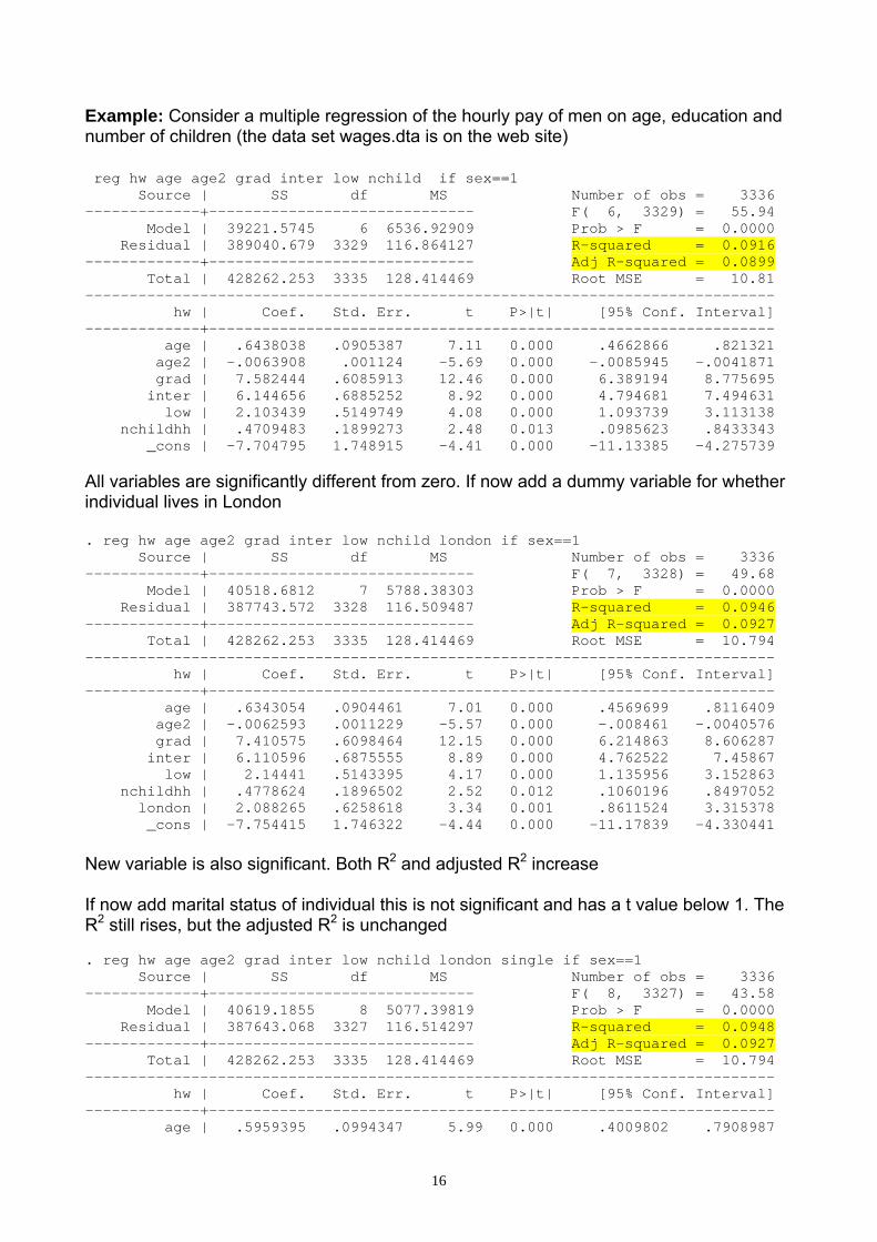
Example: Consider a multiple regression of the hourly pay of men on age, education and number of children (the data set wages.dta is on the web site) reg hw age age2 grad inter low nchild if sex==1 Source | SS df MS Number of obs = 3336 -------------+------------------------------ F( 6, 3329) = 55.94 Model | 39221.5745 6 6536.92909 Prob > F = 0.0000 Residual | 389040.679 3329 116.864127 R-squared = 0.0916 -------------+------------------------------ Adj R-squared = 0.0899 Total | 428262.253 3335 128.414469 Root MSE = 10.81 ------------------------------------------------------------------------------ hw | Coef. Std. Err. t P>|t| [95% Conf. Interval] -------------+---------------------------------------------------------------- age | .6438038 .0905387 7.11 0.000 .4662866 .821321 age2 | -.0063908 .001124 -5.69 0.000 -.0085945 -.0041871 grad | 7.582444 .6085913 12.46 0.000 6.389194 8.775695 inter | 6.144656 .6885252 8.92 0.000 4.794681 7.494631 low | 2.103439 .5149749 4.08 0.000 1.093739 3.113138 nchildhh | .4709483 .1899273 2.48 0.013 .0985623 .8433343 _cons | -7.704795 1.748915 -4.41 0.000 -11.13385 -4.275739 All variables are significantly different from zero. If now add a dummy variable for whether individual lives in London . reg hw age age2 grad inter low nchild london if sex==1 Source | SS df MS Number of obs = 3336 -------------+------------------------------ F( 7, 3328) = 49.68 Model | 40518.6812 7 5788.38303 Prob > F = 0.0000 Residual | 387743.572 3328 116.509487 R-squared = 0.0946 -------------+------------------------------ Adj R-squared = 0.0927 Total | 428262.253 3335 128.414469 Root MSE = 10.794 ------------------------------------------------------------------------------ hw | Coef. Std. Err. t P>|t| [95% Conf. Interval] -------------+---------------------------------------------------------------- age | .6343054 .0904461 7.01 0.000 .4569699 .8116409 age2 | -.0062593 .0011229 -5.57 0.000 -.008461 -.0040576 grad | 7.410575 .6098464 12.15 0.000 6.214863 8.606287 inter | 6.110596 .6875555 8.89 0.000 4.762522 7.45867 low | 2.14441 .5143395 4.17 0.000 1.135956 3.152863 nchildhh | .4778624 .1896502 2.52 0.012 .1060196 .8497052 london | 2.088265 .6258618 3.34 0.001 .8611524 3.315378 _cons | -7.754415 1.746322 -4.44 0.000 -11.17839 -4.330441 New variable is also significant. Both R2 and adjusted R2 increase If now add marital status of individual this is not significant and has a t value below 1. The R2 still rises, but the adjusted R2 is unchanged . reg hw age age2 grad inter low nchild london single if sex==1 Source | SS df MS Number of obs = 3336 -------------+------------------------------ F( 8, 3327) = 43.58 Model | 40619.1855 8 5077.39819 Prob > F = 0.0000 Residual | 387643.068 3327 116.514297 R-squared = 0.0948 -------------+------------------------------ Adj R-squared = 0.0927 Total | 428262.253 3335 128.414469 Root MSE = 10.794 ------------------------------------------------------------------------------ hw | Coef. Std. Err. t P>|t| [95% Conf. Interval] -------------+---------------------------------------------------------------- age | .5959395 .0994347 5.99 0.000 .4009802 .7908987

16

17

age2 | -.0059419 .0011738 -5.06 0.000 -.0082433 -.0036404 grad | 7.395769 .6100673 12.12 0.000 6.199624 8.591914 inter | 6.060026 .6897222 8.79 0.000 4.707704 7.412349 low | 2.119489 .5150495 4.12 0.000 1.109644 3.129335 nchildhh | .4138712 .2017817 2.05 0.040 .0182424 .8095001 london | 2.126036 .6271946 3.39 0.001 .8963097 3.355762 single | -.5346072 .5756151 -0.93 0.353 -1.663203 .5939882 _cons | -6.549751 2.175352 -3.01 0.003 -10.81491 -2.284587 Adjusted R2 can even fall when (very insignificant) variables are added and in some cases (small sample sizes) can even be negative Can also use adjusted R2 to compare non-nested models – models which one is not a special case of the other and which contain a different number of rhs variables – so using the R2 would be the wrong comparison to make Compare a regression of hourly wages on a quadratic in years of education (ie edage & edage2) with the log of years of education. Both these specifications allow for a non-linear relationship between hourly pay and years of education. These models are also non-nested because can’t easily go from one to the other by simply excluding a variable. The issue is which is best? Using the data set ps4data.dta . reg lhw edage ed2 if reg==1 Model 1 Source | SS df MS Number of obs = 255 -------------+------------------------------ F( 2, 252) = 15.11 Model | 6.05947737 2 3.02973868 Prob > F = 0.0000 Residual | 50.5286806 252 .200510637 R-squared = 0.1071 -------------+------------------------------ Adj R-squared = 0.1000 Total | 56.5881579 254 .222788023 Root MSE = .44778 ------------------------------------------------------------------------------ lhw | Coef. Std. Err. t P>|t| [95% Conf. Interval] -------------+---------------------------------------------------------------- edage | .2285597 .126396 1.81 0.072 -.0203674 .4774867 ed2 | -.0042452 .0033157 -1.28 0.202 -.0107752 .0022848 _cons | -.7740635 1.179855 -0.66 0.512 -3.097697 1.54957 ------------------------------------------------------------------------------ . reg lhw ledage if reg==1 Model 2 Source | SS df MS Number of obs = 255 -------------+------------------------------ F( 1, 253) = 29.63 Model | 5.93302893 1 5.93302893 Prob > F = 0.0000 Residual | 50.655129 253 .200217901 R-squared = 0.1048 -------------+------------------------------ Adj R-squared = 0.1013 Total | 56.5881579 254 .222788023 Root MSE = .44746 ------------------------------------------------------------------------------ lhw | Coef. Std. Err. t P>|t| [95% Conf. Interval] -------------+---------------------------------------------------------------- ledage | 1.269603 .2332282 5.44 0.000 .8102868 1.728919 _cons | -1.725876 .6565078 -2.63 0.009 -3.018793 -.4329596 - Might go with the regression with the highest R-----------------------------------------------------------------------------

2. (ie model 1)

18

19

This would be a mistake, since the R2 does not penalise the use of more rhs variables, should use adjusted R2 to make the comparison And therefore can see model 2 is preferred (as it would be if looked at the t values on the individual coefficients) Note: can’t use this to decide between models with different dependent (left hand side) variables Tests of Restrictions A variant of the test of goodness of fit of the model is instead to test a hypothesis that a sub-set of the right hand side variables are zero (rather than all of them as with the original F test or just one of them as in the t test) Can show that test becomes F = RSSrestricted – RSSunrestricted /J ~ F(J, N-Kunrestricted)

RSSunrestricted /N- Kunrestricted Or equivalently F = R2

unrestricted – R2restricted /J ~ F(J, N-Kunrestricted)

1-R2unrestricted /N- Kunrestricted

Where J = No. of variables to be tested restricted = values from model with variables set to zero (ie excluded from the regression specification) unrestricted = values from model with variables included in the regression specification Under the null that the extra variables have no explanatory power then wouldn’t expect the RSS from the two models to differ much Hence reject null if estimated F > Fcritical

20

21

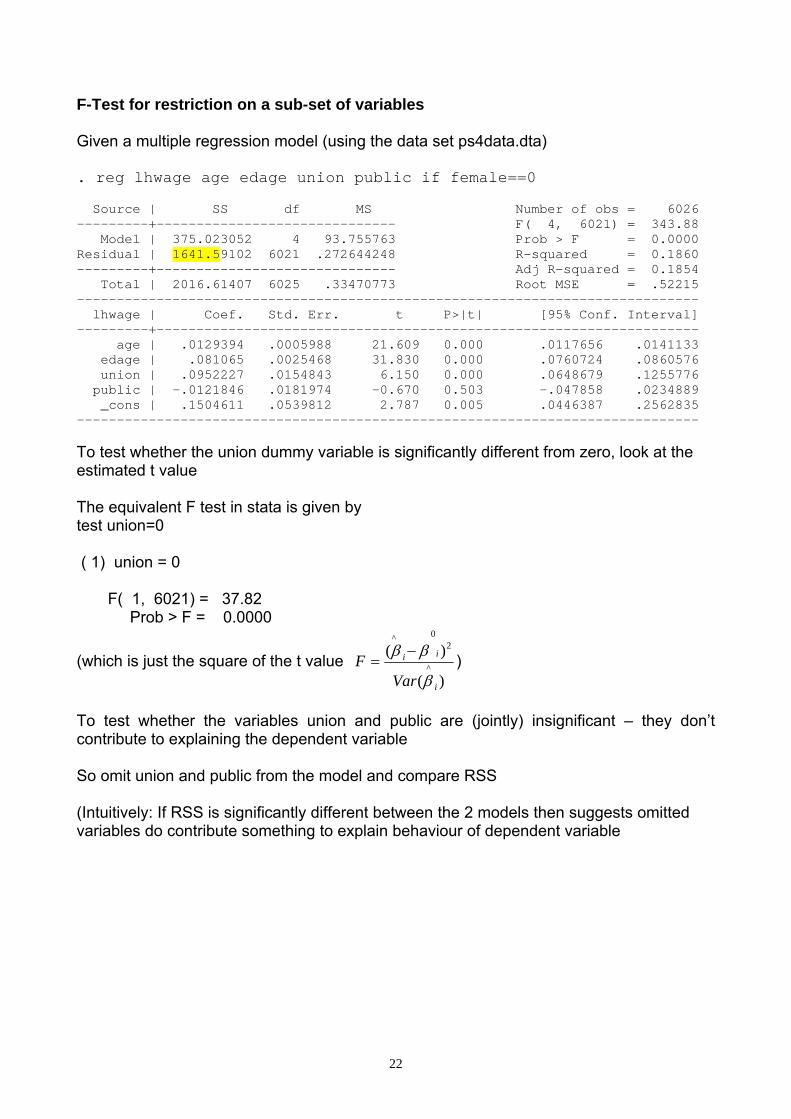
F-Test for restriction on a sub-set of variables Given a multiple regression model (using the data set ps4data.dta) . reg lhwage age edage union public if female==0 Source | SS df MS Number of obs = 6026 ---------+------------------------------ F( 4, 6021) = 343.88 Model | 375.023052 4 93.755763 Prob > F = 0.0000 Residual | 1641.59102 6021 .272644248 R-squared = 0.1860 ---------+------------------------------ Adj R-squared = 0.1854 Total | 2016.61407 6025 .33470773 Root MSE = .52215 ------------------------------------------------------------------------------ lhwage | Coef. Std. Err. t P>|t| [95% Conf. Interval] ---------+-------------------------------------------------------------------- age | .0129394 .0005988 21.609 0.000 .0117656 .0141133 edage | .081065 .0025468 31.830 0.000 .0760724 .0860576 union | .0952227 .0154843 6.150 0.000 .0648679 .1255776 public | -.0121846 .0181974 -0.670 0.503 -.047858 .0234889 _cons | .1504611 .0539812 2.787 0.005 .0446387 .2562835 ------------------------------------------------------------------------------ To test whether the union dummy variable is significantly different from zero, look at the estimated t value The equivalent F test in stata is given by test union=0 ( 1) union = 0 F( 1, 6021) = 37.82 Prob > F = 0.0000

(which is just the square of the t value )(

)(^

20^

i

ii

VarF

β

ββ −= )

To test whether the variables union and public are (jointly) insignificant – they don’t contribute to explaining the dependent variable So omit union and public from the model and compare RSS (Intuitively: If RSS is significantly different between the 2 models then suggests omitted variables do contribute something to explain behaviour of dependent variable

22

23

. reg lhwage age edage if female==0 Source | SS df MS Number of obs = 6026 ---------+------------------------------ F( 2, 6023) = 663.31 Model | 364.003757 2 182.001879 Prob > F = 0.0000 Residual | 1652.61031 6023 .27438325 R-squared = 0.1805 ---------+------------------------------ Adj R-squared = 0.1802 Total | 2016.61407 6025 .33470773 Root MSE = .52382 ------------------------------------------------------------------------------ lhwage | Coef. Std. Err. t P>|t| [95% Conf. Interval] ---------+-------------------------------------------------------------------- age | .013403 .0005926 22.615 0.000 .0122412 .0145648 edage | .0801733 .0024976 32.100 0.000 .0752771 .0850695 _cons | .1763613 .0532182 3.314 0.001 .0720345 .2806881 ------------------------------------------------------------------------------ F test of null hypothesis that coefficients on union and public are zero (variables have no explanatory power) F = RSSrestrict – RSSunrestrict /J ~ F(J, N-Kunrestrict) RSSunrestrict /N- Kunrestrict = 1652.6 – 1641.6 /2 ~ F(2, 6026 -5) 1641.6 /6026 – 5 = 20.2 From F tables, critical value at 5% level F(2, 6021) = F(2, ∞ ) = 3.00 So estimated F > Fcritical Stata equivalent is given by test union public ( 1) union = 0 ( 2) public = 0 F( 2, 6021) = 20.21 Prob > F = 0.0000 So reject null that union and public sector variables jointly have no explanatory power in the model Note that the t value on the public sector dummy indicates that the effect of this variable is statistically insignificant from zero, yet the combined F test has rejected the null that both variables have no explanatory power. Be careful that test results don’t conflict (technically the F test for joint restrictions is “less powerful test of single restrictions than the t test Since this test is essentially a test of (linear) restrictions – in the above case the restriction was that the coefficients on the sub-set of variables were restricted to zero – other important uses of this test also include

24

25

Testing linear hypotheses Eg. We know the Cobb-Douglas production function

y = ALαKβ with α+β=1

if there is constant returns to scale (d.r.s. means α+β<1 i.r.s. means α+β>1) Taking (natural) logs Lny = LnA + αLnL + βLnK (1)

and can test the null H0: by imposing the restriction that α+β=1 in (1) against an unrestricted version that does not impose the constraint. Example: Using the data set prodfn.dta containing information on the output, labour input and capital stock of 27 firms

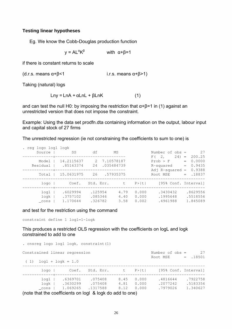
The unrestricted regression (ie not constraining the coefficients to sum to one) is

. reg logo logl logk Source | SS df MS Number of obs = 27 -------------+------------------------------ F( 2, 24) = 200.25 Model | 14.2115637 2 7.10578187 Prob > F = 0.0000 Residual | .85163374 24 .035484739 R-squared = 0.9435 -------------+------------------------------ Adj R-squared = 0.9388 Total | 15.0631975 26 .57935375 Root MSE = .18837 ------------------------------------------------------------------------------ logo | Coef. Std. Err. t P>|t| [95% Conf. Interval] -------------+---------------------------------------------------------------- logl | .6029994 .125954 4.79 0.000 .3430432 .8629556 logk | .3757102 .085346 4.40 0.000 .1995648 .5518556 _cons | 1.170644 .326782 3.58 0.002 .4961988 1.845089 and test for the restriction using the command constraint define 1 logl=1-logk This produces a restricted OLS regression with the coefficients on logL and logk constrained to add to one . cnsreg logo logl logk, constraint(1) Constrained linear regression Number of obs = 27 Root MSE = .18501 ( 1) logl + logk = 1.0 ------------------------------------------------------------------------------ logo | Coef. Std. Err. t P>|t| [95% Conf. Interval] -------------+---------------------------------------------------------------- logl | .6369701 .075408 8.45 0.000 .4816644 .7922758 logk | .3630299 .075408 4.81 0.000 .2077242 .5183356 _cons | 1.069265 .1317588 8.12 0.000 .7979026 1.340627 (note that the coefficients on logl & logk do add to one)

26

27

Using the formula F = RSSrestrict – RSSunrestrict /J ~ F(J, N-Kunrestrict) RSSunrestrict /N- Kunrestrict Stata produces the following output . test _b[logl]+_b[logk]=1 ( 1) logl + logk = 1.0 F( 1, 24) = 0.12 Prob > F = 0.7366

So estimated F < Fcritical at 5% level So accept null that H0: α+β=1 So production function is Cobb-Douglas constant returns to scale 2) Testing Stability of Coefficients Across Sample Splits Might think the estimated relationship varies over time or across easily characterised sub-groups of your data (eg by gender) In this case test the restricted model

Y = β0 + β1X1 + β2X2 + u (1)

(ie coefficients same in both periods/both sub-groups)

Against an unrestricted model which allows the coefficients to vary across the two-subgroups/time periods

Y = β01 + β1

1 X1 + β2

1 X2 + u1 (2)

Y = β02 + β1

2 X1 + β2

2 X2 + u2 (3)

Can show that the unrestricted RSS in this case equals the sum of the RSS from the two sub-regressions (2) & (3) So that

F = RSSrestrict – RSSunrestrict /J ~ F(J, N-Kunrestrict) RSSunrestrict /N- Kunrestrict becomes

F = RSSrestrict – (RSSgroup1+ RSSgroup2) /J (RSSgroup1+ RSSgroup2) /N- Kunrestrict ~ F(J, N-Kunrestrict) where j is again the number of variables restricted (in this case the entire set of rhs variables including the constant)

28

29

Eg: Chow Test for Structural Break in Time Series Data

u cons /* read in consumption function data for years 1955-99 */ twoway (scatter cons year, msymbol(none) mlabel(year)), xlabel(55(5)100) xline(90)

555657585960616263646566676869707172

737475767778

798081828384

8586

87

8889909192

939495

9697

9899

2000

0030

0000

4000

0050

0000

6000

00co

ns

55 60 65 70 75 80 85 90 95 100year

Graph suggests relationship between consumption and income changes over the sample period. (slope is steeper in 2nd period)

30

31

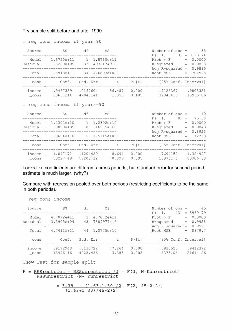
Try sample split before and after 1990 . reg cons income if year<90 Source | SS df MS Number of obs = 35 ---------+------------------------------ F( 1, 33) = 3190.74 Model | 1.5750e+11 1 1.5750e+11 Prob > F = 0.0000 Residual | 1.6289e+09 33 49361749.6 R-squared = 0.9898 ---------+------------------------------ Adj R-squared = 0.9895 Total | 1.5913e+11 34 4.6803e+09 Root MSE = 7025.8 ------------------------------------------------------------------------------ cons | Coef. Std. Err. t P>|t| [95% Conf. Interval] ---------+-------------------------------------------------------------------- income | .9467359 .0167604 56.487 0.000 .9126367 .9808351 _cons | 6366.214 4704.141 1.353 0.185 -3204.433 15936.86 . reg cons income if year>=90 Source | SS df MS Number of obs = 10 ---------+------------------------------ F( 1, 8) = 75.58 Model | 1.2302e+10 1 1.2302e+10 Prob > F = 0.0000 Residual | 1.3020e+09 8 162754768 R-squared = 0.9043 ---------+------------------------------ Adj R-squared = 0.8923 Total | 1.3604e+10 9 1.5115e+09 Root MSE = 12758 ------------------------------------------------------------------------------ cons | Coef. Std. Err. t P>|t| [95% Conf. Interval] ---------+-------------------------------------------------------------------- income | 1.047171 .1204489 8.694 0.000 .7694152 1.324927 _cons | -53227.48 59208.12 -0.899 0.395 -189761.6 83306.68 Looks like coefficients are different across periods, but standard error for second period estimate is much larger. (why?) Compare with regression pooled over both periods (restricting coefficients to be the same in both periods). . reg cons income Source | SS df MS Number of obs = 45 ---------+------------------------------ F( 1, 43) = 5969.79 Model | 4.7072e+11 1 4.7072e+11 Prob > F = 0.0000 Residual | 3.3905e+09 43 78849774.6 R-squared = 0.9928 ---------+------------------------------ Adj R-squared = 0.9927 Total | 4.7411e+11 44 1.0775e+10 Root MSE = 8879.7 ------------------------------------------------------------------------------ cons | Coef. Std. Err. t P>|t| [95% Conf. Interval] ---------+-------------------------------------------------------------------- income | .9172948 .0118722 77.264 0.000 .8933523 .9412372 _cons | 13496.16 4025.456 3.353 0.002 5378.05 21614.26 Chow Test for sample split F = RSSrestrict – RSSunrestrict /J ~ F(J, N-Kunrestrict) RSSunrestrict /N- Kunrestrict = 3.39 - (1.63+1.30)/2~ F(2, 45-2(2)) (1.63+1.30)/45-2(2)

32

33

Important: With this form of the test there are twice as many coefficients in the unrestricted regressions (income and the constant for the period 1955-89, and a different estimate for income and the constant for the period 1990-99, so the unrestricted degrees of freedom are

N = N55-89 + N90-99 = 35+10 = 45

and k = 2*2

) = 3.22 ~ F(2, 41) From table F critical at 5% level is 3.00. Therefore reject null that coefficients are the same in both time periods. Hence mpc is not constant over time. Example 2: Chow Test of Structural Break – Cross Section Data Suppose wish to test whether estimated OLS coefficients were the same for men and women in ps2data.dta Restricted regression is obtained by pooling all observations on men & women and running a single OLS regression . reg lhwage age edage union public Source | SS df MS Number of obs = 12098 ---------+------------------------------ F( 4, 12093) = 724.06 Model | 763.038968 4 190.759742 Prob > F = 0.0000 Residual | 3186.01014 12093 .263459038 R-squared = 0.1932 ---------+------------------------------ Adj R-squared = 0.1930 Total | 3949.04911 12097 .326448633 Root MSE = .51328 ------------------------------------------------------------------------------ lhwage | Coef. Std. Err. t P>|t| [95% Conf. Interval] ---------+-------------------------------------------------------------------- age | .0100706 .0004335 23.231 0.000 .0092209 .0109204 edage | .0869484 .0018669 46.574 0.000 .083289 .0906078 union | .1780204 .0109133 16.312 0.000 .1566285 .1994123 public | -.0250529 .0114298 -2.192 0.028 -.0474571 -.0026487 _cons | .0177325 .0393914 0.450 0.653 -.059481 .094946 ------------------------------------------------------------------------------ Unrestricted regression obtained by running separate estimates for men and women (effectively allowing separate estimates of the constant and all the slope variables) and then adding the residual sums of squares together

34

35

Men . reg lhwage age edage union public if female==0 Source | SS df MS Number of obs = 6026 ---------+------------------------------ F( 4, 6021) = 343.88 Model | 375.023052 4 93.755763 Prob > F = 0.0000 Residual | 1641.59102 6021 .272644248 R-squared = 0.1860 ---------+------------------------------ Adj R-squared = 0.1854 Total | 2016.61407 6025 .33470773 Root MSE = .52215 ------------------------------------------------------------------------------ lhwage | Coef. Std. Err. t P>|t| [95% Conf. Interval] ---------+-------------------------------------------------------------------- age | .0129394 .0005988 21.609 0.000 .0117656 .0141133 edage | .081065 .0025468 31.830 0.000 .0760724 .0860576 union | .0952227 .0154843 6.150 0.000 .0648679 .1255776 public | -.0121846 .0181974 -0.670 0.503 -.047858 .0234889 _cons | .1504611 .0539812 2.787 0.005 .0446387 .2562835 Women . reg lhwage age edage union public if female==1 Source | SS df MS Number of obs = 6072 ---------+------------------------------ F( 4, 6067) = 464.55 Model | 407.028301 4 101.757075 Prob > F = 0.0000 Residual | 1328.94152 6067 .21904426 R-squared = 0.2345 ---------+------------------------------ Adj R-squared = 0.2340 Total | 1735.96982 6071 .285944626 Root MSE = .46802 ------------------------------------------------------------------------------ lhwage | Coef. Std. Err. t P>|t| [95% Conf. Interval] ---------+-------------------------------------------------------------------- age | .0051823 .0005881 8.811 0.000 .0040293 .0063353 edage | .0854792 .0025947 32.944 0.000 .0803927 .0905657 union | .2086894 .0145456 14.347 0.000 .1801748 .2372039 public | .0784844 .0141914 5.530 0.000 .0506642 .1063045 _cons | .066159 .0545192 1.213 0.225 -.040718 .1730359 F = RSSrestrict – RSSunrestrict /J ~ F(J, N-Kunrestrict) RSSunrestrict /N- Kunrestrict becomes F = RSSpooled – (RSSmen +RSSwomen)/No. Restricted

(RSSmen +RSSwomen)/N- Kunrestrict = 3186 – (1641.6 + 1328.9) /5 ~ F(5, 12098 -10) (1641.6 + 1328.9) /12098 – 2(5) = 175.4 Note 1. J= 5 because 5 values are restricted – (constant, age, edage, union, public) 2. N-Kunrestricted = 12098 –2(5) because in the unrestricted regression there are 2*5 estimated parameters (5 for men and 5 for women) From F tables, critical value at 5% level F(5, 12088) = F(5, ∞ ) = 2.21 So estimated F > Fcritical Reject null that coefficients are the same for men and women

36