correlation and simple linear regression - seth spielman · goals • introduce correlation •...
TRANSCRIPT

Correlation and Simple Linear Regression
GEOG 5023 Spring 2015

Goals• Introduce Correlation
• Basic ideas
• Spatial correlation
• Computing in R
• Flavors (Pearson, Spearman)
• Hypothesis tests
• Simple linear regression
• Least Squares
• Computing with R
• Basic diagnostics
• Does not discuss PREDICTION…

Z-Scores• When we discussed hypothesis tests we introduced
the idea of “standardized score” Z-Score.
• Expressed values in terms of SD away from the mean.

Z-Scores
• If a value is above the mean it’s Z-Score is positive.
• Below the mean it’s negative.
• Consider two characteristics of the ith observation:
Getting to know notation: What does the “E” thingy mean.

Z-Scores• For the ith observation
• If variable a is above the mean its z-score will be positive.
• If variable b is below the mean its z-score will be negative.
• If we multiplied these z-scores together they’d be negative.

Computing Correlation• If a and b tend to both be above/below the mean at the
same time:
• The product of their z-scores will be positive.
• If a and b tend to move in opposite directions, when a is above the mean b is below the mean:
• The product of their z-scores will be negative.
• CORRELATION IS AVERAGE OF THE PRODUCT OF THE Z-SCORES.

The correlation coefficient

Pearson’s correlation coefficient (r)
• Ranges from -1 to +1
• Points that are not linearly related have a correlation of 0
• The farther the correlation is from 0, the stronger the linear relationship

Correlation and slope

Covariance• The degree to which two variables co-vary
• High positive covariance both are above/below the mean at the same time.
• Low/no covariance, the movement is erratic and sums to zero.
• Magnitude (size) depends on the unit of measurement

Pearson’s correlation coefficient (r)
sx = sd of variable x!sy = sd of variable y
The average of the product!of the z-scores.
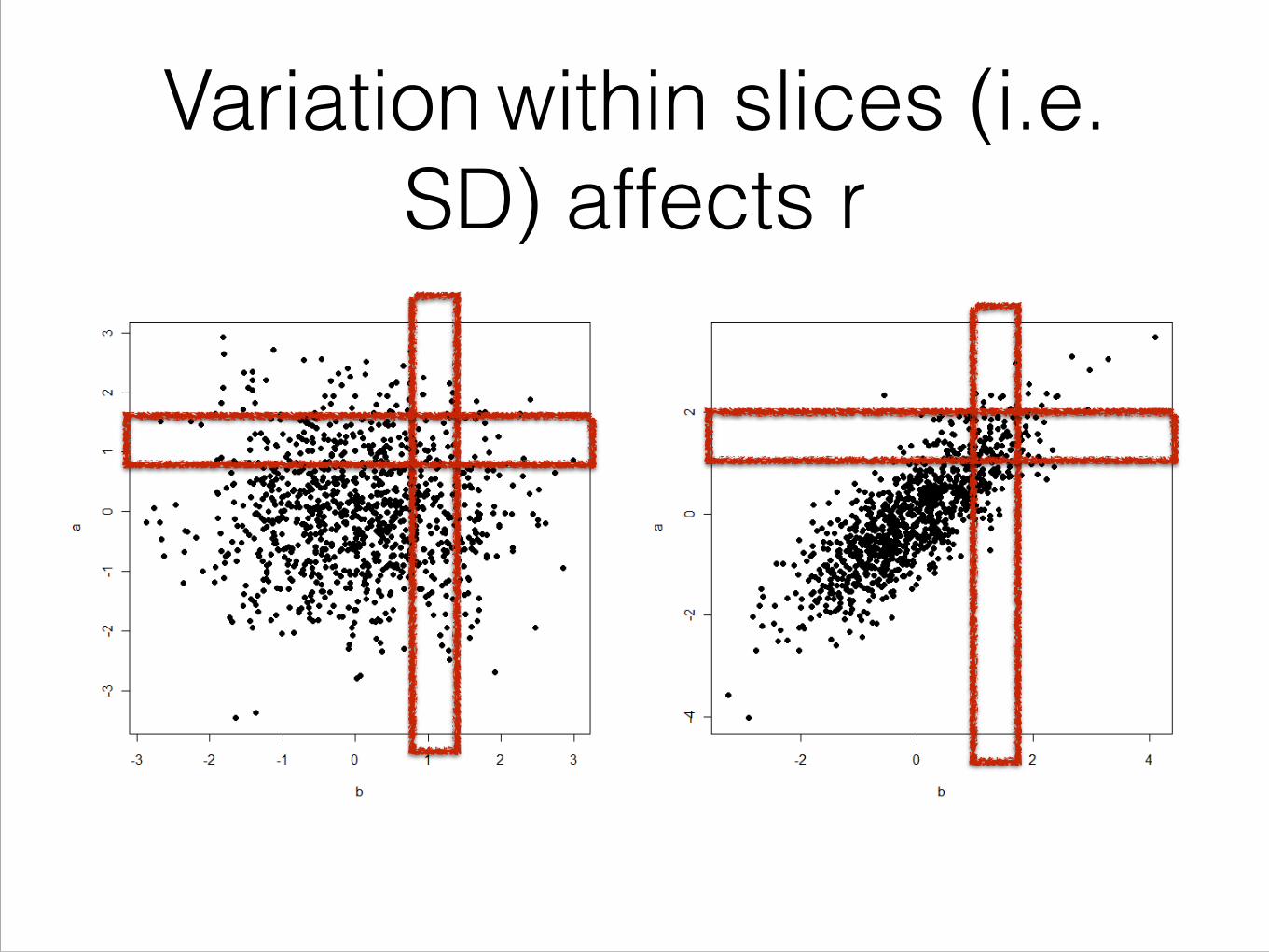
Variation within slices (i.e. SD) affects r

Significance Testing for r• The sample correlation coefficient (r) is an estimate of
the population correlation coefficient ρ.
• Like all sample statistics it is subject to chance variations.
• So we might want to test the null hypothesis that H0: ρ = 0.
• We worry that the correlation we observed might be due to random chance and that the true correlation is zero.

Our Population
The true correlation (ρ)
Samples...

Correlation: samples (red) Population correlation (blue)

Code for preceding figures###GENERATE DATA rnormcor <- function(x,rho) rnorm(1,rho*x,sqrt(1-rho^2)) a <- rnorm(10000,0,1) b <- sapply(a, rnormcor, rho = 0.60) !##PLOT DATA plot(a~b) !##CREATE A TABLE (DATA.FRAME) data.ab <- data.frame(a,b) !##A FUNCTION FOR TAKING A SAMPLE FROM THE SIMULATED DATA ##AND FITTING A REGRESSION ON THE SAMPLE ##RETURNS A GRAPH W/ REGRESSION LINE plot.sample <- function(){ samp <- data.ab[sample(1:dim(data.ab)[1], 100), ] plot(samp$a ~ samp$b, pch = 16, xlim = c(-4,4), ylim = c(-4,4)) abline(lm(samp$a~samp$b), col="red") } !##DRAW PLOTS IN A 3 X 3 GRID dev.off() par(mfrow=(c(3,3))) !#PLOT DATA plot(a~b, xlim = c(-4,4), ylim = c(-4,4)) #ADD A LINE WITH THE THE "TRUE" REGRESSION #WE KNOW THIS IS THE tRUtE BECAUSE WE ARE FITTING #THE MODEL WITH THE ENTIRE POPULATION abline(lm(a~b), col="red") !#SAMPLE 100 POINTS FROM 1st GRAPH AND FIT MODEL plot.sample() plot.sample() #REPEAT ABOVE plot.sample() plot.sample() plot.sample() plot.sample() plot.sample() plot.sample()

Example• Dataset: Income, poverty and health data for
180+ WHO countries !
• Research question: Are literacy and fertility rates (TFR) related? !
• H0: The correlation between literacy and TFR = 0 • Ha: The correlation between literacy and TFR ≠ 0

Pearson’s Correlation in R• First, let’s plot it to
make sure we have a linear relationship!
!> who<-read.csv(“path/WHO.csv”)!
> plot(who$TFR, who$literacy, ylab="Percent of adults who are literate", xlab="Total fertility rate")

Check the data
• Are any of the variables factors?
• Should they be factors?
• There was something fishy in in the input file…
• Try re-reading the .csv file with the additional argument na.strings = “.”

Pearson’s Correlation in R> cor(who$TFR,who$literacy, use="complete.obs")![1] -0.7807813!!> cor.test(who$TFR,who$literacy, use="complete.obs")!! Pearson's product-moment correlation!!data: TFR and literacy !t = -13.9714, df = 125, p-value < 2.2e-16!alternative hypothesis: true correlation is not equal to 0 !95 percent confidence interval:! -0.8406480 -0.7020638 !sample estimates:! cor !-0.7807813!!• What do we conclude?
Need to tell R what to do #with missing values!

Pearson’s correlation coefficient
• Measure of the intensity of the linear association between two variables • It is possible to have non-linear associations • Need to examine data for linearity – important
to plot data

Ranked Correlation Tests
• Similar to the t-test, where we used the Mann-Whitney RANK sum test, we have a version of the correlation test that used RANKED data • Spearman’s Ranked Correlation Coefficient
• Two separate ranks of data are developed, one for each variable
• The Pearson correlation is calculated on the ranks.

Spearman’s in R
> plot(who$IMR, who$GNI, ylab="Gross national income ($)", xlab="Infant mortality rate")

Spearman’s in R> cor.test(who$IMR, who$GNI, method="spearman",use="complete.obs")!
! Spearman's rank correlation rho!
!data: IMR and GNI !S = 1812450, p-value < 2.2e-16!alternative hypothesis: true rho is not equal to 0 !sample estimates:! rho !-0.864718!
!• What do we conclude? • try cor(rank(who[,"IMR"]),rank(who[,"GNI"]))

Notes on r• There is no “rule of thumb” about when r is
“sufficiently high” for a substantively meaningful correlation to exist in a data set
• When we have a large sample size, a low r may be good enough!
• Some judgement is important!
• Significance is a very low bar…

Self-correlation in Spatial Analysis
• In spatial analysis self-correlation (autocorrelation) is commonly used to describe spatial patterns.
• The relationship between a value over here compared to the value over there

Moran’s I = Spatial Auto Correlation
Ii =Yi � Y
sdy
NX
j=1
wijYj � Y
sdy
Self (Z-Score) Neighbors (Z-Score)

Simple Linear Regression
AKA the Linear Model

What is regression?
• Used for both prediction and inference.
• You are probably concerned with inference.
• Model the mean of a dependent variable (y) based on the value(s) of one or more independent variables (x)
• Does X affect Y? If so, how?
• What is the change in Y given a one unit change in X?
Y = b0 + b1x+ ✏

Regression Models
• Regression models assume:
1. There is a distribution of Y for each level of X.
2. The mean of this distribution depends upon X.
3. The SD of this distribution does not depend upon X.

Mean of Y, conditional on X

The SD of Y, is NOT conditional on X

Critical Assumptions
• This simple idea, that for each level of X there is a normal distribution describing Y.
• Homoscedacity: The SD of this distribution is not conditional on X.
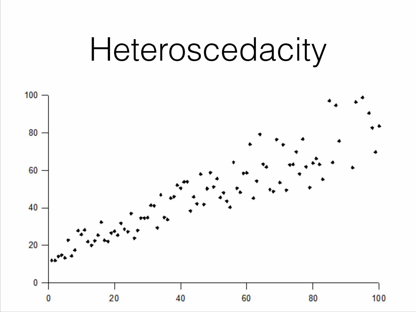
Heteroscedacity

Something to remember• Regression analysis is a SIMPLIFICATION of reality and provides us with:
• A simplified view of the relationship between 2 or more variables
• A way of fitting a model to our data.
• Means for evaluating the importance of the variables to the outcome of interest.
• A way to assess the fit of the model and to compare models.
Yi = �0 + �1Xi1 + �2Xi2 + · · ·+ �pX1p + ✏i

“Remember that all models are wrong; the practical question is how
wrong they have to be to be not useful.”
-George Box

We want to fit a line through this data.


What are the criteria for a good line through the data?

Are any of these lines the best possible line?

Least Squares• A good line minimizes the distance between each data
point and the line.
• This means that our model (which at this point is just a line) is as close as possible to our data.
• This is referred to a the “least squares” line.
• To get this line we have to estimate some parameters.
• Simplest method of estimation is OLS (Ordinary Least Squares)

Residuals• A good model is one that
describes the data well. • We can measure how well
a model describes the data by looking at the “residuals”
• A model with small residuals is said to “fit” the data.
• The process of doing a regression is sometime called “fitting a model to the data”
Regression Model
Estimate of Y conditional on X
Difference between observed and estimated Y = Residual

bxay +=ˆin
terc
ept
y
x

y
x

y
x
xy
bΔ
Δ== slope
(0, a)
The red bars are the residuals (only two are shown, but each point has one)
yye i ˆ−=
y
iy

Least Squares• We want to find the line that minimizes the residuals,
the difference between our regression prediction and our observed data – the line with the least square error.

An example in R• The LA_RAIN.csv dataset contains 43 years worth of
precipitation measurements (in inches) taken at six sights in the Owens Valley labeled APMAM (Mammoth Lake), APSAB (Lake Sabrina), APSLAKE (South Lake), OPBPC (Big Pine Creek), OPRC (Rock Creek), and OPSLAKE, and stream runoff volume (measured in acre-feet) at a sight near Bishop, California (labeled BSAAM).
• Lets model the relationship between precip and runoff at one weather station.
• Use the function lm() to build a“linear model”

An example in R
> la_rain <- read.csv("~/Dropbox/GEOG 5023/Data/LA_RAIN.csv")!> summary(la_rain)!> summary(la_rain)! Year APMAM APSAB APSLAKE OPBPC OPRC OPSLAKE BSAAM ! Min. :1948 Min. : 2.700 Min. : 1.450 Min. : 1.77 Min. : 4.050 Min. : 4.350 Min. : 4.600 Min. : 41785 ! 1st Qu.:1958 1st Qu.: 4.975 1st Qu.: 3.390 1st Qu.: 3.36 1st Qu.: 7.975 1st Qu.: 7.875 1st Qu.: 8.705 1st Qu.: 59857 ! Median :1969 Median : 7.080 Median : 4.460 Median : 4.62 Median : 9.550 Median :11.110 Median :12.140 Median : 69177 ! Mean :1969 Mean : 7.323 Mean : 4.652 Mean : 4.93 Mean :12.836 Mean :12.002 Mean :13.522 Mean : 77756 ! 3rd Qu.:1980 3rd Qu.: 9.115 3rd Qu.: 5.685 3rd Qu.: 5.83 3rd Qu.:16.545 3rd Qu.:14.975 3rd Qu.:16.920 3rd Qu.: 92206 ! Max. :1990 Max. :18.080 Max. :11.960 Max. :13.02 Max. :43.370 Max. :24.850 Max. :33.070 Max. :146345 !!> plot(la_rain) #useful for small data.frames (NEXT SLIDE)

Which weather station should we use?

An example in R> lm(BSAAM ~ APSAB, data=la_rain) #Not much information!!Call:!lm(formula = BSAAM ~ APSAB, data = la_rain)!!Coefficients:!(Intercept) APSAB ! 67152 2279 !!> !> aLmObject <- lm(BSAAM ~ OPSLAKE, data=la_rain)!> !> summary(aLmObject)!!Call:!lm(formula = BSAAM ~ OPSLAKE, data = la_rain)!!Residuals:! Min 1Q Median 3Q Max !-17603.8 -5338.0 332.1 3410.6 20875.6 !!Coefficients:! Estimate Std. Error t value Pr(>|t|) !(Intercept) 27014.6 3218.9 8.393 1.93e-10 ***!OPSLAKE 3752.5 215.7 17.394 < 2e-16 ***!---!Signif. codes: 0 ‘***’ 0.001 ‘**’ 0.01 ‘*’ 0.05 ‘.’ 0.1 ‘ ’ 1!!Residual standard error: 8922 on 41 degrees of freedom!Multiple R-squared: 0.8807,! Adjusted R-squared: 0.8778 !F-statistic: 302.6 on 1 and 41 DF, p-value: < 2.2e-16!!
Is this a good model??

Interpreting Parameters
• In a simple regression model we have two parameters.
• Slope: The expected change in Y for a unit change in X.
• Intercept: The expected value of Y when X is zero.
The Intercept• Sometimes X cannot logically equal zero, thus its
useful to transform the variable such that the intercept is interpretable.
• For example, subtracting the mean from each observation such that the value X=0 is the man of X.
• Examples in Gelman.

Changing the meaning of the intercept.
> ##RECODE OPSLAKE Variable!> la_rain$OPSLAKEmean0 <- la_rain$OPSLAKE - mean(la_rain$OPSLAKE)!> !> summary(lm(BSAAM ~ OPSLAKEmean0, data=la_rain))!!Call:!lm(formula = BSAAM ~ OPSLAKEmean0, data = la_rain)!!Residuals:! Min 1Q Median 3Q Max !-17603.8 -5338.0 332.1 3410.6 20875.6 !!Coefficients:! Estimate Std. Error t value Pr(>|t|) !(Intercept) 77756.0 1360.7 57.15 <2e-16 ***!OPSLAKEmean0 3752.5 215.7 17.39 <2e-16 ***!---!Signif. codes: 0 ‘***’ 0.001 ‘**’ 0.01 ‘*’ 0.05 ‘.’ 0.1 ‘ ’ 1!!Residual standard error: 8922 on 41 degrees of freedom!Multiple R-squared: 0.8807,! Adjusted R-squared: 0.8778 !F-statistic: 302.6 on 1 and 41 DF, p-value: < 2.2e-16

Hypothesis tests on regression coefficients.
• We can evaluate the model by looking at the hypothesis tests included in the output.
• Understand the t-test on regression coefficients.
• Derive R-squared value.

Hypothesis tests about regression coefficients
• Each regression coefficient is t-tested.
• The null hypothesis for this test is that the coefficient = 0.
In the previous slide 2279/1909 = 1.194
t =observed difference� expected difference
standard error
=(� � 0)� 0
standard error

Why does the t-test work on regression coefficients?
• Regression coefficients have a bell shaped sampling distribution.
• In regression the standard errors of that distribution are estimated.!
• That estimate is used to construct a t-test.
• We can simulate the standard error of regression coefficients under the null hypothesis (see next slide). Those simulated results should be similar to the estimate.

Why does the t-test work on regression estimates?
###GENERATE DATA!rnormcor <- function(x,rho) rnorm(n=1, mean= rho*x, sd=sqrt(1-rho^2))!a <- rnorm(10000,0,1)!b <- sapply(a, rnormcor, rho = 0.01) #rho = correlation between a and b!!##PLOT DATA!plot(a~b)!!##CREATE A TABLE (DATA.FRAME)!data.ab <- data.frame(a,b)!!##Run a regression of a on b in a loop.!betas <- NA!for(i in 1:1000){! rows <- sample(1:nrow(data.ab), 100) #get a random list of 100 row numbers! samp <- data.ab[rows, ] #subset data.frame using row numbers ! reg <- lm(samp$a~samp$b) #run a regression! betas[i] <- coef(reg)[2] #save the slope of the regression!} !hist(betas)!!sd(betas)![1] 0.1035647!reg <- lm(samp$a~samp$b)!summary(reg)!!Call:!lm(formula = samp$a ~ samp$b)!!Residuals:! Min 1Q Median 3Q Max !-2.9138 -0.6561 0.1799 0.6444 2.4694 !!Coefficients:! Estimate Std. Error t value Pr(>|t|)!(Intercept) -0.0008909 0.1063534 -0.008 0.993!samp$b 0.0232551 0.1014510 0.229 0.819!!Residual standard error: 1.054 on 98 degrees of freedom!Multiple R-squared: 0.0005359,! Adjusted R-squared: -0.009663 !F-statistic: 0.05254 on 1 and 98 DF, p-value: 0.8192
Notice that the variation in our simulated regression coefficients sd(betas) is close to estimate of the standard error of the slope from a single regression. The LM function does a good job of estimating the random variation in regression coefficients.
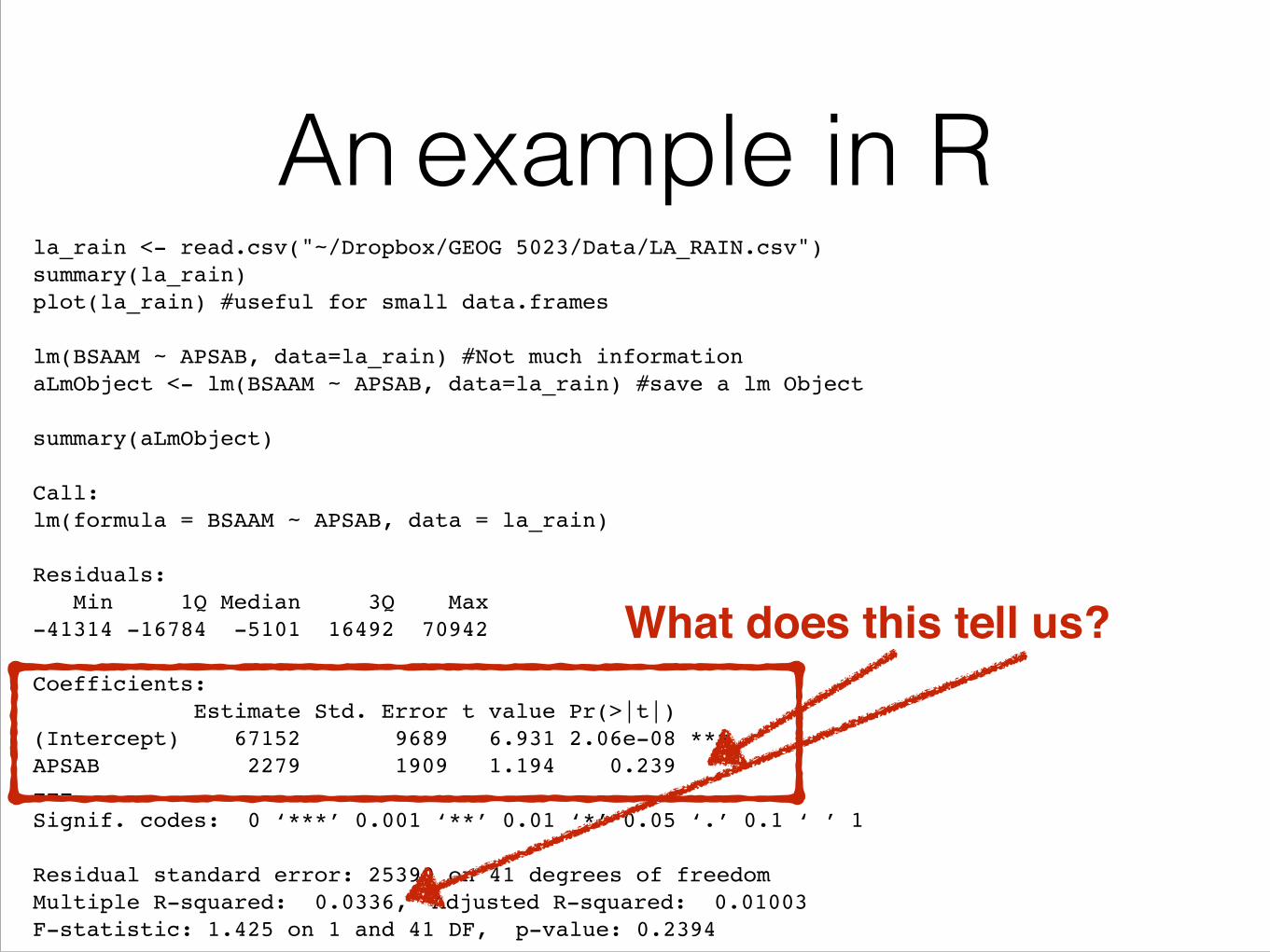
An example in Rla_rain <- read.csv("~/Dropbox/GEOG 5023/Data/LA_RAIN.csv")!summary(la_rain)!plot(la_rain) #useful for small data.frames!!lm(BSAAM ~ APSAB, data=la_rain) #Not much information!aLmObject <- lm(BSAAM ~ APSAB, data=la_rain) #save a lm Object!!summary(aLmObject)!!Call:!lm(formula = BSAAM ~ APSAB, data = la_rain)!!Residuals:! Min 1Q Median 3Q Max !-41314 -16784 -5101 16492 70942 !!Coefficients:! Estimate Std. Error t value Pr(>|t|) !(Intercept) 67152 9689 6.931 2.06e-08 ***!APSAB 2279 1909 1.194 0.239 !---!Signif. codes: 0 ‘***’ 0.001 ‘**’ 0.01 ‘*’ 0.05 ‘.’ 0.1 ‘ ’ 1!!Residual standard error: 25390 on 41 degrees of freedom!Multiple R-squared: 0.0336,! Adjusted R-squared: 0.01003 !F-statistic: 1.425 on 1 and 41 DF, p-value: 0.2394
What does this tell us?

How much of the variation in the outcome (Y) is explained by the model?• Remember, regression is a model of the mean of Y
conditional on the X’s.
• The basic idea is that the mean of Y is somehow affected by X.
• A change in X of 1 is associated with a change of beta in Y.
• We need a way to tell how much of the change in Y is attributable to changes in X.

Decomposing variability in Y
• Deviations from the mean can be partially explained by a covariate (X).
• Some fraction of those deviations from the mean will be due to X.
• Some fraction of those deviations will be unexplained by X.

Decomposing Variance in Y
• For example, the girth of a tree may be strongly related to its age.
• Tree girth (Y) is partially explained by tree age (X).
• How much of the variability in tree girth is explained by tree age?

Decomposing Variance in Y• If we disregard tree age (X), the explanatory
variable.
• We could compute the variance in girth (Y).
• Sum of the squared deviations from the mean.
• That variance is not just noise, some trees are thicker than others because of ____(insert X or explanatory variable)__.

Relating total variance to a linear model.
• If we add up:
• Squared difference between our model predictions (yhat) and the mean (ybar).
• The squared residuals (yi-yhat).
• We should get the total squared deviations from the mean.

Partitioning Sum of Squares

Decomposing variability in Y
SS deviations from mean
Regression (explained) SS Residual SS

Coefficient of Determination
• The percent of the total sum of squares explained by the regression

The equation∑∑∑===
−+−=−n
iii
n
ii
n
ii yyyyyy
1
2
1
2
1
2 )ˆ()ˆ()(
Total sum of squares (TSS)
Regression (explained) sum of squares (ESS)
Residual (unexplained) sum of squares (RSS)
∑
∑
=
=
−
−= n
ii
n
ii
yy
yyR
1
2
1
2
2
)(
)ˆ(The proportion of the total explained variation in y is called the coefficient of determination (R2)

Coefficient of determination (R2)
• R2 of .63 indicates that the variable(s) in the model explain 63% of variance in the outcome !
• Large R2 does not necessarily imply a “good” model • R2 does not:
• Measure the magnitude of the slope • Measure the appropriateness of the model
• As predictors are added to the model R2 will increase • Adjusted R2 is adjusted for the number of predictors in the
model • Generally, you should report adjusted R2

A note about residuals
• Unless the r2 is 100%, there will be some amount of variation in y which remains unexplained by x • The unexplained variation is the error
component of the regression equation

Signal and Noise• We can think of a regression model as having two
parts:
• One part predicts the average of Y for a given value of X.
• The second part is random error, the expected value is zero (E(ε)=0), we assume error has a normal distribution and independent errors.
• Signal + noise

A Diversion…

Galton: Darwin’s cousin, the inventor of regression, and an odd guy

Galton: Darwin’s cousin, the inventor of regression, and an odd guy
“I may here speak of some attempts by myself, to obtain materials for a ‘Beauty Map” of the British Isles. Whenever I have occasion to classify the persons I meet into three classes, “good, medium, bad,” I use a needle mounted as a pricker, wherewith to prick holes, unseen, in a piece of paper, torn rudely into a cross with a long leg. I use its upper end for “good”, the cross arm for “medium,” the lower end for “bad.” The prick-holes keep distinct, and are easily read off at leisure. The object, place, and date are written on the paper. I used this plan for my beauty data, classifying the girls I passed in streets or elsewhere as attractive, indifferent, or repellent. Of course this was a purely individual estimate, but it was consistent, judging from the conformity of different attempts in the same population. I found London to rank highest for beauty: Aberdeen lowest.”


The model is an estimate.
• Don’t know the truth, only estimates based on our data.
• Confidence intervals for parameters.
• The fact that the model parameters (slope and intercept) are estimated means that prediction should account for this uncertainty.

Intervals for Parameters> lm1 <- lm(IMR~logGNI, who)!> confint(lm1)! 2.5 % 97.5 %!(Intercept) 212.91745 260.11324!logGNI -25.65125 -20.24836
These are confidence intervals for the regression coeffs.

Prediction> lm1<-lm(who$IMR~who$logGNI)!
!> new<-data.frame(logGNI=c(6.5,7.5,8,9))!> predict(lm1, newdata=new, interval="confidence")!
! fit lwr upr!1 87.34163 80.60152 94.08175!2 64.39183 59.75707 69.02659!3 52.91693 49.04650 56.78736!4 29.96713 26.37193 33.56232

Looking at the residualsDid we violate any of the regression
assumptions?
> par(mfrow=c(2,1)) > plot(lm1,which=1:2)
!• How do they look?
outliers

Histogram of the Residuals
• Some outliers visible…
Histogram of residuals
resid(lm1)
Frequency
-50 0 50 100
020
4060
80
hist(resid(lm1), main="Histogram of residuals")

Exercise• The LA_RAIN.csv dataset contains 43 years worth of precipitation
measurements (in inches) taken at six sights in the Owens Valley labeled APMAM (Mammoth Lake), APSAB (Lake Sabrina), APSLAKE (South Lake), OPBPC (Big Pine Creek), OPRC (Rock Creek), and OPSLAKE, and stream runoff volume (measured in acre-feet) at a sight near Bishop, California (labeled BSAAM).
• Which weather station (or sets of weather stations) is the best predictor of runoff?
• If you had to close all but one weather stations, and you wanted to estimate runoff effectively, which station would you keep open and why?
• If you could keep open two stations which two would you keep open? Hint: lm(BSAAM ~ station1+ station2)
• For those with advanced regression experience: use regsubsets() in the “leaps” package to explore all possible regression models.