Corporate Cash Savings:

Precaution versus Liquidity

Martin Boileau and Nathalie Moyen

December 2009

AbstractCash holdings as a proportion of total assets of U.S. corporations have roughly doubled between1971 and 2006. Prior research attributes the large cash increase to a rise in firms’ idiosyncraticrisk. We investigate two mechanisms by which increased idiosyncratic risk can lead to higher cashholdings. The first is linked to the precautionary motive inducing firms to be prudent about theirfuture prospects. The second mechanism is linked to the liquidity motive requiring firms to meettheir current liquidity needs. We find that the mechanism embedded in the liquidity motive bestexplains how the increased idiosyncratic risk nearly doubled cash holdings. As for the precautionarymotive, its importance has decreased over time to the point of generating very little precautionarysavings.

Boileau: Department of Economics and CIRPEE, University of Colorado, 256 UCB, Boulder Col-orado 80309, United States. Tel.: 303-492-2108. Fax: 303-492-8960. E-mail: boileau@colorado.edu.

Moyen: Leeds School of Business, University of Colorado, 419 UCB, Boulder Colorado 80309,United States. Tel.: 303-735-4931. Fax: 303-492-5962. E-mail: moyen@colorado.edu.

1 Introduction

Cash holdings as a proportion of total assets of North American COMPUSTAT firms have increased

dramatically since the 1970’s. Figure 1 documents this large and steady increase for our sample

of North American firms.1 Figure 1 also documents that the increase is accompanied by a steady

decline in the capital share of total assets. As for leverage, Figure 1 shows that it is volatile but it

does not display an obvious trend.

The increase in cash holdings is consistent with the observed post-WWII rise in firms’ idiosyn-

cratic risk documented by Campbell et al. (2001). In what follows, we investigate two mechanisms

by which increased idiosyncratic risk can lead to higher cash holdings. The first mechanism is the

precautionary motive. It arises because firms face various tax rates, as well as adjustment and

issuing costs, which may lead to convex marginal payouts. With convex marginal payouts, firms

act prudently and save more to self-insure against future adverse shocks. With a precautionary

motive, an increase in firms’ idiosyncratic risk raises the need to self-insure and therefore raises

cash holdings. This mechanism is similar to that discussed in Carroll and Kimball (2006), where a

convex marginal utility yields a precautionary motive for consumers.

The second mechanism is the liquidity motive. It arises because it is more costly for firms

to alter their investment, dividend, debt and equity policies than to accumulate cash to meet its

liquidity requirements. With a liquidity motive, a rise in firms’ idiosyncratic risk escalates the

need for liquidity and therefore increases required cash holdings. This mechanism is similar to that

discussed in Telyukova and Wright (2008), where liquidity needs yield a motive for consumers to

accumulate money.

We find that the astounding increase in cash holdings since the 1970’s is attributable to the

liquidity motive. Our finding obtains from a standard dynamic model of a firm’s investment and

financial decisions augmented by both a precautionary motive and a liquidity motive to hold cash.

Importantly, our model recognizes that cash is a dominated security in terms of return. We show1Cash refers to COMPUSTAT Mnemonic CHE and is composed of cash (CH) and short-term investments (IVST).

It includes, among others, the following items: cash in escrow; government and other marketable securities; lettersof credits; time, demand, and certificates of deposit; restricted cash.

2

that the model offers a reasonable description of firms’ behavior, and can be used to study the

large increase in cash holdings. We focus our analysis on two extreme periods: the first third of

our sample period from 1971 to 1982 and the last third from 1995 to 2006. We find that both

the precautionary and liquidity motives play important roles in explaining cash holdings in the

first period, but that the liquidity motive explains most of the cash holdings in the last period.

Consequently, we conclude that the increase in firms’ idiosyncratic risk raises cash holdings via the

liquidity motive.

Bates, Kahle, and Stulz (2008) first noted the dramatic increase in cash holdings. In their

empirical analysis, they identify the increase in industry cash flow risk as the main determinant of

the increase in cash holdings. They hypothesize that the large cash increase may be attributable to

the precautionary motive. In our study, we disentangle the two mechanisms by which risk can affect

cash holdings: through precautionary savings as firms self-insure against future adverse shocks and

through liquidity needs as firms meet their current liquidity requirements.

Our model does not consider the other motives to hold cash discussed in Bates, Kahle, and Stulz

(2008), as they do not find wide empirical support for these. Our neoclassical framework does not

feature the agency motive to hold cash. We recognize that the relationship between higher cash

holdings (or lower cash value) and higher agency costs is well documented in other contexts.2

In addition, our model does not feature the tax motive to hold cash. We recognize that Foley

et al. (2007) show convincingly that U.S. multinationals accumulate cash in their subsidiaries to

avoid the tax costs associated with repatriated foreign profits. However, Bates, Kahle, and Stulz

(2008) note that the large increase in cash holdings is observed also for domestic firms.

Our model does not feature a fixed transaction cost motive to hold cash. We recognize that

Mulligan (1997) provides ample empirical evidence for the transaction cost motive of Baumol (1952)

and Miller and Orr (1966), where there is a fixed cost of converting non-liquid assets into cash.2For example, see Dittmar and Mahrt-Smith (2007), Dittmar et al. (2003), Faulkender and Wang (2006), Harford

(1999), Harford et al. (2008), and Pinkowitz et al. (2006). Our modeling choice however is motivated by the fact thatOpler et al. (1999) find little evidence that cash holdings lead to larger capital investments or mergers and acquisitionsas predicted by the free cash flow hypothesis of Jensen (1986). Also, Bates, Kahle, and Stulz (2008) obtain results,using the Gompers, Ishii, and Metrick (2003) entrenchment index among other measures, that fail to support theagency problem explanation for the overall rise in cash holdings of U.S. firms.

3

Instead of a fixed conversion cost, we assume that firms can convert capital and debt into cash, but

only at discrete intervals of time.

There are a number of papers examining the cash hoarding behavior of U.S. firms. Nikolov

(2008) shows that increased market competition can in part explain the rise in cash holdings,

especially for financially constrained firms in riskier industries. Almeida, Campello, and Weisbach

(2004) and Han and Qiu (2007) document that financially constrained firms accumulate cash out

of cash flow, while unconstrained firms do not. Acharya, Almeida, and Campello (2007) show that

this behavior is strongest for constrained firms that suffer from a low correlation between operating

income flow and investment opportunities. When controlling for measurement errors, Riddick and

Whited (2008) find that cash holdings are negatively associated with cash flows.

The model of Gamba and Triantis (2008) is closely related to our model in that a firm can

finance its investment through debt issues, equity issues, and internal funds, where only internal

funds do not trigger transaction costs. Their focus is on valuing financial flexibility, while we focus

on exploring the motives behind the large increase in cash holdings.

Bolton, Chen, and Wang (2009) present another closely related model, and like ours, it recog-

nizes that cash is dominated in return. They propose a dynamic model of investment decisions for

financially constrained firms with constant returns to scale in production. Among other contribu-

tions, they find that Tobin’s marginal q may be inversely related to investment, and that financially

constrained firms may have lower equity betas because of precautionary cash holdings. Our paper

departs from the assumption of constant returns to scale in production, and examines the effect of

the capital share on the relative strengths of the precautionary and liquidity motives to hold cash.

The paper is organized as follows. Section 2 presents the model, and provides some analytical

results characterizing the behavior of cash holdings. The model however does not possess an ana-

lytical solution. Section 3 discusses the calibration of the model. Section 4 presents our simulation

results. We first ensure that the model broadly reproduces observed facts. We then use the model

to study the rise in cash holdings. Section 5 offers some concluding remarks.

4

2 The Model

We study how a firm manages its cash holdings in an otherwise standard dynamic model of financial

and investment decisions. The firm does not consider cash as a perfect substitute for debt: cash

is not negative debt. Instead, cash savings serve two purposes. They may provide self-insurance

against future adverse shocks, and they may provide liquidity to meet current adverse shocks.

To operationalize both motives, we assume that the firm faces shocks to its revenues and

expenses. Knowing the current realization of the revenue shock, the firm chooses how much to

invest, how much cash to save, how much debt to issue, how much to pay out or how much equity

to raise. During the year, however, the firm may face expenses that turn out to be either lower or

higher than expected back at the beginning of the year. When expenses are higher than expected,

the firm cannot scale back its investment commitments, take back its distributed dividend, or

go back to external markets with more favorable issuing conditions. The higher than expected

expenses are met with cash. As is explained in details below, the firm holds sufficient cash to pay

the unknown expenses that occur during the year. The firm may also hold additional cash as a

precaution against future adverse shocks to revenues.

2.1 The Firm

The firm, acting in the interest of shareholders, maximizes the discounted expected stream of

payouts Dt taking into account taxes and issuing costs. When payouts are positive, shareholders

pay taxes on the distributions according to a tax schedule T (D). The schedule recognizes that firms

can minimize taxes for smaller payouts by distributing them in the form of share repurchases. Firms,

however, have no choice but to trigger the dividend tax for larger payouts. Following Hennessy

and Whited (2007), the tax treatment of payouts is captured by a schedule that is increasing and

convex:

T (Dt) = τDDt +τDφ

exp−φDt −τDφ, (1)

where φ > 0 controls the convexity of T (D) and 0 < τD < 1 is the tax rate. When payouts are

negative, shareholders send cash infusions into the firm as in the case of an equity issue. The convex

5

schedule T (D) also captures the spirit of Altinkilic and Hansen (2000), where equity issuing costs

are documented to be increasing and convex. Figure 2 displays the schedule T (D) for different

values of τD and φ.

Net payouts are

U(Dt) = Dt − T (Dt). (2)

For finite values of Dt, this function is increasing U ′(Dt) = 1 − τD + τD exp(−φDt) > 0, concave

U ′′(Dt) = −φτD exp(−φDt) < 0, and its third derivative is positive U ′′′(Dt) = φ2τD exp(−φDt) > 0.

As a result, the net payout function ensures that the firm is risk averse and has a precautionary mo-

tive. In this context, the parameter φ is the coefficient of absolute prudence: φ = −U ′′′(Dt)/U ′′(Dt).

The firm faces two sources of risk. The first source of risk comes from stochastic revenues.

Revenues Yt are generated by a decreasing returns to scale function of the capital stock Kt:

Yt = exp(zt)ΓKαt , (3)

where zt is the current realization of the shock to revenues, the parameter 0 < α < 1 denotes the

capital share, and Γ > 0 is a scale parameter. The revenue shock follows the autoregressive process

zt = ρzzt−1 + σεεt, (4)

where εt is the innovation to the revenue shock, and the parameters 0 < ρz < 1 and σε > 0 denote

persistence and volatility. The innovations are independent and identically distributed random

variables drawn from a standard normal distribution.

The second source of risk comes from stochastic expenses Ft. The firm’s expenses are given by

Ft = F + ft, (5)

where F ≥ 0 is the predictable level of expenses and ft is the current realization of the expense

innovation. For simplicity, the expense innovations are assumed to be independent of the revenue

innovations and drawn from a uniform distribution ft ∈ −σF , . . . , σF where σF > 0.

The firm makes its investment and financial decisions with knowledge of the current realization

of the revenue shock but not the realization of the expense shock. The firm chooses how much to

6

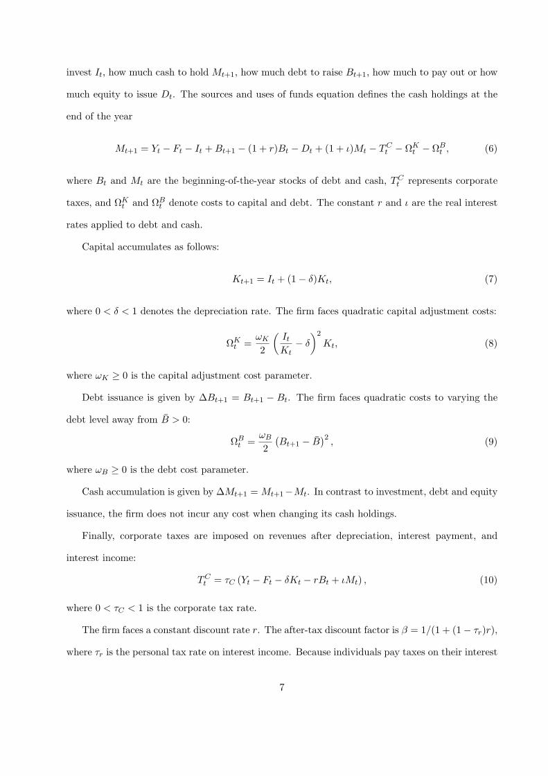
invest It, how much cash to hold Mt+1, how much debt to raise Bt+1, how much to pay out or how

much equity to issue Dt. The sources and uses of funds equation defines the cash holdings at the

end of the year

Mt+1 = Yt − Ft − It +Bt+1 − (1 + r)Bt −Dt + (1 + ι)Mt − TCt − ΩKt − ΩB

t , (6)

where Bt and Mt are the beginning-of-the-year stocks of debt and cash, TCt represents corporate

taxes, and ΩKt and ΩB

t denote costs to capital and debt. The constant r and ι are the real interest

rates applied to debt and cash.

Capital accumulates as follows:

Kt+1 = It + (1− δ)Kt, (7)

where 0 < δ < 1 denotes the depreciation rate. The firm faces quadratic capital adjustment costs:

ΩKt =

ωK2

(ItKt− δ

)2

Kt, (8)

where ωK ≥ 0 is the capital adjustment cost parameter.

Debt issuance is given by ∆Bt+1 = Bt+1 − Bt. The firm faces quadratic costs to varying the

debt level away from B > 0:

ΩBt =

ωB2(Bt+1 − B

)2, (9)

where ωB ≥ 0 is the debt cost parameter.

Cash accumulation is given by ∆Mt+1 = Mt+1−Mt. In contrast to investment, debt and equity

issuance, the firm does not incur any cost when changing its cash holdings.

Finally, corporate taxes are imposed on revenues after depreciation, interest payment, and

interest income:

TCt = τC (Yt − Ft − δKt − rBt + ιMt) , (10)

where 0 < τC < 1 is the corporate tax rate.

The firm faces a constant discount rate r. The after-tax discount factor is β = 1/(1 + (1− τr)r),

where τr is the personal tax rate on interest income. Because individuals pay taxes on their interest

7

income at a lower rate than the rate at which corporations deduct their interest payment τr < τC ,

debt financing is tax-advantaged. To counter this benefit of debt financing, the convex cost in

Equation (9) bounds the debt level. In this sense, the deviation costs play a role similar to a

collateral constraint.3

Similar to the constant discount rate r, the interest rate received on cash holdings ι is assumed

to be constant over time. Moreover, cash is a dominated security in terms of return: ι < r. In

practice, a firm holding cash incurs a real return loss equal to the inflation.

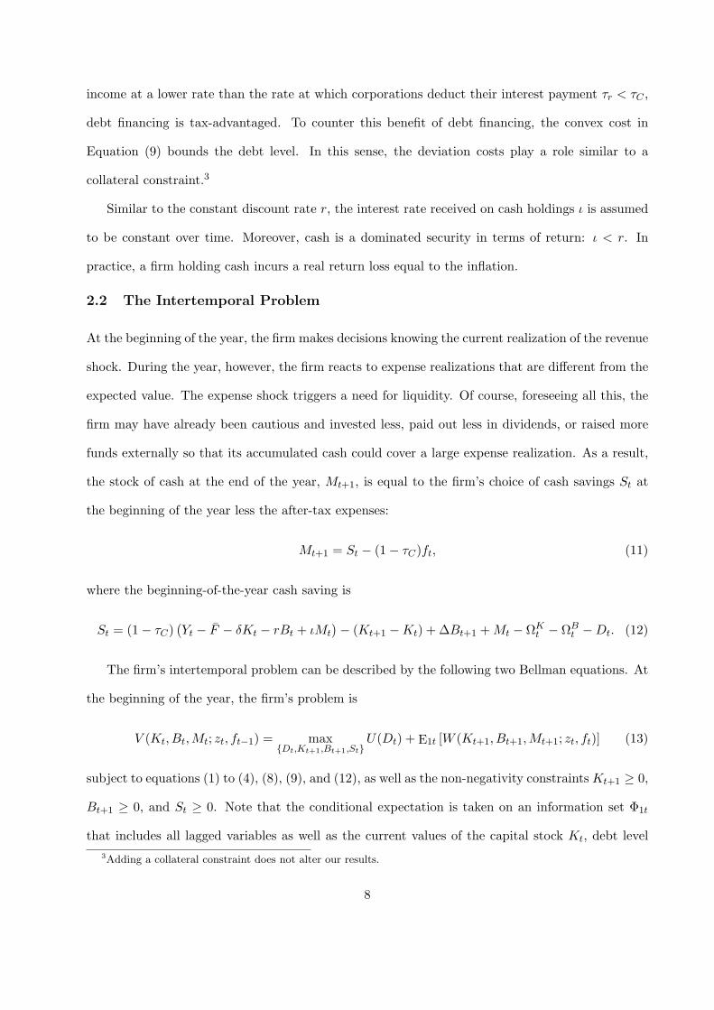
2.2 The Intertemporal Problem

At the beginning of the year, the firm makes decisions knowing the current realization of the revenue

shock. During the year, however, the firm reacts to expense realizations that are different from the

expected value. The expense shock triggers a need for liquidity. Of course, foreseeing all this, the

firm may have already been cautious and invested less, paid out less in dividends, or raised more

funds externally so that its accumulated cash could cover a large expense realization. As a result,

the stock of cash at the end of the year, Mt+1, is equal to the firm’s choice of cash savings St at

the beginning of the year less the after-tax expenses:

Mt+1 = St − (1− τC)ft, (11)

where the beginning-of-the-year cash saving is

St = (1− τC)(Yt − F − δKt − rBt + ιMt

)− (Kt+1 −Kt) + ∆Bt+1 +Mt − ΩK

t − ΩBt −Dt. (12)

The firm’s intertemporal problem can be described by the following two Bellman equations. At

the beginning of the year, the firm’s problem is

V (Kt, Bt,Mt; zt, ft−1) = maxDt,Kt+1,Bt+1,St

U(Dt) + E1t [W (Kt+1, Bt+1,Mt+1; zt, ft)] (13)

subject to equations (1) to (4), (8), (9), and (12), as well as the non-negativity constraints Kt+1 ≥ 0,

Bt+1 ≥ 0, and St ≥ 0. Note that the conditional expectation is taken on an information set Φ1t

that includes all lagged variables as well as the current values of the capital stock Kt, debt level3Adding a collateral constraint does not alter our results.

8

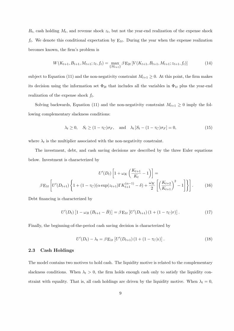
Bt, cash holding Mt, and revenue shock zt, but not the year-end realization of the expense shock

ft. We denote this conditional expectation by E1t. During the year when the expense realization

becomes known, the firm’s problem is

W (Kt+1, Bt+1,Mt+1; zt, ft) = maxMt+1

β E2t [V (Kt+1, Bt+1,Mt+1; zt+1, ft)] (14)

subject to Equation (11) and the non-negativity constraint Mt+1 ≥ 0. At this point, the firm makes

its decision using the information set Φ2t that includes all the variables in Φ1t plus the year-end

realization of the expense shock ft.

Solving backwards, Equation (11) and the non-negativity constraint Mt+1 ≥ 0 imply the fol-

lowing complementary slackness conditions:

λt ≥ 0, St ≥ (1− τC)σF , and λt [St − (1− τC)σF ] = 0, (15)

where λt is the multiplier associated with the non-negativity constraint.

The investment, debt, and cash saving decisions are described by the three Euler equations

below. Investment is characterized by

U ′(Dt)[1 + ωK

(Kt+1

Kt− 1

)]=

β E1t

[U ′(Dt+1)

1 + (1− τC)(α exp(zt+1)ΓK(α−1)

t+1 − δ) +ωK2

[(Kt+2

Kt+1

)2

− 1

]]. (16)

Debt financing is characterized by

U ′(Dt)[1− ωB

(Bt+1 − B

)]= β E1t

[U ′(Dt+1) (1 + (1− τC)r)

]. (17)

Finally, the beginning-of-the-period cash saving decision is characterized by

U ′(Dt)− λt = β E1t[U ′(Dt+1) (1 + (1− τC)ι)

]. (18)

2.3 Cash Holdings

The model contains two motives to hold cash. The liquidity motive is related to the complementary

slackness conditions. When λt > 0, the firm holds enough cash only to satisfy the liquidity con-

straint with equality. That is, all cash holdings are driven by the liquidity motive. When λt = 0,

9

the firm may hold more cash than required by the liquidity motive. We summarize these findings

in the following proposition.

Proposition 1 When λt > 0, St = (1 − τC)σF so that the firm holds cash only as a safeguard

against the year-end expense shock realization. When λt = 0, St ≥ (1− τC)σF so that the firm may

hold more cash.

Cash holdings are characterized by Equation (18), rewritten as

U ′(Dt)− λt = βRM E1t[U ′(Dt+1)

], (19)

where RM = 1 + (1 − τC)ι is the net return to cash. Note that βRM < 1 reflects the impatience

embedded in cash holdings. Because of this impatience, Equation (19) naturally yields a stationary

distribution of dividends over time when λt > 0. As Proposition 1 describes, this occurs when cash

holdings are entirely driven by the liquidity motive.

Obtaining a stationary distribution when λt = 0 requires that U ′(D) be convex. To see this,

note that Equation (19) implies that U ′(Dt) < E1t [U ′(Dt+1)] when λt = 0. By Jensen’s inequality,

this inequality is satisfied when U ′(·) is convex. U ′(·) is indeed convex because of our assumptions

about the schedule of taxes and equity issuing costs T (Dt). The convexity of the marginal net

payout function may therefore generate precautionary savings, so that cash holdings may be larger

than required by the liquidity motive. We summarize these findings in the following proposition.

Proposition 2 When λt = 0 and U ′(Dt) is convex, St ≥ (1−τC)σF and the firm may hold cash as

a safeguard against both the year-end expense shock realization and as a precaution against future

shocks.

The relative strengths of the precautionary and liquidity motives depend on the firm’s decisions

with respect to debt and investment. To see the effect of the debt decision on cash holdings,

Equation (17) is rewritten as

E1t [mt+1]RBt = 1, (20)

10

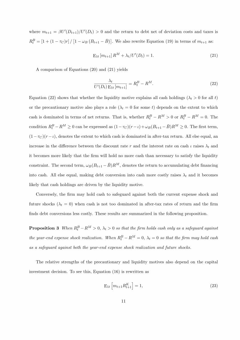
where mt+1 = βU ′(Dt+1)/U ′(Dt) > 0 and the return to debt net of deviation costs and taxes is

RBt = [1 + (1− τC)r] /[1− ωB

(Bt+1 − B

)]. We also rewrite Equation (19) in terms of mt+1 as:

E1t [mt+1]RM + λt/U′(Dt) = 1. (21)

A comparison of Equations (20) and (21) yields

λtU ′(Dt) E1t [mt+1]

= RBt −RM . (22)

Equation (22) shows that whether the liquidity motive explains all cash holdings (λt > 0 for all t)

or the precautionary motive also plays a role (λt = 0 for some t) depends on the extent to which

cash is dominated in terms of net returns. That is, whether RBt −RM > 0 or RBt −RM = 0. The

condition RBt −RM ≥ 0 can be expressed as (1−τC)(r− ι)+ωB(Bt+1− B)RM ≥ 0. The first term,

(1−τC)(r− ι), denotes the extent to which cash is dominated in after-tax return. All else equal, an

increase in the difference between the discount rate r and the interest rate on cash ι raises λt and

it becomes more likely that the firm will hold no more cash than necessary to satisfy the liquidity

constraint. The second term, ωB(Bt+1− B)RM , denotes the return to accumulating debt financing

into cash. All else equal, making debt conversion into cash more costly raises λt and it becomes

likely that cash holdings are driven by the liquidity motive.

Conversely, the firm may hold cash to safeguard against both the current expense shock and

future shocks (λt = 0) when cash is not too dominated in after-tax rates of return and the firm

finds debt conversions less costly. These results are summarized in the following proposition.

Proposition 3 When RBt −RM > 0, λt > 0 so that the firm holds cash only as a safeguard against

the year-end expense shock realization. When RBt −RM = 0, λt = 0 so that the firm may hold cash

as a safeguard against both the year-end expense shock realization and future shocks.

The relative strengths of the precautionary and liquidity motives also depend on the capital

investment decision. To see this, Equation (16) is rewritten as

E1t

[mt+1R

Kt+1

]= 1, (23)

11

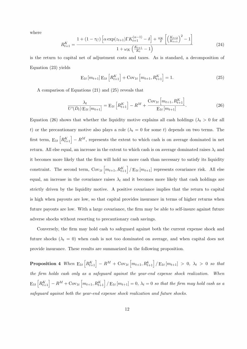
where

RKt+1 =1 + (1− τC)

[α exp(zt+1)ΓK(α−1)

t+1 − δ]

+ ωK2

[(Kt+2

Kt+1

)2− 1

]1 + ωK

(Kt+1

Kt− 1

) (24)

is the return to capital net of adjustment costs and taxes. As is standard, a decomposition of

Equation (23) yields

E1t [mt+1] E1t

[RKt+1

]+ Cov1t

[mt+1, R

Kt+1

]= 1. (25)

A comparison of Equations (21) and (25) reveals that

λtU ′(Dt) E1t [mt+1]

= E1t

[RKt+1

]−RM +

Cov1t

[mt+1, R

Kt+1

]E1t [mt+1]

. (26)

Equation (26) shows that whether the liquidity motive explains all cash holdings (λt > 0 for all

t) or the precautionary motive also plays a role (λt = 0 for some t) depends on two terms. The

first term, E1t

[RKt+1

]− RM , represents the extent to which cash is on average dominated in net

return. All else equal, an increase in the extent to which cash is on average dominated raises λt and

it becomes more likely that the firm will hold no more cash than necessary to satisfy its liquidity

constraint. The second term, Cov1t

[mt+1, R

Kt+1

]/E1t [mt+1] represents covariance risk. All else

equal, an increase in the covariance raises λt and it becomes more likely that cash holdings are

strictly driven by the liquidity motive. A positive covariance implies that the return to capital

is high when payouts are low, so that capital provides insurance in terms of higher returns when

future payouts are low. With a large covariance, the firm may be able to self-insure against future

adverse shocks without resorting to precautionary cash savings.

Conversely, the firm may hold cash to safeguard against both the current expense shock and

future shocks (λt = 0) when cash is not too dominated on average, and when capital does not

provide insurance. These results are summarized in the following proposition.

Proposition 4 When E1t

[RKt+1

]− RM + Cov1t

[mt+1, R

kt+1

]/E1t [mt+1] > 0, λt > 0 so that

the firm holds cash only as a safeguard against the year-end expense shock realization. When

E1t

[RKt+1

]−RM + Cov1t

[mt+1, R

Kt+1

]/E1t [mt+1] = 0, λt = 0 so that the firm may hold cash as a

safeguard against both the year-end expense shock realization and future shocks.

12

3 Data and Calibration

The model is solved numerically because it does not possess an analytical solution. The numerical

method, described in the appendix, requires values for all parameters. To this end, a number of

parameters are set to values that are directly estimated from the data. The remaining parameters

are set to values chosen to ensure that simulated series from the model replicate important features

of the data. The data comes from the North American COMPUSTAT file and covers the period

from 1971 to 2006. To explain the large change in cash holdings, the data is split in two extreme

time periods: the first third of the sample period from 1971 to 1982 and the last third from

1995 to 2006. The COMPUSTAT sample includes firm-year observations with positive values for

total assets (COMPUSTAT Mnemonic AT), property, plant, and equipment (PPENT), and sales

(SALE). The sample includes firms from all industries, except for utilities and financials, with at

least five years of consecutive data. The data is winsorized to limit the influence of outliers at the

1% and 99% tails. The final sample contains 53,067 firm-year observations for the 1971 to 1982

period and 67,720 firm-year observations for the 1995 to 2006 period.

3.1 Parameters Estimated from the Data

Table 1 presents the first set of parameter estimates for both periods. The capital share of revenues

α, the scale of revenues Γ, the persistence of the revenue shock ρz, and the volatility of its innovations

σε are estimated from the revenue Equation (3) and the autoregressive process (4). For each of the

two time periods, the four parameters are estimated for each firm, and then averaged over all firms.

Revenues Yt are measured as sales, and the beginning-of-the-period capital stock Kt is measured

as lagged property, plant, and equipment.4

For the 1971-1982 period, the averages are α = 0.5785, Γ = 2.2731, ρz = 0.2452, and σε =

0.2104. For the 1995-2006 period, the averages are α = 0.4233, Γ = 3.1799, ρz = 0.2062 and

σε = 0.3093. The share α of physical capital that explains revenues has decreased over time but the4As an alternative, the capital stock could be reconstructed from the accumulation Equation (7) using capital

expenditures (CAPX) assuming an initial value for the capital stock and a value for the depreciation rate. We donot pursue this alternative approach for two reasons. First, it requires a value for the depreciation rate, which wouldprevent our estimation of the depreciation rate. Second, measuring the capital stock as lagged property, plant, andequipment results in parameter estimates that are close to those obtained elsewhere in the literature.

13

scale Γ has increased. Note that the values for the capital share α are in line with the values used in

Moyen (2004), Hennessy and Whited (2005, 2007), and Gamba and Triantis (2008). Over time, the

economic environment became less predictable and more volatile: the persistence ρz of the revenue

shock has decreased and the volatility σε has increased. The parameters of the stochastic process

indicate a significant increase in the unconditional variance of the revenue shock σ2ε /(1− ρ2

z) from

4.71 percent during the 1971-1982 period to 9.99 percent during the 1995-2006 period.

The corporate tax rate τC is set to the top marginal rate. The top marginal tax rate was 48%

from 1971 to 1978 and 46% from 1979 to 1982. The top corporate marginal tax rate has been

constant at 35% since 1993. As a result, the corporate tax rate is set to its twelve year average of

τC = 0.4733 for the first period and to τC = 0.35 for the last period. The personal tax rates are

set to the average marginal tax rates reported in NBER’s TAXSIM. Over the 1971-1982 period,

the marginal interest income tax rate averaged τr = 0.2761 while the marginal dividend tax rate

averaged τD = 0.3948. Since the Reagan era, the U.S. tax rates are lower. Thus, over the 1995-2006

period, the marginal interest income tax rate averaged τr = 0.2440 while the marginal dividend tax

rate averaged τD = 0.2325.

The real interest rate r is set to the average of the monthly annualized t-bill rate deflated by

the consumer price index. High inflation characterized much of the period from 1971 to 1982. As a

result, the real interest rate was quite low, at r = 0.5848%. As for the later period of 1995 to 2006,

the real interest rate was higher, at r = 1.6091%. For the interest rate earned on cash holdings ι, we

disentangle the two components of cash (CHE): short-term investments (IVST) and cash (CH).5 In

1971-1982, firms held 30.66 percent of their cash in short-term investments earning a rate of return

r and 69.34 percent in cash earning a zero nominal interest rate. Given an average inflation rate5The cash (CH) item includes: bank and finance company receivables; bank drafts; bankers’ acceptances; cash

on hand; certificates of deposit included in cash by the company; checks; demand certificates of deposit; demanddeposits; letters of credit; and money orders. The short-term investments (IVST) item includes accrued interestincluded with short-term investments by the company; cash in escrow; cash segregated under federal and otherregulations; certificates of deposit included in short-term investments by the company; certificates of deposit reportedas separate item in current assets; commercial paper; gas transmission companies’ special deposits; good faith andclearing house deposits for brokerage firms; government and other marketable securities (including stocks and bonds)listed as short term; margin deposits on commodity futures contracts; marketable securities; money market fund;real estate investment trusts’ shares of beneficial interest; repurchase agreements (when shown as a current asset);restricted cash (when shown as a current asset); time deposits and time certificates of deposit, savings accounts whenshows as a current asset; treasury bills listed as short term.

14

of 7.93%, the interest rate on cash holdings is set to ι = 0.3066r + 0.6934(0 − 0.0793) = −5.32%.

In 1995-2006, firms held even less of their cash savings in short-term investments but the inflation

rate was much lower at 2.60%, so that ι = 0.1564r + 0.8436(0− 0.026) = −1.94%.

3.2 Parameters Estimated by Matching Moments

The last set of parameters cannot be estimated in isolation directly from the data. The estimation

procedure, fully described in the appendix, is based on the simulated method of moments. In spirit,

the estimation strategy targets a particular moment for each parameter. In practice, a change to

one parameter affects all simulated moments. The parameters to be estimated are the depreciation

rate δ, the capital adjustment cost ωK , the constant debt level B, the debt deviation cost ωB, the

average expense level F , the expense volatility σF , and the coefficient of absolute prudence φ. The

important features of the data to replicate are selected moments of investment, debt, and cash

policies.

Two moments of the capital policy are targeted to estimate the depreciation rate δ and the

adjustment cost parameter ωK . The estimate of the depreciation rate δ ensures that the average of

investment-to-total assets simulated from the model matches the average investment found in the

data. In the COMPUSTAT data, the ratio is computed as capital expenditures (CAPX) divided

by total assets (AT). In the model simulated data, the ratio is computed as investment It divided

by total assets At = Vt + (1 + (1− τr)r)Bt −Bt+1. The estimate of the adjustment cost parameter

ωK ensures that the simulated standard deviation of investment It/At normalized by the standard

deviation of revenues Yt/At matches that of the data. We normalize by the standard deviation of

revenues so that the capital adjustment cost ωK can target the volatility of investment in reference

to the volatility of the revenue shock σε.

For the constant debt level B and the cost parameter ωB, we target two moments of the debt

policy. Our estimate of B ensures that the simulated average leverage Bt/At matches that of

COMPUSTAT firms. Leverage is measured by the sum of long-term debt (DLTT) and debt in

current liabilities (DLC) divided by total assets. Similarly to ωK , our estimate of ωB ensures that

the simulated standard deviation of debt relative to the standard deviation of revenues matches

15

that of the actual data. Because costs are more relevant to long-term debt than to short-term debt,

and because changes in debt are often related to changes in collateral, we focus on the standard

deviation of long-term debt-to-capital stock. This standard deviation is then normalized by the

standard deviation of revenues-to-capital stock.

The estimate of F ensures that the average of operating income-to-total assets ratio OIt/At

matches the data, where operating income OIt ≡ Yt−Ft is measured before depreciation (OIBDP).

The estimate of σF ensures that the standard deviation of net income-to-total assets NIt/At

matches the data, where net income is measured as NIt = (1− τC)(Yt−Ft− δKt− rBt+ ιMt). We

target net income because we want to allow for expenses similar to extraordinary items: expenses

that may not be part of the regular operations of the firm but that can affect the firm’s financial

health.

Finally, the convexity parameter φ is the coefficient of absolute prudence and, as such, it dictates

the strength of the firm’s precautionary motive. In the first time period from 1971 to 1982, we

estimate φ to ensure that the average of cash holdings-to-total assets Mt+1/At matches the data,

where cash holdings are measured by cash and short-term investments (CHE). This choice also

ensures that we have the right starting point in our study of the increase in cash holdings. Also, as

measuring the relative strength of the precautionary motive is an important goal of the paper, we

are interested in predicting average cash holdings during the 1995-2006 period without changing

the coefficient of prudence from its 1971-1982 parameter value.

The model is solved numerically under the two sets of parameters using a finite element method.

The appendix provides details on the numerical method. The resulting policy functions for capital

Kt+1, debt Bt+1, cash Mt+1, and the equity value Vt of Equation (13) are simulated from random

outcomes of the innovations to revenues εt and expenses ft. These simulated series serve to build

other series including dividends Dt, operating income OIt, net income NIt, and the total firm value

At. For each of the two calibrations, we construct 5 panels that have roughly the same number of

firm-year observations as observed in the COMPUSTAT panel.

16

4 Results

4.1 Moment Matching Results

Tables 2 and 3 present the results of the moment matching exercise. Table 2 shows the parameter

values and the target moments for the period covering 1971 to 1982, while Table 3 does so for the

period covering 1995 to 2006.

In the data, the average investment-to-total assets is 7.97 percent in the first time period and

6.01 percent in the last time period. To hit these moments, the estimated depreciation rate δ is set

to 0.1738 in the first time period and to 0.1750 in the last time period. These estimates indicate

that the reduction in capital investment from 7.97 percent to 6.01 percent results mostly from the

lower capital share α. To illustrate this point, the deterministic steady state of the capital stock in

the model is

K∗ =(

Γ(1− τC)βα1− β(1− (1− τC)δ)

) 11−α

. (27)

Using our calibrations, K∗ shrinks from 109.28 for the 1971-1982 period to 28.83 for the 1995-2006

period. The lower steady state level of capital corresponds to lower investments.

In COMPUSTAT data, investment has an average standard deviation of 16.79 percent of the

average standard deviation of revenues during the 1971-1982 years and a relative average standard

deviation of 12.05 percent during the 1995-2006 years.6 To replicate these moments, the estimates

of the capital adjustment cost ωK are set to 1.0215 in the first time period and to 0.6155 in the

last time period. These estimates are of magnitudes similar to those obtained by Cooper and

Haltiwanger (2006). All else equal, the lower capital adjustment cost in recent years stimulates the

volatility of investments It/At. This higher volatility, however, is overwhelmed by the increased

volatility of revenues Yt/At. This denominator effect explains why the lower capital adjustment

cost parameter (0.6155 < 1.0215) replicates the lower ratio of standard deviation of investment to

the standard deviation of revenues (12.05% < 16.79%) in recent years.6The relative standard deviation computed in the data differs considerably from the relative standard deviation

commonly shown using macroeconomic data. This simply results from different measurements. For example, we com-pute the standard deviation of the ratio of investment-to-total assets, while macroeconomists compute the standarddeviation of the logarithm of investment detrended using the Hodrick-Prescott filter.

17

The average leverage of COMPUSTAT firms has been fairly constant over time: 0.3052 during

the 1971-1982 period and 0.2795 during the 1995-2006 period. To replicate these moments, the

estimates of the debt target (standardized by mean total assets) B/A are set to 0.3063 in the first

time period and to 0.2853 in the last time period.

The long-term debt-to-capital stock of COMPUSTAT firms has an average standard deviation

of 16.784 percent of the average standard deviation of revenues-to-capital stock during the 1971-

1982 years and a relative average standard deviation of 21.46 percent during the 1995-2006 years.

To replicate these moments, the debt cost estimates ωB are set to 0.0147 in the first time period

and to 0.0127 in the last time period.

In COMPUSTAT data, operating income has declined from an average of 12.36 percent of total

assets during the 1971-1982 period to an average of 0.72 percent of total assets during the 1995-

2006 period. A larger average expense is required to explain the reduction in the average operating

income over time. The estimates of the average expense level (standardized by mean total assets)

F /A are set to 0.0179 for the first period and to 0.1573 for the last period.

In the data, the standard deviation of net income-to-total assets has greatly increased over time

from an average of 0.0665 during the 1971-1982 years to an average of 0.1795 during the 1995-2006

years. The estimates of the volatility parameter (standardized by mean total assets) σF /A are set

to 0.1236 for the first period and to 0.2745 for the last period.

Finally, the average of COMPUSTAT firms’ cash holdings-to-total assetsMt/At was 8.90 percent

during the 1971-1982 years. Matching this moment requires a convexity parameter estimate of

φ = 0.0047. Note that the estimated value is much smaller than the values ranging from 0.73 to

0.83 estimated in the different environment of Hennessy and Whited (2007). In that sense, our

explanation for cash holdings does not rely on a large coefficient of absolute prudence.

4.2 Do Simulated Financial Policies Behave as in the Data?

Before studying cash holdings in detail, it is important to verify that the model provides a reason-

able description of firms’ observed behavior. Admittedly, the moment matching exercise ensures

that specific simulated moments match a number of targeted moments in the data. In what fol-

18

lows, the analysis moves on to controversial moments related to dividend smoothness and debt

countercyclicality. These results appear at the bottom of Tables 2 and 3.

It has long been recognized that firms smooth dividends (see Lintner, 1956). In our COM-

PUSTAT data, payout policies are smooth in the first period. The average standard deviation of

payouts is only 3.23 percent during the 1971 to 1982 period, and rises to 10.46 percent during the

1995 to 2006 period. The model replicates the smooth payout policies in the first period. The

standard deviation is only 3.76 percent for the first period calibration, and rises to 16.42 percent

for the last period calibration. As in the data, the model suggests that payout policies are smooth

in the early period and have become more volatile over time. We note however that the model

overestimates the volatility of payouts in the last period.

In the model, firms smooth payouts to avoid large taxes on payouts and large equity issuing

costs. Specifically, the net payout function U(Dt) recognizes the convexity of taxes and issuing

costs and therefore describes firms as “risk averse.” Firms smooth payouts well in the first period.

Unavoidably, the increase in volatility in the last period substantially increases the volatility of

payouts.

It has also been recognized that firm leverage is countercyclical (see Choe, Masulis, and Nanda,

1993 and Korajczyk and Levy, 2003). In our COMPUSTAT data, the correlation between debt

levels and revenues is −0.3006 for the 1971 to 1982 period and −0.0411 for the 1995 to 2006 period.

In the model, the corresponding correlations are −0.2283 and −0.1896. Both in the data and in

the model, the debt level is countercyclical, and the negative correlation attenuates in the recent

time period. A similar pattern is observed for the correlation between changes in debt levels and

revenues. The COMPUSTAT data correlation between debt issues and revenues is −0.2415 for the

1971 to 1982 period and −0.1877 for the 1995 to 2006 period. In the model, the correlations are

−0.4326 and −0.1155.

The countercyclicality of debt in the model is surprising because standard dynamic capital

structure models with a tax benefit of debt generate procyclical debt. In these models, firms take

on more debt in persistent good times to benefit from the tax advantage because their abilities to

19

repay the debt is solid. In our model, the “risk averse” firm chooses to smooth the effect of adverse

revenue shocks on payouts by issuing more debt.

4.3 Do Simulated Cash Policies Behave as in the Data?

The analysis of cash holdings begins by verifying that the model provides a reasonable overall

description of cash holdings. The results of this analysis appear in Table 4.

In COMPUSTAT data, cash as a fraction of total assets is 8.90 percent in the 1971-1982 period.

That fraction dramatically rises to 17.09 percent in the 1995-2006 period. In the model, the

average ratio of cash holdings-to-total assets is specifically targeted by our calibration using the

convexity parameter for the first period. With the same calibrated value of the convexity parameter

(φ = 0.0047), the model predicts cash holdings of 18.13 percent of total assets in the last period,

which is relatively close to that observed in the data. Interestingly, as dramatic as the observed

cash increase has been, the model predicts even more cash when holding constant the firm’s level

of prudence (φ = 0.0047). This result suggests that firms have become less prudent over time.

Cash policies are relatively smooth in COMPUSTAT data. The standard deviation of cash-to-

total assets is only 4.96 percent during the 1971 to 1982 period and rises to 8.48 percent during

the 1995 to 2006 period. In the model, the average standard deviation is 6.31 percent for the first

period and rises to 17.55 percent for the last period. As in the data, the model predicts that cash

policies have become more volatile, although we note that the model overstates the rise in volatility.

In both the data and the model, cash holdings are nearly acyclical in the earlier period and

they become countercyclical in the later period. In the COMPUSTAT data, the correlation between

cash holdings and revenues decreases from −0.0283 for the 1971-1982 period to −0.0888 for the

1995-2006 period. In the model, the average correlation decreases from 0.0294 to −0.1069.

Table 4 also shows that cash holdings and cash flows are positively correlated in COMPUSTAT

data. The correlation between cash holdings and cash flows is 0.1905 during the 1971 to 1982

period and 0.1689 during the 1995 to 2006 period. In the model, we measure cash flows as net

income minus payouts. The average simulated correlation is 0.6809 during the first period and

0.7025 during the last period. The model correctly predicts the positive correlation, but overstates

20

it.

4.4 The Precautionary and Liquidity Motives to Hold Cash

Given that the model replicates the large increase in cash holdings, as well as several other moments,

the analysis now turns to identifying which motive to hold cash is responsible for the large increase

in cash holdings.

To gain some intuition about the model, Figures 3, 4, and 5 show different aspects of the cash

holdings decision in the model. The figures are constructed by first drawing one series of revenue

shock innovations and one series of expense shock innovations. The same series of innovations are

then used to describe the firm behavior in both periods.

Figure 3 shows that the model-simulated cash holdings are on average higher and much more

volatile in the last period than in the first period. This is consistent with the higher means and

standard deviations of the simulated cash holdings presented in Table 4.

Figures 4 and 5 display the relative strengths of the two motives to hold cash. Figure 4 plots the

multiplier λt under both parameterizations. Recall that cash savings decisions are entirely driven

by the liquidity motive when λt > 0 for all t, and that cash savings decision may also be driven by

the precautionary motive when λt = 0 for some t. The figure shows that strictly positive multiplier

values (λt > 0) occur in both parameterizations of the model, although it occurs more frequently in

the parameterization of the last period. This suggests that the liquidity motive has become more

active over time. Conversely, the precautionary motive to hold cash has become less prevalent.

Figure 5 shows how movements of the multiplier translate into actual cash savings. The figure

graphs the cash saving decision scaled by mean total assets St/A. Standardizing each observation

by the overall mean of total assets A rather than standardizing each observation by the corre-

sponding total assets At focuses attention on the variations in cash savings St while maintaining

the appropriate scale. Figure 5 shows that, for both parameterizations, cash savings are bound

below by a threshold. The threshold corresponds to the lowest cash savings required to meet the

liquidity constraint. That is, when the cash saving St is at the lower threshold, cash holdings Mt+1

are entirely driven by the liquidity motive. When the cash saving is above the threshold, cash

21

holdings are also generated by the precautionary motive.

Although the firm saves more in the last period, cash savings appear to deviate much less

frequently from the lower threshold. Together, Figures 3 to 5 suggest that firms hold more cash

in the last period than in the first period, and that this decision is related to an increase in the

relative strength of the liquidity motive.

4.5 Sensitivity Analysis

To obtain a better understanding of the mechanisms responsible for the large cash increase and

the recent dominance of the liquidity motive over the precautionary motive, Table 5 presents the

results of a sensitivity analysis. The sensitivity analysis proceeds on the basis of the first period

parameterization. In turn each parameter is reset from its first period value to its last period value,

leaving all other parameters to their first period values. The results of the sensitivity analysis

focuses on three groups of parameters.

4.5.1 Cash Policy Parameters

Propositions 1 and 2 state that the firm always holds enough cash during the year to meet its

liquidity threshold (1 − τC)σF . The firm’s cash saving decision directly depends on the volatility

of the expense shock σF and the corporate tax rate τC . Over the two periods, the expense shock

volatility (standardized by mean total assets) grows from 0.1236 to 0.2745, while the corporate tax

rate decreases from 0.4733 to 0.35. This large increase in the cash saving threshold stimulates the

liquidity motive because it forces the firm to save more cash to meet its current liquidity needs.7

Table 5 shows that the large increase of the volatility σF /A is the most important parameter

change explaining the dramatic increase in cash holdings. By changing only the expense shock

volatility to its last period value, the calibration otherwise based on the first period increases its

predicted cash holdings from 8.90 percent of total assets to 19.26 percent, even overshooting the

prediction from the last period benchmark calibration (18.13 percent). Table 5 also shows that the7Carroll and Kimball (2001) show that liquidity constraints by themselves can also induce prudence. In our

context, this means that an increase in the expense threshold may induce the firm to accumulate more precautionarysavings. However, our numerical results show that this does not happen.

22

reduction in the corporate tax rate increases cash holdings.

Equation (19) suggests that the coefficient of absolute prudence φ and the impatience regarding

cash holdings βRM are important factors in assessing the strength of the precautionary motive.

The coefficient of absolute prudence φ controls the convexity of the marginal net payout function

U ′(D). Because the coefficient remains constant over the two periods, it cannot explain the increase

in cash holdings or the diminished strength of the precautionary motive. The impatience factor

βRM grows from 0.9679 in the first period to 0.9755 during the last period. Because firms become

more patient, it should be easier for the cash Euler Equation (18) to hold with λt = 0. That is, the

strength of the precautionary motive should be increasing, rather than decreasing as is the case in

the simulated cash savings of the last period. When the firm becomes more patient, it can afford

to hold more cash.

Disaggregating the effect of the impatience factor βRM = (1 + (1− τC)ι)/(1 + (1− τr)r), Table

5 shows that the increase in the interest rate r and the decrease in the interest income tax rate

τr, which depress the discount factor β and therefore the impatience factor βRM , should reduce

the average cash holdings Mt+1/At, but interestingly they do not. A more detailed analysis reveals

that the increase in the interest rate r does reduce cash holdings, but it also reduces total assets,

such that the cash holdings-to-total asset ratio rises. Total assets decrease because they are valued

at a higher discount rate r. As for the small reduction of the interest income tax rate τr, it does

not significantly affect cash holdings.

Similarly, Table 5 shows that the large increase in average expenses F /A does not significantly

affect cash holdings.

The final cash policy parameter to discuss is the dividend tax rate τD. Figure 2 graphs the

schedules of taxes and equity issuing costs in the first period (when τD = 0.3948 and φ = 0.0047)

and in the last period (when τD = 0.2325 and φ = 0.0047). When τD decreases in the last period,

the firm faces lower taxes and issuing costs. The firm therefore has less incentive to save as a

precaution against future adverse shocks. Accordingly, Table 5 reports the lower cash holdings.

23

4.5.2 Debt Policy Parameters

Proposition 3 states that debt decisions affect cash holdings via two terms. The first term, (1 −

τC)(r−ι), describes the extent to which cash is dominated in return by debt. In the data, the extent

to which cash is dominated in return declines from 3.11 percent in the first period to 2.31 percent

in the last period. All else equal, this should raise cash holdings and stimulate the precautionary

motive. As discussed above, all changes in parameter values for the corporate tax rate τC , the

discount rate r, and the interest rate on cash ι have increased the ratio of cash holdings-to-total

assets.

The second term, ωB(Bt+1−B)RM , is related to debt costs. In the simulation, firms on average

adopt a conservative debt policy where leverage Bt+1/At is below the target B/A. In this case,

a reduction of the cost ωB should weaken the precautionary motive and the firm should hold less

cash. In fact, Table 5 shows that cash holdings is not significantly affected by changes in the debt

cost parameter ωB and target leverage B/A.

4.5.3 Capital Policy Parameters

Proposition 4 suggests that capital decisions affect cash holdings via two terms: the firstis the

extent to which cash is dominated in return by capital, E1t

[RKt+1

]− RM , and the second is the

covariance risk, Cov1t

[mt+1, R

Kt+1

]/E1t [mt+1]. An analysis of the conditional moments reveal that

the second term is negligible: the covariance varies between -0.0001 and -0.0004. In the first period,

the extent by which cash is dominated in return fluctuates wildly. For some realizations, cash is

dominated only slightly by expected returns on capital such that λt = 0 and the firm saves as a

precaution against future shocks. In the last period, the extent by which cash is dominated in

return fluctuates less, and cash is often dominated by a large margin.

The effects of capital policy parameter changes on the conditional average net return to capital

E1t

[RKt+1

]are difficult to study analytically because they cause an endogenous investment policy

reaction. To gain some insight, we examine the deterministic steady state value of the net return

to capital. Equations (23) and (24) reduce to βRK∗

= 1 and RK∗

= 1 + (1− τC)[αΓ(K∗)α−1 − δ

].

24

Accordingly, RK∗

= 1/β = 1+(1−τr)r. While the deterministic net return to capital has increased

from 1.0042 in the first period calibration to 1.0122 in the last period calibration, the extent to

which capital dominates cash in steady state return RK∗ − RM has fallen from 0.0323 in the first

period to 0.0248 in the last period. This suggests that precautionary cash savings should have

increased, which is not the case.

The important parameter effects therefore reside with the stochastic behavior of RKt+1 − RM

rather than its steady state. Its volatility is directly linked to the conditional volatility of the revenue

shock innovation σε: the increase in the standard deviation of the innovation to the revenue shock

from 0.2104 in the first period calibration to 0.3093 in the last period calibration increases cash

holdings and stimulates the precautionary motive. In contrast, the reduction in the adjustment

costs to capital ωK makes it easier to use capital to smooth dividends rather than cash holdings,

but the effect is small. In addition, Table 5 shows that changes in the depreciation rate δ and the

persistence ρz do not significantly affect cash holdings.

Interestingly, an increase in the scale parameter Γ substantially raises cash holdings, while the

reduction in the capital share α substantially reduces cash holdings. Moreover, the reduction in

the capital share α is associated with the largest reduction in cash holdings.

The scale parameter Γ and the capital share α directly affect the scale of revenues. An increase

in Γ raises revenues, while the reduction of α lowers them. To illustrate this, note that the deter-

ministic steady state revenues are given by Y ∗ = ΓK∗α. In the first period calibration, revenues Y ∗

are equal to 34.3483. All else equal, the increase in Γ from 2.2731 in the first period to 3.1799 in the

last period raises steady state revenues to 76.1730. Conversely, the reduction in α from 0.5785 in

the first period to 0.4233 in the last period lowers steady state revenues to 7.7220. These changes

in revenues are large. Larger (smaller) revenues raise (reduce) the extent to which revenue shocks

affect the firm, and therefore generates higher (lower) cash holdings and more (less) precautionary

savings.

Moving from the deterministic steady state to the stochastic environment does not alter the

intuition. The larger scale Γ yields higher and more volatile revenues as well as higher cash holdings,

25

while the smaller capital share α yields lower and less volatile revenues as well as lower cash holdings.

In the first period calibration, the average of revenues-to-total assets Yt/At is 0.1479, its standard

deviation is 0.0285, and the resulting average of cash holdings-to-total assets Mt+1/At is 0.0890.

All else equal, the increase of Γ raises all three moments to: 0.3472, 0.0665, and 0.1041. Conversely,

the reduction of α lowers all three moments to: 0.0312, 0.0061, and 0.0653.

Figures 6 and 7 provide another way to see the results. The figures show the impact of Γ and α

on the benchmark cash savings presented in Figure 4. Figure 6 adds the cash saving decisions for

two additional parameterizations. The first maintains the first period parameterization except for

Γ that is set to its last period higher value. The second maintains the last period parameterization

except for Γ that is set to its first period lower value. The figure shows that raising Γ increases

cash savings, and ensures that the savings are above the lower threshold more frequently. Lowering

Γ reduces cash savings, and binds them to the lower threshold. The figure therefore confirms that

the larger scale Γ leads to higher cash holdings and more precautionary savings.

Figure 7 presents a similar analysis for the capital share. The first calibration maintains the

first period parameterization except for α that is set to its lower last period value. The second

maintains the last period parameterization except for α that is set to its higher first period value.

The figure shows that lowering α in the first period parameterization reduces the firm’s cash savings

decision, and binds them to the lower threshold. The figure also shows that raising α in the last

period parameterization substantially increases cash savings, and ensures that they are frequently

above the threshold. The figure thus confirms that the lower capital share α leads to lower cash

holdings and less precautionary savings.

Overall, the sensitivity analysis documents that the increase in cash holdings is mostly at-

tributable to a large increase in the calibrated value of the expense shock volatility σF /A set to

match the large increase observed in the net income volatility. The sensitivity analysis also docu-

ments that the reduction in the relative strength of the precautionary motive is mostly attributable

to the reduction in the capital share α so that the related volatility of revenues no longer generates

much precautionary savings.

26

These two conclusions offer two testable predictions. First, industries that have witnessed the

largest increase in net income volatility should also exhibit the largest cash increase. Second,

changes in revenue volatility should be unrelated to changes in cash holdings. The increase in

cash holdings and the increase net income volatility have been substantial over time, while the

increase in the volatility of revenues has been less dramatic. Cash holdings-to-total assets have

nearly doubled from 0.0890 in the 1971-1982 period to 0.1709 in the 1995-2006 period; the average

standard deviation of net income-to-total assets has more than doubled from 0.0665 to 0.1795; but

the average standard deviation of revenues-to-total assets has increased from 0.2470 to only 0.2968.

This suggests that our two testable predictions may well hold in the data.

Admittedly, a full test of these predictions is outside the scope of this paper. As an illustration

of the evidence, consider a regression of the increase in average cash holdings Mt+1/At within an

industry between the first period 1971-1982 and the last 1996-2005 on a constant, the industry

change in the standard deviation of net income NIt/At between the two periods, and the industry

change in the standard deviation of revenues Yt/At between the two periods, using the cross-section

of industries defined in Fama and French (1997). The first prediction requires that the estimated

coefficient on the change in net income volatility be positive and significant. It is: the cross-sectional

estimate of the coefficient (standard deviation) is 0.7873 (0.2230). The second prediction requires

that the estimated coefficient on the change in revenue volatility be zero. It is not significantly

different from zero at the five percent confidence level: the cross-sectional estimate of the coefficient

(standard deviation) is -0.0095 (0.1687). The regression R2 is 0.4354.

4.6 Extensions

Table 6 reports the effects on cash holdings of two extensions. The extensions we consider are

the introduction of asymmetric costs to changing capital and debt and an alternative approach to

estimating the coefficient of absolute prudence.

27

4.6.1 Asymmetric Costs

The model assumes quadratic and thus symmetric costs to changing capital and debt. However, it

is not uncommon to consider asymmetric costs. For example, Gamba and Triantis (2008) assume

that a reduction in the capital stock (negative investment) is more costly than a symmetric increase.

They also assume that issuing new debt is more costly than retiring it.

These considerations are important insofar as the costs to changing capital and debt directly

affect the precautionary motive. If the firm cannot easily sell assets or issue more debt, it may

depend more heavily on cash savings as self-insurance against future adverse shocks. To study

whether these asymmetric costs are quantitatively important, the capital adjustment cost function

is changed to

ΩKt =

ωK2

(ItKt− δ

)2

Kt

[1− 1(It<0)

]+ωaK2

(ItKt− δ

)2

Kt1(It<0), (28)

where 1(It<0) is an indicator function that takes a value of one when investment is negative and zero

otherwise. For simplicity we assume that ωaK = 2ωK . Similarly, the debt issuance cost function is

changed to

ΩBt =

ωB2(Bt+1 − B

)2 [1− 1(Bt+1>B)

]+ωaB2(Bt+1 − B

)2 1(Bt+1>B), (29)

where 1(Bt+1>B) is an indicator function that takes a value of one whenBt+1 > B and zero otherwise.

For simplicity we assume that ωaB = 2ωB.

Table 6 reports the sensitivity of the mean and standard deviation of cash holdings to asymmet-

ric adjustment costs, keeping all parameters at their benchmark values. It is perhaps surprising that

the asymmetric costs do not greatly affect cash holdings. Cash holdings increase, but the increase

is small. Average cash holdings grow from 0.0890 to 0.0905 in the first period and from 0.1813 to

0.1819 in the last period. Also, asymmetric costs barely affect the volatility of cash holdings.

4.6.2 Matching Dividends

The coefficient of absolute prudence (φ = 0.0047) was set previously to match average cash holdings

in the 1971-1992 period. The coefficient value was kept constant in the 1995-2006 period so that

28

the model could generate an out-of-sample prediction on cash holdings. As a result, the simulated

cash holdings of 18.13 percent of total assets for the last period does not exactly match the observed

cash holdings of 17.09 percent.

Unfortunately, it is not feasible to estimate the coefficient of absolute prudence φ to match the

observed cash holdings in 1995-2006. Reducing the value of φ weakens the precautionary motive,

which in turn reduces cash holdings up to a point. Cash holdings are bound below by the threshold

of the liquidity constraint. Experimentation suggests that no precautionary cash holdings are

generated for coefficients φ less or equal to 0.0038, which corresponds to all liquidity-driven cash

holdings of 17.95 percent of total assets. Further lowering φ does not affect cash holdings.

It is however feasible to estimate the coefficient of absolute prudence φ to match another mo-

ment: the volatility of payouts. The coefficient φ also affects the degree to which the firm is “risk

averse,” and therefore the firm’s desire to smooth payouts.

Table 6 reports the sensitivity of the mean and standard deviation of cash holdings, where the

model is estimated to match the full set of moments. The table also presents the estimated values of

φ as well as the average standard deviations of payouts-to-total assets Dt/At. Matching on payout

volatility yields much higher values of φ. To match an average standard deviation of payouts of

0.0323 in the first period requires that φ be equal to 0.0087 instead of the benchmark value of

0.0047 estimated to match cash holdings. To match an average standard deviation of payouts of

0.1046 in the last period requires that φ be equal to 0.0181 (instead of the benchmark 0.0047).

As expected, Table 6 shows that the larger values of φ generate larger cash holdings by stimu-

lating the precautionary motive. Using the alternative estimation, average cash holdings grow to

0.0992 in the first period (from 0.0890 using the benchmark calibration), and to 0.2517 in the last

period (from 0.1813 using the benchmark calibration). Table 6 also shows that matching on payout

volatility barely affects the volatility of cash holdings.

Figure 2 displays the tax and equity issuing cost schedule T (D) for four different parameter-

izations. The figure shows that larger values of φ imply more convex equity issuing costs and

more progressive taxation. In the benchmark calibrations of the two periods, Figure 2 shows that

29

equity issuing costs have become less convex and taxes less progressive over time. In contrast,

the alternative calibrations based on the volatility of payouts show that equity costs have become

more convex and taxes more progressive over time. This is counterfactual. On the taxation side,

Piketty and Saez (2007) suggest that changes to the U.S. tax system have made the federal tax

system somewhat less progressive. On the equity issuing side, Chen and Ritter (2000) suggest that

initial public offerings on average have become less costly over time. The smoothness of dividends

therefore remains a puzzle.

5 Conclusion

Cash holdings as a proportion of total assets of North American COMPUSTAT firms have roughly

doubled since the 1970’s, at a time when firms’ idiosyncratic risk also significantly increased.

We investigate two motives by which increased idiosyncratic risk can lead to higher cash hold-

ings. We find that the liquidity motive, through the large increase in the volatility of net income

over time, best explains the increase in cash holdings. As for the precautionary motive, its impor-

tance has decreased to the point of generating very little precautionary cash holdings. In other

words, cash savings have not been generated by firms’ desire to self-insure against future adverse

shocks. We find that firms accumulate cash to meet ongoing liquidity needs.

Our study focuses on the rise in idiosyncratic risk to explain the increased cash holdings. In

doing so, we ignore two potentially important factors highlighted in Bates, Kahle, and Stulz (2008).

Firms now hold fewer inventories and account receivable than in the past, and firms are now more

R&D intensive. This suggests two distinct and potentially productive avenues for future analysis.

6 Appendix

6.1 Estimation by Simulation

Our estimation procedure follows a moment matching procedure similar to Ingram and Lee (1991).

We compute moments in the data and in the simulation as

H (x) =1F

F∑f=1

[1T

T∑t=1

h(xf,t)

]and Hs(θ) =

1F

F∑f=1

[1T

T∑t=1

h(xs,f,t(θ))

], (30)

30

where H (x) is an m-vector of statistics computed on the actual data matrix x and Hs(θ) is an

m-vector of statistics computed on the simulated data for panel s. The simulated statistics depend

on the k-vector of parameters θ. We use these statistics to construct the m < m moments H (x)

and Hs(θ) on which our estimation is based. The estimator θ of θ is the solution to

minθ

[H (x)− 1

S

S∑s=1

Hs(θ)]>

W

[H (x)− 1

S

S∑s=1

Hs(θ)]

(31)

where W is a positive definite weighting matrix.

For the first period, we compute m = 9 statistics to form the m = 7 targeted moments and

identify the k = 7 parameters of the first period (see Table 2). For the last period, we compute

m = 8 statistics to form the m = 6 targeted moments to identify the k = 6 parameters of the

last period (see Table 3). We construct simulated samples that have the same number of firm-year

observations as the data. The actual data sample has 5,469 firms and 53,067 firm-year observations

for the first period and 7,220 firms and 67,720 firm-year observations for the second sample. To

replicate the data, the simulated samples have 53,070 firm-year observations (F = 5, 307 firms and

T = 10 years) for the first period and 67,720 firm-year observations (F = 6, 772 firms and T = 10

years) for the last period. In practice, we simulate 50 years, but keep only the last 10 years. In

both periods, we construct S = 5 simulated panels. We use weighting matrix W = [(1 + 1/S)Ω]−1.

Our estimates of the covariance matrix is Σ = [B>WB]−1, where W = [(1 + 1/S)Ω]−1 and B

contains the gradient of the m moments with respect to the k parameters. We construct Ω as

D′ΩmD where D contains the gradient of the m moments with respect to the m statistics and Ωm

is an heteroscedasticity-consistent covariance matrix of the m statistics in the simulation.

6.2 Numerical Method

The model is solved numerically using finite element methods as described in Coleman’s (1990) al-

gorithm. Accordingly, the policy functions Kt+1, Mt+1, Bt+1, and co-states λt, Vt are approximated

by piecewise linear interpolants of the state variables Kt, Mt, Bt, and zt. Because mid-year expenses

ft are independently distributed, they enter as state variables only in the mid-year intertemporal

problem. The numerical integration involved in computing expectations is approximated with a

31

Gauss-Hermite quadrature rule with two quadrature nodes.

This state space grid consists of 625 uniformly spaced points for the beginning-of-the-year state

variables. The lowest and highest grid points for the endogenous state variables Kt, Mt, and Bt

are specified outside the endogenous choices of the firm. The lowest and highest grid points for the

income shock zt are specified three standard deviations away, at exp(−3σε1−ρz ) and exp(+3σε

1−ρz ).

The approximation coefficients of the piecewise linear interpolants are chosen by collocation, i.e.,

to satisfy the relevant system of equations at all grid points. The approximated policy interpolants

are substituted in the equations, and the coefficients are chosen so that the residuals are set to zero

at all grid points. The time-stepping algorithm is used to find these root coefficients. Given initial

coefficient values for all grid points, the time-stepping algorithm finds the optimal coefficients that

minimize the residuals at one grid point, taking coefficients at other grid points as given. In turn,

optimal coefficients for all grid points are determined. The iteration over coefficients stops when

the maximum deviation of optimal coefficients from their previous values is lower than a specified

tolerance level, e.g., 0.0001.

7 References

Acharya, V.V., H. Almeida, and M. Campello, 2007. Is cash negative debt? A hedging perspectiveon corporate financial policies. Journal of Financial Intermediation 16, 515-554.

Almeida, H., M. Campello, and M. Weisbach, 2004. The cash flow sensitivity of cash. Journal of

Finance 59, 1777-1804.

Altinkilic, O., and R. Hansen, 2000. Are there economies of scale in underwriting fees? Evidenceof rising external financing costs. Review of Financial Studies 13, 191-218.

Bates, T., K. Kahle, and R. Stulz, 2008. Why do U.S. firms hold so much more cash than theyused to? Journal of Finance forthcoming.

Baumol, W., 1952. The transactions demand for cash: An inventory theoretic approach. Quarterly

Journal of Economics 66, 545-556.

Bolton, P., H. Chen, and N. Wang, 2009. A unified theory of Tobin’s q, corporate investment,financing, and risk management. mimeo.

Campbell, J., M. Lettau, B. Malkiel, and Y. Xu, 2001. Have individual stocks become more volatile?An empirical exploration of idiosyncratic risk. Journal of Finance 56, 1-43.

32

Carroll, C., and M. Kimball, 2001. Liquidity constraints and precautionary saving. NBER WorkingPaper No. 8496.

Carroll, C., and M. Kimball, 2006. Precautionary saving and precautionary wealth. mimeo.

Chen, H.-C., and J.R. Ritter, 2000. The Seven Percent Solution. Journal of Finance, 55, 1105-1131.

Choe, H., R. Masulis, and V. Nanda, 1993. Common stock offerings across the business cycle:Theory and evidence. Journal of Empirical Finance 1, 3-31.

Coleman, W.J. II, 1990. Solving the stochastic growth model by policy-function iteration. Journal

of Business and Economic Statistics 8, 27-29.

Cooper, R., and J. Haltiwanger, 2006. On the nature of capital adjustment costs. Review of

Economic Studies 73, 611-633.

Dittmar, A., and J. Mahrt-Smith, 2007. Corporate governance and the value of cash holdings.Journal of Financial Economics 83, 599-634.

Dittmar, A., J. Mahrt-Smith, and H. Servaes, 2003. International corporate governance and cor-porate cash holdings. Journal of Financial and Quantitative Analysis 38, 111-133.

Fama, E., and K. French, 1997. Industry costs of equity. Journal of Financial Economics 43,153-193.

Faulkender, M., and R. Wang, 2006. Corporate financial policy and the value of cash. Journal of

Finance 61, 1957-1990.

Foley, F., J. Hartzell, S. Titman, and G. Twite, 2007. Why do firms hold so much cash? Atax-based explanation. Journal of Financial Economics 86, 579-607.

Gamba, A., and A. Triantis, 2008. The value of financial flexibility. Journal of Finance, 63,2263-2296.

Gompers, P.A., J.L. Ishii, and A. Metrick, 2003. Corporate governance and equity prices. Quarterly

Journal of Economics, 118, 107-155.

Han, S., and J. Qiu, 2007. Corporate precautionary cash holdings. Journal of Corporate Finance

13, 43-57.

Harford, 1999. Corporate cash reserves and acquisitions. Journal of Finance, 1969-97.

Harford, J., S. Mansi, and W. Maxwell 2008. Corporate governance and a firm’s cash holdings.Journal of Financial Economics 87, 535-555.

Hennessy, C. and T. Whited, 2007. How costly is external financing? Evidence from a structuralestimation. Journal of Finance 62, 1705-1745.

Hennessy, C. and T. Whited, 2005. Debt dynamics. Journal of Finance 60, 1129-1165.

Ingram, B., and B. Lee, 1991. Simulation estimation of time series models. Journal of Econometrics

47, 197-205.

33

Jensen, M., 1986. Agency costs of free cash flow, corporate finance and takeovers. American

Economic Review 76, 323-329.

Korajczyk, R. and A. Levy, 2003. Capital structure choice: Macroeconomic conditions and financialconstraints. Journal of Financial Economics 68, 75-109.

Lintner, J., 1956. Distributions of incomes of corporations among dividends, retained earnings, andtaxes. American Economic Review 46, 97-113.

Miller, M., and D. Orr, 1966. A model of the demand for money by firms. Quarterly Journal of

Economics 80, 413-435.

Moyen, N., 2004. Investment-cash flow sensitivities: Constrained versus unconstrained firms. Jour-

nal of Finance 69, 2061-2092.

Mulligan, C., 1997, Scale economies, the value of time, and the demand for money: Longitudinalevidence from firms. Journal of Political Economy 105, 1061-79.

Nikolov, B., 2008. Cash holdings and competition. mimeo.

Opler, T., L. Pinkowitz, R. Stulz, and R. Williamson, 1999. The determinants and implications ofcorporate cash holdings. Journal of Financial Economics 52, 3-46.

Piketty, T., and E. Saez, 2007. How progressive is the U.S. federal tax system? A historical andinternational perspective. Journal of Economic Perspectives 21, 3–24.

Pinkowitz, L., R. Stulz, and R. Williamson, 2006. Do firms in countries with poor protection ofinvestor rights hold more cash? Journal of Finance 61, 2725-2751.

Riddick, L., and T. Whited, 2009. The corporate propensity to save. Journal of Finance 64,1729-1766.

Telyukova, I., and R. Wright, 2008. A model of money and credit, with application to the creditcard debt puzzle. Review of Economic Studies 75, 629-647.

34

Table 1Parameter Estimates of the Calibration

The parameter estimates are based on North American data from COMPUSTAT for the sampleperiods 1971 to 1982 and 1995 to 2006. The COMPUSTAT samples include firm-year observationswith positive values for total assets (COMPUSTAT Mnemonic AT), property, plant, and equipment(PPENT), and sales (SALE). The sample includes firms from all industries, except for utilitiesand financials, with at least five years of consecutive data. The data are winsorized to limit theinfluence of outliers at the 1% and 99% tails. For each of the two time periods, we estimate thefour parameters of the revenue function per firm, and then average the estimates over all firms.The corporate tax rates are calibrated to the top marginal rate, while the personal tax rates arecalibrated to the average marginal tax rates reported in NBER’s TAXSIM. The real interest ratesare calibrated to the average of the monthly annualized t-bill rate deflated by the consumer priceindex. The interest rate earned on cash holdings is calibrated as the proportion of cash held inshort-term investments (CHE) which earns the average of the monthly annualized t-bill rate deflatedby the consumer price index, plus the proportion held in cash (CH) which earns a zero nominalinterest rate deflated by the consumer price index.

Parameters 1971-1982 Period 1995-2006 Period

Revenuesα 0.5785 0.4233Γ 2.2731 3.1799ρz 0.2452 0.2062σε 0.2104 0.3093

Tax RatesτC 0.4733 0.3500τr 0.2761 0.2440τD 0.3948 0.2325

Interest Rates (%)r 0.5848 1.6091ι -5.3194 -1.9417

35

Table 2Matching Moments for the 1971-1982 Period

The observed moments are computed using a sample of North American data from COMPUSTATfor the sample period 1971 to 1982. The simulated moments are computed using 5 simulated panelsof 5,307 firms over 10 years. I denotes investment, A total assets, Y revenues, B debt level, Kcapital stock, OI operating income, NI net income, M cash holdings, D dividends, ∆B′ debt issues,and primed variables refer to time t+ 1 values rather than time t values. The model is solved usinga finite-element method. The parameters are estimated using a just identified system of momentmatching. The number in parenthesis are the standard deviations of the estimated parameters.

Parameters Values Targeted Moments Simulated Observed

δ 0.1738 Mean(I/A) 0.0797 0.0797(0.0318)

ωK 1.0215 SD(I/A)/SD(Y/A) 0.1679 0.1679(6.5877)

B/A 0.3063 Mean(B′/A) 0.3052 0.3052(0.0757)

ωB 0.0147 SD(B′/K ′)/SD(Y/K ′) 0.1678 0.1678(0.2039)

F /A 0.0179 Mean(OI/A) 0.1300 0.1300(0.0780)

σF /A 0.1236 SD(NI/A) 0.0665 0.0665(0.0371)

φ 0.0047 Mean(M ′/A) 0.0890 0.0890(0.0659)

Other Moments Simulated Observed

SD(D/A) 0.0376 0.0323

Corr(B′/A, Y/A) -0.2283 -0.3006

Corr(∆B′/A, Y/A) -0.4326 -0.2415

36

Table 3Matching Moments for the 1995-2006 Period

The observed moments are computed using a sample of North American data from COMPUSTATfor the sample period 1971 to 1982. The simulated moments are computed using 5 simulated panelsof 6,772 firms over 10 years. I denotes investment, A total assets, Y revenues, B debt level, Kcapital stock, OI operating income, NI net income, M cash holdings, D dividends, ∆B′ debt issues,and primed variables refer to time t+ 1 values rather than time t values. The model is solved usinga finite-element method. The parameters are estimated using a just identified system of momentmatching. The number in parenthesis are the standard deviations of the estimated parameters.

Parameters Values Targeted Moments Simulated Observed

δ 0.1750 Mean(I/A) 0.0601 0.0601(0.1541)

ωK 0.6155 SD(I/A)/SD(Y/A) 0.1205 0.1205(0.5336)

B/A 0.2853 Mean(B′/A) 0.2795 0.2795(0.0191)

ωB 0.0127 SD(B′/K ′)/SD(Y/K ′) 0.2146 0.2146(0.0309)

F /A 0.1573 Mean(OI/A) 0.0072 0.0072(0.1081)

σF /A 0.2745 SD(NI/A) 0.1795 0.1795(0.1075)

Other Moments Simulated Observed

SD(D/A) 0.1642 0.1046

Corr(B′/A, Y/A) -0.1896 -0.0411

Corr(∆B′/A, Y/A) -0.1155 -0.1877

37

Table 4Cash Statistics

The observed moments are computed using a sample of North American data from COMPUSTATfor the sample periods 1971 to 1982 and 1995 to 2006. The simulated moments are computed using5 simulated panels of 5,307 firms over 10 years for the first period calibration and 5 simulatedpanels of 6,772 firms over 10 years for the last period calibration. The model is solved using afinite-element method. M denotes cash holdings, A total assets, Y revenues, CF cash flow, andprimed variables refer to time t+ 1 values rather than time t values.

1971-1982 Period 1995-2006 PeriodMoments Simulated Observed Simulated Observed

Mean(M ′/A) 0.0890 0.0890 0.1813 0.1709

SD(M ′/A) 0.0631 0.0496 0.1755 0.0848

Corr(M ′/A, Y/A) 0.0294 -0.0283 -0.1069 -0.0888

Corr(M ′/A,CF/A) 0.6809 0.1905 0.7025 0.1689

38

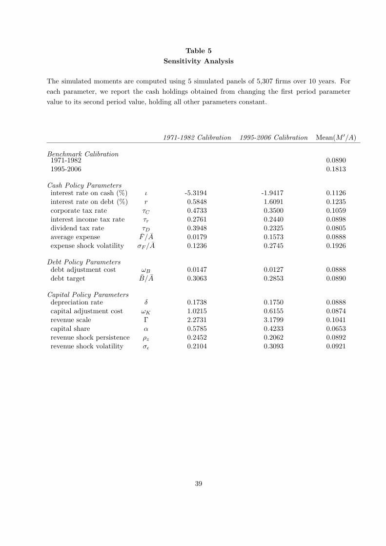
Table 5Sensitivity Analysis

The simulated moments are computed using 5 simulated panels of 5,307 firms over 10 years. Foreach parameter, we report the cash holdings obtained from changing the first period parametervalue to its second period value, holding all other parameters constant.

1971-1982 Calibration 1995-2006 Calibration Mean(M ′/A)

Benchmark Calibration1971-1982 0.08901995-2006 0.1813

Cash Policy Parametersinterest rate on cash (%) ι -5.3194 -1.9417 0.1126interest rate on debt (%) r 0.5848 1.6091 0.1235corporate tax rate τC 0.4733 0.3500 0.1059interest income tax rate τr 0.2761 0.2440 0.0898dividend tax rate τD 0.3948 0.2325 0.0805average expense F /A 0.0179 0.1573 0.0888expense shock volatility σF /A 0.1236 0.2745 0.1926

Debt Policy Parametersdebt adjustment cost ωB 0.0147 0.0127 0.0888debt target B/A 0.3063 0.2853 0.0890

Capital Policy Parametersdepreciation rate δ 0.1738 0.1750 0.0888capital adjustment cost ωK 1.0215 0.6155 0.0874revenue scale Γ 2.2731 3.1799 0.1041capital share α 0.5785 0.4233 0.0653revenue shock persistence ρz 0.2452 0.2062 0.0892revenue shock volatility σε 0.2104 0.3093 0.0921

39

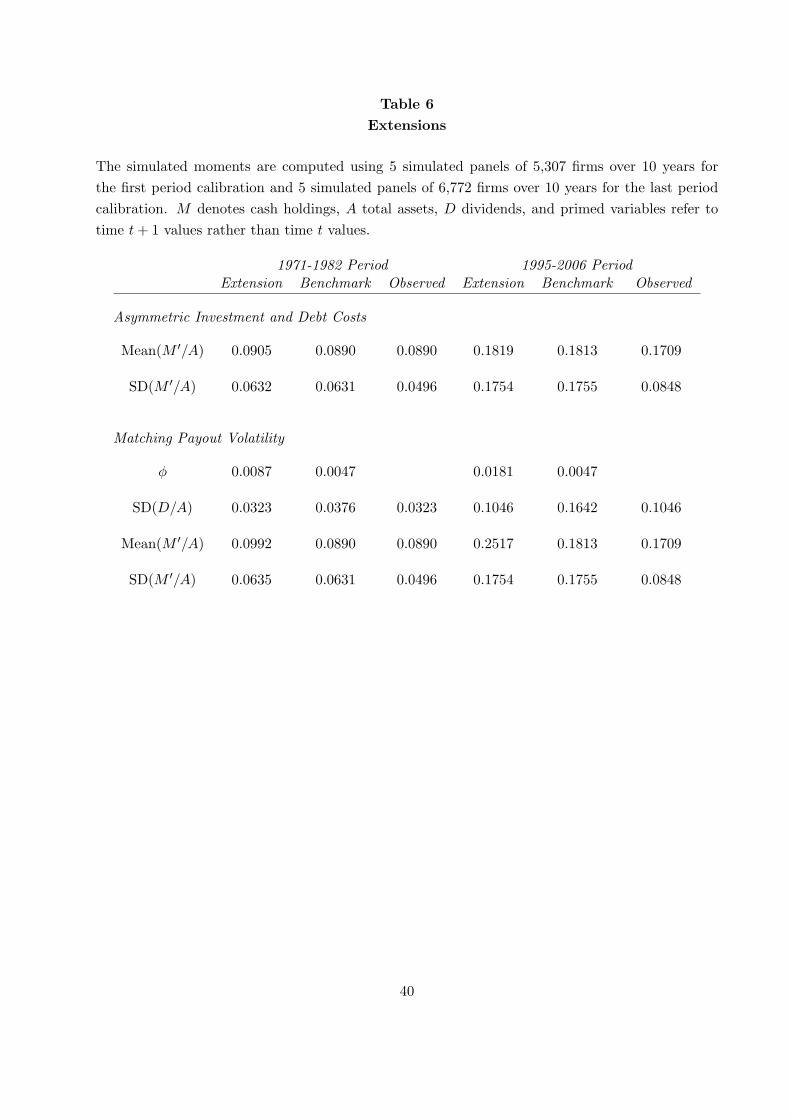
Table 6Extensions

The simulated moments are computed using 5 simulated panels of 5,307 firms over 10 years forthe first period calibration and 5 simulated panels of 6,772 firms over 10 years for the last periodcalibration. M denotes cash holdings, A total assets, D dividends, and primed variables refer totime t+ 1 values rather than time t values.

1971-1982 Period 1995-2006 PeriodExtension Benchmark Observed Extension Benchmark Observed

Asymmetric Investment and Debt Costs

Mean(M ′/A) 0.0905 0.0890 0.0890 0.1819 0.1813 0.1709

SD(M ′/A) 0.0632 0.0631 0.0496 0.1754 0.1755 0.0848

Matching Payout Volatility

φ 0.0087 0.0047 0.0181 0.0047

SD(D/A) 0.0323 0.0376 0.0323 0.1046 0.1642 0.1046

Mean(M ′/A) 0.0992 0.0890 0.0890 0.2517 0.1813 0.1709

SD(M ′/A) 0.0635 0.0631 0.0496 0.1754 0.1755 0.0848

40

0.2

0.3

0.4

0.5

Figure 1: Average North American Firm Policies

Cash M'/A

Capital K'/A

Debt B'/A

0

0.1

0.2

0.3

0.4

0.5

1972 1982 1992 2002

Figure 1: Average North American Firm Policies

Cash M'/A

Capital K'/A

Debt B'/A

0.1

0.15

0.2

0.25

Figure 2: Tax and Equity Issuing Cost Schedule T(D)

τD=0.3948 and φ=0.0047

τD=0.2325 and φ=0.0047

τD=0.3948 and φ=0.0087

0

0.05

0.1

0.15

0.2

0.25

‐10 ‐5 0 5 10

Figure 2: Tax and Equity Issuing Cost Schedule T(D)

τD=0.3948 and φ=0.0047

τD=0.2325 and φ=0.0047

τD=0.3948 and φ=0.0087

τD=0.2325 and φ=0.0181

Figure 3: Cash Holdings M'/A of Simulated Firms

0 3

0.4

Figure 3: Cash Holdings M'/A of Simulated Firms

0.2

0.3

0.4

Figure 3: Cash Holdings M'/A of Simulated Firms

1971‐1982 Calibration

1995‐2006 Calibration

0.1

0.2

0.3

0.4

Figure 3: Cash Holdings M'/A of Simulated Firms

1971‐1982 Calibration

1995‐2006 Calibration

0

0.1

0.2

0.3

0.4

Figure 3: Cash Holdings M'/A of Simulated Firms

1971‐1982 Calibration

1995‐2006 Calibration

0

0.1

0.2

0.3

0.4

Figure 3: Cash Holdings M'/A of Simulated Firms

1971‐1982 Calibration

1995‐2006 Calibration

0

0.1

0.2

0.3

0.4

Figure 3: Cash Holdings M'/A of Simulated Firms

1971‐1982 Calibration

1995‐2006 Calibration

Figure 4: Cash Savings S/Mean(A) of Simulated Firms

0.2

0.25

Figure 4: Cash Savings S/Mean(A) of Simulated Firms

0 1

0.15

0.2

0.25

Figure 4: Cash Savings S/Mean(A) of Simulated Firms

1971‐1982 Calibration

1995‐2006 Calibration

0.05

0.1

0.15

0.2

0.25

Figure 4: Cash Savings S/Mean(A) of Simulated Firms

1971‐1982 Calibration

1995‐2006 Calibration

0

0.05

0.1

0.15

0.2

0.25

Figure 4: Cash Savings S/Mean(A) of Simulated Firms

1971‐1982 Calibration

1995‐2006 Calibration

0

0.05

0.1

0.15

0.2

0.25

Figure 4: Cash Savings S/Mean(A) of Simulated Firms

1971‐1982 Calibration

1995‐2006 Calibration

0

0.05

0.1

0.15

0.2

0.25

Figure 4: Cash Savings S/Mean(A) of Simulated Firms

1971‐1982 Calibration

1995‐2006 Calibration

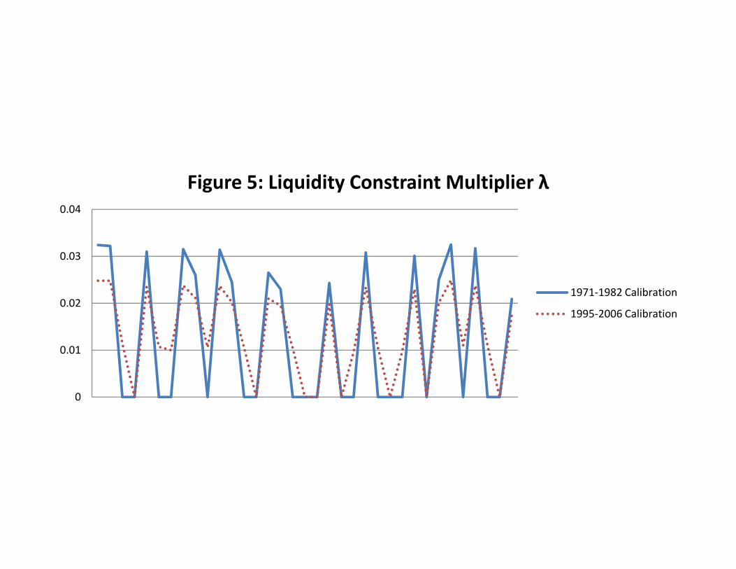
Figure 5: Liquidity Constraint Multiplier λ

0 03

0.04

Figure 5: Liquidity Constraint Multiplier λ

0.02

0.03

0.04

Figure 5: Liquidity Constraint Multiplier λ

1971‐1982 Calibration

1995‐2006 Calibration

0.01

0.02

0.03

0.04

Figure 5: Liquidity Constraint Multiplier λ

1971‐1982 Calibration

1995‐2006 Calibration

0

0.01

0.02

0.03

0.04

Figure 5: Liquidity Constraint Multiplier λ

1971‐1982 Calibration

1995‐2006 Calibration

0

0.01

0.02

0.03

0.04

Figure 5: Liquidity Constraint Multiplier λ

1971‐1982 Calibration

1995‐2006 Calibration

0

0.01

0.02

0.03

0.04

Figure 5: Liquidity Constraint Multiplier λ

1971‐1982 Calibration

1995‐2006 Calibration

0.1

0.15

0.2

0.25

Figure 6: Effect of Scale Γ on Cash Savings S/Mean(A)

1971‐1982 Calibration

1995‐2006 Calibration

1971‐1982 Calibration with 1995‐2006 Γ

0

0.05

0.1

0.15

0.2

0.25

Figure 6: Effect of Scale Γ on Cash Savings S/Mean(A)

1971‐1982 Calibration

1995‐2006 Calibration

1971‐1982 Calibration with 1995‐2006 Γ

1995‐2006 Calibration with 1971‐1982 Γ

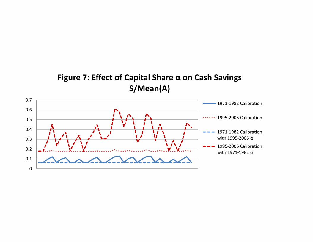
0 3

0.4

0.5

0.6

0.7

Figure 7: Effect of Capital Share α on Cash Savings S/Mean(A)

1971‐1982 Calibration

1995‐2006 Calibration

1971‐1982 Calibration with 1995‐2006 α

0

0.1

0.2

0.3

0.4

0.5

0.6

0.7

Figure 7: Effect of Capital Share α on Cash Savings S/Mean(A)

1971‐1982 Calibration

1995‐2006 Calibration

1971‐1982 Calibration with 1995‐2006 α

1995‐2006 Calibration with 1971‐1982 α