core regression: fitting lines to data sample - home | … · · 2008-09-09core regression:...

P1: FXS/ABE P2: FXS9780521740517c05.xml CUAT013-EVANS September 3, 2008 11:27

C H A P T E R

5CORE

Regression: fitting linesto data

How can we use the relationship between two numerical variables for prediction?

What is linear regression?

What is the method of least squares?

What is the three median line?

What are interpolation and extrapolation?

How do you write up the results of a regression analysis for a statistical report?

The process of fitting a straight line to bivariate data is known as linear regression. The aim of

linear regression is to model the relationship between two numerical variables by using a

simple equation, the equation of a straight line. Knowing such an equation will give us a better

understanding of the nature of the relationship. It will also enable us to make predictions from

one variable to another, for example, a young son’s adult height from his father’s height.

The easiest way to fit a line to bivariate data is to construct a scatterplot and draw the line in

‘by eye’. This is done by placing a ruler on the scatterplot so that it seems to follow the general

trend of the data. You can then use the ruler to draw a straight line. Unfortunately, unless the

points are very tightly clustered around a straight line, the results you get by using this method

will differ a lot from person to person.

To overcome this problem, a number of methods have been devised that will give the same

result for everyone. We will consider two of these methods:

the least squares method

the three median method

5.1 Least squares regression line: the theoryThe most common approach to fitting a straight line to data is to use the least squares

method. This method assumes that the variables are linearly related, and works best when

there are no clear outliers in the data.

131

SAMPLE

Cambridge University Press • Uncorrected Sample pages • 978-0-521-61328-6 • 2008 © Jones, Evans, Lipson TI-Nspire & Casio ClassPad material in collaboration with Brown and McMenamin


132 Essential Further Mathematics – Core

Some terminologyTo explain the least squares method, we need to define several terms.

The scatterplot shows five data points, (x1, y1),

(x2, y2), (x3, y3), (x4, y4) and (x5, y5). A regression

line (not necessarily the least squares line) has also

been drawn in on the scatterplot. The vertical

distances d1, d2, d3, d4 and d5 of each of the

data points from the regression line are also

shown. These vertical distances, d, are known

as residuals.

x

y

d2

regression line

d4d3

d1

d5

(x4, y4)

(x1, y1)

(x2, y2)

(x3, y3)

(x5, y5)

The least squares lineThe least squares line is the line where the sum of the squares of the residuals is as small as

possible, that is, it minimises the sum:

d21 + d2

2 + d23 + d2

4 + d25

Why do we minimise the sum of the squares of the residuals and not the sum of the residuals?

This is because the sum of the residuals is always zero for the least squares line. The least

squares line is like the mean. It balances out the data values on either side of itself. Some

residuals are positive and some negative, and in the end, they add to zero. Squaring the

residuals solves this problem.

The least squares lineThe least squares line is the line that minimises the sum of the squares of the residuals.

How do we determine the least squares regression line?One method is to use ‘trial-and-error’. We could draw in a series of lines, each with a different

slope and intercept. For each line, we could then work out the value of each of the residuals,

square them, and calculate their sum. The least squares line would be the one that minimises

that sum. To see how this might work, you can make use of the interactive ‘Regression line’ on

the CD in the back of this book.

The trial-and-error method does not guarantee that we get the exact solution. Fortunately,

the exact solution can be found mathematically, using the techniques of calculus. Although the

mathematics is beyond that required for Further Mathematics, we will make use of these

results, which are summarised on the next page.

SAMPLE



Chapter 5 — Regression: fitting lines to data 133

The equation of the least squares regression lineThe equation of the least squares regression line is given by y = a + bx ,* where:

the slope (b) is given by: b = rsy

sx

and

the intercept (a) is then given by: a = y − bx

Here:

r is the correlation coefficient

sx and sy are the standard deviations of x and y

x and y are the mean values of x and y

Exercise 5A

1 What is a residual?

2 The least-squares regression line is obtained by:

A minimising the residuals

B minimising the sum of the residuals

C minimising the sum of the squares of the residuals

D minimising the square of the sum of the residuals

E maximising the sum of the squares of the residuals

5.2 Calculating the equation of the least squaresregression lineTo use these formulas to calculate the equation of the least squares regression line, you need to

know the values of r, x and y, and sx and sy . If all you have are the actual data values, then the

accepted practice is to use a graphics calculator to do the computation.

Both methods are demonstrated in this section.

Warning!!If you do not correctly decide which is the IV (the x variable) and which is the DV (the y variable)before you start the process of calculating the equation of the least squares regression line,you may get the wrong answer.

* In mathematics you are used to writing the equation of a straight line as y = mx + c. However, statisticianswrite the equation of a straight line as y = a + bx . This is because statisticians are in the business of buildinglinear models. Putting the variable term second in the equation allows for additional variable terms to be added,for example, y = a + bx + cz. While this sort of model is beyond Further Mathematics, we will continue touse y = a + bx to represent the equation of the regression line because it is common statistical practice.

SAMPLE




How to determine the equation of a least squares regression line using the formula

The heights (x) and weights (y) of 11 people have been recorded, and the values of the

following statistics determined:

x = 173.2727 cm sx = 7.4443 cm y = 65.4545 cm sy = 7.5943 cm r = 0.8502.

Use the formula to determine the equation of the least squares regression line that will

enable weight to be predicted from height.

Steps1 Identify and write down the IV and DV. Label

as x and y respectively.Note: In saying that we want to predict weight fromheight, we are implying that height is the IV.

IV: height (x)

DV: weight (y)

2 Write down the given information. x = 173.2727 sx = 7.4443

y = 65.4545 sy = 7.5943

r = 0.8502

3 Calculate the slope. Slope :

b = rsy

sx

=0.8502 × 7.5943

7.4443

= 0.867 (correct to 2 d.p.)

4 Calculate the intercept. Intercept :

a = y − b x

= 65.4545 − 0.8673 × 173.2727

= −84.8 (correct to 1 d.p.)

5 Use the values of the intercept and the

slope to write down the least squares

regression line using the variable names.

y = −84.8 + 0.867x

or

weight = −84.8 + 0.867 × height

How to draw the graph and determine the equation of a least squares regression lineusing the TI-Nspire

The following data give the heights (in cm) and weights (in kg) of 11 people.

Height (x) 177 182 167 178 173 184 162 169 164 170 180

Weight (y) 74 75 62 63 64 74 57 55 56 68 72

Determine and graph the equation of the least squares regression line that will enable

weight to be predicted from height.

SAMPLE




Steps1 Start a new document by pressing / +N .

2 Select 3:Add Lists & Spreadsheet. Enter

the data into lists named height and

weight, as shown.

3 Identify the independent variable (IV)

and the dependent variable (DV).

IV: height

DV: weight

Note: In saying that we want to predict

weight from height, we are implying that

height is the IV.

4 Press c and select 5:Data & Statisticsand construct a scatterplot with the

height (IV) on the horizontal (or x-) axis

and weight (DV) on the vertical (or y-)

axis.

If you need help to do this see page ?.

5 Press b4:Analyze/6:Regression/2:ShowLinear (a + bx) to plot the regression line

on the scatterplot.

Note that, simultaneously, the equation

of the regression line is shown and

(possibly) the value of r2.

The equation of the regression line is

y = −84.8 + 0.867x

or weight = −84.8 + 0.867 × height

The coefficient of determination is

r2 = 0.723, correct to 3 decimal places.SAMPLE




6 If the value of r2 is not given or you wish to

have a full printout of the regression statistics

a Press c and select 1:Calculator to open

the Calculator application.

b Now press b 6:Statistics/1:StatCalculations/4:Linear Regression(a + bx) to obtain the screen shown

(Right).

c To select the variable for the X List

entry use the arrow to paste in the list

name height. Press e to move to the

Y List entry, use the arrow twice andenter to paste in the list name weight.

Press enter to exit the pop-up screen

and generate the regression results

(right).

7 Use the values of the intercept a and the

slope b to write the equation of the least

squares regression line using the variable names.

weight = −84.8 + 0.867 × height

The coefficient of determination is r2 = 0.723, correct to 3 decimal places.

How to draw the graph and determine the equation of a least squares regression lineusing the ClassPad

The following data give the heights (in cm) and weights (in kg) of 11 people.

Height (x) 177 182 167 178 173 184 162 169 164 170 180

Weight (y) 74 75 62 63 64 74 57 55 56 68 72

Determine and graph the equation of the least squares regression line that will enable

weight to be predicted from height.SAMPLE




Steps1 Open the Statistics application and enter

the data into the columns labelled heightand weight. Your screen should look like

the one shown.

2 Tap to open the Set StatGraphs dialog

box and complete as shown. For� Draw: select On� Type: select Scatter ( )� XList: select main \ height ( )� YList: select main \ weight ( )� Freq: leave as 1� Mark: leave as squareTap h to confirm your selections.

3 Tap y in the toolbar at the top of the

screen to plot the scatterplot in the

bottom half of the screen.

4 To calculate the equation of the least

squares regression line, tap Calc from the

menu bar, and then tap Linear Reg.

This opens the Set Calculation dialog box

shown below.

5 Complete the Set Calculations dialog

box as shown. For� XList: select main \ height ( )� YList: select main \ weight ( )� Freq: leave as 1� Copy Formula: select Off� Copy Residual: select OffNotes:

1 In saying that we want to predict

weight from height, we are implying

that height is the independent

variable (i.e. XList on the calculator).

2 The choice of y6 as the formula

destination is an arbitrary choice.SAMPLE




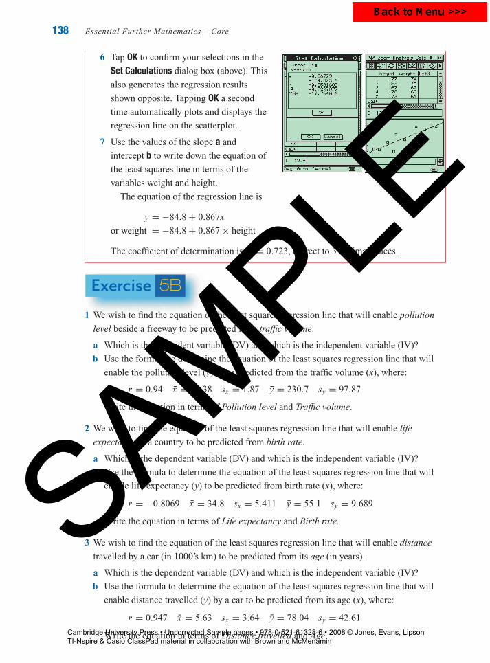
6 Tap OK to confirm your selections in the

Set Calculations dialog box (above). This

also generates the regression results

shown opposite. Tapping OK a second

time automatically plots and displays the

regression line on the scatterplot.

7 Use the values of the slope a and

intercept b to write down the equation of

the least squares line in terms of the

variables weight and height.

The equation of the regression line is

y = −84.8 + 0.867x

or weight = −84.8 + 0.867 × height

The coefficient of determination is r2 = 0.723, correct to 3 decimal places.

Exercise 5B

1 We wish to find the equation of the least squares regression line that will enable pollution

level beside a freeway to be predicted from traffic volume.

a Which is the dependent variable (DV) and which is the independent variable (IV)?

b Use the formula to determine the equation of the least squares regression line that will

enable the pollution level (y) to be predicted from the traffic volume (x), where:

r = 0.94 x = 11.38 sx = 1.87 y = 230.7 sy = 97.87

Write the equation in terms of Pollution level and Traffic volume.

2 We wish to find the equation of the least squares regression line that will enable life

expectancy in a country to be predicted from birth rate.



enable life expectancy (y) to be predicted from birth rate (x), where:

r = −0.8069 x = 34.8 sx = 5.411 y = 55.1 sy = 9.689

Write the equation in terms of Life expectancy and Birth rate.

3 We wish to find the equation of the least squares regression line that will enable distance

travelled by a car (in 1000’s km) to be predicted from its age (in years).



enable distance travelled (y) by a car to be predicted from its age (x), where:

r = 0.947 x = 5.63 sx = 3.64 y = 78.04 sy = 42.61

Write the equation in terms of Distance travelled and Age.

SAMPLE




4 The following questions relate to the formulas used to calculate the slope and intercept of

the least squares regression line.

a A least squares line is calculated and the slope is found to be negative. What does this tell

us about the sign of the correlation coefficient?

b The correlation coefficient is zero. What does this tell us about the slope of the least

squares regression line?

c The correlation coefficient is zero. What does this tell us about the intercept of the least

squares regression line?

5 The table shows the number of sit-ups and push-ups performed by six students.

Sit-ups (x) 52 15 22 42 34 37

Push-ups (y) 37 26 23 51 31 45

The number of sit-ups and the number of push-ups are linearly related. There are no outliers.

Treating the number of sit-ups as the independent (x) variable, and the number of push-ups

as the dependent (y) variable, use your calculator to show that the equation of the least

squares regression line is:

Number of push-ups = 16.45 + 0.57 × Number of sit-ups

6 The table shows average hours worked and university participation rates (%) in six

countries.

Hours worked 35.0 43.0 38.2 39.8 35.6 34.8

Participation rate (%) 26 20 36 25 37 55

Hours worked and university participation rate are linearly related and there are no outliers.

Use your calculator to show that the equation of the least squares regression line that will

enable participation rates to be predicted from hours worked is:

Participation rate = 131.4 − 2.6 × Hours worked

7 The table shows the number of runs scored and balls faced by batsmen in a cricket match.

Runs (y) 27 8 21 47 3 15 13 2 15 10 2

Balls faced (x) 29 16 19 62 13 40 16 9 28 26 6

Runs scored and balls faced are linearly related and there are no outliers.

a Show that, in terms of x and y, the equation of the regression line is: y = −2.6 + 0.73x .

b Rewrite the regression equation in terms of the variables involved.

8 The table below shows the number of TVs and cars owned (per 1000 people) in six

countries.

Number of TVs/1000 378 404 471 354 381 624

Number of cars/1000 417 286 435 370 357 550

The number of TVs and the number of cars owned are linearly related. There are no outliers.

SAMPLE




We wish to predict the number of TVs from the number of cars.

a Which is the dependent variable (y)?

b Show that, in terms of x and y, the equation of the regression line is: y = 61.2 + 0.93x .

c Rewrite the regression equation in terms of the variables involved.

5.3 Performing a regression analysisHaving learned how to calculate the equation of the least squares regression line, you are well

on the way to learning how to perform a full regression analysis. On the way you will make use

of many of the skills you have developed when working with scatterplots and correlation

coefficients.

Performing a regression analysisA full regression analysis involves several processes, which include:

constructing a scatterplot to investigate the nature of the relationship between the

variables

calculating the correlation coefficient to give a measure of the strength of the

relationship

determining the equation of the regression line

interpreting the coefficients of the least squares line

using the regression line to make predictions

using the coefficient of determination to give a measure of the predictive power of

the linear relationship

using a residual plot to test the assumption of linearity

writing a report on your findings

Some dataWe wish to investigate the nature of the relationship between life expectancy in a country and

birth rate. The ultimate aim is to find an equation that will enable life expectancy in a country

to be predicted from its birth rate. Life expectancies (in years) and birth rates (number of births

per one thousand people) have been determined for ten countries. These are displayed in the

table below.

Birth rate (per thousand) 30 38 38 43 34 42 31 32 26 34

Life expectancy (years) 66 54 43 42 49 45 64 61 61 66

The scatterplot and correlation coefficientWe start our investigation of the relationship between

life expectancy and birth rate by constructing a

scatterplot (see opposite). From the scatterplot, we

see that there is a negative linear relationship

between life expectancy in a country and birth

rate. There are no clear outliers.

4025 27 29 31 3533 37 39 41 43 45

45

65

70

60

50

55

Birth rate

Lif

e ex

pect

ancy

(ye

ars)

The correlation coefficient is r = −0.807.

From this information we can conclude that:

There is a strong, negative linear relationship between life expectancy and birth rate

(r = −0.807).

SAMPLE




The least squares regression lineThe relationship between life expectancy (y) and birth rate (x) is linear. It is therefore

appropriate to fit a least squares regression line to the data.

Using a calculator, the equation of the least squares line is found to be:

y = 105.4 − 1.44x

The line has a slope of −1.44 and intercepts

the vertical axis at 105.4. This line has been

plotted on the scatterplot opposite. Note that

the horizontal scale has been extended back

to zero so that the vertical intercept can

be seen. (This is not usually the case.)

40

50

60

70

80

90

100

110

454035302520151050

equation of liney = 105.4 – 1.44x

y intercept = 105.4

slope of line = –1.44

x

y

Interpreting the slope and the intercept of the regression line

The slope and intercept of a regression lineFor the regression equation: y = a + bx:

the slope, b, predicts the change in y when x changes by one unit:� If the slope b is positive, then y increases as x increases.

� If the slope b is negative, then y decreases as x increases.

the y-intercept predicts the value of y when x = 0

To interpret the regression equation, first write it in terms of the variables involved:

Life expectancy = 105.4 − 1.44 × Birth rate

Written in this form, the slope and intercept of the regression equation can be used to make the

following predictions:

slope On average, life expectancies (y) in countries will decrease by 1.44 years

for an increase in birth rate (x) of one birth per 1000 people.

intercept On average, the life expectancy for countries with a zero birth rate is

105.4 years.

Note: However, our prediction of the average life expectancy being 105.4 years is unlikely to be a reliableprediction. We have no information at all on countries with birth rates of less than 26 (per 1000 people) andthere is no reason to assume that the linear model we have used applies to countries with low birth rates.

Predicting life expectancies from birth ratesWe can use the regression equation to predict life expectancies from birth rates. For example,

what is the life expectancy of a country with a birth rate of 35 (per 1000 people)?

Substituting 35 for birth rate in the regression equation:

Life expectancy = 105.4 − 1.44 × 35 = 55 Years

SAMPLE




Thus, we predict:

On average, a country with a birth rate of 35 (per 1000 people) will have a life expectancy

of 55 years.

The coefficient of determinationWhile the relationship between life expectancy and birth rate does not explain all the variation

in life expectancy, knowing the birth rate in a country does give us some information about life

expectancy in that country. The coefficient of determination tells us the percentage of variation

in life expectancies (DV) that can be explained by the variation in birth rates (IV). In this way,

the coefficient of determination gives us an indication of the predictive power of the

relationship. For a perfect relationship, the coefficient of determination would explain 100% of

the variation in life expectancies. For no relationship, it explains none (0%) of the variation in

life expectancies. In this case, with r = −0.807, we have:

coefficient of determination = r2 ≈ 0.651 or 65.1%.

Thus we can conclude that:

65.1% of the variation in life expectancy can be explained by the variation in birth rates.

Thus the relationship has significant (worthwhile) predictive power. As a guide, any

relationship with a coefficient of determination greater than 30% can be regarded as having

significant predictive power.

The residual plot: testing the assumption of linearityA key assumption made when calculating a least squares regression line is that the

relationship between the variables is linear. One way of testing this assumption is to plot the

regression line on the scatterplot and see how well a straight line fits the data. However, a better

way is to use a residual plot, as this plot will show even very small departures from linearity.

Residuals revisitedWhen we fit a least squares line we assume that part of each data value can be predicted by the

regression line, the predicted value. There is also a random part that cannot be predicted by the

regression line. This random part is just the residual value we met earlier. Thus, we can write

data value = predicted value + residual value

or

residual value = data value − predicted value

Definition of a residualresidual value = data value − predicted valueSAM

PLE




Calculating residualsFor example, consider the scatterplot

opposite.

25 27 29 31 33 35 37 39 41 43 45Birth rate

Lif

e ex

pect

ancy

(ye

ars)

40

45

50

55

60

65

70

B (34, 49)

A (34, 66) data value

residual value = data value – predicted value = 9.6

(34, 56.4) predicted value

The country labelled A on the scatterplot

has a birth rate of 34 and a life expectancy

of 66 years.

For Country A:

predicted life expectancy = 105.4 − 1.44 × 34 = 56.4 years

actual life expectancy = 66 years

∴ residual value = actual value − predicted value = 66 − 56.4 = 9.6 years

The residual is positive because the actual data value lies above the prediction line (see the

scatterplot).

In contrast, consider the country labeled B on the scatterplot. It also has a birth rate of 34.

For Country B:

predicted life expectancy = 105.4 − 1.44 × 34 = 56.4 years

actual life expectancy = 49 years

∴ residual value = actual value − predicted value = 49 − 56.4 = −7.4 years

The residual is negative because the actual data value lies below the prediction line.

If we continue to calculate the residuals, we will find that some are positive and some are

negative. What we hope is that there is no clear pattern to the residuals. To see this we

construct a residual plot.

The residual plotA residual plot is a plot of the residual value for

each data value against the independent variable

(in this case, birth rate). Because the mean of the

residuals is always zero, the horizontal zero

line (red) helps us to orient ourselves. This line

corresponds to regression in the previous

scatterplot. It is, of course, extremely

tedious to construct a residual plot by hand and

we do not do this in practice. We use a graphics calculator.

25–10–8–6– 4–2

1086420

27 29 31 33 35 37 39 41 43

Res

idua

l

Birth rate

From the residual plot, we see that there is no clear pattern* in the residuals. Essentially they

are randomly scattered around the zero regression line. This confirms our original

assumption that a linear relationship between life expectancy and birth rate is reasonable. All

that is left after fitting the regression line is random variation around the line.

* From a visual inspection, it is difficult to say with certainty that a residual plot is random. It is easier to seewhen it is not random as you will see in the next chapter. For present purposes, it is sufficient to say that a clearlack of pattern in a residual plot indicates randomness.

SAMPLE




Thus, from this residual plot we can conclude that:

The assumption that there is a linear relationship between life expectancy and birth rate is

confirmed by the residual plot.

In contrast to the relationship between life expectancy and birth rate, the relationship

between the yield of a potato plot and its length is clearly non-linear. See the scatterplot

below. The clear curved pattern in the residual plot shown below confirms this assertion.

You will learn how to analyse such situations in the next chapter.

Length

05 10 15 20 25 30 35

0.5

1.0

1.5

2.0

2.5

Yiel

d (0

00’s

)

Scatterplot

Length0 5 10 15 20 25 30 35

400

200

–400

–200

0

Res

idua

lResidual plot

Reporting the results of a regression analysisThe final step in a regression analysis is to report your findings. The report is in a form that is

suitable for including in a statistical project. Note that an interpretation of the intercept of the

regression equation is not included for this example as it has no meaningful interpretation.

How to report the results of a regression analysis

Report

From the scatterplot we see that there is a strong negative, linear relationship between life

expectancy and birth rate, r = −0.807. There are no obvious outliers.

The equation of the least squares regression line is:

Life expectancy = 105.4 − 1.44 × Birth rate

The slope of the regression line predicts that, on average, life expectancy decreases by 1.44 years

for an increase in birth rate of one birth per 1000 people.

The coefficient of determination indicates that 65.1% of the variation in life expectancy is explained

by the variation in birth rate.

A residual plot shows no clear pattern and confirms that the use of a linear equation to describe the

relationship between life expectancy and birth rate is appropriate.

Using a graphics calculatorIn the regression analysis above, all statistical graphs and results were given. We will now

show how they were generated with a graphics calculator.

SAMPLE




How to conduct a regression analysis using the TINspire

The data for this analysis is shown below.

Birth rate (per thousand ) 30 38 38 43 34 42 31 32 26 34


Steps1 Write down the independent variable

(IV) and dependent variable (DV).

IV: birth

DV: life

Use the abbreviations ‘birth’ for birth

rate and ‘life’ for life expectancy.

2 Enter the data into lists named birth and

life, as shown.

3 Construct a scatterplot to investigate the

nature of the relationship between life

expectancy and birth rate.

4 Describe the relationship between life

expectancy and birth rate as shown by

the scatterplot. Mention direction, form,

strength and outliers.

From the scatterplot we see that there is a

moderately strong negative, linear

relationship between life expectancy and

birth rate. There are no obvious outliers.SAMPLE




5 Find and plot the equation of the least squares regression line and generate the full list

of regression statistics.

6 Generate a residual plot to test the linearity assumption.

Note: When you perform a regression analysis, the residuals are calculated automatically

and stored as a list called stat.resid.

Use / + to return to the scatterplot. Move the cursor to the life label (y-) and press

x to show the variable list. Use the to locate stat.resid and press enter to select. A

scatterplot of birth against residuals is displayed. If a regression line and its equation is

also shown, move the cursor to the equation until a appears (or to the line until a

appears), and press / + b 1:Remove Regression to remove.

7 Use the values of the intercept and slope

to write the equation of the least squares


Also write the values of r and the

coefficient of determination.

Regression equation:

y = 105.4 − 1.44x

or

life = 105.4 − 1.44 × birth

Correlation coefficient: r = 0.8069

Coefficient of determination: r 2 = 0.651SAMPLE




How to conduct a regression analysis using the ClassPad

The data for this analysis is shown below.

Birth rate (per thousand ) 30 38 38 43 34 42 31 32 26 34


Steps1 Write down the independent variable

(IV) and dependent variable (DV).

IV: birth

DV: life

Use the abbreviations ‘birth’ for birth

rate and ‘life’ for life expectancy.

2 Enter the data into lists named birth and

life, as shown.

3 Construct a scatterplot to investigate the

nature of the relationship between life

expectancy and birth rate.

4 Describe the relationship between life

expectancy and birth rate as shown by

the scatterplot. Mention direction, form,

strength and outliers.

From the scatterplot we see that there is a

moderately strong negative, linear

relationship between life expectancy and

birth rate. There are no obvious outliers.

5 Find an equation of the least squares

regression line and generate the full list

of regression statistics, including

residuals.

Complete the Set Calculations dialog

box as shown. For� XList: select main \ Birth ())� YList: select main \ Life ())� Freq: leave as 1� Copy Formula: select y6� Copy Residual: select list3Note: Copy Residual copies the residuals

to list3 where they can be used later to

create a residual plot.

SAMPLE




6 Tap OK to confirm your selections in the

Set Calculations dialog box (above). This

also generates the regression results

shown opposite.

7 Tapping OK a second time automatically

plots and displays the regression line on

the scatterplot.

To obtain a full-screen plot, tap rfrom the icon panel.

8 Generate a residual plot to test the

linearity assumption.

Note: When you performed a regression

analysis earlier, the residuals were

automatically calculated and stored in

list3. The residual plot is a scatterplot

with list3 on the vertical axis and birth on

the horizontal axis.

9 Use the values of the intercept and slope

to write the equation of the least squares


Also write the values of r and the

coefficient of determination.

Regression equation:

y = 105.4 − 1.44x

or

life = 105.4 − 1.44 × birth

Correlation coefficient: r = 0.8069

Coefficient of determination: r 2 = 0.651

Exercise 5C

1 The equation of a regression line that enables hand span to be predicted from height is:

Hand span = 2.9 + 0.33 × Height

Complete the following sentences:

a The independent variable is .

b The slope is and the intercept is .

c A person is 160 cm tall and has an actual hand span of 58.5 cm. Using this regression

equation, their predicted hand span is cm.

d The residual value for this person is cm.

2 The equation of a regression line that enables fuel consumption of a car (litres per

100 kilometres) to be predicted from its weight (kg) is:

Fuel consumption = −0.1 + 0.01 × Weight

SAMPLE




Complete the following sentences:

a The dependent variable is .


c A car weighs 980 kg and has an actual fuel consumption of 8.9 litres per 100 kilometres.

Using this regression equation, the car’s predicted fuel consumption is litres per

100 kilometres.

d The residual value for this car is litres/100 kilometres.

3 Use the line on the graph to determine the equation of the regression line shown on each of

the following scatterplots. Give the intercept correct to the nearest whole number and the

slope correct to one decimal place.

100908070605040302010

01 2 3 4 5 6 7 8

Days absent

Mar

k

1514131211109876

10 15 20 25 30 35Birth rate (/1000)

Dea

th r

ate

(/10

00)

4 The table below shows the scores obtained by nine students on two tests. We want to be

able to predict Test B scores from Test A scores.

Test A score (x) 18 15 9 12 11 19 11 14 16

Test B score (y) 15 17 11 10 13 17 11 15 19

Use your calculator to perform each of the following steps of a regression analysis.

a Construct a scatterplot. Name variables, test a and test b.

b Determine the equation of the least squares line along with the values of r and r2.

c Display the regression line on the scatterplot.

d Obtain a residual plot.

5 The table below shows the number of careless errors made on a test by nine students. Also

given are their test scores. We want to be able to predict test score from the number of

careless errors made.

Test score 18 15 9 12 11 19 11 14 16

Careless errors 0 2 5 6 4 1 8 3 1

Use your calculator to perform each of the following steps of a regression analysis.

a Construct a scatterplot. Name variables, score and errors.

b Determine the equation of the least squares line along with the values of r and r2.

c Display the regression line on the scatterplot.

d Obtain a residual plot.

SAMPLE




6 In an investigation of the relationship between the food energy content (in calories) and the

fat content (in g) in a standard sized packet of chips, the least squares regression line was

found to be

Energy content = 27.8 + 14.7 × Fat content with r2 = 0.7569

Use this information to complete the following sentences.

a The slope is and the intercept is .

b The regression equation predicts that the food energy content in a packet of chips

increases by calories for each additional gram of fat it contains.

c r = .

d % of the variation in food energy content of a packet of chips can be explained by

the variation in their .

e The food energy content of a standard sized packet of chips is 132 calories and it

contains 8 g of fat. The regression equation predicts its food energy content to be

calories.

f The residual value for this packet of chips is g.

7 Each of the following residual plots has been constructed after a least squares regression

line has been fitted to a scatterplot. Which of the residual plots suggest that the use of a

linear model to fit the data was not appropriate and why?

A

0

4.5

3.0

resi

dual

1.5

0.0

−1.5

2 4 6independent–var

8 10 12 14

B

resi

dual

.

independent–var

3.0

0 2 4 6 8 10 12

1.5

0.0

−1.5

−3.0

C

resi

dual

independent–var0

3

0

−3

2 4 6 8 10 12 14

8 In an investigation of the relationship between success rate (%) of sinking a putt and the

distance from the hole (in cm) of amateur golfers, the least squares regression line was

found to be:

Success rate = 98.5 − 0.278 × Distance with r2 = 0.497


a The regression equation predicts that success rate increases/decreases by % for

each additional centimetre the golfer is from the hole.

b The regression equation predicts that an amateur golfer whose ball is 90 cm from the

hole will have a % chance of sinking the putt.

c The regression equation predicts that the golfer will have 0% success rate of sinking the

putt when they are metres from the hole.

d r = correct to three decimal places.

e % of the variation in success rate can be explained by the variation in the

of the golfer from the hole.

SAMPLE




9 The scatterplot opposite shows the pay rate (dollars

per hour) paid by a company to workers with different

years of experience. Using a calculator, the equation

of the least squares regression line is found to have

the equation:

y = 8.56 + 0.289x with r = 0.967

0 2 4 6 8 10 12

141312111098765

Experience (years)

Rat

e ($

)

a Is it appropriate to fit a least squares regression

line to this data? Why?

b Work out the coefficient of determination.

c Complete the following sentence: % of the variation in a person’s pay can

be explained by the variation in their .

d Write down the equation of the least squares line in terms of the variables pay rate and

years of experience.

e In terms of the variables pay rate and years of experience, what does the y intercept tell

you?

f In terms of the variables pay rate and years of experience, what does the slope of the

regression line tell you?

g Use the least squares regression equation to:

i predict the hourly wage of a person with 8 years of experience

ii to determine the residual value if the person’s actual hourly wage is $11.20 per hour

h The residual plot for this regression analysis is

shown opposite. Does the residual plot support the

initial assumption that the relationship between

rate and years of experience is linear?

Explain your answer.

Experience

Res

idua

l

10 The scatterplot opposite shows scores on a hearing

test against age. In analysing the data, a statistician

produced the following statistics:

coefficient of determination: r2 = 0.370

least squares line: y = 4.9 − 0.04x

25 30 35 40 45 50 55 60Age (years)

1

2

3

4

5

Scor

e on

hea

ring

test

a Determine the value of Pearson’s correlation

coefficient r for this data.

b Interpret the coefficient of determination in terms

of the variables hearing test score and age.

c Write down the equation of the least squares line in terms of the variables hearing test

Score and Age.

d Complete the following sentence: The regression equation predicts that as age increases

by one year, hearing test score increases/decreases by points.

e Use the least squares regression equation to:

i predict the hearing test score of a person 20 years old

ii determine the residual value if the person’s actual hearing test score is 2.0

SAMPLE




f Use the graph to estimate the value of the residual for the person in the sample whose

age was:

i 35 years ii 55 years

g The residual plot for this regression analysis is shown opposite.

Does the residual plot support the initial assumption that the

relationship between hearing test score and age is essentially

linear? Explain your answer.

resi

dual

age30

0.6

0.0

−0.6

−1.2

34 38 42 46 56 54 58

11 How well can we predict an adult’s weight from their birth weight?

The weights (in kg) of twelve adults were recorded, along with their birth weights. The

results are shown below.

Birth weight (kg) 1.9 2.4 2.6 2.7 2.9 3.2 3.4 3.4 3.6 3.7 3.8 4.1

Adult weight (kg) 47.6 53.1 52.2 56.2 57.6 59.9 55.3 58.5 56.7 59.9 63.5 61.2

a In this investigation, which would be the dependent variable and which would be the

independent variable?

b Construct a scatterplot.

c Use the scatterplot to:

i comment on the relationship between adult weight and birth weight in terms of

direction, outliers, form and strength

ii estimate the value of Pearson’s correlation coefficient r

d Use a calculator to determine the equation of the least squares regression line, the

coefficient of determination and the value of Pearson’s correlation coefficient r.

e Interpret the coefficient of determination in terms of the adult weight and birth weight.

f Interpret the slope of the regression equation in terms of adult weight and birth weight.

g Use the regression equation to predict the weight of an adult with a birth weight of:

i 3.0 kg ii 2.5 kg iii 3.9 kg

h It is generally considered that birth weight is a ‘good’ predictor of adult weight. Do you

think this data supports this contention? Explain.

i Construct a residual plot and use it to comment on the appropriateness of assuming that

adult weight and birth weight are linearly related.

12 In a study of the effectiveness of a pain relief drug, the response time (in minutes) was

measured for different drug doses (in mg). A least squares regression analysis was

conducted to enable response time to be predicted from drug dose. The results of the

analysis are displayed below.

0.0

55

40

25

10

1.0 2.0 3.0drug_dose

resp

onse

_tim

e

4.0 5.0 6.0

Regression equation: y = a + bx

a = 55.8947

b = −9.30612

r2 = 0.901028

r = −0.949225

drug_dose

resi

dual

0.0

6

0

−6

1.0 2.0 3.0 4.0 5.0 6.0

Use this information to complete the report below. Call the two variables Drug dose and

Response time. In this analysis Drug dose is the independent variable.

SAMPLE




Report

From the scatterplot we see that there is a strong relationship between response

time and r = . There are no obvious outliers.

The equation of the least squares regression line is:

Response time = + × Drug dose

The slope of the regression line predicts that, on average, response time

increases/decreases by minutes for a one milligram increase in drug dose.

The y intercept of the regression line predicts that, on average, the response time when no

drug is administered is minutes.

The coefficient of determination indicates that, on average, % of the variation in

is explained by the variation in .

The residual plot shows a , calling into question the use of a linear equation

to describe the relationship between response time and drug dose.

13 A regression analysis was conducted to investigate the nature of the relationship between

femur (thigh bone) length and radius (the short thicker bone in the forearm) length in

18-year-old males. The bone lengths are measured in centimetres. The results of this

analysis are reported below. In this investigation, femur length was treated as the

independent variable.

42.5

24.5

25.5

26.5

27.5

43.5 44.5 45.5femur

radi

us

46.5 47.5

Regression equation: y = a + bx

a = −7.24846

b = 0.739556

r2 = 0.975891

r = 0.987872

42.5

0.15

0.00

−0.15

−0.30

43.5 44.5 45.5 46.5 47.5femur

resi

dual

Use the format of the report given in the previous question to report on the findings of this

investigation. Call the two variables Femur length and Radial length.

5.4 A graphical approach to regression:the three median lineThe three median line is a graphical method for fitting a line to data. Being a graphical

method, it is quick and requires minimal computation, which is its strength. Its other strength

is that, being based on medians, it is less sensitive to outliers than the least squares line.SAMPLE




How to find the equation of the three median line graphically

Steps1 The starting point for determining the

equation of the three median line is a

scatterplot. In this illustration we will

assume that we have two linearly related

variables, y and x, whose scatterplot is

shown opposite.

y

2

3

4

5

1

2 3 4 51 6 7 8 9 100 x

2 First count the number of points. Draw two

vertical dashed lines on the scatterplot so

that there are approximately the same number

of points in each of the three regions. If this is

not possible, make sure the two outermost

regions contain an equal number of points.Note: There are 10 points here so we cannot have thesame number of points in each region. We have put fourpoints in the central region and three in each of the outerregions. This issue is discussed in more detail later.

y

2

3

4

5

1

2 3 4 51 6 7 8 9 100 x

3 Locate the median of each group of points and

mark with a cross. See opposite.Note: Find the median of the x values and the y valuesseparately, to give an (x, y) pair of medians.

The median points, marked by crosses, are

located at: (2, 1.5), (5, 3) and (7, 3).

y

× ×

2

3

4

5

1

2 3 4 51 6 7 8 9 100 x

×

4 Place your ruler so that it forms a line that

passes through the two × ’s in the outer groups.

Keeping the ruler at the same slope, slide it one

third of the way towards the middle × and draw

in the line.2

3

4

5

1

2 3 4 51 6 7 8 9 100 x

y

×

×

×SAMPLE




5 Find the equation of the line:

y intercept = 1

slope = rise

run= 3

10= 0.3

The equation of the line is:

y = 1 + 0.3x

y

2

3

4

5

1

2 3 4 51 6 7 8 9 100 x

run = 10

rise = 3

y intercept = 1

Dividing up the pointsAs mentioned in the example, it

is not always possible to divide

the points into three equal sized

groups. If there is one extra point,

put it in the middle region. If

there are two extra points, put

one in each of the outer regions.

The table opposite should help

in this regard.

Number of Lower region Middle region Upper region

points

6 2 2 2

7 2 3 2

8 3 2 3

9 3 3 3

10 3 4 3

11 4 3 4

12 4 4 4

13 4 5 4

14 5 4 5

15 5 5 5

Choosing between the three median line and the least squares lineWhen fitting a three median or least squares regression line, the key requirements are that the:

variables are numeric

relationship is linear

In addition, for the least squares line, there should be:

no clear outliers

This is not a requirement for the three median line, because it is less influenced by outliers.

This is because it is based on medians rather than means.

Thus, the three median line should be used in preference to the least squares line if there are

clear outliers in the data. However, even when there are no outliers, the three median line is

sometimes used in preference to the least squares line as it is a quick and easy graphical

technique which requires minimal computation.

SAMPLE




Exercise 5D

1 When is it better to use a three median line rather than a least squares line to describe a

linear relationship?

2 You wish to fit a line to the following data sets. In each case, state, giving your reasons,

whether it would be appropriate to fit:

i a least squares or three median line ii a three median line only iii neither

a

2

3

4

5

1

2 3 4 51 6 7 8 9 100 x

yb

y

2

3

4

5

1

2 3 4 51 6 7 8 9 100 x

c

2

3

4

5

1

2 3 4 51 6 7 8 9 100 x

yd

2

3

4

5

1

2 3 4 51 6 7 8 9 10x0

y

3 For each of the following scatterplots, fit a three median line and find its equation.

a

0

4

6

8

10

12

2

4 6 8 102 12 14 16x

y

by

0

4

68

10

14

12

2

4 6 8 102 12 14 16x

c

468

10

161412

2

4 6 8 1020

12 14 16x

y

d

4

6

8

10

16

14

12

2

4 6 8 102 12 14 16x

y

0

SAMPLE




4 The scatterplot opposite shows the percentage

of garbage recycled against median household

income (in thousands of dollars) for 12 city

districts.

a Find the equation of the three median line

for this data.

b Interpret the slope of the three median line

in terms of the variables involved.0

10

20

30

40

50

60

5 10 15 20 25 30 35 40Median income ($000)

Perc

enta

ge r

ecyc

led

5 The scatterplot below shows life expectancy

plotted against birth rate for 10 countries.

Find the equation of the three median line

for this data.

2540

45

50

55

60

65

70

27 29 31 33 35 37 39 454341Birth rate

Life

exp

ecta

ncy

(yea

rs)

5.5 Extrapolation and interpolationWhen using a regression line to make predictions, we must be aware that, strictly speaking, the

equation we have found only applies to the range of data values used to derive the equation.

Thus, we are safe using the line to make predictions within this data range. This is called

interpolation.

Predicting within the range of data is called interpolation.

However, we must be extremely careful about how much faith we put into predictions made

outside the data range, as we have no way of knowing whether or not the equation we have

derived applies. When we make predictions outside of the data range, we say that we are

extrapolating.

Predicting outside the range of data is called extrapolation.SAMPLE




For example, if we tried to use the

regression line plotted on the scatterplot

opposite to predict the carbon monoxide

level for a traffic volume of 200 cars per

hour, we would be interpolating because

we are making a prediction within the data.

However, if we used the regression line to

predict the carbon monoxide level for a traffic

volume of 50 cars per hour, we would be

extrapolating because we are making a

prediction outside the data.

Extrapolation is a less reliable process than

interpolation because you are going

beyond your original data.

0

2

4

6

8

10

12

14

16

50 100 150 200 250 300 350 400Traffic volume

Car

bon

mon

oxid

e le

vel

Interpolation: line is used to make predictionwithin the data range.

Extrapolation: line is used to make predictionoutside the data range.

Exercise 5E

1 Complete the following sentences. Using a regression line to make a prediction:

a within the range of data that was used to derive the equation is called .

b outside the range of data that was used to derive the equation is called .

2 We wish to use the line fitted to the

scatterplot opposite to make predictions

of pay rate from years of experience.

Identify each of the following predictions

as extrapolation or interpolation.

Predicting pay rate for people with:

a 4.5 years of experience

b 15 years of experience

c no experience

d 10 years of experience

e 13 years of experience

0 1 2 3 4 5 6 7 8 9 101112 1356789

101112131415

Experience (years)

Rat

e ($

)

SAMPLE



Review


Key ideas and chapter summary

Linear regression The process of fitting a straight line to bivariate data is known as

linear regression.

Residuals The vertical distance from a data point to the straight line is called

a residual: residual value = data value − predicted value.

Least squares method The least squares method is one way of finding the equation of a

regression line. It minimises the sum of the squares of the

residuals. It works best when there are no outliers.

Equation The least squares regression line is given by y = a + bx , where a

represents the y intercept of the line and b the slope.

For the least squares regression line:

b = rsy

sxand a = y − bx .

Using the regression line The regression line y = a + bx enables the value of y to be

determined for a given value of x.

For example, the regression line

Cost = 1.20 + 0.06 × Number of pages

predicts that the cost of a 100 page books is:

Cost = 1.20 + 0.06 × 100 = $7.20

Interpolation and Predicting within the range of data is called interpolation.

Predicting outside the range of data is called extrapolation.extrapolation

Slope and intercept The slope of the regression line above predicts that the cost of a

textbook increases by 6 cents ($0.06) for each additional page.

The intercept of the line predicts that a book with no pages costs

$1.20 (this might be the cost of the cover).

Coefficient of The coefficient of determination (r2) gives a measure of the

predictive power of a regression line. For example, for the

regression line above the coefficient of determination is 0.81. From

this we conclude that 81% of the variation in the cost of a textbook

can be explained by the variation in the number of pages.

determination

Key assumption Linear regression assumes that the underlying relationship between

the numerical variables is linear (the linearity assumption).

Residual plots Residual plots can be used to test the linearity assumption. A

residual plot is a plot of the residuals against the IV.

A residual plot that appears to be a random collection of points

clustered around zero supports the linearity assumption.

A residual plot that shows a clear pattern indicates that the

relationship is not linear.

The three median line The three median line is an alternative to the least squares

regression line. It is a graphical method for fitting a line to data.

Based on medians, it can be used when there are outliers.

SAMPLE



Rev

iew


Skills check

Having completed this chapter you should be able to do the following:

determine the equation of the least squares line using the formulas b = rsy

sxand

a = y − bx

for raw data, determine the equation of the least squares line using a calculator

determine the equation of the three median line graphically

choose between using the three median line and the least squares line

interpret the slope and intercept of a regression line

interpret the coefficient of determination as part of a regression analysis

use the regression line for prediction

calculate residuals

construct a residual plot using a calculator

use a residual plot to determine the appropriateness of using the equation of the

least squares line to model the relationship

present the results of a regression analysis in report form

Multiple-choice questions

1 When using a least squares line to model a relationship displayed in a scatterplot,

one key assumption is that:

A there are two variables B the variables are related

C the variables are linearly related D r2 > 0.5

E the correlation coefficient is positive

2 In the least squares regression line y = −1.2 + 0.52x :

A the y intercept = −0.52 and slope = −1.2

B the y intercept = 0 and slope = −1.2

C the y intercept = 0.52 and slope = −1.2

D the y intercept = −1.2 and slope = 0.52

E the y intercept = 1.2 and slope = −0.52

3 If the equation of a least squares regression line is y = 8 − 9x and r2 = 0.25:

A r = −0.5 B r = −0.25 C r = −0.0625 D r = 0.25 E r = 0.50

4 The least squares regression line y = 8 − 9x predicts that, when x = 5, the value of

y is:

A −45 B −37 C 37 D 45 E 53

5 A least squares regression line of the form

y = a + bx is fitted to the data set opposite.x 25 15 10 5

y 10 10 15 25The equation of the line is:

A y = −0.69 + 24.4x B y = 24.4 − 0.69x C y = 24.4 + 0.69x

D y = 28.7 − x E y = 28.7 + x

SAMPLE



Review


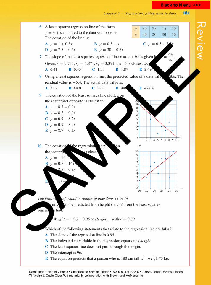
6 A least squares regression line of the form

y = a + bx is fitted to the data set opposite.y 30 25 15 10

x 40 20 30 10The equation of the line is:

A y = 1 + 0.5x B y = 0.5 + x C y = 0.5 + 7.5x

D y = 7.5 + 0.5x E y = 30 − 0.5x

7 The slope of the least squares regression line y = a + bx is given by: b = rsy

sx.

Given, r = 0.733, sx = 1.871, sy = 3.391, then b is closest to:

A 0.41 B 0.45 C 1.33 D 1.87 E 2.49

8 Using a least squares regression line, the predicted value of a data value is 78.6. The

residual value is −5.4. The actual data value is:

A 73.2 B 84.0 C 88.6 D 94.6 E 424.4

9 The equation of the least squares line plotted on

the scatterplot opposite is closest to:

A y = 8.7 − 0.9x

B y = 8.7 + 0.9x

C y = 0.9 − 8.7x

D y = 0.9 − 8.7x

E y = 8.7 − 0.1x

y

x01 2 3 4 5 6 7 8 9 10

123456789

10

10 The equation of the regression line plotted on

the scatterplot opposite is closest to:

A y = −14 + 0.8x

B y = 0.8 + 14x

C y = 2.5 + 0.8x

D y = 14 − 0.8x

E y = 17 + 1.2x

x20 22 24 26 28 30

0123456789

10

y

The following information relates to questions 11 to 14

Weight (in kg) can be predicted from height (in cm) from the least squares

regression line:

Weight = −96 + 0.95 × Height, with r = 0.79

11 Which of the following statements that relate to the regression line are false?

A The slope of the regression line is 0.95.

B The independent variable in the regression equation is height.

C The least squares line does not pass through the origin.

D The intercept is 96.

E The equation predicts that a person who is 180 cm tall will weigh 75 kg.

SAMPLE



Rev

iew


12 This regression line predicts that, on average, weight:

A decreases by 96 kg for each one centimetre increase in height

B increases by 96 kg for each one centimetre increase in height

C decreases by 0.79 kg for each one centimetre increase in height

D decreases by 0.95 kg for each one centimetre increase in height

E increases by 0.95 kg for each one centimetre increase in height

13 Noting that the value of the correlation coefficient is r = 0.79, we can say that:

A 62% of the variation in weight can be explained by the variation in height

B 79% of the variation in weight can be explained by the variation in height

C 88% of the variation in weight can be explained by the variation in height

D 79% of the variation in height can be explained by the variation in weight

E 95% of the variation in height can be explained by the variation in weight

14 A person of height 179 cm weighs 82 kg. If the regression equation is used to predict

their weight, then the residual will be closest to:

A −8 kg B 3 kg C 8 kg D 9 kg E 74 kg

15 If a three median line is fitted to the scatterplot

shown, then its slope is closest to:

A 0.2

B 0.4

C 0.6

D 0.8

E 1.0

x20 22 24 26 28 30

0123456789

10

y

Extended-response questions

1 In an investigation of the relationship between the hours of sunshine (per year) and

days of rain (per year) for 25 cities, the least squares regression line was found

to be:

Hours of sunshine = 2847 − 6.88 × Days of rain with r2 = 0.4838


a In this regression equation, the independent variable is .


c The regression equation predicts that a city that has 120 days of rain per year will

have hours of sunshine per year.

d The slope of the regression line predicts that the hours of sunshine per year will

by hours for each additional day of rain.

e r = , correct to three decimal places.

f % of the variation in sunshine hours can be explained by the variation in .

SAMPLE



Review


g One of the cities used to determine the regression equation had 142 days of rain

and 1390 hours of sunshine.

i The regression equation predicts its hours of sunshine to be hours.

ii The residual value for this city is hours.

h Using a regression line to make predictions within the range of data used to

determine the regression equation is called .

2 The cost of preparing meals in a school canteen is linearly related to the number of

meals prepared. To help the caterers predict the costs, data was collected on the cost

of preparing meals for different levels of demands. The data is shown below.

Number of meals 30 35 40 45 50 55 60 70 75 80 65

Cost (dollars) 138 154 159 182 198 198 214 238 234 244 208

a In this situation, the dependent variable is .

b Use your calculator to show that the equation of the least squares line that relates

the cost of preparing meals to the number of meals produced is:

Cost = 81.50 + 2.10 × Number of meals

c Use the equation to predict the cost of producing:

i 48 meals. In making this prediction are you interpolating or extrapolating?

ii 21 meals. In making this prediction are you interpolating or extrapolating?

d Complete the following sentences by filling in the missing information.

i The intercept of the regression line predicts that the fixed costs of preparing

meals is $ .

ii The slope of the regression line predicts that meal preparation costs increase by

$ for each additional meal produced.

e The correlation coefficient is r = 0.9784. Use this information to complete the

following sentence: The coefficient of determination equals . This indicates

that % of the variation in the of preparing meals is explained by the

variation in the of meals produced.

3 The scatterplot opposite shows the level of

carbon monoxide in the air alongside a

freeway against traffic volume on the

freeway. Also shown is the least

squares regression line that enables carbon

monoxide levels to be predicted from

traffic volume.

0

2

4

6

8

10

12

14

16

100 200 300 400

Traffic volume

Car

bon

mon

oxid

e le

vel

a Name the dependent variable in this analysis.

b From the scatterplot, work out the equation of

the least squares regression line and write it in the form:

Carbon monoxide level = a + b × Traffic volume

(cont’d.)

SAMPLE



Rev

iew


c In terms of carbon monoxide levels and traffic volume, what does the y-intercept

tell you?

d In terms of carbon monoxide levels and traffic volume, what does the slope of the

regression line tell you?

e Use the least squares regression equation to predict the average carbon monoxide

level when the traffic volume is:

i 80 ii 600 Is this an extrapolation or interpolation?

f Using r = 0.9851, calculate the value of the coefficient of determination and

interpret in terms of carbon monoxide levels and traffic volume.

4 We wish to find the equation of the least squares regression line that will enable

height (in cm) to be predicted from femur (thigh bone) length (in cm).

a Which is the DV and which is the IV?

b Use the following summary statistics to determine the equation of the least squares

regression line that will enable height (y) to be predicted from femur length (x).

r = 0.9939 x = 24.246 sx = 1.873 y = 166.092 sy = 10.086

Write the equation in terms of height and femur length.

c Interpret the slope of the regression equation in terms of height and femur length.

d Determine the value of the coefficient of determination and interpret in terms of

height and femur length.

5 The data below shows the height (in cm) of a group of 10 children aged 2 to

11 years.

Height (cm) 86.5 95.5 103.0 109.8 116.4 122.4 128.2 133.8 139.6 145.0

Age (years) 2 3 4 5 6 7 8 9 10 11

The task is to determine the equation of a least squares regression line which can be

used to predict height from age.

a In this analysis, which would be the DV and which would be the IV?

b Use your calculator to confirm that the equation of the least squares regression

line is

Height = 76.64 + 6.366 × Age and r = 0.9973

c Use the regression line to predict the height of a one-year-old child. In making

this prediction are you extrapolating or interpolating?

d What is the slope of the regression line and what does it tell you in terms of the

variables involved?

e Calculate the value of the coefficient of determination and interpret in terms of

the relationship between age and height.

f Use the least squares regression equation to:

i predict the height of the 10-year-old child in this sample

ii determine the residual value for this child

SAMPLE



Review


g i Use your calculator to confirm that the residual

plot for this analysis is as shown opposite.

ii Explain why this residual plot suggests that

a linear equation is not the most appropriate

model for this relationship.

2

−3.0

−1.5

0.0

1.5

3 4 5 6 7age

resi

dual

8 9 10 11

6 The scatterplot opposite shows female workplace

accident rates plotted against male workplace

accident rates in a selection of countries.

020 40 60 80 100 120

5101520253035404550

Male rateFe

mal

e ra

te

a Explain why it would be questionable to use

a least squares regression line in this situation.

b Fit a three median line to the scatterplot and

find its equation.

7 Can the weight of a mouse’s heart be reliably predicted from its body weight? The

body weights (in g) and the heart weights (in mg) of a random sample of 12

laboratory mice are as shown below.

Body weight (g) 27 30 37 38 32 36 38 42 36 44 33 38

Heart weight (mg) 118 136 156 150 140 155 144 159 149 170 131 160

a In this investigation, which would be the dependent variable and which would be

the independent variable?

b Perform a regression analysis to investigate the nature of the relationship between

heart weight and body weight in mice. As part of this analysis, use your calculator

to:

i generate a scatterplot

ii determine the equation of the least squares regression line, the coefficient of

determination and the value of Pearson’s correlation coefficient r

iii construct a residual plot

c Use the information generated in b to write a report on your investigation. Use the

format of the report given in Section 5.3. The two variables are heart weight and

body weight.SAMPLE


core regression: fitting lines to data sample - home | … · · 2008-09-09core regression:...

Documents