Regression and Curve fitting using Excel- Microsoft Office 2007

By Mohd Hanapiah Mohd Yusoff

1.0 Linear Regression

In curve fitting of experimental data, linear regression would mean fitting a simple equation such as

y ( x )=mx ± C

onto a set of data {x , y }. The x and y are independent and dependent variables, respectively, and m and C are constants. The curve-fitting procedure would be to determine the value of m and C. The most commonly used technique is the least-square method [Ref: Excel Help, LINEST].

In this example, we demonstrate linear least square fitting using Microsoft Excel 2007.

1.1 Plotting

Consider a set of data {x , y }with its uncertainty or error {∆ x , ∆ y } respectively.

Highlight the data x and y,

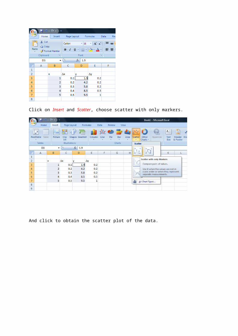
Click on Insert and Scatter, choose scatter with only markers.

And click to obtain the scatter plot of the data.

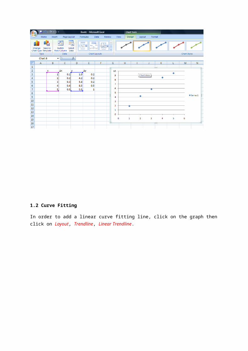
1.2 Curve Fitting

In order to add a linear curve fitting line, click on the graph then click on Layout, Trendline, Linear Trendline.

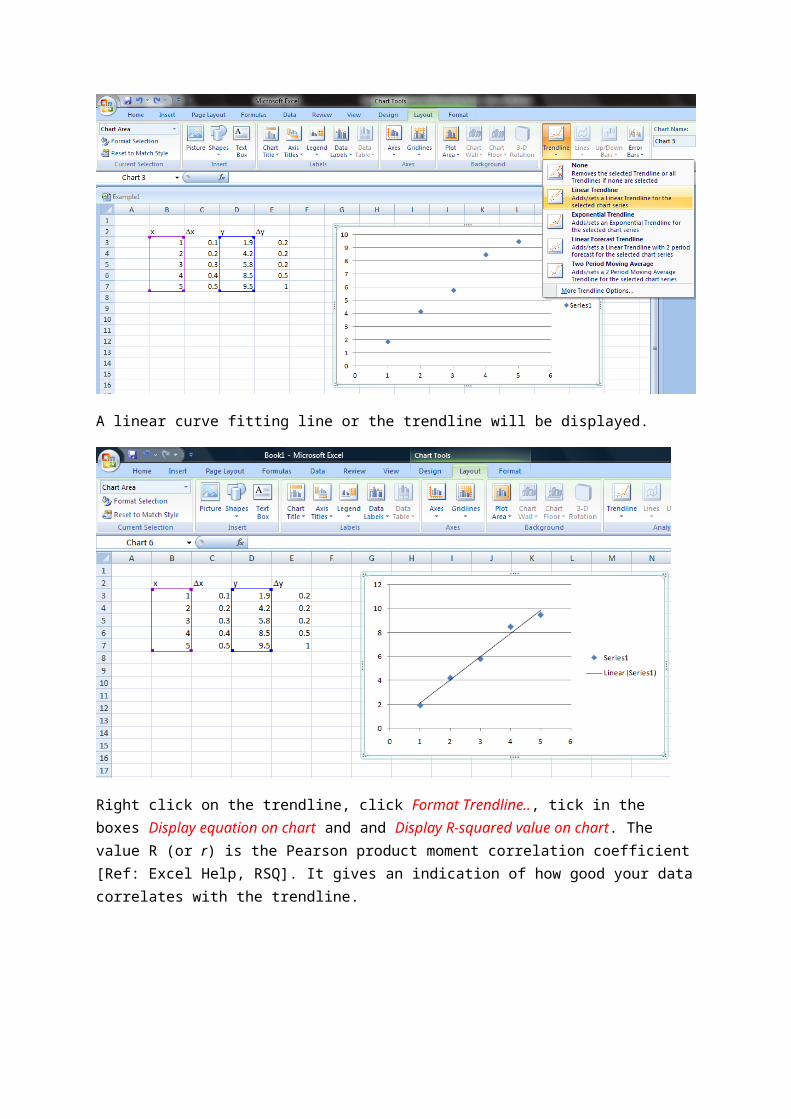
A linear curve fitting line or the trendline will be displayed.

Right click on the trendline, click Format Trendline.., tick in the boxes Display equation on chart and and Display R-squared value on chart. The value R (or r) is the Pearson product moment correlation coefficient [Ref: Excel Help, RSQ]. It gives an indication of how good your data correlates with the trendline.

You can extrapolate the trendline either forward or backward. Type an input in the Forecast Backward box, eg. 1.0 period. Observe the trendline extending to the y-axis.

1.3 Error Bars

In order to include error bars on your graph, click on the chart, choose Layout and then click on Error Bars and More Errors Bars Options. The Format Error Bars dialog box will appear. It will display either the vertical or horizontal error bars dialog box by clicking the vertical or the horizontal error bars on the chart.

Check on the Custom input for the Error Amount, and click on Specify Value. The Custom Error Bars dialog box will be displayed.

In the Positive Error Value and Negative Error Value highlight the range of values given in the column for y and click OK and close the Format Error Bars dialog box.

Click on the horizontal error bar on the chart, and repeat the process to format the horizontal error bars.

The final plot will appear like this.

Click on the chart then click on Layout, and under Labels, you can add chart title, label the axes and so on.

Exercise

1. Radioactive Decay

R=R0 e−λT (1)

Sample Problem 43-4, p. 1073. Fundamentals of PHYSICS (6ed-2001), part 5, John Wiley and Sons, (Halliday, Resnick and Walker). Calculate the value of R0 and

T (min) R(counts/s)4 392.2

36 161.468 65.5

100 26.8132 10.9164 4.56196 1.86218 1

Plot the data given using exponential regression in Excel. Present your result as shown in the chart given below. Give particular attention to the decimal points used on the chart for the axes and the equation. You are to reproduce the exact same plot. Compare the result obtained with result given in the text book.

Figure: Ex1

Reproduce the plot as in the textbook by using Excel. Calculate R0 from this plot. (The plot in the textbook is the same as the figure below).

Figure: Ex2

The results from Figures, Ex1 and Ex2 are the same. Figure Ex2 is obtained by linearizing the exponential relation of equation (1).