Core Analysis of the Round Tank Queen Reservoir, Chaves County,

New Mexico

By: Garrett Wilson

Table Of Contents

1. Introduction 2. Apparatus 3. Procedure 4. Results and Calculations

1. Porosity 2. Permeability 3. Fluid Displacement 4. Relative Permeability

5. Discussion 1. Porosity vs. Permeability 2. Fines Migration 3. Thin Section Analysis 4. SEM Imaging

6. Conclusion

Introduction

• This research was commissioned as one facet of a larger project entitled “Mini-Waterflood: A New Cost Effective Approach to Extend the Economic Life of Small, Mature Oil Reservoirs.”

• The part of the mini-waterflood project described by this research concerns experimental core studies aimed at gaining information as to the fluid movement and displacement within the Round Tank Queen formation.

• These core studies encompass flooding with oil from the Queen formation and brine from the San Andres formation located below the Queen.

• The information gained through this research will be used for reservoir characterization and as input data for reservoir simulation.

The Round Tank Queen

• The Round Tank Queen Associated Pool, located in Chaves County, New Mexico, was established in 1970. The discovery well was the JW State # 1, located in Unit K, Section 30, T15S-R29E.

• To date, nine wells have produced approximately 26000 barrels of oil, 4.2 BCF of gas and 788 barrels of water.

• A gas cap in the formation covers approximately four sections. Oil in the formation is largely devoid of gas.

• Gas composition is 61% nitrogen and 39% hydrocarbon gas with a BTU content of 513 BTU/ft3. The initial reservoir pressure was 600 psi, but over time, reservoir pressure has dropped to 50 psi and the reservoir temperature to 75°F. (Stubbs)

Round Tank Queen Core 1492-1494 Ft.

The core that was flooded was located at a depth of 1492 to 1494 feet. Although the main pay zone is located three feet below at a depth of 1497 to 1501 feet, this section of the core can be characterized as friable and thus was either rubblized or washed away during acquisition of the core..

Round Tank Queen # 6-Y Log

Gamma Ray Neutron Porosity

Core # 2 – 1493.2 Ft.

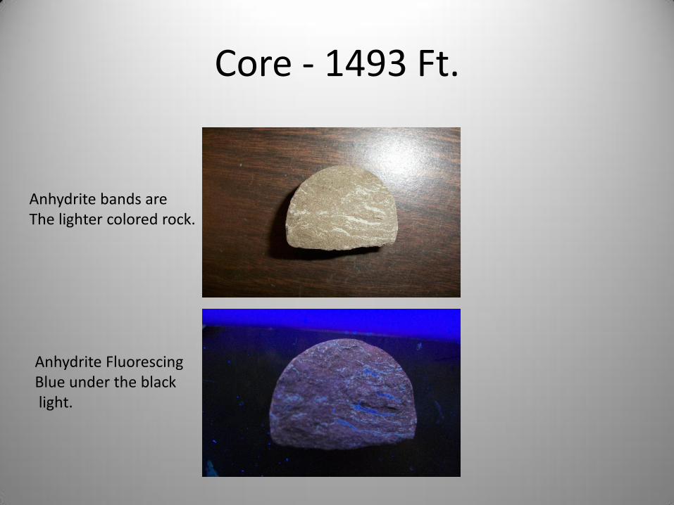
Core - 1493 Ft.

Anhydrite Fluorescing Blue under the black light.

Anhydrite bands are The lighter colored rock.

The Core Flooding System

Brine Pump

Brine Filters

Core

Core System Volume = 2.6 ml

100 mL

0 mL

Collection beaker accurate to 0.2 mL.

Oil Pump

Viton® Core Sleeve

Viscometer

Oil

154.5 (Seconds)

x 0.1033 (Constant)

x 0.86 (g/mL oil density)

= 13.67 cp

Brine

106 (Seconds)

x 0.015 (Constant)

x 1.12 (g/mL brine density)

= 1.56 cp

Density Meter

• The densities of the San Andres brine and Queen oil were measured using an Anton Paar mPDS 2000V3 density meter. Using a small syringe, the fluid being measured is injected into the meter, which then gives a τ value for that fluid.

• A and B can be solved for simultaneously by plugging in the known density of air, pure water and their corresponding τ values.

Air density = 0.0010208 g/mL Water Density = 1 g/mL τair= 3718.7 τwater= 3980.9 τbrine= 4012.1 τoil= 3946.2 A= -6.83441575 B= 4.942977 x 10-7 ρoil= 0.86 g/ml ρBrine= 1.12 g/ml

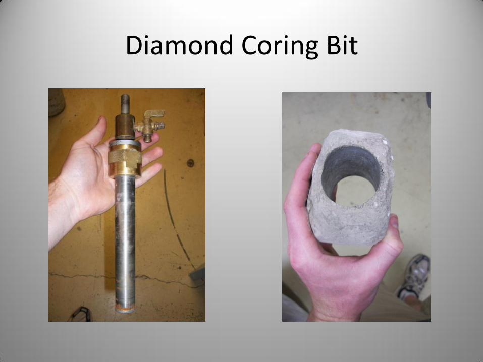
Diamond Coring Bit

Core Flooding Procedure

1. Measure the core flooding system volume. The system volume is subtracted from the amount of fluid injected into the core plug for both the porosity and permeability measurements. Place the distribution plugs against each other and close the output valve. Vacuum the air out of the system and then inject fluid until the pump pressure remains constant and the flow rate stops. The difference between the beginning pump volume and the ending pump volume equals the system volume.

2. Place the core plug inside a core sleeve and insert into the core holder.

3. Flood the core plug with THF (Tetrahydrofuran) until the THF at the output is relatively clear. When the THF is clear, it can be assumed that negligible amounts of oil and brine remain in the pore space. For better cleaning, close the output valve and pressure up the entire core plug to ensure maximum THF saturation. Remove the core plug from the core holder and rotate 180° to clean the lower portion of the core plug where any brine may be trapped.

Core Flooding Procedure

4. Flood with nitrogen until THF is no longer detected at the output.

5. Close the output valve and vacuum the core plug to evacuate any remaining matter for 1 day.

6. Flood with brine to measure porosity, and to saturate the core plug. Measure the amount of brine that the core plug will accept at a constant pressure.

7. Let sit 1-2 days to age.

8. Determine the permeability with brine by observing the variation in flow rates at multiple constant pressure drops or by observing the variation in pressure drops at multiple flow rates.

Core Flooding Procedure

9. Flood with oil at a constant pressure until no brine is seen at the output. Measure the volumes of input/output oil and brine as well as the flow rates. During this process determine the oil to water unsteady-state relative permeabilities.

10. Let the plug sit 2-3 days to age.

11. Inject several pore volumes (PVs) of oil at the same pressure drop to see if more water is produced. Determine the effective permeability of oil at interstitial water saturation.

12. Flood with brine at a constant pressure drop until no oil is seen at the output. Measure the volumes of input/output oil and brine as well as the flow rates.

13. Inject brine at a higher or lower pressure drop to determine an increase of oil production, if any.

Note: Steps 12-13 were not conducted on Core #1 and Core #3 because of the decrease in permeability.

Porosity Calculations – Core #1 1492.8 ft.

21.31 ml injected into the core at 500 psi

- 4.23 ml system volume

= 17.08 ml porous volume / core bulk volume of 97.87 ml

= 17.45 % porosity

Porosity Calculations - Core #2 1493.2 Ft.

13.4 ml injected into the core at 500 psi

- 2.6 ml system volume

= 10.8 ml porous volume / core bulk volume of 54.4 ml

= 19.8% porosity

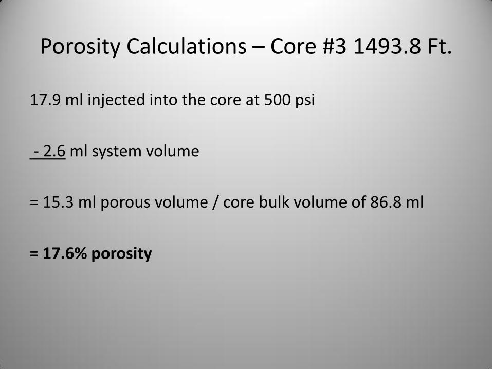
Porosity Calculations – Core #3 1493.8 Ft.

17.9 ml injected into the core at 500 psi

- 2.6 ml system volume

= 15.3 ml porous volume / core bulk volume of 86.8 ml

= 17.6% porosity

Porosity Measurement Sources of Error

• Chips in the core – Filled with epoxy

• Inadequate removal of insitu brine and oil – THF was relatively clear

• Errors in the system volume measurements – System volume measurements remained

consistent.

• The porosity measured was probably accurate to within ± 10 %.

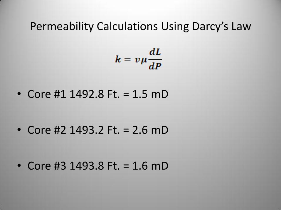
Permeability Calculations Using Darcy’s Law

• Core #1 1492.8 Ft. = 1.5 mD

• Core #2 1493.2 Ft. = 2.6 mD

• Core #3 1493.8 Ft. = 1.6 mD

Permeability Measurement Sources of Error

• Fines Migration

– THF injection reduced the permeability by 30% over 48 hours

• Possible clay swelling

• Fluid movement between the inside of the core sleeve and the outside of the core

– Overburden pressure was kept at 3500 psi.

Volume Recovered vs. Volume Injected

• Misreading the output amounts for core #1 caused error in the measurement of that core’s water injected vs. oil recovered data.

• For core #2, a full flooding schedule was able to be completed and so the data was acquired for oil injection at 150 and 500 psi dP, as well as water injection at 500 psi dP.

• Due to the loss of permeability in core #3, oil injection data was the only data gathered.

• A possible source of error is from flooding with oil and water multiple times, which reduced the permeability.

Oil Recovered vs. Brine Injected Core #2

0.0

0.1

0.2

0.3

0.4

0.5

0.6

0.7

0 1 2 3 4 5 6

Volume of Water Produced (PVs)

Volume of Oil Injected (PVs)

Brine Produced vs. Oil Injected For Core # 2 at 1493.2 Ft.

500 Psi dP 150 Psi dP

Interstitial water at 500 psi dP= 43% Interstitial water at 150 psi dP= 37%

Brine Recovered vs. Oil Injected Core #2

0.00

0.05

0.10

0.15

0.20

0.25

0.30

0.0 0.2 0.4 0.6 0.8 1.0 1.2 1.4 1.6 1.8 2.0

Oil Produced (PVs)

Brine Injected (PVs)

Brine Injected vs. Oil Recovered at 500 psi dP

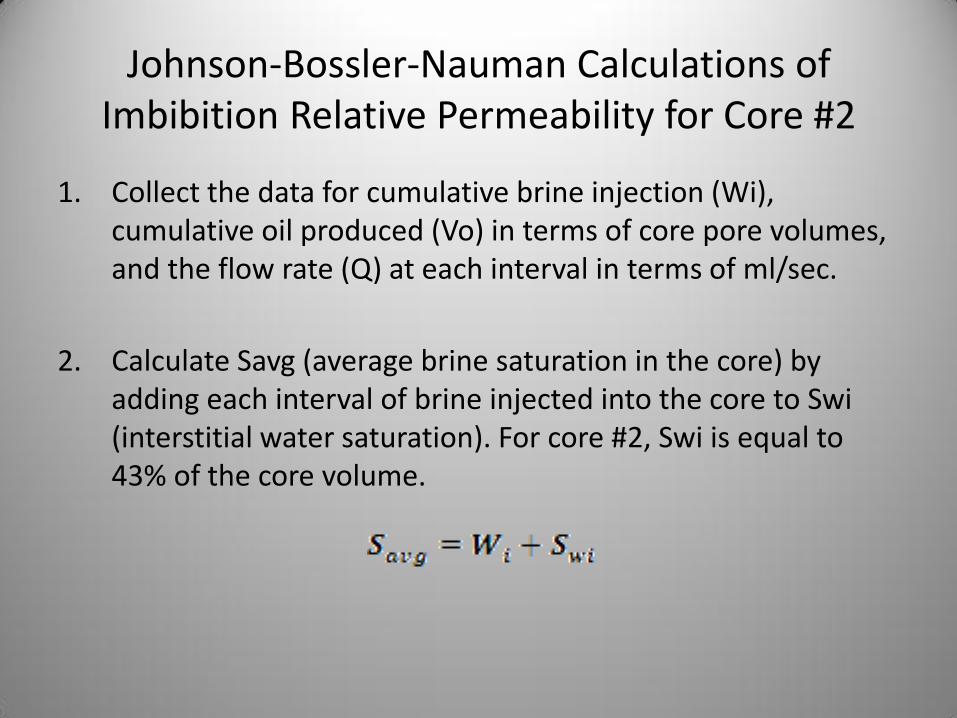
Johnson-Bossler-Nauman Calculations of Imbibition Relative Permeability for Core #2

1. Collect the data for cumulative brine injection (Wi), cumulative oil produced (Vo) in terms of core pore volumes, and the flow rate (Q) at each interval in terms of ml/sec.

2. Calculate Savg (average brine saturation in the core) by adding each interval of brine injected into the core to Swi (interstitial water saturation). For core #2, Swi is equal to 43% of the core volume.

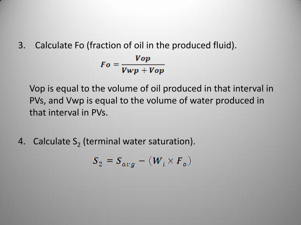
3. Calculate Fo (fraction of oil in the produced fluid).

Vop is equal to the volume of oil produced in that interval in PVs, and Vwp is equal to the volume of water produced in that interval in PVs.

4. Calculate S2 (terminal water saturation).

5. Calculate the relative injectivity constant.

– keo, in Darcy, is equal to the effective permeability of oil at interstitial water conditions, which is 1.17 for core #2.

– ∆P was held constant at 34 atmospheres.

– μo is equal to 13 cp.

– L and A are respectively equal to 3.8 cm and 11.335 cm2.

– Multiply this constant by Q at each interval to solve for 1/Ir.

– Ir constant is equal to 0.009098783.

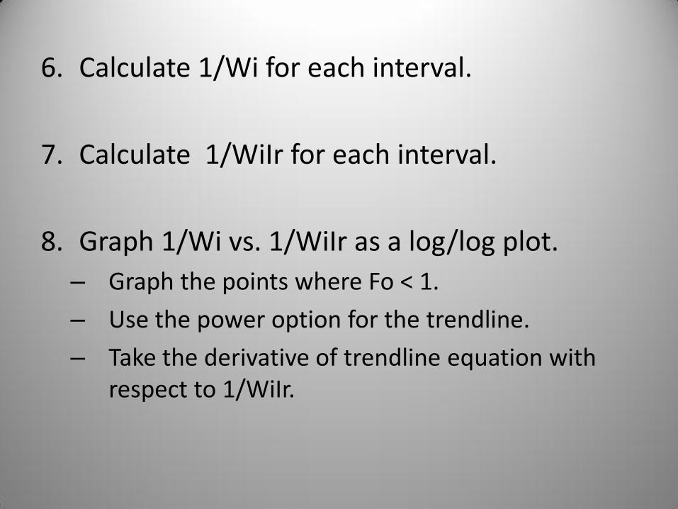
6. Calculate 1/Wi for each interval.

7. Calculate 1/WiIr for each interval.

8. Graph 1/Wi vs. 1/WiIr as a log/log plot.

– Graph the points where Fo < 1.

– Use the power option for the trendline.

– Take the derivative of trendline equation with respect to 1/WiIr.

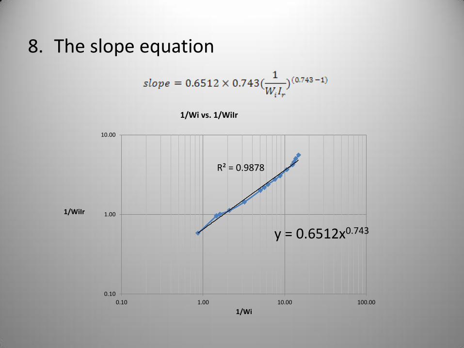
8. The slope equation

y = 0.6512x0.743

R² = 0.9878

0.10

1.00

10.00

0.10 1.00 10.00 100.00

1/WiIr

1/Wi

1/Wi vs. 1/WiIr

9. Calculate kro.

10.Calculate krw/kro.

11.Calculate krw.

Relative Permeability Curves

0.00

0.05

0.10

0.15

0.20

0.25

0.30

0.40 0.45 0.50 0.55 0.60 0.65 0.70 0.75

Relative Permeability

Average Water Saturation (%)

Imbibition Relative Permeability For Core #2 at 500 psi dP

kro

krw

Sources of Error in Relative Permeability Calculations

• Limitations involving the measurement equipment used during the procedures were thought to be the one the main facotrs for the errors in the relative permeability calculations.

• The beaker measuring the volume of oil and brine at the output side of the core was only accurate to 0.2 ml.

• This lead to difficulty in calculating the fraction of oil and water (Fo, Fw) produced from the core.

• Evidence of fine migration and clay swelling also renders the results questionable.

The Relationship Between Porosity and Permeability

• This graph shows the observed correlation between porosity and permeability for 610 sandstone samples.

• The permeability and porosity values for even core #2 plot well off of any of the trendlines shown by the graph.

• Permeability values started at unusually low levels and decreased as experimentation for each core continued.

1

0

0

Bri

ne

Per

mea

bil

ity,

Per

cent

of

Ori

gin

al

Brine Injected, Pore Volumes

Direction of

Flow Reversed

Fines Migration

Clay Swelling and/or

Fines Migration

Reduction in Permeability Due to

Fines Migration and/or Clay Swelling

(Core Labs Inc.)

Fines Migration

0

0.1

0.2

0.3

0.4

0.5

0.6

0 50 100 150 200 250

Permeability of Brine (mDs)

Water Injected (Pore Volumes)

Permeability vs. Pore Volumes Injected at Constant 200 Psi dP

Absolute permeability of brine increasing as brine saturation increases

Reversed Flow

Reversed Flow Reversed Flow

Thin Sections Analysis at 1492 Ft.

• Thin sections were made at 1 foot intervals from 1492-1494 ft. and 1500-1502 ft.

• Blue shows porosity. Yellow indicates Potassium Feldspar. The bright, multicolored areas are anhydrite.

The field of view for this picture is 80 microns and the average grain size is estimated to be less than 10 microns. The amount of blue indicates fairly high porosity. The picture shows fine grained sandstone and as permeability is a function of grain size squared, this partially explains the low permeability exhibited by the rock.

Thin Section Showing Poikilotopic Anhydrite Cement at 1492 ft.

• Poikilotopic means one large crystal that engulfs many small grains.

• This image shows a good example of poikilotopic anyhydrite as the anhydrite seems to surround all of the sand grains and provide a colorful backdrop.

SEM Imaging

• Photographs were taken using either BSE imaging or SE imaging.

• This picture is a BSE image of Anhydrite at 1502 ft.

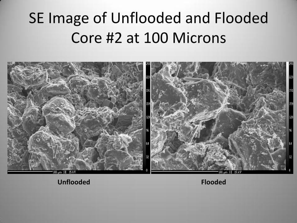
SE Image of Unflooded and Flooded Core #2 at 100 Microns

Unflooded Flooded

SE Image of Unflooded and Flooded Core #2 at 50 Microns

Unflooded Flooded

SE Image of Unflooded and Flooded Core at 20 Microns

Unflooded Flooded

Conclusions

1. Despite the differences in the San Andres and Queen brines, the San Andres brine and the Queen rock seem to be compatible.

2. Fines migration and clay swelling is suspected to occur in the core and will rapidly reduce permeability during water flooding.

3. Anhydrite layering occurs to a lesser degree in the pay zone, but some anhydrite to gypsum transformation may still occur during water flooding of the pay zone. This will cause the anhydrite to swell which will reduce permeability.

Conclusions

4. When performing core analysis, measurement utensils with greater precision should be utilized.

5. Further work should be conducted on mitigating the transformation of anhydrite cement to gypsum cement as well as lessening the effects of fines migration and clay swelling.

Questions???