copyright by pamela murray-tuite 2003chandra bhat daene mckinney david eaton . identification of...
TRANSCRIPT

Copyright
by
Pamela Murray-Tuite
2003

The Dissertation Committee for Pamela Marie Murray-Tuite Certifies that
this is the approved version of the following dissertation:
IDENTIFICATION OF VULNERABLE TRANSPORTATION
INFRASTRUCTURE AND HOUSEHOLD DECISION MAKING
UNDER EMERGENCY EVACUATION CONDITIONS
Committee:
Hani S. Mahmassani, Supervisor
Randy B. Machemehl
Chandra Bhat
Daene McKinney
David Eaton

IDENTIFICATION OF VULNERABLE TRANSPORTATION
INFRASTRUCTURE AND HOUSEHOLD DECISION MAKING
UNDER EMERGENCY EVACUATION CONDITIONS
by
Pamela Marie Murray-Tuite, B.S.C.E., M.S.E.
Dissertation
Presented to the Faculty of the Graduate School of
The University of Texas at Austin
in Partial Fulfillment
of the Requirements
for the Degree of
Doctor of Philosophy
The University of Texas at Austin
December, 2003

UMI Number: 3122770
Copyright 2003 by
Murray-Tuite, Pamela Marie
All rights reserved.
________________________________________________________
UMI Microform 3122770
Copyright 2004 ProQuest Information and Learning Company.
All rights reserved. This microform edition is protected against
unauthorized copying under Title 17, United States Code.
____________________________________________________________
ProQuest Information and Learning Company 300 North Zeeb Road
PO Box 1346 Ann Arbor, MI 48106-1346
Dedication
This dissertation is dedicated to the memory of all lives lost during the
September 11, 2001 terrorist attacks and their families.

Acknowledgements
My tenure as a graduate student has spanned the most enjoyable four years
of my life. I would like to take this opportunity to thank all of the Transportation
Engineering professors at the University of Texas at Austin for their support,
guidance, and instruction. Dr. Mahmassani has made the development of my
research interests possible and served as a mentor, encouraging me to grow both
personally and academically. Much appreciation is owed to Dr. Bhat and Dr.
Machemehl who offered advice on personal and professional matters. The
comments and constructive criticism offered by the committee members has been
instrumental to the completion and focus of this dissertation.
Furthermore, I acknowledge the blessings of family bestowed upon me. I
thank my husband Kenneth for his support, encouragement, and love. My
parents, Sandra and Thomas Murray, and brother, Jeffrey Murray, have been
unwavering in their support of my work and career.
This dissertation work was funded by the Southwest Region University
Transportation Center.
v

IDENTIFICATION OF VULNERABLE TRANSPORTATION
INFRASTRUCTURE AND HOUSEHOLD DECISION MAKING
UNDER EMERGENCY EVACUATION CONDITIONS
Publication No._____________
Pamela Marie Murray-Tuite, Ph.D.
The University of Texas at Austin, 2003
Supervisor: Hani S. Mahmassani
This dissertation combines two primary problems under general disaster
considerations. First, a methodology is presented to identify vulnerable
transportation infrastructure, which is defined as the set of network links, the
damage of which results in the maximum disruption of the network’s origin-
destination connectivity. The disrupting agent is permitted a limited number of
resources with which to damage the network. The measure of disruption,
resulting from the damage, is based on a given set of traffic conditions, the
availability of alternate paths, and roadway design characteristics. A bi-level
mathematical programming model represents the interaction of the traffic
assignment and the disruption measure. This bi-level model allows the problem
to be viewed as a game between an evil entity, who seeks to disrupt the network,
vi

and a traffic management agency that routes vehicles so as to avoid vulnerable
links to the greatest degree possible while meeting origin-destination demands.
The second problem is to mathematically describe household decision
making behavior in an emergency evacuation. Traditional transportation network
evacuation models have omitted a commonly observed sociological phenomenon
– that families gather together before evacuating an area. This omission can lead
to overly optimistic evacuation times, and the evacuation models fail to capture
underlying traffic patterns that only arise during times of crises. Two linear
integer programs are developed to model the decision making behavior; the first
describes a meeting location selection process and the second assigns trip chains
for drivers to pick up family members who may not have access to a vehicle. The
mathematical programs are combined with a traffic assignment-simulation
package for evacuation analysis.
Interactions between the two problems are also explored. Evacuation
conditions are examined when the traffic management agency routes traffic
around vulnerable links. The impact of the unusual traffic patterns, that arise
using the household decision making behavior evacuation model, is evaluated in
terms of shifts in the relative vulnerability of the transportation links. Finally, the
routing strategies are evaluated for extensions in network evacuation times.
vii

Table of Contents
List of Tables.......................................................................................................... xi
List of Figures ...................................................................................................... xiv
Chapter 1: Introduction ........................................................................................... 1
1.1 Motivation ................................................................................................ 1 1.2 Problem Statement and Objectives .......................................................... 3
1.2.1 Identification of Vulnerable Transportation Infrastructure Elements ....................................................................................... 3
1.2.2 Model of Household Decision Making in an Emergency Evacuation........................................................ 4 1.2.3 Combining the Problems: Vulnerability of Networks under
Evacuation Flow Patterns............................................................. 6 1.3 Research Significance and Contributions ................................................ 7 1.4 Structure and Overview of the Dissertation ............................................. 7
Chapter 2: General Background.............................................................................. 9 2.1 Network Reliability .................................................................................. 9
2.1.1 Other Fields ................................................................................ 10 2.1.2 Transportation Engineering........................................................ 11 2.1.3 Aggregation................................................................................ 13
2.2 Evacuation Behavior .............................................................................. 15 2.2.1 Early Studies .............................................................................. 16 2.2.2 Technological Advances ............................................................ 17 2.2.3 Modeling .................................................................................... 18
2.3 Vehicle Routing...................................................................................... 19 2.3.1 The Basic Vehicle Routing Problem.......................................... 19 2.3.2 Vehicle Routing with Time Windows........................................ 23
2.4 Summary ................................................................................................ 25
viii

Chapter 3: Identification of Vulnerable Transportation Infrastructure ................. 27 3.1 Development of the Disruption Index.................................................... 29 3.2 Bi-Level Formulation............................................................................. 37
3.2.1 Formulation ................................................................................ 37 3.2.2 Solution Framework................................................................... 40 3.2.3 Sample Network ....................................................................... 40 3.2.4 Results and Discussion for Single Links.................................... 42 3.2.5 Results and Discussion for Joint Link Consideration ................ 48
3.3 Application of Game Theory.................................................................. 57 3.3.1 Game1: No-Information for the Traffic Management Agency.. 58 3.3.2 Game 2: Some Information for the TMA................................... 58 3.3.3 Game 3: One Move for Each Player, Full Information.............. 60 3.3.4 Game 4: Perfect Information for Both Players, Multiple
Moves ......................................................................................... 86 3.4 Summary ................................................................................................ 87
Chapter 4: Model of Household Decision Making In An Emergency Evacuation.................................................................................................... 89 4.1 Modeling Framework and Problem Formulation................................... 90 4.2 Experimental Design .............................................................................. 98 4.3 Experimental Results............................................................................ 105 4.4 Summary .............................................................................................. 133
Chapter 5: Case Study ......................................................................................... 135 5.1 Simulation Test Bed ............................................................................. 136 5.2 Experimental Design ............................................................................ 138
5.2.1 Household Characteristics....................................................... 138 5.2.2 Household Decision Making Objective Function Weights..... 139 5.2.3 Household Dwell Time ........................................................... 139 5.2.4 Evil Entity Resources and Targets and Traffic Management
Agency Strategies..................................................................... 140
ix

5.2.5 Traffic Assignment.................................................................. 142 5.2.6 Alternate Paths ........................................................................ 142 5.2.7 Evaluation Times..................................................................... 142 5.2.8 Combinations of Factors Examined ........................................ 143
5.3 Experimental Procedure ...................................................................... 145 5.3.1 Establish Baseline Conditions .................................................. 146 5.3.2 Simulate Evacuation Conditions with Trip Chains .................. 147 5.3.3 Determine Infrastructure Vulnerabilities under Evacuation
Conditions and Traffic Management Agency Strategies ......... 147 5.3.4 Comparison of Peak Period and Evacuation Conditions ........ 148
5.4 Results .................................................................................................. 148 5.5 Summary .............................................................................................. 166
Chapter 6: Summary and Conclusions ................................................................ 167 6.1 Summary .............................................................................................. 167 6.2 Conclusions Specific to the Networks Considered .............................. 169 6.3 Future Work ......................................................................................... 172
Appendix A Joint Vulnerability Index Computer Code..................................... 173
Appendix B Flow Distributions ......................................................................... 188
Appendix C Household Generation Code.......................................................... 202
Appendix D Link Characteristics for Figure 5.1................................................ 245
Appendix E Payoff Matrix for Baseline Conditions .......................................... 257
Bibliography........................................................................................................ 269
Vita .................................................................................................................... 277
x

List of Tables
Table 3.1 Notation for the Development of the Disruption Index and the
Bi-Level Formulation …………………………………………...... 32
Table 3.2 Link Characteristics for the Sample Network ................................ 41
Table 3.3 Flow Distribution and Vulnerability Indices Results ..................... 43
Table 3.4 Disruption Indices for the Sample Network and Various
Demand Levels .............................................................................. 47
Table 3.5 Joint Vulnerability Indices for Origin-Destination (1,2) ................ 48
Table 3.6 Joint Vulnerability Indices for Origin-Destination (1,6) ................ 50
Table 3.7 Joint Vulnerability Indices for Origin-Destination (5,2) and
All Demand Levels ......................................................................... 51
Table 3.8 Joint Vulnerability Indices for Origin-Destination (5,6) ................ 52
Table 3.9 Joint Disruption Indices for Sample Network ............................... 54
Table 3.10 General Payoff Matrix .................................................................... 60
Table 3.11 Payoff Matrix for n=1, Original Demand Level ............................ 62
Table 3.12 Payoff Matrix for n=1, 3/4 Demand Level ..................................... 63
Table 3.13 Payoff Matrix for n=1, 1/2 Demand Level ..................................... 64
Table 3.14 Payoff Matrix for n=2, Original Demand Level ............................ 65
Table 3.15 Payoff Matrix for Misinformation about Player T’s Resources,
Original Demand Scenario ............................................................. 70
Table 3.16 Payoff Matrix for n=2, 3/4 Demand Level ..................................... 71
xi

Table 3.17 Payoff Matrix for Misinformation about Player T’s Resources,
3/4 Demand Scenario ..................................................................... 77
Table 3.18 Payoff Matrix for n=2, 1/2 Demand Level ..................................... 78
Table 3.19 Payoff Matrix for Misinformation about Player T’s Resources,
1/2 Demand Scenario .................................................................... 85
Table 4.1 Summary of Notation ..................................................................... 92
Table 4.2 Perceived Zonal Travel Times to Residential Zones ................... 106
Table 4.3 Perceived Travel Times to School Zones ..................................... 107
Table 4.4 Meeting Location Selection ......................................................... 108
Table 4.5 Sample Trip Chains for Various Household Types ..................... 109
Table 4.6 Comparison of Pick-Up Assignments Due to Variation in Dwell
Time and Weight on Perceived Total Fleet Travel Time ............. 115
Table 4.7 Network Clearance Times for Various Vehicle Loading
Methods ........................................................................................ 119
Table 4.8 Network Clearance Profiles for Various Dwell Times and
Weights ......................................................................................... 125
Table 4.9 Comparison of Average Times, Distances, and Evacuation
Times for Different Lengths of School Links for Activity
Chains with Minimum Waiting Times of 5.0 Minutes at
Intermediate Nodes ....................................................................... 132
Table 5.1 Combination of Experimental Factors .......................................... 144
Table 5.2 Payoff Matrices for the General Information Game ..................... 159
xii
Table 5.3 Payoff Values for Player M’s Strategy “Avoid Link 306” at
Different Time Points ................................................................... 162
xiii

List of Figures
Figure 3.1 Sample Network …………………………………………………...41
Figure 3.2 Comparison of Vulnerability Indices for Alternate Paths for OD
(5,6) ……………………………………………………………… 45
Figure 3.3 Comparison of Disruption Indices and Percentage of OD (5,6)
Flow Assigned to Link ………………………………...………….47
Figure 3.4 Sample Network after Player T’s First Move …………………….86
Figure 4.1 Sample Network............................................................................. 101
Figure 4.2 Sample Network with Zones .......................................................... 102
Figure 4.3 Network Clearance for All Weight (λ = 1.0) on Total Fleet Time 120
Figure 4.4 Network Clearance for Half Weight (λ = 0.5) on Total Fleet
Time ............................................................................................... 121
Figure 4.5 Network Clearance for No Weight (λ = 0.0) on Total Fleet Time. 123
Figure 4.6 Comparison of 80% Network Clearance Times and Minimum
Dwell Times for Various Total Fleet Time Weights...................... 127
Figure 4.7 Comparison of Network Clearance for Total Fleet Time Weights
with Minimum Dwell Time 1 Minute at School and Meeting
Locations ........................................................................................ 129
Figure 4.8 Comparison of Network Clearance for Total Fleet Time Weights
with Minimum Dwell Time 3 Minutes at School and Meeting
Locations ........................................................................................ 130
xiv

Figure 4.9 Comparison of Network Clearance for Total Fleet Time Weights
with Minimum Dwell Time 5 Minutes at School and Meeting
Locations ........................................................................................ 131
Figure 5.1 Simplified Version of South Central Fort Worth, TX.................... 137
Figure 5.2 Selected Links .............................................................................. 141
Figure 5.3 Ten Most Vulnerable Links for Peak Period Conditions ............... 150
Figure 5.4 Ten Most Vulnerable Links for Evacuation Case 1 ....................... 152
Figure 5.5 Ten Most Vulnerable Links for Evacuation Case 2 ....................... 154
Figure 5.6 Eleven Most Vulnerable Links for Evacuation Case 3 .................. 156
xv

Chapter 1
Introduction
Threats of terrorism, war, and natural disasters have created an
environment in which the evacuation of a city or region may be necessary. The
transportation network of the affected area plays a crucial role in the success of
moving the area residents to safety. Transportation engineers and planners
continually seek to improve the mobility of residents through the network,
particularly during emergency situations. In preparation for these times of
unusual and extreme traffic conditions, the ability to identify vulnerable
transportation infrastructure, an understanding of evacuation behavior at the
household level, and the associated simulation tools are of critical importance.
This chapter introduces the motivation for this work, the problem and
related objectives, the contributions of this work to the fields of transportation
engineering, evacuation planning, and critical infrastructure protection, and
outlines the remainder of this dissertation.
1.1 MOTIVATION
Disaster management and related emergency evacuation are not new fields
of study. Analyses of literature trends indicate that prior to the Cold War, much
of the research was focused on evacuation procedures and the determination of
factors that were more likely to cause people to leave their homes in response to
natural threats, such as floods and hurricanes. Fear of nuclear attacks and the
construction of nuclear power plants motivated a great deal of evacuation
1

planning activity in the 1970’s in response to a new type of threat. In the late
twentieth and early twenty-first centuries, hurricanes caused the timing of
evacuation orders to be evaluated more carefully. Now, amid the rising fear of
terrorism in the United States, there has been another shift in focus from natural
disasters to those caused by mankind.
Three time periods can be associated with a disaster. The first is the pre-
disaster phase. During this time, especially for natural events, authorities may
initiate the evacuation process. Warning technology, such as weather tracking
devices, can be extremely valuable at this time. The second phase is the actual
disaster strike and the limited time period that immediately follows. This period
may encompass an earthquake or bombing and the immediate aftermath. During
this time, victims may suddenly flee while rescue workers respond to the site. In
the third phase, evacuees have abandoned the disaster area and only the rescue
workers remain. At this time recovery begins. Due to the wide array of different
evacuation scenarios, the focus of this work is on the first two phases, which are
associated with the actual evacuation process.
Simulation methods are commonly used for transportation strategy
evaluation. The transportation network is modeled and traffic movements are
simulated through a series of behavior rules. However, previous models have not
adequately captured the interaction among the existing transportation
infrastructure, the provision and exchange of information enabled by modern
information and communications technologies, and the behavior of evacuees.
Traditional evacuation models assume that residents immediately leave the
threatened area; however, this is not always the case. Parents may actually head
toward danger to gather family members prior to evacuating the area. In this
work, some of the apparently disorganized traffic caused by this behavior is
explained by a series of mathematical programs, which emulate household
decision-making behavior. To determine the importance of specific roads to the
2

connectivity of origins and destinations, a measure called the vulnerability index
was developed. For each link, the vulnerability indices are then aggregated across
all origin-destination pairs into a disruption index, which allows for the
identification of roadways that should be protected or where redundancy is
needed in the transportation network.
1.2 PROBLEM STATEMENT AND OBJECTIVES
The overall problem investigated in this dissertation is to develop a
decision-aiding methodology for emergency evacuation planning for a city that
considers transportation infrastructure vulnerability, realistic evacuee behavior,
and the potential of information and communication technology. There are two
primary problems addressed within the overall problem. The first involves the
identification of vulnerable transportation infrastructure elements. The second
pertains to accurately emulating network evacuation flow patterns resulting from
the depiction of individual behavior at the household level. Each of these is
explained further in the following sections.
1.2.1 Identification of Vulnerable Transportation Infrastructure Elements
The identification of vulnerable transportation infrastructure elements
poses numerous challenges to the planning, engineering, and infrastructure
protection communities. The definition of vulnerable, or critical, infrastructure
elements may vary depending on the specific problem context. For instance, a
bridge may be vulnerable to flooding. Another bridge may be vulnerable to a
terrorist attack because of its history or landmark status. The definition of
vulnerable, or critical, infrastructure used in this dissertation applies to a link, or
3
set of links, the damage of which causes the most disruption to the origin-
destination connectivity of the network. The problem of interest is to characterize
the vulnerability of transportation infrastructure elements and identify the most
vulnerable elements in a network for particular threat scenarios. More formally,
the problem is to identify a set of transportation network links, the damage of
which will maximally disrupt the origin-destination connectivity of the network.
The objectives pertaining to this problem are
1. To develop a mathematical measure of origin-destination
connectivity vulnerability for a link, or set of links;
2. To extend the origin-destination vulnerability measure to the
network level; and
3. To examine the impact of routing strategies and information on
the vulnerability of transportation network links.
These objectives are addressed in detail in chapter 3. In chapter 5, the
measures developed for objectives (1) and (2) are applied to a larger network.
Objective (3) is explored in both chapters 3 and 5.
1.2.2 Model of Household Decision Making in an Emergency Evacuation
Accurately modeling emergency evacuation conditions is extremely
difficult due to the lack of empirical evidence. Each emergency presents a
different set of conditions. The differences may be due to the type of emergency,
the experience of the community with similar events, the amount of warning that
precedes the incident, the predicted severity and scope of the disaster, and
conditions external to the community. Transportation evacuation model
verification is highly impractical to conduct prior to an evacuation because there
are ethical and practical constraints to conducting a “test” evacuation of a city.
4

Numerous evacuation studies have been conducted after the event has
occurred. The majority of these have been conducted by agencies whose primary
responsibility is not related to transportation engineering. A key finding from
these studies that has been omitted from the majority of the transportation
evacuation models is that families tend to gather together and then evacuate as a
single unit. This omission leads to inaccuracy in many aspects of the evacuation
model. Underlying traffic patterns, such as those that arise when parents go to
schools to collect their children, are not captured in traditional models.
Congestion is not properly predicted. As a result, the evacuation time prediction
may be biased to the low side.
The problem addressed in chapter 4 of this dissertation is to develop a
mathematical model of intra-household logistics during an emergency evacuation,
including the processes by which family members gather and meet to evacuate
jointly. The model would then be incorporated into a traffic assignment-
simulation methodology to represent the dynamics of the resulting network flow
patterns during the evacuation. Intra-household logistics modeling entails two
primary decision dimensions: meeting location selection and the sequencing of
pick-up assignments, resulting in trip chains to be completed by the household
members using the transportation network, parts of which may be damaged or
operationally modified (due to traffic management or vulnerability protection
actions). The objectives associated with this problem consist of the following:
1. Formulate an optimization-based model of intra-household
logistics decision-making behavior; the formulation captures
trade-offs among key factors considered by the household in
the decision process.
2. Examine the sensitivity of the decision behavior outcomes
with respect to the relative weights associated in the above
5

trade-offs, and identify switchover points at which changes in
behavior or pick-up assignments might result.
3. Represent and characterize the traffic conditions that arise
when the resulting emergency trip chaining behavior of
multiple households interact through the transportation
network, using a state-of-the-art dynamic network traffic
simulation-assignment methodology.
These three objectives are addressed in chapter 4. The model developed
in objective (1), the results of objective (2), and the combined household decision
making behavior – traffic simulation package of objective (3) are further explored
in chapter 5. The difference in the approach to objective (3) in chapters 4 and 5 is
the influence of non-driving entities, such as a traffic management agency. In
chapter 4, the traffic management agency allows the use of any network link. In
chapter 5, some links are assigned a very high cost which influences the route
selection between origin-destination pairs.
1.2.3 Combining the Problems: Vulnerability of Networks under Evacuation Flow Patterns
The two primary problems discussed in sections 1.2.1 and 1.2.2 are
considered jointly in chapter 5. This gives rise to two types of problem situations:
(1) determining the vulnerability of network infrastructure elements under
evacuation flow patterns; and (2) designing or inducing evacuation patterns that
are less susceptible to disruption and are hence more likely to successfully and
safely complete the evacuation process in the event of disruptive action. Traffic
management agency routing strategies can then be devised and evaluated in terms
of the effect on evacuation time and associated impact on transportation
infrastructure vulnerability rankings.
6

1.3 RESEARCH SIGNIFICANCE AND CONTRIBUTIONS
This research contributes to the field of transportation engineering in two
main arenas. The first area is network reliability and vulnerability. In this
dissertation, an index is developed to characterize the relative importance of a
given link, or set of links, to the network’s origin-destination connectivity, for a
given set of network flow conditions. The second area of significance is in
evacuation modeling. Traditional engineering models have omitted an important
factor at the family, or household, level. In this work, a series of linear integer
programs is presented to describe the meeting location selection and the trip
chaining assignment decisions for gathering family members, prior to evacuation.
Without this component, evacuation models fail to capture an essential portion of
the travel made within the city. The interaction of the drivers seeking to pick up
family members and the drivers leaving the city has not been adequately studied.
Integration of the mathematical programs for intra-household logistics decision
with a network traffic simulation-assignment methodology leads to a more
realistic representation of evacuation scenarios and the associate vehicular traffic
flow patterns in the network.
1.4 STRUCTURE AND OVERVIEW OF THE DISSERTATION
This dissertation is organized in six chapters. Following the problem
definition, motivation, and objectives discussed in the present chapter, the next
chapter presents a general overview of the literature related to network reliability,
evacuation behavior, and vehicle routing problems. Chapter 3 presents the
modeling framework for the identification of vulnerable transportation
7

infrastructure elements and an example of the methodology applied to a small
transportation network. The underlying problem in chapter 3 is considered from a
game theoretic perspective, in which an evil entity seeks to disrupt the network
flow and a traffic management agency employs advanced traveler information
systems and other means to route vehicles around vulnerable links. In the fourth
chapter, the household evacuation behavior models are developed, including an
application to a sample network. The behavior models assume that family
members gather together prior to evacuating the city. Chapter 5 presents a
hypothetical case study in which the models from Chapters 3 and 4 are applied to
a moderately sized network. Finally, in chapter 6, the summary, conclusions, and
directions for future work are presented.
8

Chapter 2
General Background
This chapter presents general background literature for this dissertation and is
divided into three sections. In the first section, a general overview of previous
studies pertaining to network reliability and vulnerability, which is the subject of
chapter 3, is presented. The second part of the chapter discusses observed
evacuation behavior. The third section identifies mathematical models that are
related to the household evacuation model presented in Chapter 4.
2.1 NETWORK RELIABILITY
Network reliability has been a growing area of interest to the transportation
community. Other fields, such as telecommunications and water resources, have
addressed network reliability over the years (see for example Lee, 1980;
Aggarwal, 1985; Yang et al, 1996). The definition of network reliability that is of
interest here pertains to connectivity. Specifically, the network reliability is the
probability that the origin and destination are connected due to the probabilities of
link existence. Difficulties exist in directly applying the definitions and
methodologies of the fields of telecommunications and water resources to the
transportation arena.
9

2.1.1 Other fields
There are several characteristics of telecommunications systems that
create difficulties in directly applying methodologies to the transportation
networks. For example, the radio or optical signal, or whatever is flowing on the
network, may degrade over the distance of the link (Caccetta, 1984). Another
example is the treatment of the flow that is on the network. If a communications
link is damaged, the calls using that link are dropped with little impact to the
remainder of the network. In the transportation network, the vehicles may
become damaged and cause queueing in the network. Finally, simplified versions
of telecommunication networks can be represented as having equal probabilities
of operating (Nel and Colbourn, 1990). Rarely, if ever, is this the case in a
transportation network. Instead of information, there are vehicles flowing through
the network and these vehicles are dispersed across nearly all competitive paths
from an origin to a destination; only in extreme cases are roads completely closed,
for any reason.
The use of nearly all paths, with similar travel times, is due to the fact that
the vehicles are driven by people who have the ability to choose routes based on
their perception of the state of the transportation network and not necessarily the
actual state of the system. Furthermore, each driver may place different weights
on factors that affect his or her route choice. For instance, one driver may decide
that travel time is the most important criterion, regardless of the number of turns,
the type of road, the safety of the road, and the number of traffic calming
measures. Other drivers may prefer a simple route, with very few road changes
and turns, even if the travel time is slightly longer.
10

2.1.2 Transportation Engineering
Unlike information or water, drivers have the ability to act as individual
particles. Since there are differences in the commodity flowing on the network,
methods from telecommunications and water resources need to be carefully
adapted to the particular characteristics of a transportation system.
From the transportation engineering perspective, the focus of recent works
related to network reliability has been on the probability of a pathway being
completely operational and with damage to none of the links. Numerous
methodologies, such as game theory (see Bell, 2000; Cassir and Bell, 2000; Bell,
1999), Monte Carlo simulation (see Chen et al, 1999), stochastic user equilibrium,
and minimum cut sets have been employed, albeit for different problem
formulations.
Iida and Wakabayashi (1989) proposed two approximation methods for
determining the connectivity reliability between a pair of nodes in a transportation
network. These methods were based on reliability graph analysis using minimal
path sets and cut sets. In this work, Iida and Wakabayashi noted that to find an
exact value for the reliability, complete enumeration of the minimal path sets
and/or minimum cut sets was necessary. Due to the cumbersome nature of
finding the exact solution, the authors presented a method that would approximate
the reliability by using only partial sets. One of the assumptions that is critical to
the use of this work is that the reliability of individual links is known a priori.
Iida (1999) presented basic equations for connectivity reliability when a
system is in a series or in parallel. For Iida’s (1999) work to apply to a network,
one must be able to predict the probability that a link would be damaged and to
what extent. In the case of terrorism a great deal of uncertainty exists in
identifying specific transportation links that may be impacted. Additionally, even
11

if the link is correctly identified as a target, slight miscalculations on the part of
the actor may lead to that link being missed and an adjacent one being hit.
Asakura (1999) incorporated a stochastic user equilibrium model into a
performance reliability model. In this work, he examined the role of information
on user’s route choice. Like Iida’s (1999) work, the probability of the links
existing was assumed known.
Many of the previous works presented above are more applicable to
vehicle accidents or natural disasters, particularly flooding, where the probability
of a roadway being affected is more easily quantifiable due to either historical
data or the surrounding environment. The development of a mathematical
measure of importance for links under any conditions and in any network, with or
without a history of flooding or earthquake damage, will greatly aid both public
and private sectors. By defining the value to be within given limits, one may
determine the importance of a link in connecting an origin and a destination.
In the field of operations research, some work has addressed determining
vital arcs in a network. Corley and Sha (1982), Malik, Mittal, and Gupta (1989)
and Ball, Golden, and Vohra (1989) defined the most vital arcs problem as
determining the subset of arcs whose removal from the network would result in
the greatest increase in the shortest path between a given pair of nodes. This
problem concept is similar to that found in the definition of edge persistence in
the telecommunications industry (Caccetta, 1984). However, edge persistence
pertains to the number of links that must be removed from the network and not
the identification of the importance of particular links. Malik, Mittal, and Gupta
(1989) proposed an exact algorithm for determining the k most vital arcs. Ball,
Golden and Vohra (1989) showed that the most vital arcs problem is closely
related to the most relevant arcs problem, the solution of which provides a lower
bound on the optimal solution of the most vital arcs problem. The authors
described an algorithm to solve the most relevant arcs problem. The most vital
12

arcs problem is NP hard but the most relevant arcs problem admits a polynomial
time solution algorithm.
Studies conducted in the operations research field are more directly
applicable to the work presented here. The problems examined by the authors
mentioned above are related to the links in the shortest path. In this work, all
links are evaluated, not just the most critical ones. In chapter 3, a methodology
for determining the relative importance of links in the network is presented. By
examining the values of the disruption indices (see chapter 3), one can rank the
links in terms of importance; the arcs with the highest rank correspond to the links
that would be identified using the approaches of Corley and Sha (1982), Malik,
Mittal, and Gupta (1989), and Ball, Golden and Vohra (1989).
2.1.3 Aggregation
In Chapter 3, a methodology for the determination of the vulnerability of a
link, or set of links, is developed. An index is presented that represents the
importance of the set of links to the connectivity of an origin-destination pair.
This index is then aggregated over all origin-destination pairs to obtain a network
level measure.
The issues of aggregating data with different units and different
perspectives have been studied in detail. There are numerous approaches to
grouping data and group decision making. Regarding the decision making,
common methods include game theory and utility theory. As recognized by
Keeney and Raiffa (1976), the decision maker can be a group of individuals, each
of whom have a stake in the outcome, or a single individual, who must consider
the groups but develop his or her own utility measure. The research presented
here is related to the second type of decision maker, that of the single individual.
13

The vulnerability index that was developed for the links in a path
connecting a single origin to a single destination can be likened to the concept of
utility. Both measures are functions of variables in the immediate environment of
the individual. If the strict utility (the utility measure is directly proportional to
the choice probability) model holds, then both the criticality index and utility
value are between 0 and 1 (see Luce, 1959; Ben-Akiva and Lerman, 1985). Due
to these similarities, further discussion of previous works will focus on those
related to utility aggregation.
One of the most common uses of utility aggregation can be found in the
social welfare arena. Harsanyi (1955) supported the formulation of the social
welfare function as a sum of the weighted utilities. This particular formulation
has been prevalent even before the 1900’s (Sen, 1973). Sen recognized the
possibility of bypassing individual utilities and defining the welfare function
directly on the distribution of incomes. This functional form is frequently used in
public policy. Furthermore, Sen (1973) recognized that when utilities are
employed, the function with the utilities is simply a special case of the more
general form.
Keeney and Raiffa (1976) employed the formulation discussed above and
reduced the problem of group preference aggregation to one of determining the
relative weights that should be given to each party. The weights are assigned to
the individual’s utility function in the overall decision maker’s utility function;
thus, the decision maker’s utility function is a function of the weighted individual
parties’ utility functions.
Kantor and Nelson (1979) introduced the concept of conditional utilities to
the method employed by Keeney and Raiffa. The conditional utilities depended
on the present state of the system and the possible actions by the decision maker,
rather than the possible outcome of the actions by the decision maker.
Conditional utilities allow for a more flexible model as states change over time.
14

Brock (1980) presented a theory of preference aggregation that
characterizes an equitable distribution of utility gains. Brock’s contribution to
this area of weighted utilities is the distinction between hypothetical and
operational interpersonal comparisons. In the hypothetical realm, utility
distributions are identified for any possible situation which may arise. However,
when the plan is put into practice, there may not be a need for interpersonal
comparisons of utility.
Rawls (1971) acknowledged that there is no single answer to the problem
of assigning weights when there are competing principles of justice. Intuition
plays a role at this juncture. Based on this observation, the work presented here
will provide the opportunity for the decision maker to employ his/her intuition for
the particular environment in which he/she works.
The research presented in this dissertation draws from a variety of fields
including operations research, water resources, telecommunications, and decision
making. The initial formulation of the vulnerability index is related to the
concepts of network reliability and vital arcs. Adjustment factors to this index are
based on the idea of weighting, which comes from multiple decision maker
problems. (Weights and multi-objective decision making are also employed in
chapter 4). The vulnerability index is a new measure, and the adjustment factor is
a response to initial difficulties identified with the interpretation of the index. The
literature presented above shows the relationship of this work to that of previous
researchers.
2.2 EVACUATION BEHAVIOR
A large number of studies have been conducted after all types of disasters.
The majority of these works are more than twenty years old. More recent
publications focus less on the evacuation itself and more on the technology
15

employed during recovery and reconstruction efforts. This section presents an
overview of evacuation literature.
2.2.1. Early Studies
Many of the early publications on evacuations were the result of
observations of human behavior while others outlined plans for community
preparedness. Advanced modeling of evacuation procedures, however, did not
occur until computers were easily accessible.
Fritz and Mathewson (1957) observed a “convergence behavior” that
occurs once a disaster has struck. People, information, and supplies have been
noted to head toward the disaster area. This observation is related to the search
and recovery aspects of a modern disaster.
Gillespie and Perry (1976) also focused on collective behavior during
mass emergencies. They observed that when typical societal conditions no longer
exist, a new “norm” is, at least temporarily, established. The establishment of a
new “norm” is particularly observable during riots and other violent outbursts, but
can also be found in panic situations, such as those that may be present in
unexpected evacuation scenarios.
Herr (1984) reported that the work of Hans and Sell found that in 70
events, a state of panic, manifested in excessive driving speed, did not exist.
Zelinsky and Kosinkski (1991) also rejected the idea that panic evacuations do not
occur. Sattayhatewa and Ran (2000), however, stated that people do panic and
disregard others while seeking to evacuate.
Regardless of whether panic occurs while people are driving, the time to
evacuate an area using vehicles needs to be estimated so that officials can know
when to give warnings and orders to evacuate an area. There have been numerous
16

studies pertaining to community preparedness and estimations for evacuation
times in the case of nuclear events (see, for example: Moore, et al, 1963;
McLuckie, 1975; Brand, 1984; Gillespie, et al, 1993; Lindell and Perry, 1992).
Other works, such as Palm and Hodgson (1993) and Perry and Mushkatel (1984)
used surveys to identify characteristics of individuals who are more likely to
evacuate in the event of natural disasters. Zelinsky and Kosinski (1991) also
studied the importance of a number of variables to the propensity for an
individual to evacuate.
As noted in Dow and Cutter (2002), one of the most important
observations obtained from the early research is that household members being
together is important to the decision to evacuate. This issue was researched by
Perry, Lindell and Greene (1981), Johnson (1988), Sime (1993), and Zelinsky and
Kosinski (1991), among others.
The use of survey information and advances in technology can improve
the understanding of evacuees’ behavior. Many of the survey studies were
mentioned above. Some of the advances in technology and their application to
evacuations is discussed in the next section.
2.2.2 Technological Advances
The most important advances in technology for evacuation have been in
the area of information transfer. Satellites have become available for evacuation
efforts. Walter (1990) explained the use of satellites for advanced warning and
search-and-rescue efforts. Cellular phones are another example of how
information may be relayed. Comfort (2000) observed the use of two-way radios,
satellite telephones, cellular telephones, aerial photography, geographic
17

information systems, satellite imagery, and computer modeling in the first three
days following an earthquake in Turkey on August 17, 1999.
While rescue workers use the satellites and other technological advances
for detailed information, more general information can be passed on to the public
through other mass communication media, such as television, radio, and the
world-wide-web. Rattien (1990) discusses the role of the media in disaster
management. The influence of information on drivers’ behavior leads to new
modeling challenges. A brief overview of some of the evacuation models is
presented in the next section.
2.2.3 Modeling
The need to model transportation related evacuation issues has been
identified by numerous researchers. Ardekani and Hobeika (1988) sited the need
for a “real-time microcomputer-based transportation decision tool” (p.123) in
their aftermath study of the Mexico City Earthquake in 1985. Plowman (2001)
sited a modeling tool for hurricane evacuations; however, the considerable
advanced warning associated with hurricane scenarios leads to difficulty in
directly applying tools for modeling hurricane evacuations to disasters, such as
terrorist incidents, which occur with little advanced warning.
There have been numerous models developed to simulate evacuations of
both structures and cities. Helbing has modeled pedestrian evacuation of a room
using the principles of physics. For the transportation aspects, dynamic traffic
assignment has become a common methodology; see for instance: Sattayhatewa
and Ran (2000); and Sheffi, et al (1981). Two examples of urban or regional
evacuation models are NETVAC (Sheffi, et al, 1981), a macroscopic traffic
simulation model, and REMS (Tufekci and Kisko, 1991), a model with both
18

macro- and microscopic features. Karbowicz and Smith (1983) employed a
heuristic to determine the shortest (in terms of both time and distance) evacuation
route in a stochastic network; the type of network they examined was that of a
building. The concept of the heuristic is easily transferable to a transportation
network, although the number of decision points increases dramatically from that
of a building.
Use of simulation models can aid decision makers in determining where
the important links are in a network. By examining queue lengths, one can easily
identify problem areas; however, the relative importance of a particular link to the
connectivity of specific origins and destinations is not always easily determined.
This issue is examined more thoroughly in this dissertation.
2.3 VEHICLE ROUTING
This section of the literature review focuses on vehicle routing, which is
instrumental to modeling the decisions of a household during an evacuation
scenario. Vehicle routing and many of its variants have been studied extensively.
The problem and several examples of prior research are presented below.
2.3.1. The Basic Vehicle Routing Problem
In the basic vehicle routing problem (VRP), there is a set of customers
with a given demand. A fleet of vehicles is originally stationed at a central depot.
The vehicles are sent to the customers to meet their demands. The problem is to
minimize the travel cost for the fleet. Capacity constraints for the vehicles must
be considered. A common simplifying assumption made by researchers is that the
capacities of all of the vehicles are identical.
19

The VRP, adapted from the formulation of the vehicle routing problem
with time windows by Desrochers et al (1988) is as follows:
∑∈Aji
ijij xc),(
min (2.1)
subject to
for ∑∈
=Nj
ijx 1 Ni ∈ (2.2)
0=− ∑∑∈∈ Nj
jiNj
ij xx for Ni ∈ (2.3)
jiji DtD ≤+ for Iji ∈),( (2.4)
iji qyy +≤ for Iji ∈),( (2.5)
Qyi ≤≤0 for Ni ∈ (2.6)
}1,0{∈ijx for Aji ∈),( (2.7)
where cij is the cost of using arc (i,j),
xij is an integer variable, taking the value 1 if arc (i,j) is used and 0
otherwise,
N is the set of nodes in the graph,
A is the set of arcs in the graph,
I is the set of customers requiring service,
Di is the departure time from node i,
yi is the load in the vehicle arriving at node i,
qi is the demand at customer i, and
Q is the capacity of the vehicle.
The constraints are interpreted as follows. Constraint 2.2 requires every
family member to be picked up only once. Equation (2.3) is the constraint that
requires the number of vehicles entering an intermediate node is the same as the
number of vehicles leaving that intermediate node. Constraint 2.4 ensures that the
20

departure time from j must be greater than the departure time from i and the travel
time from i to j. If a link between 2 nodes is used, then the load of the vehicle
arriving at the first node is at most the load of the vehicle arriving at the second
node plus the demand that was picked up from the first node. Equation 2.6
ensures that the load of the vehicle arriving at node i is less than capacity.
The vehicle routing problem has often been likened to the traveling
salesman problem (TSP), in which a salesman starts at the home city and must
visit each of the cities in the network once and only once and finally return home
(see for example Lin and Kernighan, 1972). Due to the similarities, TSP
heuristics can be employed in the solution of VRP’s.
In the traveling salesman problem realm, one of the variants is the
existence of multiple salesmen, who together must meet all of customer
visitations. Simchi-Levi and Berman (1990) investigated the optimal locations
and districting for the case where there are two salesmen. In this dissertation, the
starting locations of the vehicles is fixed, but among the household’s drivers,
districting may be performed.
Clarke and Wright (1963) considered a case in which the capacities of the
vehicles in the fleet varied. In their work, they noted that if the capacity of the
largest vehicle was greater than the sum of all of the customer demands, the
problem became a TSP. Some of the assumptions made by Clarke and Wright
may not be applicable when the commodity being picked up is people and the
household has a limited number of vehicles. The first assumption that may not be
applicable is that the demand at the pick-up locations is such that each customer
may be serviced by its own vehicle. The second assumption allows for the
splitting of loads among vehicles. Initially, this assumption seems ridiculous
when the commodity is people; however, this may be allowable when there are
multiple children at one school and one of the vehicles has insufficient space for
all of the children. Clarke and Wright provide a methodology for solving the
21

problem by hand. The savings associated with connecting two pick-up locations
is calculated and locations are linked so as to maximize the savings.
Nag et al (1988) also examined the vehicle routing problem with a
heterogeneous fleet and the inability of certain types of vehicles to service some
customers. This problem particularly relates to the evacuation problem where a
household has more than one vehicle, such as a sports car and a sports utility
vehicle (SUV), and different numbers of children at different schools. For
instance, the SUV would be needed to pick up three children at elementary school
because the sports car only has one additional seat. The sports car could be used
to pick up the one child at middle school, or the SUV could be used to collect all
of the children. Nag et al propose four heuristic methods to solve this more
complicated version of the vehicle routing problem. In the simplest heuristic, the
authors create an artificial capacity for all of the vehicles of the same type. This
artificial capacity is not applicable to the evacuation scenario since uneven load
concerns are ignored, rather, the goal is to collect everyone as rapidly as possible.
Like other methodologies, clusters are formed and the nodes within the cluster are
sequenced using traveling salesman techniques; again, this needs to be carefully
adapted to the evacuation scenario since the vehicles are not necessarily returning
to their points of origin.
Another variation of the VRP, that is relevant to the evacuation problem,
has been investigated by Laporte, et al (1984). The variation was to constrain the
maximum distance traveled by any vehicle. This distinction is particularly
relevant to the case when family members are attempting to reach a meeting place
at approximately the same time (see Chapter 4). Laporte, et al, treats the upper
bounds on the maximum distance as constraints; whereas the formulation for this
dissertation incorporates the desire for similar arrival times as part of the objective
function.
22

In earlier work, Russell (1977) bounded the maximum travel distance for
the M-tour TSP. Russell’s (1977) description of the M-tour traveling salesman
problem is nearly identical to that of the vehicle routing problem with differences
being found in the constraints. Another of the constraints was related to timing.
Some cities, or customers, were only available for visitation during certain time
windows. This work appears to be an early generalization of the vehicle routing
problem with time windows, which is discussed in the following section.
2.3.2. Vehicle Routing with Time Windows
The vehicle routing problem with time windows (VRPTW) is similar to
the vehicle routing problem with additional constraints that require the vehicles to
arrive at the customer location within a given time frame. Any early arrivals
incur waiting time. Golden and Assad (1986) present a general description of the
problem.
The VRPTW is known to be NP-hard, meaning that solution procedure is
known to exist that is of polynomial computational complexity (Baker and
Schaffer, 1986). Many of the previous works in this area present heuristic
methods for solving this problem.
Solomon (1987) presented heuristics to solve the VRPTW that were
extensions of previously developed VRP heuristics. The added complexity was in
the incorporation of time. The assumption of a homogeneous fleet simplifies the
problem by eliminating the need to associate different capacity constraints with
individual vehicles. Among the heuristics extended were savings, time-oriented
nearest neighbor, and insertion. The insertion technique was recommended based
on the problems considered.
23

Kolen, et al (1987) used branch-and-bound techniques to solve the
VRPTW. The underlying assumptions of Kolen, et al’s research match those of
Solomon (1987) in that there is a single depot for a fleet of homogeneous
vehicles.
Baker and Schaffer (1986) modified the branch exchange techniques
commonly used to solve the VRP to account for the additional constraints of time
windows. The use of branch exchange techniques to improve existing heuristics
was an extension of a then working paper by Solomon. For the branch exchange
procedure, there may be a reordering of the nodes within a given vehicle’s route
or there may be a switching of two arcs between two vehicles’ routes. By
employing the branch exchange techniques, Baker and Schaffer (1986) were able
to find solutions that were closer to optimality than the original tours generated
using the original nearest neighbor and insertion heuristics.
Solomon, Baker, and Schaffer (1988) focused on the extension of the
branch exchange solution improvement procedures to the time window
constrained vehicle routing and scheduling problem and implementation methods
for these procedures. In order to reduce computation time, the authors eliminated
unnecessary feasibility checks that were due to the nature of the problem. The
complexity of the algorithms is actually increased while the running time was
decreased.
There are several differences between previous works and the research
presented here. First, the vehicles are not located at a single depot. In this
problem, the vehicles are assumed to be located wherever their drivers are at the
time the evacuation begins. For instance, the starting location of vehicles may
include work places, shopping or recreation areas, home, and high schools.
Second, the fleet of vehicles available to a household is not assumed to be
homogeneous. In the case where a household owns more than one vehicle, one
24

may be a sports utility vehicle, a family sedan, or a sports car. The capacities of
these vehicles vary.
The time windows as defined for the typical VRPTW are not directly
applicable to the case at hand. In the initial formulation considered here, no time
windows are considered; however, time windows could be included in certain
scenarios, such as flooding or hazardous materials incidents. The nature of some
emergencies requires that people close to the incident be evacuated first. In these
situations, there may not be a specific time window for the affected citizens to be
picked up; rather, if they are not picked up before a certain time, another agency
will move them to a safer location.
This work shares several assumptions with the previous studies discussed
in this section. Like Solomon (1987), all vehicles are initially assumed to leave
their starting locations at the earliest possible time. In the evacuation problem,
the driver sees no benefit to waiting at the origin. This assumption may be
modified in the event that the incident is localized and initially contained, but
allowed to spread after an initial evacuation has begun. Each vehicle is assumed
to have a pre-specified capacity, though not all of the vehicles are assigned the
same capacity. Additional similarities between the vehicle routing problem and
the research presented here will be shown in chapter 4.
2.4 SUMMARY
This chapter has presented an overview of the literature related to this
dissertation. The first section was related to network reliability and vulnerability,
which pertains to chapter 3. In the second portion of this chapter, observed
evacuation behavior was discussed. In the third section, the vehicle routing
problem and some of its variants was presented. Both the second and third parts
of this chapter relate to chapter 4. Since chapter 5 incorporates the methodologies
25

from chapters 3 and 4, all of the literature presented in this chapter pertains to
chapter 5.
26

Chapter 3
Identification Of Vulnerable Transportation Infrastructure
Critical transportation infrastructure consists of links that are particularly
important to the connectivity of origins and destinations. Intuitively, these links
are bridges, tunnels, or other roadways that connect multiple origins and
destinations and carry heavy volumes of traffic. Proving that intuition is indeed
correct can be difficult. As noted in chapter 2, the most vital links are defined as
those whose removal from the network results in the greatest increase in shortest
path travel time (Corley and Sha, 1982; Malik, Mittal, and Gupta, 1989; and Ball,
Golden, and Vohra, 1989). Identifying the optimal solution to the most vital arcs
problem is extremely difficult because it requires complete enumeration of all of
the options. Furthermore, the most vital arc problem primarily applies to single
origin-destination pairs and not the network as a whole. The classic minimum cut
problem also identifies a set of links whose removal from the network will
completely sever the destination from the origin. Neither of these two approaches
allows for the determination of relative importance of links other than these vital
arcs. The relative importance of all links can be used by traffic management
agencies under emergency conditions due to natural disasters as well as anthropic
disasters. Furthermore, the solution to the minimum cut problem may not be
unique. Neither the most vital arcs problem nor the minimum cut problem
accounts for the resources that may be required to remove the links from the
network.
With the increase in global awareness of terrorism, the issue of physically
disabling roadways, bridges, and tunnels has become of greater concern.
Terrorists, or evil entities, have a limited amount of resources with which to cause
27

damage to a transportation network. With the resources available, the evil entity
seeks to inflict the maximum disruption to the network in terms of both
connectivity and the amount of vehicles that are impacted.
In this chapter, a vulnerability index is developed that identifies the
relative importance of a link, or set of links, to the connectivity of a given origin-
destination pair. An aggregation of the vulnerability indices over the network’s
origin-destination pairs yields the disruption index. This disruption index is used
to address the problem: given a limited amount of resources for causing damage
to a transportation network, the transportation network itself, and a traffic
assignment determine the set of links whose damage causes the maximum
disruption to the network. The problem is formulated as a bi-level mathematical
programming model. At the lower level is the system optimal traffic assignment
problem. At the upper level is a linear integer program that has the objective of
maximizing the damage to the network in terms of the disruption index.
This bi-level mathematical program can be viewed as a game between a
traffic management agency and an evil entity. The evil entity’s objective is
represented by the upper level problem while the traffic management agency
(TMA) is represented at the lower level. The evil entity selects a set of roads to
target from a list of scenarios based on the available resources. The selected
scenario has the greatest disruption index. The TMA’s strategy depends on the
information available to it. Four games of varying information are examined in
this chapter. In the first, the traffic management agency has no knowledge of the
threat from the evil entity. In the second game, the traffic management agency
knows that the evil entity is planning to disrupt the network, but the evil entity is
unaware that the traffic management agency has this information. In the third
game, the traffic management agency knows that the evil entity is planning an
attack and reroutes vehicles to avoid these links while ensuring that origin-
destination demands are met. For this scenario, all of the resources are consumed
28

simultaneously. Finally, the fourth game is similar to the third except that links
are damaged sequentially, rather than simultaneously. In this chapter, the games
are conducted on a simple network for ease of explanation. In chapter 5, a larger
network is examined.
The remainder of this chapter is divided into the following sections. First,
the vulnerability and disruption indices are developed. Second, the bi-level
mathematical formulation of the problem is presented. Third, a small sample
network is evaluated in terms of the four games. Finally, a summary of the
chapter is presented.
3.1 DEVELOPMENT OF THE DISRUPTION INDEX
In this section, a methodology for the determination of two indices is
presented. First, a vulnerability index is developed. This index is a measure of
importance of a link, or set of links, to the connectivity of an origin-destination
pair based on current traffic and infrastructure states. Second, a disruption index
is developed. The disruption index is the aggregation of the vulnerability indices
across all origin-destination pairs, thus providing a state-based measure of
network vulnerability. The disruption index is the measure by which the “evil-
entity” is envisioned to select links to damage.
The vulnerability index explicitly accounts for flow, the availability of
alternate paths, travel time, marginal costs, and capacity of links. Traffic
conditions may be generated by different methods. User equilibrium minimizes
travel time from the individual driver’s perspective. System optimal traffic
assignment, used in this chapter, minimizes travel time at the network level. This
assignment yields the best possible traffic conditions from the network, not the
individual driver’s perspective. When the traffic management agency has control
over the traffic, the vehicles are routed to optimize conditions at the network
29
level. In the games discussed in this chapter, the TMA seeks to route vehicles so
as to avoid threatened links. Without guidance from the TMA, more drivers than
necessary may choose paths containing vulnerable links and unnecessarily put
themselves in danger.
Within a scenario, a set of links is examined. The amount of resources
available to an evil entity determines the number of links in the scenario. The
number of possible scenarios increases combinatorially with an increase in the
amount of available resources. To determine the vulnerability index for a given
origin-destination (O-D) pair, the flow on the scenario’s links is examined. The
formulation of the index seeks to find other paths, with excess capacity, for the
flow on the link(s) of interest. Scenarios that consist of more than one link
present a challenge. The flows are not necessarily additive. For instance, two
links may lie on the same path and the flow exits one of the links and enters the
other. This is the same flow and, therefore, cannot be added to itself. Therefore,
the relationship between link and path flows must be known. In this work, the
relationships between the links and paths are known.
When the flow on the scenario’s link(s) belongs to more than one O-D
pair (multi-commodity flow), the allocation of excess capacity becomes an issue.
For this dissertation, no prioritization among the O-D pairs is permitted. If there
is insufficient excess capacity to accommodate the flow on the links of interest for
a given origin-destination pair, the links are critical to that O-D pair and the
vulnerability index takes its maximum value of 1.0.
Examination of alternate paths for the accommodation of the flow on the
link(s) of interest implements a utility of the alternate path. This utility
incorporates the amount of excess capacity available for a given O-D pair, the
maximum flow service rate, the free flow travel time, and the marginal path cost
(travel time). Provided there is sufficient excess capacity to accommodate the
flow on the scenario’s link(s), greater utilities of the alternate paths indicate less
30

vulnerable links. The methodology for the determination of the vulnerability
index, and subsequently, the disruption index is presented below. The notation
that is used for the development of the index and subsequent sections of this
chapter is given in table 3.1.
The transportation network is represented as a directed graph G(N,A)
consisting of a set of nodes N and a set of arcs A connecting those nodes. Some
of these nodes are origins (R), some are destinations (S), and some are
intermediate nodes with no vehicles entering or leaving the network at those
points. The total demand from a given origin to a given destination qr,s is given as
a parameter. Traffic is assigned to paths connecting the origin-destination pairs;
the path flows are known. The non-negative cost tl of using each link is
known, as well as the current link demand x
Al ∈
l.
31

Table 3.1 Notation for the Development of the Disruption Index and the Bi-Level Formulation
Notation Interpretation Sets and Indices
hj Bottleneck link of path j I Set of possible scenarios for link damage i Scenario index j Path index l, a Link indices Lj Set of links in path j Li Set of links in scenario i R Set of origin nodes r Origin index S Set of destination nodes s Destination index
Parameters Kr,s Total number of paths connecting r and s – may be limited by user ρl Maximum service flow rate of link l (vph) ρj
r,s Maximum service flow rate of path j from origin r to destination s (vph) qr,s Total origin-destination demand (vph) from r to s T0
r,s Path travel time threshold for origin-destination pair (r,s) T0
j Free flow path travel time for path j (min) Variables
cl Excess capacity of link l (vph) [ 0, ρl ] Cj
r,s Excess capacity on path j available to r,s (vph) Di Value of disruption for scenario i [ 0, |R|x|S| ] fj
r,s Flow on path j from r to s (vph) gj
r,s Utility of alternate path j [ 0, 1 ] ki
r,s Number of alternate paths needed to accommodate xir,s
Mir,s Adjusted vulnerability index for link l evaluated for r,s
tl(xl) Flow dependent link travel time (min) on link l τj Marginal travel time (min) of path j U Value to be maximized in the upper level problem Vi
r,s Vulnerability index for scenario i evaluated for origin-destination pair (r,s) xl Total link flow (vph) xl
r,s Flow on link l from r to s (vph) Xi,j Amount of flow on link in Li to be accommodated by alternate path j Xi Total flow on the links in Li
Xir,s Total flow on the links in Li corresponding to origin r and destination s
yi Integer decision variable; = 1 if scenario i is selected and 0 otherwise Φ Arc-path incidence matrix Φi Arc-path incidence matrix for links in scenario i
For a given scenario i, the O-D flow that is affected is the sum of the O-D
flows on the paths containing the links (Li) in scenario i:
32

∑Φ=j
srji
sri fX ,, (3.1)
The total flow is the sum of the flows on paths containing the links of interest, or
the sum of the origin-destination specific flows:
∑=sr
srii XX
,
, (3.2)
If the set of links (Li) in the scenario were damaged, Xi is the amount of flow that
would have to be accommodated by excess capacity on alternate paths. These
alternate paths cannot contain any of the links in Li.
Let Lj be the set of links in path j. Let hj be the bottleneck link of path j,
where the bottleneck is defined as the link with the minimum excess capacity cl.
Excess capacity is calculated as the difference in the link maximum service flow
rate ρl and the current flow xl on link l.
lll xc −= ρ (3.3)
The path service rate ρjr,s is the minimum service rate of the links in the path:
lLl
srj
jρρ
∈= min, . (3.4)
As a cursory first step to determining whether Xir,s can be accommodated
by the remainder of the network, the classical maximum flow problem is
employed. Flow from and an origin is maximized, subject to flow conservation
constraints, capacity constraints, and non-negativity constraints (Bertsimas and
Tsitsiklis, 1997). This step is repeated for every O-D pair with flow on links in
Li. In this cursory step, all of the excess capacity is allocated to the O-D pair
under consideration. If the maximum flow through the network, without Li, using
cl as the capacity of link l is less than Xir,s, there is no need to continue, the origin-
destination vulnerability Vir,s is the maximum (1.0).
Once it has been determined that Xir,s can be accommodated by the
remaining network, the alternate paths that are considered are restricted by several
33
factors. First, as previously mentioned, the path may not contain any of the links
in the set Li. Second, the travel time Tjr,s on the alternate path j must be less than
some threshold value T0r,s. This threshold is determined by the analyst and serves
two purposes: (1) to eliminate paths with endless cycles and (2) to reduce the
number of paths considered. Alternate paths are considered in order of marginal
path travel times with the lowest marginal travel time path being considered first.
The number of alternate paths (kir,s) considered depends on the excess path
capacity available to the O-D pair (Cjr,s), which is defined as the minimum of
adjusted link excess capacities. These link excess capacities are adjusted by the
ratio of the scenario O-D flow to the total scenario flow that could use the link
(see equation 3.5). In other words, a portion of the link’s excess capacity is
allocated for all of the affected origin-destination pairs that could use the link.
⎟⎟⎟⎟
⎠
⎞
⎜⎜⎜⎜
⎝
⎛
∑=
∈','
','
,, min
sr
sri
sri
lLl
srj X
XcC
j (3.5)
where (r’,s’) is an O-D pair with flow on the scenario’s links.
Alternate paths are considered until Xir,s has been accommodated, a predetermined
maximum number of alternate paths Kr,s have been considered, or no additional
alternate paths exist. When Xir,s has been accommodated on alternate paths, the
number of paths used to accommodate this flow is kr,s. If Xir,s has not been
accommodated by alternate paths before Kr,s is reached or no additional alternate
paths are available, the set of links Li forms a “flow dependent cut set.” For the
purposes of this work, a flow dependent cut set is a set of links whose removal
from the network will result in the inability of the network to transmit the origin-
destination demand. The vulnerability index (Vir,s ) takes its maximum value (1.0)
for a scenario in which a flow dependent cut set is formed.
If the set of links Li forms neither a cut-set (from the cursory step) nor a
flow dependent cut set, the flow Xir,s can be accommodated by alternate paths.
34

The utility (gj) of alternate path j is then determined for the given r and s. The
utility of the alternate path is a measure of the relative usefulness of the alternate
path. In this dissertation, “utility” is the combination of the relative capacity and
the ratio of the free flow path travel time and the marginal path travel time for
alternate path j shown in equation (3.6).
j
j
h
srjsr
jTC
gj τρ
0,, = (3.6)
In the denominator of the first term of the right hand side, the saturation
flow is a characteristic of the link type, such as freeway or arterial, signalized or
unsignalized. For the period of analysis, the saturation flow is treated as a
constant. The excess capacity of the alternate path, in the numerator of the first
term, may vary among evaluation periods (such as peak and off-peak). The
excess capacity cannot exceed the saturation flow, resulting in a maximum value
of 1.0 for that ratio. The first term indicates that as the excess capacity of the
bottleneck link increases, the feasibility of that alternate path increases. If the
excess capacity of path j (Cjr,s) is zero, the bottleneck link is at capacity and that
path is not a viable alternative.
As in the first term, the second ratio of the right hand side of equation
(3.6) contains a term describing characteristics of the baseline path and a term
describing the current state of the path/network. The ratio of the free flow travel
time on path j and the marginal path travel time is bounded by 0.0 and 1.0. The
upper bound may be reached but the lower bound is never achieved, only
approached. Since each of the ratios in equation (3.6) are bounded by 0.0 and 1.0,
the utility gjr,s of alternate path j is bounded by 0.0 and 1.0, inclusive.
In the formulation of the vulnerability index (equation 3.7), the utility of
the alternate paths required to accommodate the flow on the damaged link are
multiplied by the proportion of that flow that would be diverted to that path. Use
of the proportion bounds the vulnerability index when the adjusted utilities are
35

aggregated to form the disruption index. The vulnerability index for scenario i
with respect to origin r and destination s (Vir,s) ranges from 0.0 to 1.0 with 1.0
indicating that links in Li are extremely important to the connectivity of r and s
given the current state of the network.
⎪⎪⎩
⎪⎪⎨
⎧
∑−
>
=
=otherwise
x
Xg
KkifV
sra
jak
j
srj
srsr
sra sr
,,
1
,
,,
, ,
0.1
0.1 (3.7)
When kir,s exceeds Kr,s, an insufficient number of alternate paths available
are to accommodate the O-D flow from the link of interest due to network
constraints or the method in which excess capacity is allocated. In order for
scenario i to have an index of 0.0, there must be at least one alternate path that
currently has no flow and can accommodate Xir,s. This unlikely set of conditions
suggests that each link will have a positive vulnerability index.
To complete the interpretation of the vulnerability index at the origin-
destination level, an adjustment factor is applied to Vir,s based on the proportion of
the origin-destination flow carried on the link(s) of interest. Let χir,s denote the
coefficient of Vir,s.
⎟⎟
⎠
⎞
⎜⎜
⎝
⎛= sr
srisr
i qX
,
,,χ (3.8)
The general form of the adjusted vulnerability index Mir,s is given in equation
(3.9). sr
isr
isr
i VM ,,, χ= (3.9)
Finally, the disruption index (Di) for scenario i is defined in equation
(3.10) as the sum, over all origin-destination pairs, of the adjusted vulnerability
indices of scenario i.
36

∑=sr
srii MD
,
, (3.10)
The disruption index is bounded by 0.0 and the number of origin-
destination combinations ( |R|x|S| ). A value of 0.0 indicates that, for the given
traffic conditions, damaging the set of links Li, would have no impact on the
given traffic. A value at the upper bound indicates that the set of links Li affects
every origin-destination pair in the network, these links carry all of the flow, and
there is insufficient capacity to accommodate this flow on alternate paths.
3.2 BI-LEVEL FORMULATION
In this section, a bi-level formulation is presented to identify vulnerable
links and sets of links in the transportation network. Game theory can be used to
solve the formulation. In the game context, one player represents an “evil entity”
seeking to disrupt the network to the greatest degree given the resources available.
The disruption index, developed in section 3.1, is the criterion by which this
player makes decisions. The other player in the game is a traffic management
agency who seeks to route traffic away from the vulnerable links.
The transportation network is represented by a directed graph G(N,A)
consisting of a set of nodes N and arcs A. A flow dependent cost is associated
with traversing each arc l, and is in terms of travel time tl(xl).
3.2.1 Formulation
The upper level problem (P1) is a decision making problem for the “evil
entity.” This decision maker first examines his resources to determine how many
links (n) he can damage. Based on the resources, he creates scenarios, which are
37

sets of n links to be damaged simultaneously. The scenario selected maximizes
the disruption across all origin-destination pairs in the network.
(P1) (3.11) ∑==
I
iii yDU
1max
subject to
(3.12) ∑ ==
I
iiy
11
{ }1,0∈iy (3.13)
The decision variables of P1 are binary integers which take the value 1 if
scenario i is selected and 0 otherwise. Equation (3.12) ensures that only one
scenario is chosen.
The lower level problem (P2) represents the minimization of travel time
for all users in the network. This system optimal traffic assignment (Sheffi, 1985)
represents the case where traffic managers direct vehicles to different paths. By
using this formulation, the network is at its best possible state from the collective
view of the users.
(P2) ( )∑=∈Al
lll xtxxz )()(min (3.14)
s.t. (3.15) srqfj
srsrj ,,, ∀∑ =
(3.16) srjf srj ,,0, ∀≥
JJAA fx |||| ×Φ= (3.17)
where xA is the vector of arc flows and Al xx ∈
f J be the vector of path flows.
The objective function of P2 minimizes the flow dependent travel time for
all network users. Equation (3.15) ensures that the sum of the flows on the paths
38

connecting r and s meet the demand for the origin-destination pair. The second
constraint is the non-negativity constraint. The final equation relates the link and
path flows through an arc-path incidence matrix Φ|A|x|J| (Jahn, et al, 2002); the
values of the entries of this matrix are 0 if link l does not lie on path j and 1 if link
l does lie on path j.
Since the lower level problem is to be solved before the upper level
problem, P2 can be incorporated into the constraint set of P1 (see Shimizu, et al.,
1997). Let X* be an optimal solution vector of flows from the system optimal
formulation. The coefficient Di is a function of X* and can be represented as
Di(X*). The two problem formulations P1 and P2 are combined into a bi-level
formulation in P3.
(P3) ( )∑==
I
iii yXDU
1
*max (3.18)
s.t. (3.19) ∑ ==
I
iiy
11
{ }1,0∈iy (3.20)
(3.21) ∑ ∑ ⎟⎟⎠
⎞⎜⎜⎝
⎛∑⇐
∈Al sr sr
srll
srl xtxX
, ,
,,* min
s.t. (3.22) srqfj
srsrj ,,, ∀∑ =
(3.23) srjf srj ,,0, ∀≥
(3.24) 0, ≥srlx
JJAA fx |||| ×Φ= (3.25)
The lower level problem is a nonlinear programming formulation in terms
of the decision variables xlr,s. The coefficients (Di) of the decision variables of P1
are functions of the decision variables of P2’. Because the lower level problem is
39
solved before the upper level problem, the upper level problem is linear in terms
of yi. The upper level problem is solved for each alternative optimum found in
the lower level problem.
3.2.2 Solution Framework
The bi-level problem is solved sequentially. The lower level problem is
continuously differentiable over the allowable range of x. As noted by Lee and
Nie (2001) and Mouskos and Mahmassani (1989), the system optimal traffic can
be solved by modified versions of the Frank-Wolfe algorithm (Bertsekas, 1999,
p.215-218). The resulting vector of link flows is used in the calculation of the
upper level decision variable coefficients. The upper level problem is not
continuously differentiable in y, due to the discrete nature of the variable. The
linear nature of the upper level problem allows for solution methodologies such as
the Simplex Algorithm (see Bertsimas and Tsitsiklis, 1997, Ch.3, pp. 81-137).
3.2.3 Sample Network
The simple network shown in figure 3.1 will be used for this discussion.
The network consists of six nodes and eight links. Two of the nodes (1 and 5) are
origins and two are destinations (2 and 6), resulting in four origin-destination
pairs.
40

1 2
3 4
5 6
1 2
3
4
5 6
7
8
Figure 3.1 Sample Network
The link characteristics for the network shown in figure 3.1 are presented in table
3.2.
Table 3.2 Link Characteristics for the Sample Network
Link 1 2 3 4 5 6 7 8 Max Service Rate (vphpl)
2000 1700 1600 1700 1800 1800 1800 2000
Number of Lanes 2 1 1 1 2 1 1 2
Free Flow Travel Time
10 2 2 1.5 6 2 3 11
For the example presented in this paper, the flow dependent travel times
are determined from the BRP formula (equation 3.26). The variable tf represents
the free flow travel time on the link. 4
15.0 ⎟⎟⎠
⎞⎜⎜⎝
⎛+=
l
lfl
xttρ
(3.26)
For illustration purposes, three different demand levels are examined. The
first set of total origin-destination demands are q1,2 = 3000 vph, q1,6 = 1000 vph,
41

q5,2 = 1100 vph, and q5,6 = 2500 vph. The second set of demands are three
quarters of the first set: q1,2 = 2250 vph, q1,6 = 750 vph, q5,2 = 825 vph, and q5,6 =
1875 vph. The third set of demands is half of the first set: q1,2 = 1500 vph, q1,6 =
500 vph, q5,2 = 550 vph, and q5,6 = 1250 vph. The resulting flow distributions and
disruption indices are presented in table 3.3.
3.2.4 Results and Discussion for Single Links
The results for the sample network shown in figure 3.1 and the link
characteristics in table 3.2 are displayed in tables 3.3 and 3.4. The first table
presents one of the optimal flow distributions resulting from the system optimal
traffic assignment and the resulting values of the vulnerability indices. The
second table presents the values of the disruption indices for each of the links.
42
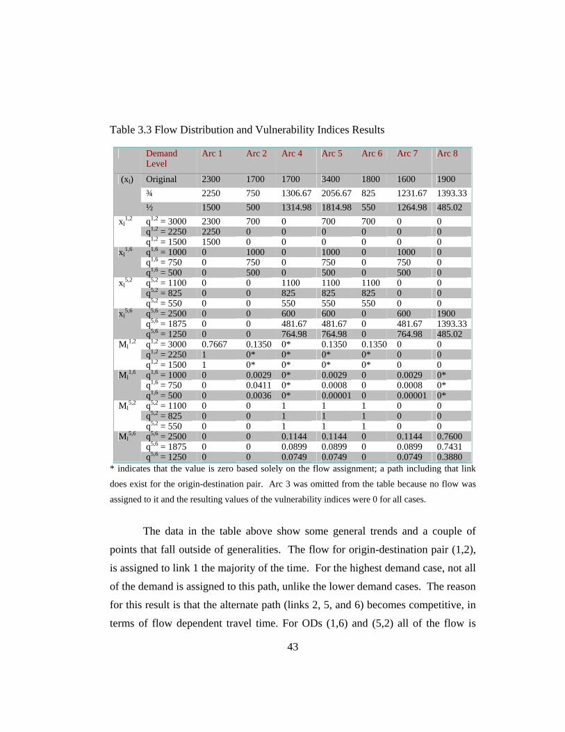
Table 3.3 Flow Distribution and Vulnerability Indices Results
Demand Level
Arc 1 Arc 2 Arc 4 Arc 5 Arc 6 Arc 7 Arc 8
Original 2300 1700 1700 3400 1800 1600 1900 ¾ 2250 750 1306.67 2056.67 825 1231.67 1393.33
(xl)
½ 1500 500 1314.98 1814.98 550 1264.98 485.02 q1,2 = 3000 2300 700 0 700 700 0 0 q1,2 = 2250 2250 0 0 0 0 0 0
xl1,2
q1,2 = 1500 1500 0 0 0 0 0 0 q1,6 = 1000 0 1000 0 1000 0 1000 0 q1,6 = 750 0 750 0 750 0 750 0
xl1,6
q1,6 = 500 0 500 0 500 0 500 0 q5,2 = 1100 0 0 1100 1100 1100 0 0 q5,2 = 825 0 0 825 825 825 0 0
xl5,2
q5,2 = 550 0 0 550 550 550 0 0 q5,6 = 2500 0 0 600 600 0 600 1900 q5,6 = 1875 0 0 481.67 481.67 0 481.67 1393.33
xl5,6
q5,6 = 1250 0 0 764.98 764.98 0 764.98 485.02 q1,2 = 3000 0.7667 0.1350 0* 0.1350 0.1350 0 0 q1,2 = 2250 1 0* 0* 0* 0* 0 0
Ml1,2
q1,2 = 1500 1 0* 0* 0* 0* 0 0 q1,6 = 1000 0 0.0029 0* 0.0029 0 0.0029 0* q1,6 = 750 0 0.0411 0* 0.0008 0 0.0008 0*
Ml1,6
q1,6 = 500 0 0.0036 0* 0.00001 0 0.00001 0* q5,2 = 1100 0 0 1 1 1 0 0 q5,2 = 825 0 0 1 1 1 0 0
Ml5,2
q5,2 = 550 0 0 1 1 1 0 0 q5,6 = 2500 0 0 0.1144 0.1144 0 0.1144 0.7600 q5,6 = 1875 0 0 0.0899 0.0899 0 0.0899 0.7431
Ml5,6
q5,6 = 1250 0 0 0.0749 0.0749 0 0.0749 0.3880 * indicates that the value is zero based solely on the flow assignment; a path including that link
does exist for the origin-destination pair. Arc 3 was omitted from the table because no flow was
assigned to it and the resulting values of the vulnerability indices were 0 for all cases.
The data in the table above show some general trends and a couple of
points that fall outside of generalities. The flow for origin-destination pair (1,2),
is assigned to link 1 the majority of the time. For the highest demand case, not all
of the demand is assigned to this path, unlike the lower demand cases. The reason
for this result is that the alternate path (links 2, 5, and 6) becomes competitive, in
terms of flow dependent travel time. For ODs (1,6) and (5,2) all of the flow is
43
assigned to the same path for each of the demand levels examined. Only one path
connects node 5 to node 2, but for (1,6), the traffic assignment is a result of travel
time. Origin-destination pair (5,6) offers the opportunity to examine capacity
constraints. The path consisting of links 4, 5, and 7 has a smaller travel time than
the alternate path (link 8). The existence of only one path connecting nodes 5 and
2 leads to a priority assignment of this OD flow to the links in the single path,
which shares links with the shortest time path for (5,6). At the highest demand
level, the capacity constraint on link 4 prohibits any additional flow (above
600vph) for (5,6) from being assigned to path 4, 5, 7. The traffic assignments at
the lower demand levels reflect the dependency of travel time on the link flow
levels.
Although intuition may lead to the expectation that increased demand will
lead to higher vulnerability indices, this is not always true. The index formulation
captures more of the intricacies of traffic assignment and network design than
intuition. The value of the indices for the links connecting node 5 and node 2 do
not change, as expected, since there is only one path, and therefore, each link is
critical. At the highest demand level in this example, link 1 achieves its lowest
vulnerability index. This result captures the fact that only at this level is the OD
flow distributed between two possible paths. The most counter-intuitive result
occurs for OD pair (1,6). The lower two demand levels follow the expected trend
of more traffic leads to a higher vulnerability index. This generalization is
followed by links 5 and 7 for all demand levels. However, link 2 has a higher
vulnerability index than links 5 and 7 for the lower two demand levels. The
design of the network allows for three alternate paths to exist between node 1 and
node 6. Only one of these paths contains link 2, while two of the paths contain
links 5 and 7. This difference allows the value of the index to vary between link 2
and links 5 and 7. The reason for the index being greater for link 2 is that the
alternate path with the lower marginal travel time also has less excess capacity so
44

the overall utility for the vehicles that would be reassigned to that path is lower,
resulting in a higher vulnerability index. The network does better as a whole
using the marginal path cost as the order for reassignment rather than ordering by
path excess capacity. At the highest demand level, the index is the same for all of
the links in the path; this is due to one of the alternate paths having no excess
capacity to accommodate the flow on link 2. Origin-destination pair (5,6) does
follow the intuitive trend and the results show an increase in vulnerability indices
for both paths as demand increases (see also figure 3.2).
0
0.1
0.2
0.3
0.4
0.5
0.6
0.7
0.8
0 10 20 30 40 50 60 70 80
Percentage of OD Flow
Vul
nera
bilit
y In
dex
Links 4,5,7Link 8
q(5,6)=2500
q(5,6)=2500q(5,6)=1875
q(5,6)=1875
q(5,6)=1250
q(5,6)=1250
Figure 3.2 Comparison of Vulnerability Indices for Alternate Paths for OD (5,6)
Figure 3.2 shows some of the complexities in predicting the relative
importance of a specific link to the connectivity of an origin-destination pair. The
curve connecting the data points for link 8 is linear and has a positive slope; this
reflects two attributes of the network state. First, insufficient capacity exists on
alternate paths to accommodate the flow on link 8 from node 5 to node 6.
45

Second, the proportion of the OD flow assigned to link 8 maps directly to the
vulnerability index. Links 4, 5, and 7 have the same vulnerability index for the
given origin-destination pair. This result reflects the fact that these three links lie
on the same path and no alternate path for that OD pair shares one of these links.
The non-linear nature of the curve connecting the data points for these links
indicates that an alternate path can accommodate the flow on the path consisting
of links 4, 5, and 7, for at least some demand levels. Furthermore, the relatively
low value of the vulnerability index emphasizes the existence of a viable
alternative path with sufficient excess capacity.
The vulnerability index is an appropriate measure for determining the
importance of a link to origin-destination connectivity, but the disruption index
needs to be calculated for the network level. The disruption indices are calculated
as the sum of the vulnerability indices across all origin-destination pairs. The
disruption indices for the single arcs and different demand levels are given in
table 3.4. This measure allows for an ordering of links in terms of vulnerability
from the network perspective.
Figure 3.3 provides a demonstration of how the disruption index can be
vastly different from the vulnerability index shown in figure 3.2. In the figure
below, the disruption indices are not identical for links 4, 5, and 7. This is due to
the assignment of various other OD flows to these links. The disruption index for
link 8 is the same as the vulnerability index because the only traffic assigned to
that link is for the origin-destination pair (5,6).
46
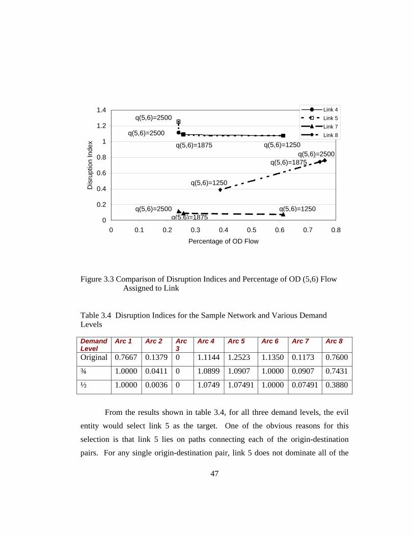
0
0.2
0.4
0.6
0.8
1
1.2
1.4
0 0.1 0.2 0.3 0.4 0.5 0.6 0.7 0.8
Percentage of OD Flow
Dis
rupt
ion
Inde
x
Link 4Link 5Link 7Link 8
q(5,6)=2500
q(5,6)=2500
q(5,6)=2500
q(5,6)=2500q(5,6)=1875
q(5,6)=1875
q(5,6)=1875
q(5,6)=1250
q(5,6)=1250
q(5,6)=1250
Figure 3.3 Comparison of Disruption Indices and Percentage of OD (5,6) Flow Assigned to Link
Table 3.4 Disruption Indices for the Sample Network and Various Demand Levels
Demand Level
Arc 1 Arc 2 Arc 3
Arc 4 Arc 5 Arc 6 Arc 7 Arc 8
Original 0.7667 0.1379 0 1.1144 1.2523 1.1350 0.1173 0.7600
¾ 1.0000 0.0411 0 1.0899 1.0907 1.0000 0.0907 0.7431
½ 1.0000 0.0036 0 1.0749 1.07491 1.0000 0.07491 0.3880
From the results shown in table 3.4, for all three demand levels, the evil
entity would select link 5 as the target. One of the obvious reasons for this
selection is that link 5 lies on paths connecting each of the origin-destination
pairs. For any single origin-destination pair, link 5 does not dominate all of the
47

other links in the network, but when the network is considered as a whole, link 5
becomes the most vulnerable link.
This section has presented results of single link vulnerability and
disruption analysis. The next section allows for links to be considered jointly.
3.2.5 Results and Discussion for Joint Link Consideration
Due to the small nature of the sample network and for ease of discussion,
the scenarios considered for multiple arc damage are first limited to two links.
The results for the joint consideration of the links are presented below. The
demand levels from the previous section are used here. The results are separated
by origin-destination pair. Table 3.5 is for (1,2), table 3.6 is for (1,6), table 3.7 is
for (5,2), and table 3.8 is for (5,6).
Table 3.5 Joint Vulnerability Indices for Origin-Destination (1,2)
Demand Link 2 Link 3 Link 4 Link 5 Link 6 Link 7 Link 8 Original 1.0000 0.7667 0.7667 1.0000 1.0000 0.7667 0.7667 Link
1 ¾ & ½ 1.0000 1.0000 1.0000 1.0000 1.0000 1.0000 1.0000 Original 0.1350 0.1350 0.1350 0.1350 0.1350 0.1350 Link
2 ¾ & ½ 0.0000 0.0000 0.0000 0.0000 0.0000 0.0000 Original 0.0000 0.1350 0.1350 0.0000 0.0000 Link
3 ¾ & ½ 0.0000 0.0000 0.0000 0.0000 0.0000 Original 0.1350 0.1350 0.0000 0.0000 Link
4 ¾ & ½ 0.0000 0.0000 0.0000 0.0000 Original 0.1350 0.1350 0.1350 Link
5 ¾ & ½ 0.0000 0.0000 0.0000 Original 0.1350 0.1350 Link
6 ¾ & ½ 0.0000 0.0000 Original 0.0000 Link
7 ¾ & ½ 0.0000
For the origin-destination pair (1,2), at the highest demand level, only
links 1, 2, 5, and 6 had a vulnerability index greater than 0.0 due to the traffic
48

assignment. These links represent two of the three possible paths connecting that
O-D pair. Let path 1 contain link 1 and path 2 consist of links 2, 5, and 6. The
third path (arcs 3, 4, 5, and 6) had no excess capacity available. Any combination
of link 1 and a link from path 2 resulted in a joint vulnerability index of 1.0 since
no alternate path was available. When one link from path 2 was considered with
another arc from the same path, the joint index was the maximum of the
individual link vulnerability indices, which in this case were identical. Any
combination of links 3, 4, 7, and 8 resulted in a joint vulnerability index of 0.0
because none of the flow from node 1 to node 2 was assigned to these arcs.
Finally, consideration of links 3, 4, 7, or 8 and one of the links from paths 1 or 2
yielded a joint index equivalent to the individual index for the arc from path 1 or
2.
At the lower demand levels, all of the flow for (1,2) was assigned to path
1. When link 1 was combined with any other link, the join vulnerability index
was 1.0. If the combination of arcs did not include link 1, the joint index was 0.0.
49

Table 3.6 Joint Vulnerability Indices for Origin-Destination (1,6)
Demand Link 2 Link 3 Link 4 Link 5 Link 6 Link 7 Link 8
Original 0.0029 0.0000 0.0000 0.0029 0.0000 0.0029 0.0000
¾ 0.0411 0.0000 0.0000 0.0008 0.0000 0.0008 0.0000
Link
1
½ 0.0036 0.0000 0.0000 0.00001 0.0000 0.00001 0.0000
Original 1.0000 0.0029 0.0029 0.0029 0.0029 1.0000
¾ 1.0000 0.0411 0.0411 0.0411 0.0411 1.0000
Link
2
½ 1.0000 0.0036 0.0036 0.0036 0.0036 0.0036
Original 0.0000 1.0000 0.0000 1.0000 0.0000
¾ 0.0000 1.0000 0.0000 1.0000 0.0000
Link
3
½ 0.0000 1.0000 0.0000 1.0000 0.0000
Original 0.0029 0.0000 0.0029 0.0000
¾ 0.0008 0.0000 0.0008 0.0000
Link
4
½ 0.00001 0.0000 0.00001 0.0000
Original 0.0029 0.0029 1.0000
¾ 0.0008 0.0008 1.0000
Link
5
½ 0.00001 0.00001 1.0000
Original 0.0029 0.0000
¾ 0.0008 0.0000
Link
6
½ 0.00001 0.0000
Original 1.0000
¾ 1.0000
Link
7
½ 1.0000
Table 3.6 presents the joint vulnerability indices for origin-destination pair
(1,6). There are three possible paths connecting this pair of nodes. Let path 4
consist of links 2, 5, and 7; path 5 consist of arcs 3, 4, 5, and 7; and path 6 consist
of links 3 and 8.
Examination of the joint index of links 2 and 8 at different demands
reveals that traffic levels play a crucial role in the calculation of vulnerability
50

indices. At the two higher demands, link 4 does not have sufficient excess
capacity to accommodate the flow on link 2, which means that path 5 is
insufficient as the only alternate path from node 1 to node 6. Since arcs 2 and 8
are members of paths 4 and 6, respectively, their joint vulnerability index is 1.0.
At the lowest demand level, path 5 can accommodate the flow on path 4. As a
result, the joint vulnerability index of links 2 and 8 is the same as the individual
index of link 2 (since arc 8 carries no flow from node 1 to node 6).
Arcs 2 and 3 form an obvious cut set for this OD pair; consequently, their
joint vulnerability index is 1.0. Link combinations 3 and 5, 3 and 7, 5 and 8, and
7 and 8 also form cut sets and have joint indices of 1.0 for all demand levels.
Links 1 and 6, by the network configuration, cannot carry any flow
between OD (1,6) so either of these links in combination with any other arc has a
joint vulnerability index equivalent to that other arc’s individual index.
Table 3.7 Joint Vulnerability Indices for Origin-Destination (5,2) and All Demand Levels
Link 2 Link 3 Link 4 Link 5 Link 6 Link 7 Link 8
Link 1 0.0000 0.0000 1.0000 1.0000 1.0000 0.0000 0.0000
Link 2 0.0000 1.0000 1.0000 1.0000 0.0000 0.0000
Link 3 1.0000 1.0000 1.0000 0.0000 0.0000
Link 4 1.0000 1.0000 1.0000 1.0000
Link 5 1.0000 1.0000 1.0000
Link 6 1.0000 1.0000
Link 7 0.0000
Table 3.7 demonstrates the simplicity of the case when only one path
exists between an origin-destination pair, such as (5,2) in this example. The path
(path 7) consists of links 4, 5, and 6. Each arc is a cut set for this OD pair. As
51

such, any combination of links with arcs 4, 5, or 6 yields a joint vulnerability
index of 1.0. If none of the links of path 7 are in the combination under
consideration, the index is 0.0.
Table 3. 8 Joint Vulnerability Indices for Origin-Destination (5,6)
Demand Link 2 Link 3 Link 4 Link 5 Link 6 Link 7 Link 8
Original 0.0000 0.0000 0.1144 0.1144 0.0000 0.1144 0.7600
¾ 0.0000 0.0000 0.0899 0.0899 0.0000 0.0899 0.7431
Link
1
½ 0.0000 0.0000 0.0749 0.0749 0.0000 0.0749 0.3880
Original 0.0000 0.1144 0.1144 0.0000 0.1144 0.7600
¾ 0.0000 0.0899 0.0899 0.0000 0.0899 0.7431
Link
2
½ 0.0000 0.0749 0.0749 0.0000 0.0749 0.3880
Original 0.1144 0.1144 0.0000 0.1144 0.7600
¾ 0.0899 0.0899 0.0000 0.0899 0.7431
Link
3
½ 0.0749 0.0749 0.0000 0.0749 0.3880
Original 0.1144 0.1144 0.1144 1.0000
¾ 0.0899 0.0899 0.0899 1.0000
Link
4
½ 0.0749 0.0749 0.0749 1.0000
Original 0.1144 0.1144 1.0000
¾ 0.0899 0.0899 1.0000
Link
5
½ 0.0749 0.0749 1.0000
Original 0.1144 0.7600
¾ 0.0899 0.7431
Link
6
½ 0.0749 0.3880
Original 1.0000
¾ 1.0000
Link
7
½ 1.0000
Origin-destination pair (5,6) is slightly more complex than (5,2) but less
so than (1,2) and (1,6). There are only two paths connecting nodes 5 and 6. Let
path 8 consist of link 8 and path 9 consist of arcs 4, 5, and 7. The joint
vulnerability index of one of the remaining four links in the network and one of
52

the arcs in path 8 or 9 is equivalent to the individual index of the link in path 8 or
9. Since only one alternate path to path 9 exists in the sample network, each link
in path 9 has the same index value and this holds true when any combination of
those arcs is considered. Finally, when link 8 is examined jointly with any of the
links in path 9, a cut set is formed and the joint vulnerability index is 1.0.
The joint vulnerability indices reflect two interesting points. First,
although links that lie on the same path have identical joint vulnerability indices
for a given OD pair for the highest demand level, there are exceptions. One of
these exceptions would occur when (1,6) is considered; either links 2 and 5 or 2
and 7 would have a higher index than links 5 and 7. When links lie on the same
path, the maximum index for those arcs is taken as the joint vulnerability index.
The second point is that a joint index of 1.0000 indicates either (a) only one path
connects the OD pair, as in (5,2) or (b) those links taken together may indicate a
cut set for that OD pair. An exception to (b) is: an alternate path may exist but
has insufficient excess capacity to accommodate the necessary flow.
Like in the single link example, the disruption index is simply the sum of
the vulnerabilities indices across all OD pairs. The following table provides the
disruption indices for the pair-wise joint consideration of arcs in the sample
network.
53

Table 3.9 Joint Disruption Indices for Sample Network
Demand Link 2 Link 3 Link 4 Link 5 Link 6 Link 7 Link 8
Original 1.0029 0.7667 1.8811 2.1173 2.0000 0.8840 1.5267
¾ 1.0411 1.0000 2.0899 2.0907 2.0000 1.0907 1.7431
Link 1
½ 1.0036 1.0000 2.0749 2.07491 2.0000 1.07491 1.3880
Original 1.1350 1.2523 1.2523 1.1379 0.2523 1.8949
¾ 1.0000 1.1310 1.1310 1.0411 0.1310 1.7431
Link 2
½ 1.0000 1.0785 1.0785 1.0036 0.0785 0.3916
Original 1.1144 2.2494 1.1350 1.1144 0.7600
¾ 1.0899 2.0899 1.0000 1.0899 0.7431
Link 3
½ 1.0749 2.0749 1.0000 1.0749 0.3880
Original 1.2523 1.2494 1.1173 2.0000
¾ 1.0907 1.0899 1.0907 2.0000
Link 4
½ 1.07491 1.0749 1.07491 2.0000
Original 1.2523 1.2523 3.1350
¾ 1.0907 1.0907 3.0000
Link 5
½ 1.07491 1.07491 3.0000
Original 1.2523 1.8950
¾ 1.0907 1.7431
Link 6
½ 1.07491 1.3880
Original 2.0000
¾ 2.0000
Link 7
½ 2.0000
For all demand levels, the maximum value of the disruption index occurs
when links 5 and 8 are damaged simultaneously. Damage to these links will
provide a cut set for origin-destination pairs (1,6), (5,2), and (5,6).
For the OD pair (1,2) the results for three or more links being damaged
simultaneously can frequently be summarized in terms of the results for the n=2
case. The most interesting result occurs when links 1,2, and 3 or 1,2, and 4 are
54

considered. Either of these two groups forms a traditional cut set for the origin-
destination pair and the joint vulnerability index is 1.0. Any additional links
examined with one of these triplets cannot contribute any vulnerability and the
index remains at 1.0. Since link pairs 1 and 5 and 1 and 6 already form a cut set,
any additional links that are considered with them will have a joint vulnerability
index of 1.0. Links 7 and 8 cannot carry flow for OD (1,2) so disabling either or
both of these two links will yield the same index as in the n-1 case (or n-2, if both
are damaged). Links 3 and 4 lie on the same alternate path for OD pair (1,2) and
only one alternate path contains each of these links; therefore, the vulnerability
index for both of these links will be the same. Damaging both links 3 and 4
would be redundant for (1,2). Combinations of these two arcs and other arcs will
yield an index equivalent to the n-1 case. A similar case arises with links 5 and 6
which lie on the same two alternate paths for OD (1,2) and the indices are treated
in a similar manner to the case of links 3 and 4. Links 2, 3, and 4 are upstream of
link 5 so damaging any of the previous links is redundant to damaging link 5.
The value of the joint index is taken as the maximum value of the (n-1) index
without consideration of link 5 and the (n-1) index without links 2, 3, or 4,
respectively. A similar situation arises when links 2, 3, or 4 are examined in
conjunction with link 6 since this link is downstream of the others.
Joint analysis of three or more links for OD (1,6) can also be summarized
in terms of the n=2 scenario. Links 1 and 6 cannot contribute to the vulnerability
of another grouping of arcs, so consideration of n-1 other links and one of these
links yields a joint index equivalent to the joint index of the n-1 links. If both
links 1 and 6 are considered with n-2 additional links, the joint index for the n
links is the same as that for the n-2 additional arcs. Links 2 and 3, 5 and 8, and 7
and 8 form cut sets for this OD pair. Damage to any other link in conjunction
with one of these pairs would be redundant and the value of the index remains at
1.0 as in the n=2 case. The triplet {2,4,8} also forms a cut set and in cases where
55

n > 3, damage to any link in combination with this triplet would be redundant and
the joint index value remains at 1.0. Link 7 is downstream of link 5 and is the
only arc to which OD (1,6) traffic can flow after leaving link 5; therefore, from
the single OD perspective, damaging both links 5 and 7 is redundant. The joint
vulnerability index for a set of links containing both arcs 5 and 7 is the maximum
of the joint vulnerability index of the set of links without link 5 and the joint index
of the set of links without link 7. Using the set {2,5,7} as an example, the joint
vulnerability index would be the maximum of M1,6{2,5} and M1,6
{2,7}, which are
equivalent and the values for different demand levels are given in table 3.6. Links
2 and 4 are upstream of link 5 and no other path for this OD pair uses link 5 so
damage to the pair {2,4} is redundant to disabling link 5. The joint vulnerability
index for n links including {2,4,5} is the maximum of the index for the n-1 case
where link 5 is not in the set and the n-2 set where links 2 and 4 are not in the set.
For the triplet {2,4,5} and the ¾ demand case, M1,6{2,4,5} is the maximum of
M1,6{2,4} (=0.0411) and M1,6
{5} (=0.0008). A comparable scenario arises when
links 2,4, and 7 are among the links of interest. (Recall that link 7 is the only
downstream arc of link 5 for this OD pair). As previously mentioned, link 5 is
downstream of link 4 and damage to link 4 is redundant to disabling link 5;
however, the converse is not true since link 5 is on two of the possible paths.
When links 4 and 5 are in the set of links of interest, the joint vulnerability index
is the maximum of the n-1 case without link 4 and the n-1 case without link 5.
This analysis further extends to the situation in which links 4 and 7 are in the set
of arcs of interest. Finally, traffic from link 3 must enter either link 4 or link 8.
Damaging link 3 and the pair {4,8} is redundant. The joint vulnerability index for
a set of n links containing {3,4,8} can be calculated as the maximum of the n-2
index without {4,8} and the n-1 index without link 3.
Joint vulnerability indices for OD (5,2) for any number of links can be
easily determined since one path connects this pair of nodes. If the arc
56

combination contains links 4, 5, and/or 6, the index is 1.0. If none of the three
links are present, the value is 0.
Recall that for OD (5,6) there are only two possible paths - {4,5,7} and
{8}. As in the n=2 case, any combination of link 8 and one of {4,5,7} results in a
cut set and the joint vulnerability index is 1.0. Any additional link considered
with the pair will have no impact on the value of the index; M5,6{4,8,n-2} = M5,6
{5,8,n-
2}= M5,6{7,8,n-2} = 1.0. If the triplet {4,5,7} is considered by itself or with links
from the set {1,2,3,6} the joint index is the maximum value of the individual
index for links 4, 5, and 7, such as in the n=2 case. If any combination of links 1,
2, 3, and 6 are considered jointly with link 8, the joint index is simply the value of
M5,6{8} or the n=1 case for link 8. When the links of interest solely consist of
members of {1,2,3,6}, the joint index for this OD pair is 0.0.
3.3 APPLICATION OF GAME THEORY A two player non-zero sum game is envisioned where one player is an evil entity,
such as a terrorist cell, intent on destroying a transportation infrastructure link, or
set of links, and the other player is the traffic management agency who tries to
keep as many drivers safe as possible. The secondary objective of the traffic
management agency is to allow each driver to reach their destination, if possible.
There are four cases of information in this game. In the first, the traffic
management agency is not aware of an impending threat to the transportation
system. In the second situation, the traffic management agency is suspects that
the terrorists will take action, but the cell is not aware of that information has
reached its opponent. Third, the agency perceives a general threat and the cell
suspects that information has been leaked to the other team. Finally, the two
players alternate moves with perfect information; the terrorists damage one link,
the traffic management agency re-routes traffic, then the terrorists damage another
57

link, and so on until either all of the resources have been used or there are no
origin-destination pairs that remain connected.
Let Player M be the traffic management agency and Player T be the
terrorist cell. Player M routes traffic to minimize the network travel time (system
optimal). Let the payoff for player M be the percentage of vehicles that arrive
safely at their destinations. Player T will seek to cause as much disruption to the
flow of traffic as possible. Let the payoff for player T be the disruption index
discussed in section 3.1; the objective function and constraints are given in P1 in
section 3.2.1.
3.3.1 Game 1: No-Information for the Traffic Management Agency
When Player M is not aware that it should be involved in a game, the
game becomes the bi-level mathematical program discussed in the previous
section. For the sake of consistency, Player M routes traffic according to the
system-optimal traffic assignment, but, in this game, does not try to avoid any
links. Since this game reduces to the formulation in section 3.2, the results are the
same.
3.3.2 Game 2: Some Information for the TMA
If Player M suspects that Player T will make a move, Player M will route
traffic so as to minimize travel time around the suspected targeted set of links.
Player M moves first in this game. Player M is aware of the objective function
for player T; therefore, the game is simple to solve. Little guess work is required
on the part of player M and none on the part of player T. In the event that there
are multiple optima for player T, player M assigns probabilities to the strategies.
58

The mathematical program (P4) used by player M is a modified version
(P2).
(P4) (3.27) ∑ ∑+∑ ∑ ⎟⎟⎠
⎞⎜⎜⎝
⎛∑=
≠∈ * ,*
,*
*, , ,
,,)(minl sr
lsr
lllAl sr sr
srll
srl Hxxtxxz
s.t. (3.28) srqx sr
j
srlLl j
,min ,, ∀=∑ ⎟⎟⎠
⎞⎜⎜⎝
⎛
∈
(3.29) 0, ≥srlx
Alxsr
lsr
l ∈∀∑ ≤,
, ρ (3.30)
where l* is a link selected for damage by Player T and Hl* is a high cost for using
link l*. In this game, l* is known by Player M. Equation (3.30) represents
capacity constraints for every link in the network.
From the results in table 3.4 for n=1, Player M will seek to avoid link 5 for
all of the demand levels. Player M knows that Player T will target link 5 based on
the system optimal traffic assignment when Player M has no information about
Player T. Examination of table 3.9 for the n=2 case reveals that Player M avoids
routing traffic on links 5 and 8 for all of the demand cases. When n is 3 or higher,
Player M cannot route traffic away from links 1, 5, and 8 simultaneously. These
three links have a joint disruption index of 4.0 (for all demand levels), indicating
that all four of the network’s origin-destination pairs would be severed. Any
higher value of n cannot disrupt the OD connectivity of this sample network
further than the n=3 case.
Since Player T is unaware of the information that Player M has received,
Player M’s strategy is to maximize its own payoff, which in this case also
minimizes the payoff to Player T (see table 3.11 in the next section). The next
game allows for knowledge on the part of both players.
59

3.3.3 Game 3: One Move for Each Player, Full Information
In this game, each player optimizes their own position while trying to
predict the opponent’s strategy. Assume that each player has full knowledge of
the other’s payoffs. Player M investigates various strategies through the
equations in (P4) and Player T employs (P1) for each of Player M’s possible
strategies. Let m denote the strategy of Player M and e denote the strategy of
Player T. Let pm,e be the payoff to Player M and Dm,e be the payoff to Player T,
where Dm,e is the value of the disruption index for strategy e when traffic is routed
by strategy m. The payoff to Player M is calculated in the following manner:
100
,
,, , *
,*
,
, ×∑
∑ ∑ ∑−
= ∈
sr
srsr sr el
srl
sr
emq
xqp (3.31)
Equation (3.31) represents the percentage of network demand that is not routed on
targeted links l* dictated by Player T’s strategy e.
Assume that each player has full knowledge of the other’s payoffs. The
general payoff matrix for both players is given in table 3.10.
Table 3.10 General Payoff Matrix
Link Set 1 Link Set 2 … Link Set y Routing 1 p1,1, D1,1 p1,2, D1,2 … p1,y, D1,yRouting 2 p2,1, D2,1 p2,2, D2,2 … p2,y, D2,y… Routing w pw,1, Dw,1 pw,2, Dw,2 … pw,y, Dw,y
Player M moves first. Player M may approach the same from several
perspectives such as:
1. Minimize the maximum payoff to Player T:
60

⎟⎠⎞
⎜⎝⎛= em
emDz ,1 maxmin (3.32)
2. Maximize the minimum payoff to Player M:
⎟⎠⎞
⎜⎝⎛= em
empz ,2 minmax (3.33)
3. A combination of (1) and (2):
),( 213 zzfz = (3.34)
There may be an equilibrium point that is not an optimal solution for
either player. According to Nash equilibrium, deviating from this point will cause
at least one of the players to do “no better” than the equilibrium point.
For the original demand level, the resulting payoff matrix, evaluated for
the potential damage of only one link, is given below. Table 3.11 is interesting in
that one can observe the exact consequences of an error in Player M’s prediction
of player T’s move. The flow distributions on which table 3.11 can be found in
Appendix B.
61

Table 3.11 Payoff Matrix for n=1, Original Demand Level
Link 1 Link 2 Link 3 Link 4 Link 5 Link 6 Link 7 Link 8 Do nothing
60.52, 1.000
86.84, 0.110
100.00, 0
82.49, 1.053
69.33, 1.059
85.53, 1.000
83.80, 0.059
70.14, 0.908
Avoid 1 69.74, 0.767
77.63, 0.138
100.00, 0
77.63, 1.114
55.26, 1.252
76.32, 1.135
78.95, 0.117
75.00, 0.760
Avoid 2 60.52, 1.000
100.00, 0
86.84, 0.336
77.63, 1.202
77.63, 1.380
85.52, 1.000
92.11, 0.380
61.84, 1.134
Avoid 3 60.52, 1.000
86.84, 0.110
100.00, 0
82.49, 1.053
69.33, 1.059
85.53, 1.000
83.80, 0.059
70.14, 0.908
Avoid 4 60.52, 1.000
86.84, 0.698
100.00, 0
85.53, 1.000
72.34, 1.628
85.53, 1.000
86.84, 0.628
67.11, 1.000
Avoid 5 60.52, 1.000
100.00, 0
86.84, 0.001
85.53, 1.000
85.53, 1.000
85.53, 1.000
100.00, 0
53.95, 1.000
Avoid 6 60.52, 1.000
86.84, 0.132
100.00, 0
82.82, 1.048
69.66, 1.054
85.53, 1.000
84.13, 0.054
69.82, 0.918
Avoid 7 62.60, 0.947
97.92, 0.038
86.84, 0.089
85.53, 1.000
83.45, 1.038
83.45, 1.038
100.00, 0
53.95, 1.089
Avoid 8 60.52, 1.000
86.84, 0.003
100.00, 0
77.63, 1.114
64.47, 1.117
85.53, 1.000
78.95, 0.117
75.00, 0.760
The strategy “avoid 3” is redundant to the “do-nothing” alternative, so this
row may be eliminated as a viable strategy for Player M. For 7 of the 8 (non-
redundant) cases, Player T receives the greatest payoff by damaging link 5. The
one exception is when Player M uses the strategy “avoid link 7” and Player T then
damages link 8. From Player T’s perspective, column “Link 5” dominates “Link
1,” “Link 2,” “Link 3,” “Link 4,” “Link 6,” and “Link 7.” From the resulting
matrix, consisting of columns “Link 5” and “Link 8,” one can see that row “Avoid
5” dominates “Avoid 7.” Once this row is eliminated, column “Link 5”
dominates “Link 8.” Therefore, Player T’s best strategy is to damage arc 5. To
both maximize his own payoff and minimize the payoff to Player T, Player M will
choose the strategy “Avoid Link 5.”
By playing the strategy “Avoid Link 5” and “Link 5” is selected by Player
T, the payoff for Player M is 85.53%, which means that 85.53% of the vehicles
were able to safely reach their destinations. The “Do Nothing” alternative for
62

Player M only allows 69.33% of the vehicles to safely reach their destinations.
By correctly predicting Player T’s strategy, Player M is able to theoretically save
1231.2 vehicles/hour from damage or from becoming trapped in the network due
to the directional nature of the links.
Table 3.12 is the payoff matrix for the two player game when the demand
is at the ¾ level and Player T has limited resources and can damage only one link.
The corresponding flow distributions for each of Player M’s strategies are found
in Appendix B.
Table 3.12 Payoff Matrix for n=1, 3/4 Demand Level
Link 1 Link 2 Link 3 Link 4 Link 5 Link 6 Link 7 Link 8 Do nothing
60.53, 1.000
86.84, 0.041
100.00, 0
77.08, 1.090
63.92, 1.091
85.53, 1.000
78.39, 0.091
75.56, 0.743
Avoid 1 77.63, 0.567
70.18, 0.194
99.56, 0.004
80.10, 1.064
50.28, 1.215
68.42, 1.138
81.86, 0.077
72.09, 0.848
Avoid 2 (opt 1)
60.53, 1.000
100.00, 0
86.84, 0.396
73.10, 1.182
73.10, 1.182
85.52, 1.000
87.57, 0.182
66.38, 1.018
Avoid 2 (opt 2)
60.53, 1.000
100.00, 0
86.84, 0.396
73.10, 1.372
73.10, 1.443
85.52, 1.000
87.57, 0.443
66.38, 1.022
Avoid 3 60.53, 1.000
86.84, 0.041
100.00, 0
77.08, 1.090
63.92, 1.091
85.53, 1.000
78.39, 0.091
75.56, 0.743
Avoid 4 60.53, 1.000
86.84, 0.513
100.00, 0
85.53, 1.000
72.37, 1.003
85.53, 1.000
86.84, 0.003
67.11, 1.000
Avoid 5 60.53, 1.000
100.00, 0
86.84, 2 x 10⁻⁴
85.53, 1.000
85.53, 1.000
85.53, 1.000
100.00, 0
53.95, 1.000
Avoid 6 60.53, 1.000
86.84, 0.038
100.00, 0
77.02, 1.090
63.86, 1.091
85.53, 1.000
78.34, 0.091
75.61, 0.741
Avoid 7 62.61, 0.947
97.92, 0.028
86.84, 0.066
85.53, 1.000
83.44, 1.028
83.44, 1.028
100.00, 0
53.95, 1.066
Avoid 8 60.53, 1.000
86.84, 2 x 10⁻⁴
100.00, 0
70.18, 1.117
57.02, 1.117
85.53, 1.000
71.49, 0.117
82.46, 0.533
*Options 1 and 2 for strategy Avoid 2 yielded equivalent objective value
functions to four decimal places.
The results in table 3.12 are similar to those in table 3.11. Like the higher
demand case, Player T’s strategy Target Link 5 dominates all of the others except
Target Link 8; the matrix can thus be reduced to the columns titled “Link 5” and
“Link 8.” For Player M, strategy Avoid Link 3 is equivalent to the “Do Nothing”
63

alternative. “Avoid 1” is an inferior strategy to the “Do Nothing” alternative and
can be eliminated from consideration. “Avoid 5” dominates “Avoid 7.” From the
remaining matrix, Player T would target link 5. The cell “Avoid 5”, “Link 5” is a
Nash equilibrium point; deviation from this point results in Player M doing worse.
Table 3.13 represents the payoff matrix for the case where Player T has
the resources to damage only one link and the demand is half of the original.
Table 3.13 Payoff Matrix for n=1, 1/2 Demand Level
Link 1 Link 2 Link 3 Link 4 Link 5 Link 6 Link 7 Link 8 Do nothing/ Avoid 3
60.53, 1.000
86.84, 0.004
100.00, 0
77.08, 1.075
63.92, 1.075
85.53, 1.000
78.39, 0.075
75.56, 0.388
Avoid 1 93.42, 0.167
55.26, 0.087
98.68, 0.095
70.54, 1.083
25.81, 1.164
52.63, 1.052
73.18, 0.112
80.77, 0.639
Avoid 2 (opt 1)
60.53, 1.000
100.00, 0
86.84, 0.518
73.10, 1.153
73.10, 1.153
85.52, 1.000
87.57, 0.153
66.38, 0.777
Avoid 2 (opt 2)
60.53, 1.000
100.00, 0
86.84, 0.518
73.10, 1.589
73.10, 1.384
85.52, 1.000
87.57, 0.383
66.38, 0.659
Avoid 4 60.53, 1.000
86.84, 0.662
100.00, 0
85.53, 1.000
72.37, 1.001
85.53, 1.000
86.84, 0.001
67.11, 1.000
Avoid 5 60.53, 1.000
100.00, 0
86.84, 4 x 10⁻⁵
85.53, 1.000
85.53, 1.000
85.53, 1.000
100.00, 0
53.95, 1.000
Avoid 6 60.53, 1.000
86.84, 0.005
100.00, 0
65.40, 1.075
52.24, 1.075
85.53, 1.000
66.72, 0.075
87.23, 0.388
Avoid 7 60.53, 1.000
100.00, 0
86.84, 4 x 10⁻⁵
85.53, 1.000
85.53, 1.000
85.53, 1.000
100.00, 0
53.95, 1.000
Avoid 8 60.53, 1.000
86.84, 0.000
100.00, 0
70.18, 1.023
57.02, 1.023
85.53, 1.000
71.49, 0.023
82.46, 0.078
For Player T, the strategy “Target Link 5” dominates “Target Link 1,”
“Target Link 2,” “Target Link 3,” “Target Link 6,” “Target Link 7,” and “Target
Link 8.” From the payoff matrix consisting of only the columns “Link 4” and
“Link 5,” Player M would select either “Avoid Link 5” or “Avoid Link 7.”
Referring to table B.3, one can see that these two strategies yield equivalent flow
distributions.
When Player T has the resources to damage two links simultaneously,
there are numerous alternative optima for the routing strategies of Player M. A
64
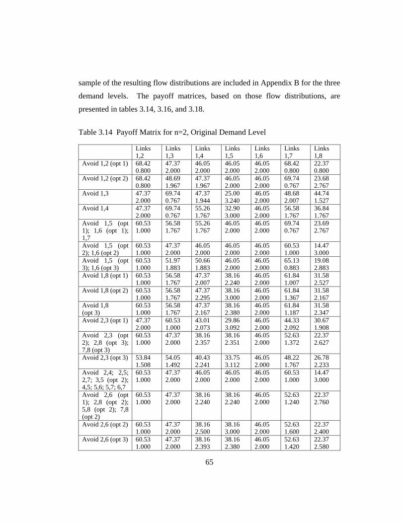
sample of the resulting flow distributions are included in Appendix B for the three
demand levels. The payoff matrices, based on those flow distributions, are
presented in tables 3.14, 3.16, and 3.18.
Table 3.14 Payoff Matrix for n=2, Original Demand Level
Links 1,2
Links 1,3
Links 1,4
Links 1,5
Links 1,6
Links 1,7
Links 1,8
Avoid 1,2 (opt 1) 68.42 0.800
47.37 2.000
46.05 2.000
46.05 2.000
46.05 2.000
68.42 0.800
22.37 0.800
Avoid 1,2 (opt 2) 68.42 0.800
48.69 1.967
47.37 1.967
46.05 2.000
46.05 2.000
69.74 0.767
23.68 2.767
Avoid 1,3 47.37 2.000
69.74 0.767
47.37 1.944
25.00 3.240
46.05 2.000
48.68 2.007
44.74 1.527
Avoid 1,4 47.37 2.000
69.74 0.767
55.26 1.767
32.90 3.000
46.05 2.000
56.58 1.767
36.84 1.767
Avoid 1,5 (opt 1); 1,6 (opt 1); 1,7
60.53 1.000
56.58 1.767
55.26 1.767
46.05 2.000
46.05 2.000
69.74 0.767
23.69 2.767
Avoid 1,5 (opt 2); 1,6 (opt 2)
60.53 1.000
47.37 2.000
46.05 2.000
46.05 2.000
46.05 2.000
60.53 1.000
14.47 3.000
Avoid 1,5 (opt 3); 1,6 (opt 3)
60.53 1.000
51.97 1.883
50.66 1.883
46.05 2.000
46.05 2.000
65.13 0.883
19.08 2.883
Avoid 1,8 (opt 1) 60.53 1.000
56.58 1.767
47.37 2.007
38.16 2.240
46.05 2.000
61.84 1.007
31.58 2.527
Avoid 1,8 (opt 2) 60.53 1.000
56.58 1.767
47.37 2.295
38.16 3.000
46.05 2.000
61.84 1.367
31.58 2.167
Avoid 1,8 (opt 3)
60.53 1.000
56.58 1.767
47.37 2.167
38.16 2.380
46.05 2.000
61.84 1.187
31.58 2.347
Avoid 2,3 (opt 1) 47.37 2.000
60.53 1.000
43.01 2.073
29.86 3.092
46.05 2.000
44.33 2.092
30.67 1.908
Avoid 2,3 (opt 2); 2,8 (opt 3); 7,8 (opt 3)
60.53 1.000
47.37 2.000
38.16 2.357
38.16 2.351
46.05 2.000
52.63 1.372
22.37 2.627
Avoid 2,3 (opt 3) 53.84 1.508
54.05 1.492
40.43 2.241
33.75 3.112
46.05 2.000
48.22 1.767
26.78 2.233
Avoid 2,4; 2,5; 2,7; 3,5 (opt 2); 4,5; 5,6; 5,7; 6,7
60.53 1.000
47.37 2.000
46.05 2.000
46.05 2.000
46.05 2.000
60.53 1.000
14.47 3.000
Avoid 2,6 (opt 1); 2,8 (opt 2); 5,8 (opt 2); 7,8 (opt 2)
60.53 1.000
47.37 2.000
38.16 2.240
38.16 2.240
46.05 2.000
52.63 1.240
22.37 2.760
Avoid 2,6 (opt 2) 60.53 1.000
47.37 2.000
38.16 2.500
38.16 3.000
46.05 2.000
52.63 1.600
22.37 2.400
Avoid 2,6 (opt 3) 60.53 1.000
47.37 2.000
38.16 2.393
38.16 2.380
46.05 2.000
52.63 1.420
22.37 2.580
65

Avoid 2,8 (opt 1); 3,6; 3,7 (opt 2); 3,8; 4,8; 5,8 (opt 1); 6,8; 7,8 (opt 1)
47.37 2.000
60.53 1.000
38.16 2.177
25.00 3.240
46.05 2.000
39.47 2.240
35.53 1.760
Avoid 3,4; 3,5 (opt 1); 3,7 (opt 1); 4,6
47.37 2.000
60.53 1.000
46.05 2.000
32.90 3.000
46.05 2.000
47.37 2.000
27.63 2.000
Avoid 3,5 (opt 3); 3,7 (opt 3)
53.84 1.508
54.05 1.492
46.05 2.000
39.37 3.000
46.05 2.000
53.84 1.508
21.16 2.492
Avoid 4,7 60.53 1.000
49.45 1.947
48.13 1.947
46.05 2.000
46.05 2.000
62.60 0.947
16.55 2.947
Avoid 5,8 (opt 3) 49.42 1.844
58.48 1.156
46.05 2.000
34.94 3.000
46.05 2.000
49.42 1.844
25.58 2.156
Links
2,3 Links 2,4
Links 2,5
Links 2,6
Links 2,7
Links 2,8
Links 7,8
Avoid 1,2 (opt 1) 78.95 1.121
77.63 1.121
77.63 1.121
77.63 1.121
100.00 0.000
53.95 2.000
53.95 2.000
Avoid 1,2 (opt 2) 77.63 1.135
76.32 1.135
76.32 1.135
76.32 1.135
98.68 0.019
52.63 2.019
53.95 2.000
Avoid 1,3 77.63 1.135
55.26 2.375
55.26 2.375
63.16 2.135
69.74 1.375
52.63 1.895
53.95 2.000
Avoid 1,4 77.63 1.135
63.16 2.135
63.16 2.135
63.16 1.676
77.63 1.135
44.74 2.135
53.95 2.000
Avoid 1,5 (opt 1); 1,6 (opt 1); 1,7
77.63 1.135
76.32 1.135
76.32 1.135
76.32 1.135
90.79 0.135
44.74 2.135
53.95 2.000
Avoid 1,5 (opt 2); 1,6 (opt 2)
88.84 1.000
85.53 1.000
85.53 1.000
85.53 1.000
100.00 0.000
53.95 2.000
53.95 2.000
Avoid 1,5 (opt 3); 1,6 (opt 3)
82.24 1.078
80.92 1.078
80.92 1.078
80.92 1.078
95.39 0.078
49.34 2.078
53.95 2.000
Avoid 1,8 (opt 1) 77.63 1.135
68.42 1.375
68.42 1.375
76.32 1.135
82.89 0.375
52.63 1.895
53.95 2.000
Avoid 1,8 (opt 2) 77.63 1.135
68.42 2.135
68.42 2.135
76.32 1.135
82.89 0.735
52.63 1.535
53.95 2.000
Avoid 1,8 (opt 3)
77.63 1.135
68.42 1.515
68.42 1.515
76.32 1.135
82.89 0.555
52.63 1.715
53.95 2.000
Avoid 2,3 (opt 1) 86.84 1.000
69.33 2.092
69.33 2.092
72.37 1.537
83.80 1.092
56.99 1.908
53.95 2.000
Avoid 2,3 (opt 2); 2,8 (opt 3); 7,8 (opt 3)
86.84 1.000
77.63 1.351
77.63 1.351
85.53 1.000
92.11 0.351
61.84 1.628
53.95 2.000
Avoid 2,3 (opt 3) 86.84 1.000
73.22 2.112
73.22 2.112
78.84 1.351
87.70 1.112
59.57 1.741
53.95 2.000
Avoid 2,4; 2,5; 2,7; 3,5 (opt 2); 4,5; 5,6; 5,7; 6,7
86.84 1.000
85.53 1.000
85.53 1.000
85.53 1.000
100.00 0.000
53.95 2.000
53.95 2.000
66

Avoid 2,6 (opt 1); 2,8 (opt 2); 5,8 (opt 2); 7,8 (opt 2)
86.84 1.000
77.63 1.240
77.63 1.240
85.53 1.000
92.11 0.240
61.84 1.760
53.95 2.000
Avoid 2,6 (opt 2) 86.84 1.000
77.63 2.000
77.63 2.000
85.53 1.000
92.11 1.000
61.84 1.400
53.95 2.000
Avoid 2,6 (opt 3) 86.84 1.000
77.63 1.380
77.63 1.380
85.53 1.000
92.11 0.380
61.84 1.580
53.95 2.000
Avoid 2,8 (opt 1); 3,6; 3,7 (opt 2); 3,8; 4,8; 5,8 (opt 1); 6,8; 7,8 (opt 1)
86.84 1.000
64.47 2.240
64.47 2.240
72.37 2.000
78.95 1.240
61.84 1.760
53.95 2.000
Avoid 3,4; 3,5 (opt 1); 3,7 (opt 1); 4,6
86.84 1.000
72.37 2.000
72.37 2.000
72.37 1.557
86.84 1.000
53.95 2.000
53.95 2.000
Avoid 3,5 (opt 3); 3,7 (opt 3)
86.84 1.000
78.84 2.000
78.84 2.000
78.84 1.335
93.32 1.000
53.95 2.000
53.95 2.000
Avoid 4,7 84.76 1.038
83.45 1.038
83.45 1.038
83.45 1.038
97.92 0.038
51.87 2.038
53.95 2.000
Avoid 5,8 (opt 3) 86.84 1.000
74.42 2.000
74.42 1.508
74.42 1.508
88.89 1.000
53.95 2.000
53.95 2.000
Links
3,4 Links 3,5
Links 3,6
Links 3,7
Links 3,8
Links 6,7
Links 6,8
Avoid 1,2 (opt 1) 64.47 1.498
64.47 2.121
64.47 1.124
78.95 1.121
46.05 2.121
77.63 1.121
31.58 3.121
Avoid 1,2 (opt 2) 64.47 1.530
63.16 2.135
63.16 1.198
78.95 1.116
46.05 2.116
76.32 1.135
30.26 3.135
Avoid 1,3 77.63 1.114
55.26 2.249
76.32 1.135
78.95 1.114
75.00 0.760
55.26 2.375
51.32 1.895
Avoid 1,4 85.53 1.000
63.16 2.135
76.32 1.135
86.84 1.000
67.11 1.000
63.16 2.135
43.42 2.135
Avoid 1,5 (opt 1); 1,6 (opt 1); 1,7
72.37 1.415
63.16 2.135
63.16 1.550
86.84 1.000
53.95 2.000
76.32 1.135
30.26 3.135
Avoid 1,5 (opt 2); 1,6 (opt 2)
72.37 1.001
72.37 2.000
72.37 1.001
86.84 1.000
53.95 2.000
85.53 1.000
39.47 3.000
Avoid 1,5 (opt 3); 1,6 (opt 3)
72.37 1.207
67.76 2.078
67.76 1.285
86.84 1.000
53.95 2.000
80.92 1.078
34.87 3.078
Avoid 1,8 (opt 1) 64.47 2.421
55.26 3.135
63.16 1.556
78.95 2.000
61.84 1.760
68.42 1.375
38.16 2.895
Avoid 1,8 (opt 2) 72.37 1.421
63.16 2.135
63.16 1.556
86.84 1.000
53.95 2.000
68.42 2.135
38.16 2.535
Avoid 1,8 (opt 3)
68.42 2.421
59.21 2.223
63.16 1.556
82.89 1.088
57.89 1.880
68.42 1.515
38.16 2.715
Avoid 2,3 (opt 1) 82.49 1.053
69.33 2.053
85.53 1.000
83.80 1.053
70.14 0.908
69.33 2.092
55.67 1.908
67

Avoid 2,3 (opt 2); 2,8 (opt 3); 7,8 (opt 3)
67.38 2.336
67.38 2.111
72.37 1.336
81.85 1.111
58.94 1.848
77.63 1.351
47.37 2.628
Avoid 2,3 (opt 3) 75.361 1.331
68.68 2.072
79.05 1.259
83.15 1.072
64.32 1.380
73.22 2.112
51.78 2.233
Avoid 2,4; 2,5; 2,7; 3,5 (opt 2); 4,5; 5,6; 5,7; 6,7
72.37 1.001
72.37 2.000
72.37 1.001
86.84 1.000
53.95 2.000
85.53 1.000
39.47 3.000
Avoid 2,6 (opt 1); 2,8 (opt 2); 5,8 (opt 2); 7,8 (opt 2)
64.47 2.336
64.47 3.000
72.37 1.336
78.95 2.000
61.84 1.760
77.63 1.240
47.37 2.760
Avoid 2,6 (opt 2) 72.37 1.337
72.37 2.000
72.37 1.336
86.84 1.000
53.95 2.000
77.63 2.000
47.37 2.400
Avoid 2,6 (opt 3) 68.42 2.336
68.42 2.088
72.37 1.336
82.89 1.088
57.89 1.880
77.63 1.380
47.37 2.580
Avoid 2,8 (opt 1); 3,6; 3,7 (opt 2); 3,8; 4,8; 5,8 (opt 1); 6,8; 7,8 (opt 1)
77.63 1.114
64.47 2.114
85.53 1.000
78.95 1.114
75.00 0.760
64.47 2.240
60.53 1.760
Avoid 3,4; 3,5 (opt 1); 3,7 (opt 1); 4,6
85.53 1.000
72.37 2.000
85.53 1.000
86.84 1.000
67.11 1.000
72.37 2.000
52.63 2.000
Avoid 3,5 (opt 3); 3,7 (opt 3)
79.05 1.148
72.27 2.000
79.05 1.148
86.84 1.000
60.63 1.492
78.84 2.000
46.16 2.492
Avoid 4,7 72.37 1.094
70.29 2.038
70.29 1.132
86.84 1.000
53.95 2.000
83.45 1.038
37.40 3.038
Avoid 5,8 (opt 3) 83.48 1.079
72.37 2.000
83.48 1.079
86.84 1.000
65.06 1.156
74.42 2.000
50.58 2.156
Links
4,5 Links 4,6
Links 4,7
Links 4,8
Links 5,6
Links 5,7
Links 5,8
Avoid 1,2 (opt 1) 77.63 1.121
77.63 1.121
77.63 1.121
31.58 2.498
77.63 1.121
77.63 1.121
31.58 3.121
Avoid 1,2 (opt 2) 76.32 1.135
76.32 1.135
77.63 1.116
31.58 2.530
76.32 1.135
76.32 1.135
30.26 3.135
Avoid 1,3 55.26 2.375
68.42 1.312
64.47 2.240
52.63 2.000
55.26 2.375
55.26 2.375
30.26 3.135
Avoid 1,4 63.16 2.135
76.32 1.135
72.37 2.000
52.63 2.000
63.16 2.135
63.16 2.135
30.26 3.135
Avoid 1,5 (opt 1); 1,6 (opt 1); 1,7
76.32 1.135
76.32 1.135
85.53 1.000
39.47 2.415
76.32 1.135
76.32 1.135
30.26 3.135
Avoid 1,5 (opt 2); 1,6 (opt 2)
85.53 1.000
85.53 1.000
85.53 1.000
39.47 2.001
85.53 1.000
85.53 1.000
39.47 3.000
Avoid 1,5 (opt 3); 1,6 (opt 3)
80.92 1.078
80.92 1.078
85.53 1.000
39.47 2.207
80.92 1.078
80.92 1.078
34.87 3.078
68

Avoid 1,8 (opt 1) 68.42
1.375 68.42 1.375
77.63 1.240
39.47 2.421
68.42 1.375
68.42 1.375
30.26 3.135
Avoid 1,8 (opt 2) 68.42 2.135
68.42 1.388
77.63 2.000
39.47 2.421
68.42 2.135
68.42 2.135
30.26 3.135
Avoid 1,8 (opt 3)
68.42 1.515
68.42 1.381
77.63 1.380
39.47 2.421
68.42 1.515
68.42 1.515
30.26 3.135
Avoid 2,3 (opt 1) 69.33 2.092
82.49 1.073
69.33 2.092
52.63 2.000
69.33 2.092
69.33 2.092
39.47 3.000
Avoid 2,3 (opt 2); 2,8 (opt 3); 7,8 (opt 3)
77.63 1.351
77.63 1.226
77.63 1.351
39.47 2.336
77.63 1.351
77.63 1.351
39.47 3.000
Avoid 2,3 (opt 3) 73.22 2.112
79.91 1.176
73.22 2.112
46.16 2.259
73.22 2.112
73.22 2.112
39.47 3.000
Avoid 2,4; 2,5; 2,7; 3,5 (opt 2); 4,5; 5,6; 5,7; 6,7
85.53 1.000
85.53 1.000
85.53 1.000
39.47 2.001
85.53 1.000
85.53 1.000
39.47 3.000
Avoid 2,6 (opt 1); 2,8 (opt 2); 5,8 (opt 2); 7,8 (opt 2)
77.63 1.240
77.63 1.240
77.63 1.240
39.47 2.336
77.63 1.240
77.63 1.240
39.47 3.000
Avoid 2,6 (opt 2) 77.63 2.000
77.63 1.202
77.63 2.000
39.47 2.336
77.63 2.000
77.63 2.000
39.47 3.000
Avoid 2,6 (opt 3) 77.63 1.380
77.63 1.221
77.63 1.380
39.47 2.336
77.63 1.380
77.63 1.380
39.47 3.000
Avoid 2,8 (opt 1); 3,6; 3,7 (opt 2); 3,8; 4,8; 5,8 (opt 1); 6,8; 7,8 (opt 1)
64.47 2.240
77.63 1.177
64.47 2.240
52.63 2.000
64.47 2.240
64.47 2.240
39.47 3.000
Avoid 3,4; 3,5 (opt 1); 3,7 (opt 1); 4,6
73.37 2.000
85.53 1.000
72.37 2.000
52.63 2.000
72.37 2.000
72.37 2.000
39.47 3.000
Avoid 3,5 (opt 3); 3,7 (opt 3)
78.84 2.000
85.53 1.000
78.84 2.000
46.16 2.148
78.84 2.000
78.84 2.000
39.47 3.000
Avoid 4,7 83.45 1.038
83.45 1.038
85.53 1.000
39.47 2.094
83.45 1.038
83.45 1.038
37.40 3.038
Avoid 5,8 (opt 3) 74.42 2.000
85.53 1.000
74.42 2.000
50.58 2.079
74.42 2.000
74.42 2.000
39.47 3.000
69

Reduction of the matrix shown in table 3.14 reveals a single equilibrium
point. For Player T, “Target Links 5,8” dominates all other strategies except
“Target Links 1,5.” Using only these two columns, Player M’s strategy “Avoid
1,5 (option 2); 1,6 (option 2)” dominates all other strategies except the strategy
beginning with “Avoid 2,4; 2,5.” The two remaining strategies for Player M are
equivalent and referring to table B.4, they yield identical flow distributions.
Although Player M’s dominant strategy did not include a reference to “avoid 5,8,”
the flow distribution for the dominant strategy is also an alternative optimal flow
pattern for “avoid 5,8.” The original tables did not reflect this fact because the
sample of alternative optimal solutions was limited to three for each set of links.
As a side note, if Player M had been misinformed about the amount of
resources available to the “evil entity,” the routing strategy selected would not
have yielded as high a payoff as when Player M had the correct information. If
Player T really only had the resources to damage one link but Player M thought
there were enough resources to damage two links, the payoff matrix in table 3.15
would have resulted. This table is based on Player M’s dominant routing strategy,
determined from table 3.14.
Table 3.15 Payoff Matrix for Misinformation about Player T’s Resources, Original Demand Scenario
Player Link 1 Link 2 Link 3 Link 4 Link 5 Link 6 Link 7 Link 8
M 60.52 100.00 86.84 85.53 85.53 85.53 100.00 53.95
T 1.000 0 0.001 1.000 1.000 1.000 0 2.000
Based on the payoffs in table 3.15, Player T would select link 8 as the
target. The payoff to Player T would be 2.000. Player M would receive a payoff
of 53.95, which is greater than the predicted 39.47 from table 3.14. However, if
Player M had known that Player T only had the resources to damage one link, and
70

that link had still been link 8 (although this is not the optimal strategy for Player
T), Player M would have routed traffic so as to receive a payoff of 75.00 (see
table 3.11). Player T’s payoff would have been only 0.760. The misinformation
about the amount of resources would have been an advantage to Player T.
Table 3.16 Payoff Matrix for n=2, 3/4 Demand Level
Links 1,2
Links 1,3
Links 1,4
Links 1,5
Links 1,6
Links 1,7
Links 1,8
Avoid 1,2 (opt 1)
75.44 0.622
47.37 2.000
45.61 2.011
45.61 2.011
46.61 2.000
75.00 0.633
29.83 2.609
Avoid 1,2 (opt 2)
75.44 0.622
49.56 1.944
48.25 1.944
46.05 2.000
46.05 2.000
77.63 0.567
31.58 2.567
Avoid 1,3 (opt 1)
47.37 2.000
77.19 0.578
57.61 1.687
27.79 3.001
46.05 2.000
58.93 1.720
49.41 1.422
Avoid 1,3(opt 2); 1,6(opt 2)
47.81 1.967
77.19 0.600
57.97 1.677
28.15 3.017
46.05 2.000
59.73 1.677
49.48 1.442
Avoid 1,3(opt 3)
47.81 1.967
77.19 0.600
57.97 1.703
28.15 3.017
46.05 2.000
59.73 1.700
49.48 1.422
Avoid 1,4 47.81 1.967
77.19 0.600
63.16 1.567
33.33 2.018
46.05 2.000
64.91 1.533
44.30 1.600
Avoid 1,5(opt 1); 2,4; 2,5; 2,7; 3,5(opt 2); 3,7(opt 2); 4,5; 5,6; 5,7; 5,8(opt 2); 6,7; 7,8(opt 1)
60.53 1.000
47.37 2.000
46.05 2.000
46.05 2.000
46.05 2.000
60.53 1.000
14.47 3.000
Avoid 1,5(opt 2); 1,7
60.53 1.000
64.47 1.567
63.16 1.567
46.05 2.000
46.05 2.000
77.63 0.567
31.58 2.567
Avoid 1,5(opt 3)
60.53 1.000
55.73 1.788
54.41 1.789
46.05 2.000
46.05 2.000
68.88 0.788
22.83 2.788
Avoid 1,6(opt 1); 2,3(opt 1); 3,6; 5,8(opt 1)
47.37 2.000
60.53 1.000
37.55 2.174
24.38 3.604
46.05 2.000
38.86 2.226
36.14 1.741
Avoid 1,6 (opt 3)
47.37 2.000
68.88 0.788
47.09 1.940
25.58 3.001
46.05 2.000
48.41 1.986
43.31 1.566
Avoid 1,8 (opt 1)
47.37 2.000
77.19 0.578
47.37 1.869
17.54 3.121
46.05 2.000
48.68 2.044
59.65 1.111
Avoid 1,8 (opt 2)
47.81 1.967
77.19 0.600
47.81 1.860
17.98 3.108
46.05 2.000
49.56 2.000
59.65 1.133
Avoid 1,8 (opt 3)
47.81 1.967
77.19 0.600
47.81 1.889
17.98 3.105
46.05 2.000
49.56 2.020
59.65 1.113
71

Avoid 2,3(opt 2); 2,6(opt 3); 2,8(opt 1)
60.53 1.000
47.37 2.000
30.70 2.653
30.70 3.236
46.06 2.000
45.18 1.724
29.83 2.233
Avoid 2,3(opt 3); 7,8(opt 3)
54.20 1.481
53.69 1.519
35.00 2.295
28.68 3.416
46.05 2.000
43.15 1.807
31.85 2.141
Avoid 2,6 (opt 1)
60.53 1.000
47.37 2.000
33.62 2.280
33.62 2.280
46.05 2.000
48.10 1.280
26.90 2.622
Avoid 2,6 (opt 2)
60.53 1.000
47.37 2.000
33.62 2.720
30.70 2.346
46.05 2.000
45.18 1.346
29.83 2.533
Avoid 2,8 (opt 2)
60.53 1.000
47.37 2.000
30.70 2.346
30.70 2.346
46.05 2.000
45.18 1.346
29.82 2.533
Avoid 2,8 (opt 3)
60.53 1.000
47.37 2.000
30.70 3.752
30.70 3.471
46.05 2.000
45.18 2.064
29.82 1.933
Avoid 3,4; 3,5(opt 1); 3,7(opt 1); 4,6; 4,8(opt 2)
47.37 2.000
60.53 1.000
46.05 2.000
32.89 2.003
46.05 2.000
47.37 2.000
27.63 2.000
Avoid 3,5(opt 3); 3,7(opt 3)
54.82 1.500
54.82 1.500
46.05 2.000
40.35 2.104
46.05 2.000
54.82 1.500
21.93 2.500
Avoid 3,8; 4,8(opt 1); 5,8(opt 3); 6,8; 7,8(opt 2)
47.37 2.000
60.53 1.000
30.70 2.292
17.54 3.121
46.05 2.000
32.02 2.467
42.98 1.533
Avoid 4,7
60.53 1.000
49.46 1.947
48.15 1.947
46.05 2.000
46.05 2.000
62.62 0.947
16.57 2.947
Avoid 4,8 (opt 3)
47.37 2.000
60.53 1.000
37.28 2.18
24.12 3.607
46.05 2.000
38.60 2.232
36.40 1.733
Links
2,3 Links 2,4
Links 2,5
Links 2,6
Links 2,7
Links 2,8
Links 7,8
Avoid 1,2 (opt 1)
71.93 1.132
70.18 1.144
70.18 1.144
70.61 1.133
99.56 0.011
54.39 1.987
53.95 2.000
Avoid 1,2 (opt 2)
69.74 1.138
68.42 1.138
68.42 1.138
68.42 1.138
97.81 0.018
51.75 2.018
53.95 2.000
Avoid 1,3 (opt 1)
70.18 1.138
50.59 2.139
50.59 2.139
55.70 1.651
65.07 1.280
42.39 1.982
53.95 2.000
Avoid 1,3(opt 2); 1,6(opt 2)
69.74 1.138
50.52 2.155
50.52 2.155
55.70 1.643
64.99 1.249
42.03 1.981
53.95 2.000
Avoid 1,3(opt 3)
69.74 1.138
50.52 2.155
50.52 2.155
55.70 1.643
64.99 1.271
42.03 1.961
53.95 2.000
Avoid 1,4 69.74 1.138
55.70 1.156
55.70 1.156
55.70 1.634
70.18 1.105
36.84 2.138
53.95 2.000
Avoid 1,5(opt 1); 2,4; 2,5; 2,7; 3,5(opt 2); 3,7(opt 2); 4,5; 5,6; 5,7; 5,8(opt 2); 6,7; 7,8(opt 1)
86.84 1.000
85.53 1.000
85.53 1.000
85.53 1.000
100.00 0.000
53.95 2.000
53.95 2.000
72

Avoid 1,5(opt 2); 1,7
69.74 1.138
68.42 1.138
68.42 1.138
68.42 1.138
82.89 0.138
36.84 2.138
53.95 2.000
Avoid 1,5(opt 3)
78.48 1.094
77.17 1.094
77.17 1.094
77.17 1.094
91.64 0.094
45.59 2.094
53.95 2.000
Avoid 1,6(opt 1); 2,3(opt 1); 3,6; 5,8(opt 1)
86.84 1.000
63.86 2.604
63.86 2.604
72.37 1.512
78.34 1.604
62.45 1.741
53.95 2.000
Avoid 1,6 (opt 3)
79.48 1.094
56.70 2.095
56.70 2.095
64.01 1.607
71.17 1.483
52.91 1.872
53.95 2.000
Avoid 1,8 (opt 1)
70.18 1.138
40.35 2.258
40.35 2.258
55.70 1.638
54.82 1.604
52.63 1.671
53.95 2.000
Avoid 1,8 (opt 2)
69.74 1.138
40.35 2.246
40.35 2.246
55.70 1.629
54.82 1.571
52.19 1.672
53.95 2.000
Avoid 1,8 (opt 3)
69.74 1.138
40.35 2.243
40.35 2.243
55.70 1.629
54.82 1.592
52.19 1.652
53.95 2.000
Avoid 2,3(opt 2); 2,6(opt 3); 2,8(opt 1)
86.84 1.000
70.18 2.236
70.18 2.236
85.53 1.000
84.65 1.236
69.30 1.233
53.95 2.000
Avoid 2,3(opt 3); 7,8(opt 3)
86.84 1.000
68.15 2.416
68.15 2.416
79.20 1.305
82.63 1.416
65.00 1.621
53.95 2.000
Avoid 2,6 (opt 1)
86.84 1.000
73.10 1.280
73.10 1.280
85.53 1.000
87.57 0.280
66.38 1.622
53.95 2.000
Avoid 2,6 (opt 2)
86.84 1.000
73.10 1.446
73.10 1.446
85.53 1.000
87.57 0.446
66.38 1.055
53.95 2.000
Avoid 2,8 (opt 2)
86.84 1.000
70.18 1.346
70.18 1.346
85.53 1.000
84.65 0.346
69.30 1.533
53.95 2.000
Avoid 2,8 (opt 3)
86.84 1.000
70.18 2.471
70.18 2.471
85.53 1.000
84.65 1.471
69.30 0.933
53.95 2.000
Avoid 3,4; 3,5(opt 1); 3,7(opt 1); 4,6; 4,8(opt 2)
86.84 1.000
72.37 1.003
72.37 1.003
72.37 1.503
86.84 0.003
54.95 2.000
53.95 2.000
Avoid 3,5(opt 3); 3,7(opt 3)
88.60 1.000
79.82 1.104
79.82 1.104
79.82 1.302
94.30 0.104
55.70 2.000
53.95 2.000
Avoid 3,8; 4,8(opt 1); 5,8(opt 3); 6,8; 7,8(opt 2)
86.84 1.000
57.02 57.02 2.121
72.37 1.500
71.49 1.121
69.30 1.533
53.95 2.000
Avoid 4,7
84.75 1.028
83.43 1.028
83.43 1.028
83.43 1.028
97.91 0.028
51.85 2.028
53.95 2.000
Avoid 4,8 (opt 3)
86.84 1.000
63.60 2.607
63.60 2.607
72.37 1.507
78.07 1.607
62.72 1.733
53.95 2.000
Links
3,4 Links 3,5
Links 3,6
Links 3,7
Links 3,8
Links 6,7
Links 6,8
Avoid 1,2 (opt 1)
57.02 1.674
57.02 2.141
57.46 1.136
71.49 1.141
39.47 2.119
70.18 1.144
25.00 3.119
Avoid 1,2 (opt 2)
57.46 2.121
55.26 2.138
33.26 1.216
71.93 1.121
39.04 2.121
68.42 1.138
22.37 3.138
73

Avoid 1,3 (opt 1)
80.42 1.062
50.59 2.199
68.86 1.137
81.73 1.06
72.21 0.845
50.59 2.139
41.07 1.982
Avoid 1,3(opt 2); 1,6(opt 2)
79.90 1.097
50.08 2.202
67.98 1.172
81.66 1.064
71.85 0.876
50.52 2.155
40.27 2.014
Avoid 1,3(opt 3)
80.34 1.092
50.52 2.197
67.98 1.172
82.10 1.058
71.41 0.889
50.52 2.155
40.27 1.994
Avoid 1,4 85.09 1.033
55.26 2.138
67.98 1.172
86.84 1.000
66.67 1.033
55.70 1.156
35.09 2.172
Avoid 1,5(opt 1); 2,4; 2,5; 2,7; 3,5(opt 2); 3,7(opt 2); 4,5; 5,6; 5,7; 5,8(opt 2); 6,7; 7,8(opt 1)
72.37 1.000
72.37 2.000
72.37 1.000
86.84 1.000
53.95 2.000
85.53 1.000
39.47 3.000
Avoid 1,5(opt 2); 1,7
72.37 2.000
55.26 2.138
55.26 2.138
86.84 1.000
53.95 2.000
68.42 1.138
22.37 3.138
Avoid 1,5(opt 3)
72.37 1.281
64.01 2.094
64.01 1.376
86.84 1.000
53.95 2.000
77.17 1.094
31.12 3.094
Avoid 1,6(opt 1); 2,3(opt 1); 3,6; 5,8(opt 1)
77.02 1.090
63.86 2.090
85.53 1.000
78.34 1.090
75.61 0.741
63.86 2.604
61.14 1.741
Avoid 1,6 (opt 3)
78.21 1.081
56.70 2.176
77.17 1.094
79.53 1.081
74.42 0.778
56.70 2.095
51.59 1.872
Avoid 1,8 (opt 1)
70.18 1.117
40.35 2.254
68.86 1.137
71.49 1.117
82.46 0.533
40.35 2.258
51.32 1.671
Avoid 1,8 (opt 2)
69.74 1.15
39.91 2.258
67.98 1.172
71.49 1.120
82.02 0.567
40.35 2.246
50.44 1.705
Avoid 1,8 (opt 3)
70.18 1.150
40.35 2.255
67.98 1.172
71.93 1.116
81.58 0.580
40.35 2.243
50.44 1.685
Avoid 2,3(opt 2); 2,6(opt 3); 2,8(opt 1)
63.60 1.607
63.60 2.117
72.37 1.490
78.07 1.117
62.72 1.733
70.18 2.236
54.82 2.233
Avoid 2,3(opt 3); 7,8(opt 3)
68.58 1.415
62.259 2.126
78.69 1.289
76.73 1.126
70.38 1.212
68.15 2.416
56.85 2.141
Avoid 2,6 (opt 1)
59.94 2.396
59.94 2.182
72.37 1.396
74.41 1.182
66.38 1.622
73.10 1.280
51.90 2.622
Avoid 2,6 (opt 2)
72.37 1.396
72.37 2.000
72.37 1.396
86.84 1.000
53.95 2.000
73.10 1.446
51.90 2.055
Avoid 2,8 (opt 2)
57.02 2.396
57.02 2.224
73.37 1.396
71.49 1.224
69.30 1.533
70.18 1.346
54.82 2.533
Avoid 2,8 (opt 3)
70.18 1.519
70.18 2.029
72.37 1.490
84.65 1.029
56.14 1.933
70.18 2.471
54.82 1.933
Avoid 3,4; 3,5(opt 1); 3,7(opt 1); 4,6; 4,8(opt 2)
85.53 1.000
72.37 2.000
85.53 1.000
86.84 1.000
67.11 1.000
72.37 1.003
52.63 2.000
Avoid 3,5(opt 3); 3,7(opt 3)
79.82 1.096
74.12 2.000
79.82 1.096
88.60 1.000
61.40 1.500
79.82 1.104
46.93 2.500
74
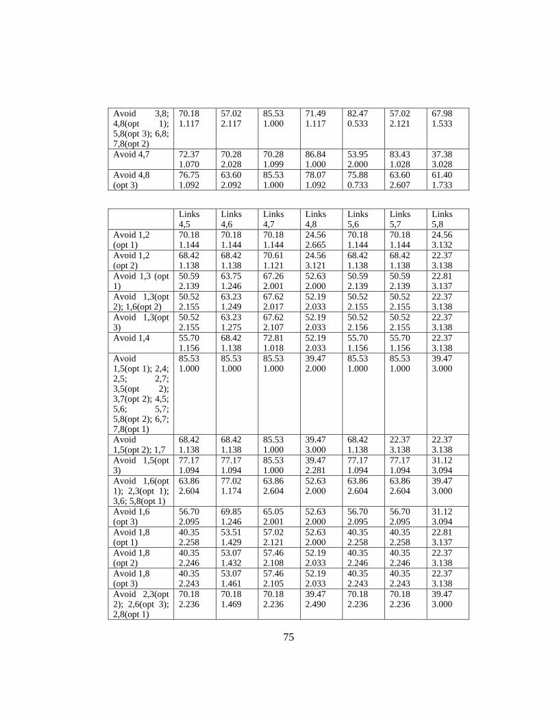
Avoid 3,8; 4,8(opt 1); 5,8(opt 3); 6,8; 7,8(opt 2)
70.18 1.117
57.02 2.117
85.53 1.000
71.49 1.117
82.47 0.533
57.02 2.121
67.98 1.533
Avoid 4,7
72.37 1.070
70.28 2.028
70.28 1.099
86.84 1.000
53.95 2.000
83.43 1.028
37.38 3.028
Avoid 4,8 (opt 3)
76.75 1.092
63.60 2.092
85.53 1.000
78.07 1.092
75.88 0.733
63.60 2.607
61.40 1.733
Links
4,5 Links 4,6
Links 4,7
Links 4,8
Links 5,6
Links 5,7
Links 5,8
Avoid 1,2 (opt 1)
70.18 1.144
70.18 1.144
70.18 1.144
24.56 2.665
70.18 1.144
70.18 1.144
24.56 3.132
Avoid 1,2 (opt 2)
68.42 1.138
68.42 1.138
70.61 1.121
24.56 3.121
68.42 1.138
68.42 1.138
22.37 3.138
Avoid 1,3 (opt 1)
50.59 2.139
63.75 1.246
67.26 2.001
52.63 2.000
50.59 2.139
50.59 2.139
22.81 3.137
Avoid 1,3(opt 2); 1,6(opt 2)
50.52 2.155
63.23 1.249
67.62 2.017
52.19 2.033
50.52 2.155
50.52 2.155
22.37 3.138
Avoid 1,3(opt 3)
50.52 2.155
63.23 1.275
67.62 2.107
52.19 2.033
50.52 2.156
50.52 2.155
22.37 3.138
Avoid 1,4 55.70 1.156
68.42 1.138
72.81 1.018
52.19 2.033
55.70 1.156
55.70 1.156
22.37 3.138
Avoid 1,5(opt 1); 2,4; 2,5; 2,7; 3,5(opt 2); 3,7(opt 2); 4,5; 5,6; 5,7; 5,8(opt 2); 6,7; 7,8(opt 1)
85.53 1.000
85.53 1.000
85.53 1.000
39.47 2.000
85.53 1.000
85.53 1.000
39.47 3.000
Avoid 1,5(opt 2); 1,7
68.42 1.138
68.42 1.138
85.53 1.000
39.47 3.000
68.42 1.138
22.37 3.138
22.37 3.138
Avoid 1,5(opt 3)
77.17 1.094
77.17 1.094
85.53 1.000
39.47 2.281
77.17 1.094
77.17 1.094
31.12 3.094
Avoid 1,6(opt 1); 2,3(opt 1); 3,6; 5,8(opt 1)
63.86 2.604
77.02 1.174
63.86 2.604
52.63 2.000
63.86 2.604
63.86 2.604
39.47 3.000
Avoid 1,6 (opt 3)
56.70 2.095
69.85 1.246
65.05 2.001
52.63 2.000
56.70 2.095
56.70 2.095
31.12 3.094
Avoid 1,8 (opt 1)
40.35 2.258
53.51 1.429
57.02 2.121
52.63 2.000
40.35 2.258
40.35 2.258
22.81 3.137
Avoid 1,8 (opt 2)
40.35 2.246
53.07 1.432
57.46 2.108
52.19 2.033
40.35 2.246
40.35 2.246
22.37 3.138
Avoid 1,8 (opt 3)
40.35 2.243
53.07 1.461
57.46 2.105
52.19 2.033
40.35 2.243
40.35 2.243
22.37 3.138
Avoid 2,3(opt 2); 2,6(opt 3); 2,8(opt 1)
70.18 2.236
70.18 1.469
70.18 2.236
39.47 2.490
70.18 2.236
70.18 2.236
39.47 3.000
75
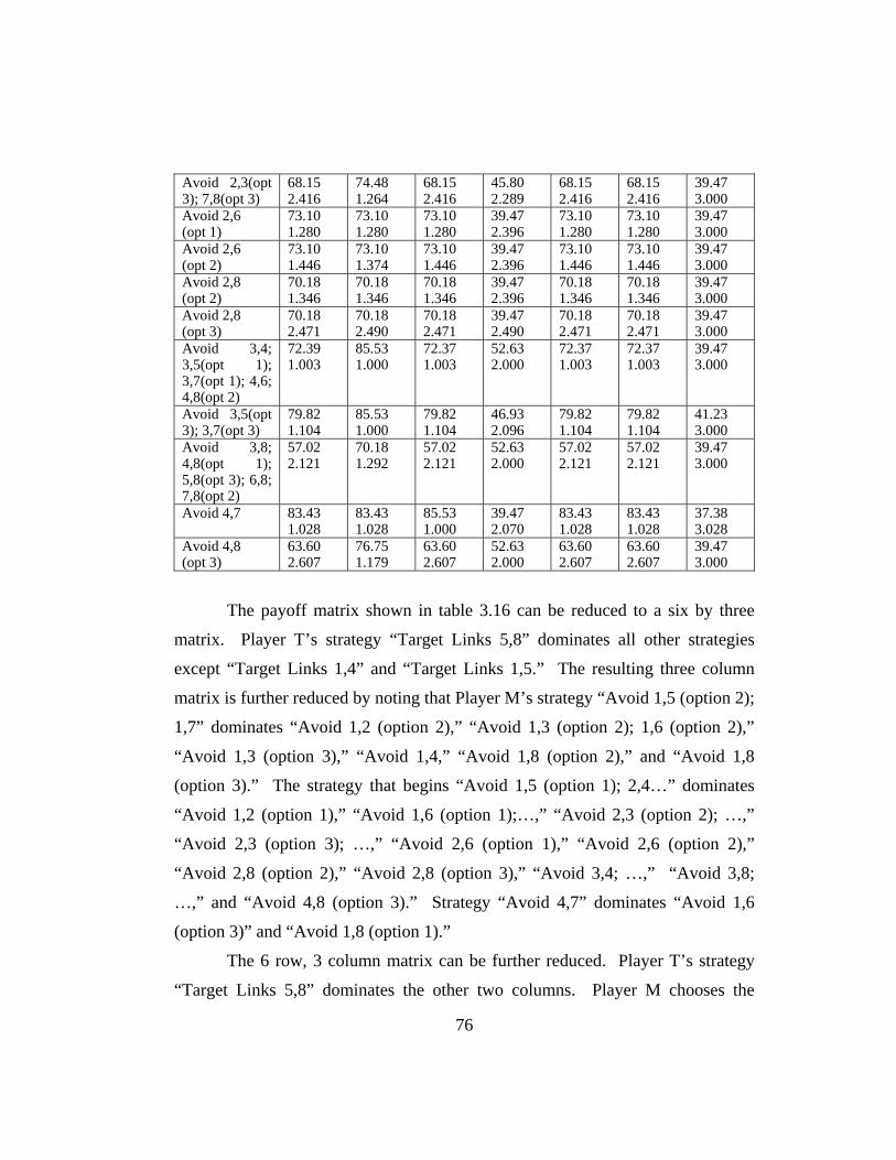
Avoid 2,3(opt 3); 7,8(opt 3)
68.15 2.416
74.48 1.264
68.15 2.416
45.80 2.289
68.15 2.416
68.15 2.416
39.47 3.000
Avoid 2,6 (opt 1)
73.10 1.280
73.10 1.280
73.10 1.280
39.47 2.396
73.10 1.280
73.10 1.280
39.47 3.000
Avoid 2,6 (opt 2)
73.10 1.446
73.10 1.374
73.10 1.446
39.47 2.396
73.10 1.446
73.10 1.446
39.47 3.000
Avoid 2,8 (opt 2)
70.18 1.346
70.18 1.346
70.18 1.346
39.47 2.396
70.18 1.346
70.18 1.346
39.47 3.000
Avoid 2,8 (opt 3)
70.18 2.471
70.18 2.490
70.18 2.471
39.47 2.490
70.18 2.471
70.18 2.471
39.47 3.000
Avoid 3,4; 3,5(opt 1); 3,7(opt 1); 4,6; 4,8(opt 2)
72.39 1.003
85.53 1.000
72.37 1.003
52.63 2.000
72.37 1.003
72.37 1.003
39.47 3.000
Avoid 3,5(opt 3); 3,7(opt 3)
79.82 1.104
85.53 1.000
79.82 1.104
46.93 2.096
79.82 1.104
79.82 1.104
41.23 3.000
Avoid 3,8; 4,8(opt 1); 5,8(opt 3); 6,8; 7,8(opt 2)
57.02 2.121
70.18 1.292
57.02 2.121
52.63 2.000
57.02 2.121
57.02 2.121
39.47 3.000
Avoid 4,7
83.43 1.028
83.43 1.028
85.53 1.000
39.47 2.070
83.43 1.028
83.43 1.028
37.38 3.028
Avoid 4,8 (opt 3)
63.60 2.607
76.75 1.179
63.60 2.607
52.63 2.000
63.60 2.607
63.60 2.607
39.47 3.000
The payoff matrix shown in table 3.16 can be reduced to a six by three
matrix. Player T’s strategy “Target Links 5,8” dominates all other strategies
except “Target Links 1,4” and “Target Links 1,5.” The resulting three column
matrix is further reduced by noting that Player M’s strategy “Avoid 1,5 (option 2);
1,7” dominates “Avoid 1,2 (option 2),” “Avoid 1,3 (option 2); 1,6 (option 2),”
“Avoid 1,3 (option 3),” “Avoid 1,4,” “Avoid 1,8 (option 2),” and “Avoid 1,8
(option 3).” The strategy that begins “Avoid 1,5 (option 1); 2,4…” dominates
“Avoid 1,2 (option 1),” “Avoid 1,6 (option 1);…,” “Avoid 2,3 (option 2); …,”
“Avoid 2,3 (option 3); …,” “Avoid 2,6 (option 1),” “Avoid 2,6 (option 2),”
“Avoid 2,8 (option 2),” “Avoid 2,8 (option 3),” “Avoid 3,4; …,” “Avoid 3,8;
…,” and “Avoid 4,8 (option 3).” Strategy “Avoid 4,7” dominates “Avoid 1,6
(option 3)” and “Avoid 1,8 (option 1).”
The 6 row, 3 column matrix can be further reduced. Player T’s strategy
“Target Links 5,8” dominates the other two columns. Player M chooses the
76

routing strategy “Avoid 3,5 (option 3); 3,7 (option 3)” to receive the payoff of
41.22. Player T’s resulting payoff is 3.00. Although the strategy label does not
include “Avoid 5,8,” the strategy is actually a fourth option for “Avoid 5,8.”
If Player M had over-estimated the amount of resources available to
Player T, would have received an advantage and Player M a disadvantage. The
payoff matrix associated with the routing strategy selected by Player M as a result
of table 3.16 is presented in table 3.17.
Table 3.17 Payoff Matrix for Misinformation about Player T’s Resources, 3/4 Demand Scenario
Player Link 1 Link 2 Link 3 Link 4 Link 5 Link 6 Link 7 Link 8
M 60.53 94.30 94.30 85.53 79.82 85.53 94.30 61.40
T 1.000 0.302 0.096 1.000 1.104 1.000 0.104 1.500
As in the previous demand case, Player T would select link 8 as the target.
Player M would receive a higher payoff than in the case where Player T actually
had the resources to damage two links, but had Player M known that link 8 was
the only target, traffic could have been routed appropriately. As in table 3.12,
Player M would have received a payoff of 82.46 if the correct information about
Player T’s resources had been obtained. By providing misinformation, Player T
would have obtained a payoff of 1.500 instead of 0.533.
77

Table 3.18 Payoff Matrix for n=2, 1/2 Demand Level
Links 1,2
Links 1,3
Links 1,4
Links 1,5
Links 1,6
Links 1,7
Links 1,8
Avoid 1,2 (opt 1)
89.47, 0.267
51.32, 1.900
48.68, 1.929
44.74, 2.029
46.05, 2.000
92.11, 0.195
48.68, 2.127
Avoid 1,2 (opt 2)
89.47, 0.333
51.32, 1.833
48.68, 1.933
44.74, 2.100
46.05, 2.000
92.11, 0.267
48.68, 2.067
Avoid 1,3 47.37, 2.000
92.11, 0.200
63.08, 1.460
18.34, 2.954
46.05, 2.000
64.39, 0.922
73.76, 0.758
Avoid 1,4 48.68 1.761
92.11 0.267
78.95 1.167
34.21 2.029
46.05, 2.000
81.58 0.507
59.21 1.267
Avoid 1,5(opt 1); 1,7
60.53 1.000
80.26 1.167
78.95 1.167
46.05, 2.000
46.05, 2.000
93.42 0.167
47.37 1.995
Avoid 1,5(opt 2); 2,4; 2,5; 3,5(opt 2); 3,7(opt 2); 4,5; 4,7; 5,6; 5,7; 5,8(opt 2); 6,7; 7,8(opt 2)
60.53 1.000
47.37 2.000
46.05 2.000
46.05 2.000
46.05 2.000
60.53 1.000
14.47 3.000
Avoid 1,6 (opt 1)
47.37 2.000
60.53 1.000
25.93 2.343
12.77 3.102
46.05 2.000
27.24 2.450
47.76 1.388
Avoid 1,6 (opt 2)
48.68 1.900
92.11 0.267
64.50 1.428
19.77 2.912
46.05 2.000
67.13 0.848
73.66 0.828
Avoid 1,8 (opt 1)
48.68 1.900
92.11 0.267
48.68 1.644
3.95 3.258
46.05 2.000
51.32 1.108
89.47 0.347
Avoid 1,8 (opt 2)
48.68 1.900
93.42 0.267
48.68 1.737
3.95 3.258
46.05 2.000
51.32 1.521
89.47 0.287
Avoid 2,3 (opt 1)
47.37 2.000
60.53 1.000
26.16 2.340
13.01 3.096
46.05 2.000
27.48 2.445
47.52 1.395
Avoid 2,3 (opt 2)
60.53 1.000
49.57 2.000
21.75 2.589
21.75 2.585
46.05 2.000
36.23 1.597
38.77 2.161
Avoid 2,3 (opt 3)
56.42 1.312
55.10 1.688
22.63 2.647
18.53 2.876
46.05 2.000
33.00 2.011
42.00 1.811
Avoid 2,6 (opt 1)
60.53 1.000
47.37 2.000
21.67 2.447
21.67 2.447
46.05 2.000
36.14 1.447
38.86 2.259
Avoid 2,6 (opt 2)
60.53 1.000
60.53 2.000
21.67 3.031
21.67 2.592
46.05 2.000
36.14 2.279
38.86 1.659
Avoid 2,6 (opt 3)
60.53 1.000
47.37 2.000
21.67 2.814
21.67 2.778
46.05 2.000
36.14 1.885
38.86 1.959
Avoid 2,8 (opt 1)
60.53 1.000
47.37 2.000
15.79 2.529
15.79 2.529
46.05 2.000
30.26 1.529
44.74 2.080
Avoid 2,8 (opt 2)
60.53 1.000
47.37 2.000
15.79 3.149
15.79 2.708
46.05 2.000
30.26 2.395
44.74 1.480
Avoid 2,8 (opt 3)
60.53 1.000
47.37 2.000
15.79 2.910
15.79 2.888
46.05 2.000
30.26 1.981
44.74 1.780
78
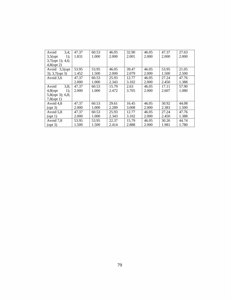
Avoid 3,4; 3,5(opt 1); 3,7(opt 1); 4,6; 4,8(opt 2)
47.37 1.831
60.53 1.000
46.05 2.000
32.90 2.001
46.05 2.000
47.37 2.000
27.63 2.000
Avoid 3,5(opt 3); 3,7(opt 3)
53.95 1.452
53.95 1.500
46.05 2.000
39.47 2.079
46.05 2.000
53.95 1.500
21.05 2.500
Avoid 3,6 47.37 2.000
60.53 1.000
25.93 2.343
12.77 3.102
46.05 2.000
27.24 2.450
47.76 1.388
Avoid 3,8; 4,8(opt 1); 5,8(opt 3); 6,8; 7,8(opt 1)
47.37 2.000
60.53 1.000
15.79 2.472
2.63 3.705
46.05 2.000
17.11 2.607
57.90 1.080
Avoid 4,8 (opt 3)
47.37 2.000
60.53 1.000
29.61 2.289
16.45 3.008
46.05 2.000
30.92 2.383
44.08 1.500
Avoid 5,8 (opt 1)
47.37 2.000
60.53 1.000
25.93 2.343
12.77 3.102
46.05 2.000
27.24 2.450
47.76 1.388
Avoid 7,8 (opt 3)
53.95 1.500
53.95 1.500
22.37 2.414
15.79 2.888
46.05 2.000
30.26 1.981
44.74 1.780
79

Links 2,3
Links 2,4
Links 2,5
Links 2,6
Links 2,7
Links 2,8
Links 7,8
Avoid 1,2 (opt 1) 53.95, 1.052
51.32, 1.081
51.32, 1.081
52.63, 1.052
94.74, 0.035
51.32, 1.966
53.95, 2.000
Avoid 1,2 (opt 2)
53.95, 1.052
51.32, 1.152
51.32, 1.152
51.63, 1.152
96.05, 0.104
51.32, 2.004
53.95, 2.000
Avoid 1,3 55.26, 1.060
26.24, 2.014
26.24, 2.014
40.79, 1.563
40.71, 1.407
36.92, 1.618
53.95, 2.000
Avoid 1,4 53.95, 1.052
40.79, 1.081
40.79, 1.081
40.79, 1.521
55.26, 0.952
21.05, 2.052
53.95, 2.000
Avoid 1,5(opt 1); 1,7
53.95, 1.052
52.63, 1.052
52.63, 1.052
52.63, 1.052
67.11, 0.052
21.05, 2.052
53.95, 2.000
Avoid 1,5(opt 2); 2,4; 2,5; 3,5(opt 2); 3,7(opt 2); 4,5; 4,7; 5,6; 5,7; 5,8(opt 2); 6,7; 7,8(opt 2)
86.84, 1.000
85.53, 1.000
85.53, 1.000
85.53, 1.000
100.00, 0.000
53.95, 2.000
53.95, 2.000
Avoid 1,6 (opt 1) 86.84, 1.000
52.24, 2.102
52.24, 2.102
72.37, 1.502
66.72, 1.102
74.07, 1.388
53.95, 2.000
Avoid 1,6 (opt 2) 53.95, 1.052
26.35, 1.964
26.35, 1.964
40.79, 1.523
40.82, 1.293
35.50, 1.613
53.95, 2.000
Avoid 1,8(opt 1) 53.95, 1.052
10.53, 2.310
10.53, 2.310
40.79, 1.516
25.00, 1.554
51.32, 1.132
53.95, 2.000
Avoid 1,8(opt 2) 53.95, 1.052
10.53, 2.751
10.53, 2.751
40.79, 1.516
25.00, 1.641
51.32, 1.072
53.95, 2.000
Avoid 2,3(opt 1) 86.84, 1.000
52.48, 2.096
52.48, 2.096
72.37, 1.507
66.95, 1.096
73.84, 1.395
53.95, 2.000
Avoid 2,3(opt 2) 86.84, 1.000
61.23, 1.585
61.23, 1.585
85.53, 1.000
75.70, 0.585
78.25, 1.161
53.95, 2.000
Avoid 2,3 (opt 3) 86.84, 1.000
58.00, 1.876
58.00, 1.876
81.42, 1.191
72.47, 0.876
77.37, 1.123
53.95, 2.000
Avoid 2,6(opt 1) 86.84, 1.000
61.14, 1.447
61.14, 1.447
85.53, 1.000
75.61, 0.447
78.34, 1.259
53.95, 2.000
Avoid 2,6(opt 2) 86.84, 1.000
61.14, 1.592
61.14, 1.592
85.53, 1.000
75.61, 0.592
78.34, 0.659
53.95, 2.000
Avoid 2,6(opt 3) 86.84, 1.000
61.14, 1.778
61.14, 1.778
85.53, 1.000
75.61, 0.778
78.34, 0.959
53.95, 2.000
Avoid 2,8(opt 1) 86.84, 1.000
55.26, 1.529
55.26, 1.529
85.53, 1.000
69.74, 0.529
84.21, 1.080
53.95, 2.000
Avoid 2,8(opt 2) 86.84, 1.000
55.26, 1.708
55.26, 1.708
85.53, 1.000
69.74, 0.708
84.21, 0.480
53.95, 2.000
Avoid 2,8(opt 3) 86.84, 1.000
55.26, 1.888
55.26, 1.888
85.53, 1.000
69.74, 0.888
84.21, 0.780
53.95, 2.000
80

Avoid 3,4; 3,5(opt 1); 3,7(opt 1); 4,6; 4,8(opt 2)
86.84, 1.000
72.37, 1.001
72.37, 1.001
72.37, 1.501
86.84, 0.001
53.95, 2.000
53.95, 2.000
Avoid 3,5(opt 3); 3,7(opt 3)
86.84, 1.000
78.95, 1.079
78.95, 1.079
78.95, 1.289
93.42, 0.079
53.95, 2.000
53.95, 2.000
Avoid 3,6 86.84, 1.000
52.24, 2.102
52.24, 2.102
72.37, 1.502
66.72, 1.102
74.07, 1.388
53.95, 2.000
Avoid 3,8; 4,8(opt 1); 5,8(opt 3); 6,8; 7,8(opt 1)
86.84, 1.000
42.11, 2.705
42.11, 2.705
72.37, 1.500
56.58, 1.705
84.21, 1.080
53.95, 2.000
Avoid 4,8(opt 3) 86.84, 1.000
55.92, 2.008
55.92, 2.008
72.37, 1.557
70.40, 1.008
70.40, 1.500
53.95, 2.000
Avoid 5,8(opt 1) 86.84, 1.000
52.24, 2.102
52.24, 2.102
72.37, 1.502
66.72, 1.102
74.07, 1.388
53.95, 2.000
Avoid 7,8(opt 3)
86.84, 1.000
55.26, 1.888
55.26, 1.888
78.95, 1.289
69.74, 0.888
77.63, 1.280
53.95, 2.000
Links 3,4
Links 3,5
Links 3,6
Links 3,7
Links 3,8
Links 6,7
Links 6,8
Avoid 1,2 (opt 1) 42.11, 2.069
38.16, 2.069
39.47, 1.145
56.58, 1.063
26.32, 2.006
51.32, 1.081
7.89, 3.012
Avoid 1,2 (opt 2) 43.42, 1.948
39.47, 2.052
40.79, 1.135
56.58, 1.048
25.00, 1.948
51.32, 1.152
7.89, 2.952
Avoid 1,3 70.97, 1.077
26.24, 2.137
53.95, 1.060
72.29, 1.077
81.66, 0.558
26.24, 2.014
35.61, 1.618
Avoid 1,4 84.21, 1.100
39.47, 2.052
51.32, 1.152
86.84, 1.000
65.79, 1.100
40.79, 1.081
18.42, 2.152
Avoid 1,5(opt 1); 1,7
72.37, 2.000
39.47, 2.052
39.47, 2.052
86.84, 1.000
53.95, 2.000
52.63, 1.052
6.58, 2.935
Avoid 1,5(opt 2); 2,4; 2,5; 3,5(opt 2); 3,7(opt 2); 4,5; 4,7; 5,6; 5,7; 5,8(opt 2); 6,7; 7,8(opt 2)
72.37, 1.000
72.37, 2.000
72.37, 1.000
86.84, 1.000
53.95, 1.714
85.53, 1.000
39.47, 2.778
Avoid 1,6 (opt 1) 65.40, 1.075
52.24, 2.075
85.53, 1.000
66.72, 1.075
87.23, 0.388
52.24, 2.102
72.76, 1.388
Avoid 1,6 (opt 2) 69.77, 1.183
25.03, 2.135
51.32, 1.152
72.40, 1.083
80.23, 0.661
26.35, 1.964
32.87, 1.713
Avoid 1,8(opt 1) 53.95, 1.135
9.21, 2.087
51.32, 1.152
56.58, 1.035
96.05, 0.180
10.53, 2.310
48.68, 1.232
Avoid 1,8(opt 2) 55.26, 1.133
10.53, 2.085
51.32, 1.152
57.90, 1.033
94.74, 0.220
10.53, 2.751
48.68, 1.172
Avoid 2,3(opt 1) 65.64, 1.075
52.48, 2.075
85.53, 1.000
66.95, 1.075
86.99, 0.395
52.48, 2.096
72.52, 1.395
81

Avoid 2,3(opt 2) 50.27, 1.655
50.27, 2.139
72.37, 1.516
64.75, 1.139
76.04, 1.328
61.23, 1.585
63.77, 2.161
Avoid 2,3 (opt 3) 56.68, 1.509
52.57, 2.106
76.47, 1.403
67.05, 1.106
77.85, 1.086
58.00, 1.876
67.00, 1.772
Avoid 2,6(opt 1) 47.98, 1.671
47.98, 2.153
72.37, 1.518
62.45, 1.153
78.34, 0.966
61.14, 1.447
63.86, 2.259
Avoid 2,6(opt 2) 61.14, 1.589
61.14, 2.071
72.37, 1.518
75.61, 1.071
65.18, 1.659
61.14, 1.592
63.86, 1.659
Avoid 2,6(opt 3) 54.56, 1.630
54.56, 2.112
72.37, 1.518
69.03, 1.112
71.76, 1.459
61.14, 1.778
63.86, 1.903
Avoid 2,8(opt 1) 42.11, 1.782
42.11, 2.138
72.37, 1.644
56.58, 1.138
84.21, 0.783
55.26, 1.529
69.74, 2.080
Avoid 2,8(opt 2) 55.26, 1.722
55.26, 2.078
72.37, 1.644
69.74, 1.078
71.05, 1.480
55.26, 1.708
69.74, 1.480
Avoid 2,8(opt 3) 48.68, 1.752
48.68, 2.108
72.37, 1.644
63.16, 1.108
77.63, 1.280
55.26, 1.888
69.74, 1.780
Avoid 3,4; 3,5(opt 1); 3,7(opt 1); 4,6; 4,8(opt 2)
85.53, 1.000
72.37, 2.000
85.53, 1.000
86.84, 1.000
67.11, 1.000
72.37, 1.001
52.63, 2.000
Avoid 3,5(opt 3); 3,7(opt 3)
78.95, 1.074
72.37, 2.000
78.95, 1.074
86.84, 1.000
60.53, 1.428
78.95, 1.079
46.05, 2.439
Avoid 3,6 65.40, 1.075
52.24, 2.075
85.53, 1.000
66.72, 1.075
87.23, 0.388
52.24, 2.102
72.76, 1.388
Avoid 3,8; 4,8(opt 1); 5,8(opt 3); 6,8; 7,8(opt 1)
55.26, 1.023
42.11, 2.023
85.53, 1.000
56.58, 1.023
97.37, 0.080
42.11, 2.705
82.90, 1.080
Avoid 4,8(opt 3) 69.08, 1.078
55.92, 2.078
85.53, 1.000
70.40, 1.078
83.55, 0.500
55.92, 2.008
69.08, 1.500
Avoid 5,8(opt 1) 65.40, 1.075
52.24, 2.075
85.53, 1.000
66.72, 1.075
87.23, 0.388
52.24, 2.102
72.76, 1.388
Avoid 7,8(opt 3) 55.26, 1.430
48.68, 2.108
78.95, 1.322
63.16, 1.108
84.21, 0.706
55.26, 1.888
69.74, 1.780
82

Links 4,5
Links 4,6
Links 4,7
Links 4,8
Links 5,6
Links 5,7
Links 5,8
Avoid 1,2 (opt 1) 51.32, 1.081
51.32, 1.081
55.26, 1.074
10.53, 3.046
51.32, 1.081
51.32, 1.081
6.58, 3.052
Avoid 1,2 (opt 2)
51.32, 1.152
52.63, 1.052
53.95, 1.148
10.53, 2.948
51.32, 1.152
51.32, 1.152
6.58, 3.052
Avoid 1,3 26.24, 2.014
39.39, 1.320
57.82, 1.954
52.63, 2.000
26.24, 2.014
26.24, 2.014
7.89, 3.060
Avoid 1,4 40.79, 1.081
52.63, 1.052
73.68, 1.029
51.32, 2.100
40.79, 1.081
40.79, 1.081
6.58, 3.052
Avoid 1,5(opt 1); 1,7
52.63, 1.052
52.63, 1.052
85.53, 1.000
39.47, 3.000
52.63, 1.052
52.63, 1.052
6.58, 3.052
Avoid 1,5(opt 2); 2,4; 2,5; 3,5(opt 2); 3,7(opt 2); 4,5; 4,7; 5,6; 5,7; 5,8(opt 2); 6,7; 7,8(opt 2)
85.53, 1.000
85.53, 1.000
85.53, 1.000
39.47, 2.000
85.53, 1.000
85.53, 1.000
39.47, 3.000
Avoid 1,6 (opt 1) 52.24, 2.102
65.40, 1.343
52.24, 2.102
52.63, 2.000
52.24, 2.102
52.24, 2.102
39.47, 3.000
Avoid 1,6 (opt 2) 26.35, 1.964
38.19, 1.313
59.24, 1.912
51.32, 2.100
26.35, 1.964
26.35, 1.964
6.58, 3.052
Avoid 1,8(opt 1) 10.53, 2.310
22.37, 1.529
43.42, 2.258
51.32, 2.100
10.53, 2.310
10.53, 2.310
6.58, 3.052
Avoid 1,8(opt 2) 10.53, 2.751
22.37, 1.623
43.42, 2.699
51.32, 2.100
10.53, 2.751
10.53, 2.751
6.58, 3.052
Avoid 2,3(opt 1) 52.48, 2.096
65.64, 1.340
52.48, 2.096
52.63, 2.000
52.48, 2.096
52.48, 2.096
39.47, 3.000
Avoid 2,3(opt 2) 61.23, 1.585
61.23, 1.517
61.23, 1.585
39.47, 2.516
61.23, 1.585
61.23, 1.585
39.47, 3.000
Avoid 2,3 (opt 3) 58.00, 1.876
62.10, 1.554
58.00, 1.876
43.58, 2.403
58.00, 1.876
58.00, 1.876
39.47, 3.000
Avoid 2,6(opt 1) 61.14, 1.447
61.14, 1.447
61.14, 1.447
39.47, 2.518
61.14, 1.447
61.14, 1.447
39.47, 3.000
Avoid 2,6(opt 2) 61.14, 1.592
61.14, 1.797
61.14, 1.592
39.47, 2.518
61.14, 1.592
61.14, 1.592
39.47, 3.000
Avoid 2,6(opt 3) 61.14, 1.778
61.14, 1.644
61.14, 1.778
39.47, 2.518
61.14, 1.778
61.14, 1.778
39.47, 3.000
Avoid 2,8(opt 1) 55.26, 1.529
55.26, 1.529
55.26, 1.529
39.47, 2.644
55.26, 1.529
55.26, 1.529
39.47, 3.000
Avoid 2,8(opt 2) 55.26, 1.708
55.26, 2.039
55.26, 1.708
39.47, 2.644
55.26, 1.708
55.26, 1.708
39.47, 3.000
Avoid 2,8(opt 3) 55.26, 1.888
55.26, 1.803
55.26, 1.888
39.47, 2.644
55.26, 1.888
55.26, 1.888
39.47, 3.000
83

An equilibrium solution was determined for the payoff matrix shown in
table 3.18. Examination of the columns revealed that Player T’s option to target
1,4 dominated strategy target 1,3. Targeting links 2 and 4 yielded a greater payoff
to Player T than disrupting links 2 and 3. Option (2,5) had equivalent payoffs to
option (2,4) for Player T. The strategy to target 1,5 dominated options (1,2),
(1,6), (1,7), (2,5), (3,7), (3,8), (4,5), (4,6), (4,7), (5,6), and (5,7). Damaging links
5 and 8 provided Player T with a greater payoff than disrupting (1,8), (2,6), (2,7),
(2,8), (3,4), (3,5), (3,6), (4,8), (6,7), (6,8), and (7,8). Player M’s payoffs were
then examined for the remaining three columns [(1,4), (1,5), and (5,8)] of the
matrix. Strategy “avoid (1,5) option 1” dominated alternatives “avoid (1,2)
options 1 and 2,” “avoid (1,4),” “avoid (1,6) option 2,” and “avoid (1,8) options 1
and 2.” Strategy “avoid (1,5) option 2” dominated alternatives “avoid (1,6)
option 1,” “avoid (2,3) options 1, 2, and 3,” “avoid (2,6) options 1, 2, and 3,”
“avoid (2,8) options 1, 2, and 3,” “avoid (3,4),” “avoid (3,5) option 3,” “avoid
(3,6),” “avoid (3,8),” “avoid (4,8) option 3,” “avoid (5,8) option 1,” and “avoid
(7,8) option 3.” Only three strategies remained for Player M: “avoid (1,3),”
“avoid (1,5) option 1,” and “avoid (1,5) option 2.” Examination of the remaining
Avoid 3,4; 3,5(opt 1); 3,7(opt 1); 4,6; 4,8(opt 2)
72.37, 1.001
85.53, 1.000
72.37, 1.000
52.63, 2.000
72.37, 1.001
72.37, 1.001
36.84, 3.000
Avoid 3,5(opt 3); 3,7(opt 3)
78.95, 1.079
85.53, 1.000
78.95, 1.079
46.05, 2.074
78.95, 1.079
78.95, 1.079
39.47, 3.000
Avoid 3,6 52.24, 2.102
65.40, 1.343
52.24, 2.102
52.63, 2.000
52.24, 2.102
52.24, 2.102
39.47, 3.000
Avoid 3,8; 4,8(opt 1); 5,8(opt 3); 6,8; 7,8(opt 1)
42.11, 2.705
55.26, 1.472
42.11, 2.705
52.63, 2.000
42.11, 2.705
42.11, 2.705
39.47, 3.000
Avoid 4,8(opt 3) 55.92, 2.008
69.08, 1.289
55.92, 2.008
52.63, 2.000
55.92, 2.008
55.92, 2.008
39.47, 3.000
Avoid 5,8(opt 1) 52.24, 2.102
65.40, 1.343
52.24, 2.102
52.63, 2.000
52.24, 2.102
52.24, 2.102
39.47, 3.000
Avoid 7,8(opt 3) 55.26, 1.888
61.84, 1.414
55.26, 1.888
46.05, 2.322
55.26, 1.888
55.26, 1.888
39.47, 3.000
84

matrix revealed “target links (5,8)” as the dominant strategy for Player T. Player
M’s best strategy was “avoid (1,5) option 2,” which was equivalent to “avoid
(5,8) option 2.” At this equilibrium point, Player M received a payoff of 39.47%
of drivers safely reaching their destinations and Player T’s payoff was 3.000.
If Player M had overestimated Player T’s resources and Player T really
only had enough supplies to damage one of the links, the following payoff matrix,
shown in table 3.19 would have resulted from the routing strategy “avoid (1,5)
option 2 / avoid (5,8) option 2”.
Table 3.19 Payoff Matrix for Misinformation about Player T’s Resources, ½ Demand Scenario
Player Link 1 Link 2 Link 3 Link 4 Link 5 Link 6 Link 7 Link 8
M 60.53 100.00 86.84 85.53 85.53 85.53 100.00 53.95
T 1.000 0.000 3.7 x 10⁻⁵ 1.000 1.000 1.000 0.000 1.778
Player T would select link 8 as the target to obtain the largest payoff.
Player M’s payoff would then be 53.95% of the drivers safely reaching their
destinations. This payoff was greater than the case where Player T actually did
have the resources to damage both links 5 and 8. However, recall from table 3.13,
that if Player M knew that Player T had selected link 8, Player M could have
implemented a routing strategy that would have allowed 82.46% of travelers to
safely reach their destinations. By employing misinformation about the amount
of resources, Player T was able to obtain a payoff of 1.778 (table 3.19), which is
more desirable than 0.533 (table 3.13).
The payoff matrices are not presented here for the n=3 case because
Player T has a single dominant strategy. To achieve the largest payoff, Player T
would target links 1, 5, and 8. These three links form a traditional cut set for the
85

network and Player M cannot route traffic to avoid links 1, 5, and 8
simultaneously. The payoff for Player T is 4.0 and the payoff to Player M is 0.
3.3.4 Game 4: Perfect Information for Both Players, Multiple Moves
In Game 4, Player M and Player T alternate moves. First Player M assigns
traffic to avoid a predicted set of links. Player T then damages a set of links.
Player M then reassigns traffic to avoid the set that was damaged. Player T
selects the next set of links to be damaged, and so on until Player T’s resources
are gone or Player M cannot route traffic to connect any origin-destination pair.
Due to the small nature of the sample network, assume that each
successive set of damaged links only consists of one arc. For this game, the
original demand levels are used.
From the results in the previous games, Player M first chooses the strategy
“Avoid Link 5” and Player T selects “Link 5.” The origin-destination pair (5,2)
has now been severed – no route exists between the two nodes. The demand for
this O-D pair is removed from consideration of the remaining links. The modified
network is shown below in figure 3.4.
1 2
3 4
5 6
1 2
3
4
6
7
8
Figure 3.4 Sample Network after Player T's First Move
86

Clearly, links 2, 4, 6, and 7 are of no use to the connectivity of the
remaining origin-destination pairs and the only links of interest are 1, 3, and 8.
Recall that the O-D demands are q1,2 = 3000, q1,6 = 1000, and q5,6 = 2500. Since
only one path connects each origin-destination pair and sufficient capacity is
available on that path, all of the vehicles are assigned to link 1 for (1,2) and to
links 3 and 8 for (1,6) and to link 8 for (5,6). The resulting vulnerability indices
are M11,2 = 1.0, M3
1,6 = 1.0, M81,6= 1.0, and M8
5,6 = 1.0. Summing over the O-D
pairs, link 8 has the highest disruption index and will be targeted by Player T.
Destroying this link will sever origins 1 and 5 from destination 6. After this move
by T, only one O-D pair (1,2) is still connected. In the final move, Player T will
damage link 1. Thus, after 3 moves by Player T, a cut set of the network has been
determined.
3.4 SUMMARY
In this chapter, a bi-level mathematical programming formulation has been
presented to identify vulnerable links in a road transportation network. Game
theory may be used to solve this formulation, or interesting variants thereof. For
illustrative purposes, a two player, non-zero sum game was presented, with four
different cases of information. The payoff for the “evil entity” was the disruption
index. The development of this measure was also presented in this chapter.
Various attributes of the network were incorporated into the index, including
current traffic flow, travel time, availability of alternate paths, and relative excess
capacity on the alternate paths.
A small sample network was provided to illustrate the application of all of
the concepts developed in this chapter. For each of the games envisioned, the
most vulnerable link in the network was the one connecting the most origin-
destination pairs and currently carrying flow to each of the destinations. The
87

interplay of traffic assignment, flow dependent travel time, and network design
allow the disruption index to capture effects of damage to one link, or set of links,
on origin-destination connectivity and the network as a whole.
88

Chapter 4
Model Of Household Decision Making In An
Emergency Evacuation
This chapter presents the mathematical modeling of household behavior in
an emergency evacuation and integrates this behavior with a traffic simulation-
assignment methodology to estimate network evacuation time. As noted in
Chapter 2, families tend to unite prior to the evacuation of a building or town.
Conventional evacuation models disregard this observed behavior. Stern and
Sinuany-Stern (1989) and Sinuany-Stern and Stern (1993) did include some
human factors into their evacuation model, but these aspects are related to the
diffusion of evacuation instructions and individual’s preparation time. These
studies still overlook family gathering behavior. Omission of this phenomenon in
simulation models has two major implications. First, the models fail to capture
some of the complex travel patterns and the resulting network traffic patterns that
are exhibited only during emergency situations. Second, the estimated evacuation
times may be overly optimistic.
In this chapter, each household is modeled as a single entity that makes
two primary decisions sequentially. The first decision is the location where the
family will meet; this site may have been selected well in advance of the
evacuation. The second decision is the assignment of drivers to pick up other
family members who may not have access to vehicles. These decisions result in
forming trip chains, thus addressing the first implication mentioned in the
previous paragraph – that complex travel patterns have not been adequately
captured by traditional engineering models.
89

The second implication, that predicted evacuation times are overly
optimistic, is examined through traffic simulation. The impacts of trip chains and
the factors involved in the activity chain generation process on evacuation time
are examined in this chapter. Furthermore, network clearance comparisons are
made with cases in which no trip chains are considered.
The remainder of this chapter is organized as follows. The first section
presents the modeling framework and formulation, corresponding to the first
objective identified in section 1.2.2 of chapter 1. The second portion of this
chapter explains the experimental design. In the third section, the results are
presented and discussed in terms of objectives 2 and 3 of section 1.2.2. Finally, a
summary is provided.
4.1 MODELING FRAMEWORK AND PROBLEM FORMULATION
The notation used in this formulation is presented in table 4.1. The
general problem can be stated as follows: given a set of households, their decision
making rules, and a transportation network G(N,A) consisting of a set of nodes N
and arcs A, determine the evacuation time for the network. The characteristics of
the network’s nodes and links are known, and the associated time-varying OD
demand pattern for regular (non emergency) peak period conditions is given.
The evacuation time (E) is defined as the time elapsed between the instant
the evacuation is ordered and the instant the last vehicle exits the network.
orderfinal TTE −= (4.1)
where . (4.2) ⎟⎟⎠
⎞⎜⎜⎝
⎛∑+∑+=∈∈ ψξ
θj
vj
i
vi
vv
final tpT max
ξ is the subset of intermediate nodes visited by vehicle v and hI∈ξ
90
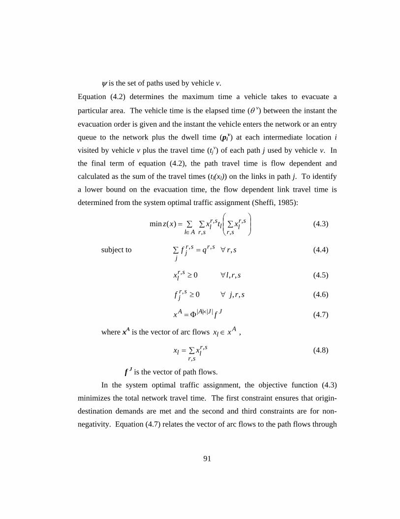
ψ is the set of paths used by vehicle v.
Equation (4.2) determines the maximum time a vehicle takes to evacuate a
particular area. The vehicle time is the elapsed time (θ v) between the instant the
evacuation order is given and the instant the vehicle enters the network or an entry
queue to the network plus the dwell time (piv) at each intermediate location i
visited by vehicle v plus the travel time (tjv) of each path j used by vehicle v. In
the final term of equation (4.2), the path travel time is flow dependent and
calculated as the sum of the travel times (tl(xl)) on the links in path j. To identify
a lower bound on the evacuation time, the flow dependent link travel time is
determined from the system optimal traffic assignment (Sheffi, 1985):
(4.3) ∑ ∑ ⎟⎟⎠
⎞⎜⎜⎝
⎛∑=
∈Al sr sr
srll
srl xtxxz
, ,
,,)(min
subject to (4.4) srqfj
srsrj ,,, ∀∑ =
(4.5) srlx srl ,,0, ∀≥
(4.6) srjf srj ,,0, ∀≥
JJAA fx |||| ×Φ= (4.7)
where xA is the vector of arc flows , Al xx ∈
∑=sr
srll xx
,
, (4.8)
f J is the vector of path flows.
In the system optimal traffic assignment, the objective function (4.3)
minimizes the total network travel time. The first constraint ensures that origin-
destination demands are met and the second and third constraints are for non-
negativity. Equation (4.7) relates the vector of arc flows to the path flows through
91

an arc-path incidence matrix Φ (Jahn, et al, 2002), the entries of which are 1 if
link l lies on path j and 0 otherwise.
Table 4.1 Summary of Notation
Notation Interpretation E Network evacuation time Tfinal Time at which the final vehicle exits the network Torder Time at which the evacuation order is given v, w Vehicle index θv Initial delay/waiting time of a vehicle entering the network ξh Set of intermediate destinations for vehicle v of household h i Index of the set Iv
h Ih Set of intermediate destinations for household h, not including the meeting location pi Time spent at intermediate destination i r,s Origin-destination pair l Link index Lj Set of links in path j tl Link travel time xl
r,s Flow on link l pertaining to r,s qr,s Origin-destination demand Gh Graph representing the household’s evoked network Nh Set of nodes in Gh
Ah Set of arcs in Gh
Vh Set of vehicles belonging to household h Rh Set of origin nodes where household h has a vehicle Uh Set of possible meeting places for household h u Member of the set Uh
τr,s Perceived travel time from location r to s S Final destination/place of safety, such as a shelter du,S Distance between the meeting place and S bS
Maximum tolerable distance between u and S
F Location of destruction, fire, storm, or other danger du,F
Distance between u and F
bF Minimum tolerable distance between u and F mu Maximum distance between u and the nodes in sets Iv
h and Rh
yu The decision variables are yu which take the value 1 if location u is selected and 0 otherwise.
92

The set of intermediate destinations (ξ) visited by a vehicle is determined
by a sequence of decisions at the household level. These intermediate
destinations are determined through two linear integer programs. The first
addresses the selection of a meeting location where the family gathers prior to
evacuating the town, or threatened area. The second mathematical program
assigns drivers to pick up sites where other family members, who may not have
access to vehicles, are located. The second program also determines the sequence
of these pick ups.
When making decisions, the household is assumed to ignore the actual
nodes of the network and to consider the intermediate destinations as the “nodes”
of their overall path. Thus, for decision making purposes, the family uses a
perceived aggregated network that extracts relevant information from the actual
underlying network. In other words, they create an evoked network that is
specific to that household Gh(Nh,Ah), and solve their logistical problems without
further consideration of the actual transportation network. In this household-
specific network, the only nodes included in the set Nh are the origins of the
household vehicles Rh and the intermediate household destinations Ih, including
possible meeting locations Uh, (where the superscript h denotes the
household).
hh IU ⊆
hhh RIN ∪= (4.6)
The formulation for deciding the household meeting location minimizes
the maximum travel time from any of the locations at which there are family
members ( )hh RI ∪ . The set of possible meeting locations is determined by the
household’s decision makers; this set may consist of home, schools, shopping
areas, parks, or any subset of these. If the danger prevents two or more family
members from meeting safely, they are considered separate entities. In order for a
location to be considered, the site must be a minimum distance from the danger
93

and within a given distance from the final shelter location. This last constraint
ensures that the meeting location that is selected is not on the side of town furthest
from the final evacuation path and safety. Once all family members have reached
the meeting location, the family continues on to the final shelter as a single unit.
The linear integer programming formulation is presented next, with the applicable
notation defined in table 4.1.
The mathematical programming formulation is as follows:
uh
UmZ
h=min (4.7)
subject to
( ) hhhu
uju UuRIjmy ∈∀∪∈∀≤,τ (4.8)
∑ =∈ hUu
uy 1 (4.9)
SSu bd ≤, (4.10)
(4.11) FFu bd ≥,
{ } hu Uuy ∈∀∈ 1,0 (4.12)
The objective function (4.7) minimizes the maximum perceived travel
time of all family members’ initial locations from the meeting place. The first
constraint (4.8) determines the maximum travel time for every possible meeting
place u. The second constraint (4.9) ensures that only one meeting location is
selected. The third (4.10) and fourth (4.11) constraints are distance requirements.
Finally, the fifth constraint (4.12) is the requirement that the decision variables yu
be zero or one (Desrochers et al, 1988).
The intermediate destination nodes are determined by the assignment of
vehicles to pick up non-driving household members, based on the meeting
location. The definition of the variables for the trip chain assignments is found in
table 4.1. Additionally, Vh is the set of vehicles available to household h. The
94

decision variables are xvij which take the value 1.0 if vehicle v uses the hyperlink
connecting nodes i and j. Indices for the vehicles are denoted by v and w; Cv is
the capacity of vehicle v.
Two, possibly conflicting, objectives are involved in the pick-up, and
resulting trip chain, assignments. Household decision makers may wish to (1)
minimize the total travel time for household’s fleet of vehicles and (2) minimize
the waiting time at the meeting location. Risk is associated with traveling on the
network because there could be an incident on the roadway; more household
drivers on the network increases the risk to the household as whole. However,
having one driver wait at the meeting location while another driver picks up all of
the children could cause frustration and concern on the part of the driver who is
waiting and one of the children may be waiting for the parent for a considerable
amount of time. Thus, household decision makers must make trade offs between
the dangers of multiple household vehicles traveling and waiting at the meeting
location for an extended period of time. To minimize the time that family
members in one vehicle are waiting for family members in another vehicle, their
arrival times at the meeting location should be close together. This part of the
objective function is given by:
∑ ∑ ∑−∈ ∈ ∈h h hVwv Nji Nji
ijw
ijijv
ij xx, , ,
min ττ (4.13)
The trade off between waiting time and multiple vehicles traveling can be
mathematically expressed as a linear combination of equation (4.13) and the
objective function of the classic VRP (see chapter 2). This second part of the
overall objective function is as follows:
95
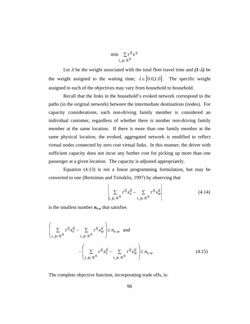
∑∈ h
ij
Nji
ij x,
min τ
Let λ be the weight associated with the total fleet travel time and (1-λ) be
the weight assigned to the waiting time; [ ]0.1,0.0∈λ . The specific weight
assigned to each of the objectives may vary from household to household.
Recall that the links in the household’s evoked network correspond to the
paths (in the original network) between the intermediate destinations (nodes). For
capacity considerations, each non-driving family member is considered an
individual customer, regardless of whether there is another non-driving family
member at the same location. If there is more than one family member at the
same physical location, the evoked, aggregated network is modified to reflect
virtual nodes connected by zero cost virtual links. In this manner, the driver with
sufficient capacity does not incur any further cost for picking up more than one
passenger at a given location. The capacity is adjusted appropriately.
Equation (4.13) is not a linear programming formulation, but may be
converted to one (Bertsimas and Tsitsiklis, 1997) by observing that
∑ ∑−∈ ∈h hNji Nji
ijw
ijijv
ij xx, ,
ττ (4.14)
is the smallest number nv,w that satisfies
wvNji Nji
ijw
ijijv
ij nxxh h
., ,
≤⎟⎟
⎠
⎞
⎜⎜
⎝
⎛∑ ∑−∈ ∈
ττ and
wvNji Nji
ijw
ijijv
ij nxxh h
., ,
≤⎟⎟
⎠
⎞
⎜⎜
⎝
⎛∑ ∑−−∈ ∈
ττ (4.15)
The complete objective function, incorporating trade offs, is:
96
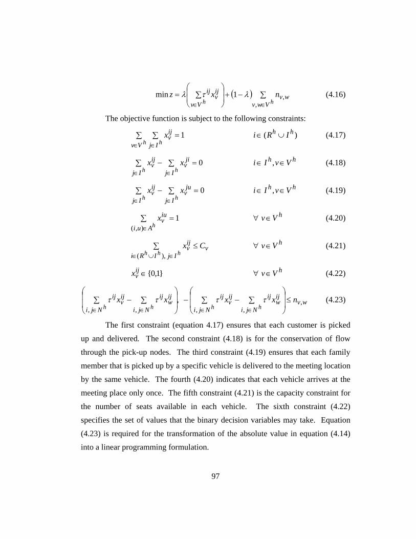
( ) ∑−+⎟⎟⎠
⎞⎜⎜⎝
⎛∑=
∈∈ hh Vwvwv
ijv
Vv
ij nxz,
,1min λτλ (4.16)
The objective function is subject to the following constraints:
(4.17) ∑ ∑ =∈ ∈h hVv Ij
ijvx 1 )( hh IRi ∪∈
(4.18) 0
1
(4.21)
}
=∑−∑∈∈ hh Ij
jiv
Ij
ijv xx hh VvIi ∈∈ ,
(4.19) 0=∑ ∑−∈ ∈h hIj Ij
juv
ijv xx hh VvIi ∈∈ ,
(4.20) ),(
=∑∈ hAui
iuvx hVv ∈∀
∑ ≤∈∪∈ hhh IjIRi
vijv Cx
),(
hVv ∈∀
(4.22) 1,0{∈ijvx hVv ∈∀
wvNji Nji
ijw
ijijv
ij
Nji Nji
ijw
ijijv
ij nxxxxh hh h
,, ,, ,
, ≤⎟⎟
⎠
⎞
⎜⎜
⎝
⎛∑ ∑−−⎟
⎟
⎠
⎞
⎜⎜
⎝
⎛∑ ∑−
∈ ∈∈ ∈ττττ (4.23)
The first constraint (equation 4.17) ensures that each customer is picked
up and delivered. The second constraint (4.18) is for the conservation of flow
through the pick-up nodes. The third constraint (4.19) ensures that each family
member that is picked up by a specific vehicle is delivered to the meeting location
by the same vehicle. The fourth (4.20) indicates that each vehicle arrives at the
meeting place only once. The fifth constraint (4.21) is the capacity constraint for
the number of seats available in each vehicle. The sixth constraint (4.22)
specifies the set of values that the binary decision variables may take. Equation
(4.23) is required for the transformation of the absolute value in equation (4.14)
into a linear programming formulation.
97

The two linear integer programs result in the selection of a meeting
location and the trip chains assigned to each driving member of the household. In
the following section, the experimental design for the application of this model is
presented.
4.2 EXPERIMENTAL DESIGN
Three main steps are involved in the incorporation of the household
behavior model for emergency evacuations within a network traffic modeling and
simulation framework. First, a simulation is run to generate “typical” travel times
to given locations. Then, these expected travel times are used in the linear integer
programs that describe the decision-making process of the household meeting
place selection and activity chain assignment of the family’s vehicles. These
linear integer programs are solved for each household in the network. Finally, the
trip chains are employed in time-dependent traffic assignment-simulation
software.
Step 1.
In the first step, an initial time-varying assignment is performed to
generate the travel time characteristics on the network links for “everyday” traffic
conditions, employing a k-shortest paths algorithm and the user equilibrium
traffic assignment. Alternatively, actual measured travel times might be used, if
available. These times serve as the perceived travel times (τr,s) for the households’
decision makers in the evoked network Gh(Nh,Ah). The time to reach family
members and the meeting location greatly affect both the selection of the meeting
location and the assignment of drivers to pick-up sites.
98

Step 2.
In the second step of the ar integer programs
described in the previous section, are solved sequentially. These formulations are
used to determine the household meeting location and then, simultaneously, the
assignment of drivers to pick-up locations and the sequence of those pick-ups.
In the third step, the traffic is simulated using The
sequence of intermediate nodes in the trip chain is followed by the simulator. The
availability and use of information may cause the driver to follow alternate paths
in the underlying transportation network (which may not be part of the
household’s evoked network when the decisions were made). These decisions are
handled according to the logic of the simulation-assignment methodology with
trip chaining described in Abdelghany, Mahmassani, and Chiu (2001). The
simulator keeps track of congestion levels and operating speeds, allowing for
information on real-time travel conditions, which may be vastly different from
those anticipated at the time household members made their decisions.
Depending on information supply strategies, and the particular problem
formulation and operational scenario, the drivers may make changes to their
original plans.
approach, the two line
The results from the linear integer programs are a set of trip chains for
each participating vehicle in the household. This information is then used in step
3.
Step 3.
the results from step 2.
The traffic simulation-assignment tool providing the network modeling
capability for steps 1 and 3 is DYNASMART (DYnamic Network Assignment
Simulation Methodology for Advanced Road Telematics), developed at the
University of Maryland and the University of Texas at Austin. The key features
99

of this software that are employed in this work included activity chains, zones,
virtual centroids, user equilibrium traffic assignment, and system optimal traffic
assignment (Mahmassani and Sbayti, 2003).
A simplified network model of the south-central portion of Fort Worth,
Texas is used as a test bed for this work (see figure 4.1). The network consists of
184 nodes (only 180 are shown in the figure). In this model, two elementary
schools (nodes 123 and 165), two middle schools (nodes 122 and 169), and one
high school (node 170) are located throughout the network (Fort Worth
Independent School District, 2003). Each school is modeled as a distinct zone
because in DYNASMART, every zone has a virtual centroid to which demand is
attracted or from which it is produced. The centroid may be connected to
multiple links, but in this work, it is particularly important that only links entering
or leaving the schools’ nodes carry traffic related to picking up the children.
Overall, the network shown in figure 4.1 is divided into 14 zones. Three of these
are designated as business zones (7-9) ; five are school zones (10-14); and the
remaining six are residential areas (see figure 4.2).
Four additional nodes (300, 301, 302, and 303) and seven links, not shown
in figure 1, were added to the network to represent final shelter destinations.
These nodes are considered to be outside of the evacuation area.
100

2
4
98
22
139
160102159
158101157
156100
146
145140
144
176
163106
105
162104
161103
152
96
99928
66
29
91906
26
1519789
111
168110149
143
167109154148142
178177 166165108
107164155153147141
95
93
941242
10
38
33
15014
51
47
21
30
25
41
37
34
52
48
19
23
35
32
39
4544
49
28
1
7
11
67
71
74
85
73
130 81
3
20
118
132
121
120
131119
123
122
134
133
127
175
126
125
124
77
76
75
2784
6570
5
24
838069
8268
972 8636
31
43
40
13
46
50
116
169
170
112
172
113114
171
16
54
59
53
6058
551578
138136
137135
128 8887
5756
174
115
17363
18
6462
129 79
61
17
117200
Edward J. BriscoeElementary
Forest Oaks Middle School
O.D. Wyatt High School
E.M. Daggett Middle School
E.M. Daggett Elementary
199
Figure 4.1 Sample Network 101

2
4
98
22
139
160102159
158101157
156100
146
145140
144
176
163106
105
162104
161103
152
96
99928
66
29
91906
26
1519789
111
168110149
143
167109154148142
178177 166165108
107164155153147141
95
93
941242
10
38
33
15014
51
47
21
30
25
41
37
34
52
48
19
23
35
32
39
4544
49
28
1
7
11
67
71
74
85
73
130 81
3
20
118
132
121
120
131119
123
122
134
133
127
175
126
125
124
77
76
75
2784
6570
5
24
838069
8268
972 8636
31
43
40
13
46
50
116
169
170
112
172
113114
171
16
54
59
53
6058
551578
138136
137135
128 8887
5756
174
115
17363
18
6462
129 79
61
17
117
Zone
9
Zone 1 Zone 2
Zone 3 Zone 4
Zone 5 Zone 6
Zone
7
Zone
8 Zone 10
Zone 11 Zone 12
Zone 13
Zone 14
s
Figure 4.2 Sample Network with Zone
102

Census 2000 data for the Fort Worth, TX area indicated that of the
195,058 households, 65.4% are families and 34.6% are nonfamily households.
The following data is relevant to the families, but is given in terms of percentage
of the total households: 34.7% have children under 18 years old, 45.8% are
married couple families, and 14.7% are single mother households. The average
family size is slightly over 3 persons (Census 2000).
The percentages reported in the census tables are used to generate
household types and the relative numbers of each type. Thirty different basic
households are generated using the computer code found in Appendix C:
1. Single individual
2. Single parent with one elementary school child
3. Single parent with one middle school child
4. Single parent with one high school child
5. Single parent with two elementary school children
6. Single parent with two middle school children
7. Single parent with two high school children
8. Single parent with one elementary school child and one middle school
child
9. Single parent with one elementary school child and one high school child
10. Single parent with one middle school aged child and one high school aged
child
11. Couple (no children)
12. Two parents with one elementary school aged child
13. Two parents with one middle school aged child
14. Two parents with one high school aged child
15. Two parents with two elementary school aged children
16. Two parents with two middle school aged children
103

17. Two parents with two high school aged children
18. Two parents with one elementary school aged child and one middle school
aged child
19. Two parents with one middle school aged child and one high school aged
child
20. Two parents with one elementary school child and one high school child
21. Two parents with three elementary school children
22. Two parents with two elementary school children and one middle school
child
23. Two parents with one elementary school child and two middle school
children
24. Two parents with one elementary school, one middle school, and one high
school child
25. Two parents with three middle school children
26. Two parents with two middle school children and one high school child
27. Two parents with one middle school and two high school children
28. Two parents with three high school children
29. Two parents with two high school children and one elementary school
child
30. Two parents with one high school child and two elementary school
children
These thirty are then repeated in the proportions previously mentioned
until a total of 20,000 households are generated. The household’s business and
residential zones are assigned by a random number generator. The choice set for
meeting locations of a household with two parents is limited to schools where the
family had children in attendance and the home. In the case of single parents,
only the school locations of the children are in the set. If the household does not
have any children, the couple meets at the home. When the household is a single
104

individual, there is no meeting location and the individual is assigned an
immediate shelter destination.
Further assumptions that are used in the model include:
1. Households do not contain more than three children.
2. All household vehicles are capable of carrying the entire family.
3. Children are only transported by their parents’ vehicles.
4. High school children would not drive themselves.
5. Traffic management agencies, combined with law enforcement personnel,
would provide route guidance in an emergency situation so as to assign
traffic according to the system optimum.
6. The order to evacuate would be given during school hours.
Once the households are generated, the framework developed in section
4.1 is followed. In accordance with step 1, a slight increase to typical peak period
traffic is simulated using the user equilibrium traffic assignment. The travel times
from business zones to residential zones, business zones to school zones, school
zones to other school zones, and school zones to residential zones are used as the
perceived trip costs for household decision making. The meeting locations and
pick-up assignments are then generated for each household (step 2). Finally, the
activity chains determined by the pick-up assignments are used in the system
optimal traffic assignment (step 3).
4.3 EXPERIMENTAL RESULTS
Using the simulation tools, 20,000 households and 30,141 vehicles were
generated. Approximately 49% of the households had only one adult and 51%
had two. No children were present in 49% of the households, including both
single and dual parent homes. Elementary school aged children (at least one)
105

were found in 23% of the households; middle school aged children were in 23%
of the households, and high school aged children were in 24% of the households.
Approximately 13% of the households had multiple children in different schools.
Based on these household characteristics, between 33 and 57% of the total
generated vehicles would stop at schools to pick-up the children.
Typical travel times for the households were generated based on 34,021
vehicles. This increased number of vehicles allowed for a small amount of
additional travel time, which may be part of the perceived travel time in an
emergency situation. Based on 120 second cycle times for the lights, a delay of 1
minute was added for each traffic light. Delays at stop signs were assumed to be
30 seconds. The perceived zonal travel times with intersection delays are given in
minutes in tables 4.2 and 4.3.
Table 4.2 Perceived Zonal Travel Times to Residential Zones
To Zone 1 2 3 4 5 6 1 - - - - - - 2 - - - - - - 3 - - - - - - 4 - - - - - - 5 - - - - - - 6 - - - - - - 7 1.44 4.71 9.11 9.13 7.95 8.78 8 3.15 6.25 2.21 2.83 10.22 16.81 9 13.01 9.60 9.32 7.38 3.68 5.49 10 3.85 9.31 1.56 - - - 11 5.08 - 1.54 - 7.79 - 12 - 5.31 - 1.08 - 6.91 13 - - - 6.04 12.03 1.08
From
14 21.09 13.35 12.96 5.02 9.41 2.59 The blanks in tables 4.2 and 4.3 indicate that travel for that origin-
destination (OD) zone pair is forbidden except when the vehicle is “passing
through” one or both of those zones.
106

Table 4.3 Perceived Travel Times to School Zones
Zone 10 11 12 13 14 1 8.11 10.62 - - 23.52 2 15.53 - 14.27 - 18.42 3 5.53 8.38 - - 22.56 4 - - 6.13 4.74 9.98 5 - 4.71 - 16.02 15.16 6 - - 10.58 8.71 5.85 7 10.89 13.14 16.66 23.85 15.02 8 7.15 3.48 9.13 21.38 20.34 9 9.72 7.50 17.44 10.39 9.36 10 - 3.33 13.42 - 18.79 11 3.31 - - 17.58 16.54 12 14.35 - - 8.27 7.78 13 - 16.49 8.59 - 3.72 14 19.34 17.02 9.11 2.13 -
Using the perceived travel times given in tables 4.2 and 4.3 and equations
(4.7-4.12), meeting locations were assigned to the households. Table 4.4 presents
the relative frequency of meeting location selection based on household type.
Due to the assumptions of household size and vehicles being able to
accommodate all household members, several of the household types were
grouped. For instance, household types 12, 15, and 21 differ only by the number
of elementary school children; since all of these children were at the same
location and vehicle capacity constraints were not an issue, household types 15
and 21 can be modeled as type 12. Household types 1-7 were limited to choice
sets consisting of only one option, as described in the previous section. However,
the particular node in the set was allowed to vary within household types; for
instance, there were two possible elementary schools that were assigned based on
the location of the home. When the home zone was available for consideration as
a meeting location, families select this option the majority of the time. This result
was due to the assignment of schools based on the zone in which the home was
sited; such an assignment rule frequently placed the home zone in a central
location relative to the schools.
107

Table 4.4 Meeting Location Selection
Household Type
Meet at Elementary School
Meet at Middle School
Meet at High School
Meet at Home
Evacuate immediately
1 NA NA NA NA 100% 2 or 5 100% NA NA NA NA 3 or 6 NA 100% NA NA NA 4 or 7 NA NA 100% NA NA 8 50.43% 49.57% NA NA NA 9 1.54% NA 98.46% NA NA 10 NA 1.31% 98.69% NA NA 11 NA NA NA 100% NA 12, 15, or 21
14.29% NA NA 85.71% NA
13, 16, or 25
NA 18.16% NA 81.84% NA
14, 17, or 28
NA NA 29.21% 70.79% NA
18, 22, or 23
9.87% 6.89% NA 83.24% NA
19, 26, or 27
NA 0 18.39% 81.61% NA
20, 29, or 30
0.63% NA 18.56% 80.81% NA
24 17.21% 0 0 82.79% NA After the meeting location was selected, the activity chains were
determined using equations (4.16-4.23). Initially, a minimum dwell time, or
delay, of five minutes was assumed for each of the intermediate destination
nodes; smaller values of this waiting time were later considered (see below). This
delay was intended to allow for parents to find their children in the mass of
students that was likely to be awaiting transportation and secure them in the car.
If the household had two vehicles, one of them was left at the meeting location
and all of the family members evacuated in a single vehicle.
108

The value of the weight λ, associated with the total fleet travel time was
varied from 0 to 1.0. The effect of varying this weight on the pick up assignments
for one household of each type is shown in table 4.5 for the case when the waiting
time at each intermediate node is 2.10 minutes. The vehicle and fleet times are
the perceived travel times, including waiting times at the school nodes.
Table 4.5 Sample Trip Chains for Various Household Types
House-hold Type (hh #)
Weights (Total Fleet Time,
Waiting Time at Meeting Node)
(λ, 1−λ)
Car (start zone)
Stop 1 (zone)
Stop 2 (zone)
Stop 3 (zone)
Vehicle Time (min)
Fleet Time (min)
1 Any 1 (9) - - - - - 2 Any 1 (7) Elementary (11) - - 13.14 13.14 3 Any 1 (7) Middle (10) - - 10.89 10.89 4 Any 1 (7) High (14) 15.02 15.02 5 Any 1 (7) Elementary (12) - - 16.66 16.66 6 Any 1 (7) Middle (13) - - 23.85 23.85 7 Any 1 (9) High (14) - - 9.36 9.36 8 Any 1 (9) Middle (10) Elementary (11) - 15.15 15.15 9 Any 1 (9) Elementary (12) High (14) - 27.32 27.32 10 Any 1 (7) Middle (10) High (14) - 31.78 31.78
1 (9) Home (4) - - 7.38 11 Any 2 (7) Home (4) - - 9.13
16.51
1 (9) Home (2) - - 9.60 (0.0,1.0)(0.1,0.9) (0.2,0.8)(0.3,0.7) (0.4,0.6)(0.5,0.5)
2 (7) Elementary (12) Home (2) - 24.07 33.67
1 Elementary (12) Home (2) - 24.85
12
(0.6,0.4) (0.7,0.3) (0.8,0.2) (0.9,0.1) (1.0,0.0)
2 Home (2) - - 4.71 29.56
1 (7) Home (5) - - 7.95 13 Any 2 (9) Middle (13) Home (5) - 24.52
32.47
109

1 (7) Home (6) - - 8.78 14 Any 2 (9) High (14) Home (6) 14.05
22.83
1 (7) Home (4) - - 9.13 15 Any 2 (7) Elementary (12) Home (4) - 19.84
28.97
1 (7) Home (5) - - 7.95 (0.0,1.0)(0.1,0.9) (0.2,0.8) (0.3,0.7) (0.4,0.6)(0.5,0.5) (0.6,0.4)(0.7,0.3) (0.8,0.2)(0.9,0.1)
2 (5) Middle (13) Home (5) - 29.15 37.10
1 Middle (13) Home (5) - 37.98
16
(1.0,0.0) 2 Home (5) - - 0
37.98
1 (9) High (14) - - 9.36 17 Any 2 (7) High (14) - - 15.02
24.38
1 (9) Middle (13) Home (5) - 24.52 18 Any 2 (9) Elementary (11) Home (5) - 17.39
41.91
1 (9) High (14) Home (3) - 24.42 19 Any 2 (7) Middle (10) Home (3) - 14.55
38.97
1 (7) High (14) Home (6) - 19.71 (0.0,1.0)(0.1,0.9) (0.2,0.8)(0.3,0.7) (0.4,0.6)
2 (9) Elementary (12) Home (6) - 26.45 46.16
1 Elementary (12) Home (6) Home (6)
25.67 (0.5,0.5) (0.6,0.4)(0.7,0.3) (0.8,0.2)
2 High (14) Home (6) - 14.05
39.72
1 Elementary (12) High (14) Home (6)
31.23
20
(0.9,0.1)(1.0,0.0)
2 Home (6) - - 5.49
36.72
1 (9) Elementary (11) - - 7.50 21 Any 2 (9) Elementary (11) - - 7.50
15.00
110

1 (7) Middle (13) Home (6) - 27.03 (0.0,1.0)
(0.1,0.9)(0.2,0.8) (0.3,0.7)(0.4,0.6) (0.5,0.5)
2 (7) Elementary (12) Home (6) - 25.67 52.70
1 Home (6) - - 8.78
22
(0.6,0.4)(0.7,0.3) (0.8,0.2)(0.9,0.1) (1.0,0.0)
2 Elementary (12) Middle (13) Home (6)
30.21 38.99
1 (9) Middle (10) Home (3) - 13.38 (0.0,1.0) 2 (7) Elementary (11) Home (3) - 16.78
30.16
1 Elementary (11) Home (3) - 11.14 (0.1,0.9) (0.2,0.8) (0.3,0.7) (0.4,0.6) (0.5,0.5) (0.6,0.4) (0.7,0.3) (0.8,0.2) (0.9,0.1)
2 Middle (10) Home (3) - 14.55 25.69
1 Elementary (11) Middle (10) Home (3)
16.57
23
(1.0,0.0)
2 Home (3) - - 9.11
25.68
1 (7) Elementary (11) Middle (10) Home (3)
22.21 (0.0,1.0)(0.1,0.9)(0.2,0.8) (0.3,0.7) (0.4,0.6) (0.5,0.5)
2 (9) High (14) Home (3) - 24.42
46.63
1 (7) Middle (10) Elementary (11) Home (3)
19.96
24
(0.5,0.5)(0.6,0.4) (0.7,0.3)(0.8,0.2) (0.9,0.1)(1.0,0.0)
2 (9) High (14) Home (3) - 24.42
44.38
1 (9) Middle (13) Home (4) - 18.53 25 Any 2 (7) Home (4) - - 9.13
27.66
111

1 (7) Middle (13) Home (4) - 31.99 (0.0,1.0)
(0.1,0.9) (0.2,0.8) (0.3,0.7)
2 (7) High (14) Home (4) - 22.14 54.13
1 (7) Home (4) - - 9.13
26
(0.4,0.6) (0.5,0.5) (0.6,0.4) (0.7,0.3) (0.8,0.2) (0.9,0.1) (1.0,0.0)
2 (7) High (14) Middle (13) Home (4)
27.39 36.52
1 (9) Middle (10) Home (3) - 13.38 27 Any 2 (9) High (14) Home (3) - 24.42
37.80
1 (7) Home (4) - - 9.13 28 Any 2 (9) High (14) Home (4) - 16.48
25.61
1 (9) High (14) - - 9.36 29 Any 2 (9) Elementary (12) High (14) - 27.32
36.68
1 (9) Elementary (12) Home (6) - 26.45 (0.0,1.0) (0.1,0.9) (0.2,0.8) (0.3,0.7) (0.4,0.6)
2 (7) High (14) Home (6) - 19.71 46.16
1 High (14) Home (6) - 14.05 (0.5,0.5) (0.6,0.4) (0.7,0.3) (0.8,0.2)
2 Elementary (12) Home (6) - 25.67 39.72
1 Home (6) - - 5.49
30
(0.9,0.1) (1.0,0.0) 2 Elementary (12) High (14) Home
(6) 31.23
36.72
Some of the household types did not show any change in the pick-up
assignments when the weights on the total fleet time and the dwell time at the
intermediate destinations varied. According to the assumptions made previously,
type 1 households evacuated directly from their starting nodes so there was no
opportunity to change pick-up assignments. As shown in table 4.5, household
types 2-10 did not vary their intermediate nodes. These families consisted of one
or two children and only one adult. Due to the restriction of the meeting location
to one of the school nodes where the household’s children were in attendance,
once the meeting location was selected, there was only one (maximum)
intermediate node on the evoked network before the meeting node. Household
112

type 11 had no children, so there were no pick-ups to be made. In table 4.5, types
13, 14, 25, and 28 did not change which driver would collect the child. The
starting location of the two household vehicles and the location of the home (and
consequently the school) placed the child in much closer proximity to one of the
adults. The other driver had a long trip to reach both the school and the meeting
location (home) so minimization of the total fleet time and minimization of the
waiting time at the meeting location yielded the same assignment. In the case of
the household selected to represent type 15, the two household drivers started
from the same zone making the perceived travel times identical for both adults
and reassignment unnecessary. Household types 17 and 21 did not show any
change in pick ups because the meeting locations were the schools where the
household’s children were located. For the household selected for type 18, the
business zones for the two drivers were the same. Since there were two schools at
which to stop, each driver went to one. In this case, the schools were relatively
far apart and the assignment minimizes both the total fleet time and the waiting
time at the meeting location. In the household for type 19, each driver picked up
the child that was closest to him/her; thus minimizing both total fleet time and
waiting time. The assignment shown in table 4.5 for the household of type 27 is
optimal in terms of both total fleet time and waiting time so the weights in
equation (4.16) have no effect. The representative of type 29 had two drivers
starting at the same zone, the meeting location was one of the school zones, and
there was only one additional pick-up to be made. These conditions led to there
being no need to alter the assignments. For each of household types 13, 14, 15,
17, 18, 19, 21, 25, 27, 28, and 29, this lack of variation in assignment would not
hold for every household of these types because of different residential, school,
and work zones.
Changing the weights did affect the pick-up assignments for the
representatives of household types 12, 16, 20, 22, 23, 24, 26, and 30. The first set
113

of assignments represented the case where the waiting time at the meeting
location was minimized. The last set of assignments resulted from the
minimization of total fleet travel time. In the representative households with
types 12, 22, and 24, when less than half of the weight was placed on the waiting
time, the decision makers selected the second set of assignments. The case of 24
offered one additional interesting observation; the equilibrium point between the
two solutions was captured at weights (0.5,0.5). The other cases that show
multiple optimal solutions also had equilibrium points, but these were not
captured by the weights selected for exploration. In the case of household type
16, the solution that minimized the total fleet time was only selected when that
term was the only one considered (1.0, 0.0). The total fleet time for this second
set of assignments was less than one minute below that of the first set while the
waiting time was nearly 38 minutes, or approximately 16 minutes greater than the
first set of trip chains. The representative of household type 20 had three optimal
solutions. The first set minimized the waiting time at the meeting location and the
third set minimized the total fleet travel time. The middle set had values of the
total fleet travel time and waiting time between those of the first and third sets of
assignments. Correspondingly, the mid-ranged weights made the second set of
assignments optimal. This second set was also the most intuitive solution where
each adult collected the child/children closest to him/her and the schools were
considered on the way to the meeting location. A similar result occurred for the
households representing types 23 and 30 and, again, the second set of assignments
making the most intuitive sense of the three. Finally, the household for type 26
used the solution that minimized the total fleet time for the majority of the
weights considered. The school locations corresponding to this household were
relatively close together and could be considered on the way to both each other
and the meeting location. Sending two drivers to the same relative area was not
beneficial in the majority of the cases considered.
114

One of the key components to the pick-up assignments was the time each
driver anticipated spending at the intermediate destination nodes collecting the
children. The effect of varying these delay times at the school nodes and the
weights in equation (4.16) was examined for household types 12-30. Three
delays were examined – 1.00, 3.00, and 5.00 minutes. The household types that
showed a change in the pick-up assignment due to the interaction of the weights
and delays are shown in table 4.6. Only four representative households showed
variation; the remainder yielded the same results as in table 4.5.
Table 4.6. Comparison of Pick-Up Assignments Due to Variation in Dwell Time and Weight on Perceived Total Fleet Travel Time
House-hold Type
Delay (p) at
Pick-up (min)
Weight on Total Fleet Time (λ)
Vehicle Trip Chain (zones)
Trip Chain Time (min)
Fleet Time (min)
Wait Time (min)
1 7–13-6 25.93 0.0, 0.1, 0.2, 0.3, 0.4, 0.5 2 7–12-6 24.57
50.5 1.36
1 7-6 8.78
1.00
0.6, 0.7, 0.8, 0.9, 1.0 2 7–12–13-6 28.01
36.79 19.23
1 7–13-6 27.93 0.0, 0.1, 0.2, 0.3, 0.4, 0.5, 0.6 2 7–12-6 26.57
54.5 1.36
1 7-6 8.78
3.00
0.7, 0.8, 0.9, 1.0 2 7–12–13- 6 32.01
40.79 23.23
1 7–13-6 29.93 0.0, 0.1, 0.2, 0.3, 0.4, 0.5, 0.6 2 7–12-6 28.57
58.5 1.36
1 7-6 8.78
22
5.00
0.7, 0.8, 0.9, 1.0 2 7–12–13-6 36.01
44.79 27.23
115
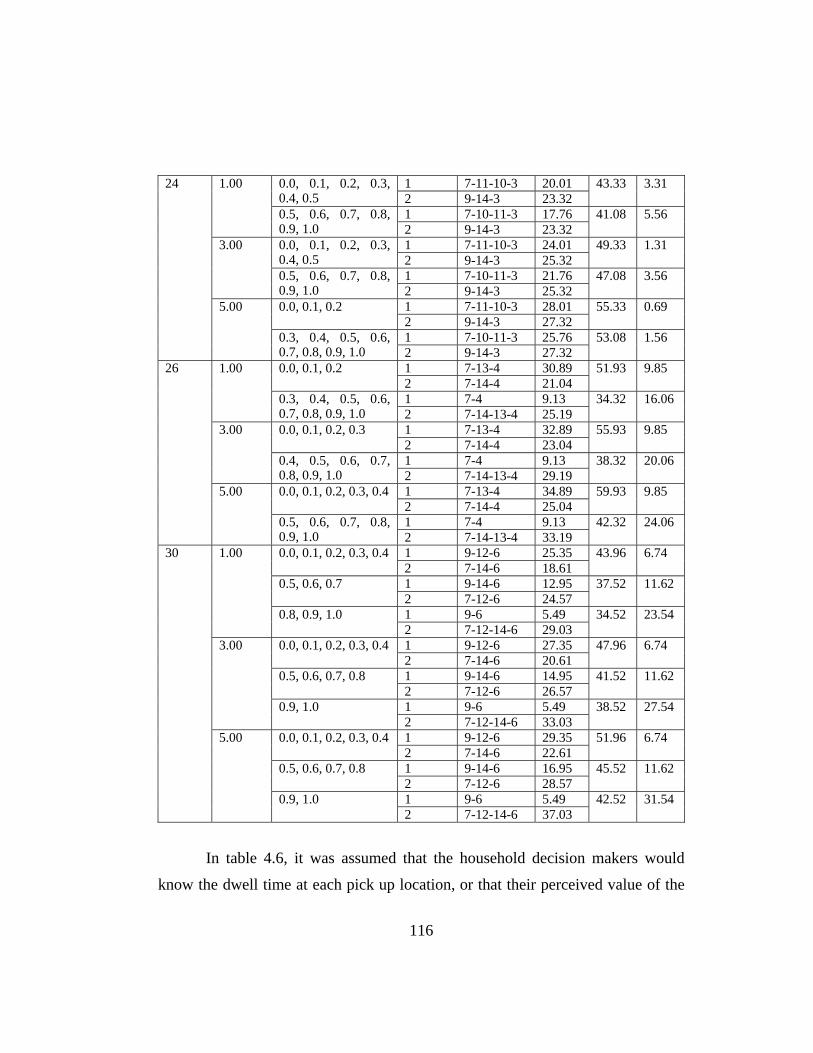
1 7-11-10-3 20.01 0.0, 0.1, 0.2, 0.3,
0.4, 0.5 2 9-14-3 23.32 43.33 3.31
1 7-10-11-3 17.76
1.00
0.5, 0.6, 0.7, 0.8, 0.9, 1.0 2 9-14-3 23.32
41.08 5.56
1 7-11-10-3 24.01 0.0, 0.1, 0.2, 0.3, 0.4, 0.5 2 9-14-3 25.32
49.33 1.31
1 7-10-11-3 21.76
3.00
0.5, 0.6, 0.7, 0.8, 0.9, 1.0 2 9-14-3 25.32
47.08 3.56
1 7-11-10-3 28.01 0.0, 0.1, 0.2 2 9-14-3 27.32
55.33 0.69
1 7-10-11-3 25.76
24
5.00
0.3, 0.4, 0.5, 0.6, 0.7, 0.8, 0.9, 1.0 2 9-14-3 27.32
53.08 1.56
1 7-13-4 30.89 0.0, 0.1, 0.2 2 7-14-4 21.04
51.93 9.85
1 7-4 9.13
1.00
0.3, 0.4, 0.5, 0.6, 0.7, 0.8, 0.9, 1.0 2 7-14-13-4 25.19
34.32 16.06
1 7-13-4 32.89 0.0, 0.1, 0.2, 0.3 2 7-14-4 23.04
55.93 9.85
1 7-4 9.13
3.00
0.4, 0.5, 0.6, 0.7, 0.8, 0.9, 1.0 2 7-14-13-4 29.19
38.32 20.06
1 7-13-4 34.89 0.0, 0.1, 0.2, 0.3, 0.4 2 7-14-4 25.04
59.93 9.85
1 7-4 9.13
26
5.00
0.5, 0.6, 0.7, 0.8, 0.9, 1.0 2 7-14-13-4 33.19
42.32 24.06
1 9-12-6 25.35 0.0, 0.1, 0.2, 0.3, 0.4 2 7-14-6 18.61
43.96 6.74
1 9-14-6 12.95 0.5, 0.6, 0.7 2 7-12-6 24.57
37.52 11.62
1 9-6 5.49
1.00
0.8, 0.9, 1.0 2 7-12-14-6 29.03
34.52 23.54
1 9-12-6 27.35 0.0, 0.1, 0.2, 0.3, 0.4 2 7-14-6 20.61
47.96 6.74
1 9-14-6 14.95 0.5, 0.6, 0.7, 0.8 2 7-12-6 26.57
41.52 11.62
1 9-6 5.49
3.00
0.9, 1.0 2 7-12-14-6 33.03
38.52 27.54
1 9-12-6 29.35 0.0, 0.1, 0.2, 0.3, 0.4 2 7-14-6 22.61
51.96 6.74
1 9-14-6 16.95 0.5, 0.6, 0.7, 0.8 2 7-12-6 28.57
45.52 11.62
1 9-6 5.49
30
5.00
0.9, 1.0 2 7-12-14-6 37.03
42.52 31.54
In table 4.6, it was assumed that the household decision makers would
know the dwell time at each pick up location, or that their perceived value of the
116

delay was as stated. This delay time was simply added to the perceived travel
time in the network.
Changing the value of the delay and varying the weight on the total fleet
time did not cause any additional optimal solutions to be generated. As can be
seen in table 4.6, the weights of the total fleet time associated with each
assignment shifted. For the representatives of household types 22 and 26, there
were two optimal routings on the household’s evoked network. The first one
presented in table 4.6 minimized the waiting time at the meeting location and
assigned one pick-up to each driver. Since each driver saw the same increase in
the dwell time at the school, the waiting time at the meeting location did not
change for this assignment. The second set of routings minimized the total fleet
time. All of the pick-ups were assigned to one of the vehicles; thus the increase in
delay was experienced twice by the same vehicle. As the dwell time increased,
the waiting time at the meeting location became greater for the second assignment
than for the first (which remained constant); thus, greater weight on the total fleet
time was required to shift the solution from the trip chain assignment that
minimized the waiting time to the one that minimized the total fleet time. In the
case of the household representing type 24, a delay of 5.00 minutes caused the
individual vehicle time of driver 1 to become greater than that of driver 2 in the
first assignment and less than that of driver 2 for the second assignment. The
opposite situation held for dwell times of 1.00 and 3.00 minutes. The difference
between the total fleet times and waiting times of the two assignments for the 1.00
and 3.00 minute delay cases both were 2.25 minutes. While the difference in the
total fleet time remained the same for the 5.00 minute case, the difference in the
waiting time was smaller thus making the second sequencing more appealing at
lower weight on the total fleet time. Finally, the representative of household type
30 had three optimal solutions. The first set of trip chains shown in table 4.6
minimized the waiting time, the third minimized the total fleet time, and the
117

second fell in between the first and the third. Switching from the second to the
third solution required greater weight on the total fleet time for the greater delay
cases because the waiting time increased by more than 15 minutes while the total
fleet time decreased by only 3 minutes.
The activity chains for all of the households, not just the representatives,
served as input to the traffic simulation-assignment package DYNASMART. The
vehicles generated for the activity chains were distributed over slightly more than
3 minutes allowing for some delay in the receipt of the evacuation order.
Referring to equation (4.2), the delay wv of the vehicles ranged from 0.00 to 3.01
minutes. Several different waiting times (pi) at each intermediate node were
considered. At school locations, the waiting times varied from 1.0 to 5.0 minutes.
The final waiting time at the meeting location was also allowed to vary. The
meeting location waiting time was taken to be the expected waiting time until the
other vehicle arrived plus a constant. The average travel times (including entry
queue waiting times) corresponding to the third term of the right hand side of
equation (4.2) and evacuation times (left hand side of equation (4.2)) for these
different cases are also displayed in table 4.7. The time of the evacuation order
Torder was taken as 0.0; thus equation (4.1) reduced to equation (4.2). The
resulting evacuation time of the network is presented in table 4.7 for the case
where the weight on the total fleet time was 0.5; this weight was selected based on
the results of tables 4.5 and 4.6. Two additional weights were examined and the
results are provided in table 4.8.
Table 4.7 also presents times required to clear the network when various
percentages of the peak period traffic (30,141 vehicles) were considered. Two
methods for generating the traffic were employed. First, all of the vehicles were
given the same start time. Second, the start times were distributed over 45
minutes.
118

Table 4.7 Network Clearance Times for Various Vehicle Loading Methods
Generation Method Number of Vehicles
Percentage of Activity Chain Vehicles
Average Network Travel Time (min)
Average travel time + entry queue time (min)
Network Clearance Time (min)
Activity Chain (minimum wait 5.0 min at school and meeting location)
30141 100% 45.5 123.2 459.6
Activity Chain (minimum wait 4.0 min at school and meeting location)
30141 100% 43.3
118.8 440.5
Activity Chain (minimum wait 3.0 min at school and meeting location)
30141 100% 45.9 122.3 450.2
Activity Chain (minimum wait 2.0 min at school and meeting location)
30141 100% 42.3
117.7 436.4
Activity Chain (minimum wait 1.0 min at school and meeting location)
30141 100% 43.7 119.0 432.0
No activity chain, all at once 30141 100% 33.3 78.4 229.1 No activity chain, all at once 37675 125% 45.9 115.9 335.5 No activity chain, all at once 45206 150% 40.9 125.0 343.5 No activity chain, all at once 48221 160% 42.9 145.7 361.6 No activity chain, all at once 49732 165% 42.0 142.7 371.1 No activity chain, all at once 51240 170% 42.5 147.2 378.0 No activity chain, all at once 52742 175% 50.7 164.5 455.2 No activity chain, distribute over 45 minutes
30098 99.9% 17.2 18.9 157.7
No activity chain, distribute over 45 minutes
55259 183% 40.7 57.5 275.1
No activity chain, distribute over 45 minutes
60306 200% 41.5 60.7 334.9
No activity chain, distribute over 45 minutes
63336 210% 45.3 67.9 379.7
Examination of table 4.7 revealed that although decreasing the waiting
times at intermediate nodes for activity chains resulted in shorter evacuation
times, these clearance times are still between seven and eight hours. To achieve
similar results without trip chains, approximately 175% of the original demand
must be loaded simultaneously or between 180 and 207% of the original demand
when vehicles were loaded over 45 minutes.
119

The measure of effectiveness of an evacuation may not be 100% of the
vehicles clearing the network. Figures 4.3-4.9 and table 4.8 illustrate the
interaction of the dwell times at the home and schools and the weight on the total
fleet time.
5 0
5 5
6 0
6 5
7 0
7 5
8 0
8 5
9 0
9 5
1 0 0
7 5 1 7 5 2 7 5 3 7 5 4 7 5
E la p s e d T im e
W a it 1 .0 0W a it 3 .0 0W a it 5 .0 0W a it R a n d o m
Per
cent
age
of V
ehic
les
Eva
cuat
ed %
)
Figure 4.3 Network Clearance for All Weight (λ = 1.0) on Total Fleet Time
When all of the weight was placed on the total fleet time, the network
clearance profile found in figure 4.3 was generated. All of the dwell times
considered yielded similar time requirements to evacuate 50% of the population.
At the 60% mark, the scenario of a 5.0 minute dwell time exhibited an increase in
time requirements compared to the other three waiting time cases; this deviation
persisted until approximately the 85% mark where the elapsed time for the 5.0
120

minute scenario was similar to the 1.0 minute case. This result was anticipated
since the larger waiting times delay vehicles from reaching their final
destinations. When the measure of effectiveness was 75% (or greater) of the
population evacuated, a dwell time of 3.0 minutes yielded the quickest
evacuation. This dwell time resulted in lower time requirements than the other
cases because holding the vehicles at their intermediate destinations prevented
some of the congestion that arose in the 1.0 minute case. The fact that the dwell
time of 3.0 minutes was an improvement to the 5.0 minute case suggests that 5.0
minutes, although reducing network congestion, impeded the vehicles making
stops. Finally, the randomly generated dwell time scenario produced evacuation
times between the best case (3.0 min) and the worst case (5.0 min).
50
55
60
65
70
75
80
85
90
95
100
75 125 175 225 275 325 375 425 475
Elapsed Time (min)
Per
cent
age
of V
ehic
les
Eva
cuat
ed (%
)
Wait 1.00Wait 3.00Wait 5.00Wait Random 1-5
Figure 4.4 Network Clearance for Half Weight (λ = 0.5) on Total Fleet Time
121

There was less disparity in the evacuation times for the various dwell
times when half of the weight was placed on minimizing the total fleet time and
the other half on minimizing the waiting time at the meeting location than in the
case where all of the weight was placed on the total fleet time. In figure 4.4, as in
figure 4.3, the dwell time of 5.0 minutes yields longer evacuation times than the
other three cases. However, in this weighting scenario, the 1.0 minute delay time
yielded a faster evacuation than the 3.0 minute case. Recall from table 4.5 that
the household pick-up assignments sometimes changed when the weight on the
total fleet time was varied from 1.0 to 0.5. This trip chain alteration caused the
difference in evacuation time requirements. Finally, when the measure of
effectiveness was 85% or greater of the population evacuated, the randomly,
uniformly generated dwell time produced the least network clearance time; this
suggested that the interaction of various pick-up assignments and dwell times
could improve the evacuation speed, compared to the uniform assignment of
delays to all households.
122

50
55
60
65
70
75
80
85
90
95
100
75 175 275 375 475
Elapsed Time (min)
Perc
enta
ge o
f Veh
icle
s Ev
acua
ted
(%)
Wait 1.00Wait 3.00Wait 5.00Wait Random
Figure 4.5 Network Clearance for No Weight on (λ = 0.0) Total Fleet Time
As noted in table 4.5, changing the weight among 1.0, 0.5, and 0.0 on the
minimization of the total fleet time in equation 4.16 may result in up to three
different household pick-up assignments. These variations in assignments
account for the differences found in figures 4.3-4.5. As in figure 4.4, figure 4.5
showed that the randomly generated dwell time yielded the lowest evacuation
time when the measure of effectiveness was 85%, or greater, of the population
evacuated. At 70% and greater, the 3.0 minute dwell time required the most time
to evacuate the network; this was opposite of the case where the weight of the
total fleet time was 1.0. Figure 4.5 shows that a delay time of 5.0 minutes
performed better than a dwell time of 1.0 minutes where the measure of
123

effectiveness between 80 and 95% network clearance. The interaction of the
pick-up assignments, dwell time of 1.0 minute, and congestion delayed vehicles
more than the conditions associated with the case where the dwell time was 5.0
minutes.
Some of the particular points of interest from figures 4.3-4.5 are displayed
in table 4.8, which presents the amount of time required to evacuate different
percentages of the population for various delays when the weight on the total fleet
time (see equation 4.16) was 1.0, 0.5, 0.0, and randomly, uniformly generated.
124

Table 4.8 Network Clearance Profiles for Various Dwell Times and Weights
Weight
on Total
Fleet
Time
Min.
Dwell
Time at
School &
Home
Time for
50% to
Evacuate
(min)
Time for
60% to
Evacuate
(min)
Time for
70% to
Evacuate
(min)
Time for
80% to
Evacuate
(min)
Time for
90% to
Evacuate
(min)
Time for
100% to
Evacuate
(min)
1.00 77.03 96.52 151.69 219.01 297.75 456.4
2.00 76.81 95.73 149.01 208.45 280.36 443.4
3.00 76.56 95.14 146.14 206.35 267.75 422.8
4.00 77.70 96.19 147.71 208.37 284.56 456.5
5.00 80.03 108.81 186.41 246.41 294.23 486.3
1.0
Random 78.06 98.61 154.37 214.65 285.96 478.0
1.00 78.72 100.23 162.88 232.11 292.04 432.0
2.00 79.63 102.70 162.67 232.12 286.21 436.4
3.00 81.20 104.75 167.27 240.8 305.39 450.2
4.00 81.66 105.06 164.55 232.61 291.97 440.5
5.00 82.11 108.00 173.14 246.89 308.07 459.6
0.5
Random 80.64 104.16 165.08 231.27 287.81 425.8
1.00 79.46 103.29 170.40 250.32 315.09 453.2
2.00 80.41 105.58 169.96 244.44 303.74 450.1
3.00 83.04 111.94 182.05 266.66 322.38 478.0
4.00 81.77 107.98 170.26 248.07 306.90 444.3
5.00 82.70 109.87 175.13 247.76 300.32 449.7
0.0
Random 81.09 104.50 162.93 240.66 292.33 425.8
1.00 79.01 98.78 152.00 216.49 274.94 413.0
2.00 79.50 100.25 155.30 223.45 276.13 398.4
3.00 81.90 108.76 173.58 264.84 324.85 465.7
4.00 80.98 104.12 164.20 232.86 282.94 413.9
5.00 82.40 109.59 176.78 252.33 310.87 476.3
Random
Random 80.09 102.94 161.41 230.84 290.24 432.3
125
Examination of table 4.8 revealed several interesting points. Within each
weighting scenario, the time to evacuate 50% of the population varied by less than
3.5 minutes, regardless of the dwell time. Over all of the weighting and dwell
time cases, the evacuation time for 50% of the population differed by less than 6.5
minutes. The higher levels of evacuation showed greater disparity within a given
weighting scenario and overall. At the 60% level, the difference in times varied
between approximately 8 and 14 minutes within a given weighting case and just
over 14 minutes for the entire sample. For the 70% level, the disparity increased
and ranged between 19 and 40 minutes for the weighting cases and 40 minutes
overall. The 80% level showed an even further spread of evacuation times with
60 minutes between the λ = 1, 3.0 minute dwell time and the λ = 0, 3.0 minute
dwell time. Within a given weighting value, the difference in time requirements
varied between 16 and 48 minutes. The 90% evacuation level presented less
overall disparity (57 minutes) than the 80% clearance level. The range within a
weight was 22 to 50 minutes. Finally, to completely clear the network, the time
required varied between 34 and 78 minutes within a given weight and 88 minutes
overall. Except for the 100% evacuation level, the λ = 1, 3.0 minute dwell time
combination yielded the smallest time requirements; for the 100% level, the
shortest evacuation time was obtained when the weight was randomly generated
and the dwell time was 2.0 minutes. The combination of factors that generated
the highest clearance times changed with the evacuation level. A dwell time of
3.0 minutes and λ = 0 yielded the highest evacuation time for the 50% and 80%
clearance levels. For the 60% level, the combination yielding the highest network
clearance time was randomly generated weights and 5.0 minute dwell times. At
the 70% and 100% levels, the factors with the greatest evacuation time
requirements were λ = 1 and 5.0 minute dwell time. Finally, for the 90%
clearance level, randomly generated weights and 3 minute delay times yielded the
highest evacuation times.
126

The data from table 4.8 for the measure of effectiveness 80% network
clearance was used to create figure 4.6.
150
170
190
210
230
250
270
290
0 1 2 3 4 5 6
Minimum Dwell Time
Tim
e R
equi
red
for 8
0% N
etw
ork
Cle
aran
ce
λ = 0.0
λ = 0.5
λ = 1.0
l Random
Figure 4.6 Comparison of 80% Network Clearance Times and Minimum Dwell Times for Various Total Fleet Time Weights
The complex interactions of dwell times, the weights on the two
minimization objectives, and the related pick-up assignments were further
demonstrated in figure 4.6. The nonlinear nature of the graphs demonstrated
these complexities. The randomly generated weights led to the greatest distance
between the peaks and valleys of the curve. The curve for λ = 0 was the most
symmetrical about dwell time of 3.0 minutes. When none of the weight was
placed on the minimization of total fleet travel time, the lowest point of the curve
occurred at a dwell time of 3.0 minutes; this result was opposite to that of the case
where all of the weight was placed on the minimization of total fleet travel time
and the highest point of the curve was at a dwell time of 3.0 minutes. A weight of
127

1.0 on the total fleet time led to a fairly linear curve for dwell times of 1.0 to 4.0
minutes. This trend was broken for dwell times between 4.0 and 5.0 minutes.
There are several more observations of note pertaining to figure 4.6. The
times for 80% of the population to evacuate for the 5.0 minute dwell time were
fairly close for all of the fleet time weights examined. Excluding the random
generation case, the weight of 0.0 on the minimization of the total fleet travel time
(consequently all of the importance was placed on the minimization of the waiting
time at the meeting location) yielded the highest evacuation time for all dwell
times. Again, excluding the random scenario, the 80% evacuation time was the
lowest when all of the weight was placed on the minimization of the total fleet
time. Finally, equal weights on the minimization of total fleet time and the
minimization of the difference in arrival times at the meeting location yielded
80% evacuation times between those associated with the extreme weights, for all
dwell times considered.
Figures 4.7-4.9 allow the interaction of dwell time and weight on the total
fleet time to be examined from the reverse perspective of figures 4.3-4.5. Figures
4.7, 4.8, and 4.9 present the time required to evacuate various percentages of the
population for minimum dwell times of 1.0, 3.0, and 5.0 minutes, respectively.
128

50
55
60
65
70
75
80
85
90
95
100
50 150 250 350 450
Elapsed Time (min)
Perc
enta
ge o
f Veh
icle
s Ev
acua
ted
(%)
λ = 0.0
λ = 0.5
λ = 1.0
Random
Figure 4.7 Comparison of Network Clearance for Total Fleet Time Weights with Minimum Dwell Time 1 Minute at School and Meeting Locations
The four curves shown in figure 4.7 had approximately the same shape
although the slope varied. At 60% network clearance, the curve for the case
where none of the weight was placed on the minimization of the total fleet travel
time indicated that more time was needed than for the other weights. This trend
persisted until the 93% network clearance level. The randomly generated weight
scenario showed an improvement over the deterministic cases for 80% or higher
levels of population evacuation. The case where equal weight was placed on the
minimization of total fleet travel time and the minimization of waiting time at the
meeting location yielded evacuation times that were between the two extreme
weighting cases for 50-85% network clearance. After the 85% mark, the equal
weight scenario produced lower evacuation times than either of the two extremes.
This last observation, combined with the results for the randomly generated
129

weights suggested that variable assignments improved the evacuation speed over
the strict minimization of one of the two criteria in equation 4.16.
50
55
60
65
70
75
80
85
90
95
100
75 125 175 225 275 325 375 425 475
Elapsed Time (min)
Perc
enta
ge o
f Veh
icle
s Ev
acua
ted
(%)
λ = 0.0
λ = 0.5
λ = 1.0
Random
Figure 4.8 Comparison of Network Clearance for Total Fleet Time Weights with Minimum Dwell Time 3 Minutes at School and Meeting Locations
The results for a dwell time of 3.0 minutes were very different from those
of a dwell time of 1.0 minute. At no point in figure 4.8 did the randomly
generated weight scenario perform better than all of the deterministic waiting
cases. Placing all of the weight on minimizing the total fleet travel time yielded
the least evacuation times. As in the 1.0 minute dwell time case, the minimization
of the waiting time at the meeting location required the most time to evacuate a
given percentage of the population. Splitting the weight equally between the two
criteria led to evacuation times between the two extremes.
130

50
55
60
65
70
75
80
85
90
95
100
75 175 275 375 475
Elapsed Time (min)
Perc
enta
ge o
f Veh
icle
s Ev
acua
ted
(%)
λ = 0.0
λ = 0.5
λ = 1.0
Random
Figure 4.9 Comparison of Network Clearance for Total Fleet Time Weights with Minimum Dwell Time 5 Minutes at School and Meeting Locations
The most noticeable difference between figure 4.9 and figures 4.7 and 4.8
was the closeness of the four curves; the evacuation times varied little for the four
weighting cases. For 60-75% network clearance levels, minimizing the total fleet
travel time produced greater time requirements than the other three weighting
scenarios. At the 78-92% evacuation level, the randomly generated weighting
case yielded slightly higher time requirements than the other scenarios.
Part of the reason for the extensive evacuation time was the structure of
the network. For the original results presented above, the links connecting four of
the five schools to the rest of the network were extremely short. Although these
lengths simulate an appropriate length of a driveway to the school, they do not
capture the effects of parents parking in other areas during these usual conditions.
To examine the scenario where additional space may be used, various lengths of
131

the links connecting the schools at nodes 122, 123, 165, and 170 were examined
for the case where waiting time at the school was 5.0 minutes and the minimum
waiting time at the meeting location was 5.0 minutes. Table 5 shows the results
for 1.25, 1.5, 1.75, and 2.0 times the original lengths of the links of interest. From
these results, one can observe the complexities of the network simulation.
Moderate increases (1.25 and 1.50) in the length of the link actually increases the
total evacuation time and the corresponding average travel time, with and without
entry queue delays. Higher multiples (1.75 and 2.0) of the original length
decrease the total evacuation time from the original case, decrease the average
network travel time, but slightly increase the average entry queue waiting time.
Clearly, doubling the length of the school links provides the most significant
improvement. The evacuation time decreases by slightly more than thirty minutes
and the average travel times with and without entry queue delays decrease. For
all of the cases examined, the average distance traveled did not vary by more than
0.9% of the original.
Table 4.9 Comparison of Average Times, Distances, and Evacuation Times for Different Lengths of School Links for Activity Chains with Minimum Waiting Times of 5.0 Minutes at Intermediate Nodes
Length of Link Leading To and From School Nodes (ft)
Average Network Travel Time (minutes)
Average Travel Time + Entry Queue Time (minutes)
Average Distance Traveled (mi)
Network Clearance Time (minutes)
528 (original) 45.8 115.9 6.9020 383.4 660 (1.25x orig) 46.9 127.6 6.9045 398.5 792 (1.50 x orig) 48.7 127.6 6.9150 399.5 924 (1.75x orig) 40.9 119.5 6.9456 381.4 1056 (2.00x orig) 43.5 114.2 6.9613 351.7
132

Comparing the evacuation times for the extended link length scenarios
(table 4.9) with the various vehicle loading strategies displayed in table 4.7,
indicates that between 150 and 175% of the original demand would be required
when all of the vehicles are loaded at the same time. For the case when the length
is doubled, this range can be narrowed to 150-160%. When the vehicles are
spread over 45 minutes of generation time, more than 200% of the original
demand would be required to achieve a similar network clearance time.
4.4 SUMMARY
The framework presented in this chapter allows for representation of more
realistic evacuation scenarios, by incorporating critical aspects of household travel
behavior that have been omitted from traditional evacuation models. The
omission resul overly optimistic evacuation times. This framework was
incorporated into a traffic assignment-simulation tool. The methodology used
here allows for an evacuation simulation to more accurately capture the traffic
flows that arise when parents pick up their children at the schools before
evacuating the city. Such an emergency situation may arise in the case of sudden
disasters or threats like earthquakes or terrorist incidents.
ts in
The results presented in this work are specific to the geometry of the
network and the relative locations of schools, residential areas, and work areas,
but some results can be generalized. First, the household’s decision of where to
meet plays a crucial role in the assignment of pick-ups to vehicles. Second,
allowing the household’s decision makers to assign weights to the total fleet travel
time and the waiting time leads to a small solution set (in this work one, two, or
three options) to be considered for vehicle routing. Two of the solutions were the
one that minimized total fleet travel time and the one that minimized waiting time.
133

Third, attempting to coordinate arrival times is better applied to larger households
than to smaller ones.
Comparison of network clearance times suggests that at least 175% of the
original demand should be used if trip chains are ignored and vehicles proceed to
their homes. Additional link length at school locations allows this factor to be
reduced to some degree. The exact multiplicative factor depends on the loading
scenario employed by the planning agency and any additional special emergency
considerations that may be taken into account. The complex interactions of all of
these factors require careful consideration by evacuation planners and
transportation engineers.
134

Chapter 5
Case Study
This chapter presents a case study that illustrates how the concepts
developed in chapters 3 and 4 interrelate. Following a threat to the transportation
infrastructure, the public is advised to evacuate; the traffic management agency
lacks the ability to control the heavy demand that will be placed on the network.
Residents in a threatened area will logically attempt to evacuate, regardless of
whether this sudden rush of traffic causes or exacerbates any transportation
problems. Evacuations due to imminent disasters have somewhat different
characteristics than those associated with advanced warning evacuations, such as
those due to hurricanes. The immediate nature of the disaster causes the traffic to
be concentrated over a much shorter period than for a planned evacuation. This
chapter focuses on evacuations due to an immediate threat, whether natural or
man-made.
As noted in chapters 2 and 4, a common observation about evacuating
households is that the family members tend to gather prior to fleeing the area.
The household level decision making model developed in chapter 4 is applied in
this chapter. The household selects a meeting location and then assigns drivers to
pick up family members without access to vehicles. All of the drivers then gather
at the meeting location and evacuate as a single unit.
The evacuating traffic may create vulnerabilities in the network that do not
exist under typical, everyday conditions. In this chapter, the network links are
evaluated from the perspective of the evil entity for the unusual traffic patterns
that arise in an emergency evacuation.
135

The specific objectives covered in this chapter are (1) to examine the
impact of emergency trip-chaining behavior on the vulnerability of transportation
network links and (2) to examine the impact of strategies, designed to route
vehicles around vulnerable transportation infrastructure, on city evacuation times.
Several tasks are required to meet these objectives. First, baseline traffic
conditions are simulated. Second, as in chapter 3, the vulnerabilities of the
transportation network links are determined for this traffic pattern. Third, an
evacuation is simulated using the trip-chaining assignment model developed in
chapter 4. Fourth, the vulnerability of the links is determined under the
evacuation conditions. Finally a comparison is made between the baseline case
and the evacuation scenario.
The remainder of this chapter is directed toward accomplishing the tasks
listed above and is organized in the following manner. First, the simulation test
bed is described. Second, the experimental design is presented. Third, the
experimental procedure is outlined. Fourth, the results are discussed. Finally, a
summary of the chapter is provided.
5.1 SIMULATION TEST BED
The simulation test bed used for this case study was adapted from the
network representing the south-central I-35 portion of Fort Worth, Texas. As in
chapter 4, the original network was modified to include estimated school
locations. The network is repeated in figure 5.1 for ease of discussion.
The network consists of 184 nodes (only 180 are shown in the figure). In
this model, two elementary schools (nodes 123 and 165), two middle schools
(nodes 122 and 169), and one high school (node 170) are located on the network.
Each school is modeled as its own zone, and the remainder of the nodes are
divided into three business zones and six residential zones.
136

2
4
98
22
139
160102159
158101157
156100
146
145140
144
176
163106
105
162104
161103
152
96
99928
66
29
91906
26
1519789
111
168110149
143
167109154148142
178177 166165108
107164155153147141
95
93
941242
10
38
33
15014
51
47
21
30
25
41
37
34
52
48
19
23
35
32
39
4544
49
28
1
7
11
67
71
74
85
73
130 81
3
20
118
132
121
120
131119
123
122
134
133
127
175
126
125
124
77
76
75
2784
6570
5
24
838069
8268
972 8636
31
43
40
13
46
50
116
169
170
112
172
113114
171
16
54
59
53
6058
551578
138136
137135
128 8887
5756
174
115
17363
18
6462
129 79
61
17
117
Zone
9
Zone 1 Zone 2
Zone 3 Zone 4
Zone 5 Zone 6
Zone
7
Zone
8 Zone 10
Zone 11 Zone 12
Zone 13Zone 14
Figure 5.1 Simplified Version of South Central Fort Worth, TX
137

The link information pertaining to figure 5.1 is presented in Appendix D.
The appendix contains the link number, the upstream and downstream nodes, the
length of the link, the maximum service capacity, and the free flow speeds and
travel times for each link.
5.2 EXPERIMENTAL DESIGN
5.2.1 Household Characteristics
This chapter takes the lessons learned from the variable exploration in
chapters 3 and 4 and applies them to the network shown in figure 5.1. The
following sections describe the values of the variables that are used in this case
study. These variables include household characteristics, household decision
making objective function weights, household dwell times at intermediate nodes
in the trip chain, evil entity resources and targets, traffic management agency
strategies, traffic assignment, number of alternate paths, and evaluation times.
The final portion of section 5.2 outlines the combinations of these variables that
are explored in this study.
In the simulations 20,000 households produced 30,141 vehicles. The
household composition (number of adults and children of various ages) is
identical to that found in chapter 4. Approximately 49% of the households have
only one adult, and 51% have two. No children are present in 49% of the
households, including homes with one or two adults. At least one elementary
school aged child is found in 23% of the households, at least one middle school
child in 23%, and at least one high school child in 24% of the households.
Approximately 13% of the households have multiple children in different schools.
138

Due to these household characteristics, between 33 and 57% of the total generated
vehicles would stop at schools to pick-up their children.
5.2.2 Household Decision Making Objective Function Weights
5.2.3 Household Dwell Times
As in chapter 4, the network impacts of several weights associated with
the components of the household trip chaining objective function – the
minimization of total household fleet travel time and the minimization of waiting
time spent at the meeting location - are examined. However, the ranges of values
of these factors are more limited in this chapter. Based on the results in chapter 4,
three deterministic weights on the minimization of the total fleet time are
considered (λ = 0.0, 0.5, and 1.0). Case 1 reflects a weight of 0.0 on the
minimization of total household fleet travel time; case 2 indicates a weight of 0.5
on the minimization of total fleet travel time; and case 3 reflects a weight of 1.0.
These cases are the ones known to generate different household trip chains.
Dwell times at intermediate nodes reflect the ease with which parents are
able to locate their children at the schools and secure them in the vehicles.
Recognizing that these dwell times will not be deterministic, households are
assigned dwell times from a random uniform distribution that ranges from 1 to 5
minutes.
139

5.2.4 Evil Entity Resources and Targets and Traffic Management Agency Strategies
In this case study, the evil entity has the resources to damage only one
link. For the baseline conditions and each of the evacuation weighting cases, each
link is examined in a scenario where the evil entity targets that particular link. By
limiting the number of links in the set of possible targets to one, different types of
links can be more precisely examined.
Based on baseline vulnerability and trip chaining information, a sample of
different types of links from figure 5.1 is presented for discussion. Both the
traffic management agency and the evil entity consider this sample of links
potential targets. Traffic management agency strategies avoid only one of the
links in the sample. Similarly the evil entity’s targeting scenario focuses on
damaging only one of the sample links. The total sample includes arterial (link
306), overpass (link 43), freeway (link 123), frontage road (link 83), and
residential (link 191) arcs. Also included are links between two schools (link
148) and between a school and a residential area (link 146). These links are
circled denoted in figure 5.2. The link characteristics can be found in Appendix
D.
140

2
4
98
22
139
160102159
158101157
156100
146
145140
144
176
163106
105
162104
161103
152
96
99928
66
29
91906
26
1519789
111
168110149
143
167109154148142
178177 166165108
107164155153147141
95
93
941242
10
38
33
15014
51
47
21
30
25
41
37
34
52
48
19
23
35
32
39
4544
49
28
1
7
11
67
71
74
85
73
130 81
3
20
118
132
121
120
131119
123
122
134
133
127
175
126
125
124
77
76
75
2784
6570
5
24
838069
8268
972 8636
31
43
40
13
46
50
116
169
170
112
172
113114
171
16
54
59
53
6058
551578
138136
137135
128 8887
5756
174
115
17363
18
6462
129 79
61
17
117
Link 306
Link 43
Link 83
Link 123
Link 146
Link 191
141Figure 5.2 Selected Links

5.2.5 Traffic Assignment
5.2.6 Alternate Paths
5.2.7 Evaluation Times
The vehicle routing is roughly based on the system optimal traffic
assignment. Only one additional iteration of the assignment procedure is used;
thus generating an imperfect system optimal traffic assignment that is more likely
to be seen in a true evacuation scenario. A traffic management agency would
seek to influence vehicles but in the stress caused by danger, the response to
guidance is variable.
Another advantage to the traffic assignment approach is the ability to add
costs to threatened links, while maintaining connectivity. To incorporate this
additional cost in DYNASMART-P, the links are converted to tolled facilities.
By charging a toll, the threatened link can still be used for connectivity purposes,
but the cost prohibits vehicles from using the link when an alternative path is
available.
The disruption index developed in chapter 3 allows for the network
analyst to limit the number of alternate paths considered for an origin-destination
pair. In this case study, up to five paths are generated for each pair.
In a dynamic network, flows are not at steady state; thus, time instances
must be selected for evaluation purposes. The vulnerability and disruption indices
142

are calculated at 30 minutes. This time point is selected for two reasons. First, the
simulation tool has enough time to load the network. Second, approximately 50%
of the vehicles are still in the network for all of the simulations conducted. Two
additional time points (60 and 120 minutes) are examined for a selected traffic
management agency strategy. These additional time instances reveal changes in
the traffic patterns as the simulation progresses.
Using a specific time instance in a dynamic network raises the question of
how to measure the flow. In this work, instantaneous flow is used. Due to the
nature of instantaneous flow, it may exceed link capacity; to adjust for this
temporary condition, the maximum flow value is set to the maximum flow service
rate of the link.
5.2.8 Combinations of Factors Examined
Table 5.1 provides a summary of the combinations of factors examined in
the simulations. This table indicates that the weighting cases identified in section
5.2.2, the sample of links from section 5.2.4, and the time instances from section
5.2.7 are explored in different combinations. The remainder of the variables
identified in above sections are treated as constants.
143

Table 5.1 Combinations of Experimental Factors
Time
Instant
(min)
Traffic
Management
Agency
Strategy
Evil Entity Target
Scenario
Baseline / Evacuation Case*
Baseline (30,149 vehicles)
Evacuation Case 1 (λ = 0.0)
Evacuation Case 2 (λ = 0.5)
30 Do nothing Each of links 1-452,
individually
Evacuation Case 3 (λ = 1.0)
Evacuation Case 1 (λ = 0.0)
Evacuation Case 2 (λ = 0.5)
30 Avoid Link
123
Each of links 123, 146,
148, 191, 306, 43, and
83, individually Evacuation Case 3 (λ = 1.0)
Evacuation Case 1 (λ = 0.0)
Evacuation Case 2 (λ = 0.5)
30 Avoid Link
146
Each of links 123, 146,
148, 191, 306, 43, and
83, individually Evacuation Case 3 (λ = 1.0)
Evacuation Case 1 (λ = 0.0)
Evacuation Case 2 (λ = 0.5)
30 Avoid Link
148
Each of links 123, 146,
148, 191, 306, 43, and
83, individually Evacuation Case 3 (λ = 1.0)
Evacuation Case 1 (λ = 0.0)
Evacuation Case 2 (λ = 0.5)
30 Avoid Link
191
Each of links 123, 146,
148, 191, 306, 43, and
83, individually Evacuation Case 3 (λ = 1.0)
Evacuation Case 1 (λ = 0.0)
Evacuation Case 2 (λ = 0.5)
30 Avoid Link
43
Each of links 123, 146,
148, 191, 306, 43, and
83, individually Evacuation Case 3 (λ = 1.0)
144

Evacuation Case 1 (λ = 0.0)
Evacuation Case 2 (λ = 0.5)
30 Avoid Link
83
Each of links 123, 146,
148, 191, 306, 43, and
83, individually Evacuation Case 3 (λ = 1.0)
Evacuation Case 1 (λ = 0.0)
Evacuation Case 2 (λ = 0.5)
30 Avoid Link
306
Each of links 123, 146,
148, 191, 306, 43, and
83, individually Evacuation Case 3 (λ = 1.0)
Evacuation Case 1 (λ = 0.0)
Evacuation Case 2 (λ = 0.5)
60 Avoid Link
306
Each of links 123, 146,
148, 191, 306, 43, and
83, individually Evacuation Case 3 (λ = 1.0)
Evacuation Case 1 (λ = 0.0)
Evacuation Case 2 (λ = 0.5)
120 Avoid Link
306
Each of links 123, 146,
148, 191, 306, 43, and
83, individually Evacuation Case 3 (λ = 1.0)
* All of the evacuation cases use 30,141 vehicles.
Table 5.1 presents the combinations of variables that will be investigated
in this chapter. The experimental procedure that outlines how these variables will
be allowed to interact is presented in the following section.
5.3 XPERIMENTAL PROCEDURE E The five steps of the experimental procedure outlined at the beginning of
this chapter are explored in further detail in the following sections. The first
portion describes tasks 1 (establishing baseline traffic conditions) and 2
(determining the link vulnerabilities associated with the baseline conditions). The
second section corresponds to the third step (simulating evacuation conditions).
The fourth (determining link vulnerabilities for evacuation conditions) and fifth
145

tasks (comparing network conditions and link vulnerabilities from tasks 1-4) are
described in section 5.3.3 and 5.3.4, respectively.
5.3.1 Establish Baseline Conditions
The first step to making a comparison is to establish a baseline. There are
actually two reference points to be established. The first baseline reveals typical
traffic patterns and network clearance time. The second is the set of disruption
indices associated with the everyday traffic patterns at a given time. These points
of reference correspond to the first two tasks previously described.
In the first task, peak period traffic conditions are simulated. The test bed
is shown in section 5.1 (and in chapter 4). As in chapter 4, approximately 30,100
vehicles, generated over 45 minutes, are simulated to establish peak period
conditions. The traffic simulation-assignment software DYNASMART-P
(DYnamic Network Analysis Simulation Methodology for Advanced Road
Telematics) is used for this purpose.
The network is then evaluated using the gaming approach developed in
chapter 3 to establish the baseline vulnerabilities (task 2). To summarize the
gaming approach, an evil-entity seeks to maximize disruption to the network by
damaging a set of links. This damage disrupts origin-destination flows and
possibly disconnects some destinations from certain origins. The opponent to the
evil entity is a traffic management agency who, upon receiving information about
a threat, seeks to route vehicles around the vulnerable links. In establishing the
baseline, the traffic management agency is assumed to have no information of a
threat to the infrastructure (this corresponds to game 1 developed in chapter 3).
146

5.3.2 Simulate Evacuation Conditions with Trip Chains
As in chapter 4, the number of households remains constant at 20,000.
The number of vehicles that are associated with these households is also constant
at 30,141; these vehicles are generated over 3.1 minutes. For each of the
household decision making weights described in section 5.2.2, trip chains are
generated using the code found in Appendix C. The activity chains generated in
each case are used by DYNASMART-P to simulate corresponding traffic
conditions.
5.3.3 Determine Infrastructure Vulnerabilities under Evacuation Conditions and Traffic Management Agency Strategies For each weight on the total fleet travel time mentioned in section 5.2.2,
the link vulnerabilities are evaluated at a given point in time using two gaming
approaches. Link vulnerabilities are determined using the procedure developed in
chapter 3. The disruption index is the measure of vulnerability and is calculated
based on the state of the network. Recall that the disruption index directly
accounts for the availability of alternate paths, traffic flow, excess path capacity,
free flow travel time, and marginal path cost.
In the first game, the traffic management agency (Player M) is assumed to
have no information about the evil entity’s (Player T’s) target. Recall that this
lack of information corresponds to both game 1 in chapter 3 and the baseline
established in task 2. In the second game, Player M has general information about
the type of link to be targeted (e.g. freeway, arterial in a residential zone, arterial
near a school zone) while Player T has perfect information about the other’s
moves and payoffs. Player M can route vehicles to avoid links but cannot
prohibit vehicles from reaching their destinations.
147

5.3.4 Comparison of Peak Period and Evacuation Conditions
The network is examined from two perspectives – network clearance and
link vulnerabilities. Each evacuation case is compared to the other evacuation
cases and the baseline peak period conditions in terms of those two aspects. The
traffic management strategies of avoiding types of targeted links are compared to
the evacuation cases where none of the links are avoided and the peak period
baseline. The comparison step of the evaluation framework is covered in the
results section, presented next.
5.4 RESULTS Using the experimental procedure described in section 5.3 and the factors
outlined in section 5.2, results are generated. These results focus of link
vulnerabilities and network clearance times for the baseline peak period
conditions and the combinations of evacuation cases, traffic management agency
strategies, and evil entity scenarios. The payoff matrix for Game 1 with the
baseline peak period conditions is presented in Appendix E for time 30. Also
displayed are the payoffs for the evacuation conditions where no links are
intentionally avoided. The payoff to the evil entity is the value of the disruption
index. As in chapter 3, the payoff to the traffic management agency (Player M) is
the percent of vehicles safely reaching their destinations. Recall that in Game 1,
Player M has no information about a threat to the network and Player T has the
resources to damage only one link.
At such a large network scale and typical traffic patterns, the damage of a
single link would have little effect on the network. Only eighteen links resulted
148
in a payoff to Player M of less than 80%, of which six yielded payoffs of less than
70% (see Appendix E). In the peak-period baseline case, links 14 and 306
connected forty-one origin-destination pairs, which was the maximum of any of
the 452 links.
The ten most vulnerable roadways under typical peak period conditions
are discussed below and shown in figure 5.3. The highest disruption index value
is 16.681, associated with link 306 (labeled 1 on figure 5.3). This link leads to the
high school zone, a middle school zone, a residential zone, and an evacuation
shelter. The second greatest disruption index (16.374) occurs for link 310
(numbered 2), which connects to link 306. Link 323 (labeled 3) has the third
highest index; this link is a freeway section which leads from one of the major
business zones. The fourth most vulnerable link is 107 (numbered 4), which is a
freeway link downstream from link 323. The fifth greatest disruption index
(13.712) is associated with link 123 (labeled 5), which is the freeway link
between links 323 and 107. Sixth (11.692) is link 43 (numbered 6), which crosses
the freeway. The seventh highest disruption index (11.488) is associated with link
117 (labeled 7), which is a freeway link downstream of link 306. The difference
in the disruption index values for the freeway links are due to the presence of on
and off ramps. Link 48 (numbered 8) had the eighth highest disruption index
value (11.363); this link leads to link 310 and ias one of the downstream links
from link 43. Ninth, link 105 (labeled 9) has an index of 11.005; this roadway
segment is also on the freeway, downstream from link 117. Finally, the tenth
greatest disruption index (9.000) is associated with link 305 (numbered 10),
which is the approach to the high school.
149

150
2
4
98
22
139
160102159
158101157
156100
146
145140
144
176
163106
105
162104
161103
152
96
99928
66
29
91906
26
1519789
168110149
143
167109154148142
178177 166165108
107164155153147141
95
93
941242
10
38
33
47
111
15014
51
21
30
25
41
37
34
52
48
19
23
35
32
39
4544
28
49
1
7
11
67
71
74
85
73
130 81
3
20
118
132
121
120
131119
123
122
134
133
127
175
126
125
124
77
76
75
2784
6570
5
24
838069
8268
972 8636
31
43
40
116
13
46
50
169
170
112
172
113114
171
16
54
59
53
6058
551578
138136
137135
128 8887
5756
174
115
17363
18
6462
129 79
61
17
117
Zone 1 Zone 2
Zone 3 Zone 4
Zone 5
Zone
7
Zone
8
Zone 6
Zone 10
Zone 11 Zone 12
Zone 13Zone 14
12
3
5
610
78
4
9
Figure 5.3 Ten Most Vulnerable Links for Peak Period Conditions

The peak period baseline conditions yielded the greatest disruption index
of the four traffic patterns in Appendix E. It is important to note that the
disruption index (payoff to Player T) did not capture vehicles that were not on the
network at the instant under consideration. Any vehicle that was stopped at an
intermediate node was not part of the index calculations.
Among the evacuation cases in Appendix E, the maximum disruption
value increased with greater values of the weight associated with the total
household fleet travel time. For each of the weights, the greatest disruption index
was associated with link 305, which led to the high school. Since only one high
school was available for all of the households in this particular network, this link
could affect every other zone. Under typical traffic conditions, link 305 was the
tenth most vulnerable; thus changes in vulnerability occur when parents pick up
their children at school in an emergency compared to typical daily child transport.
The ten most vulnerable links for each weighting case described in section 5.2.4
are shown in figures 5.4 (case 1), 5.5 (case 2), and 5.6 (case 3).
151

2
3
2
4
3
3
4
5
19
23
35
32
39
4544
49
28
1
7
11
67
74
71 85
73
130 81
3
20
118
132
121
120
131119
123
122
134
133
127
175
126
125
124
77
76
75
2784
6570
5
24
838069
8268
972 8636
31
43
40
13
46
50
116
658
551578
138136
137135
128 8887
5756
662
129 79
61
17
117
Zone 10
Zone 11
Zone 1
Zone 3
Zone 5
Zon
e 7
Zone
8
Figure 5.4 Ten Most Vulnerable Lin
3
4
6
2
2
4
98
22
139
160102159
158101157
156100
146
145140
144
176
163106
105
162104
161103
152
96
99928
66
29
91906
26
1519789
111
168110149
143
167109154148142
178177 166165108
107164155153147141
95
93
941242
10
38
33
15014
51
47
1
0
5
1
7
4
8
2
1714
Zone 12
Zone 2
Zone 4
Zone 6
6
553
10
152
169
170
112
172
113114
59
16
0
174
115
17363
18
4
Zone 13Zone 14
ks for Evacuation Case 1
1 5 6
Figure 5.4 shows the ten most vulnerable links for evacuation case 1 when
the traffic management agency strategy is to “do nothing,” i.e. no links are
intentionally avoided. The most vulnerable link is the one leading to the high
school. This particular link connects 13 different origin-destination pairs. The
high school represents a high demand node; it is also a unique node because no
alternative high school was available to households in the network. The second
most vulnerable link is an evacuation freeway link leading out of the network to a
shelter. This link is one of four possible links leaving the endangered area and
may be used to connect 14 origin-destination pairs. The third most vulnerable
link is an overpass; under peak period conditions, this link is the sixth most
vulnerable. In this evacuation case, the fourth most vulnerable arc is the freeway
link that corresponds to the fourth most vulnerable link under peak period
conditions. The link leading from the high school to the remainder of the network
is the fifth most vulnerable link in evacuation case 1. As with the most vulnerable
link, this result is heavily dependent on the network design – there is only one link
leading to/from a heavy demand node. Four links are tied as the sixth most
vulnerable. Three of these links are associated with travel to and from the middle
and elementary schools. Comparing this result to the peak period conditions
emphasizes the impact of trip chaining on the traffic patterns. The fourth of the
tied links leads to both the high school and a middle school. This particular link
is the eighth most vulnerable under peak period conditions. Finally, the tenth
most vulnerable link for evacuation case 1 is a freeway on ramp that connects to
the fourth most vulnerable link.
153

154
2
4
98
22
139
160102159
158101157
156100
146
145140
144
176
163106
105
162104
161103
152
96
99928
66
29
91906
26
1519789
168110149
143
167109154148142
178177 166165108
107164155153147141
95
93
941242
10
38
33
15014
51
47
111
21
30
25
41
37
34
48
52
19
23
35
32
39
4544
49
28
1
7
11
67
71
74
85
73
130 81
3
20
118
132
121
120
131119
123
122
134
133
127
175
126
125
124
77
76
75
2784
6570
5
24
838069
8268
972 8636
31
43
40
13
46
50
116
169
170
112
172
113114
171
16
54
59
53
6058
551578
138136
137135
128 8887
5756
174
115
17363
18
6462
129 79
61
17
117
Zone 10
Zone 11 Zone 12
Zone 13Zone 14
Zone
9
Zone 1 Zone 2
Zone 3 Zone 4
Zone 5 Zone 6
Zone
7
Zone
8
Figure 5.5 Ten Most Vulnerable Links for Evacuation Case 2
1
2
3
45
67
89
10

Figure 5.5 presents the ten most vulnerable links for evacuation case 2.
As in the previous case, shown in figure 5.4, the first and fifth most vulnerable
links are associated with the unique high demand node (the high school, in this
study). The second most vulnerable link (arc 306) in case 2 is the most vulnerable
link under baseline peak period conditions. This link leads to two different
schools and (not shown on the map) one of the shelters outside of the endangered
network. The third most vulnerable link in case 2 is the freeway link that is the
fourth most vulnerable for baseline conditions and evacuation case 1. The fourth
most vulnerable link (310) in case 2 is the upstream link of the second most
vulnerable link (306). Link 310 is the second most vulnerable under peak period
conditions. Case 2’s sixth most vulnerable link is a freeway on ramp
corresponding to the tenth most vulnerable link in case 1. The seventh most
vulnerable link is the overpass that is the sixth most vulnerable for baseline
conditions and the third most vulnerable for case 1. The eighth most vulnerable
link leads from the high school and nearby middle school toward the freeway.
Case 2 is the only case where this link is in the top ten, indicating that the three
different sets of trip chains have different impacts on the link vulnerabilities. The
ninth most vulnerable link is upstream of link 310 and corresponds to the sixth
most vulnerable link in case 1 and the eighth most vulnerable link for baseline
conditions. Finally, the tenth most vulnerable link for case 2 leads out of the
endangered area and is the same link that is the second most vulnerable in case 1.
155

2
4
98
22
139
160102159
158101157
156100
146
145140
144
176
163106
105
162104
161103
152
96
99928
66
29
91906
26
1519789
111
168110149
143
167109154148142
178177 166165108
107164155153147141
95
93
941242
10
38
33
15014
51
47
21
30
25
41
37
34
52
48
19
23
35
32
39
4544
49
28
1
7
11
67
71
74
85
73
130 81
3
20
118
132
121
120
131119
123
122
134
133
127
175
126
125
124
77
76
75
2784
6570
5
24
838069
8268
972 8636
31
43
40
13
46
50
116
169
170
112
172
113114
171
16
54
59
53
6058
551578
138136
137135
128 8887
5756
174
115
17363
18
6462
129 79
61
17
117
Zone 1 Zone 2
Zone 3 Zone 4
Zone 5 Zone 6
Zone
7
Zone
8 Zone 10
Zone 11 Zone 12
Zone 13Zone 14
1
235 4
6
7
8
9
9 9
Figure 5.6 Eleven Most Vulnerable Links for Evacuation Case 3
156

Figure 5.6 shows the eleven most vulnerable links for evacuation case 3.
One interesting observation is the freeway links that are in the top ten most
vulnerable for the other evacuation cases and the baseline conditions are not in the
top ten in this case. The traffic patterns generated by the trip chains vary across
the cases examined. However, several links are found in the top ten for every
case. The most vulnerable link is the one leading to the single high school in the
network. The overpass (seventh most vulnerable in this case), one of the links
immediately downstream of the overpass (fifth most vulnerable in this case), one
of the links leading from the endangered network to shelter (sixth most
vulnerable), and the link leading from the high school (fourth most vulnerable
here) are also in the top ten of cases 1 and 2. Recall that the impact of the high
school location is related to the network design which limits access to and egress
from this unique node. As in case 2, the second most vulnerable link in case 3 is
link 306, which also corresponds to the most vulnerable link for the baseline
conditions. The third most vulnerable link is link 310, which is the fourth most
vulnerable in case 2 and the second most vulnerable for peak period conditions.
The one link unique to case 3 is the freeway link ranking eight in the most
vulnerable links. As in case 1, links associated with middle and elementary
schools (tied for ninth here) are among the most vulnerable.
Greater weights on the minimization of total household fleet travel time do
not uniformly increase the vulnerabilities of school related links. For instance,
link 147 has the same value of the disruption index for weights 0.5 and 1.0, but
link 151 has higher values of the disruption index for weights 0 and 1.0 than for
0.5. These results reflect the fact that the weights generate different trip chains.
The effects of the weights are further investigated in the game where
Player M (the traffic management agency) has general information about a threat
to a type of link. As mentioned in section 5.2.4 and shown in figure 5.2, the types
157

of links considered are arterial (link 306), freeway (link 123), arterial between two
schools (148), arterial connecting a school and residential zone (146), frontage
road (83), residential (191), and an overpass (link 43). Each one of these links is
avoided, individually, by the traffic management agency. Table 5.2 provides the
payoff matrices when these links are avoided and targeted, in turn, at time 30.
158

Table 5.2 Payoff Matrices for the General Information Game
Player T λ = 0.0 λ = 0.5 λ = 1.0Player M Strategy: Player M Player T Player M Player T Player M Player TStrategy Target Payoff Payoff Payoff Payoff Payoff PayoffAvoid 123 123 99.86 0.183 99.95 0.852 99.82 0.328
146 94.48 2.991 94.21 2.023 97.13 1.186148 97.67 2.623 96.68 1.02 98.43 3.088191 100 0 100 0 100 0306 85.62 8.619 79.33 10.06 79.69 9.50543 88.56 6.618 89.63 7.54 86.34 6.21883 100 0 100 0 100 0
Avoid 146 123 99.64 1.378 99.46 1.821 99.73 0.951146 98.03 0.864 100 0 100 0148 99.47 1.409 99.09 1.831 92.9 4.236191 100 0 100 0 100 0306 86.61 10.19 81.96 10.066 84.77 12.443 88.66 8.764 84.36 8.95 89.17 9.20683 99.86 0.143 99.85 0.25 99.84 0.143
Avoid 148 123 98.95 1.924 98.25 2.19 98.99 1.999146 93.99 3.332 99.41 2.904 95.93 2.305148 94.72 2.473 99.71 0.834 97.74 1.248191 100 0 100 0 100 0306 90.49 8.161 87.6 9.94 89.73 9.11943 90.3 6.969 87.11 8.229 90.66 6.21383 100 0 100 0 100 0
Avoid 191 123 99.7 0.84 99.32 1.05 99.85 0.377146 96.3 1.884 96.67 2.668 96.96 1.369148 98.26 3.523 97.4 2.48 93.06 3.556191 100 0 100 0 100 0306 85.7 9.568 86.42 9.192 83.55 10.8443 87.67 7.529 86.97 8.961 88.81 7.1283 100 0 99.85 0.2 99.84 0.2
Avoid 306 123 99.72 1.438 99.57 2.576 99.56 0.716146 95.82 3.361 97.42 4.423 96.38 0.917148 98.56 3.218 95 2.506 94.69 3.203191 100 0 100 0 100 0306 99.1 0.49 100 0 100 043 96.54 6.046 96.08 6.079 97.13 6.28583 100 0 100 0 100 0
159

Player T λ = 0.0 λ = 0.5 λ = 1.0Player M Strategy: Player M Player T Player M Player T Player M Player TStrategy Target Payoff Payoff Payoff Payoff Payoff PayoffAvoid 43 123 97.47 1.597 96.79 1.68 96.75 1.59
146 97.95 2.675 94.15 3.275 96.89 3.078148 95.47 3.842 96.48 3.583 97.2 2.599191 100 0 100 0 99.9 0.176306 88.8 7.323 90.72 7.191 85.12 6.88643 99.6 0.738 99.36 1.111 96 1.01683 100 0 100 0 100 0
Avoid 83 123 99.63 0.838 99.66 1.124 99.75 0.455146 96.71 2.727 96.62 2.692 94.44 3.603148 85.01 5.138 98.36 2.234 97.19 2.43191 100 0 100 0 100 0306 82.86 8.288 85.05 12.567 89.42 8.13643 85.22 8.006 90.51 7.297 91.21 6.63583 100 0 100 0 100 0
The weight associated with the minimization of total fleet travel time (and
consequently the weight associated with the minimization of waiting time at the
meeting location) cause different trip chains to be generated for the households.
Avoiding a link affects the actual routing of the vehicles on the network but, in
the simulations examined here, is not permitted to impact the sequencing of stops
at intermediate nodes. Since the weights affect the trip chains and not the actual
routing, no particular weight of the total fleet travel time consistently yields a
higher payoff to Player M or Player T.
A comparison of the results from Appendix E and 5.2 indicates that
charging an additional cost for using the link successfully reduces lane usage from
the baseline peak period conditions and the evacuation cases where no links are
intentionally avoided, regardless of the weight associated with the total household
fleet travel time. The payoffs for Player M increase when a toll is charged for
using link 123 (freeway) and that link is targeted by Player T. The payoff to
Player T decreases for this strategy-targeting scenario combination. The same
trend is observed for the arterial link (306), frontage road link (83), overpass (43),
and the arterial road leading from a school zone to a residential zone (146).
160

However, this trend did not initially hold for link 148, which is an arterial
roadway between two closely located schools. The weight of 0.5 on the
minimization of total household fleet travel time follows the previously described
pattern. The 0 and 1.0 weight cases result in a lower payoff for Player M than the
baseline peak period conditions, but these payoffs are also lower than those for
the evacuation conditions when no links were avoided. This result is explained by
alternate paths becoming congested and drivers being willing to pay the additional
cost of using the link. Subsequently examined higher tolls prohibited the use of
link 148, resulting in a payoff of 100% to Player M and a payoff of 0 to Player T.
Link 191 (residential) carries no flow in any of the evacuation case – traffic
management agency strategy combinations so Player M received a payoff of
100%, which is higher than the payoff for the baseline peak period conditions.
For the majority of Player M’s strategies shown in table 5.2 and the “do-
nothing” evacuation strategies in Appendix E, targeting link 306 yields the
highest payoff for Player T. The one exception occurs when Player M correctly
anticipates Player T’s move and avoids link 306. These observations indicate that
link 306 lies on the shortest paths for many origin destination pairs, but there are
alternate paths available. When link 306 is avoided, less flow is found on the
link, but the times required for various percent network clearances are greater
than for the other traffic management agency strategies.
The impact of the passage of time on the link vulnerabilities is further
examined for Player M’s strategy “avoid link 306.” Table 5.3 displays the payoff
values for times 30, 60, and 120 minutes for the different evacuation cases.
161

Table 5.3 Payoff Values for Player M’s Strategy “Avoid Link 306” at Different Time Points
Player T λ = 0 λ = 0.5 λ = 1.0Target Time Player M Player T Player M Player T Player M Player T
123 30 99.72 1.438 99.57 2.576 99.56 0.71660 99.48 1.457 99.21 2.032 99.80 0.392
120 100.00 0.000 100.00 0.000 100.00 0.000146 30 95.82 3.361 97.42 4.423 96.38 0.917
60 97.42 2.459 95.73 3.139 97.09 2.871120 98.93 1.235 98.97 0.736 95.57 2.645
148 30 98.56 3.218 95.00 2.506 94.69 3.20360 99.87 0.066 98.84 2.188 97.87 2.867
120 98.78 0.232 97.90 0.489 99.39 0.693191 30 100.00 0.000 100.00 0.000 100.00 0.000
60 100.00 0.000 100.00 0.000 100.00 0.000120 100.00 0.000 100.00 0.000 100.00 0.000
306 30 99.10 0.490 100.00 0.000 100.00 0.00060 100.00 0.000 100.00 0.000 99.86 0.720
120 100.00 0.000 100.00 0.000 100.00 0.00043 30 96.54 6.046 96.08 6.079 97.13 6.285
60 95.90 4.445 96.76 4.840 97.96 4.897120 100.00 0.000 99.18 2.000 100.00 0.000
83 30 100.00 0.000 100.00 0.000 100.00 0.00060 100.00 0.000 100.00 0.000 100.00 0.000
120 100.00 0.000 100.00 0.000 100.00 0.000
The general trend observed from table 5.3 is that as the simulation
progresses, the payoffs to Player M increase and the payoffs to Player T decrease.
The results pertaining to Player T are consistent with intuition because as vehicles
reached their destinations, the network became less congested, leading to
additional excess capacity on alternate paths. As can be seen when link 123 is
targeted, the payoff to Player M may not increase when the payoff to Player T
decreases; this is due to the nature of Player M’s payoff calculation as a
percentage of the vehicles safely reaching their destinations based on the amount
of vehicles in the network at the given time point. As the simulation progresses,
links 146 and 148 showed an increase in the payoff to Player T, thus supporting
the concept of traffic patterns evolving over time.
162

Player M’s strategy affects the network clearance times during the
evacuation. Figures 5.7-5.9 present the time required to clear different
percentages of the network for the various Player M strategies. Figure 5.7
corresponds to the evacuation case 1 (no weight on the minimization of total fleet
travel time); figure 5.8 is for evacuation case 2 (0.5 weight); and figure 5.9 is for
the evacuation case 3 (1.0 weight).
0
50
100
150
200
250
300
350
400
450
50 60 70 80 90 100
Percent Network Clearance
Tim
e (m
inut
es)
Avoid 123
Avoid 146
Avoid 148
Avoid 191
Avoid 306
Avoid 43
Avoid 83
Do Nothing
Baseline - PeakPeriod
Figure 5.7 Network Clearance for Evacuation Case 1
Compared to the baseline peak period conditions, evacuation case 1,
combined with traffic management agency strategies of avoiding threatened links,
shows an increase in the time required to clear a given percentage of the network.
Avoiding link 306 increases the network clearance time to the greatest degree.
Referring to figure 5.1, avoiding this link would intuitively result in longer paths
to reach two of the schools. Avoiding the freeway link (123) leads to the next
163

largest increase in network clearance time. This link allows for the highest speeds
and not using the link would force the vehicles to use slower roads and thus
increase the network clearance times. Avoiding any of the remaining links,
except 43, yields network clearance times similar to those of the “do nothing”
strategy for the traffic management agency, suggesting that these links have little
individual impact on the network. The clearance times for Player M’s strategy to
avoid link 43 are actually lower than those for the do nothing strategy. This result
is due to the traffic simulation approach described in section 5.2.5. .
0
50
100
150
200
250
300
350
400
450
50 60 70 80 90 100
Percent Network Clearance
Tim
e (m
inut
es)
Avoid 123
Avoid 146
Avoid 148
Avoid 191
Avoid 306
Avoid 43
Avoid 83
Do Nothing
Baseline - PeakPeriod
Figure 5.8 Network Clearance for Evacuation Case 2
Figure 5.8 reveals similar pattern to figure 5.7. The network clearance
times for the case where the households place half of the weight on the
minimization of total household fleet travel time and half on the minimization of
164
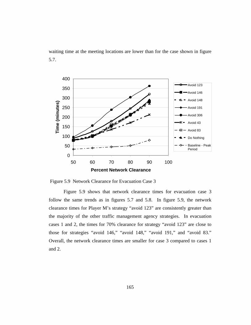
waiting time at the meeting locations are lower than for the case shown in figure
5.7.
0
50
100
150
200
250
300
350
400
50 60 70 80 90 100
Percent Network Clearance
Tim
e (m
inut
es)
Avoid 123
Avoid 146
Avoid 148
Avoid 191
Avoid 306
Avoid 43
Avoid 83
Do Nothing
Baseline - PeakPeriod
Figure 5.9 Network Clearance for Evacuation Case 3
Figure 5.9 shows that network clearance times for evacuation case 3
follow the same trends as in figures 5.7 and 5.8. In figure 5.9, the network
clearance times for Player M’s strategy “avoid 123” are consistently greater than
the majority of the other traffic management agency strategies. In evacuation
cases 1 and 2, the times for 70% clearance for strategy “avoid 123” are close to
those for strategies “avoid 146,” “avoid 148,” “avoid 191,” and “avoid 83.”
Overall, the network clearance times are smaller for case 3 compared to cases 1
and 2.
165

5.5 SUMMARY
In this chapter, a simplified model of a portion of Fort Worth, Texas was
used to illustrate the logical and methodological interrelation between the
approaches developed in chapters 3 and 4. Baseline peak period traffic conditions
and the infrastructure vulnerabilities associated with those conditions were
determined for the cases where the evil entity had the resources to damage one
link.
In the baseline peak period case, the most vulnerable links were freeway
links near a major business zone and the links leading to a node common to the
most origin-destination pairs. These links would have intuitively been the most
vulnerable, and this intuition was supported by the mathematical model.
The link vulnerabilities were also determined for evacuation conditions.
The different traffic patterns that result from evacuations produced different
disruption index values. Link vulnerability rankings changed as a consequence of
the unusual traffic patterns. In both the evacuation and baseline scenarios, the
most vulnerable link connected the greatest number of origin-destination pairs.
The type of link selected for damage, or avoidance, plays a critical role in
the determination of payoffs and the resulting network clearance times. Seeking
to avoid the vulnerable links generally yielded longer evacuation times; however,
had those links been targeted, a high percentage of the vehicles would still safely
reach their destinations. Thus, correctly predicting the target and avoiding the
threatened link lengthens evacuation times (relative to the no-damage scenario)
but ensures that a greater percentage of the population would successfully
complete the evacuation in the event the link is indeed damaged.
166

Chapter 6
Summary And Conclusions
This chapter presents a summary and the conclusions of this dissertation.
Both the conclusions specific to the examples presented in chapters 3, 4, and 5
and generalized conclusions are found in the following pages. This chapter is
organized as follows. First, a summary of the work is given. Second, the
conclusions specific to the networks shown in this dissertation and general
conclusions and recommendations for the methodologies developed for this work
are presented. Finally, directions for future work are suggested.
6.1 SUMMARY
In this dissertation two primary contributions are made to the
transportation engineering field of knowledge. The first is in the area of network
vulnerability. The second is in evacuation modeling. These two contributions
have implications for fields outside of transportation engineering, such as
evacuation planning, community and urban planning, military strategic strike
planning, national defense, and antiterrorism defense.
The contribution to network vulnerability is primarily found in chapter 3
with a larger application provided in chapter 5. In chapter 3, two mathematical
indices are presented. The vulnerability index is a measure of the importance of a
specific link, or set of links, to the connectivity of an origin-destination pair. This
index ias based on existing flow patterns, traffic conditions, and network design.
The second measure, the disruption index, is an aggregation of the vulnerability
167

indices across all origin-destination pairs in the network. The disruption index is
a measure of the impact of damaging a specific link, or set of links, on the
network as a whole. The disruption index - and the vulnerability index at the OD
level – allows for the links of the network to be ranked in order of importance. A
bi-level formulation, that uses the disruption index as one of its factors, was
developed for the identification of the most vulnerable link, or set of links, in the
transportation network. Several games were envisioned based on the bi-level
formulation. The games consisted of two players: an evil entity, who seeks to
maximize disruption of the network, and a traffic management agency, who
routes vehicles in order to maximize the number of drivers who safely reach their
destinations. Various rules and information for the games were considered, the
conclusions for which are presented in section 6.2.
The second contribution to the field is related to evacuation modeling. In
chapter 4, a series of mathematical expressions for household decision making
under emergency evacuation conditions was presented. First, a family’s decision
makers select a meeting location. In this work, the objective is to minimize the
maximum cost (time or distance) of reaching the meeting location from all of the
sites at which household members are located at the time the evacuation order is
given. Once the meeting location is chosen, the drivers are assigned to pick up
other household members (such as school children) who are not able to drive
themselves. The mathematical expression presented in chapter 4 allowes for trade
offs between two criteria: (1) the minimization of total fleet travel time and (2) the
minimization of waiting time at the meeting location. The advantage of the first
criterion is the most efficient trip chains were generated. The disadvantage of (1)
is that a single driver (in a two driver household) may be assigned to pick up all of
the children allowing for the compilation of unforeseen delays. Criterion (2) also
allows for the possibility of one driver picking up all of the children, but this
result only occurs when the other driver has a longer perceived time to reach the
168

meeting location. The disadvantage of the second criterion is more of the family
members could be in the network (instead of waiting and worrying) and counter-
intuitive assignments may be generated; for instance, a driver may be given a
sequence of pick ups that requires more time than if the intermediate nodes are in
a different order. The factors that influenced the trip chain assignments were
thoroughly explored in chapters 4 and 5.
Chapter 5 presented a case study in which the methodologies of chapters 3
and 4 were applied to the same network. The impact of vulnerable link avoidance
strategies on evacuation time was examined. The vulnerabilities of the links were
determined at different times during an evacuation to identify weaknesses in the
network design that are not evident under typical traffic conditions.
6.2 CONCLUSIONS AND RECOMMENDATIONS
The methodologies presented in the previous chapters are applicable to
any transportation network. From the network designs and results obtained in
this work, several conclusions and recommendations can be made.
For small networks, such as that in chapter 3, and a limited number of
resources available to an evil entity, the disruption index can lead to the
identification of cut sets. Larger, well connected networks, such as that found in
chapter 5, require a substantially greater number of resources to completely sever
the origins from the destinations. The vulnerability and disruption indices can,
however, identify the links that are most vulnerable to damage given a specified
number of resources.
Having accurate information about the amount of resources available to an
evil entity is integral to the strategy selection of a traffic management agency.
Underestimation leads to fewer vehicles safely reaching their destinations.
Overestimation also yields an advantage to the evil entity. Although a greater
169

number of vehicles will safely reach their destinations than originally anticipated,
the routing strategy selected may cause a different set of links to be targeted.
These links may not require as many resources to damage and the evil entity will
receive a higher payoff than if the traffic management agency had perfect
information.
Routing vehicles to avoid vulnerable transportation infrastructure yields
longer evacuation times. Emergency evacuation scenarios utilize virtually all
available capacity.
Using the decision making model presented in chapter 4 yields a more
accurate evacuation model. Incorporating household interactions captures traffic
patterns that do not exist under daily network demands. These traffic patterns
lead to changes in link vulnerabilities from the typical conditions.
When the weights associated with the minimization of total fleet time and
the minimization of the waiting time at the meeting locations are unknown, a
deterministic dwell time of 5.0 minutes at the intermediate destinations should be
used for the combination of network design and household characteristics
employed in chapter 4. This dwell time yields the least disparity among the
evacuation times for the different weights. However, using a random dwell time
is more realistic. Varying the weight associated with the total fleet time across
households should also yield a more realistic evacuation scenario since decision
makers have different values.
Although no more than three solutions to the trip chain assignments were
generated in this work, that is not the limit on the number of possible pareto
optimal solutions to the problem, depending on the weights of the objective
function criteria. The beginning and meeting locations of the household members
may create a case where only one solution exists to the objective function
regardless of the weight applied to the two criteria – provided that the sum of the
weights is 1.0. The actual weights applied to the two criteria depend on the
170
values of the household decision makers; for a generalized modeling scenario, an
intermediate value for each weight should be selected.
The other factor that plays a critical role in the pick up assignment and
sequencing of intermediate destinations is the dwell time at those intermediate
destinations. Certain values of the dwell time may produce vastly different
evacuation times, depending on the weights assigned to the two criteria. The
dwell time not only affects the trip chain assignment but also allows for the
possibility of overall network congestion alleviation. Removing some vehicles
from the roads for a period of time (the delay) permits the drivers that are still in
the network to proceed at a higher speed, thus resulting in a shorter evacuation.
Simulation is required to find both the dwell time that offers the least disparity in
evacuation times, regardless of the household’s weighting selections, and the
dwell time that minimizes evacuation time. Evacuation planners using this model
should also keep in mind that they have little control over the individual
household’s delays at the intermediate nodes.
As should be obvious to planners, antiterrorists, and the military, the
mostly likely targeted roads in an non-prioritized network are the links whose
damage that can have the most impact on the transportation network as a whole.
These links tend to be heavily traveled and used by drivers from more than one
origin-destination pair. The joint disruption index for these links is higher than
the joint index for other sets of links. In a prioritized network, where a particular
origin-destination pair is valued more than other origin-destination pairs, the most
likely targeted road is the most heavily traveled link connecting the OD pair of
interest. If only the one origin-destination pair is considered, the vulnerability
index aides in the identification of the most vulnerable link. Building additional
roads to divert traffic away from these highly vulnerable links can save lives
when limited threats (i.e. the disaster causing agent cannot destroy every
roadway) are realized. Furthermore, this redundancy in the network can allow
171
drivers to reach their desired destinations in a timely manner even if their primary
route is unavailable.
6.3 FUTURE WORK
The work performed for this dissertation has lead to three future
directions. First, the vulnerability and disruption indices may be used in location
analysis. These indices may be used in the site selection for schools, government
centers, and other buildings of interest. In terms of combining location analysis
and evacuations, if a terrorist threat is perceived, officials may want to move the
school children to another location, close to the original. The relocation may
serve several functions including, but not limited to, the minimization of the
disruption indices of the roads within a given radius of the school and the
provision of greater access for the parents to reach their children and complete the
evacuation in a more timely manner. Second, additional information levels for
further gaming applications may be considered. Finally, the role and impacts of
information supply strategies for travelers may be evaluated for evacuation
purposes and routing around vulnerable transportation infrastructure.
172

APPENDIX A
Joint Vulnerability Index Computer Code
A.1 MODULE COMMON_VAR
parameter (imaxlink=8) parameter (imaxnode=6) parameter (imaxO=2) parameter (imaxD=2) parameter (imaxpath=3) parameter (itotp=9) integer iorigin integer idest integer ican integer indlink ! number of damaged links integer inumpath(imaxnode,imaxnode) integer ipODid(imaxnode,imaxnode,itotp) ! assigns path number to OD integer iplink(itotp,imaxlink) !1 if link on path integer idlink(imaxlink) ! damaged link(s) integer jO(itotp) ! origin node of path integer jD(itotp) ! destination node of path integer iODaf(imaxnode,imaxnode) ! 1 if OD affected, 0 o.w. integer inODaf ! number of ODs affected integer ishare(itotp,itotp,imaxlink) ! 1 if paths share link integer imshared(imaxlink) !1 if link is shared integer ishrsmOD(imaxlink) !1 if link is shared by paths with same OD integer ishrdfOD(imaxlink) !1 if link is shared by paths with dif OD integer icantpath(itotp) ! path can't be used for reassignment integer ibneklink(itotp) ! bottleneck link of path j integer ibestp(imaxnode,imaxnode) !current best path from O to D integer iflag(itotp) !flags path when full due to reassignment integer iadflow(imaxnode,imaxnode,itotp) !flow reassigned to OD path integer ictOsh(imaxlink) !counts the number of origins shared by a link integer ictDsh(imaxlink) !counts the number of destinations shared integer iOsh(imaxlink,imaxlink) !origins shared by link integer iDsh(imaxlink,imaxlink) !destinations shared by link
173
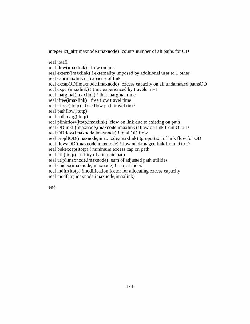
integer ict_alt(imaxnode,imaxnode) !counts number of alt paths for OD real totafl real flow(imaxlink) ! flow on link real extern(imaxlink) ! externality imposed by additional user to 1 other real cap(imaxlink) ! capacity of link real excapOD(imaxnode,imaxnode) !excess capacity on all undamaged pathsOD real exper(imaxlink) ! time experienced by traveler n+1 real marginal(imaxlink) ! link marginal time real tfree(imaxlink) ! free flow travel time real ptfree(itotp) ! free flow path travel time real pathflow(itotp) real pathmarg(itotp) real plinkflow(itotp,imaxlink) !flow on link due to existing on path real ODlinkfl(imaxnode,imaxnode,imaxlink) !flow on link from O to D real ODflow(imaxnode,imaxnode) ! total OD flow real proplfOD(imaxnode,imaxnode,imaxlink) !proportion of link flow for OD real flowaOD(imaxnode,imaxnode) !flow on damaged link from O to D real bnkexcap(itotp) ! minimum excess cap on path real util(itotp) ! utility of alternate path real utlp(imaxnode,imaxnode) !sum of adjusted path utilities real cindex(imaxnode,imaxnode) !critical index real mdftr(itotp) !modification factor for allocating excess capacity real modfctr(imaxnode,imaxnode,imaxlink) end
174

A.2 SUBROUTINE BOTTLENECK(IPATH) ! this subroutine finds the bottleneck of each path use common_var ibneklink(ipath)=0 bnkexcap(ipath)=0.0 temp_val=99999.9 do j=1,imaxlink if(iplink(ipath,j).eq.1)then if(ictOsh(j).gt.1)then call modify_xcap(j) mdftr(j)=modfctr(jO(ipath),jD(ipath),j) if(mdftr(j)*(cap(j)-flow(j)).lt.temp_val)then ibneklink(ipath)=j bnkexcap(ipath)=mdftr(j)*(cap(j)-flow(j)) temp_val=bnkexcap(ipath) endif else if(cap(j)-flow(j).lt.temp_val)then ibneklink(ipath)=j bnkexcap(ipath)=cap(j)-flow(j) temp_val=bnkexcap(ipath) endif endif endif enddo return end
A.3 SUBROUTINE FIND_BPATH(IORIG,JDEST,ICANPATH)
! this subroutine finds the best path for the OD pair that does not contain the ! damaged links use common_var integer icanpath icanpath=0 temppm=999999.9 do iii=1,itotp do jjj=1,inumpath(iorig,jdest) if(ipODid(iorig,jdest,jjj).eq.iii)then call bottleneck(iii)
175

if(bnkexcap(iii).lt.1.0) iflag(ipODid(iorig,jdest,jjj))=1 if(icantpath(ipODid(iorig,jdest,jjj)).ne.1.and. + iflag(ipODid(iorig,jdest,jjj)).ne.1)then icanpath=1 call find_pathmarg(iii) if(pathmarg(iii).lt.temppm)then temppm=pathmarg(iii) ibestp(iorig,jdest)=ipODid(iorig,jdest,jjj) endif endif endif enddo enddo return end
A.4 SUBROUTINE FIND_PATHMARG(IPATH)
use common_var pathmarg(ipath)=0 ptfree(ipath)=0 do il=1,imaxlink if(iplink(ipath,il).eq.1)then call totmarg(il) pathmarg(ipath)=pathmarg(ipath)+iplink(ipath,il)*marginal(il) ptfree(ipath)=ptfree(ipath)+tfree(il)*iplink(ipath,il) endif enddo return end
176

A.5 PROGRAM MAINPROG
use common_var REAL DISRUPT real playerM !payoff to player M CALL read_input Do i=1,imaxnode Do j=1,imaxnode inumpath(i,j)=0 enddo enddo Do k=1, itotp inumpath(jO(k),jD(k))=inumpath(jO(k),jD(k))+1 ipODid(jO(k),jD(k),inumpath(jO(k),jD(k)))=k call bottleneck(k) call utility(k) enddo Call ODaffected Call SharedLinks ! DETERMINE IF A PATH HAS ANY EXCESS CAPACITY do ii=1,itotp do jj=1,imaxlink if(iplink(ii,jj).eq.1.and.cap(jj)-flow(jj).lt.0.0) icantpath(ii)=1 enddo enddo ! DETERMINE AMOUNT OF OD FLOW THAT MUST BE ! ACCOMMODATED ON ALTERNATE PATHS do i=1,imaxnode do j=1,imaxnode if(iODaf(i,j).eq.1)then do k=1,itotp jointpath=0 if(jO(k).eq.i.and.jD(k).eq.j)then do idk=1,indlink if(iplink(k,idlink(idk)).eq.1.and.jointpath.ne.1)then flowaOD(i,j)=flowaOD(i,j)+plinkflow(k,idlink(idk)) totafl=totafl+plinkflow(k,idlink(idk)) ! total damaged flow jointpath=1
177

endif enddo endif enddo endif enddo enddo ! DETERMINE IF THERE ARE ANY ALTERNATE PATHS DO i=1,imaxnode do j=1,imaxnode if(iODaf(i,j).eq.1)then do k=1,itotp if(jO(k).eq.i.and.jD(k).eq.j)then
endif
ict_alt(i,j)=ict_alt(i,j)+1 endif enddo endif enddo enddo do i=1,imaxnode do j=1,imaxnode if(iODaf(i,j).eq.1)then do k=1,itotp if(jO(k).eq.i.and.jD(k).eq.j)then if(icantpath(k).ne.1)then excapOD(i,j)=excapOD(i,j)+bnkexcap(k) call utility(k)
endif enddo endif enddo enddo open(unit=75, file='utility_n.dat', status='unknown') do k=1,itotp write(75,700) k,util(k) enddo close(75) ! index needs to be adjusted by flow
178

do i=1,imaxnode do j=1,imaxnode if(iODaf(i,j).eq.1.and.flowaOD(i,j).gt.0.0)then ! if OD pair affected then need reassignment if(inumpath(i,j).eq.1)then ! no reassignment is possible cindex(i,j)=1.0 else if(excapOD(i,j).lt.flowaOD(i,j))then cindex(i,j)=flowaOD(i,j)/ODflow(i,j) else Call Reassignment(i,j) if(ican.eq.0) then cindex(i,j)=1.0 else do k=1,itotp if(jO(k).eq.i.and.jD(k).eq.j)then if(icantpath(k).ne.1)then utlp(i,j)=utlp(i,j)+iadflow(i,j,k)/flowaOD(i,j)*util(k) write(*,*)k,iadflow(i,j,k),flowaOD(i,j),util(k) endif endif enddo cindex(i,j)=(1-utlp(i,j))*flowaOD(i,j)/ODflow(i,j) endif endif endif else cindex(i,j)=0 endif enddo enddo DISRUPT=0.0 open(unit=71, file='index.dat', status='unknown') do i=1,imaxnode do j=1,imaxnode if(iODaf(i,j).eq.1) write(71,711) i,j,cindex(i,j) DISRUPT=DISRUPT+cindex(i,j) enddo enddo write(71,712) DISRUPT
179
playerM=(1-totafl/3800)*100 ! for ½ demand scenario write(71,*) 'Percent safely reaching destinations: ' write(71,712) playerM close(71) 700 format(I6, f15.9) 711 format(2I6,f15.9) 712 format(f15.9) end program mainprog
A.6 SUBROUTINE MODIFY_XCAP(IILINK)
! this subroutine modifys the excess capacity of the bottleneck link ! by xa(O"D")/sum(xaO'D') where O"D" is the OD pair currently being ! examined and O'D' is the set of OD pairs affected by the damaged link ! and the bottleneck link of the path ! for the joint case, the denominator is the sum over all a and O'D' use common_var integer iODlflwck(imaxnode,imaxnode,imaxlink) real modflow(imaxnode,imaxnode,imaxlink) real modjflow(imaxlink) do imo=1,imaxnode do imd=1,imaxnode iODlflwck(imo,imd,imaxlink)=0 enddo enddo if(ictOsh(iilink).gt.1)then do imi=1,ictOsh(iilink) if(iODaf(iOsh(iilink,imi),iDsh(iilink,imi)).eq.1.and. + iODlflwck(iOsh(iilink,imi),iDsh(iilink,imi),iilink).ne.1.and. + ict_alt(iOsh(iilink,imi),iDsh(iilink,imi)).gt.1)then DO K=1,itotp IF(jO(K).eq.iOsh(iilink,imi).and.jD(K).eq. + iDsh(iilink,imi))then if(icantpath(K).ne.1)then
180
if(iplink(K,iilink).eq.1)then modjflow(iilink)=modjflow(iilink)+ + flowaOD(iOsh(iilink,imi),iDsh(iilink,imi)) iODlflwck(iOsh(iilink,imi),iDsh(iilink,imi),iilink)=1 endif endif endif enddo endif enddo do imi=1,ictOsh(iilink) if(iODaf(iOsh(iilink,imi),iDsh(iilink,imi)).eq.1)then modfctr(iOsh(iilink,imi),iDsh(iilink,imi),iilink)= + flowaOD(iOsh(iilink,imi),iDsh(iilink,imi))/modjflow(iilink) endif if(iODaf(iOsh(iilink,imi),iDsh(iilink,imi)).eq.1.and. + modjflow(iilink).le.0.000001)then modfctr(iOsh(iilink,imi),iDsh(iilink,imi),iilink)=1.0 endif enddo endif return end
181

A.7 SUBROUTINE ODAFFECTED
! this subroutine identifies the OD pairs affected by the damaged link ! due to path ODs and the presence of OD flow on that link use common_var inODaf=0 do i=1, itotp do j=1, imaxlink do k=1, indlink if(iplink(i,j).eq.1.and.j.eq.idlink(k)) then iODaf(jO(i),jD(i))=1 inODaf=inODaf+1 icantpath(i)=1 endif enddo enddo enddo return end
182

A.8 SUBROUTINE READ_INPUT
use common_var integer ilink, jpath open(unit=1, file='linkstate.dat', status='old') do i=1,imaxlink read(1,100) ilink, tfree(ilink), cap(ilink), flow(ilink) enddo close(1) open(unit=2, file='paths.dat', status='old') do i=1,itotp read(2,200) jpath,jO(jpath),jD(jpath),pathflow(jpath) do k=1, imaxlink read(2,201) iplink(i,k) plinkflow(i,k)=pathflow(jpath)*iplink(i,k) enddo enddo close(2) do i=1,imaxnode do j=1,imaxnode do k=1,itotp if(jO(k).eq.i.and.jD(k).eq.j)then ODflow(i,j)=ODflow(i,j)+pathflow(k) endif enddo enddo enddo open(unit=3, file='damage_link.dat', status='old') read(3,201) indlink do i=1,indlink read(3,201) idlink(i) write(*,*) idlink(i) enddo close(3) 100 format(I6, 3f10.2) 200 format(3I6, f10.2) 201 format(I3) return end
183

A.9 SUBROUTINE REASSIGNMENT(IOR,JDE)
! this subroutine reassigns the traffic from the damaged link ! to the other paths connecting the O-D pair use common_var real freqrd(imaxnode,imaxnode) freqrd(iOr,jDe)=0 do k=1,inumpath(iOr,jDe) if(icantpath(ipODid(iOr,jDe,k)).eq.1)then freqrd(iOr,jDe)=freqrd(iOr,jDe)+pathflow(ipODid(iOr,jDe,k)) endif enddo CALL find_bpath(iOr,jDe,ican) ! now reassign one at a time if(ican.ne.0)then do iflow=1, int(freqrd(iOr,jDe)) pathflow(ibestp(iOr,jDe))=pathflow(ibestp(iOr,jDe))+1 do il=1,imaxlink if(iplink(ibestp(iOr,jDe),il).eq.1)then flow(il)=flow(il)+1 endif enddo iadflow(iOr,jDe,ibestp(iOr,jDe))=iadflow(iOr,jDe,ibestp(iOr,jDe))+1 if(iflow.lt.int(freqrd(iOr,jDe)))then call find_bpath(iOr,jDe,ican) endif if(ican.eq.0) goto 666 enddo endif 666 return return end
A.10 SUBROUTINE SHAREDLINKS
! this subroutine identifies which paths share links use common_var integer ickODPL(itotp,imaxlink)
184

integer idfODpl(itotp,imaxlink) do i=1,imaxlink ictOsh(i)=0 ictDsh(i)=0 !THESE 2 VARIABLES HAVE IDENTICAL VALUES enddo do i=1, itotp-1 do j=i+1, itotp do k=1, imaxlink if(iplink(i,k).eq.1.and.iplink(i,k).eq.iplink(j,k))then ishare(i,j,k)=1 imshared(k)=1 if(jO(i).eq.jO(j).and.jD(i).eq.jD(j))then ishrsmOD(k)=1 if(ickODPL(i,k).ne.1)then ODlinkfl(jO(i),jD(i),k)=ODlinkfl(jO(i),jD(i),k)+ + plinkflow(i,k)+plinkflow(j,k) ickODPL(i,k)=1 ickODPL(j,k)=1 endif else ishrdfOD(k)=1 if(ickODPL(i,k).ne.1)then ODlinkfl(jO(i),jD(i),k)=ODlinkfl(jO(i),jD(i),k)+plinkflow(i,k) ickODPL(i,k)=1 endif if(iODaf(jO(i),jD(i)).eq.1.and.iODaf(jO(j),jD(j)).eq.1. + and.idfODpl(i,k).ne.1)then ictOsh(k)=ictOsh(k)+1 ictDsh(k)=ictDsh(k)+1 iOsh(k,ictOsh(k))=jO(i) iDsh(k,ictDsh(k))=jD(i) idfODpl(i,k)=1 endif if(ickODPL(j,k).ne.1)then ODlinkfl(jO(j),jD(j),k)=ODlinkfl(jO(j),jD(j),k)+plinkflow(j,k) ickODPL(j,k)=1 endif if(iODaf(jO(i),jD(i)).eq.1.and.iODaf(jO(j),jD(j)).eq.1. + and.idfODpl(j,k).ne.1)then ictOsh(k)=ictOsh(k)+1 ictDsh(k)=ictDsh(k)+1 iOsh(k,ictOsh(k))=jO(j)
185

iDsh(k,ictDsh(k))=jD(j) idfODpl(j,k)=1 endif endif else ishare(i,j,k)=0 endif enddo enddo enddo ! this section checks for the OD being affected ! if not, then the OD flow is not counted in the proportion ! calculated in the next section do i=1,imaxnode do j=1,imaxnode if(iODaf(i,j).ne.1)then do ip=1,itotp do k=1,imaxlink ODlinkfl(i,j,k)=ODlinkfl(i,j,k)-plinkflow(ip,k) if(ODlinkfl(i,j,k).lt.0.00001)ODlinkfl(i,j,k)=0.0 enddo enddo endif enddo enddo do i=1,imaxnode do j=1,imaxnode if(iODaf(i,j).eq.1)then do ip=1,itotp if(jO(ip).eq.i.and.jD(ip).eq.j)then do k=1,imaxlink if(flow(k).le.0.00001)then proplfOD(i,j,k)=0.0 else if(imshared(k).ne.1) proplfOD(i,j,k)=1.0 if(iplink(ip,k).eq.1.and.imshared(k).eq.1)then if(ishrdfOD(k).eq.1.and.plinkflow(ip,k).gt.0.00001) + then proplfOD(i,j,k)=ODlinkfl(i,j,k)/flow(k) else proplfOD(i,j,k)=0.0 endif
186

if(ishrsmOD(k).eq.1.and.ishrdfOD(k).ne.1)then proplfOD(i,j,k)=1.0 endif if(ishrsmOD(k).eq.1.and.ishrdfOD(k).eq.1)then proplfOD(i,j,k)=ODlinkfl(i,j,k)/flow(k) endif endif endif enddo endif enddo endif enddo enddo return end
A.11 SUBROUTINE TOTMARG(L) ! This subroutine calculates the total marginal cost of adding one user to the link use common_var if(flow(l).lt.cap(l))then extern(l)=0.6*((flow(l))**3)/((cap(l))**4) exper(l)=tfree(l)+0.15*((flow(l)/cap(l))**4) marginal(l)=exper(l)+flow(l)*extern(l) endif return end
A.12 SUBROUTINE UTILITY(KPATH) ! this subroutine calculates the utility of an alternate path use common_var call find_pathmarg(kpath) util(kpath)=(bnkexcap(kpath)/cap(ibneklink(kpath)))* + ptfree(kpath)/pathmarg(kpath) return end
187

Appendix B
Flow Distributions
Table B.1 Flow Distributions For Table 3.11, Original Demand Level
Player M Strategy
Flow Link 1 Link 2 Link 3 Link 4 Link 5 Link 6 Link 7 Link 8
xl 2300 1700 0 1700 3400 1800 1600 1900 xl
1,2 2300 700 0 0 700 700 0 0 xl
1,6 0 1000 0 0 1000 0 1000 0 xl
5,2 0 0 0 1100 1100 1100 0 0
Do nothing / Avoid 3
xl5,6 0 0 0 600 600 0 600 1900
xl 2300 1700 0 1700 3400 1800 1600 1900 xl
1,2 2300 700 0 0 700 700 0 0 xl
1,6 0 1000 0 0 1000 0 1000 0 xl
5,2 0 0 0 1100 1100 1100 0 0
Avoid 1
xl5,6 0 0 0 600 600 0 600 1900
xl 3000 0 1000 1700 1700 1100 600 2900 xl
1,2 3000 0 0 0 0 0 0 0 xl
1,6 0 0 1000 0 0 0 0 1000 xl
5,2 0 0 0 1100 1100 1100 0 0
Avoid 2
xl5,6 0 0 0 600 600 0 600 1900
xl 3000 1000 0 1100 2100 1100 1000 2500 xl
1,2 3000 0 0 0 0 0 0 0 xl
1,6 0 1000 0 0 1000 0 1000 0 xl
5,2 0 0 0 1100 1100 1100 0 0
Avoid 4
xl5,6 0 0 0 0 0 0 0 2500
xl 3000 0 1000 1100 1100 1100 0 3500 xl
1,2 3000 0 0 0 0 0 0 0 xl
1,6 0 0 1000 0 0 0 0 1000 xl
5,2 0 0 0 1100 1100 1100 0 0
Avoid 5
xl5,6 0 0 0 0 0 0 0 2500
xl 3000 1000 0 1306 2306 1100 1206 2294 xl
1,2 3000 0 0 0 0 0 0 0 xl
1,6 0 1000 0 0 1000 0 1000 0 xl
5,2 0 0 0 1100 1100 1100 0 0
Avoid 6
xl5,6 0 0 0 206 206 0 206 2294
xl 2842 158 1000 1100 1258 1258 0 3500 xl
1,2 2842 158 0 0 158 158 0 0 xl
1,6 0 0 1000 0 0 0 0 1000 xl
5,2 0 0 0 1100 1100 1100 0 0
Avoid 7
xl5,6 0 0 0 0 0 0 0 2500
188

xl 3000 1000 0 1700 2700 1100 1600 1900 xl
1,2 3000 0 0 0 0 0 0 0 xl
1,6 0 1000 0 0 1000 0 1000 0 xl
5,2 0 0 0 1100 1100 1100 0 0
Avoid 8
xl5,6 0 0 0 600 600 0 600 1900
189

Table B.2 Flow Distributions for Table 3.12 (n=1, 3/4 Demand)
Player M Strategy
Flow Link 1 Link 2 Link 3
Link 4* Link 5* Link 6*
Link 7 Link 8
x * l 2250 750 0 1306.67 2056.67 825 1231.67 1393.33 xl
1,2 2250 0 0 0 0 0 0 0 xl
1,6 0 750 0 0 750 0 750 0
Do nothing / Avoid 3
xl5,6 0 0 0 481.67 481.67 0 481.67 1393.33
xl 1275 1700 25 1134.13 2834.13 1800 1034.13 1590.87 xl
1,2 1275 950 25 25 975 975 0 0 xl
1,6 0 750 0 0 750 0 750 0
Avoid 1
xl5,6 0 0 0 284.13 284.13 0 284.13 1590.87
xl 2250 0 750 1533.49 1533.49 825 708.49 1916.51 xl
1,2 2250 0 0 0 0 0 0 0 xl
1,6 0 0 750 0 0 0 0 750
Avoid 2 (opt 1)
xl5,6 0 0 0 708.49 708.49 0 708.49 1166.51
xl 2250 0 750 1533.50 1533.50 825 708.50 1916.50 xl
1,2 2250 0 0 0 0 0 0 0 xl
1,6 0 0 750 700 700 0 700 50
Avoid 2 (opt 2)
xl5,6 0 0 0 8.50 8.50 0 8.50 1866.50
xl 2250 750 0 825 1575 825 750 1875 xl
1,2 2250 0 0 0 0 0 0 0 xl
1,6 0 750 0 0 750 0 750 0
Avoid 4
xl5,6 0 0 0 0 0 0 0 1875
xl 2250 0 750 825 1575 825 0 2625 xl
1,2 2250 0 0 0 0 0 0 0 xl
1,6 0 0 750 0 750 0 0 750
Avoid 5
xl5,6 0 0 0 0 0 0 0 1875
xl 2250 750 0 1309.79 2059.79 825 1234.79 1390.21 xl
1,2 2250 0 0 0 0 0 0 0 xl
1,6 0 750 0 0 750 0 750 0
Avoid 6
x 5,6l 0 0 0 484.79 484.79 0 484.79 1390.21
xl 2131.22 118.78 750 825 943.78 943.78 0 2625 xl
1,2 2131.22 118.78 0 0 118.78 118.78 0 0 xl
1,6 0 0 750 0 0 0 0 750
Avoid 7
xl5,6 0 0 0 0 0 0 0 1875
xl 2250 750 0 1700 2450 825 1625 1000 xl
1,2 2250 0 0 0 0 0 0 0 xl
1,6 0 750 0 0 750 0 750 0
Avoid 8
xl5,6 0 0 0 875 875 0 875 1000
* Links 4, 5, and 6 always carry all of the OD (5,2) flow which is 825 vph in this
case.
190

Table B.3 Flow Distributions for Table 3.13(n=1, 1/2 Demand)
Player M Strategy
Flow Link 1 Link 2 Link 3
Link 4* Link 5* Link 6*
Link 7 Link 8
xl* 1500 500 0 1314.98 1814.98 550 1264.98 485.02 xl
1,2 1500 0 0 0 0 0 0 0 xl
1,6 0 500 0 0 500 0 500 0
Do nothing / Avoid 3
xl5,6 0 0 0 764.98 764.98 0 764.98 485.02
xl 250 1700 50 1119.35 2819.35 1800 1019.35 730.65 xl
1,2 250 1250 0 0 1250 1250 0 0 xl
1,6 0 450 50 0 450 0 450 50
Avoid 1+
(opt 1)
xl5,6 0 0 0 569.35 569.35 0 569.35 680.65
xl 1500 0 500 1476.75 1476.75 550 926.75 823.25 xl
1,2 1500 0 0 0 0 0 0 0 xl
1,6 0 0 500 0 0 0 0 500
Avoid 2 (opt 1)
xl5,6 0 0 0 926.75 926.75 0 926.75 323.25
xl 1500 0 500 1476.84 1476.84 550 926.84 823.16 xl
1,2 1500 0 0 0 0 0 0 0 xl
1,6 0 0 500 500 500 0 500 0
Avoid 2 (opt 2)
xl5,6 0 0 0 426.84 426.84 0 426.84 823.16
xl 1500 500 0 550 1050 550 500 1250 xl
1,2 1500 0 0 0 0 0 0 0 xl
1,6 0 500 0 0 500 0 500 0
Avoid 4
xl5,6 0 0 0 0 0 0 0 1250
xl 1500 0 500 550 550 550 0 1750 xl
1,2 1500 0 0 0 0 0 0 0 xl
1,6 0 0 500 0 0 0 0 500
Avoid 5
xl5,6 0 0 0 0 0 0 0 1250
xl 1500 500 0 1314.81 1814.81 550 1264.81 485.19 xl
1,2 1500 0 0 0 0 0 0 0 xl
1,6 0 500 0 0 500 0 500 0
Avoid 6
xl5,6 0 0 0 764.81 764.81 0 764.81 485.19
xl 1500 0 500 550 550 550 0 1750 xl
1,2 1500 0 0 0 0 0 0 0 xl
1,6 0 0 500 0 0 0 0 500
Avoid 7
xl5,6 0 0 0 0 0 0 0 1250
xl 1500 500 0 1700 2200 550 1650 100 xl
1,2 1500 0 0 0 0 0 0 0 xl
1,6 0 500 0 0 500 0 500 0
Avoid 8
xl5,6 0 0 0 1150 1150 0 1150 100
* Links 4, 5, and 6 always carry all of the OD (5,2) flow which is 550 vph in this case. + Options 1 and 2 for Avoid 2 have the equivalent values of the objective function to four decimal places.
191

Table B.4 Flow Distribution Corresponding to Table 3.14, n=2, Original Demand
Player M Strategy
Flow Link 1 Link 2 Link 3 Link 4* Link 5* Link 6* Link 7 Link 8
xl* 2400 0 1600 1700 1700 1700 0 3500 xl
1,2 2400 0 600 600 600 600 0 0 xl
1,6 0 0 1000 0 0 0 0 1000
Avoid 1,2 (opt 1)
xl5,6 0 0 0 0 0 0 0 2500
xl* 2300 100 1600 1700 1800 1800 0 3500 xl
1,2 2300 100 600 600 700 700 0 0 xl
1,6 0 0 1000 0 0 0 0 1000
Avoid 1,2 (opt 2)
xl5,6 0 0 0 0 0 0 0 2500
xl* 2300 1700 0 1700 3400 1800 1600 1900 xl
1,2 2300 700 0 0 700 700 0 0 xl
1,6 0 1000 0 0 1000 0 1000 0
Avoid 1,3
xl5,6 0 0 0 600 600 0 600 1900
xl* 2300 1700 0 1100 2800 1800 1000 2500 xl
1,2 2300 700 0 0 700 700 0 0 xl
1,6 0 1000 0 0 1000 0 1000 0
Avoid 1,4
xl5,6 0 0 0 0 0 0 0 2500
xl* 2300 700 1000 1100 1800 1800 0 3500 xl
1,2 2300 700 0 0 700 700 0 0 xl
1,6 0 0 1000 0 0 0 0 1000
Avoid 1,5 (opt 1); 1,6(opt 1); 1,7
xl5,6 0 0 0 0 0 0 0 2500
xl* 3000 0 1000 1100 1100 1100 0 3500 xl
1,2 3000 0 0 0 0 0 0 0 xl
1,6 0 0 1000 0 0 0 0 1000
Avoid 1,5 (opt 2); 1,6(opt 2)
xl5,6 0 0 0 0 0 0 0 2500
xl* 2650 350 1000 1100 1450 1450 0 3500 xl
1,2 2650 350 0 0 350 350 0 0 xl
1,6 0 0 1000 0 0 0 0 1000
Avoid 1,5 (opt 3); 1,6(opt 3)
xl5,6 0 0 0 0 0 0 0 2500
xl* 2300 700 1000 1700 2400 1800 600 2900 xl
1,2 2300 700 0 0 700 700 0 0 xl
1,6 0 0 1000 0 0 0 0 1000
Avoid 1,8(opt 1)
xl5,6 0 0 0 600 600 0 600 1900
xl* 2300 700 1000 1700 2400 1800 600 2900 xl
1,2 2300 700 0 0 700 700 0 0 xl
1,6 0 0 1000 300 300 0 600 400
Avoid 1,8(opt 2)
xl5,6 0 0 0 300 300 0 0 2500
xl* 2300 700 1000 1700 2400 1800 600 2900 xl
1,2 2300 700 0 0 700 700 0 0 xl
1,6 0 0 1000 300 300 0 300 700
Avoid 1,8(opt 3)
xl5,6 0 0 0 300 300 0 300 2200
xl* 3000 1000 0 1330.96 2330.96 1100 1230.96 2269.04 xl
1,2 3000 0 0 0 0 0 0 0 xl
1,6 0 1000 0 0 1000 0 1000 0
Avoid 2,3(opt 1)
xl5,6 0 0 0 230.96 230.96 0 230.96 2269.04
192

xl* 3000 0 1000 1700 1700 1100 600 2565.03 xl
1,2 3000 0 0 0 0 0 0 0 xl
1,6 0 0 1000 220.66 220.66 0 220.66 345.53
Avoid 2,3(opt 2); 2,8(opt 3); 7,8(opt 3)
xl5,6 0 0 0 379.34 379.34 0 280.50 2219.50
xl* 3000 507.95 492.05 1527.02 2034.97 1100 934.97 2565.03 xl
1,2 3000 0 0 0 0 0 0 0 xl
1,6 0 507.95 492.05 146.51 654.45 0 654.47 345.53
Avoid 2,3(opt 3)
xl5,6 0 0 0 280.50 280.50 0 280.50 2219.50
xl* 3000 0 1000 1100 1100 1100 0 3500 xl
1,2 3000 0 0 0 0 0 0 0 xl
1,6 0 0 1000 0 0 0 0 1000
Avoid 2,4; 2,5; 2,7; 3,5(opt 2); 4,5; 5,6; 5,7; 6,7
xl5,6 0 0 0 0 0 0 0 2500
xl* 3000 0 1000 1700 1100 1100 600 2900 xl
1,2 3000 0 0 0 0 0 0 0 xl
1,6 0 0 1000 0 0 0 0 1000
Avoid 2,6(opt 1); 2,8(opt 2); 5,8(opt 2); 7,8(opt 2)
xl5,6 0 0 0 0 0 0 600 1900
xl* 3000 0 1000 1700 1700 1100 600 2900 xl
1,2 3000 0 0 0 0 0 0 0 xl
1,6 0 0 0 600 600 0 600 400
Avoid 2,6(opt 2)
xl5,6 0 0 0 0 0 0 0 2500
xl* 3000 0 1000 1700 1700 1100 600 2900 xl
1,2 3000 0 0 0 0 0 0 0 xl
1,6 0 0 1000 300 300 0 300 700
Avoid 2,6(opt 3)
xl5,6 0 0 0 300 300 0 300 2200
xl* 3000 1000 0 1700 2700 1100 1600 1900 xl
1,2 3000 0 0 0 0 0 0 0 xl
1,6 0 1000 0 0 1000 0 1000 0
Avoid 2,8(opt 1); 3,6; 3,7(opt 2); 3,8; 4,8; 5,8(opt 1); 6,8; 7,8(opt 1)
xl5,6 0 0 0 600 600 0 600 1900
xl* 3000 1000 0 1700 2700 1100 1000 2500 xl
1,2 3000 0 0 0 0 0 0 0 xl
1,6 0 1000 0 0 1000 0 1000 0
Avoid 3,4; 3,5(opt 1); 3,7(opt 1); 4,6
xl5,6 0 0 0 600 600 0 0 2500
xl* 3000 507.95 492.05 1100 1607.95 1100 507.95 2992.05 xl
1,2 3000 0 0 0 0 0 0 0 Avoid 3,5(opt 3); xl
1,6 0 507.95 492.05 0 507.95 0 507.95 492.05
193

3,7(opt 3)
xl5,6 0 0 0 0 0 0 0 2500
xl* 2842.07 157.93 1000 1100 1257.93 1257.93 0 3500 xl
1,2 2842.07 157.93 0 0 157.93 157.93 0 0 xl
1,6 0 0 1000 0 0 0 0 1000
Avoid 4,7
xl5,6 0 0 0 0 0 0 0 2500
xl* 3000 844.35 155.65 1100 1944.35 1100 844.35 2655.65 xl
1,2 3000 0 0 0 0 0 0 0 xl
1,6 0 844.35 155.65 0 844.35 0 844.35 155.65
Avoid 5,8(opt 3)
xl5,6 0 0 0 0 0 0 0 2500
194

Table B.5 Flow Distribution Corresponding to Table 3.16, n=2, 3/4 Demand
M’s Strat.
Flow Link 1 Link 2 Link 3 Link 4* Link 5* Link 6* Link 7 Link 8
xl* 1400 0 1600 1700 1700 1675 25 2600 xl
1,2 1400 0 850 850 850 850 0 0 xl
1,6 0 0 750 0 0 0 25 750
Avoid 1,2 (opt 1)
xl5,6 0 0 0 25 25 0 0 1850
xl* 1275 125 1600 1675 1800 1800 0 2625 xl
1,2 1275 0 850 850 975 975 0 0 xl
1,6 0 0 750 0 0 0 0 750
Avoid 1,2 (opt 2)
xl5,6 0 0 0 0 0 0 0 1875
xl* 1300 1700 0 1116.16 2816.16 1775 1041.16 1583.84 xl
1,2 1300 950 0 0 950 950 0 0 xl
1,6 0 750 0 0 750 0 750 0
Avoid 1,3 (opt 1)
xl5,6 0 0 0 291.16 291.16 0 291.16 1583.84
xl* 1275 1700 25 1120.61 2820.61 1800 1020.61 1604.39 xl
1,2 1275 975 0 0 975 975 0 0 xl
1,6 0 725 25 0 725 0 725 25
Avoid 1,3 (opt 2); 1,6 (opt 2)
xl5,6 0 0 0 295.61 295.61 0 295.61 1579.39
xl* 1275 1700 25 1120.61 2820.61 1800 1020.61 1604.39 xl
1,2 1275 975 0 0 975 975 0 0 xl
1,6 0 725 25 25 750 0 750 0
Avoid 1,3 (opt 3)
xl5,6 0 0 0 270.61 270.61 0 270.61 1604.39
xl* 1275 1700 25 825 2525 1800 725 1900 xl
1,2 1275 975 0 0 975 975 0 0 xl
1,6 0 725 25 0 725 0 725 25
Avoid 1,4
xl5,6 0 0 0 0 0 0 0 1875
xl* 2250 0 750 825 825 825 0 2625 xl
1,2 2250 0 0 0 0 0 0 0 xl
1,6 0 0 750 0 0 0 0 750
Avoid 1,5 (opt1); 2,4; 2,5; 2,7; 3,5 (opt2); 3,7 (opt2); 4,5; 5,6; 5,7; 5,8 (opt2); 6,7; 7,8 (opt 1)
xl5,6 0 0 0 0 0 0 0 1875
xl* 1275 975 750 825 1800 1800 0 2625 xl
1,2 1275 975 0 0 975 975 0 0 xl
1,6 0 0 750 0 0 0 0 750
Avoid 1,5 (opt2); 1,7 xl
5,6 0 0 0 0 0 0 0 1875 xl* 1773.64 476.36 750 825 1301.36 1301.36 0 2625 Avoid
1,5 xl1,2 1773.64 476.36 0 0 476.36 476.36 0 0
195

xl1,6 0 0 750 0 0 0 0 750 (opt 3)
xl5,6 0 0 0 0 0 0 0 1875
xl* 2250 750 0 1309.79 2059.79 825 1234.79 1390.21 xl
1,2 2250 0 0 0 0 0 0 0 xl
1,6 0 750 0 0 750 0 750 0
Avoid 1,6 (opt1); 2,3 (opt1); 3,6; 5,8 (opt 1)
xl5,6 0 0 0 484.79 484.79 0 484.79 1390.21
xl* 1773.64 1226.36 0 1242.00 2468.36 1301.36 1167.00 1458 xl
1,2 1773.64 476.36 0 0 476.36 476.36 0 0 xl
1,6 0 750 0 0 750 0 750 0
Avoid 1,6 (opt 3)
xl5,6 0 0 0 417 417 0 417 1458
xl* 1300 1700 0 1700 3400 1775 1625 1000 xl
1,2 1300 950 0 0 950 950 0 0 xl
1,6 0 750 0 0 750 0 750 0
Avoid 1,8 (opt 1)
xl5,6 0 0 0 875 875 0 875 1000
xl* 1275 1700 25 1700 3400 1800 1600 1025 xl
1,2 1275 975 0 0 975 975 0 0 xl
1,6 0 725 25 0 725 0 725 25
Avoid 1,8 (opt 2)
xl5,6 0 0 0 875 875 0 875 1000
xl* 1275 1700 25 1700 3400 1800 1600 1025 xl
1,2 1275 975 0 0 975 975 0 0 xl
1,6 0 725 25 25 750 0 750 0
Avoid 1,8 (opt 3)
xl5,6 0 0 0 850 850 0 850 1025
xl* 2250 0 750 1700 1700 825 875 1750 xl
1,2 2250 0 0 0 0 0 0 0 xl
1,6 0 0 750 375 375 0 375 375
Avoid 2,3 (opt2); 2,6 (opt3); 2,8 (opt 1)
xl5,6 0 0 0 500 500 0 500 1375
xl* 2250 360.48 389.52 1454.89 1815.37 825 990.37 1634.63 xl
1,2 2250 0 0 0 0 0 0 0 xl
1,6 0 360.48 389.52 53.64 414.12 0 414.12 335.88
Avoid 2,3 (opt3); 7,8 (opt 3)
xl5,6 0 0 0 576.25 576.25 0 576.25 1298.75
xl* 2250 0 750 1533.48 1533.48 825 708.48 1916.52 xl
1,2 2250 0 0 0 0 0 0 0 xl
1,6 0 0 750 0 0 0 0 750
Avoid 2,6 (opt 1)
708.48 xl5,6 0 0 708.48 0 708.48 1916.52
xl* 2250 0 750 1533.48 1533.48 825 708.48 1916.52 xl
1,2 2250 0 0 0 0 0 0 0 xl
1,6 0 0 750 708.48 708.48 0 708.48 41.52
Avoid 2,6 (opt 2)
0 xl5,6 0 0 0 0 0 0 1875
xl* 2250 0 750 1700 1700 825 875 1750 xl
1,2 2250 0 0 0 0 0 0 0 xl
1,6 0 0 750 0 0 0 0 750
Avoid 2,8 (opt 2)
xl5,6 0 0 0 875 875 0 875 1000
xl* 2250 0 750 1700 1700 825 875 1750 xl
1,2 2250 0 0 0 0 0 0 0 xl
1,6 0 0 750 750 750 0 750 0
Avoid 2,8 (opt 3)
xl5,6 0 0 0 125 125 0 125 1750
196

xl* 2250 750 0 825 1575 825 750 1875 xl
1,2 2250 0 0 0 0 0 0 0 xl
1,6 0 750 0 0 750 0 750 0
Avoid 3,4; 3,5 (opt1); 3,7 (opt1); 4,6; 4,8 (opt 2)
xl5,6 0 0 0 825 0 0 0 1875
xl* 2250 325 325 825 1150 825 325 2200 xl
1,2 2250 0 0 0 0 0 0 0 xl
1,6 0 325 325 0 325 0 325 325
Avoid 3,5 (opt3); 3,7 (opt 3)
xl5,6 0 0 0 0 0 1875
xl* 2250 750 0 1700 2450 825 1625 1000 xl
1,2 2250 0 0 0 0 0 0 0 xl
1,6 0 750 0 0 750 0 750 0
Avoid 3,8; 4,8 (opt1); 5,8 (opt3); 6,8; 7,8 (opt 2)
xl5,6 0 0 0 875 875 0 875 1000
xl* 2130.69 119.31 750 825 944.31 944.31 0 2625 xl
1,2 2130.69 119.31 0 0 119.31 119.31 0 0 xl
1,6 0 0 750 0 0 0 0 750
Avoid 4,7
xl5,6 0 0 0 0 0 0 0 1875
xl* 2250 750 0 1325 2075 825 1250 1375 xl
1,2 2250 0 0 0 0 0 0 0 xl
1,6 0 750 0 0 750 0 750 0
Avoid 4,8 (opt 3)
xl5,6 0 0 0 500 500 0 500 1375
* Links 4, 5, and 6 always carry all of the OD (5,2) flow which is 875 vph in this case.
197

Table B.6 Flow Distribution for Table 3.18, n=2, ½ Demand Level
Player M Strategy
Flow Link 1 Link 2 Link 3
Link 4* Link 5* Link 6*
Link 7 Link 8
xl* 1500 500 0 1314.98 1814.98 550 1264.98 485.02 xl
1,2 1500 0 0 0 0 0 0 0 xl
1,6 0 500 0 0 500 0 500 0
Do nothing
xl5,6 0 0 0 764.98 764.98 0 764.98 485.02
xl 250 150 1600 1700 1850 1800 50 1700 xl
1,2 250 150 1100 1100 1250 1250 0 0 xl
1,6 0 0 500 0 0 0 0 500
Avoid 1,2 (opt 1)
xl5,6 0 0 0 50 50 0 50 1200
xl 250 150 1600 1700 1850 1800 50 1700 xl
1,2 250 100 1150 1150 1250 1250 50 0 xl
1,6 0 50 450 0 50 0 0 450
Avoid 1,2 (opt 2)
xl5,6 0 0 0 0 0 0 0 1250
xl 300 1700 0 1103 2803 1750 1053 697 xl
1,2 300 1200 0 0 1200 1200 0 0 xl
1,6 0 500 0 0 500 0 500 0
Avoid 1,3
0 xl5,6 0 0 553 553 0 553 697
xl 250 1700 50 550 2250 1800 450 1300 xl
1,2 250 1250 0 0 1250 1250 0 0 xl
1,6 0 450 50 0 450 0 450 50
Avoid 1,4
xl5,6 0 0 0 0 0 0 0 1250
xl 250 1250 500 550 1800 1800 0 1750 xl
1,2 250 1250 0 0 1250 1250 0 0 xl
1,6 0 0 500 0 0 0 0 500
Avoid 1,5 (opt 1); 1,7 xl
5,6 0 0 0 0 0 0 0 1250 xl 1500 0 500 550 550 550 0 1750 xl
1,2 1500 0 0 0 0 0 0 0 xl
1,6 0 0 500 0 0 0 0 500
Avoid 1,5(opt 2); 2,4; 2,5; 2,7; 3,5(opt 2); 3,7 (opt 2); 4,5; 4,7; 5,6; 5,7; 5,8(opt 2); 6,7; 7,8(opt 2)
xl5,6 0 0 0 0 0 0 0 1250
xl 1500 500 0 1314.81 1814.81 550 1264.81 485.19 xl
1,2 1500 0 0 0 0 0 0 0 xl
1,6 0 500 0 0 500 0 500 0
Avoid 1,6 (opt 1)
xl5,6 0 0 0 764.81 764.81 0 764.81 485.19
198

xl 250 1700 50 1098.90 2798.90 1800 998.90 751.10 xl
1,2 250 1250 0 0 1250 1250 0 0 xl
1,6 0 450 50 0 450 0 450 50
Avoid 1,6 (opt 2)
xl5,6 0 0 0 548.90 548.90 0 548.90 701.10
xl 250 1700 50 1700 3400 1800 1600 150 xl
1,2 250 1250 0 0 1250 1250 0 0 xl
1,6 0 450 50 0 450 0 450 50
Avoid 1,8 (opt 1)
xl5,6 0 0 0 1150 1150 0 1150 100
xl 250 1700 50 1700 3400 1800 1600 150 xl
1,2 250 1250 0 0 1250 1250 0 0 xl
1,6 0 450 50 50 500 0 500 0
Avoid 1,8 (opt 2)
xl5,6 0 0 0 1100 1100 0 1100 150
xl 1500 500 0 1305.76 1805.76 550 1255.76 494.24 xl
1,2 1500 0 0 0 0 0 0 0 xl
1,6 0 500 0 0 500 0 500 0
Avoid 2,3 (opt 1)
xl5,6 0 0 0 755.76 755.76 0 755.76 494.24
xl 1500 0 500 1473.40 1473.40 550 923.40 826.60 xl
1,2 1500 0 0 0 0 0 0 0 xl
1,6 0 0 500 83.82 83.82 0 83.82 419.18
Avoid 2,3 (opt 2)
xl5,6 0 0 0 839.58 839.58 0 839.58 410.42
xl 1500 155.95 344.05
1440.06 1596.01 550 1046.01 703.99
xl1,2 1500 0 0 0 0 0 0 0
xl1,6 0 155.95 344.
05 137.83 293.78 0 293.78 206.22
Avoid 2,3 (opt 3)
xl5,6 0 0 0 752.23 752.23 0 752.23 497.77
xl 1500 0 500 1476.75 1476.75 550 926.75 823.25 xl
1,2 1500 0 0 0 0 0 0 0 xl
1,6 0 0 500 0 0 0 0 500
Avoid 2,6 (opt 1)
xl5,6 0 0 0 926.75 926.75 0 926.75 323.25
xl 1500 0 500 1476.75 1476.75 550 926.75 823.25 xl
1,2 1500 0 0 0 0 0 0 0 xl
1,6 0 0 500 500 500 0 500 0
Avoid 2,6 (opt 2)
xl5,6 0 0 0 426.75 426.75 0 426.75 823.25
xl 1500 0 500 1476.75 1476.75 550 926.75 823.25 xl
1,2 1500 0 0 0 0 0 0 0 xl
1,6 0 0 500 250 250 0 250 250
Avoid 2,6 (opt 3)
xl5,6 0 0 0 676.75 676.75 0 676.75 573.25
199

xl 1500 0 500 1700 1700 550 1150 600 xl
1,2 1500 0 0 0 0 0 0 0 xl
1,6 0 0 500 0 0 0 0 500
Avoid 2,8 (opt 1)
xl5,6 0 0 0 1150 1150 0 1150 100
xl 1500 0 500 1700 1700 550 1150 600 xl
1,2 1500 0 0 0 0 0 0 0 xl
1,6 0 0 500 500 500 0 500 0
Avoid 2,8 (opt 2)
xl5,6 0 0 0 650 650 0 650 600
xl 1500 0 500 1700 1700 550 1150 600 xl
1,2 1500 0 0 0 0 0 0 0 xl
1,6 0 0 500 250 250 0 250 250
Avoid 2,8 (opt 3)
xl5,6 0 0 0 900 900 0 900 350
xl 1500 500 0 550 1050 550 500 1250 xl
1,2 1500 0 0 0 0 0 0 0 xl
1,6 0 500 0 0 500 0 500 0
Avoid 3,4; 3,5 (opt 1); 3,7(opt 1); 4,6; 4,8(opt 2)
xl5,6 0 0 0 0 0 0 0 1250
xl 1500 250 250 550 800 550 250 1500 xl
1,2 1500 0 0 0 0 0 0 0 xl
1,6 0 250 250 0 250 0 250 250
Avoid 3,5 (opt 3); 3,7 (opt 3)
xl5,6 0 0 0 0 0 0 0 1250
xl 1500 500 0 1314.81 1814.81 550 1264.81 485.19 xl
1,2 1500 0 0 0 0 0 0 0 xl
1,6 0 500 0 0 500 0 500 0
Avoid 3,6
xl5,6 0 0 0 764.81 764.81 0 764.81 485.19
xl 1500 500 0 1700 2200 550 1650 100 xl
1,2 1500 0 0 0 0 0 0 0 xl
1,6 0 500 0 0 500 0 500 0
Avoid 3,8; 4,8 (opt 1); 5,8(opt 3); 6,8; 7,8(opt 1)
xl5,6 0 0 0 1150 1150 0 1150 100
xl 1500 500 0 1175 1675 550 1125 625 xl
1,2 1500 0 0 0 0 0 0 0 xl
1,6 0 500 0 0 500 0 500 0
Avoid 4,8 (opt 3)
xl5,6 0 0 0 625 625 0 625 625
xl 1500 500 0 1314.82 1814.82 550 1264.82 485.18 xl
1,2 1500 0 0 0 0 0 0 0 xl
1,6 0 500 0 0 500 0 500 0
Avoid 5,8 (opt 1)
xl5,6 0 0 0 764.82 764.82 0 764.82 485.18
200

xl 1500 250 250 1700 1700 550 1150 600 xl
1,2 1500 0 0 0 0 0 0 0 xl
1,6 0 250 250 250 250 0 250 250
Avoid 7,8 (opt 3)
xl5,6 0 0 0 900 900 0 900 600
* Links 4, 5, and 6 always carry all of the OD (5,2) flow which is 550 vph in this case.
201

Appendix C
Household Generation Code
C.1 MODULE COMMON_VAR parameter(ihhs=20000) parameter(imaxkid=3) parameter(imaxveh=35000) integer iagek(ihhs,imaxkid) integer ihomez(ihhs) integer ibusz(ihhs,2) integer ieschlz(ihhs) integer imschlz(ihhs) integer ihschlz(ihhs) integer itype(ihhs) integer inumkids(ihhs) integer ivehnum(ihhs,2) integer ictnofam integer ictfam integer ictmcf integer ictsmf integer ictkids integer ictveh integer iupn(imaxveh) integer idwn(imaxveh) integer iuserc(imaxveh) integer ivehtype(imaxveh) integer ivehocc(imaxveh) integer inumndp(imaxveh) !number of nodes in path integer inumdest(imaxveh) integer iinfo(imaxveh) integer ivtohh(imaxveh) !based on veh number tells hh number
real nofam real fam real mcf real smf
202

real kids real startt(imaxveh) real sband(imaxveh) real response(imaxveh) ! percent response for BR users, else 0 real acttime(6) ! activity duration
end
203

C.2 PROGRAM FAMILY_GEN c *********** Ft. Worth Census 2000 data ****************** c Total number of households = 195,058 for entire city
c 6. Single parent with two middle school children
c Since we are only modeling a portion of the city, generate 20,000 hhs c Non families = 34.6% (type 1) c Families = 65.4% c 34.7% (of the total hhs) have children c 45.8% (of the total hhs) are married couple families c 14.7% (of the total hhs) are single mother families c ************************************************************ use portlib use common_var c ******************* Family types ******************* c 1. Single individual c 2. Single parent with one elementary school child c 3. Single parent with one middle school child c 4. Single parent with one high school child c 5. Single parent with two elementary school children
c 7. Single parent with two high school children c 8. Single parent with one elementary school child and one middle school
child c 9. Single parent with one elementary school child and one high school
child c 10. Single parent with one middle school aged child and one high school
aged child c 11. Couple (no children) c 12. Two parents with one elementary school aged child c 13. Two parents with one middle school aged child c 14. Two parents with one high school aged child c 15. Two parents with two elementary school aged children c 16. Two parents with two middle school aged children c 17. Two parents with two high school aged children c 18. Two parents with one elementary school aged child and one middle
school aged child c 19. Two parents with one middle school aged child and one high school
aged child c 20. Two parents with one elementary school child and one high school
child c 21. Two parents with three elementary school children
204

c 22. Two parents with two elementary school children and one middle school child
c 23. Two parents with one elementary school child and two middle school children
c 24. Two parents with one elementary school, one middle school, and one high school child
c 25. Two parents with three middle school children c 26. Two parents with two middle school children and one high school
child c 27. Two parents with one middle school and two high school children c 28. Two parents with three high school children c 29. Two parents with two high school children and one elementary school
child c 30. Two parents with one high school child and two elementary school
children c***************************************************************** nofam=0.346*ihhs fam=0.654*ihhs mcf=0.458*ihhs smf=0.147*ihhs kids=0.347*ihhs ictveh=0 do ii=1, ihhs r1=random(0) if(r1.lt.0.50.and.ictnofam.lt.int(nofam))then itype(ii)=1 ictveh=ictveh+1 ivehnum(ii,1)=ictveh ivehnum(ii,2)=0 ivtohh(ictveh)=ii ictnofam=ictnofam+1 inumkids(ii)=0 ieschlz(ii)=0 imschlz(ii)=0 ihschlz(ii)=0 r2=random(0) if(r2.lt.0.17)ihomez(ii)=1 if(r2.ge.0.17.and.r2.lt.0.34)ihomez(ii)=2 if(r2.ge.0.34.and.r2.lt.0.51)ihomez(ii)=3
205

if(r2.ge.0.51.and.r2.lt.0.68)ihomez(ii)=4 if(r2.ge.0.68.and.r2.lt.0.85)ihomez(ii)=5 if(r2.ge.0.85)ihomez(ii)=6 r3=random(0) if(r3.le.0.50)then ibusz(ii,1)=7 call zone7(ictveh) endif if(r3.gt.0.50.and.r3.le.0.51)then ibusz(ii,1)=8 call zone8(ictveh) endif if(r3.gt.0.51)then ibusz(ii,1)=9 call zone9(ictveh) endif ibusz(ii,2)=0 else !family ictfam=ictfam+1 r4=random(0) if(r4.lt.0.30.and.ictsmf.lt.int(smf))then ictsmf=ictsmf+1 ictveh=ictveh+1 ivehnum(ii,1)=ictveh ivehnum(ii,2)=0 ivtohh(ictveh)=ii ictkids=ictkids+1 r2=random(0) if(r2.lt.0.17)ihomez(ii)=1 if(r2.ge.0.17.and.r2.lt.0.34)ihomez(ii)=2 if(r2.ge.0.34.and.r2.lt.0.51)ihomez(ii)=3 if(r2.ge.0.51.and.r2.lt.0.68)ihomez(ii)=4 if(r2.ge.0.68.and.r2.lt.0.85)ihomez(ii)=5 if(r2.ge.0.85)ihomez(ii)=6 r3=random(0) if(r3.le.0.49)then ibusz(ii,1)=7 call zone7(ictveh) endif if(r3.gt.0.49.and.r3.le.0.51)then ibusz(ii,1)=8 call zone8(ictveh)
206

endif if(r3.gt.0.51)then ibusz(ii,1)=9 call zone9(ictveh) endif ibusz(ii,2)=0 r5=random(0) ! number of kids if(r5.lt.0.6)then ! 1 kid inumkids(ii)=1 r6=random(0) ! age of kid if(r6.le.0.33) then iagek(ii,inumkids(ii))=1 itype(ii)=2 if(ihomez(ii).eq.1.or.ihomez(ii).eq.3.or.ihomez(ii). eq.5)then ieschlz(ii)=11 else ieschlz(ii)=12 endif imschlz(ii)=0 ihschlz(ii)=0 endif if(r6.gt.0.33.and.r6.le.0.66) then iagek(ii,inumkids(ii))=2 itype(ii)=3 if(ihomez(ii).eq.1.or.ihomez(ii).eq.2.or.ihomez(ii). eq.3)then imschlz(ii)=10 else imschlz(ii)=13 endif ieschlz(ii)=0 ihschlz(ii)=0 endif if(r6.gt.0.66) then iagek(ii,inumkids(ii))=3 itype(ii)=4 ieschlz(ii)=0 imschlz(ii)=0 ihschlz(ii)=14 endif else ! 2 kids
207

do k=1,2 r6=random(0) ! age of kid if(r6.le.0.33) iagek(ii,k)=1 if(r6.gt.0.33.and.r6.le.0.66) iagek(ii,k)=2 if(r6.gt.0.66) iagek(ii,k)=3 enddo if(iagek(ii,1).eq.1.and.iagek(ii,2).eq.1)then itype(ii)=5 if(ihomez(ii).eq.1.or.ihomez(ii).eq.3.or.ihomez(ii). eq.5)then ieschlz(ii)=11 else ieschlz(ii)=12 endif imschlz(ii)=0 ihschlz(ii)=0 endif if(iagek(ii,1).eq.2.and.iagek(ii,2).eq.2)then itype(ii)=6 if(ihomez(ii).eq.1.or.ihomez(ii).eq.2.or.ihomez(ii). eq.3)then imschlz(ii)=10 else imschlz(ii)=13 endif ieschlz(ii)=0 ihschlz(ii)=0 endif if(iagek(ii,1).eq.3.and.iagek(ii,2).eq.3)then itype(ii)=7 ieschlz(ii)=0 imschlz(ii)=0 ihschlz(ii)=14 endif if((iagek(ii,1).eq.1.and.iagek(ii,2).eq.2).or. (iagek(ii,2).eq.1.and.iagek(ii,1).eq.2))then itype(ii)=8 if(ihomez(ii).eq.1.or.ihomez(ii).eq.3.or.ihomez(ii). eq.5)then ieschlz(ii)=11 else ieschlz(ii)=12
208

endif if(ihomez(ii).eq.1.or.ihomez(ii).eq.2.or.ihomez(ii). eq.3)then imschlz(ii)=10 else imschlz(ii)=13 endif ihschlz(ii)=0 endif if((iagek(ii,1).eq.1.and.iagek(ii,2).eq.3).or. (iagek(ii,2).eq.1.and.iagek(ii,1).eq.3))then itype(ii)=9 if(ihomez(ii).eq.1.or.ihomez(ii).eq.3.or.ihomez(ii). eq.5)then ieschlz(ii)=11 else ieschlz(ii)=12 endif imschlz(ii)=0 ihschlz(ii)=14 endif if((iagek(ii,1).eq.2.and.iagek(ii,2).eq.3).or. (iagek(ii,2).eq.2.and.iagek(ii,1).eq.3))then itype(ii)=10 if(ihomez(ii).eq.1.or.ihomez(ii).eq.2.or.ihomez(ii). eq.3)then imschlz(ii)=10 else imschlz(ii)=13 endif ieschlz(ii)=0 ihschlz(ii)=14 endif endif else !married couple fam ictmcf=ictmcf+1 r2=random(0) if(r2.lt.0.17)ihomez(ii)=1 if(r2.ge.0.17.and.r2.lt.0.34)ihomez(ii)=2 if(r2.ge.0.34.and.r2.lt.0.51)ihomez(ii)=3 if(r2.ge.0.51.and.r2.lt.0.68)ihomez(ii)=4
209

if(r2.ge.0.68.and.r2.lt.0.85)ihomez(ii)=5 if(r2.ge.0.85)ihomez(ii)=6 ictveh=ictveh+1 ivehnum(ii,1)=ictveh ivtohh(ictveh)=ii r3=random(0) if(r3.le.0.49)then ibusz(ii,1)=7 call zone7(ictveh) endif if(r3.gt.0.49.and.r3.le.0.50)then ibusz(ii,1)=8 call zone8(ictveh) endif if(r3.gt.0.50)then ibusz(ii,1)=9 call zone9(ictveh) endif ictveh=ictveh+1 ivehnum(ii,2)=ictveh ivtohh(ictveh)=ii r8=random(0) if(r8.le.0.48)then ibusz(ii,2)=7 call zone7(ictveh) endif if(r8.gt.0.48.and.r8.le.0.49)then ibusz(ii,2)=8 call zone8(ictveh) endif if(r8.gt.0.49.and.r8.le.0.99)then ibusz(ii,2)=9 call zone9(ictveh) endif if(r8.gt.0.99)then ibusz(ii,2)=ihomez(ii) if(ihomez(ii).eq.1)call zone1(ictveh) if(ihomez(ii).eq.2)call zone2(ictveh) if(ihomez(ii).eq.3)call zone3(ictveh) if(ihomez(ii).eq.4)call zone4(ictveh) if(ihomez(ii).eq.5)call zone5(ictveh) if(ihomez(ii).eq.6)call zone6(ictveh)
210

endif r7=random(0) if(r7.le.0.30) then inumkids(ii)=0 itype(ii)=11 endif if(r7.gt.0.30.and.r7.le.0.60)then inumkids(ii)=1 r6=random(0) ! age of kid if(r6.le.0.33) then iagek(ii,inumkids(ii))=1 itype(ii)=12 if(ihomez(ii).eq.1.or.ihomez(ii).eq.3.or.ihomez(ii). eq.5)then ieschlz(ii)=11 else ieschlz(ii)=12 endif imschlz(ii)=0 ihschlz(ii)=0 endif if(r6.gt.0.33.and.r6.le.0.66) then iagek(ii,inumkids(ii))=2 itype(ii)=13 if(ihomez(ii).eq.1.or.ihomez(ii).eq.2.or.ihomez(ii). eq.3)then imschlz(ii)=10 else imschlz(ii)=13 endif ieschlz(ii)=0 ihschlz(ii)=0 endif if(r6.gt.0.66) then iagek(ii,inumkids(ii))=3 itype(ii)=14 ieschlz(ii)=0 imschlz(ii)=0 ihschlz(ii)=14 endif endif if(r7.gt.0.60.and.r7.le.0.88)then
211

inumkids(ii)=2 do k=1,2 r6=random(0) ! age of kid if(r6.le.0.33) iagek(ii,k)=1 if(r6.gt.0.33.and.r6.le.0.66) iagek(ii,k)=2 if(r6.gt.0.66) iagek(ii,k)=3 enddo if(iagek(ii,1).eq.1.and.iagek(ii,2).eq.1)then itype(ii)=15 if(ihomez(ii).eq.1.or.ihomez(ii).eq.3.or.ihomez(ii). eq.5)then ieschlz(ii)=11 else ieschlz(ii)=12 endif imschlz(ii)=0 ihschlz(ii)=0 endif if(iagek(ii,1).eq.2.and.iagek(ii,2).eq.2)then itype(ii)=16 if(ihomez(ii).eq.1.or.ihomez(ii).eq.2.or.ihomez(ii). eq.3)then imschlz(ii)=10 else imschlz(ii)=13 endif ieschlz(ii)=0 ihschlz(ii)=0 endif if(iagek(ii,1).eq.3.and.iagek(ii,2).eq.3)then itype(ii)=17 ieschlz(ii)=0 imschlz(ii)=0 ihschlz(ii)=14 endif if((iagek(ii,1).eq.1.and.iagek(ii,2).eq.2).or. (iagek(ii,1).eq.2.and.iagek(ii,2).eq.1))then itype(ii)=18 if(ihomez(ii).eq.1.or.ihomez(ii).eq.3.or.ihomez(ii). eq.5)then ieschlz(ii)=11 else
212

ieschlz(ii)=12 endif if(ihomez(ii).eq.1.or.ihomez(ii).eq.2.or.ihomez(ii). eq.3)then imschlz(ii)=10 else imschlz(ii)=13 endif ihschlz(ii)=0 endif if((iagek(ii,1).eq.1.and.iagek(ii,2).eq.3).or. (iagek(ii,1).eq.3.and.iagek(ii,2).eq.1))then itype(ii)=20 if(ihomez(ii).eq.1.or.ihomez(ii).eq.3.or.ihomez(ii). eq.5)then ieschlz(ii)=11 else ieschlz(ii)=12 endif imschlz(ii)=0 ihschlz(ii)=14 endif if((iagek(ii,1).eq.2.and.iagek(ii,2).eq.3).or. (iagek(ii,1).eq.3.and.iagek(ii,2).eq.2))then itype(ii)=19 if(ihomez(ii).eq.1.or.ihomez(ii).eq.2.or.ihomez(ii). eq.3)then imschlz(ii)=10 else imschlz(ii)=13 endif ihschlz(ii)=14 ieschlz(ii)=0 endif endif if(r7.gt.0.88)then inumkids(ii)=3 do k=1,3 r6=random(0) ! age of kid if(r6.le.0.33) iagek(ii,k)=1 if(r6.gt.0.33.and.r6.le.0.66) iagek(ii,k)=2 if(r6.gt.0.66) iagek(ii,k)=3
213

enddo if(iagek(ii,1).eq.1.and.iagek(ii,2).eq.1.and. iagek(ii,3).eq.1)then itype(ii)=21 if(ihomez(ii).eq.1.or.ihomez(ii).eq.3.or.ihomez(ii). eq.5)then ieschlz(ii)=11 else ieschlz(ii)=12 endif imschlz(ii)=0 ihschlz(ii)=0 endif if((iagek(ii,1).eq.1.and.iagek(ii,2).eq.1.and. iagek(ii,3).eq.2).or.(iagek(ii,1).eq.1.and.iagek(ii,2) .eq.2.and.iagek(ii,3).eq.1).or.(iagek(ii,1).eq.2.and. iagek(ii,2).eq.1.and.iagek(ii,3).eq.1))then itype(ii)=22 if(ihomez(ii).eq.1.or.ihomez(ii).eq.3.or.ihomez(ii). eq.5)then ieschlz(ii)=11 else ieschlz(ii)=12 endif if(ihomez(ii).eq.1.or.ihomez(ii).eq.2.or.ihomez(ii). eq.3)then imschlz(ii)=10 else imschlz(ii)=13 endif ihschlz(ii)=0 endif if((iagek(ii,1).eq.1.and.iagek(ii,2).eq.2.and. iagek(ii,3).eq.2).or.(iagek(ii,1).eq.2.and.iagek(ii,2) .eq.2.and.iagek(ii,3).eq.1).or.(iagek(ii,1).eq.2.and. iagek(ii,2).eq.1.and.iagek(ii,3).eq.2))then itype(ii)=23 if(ihomez(ii).eq.1.or.ihomez(ii).eq.3.or.ihomez(ii). eq.5)then ieschlz(ii)=11 else ieschlz(ii)=12
214

endif if(ihomez(ii).eq.1.or.ihomez(ii).eq.2.or.ihomez(ii). eq.3)then imschlz(ii)=10 else imschlz(ii)=13 endif ihschlz(ii)=0 endif if((iagek(ii,1).eq.1.and.iagek(ii,2).eq.2.and. iagek(ii,3).eq.3).or.(iagek(ii,1).eq.1.and.iagek(ii,2) .eq.3.and.iagek(ii,3).eq.2).or.(iagek(ii,1).eq.2.and. iagek(ii,2).eq.1.and.iagek(ii,3).eq.3).or.(iagek(ii,1) .eq.2.and.iagek(ii,2).eq.3.and.iagek(ii,3).eq.1).or. (iagek(ii,1).eq.3.and.iagek(ii,2).eq.2.and.iagek(ii,3) .eq.1).or.(iagek(ii,1).eq.3.and.iagek(ii,2).eq.1.and. iagek(ii,3).eq.2))then itype(ii)=24 if(ihomez(ii).eq.1.or.ihomez(ii).eq.3.or.ihomez(ii). eq.5)then ieschlz(ii)=11 else ieschlz(ii)=12 endif if(ihomez(ii).eq.1.or.ihomez(ii).eq.2.or.ihomez(ii). eq.3)then imschlz(ii)=10 else imschlz(ii)=13 endif ihschlz(ii)=14 endif if(iagek(ii,1).eq.2.and.iagek(ii,2).eq.2.and. iagek(ii,3).eq.2)then itype(ii)=25 if(ihomez(ii).eq.1.or.ihomez(ii).eq.2.or.ihomez(ii). eq.3)then imschlz(ii)=10 else imschlz(ii)=13 endif ieschlz(ii)=0
215

ihschlz(ii)=0 endif if((iagek(ii,1).eq.2.and.iagek(ii,2).eq.2.and. iagek(ii,3).eq.3).or.(iagek(ii,1).eq.2.and.iagek(ii,2) .eq.3.and.iagek(ii,3).eq.2).or.(iagek(ii,1).eq.3.and. iagek(ii,2).eq.2.and.iagek(ii,3).eq.2))then itype(ii)=26 if(ihomez(ii).eq.1.or.ihomez(ii).eq.2.or.ihomez(ii). eq.3)then imschlz(ii)=10 else imschlz(ii)=13 endif ieschlz(ii)=0 ihschlz(ii)=14 endif if((iagek(ii,1).eq.3.and.iagek(ii,2).eq.3.and. iagek(ii,3).eq.2).or.(iagek(ii,1).eq.3.and.iagek(ii,2) .eq.2.and.iagek(ii,3).eq.3).or.(iagek(ii,1).eq.2.and. iagek(ii,2).eq.3.and.iagek(ii,3).eq.3))then itype(ii)=27 if(ihomez(ii).eq.1.or.ihomez(ii).eq.2.or.ihomez(ii). eq.3)then imschlz(ii)=10 else imschlz(ii)=13 endif ieschlz(ii)=0 ihschlz(ii)=14 endif if(iagek(ii,1).eq.3.and.iagek(ii,2).eq.3.and. iagek(ii,3).eq.3)then itype(ii)=28 ieschlz(ii)=0 imschlz(ii)=0 ihschlz(ii)=14 endif if((iagek(ii,1).eq.3.and.iagek(ii,2).eq.3.and. iagek(ii,3).eq.1).or.(iagek(ii,1).eq.3.and.iagek(ii,2) .eq.1.and.iagek(ii,3).eq.3).or.(iagek(ii,1).eq.1.and. iagek(ii,2).eq.3.and.iagek(ii,3).eq.3))then itype(ii)=29
216

if(ihomez(ii).eq.1.or.ihomez(ii).eq.3.or.ihomez(ii). eq.5)then ieschlz(ii)=11 else ieschlz(ii)=12 endif imschlz(ii)=0 ihschlz(ii)=14 endif if((iagek(ii,1).eq.1.and.iagek(ii,2).eq.1.and. iagek(ii,3).eq.3).or.(iagek(ii,1).eq.1.and.iagek(ii,2) .eq.3.and.iagek(ii,3).eq.1).or.(iagek(ii,1).eq.3.and. iagek(ii,2).eq.1.and.iagek(ii,3).eq.1))then itype(ii)=30 if(ihomez(ii).eq.1.or.ihomez(ii).eq.3.or.ihomez(ii). eq.5)then ieschlz(ii)=11 else ieschlz(ii)=12 endif imschlz(ii)=0 ihschlz(ii)=14 endif endif endif endif enddo call output_gen stop end
217

C.3 subroutine output_gen use common_var ! this subroutine writes the output files crt_time=0.00 do i=1, ictveh iuserc(i)=2 ivehtype(i)=1 ivehocc(i)=1 inumndp(i)=1 inumdest(i)=1 iinfo(i)=0 sband(i)=0.0 response(i)=0.0 if((mod(i,100)).eq.0)then crt_time=crt_time+0.01 endif startt(i)=crt_time c startt(i)=0.0 enddo ! normal rush hour file open(unit=1, file='rushhour.dat', status='unknown') write(1,*) ictveh, 1, ' household data' write(1,*) ' #',' upstrm',' dnsm ',' start ',' class', ' type ',' occp ','#node ','#dest ',' info ',' band ', ' respns' do i=1, ictveh c if(i.gt.60281)then write(1,100) i,iupn(i),idwn(i),startt(i),iuserc(i),ivehtype(i), ivehocc(i),inumndp(i),inumdest(i),iinfo(i),sband(i), response(i) do j=1,inumdest(i) write(1,101) ihomez(ivtohh(i)),0 enddo c endif enddo close(1) open(unit=2, file='members.dat', status='unknown') write(2,*) ' ihh# ',' type ',' e zone ',' m zone ',' h zone ',
218

' home ',' numv ' do i=1,ihhs if(ivehnum(i,2).eq.0)inumhhv=1 if(ivehnum(i,2).ne.0)inumhhv=2 write(2,200) i,itype(i),ieschlz(i),imschlz(i),ihschlz(i), ihomez(i),inumhhv write(2,201) ivehnum(i,1), ibusz(i,1) if(ivehnum(i,2).ne.0)write(2,201) ivehnum(i,2), ibusz(i,2) enddo close(2) 100 format(3I7,F8.2,6I6,2F8.4) 101 format(I12,F7.2) 200 format(7I8) 201 format(2I10) return end
219

C.4 SUBROUTINE ZONE1(IVEH) ! this subroutine assigns up and downstream nodes of origin links in zone 1 to veh use portlib use common_var r101=random(0) r102=random(0) if(r101.lt.0.50)then if(r102.lt.0.10)then iupn(iveh)=81 idwn(iveh)=82 endif if(r102.ge.0.10.and.r102.lt.0.20)then iupn(iveh)=82 idwn(iveh)=83 endif if(r102.ge.0.20.and.r102.lt.0.30)then iupn(iveh)=130 idwn(iveh)=131 endif if(r102.ge.0.30.and.r102.lt.0.40)then iupn(iveh)=131 idwn(iveh)=80 endif if(r102.ge.0.40.and.r102.lt.0.50)then iupn(iveh)=68 idwn(iveh)=69 endif if(r102.ge.0.50.and.r102.lt.0.60)then iupn(iveh)=69 idwn(iveh)=68 endif if(r102.ge.0.60.and.r102.lt.0.70)then iupn(iveh)=80 idwn(iveh)=131 endif if(r102.ge.0.70.and.r102.lt.0.80)then iupn(iveh)=131
220

idwn(iveh)=130 endif if(r102.ge.0.80.and.r102.lt.0.90)then iupn(iveh)=80 idwn(iveh)=132 endif if(r102.ge.0.90)then iupn(iveh)=82 idwn(iveh)=81 endif else if(r102.lt.0.10)then iupn(iveh)=81 idwn(iveh)=130 endif if(r102.ge.0.10.and.r102.lt.0.20)then iupn(iveh)=82 idwn(iveh)=131 endif if(r102.ge.0.20.and.r102.lt.0.30)then iupn(iveh)=130 idwn(iveh)=81 endif if(r102.ge.0.30.and.r102.lt.0.40)then iupn(iveh)=131 idwn(iveh)=82 endif if(r102.ge.0.40.and.r102.lt.0.50)then iupn(iveh)=68 idwn(iveh)=131 endif if(r102.ge.0.50.and.r102.lt.0.60)then iupn(iveh)=69 idwn(iveh)=80 endif if(r102.ge.0.60.and.r102.lt.0.70)then iupn(iveh)=80 idwn(iveh)=83 endif if(r102.ge.0.70.and.r102.lt.0.80)then iupn(iveh)=131 idwn(iveh)=68
221

endif if(r102.ge.0.80.and.r102.lt.0.90)then iupn(iveh)=80 idwn(iveh)=69 endif if(r102.ge.0.90)then iupn(iveh)=82 idwn(iveh)=3 endif endif return end
222

C.5 SUBROUTINE ZONE2(IVEH) use portlib use common_var r201=random(0) r202=random(0) if(r201.lt.0.50)then if(r202.lt.0.10)then iupn(iveh)=139 idwn(iveh)=97 endif if(r202.ge.0.10.and.r202.lt.0.20)then iupn(iveh)=97 idwn(iveh)=144 endif if(r202.ge.0.20.and.r202.lt.0.30)then iupn(iveh)=98 idwn(iveh)=151 endif if(r202.ge.0.30.and.r202.lt.0.40)then iupn(iveh)=151 idwn(iveh)=96 endif if(r202.ge.0.40.and.r202.lt.0.48)then iupn(iveh)=102 idwn(iveh)=103 endif if(r202.ge.0.48.and.r202.lt.0.58)then iupn(iveh)=103 idwn(iveh)=104 endif if(r202.ge.0.58.and.r202.lt.0.68)then iupn(iveh)=97 idwn(iveh)=139 endif if(r202.ge.0.68.and.r202.lt.0.78)then iupn(iveh)=144 idwn(iveh)=97 endif
223

if(r202.ge.0.78.and.r202.lt.0.88)then iupn(iveh)=151 idwn(iveh)=98 endif if(r202.ge.0.88.and.r202.lt.0.95)then iupn(iveh)=96 idwn(iveh)=151 endif if(r202.ge.0.95)then iupn(iveh)=104 idwn(iveh)=103 endif else if(r202.lt.0.10)then iupn(iveh)=139 idwn(iveh)=98 endif if(r202.ge.0.10.and.r202.lt.0.20)then iupn(iveh)=98 idwn(iveh)=139 endif if(r202.ge.0.20.and.r202.lt.0.30)then iupn(iveh)=97 idwn(iveh)=151 endif if(r202.ge.0.30.and.r202.lt.0.40)then iupn(iveh)=151 idwn(iveh)=97 endif if(r202.ge.0.40.and.r202.lt.0.50)then iupn(iveh)=103 idwn(iveh)=151 endif if(r202.ge.0.50.and.r202.lt.0.60)then iupn(iveh)=144 idwn(iveh)=96 endif if(r202.ge.0.60.and.r202.lt.0.70)then iupn(iveh)=96 idwn(iveh)=144 endif if(r202.ge.0.70.and.r202.lt.0.80)then
224

iupn(iveh)=96 idwn(iveh)=104 endif if(r202.ge.0.80.and.r202.lt.0.90)then iupn(iveh)=104 idwn(iveh)=96 endif if(r202.ge.0.90)then iupn(iveh)=151 idwn(iveh)=103 endif endif return end
225

C.6 SUBROUTINE ZONE3(IVEH) use portlib use common_var r301=random(0)
if(r302.ge.0.85)then
r302=random(0) if(r301.lt.0.50)then if(r302.lt.0.10)then iupn(iveh)=84 idwn(iveh)=132 endif if(r302.ge.0.10.and.r302.lt.0.20)then iupn(iveh)=132 idwn(iveh)=70 endif if(r302.ge.0.20.and.r302.lt.0.30)then iupn(iveh)=84 idwn(iveh)=85 endif if(r302.ge.0.30.and.r302.lt.0.50)then iupn(iveh)=85 idwn(iveh)=86 endif if(r302.ge.0.50.and.r302.lt.0.60)then iupn(iveh)=73 idwn(iveh)=74 endif if(r302.ge.0.60.and.r302.lt.0.70)then iupn(iveh)=74 idwn(iveh)=75 endif if(r302.ge.0.70.and.r302.lt.0.85)then iupn(iveh)=73 idwn(iveh)=40 endif
iupn(iveh)=74 idwn(iveh)=11 endif
226
else if(r302.lt.0.10)then iupn(iveh)=74 idwn(iveh)=73 endif if(r302.ge.0.10.and.r302.lt.0.20)then iupn(iveh)=86 idwn(iveh)=9 endif if(r302.ge.0.20.and.r302.lt.0.30)then iupn(iveh)=86 idwn(iveh)=85 endif if(r302.ge.0.30.and.r302.lt.0.40)then
iupn(iveh)=70
iupn(iveh)=85 idwn(iveh)=7 endif if(r302.ge.0.40.and.r302.lt.0.50)then iupn(iveh)=84 idwn(iveh)=65 endif if(r302.ge.0.50.and.r302.lt.0.60)then iupn(iveh)=84 idwn(iveh)=83 endif if(r302.ge.0.60.and.r302.lt.0.70)then iupn(iveh)=132 idwn(iveh)=84 endif if(r302.ge.0.70.and.r302.lt.0.80)then iupn(iveh)=132 idwn(iveh)=80 endif if(r302.ge.0.80.and.r302.lt.0.90)then iupn(iveh)=70 idwn(iveh)=132 endif if(r302.ge.0.90)then
idwn(iveh)=69 endif endif
227

return end
228

C.7 SUBROUTINE ZONE4(IVEH) use portlib use common_var r401=random(0) r402=random(0) if(r401.le.0.50)then if(r402.lt.0.10)then iupn(iveh)=145 idwn(iveh)=146 endif if(r402.ge.0.10.and.r402.lt.0.20)then iupn(iveh)=99 idwn(iveh)=176 endif if(r402.ge.0.20.and.r402.lt.0.30)then iupn(iveh)=105 idwn(iveh)=106 endif if(r402.ge.0.30.and.r402.lt.0.40)then iupn(iveh)=141 idwn(iveh)=93 endif if(r402.ge.0.40.and.r402.lt.0.50)then iupn(iveh)=177 idwn(iveh)=147 endif if(r402.ge.0.50.and.r402.lt.0.60)then iupn(iveh)=153 idwn(iveh)=198 endif if(r402.ge.0.60.and.r402.lt.0.70)then iupn(iveh)=148 idwn(iveh)=177 endif if(r402.ge.0.70.and.r402.lt.0.80)then iupn(iveh)=154 idwn(iveh)=95 endif
229

if(r402.ge.0.80.and.r402.lt.0.90)then iupn(iveh)=110 idwn(iveh)=109 endif if(r402.ge.0.90)then iupn(iveh)=92 idwn(iveh)=140 endif else if(r402.lt.0.10)then iupn(iveh)=145 idwn(iveh)=176 endif if(r402.ge.0.10.and.r402.lt.0.20)then iupn(iveh)=176 idwn(iveh)=105 endif if(r402.ge.0.20.and.r402.lt.0.30)then iupn(iveh)=106 idwn(iveh)=99 endif if(r402.ge.0.30.and.r402.lt.0.40)then iupn(iveh)=99 idwn(iveh)=152 endif if(r402.ge.0.40.and.r402.lt.0.50)then iupn(iveh)=152 idwn(iveh)=146 endif if(r402.ge.0.50.and.r402.lt.0.60)then iupn(iveh)=141 idwn(iveh)=147 endif if(r402.ge.0.60.and.r402.lt.0.70)then iupn(iveh)=153 idwn(iveh)=155 endif if(r402.ge.0.70.and.r402.lt.0.80)then iupn(iveh)=198 idwn(iveh)=177 endif if(r402.ge.0.80.and.r402.lt.0.90)then
230

iupn(iveh)=154 idwn(iveh)=109 endif if(r402.ge.0.90)then iupn(iveh)=110 idwn(iveh)=95 endif endif return end
231

C.8 SUBROUTINE ZONE5(IVEH) use portlib use common_var r501=random(0) r502=random(0) if(r501.lt.0.50)then if(r502.lt.10)then iupn(iveh)=133 idwn(iveh)=75 endif if(r502.ge.0.10.and.502.lt.0.20)then iupn(iveh)=75 idwn(iveh)=76 endif if(r502.ge.0.20.and.r502.lt.0.25)then iupn(iveh)=76 idwn(iveh)=77 endif if(r502.ge.0.25.and.r502.lt.0.50)then iupn(iveh)=77 idwn(iveh)=78 endif if(r502.ge.0.50.and.r502.lt.0.62)then iupn(iveh)=135 idwn(iveh)=87 endif if(r502.ge.0.62.and.r502.lt.0.78)then iupn(iveh)=137 idwn(iveh)=88 endif if(r502.ge.0.78)then iupn(iveh)=134 idwn(iveh)=77 endif else if(r502.lt.0.10)then iupn(iveh)=75 idwn(iveh)=74
232

endif if(r502.ge.0.10.and.r502.lt.0.25)then iupn(iveh)=76 idwn(iveh)=75 endif if(r502.ge.0.25.and.r502.lt.0.35)then iupn(iveh)=77 idwn(iveh)=76 endif if(r502.ge.0.35.and.r502.lt.0.50)then iupn(iveh)=76 idwn(iveh)=13 endif if(r502.ge.0.50.and.r502.lt.0.62)then iupn(iveh)=87 idwn(iveh)=88 endif if(r502.ge.0.62.and.r502.lt.0.75)then iupn(iveh)=79 idwn(iveh)=78 endif if(r502.ge.0.75)then iupn(iveh)=79 idwn(iveh)=17 endif endif return end
233
C.9 SUBROUTINE ZONE6(IVEH) use portlib use common_var r601=random(0) if(r601.lt.0.30)then iupn(iveh)=111 idwn(iveh)=110 endif if(r601.ge.0.30.and.r601.lt.0.60)then iupn(iveh)=110 idwn(iveh)=111 endif if(r601.ge.0.60.and.r601.lt.0.70)then iupn(iveh)=113 idwn(iveh)=112 endif if(r601.ge.0.70.and.r601.lt.0.80)then iupn(iveh)=112 idwn(iveh)=113
idwn(iveh)=111
endif if(r601.ge.0.80.and.r601.lt.0.85)then iupn(iveh)=115 idwn(iveh)=173 endif if(r601.ge.0.85.and.r601.lt.0.90)then iupn(iveh)=173 idwn(iveh)=115 endif if(r601.ge.0.90.and.r601.lt.0.95)then iupn(iveh)=111 idwn(iveh)=112 endif if(r601.ge.0.95)then iupn(iveh)=112
endif return end
234

C.10 SUBROUTINE ZONE7(IVEH) ! assigns up and downstream nodes of origin links to veh use portlib use common_var r701=random(0) r702=random(0) r703=random(0) if(r701.lt.0.97)then !southbound if(r703.lt.0.97)then !frontage road if(r702.lt.0.96)then iupn(iveh)=199 idwn(iveh)=116 endif if(r702.ge.0.96.and.r702.lt.0.97)then iupn(iveh)=116 idwn(iveh)=1 endif if(r702.ge.0.97.and.r702.lt.0.98)then iupn(iveh)=1 idwn(iveh)=20 endif if(r702.ge.0.98.and.r702.lt.0.99)then iupn(iveh)=3 idwn(iveh)=24 endif if(r702.ge.0.99)then iupn(iveh)=5 idwn(iveh)=27 endif else if(r702.lt.0.15)then iupn(iveh)=116 idwn(iveh)=81 endif if(r702.ge.0.15.and.r702.lt.0.27)then iupn(iveh)=1 idwn(iveh)=81
235

endif if(r702.ge.0.27.and.r702.lt.0.40)then iupn(iveh)=3 idwn(iveh)=82 endif if(r702.ge.0.40.and.r702.lt.0.52)then iupn(iveh)=5 idwn(iveh)=83 endif if(r702.ge.0.52.and.r702.lt.0.65)then iupn(iveh)=83 idwn(iveh)=80 endif if(r702.ge.0.65.and.r702.lt.0.77)then iupn(iveh)=83 idwn(iveh)=82 endif if(r702.ge.0.77.and.r702.lt.0.90)then iupn(iveh)=83 idwn(iveh)=84 endif if(r702.ge.0.90)then iupn(iveh)=83 idwn(iveh)=5 endif endif else !northbound if(r703.lt.0.20)then !frontage road if(r702.lt.0.10)then iupn(iveh)=2 idwn(iveh)=116 endif if(r702.ge.0.10.and.r702.lt.0.50)then iupn(iveh)=4 idwn(iveh)=22 endif if(r702.ge.0.50)then iupn(iveh)=6 idwn(iveh)=26 endif else if(r702.lt.10)then
236

iupn(iveh)=2 idwn(iveh)=139 endif if(r702.ge.0.10.and.r702.lt.0.13)then iupn(iveh)=4 idwn(iveh)=89 endif if(r702.ge.0.13.and.r702.lt.0.25)then iupn(iveh)=89
iupn(iveh)=90
idwn(iveh)=97 endif if(r702.ge.0.25.and.r702.lt.0.28)then iupn(iveh)=89 idwn(iveh)=4 endif if(r702.ge.0.28.and.r702.lt.0.40)then iupn(iveh)=89 idwn(iveh)=90 endif if(r702.ge.0.40.and.r702.lt.0.45)then iupn(iveh)=6 idwn(iveh)=90 endif if(r702.ge.0.45.and.r702.lt.0.50)then
idwn(iveh)=6 endif if(r702.ge.0.50.and.r702.lt.0.65)then iupn(iveh)=90 idwn(iveh)=89 endif if(r702.ge.0.65.and.r702.lt.0.72)then iupn(iveh)=90 idwn(iveh)=91 endif if(r702.ge.0.72.and.r702.lt.0.78)then iupn(iveh)=91 idwn(iveh)=90 endif if(r702.ge.0.78.and.r702.lt.0.89)then iupn(iveh)=91 idwn(iveh)=140
237

endif if(r702.ge.0.89)then iupn(iveh)=91 idwn(iveh)=144 endif endif endif return end
238

C.11 SUBROUTINE ZONE8(IVEH) use portlib
endif
use common_var r801=random(0) r802=random(0) r803=random(0) if(r801.lt.0.50)then ! southbound if(r802.lt.0.45)then !frontage road if(r803.lt.0.20)then iupn(iveh)=65 idwn(iveh)=7 endif if(r803.ge.0.20.and.r803.lt.0.40)then iupn(iveh)=7 idwn(iveh)=31 endif if(r803.ge.0.40.and.r803.lt.0.65)then iupn(iveh)=9 idwn(iveh)=40
if(r803.ge.0.65.and.r803.lt.0.93)then iupn(iveh)=40 idwn(iveh)=11 endif if(r803.ge.0.93)then iupn(iveh)=11 idwn(iveh)=43 endif else if(r803.lt.0.20)then iupn(iveh)=65 idwn(iveh)=84 endif if(r803.ge.0.20.and.r803.lt.0.40)then iupn(iveh)=7 idwn(iveh)=85 endif if(r803.ge.0.40.and.r803.lt.0.60)then
239
iupn(iveh)=9 idwn(iveh)=86 endif if(r803.ge.0.60.and.r803.lt.0.80)then iupn(iveh)=40 idwn(iveh)=73 endif if(r803.ge.0.80)then iupn(iveh)=11 idwn(iveh)=74 endif endif else !northbound if(r802.lt.0.45)then !frontage road if(r803.lt.0.25)then iupn(iveh)=12 idwn(iveh)=42 endif if(r803.ge.0.25.and.r803.lt.0.50)then iupn(iveh)=10 idwn(iveh)=38 endif if(r803.ge.0.50.and.r803.lt.0.75)then iupn(iveh)=8 idwn(iveh)=66 endif if(r803.ge.0.75)then iupn(iveh)=66 idwn(iveh)=29 endif else if(r803.lt.0.15)then iupn(iveh)=12 idwn(iveh)=94 endif if(r803.ge.0.15.and.r803.lt.30)then iupn(iveh)=94 idwn(iveh)=12 endif if(r803.ge.0.30.and.r803.lt.50)then iupn(iveh)=94 idwn(iveh)=142
240

endif if(r803.ge.0.50.and.r803.lt.0.70)then iupn(iveh)=94
endif
idwn(iveh)=149 endif if(r803.ge.0.70.and.r803.lt.0.80)then iupn(iveh)=10 idwn(iveh)=93 endif if(r803.ge.0.80.and.r803.lt.0.90)then iupn(iveh)=8 idwn(iveh)=92 endif if(r803.ge.0.90)then iupn(iveh)=66 idwn(iveh)=140 endif endif
return end
241

C.12 SUBROUTINE ZONE9(IVEH) use portlib use common_var r901=random(0) r902=random(0) r903=random(0) if(r901.lt.0.03)then !southbound if(r902.lt.0.50)then !frontage road if(r903.lt.0.50)then iupn(iveh)=13 idwn(iveh)=50 endif if(r903.ge.0.50.and.r903.lt.0.75)then iupn(iveh)=15 idwn(iveh)=56 endif if(r903.ge.0.75)then iupn(iveh)=17 idwn(iveh)=61 endif else if(r903.lt.0.20)then iupn(iveh)=13 idwn(iveh)=76 endif if(r903.ge.0.20.and.r903.lt.0.40)then iupn(iveh)=15 idwn(iveh)=88 endif if(r903.ge.0.40.and.r903.lt.0.60)then iupn(iveh)=17 idwn(iveh)=79 endif if(r903.ge.0.60.and.r903.lt.0.80)then iupn(iveh)=88 idwn(iveh)=15 endif if(r903.ge.0.80)then
242

iupn(iveh)=88 idwn(iveh)=87 endif endif else !northbound if(r902.lt.0.98)then !frontage road if(r903.lt.0.96)then iupn(iveh)=200 idwn(iveh)=117 endif if(r903.ge.0.96.and.r903.lt.0.97)then iupn(iveh)=117 idwn(iveh)=63 endif if(r903.ge.0.97.and.r903.lt.0.98)then iupn(iveh)=18 idwn(iveh)=59 endif if(r903.ge.0.98.and.r903.lt.0.99)then iupn(iveh)=16 idwn(iveh)=54 endif if(r903.ge.0.99)then iupn(iveh)=14 idwn(iveh)=47 endif else if(r903.lt.0.30)then iupn(iveh)=117 idwn(iveh)=79 endif if(r903.ge.0.30.and.r903.lt.0.60)then iupn(iveh)=117 idwn(iveh)=115 endif if(r903.ge.0.60.and.r903.lt.0.65)then iupn(iveh)=114 idwn(iveh)=16 endif if(r903.ge.0.65.and.r903.lt.0.80)then iupn(iveh)=114 idwn(iveh)=113
243
endif if(r903.ge.0.80.and.r903.lt.0.95)then iupn(iveh)=114 idwn(iveh)=173 endif if(r903.ge.0.95)then iupn(iveh)=16 idwn(iveh)=114 endif endif endif return end
244

Appendix D
Link Characteristics For Figure 5.1
Link Upstream Downstream Length Speed Max Service Rate
Node Node (ft) (mph) (vphpl)1 1 2 420 40 18002 1 20 1190 40 18003 1 81 1640 40 18004 2 1 420 40 18005 2 116 1410 40 18006 2 139 1200 40 18007 3 4 450 40 18008 3 24 1350 40 18009 3 82 1280 40 1800
10 4 3 450 40 180011 4 22 200 40 180012 4 89 390 40 180013 5 6 320 40 180014 5 27 700 40 180015 5 83 1450 40 180016 6 5 320 40 180017 6 26 400 40 180018 6 90 380 40 180019 7 8 320 40 180020 7 31 400 40 180021 7 85 1610 40 180022 8 7 320 40 180023 8 66 1500 40 180024 8 92 580 40 180025 9 10 320 40 180026 9 40 1730 40 180027 9 86 1830 40 180028 10 9 320 40 180029 10 38 670 40 180030 10 93 550 40 180031 11 12 320 40 180032 11 43 200 40 180033 11 74 3270 40 180034 12 11 320 40 180035 12 42 950 40 1800
245

Link Upstream Downstream Length Speed Max Service Rate Node Node (ft) (mph) (vphpl)
36 12 94 480 40 180037 13 14 320 40 180038 13 50 2720 40 180039 13 76 3790 40 180040 14 13 320 40 180041 14 47 2400 40 180042 14 150 100 30 180043 15 16 580 40 180044 15 56 1100 40 180045 15 88 1350 40 180046 16 15 580 40 180047 16 54 480 40 180048 16 114 250 40 180049 17 18 320 40 180050 17 61 650 40 180051 17 79 3370 40 180052 18 17 320 40 180053 18 59 1790 40 180054 18 173 330 40 180055 19 20 600 40 180056 19 23 1000 65 220057 20 3 400 40 180058 21 116 2200 65 220059 22 2 1390 40 180060 22 21 600 40 180061 23 24 1300 40 180062 23 28 3820 65 220063 24 5 450 40 180064 25 21 1200 65 220065 26 4 1400 40 180066 26 25 1180 40 180067 27 28 1370 40 180068 27 65 250 40 180069 28 32 2180 65 220070 29 6 150 40 180071 30 25 3520 65 220072 30 29 1220 40 180073 31 32 1400 40 180074 31 36 3740 40 180075 32 35 1160 65 2200
246

Link Upstream Downstream Length Speed Max Service Rate Node Node (ft) (mph) (vphpl)
76 33 8 700 40 180077 34 30 2180 65 220078 34 33 1200 40 180079 35 36 1180 40 180080 35 39 1890 65 220081 36 9 630 40 180082 37 34 950 65 220083 38 33 3400 40 180084 38 37 1250 40 180085 39 40 1650 40 180086 39 44 3690 65 220087 40 11 850 40 180088 40 73 3270 40 180089 41 37 2450 65 220090 42 10 1630 40 180091 42 41 1100 40 180092 43 44 990 40 180093 43 46 2770 40 180094 44 45 510 65 220095 45 46 1270 40 180096 45 49 2630 65 220097 46 13 280 40 180098 47 12 850 40 180099 48 41 4520 65 2200
100 48 47 1620 40 1800101 49 50 1640 40 1800102 49 55 2600 65 2200103 50 15 1880 40 1800104 51 14 450 40 1800105 52 48 2730 65 2200106 52 51 1500 40 1800107 53 52 850 65 2200108 54 51 3670 40 1800109 54 53 1320 40 1800110 55 56 2020 40 1800111 55 58 3500 65 2200112 56 57 200 40 1800113 57 17 1350 40 1800
247
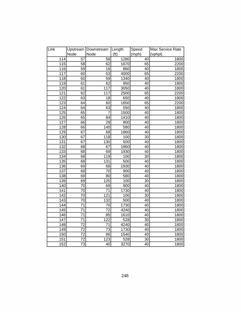
Link Upstream Downstream Length Speed Max Service Rate Node Node (ft) (mph) (vphpl)
114 57 58 1280 40 1800115 58 62 1670 65 2200116 59 16 860 40 1800117 60 53 4000 65 2200118 60 59 1340 40 1800119 61 62 950 40 1800120 61 117 3050 40 1800121 62 117 2500 65 2200122 63 18 650 40 1800123 64 60 1650 65 2200124 64 63 550 40 1800125 65 7 1500 40 1800126 65 84 1410 40 1800127 66 29 800 40 1800128 66 140 580 40 1800129 67 68 1860 40 1800130 67 118 100 30 1800131 67 130 500 40 1800132 68 67 1860 40 1800133 68 69 1930 40 1800134 68 119 100 30 1800135 68 131 500 40 1800136 69 68 1930 40 1800137 69 70 900 40 1800138 69 80 580 40 1800139 69 120 100 30 1800140 70 69 900 40 1800141 70 71 1730 40 1800142 70 121 100 30 1800143 70 132 500 40 1800144 71 70 1730 40 1800145 71 72 4240 40 1800146 71 85 1610 40 1800147 71 122 528 30 1800148 72 71 4240 40 1800149 72 73 1730 40 1800150 72 86 1540 40 1800151 72 123 528 30 1800152 73 40 3270 40 1800
248

Link Upstream Downstream Length Speed Max Service Rate Node Node (ft) (mph) (vphpl)
153 73 72 1730 40 1800154 73 74 1350 40 1800155 73 124 100 30 1800156 74 11 3270 40 1800157 74 73 1350 40 1800158 74 75 1280 40 1800159 74 125 100 30 1800160 75 74 1280 40 1800161 75 76 1350 40 1800162 75 126 100 30 1800163 75 133 100 30 1800164 76 13 3790 40 1800165 76 75 1350 40 1800166 76 77 580 40 1800167 76 175 100 30 1800168 77 76 580 40 1800169 77 78 4410 40 1800170 77 127 100 30 1800171 77 134 100 30 1800172 78 77 4410 40 1800173 78 79 2510 40 1800174 78 87 960 40 1800175 78 128 100 30 1800176 79 17 3370 40 1800177 79 78 2510 40 1800178 79 117 8040 40 1800179 79 129 100 30 1800180 80 69 580 40 1800181 80 83 1190 40 1800182 80 131 1930 40 1800183 80 132 900 40 1800184 81 1 1640 40 1800185 81 82 1990 40 1800186 81 116 2890 40 1800187 81 130 1320 40 1800188 82 3 1280 40 1800189 82 81 1990 40 1800190 82 83 1800 40 1800191 82 131 1500 40 1800
249

Link Upstream Downstream Length Speed Max Service Rate Node Node (ft) (mph) (vphpl)
192 83 5 1450 40 1800193 83 80 1190 40 1800194 83 82 1800 40 1800195 83 84 900 40 1800196 84 65 1410 40 1800197 84 83 900 40 1800198 84 85 1730 40 1800199 84 132 1730 40 1800200 85 7 1610 40 1800201 85 71 1610 40 1800202 85 84 1730 40 1800203 85 86 4240 40 1800204 86 9 1830 40 1800205 86 72 1540 40 1800206 86 85 4240 40 1800207 87 78 960 40 1800208 87 88 800 40 1800209 87 135 100 30 1800210 87 136 100 30 1800211 88 15 1350 40 1800212 88 87 800 40 1800213 88 137 100 30 1800214 88 138 100 30 1800215 89 4 390 40 1800216 89 90 1700 40 1800217 89 97 960 40 1800218 90 6 380 40 1800219 90 89 1700 40 1800220 90 91 320 40 1800221 91 90 320 40 1800222 91 140 800 40 1800223 91 144 800 40 1800224 92 8 580 40 1800225 92 140 1600 40 1800226 92 141 900 40 1800227 92 146 900 40 1800228 93 10 550 40 1800229 93 141 3830 40 1800230 93 142 960 40 1800
250

Link Upstream Downstream Length Speed Max Service Rate Node Node (ft) (mph) (vphpl)
231 93 177 800 40 1800232 94 12 480 40 1800233 94 142 1650 40 1800234 94 143 100 30 1800235 94 149 800 40 1800236 95 110 2510 40 1800237 95 149 1000 40 1800238 95 154 1650 40 1800239 96 104 2580 40 1800240 96 144 1300 40 1800241 96 151 2100 40 1800242 96 176 1300 40 1800243 97 89 960 40 1800244 97 139 2280 40 1800245 97 144 2100 40 1800246 97 151 1100 40 1800247 98 103 3400 40 1800248 98 116 2310 40 1800249 98 139 1200 40 1800250 98 151 1450 40 1800251 99 106 1280 40 1800252 99 152 1570 40 1800253 99 155 1320 40 1800254 99 176 1040 40 1800255 100 101 1280 40 1800256 100 116 5000 40 1800257 100 156 100 30 1800258 100 181 16000 40 1800259 101 100 1280 40 1800260 101 102 510 40 1800261 101 157 100 30 1800262 101 158 100 30 1800263 102 101 510 40 1800264 102 103 1410 40 1800265 102 159 100 30 1800266 102 160 100 30 1800267 103 98 3400 40 1800268 103 102 1410 40 1800269 103 104 2090 40 1800
251

Link Upstream Downstream Length Speed Max Service Rate Node Node (ft) (mph) (vphpl)
270 103 151 2300 40 1800271 103 161 100 30 1800272 104 96 2580 40 1800273 104 103 2090 40 1800274 104 105 650 40 1800275 104 162 100 30 1800276 105 104 650 40 1800277 105 106 1060 40 1800278 105 176 1650 40 1800279 106 99 1280 40 1800280 106 105 1060 40 1800281 106 107 1230 40 1800282 106 163 100 30 1800283 107 106 1230 40 1800284 107 108 3210 40 1800285 107 155 1000 40 1800286 107 164 100 30 1800287 108 107 3210 40 1800288 108 109 1610 40 1800289 108 165 528 30 1800290 108 166 100 30 1800291 109 108 1610 40 1800292 109 110 1730 40 1800293 109 154 2640 40 1800294 109 167 100 30 1800295 110 95 2510 40 1800296 110 109 1730 40 1800297 110 111 7330 40 1800298 110 168 100 30 1800299 111 110 7330 40 1800300 111 112 1930 40 1800301 111 169 3800 40 1800302 112 111 1930 40 1800303 112 113 5210 40 1800304 112 169 3800 40 1800305 112 170 528 30 1800306 113 112 5210 40 1800307 113 114 1990 40 1800308 113 172 100 30 1800
252

Link Upstream Downstream Length Speed Max Service Rate Node Node (ft) (mph) (vphpl)
309 114 16 250 40 1800310 114 113 1990 40 1800311 114 171 100 30 1800312 114 173 2800 40 1800313 115 117 2730 40 1800314 115 173 3530 40 1800315 115 174 100 30 1800316 116 1 1410 40 1800317 116 19 2000 65 2200318 116 81 2890 40 1800319 116 98 2310 40 1800320 116 100 8000 40 1800321 116 179 8000 65 2200322 117 63 3050 40 1800323 117 64 2500 65 2200324 117 79 8040 40 1800325 117 115 2730 40 1800326 117 180 5000 65 2200327 118 67 100 30 1800328 119 68 100 30 1800329 120 69 100 30 1800330 120 183 16000 30 1800331 121 70 100 30 1800332 122 71 528 30 1800333 123 72 528 30 1800334 124 73 100 30 1800335 125 74 100 30 1800336 126 75 100 30 1800337 127 77 100 30 1800338 128 78 100 30 1800339 128 183 16000 30 1800340 129 79 100 30 1800341 130 67 500 40 1800342 130 81 1320 40 1800343 130 131 1860 40 1800344 131 68 500 40 1800345 131 80 1930 40 1800346 131 82 1500 40 1800347 131 130 1860 40 1800
253

Link Upstream Downstream Length Speed Max Service Rate Node Node (ft) (mph) (vphpl)
348 132 70 500 40 1800349 132 80 900 40 1800350 132 84 1730 40 1800351 133 75 100 30 1800352 134 77 100 30 1800353 135 87 100 30 1800354 136 87 100 30 1800355 137 88 100 30 1800356 138 88 100 30 1800357 139 2 1200 40 1800358 139 97 2280 40 1800359 139 98 1200 40 1800360 140 66 580 40 1800361 140 91 800 40 1800362 140 92 1600 40 1800363 140 145 800 40 1800364 141 92 900 40 1800365 141 93 3830 40 1800366 141 147 800 40 1800367 142 93 960 40 1800368 142 94 1650 40 1800369 142 148 800 40 1800370 143 94 100 30 1800371 144 91 800 40 1800372 144 96 1300 40 1800373 144 97 2100 40 1800374 144 145 920 40 1800375 145 140 800 40 1800376 145 144 920 40 1800377 145 146 1580 40 1800378 145 176 2300 40 1800379 146 92 900 40 1800380 146 145 1580 40 1800381 146 147 900 40 1800382 146 152 1000 40 1800383 147 141 800 40 1800384 147 146 900 40 1800385 147 153 1000 40 1800386 147 177 3830 40 1800
254

Link Upstream Downstream Length Speed Max Service Rate Node Node (ft) (mph) (vphpl)
387 148 142 800 40 1800388 148 149 1650 40 1800389 148 154 1000 40 1800390 148 177 960 40 1800391 149 94 800 40 1800392 149 95 1000 40 1800393 149 148 1650 40 1800394 150 14 1600 40 1800395 151 96 2100 40 1800396 151 97 1100 40 1800397 151 98 1450 40 1800398 151 103 2300 40 1800399 152 99 1570 40 1800400 152 146 1000 40 1800401 152 153 1000 40 1800402 153 147 1000 40 1800403 153 152 1000 40 1800404 153 155 1500 40 1800405 153 178 3830 40 1800406 154 95 1650 40 1800407 154 109 2640 40 1800408 154 148 1000 40 1800409 154 178 960 40 1800410 155 99 1320 40 1800411 155 107 1000 40 1800412 155 153 1500 40 1800413 156 100 100 30 1800414 157 101 100 30 1800415 158 101 100 30 1800416 159 102 100 30 1800417 160 102 100 30 1800418 161 103 100 30 1800419 162 104 100 30 1800420 163 106 100 30 1800421 164 107 100 30 1800422 165 108 528 30 1800423 166 108 100 30 1800424 167 109 100 30 1800425 168 110 100 30 1800
255

Link Upstream Downstream Length Speed Max Service Rate Node Node (ft) (mph) (vphpl)
426 168 184 16000 30 1800427 169 111 3800 40 1800428 169 112 3800 40 1800429 169 184 16000 40 1800430 170 112 528 30 1800431 171 114 100 30 1800432 172 113 100 30 1800433 173 18 330 40 1800434 173 114 2805 40 1800435 173 115 3530 40 1800436 174 115 100 30 1800437 175 76 100 30 1800438 176 96 1300 40 1800439 176 99 1040 40 1800440 176 105 1650 40 1800441 176 145 2300 40 1800442 177 93 800 40 1800443 177 147 3830 40 1800444 177 148 960 40 1800445 177 178 960 40 1800446 178 153 3830 40 1800447 178 154 960 40 1800448 178 177 960 40 1800449 179 116 8000 65 2200450 179 181 8000 65 2200451 180 117 8000 65 2200452 180 182 11000 65 2200
256

Appendix E
Payoff Matrix for Baseline Conditions
No Evacuation λ = 0 λ = 0.5 λ = 1Link Player M Player T Player M Player T Player M Player T Player M Player T
1 100.00 0.000 98.68 1.163 99.15 0.876 99.53 0.9462 99.82 0.072 99.1 0.402 98.88 0.262 98.97 0.3333 95.42 2.506 100 0 100 0 100 04 99.15 0.379 99.27 0.518 99.94 0.074 100 05 100.00 0.000 99.07 0.663 98.9 0.949 99.41 1.0526 100.00 0.000 99.41 0.645 99.28 0.736 100 07 99.51 0.539 97.24 0.879 96.13 1.089 94.41 0.9638 98.92 0.603 98.21 0.566 96 1.355 98.23 0.549 79.17 3.359 100 0 100 0 100 0
10 78.44 2.625 99.89 0.027 99.96 0.008 99.96 0.00911 99.33 0.307 93.29 2.534 93.26 2.042 89.68 2.72512 99.51 0.539 100 0 97.03 1.233 100 013 91.02 3.844 96.23 2.901 96.95 2.28 97.84 1.23314 93.86 2.423 97.23 1.321 94.19 2.805 94.87 2.7815 92.86 2.050 93.21 2 95.88 1.191 97.72 1.6516 91.51 2.327 98.74 1.677 98.91 1.197 98.24 1.88717 86.42 1.734 96.53 2.211 92.78 2.65 91.26 2.64518 86.32 5.099 97.83 1.775 97.14 2.082 99.82 0.26519 100.00 0.000 96.89 2.571 97.26 1.508 94.08 2.46320 91.71 3.593 98.64 1.8 98.32 2.065 97.18 2.30121 93.40 3.041 99.27 3 98.99 3 99.21 322 93.62 3.079 98.95 3.4 98.84 3.167 99.21 323 96.89 1.434 99.57 0.123 99.45 0.3 94.72 1.89224 97.40 1.585 97.43 2.247 97.46 1.252 95.34 2.59625 99.57 1.000 92.82 2.758 90.57 2.222 91.79 2.85126 95.73 2.268 100 0 99.64 0.083 100 027 94.97 3.045 93.98 2 91.91 2 95.2 228 91.86 3.854 95.35 1.764 93.45 1.802 96.69 1.68329 98.17 0.948 94.37 0.97 98.8 1.104 94.84 0.83130 98.18 2.261 97.36 1.495 97.01 0.753 94.31 1.85231 94.64 2.871 95.43 1.488 94.16 2.28 94.2 232 92.40 3.629 97.59 0.67 98.15 1.456 96.91 2.06533 99.52 0.147 98.61 2 98.68 2.285 99.57 1.26834 99.52 0.147 98.61 2 96.94 3.525 98.38 1.66635 92.56 4.518 92.81 3.052 98.48 2.125 94.69 2.31936 91.34 4.817 95.53 3 92.78 4.98 94.2 237 97.63 1.022 99.68 0.286 99.68 0.131 99.72 0.167
257

No Evacuation λ = 0 λ = 0.5 λ = 1Link Player M Player T Player M Player T Player M Player T Player M Player T
38 87.91 6.156 99.3 1.178 99.22 1.001 98.89 1.28939 85.98 4.459 100 0 98.95 0.875 99.11 0.97440 82.36 6.700 99.3 1.178 98.4 1.72 98.46 1.98641 98.13 1.841 100 0 99.81 0.819 99.26 0.18442 96.68 1.048 100 0 100 0 100 043 75.25 11.692 89.52 7.688 88.46 8.696 89.75 7.68344 84.71 2.595 95.04 1.29 95.78 2.985 95.55 1.34845 86.96 5.246 98.28 2 99.53 1.268 98.23 2.10846 90.98 0.345 94.81 3.118 96.8 3.8 93.44 3.98747 87.55 5.346 97.64 4.411 95 6.617 97.62 3.88448 70.23 11.363 90.05 7 88.48 8.638 89.34 9.05149 88.19 0.860 98.53 2.079 96.44 2.444 95.63 3.31550 95.80 0.902 95.99 1.114 96.27 2.013 99.43 0.63451 98.16 0.466 100 0 100 0 100 052 99.37 0.096 99.04 1.347 97.2 2.401 99.33 1.26253 97.71 0.862 98.96 1.88 98.74 2.543 99.52 2.21654 83.77 3.185 99.51 0.213 96.75 1.352 95.86 2.13955 99.51 0.539 100 0 100 0 100 056 97.28 0.994 80.96 3.679 81.67 4.142 85.24 4.38657 99.34 0.612 98.26 0.558 96.19 0.847 98.27 0.5358 99.49 0.025 79.84 5.091 89.66 3.937 78.42 4.65459 99.33 0.307 100 0 100 0 99.88 0.01760 100.00 0.000 93.29 3.325 93.26 2.042 89.8 2.61861 100.00 0.000 93.37 1 96.03 1 97.86 162 97.28 0.994 87.58 2.679 85.64 3.142 87.38 3.38663 98.92 0.339 91.39 1.604 91.66 2.414 96.02 1.56664 99.49 0.025 86.55 3.07 96.4 1.884 88.62 2.03665 86.53 1.734 97.85 1.581 95.12 1.898 95.52 1.45266 99.49 0.025 98.64 0.638 97.61 0.761 95.7 1.20367 94.86 1.229 97.23 1.321 94.82 1.996 96.06 1.7868 99.00 0.203 99.68 0.4 98.77 1.475 98.12 1.83369 92.14 2.221 84.82 4 80.46 5.138 83.44 5.16770 75.39 5.879 99.54 0.445 96.23 2.354 91.96 3.20471 100.00 0.000 87.91 2.433 98.78 1.229 92.92 0.83472 95.30 0.707 99.54 0.445 97.56 1.079 97.44 1.13373 92.87 1.666 98.48 2 98.32 2.065 97.18 2.30174 98.84 0.584 100 0 100 0 100 075 85.01 3.888 83.3 6 78.79 7.203 80.62 7.46776 88.43 7.397 98.95 3.4 98.84 3.167 99.02 3.522
258

No Evacuation λ = 0 λ = 0.5 λ = 1Link Player M Player T Player M Player T Player M Player T Player M Player T
77 95.30 0.707 87.44 2.878 96.35 2.202 90.36 1.96678 90.26 6.433 99.11 3.2 98.99 3 99.02 3.52279 100.00 0.000 94.2 1 92.22 1 95.3 180 85.01 3.888 89.1 5 86.57 6.203 85.32 6.46781 98.84 0.584 94.2 1 92.22 1 95.3 182 85.56 6.989 86.55 6.078 95.33 5.202 89.37 5.48983 98.17 0.948 99.84 0.2 99.85 0.167 100 084 100.00 0.000 94.21 1.771 98.8 1.104 94.84 0.83185 98.29 0.325 97.4 1 94.77 2 94.2 286 86.72 3.707 91.7 4 91.8 4.203 91.12 4.46787 94.84 2.123 97.4 1 93.49 2.297 92.48 3.19888 99.01 0.050 100 0 100 0 100 089 85.56 6.989 92.33 5.306 96.53 4.162 94.54 4.65890 93.52 4.703 99.58 1.052 98.83 2 99.16 1.18491 98.89 0.449 93.23 2 99.64 0.189 95.52 1.13592 99.15 0.770 97.59 0.658 98 1.518 96.91 2.05493 92.58 2.844 100 0 100 0 100 094 85.86 4.477 89.29 4.658 89.8 5.722 88.03 6.52195 97.02 0.588 100 0 100 0 99.96 0.02696 88.84 3.889 89.29 4.658 89.8 5.722 88.07 6.49597 89.60 3.432 100 0 100 0 99.96 0.02698 89.26 6.952 97.92 3 97.86 3.943 99.12 1.21999 86.67 6.690 99.11 3.306 96.89 3.973 99.02 3.522
100 92.50 4.749 97.92 3 98.34 3 99.86 1.035101 91.14 3.340 91.7 4 91.65 4.11 92.74 4102 97.70 0.540 97.59 0.658 98.15 1.611 95.33 2.495103 73.62 9.767 90.51 5.869 89.97 5.821 90.92 6.043104 82.01 6.823 99.3 1.178 98.22 2.539 97.72 2.17105 79.17 11.005 97.02 6.306 95.23 6.973 98.87 4.557106 90.99 4.289 99.3 1.178 98.22 2.539 98.68 1.624107 70.16 15.215 96.32 7.485 93.45 9.513 97.56 6.181108 91.02 2.635 100 0 100 0 99.04 0.547109 96.28 3.705 96.48 6.635 93.6 8.782 97.74 5.098110 97.92 0.511 99.56 0.199 98.64 0.513 96.66 1.669111 99.79 0.038 98.03 0.459 99.52 1.16 98.67 0.827112 78.06 5.392 93.81 2.689 93.67 4.268 91.97 4.205113 87.08 0.942 95.98 2.181 96.54 1.686 96.42 2.852114 90.97 3.070 97.84 0.508 97.13 2.589 95.55 1.338
259

No Evacuation λ = 0 λ = 0.5 λ = 1Link Player M Player T Player M Player T Player M Player T Player M Player T115 90.77 3.108 95.86 0.953 96.65 3.666 94.22 2.161116 80.36 3.743 98.44 2.417 97.81 3.232 98.47 2.954117 73.88 11.488 99.84 0.85 99.85 0.731 99.81 1.083118 91.67 1.933 99.95 0.108 99.82 0.379 99.93 0.154119 95.86 0.785 95.89 1.56 96.04 2.607 99.31 0.874120 99.38 0.157 99.95 0.012 99.95 0.017 100 0121 86.63 3.891 91.75 2.483 92.68 5.217 93.53 3.023122 93.74 2.731 100 0 100 0 100 0123 65.55 13.712 99.79 0.958 99.67 1.11 99.75 1.237124 98.58 1.038 100 0 100 0 100 0125 94.48 1.149 98.43 1.902 98.49 1.598 98.61 1.649126 99.81 0.032 100 0 99.37 0.809 98.82 1127 80.09 4.363 100 0 98.67 1.275 94.52 2.071128 98.96 1.052 99.57 0.123 100 0 100 0129 98.21 0.781 100 0 100 0 100 0130 100.00 0.000 100 0 100 0 100 0131 99.82 0.024 99.52 1 99.83 0.114 99.94 0.04132 99.82 0.024 99.52 1 99.83 0.114 99.94 0.04133 95.43 1.252 100 0 100 0 100 0134 98.96 0.459 100 0 100 0 100 0135 97.97 0.814 100 0 96.74 0.896 100 0136 100.00 0.000 99.52 1 96.56 1.01 99.94 0.04137 93.97 3.483 93.79 0.937 96.26 0.943 98.01 0.929138 98.92 0.147 97.3 1.91 97.78 1.648 95.38 1.487139 98.07 1.040 100 0 99.81 0.198 100 0140 97.07 0.405 93.91 3.91 94.24 3.244 95.31 1.777141 94.37 2.800 92.65 2.538 94.42 3.891 95.77 3.947142 99.88 0.020 97.25 1.135 98.26 1.27 94.4 1.554143 94.75 1.066 95.32 2.7 98.24 1.708 96.76 1.681144 92.34 1.213 92.94 5.598 92.15 5.838 92.34 3.204145 98.97 0.211 98.39 2.131 99.56 1.087 98.06 1.193146 94.48 1.991 98 1.645 97.61 2.599 92.62 3.957147 92.95 4.000 91.43 6 93.61 7 95.29 7148 91.32 2.123 95.17 2.836 95.87 3.633 98.58 2.069149 100.00 0.000 98.7 1.556 97.07 2.25 96.31 3.375150 99.42 1.027 93.93 2.806 94.9 1.204 94.05 2.302151 94.16 3.000 93.43 4 91.6 3 93.85 4152 99.82 0.040 100 0 99.08 0.213 98.28 1.198
260

No Evacuation λ = 0 λ = 0.5 λ = 1Link Player M Player T Player M Player T Player M Player T Player M Player T153 90.50 3.507 99.74 1.067 99.85 1 99.59 1.553154 100.00 0.000 98.92 1.199 98.65 1.037 98.77 1.138155 99.82 0.040 99.63 0.43 100 0 99.7 0.229156 94.32 4.112 95.62 1.659 99.12 0.438 98.63 0.856157 90.50 3.507 99.65 1.132 99.85 1 99.85 1.35158 99.51 0.112 99.35 1 97.78 2.16 98.97 1159 99.51 0.084 97.13 1.21 98.5 1.431 99.54 0.607160 83.25 8.129 98.03 0.308 98.51 0.906 97.99 1.523161 98.09 1.131 99.06 0.152 98.81 0.287 99.6 0.201162 100.00 0.000 100 0 100 0 99.06 0.422163 99.43 0.350 99.78 0.333 99.32 0.775 99.78 0.169164 97.88 1.384 100 0 99.77 0.148 99.58 0.25165 83.25 8.129 100 0 98.95 0.875 98.97 1.082166 99.49 0.372 99.06 0.152 98.9 0.286 99.32 0.367167 99.31 0.365 100 0 99.96 0.011 100 0168 97.43 2.990 100 0 100 0 99.86 0.108169 99.34 0.468 99.06 0.152 98.9 0.286 99.32 0.367170 100.00 0.000 100 0 100 0 100 0171 100.00 0.000 100 0 100 0 100 0172 97.43 2.990 100 0 100 0 99.86 0.108173 99.51 0.411 100 0 100 0 100 0174 97.37 1.919 98.37 0.791 98.6 0.953 99.32 0.367175 99.88 0.093 100 0 100 0 100 0176 97.08 0.898 99.24 0.267 99.35 0.501 99.16 0.5177 96.55 4.156 99.31 0.639 99.7 0.667 100 0178 94.70 3.195 99.95 0.009 99.96 0.011 99.96 0.02179 97.87 0.717 100 0 99.95 0.001 100 0180 97.63 1.512 93.65 0.967 96.26 0.943 98.01 0.929181 93.57 1.018 96.6 2.726 97.55 1.429 93.13 1.93182 100.00 0.000 97.41 1.637 99.29 0.261 100 0183 99.65 0.048 99.43 1.063 99.62 0.248 99.71 0.721184 100.00 0.000 98.39 1.433 99.18 0.835 99.49 0.969185 99.15 0.424 99.55 0.416 99.05 0.737 98.85 0.671186 100.00 0.000 97.91 1.247 97.93 1.447 99.88 0.05187 96.09 2.200 100 0 100 0 100 0188 99.82 1.000 97.24 0.879 95.98 1.589 94.41 0.963189 100.00 0.000 98.95 0.287 99.23 0.477 99.65 0.206190 96.09 2.200 99.16 0.916 98.9 1.237 98.85 0.671
261

No Evacuation λ = 0 λ = 0.5 λ = 1Link Player M Player T Player M Player T Player M Player T Player M Player T191 96.09 1.162 100 0 100 0 100 0192 87.31 4.484 96.22 3.477 96.45 2.665 96.17 2.21193 92.34 2.308 93.21 2 95.71 1.721 97.72 1.65194 99.76 0.033 98.22 0.529 98.21 1.337 94.06 1.168195 94.30 0.995 100 0 100 0 100 0196 95.30 0.979 98.75 1.502 99.09 0.931 99.31 0.816197 91.95 2.419 98.67 0.365 98.04 1.866 98.25 0.777198 98.98 0.300 100 0 100 0 99.13 0.287199 96.71 0.752 97.28 1.11 99.37 0.809 98.62 1.492200 97.01 1.097 97.57 1.768 97.49 1.489 92.79 2.866201 96.20 2.256 99.27 3 98.86 3.25 98.58 4.297202 91.18 2.704 97 1.188 98.59 0.978 98.47 0.993203 98.76 0.425 100 0 100 0 99.71 0.084204 99.57 1.000 97.36 1.495 96.66 0.837 95.05 1.668205 95.44 2.789 93.98 2 91.91 2 95.2 2206 97.01 1.096 96.57 1.312 98.24 0.367 98.72 0.718207 98.75 0.576 100 0 100 0 99.86 0.108208 97.37 1.919 98.18 0.971 98.07 1.292 99.32 0.367209 100.00 0.000 100 0 100 0 100 0210 100.00 0.000 100 0 100 0 100 0211 82.33 8.256 97.42 2.071 96.9 2.442 98.89 1.517212 98.75 0.576 100 0 100 0 98.97 1.218213 94.99 1.682 98.48 1.056 99.61 0.343 99.45 0.419214 99.79 0.075 99.92 0.158 99.62 0.84 99.44 0.654215 91.24 1.333 98.16 0.872 99.15 0.275 99.7 0.319216 99.16 0.611 100 0 100 0 100 0217 100.00 0.000 100 0 97.75 0.994 100 0218 97.69 1.241 97.86 1.743 95.65 1.296 99.52 0.36219 93.95 0.720 100 0 100 0 99.82 0.126220 85.84 4.951 98.23 1.487 96.95 2.138 99.82 0.265221 91.99 1.907 98.84 1.352 95.8 1.265 99.64 0.416222 94.85 3.085 99.65 0.345 100 0 100 0223 94.72 1.625 98.18 1.615 96.99 2.111 99.82 0.265224 99.27 0.151 99.95 0.1 99.41 0.364 96.04 1.75225 94.97 1.755 99.6 0.474 99.01 0.207 99.29 1.257226 96.98 4.000 97.58 1.878 99.04 0.681 97.2 0.89227 99.72 0.107 99.9 0.269 100 0 98.9 0.366228 95.13 1.453 94.57 1.52 99.66 0.144 94.84 0.831
262

No Evacuation λ = 0 λ = 0.5 λ = 1Link Player M Player T Player M Player T Player M Player T Player M Player T229 95.53 1.560 99.6 0.474 100 0 100 0230 100.00 0.000 99.66 0.275 99.05 0.39 99.3 0.517231 98.84 2.000 98.15 0.887 97.46 0.726 97.24 1.025232 99.52 0.089 93.61 3.052 97.61 3.285 95.14 2.368233 98.26 2.989 95.55 1.509 99.42 0.54 97.62 0.256234 100.00 0.000 94.04 2 97.16 2.018 93.39 2.338235 93.56 4.488 95.94 2.491 93.11 4.48 97.08 1.023236 99.10 3.119 94.66 2.808 93.85 1.732 94.48 2.215237 94.74 2.014 97.15 2.877 98.68 2.285 99.42 1.896238 85.54 3.814 99.03 0.967 99.55 0.667 100 0239 100.00 0.000 100 0 100 0 100 0240 98.33 1.137 99.69 1.114 99.61 0.266 99.88 0.029241 98.81 0.038 99.86 0.103 99.34 0.298 99.73 0.066242 99.84 0.006 93.99 2.962 92.27 2.029 98.24 1.25243 96.94 0.685 98.16 0.872 99.87 0.036 99.88 0.193244 100.00 0.000 100 0 100 0 100 0245 100.00 0.000 100 0 99.85 0.021 100 0246 100.00 0.000 99.61 1 100 0 100 0247 100.00 0.000 100 0 99.85 0.333 99.86 0.25248 99.33 0.137 98.27 1.671 95.98 1.692 97.07 1.388249 100.00 0.000 100 0 99.74 0.073 100 0250 99.20 0.076 95.35 1.346 93.27 0.955 98.38 1251 100.00 0.000 99.03 0.865 99.77 0.04 99.92 0.05252 100.00 0.000 100 0 100 0 100 0253 100.00 0.000 94.77 2.135 92.21 2.655 98.04 1.7254 96.39 1.253 99.41 1.257 96.12 2.11 99.61 0.095255 99.60 0.405 100 0 100 0 100 0256 97.17 1.863 100 0 100 0 100 0257 98.36 0.390 100 0 100 0 100 0258 100.00 0.000 100 0 100 0 100 0259 98.63 1.152 100 0 100 0 100 0260 99.60 0.405 100 0 100 0 100 0261 100.00 0.000 100 0 100 0 100 0262 100.00 0.000 100 0 100 0 100 0263 99.20 1.036 100 0 100 0 100 0264 99.60 0.405 100 0 100 0 100 0265 100.00 0.000 100 0 100 0 100 0266 100.00 0.000 100 0 100 0 100 0
263

No Evacuation λ = 0 λ = 0.5 λ = 1Link Player M Player T Player M Player T Player M Player T Player M Player T267 100.00 0.000 99.04 0.724 97.27 0.856 97.58 0.797268 99.82 0.036 100 0 100 0 100 0269 100.00 0.000 100 0 99.85 0.333 99.86 0.25270 98.76 0.576 100 0 100 0 100 0271 99.82 0.036 100 0 97.63 0.737 99.8 0.323272 100.00 0.000 100 0 100 0 100 0273 100.00 0.000 99.04 0.724 97.27 0.856 97.58 0.797274 100.00 0.000 100 0 99.85 0.333 99.86 0.25275 100.00 0.000 97.2 1.174 99.29 0.248 97.24 0.957276 100.00 0.000 95.75 2.724 96.91 0.991 94.53 1.951277 100.00 0.000 100 0 99.85 0.333 99.86 0.25278 100.00 0.000 100 0 99.76 0.114 100 0279 100.00 0.000 99.77 1.052 99.7 0.145 100 0280 100.00 0.000 95.75 2.724 96.67 1.104 94.53 1.951281 100.00 0.000 99.03 0.865 99.62 0.373 99.78 0.3282 100.00 0.000 99.9 0.174 100 0 100 0283 100.00 0.000 95.52 3.775 96.84 1.022 94.53 1.951284 97.73 3.000 93.51 3.731 91.67 3.133 93.39 3.917285 95.89 1.420 98.87 1.036 95.82 2.295 95.18 2.24286 100.00 0.000 99.92 0.053 97.63 0.824 99.42 0.384287 95.89 1.420 94.39 4.811 92.51 3.421 89.05 4.925288 100.00 0.000 95.13 3.117 96.41 2.8 95.56 4.351289 89.15 5.000 91.42 7 90.91 5 90.4 4290 93.11 5.000 95.84 3.748 95.84 3.523 92.96 2.953291 89.23 5.493 97.31 4.269 98.43 3.027 95.61 2.294292 100.00 0.000 96.24 2.957 95.01 3.036 95.36 3.708293 90.60 1.468 100 0 98.57 0.773 99.38 0.536294 98.04 3.000 96.77 1.687 97.73 0.66 97.06 1.317295 81.72 5.533 97.15 2.877 98.68 2.285 98.72 2.283296 87.78 3.969 98.76 2.753 98.88 2.181 95.6 2.297297 99.34 3.000 92.06 4.801 89.27 4.624 91.26 5.361298 85.59 3.327 98.61 2.301 97.43 1.581 98.06 2.284299 68.14 8.738 97.04 5.694 97.57 4.493 94.76 6.177300 99.66 2.000 91.76 4.269 92.96 4.517 91.6 6.262301 86.28 2.912 94.22 2.833 88.87 4.329 95.45 2.754302 69.84 8.617 93.29 5.641 94.13 5.486 92.49 6.497303 99.93 0.028 93.61 3.844 89.05 8.655 92.36 5.117304 85.66 5.853 97.55 1.721 97.76 2.603 94.81 4.545
264

No Evacuation λ = 0 λ = 0.5 λ = 1Link Player M Player T Player M Player T Player M Player T Player M Player T305 88.70 9.000 81.89 9.491 77.17 12.8 78.02 13.36306 51.37 16.681 89.54 6.504 83.07 11.77 84.8 10.96307 95.54 1.412 93.7 3.511 91.96 6.211 89.9 5.09308 98.57 0.155 98.74 1.035 97.64 1.078 97.01 1.305309 93.14 1.687 93.55 5.737 93.9 7.469 91.77 6.626310 52.05 16.374 89.72 6.199 85.98 9.376 85.15 10.639311 99.22 0.157 98.88 0.739 97.46 2.469 97.72 1.41312 100.00 0.000 98.94 0.287 97.43 1.587 97.35 0.311313 92.08 5.994 99.53 0.589 99.95 0.5 97.64 1.232314 97.92 1.366 100 0 99.09 2 99.52 2315 95.29 1.869 100 0 100 0 100 0316 99.38 1.000 100 0 100 0 100 0317 96.97 1.461 80.96 3.679 81.67 4.142 85.24 4.386318 99.88 0.004 100 0 100 0 100 0319 99.45 0.026 95.22 1.637 93.06 1.377 98.2 1.429320 100.00 0.000 100 0 100 0 100 0321 100.00 0.000 74.95 8.184 82.08 8.29 74.53 7.717322 96.69 1.463 100 0 100 0 100 0323 66.30 15.388 99.79 0.958 99.67 1.11 99.75 1.237324 99.07 0.322 100 0 100 0 100 0325 98.66 0.361 100 0 100 0 99.81 1326 100.00 0.000 91.29 3.205 92.74 5.704 91.3 3.555327 100.00 0.000 100 0 100 0 100 0328 98.96 0.459 100 0 100 0 100 0329 97.90 1.064 100 0 99.81 0.198 100 0330 100.00 0.000 100 0 100 0 100 0331 99.88 0.020 97.25 1.135 98.26 1.27 94.5 1.554332 100.00 0.000 93.58 7 93.66 6 85.19 6333 100.00 0.000 89.23 6 88.12 6 89.94 7334 99.82 0.040 99.77 0.14 100 0 99.7 0.229335 99.51 0.084 97.13 1.21 98.5 1.431 99.54 0.607336 100.00 0.000 100 0 99.48 0.033 99.06 0.422337 100.00 0.000 100 0 100 0 100 0338 99.88 0.093 100 0 100 0 100 0339 100.00 0.000 100 0 100 0 100 0340 97.87 0.717 100 0 99.95 0.001 100 0341 98.56 0.733 100 0 100 0 100 0342 100.00 0.000 98.96 1 98.7 0.513 99.94 0.04
265

No Evacuation λ = 0 λ = 0.5 λ = 1Link Player M Player T Player M Player T Player M Player T Player M Player T343 97.36 1.490 100 0 100 0 100 0344 95.61 1.228 100 0 100 0 100 0345 99.47 0.072 100 0 100 0 100 0346 96.09 2.199 97.97 0.637 97.15 0.758 100 0347 100.00 0.000 99.44 1 98.87 0.399 100 0348 99.08 0.162 95.56 3.395 98.66 1.948 98.27 2.382349 97.98 0.497 97.38 0.831 99.03 0.497 98.21 0.638350 94.05 1.208 98.61 0.749 99.55 0.32 98.81 0.381351 99.43 0.350 100 0 99.43 0.033 99.74 0.189352 100.00 0.000 100 0 100 0 100 0353 100.00 0.000 100 0 100 0 100 0354 100.00 0.000 100 0 100 0 100 0355 94.99 1.682 99.67 0.056 99.25 0.282 99.58 0.25356 99.79 0.075 99.34 0.108 99.58 0.031 99.67 0.149357 100.00 0.000 99.8 0.145 99.02 0.809 100 0358 100.00 0.000 100 0 100 0 100 0359 100.00 0.000 99.5 0.553 99.59 0.406 99.8 0.347360 82.40 2.846 100 0 99.37 0.809 99.94 0.013361 95.47 1.881 99.02 0.637 97.59 0.605 99.88 0.193362 97.97 2.000 100 0 100 0 100 0363 98.17 1.443 99.81 0.038 100 0 99.29 1.257364 94.95 1.832 99.6 0.474 100 0 97.27 0.668365 98.26 0.856 99.58 0.233 99.49 0.362 99.67 0.094366 96.32 5.110 98 1.645 99.55 0.32 97.52 0.796367 97.18 1.257 95.38 1.152 99.87 0.04 97.62 0.256368 100.00 0.000 99.66 0.275 99.1 0.495 98.93 1369 98.82 2.000 99.6 0.509 98.6 0.89 99.47 0.358370 100.00 0.000 91.15 1 98.73 1.018 93.32 0.781371 98.33 1.137 99.42 1.189 98.21 0.66 99.76 0.223372 100.00 0.000 99.03 0.615 98.8 1.132 99.86 0.25373 100.00 0.000 98.16 0.872 99.87 0.036 99.88 0.193374 100.00 0.000 100 0 98.28 1.065 99.6 0.693375 82.84 1.613 99.85 0.04 97.95 1.207 99.88 0.193376 96.51 0.754 100 0 100 0 99.29 1.257377 99.03 1.224 100 0 100 0 100 0378 100.00 0.000 99.81 0.038 99.7 0.667 99.72 0.5379 100.00 0.000 100 0 100 0 98.82 1380 80.21 3.618 100 0 100 0 100 0
266

No Evacuation λ = 0 λ = 0.5 λ = 1Link Player M Player T Player M Player T Player M Player T Player M Player T381 99.20 1.122 99.9 0.269 100 0 99.17 0.274382 99.83 0.073 100 0 100 0 99.72 0.092383 97.58 1.163 100 0 100 0 97.27 0.668384 81.62 1.718 100 0 100 0 98.82 1385 96.89 5.000 99.45 1.074 100 0 96.52 1.092386 99.12 0.577 98.45 0.84 100 0 99.44 0.162387 97.74 0.268 99.42 0.152 99.1 0.495 99.1 0.841388 100.00 0.000 99.88 0.056 99.08 0.505 99.61 0.224389 94.94 3.356 97.24 1.864 95.4 2.598 98.94 0.614390 94.64 0.763 100 0 100 0 99.94 0.013391 99.15 1.415 97.53 2.777 96.7 3.79 98.9 1.982392 98.14 1.251 96.11 2.204 94.81 1.827 96.91 1.224393 91.87 2.670 99.12 0.495 99.55 0.833 100 0394 97.81 0.651 100 0 100 0 100 0395 99.84 0.006 94.96 2.346 93.47 0.897 98.38 1396 96.94 0.685 100 0 100 0 100 0397 99.82 0.036 99.86 0.103 99.13 0.356 99.73 0.066398 100.00 0.000 100 0 100 0 100 0399 99.25 0.078 100 0 100 0 100 0400 98.87 0.311 100 0 100 0 100 0401 99.83 0.073 100 0 100 0 99.72 0.092402 94.94 1.249 100 0 99.7 0.165 96.08 1.668403 98.12 0.388 100 0 100 0 100 0404 97.73 3.000 99.72 0.731 100 0 96.24 1.184405 97.80 2.073 98.97 1.174 99.7 0.165 99.49 0.477406 99.52 2.000 97.58 1.572 98.59 0.571 98.27 0.604407 92.06 5.000 96.78 2.818 96.12 2.864 99 0.533408 96.94 0.375 100 0 98.78 0.67 99.38 0.536409 79.94 3.928 100 0 99.79 0.104 100 0410 97.14 1.175 99.63 0.206 96.42 1.965 99.61 0.095411 97.73 3.000 94.48 2.865 92.21 2.655 94.28 2.884412 98.74 0.245 99.24 0.83 99.4 0.33 95.57 2.145413 98.36 0.390 100 0 100 0 100 0414 100.00 0.000 100 0 100 0 100 0415 100.00 0.000 100 0 100 0 100 0416 100.00 0.000 100 0 100 0 100 0417 100.00 0.000 100 0 100 0 100 0418 99.82 0.036 100 0 97.63 0.737 99.8 0.323
267

No Evacuation λ = 0 λ = 0.5 λ = 1Link Player M Player T Player M Player T Player M Player T Player M Player T419 100.00 0.000 97.47 0.941 99.79 0.072 97.78 0.721420 100.00 0.000 99.9 0.174 100 0 100 0421 100.00 0.000 99.92 0.053 97.63 0.824 99.42 0.384422 100.00 0.000 89.95 7 89.56 6 87.81 7423 93.11 5.000 95.84 3.748 95.92 3.054 91.01 3.359424 98.04 3.000 96.92 1.395 97.73 0.66 97.06 1.317425 85.59 3.328 98.7 1.442 97.93 0.487 98.56 1.202426 100.00 0.000 99.81 1.059 99.48 1.102 99.22 1.164427 84.90 2.614 98.68 3.465 96.39 2.459 97.69 4.574428 94.17 1.665 94.04 3.185 93.63 4.846 97.06 2.449429 100.00 0.000 96.32 0.861 97.91 2.296 96.66 1.067430 100.00 0.000 90.8 7.206 88.77 8.796 85.32 9.559431 99.78 0.070 98.88 0.739 97.46 2.469 97.72 1.41432 98.57 0.155 98.74 1.035 97.7 1.026 94.8 1.537433 98.93 0.587 99.26 0.711 96.43 3.517 99.22 1.63434 79.06 5.175 99.56 0.199 97.35 1.738 95.72 2.588435 98.48 0.292 99.58 0.089 100 0 97.78 0.232436 95.29 1.869 100 0 100 0 100 0437 99.31 0.365 100 0 99.96 0.011 100 0438 96.39 1.253 99.55 1.218 96.51 1.415 99.61 0.095439 100.00 0.000 93.8 3 91.97 2.695 97.96 1.75440 100.00 0.000 100 0 100 0 100 0441 100.00 0.000 99.85 0.04 99.37 0.809 100 0442 95.40 0.644 99.66 0.275 99.79 0.104 99.77 0.172443 84.74 1.024 100 0 100 0 99.26 0.184444 99.69 0.467 97.82 1.068 96.65 1.205 98.75 0.798445 98.69 2.000 98.78 0.659 99.76 0.171 98.33 0.523446 93.13 2.392 100 0 100 0 100 0447 97.36 3.134 98.09 1.558 99.76 0.171 98.33 0.523448 85.93 0.855 99.66 0.275 99.49 0.269 99.49 0.477449 100.00 0.000 100 0 100 0 100 0450 100.00 0.000 74.95 8.184 82.08 8.29 74.53 7.717451 100.00 0.000 100 0 100 0 100 0452 100.00 0.000 91.29 3.205 92.74 5.704 91.3 3.555
268

Bibliography
Aggarwal, K.K. (1985). Integration of Reliability and Capacity in Performance
Measure of a Telecommunication Network. IEEE Transactions on
Reliability. Vol. R-34, No. 2, pp. 184-186.
Ardekani, S.A. and A.G. Hobeika (1988). Logistics Problems in the Aftermath of
the 1985 Mexico City Earthquake. Transportation Quarterly. Vol. 42, No. 1,
pp. 107-124.
Asakura, Y. (1999) Evaluation of Network Reliability Using Stochastic User
Equilibrium. Journal of Advanced Transportation. Vol. 33, No. 2, pp. 147-
158.
Baker, E.K. and J.R. Schaffer. (1986). Solution Improvement Heuristics for the
Vehicle Routing and Scheduling Problem with Time Window Constraints.
American Journal of Mathematical and Management Sciences. Vol. 6, Nos. 3,
4, pp. 261-300.
Ball, M.O., Golden, B.L., and R.V. Vohra. (1989) Finding the Most Vital Arcs in
a Network. Operations Research Letters. Vol. 8, April, pp. 73-76.
Bell, M.G.H. (1999). Measuring Network Reliability: A Game Theoretic
Approach. Journal of Advanced Transportation. Vol. 33, No. 2, pp. 135-146.
Bell, M.G.H. (2000). A Game Theory Approach to Measuring Performance
Reliability of Transport Networks. Transportation Research Part B. Vol. 34,
pp. 533-545.
Ben-Akiva, M. and S.R. Lerman. (1985). Discrete Choice Analysis: Theory and
Application to Travel Demand. Cambridge, Massachusetts: MIT Press.
Bertsimas, D. and J.N. Tsitsiklis. (1997). Introduction to Linear Optimization.
Belmont, Massachusetts: Athena Scientific.
269

Brams, S.J. and D.M. Kilgour (1988). Game Theory and National Security. New
York: Basil Blackwell Inc.
Brand, D. (1984). The Transportation Assumptions of Crisis Relocation Planning.
The Counterfeit Ark: Crisis Relocation for Nuclear War. Edd. J. Leaning and
L. Keyes. Cambridge, Massachusetts: Ballinger Publishing Company, pp. 79-
117.
Brock, H. (1980). The Problem of ‘Utility Weights’ in Group Preference
Aggregation. Operations Research. Vol. 28, No. 1, pp. 176-187.
Caccetta, L. (1984). Vulnerability of Telecommunications Networks. Networks.
Vol. 14, pp. 141-146.
Cassir, C. and M. Bell (2000). The N+M Person Game Approach to Network
Reliability. Reliability of Transport Networks. England: Research Studies
Press Ltd., pp. 91-102.
Census 2000 data. Accessed July 1, 2003.
http://factfinder.census.gov/bf/_lang=en_vt_name=DEC_2000_SF1_U_GCTP
7_ST7_geo_id=04000US48.html
Chen, A., Yang, H., Lo, H.K., and W.H. Tang (1999). A Capacity Related
Reliability for Transportation Networks. Journal of Advanced Transportation.
Vol. 33, No. 2, pp. 183-200.
Clarke, G. and J.W. Wright (1963). Scheduling of Vehicles from a Central Depot
to a Number of Delivery Points. Operations Research. Vol. 12, pp. 568-581.
Comfort, L. K. (2000). Information Technology and Efficiency in Disaster
Response: The Marmara, Turkey Earthquake, 17 August 1999. In Quick
Response Report http://www.colorado.edu/hazards/qr/qr130/qr130.html. Vol.
130, October 8th.
Corley, H.W. and D.Y. Sha (1982). Most Vital Links and Nodes in Weighted
Networks. Operations Research Letters. Vol. 1, No. 4, pp. 175-180.
270

Desrochers, M., Lenstra, J.K., Savlesbergh, M.W.P., and F. Soumis (1988).
Vehicle Routing with Time Windows: Optimization and Approximation.
Vehicle Routing: Methods and Studies. North-Holland: Elsevier Science
Publishers, B.V.
Dow, K. and S.L. Cutter (2002). Emerging Hurricane Evacuation Issues:
Hurricane Floyd and South Carolina. Natural Hazards Review.February, pp.
12-18.
Fort Worth Independ School Directory.
http://www.fortworthisd.org/
ent School District (2003).
accessed July 1, 2003.
Fritz, C.E. and J.H. Mathewson (1957). Convergence Behavior in Disasters: A
Problem in Social Control. Publication 476. National Academy of Sciences –
National Research Council. Washington, D. C.
Gillespie, D.F. et al. (1993). Partnerships for Community Preparedness. Program
on Environment and Behavior Monograph No. 54. Institute of Behavioral
Science, University of Colorado.
Gillespie, D.F. and R.W. Perry (1976). An Integrated Systems and Emergent
Norm Approach to Mass Emergencies. Mass Emergencies. Vol. 1, No. 4, pp.
303-312.
Golden, B.L. and A.A. Assad (1986). Vehicle Routing with Time-Window
Constraints. American Journal of Mathematical and Management Sciences.
Vol. 6, Nos. 3,4, pp. 251-260.
Harsanyi, J.C. (1955). Cardinal Welfare, Individualistic Ethics, and Interpersonal
Comparisons of Utility. The Journal of Political Economy. Vol. 63, No. 4, pp.
309-321.
Herr, P. (1984). Alarms of Struggle and Flight: Citizen Response to Crisis
Relocation. The Counterfeit Ark: Crisis Relocation for Nuclear War. Edd. J.
Leaning and L. Keyes. Cambridge, Massachusetts: Ballinger Publishing
Company, pp. 63-78.
271

Iida, Y. (1999). Basic Concepts and Future Directions of Road Network
Reliability Analysis. Journal of Advanced Transportation. Vol. 33, No. 2, pp.
125-134.
Iida, Y. and H. Wakabayashi (1989). An Approximation Method of Terminal
Reliability of Road Network Using Partial Minimum Path and Cut Sets.
Transport Policy, Management, and Technology Towards 2001: Selected
Proceedings of the Fifth World Conference on Transport Research. Ventura,
California: Western Periodicals Co.
Jensen, P.A. (2000). Network Flow Programming Methods. Network Flow
Programming. Austin, Texas.
Kantor, P. and R.J. Nelson (1979). Social Decision Making in the Presence of
Complex Goals, Ethics and the Environment. Theory and Decision. Vol. 10,
pp. 181-200.
Karbowicz, C.J. and J. MacGregor Smith (1983). A k-Shortest Paths Routing
Heuristic for Stochastic Network Evacuation Models.
Keeney, R. and H. Raiffa (1976). Decisions with Multiple Objectives. New York:
John Wiley & Sons.
Kolen, A.W.J., Rinnooy Kan, A.H.G., and H.W.J.M. Trienekens (1987). Vehicle
Routing with Time Windows. Operations Research. Vol. 35, No. 2, pp. 266-
273.
Laporte, G., Desrochers, M., and Y. Nobert (1984). Two Exact Algorithms for
the Distance-Constrained Vehicle Routing Problem. Networks. Vol. 14, pp.
161-172.
Lee, D-H. and Y. Nie (2001). Accelerating Strategies and Computational Studies
of the Frank-Wolfe Algorithm for the Traffic Assignment Problem.
Transportation Research Record. Vol. 1771, pp. 97-105.
Lee, S.H. (1980). Reliability Evaluation of a Flow Network. IEEE Transactions
on Reliability. Vol. R-29, No. 1, pp. 24-26.
272

Lin, S. and B.W. Kernighan (1972). An Effective Heuristic Algorithm for the
Traveling-Salesman Problem. Operations Research. Vol. 21, pp. 498-516.
Lindell, M.K. and R.W. Perry (1992). Behavioral Foundations of Community
Emergency Planning. USA: Hemisphere Publishing Company.
Luce, R. (1959). Individual Choice Behavior: A Theoretical Analysis. New York:
Wiley.
Mahmassani, H.S. and H.A. Sbayti (2003). DYNASMART-P Version 0.930.6
User’s Guide. Prepared for U.S. Department of Transportation.
Malik, K., Mittal, A.K., and S.K. Gupta (1989). The k Most Vital Arcs in the
Shortest Path Problem. Operations Research Letters. Vol. 8, August, pp. 223-
227.
McLuckie, B.F. (1975). Centralization and Natural Disaster Response: A
Preliminary Hypothesis and Interpretations. Mass Emergencies. Vol. 1, No. 1,
pp. 1-10.
Moore, H.E. et al. (1963). Before the Wind: A Study of the Response to Hurricane
Carla. National Academy of Sciences – National Research Council:
Washington, D.C.
Mouskos, K.C. and H.S. Mahmassani (1989). Guidelines and Computational
Results for Vector Processing of Network Assignment Codes on
Supercomputers. Transportation Research Record. Vol. 1251, pp. 10-16.
Nag, B., Golden, B.L., and A. Assad (1988). Vehicle Routing with Site
Dependencies. Vehicle Routing: Methods and Studies. North-Holland:
Elsevier Science Publishers B.V.
Nel, L.D. and C.J. Colbourn (1990). Combining Monte Carlo Estimates and
Bounds for Network Reliability. Networks. Vol. 20, pp. 277-298.
Palm, R.I. and M.E. Hodgson (1993). Natural Hazards in Puerto Rico: Attitudes,
Experiences, and Behavior of Homeowners. Institute of Behavioral Science,
University of Colorado.
273
Perry, R.W. and A.H. Mushkatel (1984). Disaster Management: Warning
Response and Community Relocation. Quorum Books: Westport, Connecticut.
Plowman, T. (2001). Danger! Hurricane Coming. Planning. December, pp. 16-
21.
Rapoport, A. (1966). Two-Person Game Theory: The Essential Ideas. Ann Arbor,
Michigan: The University of Michigan Press.
Rattien, S. (1990). The Role of the Media in Hazard Mitigation and Disaster
Management. Disasters: The Journal of Disaster Studies and Management.
Vol. 14, No. 1.
Rawls, J. (1971). A Theory of Justice. Belknap Press of Harvard University Press:
Cambridge, Massachusetts.
Russell, R.A. (1977). An Effective Heuristic for the M-Tour Traveling Salesman
Problem with Some Side Constraints. Operations Research. Vol. 25, No. 3,
pp. 517-524.
Sattayhatewa, P. and B. Ran (2000). Developing a Dynamic Traffic Management
Model for Nuclear Power Plant Evacuation. Preprint CD. 79th Annual
Meeting of the Transportation Research Board. Washington, D.C.
Sen, A. (1973). On Economic Inequality. Clarendon Press, Oxford.
Sheffi, Y. (1985). Urban Transportation Networks: Equilibrium Analysis with
Mathematical Programming Methods. New Jersey: Prentice-Hall, Inc.
Sheffi, Y., Mahmassani, H., and W.B. Powell (1981). A Transportation Network
Evacuation Model. Transportation Research – A. Vol. 16A, No. 3, pp. 209-
218.
Shimizu, K., Ishizuka, Y., and J.F. Bard (1997). Two-Level Mathematical
Programming Problem. Nondifferentiable and Two-Level Mathematical
Programming. Boston, Massachusetts: Kluwer Academic Publishers, pp. 229-
258.
274

Simchi-Levi, D. and O. Berman (1990). Optimal Locations and Districts of Two
Traveling Salesmen on a Tree. Networks. Vol. 20, pp. 803-815.
Sinuany-Stern, Z. and E. Stern (1993). Simulating the Evacuation of a Small
City: The Effects of Traffic Factors. Socio-Economic Planning Sciences.
Vol. 27, No. 2, pp. 97-108.
Solomon, M.M. (1990). Algorithms for the Vehicle Routing and Scheduling
Problems with Time Window Constraints. Operations Research. Vol. 35, No.
2, pp. 254-265.
Solomon, M.M., Baker, E.K., and J.R. Schaffer (1988). Vehicle Routing and
Scheduling Problems with Time Window Constraints: Efficient
Implementations of Solution Improvement Procedures. North-Holland:
Elsevier Science Publishers B.V.
Stern, E. and Z. Sinuany-Stern (1989). A behavioural-based simulation model for
urban evacuation. Papers of the Regional Science Association. Vol. 66, pp.
87-103.
Student Records Office Research and Evaluation Department. Street Index Book
FWISD. http://www.fortworthisd.org/ accessed July 1, 2003.
Thomas, L.C. (1984). Games, Theory, and Applications. New York: Ellis
Horwood Limited, p. 57.
Tufekci, S. and T.M. Kisko (1991). Regional Evacuation Modeling System
(REMS): A Decision Support System for Emergency Area Evacuations.
Computers and Industrial Engineering. Vol. 21, pp. 89-93.
Walter, L.S. (1990). The Uses of Satellite Technology in Disaster Management.
Disasters: The Journal of Disaster Studies and Management. Vol. 14, No. 1.
Yang, S.-L., Hsu, N-S, Louie, P.W.F., and W.W-G Yeh (1996). Water
Distribution Network Reliability: Connectivity Analysis. Journal of
Infrastructure Systems. June, pp. 54-64.
275

Zelinsky, W. and L.A. Kosinski (1991). The Emergency Evacuation of Cities: A
Cross-National Historical and Geographical Study. USA: Rowman and
Littlefield Publishers, Inc.
276

Vita
Pamela Marie Murray-Tuite was born on November 15, 1975 in Vineland,
New Jersey. She is the daughter of Sandra and Thomas Murray. After graduating
from Watchung Hills Regional High School in 1994, Ms. Murray-Tuite entered
Duke University in Durham, North Carolina. In May 1998, she received the
degree of Bachelor of Science in Civil Engineering. Ms. Murray-Tuite enrolled at
the University of Texas at Austin in the fall of 1998 and received a Master of
Science degree in Civil Engineering (Transportation) in December 1999. In
January 2000, she began doctorate studies in Civil Engineering (Transportation)
at the University of Texas at Austin.
As a doctoral candidate, Ms. Murray-Tuite gained teaching experience by
serving as a teaching assistant for Elementary Statistics for Engineers. She
conducted small group sessions and provided individual instruction, as well.
Ms. Murray-Tuite has been the author of, and contributed to, several
published papers and technical reports. These include:
• Murray-Tuite, P.M. and H.S. Mahmassani. “Model of Household Trip
Chain Sequencing in an Emergency Evacuation.” Forthcoming in
Transportation Research Record. Transportation Research Board –
National Research Council. Washington, D.C.: National Academy Press.
• Murray, P.M., Mahmassani, H.S. and K.F. Abdelghany. (2001).
“Methodology for Assessing HOT Lane Usage and Network
Performance”. Transportation Research Record 1765. Transportation
277

Research Board – National Research Council. Washington, D.C.:
National Academy Press.
• Abdelghany, A.F., Abdelghany, K.F., Mahmassani, H.S. and P.M.
Murray. (2000). “Dynamic Traffic Assignment in the Design and
Evaluation of High-Occupancy Toll Lanes. Transportation Research
Record 1733. Transportation Research Board – National Research
Council. Washington, D.C.: National Academy Press.
• Murray, P., Mahmassani, H.S. Abdelghany, A., and S. Handy. Defining
Special Use Lanes. Report No. 1832-F.
• Murray, P., Mahmassani, H.S., and S. Handy. Defining Special Use Lanes.
Report No. 1832-S.
Ms. Murray-Tuite is currently a senior consultant with Booz Allen
Hamilton. She is part of the Homeland Security / Information Assurance / Public
Safety / Law Enforcement / Trade Team.
Permanent Address: 8206 Townsend Street, Apt. 204, Fairfax, VA 22031
This dissertation was typed by the author.
278