copyright by david john carrejo 2004

Copyright

by

David John Carrejo

2004

The Dissertation Committee for David John Carrejo Certifies that this is the

approved version of the following dissertation:

Mathematical Modeling and Kinematics: A Study of Emerging Themes and Their Implications for Learning Mathematics Through An Inquiry-

Based Approach

Committee:

Jill Marshall, Co-Supervisor

Anthony Petrosino, Co-Supervisor

Ralph W. Cain

Mary H. Walker

Susan M. Williams


Based Approach

by

David John Carrejo, B.S., M.A.T.

Dissertation Presented to the Faculty of the Graduate School of

The University of Texas at Austin

in Partial Fulfillment

of the Requirements

for the Degree of

Doctor of Philosophy

The University of Texas at Austin August, 2004

Dedication

To my father, Sabino Carrejo, and in memory of my mother, Amalia Carrejo Their love

and hopes for me made everything possible.

To my wife, Denise, for her undying love and support

v

Acknowledgements

There are many people who are most deserving of my thanks and gratitude for

guiding me and encouraging me throughout what proved to be a difficult, though

significant and rewarding accomplishment.

First and foremost, I am forever in debt to my co-supervisor and friend, Dr. Jill

Marshall. At a time when I had doubts about my abilities and desires as a teacher and

researcher and when I seriously considered whether I should even pursue a doctorate, Jill

unselfishly provided the emotional support and means I needed to build confidence in

myself and realize my goal. It is no understatement to say that without her untiring

efforts to provide me with immediate feedback and take the time to fully discuss my

ideas with me, I would not have been able to finish my degree. I sincerely hope to

continue working with her in the future.

Second, I am very thankful for the support and friendship I receive from my co-

supervisor, Dr. Anthony Petrosino. Since my arrival at the University of Texas, he has

been a source of inspiration and has been most generous in helping me shape my ideas

and helping me keep myself “grounded” when I thought my views were far-fetched or

when I thought I had good reason to panic in difficult situations. He has been a good

friend, and it is reassuring to know that I can discuss many things with him including

vi

music, sports, or whatever happens to be an interesting topic under the sun. I also hope to

collaborate with him in the future.

I offer deep gratitude to the other members of my committee who provided me

much needed encouragement during difficult times: Dr. Ralph Cain, Dr. Mary Walker,

and Dr. Susan Williams. I would especially like to thank Mary for finding the financial

support and personal connections I needed to collect my first round of data.

I would like to thank my research participants, both in-service and pre-service

teachers, for allowing me to watch over their shoulders with a video camera and interrupt

their personal schedules for interviews. I hope that the approach taken to learn math and

science has benefited them and will benefit their future students. They are the primary

motivation for me to pursue the work I wish to undertake.

I would like to thank Dr. Walter Stroup for giving me the opportunity to work as

his teaching assistant during the last year of my program. Not only did he provide some

critical financial assistance I needed to complete my degree but, more importantly, he

also provided a valuable learning experience for me by letting me become involved in his

work training pre-service teachers to understand and appreciate the importance of

cognition and student learning. I hope to emulate his approach to teaching undergraduate

students in my own career. I would also like to thank him for allowing me to share my

research ideas with him and obtain feedback. Along the way, we had many wonderful

conversations about constructivism, Jean Piaget, and technology. I hope these

conversations continue.

I would like to thank my first mentor, David Dennis, for getting me started on the

path to studying, learning and teaching mathematics in a most incredible way through

history and through epistemology. He was a remarkable influence.

vii

I thank my fellow graduate students, Jennifer Wilhelm, Katie Makar, and Kevin

LoPresto. I value them highly as friends and I hope to keep them as friends no matter

where we may be. Should our paths not cross again, I want them to know that the

journey I undertook would not have been as meaningful without them. A word of thanks

is given to Melissa Tothero for lending me a sympathetic ear and giving me many pep

talks along the way. I am grateful for the brief, though very good friendships I shared

with Erica Slate and Sibel Kazak. I wish our time together had not been so short. I wish

them the best, always.

There are many others who I hope realize the vital role they played in giving me

the “shoulder” I needed and for the profound influence they have had on my life: David

and Dolores Harvey, Luz Ulrickson, Frank Rimkus, Scott D'Urso, Erika Sipiora, Terry

and Robert Cardwell, Juanita and Dan Albro, Ninfa and Mike Milyard, Martha and

Russell Fontenot and their children, Tracey, Jolie, David, and Corey. They are forever

with me in my heart and prayers.

Much love and many blessings go to my wife’s parents, Robert and Alicia Piñon,

and my sisters-in-law, Jennifer and Tessa. They always offered me their prayers and love

as I went through the process, and they kept the votive candle burning for me. I am

extremely grateful to the entire Piñon family for their love and encouragement.

God has blessed me with the most remarkable family. Their love and prayers

were vital to my success. To my brothers Robert and Paul, my sister, Loretta McInnis,

my brother-in-law, Howard, my nephew, Kyle Carrejo and my step-niece, Elisabeth

McInnis, I offer my most sincere thanks along with my undying love. I thank the spirit of

my mother, Amalia, who continues to live in me no matter where I go or what I do. To

my father, Sabino, the greatest teacher I have ever had and the most profound influence

on my life, I don’t know how to say “thank you” except to offer my love and gratitude for

viii

all the sacrifices he made, the valuable lessons he taught, and all the love he shared in

order for me to reach this point and overcome many, many obstacles along the way.

Finally, I don’t know where to begin to express my thanks to my beautiful wife,

Denise. The amount of love and support she provided for me is beyond words. She

endured my frustrations, my harried excitement, my late night hours, my incoherent

ramblings, my doubts, my fears, and my many tears with me. God has blessed me with a

beloved wife with whom I am grateful to share this accomplishment.

ix


Based Approach

Publication No._____________

David John Carrejo, Ph.D.

The University of Texas at Austin, 2004

Supervisors: Jill Marshall and Anthony Petrosino

In recent years, emphasis on student learning of mathematics through “real world”

problems has intensified. With both national and state standards calling for more

conceptual learning and understanding of mathematics, teachers must be prepared to

learn and implement more innovative approaches to teaching mathematical content.

Mathematical modeling of physical phenomena is presented as a subject for new and

developing research areas in both teacher and student learning. Using a grounded theory

approach to qualitative research, this dissertation presents two related studies whose

purpose was to examine the process by which in-service teachers and students enrolled in

an undergraduate physics course constructed mathematical models to describe and predict

the motion of an object in both uniform and non-uniform (constant acceleration) contexts.

This process provided the framework for the learners’ study of kinematics.

Study One involved twenty-three in-service physics and math teachers who

participated in an intensive six-hour-a-day, five-day unit on kinematics as part of a

x

professional development institute. Study Two involved fifteen students participating in

the same unit while enrolled in a physics course designed for pre-service teachers and

required in their undergraduate or graduate degree programs in math and science

education. Qualitative data, including videotapes of classroom sessions, field notes,

researcher reflections, and interviews are the focus of analysis. The dissertation presents

and analyzes tensions between learner experience, learning standard concepts in

mathematics and learning standard concepts in physics within a framework that outlines

critical aspects of mathematical modeling (Pollak, 2003): 1) understanding a physical

situation, 2) deciding what to keep and what not to keep when constructing a model

related to the situation, and 3) determining whether or not the model is sufficient for

acceptance and use. Emergent themes related to the construction of the learners’ models

included several robust conceptions of average velocity and considerations of what

constitutes a “good enough” model to use when describing and predicting motion. The

emergence of these themes has implications for teaching and learning mathematics

through an inquiry-based approach to kinematics.

xi

Table of Contents

Table of Contents................................................................................................xi

List of Tables ....................................................................................................xiv

List of Figures....................................................................................................xv

List of Illustrations............................................................................................xvi

Chapter 1: Introduction .......................................................................................1

Need for Modeling in the Curriculum..........................................................1

Inherent Tensions in Learning with Models .................................................1

Kinematics as a Learning Context ...............................................................4 Critical Concepts in Kinematics...................................................................5

A Proposed Theory of Learning in Kinematics ............................................7

Chapter 2: Review of Literature ........................................................................15 Mathematical Modeling and the Study of Motion ......................................17

Discussion.................................................................................................36

The Role of Technology In Modeling ...............................................36

Reification, Guided Reinvention, and Modeling................................38 Modeling as Scientific Activity: A Historical Perspective..........................40

A More Inclusive Perspective of Modeling................................................42

Chapter 3: Method ............................................................................................44

Study One .................................................................................................44 Setting ..............................................................................................44

Participants .......................................................................................45

Design ..............................................................................................46

Procedure..........................................................................................47 Study Two.................................................................................................49

Setting ..............................................................................................49

Participants .......................................................................................50

xii

Design ..............................................................................................51

Procedure..........................................................................................53 Data Collection..........................................................................................54

Data Analysis ............................................................................................55

Grounded Theory..............................................................................55

Coding..............................................................................................56

Chapter 4: Results .............................................................................................62

Study One .................................................................................................62

Pre post-test ......................................................................................62

Qualitative Analysis of Classroom Practice.......................................64 Teachers’ Prior Conceptions of Describing Motion ..................64

Studying Uniform Motion ........................................................66

Coding .....................................................................................68

Line Fitting ..............................................................................69 Episode 1 ........................................................................70

Episode 2 ........................................................................75

Episode 3 ........................................................................78

Episode 4 ........................................................................83 Studying Non-Uniform Motion ................................................87

Summary Data..................................................................................91

Understanding the Physical Situation .......................................91

Deciding What to Keep and What Not to Keep ........................92 Deciding Whether the Model is Sufficient for Acceptance .......92

Study Two.................................................................................................94

Qualitative Analysis of Classroom Practice.......................................94 Learners’ Prior Conceptions of Describing Motion...................95

Studying Uniform Motion ........................................................96

Episode 1 ........................................................................99

Episode 2 ......................................................................107 Studying Non-Uniform Motion ..............................................111

xiii

Summary Data................................................................................115

Understanding the Physical Situation .....................................115 Deciding What to Keep and What Not to Keep ......................116

Deciding Whether the Model is Sufficient for Acceptance .....116

Student Interviews..................................................................117

Chapter 5: Summary and Discussion ...............................................................122 Overview of Findings ..............................................................................122

Constructing a Model That’s Good Enough ....................................122

Constructing a “Usable” Velocity ...................................................123

Revisiting Tensions and Emerging Themes.....................................126 Implications for Current Theory ..............................................................128

Limitations of The Studies.......................................................................130

Limitations of the Methodology......................................................130

Trustworthiness......................................................................131 Replicability and Commensurability ......................................132

Usefulness..............................................................................134

Recommendations for Further Research ..................................................135

Appendix A: Kinematics Activities ..................................................................138

Appendix B: Kinematics Pre Post-Test.............................................................140

Appendix C: Interview Protocol for Study Two................................................151

Bibliography ....................................................................................................152

Vita ................................................................................................................159

xiv

List of Tables

Table 1.1: Sample data from a hypothetical experiment investigating constant motion........................................................................................ 8 Table 3.1: Subjects taught by teachers in Study One. .............................................. 46 Table 3.2: Subject majors of students in Study Two................................................ 51 Table 4.1: Teacher performance on selected test items............................................ 63 Table 4.2: Data collected from the teachers’ bowling ball experiment..................... 68 Table 4.3: Categories from open coding.................................................................. 69 Table 4.4: One group of teachers’ calculation of average speed. ............................. 80 Table 4.5: Data from a car rolling down a ramp. ..................................................... 87 Table 4.6: Motions performed and considered constant by students in Study Two. ........................................................................................ 97 Table 4.7: Student concerns about motions performed and considered constant. ..... 98 Table 4.8: Summary of qualitative data involving student thinking about line fitting. ........................................................................................... 111 Table 4.9: Summary of student thinking on car and ramp problem........................ 115 Table 4.9.1: Data table presented in question two of the interview protocol. ............ 118 Table 4.9.2: Summary of student thinking on interview protocol. ............................ 119 Table 5.1: Sample data with added difference column........................................... 124 Table 5.2: Epistemological questions to support further research. ......................... 136

xv

List of Figures

Figure 1.1: Tensions during the mathematical modeling process. ............................... 3 Figure 1.2: Equations for: a) constant velocity and b) constant acceleration, .............. 6 Figure 1.3: Mathematical definition of average velocity. ............................................ 6 Figure 1.4: Mathematical definition of average velocity for uniformly accelerated

motion...................................................................................................... 7 Figure 1.5: Plot of sample data from hypothetical experiment. ................................... 9 Figure 1.6: Summary of tensions from hypothetical experiment. .............................. 11 Figure 1.7: Giere’s equation for linear motion.......................................................... 12 Figure 2.1: A “step” graph as a discrete “companion” to a continuous graph. ........... 34 Figure 3.1: Algorithm for data analysis. ................................................................... 58 Figure 3.2: Open coding of data as text using HyperRESEARCH. ........................... 59 Figure 4.1: Teachers’ standard procedure for collecting data about time and position while rolling a bowling ball. ..................................................... 67 Figure 4.2: A summary of tensions for Episode 1. .................................................... 75 Figure 4.3: A summary of tensions for Episode 2. .................................................... 78 Figure 4.4: A summary of tensions for Episode 3. .................................................... 83 Figure 4.5: A summary of tensions for Episode 4. .................................................... 86 Figure 4.6: The teachers’ constructed model for describing and predicting uniform motion. ..................................................................................... 86 Figure 4.7: Jimmy and John’s plot of calculated rates............................................. 104 Figure 4.8: A summary of tensions related to average and scale. ............................ 110 Figure 4.9: An example of a ticker timer strip with added student markings (vertical lines) made during the student’s analysis. ............................... 112 Figure 4.9.1: A multi-step process in predicting the position of a car rolling down a ramp. ....................................................................................... 113 Figure 4.9.2: Ball and ramp set-up from interview protocol....................................... 117 Figure 4.9.3: Student approaches of finding an average velocity. .............................. 120 Figure 5.1: A revised tensions diagram. ................................................................. 127

xvi

List of Illustrations

Illustration 4.1: Harry’s first conception of average speed for non-uniform motion ..............................................................88 Illustration 4.2: Harry’s second conception of average speed for non-uniform motion. .............................................................89

1

Chapter 1: Introduction

NEED FOR MODELING IN THE CURRICULUM

The National Science Education Standards (1996) authored by the National

Research Council (NRC) and The Principles and Standards for School Mathematics

(2000) authored by the National Council of Teachers of Mathematics (NCTM) emphasize

a critical need for students to study both science and mathematics in real-world contexts.

Both documents stress an important role for inquiry-based learning when students

examine problems and situations related to physical phenomena. These problems should

involve real-time data collection that includes the study of variation and error in data sets.

Using data from actual investigations from science in mathematics courses, students encounter all the anomalies of authentic problems – inconsistencies, outliers, and errors – which they might not encounter with contrived textbook data. (NRC, p. 214)

Through scientific experiments, the integration of science and mathematics is greatly

encouraged and enhanced (p. 218). From a mathematical standpoint, the ability to

represent situations verbally, numerically, graphically, geometrically, or symbolically can

be fostered (NRC citing NCTM, p. 219). Conceptual understanding of key mathematical

topics, such as function, can be achieved. Both representations and the function concept

are given high priority in the NCTM standards. Furthermore, inquiry approaches

integrate mathematics and science in classrooms and provide rich learning experiences

for students (National Research Council, 2000).

INHERENT TENSIONS IN LEARNING WITH MODELS

In recent years, research on modeling in mathematics and science education has

become more prominent and calls for model-based approaches have intensified (Confrey

2

& Doerr, 1994; Doerr & Tripp, 1999; Doerr & English, 2003; Halloun, 1996; Hestenes,

1992 & 1993; Lesh & Doerr, 2003; Wells, Hestenes, & Swackhamer, 1995).

Mathematical modeling is an important element of inquiry-based approaches. Scientific

models may include or consist entirely of mathematized descriptions of phenomena. A

scientific model becomes a mathematical model if the model describes or represents a

real-world situation with a mathematical construct involving mathematical concepts and

tools (Pollak, 2003). A mathematical model is resident in certain realms of mathematics

such as algebra, geometry, and statistics along with their algorithms and formulae. Like

other scientific models, mathematical models are accompanied by a set of ideas that

explain a process and can predict how certain phenomena will occur or behave while

under observation (Lehrer & Schauble, 2000).

Building on constructivist theories of scientific and mathematical knowledge

(Glasersfeld, 2001), a solid theoretical foundation for modeling should encompass the

idea that representations (mathematical and non-mathematical), discourse, argumentation,

and negotiation and validation of models are critical to the implementation of authentic

modeling activities in classrooms. These ideas related to constructivist-driven inquiry

have implications for both science and mathematics education in terms of scientific

knowledge being developed not only from personal models but also the social

construction of models. Construction of mathematical models within the social setting of

the classroom is a facet of classroom mathematical practice. These constructions must

then be situated in the larger framework of long-accepted standard models in science and

mathematics.

It is important to highlight conflicts that may exist for the learner immersed in the

process of constructing a mathematical model. Tensions may emerge between the

learner’s real-world experience in contextual inquiry, learning standard concepts in math,

3

and learning standard concepts in science domains such as physics (see Figure 1.1). All

three will play a role in the mathematical modeling process since students will not only

encounter instruction in both content domains but will also have perceptions, based on

prior experience or from the modeling process itself, that will not necessarily resemble

standard concepts taught in either mathematics or physics.

Figure 1.1: Tensions during the mathematical modeling process.

Similar tensions are identified and discussed by Woolnough (2000) who states,

“We would contend that most students, even those who perform well in math and

physics, fail to make substantial links between these contexts, largely because of conflicts

between the different belief systems” (p. 265). Some possible sources of these tensions

emerge from modeling approaches to inquiry in response to an important question asked

by many teachers, mathematicians, and physicists: “What do we want students to learn

and know in mathematics and science?” Identifying what insight, knowledge, and skills

students need is a difficult task especially as teachers, mathematicians, and physicists

may respond quite differently. Though difficult, identifying these elements of student

learning is a fundamental goal of mathematics and science education. Furthermore, Niss

(2001) states,

4

The question “how can we make sure that all students in the world will acquire the insight, knowledge and skills in mathematics that they need?” is in fact a tremendously serious and relevant question in mathematical education, but it is not a research question as it stands, because it does not allow for clear and specific answers. However, questions such as this one may well serve as starting points for processes that do result in the formulation of research questions proper. (p. 76)

Furthermore, existing tensions in areas related to mathematical modeling also merit

further research because teachers immersed in inquiry-based classroom environments

require support and professional development in both content and pedagogical content

knowledge (Lehrer & Schauble, 2000; Petrosino, 2003).

KINEMATICS AS A LEARNING CONTEXT

Kinematics (the study of motion) is considered a rich topic for investigation as a

context for modeling primarily for two reasons:

1. Kinematics provides a very natural context in which to place teachers and

students in a familiar activity.

2. Historically, ideas related to kinematics have supported the development of many

important fields in mathematics including algebra and calculus (Edwards, 1979),

two domains that are also prominent in physics textbooks. Kinematics, therefore,

is a fundamental area of study that links important mathematics and science

fields.

Modeling experiments in this domain can foster the development of mathematical

concepts such as function while at the same time fostering understanding of critical ideas

in physics such as velocity and acceleration.

From a mathematical standpoint, functional reasoning (or cognitive reasoning

involving a function concept), may involve a complementarity between representations.

Otte (1994) claims, “A mathematical concept, such as the concept of function, does not

5

exist independently of the totality of its possible representations, but it is not to be

confused with any such representation, either” (p. 55). Furthermore, a robust

understanding of function, presumably, involves a grasp of three distinct representations

(equation, graph, data table) and the connections between them (Kaput, 1996).

Kinematics, through reliance on a function concept to model motion, provides an

opportunity to examine the possible tensions present when learners rely on function

representations and attempt to make connections between them during the modeling

process. Furthermore, kinematics emphasizes an important aspect of modeling and

creating models – the ability of such a model to describe observed behavior and predict

future behavior.

CRITICAL CONCEPTS IN KINEMATICS

The researcher’s initial research question concerned the depths of understanding

in-service physical science teachers have of two fundamental equations related to

kinematics and how that understanding evolves during modeling activities. More

specifically, the researcher wished to probe their understanding of the formulas

describing: a) uniform motion (constant velocity or zero acceleration) and b) uniformly

accelerating motion (constantly changing velocity or constant acceleration). The first

formula can be discussed and represented (in a mathematical sense) as a linear

relationship between two variables, namely, position (p) and time (t). The latter formula

can be represented as a quadratic relationship between the same two variables. Given an

understanding (in a physical sense) of position, time, velocity, and acceleration, teachers’

mathematical background knowledge would allow them to see how these pertinent

concepts could be related via the formulas involving standard mathematical symbols (see

Figure 1.2).

6

a) p(t) = vt + po

b) p(t) =1

2at

2+ vot + po

Figure 1.2: Equations for: a) constant velocity and b) constant acceleration,

These formulas are part of the standard physics curriculum. In many cases, the

formulas are written without the function notation, p, rather than p(t), Furthermore, these

mathematical equations (or functions) are typically introduced through direct instruction,

with derivations requiring algebraic manipulation. This is especially true for equation b)

where, arguably, learners may not have an intuitive understanding of certain features of

the equation such as “1/2” and “t2.” Learner understanding usually rests on more

procedure-driven exercises with the equations. A-priori knowledge of linear and

quadratic equations, average and instantaneous velocity (key calculus concepts) and/or

geometric structures are often used to justify the equations in formal ways, yet the

relevance of the equations to learner experience could often be overlooked.

The value of p0 in both equations indicates the starting position of the object (at t

= 0) with regard to an accepted reference point. The value of

v in the first equation

indicates the average velocity of the object. The mathematical definition is shown in

Figure 1.3.

v =!x

!t=x

2" x

1

t2" t

1

Figure 1.3: Mathematical definition of average velocity.

The values of x1 and x2 indicate two positions of the object at times t1 and t2, respectively.

To obtain equation a) in Figure 2 algebraically, we set t1 = 0. For the case of linear or

7

constant motion, the average velocity may be interpreted as the slope of a straight line

plotted on a position-time graph (x versus t where x represents a position of the object at a

time, t). One possible source of tension in this case is that, from a mathematical

perspective, slope is generally considered without units of measure whereas in physics

velocity discussions involve units. In the second equation, v0 is the object’s initial

velocity (or its velocity at t = 0). The variable, v0 , arises in the standard equation for

constant acceleration (b, in Figure 1.2) when a mathematical definition of average

velocity that differs from the previous, linear case is substituted into equation (a) in

Figure 1.2. For uniformly accelerated motion, the value of

v is shown in Figure 1.4.

v =1

2vo + v f( )

Figure 1.4: Mathematical definition of average velocity for uniformly accelerated motion.

The formula is also known as The Mean Speed Theorem. The value, vf , indicates the

object’s velocity at the end of the time interval of interest. The value of a in equation b)

in Figure 1.2 represents the object’s constant acceleration and appears when the value of

vf is substituted from the definition of constant acceleration,

a =v f ! vo

t f ! to. In cases where

motion exhibits constant acceleration (or approximately constant acceleration) equation

b) is typically introduced in physics textbooks as a special case. For both equations, given

any time t, the final position, p, of the object can be determined.

A PROPOSED THEORY OF LEARNING IN KINEMATICS

Critical themes in mathematical modeling within the context of kinematics that

may be key sources of tension for learners - whether students or teachers - are identified

and discussed in this dissertation. Some primary tensions that could arise in a learner’s

8

mind upon studying these equations or models of motion relate to the distinct perceptions

held by the mathematics and physics communities concerning these models. For

example, perceptions of error and perceptions of discrete and continuous measure can be

discussed in abstract terms (e.g. the symbolic combined with reliance on formal

mathematical systems or structures) or in terms consistent with physical experience

(observations and experiments combined with data interpretation).

One hypothetical example that highlights these perceptions involves a simple

experiment where students examine a car rolling along an inclined plane. As the car

rolls, students track its position over time using an acceleration timer. For each given

moment in time, the students associate a measured position from an accepted starting

point. Sample data for this experiment are shown in Table 1.1.

Time (s) Position(m) 0 0 1 .93 2 2.96 3 6.80 4 13.85 5 25.07

Table 1.1: Sample data from a hypothetical experiment investigating constant motion.

In an effort to predict the position at six seconds, students encounter variation in the data

and choose to examine both the table and the related graph of position versus time (see

Figure 1.5).

9

Figure 1.5: Plot of sample data from hypothetical experiment.

Next, students try to determine a rate of change in position hoping this will allow them to

determine the car’s position at the six-second mark. However, since the data exhibit no

consistent difference between position values, the students are unsure of what the

position of the car would be after six seconds. Relying heavily on their personal

experience, the students discuss human error in reading measurements accurately.

Alluding to their prior, formal knowledge of mathematics, the students also discuss the

possibility of taking many measurements on a finer scale of time since they believe more

data points will show whether or not there truly is a trend in the data. Furthermore, they

allude to their prior formal knowledge of physics by discussing what the “true” change of

position should be if the car was “really showing constantly increasing motion.”

Over time, a consensus for a final answer is difficult to achieve. The students

claim the motion isn’t linear, but want to come to a consensus on how they would justify

such a claim since they recognize that experimental error is involved. Furthermore,

10

they’re curious in comparing this type of motion with a constant motion and how they

may use their knowledge of constant motion to answer the question about predicting the

car’s position at six seconds. Based on student discussions and students’ engagement

with the task, a professional teacher could make several considerations of the modeling

process and the task at hand in order to guide her students’ efforts:

1. No motion in nature truly exhibits constant acceleration. Therefore, a model

should reflect a certain amount of error that cannot be avoided. Furthermore,

models should be learned and understood as incorporating error and are,

therefore, limited in their capabilities to describe and predict.

2. A mathematical model need not reflect error. It needs to be precise and accurate

in order to make motion descriptions generalizable to many situations. Abstract

models are more important for “applications” in mathematics.

3. A mathematical model would not reflect error had the students conducted a

“perfect” experiment explaining how motion should behave under “ideal”

circumstances. Personal experience is limited in how students should understand

motion. Ideal situations create the best models and are the best means to study

mathematical models.

These considerations are summarized with respect to the tensions diagram presented

earlier (see Figure 1.6).

11

Figure 1.6: Summary of tensions from hypothetical experiment.

Furthermore, these discussions support further considerations of accuracy and what

measurements are “good enough” to use in order to answer a prediction question. In this

example, student experience with the phenomenon, along with their prior, formal

knowledge of both mathematics and physics, could lead to deeper investigation of

tensions among all three areas.

The tension between scientists’ personal experience in conducting motion

experiments and mathematical modeling of motion such as free-fall has also been in

evidence historically. For example, Dear (1995) outlines a criticism of Galileo’s rule of

free fall presented by Honoré Fabri, theologian and philosopher. Fabri claimed that

Galileo’s rule of odd numbers treats physics as mathematics, which Fabri believed was

not possible. Dear, explaining Fabri’s contention, writes, “The essential problem with

Galileo’s odd-number rule was that it could not be based on experience, or ‘experiences,’

because sensory data could never provide sufficient precision to guarantee it” (p. 141).

Tensions between learner’s personal experience and the branches of mathematics and

physics cannot easily be dismissed especially in the context of constructing mathematical

models. For example, personal experience can influence perceptions of what is

12

“concrete” or “real” and what is “abstract.” Historically, this perception was a key

consideration in the development of critical areas of modern mathematics and was based

on nominalism and several views of constructivism. For example, Sepkoski (in press)

writes,

Newton’s mathematical methodology, particularly in the Principia, has been much discussed by historians. I.B. Cohen has described what he calls the “Newtonian style,” which involves “the possibility of working out the mathematical consequences of assumptions that are related to possible physical conditions, without having to discuss the physical reality of those conditions at the earliest stages” [1980, p. 30]. This “style” relied heavily on modeling nature mathematically, but the final relationship of those models to physical reality remained a sticky issue for Newton. (p. 19)

Sepkoski also writes that Sir Isaac Newton “wanted a genuine correspondence between

mathematical models and nature” (p. 19).

The importance of learners being required to “fit” their observations to an abstract

model (one view of a linear or quadratic formula) in mathematics and physics may be re-

examined in the context of an argument put forth by Giere (1999). He claims that a

“technically correct” equation for linear motion can be written – one that involves margin

of error (see Figure 1.7).

Figure 1.7: Giere’s equation for linear motion (p. 49).

13

However, he claims “this is not necessarily the best way of interpreting the actual use of

abstract models in the sciences” (p. 50). Giere contends that identifying models with

equations stems from a positivistic view of science, which seeks to avoid abstract entities

such as variables. Thus, when presented with a mathematical formula, some scientists

believe that the symbols should have some referent in the real world. However, the use of

symbolic language disassociates the model from the world since symbolic language bears

its own structure and requires its own rules of use. A similarity between the model and

the world must be drawn, but the abstract nature of the model must remain intact. In

Giere’s view (and perhaps in the view of other scientists), “Mathematical modeling is a

matter of constructing an idealized, abstract model which may then be compared for its

degree of similarity with a real system” (p. 50). The crux of Giere’s claims can be

analyzed in the context of how that abstraction takes place, especially in light of pre-

conceptions, prior knowledge, and experience, which students will not easily dismiss.

Furthermore, the realm of physics acknowledges error more readily than mathematics,

yet the presentation and use of abstract models in the physics curriculum are common and

expected. One may even propose that learning formal, decontextualized mathematical

structures is the ultimate goal of mathematical modeling in science.

Woolnough (2000) emphasizes that students must see “links between the

mathematical processes they are using and the physics they are studying” (p. 259). In

order to help students obtain learning goals, teachers must also be able to create and

strengthen such links. Teachers who believe in inquiry-based approaches based on

constructivist theories of learning will need to understand and address tensions

(epistemological or other kinds) to connect student learning to curriculum goals. As

teachers immersed in a modeling environment move within the realms of personal

experience, mathematics and science, emerging tensions could become apparent to them.

14

If teachers are to move effectively between these realms, they must make choices on how

to relieve resulting tensions within themselves and their students; such choices have a

profound impact on the use of modeling approaches in the classroom.

With regard to the prior example of students experimenting with a rolling car,

many teachers may resolve the issue by circumventing the tensions through direct

instruction methods that don’t facilitate conceptual understanding. In other cases,

teachers may possibly abandon the experiment altogether. Another case in point is the

way that teachers choose to teach critical concepts in kinematics. This might be done

strictly within the realm of calculus (e.g., through the use of limits and precise definitions

of instantaneous velocity) or physics (qualitative descriptions or the standard equations

for motion) or by invoking personal experience and the disparity between abstract models

and the “real world” yet informing students that the standard models are “true” and

“correct” without question. This dissertation seeks to study the tensions that arise when

learners (both teachers and students) attempt to address motion in a way that moves

between these realms and their level of understanding in all three areas. Tensions will be

discussed in terms of possible learning trajectories and developing educational goals.

15

Chapter 2: Review of Literature

The use of models and modeling approaches to learn and teach mathematics and

science is the focus of a large amount of research ranging from the theoretical to the more

applied role of modeling in classrooms. Edited volumes (Matos, Blum, Houston, &

Carreira, 2001; Lesh & Doerr, 2003) and a special edition of a peer reviewed journal

(Mathematical Thinking and Learning, 2003) exemplify the growing interest and

increasing possibility for further research in this area. Niss (2001) outlines relevant issues

regarding mathematical modeling in school curriculum and classrooms. Furthermore, he

discusses some of the more significant problems facing mathematical modeling as an area

of research in math and science education including:

• To what extent, and how, can students learn to critically and reflectively analyze and assess a given model with respect to its foundation (origin, nature, and shape), justification (the validation it has been subjected to, and the outcome thereof), behavior (types of result that it does yield or can in principle yield), mathematical properties (e.g. parameter or initial value sensitivity, solvability, robustness and stability of results), and possible modifications of or alternatives to it?

• What competencies are involved in such analysis, how are these related, and what difficulties do students have in acquiring and consolidating them?

• How does all this depend on the specific context in which the model is situated or on the mathematical domains involved in its formulation or handling? (p. 82)

Niss’ first contention, in particular, supports the examination of possible tensions

between the realms of student experience, standard mathematics, and standard physics.

Furthermore, these pertinent issues have also been outlined in a recent discussion

document and are currently forming part of the basis for international research by the

International Commission on Mathematical Instruction (ICMI), (2003).

16

What seems apparent based on a review of the literature is that there is yet to be a

unified philosophy of mathematical modeling or a unified modeling paradigm for

mathematics and science education. Part of the reason for this may be the absence of a

philosophy of modeling for science as each scientific field (and its respective scientists)

have differing views of modeling and its possible significance in the development of

scientific knowledge (Bailer-Jones, 2002). Even if a uniform theory of modeling for the

sciences comes into existence, the education system might offset different goals for

students as they engage in modeling activities. In particular, schools might want students

to discover or learn existing, already validated models, while no scientist would want to

spend time validating an already accepted model. Furthermore, national standards expect

students to connect mathematics and science to real world phenomena and experience

science through authentic activities. Traditional mathematics and science typically values

abstract “truths” over real phenomena. This makes it difficult for classroom interactions

to satisfy the goals of the various sciences (including mathematics), which may be in

conflict with each other, not to mention instructional goals of the education system.

Reflecting these considerations, this chapter has two goals:

1. To construct a theoretical framework or “lens” for examining and discussing the

use of models and modeling approaches in math and science classrooms in the

context of highlighting emerging tensions that learners may encounter when

immersed in such approaches to study kinematics (as shown in Figure 1.1).

2. To highlight research that addresses potential links between modeling approaches

and the study of motion.

The framework and review of literature also support a rationale for further study of the

role of mathematical modeling in teaching and learning critical concepts of kinematics.

17

This chapter presents an analysis of the relevant literature within the framework

of existing tensions between the realms of learner experience and learning standard

concepts in mathematics and science as presented in Figure 1.1. Following the analysis is

a discussion addressing critical areas that were apparent throughout the reviewed

literature. These areas of consideration include the role of technology in modeling,

reification and modeling, and guided reinvention and modeling. The discussion provides

needed support and validation for the study of tensions between the science, math, and

experiential domains that may emerge in a mathematical modeling approach. Following

the discussion, the researcher presents an overview of modeling as scientific activity and

the perspective on modeling chosen to support the theoretical framework presented in

Figure 1.1 as well as analyze and interpret the data in the study.

MATHEMATICAL MODELING AND THE STUDY OF MOTION

A review of literature reveals that much has been written regarding qualitative

graphing approaches to motion and the learning trajectories and difficulties learners have

in interpreting graphs of motion (Beichner, 1994; Boyd & Rubin, 1996; McDermott,

Rosenquist, & Zee, 1987; Leinhardt, Zaslavsky, & Stein, 1990; Nemirovsky & Rubin,

1992; Nemirovsky, Tierney, & Wright, 1998; Testa, Monroya, & Sassi, 2002). Stroup

(2002) presents a synthesis of the research on qualitative reasoning (in this case,

qualitative graphing) in motion experiments and how learners develop the “qualitative

calculus,” a cognitive structure that, upon examination, provides insight into the learning

of calculus as mathematics of change. The author also discusses the relevance of this

work to existing research on slope, ratio, and proportion (more quantitative type

reasoning). This body of research raises an important question of how learners can

connect both qualitative and quantitative aspects of describing motion for a robust

understanding of calculus as mathematics of change. It is important that study of the

18

more discrete, or quantitative, aspect of understanding motion responsibly build a bridge

to the current research focusing on more qualitative aspects of understanding motion

(such as qualitative graphing) in mathematics education. Lehrer, Schauble, Strom, and

Pligge (2001) explain that emphasis on strictly qualitative approaches to modeling could

trivialize mathematics as well as ignore more quantitative approaches that are a trend in

modern science (p. 42).

Doerr and Tripp (1999) conducted a study investigating possible shifts in student

thinking as students developed mathematical models. One task in their study involved

Newtonian motion and a ball being tossed in the air. Both qualitative and quantitative

aspects were considered using the graphing calculator as a tool for study. While

attempting to connect quantitative measures of velocity (using readings of position from

the calculator) and a qualitative graph of position versus time, three students in the study

worked with different representations of the motion and argued whether the

representations accurately represented the ball’s motion.

Doerr and Tripp recognize that shifts in thinking about representations occur

when students are afforded the opportunity to ask questions, conjecture, and utilize

technology as a tool. A “shift in thinking” is defined as “a passing from one form, place,

or stage to another in one’s thinking” (p. 238). Furthermore, such a shift is considered a

result of students encountering a “model mismatch” (p. 236) or a conflict between

students’ mental models and empirical data or a conflict between different graphs of the

data. The former is considered a model-reality mismatch while the latter is considered a

within-model mismatch.

In their study, Doerr and Tripp provide a brief example on which further research

investigating the possible sources of cognitive conflicts (or cognitive tensions) can be

19

justified. Yet, the study does not examine these shifts in depth. For example, the authors

make the following claims:

1. One student’s recognition about the possible effect of gravity on the ball was not

considered a productive or stable shift in reasoning.

2. One student’s belief that the position-time graph of the ball may not be an

accurate representation of the ball’s motion is not considered a helpful or

productive shift in thinking.

3. The students’ belief that the ball exhibited a constant, rather than changing, speed

based on their work with a finite set of empirical data could not be fully

examined.

With regard to the final claim, the authors indicate that the falling ball problem

was finished outside of class and that the students’ final written report presented a model

“more closely aligned with the usual Newtonian model to describe and predict the

increasing speed of falling objects” (p. 250). The authors admit that they had no

knowledge of how the model development took place; they also do not describe or

present the students’ final model in the published study.

Even though Bowers and Tripp (1999) acknowledge that cognitive conflicts exist

in the minds of students during the modeling, they do not fully address the possible

sources of these conflicts or how to resolve them. Furthermore, there is no discussion of

how teachers should address such conflicts should they emerge in classroom activity. A

more recent study attempts to highlight teachers’ thoughts about representing motion and

its impact on classroom teaching.

Research conducted by Bowers and Doerr (2001) on both in-service and

preservice teachers further emphasizes the importance of both qualitative and quantitative

aspects in understanding critical ideas related to motion. Their research, partially based

20

on the assumption that students have difficulty in understanding intensive quantities, such

as velocity, reveals certain learner insights that may be examined more closely through a

modeling approach. The authors identified their participants as both students and

teachers and were interested in both their mathematical and pedagogical insights under

each identity. When viewing participants as students, Bowers and Doerr identify a key

mathematical insight that students may or may not hold: there exists a fundamental

difference between average and instantaneous velocity.

In one experiment, a velocity graph of a bouncing ball was provided to the

participants who were required to create the corresponding position-time graph. Over

half of the students at one research site used the formula

d = r ! t (or distance equals rate

times time) to create a table and plot a graph, ignoring the fact that (1) the distance is not

the same as the position and (2) that the “rate” in this equation is an average velocity, and

not the instantaneous velocity given by the velocity-time graph. Upon creating a

position-time graph of the bouncing ball in MathWorlds, an interactive graphing

software, and comparing it with his self-generated graph from the table, one participant

noticed that the two graphs were not the same. This activity, followed by a class

discussion of the difference between average and instantaneous speed, led to what the

authors claim as “a more meaningful interpretation of the Mean Value Theorem based on

a graphical interpretation of rate” (p. 124)1. The authors claim that students defined the

average rate as “the constant rate at which another character would travel in order to

cover the same distance as the bouncing ball during the same given time interval” (p.

126). They consider this an important insight as the theorem provides a mathematical

foundation for studying limits and derivatives in calculus.

1 The Mean Value Theorem states that for a continuous graph over a given interval, there exists at least one point on the graph where a constructed tangent line containing that point has the same slope as a constructed secant line containing the endpoints (defined by the interval) of the graph.

21

Further, in viewing participants as students, Bowers and Doerr identify two key

pedagogical insights held by teachers: 1) there is a distinction that can be made between

calculational and conceptual explanations of the shape of a graph, 2) there is little

agreement as to when or how students should be expected to connect graphical and

symbolic representations of the same motion. In the latter case, the authors do not feel

that an answer is necessary. Furthermore, they argue that a single correct answer may not

even exist. Regarding their participants as teachers, Bowers and Doerr identify two more

pedagogical insights the teachers held: 1) it is possible for teachers to build on students’

original perceptions (in this case, they are called “incorrect” but potentially viable), and

2) technology can both support and constrain student learning as well as support and

contradict intended pedagogy.

The previous study highlights several major considerations regarding qualitative

and quantitative aspects of studying motion and the importance of further study linking

modeling to these aspects. One is the possible intuitive reasoning tendency of students to

approach intensive quantities, such as velocity, numerically. Another is the tension

between average and instantaneous velocity; normally, the distinction is taught formally

through precise mathematical definitions in the calculus. Difficulty in understanding the

distinction is worthy of study. Finally, the key pedagogical insights regarding

calculational and conceptual changes in graphs and when students should make

transitions (or connections) between the two are seemingly evident in teachers’ minds.

Although their concerns about student understanding of velocity are notable,

Bowers and Doerr rely less on experimentation and student perceptions of physical

phenomena (i.e. their experience). In short, they avoid the “learner experience” vertex in

Figure 1.1. As a result, some student perceptions, including those related to error and

measurement could not be explored. The authors’ study is conducted well within the

22

realm of mathematics rather than physics despite their concern about students’ reasoning

about ratio and proportion, a content area that spans both realms, thus providing a partial

bridge between the top two vertices in Figure 1.1. Whereas Bowers and Doerr recognize

that understanding intensive quantities could rely on ratio and proportional reasoning,

other research has examined the origins of reasoning considered “quantitative” without

regard to such reasoning.

Hoping that students would develop an understanding of possible connections

between quantitative patterns and motion, Ford (2003) focused on middle school

students’ ability to create, interpret, and refine representations while participating in a

curriculum unit on motion. He emphasizes that he wanted students to create “good”

representations and create symbol systems to describe motion. In his research, Ford

defines “symbol” as “an inscription, other than text” that could be contained in a

representation (p. 10).

Ford chose to examine students’ work on their investigation of free fall,

specifically, a ball pushed across a desk which was allowed to roll off the edge and fall to

the floor. Student representations were created in two ways: 1) via paper and pencil, and

2) via a computer software program, BoxerTM, which allows students to program position

commands (individual ones such as “fd,” which can be nested using the “repeat”

command) in a computer so that an object on the screen will move according to the

commands. In the latter case, students were allowed to play with the software before

attempting to represent the motions presented to them in class. Their task was to create a

computer simulation that acted, as closely as possible, like the motions presented.

Student representations that stemmed from individual student work were presented to the

class. Following small group discussion, the students reached a consensus as to which

were the best representations of free fall.

23

Ford makes clear that “quantitative” understanding does not necessarily imply a

link to empirical measure. A student could introduce a “quantity” as an “expressive

utility” (p. 13) e.g., marks, dashes, or whole numbers that don’t necessarily refer to

standard measurement but some other idea such as order or frequency. Ford determined

that some students did not use quantitative tools at all; rather they relied on text or

symbols linked to text (e.g. a certain symbol represents “fast”, another “faster”, etc.).

Other students used some type of measurable quantity but in the form of changing

symbol size. For example, one student’s representation involved a picture of ball

increasing in diameter as its speed increased – the larger the diameter of the ball, the

faster the ball is moving. In other cases, quantities of symbols indicated speed, e.g. more

arrows in the representation indicated a greater speed.

Ford admits that from the given data, it is difficult to interpret how students

attached meaning to their quantitative representations.

The absence of student reference to empirical measurement throughout the unit suggests, however, that the changes in pictures did not stem from attempts to articulate hypothetical patterns with the intent of testing these patterns. It seems more likely that the students were simply trying to copy, show, or express artistically, what they perceived about free fall. (pp. 15-16)

However, in some representations, students placed line segments (slash-like marks) in a

triangle-like pattern to possibly express a quantifiable pattern of speed change. Ford sees

this as a trend toward quantitative representation since the slash marks appeared to

change function from the artistic to the empirical when students were allowed to revise

their representations. The author does admit, however, that students did not necessarily

interpret the change in function that way.

Ford also determined that students felt it necessary to represent the continuity of

changing speed (i.e. the continuity of motion and time). He claims that there is an

inherent “opposition” or tension between quantification and the nature of notational

24

systems. Furthermore, he concludes, “continuity cannot be expressed by a notational

system” (p. 19) because “minuscule differences in location are impossible to perceive”

(p. 19) thereby implying that they are impossible to notate. He feels that students

experienced this tension and reflected it in their representations. Student use of arrows,

for example, could show speed change, but if they are staggered, then Ford interprets this

as an attempt by the student to reflect continuity of motion more adequately rather than to

quantify speed. Likewise, the placement of arrows around successive pictures of an

object (a ball) does not clearly indicate that a set of arrows is either quantifying the speed

of the ball or is being used to show continuous movement in time. Ford sees quantitative

modeling of continuous processes of change as a “particularly fruitful instructional issue”

because it is a “general problem for any quantitative modeling of continuous processes of

change” (p. 21).

Relying on Sfard’s (2000) work on symbol meaning (which claims that the

relationship between symbols and meaning is reflective), Ford suggests that “well-

developed” meaning does not necessarily precede the use of a symbol. He emphasizes

that the two are mutually constitutive and that students need support to link both symbol

and meaning. Citing Sfard, the author claims, “Circularity is a necessary reality of

symbolization in mathematics” (p. 22).

Apart from analyzing the origins of quantitative reasoning, including measure, in

young students, a key consideration from this study is the examination of what students

consider “good enough” when deciding what representation best described free fall. Also

important is the apparent tension between representing “continuous” phenomenon

mathematically and personal experience. Therefore, Ford remains within the realms of

physics and personal experience. While exposing possible connections between these

two realms, he doesn’t explore fully the relationship of each to learning formal

25

mathematics. The question of how students could learn more formal concepts in math and

science through modeling warrants further attention.

In their research, Noble, Flerlage, and Confrey (1993) approach the study of

motion and modeling through inquiry. Within a constructivist framework, the authors

argue that microworlds (technology), simulations, and models can be brought together to

create a “small world” experience for students attempting to answer a real-world

problem. They claim that a “multiple representation” environment provides the richest

experience for students to explore their ideas. The integration of all of these models can

be brought together in a unit consisting of three sections: 1) experiment with a physical

system, 2) computer simulation of the physical system, and 3) a multi-representational

analytic tool for analyzing the data gathered from the simulation.

The authors’ study involved twenty-two 9th-12th graders at an alternative school

who were enrolled in an integrated mathematics and physics course. A unit on projectile

motion was introduced to the students and centered on what the authors identify as an

“essential question” (p. 9) referring to the firing of a tranquilizer gun to shoot a monkey

falling out of a tree. Given a specific set-up involving a blowpipe for shooting a projectile

at a cardboard target, the students were asked, “How does the set-up need to be arranged

in order for the marble (projectile) to hit the monkey (target)?” The authors hoped that

students would be able to describe the properties of a projectile’s path through space as

well as explain why aiming a projectile right at a falling target allows the two objects to

meet.

Students experimented with an apparatus and this constituted the first piece of the

unit, experiment with a physical system. Students were then allowed to choose the

“variables” (p. 12) they wished to consider. They organized their data and began to

develop conjectures through class discussion. These conjectures were later refined

26

during small group work. The authors determined that there were limitations for students

in attempting to answer the question because of issues raised by the students that the

physical set-up could not address (e.g. effect of gravity, lack of prior knowledge of

equations or models). The authors determined that “it is preferable to have a

representation of these situations that exists outside of students’ minds, so that multiple

students can see it and talk about it” (p. 19). The students were introduced to the

software, Interactive Physics, in order to proceed to the next part of the unit, computer

simulation of the physical system.

Students were given a chance to play with the software and collect new data once

the physical set-up had been simulated. During play, the authors note that students didn’t

seem to presume that the objects in the software were behaving like the objects in the

experiment. Therefore, students were given the task of examining how closely they

could model the experiment using the software and determining the model’s validity. A

more general question about free-fall was posed in order to help the students determine

whether a constructed computer simulation could adequately answer questions regarding

real-world problems. According to the authors, the students felt confident in using the

simulation to address the monkey problem once again. The authors claim that the

participants were able to address other issues such as gravity and zero-reference points

utilizing the software because the computer environment extends the bounds of the

classroom experience (i.e. the real world).

Noble and her colleagues were able to observe a wide variety of student thinking

regarding the problem of the monkey in the tree. Students raised issues of motion with

and without gravity, comparing accelerating and decelerating objects (e.g. the falling

monkey and the tranquilizer dart), considering positions and velocities of objects (though

not formal or quantitative descriptions) when attempting to describe motion. Since these

27

issues are were? Strictly? qualitative in nature, the authors decided to proceed to the third

piece of the unit, using an analytic tool for the data, in an attempt to have students

describe motion quantitatively (i.e. using a descriptive quantity related to empirical

measure).

The students were introduced to a computer software program, Function ProbeTM,

a multi-representation tool that links tables, graphs, and equations of functional

relationships. The authors decided that they would prepare data of projectile positions

and velocities versus time taken from the second part of the unit. These data reflected

motion with gravity and without gravity; thus, students worked with two sets of data in

the software. Whereas students, using velocity-time graphs, were able to explore visually

why the marble and target can meet, the development of a mathematical model, e.g. a

function or equation, was provided via direct instruction from the teacher. The authors

claim that the unit could provide students with the foundation to construct such equations

on their own.

Noble and her colleagues focus on a more inquiry-based approach where students

conduct and analyze a physical experiment through data, thereby exploring possible

connections between the realms of physics and personal experience. However, other

considerations from the study involve student learning of the mathematical model and

formal mathematics, which the authors do not fully address. This question remains open

to discussion since a formal equation was introduced to the students, though the

researchers assumed that the students, based on their work with the experiment, could

reasonably construct the equation on their own or have more in-depth understanding of

the equation as they learn formal algebra.

To examine a possible link between modeling and learning formal mathematics,

Doorman (2001) creates a hypothetical learning trajectory specifically targeting modeling

28

and motion. He specifies a distinction between model exploration and model building,

implying that learners should be able to create or construct models of motion. However,

he states, “During such a process it can not be expected that students invent all the

mathematics by themselves” (p. 1). He argues that a fundamental goal of his proposed

unit on modeling motion should lead students to a deeper understanding of more formal

mathematics; thus, careful guidance by the teacher is necessary for students not only to

create representations of motion but also understand those representations in such a way

that a foundation for formal, symbolic mathematics is laid.

The author focuses on a graphical approach to motion. The key representations

that students create and encounter are graphs of position- and velocity-time. He argues

that much attention has been given to calculations with formal equations and topics such

as area and slope have been neglected. Therefore, the graphical approach allows for what

he considers to be the key concepts (e.g. tangent, locally straight) underlying formal

manipulations.

Doorman’s theory on models and modeling involves not only the representation

itself but also the ideas that accompany such a representation including activity, purpose

and reasoning about situations. The author addresses the “learning paradox” (citing Von

Glasersfeld, 1998) in the context of modeling motion: in order for a learner to reach a

deeper understanding of motion, the learner should understand the representation (in this

case, features and properties of the graph), but in order to understand the representation

(graph), the learner must understand properties of motion. Doorman argues that, “to

understand the final models, a modeling process where the situation and the model co-

evolve is needed to overcome the learning paradox” (p. 3). The focus is on the possible

emergence of formal mathematical knowledge – a connection between formal

mathematical concepts and the physical reality these concepts describe.

29

Rather than a constructivist approach, Doorman (citing Freudenthal, 1991)

advocates guided reinvention, which focuses more on the learning approach rather than

on the invention (or construction) of models. The choice of activities must foster what is

called progressive mathematics. In this case, representations provide a foothold for

students to understand formal, symbolic mathematics and manipulations. Although not

participating in the invention itself, the learner may still ask the question, “How could I

have invented this?” (p. 3). The aim of the unit and the goals of the unit must be made

clear to the students who, at times, will decide the next set of questions to answer after a

leading question has been presented. However, “leading questions” (or a “leading

framework”) are necessary for what Doorman calls “a sensible approach of the problems

by the students” (p. 3).

Utilizing a map of hurricane positions and stroboscopic photographs (much like a

ticker-timer tape or trace graph) students and their instructor discuss two types of discrete

graphs: graphs of displacement and graphs of total distance traveled. These graphs

involve straight vertical line segments (displacement and distance plotted per unit of

time) placed in the first quadrant of a Cartesian coordinate system. Doorman argues that

one of the key aims of the activity is to describe change in position (patterns) and to make

predictions of the position of the hurricane. During these activities, students should

progress to find the relation between a linear position-time graph and a constant velocity-

time graph.

In this unit, discrete graphs are heavily emphasized. Once students have fully

understood discrete representations (trace graphs) and associated displacement and

distance-traveled graphs, a point of departure is made to discuss the medieval intuition of

instantaneous speed, i.e. if a velocity stays constant over a certain interval of time, then

the instantaneous velocity is the constant velocity over that interval. Doorman claims,

30

“Students come up with the idea of symbolizing instantaneous velocities with discrete

bars representing increasing displacements” (p. 5). In this case, students had been

introduced to Galileo’s work on free-fall where velocity increases constantly and is

proportional to time. He further claims that if students struggle with this concept, then it

should be presented to them outright.

Doorman identifies what may be considered a tension between building on

students’ ideas and inventions and what educational goals must be achieved. He feels

that a “top-down element is inevitable in instruction” (p. 6). However, students should

experience this as “bottom-up” - a reinforcement of the theory of guided reinvention

where students are led (or guided) to the desired goal but have the experience that the

mathematical knowledge achieved is their own. Given these considerations, Doorman

implies that the realm of mathematics must take precedence over physics and physical

experience. While attempting to make connections among all three, the author concedes

that the learning of formal mathematics is the desired goal.

In previous work, Gravemeijer & Doorman (1999) present a very similar

framework for learning. They outline their theoretical framework for guided reinvention

and progressive mathematics in more detail and present some major claims related to the

previously cited work:

1. A pure mathematical problem can be a context problem.

2. Historically, discrete functions and graphs played a key role between context

problems with motion and the development of formal calculus.

3. Graphical approaches offer only an implicit notion of the derivative as a measure

for a rate of change. Since the focus is on the graph, students only gain an

intuitive feel for the derivative.

4. Students should develop or reinvent symbol systems for themselves.

31

5. If students were to invent distance-time and speed-time graphs by themselves,

then the dichotomy between formal mathematics and authentic experience would

not occur. Furthermore, “the mathematical ways of symbolizing would emerge in

a natural way in the students’ activities, and the accompanying formal

mathematics would be experienced as an extension of their own authentic

experience” (p. 115).

6. “The idea of instantaneous velocity seems to be more accessible than a seemingly

simple concept such as average speed” (p. 123).

7. Students must first encounter functions as “calculational prescriptions” eventually

transforming them into objects (i.e. the process of reification as developed by

Sfard (1991)). Thus, more student experience with function as “procedure” is

necessary.

8. Emergent models come from situation-specific solution methods. Methods are

then modeled. However, these models do not need to be invented by the students.

Rather models that show a close link to the learning history of the students can be

chosen, and these models will closely resemble the solution method.

In the case of emergent models, the link between a model as a procedure for

“calculational” means and as a representation supported by the ideas and theories that

created it is yet another tension worthy of examination. Some research has been

conducted to highlight this tension and to investigate what possible “models” could

resemble student methods through the solution process.

Shternberg and Yerushalmy (2003) present two interpretations of mathematical

models: didactical (models of mathematical concepts) and mathematical (models of

physical phenomena). The focus is on the learning of function as a mathematical concept

through the construction of a mathematical language to describe a physical situation. The

32

authors claim that such situations or phenomena are external to mathematics. The

construction of mathematical language allows a learner to reason about the phenomenon.

The purpose of a didactical model is to present something concrete to the learner (e.g.

Cuisenaire Rods, blocks, computer tools, etc.) that is conducive to performing certain

operations on the model. These operations correspond to those actions made on (yet

unknown) mathematical concepts.2

The authors claim that three fields of knowledge are involved in mathematical

modeling: 1) the physical or signified field described verbally or numerically, 2) the

signified mathematical field consisting of abstract mathematical concepts, and 3) the

signifier where both didactical and mathematical models are fully developed and

understood by the learner. They further argue that in traditional instruction 2) precedes

1) and 3) remains unexplored in most cases. Because of this approach, connections

between the physical field and the mathematical field are weak, i.e. “the construction of

formal mathematical language often remains meaningless and cannot be applied later on”

(p. 480). The authors make a strong claim about the necessity of 3), particularly the need

for didactical models, to create and strengthen connections between mathematics and the

physical world. Furthermore, the use of real world contexts creates meaningful modeling

experiences for students.

In their study, the authors presented a real world problem to thirty high school

calculus students. They wished to observe what “modeling actions” (p. 481) the students

would perform and what possible models would be constructed. Students were given a

2 For example, one Cuisenaire Rod of unknown length called “short blue” placed end to end with another Rod of unknown length called “long blue” presents the “sum” of “short blue plus long blue.” If more standard variable names are presented to or created by the learner, this action becomes a possible model for the algebraic operation of adding variable x to variable y to obtain the sum x + y. When encountering polynomial addition of this type, the learner could rely on this possible model to aid in understanding this concept.

33

car problem involving the measure of a car’s speed at 2-second time intervals starting at

rest and continuing for 10 seconds. The data indicate that the car’s acceleration is

decreasing by 1 m/s2 every second, that is, the change in acceleration is -1 m/s3. The

authors asked, “What is the distance traveled during the 10 seconds?”

The authors claim that calculus can be used to solve the problem. Specifically,

they assume that students know a velocity equation related to non-uniform motion that

can be integrated to determine total distance traveled. Furthermore, they feel that it is not

too difficult to identify the quadratic pattern of the data. They expect that it would be

difficult for students to guess the formula and that they would have to construct it in some

way. Because of this, the authors feel that this situation is good for examining student

modeling approaches.

Furthermore, the authors feel there is a strong disconnect between the math and

physics world. They claim that physics students feel that formulas, algorithms, symbols,

etc. are from the mathematical world and that the purpose of these is not so easily defined

in the physics world. In one interview, the authors identify how one student felt that his

derived formula may not be valid for the given situation and how he decided to abandon

the problem altogether. The authors feel this is a significant example to support their

argument for the use of didactical models.

The didactical models chosen and supported by Shternberg and Yerushalmy are

included as features of a graphing software, Function SketcherTM. In this software,

students are able to create smooth graphs and through didactical models examine a

graph’s qualitative properties (e.g. steepness, direction). One model involves seven

graphical icons and a list of corresponding properties. For example, a “piece” of a

straight line graph (one graphical icon) with positive slope is presented in one window

and its associated qualitative property, “ascending”, is presented in another, adjacent

34

window. Another model, “stair”, is presented as a discrete companion to a continuous

graph. A staircase can be created on a graph to show “steps” – horizontal segments

determined by the unit time interval and vertical segments determined by function value.

Each new step begins at the previous function value (see Figure 2.1).

Figure 2.1: A “step” graph as a discrete “companion” to a continuous graph.

According to the authors, these models, serving as mathematical models for the

physical situation, support reasoning about functions. Although they claim that

mathematical modeling is not fully accomplished or understood by the students, the focus

of the study is to identify model type reasoning in students and what contribution

didactical models play in such reasoning.

The authors interviewed pairs of 7th graders solving the car problem after working

with Function Sketcher and having “limited experience in connecting function

expressions to graph shapes” (p. 488). Furthermore, the students had not experienced

modeling situations using discrete numerical measures and requiring a numerical

solution. They were also used to using the “stair” model in terms of one-unit time

intervals. All students were able to give a qualitative, graphical description of the

motion, i.e. the curve (graph) should look a certain way. However, the authors point out

that student reasoning focused on more local aspects of the graph rather than global

35

properties. Trying to determine a numerical solution, students were undecided as to the

value of determining intermediate values between the given ones. Faced with a non-

constant rate of change of velocity (i.e., a non-constant acceleration), several students

could not see the possible importance of calculating average values. In one case,

however, a pair of students decided to look at the velocity-time graph (rather than the

data) to think about “the inner interval” (p. 491) (between minimum and maximum speed

values) and how an average calculation could assist them in finding the total distance

traveled.

In conclusion, the authors determined that students must go through multiple

transitions before reaching a numerical solution to the car problem:

1. Recognize differences between discrete and continuous models of motion,

2. Depart from the continuous model to focus on the discrete model,

3. Distinguish qualitatively and quantitatively between the discrete description and

the continuous curve,

4. Use the discrete model to reach a numerical solution.

The authors conclude,

We conjecture that symbolic constructions associated with visual properties of rate of change, constitute an important stage in the formation of the concept of function. We wonder whether establishing the didactical model as both a model of the concept of function and as a tool for modeling phenomena would bridge the two signified fields - the formal mathematical and the physical one – in meaningful ways. (p. 20)

The authors point out that their participants made a distinction between the graph as a

model of the motion and the graph as a tool for computation. Although the procedure

made sense to some students, they were not able to come up with a numerical solution

bringing into consideration the possibility that analysis of a continuous graph is linked to

analysis of discrete data is a source of tension for students. To this end, the authors

36

attempted to connect the mathematics and physics realms, though the role of

experimentation and student experience was not essential to the study.

DISCUSSION

The research presented in this review has provided theories of, and approaches to,

the study of motion through modeling. Although most authors used some type of model-

based approach in their work, a unifying, consistent theory or approach is not evident.

Furthermore, a viable approach to bridging the realms of personal experience, critical

concepts in mathematics, and critical concepts in kinematics is not apparent.

Considering what the literature review indicates about the possible development of such

an approach, the researcher claims that the role of technology in modeling,

constructivism and modeling, and modeling as an activity in science are relevant issues.

Discussion of these issues helps provide a rationale for the present study of tensions

experienced by learners in a mathematical modeling process as they attempt to connect

learning mathematics and science to their real-world experience.

The Role of Technology In Modeling

All of the studies in this review relied to a great extent on the use of technology.

Because we live in a technology-rich society and many real-world problems involve (and

in some cases stem from) technology, its use as both a tool and as a form of

representation involved in modeling motion requires further examination for several

reasons. First, although qualitative graphing approaches necessitate on-going

development and use of certain software (such as graphing software), the most fruitful

technology (in terms of student success in learning) to use with well-designed activities

in quantitative approaches is a separate field of discussion not fully addressed by the

literature. Links could either be established between existing qualitative software and

37

current quantitative software (including data collection capabilities) or the multiple

representations facet of existing software (such as Science WorkshopTM, FathomTM, or

MathWorldsTM) could be utilized in new ways. However, one key point for discussion

related to the development of such links is the possible impact technology will have on

the student’s view of modeling. For example, the use of technology in other subject areas

such as geometry has raised the question of the very nature of the subject and what

students could be and should be learning (de Villiers, 1998; Goldenberg & Cuoco, 1998).

Second, computer simulations may or may not add a different dimension to

student observation of phenomena leaving a possible disconnect between math and

science and the “real world.” For example, having simulations that “behave like” a

physical phenomenon as the focus of student analysis and discussion rather than the

phenomenon itself changes the learning context. In a study conducted by Boyd and

Rubin (1996), the use of interactive video by students learning motion in a qualitative

graphing context led the author to two important conclusions.

1. An object appearing in a video (rather than what they call a “real-life” context)

may significantly affect its representation on a graph.

2. Graphs derived from video may allow students to question standard mathematics

and physics conventions (such as representing distance on the vertical axis of a

motion graph).

In some cases, student interaction with simulations as a vital part of student literacy in

programming is a separate area of research (diSessa, 2000; Papert, 1993) that has yet to

be fully connected (if ever) to views of modeling or a modeling paradigm.

Third, a recent question posed on the relevance of the “crucial need” for

technology in modeling (ICMI, 2003) cannot be answered by the literature under review.

Considering possible circumstances where an aspect of modeling can’t be developed

38

without technology was not the researchers’ focus. In all cases presented in this review,

technology was implemented as an integral part of the research. This leaves open the

question of how students’ learning needs in a particular subject area could better

determine what technology could be used and examined (Roth, Woxzczyna, & Smith,

1996; Russell, Lucas, & McRobbie, 2003). Considering how parallels between student

approaches and historical approaches to a problem (where the nature of technology was

quite different) can be analyzed and discussed, a more “authentic” approach (or,

arguably, a more constructivist approach) to modeling would allow students a choice in

what tools (including current technology) they need to answer a specific question.

Furthermore, key questions asked by students during the modeling process would

certainly aid a teacher’s (or researcher’s) decision to introduce or implement certain

technologies and aid in examination of student thinking during the same process.

Reification, Guided Reinvention, and Modeling

Studies that rely on theories such as reification and guided reinvention (Ford,

2003; Doorman, 2001; Gravemeijer & Doorman, 1999), which present a more objective,

absolutist view of mathematics, ignore the complexity of the mathematical modeling

process by neglecting the realms of science and personal experience.

In his study, Ford (2003) relies on reification theory (Sfard & Linchevski, 1994)

as a theory of symbol development in young children, thereby providing a trajectory for

learning formal mathematics. This theory has been challenged (Confrey & Costa, 1996)

as the sole interpretation of the development of mathematical knowledge which relies on

a single interpretation of the history of mathematics. The challenge is based on Sfard’s

argument that the concept of function arose “exclusively from symbolic algebra” (p.

157). Confrey & Costa (1996) argue that,

39

An alternative historical approach would embed the development of function in its original problem-centered contexts: scientific investigations of motion; analyses of images resulting from curve-drawing devices; use of tables to aid in computational accuracy for navigation or for economics. (p. 158)

Likewise, guided reinvention, as utilized by Doorman (2001) as well as Gravemeijer and

Doorman (1999), appears to rely on a highly interpretive history.

In a recent work that studies student learning of algebra through guided

reinvention (van Amerom, 2002), the evolution of mathematical concepts is interpreted in

the narrowest sense – ideas and approaches of the past are considered primitive and

undeveloped, and a complete knowledge of subject matter is only possessed in the

present time. Claiming the use of history as an ideal starting point for student learning

does not mask this perception and what implications it has on teaching, learning and

curricular goals.

Urging that ideas are taught genetically does not mean that they should be presented in the order in which they arose, not even with all the deadlocks closed and all the detours cut out. What the blind invented and discovered, the sighted afterwards can tell how it should have been discovered if there had been teachers who had known what we know now. It is not the historical footprints of the inventor we should follow but an improved and better guided course of history. (p. 36)

Viewing mathematical content as objective history raises concerns that have been

addressed in pertinent works (Confrey & Costa, 1996; Ernest, 1998).

Another implication of the use of guided reinvention include certain researchers’

use of leading questions (Doorman, 2001; Gravemeijer & Doorman, 1999) thereby not

allowing a full exploration of pre-existing knowledge or capabilities of learners. These

explorations are a fundamental trait of constructivist approaches to teaching and could

prove to be more fruitful for student learning. Von Glasersfeld (2000) addresses teachers

who are concerned with the problems of day-to-day teaching and the adoption of

constructivist principles. He proposes that educators reconsider the purposes and goals of

40

education. For example, constructivist didactics would require that teachers create

opportunities to trigger students’ own thinking. Furthermore, those opportunities should

allow students to test and refine continuously their own thinking about a problem

situation and solution.

MODELING AS SCIENTIFIC ACTIVITY: A HISTORICAL PERSPECTIVE

The use of models in science has an interesting, though brief history. It has only

been within the past 50 years that the use of models has been recognized as a notable

aspect of scientific practice (Bailer-Jones, 1999). In the literature presented linking

modeling and kinematics, little (if anything) is written to assure the reader that what is

presented is “authentic” math or science in the sense that the modeling process is a part of

science, mathematics, or even engineering and that students should learn modeling from

this perspective and feel integrated into a larger community, as per the NRC and NCTM

Standards. Tracing the development of models in the philosophy and history of science

(including mathematics) is warranted for two reasons:

1. Tracing such development could shed light on the kind of tensions encountered by

teachers and students in the modeling process,

2. Understanding the philosophy and history of model development could aid

teachers, practitioners, and researchers in the development of instructional

material, approaches, and curricula that support robust modeling approaches and

active learning.

Bailer-Jones (1999) presents three notable phases of the use of models in science

and beliefs about models in the philosophy of science: the formal use of models, the

functional use of models, and the role of models in human cognition. Following an initial

period of 40 years in the early 20th century during which a degree of uncertainty about the

connection between models and theory existed in the scientific community, the use of

41

models became popular in certain scientific circles. The main focus was on the use of

models as part of scientific practice and solving problems. The main tension that lies at

the heart of this focus is summarized by what Bailer-Jones calls “two competing goals:”

(p. 32)

1. Establishing (defining) what scientific models are (relying on formal structures or

systems, i.e. symbols, mathematics, etc.),

2. Determining the function of models (how they solve problems and how they

should be understood from a practical view).

The author concedes in her review, “It will become evident that proponents of either goal

could not entirely ignore the other, competing goal” (p. 32). Following an intense period

of debate and speculation regarding these two goals, the birth of metaphor and the use of

analogy in science created the most recent phase connecting the use of models to human

cognition. The most noteworthy, objective claims made by Bailer-Jones (and ones that

require immediate attention) include how this connection requires the restriction of the

study of models to “domains that are easily tractable” (p. 36) and how this connection

“circumvents the dilemma between a tidy, formal account and a functional, pragmatic

characterization of scientific models” (p. 37). Given these considerations, examining the

nature and sources of possible tensions encountered by learners is of crucial importance

to the study of modeling as practice in the classroom.

In summary, a historical development of the use of models and beliefs about

models can contribute greatly to the use of modeling in classrooms. For example, Raisis

(1999) provides an interesting example related to Galileo’s work in studying motion.

Raisis explains how motion observed on a linear oscillator is and can be used to model

pendulum motion. With this example, he touches on the transferability of models from

one physical situation to a seemingly different one (at a superficial level). He also

42

emphasizes the need for verification of models, which is an important part of scientific

practice. From a constructivist perspective, based on the work of Jean Piaget (Gruber &

Vonéche, 1995; Piaget, 1970), this example provides the opportunity for learner

reflection, based on experience, and provides the means for learners to develop abstract

thinking. In the classroom, both physical situations can be contextualized within well-

structured activities.

A MORE INCLUSIVE PERSPECTIVE OF MODELING

Pollak (2003) studies the history of the teaching of modeling in classrooms and

provides a well-developed outline of perspectives on modeling as an activity and their

relevance to the learning of mathematics. The crucial problem related to the use of

models and modeling in classrooms (as Pollak claims) is connecting mathematics to the

“rest of the world.” He claims that typical approaches to “applied mathematics” (which

he admits is a phrase used quite freely among mathematicians) miss three crucial aspects

of mathematical modeling. He claims, “What is usually missing is the understanding of

the original situation, the process of deciding what to keep and what to throw away, and

the verification that the results make sense in the real world” (p. 650). Though

mathematical modeling (or modeling in general) does not follow a particular order

(which Pollak emphasizes), of critical importance is how these three aspects more

adequately reflect the use of modeling (including mathematical modeling) in scientific

practice in light of history and philosophy (Dear, 1995; Von Glasersfeld, 2001; Bailer-

Jones, 1999 & 2002, Sepkoski, in press). Furthermore, based on Pollak’s review, they

provide a reasonable framework by which to study modeling approaches in classrooms.

In a recent study, Bailer-Jones (2003) interviewed scientists regarding their

perceptions of models and their use in the scientific community. She concluded that

scientists made the following points about models:

43

1. Models necessarily referred to a physical system,

2. Models are characterized by simplifications and omissions

3. Models are expected to be subject to empirical testing.

These points parallel the argument made by Pollak. Furthermore, Bailer-Jones’ second

and third conclusions help confirm that modeling is an authentic scientific activity in

light of an official statement presented by the American Physical Society (APS) on the

nature of science.

The success and credibility of science are anchored in the willingness of scientists to:

1. Expose their ideas and results to independent testing and replication by others. This requires the open exchange of data, procedures and materials.

2. Abandon or modify previously accepted conclusions when confronted with more complete or reliable experimental or observational evidence (APS, 1999).

Both Bailer-Jones and the APS provide validation for using Pollak’s aspects of

mathematical modeling as a lens through which to study the emerging tensions between

learner experience, standard mathematics, and standard physics.

The dissertation focuses on what are considered highly critical aspects of

mathematical modeling (Pollak, 2003).

1. Understanding a physical situation,

2. Deciding what to keep and what not to keep when constructing a model,

3. Determining whether or not the model is sufficient for acceptance.

The researcher’s goal, by examining this process, is to determine characteristics of

epistemological tensions that arise when teachers are immersed in a modeling process to

describe and predict a physical phenomenon. Furthermore, the researcher expects to

identify core themes (categories) that emerge from the practice of constructing

mathematical models related to motion.

44

Chapter 3: Method

This chapter outlines the settings, participants, designs, and procedures for two

studies: 1) a preliminary, exploratory study (herein known as Study One) of twenty-three

in-service teachers immersed in a professional development institute that incorporated an

inquiry-based approach to studying physics, and 2) a confirmatory study (herein known

as Study Two) involving sixteen students enrolled in an inquiry-based physics course

required in their various undergraduate degree programs or graduate degree programs in

math and science education. In these studies, I use a grounded theory framework (Glaser

& Strauss, 1967) to analyze the teachers’ approaches to constructing a mathematical

model of motion during their study of kinematics. The grounded theory framework also

links the two studies. Methods of data collection and analysis used in both studies are

discussed in detail. An explanation of the grounded theory approach to qualitative

research and a discussion of its use in classroom settings (Cobb, Stephan, McClain, &

Gravemeijer, 2001; Mann, 2002) and in science education (Taber, 2000) are highlighted

in the data analysis section.

STUDY ONE

Setting

Study One took place in the context of a three-week long summer professional

development program (herein known as the Institute) for in-service teachers at a state

university in Texas. The Institute’s primary goal was to help secondary level teachers

prepare their students for more advanced coursework in mathematics and science.

Teachers of Advanced Placement (AP) courses were given the opportunity to learn more

45

about their subject area at a more conceptual level. High school teachers of regular math

and science courses as well as middle school teachers participated.

During the Institute, all participants lived on campus, received meal plans, and

earned three hours of graduate credit for the completion of coursework and 27 hours

toward Gifted and Talented certification. All Institute courses were co-taught by

members of the university faculty and secondary school master teachers with experience

preparing students to be successful in Advanced Placement courses and on AP

examinations. The Institute course on physics was co-facilitated by a university

professor who is a physicist and science education researcher, and a Master Teacher with

both teaching and professional experience in physics and calculus. In addition to building

upon their content knowledge, teachers enrolled in the physics course also had the

opportunity to read and discuss research related to their content domain.

Participants

Twenty-three teachers representing nine districts in Texas took part in the summer

Institute course. Teachers’ classroom experience varied by subject, and several teachers

possessed teaching experience in more than one subject area as shown in Table 3.1. Of

the 14 teachers who taught physics, eleven of them taught at least one other subject,

excluding middle school science (grades 6-8). Of the middle school teachers, one taught

both 7th and 8th grade science.

46

Subjects taught Number of teachers %

Physics 14 61 Chemistry 4 17

Integrated Physics & Chemistry (IPC) 5 22 Pre-calculus 1 4

Calculus 1 4 Algebra 1 1 4 Biology 2 9

6th grade science 2 9 7th grade science 2 9 8th grade science 2 9

Table 3.1: Subjects taught by teachers in Study One.

Of the 23 teachers enrolled, twelve (52%) reported a bachelor’s degree as their highest

degree, and eleven (48%) reported having a master’s degree. Eleven teachers (48%) had

fewer than five years of teaching experience, while five teachers (22%) had between five

and ten years. Four teachers (17%) reported they had ten to fifteen years of teaching

experience; three teachers (13%) had more than fifteen years.

Design

The facilitators of the physics course implemented Physics by InquiryTM

(McDermott, 1996), a set of laboratory-based modules designed to prepare preservice and

in-service K-12 teachers to teach physics using an inquiry-based approach. The first

week of the course focused on circuits, and the second week focused on optics. The third

and final week of the institute focused on kinematics, but involved a unit developed

independently and introduced separately from the Physics by Inquiry approach to the

same topic.

Physics by Inquiry provides modules in kinematics that involve some lab

experiments with activities such as rolling a ball on a track, using a fan cart attached to a

47

ticker-tape timer, and observing a fan belt attached to two pulleys. However, these

experiments do not involve collection and analysis of real-time data as an integral part of

the construction of the mathematical models for motion. Quantitative descriptions of

position and time are only briefly discussed while more emphasis is placed on qualitative

graphing (position-time and velocity-time graphs). Furthermore, the experiments can

more aptly be described as demonstrations that are followed immediately by introduction

of formal (symbolic) mathematics, including precise definitions (e.g., instantaneous

velocity) and procedures (e.g., finding the area under a graph). In these modules, the

learner is given more guidance through the experiments, which require direct instruction

from the facilitator or teacher. There is less emphasis on an inquiry process that might

allow a learner to formulate his or her own mathematical models of the physical

phenomena. The module on kinematics leaves several areas open for strengthening its

inquiry-based approach to studying uniform and non-uniform motion.

The university professor and Master Teacher developed a kinematics unit based

on activities that the researcher had used in college physics courses for preservice

teachers and that the Master Teacher used for Advanced Placement Physics classes. This

unit facilitated a classroom environment for studying mathematical modeling from a

constructivist point of view. Building on the assumption that the teachers’ prior

knowledge might include only a procedural understanding of the equations, the primary

goal of the implementation was to facilitate a more conceptual understanding of both

uniform and non-uniform motion equations.

Procedure

Over a five-day period, for six to seven hours each day, teachers pursued

activities that were designed to address the important ideas of motion such as position,

direction, velocity, and acceleration. During the institute, teachers built representations to

48

help them address the challenge of predicting the position of an object at any given time

and vice versa. This challenge was presented to them in the context of both uniform and

non-uniform motion.

The developed kinematics unit consisted of 15 “lessons” (more aptly called

“activities”) outlining learning objectives and/or experiments to target understanding of

uniform and non-uniform motion. However, because of time constraints, only nine

activities were formally implemented. Of the six activities not used, two involved

studying ballistics with a video camera, and two involved creating motion stories, or

written descriptions of motion. Two activities, “Review of developing an equation from

data” and “A discussion of motion modeling” were not formally introduced; rather,

reviews and discussions of activities took place throughout the implementation.

Of the nine activities implemented, four were not included as a focus of this

study. One involved creating qualitative graphs with a graphing calculator connected to a

motion sensor and two involved studying regression with a graphing calculator. The

qualitative graphing activity was recorded and documented but not included in my pool

of data. Likewise, the activities involving basic use of the graphing calculator as a tool

for studying regression were recorded and documented, but not analyzed. The three

activities not used followed all other activities involving experiments with uniform and

non-uniform motion and construction of a mathematical model. Finally, one other

activity involved creating position-time graphs from given velocity-time graphs and was

not analyzed for Study One.

The remaining five activities used and analyzed for Study One are identified and

categorized as follows:

1. Describing motion (Activity 1)

2. Constant velocity

49

a. Measuring constant velocity (Activity 2)

b. Developing equations for constant velocity (Activity 3)

3. Accelerated motion

a. Acceleration with a spark timer (Activity 4)

b. Developing equations for accelerated motion (Activity 5)

Full descriptions including learning objectives and/or experiments for each activity are

provided in Appendix A. For all activities, teachers worked in groups of three to four

members each. Whole group or class discussions took place after each activity.

Typically, presentations were required of each group and were the focus of discussion

and debate. The classroom was equipped with a large variety of tools and instruments

(e.g. stopwatches, meter sticks, tape, large note pads, etc.) which teachers had at their

disposal. Special requests for equipment were not ignored; however, for the kinematics

unit, none were made. Decisions to modify an activity or include or exclude an activity

were left to the discretion of the co-facilitators and were based on quality of teacher

interaction with an activity as well as time considerations. The impact of modifications

made to activities or to the direction of the unit is highlighted in the results chapter where

applicable.

STUDY TWO

Setting

Study Two took place in the context of a 14-week semester course in physics for

preservice teachers. The physics course was offered during the fall term following the

summer Institute by the college of natural sciences at the same university in Texas. The

course was taught by the university professor, UP, using the same circuit and optics units

from Physics by InquiryTM as well as the framework of the kinematics unit implemented

50

in Study One. Preservice teachers studied kinematics for a five-week period scheduled

near the end of the course. Class meetings were two days a week and students met with

the class for a minimum of three hours each week within the two-day period. The course

is designed to serve as a relevant domain (or content) course for undergraduate and

master students seeking careers in math and science education.

The fundamental goals of the course as outlined for students in the course

syllabus included (but were not limited to) the following:

1. Developing a deeper conceptual understanding of targeted physical science

concepts and creating a coherent conceptual model of the concepts,

2. Experiencing physics content through a process of guided inquiry and developing

an understanding of how the process of inquiry interacts with student learning,

3. Developing an understanding of what is meant by pedagogical content

knowledge,

4. Becoming familiar with potential difficulties experienced by students in learning

particular topics in physical science, and the effectiveness of various modes of

teaching and learning to overcome such difficulties.

Participants

Fifteen students, five graduate and ten undergraduate, enrolled in the physics

course. Majors (disciplines) varied within the student group as shown in Table 3.2.

51

Major/Discipline Number of Students

Mathematics Education 1 Science Education 4

Biology 1 Biology (education concentration) 1

Chemistry (education concentration) 1 Mathematics 1 Government 1

Elementary Education 5

Table 3.2: Subject majors of students in Study Two.

All five graduate students were math and science education majors. One of the graduate

students held a master’s degree in physics. Of the remaining eleven undergraduate

students, one was a senior, six were juniors, and four were sophomores. Six of the sixteen

students enrolled held teacher certification.

Design

As in Study One, the kinematics unit facilitated a classroom environment for

studying mathematical modeling through a constructivist “lens.” Similar assumptions

were made regarding learners’ prior, procedural knowledge of equations. However, the

primary goal of the implementation shifted from focusing on more conceptual

understanding of both standard uniform and standard non-uniform motion equations to

the construction of feasible mathematical models regardless of their resemblance (exact

or not) to the standard equations. The university professor, UP, and the researcher came

to the conclusion that learners from Study One possessed sound mathematical constructs

and beliefs about mathematical models, but that an evident conflict existed between

teachers’ prior knowledge of the standard linear and quadratic models and their

52

constructed mathematical models. Those conflicts also formed the basis for some of the

changes made in Study Two.

The conflict between prior knowledge and formation of mathematical models is a

critical aspect of learning, worthy of analysis, and is highlighted in the discussion

chapter. However, based on observations of this conflict in Study One, the university

professor and the researcher believed the teachers strayed from a more authentic

approach to modeling. Rather than examining, modifying, and re-examining their own

models and the conjectures that led to their construction, the teachers began to recall parts

(as well as representations) of the standard equations and tried to apply them to their data

sets in a way disconnected from their lab experience. We also believed the conflict was

the primary cause of the “breakdown” of certain activities, particularly those that

followed the construction of a mathematical model for constant motion. The tensions

between standard concepts in math, standard concepts in physics, and learner’s

experience were salient and quickly became an issue for examination. Furthermore, in

the context of grounded theory, the observations facilitated the formulation of selective

coding and a modified plan for Study Two.

With the grounded theory design in place, the professor and researcher modified

the kinematics unit in Study Two primarily for two reasons. First, participants in Study

Two would have more opportunities for discussion in an authentic, inquiry-based set of

activities. Second, the emergence of category characteristics from Study One allowed for

selective coding and affirmation of core categories or themes. Both the researcher and the

professor concluded that a better modeling approach would allow students to construct,

analyze and re-construct mathematical models for which they could claim ownership.

The modified approach would also allow for a more thorough examination of the

observed tensions from Study One.

53

Procedure

The five activities used and analyzed in Study One became the fundamental parts

of the unit in Study Two. Other activities from the original unit were not considered and

omitted. Preservice teachers’ engagement in the modeling process and the construction

of viable mathematical models were the key areas of consideration as the unit was

implemented. The key activities and their categorizations resembled those of Study One.

1. Describing motion (Activity 1)

2. Constant velocity

a. Measuring constant velocity (Activity 2)

b. Developing a mathematical model for constant velocity (Activity 3)

3. Accelerated motion

a. Acceleration with a spark timer (Activity 4)

b. Developing a mathematical model for accelerated motion (Activity 5)

The preservice teachers worked in groups of two to four members for all activities.

Group presentations were required and became the focus of whole class discussions. As

in Study One, the course took place in a classroom laboratory equipped with various tools

and instruments at the preservice teachers’ disposal. Special requests for equipment were

again considered. Given the more selective focus of the unit, another modification was

made in the form of additional time provided to the teachers to work through problem

sets upon completing an activity. Their engagement with these problems (both in small

and whole group meetings) provided further opportunities for the researcher to analyze

and understand their thinking about mathematical modeling. Problem sets are provided

as appendices and key problems are highlighted in the results chapter where applicable.

54

DATA COLLECTION

Data collection typically involved whole class and group observations. All

sessions were videotaped extensively. For a grounded theory approach, the “rigor of the

coding methods necessitates full transcripts” (Mann, 1993, p. 135) of observations and

possible interviews. Qualitative notes, including researcher reflections, were compiled

from this analysis. Classroom artifacts, including representations from individual groups,

as well as representations created from whole class discussions were kept and analyzed.

In-service teachers in Study One were given a pre and post-test consisting of

qualitative and quantitative questions related to motion (see Appendix B). Test questions

were pooled from two national diagnostic tests, Test of Understanding Graphs –

Kinematics (Beichner, 1996) and the Force Concept Inventory (Halloun, Hake, Mosca, &

Hestenes, 1992), Physics by InquiryTM modules, and a research article on student learning

of kinematics (McDermott, et al. 1997). Three additional questions, created by the

researcher and professor, involved the construction of an equation from a given graph

(linear and quadratic in form) and a given data set (involving time and position). The test

items can be categorized under the following headings:

1. Qualitative reasoning: interpreting position-, velocity-, and acceleration-time

graphs to answer questions that do not require a numerical answer related to

measure,

2. Quantitative reasoning: interpreting position-, velocity-, and acceleration-time

graphs to answer questions that require a numerical answer related to measure and

proportion,

3. Function reasoning: interpreting an equation involving standard mathematical

symbols or deriving an equation from either its graphical or data representation

(table).

55

The main goal of the test was to determine the depth of knowledge the teachers held

regarding motion from both qualitative and quantitative perspectives.

Preservice teachers in Study Two were interviewed individually upon their

completion of the unit. The interview relied on an instrument developed by the researcher

(see Appendix C). The main goal of the instrument was to probe teachers’ perceptions of

the modeling process they encountered in the course as well as their mathematical

conceptions of working with a data set. All questions on the instrument were within the

context of modeling motion. All interviews were recorded using a hand-held tape

recorder and were transcribed. Artifacts created during the interviewing process were

also included in the data analysis.

DATA ANALYSIS

Grounded Theory

Originally conceived by Glaser & Strauss (1967) for social research, a grounded

theory approach to qualitative research is similar to other types of qualitative research in

that a general area of interest is determined, followed by the formation of a question that

is both credible and relevant to the researcher. The approach is grounded in the sense

that both analysis and researcher-participant interaction are firmly rooted in the social

context of the study (Mann, 1993). Theory develops through careful analysis of data.

The emphasis on theory development rather than assumption is what typically sets a

grounded theory approach apart from other qualitative approaches.

Mann (1993) explains, “Like other scientific approaches, grounded theories try to

explain the past, interpret the present, and predict the future” (p. 132). Citing Cross

(1987), Mann argues that grounded theory provides an interesting “bridge” across what

she considers a gap in approaches to qualitative research in a typical classroom (pp. 133-

56

134). One type involves traditional classroom experiments that neglect the context in

which they are studied. Thus, researchers and practitioners who are interested in the

contextual setting cannot benefit from the findings of a particular study. As a result,

findings from one study cannot be applied to similar contexts and are only generalizable

to a certain degree. On the other hand, qualitative research that focuses on detailed

descriptions rather than interpretation of results is not necessarily viewed as yielding

generally applicable results. Hence, findings can only be interpreted within the highly

specific context (perhaps only the one study) in which they were generated.

Addressing generalizability of qualitative studies, Taber (2000) cites Kvale’s

(1996) argument that generalizability from studies should not only imply “statistical

generalization” but also “analytical generalization,” which “involves a reasoned judgment

about the extent to which the findings from one study can be used as a guide to what

might occur in another situation” (p. 233). Similarly, Mann (1993) states that grounded

theory is a fitting research approach to try and bridge the qualitative breach gap “in that

its goal is to transform the experiences of one setting into a model that accurately reflects

that setting” and yet “be general enough to apply to a range of situations in the context”

(p. 134) – the context in this case being a classroom setting. Furthermore, a grounded

theory approach does not require a significant change in the setting to “trigger a study”

(p. 134). Data can be collected from the normal flow of activity in the classroom while

still leaving room for the possibility of making slight changes in the direction of the

research based on classroom outcomes.

Coding

To code the data in Studies One and Two, the researcher utilized a grounded

theory approach similar to that described by Cobb, Stephan, McClain, & Gravemeijer

(2001) in their analysis of transcripts from classroom mathematical practices. The first

57

phase of analysis involved examining the video and transcripts chronologically to

identify episodes. An episode was characterized as a segment in which a mathematical

theme (or perhaps themes) is the focus of activity and discourse (p. 128).

Observations and conjectures were developed about reasoning and the context in

which the reasoning takes place. As described by Cobb et. al (2001), “ The result of this

first phase of the analysis is a chain of conjectures, refutations, and revisions that is

grounded in the details of the specific episodes” (p. 128).

In grounded theory, three types of coding are typically involved in data analysis:

• Open coding (creating categories for data)

• Axial coding (determining characteristics or dimensions of categories and

creating a core category or categories)

• Selective coding (data collection and analysis focuses on the core category and

supporting categories)

Mann (1993) points out that coding levels interact with each other throughout the data

collection process. Grounded theory emphasizes the need for prior data analysis and the

emergence of categories to guide further data collection. This procedure is identified as

theoretical sampling (p. 135). Mann states, “Subsequent data collection is then directed

by the earlier results, for example, the need to learn more about a category or to look for

negative cases” (p. 135).

The reporting of grounded theory along with supporting evidence (data) does not

typically follow the requirements of a traditional research plan (Taber, 2000), i.e. data

collection, followed by data analysis, and, then, reporting results. Grounded theory

allows early data collection and results of analysis to feed back into the process of yet

more data collection and ultimately into the development of the theory. The graphic

shown in Figure 3.1 displays the schematic used for this dissertation.

58

Figure 3.1: Algorithm for data analysis.

Key episodes for both Studies are presented in the results section. Through open,

axial, and selective coding, patterns in thinking as well as emerging mathematical

constructs, are identified throughout the implementation of the kinematics unit in both

studies. The key episodes need not be interpreted as isolated incidents to support certain

claims; rather, they highlight the emergent patterns and constructs that are discussed in

summary data and reflect teacher thinking throughout the modeling process. Both key

episodes and summary data, compiled through the use of selective coding (including the

59

feasible use of prior research, which Mann (1993) contends now plays a larger role at this

stage of coding), were critical in developing the final model of classroom practice and

activity and the associated grounded theory.

For open coding, the researcher relied on a qualitative research tool called

HyperRESEARCHTM (ResearchWare, Inc., 2003), a piece of software that allows a

researcher to import transcripts as text, create codes (along with their descriptions), and

highlight and code pieces of text ranging from a few words to a complete transcript of a

discussion. Figure 3.2 illustrates an example of the process of open coding using

HyperRESEARCHTM on a small section of transcribed dialogue.

Figure 3.2: Open coding of data as text using HyperRESEARCH.

Data as text are shown in the far right window with three codes assigned to a section of

text. The second window shows an example of a master code list, which contains the

actual codes used through the process. The first window is linked to the third window by

compiling all assigned codes and identifying the associated text for each code. By

clicking on a code in the first window, the associated text is automatically highlighted in

the third window (as shown in Figure 9). The axial coding process proceeds by printing

60

all coded text and identifying characteristics of open categories. In the above example,

the researcher might identify what categories were related to participants’ approaches to

“line fitting.” “Scale” and “slope” could be content areas of focus, but determining

characteristics of “line fitting” would only be verified across coded text. In some cases,

axial coding could lead to the creation of new categories not identified during the open

coding process (Mann, 1993).

Following Cobb, et al. (2001) the researcher modified the coding approach by

allowing previously developed categories to be used across investigations rather than

within a single investigation (p. 127). The same approach supports conducting and

linking the two studies presented in this dissertation. Capitalizing on prior results and

analysis when conducting a new investigation further supports generalizability arguments

as well as the attempt to develop more reasonable, coherent interpretations of

mathematical practice. These interpretations are further enhanced through a

constructivist “lens.”

The approach to coding data in these studies fits well with constructivist views on

learning whereby learners rely on prior knowledge or what pre-conceptions they may

have regarding certain phenomena. Learners in general, as with the teachers in these

studies, had time and space to make sense of their experiences. In this sense, the “core”

of a grounded theory will remain the same across classroom settings while approaches to

data collection and interpretation will reasonably change to not only reflect the setting but

also be useful enough to apply to other classroom settings.

One other important aspect of grounded theory that guided the analysis is

theoretical sensitivity (Glaser, 1978). Taber (2000) defines theoretical sensitivity as

commencing research “with an open mind, so that observations are coloured as little as

possible by expectations based on existing theories” (p. 470). For these studies, a

61

constructivist “lens” supports the necessary theoretical sensitivity. The researcher

understands that student construction of knowledge involves more than direct instruction

and memorization of facts (Glasersfeld, 2001). Furthermore, an understanding of a

“voice and perspective” paradigm (Confrey, 1998) plays a crucial role in interpreting and

understanding students’ scientific and mathematical views. Voice refers to a student’s

articulation of a model that may be operating in his/her mind. An observer recognizing

and acknowledging this articulation makes an interpretation based on his/her own

perspective. Interactions with students in this way allow an observer to “rethink”

mathematical content and place value on the realization that the observer (teacher or

researcher) is also a learner. By utilizing this paradigm, a researcher becomes more

“theoretically sensitive” to the study being undertaken without bias and without

neglecting emerging categories or themes that are creating a “story” – a set of linked

themes that form the core category (or categories) of the grounded theory. The proposed

tensions diagram (outlined in Chapter 1) along with Pollak’s aspects of mathematical

modeling provides the lens through which to analyze and discuss the data collected

throughout the Grounded Theory approach.

62

Chapter 4: Results

This chapter presents the results of qualitative analysis conducted on transcript

data and other artifacts collected from two separate, but linked, studies. Utilizing a

grounded theory approach, the analysis established open and axial coding results for

Study One. Selective coding and identification of core categories, based on open and

axial codes from Study One, supported the analysis of Study Two. The researcher

collected quantitative results from Study One based on pre- and post-tests administered to

the subjects before and after implementation of the unit, respectively.

STUDY ONE

Pre post-test

Analysis of pre post-test results provides support for the initial stage of a

grounded theory approach: entering the field with a question. Some measure of teachers’

ability to grasp both the qualitative and quantitative approaches to kinematics would help

determine whether the initial question regarding depth of teacher understanding of

kinematics equations was worth pursuing. If not, the researcher hoped to determine what

other possible research question(s) could arise from the results of the test. Initial analysis

involves the test questions grouped in two categories:

1. Quantitative reasoning (interpreting position-, velocity-, and acceleration-time

graphs to answer questions that require a numerical answer related to measure and

proportion),

2. Function reasoning (interpreting an equation involving standard mathematical

symbols or deriving an equation from either its graphical or data representation

(table)).

63

Category one included questions 3, 10, 14, 17, and 18, while category two included

questions 16, 20, and 21 (see Appendix B). Table 4.1 shows the particular concepts or

skills associated with each of these questions along with the percentage of teachers (N =

23) who were successful in answering these questions.

Question number Concept/skill Pre-

test Post-test

3 a) Calculating acceleration as slope of velocity graph 48% 78%

10 b) Calculating position from a velocity graph 43% 87% 14 c) Calculating velocity from a position graph 39% 70%

16 d) Interpreting coefficients and constants in an equation 52% 91%

17 e) Comparing quantitatively the speed of two objects 61% 61%

18 f) Comparing quantitatively the acceleration of two objects 52% 61%

20 g) Construct an equation from a given graph (linear or quadratic) 43% 65%

21 h) Construct an equation from a given data set 13% 39%

Table 4.1: Teacher performance on selected test items.

Results from the pre-test indicate that the initial question was valid from the

standpoint of how well teachers can apply certain mathematical knowledge (e.g. slope,

Cartesian graphing, equations) to physics content, in this case, kinematics and graphing.

Utilizing a simple rubric, the average score on the test improved from 59% to 69%

correct. Teachers were better able to answer the quantitative-type questions on the post-

test, but clear indications of where teacher strengths and weaknesses lie with regard to

conceptual understanding of motion equations was not apparent. Although improvement

on concepts a), b), c), d), and g) is significant, results for concepts e), f), and h) show

problems with more quantitative-type reasoning. Furthermore, results for questions d),

g), and h) do not necessarily reflect more in-depth understanding. Teacher improvement

64

on concept d) could reflect teachers’ recall of a memorized equation format, and teacher

improvement on g) and h) could reflect teachers’ reliance on a memorized procedure.

Qualitative Analysis of Classroom Practice

All classroom episodes from Study One were transcribed and coded using both

open and axial coding schemes. Four pertinent episodes are presented along with

interpretation and discussion of each episode. The researcher’s purpose in presenting

these data is to provide a strong indication of the scope of analysis. The episodes along

with supporting discussion highlight the open categories assigned to the full set of data

and the open categories’ relationship to each other as indicated by established axial

categories. Since learner reasoning consisted of the interaction and discussion of several

mathematical content areas, summary data are presented and discussed within a

framework established by three critical aspects of mathematical modeling (Pollak, 2003):

1) understanding a physical situation, 2) deciding what to keep and what not to keep

when constructing a mathematical model, and 3) determining whether or not the model is

sufficient for acceptance. This section begins with an examination and a discussion of

teachers’ involvement with the first activity of the unit.

Teachers’ Prior Conceptions of Describing Motion

The kinematics unit began with teachers creating and representing a motion of

their choice using a small rectangular block. The purpose of the activity was to elicit

teachers’ prior knowledge and beliefs of what they deemed important concepts (or

relevant issues) for describing motion.

UP: You want to enact the motion with that object. We want you to be able to describe it so well, so accurately, so clearly that somebody ten years from now can come in and find what you’ve written on your paper as far as a description and recreate that motion exactly. You want to be able to think

65

about describing it as thoroughly as possible so that the other person trying to recreate it would have the best chance.

Working in six groups of three to four members each, teachers’ pre-conceived notions of

what should or should not be involved in the description of their motion were evident:

• The block’s starting position. Of the six groups, only one group of four teachers

considered the initial or starting position of the block to be important for the

description.

• The block’s direction of motion. Of the six groups, only one group of four

teachers considered direction of the object’s motion important for the description.

• The block’s speed. Three groups considered speed (rate of change of position)

important for the description. In particular, only Group 6 mentioned a

quantifiable rate.

• Time. Two groups felt some conception of time was important for the description.

Given the teachers’ prior experience of teaching math and physics and the

assumption that they both knew and understood the standard equations for motion, the

lack of consensus in establishing the critical concepts (outlined in Chapter 1) for

describing and predicting motion provides further indication that the researcher’s initial

question was valid. Such concepts are key elements for understanding and deriving the

standard equations for uniform and non-uniform motion. Furthermore, results from the

initial activity provided an indication that the modeling approach was something that

most teachers were encountering for the first time. The teachers, relying on much group

activity and discussion, were clearly immersed in the modeling process from the onset of

the first activity.

66

Studying Uniform Motion

The focus of the unit shifted to the first activity or experiment – rolling a bowling

ball down a hallway. The activity was chosen to provide the teachers with the physical

phenomenon of uniform (constant velocity, non-accelerating) motion. The task involved

describing the motion of the bowling ball and predicting where the ball would be at any

given time (assuming that the ball would continue rolling indefinitely). The set-up

involved a homemade ramp with one end placed on the end of a metal folding chair and

the other end placed on the floor. The teachers agreed to this set-up since no one felt that

there would be any consistency in the trials if a person simply pushed the ball down the

hall. It was not explicit however that the teachers were considering a constant or uniform

rate of speed.

The teachers were given the opportunity to discuss (in small groups) what they

believed would be a good procedure for running the experiment given the required set-up.

While determining a procedure, they were required to think about how their procedure

would answer the prediction question. Teachers volunteered to share their procedure or,

at least, what ideas were important for the procedure, with the rest of the class.

After some whole-class discussion, a standard procedure was accepted (see Figure

4.1).

67

Figure 4.1: Teachers’ standard procedure for collecting data about time and position while rolling a bowling ball.

The following is a direct translation from the classroom artifact.

• Using the floor tiles, position people with stopwatches every 3 feet (1 tile = 1

foot)

• Roll the ball down the ramp

• When ball hits the floor, everyone should start their stopwatch

• Stop your stopwatch as the ball reaches the line you are standing on

• Plot your data on a position-time graph at the front of the room

For the final instruction of the procedure, the position-time “graph” became a position

time “chart” after the experiment was completed (see Table 4.2). “Position” in this case

identifies a person not a unit of measure; for example, position 1 may be interpreted as

the first person standing three tiles from the bottom of the ramp, position 2, the person

standing six tiles from the bottom of the ramp, etc.) It’s important to note here that each

position had a “mirror” position, i.e. a teacher at one position had another teacher

standing directly across from him/her so that the ball rolled in between them. The times

68

indicated in the table are the result of each pair of teachers taking an average of their two

times.

Position Time (s) 1 2.10 2 2.22 3 2.84 4 2.82 5 4.19 6 4.72 7 5.15 8 5.6 9 6.0 10 6.6 11 7.05

Table 4.2: Data collected from the teachers’ bowling ball experiment.

The teachers agreed that the value for position 4 was an anomaly and it was not

considered as they attempted to answer the prediction question. With data collected and

a representation of the ball’s motion created by the entire group, the teachers were

instructed to work in small groups to answer the questions of where the ball would be

after ten seconds and after twenty seconds. The professor, UP, and the Master Teacher,

MT, emphasized that they were not as concerned with establishing a final answer as they

were with having teachers present and discuss their procedure for finding the answer.

Coding

Open coding of the qualitative data reveals eight categories outlined in Table 4.3.

Descriptions of each category determined by observations and transcriptions of teacher

investigations and/or discussions are also provided.

69

Code name Code description POSITION Considering the “location” of an object in motion DIRECTION Considering the direction of the motion RATE Attempting to quantify the speed of the object in motion LINE FITTING Attempting to use regression to answer a question SCALE Considering the size of an interval on a coordinate axis

SLOPE Mentioning or exhibiting some understanding of slope of a Line

AVERAGE Considering some sort of statistical average

PRIOR KNOWLEDGE Recalling/attempting to use previously learned math/science Concepts

Table 4.3: Categories from open coding.

Open codes were created and saved in a HyperRESEARCH project and were assigned to

sections of highlighted text. Several open codes often occurred simultaneously within an

episode revealing the high level of interaction among these concepts or categories.

Line Fitting

The first open category that was subjected to axial coding was “line fitting.” It

immediately became apparent that line fitting was a mathematical practice (or focused

activity) pursued by the teachers in their attempt to answer the prediction question. The

teachers, working in small groups, decided to use two types of formats to represent the

data – a graph or a table (chart). Whole class examination of how the groups created

each, along with their justification for using each to answer the prediction question,

would allow the class to agree upon a model not only to describe the motion but also

predict the motion at any given time. Teachers immediately began to encounter the issue

of “messy data”, i.e. data that did not provide some sort of pattern that could provide an

easy means for determining subsequent data points in either a graph or a table. Three

groups (four teachers each) who created graphs decided to utilize some type of statistical

regression for what they perceived to be a linear relationship between time and position.

70

The researcher explored the possible dimensions of the category of “line fitting”

by examining episodes that spanned across the entire set of data and showed line fitting

as an open code. The results showed that other open categories related to line fitting

were “position (specifically, starting position),” “scale,” “average,” and “prior

knowledge.” Presentation and discussion of four key episodes from Study One clarify

the relationship of these four categories to each other and provide a more complete

characterization of the category “line fitting.”

Episode 1

The first episode comes from a series of whole group discussions the teachers

were holding after they had worked in small groups to determine a procedure for

answering the position question. One group’s presentation to the rest of the class

involved their use of a position-time plot of the data and this was the sole focus of their

procedure. Their first intuition was to calculate a speed for the ball based on their given

data. Having calculated a speed, they would be able to extend their plot and identify the

ball’s position at ten seconds and at twenty seconds.

The group starts their presentation by discussing how they subtracted 2.10

seconds from all of the given times listed in the data table in order to have a time of “0”

associated with the first position.3 They also subtracted the distance between the bottom

of the ramp and the first mark on the floor (three tiles or three feet) from all of the

marked positions (e.g. position 1 now equals zero feet instead of three feet, position 2

now equals three feet instead of six feet, etc.). Therefore, they worked with adjusted

data and initial entries of a zero position at zero seconds. Their rationale for adjusting the

data was based on their uncertainty of the ball’s behavior once it left the ramp and hit the

floor until it reached the first mark on the floor. 3 A few class utterances indicate that one name for this is “zeroing the data.”

71

Based on the accepted data table from the experiment, their original graph was a

plot of time versus position. The data looked linear to them, and they initially considered

the slope of the line as indicative of the speed of the ball. However, they realized that

they could not calculate the speed from their graph because they believed a slope

calculated from their plot would be “one over the speed.” Therefore, they constructed a

new plot with positions marked on the vertical axis and times marked on the horizontal

axis. The group leader explained the value of creating both graphs.

Shelly: We talked about how if you’re gonna go from here to motion graphs which are generally time on the x-axis, that we would want our students to make up graphs. So, we then made time on the x-axis and distance on the y-axis so that the students could see, and so we could see also, the difference. From this [the original graph], you can’t…from the slope of this line, you can’t calculate the speed. ‘Cause it’s actually one over the speed. But from this [the new graph], you can calculate speed. So, that’s what we did.

They were questioned on how they went about calculating a speed from their graph.

UP: So, operationally, when you say, “calculating the speed,” what do you mean?

Shelly: Well, when you take the slope of the line…

UP: And how do you do that?

Shelly: Um. y minus y over x minus x.

UP: So, you can pick any two points to do that?

Shelly: You can pick any two points because what we did also is we made a best-fit straight line.

UP: And how did you do that?

Shelly: We, um…well, I’m going to say best fit, but this is what we did. We took our ruler and we tried to cover the most points and then we drew a line that covered the most points.

72

The group decided that reliance on a straight line drawn with a ruler should be involved

in calculating the speed of the ball and answering the prediction question. They felt

comfortable that a calculated slope from the constructed line would give them an

approximation of the speed of the ball since the line seemed to “fit” their plotted data.

Charlie: We compared our new slope, and we got to the number, 6.04 meters per second, and we compared it to …

MT: Charlie, just to be sure I understand, that is the slope between what two points?

Charlie: No, that was our best-fit slope.

Shelly: Well, let me go over the graphing part because we sort of did it simultaneously. We looked at … we looked at this one [the second graph of position versus time] and just picked two points that we could really read the distance on and the time clearly, like we wouldn’t have to guess…estimate too much.

Charlie: On the best-fit line, right?

Shelly: On the best-fit line.

MT: So, not the data points, necessarily?

Shelly: Not the data points. On the line.

MT: Well, wait a minute…and I’m going to play student here…wait a minute. You can’t use the line. That wasn’t the experiment. You have to use the data points.

The group did not provide a response for this challenge and continued to explain their

procedure revealing that they were also considering interpolation.

Shelly: OK. And drawing our line what we did is we tried to cover the most points, and we drew this line….I know there’s a way to explain this. So that we could use the data we got to find other instances on the uh…to find data points between the times, between the distances at which we took the data.

73

MT: But, if you wanted that, why didn’t you just connect the dots? ‘Cause that would give you a straight line between the dot and the dot and that would give you a better answer.

Charlie: Because…you can assume that…and you can say…would you think that there was, do you think if you did the exact experiment every time, every time you hit that stopwatch, you would hit the exact same time? (Penny nods her head in agreement.)

MT: Probably not.

Charlie: Right. So, then you would say that there would be some error in that right? Now that distance from the slope you can consider how on or off am I being. You can say that the more times you do it, the more of an average it will slide to that best fit. So, the more times you hit that stopwatch might not be right on, but you can say it’s about the same point almost every time and that’s where the best-fit is.

In conclusion, the group does not provide a numerical (quantitative) answer for the

prediction, though they indicate that they would extend their best-fit line to find the

associated position for the indicated time of ten seconds.

The group’s reliance on a constructed best-fit line reveals some tensions that

affect their ability to answer the prediction question. Through their discussion of error

and the use of mathematical techniques, the group implies that a “correct” speed for the

ball should be determined as opposed to a viable or “usable” speed. This distinction

allows them to leave the realm of experience and enter the realms of standard

mathematics and physics. They rely on the standard notion of average speed in physics

(which they associate with the mathematical concept of slope) where initial and starting

points over a given time interval are the only considerations (e.g., v =x f ! xi

t f ! ti).

However, data interpolation or finding a finer scale to make more sense of

behavior between initial and starting points, which is a technique of formal mathematics,

provides another interpretation of finding a “correct” speed. Thus, two mathematical

74

definitions of “correct” speed, one more familiar to standard physics4 and the other from

standard math, which relies on more abstract concepts related to the graph representation,

come to the fore. Yet, a more usable speed (one that is close to the “correct” speed)

comes through repeatability and becomes more of an “average” speed (e.g. “the more of

an average it will slide to that best-fit”).

Discussions of error and the notion of a usable speed indicate that the group has

re-entered the realm of experience where they work with the data and have an

understanding of the physical situation (e.g. the ball’s behavior at the start of the roll

which forces the group to shift their data points for a new “zero”). Still, their statements

imply an expectation of how the ball should be rolling, i.e., what the experiment would

reveal if they were able to stop the stopwatch exactly the same way every time. They

firmly believe that the data should define a perfectly straight line, one that reflects an

idealized mathematical model, their best fit line. Furthermore, with regard to using an

abstract mathematical model and relying on their experience with the experiment, the

group is forced to address the Master Teacher’s challenge that they relied on the best-fit

line to make sense of the experiment rather than the actual data points. All issues

considered, the group exhibits a firm belief in the abstract model, but are unable to fully

explain their use of it (or any of its specific features) and relate it to working with the

experiment data. Figure 4.2 shows an interpretation and summary of tensions for the

episode.

4 Physics also acknowledges an instantaneous velocity, found by taking the limit as the time interval goes to zero, but from practical considerations of measurement, the speed which is actually measured is always an average over some time interval.

75

Figure 4.2: A summary of tensions for Episode 1.

Episode 2

The issue of finding or calculating a speed for the ball continued throughout the

discussions. One group decided to concentrate more on the data – the agreed upon time

values. While constructing a best-fit line was considered a priority, it only became part

of the group’s procedure after they examined the data table more closely. Their rationale

for examining the table was based on “eyeballing” the data to see if there was a trend.

The group leader affirmed that his group preferred working with the "cleaner" data, that

is, the ones that showed a more consistent pattern of change determined by examining

calculated differences between time values, which they called “deltas.” The messy data

(times and associated positions they considered more erratic) were not considered

essential.

Sam: Subtract [meaning calculate] the difference between each one of these times and see how close these are to a pattern. So, these I think [the differences] from about 6 [position 6] down were very close. From here up they were scattered to where the confidence level was very poor, so not very accurate to work with. These [from position 6 downward], I think everybody saw, formed a very, very straight line.

76

He later indicates that the erratic data may be associated with the uncertainty of the ball’s

behavior at the beginning of the roll. However, a firm belief in the reliability of the

“clean” data permits him to conjecture that he can “extrapolate back” from the “clean”

data and construct table values that are consistent with the accepted pattern. As a result,

the group provided a means to describe an ideal situation involving the ball rolling down

the ramp.

Sam: [Referring to the “messy” data]. Is this the bounce? Is this rolling over the finger grips or whatever that’s in the ball? It concerns error. That’s for another problem. But this data [the “clean” data] is very, very consistent along here so I can use that as my points and extrapolate back. I can take that line now and go back and measure from where it hit and where it was dropped.

The group leader also emphasizes that “extrapolating back” can determine (or allow one

to calculate) the “true” zero. The “true” zero makes sense in more abstract mathematics

since the group’s notion “true” zero was not derived from one of the marks on the floor.

The notion of “true” zero is unlike the notion of “zero” held by the group in Episode 1.

The group leader mentions that a “true” zero would actually hit a negative intercept on

the y-axis. Later, during subsequent group discussions, he draws a graph to clarify the

procedure his group used. The Master Teacher notices one prominent feature of using

the “deltas” to complete the graph.

MT: One thing that I think is important is that you chose to use smaller time intervals. Right?

Sam: Enough to give me confidence, yes, but high tolerance between the intervals.

UP: Sam, when you said, that gave you a better tolerance, operationally, how did you judge that that gave you a better tolerance.

Sam: The time difference between this and that [indicating final position and a ‘close to final’ position on graph] and that and that

77

[indicating two points at the start of where they saw the recognizable velocity pattern] were very, very close together. The difference in time between each one.

UP: OK. So you looked and you looked further down [toward the origin] and made that subtraction and the value got larger.

Sam: And all of a sudden there was a big jump in that. And so, once I had a consistent pattern here and a big variance here and when I knew that was a starting point where things were erratic in its motion or calculation or whatever, that was enough...I think there's five points here...there was enough confidence at that point to tell me that's a good line of best-fit for my extrapolation.

The group decided, after finding a high level of tolerance with the “clean” data, to draw a

best-fit line. Since they concentrated only on the latter data in the table, their constructed

line came close to passing through all of the latter data points. The group leader

mentions “averaging” for the first time when explaining how their line was constructed.

Sam: You’re averaging out visually what’s above and below the line for any variance. I mean there wasn’t hardly enough to play with. They basically almost went through the points. I blew the scale up on the graph paper. It just made it nice and easy.

Furthermore, they felt confident with this procedure after disregarding the earlier data in

the table.

Several tensions of notable consideration are present in this episode. Like the

group in Episode 1, the group in Episode 2 believes that a true or “correct” speed is

possible to obtain, yet they rely more intently on the data set before constructing their

best-fit line. From their experience, they believe that the data are an accurate

representation of what happened with the bowling ball. Yet, they leave the realm of

experience by dismissing certain points, which they feel are impeding their progress in

finding an answer to the prediction question. They rely on more mathematical techniques

by adjusting scale and considering smaller time intervals. Of considerable note, is their

78

belief that by dismissing data points from the experiment, they can “extrapolate back” to

describe the “correct” behavior of the bowling ball under a good physics experiment.

Thus, they have also left the realm of experience to venture in the realm of standard, or

traditional, physics. Furthermore, they believe that the question of finding the “true” zero

is best answered by mathematics rather than physics. Finally, the group’s consideration

of “messy” data (e.g. “that’s for another problem”) indicates that they may not

necessarily believe that mathematics should address issues of error (although the group

leader does mention “averaging out” variance through examination of the best-fit line). It

may also indicate that a different mathematical approach is necessary to handle “error” in

data sets. Figure 4.3 shows an interpretation and summary of tensions for the episode.


Episode 3

Whereas the groups in Episodes 1 and 2 relied on constructing a line on the graph,

one group understood that a line could be drawn, but their notion of best fit was to rely

solely on the data. Like the group in Episode 1, they recognized that a constant difference

pattern could represent the slope of a line.

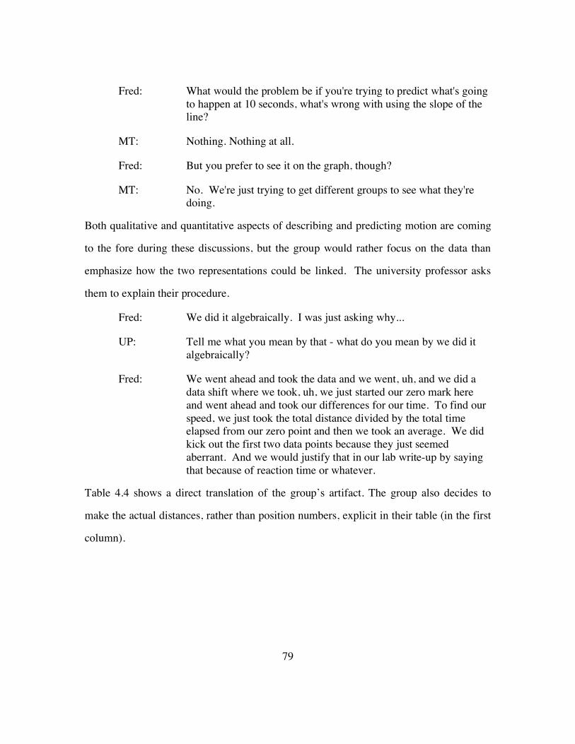
79

Fred: What would the problem be if you're trying to predict what's going to happen at 10 seconds, what's wrong with using the slope of the line?

MT: Nothing. Nothing at all.

Fred: But you prefer to see it on the graph, though?

MT: No. We're just trying to get different groups to see what they're doing.

Both qualitative and quantitative aspects of describing and predicting motion are coming

to the fore during these discussions, but the group would rather focus on the data than

emphasize how the two representations could be linked. The university professor asks

them to explain their procedure.

Fred: We did it algebraically. I was just asking why...

UP: Tell me what you mean by that - what do you mean by we did it algebraically?

Fred: We went ahead and took the data and we went, uh, and we did a data shift where we took, uh, we just started our zero mark here and went ahead and took our differences for our time. To find our speed, we just took the total distance divided by the total time elapsed from our zero point and then we took an average. We did kick out the first two data points because they just seemed aberrant. And we would justify that in our lab write-up by saying that because of reaction time or whatever.

Table 4.4 shows a direct translation of the group’s artifact. The group also decides to

make the actual distances, rather than position numbers, explicit in their table (in the first

column).

80

Distance

from ramp Distance

from origin Time Adjusted time Speed

3 0 2.1 0 0 6 3 2.22 .12 25 9 6 2.84 .74 8

12 9 Error Error Error 15 12 4.19 2.09 5.74 18 15 4.72 2.62 5.72 21 18 5.15 3.05 5.9 24 21 5.6 3.5 6 27 24 6.0 3.9 6.15 30 27 6.6 4.5 6 33 30 7.05 4.95 6.06

Avg speed = 5.9 ft/s

Table 4.4: One group of teachers’ calculation of average speed.

The university professor asks them to explain their rationale for disregarding certain data

points.

UP: You said they seemed aberrant. How do they...?

Fred: Well they didn't seem consistent. You've got all these numbers here right around 5...

UP: What are those numbers and how did you get them?

Fred: We took the total distance divided by the total time. We got the average...

Charlie: So you were just changing the averages the whole time as you went.

Penny: See? Then you took the average of those averages. I mean I'm looking at you took 3 meters and you divided it by the total time it took to travel 3 meters.

Fred: We didn't do the intervals. I suggested we consider doing that but then, no, we'll get better data ... I said you will, but it'll be...

Penny: But, see I think the 6.06 for you is really the average...

81

Fred: That is the average for the entire event.

Penny: And then you just kicked out your other data. OK.

Another member of the group points out that the first non-zero value for speed (25

m/s) seemed strange because their second non-zero value was drastically different (8

m/s). She admits that the group felt something was happening with the ball; they relied

on this belief to support their rationale for ignoring certain data points. She also claims

that once the group noticed a more consistent pattern in the latter data points, they

“wanted to get a more representative figure of the averages”…by taking “the average of

the averages” (noting that each time entered in the original data table was determined by

taking the average of two stopwatch times). Notions or pre-conceptions of “average” are

evident in this discussion. These notions appear to be based on how the group should

justify using an adjusted distance and an adjusted time for the experiment and the group’s

perception of error.

Later in the discussion, Penny challenges the group by saying that their

adjustments "folded" in the error anyway. Fred says this is not the case because the ball

keeps rolling and the group took an average for the entire event. The group believes that

taking an average resolves the issue of experimental error. One member of the group is

adamant in her belief that the adjusted times and adjusted distances do not contain a new

type of “error” since the original data were “consistently wrong,” yet, several other

members of the class, including Penny, disagree. Error is still inherent in the data. The

Master Teacher also challenges the group by saying their belief is correct only if the

original starting point data (three meters with an associated time of 2.10 seconds) is

correct; yet the class cannot agree. The challenge implies that the group was not

necessarily thinking about how adjustments in the data could disassociate the data from

the actual experiment.

82

Another member of the class points out that over a long period of time, the

adjustment in time will make no difference since subtracting 2.10 seconds from a very

large time value is not significant to him. He argues that he is not “buying into” their

calculated average speed (taken over the whole event), because there are too few data

points to calculate a representative speed for the entire event. Yet another member of the

class, Bill, seems to feel that "double smoothing" is a legitimate concern. He feels that

averaging averages is a bad thing statistically because “you’re losing field effect,”

implying a belief that the data should closely represent what took place in the experiment.

Like the group in Episode 2, the group in Episode 3 believes that the data table

provides a viable representation of the bowling ball’s behavior during the experiment.

However, their reliance on a data “shift” (like that of the group in Episode 1) and their

belief in the viability of the new set of data created by the shift allows them to leave the

realm of experience and rely on more formal mathematical techniques. What makes this

group’s procedure distinct from previous ones is that they want to deal more directly with

the issue of experimental error. Their “averaging of averages” seems to provide them

with a good sense of how to answer the prediction question, yet they are challenged by

other members of the class on three points: 1) they have either “folded in” error or have

disassociated the data from the experiment despite their mathematical technique of

averaging, 2) there are not enough data points for the group to claim that the calculated

average is representative of the “true” speed of the ball, and 3) the “true zero” cannot be

found from the “shifted” data despite one group member’s firm belief that the new data

set is inherently correct with regard to both the starting position of the ball and the

“absence” of error. Figure 4.4 shows an interpretation and summary of tensions for the

episode.

83


Episode 4

Given the different procedures for calculating speed, a discussion ensues on

which might be the best method for determining the speed of the ball. Considerations of

error were evident.

Charlie: We did like every single possible combination. Doing intervals, whole averages, and everything. And, honestly, doing the overall average is like final distance, final time to original time, original distance, um point, was the best. If you got off of that, then you got ridiculous...like you would get 6.4 if you threw out the first three and found the individual averages, then you get 6.29 if you did, um, you get 6.29 if you just do the individual averages. I think 6.0 is the closest and what it should be.

UP: Charlie, you said it gives you the best and it's the closest and what it should be. How do you judge what is best and how do you judge what it should be?

Charlie: I think if it fit the data.

Fred: The collective data. Yeah.

UP: How did you make a judgment that it fit the data?

Penny: From our graph.

84

Charlie: From our graph.

UP: OK. So you drew those lines and you decided that covered the most points when you did it that way?

Charlie: I don't know. For some reason, I feel that 6 is a very happy number.

MT: Oh, you wanted a round number, then?

Charlie: No. Anything like 5.94, 6.06. I mean that's, we're talking it's obvious it's something there. So, I think anything around 6 is doing okay. The further we get away from 6, the more screwy things get.

UP: Operationally, what does that mean operationally for something to get screwy? What happened, what did you see on the paper?

Charlie: OK. What we were doing...if you take individual times and individual distances, like for every 3 feet and you calculated the time that it was, you're incorporating a lot of error in there, I think, because each person has a different reaction time on that stopwatch and you're depending that time over two people. And being someone who operated two of those stopwatches, it's kind of screwed up. I mean, in one of those intervals I got 7.5 feet per second just by calculating over 3 feet it went from 21 to 24; it elapsed .4 so I got 7.5 feet per second. And those numbers are really just all over the place between 5 and 7.5. Doing I think the intervals is maybe too close. Just like saying should I go down to 1 foot, it would make it worse.

MT: So we are at least saying that how you choose your intervals substantially impacts your final number [meaning it impacts the final representative number or average]. Does it impact significantly the answer? How much difference is it really making?

Laura: There's a lot more scatter in those data points.

Charlie: Between 5 and 7.5 were the numbers in that range [the scattered points] as opposed to the other one were it's between 5.72 and 6.1.

UP: So, there was a little bit of an operational definition of screwy. OK. You said, you said I got more scattered. I looked at the

85

difference between the largest value I got and the smallest value I got and that was a bigger difference than when I did it this other way. So that difference is directly proportional to screwy; it was more screwy when you did it with the single intervals. So, why then did we insist on all these data points? Why didn't we just put a bunch of people with a stopwatch down at the end of the hall?

Fred: May not have been real practical [implying, perhaps, not practical from a physical standpoint].

Joyce: It's not really as fast as it is at the beginning.

UP: So, she's assuming there maybe some interesting things were going on between the beginning and the end.

Episode 4 provides an indication of the type of reasoning exhibited by the group

in Episode 3 that could also be indicative of other class member’s reasoning. Of notable

consideration in this vignette is the continuing consideration of “averaging” and what is

“good enough” to describe and predict the motion of the bowling ball. These

considerations can most likely describe certain characteristics of the open code “line

fitting.” They also characterize how these considerations may take form in the realms of

experience, mathematics, and physics when discussing modeling and critical concepts in

kinematics.

1. How to calculate an average (e.g. over the time it takes for the whole event to take

place or over a certain number of time intervals),

2. How averaging connects to perceptions of error,

3. How averaging provides both a description and a prediction of motion that’s

“good enough” to satisfy learners involved in mathematical modeling of motion.

Figure 4.5 shows an interpretation and summary of tensions for the episode.

86


By the beginning of the second day, teachers had agreed somewhat upon a general

mathematical model (also deemed a “procedure”) to describe and predict the motion of

the bowling ball. The model included “initial position,” “velocity over an interval of

time,” and “elapsed time.” To find the “new position” of a moving object, multiply

“velocity over an interval of time,” and “elapsed time”; then, add the “initial position” or

the starting distance from a reference point (see Figure 4.6). New position = (velocity over interval)(time elapsed)

+ initial positon

v =x2 ! x1

t2 ! t1

Read from graph

Figure 4.6: The teachers’ constructed model for describing and predicting uniform motion.

Noting teachers’ preferences for representations, “velocity over interval” could be could

be computed using values from a data table or read from a graph utilizing some

quantitative measure including units (e.g. meters and seconds). The question of which

interval to choose (either individual ones or one that expanded over the entire event) was

87

still an open issue. The validity of the mathematical model for constant motion was

tested with an activity involving a non-uniform motion.

Studying Non-Uniform Motion

Teachers’ understanding of the general model for motion would be probed further

as they encountered a situation where an object would be moving with constant

acceleration, that is, the velocity is not constant but is increasing in a predictable way.

The teachers now work with some data provided by the professor and master teacher (see

Table 4.5). The challenge was to fill out the chart for the car’s position at zero seconds

and its position at seven seconds.

Time Position 0s ? 1s 1.5 cm 2s 6 cm 3s 13.5 cm 4s 24 cm 5s 37.5 cm 6s 54 cm 7s ?

Table 4.5: Data from a car rolling down a ramp.5

A focus group is now the subject of analysis. They were identified as the one

group that decided to rely on the mathematical model (or general procedure) constructed

by the class. One group decided to rely on prior knowledge that this experiment yields a

quadratic function and they soon became absorbed in remembering standard physics

equations and artificially constructing a quadratic function. One other group decided to

utilize a graphing calculator and its built-in regression capabilities to determine an

equation. The focus group relied heavily on the data and calculating change in position

5 The table is a direct translation from the worksheet provided to the teachers.

88

over time (i.e. velocity). The episode shows teachers encountering “clean” data yet still

having difficulty with “interval” considerations when finding a representative speed.

Harry: In essence what we would be doing is this [He plots the data points on a graph]. So what we’d be doing is from here to here [referring to the heights of two vertical line segments drawn from the x-axis to each of the first two non-zero points on the plot] we’d say this is a straight line [connecting the two “heights” or vertical line segments] and then we’d have that [see Figure 4.7]. Over this time interval [the third one], we have this average velocity [referring to the slanted line connected the two vertical lines]. It’s only approximate.

Illustration 4.1 shows a reproduction of Harry’s drawing. His reasoning about average

velocity is more geometrical but he is still thinking in terms of taking individual averages

and not an average for the entire event.

1 2

1

3

1

4

1

Illustration 4.1: Harry’s first conception of average speed for non-uniform motion.

Penny considers taking the average within each interval as well.

Penny: Between each two points find the average velocity.

Cathy: Well, they’re increasing by the same amount at each point.

Harry: Well, that’s just one approach. But, it’s going to give you an approximation.

UP: I think Cathy said an important thing. She said they’re increasing by the same amount, so would that let you…if it’s increasing by the same amount, could you figure out what the halfway velocity was?

Cathy: Except for the starting point [since they don’t know position at time 0].

89

Harry: I don’t understand. We can figure out the halfway point velocity regardless, can’t we? Doesn’t matter if this increased the same amount as that [comparing two intervals], I can still find the halfway point here and the halfway point here, can’t I? Just by doing the average? So, I don’t understand.

Nancy: Because we want to use the same, um, the same, um, formula that we used before.

Harry: Yeah, so it’d be the velocity times the elapsed time.

Nancy: For each section.

Harry: Yeah, each section.

Nancy and Penny are relying heavily on the model to make sense of non-uniform

motion. They believe that the model can work if they find a representative speed. The

group soon decides to calculate velocity by taking each individual position (rather than

change in position) and dividing each by the respective point in time (rather than change

in time). They focus now on each point rather than each interval. Pondering whether

they are calculating the velocities correctly, the group decides to follow Harry’s

suggestion to use a more geometrical approach, which is to connect the data to a graph

representation and then use the graph to interpret velocity. Harry’s reasoning now shifts

to looking at an overall average first.

Harry: Let’s do a gross one; what if we did a distance here, this whole thing and get the average velocity between these two points [see Illustration 4.2].

1 2

1

3

1

4

1

Illustration 4.2: Harry’s second conception of average speed for non-uniform motion.

90

The group uses their point (rather than interval calculations) to determine the initial

velocity (start of the secant line) and the final velocity (end of the secant line). They then

sum these velocities and divide by two to obtain an average velocity they feel is worthy

to be placed in the general model. They multiply this average to elapsed time to

determine a position for seven seconds (although they are unsure of the initial position of

the cart and have not used it as part of their calculation). While happy with their answer

at first, they are unsure how close their final answer is to a “true” answer calculated

using a “true” velocity.

Harry: I don’t know. I don’t know. But, you would think that if it were a straight line between here and here, then that would give us an approximation. But if we made it smaller, and did each of those [meaning piecewise over each interval and not one piece over a large interval] and added them up, that should give us a closer approximation ‘cause it’s closer to what the curve actually is. I wonder.

Penny: That’s where I stopped. I don’t know how to do that anymore.

Penny begins to show her frustration. As the group attempts to answer a

subsequent question about the car’s position at 10 seconds, they rely firmly on the data

and the graph before them. They are utilizing the graph in a much more quantitative

way, and, perhaps, the changing velocity forces them to analyze their representation more

intensely.

However, within a short period of time, the group decides that they must find a

formula and equation despite the master teacher’s assistance in helping them clarify their

notion of velocity and how to calculate a velocity over an interval so they may rely on the

general model. Harry now believes that they can refine their procedure by taking more

averages between points, that is to say, by making smaller and smaller segments that will

approximate the curve. While this episode provides a good glimpse of some possible

91

seeds of calculus reasoning (i.e. calculus as math of change), the group soon believes,

based solely on their prior knowledge from physics and math, that the data exhibit a

quadratic relationship, and the remaining time is spent trying to determine, albeit without

much direction or insight related to the data, the values of the parameters in the equation

y = ax2+ bx + c .

Summary Data

The researcher utilizes Pollak’s (2003) critical aspects of modeling (listed as

subheadings in this section) to consolidate key issues in the teachers’ approach to

mathematical modeling of motion. Three of the groups did not make final presentations

to the class regarding their procedure for describing and predicting the uniform motion of

the bowling ball. However, data from observations of individual groups working

independently of the class is reflected in this summary section along with observations of

whole class discussions. Only one group of three teachers decided to pursue the

possibility of applying the model for uniform motion to the situation of the car rolling

down the ramp. All other members of the class relied on their prior knowledge of formal

mathematics or on the regression capabilities of a graphing calculator.

Understanding the Physical Situation

Assuming that the course’s approach to kinematics was a new experience for

many of the teachers, the researcher expected more discussion by the teachers about

sources of error or possible set-up problems they might encounter with getting the ball to

exhibit uniform motion. However, there is no evidence to suggest that the teachers as a

class thought intently about such issues. Four teachers wanted to mark the ramp's

position so they could tell after the experiment whether or not the ramp moved. They felt

it would affect their data collection once the ball hit the floor. Eight teachers were

92

concerned about the bounce the ball made at the end of the ramp and claimed that

particular part of the roll should not be considered. Two teachers were concerned with

the ball accelerating (since it was starting on a ramp), and one of them reemphasized his

concern during the experiment. However, his concern did not alter the teachers’

approach for rolling the ball. One teacher was concerned that the finger holes of the

bowling ball face upward since finger holes touching the floor would affect the ball’s

motion – it would cause “variation” in the roll.

Deciding What to Keep and What Not to Keep

Deciding what to keep and what not to keep in the mathematical model is inherent

throughout several episodes in the data. These episodes involved issues of what data

points should be used, what scale should be used, and whether or not an average should

be used. Determining the starting position (or point) of the ball’s motion was also a key

issue in this process. Of the 23 teachers, eight decided to dismiss certain data that were

collected at the beginning of the roll. Of the twelve teachers who constructed a graph,

eight considered adjusting the scale on the axis either by increasing the size of the

intervals or creating smaller intervals to “smooth out” the line. Furthermore, eight

teachers held notions of interpolating. Of the 23 teachers, twelve considered an average

for their procedure. Of these twelve teachers, four were confident in their calculation of

an average and were confident in justifying the use of an average. Finally, of the 23

teachers, twelve shifted their data and held discussions about the starting point of the

ball’s roll.

Deciding Whether the Model is Sufficient for Acceptance

This phase of the process became muddled once teachers began to rely on their

prior, formal knowledge of algebra. One teacher attempted to describe the motion using

93

the formal equation, y = mx + b, and relate it the teachers’ notions of constructing a best-

fit line. He states explicitly that he remembered the equation from his own education

experience in a math class. This prompted a class discussion where teachers were unable

to connect their understanding of a best-fit line or their work with the experiment data to

the symbolic mathematics. Although the teachers agreed upon a model that resembles a

linear relationship between position and time, there is no evidence to suggest that they

came to a consensus that this model was the best to describe and predict the ball’s motion

as evident by their reliance on the graphing calculator and other formal mathematical

knowledge (e.g. a quadratic equation) to pursue and complete future activities in the unit.

Time constraints did not allow the teachers to fully explore an example of non-

uniform motion, specifically, an acceleration timer attached to a car rolling down a ramp.

The data explored by the teachers were sample data presented to them in the form of a

worksheet. While they were able to conduct several runs of the experiment (several trials

to collect acceleration timer data), their experience with non-uniform motion was more

observation than exploration and analysis of data.

Given how teachers’ considerations of scale, averaging data, and the object’s

initial position heavily influenced line-fitting as a mathematical activity, the researcher

identified these as the characteristics of the open code “line fitting.” In the next phase of

the investigation, these characteristics (codes) became the focus of selective coding and

became highly relevant for the researcher examining possible tensions that learners

confront when relating physical experience to a mathematical model. While code names

remained the same, two code descriptions altered slightly to reveal more dimensions of a

particular code based on the qualitative data.

1. Position – Considering the “location” of an object in motion with more

consideration given to thoughts about the initial position of the object.

94

2. Scale – Considering the size of an interval on a coordinate axis. Involved in such

considerations are “finer scales” and interpolating data.

3. Average – Considering some sort of statistical or numerical average of data points

when calculating velocity over an interval.

In summary, the researcher hoped to identify one of these as the core category to develop

a grounded theory along with supporting categories necessary to complete the theory.

The researcher concentrated on these categories when the unit was implemented again,

over a more prolonged period of time and bearing some modifications based on the first

implementation.

STUDY TWO

Since the researcher and university professor assumed that the participants in

Study Two would not be as familiar with the standard models or equations, they further

assumed that prior, formal knowledge of the equations would not be a significant

influence on students’ thought processes during the activities. Therefore, the setting for

Study Two allowed for deeper examination of students’ prior conceptions of both types

of motion with the researcher focusing on the categories of scale, average, and initial

position. In the second implementation, participants were allowed to create motions they

considered uniform or “constant” and non-uniform or “accelerating.”6.

Qualitative Analysis of Classroom Practice

All classroom episodes from Study Two were transcribed and coded using a

selective coding scheme. As in Study One, four pertinent episodes are presented along

with interpretation and discussion of each episode. The episodes presented provide

confirmation of similar tensions arising between learner experience, standard 6 As a class, they were also allowed to agree upon a single experiment to conduct for each if they so desired.

95

mathematics, and standard physics when learners are immersed in the mathematical

modeling process. Furthermore, the episodes and summary data provide an

understanding of the influence of the selected categories on the mathematical modeling of

uniform and non-uniform motion using discrete data. As with Study One, since learner

reasoning consisted of the interaction and discussion of these selected categories or

content areas, summary data are presented using the same three critical aspects of

mathematical modeling presented by Pollak (2003).

Learners’ Prior Conceptions of Describing Motion

The unit began with the activity of creating and describing a motion.

UP: Your first task is going to be to create a motion and the thing that is going to move is this…a little wooden block. We want you to describe that motion as accurately as possible, the goal being that the other group would be able to take your description and reproduce your motion exactly. So, you’re gonna show me what your little block is doing, but not show the other group and the idea is for us to think about what it really takes to describe a motion very thoroughly and very accurately so that the other group will be able to do it too.

Working in small groups of two to three members each, students’ prior notions of what

should or should not be involved in the descriptions of their motions were evident.

Specifically, discussions centering on motion “intervals” formed almost immediately and

revolved around certain questions:

• Is identification of endpoints (e.g. starting point and ending point of the motion)

enough to say two motions are the same? For example, does the motion of the

block in-between the starting point and the ending point warrant consideration?

• What is the difference between the path of an object in motion and the total

distance the object travels during that motion? For example, does it matter if you

can locate the object at any point during its motion?

96

The majority of students (12 out of 16 students) did not initially consider a relationship

between position and time as relevant to their description. Of the four students that did

relate position and time, three relied on prior knowledge of a symbolic formula (from

trigonometry). It is not clear that they had a conceptual understanding of the formula.

One student out of the remaining twelve did not feel that quantifying the motion

was necessary at all for description and reproduction. In eight of the remaining eleven

cases, starting and ending points of the motion alone were considered important, whereas

the remaining three of the eleven students eventually reconsidered the possibility of time

as important to the description though it is not clear that their beliefs changed since the

outset of the activity. Of the eight students, one student felt that a speed could not be

determined through any means at their disposal.

Of the sixteen students in the course, only four believed in a difference between

the path of the object and the object’s total traveling distance. Furthermore, nine of

sixteen students considered the motion of the ball in-between start and end points

important for their descriptions. Two of the sixteen students considered a generalized

description of motion to be possible. They, along with one other student, felt that a

generalized description needed to be considered “good enough” based on some criteria

(e.g., a certain number of decimal points in a measured position or distance should be

used).

Studying Uniform Motion

The next activity in the unit involved the students creating a motion they believed

was constant. Unlike the teachers in Study One, the students in Study Two were not

restricted to thinking about rolling a ball down the hallway although six students working

in two separate groups conducted such an experiment. Upon choosing a motion to create,

they were to perform their experiment, justify that the motion created was constant, and

97

predict where the object would be one, five, and ten seconds after the observed motion

stopped (assuming that the motion would continue indefinitely). Table 4.6 summarizes

the motions created by the students.

Motion Experiment Number of Students

Describing/predicting the motion of a metronome 2 Rolling a wooden ball in a round lid 1 Walking at a steady pace 3 Rolling a bowling ball down the hallway 4 Rolling a small wooden ball down the hallway 2 Moving a book in front of a motion detector 2 Describing/predicting a fixed pendulum swing 1

Table 4.6: Motions performed and considered constant by students in Study Two.

Students performed their experiments in separate groups, collected data on their

experiment and analyzed them. They were required to present the motion experiment,

the experiment data, and the procedure for answering the prediction question to the class

during the following meeting period. Table 4.7 highlights major areas of concern for

students as they presented and discussed their motions.

98

Motion Experiment Concern(s)

Describing/predicting the motion of a metronome

• Direction reversals, perceived by some to include a slight pause in the motion, do not allow for motion to be described as constant

• What’s happening in-between swings (or in-between the time interval of interest) is not constant

Rolling a wooden ball in a round lid

An average time may or may not be good enough to use to describe and predict a constant motion

Walking at a steady pace Best to ignore motion variation between time intervals (e.g. swinging of arms, “jerky” motion, etc.)

Rolling a bowling ball

• Friction, affecting the ball’s position over time, is a physical consideration that may or may not be resolved by calculating average velocity

• If actual calculations are not matching theoretical values, then the motion is not constant

• Calculating a velocity over longer distance and longer time interval makes more sense

Rolling a small wooden ball Larger time intervals are better for describing and predicting motion because physical instances over larger time periods make more sense

Moving a book in front of a motion detector

• What’s happening in-between time intervals may or may not be constant

• An infinite number of time intervals may be used to better describe a constant motion

Describing/predicting a fixed pendulum swing

Despite variation, time values are close enough to each other to pick one of the values that represents the “correct” time

Table 4.7: Student concerns about motions performed and considered constant.

Following student presentations, the university professor wanted the class to reach a

consensus about how to determine whether or not a motion is constant. The class agreed

that for describing and predicting constant motion, using the equation d = rt seemed a

feasible approach, although calculating the rate (the value of r) remained an open issue.

Experience with variation in data influenced students’ thinking about the best rate to use

when describing and predicting motion. More specifically, conflicting beliefs about

99

using an average rate, a rate based on average time, or a “good enough” rate influenced

their construction of a mathematical model. Their beliefs were further tested when

presented with more formal physics questions regarding constant velocity and involving

data tables. Relying on d = rt as their agreed upon mathematical model, students,

working in groups, approached each problem and presented their results to the class.

Presentation and discussion of three critical episodes as well as summary data exemplify

the influence the core categories of scale, averaging data, and initial position had on

students’ mathematical modeling of uniform motion. Underlying the influence of the

core categories were students’ perceptions of what is “good enough” to use for a rate

when constructing a mathematical model to describe motion.

Episode 1

The first episode involves two consecutive presentations from students (in groups

of two) after working on a problem given to them on a worksheet:

Some students are studying the motion of a bowling ball rolling down a lane at the bowling alley. A student with a stopwatch is positioned at the start of the lane, and every two meters after that. Each student stops her watch as the ball passes her. They want to predict how long it will take the ball to reach the pins, 1 meter beyond the last student. Explain how you would help them figure this out, first in words, and then with an equation. Explain why the equation is the right equation to use.

Student 1 .27 s Student 2 .75 s Student 3 1.25 s Student 4 1.77 s Student 5 2.25 s Student 6 2.74 s Student 7 3.25 s Student 8 3.76 s Student 9 4.24 s Student 10 4.75 s

100

Students encountering this problem continued discussions related to average, scale, and

starting position of the object.

Lee: We took two different approaches ‘cause we didn’t know which one would be more accurate. The first thing we did…the first attempt to figure out how many seconds it would be to get to the pins is that we took the time difference between each student and we added them all up and divided by 9 to get an average time between each student.

Both students agreed on an average time value of .4977 seconds when using this

approach. The associated rate, thus, became 4.0184 meters per second. Using this rate,

both students obtained a value of 5.22 seconds as the final answer to the question. After

checking their procedure using their calculated rate to obtain other known values in the

table, they encountered what they called “inaccuracies.”

Lee: So there’s kind of…we were like maybe this isn’t the right way to go. So the other way we tried was taking student ten’s measurement of 4.75 seconds and subtracting that from student one’s and finding…that gave us 4.48. So, then we divided that by 20 and we came up with a rate of 4.46 [meaning 4.46 = 20 m/4.48]. Then using that rate, our time we came up with 4.708. That doesn’t make sense because student 10 is set at 4.75 seconds.

Linda: But, using the average, like, there was too far of a distance. It was like over a 1 second…no…it was like a 1 second distance, wasn’t it? [By distance, she means difference].

UP: So, what do you mean over the average, there was a 1 second distance?

Lee: Like coming up with this 5.22, it’s saying that it took whatever the difference between 5.22 and 4.75 seconds for it to go one meter. Which doesn’t make sense to us because on the other ones, the differences, it took 2 meters in a half second. It went two meters in a half second. We’re kind of lost.

UP: So, you’re still not happy with your….

101

Lee: Not happy with either way we went because we found discrepancies.

Following Lee and Linda’s presentation, the next group of students encounters a similar

situation calculating average, yet they are explicit in connecting the calculation of

average to initial position. They compare their procedure to the previous group’s

procedure.

Stephen: We started out by looking at student one being at position zero, at the start point. The thing is we found two ways to do this. You could take the rate between each student. So, the rate being…[he

writes

R =!x

!t] where delta x is equal to the final position minus

the initial and delta t being the final time minus the initial time [he writes

x f ! xi and

t f ! ti on the board.]

UP: Which is what Lee and Linda did, right? If you’re assuming they’re all standing two meters apart.

Stephen: Yeah. Our pins were actually at 19 meters. You guys [Linda and Lee] went two meters ahead of that, so that’s why our end number’s going to be a little bit different. We found a rate between each person and we were able to get 4.02 seconds [meaning meters per second].

Lee: So you’re just taking two meters off because from the...

Stephen: Student one is at point 0.

Lee: Release position to student 1.

Stephen: So you can do this two ways. You can throw out student one’s number or you can keep it and say between student one and student two you have approximately .5 seconds. Then in between student two and student three there’s .5 seconds. The distance the ball traveled is the same for each, so it’s approximately…the numbers aren’t exact, but it’s approximately 4.02 meters per second. And that’s what they [Linda and Lee] got the first time.

Lee: 4.0184. Yeah, same thing.

102

Stephen and Veronica continue their presentation by outlining their second method of

calculating the final answer and the viability of another approach.

Stephen: They’re about the same thing. We went back and we saw if you took the initial time, which is .27, and the final time, 4.75, and then the distance in between those, you get the same exact thing. Well, it’s a 4.0187. But the thing is…for each student getting a different time and a rate between each student is different….like, between student one and student two, we got a rate of 4 meters per second. Between student three and student four I’ve got a rate of 3.85 meters per second. So, that’s a big difference. But the thing is we’re talking students hitting stopwatches and we’re talking about a bowling ball that has no internal, like, motor or anything. So, we’re assuming acceleration is zero. We can assume that this velocity, or this speed, is the same. So 19 meters divided by 4.02 meters per second, we…gives you 4.72 seconds, but you have to also take into account the first student’s time, .27 seconds. We got 4.99 seconds on a stopwatch, if you stopped it at the 19-meter mark.

UP: You got the same rate, but you’re using a different distance. You’re using a distance of 19 meters. You guys [Linda and Lee] used a distance of…

Lee: 21. What was y’all’s final?

Veronica: Answer? 4.99.

Dave: Add .27 seconds to what you…

Dave implies that the .27 value could be considered a starting position and should be

added after calculating d = rt. However, Linda and Lee don’t appear to understand this

fully at this point.

UP [to Linda and Lee]: So…you all weren’t happy with yours, though.

Linda: We just didn’t think that ours was very, like, accurate.

UP: But you had a reason because it didn’t match when you did it the other way.

103

Linda: Well, we came out to like 19 instead of 20. When we should have been getting 20, we were getting 19 so there was a little bit of an inaccuracy right there.

Lee: Well, if we take…like we did it another way and we took from student ten’s time and subtracted it from student one’s time? And that gave us the time of it getting to the pins at 4.708. Well, if you add .27 to that, it gives us like 4.97. So, it’s like 2/10ths off.

Stephen: But I think you gotta look at where your data’s coming from. Ours is coming from a lot of uncertainty. So, if we were gonna do a prediction it’s only gonna be an estimation.

Lee: Well, doing it either way is gets us within .03, .04. Give or take. Plus or minus.

Observing both methods, Lee wonders which procedure is most beneficial. Students

show differing opinions about this as exemplified in the following vignette.

Lee: You know how we did it both ways, like, taking the average between each second? Then taking like just from the end to the beginning? Well, we’re wondering which way you think could be more accurate. Because, like taking from the beginning to the end just kind of auto corrects that average, y’know ‘cause the students, as we’ve seen through the numbers…like one stops a little sooner, one a little later…

Stephen: I think with a lot more data points…I think by doing the average in-between would end up canceling out the error. If you think …OK, student one to student two to student three…student one stops his stopwatch early which means the rate between him or…. student one to student two to student three…student two stops his stopwatch early which mans the rate between student one to student two is going to be small. But, the rate between student two and student three is already now larger. So, it’s adding out. They’re canceling each other out.

Dave: I like looking at each one of the intervals. I mean as long as we have these intervals, we might as well look at ‘em. And not take the big leap from student one to student ten.

Adrian: Yeah, from student one to student ten.

Dave: If you got the data, look at it.

104

Adrian: Might as well use it.

UP: So you look at it, and we’ve seen some variation.

Adrian: Slight.

Dave: That’s what averages are for.

UP: However much variation, you take the average and that’s…?

Dave: Well, that’s not all. You have to define your acceptable losses.

Neither Dave nor other members of the class explain what “acceptable losses” implies or

how to resolve the issue of using an average over a finite number of points or an

undetermined, infinite number of points. Following Stephen and Veronica’s

presentation, Jimmy and John’s presentation further exemplifies students’ thoughts with

regard to scale and average.

Jimmy: [Referring to the plot presented in Figure 4.7] We went ahead and found the exact time between every student. There’s 9 different times between every student. Then we used this formula right here

[writing

D =m

t] and we divided…this [m, representing meters]

was 2 because there were two meters between each student…so we divided 2 by the time between each student. After we did this, we realized there’s no trend as you can see. So we took the average of all the different parts.

Figure 4.7: Jimmy and John’s plot of calculated rates.

105

Stephen: You’re comparing the rates per…compared to the student.

Jimmy: Yeah. This is the…between student one and student two, the ball was moving at 4.16 meters per second. Between student one and student two, the ball was moving at 4 meters per second [meaning between student two and student three]. It was speeding up and slowing down and speeding up and slowing down or just people were screwing up pressing [the stopwatch].

UP: So, they’re arguing there’s no pattern in that.

Dave: I’m saying that’s…just that your graph there is so spread out, it doesn’t look like a pattern. I think in reality that’s a very good pattern because it’s very minuscule differences. I think that’s what you’re going to get to. That the average of those was a pretty good number that was close to all of those. [Jimmy writes 4.036]

UP: So you’re saying you took all of those and you average them and you got this. How did you decide that it was a good idea to take the average?

Jimmy: Because the ball was not moving at a constant speed. It was changing.

UP: So, if it’s not moving at a constant speed, you just always take the average?

Jimmy: Seemed pretty logical at the time.

UP: What if it had been…what if you had seen the plot and the lower intervals were lower speeds and as you got to larger [meaning further out on the axis] intervals, the speeds got higher and higher?

Jimmy: We would have had a nice trend line, there.

UP: Would you have still taken the average?

Jimmy: Yes. Because….no, you have not taken the average. [John is shaking his head in disagreement.] I would have just found this little time, like, one meter after this guy right here [the last student] and then I would have gotten my calculator out and traced and then found the 9 1/2 spot since it’s only one meter.

106

Jimmy relies on a more local part of the graph implying that, in the hypothetical

consideration presented by the professor, the last set of rates would have been more

reliable and he would have used those to find the next rate in the sequence. The

discussion returns to the final answer that Jimmy and John calculated.

UP: You found your rate. What did you do?

Jimmy: 4.036. I rounded down to 4.0 instead of 4.02 like he [Stephen] used.

Lee: Why did you round down?

Jimmy: Rounded 4.036 to 4.0. The average between all these students is 4 meters a second or 4.036.

Lee: Why did you go from 4.036 to 4 seconds [meaning meters per second]? Since we’re dealing in seconds it seems like we should leave it out to at least 4 decimal places.

Jimmy and John decide on a final rate of 4.036 meters per second, but used 4

meters per second to calculate the final number of seconds for the final meter. They also

decided on using a distance of 20 meters for the pins rather than 19 meters or 21 meters

as other groups had. They obtain a time (a final answer) of 4.75 seconds and add .25

seconds to obtain a final time of 5 seconds. John attempts to explain the disagreements

that he and Jimmy had in determining a final rate.

John: Jimmy wanted to use this [4.036]. I wanted to use this [4.0]. We could have used either one. Given all the scatter, it seemed kind of cheesy to do this [use 4.036] when there’s so much [scatter]…

Dave: I also agree with John in that using 4 is probably a good enough measurement because in the problem it says that the students are all 2 meters apart, not 2.00036284 apart. So, if the problem itself was only worried about 2 meters apart and the pins are exactly one meter apart after that, then isn’t it okay to just say this is going 4 seconds [meaning meters per second?] because it’s about the same level of error as…

107

Lee: But the decimal places they went out to measure seconds was two.

This series of vignettes highlights the tensions between learner experience (what is

happening in the experiment, e.g. sources of error), standard mathematics (considerations

of scale and starting position), and standard physics (relying on the data and calculating a

“correct” speed). These tensions, along with considerations of a “good enough” rate to

use, have an influence on how students construct and utilize mathematical models.

Episode 2

The following episode comes from a class period during which the university

professor reviewed what the class had decided upon as a procedure (or model) to describe

and predict constant motion. Paul points out that calculating the rate or velocity should

be done by interval (e.g. a final position minus an initial position divided by total time for

each time period). The professor points out that there are two cases in her mind based on

what the class did: where the change between intervals is exact (as shown in some of the

problems on the handout) and where the change is not exact, but includes error (as shown

in the class experiments). Stephen believes that Paul’s method of rate is still valid to use

despite error and variation in the data; he believes it to be a good procedure that could

come close to modeling a “perfect” experiment.

Stephen: If our equipment was perfect and our timing was perfect, and if our measurements were perfect, I think we would boil it down to something like that. Say the bowling ball goes ten meters. We can find the distance versus time from 2 to 4 meters and divide that by time. That should be the same rate if we did it from 6 to 8 meters and divided it by that time also.

Lee: Yeah, if it’s truly constant you don’t have to worry about the time in between. Like, all that’s important is the final and the initial.

Based on this argument, the question asked of the class was How do you judge a motion

to be “truly constant?”

108

Stephen: So this is like defining constant motion?

John: Is the question what do you do when you have constant motion or how do you know you have constant motion?

This brief exchange highlights a tension between the mathematics and science realms.

One may argue that someone may see a distinction between the model as descriptive (or

as a representation) and the model as a calculational tool.

The professor reminds the class how Jimmy and John calculated an average rate.

Paul argues that both methods are the same. He feels that the “average of a sum” is the

same as “the sum of the averages.” The professor disagrees because what happens in

each of the intervals may not be the same. She brings up the bowling ball example where

the roll is much faster at the beginning. Paul disagrees although the professor believes it

depends on how you measure time intervals.

Dave: Adding up all the little averages is the same thing as taking one big average. You’re adding up to the same thing.

Paul: Because if one has a larger velocity then the next time interval will have a smaller one.

John: But in the bowling ball example that we worked in class last time, what you were looking at was not the actual speed, but a lot of what seemed to be like a lot of error in the way the stopwatches were going and if you just looked at the last guy, and the last guy was very bad with the stopwatch, he would throw off the whole. So, in that example, you’re better off looking at all the intervals.

UP: But what Paul is saying is if you include that last interval, you’ve got that bad set of data for the last interval, too, and it’s going to drag down your whole average.

John: Yeah, but it doesn’t have the whole weight. It doesn’t have the same weight as…

UP: I think it depends upon how your data are sampled.

John: I have to think about that.

109

The professor asks when is it good to rely on Paul’s method and when is it good

to rely on Lee’ method (averaging)? Lee feels that if there’s no pattern in the data, you

must rule out constant motion. The professor reminds them that they did not rule out

constant motion with the bowling ball experiment despite variation in the data. However,

Lee says that’s all they had to perform calculations.

Lee: It’s extremely hard to find constant motion in anything. ‘Cause there’s factors. Friction. Gravity. Unless you say in this specific environment “regardless of gravity”, “regardless of friction…”

The professor reminds them they had discussions of “good enough” regarding

Stephanie’s experiment with the ball and lid. She also reminds them of Jimmy’s graph

and the how his use of scale confused other class members. Dave has some general

considerations with regard to variation in data.

Dave: Is that change in there really significant? How do you look at your data and say, “well, this is a significant difference” or not? Compared to those students who are each two meters apart (referring to the worksheet problem), but I guarantee you they’re not two meters apart. They may be 2.004 or 2.02 meters apart, but the problem doesn’t care about that small difference. So, if that’s already your limiting factor, saying that you’re exactly two meters apart…if that’s a limiting factor, then your rate should also only be looked at to that limiting factor. Like, if it’s 4.282 versus 4.284, well that little difference doesn’t compare to the thing that is not looked at with the 2 meters apart. So, that’s when we can tell, “is there a pattern or not?” “Is this constant or not?”

Lee: But that’s compounded by the fact that people are sitting there trying to stop it as close as they can.

In the meantime, John posts his and Jimmy’s rate plot on the board. The

professor reminds them again of Jimmy’s argument. At first, Dave feels there is still a

pattern in Jimmy’s data despite the scale. Lee supports this argument.

Lee: Yeah, all you have to do is knock it down, knock those two decimal points off.

110

Dave: But then there’s always…you can’t always do that either. You can’t say, “This is 2. This one’s 6. I’m just gonna call that 4.” There’s gotta be some way to limit that as well.

Stephen: If you knew a theoretical, what the speed should be, then you can compare it using statistical analysis.

Dave: If this is just a problem, you don’t wanna say, “I’ve got this data that already has what…I already have the answer.” That’s not what physics … we don’t want to find an answer we already know.

There is no consensus for finding a representative rate. In summary, both Episode

1 and Episode 2 help support an earlier conjecture made in Study One with regard to

average, yet issues of scale have become more prominent. Figure 4.8 outlines the

tensions more fully.

Figure 4.8: A summary of tensions related to average and scale.

Students working with the constant motion problem(s) encountered these tensions

and attempted to resolve them. Robust learning trajectories are evident as students,

immersed in the mathematical modeling process and encountering tensions or conflicts,

constructed and established beliefs in their mathematical models for uniform motion.

Table 4.8 provides a summary of qualitative data involving student thinking about the

111

selective codes or dimensions of “line fitting” during the constant motion activities

presented in the unit.

Content Student Thinking with Regard to Line Fitting

Average velocity Eight students felt that taking an average rate of some kind was important, but consensus about how it should be calculated or when it should be considered were not reached.

Scale issues Thirteen students showed evidence of immersing themselves in the experiments/activities and took part in discussions about error and what may or may not be “good enough” when describing and predicting uniform motion. During uniform motion activities, 12 students believed that a distance could be determined by multiplying a rate times a time (i.e. d = rt) Of the 12 students who believed d = rt to be a valid equation and should be used for the mathematical model, 10 students modified their model by adding an initial position (i.e. d = rt + p0)

Learning a standard equation (mathematical

model) for uniform motion Of the 10 students who believed d = rt + p0 was a valid

mathematical model, 6 considered d = r(t-1) + p0 was equally valid when concerned about locating the starting position of the object.

Table 4.8: Summary of qualitative data involving student thinking about line fitting.

Studying Non-Uniform Motion

The final activity of the unit involved a car, attached to an acceleration timer,

rolling down a ramp. Unlike Study One, learners had sufficient time to engage in this

experiment and build on their prior experiences and knowledge of uniform motion. For

this experiment, one end of a long strip of paper was fed through the timer and attached

to the wooden car. As the car was released down the ramp, the timer made marks on the

paper strip at the rate of 60 marks per second. Students working in groups of two and

four members each analyzed a strip of paper with data marks (see Figure 4.9).

112

Figure 4.9: An example of a ticker timer strip with added student markings (vertical lines) made during the student’s analysis.

All students were asked to justify that the motion was not constant and once again predict

where the car would be after one, five, and ten seconds had elapsed assuming that the car

kept rolling indefinitely. All but six students initially made a table via paper and pencil.

These six students decided to use an Excel spreadsheet to plot their data and allow the

technology to provide a means of answering the prediction question by somehow

building on their existing table with theoretical data. However, two students decided to

abandon this idea and joined a group of two students working with the raw data. During

the subsequent class period, students gave presentations on their procedure for describing

and predicting the motion of the car. Issues of scale, average, and starting position

continued to influence student thinking as they worked with the car and ramp data.

Student presentations focused on average and scale when describing and

predicting the motion of the car. Tensions between learner experience, standard physics,

and standard mathematics, can be highlighted by examining one group of four students’

construction of a mathematical model for uniform acceleration. Variation in the data did

not hamper their perception that the velocities, calculated over intervals, were changing.

Furthermore, they believed that the length of time intervals, which were roughly 1/60th of

a second each, was sufficient to calculate change in position over change in time for each

113

interval. However, they were confused as to whether finding an average or representative

velocity was a good idea. Focusing on how the velocities were changing (i.e. looking at

acceleration) did not immediately lead to a solution for the prediction question. Given

that the velocities were not changing at exactly the same rate, the group also wondered if

using an average acceleration to describe how the velocities were changing would

become a source of perturbation.

Once an agreement had been reached to use an average acceleration to determine

subsequent velocities and, hence, subsequent positions, the group was still unsure of their

method since it was recursive and tedious. A more general method for prediction

position was not apparent. The discussion of whether a representative velocity could be

found resumed. After some debate, the group decided to use an average velocity, but felt

that finding the position of the car at any given time was a multi-step process. One

member of the group summarized his thinking on the board (see Figure 4.9.1).

1)!!vf = a!t

2)!!vaverage =vi + vf

2

3)!!distance = vaverage !t

Figure 4.9.1: A multi-step process in predicting the position of a car rolling down a ramp.

114

After some thought, the student modified two of the equations by adding vi to the first

equation (since the initial velocity may not be zero) and writing Δt instead of t in the third

equation. Independently of the others, the student substituted equations 1 and 2 into

equation 3 to obtain x = vi+ a!t + v

i

2

"#$

%&'!t or x = 1

2a !t( )

2

+ vi!t . Based on work with

uniform motion, the student adds the initial position to obtain a final equation of

x =1

2a !t( )

2

+ vi!t + x

0. In summary, the difficulty in calculating and interpreting an

average was a major influence on the students’ construction of a mathematical model.

Furthermore, though time intervals were small, they were considered good enough for

their purpose of answering the prediction question. Finally, previous experience in

recognizing the importance of including the starting position in the model, coupled with

some fundamental algebraic substitution and manipulation, allowed the student to

construct a more standard equation.

Other students’ work with this same problem especially exhibited the influence

that considerations of average had on their final procedures or mathematical models.

Table 4.9 summarizes qualitative data on student work with the problem of the car rolling

down the ramp.

115

Student Thinking on Car and Ramp Problem Number of students

Given calculated velocities and rate of change of velocities (accelerations), a recursive method can be used to find positions at given times. However, using an average velocity may or may not be useful.7

5

A spreadsheet can be used to multiply the acceleration and the square of the associated time and obtain the associated position. However, no rationale was given for this procedure other than the process yielded the “correct” answers.

2

No procedure was presented since the students were unsure of how to handle the variation in the position-time data. They disagreed among themselves as to whether or not using an average was reasonable.

2

Using an average velocity is reasonable. However, the students did not construct a more formal, standard equation resembling a quadratic function. They used the form of the model for uniform motion.

2

Table 4.9: Summary of student thinking on car and ramp problem.

Summary Data

The researcher again utilizes Pollak’s (2003) critical aspects of mathematical

modeling to summarize some key student ideas during the modeling process. One

member of the class took a leave of absence for personal reasons and did not participate

in either uniform motion on non-uniform motion activities and related discussions with

the rest of the class. Upon completion of the unit, the researcher interviewed students

using a protocol designed to elicit their final thoughts about modeling motion and their

approach to working with raw data to predict the position of an object at a specified time.

Understanding the Physical Situation

Students in Study Two were involved in more discussions than the teachers in

Study One about physical considerations of motion experiments. For example, four

7 Two of these students originally worked with an Excel spreadsheet to assist them in answering the prediction question.

116

students were very concerned about friction affecting their bowling ball experiment.

They were also concerned about the acceleration and bounce of the ball as it came down

the ramp. Four students were concerned about the pauses and possible acceleration of the

metronome arm and these affected discussions about whether or not the motion is

constant. Two students also considered the possible differences between the motion of a

bowling ball and the motion of the metronome in terms of how behavior in-between

timed intervals could affect a description of motion. During the motion detector

experiment, two students were confused about the cause of certain jumps in the presented

graph and tried to relate certain motions to those jumps. During the car and ramp

experiment, one student was particularly concerned about friction and a possible “drag”

in the car whereas another student, realizing the same scenario, was willing to take the

midpoint of each mark on the tape to account for such error and take his measurements.

Deciding What to Keep and What Not to Keep

Discussions of error and variation were at the heart of several vignettes. For

example, five students working with their experiments decided that an object’s behavior

within a timed interval was not relevant to describing and predicting motion. When

discussing a possible mathematical model for uniform motion, four students considered

the number of decimal places that should be used for a final rate or a final time. One

student during the car and ramp experiment suggested throwing out what were deemed

“kinks” (or troublesome points) in the data whereas three other students abandoned the

experiment data altogether and tried a more theoretical approach.

Deciding Whether the Model is Sufficient for Acceptance

Unlike the participants in Study One, prior, formal knowledge was not as much of

an influence on student solution strategies in Study Two. Reliance on prior exposure or

117

memorization of formal equations was virtually non-existent whereas some

understanding of position-time and velocity-time graphs was more of a catalyst for

discussion and student thinking rather than a hindrance to their experience with the

modeling process. Ideas of sufficiency centered on average, scale, supported by an

underlying notion of what is “good enough” when constructing and presenting a

mathematical model.

Student Interviews

All students were interviewed following the completion of the unit. The protocol

consisted of two questions developed by the researcher. The first was designed to probe

student understanding of a physical situation and to probe their understanding of how

they would mathematically describe and predict the motion of a ball given a particular

experiment set-up involving a multi-piece ramp (see Figure 4.9.2).

Figure 4.9.2: Ball and ramp set-up from interview protocol.

The researcher hoped that students would identify the different types of motion involved,

namely, accelerating down an incline, rolling along a flat surface, and decelerating up an

incline. Furthermore, the researcher hoped that, based on their experience with the unit,

students would be able to explain how they would proceed to describe and predict the

motion of the ball at any point on the ramp. The second question involved students

analyzing a given data table (see Table 4.9.1) to predict the position of an object at a

specified time.

118

Time (s) Position (m) 0 0 .5 .6 1 2.5

1.5 5.62 2 10

2.5 15.6 3 22.5

3.5 30.7 4 39.8 . . . . . .

20 ?

Table 4.9.1: Data table presented in question two of the interview protocol.

The researcher hoped that students, again based on their experience with the unit, would

be able to provide a procedure and provide an answer to the question of where the object

would be at the specified time of twenty seconds. A range of possible answers was

deemed acceptable based on students’ considerations of rounding or averaging. Table

4.9.2 summarizes student thinking while answering both questions.

119

Student Considerations/Responses Number of students

Identified three phases of the motion and indicated the ball’s behavior would be different for each part 10

Identified or recognized physical factors (or “variables”) that could affect the motion (e.g., friction, gravity, bounce, etc.)

10

Would use a rate to help predict the position of the ball 7

Question 1

Indicated the initial position of the ball is important for the description 4

Examined trend in data by plotting a graph or calculating differences (velocity) over intervals8

14

Believed that the answer could be found recursively after considering first and second differences in position (velocity and acceleration, respectively)

6

Wanted to rely on a linear equation (e.g. p = rt) and a calculated average (velocity or acceleration) to answer the question9

6 Question 2

Wanted to rely on a non-linear equation (e.g. p = 1 2(at 2 ) ) and a notion of average (velocity or acceleration) or a “good enough” rate to use.

4

Table 4.9.2: Summary of student thinking on interview protocol.

In summary, when examining the non-uniform data, two learners would consider

the sum of the initial velocity and the final velocity over the given time period and divide

by two (the number of values considered). In another method, five learners would

calculate a first difference column and take the numerical average of acceleration values

to determine an average velocity. In a third method, three learners would take the total

distance from rest and divide each by the total time it took to travel that distance to

determine an average velocity. The third method is equivalent to calculating a velocity

8 In two cases, slight variation in difference values resulted in a student expressing that exact numbers should be necessary for a motion to be truly constant. 9 Different conceptions as well as different approaches to taking an average were evident and would affect students’ final answers. For example, considerations of interval size over which to take the average could affect precision or rounding. Arithmetical errors occurred in some cases, yet they did not hinder analysis of student thinking. For example, a student’s procedure could be deemed reasonable and interesting, yet the final answer would be affected by the student forgetting to divide by .5 during some part of the process.

120

where the value of zero is always the initial value for both position and time. Figure

4.9.3 includes examples of student work highlighting all three methods.

Method 1

Method 2

Method 3

Figure 4.9.3: Student approaches of finding an average velocity.

121

In the first method, the student believed that velocities calculated over each interval

ranged over a “low” and “high” scale. She claimed that taking the lowest value, adding it

to the highest value, and dividing the sum by two would be the best average velocity to

use when predicting the position of the object. Similar results were found, for example,

in Episode 1 and Episode 2 of Study Two, when students encountered the case of uniform

motion. These observations, along with other observations from both studies, are

summarized and analyzed in the following chapter.

At the end of the interview, each student was asked whether he or she preferred

using an equation, a data table, or a graph as a mathematical tool or mathematical model

for studying motion. Three believed in working solely with the data table. Of the

remaining twelve, seven believed that they would consider an equation the most valuable

model and would not consider using either a data table or a graph. In one of these cases,

a student remarked that trends could never be seen from raw data. Of the remaining five,

two felt that tables and graphs were just as important as equations and would want their

future students to work with all three. Of the remaining three students, two believed that

using a graph but not a data table was just as valuable as an equation. The remaining

student believed in relying heavily on the data table along with the equation. The same

student stated that equations were important to learn because “that’s what you always

have to do” when learning physics.

122

Chapter 5: Summary and Discussion

OVERVIEW OF FINDINGS

The results of both studies reveal the complexity involved when constructing a

mathematical model to describe and predict the motion of an object. When immersed in

a set of modeling activities that do not rely on direct instruction methods or procedures,

learners become engaged in an authentic process that is both mathematical and scientific

in nature. Such engagement aligns closely with expectations outlined by national

standards and by national science and mathematics organizations. Within the process of

constructing a mathematical model, learners attempt to reconcile conflicts or tensions

among their personal experience with the phenomenon, learning standard mathematical

concepts, and learning standard physics concepts. Analysis of efforts to link all three

realms results in the emergence of critical themes that are highly relevant to both learners

and teachers as they are engaged in the mathematical modeling process. The researcher

examined the episodes identified as typical in the grounded theory coding using the

tensions framework shown in Figure 1. Examining the learner’s experience through this

lens resulted in the emergence of two critical themes: 1) Constructing a model that’s good

enough and 2) conceptions of average when constructing a “usable” velocity. Note that in

both cases it is viewing the process with regard to tensions that gives rise to the theme.

Constructing a Model That’s Good Enough

Considerations of what makes a model “good enough” to use rest on deeply held

convictions of how a mathematical model should or should not accurately and precisely

describe and explain a real world phenomenon. While such a theme may seem obvious

or trite, it is of profound significance for two reasons. First, the demand that learners

123

make connections between mathematics and the real world have been and will continue

to be at the forefront of most major reform efforts. Both teachers and students will often

question the nature of mathematics and the reasons for learning mathematics as they try

to meet educational goals. Such questions deserve to be answered and need to be

addressed to support reform efforts. Secondly, learners’ questions of what is “good

enough” could rest on the development (or lack of development) of certain mathematical

constructs. Exploring the nature of student thinking regarding these constructs could

provide rich learning trajectories that could help students link the real world with more

abstract, mathematical models in a far more conceptual way. It would also provide for

them another facet of the nature of mathematical thinking and learning and provide

mathematical empowerment they otherwise would not obtain through direct instruction

(e.g., being told that the model is already accepted and they must learn it as such).

Constructing a “Usable” Velocity

The second theme concerns learners’ conceptions of average when considering or

calculating a “usable” velocity – one they believed would help them answer the

prediction parts of each task. Based on interviews and class observations, a notable

number of participants in both studies showed four different methods or procedures for

calculating or using such an average determining a velocity that could be used to predict

the position of an object at a given time. To highlight these methods, consider the data in

Table 5.1, which is similar to the position-time data presented in the student interview

protocol. A first difference column (labeled “Velocity”) has been added.

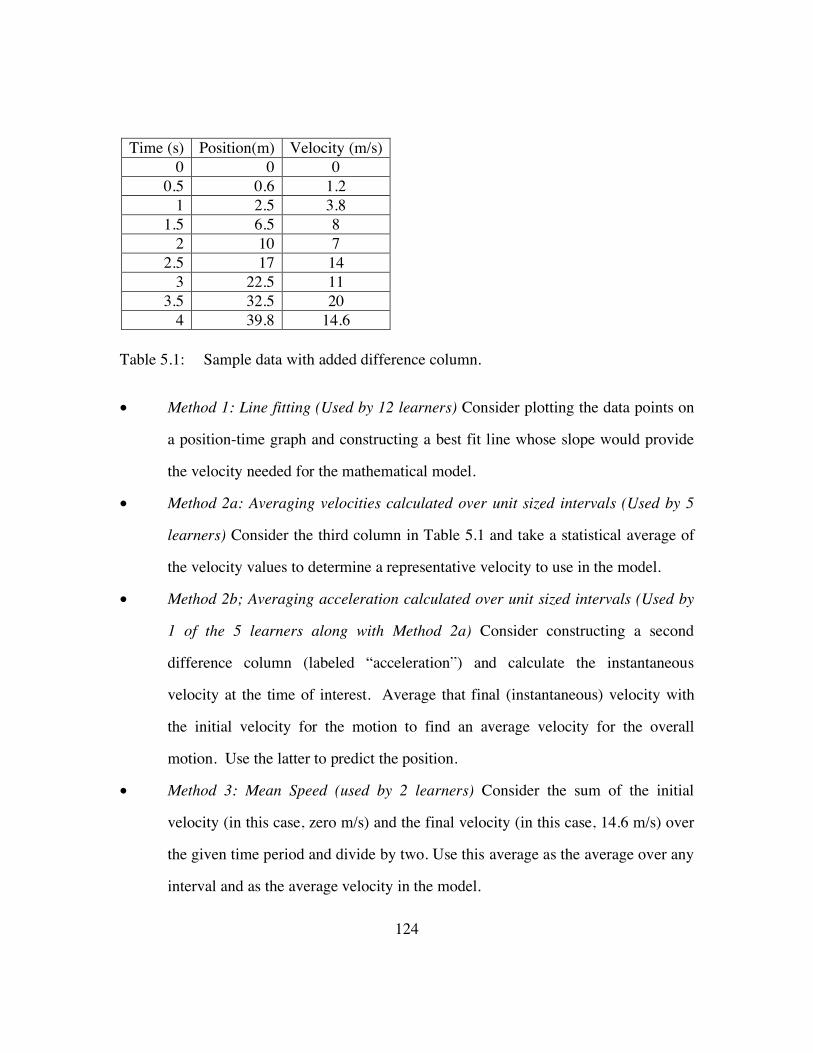
124

Time (s) Position(m) Velocity (m/s)

0 0 0 0.5 0.6 1.2

1 2.5 3.8 1.5 6.5 8

2 10 7 2.5 17 14

3 22.5 11 3.5 32.5 20

4 39.8 14.6

Table 5.1: Sample data with added difference column.

• Method 1: Line fitting (Used by 12 learners) Consider plotting the data points on

a position-time graph and constructing a best fit line whose slope would provide

the velocity needed for the mathematical model.

• Method 2a: Averaging velocities calculated over unit sized intervals (Used by 5

learners) Consider the third column in Table 5.1 and take a statistical average of

the velocity values to determine a representative velocity to use in the model.

• Method 2b; Averaging acceleration calculated over unit sized intervals (Used by

1 of the 5 learners along with Method 2a) Consider constructing a second

difference column (labeled “acceleration”) and calculate the instantaneous

velocity at the time of interest. Average that final (instantaneous) velocity with

the initial velocity for the motion to find an average velocity for the overall

motion. Use the latter to predict the position.

• Method 3: Mean Speed (used by 2 learners) Consider the sum of the initial

velocity (in this case, zero m/s) and the final velocity (in this case, 14.6 m/s) over

the given time period and divide by two. Use this average as the average over any

interval and as the average velocity in the model.

125

• Method 4: (Used by 3 learners) Take the given position values and divide each by

their respective time values (e.g.,

.6 m

.5 s,

2.5 m

1 s,

5.62 m

1.5 s, etc.). This third

method reflects students’ wanting to take a speed with regard to an initial

reference point of zero, that is, an overall speed for the complete motion up to that

point. Once the overall average at each time had been calculated, (3a) some

learners would simply take the statistical average of the overall averages (which

would not give the right answer). Other learners looked for a pattern in the

overall averages and were able to use it to predict the overall average at any given

time, and then use that overall average to predict the position at that time.

Such considerations of average velocity are interesting from both historical and

epistemological standpoints. Method 3 reflects procedures in standard physics, where

beginning and end points of the motion over a specified time interval are the crucial

points of consideration. What happens “in-between” is not given as much priority,

although standard physics does accept mathematical techniques for finding instantaneous

velocity and relies on mathematical definitions of limit and infinitesimal measure for

traditional instruction. The second method (2a and 2b) also reflects procedures in

standard mathematics. They serve as an introduction to the definition of the derivative as

the slope of the tangent line at a given point on a curve. Taking the limit of secant lines

for given time intervals closely approximate the desired curve to describe the motion.

Of notable interest is the fourth method. According to Drake (1990), “One kind

of ‘proportionality’ among times, distances, and speeds is implied when these units are

taken in succession, but not the proportionality existing when they are taken cumulatively

from rest” (p. 33). He argues that this ‘proportionality’ is not a ‘proportion’ in the

algebraic sense when considering time and speed as continuous quantities. Yet,

historically, some scholars believed that the quantities of time, speed, and distance should

126

be measured from rest. Given such a consideration, time and speed accumulate the same

way (in successive units), while distances do not. Drake, argues, “No proportionality

(defined by Euclid as ‘sameness of ratio’) could exist between speeds and distances in

fall, as it could exist between speeds and times” (p. 34). Thus, learners’ attempts to

distinguish between position and distance may exhibit a different type of proportional

reasoning. From a mathematics and physics standpoint, it also brings to mind

considerations of what measures are continuous and what are not. Relying on this notion

of velocity, scholars before and after Galileo’s time, held discussions about the possibility

of instantaneous speed and whether or not a single point could be both the beginning

point and end point of a motion.

Revisiting Tensions and Emerging Themes

The emerging themes of what makes a model “good enough” and learners’

conceptions of average in the context of constructing a mathematical model for motion

are shown on the revised tensions diagram shown in Figure 5.1.

127

Figure 5.1: A revised tensions diagram.

The inner box contains Pollak’s three aspects of mathematical modeling that may be used

as a lens to examine modeling approaches in mathematics and science classrooms. The

key themes that emerge in using such an approach to modeling motion are the result of

examining tensions between the realms of learner experience, standard mathematics, and

standard physics. The diagram also shows the continuing tension that exists between the

realms of math and science as each has differing views of each theme. The identification

of these themes has implications for current theory and for classroom practice and

teachers’ decision-making when both teachers and students are immersed in a modeling

approach to studying motion.

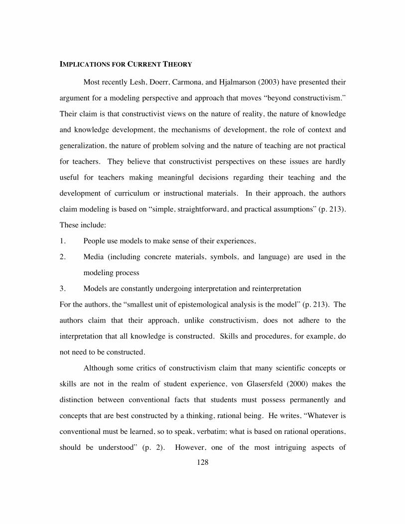
128

IMPLICATIONS FOR CURRENT THEORY

Most recently Lesh, Doerr, Carmona, and Hjalmarson (2003) have presented their

argument for a modeling perspective and approach that moves “beyond constructivism.”

Their claim is that constructivist views on the nature of reality, the nature of knowledge

and knowledge development, the mechanisms of development, the role of context and

generalization, the nature of problem solving and the nature of teaching are not practical

for teachers. They believe that constructivist perspectives on these issues are hardly

useful for teachers making meaningful decisions regarding their teaching and the

development of curriculum or instructional materials. In their approach, the authors

claim modeling is based on “simple, straightforward, and practical assumptions” (p. 213).

These include:

1. People use models to make sense of their experiences,

2. Media (including concrete materials, symbols, and language) are used in the

modeling process

3. Models are constantly undergoing interpretation and reinterpretation

For the authors, the “smallest unit of epistemological analysis is the model” (p. 213). The

authors claim that their approach, unlike constructivism, does not adhere to the

interpretation that all knowledge is constructed. Skills and procedures, for example, do

not need to be constructed.

Although some critics of constructivism claim that many scientific concepts or

skills are not in the realm of student experience, von Glasersfeld (2000) makes the

distinction between conventional facts that students must possess permanently and

concepts that are best constructed by a thinking, rational being. He writes, “Whatever is

conventional must be learned, so to speak, verbatim; what is based on rational operations,

should be understood” (p. 2). However, one of the most intriguing aspects of

129

constructivism is that it allows one to look more closely at the nature and importance of

certain skills within given contexts and why those skills may or not be important. For

example, taking the derivative of a function is an important skill in calculus, but why this

skill is important is a fundamental question teachers try to answer on a fairly routine

basis. According to Ernest (1991), Imre Lakatos, author of Proofs and Refutations (1976)

and creator of the quasi-empiricist view of mathematics, believed,

The epistemological task of the philosophy of mathematics is not simply to answer the question “how is (any) mathematical knowledge possible?” but to account for the actual mathematical knowledge that exists. (pp. 35-36)

Much of what von Glasersfeld proposes parallels rather than contradicts the “beyond

constructivism” paradigm presented by Lesh et al. (2003). Even though Lesh et al. (2003)

acknowledge that cognitive conflicts exist in the minds of students during the modeling

process and that they are important to outline for teachers, the authors do not fully

address the possible sources of these conflicts or how to resolve them. These limitations

are noteworthy in light of the authors’ arguments that their modeling approach is more

practical for the classroom teacher.

Results of the two studies indicate that learners (both teachers and students)

possess the capability of constructing and developing powerful mathematical models (e.g.

d = rt, d = rt + p0, etc.) using a more constructivist approach. In the case of Stephen’s

group, who developed a three-step process to find an answer to a prediction question in

the non-uniform case, the modeling process hardly lies “beyond constructivism.” While

the researcher concedes that Stephen’s “final step” of substituting equations into one

another to yield the final quadratic form may be viewed as more skills-based, an

argument can be made that students like those in Stephen’s group, who are immersed in

an authentic modeling process and constructing their own models, are in a good position

to better understand and appreciate the usefulness and importance of certain skills

130

(algebraic or other). A “beyond constructivism” paradigm would argue that the final

quadratic form is a critical concept that students must learn in terms of its “usefulness,”

“applicability,” and “importance” in the standard curriculum. While this argument may

be true, definitions of “usefulness,” “applicability,” and “importance” are necessarily tied

to views of mathematics and related tasks, visions to meet educational goals, and

thoughts about assessment, each of which may not necessarily be uniform among all

teachers and researchers. The final quadratic form developed by Stephen’s group, for

example, might reflect a different meaning of “usefulness” than one supported by a

standard, traditional curriculum.

LIMITATIONS OF THE STUDIES

Limitations of the Methodology

Given the use of the Grounded Theory approach to data collection, certain

limitations of the method are evident. Taber (2000) warns of a researcher relying too

formally on the “algorithm” for grounded theory (such as the one presented in Chapter 1).

What appears to outline a procedure for making clear-cut decisions actually indicates that

the development of a theory is never complete. The principle of “theoretical saturation”

(p. 471), where further data collection would not significantly alter the model, acts as a

guide for the researcher who ultimately must publish results. According to Glaser

(1978), “Grounded theory … makes [the analyst] humble to the fact that no matter how

far he goes in generating theory, it appears as merely ‘openers’ to what he sees that could

lie beyond” (p. 6). However, according to Glaser and Strauss (1967), the temptation to

collect more data is especially strong in terms of wanting to either elaborate or confirm

current findings. The authors assure that researcher anxiety “to know everything” is not

necessary for theoretical saturation. Yet, given the implications of certain findings while

131

conducting classroom research, there is always the concern that certain factors or thought

processes could initially be overlooked or considered trivial. It is only through repeated

implementations relying on sound conjectures can other factors either be brought to the

fore or determined irrelevant.

To discuss other limitations, the researcher relies on the framework presented by

Cobb et al. (2001) and their work on analyzing classroom mathematical practices using a

modified Grounded Theory approach. Specifically, Cobb and his colleagues analyze

their methodology in terms of trustworthiness, replicability and commensurability, and

usefulness.

Trustworthiness

The difficulty of presenting critical episodes in isolation cannot be overlooked.

Episodes indicating certain mathematical threads of reasoning make sense only within the

context of the entire study, and the reader must rely on the researcher’s claim that

presented inferences or themes span the entire data set. Furthermore, isolating certain

episodes immediately leads to a tendency on the part of the reader to present alternative

interpretations of reasoning exhibited in the vignette. This may be done without the

reader realizing the full scope of the analysis undertaken to choose the episodes as

examples of an identified pattern of reasoning evident throughout the entire data set.

The researcher hopes that this issue has been addressed by presenting and evaluating two

studies rather than one. The process of using two studies allows for development and

refinement of initial conjectures as the researcher moves from one study to the next. The

researcher also concedes that conjectures developed from a grounded theory approach are

always open to refutation and alternative interpretation. However, given the possibility of

conducting further studies, the researcher feels confident that the validity of inferences

and conjectures can become more firmly established.

132

Replicability and Commensurability

Cobb et al. (2001) claim that mathematics education research is “replete with

more than its share of disparate and irreconcilable findings” (p. 153). The researcher

must answer the question of whether or not implementation of the same unit in a different

classroom would yield the same findings and conclusions. The possibility of answering

such a question stems from the importance of considering classroom context and setting

not only when implementing the unit but also when analyzing data. According to Cobb

and his colleagues,

In contrast to traditional experimental research, the challenge as we see it is not that of replicating instructional treatments by ensuring that instructional sequences are enacted in exactly the same way in different classrooms. The conception of teachers as professionals who continually adjust their plans on the basis of ongoing assessments of their students’ reasoning would in fact suggest that complete replicability is neither desirable nor, perhaps, possible (Ball, 1993; Carpenter & Franke, 1998; Gravemeijer, 1994). The challenge for us is instead to develop ways of analyzing treatments so that their realizations in different classrooms can be made commensurable. (p. 153)

In short, the advantage of the researcher’s approach is that students’ learning outcomes

can be related to a learning situation, a desirable goal established by school reformers that

the researcher feels would not be contested by professional teachers or mathematics and

science education researchers. As presented in Chapter 3, Grounded Theory research is

context-based and one of its main goals is “analytical generalization.” Context and

meaning come to the fore when comparing two different classroom situations that are

provided the same implementation or instructional treatment thereby making the two

situations commensurable. Cobb et al. (2001) state,

An analytical approach of this type can lead to greater precision and control by facilitating disciplined, systematic inquiry into instructional innovation and change that embraces the messiness and complexity of the classroom. (p. 154)

133

Naturally, there are other limitations related to typical classroom practice that

inhibit the implementation (though not the validity) of such an approach. One

consideration is time constraints of the typical school schedule. For example, results for

Study One may be evaluated in light of the time constraints experienced by the teachers

to complete activities, especially the activity on non-uniform motion. However, had they

been able to analyze the non-uniform data as they did the uniform data, the teachers’ lack

of consensus about the model developed in the uniform case may have yielded the same

tensions exemplified by the one group who relied on the model rather than the calculator

to analyze the car and ramp data presented in the worksheet.

A second limitation is the difficulty of analyzing and documenting individual

student learning. The interviews conducted in Study Two, for example, played a dual

role in not only probing student thinking, but also evaluating how much the students had

learned throughout the course of the unit. Analysis of these interviews is complex in that

both lenses may be used to develop conjectures and recommendations for further study

and future implementations.

Thirdly, while a grounded theory approach is context-based, the studies presented

do not account for either gender differences or other issues related to equity. For many

schools, these are considerable factors for analysis and debate. Finally, one crucial factor

is that both studies were heavily concerned with mathematical meaning of critical

concepts in kinematics. The researcher assumes a certain level of content knowledge on

the part of the teacher and his or her concern about whether or not such an approach will

help teachers and students realize certain education goals. During Study One and Study

Two, learners’ alluded to the significant role the teacher plays in inquiry-based learning

and the importance of content knowledge.

134

Molly: I just have a comment. In looking at all this, I think I must have a very superficial understanding. If someone were to ask me a general procedure for finding position, I would have just basically given them how we must know speed and how it changes over time; we must select and measure a starting and ending point for this change in position, and we must have an elapsed time over which to make this measurement. Now as far as any calculations, y’know, under general…, I probably wouldn’t have included that and I’m thinking I may be missing the whole point.

Joan: I just realized how much content knowledge that science and math teachers have to have to get these kinds of discourse patterns in a classroom. To look at these relationships, the level of content knowledge that somebody needs is…well, that’s my observation. But your strategy, though, to get people to see these relationships which has really moved away from just the procedural was to create these discourse patterns, and I look at the level of knowledge you have to have in order to really create that and to have people who are making sense of it all along the way. I was watching the pedagogy as much as trying to get the [ideas].

The researcher feels that the studies make a contribution by providing an indication, at

least, of the type of content knowledge necessary or desirable for teachers to implement

such an approach to studying kinematics (e.g. function, average) given calls for reform

and guidelines presented by both national and state standards for mathematics and

science.

Usefulness

The studies presented provide a means to support discussions regarding

professional development of teachers. Cobb and his colleagues write,

We have noted that what we need in order to improve our instructional designs are accounts of students’ learning that are tied to analyses of what happened in the classrooms where that learning occurred. Analyses of classroom mathematical practices, when coordinated with psychological analyses of individual students’ reasoning, provide situated accounts of students’ learning in which the process of their learning is directly related to the means by which it was supported. (p. 154)

135

Given that both studies link classroom setting and learning, the opportunity for teachers

to link context and instructional practice is evident,. Through such studies, teachers can

learn how to test, adapt, and modify certain approaches in the classroom based on student

learning and desired outcomes. The complexity of such an approach, however,

necessarily requires change to be a more time-consuming, and continuous, process of

learning and implementing on the part of the classroom teacher.

RECOMMENDATIONS FOR FURTHER RESEARCH

Both studies provide examples of the kind of research recommended by the

International Commission on Mathematics Instruction (2003). In particular, both studies

help address two critical questions (or issues) posed by ICMI.

Taking account of teaching objectives and students’ personal situations (experience, competence), how can teachers set up authentic applications and modeling tasks? (p. 12)

What is essential in a teacher education program to ensure that prospective teachers will acquire modeling competencies and be able to teach applications and modeling in their professional future? (p. 13)

Further implementations of the unit would provide more specific answers to the

questions. Finally, teachers’ beliefs and perceptions of models in science and science

education have an effect on students’ learning outcomes. The impact or implications on

instruction or classroom practice requires further investigation to support implementation

of modeling approaches. Such studies in this vein are rare (Driel & Verloop, 1999; Driel

& Verloop, 2002; Justi & Gilbert, 2002).

Other specific issues, also raised by ICMI (2003) and related to epistemology, are

also addressed by the dissertation. Table 5.2 outlines these issues and recommendations

for further research based on the two studies.

136

Questions and Recommendations for Research Related to Epistemology

What are the process components of modeling? What is meant by or involved in each (ICMI, p.11)? • Pollak’s aspects of modeling should be tested and re-tested as a viable lens through

which to study modeling approaches in classrooms. A sound question to ask is whether his criteria indicate an approach to modeling inherent in learners’ thought processes.

• Do learners have an inherent notion (or concept) of average or average speed that emerges in the context of studying kinematics using a modeling approach? If so, how can this notion contribute to current research on understanding of average (Mokros & Russell, 1995) or average speed (Reed & Jazo, 2002)?

• How can an inherent notion (or concept) of average or average speed contribute to learners grasping both qualitative AND quantitative aspects of motion graphs (i.e., How can further research on this notion of average contribute to the established research on qualitative graphing)?

What is the meaning and role of abstraction, formalization and generalization in applications and modeling (ICMI, p.11)? • Given that learners in both studies were able to develop some forms of linear and/or

quadratic equations, how could a modeling approach to kinematics be modified to further support learners constructing mathematical models such as x = vt + x

0 and

x =1

2a !t( )

2

+ vi!t + x

0?

What is the role of pure mathematics in developing modeling ability (ICMI, p. 13)? • How would students be able to take their constructions (models) and relate them to

more abstract concepts in formal mathematics (i.e. identify them as parts of a more formal, abstract system)?

Table 5.2: Epistemological questions to support further research.

Learners’ involvement with the unit on kinematics highlights the need to bridge a

gap between mathematics and physics concepts and the practices of experimentation, data

137

gathering, and analysis of real world data. Woolnough (2000) emphasizes that students

must see “links between the mathematical processes they are using and the physics they

are studying” (p. 259). In order to help students obtain learning goals, teachers must also

be able to create and strengthen such links. A difficult, though notable, goal is to have

teachers link not only the math and physics worlds through critical concepts, but also link

the math and science realms to learners’ experience. A model-based or inquiry-based

approach appears to be the best means to reach this goal, though much work must be

done in terms of teacher preparation and re-evaluating certain educational goals before

substantial, worthwhile benefits are realized. Furthermore, establishing a uniform theory

of modeling in mathematics and science classrooms can support efforts to reach the goal

and maximize benefits for both teachers and students.

138

Appendix A: Kinematics Activities

I. Describing motion (Activity 1) a. Objectives

i. Identify critical concepts in describing motion (position and time). ii. Differentiate position and distance, clock time and time of travel.

iii. Understand that position can be predicted from a starting position and time and knowledge of how position is changing with time (velocity).

b. Activities i. Invent and describe a motion. In groups of 3-4, think of a motion

that a racquetball might undergo. It should be simple enough that you can reproduce it accurately. Create a description of the motion that is detailed enough so that another group could reproduce the motion exactly. Have groups exchange descriptions and attempt to reproduce the motions. Identify the important elements of a complete description.

II. Constant velocity a. Measuring constant velocity (Activity 2)

i. Objectives 1. Explain a procedure for finding the position of the object at

some future time, t, using only a data table. 2. Use a graph to predict the position of an object at some

future time. 3. Interpret the slope of a position-time graph as the velocity

of a moving object. 4. Be able to draw a best fit line to represent a set of data. Be

able to explain why a best fit line is a better representation of nature than the actual data points.

5. Derive an algebraic equation to represent an object moving with constant velocity.

ii. Activities 1. Have each group suggest a procedure for graphing the

relationship between the position of a rolling ball and elapsed time. Each group should present its proposal to the class. The instructor chooses the best of the proposed ideas as the official class procedure.

2. Have each group member fill out a Lab Proposal sheet. 3. Conduct lab and collect data 4. Discuss the meaning of the collected data. Determine

procedure for determining times and positions beyond the known data set.

139

5. Graph data and find an equation to represent the gathered data. Predict the ball’s position for various times. Discuss the significance of the slope of the line.

b. Developing equations for constant velocity (Activity 3) i. Objectives

1. Be able to determine the equation describing constant velocity motion from position and time data

ii. Activities 1. Practice determining equations of motion from data 2. Determine the equation of motion from the description of

motion 3. Determine a possible motion that an equation might

describe III. Accelerated motion

a. Acceleration with a spark timer (Activity 4) i. Objectives

1. Create a position-time and velocity-time table for accelerated motion

2. Find the average velocity for an accelerating object during successive small intervals

3. Predict the future position and velocity of an accelerating object

4. Create an equation for uniformly accelerated motion ii. Activities

1. Use a spark timer, a ramp, and a cart to gather position-time data for accelerated motion. Use a different angle for each group.

2. Mark each consecutive 0.1s interval and calculate the average velocity for each interval.

3. Use a differences table to find patterns in the carts position and velocity values.

4. Use differences to derive an equation. b. Developing equations for accelerated motion (Activity 5)

i. Objectives 1. Be able to determine the equation describing accelerated

motion from position and time data ii. Activities

1. Practice determining equations of motion from data 2. Determine the equation of motion from the description of

motion 3. Determine a possible motion that an equation might

describe

140

Appendix B: Kinematics Pre Post-Test

Question 1:

Question 2:

Question 3:

141

Question 4:

Question 5:

Question 6:

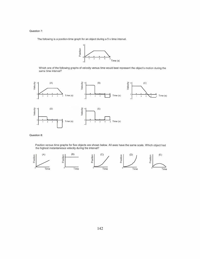
142

Question 7:

Question 8:

143

Question 9: The figure below shows a position time graph for the motions of two objects A and B that are moving along the same meter stick.

(a) At the instant t = 2 s, is the speed of object A greater than, less than, or equal to the speed of object B? Explain your reasoning.

(b) Do objects A and B ever have the same speed? If so, at what times? Explain your reasoning.

144

Question 10:

Question 11:

145

Question 12:

Question 13:

146

Question 14:

Question 15:

Question 16: An object with constant acceleration obeys the following equation:

16t2 + 8t = x + 15

a) How do you interpret the number 16?

b) How do you interpret the number 8?

c) How do you interpret the number 15?

147

Question 17:

Question 18:

Block a

Block b

148

Question 19:

149

Question 20: Derive or construct an equation that could describe the motion of the person who created each of the following graphs. Explain your methods and reasoning. a)

b)

p

t

p

t (1, - 1)

(2, 2)

(3, 7)

150

Question 21. Derive or construct an equation to describe the following set of data collected by a person using a motion detector. Explain your methods and reasoning.

Time (s) Position (cm) 1 8 2 26 3 56 4 98 5 152 6 218 7 296

8 386

151

Appendix C: Interview Protocol for Study Two

1. Suppose that you are part of a group of students who are given a task to create a motion using a rubber ball. Your group must be able to describe the motion of the ball as clearly and completely as they can in written form so that another group of students can see the description and recreate the motion exactly. Suppose your group decides to use the following set-up.

2. Suppose one of your fellow group members presents you with this data collected from an experiment involving a rubber ball in motion.

Time (s) Position (m) 0 0 .5 .6 1 2.5

1.5 5.62 2 10

2.5 15.6 3 22.5

3.5 30.7 4 39.8 . . . . . .

20 ?

How would you predict the position of the ball at 20 seconds?

152

Bibliography

Amerom, B. v. (2002). Reinvention of early algebra: Developmental research on the transition from arithmetic to algebra. Utrecht: CD-b Press.

Bailer-Jones, D.M. (1999). Tracing the development of models in the philosophy of science. In L. Magnani, N.J. Nersessian, & P. Thagard (Eds.), Model-based reasoning in scientific discovery (pp. 23-40). New York, NY: Kluwer Academic/Plenum Publishers.

Bailer-Jones, D.M. (2002). Scientists' thoughts on scientific models. Perspectives on Science 2002, 10(3), 275-301.

Ball, D. (1993). With an eye on the mathematical horizon: Dilemmas of teaching elementary school mathematics. Elementary School Journal, 93, 373-397.

Beichner, R.J. (1994). Testing student interpretation of kinematics graphs. American Journal of Physics, 62, 750-762.

Beichner, R.J. (1996). Test of Understanding Graphs - Kinematics. North Carolina State University. Available from author.

Bowers, J., & Doerr, H. M. (2001). An analysis of prospective teachers' dual roles in understanding the mathematics of change: Eliciting growth with technology. Journal of Mathematics Teacher Education, 4, 115-137.

Boyd, A., & Rubin, A. (1996). Interactive video: A bridge between motion and math. International Journal of Computers for Mathematical Learning, 1, 57-93.

Carpenter, T.P., & Franke, M.L. (1998). Teachers as learners. Principled Practice, 2, 1-3.

Cobb, P., Stephan, M., McClain, K., & Gravemeijer, K. (2001). Participating in classroom mathematical practices. The Journal of the Learning Sciences, 10(1&2), 113-163.

Cohen, I.B. (1980). The Newtonian revolution. Cambridge, UK: Cambridge University Press.

Confrey, J. (1998). Voice and perspective: Hearing epistemological innovation in students’ words. In M. Larochelle, N. Bednarz & J. Garrison (Eds.), Constructivism and education (pp. 104-120). New York, NY: Cambridge University Press.

153

Confrey, J., & Costa, S. (1996). A critique of the selection of "mathematical objects" as a central metaphor for advanced mathematical thinking. International Journal of Computers for Mathematical Learning, 1, 139-168.

Confrey, J., & Doerr, H. (1994). Student modelers. Interactive Learning Environments, 4(3), 199-217.

Cross, K.P. (1987). The need for classroom research. In J.G. Kurfiss, L. Hilsen, L. Mortensen, & E. Wadsworth (Eds.), To improve the academy (pp. 3-17). Stillwater, OK: Professional & Organizational Development Network in Higher Education.

Dear, P. (1995). Discipline & experience: The mathematical way in the scientific revolution. Chicago, IL: The University of Chicago Press.

Dennis, D. (2000). The role of historical studies in mathematics and science educational research. In A. Kelly & R. Lesh (Eds.), Handbook of research design in mathematics and science education (pp. 799-813). Mahwah, NJ: Lawrence Erlbaum Associates.

diSessa, A. (2000). Changing minds: Computers, learning, and literacy. Cambridge, MA: MIT Press.

Doerr, H., & English, L. (2003). A modeling perspective on students' mathematical reasoning about data. Journal for Research in Mathematics Education, 34(2), 110-136.

Doerr, H., & Tripp, J. (1999). Understanding how students develop mathematical models. Mathematical Thinking and Learning, 1(3), 231-254.

Doorman, M. (2001). How to guide students? A reinvention course on modeling motion. Paper presented at the Netherlands and Taiwan conference on common sense in mathematics education, Taipei, Taiwan.

Driel, J.H. v., & Verloop, N. (1999). Teachers' knowledge of models and modelling in science. International Journal of Science Education, 21(11), 1141-1153.

Driel, J.H. v., & Verloop, N. (2002). Experienced teachers’ knowledge of teaching and learning of models and modelling in science education. International Journal of Science Education, 24(12), 1255-1272.

Edwards, C.H. (1979). The historical development of the calculus. New York, NY: Springer-Verlag.

154

Ernest, P. (1991). The philosophy of mathematics education. Philadelphia, PA: Falmer Press.

Ernest, P. (1998). Social constructivism as a philosophy of mathematics. Albany, NY: State University of New York Press.

Ford, M. J. (2003). Representing and meaning in history and in classrooms: Developing symbols and conceptual organizations of free-fall motion. Science & Education, 12, 1-25.

Freudenthal, H. (1991). Revisiting mathematics education. Dordrecht: Kluwer Academic Publishers.

Giere, R. N. (1999). Using models to represent reality. In L. Magnani, N.J. Nersessian, & P. Thagard (Eds.), Model-based reasoning in scientific discovery (pp. 41-57). New York, NY: Kluwer Academic/Plenum Publishers.

Glaser, B.G. (1978). Theoretical sensitivity: Advances in the methodology of grounded theory. Mill Valley, CA: Sociology Press.

Glaser, B. G., & Strauss, A. L. (1967). The discovery of Grounded Theory: Strategies for qualitative research. Hawthorne, NY: Aldine de Gruyter Publishing.

Glasersfeld, E. v. (1998). Scheme theory as a key to the learning paradox. Invited paper presented at the 15th Advanced Course, Archives Jean Piaget, Geneva.

Glasersfeld, E. v. (2000). Radical constructivism and teaching. Available: http://www.umass.edu/srri/vonGlasersfeld/onlinePapers/html/geneva/

Glasersfeld, E. v. (2001). The radical constructivist view of science. Foundations of Science, 6, 31-43.

Goldenberg, E. P., & Cuoco, A. (1998). What is dynamic geometry? In R. Lehrer & D. Chazan (Eds.), Designing learning environments for developing understanding of geometry and space (pp. 351-367). Mahwah, NJ: Lawrence Erlbaum Associates.

Gravemeijer, K. (1994). Educational development and developmental research. Journal for Research in Mathematics Education, 25, 443-471.

Gravemeijer, K., & Doorman, M. (1999). Context problems in realistic mathematics education: A calculus course as an example. Educational Studies in Mathematics, 39, 111-129.

155

Gruber, H.E., & Vonéche, J.J. (1995). Looking back at the essential. In H.E. Gruber & J.J. Vonéche (Eds.), The essential Piaget (pp. 864-878). Northvale, NJ: Jason Aronson, Inc.

Halloun, I. (1996). Schematic modeling for meaningful learning of physics. Journal of Research in Science Teaching, 33(9), 1019-1041.

Halloun, I, Hake, R.R., Mosca, E.P., & Hestenes, D. (1992). The Force Concept Inventory. Available: http://modeling.la.asu.edu/R&E/Research.html.

Hestenes, D. (1992). Modeling games in the Newtonian world. American Journal of Physics, 60, 732-748.

Hestenes, D. (1993). Modeling is the name of the game. Paper presented at the National Science Foundation Modeling Conference. Dedham, MA.

International Commission on Mathematics Instruction. (2003). ICMI Study 14: Applications and modeling in mathematics education [Discussion document]. Kassel, Germany: University of Kassel.

Justi, R.S., & Gilbert, J.K. (2002). Modelling, teachers' views on the nature of modelling, and implications for the education of modellers. International Journal of Science Education, 24(4), 369-387.

Kaput, J. (1996). Representations, inscriptions, descriptions and learning: A kaleidoscope of windows. Journal of Mathematical Behavior, 2, 265-281.

Kvale, S. (1996). InterViews: An introduction to qualitative research interviewing. Thousand Oaks, CA: SAGE Publications.

Lakatos, I. (1976). Proofs and refutations. Cambridge, UK: Cambridge University Press.

Lehrer, R., & Schauble, L. (2000). Modeling in mathematics and science. In R. Glaser (Ed.), Advances in instructional psychology: Educational design and cognitive science (Vol. 5, pp. 101-159). Mahwah, NJ: Lawrence Erlbaum Associates.

Lehrer, R., Schauble, L., Strom, D., & Pligge, M. (2001). Similarity of form and substance: Modeling material kind. In S. M. Carver & D. Klahr (Eds.), Cognition and instruction: Twenty-five years of progress (pp. 39-74). Mahwah, NJ: Lawrence Erlbaum Associates.

Leinhardt, G., Zaslavsky, O., & Stein, M.K. (1990). Functions, graphs, and graphing: Tasks, learning, and teaching. Review of Educational Research, 60, 1-64.

156

Lesh, R., & Doerr, H. (Eds.). (2003). Beyond constructivism: Models and modeling perspectives on mathematics problem solving, learning, and teaching. Mahwah, NJ: Lawrence Erlbaum Associates.

Lesh, R., Doerr, H., Carmona, G., & Hjalmarson, M. (2003). Beyond constructivism. Mathematical Thinking and Learning, 5(2&3), 211-233.

Mann, M. P. (1993). Grounded Theory and classroom research. Excellence in College Teaching, 4, 131-143.

Matos, J. F., Blum, W., Houston, S. K., & Carreira, S. P. (Eds.) (2001). Modelling and mathematics education. Chichester, England: Horwood Publishing.

McDermott, L.C. (1996). Physics by inquiry. New York, NY: John Wiley & Sons.

McDermott, L. C., Rosenquist, M. L., & Zee, E. H. v. (1987). Student difficulties in connecting graphs and physics: Examples from kinematics. American Journal of Physics, 55(6), 503-513.

Mokros, J., & Russell, S.J. (1995). Children's concepts of average and representativeness. Journal for Research in Mathematics Education, 26(1), 20-39.

National Council of Teachers of Mathematics. (2000). Principles and standards for school mathematics. Reston, VA: Author.

National Research Council. (1996). National science education standards. Washington, DC: National Academy Press.

National Research Council. (2000). Strengthening the linkages between the sciences and the mathematical sciences. Washington, D.C.: National Academy of Sciences.

Nemirovsky, R., & Rubin, A. (1992). Students' tendency to assume resemblances between a function and its derivative. Cambridge, MA: TERC.

Nemirovsky, R., Tierney, C., & Wright, T. (1998). Body motion and graphing. Cognition and Instruction, 16(2), 119-172.

Niss, M. (2001). Issues and problems of research on the teaching and learning of applications and modeling. In J. F. Matos, W. Blum, S. K. Houston & P. Carreira (Eds.), Modeling and mathematics education: ICTMA 9 - Applications in science and technology (pp. 72-88). Chichester, England: Horwood Publishing.

157

Noble, T., Flerlage, D., & Confrey, J. (1993, April 12-16). Experiment, simulation, and analytic teaching and learning in an integrated physics and mathematics class. Paper presented at the annual meeting of the American Educational Research Association, Atlanta, GA.

Otte, M. (1994). Is radical constructivism coherent? In P. Ernest (Ed.), Constructing mathematical knowledge: Epistemology and mathematical education (pp. 50-61). Bristol, PA: Falmer Press.

Papert, S. (1980). Mindstorms: Children, computers, and powerful ideas. New York, NY: BasicBooks.

Petrosino, A. (2003). Commentary: A framework for supporting learning and teaching about mathematical and scientific models. Contemporary Issues in Technology and Teacher Education [Online serial], 3(3). Available: http://www.citejournal.org/vol3/iss3/science/article1.cfm

Piaget, J. (1970). Genetic epistemology. New York, NY: W.W. Norton and Company.

Pollak, H. O. (2003). A history of the teaching of modeling. In G. M. A. Stanic & J. Kilpatrick (Eds.), A history of school mathematics (Vol. 1, pp. 647-672). Reston, VA: National Council of Teachers of Mathematics.

Raisis, V. (1999). Expansion and justification of models: The exemplary case of Galileo Galilei. In L. Magnani, N.J. Nersessian, & P. Thagard (Eds.), Model-based reasoning in scientific discovery (pp. 149-164). New York, NY: Kluwer Academic/Plenum Publishers.

Reed, S.K., & Jazo, L. (2002). Using multiple representations to improve conceptions of average speed. Journal of Educational Computing Research, 27(1&2), 147-166.

ResearchWare, Inc. (2004). HyperRESEARCH (Version 2.6) [Computer software]. Randolph, MA: Author. Available: http://www.researchware.com/

Roth, W-M., Woszczyna, C., & Smith, G. (1996). Affordances and constraints of computers in science education. Journal of Research in Science Teaching, 33(9), 995-1017.

Russell, D.W., Lucas, K.B., & McRobbie, C.J. (2003). The role of the microcomputer-based laboratory display in supporting the construction of new understandings in kinematics. Research in Science Education, 33, 217–243.

Sepkoski, D. (in press). Nominalism and constructivism in seventeenth-century mathematical philosophy. To appear in Historia Mathematica.

158

Sfard, A. (1991). On the dual nature of mathematical conceptions: Reflections on processes and objects as different sides of the same coin. Educational Studies in Mathematics, 22, 1-36.

Sfard, A., & Linchevski, L. (1994). The gains and the pitfalls of reification-The case of algebra. Educational Studies in Mathematics, 26, 191-228.

Sfard, A. (2000). Symbolizing mathematical reality into being - Or how mathematical discourse and mathematical objects create each other. In P. Cobb, E. Yackel, and K. McClain (Eds.), Symbolizing and communicating in mathematics classrooms: Perspectives on discourse, tools, and instructional design (pp. 37-98). Mahwah, NJ: Lawrence Erlbaum Associates.

Shternberg, B., & Yerushalmy, M. (2003). Models of functions and models of situations: On the design of modeling-based learning environments. In R. Lesh & H. Doerr (Eds.), Beyond constructivism: Models and modeling perspectives on mathematics problem solving, learning, and teaching (pp. 479-498). Mahwah, NJ: Lawrence Erlbaum Associates.

Stroup, W. (2002). Understanding qualitative calculus: A structural synthesis of learning research. International Journal of Computers for Mathematical Learning, 7, 167-215.

Taber, K. (2000). Case studies and generalizability: Grounded Theory and research in science education. International Journal of Science Education, 22(5), 469-487.

Testa, I., Monroya, G., & Sassi, E. (2002). Students’ reading images in kinematics: The case of real-time graphs. International Journal of Science Education, 24(3), 235-256.

Villiers, M. de (1998). An alternative approach to proof in dynamic geometry. In R. Lehrer & D. Chazan (Eds.), Designing learning environments for developing understanding of geometry and space (pp. 369-393). Mahwah, NJ: Lawrence Erlbaum Associates.

Wells, M., Hestenes, D., & Swackhamer, G. (1995). A modeling method for high school physics instruction. American Journal of Physics, 63(7), 606-619.

Woolnough, J. (2000). How do students learn to apply their mathematical knowledge to interpret graphs in physics? Research in Science Education, 30(3), 259-267.

159

Vita

David John Carrejo was born in El Paso, Texas on March 25, 1970, the youngest

of four children of Sabino and the late Amalia Carrejo. After graduating from Cathedral

High School in El Paso in 1988, he attended the University of Texas at El Paso (UTEP)

where he earned a Bachelor of Science in Mathematics in 1995 and a Master of Arts in

Teaching Mathematics in 1998. While earning his degrees, he taught algebra at

Cathedral High School and algebra, pre-calculus and mathematics for preservice

elementary teachers at UTEP. In 1999, he enrolled at the University of Texas at Austin

to begin work on a doctoral degree in Mathematics & Science Education. His education

at UT Austin has included experience as a graduate research assistant in several research

areas including systemic reform in mathematics education, after-school mathematics

programs, and design experiments in the mathematics classroom. He was also an active

teaching assistant in the secondary teacher preparation program, UTeach.

Permanent address: 8600 Brodie Lane #1428

Austin, Texas 78745

This dissertation was typed by the author.

copyright by david john carrejo 2004

Documents