© copyright by brian david yanoff, 2000
TRANSCRIPT

© Copyright by Brian David Yanoff, 2000
TEMPERATURE DEPENDENCE OF THE PENETRATION DEPTH IN THEUNCONVENTIONAL SUPERCONDUCTOR Sr2RuO4
BY
BRIAN DAVID YANOFF
B.A., Swarthmore College, 1993M.S., University of Illinois, 1994
THESIS
Submitted in partial fulfillment of the requirementsfor the degree of Doctor of Philosophy in Physics
in the Graduate College of theUniversity of Illinois at Urbana-Champaign, 2000
Urbana, Illinois
iii
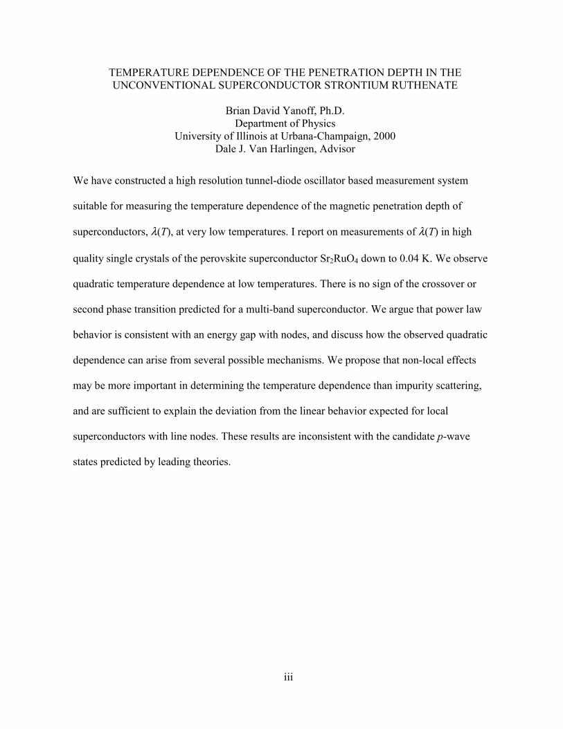
TEMPERATURE DEPENDENCE OF THE PENETRATION DEPTH IN THEUNCONVENTIONAL SUPERCONDUCTOR STRONTIUM RUTHENATE
Brian David Yanoff, Ph.D.Department of Physics
University of Illinois at Urbana-Champaign, 2000Dale J. Van Harlingen, Advisor
We have constructed a high resolution tunnel-diode oscillator based measurement system
suitable for measuring the temperature dependence of the magnetic penetration depth of
superconductors, λ(T), at very low temperatures. I report on measurements of λ(T) in high
quality single crystals of the perovskite superconductor Sr2RuO4 down to 0.04 K. We observe
quadratic temperature dependence at low temperatures. There is no sign of the crossover or
second phase transition predicted for a multi-band superconductor. We argue that power law
behavior is consistent with an energy gap with nodes, and discuss how the observed quadratic
dependence can arise from several possible mechanisms. We propose that non-local effects
may be more important in determining the temperature dependence than impurity scattering,
and are sufficient to explain the deviation from the linear behavior expected for local
superconductors with line nodes. These results are inconsistent with the candidate p-wave
states predicted by leading theories.

iv
This thesis is dedicated to my wife, Liz. Without her love, encouragement,
support, patience and understanding, this thesis would not be what it is. And I
dedicate it also to my newborn daughter, Eliana, whose anticipated arrival
within days of my defense was the best incentive of all to finish!
v
Acknowledgments
First I would like to thank my research advisor, Dale Van Harlingen, for his patience,
support and guidance, and for allowing me the latitude to pursue the research of which this
thesis is a product. I also thank all the members of the DVH group that helped me in so many
ways over the years. Special thanks also goes to Ismardo Bonalde for sharing his knowledge of
dilution refrigerators, tunnel diode oscillators, and for working with me on the design and
operation this experiment. Thanks to Elbert Chia for helping us run the system, and for asking
questions that forced me think hard about the most fundamental issues. Thanks to Prof. Myron
Salamon for helping us interpret our results, and to Cliff and Spencer in the machine shop for
making many of the parts for the system.
Lastly, I gratefully acknowledge the support of the National Science Foundation under
award number NSF DMR97-05695 and, through its Science and Technology Center for
Superconductivity under award number STC DMR91-20000.

vi
Table of Contents
1 Review of Experimental Techniques ...........................................................1
1.1 Self-Inductive Resonant Oscillator Techniques..........................................1
1.2 Microwave Surface Impedance................................................................10
1.3 Mutual Inductance....................................................................................12
1.4 SQUID Magnetometry..............................................................................14
1.5 Torque Magnetometry..............................................................................15
1.6 Muon Spin Relaxation ..............................................................................16
1.7 Josephson Junction Modulation...............................................................19
References .........................................................................................................20
2 Experimental Design .....................................................................................22
2.1 Tunnel Diode Oscillator Circuit Design ....................................................23
2.2 Mechanical Design...................................................................................25
2.3 Calibration................................................................................................34
2.4 Performance ............................................................................................37
References .........................................................................................................39
3 Penetration Depth in Unconventional Superconductors.......................40
3.1 Conventional Superconductors ................................................................40
3.2 Unconventional Superconductors ............................................................44
3.3 Nodes in the Energy Gap.........................................................................47
3.4 Perturbing Effects ....................................................................................52
References .........................................................................................................54
4 Strontium Ruthenate .....................................................................................56

vii
4.1 Crystal Growth and Characterization .......................................................56
4.2 Superconducting Properties.....................................................................60
4.3 Prominent Theoretical Concepts..............................................................68
References .........................................................................................................72
5 Penetration Depth of Strontium Ruthenate..............................................75
5.1 Samples ...................................................................................................75
5.2 Calibration................................................................................................76
5.3 Results .....................................................................................................79
5.4 Interpretation............................................................................................83
References .........................................................................................................90
6 Conclusions and Future Directions............................................................91
6.1 Future Directions......................................................................................92
References .........................................................................................................95
Appendix A Samples.......................................................................................... 96
A.1 Crystal Batches........................................................................................ 96
A.2 SRO Sample Geometry ......................................................................... 100
Vita ............................................................................................................................. 104

1
1 Review of Experimental Techniques
In this chapter I will review a number of experimental techniques which have been used
successfully to measure the penetration depth of superconductors. Since the experiments
described in this thesis use a self-inductive tunnel diode oscillator technique, I will start with a
fairly detailed discussion of oscillator measurements of superconducting samples. I will also
discuss the techniques of mutual inductance, microwave surface impedance, torque
magnetometry and Josephson junction modulation.
1.1 Self-Inductive Resonant Oscillator Techniques
One of the most useful devices, for many different kinds of measurements, is the
resonant oscillator. The technique is quite simple in its design. An oscillation is established
whose frequency can be made to depend on the physical quantity under investigation with a
known relationship. The frequency can be measured with great precision simply by counting
the number of cycles of the oscillation, and this can be converted to a precise value of the
physical quantity in question.
Perhaps the best known example of the oscillator is the use of a pendulum to measure
the acceleration due to gravity. If the length L of the pendulum is known, the frequency of
oscillation Lg /=ω gives the acceleration. A very useful oscillator technique for solid state
physics employs an electronic rather than mechanical resonance. An inductor-capacitor (LC)
resonant circuit is constructed, and provided with a source of gain in a positive feedback
configuration. The result is an oscillation at the resonant frequency of the LC circuit. By
rendering the inductance or capacitance sensitive to a physical property of a sample, such as
2
dielectric constant or magnetic susceptibility, the resonant frequency will shift with changes to
these properties.
There are a number of advantages of electronic oscillators over their mechanical analogs.
The frequency can be made significantly higher, which allows for a precise measurement of
frequency in a shorter time interval. These higher frequencies are accompanied by sharper
resonance (greater quality factor, Q) which contributes to a stable and sensitive frequency
response. If designed and constructed well, electronic oscillators can be made fairly insensitive
to mechanical and electrical disturbances, and to other environmental factors as well.
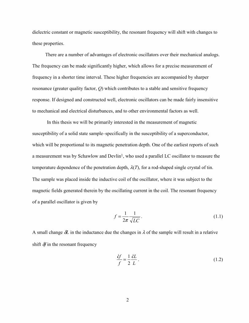
In this thesis we will be primarily interested in the measurement of magnetic
susceptibility of a solid state sample–specifically in the susceptibility of a superconductor,
which will be proportional to its magnetic penetration depth. One of the earliest reports of such
a measurement was by Schawlow and Devlin1, who used a parallel LC oscillator to measure the
temperature dependence of the penetration depth, λ(T), for a rod-shaped single crystal of tin.
The sample was placed inside the inductive coil of the oscillator, where it was subject to the
magnetic fields generated therein by the oscillating current in the coil. The resonant frequency
of a parallel oscillator is given by
LCf 1
21π
= . (1.1)
A small change δL in the inductance due the changes in λ of the sample will result in a relative
shift δf in the resonant frequency
LL
ff δδ
21= . (1.2)
3
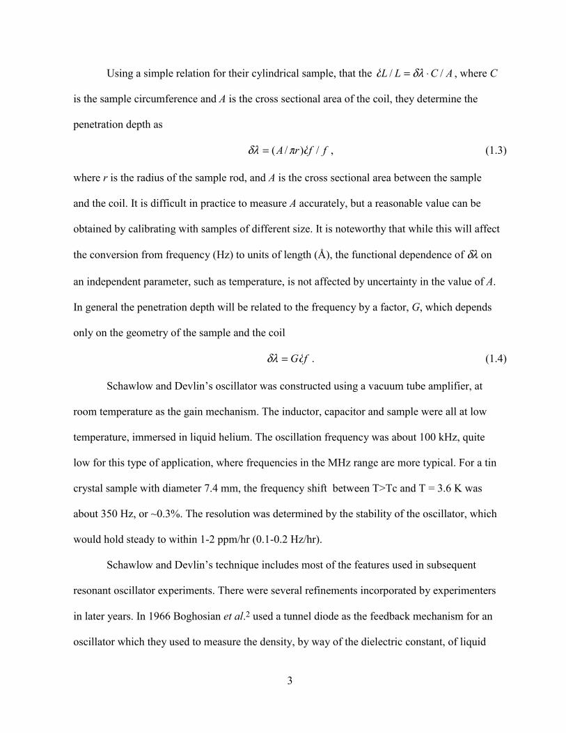
Using a simple relation for their cylindrical sample, that the ACLL // ⋅= δλδ , where C
is the sample circumference and A is the cross sectional area of the coil, they determine the
penetration depth as
ffrA /)/( δπδλ = , (1.3)
where r is the radius of the sample rod, and A is the cross sectional area between the sample
and the coil. It is difficult in practice to measure A accurately, but a reasonable value can be
obtained by calibrating with samples of different size. It is noteworthy that while this will affect
the conversion from frequency (Hz) to units of length (Å), the functional dependence of δλ on
an independent parameter, such as temperature, is not affected by uncertainty in the value of A.
In general the penetration depth will be related to the frequency by a factor, G, which depends
only on the geometry of the sample and the coil
fGδδλ = . (1.4)
Schawlow and Devlin’s oscillator was constructed using a vacuum tube amplifier, at
room temperature as the gain mechanism. The inductor, capacitor and sample were all at low
temperature, immersed in liquid helium. The oscillation frequency was about 100 kHz, quite
low for this type of application, where frequencies in the MHz range are more typical. For a tin
crystal sample with diameter 7.4 mm, the frequency shift between T>Tc and T = 3.6 K was
about 350 Hz, or ~0.3%. The resolution was determined by the stability of the oscillator, which
would hold steady to within 1-2 ppm/hr (0.1-0.2 Hz/hr).
Schawlow and Devlin’s technique includes most of the features used in subsequent
resonant oscillator experiments. There were several refinements incorporated by experimenters
in later years. In 1966 Boghosian et al.2 used a tunnel diode as the feedback mechanism for an
oscillator which they used to measure the density, by way of the dielectric constant, of liquid

4
3He under pressure. In this case the liquid He filled the space between the plates of the
capacitor, thus changes in dielectric constant were measured through the change in capacitance,
rather than inductance. The use of a tunnel diode as the gain mechanism improved the system
in several ways. First the frequency of the circuit was made higher, ~10 MHz, allowing a
measurement with greater relative precision. Second, due to the low power requirements of the
tunnel diode, the entire circuit, except for power supply, was maintained in the low temperature
part of the cryostat, contributing to improved short term stability of the oscillator of 0.2 ppm.
Lastly, the higher frequency increases the Q ~ f/∆f, also contributing to improved sensitivity.
Figure 1.1 shows the IV curve for the tunnel diode used in our circuit (Germanium
Power Devices model BD-3). The important feature of the tunnel diode is the region of
negative differential resistance. The shape of this characteristic curve comes from a
combination of ordinary exponential diode behavior and quantum mechanical tunneling across
the diode depletion layer (see for example Chow3). The negative resistance, Rn (a negative
quantity), characterizes the gain of a given tunnel diode: a diode with greater gain has a smaller
magnitude of Rn.
0 50 100 150 2000
20
40
60
80
100
120
140
160
0 50 100 150 2000
20
40
60
80
100
120
140
160
Rn = -870 Ω
I (µA
)
V (mV)
Rn = -750 Ω
I (µA
)
V (mV)
Figure 1.1
Measured current-voltage
characteristic for two tunnel diodes
(model BD-3) Variation among
devices of the same model is
typical.
5
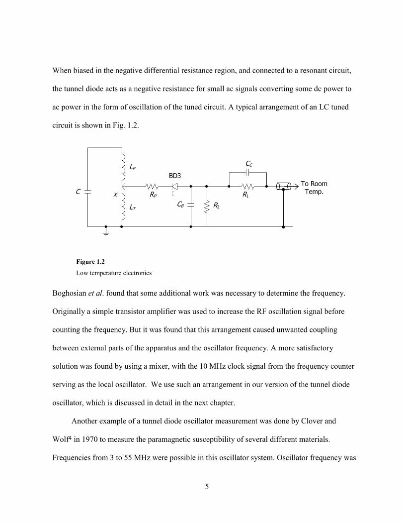
When biased in the negative differential resistance region, and connected to a resonant circuit,
the tunnel diode acts as a negative resistance for small ac signals converting some dc power to
ac power in the form of oscillation of the tuned circuit. A typical arrangement of an LC tuned
circuit is shown in Fig. 1.2.
LP
LT
C
BD3
CB
R1
R2
RP
CC
To RoomTemp.x
Figure 1.2
Low temperature electronics
Boghosian et al. found that some additional work was necessary to determine the frequency.
Originally a simple transistor amplifier was used to increase the RF oscillation signal before
counting the frequency. But it was found that this arrangement caused unwanted coupling
between external parts of the apparatus and the oscillator frequency. A more satisfactory
solution was found by using a mixer, with the 10 MHz clock signal from the frequency counter
serving as the local oscillator. We use such an arrangement in our version of the tunnel diode
oscillator, which is discussed in detail in the next chapter.
Another example of a tunnel diode oscillator measurement was done by Clover and
Wolf4 in 1970 to measure the paramagnetic susceptibility of several different materials.
Frequencies from 3 to 55 MHz were possible in this oscillator system. Oscillator frequency was
6
stable to 1 ppm when immersed in liquid nitrogen, but only 10 ppm in liquid helium. The
increased fluctuation is attributed to bubbles in the helium which could enter the coil. When the
helium bath temperature was reduced below the lambda point, so that the boiling stopped, the
fluctuations were reduced. The design of our system allows (actually, requires) that the coil and
sample occupy a vacuum space, so the interfering effect of bubbles was not a problem.
However, this arrangement lacks the very stable temperature which is achieved by immersing
the oscillator circuit.
The publication of Van Degrift5 describes the design and operation of a tunnel diode
oscillator (TDO) with stability of 0.001 ppm at low temperatures. This treatment of precision
TDO design served as our primary reference when putting together our oscillator. I will discuss
the details of our implementation of this design in the next chapter. In principle, other
techniques are possible for creating oscillators. For example, the gain mechanism could be
provided by a FET amplifier. A number of FETs suitable for use at low temperatures are listed
by Wagner et al.6
1.1.1 Calibrating an oscillator
One of the challenges of using the oscillator technique for experiments like the ones
described here is the problem of calibration. Though glossed over in many discussions, making
an accurate conversion from frequency response to changes in the physical quantity under
study is often more difficult than it would first appear. In our case we must determine how
changes in the frequency, in units of Hz, correspond to changes in penetration depth, in units of
length. This calibration represents a simple multiplication of the raw data, so the functional
dependence of ∆λ(T) will not be affected. However, other quantities calculated from ∆λ(T), in

7
particular the absolute magnitude of λ, are affected by this scale factor, so it is best to have an
accurate calibration, if possible.
We need to know the relationship between the expulsion of the magnetic field by the
sample and the change this causes in the inductance of the coil, and hence the frequency of the
oscillator7. The energy of a coil of inductance L0 carrying a current I is given by
202
1 ILU = . (1.5)
The energy is contained in the magnetic field and can be determined from the distribution of
magnetic induction, B0, and magnetic field H0 for the empty coil:
∫ ⋅=space all
0081 dVU HBπ
. (1.6)
If a sample is placed inside the coil the fields become B and H, the inductance becomes L, and
the change in energy is
∫ −=⋅−⋅=∆space all
2000 )(
21)(
81 ILLdVU HBHBπ
. (1.7)
It turns out that if the sources of magnetic field (the wires and current) are fixed, then this
expression can be rewritten as
∫ ⋅=∆sV
dVU 021 BM , (1.8)
where M is the magnetization of the sample, and the integral extends only over the volume Vs
of the sample (see for example, Jackson8). If an ellipsoidal sample with magnetic susceptibility
χm is placed in a uniform magnetic field, B0, the magnetization induced in the sample will be
0414
BN
Mm
m
χππχ
+= , (1.9)

8
where N is the demagnetizing factor, which depends only on the shape of the sample (N = 1/3
for a sphere). The inductance of the empty coil can be found, in the long solenoid limit, from
π8/21 2
02
0 cVBIL = , where Vc is the effective volume of the coil. The change in inductance,
∆L, relative to the empty coil, when the sample is placed inside is
c
s
m
m
VV
NLL ⋅
+=∆
χππχ41
4
0
. (1.10)
This will cause a change in frequency, according to Eq. 1.2, of
m
m
c
s
NVV
ff
χππχ41
420 +
⋅=∆ . (1.11)
The idea of the calibration procedure is to measure the frequency shift, relative to an
empty coil, when we insert a sample of known dimension and demagnetizing factor (a sphere
of aluminum, diameter 0.79 mm, N = 1/3). The electromagnetic skin depth of the sphere is
much less than its size, so we can take the sphere as perfectly screening, which corresponds to a
susceptibility χm = –1/4π. From the frequency shift we determine Vc from Eq. 1.10 as
sphere
sc f
fVV
∆= 0
2234π . (1.12)
Now the volume and shape of the real sample are measured from microscope
photographs. The shape is approximated as an ellipsoid to determine the approximate
demagnetizing factor. Using Eq. 1.10 again χm = -1/4π, and with N appropriate to our
approximated ellipsoid, and we find
c
s
VV
Nff
2)1(4 δπδ−
= (1.13)

9
The frequency shift we measure is δf(T) = f(T)–f(Tmin). This represents small changes in the
penetration of the field around the perimeter. The penetration depth is much smaller than the
dimensions of the sample (except very close to Tc). We can picture the change in volume as a
ribbon of excluded field around the perimeter of the sample (see Fig. 1.3), representing a
volume
δλδ ⋅= PtVs (1.14)
where t is the thickness of the (plate-like) sample and P is its perimeter. Using Eq. 1.2, putting
in the expression for Vc and solving for δλ we find
fPt
Nf
V
sphere
sphere δδλ )1(23 −
∆= . (1.15)
Referring to Eq. 1.4 we would define )2/()1(3 PtfNVG spheresphere ∆−= .
t
λλλλ
B
Figure 1.3
The sample in a magnetic field. The shaded volume is
penetrated by the field. The thickness of the crystal is t.
This technique should work for ellipsoidal samples, in which the interior field is
proportional to the applied field. However, for other shapes this is not true, and this technique
will be accurate only to the extent that the shape of a given sample can be approximated as an
ellipsoid. There is an alternative approach which does not require that we approximate the
sample shape. We can determine G, which depends only on geometrical factors, for a sample of
known response with the same shape as the sample we wish to study. We make G an adjustable
10
parameter and fit the data to the expected response. We can use the same G for the sample of
unknown response which we wish to study. This has the advantage that we do not need to
calculate G directly from the shape. One drawback is that if each sample has a different shape,
then we need a different calibration sample for each real sample. In addition, depending on the
shape of the sample, it may not be trivial to manufacture a calibration sample in the same
shape. However, from our experience this technique works better for our samples than the other
technique.
1.2 Microwave Surface Impedance
The microwave surface impedance (MSI) technique is fundamentally very similar to the
oscillator techniques described in the first section. But because of the historical importance of
this method in determining λ(T) for the cuprates, which will be discussed in a later chapter, it
warrants a more specific treatment.
The absorption of microwaves by a superconductor, at frequencies corresponding to less
than the gap energy, depends on the density of quasiparticle states. At low temperatures,
absorption in the superconducting state is extremely small. To amplify the effect of the
absorption, a cavity can be constructed whose walls are made of, or coated with, the
superconductor one wishes to study. Microwaves can then bounce back and forth many times
off the surfaces, multiplying the absorption. The absorption is measured in terms of the Q of the
cavity, which is measured as follows9: A pulse of rf power from an external source, at the
cavity resonant frequency, is introduced by a coaxial cable into the cavity. The detected waves
are observed on a fast oscilloscope, and the decay time, τ , is measured, giving Q = ω0/τ . The
value of Q can cover many orders of magnitude as a function of temperature, from as small as
104 to as large as 1012. The resonant frequency, typically in the range of ~10 GHz, will also
11
vary with the temperature, because the variation of penetration depth will modify the effective
size of the cavity.
It is not always convenient to make the entire cavity out of the superconductor under
study. Sridhar et al.9 devised a cavity, coated inside with superconducting Pb, maintained at 4.2
K by a helium bath. Into this cavity extends a sapphire rod which carries the sample–in this
case a single crystal of high temperature superconductor. The cavity is under vacuum, allowing
the sapphire rod and sample to be varied in temperature independently from the cavity walls.
Meanwhile, the Pb coating on the walls, well below Tc, will have very small absorption,
allowing the sample response to be detected independently.
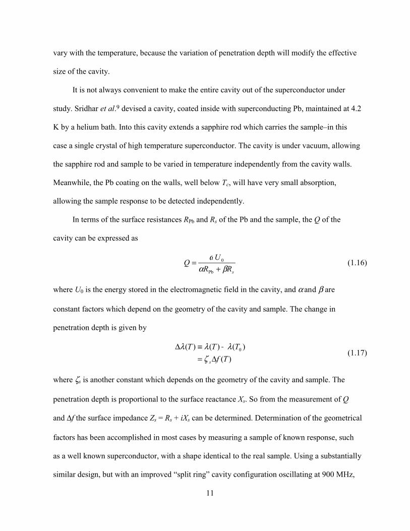
In terms of the surface resistances RPb and Rs of the Pb and the sample, the Q of the
cavity can be expressed as
sRRU
Qβα
ω+
=Pb
0 (1.16)
where U0 is the energy stored in the electromagnetic field in the cavity, and α and β are
constant factors which depend on the geometry of the cavity and sample. The change in
penetration depth is given by
)()()()( 0
TfTTT
s∆=−≡∆
ζλλλ
(1.17)
where ζs is another constant which depends on the geometry of the cavity and sample. The
penetration depth is proportional to the surface reactance Xs. So from the measurement of Q
and ∆f the surface impedance Zs = Rs + iXs can be determined. Determination of the geometrical
factors has been accomplished in most cases by measuring a sample of known response, such
as a well known superconductor, with a shape identical to the real sample. Using a substantially
similar design, but with an improved “split ring” cavity configuration oscillating at 900 MHz,
12
Hardy et al.10, 11 have reported resolution in measurements of ∆λ(T) on single crystals of
YBCO of better than 1Å.
1.3 Mutual Inductance
A very useful technique for measuring the penetration depth is based on the screening of
the mutual inductance which occurs when a superconducting film is placed between a driving
and receiving coil. Such an experiment is described, for example, by Fiory and Hebard.12 In
this experiment the drive coil and the receiving coil, placed on opposite sides of the film, are
each wound with half their turns clockwise and half counterclockwise (astatic). Other
configurations are possible. For example, the coils can both be placed on the same side of the
film, and different variations of coil winding are possible. However, the general principle
remains the same: The magnetic field from the drive coil induces a screening current K(r) in
the film, which depends on the complex impedance of the superconductor Z(ω) = R + iL. For an
oscillatory field and zero temperature the film would be purely inductive with a sheet kinetic
inductance FsK dencmLi 22* /=ω , where dF is the film thickness. The measured inductive
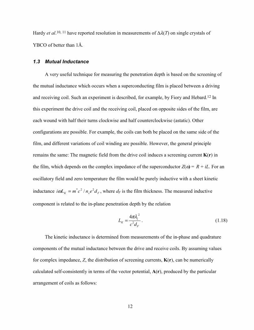
component is related to the in-plane penetration depth by the relation
FK dc
L 2
2||4πλ
= . (1.18)
The kinetic inductance is determined from measurements of the in-phase and quadrature
components of the mutual inductance between the drive and receive coils. By assuming values
for complex impedance, Z, the distribution of screening currents, K(r), can be numerically
calculated self-consistently in terms of the vector potential, A(r), produced by the particular
arrangement of coils as follows:
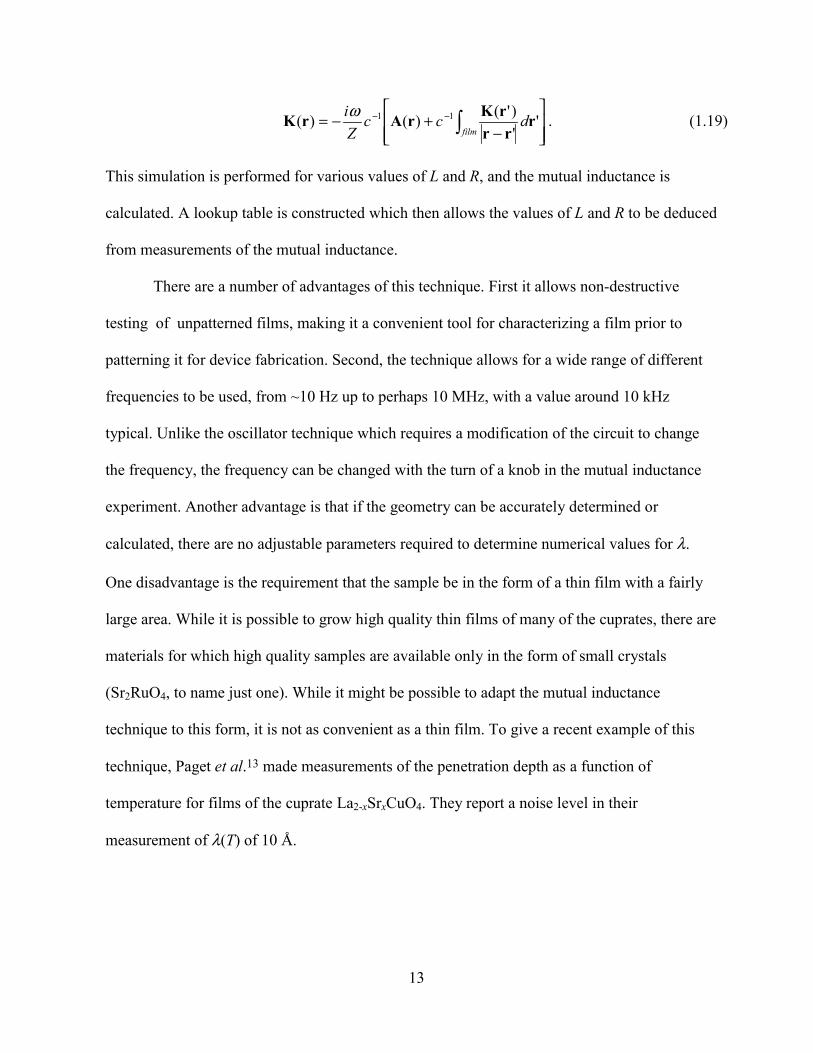
13
−
+−= ∫−−
filmdcc
Zi '
')'()()( 11 r
rrrKrArK ω . (1.19)
This simulation is performed for various values of L and R, and the mutual inductance is
calculated. A lookup table is constructed which then allows the values of L and R to be deduced
from measurements of the mutual inductance.
There are a number of advantages of this technique. First it allows non-destructive
testing of unpatterned films, making it a convenient tool for characterizing a film prior to
patterning it for device fabrication. Second, the technique allows for a wide range of different
frequencies to be used, from ~10 Hz up to perhaps 10 MHz, with a value around 10 kHz
typical. Unlike the oscillator technique which requires a modification of the circuit to change
the frequency, the frequency can be changed with the turn of a knob in the mutual inductance
experiment. Another advantage is that if the geometry can be accurately determined or
calculated, there are no adjustable parameters required to determine numerical values for λ.
One disadvantage is the requirement that the sample be in the form of a thin film with a fairly
large area. While it is possible to grow high quality thin films of many of the cuprates, there are
materials for which high quality samples are available only in the form of small crystals
(Sr2RuO4, to name just one). While it might be possible to adapt the mutual inductance
technique to this form, it is not as convenient as a thin film. To give a recent example of this
technique, Paget et al.13 made measurements of the penetration depth as a function of
temperature for films of the cuprate La2-xSrxCuO4. They report a noise level in their
measurement of λ(T) of 10 Å.
14
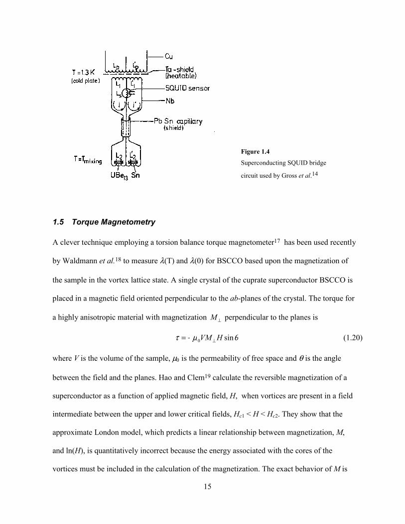
1.4 SQUID Magnetometry
One of the most valuable tools in low temperature physics is the superconducting
quantum interference device (SQUID), an exquisitely sensitive detector of magnetic flux. A
SQUID is adaptable to a large number of different measurements. Not surprisingly, one such
application is the measurement of magnetic flux excluded by a superconductor, i.e. the
penetration depth. Just one example of this technique is the measurement of the temperature
dependence of the penetration depth of the heavy fermion superconductor, UBe13, by Gross et
al.14 Here the SQUID is configured in a bridge circuit using coils and wire made entirely of
superconducting Nb. (See Fig. 1.4) Because the flux enclosed by a loop of superconductor is
trapped inside, the wires and coils act as a so-called flux transformer. Currents are established
by applying a small field to coils L1 and L'1 using copper coils Lp and L'p. The currents divide
among the coils according to the inductance of each, and some of the current flows through
coils Ls, coupled to the SQUID, and L2 and L'2 containing the sample, and a reference sample of
Sn. The change in the inductance in coil L2 as a function of the penetration depth of the UBe13
sample is the same as in the oscillator technique. In this case the change in inductance is
detected as a change in current flowing through coil Ls coupled to the SQUID. One of the
principle advantages of the SQUID technique is that the currents and magnetic fields are all dc.
The behavior of the penetration depth has been shown to have some dependence on high
frequencies for certain heavy fermion superconductors,15, 16 and in these cases the SQUID
technique is most appropriate.
15
Figure 1.4
Superconducting SQUID bridge
circuit used by Gross et al.14
1.5 Torque Magnetometry
A clever technique employing a torsion balance torque magnetometer17 has been used recently
by Waldmann et al.18 to measure λ(T) and λ(0) for BSCCO based upon the magnetization of
the sample in the vortex lattice state. A single crystal of the cuprate superconductor BSCCO is
placed in a magnetic field oriented perpendicular to the ab-planes of the crystal. The torque for
a highly anisotropic material with magnetization ⊥M perpendicular to the planes is
θµτ sin0 HVM ⊥−= (1.20)
where V is the volume of the sample, µ0 is the permeability of free space and θ is the angle
between the field and the planes. Hao and Clem19 calculate the reversible magnetization of a
superconductor as a function of applied magnetic field, H, when vortices are present in a field
intermediate between the upper and lower critical fields, Hc1 < H < Hc2. They show that the
approximate London model, which predicts a linear relationship between magnetization, M,
and ln(H), is quantitatively incorrect because the energy associated with the cores of the
vortices must be included in the calculation of the magnetization. The exact behavior of M is
16
not linear with ln(H), but they find that in an intermediate region of field the curve is close to
linear and the magnetization due to the vortex lattice can be well approximated by
θβ
λπµα
cosln
82
20
0
HHM c
ab
⊥⊥
Φ= , (1.21)
where α = 0.77 and β = 1.44 are determined by fitting to the more exact theoretical results, and
Φ0 is the magnetic flux quantum. We see that the magnetization is proportional to λ-2 and can
be extracted from the torque measurement.
The “pico-torquemeter” is constructed from a 22 mm long, 50 µm diameter PtW torsion
wire with a plastic disk carrying the sample. Deflections in angle as small as 2⋅ 10-6 degrees are
measured by non-contact differential capacitance between a fixed plate and a gold plate on the
torsion wire. Typical resolution is ~1 Å for sample weights of ~100 µg. Fields up to 16 T can
be applied by a superconducting solenoid. The large fields allow the neglect of demagnetizing
factors, since the sample is fully penetrated by vortices.
1.6 Muon Spin Relaxation
One of the most important of the modern techniques for measuring the penetration
depth in superconductors is positive muon spin relaxation (µSR). The experiment is performed
as follows: The superconducting sample is cooled in a magnetic field between Hc1 and Hc2,
where Hc1 and Hc2 are the lower and upper critical fields, respectively, of the superconductor,
such that a regular vortex lattice is formed inside the sample. The penetration depth λ
characterizes the spatial extend of the field of a vortex. A beam of spin polarized muons is
directed at the sample and the muons come to rest, one at a time, inside the sample. The state of
the muon evolves in the local magnetic environment, its spin precessing in the field. The muon
decays with an average lifetime of 2.2 µsec, emitting a positron preferentially along its
17
direction of spin. Detection of the emitted positron allows one to determine the polarization of
the muon at the time of its decay. By building up a large sample of such decay events, the
average distribution of magnetic fields inside the sample can be determined. From this
distribution, by making certain assumptions about the vortex lattice, the penetration depth can
be calculated.
The number of detected positrons as a function of time is given by
( ) ( )[ ] tAtBNtN P00 1)/exp( −−+= µτ (1.22)
where B is a time-independent background, τ µ = 2.2 µsec is the lifetime of the muon, P(t) is the
component of muon polarization in the direction of the detector. The polarization precesses in
the local field Blocal according to
)cos()()( local φγ µ += tBtGt xxP (1.23)
where γ µ is the gyromagnetic ratio of the muon and Gxx(t) represents the polarization relaxation,
for which it is usual to take a Gaussian approximation, ( ) )2/exp( 22ttGxx σ−= . The width, σ,
of this polarization decay distribution gives us λ through the relation 3
02
16πσλ Φ= . Physically,
this result comes about as a root-mean-squared average of the field variations due to the vortex
lattice.20
An important advantage of the µSR technique is that it measures bulk behavior, and is
insensitive to surface properties, effects of shape, thermal expansion, multiple connectivity of
the sample, etc. In addition, it allows an accurate absolute determination of λ. In contrast, the
technique of microwave surface impedance, and other resonant techniques which measure the
Meissner currents circulating on the sample’s surface, can be more susceptible to surface
effects. And they likewise do not allow an absolute determination of λ.
18
One might ask why anyone would use techniques other than µSR at all, given their
shortcomings. The µSR technique has a number of significant disadvantages from which some
other techniques, notably microwave surface impedance, do not suffer. A source of muons is
required for the µSR technique, which requires the experiment to be performed at the site of a
particle accelerator beam line. Such facilities are in heavy demand, which requires that they be
shared among researchers from around the world. Experiments using the beam line must
therefore be designed and built off site, transported to the beam line, and measurements taken
in the short time allotted. Aside from such administrative issues, there is another important
difference between µSR and microwave techniques. While microwave surface impedance
cannot always accurately determine the absolute value of λ, it can measure variations of λ with
much higher sensitivity than µSR. Also, while the theory used to extract λ from µSR
measurements is well developed, there is a significant amount of modeling involved, and some
results may depend on the details of the model. Other techniques are able to measure variations
of λ directly.
The technique of µSR is more general than it might appear from the above treatment. In
fact it provides a useful measurement of the magnetic properties of a wide variety of different
material types. An important example is the measurement of µSR in superconductors in zero
applied field. If the superconductor exhibits time-reversal symmetry breaking, spontaneous
magnetic fields are predicted to appear within the material. Such effects have been observed in
UPt321, UBe1322 and Sr2RuO423, as I will discuss in more detail in a later chapter.
19
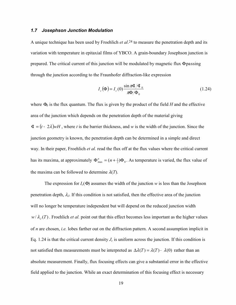
1.7 Josephson Junction Modulation
A unique technique has been used by Froehlich et al.24 to measure the penetration depth and its
variation with temperature in epitaxial films of YBCO. A grain-boundary Josephson junction is
prepared. The critical current of this junction will be modulated by magnetic flux Φ passing
through the junction according to the Fraunhofer diffraction-like expression
( )0
0sin)0(
ΦΦΦΦ
=Φπ
πcc II (1.24)
where Φ0 is the flux quantum. The flux is given by the product of the field H and the effective
area of the junction which depends on the penetration depth of the material giving
( )wHt λ2+=Φ , where t is the barrier thickness, and w is the width of the junction. Since the
junction geometry is known, the penetration depth can be determined in a simple and direct
way. In their paper, Froehlich et al. read the flux off at the flux values where the critical current
has its maxima, at approximately 021
max )( Φ+=Φ nn . As temperature is varied, the flux value of
the maxima can be followed to determine λ(T).
The expression for Ic(Φ) assumes the width of the junction w is less than the Josephson
penetration depth, λJ. If this condition is not satisfied, then the effective area of the junction
will no longer be temperature independent but will depend on the reduced junction width
)(/ Tw Jλ . Froehlich et al. point out that this effect becomes less important as the higher values
of n are chosen, i.e. lobes farther out on the diffraction pattern. A second assumption implicit in
Eq. 1.24 is that the critical current density Jc is uniform across the junction. If this condition is
not satisfied then measurements must be interpreted as )0()()( λλλ −=∆ TT rather than an
absolute measurement. Finally, flux focusing effects can give a substantial error in the effective
field applied to the junction. While an exact determination of this focusing effect is necessary

20
for an absolute measurement, the effect should be independent of temperature, and so once
again allows a relative measurement.
References
1 A. L. Schawlow and G. E. Devlin, Physical Review 113, 120 (1959).
2 C. Boghosian, H. Meyer, and E. Rives John, Physical Review 146, 110 (1966).
3 W. F. Chow, Principles of Tunnel Diode Circuits (John Wiley & Sons, Inc., New York,1969).
4 R. B. Clover and W. P. Wolf, Review of Scientific Instruments 41, 617 (1970).
5 C. T. Van DeGrift, Review of Scientific Instruments 46, 599 (1975).
6 R. R. Wagner, P. T. Anderson, and B. Bertman, Review of Scientific Instruments 41,917 (1970).
7 F. Habbal, G. E. Watson, and P. R. Elliston, Review of Scientific Instruments 46, 192(1975).
8 J. D. Jackson, Classical Electrodynamics (Wiley, New York, 1999).
9 S. Sridhar and W. L. Kennedy, Review of Scientific Instruments 59, 531 (1988).
10 W. N. Hardy, D. A. Bonn, D. C. Morgan, et al., Physical Review Letters 70, 3999(1993).
11 D. A. Bonn, S. Kamal, K. Zhang, et al., Physical Review B 50, 4051 (1994).
12 A. T. Fiory and A. F. Hebard, Applied Physics Letters 52, 2165 (1988).
13 K. M. Paget, S. Guha, M. Z. Cieplak, et al., Physical Review B 59, 641 (1999).
14 F. Gross, B. S. Chandrasekhar, D. Einzel, et al., Zeitschrift fur Physik B 64, 175 (1986).
15 P. J. C. Signore, B. Andraka, M. W. Meisel, et al., Physical Review B 52, 4446 (1995).
16 W. O. Putikka, P. J. Hirschfeld, and P. Wolfe, Physical Review B 41, 7285 (1990).
17 F. Steinmeyer, R. Kleiner, P. Muller, et al., Europhysics Letters 25, 459 (1994).
18 O. Waldmann, F. Steinmeyer, P. Muller, et al., Physical Review B 53, 11825 (1996).
19 Z. Hao and J. R. Clem, Physical Review Letters 67, 2371 (1991).
21
20 P. Pincus, A. C. Gossard, V. Jaccarino, et al., Physics Letters 13, 21 (1964).
21 G. M. Luke, A. Keren, L. P. Le, et al., Physical Review Letters 71, 1466 (1993).
22 G. M. Luke, L. P. Le, B. J. Sternlieb, et al., Physics Letters A 157, 173 (1991).
23 G. M. Luke, Y. Fudamoto, K. M. Kojika, et al., Nature 394, 558 (1998).
24 O. M. Froehlich, H. Schulze, R. Gross, et al., Physical Review B 50, 13894 (1994).
22
2 Experimental Design
The principles of resonant oscillator measurements in general, and tunnel diode oscillators
in particular were discussed in chapter 1. In this chapter I will discuss the details of the
construction and performance of our tunnel diode oscillator system. We will first consider the
design of the electronic oscillator circuit and then discuss the pieces that mechanically hold the
system together.
In this experiment we measure the temperature dependence of the penetration depth in
the temperature range from 1 K down to lowest temperature that can be attained in our 3He-4He
dilution refrigerator (DR). Under the full heat load of the experiment, our DR can reach a
temperature of approximately 30 mK. Our DR, an Oxford Instruments Kelvinox 25, has a
rather modest cooling power of only 25 µW at 100 mK. The cooling power of a DR will drop
as 2T ,1 so below 100 mK the cooling power drops rapidly. It is only through careful design
that this low a temperature can be reached in a DR of this power. The dewar which houses the
DR is surrounded by a dual-layer mu-metal shield which shields the experiment from the
earth’s field, to a level less than 1 mT. This prevents the effects of vortices becoming trapped in
the sample as it cools below Tc.
Craig Van Degrift2 conducted a systematic study of low temperature tunnel diode
oscillators, and presents design specifications for a tunnel diode oscillator (TDO) with
frequency stability of 0.001 ppm. Our experiment is modeled after the design described in this
paper. One of the main advantages of a TDO over other methods of generating oscillations is
the small size and low power requirements of the tunnel diode, which permit the oscillator
circuit to be located in the low temperature portion of the apparatus–even immersed in liquid
helium. Immersion, in particular, provides a very stable temperature environment for the

23
components of the oscillator, contributing to a very stable oscillation frequency. If the circuit
cannot be immersed, as in our case, it is possible to use temperature control techniques to
maintain a stable low temperature in the circuit.
LP
LT
C
BD3
CB
R1
R2
RP
CC
To RoomTemp.x
Figure 2.1
Schematic diagram of low temperature oscillator circuit. The circuit components used in our experiment are C =
100 pF, RP = 300 Ω, CB = 10 nF, R2 = 300 Ω, Cc = 20 pF, R1 = 1400 Ω
2.1 Tunnel Diode Oscillator Circuit Design
The design of the experiment is based directly on the design described by Craig Van
Degrift2. The oscillator portion of the circuit, a parallel LC resonant circuit, is inside the
cryostat, at low temperature. The gain required for oscillation is provided by a tunnel diode
(Germanium Power Devices model BD-3).
24
+15 V
-15 V
20 µHHP 10514 ABalanced Mixer
5 k10 k
0.1 µ
1 k
REF1010 V
0.1 µ 0.01 µRF
50 dB
SRS DS 345Synthesizer
OPA 177
To Low Temp Circuit
HP 53131AUniversal
freq.counter
Vbias
SR 560or
SR 530 lockinsignal monitor
10-30 MHz 5-20 kHz
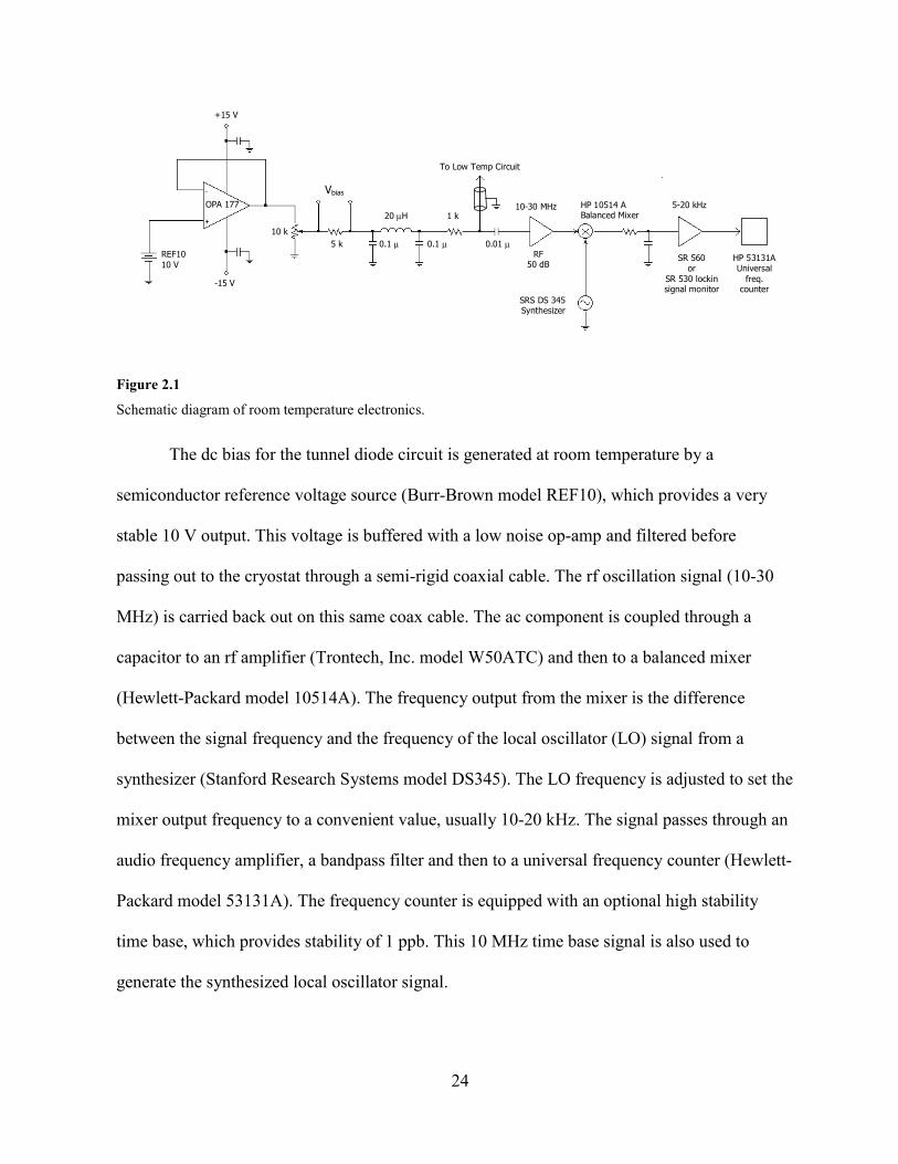
Figure 2.1
Schematic diagram of room temperature electronics.
The dc bias for the tunnel diode circuit is generated at room temperature by a
semiconductor reference voltage source (Burr-Brown model REF10), which provides a very
stable 10 V output. This voltage is buffered with a low noise op-amp and filtered before
passing out to the cryostat through a semi-rigid coaxial cable. The rf oscillation signal (10-30
MHz) is carried back out on this same coax cable. The ac component is coupled through a
capacitor to an rf amplifier (Trontech, Inc. model W50ATC) and then to a balanced mixer
(Hewlett-Packard model 10514A). The frequency output from the mixer is the difference
between the signal frequency and the frequency of the local oscillator (LO) signal from a
synthesizer (Stanford Research Systems model DS345). The LO frequency is adjusted to set the
mixer output frequency to a convenient value, usually 10-20 kHz. The signal passes through an
audio frequency amplifier, a bandpass filter and then to a universal frequency counter (Hewlett-
Packard model 53131A). The frequency counter is equipped with an optional high stability
time base, which provides stability of 1 ppb. This 10 MHz time base signal is also used to
generate the synthesized local oscillator signal.
25
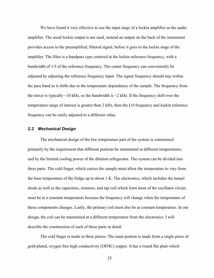
We have found it very effective to use the input stage of a lockin amplifier as the audio
amplifier. The usual lockin output is not used, instead an output on the back of the instrument
provides access to the preamplified, filtered signal, before it goes to the lockin stage of the
amplifier. The filter is a bandpass type centered at the lockin reference frequency, with a
bandwidth of 1/5 of the reference frequency. The center frequency can conveniently be
adjusted by adjusting the reference frequency input. The signal frequency should stay within
the pass band as it shifts due to the temperature dependence of the sample. The frequency from
the mixer is typically ~10 kHz, so the bandwidth is ~2 kHz. If the frequency shift over the
temperature range of interest is greater than 2 kHz, then the LO frequency and lockin reference
frequency can be easily adjusted to a different value.
2.2 Mechanical Design
The mechanical design of the low temperature part of the system is constrained
primarily by the requirement that different portions be maintained at different temperatures,
and by the limited cooling power of the dilution refrigerator. The system can be divided into
three parts. The cold finger, which carries the sample must allow the temperature to vary from
the base temperature of the fridge up to about 1 K. The electronics, which includes the tunnel
diode as well as the capacitors, resistors, and tap coil which form most of the oscillator circuit,
must be at a constant temperature because the frequency will change when the temperature of
these components changes. Lastly, the primary coil must also be at constant temperature. In our
design, the coil can be maintained at a different temperature from the electronics. I will
describe the construction of each of these parts in detail.
The cold finger is made in three pieces. The main portion is made from a single piece of
gold-plated, oxygen free high conductivity (OFHC) copper. It has a round flat plate which

26
covers the entire bottom mounting surface of the mixing chamber of the fridge, where it is held
with stainless steel screws threaded into tapped holes in the mixing chamber. A cylindrical
finger extends from the center of the flat part. Attached to the end of the large finger with silver
conducting epoxy is a smaller diameter finger of OFHC copper. At the end of this smaller
finger, a 1.25 mm diameter sapphire rod is affixed with Stycast 1266 epoxy. The sample is held
on the end of the sapphire rod with a small amount of silicone vacuum grease or GE varnish.
Near the end of the small copper finger is a small chamber formed by hollowing out a portion
of the copper and covered by a cylindrical shield. Inside this chamber is a calibrated RuO2 chip
resistor (called “RuO2 A”) which we use to measure the temperature of the sample. This
thermometer was calibrated against two different calibrated resistor thermometers and against a
60Co nuclear orientation thermometer. Whether the temperature of the thermometer on the
small copper finger, and the sample on the end of the sapphire rod are the same, of course,
depends on establishing thermal equilibrium. I will discuss this in more detail later in this
chapter.
The primary coil is made from 0.0025" diameter (42 gauge) copper wire. It is made by
hand in the following way: A drill bit is selected with the desired inner diameter of the finished
coil. A small piece of very thin Mylar is wrapped several times around the shank of the drill bit.
Then two pieces of wire are wrapped side-by-side over the Mylar with the windings packed
close together until the desired length is reached. A small amount of clear Stycast 1266 epoxy
is applied to the wires and the curing accelerated by careful application of heat with a heat gun.
When the glue is nearly fully cured, one of the two wires is carefully unwound, leaving behind
a single wire which forms the coil with uniform spacing between turns equal to one wire
diameter. The advantage of this technique over simply winding the turns closely packed
27
together is that the shunting capacitance between adjacent turns is significantly reduced.
Several additional thin layers of Stycast are applied to the coil to strengthen it before the coil
and Mylar are then slid off the end of the drill bit. The Mylar is peeled away from the inside of
the coil, leaving the coil as a free-standing piece of wire and Stycast.
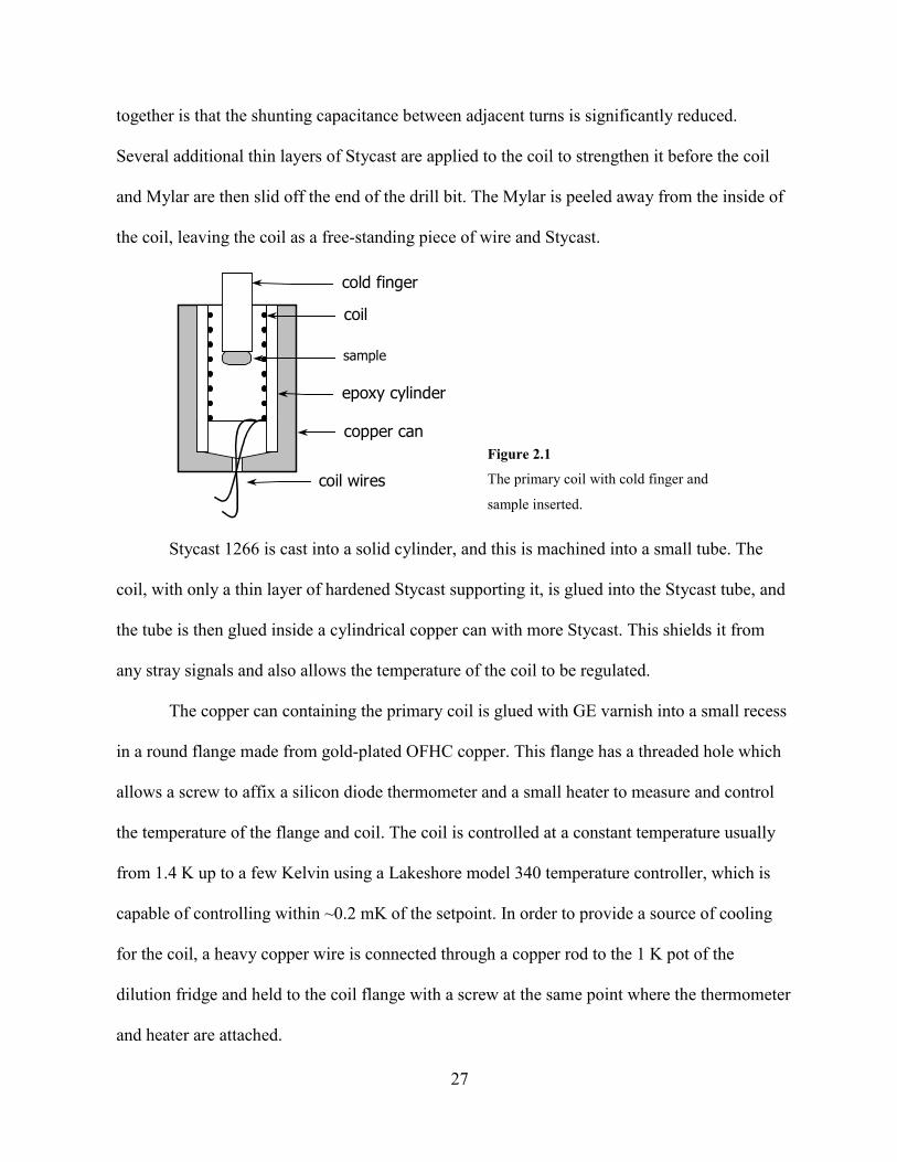
coil
cold finger
sample
epoxy cylinder
coil wires
copper canFigure 2.1
The primary coil with cold finger and
sample inserted.
Stycast 1266 is cast into a solid cylinder, and this is machined into a small tube. The
coil, with only a thin layer of hardened Stycast supporting it, is glued into the Stycast tube, and
the tube is then glued inside a cylindrical copper can with more Stycast. This shields it from
any stray signals and also allows the temperature of the coil to be regulated.
The copper can containing the primary coil is glued with GE varnish into a small recess
in a round flange made from gold-plated OFHC copper. This flange has a threaded hole which
allows a screw to affix a silicon diode thermometer and a small heater to measure and control
the temperature of the flange and coil. The coil is controlled at a constant temperature usually
from 1.4 K up to a few Kelvin using a Lakeshore model 340 temperature controller, which is
capable of controlling within ~0.2 mK of the setpoint. In order to provide a source of cooling
for the coil, a heavy copper wire is connected through a copper rod to the 1 K pot of the
dilution fridge and held to the coil flange with a screw at the same point where the thermometer
and heater are attached.
28
The sample, on the end of the cold finger’s sapphire rod, must be positioned in the
center of the primary coil. A hollow tube is used to hold and align the coil flange in position
relative to the cold finger. The tube is made from Vespel SP-22 (available from DuPont) which
is selected for its extremely low thermal conductivity at low temperatures. To maximize the
thermal resistance, the Vespel support tube is machined to 0.050" wall thickness. It is
constructed from three separate pieces which are nested, one inside the other, and connected
with brass flanges on their ends as shown in Fig. 2.2. This arrangement allows the length of the
tube to double back on itself, adding to the thermal path length without adding to the overall
length of the part. We have taken great care to minimize the amount of heat which can flow
from the coil (at a temperature of several Kelvin) to the other end of the Vespel support tube,
which is fixed to the cold finger and mixing chamber (at a temperature down to 30 mK). Any
excess heat load on the mixing chamber will raise the temperature, and we will be unable to
reach the lowest temperatures needed for the experiment.
The oscillator electronics is housed inside a small gold-plated copper can constructed
such that half of the cylinder can be removed, allowing adjustment of the circuit inside. The
circuit itself is held on both sides of a piece of copper plate, which stands vertically inside the
housing. Connections between components on opposite sides of the plate pass through drilled
holes. The wires are secured in the holes, thermally anchored to, but electrically insulated from
the plate, using black Stycast 2850 epoxy. The copper plate is the ground for the circuit.
Several pins made from thick copper wire are soldered to the plate using Sn-Ag solder (97%
Sn, 3% Ag, Kester Lead-Free solder), which has a lower superconducting temperature (3.7 K)
than ordinary Pb-Sn solder (7.3 K). Ground connections in the circuit are soldered to these pins
using Pb-Sn solder. A short piece of semi-rigid coax with an SMA coaxial connector on its free
29
end is soldered into the fixed side of the circuit housing. The shield of the coax anchors the
ground for the housing and the center conductor carries the signal and bias voltage. The center
conductor of the coax is exposed inside the housing and passes from behind the copper plate
through a hole to the front and is soldered to the circuit. A heavy copper wire is soldered to the
housing at the point where the coax enters, and is soldered to the circuit, providing both
electrical ground and thermal anchoring of the circuit to the housing. To further increase the
thermal anchoring of the copper plate a copper braid is attached to the plate at one end with a
small screw. The other end is connected with a screw to the outside of the cylindrical enclosure.
The wires from the primary coil pass through a small copper tube, through a hole in the top of
the electronics housing and connect to the oscillator circuit with a tiny two-pin connector
(Microtech Inc.).
The circuit employs a tapped inductor coil. While the original paper by Van Degrift
used a single coil with a tap connection in the middle, we have found it easier to make two
separate coils. The tap coil is wound on and glued permanently to a piece of quartz tubing, and
held by a small nylon spacer inside a copper can in the electronic circuit housing. This tiny can
is fixed to the copper plate with an 0-80 screw.
The electronics housing is held beneath the coil flange by three spacers made of
graphite, each with a small cardboard washer. These insulate the electronics thermally from the
coil flange, allowing them to be controlled at different temperatures. The electronics
temperature is controlled by the Lakeshore controller using a calibrated Cernox thermometer
and small heater. Because heat is also generated within the oscillator circuit, the electronics is
often significantly warmer than the coil flange. If the temperature of the coil flange rises too
high, excess heat will be conducted to the mixing chamber through the Vespel support, raising

30
the mixing chamber temperature. To provide cooling for the electronics, a heavy copper wire
conducts heat from the electronics to the top plate of the vacuum can, which is at the helium
bath temperature of 4.2 K.

31
Figure 2.2
Schematic of tunnel diode oscillator system. MC is the mixing chamber of the dilution refrigerator. The 1K pot
and vacuum can top plate are also shown. For clarity, the vacuum can itself is not shown.
cold finger
Vespel tube
Cu rod
thermometer
sample
coax
Cu wire
heater, thermom.
heater, thermom.
Cu wire
Cu braid
1K pot
MC
graphite spacer
coil
vacuum can top plate
thermalanchor
oscillator circuit
Cu braid
32
(b)
(a)
(c)
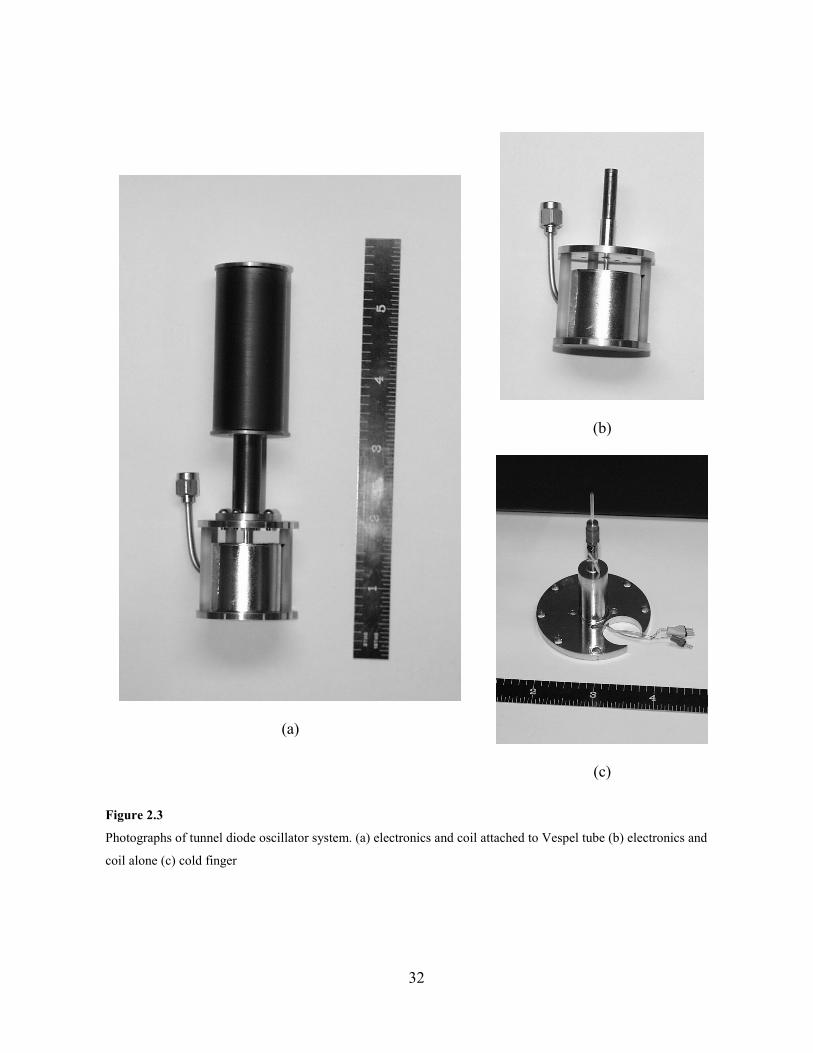
Figure 2.3
Photographs of tunnel diode oscillator system. (a) electronics and coil attached to Vespel tube (b) electronics and
coil alone (c) cold finger

33
2.2.1 Thermal Conductivity
There are two aspects of the design of our system where the thermal conductivity of
materials is important. In one case we want the conductivity as high as possible, and in the
other as low as possible. The thermometer resides on the copper portion of the cold finger
where it can be relied upon to accurately reflect the temperature of the mixing chamber. But the
sample is located at the tip of the sapphire rod. Thus we rely on the thermal conductivity of the
sapphire rod to maintain equilibrium between the thermometer and sample. At temperatures
below about 100 mK, the thermal conductivity of most electrically insulating materials become
very small and it may require a long time to establish thermal equilibrium. A single crystal of
high purity sapphire of the type used for our cold finger has very high thermal conductivity
compared to most insulators.
Using data from the low temperature book by Pobell3, we calculate the thermal
conductivity of our sapphire rod at 100 mK to be approximately 4 nW/K. The heat delivered to
the sample by thermal radiation is somewhat difficult to estimate. To determine whether the
thermal conductivity of the sapphire would be adequate to cool samples to temperatures near
the mixing chamber temperature, we affixed a second RuO2 resistor chip thermometer to the
end of the sapphire rod and performed sweeps of the mixing chamber temperature. To the
extent that the thermometer on the end of the sapphire rod agreed with that on the copper part
of the cold finger, it can be assumed that the sample will be in thermal equilibrium. The
thermometers agree very well above 100 mK. Below this temperature it required many minutes
(at least) for the sample to come to equilibrium.
Sapphire has several advantageous characteristics as a cold finger material. It has no
magnetic susceptibility (at least in this temperature range) and is electrically insulating. The
34
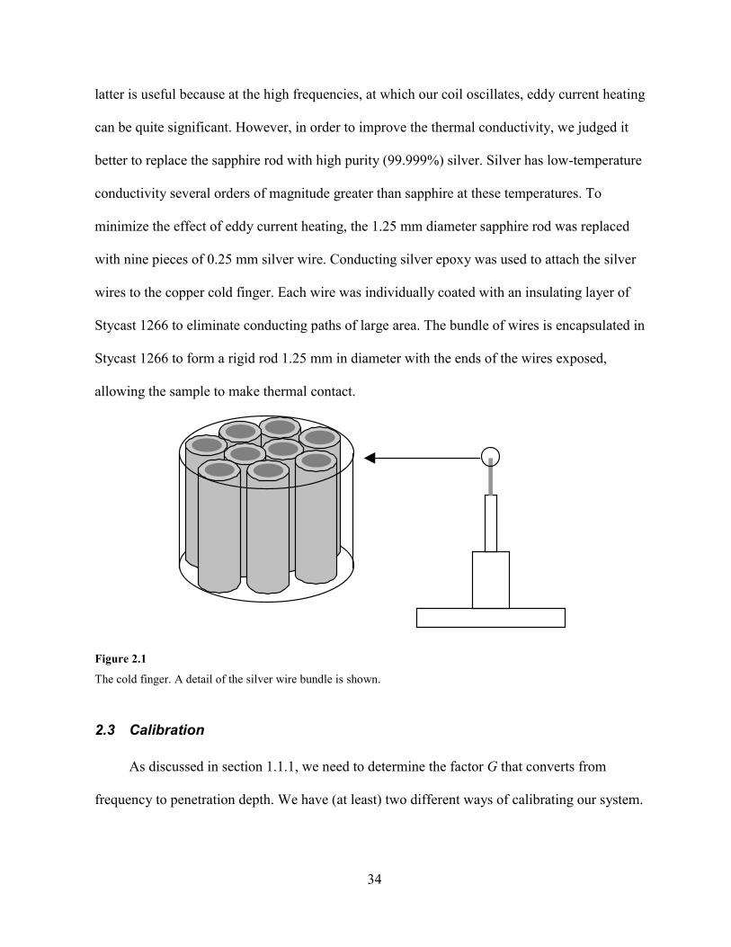
latter is useful because at the high frequencies, at which our coil oscillates, eddy current heating
can be quite significant. However, in order to improve the thermal conductivity, we judged it
better to replace the sapphire rod with high purity (99.999%) silver. Silver has low-temperature
conductivity several orders of magnitude greater than sapphire at these temperatures. To
minimize the effect of eddy current heating, the 1.25 mm diameter sapphire rod was replaced
with nine pieces of 0.25 mm silver wire. Conducting silver epoxy was used to attach the silver
wires to the copper cold finger. Each wire was individually coated with an insulating layer of
Stycast 1266 to eliminate conducting paths of large area. The bundle of wires is encapsulated in
Stycast 1266 to form a rigid rod 1.25 mm in diameter with the ends of the wires exposed,
allowing the sample to make thermal contact.
Figure 2.1
The cold finger. A detail of the silver wire bundle is shown.
2.3 Calibration
As discussed in section 1.1.1, we need to determine the factor G that converts from
frequency to penetration depth. We have (at least) two different ways of calibrating our system.

35
The first is to measure the frequency shift when a sphere is inserted into the coil. The second is
to make a sample of known response in the same shape as the real sample.
For consistency, we performed the first technique at 4.2 K, with exchange gas in the
vacuum space to maintain thermal equilibrium with the main helium bath. The oscillator
system is assembled as usual, but without a sample, and cooled in the usual way to 4.2 K.
Oscillation is established and the resonant frequency is noted. The system is then warmed to
room temperature and the process repeated, but this time with a 1/32 in. (0.79 mm) diameter
aluminum sphere installed as a sample. At 4.2 K the aluminum is well above its
superconducting transition temperature, but the ordinary electromagnetic skin depth serves to
screen the high frequency magnetic field from the interior. The increase in resonant frequency,
relative to the empty coil, is recorded. Let us call this frequency difference ∆fsphere. We now use
Eq. 1.12 to determine Vc. As discussed in Ch. 1 this technique will be accurate only for
ellipsoidal samples. A typical value is G = 17, obtained for a typical sample (C82A1-2a). By
comparing ∆λ(T) with values of λ(0) from the literature, it appeared that this calibration
technique severely overestimates the change in penetration depth for our samples. We turned
then to the second technique.
36
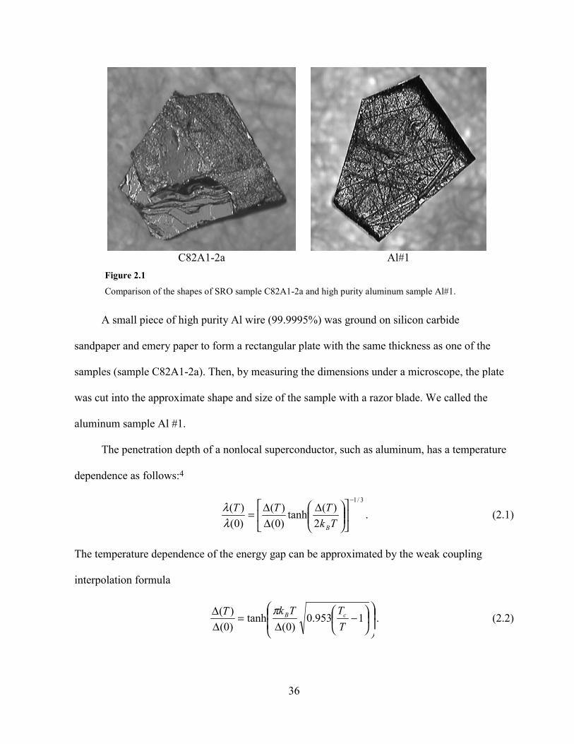
C82A1-2a Al#1Figure 2.1
Comparison of the shapes of SRO sample C82A1-2a and high purity aluminum sample Al#1.
A small piece of high purity Al wire (99.9995%) was ground on silicon carbide
sandpaper and emery paper to form a rectangular plate with the same thickness as one of the
samples (sample C82A1-2a). Then, by measuring the dimensions under a microscope, the plate
was cut into the approximate shape and size of the sample with a razor blade. We called the
aluminum sample Al #1.
The penetration depth of a nonlocal superconductor, such as aluminum, has a temperature
dependence as follows:4
3/1
2)(tanh
)0()(
)0()(
−
∆∆∆=
TkTTTBλ
λ . (2.1)
The temperature dependence of the energy gap can be approximated by the weak coupling
interpolation formula
−
∆=
∆∆ 1953.0
)0(tanh
)0()(
TTTkT cBπ
. (2.2)
37
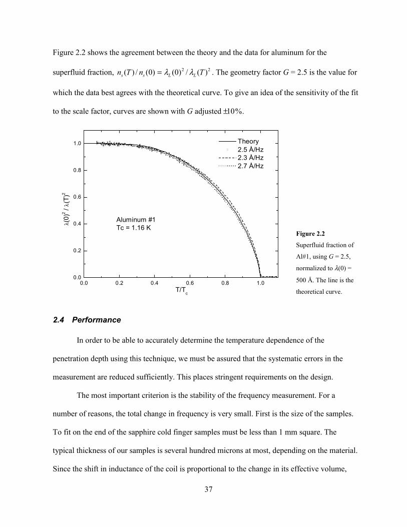
Figure 2.2 shows the agreement between the theory and the data for aluminum for the
superfluid fraction, 22 )(/)0()0(/)( TnTn LLss λλ= . The geometry factor G = 2.5 is the value for
which the data best agrees with the theoretical curve. To give an idea of the sensitivity of the fit
to the scale factor, curves are shown with G adjusted ±10%.
0.0 0.2 0.4 0.6 0.8 1.00.0
0.2
0.4
0.6
0.8
1.0 Theory 2.5 Å/Hz 2.3 Å/Hz 2.7 Å/Hz
Aluminum #1Tc = 1.16 Kλ(
0)2 /
λ(T)
2
T/Tc
Figure 2.2
Superfluid fraction of
Al#1, using G = 2.5,
normalized to λ(0) =
500 Å. The line is the
theoretical curve.
2.4 Performance
In order to be able to accurately determine the temperature dependence of the
penetration depth using this technique, we must be assured that the systematic errors in the
measurement are reduced sufficiently. This places stringent requirements on the design.
The most important criterion is the stability of the frequency measurement. For a
number of reasons, the total change in frequency is very small. First is the size of the samples.
To fit on the end of the sapphire cold finger samples must be less than 1 mm square. The
typical thickness of our samples is several hundred microns at most, depending on the material.
Since the shift in inductance of the coil is proportional to the change in its effective volume,
38
these tiny samples provide a smaller signal than would larger samples. The second reason is
that for the cuprate materials our measurements are taking place well below Tc. Since the
penetration depth has its largest change around Tc, this means the signal is inherently small in
our temperature range. Even assuming the linear behavior in BSCCO, as reported by Lee et al.5
continues to hold below 1 K, the total change in λ from 1 K down to 30 mK would be ~10 Å.
For our samples, this would correspond to a frequency shift of ~100 mHz. In order to get a
sensitive measurement of λ(T) we would therefore need frequency stability on the order of 10
mHz.
The overall frequency stability is a function of several variables. Most important, and at
the same time easiest to achieve is the stability of the local oscillator. The HP 53131A
frequency counter has a high stability 10 MHz time base, with stability of 1 ppb. This time base
is also used to drive the synthesizer, giving it the same stability. The frequency will also vary
with bias voltage because the capacitance of the tunnel diode is voltage dependent. We estimate
the necessary stability at 2 ppm. The bias voltage is approximately 2 V, so we require stability
of ~4 µV. By carefully constructing the room temperature electronics, we are able to achieve
this stability. Finally, the frequency will drift with changes in the temperature of the oscillator
circuit and the primary coil. The circuit is sensitive to temperature fluctuations at ~100 Hz/K.
For 10 mHz resolution we require temperature stability of ~0.1 mK. The stability requirements
for the coil temperature are less stringent. Frequency varies at a rate of ~5 Hz/K for fluctuations
of the coil, so it needs to be stable to within ~2 mK. Both of these temperature stability
requirements are accomplished by controlling with temperature sensors and heaters using a
very good temperature controller (Lakeshore 340).
39
References
1 O. V. Lounasmaa, Experimental Principles and Methods Below 1K (Academic Press,New York, 1974).
2 C. T. Van DeGrift, Review of Scientific Instruments 46, 599 (1975).
3 F. Pobell, Matter and Methods at Low Temperatures (Springer-Verlag, Berlin, NewYork, 1996).
4 P. M. Tedrow, G. Faraci, and R. Meservey, Physical Review B 4, 74 (1971).
5 S.-F. Lee, D. C. Morgan, R. J. Ormeno, et al., Physical Review Letters 77, 735 (1996).
40
3 Penetration Depth in Unconventional Superconductors
In this chapter I will discuss the behavior of the penetration depth in unconventional
superconductors. I will begin by discussing the BCS treatment of conventional superconductors
following closely the treatment by Tinkham1. I will then contrast the behavior of
unconventional materials.
3.1 Conventional Superconductors
To determine magnetic penetration depth of a superconductor, we must understand how
the electrons respond to electromagnetic field, i.e. a magnetic vector potential A, where the
field AB ×∇= . The current density is simply proportional to the velocity v of the electrons,
and their density n: vJ ne= . The velocity is determined by to the canonical momentum
Avpcem −= . The resulting current becomes
21 JJ
ApJ
+≡
−=
mce
mne
(3.1)
The second of the two terms in the current,
AJmcne2
2 −= , (3.2)
represents the diamagnetic response of the superconducting electrons, which oppose the field.
This term represents a perfect diamagnetic response. Since n is the total density of electrons,
this term is independent of temperature in the superconducting state. Evidently the remaining
term must cancel this diamagnetic response in order to give the correct temperature dependence
of the response. For this reason J1 is often referred to as the paramagnetic response, because it
41
opposes the diamagnetic current. This term is also sometimes called the quasiparticle back flow
term because it represents the flow of quasiparticles in opposition to this diamagnetic flow.
However, it is important to realize that the supercurrent is actually the sum of both responses,
and not just J2.
Let us examine the form taken by the Fourier transform of the current response. We can
write the current as )()()4/()( qaqqJ Kc π−= , where a(q) is the Fourier transform of the field
A(r). In terms of J1 and J2 we would write
[ ] )()()(4
)( 1212 qaqqJJqJ KKc +−=+=π
. (3.3)
Now, putting in the expression for J2 from above and making explicit the temperature
dependence of J, we find
)(),(44
),( 1
2
qaqqJ
+−−= TK
mcne
ccT ππ
, (3.4)
where we can recognize the form of the first term as the London penetration depth at zero
temperature, 222 /4)0( mcneL πλ =− . So the K(q,T) becomes
[ ]),()0(1)0(),( 122 TKTK LL qq λλ += − . (3.5)
We identify the q →0 limit of K as the penetration depth )(),0( 2 TTK L−= λ . As mentioned
earlier, we expect the (negative) K1 term to partially cancel the temperature-independent first
term, resulting in the temperature dependence of the penetration depth.
To calculate the temperature dependence of the penetration depth in the BCS model we
will need to find the expression for the paramagnetic response J1(T), which will give us K1(T).
Recalling Eq. 3.1, we see that J1 = nep/m. To calculate this quantity in the BCS model we can
42
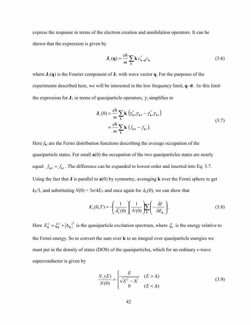
express the response in terms of the electron creation and annihilation operators. It can be
shown that the expression is given by
∑ −=k
kqkkqJ ccme *
1 )( (3.6)
where J1(q) is the Fourier component of J1 with wave vector q. For the purposes of the
experiments described here, we will be interested in the low frequency limit, q→0. In this limit
the expression for J1 in terms of quasiparticle operators, γ , simplifies to
( )
( ).
)0(
10
1*10
*01
∑
∑
−=
−=
kkk
kkkkk
k
kJ
ffmeme
γγγγ(3.7)
Here fki are the Fermi distribution functions describing the average occupation of the
quasiparticle states. For small a(0) the occupation of the two quasiparticles states are nearly
equal: 10 kk ff ≈ . The difference can be expanded to lowest order and inserted into Eq. 3.7.
Using the fact that J is parallel to a(0) by symmetry, averaging k over the Fermi sphere to get
kF/3, and substituting N(0) = 3n/4EF and once again for λL(0), we can show that
∑
∂∂−
−=
k kEf
NTK
L )0(1
)0(1),0( 21 λ
. (3.8)
Here 222kkk ∆+= ξE is the quasiparticle excitation spectrum, where kξ is the energy relative to
the Fermi energy. So to convert the sum over k to an integral over quasiparticle energies we
must put in the density of states (DOS) of the quasiparticles, which for an ordinary s-wave
superconductor is given by
∆<
∆>∆−=
)(0
)()0()(
22
E
EE
E
NEN s (3.9)
43
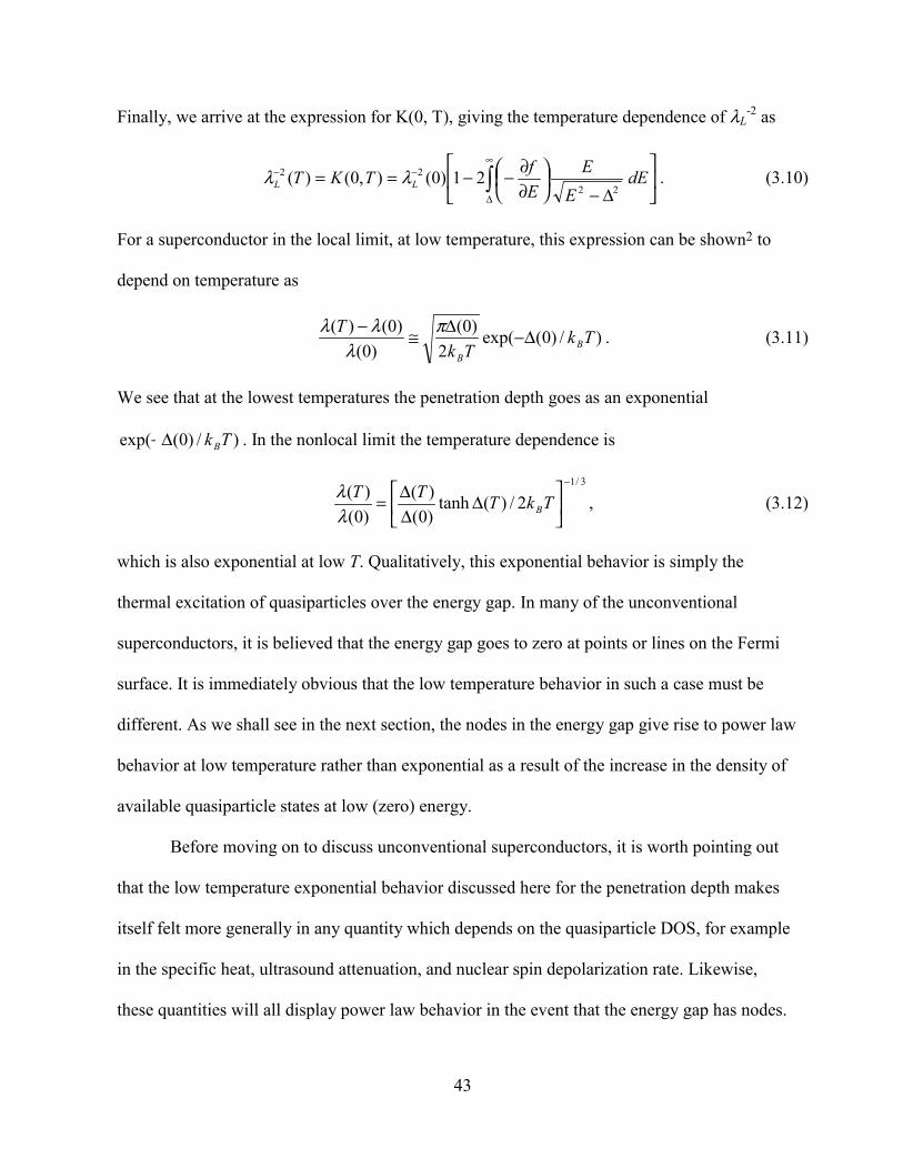
Finally, we arrive at the expression for K(0, T), giving the temperature dependence of λL-2 as
∆−
∂∂−−== ∫
∞
∆
−− dEE
EEfTKT LL 22
22 21)0(),0()( λλ . (3.10)
For a superconductor in the local limit, at low temperature, this expression can be shown2 to
depend on temperature as
)/)0(exp(2
)0()0(
)0()( TkTk
TB
B
∆−∆≅− πλ
λλ . (3.11)
We see that at the lowest temperatures the penetration depth goes as an exponential
)/)0(exp( TkB∆− . In the nonlocal limit the temperature dependence is
3/1
2/)(tanh)0()(
)0()(
−
∆
∆∆= TkTTT
Bλλ , (3.12)
which is also exponential at low T. Qualitatively, this exponential behavior is simply the
thermal excitation of quasiparticles over the energy gap. In many of the unconventional
superconductors, it is believed that the energy gap goes to zero at points or lines on the Fermi
surface. It is immediately obvious that the low temperature behavior in such a case must be
different. As we shall see in the next section, the nodes in the energy gap give rise to power law
behavior at low temperature rather than exponential as a result of the increase in the density of
available quasiparticle states at low (zero) energy.
Before moving on to discuss unconventional superconductors, it is worth pointing out
that the low temperature exponential behavior discussed here for the penetration depth makes
itself felt more generally in any quantity which depends on the quasiparticle DOS, for example
in the specific heat, ultrasound attenuation, and nuclear spin depolarization rate. Likewise,
these quantities will all display power law behavior in the event that the energy gap has nodes.
44
3.2 Unconventional Superconductors
In this section we would like to understand how to calculate the temperature
dependence of the penetration depth in unconventional superconductors. First let us take a
moment to define just what is usually meant by the term unconventional superconductor. The
order parameter (OP) is a quantity which is zero in the normal state and non-zero in the
superconducting state. In addition, the magnitude of the OP tells us the strength of the
superconducting order. A superconductor is considered unconventional if its OP has a lower
symmetry than the crystal lattice of the material. The energy gap of an ordinary superconductor
fits the criteria to be used as an OP. It is believed that the reduced symmetry which applies to
the OP in an unconventional superconductor applies also to the energy gap. And so the energy
gap can be taken as virtually synonymous with the OP.
Why is unconventional symmetry important? Consider a conventional superconductor,
where the mechanism giving rise to superconductivity is well understood. In this case an
attractive interaction between electrons with opposite momentum and spin is mediated by the
crystal lattice in the form of phonons, giving rise to the familiar Cooper pairing. One property
of this interaction is that it is isotropic, except for slight distortions due to the shape of the
crystal lattice and Fermi surface. This symmetry is called s-wave because it represents a state
with zero angular momentum, and for a cubic crystal has the familiar spherical shape of an
atomic s orbital. Unconventional superconductors exhibit a variety of behaviors which are
generally thought to be incompatible with conventional superconductivity. The assumption is
that these differences can be explained if alternative mechanisms, other than phonons, give rise
to superconductivity. In almost all unconventional superconductors these mechanisms are
unknown. (The only exception which comes to mind is superfluid 3He.3)

45
One critical property of these alternative mechanisms is that they may exhibit a
symmetry other than s-wave. In simple terms we can understand this to mean that the
interaction between the electrons is anisotropic in a non-trivial way. The symmetry of this
anisotropic interaction is necessarily reflected in the symmetry of the superconducting state. It
turns out that a number of experiments (including the ones described in this thesis) are capable
of probing the symmetry of the superconducting state. If the symmetry can be determined, it
strongly constrains the possible mechanisms of superconductivity.
The microscopic theories of different sorts of unconventional interactions, applicable to
different unconventional materials, are under study by many theorists. At the current time it is
fair to say that there is no real consensus as to which of the leading candidates (if any) may be
correct for a given material. Fortunately, in order to explore the symmetry of the
superconducting state we do not need to make direct reference to any particular microscopic
model of superconductivity. Instead we are guided by the phenomenological Ginzburg-Landau
theory, and by the very powerful results of group theory.
Group theory breaks down the full symmetry of the crystal lattice into a certain number
of irreducible representations, Γ , with basis functions fΓ(kF). The order parameter can be
expanded in terms of all the possible basis functions as follows:
∑Γ
ΓΓ=∆ )()( F
)(F kk fη , (3.13)
where η(Γ ) are expansion coefficients.4 The actual realization of superconductivity is
determined by the order parameter which minimizes the free energy. An important assumption
is that the Ginzburg-Landau free energy functional can be expanded in powers of the order
parameter, i.e. in powers of η(Γ ). This expansion is written down and, by making suitable
assumptions and by comparing with experiments, the expression for the free energy can be
46
minimized. The result is a determination of one irreducible representation which has a Tc higher
than all the others. It is the symmetry of this representation which determines the symmetry of
the order parameter. Of course, this procedure works equally well for conventional
superconductors. By definition the result for conventional superconductors is always that the
symmetry which minimizes the free energy is the usual s-wave symmetry.
There are two crucial properties which are determined solely by the symmetry of the
OP: the parity and the presence of nodes. There are a finite number of distinct crystal lattice
formations which can exist in the solid state of matter, all of which have inversion symmetry.
As a result, all of the irreducible representations of the symmetry group of a crystal lattice will
have definite parity, i.e. they have either even or odd symmetry under inversion. The reason
this is so important is that the superconducting state is composed of pairs of electrons, which
are Fermions, and must obey Fermi-Dirac statistics. In particular, the total state (including both
orbital and spin components) must be antisymmetric under exchange of the two electrons. The
critical point is this: The symmetry of the OP is the symmetry of the orbital part of the
underlying superconducting state. Now, if the OP has even symmetry, as in the s-wave case,
then the spin component of the superconducting state must be a singlet, because the
antisymmetric symmetry of the singlet preserves the overall antisymmetry of the state.
Likewise, if the OP has odd symmetry, then the spin state must have even symmetry. The spin
symmetry is triplet in this case. However, we should be careful not to assume that there are
three degenerate spin states. It is not necessarily the case that all three triplet spin states are
degenerate in energy with respect to the interaction potential. If the triplet degeneracy is split
then it is possible for only one or two of the states to be present. In any case, it is clear from this
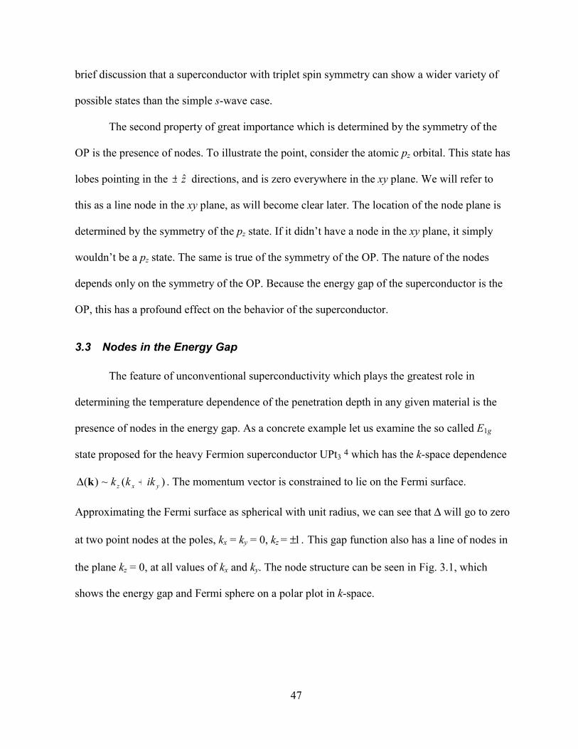
47
brief discussion that a superconductor with triplet spin symmetry can show a wider variety of
possible states than the simple s-wave case.
The second property of great importance which is determined by the symmetry of the
OP is the presence of nodes. To illustrate the point, consider the atomic pz orbital. This state has
lobes pointing in the z± directions, and is zero everywhere in the xy plane. We will refer to
this as a line node in the xy plane, as will become clear later. The location of the node plane is
determined by the symmetry of the pz state. If it didn’t have a node in the xy plane, it simply
wouldn’t be a pz state. The same is true of the symmetry of the OP. The nature of the nodes
depends only on the symmetry of the OP. Because the energy gap of the superconductor is the
OP, this has a profound effect on the behavior of the superconductor.
3.3 Nodes in the Energy Gap
The feature of unconventional superconductivity which plays the greatest role in
determining the temperature dependence of the penetration depth in any given material is the
presence of nodes in the energy gap. As a concrete example let us examine the so called E1g
state proposed for the heavy Fermion superconductor UPt3 4 which has the k-space dependence
)(~)( yxz ikkk +∆ k . The momentum vector is constrained to lie on the Fermi surface.
Approximating the Fermi surface as spherical with unit radius, we can see that ∆ will go to zero
at two point nodes at the poles, kx = ky = 0, kz = ±1. This gap function also has a line of nodes in
the plane kz = 0, at all values of kx and ky. The node structure can be seen in Fig. 3.1, which
shows the energy gap and Fermi sphere on a polar plot in k-space.

48
Figure 3.1
Energy gap in the E1g state. The white surface is the
Fermi sphere. The shaded surface is the boundary of the
energy gap in k-space.
Annett, Goldenfeld and Renn5 point out that the existence of nodes will depend on two
factors: The symmetry of the energy gap, and the shape of the Fermi surface. For a node to
exist, the gap function must vanish at a point in k-space where the Fermi surface exists. This is
especially relevant to the case of a layered material where, rather than spherical, the Fermi
surface has a cylindrical shape extending infinitely in the direction of the axis. Since the ends
of the cylinder are open, this portion of k-space is inaccessible. Any nodes which, by symmetry
consideration, would occupy this region (e.g. the point nodes in the E1g state) would not, in
fact, exist in this case.
Let us examine the behavior of the quasiparticle DOS when there is a node in the gap.
N(E) dE is the number of states between energy E and E + dE, which is proportional to the
available volume of k-space between these energies, as illustrated in Fig. 3.2 for a point node,
and Fig. 3.3 for a line node. According to Sigrist,6 at low temperatures the form of the DOS
will depend solely on the topology of the nodes. If they are line nodes, then the EEN ∝)( , and
if they are point nodes, then 2)( EEN ∝ .
The expression for the paramagnetic response has the form
∫∞
∞−
∂∂∝ dEENEfTK s )(),0(1 . (3.14)
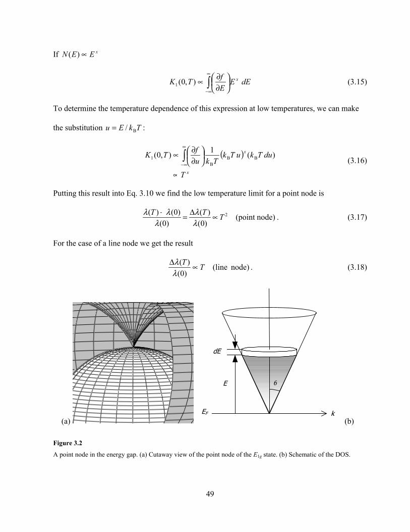
49
If xEEN ∝)(
∫∞
∞−
∂∂∝ dEEEfTK x),0(1 (3.15)
To determine the temperature dependence of this expression at low temperatures, we can make
the substitution TkEu B/= :
( )x
x
T
duTkuTkTku
fTK
∝
∂∂∝ ∫
∞
∞−
)(1),0( BBB
1 (3.16)
Putting this result into Eq. 3.10 we find the low temperature limit for a point node is
node)(point )0()(
)0()0()( 2TTT ∝∆=−
λλ
λλλ . (3.17)
For the case of a line node we get the result
node) (line)0()( TT ∝∆
λλ . (3.18)
(a)
E
EF
θ
dE
k (b)
Figure 3.2
A point node in the energy gap. (a) Cutaway view of the point node of the E1g state. (b) Schematic of the DOS.

50
So first, the observation of power law behavior in the ∆λ(T) is strong evidence of
unconventional superconductivity, with nodes in the energy gap. And the specific power law
can distinguish the dimensionality of the node structure.
(a)
E
EF
θ
dE
L
k (b)
Figure 3.3
A line node in the energy gap. (a) Cutaway view of the line node of the E1g state. (b) Schematic of the DOS.
The cuprate high temperature superconductors provide us with a prototype with which
to compare the results of this section. In recent years, with the availability of very high quality
samples of a number of these materials, λ(T) has been found to agree very well with a model
consisting of an energy gap with line nodes. However, for many years there was considerable
confusion.
It is now believed that the energy gap in the cuprates has d-wave symmetry. These
materials have a highly layered structure, with a strongly two dimensional band structure. The
Fermi surface is roughly cylindrical, rather than spherical, and extends infinitely in the
direction perpendicular to the planes. The energy gap is thought to have the form
22)( yx kk −=∆ k . Within the planes there are nodes in the gap wherever 22yx kk = , i.e. at ±45° and
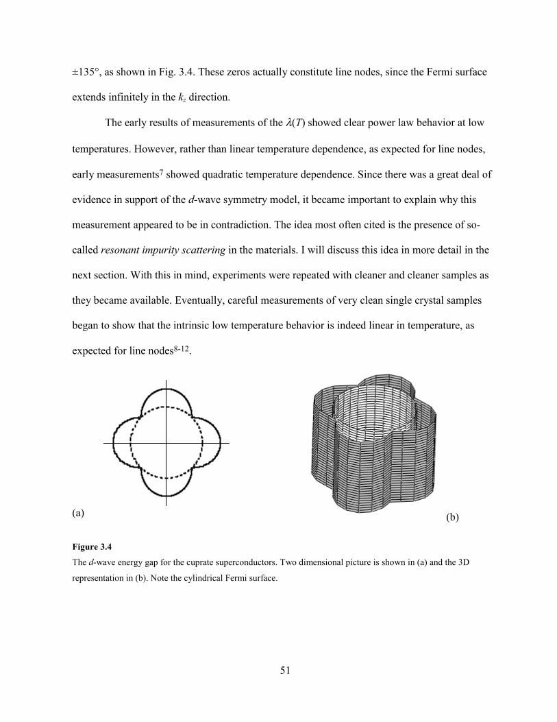
51
±135°, as shown in Fig. 3.4. These zeros actually constitute line nodes, since the Fermi surface
extends infinitely in the kz direction.
The early results of measurements of the λ(T) showed clear power law behavior at low
temperatures. However, rather than linear temperature dependence, as expected for line nodes,
early measurements7 showed quadratic temperature dependence. Since there was a great deal of
evidence in support of the d-wave symmetry model, it became important to explain why this
measurement appeared to be in contradiction. The idea most often cited is the presence of so-
called resonant impurity scattering in the materials. I will discuss this idea in more detail in the
next section. With this in mind, experiments were repeated with cleaner and cleaner samples as
they became available. Eventually, careful measurements of very clean single crystal samples
began to show that the intrinsic low temperature behavior is indeed linear in temperature, as
expected for line nodes8-12.
(a) (b)
Figure 3.4
The d-wave energy gap for the cuprate superconductors. Two dimensional picture is shown in (a) and the 3D
representation in (b). Note the cylindrical Fermi surface.
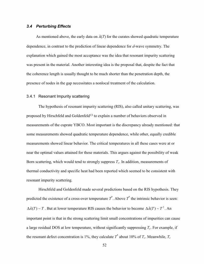
52
3.4 Perturbing Effects
As mentioned above, the early data on λ(T) for the curates showed quadratic temperature
dependence, in contrast to the prediction of linear dependence for d-wave symmetry. The
explanation which gained the most acceptance was the idea that resonant impurity scattering
was present in the material. Another interesting idea is the proposal that, despite the fact that
the coherence length is usually thought to be much shorter than the penetration depth, the
presence of nodes in the gap necessitates a nonlocal treatment of the calculation.
3.4.1 Resonant Impurity scattering
The hypothesis of resonant impurity scattering (RIS), also called unitary scattering, was
proposed by Hirschfeld and Goldenfeld13 to explain a number of behaviors observed in
measurements of the cuprate YBCO. Most important is the discrepancy already mentioned: that
some measurements showed quadratic temperature dependence, while other, equally credible
measurements showed linear behavior. The critical temperatures in all these cases were at or
near the optimal values attained for these materials. This argues against the possibility of weak
Born scattering, which would tend to strongly suppress Tc. In addition, measurements of
thermal conductivity and specific heat had been reported which seemed to be consistent with
resonant impurity scattering.
Hirschfeld and Goldenfeld made several predictions based on the RIS hypothesis. They
predicted the existence of a cross-over temperature T*. Above T* the intrinsic behavior is seen:
TT ~)(λ∆ . But at lower temperature RIS causes the behavior to become 2~)( TTλ∆ . An
important point is that in the strong scattering limit small concentrations of impurities can cause
a large residual DOS at low temperature, without significantly suppressing Tc. For example, if
the resonant defect concentration is 1%, they calculate T* about 10% of Tc. Meanwhile, Tc
53
would be suppressed by only 1%. At more realistic concentrations of only 0.1%, T* would be as
low as 2-3% of Tc. No explanation is given, however, for the source of RIS.
The predictions quoted here are very interesting. They suggest that if we can make
measurements down to sufficiently low temperature, it should be possible to observe the
crossover of a linear sample to quadratic behavior, verifying the RIS model.
3.4.2 Nonlocal Effects
A different idea has been proposed by Kosztin and Leggett14 to explain the quadratic
dependence. They point out that calculations have been made in the cuprates assuming the local
limit. This seems reasonable at first glance since average coherence lengths are on the order of
several Ångstroms, which is small compared to the penetration depths of several thousand
Ångstroms. However, the coherence length, can be expressed as 00 / ∆= πξ Fv . Considering
that ∆0 = ∆0(k) is anisotropic, it might be more appropriate to adopt an anisotropic coherence
length, )(/)( kk ∆= πξ Fv . Under this assumption, the coherence length can be seen to diverge
at points on the Fermi surface where the gap vanishes. In these directions nonlocal effects could
be important. Nonlocal electrodynamics would be expected to be important on only a small
fraction of the Fermi surface, of order 000 / λξα ≡ . The absolute value, λ(0), would not be
significantly affected because the whole Fermi surface contributes to its value. However, the
low temperature power law could be strongly affected because the effect is concentrated around
the nodes of the gap, which, as we have seen, dominate the temperature dependence.
This paper predicts a crossover temperature (in units where kB = 1),
00000* / λξα ∆=∆=T , below which these effects will be important. For YBCO, with typical
values ∆0 ≈ 250 K, ξ 0 ≈ 14 Å, and λ0 ≈ 1400 Å, we find T* ≈ 2.5 K. An important result of this
54
calculation for YBCO is that the nonlocal effects will not be seen for magnetic fields parallel to
the ab planes. This occurs because the wavevectors for the quasi-two dimensional YBCO are
constrained to lie in the ab plane, and will not have a component parallel to direction of field
penetration (the c direction) in this orientation. Finally, the conclusion is the same as the
previous section: at low temperature, but above T*, linear behavior will be observed, while
below T* the behavior will cross over to quadratic.
It is interesting to consider this scenario for the material Sr2RuO4, under study in this
thesis. Putting in typical measured values of penetration depth, coherence length and energy
gap, we find a value cTT ≈* . This will be discussed further in the chapter on Sr2RuO4.
References
1 M. Tinkham, Introduction to Superconductivity (McGraw-Hill, Inc., New York, 1996).
2 B. Muhlschlegel, Zeitschrift fur Physik 155, 21 (1959).
3 A. Leggett, Reviews of Modern Physics 47, 331 (1975).
4 J. A. Sauls, Advances in Physics 43, 113 (1994).
5 J. Annett, N. Goldenfeld, and S. R. Renn, in Physical Properties of High TemperatureSuperconductors, edited by D. M. Ginsberg (World Scientific, Singapore, 1990), Vol. 2.
6 M. Sigrist and K. Ueda, Reviews of Modern Physics 63, 239 (1991).
7 J. Annett, N. Goldenfeld, and S. R. Renn, Physical Review B 43, 2778 (1991).
8 S.-F. Lee, D. C. Morgan, R. J. Ormeno, et al., Physical Review Letters 77, 735 (1996).
9 D. M. Broun, D. C. Morgan, R. J. Ormeno, et al., Physica C 282, 1467 (1997).
10 W. N. Hardy, D. A. Bonn, D. C. Morgan, et al., Physical Review Letters 70, 3999(1993).
11 K. Zhang, D. A. Bonn, S. Kamal, et al., Physical Review Letters 73, 2484 (1994).
12 O. Waldmann, F. Steinmeyer, P. Muller, et al., Physical Review B 53, 11825 (1996).

55
13 P. Hirschfeld, J. and N. Goldenfeld, Physical Review B 48, 4219 (1993).
14 I. Kosztin and A. Leggett, Physical Review Letters 79, 135 (1997).
56
4 Strontium Ruthenate
Strontium ruthenate (SRO) is the first reported perovskite superconductor without
copper. With a chemical formula Sr2RuO4, it has the same crystal structure as the high
temperature superconductor La2CuO4. While SRO has been known for some time,1 it was not
until more recently that SRO was shown to be a superconductor.2 Critical temperatures of the
earliest samples were around 1 K, with more recent samples displaying Tc as high as 1.5 K.
As superconductivity in SRO was investigated in detail, it quickly became apparent that
SRO is an unconventional superconductor. The experimental evidence, when taken together
with theoretical models, seems to support the conclusion that SRO has p-wave symmetry.
I will discuss the experimental measurements that have been made on SRO, and review
the important features of the theories which have been proposed to explain the unconventional
nature of superconductivity in this material.
4.1 Crystal Growth and Characterization
The first report of superconductivity in SRO came from Maeno et al.2. High quality
crystals are grown using a floating zone method in air or in a controlled atmosphere of 10%
oxygen and 90% argon using excess Ru as a flux. It was found that a mixture of SRO and pure
Ru metal forms a eutectic. This results in a characteristic spontaneous separation of the two
components of the eutectic. The result is that Sr2RuO4 crystallizes in its exact stoichiometry
from a mixture containing excess Ru, with pockets of pure Ru metal forming a lamellar
structure embedded in a single crystal Sr2RuO4 matrix.3 Maeno et al. found that a radial
concentration gradient of Ru forms in the cross section of the growth rod. The outer surface has
a lower concentration of Ru, and in a sheath approximately 0.5 mm thick, pure Sr2RuO4
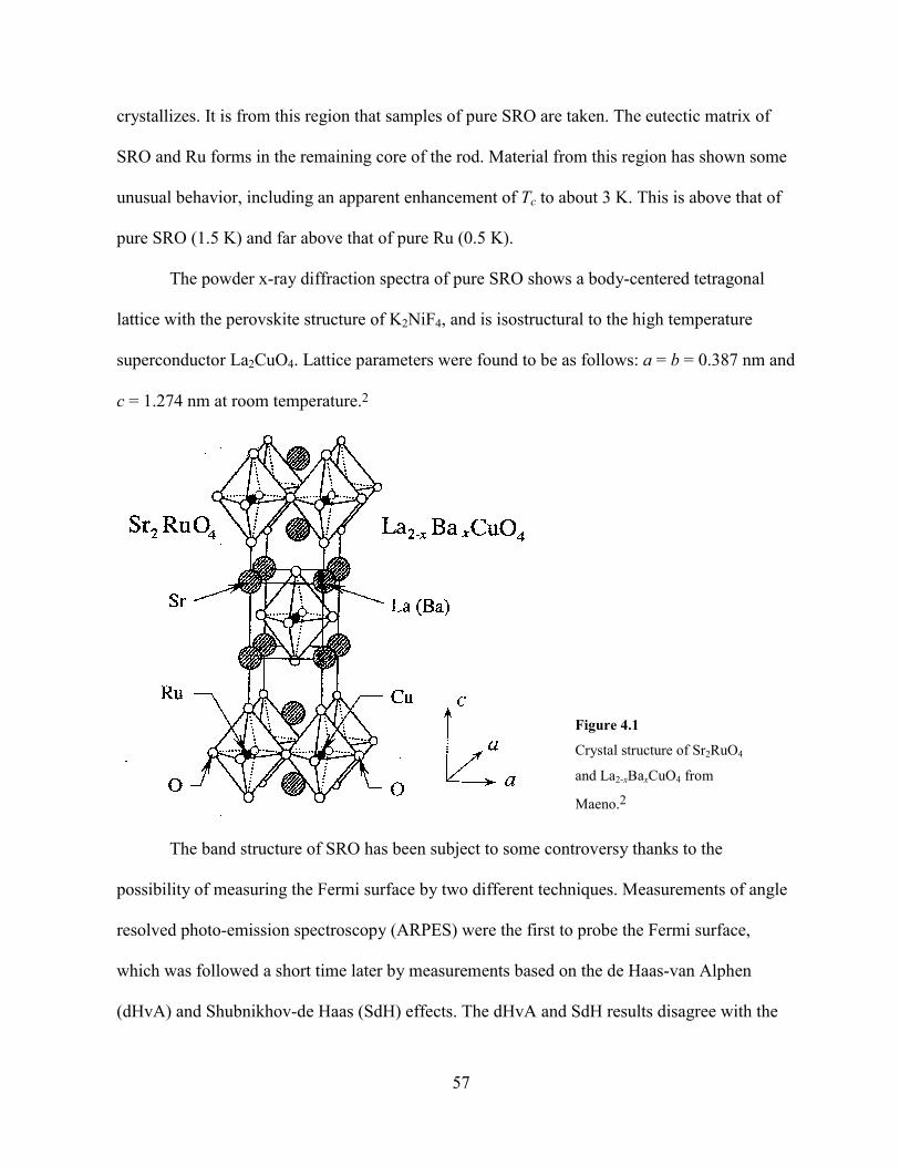
57
crystallizes. It is from this region that samples of pure SRO are taken. The eutectic matrix of
SRO and Ru forms in the remaining core of the rod. Material from this region has shown some
unusual behavior, including an apparent enhancement of Tc to about 3 K. This is above that of
pure SRO (1.5 K) and far above that of pure Ru (0.5 K).
The powder x-ray diffraction spectra of pure SRO shows a body-centered tetragonal
lattice with the perovskite structure of K2NiF4, and is isostructural to the high temperature
superconductor La2CuO4. Lattice parameters were found to be as follows: a = b = 0.387 nm and
c = 1.274 nm at room temperature.2
Figure 4.1
Crystal structure of Sr2RuO4
and La2-xBaxCuO4 from
Maeno.2
The band structure of SRO has been subject to some controversy thanks to the
possibility of measuring the Fermi surface by two different techniques. Measurements of angle
resolved photo-emission spectroscopy (ARPES) were the first to probe the Fermi surface,
which was followed a short time later by measurements based on the de Haas-van Alphen
(dHvA) and Shubnikhov-de Haas (SdH) effects. The dHvA and SdH results disagree with the
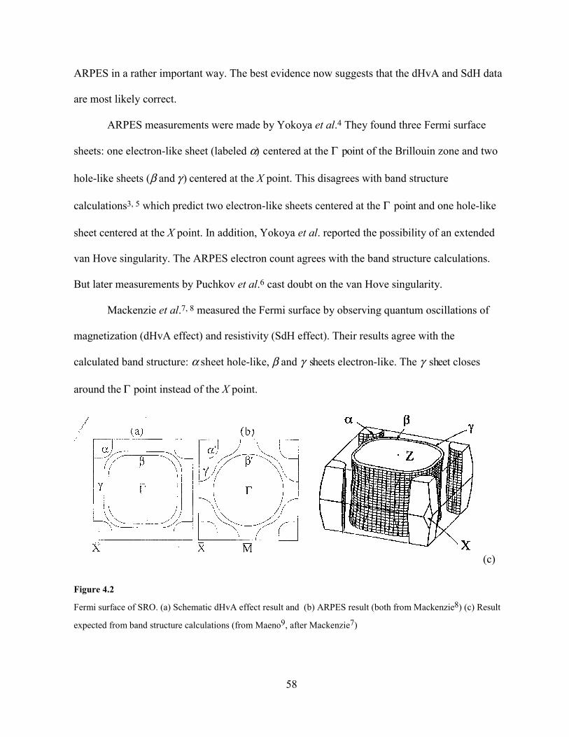
58
ARPES in a rather important way. The best evidence now suggests that the dHvA and SdH data
are most likely correct.
ARPES measurements were made by Yokoya et al.4 They found three Fermi surface
sheets: one electron-like sheet (labeled α) centered at the Γ point of the Brillouin zone and two
hole-like sheets (β and γ ) centered at the X point. This disagrees with band structure
calculations3, 5 which predict two electron-like sheets centered at the Γ point and one hole-like
sheet centered at the X point. In addition, Yokoya et al. reported the possibility of an extended
van Hove singularity. The ARPES electron count agrees with the band structure calculations.
But later measurements by Puchkov et al.6 cast doubt on the van Hove singularity.
Mackenzie et al.7, 8 measured the Fermi surface by observing quantum oscillations of
magnetization (dHvA effect) and resistivity (SdH effect). Their results agree with the
calculated band structure: α sheet hole-like, β and γ sheets electron-like. The γ sheet closes
around the Γ point instead of the X point.
(c)
Figure 4.2
Fermi surface of SRO. (a) Schematic dHvA effect result and (b) ARPES result (both from Mackenzie8) (c) Result
expected from band structure calculations (from Maeno9, after Mackenzie7)

59
The controversy has largely been resolved in favor of the dHvA results. ARPES
measures only the surface of the sample, whereas dHvA effect measures the bulk material. It is
likely that the ARPES data is not representative of the bulk due to a rearrangement of the bonds
at the surface of freshly cleaved samples, which distorts the Fermi surface locally.
It is interesting to note that dHvA measurements have not been made on the high
temperature superconductors. This experiment is only possible at very low temperatures, in
very pure samples, and requires a magnetic field which exceeds Hc2, so that the field penetrates
the material uniformly. The HTSC materials can be divided into two categories: those which
require doping to be superconducting, and those which are superconducting at stoichiometric
concentrations. Some which require substitutional doping, such as La2-xSrxCuO4, have values of
Hc2 which can be reached in the laboratory, but the random nature of doping makes dHvA
effect unobservable. The stoichiometric materials, such as YBa2Cu3O7, have high values of Hc2
currently unattainable in the laboratory (at least for non-pulsed magnets required for dHvA
measurements). Akima et al.10 measured Hc2 for SRO for fields applied parallel to the ab plane
and parallel to the c-axis, finding µ0Hc2,ab(0) = 1.5 T and µ0Hc2,c(0) = 0.075 T. The relatively
low values of Hc2 provides a unique opportunity to measure the Fermi surface of a perovskite
superconductor with both ARPES and dHvA effects.
Below 25 K the resistivity shows SRO to be a two dimensional Fermi liquid, with
( ) 2)0( ATT += ρρ behavior indicating the importance of electron-electron scattering at low
temperatures. The resistivity is anisotropic, with residual low T values of )0(abρ = 0.9 µΩcm
and )0(cρ = 500 µΩcm.9

60
Figure 4.3
Resistivity of SRO from Maeno.9
4.2 Superconducting Properties
A large number of different measurements have been made of the superconducting
properties of SRO. On the whole they paint a consistent picture of SRO as an unconventional
superconductor. Important results have been reported from measurements of muon spin
relaxation (µSR), from nuclear magnetic resonance (NMR) and nuclear quadrupole resonance
(NQR) measurements of nuclear spin relaxation time and electronic spin susceptibility, from
specific heat and thermal conductivity, and from studies of the effect of impurities and disorder
on the superconducting properties. I will review these results and discuss their relevance to
issues of unconventional superconductivity in SRO.
The most pivotal evidence for unconventional superconductivity is the 17O nuclear
quadrupole resonance (NQR) measurement of the temperature dependence of the Knight shift.
The measurement shows that there is no change in the spin susceptibility of the electrons, for
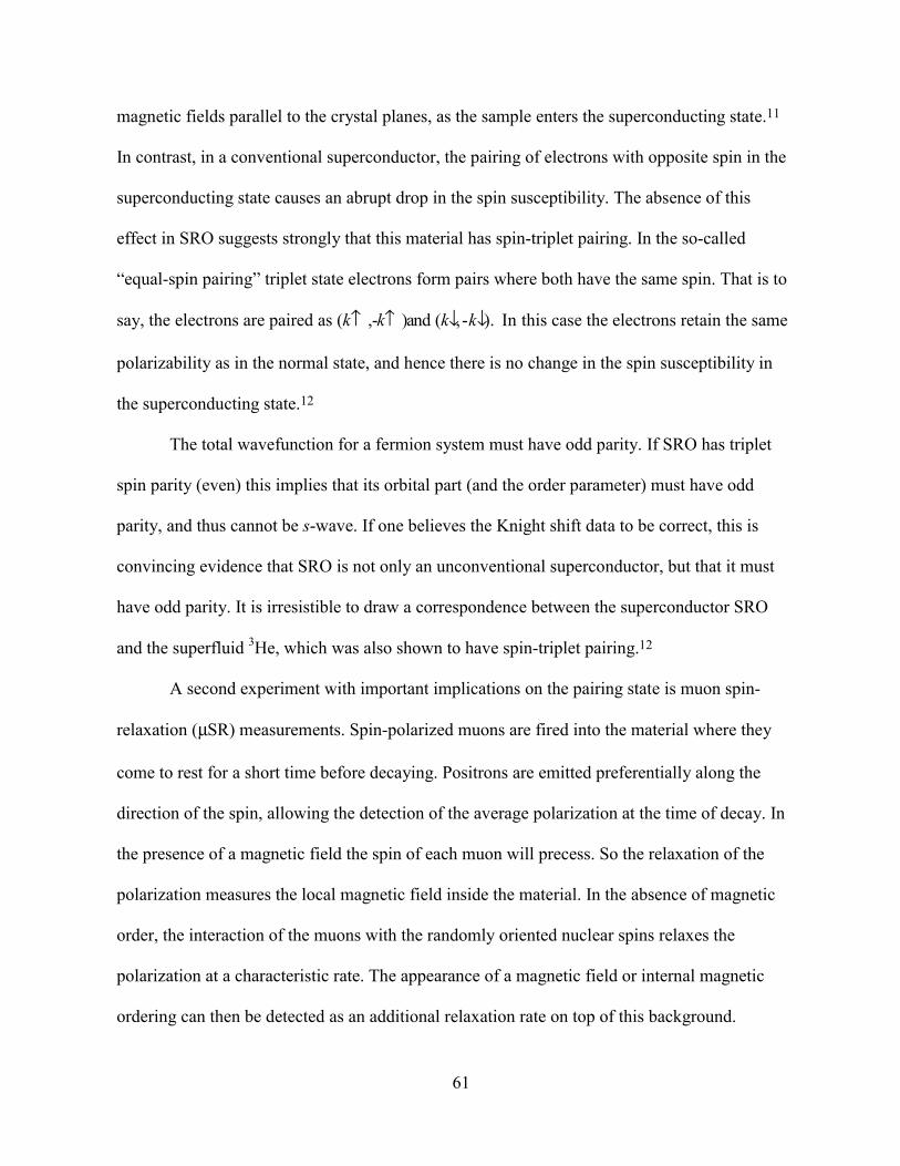
61
magnetic fields parallel to the crystal planes, as the sample enters the superconducting state.11
In contrast, in a conventional superconductor, the pairing of electrons with opposite spin in the
superconducting state causes an abrupt drop in the spin susceptibility. The absence of this
effect in SRO suggests strongly that this material has spin-triplet pairing. In the so-called
“equal-spin pairing” triplet state electrons form pairs where both have the same spin. That is to
say, the electrons are paired as (k↑ , -k↑ ) and (k↓, -k↓). In this case the electrons retain the same
polarizability as in the normal state, and hence there is no change in the spin susceptibility in
the superconducting state.12
The total wavefunction for a fermion system must have odd parity. If SRO has triplet
spin parity (even) this implies that its orbital part (and the order parameter) must have odd
parity, and thus cannot be s-wave. If one believes the Knight shift data to be correct, this is
convincing evidence that SRO is not only an unconventional superconductor, but that it must
have odd parity. It is irresistible to draw a correspondence between the superconductor SRO
and the superfluid 3He, which was also shown to have spin-triplet pairing.12
A second experiment with important implications on the pairing state is muon spin-
relaxation (µSR) measurements. Spin-polarized muons are fired into the material where they
come to rest for a short time before decaying. Positrons are emitted preferentially along the
direction of the spin, allowing the detection of the average polarization at the time of decay. In
the presence of a magnetic field the spin of each muon will precess. So the relaxation of the
polarization measures the local magnetic field inside the material. In the absence of magnetic
order, the interaction of the muons with the randomly oriented nuclear spins relaxes the
polarization at a characteristic rate. The appearance of a magnetic field or internal magnetic
ordering can then be detected as an additional relaxation rate on top of this background.
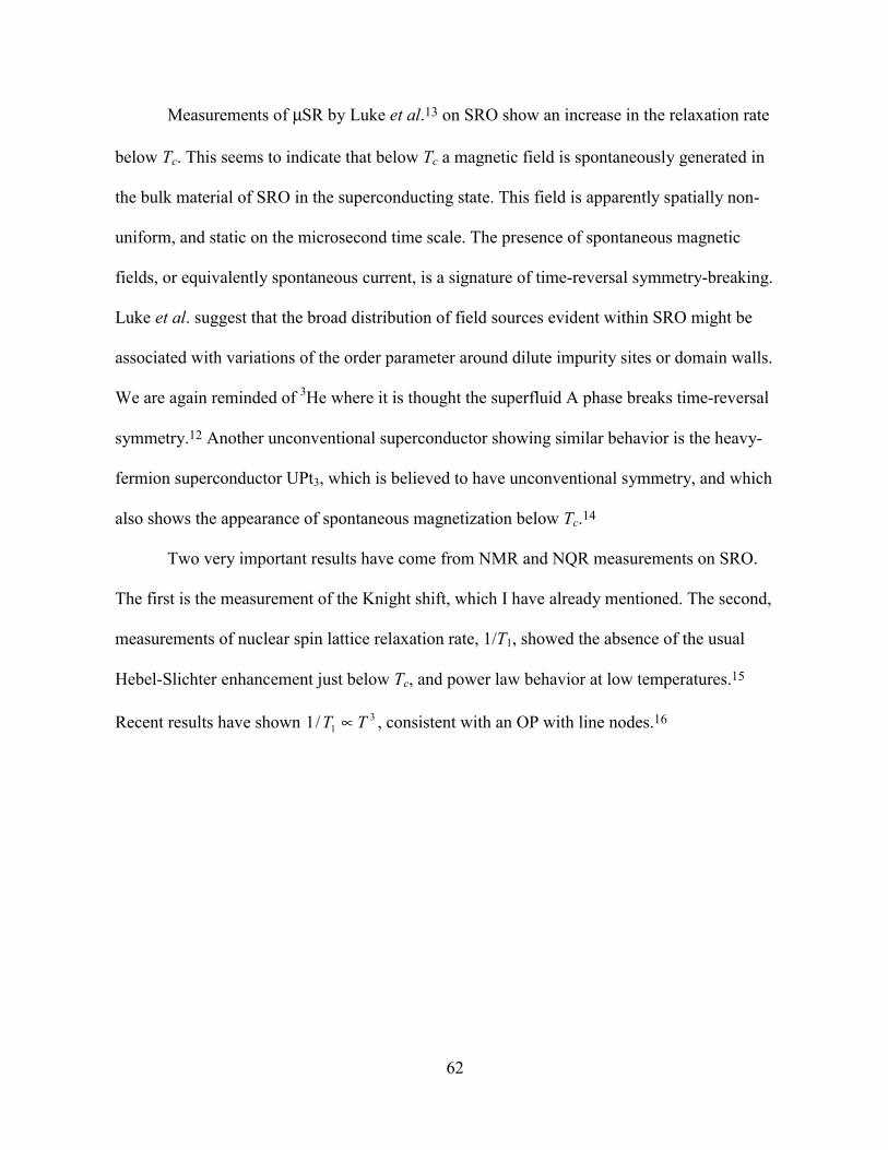
62
Measurements of µSR by Luke et al.13 on SRO show an increase in the relaxation rate
below Tc. This seems to indicate that below Tc a magnetic field is spontaneously generated in
the bulk material of SRO in the superconducting state. This field is apparently spatially non-
uniform, and static on the microsecond time scale. The presence of spontaneous magnetic
fields, or equivalently spontaneous current, is a signature of time-reversal symmetry-breaking.
Luke et al. suggest that the broad distribution of field sources evident within SRO might be
associated with variations of the order parameter around dilute impurity sites or domain walls.
We are again reminded of 3He where it is thought the superfluid A phase breaks time-reversal
symmetry.12 Another unconventional superconductor showing similar behavior is the heavy-
fermion superconductor UPt3, which is believed to have unconventional symmetry, and which
also shows the appearance of spontaneous magnetization below Tc.14
Two very important results have come from NMR and NQR measurements on SRO.
The first is the measurement of the Knight shift, which I have already mentioned. The second,
measurements of nuclear spin lattice relaxation rate, 1/T1, showed the absence of the usual
Hebel-Slichter enhancement just below Tc, and power law behavior at low temperatures.15
Recent results have shown 31/1 TT ∝ , consistent with an OP with line nodes.16
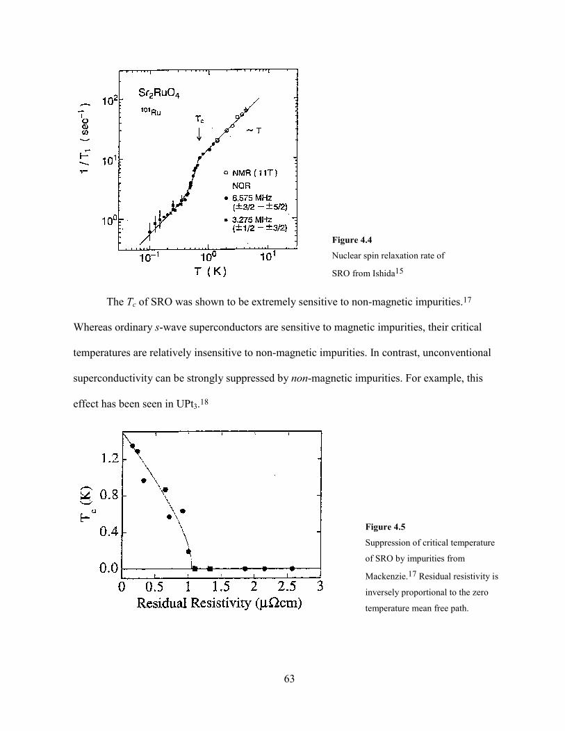
63
Figure 4.4
Nuclear spin relaxation rate of
SRO from Ishida15
The Tc of SRO was shown to be extremely sensitive to non-magnetic impurities.17
Whereas ordinary s-wave superconductors are sensitive to magnetic impurities, their critical
temperatures are relatively insensitive to non-magnetic impurities. In contrast, unconventional
superconductivity can be strongly suppressed by non-magnetic impurities. For example, this
effect has been seen in UPt3.18
Figure 4.5
Suppression of critical temperature
of SRO by impurities from
Mackenzie.17 Residual resistivity is
inversely proportional to the zero
temperature mean free path.
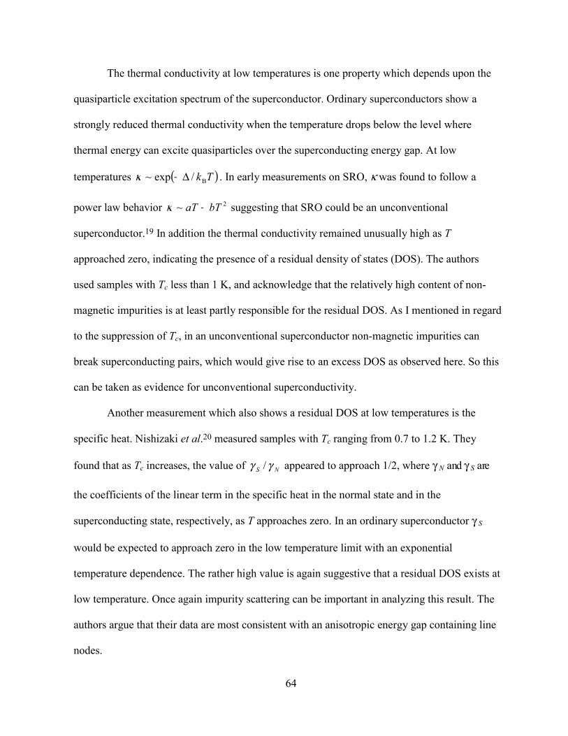
64
The thermal conductivity at low temperatures is one property which depends upon the
quasiparticle excitation spectrum of the superconductor. Ordinary superconductors show a
strongly reduced thermal conductivity when the temperature drops below the level where
thermal energy can excite quasiparticles over the superconducting energy gap. At low
temperatures ( )TkB/exp~ ∆−κ . In early measurements on SRO, κ was found to follow a
power law behavior 2~ bTaT +κ suggesting that SRO could be an unconventional
superconductor.19 In addition the thermal conductivity remained unusually high as T
approached zero, indicating the presence of a residual density of states (DOS). The authors
used samples with Tc less than 1 K, and acknowledge that the relatively high content of non-
magnetic impurities is at least partly responsible for the residual DOS. As I mentioned in regard
to the suppression of Tc, in an unconventional superconductor non-magnetic impurities can
break superconducting pairs, which would give rise to an excess DOS as observed here. So this
can be taken as evidence for unconventional superconductivity.
Another measurement which also shows a residual DOS at low temperatures is the
specific heat. Nishizaki et al.20 measured samples with Tc ranging from 0.7 to 1.2 K. They
found that as Tc increases, the value of NS γγ / appeared to approach 1/2, where γ N and γ S are
the coefficients of the linear term in the specific heat in the normal state and in the
superconducting state, respectively, as T approaches zero. In an ordinary superconductor γ S
would be expected to approach zero in the low temperature limit with an exponential
temperature dependence. The rather high value is again suggestive that a residual DOS exists at
low temperature. Once again impurity scattering can be important in analyzing this result. The
authors argue that their data are most consistent with an anisotropic energy gap containing line
nodes.
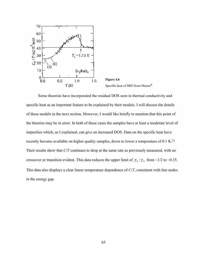
65
Figure 4.6
Specific heat of SRO from Maeno9
Some theorists have incorporated the residual DOS seen in thermal conductivity and
specific heat as an important feature to be explained by their models. I will discuss the details
of these models in the next section. However, I would like briefly to mention that this point of
the theories may be in error. In both of these cases the samples have at least a moderate level of
impurities which, as I explained, can give an increased DOS. Data on the specific heat have
recently become available on higher quality samples, down to lower a temperature of 0.1 K.21
Their results show that C/T continues to drop at the same rate as previously measured, with no
crossover or transition evident. This data reduces the upper limit of NS γγ / from ~1/2 to ~0.35.
This data also displays a clear linear temperature dependence of C/T, consistent with line nodes
in the energy gap.

66
Figure 4.7
New specific heat data from
Maeno21
Akima et al.10 used their measurements of Hc2, mentioned in the previous section, to
calculate the anisotropic coherence lengths, ξ ab and ξ c, in terms of the upper critical fields and
the magnetic flux quantum, Φ0, using the Ginzburg-Landau formulas for an anisotropic
superconductor, )2/( 20||2 abccH πξΦ= , and )2/(0||2 cababcH ξπξΦ= . They find the zero
temperature values )0(abξ = 660 Å and )0(cξ = 33 Å. We can compare these values with the
small angle neutron scattering estimate of the zero temperature penetration depth by Riseman et
al.,22 who find λab(100 mK) = 1940 ± 160 Å. The cuprates are firmly placed in the local limit
since their penetration depth is several orders of magnitude larger than their coherence length.
However, in SRO at low temperatures we see that the coherence length and penetration depth
are different by only a factor of three. SRO is clearly not in the extreme local limit and, even
based on these values alone, should probably be considered marginally nonlocal. In the next
chapter I will argue that, on the basis of our results indicating the possible presence of nodes in
the energy gap, SRO should be considered a nonlocal unconventional superconductor.

67
Finally, there is some recent evidence for unusual behavior of vortices at low
temperatures. Mota et al.23 have reported on measurements of magnetic flux flow. They cool
the sample in a magnetic field and observe the rate at which magnetic flux escapes under the
influence of the mutual repulsion of the vortices and the pinning in the material. They find that
at ~50 mK there is an abrupt drop in the flux creep. They attribute this result in SRO to a
second superconducting transition from a state which does not break time reversal symmetry
into one that does. They base this conclusion on their observation of a nearly identical effect in
UPt3 at the lower of its two superconducting transitions, where it is believed to break time
reversal symmetry.24 Mota et al. suggest that in the time reversal symmetry breaking state,
vortices become strongly pinned at the boundaries between domains of alternating (broken)
time reversal symmetry. It is not clear how this result should be reconciled with the µSR
measurement which shows that time reversal symmetry is broken not at 50 mK, but right at Tc.
It might be possible to detect this sudden breaking of time reversal symmetry using our tunnel
diode oscillator system if the sample were cooled in an applied magnetic field, rather than zero-
field cooled as it is for the results reported in this thesis.
Measurements of the temperature dependence of the penetration depth can play an
important role in resolving some of the questions about SRO which remain unanswered. As
discussed in chapter 3 the penetration depth at low temperatures is sensitive to the DOS.
Observation of power law behavior in penetration at low T is indicative of nodes in the energy
gap.
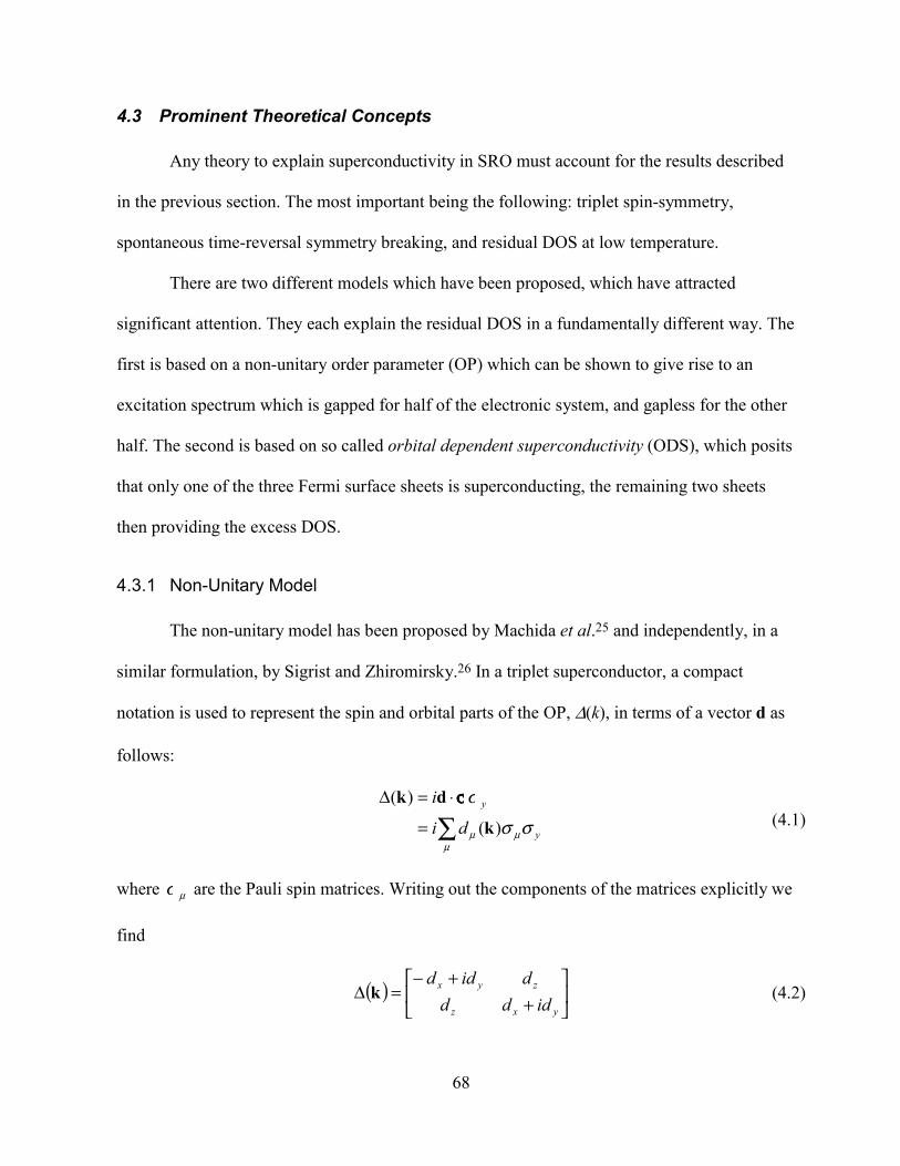
68
4.3 Prominent Theoretical Concepts
Any theory to explain superconductivity in SRO must account for the results described
in the previous section. The most important being the following: triplet spin-symmetry,
spontaneous time-reversal symmetry breaking, and residual DOS at low temperature.
There are two different models which have been proposed, which have attracted
significant attention. They each explain the residual DOS in a fundamentally different way. The
first is based on a non-unitary order parameter (OP) which can be shown to give rise to an
excitation spectrum which is gapped for half of the electronic system, and gapless for the other
half. The second is based on so called orbital dependent superconductivity (ODS), which posits
that only one of the three Fermi surface sheets is superconducting, the remaining two sheets
then providing the excess DOS.
4.3.1 Non-Unitary Model
The non-unitary model has been proposed by Machida et al.25 and independently, in a
similar formulation, by Sigrist and Zhiromirsky.26 In a triplet superconductor, a compact
notation is used to represent the spin and orbital parts of the OP, ∆(k), in terms of a vector d as
follows:
∑=
⋅=∆
µµµ σσ
σ
y
y
di
i
)(
)(
k
dk σσσσ(4.1)
where µσ are the Pauli spin matrices. Writing out the components of the matrices explicitly we
find
( )
+
+−=∆
yxz
zyx
iddddidd
k (4.2)
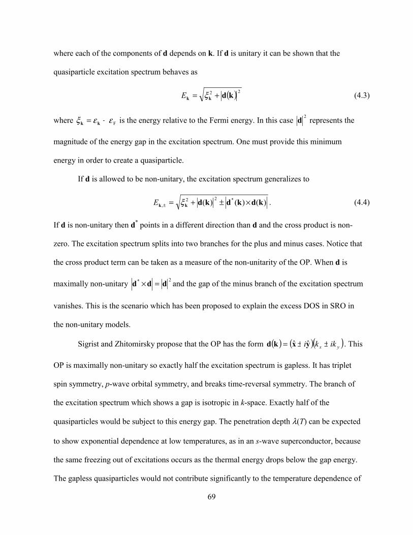
69
where each of the components of d depends on k. If d is unitary it can be shown that the
quasiparticle excitation spectrum behaves as
( ) 22 kdkk += ξE (4.3)
where Fεεξ −= kk is the energy relative to the Fermi energy. In this case 2d represents the
magnitude of the energy gap in the excitation spectrum. One must provide this minimum
energy in order to create a quasiparticle.
If d is allowed to be non-unitary, the excitation spectrum generalizes to
)()()( *22, kdkdkdkk ×±+=± ξE . (4.4)
If d is non-unitary then d* points in a different direction than d and the cross product is non-
zero. The excitation spectrum splits into two branches for the plus and minus cases. Notice that
the cross product term can be taken as a measure of the non-unitarity of the OP. When d is
maximally non-unitary 2* ddd =× and the gap of the minus branch of the excitation spectrum
vanishes. This is the scenario which has been proposed to explain the excess DOS in SRO in
the non-unitary models.
Sigrist and Zhitomirsky propose that the OP has the form ( ) ( )( )yx ikki ±±= yxkd ˆˆ . This
OP is maximally non-unitary so exactly half the excitation spectrum is gapless. It has triplet
spin symmetry, p-wave orbital symmetry, and breaks time-reversal symmetry. The branch of
the excitation spectrum which shows a gap is isotropic in k-space. Exactly half of the
quasiparticles would be subject to this energy gap. The penetration depth λ(T) can be expected
to show exponential dependence at low temperatures, as in an s-wave superconductor, because
the same freezing out of excitations occurs as the thermal energy drops below the gap energy.
The gapless quasiparticles would not contribute significantly to the temperature dependence of
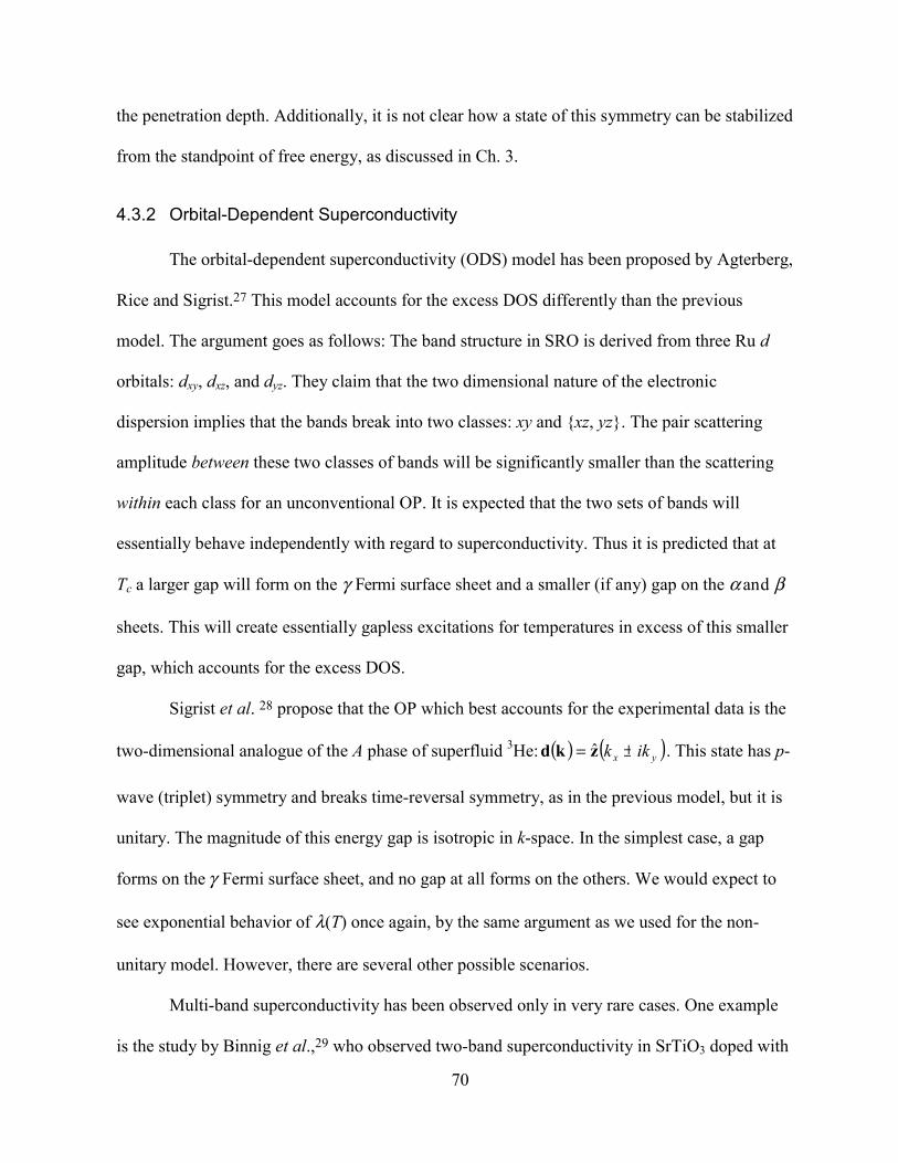
70
the penetration depth. Additionally, it is not clear how a state of this symmetry can be stabilized
from the standpoint of free energy, as discussed in Ch. 3.
4.3.2 Orbital-Dependent Superconductivity
The orbital-dependent superconductivity (ODS) model has been proposed by Agterberg,
Rice and Sigrist.27 This model accounts for the excess DOS differently than the previous
model. The argument goes as follows: The band structure in SRO is derived from three Ru d
orbitals: dxy, dxz, and dyz. They claim that the two dimensional nature of the electronic
dispersion implies that the bands break into two classes: xy and xz, yz. The pair scattering
amplitude between these two classes of bands will be significantly smaller than the scattering
within each class for an unconventional OP. It is expected that the two sets of bands will
essentially behave independently with regard to superconductivity. Thus it is predicted that at
Tc a larger gap will form on the γ Fermi surface sheet and a smaller (if any) gap on the α and β
sheets. This will create essentially gapless excitations for temperatures in excess of this smaller
gap, which accounts for the excess DOS.
Sigrist et al. 28 propose that the OP which best accounts for the experimental data is the
two-dimensional analogue of the A phase of superfluid 3He: ( ) ( )yx ikk ±= zkd ˆ . This state has p-
wave (triplet) symmetry and breaks time-reversal symmetry, as in the previous model, but it is
unitary. The magnitude of this energy gap is isotropic in k-space. In the simplest case, a gap
forms on the γ Fermi surface sheet, and no gap at all forms on the others. We would expect to
see exponential behavior of λ(T) once again, by the same argument as we used for the non-
unitary model. However, there are several other possible scenarios.
Multi-band superconductivity has been observed only in very rare cases. One example
is the study by Binnig et al.,29 who observed two-band superconductivity in SrTiO3 doped with
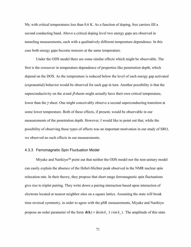
71
Nb, with critical temperatures less than 0.6 K. As a function of doping, free carriers fill a
second conducting band. Above a critical doping level two energy gaps are observed in
tunneling measurements, each with a qualitatively different temperature dependence. In this
case both energy gaps become nonzero at the same temperature.
Under the ODS model there are some similar effects which might be observable. The
first is the crossover in temperature dependence of properties like penetration depth, which
depend on the DOS. As the temperature is reduced below the level of each energy gap activated
(exponential) behavior would be observed for each gap in turn. Another possibility is that the
superconductivity on the α and β sheets might actually have their own critical temperature,
lower than the γ sheet. One might conceivably observe a second superconducting transition at
some lower temperature. Both of these effects, if present, would be observable in our
measurements of the penetration depth. However, I would like to point out that, while the
possibility of observing these types of effects was an important motivation in our study of SRO,
we observed no such effects in our measurements.
4.3.3 Ferromagnetic Spin Fluctuation Model
Miyake and Narikiyo30 point out that neither the ODS model nor the non-unitary model
can easily explain the absence of the Hebel-Slichter peak observed in the NMR nuclear spin
relaxation rate. In their theory, they propose that short range ferromagnetic spin fluctuations
give rise to triplet pairing. They write down a pairing interaction based upon interaction of
electrons located at nearest neighbor sites on a square lattice. Assuming the state will break
time reversal symmetry, in order to agree with the µSR measurements, Miyake and Narikiyo
propose an order parameter of the form )sin(sinˆ)( yx kik ±= zkd . The amplitude of this state
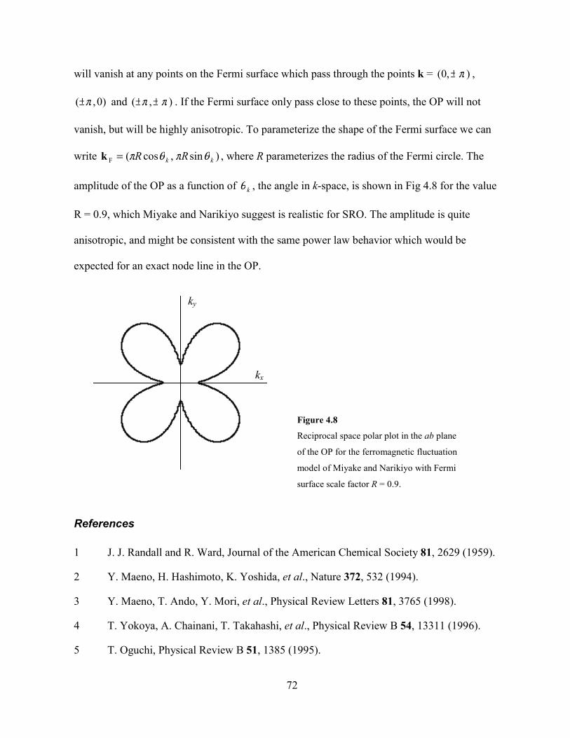
72
will vanish at any points on the Fermi surface which pass through the points k = ),0( π± ,
)0,( π± and ),( ππ ±± . If the Fermi surface only pass close to these points, the OP will not
vanish, but will be highly anisotropic. To parameterize the shape of the Fermi surface we can
write )sin,cos(F kk RR θπθπ=k , where R parameterizes the radius of the Fermi circle. The
amplitude of the OP as a function of kθ , the angle in k-space, is shown in Fig 4.8 for the value
R = 0.9, which Miyake and Narikiyo suggest is realistic for SRO. The amplitude is quite
anisotropic, and might be consistent with the same power law behavior which would be
expected for an exact node line in the OP.
Figure 4.8
Reciprocal space polar plot in the ab plane
of the OP for the ferromagnetic fluctuation
model of Miyake and Narikiyo with Fermi
surface scale factor R = 0.9.
References
1 J. J. Randall and R. Ward, Journal of the American Chemical Society 81, 2629 (1959).
2 Y. Maeno, H. Hashimoto, K. Yoshida, et al., Nature 372, 532 (1994).
3 Y. Maeno, T. Ando, Y. Mori, et al., Physical Review Letters 81, 3765 (1998).
4 T. Yokoya, A. Chainani, T. Takahashi, et al., Physical Review B 54, 13311 (1996).
5 T. Oguchi, Physical Review B 51, 1385 (1995).
kx
ky
73
6 A. V. Puchkov, Z. X. Shen, T. Kimura, et al., Physical Review B 58, 13322 (1998).
7 A. P. Mackenzie, S. R. Julian, A. J. Diver, et al., Physical Review Letters 76, 3786(1996).
8 A. P. Mackenzie, S. Ikeda, Y. Maeno, et al., Journal of the Physical Society of Japan67, 385 (1998).
9 Y. Maeno, S. Nishizaki, K. Yoshida, et al., Journal of Low Temperature Physics 105,1577 (1996).
10 T. Akima, S. NishiZaki, and Y. Maeno, Journal of the Physical Society of Japan 68, 694(1999).
11 K. Ishida, H. Mukuda, Y. Kitaoka, et al., Nature 396, 658 (1998).
12 A. Leggett, Reviews of Modern Physics 47, 331 (1975).
13 G. M. Luke, Y. Fudamoto, K. M. Kojika, et al., Nature 394, 558 (1998).
14 G. M. Luke, A. Keren, L. P. Le, et al., Physical Review Letters 71, 1466 (1993).
15 K. Ishida, Y. Kitaoka, K. Asayama, et al., Physical Review B 56, 505 (1997).
16 K. Ishida, (Private communication, 1999).
17 A. P. Mackenzie, R. K. W. Haselwimmer, A. W. Tyler, et al., Physical Review Letters80, 161 (1998).
18 J. B. Kycia, J. I. Hong, M. J. Graf, et al., Preprint , 0 (1997).
19 H. Suderow, J. P. Brison, J. Flouquet, et al., Journal of Physics: Condensed matter 10,597 (1998).
20 S. Nishizaki, Y. Maeno, S. Farner, et al., Physica C 282, 1413 (1997).
21 Y. Maeno, S. Nishizaki, and Z. Q. Mao, Journal of Superconductivity 12, 535 (1999).
22 T. M. Riseman, P. G. Kealey, E. M. Forgan, et al., Nature 396, 242 (1998).
23 A. C. Mota, E. Dumont, A. Amann, et al., Physica B 259, 934 (1999).
24 A. Amann, A. C. Mota, M. B. Maple, et al., Physical Review B 57, 3640 (1998).
25 K. Machida, M.-a. Ozaki, and T. Ohmi, Journal of the Physical Society of Japan 65,3720 (1996).

74
26 M. Sigrist and E. Zhitomirsky Michael, Journal of the Physical Society of Japan 65,3452 (1996).
27 D. F. Agterberg, T. M. Rice, and M. Sigrist, Physical Review Letters 78, 3374 (1997).
28 M. Sigrist, D. F. Agterberg, A. Furusaki, et al., Preprint , 0 (1999).
29 G. Binnig, A. Baratoff, H. E. Hoenig, et al., Physical Review Letters 45, 1352 (1980).
30 K. Miyake and O. Narikiyo, Physical Review Letters 83, 1423 (1999).
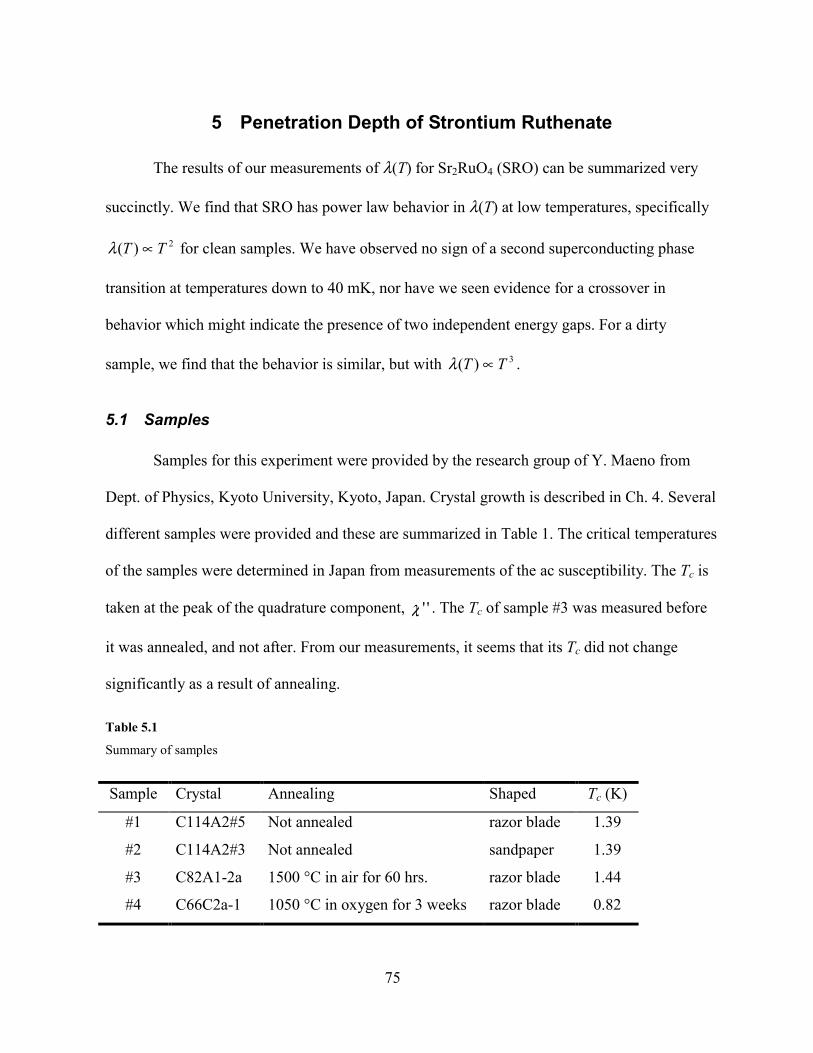
75
5 Penetration Depth of Strontium Ruthenate
The results of our measurements of λ(T) for Sr2RuO4 (SRO) can be summarized very
succinctly. We find that SRO has power law behavior in λ(T) at low temperatures, specifically
2)( TT ∝λ for clean samples. We have observed no sign of a second superconducting phase
transition at temperatures down to 40 mK, nor have we seen evidence for a crossover in
behavior which might indicate the presence of two independent energy gaps. For a dirty
sample, we find that the behavior is similar, but with 3)( TT ∝λ .
5.1 Samples
Samples for this experiment were provided by the research group of Y. Maeno from
Dept. of Physics, Kyoto University, Kyoto, Japan. Crystal growth is described in Ch. 4. Several
different samples were provided and these are summarized in Table 1. The critical temperatures
of the samples were determined in Japan from measurements of the ac susceptibility. The Tc is
taken at the peak of the quadrature component, ''χ . The Tc of sample #3 was measured before
it was annealed, and not after. From our measurements, it seems that its Tc did not change
significantly as a result of annealing.
Table 5.1
Summary of samples
Sample Crystal Annealing Shaped Tc (K)
#1 C114A2#5 Not annealed razor blade 1.39
#2 C114A2#3 Not annealed sandpaper 1.39
#3 C82A1-2a 1500 °C in air for 60 hrs. razor blade 1.44
#4 C66C2a-1 1050 °C in oxygen for 3 weeks razor blade 0.82

76
All samples were cut from larger pieces to a size small enough to fit on the end of our
cold finger, approximately 1 mm in diameter. Samples #1, 3 and 4 were shaped by cutting with
a razor blade under a microscope. Their perimeter is somewhat irregular as a result of this
process, but they are all shaped like flat plates. Sample #2 was cut from the same large crystal
as sample #1, but instead of a razor blade, I used fine sandpaper to form the shape. I glued the
sample to a glass slide with super glue, leaving a small portion projecting over the edge. By
holding the slide vertically I carefully ground the projecting portion of the crystal on 400 grit
silicon carbide sandpaper until it was flush with the edge of the slide. The glue was easily
dissolved with acetone and the process repeated to form the remaining edges of the sample. In
this way I prepared the sample in a fairly regular octagonal shape.
5.2 Calibration
We tried both of the calibration techniques discussed in Ch. 1. We found that the aluminum
sphere technique overestimates the change in penetration depth. For the second calibration
procedure I fashioned a dummy sample of high purity aluminum (sample Al#1) in the same
shape and size as sample #3. This technique worked more successfully. In Fig. 5.1 the data for
the Al#1 sample are compared with the theoretical curve of λ(0)2/λ(T)2. I have taken the values
for pure aluminum as λ(0) = 500 Å and ∆(0) = 0.18 meV. As discussed in Ch. 2, I used the
weak coupling interpolation formula for ∆(T) and the expression for λ(T) appropriate for a non-
local superconductor. The value of Tc which best fits the data is 1.16 K, which compares
favorably with the value of 1.18 K from tables. I found that by adjusting the geometrical
scaling factor to a value of G = 2.5 Å/Hz for the Al#1 sample, the data could be made to lie
directly over the theoretical curve. Since G depends only on the geometry of the sample and
coil, this same value can be used to scale the data for sample #3. We discovered only relatively
77
late in the course of this study that the first calibration procedure was not adequate. Rather than
make a dummy sample for every SRO sample, I have used the results of the sample #3
calibration. By comparing the data from other samples with the calibrated data from sample #3
we can estimate the geometry factor for the other samples.
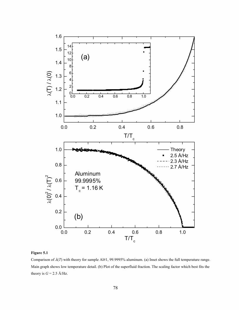
78
0.0 0.2 0.4 0.6 0.8 1.00.0
0.2
0.4
0.6
0.8
1.0
0.0 0.2 0.4 0.6 0.8
1.0
1.1
1.2
1.3
1.4
1.5
1.6
Theory 2.5 Å/Hz 2.3 Å/Hz 2.7 Å/Hz
Aluminum 99.9995%Tc = 1.16 K
λ(0)
2 / λ(
T)2
T/Tc
(b)
(a)λ(
T) /
λ(0)
T/Tc
0.0 0.2 0.4 0.6 0.8 1.00
2
4
6
810
12
14
Figure 5.1
Comparison of λ(T) with theory for sample Al#1, 99.9995% aluminum. (a) Inset shows the full temperature range.
Main graph shows low temperature detail. (b) Plot of the superfluid fraction. The scaling factor which best fits the
theory is G = 2.5 Å/Hz.
79
5.3 Results
Results for the high purity aluminum sample, Al#1, are shown in Fig. 5.1. Graph (a)
shows λ(T) plotted as a function of T/Tc. Graph (b) shows λ(0)2/λ(T)2 as a function of T/Tc,
which is proportional to the superfluid density. The agreement with the theoretical curve is
excellent, when the scale factor G = 2.5 Å/Hz. To give an idea of the sensitivity of the shape of
the curve to the value of G, the dashed lines show the dependence of the data when G is varied
±10%. Because sample Al#1 was prepared with nominally the same shape as SRO sample #3,
we use this value of G, adjusted slightly to account for the very small difference in shape, to
scale the data for sample #3. Likewise, the various shapes of each of the other samples were
used to determine values of G relative to sample #3. Figure 5.2 summarizes the penetration
depth for samples #1-4 with the magnetic field oriented perpendicular to the ab-planes of the
crystals. On this scale, the general behavior of all four samples is quite similar, but there are
clear differences in the location and sharpness of the transitions. Sample #3 has the highest Tc =
1.44 K, and also shows the sharpest transition. It is interesting to note the difference between
samples #1 and 2, which are cut from the same crystal. Sample #2 shows a much more rounded
transition as a result of the damage that occurred on the surface as a result of grinding it on
sandpaper. Sample #3 has a significantly lower Tc = 0.82 K.
Figure 5.3 shows the temperature region from T/Tc = 0 to 0.8, plotted against (T/Tc)2 for
samples #1-3. It is evident from these graphs that at temperatures below approximately 0.4 Tc,
all three samples have 2)( TT ∝∆λ . In addition, a graph of sample #3 is shown with the field
oriented parallel to the ab-planes. The temperature dependence is virtually identical to the
perpendicular orientation, showing quadratic temperature dependence below 0.4 Tc. Figure 5.4
shows a detail of the low temperature region, below 0.7 K, for sample #2 as a function of 2T .

80
The clear linear behavior displayed indicates once again that 2)( TT ∝∆λ at low temperature
and is typical of samples #1-3.
0.0 0.2 0.4 0.6 0.8 1.0 1.2 1.4 1.6 1.8
0
5000
10000
15000
20000
25000
30000
35000
40000
0.0 0.2 0.4 0.6 0.8 1.0 1.2 1.4 1.6 1.8
0
5000
10000
15000
20000
25000
30000
35000
40000
0.0 0.2 0.4 0.6 0.8 1.0 1.2 1.4 1.6 1.8
0
5000
10000
15000
20000
25000
30000
35000
40000
0.0 0.2 0.4 0.6 0.8 1.0 1.2 1.4 1.6 1.8
0
5000
10000
15000
20000
25000
30000
35000
40000
Sample #1
∆λ (
Å)
T (K)
Sample #2
T (K)
Sample #3
T (K)
Sample #4
T (K)
Figure 5.2
Penetration depth of SRO samples #1-4 with magnetic field oriented perpendicular to the ab-planes of the crystals.
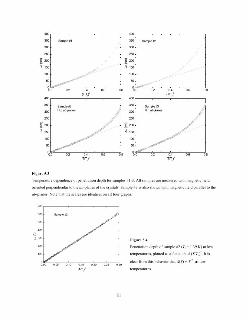
81
0.0 0.2 0.4 0.6 0.80
50
100
150
200
250
300
350
400
0.0 0.2 0.4 0.6 0.80
50
100
150
200
250
300
350
400
0.0 0.2 0.4 0.6 0.80
50
100
150
200
250
300
350
400
0.0 0.2 0.4 0.6 0.80
50
100
150
200
250
300
350
400
Sample #1
∆λ (n
m)
(T/Tc)2
Sample #2
∆λ (n
m)
(T/Tc)2
Sample #3H ⊥ ab planes
∆λ (n
m)
(T/Tc)2
Sample #3H || ab planes
∆λ (n
m)
(T/Tc)2
Figure 5.3
Temperature dependence of penetration depth for samples #1-3. All samples are measured with magnetic field
oriented perpendicular to the ab-planes of the crystals. Sample #3 is also shown with magnetic field parallel to the
ab-planes. Note that the scales are identical on all four graphs.
0.00 0.05 0.10 0.15 0.20 0.25 0.300
100
200
300
400
500
600
700
Sample #2
∆λ
(Å)
(T/Tc)2
Figure 5.4
Penetration depth of sample #2 (Tc = 1.39 K) at low
temperatures, plotted as a function of (T/Tc)2. It is
clear from this behavior that λ(T) ∝ 2T at low
temperatures.

82
0.0 0.2 0.4 0.6 0.8 1.00.0
0.2
0.4
0.6
0.8
1.0
0.0 0.2 0.4 0.6 0.8 1.00.0
0.2
0.4
0.6
0.8
1.0
0.0 0.2 0.4 0.6 0.8 1.00.0
0.2
0.4
0.6
0.8
1.0
0.0 0.2 0.4 0.6 0.8 1.00.0
0.2
0.4
0.6
0.8
1.0
Sample #1
λ(0)
2 / λ(
T)2
T/TC
Sample #2
λ(0)
2 / λ(
T)2
T/TC
Sample #3
λ(0)
2 / λ(
T)2
T/TC
Sample #4
λ(0)
2 / λ(
T)2
T/TC
Figure 5.5
Summary of temperature dependence of )0(/)()(/)0( 22ss nTnT ∝λλ , the superfluid fraction, for samples
#1-4. The value of λ(0) = 1900 Å is used for samples #1-3, and λ(0) = 2230 Å is used for sample #4.
0.0 0.2 0.4 0.6 0.8 1.00.0
0.2
0.4
0.6
0.8
1.0
0.0 0.2 0.4 0.6 0.8 1.00.0
0.2
0.4
0.6
0.8
1.0
0.0 0.2 0.4 0.6 0.8 1.00.0
0.2
0.4
0.6
0.8
1.0
Sample #1
λ(0)
2 / λ(
T)2
T/TC
Local Theory
Nonlocal Theory
Figure 5.6
Comparison of superfluid fraction of
sample #1 with local and nonlocal s-
wave models.

83
5.4 Interpretation
Our observation of power law behavior implies that the energy gap has nodes. The non-
unitary and orbital dependent superconductivity (ODS) models of superconductivity are
inconsistent with this result. As discussed in the previous chapter, there are several possible
scenarios under the ODS model. The simplest is an energy gap on one Fermi surface sheet, and
none on the other. This would give exponential dependence of λ(T), contrary to our observation
of power law dependence. We see evidence neither for a second superconducting transition nor
for the crossover of temperature dependence which might result from two different energy
gaps. Likewise, the non-unitary model predicts an exponential dependence with does not
appear in SRO.
Our observation of temperature dependence of 2)( TT ∝∆λ can be taken as strong
evidence that the energy gap has nodes, as discussed in Ch. 3. The naïve conclusion might be
that the 2T dependence implies that there are point nodes. However, it has been found
experimentally that low temperature NMR spin relaxation rate 31/1 TT ∝ ,1 and electronic
specific heat 2TCe ∝ .2 Both of these (in my opinion, highly credible) results are consistent
with line nodes in the gap. Therefore, we need to consider carefully whether our results are
consistent with these and other measurements made up to now on SRO. In the local limit, in the
absence of impurities, the penetration depth will show linear temperature dependence in the
presence of line nodes. We are faced with the same dilemma which confronted those studying
the cuprates, when early measurements of λ(T) showed quadratic behavior. Thanks to the work
on the cuprates there are a number of well documented possibilities to explore. We believe that
our data are consistent with line nodes in the energy gap when we take into account one or
more of these effects.
84
5.4.1 Resonant Impurity Scattering
As discussed in Ch. 3, Hirschfeld and Goldenfeld3 noted that the effect of resonant
impurity scattering (RIS) on the cuprate superconductors is to change the intrinsic TT ∝)(λ to
quadratic, and this would be the most obvious explanation for quadratic dependence in SRO. It
is possible that just such an effect is at play in our measurements of SRO. Hirschfeld and
Goldenfeld introduce a crossover temperature T*, below which the intrinsic linear behavior due
to line nodes would be modified by RIS to quadratic. For the strong scattering limit, the Tc
suppression (Tc0 - Tc)/Tc0 is estimated to be on the order of Γ /∆0, where Tc0 is the critical
temperature in the absence of impurities, Γ is the scattering rate, and ∆0 is the maximum energy
gap. For very small impurity levels the crossover temperature will be approximately
2/10
* )(~ Γ∆T . So we can estimate that 2/1
0
00
* ~
−∆
c
cc
TTT
T . Taking ∆0 = 1.76 Tc, and Tc0 =
1.5 K, we find T* ~ 0.7 K. This value is close to the range over which the 2T dependence was
found to fit the data for samples #1-3. However, we do not observe a linear dependence in any
temperature range in any of the samples we have measured. It could be that the value of T* is so
high that linear behavior, which would only show up in the low temperature limit, is hidden by
the nonlinearity that normally appears at higher temperatures. For example in the best
measurements of the cuprates, linear temperature dependence is observed at temperatures
below around 15-25% of Tc. In our measurements, since T* and the range of quadratic behavior
is about half of Tc, it is possible that the linear range is simply not observable. Were they
available to us, it is conceivable that measurements on even cleaner samples might exhibit a
clear crossover between quadratic and linear behavior.
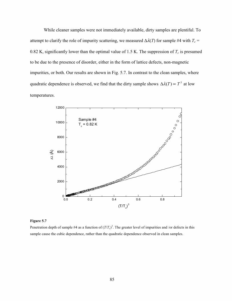
85
While cleaner samples were not immediately available, dirty samples are plentiful. To
attempt to clarify the role of impurity scattering, we measured ∆λ(T) for sample #4 with Tc =
0.82 K, significantly lower than the optimal value of 1.5 K. The suppression of Tc is presumed
to be due to the presence of disorder, either in the form of lattice defects, non-magnetic
impurities, or both. Our results are shown in Fig. 5.7. In contrast to the clean samples, where
quadratic dependence is observed, we find that the dirty sample shows 3)( TT ∝∆λ at low
temperatures.
0.0 0.2 0.4 0.6 0.80
2000
4000
6000
8000
10000
12000
Sample #4Tc = 0.82 K
∆λ
(Å)
(T/Tc)3
Figure 5.7
Penetration depth of sample #4 as a function of (T/Tc)3. The greater level of impurities and /or defects in this
sample cause the cubic dependence, rather than the quadratic dependence observed in clean samples.
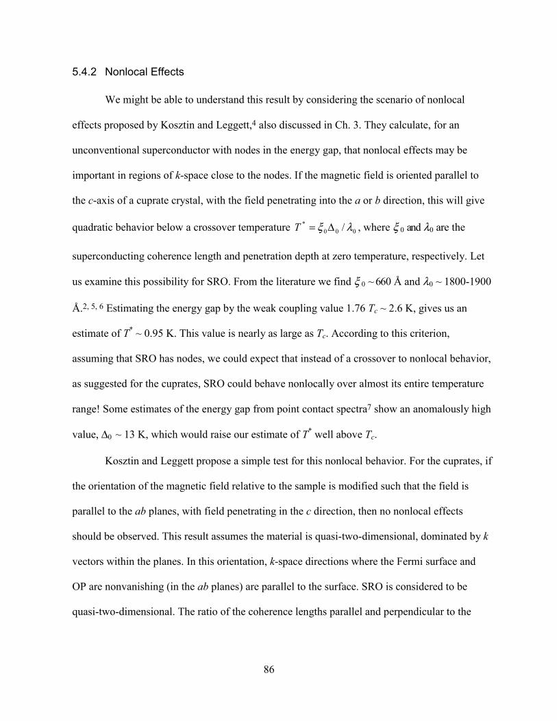
86
5.4.2 Nonlocal Effects
We might be able to understand this result by considering the scenario of nonlocal
effects proposed by Kosztin and Leggett,4 also discussed in Ch. 3. They calculate, for an
unconventional superconductor with nodes in the energy gap, that nonlocal effects may be
important in regions of k-space close to the nodes. If the magnetic field is oriented parallel to
the c-axis of a cuprate crystal, with the field penetrating into the a or b direction, this will give
quadratic behavior below a crossover temperature 000* / λξ ∆=T , where ξ 0 and λ0 are the
superconducting coherence length and penetration depth at zero temperature, respectively. Let
us examine this possibility for SRO. From the literature we find ξ 0 ~ 660 Å and λ0 ~ 1800-1900
Å.2, 5, 6 Estimating the energy gap by the weak coupling value 1.76 Tc ~ 2.6 K, gives us an
estimate of T* ~ 0.95 K. This value is nearly as large as Tc. According to this criterion,
assuming that SRO has nodes, we could expect that instead of a crossover to nonlocal behavior,
as suggested for the cuprates, SRO could behave nonlocally over almost its entire temperature
range! Some estimates of the energy gap from point contact spectra7 show an anomalously high
value, ∆0 ~ 13 K, which would raise our estimate of T* well above Tc.
Kosztin and Leggett propose a simple test for this nonlocal behavior. For the cuprates, if
the orientation of the magnetic field relative to the sample is modified such that the field is
parallel to the ab planes, with field penetrating in the c direction, then no nonlocal effects
should be observed. This result assumes the material is quasi-two-dimensional, dominated by k
vectors within the planes. In this orientation, k-space directions where the Fermi surface and
OP are nonvanishing (in the ab planes) are parallel to the surface. SRO is considered to be
quasi-two-dimensional. The ratio of the coherence lengths parallel and perpendicular to the

87
planes2 is ξ ab/ξ c = 20, which is quite large (although the cuprates have values closer to 100). I
believe that if we assume the presence of nodes then the model should apply equally to SRO.
We measured λ(T) for sample #3 with the field oriented parallel to the planes. This was
accomplished by attaching a small plastic cube to the end of the cold finger, and gluing the
crystal against the side of the cube, with its edge contacting the end of the cold finger.
However, our measurements give the same result for this field orientation: 2)( TT ∝λ , in
seeming conflict with the nonlocal theory. However, because the cube was fashioned by hand,
I estimate that the orientation is only parallel to within ~5-10°. It is possible that the small
misorientation is sufficient to allow a component of the screening currents flowing in the
direction where the nonlocal effect appears. To rule this out one could attempt a more careful
orientation of the sample and field. But the effect might be so sensitive to orientation that it
would be necessary to construct a system which would allow in-situ adjustment of the angle.
An additional effect could come from the c-axis penetration depth which participates in the
effect when the field is oriented in this direction. It is possible that the temperature dependence
of λc could dominate, obscuring the intrinsic dependence of the in-plane penetration depth in
this orientation.
Another explanation for the cubic behavior in the dirty sample is more interesting.
Kosztin and Leggett find, more generally, that if the intrinsic behavior in the local limit is
∆λ(T) then taking into account nonlocal effects, we would expect )()( TTTnonlocal λλ ∆⋅∝∆ . Let
us assume that the clean samples have intrinsic linear behavior in the absence of the nonlocal
effect. Then we would expect quadratic behavior when we take into account the nonlocal
effect. Similarly, let us assume that the dirty sample, due to impurity scattering, would have

88
quadratic behavior in the absence of nonlocal effects. Then we might expect to observe cubic
dependence in this sample when the nonlocal effect is included.
In general, the effect of impurities on a nonlocal superconductor is to drive it towards
more local behavior with increasing impurity content, because the coherence length is reduced
and the penetration depth is increased. We need to estimate to what extent the dirty sample can
still be considered nonlocal. Mackenzie et al.8 studied systematically the dependence of Tc on
non-magnetic impurities in SRO. Using their estimates for mean free path, interpolated from
their graph of resistivity ρ(T), I estimate that sample #4 has a mean free path ~ 1750 Å. This
value, while significantly suppressed from the clean sample value of ~7000 Å, is still larger
than the clean sample coherence length of ξ 0 = 660 Å. Impurities can be expected to reduce the
coherence length to a value9
111
0
+=ξξ
. (5.1)
Putting in the values I find ξ ~ 480 Å. We can also estimate the effect of impurities on the
effective zero-temperature penetration depth, which should be greater in a dirty sample because
scattering from impurities reduces the superfluid density, thereby reducing the screening of the
magnetic field. The effective penetration depth can be expressed as
2/10)(),(
=
ξξλλ TTeff . (5.2)
I estimate λeff (T=0) = 2230 Å. Using ξ and λeff (0), and assuming that the gap, ∆0, is not
strongly affected by impurities, I estimate T* = ∆0ξ /λ = 0.6 K. This value is identical to the
range over which we can fit cubic dependence in sample #4. The precise agreement is
somewhat coincidental, considering the crude approximations used in this estimate. However, it
89
is suggestive that this model combining nonlocality and impurity scattering might apply in the
case of SRO and, if correct, would support the conclusion that the clean samples have line
nodes in the gap. One might further test this conclusion by measuring a sample with critical
temperature in the intermediate range between the samples measured here, say 1.2 K.
5.4.3 High Frequency Effects
Historically, in the heavy fermion superconductors, there was an inconsistency in
measurements of λ(T) at low temperatures. These unconventional superconductors are believed
to have line nodes in the energy gap as well. These materials are exquisitely sensitive to
impurities and defects, and resonant impurity scattering was considered important, as in the
cuprates. However, an additional effect was noted by Signore et al.,10, 11 who found that the
response of very clean samples of UPt3 (Tc ~ 0.5 K) was dependent upon the frequency of
measurement. Signore et al. showed that for low frequencies (from DC to at least 5 kHz) the
temperature dependence TT ∝)(λ , while at frequencies above 3 MHz, 2)( TT ∝λ . The effect
of frequency can generally be ignored for ordinary superconductors until the frequency exceeds
the energy gap (in the GHz range) where Cooper pairs can be broken by the absorption of
photons. However, in an unconventional superconductor with nodes in the energy gap, it is
possible for significantly lower frequencies to break Cooper pairs in the region of the nodes.
This effect could be manifested in SRO in our experiments because our measurement
frequency is tens of MHz. The only way to rule out this effect would be to construct an entirely
new apparatus, such as a SQUID or mutual inductance system, to measure the penetration
depth at lower frequency.

90
References
1 K. Ishida, (Private communication, 1999).
2 Y. Maeno, S. Nishizaki, and Z. Q. Mao, Journal of Superconductivity 12, 535 (1999).
3 P. Hirschfeld, J. and N. Goldenfeld, Physical Review B 48, 4219 (1993).
4 I. Kosztin and A. Leggett, Physical Review Letters 79, 135 (1997).
5 T. M. Riseman, P. G. Kealey, E. M. Forgan, et al., Nature 396, 242 (1998).
6 C. M. Aegerter, S. H. Lloyd, C. Ager, et al., Journal of Physics: Condensed matter 10,7445 (1998).
7 F. Laube, G. Goll, H. v. Lohneysen, et al., cond-mat/9907267 (1999).
8 A. P. Mackenzie, R. K. W. Haselwimmer, A. W. Tyler, et al., Physical Review Letters80, 161 (1998).
9 M. Tinkham, Introduction to Superconductivity (McGraw-Hill, Inc., New York, 1996).
10 P. J. C. Signore, B. Andraka, M. W. Meisel, et al., Physical Review B 52, 4446 (1995).
11 P. J. C. Signore, J. P. Koster, E. A. Knetsch, et al., Physical Review B 45, 10151(1992).
91
6 Conclusions and Future Directions
I have shown that the temperature dependence of the penetration depth is a valuable
measurement technique for probing the behavior of the order parameter in unconventional
superconductors. We have constructed a high resolution tunnel-diode oscillator-based
measurement system suitable for measuring the temperature dependence of the magnetic
penetration depth of superconductors, λ(T), at very low temperatures. I have reported on
measurements of λ(T) in high quality single crystals of the unconventional perovskite
superconductor Sr2RuO4 (SRO) down to 0.04 K. We observe quadratic temperature
dependence at low temperatures. I have argued that power law behavior is consistent with an
energy gap with nodes. We believe that SRO has line nodes, and propose several possible
mechanisms to explain the observed quadratic dependence. We propose that non-local effects
may be more important in determining the temperature dependence than impurity scattering,
and is sufficient to explain the deviation from the linear behavior expected for local
superconductors with line nodes.
Our results appear to be inconsistent with the leading theories of superconductivity in
SRO. Both the orbital dependent superconductivity (ODS) model and the non-unitary model
predict exponential temperature dependence at low temperatures, because the magnitude of the
energy gap is isotropic. In addition, there is no sign of the crossover or second phase transition
predicted by the orbital dependent superconductivity model.
In a December 1998 article in Nature,1 Maurice Rice described the ODS model as “a
complete description of the unconventional superconductivity of Sr2RuO4,” and declared that
the consensus understanding of SRO as a two-dimensional analog of the A-phase of superfluid
3He was, at that time, well established. Our measurements have shown that what once seemed

92
clear is again muddy. SRO displays some of the features of the ODS model (triplet spin
symmetry, time reversal symmetry breaking) but the low temperature penetration depth fails to
agree with the theory. It is time to reevaluate the picture of SRO, especially in relation to other
unconventional superconductors.
SRO combines the properties of a number of unconventional superconductors. Our
measurements show that, in addition to the perovskite crystal structure, SRO shares with the
cuprates a gap structure with line nodes of some sort. In common with the heavy fermion
superconductors and superfluid 3He-A, SRO displays triplet pairing and time reversal
symmetry breaking. If we add to this picture the likely scenario that SRO is, in fact, a nonlocal
superconductor, we must then begin to understand a material that is in some ways familiar and
in other ways rather unfamiliar.
6.1 Future Directions
There are several experiments which could be performed in the future which might help
clarify our understanding of SRO. While our measurements were made on samples of the
highest quality available today, measurements of the penetration depth in the future on crystals
of even higher quality may prove valuable in elucidating the role of impurities and defects. As
in the measurements of the cuprates, we may find that a more consistent picture emerges when
further control is gained over impurity and defect levels in these samples. In addition, it might
prove fruitful in understanding the role of defects and impurities to extend the measurements
reported here on a crystal of intentionally lower quality, by measuring samples with a range of
different critical temperatures. In Ch. 1 I discussed a number of different techniques for
measuring the penetration depth. While the self-inductive tunnel-diode oscillator technique
which we employed is one of the best ways of making precision measurements of temperature
93
dependence, it would be gratifying to see some of the other techniques employed for
comparison. In particular, those techniques which operate at lower frequency, such as mutual
inductance and SQUID measurements, would be useful in eliminating the possibility of pair-
breaking effects at high frequency. The addition of a small Helmholtz coil to our oscillator
system would allow us to apply a magnetic field to the sample and possibly observe the time
reversal symmetry breaking effects reported by Mota et al.2
One of the best ways of unambiguously determining the symmetry of the order parameter
is to employ a method sensitive to the phase rather than the amplitude. Such an experiment was
performed on the cuprate YBCO by Wollman et al.3 in our research group using Josephson
tunneling from a conventional s-wave superconductor into YBCO in a SQUID geometry which
creates interference between different directions in k-space. A member of our group is
attempting to make similar measurements on SRO using indium contacts on SRO crystals.
6.1.1 Other Materials
As discussed in previous chapters, the penetration depth in the cuprates has a linear
temperature dependence at temperatures down to approximately 1 K. There are a number of
interesting determinations that remain to be made below 1 K in these materials. For example,
both the resonant impurity scattering and nonlocal models predict that the penetration will cross
over from linear to quadratic temperature dependence at very low temperatures. The crossover
from linear to quadratic dependence was explored systematically by Bonn et al.4 as part of a
study of the effect of the introduction of Zn and Ni impurities into YBCO. In this case the
crossover temperature, T*, from linear to quadratic dependence is increased by addition of
impurities. But it would be interesting to attempt to observe T* in a pure sample by going to
very low temperatures. Another potentially important result concerns an observation, made by
94
Movshovich et al., of an anomaly in the thermal conductivity of BSCCO doped with Ni as a
magnetic impurity. They report a dramatic drop in thermal conductivity at ~0.2 K which they
interpret as the opening of a full energy gap in the region of the nodes as a result of a second
phase transition. One of our first goals when this project began was to attempt measurements of
these effects, and we focused on these in the early stages. However, we found that several
factors precluded good measurements. The signal to noise ratio depends on the intrinsic change
in the penetration depth which occurs, and also on the filling factor of the sample within the
measurement coil. Both of these factors were working against us in the cuprate measurement,
as the intrinsic change in penetration depth is very small at these temperatures, and the samples
to which we had access were also very small. However, armed with this knowledge, it should
be possible to obtain larger samples of doped cuprates and may be possible to construct a
system which would be able to detect this very small effect in the penetration depth.
The opportunity exists to measure a number of other materials using our system. For
example, recently a family of borocarbide superconductors was discovered with the formula
RNi2B2C, where R stands for one of the rare earth elements Y (Yttrium), Lu (lutetium), Tm
(thulium), Er (erbium), Ho (holmium), or Dy (dysprosium). (See Canfield et al.5 for a recent
review.) One of the remarkable properties of these materials is the coexistence of
antiferromagnetic and superconducting order. Because the rare earth elements have closely
similar chemical properties, and because the magnetic moments of their nuclei vary in a
consistent way across the periodic table, the interaction between magnetic and superconducting
properties can be studied systematically. We have begun to make some measurements of the
temperature dependence of the penetration depth in these materials. Shown in Fig 6.8 are
preliminary results for the nonmagnetic member of the family, LuNi2B2C.
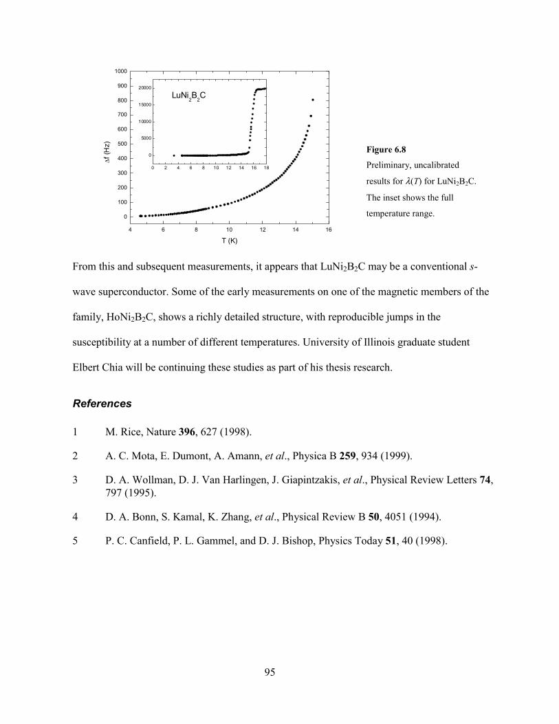
95
4 6 8 10 12 14 16
0
100
200
300
400
500
600
700
800
900
1000
LuNi2B
2C
∆f (
Hz)
T (K)
0 2 4 6 8 10 12 14 16 18
0
5000
10000
15000
20000
Figure 6.8
Preliminary, uncalibrated
results for λ(T) for LuNi2B2C.
The inset shows the full
temperature range.
From this and subsequent measurements, it appears that LuNi2B2C may be a conventional s-
wave superconductor. Some of the early measurements on one of the magnetic members of the
family, HoNi2B2C, shows a richly detailed structure, with reproducible jumps in the
susceptibility at a number of different temperatures. University of Illinois graduate student
Elbert Chia will be continuing these studies as part of his thesis research.
References
1 M. Rice, Nature 396, 627 (1998).
2 A. C. Mota, E. Dumont, A. Amann, et al., Physica B 259, 934 (1999).
3 D. A. Wollman, D. J. Van Harlingen, J. Giapintzakis, et al., Physical Review Letters 74,797 (1995).
4 D. A. Bonn, S. Kamal, K. Zhang, et al., Physical Review B 50, 4051 (1994).
5 P. C. Canfield, P. L. Gammel, and D. J. Bishop, Physics Today 51, 40 (1998).

96
Appendix A Samples
This appendix contains a series of photographs and lists of pertinent data on each of the
samples discussed in this thesis.
A.1 Crystal Batches
The SRO crystals were grown by Y. Maeno, Dept. of Physics, Kyoto University, Kyoto,
Japan. A graph of the ac magnetic susceptibility was provided for a representative sample from
the same batch as each of the samples we were given. This serves as an accurate measure of the
critical temperature, and the sharpness of the transition is indicative of the quality of the
samples. The graphs are reproduced here. The top graph in each figure is the real part of the
complex susceptibility, 'χ , and the lower graph is imaginary part, ''χ . The critical temperature
is determined by the peak in ''χ .
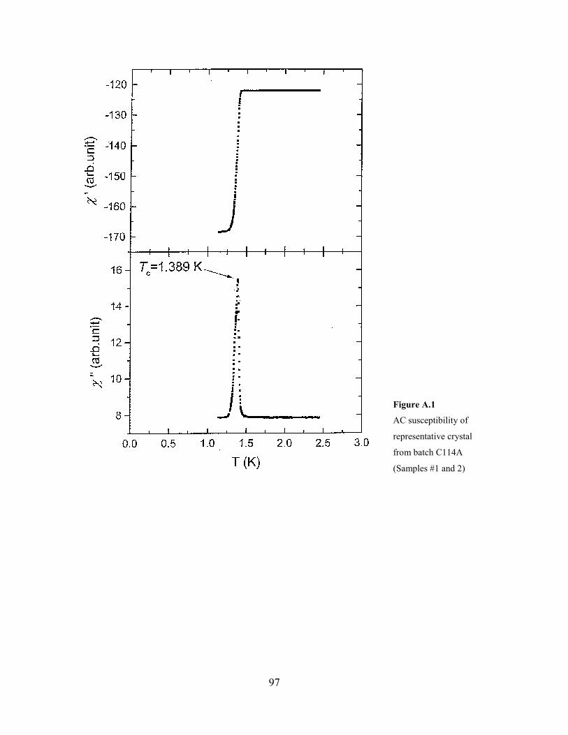
97
Figure A.1
AC susceptibility of
representative crystal
from batch C114A
(Samples #1 and 2)
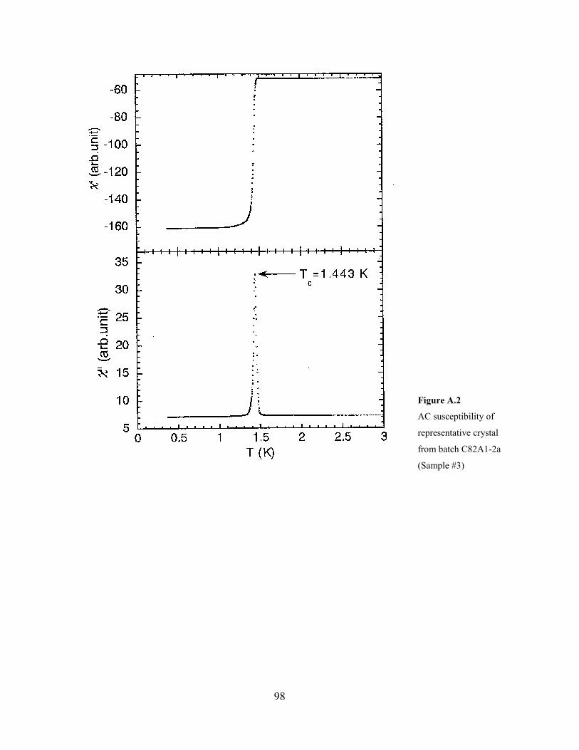
98
Figure A.2
AC susceptibility of
representative crystal
from batch C82A1-2a
(Sample #3)
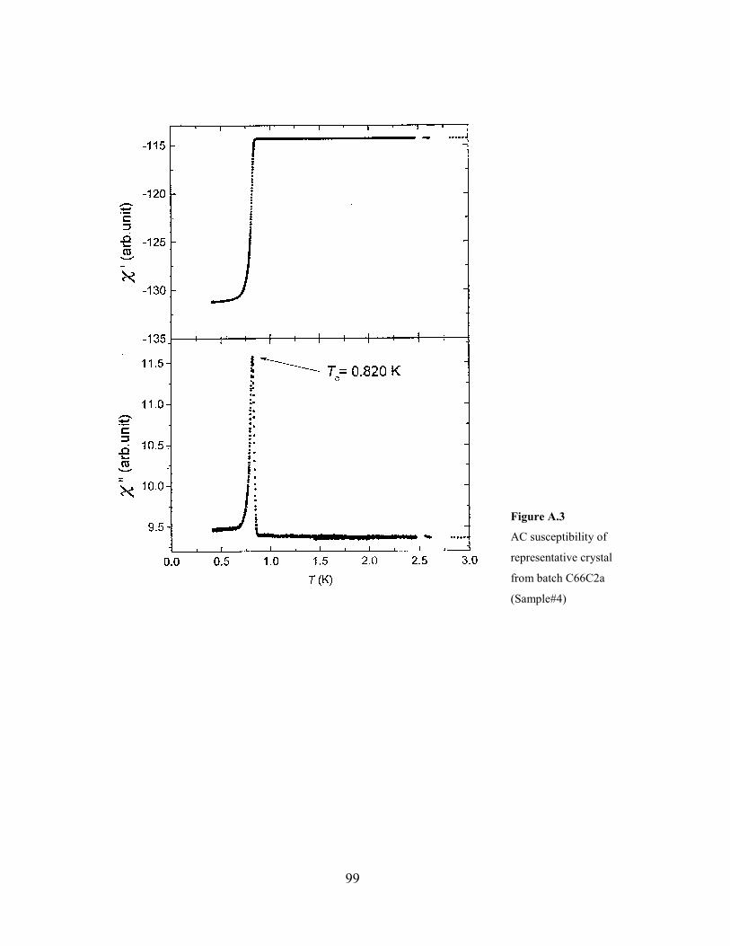
99
Figure A.3
AC susceptibility of
representative crystal
from batch C66C2a
(Sample#4)
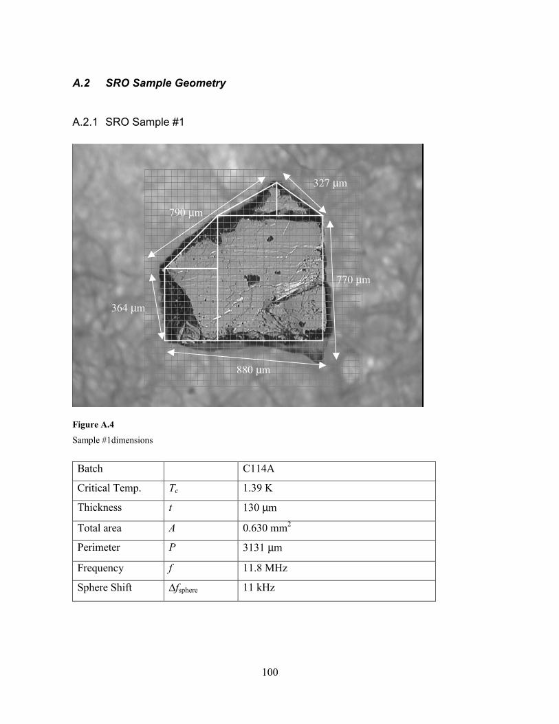
100
A.2 SRO Sample Geometry
A.2.1 SRO Sample #1
Figure A.4
Sample #1dimensions
Batch C114A
Critical Temp. Tc 1.39 K
Thickness t 130 µm
Total area A 0.630 mm2
Perimeter P 3131 µm
Frequency f 11.8 MHz
Sphere Shift ∆fsphere 11 kHz
770 µm
327 µm
790 µm
880 µm
364 µm

101
A.2.2 SRO Sample #2
Figure A.5
Sample #2 dimensions
Batch C114A
Critical Temp. Tc 1.39 K
Thickness t 100 µm
Total area A 0.801 mm2
Perimeter P 3322 µm
Frequency f 17.38 MHz
Sphere Shift ∆fsphere 16 kHz
534 µm
1060 µm
940 µm
1070 µm
252 µm
602 µm
354 µm
473 µm
308 µm
272 µm
527 µm
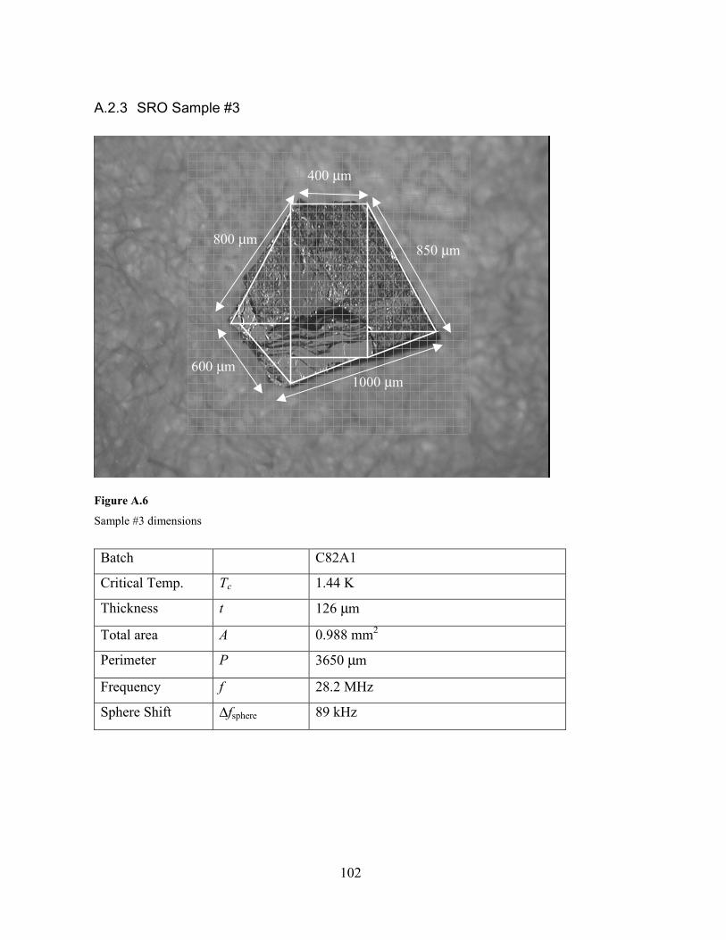
102
A.2.3 SRO Sample #3
Figure A.6
Sample #3 dimensions
Batch C82A1
Critical Temp. Tc 1.44 K
Thickness t 126 µm
Total area A 0.988 mm2
Perimeter P 3650 µm
Frequency f 28.2 MHz
Sphere Shift ∆fsphere 89 kHz
1000 µm600 µm
850 µm800 µm
400 µm
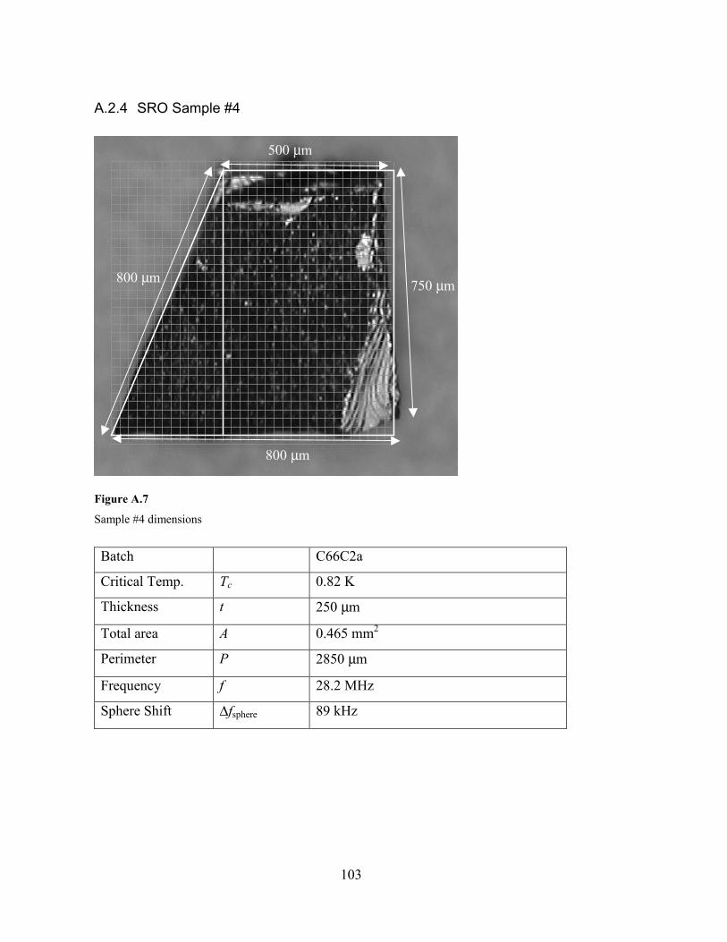
103
A.2.4 SRO Sample #4
Figure A.7
Sample #4 dimensions
Batch C66C2a
Critical Temp. Tc 0.82 K
Thickness t 250 µm
Total area A 0.465 mm2
Perimeter P 2850 µm
Frequency f 28.2 MHz
Sphere Shift ∆fsphere 89 kHz
750 µm
500 µm
800 µm
800 µm
104
Vita
Brian David Yanoff was born on May 30, 1971, in Philadelphia, Pennsylvania. He
attended Swarthmore College where, in addition to majoring in physics with a minor in
computer science, he also met his wife, Liz. During the summers of 1991 and 1992 he worked
with Swarthmore Professor Peter Collings on light scattering experiments to study the phase
transition between the isotropic liquid and the A* liquid crystal phases. Brian was elected a
junior member of Sigma Xi, the scientific research society, in 1993. After graduating with
honors in 1993, Brian’s fascination with phase transitions and the use of computers in
condensed matter research led him to the University of Illinois, where, in the summer of 1994,
he began work in the research group of Prof. Dale Van Harlingen. His initial projects
concerned the behavior of superconductors in mesoscopic systems, but he soon turned to a
study of the symmetry of the unconventional heavy fermion superconductor UPt3, attempting a
rather difficult phase sensitive measurement of the order parameter. In November 1998 he
began a collaboration with postdoc Ismardo Bonalde, to study the temperature dependence of
the magnetic penetration depth in a number of unconventional superconductors at very low
temperatures. Following graduation Brian will begin work at the General Electric Company’s
Corporate Research and Development Center, in Schenectady, NY, to help design and develop
digital x-ray detectors for medical applications.