copyright by brian tinkey 2000 · setup and administrative details. v. ... 4.4 ae response of full...
TRANSCRIPT

Copyright
by
Brian Tinkey
2000

Nondestructive Testing of Prestressed Bridge Girders with
Distributed Damage
by
Brian Victor Tinkey, B.S.C.E
Thesis
Presented to the Faculty of the Graduate School of
The University of Texas at Austin
in Partial Fulfillment
of the Requirements
for the Degree of
Master of Science in Engineering
The University of Texas at Austin
May 2000
Nondestructive Testing of Prestressed Bridge Girders with
Distributed Damage
Approved by Supervising Committee:
Dedication
For my Parents, Doyle and LuAnn Tinkey, who have provided me encouragement
and support not only through graduate school but through every phase of my life.

Acknowledgements
I would like to thank all of the people that helped me with this thesis and
helped me enjoy the time I spent at The University of Texas at Austin.
First of all I would like to thank the Texas Department of Transportation,
especially Brian Merrill, for the funding and the invaluable resource they
provided for Project 1857.
I would like to thank the professors and fellow students who worked on
this project with me. These include Dr. Timothy Fowler, Dr. Richard Klingner,
Dr. Michael Kreger, Anna Boenig, Luz Fúnez, Joe Roche, Yong-Mook Kim, and
Piya Chotickai. I would especially like to thank my immediate supervisor, Dr.
Fowler for his support and guidance throughout this project. He was a great help
both technically and morally. I would also like to thank Anna Boeing (Founder of
MASC) who kept me sane through all of the testing with her great attitude and
good sense of humor.
I appreciate the other people who helped me with testing including Nat
Ativitavas, John Heffington, Brent Wenger, Chuck Barnes, and Yajai Promboon.
This also includes the staff at Ferguson Laboratory who helped with ideas, test
setup and administrative details.
v

The friends that I met here were also invaluable. I would like to
specifically mention Matt Rechtien and his dog Turbo, who were great friends to
me throughout graduate school, but who especially helped me get adjusted to
Austin when I first arrived.
Finally, I would like to mention Yajai Promboon who helped me in every
aspect during my life in Texas, but more importantly, she was a pleasure to be
around. She made my time at UT a memorable one.
May 2000
vi
Nondestructive Testing of Prestressed Bridge Girders with Distributed Damage
Brian Victor Tinkey, MSE
The University of Texas at Austin, 2000
Supervisors: Timothy Fowler
Richard Klingner
Four different nondestructive tests were evaluated for detecting and
quantifying the amount of distributed damage in prestressed concrete bridge
girders. This was in response to a number of bridges throughout Texas exhibiting
premature concrete deterioration due to a combination of delayed ettringite
formation and alkali silica reaction.
Visual inspection, acoustic emission, short pulse radar, and impact echo
are described and possible procedures to apply these methods to concrete with
distributed damage are presented and evaluated.
vii

Table of Contents
List of Tables .......................................................................................................... xi
List of Figures ...................................................................................................... xiii
Chapter 1 – Introduction ....................................... Error! Bookmark not defined. 1.1 Background of Project ............................ Error! Bookmark not defined. 1.2 Background of Project ............................ Error! Bookmark not defined. 1.3 Scope of This Thesis .............................. Error! Bookmark not defined. 1.4 Organization of Thesis ........................... Error! Bookmark not defined. 1.5 Other Researchers on the Project ........... Error! Bookmark not defined.
Chapter 2 – Description of Test Specimens .......... Error! Bookmark not defined. 2.1 Description of Box Girders .................... Error! Bookmark not defined. 2.2 Description of Type C Girders ............... Error! Bookmark not defined.
Chapter 3 – Visual Inspection ............................... Error! Bookmark not defined. 3.1 Introduction to Visual Inspection ........... Error! Bookmark not defined. 3.2 Application of Visual Inspection to ConcreteError! Bookmark not defined. 3.3 Results of Visual Inspection on Box Girder SectionsError! Bookmark not defined. 3.4 Results of Visual Inspection on Type C Girder SectionsError! Bookmark not defined. 3.5 Discussion .............................................. Error! Bookmark not defined. 3.4 Conclusion .............................................. Error! Bookmark not defined.
Chapter 4 - Acoustic Emission .............................. Error! Bookmark not defined. 4.1 Introduction to Acoustic Emission ......... Error! Bookmark not defined. 4.2 Application of Acoustic Emission to Concrete in GeneralError! Bookmark not defined.
4.2.1 Difficulties with Acoustic Emission in ConcreteError! Bookmark not defined. 4.2.2 Kaiser Effect ............................... Error! Bookmark not defined. 4.2.3 Rate Process Analysis ................ Error! Bookmark not defined. 4.2.4 Moment Tensor Analysis ........... Error! Bookmark not defined.
viii

4.3 Acoustic Emission Response of Flexural Cracking in Unreinforced Concrete .............................................. Error! Bookmark not defined. 4.3.1 Test Setup ................................... Error! Bookmark not defined. 4.3.2 Analysis and Results .................. Error! Bookmark not defined. 4.3.3 Discussion .................................. Error! Bookmark not defined.
4.4 AE Response of Full Scale Prestressed Box Girders in FlexureError! Bookmark not define4.4.1 Setup of Flexure-Dominated Box Girder TestsError! Bookmark not defined. 4.4.2 Results of Flexure-Dominated Tests on Box GirdersError! Bookmark not defined.
4.4.2.1 BG1 ................................ Error! Bookmark not defined. 4.4.2.2 BG2 ................................ Error! Bookmark not defined. 4.4.2.3 BG4 ................................ Error! Bookmark not defined.
4.4.3 Discussion of Flexure-Dominated Tests on Box GirdersError! Bookmark not define4.5 AE Response of Full Scale Prestressed Box Girders in ShearError! Bookmark not defined.
4.5.1 Setup of Shear-Dominated Tests on Box GirdersError! Bookmark not defined. 4.5.2 Results of the Shear-Dominated Tests on Box GirdersError! Bookmark not defined.
4.5.2.1 BG1S .............................. Error! Bookmark not defined. 4.5.2.2 BG2S .............................. Error! Bookmark not defined. 4.5.2.3 BG4S .............................. Error! Bookmark not defined.
4.5.3 Discussion of the Shear-Dominated Tests on Box GirdersError! Bookmark not defin4.6 Shear tests of Full Scale Type C Girders Error! Bookmark not defined.
4.6.1 Test Setup for Shear-Dominated Test on Type C GirdersError! Bookmark not defin4.6.2 Results of Shear-Dominated Test on Type C GirdersError! Bookmark not defined.
4.6.2.1 G2WS ............................. Error! Bookmark not defined. 4.6.2.2 G2ES .............................. Error! Bookmark not defined. 4.6.2.3 G1WS ............................. Error! Bookmark not defined. 4.6.2.4 G1ES .............................. Error! Bookmark not defined.
4.6.3 Discussion of Shear-Dominated Tests on Type C GirdersError! Bookmark not defin4.7 Discussion of Acoustic Emission Testing and Evaluation CriteriaError! Bookmark not defin4.8 Conclusions from Acoustic Emission TestingError! Bookmark not defined.
ix
Chapter 5 – Short-Pulse Radar .............................. Error! Bookmark not defined. 5.1 Introduction to Short Pulse Radar .......... Error! Bookmark not defined. 5.2 Test Setup ............................................... Error! Bookmark not defined. 5.3 Results of the Short Pulse Radar Survey Error! Bookmark not defined. 5.4 Discussion .............................................. Error! Bookmark not defined. 5.5 Conclusion .............................................. Error! Bookmark not defined.
Chapter 6 – Impact-Echo ....................................... Error! Bookmark not defined. 6.1 Introduction to Impact-Echo .................. Error! Bookmark not defined. 6.2 Application of Impact-Echo to Concrete with Distributed DamageError! Bookmark not def6.3 Testing Program ..................................... Error! Bookmark not defined. 6.4 Results .................................................... Error! Bookmark not defined. 6.5 Discussion of Impact Echo Results ........ Error! Bookmark not defined. 6.6 Conclusions Regarding Impact-Echo ..... Error! Bookmark not defined.
Chapter 7 – Summary and Conclusions ................ Error! Bookmark not defined. 7.1 Visual Inspection .................................... Error! Bookmark not defined. 7.2 Acoustic Emission .................................. Error! Bookmark not defined. 7.3 Short-Pulse Radar ................................... Error! Bookmark not defined. 7.4 Impact-Echo ........................................... Error! Bookmark not defined. 7.5 Conclusions and Recommendations ....... Error! Bookmark not defined.
Appendix A – Impact-Echo Data .......................... Error! Bookmark not defined.
References ............................................................. Error! Bookmark not defined.
Vita ...................................................................... Error! Bookmark not defined.
x

List of Tables
Table 2.1 - Description of Tests on Box Girder SpecimensError! Bookmark not defined.
Table 3.1 - Crack Ratios for Type C Girders ........ Error! Bookmark not defined.
Table 4.1 – Felicity Ratios for the Second and Third Loading (Yuyama and
Murakami 1996) ............................... Error! Bookmark not defined.
Table 4.2 - Properties of Mixtures Used on Plain Concrete SpecimensError! Bookmark not defined.
Table 4.3 - Test Parameters for Unreinforced Concrete SpecimensError! Bookmark not defined.
Table 4.4 - K values used in Historic Index (Fowler et al. 1989)Error! Bookmark not defined.
Table 4.5 - Test Parameters for Full-Scale Tests .. Error! Bookmark not defined.
Table 4.6 - Felicity Ratios for BG1 ....................... Error! Bookmark not defined.
Table 4.7 - Values for K used in Calculating Historic IndexError! Bookmark not defined.
Table 4.8 Felicity Ratios for BG2 ......................... Error! Bookmark not defined.
Table 4.9 - Felicity Ratios for BG4 ....................... Error! Bookmark not defined.
Table 4.10 - Felicity Ratios for BG1S ................... Error! Bookmark not defined.
Table 4.11 - Felictiy Ratios for BG2S .................. Error! Bookmark not defined.
Table 4.12 - Definition of a “Telltale” Hit for the Swansong II FilterError! Bookmark not defined.
Table 4.13 - Felicity Ratios for BG4S ................... Error! Bookmark not defined.
Table 4.14 – Crack Ratios for Type C Girders ..... Error! Bookmark not defined.
Table 4.15 - Dimensions of Test Setup ................. Error! Bookmark not defined.
Table 4.16 - Dimension for Sensor Placement on Type C GirdersError! Bookmark not defined.
Table 4.17 - Felicity Ratios for G2ES ................... Error! Bookmark not defined.
Table 4.18 - Felicity Ratios for G1WS ................. Error! Bookmark not defined.
Table 4.19 - Felicity Ratios for G1ES ................... Error! Bookmark not defined.
xi

Table 4.20 – Suggested Evaluation Criteria for Distributed DamageError! Bookmark not defined.
Table 5.1 - Typical Dielectric Constants for Various MaterialsError! Bookmark not defined.
Table 6.1 - Results of Finite Element Models For 130 mm Thick Concrete
Plate (Kesner 1997) .......................... Error! Bookmark not defined.
Table 6.2 - Results of Impact-Echo Tests on BG1 Error! Bookmark not defined.
Table 6.3 - Results of Impact-Echo Tests on BG3 Error! Bookmark not defined.
Table 6.4 - Decay Constants for a Test Performed on BG3Error! Bookmark not defined.
xii

List of Figures
Figure 2.1 – Cross-section Dimensions of Box Girder SpecimensError! Bookmark not defined.
Figure 2.2 - Plan View of Box Girder ................... Error! Bookmark not defined.
Figure 2.3 - Overall View of Box Girder .............. Error! Bookmark not defined.
Figure 2.4 - Typical End Conditions of Girders with Intermediate DamageError! Bookmark not defin
Figure 2.5 – Cross-section of the Type C SpecimensError! Bookmark not defined.
Figure 2.6 - View of Type C Girder with Slab Prior to TestingError! Bookmark not defined.
Figure 3.1 – End View of A-Side of BG1 ............. Error! Bookmark not defined.
Figure 3.2 - Side of BG1 at A-End ........................ Error! Bookmark not defined.
Figure 3.3 – End View of B-End of BG1 .............. Error! Bookmark not defined.
Figure 3.4 – Side View of B-Side of BG1 ............ Error! Bookmark not defined.
Figure 3.5 - Spalled Concrete on Specimen BG2 Error! Bookmark not defined.
Figure 3.6 - End Damage on Specimen BG2 ........ Error! Bookmark not defined.
Figure 3.7 – End View of A-End of BG3 ............. Error! Bookmark not defined.
Figure 3.8 – Side View on B-End of BG3 ............ Error! Bookmark not defined.
Figure 3.9 - Damage at Interior Blockout on BG3 Error! Bookmark not defined.
Figure 3.10 – Side View of A-End of BG4 ........... Error! Bookmark not defined.
Figure 3.11 - Typical Damage Along the Length of BG4Error! Bookmark not defined.
Figure 3.12 - Northwest end of BG4 ..................... Error! Bookmark not defined.
Figure 3.13 West End of Girder 1 ......................... Error! Bookmark not defined.
Figure 3.14 - East End of Girder 1 ........................ Error! Bookmark not defined.
Figure 4.1 - Sample Acoustic Emission Waveform Showing Evaluation
Parameters ........................................ Error! Bookmark not defined.
xiii
Figure 4.2 – Example of Rectified Acoustic Emission Waveform Illustrating
MARSE ............................................ Error! Bookmark not defined.
Figure 4.3 – Example of Attenuation in Concrete (Uomoto 1987)Error! Bookmark not defined.
Figure 4.4 – Typical Graphs Showing Attenuation of Acoustic Emission in
Concrete (Uomoto 1987) .................. Error! Bookmark not defined.
Figure 4.5 - Moment Tensor Results on Prestressed Girder (Yepez 1997)Error! Bookmark not define
Figure 4.6- Experimental Setup Used for Plain Concrete TestsError! Bookmark not defined.
Figure 4.7 - Dimensions of plain concrete specimensError! Bookmark not defined.
Figure 4.8 - AE Response of a Typical Notched SpecimenError! Bookmark not defined.
Figure 4.9 - Historic Index for a Typical Prenotched SpecimenError! Bookmark not defined.
Figure 4.10 – Typical AE Response of Notch Free SpecimenError! Bookmark not defined.
Figure 4.11 - Historic Index for a Typical Notch free SpecimenError! Bookmark not defined.
Figure 4.12 - Detail of Spreader Beams used in Flexure TestsError! Bookmark not defined.
Figure 4.13 - BG1 Prior to Testing ....................... Error! Bookmark not defined.
Figure 4.14 - Loading Schedule for BG1 .............. Error! Bookmark not defined.
Figure 4.15 - Attenuation Curve for R6I Sensor ... Error! Bookmark not defined.
Figure 4.16 – Plan View of Sensor Locations on Box Girder SpecimensError! Bookmark not defined
Figure 4.17 - Load vs. Cumulative MARSE before Cracking for BG1Error! Bookmark not defined.
Figure 4.18 – Time Based Graphs for BG1 .......... Error! Bookmark not defined.
Figure 4.19 - Cumulative MARSE vs, Load for BG2Error! Bookmark not defined.
Figure 4.20 - Time Based Graphs for BG2 ........... Error! Bookmark not defined.
Figure 4.21 - Cumulative MARSE vs. Load for BG4Error! Bookmark not defined.
Figure 4.22 - Time Based Graphs for BG4 ........... Error! Bookmark not defined.
xiv
Figure 4.23 - Felicity Effect for Flexure SpecimensError! Bookmark not defined.
Figure 4.24 - Test Setup for BG1S and BG4S ...... Error! Bookmark not defined.
Figure 4.25 – Test Setup of BG2S ........................ Error! Bookmark not defined.
Figure 4.26 - Sensor Locations on all Shear SpecimensError! Bookmark not defined.
Figure 4.27 - Loading Schedule for BG1S ............ Error! Bookmark not defined.
Figure 4.28 - Load Vs Cumulative MARSE for BG1SError! Bookmark not defined.
Figure 4.29 - Time Based Graphs for BG1S ......... Error! Bookmark not defined.
Figure 4.30 - Cumulative MARSE vs. Load for BG2SError! Bookmark not defined.
Figure 4.31 - Time Based Graphs for BG2S ......... Error! Bookmark not defined.
Figure 4.32 - Bearing Failure of BG4S ................. Error! Bookmark not defined.
Figure 4.33 - Compression Strut Failure of BG1S Error! Bookmark not defined.
Figure 4.34 - Amplitude vs Log Duration for BG4SError! Bookmark not defined.
Figure 4.35 - Amplitude vs Log Duration for BG4S after Swansong II FilterError! Bookmark not def
Figure 4.36 - Cumulative MARSE vs. Load for BG4SError! Bookmark not defined.
Figure 4.36 - Time Based Graphs for BG4S ......... Error! Bookmark not defined.
Figure 4.38 - Felicity Ratios for the Shear-Dominated Test on Box GirdersError! Bookmark not defin
Figure 4.39 - Test Setup for Type C Girders ......... Error! Bookmark not defined.
Figure 4.40 - Sensor Placement for Type C SpecimensError! Bookmark not defined.
Figure 4.41 - Loading Schedule for G2WS ........... Error! Bookmark not defined.
Figure 4.42 - Cumulative MARSE vs. Load for G2WSError! Bookmark not defined.
Figure 4.43 - Time Based Graphs for G2WS ........ Error! Bookmark not defined.
Figure 4.44 - Loading Schedule for G2ES ............ Error! Bookmark not defined.
Figure 4.45 - Cumulative MARSE vs. Load for G2ESError! Bookmark not defined.
xv

Figure 4.46 - Time Based Graphs for G2ES ......... Error! Bookmark not defined.
Figure 4.47 - Loading Schedule for G1WS ........... Error! Bookmark not defined.
Figure 4.48 - G1WS under test at 270 kips ........... Error! Bookmark not defined.
Figure 4.49 - Cumulative MARSE vs. Load for G1WSError! Bookmark not defined.
Figure 4.50 - Time Based Graphs for G1WS ........ Error! Bookmark not defined.
Figure 4.51 - Loading Schedule for G1ES ............ Error! Bookmark not defined.
Figure 4.52 - Cumulative MARSE vs. Load for G1ESError! Bookmark not defined.
Figure 4.53 - Time Based Graphs for G1ES ......... Error! Bookmark not defined.
Figure 4.54 - Felicity Ratios for the Shear Tests on Type C GirdersError! Bookmark not defined.
Figure 4.55 – Proposed Evaluation Criteria and Test ResultsError! Bookmark not defined.
Figure 5.1 - Propagation of Electromagnetic Waves through Media of
Different Dielectric Constants .......... Error! Bookmark not defined.
Figure 5.2 - Typical A-Scan and B-Scan From Sample BG2Error! Bookmark not defined.
Figure 5.3 - Short Pulse Radar Equipment ............ Error! Bookmark not defined.
Figure 5.4 - Dielectric Values on West Side of BG2Error! Bookmark not defined.
Figure 5.5 -Dielectric Values on East Side of BG2 at the A-EndError! Bookmark not defined.
Figure 5.6 - Dielectric Values on the East Side of BG4Error! Bookmark not defined.
Figure 6.1 - Schematic Representation of Impact-Echo TestError! Bookmark not defined.
Figure 6.2 – Typical Displacement History for an Impact-Echo TestError! Bookmark not defined.
Figure 6.3 - Frequency Spectrum of a Typical Impact-Echo TestError! Bookmark not defined.
Figure 6.4 - Calculation of the Decay Coefficient Error! Bookmark not defined.
Figure 6.5 - Photo of the Test Point 8 feet from Centerline on BG1Error! Bookmark not defined.
Figure 6.6 - Photo of the Test Point 7 feet from the South End of BG1Error! Bookmark not defined.
xvi
xvii
Figure 6.7 - Photo of the Test Point 3 feet from the North End of BG3Error! Bookmark not defined.
Figure 6.8 - Photo of the Test Point 22 feet from the South End of BG3Error! Bookmark not defined
Figure 6.9 - Photo of DOCtor Impact-Echo EquipmentError! Bookmark not defined.
Figure 6.10 - (a) Unfilterd Displacement History in Time Domain (b)
Unfiltered Frequency Spectrum ....... Error! Bookmark not defined.
Figure 6.11 - (a) Filterd Displacement History in Time Domain (b) Filtered
Frequency Spectrum ......................... Error! Bookmark not defined.
Figure 6.12 - Results of Filtering the Displacement HistoryError! Bookmark not defined.
Figure A.1 - 1st Impact Echo test on BG1-8 Feet from CenterError! Bookmark not defined.
Figure A.2 - 2st Impact Echo test on BG1-8 Feet from CenterError! Bookmark not defined.
Figure A.3 - 1st Impact Echo test on BG1-7 Feet from South EndError! Bookmark not defined.
Figure A.4 - 2nd Impact Echo test on BG1-7 Feet from South EndError! Bookmark not defined.
Figure A.5 - 1st Impact Echo test on BG1-5 Feet from South EndError! Bookmark not defined.
Figure A.6 - 2nd Impact Echo test on BG1-5 Feet from South EndError! Bookmark not defined.
Figure A.7 - 1st Impact Echo test on BG3-3 Feet from North EndError! Bookmark not defined.
Figure A.8 - 2nd Impact Echo test on BG3-3 Feet from North EndError! Bookmark not defined.
Figure A.9 - 1st Impact Echo test on BG3-22 Feet from South EndError! Bookmark not defined.
Figure A.10 - 2nd Impact Echo test on BG3 - 22 Feet from South EndError! Bookmark not defined.

xviii

Chapter 1 – Introduction
Throughout Texas, many bridges are currently experiencing premature
concrete deterioration due to a combination of delayed ettringite formation and
alkali-silica reaction. Texas Department of Transportation (TxDOT) has
sponsored Research Project 1857 to help decide whether to repair or replace these
bridges. The goal of this research is to determine how the amount of deterioration
can be quantified, how quickly it is progressing, and how it affects the strength of
those bridges.
1.1 BACKGROUND OF PROJECT
Within the last 10 years TxDOT became aware of deterioration in several
prestressed girders throughout the state. The damage is due to a combination of
delayed ettringite formation and alkali-silica reaction (Lawrence 1997). During a
statewide bridge inspection program, other bridges throughout Texas that were
built around the same time were determined to have the same problem. A few
examples of these bridges include:
Woodlands Parkway and IH45 in Houston;
US90 and San Jacinto River;
FM 1979 at Lake Ivie in Concho County;
US 54 and Sheridan Road in El Paso;
Project 1857 was implemented to determine how the deterioration affects
the long-term serviceability and strength of structures in service.
1
1.2 BACKGROUND OF PROJECT
The original scope of the project as outlined in the project proposal
(Klingner and Fowler 1998) consists of seven tasks:
Task 1 – Conduct field investigations to confirm and monitor existing
premature concrete deterioration, the rate of increase of such
deterioration, and the effect of different remedial measures on
that rate of increase.
Task 2 – Conduct laboratory investigations of local effects of premature
concrete deterioration.
Task 3 – Develop nondestructive evaluation techniques for determining
degree and type of concrete deterioration.
Task 4 – Develop petrographic techniques for assessing severity of
deterioration from samples taken from field investigations.
Task 5 – Develop engineering models for evaluating the global reduction
in capacity of a structural element due to local premature
concrete deterioration.
Task 6 – Develop an overall methodology for predicting the probable loss
in capacity over time of a deteriorated structural element,
based on external evidence, nondestructive evaluation, and
engineering models.
2
Task 7 – Develop recommended actions by TxDOT for handling any
given case of premature concrete deterioration.
1.3 SCOPE OF THIS THESIS
The overall scope of this thesis can be directly related to Task 3 as
outlined in Section 1.2, and consists of the following 3 objectives:
• Develop nondestructive tests to detect concrete deterioration.
• Once deterioration is detected, use nondestructive tests to determine
the degree and location of damage.
• In the presence of distributed damage, suggest methods to further
monitor the deterioration.
To accomplish these tasks, four possible nondestructive test methods were
identified and preliminary tests were performed to evaluate their effectiveness in
quantifying distributed damage in concrete. These test methods were visual
inspection, short-pulse radar, impact-echo and acoustic emission.
Possible methods that are not covered here are liquid-penetrant,
radiography, and ultrasonics. Liquid penetrant was not investigated deeply
because all the deteriorated specimens have extensive map cracking (small,
shallow cracks distributed in a spider-web pattern) making it difficult to
distinguish between different degrees of damage. Radiography was not
researched due to safety issues and the large radiation source that would be
required for concrete. Ultrasonics was initially ruled out due to the high
attenuation of ultrasound in concrete, but will be investigated later by Piya
Chotickai, another researcher on the project. His research will consist of
3

evaluating additional test methods and developing test procedures for bridges in
service.
1.4 ORGANIZATION OF THESIS
Since each nondestructive test method is independent, this thesis is
organized with each test method in a separate chapter. In addition, a separate
chapter is dedicated to describing test specimens, which are similar for every
method. Therefore, Chapter 2 describes the specimens used for all of the test
methods; Chapter 3 discusses visual inspection; Chapter 4 discusses acoustic
emission; Chapter 5 discusses short-pulse radar; Chapter 6 discusses impact-echo;
and Chapter 7 summarizes findings and presents principal conclusions and
recommendations.
1.5 OTHER RESEARCHERS ON THE PROJECT
The supervising professors on the project include Dr. Timothy J. Fowler,
Dr. Richard E. Klingner, and Dr. Michael E. Kreger. Fellow student researchers
include:
Anna Boenig, who is evaluating how the distributed damage affects
the strength of concrete box girders both locally and globally. In
addition, she is concerned with the observation of bridges in service to
determine the rate at which the damage is progressing.
Yong-mook Kim, who is working on a similar project with Type C
girders that were removed from a bridge in Beaumont. He is working
on the immediate implications of the damage, and whether or not the
bridges need to be taken out of service.
4

5
Luz Funez, who completed a preliminary report on the field
observations, including observation methods and general trends seen
in existing bridges.
Joe Roche, who will complete a full-scale fatigue test on a box girder
section, as well as small-scale pullout tests to determine how
distributed damage affects the development of the strand.
Piya Chotickai, who will continue with the research presented in this
thesis and apply it to field specimens displaying distributed damage.

6

Chapter 2 – Description of Test Specimens
Nondestructive testing was performed on two different prestressed girder
sections, a box section and a Type C section. The specimens were experiencing
varying degrees of damage from a combination of delayed ettringite formation
(DEF) and alkali-silica reaction (ASR).
The specimens described in this chapter were tested at the Ferguson
Structural Engineering Laboratory at the J.J. Pickle Research Campus of The
University of Texas at Austin.
2.1 DESCRIPTION OF BOX GIRDERS
Four prestressed concrete box girders were shipped to Ferguson Structural
Engineering Laboratory in the spring of 1999 from the Heldenfels Brothers, Inc.
plant in San Marcos, Texas. These girders where chosen from approximately 55
similar girders that displayed distributed damage early enough that they were
never put into service. Since they were cast in September of 1991, the girders had
been stored outside, exposed to weather in the casting yard.
Dimensions of the cross section are shown in Figure 2.1. The overall
dimensions of the girders are 4 feet wide and 27 inches tall. The wall thickness is
5 inches with a styrofoam filler that was used as formwork for the void. The void
was included to conserve concrete and decrease weight. In addition, 30 - ½ inch,
270 ksi, low-relaxation prestressing strands are spaced at 2-inch intervals as
7

shown in the figure. Concrete design strength was 6000 psi; the actual strength
measured from cores taken after testing, however, was closer to 10,000 psi.
5.5 in
16 in
38 in 5 in5 in
Styrofoam Filler
5.5 in
Figure 2.1 – Cross-section Dimensions of Box Girder Specimens
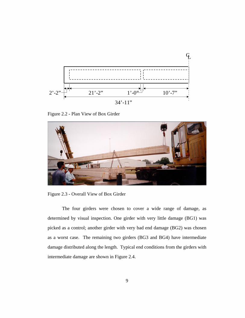
The lengths of the girders were 69 feet and 11 inches, with 2 foot 2 inch
solid end blocks and two intermittent 1 foot solid blockouts. A plan view of half
of one girder is shown in Figure 2.2. An overall view of one of the box girders
being moved into the laboratory is shown in Figure 2.3.
8
21’-2” 10’-7”2’-2”
34’-11”
1’-0”
CL
Figure 2.2 - Plan View of Box Girder
Figure 2.3 - Overall View of Box Girder
The four girders were chosen to cover a wide range of damage, as
determined by visual inspection. One girder with very little damage (BG1) was
picked as a control; another girder with very bad end damage (BG2) was chosen
as a worst case. The remaining two girders (BG3 and BG4) have intermediate
damage distributed along the length. Typical end conditions from the girders with
intermediate damage are shown in Figure 2.4.
9

Figure 2.4 - Typical End Conditions of Girders with Intermediate Damage
The control specimen, BG1, and the most deteriorated specimen, BG2,
were tested in flexure; one of the remaining halves from each girder was then
tested in shear. Specimens were taken from the other half for concrete strength
and pullout tests after the flexure test was completed. BG3 and BG4 were left
outside to monitor crack growth and for future testing. BG4 was continually
wetted and dried with a soaker hose in an attempt to accelerate damage, and was
then tested in flexure and shear. Table 2.1 summarizes the specimens and the
tests performed on each.
10
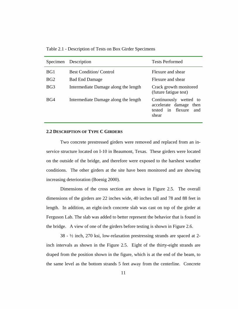
Table 2.1 - Description of Tests on Box Girder Specimens
Specimen Description Tests Performed
BG1 Best Condition/ Control Flexure and shear BG2 Bad End Damage Flexure and shear BG3 Intermediate Damage along the length Crack growth monitored
(future fatigue test) BG4 Intermediate Damage along the length Continuously wetted to
accelerate damage then tested in flexure and shear
2.2 DESCRIPTION OF TYPE C GIRDERS
Two concrete prestressed girders were removed and replaced from an in-
service structure located on I-10 in Beaumont, Texas. These girders were located
on the outside of the bridge, and therefore were exposed to the harshest weather
conditions. The other girders at the site have been monitored and are showing
increasing deterioration (Boenig 2000).
Dimensions of the cross section are shown in Figure 2.5. The overall
dimensions of the girders are 22 inches wide, 40 inches tall and 78 and 88 feet in
length. In addition, an eight-inch concrete slab was cast on top of the girder at
Ferguson Lab. The slab was added to better represent the behavior that is found in
the bridge. A view of one of the girders before testing is shown in Figure 2.6.
38 - ½ inch, 270 ksi, low-relaxation prestressing strands are spaced at 2-
inch intervals as shown in the Figure 2.5. Eight of the thirty-eight strands are
draped from the position shown in the figure, which is at the end of the beam, to
the same level as the bottom strands 5 feet away from the centerline. Concrete
11
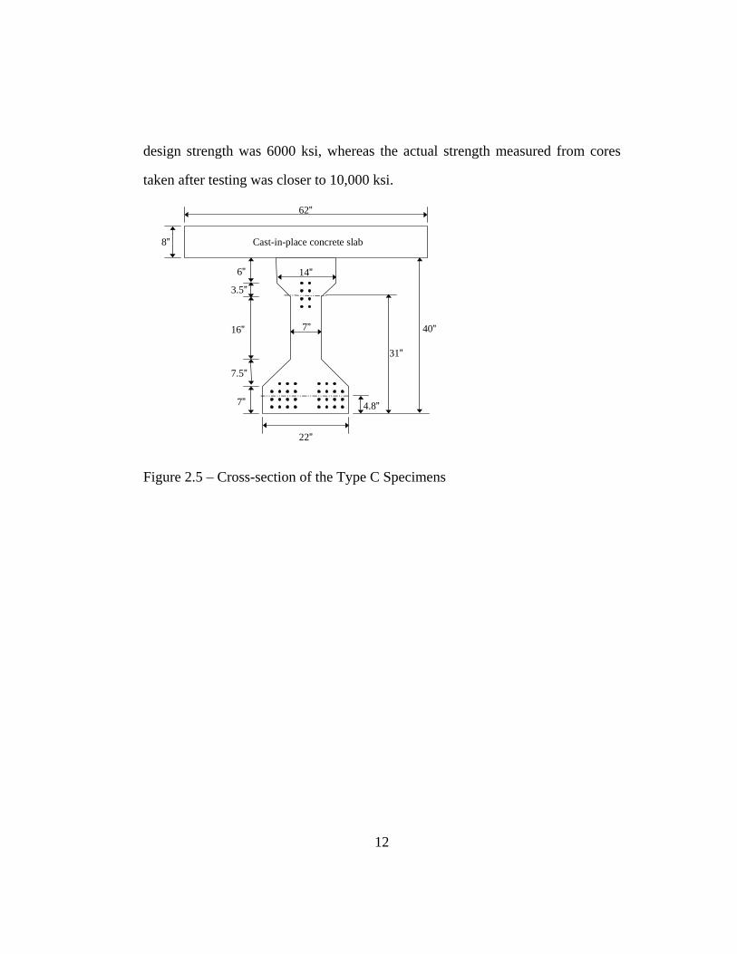
design strength was 6000 ksi, whereas the actual strength measured from cores
taken after testing was closer to 10,000 ksi.
62”
6”
8”
3.5”
31”
4.8”
16”
7.5”
7”
22”
40”
Cast-in-place concrete slab
7”
14”
Figure 2.5 – Cross-section of the Type C Specimens
12
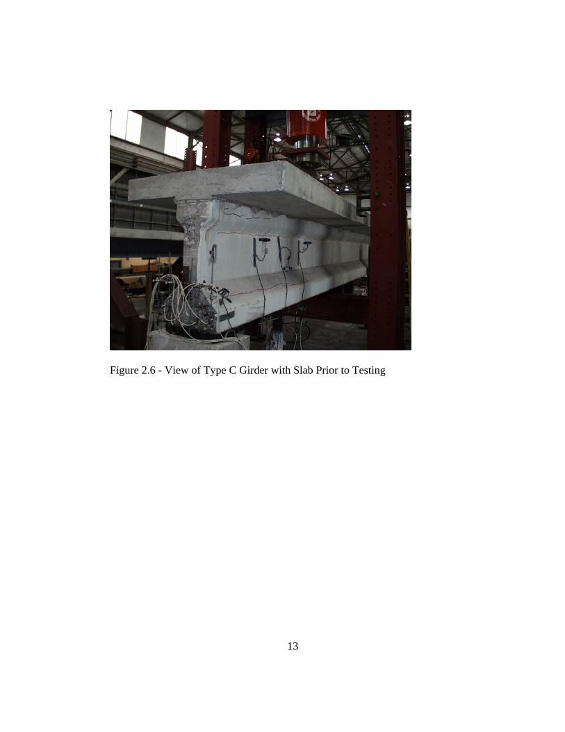
Figure 2.6 - View of Type C Girder with Slab Prior to Testing
13

Chapter 3 – Visual Inspection
As a basis for comparison, a visual inspection was carried out on all of the
full-scale test specimens. Visual inspections are quick, convenient, inexpensive
and are a necessary first step. Unfortunately, they can be used to inspect only the
surface, are inspector-dependent, and do not provide quantitative information.
Even with these drawbacks, visual inspection is one of the most common
nondestructive test methods.
3.1 INTRODUCTION TO VISUAL INSPECTION
Visual inspection is a surface inspection, with or without optical aids.
Although this method is often overlooked as a nondestructive test, it can give a
good indication of larger defects.
Visual inspection can use a variety of measuring devices including tape
measures, calipers, crack comparators (a device with lines of specific widths to
compare to crack widths), or feeler gages (metal shims of specific thickness).
These devices can give good estimates of the length and width of cracks and other
surface defects, as well as their position in the specimen.
In addition to measuring devices, optical aids can facilitate visual
inspections. One of the more common aids are small, hand-held lenses that can
improve the accuracy of crack comparators. Other aids include fiber-optic
borescopes that can inspect areas with limited access, and miniature cameras that
can be positioned remotely when human access is not possible (Halmshaw 1991).
14
3.2 APPLICATION OF VISUAL INSPECTION TO CONCRETE
In concrete specimens, visual inspection normally consists of the
documentation of visual cracks and spalled concrete. Areas of concern are
inspected and sketched to scale. Crack widths are measured so that changes over
time can be monitored. Stains, efflorescence, or other surface indications are also
noted.
From these data it may be possible to determine how the load is affecting
the specimen. For example, orientation of cracks can indicate whether the
specimen is cracking under shear, flexure or another influence such as alkali-silica
reaction. Also, monitoring crack growth over time can indicate how quickly
deterioration is increasing.
3.3 RESULTS OF VISUAL INSPECTION ON BOX GIRDER SECTIONS
As mentioned in Chapter 2, four prestressed box girder sections were
delivered to Ferguson Laboratory for testing. Before testing, the condition of the
girders was inspected visually by researchers Luz Fúnez, Anna Boenig, and Brian
Tinkey. The tools used in the inspection consisted of a tape measure and a visual
crack-width gage without magnification. The results are presented in this section.
The least deteriorated specimen was BG1; it serves as the control against
which the other girders may be compared. Even this specimen was showing some
signs of deterioration. Most of the damage was concentrated in the 26 inch long
end block, with crack widths ranging from 0.002 inches to 0.06 inches. In
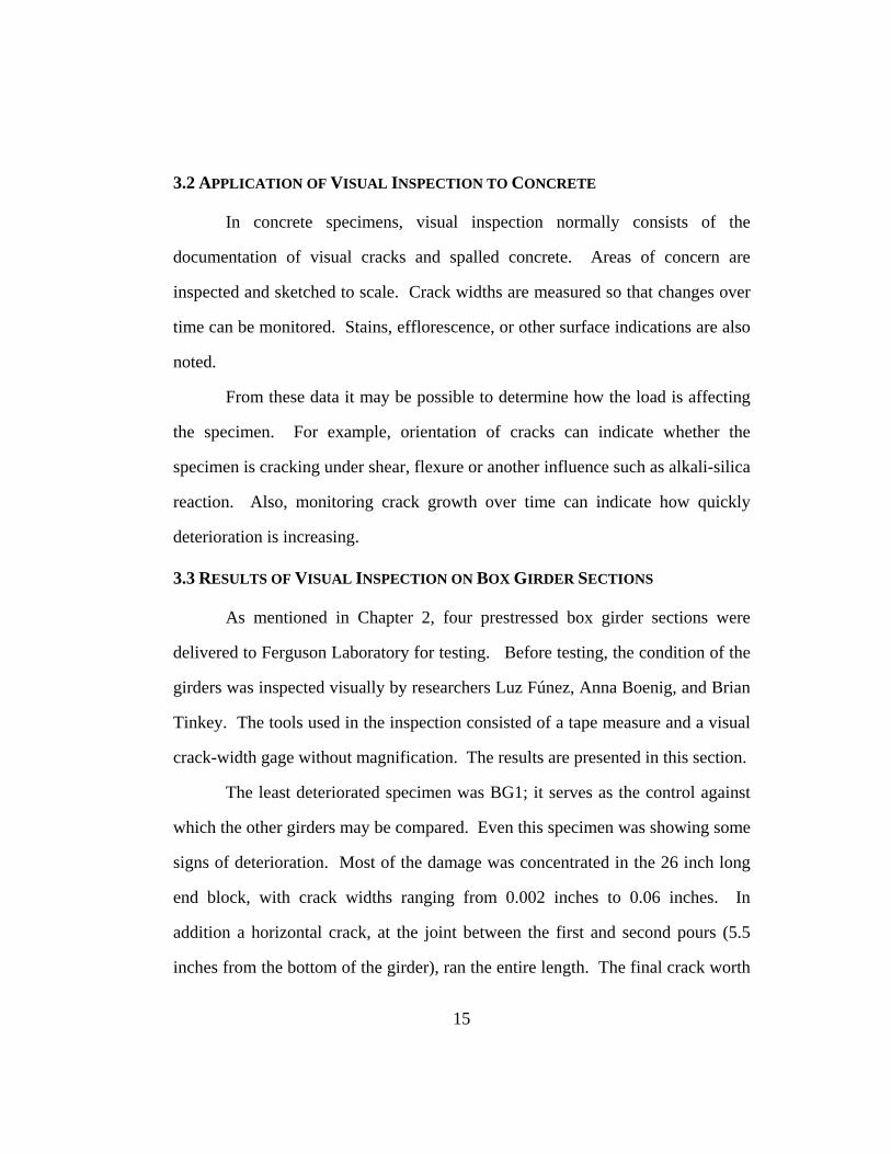
addition a horizontal crack, at the joint between the first and second pours (5.5
inches from the bottom of the girder), ran the entire length. The final crack worth
15

noting was a horizontal crack 17 inches from the bottom that ran intermittently
along the length. Girder BG1 is shown in Figure 3.1 to Figure 3.4.
Light Cracking
Figure 3.1 – End View of A-Side of BG1
16
Horizontal Crack
Figure 3.2 - Side of BG1 at A-End
Light Cracking
Figure 3.3 – End View of B-End of BG1
17

Figure 3.4 – Side View of B-Side of BG1
The specimen with the worst end damage was BG2. The ends of this
specimen had cracks 10 to 20 inches long and up to 3/8 to 1/2 inch wide. In
addition, at the ends some of the corners had spalled off, exposing corroded
reinforcement. The horizontal cracks along the length 5.5 inches from the bottom
and 17 inches from the bottom that were seen in BG1 were also seen in BG2 with
a width of approximately 0.013 inches. Girder BG2 is shown in Figure 3.5 and
Figure 3.6.
Horizontal Cracks
18

Figure 3.5 - Spalled Concrete on Specimen BG2
Figure 3.6 - End Damage on Specimen BG2
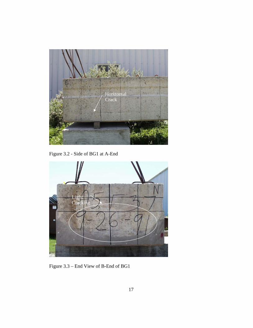
The third girder, BG3, was chosen because its damage, while not as severe
as that of BG2, was more distributed along the length, and was also quite severe
at the ends and near the interior blockouts. A crack along the pour joint had a
19

maximum width of 0.01 inches. Figures 3.7 though 3.9 document the condition
of BG3.
Figure 3.7 – End View of A-End of BG3
20
Spalled Concrete
Heavy Cracking
Figure 3.8 – Side View on B-End of BG3
Multiple Horizontal Cracks
Figure 3.9 - Damage at Interior Blockout on BG3
21

The final specimen, BG4, was continually wetted and dried to accelerate
deterioration. Its most significant damage was in the solid ends and at the solid
blockouts. The crack patterns at these locations most closely resembled the ends
of BG2. Efflorescence was seen at these locations. At one of the interior
blockouts, water could be found leaking from the girder, indicating a full-
thickness crack. Other locations along the beam had intermittent cracking with
heavy staining from corroding transverse reinforcement. Figures 3.10 though
3.12 demonstrate the condition of BG4.
Figure 3.10 – Side View of A-End of BG4
Efflorescence
22

Horizontal Cracks
Figure 3.11 - Typical Damage Along the Length of BG4
Figure 3.12 - Northwest end of BG4
23

During the shear test of BG4, water was observed leaking out of the
girder. This indicates that the bottom face of the girder had no through-thickness
cracks.
3.4 RESULTS OF VISUAL INSPECTION ON TYPE C GIRDER SECTIONS
Because the two Type C girder specimens had been removed from a
bridge in service, one face of each girder was painted, making visual inspection
there difficult.
The same general cracking trends were noticed in these girders as in the
box girders. The ends showed more deterioration, and cracks away from the end
sections were orientated horizontally.
Each end of the girders was visually inspected by researcher Yong-Mook
Kim and rated for comparison purposes. The total area of the cracks 4 feet from
the end was calculated and then divided by the total surface area to develop a
surface crack ratio. Smaller the crack ratio, the better the condition. This ratio for
each end just before testing is shown in Table 3.1.
Table 3.1 - Crack Ratios for Type C Girders
Specimen Crack Ratio, %
Girder 1 - East End (G1ES) 1.64
Girder 1 – West End (G1WS) 1.57
Girder 2 – East End (G2ES) 0.71
Girder 2 - West end (G2WS) 1.76
24
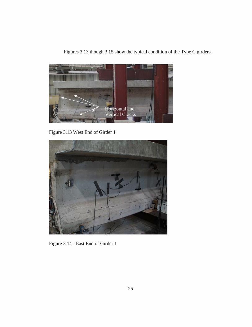
Figures 3.13 though 3.15 show the typical condition of the Type C girders.
Horizontal and Vertical Cracks
Figure 3.13 West End of Girder 1
Figure 3.14 - East End of Girder 1
25

Figure 3.15 – East End of Girder 2
3.5 DISCUSSION
Results of visual inspection are difficult to quantify. One possible
numerical index is the crack ratio presented in Section 3.2. Other possible indices
include the sum of the lengths of the cracks multiplied by their corresponding
widths, the sum of the lengths of the cracks multiplied by their widths squared,
the largest crack width, or the number of cracks.
Although visual inspection is quick and easy, it has drawbacks, notably its
dependence on surface condition. Bridges in service usually have some type of
obstruction on the surface, making accurate visual inspection difficult. These
obstructions can consist of paint, as on the Type C girders, or other substances
such as efflorescence, dirt, mold, or corrosion stains.
Another problem with the method is the difficulty of acquiring accurate
measurements. Crack-width readings using a crack comparator, even with
26

27
magnification, are very operator-sensitive. Visual inspections of other materials
often use a more consistent feeler gage, consisting of a series of flat metal sheets
of different thicknesses. By inserting each sheet into the crack until the correct
size is found, the crack width can be accurately and consistently determined.
Unfortunately, in concrete the surface of the crack can be jagged, making it
difficult to insert a feeler gage.
Finally, visual inspection is a surface method only, and cannot determine
the depth of cracks or identify interior defects. Although clues such as staining
and efflorescence can indicate the depth of deterioration, they are not always
present at deep cracks. Finally, visual inspection is limited to areas that are easily
accessible.
3.4 CONCLUSION
Visual inspection is a rapid nondestructive test method that can give an
initial qualitative evaluation of damage. It is the most commonly used test
method, and requires very little equipment. It is highly subjective, however, and
can evaluate only surface conditions.

28
Chapter 4 - Acoustic Emission
Acoustic emission is a passive, non-destructive test method that has been
very effective for steel and fiber-reinforced plastics (Fowler 1997). It has been
incorporated into many testing programs, including standard procedures
developed by the Association of American Railroads (AAR IM-101), the
American Society for Nondestructive Testing (ASNT-CARP 1999), the American
Society for Testing and Materials (ASTM E 1316), and the American Society of
Mechanical Engineers (ASME Code Section 5 Article 12). This research is
directed at applying acoustic emission to concrete applications. If successful, this
technology will be extremely useful in civil engineering. Some of the benefits
include the fact that it is a global test (one test can investigate the entire specimen)
and that it detects only structurally significant flaws.
4.1 INTRODUCTION TO ACOUSTIC EMISSION
Acoustic emission (AE) is produced when energy is suddenly released
from a material under stress, due to a change of state of the material such as crack
growth or dislocations. This energy release causes transient elastic stress waves
to propagate throughout the specimen. These stress waves are recorded by
sensitive resonant piezoelectric sensors mounted on the surface.
Acoustic emission sensors can be classified into two categories: resonant
and wideband. Resonant sensors are more sensitive at certain frequencies, which
29

depend on the internal resonant frequency of a ceramic piezoelectric crystal.
Wideband sensors are manufactured similarly, but use an energy-absorbing
backing material to damp out the predominant frequencies. This results in a wider
frequency range but lower sensitivity. In the studies presented in this thesis, low-
frequency resonant sensors were used, since concrete attenuates emission strongly
and maximum sensitivity was required.
Traditionally, in AE testing a number of parameters are recorded from the
signals, or sensor “hits;” from these parameters, the condition of the specimen is
determined. Important parameters include hit arrival time, amplitude, duration,
and MARSE. These parameters are defined below and shown in Figures 4.1 and
4.2. For illustrative purposes, a waveform generated by a pencil lead broken on a
steel surface, captured by a wideband sensor, is used for illustration in Figures 4.1
and 4.2. Voltage
Hit Arrival Time (FirstThreshold Crossing)
Time
Delay Time
Am
plitu
de
P-WaveDuration
Signal Strength (Area under the Amplitude Time Envelope)
Threshold
Last Threshold Crossing
Figure 4.1 - Sample Acoustic Emission Waveform Showing Evaluation Parameters
30
Absolute Valueof Voltage
Time
MARSE (Area under the rectifiedVoltage-Time Envelope)
Threshold
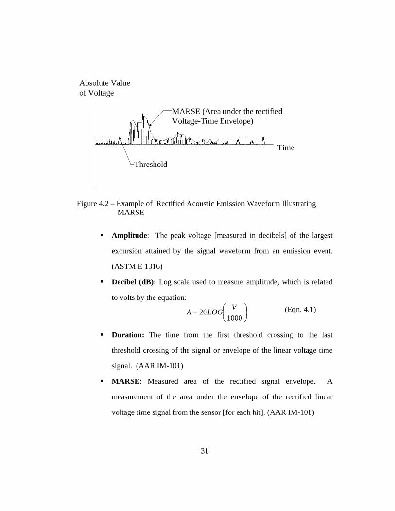
Figure 4.2 – Example of Rectified Acoustic Emission Waveform Illustrating MARSE
Amplitude: The peak voltage [measured in decibels] of the largest
excursion attained by the signal waveform from an emission event.
(ASTM E 1316)
Decibel (dB): Log scale used to measure amplitude, which is related
to volts by the equation:
⎟⎠⎞
⎜⎝⎛=1000
20 VLOGA (Eqn. 4.1)
Duration: The time from the first threshold crossing to the last
threshold crossing of the signal or envelope of the linear voltage time
signal. (AAR IM-101)
MARSE: Measured area of the rectified signal envelope. A
measurement of the area under the envelope of the rectified linear
voltage time signal from the sensor [for each hit]. (AAR IM-101)
31
Signal Strength: Area under the envelope of the linear voltage time
signal from the sensor. The signal strength will normally include the
absolute area of both the positive and negative envelopes. (AAR IM-
101)
Sensor Hit (Hit): Detection and measurement of an AE signal on a
channel. (AAR IM-101)
Voltage Threshold (Threshold): A voltage level on an electronic
comparator such that signals with absolute amplitude larger than this
level will be recognized. (AAR IM-101)
4.2 APPLICATION OF ACOUSTIC EMISSION TO CONCRETE IN GENERAL
Wave propagation through a material depends on the material’s damping,
geometry and elastic properties. Concrete poses a problem for wave propagation
because it is heterogeneous and contains microcracks. Its constituents such as
hydrated cement and aggregate vary significantly in size and material properties.
In addition, its properties can vary due to uneven consolidation, differential
shrinkage, or bleed water. This non-homogeneity causes considerable scatter in
results for practically any test performed on concrete, including acoustic emission.
This section covers some of the research done on reducing these effects.
4.2.1 Difficulties with Acoustic Emission in Concrete
Due to its heterogeneity and microcracks, concrete attenuates the acoustic
emission more quickly than steel or fiber-reinforced plastics. Figure 4.3 shows an
example of how amplitude is reduced as a function of the distance between a
32
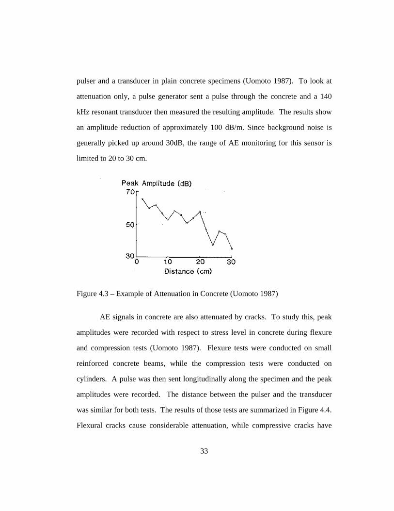
pulser and a transducer in plain concrete specimens (Uomoto 1987). To look at
attenuation only, a pulse generator sent a pulse through the concrete and a 140
kHz resonant transducer then measured the resulting amplitude. The results show
an amplitude reduction of approximately 100 dB/m. Since background noise is
generally picked up around 30dB, the range of AE monitoring for this sensor is
limited to 20 to 30 cm.
Figure 4.3 – Example of Attenuation in Concrete (Uomoto 1987)
AE signals in concrete are also attenuated by cracks. To study this, peak
amplitudes were recorded with respect to stress level in concrete during flexure
and compression tests (Uomoto 1987). Flexure tests were conducted on small
reinforced concrete beams, while the compression tests were conducted on
cylinders. A pulse was then sent longitudinally along the specimen and the peak
amplitudes were recorded. The distance between the pulser and the transducer
was similar for both tests. The results of those tests are summarized in Figure 4.4.
Flexural cracks cause considerable attenuation, while compressive cracks have
33
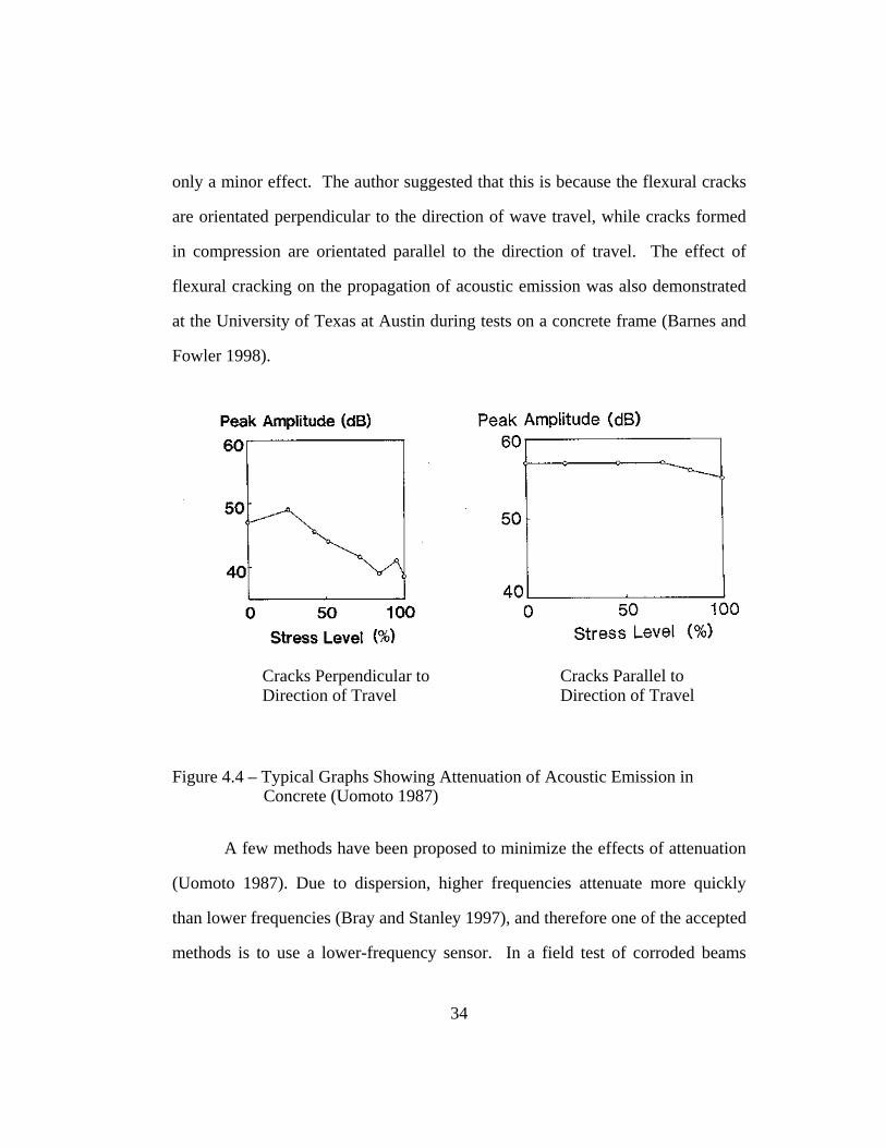
only a minor effect. The author suggested that this is because the flexural cracks
are orientated perpendicular to the direction of wave travel, while cracks formed
in compression are orientated parallel to the direction of travel. The effect of
flexural cracking on the propagation of acoustic emission was also demonstrated
at the University of Texas at Austin during tests on a concrete frame (Barnes and
Fowler 1998).
Cracks Parallel to Direction of Travel
Cracks Perpendicular to Direction of Travel
Figure 4.4 – Typical Graphs Showing Attenuation of Acoustic Emission in Concrete (Uomoto 1987)
A few methods have been proposed to minimize the effects of attenuation
(Uomoto 1987). Due to dispersion, higher frequencies attenuate more quickly
than lower frequencies (Bray and Stanley 1997), and therefore one of the accepted
methods is to use a lower-frequency sensor. In a field test of corroded beams
34
(Kamada et al 1996), 150 kHz sensors and 60 kHz sensors were used to monitor a
structure, and the only usable data came from the 60 kHz sensors. Another
method is to attach the sensors to the reinforcement instead of the concrete. Since
steel is more homogenous than concrete, the acoustic emission has less
attenuation.
Micro-cracking in reinforced concrete, while normal and usually not
structurally significant, creates a large amount of acoustic emission. This may
interfere with emission from a defect, complicating acoustic emission testing in
reinforced concrete. Also, if flexural cracks lie between the acoustic emission
source and the sensor, the signal may be greatly attenuated or even blocked. Even
with these difficulties, acoustic emission has been applied to concrete with
promising results (Barnes and Fowler 1998). Research has shown that as damage
increases the rate of emission and event amplitude increase (Karabinis and Fowler
1983).
Prestressed concrete, in contrast, is usually designed not to crack; any
cracking and associated emission are significant. Also, the attenuating effect of
cracks on wave propagation is eliminated. These factors combine to create an
ideal environment for acoustic emission (Yepez 1997).
4.2.2 Kaiser Effect
The Kaiser Effect is one of the more studied acoustic emission phenomena
in concrete. The American Society of Testing and Materials (ASTM) defines it
as follows:
35

Kaiser Effect – the absence of detectable acoustic emission at a fixed
sensitivity level [threshold], until previously applied stress levels are exceeded.
(ASTM E 1316)
The most obvious application of the Kaiser Effect is to determine the
maximum prior stress in a structure. This application has been debated, though,
since some research shows that in concrete the Kaiser Effect is only temporary
(Nielsen and Griffen 1977). After a long period of time, the beam can “heal”
itself so that it will produce acoustic emission on subsequent loading at levels
lower than previously applied. Other researchers report that the maximum prior
stress can be determined from of rate of emission and rate of signal strength, or
total events vs. load plots (Uomoto 1987). Even those researchers concede that
there are limitations such as the prior stress must be below a critical level, and that
most of the cement hydration must be completed to be valid.
Of more significance for structural evaluation is when the Kaiser Effect
starts to break down. It has been found that the Kaiser Effect starts to break down
as flexure crack widths increase and shear cracks start to play a role (Yuyama et
al. 1996). This Effect, called the Felicity Effect, shows great promise for
evaluation because it is only apparent when there is damage to the specimen, and
is greater when the damage is worse. This effect is defined by ASTM as:
36
Felicity Effect – the presence of acoustic emission, detectable at a fixed
predetermined sensitivity level [threshold] at stress levels below those previously
applied. (ASTM E 1316)
Studies have shown that the Felicity Effect starts to appear when crack
widths are greater than 0.15 to 0.20 mm or when delaminations are present.
(Yuyama et al. 1996). An evaluation criterion, the Felicity ratio, has been
proposed to quantify the degree of deterioration. This ratio is defined as the stress
at the onset of AE divided by the maximum prior stress and a Felicity ratio less
than unity indicates damage (Yuyama et al. 1994).
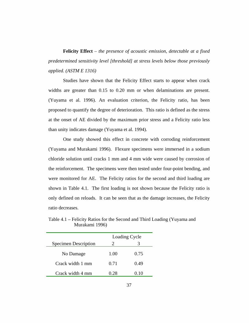
One study showed this effect in concrete with corroding reinforcement
(Yuyama and Murakami 1996). Flexure specimens were immersed in a sodium
chloride solution until cracks 1 mm and 4 mm wide were caused by corrosion of
the reinforcement. The specimens were then tested under four-point bending, and
were monitored for AE. The Felicity ratios for the second and third loading are
shown in Table 4.1. The first loading is not shown because the Felicity ratio is
only defined on reloads. It can be seen that as the damage increases, the Felicity
ratio decreases.
Table 4.1 – Felicity Ratios for the Second and Third Loading (Yuyama and Murakami 1996)
Loading Cycle Specimen Description 2 3
No Damage 1.00 0.75
Crack width 1 mm 0.71 0.49
Crack width 4 mm 0.28 0.10
37
The Felicity ratio has also proven useful in determining the adequacy of
repaired concrete beams (Yuyama et al 1994).
Both the Kaiser Effect and the Felicity Effect are illustrated in detail in
Section 4.4.
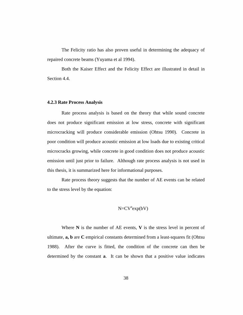
4.2.3 Rate Process Analysis
Rate process analysis is based on the theory that while sound concrete
does not produce significant emission at low stress, concrete with significant
microcracking will produce considerable emission (Ohtsu 1990). Concrete in
poor condition will produce acoustic emission at low loads due to existing critical
microcracks growing, while concrete in good condition does not produce acoustic
emission until just prior to failure. Although rate process analysis is not used in
this thesis, it is summarized here for informational purposes.
Rate process theory suggests that the number of AE events can be related
to the stress level by the equation:
N=CVaexp(bV)
Where N is the number of AE events, V is the stress level in percent of
ultimate, a, b are C empirical constants determined from a least-squares fit (Ohtsu
1988). After the curve is fitted, the condition of the concrete can then be
determined by the constant a. It can be shown that a positive value indicates
38

significant emission at low loads, while a negative a value relates sound concrete
which produces little emission at low loads.
Tests on concrete cores have shown that the extent of microcracking may
be more accurately determined from rate process analysis of acoustic emission
data than from visual examination of the crack density (Ohtsu et al 1988). It has
also been shown that rate process analysis is in agreement with the ultrasonic
technique of non-destructive testing (Ohtsu 1990).
4.2.4 Moment Tensor Analysis
Although the results from the Kaiser Effect and rate process analysis show
promise for determining structural integrity, more quantitative information would
be beneficial. The advantage of moment tensor analysis lies in its ability to
indicate source location, crack classification, and direction of crack propagation.
Moment tensor analysis is based on the change in stress geometry that
occurs at the source of the acoustic emission. To develop this analysis, crack
motion is described by a set of linear equations with 6 unknowns, corresponding
to the elements in the 3-dimensional moment tensor. An eigenvalue
decomposition is then performed, from which crack type and crack propagation
data are found. More specifically, eigenvalues have been found to relate to the
type of crack – shear, tensile, or mixed. Physically, the values represent the
direction of the dislocation displacement vector in relation to the crack normal
vector. If the dislocation displacement vector is perpendicular to the crack normal
vector (that is, in the direction of the crack), the crack is a shear crack. If the
39
dislocation displacement vector is parallel to the crack normal vector (that is,
perpendicular to the crack) the crack is classified as a tensile crack. Since cracks
are rarely entirely shear or tensile, results are reported as percent shear. The
direction of crack propagation can be found through the eigenvectors.
The major problem with moment tensor analysis is that 6 clear P-waves
need to be recorded for the same event. During one study, 1024 sets of
waveforms were recorded and only 19 sets were found to be usable (Yuyama et al
1995). Other studies confirm that most recorded data are not usable for analysis
(Yepez 1997).
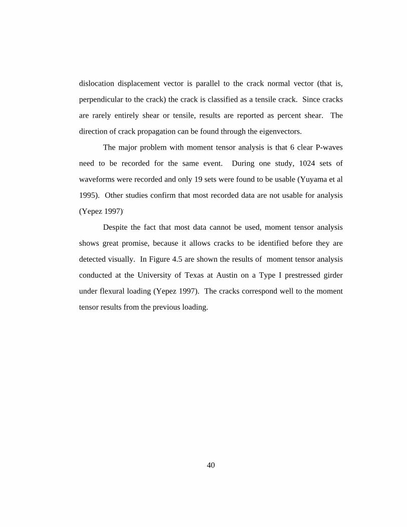
Despite the fact that most data cannot be used, moment tensor analysis
shows great promise, because it allows cracks to be identified before they are
detected visually. In Figure 4.5 are shown the results of moment tensor analysis
conducted at the University of Texas at Austin on a Type I prestressed girder
under flexural loading (Yepez 1997). The cracks correspond well to the moment
tensor results from the previous loading.
40

-0.2 0 0.2 0.4 0.6 0.8 1
L4B1N - WEST FACEEvents @ P = 135 k, Cracks @ 161 k
-0.05
0.05
0.15
0.25
0.35
0.45
DISTANCE (m)
DISTANCE (m)
Sensors/bottom Sensors/West face Sensors/East face Flexure type Mixed type Shear type
west face east face
L4B1N - END VIEWEvents @ 135 k
-0.05
0.05
0.15
0.25
0.35
0.45
-0.125 0 0.125 0.25
Z coor (m)
Y coor (m)
Figure 4.5 - Moment Tensor Results on Prestressed Girder (Yepez 1997)
4.3 ACOUSTIC EMISSION RESPONSE OF FLEXURAL CRACKING IN UNREINFORCED CONCRETE
The acoustic emission testing completed for this thesis can be divided into
two parts. The first part involves understanding the AE response of plain concrete
as it cracks; the second part involves applying that understanding to full-scale
specimens. This section describes the behavior of the plain concrete specimens.
41
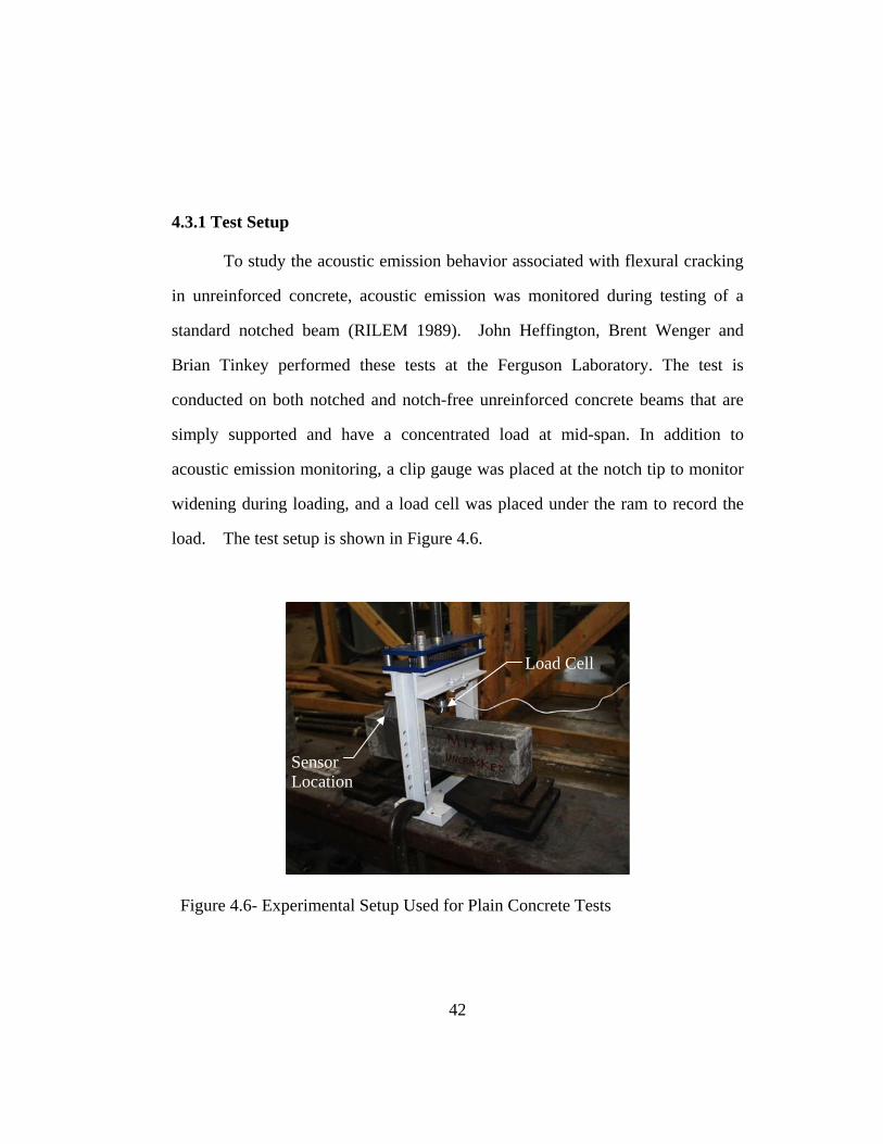
4.3.1 Test Setup
To study the acoustic emission behavior associated with flexural cracking
in unreinforced concrete, acoustic emission was monitored during testing of a
standard notched beam (RILEM 1989). John Heffington, Brent Wenger and
Brian Tinkey performed these tests at the Ferguson Laboratory. The test is
conducted on both notched and notch-free unreinforced concrete beams that are
simply supported and have a concentrated load at mid-span. In addition to
acoustic emission monitoring, a clip gauge was placed at the notch tip to monitor
widening during loading, and a load cell was placed under the ram to record the
load. The test setup is shown in Figure 4.6.
Load Cell
Sensor Location
Figure 4.6- Experimental Setup Used for Plain Concrete Tests
42

Three different mixture designs were cast, two lightweight and one
normal-weight. Mechanical properties of the mixtures as well as their failure
loads are shown in Table 4.2. Mixture 1 used lightweight coarse aggregate. This
mixture achieved the highest compressive strength of the three mixtures used in
these tests, an expected result due to its high cement content and low water-
cement ratio. Mixture 2 also used lightweight coarse aggregate. The cement
content in this mix was decreased while the water-cement ratio was increased, to
produce lower compressive and tensile strengths. During the casting of the beams
and cylinders with Mixture 2, the paste segregated from the aggregate due to the
high slump. This segregation, however, did not seem to decrease the strengths.
Mixture 3 used normal-weight river gravel as the coarse aggregate, and was a
control mixture against which Mixtures 1 and 2 could be compared. Using each
of the mixture designs, two beams were cast with an initial notch and one was left
without any initial notch, for a total of three beams for each mixture.
Table 4.2 - Properties of Mixtures Used on Plain Concrete Specimens
Concrete Mix
Average Comp. Strength
(psi)
Average Split Tensile Strength
(psi)
Notch free Max Load
(lbs.)
Notched Max. Load
(lbs.)
1 8114 520 1542 473
2 4191 424 1214 399
3 6750 543 1468 596
Dimensions of the specimens deviated slightly from the RILEM standard
due to the availability of molds. The nominal dimensions of the specimens were
3 inches wide, 4 inches deep and 16 inches long. An initial notch approximately
43
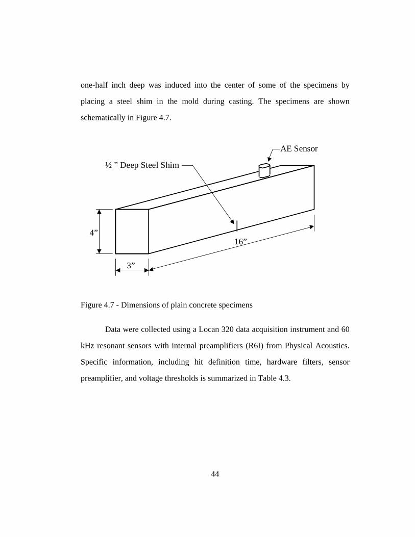
one-half inch deep was induced into the center of some of the specimens by
placing a steel shim in the mold during casting. The specimens are shown
schematically in Figure 4.7.
4”
3”
16”
½ ” Deep Steel Shim
AE Sensor
Figure 4.7 - Dimensions of plain concrete specimens
Data were collected using a Locan 320 data acquisition instrument and 60
kHz resonant sensors with internal preamplifiers (R6I) from Physical Acoustics.
Specific information, including hit definition time, hardware filters, sensor
preamplifier, and voltage thresholds is summarized in Table 4.3.
44

Table 4.3 - Test Parameters for Unreinforced Concrete Specimens
Quantity Values
Hit Definition Time (HDT) 1000 μs
Voltage Threshold 45 dB
Sensor Preamplifier (R6I) 40 dB
Data Acquisition Preamplifier 20 dB
Bandpass Data Acquisition Filter 0-1000 kHz
Bandpass Sensor Filter 30-165 kHz
4.3.2 Analysis and Results
From examining the data, it appeared that the most useful parameter for
analysis was cumulative MARSE. As outlined previously, MARSE is the area
under the rectified amplitude vs. time envelope for each hit. Cumulative MARSE
is the sum of the MARSE from all prior hits. Traditionally, an increase in the
slope of a graph of cumulative MARSE vs. time indicates a significant change in
state in the specimen. (ASNT – CARP 1999) For example, in steel an increase in
slope may indicate yielding, while in reinforced concrete a slope increase could
indicate a new shear or flexure crack.
The cumulative MARSE plot of a representative notched specimen just
prior to fracture is shown in Figure 4.8. This chart shows two distinct slope
changes, or “knees,” that indicate a significant change in the specimen. The first
knee coincides with the first opening of the notch, corroborated by the clip gauge
and a metallic sound heard at that time. The combination of these events
indicates that the slope increase is most likely due to debonding of the steel shim
45

used for the notch initiation. After the crack opened, no further damage occurred
as shown by the flat slope of cumulative MARSE. Knee 2 occurs immediately
before the final fracture. From watching the acoustic emission while loading it
was possible to predict that failure was about to occur from the increased rate of
emission.
0
50
100
150
200
250
300
350
400
450
500
0 100 200 300 400 500 600
Time (Seconds)
0
10000
20000
30000
40000
50000
60000
70000
Load Cumulative MARSE
Knee 1Shim Debond
Knee 2Fracture of Specimen
Figure 4.8 - AE Response of a Typical Notched Specimen
To more accurately identify knees in the curve of cumulative MARSE, an
analysis tool called Historic Index has been developed. This tool was developed
for testing pressure vessels and is currently incorporated into the MONPAC-
PLUS (Fowler et al. 1989) standard for testing metal tanks and vessels. In
essence, historic index compares the average MARSE of the last few hits with the
46

average MARSE of all hits up to that point. The equation for historic index as
outlined in the MONPAC-PLUS procedure is shown below:
( )⎟⎟⎟⎟
⎠
⎞
⎜⎜⎜⎜
⎝
⎛
−=
∑
∑
=
+=N
ioi
N
Ktot
S
S
KNNtH
1
1 (Eqn. 4.2)
where N is the current number of hits, Soi is the MARSE of a particular hit, and K
is defined by the table below.
Table 4.4 - K values used in Historic Index (Fowler et al. 1989)
Number of Hits K<10 Not Applicable
10-15 016-75 N-15
76 to 1000 0.8N>1000 N-200
In this study the historic index was calculated using a program written in
C++ and then plotted in a program written in LabView. Figure 4.9 shows the
historic index for the small-scale specimen whose cumulative MARSE plot is
shown in Figure 4.8. The knees in the MARSE curve can readily be identified
because they correspond to sharp increases in the historic index plot. The first
peak in Figure 4.9 lasts for a long time, since historic index is independent of time
and is only updated when a new hit occurs. After the shim had fully debonded,
very few new hits occurred, resulting in a long plateau.
47

Fracture of Specimen
Shim Debond
Figure 4.9 - Historic Index for a Typical Prenotched Specimen
While the notched specimens displayed little acoustic emission except at
the knees in the cumulative MARSE curve, the notch-free specimens (Figure
4.10) showed relatively constant low-level emission until just prior to failure,
when the rate of emission increased significantly. A probable explanation for the
difference in trends between the notched and the notch-free specimens can be
explained by crack initiation. Cracks form in concrete when distributed
microcracks coalesce into a single crack. The notched specimens have a
significant stress concentration, focusing the microcracking to a small area. If the
microcracking occurs only in a small area, less microcracking will occur before a
crack forms. Because acoustic emission detects the stress waves emitted from the
microcracking, a notched specimen will have less emission. Another explanation
is that the notched specimen fails at a much lower load than the notch-free
48

specimens. The higher loads produce a higher stress, which will cause more
microcracking and more emission.
0
200
400
600
800
1000
1200
1400
0 50 100 150 200 250
Time (Seconds)
0
10000
20000
30000
40000
50000
60000
70000
80000
90000
Load Cumulative MARSE
Fracture of Specimen
Figure 4.10 – Typical AE Response of Notch Free Specimen
As with the notched specimens, the historic index of the notch-free
specimens is a good indicator of significant events. Figure 4.11 shows the
historic index for the specimen whose cumulative MARSE plot is shown in
Figure 4.10. The only large, sharp jump in this graph corresponds to fracture of
the specimen. The historic index for the notch-free specimen has more scatter
than that of the notched specimen.
At the beginning of the notched specimen’s test, large MARSE hits were
received, creating a high cumulative MARSE. Since historic index compares the
MARSE of the last few hits with that of all hits up to that point, hits with much
higher MARSE are required to create a jump with the notched specimen than with
49

the notch-free specimen. The historic index for notched specimen is about 0.4
when no significant event is occurring, instead of the corresponding value of 1.0
for the notch-free specimen.
Fracture of Specimen
Figure 4.11 - Historic Index for a Typical Notch free Specimen
4.3.3 Discussion
The major source of acoustic emission for these small-scale, unreinforced
specimens was from microcracking and cracking of concrete. Other mechanisms.
such as steel yielding or debonding, were not present in these unreinforced
specimens. Once one major crack develops, an unreinforced specimen fails.
More acoustic emission is evident from notch-free specimens before failure,
because microcracking is distributed, rather than concentrated in a particular area
as with the notched specimens. Significant events identified directly by a large
increase in the cumulative MARSE plot, or indirectly from the historic index.
50
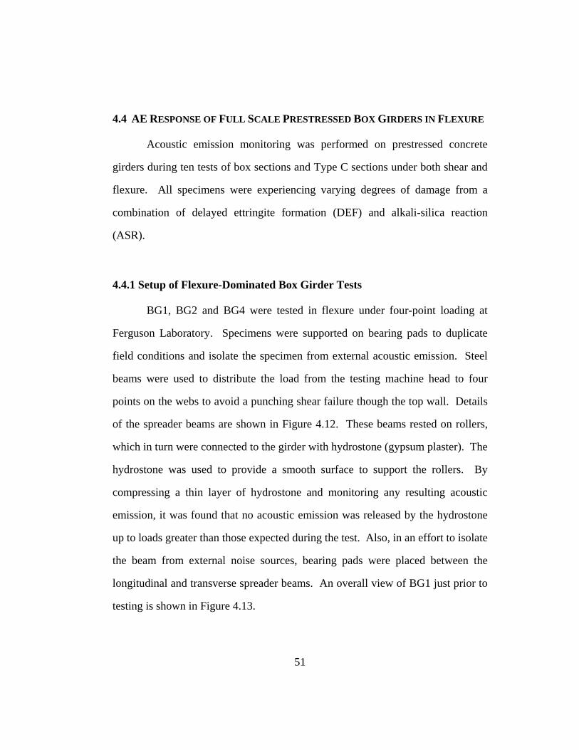
4.4 AE RESPONSE OF FULL SCALE PRESTRESSED BOX GIRDERS IN FLEXURE
Acoustic emission monitoring was performed on prestressed concrete
girders during ten tests of box sections and Type C sections under both shear and
flexure. All specimens were experiencing varying degrees of damage from a
combination of delayed ettringite formation (DEF) and alkali-silica reaction
(ASR).
4.4.1 Setup of Flexure-Dominated Box Girder Tests
BG1, BG2 and BG4 were tested in flexure under four-point loading at
Ferguson Laboratory. Specimens were supported on bearing pads to duplicate
field conditions and isolate the specimen from external acoustic emission. Steel
beams were used to distribute the load from the testing machine head to four
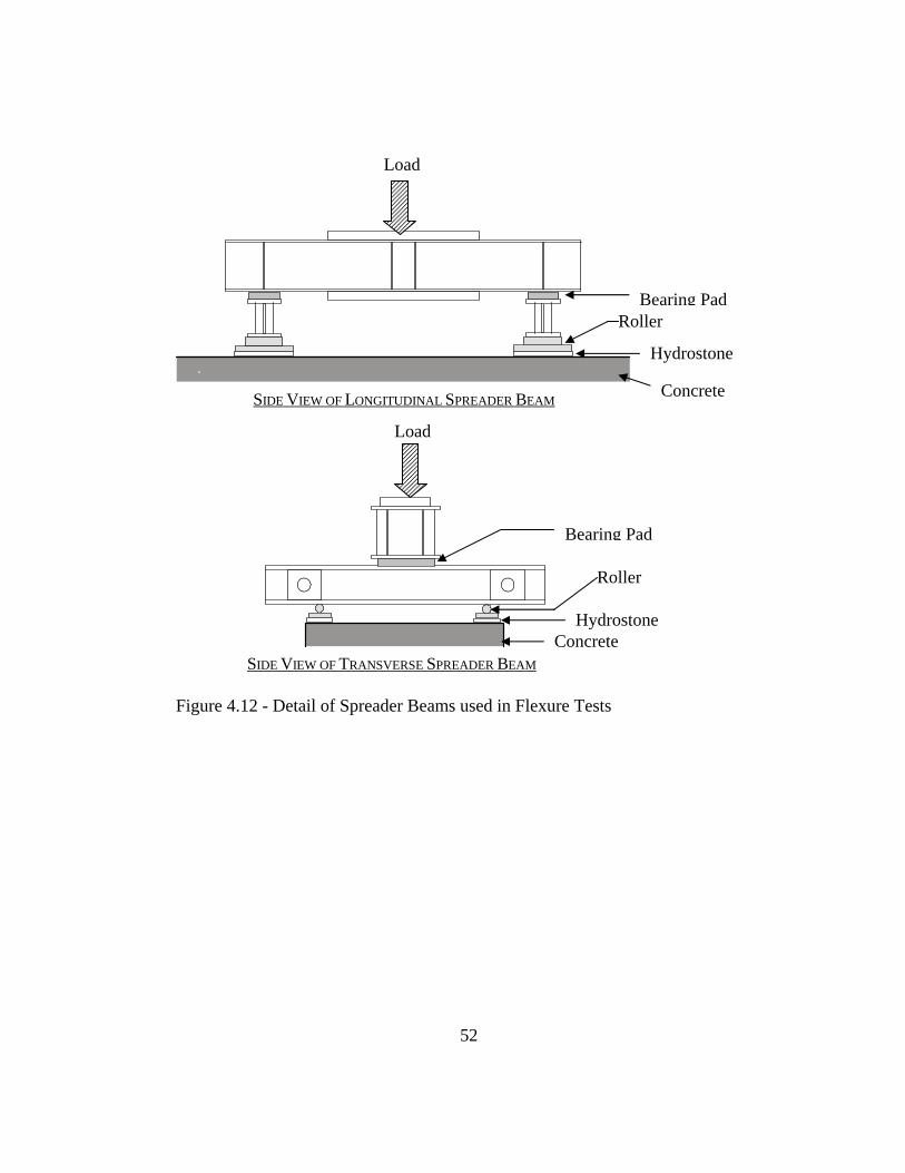
points on the webs to avoid a punching shear failure though the top wall. Details
of the spreader beams are shown in Figure 4.12. These beams rested on rollers,
which in turn were connected to the girder with hydrostone (gypsum plaster). The
hydrostone was used to provide a smooth surface to support the rollers. By
compressing a thin layer of hydrostone and monitoring any resulting acoustic
emission, it was found that no acoustic emission was released by the hydrostone
up to loads greater than those expected during the test. Also, in an effort to isolate
the beam from external noise sources, bearing pads were placed between the
longitudinal and transverse spreader beams. An overall view of BG1 just prior to
testing is shown in Figure 4.13.
51
Load
SIDE VIEW OF LONGITUDINAL SPREADER BEAM
SIDE VIEW OF TRANSVERSE SPREADER BEAM
Roller Bearing Pad
Hydrostone
Concrete
Load
Bearing Pad
Hydrostone Concrete
Roller
Figure 4.12 - Detail of Spreader Beams used in Flexure Tests
52

BG1
Figure 4.13 - BG1 Prior to Testing
The loading schedule for the specimens was developed so that the Kaiser
and Felicity Effects could be studied. Load was increased in 10-kip increments,
and held at the higher load until the rate of acoustic emission decreased. The load
was then decreased to 5 kips and held there for approximately 4 minutes. This
cycle was then repeated until failure. The actual loading schedule for BG1 while
acoustic emission was being monitored is shown in Figure 4.14. Notice there is a
slight unintentional drop in load, due to relaxation of the specimen.
53

Figure 4.14 - Loading Schedule for BG1
The expected flexure area was bracketed on both sides with six 60 kHz
resonant sensors (R6I). Sensor spacing was based on an attenuation test
performed on the web of a prestressed girder. This test was performed by
breaking a 0.3mm Pentel 2H pencil leads on the concrete every 6 inches away
from an R6I sensor for a total of 10 feet. Amplitudes of the resulting hits were
then plotted to generate the attenuation curve of Figure 4.15. From the results in
Figure 4.15 it can be seen that in 10 feet there was a loss of 40 dB. The
attenuation in this test is much lower than that shown in Section 4.2 since
prestressed concrete was tested and a sensor with a lower resonant frequency was
used. As explained in Section 4.2.1, prestressed concrete does not have the
nonstructural cracking that may be found in reinforced concrete, and lower
frequencies attenuate less than higher ones, both leading to a more favorable
attenuation curve. A six-foot spacing of sensors was chosen, with sensors placed
alternately on opposite sides of the beam (Figure 4.16).
54

Attenuation Test
0
20
40
60
80
100
0 1 2 3 4 5 6 7 8 9 10 11
Distance From Sensor (Feet)
Figure 4.15 - Attenuation Curve for R6I Sensor
Void
6 Feet 6 Feet
Sensor on West Side of GirderSensor on East Side of Girder
CL
Figure 4.16 – Plan View of Sensor Locations on Box Girder Specimens
55
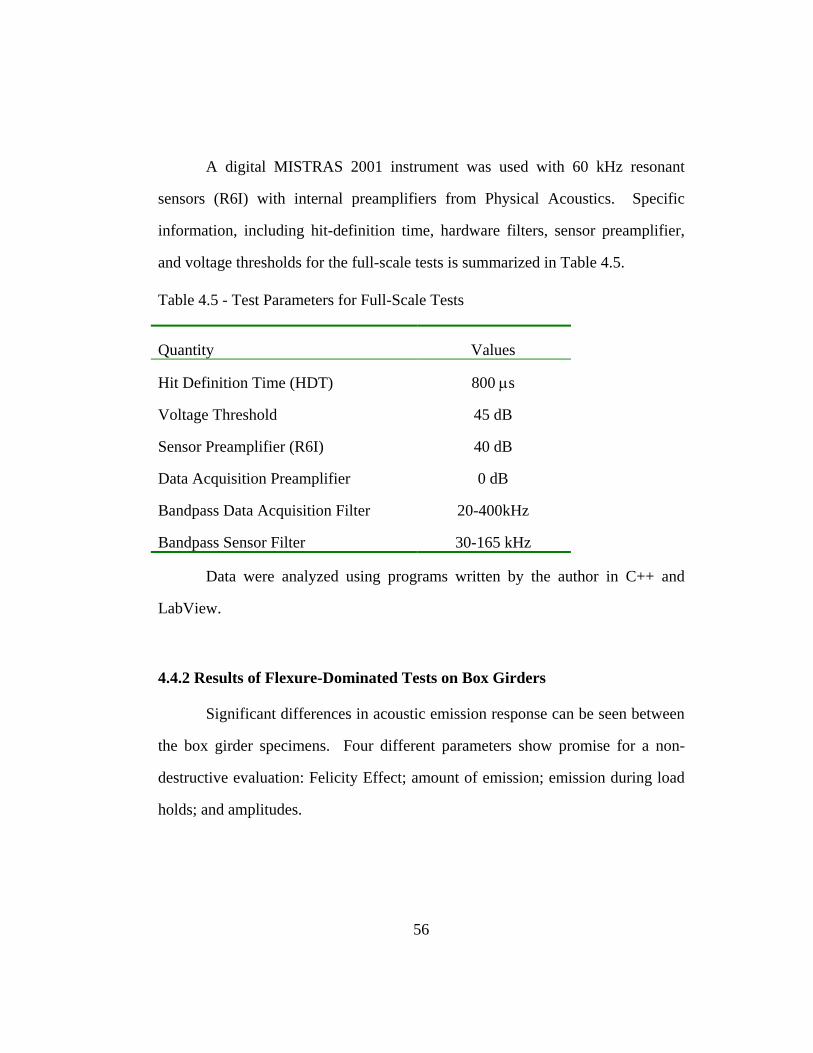
A digital MISTRAS 2001 instrument was used with 60 kHz resonant
sensors (R6I) with internal preamplifiers from Physical Acoustics. Specific
information, including hit-definition time, hardware filters, sensor preamplifier,
and voltage thresholds for the full-scale tests is summarized in Table 4.5.
Table 4.5 - Test Parameters for Full-Scale Tests
Quantity Values
Hit Definition Time (HDT) 800 μs
Voltage Threshold 45 dB
Sensor Preamplifier (R6I) 40 dB
Data Acquisition Preamplifier 0 dB
Bandpass Data Acquisition Filter 20-400kHz
Bandpass Sensor Filter 30-165 kHz
Data were analyzed using programs written by the author in C++ and
LabView.
4.4.2 Results of Flexure-Dominated Tests on Box Girders
Significant differences in acoustic emission response can be seen between
the box girder specimens. Four different parameters show promise for a non-
destructive evaluation: Felicity Effect; amount of emission; emission during load
holds; and amplitudes.
56
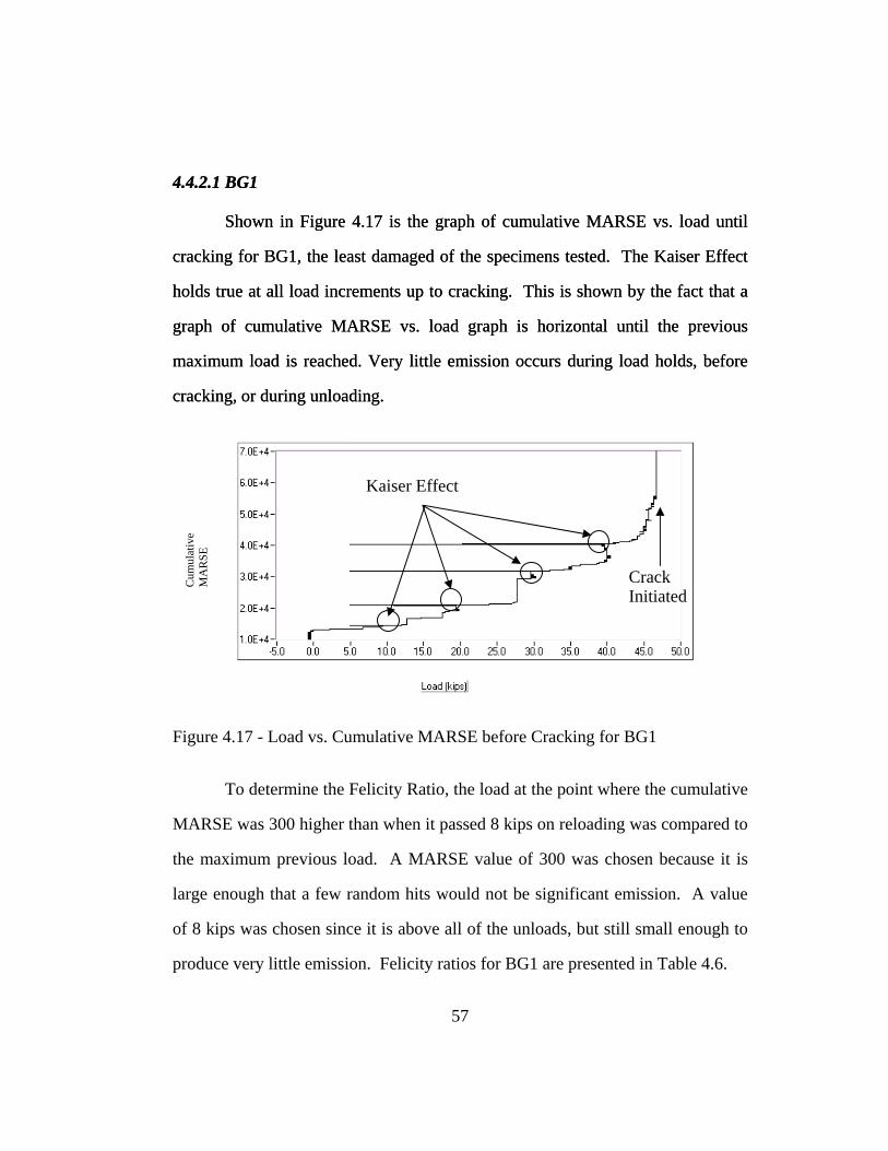
4.4.2.1 BG1 4.4.2.1 BG1
Shown in Figure 4.17 is the graph of cumulative MARSE vs. load until
cracking for BG1, the least damaged of the specimens tested. The Kaiser Effect
holds true at all load increments up to cracking. This is shown by the fact that a
graph of cumulative MARSE vs. load graph is horizontal until the previous
maximum load is reached. Very little emission occurs during load holds, before
cracking, or during unloading.
Kaiser Effect
Crack Initiated
Cum
ulat
ive
MA
RSE
Figure 4.17 - Load vs. Cumulative MARSE before Cracking for BG1
To determine the Felicity Ratio, the load at the point where the cumulative
MARSE was 300 higher than when it passed 8 kips on reloading was compared to
the maximum previous load. A MARSE value of 300 was chosen because it is
large enough that a few random hits would not be significant emission. A value
of 8 kips was chosen since it is above all of the unloads, but still small enough to
produce very little emission. Felicity ratios for BG1 are presented in Table 4.6.
57
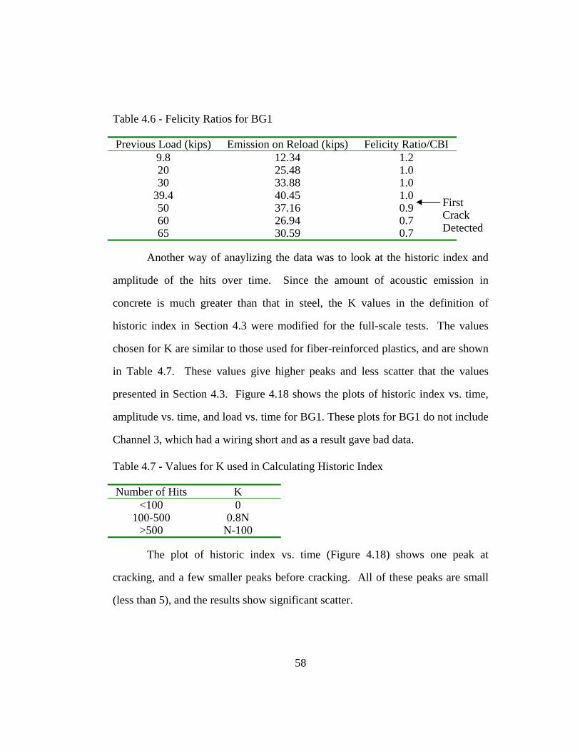
Table 4.6 - Felicity Ratios for BG1
Previous Load (kips) Emission on Reload (kips) Felicity Ratio/CBI 9.8 12.34 1.2 20 25.48 1.0 30 33.88 1.0
39.4 40.45 1.0 50 37.16 0.9 60 26.94 0.7 65 30.59 0.7
First Crack Detected
Another way of anaylizing the data was to look at the historic index and
amplitude of the hits over time. Since the amount of acoustic emission in
concrete is much greater than that in steel, the K values in the definition of
historic index in Section 4.3 were modified for the full-scale tests. The values
chosen for K are similar to those used for fiber-reinforced plastics, and are shown
in Table 4.7. These values give higher peaks and less scatter that the values
presented in Section 4.3. Figure 4.18 shows the plots of historic index vs. time,
amplitude vs. time, and load vs. time for BG1. These plots for BG1 do not include
Channel 3, which had a wiring short and as a result gave bad data.
Table 4.7 - Values for K used in Calculating Historic Index
Number of Hits K<100 0
100-500 0.8N>500 N-100
The plot of historic index vs. time (Figure 4.18) shows one peak at
cracking, and a few smaller peaks before cracking. All of these peaks are small
(less than 5), and the results show significant scatter.
58
The amplitude vs. time plot (Figure 4.18) shows very few high amplitude
hits until cracking. In fact, there is only one hit above 90 dB before cracking.
59
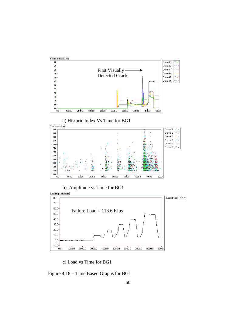
First Visually Detected Crack
a) Historic Index Vs Time for BG1
b) Amplitude vs Time for BG1
Failure Load = 118.6 Kips
c) Load vs Time for BG1
Figure 4.18 – Time Based Graphs for BG1
60
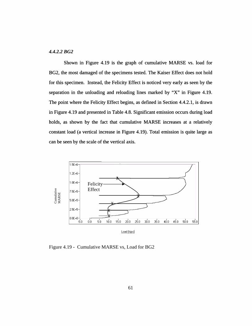
4.4.2.2 BG2
Shown in Figure 4.19 is the graph of cumulative MARSE vs. load for
BG2, the most damaged of the specimens tested. The Kaiser Effect does not hold
for this specimen. Instead, the Felicity Effect is noticed very early as seen by the
separation in the unloading and reloading lines marked by “X” in Figure 4.19.
The point where the Felicity Effect begins, as defined in Section 4.4.2.1, is drawn
in Figure 4.19 and presented in Table 4.8. Significant emission occurs during load
holds, as shown by the fact that cumulative MARSE increases at a relatively
constant load (a vertical increase in Figure 4.19). Total emission is quite large as
can be seen by the scale of the vertical axis.
Felicity Effect
Cum
ulat
ive
MA
RSE
Figure 4.19 - Cumulative MARSE vs, Load for BG2
61
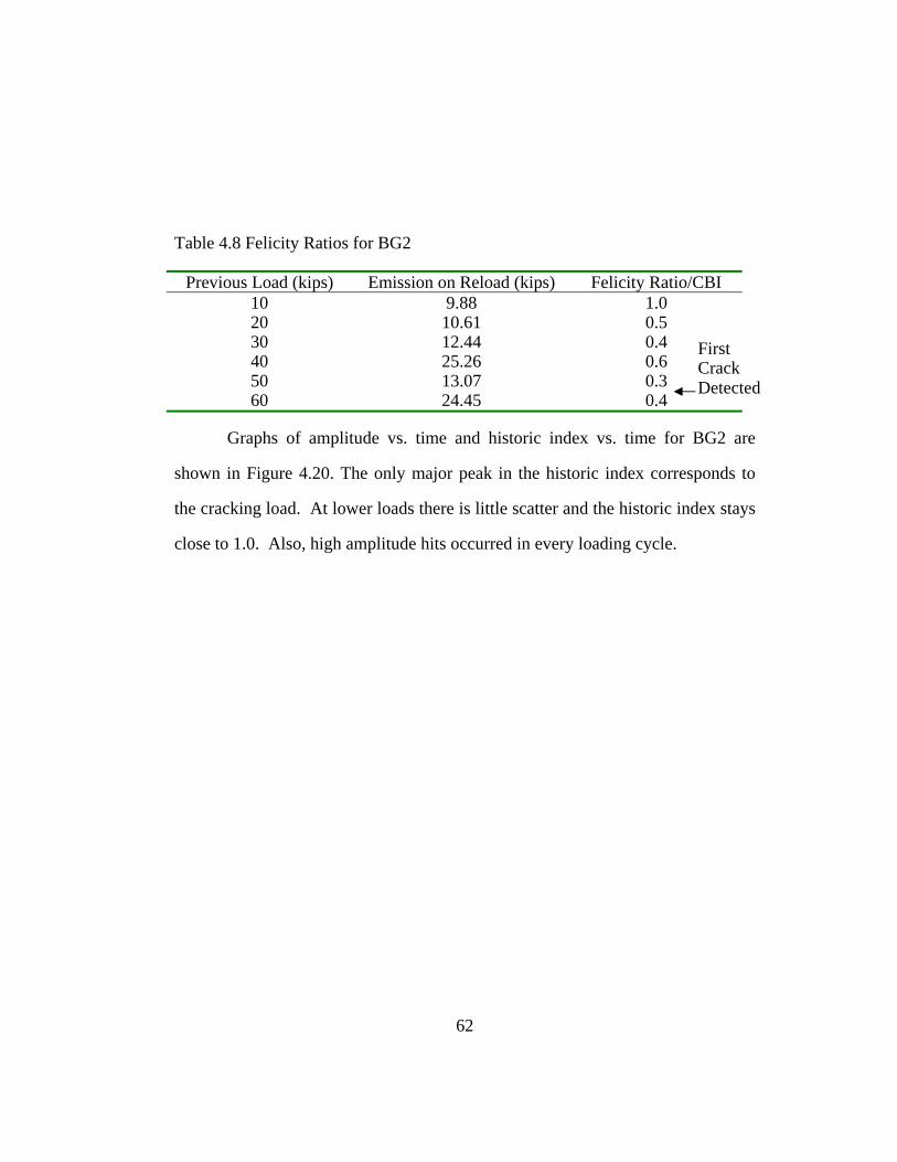
Table 4.8 Felicity Ratios for BG2
Previous Load (kips) Emission on Reload (kips) Felicity Ratio/CBI10 9.88 1.0 20 10.61 0.5 30 12.44 0.4 40 25.26 0.6 50 13.07 0.3 60 24.45 0.4
First Crack Detected
Graphs of amplitude vs. time and historic index vs. time for BG2 are
shown in Figure 4.20. The only major peak in the historic index corresponds to
the cracking load. At lower loads there is little scatter and the historic index stays
close to 1.0. Also, high amplitude hits occurred in every loading cycle.
62

First Visually Detected Crack
a) Historic Index vs Time for BG2
b)Amplidue vs Time for BG2
Failure Load = 116.3 Kips
c) Load vs Time for BG2
Figure 4.20 - Time Based Graphs for BG2
63

4.4.2.3 BG4 4.4.2.3 BG4
The graph of cumulative MARSE vs. load for BG4 is shown in Figure
4.21. Felicity Ratios were calculated, and are shown in Table 4.9. Felicity Ratios
stayed high (greater than 0.9) until cracking, and then dropped off dramatically.
This same trend was seen in BG1. The amount of emission in Figure 4.21 is
small, and very similar to that of BG1. In addition, most emission occurs during
loading, and very little during load holds.
Felicity Effect
Cum
ulat
ive
MA
RSE
Figure 4.21 - Cumulative MARSE vs. Load for BG4
Table 4.9 - Felicity Ratios for BG4
Previous Load (kips) Emission on Reload (kips) Felicity Ratio/CBI10.0 14.2 1.42 20.1 22.8 1.13 30.7 29.5 0.96 40.4 36.6 0.91 50.5 45.2 0.90 62.5 34.8 0.56
First Crack Detected
Graphs of amplitude vs. time and historic index vs. time for BG4 are
shown in Figure 4.22. The only major peak in the historic index corresponds to
64

the cracking load. Amplitudes steadily increase until the cracking load, where hits
over 95 dB are recorded.
65
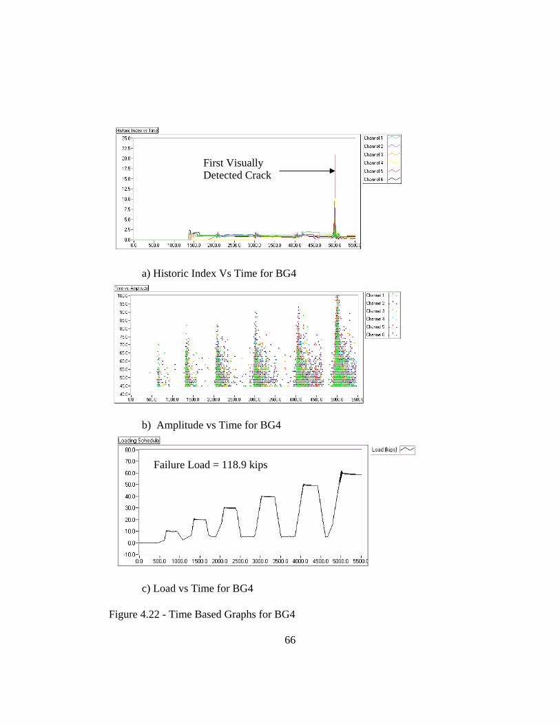
First Visually Detected Crack
a) Historic Index Vs Time for BG4
b) Amplitude vs Time for BG4
Failure Load = 118.9 kips
c) Load vs Time for BG4
Figure 4.22 - Time Based Graphs for BG4
66

4.4.3 Discussion of Flexure-Dominated Tests on Box Girders
Although BG4 was expected to be in the worst condition due to the
continuous wetting, this was not seen in the flexure-dominated tests. Although
some areas were significantly deteriorated, these were located at large blocks of
concrete, such as at the ends and the interior block-outs. The critical region near
midspan had no major cracks, and no crack existed along the interface of the two
pours as in the other specimens. Reinforcement was not corroded and no water
leaked out of the flexural zone at failure, indicating very few pre-existing cracks
in the flexural area. The final indication of very little distributed damage is that
BG4 failed at the highest load.
The lack of damage in BG4 is also shown in its acoustic emission
response. In all key AE parameters, BG4 was similar to BG1, the control beam.
Although slight differences exisit, indicating that BG4 is slightly more
deteriorated than BG1, these two are grouped together as the less-damaged
specimens for the remainder of this discussion.
The acoustic emission response of damaged specimens was considerably
different from that of the less-damaged ones.
1. The most striking difference is in the amount of emission. The graphs
of cumulative MARSE vs. load, demonstrate that the damaged
specimen has an order of magnitude more emission before cracking
than the less-damaged specimens. This is partly due to the fact that
BG2 cracked at a higher load (60 kips compared to 50 kips), but there
is also more emision at similar load levels.
67

2. Another important difference is that BG2 has more emission during
load holds. This can be seen from the increase in cumulative MARSE
while the load is staying constant, or slightly decreasing.
3. Finally, the Felicity effect is noticed before cracking in the badly
damaged specimen, while in the better specimens it was not seen until
after crack initiation. Felicity ratios for BG1, BG2 and BG4 are
presented in Figure 4.23. The Felicity Ratio for BG1 does not decrease
below 1.0 until cracking has occurred. For the more heavily damaged
specimen, BG2, however the Felicity Ratio is considerably below 1.0
after the first interval.
0
0.2
0.4
0.6
0.8
1
1.2
1.4
1.6
0 10 20 30 40 50 60 70
Load (Kips)
BG1 BG2 BG4
Crack occurs
Figure 4.23 - Felicity Effect for Flexure Specimens
It was intially thought that the historic index would be a good indicator of
significant events. It is true that at first cracking, the historic index has a
68

sigificant peak for all the specimens. The good specimen, BG1, however, has
peaks at relatively low loads of 20 kips and 30 kips. These may be due to the
definition of historic index. Since historic index compares the MARSE of the last
few hits to all of the previous hits, large MARSE hits early in the test create a
high average MARSE at the begining. In contrast, later in the test there is a larger
base for average MARSE. Therefore a large peak in the historic index later in the
test is more indicative of damage than one earlier in the test. Due to this fact,
historic index is a better indicator of a sigificant event on the more damaged
specimen that has many hits immediately, where there are insigificant peaks in the
good specimen.
One interesting trend in the data were the amplitude of the hits over time.
The less damaged specimens had very few hits over 90 dB, whereas the more
damaged specimen had hits over 90 dB almost immediately.
4.5 AE RESPONSE OF FULL SCALE PRESTRESSED BOX GIRDERS IN SHEAR
After the flexure tests were completed, there was concern that the badly
deteriorated ends would weaken the bond of the concrete to the prestressing
strands and decrease the capacity of the girder as governed by shear. To test this,
one end from BG1, BG2 and BG4 were tested in shear while monitoring acoustic
emission.
4.5.1 Setup of Shear-Dominated Tests on Box Girders
The setup for the shear tests was similar to that of the flexural tests. Steel
spreader beams were used to distribute the load to four points on the web. Again,
69

these beams rested on rollers, which were connected to the girder with
hydrostone. Bearing pads were placed between the steel beams to isolate the test
specimen from vibrations in the testing machine. Stronger spreader beams were
required due to the increased load that was expected.
To distinguish the shear tests from the flexural tests, a different
nomenclature was adopted. The shear test of the control beam (BG1) was
designated BG1S; the shear test of the more deteriorated beam (BG2) was
designated BG2S; and the shear test of the wetted beam was designated BG4S.
BG1S and BG4S were set up with a shear span of 2 times the distance
from the top to the centroid of the prestressing strand, or 46 inches. One support
was located near the end of the solid end block, and the other support was located
approximately at the interior solid blockout. This resulted in a distance between
the supports of 276.5 inches. Figure 4.24 shows the setup for these specimens;
the large arrows represent where the beams loaded the rollers on the webs.
9.5 in.
46 in.N
Void
276.5 in.
66 in.
6 in. 16.5 in.
9” Wide Bearing Pads
Figure 4.24 - Test Setup for BG1S and BG4S
70

The test setup for BG2S was similar except that it had a shear span of 1.5
times the distance from the top to the centroid of the prestressing strand, or 35.5
inches. One support was located on the northernmost point of the solid end block,
and the other support was located approximately at the interior solid blockout.
This resulted in a distance between the supports of 266 inches. Figure 4.25 shows
the setup for BG2S. The setup of BG2S was intended to force crushing of the
compression strut, while BG1S and BG4S represented support conditions used in
the field.
N
266 in.
66 in. 35.5 in.
Void
20 in.
6 in. 6 in.
Figure 4.25 – Test Setup of BG2S
The sensor arrangement was similar to that of the flexure tests, but the
sensor were spaced closer together because the area of interest is smaller.
Unfortunately the sensors were not able to bracket the shear area. Rather, they
were placed a little to one side because of other transducers. This offset was not a
problem since the entire shear area could be monitored with this configuration. A
diagram showing the sensor placement for both tests is shown in Figure 4.26
71

N
Void
25.5 in 25.5 in 42 in
Sensor on West Side of GirderSensor on East Side of Girder
Figure 4.26 - Sensor Locations on all Shear Specimens
The loading schedule for the shear tests was constructed so that the
Felicity Effect could be examined. Since the maximum load was expected to be
considerably larger than in the flexure tests, a loading increment of 20 kips rather
than 10 kips, was used. The loading schedule for BG1S is shown in Figure 4.27.
BG2S was accidentally loaded to an increase of 55 kips at the first interval, but
the proper increase of 20 kips was used in subsequent intervals.
72

Figure 4.27 - Loading Schedule for BG1S
4.5.2 Results of the Shear-Dominated Tests on Box Girders
4.5.2.1 BG1S
Figure 4.28 shows the graph of cumulative MARSE vs. load for BG1S, up
to the cracking load of 160 kips. The Felicity ratio was as in the flexure tests (a
cumulative MARSE increase of 300 above the value at 8 kips when reloading).
Results are shown in Table 4.10. The Felicity ratio is around 0.9 for BG1S until
about 80 kips; during the next increment it then starts to and emission during load
holds begins to increase.
73

Felicity Effect
Cum
ulat
ive
MA
RSE
Figure 4.28 - Load Vs Cumulative MARSE for BG1S
Table 4.10 - Felicity Ratios for BG1S
Previous Load (kips) Emission on Reload (kips) Felicity Ratio/CBI 20 22.80 1.14 41 35.89 0.88 61 55.70 0.91 80 75.52 0.94 101 72.53 0.72 122 86.36 0.71 142 77.02 0.54 162 80.38 0.50 182 77.02 0.42 201 40.00 0.20
First Detected Crack
The time based graphs for BG1S are shown in Figure 4.29. Amplitudes at
low loads are larger than in the flexure tests, but still relatively low. In fact no
hits above 90 dB occur until 140 kips is reached. Historic index shows a major
peak at the cracking load.
74
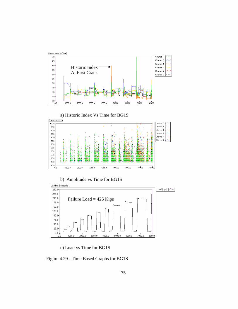
Historic Index At First Crack
a) Historic Index Vs Time for BG1S
b) Amplitude vs Time for BG1S
Failure Load = 425 Kips
c) Load vs Time for BG1S
Figure 4.29 - Time Based Graphs for BG1S
75
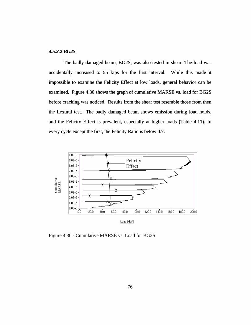
4.5.2.2 BG2S 4.5.2.2 BG2S
The badly damaged beam, BG2S, was also tested in shear. The load was
accidentally increased to 55 kips for the first interval. While this made it
impossible to examine the Felicity Effect at low loads, general behavior can be
examined. Figure 4.30 shows the graph of cumulative MARSE vs. load for BG2S
before cracking was noticed. Results from the shear test resemble those from then
the flexural test. The badly damaged beam shows emission during load holds,
and the Felicity Effect is prevalent, especially at higher loads (Table 4.11). In
every cycle except the first, the Felicity Ratio is below 0.7.
Cum
ulat
ive
MA
RSE
Felicity Effect
Figure 4.30 - Cumulative MARSE vs. Load for BG2S
76

Table 4.11 - Felictiy Ratios for BG2S
Previous Load (kips) Emission on Reload (kips) Felicity Ratio/CBI56 58.32 1.04 73 49.72 0.68 95 16.82 0.18 114 63.56 0.56 133 37.38 0.28 153 56.00 0.37 172 53.46 0.31 194 42.25 0.22 212 48.23 0.23
First Detected Crack
Figure 4.31 shows hit amplitudes consistently above 90 dB for the entire
test, and a few are from 95 to 100 dB.
77

a) Historic Index vs Time for BG2S
Pause
b)Amplitude vs Time for BG2S
Failure Load = 358 Kips
c) Load vs Time for BG2S
Figure 4.31 - Time Based Graphs for BG2S
78

4.5.2.3 BG4S
BG4S was the final shear test performed on a box girder section. This
specimen failed very differently than the previous two shear specimens. BG4S
had a bearing failure (Figure 4.32) while the previous specimens failed in the
compression strut (Figure 4.33). A weak plane (vertical delamination) was created
in the center of the web due to a combination of premature concrete deterioration
and corrosion of the reinforcement.
Figure 4.32 - Bearing Failure of BG4S
79

Figure 4.33 - Compression Strut Failure of BG1S
During the test, a metallic clicking sound was heard periodically from the
test setup. Although it did not originate from the test specimen, its cause was not
found. By watching the acoustic emission as the noise was heard, the associated
emission was determined to be low amplitude, long duration, and high MARSE,
all characteristic of mechanical rubbing. This is also shown in the plot of
amplitude vs. log duration in Figure 4.34. As this clicking was heard, hits were
noticed in the area marked on that figure. No emission in this area had been noted
in any other tests, indicating that it was probably due to external sources. This
external emission was eliminated with a Swansong II filter.
80
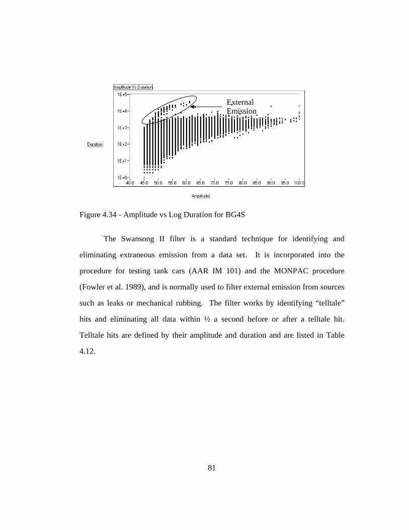
External Emission
Figure 4.34 - Amplitude vs Log Duration for BG4S
The Swansong II filter is a standard technique for identifying and
eliminating extraneous emission from a data set. It is incorporated into the
procedure for testing tank cars (AAR IM 101) and the MONPAC procedure
(Fowler et al. 1989), and is normally used to filter external emission from sources
such as leaks or mechanical rubbing. The filter works by identifying “telltale”
hits and eliminating all data within ½ a second before or after a telltale hit.
Telltale hits are defined by their amplitude and duration and are listed in Table
4.12.
81
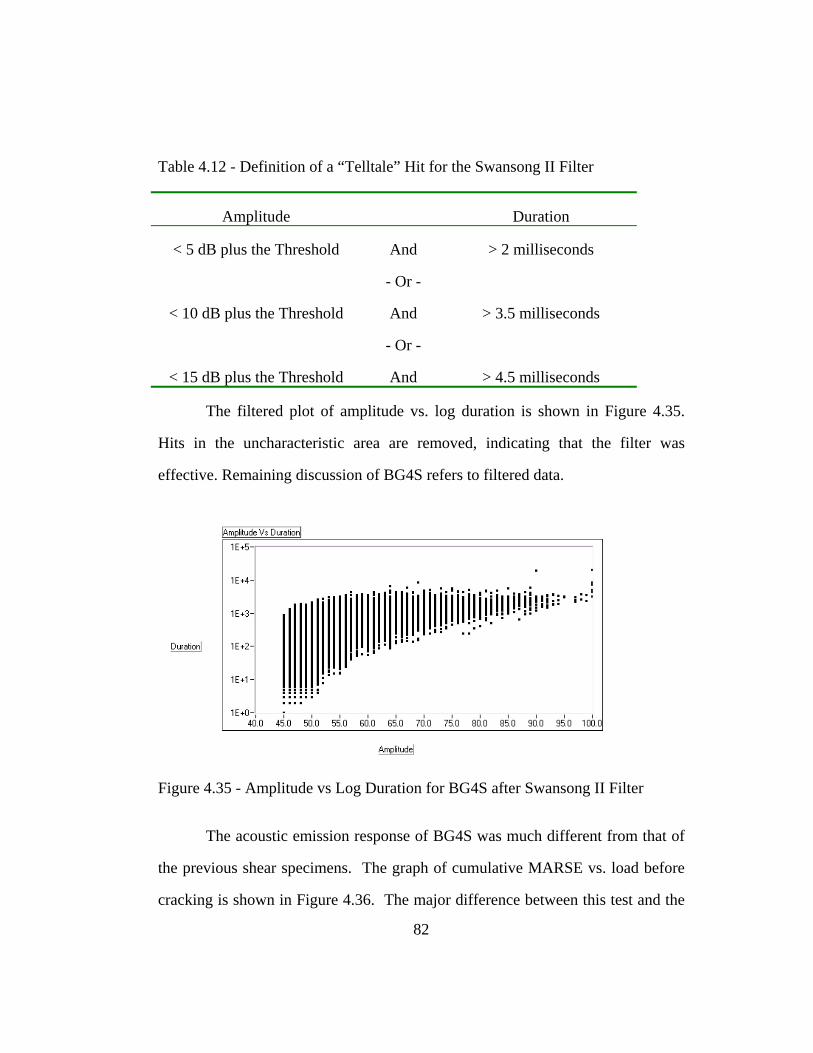
Table 4.12 - Definition of a “Telltale” Hit for the Swansong II Filter
Amplitude Duration
< 5 dB plus the Threshold And > 2 milliseconds
- Or -
< 10 dB plus the Threshold And > 3.5 milliseconds
- Or -
< 15 dB plus the Threshold And > 4.5 milliseconds
The filtered plot of amplitude vs. log duration is shown in Figure 4.35.
Hits in the uncharacteristic area are removed, indicating that the filter was
effective. Remaining discussion of BG4S refers to filtered data.
Figure 4.35 - Amplitude vs Log Duration for BG4S after Swansong II Filter
The acoustic emission response of BG4S was much different from that of
the previous shear specimens. The graph of cumulative MARSE vs. load before
cracking is shown in Figure 4.36. The major difference between this test and the
82

previous shear tests is the emission during unloading. This trend is shown clearly
for loads above 125 kips in Figure 4.36. If lower loads are examined more
carefully, however, emission during unloads can be seen even in the first few
cycles. This graph also shows that the overall amount of MARSE is low relative
to the other shear specimens. The Felicity ratios for this specimen are shown in
Table 4.13. They stay around 1.0 until about half the cracking load, and then start
to decrease.
Felicity Effect
Cum
ulat
ive
MA
RSE
Figure 4.36 - Cumulative MARSE vs. Load for BG4S
83

Table 4.13 - Felicity Ratios for BG4S
Previous Load (kips) Emission on Reload (kips)
Felicity Ratio
40.7 43.0 1.1 60.0 66.2 1.1 82.3 81.5 1.0 99.8 103.2 1.0 121 127.2 1.1
140.2 101.7 0.7 161.6 127.2 0.8 181.8 99.1 0.5 201.6 123.8 0.6 223.3 142.9 0.6 242 109.2 0.5
262.2 94.2 0.4
First Detected Crack
As shown in Figure 4.37, no large peaks occur in the historic index before
cracking, and no high amplitude hits occur until the 125 kip loading increment.
Significantly, this is also where the Felicity ratio begins to decrease.
84
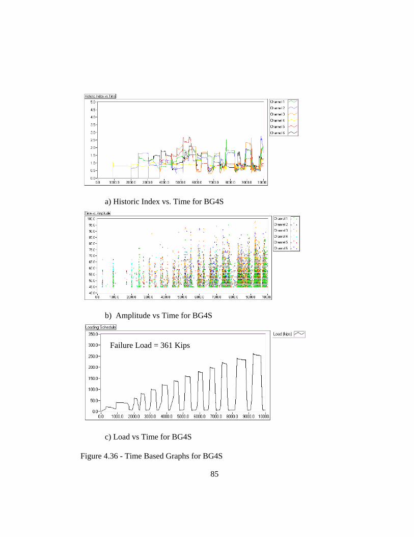
a) Historic Index vs. Time for BG4S
b) Amplitude vs Time for BG4S
Failure Load = 361 Kips
c) Load vs Time for BG4S
Figure 4.36 - Time Based Graphs for BG4S
85
4.5.3 Discussion of the Shear-Dominated Tests on Box Girders
Although BG4S had significant deterioration, as can be seen by its failure
mode, it did not have the largest amount of acoustic emission, and its Felicity
ratios did not decrease rapidly, as was seen in the other badly damaged girders.
One possible explanation, based on the crack pattern at failure (Figure 4.34), is
that a delamination at the end may have blocked the acoustic emission from the
sensors. A delamination at the end would also explain the emission during
unloading. A delamination may cause the outside wall to move slightly outward
during loading. This would not create emission since there would be no rubbing
between surfaces. On unloading, however, the delamination would close, and
cause rubbing on the two surfaces. The high Felicity ratios are then explained
because of the orientation of the delamination. If the internal stress due to the
premature concrete deterioration were relieved by a vertical crack in the plane of
the web, the loading method used would not stress this type of defect. In the other
shear tests most of the cracking was parallel to the axis of the beam, and the
horizontal shear would cause rubbing between the crack surfaces.
If the vertical delamination in the web is the cause for the difference in
acoustic emission response of this test specimen, future tests should either use
impact-echo to inspect for delaminations before monitoring with acoustic
emission, or should monitor acoustic emission closely during unloading cycles.
The other two shear tests, BG1S and BG2S, can be compared directly
since they failed by the same mechanism. As shown in Chapter 3, BG2S was
more deteriorated than BG1S. From these tests cumulative MARSE is a good
86
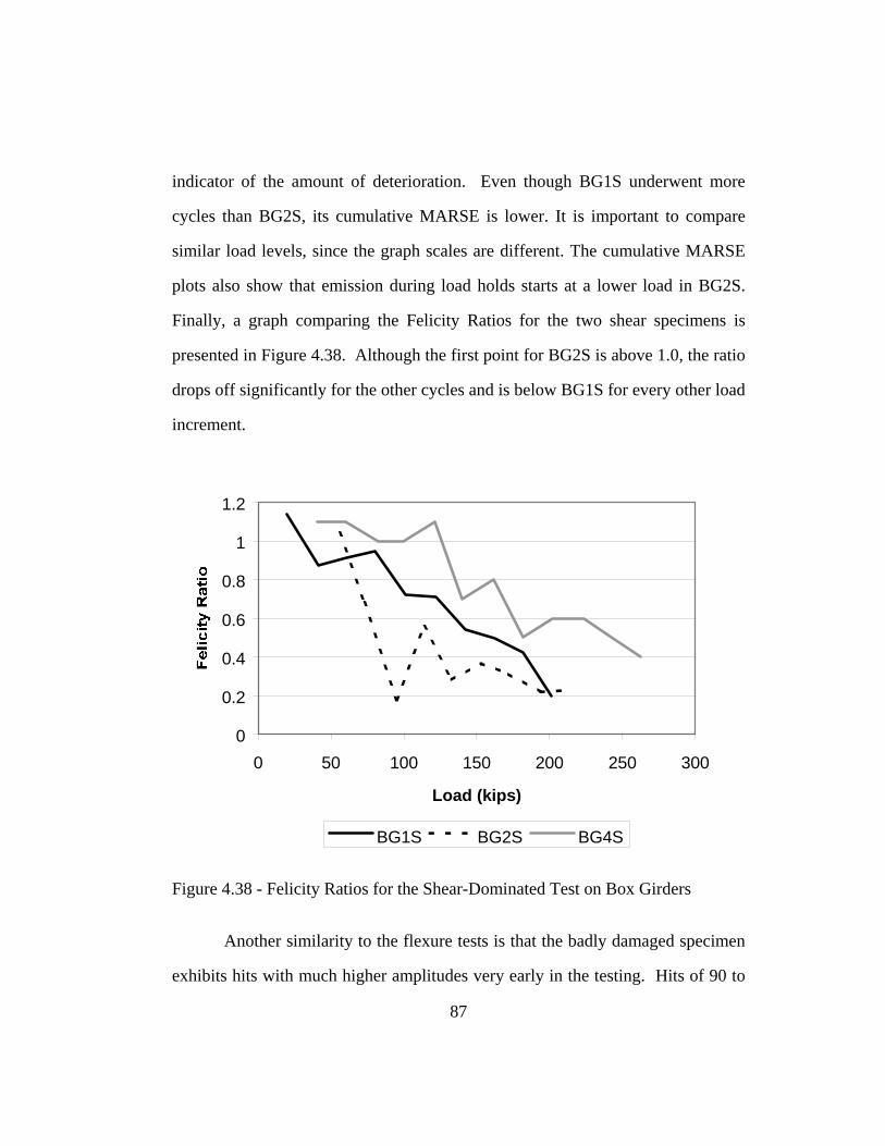
indicator of the amount of deterioration. Even though BG1S underwent more
cycles than BG2S, its cumulative MARSE is lower. It is important to compare
similar load levels, since the graph scales are different. The cumulative MARSE
plots also show that emission during load holds starts at a lower load in BG2S.
Finally, a graph comparing the Felicity Ratios for the two shear specimens is
presented in Figure 4.38. Although the first point for BG2S is above 1.0, the ratio
drops off significantly for the other cycles and is below BG1S for every other load
increment.
0
0.2
0.4
0.6
0.8
1
1.2
0 50 100 150 200 250 300
Load (kips)
BG1S BG2S BG4S
Figure 4.38 - Felicity Ratios for the Shear-Dominated Test on Box Girders
Another similarity to the flexure tests is that the badly damaged specimen
exhibits hits with much higher amplitudes very early in the testing. Hits of 90 to
87
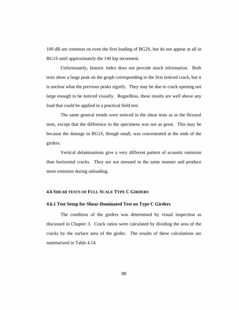
100 dB are common on even the first loading of BG2S, but do not appear at all in
BG1S until approximately the 140 kip increment.
Unfortunately, historic index does not provide much information. Both
tests show a large peak on the graph corresponding to the first noticed crack, but it
is unclear what the previous peaks signify. They may be due to crack opening not
large enough to be noticed visually. Regardless, these results are well above any
load that could be applied in a practical field test.
The same general trends were noticed in the shear tests as in the flexural
tests, except that the difference in the specimens was not as great. This may be
because the damage in BG1S, though small, was concentrated at the ends of the
girders.
Vertical delaminations give a very different pattern of acoustic emission
than horizontal cracks. They are not stressed in the same manner and produce
more emission during unloading.
4.6 SHEAR TESTS OF FULL SCALE TYPE C GIRDERS
4.6.1 Test Setup for Shear-Dominated Test on Type C Girders
The condition of the girders was determined by visual inspection as
discussed in Chapter 3. Crack ratios were calculated by dividing the area of the
cracks by the surface area of the girder. The results of these calculations are
summarized in Table 4.14.
88
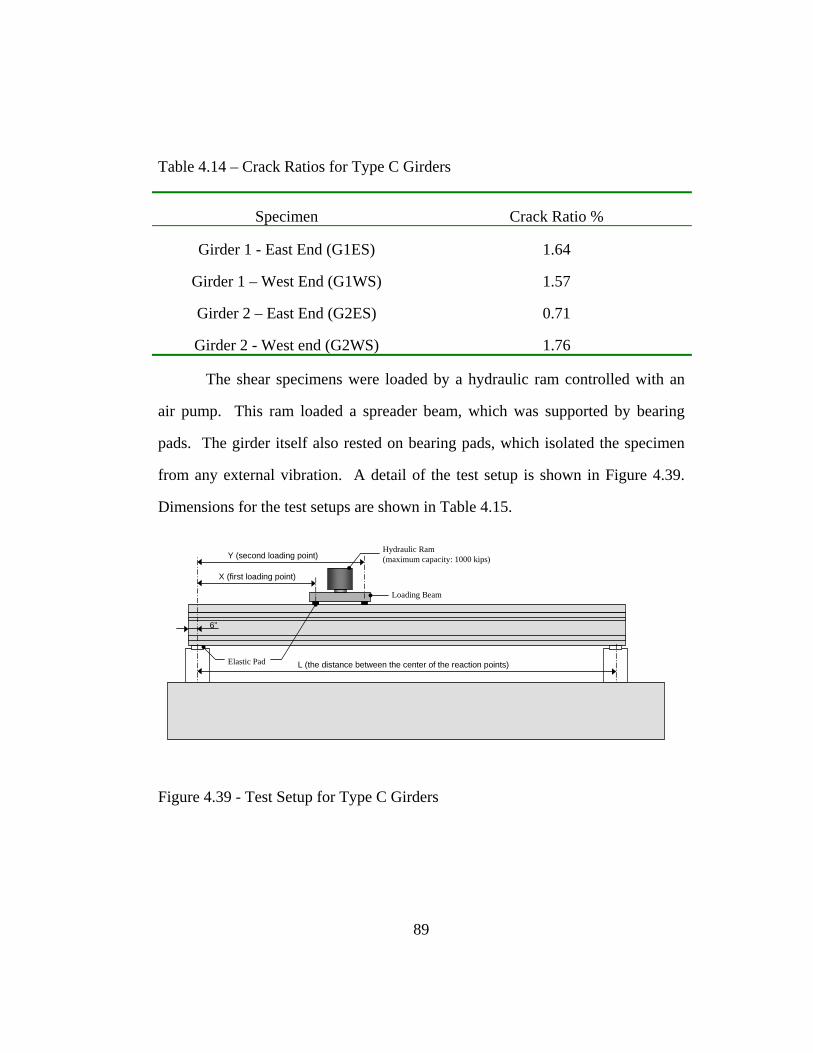
Table 4.14 – Crack Ratios for Type C Girders
Specimen Crack Ratio %
Girder 1 - East End (G1ES) 1.64
Girder 1 – West End (G1WS) 1.57
Girder 2 – East End (G2ES) 0.71
Girder 2 - West end (G2WS) 1.76
The shear specimens were loaded by a hydraulic ram controlled with an
air pump. This ram loaded a spreader beam, which was supported by bearing
pads. The girder itself also rested on bearing pads, which isolated the specimen
from any external vibration. A detail of the test setup is shown in Figure 4.39.
Dimensions for the test setups are shown in Table 4.15.
Hydraulic Ram(maximum capacity: 1000 kips)
X (first loading point)
Y (second loading point)
L (the distance between the center of the reaction points)
6”
Elastic Pad
Loading Beam
Figure 4.39 - Test Setup for Type C Girders
89

Table 4.15 - Dimensions of Test Setup
Dimension in Figure 4.39 G1ES G1WS G2ES G2WS
L (Length in Feet) 30 30 35 35
X (Distance to the first loading point in Feet) 6 6 6 10
Y (Distance to the second loading point in Feet) 10 10 10 14
Sensor placement was based upon the same attenuation test that was
described in the test setup for the flexure tests. Sensor placement is shown in
Figure 4.40, and dimensions for this figure are shown in Table 4.16. Emission
was recorded using a 6-channel MISTRAS digital acoustic emission system and
R6I sensors. Data were analyzed using programs written by the author in C++ and
LabView.
X1 X2 X3
Sensor on West SideSensor on East Side
Figure 4.40 - Sensor Placement for Type C Specimens
90

Table 4.16 - Dimension for Sensor Placement on Type C Girders
Dimension in Figure 4.40 (in inches) G1ES G1WS G2ES G2WS
X1 41 41 41 52
X2 25.5 25.5 25.5 25.5
X3 25.5 25.5 25.5 25.5
4.6.2 Results of Shear-Dominated Test on Type C Girders
4.6.2.1 G2WS
The first specimen tested was G2WS. Although mistakes were made in
both the setup and the loading schedule, this specimen was still useful in that
much was learned for the subsequent tests.
Since this was the first test, the ideal loading schedule was not clear. A
loading increment of 40 kips was initially chosen, which is about 10% of the
predicted capacity. After a load hold the load would then be reduced 40 kips.
Due to the amount of acoustic emission generated the loading increment was cut
back to 5%, or 20 kips, and finally after 200 kips the specimen was loaded
without unloads until failure. Only one full unload was performed, due to a stop
at the end of the day and a restart the next morning. The actual loading schedule
for G2WS is shown in Figure 4.41. With the hydraulic ram instead of the
displacement-controlled loading setup used for the box girders, it is much more
difficult to control the load.
91

Figure 4.41 - Loading Schedule for G2WS
Since the loading schedule is inconsistent, it is difficult to draw
conclusions from the data. The graph of cumulative MARSE vs. load is shown in
Figure 4.42. It can be seen from the full unload that 10% unloads are insufficient
to determine the Felicity Ratio, and emission in fact begins at a very low load.
Significant emission occurs during unloaded periods, an indication that further
unloads are necessary. Finally, significant emission occurs during load holds, as
in the badly damaged specimens described earlier in this chapter.
92
Cum
ulat
ive
MA
RSE
Figure 4.42 - Cumulative MARSE vs. Load for G2WS
Historic index, amplitude, and load are plotted in Figure 4.43 up to the
point that unloading stopped. Historic Index shows no significant peak in this
time period. Amplitude of hits starts off low but reach 90 to 100 dB by the 120
kip loading increment.
93

a) Historic Index vs. Time for G2WS
b) Amplitude vs. Time for G2WS
Failure Load = 502 kips
c) Load vs. Time for G2WS
Figure 4.43 - Time Based Graphs for G2WS
94

4.6.2.2 G2ES
From the visually determined crack ratio, G2ES was the least damaged
specimen. Lessons from the first test were implemented and a shorter shear span
was used with full unloads (Figure 4.44). This figure shows an apparent error in
the load cell during the 180 kip load hold. This problem was corrected and the
rest of the load values are correct. The loading schedule has constant intervals
with full unloads, making it more convenient for studying the Felicity Effect.
Since a shorter shear span was used, the sensors were shifted closer to the end in
order to better bracket the area of interest.
Load Cell Problem –Actual Load is 180 kips
Figure 4.44 - Loading Schedule for G2ES
The first major shear crack was noticed at 440 kips. Cumulative MARSE
vs. load up to that point is plotted in Figure 4.45. As the load increases, emission
during load holds increases and the Felicity Ratio decreases. The Felicity Ratio
was calculated defining significant emission as the load where the cumulative
95

MARSE is 300 above the value when the load passes 10 kips. In the analysis 10
kips was used instead of 8 kips (the value used with the box girder specimens),
because it was more difficult to control the load with the hydraulic ram. Although
unloads were targeted at 5 kips, many were closer to 7 or 8 kips thus necessitating
a higher load definition. The results of the Felicity Ratios are shown in Table
4.17. The Kaiser Effect is present until about 200 kips, and then starts to decrease.
The decrease is also more significant near the cracking load.
Cum
ulat
ive
MA
RSE
Felicity Effect
Figure 4.45 - Cumulative MARSE vs. Load for G2ES
96

Table 4.17 - Felicity Ratios for G2ES
Previous Load (kips) Emission on Reload (kips) Felicity Ratio/CBI40 51 1.28 83 91 1.10 121 118 0.98 141 140 0.99 162 152 0.94 182 166 0.91 199 194 0.97 220 160 0.73 241 203 0.84 279 245 0.88 319 233 0.73 360 246 0.68 399 133 0.33 440 46 0.1
The graph of historic index vs. time (Figure 4.46) displays one major peak
at the cracking load, with a value of 101, off the chart. No other significant peak
is noticed. In the same figure, hit amplitudes are plotted vs. time. High amplitude
hits begin at 180 kips, but do not become very prevalent until the 240 kip load
increment, which is also where the Felicity ratios begin to drop.
97

Historic Index of 101At First Visually Detected Crack
a) Historic Index vs. Time for G2ES
b) Amplitude vs. Time for G2ES
Load Cell Error –Actual Load is 180 Kips Failure Load = 496 Kips
c) Load vs. Time for G2ES
Figure 4.46 - Time Based Graphs for G2ES
98

4.6.2.3 G1WS
The crack ratio of G1WS shows that it was one of the more damaged Type
C specimens. G1WS was tested similarly to G2ES, except that it was shorter,
giving a smaller shear force from a similar load. The rest of the setup, including
sensor placement, was similar to that of G2ES. The loading schedule consisted of
30 kip increments with full unloading (Figure 4.47).
Figure 4.47 - Loading Schedule for G1WS
A diagonal shear crack was noticed at 360 kips, a lower load than the
previous specimen. Horizontal cracks were also noticed in the web even earlier at
270 kips (Figure 4.48). In this figure cracks marked in red were pre-existing and
are due to the premature concrete deterioration, whereas the cracks marked in
black opened during loading. These cracks are primarily oriented horizontally and
not in the diagonal pattern typical of shear cracking.
99

Figure 4.48 - G1WS under test at 270 kips
The graph of cumulative MARSE vs. load for G1WS before cracking is
shown in Figure 4.49. One trend not evident in other specimens is the large
amount of emission in the first few loading increments. The reason for this is
unclear, and it affects only the first few increments. The remaining data show
little emission during load holds until the horizontal cracks opened at 270 kips. In
this test the Felicity Effect is seen at very low loads. Felicity Ratios were
calculated for G2ES (Table 4.18). They start off extremely low and decrease
steadily as the load increases.
100

Figure 4.49 - Cumulative MARSE vs. Load for G1WS
Table 4.18 - Felicity Ratios for G1WS
Previous Load (kips) Emission on Reload (kips)
Felicity Ratio/CBI
63 38 0.60 63 28 0.45 91 25 0.28 121 29 0.24 151 41 0.27 182 36 0.20 214 38 0.18 242 22 0.09 271 36 0.13 304 19 0.06 339 22 0.07 366 24 0.07 399 20 0.05
The graph of historic index (Figure 4.50) displays a small peak
corresponding to the first noticed crack, and it may provide some insight into why
a crack was noticed earlier than in the previous specimen. Although a small peak
Cum
ulat
ive
MA
RSE
Felicity Effect
First Detected Crack
101

exists, it is not nearly as large as was seen previously for the first crack. One
possible explanation for this is that the cracks were pre-existing and opened wider
during loading. When a crack opens, the historic index normally has a very large
peak; in fact, for this specimen a peak during the 400 kip loading had a magnitude
of 55. If the cracks were pre-existing, however, there would not be crack growth
and therefore would not exhibit the same peak in historic index. Other evidence
that the cracks were pre-existing, is that they do not run diagonally as expected,
but rather horizontally. The horizontal cracks are consistent with the distributed
damage seen in the field.
The graph of hit amplitude vs. time shows relatively low amplitudes until
the horizontal cracks open at 270 kips.
102

a) Historic Index vs. Time for G1WS
b) Amplitude vs. Time for G1WS
First Visually Detected Crack
Failure Load = 634 kips
c) Load vs. Time for G1WS
Figure 4.50 - Time Based Graphs for G1WS
103

4.6.2.4 G1ES
The final shear specimen, G1ES, was one of the more damaged
specimens, and in a similar condition to G1WS based on crack ratios. Details of
the test setup were identical to G1WS with respect to shear span and sensor
placement. A 30 kip loading increment was used, similar to the previous test.
The actual loading schedule is shown in Figure 4.51. The main difference from
G1WS was the cracking loads. In G1ES the first crack was noticed at 500 kips
compared to 270 kips in G1WS. Even though their cracking loads varied, the
failure loads for these two specimens were similar.
Figure 4.51 - Loading Schedule for G1ES
The plot of cumulative MARSE vs. load for G1ES is shown in Figure
4.52. Little emission occurs during load holds until about 270 kips. The Felicity
Effect is prevalent throughout the test. Felicity ratios were calculated using the
same definition of 300 cumulative MARSE above the value at 10 kips, and are
104

presented in Table 4.19. The Felicity Ratio begins at 0.76 and decreases rapidly,
the same trend seen in G1WS.
Figure 4.52 - Cumulative MARSE vs. Load for G1ES
Table 4.19 - Felicity Ratios for G1ES
Previous Load (kips) Emission on Reload (kips)
Felicity Ratio
43 33 0.76 70 49 0.69
102.5 41 0.40 123 59 0.48
154.5 42 0.27 193 60 0.31 212 17 0.08
256.5 56 0.22 272.5 77 0.28 308 54 0.17 333 77 0.23 361 59 0.16 398 49 0.12 429 82 0.19 460 67 0.14
Cum
ulat
ive
MA
RSE
Felicity Effect
First Detected Crack
105

The graph of historic index shows one large peak, corresponding to the
first noticed crack, with a value of 168. In Figure 4.53, few high amplitude hits
occur until approximately 270 kips, the same load where emission during load
holds starts to increase.
106

Historic Index Value of 168
a) Historic Index Vs Time for G1ES
b) Amplitude vs Time for G1ES
Failure Load = 621 kips
c) Load vs Time for G1ES
Figure 4.53 - Time Based Graphs for G1ES
107
4.6.3 Discussion of Shear-Dominated Tests on Type C Girders
Shear tests on Type C girders gave results similar to those on the box
girder specimens. From the cumulative MARSE plots, it is seen that emission
during load holds increases as damage increases. Also from the cumulative
MARSE plot, Felicity Ratios can be extracted. From G2WS, it was discovered
that the Felicity Ratios were quite large and full unloading of the specimen was
required to estimate them accurately. A graph comparing Felicity Ratios for the
three shear specimens with full unloading cycles is presented in Figure 4.54. A
slightly different definition of the Felicity Ratio was used compared to the box
girders, because of the increased difficulty in controlling the load with the
hydraulic ram vs. the mechanical displacement-controlled testing frame. The
slight change does not affect the results or conclusions. The Felicity Ratios show
a dramatic difference between the girder with a low crack ratio (G2ES) and the
two girders with the higher crack ratios (G1ES and G1WS).
108

0.00
0.20
0.40
0.60
0.80
1.00
1.20
1.40
0 100 200 300 400 500
Load (kips)
Felic
ity R
atio
G1ES G1WS G2ES
Figure 4.54 - Felicity Ratios for the Shear Tests on Type C Girders
Unlike the box girders, the magnitude of the hit amplitudes does not seem
to be a good evaluation criterion. All specimens show similar trends, regardless
of damage.
Emission during load holds does not seem to be a good evaluation
criterion either. There is little difference at load holds between the specimens
with more deterioration and the one with little deterioration.
In these tests the historic index seems to be a good indicator of cracking.
Before cracking, it shows considerable scatter without very large peaks, it can be
used, however to determine if a crack is due to loading or to opening of an
existing crack.
109

4.7 DISCUSSION OF ACOUSTIC EMISSION TESTING AND EVALUATION CRITERIA
Acoustic emission shows considerable promise for evaluating distributed
damage in prestressed concrete. In particular, Felicity Ratios are vastly different
between the badly damaged specimens and less damaged ones, even at relatively
low loads. Other potential evaluation parameters include the amount of emission,
emission during load holds, and amplitude of hits.
From these tests, preliminary evaluation criteria were identified. Amount
of emission and emission during load holds were not included as criteria, since the
amount of emission depends on the geometry of the specimen, and emission
during load holds depends on the length of time the load is held. The most
promising evaluation criteria involve emission during unloading, historic index,
amplitudes of hits, and the Felicity Ratio.
It was determined from the data that specimens should be loaded to at
least 50% of the predicted cracking load, since at this level acoustic emission
responses are distinct, and no additional damage is induced. The predicted
cracking loads used in this analysis were 60 kips for the flexure tests, 200 kips for
the shear tests on box girders, and 450 kips for the shear tests on Type C girders.
The following evaluation criteria relate to the behavior of the specimens at a load
level of 50% of the cracking load.
• Emission during Unloading – The importance of this parameter was
seen in BG4S, the specimen that failed in a bearing mode. If
significant emission is seen during loading, the area being tested
should be inspected for delaminations.
110
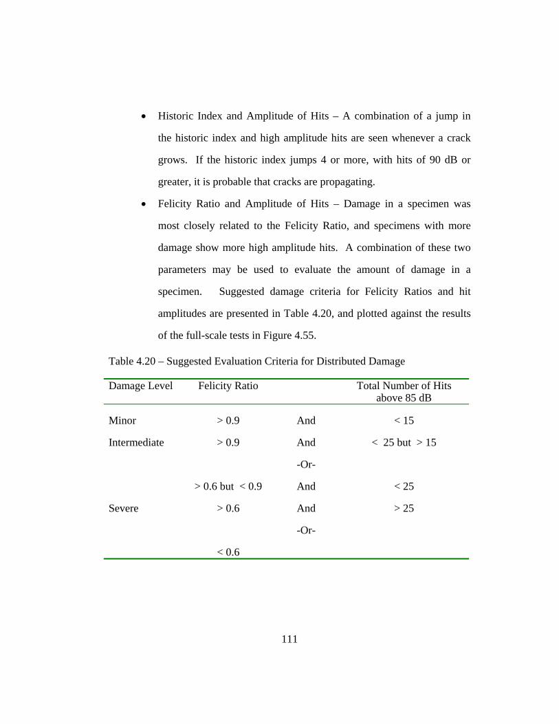
• Historic Index and Amplitude of Hits – A combination of a jump in
the historic index and high amplitude hits are seen whenever a crack
grows. If the historic index jumps 4 or more, with hits of 90 dB or
greater, it is probable that cracks are propagating.
• Felicity Ratio and Amplitude of Hits – Damage in a specimen was
most closely related to the Felicity Ratio, and specimens with more
damage show more high amplitude hits. A combination of these two
parameters may be used to evaluate the amount of damage in a
specimen. Suggested damage criteria for Felicity Ratios and hit
amplitudes are presented in Table 4.20, and plotted against the results
of the full-scale tests in Figure 4.55.
Table 4.20 – Suggested Evaluation Criteria for Distributed Damage
Damage Level Felicity Ratio Total Number of Hits above 85 dB
Minor > 0.9 And < 15
Intermediate > 0.9 And < 25 but > 15
-Or-
> 0.6 but < 0.9 And < 25
Severe > 0.6 And > 25
-Or-
< 0.6
111
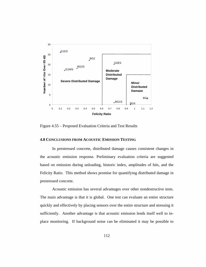
0
5
10
15
20
25
30
0 0.1 0.2 0.3 0.4 0.5 0.6 0.7 0.8 0.9 1 1.1 1.2
Felicity Ratio
BG1
BG4BG1S
G2ESBG2
BG2S
G1ES
G1WS
Severe Distributed Damage
Moderate Distributed Damage
Minor Distributed Damage
Figure 4.55 – Proposed Evaluation Criteria and Test Results
4.8 CONCLUSIONS FROM ACOUSTIC EMISSION TESTING
In prestressed concrete, distributed damage causes consistent changes in
the acoustic emission response. Preliminary evaluation criteria are suggested
based on emission during unloading, historic index, amplitudes of hits, and the
Felicity Ratio. This method shows promise for quantifying distributed damage in
prestressed concrete.
Acoustic emission has several advantages over other nondestructive tests.
The main advantage is that it is global. One test can evaluate an entire structure
quickly and effectively by placing sensors over the entire structure and stressing it
sufficiently. Another advantage is that acoustic emission lends itself well to in-
place monitoring. If background noise can be eliminated it may be possible to
112
113
leave sensors on a bridge, continuously monitor normal traffic, and determine the
increase in distributed damage. If a continuous monitoring program were not
adopted, another less convenient solution would be to close the bridge and run
equipment of known weight over it. Although this application was not researched
as part of this thesis, the groundwork was laid for its possible future development.
Acoustic emission also has some drawbacks. One of the most significant
drawbacks is that it is application specific. The results presented here apply only
to prestressed concrete girders with loading conditions and sensor arrangements
similar to those presented in this thesis. Also, as seen in BG4S, the loading
method must stress the defect for detection. Another drawback is the high
attenuation of acoustic emission in concrete. Although low-frequency sensors
minimize this effect, it is still significant.
114

Chapter 5 – Short-Pulse Radar
Short-Pulse Radar is a nondestructive test method that has been used
successfully to find delaminations, reinforcement, layer thicknesses and defects in
concrete, pavement and soils. This chapter describes the method and summarizes
experience in applying it to concrete with distributed damage.
5.1 INTRODUCTION TO SHORT PULSE RADAR
Short-Pulse Radar, sometimes referred to as Ground-Probing Radar
(GPR), is based on reflections of electromagnetic energy from materials with
different dielectric constants. It works like ultrasonic and pulse-echo methods,
but uses electromagnetic energy rather than sound.
When electromagnetic energy encounters a boundary between two
different materials, some is transmitted and the rest is reflected. How much is
transmitted and how much is reflected depends on the relative values of the
dielectric constants of the materials. The reflection coefficient at the interface of
the two materials is given by:
21
2112
rr
rr
eeee
+
−=ρ (Eqn 5.1)
115

where ρ12 is the reflection coefficient, and er is the dielectric constant relative to
air for each material. Typical dielectric constants for various materials are shown
in Table 5.1.
The velocity with which the electromagnetic wave travels through a
substance depends on the dielectric constant and is calculated as shown below:
reCV = (eqn 5.2) ,
where C is the speed of light and V is the velocity of the wave though the material
with relative dielectric constant er. As shown in Figure 5.1, an incident wave is
introduced from the antenna. At the boundary between Medium 1 and Medium 2
some of the energy is transmitted and the rest is reflected back. The same thing
happens at the boundary between Medium 2 and Medium 3. By recording the
time between reflections, the thickness of Medium 2 can be calculated.
116

Table 5.1 - Typical Dielectric Constants for Various Materials
Material Approximate Relative Dielectric Constant
At 25 C
Clay Soil (Dry) 2.5
Air 1
Concrete 6
Styrofoam 1.03
Water 78
Steel ∞
Antenna
Medium 1
Medium 2
Medium 3
Incident Wave
First Reflection
Second Reflection
Depth of Layer
Figure 5.1 - Propagation of Electromagnetic Waves through Media of Different Dielectric Constants
117

Radar systems are set up with a “pitch-catch” antenna housing both an
emitter and a receiver. The antenna emits a signal, pauses to pick up the
reflections, and then emits a new signal. This happens at high speed, creating an
almost continuous scan.
For evaluation purposes each signal (A-Scan) is plotted next to the
previous one creating a color-coded chart called a B-Scan. Figure 5.2
demonstrates this more clearly. On the left side of Figure 5.2 is one received
signal, or A-Scan. In this area there are 2 small colored lines, a pink one and a
green one. Any signal to the right of the green line will be shown green in the B-
Scan, and any signal to the left of the pink line will be represented as pink in the
B-Scan. Between these two lines the color changes accordingly. In essence, A-
Scans are color-coded and plotted next to each other to create a B-Scan, shown to
the right of the A-Scan. Differences in the signal, and the corresponding
discontinuities in the specimen, are easier to see on the B-Scan than on the A-
Scan.
118

Direction of Travel along the Beam
Figure 5.2 - Typical A-Scan and B-Scan From Sample BG2
5.2 TEST SETUP
Pulse Radar, Inc. (Houston, Texas) was contracted to perform a short-
pulse radar survey on the box girder specimens at Ferguson Laboratory. Their
equipment consisted of a 1 GigaHertz center frequency antenna with a high-speed
data acquisition computer and a wheel mounted encoder to measure distance
A-Scan B-Scan
Air
on o
ther
side
of
the
Gird
er
Inte
rfer
ence
fr
om A
nten
na
Are
a of
In
tere
st
119

(Figure 5.3). Because the antenna covered about half the depth of the beam, two
passes were required to monitor the entire side of the girder.
Data Acquisition Computer
Antenna
Distance Measuring Instrument
Figure 5.3 - Short Pulse Radar Equipment
Since microwaves reflect only at a change in dielectric constant, short-
pulse radar cannot detect closed cracks. Although it was anticipated that it would
be difficult to identify the individual cracks, it was postulated that distributed
cracking could affect the overall dielectric constant, and that this change in
dielectric constant would be detected by the reflection of electromagnetic energy
and by changes in the velocity of the wave in the concrete.
120
To test this hypothesis, two different specimens were tested, the girder
with bad end damage, (BG2), and the girder which was continuously soaked with
water, (BG4). BG2 was chosen because the damage at the its ends was
significantly worse than at other places along its length, which should cause a
variation of dielectric constants between the ends and other areas. The
continuously soaked girder was chosen because it had a variation of damage along
the length, and was wet at the time of test. It was hoped that water, which has a
much higher dielectric constant than concrete, would soak into the cracks,
creating a much larger change in dielectric constant between the badly damaged
areas and the less damaged ones. As can be seen in the table of typical dielectric
constants, if air fills the cracks, the dielectric constant should decrease; if water
fills them the dielectric constant should increase.
Francisco Alvarez (Pulse Radar, Inc.) completed the testing along with
researchers Brian Tinkey and Anna Boenig. The complete west side and
southeast side of girder BG2 were scanned along the bottom and top of the girder.
The northeast side was not scanned due to access problems. On BG4, only the
bottom half of the west side was tested due to the location of the girder. Results
are presented in the next section.
5.3 RESULTS OF THE SHORT PULSE RADAR SURVEY
Pulse Radar, Inc. completed the analysis and a issued a report to The
University of Texas at Austin, along with all the data files and software required
for further review. Figures 5.4 though 5.6, taken from that report provide a brief
summary of their findings.
121

Figure 5.4 - Dielectric Values on West Side of BG2
Figure 5.5 -Dielectric Values on East Side of BG2 at the A-End
Figure 5.6 - Dielectric Values on the East Side of BG4
122

123
An independent review of the data at the University of Texas did not
discover any other significant results.
5.4 DISCUSSION
It can be seen from Figures 5.4 and 5.5 that while dielectric values do vary
along the length of BG2, this variation seems random, and does not correlate with
observed damage.
Interestingly, the dielectric values for BG4 are considerably higher than
for BG2. This was expected, because it was saturated with water at the time of
testing.
Assuming that a difference in dielectric constants could be determined,
this method has other difficulties. The first difficulty is accessibility. The
antenna for the short pulse radar is quite large and requires sufficient space
between the girders. Another difficulty is that this method would give an average
dielectric constant over the depth, so that variations in deterioration within the
width would not be detectable. Finally, data interpretation can be complicated
and should only be done by experienced individuals.
5.5 CONCLUSION
Although short-pulse radar may be able to detect distributed damage, that
hypothesis was not demonstrated here. At this time, short-pulse radar is unable to
reliably distinguish the variation in amount of cracking. Although it can be
successfully used to locate inclusions, delaminations, and other larger defects
accurately and quickly, the detection of small, distributed cracks seems beyond its
capacity. Much more research and development must be undertaken to make this
method useful.
124

Chapter 6 – Impact-Echo
6.1 INTRODUCTION TO IMPACT-ECHO
Impact-Echo is a non-destructive test method based on the propagation of
a stress wave through concrete. An impact, usually caused by a small steel ball, is
made on the surface, sending a pressure wave into the concrete. This wave is then
reflected off the back surface or a defect. By analyzing the frequency of the
reflected waves along with their known wave speed in concrete, it is possible to
determine the depth to the back surface or the defect.
Impact-echo is preferred over ultrasonics for concrete due to the high
attenuation of ultrasound in concrete. Since the aggregate in concrete is rather
large compared to the wavelength of ultrasound, it is difficult to generate a large
enough pulse with a piezoelectric sensor which will not attenuate quickly and will
make the concrete appear homogeneous.
Figure 6.1 shows a schematic representation of a typical impact-echo test.
Three types of waves are generated from the surface impact. The R-wave, or
Rayleigh wave, is a surface wave that usually passes the transducer only once.
The S-wave, or shear wave, has a maximum amplitude at 45 degrees from the
impact and therefore travels away from the point of impact causing very little
displacement at the sensor when reflected off the back wall. In contrast, the P-
wave or compression wave has maximum amplitude at the center and will have
the most influence on a transducer placed near the point of impact.
125
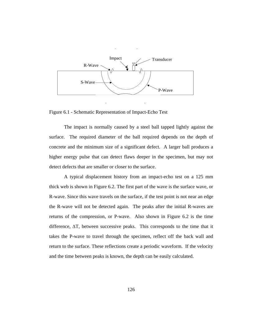
P-Wave
S-Wave
R-WaveImpact Transducer
Figure 6.1 - Schematic Representation of Impact-Echo Test
The impact is normally caused by a steel ball tapped lightly against the
surface. The required diameter of the ball required depends on the depth of
concrete and the minimum size of a significant defect. A larger ball produces a
higher energy pulse that can detect flaws deeper in the specimen, but may not
detect defects that are smaller or closer to the surface.
A typical displacement history from an impact-echo test on a 125 mm
thick web is shown in Figure 6.2. The first part of the wave is the surface wave, or
R-wave. Since this wave travels on the surface, if the test point is not near an edge
the R-wave will not be detected again. The peaks after the initial R-waves are
returns of the compression, or P-wave. Also shown in Figure 6.2 is the time
difference, ΔT, between successive peaks. This corresponds to the time that it
takes the P-wave to travel through the specimen, reflect off the back wall and
return to the surface. These reflections create a periodic waveform. If the velocity
and the time between peaks is known, the depth can be easily calculated.
126

Figure 6.2 – Typical Displacement History for an Impact-Echo Test
If a defect is present in the specimen, the P-wave will reflect off both the
defect and the back wall, complicating the displacement plot. It is nearly always
difficult in practice to read the time between peaks directly from the plot since
there are reflections from reinforcement, defects, sides, and voids. To solve this
problem, a Fast Fourier Transform is used to transform the displacement history
from the time domain to the frequency domain. Peaks on the frequency spectrum
correspond to the dominant frequencies in the wave. Figure 6.3 is the frequency
spectrum for the waveform shown previously in the time domain in Figure 6.2.
Since this was from a solid specimen there is only one peak, corresponding to the
thickness of the web. If a defect were present in the sample there would be two
frequency peaks, one for the defect and the other for the back wall.
127
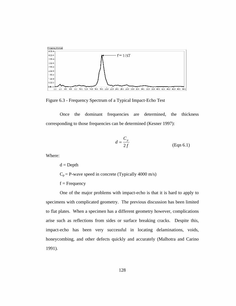
Figure 6.3 - Frequency Spectrum of a Typical Impact-Echo Test
Once the dominant frequencies are determined, the thickness
corresponding to those frequencies can be determined (Kesner 1997):
fC
d p
2= (Eqn 6.1)
Where:
d = Depth
Cp = P-wave speed in concrete (Typically 4000 m/s)
f = Frequency
One of the major problems with impact-echo is that it is hard to apply to
specimens with complicated geometry. The previous discussion has been limited
to flat plates. When a specimen has a different geometry however, complications
arise such as reflections from sides or surface breaking cracks. Despite this,
impact-echo has been very successful in locating delaminations, voids,
honeycombing, and other defects quickly and accurately (Malhotra and Carino
1991).
128

6.2 APPLICATION OF IMPACT-ECHO TO CONCRETE WITH DISTRIBUTED DAMAGE
Research was completed at Cornell University on applying impact-echo to
concrete with distributed damage (Kesner 1997). A different type of analysis is
required for concrete with distributed damage because instead of a discrete flaw,
an overall degradation of the concrete must be detected. A method was proposed
to quantify the amount of damage by monitoring how quickly the P-wave
attenuates.
As a compression wave (P-wave) travels through concrete, some of its
energy is lost due to scattering from voids, microcracks, and aggregate. When
concrete cracks due to premature concrete deterioration the scattering increases,
causing more rapid attenuation. By quantifying how quickly the compression
wave attenuates, it should be possible to quantify distributed damage in the
concrete.
Kesner (1997) used finite element models to determine the theoretical
response to a distributed damage. To model distributed cracking, some elements
in the model were “softened” by lowering their modulus of elasticity.
Analytically the P-wave attenuated by scattering at the interfaces between the
softer elements and the normal elements. The resulting displacement histories
from simulated impact-echo tests on these models were then filtered by a high-
pass Butterworth filter with a 10 kHz cutoff to eliminate the low frequency
components. This allowed for clear compression wave peaks and a more
pronounced decay of the wave. Four major results were discovered from these
models; as damage increased:
129
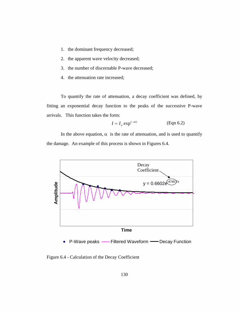
1. the dominant frequency decreased;
2. the apparent wave velocity decreased;
3. the number of discernable P-wave decreased;
4. the attenuation rate increased;
To quantify the rate of attenuation, a decay coefficient was defined, by
fitting an exponential decay function to the peaks of the successive P-wave
arrivals. This function takes the form: (Eqn 6.2) )(exp t
oII α−=
In the above equation, α is the rate of attenuation, and is used to quantify
the damage. An example of this process is shown in Figures 6.4.
y = 0.6602e-4740.7x
Time
Am
plitu
de
P-Wave peaks Filtered Waveform Decay Function
Decay Coefficient
Figure 6.4 - Calculation of the Decay Coefficient
130

Results from the finite element models of Kesner (1997) are summarized
in Table 6.1. As damage level increases, the number of P-wave arrivals decreases
and the decay coefficient increases.
Table 6.1 - Results of Finite Element Models For 130 mm Thick Concrete Plate (Kesner 1997)
Damage Level No. of P-wave Arrivals Decay Constant
Little or None 13 or More Less than 3100
Minimal 13 to 11 3100 to 4000
Moderate 11 to 10 4000 to 5000
Severe 9 or Less Greater than 5000
The method described above was also applied by Kesner (1997 in a field
test on box girders from the same batch described in Chapter 2. Results from
those tests were consistent with the finite element simulations. Sections with little
to no damage had 17 to 24 discernible P-waves and decay coefficients of 1700
and 2030. A beam with moderate damage had 12 P-wave peaks with a decay
coefficient of 4550. Finally,a heavily damaged specimen had a decay of 11600
using 4 P-wave arrivals, and 8950 using 6 P-wave arrivals.
6.3 TESTING PROGRAM
Impact-echo testing was performed at The University of Texas at Austin
to evaluate the results presented in the previous section, and to explore the overall
value of the impact-echo method to members with distributed damage. Two
results from the Cornell study, reduction in dominant frequency and in apparent
131

wave velocity, were not investigated since they were most likely due to the
method of modeling attenuation. Because wave speed is related to the modulus of
elasticity, “softening” elements would naturally decrease the wave speed and the
dominant frequency. The major conclusions of the Cornell study, however (the
number of discernable p-wave peaks and the decay coefficient), were investigated
at the University of Texas at Austin.
Specimens BG1 and BG3 were tested at Ferguson Laboratory and
analyzed to find their decay constants. These girders are described in Chapters 2
and 3. Both were from the same set of girders that were tested in the Cornell
study (Section 6.2). In view of this, differences in geometry are not a factor.
Since the testing at The University of Texas at Austin was performed after the
Cornell testing, the girders would have had about 4 more years to deteriorate
further, and should therefore have been in worse condition.
As discussed in Chapter 3, BG1 was a control girder with the least amount
of cracking of any of the girders tested. Impact-echo tests were performed in
areas of that girder that appeared visually to be in good condition. Although this
girder had little damage compared to the others, it was not damage-free. Data
were taken 5 feet from the south end, 7 feet from the south end, and 8 feet from
the centerline. These areas were chosen since the visible damage there was small,
clear P-wave peaks could be found on the waveform, and the test indicated that
the thickness was close to the expected 127 mm, indicating solid concrete.
Figures 6.5 and Figure 6.6 show the damage. The tested areas have light spider-
web cracking, but no major cracks.
132

Small Horizontal Crack
Spider-web Cracking
Test Point
Figure 6.5 - Photo of the Test Point 8 feet from Centerline on BG1
133

Small Horizontal Crack
Spider-web Cracking
Test Point
Figure 6.6 - Photo of the Test Point 7 feet from the South End of BG1
For comparison, tests were also conducted on BG3, the specimen with
damage along its length. This specimen was chosen for its extensive spider-web
cracking lack of many large cracks. Tests were performed on this girder 3 feet
from the north end and 22 feet from the south end. The point 3 feet from the
north end is shown in Figure 6.7. There is extensive cracking on the left hand side
as well as above the test point. The other testing point on BG3 is shown in Figure
6.8. Although there was no cracks in the immediate area, there were some in the
web on the left side.
134
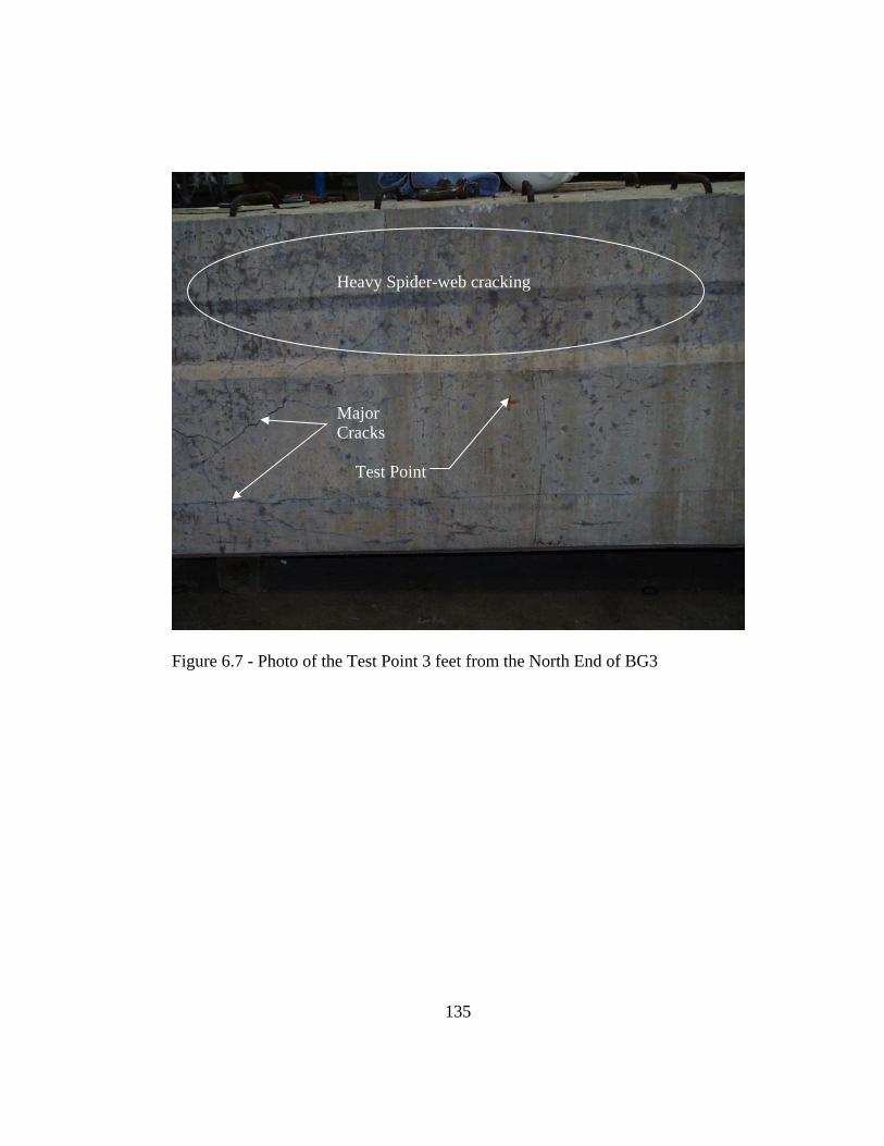
Heavy Spider-web cracking
Major Cracks
Test Point
Figure 6.7 - Photo of the Test Point 3 feet from the North End of BG3
135
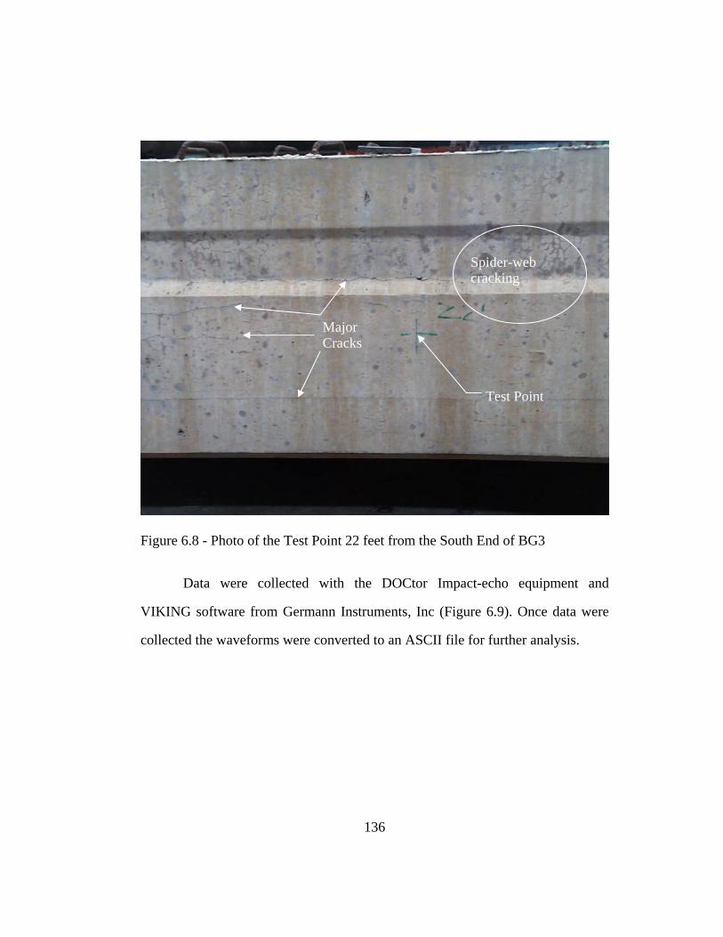
Spider-web cracking
Major Cracks
Test Point
Figure 6.8 - Photo of the Test Point 22 feet from the South End of BG3
Data were collected with the DOCtor Impact-echo equipment and
VIKING software from Germann Instruments, Inc (Figure 6.9). Once data were
collected the waveforms were converted to an ASCII file for further analysis.
136

Figure 6.9 - Photo of DOCtor Impact-Echo Equipment
The displacement history for each test was filtered using a high-pass, 5th -
order Butterworth filter in LabView. As suggested, a 10 kHz cutoff frequency
was used. An unfiltered waveform and its resulting frequency spectrum are
shown in Figure 6.10. Low-frequency elements were not as prevalent in the
actual tests as in the finite-element simulations. The filter did make slight
difference, however, and was used for all tests. The same test, filtered, is shown
in Figure 6.11. All frequencies under 10 kHz are removed.
137

(a)
(b)
Figure 6.10 - (a) Unfilterd Displacement History in Time Domain (b) Unfiltered Frequency Spectrum
138

(a)
(b)Figure 6.11 - (a) Filterd Displacement History in Time Domain (b) Filtered
Frequency Spectrum
A summary of the procedure used in this analysis is outlined below:
1. Perform impact-echo test.
2. Convert the waveform to an ASCII file.
3. Filter out low frequencies using a Butterworth filter (this can be done
easily in programs such as LabView or Matlab).
4. Plot the filtered displacement history and identify the peaks.
5. Using regression analysis to fit an exponential attenuation curve to the
peaks.
139

6.4 RESULTS
Two tests were performed at each location on BG1, for a total of 6 tests.
The filtered waveforms, the peaks used to fit the decay function, and the best-fit
decay function are given in Appendix B. Fewer clear peaks were available than
in the Cornell research. Instead of the 17 to 24 peak peaks available to calculate
the decay constant, 4 to 7 peaks were used. Results are summarized in Table 6.2.
Table 6.2 - Results of Impact-Echo Tests on BG1
Sample Location Test Number No of Peaks Used Decay Constant
8 feet from Centerline 1 4 5957
2 6 4741
7 feet from South End 1 5 4910
2 5 2891
5 feet from South End 1 6 3035
2 7 3211
Average 5.5 4124
BG3 had considerably more damage than BG1 and was tested for
comparison. Again, two tests were conducted per point, for a total of 4 tests.
Plots displaying the filtered waveforms, the peaks used to fit the decay function,
and the best fit decay function are given in Appendix B. For the worst samples,
no more than 5 peaks in any waveform were used to calculate the decay constant.
Although the damage appeared visibly worse near the end of the girder, the decay
constant was lower there. The results are summarized in Table 6.3.
140

Table 6.3 - Results of Impact-Echo Tests on BG3
Sample Location Test Number No of Peaks Used Decay Constant
22 feet from South End 1 4 7316
2 4 8274
3 feet from North End 1 5 5480
2 4 5031
Average 4.25 6525
6.5 DISCUSSION OF IMPACT ECHO RESULTS
The impact-echo method clearly shows promise for quantifying the
amount of distributed damage. Difficulties need to be resolved, however before
the method can be used reliably for that purpose.
The most striking difficulty was choosing the P-wave peaks. It is difficult
to choose how many peaks in the waveform should be skipped to account for the
R-wave, and how far the P-wave arrivals can be distinguished. The R-Wave
arrives at the beginning of the displacement history, and should not be included
when calculating the decay constant. It is sometimes difficult to distinguish,
though, where the surface wave ends and the P-wave arrivals begin. In this
analysis, two peaks were skipped to account for the surface wave. If only one
peak had been skipped, however the attenuation constants would have changed
greatly. Increasing the number of peaks for the same displacement history would
decrease the decay constant. It is often difficult, however, to use the same
number of points in each waveform.
141

As discussed above, the value of the decay constant could vary greatly
depending on how many and which peaks were chosen. To illustrate this, a test
from BG3 with many easily discernable peaks was analyzed using a variety of
peaks. The results are presented in Table 6.4. Calculated decay constants range
from 3000 to 10000, depending on the P-wave arrivals that were chosen.
Table 6.4 - Decay Constants for a Test Performed on BG3
Decay Constant
Number of Peaks If 2 Peaks are Skipped for R-Wave
If 1 Peak is Skipped for R-Wave
3 8185 97534 5032 84615 4040 62096 3210 51297 3145 42198 3678 39579 3423 401810 3240 380711 3319 360612 N/A 3639
Another difficulty is the possibility of reflections from sides or surface
cracks. If the point being tested is close to a geometrical discontinuity, the
reflected waves can become very complex, creating difficulty in identifying
successive P-wave arrivals. Thus, impact-echo lends itself best to plate-like
specimens such as girder webs. If girder flanges are to be tested, where
prestressing strand might debond, the geometry makes the analysis very difficult.
There are a few possible ways to improve the impact-echo method. One
way is average the peaks of many tests to get a more accurate decay curve. The
data in Appendix B commonly show interference in the signal, causing a variation
142

in peak height in the displacement history. If several tests were performed at one
point and the signals were combined, interference from one test would not
significantly affect the results.
Since the impact-echo method is concerned only with peaks from
reflections from the backwall, another possible method of improving the results
would be to use a bandpass filter around the dominant frequency to eliminate any
interference. Results from a 5th-order Butterworth bandpass filter are shown in
Figure 6.12. The significance of the R-wave is decreased, and the subsequent P-
wave peaks are larger and easier to identify. Even when using these techniques,
however, it is still necessary to determine how many peaks chosen.
143

Unfiltered Signal
10 kHz Highpass Filter
10 kHz to 20 kHz Bandpass Filter
Figure 6.12 - Results of Filtering the Displacement History
6.6 CONCLUSIONS REGARDING IMPACT-ECHO
Although the impact-echo method can in theory, be used to detect
distributed damage in concrete, it is difficult to apply to field specimens at this
time. The current procedure of fitting a decay curve can be easily biased by the
144

145
method of picking the P-wave peaks. If the difficulty of picking P-wave arrivals
were solved and a correlation with the decay constant were still present, Impact-
echo would be valuable. Setup is quick, and many points can be tested quickly.
In addition, if the distributed cracking has created a delamination, its size and
shape could be determined easily.
Difficulties with the impact-echo method include the fact that it is a local
test, developed for flat plates. If many boundaries are present near the test point,
analysis of the data becomes quite difficult.

146
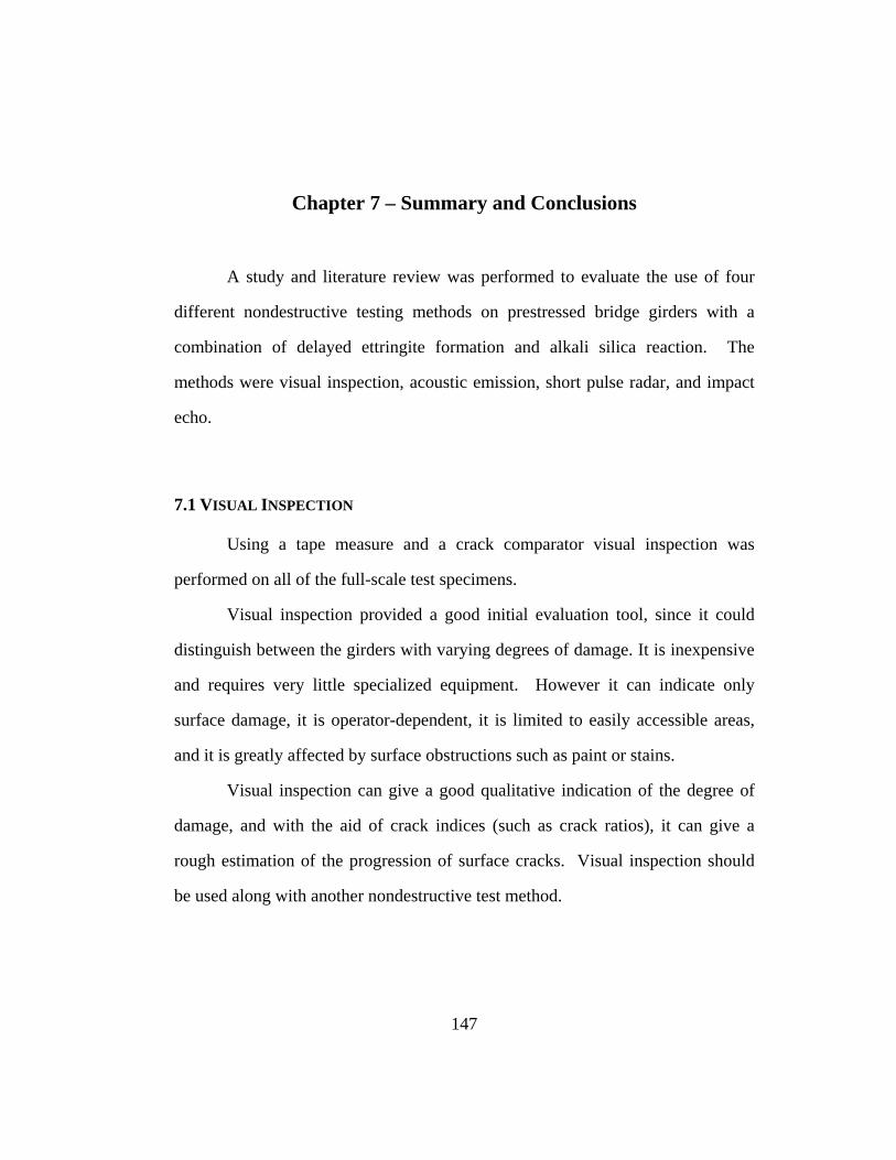
Chapter 7 – Summary and Conclusions
A study and literature review was performed to evaluate the use of four
different nondestructive testing methods on prestressed bridge girders with a
combination of delayed ettringite formation and alkali silica reaction. The
methods were visual inspection, acoustic emission, short pulse radar, and impact
echo.
7.1 VISUAL INSPECTION
Using a tape measure and a crack comparator visual inspection was
performed on all of the full-scale test specimens.
Visual inspection provided a good initial evaluation tool, since it could
distinguish between the girders with varying degrees of damage. It is inexpensive
and requires very little specialized equipment. However it can indicate only
surface damage, it is operator-dependent, it is limited to easily accessible areas,
and it is greatly affected by surface obstructions such as paint or stains.
Visual inspection can give a good qualitative indication of the degree of
damage, and with the aid of crack indices (such as crack ratios), it can give a
rough estimation of the progression of surface cracks. Visual inspection should
be used along with another nondestructive test method.
147

7.2 ACOUSTIC EMISSION
Acoustic emission testing was performed on prestressed concrete girders
with a wide range of damage. In total, ten tests were monitored on box and Type
C sections under both shear and flexure.
Acoustic emission shows promise for quantifying distributed damage in a
specimen. Based on this study, preliminary evaluation criteria are proposed
(Section 4.7) using the emission during unloading, historic index, amplitude of
hits, and the Felicity ratio. Emission during unloading was related to
delaminations; historic index and high amplitude hits were related to crack
growth; and the Felicity ratio and high amplitude hits could be correlated to
damage.
Acoustic emission can inspect a large area of the bridge at one time and it
lends itself well to in place monitoring. Its drawbacks include:
i) the need to stress a defect enough for it to be detected. This is not
normally a problem since a structurally significant defect will be
stressed;
ii) the high attenuation of acoustic emission in concrete, which creates
a need for many sensors;
iii) the need for road closures if a continuous monitoring program is
not adopted.
If practical issues such as background noise from the traffic, protection of
sensors and environmentally induced emission from rain or freezing can be
148

resolved, acoustic emission would be ideal for monitoring the increase of
distributed damage.
Acoustic Emission should be investigated further by verifying the
laboratory results with field tests and determining the level and significance of
background noise.
7.3 SHORT-PULSE RADAR
Short-pulse radar was used to examine two different box girders and
thereby determine if differences could be seen between the varying degrees in
damage along their length. One specimen was wet when testing so that water
would fill the cracks and increase the dielectric constant; the other specimen was
left dry to see if the air in the cracks would lower the dielectric constant.
Results from this testing did not show that this method could accurately
gage the amount of damage at this time. Although a variation of dielectric
constants was seen, it did not correlate with the areas of increased damage.
If in the future this method were able to determine the amount of
distributed damage, it would have the advantage of speed. Since electromagnetic
waves are airborne, no attachments to the girder are required, and results is very
rapid.
Short-pulse radar should not be used to quantify the amount of distributed
damage in concrete until more research is completed.
149

7.4 IMPACT-ECHO
Impact-echo testing was performed on the webs of two box girders with
different amounts of deterioration. Data from these tests were analyzed as
proposed by Kesner (1997) to determine if the amount of distributed cracking
could be determined by P-wave attenuation.
Results presented in this thesis were encouraging, however, they were
found to be easily biased. The proposed method involves choosing the peaks of
the returning P-waves and fitting an exponential curve to them in order to
measure how attenuation. The number of returning P-waves included in the
regression could greatly change the results. In addition, it was sometimes difficult
to distinguish the peaks of the P-waves due to interference from other reflections.
If a standard and reliable method of picking the P-wave peaks were found,
the impact-echo method would be a valuable tool. The test is quick to set up and
perform, but can determine the condition of the concrete only at the point where
that the test is performed.
Research should be performed to standardize the method of choosing the
P-wave arrivals before the test is used in the field. This process could possibly
be helped by using a bandpass filter to isolate the frequency of interest, and by
combining multiple tests at the same point to eliminate the interference that might
occur in any single test. The effectiveness of these suggestions was not
determined.
150
7.5 CONCLUSIONS AND RECOMMENDATIONS
A summary of the major conclusions and recommendations that were
arrived at through this study are listed below.
• Visual inspection provides a good qualitative evaluation and should be
preformed first before any other tests are conducted.
• Acoustic emission shows promise for evaluating the amount of distributed
damage in concrete.
• Evaluation criteria for acoustic emission on prestressed girders with
distributed damage were proposed and should be verified with field tests.
• Short-pulse radar did not demonstrate the ability of detecting distributed
damage.
• Impact-echo testing was encouraging, however somewhat subjective.
• A more standard procedure for impact-echo testing should be further
researched before implementation.
• Other nondestructive tests that were not discussed, such as ultrasonics, should
be investigated.
151
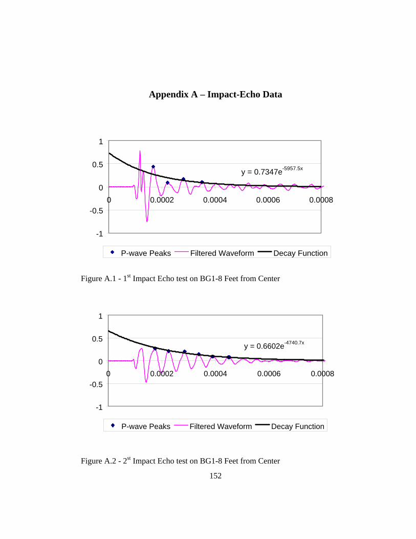
Appendix A – Impact-Echo Data
y = 0.7347e-5957.5x
-1
-0.5
0
0.5
1
0 0.0002 0.0004 0.0006 0.0008
P-wave Peaks Filtered Waveform Decay Function
Figure A.1 - 1st Impact Echo test on BG1-8 Feet from Center
y = 0.6602e-4740.7x
-1
-0.5
0
0.5
1
0 0.0002 0.0004 0.0006 0.0008
P-wave Peaks Filtered Waveform Decay Function
Figure A.2 - 2st Impact Echo test on BG1-8 Feet from Center
152

y = 0.8036e-4910.2x
-1
-0.5
0
0.5
1
0 0.0002 0.0004 0.0006 0.0008
P-wave Peaks Filtered Waveform Decay Function
Figure A.3 - 1st Impact Echo test on BG1-7 Feet from South End
y = 0.4624e-2890.9x
-1
-0.5
0
0.5
1
0 0.0002 0.0004 0.0006 0.0008
P-wave Peaks Filtered Waveform Decay Function
Figure A.4 - 2nd Impact Echo test on BG1-7 Feet from South End
153
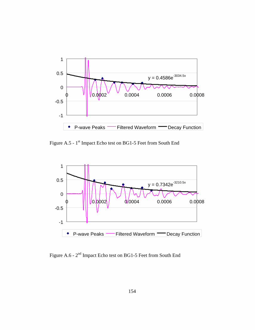
y = 0.4586e-3034.5x
-1
-0.5
0
0.5
1
0 0.0002 0.0004 0.0006 0.0008
P-wave Peaks Filtered Waveform Decay Function
Figure A.5 - 1st Impact Echo test on BG1-5 Feet from South End
y = 0.7342e-3210.5x
-1
-0.5
0
0.5
1
0 0.0002 0.0004 0.0006 0.0008
P-wave Peaks Filtered Waveform Decay Function
Figure A.6 - 2nd Impact Echo test on BG1-5 Feet from South End
154

y = 0.755e-5480x
-1
-0.5
0
0.5
1
0 0.0002 0.0004 0.0006 0.0008
P-wave Peaks Filtered Waveform Decay Function
Figure A.7 - 1st Impact Echo test on BG3-3 Feet from North End
y = 0.3802e-5031.5x
-1
-0.5
0
0.5
1
0 0.0002 0.0004 0.0006 0.0008
P-wave Peaks Filtered Waveform Decay Function
Figure A.8 - 2nd Impact Echo test on BG3-3 Feet from North End
155
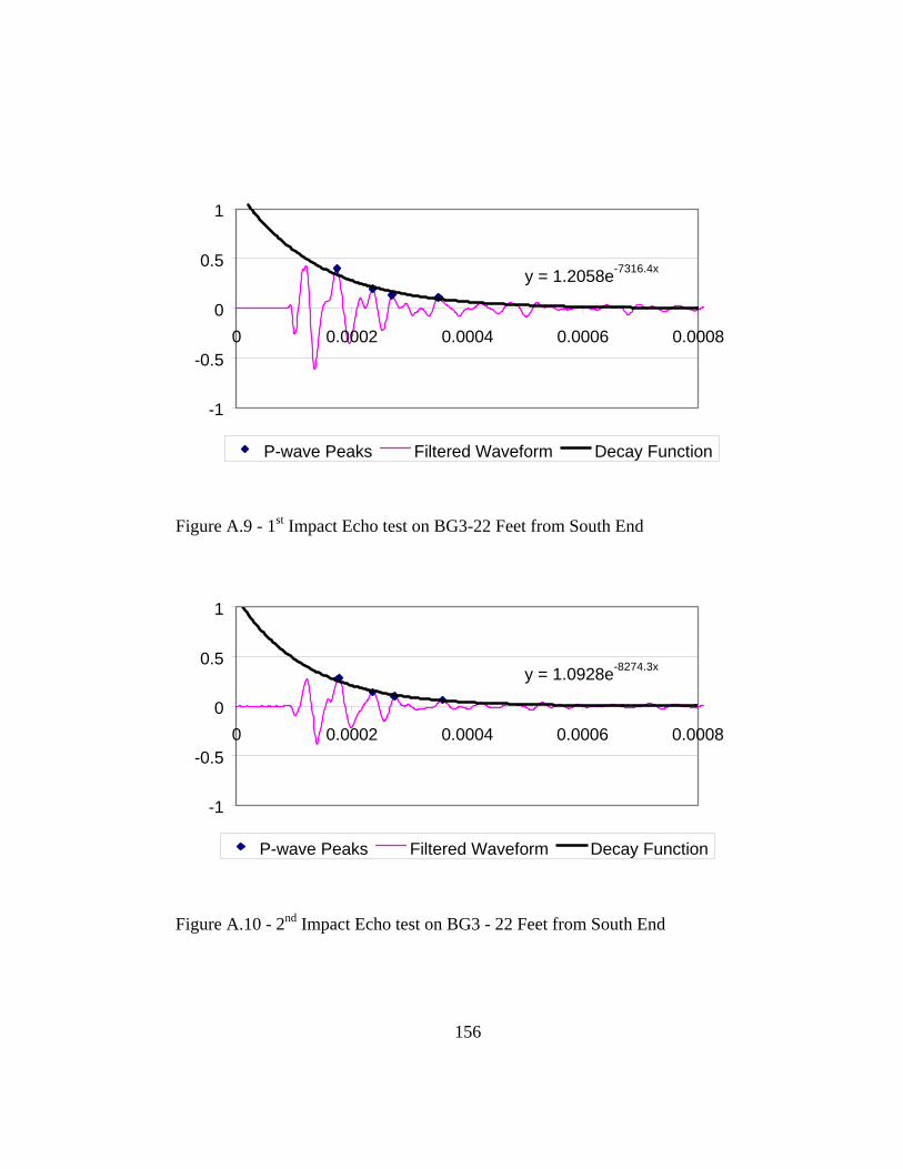
y = 1.2058e-7316.4x
-1
-0.5
0
0.5
1
0 0.0002 0.0004 0.0006 0.0008
P-wave Peaks Filtered Waveform Decay Function
Figure A.9 - 1st Impact Echo test on BG3-22 Feet from South End
y = 1.0928e-8274.3x
-1
-0.5
0
0.5
1
0 0.0002 0.0004 0.0006 0.0008
P-wave Peaks Filtered Waveform Decay Function
Figure A.10 - 2nd Impact Echo test on BG3 - 22 Feet from South End
156

1

References
American Society of Mechanical Engineers, “Acoustic Emission Examination of
Metallic Vessels During Pressure Testing” AMSE Code Section 5 Article 12, Boiler and Pressure Vessel Code, New York, 1998
American Society of Nondestructive Testing, “Recommended Practice for
Acoustic Emission Evaluation of Fiber Reinforced Plastic Tanks and Pressure Vessels” ,Committee on Acoustic Emission from Reinforced Plastics, Draft I October 1999
American Society of Testing and Materials, ASTM E1316-94 ,”Standard
Terminology of Nondestructive Examinations”, 1994 Association of American Railroads, Operation and Maintenance Department,
“Procedure for Acoustic Emission Evaluation of Tank Cars and IM101 Tanks”, Issue 8,Washington D.C. October 1999
Barnes, C.A and Fowler, T.J. “Acoustic Emission Monitoring of Reinforced
Concrete Structures” Proceedings of the Sixth International Symposium on Acoustic Emission from Composite Materials (AECM-6) San Antonio, Texas American Society of Nondestructive Testing, June 1998 pp183-191
Boenig, A., “Bridges with Premature Concrete Deterioration: Field Observations
and Large-Scale Structural Testing”, M.S. Thesis, University of Texas at Austin, May 2000
Bray, D.E., Stanley, R.K. “Nondestructive Evaluation a Tool in Design
Manufacturing and Service” CRC Press, 1997 Diederichs, U., Schneider, U. and Terrien, M., “Formation and Propagation of
Cracks and Acoustic Emission”, Development in Civil Engineering 7: Fracture Mechanics of Concrete, 1983, Edited by F.H. Wittman.
Fowler, T.J., Blessing, J.A., Conlisk, P.J., Swanson, T.L., “The Monpac System”,
Journal of Acoustic Emission, Volume 8, Number 3
157

Fowler,T.J. “Experience with the Mandatory Acoustic Emission Test of an ASME Section X FRP Pressure Vessel” Procedings of NACE Corrosion 97 Conference, Paper 370, 1997
Funez, L.M., “Field Observations of Bridges with Premature Concrete
Deterioration: Structural Implications”, M.S. Report, University of Texas at Austin, December 1999.
Halmshaw, R “Non-Destructive Testing” Second Ed.. Edward Arnold, London,
England ,1991 Ishibashi, A., Matsuyama, K., Ohta, S., Ohtsu, M., “Acoustic Emission
Application for Diagnosis of Deteriorated Concrete of Harbor Structures” Kamada, T., Iwanami,M., Nagataki, S., Yuyama, S. and Ohtsuki, N. “Application
of Acoustic Emission Evaluation of Structural Integrity in Marine Concrete Structures”, Progress in AE VIII (JSNDI), Proc. 13th Inter. AE Symp. Nov. 27-30, 1996, Nara Japan pp355-360.
Karabinis, A.H, and Fowler, T.J. “Experiences with Two Reinforced Concrete
Aeration Basins”, Presented at the 1983 Fall Convention, American Concrete Institute, Kansas City, Missouri September 25-30.
Karihaloo, B.L. and Nallathambi, P., “Notched Beam Test: Mode 1 Fracture
Toughness”, RILEM Technical Committee 89-FMT Report: Fracture Mechanics Test Methods for Concrete, 1989, Edited by S.P. Shah and A. Carpinteri.
Kesner, Keith Evan “Detection and Quantification of Distributed Damage in
Concrete Using Transient Stress Waves”, Thesis at Cornell University, December 1997
Kim, Y. Personal Communication Between Yong-Mook Kim and Author at The
University of Texas at Austin, March 2000. Klingner, R.E., Fowler, T.J “Structural Assessment of In-Service Bridges with
Premature Concrete Deterioration”, Project Proposal for TxDot Project 0-1857, Submitted 1998.
Lawrence, 1997: Lawrence, B.L., E.D. Moody, R.N. Guillemette and R. L.
Carrasquillo, “Evaluation and Mitigating Measures for Premature Concrete Deterioration in Texas Department of Transpiration Concrete Elements.”
158

Malhotra V.M., Carino, N.J “CRC Handbook on Nondestructive Testing of
Concrete” CRC Press, 1991 Masi, A.K. and Sahu R. “Acoustic Emissions from Reinforced Concrete”
Experimental Mechanics, December 1994 pp 379-388 Murakami, Y. and Yuyama,S. “Acoustic Emission Evaluation of Structural
Integrity in Reinforced Concrete Beams due to Corrosion of Reinforcement”, Progress in AE VIII (JSNDI), Proc. 13th Inter. AE Symp. Nov. 27-30, 1996, Nara Japan pp217-244.
Nielsen, John and Griffen, D.F. “Acoustic Emission of Plain Concrete” Journal
of Testing and Evaluation, JTEVA, Vol 5, No.6 , Nov 1977, pp 467-483. Niseki, S., Satake, M. nad Gohke, m. “Quick Detection of Alkali-Agregate
Reaction by Acoustic Emission Monitoring” Progress in Acoustic Emission V, The Japanese Society of NDI, pg 529 1990
Ohtsu, M “Determination of Crack orientaion by Acoustic Emission”, Materials
Evaluation, Sept 1987 pp 1070-1075. Ohtsu, M “Estimation of Crack and Damage Progression in Concrete by
Quantitative Acoustic Emission Analysis”, Materials Evaluation, May 1999 pp521-525
Ohtsu, M, Sakimoto, T., Kacai, Y., Yuji, S. “Evaluation of Concrete Structure
Deterioration via AE Observation of Core Tests” Journal of Acoustic Emission Vol 7, No 4. Acoustic Emissions Group, pp 167-172 1988
Ohtsu, M. “Rate Process Analysis of AE Activity in Uniaxial Compression Test
of Core Specimens” Progress in Acoustic Emission V, Japaneese Society of NDI, pg 311, 1990
Ohtsu, M., Okamoto, T., Yuyama, S. ”Moment Tensor Analysis of Acoustic
Emission for Cracking Mechanisms in Concrete”, ACI Structural Journal, March-April 1998 pp 87-95
159
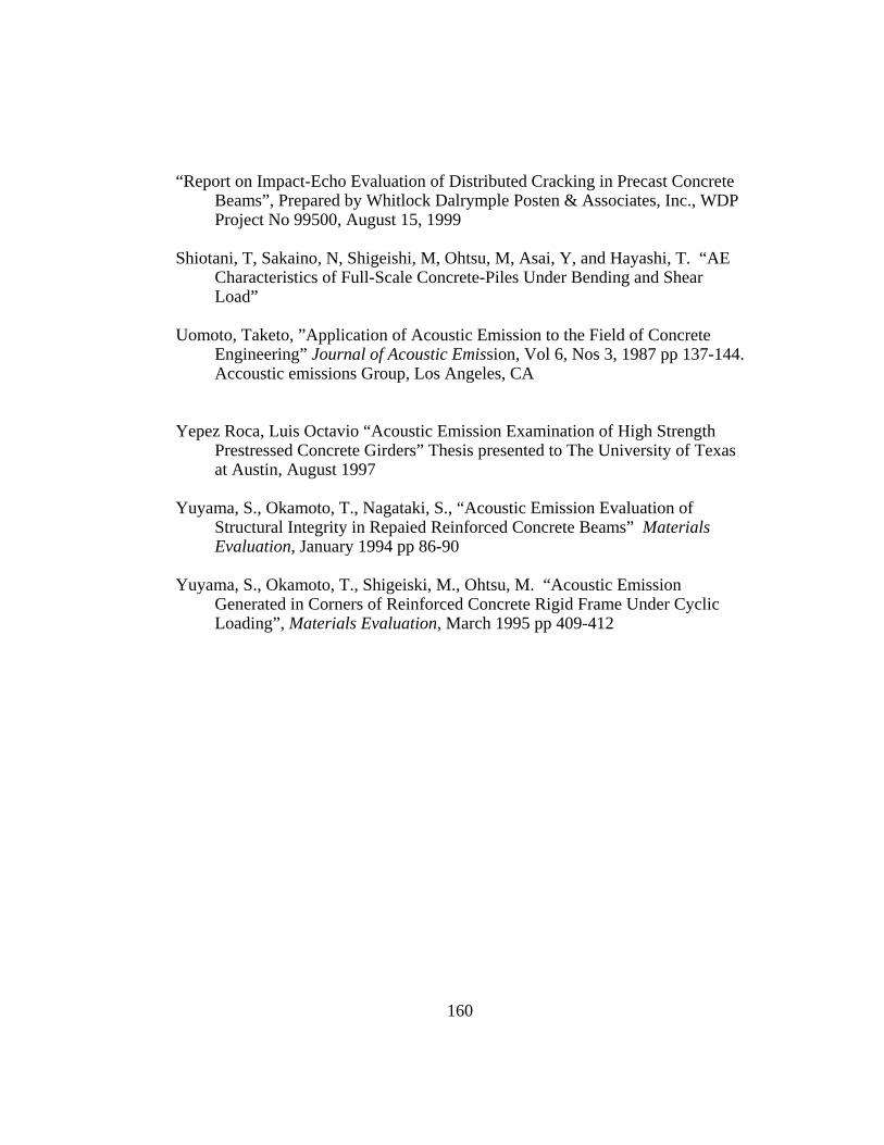
160
“Report on Impact-Echo Evaluation of Distributed Cracking in Precast Concrete Beams”, Prepared by Whitlock Dalrymple Posten & Associates, Inc., WDP Project No 99500, August 15, 1999
Shiotani, T, Sakaino, N, Shigeishi, M, Ohtsu, M, Asai, Y, and Hayashi, T. “AE
Characteristics of Full-Scale Concrete-Piles Under Bending and Shear Load”
Uomoto, Taketo, ”Application of Acoustic Emission to the Field of Concrete
Engineering” Journal of Acoustic Emission, Vol 6, Nos 3, 1987 pp 137-144. Accoustic emissions Group, Los Angeles, CA
Yepez Roca, Luis Octavio “Acoustic Emission Examination of High Strength
Prestressed Concrete Girders” Thesis presented to The University of Texas at Austin, August 1997
Yuyama, S., Okamoto, T., Nagataki, S., “Acoustic Emission Evaluation of
Structural Integrity in Repaied Reinforced Concrete Beams” Materials Evaluation, January 1994 pp 86-90
Yuyama, S., Okamoto, T., Shigeiski, M., Ohtsu, M. “Acoustic Emission
Generated in Corners of Reinforced Concrete Rigid Frame Under Cyclic Loading”, Materials Evaluation, March 1995 pp 409-412

161