Take the steps...

Transportation Research

Research...Knowledge...Innovative Solutions!

Self-Compacting Concrete (SCC) forPrestressed Bridge Girders

2008-51

Technical Report Documentation Page1. Report No. 2. 3. Recipients Accession No. MN/RC 2008-51

4. Title and Subtitle 5. Report Date October 2008 6.

Self-Compacting Concrete (SCC) for Prestressed Bridge Girders

7. Author(s) 8. Performing Organization Report No. Bulent Erkmen, Carol K. Shield, Catherine E. French 9. Performing Organization Name and Address 10. Project/Task/Work Unit No.

11. Contract (C) or Grant (G) No.

Department of Civil Engineering University of Minnesota 500 Pillsbury Dr. SE Minneapolis, Minnesota 55455-0220

(c) 81655 (wo) 82

12. Sponsoring Organization Name and Address 13. Type of Report and Period Covered Final Report 14. Sponsoring Agency Code

Minnesota Department of Transportation 395 John Ireland Boulevard Saint Paul, Minnesota 55155 15. Supplementary Notes http://www.lrrb.org/PDF/200851.pdf 16. Abstract (Limit: 200 words) Researchers conducted an experimental program to investigate the viability of producing self-consolidating concrete (SCC) using locally available aggregate, and the viability of its use in the production of precast prestressed concrete bridge girders for the State of Minnesota. Six precast prestressed bridge girders were cast using four SCC and two conventional concrete mixes. Variations in the mixes included cementitious materials (ASTM Type I and III cement and Class C fly ash), natural gravel and crushed stone as coarse aggregate, and several admixtures. The girders were instrumented to monitor transfer length, camber, and prestress losses. In addition, companion cylinders were cast to measure the compressive strength and modulus of elasticity, and to monitor the creep and shrinkage over time. The viability of using several test methods to evaluate SCC fresh properties was also investigated. The test results indicated that the overall performance of the SCC girders was comparable to that of the conventional concrete girders. The measured, predicted, and calculated prestress losses were generally in good agreement. The study indicated that creep and shrinkage material models developed based on companion cylinder creep and shrinkage data can be used to reasonably predict measured prestress losses of both conventional and SCC prestressed bridge girders.

17. Document Analysis/Descriptors 18. Availability Statement Self-consolidating concrete, Fresh property tests, Prestressed bridge girders, Prestress losses, Creep, Shrinkage, Camber, Transfer length

No restrictions. Document available from: National Technical Information Services, Springfield, Virginia 22161

19. Security Class (this report) 20. Security Class (this page) 21. No. of Pages 22. Price Unclassified Unclassified 347

Self-Compacting Concrete (SCC) for

Prestressed Bridge Girders

Final Report

Prepared by:

Bulent Erkmen Carol Shield

Catherine French

Department of Civil Engineering University of Minnesota

October 2008

Published by:

Minnesota Department of Transportation Research Services Section

395 John Ireland Boulevard, Mail Stop 330 St. Paul, MN 55118

This report represents the results of research conducted by the authors and does not necessarily represent the views or policies of the Minnesota Department of Transportation and/or the Center for Transportation Studies. This report does not contain a standard or specified technique.

Acknowledgements

The authors gratefully acknowledge the contribution of materials, labor, and the use of prestressing beds at County Materials. They also acknowledge the technical contributions of Dave Anderson of Cretex Companies on SCC mix design, as well as the contribution of materials, labor, the use of prestressing beds, and the use of the storage area at the Elk River Concrete Plant of Cretex Concrete Products North, inc.

Table of Contents

Chapter 1 Introduction .....................................................................................................................1 1.1 Background................................................................................................................................1 1.1.1 Materials and Mix Proportioning............................................................................................2 1.1.2 History and Present Situation..................................................................................................3 1.2 Statement of Problem.................................................................................................................3 1.3 Research Objectives...................................................................................................................5 1.4 Summary of Approach...............................................................................................................5 1.5 Organization of Report ..............................................................................................................6 Chapter 2 Development of Self-Consolidating Concrete, Test Methods, and Evaluation of Fresh Properties and Robustness .....................................................................................................7 2.1 Introduction................................................................................................................................7 2.2 Mix Design and Preparation ......................................................................................................9 2.2.1 Cementitious Materials ...........................................................................................................9 2.2.2 Aggregate................................................................................................................................9 2.2.3 Admixture .............................................................................................................................10 2.2.4 Mix Proportions ....................................................................................................................10 2.2.5 Mixing Procedure..................................................................................................................11 2.3 Test Methods............................................................................................................................11 2.3.1 Slump Flow, Visual Stability Index, and T50........................................................................11 2.3.2 U-box Test ............................................................................................................................12 2.3.3 Column Segregation Test......................................................................................................12 2.3.4 L-box Test.............................................................................................................................13 2.4 Results and Discussion ............................................................................................................14 2.4.1 Effect of Flowability and Filling Height on U-box Test Results..........................................14 2.4.2 Effect of Concrete Temperature on SCC Flowability...........................................................14 2.4.3 Effect of HRWR Dosage and SCC Flowability....................................................................15 2.4.4 Effect of Crushed Coarse Aggregate and Slag on SCC Flowability ....................................15 2.4.5 Effect of Cement Shipment on SCC Flowability..................................................................16 2.4.6 Column Segregation and L-box Tests...................................................................................19 2.5 Conclusions..............................................................................................................................19 Chapter 3 Evaluation of SCC Segregation and Coarse Aggregate Passing Ability ......................28 3.1 Introduction..............................................................................................................................29 3.2 Research Significance..............................................................................................................30 3.3 Experimental Program .............................................................................................................30 3.3.1 Materials ...............................................................................................................................30 3.3.2 Mix Proportions ....................................................................................................................31 3.4 Test Methods............................................................................................................................32 3.4.1 Slump flow, Visual stability index, and T50 ..........................................................................33 3.4.2 U-box Test ............................................................................................................................33 3.4.3 Column Segregation Test......................................................................................................34 3.4.4 Evaluation of Segregation in the Absence of Flow ..............................................................36 3.4.5 L-box Test.............................................................................................................................38 3.4.6 Evaluation of Horizontal Segregation...................................................................................39 3.4.7 Proposed Measure of Coarse Aggregate Blockage...............................................................40

3.5 Results and Discussion ............................................................................................................40 3.5.1 Overall Mix Rating for Fresh Concrete Properties ...............................................................41 3.5.2 Relationship between SASTM and Smod1...................................................................................41 3.5.3 Relationship between Smod1 and Smod2 ...................................................................................42 3.5.4 Relationship between ASTM based indices (SASTM and Smod1) and SVIM..............................42 3.5.5 Relationship between SVIM and SMIM ..................................................................................43 3.5.6 Vertical Segregation, Flowability, T50, and VSI ...................................................................44 3.5.7 Relationship between SVIM and h2/h1 for U-box and L-box ...............................................45 3.5.8 L-box Horizontal Segregation...............................................................................................46 3.5.9 Coarse Aggregate Blockage Index........................................................................................48 3.5.10 Repeatability of Test Results ..............................................................................................49 3.6 Summary and Conclusions ......................................................................................................49 Chapter 4 Time-Dependent Behavior of Full-Scale Self-Consolidating Concrete Precast Prestressed Girders – Measured versus Design .............................................................................63 4.1 Introduction..............................................................................................................................63 4.2 Research Significance..............................................................................................................64 4.3 Girder Design...........................................................................................................................64 4.4 Girder Instrumentation.............................................................................................................64 4.5 Girder Materials .......................................................................................................................65 4.5.1 Aggregate..............................................................................................................................65 4.5.2 Cementitious Materials .........................................................................................................65 4.5.3 Admixtures............................................................................................................................66 4.6 Fresh Concrete Properties ........................................................................................................66 4.7 Fabrication of the Girders and Companion Cylinders .............................................................67 4.8 Results and Discussion ............................................................................................................68 4.8.1 Concrete Compressive Strength and Modulus of Elasticity .................................................68 4.8.2 Transfer length ......................................................................................................................68 4.8.3 Camber..................................................................................................................................70 4.8.4 Prestress losses......................................................................................................................71 4.9 Summary and Conclusions ......................................................................................................75 Chapter 5 Measured and Predicted Long-Term Behavior of Self-Consolidating and Conventional Concrete Bridge Girders using Companion Cylinder Creep and Shrinkage Data ..86 5.1 Introduction..............................................................................................................................86 5.2 Research Significance..............................................................................................................87 5.3 Research Program ....................................................................................................................87 5.3.1 Girder Design and Instrumentation.......................................................................................88 5.3.2 Concrete Materials and Mix Proportions..............................................................................88 5.3.3 Fresh Concrete Properties .....................................................................................................89 5.3.4 Girder and Companion Cylinder Fabrication .......................................................................89 5.3.5 Creep and Shrinkage Cylinder Monitoring...........................................................................91 5.3.6 Concrete Compressive Strength, Modulus of Elasticity, and Concrete Ageing ...................91 5.4 Experimental Methods for Determining Prestress Losses .......................................................92 5.4.1 Monitoring Prestress Losses by Vibrating Wire Strain Gages .............................................93 5.4.2 Predicting Prestress Losses by Flexural Crack Re-opening Loads.......................................94 5.4.3 Determining Prestress Losses by Exposing and Cutting Strands .........................................96 5.5 Hybrid Numerical-Experimental Method for Predicting Prestress Losses..............................97

5.5.1 Concrete Shrinkage and Creep Material Models ..................................................................97 5.5.2 Adjustments to Concrete Creep and Shrinkage Material Models for Relative Humidity

and Volume to Surface Ratio................................................................................................100 5.5.3 Adjustment for Ambient Relative Humidity.......................................................................101 5.5.4 Adjustment for Volume-Surface Ratio ...............................................................................102 5.6 Results and Discussion ..........................................................................................................103 5.6.1 Finite Element Predicted and VWSG Measured Prestress Losses .....................................103 5.6.2 Predicted Prestress Losses Using Flexural Crack Re-opening Loads ................................104 5.6.3 Predicted Prestress Losses Using Strand Cutting Data.......................................................106 5.7 Summary and Conclusions ....................................................................................................107 Chapter 6 Summary, Conclusions, and Recommendations .........................................................126 6.1 Summary ................................................................................................................................126 6.2 Conclusions............................................................................................................................126 6.3 Future Research .....................................................................................................................129 References....................................................................................................................................131 Appendix A Cement and High Range Water Reducer Interaction Literature Appendix B Girder Instrumentation and Results Appendix C Creep and Shrinkage Instrumentation and Data Appendix D Hardened Concrete Properties Appendix E Prestress Losses Due to Thermal Effects Appendix F Flexural Crack Initiation and Crack Re-Opening Tests Appendix G Prestressing Strand Tension Test Appendix H Finite Element Models and Input Files

List of Tables

Table 2-1 Chemical and physical properties of ASTM Type III cements....................................21 Table 2-2 Mix proportions of tested SCC.....................................................................................22 Table 2-3 Fresh concrete properties of tested SCC ......................................................................23 Table 3-1 Mix proportions ............................................................................................................51 Table 3-2 Properties of concrete aggregate ..................................................................................52 Table 3-3 Concrete fresh properties and segregation test results .................................................53 Table 3-4 Fresh properties rating criteria......................................................................................54 Table 3-5 Repeatability of test results ..........................................................................................54 Table 4-1 Mix proportions ............................................................................................................77 Table 4-2 Properties of concrete aggregate ..................................................................................77 Table 4-3 Concrete fresh properties..............................................................................................78 Table 4-4 Concrete compressive strength and modulus of elasticity ...........................................78 Table 4-5 Measured and predicted transfer lengths......................................................................79 Table 4-6 Measured and predicted prestress losses due to elastic shortening ..............................79 Table 4-7 Measured and predicted long-term prestress losses .....................................................80 Table 5-1 As-built mix proportions ............................................................................................109 Table 5-2 Concrete fresh properties............................................................................................109 Table 5-3 Companion cylinder average compressive strength and modulus of elasticity..........110 Table 5-4 ACI 209 Recommended shrinkage equations and correction factors cylinders

for conditions other than the standard conditions .......................................................110 Table 5-5 ACI 209 Recommended creep equations for standard conditions and correction

factors for cylinders with conditions other than the standard conditions....................111 Table 5-6 Creep and Shrinkage Correction Factors....................................................................111 Table 5-7 Least square fit parameters for ACI 209 creep and shrinkage equations ...................112 Table 5-8 Prestress losses obtained from first flexural crack re-opening moments and

experimentally measured with vibrating wire gages ...................................................113 Table 5-9 Measured and calculated tendon prestressing forces just before flexural loading .....114

List of Figures

Figure 2-1 Slump flow test used to evaluate flowability of SCC mixes.......................................24 Figure 2-2 Modified U-box and schematic of the apparatus ........................................................24 Figure 2-3 Constructed column segregation test apparatus and schematic of the apparatus........25 Figure 2-4 Constructed L-box and schematic of the apparatus ....................................................25 Figure 2-5 Relationship between U-box filling height and h2/h1 value of U-box.........................26 Figure 2-6 Relationship between HRWR dosage and slump flow ...............................................26 Figure 2-7 Segregation resistance of the mixes (V-SMI) measured with vertical column............27 Figure 2-8 Horizontal stability mass index (H-SMI) measured with L-box test...........................27 Figure 3-1 Modified U-box and schematic of the apparatus .........................................................55 Figure 3-2 Detail of modified column segregation mold (S5 and S4, and S3 and S2 single

units for original ASTM column mold) .....................................................................55 Figure 3-3 Constructed L-box and schematic of the apparatus .....................................................56 Figure 3-4 Relationship between modified segregation index Smod1 and SASTM ............................56 Figure 3-5 Relationship between column mold segregation indices Smod1 and Smod2 ...................57 Figure 3-6 Relationship between Smod1 and column mold segregation index SVIM ......................57 Figure 3-7 Relationship between column mold mass and volume segregation indices ...............58 Figure 3-8 Relationship between slump flow and column segregation index SVIM .....................58 Figure 3-9 Relationship between T50 and column segregation index SVIM...................................59 Figure 3-10 Relationship between VSI and column segregation index SVIM ...............................59 Figure 3-11 Relationship between h2/h1 and column segregation index SVIM .............................60 Figure 3-12 Relationship between L-box horizontal segregation (four sections) and

column vertical segregation indices ...........................................................................60 Figure 3-13 Relationship between L-box horizontal segregation from three sections and

column vertical segregation indices ...........................................................................61 Figure 3-14 L-box sections segregation mass indices ..................................................................61 Figure 3-15 Relationship between L-box h2/h1 and CBI, and region with satisfactory coarse

aggregate passing and concrete filling and passing abilities ......................................62 Figure 4-1 36M I-girder cross section details (all dimensions in in.) ...........................................81 Figure 4-2 Location of vibrating wire strain gages, (a) midspan Plant-A, (b) at L/3 and L/6

Plant-A, and (c) Plant-B at L/6 and midspan .............................................................81 Figure 4-3 Instrumentation for transfer length..............................................................................82 Figure 4-4 Measured concrete strains and predicted transfer length (Girder A-SCC1) ...............82 Figure 4-5 Stretched-wire system used to measure camber..........................................................83 Figure 4-6 Measured and predicted midspan camber for Plant-A girders....................................83 Figure 4-7 Measured and predicted midspan camber for Plant-B girders ....................................84 Figure 4-8 Measured and predicted prestress losses for Plant-A girders.......................................84 Figure 4-9 Measured and predicted prestress losses for Plant-B girders......................................85 Figure 5-1 Girder cross section (36M I-girder) details (all dimensions in in., strands placed

at 2 in. centers in the horizontal direction) ...............................................................115 Figure 5-2 Location of vibrating gages at midspan, (a) Plant-A, (b) Plant-B (nominal

dimensions, as-built dimension ±0.5'') .....................................................................115 Figure 5-3 Creep loading frame details (dimensions given by Mokhtarzadeh, 1998).................116 Figure 5-4 Configuration of surface strain gages and LVDTs on bottom girder surface and

wraparound crack configuration (B-SCC1) .............................................................117

Figure 5-5 Load-strain behavior of surface strain gages placed over and next to a crack (B-SCC1)..................................................................................................................118

Figure 5-6 Exposed strand at L/2 before cutting and instrumentation.........................................118 Figure 5-7 Plant-A companion cylinders measured shrinkage strains and ACI 209

prediction..................................................................................................................119 Figure 5-8 Plant-B companion cylinders measured shrinkage strains and ACI 209

prediction..................................................................................................................119 Figure 5-9 Plant-A companion cylinder measured creep coefficients and ACI 209

prediction..................................................................................................................120 Figure 5-10 Plant-B companion cylinder measured creep coefficients and ACI 209

prediction..................................................................................................................120 Figure 5-11 Plant-A measured shrinkage strains and ACI 209 least square fit curves................121 Figure 5-12 Plant-A companion cylinder measured creep data and ACI 209 least square fit

curves........................................................................................................................121 Figure 5-13 Measured and PBEAM predicted prestress losses of Girder A-CM at L/2..............122 Figure 5-14 Measured and PBEAM predicted prestress losses of Girder A-SCC1 at L/2 ..........122 Figure 5-15 Measured and PBEAM predicted prestress losses of Girder A-SCC2 at L/2 ..........123 Figure 5-16 Measured and PBEAM predicted prestress losses of Girder B-CM at L/2..............123 Figure 5-17 Measured and PBEAM predicted prestress losses of Girder B-SCC1 at L/2 ..........124 Figure 5-18 Measured and PBEAM predicted prestress losses of Girder B-SCC2 at L/2 ..........124 Figure 5-19 PBEAM concrete fibers, (a) fibers with identical material models, and (b)

bottom concrete fiber with modified material models (creep and shrinkage)..........125

EXECUTIVE SUMMARY

Self-consolidating concrete (SCC), which is different from conventional concrete especially in its fresh state, is a highly workable concrete that flows through congested reinforcement under its own weight alone, filling the formwork without segregation of its constituent materials with a void-free structure, and can be placed without any vibration. Self-consolidating concrete was first developed in Japan in the early 1980s, and the main issues that promoted the development of SCC were the shortage of skilled labor and the emergence of heavily reinforced structures that made it difficult to sufficiently consolidate the concrete which is crucial for its durability.

Although some raw materials and chemical admixtures may increase the initial cost, its use is on the rise worldwide for precast concrete construction mainly due to its ease of placement over conventional concrete. Some benefits of using SCC for precast concrete applications are easily quantified such as faster construction, reduced noise level, and improved surface finish which eliminates the need for patching. Other less tangible benefits include worker safety improvements and extended life of the precasting forms.

Although SCC has been developed and successfully used for numerous precast and cast-in-place applications worldwide, and both fresh and hardened properties of SCC have been investigated, concerns have remained regarding mix proportioning, acceptance criteria of SCC in its plastic state, and long term behavior (e.g., creep and shrinkage) of SCC precast/pretensioned elements in service. Limited literature is available to evaluate the hardened and long-term behavior of SCC members, particularly creep, shrinkage, and elastic modulus. Furthermore, there is a wide variation in the findings regarding the long-term behavior of SCC. Due to these reasons, many state departments of transportation, including the Minnesota Department of Transportation (Mn/DOT), have been hesitant to allow SCC for precast bridge girder applications.

This study was initiated with the intent to investigate the viability of using SCC developed at local precast plants with locally available materials for the construction of precast prestressed SCC girders in the State of Minnesota. The primary objective of the research was to determine both short-term and long-term properties of SCC bridge girders, evaluate the applicability and accuracy of available test procedures, design equations, and material models for SCC bridge girders.

The research was divided into several phases. In the first phase, SCC trial mixes were developed using locally available materials from two local precast concrete plants (Plant-A and Plant-B). The developed trial SCC mixes were studied to identify the main parameters that affect the performance of SCC in its fresh state (e.g., flowability and segregation resistance) such as cement, high-range water reducing admixture dosage, and fresh concrete temperature. It was found that variations in cement from the same supplier with no difference in the cement mill report can significantly affect the flowability of SCC, and recommendations were included for the effect of concrete temperature and admixture dosage on fresh concrete properties. In addition, a testing program was undertaken to evaluate the static and dynamic one-dimensional free flow and flow through reinforcing obstacle segregation resistances of SCC and passing ability of coarse aggregate through reinforcing obstacles. Correlations between different test

results were investigated to minimize the required number of test methods to adequately evaluate SCC mixtures.

The next phase involved casting four SCC and two conventional concrete precast prestressed bridge girders using locally available materials from Plant-A and Plant-B (three girders per plant). The girders were Mn/DOT 36M I-girders with a span length of 38 ft, and design concrete compressive strengths of 7.5 ksi at release and 9.0 ksi at 28 days. The girders were designed incorporating 36 straight strands in the bottom flange, and four strands in the top flange to avoid the need to drape strands (total of 40 strands). This large amount of prestressed strand was used to create a situation with congested reinforcement to challenge the SCC flow. In addition, the large amount of prestress maximized the allowable compressive stresses at release in the bottom concrete fiber to maximize the concrete creep. The section represented one of the most severe cases for the application of SCC. In addition to the girders, companion cylinders were cast to monitor compressive strength, modulus of elasticity, creep, and shrinkage over time. The girders were instrumented and stored in an outdoor storage site for a period of approximately 2 years to monitor both short-term and long-term performance, which included transfer length, camber, and prestress losses.

Both short-term (e.g., elastic shortening) and long-term performance of the girders (e.g., prestress losses) were measured and compared to AASHTO (2004 and 2007), PCI Design Handbook 6th Edition (2004), and PCI General Method (PCI, 1975) predictions. The results indicated that the predicted total long-term prestress losses calculated with AASHTO 2004, PCI Design Handbook 6th Edition (2004), and PCI General Method (PCI, 1975) using measured material properties obtained from conventional cylinders were conservative for both SCC and conventional concrete girders. (Note that the SCC conventional cylinders were fabricated with a slightly modified process; rather than rodding the cylinders after each lift, the sides of the mold were tapped with a rubber mallet.) The predicted long-term losses at the end of the monitoring periods (i.e., approximately 600 days and 450 days for Plant-A and Plant-B, respectively) were larger than measured losses by 2 to 5% for AASHTO 2004 Lump Sum Method, 12 to 15% for AASHTO 2004 Refined Method, 4 to 7% for PCI General Method, and 8 to 11% for PCI Design Handbook Method for all girders. However, the long-term prestress losses computed with AASHTO-2007 (Approximate Estimate of Time-Dependent Losses) were either not conservative or very close to the measured losses for both the SCC and conventional concrete girders at the end of the monitoring periods. The magnitude of the difference between the measured and predicted losses was comparable for both the conventional and SCC girders.

Finally the girders were tested in three-point bending to determine the cracking and crack re-opening loads at the University of Minnesota Structures Laboratory. The experimentally measured crack re-opening loads were used to indirectly calculate the remaining effective prestressing forces and total prestress losses. Also, a semi-destructive test method was used to experimentally measure the remaining tendon forces to verify the field measured losses. The measured girder prestress losses were compared to those determined from a fiber-based finite element analysis incorporating time-dependent creep and shrinkage models based on companion cylinder data. The measured, predicted, and calculated prestress losses were generally in good agreement. The study indicated that creep and shrinkage material models developed based on

measured companion cylinder creep and shrinkage data can be used to reasonably predict measured field prestress losses of both conventional and SCC prestressed bridge girders.

1

Chapter 1 Introduction

1.1 Background

Self-consolidating concrete (SCC), self-compacting concrete, self-leveling concrete, and vibration-free concrete are terms used to identify a relatively new type of concrete that was first developed in Japan in the early 1980s. Issues that promoted the development of SCC included the shortage of skilled labor in Japan (Okamura, 1997) and the emergence of heavily reinforced structures that made it difficult to sufficiently compact concrete which is crucial for its durability (Bilberg, 1999).

SCC is different from conventional concrete in that it is highly workable and flows through congested reinforcement under its own weight alone, filling the formwork without segregation of its constituent materials with a void-free structure, and can be placed without any vibration. Flowable concrete can be produced by increasing the water to cementitious materials ratio (w/cm); however adequate concrete strength and durability require limitations on the w/cm ratio. Moreover, as the w/cm ratio increases, concrete viscosity decreases and the likelihood of concrete segregation increases. Under these circumstances, it has been difficult to produce flowable and at the same time stable (i.e., non-segregating) concrete.

Required fresh properties of SCC include adequate flowability, good passing and filling abilities, segregation resistance and stability, which are achieved by properly proportioning the constituent materials and related admixtures. Because SCC consolidates without the help of any external force or action like mechanical vibration, the fresh properties control the quality of the placement and final product. Moreover, when the fresh state of SCC displays signs of segregation and insufficient ability of flow and deformability, then the concrete will not perform as expected (e.g., poor mechanical and aesthetic properties). Therefore, it is essential to evaluate the fresh properties of SCC properly. Although, a large number of test methods are available, there is no single test method that is adequate by itself to quantify a mix as SCC. In general, at least three to four test methods are used in conjunction to evaluate SCC mixes in their fresh state. Producing stable SCC with specified fresh and hardened concrete properties with locally available materials is a blend of art and engineering requiring a balance between a large number of parameters such as combination of cementitious material, proportions of fine and coarse aggregate, and adjustment of w/cm or admixture dosage to achieve a required minimum segregation resistance and good flowability.

Mainly due to the advantages of SCC over conventional concrete (e.g., ease of placement), its usage is on the rise worldwide for precast concrete construction. Although some raw materials and chemical admixtures may increase the initial cost, precast concrete plants may realize many economic benefits from utilizing SCC. Some benefits are easily quantified such as faster construction, reduced noise level, and improved surface finish, which eliminates patching, but other benefits (e.g., worker safety improvements and extended life of forms) are less tangible. In addition, SCC has made the construction of highly congested structural elements possible.

2

1.1.1 Materials and Mix Proportioning

It is necessary to limit the amount of coarse aggregate in SCC mixes to prevent blockage and segregation (Okamura, 1997; Khayat et al., 2004). When the coarse aggregate content of SCC mixes increases, the frequency of collision and contact between aggregate particles increases as the relative distance between the particles decreases when passing through narrow openings, such as the space between prestressing strands in a prestressed concrete girder. A limiting value of coarse aggregate content around 50% of total aggregate content was proposed by Okamura. This limit varies from 36% to 60% in the literature, with the average around 50%.

Concrete with high flowability can be achieved with increased water-to-cementitious materials ratio (w/cm), but increased w/cm ratio leads to decreased viscosity, increased segregation, and poor hardened concrete properties (e.g., strength, durability). However, with high range water reducers (HRWR), which are chemical admixtures also known as superplasticizers, adequate flowability can be achieved with little decrease in viscosity and segregation resistance (Okamura, 1997). For production of SCC, an HRWR (superplasticizer) is indispensable, and an optimum combination of w/cm ratio and HRWR dosage must be established in terms of type and quantity to achieve SCC with both adequate flowability and segregation resistance.

Segregation resistance of SCC can also be increased by improving concrete viscosity (cohesiveness), which can be done by using viscosity-modifying admixtures (VMA). These admixtures can be used to control bleeding, segregation, and surface settlement of SCC mixes (Khayat et al., 1997). Another advantage of using VMA is that it lessens the sensitivity of the fresh properties of mixes to small variations in aggregate moisture content (Gurjar, 2004). However, high viscosity can reduce the ability of concrete to deform (i.e., flow) under its own weight and pass through obstacles. Therefore, an adequate balance must be reached between deformability and segregation resistance (Yahia et al., 1999). Viscosity modifying admixtures may not be necessary when using high powder content and/or well-graded aggregates.

Another way to increase concrete viscosity and reduce inter-particle friction is to incorporate continuously graded pozzolanic additives also known as fillers in the mix. Fly ash, slag and silica fume are some of the fillers commonly used to produce SCC in order to improve strength, workability, durability, flowability, and to reduce the cost. The roles of these mineral additives include: 1) increasing hydration products and reducing the porosity of concrete, 2) adjusting grading of the components to achieve optimum compaction, 3) improving the workability and flowability, 4) improving the durability and resistance to chemical attack, and 5) achieving both economic and environmental benefits by partial cement replacement (Jianxiong et al., 1999).

The main differences between a typical conventional concrete mix and an SCC mix is that SCC incorporates a lower content of coarse aggregate (i.e., a portion of coarse aggregate content is replaced with fillers such as fly ash, cement, and silica fume) to prevent segregation, and a high dosage of superplasticizer, typically 8 to 14 oz/cwt, to improve flowability.

3

1.1.2 History and Present Situation

By the early 1990’s Japan had developed and used SCC that did not require vibration to achieve full compaction (Ouchi et al., 2003). In 2000, approximately 10 years after the development of SCC, the amount of SCC used in structures including tunnels, walls, bridge towers, and bridge girders was about 550,000 yd3 in Japan (Ouchi et al., 2003). In Yokohama City, Japan, SCC has been successfully pumped using a 250 ft pipeline for construction of a heavily reinforced tunnel (Takeuchi et. al., 1994).

The use of SCC spread quickly to Europe. In 1996, a large consortium was formed by European countries to develop SCC for practical application. As a result, a large number of SCC bridges, walls, and tunnel linings have been constructed in Europe (Ouchi et al., 2003). By 2001, SCC had been used in 19 highway bridges in Sweden due to improved labor conditions (Persson, 2001), and approximately 20,000 yd3 of SCC were used in the Sodra Lanken Project, which was one of the largest infrastructure projects in Sweden.

In the United States and Canada, SCC is still a relatively new technology gaining interest by the precast concrete industry and admixture manufacturers (Ramsburg et al., 2003). The Bourbon-Canal Hotel ballroom in New Orleans, Louisiana was one of the largest domestic applications of SCC with 800 yd3 of concrete. The 5,000 yd3 monolithic continuous pour foundation for Chicago’s Trump International Hotel and Tower was the single largest pour of SCC in North America at the time of this report. The New York State Department of Transportation, Virginia Department of Transportation, and Nebraska Department of Roads have used SCC for prestressed concrete bridge girders, pilings, deck slabs, and retaining walls. In Canada, 2745 yd3 of ready-mix SCC was successfully used in the construction of 180 columns at the expansion of the Pearson International Airport in Toronto (Lessard et. al., 2002). Because there was insufficient overhead clearance to allow placement and consolidation of conventional concrete, SCC was the only solution (Lessard et. al., 2002).

1.2 Statement of Problem

Because SCC does not need vibration to be consolidated, faster construction is possible with less labor and potentially large economic benefits. Therefore, there is an increasing interest in local precast concrete plants to use SCC for precast concrete bridge girders in the State of Minnesota mainly due to the associated economic benefits. For example, patching, which is done to fill the “bug” holes and improve the surface finish of conventional concrete girders can be eliminated when good (i.e., adequate flowability and segregation resistance) SCC mixes are used for the girders. The workers at the precast plant will also benefit from the reduced noise associated with the consolidation operation when fabricating conventional concrete bridge girders. However, at present, many state departments of transportation (DOT) including the Minnesota Department of Transportation (Mn/DOT) do not allow SCC for precast bridge girder applications.

Although SCC has been developed and successfully used for several precast and cast-in-place applications, and both fresh and hardened properties of SCC have been investigated, there remain concerns regarding mix proportioning, acceptance criteria in its plastic state, and long

4

term behavior (e.g., creep and shrinkage) of SCC precast/pretensioned elements in service. Limited literature is available to evaluate hardened and long-term behavior of SCC members; particularly creep, shrinkage, and elastic modulus. Furthermore, there is a wide variation in the findings regarding the long-term behavior of SCC. Due to lower content of coarse aggregate, high content of filler materials, and large amounts of admixtures used, SCC may have a lower modulus of elasticity and higher creep and shrinkage strains than comparable strength conventional concrete. These differences affect prestress losses, deformations, and long-term behavior of SCC elements and structures. It is likely that the contradictory literature on hardened and long-term behavior of SCC is due to the variability in locally available materials (e.g., coarse aggregate, fine aggregate, and cement) used for SCC.

Additional reasons why many state DOT’s do not allow SCC for prestressed concrete bridge girder applications include the following:

1. lack of experience in terms of batching, handling, and evaluating SCC in the field, 2. concerns over batch to batch consistency (robustness) of the concrete mixture, 3. lack of standardized ASTM test methods to evaluate the fresh state, 4. lack of information regarding the applicability of available design tools, 5. limited information regarding bond behavior, transfer length, and flexural characteristics

of SCC bridge girders, and 6. limited available data regarding the short-term and long-term behavior of SCC precast

bridge girders.

The ACI building code provisions (ACI 318-05; 2005) and the AASHTO standard specifications (2007) for highway bridges do not distinguish between conventional concrete and SCC. The available design tools and material models such as creep and shrinkage used to predict flexural performance and time dependent behavior of bridge girders are based on research done with conventional (i.e., vibrated) concrete. Therefore, these models and tools may not be suitable to use for SCC bridge girders. In other words, there is little information in the available literature about the applicability of equations and design tools in the AASHTO and ACI specifications to prestressed SCC members. In addition, the process used to fabricate cylinders to evaluate the mechanical and time-dependent properties of SCC concrete is very different from that used to fabricate members. Consequently, it is uncertain whether the companion cylinders provide representative information for the associated girders. In other words, there is a fair amount of companion cylinder data on creep and shrinkage of SCC, but not much data is available to determine if there is a satisfactory correlation between the companion cylinders and associated girders.

In summary, there is a need for research to investigate both short-term and long-term performance of SCC girders fabricated with locally available materials and to check the accuracy and applicability of available test procedures, design tools, and material models before Mn/DOT can confidently allow the use of SCC for bridge girders in the State of Minnesota.

5

1.3 Research Objectives

This study was initiated with the intent to investigate the viability of using self-consolidating concrete developed at local precast plants with only locally available materials for the construction of prestressed SCC girders in the State of Minnesota. The primary objective of the research was to determine both short-term and long-term properties of SCC bridge girders, evaluate the applicability and accuracy of available test procedures, design equations and material models for SCC bridge girders. In addition to SCC girders, conventional concrete girders with the same or similar materials were fabricated on the same bed at the same time. Because the girders were fabricated with SCC and conventional concrete using similar design parameters (e.g., specified nominal release and 28-day compressive strength, initial prestressing force, girder dimensions, strand layout), a performance evaluation could be conducted that was independent of many design parameters. The specific objectives of this study were as follows:

1. to develop SCC with satisfactory fresh (i.e., adequate segregation resistance, flowability, and filling and passing abilities) and hardened (e.g., concrete compressive strength) properties using locally available materials,

2. to investigate the ability of local precast concrete plants to mix large batches of SCC for fabrication of SCC girders,

3. to check the applicability of available design tools, such as those for transfer length, for SCC bridge girders,

4. to monitor time dependent behavior of companion cylinders, and to investigate whether companion cylinder data such as fitted creep and shrinkage material models could be used to predict the monitored time dependent behavior of associated girders.

1.4 Summary of Approach

In order to achieve the objectives of this research, SCC mixes were developed with locally available materials from two precast concrete plants for use in precast prestressed bridge girders. In addition to SCC girders, a conventional concrete girder was cast simultaneously on the same precasting bed for each plant. The girders were instrumented to monitor both short-term and long-term performance, which included transfer length, camber, and prestress losses. The measured girder properties were also predicted using the available design tools such as ACI 318-05 and AASHTO-2007 to evaluate their applicability for prestressed SCC girders.

Companion creep and shrinkage cylinders were fabricated and cured with each girder. The companion cylinders were monitored to develop creep and shrinkage material models. The material models were used with a finite element tool to investigate whether the measured short-term and long-term performance of the girders could be predicted using the companion cylinder data.

6

1.5 Organization of Report

This report is presented in six chapters. Chapter 2 describes the development of SCC mixes using locally available materials, and includes a study of the parameters affecting the performance of SCC in its fresh state such as cement and temperature effects. Chapter 3 summarizes the test methods and procedures developed/modified to evaluate SCC fresh properties. The chapter also includes a parametric study investigating the relationship between different test results to minimize the required number of test methods to evaluate SCC mixes adequately. Chapter 4 includes an evaluation of the measured girder short-term and long-term performance in comparison to design code specifications. Chapter 5 contains developed creep and shrinkage material models, and the results of a finite element study to predict girder short-term and long-term performance including prestress losses. The computed and measured results were compared to investigate whether companion cylinder data (e.g., creep and shrinkage) can be used to predict girder behavior. Chapters 2 through 5 were written in the format of self-standing articles. In other words, these chapters are comprehensive in terms of the content, and they include separate introduction, methodology, results, and conclusions. To achieve a comprehensive content for each chapter, it was necessary to include some repetitive information regarding mix proportions and girder design. Chapter 6 contains a summary of the project, general conclusions, and recommendations for future studies.

7

Chapter 2 Development of Self-Consolidating Concrete, Test Methods, and Evaluation of Fresh Properties and Robustness

This chapter presents the preliminary efforts to proportion and batch Self-Consolidating Concrete (SCC) mixes in small batches (1.0 to 3.5 ft3) that might be appropriate for precast prestressed bridge girders. Self-Consolidating Concrete has been developed for use in precast prestressed concrete bridge girders in the State of Minnesota through a partnership with the University of Minnesota (UMN), the Minnesota Department of Transportation (Mn/DOT), and two precast concrete producers. Locally available materials from each plant were used with a number of cementitious and filler materials (ASTM Type III cement, blast furnace slag). Self-consolidating concrete was successfully proportioned with both natural river gravel and crushed stone as coarse aggregate. Moreover, with natural river gravel, air-entrained SCC was successfully developed without using a viscosity-modifying admixture (VMA). The effect of a number of parameters on the fresh properties of SCC including concrete temperature, change of cement properties from shipment to shipment, and type of coarse aggregates (natural and crushed) was investigated.

A number of test methods (e.g., slump flow, L-box, and U-box) were utilized to evaluate the SCC fresh state concrete properties such as flowability and segregation resistance. At the time of this study, none of these test methods had been integrated into any American standards. The slump flow test was employed to evaluate concrete flowability while self-leveling and passing abilities of the mixes were investigated using L-box and U-box tests. In addition, the L-box test procedure was modified to evaluate not only flowability and passing ability but also horizontal segregation resistance of SCC mixes. A vertical column segregation test similar to the ASTM Column Technique was used to evaluate vertical segregation of SCC mixes.

2.1 Introduction

Self-consolidating concrete (SCC), originally developed in Japan due to a shortage of skilled labor and poor compaction of ordinary concrete, is a concrete mix that flows and fills the formwork under its own weight without mechanical vibration and segregation. In other words, SCC is required to fill the formwork with a void-free structure and flow through congested reinforcement without segregation of its constituent materials.

Although SCC is a relatively recent development, it has demonstrated substantial economic and environmental benefits in terms of faster construction, easier and vibration-free placement, reduction in noise and labor, better surface finish, and safer working environment. Therefore, recently, SCC has gained a wide use in many countries for several applications and structural configurations (Lachemi et. al., 2003). For example, SCC has been successfully pumped using a 250 ft pipeline for construction of a heavily reinforced tunnel in Yokohama City, Japan (Takeuchi et. al., 1994). Other areas where SCC is employed involve the filling of formwork with restricted access for consolidation of concrete. For instance, 2745 yd3 of Ready-Mix SCC was successfully used in the construction of 180 columns at the expansion of the Pearson International Airport in Toronto (Lessard et. al., 2002). Because there was insufficient overhead

8

clearance to allow placement and consolidation of conventional concrete, SCC was the only solution (Lessard et. al., 2002).

The main challenge in producing SCC is to not only obtain sufficient flowability and stability, but also sufficient “robustness”, which is the sensitivity of SCC fresh properties such as flowability to small changes in constituent material properties and mix proportions (Hammer et. al., 2002). The robustness of SCC is essential especially for precast concrete plant applications where large quantities of concrete are produced daily. Therefore, the proportioned SCC should be robust enough such that small variations in physical and/or chemical properties of constituent materials do not affect the fresh properties significantly. Moreover, some variables such as free water content of aggregates can fluctuate to some extent during production on a given day. Therefore, fresh properties of a good SCC mix should not be sensitive to small fluctuations in the mix proportions (Daczko, 2002). Otherwise, whenever there is a small variation in material properties, new mix designs need to be developed, and the fresh properties have to be re-evaluated to ensure that the mix has satisfactory fresh properties. However, this may not be economically feasible for precast concrete plants, where continuous production is required.

The required fresh properties of SCC (i.e., adequate flowability, good passing and filling abilities, and adequate segregation resistance) are achieved by effective proportioning of constituent materials and concrete admixtures. In the design of SCC, high-range water reducer (HRWR) admixtures are essential to achieve required flowability and high concrete strength with minimized water-cementitious material ratio (w/cm). The stability of SCC is achieved through the selection of compatible constituent materials (i.e., cementitious material, filling material, and aggregate), material proportions, and viscosity-enhancing admixtures (VMA) (Daczko, 2002).

Because SCC consolidates without the help of any external force or action like mechanical vibration, the fresh properties of SCC control the quality of concrete placement and the final product. Moreover, when fresh SCC displays signs of segregation and insufficient ability to flow or deform then the concrete will not perform as intended (e.g., poor mechanical and aesthetic properties). Therefore, it is essential to develop and utilize testing methods that can be used to evaluate fresh properties of SCC accurately. Based on the existing literature (e.g., PCI, 2003; and EFNARC, 2005), slump flow, visual stability index (VSI), J-ring, L-box, U-box, V-funnel, mortar V-funnel, filling vessel, and column segregation mold tests are some of the available testing methods used to evaluate fresh properties of self-consolidating concrete. Although a large number of test methods were available in the literature to evaluate fresh properties of SCC, none of them had been incorporated into any American standards when the experimental work presented herein was conducted. Moreover, there was no single testing method deemed adequate by itself to quantify a mix as SCC. In general, three to four test methods are used in conjunction to evaluate SCC mixes in their fresh state.

This chapter outlines the results of the portion of the research project aimed at producing trial SCC mixes using locally available materials from two precast concrete plants (i.e., Plant-A and Plant-B) for use in precast prestressed concrete bridge girders. The sensitivity of the developed SCC mixes to cement properties, w/cm, HRWR dosage, and temperature were also investigated. Recommendations on how these parameters can impact the mix proportions and fresh concrete properties for precast applications are summarized. The chapter also includes descriptions of

9

testing methods to evaluate the fresh properties of SCC. A modified L-box testing procedure, which may be helpful to evaluate segregation resistance of SCC, is discussed. The effect of U-box test filling height on the test results is also included. In Chapter 3, a more detailed investigation regarding the effectiveness of these test methods in identifying SCC mixes with satisfactory fresh properties such as vertical and horizontal segregation resistance is presented.

2.2 Mix Design and Preparation

The objectives of this part of the study were; 1) to investigate viability of developing SCC mixes with satisfactory fresh properties (i.e., flowability, filling and passing abilities, and segregation resistance) using only locally available materials, 2) to study capabilities of selected test methods to evaluate SCC fresh properties, and 3) to evaluate sensitivity (robustness) of the developed SCC fresh properties to small changes in constituent material properties and mix proportions. The main requirements for the developed SCC mixes were satisfactory fresh properties (i.e., slump flow larger than 24 in., adequate segregation resistance, and good passing and filling properties). However, it should be noted that there were also additional requirements (e.g., release design compressive strength of 7.5 ksi) for the girder mixes, which were not evaluated for the trial mixes because the main focus of this part of the study was to study fresh properties. The girder mixes, which are presented in Chapter 3, were different than the trial mixes presented here.

2.2.1 Cementitious Materials

For both plants, two sets of SCC trial mixes were developed and evaluated. Aggregates, admixtures and cements were provided by the plants. The cement came from different suppliers for each plant. For the first set of mixes, ASTM Type III cement was the only cementitious material used. Moreover, the cement used for Plant-A trial mixes was obtained in four shipments at different times, which are designated as AS1, AS2, AS3, and AS4. For Plant-B, the cement was obtained in a single shipment (BS1). The chemical and physical properties of the cements from each shipment are given in Table 2-1. For the second set of SCC mixes, in addition to cement, pozzolanic materials were used. Class C fly ash was used in the Plant-A mixes, and blast furnace slag was used as a supplementary cementitious material in the Plant-B mixes.

2.2.2 Aggregate

For Plant-A mixes, natural gravels with nominal maximum particle size of 3/4 in. and 3/8 in. were used as coarse aggregates. The bulk-specific gravity of these aggregates was 2.72, and their absorptions were 1.0% and 1.5%, respectively. Locally available natural sand with 2.71 bulk specific gravity, 3.3 fineness modulus, and 0.9 % absorption was used. For Plant-B mixes, two types of crushed limestone with nominal maximum particles size of 3/4 in. and 1/2 in. were used as coarse aggregates, and natural sand with 3.2 fineness modulus was used as the fine aggregate. The specific gravity and absorption values of the coarse aggregates and sand were 2.71 and 2.65, and 1.3 % and 1.2%, respectively.

10

2.2.3 Admixture

Different types and brands of admixtures were used for each plant. For the Plant-A mixes, two polycarboxylate-based high-range water-reducing admixtures were used at equal dosages of 9.8 fl oz/cwt. A fixed set-retarding agent (SRA) at a dosage of 0.98 fl oz/cwt was used for all mixes to reduce the loss of fluidity. Also a resin type air-entraining admixture (AEA) was used at a fixed dosage of 0.37 fl oz/cwt. For the Plant-B mixes, a polycarboxylate-based high-range water-reducing admixture, which was different than those used for Plant-A, was the only admixture, and it was used at a fixed dosage of 9.5 fl oz/cwt. All admixtures used for the individual plants were provided by the same manufacturer. The concrete mixes were proportioned without any VMA.

2.2.4 Mix Proportions

As summarized in Table 2-2, except for mix B-BS1-BS, which incorporated blast furnace slag, the investigated mixes were prepared with ASTM Type III cement as the only cementitious material. The mixes were coded according to the following scheme: X-Y[-Q], where X represents the plant that provided the coarse and fine aggregates, Y represents the cement provider and shipment lot number (Table 2-1), and Q, when present, represents the specific purpose of the mix designs (i.e., BS for blast furnace slag, U for U-box test, C for cement, S for segregation, and WR for HRWR).

The following is a brief description of the comparisons that can be made among the mixes:

• Mixes A-AS1, A-AS2, A-AS3, A-AS4, and A-BS1 had the same mix proportions, types of materials, and dosages of admixtures. However, cement from different shipments was used for each mix to study the effect of cement shipment on SCC flowability. Also two conventional concrete mixes (A-AS1-C and A-BS1-C) were batched without any chemical admixtures to investigate the effect of cement chemical/physical properties on conventional slump.

• Mixes B-BS1 and B-BS1-BS were prepared using crushed coarse aggregates, cement, and admixtures obtained from Plant B. The effect of crushed coarse aggregates and blast furnace slag on SCC flowability and passing ability were studied with these mixes.

• Mixes A-AS2-U1, A-AS2-U2, and A-AS2-U3 were proportioned with the same materials and proportions with the exception of the w/cm and HRWR dosage. The HRWR dosage and/or w/cm were modified for each mix to have SCC mixes with different slump flow values to study the effect of flowability and filling height on U-box test results.

• Mix A-AS2-U2 was also used as the reference mix to study the effect of concrete temperature on SCC flowability.

• Mixes A-AS3-WR1, A-AS3-WR2, and A-AS3-WR3 were reference mixes that were designed to study the effect of HRWR dosage on flowability. The constituent materials and mix proportions were the same for these mixes except w/cm and/or HRWR dosage.

11

• Mix A-AS4-WR was similar to A-AS3-WR1, A-AS3-WR2 and A-AS3-WR3 in terms of the type and proportion of the constituent materials, but cement from a different shipment (i.e., AS4) was used.

2.2.5 Mixing Procedure

All mixes were prepared in a 3.5 ft3 capacity drum mixer. The mixing sequence consisted of homogenizing fine and coarse aggregates for about 1 minute before introducing premixed water with the air-entraining admixture (AEA), if used. After 1 minute of mixing, cementitious materials were added, and the mix was mixed for another 3 minutes. High-range-water-reducing admixtures (HRWR) and SRA were then added, and the concrete was kept at rest for 3 minutes to allow the admixtures to activate. At the end of the 3-minute rest, the concrete was remixed for another 2 minutes.

2.3 Test Methods

The various tests were conducted in the following sequence: slump flow and visual assessment (VSI), L-box, U-box, and column segregation test. The time required to carry out the tests was limited to 20 minutes. The testing procedures are described in the following sections.

2.3.1 Slump Flow, Visual Stability Index, and T50

The slump flow test is used to assess the horizontal free flow of SCC in the absence of obstruction (PCI, 2003). The slump cone can be used in either the upright or inverted position resulting in nearly the same spread for both cases (PCI, 2003). In this study, the slump cone was used in the upright position throughout the experiments as shown in Figure 2-1. The slump flow table was made of a 1/2 in. thick plexiglass sheet attached to a stiff wood base plate. Typical requirements for slump flow values are between 25 and 31 in. (EFNARC, 2005)

The Visual Stability Index (VSI) is a visual assessment of the slump flow patty to evaluate several parameters such as stability and distribution of coarse aggregates (PCI 2003). The mixes were rated in 0.5 increments by visual examination according to guidelines provided by PCI (PCI, 2003), where a value of 0.0 stands for highly stable mixes, and a value of 3.0 stands for mixes which are highly unstable (i.e., high segregation tendency). Visual stability index (VSI) values larger than 2.0 indicate evidence of segregation and/or excessive bleeding and are not acceptable for typical SCC applications.

The time that the concrete takes to reach the 20 in. (500 mm) diameter circle drawn on the slump base plate after starting to raise the slump cone is deemed T50. The T50 time, which is a secondary indication of concrete flow and viscosity, can be used as a preliminary indicator of production uniformity of a given SCC mix (PCI 2003). Lower values of T50 indicate greater flowability; a time of 3 to 7 seconds is generally acceptable for civil engineering applications (EFNARC, 2002).

12

2.3.2 U-box Test

This test was developed for evaluating the self-compatibility and filling ability of SCC in heavily reinforced areas (PCI, 2003). The apparatus consists of a vessel that is divided into two components by a middle wall as shown in Figure 2-2. A sliding gate is fitted between the two sections, and three No.4 reinforcing bars are installed at the gate with center-to-center spacing of 2 in. The left-hand section of the apparatus is filled in one lift of concrete, and after a 1 minute rest, the sliding gate is opened allowing concrete to flow into the other compartment. When the concrete flow stops, the height of concrete in each compartment is measured. The results are presented as the ratio of the concrete heights on the two sides of the obstacle (h2/h1), which is called the U-box blocking ratio (see Figure 2-2). Acceptable values of h2/h1 are between 0.80 and 1.00 in. (JSCE, 1998).

The U-box apparatus used in this study was slightly different from that proposed by (PCI, 2003). The height of the filling component was increased from 24 in. to 48 in. to study the effect of filling height (h1 before the gate is opened) on the results (i.e., h2/h1). The U-box apparatus recommended by (PCI, 2003) had a total height of approximately 24 in., and approximately 0.67 ft3 of SCC was required to perform the test. Due to the large volume of concrete used, the apparatus is difficult to handle and subsequently clean (Ramage et al., 2004). Self-consolidating concrete mixes A-AS2-U1, A-AS2-U2, and A-AS2-U3, which had slump flow values of 19.5, 24.5, and 27.5 in., respectively, were proportioned to study the effect of flowability and filling height on h2/h1.

2.3.3 Column Segregation Test

This test method is intended to provide the user with a procedure to determine the vertical segregation and stability of SCC. The original apparatus (Brameshuber et al., 2002) consisted of an 8 in. diameter, 26 in. high Schedule 40 PVC pipe separated into four equal sections each measuring 6.5 in. in height. Because segregation was believed to be most prevalent within the top few inches of the apparatus, the apparatus was modified by dividing the top 6.5 in. section into two sections measuring 2.0 and 4.5 in. each in height. The 2.0 in. column section was placed at the very top as shown in Figure 2-3.

The mold was slightly overfilled in one lift. The surface of the concrete was then leveled to the top of the mold by means of both lateral and horizontal motion of a thin steel plate (less than 1/16 in. in thickness). The same steel plate and technique was used to separate the column sections after a rest of 10 to 15 minutes. The concrete for each column section was placed into individual containers and weighed. The concrete was then wet-washed through a No. 4 sieve leaving the coarse aggregates on the sieve, which were then oven-dried and weighed for each column section.

The vertical segregation resistance was evaluated by means of a Vertical Stability Mass Index (V_SMI) and Vertical Stability Volume Index (V_SVI), which are expressed as follows:

13

_ and _1

1

1

1

hMCA

hMCA

SVIVMC

MCAMC

MCASMIV

i

ii

i

ii == (2-1)

where MCAi is the mass of oven-dried coarse aggregate from column section “i”; MCi is the mass of the fresh concrete in column section “i” ; and hi is the height of column section “i”.

The V_SMI index (and V_SVI index) represents the mass of coarse aggregate per unit mass (volume) of concrete in each section relative to the mass of coarse aggregate per unit mass (volume) of concrete in the base section (i.e., section S1 in Figure 2-3). This definition for segregation indices allowed comparing the test results from different mixes. If there is no segregation, then both V_SVI and V_SMI should be unity for all column sections. A value of larger/smaller than unity indicates that the section has more/less coarse aggregate relative to the base section per unit concrete mass (volume).

2.3.4 L-box Test

This test assesses the flowability of SCC, and the extent to which it is subjected to blocking by reinforcement. The L-box test consists of an L-shaped apparatus as shown in Figure 2-4. The vertical and horizontal sections are separated by a movable gate, in front of which a reinforcing bar obstacle is placed (Khayat et. al. 2004). The vertical section is filled with concrete and left at rest for 1 minute. Then the gate is lifted, and concrete flows under its own weight through the reinforcement into the horizontal section. The concrete heights in the vertical section (h1) and at the end of horizontal section (h2) are determined. The h2/h1 value, which is termed the L-box blocking ratio, is calculated to evaluate the self-leveling characteristic and the degree to which the passage of the mix through the obstacle is restricted.

The L-box test is used to measure the flowability and blocking properties of SCC mixes. However, this test procedure was modified by the authors to obtain further information regarding the concrete horizontal segregation resistance. To this end, the horizontal section of the L-box beyond the gate was subdivided into three sections each approximately 8.7 in. long as shown in Figure 2-4. When the flow ceased, the concrete height was measured at an adequate number of points along the flow direction to determine the volume of concrete in each section. After allowing the concrete to sit for 5 to 10 minutes, thin steel plates (less than 1/16 in. thick) were used to separate each section. The form wall at the end of the horizontal section was then removed, and the concrete in each section was placed in containers. As soon as the concrete in each section (including the vertical section) was removed, the weight of concrete in each section was measured, and the concrete was wet-washed through a No. 4 sieve leaving the coarse aggregates on the sieve. After the coarse aggregates were oven-dried, the mass of the coarse aggregate in each section was determined. The horizontal segregation resistance was evaluated by means of Horizontal Stability Mass Index (H_MSI) and Horizontal Stability Volume Index (H_VSI) using Eqn. (2-2).

_ and _LV

LV

i

ii

LV

LV

i

ii V

MCAV

MCASVIHMC

MCAMC

MCASMIH == , (2-2)

14

where MCAi (MCALV) is the mass of oven-dried coarse aggregate from L-box section “i” (LV); MCi (MCLV) is the mass of the fresh concrete in column section “i” (LV); and Vi (VLV) is the volume of concrete in L-box section “i” (LV).

The H_SMI and H_SVI indices were calculated relative to the base vertical section (i.e., section LV in Figure 2-4). In other words, H_SMI and H_SVI values were scaled such that they were unity for the vertical section of L-box. If there is no segregation then H_SVIi and H_SMIi should be unity for each section. An L-box section with horizontal stability indices larger/smaller than unity indicates that the section has more/less coarse aggregate per unit concrete mass (volume) than the vertical section LV.

2.4 Results and Discussion

2.4.1 Effect of Flowability and Filling Height on U-box Test Results

The U-box test was performed at four different filling heights (i.e., 48, 36, 24, and 18 in.). Values of h1/h2 for each mix and filling height are shown in Figure 2-5. Except for the 18 in. filling height for A-AS2-U1, the results indicate that h2/h1 was not sensitive to the U-box filling height for SCC mixes with poor (A-AS2-U1), moderate (A-AS2-U2), and good (A-AS2-U3) flowability. The sliding door did not operate properly when the test was performed with a filling height of 18 in. for A-AS2-U1, which may be the cause of the low reading for that filling height. The results also show that the test was less sensitive to U-box filling height as slump flow increased. This is expected because a mix with high flowability will have equal or very similar concrete pressure heads in both vertical vessels even in the case of segregation or blockage. A mix of just aggregates and water, which is an extreme example of mixes with high flowability and poor segregation resistance, should have almost equal pressure heads (h2/h1 value of 1.0) because segregated water will flow into the downstream vertical compartment until there is no pressure head difference between the two compartments.

Although a large number of SCC mixes with different aggregate size and types were not tested, it may be concluded that U-box filling heights from 18 to 48 inches do not affect h2/h1 for SCC mixes with a slump flow value larger than 20 in. Therefore, U-box filling height might be decreased from 24 to 18 in. to minimize the amount of concrete used and the labor associated with the test.

2.4.2 Effect of Concrete Temperature on SCC Flowability

The effect of temperature on SCC flowability was investigated by batching reference mix A-AS2-U2 at three different temperatures. During testing, the average room temperature was 77 °F. First, the reference mix was prepared under laboratory conditions. In other words, the aggregates were at room temperature, and tap water was used as the mixing water. A slump flow of 24.5 in., T50 of 2 sec. and VSI of 1.0 were measured for the reference mix. The concrete temperature, which was measured just prior to the slump flow test, was 76 °F. The reference mix was re-prepared using cold mixing water. The same water supply was used for mixing water,

15

however; the mixing water and aggregate were refrigerated for approximately two hours to cool them down. Moisture content was measured using the cooled aggregate. Just before batching the low concrete temperature mix, the mixer was filled with cold water to cool it. The concrete temperature was measured as 45 °F just prior to the slump flow test. A slump flow of 21 in., T50 of 5 sec. and VSI of 1.0 were measured for the reference mix at 45°F. A third batch was prepared using hot water as the mixing water. The same water supply was used for hot water, which was heated in an oven. The aggregates used were at room temperature (about 77 °F). A slump flow of 27 in., T50 of 1 sec. and VSI of 1.0 were measured for the mix. The measured concrete temperature just prior to the slump flow test was 91 °F.

The test results show that temperature may significantly affect flowability and T50 (viscosity) measured for SCC mixes. For the investigated mix, slump flow increased approximately 1.5 in. and T50 decreased approximately 1 sec. for each 10 °F concrete temperature increase. In other words, as concrete temperature increased the flowability increased, and T50, which is an indication of concrete viscosity, decreased (viscosity decreases). Therefore, when there are big concrete temperature fluctuations, fresh properties of SCC mixes should be reevaluated to ensure that the mix fresh properties meet the project requirements. However, it is possible to design SCC mixes that have acceptable fresh properties over a fairly large range of temperatures.

2.4.3 Effect of HRWR Dosage and SCC Flowability

The new generation high range water reducing admixtures (HRWR), which are essential for producing SCC, can significantly affect the cost of SCC (Martin et al., 2002). Therefore, it was important to investigate the relationship between HRWR dosage and SCC flowability. In addition, this relationship was needed to predict the amount of HRWR needed to achieve desired flowability while the mix proportions were adjusted to achieve other fresh and/or hardened concrete properties such as segregation resistance and compressive strength.

The relationship determined between slump flow values and HRWR dosage for A-AS3-WR1, A-AS3-WR2, A-AS3-WR3, and A-AS4-WR mixes is shown in Figure 2-6. The results show that for each water-cement ratio there is a HRWR saturation dosage, after which any increase in HRWR does not improve flowability significantly. The results also indicate that saturation dosage is not sensitive to small changes in w/cm for the mixes studied. The saturation dosage of HRWR determined for A-AS3-WR2 and A-AS4-WR, which had the same w/c and the same mix proportion but cement from different shipments were about 9.8 and 13.7 fl oz/cwt, respectively. Therefore, test results show that the saturation dosage for HRWR is controlled by an interaction between the cement chemical/physical properties and the HRWR. In addition, the results show that the relationship between slump flow and HRWR dosage is very sensitive to cement chemical and/or physical properties. The effect of HRWR on slump flow was much more significant for A-AS4-WR than all other three SCC mixes (e.g., A-AS3-WR1).

2.4.4 Effect of Crushed Coarse Aggregate and Slag on SCC Flowability

In general, filler materials such as fly ash, blast furnace slag, and silica fume are used in addition to cement to improve strength, workability, durability, flowability, and to reduce the cost. The

16

roles of these mineral additives include: 1) increasing hydration products and reducing the porosity of concrete, 2) adjusting grading of the mix to achieve an optimum compaction of the ingredients, 3) improving the workability and flowability, 4) improving concrete durability and resistance to chemical attack, and 5) achieving both economical and environmental benefits by partial cement replacement (Jianxiong et al., 1999).

The mixes B-BS1 and B-BS1-BS had the same constituent materials and mix proportions. However, for B-BS1-BS cement was replaced by 30 % with blast furnace slag. The measured fresh concrete properties of the mixes are shown in Table 2-3. With the incorporation of blast furnace slag, the slump flow increased from 24 to 26 in., and T50 decreased from 7 to 6 sec., which is an indication of decreased concrete viscosity. However, this viscosity improvement was not visually recognized, and both mixes were rated 1.5 for visual stability index VSI. Moreover, incorporation of blast furnace slag also significantly improved the passing and filling abilities of the mix. The measured L-box and U-box h2/h1 ratios, which are good indications of passing and filling abilities of SCC, for the cement only mix (i.e., B-BS1) were 0.55 and 0.50 and for the mix incorporating blast furnace slag (i.e., B-BS1-BS) were 0.68 and 0.70, respectively. Therefore, replacing cement with blast furnace slag by 30 % increased flowability, decreased viscosity, and improved the filling and passing abilities of concrete.

Also the measured fresh concrete properties of mixes that were proportioned with crushed coarse aggregate (B-BS1 and B-BS1-BS) and those with natural rounded coarse aggregate (A-AS2-U2 and A-AS2-U3) were compared for mixes with similar slump flow to investigate the effect of coarse aggregates on the filling and passing abilities of SCC. The U-box h2/h1 ratios shown in Table 2-3 indicate that mixes with natural shaped coarse aggregate had significantly better filling and passing abilities than those with crushed coarse aggregate. Even, A-AS2-U1, which had significantly lower slump flow (19.5 in.) than B-BS1 and B-BS1-BS (24 and 26 in.), had better filling and passing abilities (h2/h1 = 0.70) than B-BS1 and B-BS1-S (h2/h1 = 0.50). Therefore, the experimental data indicates that crushed coarse aggregate can significantly affect filling and passing abilities of SCC. This is not surprising as the hard angular corners on the crushed aggregate would not flow by one another as well as the rounded natural coarse aggregate.

2.4.5 Effect of Cement Shipment on SCC Flowability

The effect of change in cement properties from shipment to shipment on flowability was determined based on the slump flow values measured for A-AS1, A-AS2, A-AS3, A-AS4, and A-BS1. These mixes had the same aggregates, cement type and supplier (except A-BS1), and the same admixtures and dosages (see Table 2-2). Although an average flowability of 26 inch was measured for A-AS1, the average flowability measured for A-AS2, A-AS3, and A-AS4 was only 19.5 inch. The average flowability measured for A-BS1, for which cement was obtained from Plant-B supplier, was 27 in.

In addition to the SCC mixes, two conventional concrete mixes (A-AS2-C and A-BS1-C), with identical mix proportions, were prepared with cements AS2 and BS1. For those two mixes, w/c was 0.51 and no admixtures (i.e., HRWR, SRA, and AEA) were used. The slump values (ASTM C143-00) measured for both conventional concrete mixes were 6 in. Although the chemical and

17

physical properties of the cement mill certificate confirmed that all cement used from both suppliers was ASTM Type III (see Table 2-2), different slump flow values were measured for SCC mixes with cement AS2 (A-AS2) and BS1 (A-BS1). Because there were no measurable physical or chemical differences on the mill sheets between cement shipments AS1, AS2, AS3, and BS1, and the same slump values were obtained for the conventional concrete mixes made using these cements (i.e., A-AS2-C and A-BS1-C) that did not incorporate admixtures, it is likely that the performance of the admixtures used was affected by some physical and/or chemical parameters of cement which were not evident on the mill sheet.

The literature was further investigated to get a better understanding of the potential interaction between cement and admixtures, superplasticizers (i.e., HRWR) in particular. The findings are described in detail in Appendix A. The following is a brief summary.

The available literature (Yutaka et al., 2003; and Nkinamubanzi et al., 2000) indicates that the physical and chemical properties of cement can significantly affect the workability and rheology of concrete produced with the aid of superplasticizers. The effect of variation in cement properties can be much more significant especially in the case of SCC, which is produced with low w/cm ratios and high dosages of superplasticizers. Most of the available literature indicates that the soluble alkalis (in fact the soluble sulfate ions (SO4

2-) from alkalis), tri-calcium aluminate (C3A) and free lime content of cement, type and amount of CaSO4, cement fineness, absorbed and adsorbed amounts of superplasticizer by cement, and available amount of superplasticizer in the solution phase are the major factors affecting the initial fluidity and loss of fluidity. Therefore, there are a large number of factors influencing the fluidity and hydration process of cement, and some of these factors may have synergistic effects. Therefore, theories based on single parameters seem to be insufficient to explain the phenomenon. Moreover, the wide variety of cements and superplasticizers tested in the literature and variety in the provided and measured characteristics make it very difficult to compare the findings from different studies.

In addition, the available literature does not typically distinguish between the adsorbed and absorbed amounts of superplasticizers, and typically report the sum of the absorbed and adsorbed amounts as the amount adsorbed. However, it is crucial to distinguish between the two, as only the adsorbed amount of superplasticizer acts as a dispersant for cement particles (Yutaka et al., 2003).

Although only the adsorbed amount of superplasticizer that acts as a dispersant, the absorbed amount and available amount of superplasticizer in the solution are probably as important as the adsorbed amount. Superplasticizer can exist at three locations in a cement-superplasticizer-water mix: 1) absorbed in the cement grains, 2) absorbed on the surface of the cement grains, and 3) in the solution. The electrostatic repulsive forces that cause dispersion of cement particles, and these repulsive forces are related to the amount of the admixture adsorbed per unit surface of cement hydrate and the amount of admixture surrounding each particle. However, for a given dosage of superplasticizer that is lower than the saturation dosage (the minimum dosage after which any further increase in the dosage does not increase fluidity) the amount of superplasticizer absorbed in the cement particles is also significant. That is because as the absorbed amount of superplasticizer increases, the available amount of superplasticizer in the

18

solution decreases, resulting in a decreased net repulsive force even if the adsorbed amount is still the same. Therefore, any cement property that affects the total absorbed amount of superplasticizer and adsorbed amount of superplasticizer per unit surface of cement hydrates will affect the repulsive forces and workability of concrete mixes.

The available literature proposes that there is an optimum soluble alkali content (in fact soluble sulfate ion (SO4

2-) concentration) at which cement/superplasticizer combinations result in high initial fluidity and less loss of fluidity. In addition, it has been reported by many researchers (Yukata et al., 2003; and Chandra et al., 2002) that there is a competitive adsorption between superplasticizers and SO4

2- ions. For a given constant dosage of superplasticizer, the relationship between flowability and SO4

2- ion concentration might be explained as follows based on the theory of repulsive forces between cement grains.

Case 1— When the soluble alkali content (SO42- ion concentration) is less than the optimum

content, any further increase in the alkali content of cement causes a decrease in the amount of absorbed superplasticizer (SO4

2- from added alkali is absorbed instead of superplasticizer). However, the adsorbed amount of superplasticizer does not change significantly as long as the increased amount of alkali is not significant. Because the dosage of superplasticizer is constant, the concentration of superplasticizer in the solution increases due to the decreased absorbed amount. Increased amount of superplasticizer in the solution causes an increase in the repulsive forces between cement particles and fluidity increases. That is similar to the case that flowability increases with increasing superplasticizer dosage.

Case 2— When the soluble alkali content (SO42- ion concentration) is equal to the optimum

content, most of the superplasticizer exists in the solution and adsorbed on the surface of cement grains. That is because the soluble alkali, SO4

2- is mostly absorbed. Because the amount of superplasticizer is highest in the solution and on the surface of cement grains, the repulsive forces and fluidity are also highest. This is likely to correspond to saturation dosage of superplasticizer, at which any further increase in superplasticizer dosage does not affect the fluidity.

Case 3— When the alkali content (SO42- ion concentration) is more than the optimum, then any

further increase in alkali content causes a decrease in superplasticizer adsorbed on the cement surface and an increase in superplasticizer in the solution phase. The adsorbed amount of superplasticizer decreases as the SO4

2- ions are much more quickly adsorbed. As the adsorbed amount of superplasticizer decreases, the repulsive forces and fluidity between cement particles also decreases. Although the concentration of superplasticizer in the solution phase increases, this does not increase the repulsive forces beyond the optimum. In other words, once the cement grains are surrounded with the maximum number of superplasticizer molecules in the mix, which corresponds to saturation dosage of superplasticizer, any further increase in the concentration of superplasticizer in the solution phase will not affect the repulsive forces and fluidity.

The proposed mechanisms among cement, superplasticizer, and soluble alkali content of cement are similar to what is proposed by Yukata et al. (2003). However, it is not possible to verify this hypothesis due to limited available literature and difficulty of distinguishing between the amount of superplasticizer absorbed and adsorbed. However, the proposed three cases, which are based

19

on Yukata’s hypothesis (2003), are sufficient to explain most of the cement/superplasticizer interaction presented in the available literature.

2.4.6 Column Segregation and L-box Tests

For an ideal SCC mix, which has perfect segregation resistance, the distribution of coarse aggregates should be uniform along the column height and V_SMI should be unity for all column sections. However, a V_SMI value that is different than unity implies that the amount of coarse aggregate per unit concrete mass is either less or more than the bottom column section. In other words, the further V_SMI is than unity (either larger or smaller), the higher the segregation tendency of the mix. The segregation resistance of the mixes (A-AS1, B-BS1, and A-AS3-S) is shown in Figure 2-7. Mixes A-AS1 and B-BS1 had good segregation resistance, but A-AS3-S had relatively poor segregation resistance. As shown in Figure 2-7, the segregation tendency of A-AS3-S was almost double those of A-AS1 and B-BS1 for the top 2.0 in column section.

Mix B-BS1 had a high tendency of blockage and poor filling characteristic measured with the U-box (h2/h1 = 0.55) and L-box (h2/h1 = 0.50) tests as shown in Table 2-3. Mix A-AS1 had good passing and filling characteristic (0.70 for L-box and 0.90 for U-box). On the other hand, mix A-AS3-S had very good passing characteristic (h2/h1 =1 for L-box and 0.98 for U-box), but very poor segregation resistance, which was observed during the slump flow test (a VSI value of 2.5) and measured with column segregation test. Figure 2-8 shows H_SMI values measured for compartments LV, LS1, LS2, and LS3 of the L-box for mixes B-BS1, A-AS1, and A-AS3-S. For an ideal mix, which is defined as a mix without any segregation and blockage tendency, H_SMI values should be unity and equal for every section of the box.

It is interesting to note that H_SMI values computed from the L-box sections after the gate for B-BS1 and A-AS1 mixes, which had a high segregation resistance, were smaller than unity while the H_MSI values were much larger than unity for the A-AS3-S mix, which had a high tendency for segregation. Therefore, the L-box test and H_SMI values may be used to evaluate segregation resistance of SCC mixes. In Chapter 3, a more detailed study was performed to investigate whether the L-box test can be used to predict segregation tendency of SCC mixes, and good correlation was found between segregation tendency of SCC mixes evaluated with L-box and with column segregation tests. Also good correlation was found between volume and mass based stability indexes.

Khayat et al. (2004) and Ramage et al. (2004) have established good correlation between L-box and U-box test results (h2/h1). Therefore, the L-box test can be used instead of both U-box and column segregation tests to evaluate filling, passing, and segregation resistance of SCC mixes. Therefore, the L-box and slump flow tests are probably adequate to evaluate fresh properties of SCC mixes properly.

2.5 Conclusions

Based on the results of this study, the following conclusions can be made:

20

1. Self-consolidating concrete with adequate fresh properties was developed successfully with locally available materials for two precast concrete plants in the State of Minnesota.

2. Variations in cement from the same supplier which show no difference in the cement mill report can significantly affect the flowability of SCC, and the available literature indicates that alkali content (soluble sulfate ion SO4

2- concentration) of cement can significantly effect the performance of HRWR.

3. U-box filling height has a negligible effect on the test result (h2/h1), and the test result is less sensitive to filling height for SCC mixes with higher flowability. The filling height in the standard test could be decreased to 18 in. from 24 in. to decrease the amount of concrete used and to minimize the associated labor.

4. Flowability of SCC increases as concrete temperature increases. Flowability increased by approximately 1.5 in., and T50 decreased approximately 1 sec for each 10 °F increase in the concrete mixing temperature.

5. Flowability of SCC does not improve significantly once HRWR saturation dosage is reached. HRWR saturation dosage is a function of cement source and shipment and w/c.

6. The modified L-box testing procedure may be useful as a means of evaluating segregation resistance of SCC.

21

Table 2-1 Chemical and physical properties of ASTM Type III cements

Plant A Plant B Test of chemical analysis

AS1 AS2 AS3 AS4 BS1

Silicon dioxide (SiO2),% 20.12 20.4 20.7 20.5 20.57 Aluminum oxide (Al2O3), % 4.81 5.14 5.31 5.07 4.82 Iron oxide Fe2O3, % 2.06 1.95 1.95 2.08 2.14 Calcium oxide (CaO), % 64.32 63.79 64.81 63.95 64.04 Magnesium oxide (MgO), % 1.94 2.24 1.67 2.04 2.42 Sulfur trioxide (SO3), % 3.88 3.95 3.61 3.71 3.11 Sodium oxide Na2O, % 0.22 0.25 0.29 0.27 0.25 Potassium oxide (K2O), % 0.48 0.49 0.41 0.46 0.49 Mangaan trioxide (Mn2O3), % 0.04 0.04 0.03 0.04 0.04 C3S, % 62.55 56.04 57.75 58.23 60.04 C2S, % 10.51 16.22 15.79 14.34 13.67 C3A, % 9.26 10.31 10.77 9.79 9.16 C4AF, % 6.27 5.94 5.94 6.12 6.52 Equivalent alkali (Na2O) 0.54 0.57 0.56 0.55 0.57 Lime saturation factor 101.5 98.96 98.94 99.24 99.02 Al2O3/ Fe2O3 2.33 2.63 2.72 2.53 2.25 Blaine fineness, m2/kg N/A 593 563 620 644

22

Table 2-2 Mix proportions of tested SCC

Constitute Materials (lb/yd3) Admixtures (oz/cwt) Mix No

Water Cement Slag w/cm CA I† CA II* Fine I II III AEA SRA

A-AS1 277 800 0 0.35 833 819 1289 9.8 9.8 0 0.37 0.98 A-AS2-C†† 389 763 0 0.51 833 819 1289 9.8 0 0 0 0 A-BS1-C†† 389 763 0 0.51 833 819 1289 9.8 0 0 0 0 A-AS2 277 800 0 0.35 833 819 1289 9.8 9.8 0 0.37 0.98 A-AS3 277 800 0 0.35 833 819 1289 9.8 9.8 0 0.37 0.98 A-AS4 277 800 0 0.35 833 819 1289 9.8 9.8 0 0.37 0.98 A-BS1 277 800 0 0.35 833 819 1289 9.8 9.8 0 0.37 0.98 B-BS1 275 773 0 0.36 861 655 1473 0 0 9.5 0 0 B-BS1-BS 274 539 231 0.36 857 655 1467 0 0 9.5 0 0 A-AS2-U1 277 800 0 0.35 833 819 1289 10.7 10.7 0 0.37 0.98 A-AS2-U2 320 800 0 0.40 833 819 1289 10.7 10.7 0 0.37 0.98 A-AS2-U3 352 800 0 0.44 833 819 1289 11.7 11.7 0 0.37 0.98 A-AS3-WR1 264 800 0 0.33 833 819 1289 9.8 9.8 0 0.37 0.98 A-AS3-WR2 296 800 0 0.37 833 819 1289 9.8 9.8 0 0.37 0.98 A-AS3-WR3 320 800 0 0.40 833 819 1289 7.8 7.8 0 0.37 0.98 A-AS4-WR 296 800 0 0.37 833 819 1289 7.8 7.8 0 0.37 0.98 A-AS3-S 360 800 0 0.45 833 819 1289 11.7 11.7 0 0.37 0.98 † CA I for Plant-A was ¾ in. maximum nominal size natural gravel. For Plant-B it was ¾" maximum nominal size crushed limestone * CA II for Plant-A was 3/8 in. maximum nominal size natural gravel. For Plant-B it was 3/8" maximum nominal size crushed limestone †† Conventional concrete mixes

23

Table 2-3 Fresh concrete properties of tested SCC

Slump flow test L-box U-box Mix No Flow (in.) T50

(sec) VSI h2/h1 h2/h1 N * Stdev §

(in.)

A-AS1 26 2 1.0 0.70 0.90 >15 2.0 A-AS2-C 6† 1 A-BS1-C 6† 1 A-AS2 19.5 N/A 0 >10 1.0 A-AS3 19.5 N/A 0 8 1.0 A-AS4 19.5 N/A 0 3 1.0 A-BS1 27 <1 1.5 4 1.5 B-BS1 24 7 1.5 0.55 0.50 6 1.0 B-BS1-BS 26 6 1.5 0.68 0.70 4 1.0 A-AS2-U1 19.5 N/A 0 0.77 2 1.0 A-AS2-U2‡ 24.5 2 1.0 0.95 2 1.0 A-AS2-U3 27.5 1 1.5 0.98 2 1.5 A-AS3-WR1 19.5 N/A 0.5 1 A-AS3-WR2 22.0 4 1.0 1 A-AS3-WR3 23.5 4 1.0 1 A-AS4-WR 26.0 2 1.5 1 A-AS3-S 32.5 <1 2.5 1.0 0.98 1 * “N” refers to number of slump flow test, for which average slump flow values were measured † Slump for conventional concrete ‡ batched at room temperature § Standard deviation of measured slump flow

The shaded cells indicate fresh properties that are typically undesirable

24

Figure 2-1 Slump flow test used to evaluate flowability of SCC mixes

5.5 in.

h1

5.5 in. 5.5 in.

48 in.

h2

No. 4 rebar at 2 in. center-to-center spacing

Sliding gate

Figure 2-2 Modified U-box and schematic of the apparatus

25

8 in.

2.0 in. 4.5 in. 6.5 in. 6.5 in.

6.5 in. S1

S2

S3

S4

S5

Schedule 40 PVC

Figure 2-3 Constructed column segregation test apparatus and schematic of the apparatus

Figure 2-4 Constructed L-box and schematic of the apparatus

4 in. 8.7 in. 8.7 in. 8.7 in.

18 in.

6 in.

24 in.

(Elevation View)

(Plan View)

8 in.

Sliding gate

(Front View)

3 No. 4 smooth reinforcing bars with 2 in. clear spacing between walls and bars, and 1 1/8 in. between bars

LV LS1 LS2 LS3

26

0.4

0.6

0.8

1.0

1.2

0 5 10 15 20 25 30 35 40 45 50 55

A-AS2-U1 A-AS2-U2 A-AS2-U3

Filling Height (in.)

U-b

ox b

lock

ing

ratio

(h2/h

1) 27.5 "

25 " flow

19.5 "

Figure 2-5 Relationship between U-box filling height and h2/h1 value of U-box

5

10

15

20

25

30

35

5 7 9 11 13 15 17 19

A-AS3-WR1 A-AS3-WR2A-AS3-WR3 A-AS4-WR

HRWR dosage (oz/cwt)

Slum

p flo

w (i

n.)

Figure 2-6 Relationship between HRWR dosage and slump flow

27

0.4

0.5

0.6

0.7

0.8

0.9

1.0

1.1

0 5 10 15 20 25 30

B-BS1 A-AS3-SA-AS1 ideal mixture

S1 S2 S3 S4 S5 Column sections

Height along PVC column (in.)

Ver

tical

stab

ility

mas

s ind

ex (V

_SM

I)

Figure 2-7 Segregation resistance of the mixes (V-SMI) measured with vertical column

0.0

0.2

0.4

0.6

0.8

1.0

1.2

1.4

0 5 10 15 20 25 30 35

A-AS3-SB-BS1A-AS1ideal mixture

LV LS1 LS2 LS3

Hor

izon

tal s

tabi

lity

mas

s ind

ex (H

_SM

I)

Distance along flow direction (in.)

L-box sections

Figure 2-8 Horizontal stability mass index (H-SMI) measured with L-box test

28

Chapter 3 Evaluation of SCC Segregation and Coarse Aggregate Passing Ability

Self-consolidating concrete (SCC) must be able to flow through congested structural elements under its own weight, effectively fill the formwork without segregating, and consolidate without the need for any kind of vibration. Therefore, adequate flowability, good passing and filling abilities and good segregation resistance (i.e., stability) are essential properties of fresh SCC to ensure the quality of concrete placement, consolidation, and final product. A testing program was undertaken to evaluate segregation tendencies of SCC and the passing ability of coarse aggregate through reinforcing obstacles. The viability of several test methods for segregation resistance was investigated including slump flow, visual stability index (VSI), column mold test, U-Box, and L-Box.

Segregation of SCC is often classified as either static segregation or dynamic segregation (Assaad et al., 2004; Khayat et al., 2004), where static segregation occurs in the absence of flow and dynamic segregation occurs in the presence of flow. Static segregation is typically observed as a variation in coarse aggregate content in the vertical direction, while dynamic segregation is typically observed as a variation in coarse aggregate in the horizontal (flow) direction. Several different test methods were used to investigate segregation under both of these situations. The column mold test was employed to evaluate segregation of SCC in the absence of flow (i.e. due to gravity and placement). The vertical segregation resistance was evaluated based on the amount of coarse aggregate in the top and bottom column sections as recommended by ASTM (2006), as well as the distribution of coarse aggregate along the column height. The effect of top column section length on assessment of vertical segregation resistance was also investigated. Two simplified versions of the ASTM segregation equation were developed; and viability of using the simplified equations to predict vertical segregation was studied. A modified L-box testing procedure was developed for evaluating horizontal segregation resistance of SCC and passing tendencies of coarse aggregate through reinforcing obstacles. The measured segregation tendency of the mixes was compared to a number of SCC fresh property measurements obtained from the slump flow, U-box, and L-box tests to investigate potential correlation.

Test results indicated that there was no correlation between segregation resistance (vertical or horizontal) and any other fresh concrete properties of SCC measured with the selected test methods. However, good correlation was found between vertical segregation measured with the column mold and horizontal segregation tendency of SCC. Therefore, at least one of the segregation test methods (either column mold or L-box test) needs to be performed to evaluate segregation resistance. Simplified versions of the ASTM segregation equation adequately assess segregation resistance, with no additional information required regarding the distribution of coarse aggregate throughout the height of the column. The L-box test and modified testing procedure were not suitable for evaluation of segregation tendency due to one-dimensional free flow (i.e., no reinforcing obstacle) because of the complexity of dynamic effects, but provided useful information regarding the distribution of coarse aggregate along the flow direction. The L-box blocking ratio was useful to evaluate the passing and filling abilities of SCC through a reinforcing obstacle while the coarse aggregate blockage index adequately assessed coarse aggregate passing tendency through the obstacle. A control mix was batched five times, and repeatability of various responses was investigated.

29

3.1 Introduction

Self-consolidating concrete (SCC) provides substantial economic and environmental benefits over conventional concrete in terms of faster construction; reduced labor; better surface finish; easier, quieter, vibration free placement; and safer working environment (Martin, 2002). Consequently, SCC has gained widespread acceptance in many countries, especially in Europe and Japan, for different applications and structural configurations (Lachemi et. al., 2003). In the United States, SCC is still a relatively new material gaining growing interest by the precast concrete industry and admixture manufacturers (Ramsburg et al., 2003).

Self-consolidating concrete must have good flowability, adequate segregation resistance, good passing ability around reinforcing obstacles, and good filling properties in its fresh state. Segregation resistance plays an important role because poor segregation resistance can cause poor distribution of coarse aggregate, blocking of flow around reinforcement, and high drying shrinkage as well as non-uniform concrete compressive strength (Bui et al., 2002). Adequate segregation resistance means that the distribution of coarse aggregate in the concrete is relatively uniform in both the vertical and horizontal directions. In other words, adequate segregation resistance implies a near homogeneous distribution of coarse aggregate at all levels through the structure height and along the length of the structure and near-homogenous in-place quality of the hardened concrete. Segregation is caused by two main processes: gravity and flow. Gravity can cause an uneven vertical distribution of the coarse aggregate, typically with less coarse aggregate found near the top of the element, even in the absence of flow. The flow of fresh SCC, on the other hand, can cause an uneven horizontal distribution of the coarse aggregate. This can occur in both free and obstructed flow. The presence of reinforcing obstacles increases resistance to concrete flow and can cause coarse aggregate blockage and separation from the paste (i.e., uneven distribution of coarse aggregate). Segregation has also been observed due to transportation and placement of the fresh concrete (Assaad et al., 2004), likely due to the introduction of energy into the system.

A large number of testing procedures have been developed to evaluate the fresh properties of SCC. Some of these tests are slump flow, T50, L-box, U-box, J-ring, and sieve and column mold segregation tests. However, there is currently no single testing method adequate to assess fully the quality of a SCC concrete mix. In general, a combination of these test methods is used to evaluate SCC mixes. For example, ASTM has adopted the slump flow test for flowability (ASTM C1611-05), column mold test to evaluate the tendency for segregation due to placing (dropping) and gravity (ASTM C1610-06), and J-ring test for passing ability (ASTM 1621-08). The column mold and L-box testing methods have been employed in this study to assess segregation tendency due to gravity and flow. Several modifications to the ASTM column mold test were investigated to improve the evaluation of the segregation tendency of SCC due to gravity and placement. The L-box testing procedure and apparatus were also modified to evaluate the segregation tendency due to free and obstructed flow. This paper discusses various ways that segregation resistance can be evaluated and expressed.

To assess the ability of the various testing methods to predict the viability of SCC, a range of concrete mixes were developed. These concrete mixes were intended to cover the range of mixes that might be employed with a given cement and aggregate source. Some of these mixes

30

were purposely proportioned to yield mixes likely to segregate by varying the water-cementitious ratio (w/cm) and more importantly, the coarse-total aggregate ratio. The water-cementitious material ratios varied between 0.33 and 0.38 and the coarse-total aggregate ratio varied from 0.35 to 0.65 for these mixes. The mixes were proportioned both with natural rounded river rock with a maximum size of 3/4 in. and crushed stone with a maximum particle size of 3/4 in. ASTM Type I and Type III cements and Class C fly ash were used as cementitious material, and various concrete admixtures were employed to achieve flowability and stability. The mixes had slump flow values between 25 to 31 in. and visual stability index (VSI) from 0.0 to 2.5.

3.2 Research Significance

The fresh properties of SCC can have significant affects on the placement, segregation, and mechanical and physical properties of the final product. A SCC mix that is not evaluated correctly for segregation resistance and filling and passing abilities before its use for structural members can result in substantial economical losses. However, sometimes the results of misevaluation can be more significant than economical losses. Poor passing and filling characteristics might be recognized during casting, but poor segregation tendency may not be easily recognized, which can result in structures with poor and non-uniform mechanical properties. Therefore, it is important to select reliable but simple testing methods to evaluate SCC fresh state properties. This chapter compares the column mold, VSI, T50, and L-box tests to evaluate segregation resistance of SCC. In addition, the results of the segregation tests were compared to results of slump flow tests, which provides an indication of concrete flowability and the U-box test, which provides an indication of concrete blockage and filling properties to investigate if there was any correlation among those properties. Such data are useful in the determination of the minimum number of test methods needed to provide quality assurance in the use of SCC in structural members.

3.3 Experimental Program

3.3.1 Materials

In total, nineteen SCC mixes were developed and batched using two sets of locally available aggregates. Fifteen of them were batched in small quantities (3.5 ft3 in size) and evaluated at the University of Minnesota Structures Laboratory. The remaining four mixes, which were used to cast four SCC girders, were batched in larger quantities (3-4 yd3 in size) at two local precast concrete plants (two mixes per plant), and evaluated in the field.

Table 3-1 shows the mix proportions for the 19 mixes evaluated. The first 13 mixes listed are very similar with the exception of the coarse aggregate to total aggregate ratio and in one case (A1-50D) the source for the coarse aggregate. They were all batched using the same source of cement and admixtures. The next two mixes were similar to well behaving SCCs from the first 13 mixes, but were batched using cement from the same supplier but provided in a different shipment. Previous research has shown that mixes that are identical with exception of cement lot can produce drastically different SCCs (Erkmen et al., 2005). The last four mixes listed in the

31

table were developed by local precasters and used to cast full-scale pretensioned SCC bridge girders.

The mix IDs contain information about the aggregate, cement, and coarse aggregate/total aggregate content. The mixes were designated according to the following scheme: XY-Q, where X represents the Set-A or B aggregate/cement combinations, Y represents cement lot and Q represent the coarse aggregate to total aggregate mass-ratio for that mix. Mixes with the same XY-Q, but potentially different admixture doses were distinguished by a letter (A, B, C, etc) following the Q, and the large batch mixes were designated as XY-QG1 and XY-QG2, where “G1” and “G2” represent large batch mixes associated with girders cast at the respective plants. For example, A1-55B represents the 2nd mix that contained Set A aggregates, Lot 1 cement, and had a coarse aggregate to total aggregate ratio of 0.55. A detailed description of the constituent materials used in the mixes follows.

Cementitious Material— ASTM Type III cement was used for all mixes except B-G1 and B-G2, for which ASTM Type I cement was used. Class C fly ash was used for three large batch and one small batch mix in different proportions as supplementary cementitious material. Type III cement was obtained in three shipments (A1, A2, and A3) at different times from the same supplier. Therefore, the Type III cements obtained with different shipments are not necessarily identical. Type I cement was obtained from a single shipment (B1).

Aggregate— Two sets of locally available aggregate (Set-A and Set-B) were used. Set-A aggregate included continuously graded natural round river rock with nominal maximum particle sizes of 3/4 and 3/8 in. as coarse aggregate, and natural sand with a 3.3 fineness modulus as fine material. Set-B aggregate, on the other hand, included crushed limestone with maximum particle sizes of 3/4 and 1/2 in. as coarse aggregate and natural sand with a 2.6 fineness modulus as fine aggregate. Although Set-A and Set-B aggregates were different in terms of size, shape and source, the specific gravity of all aggregates was approximately 2.7. The specific gravity and absorption characteristics of the aggregate are given in Table 3-2.

Admixtures— A polycarboxylate-based high-range water-reducing (HRWR) admixture (ASTM C 494 Type F) was used at a dosage of 6.5 oz/cwt to 14.5 oz/cwt of cementitious material (cement and fly ash). When needed (as determined according to the Mix Proportions section), a viscosity modifying admixture (VMA) was used at a dosage of 1.0 oz/cwt to 2.5 oz/cwt of cementitious material to improve segregation resistance of the mixes. In addition, an ASTM C 494 Type D set-retarding agent (SRA), also used as a stabilizer, was employed to minimize fluidity loss during the testing period. Different types and brands of admixtures were used by each precast concrete plant; the admixtures used for B1-47G1 and B1-47G2 were different from those used for the rest of the mixes.

3.3.2 Mix Proportions

As summarized in Table 3-1, the first 13 SCC mixes were prepared with a constant cement content of 30.3 lb/ft3 and water-cement ratio (w/c) ratio of 0.38. The cement (ASTM Type III) was the only cementitious material and was obtained in a single cement shipment (i.e., cement

32

was identical among these mixes). ASTM Type III cement obtained with two additional shipments from the same source was used to batch an additional four mixes. These mixes had varying contents of Class C fly ash (0 to 30.3 lb/ft3) as supplementary cementitious material. ASTM Type I cement, which was obtained from a different source was used in combination with Class C fly ash to proportion two additional mixes. For Mixes B1-47G1 and B1-47G2, Set-B aggregate was used. For the remaining mixes, natural gravels with nominal maximum particle sizes of 3/4 and 3/8 in. (CA-I and CA-II) were used in combination as coarse aggregate (Set-A). The only exception was A1-50D, for which 3/4 in. natural rounded aggregate was replaced with 3/4 in. crushed limestone. The ratio of CA-I to CA-II was kept constant at 1.01 while the total coarse aggregate ratio varied from 0.35 to 0.65 to cover a wide range of coarse aggregate and mortar content in proportioning and evaluating segregation resistance of SCC. A limiting value of coarse aggregate to total aggregate content of approximately 0.50 was proposed by Okamura (1997). The ratio was found to be between 0.36 and 0.65 in the literature, with the average around 0.50.

The HRWR was adjusted (6.7 to 9.5 oz/cwt) to obtain a target slump spread between 23 and 31 in. The mixes with slump spread larger or smaller than these limits were believed to be either highly susceptible to segregation or too viscous to be called SCC. A viscosity-modifying admixture (VMA) was used only for four mixes at a dosage of 1.0 oz/cwt to 2.5 oz/cwt of cementitious material, and set-retarding agent was employed at a fixed dosage of 6.0 oz/cwt. The mix proportions and admixture dosage were determined based on a trial and error procedure. Small batches of 1.0 ft3 were prepared, and the fresh properties were evaluated based on slump flow and VSI tests. The mix proportions were adjusted to cover a large range of SCC mixes in terms of fresh properties such as slump flow and segregation resistance, which was assessed based on VSI.

Mixing procedure—All small batch mixes were prepared in a drum mixer with a 3.5 ft3 capacity. The mixing sequence consisted of homogenizing fine and coarse aggregate for about 1 minute before introducing mixing water. After 1 minute of mixing with the water, cementitious materials (cement and, if any, fly ash) were added, and the mix was mixed for an additional 3 minutes. After these 3 minutes of mixing, HRWR and SRA were added. Then the concrete was kept at rest for 3 minute to allow the admixtures to initiate. At the end of the rest, the concrete was remixed for 2 additional minutes. If required, VMA was added and the concrete was mixed for approximately 1 additional minute before evaluating the fresh properties. A similar mixing protocol was applied to the large batches mixed at the precast concrete plants.

3.4 Test Methods

Several tests were conducted in the following sequence to evaluate the concrete fresh properties: T50, slump flow, visual assessment, L-box, U-box, and column segregation test. After the slump flow test, which was completed within 2 minutes, the concrete in the mixer was remixed for approximately 10 sec. to ensure concrete homogeneity before filling the other testing apparatuses. After concrete remixing, an adequate amount of concrete sample was discharged to buckets from the concrete mixer. L-box, U-box, and column mold apparatuses were each filled with concrete in a single lift from a large container. The three molds were filled with concrete

33

within 2 to 3 minutes, and all tests were carried out within 20 minutes. The description and testing procedures are summarized in the following sections.

3.4.1 Slump flow, Visual stability index, and T50

The slump flow test was the first test method approved and standardized as ASTM C1611 (2005). The test is used to assess the horizontal unconfined free flow of SCC, defined as the average distance of lateral flow of the concrete. This test method is intended to monitor the consistency of fresh SCC with coarse aggregate up to 1 in. in both laboratory and field settings (ASTM, 2005). Typical requirements for slump flow values are between 25 and 31 in. (EFNARC, 2002), but lower values are acceptable for applications that do not involve long members (i.e., long concrete flow distance) and highly congested sections.

ASTM C 1611-05 also provides a visual rating criterion of the SCC slump flow spread known as the Visual Stability Index (VSI) that can be used to classify the ability of SCC to resist segregation. According to ASTM C 1611-05, a VSI value between 0 (highly stable) and 3 (highly unstable) in 1.0 increments is assigned to characterize the stability of the mix. In the case of severe segregation, most coarse aggregates remain in the center of the pool of SCC and mortar and cement paste at the flow periphery. In the case of minor segregation, however, a border of mortar without coarse aggregate can occur at the edge of the pool of SCC. The VSI values do not quantify concrete segregation resistance, but are used to assess the likelihood of segregation resistance qualitatively. The mixes studied in this paper were rated by visual examination according to the guidelines provided by ASTM C1611-05 and PCI Interim Guidelines (PCI 2003). In cases where the VSI appeared to fall between unit increments, 0.5 increments were used, as recommended by PCI (2003). Visual stability index values larger than 2.0 indicate evidence of segregation and/or excessive bleeding and are not acceptable for typical SCC applications.

The velocity of concrete flow during the slump flow test provides an indication of viscosity (i.e., concrete resistance to flow). ASTM C 1611 (2005), PCI Interim Guidelines (2003), and EFNARC (2002) provide a procedure that can be used as an indication of relative viscosity of SCC mixes. During the slump flow test, the time taken for the concrete to reach a 20 in. (500 mm) diameter circle drawn on the slump flow table is measured, termed the T50 value, which provides a relative measure of viscosity and unconfined flow rate of SCC. A larger value normally corresponds to increased viscosity and stability. A time of 3-7 seconds is acceptable for civil engineering applications (EFNARC, 2002). The limit on lower side was put in place to control formwork pressures. In the case of bridge girders, formwork pressure is not a concern, so a reasonable range of acceptable times would be 0-7 seconds for bridge girder applications.

3.4.2 U-box Test

The U-box test is used to evaluate the filling and passing abilities of SCC in heavily reinforced areas under a head of fresh concrete (PCI 2003). The testing apparatus consists of a U-shaped pipe that is divided by a middle wall into two sections as shown in Figure 3-1. A sliding gate is located between the two sections, in line with three No. 4 reinforcing bars with center-to-center

34

spacing of 2 in. The obstacle (No. 4 bars) was installed to simulate the flow of SCC through heavily reinforced sections. The test is performed by first filling the left chamber with concrete while the gate between the two chambers is closed. One minute after filling the left chamber, the gate is removed allowing the concrete to flow into the right chamber. After the concrete flow stops, the heights of concrete in each chamber (i.e., h1 and h2) are measured. The ratio of h2 to h1 (h2/h1) is used to evaluate the passing and filling abilities of SCC.

The apparatus and testing procedure used for this study were adapted from the PCI Interim Guidelines (2003). The U-box has not been integrated into any ASTM standards to date, and there is not a common criteria used for the U-box to evaluate fresh properties of SCC. Ferraris et al. (2000) recommended that the height of the concrete in the section past the obstacle, h2, be at least 70% of the maximum possible height (i.e., condition of h2 = h1,), for the concrete to be a viable SCC. This criterion results in a minimum h2/h1 ratio of 0.54 regardless of filling height. A U-box with slightly different geometry is used by the Japan Society of Civil engineering (JSCE). The criterion recommended by JSCE (1998) is that a concrete should have a minimum h2 value of 11.8 in. for a 24 in. filling height of concrete (i.e., h2/h1 ratio of about 80%), to be considered a viable SCC. The PCI Interim Guidelines (2003) does not specify any requirements for the h2/h1 ratio.

The U-box apparatus used in this study was slightly different from that proposed by PCI (2003). The height of the filling compartment was increased from 24 to 48 in. to better simulate the heights found in prestressed concrete girders. Later, the same apparatus was used to show that the h2/h1 ratio was not sensitive to the U-box filling height for SCC mixes with poor, moderate, and good flowability (Erkmen et al., 2005). In this study, SCC mixes with h2/h1 larger than 0.80 were considered to have satisfactory filling and passing abilities measured with U-box.

3.4.3 Column Segregation Test

This test method is intended to investigate the potential vertical segregation resistance of SCC. ASTM adopted this test method, which is called the Column Technique (ASTM C1610/C 1610M), in 2006, and it is one of three test methods accepted by ASTM to evaluate fresh properties of SCC. The apparatus, as approved by ASTM, consists of an 8 in. diameter, 26 in. height of Schedule 40 plastic pipe separated into three sections. The top and bottom sections are 6.5 in., and the middle section is 13 in. in height as shown in Figure 3-2. Couplers, brackets, clamps, or other equivalent fastening systems are used to secure the column sections to a vertical support. The bottom section is secured to a rigid non-absorbent base plate to form a mortar-tight joint.

The ASTM testing procedure can be summarized as follows: 1) the sample of freshly-mixed concrete is remixed in a sample receptacle using a shovel or scoop to ensure homogeneity; 2) the column mold is filled above the rim using a shovel , scoop, or plastic pail; 3) the concrete surface is leveled with the mold top rim by sliding a strike-off bar across the top rim of the mold with a sawing motion; 4) after 15±1 min., the top column section is separated using a horizontal rotating motion and a collector plate; 5) concrete in the top and bottom sections of the column are wet washed on a 4.75 mm (No. 4) sieve to separate coarse and fine aggregate; and finally, 6)

35

the mass of coarse aggregate from the top and bottom column sections are determined at their surface-dry condition. The masses of the coarse aggregate are used to calculate a vertical segregation index (SASTM),

( )TBASTM

TBTB

TBASTM

CACA if S

CACA if CACACACAS

0

, 1002

<=

≥×⎥⎦

⎤⎢⎣

⎡+−

= (3-1)

where CAB and CAT are the mass of the coarse aggregate in the top and bottom sections, respectively.

A similar apparatus and testing procedure were developed and used in Germany to detect the segregation resistance of SCC mixes in the absence of flow (Brameshuber W. and Uebachs S., 2002) long before the ASTM Column Technique was published. In the German test, a plastic tube of 5.9 in. (150 mm) diameter and 19.7 in. (500 mm) height was divided into three identical sections. The joints between the sections were sealed using adhesive tape to achieve watertight joints. After 30 minutes, the tape was removed and each section was separated using steel slides. The concrete in each section was wet washed using an 8 mm sieve for 16 mm maximum aggregate concrete, and 4 mm sieve for 8 mm maximum aggregate concrete. Finally, the coarse aggregate was dried, and the mass of coarse aggregate from each of the three sections was determined. A segregation index for each column section (Sn) was determined from the data as

n forCA

CACA

S

i

i

ni

i

n 3,2,1 100

3

33

1

3

1 =×⎟⎠

⎞⎜⎝

⎛

−⎟⎠

⎞⎜⎝

⎛

=

∑

∑

=

= , (3-2)

where Sn is segregation index of column section “n”, and CAi is the mass of coarse aggregate from column section “i”. According to this test method, SCC is classified as resistant to segregation when all three segregation indices were no greater than 10, meaning that the amount of coarse aggregate in any section did not deviate by more than 10% from the average coarse aggregate content over the entire height of the column.

3.4.3.1 Modified Column Segregation Apparatus and Testing Procedure

A slightly different column mold and testing procedure than those adopted by ASTM (2006) were used in the investigation to evaluate segregation resistance of SCC in the absence of flow. There are a number of reasons why a different testing apparatus and procedure than those proposed by ASTM were used. First, when the experimental part of this study was conducted, there was no adopted ASTM testing method for segregation of SCC in the absence of flow. Second, the modified test apparatus allowed a more detailed analysis of concrete segregation resistance in the absence of flow. For example, a continuous distribution of coarse aggregate along the column height was determined, and the effect of the top PVC section size (i.e., height) on the test results was investigated.

36

In the present study, the top 6.5 in. ASTM column mold was subdivided into two sections measuring 2.0 in. and 4.5 in. in height, with the 2.0 in. section placed at the top as shown in Figure 3-2. The subdivision into the two smaller sections was done because the authors anticipated that segregation would affect the top few inches of the column in a more significant way than the rest of the column height. A PVC end cap was used for the bottom PVC section, and commercially available hose clamps and duct tape were used to achieve watertight joints between the sections. The column mold was secured to an L-shaped plate to minimize any external disturbance and vibration during testing.

The adapted test procedure was a modification to those employed by ASTM (2006) and Brameshuber et al. (2002). The mold was filled above the rim in a single lift by pouring the SCC continuously from a bucket. The concrete was left to rest for approximately 15 minutes. At the end of the resting period, the surface of the concrete was leveled to the rim of the mold by running a strike off plate (1/16 in. thick steel plate) across the surface using a sawing motion. The same steel plate and technique was used to separate all column sections. In the adapted test, the mass of concrete in each of the column sections, not just the top and bottom sections, was determined before the concrete from each section was wet-washed through a No.4 sieve. The mass of the oven-dried aggregate passing a No. 4 sieve was measured for each column section.

The most significant difference between the ASTM method and the modified test procedure was the aggregate moisture state when the coarse aggregate mass was measured. Instead of the surface-dry condition state as proposed by ASTM, the oven-dry condition was selected for several reasons. Bringing coarse aggregate to a surface-dry condition is tedious and more importantly subjective. In other words, the effect of the operator’s judgment can be significant. In addition, although it was not quantitatively measured, it was found that dry sieving further reduced the amount of coarse aggregate remaining on the sieve, which indicates that wet sieving may not be the ideal method to separate coarse and fine aggregates. The only disadvantage of using aggregate in the oven-dry state is the longer time that it takes to achieve the oven-dried moisture condition. Therefore, the oven-dry condition is more suitable at mix development stage whereas the surface-dry aggregate condition is probably more suitable for field applications and quality control purposes.

3.4.4 Evaluation of Segregation in the Absence of Flow

Two methods of calculating the variation of coarse aggregate in the vertical direction for each column were considered: one based on the mass of the coarse aggregate normalized by the concrete volume (SVIi) and one based on normalization by the fresh concrete mass (SMIi).

∑

∑

∑

∑

=

=

=

= == 5

1

5

15

1

5

1 and

ii

ii

i

ii

ii

ii

i

ii

MC

MCA

MCMCASMI

h

MCA

hMCASVI (3-3)

where SVIi and SMIi, which are unitless, are the segregation volume and segregation mass indices for column section i, respectively; hi is the height of column section i; MCAi is the mass

37

of oven-dried coarse aggregate from column section i; and MCi is the mass of the fresh concrete in column section i. The SVIi index (and SMIi index) represents the mass of coarse aggregate per unit volume (mass) of concrete in the test section relative to the average mass of coarse aggregate per unit volume (mass) of concrete in the total sample. If there is no segregation, then both SVIi and SMIi should be unity for all column sections.

In addition to the segregation indices defined as above for any column sections, single segregation resistance indices for volume and mass (i.e., SVIM and SMIM) representative of the entire column can be expressed as follows:

1001 and 10015

1

5

1×−=×−= ∑∑

== iiM

iiM SMI SMI SVISVI , (3-4)

where SVIM and SMIM are the segregation volume and segregation mass indices for the sample concrete mix, respectively. If there is no segregation in the concrete, then SVIM and SMIM should be zero for the mix.

In addition to calculating the indices proposed above, the results from the modified testing apparatus were used to calculate the ASTM segregation index given by Eqn. (3-1), which only depends on the coarse aggregate in the top and bottom 6.5 in. sections of the column. Equation (3-1) was slightly modified to account for the variation in the geometry of the apparatus as follows:

( )

( )( ) ( )

( )541

541541

541

0

, M 1002

MCAMCAMCA if S

MCAMCACA if MCAMCAMCAMCAMCAMCAS

ASTM

ASTM

+<=

+≥×⎥⎦

⎤⎢⎣

⎡+++−

= (3-5)

where MCA1 is the mass of coarse aggregate from the bottom 6.5 in. column section and the sum of MCA4 and MCA5 represents the mass of coarse aggregate in the top 6.5 in. (i.e., 4.5 and 2.0 in. column sections). However, it should be noted that the ASTM index (SASTM) was calculated using the oven-dry aggregate moisture condition instead of the ASTM proposed surface-dry condition.

A variation of the ASTM segregation index that relies only on the coarse aggregate content of the bottom 6.5 in. and the top 2.0 in. of the column was also considered as follows:

51

1mod

51

51

51

1mod

0.25.6

if 0

0.25.6

if 10020.2

5.6

0.25.6

MCAMCA S

MCAMCA MCAMCA

MCAMCA

S

<×=

≥××

⎥⎥⎥⎥

⎦

⎤

⎢⎢⎢⎢

⎣

⎡

⎟⎠⎞

⎜⎝⎛ +×

−×=

(3-6)

38

This form of the modified segregation index, Smod1, like the ASTM index, compares the coarse aggregate distribution at the top of the column to that at the bottom, with the exception that the test section heights at the top and bottom of the column are not equal. Consequently, the mass at the bottom of the section was normalized with respect to a 2.0 in. tall section, such that the Smod1 index represents the difference in the coarse aggregate content of the top 2.0 in. column section relative to the bottom section, further normalized with respect to the average content of coarse aggregate in the top and bottom column sections. The effect of changing the length of the top section can be determined by comparing the test results of Eqn. (3-6) to those of Eqn. (3-5). If the vertical segregation is concentrated in the top few inches of the column, then the index calculated using Eqn. (3-6) should be more sensitive.

A second variation of the ASTM segregation index was also considered which involved examining the amount of coarse aggregate in the top 2.0 and 4.5 in. column sections only,

54

2mod

54

54

54

2mod

0.25.4

if 0

0.25.4

if 10020.2

5.4

0.25.4

MCAMCA S

MCAMCA MCAMCA

MCAMCA

S

<×=

≥××

⎥⎥⎥⎥

⎦

⎤

⎢⎢⎢⎢

⎣

⎡

⎟⎠⎞

⎜⎝⎛ +×

−×=

(3-7)

The modified segregation index Smod2 indicates the segregation of the top 2.0 in. column section relative to the next 4.5 in. column section, normalized with respect to the average content of coarse aggregate in the two column sections. Correlation between the modified indices (i.e., Smod1 and/or Smod2) and mix segregation indices (e.g., SASTM, SVIM, and SMIM) could enable significant simplification and time savings in conducting vertical column segregation tests.

3.4.5 L-box Test

The L-box test assesses the flowability of SCC through obstacles (Khayat, et al., 2004; PCI Interim Guidelines 2003). Although, this test method has not yet been standardized by ASTM, it is one of the most common test methods in the literature. The apparatus consists of an L-shaped fixture, where the vertical and horizontal sections are separated by a movable gate, in front of which a reinforcing bar obstacle is placed as shown in Figure 3-3. In this study, the vertical section was filled with fresh concrete and left to rest for 1 minute, then the gate was lifted to let the concrete flow into the horizontal section. The heights of the concrete left in the vertical section (h1) and at the end of the horizontal section (h2) were measured to calculate the blocking ratio, h2/h1, which is an indication of the self-leveling and blockage characteristics of the SCC. Different acceptable limits for blocking ratio have been proposed by different researchers. For example, Skarendahl (1999) recommends values between 0.80 and 0.85; EFNARC guidelines (2002) propose values between 0.80 and 1.0; ACI Committee 237 Self-Consolidating Concrete (ACI, 2007) recommends values larger than 0.80; but the PCI Interim Guidelines (2003) do not propose any limits. In this investigation, SCC with h2/h1 larger than 0.80 was considered to have satisfactory self-leveling and concrete passing properties measured with L-box.

39

The PCI guidelines (2003) and EFNARC (2002) propose that if the L-box apparatus is designed for disassembly after the concrete is allowed to harden, horizontal segregation of the concrete may also be detected by subsequent sawing and inspection of the SCC in the horizontal sections. However, no specific method has been included in these documents. In this study, a procedure analogous to the column segregation test procedure was adopted to evaluate horizontal segregation resistance of SCC (both with reinforcing obstacle and without) and the passing ability of coarse aggregate through the obstacle.

3.4.5.1 Modification to Existing Guidelines

For this purpose, the horizontal section was divided into three sections (LS1, LS2, and LS3) each measuring approximately 8.7 in. in length as shown in Figure 3-3. When the concrete flow ceased, the concrete height was measured at the ends of each section to determine the volume of concrete in each section. The height of the concrete was assumed constant across the short dimension of the horizontal segment and to vary linearly along the length of each horizontal segment in the flow direction. After allowing the concrete to sit for approximately 10 minutes, thin steel plates (less than 1/16 in. in thickness) were used to separate each section. The end form of the horizontal section was removed, and concrete in each section was taken into containers to measure the mass of concrete in each section. The concrete was wet-washed using a No. 4 sieve to separate coarse aggregate, and finally the mass of the oven-dried coarse aggregate was measured for each section as described for the column segregation test.

3.4.6 Evaluation of Horizontal Segregation

The segregation resistance of the concrete was evaluated based on the variation of coarse aggregate mass in the horizontal sections relative to the average coarse aggregate mass per unit concrete volume and per unit concrete mass. The segregation tendency of the mix was predicted using mix volume horizontal segregation index H_VSIM and mix mass horizontal segregation index H_MSIM as follow;

1001__ and 1001__4

1

4

1

×−=×−= ∑∑== i

iMi

iM SMIHSMI H SVIHSVIH ,(3-8)

where H_SVIi and H_SMIi are the mass and volume segregation indices for horizontal section i, calculated as follow;

∑∑∑∑

====

== 4

1

4

1

4

1

4

1

_ and_

ii

ii

iii

ii

ii

iii

MCMCA

MCMCASMI H VMCA

VMCASVIH , (3-9)

where MCAi is the mass of oven-dried coarse aggregate in section i, MCi is the mass of wet concrete in section i, and Vi stands for the volume of concrete in section “i”. If there is no segregation then H_SVIi and H_SMIi should be unity for each section (and H_SVIM and H_SMIM should be zero).

40

The free flow (no reinforcing obstacle) horizontal segregation of mixes was also evaluated using Eqn. (3-8) and Eqn. (3-9), but the vertical section (LV, section before the reinforcing obstacle) was not included.

3.4.7 Proposed Measure of Coarse Aggregate Blockage

The blockage of coarse aggregate due to the obstacle and segregation were measured by comparing the amount of coarse aggregate from the vertical section (LV) to the amount of coarse aggregate in the section just after the obstacle (LSi). The blocking tendency of the coarse aggregate was expressed with a blockage index CBI, which was calculated according to the following equation

( )

1002

1

1

11 ×

⎟⎟⎠

⎞⎜⎜⎝

⎛+

−=

LS

LS

LV

LV

LSLSLVLV

MCMCA

MCMCA

MCMCAMCMCACBI (3-10)

If the mix has good segregation resistance and the obstacle has no or negligible effect on the flow of the concrete, then the CBI should be zero. As the segregation and blockage of coarse aggregate increase, the CBI will increase. A number larger than zero indicates that there is more coarse aggregate per unit concrete mass in the vertical section than just after the gate (LS1), and a number smaller than zero indicates that there is less coarse aggregate per unit mass in the vertical section than after the gate.

If SCC flows as freely as water in the L-box, the blocking ratio h2/h1 will be equal to 1.0 showing good passing and self-leveling abilities. However, a high value of blocking ratio does not always indicate a good SCC mix. A mix with high segregation tendency but good free flowability (i.e., slump flow) can also have high values of blocking ratio (e.g., a mix of just coarse aggregate and water). In such a mix, however, coarse aggregate may stay in the bottom of the vertical section, and the separated paste flow into the horizontal section under the static pressure head until the head is equalized in the horizontal and vertical sections. On the other hand, a SCC mix with perfect horizontal segregation resistance but inadequate flowability may have a high tendency of concrete blockage (i.e., small value of h2/h1), but the concrete in the vertical section and that passing the gate still may have the same amount of coarse aggregate per unit concrete mass (i.e., small value of CBI). However, a combination of coarse aggregate blockage index CBI and blocking ratio h2/h1 should be adequate to distinguish SCC mixes with good flowability and passing ability. Such mixes should have large values of h2/h1, but small values of CBI.

3.5 Results and Discussion

The measured concrete fresh properties for all 22 samples are show in Table 3-3. A wide variety of mixes were covered in terms of fresh concrete properties and segregation resistance.

41

3.5.1 Overall Mix Rating for Fresh Concrete Properties

An overall SCC rating system was developed that can be used to group SCC mixes as those with good, medium, and poor fresh properties (e.g., vertical segregation, horizontal segregation, flow, and filling and passing abilities). First, for each measured SCC fresh property parameter such as flowability, h2/h1 ratios, and segregation indices, rating criteria were selected for good, moderate, and poor ratings. Table 3-4 shows the selected parameters for each test method and the associated rating criteria. For vertical and horizontal segregation, only SVIM and H-SMIM (computed for all L-box sections) were considered because these two indices were found to be more conservative than the other segregation indices in terms of vertical and horizontal segregation evaluation. Table 3-3 also shows the overall fresh properties mix rating obtained for each mix based on the criteria listed in the footnote to the table. That is, for a given mix, an overall rating of “poor” was assigned if two or more of the individual tests indicated poor ratings for the mix; “good” was assigned if none of the individual tests indicated a poor rating, and if the number of good values from the individual tests exceed the moderate values from the individual tests; and all other mixes were assigned an overall rating of “moderate.” In total, five mixes (i.e., A1-35A, A1-40, A1-65A, and A1-65B) were found to have poor, three mixes (i.e., A1-50C, A1-55A, and A1-55B) medium, and fourteen mixes (e.g., A1-35B, A1-60, and A1-50B) good overall fresh concrete properties.

There was no apparent correlation obtained between the individual ratings of slump flow, T50, VSI, h2/h1 ratios (for L-box and U-box) and the overall fresh properties mix rating. This indicates that if these parameters are the only available tools to evaluate fresh concrete properties, then multiple test methods/testing parameters are needed to evaluate SCC fresh properties. The correlation between the rating of segregation parameters (SVIM and H_SMIM) and overall mix rating were satisfactory. All mixes with overall ratings of poor fresh properties also had poor ratings for vertical and horizontal segregation indices (SVIM and H_SMIM). In other words, satisfactory correlation was found between the rating of segregation tendencies of the mixes measured with either the column mold or L-box tests and the overall fresh properties mix rating of SCC. Therefore, one of these test methods in addition to slump flow may be adequate to evaluate the fresh properties of SCC mixes. Neither the L-box nor the column mold provided adequate information regarding the slump flow property of SCC.

3.5.2 Relationship between SASTM and Smod1

Brameshuber et al. (2002) and ACI Committee 237 (ACI, 2007) suggest that a SCC mix can be classified as segregation resistant if the ASTM segregation index (SASTM) is less than 10%. The relationship between the ASTM segregation index (SASTM) and the first modified segregation index (Smod1) for the mixes studied is shown in Figure 3-4. The modified segregation index Smod1 was calculated to investigate the effect of the top column section size (i.e., depth) on the segregation index, and to determine an appropriate range of acceptable values. The correlation between SASTM and Smod1 shows good agreement with a correlation coefficient of 0.95. When a limiting value of 10% was used to evaluate segregation resistance, only three mixes (A1-40, A1-50A, and A1-55A) were classified as segregated based on SASTM, and the correlation decreased to 0.2 when those mixes were not included. The modification makes the test method more sensitive

42

to changes in the very top of the column, so when a mix is grossly segregated, then SASTM and Smod1 correlate well, but when the segregation is limited to the very top of the column, then Smod1 is much more sensitive and does not correlate well with SASTM.

As expected, the modification to the index (Smod1) was more sensitive and using the same 10% limit, an additional four samples (seven in total) were classified as segregated based on Smod1. This finding is consistent with the fact that vertical segregation is most critical at the top concrete surface to which the paste and water will migrate if they segregate. Therefore, the limiting value of segregation index should be a function of column top section height, and should depend on project requirements. Upper limits between 0.1 and 0.2 are reasonable.

The best fit linear relationship between the segregation indices is given by SASTM = 0.45Smod1-0.68, which indicates that, on average, the amount of coarse aggregate per unit mass of concrete in the top 2.0 in column section is only about 45% of that in the top 6.5 in. column section. Therefore, a limiting value of 10% for SASTM corresponds to a limiting value of 24% for Smod1. In this paper, a limiting value of 20% was used for Smod1 to evaluate segregation resistance of SCC. The segregation limit lines corresponding to limiting values of segregation indices are shown in Figure 3-4. All mixes evaluated as segregation resistant based on SASTM and the 10% limit were within the segregation limits for Smod1 and the 20% limit, except for the A1-35A mix, which was considered segregation-resistant by SASTM, but had a Smod1 value of 26.

3.5.3 Relationship between Smod1 and Smod2

The column segregation test can be difficult to perform due to the large volume of concrete used, associated complicated testing procedure, and wet concrete washing involved. The modified segregation index Smod2 is relatively easier to perform compared to the SASTM and Smod1 tests because only the amount of coarse aggregate from the top 2.0 in. and 4.5 in. sections is needed. In other words, Smod2 was calculated to investigate whether it can be used instead of SASTM and Smod1 to evaluate segregation resistance of SCC. The relationship between modified segregation indices is shown in Figure 3-5 and is given by Smod2 = 0.83 Smod1+1.4 with an R2 of 0.98. When only mixes with indices smaller than 20% were considered (i.e., segregated mixes excluded) R2 decreased to 0.78. However, when a segregation limit of 10 or 20% was used, both segregation indices identified the mixes identically in terms of vertical segregation. Therefore, there is good correlation between the modified segregation indices, and thus Smod2 can be used instead of Smod1 and SASTM.

A segregation limiting value of 24% for Smod1, which matched the 10% for SASTM, corresponded to a limiting value of 21% for Smod2. Therefore, a segregation limiting value between 10 and 20% for Smod2 is reasonable to evaluate the segregation resistance of SCC.

3.5.4 Relationship between ASTM based indices (SASTM and Smod1) and SVIM

The ASTM-based segregation indices (SASTM and Smod1) consider only the top and bottom column sections when evaluating segregation resistance. In other words, the middle 13 in. column section is neglected when segregation resistance is evaluated. For mixes with high segregation

43

resistance, neglecting the middle column section should not affect the segregation evaluation because the coarse aggregate distribution density is constant or close to constant. On the other hand, for mixes with moderate to poor segregation resistance, the distribution of coarse aggregate can vary significantly with the location (i.e., height). In addition, when the mixes have inadequate segregation resistance, the method of filling the column mold may have an affect on the results. For example, when the column is filled with a single lift from a sample in a bucket that has already segregated in the bucket, there will be a high density of coarse aggregate at the top column section just after filling. Although the coarse aggregate will move downward under gravity, it is questionable that it will make it all the way to the bottom column section. If the middle column section has a higher percentage of coarse aggregate than the bottom and top sections, the test methods that only use the top and bottom sections might mistakenly miss the segregation.

The mix segregation mass and volume indices (SMIM and SVIM) were calculated taking into account the effect of not just the top and bottom column sections, but all column sections. A comparison between the ASTM based segregation indices (SASTM and Smod1) and SMIM or SVIM should reveal if there is a need to consider all column sections when evaluating the segregation characteristics of SCC. The relationship between SVIM and Smod1 is shown in Figure 3-6.

For the 20% segregation limit for the indices, there were three mixes (A1-65A, A1-65B, and A1-45) that were evaluated as segregated based on SVIM, but the same mixes were evaluated as segregation resistant based on Smod1. On the other hand, 82% of all mixes evaluated as segregation resistant based on Smod1 were also evaluated as segregation resistant based on SVIM and the 20% segregation limit. When a segregation limit of 10% for SVIM was used, the number of mixes evaluated as segregated (14 mixes in total) based on SVIM was double of that evaluated based on Smod1. Therefore, the segregation index SVIM is more conservative than Smod1, and it is a more accurate indication of SCC segregation resistance. However, when a segregation limit of 15% was used for Smod1, then all mixes evaluated as segregation resistant based on SVIM and 20% segregation limit were also evaluated as segregation resistant based on Smod1 and the 15% limit.

Taking into account the fact that more than 80% of the mixes evaluated as segregation resistant based on SVIM and 20% segregation limit were also detected by Smod1 and ease of computing Smod1 relative to SVIM,, the segregation index Smod1 might be sufficient for typical SCC application, where segregation is not critical. However, for applications where segregation is critical then either segregation should be evaluated based on SVIM or if Smod1 will be used then the segregation limit should be set to 10%.

3.5.5 Relationship between SVIM and SMIM

The vertical segregation indices (SASTM, Smod1, and Smod2) are based on the amount of coarse aggregate per unit volume of concrete. However, calculation of concrete volume may not always be as easy and accurate as it is for the column mold test. For example, the segregation of concrete due to flow can be evaluated using the L-box test by determining the amount of coarse aggregate per unit volume of concrete in the horizontal sections (EFNARC 2002, and PCI 2003). However, determining the volume of concrete in the L-box sections is tedious and approximate.

44

On the other hand, the mass of concrete in each section can be measured easily, and segregation may be expressed in terms of masses for concrete and coarse aggregate.

The mass-based segregation index SMIM was calculated in addition to the volume based SVIM for the column mold test to investigate the viability of using SMIM for vertical segregation evaluation of SCC. The relationship between SMIM and SVIM is shown in Figure 3-7, and is given by SMIM = 0.86SVIM +1.89. The correlation is satisfactory with R2 of 0.98. If there is no segregation, both volume-and mass-based segregation indices should be identical due to the assumed equal specific gravity of concrete in each section. However, when there is significant amount of segregation (i.e., SVIM > 20%) the segregation indices will be different if the specific gravity of coarse aggregate (γca) is different than that of mortar (γm). There are three possible cases: 1) γca = γm then both mass and volume based segregation indices will be equal; 2) γca > γm then SVIM will be larger than SMIM; and 3) γca < γm then SVIM will be smaller than SMIM. All segregated mixes (SVIM>20) studied had SVIM larger than SMIM, which is consistent with the relative specific gravities of coarse aggregate and mortar of the mixes. In other words, the specific gravity of the mortar of the mixes was found to be between 2.3 and 2.4, and the specific gravity of the coarse aggregate was 2.7.

The values of both SVIM and SMIM were comparable for mixes with adequate segregation resistance. This is expected because the specific gravity of concrete in each column section will not vary much if there is no segregation. The segregation box based on a limiting value of 20% for both SVIM and SMIM includes all mixes evaluated as non-segregated based on either SVIM or SMIM only. Therefore, the same segregation limits or criteria can be used for both SVIM and SMIM to evaluate segregation resistance of SCC.

3.5.6 Vertical Segregation, Flowability, T50, and VSI

The slump flow, T50, VSI, and column segregation characteristics of the mixes were compared to investigate any possible relationships. The relationship between slump flow and vertical segregation index by volume SVIM is presented in Figure 3-8. The envelope curve, which is equal to 20% limiting value of SVIM for mixes with adequate segregation resistance and passes through the maximum measured SVIM value for a given slump flow for mixes with poor segregation resistance, indicates that as slump flow increases beyond 27 in., the segregation tendency of the mixes increases. This is expected because in general as slump flow increases the viscosity of the fresh concrete decreases and segregation tendency increases. However, for any specific flow values (e.g., 28 and 29 in.), there are mixes with both low and high segregation tendencies; therefore, slump flow by itself does not provide an adequate indication of concrete segregation tendency. This is expected as mixes with different viscosities and segregation tendencies can have the same slump flow by adjusting HRWR dosage or mix proportions.

Because T50 is a relative measure of concrete viscosity, it may provide some information regarding the segregation tendency of the mixes. Figure 3-9 shows the relationship between T50 and the column SVIM. Although the envelope curve indicates that segregation resistance increases as T50 increases (i.e., viscosity increases), there a number of mixes with the same T50

45

values but with different segregation tendencies. This is because T50 does not reflect only the viscosity of the fresh concrete (Hayat et al., 2004).

Figure 3-10 shows the relationship between the Visual Stability Index and segregation tendencies of the mixes based on SVIM. The results show that visual observation (i.e., VSI) is not sufficient for a quantitative estimation of the segregation resistance of SCC. Similar observations were reported by Hayat et al. (2004). There were three mixes that had a SVIM over 20%, but a visual stability index less than 2.0. Conversely, all mixes that had a VSI>1.5 also had SVIM > 20%, so a large VSI will likely mean that the mix will also have a large SVIM (i.e., high tendency to segregate).

3.5.7 Relationship between SVIM and h2/h1 for U-box and L-box

The relationship between SVIM and the h2/h1 ratios for the U-box and L-box tests is presented in Figure 3-11. There were no mixes with adequate segregation resistance (SVIM < 20%) but with poor filling and passing properties (U-box h2/h < 0.80). This might be because all of the mixes studied had large slump flow values. All non-segregated mixes (SVIM < 20%) had h2/h1 ratios larger than the minimum requirement of 0.80 for U-box, which indicates that non-segregated mixes had adequate passing and filling abilities.

There were two groups of mixes with poor segregation resistance; the first group had poor segregation resistance and poor passing and filling properties as measured by the U-box test (i.e., SVIM >20% and h2/h1 <0.80) such as A1-65A and A1-65B. These mixes had the highest coarse aggregate to total aggregate ratios (i.e., 0.65). As the amount of coarse aggregate per unit volume of concrete increases, the probability of coarse aggregate particles colliding and causing blockage increases. Segregation, which decreases the average distance between the coarse aggregate particles and their probability of collision, can further increase blockage.

The second group of mixes with poor segregation resistance had good passing and filling properties (i.e., SVIM >20% and h2/h1 >0.80) including mixes A1-35A, A1-40, A1-50A, and A1-55A. All of these mixes had slump flows between 29 and 31 in., and coarse to total aggregate ratios between 0.35 and 0.55. Relatively increased flowability and decreased coarse aggregate content were possible reasons for the good passing and filling characteristics of the mixes despite their poor segregation resistance.

Similar results were observed for the L-box. All mixes with poor segregation resistance had an L-box h2/h1 ratio larger than 0.80 (i.e., good passing and self-leveling properties). The only exception was A1-65B, which had moderate segregation resistance (SVIM = 26%) and h2/h1 ratio of 0.76. The relative low segregation resistance and h2/h1 ratio of A1-65B was likely due to large coarse aggregate to total aggregate content (i.e., 0.65). The mixes with good segregation resistance fell into two groups; one group had good passing and self-leveling properties and the other group did not. The mixes with low flowability and/or high coarse aggregate density such as A1-55B (23 in.) and A1-50D (25 in.) had poor passing and self-leveling properties despite their good segregation resistance. On the other hand, the mixes with good segregation resistance

46

and/or relatively low coarse aggregate content and good flowability had good passing and self-leveling properties such as A1-35B and A1-50B.

The U-box and L-box h2/h1 ratios are useful to evaluate passing, filling, and self-leveling characteristics of SCC. Although, they may provide some information regarding segregation resistance of SCC, there is no direct correlation between the h2/h1 ratios and segregation resistance of SCC. Having good passing, filling, and self-leveling properties (h2/h1 >0.80) does not ensure good segregation resistance. Mixes with values of h2/h1 ratio smaller than 0.80 (i.e., the ratio of concrete height in the horizontal section (after the reinforcing obstacle) to that in the vertical section) may have adequate segregation resistance, but those mixes have poor passing, filling, and self-leveling properties, and should not be used due to their potential poor passing and filling properties.

3.5.8 L-box Horizontal Segregation

Segregation of the mixes was evaluated based on the distribution of coarse aggregate along the flow direction. Two cases were considered. In the first case, all L-box sections (i.e., LV, LS1, LS2, and LS3 as shown in Figure 3-3) were included the calculation of Eqn. (3-8). This case should include the effect of segregation due to concrete dropping, segregation that happens before the gate is opened during concrete resting (i.e., approximately one minute), the effect of the obstacle on concrete segregation, and the effect of flow dragging the coarse aggregate (i.e., dynamic effect). In the second case, only the L-box sections after the obstacle (i.e., LS1, LS2, and LS3) were included in the calculations. The segregation evaluated based on only the L-box sections after the gate does not include the segregation that happened during concrete resting, and the effect of the obstacle. However, it should include some dynamic effects such as the effect of one-dimensional free flow and the effect of the apparatus wall on segregation. For mixes with low viscosity (small T50) and high segregation tendency, coarse aggregate may rebound off the far end wall of the horizontal section. However, this ‘rebound effect’ should be negligible if the coarse aggregate is contained within the LS3 section after rebound. Although it was not measured explicitly, it is believed that high friction associated with the rebound (resisting forces while the aggregate moves in the opposite direction to flow) and the 8.7 in. length of the LS3 section minimize the effect of rebound on measured L-box segregation indices. The segregation evaluated based on all four sections also includes the dynamic effects of one-dimensional free flow and apparatus wall effect, but it additionally includes the effect of segregation that happens due to gravity while the concrete is left to rest before the gate is opened and the effect of the reinforcing obstacle. Distinguishing the effect of the individual parameters was not possible.

Case 1— Horizontal Segregation as a Function of All L-box Sections: The relationship between segregation measured by the L-box and the column test is shown in Figure 3-12. Four segregation regions are shown based on a segregation limiting value of 20% for both the column segregation index and L-box segregation index. The majority of the mixes lie in either the upper right or lower left portions of the plot, indicating that almost all of the mixes that were evaluated as either good or bad for segregation resistance in the column test rated the same in the L-box test. There were only two points that did not fall into one of these two areas of the plot.

47

Therefore, the effect of one-dimensional flow and the obstacle in the L-box on horizontal segregation resistance of SCC was negligible for the mixes studied with adequate vertical segregation resistance. Analogously, almost all of the mixes with poor vertical segregation resistance were also recognized and evaluated as mixes with poor horizontal segregation resistance. This is expected because an SCC mix with poor vertical segregation resistance should further segregate when there is shear due to flow, especially for flow around an obstacle.

Moreover, because the segregation evaluation done by the column test for vertical segregation due to gravity and placement can be obtained with the L-box test, the column test maybe replaced with the L-box test to evaluate vertical and horizontal segregation resistance of SCC. In other words, because not only segregation resistance but also filling, passing, and self-leveling properties of SCC (i.e., h2/h1) can be evaluated with L-box test, it should be preferred if both L-box and column tests can not both be done.

Case 2— Horizontal Segregation as a Function of L-box Sections after the Obstacle: The relationship between resistance to segregation of the mixes calculated for the region of one-dimensional free flow in the L-box (LS1, LS2, and LS3) and the segregation resistance calculated from the column mold is shown in Figure 3-13. The horizontal segregation evaluation based on segregation properties of SCC in the region of LS1, LS2, and LS3 did not discern between the mixes that were rated with moderate (14%< SVIM ≤26%) and high (26%< SVIM) vertical segregation tendencies based on column mold results. In addition, every mix had an L-box H_SMIM value that was below 20%. Even if the limiting value of L-box H_SMIM was reduced to 10%, there were still two mixes (i.e., A1-35A and A1-65A) that did not pass the column segregation test (SVIM > 20%) that did pass the L-box segregation test (H_SMIM ≤ 10%) based on the L-box sections after the obstacle. The test data also indicated that horizontal one-dimensional free flow segregation of SCC is not as significant as segregation due to gravity. Similar findings have been reported in the literature (ACBM, 2004).

To further investigate the effect of one-dimensional free flow on horizontal segregation resistance, segregation mass indices in each L-box section (H_SMIi) were examined. Figure 3-14 shows the H_SMIi for samples A1-50A, A1-35A, A1-40, A1-55, A1-65A, and A1-65B, which were evaluated as segregated based on both the column mold and L-box tests. The average H_SMIi of the mixes was always equal to unity by definition; therefore, a value larger than unity for an L-box section indicates that the section includes more coarse aggregate per unit mass of concrete than the average.

The calculated segregation mass indices indicated that for a segregated mix as the coarse aggregate to total aggregate ratio (CA/TA) increases the H_SMI of the vertical section (the section before the obstacle) increases. This is consistent with the general trend that segregation increases with increased CA/TA. Moreover, the data indicated that segregated mixes behave differently depending on the CA/TA. When the CA/TA ratio is less than a critical value of approximately 0.60 (e.g., A1-35, A1-40, A1-55, A1-50, and A1-55) the segregated coarse aggregate moves from the vertical section (LV) into the horizontal sections with the flowing concrete when the gate opens. Therefore, the values of H_SMI for the horizontal sections are much larger than that of the vertical section for these mixes. However, for the segregated mixes with CA/TA larger than the critical value (e.g., A1-65A, and A1-65B) the majority of segregated

48

coarse aggregate remained in the vertical section. There are two possible reasons that can explain this behavior. First, as the CA/TA ratio increased, the proportion of fluid (i.e., mortar) decreased which should result in a decreased dragging force for coarse aggregate as the concrete flows. Second, as the CA/TA increased, the segregated coarse aggregate in the vertical section can cause blockage in front of the obstacle, which can reduce the amount of coarse aggregate that passed into the horizontal sections.

When only the horizontal sections are considered (LS1, LS2, and LS3), the results indicate that the amount of coarse aggregate per unit mass of concrete increases in the flow direction for the majority of the mixes. However, in a typical field application the amount of coarse aggregate per unit mass of concrete should decrease in the flow direction due to friction forces within the concrete and due to aggregate collision within the concrete and between the aggregate and surface over which the concrete flows. The contradiction observed with the test data may be due to the dynamic effect of flow (i.e., dragging force) and interaction of the flow with the walls of the L-box. The dynamic effect and wall effect should be more significant for segregated mixes as the concrete flows much faster (larger dragging force) and hits the L-box end wall with a larger speed than non-segregated mixes. Therefore, due to dynamic affects, the L-box test may not effectively evaluate one-dimensional free flow segregation resistance of SCC. In addition, although L-box tests with all sections considered exhibit good correlation between the measured horizontal segregation (H_SMIM) and vertical segregation (SVIM and SMIM) measured using the column technique, there is no or very poor correlation between H_SMIM calculated only for L-box sections located after the gate and the vertical segregation indices.

3.5.9 Coarse Aggregate Blockage Index

The L-box h2/h1 ratio is used to evaluate the passing and self-leveling properties of SCC. However, the h2/h1 ratio may not be significant for mixes with poor segregation resistance. For example, a mixture of just coarse aggregate and water will have an h2/h1 of unity, which indicates perfect passing and self-leveling. However, a combination of h2/h1 and CBI can provide further information to evaluate self-leveling and passing of coarse aggregate and concrete.

A maximum value of ±10% was selected for the CBI to characterize a mix with good coarse aggregate passing ability through the obstacle. Figure 3-15 indicates that good self-leveling properties (h2/h1>0.8) do not ensure good coarse aggregate passing properties (i.e., CBI values near zero). This is consistent with the fact that a mix with satisfactory fresh properties (e.g., segregation resistance and flowability) and a mix with poor segregation resistance but highly flowable are both likely to have satisfactory self-leveling properties. The test results also indicate that good coarse aggregate passing ability (i.e., -10%< CBI<10%) does not ensure good self-leveling properties of the concrete sample. This is probably because the h2/h1 ratio is mainly controlled by the flowing and passing of the mortar, but CBI is a function of passing ability of coarse aggregate, which seems controlled by the passing ability of mortar, flowability, segregation resistance, and dynamic forces that result from concrete flow.

49

3.5.10 Repeatability of Test Results

To evaluate the repeatability of the various results, the A1-50B mix was batched an additional five times using the same materials over the course of a three hour period. After the aggregate was proportioned, it was stored in sealed plastic buckets to ensure constant moisture content.

The measured slump flow values were between 25.5 and 27.0 in. with a standard deviation of 0.7 in. Similar results have been reported by ASTM (2005). ASTM C 1611/C 1611M reports 1.1 in. standard deviation for both single-operator and multi-operator cases based on three replicas of the test.

The values of standard deviation and relative error for the column segregation and L-box horizontal segregation tests are summarized in Table 3-5. The relative error for segregation indices SVIM and SMIM were 9% and 16%, respectively, for the Column Mold, and 12% and 7% for L-box H_SVIM and H_SMIM, respectively.. Therefore, SVIM is a more suitable segregation parameter for the column test whereas H_SMIM is more suitable for the L-box. The fact that concrete volume in the L-box sections was calculated approximately (i.e., larger error for H_SVIM), and the concrete volume for the column mold sections was known (i.e., smaller error for SVIM) is consistent with the size of the standard deviations for these tests.

The values of relative error for the column test based segregation indices SASTM, Smod1, and Smod2 were 16, 10, and 7%, respectively. The modified segregation index Smod2 exhibited the smallest relative error. Assaad et al., (2004) reported a standard deviation of 0.2% for a column segregation test from a study involving five replicate batches of a concrete mix with a mean segregation index of 3.8%. Although the ASTM Column Mold was used, the concrete was consolidated using a rodding bar, and the segregation index was taken as the coefficient of variation of the coarse aggregate concentration at four PVC sections of equal height along the column. In this study, on the other hand, a standard deviation of 2.2% was calculated for a mean segregation index of 1.8% for SASTM.

The standard deviation and relative error were 2.5% and 18% for CBI, respectively. The dynamic and L-box wall effects should be the source of high relative errors associated with the CBI. A standard deviation of 0.03 with a mean of 0.86 was obtained for L-box h2/h1. The associated error and relative error were 0.02 and 2%, respectively.

3.6 Summary and Conclusions

Nineteen SCC mixes were prepared with a wide variety of segregation resistances. These mixes were used to evaluate the ability of tests on fresh concrete to predict the viability of SCC. A modified segregation column apparatus was employed to measure the vertical segregation resistance of SCC mixes. Vertical segregation resistance was evaluated using a number of methods (SASTM, Smod1, Smod2, and SMIM and SVIM). A new testing procedure was developed using the L-box to measure the horizontal segregation of SCC and passing ability of coarse aggregate through the obstacle.

50

Based on the experimental observations cited, the following conclusions can be made for the tested mixes:

1. The column mold and L-box tests were found to be essential in the evaluation of segregation resistance of SCC. The combination of these two tests investigated segregation due to gravity, placement, and free and obstructed flow. No other test method was found to be adequate to evaluate segregation tendency of SCC mixes studied.

2. The two modified ASTM column mold based test methods and calculations (i.e., Smod1 and Smod2) can be used instead of the ASTM procedure (SASTM) to evaluate segregation resistance. When segregation resistance is critical to the application, Smod1or Smod2 with a limit of 10% should be used. However, if the application is not segregation critical, then values Smod1or Smod2 up to 20% are acceptable.

3. The proposed SMIM and SVIM include the effect of the middle column section, which is ignored in the ASTM approach, and they are useful tools to evaluate segregation resistance of SCC. However, the associated procedure is tedious, and there is good correlation with the modified ASTM based segregation indices (Smod1 and Smod2) therefore the modified ASTM-based segregation indices can be used to evaluate segregation resistance of SCC.

4. The L-box test and proposed test procedure that includes all L-box sections to evaluate horizontal segregation maybe used instead of the column test to evaluate the segregation tendency of SCC. There was good correlation between horizontal segregation due to flow and vertical segregation due to gravity and placement, therefore, the column test need not be run if the L-box test is run. However, the L-box test is not suitable to measure segregation tendency due to one-dimensional free flow, which is the segregation occurring in the horizontal sections after the gate in L-box. This is likely because the dynamic effects and L-box wall significantly affect the test results. To minimize the wall effect, the same test and procedure can be repeated without any gate at the end of the horizontal section to investigate one-dimensional free flow segregation resistance of SCC.

5. The coarse aggregate blockage index is a useful parameter to evaluate the passing ability of coarse aggregate. It can be used in conjunction with the L-box h2/h1 parameter to evaluate not only concrete passing and self-leveling properties but also passing ability of coarse aggregate through the obstacle.

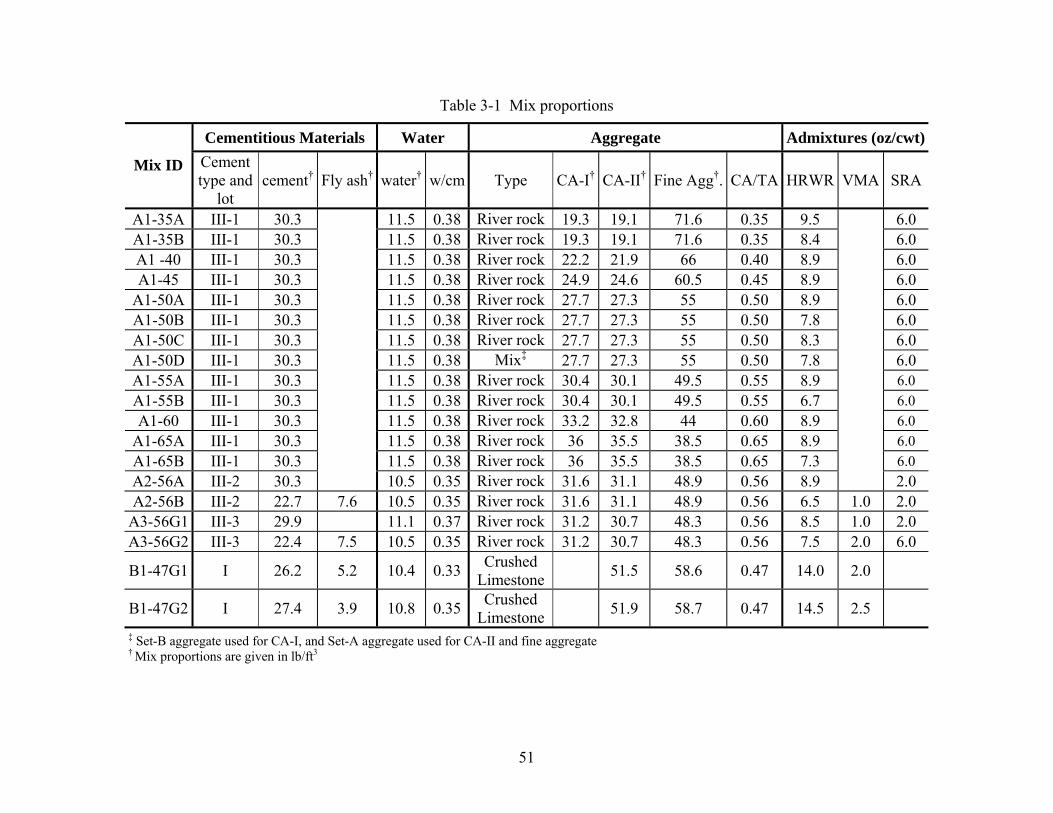
51

Table 3-1 Mix proportions

Cementitious Materials Water Aggregate Admixtures (oz/cwt)

Mix ID Cement type and

lot cement† Fly ash† water† w/cm Type CA-I† CA-II† Fine Agg†. CA/TA HRWR VMA SRA

A1-35A III-1 30.3 11.5 0.38 River rock 19.3 19.1 71.6 0.35 9.5 6.0 A1-35B III-1 30.3 11.5 0.38 River rock 19.3 19.1 71.6 0.35 8.4 6.0 A1 -40 III-1 30.3 11.5 0.38 River rock 22.2 21.9 66 0.40 8.9 6.0 A1-45 III-1 30.3 11.5 0.38 River rock 24.9 24.6 60.5 0.45 8.9 6.0

A1-50A III-1 30.3 11.5 0.38 River rock 27.7 27.3 55 0.50 8.9 6.0 A1-50B III-1 30.3 11.5 0.38 River rock 27.7 27.3 55 0.50 7.8 6.0 A1-50C III-1 30.3 11.5 0.38 River rock 27.7 27.3 55 0.50 8.3 6.0 A1-50D III-1 30.3 11.5 0.38 Mix‡ 27.7 27.3 55 0.50 7.8 6.0 A1-55A III-1 30.3 11.5 0.38 River rock 30.4 30.1 49.5 0.55 8.9 6.0 A1-55B III-1 30.3 11.5 0.38 River rock 30.4 30.1 49.5 0.55 6.7 6.0 A1-60 III-1 30.3 11.5 0.38 River rock 33.2 32.8 44 0.60 8.9 6.0

A1-65A III-1 30.3 11.5 0.38 River rock 36 35.5 38.5 0.65 8.9 6.0 A1-65B III-1 30.3 11.5 0.38 River rock 36 35.5 38.5 0.65 7.3 6.0 A2-56A III-2 30.3

10.5 0.35 River rock 31.6 31.1 48.9 0.56 8.9

2.0 A2-56B III-2 22.7 7.6 10.5 0.35 River rock 31.6 31.1 48.9 0.56 6.5 1.0 2.0

A3-56G1 III-3 29.9 11.1 0.37 River rock 31.2 30.7 48.3 0.56 8.5 1.0 2.0 A3-56G2 III-3 22.4 7.5 10.5 0.35 River rock 31.2 30.7 48.3 0.56 7.5 2.0 6.0

B1-47G1 I 26.2 5.2 10.4 0.33 Crushed Limestone 51.5 58.6 0.47 14.0 2.0

B1-47G2 I 27.4 3.9 10.8 0.35 Crushed Limestone 51.9 58.7 0.47 14.5 2.5

‡ Set-B aggregate used for CA-I, and Set-A aggregate used for CA-II and fine aggregate

† Mix proportions are given in lb/ft3

52

Table 3-2 Properties of concrete aggregate

Set-A Set-B

Materials Max. Nominal Size (in.)

Phy. Desc.

Absorption (%) SG†

Max. Nominal

Size (in.)

Phy. Desc.

Absorption(%) SG†

C.Agg-1 3/4 NG‡ 1.0 2.72 3/4 CS§ 1.3 2.71 C.Agg-2 3/8 NG 1.5 2.72 1/2 CS 1.3 2.71 Sand 3.3* 0.9 2.71 2.6* 0.6 2.68 ‡ NG ≡ Natural gravel (rounded river rock) § CS ≡ Crushed limestone * Fineness modulus † SG ≡ Specific gravity

53

Table 3-3 Concrete fresh properties and segregation test results

Column Mold Vertical Seg. Indices L-box Horizontal Seg. Indices and CBI

slump test U-box

L-box

Developed ASTM Based Four Sections Three Sections Mix ID flow (in)

T50 (sec) VSI h2/h1 h2/h1 SVIM SMIM SASTM Smod1 Smod2 H_SVIM H_SMIM H_SVIM H_SMIM

CBI

Overall Rating ‡

A1-35A 29 5 1.0 0.98 0.92 37 35 3 26 32 18 32 8 6 -23 PA1-35B 26 4 0.5 0.97 0.83 15 6 2 9 10 24 17 16 10 -3 GA1-40 29 4 1.5 0.92 0.93 62 54 24 44 28 32 46 19 18 -21 PA1-45 29 3 0.5 0.96 0.96 22 25 2 16 21 28 11 13 10 6 GA1-50A 31 3 1.5 0.98 0.98 144 126 67 147 124 20 29 17 14 10 PA1-50B 29 4 0.5 0.98 0.93 9 5 2 4 2 20 4 12 4 1 GA1-50C 25 4 0.5 0.96 0.82 11 10 0 3 4 11 16 10 4 -11 MA1-50D 25 4 1.5 0.96 0.75 13 16 0 0 0 27 3 3 1 3 GA1-55A 29 3 1.5 0.98 0.96 66 55 28 71 59 27 24 21 15 -1 MA1-55B 23 8 0.0 0.92 0.76 15 11 4 8 4 36 10 10 7 0 MA1-60 26 4 0.0 0.96 0.86 6 10 1 5 5 32 10 11 8 6 GA1-65A 28 4 1.0 0.50 0.85 25 24 2 15 19 46 25 7 9 17 PA1-65B 28 5 2.5 0.38 0.76 25 26 3 17 20 37 27 17 16 5 PA3-56G1 26 3 1.0 0.94 0.63 13 16 4 9 6 13 15 9 10 8 GA3-56G2 28 3 1.5 0.98 0.96 12 18 2 5 5 21 22 2 3 3 GB1-47G1 28 3 1.0 0.82 0.86 8 8 0 0 4 20 9 8 4 3 GB1-47G2 29 3 1.5 0.86 0.90 11 14 0 3 6 15 11 4 2 7 GA1-50B1† 25.5 4 1.0 0.94 0.85 3 5 1 2 3 27 7 11 5 0 GA1-50B2† 26 4 1.0 0.94 0.85 8 7 0 1 5 26 6 10 5 1 GA1-50B3† 27 3 1.0 0.99 0.83 8 4 3 6 7 25 9 14 5 -3 GA1-50B4† 26.5 3 1.0 0.95 0.90 9 7 5 6 3 27 4 8 3 1 G† Indicates the repeated mixes of A1-50B ‡ P =Poor, M=Moderate, G= Good overall fresh properties rating; and for individual parameters shaded cells (P), underlined cells (M), and others (G) Overall Mix Rating (MR): If total number of poor parameter (NPP) ≥ 2 MR=Poor; if NPP =1 MR= Moderate; if NPP=0 then if number of good parameter > number of moderate parameter MR=Good, otherwise MR=Medium

54

Table 3-4 Fresh properties rating criteria

Rating Criteria Test Method

Parameter (P) Nominal

Good Moderate Poor

Flow (in) 26 24≤P≤28 28<P ≤31 & 21≤P <24

P≥32 & P≤21

T50(sec) 5 P≤6 6<P ≤7 P≥8 Slump Flow

VSI 0.5 P≤1.0 1.0<P≤2.0 P≥2.5 U-box h2/h1 L-box h2/h1

0.80 0.85≤P≤1.0 0.54≤P <0.85 P <0.54

Column mold SMIM (%) 20 P≤14 14<P ≤26 P>26

H_SMIM †

(%) 20 P≤14 14<P ≤26 P>26 L-box

CBI (%) 10 P≤5 5<P ≤10 P>10 † Calculated including all four L-box sections

Table 3-5 Repeatability of test results

Column mold L-box Batch ID

Slump Flow (in.) SVIM SMIM SASTM Smod1 Smod2 h2/h1 H_SVIM H_SMIM CBI

A1-50B1 25.5 3 5 1 2 3 0.85 27 7 0 A1-50B2 26.0 8 7 0 1 5 0.85 26 6 1 A1-50B3 27.0 8 4 3 6 7 0.83 25 9 -3 A1-50B4 26.5 9 7 5 6 3 0.90 27 4 1 A1-50B5 25.5 8 15 0 0 3 0.85 33 8 4 Mean 26.1 7.2 7.6 1.8 3.0 4.2 0.86 27.6 6.8 0.6 Stdev1 0.7 2.4 4.3 2.2 2.8 1.8 0.03 3.1 1.9 2.5 Limit value 20 20 10 20 20 0.85 20 20 10 Error2 1.8 3.2 1.6 2.1 1.3 0.02 2.3 1.4 1.9 Relative error3 (%) 9 16 16 10 7 2 12 7 18

1 Stdev = standard deviation 2 Error = Limit value - lower value of 90% confidence interval (based on Limit value and Stdev) 3 Relative error =Error/Limiting value

55

5.5 in.

h1

5.5 in. 5.5 in.

48 in.

h2

No. 4 rebar at 2 in. center-to-center spacing

Sliding gate

Figure 3-1 Modified U-box and schematic of the apparatus

8"

2.0" 4.5" 6.5" 6.5" 6.5" S1

S2

S3

S4

S5

schedule 40 PVC

clamps

base plate

2.0 in.

4.5 in.

6.5 in.

6.5 in.

6.5 in.

8.0 in.

Figure 3-2 Detail of modified column segregation mold (S5 and S4, and S3 and S2 single units for original ASTM column mold)

56

Figure 3-3 Constructed L-box and schematic of the apparatus

Figure 3-4 Relationship between modified segregation index Smod1 and SASTM

4 in. 8.7 in. 8.7 in. 8.7 in.

18 in.

6 in.

24 in.

(Elevation View)

(Plan View)

8 in.

Sliding gate

(Front View)

3 No. 4 smooth reinforcing bars with 2 in. clear spacing between walls and bars, and 1 1/8 in. between bars

LV LS1 LS2 LS3

0

10

20

30

40

50

60

70

0 10 20 30 40 50 60 70 80 90 100 110 120 130 140 150

Good Moderate Poor

Segregation index Smod1 (%)

Segr

egat

ion

inde

x S A

STM

(%)

segregation limit (10 %)

segregation limits (10 & 20 %)

57

Figure 3-5 Relationship between column mold segregation indices Smod1 and Smod2

Figure 3-6 Relationship between Smod1 and column mold segregation index SVIM

0

20

40

60

80

100

120

0 10 20 30 40 50 60 70 80 90 100 110 120 130 140 150 160

Good Moderate Poor

Segregation index Smod1 (%)

Segr

egat

ion

inde

x S m

od2 (

%)

segregation limit

segregation limit

0

20

40

60

80

100

120

140

160

0 10 20 30 40 50 60 70 80 90 100 110 120 130 140 150 160

linear (equity line) GoodModerate Poor

Segregation index Smod1 (%)

Col

umn

mol

d SV

I M (%

)

segregation limit

segregation limit

58

Figure 3-7 Relationship between column mold mass and volume segregation indices

Figure 3-8 Relationship between slump flow and column segregation index SVIM

0

20

40

60

80

100

120

140

0 10 20 30 40 50 60 70 80 90 100 110 120 130

Good Moderate PoorC

olum

n m

old

SVI M

(%)

Column mold SMIM (%)

segregation limit

segregation limits

0

20

40

60

80

100

120

140

22 23 24 25 26 27 28 29 30 31 32

Good Moderate Poor

Slump flow (in.)

Col

umn

mol

d SV

I M (%

)

segregation limit envelope curve

59

Figure 3-9 Relationship between T50 and column segregation index SVIM

Figure 3-10 Relationship between VSI and column segregation index SVIM

0

20

40

60

80

100

120

140

2.0 2.5 3.0 3.5 4.0 4.5 5.0 5.5 6.0 6.5 7.0 7.5 8.0

Good Moderate Poor

T50 (sec)

Col

umn

mol

d SV

I M (%

)

segregation limit

Envelope curve

0

20

40

60

80

100

120

140

-0.5 0.0 0.5 1.0 1.5 2.0 2.5 3.0 3.5

Good Moderate Poor

Visual stability index (VSI)

Col

umn

mol

d SV

I M (%

)

segregation limit

60

Figure 3-11 Relationship between h2/h1 and column segregation index SVIM

Figure 3-12 Relationship between L-box horizontal segregation (four sections) and column vertical segregation indices

0.3

0.4

0.5

0.6

0.7

0.8

0.9

1.0

1.1

1.2

0 10 20 30 40 50 60 70 80 90 100 110 120 130 140 150

L-boxU-box

Column mold SVIM (%)

h 2/h

1 segregation

Blockage ratio

0

10

20

30

40

50

60

0 10 20 30 40 50 60 70 80 90 100 110 120 130

GoodModeratePoor

Column mold SVIM (%)

L-bo

x al

l 4 se

ctio

ns H

_SM

I M (%

)

horizontal segregation limit

vertical segregation limits

61

Figure 3-13 Relationship between L-box horizontal segregation from three sections and column vertical segregation indices

Figure 3-14 L-box sections segregation mass indices

0.6

0.7

0.8

0.9

1.0

1.1

1.2

LV LS1 LS2 LS3L-box sections

Seg

rega

tion

mas

s in

dex

(SM

I)

35 40 5550 65A 65B

L-box section

Sect

ion

segr

egat

ion

mas

s ind

ex (S

MI)

L-

box

H_S

MI i

0

10

20

30

40

50

60

0 10 20 30 40 50 60 70 80 90 100 110 120 130

GoodModeratePoor

Column mold SVIM (%)

L-bo

x al

l 3 se

ctio

ns H

_SM

I M (%

)

horizontal segregation limit

vertical segregation limit

62

Figure 3-15 Relationship between L-box h2/h1 and CBI, and region with satisfactory coarse aggregate passing and concrete filling and passing abilities

0.5

0.6

0.7

0.8

0.9

1.0

1.1

1.2

-30 -25 -20 -15 -10 -5 0 5 10 15 20 25 30

GoodModeratePoor

Coarse aggregate blockage index (%)

L-bo

x h 2

/h1

mixes with adequate coarse aggregate passing and concrete filing and

passing abilities

63

Chapter 4 Time-Dependent Behavior of Full-Scale Self-Consolidating Concrete Precast Prestressed Girders – Measured versus Design

Self-consolidating concrete (SCC) has been developed successfully with locally available materials from two precast concrete plants for use in precast prestressed bridge girders in the State of Minnesota. Four SCC mixes (i.e., two mixes per plant) were designed, evaluated, and used to cast four SCC precast prestressed bridge girders. Variations in the SCC mixes included cementitious materials (ASTM Type I and Type III cement, and Class C fly ash), natural gravel and crushed stone as coarse aggregate, and several admixtures (i.e., high-range and mid-range water reducers, viscosity-modifying admixtures, and set-retarding agents). In addition to SCC girders, a conventional concrete girder was cast simultaneously on the same precasting bed for each plant. The girders were instrumented to monitor both short-term and long-term performance, which included transfer length, camber, and prestress losses. In addition, companion cylinders were cast to monitor compressive strength, modulus of elasticity, creep, and shrinkage over time. The test results indicate that the overall performance of the SCC girders was comparable to that of conventional concrete girders and could be predicted using existing design equations.

4.1 Introduction

Self-Consolidating Concrete (SCC) flows under its own weight, fills the formwork without segregation of its constituent materials, and can be placed without vibration. Self-consolidating concrete offers substantial economic and environmental benefits including faster construction, reduction in labor, better surface finish, easier and vibration-free placement, reduced noise during placement, and a safer working environment.

Numerous investigations have been conducted over the past ten years regarding the performance of SCC in both its fresh and hardened states. This has led to the successful development and use of SCC in cast-in-place and precast applications. However, some concerns remain regarding the long-term behavior of SCC prestressed members including whether AASHTO provisions are appropriate for SCC girders. Limited and contradictory literature is available regarding the hardened and time-dependent behavior of SCC members; particularly bond behavior, elastic modulus, creep, and shrinkage (Dehn et al., 2000; Hegger et al., 2003; and Girgis and Tuan, 2004). These are the main reasons why some State Departments of Transportation do not allow SCC for prestressed concrete bridge girder applications. The purpose of this research was to investigate the viability of using SCC for construction of prestressed concrete bridge girders by comparing the behavior of girders cast with SCC to that of girders cast with conventional concrete and to standard design provisions.

In conjunction with the University of Minnesota, SCC has been developed with two precast concrete plants (i.e., Plant-A and Plant-B) using locally available materials. At each plant, two SCC girders, in addition to a conventional concrete girder, were fabricated on the same precasting bed at the same time. The mix designs used for the conventional concrete girders were typical for each plant.

64

4.2 Research Significance

Before SCC can be accepted for the construction of prestressed concrete bridge girders, both short-term and long-term performance of girders made from SCC must be established. The performance characteristics (e.g., transfer length, camber, and prestress losses) of SCC bridge girders manufactured with locally available materials were compared to those of conventional concrete girders produced with the same or similar (in the case of Plant-B) materials. Also, because the girders were fabricated with SCC and conventional concrete using similar materials and with identical design requirements (e.g., initial and 28-day concrete compressive strength, initial prestressing force, girder dimensions, and strand layout), a performance evaluation could be conducted among the girders that was independent of many design parameters. The results obtained from this study are useful for evaluating and better understanding the performance of SCC prestressed girders and for determining the adequacy of design predictions for prestressed SCC girders.

4.3 Girder Design

The girders were designed using the AASHTO LRFD Bridge Design Specifications (2004). The girders were all Mn/DOT 36M I-girders with a span length of 38 ft. The dimensions of the section are shown in Figure 4-1. The girders were designed with the maximum number of strands that could be placed within the section while satisfying AASHTO (2004) and ACI 318-05 (2005) allowable stress requirements. The maximum number of strands was employed to achieve maximum congestion to challenge the flow of SCC in addition to maximizing the compressive stress at the bottom fiber of the girder to investigate severe creep conditions. In total, 40 half-inch diameter Grade 270 low-relaxation strands were used in the section, with 36 of the strands placed in the bottom flange, and the remaining four strands placed in the top flange to control the tensile stresses at release. All strands were straight and bonded (i.e., there were no harped or unbonded strands). According to AASHTO (2004) Section 9.15.1, the strands were tensioned to 75 percent of the specified tensile strength. The selected section and strand pattern resulted in a maximum bottom fiber compressive stress of approximately 4.5 ksi (0.6fci') which was the maximum compressive stress that AASHTO (2004) and ACI 318-05 guidelines allowed. The girders were to be tested to flexural cracking; hence, shear reinforcement was provided to ensure that a shear failure would not occur before the flexural cracking moment was reached. The shear reinforcement for each girder consisted of No. 4 Grade 60 stirrups spaced at 12 in.

4.4 Girder Instrumentation

Internal and external instrumentation was placed to measure initial prestressing force, transfer length, camber, and prestress losses. Instrumentation included strain gages applied to the strands, demountable mechanical (DEMEC) strain gages, and vibrating wire strain gages (VWSG) embedded in the concrete.

Foil-type resistive strain gages were attached to approximately one quarter of the strands to determine the initial prestressing force at seven locations along the prestressing bed, including the midspan of each girder. Geokon vibrating wire strain gages (VWSGs) with a 6-in. gauge

65

length were cast in the concrete to determine elastic shortening losses, and to monitor changes in concrete strain over time due to creep, shrinkage, and environmental effects. Additional VWSGs were installed at varying depths at discrete locations (i.e., L/6, L/3, and midspan for Plant-A girders, and L/6 and midspan for Plant-B girders) to measure the variation of strain over time and to determine the girder curvature (Figure 4-2). A detailed description of girder instrumentation is presented in Appendix B.

4.5 Girder Materials

Two SCC mixes were developed per plant using locally available aggregate. Portland cement and Class C fly ash (which was used at different replacement ratios for each mix) were used as cementitious materials. At each plant, in addition to two SCC girders, one conventional concrete girder was also cast at the same time on the same bed using the same or similar materials. The design requirements for the release and 28-day concrete compressive strengths for all girders were 7.5 ksi and 9.0 ksi, respectively. The mixes were designated according to the following scheme: X-Y, where X represents Plant-A or B (i.e., A or B), and Y represents either SCC (i.e., SCC1 or SCC2) or conventional concrete mix (CM). The girders were named based on the mix used. The mix proportions used for each girder are given in Table 4-1.

4.5.1 Aggregate

For both plants, only locally available materials were used. For Plant-A, natural gravel (i.e., rounded river rock) with nominal maximum particle sizes of 3/4 and 3/8 in. were used in combination as coarse aggregate for both SCC mixes. For the conventional concrete mix (A-CM), the 3/4 in. aggregate was the only coarse aggregate used. Locally available natural sand with a 3.3 fineness modulus was used as the fine material for both SCC and conventional concrete mixes. For Plant-B, crushed limestone with a maximum particle size of 1/2 in. was used as the only coarse aggregate for the SCC mixes. For the conventional concrete mix (B-CM), natural gravel with a nominal maximum particle size of 3/4 in., but from a different source than that used for Plant-A, was the only coarse aggregate used. Locally available natural sand with a 2.6 fineness modulus was used as fine aggregate for both the SCC and conventional concrete mixes. Although both plants used different aggregate and aggregate sources, the specific gravity of all coarse aggregate was approximately 2.7. The specific gravity and absorption characteristics of the aggregate are given in Table 4-2.

4.5.2 Cementitious Materials

In addition to the conventional concrete mixes, two sets of SCC mixes were designed and tested for each plant. The main reason for developing two SCC mixes for each plant was to study the effect of supplementary cementitious materials on the performance of the mix and the girders. For Plant-A, the conventional concrete mix (A-CM) and the first SCC mix (A-SCC1) had only ASTM Type III cement as the cementitious material. For the second SCC mix (A-SCC2) Class C fly ash was used in addition to the cement as supplementary cementitious material. For Plant-B, the conventional concrete mix and both SCC mixes had Class C fly ash as supplementary

66

cementitious material but in different proportions (as shown in Table 4-1) in addition to ASTM Type I cement.

4.5.3 Admixtures

Different types and brands of admixtures were used by each plant. For Plant-A, a polycarboxylate-based high-range water-reducing (HRWR) admixture (ASTM C 494 Type F) was used at a dosage of 8.5 oz/cwt and 7.5 oz/cwt of cementitious material (cement and fly ash) for A-SCC1 and A-SCC2, respectively. A viscosity-modifying admixture (VMA) was used at a dosage of 1.0 to 2.0 oz/cwt of cementitious material to improve segregation resistance of the mixes. In addition, an ASTM C 494 Type D set-retarding agent, also used as a stabilizer, was applied to control set time of the mixes. For the conventional mix, a mid-range water-reducing admixture (MRWR) (ASTM C 494 Type A) and a set-retarding agent, which was different than that used for the SCC mixes, were the only admixtures. For Plant-B, a polycarboxylate-based HRWR admixture and VMA, which were different from those used for Plant-A, were the only admixtures used for SCC mixes. A MRWR admixture (ASTM C 494 Type A) and a stabilizer, used also as a set-retarding admixture, were added to the conventional concrete mix.

4.6 Fresh Concrete Properties

No special procedures were used to mix the concrete for the SCC girders. Various test methods (e.g., slump flow, L-box, U-box, and column segregation) were used to evaluate fresh concrete properties, such as concrete flowability and segregation resistance. A detailed description of these test methods is included in Chapter 3. All tests were performed with sample concrete obtained from the batch used to cast the girders. The slump flow test (slump flow, T50, and VSI) and L-box test h2/h1 ratio were measured just before girder casting, and the other tests (U-box, and column and L-box segregation tests) were performed concurrently with girder casting.

The measured fresh properties are summarized in Table 4-3. The A-SCC2 mix was considered satisfactory based on the slump flow test and visual stability index (VSI), which is a visual evaluation of the slump flow patty for segregation resistance based on guidelines provided by PCI (PCI 2003). However, the mix segregated during casting while flowing along the girder. After casting, it was found that the 3/8 in. aggregate bin had been contaminated with larger 3/4 in. aggregate, which had different moisture content and absorption properties, and is likely the reason why the A-SCC2 mix segregated. Therefore, the as-placed mix proportions (i.e., coarse aggregate and mixing water) for A-SCC2 were different than those shown in Table 4-1 and are unknown. Hence, the results for Girder A-SCC2 are not included in this chapter. For other mixes, the minimum and maximum slump flows were 26 and 29 in., respectively. The measured VSI and T50 values were within the design objectives (maximum VSI of 1.5, maximum T50 of 3 seconds). Most of the SCC mixes had good passing and filling characteristics based on L-box and U-box test results (Table 4-3), with the exception of A-SCC1 which had a low L-Box blocking ratio ( h2/h1=0.63 ) indicating an increased potential for difficulty flowing past reinforcement. However, the measured U-box blocking ratio for A-SCC1 mix was 0.94, which indicated good passing and filling properties. In the literature, the recommended values for L-

67

box and U-box blocking ratios vary between 0.80 and 1.0 (Skarendahl, 1999; and EFNARCH, 2002) and 0.54 and 1.0 (JSCE, 1998; PCI, 2003), respectively. In addition, the findings of Chapter 3 indicate that L-box blocking ratio is in general more conservative than U-box blocking ratio (i.e., L-box blocking ratio smaller than U-box blocking ratio). Therefore, it is likely that the limiting value of 0.80 in the literature for blocking ratio is on the conservative side for L-box. All measured fresh properties including those of Girder A-SCC2 are given in Chapter 5.

4.7 Fabrication of the Girders and Companion Cylinders

For Plant-A, two batches of concrete, each about 3 yd3, were required for the casting of each girder. Each batch was placed into a truck and transported to the casting location. All fresh state tests were conducted for the concrete delivered with the first truck for each girder. The concrete delivered with the second truck was only evaluated with the slump flow test. For Plant-B, all girders were cast with a single batch that was transported to the casting location in a concrete mixer truck.

For both plants, conventional concrete girders were cast and vibrated before casting the SCC girders. This casting sequence was selected because the conventional concrete girders were vibrated by means of form vibrators as well as hand-held vibrators, and the vibration could have affected the SCC girders if a different casting sequence had been selected.

Plant-A and Plant-B girders were cast on November 3, 2005, and July 5, 2006, respectively. Casting of each girder took about 15-20 minutes. At Plant-A, the SCC girders were cast from two points along the length. At Plant-B, the SCC girders were cast from a single point within the length of each girder. With the exception of Girder A-SCC2, none of the SCC segregated during placement and no blockage was observed. The A-SCC1 mix had moderate passing and filling properties measured with L-box (h2/h1 =0.63), but self-leveling, passing, and filling properties of the mix measured with U-box (h2/h1= 0.94) were satisfactory and no visual passing and filing problems were observed during casting.

All girders were cured together prior to release at each plant. For Plant-A, Girders A-CM and A-SCC1 reached the minimum concrete release strength of 7.5 ksi at the end of the first and third days, respectively. However, Girder A-SCC2, which was the girder that experienced segregation, reached the minimum concrete release strength (i.e., 7.5 ksi) at the end of fifth day. Therefore, all Plant-A girders were cured for five days because all girders were cast on the same precasting bed. For Plant-B, both SCC and conventional concrete girders exceeded the minimum concrete release strength at the end of the second day. Once all girders reached the required concrete release strength, the strands were cut at the end of each girder, and they were relocated outdoors to a storage site in the Plant-A precasting yard, where monitoring continued.

Commercially available 4 by 8 in. cylinder molds were used to cast cylinders to measure concrete compressive strength, static modulus of elasticity, and splitting tensile strength of the girder mixes. The cylinders were prepared based on ASTM C192/C192M for conventional concrete. There was no ASTM standard at the time of this study for making SCC companion cylinders. In this study, SCC cylinders were cast in the same way as specified by ASTM

68

C192/C192M for conventional concrete cylinders with the exception of rodding, which was replaced by tapping the outside of the mold lightly 3-4 times with a rubber mallet after each of the 2 layers was placed to release any trapped air. A more detailed description of companion cylinders including those used for creep and shrinkage specimens is included in Appendices C and D.

4.8 Results and Discussion

4.8.1 Concrete Compressive Strength and Modulus of Elasticity

Specified concrete compressive strengths at release and service were 7500 and 9000 psi, respectively. Experimentally, the concrete compressive strength and modulus of elasticity were determined based on test results (ASTM C39 and ASTM C469, respectively) obtained from companion concrete cylinders that were cast and cured with each girder. In addition to measured concrete moduli, predicted values were calculated according to ACI 318-05 Section 8.5.1 using the measured concrete compressive strength. The measured concrete compressive strength and ratio of measured to predicted elastic moduli (Em/Ep) are given in Table 4-4. The average ratios of measured moduli to the predicted moduli (Em/Ep) were reasonable (0.90 for A-SCC1, 1.00 for A-CM, 0.99 and 1.00 for B-SCC mixes, and 0.94 for B-CM). AASHTO (2004) Section C5.4.2.4 proposes a very similar equation to predict elastic moduli as ACI 318-05, but in a different format. The ratio of AASHTO predicted moduli to ACI predicted moduli was constant and equal to 0.99. In other words, if the AASHTO equation was used instead of the ACI equation to predict concrete moduli, the measured to predicted moduli ratio given in Table 4-4 would be 99% of those presented.

Some of the measured concrete moduli data might have some error due to malfunctioning of the compressometer used to measure vertical displacements/strains. It was found that the top yoke hinge of the compressometer had some resistance to rotation as the concrete cylinder was compressed under the axial load. Unfortunately, there was not enough information to adjust the data. The problem was recognized after all Plant-A cylinders were tested (approximately 652 and 409 days after girder casting for Plant-A and Plant-B, respectively). However, the authors predict a maximum error at the order of 2-5% (i.e., the reported data can be 2-5 % high).

4.8.2 Transfer length

Transfer length is the distance required to transfer the full effective prestress force from the strands to the concrete. Alternatively, the transfer length may be defined as the minimum length of bond between the concrete and strands required to develop the effective prestress force in the strands. The ACI 318-05 (2005) and AASHTO (2004) specifications do not distinguish between conventional concrete and SCC. However, there have been concerns that the ultrafine material content, large dosages of superplasticizer and stabilizer might affect the bond behavior of SCC and consequently the transfer length in SCC members (Holschemacher and Klug, 2002). Limited research has been conducted to evaluate the bond strength of strands (Girgis and Tuan, 2004; Hegger et al., 2003) and deformed reinforcing bars (Dehn et al., 2000; Chan et al., 2003)

69

in SCC members. Some of these studies have shown that SCC has higher bond strength than that of conventional concrete (Dehn et al., 2000; and Chan et al., 2003), but others indicate inadequate early-age bond strength, which results in longer transfer lengths for SCC members (Girgis and Tuan, 2004; and Hegger et al., 2003). Some of these differences in the literature might be due to factors other than the type of concrete, for example strand surface condition, strand diameter, strand release stress, and concrete compressive strength (Janney, 1954; Rose and Russell 1997). In this study, the girders at a particular plant were cast on the same bed and at the same time to minimize the effect of variation in strand diameter, strand release stress, and strand surface condition on transfer length.

To determine transfer length for the girders, a series of DEMEC gages were used to measure the concrete surface strains. From the end of each girder, a line of uniformly distributed DEMEC targets was placed on the surface of the concrete 4 in. from the girder bottom, which was at the height of the center of gravity of the strands in the bottom flange. Figure 4-3 shows a detailed drawing of the DEMEC insert strip. The DEMEC targets were spaced uniformly at 2 in. and extended about 78 in. and 56 in. along the length of the Plant-A and B girders, respectively. The number of DEMEC targets was decreased for Plant-B as it was found from the results at Plant-A that the transfer length would be well within the reduced length. The Whittemore gage used to measure the DEMEC targets had a gage length of 2 in.

The transfer length was estimated using the “95% Average Maximum Strain (AMS) Method” proposed by Russell and Burns (1993) and the “Final Average Method” developed by Cousins, et al. (1993). In the AMS method, strain readings were first smoothed by using a floating 3-point average of strain values to reduce anomalies in the data. Then the average maximum strain value was determined as the numerical average of all smoothed strains contained within the strain plateau. The intersection of the smoothed strain profile with 95% of the average maximum strain was determined, and the distance from this point to the free end of the girder was reported as the transfer length for the 95% AMS method (Figure 4-4). In the case of the Final Average Method, the method was used to eliminate data points outside the range of one standard deviation from the averaged strain plateau. Then the average strain of the remaining data points, defined as the final average strain, was determined. The transfer length was then determined as the distance of the intersection of the final average strain and the smoothed data to the free end of the girder. Figure 4-4 illustrates the raw data, smoothed data, and the results from these two methods for Girder A-SCC1.

Table 4-5 summarizes the estimated transfer lengths from both methods and the average of them for the SCC and conventional concrete girders. In addition, design transfer lengths predicted by equations in AASHTO (2004) and ACI 318-05 design provisions are included. Because neither code addresses the use of SCC in prestressing applications, and the equations are functions of strand diameter and/or effective stress in prestressing strand (fse) only, a single common transfer length was predicted for all girders as the nominal design parameters (e.g., diameter of strand, strand stress, concrete release strength, and predicted losses at release) were the same for all girders. Finally, the ACI equation was reevaluated based on the measured effective stress in the prestressing strands at release for each girder and is listed in Table 4-5.

70

The test results indicated that both AASHTO and ACI specifications overestimated transfer lengths for both the SCC and conventional concrete girders by over 100%. For Plant-A girders, the transfer length of the SCC girder was approximately 75% higher than that of the conventional concrete girder. The SCC mix had about 25% smaller concrete compressive strength and 30% smaller modulus of elasticity at release than the conventional concrete mix, which could have affected the transfer length. For Plant-B both the SCC girders and conventional concrete girder had similar transfer lengths with the SCC girder transfer lengths approximately 10% greater than the conventional concrete girder. For both plants, the transfer lengths were inversely proportional to both the concrete strength and modulus at release. The heavily prestressed section (40 strands) and concrete confinement as a result of this reinforcement can be possible reasons for the relatively short transfer lengths measured.

4.8.3 Camber

Camber is the vertical deflection of the midspan relative to a straight line between the ends of the girder. A stretch-wire system tensioned between girder ends was used to monitor the camber of the girders (Byle and Burns, 1997; Gross and Burns, 2005). The system used two pulleys, a ruler, a piano wire, a mirror, and a hanging weight. Two bearing pulleys were fitted over bolts at the two ends of the girders. A #6 piano wire was stressed between the pulleys by hanging a 35-lb weight at the end of the wire. Two steel rulers were fixed at L/4 and L/2 to measure the deflections (Figure 4-5). A small mirror was placed between the rulers and wire to eliminate parallax errors. The system had good repeatability, with the overall system accuracy estimated at about 0.02 in. (Gross and Burns, 2005).

Plots of measured camber for Plant-A and Plant-B girders are given in Figures 4-6 and 4-7, respectively, with the measured ambient temperature. All of the readings were taken before sunrise to eliminate any effect due to solar radiation on the camber measurements. Camber was monitored for all girders beginning just before release. The measured camber values indicate that there was a significant rapid increase in camber for all girders at early age, which was followed by a much smoother and slower variation in camber. When the girders were moved from the precasting bed to the storage area (November 7, 2005 Plant-A and July 14, 2006 Plant-B), the support condition changed slightly. Instead of being supported at each end, which was the case on the precasting bed, supports were located about 1 ft from the ends causing an increase in camber. In addition to the changed support condition, high initial creep and shrinkage deformations contributed to the early age camber.

Deflections (i.e., cambers) are expected to be inversely proportional to concrete modulus of elasticity. For Plant-A, the camber of the SCC girder was higher than that of the conventional concrete girder, consistent with the measured concrete modulus of elasticity associated with each girder. For Plant-B, both SCC and conventional concrete girders had similar cambers, consistent with the measured moduli values. In addition to the measured cambers, estimated values were calculated using measured material properties (modulus of elasticity at release, and prestress force at release) with the “PCI multiplier method” in the PCI Design Handbook 6th Edition (2004), which provides estimates of camber at release, erection (about 30-60 days after casting), and final stages. Because the moduli of elasticity at release for both Plant-B SCC girders were

71

so close, only the predicted camber for B-SCC1 is shown in Figure 4-7. As shown in Figures 4-6 and 4-7, the estimated camber values were slightly higher than the measured values at “erection” (30-60 days). The predicted long-term camber for Plant-A and Plant-B girders had good agreement with the measured camber. The difference between the predicted and measured camber values (i.e., error) was less than 10% and 15% for Plant-A and Plant-B girders, respectively, at any time.

4.8.4 Prestress losses

All girders were kept outdoors, where a weather station was set up to monitor relative humidity and ambient temperature. Prestress losses were measured with vibrating wire strain gauges (VWSG) embedded at the center of gravity of all the strands (cgs) at midspan of the girders. The maximum deviation between the exact location of the gauges and the cgs was approximately ±1/2 inch. The strains measured at the cgs were verified with the strain profile measured from vertically distributed gages at midspan (as shown in Figure 4-2). Changes in strain at the cgs were converted to prestress losses using the precast plant provided moduli of elasticity for the strands (28,633 ksi for Plant-A and 29,000 ksi for Plant-B) based on the assumption that the concrete and steel had perfect bond.

Because relaxation losses could not be measured using the VWSGs, calculated relaxation losses, which were based on the PCI General Method (PCI, 1975) were added to the measured losses to find the total losses at release. The elastic shortening losses, which were a significant portion of the total losses, were determined from the VWSG readings just before and after transfer. In addition, the measured material properties (e.g., concrete modulus of elasticity) were used to predict elastic shortening losses based on the assumption that the concrete and steel had perfect bond. The predicted and measured elastic shortening losses were consistent, and are given in Table 4-6. The only exception was Girder A-CM, for which the predicted elastic shortening loss using the measured concrete modulus was more than 2 ksi smaller than the measured value. Taking into consideration that the prestressing force is the same for all girders just before release and the only variable affecting elastic shortening is concrete modulus of elasticity (the same concrete and strand areas for the girders), the concrete modulus of elasticity for Girder A-CM should be smaller than that measured. One possible reason for this is that the companion cylinder used to measure modulus may have been cured differently than the girder at the precasting bed. Note that all of the cylinders were cured under the tarps with the girders, however, there may have been a variation in conditions due to the very cold ambient temperature just outside of the tarps.

Prestress losses were monitored from the time the girders were released until they were transported to the University of Minnesota for flexural crack testing. Adjustments for additional losses due to relaxation after release were not made. The additional relaxation losses, predicted using finite element program Pbeam (Suttikan, 1978) and measured material properties, were small; on the order of 0.9 ksi for Plant-A girders 600 days after release and on the order of 0.7 ksi for Plant-B girders 450 days after release (see Table 4-7). Figures 4-8 and 4-9 show the total losses determined from the measured strains versus time for Plant-A and Plant-B girders,

72

respectively. Note that there was little difference in the losses measured for Plant-A between 450 and 600 days (less than 3 ksi) as shown in Figure 4-8.

In addition, total losses were predicted using measured material properties and equations from AASHTO (2004), AASHTO (2007), PCI General Method (1975), and the PCI Design Handbook 6th Edition (2004). A summary of total long-term prestress losses computed with these methods as well as those measured for the girders is given in Table 4-7. In general, the predicted long-term losses were not very sensitive to small differences in the measured material properties (e.g., concrete modulus of elasticity). For example, the total losses predicted for Plant-A and Plant-B girder were very similar despite the fact that girders had different measured material properties. The only exception was the Plant-A conventional concrete girder (A-CM), which had a relatively larger concrete compressive strength and modulus of elasticity at release than the other girders (Table 4-4). Because similar long-term losses were predicted for both SCC girders at Plant-B, only the losses based on the measured properties of B-SCC1 are shown in Figure 4-9 for clarity. The losses predicted for B-SCC2 were slightly larger than those predicted for B-SCC1 as shown in Table 4-7.

AASHTO and PCI (Design Handbook 6th Edition) provide methods for estimating total losses at the end of the service life of the girder. However, the experimental results presented herein show losses over approximately the first 600 days for Plant-A and 450 days for Plant-B, respectively. The majority of the losses occur during the first three to five years; therefore, the measured total losses should be somewhat smaller than the AASHTO or PCI predicted values. The measured total losses are reasonable relative to the losses predicted by AASHTO and PCI using measured properties as shown in Table 4-7, and Figures 4-8 and 4-9. The PCI Design Handbook method appeared to predict the prestress losses at service based on measured losses for both SCC and conventional concrete girders conservatively. The difference between the predicted and measured losses was between 7.5 % and 11.1 % of the initial prestressing.

The long-term prestress losses predicted using AASHTO 2004, Section 5.9.5.3 Approximate Lump Estimate of the Time-dependent Losses, which are shown in Table 4-7, and Figure 4-8 and Figure 4-9, were slightly larger (conservative) than the measured losses at the end of the girder monitoring period (approximately 600 and 450 days for Plant-A and Plant-B girders, respectively). The difference between the predicted and measured losses at the end of the monitoring period for Plant-A and Plant-B was 2.4 to 5.1%, and 2.7 to 4.7% of the initial prestressing, respectively. The equation in Section 5.9.5.3 is only a function of concrete design strength (fc'), and reflects values and trends obtained from a computerized time-step analysis of a large number of bridge and building members designed for a common range of variables (AASHTO 2004).

The losses were also predicted using AASHTO 2004, Section 5.9.5.4 Refined Estimates of Time-dependent Losses, which provides guidelines to compute the contribution of creep, shrinkage, and relaxation separately using the measured material properties as shown in Table 4-7. The losses computed using Section 5.9.5.4 were significantly larger than the measured losses (i.e., conservative) for all girders. The differences between the predicted and measured losses at the end of the monitoring period for Plant-A and Plant-B ranged between 11.9 to 14.9%, and 12.4 to 14.4% of the initial prestressing, respectively. The results indicate that AASHTO Section 5.9.5.4

73

predicts more conservative prestress losses than Section 5.9.5.3, and it might be more suitable for design purposes when there are concerns regarding prestress losses.

Section 5.9.5.3 of ASSHTO 2004 was significantly updated in AASHTO 2007, and the section was named Approximate Estimate of Time-dependent Losses (AETL). The losses equation is a function of prestressing stress immediately prior to transfer, average annual ambient relative humidity, and concrete strength at strand release.

pRsthsthg

pipLT f

Af

f Δ++=Δ γγγγ 0.120.10 (4-1)

in which:

( )'15 and 01.07.1

cisth f

H+

=−= γγ (4-2)

where fpi is the prestressing steel stress immediately prior to transfer (ksi); Ag is the gross concrete area; H is the average annual ambient relative humidity (%); γh is the correction factor for relative humidity of the ambient air; γst is the correction factor for specified concrete strength at time of prestress transfer to the concrete member; ΔfpR is an estimate of relaxation loss taken 2.4 ksi for low relaxation strand; and fci’is the concrete compressive strength at time of prestress transfer (ksi).

The equation was derived through approximations of the refined method (AASHTO 2007, Section 5.9.5.4) for a wide range of standard precast prestressed concrete members (AASHTO 2007). The following section was obtained from AASHTO (2007) regarding the Eqns. (4-1) and (4-2).

The approximate estimates of time-dependent prestress losses given were derived as approximations of the terms in the refined method for a wide range of standard precast prestressed concrete I-beams, box beams, inverted tee beams, and voided slabs. The members were assumed to be fully utilized, i.e., level of prestressing is such that concrete tensile stress at full service loads is near the maximum limit. It is further assumed in the development of the approximate method that live load moments produce about one-third of the total moments, which is reasonable for I-beams and inverted tee composite construction and conservative for noncomposite boxes and voided slabs. They were calibrated with full-scale test results and with the results of the refined method, and found to give conservative results. The approximate method should not be used for members of uncommon shapes, i.e., having V/S ratios much different from 3.5 in., level of prestressing, or construction staging (AASHTO 2007, Section C5.9.5.3).

Using this method, the predicted long-term prestress losses were slightly smaller than those measured at the end of 600 and 450 days after strand release for Plant-A and Plant B, respectively. The difference between the predicted and measured losses at service for Plant-A and Plant-B was -1.0 % to -0.3 %, and -0.1% to 0.4 % of the initial prestressing, respectively, as

74

shown in Table 4-7. Although AASHTO 2007 slightly under-predicted the losses at the end of the monitoring periods for Plant-A, it should be acceptable to use AASHTO 2007 for design. The measured losses in the girders were larger than what would be seen for the same girder in a bridge structure because the girders did not have composite decks; and hence the stress at the level of gravity of strands was higher than it would have been had these girders been part of a bridge superstructure.

One possible reason for the AASHTO 2007 AETL method predicting unconservative long-term prestress losses could be that the proposed method is not appropriate for girders with large amount of prestressing strands that have a high level of prestressing as stated in section C5.9.5.3 (AASHTO, 2007). Also, it seems that the proposed method takes the field loading conditions into consideration rather than the experimental loading conditions of this study (i.e., girders that are not a part of structure, no external live or dead load applied (deck) except their own weight).

Because the PCI Design Handbook 6th Edition (2004) and AASHTO( 2004 and 2007) methods only provided an estimated total loss that can be used for design, a third method, the PCI General Method (PCI, 1975), was used with measured material properties (initial prestressing force, concrete modulus, and age of loading) to predict the total losses as a function of time. Losses predicted with the PCI General Method, also known as the PCI Committee Method, were consistent with the measured losses for the end of the recording period (Figures 4-8 and 4-9). For Plant-A, the total estimated losses were about 8 ksi higher for the SCC girder and 15 ksi higher for the conventional concrete girder (Girder A-CM) than the losses measured at the end of 600 days. For Plant-B, the predicted losses were very consistent with the measured total losses at any given time for all three girders for the first 60 days. At the end of about 450 days, the predicted losses were about 10 ksi and 13 ksi higher than the measured total losses for the SCC and conventional concrete girders, respectively. Similar results were found for Plant-A girder for the same period of time. In other words, approximately 450 days after strand release, the predicted total losses for Plant-A girders using the PCI General Method were 11.2 and 15.1 ksi higher than the measured losses.

The difference in the measured total losses at any given time between the Plant A SCC and conventional girders in Figure 4-8 was mainly due to the smaller elastic shortening losses (i.e., higher modulus of elasticity) measured for the conventional concrete girder, and higher creep and shrinkage losses measured for the SCC girder. The maximum difference between the Plant A measured SCC and conventional concrete girder creep and shrinkage related losses was found to be approximately 10 ksi. Both the Plant B conventional concrete and SCC girders had similar total losses, with a maximum difference of approximately 5 ksi at the end of monitoring period (i.e., about 450 days).

When the measured losses at the end of the monitoring period (450 and 600 days) were compared for all girders, the Plant-B conventional concrete girder had 3.4 ksi higher total losses than the Plant-A conventional concrete girder, and the Plant-A SCC girder had approximately 3 ksi higher total losses than the Plant-B SCC girders. On the other hand, when the measured losses were compared for all girders at the end of 120 days after strand release (approximately corresponding to the end of winter which is a high ambient relative humidity period for Plant-A girders), the Plant-B conventional concrete girder had approximately 8.0 ksi higher total losses

75

than the Plant-A conventional concrete girder, and the Plant-B SCC girders had about 5.0 ksi higher total losses than the Plant-A SCC girders.

The results indicate, as expected, that total losses (at the end of 120 days) are dependent on environment (e.g., relative humidity), materials, and mix designs for both conventional and self-consolidating concrete girders. The measured total losses for Plant-A girders indicates that the early age losses (first 3-4 months) in the State of Minnesota can be small depending on the season and environmental factors such as ambient relative humidity. The girders at Plant-A were cast in November, followed by a period of high relative humidity (i.e., winter in Minnesota), while the girders at Plant-B were cast during the summer, when the relative humidity was much more moderate. The rate of change of the losses in the Plant-A girders seemed to accelerate approximately 150 days after casting, when the relative humidity decreased (i.e., spring) During the spring and summer, the losses for the Plant-A SCC girder continued increasing at an increased level compared to the prediction and eventually plateaued near the value predicted using the measured properties.

4.9 Summary and Conclusions

A Mn/DOT 36M-I girder with a span length of 38 ft was designed for a compressive stress at release equal to 60 percent of the release strength using 36 strands in the bottom flange to achieve a high degree of congestion to challenge SCC flow and maximize creep. The section represented one of the most severe cases for the application of SCC to bridge girders (i.e., highly congested and large stresses to introduce creep). The design concrete compressive strength was 7.5 ksi at release and 9.0 ksi at 28 days. In total, four SCC and two conventional concrete girders were cast using locally available materials from two precast concrete plants with a variety of cementitious materials and admixtures. Both short-term (e.g., elastic shortening) and long-term performance of the girders (e.g., prestress losses) were measured and compared to AASHTO (2004 and 2007), PCI Design Handbook 6th Edition (2004), and PCI General Method (PCI, 1975) predictions. Based on the experimental observations cited and the results predicted by the design provisions, the following conclusions can be made for the fabricated girders:

1. Concrete moduli of elasticity predicted by ACI 318-05 Section 8.5.1 and AASHTO (2004) Section C5.4.2.4 for both SCC and conventional concrete were reasonable and consistent with the measured values. Therefore, both design provisions can be used to predict modulus of elasticity of the girders when experimental data is not available.

2. The SCC girders had longer transfer lengths than the conventional concrete girders with similar material properties (75% for Plant-A and 10% for Plant-B), with the concrete with higher strengths have smaller transfer lengths. However, both AASHTO and ACI transfer length predictions were conservative for girders cast with both types of concrete. The large number of strands placed in the girder and high level of prestressing stresses, which confined the concrete, could be the reason for the measured low transfer length relative to the predictions.

76

3. The PCI multiplier method using measured properties was a good predictor of camber for both SCC and conventional concrete girders. For Plant-A, the predicted camber for both conventional and SCC girders was higher than the measured camber by 3 to 8 % of the measured camber at release, erection (35 days after release), and at the end of monitoring period (600 days after release). The only exception was the conventional concrete girder at release; the predicted camber at release for the conventional concrete girder was approximately 4% smaller than the measured camber. For Plant-B, at release, the predicted cambers were approximately 3% smaller than the measured camber for both SCC and conventional concrete girders, and at erection and at the end of the monitoring period ( approximately 450 days after release) the predicted cambers were 7 to 15% higher than the measured cambers for all girders.

4. Both the SCC and conventional concrete girders had similar elastic shortening losses (from 18.3 to 20.2 ksi). These losses were well predicted with available design guidelines when measured material properties were used and were conservatively predicted when design properties were used.

5. The measured long-term prestress losses that occurred in excess of elastic shortening for Plant-A SCC girders were approximately 7 ksi higher than those measured for the conventional concrete girder approximately 600 days after release . The Plant-B SCC and conventional concrete girders had similar long-term losses in excess of elastic shortening, with a difference less than 4 ksi approximately 450 days after release.

6. The predicted total long- term prestress losses calculated with AASHTO (2004), PCI Design Handbook 6th Edition (2004), and PCI General Method (PCI, 1975) using measured material properties were conservative. The predicted long-term losses at the end of the monitoring periods were larger than the measured losses by 2 to 5% for the AASHTO 2004 Lump Sum Method, 12 to 15% for the AASHTO 2004 Refined Method, 4 to 7% for the PCI General Method, and 8 to 11% for the PCI Design Handbook Method for all girders. However, the long-term prestress losses computed with AASHTO 2007 Approximate Estimate of Time-Dependent Losses were either not conservative or very close to measured losses at the end of monitoring period of 450 days and 600 days for Plant-A and Plant-B girders, respectively. For Plant-A, the predicted losses were lower than the measured losses by 0.3 and 1.0 % for conventional concrete and SCC girders, respectively. For Plant-B, the predicted losses were 0.4 and 0.2 % higher than the measured losses for conventional concrete and B-SCC1 girders, respectively, and the predicted losses were smaller than the measured losses by 0.1% for B-SCC2 girder.

7. AASHTO 2007 design specification predicted unconservative long-term prestress losses for both conventional and SCC girders. The magnitude of the difference between the measured and predicted was comparable for both conventional and SCC girders.

8. For all methods selected to predict long-term prestress losses, the associated errors (predicted–measured) for both conventional concrete and SCC girders were comparable. The errors were between 14.9 and -0.3 % for conventional concrete and between 13.0 and -1.0 % for SCC girders.

77

Table 4-1 Mix proportions

Plant-A Plant-B Materials 1 A-

SCC1 A-

SCC2 A-CM B-SCC1 B-SCC2 B-CM

Cement 2 29.9 22.4 27.8 26.2 27.4 24.5 ClassC Fly ash 0.0 7.5 0.0 5.2 3.9 4.3 Total CM 3 29.9 29.9 27.8 31.4 31.3 28.8 Water 11.1 10.48 9.43 10.4 10.8 6.8 w/cm 0.37 0.35 0.34 0.33 0.35 0.24 3/4" Natural Gravel 31.2 31.2 60.19 — — 68.2

3/8" Natural Gravel 30.7 30.7 — — — —

½" Crushed Limestone — — — 51.5 51.9 —

Sand 48.3 48.3 52.85 58.6 58.7 46.5 HRWR 4 8.5 7.5 — 14.0 14.5 8 VMA 1.0 2.0 — 2.0 2.5 — Retarder 5 2.0 6.0 1.5 — — 4.0 MRWR — — 10.6 — — 4.0 1 Mix proportions are given in lb/ft3

2 ASTM Type III for Plant-A and Type I for Plant-B 3 Sum of cement and fly ash 4 Admixtures are given in oz/cwt 5 Different brands of retarder were used for Plant-A SCC and conventional concrete girder

Table 4-2 Properties of concrete aggregate

Plant-A Plant-B

Materials Max Size (in.)

Phy. Desc

.

Absorption (%)

SG †

Max. Size (in.)

Phy. Desc.

Absorption (%) SG †

C.Agg-1 3/4 NG 1 1.0 2.72 3/4 NG 1.8 2.70 C.Agg-2 3/8 NG 1.5 2.72 1/2 CS 2 1.3 2.71 Sand 3.3 * 0.9 2.71 2.6 * 0.6 2.68 1 Natural gravel (rounded river rock) 2 Crushed limestone * Fineness modulus † Specific gravity

78

Table 4-3 Concrete fresh properties

Plant-A Plant-B Test results

A-SCC1 A-CM B-SCC1 B-SCC2 B-CM Slump (in.) N/A 9.8 N/A N/A 9.5 Slump flow (in.) 26 28 29

VSI 1 1.0-1.5 1.0-1.5 1.5 T50 (sec) 3 3 3 L-box (h2/h1) 0.63 0.86 0.90 U-box (h2/h1) 0.94

N/A

0.82 0.86

N/A

1 VSI evaluated based on visual evaluation of mixes only during slump flow tests

Table 4-4 Concrete compressive strength and modulus of elasticity

A-SCC1 A-CM B-SCC1 B-SCC2 B-CM Days* (A/B) fc

'

(ksi) cE § fc'

(ksi) cE § fc'

(ksi) cE § fc'

(ksi) cE § fc'

(ksi) cE §

1/1 6.77 8.25 6.13 7.18 0.99 7.77 2/2† 7.08 9.99 7.80 1.07 7.74 1.02 9.35 0.95

3 7.61 9.94 4 7.68 10.60 5‡ 8.20 0.93 11.08 1.02 9.85 0.98 9.42 0.98 10.97 0.926 8.38 0.93 11.31 1.02

11/10 8.51 0.92 11.93 0.98 10.57 0.97 10.78 0.93 12.28 0.9518 11.19 1.00 11.28 0.99 13.18 0.90

29/28 8.74 0.89 11.60 0.99 10.94 1.02 11.03 1.01 13.65 0.9432 9.57 0.86 11.79 0.99 56 11.70 0.97 11.16 1.04 13.09 0.96

113/141 9.64 0.86 12.46 0.99 12.44 0.94 11.80 1.00 13.22 0.96 184/290 9.70 0.86 13.07 0.94 12.82 0.99 11.93 0.98 13.42 0.93 262/360 9.98 11.89 12.96 1.02 12.40 0.96 13.69 0.95 300/450 8.99 0.95 12.26 1.02 13.11 0.97 12.07 1.02 13.50 0.97

385 9.92 0.92 11.90 1.06

524 10.38 0.96 13.45 0.95

569 10.35 0.98 13.26 0.98

643 9.22 1.01 12.31 1.10

* Days after casting † Plant-B release

‡ Plant-A release

§ pmc EEE /=

Em = measured modulus Ep = 57000(fc')0.5 (ACI 318-05 with measured concrete strength)

79

Table 4-5 Measured and predicted transfer lengths

Plant-A Plant-B Method A-SCC1

(in.) A-CM (in.)

B-SCC1 (in.)

B-SCC2 (in.)

B-CM (in.)

95% Ave. Max. Strain Method 14.4 8.2 10.8 11.2 10.4

Final Ave. Strain Method 15.2 8.4 12.2 12.6 11.0

Average of Methods 14.8 8.3 11.5 11.9 10.7

Measured properties 30.9 30.6 31.1 31.2 31.1 ACI 318-05

Lt= (fse db)/3 Nominal properties 30.2

AASHTO (2004) ( Lt= 60 db) 30.0

Table 4-6 Measured and predicted prestress losses due to elastic shortening

Plant-A Plant-B Relaxation and elastic shortening losses A-SCC1 A-CM B-SCC1 B-SCC2 B-CM

Relaxation at release 1 (ksi) 2.8 3.2

measured (ksi) 19.0 18.3 19.3 20.2 18.5

predicted2 (ksi) 19.7 15.9 18.1 19.1 18.6 Elastic shortening losses predicted3 (ksi) 19.0

Total 4 21.8 21.1 22.5 23.4 21.7 1 Calculated with PCI General Method 2 Predicted by using measured material properties 3 Predicted by using nominal material properties with 2 days curing for all girders 4 Sum of relaxation and measured elastic shortening losses

80

Table 4-7 Measured and predicted long-term prestress losses

Plant-A Girders (ksi) Plant-B Girder (ksi) Method

A-CM A-SCC1 B-CM B-SCC1 B-SCC2 RE1

† 2.7 2.7 3.0 3.0 3.0 RE2

‡ 1.1 0.8 0.7 0.7 0.7 ES 18.3 19.0 18.5 19.3 20.2 CR+SH 15.8 24.8 16.4 18.5 19.3

Experiment

TLexp5 35.2 44.6 38.6 41.5 43.2

ES 15.8 19.5 18.3 17.9 18.8 LS4 29.9 29.9 29.9 29.9 29.9 TLp

5 45.7 49.4 48.2 47.8 48.7 AASHTO (2004) 1

Error (%) 6 5.1 2.4 4.7 3.1 2.7 RE1 2.7 2.7 3.0 3.0 3.0 RE2 1.4 0.9 1.1 1.1 1.0 ES 15.8 19.5 18.3 17.9 18.8 CR 39.2 39.3 39.3 39.4 39.4 SH 6.5 6.5 6.5 6.5 6.5 TLp 65.6 68.9 68.2 67.9 68.7

AASHTO (2004) 2

Error (%) 14.9 11.9 14.4 12.9 12.4 ES 15.8 19.5 18.3 17.9 18.8 RE 2.4 2.4 2.4 2.4 2.4 CR+SH 16.3 20.7 18.7 21.6 21.7 TLp 34.5 42.6 39.4 41.9 42.9

AASHTO (2007) 3

Error (%) -0.3 -1.0 0.4 0.2 -0.1 RE1 2.7 2.7 3.0 3.0 3.0 RE2 1.1 1.0 1.0 1.1 1.0 ES 15.8 19.5 18.3 17.9 18.8 CR 22.1 21.3 21.2 21.3 21.2 SH 8.6 8.7 8.5 8.5 8.5 TLp 50.3 53.2 52 51.8 52.5

PCI-G

(General Method)

Error (%) 7.4 4.2 6.5 5.0 4.5 RE 3.0 3.0 2.9 2.9 2.9 ES 15.8 19.5 18.3 17.9 18.8 CR 30.8 39.0 30.2 31.3 31.2 SH 5.6 5.6 5.6 5.6 5.6 TLp 55.2 67.1 57 57.7 58.5

PCI

(Design Handbook 6th Edition) Error (%) 9.8 11.0 9.0 7.9 7.5 † Relaxation losses (RE = RE1 + RE2 ) sum of before (RE1 ) and after strand release (RE2), and losses at approximately 600(Plant-A) and 450 (Plant-B) days after casting (same for PCI-G) ‡ Obtained from Pbeam girder analyses (not measured) 1 Section 5.9.5.3 (Approximate lump sum estimate of time dependent losses) 2 Section 5.9.5.4 (Refined estimates of time-dependent losses)

3 Section 5.9.5.3 (Approximate estimate of time-dependent losses) 4 Long-term prestress losses (RE+CR+SH) 5 Total measured (TLexp) and predicted (TLp) losses 6 Error = (TLexp – TLp)/fpi, where fpi is initial strand pull stress (ksi)

81

26

31 36

6

2

2 2

30

6

1.5

2

3.5 7.5

Section Properties

A = 570 in.2

I = 93528 in.4

yb = 17.96 in.

10

33

Figure 4-1 36M I-girder cross section details (all dimensions in in.)

(a) (b) (c) 4''

6.8''

17.6''

32''

Dead End

Live End

L/2 L/3 L/6 L/6 L/3 L/2 L/2 L/3 L/6

VWSG

strand

Figure 4-2 Location of vibrating wire strain gages, (a) midspan Plant-A, (b) at L/3 and L/6 Plant-A, and (c) Plant-B at L/6 and midspan

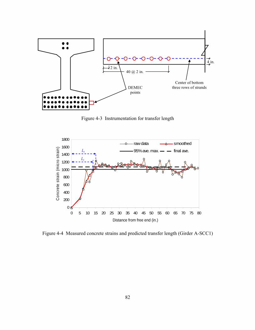
82

2 in. 40 @ 2 in.

Center of bottom three rows of strands

4 in.

DEMEC points

Figure 4-3 Instrumentation for transfer length

0

200

400

600

800

1000

1200

1400

1600

1800

0 5 10 15 20 25 30 35 40 45 50 55 60 65 70 75 80

raw data smoothed

95% ave. max. final ave.

Distance from free end (in.)

Con

cret

e st

rain

(mic

ro s

train

)

Lt

Lt

Figure 4-4 Measured concrete strains and predicted transfer length (Girder A-SCC1)

83

L/4 L/4

#6 piano wire steel ruler & mirror weight (35 lb)

pulley

Figure 4-5 Stretched-wire system used to measure camber

Figure 4-6 Measured and predicted midspan camber for Plant-A girders

0.00

0.25

0.50

0.75

1.00

1.25

1.50

1.75

0 60 120 180 240 300 360 420 480 540 600-20

0

20

40

60

80

100

12011/7/05 2/5/06 5/6/06 8/4/06 11/2/06 1/31/07 5/1/07 7/30/07

A-CM A-SCC1A-CM (PCI) A-SCC1 (PCI)Temp. (C)

Days after strand release

Cam

ber (

in.)

Date

Am

bien

t tem

pera

ture

(°C

)

84

Figure 4-7 Measured and predicted midspan camber for Plant-B girders

0

10

20

30

40

50

60

70

80

90

-5 60 125 190 255 320 385 450 515 580 645 710 775-50

-30

-10

10

30

50

70

90

11/2/05 3/2/06 6/30/06 10/28/06 2/25/07 6/25/07 10/23/07

PCI-G (A-CM)PCI-G (A-SCC1)A-CMA-SCC1RH (%)

Date

Pres

tress

loss

es (k

si)

Days after release

PCI (

A-S

CC

1)

PCI (

A-C

M)

(A-S

CC

1)

(A-C

M)

(A-S

CC

1)

(A-C

M)

RE1=2.7 ksi

AA

SHTO

-04

AA

SHTO

-07

Am

bien

t rel

ativ

e hu

mid

ity (%

)

Figure 4-8 Measured and predicted prestress losses for Plant-A girders

0.00

0.25

0.50

0.75

1.00

1.25

1.50

1.75

0 60 120 180 240 300 360 420 480-20

0

20

40

60

80

100

1207/7/06 10/5/06 1/3/07 4/3/07 7/2/07 9/30/07

B-CM B-SCC1B-SCC2 B-CM (PCI)B-SCC1&2 (PCI) Temp. (C)

Days after strand release

Cam

ber (

in.)

Date

85

0

10

20

30

40

50

60

70

80

90

-5 60 125 190 255 320 385 450 515 580 645 710-50

-30

-10

10

30

50

70

90

7/2/06 9/30/06 12/29/06 3/29/07 6/27/07 9/25/07 12/24/07 3/23/08 6/21/08

PCI-G (B-CM)B-CMB-SCC2B-SCC1RH (%)

RE1=3.0 ksi

Date Pr

estre

ss lo

sses

(ksi

)

Days after release

PCI (

B-C

M)

PCI (

B-S

CC

1)

(B-C

M)

(B-S

CC

1)

(B-C

M)

(B-S

CC

1)

AA

SHTO

-04

AA

SHTO

-07

Am

bien

t rel

ativ

e hu

mid

ity (%

)

Figure 4-9 Measured and predicted prestress losses for Plant-B girders

86

Chapter 5 Measured and Predicted Long-Term Behavior of Self-Consolidating and Conventional Concrete Bridge Girders using Companion

Cylinder Creep and Shrinkage Data

Four self-consolidating concrete (SCC) and two conventional concrete precast prestressed bridge girders were fabricated with locally available materials from two precast concrete plants (i.e., two SCC and one conventional concrete girder per plant) in the State of Minnesota. The girders were stored at an outdoor storage site between 1.5 and 2 years, where they were monitored to determine prestress losses and camber over time. In addition, companion cylinders were cast for each girder to monitor creep, shrinkage, compressive strength, and modulus of elasticity with time. The girders were brought to the University of Minnesota Structures Laboratory and tested in three-point bending to flexurally crack and then determine crack re-opening loads. The experimentally measured crack re-opening loads were used to indirectly calculate the remaining effective prestressing forces and losses. Finally, a semi-destructive test method was used to experimentally measure the remaining tendon forces to verify the field measured losses. In addition, the measured girder prestress losses were compared to those determined from a fiber-based finite element analysis incorporating time-dependent creep and shrinkage models based on companion cylinder data. The measured, predicted, and calculated prestress losses were generally in good agreement. The study indicated that creep and shrinkage material models developed based on measured companion cylinder creep and shrinkage data can be used to reasonably predict field prestress losses of both conventional and SCC prestress bridge girders.

5.1 Introduction

Self-consolidating concrete (SCC), first developed in Japan in the early 1980s (Okamura, 1997), is a relatively new type of concrete that flows under its own weight and fills formwork without segregation and without the need for mechanical vibration. Self-consolidating concrete offers substantial economic and environmental benefits including faster construction, reduction in labor, better surface finish, easier and vibration-free placement, reduced noise during placement, and a safer working environment. As a consequence, SCC has gained increased interest by the precast concrete industry in the United States (Ramsburg et al., 2003).

Numerous studies have been published over the past ten years regarding the performance of SCC in both its fresh and hardened states, which have led to successful development and use of SCC in cast-in-place and precast applications. However, concern regarding long-term behavior of SCC prestressed members especially creep and shrinkage has remained (Dehn et al., 2000; Hegger et al., 2003; and Girgis and Tuan, 2004). Many common models (e.g., ACI 209 creep and shrinkage equations) used to predict prestress losses are based on research conducted many years ago with conventional concrete, or were formulated using assumptions that do not entirely apply to SCC. Therefore, there has been some concern as to whether the current models are applicable to SCC members. For example, currently there is no ASTM standard for making SCC test cylinders. Due to the nature of SCC, there are some concerns that the mechanical properties of companion cylinders (e.g., modulus of elasticity, creep, and shrinkage) may not match those of the prestressed members and may be dependant on the method of casting the cylinders. In addition, most of the available data on the subject of long-term behavior of SCC (e.g., creep and

87

shrinkage) in the literature has been based on cylinder samples. Therefore, there has been a need to investigate the relationship between the long–term behavior of companion cylinders and large-scale structural members.

To investigate prestress losses of SCC girders, both SCC and conventional prestressed concrete bridge girders were instrumented by the University of Minnesota and monitored over a period of approximately two years. At the end of the monitoring period, two experimental methods: loading to flexural crack re-opening and strand cutting, were employed to directly and indirectly measure the prestress losses. In addition, fiber-based finite element models were created incorporating creep and shrinkage models based on measured companion cylinder creep and shrinkage data to numerically determine expected time-dependent behaviors of the girders. The calculated, predicted, and measured prestressed losses are compared herein.

The main purpose of this research was to investigate viability of predicting prestress losses of SCC concrete bridge girders using creep and shrinkage strains measured from companion cylinders, and to check the applicability of ACI 209 creep and shrinkage equations for SCC.

5.2 Research Significance

Design of prestressed concrete girders requires accurate estimates of prestress losses. Creep and shrinkage are two main contributors to prestress losses for bridge girders. Current creep and shrinkage material models (e.g., ACI 209) used to predict prestress losses were developed based on creep and shrinkage data obtained from conventional concrete cylinders. The applicability of material tests using companion cylinders to characterize the long-term and mechanical properties such as creep, shrinkage, and modulus of elasticity of SCC structural members (e.g., bridge girders) has been uncertain. In particular, the filling and consolidation method to produce companion cylinders is far different than that used in member fabrication. The results obtained from this study are useful to evaluate whether prestress losses of SCC prestressed bridge girders can be estimated using creep and shrinkage data obtained from companion cylinders. In addition, the study provides information on the adequacy of companion cylinders in predicting SCC mechanical properties.

5.3 Research Program

Two SCC girders and one conventional concrete girder were fabricated at each of two concrete precasting plants, termed Plant A and Plant B, using locally available materials. The prestress losses and companion cylinder creep and shrinkage strains were monitored for at least one year for both sets of girders. Three means of measuring prestress losses were employed in the study: 1) strain measurements obtained from vibrating wire strain gages placed near the center of gravity of strand (cgs) at midspan of the girders; 2) load measurements required to re-open flexural cracks to back-calculate prestress losses; and 3) strain measurements of prestressing strand exposed, instrumented, and severed at the end of the tests. In addition, fiber-based finite element models were used to predict girder prestress losses based on time-dependent models calibrated from companion cylinder creep and shrinkage data.

88

5.3.1 Girder Design and Instrumentation

The girders were all Mn/DOT 36M I-girders with a span length of 38 ft. The dimensions and geometry of the sections are shown in Figure 5-1. The design requirements for the release and 28-day concrete compressive strengths for all girders were 7.5 ksi and 9.0 ksi, respectively. Forty half-inch diameter Grade 270 low-relaxation strands were used in the section. There were no harped or unbonded strands. The selected section and strand pattern resulted in a maximum bottom fiber compressive stress of approximately 4.5 ksi (0.6fci') which was the maximum compressive stress that AASHTO (2004) and ACI 318-05 (2005) guidelines allowed. Shear reinforcement was provided to ensure that a shear failure would not occur before the flexural cracking moment was reached.

Both short-term and long-term instrumentation was employed to measure the initial prestressing force and prestress losses. Approximately one quarter of the total strands were instrumented at seven locations along the prestressing bed with foil-type resistance strain gages to determine the initial prestressing force. Geokon concrete embedment vibrating wire strain gages (VWSG) with a 6-in. gauge length were used to monitor concrete strains at varying depths at midspan as shown in Figure 5-2. A more detailed description of the instrumentation is provided in Appendix B.

5.3.2 Concrete Materials and Mix Proportions

Four different SCC and two different conventional concrete mixes were formulated using locally available materials by the precasters. The precasters formulated these mixes to meet the design release and 28 day concrete compressive strengths of 7.5 and 9.0 ksi respectively. In general, the precasters had significant experience with conventional prestressed concrete girders and so the mixes for these girders were typical of what would be used in standard prestressed concrete bridge girders with these specified strengths. The intention was for the precasters to also fabricate SCC girders with mixes that would be used to deliver bridge girders with the same strength requirement; however, the precasters had less experience with SCC and so were less able to control the realized strengths of the SCC mixes typically achieving lower strengths than anticipated. Table 5-1 lists the mix proportions for these formulations.

The mixes were designated according to the following scheme: X-Y, where X represents Plant-A or B (i.e., A or B), and Y represents either SCC (i.e., SCC1 or SCC2) or conventional concrete mix (CM). The girders were named based on the mix used.

For Plant-A, the conventional concrete mix (A-CM) and the first SCC mix (A-SCC1) had only ASTM Type III cement as cementitious material. For the second SCC mix (A-SCC2) Class C fly ash was used in addition to cement as supplementary cementitious material. For Plant-B, the conventional concrete and both SCC mixes had Class C fly ash as supplementary cementitious material in addition to the ASTM Type I cement.

For Plant-A SCC mixes, a polycarboxylate-based high-range water-reducing (HRWR) admixture (ASTM C 494 Type F), viscosity-modifying admixture (VMA), and a set-retarding agent (ASTM C 494 Type D) were used. For the conventional mix, a mid-range water-reducing admixture (MRWR) (ASTM C 494 Type A) and a set-retarding agent, which was different than

89

that used for the SCC mixes, were the only admixtures. For Plant-B SCC mixes, a polycarboxylate-based HRWR admixture and VMA, which were different than those used for Plant-A, were the only admixtures used. An MRWR admixture (ASTM C 494 Type A), HRWR, and a set-retarding admixture, different than those used for Plant A, were the only admixtures used for the Plant B conventional concrete mix.

For both plants, only locally available aggregates were used. For Plant-A, natural gravel (i.e., rounded river rock) with nominal maximum particle sizes of 3/4 and 3/8 in. were used in combination as coarse aggregates for both SCC mixes. For the conventional concrete mix (A-CM), the 3/4 in. aggregate was the only coarse aggregate used. For Plant-B, crushed limestone with a maximum particle size of 1/2 in. was used as the only coarse aggregate for the SCC mixes. For the conventional concrete mix (B-CM), natural gravel with a nominal maximum particle size of 3/4 in., but from a different source than that used for Plant-A, was the only coarse aggregate used. Natural sand with fineness moduli of 3.3 and 2.6 were used as fine aggregate for Plant-A and Plant-B respectively.

5.3.3 Fresh Concrete Properties

Slump flow, L-box, U-box and column segregation tests were conducted in the field to evaluate the fresh properties of the concrete, such as flowability and segregation resistance. All tests were performed while the girders were being cast. The measured fresh properties are summarized in Table 5-2. The A-SCC2 mix was considered satisfactory based on the slump flow test and visual stability index (VSI), which is a visual evaluation of the slump flow patty for segregation resistance based on guidelines provided by PCI (2003); however, the mix was observed to segregate during casting while flowing along the girder form. Approximately half the depth of the girder (i.e., 18 in.) was filled with the A-SCC2 mix, and the top half was filled with a second mix A-SCC2B developed at the time of casting to address the segregation problems with the first half of the pour. After casting was completed, it was determined that the 3/8 in. aggregate bin had been contaminated with larger 3/4 in. aggregate, which had a different moisture content and absorption properties, and is likely the reason why the A-SCC2 mix segregated. Therefore, the realized mix proportions (i.e., coarse aggregates and mixing water) for A-SCC2 and A-SCC2B mixes were different than those shown in Table 5-1 and are unknown.

5.3.4 Girder and Companion Cylinder Fabrication

Plant-A and Plant-B girders were cast on November 3, 2005, and July 5, 2005, respectively. The SCC and conventional concrete girders for each plant were cast at the same time on the same precast bed. For both plants, conventional concrete girders were cast and vibrated by means of form vibrators and hand-held vibrators before casting the SCC girders because the vibration could have affected the segregation resistance and self consolidation of the SCC girders. Even with the large amount of prestressing strand, all of the SCC mixes flowed easily into the forms and around the reinforcement (i.e., there was no sign of concrete blockage during casting).

After casting Girder A-SCC2, it was found that the coarse aggregate source had been contaminated. A truck of 3/4 in. aggregate was unloaded into the 3/8 in. aggregate bin by

90

mistake (i.e., 3/8 in. aggregate were contaminated with larger 3/4 in. aggregate). The 3/4 in. aggregate had a higher water content (1.8%) than the 3/8 in. aggregate (1.3%), and because the 3/4 in. aggregate had a smaller absorption capacity (1.0%) than the 3/8 in. aggregate (1.5 %), there was more free water in the mix (i.e., higher w/cm) than the intended amount. The increased free water and 3/4 in. coarse aggregate in the mix (A-SCC2) caused the first lift of the mix to segregate upon placement.. Before placing the second lift, the mix was reformulated (i.e., A-SCC2B) to remediate the segregation.

It was not possible to quantify the amount of aggregate contamination. Therefore, the exact proportions of the coarse aggregate and water for girder A-SCC2 and A-SCC2B were unknown, and they are not listed in Table 5-1. The listed mix proportions for A-SCC2 and A-SCC2B are those intended. Because the purpose of this paper is to determine if prestress losses in SCC girders can be predicted from the behavior of companion creep and shrinkage cylinders, and because creep and shrinkage cylinders were fabricated from concrete from both lifts of Girder A-SCC2, the behavior of this girder is included in the discussion.

Companion 4 x 11 in. creep and shrinkage cylinders were cast for each girder when the girders were fabricated; two sets were cast for Girder A-SCC2/2B to represent the two mixes used during the casting of that girder. Three sets of demountable mechanical (DEMEC) points located equidistantly (i.e., 120°) around the perimeter of the cylinder, with the pairs spaced 8 in. apart along the length, were used to measure longitudinal cylinder strains with a Whittemore gage. To ensure the same volume to surface ratio for the creep and shrinkage cylinders, both ends of the shrinkage cylinders were sealed using a two component epoxy coating as the creep cylinders were capped with a high strength capping compound. Companion 4 x 8 in. cylinders were also cast with each girder to determine strength and modulus of elasticity with time.

The companion cylinders (i.e., 4 x 11 and 4 x 8 in.) were cured with the associated girders at the prestressing bed. The conventional concrete companion cylinders were prepared based on ASTM C192/C192M. Because there were no ASTM standard procedures available specifically for making SCC cylinders, the SCC cylinders were cast similarly to the conventional cylinders with slight modifications. In the case of the SCC cylinders, the rodding used for the conventional concrete was replaced by gently tapping the outsides of the PVC molds three to four times with a mallet after each layer (in total 2 equal layers) was placed to release any trapped air. Also the molds for the SCC were filled by slowly pouring the concrete from a five-gallon plastic bucket for each layer. This mold filling method was easier and faster than filling the molds by using a scoop and it was believed that the companion cylinders prepared in this way were more representative of the concrete placed in the girders. The mold filling method should not affect the measured properties of SCC from the concrete cylinders as long as the mixes have good segregation resistance. When SCC mixes have poor or moderate segregation resistance, the mold filling method and procedure might affect the measured material properties such as strength, creep, and modulus of elasticity.

91

5.3.5 Creep and Shrinkage Cylinder Monitoring

At the end of the curing period (i.e., just before strand release) the companion cylinders were transported to the University of Minnesota Structures Laboratory where they were prepared and monitored for creep and shrinkage. The companion creep cylinders were loaded and initial creep and shrinkage readings were taken within 24 hours after strand release. The cylinders were stored in a creep room with an average temperature of 72±4°F and relative humidity of 45±15%. The girders, on the other hand, were relocated outdoors to a storage site, where a weather station was set up to monitor ambient relative humidity and temperature. The average daily ambient relative humidity had a range of 34 to 98 % with an average of 68%, and the average ambient temperature had a range of -10 to 92 °F (-23 to 33 °C) and average of 43 °F (6°C ). The girders were monitored for prestress losses for approximately 600 and 475 days for Plant-A and Plant-B girders, respectively.

In total, nine creep frames were used to load the creep cylinders, with two cylinders placed in each creep frame in series as shown in Figure 5-3. The frames were loaded within 24 hours after the associated girders were released. The axial compression force used for the creep cylinders was 56.5 kips, which corresponded to a compressive stress of 4.5 ksi (0.6fci'), equivalent to the nominal compressive stress at the bottom fiber of the girders. The only exception was the frames used to load the A-SCC2 companion cylinders. The cylinders were loaded to 4.00 ksi, which corresponded to approximately 60% of the measured concrete compressive strength at release. The main reason for this discrepancy was that the measured compressive strength of mix A-SCC2 was slightly smaller than the design value of 7500 psi at release, and there were some concerns that the cylinders could fail or be damaged as creep progressed. The measured average companion cylinder compressive strength and modulus of elasticity values at loading (i.e., within 24 hours after girder release) are given in Table 5-3. Long-term material properties of companion cylinders (e.g., fc and E) are given in Appendix D.

At predetermined time intervals (i.e., at every two days for the first week and once per week afterward), the distance between the DEMEC points on the creep and shrinkage cylinders were measured using a Whittemore gage which had a digital readout indicator with 0.0001 in (0.00254 mm) precision. A reference invar bar, used to minimize the temperature effects on readings, was used to calibrate (i.e., zero) the Whittemore gage before making any measurements. The majority of the measurements (approximately 90%) were made by the same operator. Every time a strain measurement was done for a frame, the total tensile force in the tension bars was checked, and the total compressive load was adjusted when the difference between the measured and target loads were more than ±2.5%. The creep and shrinkage tests were conducted for a duration of 574 days for Plant-A and 478 days for Plant-B cylinders.

5.3.6 Concrete Compressive Strength, Modulus of Elasticity, and Concrete Ageing

Experimentally, the concrete compressive strength and modulus of elasticity were determined based on test results (ASTM C39 and ASTM C469, respectively) obtained from companion concrete cylinders (4 x 8 in.) that were cast and cured with each girder. The measured concrete

92

compressive strength and elastic moduli at release are given in Table 5-3, and after release in Appendix D.

Concrete under ordinary ambient conditions gains strength with age because of further hydration of the cement. The finite element program (i.e., PBEAM developed by Suttikan (1978)) used to analyze the behavior of the girders over time included models for concrete aging. The built-in strength-age curves of concrete had the forms of those proposed by ACI Committee 209 (1992). The proposed model, which is given by Eqn. (5-1), has an asymptotic character with zero strength at time zero

( ) ( ) /( and /( 28'

28' btatbtatff tt +=+= εε , (5-1)

where ft' and f28 are the concrete strength at the age of t and 28 days, and εt' and ε28 are corresponding concrete strains. The constants a and b are functions of cement type, water-cement ratio, curing, etc. (ACI 209, 1992).

Similar to concrete strength, concrete modulus of elasticity also varies with time, and modulus-age curves for the concrete were predicted by rearranging Eqn. (5-1) as follows

( )( )

( ) /( /(

/(28

28

28'

'' btatE

btatbtatffE

t

tt +=

++

==εε

(5-2)

where E t' and E28 are concrete moduli at the age of t and 28 days.

In the present study, the constants a and b in Eqn. (5-1) and Eqn. (5-2) were determined using a nonlinear least square fit to the measured concrete modulus of elasticity data instead of the concrete strength data. Therefore, these constants do not necessarily represent the best fit curves to measured concrete strength data, but define the best fit curves to measured concrete modulus of elasticity. This was necessary as it is the concrete modulus that affects elastic shortening, camber, and prestress losses. A detailed description of concrete aging is included in Appendix D. It should also be noted that some of the modulus data may be in error due to malfunctioning of the compressometer used to measure vertical strain. It was found that the top yoke hinge of the compressometer had some resistance to rotation. Unfortunately, there was not enough information to determine when the problem initially developed (i.e., it is not known which readings prior to the date at which the problem was discovered were in error) and there was not enough information to determine the magnitude of the resistance and its impact on the result to adjust the data.

5.4 Experimental Methods for Determining Prestress Losses

Several experimental methods were employed to determine long-term prestress losses. These included; 1) monitoring prestress losses using vibrating wire strain gages, 2) using experimentally measured flexural crack re-opening loads and back calculating prestress losses, finally 3) a semi-destructive test method including exposing and cutting strands.

93

5.4.1 Monitoring Prestress Losses by Vibrating Wire Strain Gages

Determining prestress losses by monitoring the change in the concrete strain at the center of gravity of strands (cgs) at midspan of prestressed members is a common and direct method used by many researchers (Baran et. al., 2003; Ahlborn et. al., 2000). The change in the strain at the cgs at midspan was determined by monitoring the strain at the vibrating wire strain gage (VWSG) nearest the center of gravity of strands at midspan. This strain value was verified by interpolation of strains measured at the three or four locations through the depth of the girder at midspan. The locations of the VWSGs are shown in Figure 5-2. Assuming plane sections remain plane, a best fit line was applied to the strains measured through the depth to determine the changes in curvature at midspan. The change in measured curvature was then used to determine the change in strain in the concrete at the cgs. This value was used to verify that the strain value taken from the VWSG at the cgs was accurate. Assuming perfect bond (i.e., change in steel strain equal to change in concrete strain at same location), the change in the prestressing force was found by taking the initial prestressing force and subtracting from it the change in stress of the prestressing strand at the cgs (i.e., change in strain at cgs multiplied by the modulus of elasticity of the strand). Because prestress losses due to steel relaxation cannot be measured using strain gages, a value for steel relaxation based on the expression proposed by the PCI Committee on Prestress Losses (1975) was included in the determination of the losses by the vibrating wire strain gage measurements.

VWSGtemppT ffREREf Δ+Δ++=Δ 21 (5-3)

pTpipe fff Δ−= (5-4)

where ΔfpT is the total prestress loss, RE1 is relaxation that occurred from initial strand tensioning to strand release, RE2 is relaxation that occurred between strand release and end of monitoring time (i.e., flexural girder testing), Δftemp is the prestress loss occurring due to temperature variations during strand tensioning, concrete curing, and strand release, ΔfVWSG is the change in prestress loss measured with the vibrating wire strain gages, fpi is the initial strand tensioning stress, and fpe is the effective stress in the prestressing steel.

Because the strand length is fixed is the precasting beds and the coefficient of thermal expansion of steel and concrete differ, the increase in strand and concrete temperature due to curing prior to bond can lead to significant prestress losses. In other words, the strands were stressed at ambient temperature, but when they were heated by cement hydration they did not expand (their length was fixed by the abutments), so the strand stress reduced causing additional prestress losses. The computed temperature related losses were 4.8 and 6.8 ksi for Plant-A and Plant-B, respectively. A detailed description of the problem, and a mathematical solution developed as part of this study are presented in Appendix E as well as associated prestress losses computed for Plant-A and Plant-B.

94

5.4.1.1 Steel Relaxation

Steel relaxation is a function of the type of steel and initial stress-strength ratio. It is important to distinguish between steel relaxation that occurred while the strands were tensioned in the prestressing bed (i.e., RE1), and those that occurred after strand release (i.e., RE2). The PCI Committee on Prestress Losses (PCI, 1975) proposed a steel relaxation function

( ) ( ) ( ) ( )

( )60.0

55.045

24log24log

1

1

111

≥

⎟⎟⎠

⎞⎜⎜⎝

⎛−

−=

−

=

=

−−−∑

sy

nst

mn

n sy

nstnnnst

ff

fftt

fRE (5-5)

where tn is the time at the end of the nth time step; tn-1 is the time at the beginning of the nth time step (taken as 1/24 days when n=1); (fst)n-1 is the strand stress at the beginning of the nth time step; and fsy is the yield stress of the strand. Equation (5-5) can be used to determine RE1 in a single step (m=1) if t1 is taken as the time of strand release and (fst)0 is taken as the initial tensioning force (fpi). Due to the time it took too instrument the girder and strand, the strands remained tensioned in the prestressing beds for approximately 5 and 8 days before strand release for Plant-A and Plan-B girders, respectively. The associated relaxation losses (RE1) were 2.7 and 3.0 ksi for Plant-A and Plant-B, respectively.

The relaxation that occurred between strand release and the end of the monitoring period, RE2, (i.e., approximately 600 and 450 days for Plant-A and Plant-B) depends on other prestress losses (e.g., creep and shrinkage) and monitoring period, and it can be calculated by modifying Eqn. (5-5) to include the effect of other losses as:

( ) ( )( ) ( ) ( ) ( ) ( )

( ) ( )60.0

55.045

24log24log

1

1

1112

≥Δ−

⎟⎟⎠

⎞⎜⎜⎝

⎛−

Δ−−Δ−=

−

=

+=

−−−∑

sy

nVWRGnst

pn

mn sy

nVWRGnstnnnVWRGnst

fff

fffttffRE

(5-6)

The computed RE2 losses were 1.3, 1.1, and 1.2 ksi for A-CM, A-SCC1, and A-SCC2 girders, and 1.0, 0.9, and 0.9 ksi for B-CM, B-SCC1 and B-SCC2.

5.4.2 Predicting Prestress Losses by Flexural Crack Re-opening Loads

Determining prestress losses by loading prestressed members under flexural loads is an indirect but commonly used method to determine prestress losses. In general, prestressed members are loaded until flexural cracking occurs, and then the members are unloaded and reloaded to determine the moment corresponding to crack re-opening. Flexural crack initiation could also be used to determine prestress losses, but there is more uncertainty with this method due to the variability in concrete tensile strength.

95

All six girders in this study were tested in three-point bending with the load applied at 2L/5. The girders were loaded at 2L/5 because of space limitations in the testing laboratory, and testing the girder at 2L/5 made it possible to rotate the girders and repeat the test with the other end to verify the measured crack re-opening loads. Both ends of Girders A-SCC1 and A-CM were tested. All other girders were tested from only one end. The girders were supported on steel rollers placed approximately 6 in. from the girder ends (i.e., 37 ft between supports), and the girders were simply supported such that one end was fixed against rolling but free to rotate while the other support was completely free to translate and rotate. The testing was done in a MTS 600 kip universal testing frame using displacement-control (0.015 in. /min.).

Flexural crack initiation and re-opening had a negligible effect on the overall stiffness of the members. Therefore, the load versus deflection or load versus strain relationships measured with the embedded gages (e.g., vibrating wire and concrete embedment gages) could not be used to detect crack initiation or re-opening. Therefore, external instrumentation placed over and near the cracks was provided to detect the load corresponding to first flexural crack re-opening. The external instrumentation, consisted of surface strain gages and linear variable differential transformers (LVDTs) attached to the bottom surface of the girders at the location of maximum moment (2L/5). Figure 5-4 shows the instrumentation configuration used for Girder B-SCC1 just before the crack re-opening test (similar instrumentation was used for the other girders). The surface strain gages, represented by hollow rectangles (numbered S1-S7 and N1-N7), were placed prior to flexural crack initiation. The concrete strain gages, represented by solid rectangles (numbered NC-1 to NC-3 and OC-1 to OC-3), where gages labeled with NC were located adjacent to a crack and gages labeled with OC were placed across existing cracks) and the LVDTs were placed after flexural crack initiation, but prior to flexural crack reopening.

Evaluation of crack re-opening loads using pairs of LVDTS or strain gages placed over and adjacent to cracks have been used successfully in the past to evaluate flexural crack reopening (Baran et. al., 2003; Ahlborn et. al., 2000). In both of these past studies and in the current study, surface strain gages and LVDTs placed over or next to a crack exhibited a linear strain-load response until the crack began to open, after which they exhibited a nonlinear response as shown in Figure 5-5. During the initial linear portion, the crack was closed and the strain at the bottom surface of the girder increased linearly with load. When the load was large enough to cause a zero bottom fiber stress, the flexural crack started to re-open, and at that moment, displacements across the crack started increasing rapidly, while changes in strain next to the crack were very small or zero. The loads at which the load-strain responses diverged from the linear portion were determined as crack re-opening loads and the associated applied moments were called crack re-opening moments. In this study, the smallest loads at which the load-strain response of the gages diverged from the initial linear portion were determined using two objective and one subjective methods. A detailed description of these methods is given in Appendix, F. In general, the loads predicted with the objective methods were smaller than those predicted with the subjective method, but the difference was not more than 10 kips (approximately 90 ft-kip at 2L/5).The average of smallest loads from each method was used as crack re-opening load for back calculating prestress losses.

96

Effective prestress was determined by calculating the effective prestress required to obtain a zero bottom fiber stress when the bending moment was equal to the experimentally determined crack reopening moment,

⎥⎥⎥⎥

⎦

⎤

⎢⎢⎢⎢

⎣

⎡

+⎥⎥⎦

⎤

⎢⎢⎣

⎡+= −

b

bb

gg

tr

rocr

g

self

spe

Se

AS

MS

MA

f 111 , (5-7)

where fpe is the effective stress in the prestressing steel; As is the area of prestressing steel; gA is the gross cross-sectional area of the girders; e is the eccentricity of the prestressing strands;

bgS andbtrS are the bottom section moduli of the gross and transformed sections; Mself is the

moment due to self-weight of the girders at the crack re-opening location; and Mcr-ro is the moment at the crack re-opening section due to the applied load. The total prestress losses were calculated as

pepipT fff −=Δ , (5-8)

where ΔfpT is the total prestress loss, and fpi is the initial strand tensioning stress.

5.4.3 Determining Prestress Losses by Exposing and Cutting Strands

A semi-destructive test method was also used to determine the value of the remaining prestress. Two strands at midspan (i.e., L/2) on both sides of each girder as shown in Figure 5-6 were exposed, instrumented, and flame cut after the flexural crack re-opening tests. The concrete around the strands was removed carefully to avoid any damage to the wires as the strands were exposed over a length of approximately 18 in. Each strand was instrumented with at least three strain gages placed on individual wires as shown in Figure 5-6. The strands were tied with hose clamps at several locations to prevent unwinding of the strands during cutting and damage to the gages. Also a wet fabric, which was continually wetted during cutting, was wrapped around the strands between the cutting location and gages to protect the gages from excessive heat. The strands were flame-cut with an oxy-acetylene torch.

Strain readings were collected before cutting, during cutting, and after cutting. To minimize any unpredicted temperature effects due to flame cutting, the gages were further monitored after cutting for approximately 30 minutes while the fabric wrapped around the stands was kept wet. The selected gages and instrumentation was effective, and the gage data did not show any sign of temperature effects. The final prestressing strains were calculated simply as the difference in the strand strains before cutting and after cutting. The strains were converted to stresses by using the relationship between load and measured gage strain obtained from ancillary strand tension tests which are described in Appendix G

( )cutspsapipT Eff εΔ−=Δ (5-9)

97

where Epsa is the apparent modulus of the prestressing strand (obtained using the relationship between load and measured gage strain from ancillary strand tension tests), and (Δεs)cut is the change in the strand strain after cutting.

The location of the semi-destructive test was selected to be L/2 for two reasons. First, the girders were loaded at 2L/5 during cracking and the crack re-opening test, and L/2 was in the vicinity of the loading point but free of any visual cracks. Second, vibrating wire gages embedded into the girders during construction were located at L/2, and these gages were used to monitor the effect of exposed concrete area (i.e., reduced section due to removed concrete) on the tendon strains and stresses. The reduction in gross concrete area due to removal of the concrete was approximately 4%. The internal vibrating wire gages located in the vicinity of the exposed strands were monitored before and after concrete removal. The maximum strain variation due to the local concrete removal (i.e., reduced section) was less than 10µε (approximately 0.3 ksi)

5.5 Hybrid Numerical-Experimental Method for Predicting Prestress Losses

The main objective of this study was to determine if creep and shrinkage measurements obtained from companion cylinders could be used to predict the prestress losses over time in the fabricated girders. A fiber-based finite element program (PBEAM) was used to predict the time-dependent behavior of the girders utilizing models for creep and shrinkage based on companion creep and shrinkage cylinders cast from the seven different concrete mixes.

5.5.1 Concrete Shrinkage and Creep Material Models

For each girder mix, at least two cylinders were instrumented and monitored for drying shrinkage, and at least another two cylinders were loaded and monitored for creep. Figures 5-7 and 5-8 show the measured average shrinkage strains for Plant-A and Plant-B companion cylinders, respectively along with the shrinkage strains predicted using the ACI Committee 209 (1992) recommended equation expressed as

( ) ( ) shushα

α

tsh εtf

tε γ+

= , (5-10)

where, (εsh)t is shrinkage strain at time t; f is 55 for steam-cured concrete; (εsh)u is the ultimate shrinkage strain taken as 780; α is a constant for a given member shape and size, taken as 1.0; and γsh represents the product of applicable correction factors for conditions other than the standard conditions defined per ACI 209 (i.e., volume-surface ratio (V/S) of 1.5 in., 1-3 days steam cured, 40% ambient relative humidity, and 50% fine aggregate, etc.).

As shown in Figure 5-7 and Figure 5-8, the measured shrinkage strains of all SCC mixes were larger than those measured for the conventional concrete mixes for both plants for all times, which was expected, particularly for Plant B because of the lower w/cm for the conventional mixes. At the end of the monitoring period (i.e., 574 days after release), the shrinkage strains for the Plant-A mixes were 375με for A-CM, 460με for A-SCC1, 510με for A-SCC2, and 460με for

98

A-SCC2B, and for Plant-B, the measured shrinkage strains were 360με for B-CM and 410με for both SCC mixes (B-SCC1 and B-SCC2) at 478 days after strand release.

The ACI 209 predicted shrinkage strains adjusted for the actual conditions (V/S, cement and fine aggregate contents, etc.), and mix proportions given in Table 5-4 (not corrected for slump or slump flow) were larger than the measured shrinkage strains at all times and for all but one mix as shown in Figure 5-7 and Figure 5-8. The one exception was A-SCC2, which had larger measured shrinkage strains than those predicted for the first three months. The predicted shrinkage strains for the Plant-A conventional concrete mix (A-CM) were approximately 5% larger than those predicted for SCC mixes mainly due to higher fine-total aggregate ratio of A-CM as shown in Table 5-4. For Plant-B, the predicted shrinkage strains of the SCC mixes were the same, and they were larger than those predicted for the conventional concrete (B-CM) by approximately 15 % mainly due to higher fine-total aggregate ratio of the SCC mixes as shown in Table 5-4. Therefore, the ACI 209 proposed equations for shrinkage were conservative for both conventional and SCC mixes.

The creep strains of each creep companion cylinder were found by subtracting the initial elastic strains and the average shrinkage strains of the associated unloaded companion cylinders (at least two cylinders per mix) from the total strains measured on the creep cylinders. The creep frames were re-loaded to adjust the total creep frame load if the difference between the actual and target loads were more than ± 2.5%. Whenever a creep frame was re-loaded the gage length of the creep specimens were measured and recorded before re-loading and just after re-loading. In addition, the recorded data (i.e., strains before and after re-loading) was also used to predict the strain data that would correspond to the target load since the measured loads after re-loading were within ± 2.5% of the target loads. The procedure is further explained in Appendix C

The creep coefficients, defined as the ratio of creep strains to the initial elastic strains (when the cylinder is loaded for the first time), were also computed for each cylinder separately. The creep and creep coefficient of the mixes were computed as the average of creep strains and creep coefficients of the associated companion cylinders.

The measured total and creep strains and creep coefficients for each creep cylinder (at least two per mix) are presented in Appendix C. The average experimental creep coefficients of the mixes are shown in Figures 5-9 and 5-10 for plants A and B, respectively. In addition, creep coefficients were predicted by the procedure described in ACI 209 for each mix as

vtd

tv crut γ+

= ψ

ψ

(5-11)

where νt is the creep coefficient at time t; ψ is a constant for a given member shape and size taken as 0.6; νu is the ultimate creep coefficient taken as 2.35; d is time to one-half creep taken as 10 days, and γcr represents the product of applicable correction factors for conditions other than the standard conditions defined per ACI 209 (i.e., volume-surface ratio (V/S) of 1.5 in., 1-3 days steam cured, 40% ambient relative humidity, and 50% fine aggregate, etc.).

99

All SCC mixes had very similar measured creep behavior during early ages (i.e., the first 90 days). Mix A-SCC2 had slightly larger creep coefficients than A-SCC1 during the monitoring period but the difference was not significant despite the fact that A-SCC2 had poor segregation resistance (i.e., segregated while placed). In other words, the creep data of A-SCC2 did not indicate any noticeable sign of segregation effect on the creep. Therefore, it is likely that the segregation of the mix while filling the companion cylinders was not as significant as the segregation observed during girder casting. This is probably because the dynamic effects associated with girder casting including concrete flowing large distances through heavily reinforced sections were not present while casting the companion cylinders. Mix A-SCC2B had the largest creep coefficients after early ages (i.e., 90 days). However, the creep coefficient was not much larger than the creep coefficient of the other SCC mixes. The conventional concrete mix had the smallest creep coefficient during the monitoring period. This was expected as the conventional concrete had much larger concrete compressive strength than the other mixes. The ACI 209 predictions of creep coefficients for Plant-A mixes shown in Table 5-5 were equal for SCC mixes and similar for the conventional concrete mix (A-CM). The predicted creep coefficients were larger than the measured creep coefficients during the monitoring period. After 574 days of creep, the measured creep coefficients were 0.91 for A-CM, 1.34 for A-SCC1. The ACI 209 predicted creep coefficients (adjusted for actual conditions such as RH and V/S) were on the order of 2.0.

The measured creep coefficients of Plant-B mixes are given in Figure 5-10 along with the ACI 209 prediction (adjusted for actual conditions). Similar to the Plant-A mixes, the conventional concrete mix (B-CM) had smaller measured creep coefficients than those of the SCC mixes during the monitoring period (478 days). The SCC mixes had similar creep behavior for early ages (i.e., first 90 days), but the B-SCC2 mix had slightly larger creep coefficients than B-SCC1 after the first 90 days. The ACI 209 predictions of creep coefficients were on the order of 2.0 for all Plant B mixes at end of 478 days. The measured creep coefficients, on the other hand, were 0.99 for B-CM, 1.43 for B-SCC1 and 1.62 for B-SCC2 at the end of monitoring period. The experimental and ACI 209 creep data indicates that ACI 209 proposed creep equation is conservative for both SCC and conventional concrete.

Nonlinear least-squares analyses (LSA) of all shrinkage and creep data were done using Eqn. (5-10) and Eqn. (5-11) for shrinkage and creep, respectively, to develop shrinkage and creep models that described the experimentally derived data for use in the finite element models. Three cases were considered for both shrinkage and creep: one-parameter (LSA-1), two-parameter (LSA-2), and three-parameter (LSA-3) nonlinear least square analyses. For LSA-1, ultimate shrinkage and creep coefficients ((εsh)u and νu) were determined from the analyses (setting α=1.0, f=55, ψ=0.6, and d= 10), for LSA-2 in addition to ultimate shrinkage and creep coefficients, the constants f and d were determined from the least square analyses (setting α=1.0 and ψ=0.6), and finally for LSA-3 all three constants for shrinkage (α, f, and (εsh)u) and creep (ψ, d, and νu) were determined from the least squares analysis. ACI 209 creep and shrinkage correction factors in Eqn. (5-10) and (5-11) were taken as unity because the measured data was used.

Figure 5-11 shows the experimental shrinkage strains and fitted ACI 209 equations for A-SCC1 using the least square analyses. The experimental shrinkage data fit all but the one-parameter LSA curves well. Similar results were found for all other Plant-A mixes and Plant-B mixes, and

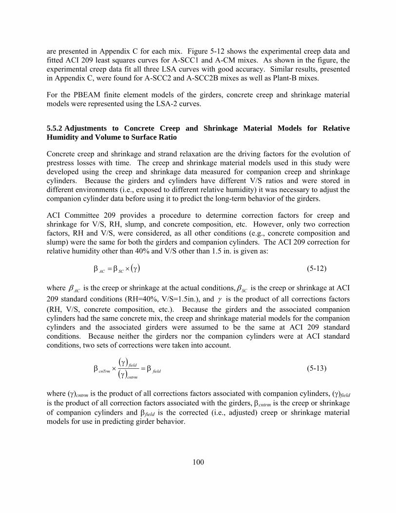
100

are presented in Appendix C for each mix. Figure 5-12 shows the experimental creep data and fitted ACI 209 least squares curves for A-SCC1 and A-CM mixes. As shown in the figure, the experimental creep data fit all three LSA curves with good accuracy. Similar results, presented in Appendix C, were found for A-SCC2 and A-SCC2B mixes as well as Plant-B mixes.

For the PBEAM finite element models of the girders, concrete creep and shrinkage material models were represented using the LSA-2 curves.

5.5.2 Adjustments to Concrete Creep and Shrinkage Material Models for Relative Humidity and Volume to Surface Ratio

Concrete creep and shrinkage and strand relaxation are the driving factors for the evolution of prestress losses with time. The creep and shrinkage material models used in this study were developed using the creep and shrinkage data measured for companion creep and shrinkage cylinders. Because the girders and cylinders have different V/S ratios and were stored in different environments (i.e., exposed to different relative humidity) it was necessary to adjust the companion cylinder data before using it to predict the long-term behavior of the girders.

ACI Committee 209 provides a procedure to determine correction factors for creep and shrinkage for V/S, RH, slump, and concrete composition, etc. However, only two correction factors, RH and V/S, were considered, as all other conditions (e.g., concrete composition and slump) were the same for both the girders and companion cylinders. The ACI 209 correction for relative humidity other than 40% and V/S other than 1.5 in. is given as:

( )γ×β=β SCAC (5-12)

where ACβ is the creep or shrinkage at the actual conditions, SCβ is the creep or shrinkage at ACI 209 standard conditions (RH=40%, V/S=1.5in.), and γ is the product of all corrections factors (RH, V/S, concrete composition, etc.). Because the girders and the associated companion cylinders had the same concrete mix, the creep and shrinkage material models for the companion cylinders and the associated girders were assumed to be the same at ACI 209 standard conditions. Because neither the girders nor the companion cylinders were at ACI standard conditions, two sets of corrections were taken into account.

( )( ) field

cntrm

fieldcnTrm β=

γ

γ×β (5-13)

where (γ)cntrm is the product of all corrections factors associated with companion cylinders, (γ)field is the product of all correction factors associated with the girders, βcntrm is the creep or shrinkage of companion cylinders and βfield is the corrected (i.e., adjusted) creep or shrinkage material models for use in predicting girder behavior.

101

5.5.3 Adjustment for Ambient Relative Humidity

The measured ambient relative humidity of the outdoor storage area had seasonal fluctuations. The average ambient relative humidity and its standard deviation were 68% and ±12% for the outdoor storage area, and 45% and ±5% for the creep room, respectively.

Committee ACI 209 recommends the following equations be used for adjusting creep and shrinkage models for ambient relative humidity, respectively

For creep: ( ) 40for ,0067.027.1 >−=γ RHRHRHCR (5-14)

For shrinkage: ( )( ) 10080for ,030.000.3

8040for ,0102.040.1≤<−=γ

≤≤−=γ

RHRHRHRH

RHSH

RHSH , (5-15)

where, (γCR)RH and (γSH)RH are correction factors for creep and shrinkage due to ambient relative humidity, respectively.

Because the two sets of girders were cast at very different times (i.e., Plant A girders cast in November when the relative humidity in Minnesota is high, and Plant B girders cast in July when the relative humidity in Minnesota is near its yearly average), the correction factors were calculated for two relative humidity cases as shown in Table 5-6. In the first case, correction factors were calculated by using the average ambient relative humidity values of the girder storage site and that of the creep room where the companion cylinders were stored. In the second case, the average RH value of the creep room was used for the companion cylinders, but the ambient relative humidity of the girder storage site was assumed to be 100%. The second case, where shrinkage was assumed to be zero (i.e., 100% RH), was intended to correspond to conditions where the girders would be covered completely with snow shortly after casting. Plant-A girders were cast on November 3, 2005, and they were exposed to winter conditions (i.e., high RH) during early age. The 100% RH case was included to investigate whether early-age behavior of the Plant-A girders could be predicted using the finite element models.

In addition, a third case was considered where the effect of the outdoor storage site average daily ambient relative humidity was included as a function of time. In this case, the creep and shrinkage strains occurring between times (days) ti and ti+1 were adjusted for the average ambient relative humidity measured over times ti and ti+1 using

( ) ( ) ( ) ( )( ) ( ) ( )( )( ) avrgcntrm

tfieldtfieldtcntrmtcntrmtfieldtfield

ii

iiii_

__ 21

11 γ

γ+γ×β−β+β=β +

++ (5-16)

where (γ)cntrm_avrg is the correction factor due to average RH value of the creep room, and (γ)field_ti and (γ)field_ti+1 are the correction factors due to the average site RH at times ti and ti+1, respectively.

102

The term ( ) ( )( )ii tcntrmtcntrm ββ −

+1 represents the variation of creep/shrinkage of companion

cylinders over one time step (taken as one day). However, because creep and shrinkage data for the companion cylinders was collected once per week for most of the monitoring period, the term was computed using the associated creep/shrinkage nonlinear least-square curves (i.e., LSA-2). Also for the same reason, only the average ambient relative humidity value (i.e., 45%) of the creep room was considered due to the limited number of available data for the creep room ((γ)cntrm_avrg). Nonlinear least-square parameters (LSA-2) shown in Table 5-7 were developed for the adjusted data ( ( )

1+itfieldβ ), which were used for the finite element analyses of the girders.

The objective of these analyses was to investigate the sensitivity of the finite element analysis results to the daily and average (average for the whole monitoring period) ambient relative humidity values of the girder storage site.

5.5.4 Adjustment for Volume-Surface Ratio

The volume-surface ratios were equal to 1.0 in. and 3.5 in. for the companion cylinders and girders, respectively. Because the V/S of the companion cylinders and the girders were different, the cylinder creep and shrinkage data were further adjusted for V/S to obtain associated material models for the girders.

Committee ACI 209 recommends the following corrections for members with V/S ratio different than 1.5 in.

For creep: ( ) 2.013.113254.0

≥⎟⎟⎠

⎞⎜⎜⎝

⎛+=γ

−SV

VSCR e (5-17)

For shrinkage: ( ) 2.02.112.0

≥=γ−

SV

VSSH e (5-18)

The creep correction factors were found to be 0.78 and 1.10, and shrinkage correction factors were 0.79 and 1.06 for the girders and companion cylinders for V/S, respectively. The total correction factors (i.e., γgirder/γcylinder) were 0.71 and 0.75 for creep and shrinkage, respectively (Table 5-6). In other words, the measured companion cylinder creep was multiplied by 0.71 and measured companion shrinkage data was multiplied by 0.75 to obtain creep and shrinkage material models adjusted for V/S for the girders, respectively. The total correction factors due to average RH and V/S were 0.60 and 0.57 for creep and shrinkage, respectively.

103

5.6 Results and Discussion

5.6.1 Finite Element Predicted and VWSG Measured Prestress Losses

The program PBEAM developed by Suttikan (1978) was used to analyze the behavior of the girders over time including creep, shrinkage, steel relaxation, and prestress losses. The inputs for the program included models for concrete aging (i.e., time dependent fc and Ec), creep, shrinkage, steel relaxation, gravity loads, and support conditions. Based upon these models and the assumption that plane sections remain plane, PBEAM determines the strains and stresses at elements and fibers throughout the girder. The original program, which was used for this study, does not consider thermal effects and steel relaxation occurring between strand tensioning and strand release (RE1). Therefore, the initial prestressing force was decreased by RE1 and tempfΔ , which were prestress losses that occurred due to relaxation prior to strand release and temperature variation during strand tensioning, concrete curing, and strand release. Other thermal effects, that occurred after girder release were not considered in the finite element models. Appendix H contains more information on the PBEAM models.

The girders were modeled using 34 discrete elements for the 38 ft girder span (each element 13.4 in. in length), and cross section was modeled using 42 fibers through the 36 in. girder depth. The creep and shrinkage material models formulated from best fit curves of the cylinder data which were adjusted for ambient RH and girder V/S ratio, were assumed to be the same for all concrete fibers in a given girder. The defined support conditions were simple support conditions, and their locations were consistent with the support locations at the storage site (i.e., approximately 6 in. from the ends)

The total prestress loss at the center of gravity of all prestressing strands (cgs) at midspan of the girders was calculated and compared to the losses measured at the same location using data from embedded VWSGs. The maximum deviation between the exact location of the gauges and cgs was ±1/2 in, and the recorded strains (prestress losses) were verified with the strain profile measured from the vertically distributed gages at the same section.

Three creep and shrinkage material models were considered as shown in Table 5-7. These were companion creep and shrinkage data with adjustment for V/S and for three different cases for girder storage site ambient relative humidity values (i.e., 100%, average RH, and RH as a function of time (i.e., RH (t)). The measured total prestress losses (with corrections for relaxation prior to release and losses associated with temperature changes prior to release) and those predicted from PBEAM at the cgs are shown in Figures 5-13 through 5-18 for all six girders.

The difference between using the average storage site ambient RH and the storage site RH as a function of time had negligible effect on the PBEAM computed prestress losses for both plants. This was expected because the effect of RH when considered as a function of time should have the same overall effect. Also the creep and shrinkage least squares equations for both cases (average RH and RH as a function of time (RH(t)) were very similar as given in Table 5-7, therefore both cases yielded similar responses.

104

For Plant-A girders, the measured total prestress losses were much smaller than those predicted with PBEAM for early ages (during approximately first 225 days). The measured losses in the Plant-A girders were almost constant for the first 150 days after casting. This was because the girders were cast in November, followed by a period of high relative humidity (i.e., winter in Minnesota). To capture the effect of ambient relative humidity on early age prestress losses, PBEAM models with 100% ambient RH were developed. The measured losses and PBEAM computed losses with 100% RH were in excellent agreement for early times (up to 125 days). They diverged after approximately 150 days after casting when the relative humidity decreased (i.e., spring). During the spring and summer, the measured losses for Plant-A girders continued increasing and eventually plateaued near the value calculated with the PBEAM model using the average relative humidity after approximately 225 days after casting. At the end of approximately 300 days after casting and for the rest of the monitoring period, the computed and measured prestress losses showed reasonable agreement for the cases of average RH and RH(t) (i.e., the maximum difference between the measured and computed prestress losses was less than 4% of the initial prestressing force for any girder).

For Plant-B girders, the PBEAM models with 100% RH (i.e., shrinkage neglected) predicted total prestress losses that were smaller than the measured total losses over all time for all girders. The computed losses for the first 120 days for the case of 100% RH were significantly lower than the measured losses (Figure 5-16 through 5-18). This was because Plant-B girders were cast in July, followed by a relatively low relative humidity period of approximately 120 days. The computed PBEAM losses based on average RH and RH(t) were consistent with the measured short-term losses (approximately 150 days after casting) for all girders. In other words, computed total losses were smaller than those measured but the difference at anytime was less than 3 ksi for both RH and RH(t). The PBEAM model slightly underpredicted the early losses (i.e., approximately first 120 days after casting) for the Plant-B girders. This was probably because the girders were cast in July, followed by a period of low relative humidity (i.e., summer in Minnesota).

Approximately 120 days after girder casting at Plant-B, the measured losses were almost constant for all girders. However, there were some seasonal fluctuations due to ambient relative humidity. For example, between 160 and 300 days after girder casting, which corresponded to winter in Minnesota, the measured loses were almost constant or decreased slightly (by less than 1.0 ksi), but. the measured and computed losses were in reasonable agreement (difference less than 3 ksi at anytime) for this period. At the end of approximately 360 days after casting and for the rest of monitoring period, the computed and measured losses were in good agreement for RH and RH(t) cases. In other words, the difference between the measured and calculated prestress losses was less than 2 ksi at the end of monitoring period for Plant-B girders.

5.6.2 Predicted Prestress Losses Using Flexural Crack Re-opening Loads

The measured first flexural crack re-opening moments at 2L/5 and the corresponding effective stress in the prestressing strands calculated using Eqn. (5-7) are documented in Table 5-8 for all six girders. The crack re-opening moments were also computed using the PBEAM finite element models developed for each girder with creep and shrinkage material models adjusted for

105

the average RH and V/S ratio, which were shown previously to predict the losses well at the time of flexural crack re-opening. The average effective stresses in the prestressing strands at the center of the strands just before flexural cracking tests were also computed by subtracting the computed total prestress losses at the same location from the initial prestressing stresses.

The experimentally measured crack re-opening moments were significantly smaller than those determined using PBEAM for all girders (36-47%) as shown in Table 5-8. Therefore, the effective stresses at the center of the prestressing strands calculated using experimentally measured crack re-opening moments with Eqn. (5-7) were 34 to 45 % smaller than those calculated using Eqn. (5-7) and PBEAM computed crack re-opening moments. Similar findings have been reported by Ahlborn et. al. (2000) and Baran et. al. (2003). Ahlborn fabricated two long-span Mn/DOT 45M girders and monitored the prestress losses for almost two years. The girders were tested in flexure, and the crack re-opening moments were determined both using concrete surface gages and PBEAM models. One girder developed vertical cracks prior to strand release, which affected the losses. The other girder did not develop any pre-release cracks, however, the PBEAM crack re-opening moments were 53% than those measured with concrete surface gages for this girder. Similar findings were reported by Baran et. al. (2003), who tested two Mn/DOT 28M girders (30 ft long) girders and determined crack re-opening loads using concrete surface gages.

The effective prestressing stresses computed with PBEAM crack re-opening moments and Eqn. (5-7) were slightly (13 to 20 ksi) higher than the strand stresses determined directly by PBEAM. However, the effective prestressing stresses computed using the total prestress losses measured/computed with VWSGs and PBEAM were in very good agreement with a maximum difference of 3 ksi.

The same creep and shrinkage material models were used for all concrete fibers in the PBEAM models. However, the fibers located near the surface were likely to have different creep and especially shrinkage behaviors than those located within the section far from the girder surface. To investigate the effect of fiber location (i.e., variation of shrinkage and creep models depending on fiber location) on crack re-opening loads, modified PBEAM girder models were developed. Due to the limitation of the maximum number of material models that can be used in the finite element program, only the creep and shrinkage material models of the concrete fibers representing the bottom surface (where cracking was assumed to occur) and top surface of the girders were modified as shown in Figure 5-19. It was assumed that all moisture exchange of those two fibers would occur through fiber surfaces exposed to the atmosphere (i.e., no moisture exchange through fiber interfaces). The average girder V/S ratio (3.49 in.) was assumed for the other concrete fibers. The V/S ratio of the fiber (1.0 in. in thickness) was calculated to be 0.93, and the companion cylinder creep and shrinkage data was adjusted accordingly for V/S to determine the adjusted creep and shrinkage material models for the top and bottom fibers. The associated creep and shrinkage adjusted coefficients due to V/S were 1.02 and 1.01, respectively, for the top and bottom fibers and 0.71 and 0.75, respectively, for the rest of the fibers, respectively.

106

The fiber creep and shrinkage material models did not affect the computed total prestress losses at the center of the strands because the total area of the bottom and top fibers was only 10 % of the girder gross area.

Resulting calculated crack re-opening moments and associated effective stress in the prestressing strand are given in Table 5-8. The calculated crack re-opening moments for the cases with the modified top and bottom fiber shrinkage and creep material models were much smaller than those calculated using a single creep and shrinkage material model for the entire girder and were much closer to those determined from the surface strain gages (i.e., 22% to 35% higher than those measured with the surface strain gages (previously 56% to 89 %). PBEAM results indicated that although the computed smaller crack re-opening moments indicated larger prestress losses from Eqn. (5-7), there was negligible change in the prestress losses determined directly for the strands.

The experimental results (i.e., measured prestress losses and those predicted using measured crack re-opening moments) indicate that the girder might not experience uniform concrete shrinkage – that is, the concrete closer to the surface of the girder may shrink at a faster rate than the interior concrete. Therefore, the initiation of cracking and crack re-opening would occur at smaller flexural loads than the model with fibers with identical creep and shrinkage material models. In other words, flexural loading tests when used with Eqn. (5-7) are not suitable methods to determine the effective stress in the prestressing strand. However, these tests provide useful information regarding the serviceability (crack formation and re-opening) of prestressed members.

5.6.3 Predicted Prestress Losses Using Strand Cutting Data

Table 5-9 shows the average effective stress in the prestressing strand determined by exposing and flame-cutting two strands from the third row from the bottom in the bottom flange of each girder. Strand stresses calculated for the same strands with PBEAM models and those determined from the strain distribution through the section height measured with the VWSGs are also included for comparison. However, because both PBEAM computed and VWSGs measured losses do not include prestress losses due to steel relaxation that occurred before strand release and temperature variations (RE1 and tempfΔ ), these two losses were added to the measured and computed losses using Eqns. (5-3) and (5-4).

As shown in Table 5-9, SCC girders had larger prestress losses (smaller strand forces) than the conventional concrete girders for both plants based on the prestressing force determined by strand cutting. It should be noted that the release strengths (and hence elastic moduli) of the conventional girders were higher than the SCC girders, so the conventional girders experienced less elastic shortening than the SCC girders. The losses determined by strand cutting were consistent with the other methods (i.e., PBEAM and VWSGs) used to determine prestress losses. The strand forces calculated by cutting the strands were smaller than those calculated both by the PBEAM models and from VWSGs strain measurements. The difference was between 4% and 9% of the initial tensioning stress for the PBEAM method, and 4% to 8% of the initial tensioning for the VWSGs. In other words, total prestress losses predicted for the cut strands with PBEAM

107

models and VWSGs data were approximately 4% to 9% smaller for Plant-A, and approximately 4% to 7% smaller for Plant-B than total prestress losses determined by strand cutting. The difference between the average strand forces determined by strand cutting and monitoring VWSG strains is believed to be due to errors associated with measuring the initial prestressing force, VWSG depth, temperature effects, and assumptions used when converting strains to stresses (i.e. perfect bond).

5.7 Summary and Conclusions

Four SCC and two conventional concrete girders (Mn/DOT 36M-I) with a span length of 38 ft were fabricated using locally available materials from two precast concrete plants. The section represented one of the most severe cases for the application of SCC to bridge girders (i.e., highly congested and large stresses to introduce creep). The design concrete compressive strength was 7.5 ksi at release and 9.0 ksi at 28 days. Companion creep and shrinkage cylinders were cast at the same time and cured with the girders. The girders were stored at an outdoor storage site where ambient relative humidity and strains at the midspan of the girders were monitored to determine prestress losses. After approximately two years, the girders were tested to determine flexural crack re-opening loads. In addition, a semi-destructive testing method was employed to directly measure the remaining effective prestressing forces. Finite element models were developed with creep and shrinkage material models fit to measured companion cylinder creep and shrinkage data and modified for the effects of RH and V/S for the girders. Based on the experimental and finite element results presented, the following conclusions can be made for the fabricated girders and employed methods to determine prestress losses:

1. The measured shrinkage strains and creep coefficients for both SCC and conventional concrete mixes were smaller than those predicted using the recommended ACI 209 procedures for cases in which the ultimate shrinkage and creep coefficients were unknown. At the end of the monitoring period, the data from the companion shrinkage and creep cylinders indicated that the measured shrinkage strains were approximately 35% smaller than those predicted by ACI 209, and the measured creep coefficients were approximately 50% and 25% smaller for conventional and SCC mixes, respectively, than the ACI 209 predictions

2. The SCC mixes were observed to have larger shrinkage and creep strains than the conventional concrete mixes. By the end of the monitoring period, the SCC girder mixes had approximately 25% and 15% higher shrinkage strains for Plant-A and Plant-B, respectively. The measured average creep coefficients of the SCC mixes were 60% and 55% larger than those measured for the conventional concrete mixes for Plant-A and Plant-B, respectively. It is not possible to determine the extent to which this is due to differences in achieved concrete strengths as opposed to the type of concrete (SCC versus conventional).

3. The finite element program PBEAM can be used with measured creep and shrinkage material models to predict long-term prestress losses for SCC girders. However, determining effective prestress forces by flexural crack re-opening loads yielded effective

108

prestressing forces that were much smaller (i.e., 28% to 38%) than those directly measured using PBEAM or VWSGs. This might be attributed to the increased rate of shrinkage of concrete near the bottom surface of the girder due to the smaller local V/S ratio near the surface. Analyses using the finite element program, PBEAM, indicated that this phenomenon would reduce the moment required to crack and re-open cracks in the girders. Although this effect has a negligible impact on the girder total prestress losses, it results in a lower prediction of crack re-opening moments.

4. Early age prestress losses are sensitive to ambient relative humidity. PBEAM finite element models can be used to predict early age girder behavior and prestress losses if the shrinkage and creep material models are adjusted for ambient relative humidity.

5. Companion cylinder creep and shrinkage models can be used for both conventional concrete and SCC girders to predict and model short-term and long-term behavior of girders including prestress losses and crack re-opening moments when the ACI 209 correction factors for relative humidity and volume-surface ratio are applied to measured creep and shrinkage data of companion cylinders.

6. Calculating prestress losses based on measured crack re-opening moments predicted the largest prestress losses. Exposing and cutting strands, finite element model, and internal gages predicted similar prestress losses.

7. Crack re-opening loads can not be calculated accurately assuming homogenous elastic beam theory with plane sections-remaining plane. The increased shrinkage near the bottom surface of the girders must be taken into account.

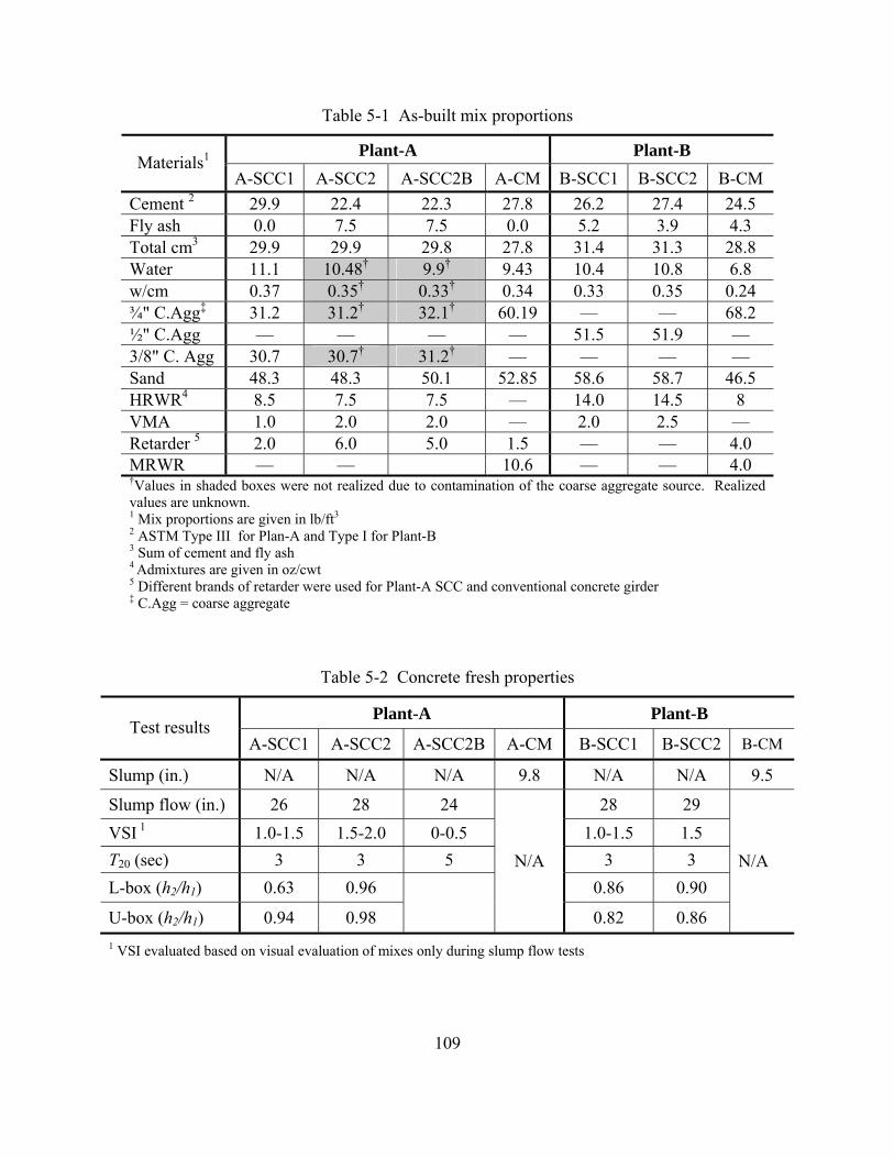
109

Table 5-1 As-built mix proportions

Plant-A Plant-B Materials1

A-SCC1 A-SCC2 A-SCC2B A-CM B-SCC1 B-SCC2 B-CM Cement 2 29.9 22.4 22.3 27.8 26.2 27.4 24.5 Fly ash 0.0 7.5 7.5 0.0 5.2 3.9 4.3 Total cm3 29.9 29.9 29.8 27.8 31.4 31.3 28.8 Water 11.1 10.48† 9.9† 9.43 10.4 10.8 6.8 w/cm 0.37 0.35† 0.33† 0.34 0.33 0.35 0.24 ¾" C.Agg‡ 31.2 31.2† 32.1† 60.19 — — 68.2 ½" C.Agg — — — — 51.5 51.9 — 3/8" C. Agg 30.7 30.7† 31.2† — — — — Sand 48.3 48.3 50.1 52.85 58.6 58.7 46.5 HRWR4 8.5 7.5 7.5 — 14.0 14.5 8 VMA 1.0 2.0 2.0 — 2.0 2.5 — Retarder 5 2.0 6.0 5.0 1.5 — — 4.0 MRWR — — 10.6 — — 4.0 †Values in shaded boxes were not realized due to contamination of the coarse aggregate source. Realized values are unknown. 1 Mix proportions are given in lb/ft3

2 ASTM Type III for Plan-A and Type I for Plant-B 3 Sum of cement and fly ash 4 Admixtures are given in oz/cwt 5 Different brands of retarder were used for Plant-A SCC and conventional concrete girder ‡ C.Agg = coarse aggregate

Table 5-2 Concrete fresh properties

Plant-A Plant-B Test results

A-SCC1 A-SCC2 A-SCC2B A-CM B-SCC1 B-SCC2 B-CM

Slump (in.) N/A N/A N/A 9.8 N/A N/A 9.5

Slump flow (in.) 26 28 24 28 29 VSI 1 1.0-1.5 1.5-2.0 0-0.5 1.0-1.5 1.5 T20 (sec) 3 3 5 3 3 L-box (h2/h1) 0.63 0.96 0.86 0.90

U-box (h2/h1) 0.94 0.98

N/A

0.82 0.86

N/A

1 VSI evaluated based on visual evaluation of mixes only during slump flow tests

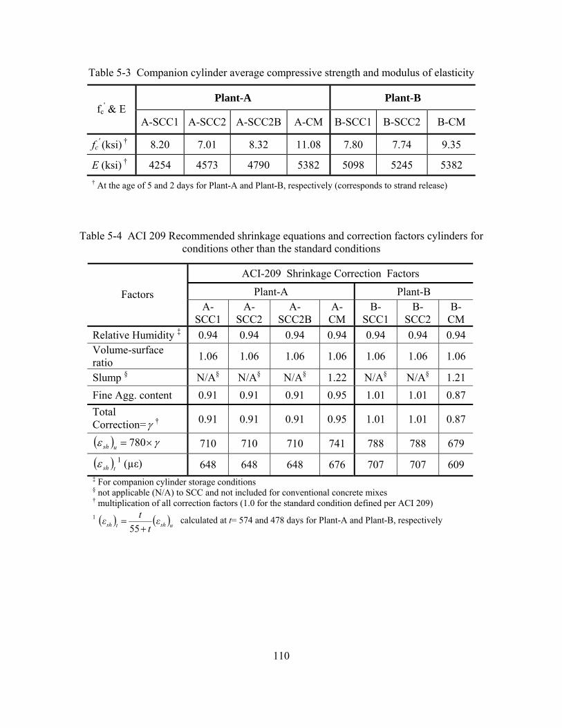
110

Table 5-3 Companion cylinder average compressive strength and modulus of elasticity

Plant-A Plant-B fc

' & E A-SCC1 A-SCC2 A-SCC2B A-CM B-SCC1 B-SCC2 B-CM

fc' (ksi) † 8.20 7.01 8.32 11.08 7.80 7.74 9.35

E (ksi) † 4254 4573 4790 5382 5098 5245 5382 † At the age of 5 and 2 days for Plant-A and Plant-B, respectively (corresponds to strand release)

Table 5-4 ACI 209 Recommended shrinkage equations and correction factors cylinders for conditions other than the standard conditions

ACI-209 Shrinkage Correction Factors

Plant-A Plant-B Factors A-

SCC1 A-

SCC2 A-

SCC2B A-CM

B-SCC1

B-SCC2

B-CM

Relative Humidity ‡ 0.94 0.94 0.94 0.94 0.94 0.94 0.94 Volume-surface ratio 1.06 1.06 1.06 1.06 1.06 1.06 1.06

Slump § N/A§ N/A§ N/A§ 1.22 N/A§ N/A§ 1.21 Fine Agg. content 0.91 0.91 0.91 0.95 1.01 1.01 0.87 Total Correction=γ † 0.91 0.91 0.91 0.95 1.01 1.01 0.87

( ) γε ×= 780ush 710 710 710 741 788 788 679

( )tshε 1 (µε) 648 648 648 676 707 707 609 ‡ For companion cylinder storage conditions § not applicable (N/A) to SCC and not included for conventional concrete mixes

† multiplication of all correction factors (1.0 for the standard condition defined per ACI 209) 1 ( ) ( )

55 ushtsh εt

tε+

= calculated at t= 574 and 478 days for Plant-A and Plant-B, respectively

111

Table 5-5 ACI 209 Recommended creep equations for standard conditions and correction factors for cylinders with conditions other than the standard conditions

Table 5-6 Creep and Shrinkage Correction Factors

Relative humidity Volume surface ratio Total correction factor†

( ) ( )cntrmfieldRH γγγ = ( ) ( )cylindergirderVS γγγ = RHVS γγγ ×= Relative humidity

cases Creep Shrinkage Creep Shrinkage Creep Shrinkage

Average RH 0.84 0.76 0.60 0.57

100% RH 0.62 0.0 0.71 0.75

0.44 0.0

†Applied to ultimate creep coefficient and ultimate shrinkage (i.e., PBEAM inputs)

ACI-209 Creep Correction Factors

Plant-A Plant-B Factors

A-SCC1 A-SCC2 A-SCC2B A-CM B-SCC1 B-SCC2 B-CM

Loading Age 0.96 0.96 0.96 0.96 1.00 1.00 1.00 Relative Humidity ‡ 0.97 0.97 0.97 0.97 0.97 0.97 0.97 Volume-surface ratio 1.11 1.11 1.11 1.11 1.11 1.11 1.11

Slump § N/A§ N/A§ N/A§ 1.47 N/A§ N/A§ 1.46

Fine Agg. content 0.99 0.99 0.99 0.99 1.01 1.01 0.98

Total Correction † 1.02 1.02 1.02 1.01 1.09 1.09 1.06

γ×= 35.2uv 2.40 2.40 2.40 2.37 2.56 2.56 2.49

tv 1 1.97 1.97 1.97 1.94 2.05 2.05 2.00 ‡ For companion cylinder storage conditions § not applicable (N/A) to SCC and not included for conventional concrete mixes

† multiplication of all correction factors (1.0 for the standard condition defined per ACI 209) 1

ut vt

tv 60.0

60.0

10 += calculated at t= 574 and 478 days for Plant-A and Plant-B, respectively

112

Table 5-7 Least square fit parameters for ACI 209 creep and shrinkage equations

Shrinkage Creep

RH cases§ RH cases§

Avrg 100% Avg 100%Mix

α f ( )ushε †

(εsh)u (εsh)u

ψ d vu†

vu vu

A-CM 1.00 19 389 222 0.0 0.60 15.5 1.21 0.73 0.53

A-CM‡ 1.00 18 202 0.60 15.8 0.72

A-SCC1 1.00 24 473 270 0.0 0.60 11.2 1.65 0.99 0.73

A-SCC1‡ 1.00 24 245 0.60 11.3 0.98

A-SCC2 1.00 18 536 306 0.0 0.60 11.3 1.74 1.04 0.77

A-SCC2‡ 1.00 17 279 0.60 11.4 1.03

A-SCC2B 1.00 14 458 261 0.0 0.60 17.3 2.26 1.36 0.99

A-SCC2B‡ 1.00 13 240 0.60 17.7 1.34

B-CM 1.00 33 376 214 0.0 0.60 9.45 1.17 0.70 0.51

B-CM‡ 1.00 28 213 0.60 8.34 0.68

B-SCC1 1.00 29 442 252 0.0 0.60 7.28 1.54 0.92 0.68

B-SCC1‡ 1.00 25 252 0.60 6.41 0.91

B-SCC2 1.00 23 426 243 0.0 0.60 10.40 1.84 1.10 0.81

B-SCC2‡ 1.00 19 246 0.60 9.19 1.07 † Determined from least square analyses (LSA-2 ) of measured companion cylinder data, no RH and V/S correction

§ Corrected for V/S ratio and RH

‡ Values in the shaded cells were corrected for outdoor storage site daily ambient (RH (t)) and average RH for creep room, and for V/S

113

Table 5-8 Prestress losses obtained from first flexural crack re-opening moments and experimentally measured with vibrating wire gages

Experimental PBEAM 1 PBEAM 2 VWSG 3

fse (ksi) fse (ksi) Girder ID Mcr-ro

(k-ft)

fse (ksi) Eqn. 5-7

Mcr-ro (k-ft) Eqn.

5-7 From PBEAM

Mcr-ro (k-ft) Eqn.

5-7 From PBEAM

fse (ksi)

A-CM 1210 118 (42%) 1888 179

(12%) 166

(19%) 1524 146 (28%)

166 (19%)

164 (20%)

A-SCC1 1165 111 (46%) 1817 168

(18%) 156

(24%) 1420 134 (34%)

156 (23%)

154 (24%)

A-SCC2 1031 98 (52%) 1812 167

(18%) 155

(24%) 1397 130 (36%)

155 (24%)

152 (25%)

B-CM 1165 113 (45%) 1871 177

(14%) 160

(22%) 1498 143 (30%)

160 (22%)

159 (22%)

B-SCC1 986 97 (53%) 1851 174

(15%) 157

(23%) 1312 126 (39%)

157 (24%)

156 (24%)

B-SCC2 986 97 (53%) 1859 176

(14%) 156

(24%) 1232 119 (42%)

156 (24%)

155 (24%)

1 The same creep and shrinkage material models used for all fibers

2 The bottom surface fiber material models adjusted for V/S ratio of that the fiber 3 According to Eqn. (5-3) Note: percentages indicate the prestress losses in percent (fpi – fpe)/fpi) at the center of strands, and relaxation losses (RE1 and RE2) were included for all cases.

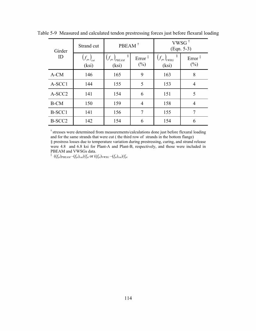
114

Table 5-9 Measured and calculated tendon prestressing forces just before flexural loading

Strand cut PBEAM † VWSG †

(Eqn. 5-3) Girder ID ( )

cutpsf (ksi)

( )PBEAMpsf §

(ksi)

Error ‡

(%) ( )

VWRGpsf § (ksi)

Error ‡

(%)

A-CM 146 165 9 163 8

A-SCC1 144 155 5 153 4

A-SCC2 141 154 6 151 5

B-CM 150 159 4 158 4

B-SCC1 141 156 7 155 7

B-SCC2 142 154 6 154 6

† stresses were determined from measurements/calculations done just before flexural loading and for the same strands that were cut ( the third row of strands in the bottom flange) § prestress losses due to temperature variation during prestressing, curing, and strand release were 4.8 and 6.8 ksi for Plant-A and Plant-B, respectively, and those were included in PBEAM and VWSGs data. ‡ ((fpi)PBEAM –(fpi)cut)/fpi or ((fpi)VWSG –(fpi)cut)/fpi

115

26

31 36

6

2

2 2

30

6

1.5

2

3.5 7.5

Section Properties

A = 570 in.2

I = 93528 in.4

yb = 17.96 in.

10

33

Figure 5-1 Girder cross section (36M I-girder) details (all dimensions in in., strands placed at 2 in. centers in the horizontal direction)

strand

VWRG

L/2 L/2 L/2 deadend

live end

(SCC2) (SCC1) (CM)

(a) (b)

6.8''

32 ''

17.6 ''

4.0 ''

Figure 5-2 Location of vibrating gages at midspan, (a) Plant-A, (b) Plant-B (nominal dimensions, as-built dimension ±0.5'')

116

upper jack plate

lower jack plate

jack

load cell

bearing blocks

companion cylinder

tension bar

upper base plate

lower base platepair of disk springs

Figure 5-3 Creep loading frame details (dimensions given by Mokhtarzadeh, 1998)

117

Figure 5-4 Configuration of surface strain gages and LVDTs on bottom girder surface and wraparound crack configuration (B-SCC1)

26.0''

7.5''

3.5''

7.5''

3.5''

295

280

295285

275260

265

255

245

255

260275285

295

290275

290285

270

260

275

290

295

245

245

255270285

295

290

295

290

295280275270

260

255

285

290285

270255

295295

285

270

265LVDT(L/2)

OC-1 NC-1

NC-1

OC-1NC-2

OC-2

OC-2NC-2

NC-3

OC-3

N1S1

N2

S2

N3

S3

N4

S4

N5

S5

N6

S6

N7

S7

N8

20.1''

LVDT(2L/5)

10.6'' 14.3'' 11.9'' 11.1'' 12.1''

web

w

eb

botto

m

botto

m su

rfac

e bo

ttom

118

Figure 5-5 Load-strain behavior of surface strain gages placed over and next to a crack (B-SCC1)

Figure 5-6 Exposed strand at L/2 before cutting and instrumentation

0

50

100

150

200

250

0 100 200 300 400 500 600 700 800Strain (με)

App

lied

load

(kip

s)

gage over crack (OC-3)

initial linear line

gage next to crack (NC-3)

crack re-opening

hose clampscutting location

wet fabricgages

~18 in.

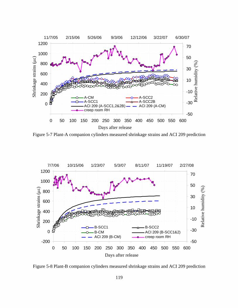
119

Figure 5-7 Plant-A companion cylinders measured shrinkage strains and ACI 209 prediction

Figure 5-8 Plant-B companion cylinders measured shrinkage strains and ACI 209 prediction

-200

0

200

400

600

800

1000

1200

0 50 100 150 200 250 300 350 400 450 500 550 600-50

-30

-10

10

30

50

70

7/7/06 10/15/06 1/23/07 5/3/07 8/11/07 11/19/07 2/27/08

B-SCC1 B-SCC2B-CM ACI 209 (B-SCC1&2)ACI 209 (B-CM) creep room RH

Days after release

Rel

ativ

e hu

mid

ity (%

)

Shrin

kage

stra

ins (με

)

-200

0

200

400

600

800

1000

1200

0 50 100 150 200 250 300 350 400 450 500 550 600-50

-30

-10

10

30

50

70

11/7/05 2/15/06 5/26/06 9/3/06 12/12/06 3/22/07 6/30/07

A-CM A-SCC2A-SCC1 A-SCC2BACI 209 (A-SCC1,2&2B) ACI 209 (A-CM)creep room RH

Days after release

Rel

ativ

e hu

mid

ity (%

)

Shrin

kage

stra

ins (με

)

120

Figure 5-9 Plant-A companion cylinder measured creep coefficients and ACI 209 prediction

Figure 5-10 Plant-B companion cylinder measured creep coefficients and ACI 209 prediction

-0.5

0.0

0.5

1.0

1.5

2.0

2.5

3.0

0 50 100 150 200 250 300 350 400 450 500 550-50

-30

-10

10

30

50

70

7/7/06 10/5/06 1/3/07 4/3/07 7/2/07 9/30/07 12/29/07

B-SCC1 B-SCC2B-CM ACI 209 (B-SCC1&2)ACI-209 (B-CM) creep room RH

Cre

ep c

oeff

icie

nt

Days after release

Rel

ativ

e hu

mid

ity (%

)

-0.5

0.0

0.5

1.0

1.5

2.0

2.5

3.0

0 50 100 150 200 250 300 350 400 450 500 550 600-70

-50

-30

-10

10

30

50

70

11/7/05 2/15/06 5/26/06 9/3/06 12/12/06 3/22/07 6/30/07

A-CM A-SCC1A-SCC2 A-SCC2BACI 209 (all mixes) creep room RH

Cre

ep c

oeff

icie

nt

Days after release

Rel

ativ

e hu

mid

ity (%

)

121

Figure 5-11 Plant-A measured shrinkage strains and ACI 209 least square fit curves

Figure 5-12 Plant-A companion cylinder measured creep data and ACI 209 least square fit curves

0.0

0.5

1.0

1.5

0 50 100 150 200 250 300 350 400 450 500 550 600

A-CM LSA-1 (CM)LSA-2 (CM) LSA-3 (CM)A-SCC1 LSA-1(SCC1)LSA-2 (SCC1) LSA-3(SCC1)

Days after release

Cre

ep c

oeff

icie

nt

0

100

200

300

400

500

600

0 50 100 150 200 250 300 350 400 450 500 550 600

A-SCC1LSA-1LSA-2LSA-3

Days after release

Shrin

kage

stra

in (μ

ε)

122

Figure 5-13 Measured and PBEAM predicted prestress losses of Girder A-CM at L/2

Figure 5-14 Measured and PBEAM predicted prestress losses of Girder A-SCC1 at L/2

0

10

20

30

40

50

60

70

80

0 60 120 180 240 300 360 420 480 540 600-60

-40

-20

0

20

40

60

80

10011/2/05 1/31/06 5/1/06 7/30/06 10/28/06 1/26/07 4/26/07 7/25/07

VWRG data Avrg RH

RH(t) RH=100%

Field RH

RE1+∆ftemp = 7.5 ksi

Days after casting

Am

bien

t rel

ativ

e hu

mid

ity (%

)

Pres

tress

loss

es (k

si)

0

10

20

30

40

50

60

0 60 120 180 240 300 360 420 480 540 600 660-60

-40

-20

0

20

40

60

80

10011/2/05 1/31/06 5/1/06 7/30/06 10/28/06 1/26/07 4/26/07 7/25/07

VWRG data Avrg RHRH(t) RH=100%Field RH

RE1+∆ftemp = 7.5 ksi

Days after casting

Am

bien

t rel

ativ

e hu

mid

ity (%

)

Pres

tress

loss

es (k

si)

123

Figure 5-15 Measured and PBEAM predicted prestress losses of Girder A-SCC2 at L/2

Figure 5-16 Measured and PBEAM predicted prestress losses of Girder B-CM at L/2

0

10

20

30

40

50

60

70

80

0 60 120 180 240 300 360 420 480 540-60

-40

-20

0

20

40

60

80

1007/5/06 10/3/06 1/1/07 4/1/07 6/30/07 9/28/07 12/27/07

VWRG data Avrg RH

RH(t) RH=100%

Field RH

RE1+∆ftemp = 9.8 ksi

Days after casting

Am

bien

t rel

ativ

e hu

mid

ity (%

)

Pres

tress

loss

es (k

si)

0

10

20

30

40

50

60

70

80

0 60 120 180 240 300 360 420 480 540 600 660-60

-40

-20

0

20

40

60

80

10011/2/05 1/31/06 5/1/06 7/30/06 10/28/06 1/26/07 4/26/07 7/25/07

VWRG data Avrg RHRH(t) RH=100%Field RH

RE1+∆ftemp = 7.5 ksi

Days after casting

Am

bien

t rel

ativ

e hu

mid

ity (%

)

Pres

tress

loss

es (k

si)

124

Figure 5-17 Measured and PBEAM predicted prestress losses of Girder B-SCC1 at L/2

0

10

20

30

40

50

60

70

80

0 60 120 180 240 300 360 420 480 540-60

-40

-20

0

20

40

60

80

1007/7/06 10/5/06 1/3/07 4/3/07 7/2/07 9/30/07 12/29/07

VWRG data Avrg RHRH(t) RH=100%

Field RH

RE1+∆ftemp = 9.8 ksi

Days after casting

Am

bien

t rel

ativ

e hu

mid

ity (%

)

Pres

tress

loss

es (k

si)

Figure 5-18 Measured and PBEAM predicted prestress losses of Girder B-SCC2 at L/2

0

10

20

30

40

50

60

70

80

0 60 120 180 240 300 360 420 480 540-60

-40

-20

0

20

40

60

80

1007/5/06 10/3/06 1/1/07 4/1/07 6/30/07 9/28/07 12/27/07

VWRG data Avrg RHRH(t) RH=100%Field RH

RE1+∆ftemp = 9.8 ksi

Days after casting

Am

bien

t rel

ativ

e hu

mid

ity (%

)

Pres

tress

loss

es (k

si)

125

7.5''

3.5''

6.0''

18.0''

26''

30''

ConcreteFiber-B

Concrete Fiber-A

Figure 5-19 PBEAM concrete fibers, (a) fibers with identical material models, and (b) bottom concrete fiber with modified material models (creep and shrinkage)

126

Chapter 6 Summary, Conclusions, and Recommendations

6.1 Summary

Many states, including Minnesota are interested in the economic and fresh state performance benefits of SCC for bridge girders such as reduced labor and eliminated need for vibration. However, the lack of adequate information regarding the performance of SCC girders, and the contradictory available literature are most likely the main reasons that more states have not already implemented the use of SCC for precast prestressed concrete bridge girders.

Self-consolidating concrete has been developed using locally available materials from two precast concrete plants. The effects of several design and manufacturing parameters such as concrete temperature, admixture dosage, and cement variability on the fresh properties were investigated. The adequacy of the available testing methods employed to evaluate fresh state properties of SCC was also investigated. Modification to some of the test methods have been recommended to investigate the possibility of minimizing the number of test methods and time to adequately evaluate SCC fresh state properties.

Four SCC and two conventional concrete 38 ft full-scale Mn/DOT 36M I-girders were fabricated using locally available materials from two precast concrete plants. The short- and long-term performance of the girders was monitored including transfer length, camber and prestress losses. Calculated values obtained using available design specifications such as the AASHTO (2007) bridge specifications AASHTO (2004) bridge specifications and ACI 318 (2005) were compared to the measured results to investigate their applicability. In addition to the girders, a large number of companion cylinders were fabricated and cured with the girders. The companion cylinders were used to monitor concrete compressive strength, modulus of elasticity, and to develop creep and shrinkage material models for the girders. A finite element program was used in conjunction with the data obtained from the companion cylinders to investigate whether the measured girder performance (e.g., prestress losses) could be predicted using the companion cylinder data.

Finally, flexural crack re-opening tests of the girders were performed as an indirect method to compute the effective prestressing force and total prestress losses. A semi-destructive test method was also employed to directly determine the remaining effective prestressing force. In addition, a large number of concrete cores were drilled along the girders and through the girder depth to investigate the uniformity of the measured material properties and compare the girder properties with the companion cylinder properties.

6.2 Conclusions

The following conclusions are a summary of those presented in the Chapter 2, 3, 4, and 5.

1. Self-consolidating concrete with adequate fresh properties has been developed successfully with locally available materials in conjunction with two precast concrete plants that produce prestressed concrete girders for the State of Minnesota.

127

2. Chemical and physical properties of cement not typically listed in the mill report can significantly affect the flowability of SCC.

3. U-box fill height has a negligible effect on the test results (h2/h1). A recommended improvement to the test method is to decrease the fill height from 24 to 18 in. to decrease the amount of concrete used and to minimize the associated labor.

4. Flowability of SCC increases as concrete temperature increases. Flowability was observed to increase by about 1 in. for each 10 ° F increase in concrete mixing temperature.

5. Flowability of SCC does not improve significantly once the HRWR saturation dosage is reached. The HRWR saturation dosage is a function of cement properties and w/cm.

6. Concrete moduli of elasticity predicted by ACI 318-05 Section 8.5.1 and AASHTO (2004) Section C5.4.2.4 for both SCC and conventional concrete were reasonable and consistent with the measured values. Therefore, both design provisions can be used to predict moduli of elasticity of SCC girders when experimental data is not available.

7. The SCC girders had longer transfer lengths than the conventional concrete girders (75% for Plant-A and 10% for Plant-B). The Plant-A conventional concrete girder had approximately 40% higher concrete compressive strength and 35% higher concrete modulus of elasticity than the Plant-A SCC girders at release, and this might have affected the transfer length of the conventional concrete girder. For Plant-B, both conventional and SCC girders had similar concrete strengths and elastic moduli at release, as well as similar transfer lengths. However, both AASHTO and ACI transfer length predictions were conservative for girders cast with both types of concrete. The large number of strands placed in the girder and high level of prestress, which could have caused the concrete to be confined, may be a reason for the measured low transfer lengths relative to the predictions.

8. The PCI multiplier method using measured properties was a good predictor of camber for both SCC and conventional concrete girders. For Plant-A, the predicted camber for both conventional and SCC girders was higher than the measured camber by 3 to 8 % of the measured camber at release, erection (35 days after release), and at the end of the monitoring period (600 days after release). The only exception was the conventional concrete girder at release; the predicted camber at release for the conventional concrete girder was approximately 4% smaller than that measured camber. For Plant-B, at release the predicted cambers were approximately 3% smaller than measured camber for the both SCC and conventional concrete girders, and at erection and at the end of monitoring period (approximately 450 days after release) the predicted cambers were 7 to 15% higher than measured cambers for all girders.

9. Both the SCC and conventional concrete girders had similar elastic shortening losses (ranging from 18.3 to 20.2 ksi). These losses were well predicted with available design

128

equations when measured material properties were used and were conservatively predicted when design properties were used.

10. The predicted total long- term prestress losses calculated with AASHTO 2004, PCI Design Handbook 6th Edition (PCI, 2004), and PCI General Method (PCI, 1975) using measured material properties were conservative. The predicted long-term losses at the end of the monitoring periods were larger than the measured losses by 2 to 5% for the AASHTO 2004 Lump Sum Method, 12 to 15% for the AASHTO 2004 Refined Method, 4 to 7% for the PCI General Method, and 8 to 11% for the PCI Design Handbook Method for all girders. However, the long-term prestress losses computed with the AASHTO 2007 Approximate Estimate of Time-Dependent Losses Method were either not conservative or very close to the measured losses at the end of monitoring period of 450 days and 600 days for Plant-A and Plant-B girders, respectively. For Plant-A, the predicted losses were lower than the measured losses by 0.3 and 1.0 % for the conventional concrete and SCC girders, respectively. For Plant-B, the predicted losses were 0.4 and 0.2 % higher than measured losses for conventional concrete and B-SCC1 girders, respectively, and the predicted losses were smaller than measured losses by 0.1% for the B-SCC2 girder.

11. The AASHTO 2007 design specification predicted unconservative long-term prestress losses for both conventional and SCC girders, and the magnitude of the difference between the measured and predicted was comparable for both conventional and SCC girders.

12. For all methods selected to predict long-term prestress losses, the associated errors (predicted–measured) for both conventional concrete and SCC girders were comparable. The errors were between 15 and -0.3 % for conventional concrete and between 13 and -1.0 % for SCC girders.

13. Self-consolidating concrete mixes had larger shrinkage and creep strains than the conventional concrete mixes. By the end of the monitoring period, the SCC mixes had 25 and 15% higher shrinkage strains than those measured for the conventional concrete for Plant-A and Plant-B, respectively. The measured average creep coefficients of the SCC mixes were 55 and 45% larger than those measured for the conventional concrete mixes for Plant-A and Plant-B, respectively. However, both measured shrinkage strains and creep coefficients for both the SCC and conventional concrete mixes were smaller than the ACI Committee 209 predictions. At the end of the monitoring period, the measured shrinkage strains were approximately 35% smaller than those predicted by ACI 209, and the measured creep coefficients were approximately 50% and 25% smaller for conventional and SCC mixes, respectively than ACI 209 predictions adjusted for mix proportions.

14. Determining the effective prestress forces by flexural crack re-opening moments yielded effective prestressing forces much smaller (i.e., 28% to 38%) than those determined by all other methods (e.g., finite element and semi-destructive testing methods). The main reason for the smaller forces determined from the flexural crack reopening was believed

129

to be due to the differential shrinkage toward the surface of the girder, where the volume-surface ratio is smaller than the average girder volume-surface ratio.

15. The finite element program PBEAM can be used to predict long-term prestress losses. However, if differential shrinkage (i.e., different shrinkage properties of fibers located at the surface (smaller volume to surface ratio) than those located within the section (higher volume-surface ratio) is not considered, the programs over predict crack re-opening moments (55% to 90% higher than those determined with concrete surface gages). In other words, crack re-opening loads can not be calculated accurately assuming homogenous elastic beam theory. The increased shrinkage near the bottom surface of the girders must be taken into account.

16. ACI Committee 209 proposed correction factors for relative humidity and volume-to-surface ratio appear to be applicable to SCC, and they can be used to adjust creep and shrinkage models for conditions different than standard conditions defined by ACI Committee 209.

17. Models developed from companion creep and shrinkage cylinders were found to adequately predict short-term and long-term behavior of both conventional concrete and SCC girders including prestress losses and crack re-opening loads.

6.3 Future Research

This research study raised a number of important issues that may warrant further investigation. They are summarized below:

1. The work presented in this study indicates that the fresh properties of SCC are sensitive to cement properties. It has been shown that even the same type cement obtained from the same provider but at different times can produce SCC with significantly different fresh properties. A detailed literature review of this problem has been included in this report. The problem seems to be complicated and a multi-disciplinary team composed of researchers from chemical and materials engineering might be required to solve the problem.

2. Girder depth may be an important factor that affects segregation resistance of SCC. Therefore, a parametric study including the effect of girder depth on segregation resistance, flowability, and filling abilities of SCC should provide useful information regarding application of SCC to precast bridge girders.

3. The computed crack re-opening loads using the finite element tool, PBEAM, were significantly larger than those experimentally computed. It has been shown that one possible explanation was due to larger shrinkage strains experienced by the fibers located at the girder surface. This might be experimentally investigated by applying a coating material (similar to that used for the ends of the shrinkage cylinders) to the girder surface to prevent shrinkage.

130

4. The companion creep and shrinkage cylinders indicated that SCC had approximately 55% to 60% higher creep and 25% to 15 % higher shrinkage strains than conventional concrete. The SCC mixes investigated here only included Class C fly ash as supplementary material. A parametric study that investigates creep and shrinkage behavior of SCC mixes with different types and varying proportions of supplementary cementitious material could be useful.

131

References

AASHTO (2004). LRFD Bridge Design Specifications, 3rd Edition. Washington, DC: American Association of State Highway and Transportation Officials.

AASHTO (2007). LRFD Bridge Design Specifications, 4th Edition. Washington, DC: American Association of State Highway and Transportation Officials.

ACBM (2004). Self-Consolidating Concrete. White Paper. Chicago, IL: The Center for Advanced Cement Based Materials.

ACI Committee 209 (1992). ACI 209R-92 Prediction of Creep, Shrinkage, and Temperature Effects in Concrete Structures. Detroit, MI: American Concrete Institute.

ACI Committee 237 (2007). ACI 237R-07 Self-Consolidating Concrete. Farmington Hills, MI: American Concrete Institute.

ACI Committee 318 (2005). ACI-318-05 Building Code Requirements for Structural Concrete and Commentary. Detroit, MI: American Concrete Institute.

Ahlborn, T., French, C., and Shield, C. (2000). High-Strength Concrete Prestressed Bridge Girders: Long Term and Flexural Behavior. Final Report No. 2000-32. Minnesota Department of Transportation.

Assaad, J., Khayat, K. H., and Daczko, J. (2004). “Evaluation of Static Stability of Self-Consolidating Concrete.” ACI Materials Journal, Vol. 101, No. 3, 207-215.

ASTM (2000) C143 Standard Test Method for Slump of Hydraulic-Cement Concrete. West Conshohocken, PA: ASTM International.

ASTM (2002) C469 Standard Test Method for Static Modulus of Elasticity and Poisson's Ratio of Concrete in Compression. West Conshohocken, PA: ASTM International.

ASTM (2004) C39 Standard Test Method for Compressive Strength of Cylindrical Concrete Specimens. West Conshohocken, PA: ASTM International.

ASTM (2005). C1611 Standard Test Method for Slump Flow of Self-Consolidating Concrete. West Conshohocken, PA: ASTM International.

ASTM (2006). C1610 Standard Test Method for Static Segregation of Self-Consolidating Concrete Using Column Technique.

Baran, E. French, C., and Shield, C. (2003). Effect of Vertical Pre-Release Cracks on Prestressed Bridge Girders. Final Report No. 2003-33. Minnesota Department of Transportation.

132

Bilberg, P. (1999). Self-Compacting Concrete for Civil Engineering Structures-the Swedish Experience. CBI Report 2:99, Swedish Cement and Concrete Research Institute, Stockholm, Sweden.

Brameshuber, W. and Uebaches, S. (2002). “The Application of Self-Compacting Concrete in Germany under Special Consideration of Rheological Aspects”, First North American Conference on the Design and Use of Self-Consolidating Concrete. 211-216.

Brite-EuRam programme: BE96-3801/BRPR-CT96-0366, “Rational production and improved working environment through using self-compacting concrete. ”

Bui, V.K., Montgomery, D. Hinczak, I., and Turner, K. (2002). “Rapid Testing Method for Segregation Resistance of Self-compacting Concrete,” Cement and Concrete Research, Vol. 32, 1489-1496.

Byle, K.A., Burns, N. H., and Carrasquillo, R. L. (1997). Time-Dependent Deformation Behavior of Prestressed High Performance Concrete Bridge Beams. Research Report 580-6, University of Texas at Austin, Austin, Texas.

Chan, Y., Chen, Y., and Liu, Y. (2003). “Development of Bond Strength of Reinforcement Steel in Self-Consolidating Concrete.” ACI Structural Journal, V. 100, No.4, 490-498.

Chandra, S.; and Bjornstrom, J. (2002). “Influence of Cement and Superplasticizers Type and Dosage on the Fluidity of Cement Mortars-Part 1.” Cement and Concrete Research, V.32, 1605- 1611.

Cousins, T.E., Stallings, J. M., and Simmons, M. B. (1993). Effect of Strand Spacing on Development Length of Prestressing Strand. Final Report submitted to the Alaska Department of Transportation and Public Facilities, Juneau, Alaska.

Daczko, J. A. (2002). “Stability of Self-Consolidating Concrete, Assumed or Ensured?” First North American Conference on the Design and Use of Self-Consolidating Concrete, Center for Advanced Cement-Based Materials, 245-252.

Dehn, F., Holschemacher, K., and Weibe, D. (2000). “Self-Compacting Concrete (SCC) Time Development of the Material Properties and the Bond Behavior.” Leipzig Annual Civil Engineering Report. No. 7, 115-124.

EFNARC (2002). Internet. Specification and Guidelines for Self-Compacting Concrete. www.efnarc.org/pdf/SandGforSCC.PDF.

EFNARC (2005). Internet. The European Guidelines for Self-Compacting Concrete: Specification, Production and Use. www.efnarc.org/pdf/SCCGuidelinesMay2005.pdf.

Erkmen, B., French, C.W, and Shield, C.K. (2005). “Development of Self-Consolidating Concrete and Evaluation of Fresh Properties.” Proceedings of Mid-Continent Transportation Research Symposium, Ames, Iowa.

133

Ferraris, C.F., Brower, L., Ozyildirim, C., and Daczko, J. (2000). “Workability of Self-Compacting Concrete,” Proceedings of the International Symposium on High Performance Concrete, Orlando, FL, USA.

Girgis, A. F.; and Tuan, C. Y. (2004). Bond Strength of Self-Consolidating Concrete for Prestressed Concrete Applications. Final Report Number SPR-P1 (04), Nebraska Department of Roads.

Gross, S. P; and Burns, N. H. (2005). Field Performance of Prestressed High Performance Concrete Highway Bridges in Texas. Research Report 9-580 and 9-589 Texas Department of Transportation.

Gurjar, A.H. (2004). Mix Design and Testing of Self-Consolidating Concrete Using Florida Materials. Report No. BD 503, Department of Civil Engineering, Embry-Riddle Aeronautical University, Daytona Beach, Florida.

Hammer, T. A., Smeplass, S., Johansen, K., and Fredvik, T. (2002). “Development of SCC with Focus on Low Cost.” First North American Conference on the Design and Use of Self-Consolidating Concrete, Center for Advanced Cement-Based Materials, 159-164.

Hegger, J., Gortz, S., Kommer, B., Tigges, C., and Drossler, C. (2003). “Prestressed Precast Beams Made of Self-Compacting Concrete.” Betonwerk Und Fertigteil Technik, V.69, No. 8, 44-48.

Holschemacher, K. and Klug, Y.(2002). “A Database for the Evaluation of Hardened Properties of SCC.” Leipzig Annual Civil Engineering Report , No. 7, 123-134.

Janney, J.R. (1954). “Nature of Bond in Pre-tensioned Prestressed Concrete.” ACI Journal V. 50, No. 9, 717–736.

JSCE (1998). Recommendations for Construction Practice of High-Fluidity Concrete. Japan Society of Civil Engineers.

Jianxiong, C., Xincheng, P., and Yubin, H. (1999). “A Study of Self-Compacting HPC with Superfine Sand and Pozzolanic Additives,” 1st International RILEM Symposium on Self-Compacting Concrete, Stockholm, Sweden.

Khayat, K. H; Assaad, J.; and Daczko, J. (2004). “Comparison of Field-Oriented Test Methods to Assess Dynamic Stability of Self-Consolidating Concrete.” ACI Material Journal, V. 101, No. 2, 168-176.

Khayat, K. H. and Guizani, Z. (1997). “Use of Viscosity-Modifying Admixture to Enhance Stability of Highly Fluid Concrete.” ACI Materials Journal, V.94, No 4, pp. 332-340.

Lachemi, M., Hossain, K. M., Lambros, V., Bouzoubaâ. (2003). “Development of Cost-Effective Self-Consolidating Concrete Incorporating Fly Ash, Slag Cement, or Viscosity-Modifying Admixtures.” ACI Materials Journal, V. 100, No. 5, 419-425.

134

Lessard, M., Talbot, C., and Baker, D. (2002). “Self-Consolidating Concrete Solves Challenging Placement Problems at the Pearson International Airport in Toronto, Canada.” First North American Conference on the Design and Use of Self-Consolidating Concrete, Center for Advanced Cement-Based Materials, 367-370.

Martin, J. D. (2000). “Economic Impact of SCC in Precast Applications.” First North American Conference on the Design and Use of Self-Consolidating Concrete, Center for Advanced Cement-Based Materials, 147-152.

Nkinamubanzi, P. C., Kim, B. G., and Aïtcin, P.C. (2000) “Some Key Factors that Control the Compatibility between Naphthalene-based Superplasticizers and Ordinary Portland Cements.” 6th CANMET/ACI International Conference on Superplasticizers and Other Chemical Admixtures in Concrete, Paris, 44-54.

Okamura, H. (1975). “Self-Compacting High-Performance Concrete.” Concrete International, Vol. 6, No. 4, 269-270.

Ouchi, M., Nakamura, S., Osterberg T., Hallberg, S., and Lyint, M. (2003). “Application of Self-Consolidating Concrete in Japan, Europe, and the United States.” Proceedings of the High Performance Concrete Symposium and Bridge Conference, 49th PCI Annual Convention and Exhibition, Orlando, Florida.

Persson, B. (2001). “A Comparison Between Mechanical Properties of Self-Compacting Concrete and the Corresponding Properties of Normal Concrete,” Cement and Concrete Research, V. 31, No. 2, 193-198.

PCI Committee on Prestress Losses (1975). “Recommendations for Estimating Prestressed Losses.” PCI Journal, V. 20, No. 4, 45-75.

PCI (2004) PCI Design Handbook: Precast and Prestressed Concrete, 6th Edition. Chicago, IL: Precast/Prestressed Concrete Institute.

PCI (2003). TR-6-03 Interim Guidelines for the Use of Self-Consolidating Concrete in Precast/Prestressed Concrete Institute Member Plants, 1st Edition. Chicago, IL: Precast/Prestressed Concrete Institute.

Ramage, B., Kahn, L.F., and Kurtis, K.E. (2004). Evaluation of Self Consolidating Concrete for Bridge Structure Application. Structural Engineering Mechanics and Material Special Research Problem Report, Georgia Institute of Technology, Atlanta, USA.

Ramage, B. (2005). Evaluation of Self Consolidating Concrete for Bridge Structure Applications, Master of Science Thesis, Georgia Institute of Technology.

Ramsburg, P., Bareno, J, Ludirdja, D., and Masek, O. (2003). “Durability of Self consolidating Concrete in Precast Application.” 2003 High Performance Concrete Symposium and Bridge Conference, 49th PC1 Annual Convention and Exhibition, Orlando, Florida.

135

Rose D. R. and Russell B. W. (1997). “Investigation of Standardized Tests to Measure the Bond Performance of Prestressing Strand.” PCI Journal, Vol. 42, No. 4, 56–80.

Russell, B. W., and Burns N. H. (1993). Design Guidelines for Transfer, Development and Debonding of Large Diameter Seven Wire Strands in Pretensioned Concrete Girders. Research Project 3-5-89/2-1210, Texas Department of Transportation.

Skarendahl, A. and Petersson, Ö. (2000). Self-Compacting Concrete. State-of-the-Art Report of RILEM Technical Committee 174, RILEM-Report No. 23, Ca-chan Cedex, France.

Suttikan, C. (1978). A Generalized Solution for Time-dependent Response and Strength of Noncomposite and Composite Prestressed Concrete Beams. Ph.D. Dissertation, University of Texas at Austin.

Takeuchi, H., Higuchi, M., and Nanni, A. (1994) “Application of Flowable Concrete in a Tunnel Lining.” Concrete International, V. 16, No. 4, 26-29.

Yahia, A., Tanimura, M., Shimabukuro, A., and Shimoyama, Y. (1999). “Effect of Rheological Parameters on Self-Compactability of Concrete Containing Various Mineral Admixtures.” Proceedings of the 1st RILEM International Symposium on Self-Compacting Concrete, Stockholm, Sweden.

Yutaka, N., and Kazuo, Y. (2003). “Cement Characteristics Affecting the Dispersing Performance of Poly β-naphthalene Sulfonate Condensate Superplasticizer and These Affecting Mechanism.” 7th CANMET/ACI International Conference on Superplasticizers and Other Chemical Admixtures in Concrete, Berlin.

APPENDIX A

CEMENT AND HIGH RANGE WATER REDUCER INTERACTION LITERATURE

A-1

A.1 Introduction

High-range water reducers (HRWR) have been used in production of concrete for almost three decades. The use of HRWR (i.e., superplasticizers) has made it possible to produce high fluidity concrete, which has adequate segregation resistance and high strength, with low water/cementitious material (w/cm) ratio. Superplasticizers improve the workability of concrete by providing a better dispersion of cement particles. However, a detailed understanding of the action of the superplasticizers on fluidity is not well understood due to its complexity (Page et al., 1999). The performance of superplasticizers in improving fluidity is known to be affected by the characteristics of both cement and superplasticizer used.

It may be expected that self-consolidating concrete produced with the same admixtures, dosage, mix proportions, and aggregates will have the same or similar workability (flowability) characteristics from batch to batch when Portland cements fulfilling the same set of acceptance standards are used. Recent studies (e.g., Yukata et al., 2003; Nkinamubanzi et al., 2000, and Kim et al., 1999), however, have shown that small variations in cement properties can significantly affect the workability and early reactions of concrete than is generally thought. Furthermore, it has been shown that variation in concrete workability due to variations in cement properties is much more significant when superplasticizers are used (Juvas et al., 2000). This is likely to cause increased waste in concrete production and considerable economical losses. Unfortunately, the quality of information provided by the cement supplier and the available knowledge about cement superplasticizer interaction is not adequate to predict and control the variations in concrete workability.

In general, cement fineness is thought to be one of the most important properties of cement.. However, the fluidity of a cement paste is not only related to its fineness but also related to its chemical composition. Several tests and long time monitoring have shown that Blaine fineness is not a sufficient parameter for explaining the variation in the properties of fresh concrete produced with superplasticizers (Juvas et al., 2000). Cement is a complex material and in addition to fineness, it has several varying characteristics. Some of these are composition and microstructure of clinker minerals, amount and form of calcium sulphate, alkalies, soluble sulfate, and amount of free lime.

A.2 Literature Review

When producing and using SCC, it is essential to achieve concrete with good workability (flowability) that can be maintained until the concrete is placed. The available literature (Juvas et al., 2000) reveals that the fresh properties of self-consolidating concrete mixes, which cannot be produced without utilizing superplasticizers, are much more susceptible to variations in cement properties. In some cases, variations in cement properties can cause large reductions in initial concrete flowability for a given SCC mixture, in other cases; the achieved flowability is very short-lived. Most of the available literature is related to the cases where the flowability is short-lived. That is probably because it is much more likely to recognize cases with short-lived

A-2

flowability. The reduction in initial flowability might only be recognized if the same mix proportions and materials (except cement) are used to produce the same SCC mix.

Most of the available literature (Nkinamubanzi et al., 2000; and Kim et al. 2000) shows that the main factors affecting the performance of the superplasticizer is the amount of superplasticizer consumed by early hydration products. Superplasticizer is utilized by cement in two ways; these are absorption of superplasticizers into initial hydrates and adsorption onto the hydrates. Yutaka et al. (2003) state that it is only the adsorbed amount of superplasticizer that acts as dispersant. Most of the available literature does not distinguish between the adsorbed and absorbed amount of superplasticizers, and report the total utilized amount of superplasticizers as the adsorbed amount. The reason for this may be that presently there is no direct method to discriminate between the amounts of superplasticizer that are either absorbed or adsorbed. The amount of superplasticizer utilized by cement particles is defined as the portion of total added superplasticizer that is not available in the solution phase.

Most of the available literature (Nkinamubanzi et al., 2000; and Yukata et al., 2003) indicates that the most significant factor affecting the performance of superplasticizers is the concentration of sulfate ions (SO4

2-) in the solution phase, which is believed to affect the amount of superplasticizer utilized by cement (i.e., sum of adsorbed and absorbed amounts). Therefore, any factor affecting the concentration of SO4

2- ions is very likely to affect the performance of superplasticizers and fluidity of concrete. The main sources of SO4

2- ions are soluble alkalis and calcium sulfate.

Juvas et al., (2000)

Juvas et al. (2000) studied the variation of workability in 50 daily collected cement samples from the same plant (a commercial cement plant) by measuring the spread of mortar on a flow table (ASTM C 230). Two sets of superplasticized mortar samples were prepared with a w/c ratio of 0.335. A polycarboxylate superplasticizer, Glenium 51 supplied by Master Builders, was utilized at a dose of 0.77 % of cement weight for the first superplasticized mortar set (SET-1), and a typical melamine plasticizer, Peramin F supplied by SEMTU OY, was utilized at a dose of 2.14 % of cement weight for the second superplasticized mortar set (SET-2). In addition, plain cement mortars with a w/c ratio of 0.465 were also prepared (i.e., no admixtures were used). The sand/cement ratio was 1.9 in all mixes.

The measured mortar spreads are shown in Figure A-1 for the 50 daily-collected samples of each of the mix types. The range of variation in spread measurements in mixes without superplasticizers was only about 1 in. However, large variations in spread flow were measured for both SET-1 and SET-2 (i.e., the mixes incorporating superplasticizers). For SET-1 and SET-2, the variations in spreads were about 3.7 and 4.4 in., respectively.

In addition, the measured spreads of the superplasticized mixes were compared to the measured Blaine fineness of the cement samples. Based on earlier experience, it was expected that the increased fineness of the cement would decrease the spread value because increased cement fineness results in increased cement surface area, which requires an increased amount of superplasticizer to saturate the cement surface to the same degree for the same amount of

A-3

cement. However, they did not find any correlation between the cement fineness and the workability (i.e., spread). Therefore, they concluded that the fluidity is influenced more by the chemical composition of cement rather than its fineness. This was consistent with results reported by Chandra and Bjomstrom (2002).

Yukata et al., (2003)

Yukata et al. (2003) investigated the effect of various cement characteristics such as the kind of calcium sulfate, the amount of alkali sulfate, the amount of free lime, and the composition of cement clinker especially C3A on performance of superplasticizer. Yukata et al. (2003) estimated the adsorbed amount of superplasticizer adsorbed per unit surface area of cement hydrates from the amount of early hydrates and SO4

2- concentration by using a theoretical equation of Langmuir-type adsorption equilibrium. Cement pastes were prepared with commercially available low-heat Portland cement (LPC), high-early-strength Portland cement (HPC), sulfate resistant Portland cement (SRC), and three kinds of normal Portland cement (NPC) obtained from different plants. Cement pastes were prepared with a w/c ratio of 0.37 at 68 ºF. The performance of the superplasticizers was evaluated by the fluidity of the cement pastes. The measurements were carried out on pastes 5, 15, and 60 min. after mixing.

Alkali Sulfate

The effect of soluble alkali on flowability was examined by adding potassium sulfate (K2SO4), which is a soluble alkali, into the mixing water and measuring the concentration of SO4

2- ion in the solution phase of the cement paste. They found a positive linear relationship between soluble alkali content and concentration of SO4

2- ions at 5, 15, and 60 min. The concentration of SO42-

ions was found to decrease with time, which indicated that the ions were consumed by hydration products. The measured relationship between concentration of SO4

2- ion and paste flow, which was parabolic, indicated that the soluble alkali content of the cement could significantly affect the flowability. The measured parabolic relationship indicated that there were optimum values of soluble alkali content of cement for the highest paste flow. Based on the experimental findings, they concluded that the effect of soluble alkali content on cement flowability was only due to the varying concentration of SO4

2- ion due to soluble alkalis. The parabolic relationship between paste flow and soluble alkali content, and existence of an optimum content of soluble alkalis for the highest paste flow was explained by two mechanisms.

...In the first mechanism, when the alkali content of the cement increases, the concentration of SO4

2- ion increases, but the amount of superplasticizer adsorbed per unit surface of cement hydrates decreases because of the competitive adsorption between superplasticizers and SO4

2- ions. Because the amount of superplasticizer adsorbed per unit surface of hydrates controls the dispersion mechanism of cement, this decrease in the adsorbed amount results in a decrease in the paste flow.

In the second mechanism, when the alkali content of the cement increases, the concentration of SO4

2- ion increases, but the increased concentration of SO42- ions results

in a decrease in the amount of superplasticizer absorbed. This decrease in absorbed

A-4

amount results in an increase in the amount of superplasticizer adsorbed per unit surface of cement hydrates and an increase in paste flow.

When the content of alkali sulfate is lower than the optimum content, the effect of the second mechanism becomes predominant to the effect of the first mechanism. If the content of alkali sulfate is higher than the optimum content, the effect of first mechanism becomes predominant to the effect of second mechanism.

Free Lime

It is known that free lime content of cement affects the early formation of hydrates. That is because calcium (Ca2+), which is one of the elements affecting the early hydration of cement, is supplied not only from C3A but also from free lime. To produce the effect of free lime, Ca(OH)2 was added to the mixing water as a source of Ca2+ ions. The experimental results indicated a decreasing trend in paste flow with the addition of Ca(OH)2, but the SO4

2- ion concentration was found to be almost constant. The amount of hydrates, on the other hand, increased with the addition of free lime. The decreased paste flowability was explained by the following mechanism:

….The amount of hydrates increases with free lime addition. The adsorption amount of superplasticizer per unit amount of hydrate decreases with the increase of hydrates. This decrease of adsorption per hydrates results in the decrease of the paste flow.

Kim et al., (2000)

Kim et al. (2000) investigated the adsorption behavior of a polynaphthalene sulfonate (PNS) superplasticizer at a given dosage and its relation to the fluidity of six cement samples each having different contents of soluble alkalis (from 0.06 to 0.72%). The soluble alkali content of the cement samples was varied by adding sodium sulfate (Na2SO4). The adsorbed amount of the superplasticizer on the surface of the cement particles was computed by measuring the amount of superplasticizer extracted from fresh cement paste samples and subtracting that from the original amount added to the mix. However, it seems that quantity reported by Kim et al. was not the adsorbed amount, but the sum of the adsorbed and absorbed amounts of superplasticizer. Many of the references (Juvas et al., 2000), including Kim et al. (2000) do not distinguish between the absorption and adsorption mechanisms and present the sum of adsorbed and absorbed amounts of superplasticizer as the adsorbed amount of superplasticizer. However, it is generally accepted that it is only the adsorbed amount of superplasticizer that contributes to the flowability of cement pastes.

The literature review performed by Kim et al. (2000) revealed two main relationships between paste flow and admixture. First, an inverse linear relationship between the amount of superplasticizer adsorbed and paste flow at 30 min. was found. However, it should be noted that Kim et al. (2000) did not distinguish between the amount of superplasticizer adsorbed and absorbed. Second, it was found that the amount of “free” or available superplasticizer in the interstitial solution of the fresh paste and paste flow were related. Kim concluded that the

A-5

superplasticizer remaining in solution might act as an additional repulsive barrier between cement particles and increases fluidity.

The experimental tests conducted by Kim indicated an inverse relationship between the amount of superplasticizer adsorbed (i.e., sum of adsorbed and absorbed amount) and the mini-slump area value of the cement pastes (i.e., area of concrete flow) at 30 min; that is, the higher the amount of superplasticizer adsorbed, the lower the initial slump value, and the higher the slump loss. The cement samples with low soluble alkali content (0.06 to 0.19%) were found to have a tendency to adsorb a high amount of superplasticizer while cements with high alkali content (maximum content was 0.72%) had a tendency to adsorb a smaller amount of superplasticizer leaving a higher amount of superplasticizer in the solution. In other words, the experimental results indicated that the soluble alkali content of cement could be an important factor affecting the adsorption behavior of superplasticizers and flow of cement pastes. In addition, a linear relationship was found between the amount of sodium sulfate (Na2SO4) added and amount of sulfate ions (SO4

2-) in the solution. Others have found similar trends between the added amount of Na2SO4 and amount of sulfate ions in the solution.

The effect of sodium sulfate addition (Na2SO4) between 0.2% and 0.8% on the superplasticizer adsorption as a function of time was investigated for cements with low soluble alkali content. The amount of superplasticizer adsorbed was reduced by as much as 50% when the amount of sodium sulfate was increased (i.e., as the amount of soluble alkalis increased for cement with low soluble alkalis). In addition, it was found that the addition of Na2SO4 contributed to increasing the slump area by reducing the amount of superplasticizer adsorbed. They also studied the effect of calcium sulfate addition, and it was found that the calcium sulfate addition did not significantly affect the adsorption of the superplasticizer. That is believed to be due to lower solubility of CaSO4 relative to (Na, K)SO4 for the amount of available water at w/c ratio of 0.35.

Based on the experimental results and data from the other published papers (Yamada et al., 1998; and Nawa et al., 1989), Kim et al. (2000) summarized the role of alkali sulfate on the dispersion mechanism of superplasticized cement pastes as follows:

When a superplasticizer is added to cement paste containing a low amount of soluble alkali, most of the superplasticizer added is consumed by the formation of organo-mineral compound and/or the hydrated products. The superplasticizer molecules “intercalated’ into the hydration products cannot contribute to improve the fluidity of cement paste.

However, when sodium sulfate is added to the cement paste, the sulfate ions dissolved from the sodium sulfate inhibit the adsorption of superplasticizer on the aluminate phases by competing with the polynaphthalenesulfonae (PNS) molecules for adsorption sites. The competition between superplasticizer and sulfate ions reduces the amount of superplasticizer consumed and thus enables more superplasticizer to remain in solution and/or to be adsorbed on the silicate phases as well.

A-6

Jiang et al., (1999)

Six commercially available cements displaying a wide composition range (i.e., their C3A content varied from 2.4% to 11% and Na2O equivalent content ranged from 0.31% to 0.925%) were selected to investigate the effect of calcium sulfate addition (in the form of hemihydrate (CaSO4·1/2H2O) and gypsum (CaSO4·2H2O)) and alkali sulfate addition (Na2SO4) on the performance of the polynaphthalene sulfonate superplasticizer. The soluble alkali content of the cement samples (i.e., soluble Na2O and K2O) ranged from 0.07% to 0.88%. Cement pastes were prepared at a w/c ratio of 0.35 and at a controlled temperature of 77±2 ºF. The workability of pastes was measured with a mini-slump test (Kantro-mini-slump test). The test results indicated that the two cements with low soluble alkali content were incompatible with the superplasticizer; that is, the initial workability was short-lived and was followed by a rapid loss of slump.

It was likely that the low alkali cements also had low SO42- ion concentrations as their sulfate

(SO3) contents (1.95% and 2.0%) were also low. There were concerns that the cement/superplasticizer incompatibility could result from inadequate calcium sulfate contents. To verify if these cement sample were undersulfated, various amounts of hemihydrate (CaSO4.1/2H2O) and gypsum (CaSO4.2H2O) were added to the mixtures while the w/c ratio and superplasticizer dosage remained constant. Due to the low solubility rate of gypsum, it was first dissolved in the mixing water to provide a saturated gypsum solution to investigate the effect of gypsum solubility. The test results indicated that the use of gypsum-saturated mixing water or addition of hemihydrate, which had higher solubility than gypsum, increased the initial fluidity somewhat but could not prevent fluidity loss.

To determine the role of soluble alkalis, sodium sulfate (Na2SO4) was added to the mixing water to achieve different soluble alkali contents for the cement samples. The soluble alkali contents of the tested cements were measured using the inductivity coupled plasma method. Depending on the clinker sulfur trioxide (SO3) content, alkalis in cement can be present as alkali sulfates (Na2SO4 or K2SO4), and/or double sulfate forms, or trapped in C3A and C2S. The ratio of sulfur to total alkali determines the quantity of alkali sulfate in a clinker. When a clinker contains a relatively large amount of SO3, a substantial fraction of alkalis goes into solution within a few minutes. In low SO3, clinker sodium oxide and potassium oxide (Na2O and K2O) are incorporated preferentially into the tricalcium aluminate (C3A) phase, but also into the dicalcium silicate (C2S) phase of Portland clinker. Therefore, although the cements may have similar SO3 and total alkali contents, the amount of alkalis that are readily soluble in them can vary widely (Jiang et al., 1999).

The measured amount of alkali and soluble alkali contents of the cement samples were compared, and no correlation was found between both. Therefore, cement with similar SO3 and total alkali contents can have widely varying readily soluble alkali contents. The test results indicated that as the Na2SO4 addition increased for low-alkali cements, the initial slump increased, and the slump loss at different times (2, 5, 15, and 30 min.) continually decreased. However, with high-alkali cements, the addition of Na2SO4 decreased the initial fluidity and increased the slump loss. Based on the experimental findings, which are compatible with findings of Yukata et al. (2003) Jjiang drew the following conclusions:

A-7

…There is an optimum soluble alkali content with respect to fluidity and fluidity loss, which was found to be 0.4-0.5 Na2O soluble equivalent. At this optimum soluble alkali content, initial fluidity is maximum and fluidity loss is minimum.

Adding Na2SO4 significantly improved fluidity in cements with less than optimum soluble alkali content, while slightly decreasing fluidity in the cements with more than the optimum content. Therefore, the existence of adequate soluble alkali in the solution during the first few minutes after mixing is of primary importance in ensuring cement/superplasticizer compatibility. In other words, inadequate soluble alkalis in solution during the first few minutes of hydration is more likely to render a cement/superplasticizer combination incompatible than excessive soluble alkalis.

This optimum alkali content is independent of the superplasticizer dosage and cement type for the cements and superplasticizer tested.

The soluble alkali content is one of the major parameters controlling fluidity and fluidity loss in cement paste containing superplasticizer. In cement with an optimum amount of soluble alkali, the tricalcium aluminate (C3A) content has practically no effect on fluidity loss.

Kim et al., (1999)

Kim et al. (1999) examined the superplasticizer/cement interaction with respect to the adsorption of superplasticizer on cement and its hydration. Four cement samples with different fineness and compositions were studied with three superplasticizers, which had low, medium, and high molecular weights. The C3A content of the cement samples varied from 6% up to 11%, their sodium oxide (Na2O) equivalent contents varied from 0.31% to 0.92%, and their soluble alkali content varied from 0.06% to 0.57% Na2O equivalent. The mini slump test was used to assess the paste fluidity. The amount of superplasticizer in the solution phase was measured and subtracted from the initial dosage to find the amount of superplasticizer adsorbed on the surface of cement particles. As mentioned earlier, although this same methodology is done in most of the available literature (Kim et al. 2000; Juvas et al. 2000; and Nkinamubanzi et al. 2000), the amount of admixture determined in this way is not only the adsorbed amount, it is the sum of the adsorbed amount on the surface and absorbed amount inside the cement particles. It is important to distinguish between these, because it is the adsorbed amount of superplasticizer that contributes to concrete fluidity.

The test results indicated that the average molecular weight of the superplasticizer is an important factor affecting the performance of the superplasticizers (fluidity) when used with high-alkali cements. However, no significant effect of molecular weight of the superplasticizer was measured when used with low-alkali-cements. In other words, alkali content of the cements was found to be an important factor affecting the performance of the superplasticizer, which was much more significant for superplasticizers with medium and high molecular weights. For low-alkali-cements, the measured initial fluidity for the same dosage and type of superplasticizers was significantly lower than those measured for high-alkali cements. In addition, significantly

A-8

higher slump losses were measured for pastes prepared with low-alkali cements compared to those measured for high-alkali cements.

The measured superplasticizer adsorptions (sum of adsorption and absorption) at 5 minute and 60 minutes were not much different for high-alkali cements. However, measured superplasticizer adsorptions at 60 minutes were significantly larger than the adsorptions measured at 5 minutes for low-alkali cements. This indicated that superplasticizers were consumed continuously during hydration for low-alkali cements. This may be the reason for the high slump losses that were observed for the low-alkali cements.

However, very similar initial slump values and superplasticizer adsorptions were measured for two cements, one of which was a low-alkali cement and the other was a high-alkali cement. The low-alkali-cement had 0.35% Na2O equivalent, 0.07% soluble Na2O equivalent, 7% C3A content, and 10% C4AF while the high-alkali-cement had 0.74% Na2O equivalent, 0.72% soluble Na2O equivalent, 6% C3A content, and 9% C4AF.

Nkinamubanzi et al., (2000)

Nkinamubanzi et al. (2000) selected sixteen different Portland cements having a wide range of tricalcium aluminate (C3A) contents (6.0 to 11.8%) and SO3 contents (0.09 to 2.90%), and made with clinkers having a wide range of alkali contents (0.07 to 0.87 of Na2O equivalent) to study the key cement characteristics that control the performance of a naphthalene-based superplasticizer. Grouts with w/c ratio of 0.35 were prepared to study the performance of the superplasticizer, and concrete having w/c ratio of 0.30 was made to confirm the results obtained with the grouts. The slump of the fresh concrete was monitored during 90 minutes following contact between the water and cement. The mini-slump test carried out on grouts made with the 16 cement samples containing 1% of superplasticizer indicated that cements with low alkali and sulfate contents had very low initial slumps compared to the slumps measured for the other cements.

Nkinamubanzi et al. (2000) subtracted the measured amount of superplasticizer in the solution phase from the initial dosage and called it the adsorbed amount of superplasticizer (although this represents the sum of the amount of superplasticizer adsorbed and absorbed). The cements with low alkali content (0.03 to 0.25% of Na2Oeq soluble) exhibited a strong adsorption of the superplasticizer, and more than 75% of the initial dosage was consumed within the first minutes following contact between the cement and the mixing water. However, in the case of the cements having high alkali content, more than 50% of the initial dosage remained in the interstitial solution. The measured amount of superplasticizer adsorbed decreased quasi-linearly when the alkali (Na2O equivalent soluble) and alkali sulfate (SO4

2-) contents of the cements increased. Based on the test results, they concluded that cements having high alkali content between 0.4% and 0.6% had good rheological behavior (i.e., no fluidity loss). Based on experimental results they concluded that:

…..The affinity between the cement grains and the superplasticizer leads to a consumption of the latter from the interstitial solution by adsorption. This phenomenon results in a loss of fluidity if there is not enough superplasticizer remaining in the

A-9

solution to ensure good fluidity of the cement grain and the cement hydrates. The superplasticizer in the mixing water acts as a sulfate ion provider and interacts with the C3A instead of performing its dispersing role.

Summary of the Literature

Cement and superplasticizers, which are indispensable for production of self-consolidating concrete, are complex materials, and their coexistence in self-consolidating concrete mixes can be much more complex. Despite the available literature and increasing interest in the field of cement/superplasticizer interaction, the current knowledge does not seem to be sufficient to explain varying cement/superplasticizer interaction. The available literature (Yutaka et al., 2003; and Nkinamubanzi et al., 2000) indicates that the physical and chemical properties of cement can significantly affect the workability and rheology of concrete produced with the aid of superplasticizers. The effect of variation in cement properties can be much more significant especially in the case of SCC, which is produced with low w/cm ratios and high dosages of superplasticizers.

Most of the available literature indicates that the soluble alkalis (in fact the soluble sulfate ions (SO4

2-) from alkalis), C3A and free lime content of cement, type and amount of CaSO4, cement fineness, absorbed and adsorbed amounts of superplasticizer by cement, and available amount of superplasticizer in the solution phase are the major factors affecting the initial fluidity and loss of fluidity. Therefore, there are a large number of factors influencing the fluidity and hydration process of cement, and some of these factors may have synergistic effects. Theories based on single parameters seem to be insufficient to explain the phenomenon. Moreover, the wide variety of cements and superplasticizers tested in the literature and variety in the provided and measured characteristics make it difficult to compare the findings from different studies. As an example, most of the available literature (e.g., Kim et al. 2000; Juvas et al. 2000; and Nkinamubanzi et al. 2000) reports the sum of the absorbed and adsorbed amounts of superplasticizer as the amount adsorbed, rather than distinguishing between the two. However, it is crucial to distinguish between the two, as it is the adsorbed amount of superplasticizer that acts as a dispersant for cement particles (Yutaka et al., 2003).

Although it is only the adsorbed amount of superplasticizer that acts as a dispersant, the absorbed amount and available amount of superplasticizer in the solution may be as important as the adsorbed amount. Superplasticizer can exist at three locations in a cement-superplasticizer-water mix. These are as absorbed in the cement grains, absorbed on the surface of the cement grains, and in the solution. It is the electrostatic repulsive forces that cause dispersion of cement particles, and these repulsive forces are related to the amount of the admixture adsorbed per unit surface of cement hydrates and the amount of admixture surrounding each particle. However, for a given dosage of superplasticizer that is lower than the saturation dosage (the minimum dosage after which any further increase in the dosage does not increase fluidity) the amount of superplasticizer absorbed in the cement particles is also significant. That is because as the absorbed amount of superplasticizer increases, the available amount of superplasticizer in the solution decreases, resulting in a decreased net repulsive force even if the adsorbed amount is still the same. Therefore, any cement property that affects the total absorbed amount of

A-10

superplasticizer and adsorbed amount of superplasticizer per unit surface of cement hydrates will affect the repulsive forces and workability of concrete mixes.

The available literature proposes that there is an optimum soluble alkali content (in fact soluble sulfate ion (SO4

2-) concentration) at which cement/superplasticizer combinations result in high initial fluidity and less loss of fluidity. In addition, it has been reported by many researchers (Yukata et al., 2003; and Chandra et al., 2002) that there is a competitive adsorption between superplasticizers and SO4

2- ions. For a given constant dosage of superplasticizer, the relationship between flowability and SO4

2- ion concentration might be explained as follows based on the theory of repulsive forces between cement grains.

CASE– I:

When the soluble alkali content (SO42- ion concentration) is less than the optimum content, any

further increase in the alkali content of cement causes a decrease in the amount of absorbed superplasticizer (SO4

2- from added alkali is absorbed instead of superplasticizer). However, the adsorbed amount of superplasticizer does not change significantly as long as the increased amount of alkali is not significant. Because the dosage of superplasticizer is constant, the concentration of superplasticizer in the solution increases due to decreased absorbed amount. Increased amount of superplasticizer in the solution causes an increase in the repulsive forces between cement particles and fluidity increases. That is similar to the case that flowability increases with increasing superplasticizer dosage.

CASE– II:

When the soluble alkali content (SO42- ion concentration) is equal to the optimum content, most

of the superplasticizer exists in the solution and adsorbed on the surface of cement grains. That is because the soluble alkali, SO4

2- is mostly absorbed. Because the amount of superplasticizer is highest in the solution and on the surface of the cement grains, the repulsive forces and fluidity are also highest. This is likely to correspond to the saturation dosage of superplasticizer, at which any further increase in superplasticizer dosage does not affect the fluidity.

CASE– III:

When the alkali content (SO42- ion concentration) is more than the optimum, then any further

increase in alkali content causes a decrease in the amount of superplasticizer adsorbed on the cement surface and an increase in the amount of superplasticizer in the solution phase. The adsorbed amount of superplasticizer decreases as the SO4

2- ions are much more quickly adsorbed. As the adsorbed amount of superplasticizer decreases, the repulsive forces and fluidity between cement particles also decreases. Although the concentration of superplasticizer in the solution phase increases, this does not increase the repulsive forces beyond the optimum. In other words, once the cement grains are surrounded with the superplasticizer molecules in the mix, any further increase in the concentration of superplasticizer in the solution phase will not affect the repulsive forces and fluidity.

The proposed mechanisms among cement, superplasticizer, and soluble alkali content of cement are similar to what is proposed by Yukata et al. (2003). However, it is not possible to verify this

A-11

hypothesis due to limited available literature and difficulty of distinguishing between the amount of superplasticizer absorbed and adsorbed. However, the proposed three cases, which are based on Yukata’s hypothesis (2003), are sufficient to explain most of the cement/superplasticizer interaction presented in the available literature.

A-12

REFERENCES

Chandra, S. and Bjornstrom, J. (2002), “Influence of Cement and Superplasticizers Type and Dosage on the Fluidity of Cement Mortars-Part 1,” Cement and Concrete Research, V.32, pp 1605, 1611.

Jiand, S., Kim, B. G., and Aïtcin, P.C. (1999), “Importace of Adequate Soluble Alkali Content to Ensure Cement/Superplasticizer Compatibility,” Cement and Concrete Research, V.29, pp.71-78.

Juvas, K., Kappi, A., Salo, K., and Nordenswan, E. (2000), “The Effect of Cement Variations on Concrete Workability,” Betonwerk und Fertigteiltechnik, V.66, Part 9.

Kim, B.G., Jiang, S., and Aïtcin, P.C. (1999), “Influence of molecular weight of PNS superplasticizers on the properties of cement pastes containing different alkali contents,” Proceedings of the International RILEM Conference "The Role of Admixtures in High Performance Concrete” Monterrey, Mexico, pp.69-96.

Kim, B.G., Jiand, S., Jolicoeur, C., and Aïtcin, P.C. (2000), “The Adsorption Behavior of PNS Superplasticizer and its Relation to Fluidity of Cement Paste,” Cement and Concrete Research, V.30, pp. 887-893.

Nawa, T.; and Eguchi, H. (1989), “Effect of sulfate on adsorption behavior of superplasticizer,” 43rd CAJ Proceedings of Cement and Concrete, pp. 90-95

Nkinamubanzi, P. C., Kim, B. G., Aïtcin, P.C. (2000), “Some Key Factors that Control the Compatibility between Naphthalene-based Superplasticizers and Ordinary Portland Cements,” 6th CANMET/ACI international conference on superplasticizers and other chemical admixtures in concrete, Paris, pp. 44-54.

Pagé, M., Nkinamubanzi, P. C., and Aïtcin, P.C. (1999), “The Cement/Superplasticizer Compatibility: a Headache for Superplasticier Manufacturer,” Proceedings of the RILEM intenational symposium on the role of admixtures in high performance concrete, RILEM publications, France, pp. 48-56.

Yamada, K.; Hanehara, S.; and Honma, K. (1998), “ The effect of naphthalene sulfonate type and polycarboxylate type superplasticizers on the fluidity of belite-rich cement concrete,” Proceeding of Self-compacting Concrete Workshop, Kochi, pp. 201-210

Yutaka, N., and Kazuo, Y. (2003), “Cement Characteristics Affecting the Dispersing Performance of Poly β-naphthalene Sulfonate condensate Superplasticizer and these Affecting Mechanism,” 7th CANMET/ACI International Conference on Superplasticizers and Other Chemical Admixtures in Concrete, Berlin.

A-13

FIGURES

6.0

7.0

8.0

9.0

10.0

11.0

0 5 10 15 20 25 30 35 40 45 50

Plain SET1 SET2

Sample Number

Mor

tar S

prea

d (in

ch)

Figure A-1 Flow table test results for samples with and without superplasticizer

APPENDIX B

GIRDER INSTRUMENTATION AND RESULTS

B-1

B.1 Introduction

Several different types of instrumentation were installed to monitor initial prestressing force, elastic shortening, transfer length, camber, and short-term and long-term prestress losses. Also instrumentation was installed to monitor the girder internal temperature, and a weather station was installed at the outdoor storage site to monitor the ambient temperature and relative humidity at the site over the monitoring period. Applicable instrumentation was monitored in three different phases: (1) during girder fabrication, (2) during the course of the long-term behavior investigation, and (3) during the loading tests to investigate crack initiation and crack reopening of the girders.

Resistive strain gages were attached to individual wires of the prestressing strand at several locations to determine the initial prestressing force; vibrating wire gages (VWSG) were used along the girders and through the section depth at several locations to monitor concrete strains, short-term and long-term prestress losses, and temperature; DEMEC gages were used to determine transfer lengths; concrete embedment resistive strain gages (PML) were also used to investigate the transfer lengths and in addition, they were used to monitor the internal concrete strains during flexural loading; and a stretch-wire system was used to monitor camber. Figures B-1 and B-2 show the locations and configurations of instrumentation used for Plant-A and Plant-B girders, respectively. Table B-1 includes a summary of the quantities and locations of the instrumentation.

B.2 Gage Coding and Location

The gages were named according to the following scheme: XY-Q, where X represented the plant at which the girder was fabricated (A or B), Y represented the girder identification number and gage location on the length of the girder, and Q represented the gage type and gage number. Gage coding and locations are summarized in Table B-2. As an example, a gage located within a girder would be assigned a Y designation of C followed by two numbers. The first number represents the girder identification number associated with the location of the girder in the casting bed (1 for SCC2, 2 for SCC1, and 3 for CM girders).The second number represents the location of the gage along the length of the girder. The Y term was assigned the letter A followed by a number such as A1 and A4, for strand gages placed between two girders as shown in Figure B-1 and B-2. All of the values of Y are shown in Figure B-1 and Figure B-2 for Plant-A and Plant-B girders, respectively. The Q term was assigned two letters followed by a single number designation; where the two-letter designations included VG for vibrating wire strain gages, SG for resistance strain gages used for the strands , and PG for PML gages. The number corresponds to which gage at the particular location. For example AC13-VG2 indicates that the gage was used in the Plant-A SCC2 girder, at location C13 (i.e., L/6 from the end), and that it was a vibrating wire gage with a gage number of two at that location along the length.

The nominal gage locations in the cross section are shown in Figures B-3 through B-5 for the Plant-A girders, and in Figures B-7 through B-9 for the Plant-B girders. The as-built gage locations were slightly different than the nominal locations, and are given in Tables B-3 through

B-2

B-5 for both plants. Figure B-10 shows a photograph of the gages located at midspan (i.e., L/2) in one of the girders.

B.2.1 Prestressing Strand Strain Gages

Bondable electrical-resistance foil type strain gages were used to monitor the initial prestressing strains. Tokyo Sokki Kekyujo Co. Ltd. Type FLK-1-11-5LT strain gages were bonded to a single wire of the strands with the gage oriented parallel to the longitudinal axis of the single wire but not to that of the strand. After the gages were applied to the strands, they were tested for conductance and resistance to ensure that they were working properly. Finally, the gages were coated with a waterproofing compound and covered by a piece of butyl rubber (SB tape) to protect them from environmental effects and impact.

The number and location of the strand gages was chosen to measure the prestressing force at several locations along the prestressing bed as shown in Figure B-1 and B-2. The number of gages was limited by the number of available channels on the data acquisition system used to monitor and store the data.

Because of the large number of the strands (i.e., 40 strands), it was not possible to distinguish the individual strands and bond strand gages at the pre-determined locations along the prestressing bed during fabrication. Therefore, the prestressing strands were stressed to the desired prestressing level in two stages. After all of the strands were placed on the prestressing bed but before they were stressed, a large number of strands were instrumented in the vicinity of the dead end of the prestressing bed (location A4). This location was selected as it was possible to distinguish and bond strand gages to individual strands near the ends without worrying about the gages being damaged in the tensioning process. Then the strands were tensioned to approximately 10% of the target prestressing force (i.e., Pull-1). This initial tensioning positioned the strands within the prestressing bed, making it possible to distinguish among the individual strands along the bed to further instrument the strands. After all of the strand strain gages were attached, the strands were further tensioned (i.e., Pull-2) to the desired level of initial tensioning. The initial prestressing stress for each instrumented strand was calculated as the sum of the two tensioning stresses. Table B-6 and Table B-7 present the strand gage data after Pull-1 and Pull-2 for Plant-A and Plant-B, respectively. Table B-8 shows the total initial prestressing stresses determined for each of the plants, measured after seating.

B.2.2 Transfer Length Instrumentation

To measure the concrete strains from the ends of the girders, and thus determine the transfer lengths of the girders, two types of instrumentation were used: detachable mechanical strain gauges (DEMEC) and concrete embedment strain gages (PML-60-2L). At the end of each girder, a line of uniformly distributed DEMEC gages was placed on the surface of the concrete 4 in. from the bottom of the girder, which was the center level of the strands in the bottom flange.

To install the DEMEC gages, the brass insert parts of the gages were first screwed to a 4.5 in. wide, 1/4 in. thick steel sheet for each transfer length region to be measured. Then the steel

B-3

sheets were screwed to plain bars every 30 in. Finally, the plain bars were tied to the strands and shear reinforcement to secure the sheet and DEMEC insert at the desired level. This method was preferred over attaching the DEMEC’s to the steel form sides to avoid damaging the formwork as the process involves drilling holes to the formwork for the mounting screws. The DEMEC gauges were spaced at a uniform spacing of 2.0 in. and extended along 78 in. of the girder length for the Plant-A girders and 56 in. for Plant-B girders. The number of gauges was decreased for the Plant-B girders as it was found that the transfer lengths were relatively short and the extra 20 in. of DEMEC instrumentation was not necessary. Figure B-11 shows the steel sheet with the DEMEC gages attached, and the gages just before strand release (after removing the metal plate used for construction purposes).

Using concrete embedment gages (Tokyo Sokki Kekyujo Co. Ltd. Type PML-60-2L) is another alternative that was used to measure the transfer length for the prestressed girders. Two sets of concrete embedment gages, each set consisting of five gages spaced with a uniform spacing of 7 in., were used to measure the concrete strain profile from the end of the girders along the center of the bottom and top strands. However, no useful data was obtained with the concrete embedment gages; therefore they were not used for the Plant-B girders.

The transfer length was estimated using the “95% Average Maximum Strain (AMS) Method” proposed by Russell and Burns (1993) and the “Final Average Method” developed by Cousins et al. (1993). The measured strains and predicted transfer lengths are presented in Figures B-12 through B-17 for both plants and in Chapter 5.

B.2.3 Camber Instrumentation

Camber of a girder at any age is defined as the vertical deflection relative to a horizontal line. A stretch-wire system tensioned between the girder ends was used to measure the camber of the girders as shown in Figure B-18. The system includes two pulleys, a ruler system, a piano wire, a mirror, and a hanging weight. Two bearing pulleys were fitted over bolts at the two ends of each girder, and a Size #6 piano-wire with a diameter of 0.016 in. was stressed by hanging a 35-lb weight to tension the wire. Two steel rulers were fixed at L/4 and L/2 to measure the deflections. All of the readings were taken before sunrise to eliminate effect of solar radiation on the camber measurements. However, the readings just after strand release were not taken before sunrise. The measured camber values are presented in Table B-9 for all of the girders.

B.2.4 Vibrating Wire Gages

Vibrating wire gages (Geokon Model VCE-4200) were used to monitor the concrete strain and temperature at discrete locations along the girders (e.g., L/2, L/4, and L/6) and through the depth of the girder sections. The measured strains were used to determine the short-term and long-term prestress losses. The gages were zeroed using the gage readings just before strand release. Figures B-19 through B-33 show the measured strain history obtained with the gages. The strains were converted to stresses to find the magnitude of the prestress losses at the location of the gages. The stresses were calculated by multiplying the measured strains by the manufacturer provided modulus of elasticity of the strands. This is based on the assumption of perfect bond

B-4

between the strands and concrete, therefore any change in strain measured by the VWSGs in the concrete should correlate with the change in strand strain at the same location. Also these gages were equipped with integral thermistors to monitor temperatures at the gage locations, which were used to compute thermal strains at the gage locations. Because these gages monitor the total strains, the thermal strains (recoverable) were subtracted from the total strains to find mechanical strains. However, because these gages cannot measure the prestress losses due to steel relaxation, which is a loss of stress at a constant strain, the actual prestress losses were slightly higher (about 3 to 4 ksi). The losses due to steel relaxation and thermal effects are discussed and presented in Chapter 5.

B.2.5 Ambient Relative Humidity and Temperature of Outdoor Storage Site

Environmental effects such as air temperature and ambient relative humidity can play an important role in girder behavior. A weather station was installed at the storage site to monitor the air temperature and ambient relative humidity at the site as shown in the photograph in Figure B-34. A Campbell Scientific CS215 Temperature and Relative Humidity Probe housed inside a solar radiation shield was used to monitor the air temperature and relative humidity. The probe was specified to work over the entire humidity range of 0-100% for the temperature range of -40 to +70°C. The probe had an accuracy of ±4% and ±0.9°C over the relative humidity and temperature ranges, respectively. Figures B-35 and B-36 show the ambient relative humidity and temperature data measured at the storage site over the long-term girder monitoring period.

B.2.6 Data Collection System

The data collection system and the configuration used during girder construction are shown in Figure B-1 and Figure B-2. The system consisted of three dataloggers (CR10), several multiplexers (AM416), vibrating wire gage interfaces (AVW4), 4-Wire Full Bridge Modules (4WFB120), a weather probe (CS215), and storage modules. Figure B-37 shows the general data acquisition system configuration used during and after the girder fabrication.

B-5

TABLES

Table B-1 Summary of girder instrumentation Gage Location Quantity per

girder Instrument

(symbol) Measured property

Plant-A Plant-B Plant-A Plant-B Strand gages

(SG) strand pull stress C11, C12, C13

C21, C22, C23 C31, C32, C33 A1, A2, A3, A4

C11 C21 C31

A1, A4

76 40

transfer length

C15 C25 C35

NA 10 NA PML (PG)

Concrete internal strain

C11, C14 C21, C24 C31, C34

C11, C14 C21, C24 C31, C34

8 8

VWSG (VG)

Prestress losses, temperature, and concrete strain

C11, C12, C13 C21, C22, C23 C31, C32, C33

C11, C13, C15 C21, C22, C23 C31, C32, C33

12 9

stretch-wire system

camber C11, C13 C21, C23 C31, C33

C11, C13 C21, C23 C31, C33

1 1

DEMEC transfer length Girder live end Girder live end 79 57

B-6

Table B-2 Gage coding and location X

(Plant) Y

(Gage Location) Q

(Gage Type) C11 VG, PG, and SG C12 VG C13 VG C14 VG and PG

(SCC2)

C15 VG† and PG‡ C21 VG, PG, and SG C22 VG C23 VG C24 VG and PG

(SCC1)

C25 VG† and PG‡ C31 VG, PG, and SG C32 VG C33 VG C34 VG and PG

(CM)

C35 VG† and PG‡ A1

A2 § A3 §

A

B

(locations between two

girders) A4

SG

† Only used for Plant-B ‡ Only used for Plant-A § Not instrumented for Plant-B VG = vibrating wire strain gages SG = resistance strain gages (for strands) PG = embedment resistance strain gages (PML)

B-7

Table B-3 Vibrating wire strain gage (VWSG) - as-built locations Plant-A Plant-B Gage

(Girder) Location Gage ID x‡ (ft) y† (in.) z* (in.) x‡ (ft) y† (in.) z* (in.) 1 19 4+1/4 2+7/8 19 6+5/8 2+1/2 2 19 4+1/4 0 19 6+5/8 0 3 19 6+3/4 0 19 17+3/4 0 4 19 17+3/4 0 19 32+1/2 0 5 19 31+3/4 0

C11

6 19 31+3/4 2+1/2

1 13-1/3 4 0 2 13-1/3 17+1/2 0 C12 3 13-1/3 31+3/4 0

1 6+1/3 4 0 6+1/3 6+5/8 3+3/4 2 6+1/3 17+3/4 0 6+1/3 6+5/8 0 3 6+1/3 31+1/2 0 6+1/3 17+5/8 0 C13

4 6+1/3 32+1/4 0

VWSG

(CM)

C15 1 35.3 3+3/4 0 1 19 4 2+3/4 18.8 7 2+1/2 2 19 4 0 18.8 6+3/4 0 3 19 6+1/2 0 18.8 17+5/8 0 4 19 17+1/2 0 18.8 32 0 5 19 31+1/2 0

C21

6 19 31+5/8 2+1/8

1 25+1/3 4 0 2 25+1/3 17+3/4 0 C22 3 25+1/3 31+1/2 0

1 31+2/3 3+3/4 0 31+2/3 6+5/8 2 2 31+2/3 17+3/4 0 31+2/3 6+3/4 0 3 31+2/3 31+3/4 0 31+2/3 17+5/8 0

C23

4 31+2/3 32 0

VWSG

(SCC1)

C25 1 2.5 5 0 1 19 4 2 18.9 7.0 2+3/4 2 19 4 0 18.9 6+3/4 0 3 19 6+1/8 0 18.9 17+5/8 0 4 19 17 0 18.9 31+3/4 0 5 19 31 0

C31

6 19 31 2+5/8

1 25+1/3 4+1/4 0 2 25+1/3 17+1/2 0 C32 3 25+1/3 31+1/2 0

VWSG

(SCC2)

C33 1 31+2/3 4+1/4 0 31+1/2 6+7/8 3+1/2

B-8

2 31+2/3 17+1/2 0 31+1/2 6+7/8 0 3 31+2/3 31+3/4 0 31+1/2 17+1/2 0 4 31+1/2 31+1/2 0

C35 1 2.5 4+3/4 0 ‡ Associated girder dead end origin (positive direction along the girder) † Section bottom fiber origin (positive direction upward along vertical centerline) * Section vertical centerline origin (positive direction right of the centerline when looking in the positive x-direction)

Table B-4 Resistance strain gages on strand - as-built locations Plant-A Plant-B Plant-A Plant-B Location x† (ft) x† (ft)

Locationx‡ (ft) x‡ (ft)

A4 23.5±0.5 15±0.5 C11 19.5±0.5 20±0.5 A3 73±0.5 NA C21 18±0.5 21±0.5 A2 113±0.5 NA C31 19±0.5 20.5±0.5 A1 178±0.5 143.5±0.5

† Prestress bed dead end origin (positive direction along the bed) ‡ Associated girder dead end origin (positive direction along the girder)

B-9

Table B-5 Concrete embedment resistance strain gages (PML) – as-builtlocations Plant-A Plant-B Girder location Gage

ID x‡ (ft) y† (in.) z* (in.) x‡ (ft) y† (in.) z* (in.) 1 19.6 4+1/4 0 18.4 4+5/8 0 2 19.6 6+3/4 0 18.4 8+1/8 0 3 19.6 17+3/4 0 18.4 17+1/1

0 0

C11

4 19.6 31+3/4 0 18.4 32+1/2 0 1 21 4+1/4 1+3/4 19.2 4+3/4 0 2 21 6+3/4 0 19.2 7+3/4 0 3 21 17+3/4 0 19.2 17+5/8 0

CM C14

4 21 31+5/8 0 19.2 32+1/2 0 1 19.5 4 0 19.6 4+3/4 2 2 20 7 0 19.6 7+3/4 0 3 19.5 17+3/4 0 19.6 18+1/4 0

C21

4 18.5 31+1/2 0 19.6 31+5/8 1+1/2 1 17 4 0 17.8 4+3/4 0 2 17 6+1/2 0 17.8 7+3/4 0 3 17 17+3/4 0 17.8 17+1/4 0

SCC1 C24

4 17 31+1/2 0 17.8 31+7/8 0 1 19 4 0 17.5 4+1/2 0 2 19 6+1/2 0 17.5 7+3/4 1+3/4 3 19 17 0 17.5 18 0

C31

4 18.5 31+1/4 0 17.5 31+5/8 0 1 17 4+1/4 0 19.4 4+5/8 0 2 17 6+1/8 0 19.4 7+3/4 0 3 17 17+1/8 0 19.4 17+3/8 0

SCC2 C34

4 17 31+1/8 0 19.4 31+1/2 0 ‡ Associated girder dead end origin (positive direction along the girder) † Section bottom fiber origin (positive direction upward along vertical centerline)

* Section vertical centerline origin (positive direction right of the centerline when looking in the positive x-direction)

B-10

Table B-6 Plant-A strand gage data GAGE (A4-Q)

Pull-1 (με)

Pull-2 (με)

Gage (C21-X)

Pull-2(με)

Gage (C31-X)

Pull-2(με)

Gage (A3-X)

Pull-2 (με)

Gage (A2-X)

Pull-2(με)

Gage (A1-X)

Pull-2(με)

Gage (C11-X)

Pull-2(με)

SG1 622 6086 SG1 5980 SG1 x SG1 6108 SG1 x SG1 x SG1 x SG2 590 6098 SG2 6044 SG2 6148 SG2 6114 SG2 6186 SG2 6069 SG2 x SG3 x ‡ x SG3 x SG3 6072 SG3 6120 SG3 6131 SG3 6118 SG3 x SG4 671 6074 SG4 5986 SG4 6048 SG4 5903 SG4 6092 SG4 x SG4 x SG5 573 6148 SG5 6172 SG5 5960 SG5 6025 SG5 6158 SG5 6228 SG5 5975 SG6 544 6115 SG6 6141 SG6 6117 SG6 5954 SG6 6131 SG6 5917 SG6 6120 SG7 519 x SG7 x SG7 6061 SG7 6023 SG7 x SG7 6156 SG7 6066 SG8 766 x SG8 6050 SG8 6007 SG8 6080 SG8 6064 SG8 x SG8 5428 SG9 737 6121 SG9 6251 SG9 6036 SG9 6039 SG9 6244 SG9 x SG9 x SG10 698 6172 SG10 6185 SG10 6071 SG10 x SG10 6096 SG10 x SG10 x SG11 740 5816 SG12 604 6255 SG13 934 6002 SG14 567 6030 SG15 574 x SG16 657 6057

AVRG 653 6081 6101 6058 6041 6138 6098 5897 STDV 109 107 100 56 75 58 116 319

CV (%) 16.67 1.76 1.64 0.92 1.24 0.94 1.91 5.41 AVRG † 632 6090 6118 6049 6065 6132 6114 6054 CV (%)† 10.74 0.85 1.10 0.41 0.68 0.59 0.71 1.21 ‡ Indicates gages that did not work † Shaded cells not included in the reduced data (either larger or smaller than AVRG±STDV) AVRG= average; STDV= standard deviation; and CV= coefficient of variation ( STDV/AVRG)

B-11

Table B-7 Plant-B strand gage data

GAGE (A4-Q)

Pull-1 (με)

Pull-2 (με)

Gage (C21-X)

Pull-2(με)

Gage (C31-X)

Pull-2(με)

Gage (A1-X)

Pull-2 (με)

Gage (C11-X)

Pull-2(με)

SG1 368 6070 SG1 6256 SG1 6268 SG1 6182 SG1 6152

SG2 449 6198 SG2 6182 SG2 6424 SG2 6192 SG2 6368

SG3 426 5943 SG3 6374 SG3 6142 SG3 6320 SG3 6101

SG4 442 6064 SG4 6386 SG4 6116 SG4 5855 SG4 6286

SG5 488 6049 SG5 6213 SG5 6213 SG5 6340 SG5 6061

SG6 426 6249 SG6 6139 SG6 6161 SG6 6013 SG6 6064

SG7 519 6404 SG8 438 6413 SG9 470 5904 SG10 454 5877 SG11 429 6223 SG12 415 6332 SG13 505 6423 SG14 708 6221 SG15 578 6118 SG16 505 6075

AVRG 476 6160 6258 6221 6150 6172

STDV 79 177 102 113 186 127

CV (%) 16.7 2.9 1.63 1.8 3.03 2.06

AVRG † 459 6160 6217 6180 6177 6133

CV (%)† 7.6 1.6 0.59 0.98 2.04 1.52 † Shaded cells not included in the reduced data (either larger or smaller than AVRG±STDV) AVRG= average; STDV= standard deviation; and CV= coefficient of variation ( STDV/AVRG)

B-12

Table B-8 Plant-A and Plant-B strand stresses after seating Plant-A Plant-B

Gage Location

AVRG Pull-2 (με) N AVRG x N AVRG Pull-2

(με) N AVRG x N

A1 6114 3 18342 6177 4 24708

A2 6132 6 36792

A3 6065 6 36390

A4 6090 10 60900 6160 10 61600

C11 6054 3 18162 6133 5 30665

C21 6118 5 30590 6217 3 18651

C31 6049 6 36294 6180 5 30900

Sum= 39 237470 Sum= 27 166524

Pull-2 =AVRG x N/Sum(N) = 6089 με Pull-2 = AVRG x N/Sum(N) = 6168 με

Pull-1 = 632 με Pull-1 = 476 με

Total Pull= (Pull-1)+(Pull-2)=6702 με Total Pull = (Pull-1)+(Pull-2)= 6644 με Total Stress after seating = 6702x10-6x30349§ =204 ksi

Total Stress after seating = 6644x10-6x30847§ = 205 ksi

§ Measured strand apparent modulus of elasticity (Appendix G)

B-13

Table B-9 Measured camber values A-CM A-SCC1 A-SCC2 Date Days‡

@ L/2 @ L/6 @ L/2 @ L/6 @ L/2 @ L/6 11/7/2005 0 0.00 0.00 0.00 0.00 0.00 0.00 11/7/2005 0 0.55 0.39 0.63 0.47 0.59 0.43 11/7/2005 0 0.55 0.43 0.63 0.49 0.63 0.47 12/2/2005 25 0.79 0.65 0.93 0.75 0.93 0.71 12/23/2005 46 0.79 0.65 0.96 0.73 0.93 0.69 1/24/2006 78 0.79 0.63 0.98 0.71 0.94 0.67 2/8/2006 93 0.87 0.69 0.98 0.75 1.06 0.77

4/13/2006 157 0.98 0.68 1.10 0.79 1.18 0.85 4/26/2006 170 0.87 0.66 1.06 0.78 1.10 0.79 6/17/2006 222 0.93 0.70 1.14 0.84 1.18 0.87 7/14/2006 249 0.98 0.72 1.14 0.91 1.18 0.91 7/24/2006 259 1.03 0.78 1.22 0.93 1.28 0.93 8/30/2006 296 0.99 0.77 1.21 0.94 1.30 0.96 9/25/2006 322 0.98 0.75 1.18 0.91 1.22 0.91 10/2/2006 329 0.98 0.75 1.22 0.91 1.24 0.89 12/12/2006 400 1.03 0.77 1.23 0.95 1.26 0.92 12/27/2006 415 1.01 0.75 1.22 0.93 1.25 0.90 2/2/2007 452 1.02 0.77 1.25 0.93 1.25 0.91

3/20/2007 498 0.98 0.73 1.22 0.92 1.24 0.89 4/27/2007 536 0.99 0.75 1.22 0.93 1.27 0.91 5/16/2007 555 1.00 0.75 1.26 0.94 1.26 0.91

B-CM B-SCC1 B-SCC2 Date Days @ L/2 @ L/6 @ L/2 @ L/6 @ L/2 @ L/6

7/7/2006 0 0.00 0.00 0.00 0.00 0.00 0.00 7/7/2006 0 0.61 0.35 0.62 0.35 0.67 0.34 7/7/2006 0 0.65 0.37 0.65 0.37 0.71 0.36

7/14/2006 7 0.74 0.44 0.73 0.42 0.78 0.39 7/24/2006 17 0.84 0.50 0.86 0.50 0.92 0.44 8/30/2006 54 0.86 0.51 0.89 0.50 0.93 0.46 9/25/2006 80 0.85 0.51 0.87 0.49 0.93 0.46 10/2/2006 87 0.86 0.51 0.89 0.49 0.97 0.47 12/12/2006 158 0.87 0.54 0.91 0.51 0.98 0.46 12/27/2006 173 0.86 0.60 0.89 0.51 0.95 0.46 2/2/2007 210 0.87 0.52 0.92 0.51 0.96 0.47

3/20/2007 256 0.90 0.53 0.89 0.50 0.95 0.48 4/27/2007 294 0.91 0.55 0.90 0.52 1.02 0.49 5/16/2007 313 0.94 0.52 0.96 0.52 1.02 0.49 6/20/2007 348 0.93 0.52 0.96 0.53 1.03 0.51 7/28/2007 386 0.95 0.53 1.00 0.55 1.07 0.53 8/23/2007 412 0.95 0.54 0.99 0.56 1.06 0.55

1 447 0.99 0.55 1.03 0.58 1.10 0.57 ‡ Days after strand release

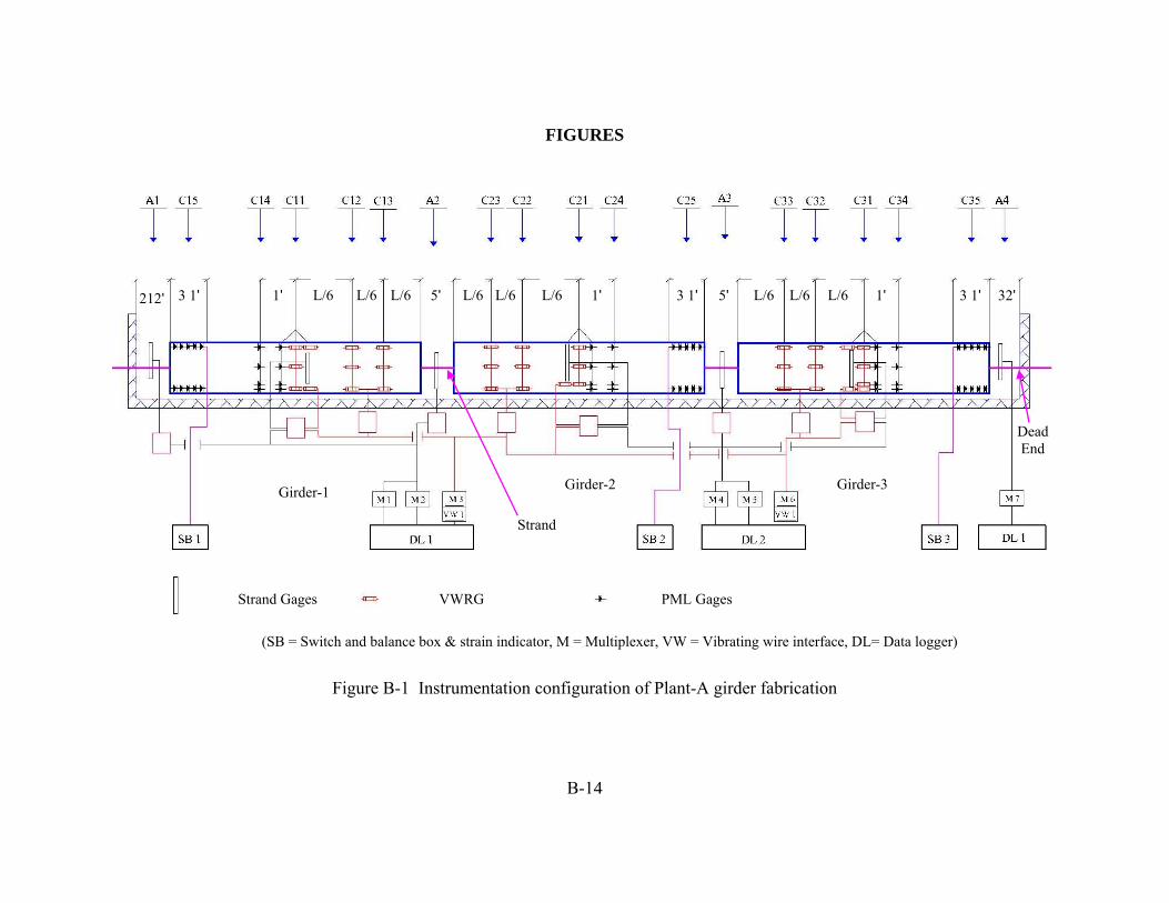
B-14

FIGURES

Figure B-1 Instrumentation configuration of Plant-A girder fabrication

Dead End

Strand

Strand Gages VWRG PML Gages

(SB = Switch and balance box & strain indicator, M = Multiplexer, VW = Vibrating wire interface, DL= Data logger)

L/6L/6L/61'3 1' 3 1' 3 1'L/6 L/6 L/6 L/6 L/6 L/61' 1' 32'5'5'212'

Girder-1 Girder-2 Girder-3

B-15

Figure B-2 Instrumentation configuration of Plant-B girder fabrication

Dead End

Strand Gages

VWSG

PML

Strand

Girder-2 Girder-3 Girder-1

L/32.5' L/6 2.5' 2.5'1' 1'1' L/3 L/6 L/3L/63.5' 18'3.5'11'

A1 C15 C14 C11 C13 C23 C21 C24 C25 C33 C31 C34 C35 A4

M = Multiplexer, VW = Vibrating wire interface, DL= Data logger

B-16

Figure B-3 Plant-A nominal locations of resistance strain gages on strand

Figure B-4 Plant-A nominal locations of concrete vibrating wire strain gages for measuring

longitudinal strains

X-VG7

X-SG9

X-VG4

X-SG3

X-SG2

X-SG1

X-SG10

(@ A1, C11, A2, C21, A3, and C31)

X-SG4

X-SG6

X-SG3

X-SG2

X-SG1

X-SG14

X-SG13

X-SG9

X-SG8 X-SG7

X-SG15

X-SG16

X-SG11

X-SG12

X-SG10

X-SG5

(@ A4)

X-VG5X-VG8

X-VG6

6.8

17.6 ''

32 ''

X-VG1

X-VG2

X-VG3

(@ C12, C13, C22, C23, C32, and C33)

X-VG6 X-VG5

6.8 ''

17.6

32 ''

4.0 ''

(@ C11, C21, and C31)

X-VG1

X-VG3 X-VG4

X-VG2

B-17

Figure B-5 Plant-A nominal locations of PML concrete embedment resistance strain gages

Figure B-6 Plant-A nominal locations of PML concrete embedment resistance strain gages to

determine transfer lengths

32 ''

4.0 ''

(@ C15, C25, and C35)

5 @ 7.5''

6.8 ''

17.6 ''

32 ''

4.0 ''

X-PG1

X-PG1

X-PG1

X-PG1

(@ C14, C11, C24, C21, C34 and C31)

B-18

Figure B-7 Plant-B nominal locations of resistive strain gages on strand

Figure B-8 Plant-B nominal locations of concrete vibrating wire strain gages for measuring longitudinal strains

4.0 ''

X-VG1

(@ C15, C25, and C35)

6.8 ''

17.6 ''

32 ''

X-VG2 X-VG1

X-VG3

X-VG4

(@ C11, C13, C21, C23, C31, and C33)

X-VG4

X-SG5

X-SG3

X-SG2

X-SG1

X-SG6

(@ A1, C11, C21, and C31)

X-SG4

X-SG6

X-SG3

X-SG2

X-SG1

X-SG14

X-SG13

X-SG9

X-SG8 X-SG7

X-SG15

X-SG16

X-SG11

X-SG12

X-SG10

X-SG5

(@ A4)

B-19

Figure B-9 Plant-B nominal locations of PML concrete embedment resistance strain gages

Figure B-10 Photograph of gages installed at midspan (L/2)

Strand gage

VWSG PML

6.8''

17.6 ''

32 ''

4.0 ''

X-PG1

X-PG1

X-PG1

X-PG1

(@ C15, C25, and C35)

B-20

Figure B-11 Installation (a), and location of instrumentation for transfer length

2 in. 40 @ 2 in.

Center of bottom three rows of strands

4 in.

DEMEC points

Metal strip Machine screws

DEMECs & contact seats

( )

(b)

B-21

Figure B-12 Measured concrete strains and predicted transfer length (A-SCC1)

Figure B-13 Measured concrete strains and predicted transfer length (A-SCC2)

0

200

400

600

800

1000

1200

1400

1600

0 5 10 15 20 25 30 35 40 45 50 55 60 65 70 75 80 85 90

raw datasmoothed95% ave. max.final ave.

Distance from free end (in.)

Con

cret

e st

rain

(με)

0

200

400

600

800

1000

1200

1400

1600

0 5 10 15 20 25 30 35 40 45 50 55 60 65 70 75 80 85 90

raw datasmoothed 95% ave. max.final ave.

Distance from free end (in.)

Con

cret

e st

rain

(με)

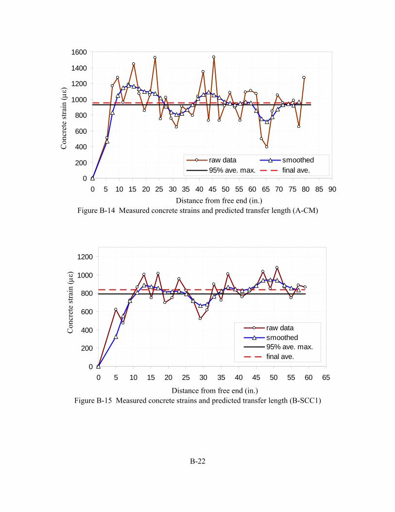
B-22

Figure B-14 Measured concrete strains and predicted transfer length (A-CM)

Figure B-15 Measured concrete strains and predicted transfer length (B-SCC1)

0

200

400

600

800

1000

1200

1400

1600

0 5 10 15 20 25 30 35 40 45 50 55 60 65 70 75 80 85 90

raw data smoothed95% ave. max. final ave.

Distance from free end (in.)

Con

cret

e st

rain

(με)

0

200

400

600

800

1000

1200

0 5 10 15 20 25 30 35 40 45 50 55 60 65

raw datasmoothed95% ave. max.final ave.

Distance from free end (in.)

Con

cret

e st

rain

(με)

B-23

Figure B-16 Measured concrete strains and predicted transfer length (B-SCC2)

Figure B-17 Measured concrete strains and predicted transfer length (B-CM)

0

200

400

600

800

1000

1200

0 5 10 15 20 25 30 35 40 45 50 55 60 65 70

raw datasmoothed95% ave. max.final ave.

Distance from free end (in.)

Con

cret

e st

rain

(με)

0

200

400

600

800

1000

1200

0 5 10 15 20 25 30 35 40 45 50 55 60 65

raw datasmoothed95% ave. max.final ave.

Distance from free end (in.)

Con

cret

e st

rain

(με)

B-24

Figure B-18 Measuring initial reference camber just before strand release

Figure B-19 A-SCC1 strains at L/2

-2500

-2000

-1500

-1000

-500

0

0 60 120 180 240 300 360 420 480 540 600 660

AC21-VG1 AC21-VG2AC21-VG3 AC21-VG4AC21-VG5 AC21-VG6

Days after casting

Stra

in (μ

ε)

Piano wire Pulley

Hanging weight

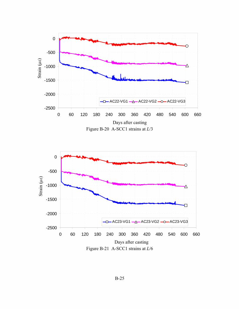
B-25

Figure B-20 A-SCC1 strains at L/3

Figure B-21 A-SCC1 strains at L/6

-2500

-2000

-1500

-1000

-500

0

0 60 120 180 240 300 360 420 480 540 600 660

AC23-VG1 AC23-VG2 AC23-VG3

Days after casting

Stra

in (μ

ε)

-2500

-2000

-1500

-1000

-500

0

0 60 120 180 240 300 360 420 480 540 600 660

AC22-VG1 AC22-VG2 AC22-VG3

Days after casting

Stra

in (μ

ε)

B-26

Figure B-22 A-SCC2 strains L/2

Figure B-23 A-SCC2 strains at L/3

-2500

-2000

-1500

-1000

-500

0

0 60 120 180 240 300 360 420 480 540 600 660

AC12-VG1 AC12-VG2 AC12-VG3

Days after casting

Stra

in (μ

ε)

-2500

-2000

-1500

-1000

-500

0

0 60 120 180 240 300 360 420 480 540 600 660

AC11-VG1 AC11-VG2AC11-VG3 AC11-VG4AC11-VG5 AC11-VG6

Days after casting

Stra

in (μ

ε)

B-27

Figure B-24 A-SCC2 strains at L/6

Figure B-25 A-CM strains at L/2

-2000

-1500

-1000

-500

0

0 60 120 180 240 300 360 420 480 540 600 660

AC31-VG1 AC31-VG2 AC31-VG3AC31-VG4 AC31-VG5 AC31-VG6

Days after casting

Stra

in (μ

ε)

-2500

-2000

-1500

-1000

-500

0

0 60 120 180 240 300 360 420 480 540 600 660

AC13-VG1 AC13-VG2 AC13-VG3

Days after casting

Stra

in (μ

ε)

B-28

Figure B-26 A-CM strains at L/3

Figure B-27 A-CM strains at L/6

-2000

-1500

-1000

-500

0

0 60 120 180 240 300 360 420 480 540 600 660

AC33-VG1 AC33-VG2 AC33-VG3

Days after casting

Stra

in (μ

ε)

-2000

-1500

-1000

-500

0

0 60 120 180 240 300 360 420 480 540 600 660

AC32-VG1 AC32-VG2 AC32-VG3

Days after casting

Stra

in (μ

ε)

B-29

Figure B-28 B-SCC1 strains at L/2

Figure B-29 B-SCC1 strains at L/6

-2500

-2000

-1500

-1000

-500

0

0 60 120 180 240 300 360 420 480 540

BC21-1 BC21-2

BC21-3 BC21-4

Days after casting

Stra

in (μ

ε)

-2500

-2000

-1500

-1000

-500

0

0 60 120 180 240 300 360 420 480 540

BC23-VG1 BC23-VG2BC23-VG3 BC23-VG4

Days after casting

Stra

in (μ

ε)

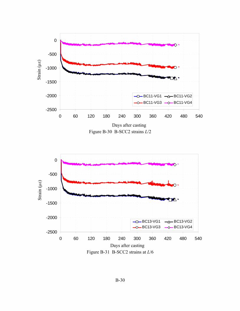
B-30

Figure B-30 B-SCC2 strains L/2

Figure B-31 B-SCC2 strains at L/6

-2500

-2000

-1500

-1000

-500

0

0 60 120 180 240 300 360 420 480 540

BC13-VG1 BC13-VG2BC13-VG3 BC13-VG4

Days after casting

Stra

in (μ

ε)

-2500

-2000

-1500

-1000

-500

0

0 60 120 180 240 300 360 420 480 540

BC11-VG1 BC11-VG2

BC11-VG3 BC11-VG4

Days after casting

Stra

in (μ

ε)

B-31

Figure B-32 B-CM strains at L/2

Figure B-33 B-CM strains at L/6

-2000

-1500

-1000

-500

0

0 60 120 180 240 300 360 420 480 540

BC33-VG1 BC33-VG2BC33-VG3 BC33-VG4

Days after casting

Stra

in (μ

ε)

-2000

-1500

-1000

-500

0

0 60 120 180 240 300 360 420 480 540

BC31-VG1 BC31-VG2BC31-VG3 BC31-VG4

Days after casting

Stra

in (μ

ε)

B-32

Figure B-34 Girder outdoor storage site

Figure B-35 Outdoor storage site ambient relative humidity data

20

30

40

50

60

70

80

90

100

110

0 60 120 180 240 300 360 420 480 540 600 660

11/7/05 2/15/06 5/26/06 9/3/06 12/12/06 3/22/07 6/30/07 10/8/07

average average daily RH

Plant-B girders Plant-A girders

Days after release of Plant-A girders

Ave

rage

dai

ly A

mbi

ent R

H (%

) Weather station

Data collection system housing

B-33

Figure B-36 Outdoor storage site average daily temperature

Figure B-37 General data acquisition system configuration

-40

-30

-20

-10

0

10

20

30

40

0 60 120 180 240 300 360 420 480 540 600 660

11/7/05 2/15/06 5/26/06 9/3/06 12/12/06 3/22/07 6/30/07 10/8/07

average average daily temp.

Days after Plant-A girder release

Dai

ly te

mpe

ratu

re (°

C)

Plant-B girders

Plant-A girders

CSI CR10 Datalogger

CSI SM16M Data Storage Module

CSI AVW4 Vibrating Wire Interface

Vibrating Wire Strain Gage

Strand Gages

CSI 4-Wire Full Bridge Modules

CSI Weather Station

CSI AM16/32 Relay Multiplexer

CSI AM16/32 Relay Multiplexer

Campbell Scientific (CSI) PS100 12V Power Supply

APPENDIX C

CREEP AND SHRINKAGE INSTRUMENTATION AND DATA

C-1

C.1 Introduction

The drying shrinkage and creep characteristics of the conventional and self-consolidating concrete mixes used in the girders were investigated with 4 by 11 in. cylinders cast and cured with the associated girders. The specimens were stored in a controlled environment with a temperature of 72±4°F and relative humidity of 45±15%. For each girder mix, at least two cylinders were instrumented and monitored for drying shrinkage, and at least another two cylinders were loaded and monitored for creep.

To study drying shrinkage characteristic of the mixes, length change and weight change of the cylinders were monitored for a period of approximately 450 days for Plant-A and for a period of approximately 600 days for Plant-B. This appendix summarizes the instrumentation used to monitor the load in the creep frames and to measure strains in the creep and shrinkage cylinders. In addition, it covers the preparation of the specimens and summarizes the results.

C.2 creep load frames

A typical creep load frame constructed and used for this study is shown in Figure C-1. The frames were initially constructed and described in details by Mokhtarzadeh (1998). The same frames were repaired and reused for this study. The repair included sand blasting all plates, replacing tension bars, disk springs, and instrumentation of the tension bars with electrical resistance strain gages to monitor frame loads (i.e., compressive forces applied to the creep specimens).

In total, nine creep load frames (Frames 2 through 10) were used for this study. Each creep load frame consisted of four 10 x 10 x 1.5 in. steel plates (upper and lower jack plates and upper and lower base plates) four 1.25 in. diameter 48 in. length fine threaded (1 1/4-12 UNF-2A) high strength (ASTM A193 Grade B7) tension bars, four pairs of disk springs (Key Bellevilles, Inc. S4250-M-375) with each pair stacked in series, and two spherical bearing blocks (one welded to the center of the lower jack plate and the other stacked in series with the companion cylinders) to minimize any bending moment and to ensure uniaxial loading. The four pairs of disk springs placed between the lower and upper base plates of the creep frame helped to maintain the load as the cylinders shortened due to creep and shrinkage.

Each tension bar was instrumented with four electrical resistance strain gages positioned in a Wheatstone bridge as shown in Figure C-2 to monitor the compressive force applied to the creep specimens. The Wheatstone bridge circuit is almost universally used in load cells and other strain gage transducers, because it facilitates cancellation of unwanted temperature effects. The strain gages were 90° 2-element cross type (Texas Measurement, Inc., FCA-3-11-1L), with a 120 ohm resistance and 0.118 in. active gage length. The lead wires from each Wheatstone bridge were labeled and connected to a strain measuring device composed of a 10-channel switch and balance unit (Measurement Group, Inc. Model SB-10) and a strain indicator unit (Measurement Group, Inc. Model P-3500) to facilitate reliable, easy, and fast measurement.

C-2

C.2.1 Creep Frame Calibration

The setup used for the creep frame calibration was slightly different from that used for loading/re-loading (Figure C-1). Each creep frame was calibrated using a standard 100 kip load cell placed in series with a steel cylinder used in place of the creep specimens as shown in Figure C-1 (a). Instead of placing the load cell just below the jack, the load cell was placed just below the lower jack plate over the steel cylinder. This configuration was found to be more practical and reliable for calibration. In the original configuration (Figure C-1 (a)), the frames were loaded and the upper jack plate was tightened to calibrate the bar readings with the load cell readings. However, the load was found to vary as the jack would lose pressure because the hydraulic hand pump valve that locks the pressure (load) of the jack was not working properly. In the calibration configuration shown in Figure C-1 (b) with the load cell placed just below the lower jack plate, the load was constant and independent of the jack once the lower jack plate was tightened. The steel cylinder was used instead of the creep specimens during the calibration to eliminate any error that could have been introduced due to concrete creep and shrinkage occurring during the calibration period.

For each creep frame, the output of the Wheatstone bridges attached to the strain gages on the four tension bars was calibrated against the load cell in series with the steel cylinder. The frames were loaded several times to verify the repeatability and accuracy of the instrumentation, and one of the frames was left loaded for a week to check the accuracy of the strain/load measuring devices over time.

C.2.2 Hydraulic Hand Pump and Hydraulic Cylinder (Jack)

An Enerpac single-acting spring return low height hydraulic cylinder (Model RSM-1500) was used together with a hydraulic hand pump to load the frames. This compact model had a capacity of 300 kips, and collapsed and extended heights of 3.94 and 4.5 inches, respectively. This model was selected because it was well suited for insertion between the upper and lower jack plates and minimized the total height of the creep frames to 48 in. In addition, the weight (58 lb) and the presence of an attached carrying handle made it convenient for this study.

C.3 Companion Cylinder Fabrication and Curing

C.3.1 Molds

The companion cylinders were cast in cylindrical molds constructed using 4 by 11 in. commercially available schedule 40 PVC pipes and end caps. Three pairs of brass inserts were bolted to the inner side of each mold using machine screws to form three 8 in. gage lines along the height of the mold that were equidistantly located (i.e., at 120°) around each mold as show in Figure C-3.

A jig similar to a compressometer used by ASTM C469 to measure static modulus of elasticity of concrete was used to position the six-brass inserts on the surface of the PVC molds as shown

C-3

in Figure C-3. The jig was composed of two yokes, three end-threaded rods, and two mounting bolts. Three sets of holes each 0.20 in. in diameter and spaced 120° around the perimeter of each yoke were drilled. These holes corresponded to the location of the brass inserts attached to the cylinder molds. The two yokes were attached using three threaded rods to keep the yokes at the 8.0 in. gage distance, and to ensure vertical alignment of the gage lines. This was important to minimize the error in measured creep and shrinkage strains due to misalignment of the gage lines. Creep and shrinkage readings with a misaligned gage line will be unconservative (i.e., smaller than the true reduction in distance). The cylinder molds were placed inside the jig and fixed in position using the two mounting bolts attached to the jig. The holes for the brass inserts were drilled using a hand operated drill through the yoke holes and into the PVC mold.

The PVC molds performed well. The constructed molds had good dimensional stability during filling and handling compared to commercially available single-use plastic molds.

C.3.2 Casting and Curing

The creep and shrinkage companion cylinders were cast and cured with the associated girders. The conventional concrete companion cylinders were prepared based on ASTM C 192/C 192M. However, there was no standard ASTM procedure available for making SCC cylinders. The SCC cylinders were cast in the same way as the conventional cylinders with the exception of the rodding procedure, which was replaced by tapping the outsides of the PVC molds slightly 3-4 times with a mallet after each of the two layers was placed to release any trapped air. The SCC cylinder molds were filled by discharging the concrete gently from a 5-gallon plastic bucket, which was much easier and quicker than filling the molds using a scoop, and it is believed that the companion cylinders prepared in this way were more representative of concrete placement in the girders. The mold filling method should not have a significant impact on the measured SCC properties as long as the mixes have good segregation resistance. However, when SCC mixes have poor or moderate segregation resistance, the mold filling method and procedure could affect the measured material properties.

All of the concrete cylinders were cured under the tarps with the associated girders. After curing was completed but before strand release, the companion cylinders were transported to the University of Minnesota Structures Laboratory, where they were prepared and monitored for creep and shrinkage.

C.3.3 Preparation, Loading, and Measurement of Creep and Shrinkage

Just before strand release, the companion creep and shrinkage cylinders were transported to the Structure Laboratory to prepare for creep and shrinkage monitoring. First, both ends of the shrinkage cylinders were sealed using a two-component epoxy coating to prevent moisture exchange with the environment through the top and bottom surfaces. This ensured the same amount of exposed cylinder surface area to exchange moisture with the environment for both the creep and shrinkage cylinders because the creep cylinders were capped with a sulfur-based high strength capping compound.

C-4

Three sets of stainless steel contact seats were threaded in place in the embedded brass inserts on the side of each creep and shrinkage specimen to form three 8.0 in. gage lines that were placed 120° apart and centered on the side of each specimen. Then each shrinkage cylinder and gage line were numbered and the initial length of the gage lines and weight of each cylinder were measured and recorded. Figure C-4 shows the name and number of the shrinkage companion cylinders used for both plants. In total, 14 (8 for Plant-A and 6 for Plant-B) shrinkage companion cylinders were prepared and monitored.

Two creep cylinders were placed in each creep frame in series as shown in Figure C-1. The unloaded length of the gage lines was measured and recorded for each cylinder. The frames were loaded within 24 hours after the associated girders were released. The spherical bearing blocks with the lower jack plate were lowered to sit on the center of the cylinders, and the frames were loaded initially to approximately 75% of the target load using the hydraulic cylinder and the load cell placed in series between the lower and upper jack plates. Then the four nuts above the lower jack plate were tightened, and the hydraulic pressure was removed. The tension force in each tension bar was read from the strain measuring device and if the tension force in the bars was unequal then the hydraulic cylinder and the load cell were repositioned until a uniform load distribution was obtained. To compensate for force losses due to seating of the nuts over the lower jack plate, a load slightly larger (5-10 % larger) than the target load (i.e., full load) was applied to the frames and the four nuts above the lower jack plate were tightened. The tension force in each bar and the total tension force were checked immediately after the loading. If the error for the bar forces or the total force were not within ±1.0%, the system was reloaded, and the force in each tension bar and the total force were adjusted accordingly. Immediately after the loading, each gage line was measured to determine initial elastic deformation of the two creep cylinders loaded. Figure C-5 and Figure C-6 show the creep load frames and the configuration of the companion cylinders for each frame for Plant-A and Plant-B, respectively.

The axial compression force applied to the creep cylinders was 56.5 kips, which corresponded to a compressive stress of 4.5 ksi (0.6fci'), the maximum compressive stress allowed at release according to AASHTO (2004) and ACI 318-05 guidelines for a nominal concrete compressive strength of 7.5 ksi at release. The only exception was Frame-9 and Frame-6, which were loaded to 54.0 kips (4.3 ksi), which corresponded to 60% of the measured concrete compressive strength of the cylinders (A-SCC2) at release (i.e., 7.12 ksi). The lower load was used for these cylinders because the concrete compressive strength of the A-SCC2 mix was measured to be 7.12 ksi, which was slightly smaller than the design value of 7500 psi at release, and there were some concerns that the cylinders could fail or be damaged during loading or as the creep progressed.

At predetermined time intervals, gage lengths of the creep and shrinkage specimens were measured and recorded, and periodically the total tensile force in the tension bars was checked for each frame. The nuts on the top of the lower jack plate were tightened to restore the total compressive force in the specimens if the difference between the measured and target loads were more than ±2.5%. Whenever there was a need to re-load a frame to adjust the loads, the gage length of all creep and shrinkage specimens were measured and recorded before doing any re-loading. Another set of readings was taken for the creep specimens just after re-loading.

C-5

The gage lengths of the specimens were measured using a Whittemore gage, which had a digital dial indicator with 0.0001 in. graduations and a maximum travel distance of 0.5 in. A reference invar bar, used to eliminate temperature affects on the readings, was used to calibrate (i.e., zero) the Whittemore gage before taking any measurements. Each gage line was measured at least five times, and additional readings were taken if the difference between the maximum and minimum readings of a gage line were more than 0.0004 in., which corresponded to approximately two times the standard deviation of the readings. The majority of the measurements (approximately 90%) were made by the same operator to minimize variability in the readings due to different pressure on the Whitmore gage.

C.3.3.1 Correction for Creep Frame Re-Loading

The creep frames were re-loaded to adjust the total creep frame load if the difference between the measured and target loads were more than ± 2.5%. Whenever a creep frame was re-loaded the gage length of the creep specimens were measured and recorded before re-loading and just after re-loading. In addition, the recorded data (i.e., strains before and after re-loading) was also used to predict the strain data that would correspond to the target load since the measured loads after re-loading were within ± 2.5% of the target loads. The recorded total strain was adjusted for the measured load being different from the target load for the data points taken on the days of reloading. Assuming that the stress versus strain behavior of the cylinders was linear between the frame load before and after re-loading as shown in Figure C-7, the total strain data corresponding to target load was predicted using

⎟⎟⎠

⎞⎜⎜⎝

⎛+−

−=⇒−⎟⎠⎞

⎜⎝⎛ +

−=

⎟⎠⎞

⎜⎝⎛ −−⎟

⎠⎞

⎜⎝⎛ +

− βαββαβcaab

PP

ba

PP

ca

1001

1001

1001

(C-1)

where P is the target creep frame load value, α is the percentage decrease in the target load at just before re-loading, β is the percentage of over/under-loading just after re-loading, c is the cylinder reading just before re-loading, b is the cylinder total strain reading corresponding to the target load, a is the cylinder reading just after re-loading. The total and creep strain data for the days that the frames were reloaded were replaced by the data adjusted for creep frame re-loading according to Eqn. (C-1).

C.3.4 Storage

The creep and shrinkage specimens were stored in an environmentally-controlled room at the University of Minnesota Structures Laboratory. A commercially available humidifier and dehumidifier were used to control the ambient relative humidity. Both units had automatic controls set to maintain an ambient relative humidity of 50±5 %. No heater or cooler was employed to control the ambient temperature. Figures F-8 and F-9 show the measured ambient relative humidity and temperature data, respectively, measured over the course of the investigation. The measured ambient relative humidity and temperature data had an average of 45±15 % and 72±4 °F, respectively.

C-6

C.4 Companion Cylinder Creep and Shrinkage Behavior

The monitored strains due to creep and shrinkage of the companion cylinders were used to develop creep and shrinkage material models for the girders. The developed models were then used with finite element tools (i.e., PBEAM) to predict the girder behavior including prestress losses.

C.4.1 Weight Change

In addition to measuring the creep and shrinkage strains, the weight of the companion shrinkage cylinders was monitored over the course of the study. The change in weight of the companion cylinders results from the transfer of moisture between the cylinders and the environment due to the difference between the state of moisture of the cylinders and the control room where they are stored. Figures F-10 and F-11 show the change in cylinder weight for the different mixes. The SCC mixes had larger weight losses for both plants. The loss of weight values were approximately 2% for A-SCC2, 1.5% for A-SCC1, 1.2% for A-CM, and approximately 1.0% for the Plant-B mixes, with slightly higher losses for the SCC specimen, at approximately 600 and 450 days after casting the Plant-A and Plant-B mixes, respectively. A direct comparison of these numbers is difficult because the mixes had different w/c ratios as shown in Table 5-1. The measured weight loss characteristics of the mixes were consistent with the measured shrinkage behaviors of the associated mixes. In other words, the mixes with larger weight losses had larger shrinkage.

C.4.2 Creep and Shrinkage Behavior of Companion Cylinders

Figures F-12 through F-19 show the cylinder shrinkage data of the mixes. The figures contain plots for each of the individual shrinkage cylinders (i.e., SH# identifies the cylinder number). For both plants, the SCC mixes had slightly larger measured shrinkage than the conventional concrete mixes. At the end of the monitoring period, the Plant-A SCC mixes had approximately 100 to 150με larger shrinkage strains than the conventional concrete, and for Plant-B, the SCC mixes had approximately 50 to 75 με larger shrinkage strains than the conventional concrete. However, it should be noted that mixes had different mix proportions as shown in Table 5-1 (e.g., w/cm). The average shrinkage values observed were compared to shrinkage values suggested by ACI Committee 209 (ACI 209R-92 1992) given in Chapter 5. For all mixes (both SCC and conventional) the measured shrinkage strains after 100 days were smaller than those suggested by ACI 209.

Figures F-20 through F-29 show the total strains, creep strains, and creep coefficients measured for the Plant-A creep cylinders. The total strains included the elastic loading and combined creep and shrinkage effects; whereas, the creep strains were calculated by deducting from the total strains, the initial elastic strain (which occurred immediately after application of the load) and the average shrinkage strain of the associated shrinkage cylinders. Figures F-30 through F-33 show the creep coefficients for the Plant-A Cylinders. Creep coefficients, which represent the ratio of the creep strains to the initial elastic strains, were calculated and compared to those

C-7

predicted by ACI 209. Figures F-30 through F-33 show the creep coefficients for the Plant-A Cylinders. Similar Figures (total strains, creep strains, and creep coefficients) are shown in Figures F-34 through F-45 for the Plant-B mixes. As shown in Figures F-33 and F-45 for Plant-A and Plant-B, respectively, for all SCC and conventional concrete mixes, the calculated creep coefficients after 5 days were smaller than those predicted by ACI 209, and the predicted creep coefficients of SCC and conventional concrete mixes were approximately 70% and 100% higher than those measured after the first 5 days, respectively. Therefore, the creep and shrinkage strains predicted by ACI 209 were conservative for both conventional and SCC concrete mixes.

C.4.3 Nonlinear Least-square Analysis of Creep and Shrinkage Data

A set of nonlinear least-square analyses of the experimental creep and shrinkage data was done for all girder mixes. The method of least square analysis, also known as regression analysis was used to represent the numerical data by adjusting the parameters of a model (i.e., a form of equation with a number of variables and constant coefficients) so as to get an optimal fit of the data. In this study, creep and shrinkage material models recommended by ACI 209 were used for nonlinear least square fit. Both ACI 209 creep and shrinkage equations have three parameters (i.e., coefficients): α , ( )ushε and f for shrinkage, andψ , d and uv for creep

( ) ( ) εtf

tε ushα

α

tsh += (C-2)

vtd

tv ut ψ

ψ

+= (C-3)

where ( )tshε is the shrinkage strain at time t, t is the time in days, α is a constant for a given member shape and size (ACI Committee 209 recommends values between 0.90<α <1.10), ( )ushε is the ultimate shrinkage strain (ACI Committee 209 recommends values between 415x10-

6< ( )ushε <1070x10-6), f is a constant in days (ACI Committee 209 recommends values between 20< f <130), tv is the creep coefficient at any t, ψ is a constant for a given member shape and size (ACI Committee 209 recommends values between 0.40<ψ <0.80), d is the time to one-half creep in days (ACI Committee 209 recommends values between 6< d <30), uv is the ultimate creep coefficient (ACI Committee 209 recommends values between 1.30< uv <4.15).

Three cases were considered for nonlinear least-squares analysis, and the results for each case are given in Table C-1 through Table C-4.

CASE-1: One Parameter Least-square Analysis (LSA-1):

In this case only the ultimate creep coefficient and ultimate shrinkage were assumed to be unknown. All other parameters were assumed to be equal to the values recommended by ACI 209 for standard conditions (i.e., α = 1.00, f = 55, ψ = 0.60, and d = 10).

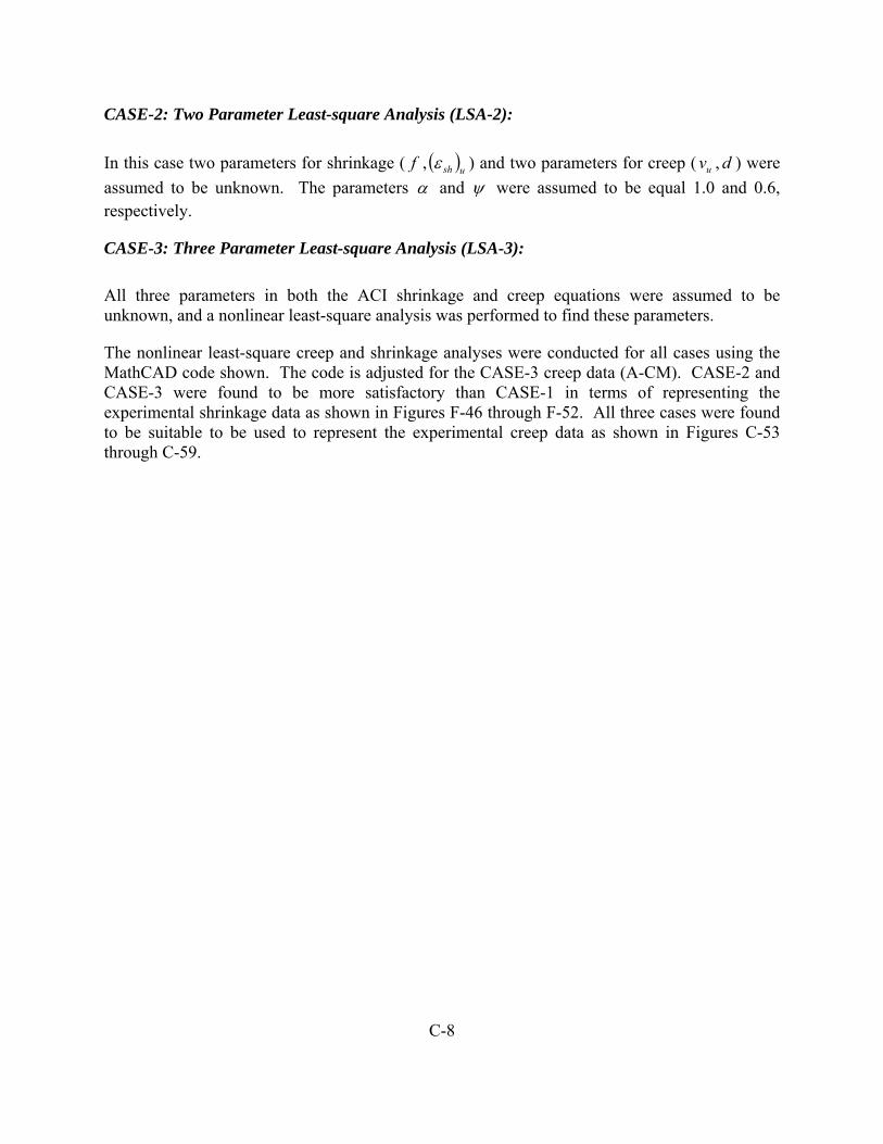
C-8

CASE-2: Two Parameter Least-square Analysis (LSA-2):

In this case two parameters for shrinkage ( f , ( )ushε ) and two parameters for creep ( uv , d ) were assumed to be unknown. The parameters α and ψ were assumed to be equal 1.0 and 0.6, respectively.

CASE-3: Three Parameter Least-square Analysis (LSA-3):

All three parameters in both the ACI shrinkage and creep equations were assumed to be unknown, and a nonlinear least-square analysis was performed to find these parameters.

The nonlinear least-square creep and shrinkage analyses were conducted for all cases using the MathCAD code shown. The code is adjusted for the CASE-3 creep data (A-CM). CASE-2 and CASE-3 were found to be more satisfactory than CASE-1 in terms of representing the experimental shrinkage data as shown in Figures F-46 through F-52. All three cases were found to be suitable to be used to represent the experimental creep data as shown in Figures C-53 through C-59.

C-9

ψ 0.47=νu 1.67=d 15.9=

d

νu

ψ

⎛⎜⎜⎝

⎞⎟⎟⎠

MinErr d νu, ψ,( ):=

# Built-in MathCAD function that finds the values of parameters that most closely solves the error minimization constraint.

Im ψ( ) 0Im νu( ) 0Im d( ) 0# Additional constraints: paramaters must be real not complex numbers

1

N

i

yi f t d, νu, ψ,( )−( )2∑=

0

# Error between the experimental and fitted data with initial calues for unknown parameters

Given

# The form of eqaution that will be fitted

f t d, νu, ψ,( ) tψ

d tψ+νu⋅:=

# Initial guesses for the unknown paramaters

ψ 1.0:=νu 575:=d 55:=

# The number of data pairs stored in INPUTN 54:=

# Store days in "t" and creep or shrinage data in "y"

y INPUT 2⟨ ⟩:=t INPUT 1⟨ ⟩:=

# This reads the input data file (days and creepcoeficent or shrinkage value) and store it as "INPUT"

MathCAD Data Fit Program -Creep Least Squares Method, 3 Parameters

# This reads the input files (days and creep coefficient or shrinkage value) and store it as “INPUT”

# Store days in “t” and creep or shrinkage data in “y”

# The number of data pairs stored in INPUT

# Initial guesses for the unknown parameters

# The form of equation that will be fitted

# Error between the experimental and fitted data with initial values for unknown parameters

# Additional constraints: parameters must be real not complex numbers

# Built-in MathCAD function that finds the values of parameters that most closely solves the error minimization constraints

C-10

TABLES Table C-1 Plant-A mixes nonlinear least square shrinkage curves

ACI 209† Least Square Shrinkage Curves

Cylinder ID LSA-1* (one parameter)

LSA-2‡ (two-parameter)

LSA-3§ (three-parameter)

A-CM α f ( )ushε α f ( )ushε

α f ( )ushε

CM-SH1 1.00 55 444 1.00 18 389 0.66 8 432 CM-SH2 1.00 55 425 1.00 22 377 0.61 8 438 CM-SH3 1.00 55 457 1.00 19 401 0.87 13 412

AVRG 1.00 55 442 1.00 19 389 0.70 9 424

A-SCC1 α f ( )ushε α f ( )ushε

α f ( )ushε

SCC1-SH1 1.00 55 540 1.00 26 487 0.69 11 544 SCC1-SH2 1.00 55 516 1.00 22 459 0.56 7 556 AVRG 1.00 55 528 1.00 24 473 0.62 9 549

A-SCC2 α f ( )ushε α f ( )ushε α f ( )ushε

SCC2-SH1 1.00 55 581 1.00 22 517 1.02 23 516 SCC2-SH2 1.00 55 642 1.00 15 555 0.84 10 575 AVRG 1.00 55 612 1.00 18 536 0.91 14 547

A-SCC2B α f ( )ushε α f ( )ushε

α f ( )ushε

F9-SCC2B-C1 1.00 55 534 1.00 14 458 0.58 5 524

† ACI 209 Equation: ( ) ( )ushtsh tft εε α

α

+=

* α = 1.00, f =55, and ( )ushε determined

‡ α = 1.00, f and ( )ushε determined § All parameters (α ,f , and ( )ushε ) determined

C-11

Table C-2 Plant-A mixes nonlinear least square creep curves

ACI 209† Least Square Creep Curves

Cylinder ID LSA-1* (one parameter)

LSA-2‡ (two-parameter)

LSA-3§ (three-parameter)

A-CM ψ d vu ψ d vu ψ d vu

F5-CM-C2 0.6 10 1.03 14.6 1.15 14.6 0.72 19.4 1.03

F2-CM-C1 0.6 10 1.08 16.4 1.26 16.4 0.74 22.6 1.10

AVRG 0.6 10 1.06 15.5 1.21 15.5 0.47 15.9 1.67

A-SCC1 ψ d vu ψ d vu ψ d vu

F5-SCC1-C4 0.6 10 1.51 0.60 10.5 1.53 0.48 8.8 1.77

F2-SCC1-C3 0.6 10 1.40 0.60 12.0 1.47 0.63 12.9 1.42

F10-SCC1-C1 0.6 10 1.79 0.60 12.9 1.92 0.53 11.6 2.10

F10-SCC1-C2 0.6 10 1.72 0.60 9.6 1.70 0.43 7.8 2.18

AVRG 0.6 10 1.60 0.60 11.2 1.65 0.51 9.7 1.85

A-SCC2 ψ d vu ψ d vu ψ d vu

F6-SCC2-C1 0.6 10 1.68 0.60 11.0 1.73 0.55 10.1 1.82

F6-SCC2-C2 0.6 10 1.68 0.60 11.5 1.75 0.59 11.4 1.76

F9-SCC2-C3 0.6 10 2.44 0.60 15.4 2.79 0.58 14.9 2.85

AVRG 0.6 10 1.94 0.60 12.9 2.08 0.57 12.3 2.14

AVRG1 0.6 10 1.68 0.60 11.3 1.74 0.57 10.7 1.79

A-SCC2B ψ d vu ψ d vu ψ d vu

F9-SCC2B-C1 0.6 10 2.38 0.60 17.3 2.83 0.72 12.7 2.49

† ACI 209 Equation: ut vtd

tv ψ

ψ

+=

* ψ = 0.6, d=10, and vu determined

‡ ψ = 0.6, d and vu determined § All parameters (ψ , d , and vu) determined

1 Frame 9 (F9-SCC2-C3) not included

C-12

Table C-3 Plant-B mixes nonlinear least square shrinkage curves

ACI 209† Least Square Shrinkage Curves

Cylinder ID LSA-1* (one parameter)

LSA-2‡ (two-parameter)

LSA-3§ (three-parameter)

B-CM Α f ( )ushε α f ( )ushε

α f ( )ushε

CM-SH1 1.00 55 408 1.00 33 374 1.37 105 350

CM-SH2 1.00 55 414 1.00 32 378 1.12 45 368

AVRG 1.00 55 411 1.00 33 376 1.23 67 358

B-SCC1 α f ( )ushε α f ( )ushε

α f ( )ushε

SCC1-SH1 1.00 55 501 1.00 27 447 0.94 22 455

SCC1-SH2 1.00 55 483 1.00 30 437 1.34 85 411

AVRG 1.00 55 492 1.00 29 442 1.13 41 430

B-SCC2 α f ( )ushε α f ( )ushε α f ( )ushε

SCC2-SH1 1.00 55 472 1.00 24 415 1.19 41 401

SCC2-SH2 1.00 55 503 1.00 21 437 1.01 22 436

AVRG 1.00 55 488 1.00 23 426 1.10 30 418

† ACI 209 Equation: ( ) ( )ushtsh tft εε α

α

+=

* α = 1.00, f =55, and ( )ushε determined

‡ α = 1.00, f and ( )ushε determined § All parameters (α ,f , and ( )ushε ) determined

C-13

Table C-4 Plant-A mixes nonlinear least square creep curves

ACI 209† Least Square Creep Curves

Cylinder ID LSA-1* (one parameter)

LSA-2‡ (two-parameter)

LSA-3§ (three-parameter)

B-CM ψ d vu ψ d vu ψ d vu

F3-CM-C1 0.6 10 1.11 0.60 7.73 1.03 0.48 6.70 1.19

F8-CM-C2 0.6 10 1.27 0.60 11.28 1.31 0.47 10.05 1.62

AVRG 0.6 10 1.19 0.60 9.45 1.17 0.47 8.28 1.40

B-SCC1 ψ d vu ψ d vu ψ d vu

F7-SCC1-C1 0.6 10 1.60 0.60 7.47 1.49 0.38 6.73 2.11

F3-SCC1-C2 0.6 10 1.67 0.60 8.62 1.60 0.36 8.53 2.66

F4-SCC1-C3 0.6 10 1.75 0.60 5.94 1.54 0.23 14.08 6.37

AVRG 0.6 10 1.67 0.60 7.28 1.54 0.30 8.56 3.18

B-SCC2 ψ d vu ψ d vu ψ d vu

F7-SCC2-C1 0.6 10 1.89 0.60 9.06 1.84 0.40 8.22 2.64

F8-SCC2-C2 0.6 10 1.84 0.60 10.23 1.85 0.41 9.29 2.61

F4-SCC2-C3 0.6 10 1.73 0.60 12.45 1.85 0.31 23.55 6.62

AVRG 0.6 10 1.82 0.60 10.40 1.84 0.37 10.53 3.15

† ACI 209 Equation: ut vtd

tv ψ

ψ

+=

* ψ = 0.6, d=10, and vu determined

‡ ψ = 0.6, d and vu determined

C-14

FIGURES

upper jack plate

jack

load cell

steelcylinders

lower jack plate

bearing block

upper jack plate

lower jack plate

jack

load cell

bearing blocks

Companion cylinders

tension bar

upper base plate

lower base plate Pair of disk spring

(Jack)

(Pair of disk spring)

spherical bearing blocks

companion cylinder

pair of disk springs

(pair of disk springs)

(a)

(b)

steel cylinder

spherical bearing blocks

Figure C-1 Details of creep load frame (a) and frame calibration setup (b)

C-15

5.0"

1.25"

Vi

Vo

R1 R2

R4 R3

Vo

Vi

(on opposite sides of the rod)

R1

vR2

R3

R4

Figure C-2 Details of tension bar instrumentation forming Wheatstone bridge (load cell)

C-16

PVC cylinder

Machine s

120°

Contact seat

Bras insert

Concrete

screws

PVC cylinder Jig Machine

screws

Brass inserts

concrte

Contact seat

120 °

Figure C-3 Jig and cross section of PVC cylinder mold and stainless contact seats (DEMEC

points) threaded in the embedded brass inserts

ACM

-SH

1

ACM

-SH

2

ACM

-SH

3

ASC

C1-

SH

1

ASC

C1-

SH

2

ASC

C2-

SH

1

ASC

C2-

SH

2

ASC

C2B

-SH

1

(Mix B-CM) (Mix B-SCC1) (Mix B-SCC2)

BCM

-SH

1

BCM

-SH

2

BSC

C1-

SH

1

BSC

C1-

SH

2

BSC

C2-

SH

1

BSC

C2-

SH

2

(Mix A-CM) (Mix A-SCC1) (Mix A-SCC2) (Mix A-SCC2B)

Figure C-4 Plant-A and Plant-B shrinkage companion cylinders

C-17

ASC

C2-

C3

(Frame # 9)

ASC

C2B

-C1

ASC

C2-

C2

(Frame # 6)

ASC

C2-

C1

ACM

-C2

(Frame # 5)

ASC

C1-

C4

ACM

-C1

(Frame # 2)

ASC

C1-

C3

ASC

C1-

C1

(Frame # 10)

ASC

C1-

C2

Figure C-5 Plant-A creep frames and creep cylinder configuration

BSC

C1-

C2

(Frame # 3)

BCM

-C1

BSC

C1-

C3

(Frame # 4)

BSC

C2-

C3

BSC

C1-

C1

(Frame # 7)

BSC

C2-

C1

BSC

C2-

C2

(Frame # 8)

BCM

-C2

Figure C-6 Plant-B creep frames and creep cylinder configuration

C-18

b

P(1-α/100)

P

Load reading

P(1+β/100)

c

a

reading

cb

a

LoadP(1-α/100) P P(1+β/100) P(1-α/100)

P(1+ β/100)

P

c

b

a

Load

Strain reading

c

a

b

P(1-α/100) P P(1+ β/100)

Load strain reading

Figure C-7 Strain correction due to creep frame re-loading

20

30

40

50

60

70

80

0 60 120 180 240 300 360 420 480 540 600

11/8/05 2/6/06 5/7/06 8/5/06 11/3/06 2/1/07 5/2/07 7/31/07

Days after Plant-A strand release

Average

Am

bien

t rel

ativ

e hu

mid

ity (%

)

Figure C-8 Control room ambient relative humidity

C-19

Figure C-9 Control room ambient temperature

Figure C-10 Plant-A cylinder weight changes (original weight (W0), measured W)

50

60

70

80

90

0 60 120 180 240 300 360 420 480 540 600

11/8/05 2/6/06 5/7/06 8/5/06 11/3/06 2/1/07 5/2/07 7/31/07

Days after Plant-A strand release

Date

Am

bien

t tem

pera

ture

(° F

)

Average

0.980

0.984

0.988

0.992

0.996

1.000

0 50 100 150 200 250 300 350 400 450 500 550 600

11/8/05 2/16/06 5/27/06 9/4/06 12/13/06 3/23/07 7/1/07

A-SCC2 A-SCC2B

A-CM A-SCC1

Days

0WW

C-20

Figure C-11 Plant-B cylinder weight changes (original weight (W0), measured W)

Figure C-12 Plant-A drying shrinkage characteristics of A-CM mix

0.988

0.990

0.992

0.994

0.996

0.998

1.000

0 50 100 150 200 250 300 350 400 450 500 550

7/10/06 10/8/06 1/6/07 4/6/07 7/5/07 10/3/07 1/1/08

B-SCC1 B-SCC2 B-CM

Days

0WW

0

100

200

300

400

500

600

700

0 50 100 150 200 250 300 350 400 450 500 550 600

11/8/05 2/16/06 5/27/06 9/4/06 12/13/06 3/23/07 7/1/07

A-CM-SH1A-CM-SH2A-CM-SH3ACI 209

Days

Shrin

kage

stra

in (μ

ε)

C-21

Figure C-13 Plant-A drying shrinkage characteristics of A-SCC1 mix

Figure C-14 Plant-A drying shrinkage characteristics of A-SCC2 and A-SCC2B mixes

0

100

200

300

400

500

600

700

800

0 50 100 150 200 250 300 350 400 450 500 550 600

11/8/05 2/16/06 5/27/06 9/4/06 12/13/06 3/23/07 7/1/07

A-SCC1-SH2A-SCC1-SH1ACI 209

Days

Shrin

kage

stra

in (μ

ε)

0

100

200

300

400

500

600

700

800

0 50 100 150 200 250 300 350 400 450 500 550 600

11/8/05 2/16/06 5/27/06 9/4/06 12/13/06 3/23/07 7/1/07

A-SCC2-SH1A-SCC2B-SH1A-SCC2-SH2ACI 209

Days

Shrin

kage

stra

in (μ

ε)

C-22

Figure C-15 Average drying shrinkage characteristics of Plant-A mixes

Figure C-16 Plant-B drying shrinkage characteristics of B-CM mix

0

100

200

300

400

500

600

700

800

0 50 100 150 200 250 300 350 400 450 500 550 600

11/8/05 2/16/06 5/27/06 9/4/06 12/13/06 3/23/07 7/1/07

A-CM A-SCC2 A-SCC1 A-SCC2B

Days

Shrin

kage

stra

in (μ

ε)

0

100

200

300

400

500

600

0 50 100 150 200 250 300 350 400 450 500 550

7/10/06 10/8/06 1/6/07 4/6/07 7/5/07 10/3/07 1/1/08

B-CM-SH1B-CM-SH2ACI 209

Days

Shrin

kage

stra

in (μ

ε)

C-23

Figure C-17 Plant-B drying shrinkage characteristics of B-SCC1 mix

Figure C-18 Plant-B drying shrinkage characteristics of B-SCC2 mix

0

100

200

300

400

500

600

700

800

0 50 100 150 200 250 300 350 400 450 500 550

7/10/06 10/8/06 1/6/07 4/6/07 7/5/07 10/3/07 1/1/08

B-SCC2-SH1

B-SCC2-SH2

ACI 209

Days

Shrin

kage

stra

in (μ

ε)

0

100

200

300

400

500

600

700

800

0 50 100 150 200 250 300 350 400 450 500 550

7/10/06 10/8/06 1/6/07 4/6/07 7/5/07 10/3/07 1/1/08

B-SCC1-SH1B-SCC1-SH2ACI 209

Days

Shrin

kage

stra

in (μ

ε)

C-24

Figure C-19 Average drying shrinkage strains of Plant-B mixes

Figure C-20 Total strain of creep cylinders of Plant-A mix A-CM

0

100

200

300

400

500

600

0 50 100 150 200 250 300 350 400 450 500 550

7/10/06 10/8/06 1/6/07 4/6/07 7/5/07 10/3/07 1/1/08

B-SCC1

B-SCC2

B-CM

Days

Shrin

kage

stra

in (μ

ε)

0

500

1000

1500

2000

2500

0 50 100 150 200 250 300 350 400 450 500 550 600

11/8/05 2/16/06 5/27/06 9/4/06 12/13/06 3/23/07 7/1/07

F5-CM-C2F2-CM-C1

Days

Tota

l stra

in (μ

ε)

C-25

Figure C-21 Creep strain of Plant-A mix A-CM

Figure C-22 Total strain of creep cylinders of Plant-A mix A-SCC1

0

1000

2000

3000

4000

0 50 100 150 200 250 300 350 400 450 500 550 600

11/8/05 2/16/06 5/27/06 9/4/06 12/13/06 3/23/07 7/1/07

F5-SCC1-C4F2-SCC1-C3F10-SCC1-C1F10-SCC1-C2

Days

Tota

l stra

in (μ

ε)

0

250

500

750

1000

0 50 100 150 200 250 300 350 400 450 500 550 600

11/8/05 2/16/06 5/27/06 9/4/06 12/13/06 3/23/07 7/1/07

F5-CM-C2F2-CM-C1

Days

Cre

ep st

rain

(με)

C-26

Figure C-23 Creep strain of Plant-A mix A-SCC1

Figure C-24 Total strain of creep cylinders of Plant-A mix A-SCC2

0

1000

2000

3000

4000

0 50 100 150 200 250 300 350 400 450 500 550 600

11/8/05 2/16/06 5/27/06 9/4/06 12/13/06 3/23/07 7/1/07

F6-SCC2-C1F6-SCC2-C2F9-SCC2-C3F9-SCC2B-C1

Days

Tota

l stra

in (μ

ε)

0

500

1000

1500

2000

0 50 100 150 200 250 300 350 400 450 500 550 600

11/8/05 2/16/06 5/27/06 9/4/06 12/13/06 3/23/07 7/1/07

F5-SCC1-C4F2-SCC1-C3F10-SCC1-C1F10-SCC1-C2

Days

Cre

ep st

rain

(με)

C-27

Figure C-25 Creep strain of Plant-A mix A-SCC2

Figure C-26 Total strain of creep cylinders of Plant-A mix A-SCC2B

0

1000

2000

3000

4000

0 50 100 150 200 250 300 350 400 450 500 550 600

11/8/05 2/16/06 5/27/06 9/4/06 12/13/06 3/23/07 7/1/07

F9-SCC2B-C1

Days

Tota

l stra

in (μ

ε)

0

500

1000

1500

2000

2500

0 50 100 150 200 250 300 350 400 450 500 550 600

11/8/05 2/16/06 5/27/06 9/4/06 12/13/06 3/23/07 7/1/07

F6-SCC2-C1F6-SCC2-C2F9-SCC2-C3F9-SCC2B-C1

Days

Cre

ep st

rain

(με)

C-28

0

500

1000

1500

2000

2500

0 50 100 150 200 250 300 350 400 450 500 550 600

11/8/05 2/16/06 5/27/06 9/4/06 12/13/06 3/23/07 7/1/07

F9-SCC2B-C1

Days

Cre

ep st

rain

(με)

Figure C-27 Creep strain of Plant-A mix A-SCC2B

Figure C-28 Average total strain of Plant-A creep cylinders

0

1000

2000

3000

4000

0 50 100 150 200 250 300 350 400 450 500 550 600

11/8/05 2/16/06 5/27/06 9/4/06 12/13/06 3/23/07 7/1/07

AVRG-CMAVRG-SCC2AVRG SCC1AVRG-SCC2B

Days

Ave

rage

tota

l stra

in (μ

ε)

C-29

Figure C-29 Average creep strain of Plant-A creep cylinders

Figure C-30 Creep coefficient of Plant-A mix A-CM

0.00

0.30

0.60

0.90

1.20

0 50 100 150 200 250 300 350 400 450 500 550 600

11/8/05 2/16/06 5/27/06 9/4/06 12/13/06 3/23/07 7/1/07

F5-CM-C2F2-CM-C1

Days

Cre

ep c

oeff

icie

nt

0

500

1000

1500

2000

2500

0 50 100 150 200 250 300 350 400 450 500 550 600

11/8/05 2/16/06 5/27/06 9/4/06 12/13/06 3/23/07 7/1/07

AVRG-CM AVRG-SCC2AVRG SCC1 AVRG-SCC2B

Days

Cre

ep st

rain

(με)

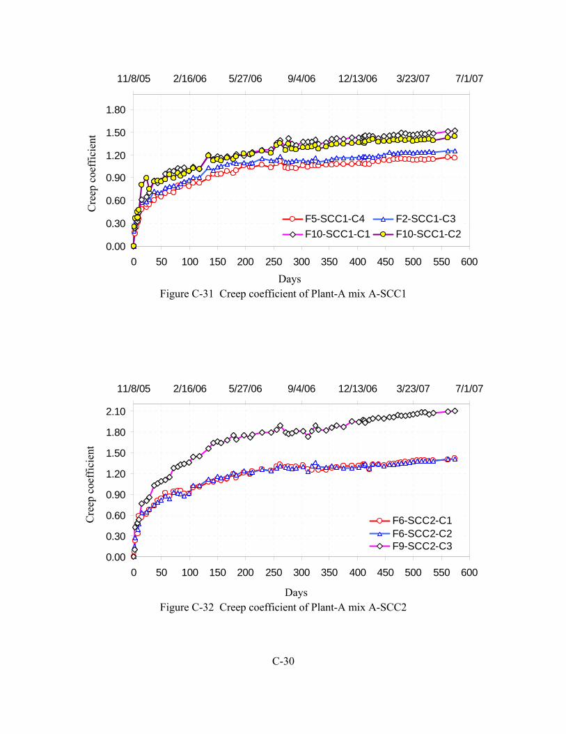
C-30

Figure C-31 Creep coefficient of Plant-A mix A-SCC1

Figure C-32 Creep coefficient of Plant-A mix A-SCC2

0.00

0.30

0.60

0.90

1.20

1.50

1.80

0 50 100 150 200 250 300 350 400 450 500 550 600

11/8/05 2/16/06 5/27/06 9/4/06 12/13/06 3/23/07 7/1/07

F5-SCC1-C4 F2-SCC1-C3F10-SCC1-C1 F10-SCC1-C2

Cre

ep c

oeff

icie

nt

Days

0.00

0.30

0.60

0.90

1.20

1.50

1.80

2.10

0 50 100 150 200 250 300 350 400 450 500 550 600

11/8/05 2/16/06 5/27/06 9/4/06 12/13/06 3/23/07 7/1/07

F6-SCC2-C1F6-SCC2-C2F9-SCC2-C3

Cre

ep c

oeff

icie

nt

Days

C-31

0.00

0.30

0.60

0.90

1.20

1.50

1.80

2.10

0 50 100 150 200 250 300 350 400 450 500 550 600

11/8/05 2/16/06 5/27/06 9/4/06 12/13/06 3/23/07 7/1/07

A-CM A-SCC1A-SCC2 A-SCC2BACI 209 (all mixes)

Ave

rage

cre

ep c

oeff

icie

nt

Days

Figure C-33 Average creep coefficients of Plant-A mixes

Figure C-34 Total strain of creep cylinders of Plant-B mix B-CM

0

500

1000

1500

2000

2500

0 50 100 150 200 250 300 350 400 450 500 550

7/10/06 10/8/06 1/6/07 4/6/07 7/5/07 10/3/07 1/1/08

F3-CM-C1F8-CM-C2

Tota

l stra

in (μ

ε)

Days

C-32

Figure C-35 Creep strain of Plant-B mix B-CM

Figure C-36 Total strain of creep cylinders of Plant-B mix B-SCC1

0

250

500

750

1000

1250

0 50 100 150 200 250 300 350 400 450 500 550

7/10/06 10/8/06 1/6/07 4/6/07 7/5/07 10/3/07 1/1/08

F3-CM-C1F8-CM-C2

Cre

ep st

rain

(με)

Days

0

1000

2000

3000

4000

0 50 100 150 200 250 300 350 400 450 500 550

7/10/06 10/8/06 1/6/07 4/6/07 7/5/07 10/3/07 1/1/08

F3-SCC1-C2F7-SCC1-C1F4-SCC1-C3

Days

Tota

l stra

in (μ

ε)

C-33

Figure C-37 Creep strain of Plant-B mix B-SCC1

Figure C-38 Total strain of creep cylinders of Plant-B mix B-SCC2

0

500

1000

1500

2000

0 50 100 150 200 250 300 350 400 450 500 550

7/10/06 10/8/06 1/6/07 4/6/07 7/5/07 10/3/07 1/1/08

F3-SCC1-C2F7-SCC1-C1F4-SCC1-C3

Cre

ep st

rain

(με)

Days

0

1000

2000

3000

4000

0 50 100 150 200 250 300 350 400 450 500 550

7/10/06 10/8/06 1/6/07 4/6/07 7/5/07 10/3/07 1/1/08

F8-SCC2-C2F4-SCC2-C3F7-SCC2-C1

Days

Tota

l stra

in (μ

ε)

C-34

Figure C-39 Creep strain of Plant-B mix B-SCC2

Figure C-40 Average total strain of Plant-B mixes

0

1000

2000

3000

4000

0 50 100 150 200 250 300 350 400 450 500 550

7/10/06 10/8/06 1/6/07 4/6/07 7/5/07 10/3/07 1/1/08

AVRG-SCC2AVRG-SCC1AVRG-CM

Days

Tota

l stra

in (μ

ε)

0

500

1000

1500

2000

0 50 100 150 200 250 300 350 400 450 500 550

7/10/06 10/8/06 1/6/07 4/6/07 7/5/07 10/3/07 1/1/08

F8-SCC2-C2F4-SCC2-C3F7-SCC2-C1

Days

Cre

ep st

rain

(με)

C-35

Figure C-41 Average creep strain of Plant-B mixes

Figure C-42 Creep coefficient of Plant-B mix B-CM

0.00

0.50

1.00

1.50

2.00

0 50 100 150 200 250 300 350 400 450 500 550

7/10/06 10/8/06 1/6/07 4/6/07 7/5/07 10/3/07 1/1/08

F3-CM-C1F8-CM-C2

Cre

ep c

oeff

icie

nt

Days

0

500

1000

1500

2000

0 50 100 150 200 250 300 350 400 450 500 550

7/10/06 10/8/06 1/6/07 4/6/07 7/5/07 10/3/07 1/1/08

AVRG-SCC2AVRG-SCC1AVRG-CM

Days

Cre

ep st

rain

(με)

C-36

Figure C-43 Creep coefficient of Plant-B mix B-SCC1

Figure C-44 Creep coefficient of Plant-B mix B-SCC2

0.00

0.50

1.00

1.50

2.00

0 50 100 150 200 250 300 350 400 450 500 550

7/10/06 10/8/06 1/6/07 4/6/07 7/5/07 10/3/07 1/1/08

F3-SCC1-C2F7-SCC1-C1F4-SCC1-C3

Cre

ep c

oeff

icie

nt

Days

0.00

0.50

1.00

1.50

2.00

0 50 100 150 200 250 300 350 400 450 500 550

7/10/06 10/8/06 1/6/07 4/6/07 7/5/07 10/3/07 1/1/08

F8-SCC2-C2F4-SCC2-C3F7-SCC2-C1

Cre

ep c

oeff

icie

nt

Days

C-37

0.00

0.50

1.00

1.50

2.00

2.50

0 50 100 150 200 250 300 350 400 450 500 550

7/10/06 10/8/06 1/6/07 4/6/07 7/5/07 10/3/07 1/1/08

B-SCC2 B-SCC1B-CM ACI 209 (CM)ACI 209 (SCC1&2)

Ave

rage

cre

ep c

oeff

icie

nt

Days

Figure C-45 Average creep coefficient of Plant-B mixes

Figure C-46 Average shrinkage strain and least square curves of mix A-CM

0

100

200

300

400

500

0 50 100 150 200 250 300 350 400 450 500 550 600

11/8/05 2/16/06 5/27/06 9/4/06 12/13/06 3/23/07 7/1/07

A-CMLSA-1LSA-2LSA-3

Days

Shrin

kage

stra

in (μ

ε)

C-38

Figure C-47 Average shrinkage strain and least square curves of mix A-SCC1

Figure C-48 Average shrinkage strain and least square curves of mix A-SCC2

0

100

200

300

400

500

600

0 50 100 150 200 250 300 350 400 450 500 550 600

11/8/05 2/16/06 5/27/06 9/4/06 12/13/06 3/23/07 7/1/07

A-SCC2LSA-1LSA-2LSA-3

Shrin

kage

stra

in (μ

ε)

Days

0

100

200

300

400

500

600

0 50 100 150 200 250 300 350 400 450 500 550 600

11/8/05 2/16/06 5/27/06 9/4/06 12/13/06 3/23/07 7/1/07

A-SCC1LSA-1LSA-2LSA-3

Shrin

kage

stra

in (μ

ε)

Days

C-39

Figure C-49 Average shrinkage strain and least square curves of mix A-SCC2B

Figure C-50 Least square shrinkage curves of mix B-CM

0

100

200

300

400

500

0 50 100 150 200 250 300 350 400 450 500 550

7/10/06 10/8/06 1/6/07 4/6/07 7/5/07 10/3/07 1/1/08

B-CMLSA-1LSA-2LSA-3

Days

Shrin

kage

stra

in (μ

ε)

0

100

200

300

400

500

600

0 50 100 150 200 250 300 350 400 450 500 550 600

11/8/05 2/16/06 5/27/06 9/4/06 12/13/06 3/23/07 7/1/07

A-SCC2BLSA-1LSA-2LSA-3

Shrin

kage

stra

in (μ

ε)

Days

C-40

Figure C-51 Least square shrinkage curves of mix B-SCC1

Figure C-52 Least square shrinkage curves of Plant-B mix B-SCC2

0

100

200

300

400

500

0 50 100 150 200 250 300 350 400 450 500 550

7/10/06 10/8/06 1/6/07 4/6/07 7/5/07 10/3/07 1/1/08

B-SCC2LSA-1LSA-2LSA-3

Days

Shrin

kage

stra

in (μ

ε)

0

100

200

300

400

500

0 50 100 150 200 250 300 350 400 450 500 550

7/10/06 10/8/06 1/6/07 4/6/07 7/5/07 10/3/07 1/1/08

B-SCC1LSA-1LSA-2LSA-3

Days

Shrin

kage

stra

in (μ

ε)

C-41

Figure C-53 Average creep coefficient and least square curves of mix A-CM

Figure C-54 Average creep coefficient and least square curves of mix A-SCC1

0.0

0.3

0.6

0.9

1.2

1.5

0 50 100 150 200 250 300 350 400 450 500 550 600

11/8/05 2/16/06 5/27/06 9/4/06 12/13/06 3/23/07 7/1/07

A-SCC1LSA-1LSA-2LSA-3

Days

Cre

ep c

oeff

icie

nt

0.0

0.3

0.6

0.9

1.2

0 50 100 150 200 250 300 350 400 450 500 550 600

11/8/05 2/16/06 5/27/06 9/4/06 12/13/06 3/23/07 7/1/07

A-CMLSA-1LSA-2LSA-3

Cre

ep c

oeff

icie

nt

Days

C-42

Figure C-55 Average creep coefficient and least square curves of mix A-SCC2

Figure C-56 Average creep coefficient and least square curves of mix A-SCC2B

0.0

0.3

0.6

0.9

1.2

1.5

1.8

0 50 100 150 200 250 300 350 400 450 500 550 600

11/8/05 2/16/06 5/27/06 9/4/06 12/13/06 3/23/07 7/1/07

A-SCC2BLSA-1LSA-2LSA-3

Cre

ep c

oeff

icie

nt

Days

0.0

0.3

0.6

0.9

1.2

1.5

1.8

0 50 100 150 200 250 300 350 400 450 500 550 600

A-SCC2LSA-1LSA-2LSA-3

Cre

ep c

oeff

icie

nt

Days

C-43

Figure C-57 Average creep coefficient and least square curves of mix B-CM

Figure C-58 Average creep coefficient and least square curves of mix B-SCC1

Days

0.0

0.3

0.6

0.9

1.2

1.5

1.8

0 50 100 150 200 250 300 350 400 450 500 550

7/10/06 10/8/06 1/6/07 4/6/07 7/5/07 10/3/07 1/1/08

B-SCC1LSA-1LSA-2LSA-3

Cre

ep c

oeff

icie

nt

0.0

0.3

0.6

0.9

1.2

1.5

0 50 100 150 200 250 300 350 400 450 500 550

7/10/06 10/8/06 1/6/07 4/6/07 7/5/07 10/3/07 1/1/08

B-CMLSA-1LSA-2LSA-3

Cre

ep c

oeff

icie

nt

Days

C-44

Figure C-59 Average creep coefficient and least square curves of mix B-SCC2

0.0

0.3

0.6

0.9

1.2

1.5

1.8

0 50 100 150 200 250 300 350 400 450 500 550

7/10/06 10/8/06 1/6/07 4/6/07 7/5/07 10/3/07 1/1/08

B-SCC2LSA-1LSA-2LSA-3

Cre

ep c

oeff

icie

nt

Days

APPENDIX D

HARDENED CONCRETE PROPERTIES

D-1

D.1 Introduction

This appendix contains a description of the procedures used to determine the material properties of the hardened concrete used in the prestressed girders studied and summarizes the associated data including concrete compressive strength, modulus of elasticity, modulus of rupture, and split cylinder tensile strength. The companion cylinders and beams used to determine the material properties were fabricated and cured with the associated girders. After strand release, the companion cylinders and beams were transported to University of Minnesota Structures Laboratory, where they were stored in the creep room with the creep and shrinkage companion cylinders.

The conventional concrete cylinders were prepared according to ASTM C 192C/192M (2000) Standard Practice for Making and Curing Concrete Test Specimens in the Laboratory, and the beams were fabricated according to ASTM C78-08 (2002) Standard Test Method for Flexural Strength of Concrete Using Simple Beam with Third-Point Loading. Figure D-1 shows the commercially available single-use cylinder molds and the reusable steel beam molds just before casting the girders. There is no ASTM standard for making SCC cylinders and beams, but the associated conventional concrete ASTM standards were employed for the SCC specimens with the exception of rodding. The rodding was replaced by tapping the outside of the molds lightly three to four times with a mallet after each of the two concrete layers was placed to release any entrapped air. Moreover, the SCC molds were filled by discharging the concrete gently from a five-gallon plastic bucket.

The concrete material properties were monitored using the companion cylinders until the girders were tested. The material properties were also measured using concrete cores taken from each girder just after flexural testing. The measured material properties from the cores and companion cylinders were compared to determine whether the companion cylinders represented the girders in terms of measured material properties.

D.2 Concrete Compressive Strength

The concrete compressive strength was measured as per ASTM C 39C/30M (2001). The 4 by 8 in. cylinders were loaded at a rate of 450 lb/s in a Forney test machine as shown in Figure D-2. Because the Forney test machine was governed by displacement rate, the rate was manually adjusted during the test to maintain the required load rate. At least three cylinders were tested to find the compressive strength. When only three cylinders were used, the average of two cylinders that had similar results were computed and reported as the compressive strength. However, when more than three cylinders were used, then the cylinders with the smallest and largest compressive strength were not included in the calculations. The compressive strength data of the mixes is given in Table D-1. For Plant-B, the measured compressive strength at 280 days after girder casting was approximately 10% smaller than that measured at 141 days after girder casting. This was unexpected, and was likely to be due to a problem with the capping compound used. A new shipment of capping compound material was used for these cylinders,

D-2

and similar results were experienced by other researchers in the laboratory with that batch of capping compound material.

D.3 Modulus of Rupture

Flexural strength of concrete was measured as per ASTM C78 (2002) in the Forney testing machine using simple beams (6 x 6x 24 in.) as shown in Figure D-3 with third-point loading. In total, three beams were fabricated and tested per girder. The beams were tested continuously without pause. The load was applied at a constant rate that increased the extreme fiber stress at a rate of 150 psi/min. The modulus of rupture data of the beams is given in Table D-2.

D.4 Static Modulus of Elasticity

Young’s modulus of elasticity of the concrete cylinders was measured as per ASTM C469 (1994). The 4 by 8 in. cylinders were loaded at a rate of 450 lb/s in the Forney test machine. The load rate was manually adjusted. First the specimens were loaded to approximately 5 % of the compressive strength, and then unloaded to zero load. This was repeated several times to verify the consistency of the response and to ensure that the compressometer was properly seated. Finally, the specimens were loaded to 40% of the compressive strength and the corresponding load and compresometer longitudinal displacement were recorded. The compressometer displacement was measured by an LVDT as shown in Figure D-4. The modulus of elasticity was calculated as the slope of the line connecting the two data points (i.e., 5 and 40%).

At least three 4 in. by 8 in. cylinders were loaded, and the corresponding modulus of elasticity were calculated. The measured modulus of elasticity data of the girder mixes is given in Table D-3. The given results represent the average of two cylinders, which had similar data. In other words, the cylinder with very large or very small modulus of elasticity (relative to the average) was eliminated, and the average was recalculated. It should be noted that some of the data may be in error due to malfunctioning of the compressometer. It was found that the top yoke hinge of the compressometer had some resistance to rotation. Unfortunately, there was not enough information to determine when the problem initially developed (i.e., it is not known which readings prior to the date at which the problem was discovered were in error) and there was not enough information to determine the magnitude of the resistance and its impact on the result to adjust the data. However, it is believed that the magnitude of the error should be the same or comparable for the cylinders with similar compressive strengths. In other words, this error should not affect the comparison of the cores and companion cylinder data compared at the same age, with the same apparatus.

D.5 Splitting Tensile Strength

The splitting tensile strength of the girder companion cylinders was measured as per ASTM C496-96. The cylinders were loaded continuously at a loading rate of 150 psi/min using the Forney test machine as shown in Figure D-5. At least three cylinders were tested, and the

D-3

average of two cylinders which had similar splitting tensile strengths were calculated and reported. Table D-4 includes the splitting tensile strength data of the girder mixes. The splitting tensile strength was measured at 28 days, at 262 and 280 days after girder casting for Plant-A and Plant-B, respectively, and after girder testing (at 643 days for Plant-A and 450 days for Plant-B girders mixes).

D.6 Girder Concrete Cores

Upon completion of the flexural loading tests, cores were taken from both ends and from the middle section of the girders to investigate the consistency of the measured concrete properties. The cores were taken approximately 4 ft. from the ends (beyond the measured transfer lengths) and in the midspan vicinity. Because the girders were tested only at 2L/5 (also at 3L/5 for A-SCC1 and A-CM girders), the cores could be taken from the uncracked regions of the girders. As shown in Figure D-6 a concrete core drill was anchored to the girders and leveled perpendicular to the longitudinal axis of the girders. Figure D-7 shows the locations and core labels used for the cores. The cores that were taken from the flange had an approximate 3.8 in. diameter and 7.2 in. height. However, those taken from the web were only 6 in. in height (6 in. web thickness). The cores taken from the web had leveled surfaces, but the cores taken from the flanges had an angled end surface at the bottom end. The ends of these cores were adjusted by cutting the end off the cylinder.

The cores taken from the top flange along the girders (e.g., DE1, MF1, and LE1) were used to determine the variation in concrete compressive strength along the girder top flange. The cores that were taken at midspan were used to determine the concrete split tensile strength, and to investigate the potential variation in the concrete compressive strength and modulus of elasticity with the vertical location from which the core was taken (i.e., the consolidation was anticipated to be potentially different with depth).

Table D-5 identifies the cores and the material properties measured with each core.

A summary of the measured properties using the cores (i.e., concrete compressive strength, modulus of elasticity, and splitting tensile strength, which is denoted by “T”) is given in Table D-6 for all girders. The corresponding concrete properties measured using the companion cylinders at the same age are also included. Because the companion cylinders and the cores had different conditions in terms of concrete consolidation and environmental conditions to which they were exposed, they were likely to have different material properties. For example, the girders were exposed to seasonal wetting and drying cycles, and the cores taken from the bottom web (e.g., MWB1, MWB2, and MWB3) had higher pressure heads during fabrication than the cores taken from flange (e.g., MF1, MF2, and MF3). It was expected that the cores with higher pressure head could have better consolidation and durability (higher compressive strength, modulus of elasticity, and splitting tensile strength). Although there was some fluctuation of the measured concrete properties using the cores, no obvious trend was found.

D-4

In addition, the companion cylinders, cores, and modulus of rupture beams were cut along their vertical axes to investigate potential signs of mix segregation. Figure D-8 through D-10 show the aggregate distribution observed for the Plant-B samples. There was no obvious sign of segregation based on the distribution of the coarse aggregate. Similar results were found for Plant-A samples.

D-5

TABLES

Table D-1 Girder average compressive strength measured with companion cylinders A-SCC1 A-SCC2 A-SCC2B A-CM B-SCC1 B-SCC2 B-CM Days*

(A/B) fc'

(ksi) fc

'

(ksi) fc

'

(ksi) fc

'

(ksi) fc

'

(ksi) fc

'

(ksi) fc

'

(ksi) 1/1 6.77 4.65 8.25 6.13 7.18 7.77 2/2† 7.08 5.98 9.99 7.80 7.74 9.35

3 7.61 6.31 9.94 4 7.68 6.78 8.00 10.60 5‡ 8.20 7.01 8.32 11.08 9.85 9.42 10.97 6 8.38 7.39 8.49 11.31

11/10 8.51 7.60 8.93 11.93 10.57 10.78 12.28 18 11.19 11.28 13.18

29/28 8.74 8.18 9.37 11.60 10.94 11.03 13.65 32 9.57 8.80 10.01 11.79 56 11.70 11.16 13.09

113/141 9.64 8.88 12.46 12.44 11.80 13.22 184/280§ 9.70 8.49 13.07 10.42 10.97 12.17 262/290 9.98 8.40 11.89 12.82 11.93 13.42 300/360 8.99 7.98 12.26 12.96 12.40 13.69 385/450 9.92 8.75 11.90 13.11 12.07 13.50

524 10.38 9.63 13.45 569 10.35 9.40 13.26 643 9.11 8.38 10.89 12.31

* Days after casting † Plant-B release

‡ Plant-A release

§ A different capping compound was used, it is likely the reason for decreased strength measured

Table D-2 Girder modulus of rupture measured with companion beams A-SCC1 A-SCC2 A-CM B-SCC1 B-SCC2 B-CM Days*

(A/B) R

(ksi) R

(ksi) R

(psi) R

(psi) R

(psi) R

(psi) 28/28 717 674 984 1229 1117 1416

262/280 1380 1290 1472 1713 1674 1496 643/450 1550 1629 1672 1309 1101 1956

Each data point was obtained from testing a single beam

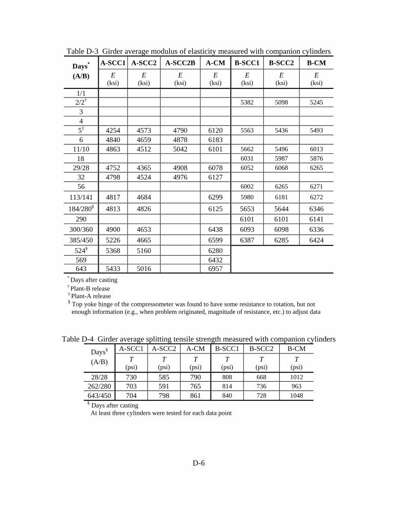
D-6

Table D-3 Girder average modulus of elasticity measured with companion cylinders A-SCC1 A-SCC2 A-SCC2B A-CM B-SCC1 B-SCC2 B-CM Days*

(A/B) E

(ksi) E

(ksi) E

(ksi) E

(ksi) E

(ksi) E

(ksi) E

(ksi) 1/1 2/2† 5382 5098 5245

3 4 5‡ 4254 4573 4790 6120 5563 5436 5493 6 4840 4659 4878 6183

11/10 4863 4512 5042 6101 5662 5496 6013 18 6031 5987 5876

29/28 4752 4365 4908 6078 6052 6068 6265 32 4798 4524 4976 6127 56 6002 6265 6271

113/141 4817 4684 6299 5980 6181 6272

184/280§ 4813 4826 6125 5653 5644 6346 290 6101 6101 6141

300/360 4900 4653 6438 6093 6098 6336 385/450 5226 4665 6599 6387 6285 6424

524§ 5368 5160 6280 569 6432 643 5433 5016 6957

* Days after casting † Plant-B release

‡ Plant-A release

§ Top yoke hinge of the compressometer was found to have some resistance to rotation, but not enough information (e.g., when problem originated, magnitude of resistance, etc.) to adjust data

Table D-4 Girder average splitting tensile strength measured with companion cylinders A-SCC1 A-SCC2 A-CM B-SCC1 B-SCC2 B-CM Days§

(A/B) T

(psi) T

(psi) T

(psi) T

(psi) T

(psi) T

(psi) 28/28 730 585 790 808 668 1012

262/280 703 591 765 814 736 963 643/450 704 798 861 840 728 1048 § Days after casting At least three cylinders were tested for each data point

D-7

Table D-5 Girder concrete core dimensions and locations

Core Approximate Location

Dimensions(in.)

Measured Concrete Property

DE1 DE2

4 ft from dead end top flange 4 x 8 fc'

MBW1 MBW2 MBW3

at L/2 and from bottom web 4 x 6 fc'& E

MTW1 MTW2 MTW3

at L/2 and from top web 4 x 6 T

MF1 MF2 MF3 MF4

at L/2 and from top flange 4 x 8 fc' & E

LE1 LE2

4 ft from live end top flange 4 x 8 fc'

fc = compressive strength, E = modulus of elasticity, and T = splitting tensile strength

D-8

Table D-6 Girder concrete core and cylinder data A-SCC1 A-SCC2† A-SCC2B† A-CM B-SCC1 B-SCC2 B-CM Core ID

fc' §

(ksi) E

(ksi) T

(psi) fc

' §

(ksi) E

(ksi)T

(psi)fc

' §

(ksi)E

(ksi)T

(psi)fc

' §

(ksi)E

(ksi)T

(psi) fc

' §

(ksi) E

(ksi)T

(psi)fc

' §

(ksi)E

(ksi)T

(psi)fc

' §

(ksi)E

(ksi)T

(psi)DE1 10.88 11.37 13.66 12.21 12.56 13.42DE2 9.18 9.20 14.56 11.98 13.10 12.98AVRG 10.03

10.29

14.11

12.10

12.83

13.20

LE1 10.82 10.40 15.05 12.60 12.68 13.56LE2 10.03 8.98 13.14 12.10 12.19 13.74AVRG 10.43

9.69

14.10

12.35

12.44

13.65

MTW1 841 882 1065 860 763 986 MTW2 781 873 1099 869 739 1098MTW3 854 926 1036 806 805 1123AVRG

848

878

1051

865

751

1111MBW1 10.32 4787 8.62 4350 12.23 6402 13.40 6178 11.86 6147 13.42 6160

MBW2 9.59 5462 8.70 4189 12.54 6212 13.15 6301 13.75 6347

MBW3 9.22 5360 9.68 4467 11.83 6054 12.20 6268 12.69 6266AVRG 9.41 5411

8.66 4409

12.23 6402

12.19 6195

12.03 6285

13.59 6307

MF1 10.29 5320 10.24 6613 12.11 6386 11.73 6250 11.86 6186 13.06 6812

MF2 11.84 5210 8.75 6737 13.75 6412 12.98 6320 12.49 6495 13.69 6649

MF3 10.72 5501 9.13 6690 13.08 6422 12.10 6198 12.10 6176 13.28 6327AVRG 10.51 5265

8.94 6714

13.42 6417

11.92 6224

11.98 6181

13.17 6731

Cores ‡ 10.10 5338 848 9.55 4409 8.94 6714 878 13.47 6410 1051 12.14 6210 865 12.32 6233 751 13.4 6519 1111Cylinders 9.11 5433 704 8.38 5016 798 10.89 12.31 6957 861 13.11 6387 840 12.07 6285 728 13.50 6424 1048 fc = compressive strength, E = modulus of elasticity, and T = splitting tensile strength shaded cells (with largest deviation from the average) not included in computation of average § corrected for specimen length to diameter ratio less than 1.8 in (ASTM C 39/C 39M, correction factor between 0.94 and 0.99) † this is the segregated girder which had two mixes, A-SCC2 up to approximately h/2, and the top half A-SCCB ‡ average of all cores (shaded cells not included)

D-9

FIGURES

Figure D-1 Companion concrete cylinder and modulus of rupture beam forms in the field

Figure D-2 Concrete compressive strength test

D-10

Figure D-3 Flexural strength of concrete beam test setup

Figure D-4 Modulus of elasticity test setup

Top yoke hinge

LVDT

D-11

Figure D-5 Split tensile strength of concrete test setup

Figure D-6 Setup for taking concrete cores

concrete core drill

D-12

Figure D-7 Concert core location and core naming convention

DE2

MTW1

MF1DE1

MF2MF3

MTW3

MBW1MBW3

MTW2

MBW2

LE1 LE2

D-13

Figure D-8 Aggregate distribution in the cylinders and girder cores of B-SCC1

Figure D-9 Aggregate distribution in the cylinders and girder cores of B-SCC2

companion cylinders

beam

cores

companion cylinders

beam

cores

D-14

Figure D-10 Aggregate distribution in the cylinders and girder cores of B-CM

companion cylinders

beam

cores

APPENDIX E

PRESTRESS LOSSES DUE TO THERMAL EFFECTS

E-1

E.1 Introduction

During fabrication of prestressed concrete members, usually the concrete is steam or heat cured to minimize the time needed to achieve the specified concrete release strength. Especially for precast concrete plants with a limited number of prestressing beds, it is important to minimize the fabrication time so that the prestressing beds can be quickly turned around to maximize production. However, the increased concrete and prestressing strand temperature during curing can lead to significant prestress losses because the strand length is fixed during the heating and the coefficient of thermal expansion of steel and concrete differ. In other words, the strands are stressed at ambient temperature, but when they are heated they cannot expand (their length is fixed by the prestressing bed abutments), so the strand stress reduces causing prestress losses. Designers rarely account for thermal effects during curing, and the associated prestress losses are partly irrecoverable once the strands bond to the concrete.

It is common to determine experimentally the remaining prestressing force (i.e., long-term prestress losses) by exposing, instrumenting, and cutting a number of strands. This semi-destructive testing method was also used in this study to verify the vibrating wire strain gage readings (i.e., prestress losses). However, if the strands were prestressed and cut at different temperatures then the data (i.e., strains associated with strand cutting and initial tensioning) needs to be corrected for temperature effects.

To estimate the magnitude of prestress losses due to thermal effects during prestressing, curing, release, and strand cutting, a five-step solution described in Section E.2 was derived based on the following assumptions: (1) bending stresses assumed to be negligible during curing, and (2) a uniform and constant temperature profile, taken as the average of the VWSG temperature readings, assumed through girder depth and along the girder length at any given time.

E.2 Derivation of Thermal Prestress Losses

In the following section, a five-step derivation of prestress losses due to thermal effects is presented. The derivation is base on following assumptions:

1. There is no thermal gradient along the girders, and temperature is constant through the girder depth.

2. Bending stresses/strains due to thermal effects are neglected. 3. Concrete modulus of elasticity is constant from bond development between concrete and

strands to strand release. 4. There is no temperature gradient along the free strands. 5. Concrete coefficient of thermal expansion is constant.

E-2

NOTATION

CC Coefficient of thermal expansion for concrete

SC Coefficient of thermal expansion for strands

GSiT Average temperature of strands in the girders at step i

GCiT Average temperature of concrete at step i

siT Temperature of free strands in the bed at step i

GSiε Total strand strain in the girder at step i

GCiε Total concrete strain at step i at the center of strands

Siε Total free strand strain at step i

GSiσ Total strand stress in the girder at step i

GCiσ Total concrete stress at step i

Siσ Total free strand stress at step i

GSLΔ Change in length for strands in the girders

GCLΔ Change in length for the girders

SLΔ Change in length for free strands

0L Total length of prestressing bed

SiL Length of free strands at step i

SA Total area of prestressing strands

SE Modulus of elasticity of prestressing strands

CA Cross-sectional area of girder section (concrete area only)

CE Modulus of elasticity of concrete

iP Total prestressing force at step i

GL Total length of girders

E-3

SUMMARY OF SOLUTION STEPS:

Step: 0 Strand tensioning

Prestressed strands

Strand

TGS0= TS0 = T0 P = P0

L0 LS0

Step: 1 Concrete and steel bonds

LS1L0-LS1

L0

strand free strand concrete

LG= L0-LS1

Step: 2 Just before release

LS2 L0-LS2

L0

Free strand TS = T0 P = P2

Step: 3 Just after release

LS3

Step: 4 Strand cutting

Free strand

TS = T4 P = P4

LS5

Girder

TGS = T1 TGC = T1 P = P1

Free strand

TS = T0 P = P1

Girder

TGS = T2 TGC = T2 P = P2

Girder

TGS = T3 TGC = T3 P = P3

Girder

TGS = T4 TGC = T4 P = P4

E-4

Step: 0 – Strand Tensioning Note: Reference for strains and stresses is just before strand tensioning (P=0 and T=T0)

Step: 1 – Concrete and Steel bonds

• For strands in the concrete:

( ) ( ) ( )000101

0010 )( SSSS

SS LLTTCAEPPLLLLL −⎥

⎦

⎤⎢⎣

⎡−+

−=−−−=Δ

( ) ( )000101

01 )( SSSS

SS LLTTCAEPPLLL −⎥

⎦

⎤⎢⎣

⎡−+

−=+−=Δ (1)

• For free strands

( ) ( )001

01 SSS

SS LAEPP

LL ⎥⎦

⎤⎢⎣

⎡ −=− (2)

Note: L0 is known as it is the total length of the bed, and LS1 is known as L0- LS1= total length of

the girders. There are two equations and two unknowns (P1 and LS0)

LS0 L0-LS0

L0

SGS

SSGS

GS

GS

AP

AEP

PPTT

00

00

00

00

=

=

==

σ

ε

SS

SSS

S

S

AP

AEP

PPTT

00

00

00

00

=

=

==

σ

ε

strand free strand

LS1 L0-LS1

L0

concrete

11

11

PPTT

GS

GS

==

11

01

PPTT

S

S

==

E-5

• Stresses and strains for strands and concrete (girder)

0 0:

)(

)(

)(

11

1101

11

01010

1

011

0101

1

==

=−+=

−+−

+=

−=Δ

−+−

=Δ

GCGC

SGSS

SSGS

SSSSS

GS

GSGSGS

SSS

GS

andconcreteFor

APandTTC

AEP

TTCAEPP

AEP

TTCAEPPconcreteinstrandFor

σε

σε

ε

εεε

ε

SSSS

SS

SSS

SSS

SSSSS

S

SSS

S

AP

APP

AP

APP

AEPTTC

AEP

TTCAEPP

AEP

TTCAEPP

strandfreeFor

10101

011

100

11

00010

1

0001

1

)(

)(

)(

=−

+=

−=Δ

=−+=

−+−

+=

−+−

=Δ

σ

σ

ε

ε

ε

E-6

Step: 2 – Just before release • For strands in the concrete (from step 1 to step 2)

( ) ( ) ( ) ( ) ( ) ( )

( ) ( ) ( ) ( ) ( )1012

2012

101212

1012

2012

10121020

)(

)(

SSS

SSS

TSSSS

SSS

SSS

TSSSSGS

LLEA

PPLLEA

PLLCTTLL

LLEA

PPLLEA

PLLCTTLLLLL

−−

+−−−−=+−

−−

+−−−−=−−−=Δ

( ) ( ) ( ) ( ) ( )1012

2012

101212 )( SSS

SSS

TSSSS LL

EAPPLL

EAPLLCTTLL −

−+−−−−=+− (3)

• For concrete (from step 1 to step 2)

( ) ( ) ( ) ( )

( ) ( ) ( )2012

101212

2012

10121020

)(

)(

SCC

TSCSS

SCC

TSCSSGC

LLEA

PLLCTTLL

LLEA

PLLCTTLLLLL

−+−−=+−

−+−−=−−−=Δ

( ) ( ) ( )2012

101212 )( SCC

TSCSS LL

EAPLLCTTLL −+−−=+− (4)

FB Diagram-1

L0-LS2

concrete

strand

2P2P

L0-LS2

2P2P

12TP12TP

concrete

LS2

L0

strand free strand

L0-LS2

2

22

2

22

GCGC

GC

GSGS

GS

PPTT

PPTT

====

22

02

PPTT

S

S

==

222 PPP GCGS =+Forces in the concrete and strand

are function of x

E-7

• Free strands (from step 1 to step 2)

( ) ( ) ( )

( ) ( )112

12

112

10012

)(

)()(

SSS

SS

SSS

SSSSS

LEA

PPLL

LEA

PPLCTTLLL

−=−

−+−=−=Δ

( ) ( )112

12)(

SSS

SS LEA

PPLL −=− (5)

There are three equations (Eqn. 1, 2, 3) and there are three unknowns LS2, PT12, P2 Therefore all unknowns can be solved. • Stresses and strains for strands and concrete (girder)

)(

)(

1222

1202

22

S

T

SGS

SS

TS

SSGS

AP

APx

AEPTTC

AEP

concreteinstrandfor

−=

−−+=

σ

ε

)(

)()(

122

12122

C

TGC

CC

TCGC

APx

EAPTTCx

concretefor

=

+−=

σ

εS

S

SSSSSSS

SSS

SSS

SSS

AP

AEP

AEPP

AEP

AEPPTTC

AEPP

ffor

22

21212

1200

122

122

)(

strandree

=

=−

+=

−=−+

−=Δ

−=Δ

σ

ε

ε

εεε

E-8

Step: 3 – Just after release

• Stresses and strains for strand and concrete (girder)

3

22

3

22

GCGC

GC

GSGS

GS

PPTT

PPTT

====

LS3

333 PPP GCGS =+

FB Diagram-2

Neglect transfer length for now

LS3

3P3P

12TP12TP

3P3P

( )

)(

)(

)(

)(

1233

1202

33

1202

2233

1202

22

233

S

T

SGS

SS

TS

SSGS

SS

TS

SSGS

SS

TS

SSGS

GSGSGS

AP

APx

AEPTTC

AEP

AEPTTC

AEPPP

AEPTTC

AEP

concreteinstrandfor

−=

−−+=

−−++−

=

−−+=

+Δ=

σ

ε

ε

ε

εεε

)(

)(

3122

323

312123

12122

233

CC

TGC

GCGCGC

CCCC

TCGC

CC

TCGC

GCGCGC

AP

AP

EAP

EAPTTC

EAPTTC

concretefor

−=

Δ+=

−+−=

+−=

+Δ=

σ

σσσ

ε

ε

εεε

E-9

• Relationships Note: There are two equations (Eqn. 6 and Eqn. 7) and two unknowns (P3 found LS3)

( )

( )(6) 0)(

)(

23

20

203

233

20

20333

33

233

233

=−

−−

−−

−==Δ

−−−

==Δ=Δ

=Δ=Δ−==Δ−==Δ

SSS

SS

SSESGS

S

SSESGCGS

ESGCGS

GGCESGC

GSGSESGS

EAPP

LLLLL

EAPP

LLLLL

itycompatibilfrom

εε

εεε

εεεεεεεεεεε

(7) 0)(

)(

323

33

233

=+−

−==Δ

−==Δ

CCSS

CCESGC

SSESGS

EAP

EAPP

EAPEAPP

εε

εε

E-10

( )

( )( ) (9) 134

334

SHCRSS

SSHCRSS

LL

LLL

εε

εε

++=

+=−

Step: 4 – Just before strand cutting Sub-Step: 4A – Just before strand cutting If no temperature change occurs but just creep and shrinkage, then due to creep and shrinkage P3 will change to P4

Note: There are two equations and two unknowns (LS4 and P4) • Stresses and strains for strand in the girder

)(

)(

)(

1244

1202

44

344

1202

33

344

S

T

SAGS

SS

TS

SSAGS

SSAGS

SS

TS

SSGS

GSAGSAGS

AP

APx

AEPTTC

AEP

AEPP

AEPTTC

AEP

concreteinstrandfor

−=

−−+=

−=Δ

−−+=

+Δ=

σ

ε

ε

ε

εεε

LS4

strand

4P4P

12TP12TP

4P4Pconcrete

4

34

34

PPP

TTTT

GCGS

AGC

AGS

==

==

LS4

Sub-Step:4A (8) 34

SHCRss EAPP

εε +=−

If creep and shrinkage losses are known so P4

E-11

• Stresses and strains for concrete (girders)

( )

( )

CC

TAGC

CCC

TGC

CC

TGC

CAGC

AGCGCAGC

SHCRCCCC

TCAGC

SHCRAGC

CCCC

TCGC

GCAGCAGC

AP

AP

APP

AP

AP

AP

AP

APP

EAP

EAPTTC

EAP

EAPTTC

concretefor

4124

343123

3123

344

434

312124

4

312123

344

)(

)(

−=

−−+−=

−=

−−=Δ

Δ+=

++−+−=

+=Δ

−+−=

+Δ=

σ

σ

σ

σ

σσσ

εεε

εεε

ε

εεε

Sub-Step: 4B – Just before strand cutting The temperature T3 changes to T4. The force P4 will not change, but the total force will change as friction due to temperature will change (i.e., superposition of forces).

Reference step is: Sub-step 4A

strand

LS5 concrete

4TABP 4TABP

Where PTAB4 is the force developed due to temperature difference (T4-T3)

Sub-Step:4B

44

44

TTTT

BGC

BGS

==

LS5

4P 4P

4P4P

412 TABT PP +412 TABT PP +

Sub-Step:4B

Total loads

E-12

• For Concrete:

54

43445 )( SCC

TABSCSSGC L

EAPLCTTLLL +−=−=Δ (10)

• For strand:

54

43445 )( SSS

TABSSSSGS L

EAPLCTTLLL −−=−=Δ (11)

Note: There are two equations (Eqn. 10 and Eqn. 11) and two unknowns (LS5 and 4TABP ), so

unknowns can be solved. After solving for the unknowns:

( )( )( )( ) ( )( )11 3434

344 +−++−

−−=

CCCSSS

CSCCSSTAB CTTEACTTEA

CCTTEAEAP

( )( ) ( )( )CCSS

CCCSSSSS EAEA

CTTEACTTEALL

++−++−

=11 3434

45

E-13

• Stresses and strains for strands in the girder

SS

TAB

S

T

SBGS

SSS

TAB

SS

T

SSBGS

SS

TABS

SS

TS

SSBGS

SS

TABSBGS

SS

TS

SSAGS

AGSBGSBGS

EAP

AP

AP

TTCEA

PAE

PAE

PTT

EAPTTC

AEPTTC

AEP

EAPTTC

AEPTTC

AEP

41244

044124

4

23

434

1202

44

4344

1202

44

444

)(

)()(

)(

)(

−−=

−+−−=

=

−−+−−+=

−−=Δ

−−+=

+Δ=

σ

ε

ε

ε

ε

εεε

• Stresses and strains for concrete (girder)

CC

TABSHCR

CCCC

TCBGC

CC

TABCSHCR

CCCC

TCBGC

CC

TABCBGC

SHCRCCCC

TCAGC

AGCBGCBGC

EAP

EAP

EAPTTTTC

EAPTTC

EAP

EAPTTC

EAPTTC

EAP

EAPTTC

431213424

434

312124

4344

312124

444

)(

)()(

)(

)(

+++−+−−+=

+−+++−+−=

+−=Δ

++−+−=

+Δ=

εεε

εεε

ε

εεε

εεε

E-14

CC

TAB

CC

TBGC

CC

TABBGC

CC

TAGC

BGCAGCBGC

SHCRCCCC

TABTCBGC

EAP

AP

AP

EAP

AP

AP

EAP

EAPPTTC

44124

44

4124

444

3412144 )(

+−=

=Δ

−=

Δ+=

++−+

+−=

σ

σ

σ

σσσ

εεε

E-15

Question – what will be strain/stress if a strand is exposed and cut at girder midspan?

This is an important question to answer because it is very common to determine remaining prestressing force by exposing and cutting strands. This semi-destructive method was also used in this study to verify field measurements.

• Stresses and strains for the strand that is exposed and cut

SS

TAB

SS

T

SSGS

SSS

TAB

SS

T

SSSGS

SSS

TAB

SS

T

SSBGS

BGSGSGS

SSS

GS

EAP

AEP

AEPε

TTCEA

PAE

PAE

PTTCε

TTCEA

PAE

PAE

Pεεε

TTCEA

ε

41245

044124

045

044124

4

455

045

)()(

)(

)(0

++−=Δ

−−++−−=Δ

−+−−=

−=Δ

−+=

ε

Exposed strand

4

44

44

PPP

TTTT

GCGS

BGC

BGS

==

==

LS5

4P 4P

4P4P

412 TABT PP +412 TABT PP +

Step: 5- After strand cutting

0

4

=

=

GSP

TT

Step: 4- just before strand cutting

E-16

Summary – Solution for the unknowns

( )( )( )( ) ( )( )11120112

011212

SSCCCSSSS

CSSCCSST LLCTTEALLCTTEA

LCLCTTEAEAP+−++−

−−=

( )( )

( )( ) ( )( )11 3434

344 +−++−

−−=

CCCSSS

CSCCSSTAB CTTEACTTEA

CCTTEAEAP

( )

SSS

SS AEL

LLPP0

0101

−+=

( ) ( )( ) ( )

10

1201

10

1012

SCCSS

CCCSSSSSS

SCCSS

CCSSS

LEALEAEACEACEATTLL

LEALEAEALEALPP

++−−

+++

=

23 PEAP SSES += ε

( )

( ) ( )ESSHCRSSSHCRSSSSES

SSES

SHCRSS

AEPAEPEAP

PEAP

AEPP

εεεεεε

ε

εε

+++=+++=

+=

++=

224

23

34

SS

TAB

SS

T

SSGS EA

PAE

PAE

Pε 41245 ++−=Δ

( )

( )ESSHCRSS

TAB

SS

T

SSGS

SS

TAB

SS

T

SS

ESSHCRSSGS

EAP

AEP

AEPε

EAP

AEP

AEAEPε

εεε

εεε

++−++−=Δ

+++++

−=Δ

41225

41225

E.3 Sensitivity Analysis

A sensitivity analysis of the prestress losses due to thermal effects was performed using the five-step solution described in Section E.2 to investigate the effect and the magnitude of free strand length, total strand area, and magnitude of temperatures at strand tensioning and release.

E-17

The results and discussions presented below are based on the following assumptions unless otherwise stated:

• Strands are pulled to 207 ksi (i.e., 0.77 fpu) • A single girder is 38 ft long • Average concrete modulus of elasticity from bond development to strand release (Ec) is

equal 5495 ksi • Prestressing bed total length is 368 ft, and 95% of the bed is occupied with girders (i.e.,

5% of the bed is free strands) • Temperature at pull 41 °F (5 ºC) • Temperature at bond 149 °F (65 ºC) for the girders, and 41 °F for free strands • Temperature at release 97 °F (36 ºC) for the girders, and 41 °F for free strands • Cross section of Mn/DOT 36M I-girder (As =40x0.1532 in.2, Ag=570 in.2) • Coefficients of thermal expansion, CC and SC , of 5.8 με/ºF and 6.8με/ºF (10.4 and 12.2

με/ºC), respectively for the concrete and steel. • Two temperature related losses are considered:

i. From pull to bond TL1= ( ) SAPP 01 − ii. From bond to release TL2= ( )( ) ST APPP 1122 −−

Where TL1 represents thermal losses from strand pull to development of bond between concrete and strands (partially recoverable), TL2 represent thermal losses from bond to strand release (partially recoverable), P0, P1, and P2 are total prestressing force at strand tensioning, bond development, and just before release, respectively as described in Section E.2.

E.3.1 Effect of Free Strand Length

Two cases were investigated. The first case was when only 10% of the total prestressing bed was used to fabricate the girders. In the second case, it was assumed that 95% of the total prestressing bed was used. In both cases, it was assumed that the prestressing bed was heated during curing to fabricate the girders. In others words, temperatures given in Section E.3 were assumed for strand pull, bond development, and strand release.

CASE 1- Assumed only one girder (38 ft) was cast on the bed, with approximately 10% of the bed occupied (90% free strand).

TL1= -2.16 ksi, and TL2=1.47 ksi (Total Prestressing Losses = -0.7 ksi) The prestressing force will decrease by 0.7 ksi just before release (0.3% of initial prestressing).

CASE 2- Assumed 9 girders were cast on the bed, with approximately 95% of the bed occupied

(5 % free strand). TL1= -19.91 ksi, and TL2=5.93 ksi (Total Prestressing Losses = -13.98 ksi)

E-18

The prestressing force will decrease by 13.98 ksi just before release (6.8% of initial prestressing).

In conclusion, these two cases indicated that the length of the free strands can significantly affect the consequence of temperature variations from strand pull to strand release. If possible, at very low pulling temperatures (e.g., 5 ºC) prestressing beds should not be used at full capacity.

E.3.2 Effect of Total Strand Area

The assumed temperatures at strand pull, bond development, and strand release are given in Section E.3 as well as bed properties (e.g., 95 % occupied with girders). The calculated prestress losses are shown in Table E-1. The prestress losses occurring due to thermal effects from strand tensioning to development of bond between the concrete and strand (i.e., TL1) are only a function of total bed length and temperature variation. Therefore, the area of total strand does not affect the prestress losses occurring between strand tensioning and bond development. In addition, concrete geometrical and material properties (i.e., concrete area, strength and modulus) have no effect on TL1 as there is no bond between strands and concrete, yet. The prestress losses TL2 due to thermal effects, on the other hand, are a function of total strand area for a given girder cross section and the magnitude of temperature variation. The relationship between TL2 and total strand area is nonlinear, and the magnitude of prestress losses decreases as the total strand area increases. The total thermal losses were between 8.8% (one strand) and 6.8% (40 strands). However, this is only valid when the temperature at release is smaller than that when bond develops, and the coefficient of thermal expansion of the strands is larger than that of concrete.

E.3.3 Effect of Variation of Temperature

Two cases were studied. In the first case, it was investigated whether prestress losses due to thermal effects were recoverable or not. In other words, it was assumed that the girders were not released after curing, and they were left in the prestressing bed until the temperature dropped to the ambient temperature at which the strands were tensioned. In other words, the girders and free strands temperatures at release are equal to the temperature when the strand was pulled.

In the second case, it was assumed that the temperature when the strands were released and when the bond between the concrete and strands developed was the same (i.e., 149 °F). These cases were investigated to determine when the girders should be released to minimize the magnitude of prestress losses due to thermal effects. The assumptions regarding the precast concrete bed (length of free strands (5%), total bed length, etc.) and temperatures are given in Section E.3.

CASE– I: Equal Temperatures at Strand Release and Strand Pulling:

If strand pull and strand release temperatures are the same (41 °F) but different than the temperature at which bond develops between the concrete and steel (149 °F ), there will be a significant amount of prestress losses as shown in Table E-2. The prestress losses will not be zero as the concrete and strands have different elastic moduli and thermal expansion coefficients. Table E-2 also indicates that as total strand area increases TL2 increases. In other words, as

E-19

strand area increases a higher portion of TL1 is recovered during cooling down from bond development to strand release. The total thermal losses were between 8 % (one strand) and 3.7 % (40 strands). In addition, total thermal losses were decreased between 0.8 % and 3.1 % when strand release and strand pull temperatures were equal (Table E-1 and Table E-2). The data shows that when girders have a significant amount of prestressing strands (i.e., 40 strands), some of the losses (approximately 3%) can be recovered if the girders are left to cool down to the tensioning temperature before release.

CASE– II: Equal Temperatures at Strand Release and Bond Development:

If the temperature at strand release is equal to the temperature at which bond develops between concrete and strands (149 °F), then there will be changes in strand stress for this period assuming that the concrete does not creep or shrink meanwhile. In other words, TL2 will be equal to zero. However, TL1 will not change (-19.91 ksi) because it is equal to the thermal losses occurring from strand pull to bond development and is independent of temperature at strand release.

Table E-3 shows the components of prestress losses due to thermal effects (TL1 and TL2,). The data shows that the magnitude of total prestress losses due to thermal effects is constant, for this case and independent of the amount of prestressing steel (TL1= -19.91 ksi, and TL2=0 ksi).

The prestress losses computed in CASE-II were always larger than those computed in CASE-I for the same amount of strands. Therefore, if the prestressing bed does not need to be re-used, it is better to wait until the difference between the temperatures at strand tensioning and strand release is negligible.

E.4 Thermal Prestress Losses for Plant-A and Plant-B

The prestress losses due to thermal effects were calculated for Plant-A and Plant-B girders, and the results are shown in Table E-4 and Table E-5 for Plant-A and Plant-B girders, respectively. The temperatures for each calculation step were obtained from the average of the vibrating wire gage temperature readings. The concrete material properties, such as modulus of elasticity, were calculated as the average of three girders cast at the site.

The calculated total thermal prestress losses were 4.7 ksi and 6.8 ksi for Plant-A and Plant-B girders, respectively. The data show that the thermal losses occurring from initial strand tensioning to development of bond between the concrete and steel are the most significant part of the losses. For Plant-A, the variation of temperature from strand tensioning to development of bond (assumed to occur at maximum curing temperature) was 140°F (60 °C), and the corresponding prestress loss was calculated to be 6.5 ksi. For Plant-B, the variation of temperature was only 95°F (35 °C), but the associated loss was 6.8 ksi. The reason for larger thermal losses for Plant-B despite the smaller temperature variation was the fact that the length of the free strands was significantly smaller for Plant-B. In other words, the girders occupied approximately 31% of the prestressing bed (69% free strand) for Plant-A, and 70 % of the prestressing bed (30% free strand) for Plant-B. Therefore, this shows that the thermal losses can be minimized by adjusting either temperature variations and/or length of free strands.

E-20

TABLES

Table E-1 Effect of total strand area on thermal prestress losses # of

strands As As/Ag*100 TL1 (ksi)

TL2 (ksi)

TL1+TL2 (ksi)

Prestress losses (%)

1 0.153 0.03 -19.91 1.68 -18.23 8.8

5 0.766 0.13 -19.91 2.53 -17.38 8.4

10 1.532 0.27 -19.91 3.34 -16.57 8.0

15 2.298 0.40 -19.91 3.99 -15.92 7.7 20 3.064 0.54 -19.91 4.52 -15.39 7.4 25 3.830 0.67 -19.91 4.96 -14.95 7.2 30 4.596 0.81 -19.91 5.34 -14.57 7.0 35 5.362 0.94 -19.91 5.65 -14.26 6.9 40 6.128 1.08 -19.91 5.93 -13.98 6.8

• Temperature at pull 41 °F • Temperature at bond 149 °F for the girders, and 41 °F for free strands • Temperature at release 97 °F for the girders, and 41 °F for free strands

Table E-2 Effect of temperature on thermal prestress losses (equal temperatures at strand release

and strand tensioning) # of

strands As As/Ag*100 TL1 (ksi)

TL2 (ksi)

TL1+TL2 (ksi)

Prestress losses (%)

1 0.153 0.03 -19.91 3.38 -16.53 8.0

5 0.766 0.13 -19.91 5.12 -14.79 7.2

10 1.532 0.27 -19.91 6.84 -13.07 6.3

15 2.298 0.40 -19.91 8.20 -11.71 5.7 20 3.064 0.54 -19.91 9.31 -10.60 5.1 25 3.830 0.67 -19.91 10.23 -9.68 4.7 30 4.596 0.81 -19.91 11.00 -8.91 4.3 35 5.362 0.94 -19.91 11.67 -8.24 4.0 40 6.128 1.08 -19.91 12.24 -7.67 3.7

• Temperature at pull 41 °F • Temperature at bond 149 °F for the girders, and 41 °F for free strands • Temperature at release 41 °F for the girders, and 41 °F for free strands

E-21

Table E-3 Effect of temperature on thermal prestress losses (equal temperatures at strand release and bond development)

# of strands As As/Ag*100 TL1

(ksi) TL2 (ksi) TL1+ TL2 (ksi)

Prestress losses (%)

1 0.153 0.03 -19.91

5 0.766 0.13 -19.91

10 1.532 0.27 -19.91

15 2.298 0.40 -19.9120 3.064 0.54 -19.9125 3.830 0.67 -19.9130 4.596 0.81 -19.9135 5.362 0.94 -19.9140 6.128 1.08 -19.91

0 -19.91 9.6

• Temperature at pull 41 °F • Temperature at bond 149 °F for the girders, and 41 °F for free strands • Temperature at release 149 °F for the girders, and 41 °F for free strands

Table E-4 Thermal prestress losses for Plant-A girders Prestress Losses Due to Thermal Effects-Inputs

Step-0 to Step-1 Step-1 to Step-2 Step-4A and B to Step-5 T0=41 °F T1 =149 °F CS=6.8*10-6 με/°F As=6.13in2 Ac=564in2 Es=28633.3 ksi Ec= 4584 ksi fs0 =201 ksi P0 =1268.5 kips L0=368ft LG= 3x38ft

T2=97 °F CC=5.8*10-6 με/ °C

Ec= 5163 ksi T4=90 °F

Ec= 5495 ksi

Prestress Losses Due to Thermal Effects

∆fs = (P1-P0)/As= -6.5 ksi ∆fs=((P2-PT12)-P1)/As= 1.6 ksi ∆fs=((P4-PTAB4)-P4)/As= 0.2 ksi

• Total Thermal Prestress Losses = -6.5+1.6+0.2 = -4.7 ksi • Note: °C =(°F-32)/1.8

E-22

Table E-5 Thermal prestress losses for Plant-B girders Prestress Losses Due to Thermal Effects-Inputs

Step-0 to Step-1 Step-1 to Step-2 Step-4A and B to Step-5 T0=77 °F T1 =140 °F CS=6.8*10-6 με/°F As=6.17in2 Ac=564in2 Es=29000 ksi Ec= 4900 ksi fs0 =202 ksi P0 =1246.3 kips L0=150 ft LG= 3x38ft

T2=93 °F CC=5.8*10-6 με/ °F

Ec= 5100 ksi T4=86°F

Ec= 6300 ksi

Prestress Losses Due to Thermal Effects

∆fs = (P1-P0)/As= -9.4 ksi ∆fs=((P2-PT12)-P1)/As= 2.5 ksi ∆fs=((P4-PTAB4)-P4)/As= 0.1 ksi

• Total Thermal Prestress Losses = -9.4+2.5+0.1 = -6.8 ksi • Note: °C =(°F-32)/1.8

APPENDIX F

FLEXURAL CRACK INITIATION AND CRACK RE-OPENING TESTS

F-1

F.1 Introduction

The girders were tested in three-point bending with the load applied at 2L/5 to determine flexural cracking and crack re-opening loads. The testing was done in an MTS 600 kip universal testing system at the University of Minnesota Structures Laboratory between June 11, 2007 and July 27, 2007 for Plant-A, and between October 7, 2007 and November 29, 2007 for Plant-B girders. Both ends of Girders A-CM and A-SCC1 were tested to investigate the repeatability of the results. These girders were tested with the load applied at 2L/5, and then they were rotated 180° and re-tested with the load applied at 2L/5 (i.e., L/5 between the two separate loading points). The age of the girders was between 462 and 617 days when they were subjected to cracking and crack re-opening tests as given in Table F-1. The younger ones were the Plant-B girders, even though they were tested later.

F.2 Test Setup and Instrumentation

The load was applied at 2L/5 through a pin assembly that was attached to the MTS crosshead as shown in Figure F-1. A steel plate with dimensions 1.5x4.5x30 in. was used at the loading point to distribute the load from the pin assembly to the girder. To ensure uniform distribution of the load across the girder width, high strength hydrostone was used between the plate and the girder to fill in any voids on the top flange surface, and a 3/4 in. thick 6x30 in. high-grade neoprene pad (80A) was used between the plate and pin assembly. The girders were simply supported on steel rollers placed approximately 6 in. from the girder ends (i.e., 37 ft clear span between the supports). One end was fixed against rolling but free to rotate while the other support was completely free to roll and rotate. The support detail for one of the ends is shown in Figure F-2.

Because the effect of formation of first flexural cracking or crack re-opening on the overall load-deflection stiffness of the girders was insignificant, the formation of the first flexural crack or crack re-opening could not be determined from the load versus deflection relationship. External instrumentation, which consisted of concrete surface stain gages and linear variable differential transformers (LVDTs), was used in combination at the bottom surface of the girders at the location of maximum moment (2L/5) to determine the cracking and crack re-opening loads. Two rows of concrete surface strain gages (PL-60-11) were placed along the girders at the bottom surface over a length of approximately 42 in. The instrumentation configuration used on the bottom surface of Girder A-SCC2 is shown in Figure F-3. This instrumentation configuration was abandoned to cover a larger area with the same number of the gages for the other girders tested as shown in Figures F-4 through F-10.

Additional concrete surface gages and LVDTs with ±0.05 in. range were placed after the crack initiation test but before the crack re-opening test to determine the crack re-opening loads as shown in Figure F-3 through Figure F-10. The supports were also instrumented with LVDTs with ±0.10 in. range to determine support displacements, if any, as shown in Figure F-2. In addition to these LVDTs, additional LVDTs (± 2.0 in. in range) were used to determine the girder deflection at midspan and at the loading point. Readings from the concrete surface gages and LVDTs were collected electronically on a National Instruments SCXI based data acquisition

F-2

system and Optim MEGADAC 3008AC data acquisition system for the Plant-A and Plant-B girders, respectively. The rate of data collection during testing was 1 Hz.

F.3 Flexural Crack Initiation and Crack Re-Opening Tests

The order of the testing utilized to determine cracking and crack re-opening loads was as follows:

1. Place external instrumentation (concrete surface gages and LVDTs to measure deflections).

2. Flexural crack initiation test and determination of cracking load. 3. Re-load to determine the cracks that open first. 4. Place additional external instrumentation (LVDTs and strain gages) in the vicinity of the

cracks that open first. 5. Flexural crack re-opening test. 6. Repeated flexural crack re-opening test.

Displacement-controlled loading was applied to all of the girders. The loading rate was 0.015 and approximately 0.05 in./min. for loading and unloading, respectively. When the first visual flexural cracks were detected, they were approximately 3 to 4 in. in length and 0.002 to 0.004 in. in width. The width of the visual crack was determined by subtracting the concrete surface strain (recorded with gages over the visual crack) corresponding to the minimum cracking load determined per Section F.4 from the concrete surface strain corresponding to the visual cracking load. Because this strain difference corresponds to the crack width, the width was computed by multiplying the strain by the gage length. After the first visual flexural crack formed, the loading was paused at predetermined load values to mark additional cracks on the girders. The load was monolithically increased until web-shear cracking was visually observed to develop. The shear cracks formed near the support at 2L/5 and extended to the vicinity of the loading point. The load was further increased until the flexural cracks penetrated all the way through the 7.5 in. bottom flange into the web. Subsequently the girders were unloaded to zero load. Table F-1 shows the loads corresponding to the first visual flexural cracking, web-shear cracking, and maximum load applied for each girder. The girders were re-loaded just after the flexural crack initiation test to visually and electronically (using the pre-attached concrete surface gages) determine the cracks that re-opened first. After the cracks that re-opened first were visually determined, the girders were unloaded to zero load, which was considered the termination of the flexural crack initiation test.

The instrumentation (gages and LVDTs) for the crack re-opening test was placed on the bottom surface of the girder just after completion of the flexural crack initiation tests. In general, the crack re-opening test to determine the zero bottom fiber tension load was performed the following day. The girders were loaded up to the load that corresponded to the first visual web-shear cracking load, which was determined from the flexural cracking test. In general, the first visual web-shear cracking load was approximately 80 to 120 kips higher than the loads required to re-open the cracks. The girders were then unloaded to zero load. This loading/unloading scheme was repeated to verify the results.

F-3

Table F-1 shows the testing dates and maximum loads that were applied for both the crack initiation and crack re-opening tests. The location of the concrete surface gages and LVDTs placed on the bottom surface of the girder and the observed cracking patterns are shown in Figures F-3 through F-10. The numbers adjacent to the cracks drawn in the figures indicate the load (in kips) that corresponded to the observed crack initiation in the flexural crack initiation tests. The recorded strains for the concrete surface gages located at the bottom concrete surface are given in Figure F-11 through Figure F-18 for each of the flexural crack initiation tests.

F.4 Flexural Crack Initiation and Crack Re-Opening Loads

The typical load-strain response from strain gages located over-crack and near-crack was linear up to the first flexural cracking and crack re-opening loads as shown in Figure F-19 and F-20 for the case of the cracking load. When the flexural cracks began to open or re-open, a sharp strain gradient was observed to occur for the gages over the crack (Figure F-19) with a corresponding strain gradient of zero or relatively smaller for the gages placed near to (but not over) the cracks (Figure F-20). This behavior of over-crack and near-crack gages was also evident from the strain distribution of concrete surface gages shown in Figure F-11 through F-18, where a sharp increase or jump in a strain data point indicates gages located over cracks, and no change or decrease in a strain data point indicate gages located near cracks. For example, in Figure F-12 (Girder A-SCC1 loading-1), Gages N4 and S5 were located over cracks, and gages S2, S3, N6 and N7 were located near flexural cracks.

In this study, the smallest loads at which the load-strain response of the gages diverged from the initial linear portion were determined using one subjective and two objective methods to find the cracking and crack re-opening loads for each girder. The technique of visually determining the point at which the load-strain relationship is no longer linear to determine the cracking and crack re-opening loads as illustrated in Figure F-19 and F-20 was simple but somewhat subjective. Because the procedure involves visual inspection, different results may be obtained by different researchers evaluating the data. Therefore, in addition to the subjective approach, two objective procedures were developed and used to estimate the cracking and crack re-opening loads. These objective procedures were based on the magnitude of load or strain divergence between the gage data and the initial linear line as shown in Figure F-21. For any load level P, the difference between the initial linear line and strain data can be expressed both in terms of strain and load using

εε −−

=Δa

bP (F-1)

and

( )baPP +×−=Δ ε (F-2)

In this study, the cracking and crack re-opening loads were determined by two objective methods: 1) when the strain difference given by Eqn. (F-1) was larger than 10 με and 2) when the load difference given by Eqn. (F-2) was greater than 5.0 kips. These values were found to be

F-4

reasonable, and they were determined considering the noise associated with the recorded data. Figures F-22 and F-23 show the two approaches applied to the load versus strain relationship shown in Figure F-19. The same equations were used for the LVDTs to determine the crack re-opening loads. Because LVDTs measure displacement (i.e., d) instead of strain, the εΔ in Eqn. (F-1) was replaced with dΔ . The limiting value of dΔ corresponding to the crack re-opening load was chosen to be the smallest displacement increment measured with the LVDTs for a 5.0 kips load increment.

All of the above proposed approaches to determine cracking and crack re-opening loads were based on the assumption that the applied load versus measured strain/displacement relationships were linear until cracking/crack re-opening loads. However, concrete is not a perfectly linear elastic material even for flexural loads smaller than those corresponding to cracking/crack re-opening (compressive stresses can be much larger than those corresponding to concrete cracking under bending type loading). On the other hand, gages placed near to a crack and over the same crack should have very similar load versus strain behavior until the crack opens/re-opens. In other words, two gages placed over and near to a crack might not have a linear load-strain behavior but they should exhibit similar behavior until the formation of first cracking/crack re-opening, and once the crack opens/re-opens, the behavior of the near/over gages should diverge.

For gages placed in the vicinity of a crack to have the same load versus strain behavior until cracking or crack re-opening, the gages should have exactly the same alignment. However, this cannot be achieved easily as placing gages on the bottom surface of the girders was difficult and tedious work. In addition, if a gage is placed over a piece of aggregate, the local strains might be different than if it was placed over concrete paste. However, the strain readings of one gage can be modified to adjust gage readings (strains) for misalignments using

R

R

R abb

aa −

+= εε (F-3)

where ε and ε are the adjusted and recorded strains, respectively, of the misaligned gage, a and Ra are slopes of the initial linear lines for the load versus strain relationships of the misaligned and reference gages, respectively, and b and Rb are the values of the load for the initial linear lines of the misaligned and reference gages corresponding to zero strain, respectively. In other words, Eqn. (F-3) can be used to ensure that both gages have the same load versus strain relationships until cracking/crack re-opening loads occur.

Once the gage readings were adjusted for potential misalignment and local affects, the linear line in Figure F-21 was replaced with the adjusted gage data of a neighboring strain gage and Eqn. (F-1) and Eqn. (F-2) were used to determine the cracking and crack re-opening loads.

The cracking and crack re-opening loads predicted using the objective and subjective methods, those corresponding to the first visual cracking, and predicted with the PBEAM finite element program using the measured material creep and shrinkage models are given in Tables F-2 through F-10. In general, the loads predicted with the objective methods (Δε and ΔP-based) were in good agreement. This was expected because the selected Δε value of 10με was

F-5

approximately equal to the strain increment measured for a ΔP value of 5 kips for the concrete surface gages. The loads predicted with the objective method were generally smaller than those predicted with the subjective methods. Also the results indicate that the cracking and crack re-opening loads based on the criterion that gages placed over and near to cracks diverge from each other when the cracks open/re-open give very similar results with the criterion that the gages diverge from the initial linear line when the cracks open/re-open.

F-6

TABLES

Table F-1: Summary of flexural cracking and crack re-opening tests

Cracking Crack re-opening Girder ID

Test No

Date Age Pvisual† Pshear

‡ Pmax Date Pmax

A-SCC2 1 6/11/2007 585 225 250 250 6/18/2007 250

1 7/05/2007 609 230 255 255 7/10/2007 255 A-SCC1

2 7/13/2007 617 220 260 275 7/17/2007 260

1 6/25/2007 599 245 285 285 6/27/2007 285 A-CM

2 7/25/2007 629 240 295 295 7/27/2007 295

B-SCC2 1 10/10/2007 462 235 260 275 10/15/2007 260

B-CM 1 10/22/2007 474 260 320 320 10/29/2007 320

B-SCC1 1 11/07/2007 490 245 265 295 11/09/2007 265

† First visual flexural cracking load ‡ First visual web-shear cracking load

F-7

Table F-2: Cracking and crack re-opening loads for Girder A-SCC2 Cracking

(kips) Crack re-opening-1

(kips) objective based on objective based onGage ID

Δε ΔP Subjectiv

e Δε ΔP subjective

S1 155 170 145 x x x S2 145 155 140 140 150 140 S3 150 170 150 135 135 135 S4 150 160 150 160 140 160 S5 150 160 150 160 160 160 N1 150 160 145 155 155 155 N2 145 160 145 200 200 200 N3 x x X 200 200 200 N4 160 170 155 165 160 165 N5 145 145 140 140 140 140 N6 145 150 140 135 135 135 N7 150 150 145 135 135 135 N8 170 175 165 165 165 165 N9 150 160 145 135 135 135 N5N7 160 175 155 155 160 155 S2S3 170 175 155 155 150 155 N4N2 215 220 190 155 160 155 NC-1 150 150 150 OC-1 155 155 155 NC&OC-1 NC-2 145 145 145 OC-2 150 135 150 NC&OC-2

Near to crack &

Over crack gages

NC-1 160 155 150 OC-1 140 145 140 NC&OC-1 135 140 135 NC-2 150 155 145 OC-2 140 140 135 NC&OC-2

Near to crack &

Over crack LVDTs

140 140 140 First visual 225 NA

PBEAM† 238 198 † Same creep and shrinkage material models for all fibers of A-SCC2 and A-SCC2B

concretes but different than A-SCC2, and bottom fiber stress equal to 7.5√f'c for cracking and 0.0 ksi for re-opening

The gages with large noise levels or broken gages are indicated by “x”. Loads determined for multiple gages indicate the lowest loads at which they diverge.

F-8

Table F-3: Cracking and crack re-opening loads for Girder A-SCC1 (Loading-1) Cracking

(kips) Crack re-opening-1

(kips) Crack re-opening-2

(kips) objective based on

objective based on

objective based on

Gage ID

Δε ΔP subjective

Δε ΔP subjective

Δε ΔP subjective

N1 150 160 150 145 150 150 150 175 160 N2 155 170 155 135 140 135 135 145 135 N3 145 160 155 140 165 160 145 155 145 N4 155 160 150 135 145 140 140 160 135 N5 150 160 155 145 160 145 170 175 165 N6 155 170 155 200 205 200 170 205 200 N7 140 150 145 155 170 155 180 200 200 N8 165 170 160 145 175 145 170 180 175 S1 145 160 145 x x x x x x S2 145 165 155 205 210 205 150 155 150 S3 165 180 165 195 195 190 185 185 180 S4 160 165 160 185 205 195 210 210 210 S5 150 155 155 155 155 150 150 165 155 S6 155 170 150 135 145 140 175 180 155 S7 145 150 160 155 160 155 140 150 140 N8S6S7 220 220 235 195 195 190 150 150 150 N4S2S3 180 175 180 135 135 145 145 150 150 S5N6N7 195 200 200 155 160 155 170 170 170 OC-1 135 145 145 140 150 140 NC-1 145 165 140 170 200 150 OC&NC-1 145 160 150 165 165 165 OC-2 140 155 145 130 140 130 NC-2 180 185 175 175 180 175 OC&NC-1

Near to crack &

Over crack gages

145 150 140 130 125 135 NC-1 190 190 185 185 185 175 OC-1 135 135 140 145 145 140 NC& OC-1 x x x 160 155 140 NC-2 160 160 140 165 165 140 OC-2 x x x 150 155 140 NC&OC-2

Near to crack &

Over crack LVDTs

170 170 155 First visual 230 NA

PBEAM † 239 198 † Same creep and shrinkage material models used for all concrete fibers, and bottom fiber stress equal

to 7.5√f'c for cracking and 0.0 ksi for re-opening. The gages with large noise levels or broken gages are indicated by “x”. Loads determined for multiple gages indicate the lowest loads at which they diverge.

F-9

Table F-4: Cracking and crack re-opening loads for Girder A-SCC1 (Loading-2) Cracking

(kips) Crack re-opening-1

(kips) Crack re-opening-2

(kips) objective based on

objective based on

objective based on

Gage ID

Δε ΔP subjective

Δε ΔP subjective

Δε ΔP subjective

S1 140 160 155 145 145 145 165 170 165 S2 155 170 155 200 205 195 200 205 200 S3 145 175 145 x X x x x x S4 145 180 150 170 170 140 155 165 145 S5 150 160 150 x X x x x x S6 150 150 145 130 140 125 135 140 130 S7 135 145 130 x X x x x x S8 155 165 155 140 140 135 155 170 150 N1 155 175 150 155 155 150 145 150 140 N2 140 150 145 140 145 140 135 175 125 N3 165 175 160 175 180 170 165 175 145 N4 140 150 135 165 170 165 190 195 190 N5 145 165 140 195 180 150 190 190 145 N6 140 150 145 165 185 130 185 185 135 N7 195 200 170 165 165 150 220 155 145 S4N4N3 220 220 205 175 175 150 165 160 150 N1S1S2 195 200 200 155 150 145 145 150 135 S6N6N5 190 195 200 145 145 135 145 145 130 OC-1 115 125 115 130 135 125 NC-1 180 185 175 175 175 170 OC&NC-1 115 125 115 130 135 130 NC-2 165 170 160 180 185 170 OC-2 165 165 155 145 155 140 NC&OC-2 175 170 170 150 155 150 NC-3 160 165 160 140 155 135 OC-3 140 150 135 135 155 130 NC&OC-3

Near to crack &

Over crack gages

175 175 175 165 165 160 NC-1 195 160 130 185 160 125 OC-1 115 115 115 145 145 130 NC&OC-1 175 175 140 165 165 165 NC-2 180 180 175 175 175 135 OC-2 155 155 140 145 140 130 NC&OC-2

Near to crack &

Over crack LVDTs

155 155 150 150 155 130 First visual 220 NA PBEAM † 239 198 † Same creep and shrinkage material models used for all concrete fibers, and bottom fiber stress

equal to 7.5√f'c for cracking and 0.0 ksi for re-opening. The gages with large noise levels or broken gages are indicated by “x”. Loads determined for multiple gages indicate the lowest loads at which they diverge.

F-10

Table F-5: Cracking and crack re-opening loads for Girder A-CM (Loading-1) Cracking

(kips) Crack re-opening-1

(kips) Crack re-opening-2

(kips) objective based on

objective based on

objective based on

Gage ID

Δε ΔP subjective

Δε ΔP subjective

Δε ΔP subjective

S1 200 205 210 200 200 190 200 200 200 S2 205 205 205 195 195 190 205 205 205 S3 195 200 190 200 210 200 200 210 205 S4 205 205 195 145 155 140 140 140 140 S5 195 200 180 180 190 180 195 195 195 S6 245 235 210 205 205 205 205 210 205 N1 210 210 205 205 205 195 210 215 210 N2 195 205 185 200 200 195 205 205 200 N3 195 195 180 150 150 145 135 135 135 N4 180 195 175 205 205 200 150 150 160 N5 205 205 230 185 190 180 190 195 185 N6 205 205 180 165 165 155 175 175 170 N7 195 200 190 205 205 200 205 205 200 N8 175 180 170 x x x x x x S4N5N6 210 210 210 140 130 140 135 130 145 N3S1S2 205 200 205 140 140 140 135 140 145 NC-1 135 140 135 185 200 180 OC-1 145 145 150 145 150 150 NC&OC-1 170 170 170 135 140 150 NC-2 180 180 170 165 180 145 OC-2

Near to crack &

Over crack gages x x x x x x

NC-1 x x x 200 200 195 OC-1 x x x 145 140 135 NC&OC-1 x x x 145 145 140 OC-2 x x x 135 135 130 NC-2 x x x 160 160 180 OC&NC-2

Near to crack &

Over crack LVDTs

x x x 145 145 140

First visual 245 NA

PBEAM † 251 206 † Same creep and shrinkage material models used for all concrete fibers, and bottom fiber stress equal to

7.5√f'c for cracking and 0.0 ksi for re-opening. The gages with large noise levels or broken gages are indicated by “x”. Loads determined for multiple gages indicate the lowest loads at which they diverge.

F-11

Table F-6: Cracking and crack re-opening loads for Girder A-CM (Loading-2) Cracking

(kips) Crack re-opening-1

(kips) Crack re-opening-2

(kips) objective based on

objective based on

objective based on

Gage ID

Δε ΔP subjective

Δε ΔP subjective

Δε ΔP subjective

S1 190 190 190 160 165 160 160 165 170 S2 170 180 165 x x x x x x S3 150 160 155 175 175 170 175 175 175 S4 160 170 165 200 205 195 200 205 205 S5 175 180 175 180 185 190 180 185 175 S6 170 175 170 200 200 200 200 200 190 S7 155 170 160 140 140 135 140 140 145 N1 220 220 235 205 205 205 205 205 205 N2 200 200 180 195 200 195 195 200 190 N3 175 190 170 185 190 185 185 190 180 N4 175 195 170 190 195 190 190 195 190 N5 150 150 145 x x x x x x N6 170 170 170 190 190 185 190 190 185 N7 150 150 150 200 205 200 200 205 195 N5S6S5 160 150 170 x x x x x x S3N2N3 170 175 175 205 195 145 175 170 170 S7N7N6 200 200 190 150 145 140 155 155 155 OC-1 135 155 150 135 155 135 NC-1 140 170 195 140 170 205 OC&NC-1 155 155 155 140 140 145 NC-2 170 170 160 170 170 150 OC-2 145 150 140 145 150 155 OC-3 180 185 200 180 185 175 NC&OC-2(3)

Near to crack &

Over crack gages

140 140 140 140 145 140 NC1 170 170 150 170 170 170 OC1 140 140 140 140 140 140 NC&OC-1 140 140 135 140 135 140 NC-2 170 170 170 170 170 165 OC-2 130 130 130 130 130 160 NC&OC-2

Near to crack &

Over crack LVDTs

140 140 135 150 160 160

First visual 240 NA

PBEAM † 251 206 † Same creep and shrinkage material models used for all concrete fibers, and bottom fiber stress equal to

7.5√f'c for cracking and 0.0 ksi for re-opening. The gages with large noise levels or broken gages are indicated by “x”. Loads determined for multiple gages indicate the lowest loads at which they diverge.

F-12

Table F-7: Cracking and crack re-opening loads for Girder B-SCC2 Cracking

(kips) Crack re-opening-1

(kips) Crack re-opening-2

(kips) objective based on

objective based on

objective based on

Gage ID

Δε ΔP subjective

Δε ΔP subjective

Δε ΔP subjective

S1 230 230 225 160 165 150 160 165 145 S2 160 175 140 130 150 120 130 150 125 S3 175 200 140 175 180 160 170 175 160 S4 160 175 140 180 180 175 175 180 170 S5 160 175 135 135 145 120 135 145 125 S6 220 225 215 150 155 140 150 155 140 S7 190 200 185 160 165 150 160 160 155 N1 150 160 130 195 200 135 155 200 125 N2 150 160 125 190 195 180 190 195 185 N3 155 165 130 200 205 135 200 205 135 N4 175 185 140 130 140 120 130 135 120 N5 165 175 135 180 180 170 175 175 165 N6 145 155 125 115 125 110 115 120 105 N7 x x x x x x x x x S1N1N2 160 165 140 160 165 155 155 160 150 N4S3S4 175 190 150 125 130 115 125 130 115 N6S6S5 155 155 135 110 115 110 115 115 105 NC1 150 165 135 155 160 130 OC1 140 145 130 x x x NC&OC-1 130 135 120 NC2 120 125 120 150 130 110 OC2 130 140 120 130 140 115 NC&OC-2

Near to crack &

Over crack gages

155 155 155 145 145 140 NC1 150 150 125 140 140 125 OC1 130 130 110 135 135 115 NC&OC-1 120 115 110 125 120 105 NC2 150 150 130 140 140 125 OC2 115 115 105 115 115 100 NC&OC-2

Near to crack &

Over crack LVDTs

115 110 105 110 105 100 First visual 235 NA PBEAM † 255 205 † Same creep and shrinkage material models used for all concrete fibers, and bottom fiber stress equal

to 7.5√f'c for cracking and 0.0 ksi for re-opening. The gages with large noise levels or broken gages are indicated by “x”. Loads determined for multiple gages indicate the lowest loads at which they diverge.

F-13

Table F-8: Cracking and crack re-opening loads for Girder B-CM Cracking

(kips) Crack re-opening-1

(kips) Crack re-opening-2

(kips) objective based on

objective based on

objective based on

Gage ID

Δε ΔP subjective

Δε ΔP subjective

Δε ΔP subjective

S1 180 180 150 x x x x x xS2 185 190 155 x x x x x xS3 185 190 165 145 150 125 140 145 120S4 175 185 155 130 140 115 130 140 115S5 180 180 155 140 150 120 140 155 120S6 185 195 170 180 185 170 175 180 165S7 180 185 165 160 175 145 170 180 150N1 180 185 160 145 150 130 145 155 130N2 175 185 160 200 210 185 195 195 185N3 165 165 145 135 145 115 135 145 120N4 225 230 215 155 160 135 150 155 135N5 175 175 150 130 135 115 130 135 115N6 200 195 170 135 145 120 135 145 120N7 190 185 160 165 175 150 170 180 155S6S7N6 205 225 205 135 140 120 135 140 120S5N4N5 180 190 170 120 125 110 120 130 110S3N2N3 170 180 155 150 155 130 145 155 130S4N4N3 120 125 110 120 125 105OC3 135 140 115 125 135 115 NC3 150 165 135 155 165 145 OC&NC-3 145 150 130 140 145 125 OC1 145 150 135 145 150 130 NC1 185 190 180 180 185 175 OC&NC-1 155 160 145 150 155 140 OC2 130 135 115 125 135 115 NC2 205 210 200 205 210 205 OC&NC-2

Near to crack &

Over crack gages

125 130 110 125 130 110 OC2 140 140 120 140 140 120 NC2 120 120 105 x x x OC&NC-2 170 175 160 OC1 135 135 110 125 120 110 NC1 165 165 145 x x x OC&NC-1

Near to crack &

Over crack LVDTs

130 130 120 First visual 260 NA

PBEAM † 257 206 † Same creep and shrinkage material models used for all concrete fibers and bottom fiber stress equal to

7.5√f'c for cracking and 0.0 ksi for re-opening. The gages with large noise levels or broken gages are indicated by “x”. Loads determined for multiple gages indicate the lowest loads at which they diverge.

F-14

Table F-9: Cracking and crack re-opening loads for Girder B-SCC1 Cracking

(kips) Crack re-opening-1

(kips) Crack re-opening-2

(kips) objective based on

objective based on

objective based on

Gage ID

Δε ΔP subjective

Δε ΔP subjective

Δε ΔP subjective

S1 170 215 120 165 165 145 165 165 145S2 160 175 120 135 150 110 135 155 110S3 145 170 120 175 175 160 175 175 165S4 125 125 105 105 110 100 105 110 100S5 165 175 125 155 160 145 155 160 145S6 150 150 120 150 150 135 145 150 135S7 170 175 130 x x x x x xN1 165 175 130 x x x x x xN2 135 140 110 130 145 110 140 165 110N3 150 160 120 130 140 110 135 140 110N4 170 185 130 140 145 115 140 145 120N5 140 150 115 170 175 160 170 175 160N6 145 155 120 155 160 145 155 160 145N7 170 175 125 120 125 110 125 125 105N8 170 180 130 x x x x x xN3S3S2 200 200 190 145 145 135 145 145 135S6N7S7 140 145 110 115 115 110 115 120 100S1N2S2 150 155 130 125 135 110 130 140 110N4S4N5 120 130 120 100 105 95 105 105 100OC-1 135 145 120 140 150 110 NC-1 135 140 110 135 140 110 OC&NC-1 165 170 160 165 170 160 OC-2 135 140 100 135 140 115 NC-2 135 145 115 135 140 115 OC&NC-2 155 160 145 155 160 150 OC-3 130 135 110 135 140 110 NC-3 175 180 165 175 175 165 OC&NC-3

Near to crack &

Over crack gages

140 145 130 140 145 130 OC-1 135 135 125 120 120 110 NC-1 160 160 145 125 130 110 OC&NC-1 135 140 125 140 140 130 OC-2 125 125 110 120 115 110 NC-2 190 190 185 120 120 110 OC&NC-2

Near to crack &

Over crack LVDTs

130 130 120 155 155 145 First visual 245 NA

PBEAM † 254 204 † Same creep and shrinkage material models used for all concrete fibers, and bottom fiber stress equal to

7.5√f'c for cracking and 0.0 ksi for re-opening. The gages with large noise levels or broken gages are indicated by “x”. Loads determined for multiple gages indicate the lowest loads at which they diverge.

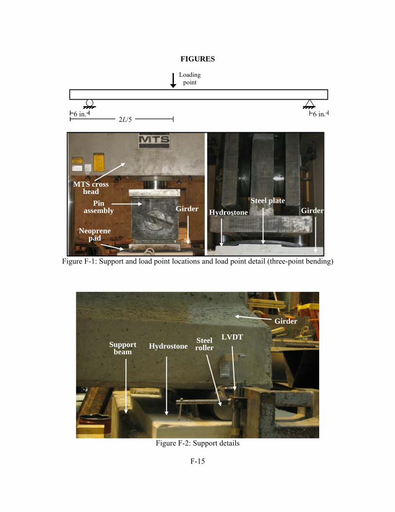
F-15

FIGURES

Figure F-1: Support and load point locations and load point detail (three-point bending)

Figure F-2: Support details

Girder

Steel roller

LVDTHydrostoneSupport

beam

6 in.6 in. 2L/5

Loading point

MTS cross head

Pin assembly

Neoprene pad

Girder GirderHydrostoneSteel plate

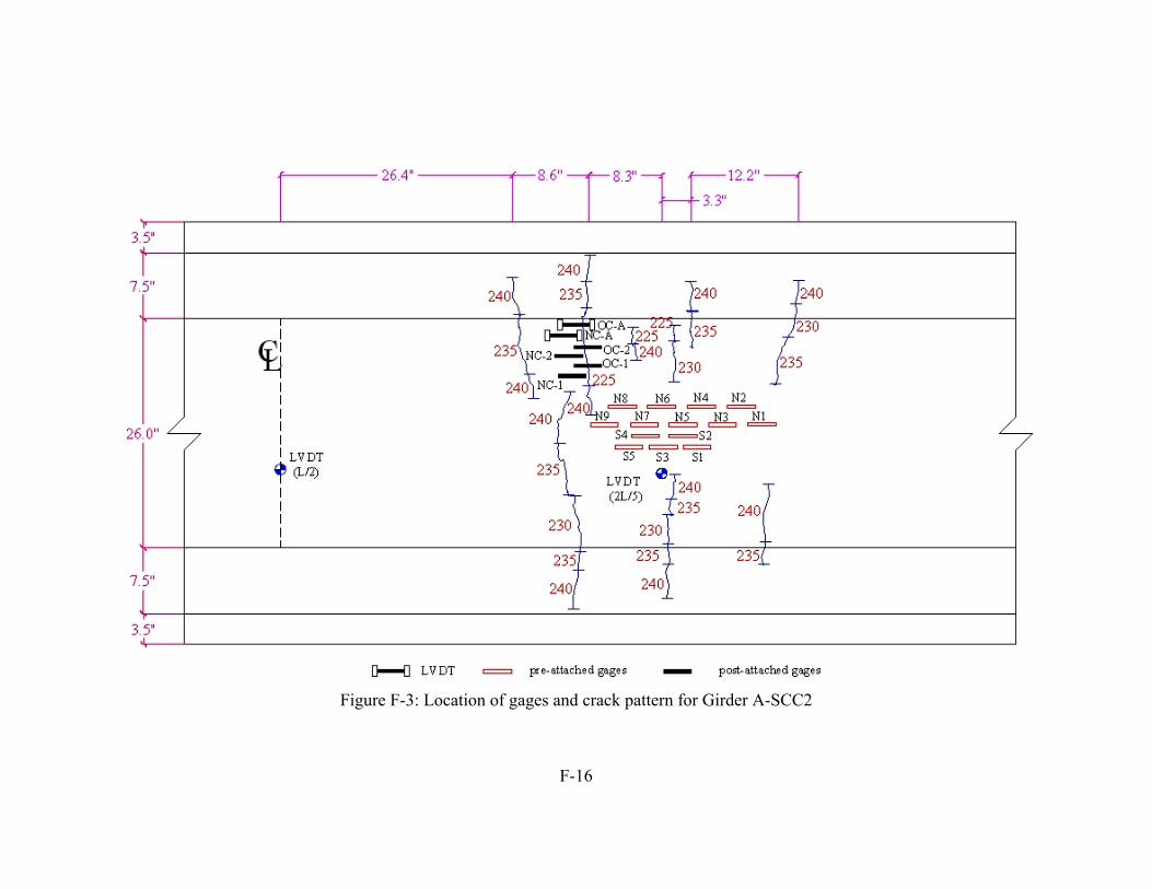
F-16

Figure F-3: Location of gages and crack pattern for Girder A-SCC2

F-17

Figure F-4: Location of gages and crack pattern for Girder A-SCC1 (Loading-1)

F-18

Figure F-5: Location of gages and crack pattern for Girder A-SCC1 (Loading-2)

F-19

Figure F-6: Location of gages and crack pattern for Girder A-CM (Loading-1)

F-20

Figure F-7: Location of gages and crack pattern for Girder A-CM (Loading-2)

F-21

Figure F-8: Location of gages and crack pattern for Girder B-SCC2

F-22

Figure F-9: Location of gages and crack pattern for Girder B-SCC1

F-23

Figure F-10: Location of gages and crack pattern for Girder B-CM

F-24

Figure F-11: Bottom fiber strain distribution for Girder A-SCC2

Figure F-12: Bottom fiber strain distribution for Girder A-SCC1 (Loading-1)

0

200

400

600

800

1000

1200

0 3 6 9 12 15 18 21 24 27 30 33 36 39 42

stra

in (m

icro

)

100 kips

125 kips

150 kips

175 kips

200 kips

225 kips

240 kips

Relative gage location (in.)

Stra

in (μ

ε)

N1 N2 N3 N4 N5 N6 N7 N8 N9

0

200

400

600

800

1000

1200

1400

0 6 12 18 24 30 36 42 48 54 60

gage location E SCC1 P1

stra

in (m

icro

)

P= 100 KipsP=125 KipsP= 150 KipsP= 175 KipsP=200 KipsP= 225 KipsP=250 Kips

Relative gage location (in.)

Stra

in (μ

ε)

N1 N2 S1 N3 S2 N4 S3 N5 S4 N6 S5 N7 S6 N8 N7

F-25

Figure F-13: Bottom fiber strain distribution for Girder A-SCC1 (Loading-2)

Figure F-14: Bottom fiber strain distribution for Girder A-CM (Loading-1)

0

200

400

600

800

1000

1200

1400

1600

0 6 12 18 24 30 36 42 48

P=260 KipsP= 240 KipsP= 220 KipsP=200 KipsP= 180 KipsP=160 KipsP=140 Kips

Relative gage location (in.)

Stra

in (μ

ε)

N1 N2 S1 N3 S2 N4 S3 N5 S4 N6 S5 N7 S6 N8

200

400

600

800

1000

1200

1400

0 6 12 18 24 30 36 42 48 54 60 66gage location

stra

in (m

icro

)

P=140 Kips

P=160 KipsP=180 Kips

P=200 Kips

P=220 Kips

P=240 Kips

Relative gage location (in.)

Stra

in (μ

ε)

S1 N1 S2 N2 S3 N3 S4 N4 S5 N5 S6 N6 S7 N7 S8

F-26

Figure F-15: Bottom fiber strain distribution for Girder A-CM (Loading-2)

Figure F-16: Bottom fiber strain distribution for Girder B-SCC2

0

200

400

600

800

1000

1200

0 6 12 18 24 30 36 42 48

P = 140 kipsP = 160 kipsP = 180 kipsP = 200 kipsP = 220 kipsP = 240 kips

Relative gage location (in.)

Stra

in (μ

ε)

S1 N1 S2 N2 S3 N3 S4 N4 S5 N5 S6 N6 S7 N7

0

100

200

300

400

500

600

700

800

900

1000

0 6 12 18 24 30 36 42 48

P=225 Kips P=200 KipsP=170Kips P=150 KipsP=130 Kips P=110 KipsP=100 Kips

Relative gage location (in.)

Stra

in (μ

ε)

S1 N1 S2 N2 S3 N3 S4 N4 S5 N5 S6 N6 S7 N7

F-27

Figure F-17: Bottom fiber strain distribution for Girder B-CM

Figure F-18: Bottom fiber strain distribution for Girder B-SCC1

0

200

400

600

800

1000

1200

0 6 12 18 24 30 36 42 48

P= 200 kipsP = 180 kipsP = 170 kipsP = 150 kipsP = 120 kipsP = 225 kipsP = 130 kips

Relative gage location (in.)

Stra

in (μ

ε)

N1 S1 N2 S2 N3 S3 N4 S4 N5 S5 N6 S6 N7 S7 N8

0

200

400

600

800

1000

1200

0 6 12 18 24 30 36 42 48

P = 250 Kips P = 225 Kips P = 200 KipsP = 190 Kips P = 180 Kips P = 170 Kips

Relative gage location (in.)

Stra

in (μ

ε)

S1 N1 S2 N2 S3 N3 S4 N4 S5 N5 S6 N6 S7 N7

F-28

Figure F-19: Sample cracking plot for gage placed over-crack

Figure F-20: Sample cracking plot for gage placed near-crack

0

50

100

150

200

250

300

0 100 200 300 400 500 600 700 800Strain (με)

Load

(kip

s)

initial linear line

gage strain

Cracking load (220 kips)

0

50

100

150

200

250

300

0 100 200 300 400 500 600 700 800 900 1000 1100 1200

Strain (με)

Load

(kip

s)

initial linear line

gage strain

Cracking load (225 kips)

F-29

Figure F-21: Strain and load divergence between gage data and initial linear line

Figure F-22: Cracking/crack re-opening loads (Objective-A)

baxy +=

gage data

εε Δ+ε

P

PP Δ−

Strain

Applied Load P

0

50

100

150

200

250

-5 0 5 10 15Δε (με)

Load

(kip

s) Cracking load

(232 kips)

F-30

Figure F-23: Cracking/crack re-opening loads (Objective-B)

0

50

100

150

200

250

-15 -10 -5 0 5ΔP (kips)

Load

(kip

s)

Cracking load (228 kips)

APPENDIX G

PRESTRESSING STRAND TENSION TEST

G-1

The initial prestressing force that to which the strands were tensioned during girder fabrication and the remaining effective prestressing force determined by exposing and cutting the strands were measured using strain gages (FLK-1-11-5LT) which were bonded to the individual wires. However, the strain measured along an individual wire is not equal to the strand stress (force/area) divided by the strand modulus of elasticity (Eps) because the individual wires are wound in a helix around the central wire. Therefore, there was a need to establish the relationship between the gage-measured strain and strand force experimentally.

Several sample strands each approximately 50 in. (127 cm) in length were obtained from the same spool as that used for the girder fabrication. Each strand was instrumented with three strain gages bonded to the mid-height of the strands. To obtain maximum consistency among the strand tension tests, initial girder prestressing, and strand cutting, the same type of strain gages were used for all three cases.

The strand tension tests were done using an MTS 600 kip universal testing system at the University of Minnesota Structures Laboratory as shown in Figure G-1. The strands were pulled with the help of two steel tubes, one placed at the end of the testing machine cylinder, and one placed on the strong floor. Strand chucks were used to grip the strand from both ends. Load-controlled testing was used with a loading rate of 3 kips/min. The strands were pulled until the strands fractured.

Sample load versus measured strain plots obtained during the of strand tension tests are given in Figures G-2 and G-3 for Plant-A and Plant-B, respectively. Each of the figures contains the load-strain plots for the three gages attached to an individual wire. The relationship between the measured strain and force (stress) was established using

psps

gage

psgage A

bA

aAPbaP +

×=→+×=

εε (G-1)

where constants a and b were determined from linear trend lines established for force versus strain plots up to a maximum force of 31 Kips, which was the maximum load that each strand was tensioned during fabrication. The stress-strain relationship was constructed dividing both sides of the relationship by strand area (i.e., Aps). The apparent modulus of elasticity, which is neither the modulus of elasticity of the steel nor that of strands, was calculated as

ps

psa AaE = (G-2)

where P is the strand load, εgage is the strain measured with the gage, and Epsa is the apparent elastic modulus of the prestressing steel.

The apparent modulus of elasticity values are summarized in Table G-1 for Plant-A and Plant-B. For each precast plant, apparent modulus of elasticity values larger and smaller than the average ± the standard deviation were not included to eliminate gages that may not have been oriented along the axis of the wire as well as the majority of the gages. The same criterion was used to

G-2

calculate the initial prestressing force to which the tendons were tensioned, and to calculate the remaining effective prestressing force for the strands.

The average apparent modulus of elasticity values were 30,349 ksi for Plant-A strands, and 30,847 ksi for Plant-B strands. These values were consistent with similar tests done by Baran (2003) with similar strands (i.e., half-inch Grade 270 low–relaxation strands). The manufacturer provided strand modulus of elasticity values were 28,633 ksi and 29,000 ksi for Plant-A and Plant-B, respectively. The apparent moduli of elasticity were used to relate the strains measured in the direction of the wire axes to the strand stress.

G-3

TABLES

Table G-1 Measured strand apparent modulus of elasticity values for Plant-A and Plant-B Epsa (ksi)

Sample ID Gage No Plant-B Plant-A

1 30837 44628 2 31275 29452 Strand–1 3 31373 29014 1 30078 29634 2 27784 29471 Strand–2 3 28216 33081 1 30105 29661 2 28902 30281 Strand–3 3 30170 29184 1 31882 x 2 30373 32663 Strand–4 3 25451 31044 1 33333 2 27830 Strand–5 3 31837 1 31863 2 31340 Strand–6 3 30980

Average 30202 31647 Standard deviation 1919 4521 Coefficient of Variation (%) 6 14 Average† 30847 30349 Coefficient of Variation (%) † 3 5 Eps

‡ 28633 29000 † The values larger and smaller than Average ±Standard Deviation not included

(shaded cells) ‡ Average strand modulus of elasticity provided by manufacturer

G-4

FIGURES

MTS cylinder

Steel tubes

Strand gages

Strand chuck

~ 50

in.

strain gage

strand cross section

Figure G-1 Strand tension setup

G-5

0.0

5.0

10.0

15.0

20.0

25.0

30.0

35.0

40.0

45.0

0 2000 4000 6000 8000 10000 12000

Strand-2 (G1)Strand-2 (G2)Strand-2 (G3)

Strain (με)

Load

(Kip

s)

Figure G-2 Load-strain relationship of sample strand-2 Plant-A

0.0

5.0

10.0

15.0

20.0

25.0

30.0

35.0

40.0

0 2000 4000 6000 8000 10000

Strand-1 (G1)Strand-1 (G2)Strand-1 (G3)

Strain (με)

Load

(Kip

s)

Figure G-3 Load-strain relationship of sample strand-1 Plant-B

APPENDIX H

FINITE ELEMENT MODELS AND INPUT FILES

H-1

H.1 Introduction

The program PBEAM developed by Suttikan (1978) was used for the analysis of girder time-dependent response. The program is capable of analyzing specimens of any cross-sectional shape having one axis of symmetry, noncomposite or composite, subjected to various sequences of loading and construction. The effects of nonlinearity of stress-strain response of materials, variation of strength with time, creep, and shrinkage of concrete, and relaxation of bonded prestressing steel after strand release are considered.

The specimens are modeled using a discrete element technique. A tangent stiffness method for solving nonlinear response is used in the instantaneous response analysis and a step-by-step method is used in the time-dependent response analysis.

The changes in strength and shrinkage of concrete are considered functions of time only, and the creep of concrete is considered proportional to the applied strains and is a function of time and age of concrete when the strains are applied. Relaxation of prestressing steel is a function of time and stress level. The program is capable of analyzing instantaneous load-defection response up to failure of the member in addition to time-dependent response analysis.

H.2 Girder Models and Assumptions

The program PBEAM has the following assumptions and limitations for the analysis.

1. Girders are straight in their original positions, and area of cross-sectional shape has one axis of symmetry

2. Strain increment distributions vary linearly through the depth of the girder 3. Strains and curvatures are small, but the displacements (horizontal, vertical, rotational)

can be any size 4. Shear deformation is negligible 5. Out-of-plane deformations are neglected 6. Only statically applied loads in the plane passing through the axis of symmetry of the

cross section are considered. 7. Uniaxial material properties assumed for the girder materials. 8. Equilibrium equations are written in the deformed state.

The 38 ft span of the girders was modeled as 34 discrete elements each measuring 13.4 in. in length. The 36 in. depth girder cross section was modeled using 42 fibers. The girders were simply supported over 37 ft during both the outdoor storage period and flexural crack and crack re-opening testing as shown in Figure H-1. However, the supports were assumed to be located at the ends of the girders (i.e., girder supported over 38 ft) for PBEAM modeling because the program requires the support to be located at element nodes. The closest nodes to the support locations were the ends of the girder. Investigation of the location of the supports in PBEAM from the ends to one node interior to the ends showed negligible difference in the PBEAM predicted losses at midspan. Concrete and steel stress-strain material properties were defined as linear elastic. The girders were only tested for flexural cracking and crack-reopening loads so

H-2

consequently the maximum concrete and steel stress levels were low, below 4.5 ksi (0.6fci') and 203 ksi (0.75 fsu) for the concrete and steel, respectively.

H.3 Steel Relaxation

The program PBEAM assumes that the steel relaxation starts to occur just after strand release. The program does not account for the portion of the relaxation occurring between strand tensioning and strand release. The magnitude of relaxation that happens between strand tensioning and strand release was calculated using

( ) ( ) ( ) ( ) ( ) ( ) ( )

( ) ( )⎪⎩

⎪⎨

⎧

<

≥⎟⎟⎠

⎞⎜⎜⎝

⎛−

−+

=+

+

4

4312

1

1

24log24log

Cffiff

CffifCCf

Cttfff

syistist

syististii

ististist (H-1)

for both plants, and the initial stress in the strands was lowered accordingly to account for the initial relaxation losses. Usually for low-relaxation strands C2 = 45, C3 = 0.55, C4 = 0.6, and C1 = fs y= 0.90fsu (Suttikan 1978), stf is the steel stress at time t in days after strand initial tensioning, and syf is the yield stress of the steel.

Although the amount of relaxation occurring between tensioning and strand release can be calculated and subtracted from the initial tensioning force, still there is a need to modify Eqn. (H-1) for PBEAM because the program does not recognize that the relaxation started to occur when the strands were initially tensioned. The program assumes that relaxation begins just after release. This detail is not documented in the PBEAM manual, and can be expressed as

( ) ( ) ( ) ( )( ) ( )( ) ( )⎟⎟⎠

⎞⎜⎜⎝

⎛−

−−−=− +

+ 312

11

24log24log CCf

Cttttfff istriri

ististist (H-2)

where tr is time in days (after initial strand tensioning) when the strands are released.

To further investigate the way that PBEAM handles steel relaxation, a simple girder section shown in Figure H-2 was modeled. The concrete was replaced with non-prestressed steel, and the prestressing strand was located at the center of the section for simplicity. There were no prestress losses due to creep and shrinkage as concrete was not used for the section. The only source of prestressing losses in the model was steel stress relaxation, and steel stress relaxation was only modeled for the prestressed strand.

The time between initial strand tensioning and strand release was assumed to be 4.0 days. The strands were assumed initially prestressed to 206.1 ksi, and the strand stress was computed to be 201.0 ksi just after strand release (i.e., the losses due to elastic shortening and relaxation). The relaxation losses that occurred only after strand release called “actual relaxation losses” were calculated using Eqn. (H-1) for ti ≥ 4.0 days, and they were compared to those computed by PBEAM as shown in Figure H-3. In addition, relaxation losses were calculated using Eqn. (H-

H-3

2). The PBEAM computed losses were approximately 2.5 ksi higher than the relaxation losses predicted by Eqn. (H-1). The PBEAM computed relaxation losses and those computed with Eqn. (H-2) were identical, which verified that PBEAM assumed relaxation starts to occur just after strand release.

The inconsistency between the Eqn. (H-1) and PBEAM calculated relaxation losses was fixed by modifying the constant C1, C2, and C3 in Eqn. (H-2). The constants were modified in such a way as to minimize the difference between the Eqn. (H-1) and PBEAM computed relaxation losses. The modified constants were found to be 0.94fsu, 75, and 0.52 for C1, C2, and C3, respectively. The relaxation losses, which were computed with modified coefficients, are shown in Figure H-3. The relaxation losses computed with the modified coefficients were not exactly equal to the relaxation losses predicted by Eqn. (H-1), but the difference at any time was less than 0.5 ksi.

For both Plant-A and Plant-B girders, the magnitude of relaxation losses that occurred from strand tensioning to strand release were calculated using Eqn. (H-1), and the prestressing force used for PBEAM modeling was adjusted accordingly. The coefficients (i.e., C1, C2, and C3) in Eqn. (H-2) were modified such that the difference between the Eqn. (H-1) losses and PBEAM calculated relaxation losses was minimized. The error was found to be smaller than 0.5 ksi for both plants.

H.4 Concrete Aging

Concrete under ordinary ambient conditions gains strength with age because of further hydration of the cement. PBEAM is capable of taking into account the effect of concrete aging when computing long-term behavior of the modeled specimens. The PBEAM built-in strength-age curves of concrete have the forms of those proposed by ACI Committee 209 (1997). The proposed curves, which have an asymptotic character and the strength is zero at time zero are given as

( ) ( ) /( and /( 28'

28' btatbtatff tt +=+= εε (H-3)

where 'tf and 28f are concrete strength at the age t and 28 days, and '

tε and 28ε are corresponding concrete strains. The constants a and b are functions of type of cement, water-cement ratio, curing, etc. The ACI Committee 209 (1997) has recommended values for these constants in the absence of experimental data. However, when experimental data is available a best-fit curve can be used to determine the constants.

Similar to concrete strength, concrete modulus of elasticity also varies with time. Although PBEAM does not provide any guidelines, modulus-age curves of concrete can be predicted using

( )( )

( ) /( /(

/(28

28

28'

'' btatE

btatbtatffE

t

tt +=

++

==εε

(H-4)

H-4

In the present study, the age function constants a and b in Eqn. (H-3) were determined using nonlinear least square fit to measured concrete modulus of elasticity data instead of concrete strength data. Therefore, these constants do not necessarily represent the best fit curves to measured concrete strength data, but define the best fit curves to the measured concrete modulus of elasticity.

Determining the constants a and b for the concrete strength-age function using the concrete modulus of elasticity-age function ensures that PBEAM uses acceptable concrete modulus of elasticity values at release, flexural testing, and when computing long-term prestress losses.

H.5 Creep and Shrinkage Material Models

Creep and shrinkage material models were developed using measured creep and shrinkage strains for the companion cylinders. However, the girders and companion cylinders had different volume-to-surface ratios (V/S), and they were subjected to different ambient relative humidity histories (RH). Because ambient relative humidity and V/S are two significant parameters that affect the magnitude of shrinkage and creep strains, the creep and shrinkage data obtained for companion cylinders were corrected for both relative humidity and V/S before they were used with PBEAM to predict long-term girder behavior.

In this study, ACI Committee 209 recommendations (1997) were used to adjust the companion creep and shrinkage data to obtain the associated material models. It was shown in Chapter 5 that the corrected creep and shrinkage data (i.e., material models) for the girders can be obtained using

( )( )cntrm

fieldcnrmfield γ

γββ ×= (H-5)

where ( )cntrmγ and ( ) fieldγ are the product of all correction factors for conditions other than the standard conditions (i.e., RH = 40%, and V/S = 1.5 in.) for companion cylinders and girders,

cntrmβ is the measured creep or shrinkage of companion cylinders, and fieldβ is the corrected (i.e., adjusted) creep or shrinkage material models.

H.5.1 Ambient Relative Humidity Correction

The companion creep and shrinkage cylinders were stored in a controlled room at University of Minnesota, where the temperature fluctuations were negligible (72±4°F). The average relative humidity and its standard deviation for the control room were 45% and 5 %.

The girders were transported after strand release to an outdoor storage site in the Plant-A precasting yard, where they were exposed to seasonal temperature and relative humidity fluctuations. The average relative humidity and its standard deviation for the outdoor storage site were 68% and 12%, respectively, for both Plant-A and Plant-B girders despite the fact that the girders were stored for different durations (approximately 600 days for Plant-A and 400 days

H-5

for Plant-B girders). Figure H-4 shows the ambient relative humidity of the girder storage site measured with a weather station that was set up at the same location.

The correction factors were calculated for six RH cases for the outdoor storage site as shown in Table H-1. These were average, average ±standard deviation, average ±2 x standard deviation, and 100% relative humidity cases. The total correction factors due to RH were between 0.62 and 1.01 for creep, and between 0.0 and 1.02 for shrinkage as given in Table H-1. Because the RH standard deviation was only 5%, only the average value of RH was used for the estimate of the control room RH.

In addition, a seventh RH case, where the effect of outdoor storage area ambient RH was included as a function of time, was also considered. In this case, the creep and shrinkage strain variations between times t1 and t2 were corrected for the average ambient relative humidity measured over times t1 and t2. However, only the average relative humidity (i.e., 45 %) was considered for the control room due to the limited number of data available for the control room. A detailed description of this case can be found in Chapter 5.

H.5.2 Volume-Surface Ratio Correction for Girders

ACI Committee 209 (1997) recommends the following equations for creep and shrinkage corrections, respectively, for members with volume-surface ratio (V/S) different than 1.5 in.

( ) 2.013.113254.0

≥⎟⎟⎠

⎞⎜⎜⎝

⎛+=

−SV

VSCR eγ (H-6)

( ) 2.02.112.0

≥=−

SV

VSSH eγ (H-7)

The calculated volume-to-surface ratios and the associated correction factors were calculated for both companion cylinders and girders. As shown in Table H-2, the total correction factors (i.e., ( ) ( )cylindergirder γγ ) for volume-to-surface ratio were calculated to be 0.71 and 0.75 for creep and shrinkage, respectively. A detailed summary of the calculations are given below:

• Creep and Shrinkage Companion Cylinders (4x 11 in.):

in. 122

22

2 ===→==r

πrhhr

SVπrhS & πhrV π

where V is the volume, S is the surface area, r is the radius, and h is the height of the cylinders.

Creep correction factor: ( ) ( ) 10.113.1132 0.154.0 =+= ×−eVSCRγ Shrinkage correction factor: ( ) 06.12.1 0.112.0 == ×−eVSSHγ

• Girders:

H-6

( )( )

49.3 259920 259920

25992057021238161 2599201238570

2

2

3

22

32

==

=×+××=

=××=

+×=×=

inin

SV

ininftinftinSinftinftinV

ALPS & LAV ggggg

where Pg is the perimeter of the girder cross section, Lg is the girder span length, and Ag is the girder cross-sectional area.

Creep correction factor: ( ) ( ) 78.013.1132 49.354.0 =+= ×−eVSCRγ Shrinkage correction factor: ( ) 79.02.1 49.312.0 == ×−eVSSHγ

The correction for volume-to-surface ratio (V/S) was done based on the total volume and total surface area of the girders. However, different fibers should have different V/S adjustment depending on their location within the section. For example, a fiber located at the mid-height of the cross section will have less surface area (i.e., larger V/S) to exchange moisture with environment relative to a fiber that is at the bottom of the cross section (i.e., smaller V/S). Additional tensile stresses should develop for the fiber located near the surface due to the differential shrinkage that occurs because of the different V/S ratio of the fibers. Therefore, this differential shrinkage behavior of the fibers can significantly affect the cracking and crack re-opening loads. When the girders were tested under flexural loading for cracking and crack re-opening, the first crack occurred in the fibers located at the bottom surface of the cross section, and the magnitude of the associated load depended on the stress state of the fibers just before flexural loading.

To investigate the effect of this differential shrinkage on cracking and crack re-opening loads predicted with PBEAM, the fiber located at the bottom surface of the cross section where first cracking occurred was modeled using creep and shrinkage data adjusted for the V/S of a fiber with 1.0 in. depth instead of V/S of the girder. The V/S of the bottom fiber was calculated as

gfgfff

gff

f LtLwtwLtw

SV

×+×+×

××=⎟

⎠⎞

⎜⎝⎛

2 2 (H-8)

where (V/S)f is the volume-surface ratio of the fiber, wf is the width of the fiber (26 in.), tf is the thickness of the fiber (1.0 in.), Lg is the girder length (38 ft), and Ag is the girder cross-sectional area.

The volume-surface ratio of the fiber was found to be 0.93 in., and it was significantly smaller than that of the girder, which was 3.49 in. The associated creep and shrinkage corrections due to V/S are given in Table H-2. The V/S creep and shrinkage correction factors were 0.71 and 0.75, respectively, for the girder V/S and 1.02 and 1.14, respectively, for the fiber V/S. The total correction factors calculated for RH and V/S are given in Table H-3.

H-7

The creep and shrinkage material models were obtained by multiplying the ultimate creep coefficients and ultimate shrinkage strains with the total correction factors calculated for V/S and RH. The creep and shrinkage material models are given in Tables H-4 and H-5 for Plant-A, and in Tables H-6 and H-7 for Plant-B.

H.6 PBEAM Input Files

This section contains the PBEAM input files for each of the six girders used to determine the long-term behavior of the girders. The creep and shrinkage material models utilized to predict the long-term girder behaviors were based on the average ambient relative humidity values of the control room and outdoor storage site and the V/S ratio of the girders (i.e., the same creep and shrinkage material models used for all fibers). The same files were used to determine crack re-opening loads. In addition, the crack re-opening loads were also determined with modified input files, where the creep and shrinkage material models for the concrete fiber at the bottom and top surfaces of the girders were developed using the V/S ratio of the bottom and top fibers to include the effect of differential shrinkage. A sample input file with uniform creep and shrinkage material models, and one that includes the effect of differential shrinkage are also included.

PBEAM does not model two important types of prestress losses: prestress losses due to steel relaxation from strand tensioning to strand release and prestress losses that occur due to thermal affects from strand tensioning to strand release. A detailed description of steel relaxation and thermal effects is included in Chapter 5 and Appendix B, respectively. These thermal and steel relaxation losses are not recoverable and therefore the initial strand tensioning stresses were decreased accordingly to account for them. The thermal effects after strand release are mostly recoverable and they were not considered in the models. Also it should be noted that vibrating wire strain gages data used to monitor prestress losses does not include thermal effects.

H-8

Plant-A: Girder CM, Long-term Behavior Plant-A: Girder CM, measured properties, CR&SH- corrected for V/S and avrg RH*** START 1 Problem #1, Plant A Girders Losses 13 0 0 0 0 0 0 0 1 1 0 1 *Table-1* 10 12 0 50 0 3 0 1 29 29 4.100e+00 1.825e+04 *Table 2: calc/print* 4.100e+00 5.000e+00 6.000e+00 7.000e+00 8.000e+00 9.000e+00 1.000e+01 1.100e+01 1.200e+01 1.300e+01 1.400e+01 1.500e+01 1.600e+01 1.700e+01 1.800e+01 1.900e+01 2.500e+01 3.500e+01 4.500e+01 6.000e+01 9.000e+01 1.250e+02 1.400e+02 1.850e+02 2.800e+02 4.500e+02 6.000e+02 1.650e+03 1.825e+04 4.100e+00 5.000e+00 6.000e+00 7.000e+00 8.000e+00 9.000e+00 1.000e+01 1.100e+01 1.200e+01 1.300e+01 1.400e+01 1.500e+01 1.600e+01 1.700e+01 1.800e+01 1.900e+01 2.500e+01 3.500e+01 4.500e+01 6.000e+01 9.000e+01 1.250e+02 1.400e+02 1.850e+02 2.800e+02 4.500e+02 6.000e+02 1.650e+03 1.825e+04 5 20 1.000e+00 1.000e+00 1.000e+10 1.000e+10 3 *Table 3A - no. material* 1 0 0 1 1 1 8.94e-02 *girder concrete prop.* 6.094e+06 1.34e-04 -4.50e-03 cr on/sh on/age on 0.55 0.90 0.73 0.70 0.60 15.5 1.0 0.0 -2.22e-04 19.0 2 0 0 0 0 0 2.816e-01 *top flange rebar* 2.900e+07 6.530e-02-6.530e-02 3 1 0 0 1 0 2.818e-01 *prestr strand* relax on* 2.86333e+7 6.530e-02-6.530e-02 2.430e+05 68.0 0.64 0.64 35 0.456e+03 *begin Table 4* 24 *number of subrectangles* 1 2 1 0.0 3.8 4.1 *girder conc* 26.0 1.75 0.875 0.0 1 1 1 0.0 3.8 4.1 22.328 0.5 2.000 0.0 1 2 1 0.0 3.8 4.1 26.000 1.5 3.000 0.0 1 1 1 0.0 3.8 4.1 22.328 0.5 4.000 0.0 1 2 1 0.0 3.8 4.1 26.000 1.5 5.000 0.0 1 1 1 0.0 3.8 4.1 22.328 0.5 6.000 0.0 1 1 1 0.0 3.8 4.1 26.000 1.25 6.875 0.0 1 4 1 0.0 3.8 4.1 16.000 3.50 8.886 0.0 1 10 1 0.0 3.8 4.1 6.000 15.5 18.750 0.0 1 2 1 0.0 3.8 4.1 8.000 2.0 27.588 0.0 1 2 1 0.0 3.8 4.1 20.00 1.5 29.376 0.0 1 1 1 0.0 3.8 4.1 30.00 0.75 30.376 0.0 1 1 1 0.0 3.8 4.1 29.388 0.50 31.000 0.0 1 2 1 0.0 3.8 4.1 30.000 1.50 32.000 0.0 1 1 1 0.0 3.8 4.1 29.388 0.50 33.000 0.0 1 1 1 0.0 3.8 4.1 30.000 0.75 33.625 0.0 1 1 1 0.0 3.8 4.1 26.840 1.00 34.500 0.0 1 1 1 0.0 3.8 4.1

H-9

30.000 1.00 35.500 0.0 2 1 1 0.0 3.8 4.1 *top rebar* 3.16 1.0 34.500 0.0 3 1 1 -1.1 3.8 4.1 *str Layer 1 * 3.6768 0.5 2.0 6.9563e-3 3 1 1 -1.1 3.8 4.1 *str Layer 2 * 3.6768 0.5 4.0 6.9563e-3 3 1 1 -1.1 3.8 4.1 *str Layer 3 * 3.6768 0.5 6.0 6.9563e-3 3 1 1 -1.1 3.8 4.1 *str Layer 3 * 0.6128 0.5 31.0 6.9563e-3 3 1 1 -1.1 3.8 4.1 *str Layer 3 * 0.6128 0.5 33.0 6.9563e-3 2 *Table 5B restraints* 0.000e+00 -1.100e+30-1.100e+30 0.456e+03 -1.100e+30 CEASE

H-10

Plant-A: Girder SCC1, Long-term Behavior

Plant-A: Girder SCC1, measured properties, CR&SH - corrected for V/S and avrg RH* START 1 Problem #1, Plant A Girders Losses 13 0 0 0 0 0 0 0 1 1 1 0 *Table-1* 10 12 0 50 0 3 0 1 30 30 4.100e+00 1.825e+04 *Table 2: calc/print* 4.100e+00 5.000e+00 6.000e+00 7.000e+00 8.000e+00 9.000e+00 1.000e+01 1.100e+01 1.200e+01 1.300e+01 1.400e+01 1.500e+01 1.600e+01 1.700e+01 1.800e+01 1.900e+01 2.500e+01 3.500e+01 4.500e+01 6.000e+01 9.000e+01 1.250e+02 1.400e+02 1.850e+02 2.800e+02 4.500e+02 6.000e+02 8.000e+02 1.650e+03 1.825e+04 4.100e+00 5.000e+00 6.000e+00 7.000e+00 8.000e+00 9.000e+00 1.000e+01 1.100e+01 1.200e+01 1.300e+01 1.400e+01 1.500e+01 1.600e+01 1.700e+01 1.800e+01 1.900e+01 2.500e+01 3.500e+01 4.500e+01 6.000e+01 9.000e+01 1.250e+02 1.400e+02 1.850e+02 2.800e+02 4.500e+02 6.000e+02 8.000e+02 1.650e+03 1.825e+04 5 20 1.000e+00 1.000e+00 1.000e+10 1.000e+10 3 *Table 3A no. material props* 1 0 0 1 1 1 8.66e-02 *girder concrete* 4.752e+06 1.48e-04 -4.50e-03 cr on/sh on/age on 0.46 0.89 0.99 0.70 0.60 11.2 1.0 0.0 -2.70e-04 24.0 2 0 0 0 0 0 2.816e-01 *top flange rebar* 2.900e+07 6.530e-02-6.530e-02 3 1 0 0 1 0 2.818e-01 *prestr strand relax on* 2.86333e+7 6.530e-02-6.530e-02 2.430e+05 68.0 0.64 0.64 35 0.456e+03 *begin Table 4* 24 *number of subrectangles* 1 2 1 0.0 3.8 4.1 *girder conc* 26.0 1.75 0.875 0.0 1 1 1 0.0 3.8 4.1 22.328 0.5 2.000 0.0 1 2 1 0.0 3.8 4.1 26.000 1.5 3.000 0.0 1 1 1 0.0 3.8 4.1 22.328 0.5 4.000 0.0 1 2 1 0.0 3.8 4.1 26.000 1.5 5.000 0.0 1 1 1 0.0 3.8 4.1 22.328 0.5 6.000 0.0 1 1 1 0.0 3.8 4.1 26.000 1.25 6.875 0.0 1 4 1 0.0 3.8 4.1 16.000 3.50 8.886 0.0 1 10 1 0.0 3.8 4.1 6.000 15.5 18.750 0.0 1 2 1 0.0 3.8 4.1 8.000 2.0 27.588 0.0 1 2 1 0.0 3.8 4.1 20.00 1.5 29.376 0.0 1 1 1 0.0 3.8 4.1 30.00 0.75 30.376 0.0 1 1 1 0.0 3.8 4.1 29.388 0.50 31.000 0.0 1 2 1 0.0 3.8 4.1 30.000 1.50 32.000 0.0 1 1 1 0.0 3.8 4.1 29.388 0.50 33.000 0.0 1 1 1 0.0 3.8 4.1 30.000 0.75 33.625 0.0 1 1 1 0.0 3.8 4.1 26.840 1.00 34.500 0.0

H-11

1 1 1 0.0 3.8 4.1 30.000 1.00 35.500 0.0 2 1 1 0.0 3.8 4.1 *top rebar* 3.16 1.0 34.500 0.0 3 1 1 -1.1 3.8 4.1 *str Layer 1 * 3.6768 0.5 2.0 6.9563e-3 3 1 1 -1.1 3.8 4.1 *str Layer 2 * 3.6768 0.5 4.0 6.9563e-3 3 1 1 -1.1 3.8 4.1 *str Layer 3 * 3.6768 0.5 6.0 6.9563e-3 3 1 1 -1.1 3.8 4.1 *str Layer 3 * 0.6128 0.5 31.0 6.9563e-3 3 1 1 -1.1 3.8 4.1 *str Layer 3 * 0.6128 0.5 33.0 6.9563e-3 2 *Table 5B restraints* 0.000e+00 -1.100e+30-1.100e+30 0.456e+03 -1.100e+30 CEASE

H-12

Plant-A: Girder SCC2, Long-term Behavior Plant-A: Girder SCC2, measured properties, CR&SH - corrected for V/S and avrg RH* Girder concrete SCC1 and SCC2B, both used for the model START 1 Problem #1, Plant A Girders Losses 13 0 0 0 0 0 0 0 1 1 1 0 *Table-1* 10 18 0 52 0 3 0 1 30 30 4.100e+00 1.825e+04 *Table 2: calc/print* 4.100e+00 5.000e+00 6.000e+00 7.000e+00 8.000e+00 9.000e+00 1.000e+01 1.100e+01 1.200e+01 1.300e+01 1.400e+01 1.500e+01 1.600e+01 1.700e+01 1.800e+01 1.900e+01 2.500e+01 3.500e+01 4.500e+01 6.000e+01 9.000e+01 1.250e+02 1.400e+02 1.850e+02 2.800e+02 4.500e+02 6.000e+02 8.000e+02 1.650e+03 1.825e+04 4.100e+00 5.000e+00 6.000e+00 7.000e+00 8.000e+00 9.000e+00 1.000e+01 1.100e+01 1.200e+01 1.300e+01 1.400e+01 1.500e+01 1.600e+01 1.700e+01 1.800e+01 1.900e+01 2.500e+01 3.500e+01 4.500e+01 6.000e+01 9.000e+01 1.250e+02 1.400e+02 1.850e+02 2.800e+02 4.500e+02 6.000e+02 8.000e+02 1.650e+03 1.825e+04 5 20 1.000e+00 1.000e+00 1.000e+10 1.000e+10 4 *Table 3A - no. material props.* 1 0 0 1 1 1 8.74e-02 *SCC2A concrete,CR,SH,AGE on* 4.550e+06 1.48e-04 -4.50e-03 0.32 0.86 1.04 0.70 0.60 11.3 1.0 0.0 -3.06e-04 18.0 2 0 0 0 0 0 2.816e-01 *top flange rebar* 2.900e+07 6.530e-02-6.530e-02 3 1 0 0 1 0 2.818e-01 *prestr strand,relax on* 2.86333e+7 6.530e-02-6.530e-02 2.430e+05 68.0 0.64 0.64 4 0 0 1 1 1 8.74e-02 *SCC2B concrete,CR,SH,AGE on* 4.760e+06 1.48e-04 -4.50e-03 0.39 0.96 1.36 0.70 0.60 17.3 1.0 0.0 -2.61e-04 14.0 35 0.456e+03 *begin Table 4* 25 *number of subrectangles* 1 2 1 0.0 3.8 4.1 *girder conc* 26.0 1.75 0.875 0.0 1 1 1 0.0 3.8 4.1 22.328 0.5 2.000 0.0 1 2 1 0.0 3.8 4.1 26.000 1.5 3.000 0.0 1 1 1 0.0 3.8 4.1 22.328 0.5 4.000 0.0 1 2 1 0.0 3.8 4.1 26.000 1.5 5.000 0.0 1 1 1 0.0 3.8 4.1 22.328 0.5 6.000 0.0 1 1 1 0.0 3.8 4.1 26.000 1.25 6.875 0.0 1 4 1 0.0 3.8 4.1 16.000 3.50 8.886 0.0 1 5 1 0.0 3.8 4.1 6.000 7.75 14.875 0.0 4 5 1 0.0 3.8 4.1 6.000 7.75 22.625 0.0 4 2 1 0.0 3.8 4.1 8.000 2.0 27.588 0.0 4 2 1 0.0 3.8 4.1 20.00 1.5 29.376 0.0 4 1 1 0.0 3.8 4.1 30.00 0.75 30.376 0.0 4 1 1 0.0 3.8 4.1 29.388 0.50 31.000 0.0

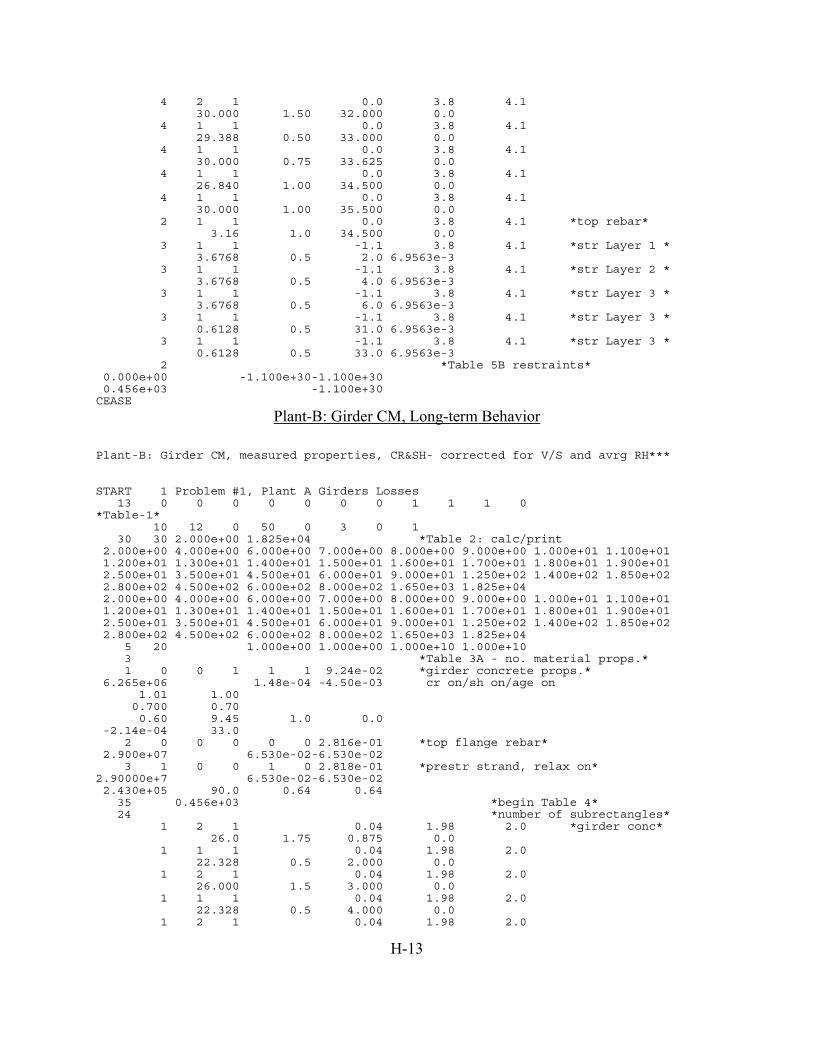
H-13

4 2 1 0.0 3.8 4.1 30.000 1.50 32.000 0.0 4 1 1 0.0 3.8 4.1 29.388 0.50 33.000 0.0 4 1 1 0.0 3.8 4.1 30.000 0.75 33.625 0.0 4 1 1 0.0 3.8 4.1 26.840 1.00 34.500 0.0 4 1 1 0.0 3.8 4.1 30.000 1.00 35.500 0.0 2 1 1 0.0 3.8 4.1 *top rebar* 3.16 1.0 34.500 0.0 3 1 1 -1.1 3.8 4.1 *str Layer 1 * 3.6768 0.5 2.0 6.9563e-3 3 1 1 -1.1 3.8 4.1 *str Layer 2 * 3.6768 0.5 4.0 6.9563e-3 3 1 1 -1.1 3.8 4.1 *str Layer 3 * 3.6768 0.5 6.0 6.9563e-3 3 1 1 -1.1 3.8 4.1 *str Layer 3 * 0.6128 0.5 31.0 6.9563e-3 3 1 1 -1.1 3.8 4.1 *str Layer 3 * 0.6128 0.5 33.0 6.9563e-3 2 *Table 5B restraints* 0.000e+00 -1.100e+30-1.100e+30 0.456e+03 -1.100e+30 CEASE

Plant-B: Girder CM, Long-term Behavior Plant-B: Girder CM, measured properties, CR&SH- corrected for V/S and avrg RH*** START 1 Problem #1, Plant A Girders Losses 13 0 0 0 0 0 0 0 1 1 1 0 *Table-1* 10 12 0 50 0 3 0 1 30 30 2.000e+00 1.825e+04 *Table 2: calc/print 2.000e+00 4.000e+00 6.000e+00 7.000e+00 8.000e+00 9.000e+00 1.000e+01 1.100e+01 1.200e+01 1.300e+01 1.400e+01 1.500e+01 1.600e+01 1.700e+01 1.800e+01 1.900e+01 2.500e+01 3.500e+01 4.500e+01 6.000e+01 9.000e+01 1.250e+02 1.400e+02 1.850e+02 2.800e+02 4.500e+02 6.000e+02 8.000e+02 1.650e+03 1.825e+04 2.000e+00 4.000e+00 6.000e+00 7.000e+00 8.000e+00 9.000e+00 1.000e+01 1.100e+01 1.200e+01 1.300e+01 1.400e+01 1.500e+01 1.600e+01 1.700e+01 1.800e+01 1.900e+01 2.500e+01 3.500e+01 4.500e+01 6.000e+01 9.000e+01 1.250e+02 1.400e+02 1.850e+02 2.800e+02 4.500e+02 6.000e+02 8.000e+02 1.650e+03 1.825e+04 5 20 1.000e+00 1.000e+00 1.000e+10 1.000e+10 3 *Table 3A - no. material props.* 1 0 0 1 1 1 9.24e-02 *girder concrete props.* 6.265e+06 1.48e-04 -4.50e-03 cr on/sh on/age on 1.01 1.00 0.700 0.70 0.60 9.45 1.0 0.0 -2.14e-04 33.0 2 0 0 0 0 0 2.816e-01 *top flange rebar* 2.900e+07 6.530e-02-6.530e-02 3 1 0 0 1 0 2.818e-01 *prestr strand, relax on* 2.90000e+7 6.530e-02-6.530e-02 2.430e+05 90.0 0.64 0.64 35 0.456e+03 *begin Table 4* 24 *number of subrectangles* 1 2 1 0.04 1.98 2.0 *girder conc* 26.0 1.75 0.875 0.0 1 1 1 0.04 1.98 2.0 22.328 0.5 2.000 0.0 1 2 1 0.04 1.98 2.0 26.000 1.5 3.000 0.0 1 1 1 0.04 1.98 2.0 22.328 0.5 4.000 0.0 1 2 1 0.04 1.98 2.0

H-14

26.000 1.5 5.000 0.0 1 1 1 0.04 1.98 2.0 22.328 0.5 6.000 0.0 1 1 1 0.04 1.98 2.0 26.000 1.25 6.875 0.0 1 4 1 0.04 1.98 2.0 16.000 3.50 8.886 0.0 1 10 1 0.04 1.98 2.0 6.000 15.5 18.750 0.0 1 2 1 0.04 1.98 2.0 8.000 2.0 27.588 0.0 1 2 1 0.04 1.98 2.0 20.00 1.5 29.376 0.0 1 1 1 0.04 1.98 2.0 30.00 0.75 30.376 0.0 1 1 1 0.04 1.98 2.0 29.388 0.50 31.000 0.0 1 2 1 0.04 1.98 2.0 30.000 1.50 32.000 0.0 1 1 1 0.04 1.98 2.0 29.388 0.50 33.000 0.0 1 1 1 0.04 1.98 2.0 30.000 0.75 33.625 0.0 1 1 1 0.04 1.98 2.0 26.840 1.00 34.500 0.0 1 1 1 0.04 1.98 2.0 30.000 1.00 35.500 0.0 2 1 1 0.04 1.98 2.0 *top rebars* 3.16 1.0 34.500 0.0 3 1 1 0.04 1.98 2.0 *str Layer 1 * 3.6768 0.5 2.0 6.8328e-3 3 1 1 0.04 1.98 2.0 *str Layer 2 * 3.6768 0.5 4.0 6.8328e-3 3 1 1 0.04 1.98 2.0 *str Layer 3 * 3.6768 0.5 6.0 6.8328e-3 3 1 1 0.04 1.98 2.0 *str Layer 3 * 0.6128 0.5 31.0 6.8328e-3 3 1 1 0.04 1.98 2.0 *str Layer 3 * 0.6128 0.5 33.0 6.8328e-3 2 *Table 5B restraints* 0.000e+00 -1.100e+30-1.100e+30 0.456e+03 -1.100e+30 CEASE

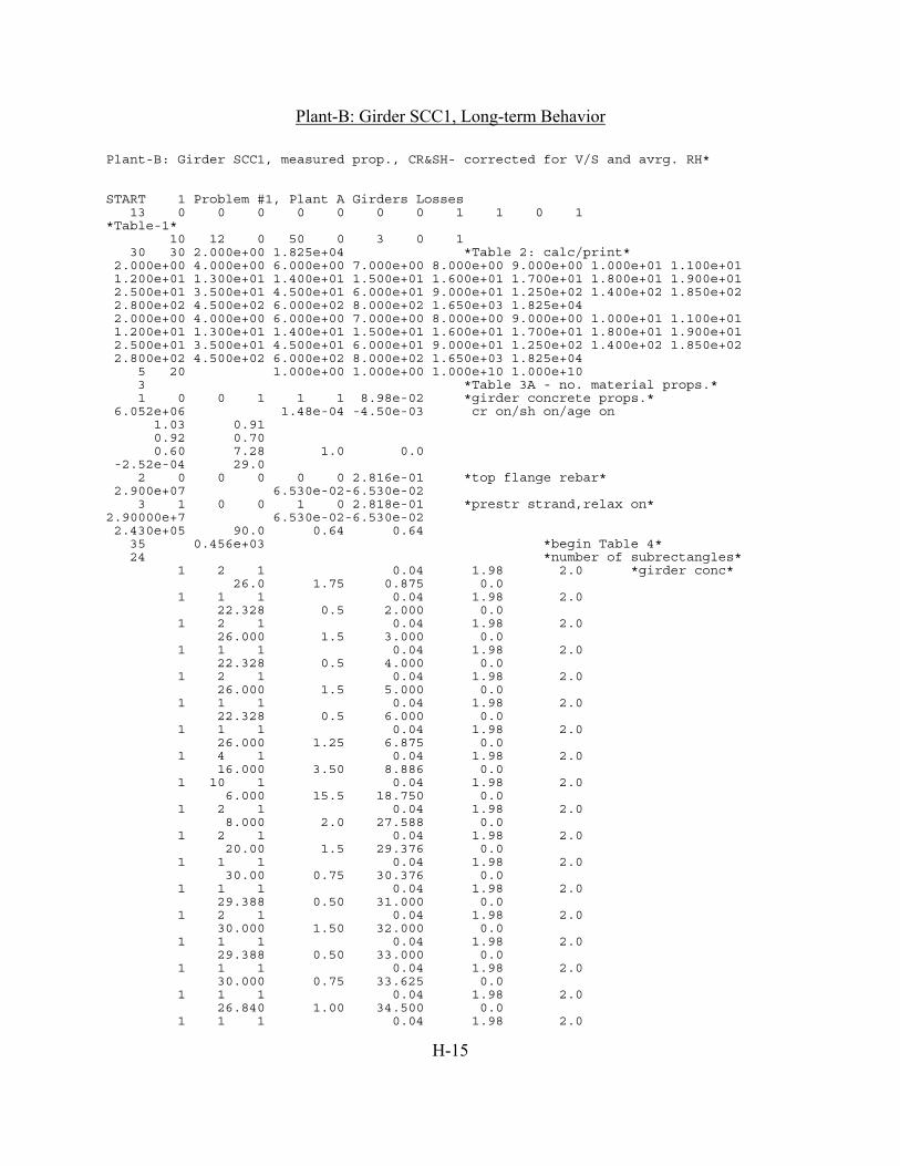
H-15

Plant-B: Girder SCC1, Long-term Behavior

Plant-B: Girder SCC1, measured prop., CR&SH- corrected for V/S and avrg. RH* START 1 Problem #1, Plant A Girders Losses 13 0 0 0 0 0 0 0 1 1 0 1 *Table-1* 10 12 0 50 0 3 0 1 30 30 2.000e+00 1.825e+04 *Table 2: calc/print* 2.000e+00 4.000e+00 6.000e+00 7.000e+00 8.000e+00 9.000e+00 1.000e+01 1.100e+01 1.200e+01 1.300e+01 1.400e+01 1.500e+01 1.600e+01 1.700e+01 1.800e+01 1.900e+01 2.500e+01 3.500e+01 4.500e+01 6.000e+01 9.000e+01 1.250e+02 1.400e+02 1.850e+02 2.800e+02 4.500e+02 6.000e+02 8.000e+02 1.650e+03 1.825e+04 2.000e+00 4.000e+00 6.000e+00 7.000e+00 8.000e+00 9.000e+00 1.000e+01 1.100e+01 1.200e+01 1.300e+01 1.400e+01 1.500e+01 1.600e+01 1.700e+01 1.800e+01 1.900e+01 2.500e+01 3.500e+01 4.500e+01 6.000e+01 9.000e+01 1.250e+02 1.400e+02 1.850e+02 2.800e+02 4.500e+02 6.000e+02 8.000e+02 1.650e+03 1.825e+04 5 20 1.000e+00 1.000e+00 1.000e+10 1.000e+10 3 *Table 3A - no. material props.* 1 0 0 1 1 1 8.98e-02 *girder concrete props.* 6.052e+06 1.48e-04 -4.50e-03 cr on/sh on/age on 1.03 0.91 0.92 0.70 0.60 7.28 1.0 0.0 -2.52e-04 29.0 2 0 0 0 0 0 2.816e-01 *top flange rebar* 2.900e+07 6.530e-02-6.530e-02 3 1 0 0 1 0 2.818e-01 *prestr strand,relax on* 2.90000e+7 6.530e-02-6.530e-02 2.430e+05 90.0 0.64 0.64 35 0.456e+03 *begin Table 4* 24 *number of subrectangles* 1 2 1 0.04 1.98 2.0 *girder conc* 26.0 1.75 0.875 0.0 1 1 1 0.04 1.98 2.0 22.328 0.5 2.000 0.0 1 2 1 0.04 1.98 2.0 26.000 1.5 3.000 0.0 1 1 1 0.04 1.98 2.0 22.328 0.5 4.000 0.0 1 2 1 0.04 1.98 2.0 26.000 1.5 5.000 0.0 1 1 1 0.04 1.98 2.0 22.328 0.5 6.000 0.0 1 1 1 0.04 1.98 2.0 26.000 1.25 6.875 0.0 1 4 1 0.04 1.98 2.0 16.000 3.50 8.886 0.0 1 10 1 0.04 1.98 2.0 6.000 15.5 18.750 0.0 1 2 1 0.04 1.98 2.0 8.000 2.0 27.588 0.0 1 2 1 0.04 1.98 2.0 20.00 1.5 29.376 0.0 1 1 1 0.04 1.98 2.0 30.00 0.75 30.376 0.0 1 1 1 0.04 1.98 2.0 29.388 0.50 31.000 0.0 1 2 1 0.04 1.98 2.0 30.000 1.50 32.000 0.0 1 1 1 0.04 1.98 2.0 29.388 0.50 33.000 0.0 1 1 1 0.04 1.98 2.0 30.000 0.75 33.625 0.0 1 1 1 0.04 1.98 2.0 26.840 1.00 34.500 0.0 1 1 1 0.04 1.98 2.0

H-16

30.000 1.00 35.500 0.0 2 1 1 0.04 1.98 2.0 *top rebars* 3.16 1.0 34.500 0.0 3 1 1 0.04 1.98 2.0 *str Layer 1 * 3.6768 0.5 2.0 6.8328e-3 3 1 1 0.04 1.98 2.0 *str Layer 2 * 3.6768 0.5 4.0 6.8328e-3 3 1 1 0.04 1.98 2.0 *str Layer 3 * 3.6768 0.5 6.0 6.8328e-3 3 1 1 0.04 1.98 2.0 *str Layer 3 * 0.6128 0.5 31.0 6.8328e-3 3 1 1 0.04 1.98 2.0 *str Layer 3 * 0.6128 0.5 33.0 6.8328e-3 2 *Table 5B restraints* 0.000e+00 -1.100e+30-1.100e+30 0.456e+03 -1.100e+30 CEASE

H-17

Plant-B: Girder SCC2, Long-term Behavior

Plant-B: Girder SCC2, measured prop., CR&SH- corrected for V/S and avrg. RH* START 1 Problem #1, Plant A Girders Losses 13 0 0 0 0 0 0 0 1 1 1 0 *Table-1* 10 12 0 50 0 3 0 1 30 30 2.000e+00 1.825e+04 *Table 2: calc/print* 2.000e+00 4.000e+00 6.000e+00 7.000e+00 8.000e+00 9.000e+00 1.000e+01 1.100e+01 1.200e+01 1.300e+01 1.400e+01 1.500e+01 1.600e+01 1.700e+01 1.800e+01 1.900e+01 2.500e+01 3.500e+01 4.500e+01 6.000e+01 9.000e+01 1.250e+02 1.400e+02 1.850e+02 2.800e+02 4.500e+02 6.000e+02 8.000e+02 1.650e+03 1.825e+04 2.000e+00 4.000e+00 6.000e+00 7.000e+00 8.000e+00 9.000e+00 1.000e+01 1.100e+01 1.200e+01 1.300e+01 1.400e+01 1.500e+01 1.600e+01 1.700e+01 1.800e+01 1.900e+01 2.500e+01 3.500e+01 4.500e+01 6.000e+01 9.000e+01 1.250e+02 1.400e+02 1.850e+02 2.800e+02 4.500e+02 6.000e+02 8.000e+02 1.650e+03 1.825e+04 5 20 1.000e+00 1.000e+00 1.000e+10 1.000e+10 3 *Table 3A - no. material props.* 1 0 0 1 1 1 9.00e-02 *girder concrete props.* 6.068e+06 1.48e-04 -4.50e-03 cr on/sh on/age on 0.93 0.96 1.10 0.70 0.60 10.40 1.0 0.0 -2.43e-04 23.0 2 0 0 0 0 0 2.816e-01 *top flange rebar* 2.900e+07 6.530e-02-6.530e-02 3 1 0 0 1 0 2.818e-01 *prestr strand,relax on* 2.90000e+7 6.530e-02-6.530e-02 2.430e+05 90.0 0.64 0.64 35 0.456e+03 *begin Table 4* 24 *number of subrectangles* 1 2 1 0.04 1.98 2.0 *girder conc* 26.0 1.75 0.875 0.0 1 1 1 0.04 1.98 2.0 22.328 0.5 2.000 0.0 1 2 1 0.04 1.98 2.0 26.000 1.5 3.000 0.0 1 1 1 0.04 1.98 2.0 22.328 0.5 4.000 0.0 1 2 1 0.04 1.98 2.0 26.000 1.5 5.000 0.0 1 1 1 0.04 1.98 2.0 22.328 0.5 6.000 0.0 1 1 1 0.04 1.98 2.0 26.000 1.25 6.875 0.0 1 4 1 0.04 1.98 2.0 16.000 3.50 8.886 0.0 1 10 1 0.04 1.98 2.0 6.000 15.5 18.750 0.0 1 2 1 0.04 1.98 2.0 8.000 2.0 27.588 0.0 1 2 1 0.04 1.98 2.0 20.00 1.5 29.376 0.0 1 1 1 0.04 1.98 2.0 30.00 0.75 30.376 0.0 1 1 1 0.04 1.98 2.0 29.388 0.50 31.000 0.0 1 2 1 0.04 1.98 2.0 30.000 1.50 32.000 0.0 1 1 1 0.04 1.98 2.0 29.388 0.50 33.000 0.0 1 1 1 0.04 1.98 2.0 30.000 0.75 33.625 0.0 1 1 1 0.04 1.98 2.0 26.840 1.00 34.500 0.0

H-18

1 1 1 0.04 1.98 2.0 30.000 1.00 35.500 0.0 2 1 1 0.04 1.98 2.0 *top rebar* 3.16 1.0 34.500 0.0 3 1 1 0.04 1.98 2.0 *str Layer 1 * 3.6768 0.5 2.0 6.8328e-3 3 1 1 0.04 1.98 2.0 *str Layer 2 * 3.6768 0.5 4.0 6.8328e-3 3 1 1 0.04 1.98 2.0 *str Layer 3 * 3.6768 0.5 6.0 6.8328e-3 3 1 1 0.04 1.98 2.0 *str Layer 3 * 0.6128 0.5 31.0 6.8328e-3 3 1 1 0.04 1.98 2.0 *str Layer 3 * 0.6128 0.5 33.0 6.8328e-3 2 *Table 5B restraints* 0.000e+00 -1.100e+30-1.100e+30 0.456e+03 -1.100e+30 CEASE

H-19

Plant-A: Girder SCC1, Cracking and Crack Re-opening Loads

Plant-A: Girder SCC1, measured properties, CR&SH - corrected for V/S and avrg RH* The creep and shrinkage material models developed for girder V/S. START 1 Problem #1, Plant A Girders Losses 13 0 0 0 0 0 0 0 1 1 1 0 *Table-1* 10 12 0 50 2 3 0 1 28 28 4.100e+00 6.010e+02 *Table 2: calc/print 4.100e+00 5.000e+00 6.000e+00 7.000e+00 8.000e+00 9.000e+00 1.000e+01 1.100e+01 1.200e+01 1.300e+01 1.400e+01 1.500e+01 1.600e+01 1.700e+01 1.800e+01 1.900e+01 2.500e+01 3.500e+01 4.500e+01 6.000e+01 9.000e+01 1.250e+02 1.400e+02 1.850e+02 2.800e+02 4.500e+02 5.990e+02 6.000e+02 6.010e+02 4.100e+00 5.000e+00 6.000e+00 7.000e+00 8.000e+00 9.000e+00 1.000e+01 1.100e+01 1.200e+01 1.300e+01 1.400e+01 1.500e+01 1.600e+01 1.700e+01 1.800e+01 1.900e+01 2.500e+01 3.500e+01 4.500e+01 6.000e+01 9.000e+01 1.250e+02 1.400e+02 1.850e+02 2.800e+02 4.500e+02 5.990e+02 6.000e+02 6.010e+02 5 20 1.000e+00 1.000e+00 1.000e+10 1.000e+10 3 *Table 3A - no. material props.* 1 0 0 1 1 1 8.66e-02 *girder concrete props. * 4.752e+06 4.50e-03 -4.50e-03 cr on/sh on/age on 0.46 0.89 0.99 0.70 0.60 11.2 1.0 0.0 -2.70e-04 24.0 2 0 0 0 0 0 2.816e-01 *top flange rebar* 2.900e+07 6.530e-02-6.530e-02 3 1 0 0 1 0 2.818e-01 *prestr strand,relax on* 2.86333e+7 6.530e-02-6.530e-02 2.430e+05 68.0 0.64 0.64 35 0.456e+03 *begin Table 4* 24 *number of subrectangles* 1 2 1 0.0 3.8 4.1 *girder conc* 26.0 1.75 0.875 0.0 1 1 1 0.0 3.8 4.1 22.328 0.5 2.000 0.0 1 2 1 0.0 3.8 4.1 26.000 1.5 3.000 0.0 1 1 1 0.0 3.8 4.1 22.328 0.5 4.000 0.0 1 2 1 0.0 3.8 4.1 26.000 1.5 5.000 0.0 1 1 1 0.0 3.8 4.1 22.328 0.5 6.000 0.0 1 1 1 0.0 3.8 4.1 26.000 1.25 6.875 0.0 1 4 1 0.0 3.8 4.1 16.000 3.50 8.886 0.0 1 10 1 0.0 3.8 4.1 6.000 15.5 18.750 0.0 1 2 1 0.0 3.8 4.1 8.000 2.0 27.588 0.0 1 2 1 0.0 3.8 4.1 20.00 1.5 29.376 0.0 1 1 1 0.0 3.8 4.1 30.00 0.75 30.376 0.0 1 1 1 0.0 3.8 4.1 29.388 0.50 31.000 0.0 1 2 1 0.0 3.8 4.1 30.000 1.50 32.000 0.0 1 1 1 0.0 3.8 4.1 29.388 0.50 33.000 0.0 1 1 1 0.0 3.8 4.1 30.000 0.75 33.625 0.0 1 1 1 0.0 3.8 4.1 26.840 1.00 34.500 0.0 1 1 1 0.0 3.8 4.1 30.000 1.00 35.500 0.0

H-20

2 1 1 0.0 3.8 4.1 *top rebars* 3.16 1.0 34.500 0.0 3 1 1 -1.1 3.8 4.1 *str Layer 1 * 3.6768 0.5 2.0 6.9563e-3 3 1 1 -1.1 3.8 4.1 *str Layer 2 * 3.6768 0.5 4.0 6.9563e-3 3 1 1 -1.1 3.8 4.1 *str Layer 3 * 3.6768 0.5 6.0 6.9563e-3 3 1 1 -1.1 3.8 4.1 *str Layer 3 * 0.6128 0.5 31.0 6.9563e-3 3 1 1 -1.1 3.8 4.1 *str Layer 3 * 0.6128 0.5 33.0 6.9563e-3 1 *Table 5A: loads* 600.0 189.0 -2.20e+05 *P1=25 2 *Table 5B restraints* 0.000e+00 -1.100e+30-1.100e+30 0.456e+03 -1.100e+30 CEASE

NOTE: The load was increased and the bottom fiber stresses were monitored. The crack re-opening load is the flexural load value corresponding to zero stress for the bottom fiber, and cracking load is the one corresponding to a stress equal to cf5.7 for the bottom fiber.

H-21

Plant-A: Girder SCC1, Cracking and Crack Re-opening Loads Including the Effect of Differential Shrinkage

Plant-A: Girder SCC1, measured prop., CR&SH - corrected for V/S and avrg RH* Creep and shrinkage material models developed for girder and bottom fiber V/S. UMN - A-SCC1, YES-rebar, unit wt, CR, SH, and Relaxation on (2/20/2007 8:00 pm) With measured proporties ELASTIC,***CR&SH-corected for V/S and avrg RH *** START 1 Problem #1, Plant A Girders Losses 13 0 0 0 0 0 0 0 1 1 1 0 *Table-1* 10 18 0 50 2 3 0 1 28 28 4.100e+00 6.010e+02 *Table 2: calc/print* 4.100e+00 5.000e+00 6.000e+00 7.000e+00 8.000e+00 9.000e+00 1.000e+01 1.100e+01 1.200e+01 1.300e+01 1.400e+01 1.500e+01 1.600e+01 1.700e+01 1.800e+01 1.900e+01 2.500e+01 3.500e+01 4.500e+01 6.000e+01 9.000e+01 1.250e+02 1.400e+02 1.850e+02 2.800e+02 4.500e+02 5.990e+02 6.000e+02 6.010e+02 4.100e+00 5.000e+00 6.000e+00 7.000e+00 8.000e+00 9.000e+00 1.000e+01 1.100e+01 1.200e+01 1.300e+01 1.400e+01 1.500e+01 1.600e+01 1.700e+01 1.800e+01 1.900e+01 2.500e+01 3.500e+01 4.500e+01 6.000e+01 9.000e+01 1.250e+02 1.400e+02 1.850e+02 2.800e+02 4.500e+02 5.990e+02 6.000e+02 6.010e+02 5 20 1.000e+00 1.000e+00 1.000e+10 1.000e+10 4 *Table 3A - no. material props.* 1 0 0 1 1 1 8.66e-02 *girder concrete props.* 4.752e+06 4.50e-03 -4.50e-03 cr on/sh on/age on 0.46 0.89 0.99 0.70 0.60 11.2 1.0 0.0 -2.70e-04 24.0 2 0 0 0 0 0 2.816e-01 *top flange rebar* 2.900e+07 6.530e-02-6.530e-02 3 1 0 0 1 0 2.818e-01 *prestr strand, relax on* 2.86333e+7 6.530e-02-6.530e-02 2.430e+05 68.0 0.64 0.64 4 0 0 1 1 1 8.66e-02 *bottom fiber* 4.752e+06 4.50e-03 -4.50e-03 cr on/sh on/age on 0.46 0.89 1.42 0.70 0.60 11.2 1.0 0.0 -3.64e-04 24.0 35 0.456e+03 *begin Table 4* 24 *number of subrectangles* 4 2 1 0.0 3.8 4.1 *girder conc* 26.0 1.75 0.875 0.0 1 1 1 0.0 3.8 4.1 22.328 0.5 2.000 0.0 1 2 1 0.0 3.8 4.1 26.000 1.5 3.000 0.0 1 1 1 0.0 3.8 4.1 22.328 0.5 4.000 0.0 1 2 1 0.0 3.8 4.1 26.000 1.5 5.000 0.0 1 1 1 0.0 3.8 4.1 22.328 0.5 6.000 0.0 1 1 1 0.0 3.8 4.1 26.000 1.25 6.875 0.0 1 4 1 0.0 3.8 4.1 16.000 3.50 8.886 0.0 1 10 1 0.0 3.8 4.1 6.000 15.5 18.750 0.0 1 2 1 0.0 3.8 4.1 8.000 2.0 27.588 0.0 1 2 1 0.0 3.8 4.1 20.00 1.5 29.376 0.0 1 1 1 0.0 3.8 4.1 30.00 0.75 30.376 0.0 1 1 1 0.0 3.8 4.1

H-22

29.388 0.50 31.000 0.0 1 2 1 0.0 3.8 4.1 30.000 1.50 32.000 0.0 1 1 1 0.0 3.8 4.1 29.388 0.50 33.000 0.0 1 1 1 0.0 3.8 4.1 30.000 0.75 33.625 0.0 1 1 1 0.0 3.8 4.1 26.840 1.00 34.500 0.0 1 1 1 0.0 3.8 4.1 30.000 1.00 35.500 0.0 2 1 1 0.0 3.8 4.1 *top rebar* 3.16 1.0 34.500 0.0 3 1 1 -1.1 3.8 4.1 *str Layer 1 * 3.6768 0.5 2.0 6.9563e-3 3 1 1 -1.1 3.8 4.1 *str Layer 2 * 3.6768 0.5 4.0 6.9563e-3 3 1 1 -1.1 3.8 4.1 *str Layer 3 * 3.6768 0.5 6.0 6.9563e-3 3 1 1 -1.1 3.8 4.1 *str Layer 3 * 0.6128 0.5 31.0 6.9563e-3 3 1 1 -1.1 3.8 4.1 *str Layer 3 * 0.6128 0.5 33.0 6.9563e-3 1 *Table 5A:loads* 600.0 189.0 -1.80e+05 *P1=25 2 *Table 5B restraints* 0.000e+00 -1.100e+30-1.100e+30 0.456e+03 -1.100e+30 CEASE

H-23

TABLES

Table H-1: Ambient relative humidity correction factors for creep and shrinkage

Girder storage site Control room ( ) ( )cntrmfield γγ

( ) fieldγ ( )cntrmγ Cases RH (%) ( )RHCRγ ( )RHSHγ

RH (%) ( )RHCRγ ( )RHSHγ

CR SH

RH1=Avrg 68 0.81 0.71 0.84 0.76

RH2=Avrg + Stdev 80 0.73 0.58 0.75 0.62

RH3=Avrg - Stdev 55 0.90 0.84 0.93 0.89 RH4=Avrg + 2Stdev 93 0.65 0.21 0.67 0.22 RH5=Avrg - 2Stdev 43 0.98 0.96 1.01 1.02 RH6=100% 100 0.60 0.0

45 0.97 0.94

0.62 0.00

Table H-2: Creep (CR) and shrinkage (SH) correction factors for girders and companion cylinders for V/S

Girder or Fiber Companion Cylinders ( ) ( )cylinderγγ

( )γ ( )cylindersγ V/S (in.) ( )VSCRγ ( )VSSHγ

V/S (in) ( )RHCRγ ( )RHSHγ

CR SH

3.49† 0.78 0.79 0.71 0.75

0.93‡ 1.12 1.21 1.0 1.10 1.06

1.02 1.14

† Girder average V/S ratio ‡ Fiber V/S ratio

H-24

Table H-3: Total CR and SH correction factors due to RH and V/S ratio

Relative humidity Girder V/S ratio Total correction factors†

( ) ( )cntrmfieldRH γγγ = ( ) ( )cylindergirderVS γγγ = RHVS γγγ ×= RH cases for

outdoor storage site CR SH CR SH CR SH

RH1=Avrg 0.84 0.76 0.60 0.57

RH2=Avrg + Stdev 0.75 0.62 0.53 0.47

RH3=Avrg - Stdev 0.93 0.89 0.66 0.67 RH4=Avrg + 2Stdev 0.67 0.22 0.48 0.17 RH5=Avrg - 2Stdev 1.01 1.02 0.72 0.77

RH6=100% 0.62 0.00

0.71 0.75

0.44 0.00 †Applied to ultimate creep coefficient and ultimate shrinkage to obtain creep and shrinkage material

models (i.e., Pbeam inputs)

H-25

Table H-4: Least square fit curves and V/S and RH corrected shrinkage material models for Plant-A mixes

Least-square Fit Parameters Corrected Shrinkage Material Models

RH cases for outdoor storage site Cylinder ID LSA-2† (two parameters) RH1 RH2 RH3 RH4 RH5 RH6

A-CM α f ( )ushε ( )ushε ( )ushε ( )ushε ( )ushε ( )ushε ( )ushε

CM-SH1 1.00 18 389 222 183 261 66 300 0 CM-SH2 1.00 22 377 215 177 253 64 290 0 CM-SH3 1.00 19 401 229 188 269 68 309 0 AVRG 1.00 19 389 222 183 261 66 300 0 AVRG‡ 1.00 18 202

A-SCC1 α f ( )ushε ( )ushε ( )ushε ( )ushε ( )ushε ( )ushε ( )ushε

SCC1-SH1 1.00 26 487 278 229 326 83 375 0 SCC1-SH2 1.00 22 459 262 216 308 78 353 0 AVRG 1.00 24 473 270 222 317 80 364 0 AVRG‡ 1.00 24 245

A-SCC2 α f ( )ushε ( )ushε ( )ushε ( )ushε ( )ushε ( )ushε ( )ushε

SCC2-SH1 1.00 22 517 295 243 346 88 398 0 SCC2-SH2 1.00 15 555 316 261 372 94 427 0 AVRG 1.00 18 536 306 252 359 91 413 0 AVRG‡ 1.00 17 279

A-SCC2B α f ( )ushε ( )ushε ( )ushε ( )ushε ( )ushε ( )ushε ( )ushε

SCC2B-C1 1.00 14 458 261 215 307 78 353 0

AVRG‡ 1.00 13 240

† Nonlinear least-square analyses for ACI 209 Equation: ( ) ( )ushtsh tft εε+

= using companion cylinder

data (not corrected for RH and/or V/S)

‡ Corrected for outdoor storage site ambient RH(t) and average RH for control room, and for V/S, so this is seventh case (shaded cells) for corrected shrinkage material model

H-26

Table H-5: Least square fit curves and V/S and RH corrected creep material models for Plant-A mixes

Least-square Fit Parameters Corrected Creep Material Models

RH cases for outdoor storage site Cylinder ID LSA-2† (two parameter) RH1 RH2 RH3 RH4 RH5 RH6

A-CM ψ d vu vu vu vu vu vu vu F5-CM-C2 0.60 14.6 1.15 0.69 0.61 0.76 0.55 0.83 0.51 F2-CM-C1 0.60 16.4 1.26 0.76 0.67 0.83 0.60 0.91 0.55 AVRG 0.60 15.5 1.21 0.73 0.64 0.80 0.58 0.87 0.53 AVRG‡ 0.60 15.8 0.72

A-SCC1 ψ d vu vu vu vu vu vu vu F5-SCC1-C4 0.60 10.5 1.53 0.92 0.81 1.01 0.73 1.10 0.67 F2-SCC1-C3 0.60 12.0 1.47 0.88 0.78 0.97 0.71 1.06 0.65 F10-SCC1-C1 0.60 12.9 1.92 1.15 1.02 1.27 0.92 1.38 0.84 F10-SCC1-C2 0.60 9.6 1.70 1.02 0.90 1.12 0.82 1.22 0.75 AVRG 0.60 11.2 1.65 0.99 0.87 1.09 0.79 1.19 0.73 AVRG‡ 0.60 11.3 0.98

A-SCC2 ψ d vu vu vu vu vu vu vu F6-SCC2-C1 0.60 11.0 1.73 1.04 0.92 1.14 0.83 1.25 0.76 F6-SCC2-C2 0.60 11.5 1.75 1.05 0.93 1.16 0.84 1.26 0.77

F9-SCC2-C3 0.60 15.4 2.79 1.67 1.48 1.84 1.34 2.01 1.23 AVRG-1 0.60 12.9 2.08 1.25 1.10 1.37 1.00 1.50 0.92 AVRG-2* 0.60 11.3 1.74 1.04 0.92 1.15 0.84 1.25 0.77 AVRG-2‡ 0.60 11.4 1.03

A-SCC2B ψ d vu vu vu vu vu vu vu F9-SCC2B-C1 0.60 17.3 2.26 1.36 1.20 1.49 1.08 1.63 0.99 AVRG‡ 0.60 17.7 1.34

† Nonlinear least-square analyses for ACI 209 Equation: ut vtd

tv 6.0

6.0

+= using companion cylinder

data (not corrected for RH and/or V/S)

‡ Corrected for storage site ambient RH(t) and average RH for control room, and for V/S, so this is a seventh case (shaded cells) for corrected creep material model for the girders

* F9-SCC2-C3 not included

H-27

Table H-6: Least square fit curves and V/S and RH corrected shrinkage material models for Plant-B mixes

Least-square Fit Parameters Corrected Shrinkage Material Models

RH cases for outdoor storage site Cylinder ID LSA-2† (two parameters) RH1 RH2 RH3 RH4 RH5 RH6

B-CM α f ( )ushε ( )ushε ( )ushε ( )ushε ( )ushε ( )ushε ( )ushε

CM-SH1 1.00 33 374 213 176 251 64 288 0

CM-SH2 1.00 32 378 215 178 253 64 291 0 AVRG 1.00 33 376 214 177 252 64 290 0 AVRG‡ 1.00 28 213

B-SCC1 α f ( )ushε ( )ushε ( )ushε ( )ushε ( )ushε ( )ushε ( )ushε

SCC1-SH1 1.00 27 447 255 210 299 76 344 0

SCC1-SH2 1.00 30 437 249 205 293 74 336 0

AVRG 1.00 29 442 252 208 296 75 340 0 AVRG‡ 1.00 25 252

B-SCC2 α f ( )ushε ( )ushε ( )ushε ( )ushε ( )ushε ( )ushε ( )ushε

SCC2-SH1 1.00 24 415 237 195 278 71 320 0

SCC2-SH2 1.00 21 437 249 205 293 74 336 0

AVRG 1.00 23 426 243 200 285 72 328 0 AVRG‡ 1.00 19 246

† Nonlinear least-square analyses for ACI 209 Equation: ( ) ( )ushtsh tft εε+

= using companion cylinder

data (not corrected for RH and/or V/S)

‡ Corrected for outdoor storage site ambient RH(t) and average RH for control room, and for V/S, this is seventh case (shaded cells) for corrected shrinkage material model for the girders

H-28

Table H-7: Least square fit curves and V/S and RH corrected creep material models for Plant-B mixes

Least-square Fit Parameters Corrected Creep Material Models

RH cases for outdoor storage site Cylinder ID LSA-2† (two parameter) RH1 RH2 RH3 RH4 RH5 RH6

B-CM ψ D vu vu vu vu vu vu vu

F3-CM-C1 0.60 7.73 1.03 0.62 0.55 0.68 0.49 0.74 0.45

F8-CM-C2 0.60 11.28 1.31 0.79 0.69 0.86 0.63 0.94 0.58 AVRG 0.60 9.45 1.17 0.70 0.62 0.77 0.56 0.84 0.51 AVRG‡ 0.60 8.34 0.68

B-SCC1 ψ d vu vu vu vu vu vu vu

F7-SCC1-C1 0.60 7.47 1.49 0.89 0.79 0.98 0.72 1.07 0.66

F3-SCC1-C2 0.60 8.62 1.60 0.96 0.85 1.06 0.77 1.15 0.70

F4-SCC1-C3 0.60 5.94 1.54 0.92 0.82 1.02 0.74 1.11 0.68 AVRG 0.60 7.28 1.54 0.92 0.82 1.02 0.74 1.11 0.68 AVRG‡ 0.60 6.41 0.91

B-SCC2 ψ d vu vu vu vu vu vu vu F7-SCC2-C1 0.60 9.06 1.84 1.10 0.98 1.21 0.88 1.32 0.81

F8-SCC2-C2 0.60 10.23 1.85 1.11 0.98 1.22 0.89 1.33 0.81

F4-SCC2-C3 0.60 12.45 1.85 1.11 0.98 1.22 0.89 1.33 0.81

AVRG 0.60 10.40 1.84 1.10 0.98 1.21 0.88 1.32 0.81

AVRG2‡ 0.60 9.19 1.07

† Nonlinear least-square analyses for ACI 209 Equation: ut vtd

tv 6.0

6.0

+= using companion cylinder data

(not corrected for RH and/or V/S) ‡ Corrected for storage site ambient RH(t) and average RH for control room, and for V/S, so this is

seventh case (shaded cells) for corrected creep material model for the girders

H-29

FIGURES

Figure H-1 Realized (a) and assumed (b) support conditions and modeled cross section

Figure H-2 Cross section used to investigate relaxation losses with PBEAM

6 '' 444 '' 6 ''

(a)

(b)

456 ''

9 in

5@0.2 in

1 in

Prestressed strand (fpi = 206.1 ksi)

Non-prestressed steel (no relaxation)

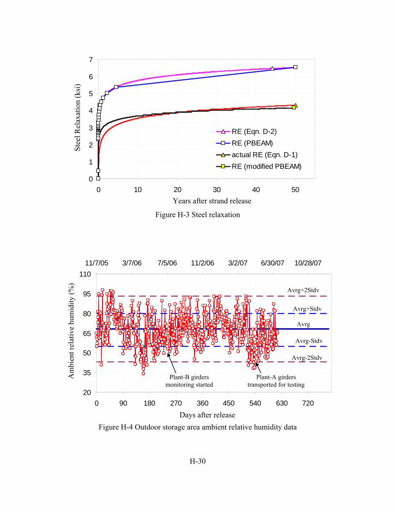
H-30

Figure H-3 Steel relaxation

Figure H-4 Outdoor storage area ambient relative humidity data

0

1

2

3

4

5

6

7

0 10 20 30 40 50

RE (Eqn. D-2)RE (PBEAM)actual RE (Eqn. D-1)RE (modified PBEAM)

Stee

l Rel

axat

ion

(ksi

)

Years after strand release

20

35

50

65

80

95

110

0 90 180 270 360 450 540 630 720

11/7/05 3/7/06 7/5/06 11/2/06 3/2/07 6/30/07 10/28/07

Avrg

Avrg+Stdv

Avrg+2Stdv

Avrg-Stdv

Avrg-2Stdv

Days after release

Am

bien

t rel

ativ

e hu

mid

ity (%

)

Plant-B girders monitoring started

Plant-A girders transported for testing