coordinating vulnerable supply chains with option contracts

Liu, et al. Coordinating vulnerable supply chains

1

Coordinating vulnerable supply chains with option contracts

Zhongyi Liu

Shengya Hua*

Guanying Wang

* Corresponding author

School of Management,People’s Public Security University of China

[email protected]

School of Economics and Management, South China Normal University

[email protected]

College of Management and Economics, Tianjin University

[email protected]


2

Coordinating vulnerable supply chains with option contracts Abstract: We investigate vulnerable supply chain coordination with an option contract in the presence of supply chain disruption risk caused by external and internal disturbances. The supply chain consists of a single risk-neutral supplier and a risk-averse retailer. We characterise the retailer’s order quantity decision under the Conditional Value-at-Risk (CVaR) criterion and the supplier’s production decision. The results show that facing disruption risk and risk-aversion, both the retailer and the supplier would be more prudent to order and produce less than the risk-neutral scenario, inducing damage to the supply chain performance. The number of options purchased is decreasing in disruption risk and the risk-aversion of the retailer. The supplier will increase production as the disruption risk decreases or the shortage penalty increases. When the supplier does not know the risk-aversion of the retailer, the former will produce more and bear a higher overstock risk. We also investigate conditions that facilitate vulnerable supply chain coordination and find that the existence of risk-aversion and disruption risk restrict the option price and exercise price to lower price levels. Finally, we compare the option contract with wholesale price contract from the supplier’s and retailer’s perspectives through a numerical study. Keywords: supply chain coordination; disruption risk; option contract; risk-averse retailer 1. Introduction

The trends of globalization and international trade have motivated companies to extend their supply chains to other countries and continents to reduce production costs and improve competitiveness (Kamalahmadi and Parast, 2017). However, supply chains have become more vulnerable because of external risks such as natural disasters, terrorism, and political instability, and these are difficult or impossible to predict. For example, when hurricane Harvey struck Texas in 2017, 33% of chemical production in the U.S. was disrupted and multiple related industries suffered losses (Spend Matters, 2018). On June 18, 2018, a powerful earthquake hit Osaka Japan and surrounding areas, and some larger businesses, such as Honda Motor, Panasonic, were forced to suspend production (Bloomberg, 2018). A series of these events increases the vulnerability of the supply chain and imposes severe costs to supply chain members.

Supply chain instability caused by inherent risks, such as production discontinuation, understock/overstock, quality defects, and profit volatility, occurs irregularly but persistently in all industries (Sterman, 2006). For instance, the six-week strike starting


3

September 16, 2019, by the United Automobile Workers (UAW) against General Motors (GM) had a huge effect on GM’s bottom line. It essentially stopped production at more than 30 GM factories and slowed production for auto parts suppliers in the US and Mexico. As a result, the automaker's losses during the strike were up to 1.75 billion U.S. dollars, according to the estimation by the Anderson Economic Group (Campbell, 2019). In addition, the mismatch between supply and demand remains a top concern in supply chain management. Take the energy sector as an example. The installed capacity of renewable energy is highly inconsistent with actual power generation. Installed capacity of wind power has grown at an average rate of 24% per year in the past decade, but it only satisfies 2% of global demand, significantly below its actual supply capacity of 14.7% of the global electricity consumption in 2012. In 2013, wind power represented the largest capacity among the intermittent renewable sources with 318 GW, but an estimated 212 GWh of electricity generated by the existing capacity were not transmitted to the grid (Lacerda and van den Bergh, 2016). This disparity also prevalently exists in the apparel, toy, and semiconductor industries (Liu et al., 2014). Left unaddressed, these supply chain instabilities negatively affect a firm’s performance. As measured by equity volatility in Hendricks and Singhal (2014), the mean abnormal equity volatility increases by 5.62% for production disruptions, 11.19% for excess inventory, and 6.28% for production delays over a 2-year period around the announcement date of a demand-supply mismatch.

The above external and internal factors that cause disruptions expose supply chain operations to risk and increase their vulnerability. There has thus been growing interest from firms seeking ways to improve flexibility for mitigating supply chain risks (Tang and Tomlin, 2008). One strategy widely used by practitioners is an option contract, as it can hedge various kinds of risks and increase the supply chain’s flexibility to market changes. Originally, options specifying policies between two parties for a future transaction on an asset were introduced in the financial market. They were then introduced into the supply chain realm as instruments for hedging risks induced by demand and price uncertainty. The option contract has been widely employed to manage risks in high-tech organizations, such as the Taiwan Semiconductor Manufacturing Company Limited, Hewlett-Packard Company, and China Telecom Corporation Limited (Luo and Chen, 2015).

In academia, it has been proven that an option contract can enhance a supply chain’s flexibility and coordinate a decentralised supply chain in a risk-neutral setting, where managers makes decisions to maximize expected profits (Zhao et al., 2010). However, there is evidence show that order quantity decisions are not always consistent with profit maximization (Fisher and Raman, 1996; Schweitzer and Cachon, 2000; Feng et al., 2011). Large leaders, such as the supplier, are considered risk neutral since they can diversify


4

their assets across multiple firms. But followers, such as the retailer, are risk averse because their employment security and incomes are tied to one firm (Wiseman and Gomez-mejia, 1998). The ability for an option contract to coordinate and improve the performance of a supply chain in a risk-averse setting thus warrants further investigation.

Motivated by the above phenomena and observations, in this paper, we study the vulnerable supply chain coordination problem and fully consider disruption risks and the retailer’s risk-aversion within a game between a supplier and a retailer that includes the opportunity to invest in an option contract. The disruption discussed in this study can be caused by both external or inherent risks. The retailer is assumed to make decisions under the CVaR criteria, which has better computational characteristics and has emerged as a practical approach for modelling risk aversion with wide applications in finance and insurance (Fan, Feng and Shou, 2020).

By analysing the Stackelberg game between the supplier and retailer, we derive the equilibrium and find that the retailer’s order quantity and supplier’s production quantity are influenced by the channel disruption risk and risk-aversion attitude. Compared with the risk-neutral case, we find that the option or exercise price must be lower to coordinate the supply chain in the risk-averse case. Moreover, to ensure that a supply chain has a positive coordinated production quantity, the disruption probability should be low, and the existence of disruption risk restricts the upper bounds of the option and exercise prices. Finally, through some numerical experiments, we compare the option contract with wholesale contract and observe that the option contract can help the supply chain hedge against disruption risk more effectively and improve the channel performance as long as the product marginal profit is not too low. Out results offer useful suggestions on operational decision for firms facing disruption risks and risk-aversion attitude, and provide new direction for supply chain managers to manage disruption risks, such as disruption risk forecasting, risk preference identification and information sharing. There are three contributions of this research: (1) an option contract is considered to coordinate a vulnerable supply chain for the first time, (2) disruption risk and risk-aversion are incorporated into a two-echelon supply chain, and (3) conditions that facilitate vulnerable supply chain coordination are explored.

The reminder of this paper is organised as follows. We review the related literature in section 2. The problem description and basic model is provided in section 3. In section 4, we characterise the risk-neutral and risk-averse retailer’s optimal order decisions, provide the risk-neutral supplier’s optimal production decision. In section 5, we explore the conditions under which the supply chain may be coordinated in a risk-averse setting and compare option contracts with wholesale price contracts by a numerical study. We summarise our conclusions and possible extensions in section 6.


5

2. Literature review Our work is closely related to the literature in supply chain disruption and coordination with option contracts. We review relevant papers from these two fields first and then explain how our work contributes to the disruption and option contracts literature.

Disruption risk has been recognised as one of the major challenges to supply chain management (Guo et al., 2016). Two main factors may cause supply chain disruptions. One is the external risks imposed on a supply chain by natural and man-made disasters such as earthquakes, floods, hurricanes, terrorist attacks, and economic crises (Anaya-Arenas et al., 2014). The other is the internal risks arising from the operations of the supply chain such as production disruptions, excess inventory, and product introduction delays (Hendricks and Singhal, 2014).

To improve disruption risk management, several mitigation strategies have been studied, such as inventory mitigation and multi-channel sourcing (e.g., Tomlin, 2006; Van Mieghem, 2007; Simchi-Levi et al., 2018; Sun and Van Mieghem, 2018). Tomlin (2006) considers that a firm can source from two suppliers, one unreliable and low-cost and one reliable and high-cost, and finds that the firm will adopt a pure mitigation strategy, i.e., carrying inventory, single-sourcing from the reliable supplier, or passive acceptance. As disruptions become less frequent but more persistent, sourcing mitigation is increasingly favoured over inventory mitigation. Contingent rerouting may also be optimal, but mitigation rather than contingent rerouting tends to be optimal if disruptions are rare. Ray and Jenamani (2014) investigate the application of multi-sourcing strategies in supply disruption risk management. Following the newsvendor framework, they study the order allocation problem for a risk-neutral and risk-averse retailer separately. Considering two unreliable suppliers, one facing disruption risk and the other facing random yield risk, Li (2015) provides the conditions under which sole- or dual-sourcing strategies should be used. Hou and Hu (2015) consider a capacity reservation contract, a make-to-order contract, and a buy-back contract, separately, in a two-channel sourcing supply chain and compare the values of these contracts from the retailer’s perspective. When a supply chain is composed of three echelons and the most upstream supplier is prone to disruption, Ang et al. (2017) explore the downstream manufacturer’s sourcing problems, Schorpp et al. (2018) study the contract design between adjacent echelons. Lucker et al. (2018) study the inventory and capacity reservation strategies when each echelon is prone to disruption. They conclude that downstream echelon should hold at least as much risk mitigation inventory as the upstream echelon and hold more reserve capacity downstream than upstream.


6

Although the above studies prove that disruption risk management can be improved by different mitigation strategies, some of them only consider a single decision maker’s behaviour and others are based on the wholesale price contracts, and do not consider supply chain coordination. Our work contributes to this strand of literature by considering the coordination of a supply chain facing disruption risk and the purchasing contract between the supplier and retailer as an option contract, which is rarely studied in the background of supply chain disruption.

Another closely related strand of literature is supply chain coordination with option contracts. Options, as financial instruments, have been studied in a large body of literature on finance (e.g., Ross, 1976; Bakshi et al., 1997; Eraker, 2004; Andersen et al., 2017). However, in the field of operations management, it has been shown that option contracts are helpful in risk sharing between supply chain members and improving supply chain performance. Barnes-Schuster et al. (2002) study the role of options in a buyer-supplier system. They illustrate how options in a two-period model provide flexibility to a buyer to respond to market changes and find the conditions that facilitate supply chain coordination. Wang and Liu (2007) develop a single-period model to study coordination and risk sharing in a retailer-led supply chain. Under this structure, they find two conditions, namely a negative correlation between exercise price and option price and a lower commitment order, should be satisfied in order to coordinate a supply chain. By using cooperative game theory, Zhao et al. (2010) find that an option contract can coordinate a supply chain with Pareto-improvement.

Some studies explore the application of option contracts when one or two supply chain members are risk averse. Feng and Wu (2018) find that an option contract can benefit the supplier under the mean-variance criteria. When a retailer is risk averse and optimizes his mean-variance utility, Zhuo et al. (2018) find that supply chain coordination is not always achieved with an option contract. Considering a spot market and demand information updating, Zhao et al. (2018) study the design of option contracts for supply chain coordination. Chen et al. (2014) find that an option contract that can coordinate a supply chain always exists when the retailer is loss-averse and the supplier is risk-neutral, and their result shows that the retailer’s loss-averse coefficient has a significant influence on the contract design. In this paper, we extend the above study by considering supply risk. We find that not only the retailer’s risk-averse, but also the channel disruption risk and supplier’s shortage penalty cost will impact the contract design. Moreover, we use the CVaR to characterize his risk preference. As far as we know, the CVaR measure starts from Rockafellar and Uryasev (2000, 2002), in which CVaR and its formula are first proposed. Following the fundamental properties of CVaR,


7

the traditional newsvendor model with the risk preferences has been examined extensively (Chen et al., 2019; Kouvelis et al., 2019; Murarka et al., 2019).

Among the extent literatures, there is a dearth of application of CVaR measure in option contract analysis (Fan et al., 2020). Liu et al. (2019) is among the few papers that investigates the coordination of both the supplier-led and retailer-led supply chains under option contract and CVaR criterion. They prove that both the supplier-led and the retailer-led supply chains can be coordinated under the same conditions. Although the above studies show that option contracts can improve the performance of supply chains in different cases, the risk faced by the supply chain members only comes from uncertain market demand. Our work contributes to this literature by considering supply chain disruption risk management with option contract and CVaR criterion, and investigating how to design an option contract to coordinate a vulnerable supply chain.

3. Model description We consider a single period problem with a two-echelon supply chain consisting of one supplier and one retailer. The retailer purchases products from the supplier to satisfy a stochastic market demand 𝐷 with probability density function 𝑓(𝑥) and cumulative distribution function 𝐹(𝑥). The supplier is subject to an external random disruption risk with probability 𝑟, 𝑟 ∈ [0,1], and implements all-or-nothing delivery, which means the supplier can deliver all products to the retailer if there is no disruption but none if a disruption occurs. The supplier sells products to the retailer via an option contract with exogenous option price 𝑐! and exercising price 𝑐". Before the selling season starts, the retailer decides the number of options he will purchase and places his option order at unit cost 𝑐!. Each option gives retailer the right (but not the obligation) to buy one unit at the exercising price 𝑐". After receiving the retailer’s order, the supplier invests in capacity and begins to produce at unit cost 𝑐. Let 𝑀 to denote the retailer’s order size and 𝑄# the supplier’s production quantity.

Once the selling season starts and the demand is realised, the retailer decides whether to exercise options according to the market demand information. If the number of options the retailer exercises is greater than the supplier’s production quantity 𝑄#, a penalty cost for each unsatisfied exercising option 𝑧 is incurred. Here 𝑧 may represent the unit cost of some emergency measures, like purchasing from a spot market or asking workers to work overtime, the supplier implements to satisfy the retailer’s requirement. The retailer sells the product to end customers at retail price 𝑝. In this problem, we consider products with a short life cycle or otherwise have little salvage value, so, without loss of generality, we assume the salvage value is zero and there is no penalty for the retailer in the occurrence of a stockout. In order to avoid trivialities, we assume 𝑐 <


8

𝑐! + 𝑐" < 𝑝, ensuring the supply chain partner’s reservation payoff is positive, and 𝑧 >𝑐, ensuring that the supplier only takes emergency measures when necessary. Notations are summarised in Table 1.

Table 1. Notations. 𝑐: supplier’s unit production cost 𝑝: retailer’s retail price 𝑐!: unit option price 𝑐": unit option exercise price 𝑧: supplier’s unit shortage penalty cost 𝑀$ , 𝑀%: risk-neutral and risk-averse retailer’s order quantity, respectively 𝑄#: supplier’s production quantity 𝑄: integrated supply chain’s production quantity 𝑟: probability of supply chain disruption 𝐷: stochastic market demand 𝑓(𝑥): probability density function of demand 𝐹(𝑥): cumulative distribution function of demand 𝜋$: retailer’s expected profit Π$: supplier’s expected profit 𝑖 = 𝑑, 𝑛: a subscript, 𝑖 = 𝑑/𝑛 means disruption risk exists/does not exist Γ: integrated supply chain’s expected profit

Previous studies focus on risk-neutral players who maximise expected profits. In this paper, we consider the retailer as a risk-averse decision maker who is sensitive to disruption risks. The risk faced by the retailer is measured by the CVaR criterion, which is widely used in the financial and insurance industries (Rockafellar and Uryasev, 2000, 2002). The CVaR criterion measures the average profit falling below the 𝜂-quantile level and has better computational characteristics than alternative methods. By denoting the retailer’s random profit as 𝜋(𝑥, 𝐷), the retailer’s 𝜂-CVaR value under an inventory policy 𝑥 is defined as

𝐶𝑉𝑎𝑅%(𝜋(𝑥, 𝐷)) = 𝐄[𝜋(𝑥, 𝐷)|𝜋(𝑥, 𝐷) ≤ 𝑞%(𝜋(𝑥, 𝐷))],

where 𝑞%(𝜋(𝑥, 𝐷)) is the 𝜂-quantile of 𝜋(𝑥, 𝐷), which is

𝑞%(𝜋(𝑥, 𝐷)) = 𝑖𝑛𝑓{𝑧|𝑃(𝜋(𝑥, 𝐷) ≤ 𝑧) ≥ 𝜂}.

Rockafellar and Uryasev (2000, 2002) show that the 𝜂-CVaR value can also be written as

𝐶𝑉𝑎𝑅%(𝜋(𝑥)) = max&∈(

{𝛼 + )%𝐄(𝜋(𝑥, 𝐷) − 𝛼)*}

= max&∈(

{𝛼 − )%𝐄(𝛼 − 𝜋(𝑥, 𝐷))+}, (1)


9

where 𝛼 is a real number and 𝜂(0 < 𝜂 ≤ 1) is the risk aversion parameter. As 𝜂 decreases and close to 0, the retailer becomes less risk averse. For the convenience of calculation, we adopt the definition of CVaR in equation (1) in our work.

4. Retailer’s and Supplier’s problems 4.1. Risk-neutral retailer’s order decision In this section, we investigate the risk-neutral retailer’s optimal order policy as the benchmark case. In this case, the retailer’s objective is to maximise expected profit. Suppose the retailer purchases via an option contract when facing disruption risk and when not. These two scenarios are compared, and managerial insights are provided.

When there is no disruption risk (𝑟 = 0 and 𝑖 = 𝑛) and the retailer is risk-neutral, the retailer’s expected profit function can be expressed as

𝜋,(𝑀,) = 𝐄[𝑝min(𝑀,, 𝐷) − 𝑐!𝑀, − 𝑐"min(𝑀,, 𝐷)], (2)

where 𝑚𝑖𝑛(𝑀,, 𝐷) is the number of exercised options. The first term in the expectation in Equation (2) is the retailer’s sales revenue, and the last two terms are the cost of buying and exercising options, respectively. By analysing the first-order-condition, we obtain the retailer’s optimal order quantity, as stated in Lemma 1.

Lemma 1. When there is no disruption risk, the risk-neutral retailer’s optimal order quantity is 𝑀,

∗ = 𝐹*)(1 − .!/*."

).

All proofs are in the Appendix for conciseness. From Lemma 1, we know (𝑝 −𝑐")𝐹U(𝑀,

∗) = 𝑐!, where 𝐹U(⋅) = 1 − 𝐹(⋅). The left-hand side of the former equation is the expected marginal profit of selling one more product, and the right-hand side is the marginal cost of buying one more option. The retailer’s optimal order quantity approaches the intersection of marginal cost and marginal profit. Note that the option and exercise prices negatively impact the retailer’s order quantity, i.e. the higher either price is, the fewer options the retailer purchases.

When disruption risk exists in the supply chain (𝑟 > 0 and 𝑖 = 𝑑), the retailer’s expected profit is

𝜋0(𝑀0) = (1 − 𝑟)𝜋,(𝑀0) + 𝑟(−𝑐!𝑀0) (3) = (1 − 𝑟)(𝑝 − 𝑐")𝐄[min(𝑀0 , 𝐷)] − 𝑐!𝑀0.

Here, 𝜋,(𝑀0) is the retailer’s expected profit without supply chain disruptions. However, if a disruption occurs, the retailer suffers a loss 𝑐!𝑀0. Recall that the supplier implements all-or-nothing delivery in the presence of disruption risk, and the retailer receives nothing when a disruption occurs. Moreover, we assume that both the supplier


10

and retailer know the disruption probability, and once a disruption occurs, the supplier cannot implement any emergency measures to obtain other products to satisfy the retailer’s order. Because the disruption is caused by external factors like natural disasters, the supplier won’t compensate the retailer for the unsatisfied order when a disruption occurs, and the retailer loses 𝑐!𝑀0.

By analysing the first-order-condition of equation (3), we obtain the retailer’s optimal order quantity in the presence of disruption risk as follows.

Proposition 1. When there is disruption risk, the risk-neutral retailer’s optimal order quantity is

𝑀0∗ = W

𝐹*)(1 − .!()*2)(/*.")

), if𝑟 ≤ 1 − .!/*."

,

0, if𝑟 > 1 − .!/*."

.

Proposition 1 generalises Lemma 1 by considering disruption risk. It shows that if the probability of disruption risk is high, i.e. 𝑟 > 1 − .!

/*.", the retailer does not place an

order. If the probability of disruption risk is low, i.e. 𝑟 ≤ 1 − .!/*."

, the retailer purchases

options. When the order quantity is positive, the retailer’s order quantity is not only sensitive to the option price but is also influenced by the disruption risk. The number of options the retailer purchases is decreasing in the level of supply chain disruption risks. Next, we compare the retailer’s actions with and without disruption risk.

Corollary 1. In presence of disruption risk, the risk-neutral retailer orders less, i.e., 𝑀0∗ ≤ 𝑀,

∗ .

From corollary 1, the disruption risk leads the retailer to order less to avoid profit loss. Consequently, the supply chain’s performance is affected by the disruption risk, which implies the supply chain could be improved.

When 𝑟 = 0, equation (3) degenerates to equation (2) with no disruptions. That is to say, the no-disruption scenario is a special case of the disruption scenario. Therefore, we only focus on the disruption scenario in the following analyses.

4.2. Risk-averse retailer’s order decision As mentioned before, the retailer isn’t always risk-neutral, especially when there is disruption risk. In what follows, we further explore the risk-averse retailer’s order decision in the presence of disruption risk. In this case, the retailer’s objective is to maximise the CVaR value but not expected profit. Specifically, we obtain the retailer’s CVaR value by substituting equation (3) into equation (1).


11

𝐶𝑉𝑎𝑅%(𝜋0(𝑀%)) = max&∈(

{𝛼 − )%𝐄[𝛼 − (−𝑐!𝑀% + (1 − 𝑟)(𝑝 − 𝑐")min(𝑀% , 𝐷)]+} (4)

By solving the above maximization problem, we obtain the retailer’s optimal decision as follows.

Proposition 2. The risk-averse retailer’s optimal order quantity is

𝑀%∗ = W

𝐹*)(()*2)(/*.")*.!()*2)(/*.")

𝜂), if𝑟 ≤ 1 − .!/*."

,

0, if𝑟 > 1 − .!/*."

.

From Proposition 2 we can see that the retailer’s order decision is affected by both the disruption probability and the retailer’s risk aversion. The number of options ordered is negatively related to the retailer’s risk-aversion (i.e. a smaller 𝜂). However, compared with Proposition 1, the threshold value of the disruption probability (i.e., 1 − .!

/*.") is the

same regardless of whether the retailer’s risk preference.

Corollary 2. Facing disruption risk, the risk-averse retailer’s order quantity is less than that of the risk-neutral retailer, i.e., 𝑀%

∗ ≤ 𝑀0∗ .

Similar to our results, Wang and Webster (2007) describe the retailer’s decision-making behaviour with prospect theory. They find that the loss-averse retailer orders less than a risk-neutral retailer, but they derive the results for the wholesale price contract and ignore the impact of disruption risk. We compensate for this by analysing a vulnerable supply chain with a more flexible two-tariff contract in a risk-averse setting. Combined with corollaries 1 and 2, we obtain 𝑀%

∗ ≤ 𝑀0∗ ≤ 𝑀,

∗ . This result implies that, in the presence of disruption risk and risk-aversion, the retailer would be more prudent to order less to avoid loss compared to a risk-neutral framework.

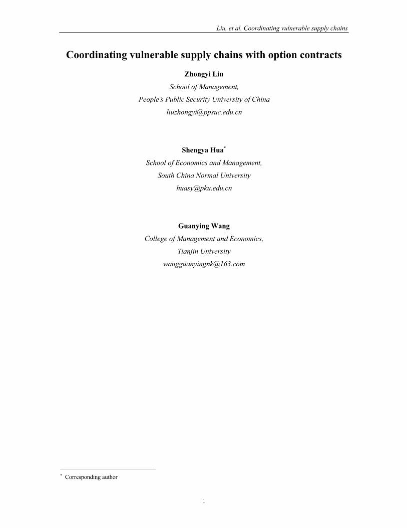
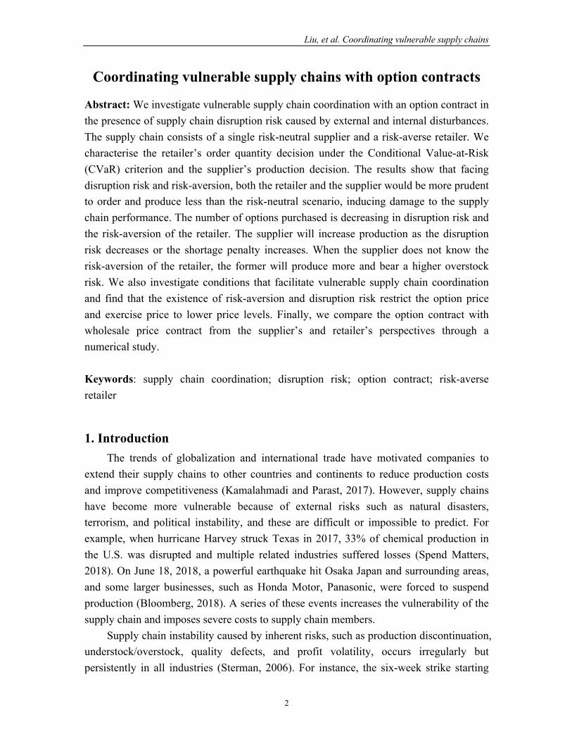
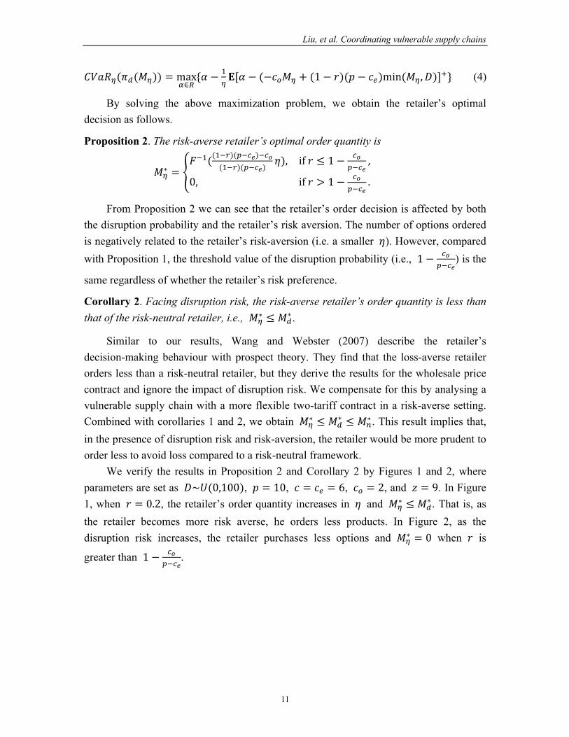
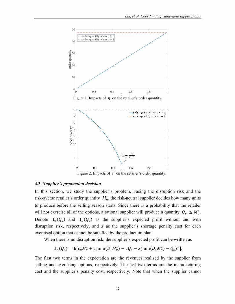
We verify the results in Proposition 2 and Corollary 2 by Figures 1 and 2, where parameters are set as 𝐷~𝑈(0,100), 𝑝 = 10, 𝑐 = 𝑐" = 6, 𝑐! = 2, and 𝑧 = 9. In Figure 1, when 𝑟 = 0.2, the retailer’s order quantity increases in 𝜂 and 𝑀%

∗ ≤ 𝑀0∗ . That is, as

the retailer becomes more risk averse, he orders less products. In Figure 2, as the disruption risk increases, the retailer purchases less options and 𝑀%

∗ = 0 when 𝑟 is

greater than 1 − .!/*."

.


12

Figure 1. Impacts of 𝜂 on the retailer’s order quantity.

Figure 2. Impacts of 𝑟 on the retailer’s order quantity.

4.3. Supplier’s production decision In this section, we study the supplier’s problem. Facing the disruption risk and the risk-averse retailer’s order quantity 𝑀%

∗, the risk-neutral supplier decides how many units to produce before the selling season starts. Since there is a probability that the retailer will not exercise all of the options, a rational supplier will produce a quantity 𝑄# ≤ 𝑀%

∗. Denote Π,(𝑄#) and Π0(𝑄#) as the supplier’s expected profit without and with disruption risk, respectively, and 𝑧 as the supplier’s shortage penalty cost for each exercised option that cannot be satisfied by the production plan.

When there is no disruption risk, the supplier’s expected profit can be written as

Π,(𝑄#) = 𝐄[𝑐!𝑀%∗ + 𝑐"min(𝐷,𝑀%

∗) − 𝑐𝑄# − 𝑧(min(𝐷,𝑀%∗) − 𝑄#)+].

The first two terms in the expectation are the revenues realised by the supplier from selling and exercising options, respectively. The last two terms are the manufacturing cost and the supplier’s penalty cost, respectively. Note that when the supplier cannot


13

satisfy all of the retailer’s option exercising requirements, the former can implement emergency measures to obtain extra products with a higher unit cost 𝑧. Therefore, the supplier can fulfil the retailer’s order and deliver 𝑚𝑖𝑛(𝐷,𝑀%

∗) units to the retailer. When disruption risk exists, the supplier’s expected profit can be expressed as

Π0(𝑄#) = 𝐄[(1 − 𝑟)Π,(𝑄#) + 𝑟(𝑐!𝑀%∗ − 𝑐𝑄#)] (5)

= 𝑐!𝑀%∗ − 𝑐𝑄# + (1 − 𝑟)𝐄[𝑐"min(𝐷,𝑀%

∗) − 𝑧(min(𝐷,𝑀%∗) − 𝑄#)+].

Equation (5) shows that the supplier earns profit Π,(𝑄#) with probability 1 − 𝑟, where 𝑐!𝑀%

∗ is the revenue the supplier earns from selling options and 𝑐𝑄# is the production cost. All of the money is transferred before a supply chain disruption occurs. When the supplier suffers from a disruption risk, nothing is delivered to the retailer and there is zero revenue. Thus, the supplier earns profit 𝑐!𝑀%

∗ − 𝑐𝑄# with probability 𝑟. By solving the above maximization problem, we obtain the supplier’s optimal

production decision as follows.

Proposition 3. The risk-neutral supplier’s optimal production quantity is

𝑄#∗ = ^𝑄)∗, if𝑧 < �̂�,𝑀%∗ , if𝑧 ≥ �̂�,

where 𝑄)∗ = 𝐹*) `1 − .()*2)4

a and �̂� = (/*.").()*2)()*%)(/*.")+.!%

.

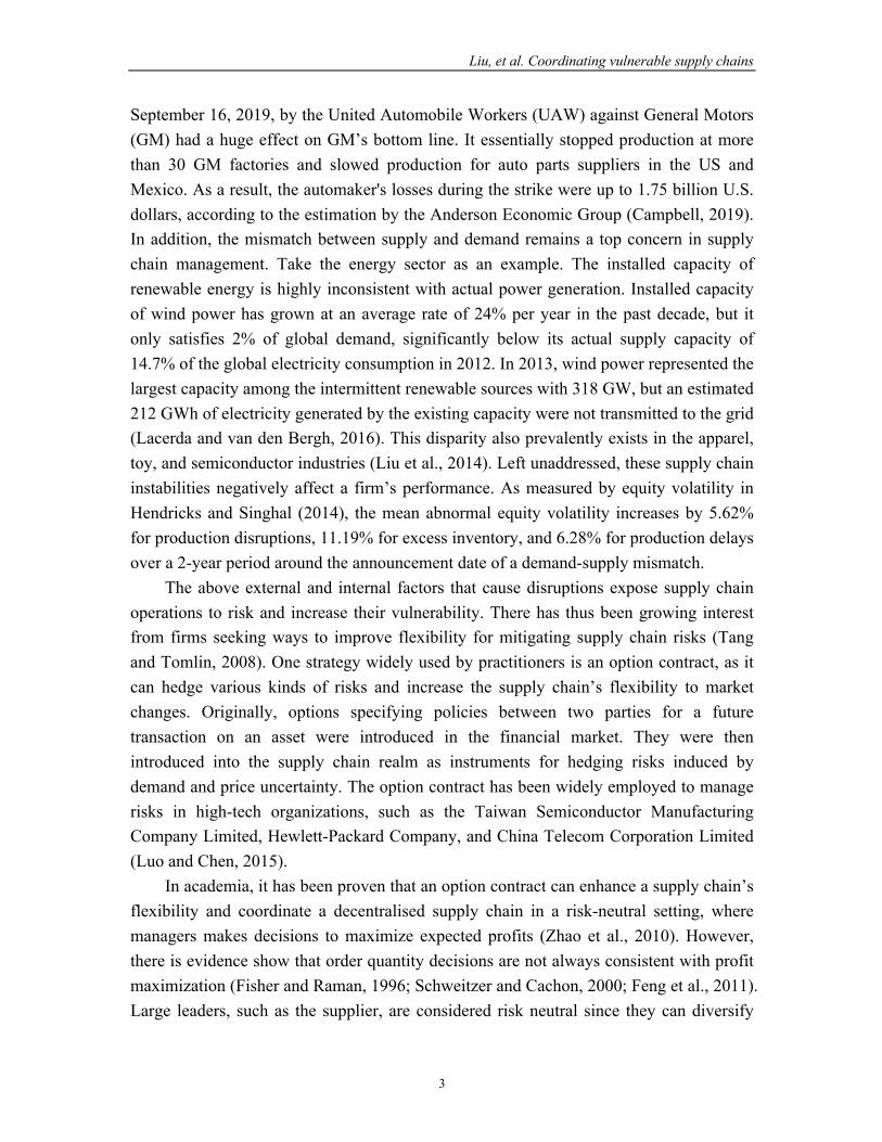
Proposition 3 indicates that if the shortage penalty cost 𝑧 is less than the critical value �̂�, the supplier will choose to produce quantity 𝑄)∗, which is less than the retailer’s option order quantity 𝑀%

∗. When 𝑧 is low, the cost caused by understock risk is lower for the supplier. This leads to less production to reduce the overstock risk, as depicted by Figure 3 when 𝐷~𝑈(0,100) , 𝑝 = 10 , 𝑐 = 𝑐" = 6 , 𝑐! = 2 , 𝑟 = 0.2 , and 𝜂 = 0.8 . From the definition of 𝑄)∗, note that 𝑄)∗ is increasing in 𝑧 and decreasing in 𝑟. That is to say, a larger unit penalty cost 𝑧 or smaller disruption probability is related to increased supplier production. Additionally, note that 𝑄)∗ is independent of option and exercise prices, which is counterintuitive. We refer to equation (5) to explain this. Given the retailer’s order quantity 𝑀%

∗, the revenue the supplier can obtain from selling options is fixed. Meanwhile, as the supplier can deliver 𝑚𝑖𝑛(𝐷,𝑀%

∗) units to the retailer by implementing emergency measures when necessary if disruption does not occur, the expected revenue from satisfying exercising options is also fixed. Then, no matter what the value of 𝑄)∗ is, the total revenue the supplier can obtain according to the option contract is fixed, i.e., 𝑄)∗ is independent of the contract parameters 𝑐! and 𝑐" . According to the definition, we know the key factors influencing the supplier’s production plan are the production cost, penalty cost, and disruption risk.


14

When the shortage penalty cost 𝑧 is greater than the critical value �̂�, the supplier will produce all the options because the understock risk is too high. By analysing the expressions of 𝑄)∗ and 𝑀%

∗, we know that a higher disruption probability leads to lower production.

Figure 3. Impacts of 𝑧 on the supplier’s production quantity.

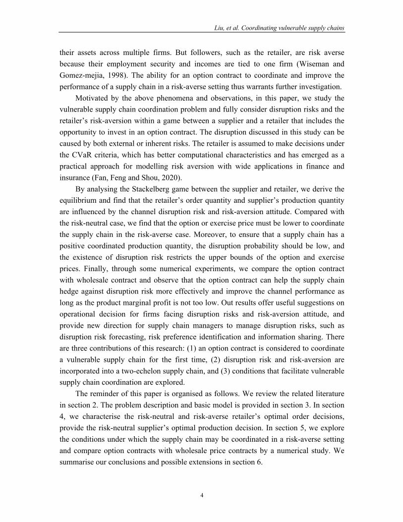
When the retailer is risk-neutral, the supplier’s production quantity is 𝑄#∗(𝜂 = 1).

We compare the supplier’s production quantities when cooperating with a risk-neutral and risk-averse retailer and obtain the following proposition.

Proposition 4. When the retailer is risk-averse, the supplier produces less products than that in the case where the retailer is risk-neutral, i.e., 𝑄#∗(𝜂 ≤ 1) ≤ 𝑄#∗(𝜂 = 1).

Proposition 4 shows the importance of information sharing between supply chain members. If there is information asymmetry between the supplier and retailer regarding the retailer’s risk preference, the supplier may produce more products and the overstock risk is much higher. The impact of the retailer’s risk averse degree 𝜂 on the production quantity is shown in Figure 4. We can observe that when the retailer is not too risk averse, the asymmetric information on 𝜂 will not impact the production quantity. However, when the retailer is very risk averse, information asymmetry will significantly influence the production quantity.


15

Figure 4. Impacts of 𝜂 on the supplier’s production quantity.

The research of Zhao et al. (2010) proves that a supply chain can be coordinated in a

risk-neutral scenario using an option contract. Yet as concluded before, facing risk-aversion and supply chain disruption risk, both the retailer and supplier order and produce less than the risk-neutral scenario. In what follows, we explore the conditions that facilitate supply chain coordination.

5. Advantage of option contract 5.1. Supply chain coordination

In a decentralised supply chain, both parties make their decisions independently, resulting in less efficient supply chain performance compared to an integrated supply chain, which is generally known as the double marginalization phenomenon (Spengler, 1950). In this section, we study how to design a proper option contract in order to coordinate the vulnerable supply chain.

Following the definition in Gan et al. (2004, 2005), for a supply chain consisting of one risk-neutral supplier and one risk-averse retailer, the option contract agreed upon by the two agents coordinates the supply chain if (1) each agent’s individual rationality or participation condition is satisfied, (2) the retailer’s CVaR criteria is maximised, and (3) the integrated supply chain’s expected profit is maximised. The first condition can be satisfied if the two agents’ individual profits are greater than zero. The second condition has also been studied in section 4. Hence, based on the above analyses, we only focus on the third condition in what follows.

From the whole supply chain’s perspective, the total expect profit, denoted Γ(𝑄), is

Γ(𝑄) = (1 − 𝑟)𝐄[𝑝min(𝐷, 𝑄) − 𝑐𝑄] + 𝑟(−𝑐𝑄). (6)

By analysing the first-order condition of equation (6), we state the integrated supply chain’s optimal decision in the following proposition.


16

Proposition 5. The integrated supply chain’s optimal order quantity is

𝑄∗ = c𝐹*) d1 −

𝑐(1 − 𝑟)𝑝e , if𝑟 ≤ 1 −

𝑐𝑝 ,

0, if𝑟 > 1 −𝑐𝑝 .

Similar to the conclusions of propositions 1 and 2, the integrated supply chain’s production quantity is positive when the disruption probability is lower than a threshold value and equals zero otherwise. However, the threshold values in propositions 1 and 2 are different from those in Proposition 5, implying the centralised supply chain has a different disruption risk tolerance compared to a decentralised supply chain. Specifically, when 𝑐 > /.!

/*.", as when the option price is low, the retailer undertakes less risk, and the

decentralised supply chain has a higher disruption risk tolerance. When 𝑐 < /.!/*."

, as

when the unit production cost is low, the risk faced by the whole supply chain is also low, and the centralised supply chain has a higher disruption risk tolerance.

From Proposition 5, we know the supply chain can be coordinated when 𝑀%∗ ≥

𝑄#∗ = 𝑄∗. Here, note that we only focus on the case when the coordinated product quantity 𝑄∗ > 0. More specifically, combined with Proposition 3, when 𝑧 < �̂�, 𝑄)∗ =𝑄∗ must be satisfied; when 𝑧 ≥ �̂�, 𝑀%

∗ = 𝑄∗ must be satisfied.

Proposition 6. A supply chain may be coordinated if either of the following two conditions is satisfied:

(1) 𝑟 ≤ 1 −max `./, .!/*."

a, 𝑧 = 𝑝 > 𝑐" +/.!%

.*()*2)()*%)/, and 𝑐 > 𝑝(1 − 𝑟)(1 − 𝜂);

(2) 𝑟 ≤ 1 −max `./, .!/*."

a, 𝑧 ≥ 𝑝 = 𝑐" +/.!%

.*()*2)()*%)/, and 𝑐 > 𝑧(1 − 𝑟)(1 − 𝜂).

In condition (1) of Proposition 6, the supplier’s production quantity equals the coordinated production quantity 𝑄∗ and the retailer’s order quantity is greater than 𝑄∗. In condition (2), both the supplier’s production quantity and the retailer’s order quantity equal 𝑄∗.

Proposition 6 implies that a low disruption probability and a risk-neutral retailer facilitate supply chain coordination. In addition, to induce the supplier to produce enough, the penalty cost should be large enough, i.e., 𝑧 ≥ 𝑝.

Proposition 7. If the retailer is risk-neutral (i.e., 𝜂 = 1), the supply chain can be

coordinated when 𝑟 ≤ 1 −max `./, .!/*."

a, 𝑧 ≥ 𝑝 ≥ 𝑐" +/.!.

.


17

Based on Proposition 7, when there is no disruption risk and the supplier implements

a make-to-order policy (𝑟 = 0 and 𝑧 = +∞), the coordination condition is 𝑝 = 𝑐" +/.!.

, which is consistent with the result in Zhao et al. (2010).

To explore the influence of the retailer’s risk aversion on coordination, we set 𝑟 = 0

and 𝑧 = +∞. From the second condition of Proposition 6, the coordination condition is 𝑝 = 𝑐" +

/.!%.*()*%)/

. Since /%.*()*%)/

> /., compared with the risk-neutral case, the option or

exercise price should be lower in the risk-averse case to facilitate coordination. To investigate the influence of disruption risk on coordination, we set 𝜂 = 1 and

𝑧 = +∞ . Besides 𝑝 = 𝑐" +/.!.

, the additional condition to ensure supply chain

coordination is 𝑚𝑎𝑥 `./, .!/*."

a ≤ 1 − 𝑟, i.e. the option or exercise price should be low.

5.2. Comparison between option contracts and wholesale price contracts

In the classical newsvendor problem, it is known that a wholesale price contract cannot coordinate a supply chain. According to the above analyses, we know coordination can be achieved by an option contract with proper parameter settings, which means the option contract performs better than the wholesale price contract from the perspective of a whole supply chain. Next, we compare the two contracts from the supplier’s and retailer’s perspectives through some numerical studies.

Under a wholesale price contract, the retailer’s CVaR value and supplier’s expected revenue can be expressed as follows.


{𝛼 − )%𝐄[𝛼 − (−𝑤𝑀% + (1 − 𝑟)𝑝min(𝑀% , 𝐷)]+}, (7)

Π0(𝑄#) = 𝑤𝑀% − 𝑐𝑄# − 𝑧(1 − 𝑟)(𝑀% − 𝑄#), (8)

where 𝑤 is the wholesale price. When 𝐷~𝑈(0,100), 𝑝 = 10, 𝑐 = 𝑐" = 6, 𝑐! = 2, 𝑤 = 7, 𝜂 = 0.8, and 𝑧 = 9,

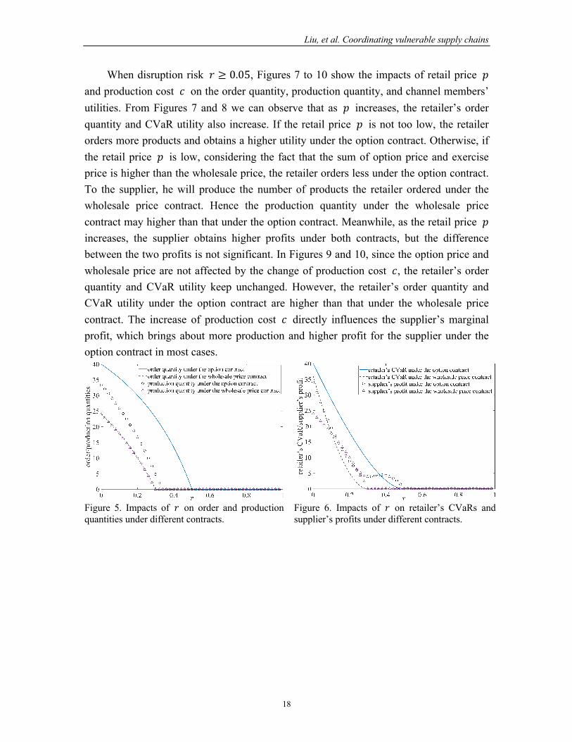
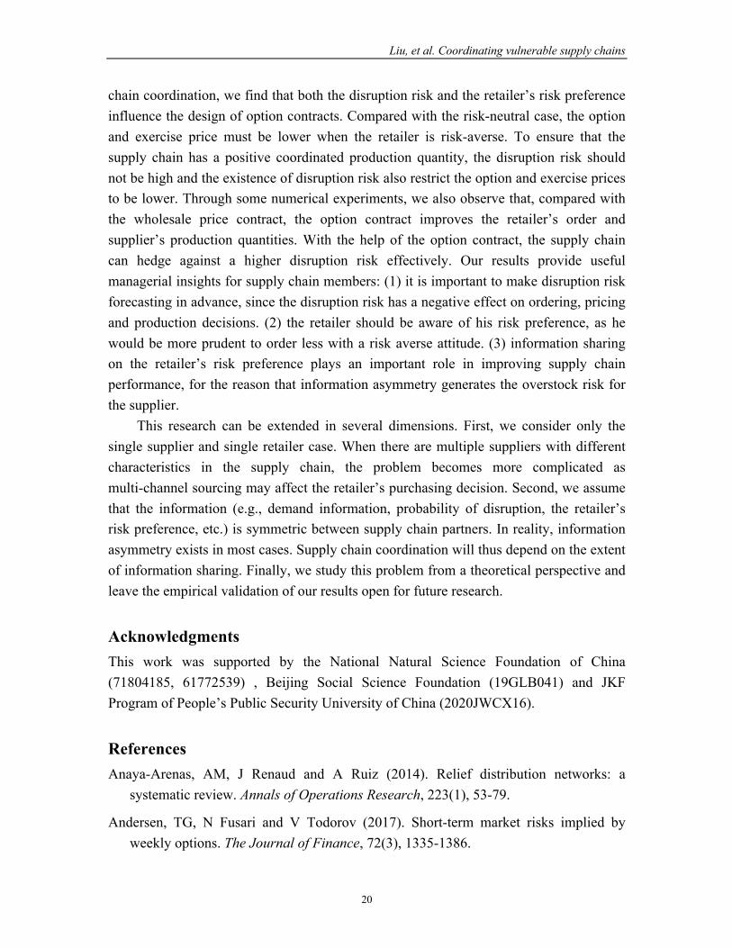
Figure 5 shows the retailer’s order and supplier’s production quantities under an option contract and a wholesale price contract. We can observe that, compared with the wholesale price contract, the retailer orders more and the supplier produces more products under the option contract. Especially, when the disruption risk 𝑟 ≥ 0.3, both the order and production quantities are zero under the wholesale price contract, but the retailer still orders and the supplier produces under the option contract. Then, we know the option contract can help a supply chain hedge disruption risk effectively. Figure 6 illustrates the retailer’s CVaR utilities and supplier’s profits under the two contracts. It shows that the retailer always obtains a higher CVaR utility under the option contract but the supplier may not always obtain a higher profit.


18

When disruption risk 𝑟 ≥ 0.05, Figures 7 to 10 show the impacts of retail price 𝑝 and production cost 𝑐 on the order quantity, production quantity, and channel members’ utilities. From Figures 7 and 8 we can observe that as 𝑝 increases, the retailer’s order quantity and CVaR utility also increase. If the retail price 𝑝 is not too low, the retailer orders more products and obtains a higher utility under the option contract. Otherwise, if the retail price 𝑝 is low, considering the fact that the sum of option price and exercise price is higher than the wholesale price, the retailer orders less under the option contract. To the supplier, he will produce the number of products the retailer ordered under the wholesale price contract. Hence the production quantity under the wholesale price contract may higher than that under the option contract. Meanwhile, as the retail price 𝑝 increases, the supplier obtains higher profits under both contracts, but the difference between the two profits is not significant. In Figures 9 and 10, since the option price and wholesale price are not affected by the change of production cost 𝑐, the retailer’s order quantity and CVaR utility keep unchanged. However, the retailer’s order quantity and CVaR utility under the option contract are higher than that under the wholesale price contract. The increase of production cost 𝑐 directly influences the supplier’s marginal profit, which brings about more production and higher profit for the supplier under the option contract in most cases.

Figure 5. Impacts of 𝑟 on order and production quantities under different contracts.

Figure 6. Impacts of 𝑟 on retailer’s CVaRs and supplier’s profits under different contracts.


19

Figure 7. Impacts of 𝑝 on order and production quantities under different contracts.

Figure 8. Impacts of 𝑝 on retailer’s CVaRs and supplier’s profits under different contracts.

Figure 9. Impacts of 𝑐 on order and production quantities under different contracts.

Figure 10. Impacts of 𝑐 on retailer’s CVaRs and supplier’s profits under different contracts.

6. Conclusion In this paper, we investigate a vulnerable supply chain coordination problem with an option contract when a risk-neutral supplier is suffering from disruption risk and the retailer is risk-averse. We characterise the risk-averse retailer’s optimal option order quantity under CVaR criteria and the supplier’s optimal option production quantity. The results show that facing disruption risk and risk-aversion, both the retailer and the supplier would be more prudent to order and produce less than the risk-neutral scenario, inducing damage to the supply chain performance. A higher disruption risk and degree of risk-aversion are negatively related to the number of orders placed. From the supplier’s perspective, the supplier’s optimal production is influenced by the disruption risk shortage penalty. As the disruption risk decreases or the shortage penalty cost increases, the supplier produces more. Further, information sharing is important. When the supplier does not know the retailer’s risk preference (or considers the retailer as risk-neutral), the former will produce more and bear a higher overstock risk. In the analysis of supply


20

chain coordination, we find that both the disruption risk and the retailer’s risk preference influence the design of option contracts. Compared with the risk-neutral case, the option and exercise price must be lower when the retailer is risk-averse. To ensure that the supply chain has a positive coordinated production quantity, the disruption risk should not be high and the existence of disruption risk also restrict the option and exercise prices to be lower. Through some numerical experiments, we also observe that, compared with the wholesale price contract, the option contract improves the retailer’s order and supplier’s production quantities. With the help of the option contract, the supply chain can hedge against a higher disruption risk effectively. Our results provide useful managerial insights for supply chain members: (1) it is important to make disruption risk forecasting in advance, since the disruption risk has a negative effect on ordering, pricing and production decisions. (2) the retailer should be aware of his risk preference, as he would be more prudent to order less with a risk averse attitude. (3) information sharing on the retailer’s risk preference plays an important role in improving supply chain performance, for the reason that information asymmetry generates the overstock risk for the supplier.

This research can be extended in several dimensions. First, we consider only the single supplier and single retailer case. When there are multiple suppliers with different characteristics in the supply chain, the problem becomes more complicated as multi-channel sourcing may affect the retailer’s purchasing decision. Second, we assume that the information (e.g., demand information, probability of disruption, the retailer’s risk preference, etc.) is symmetric between supply chain partners. In reality, information asymmetry exists in most cases. Supply chain coordination will thus depend on the extent of information sharing. Finally, we study this problem from a theoretical perspective and leave the empirical validation of our results open for future research.

Acknowledgments This work was supported by the National Natural Science Foundation of China (71804185, 61772539) , Beijing Social Science Foundation (19GLB041) and JKF Program of People’s Public Security University of China (2020JWCX16).

References Anaya-Arenas, AM, J Renaud and A Ruiz (2014). Relief distribution networks: a

systematic review. Annals of Operations Research, 223(1), 53-79.

Andersen, TG, N Fusari and V Todorov (2017). Short-term market risks implied by weekly options. The Journal of Finance, 72(3), 1335-1386.


21

Ang, E, D Iancu and R Swinney (2017). Disruption risk and optimal sourcing in multitier supply networks. Management Science, 63(8), 2397–2419.

Bakshi, G, C Cao and Z Chen (1997). Empirical performance of alternative option pricing models. The Journal of Finance, 52(5), 2003-2049.

Barnes-Schuster, D, Y Bassok and R Anupindi (2002). Coordination and flexibility in supply contracts with options. Manufacturing & Service Operations Management, 4(3), 171-207.

Bloomberg, K (2018). Osaka earthquake causes auto and electronics plants to suspend operations. The Japan Times, https://www.japantimes.co.jp/news/2018/06/18/business/osaka-earthquake-causes-auto-electronics-plants-suspend-operations/#.Xh6GI1MzZTa.

Campbell, AF (2019). The GM strike has officially ended. Here’s what workers won and lost. https://www.vox.com/identities/2019/10/25/20930350/gm-workers-vote-end-strike.

Chen, X, G Hao and L Li (2014). Channel coordination with a loss-averse retailer and option contracts. International Journal of Production Economics, 150, 52-57.

Chen, Z, K Yuan and S Zhou (2019). Supply chain coordination with trade credit under the CVaR criterion. International Journal of Production Research, 57(11), 3538-3553.

Eraker, B (2004). Do stock prices and volatility jump? reconciling evidence from spot and option prices. The Journal of Finance, 59(3), 1367-1403.

Fan Y, Y Feng and Y Shou (2020). A risk-averse and buyer-led supply chain under option contract: CVaR minimization and channel coordination[J]. International Journal of Production Economics, 219: 66-81.

Feng, T, LR Keller and X Zheng (2011) Decision making in the newsvendor problem: a cross-national laboratory study. Omega, 39(1), 41-50.

Feng, Y and Q Wu (2018). Option Contract Design and Risk Analysis: Supplier’s Perspective. Asia-Pacific Journal of Operational Research, 35(3), 1850017.

Fisher, MA and A Raman (1996). Reducing the cost of demand uncertainty through accurate response to early sales. Operations Research, 44, 87-99.

Gan, X, S Sethi and H Yan (2004). Coordination of supply chains with risk-averse agents. Production and Operations Management, 13(2), 135-149.


22

Gan, X, S Sethi and H Yan (2005). Channel coordination with a risk-neutral supplier and a downside-risk-averse retailer. Production and Operations Management, 14(1), 80-89.

Guo, S, L Zhao and L Xu (2016). Impact of supply risks on procurement decisions. Annals of Operations Research, 241(1), 411-430.

Hendricks, KB and VR Singhal (2014). The effect of demand-supply mismatches on firm risk. Production and Operations Management, 23(12), 2137-2151.

Hou, J and X Hu (2015). Comparative Studies of Three Backup Contracts Under Supply Disruptions. Asia-Pacific Journal of Operational Research, 32(2), 1550006.

Kamalahmadi, M and MM Parast (2017). An assessment of supply chain disruption mitigation strategies. International Journal of Production Economics, 184, 210-230.

Kouvelis, P and R Li (2019). Integrated Risk Management for Newsvendors with Value-at-Risk Constraints. Manufacturing & Service Operations Management, 21(4), 816-832.

Lacerda, JS and JC van den Bergh (2016). Mismatch of wind power capacity and generation: causing factors, GHG emissions and potential policy responses. Journal of Cleaner Production, 128, 178-189.

Li, X (2017). Optimal procurement strategies from suppliers with random yield and all-or-nothing risks. Annals of Operations Research, 257(1), 167-181.

Liu, Z, S Hua and X Zhai (2019). Supply chain coordination with risk-averse retailer and option contract: Supplier-led vs. Retailer-led. International Journal of Production Economics, 107518.

Liu, Z, L Chen, L Li and X Zhai (2014). Risk hedging in a supply chain: Option vs. price discount. International Journal of Production Economics, 151, 112–120.

Lucker, F, S Chopra and RW Seifert (2018). Disruption Risk Management in Serial Multi-Echelon Supply Chains: Where to Hold Risk Mitigation Inventory and Reserve Capacity. Available at SSRN: https://ssrn.com/abstract=3072382 or http://dx.doi.org/10.2139/ssrn.3072382

Luo, J and X Chen (2017). Risk hedging via option contracts in a random yield supply chain. Annals of Operations Research, 257(1), 697-719.

Murarka, U, V Sinha, LS Thakur and MK Tiwari (2019). Multiple criteria risk averse model for multi-product newsvendor problem using conditional value at risk constraints. Information Sciences, 478, 595-605.


23

Ray, P and M Jenamani (2016). Sourcing decision under disruption risk with supply and demand uncertainty: A newsvendor approach. Annals of Operations Research, 237(1), 237-362.

Rockafellar, R and S Uryasev (2000). Optimization of conditional value-at-risk. Journal of risk, 2, 21-42.

Rockafellar, R and S Uryasev (2002). Conditional value-at-risk for general loss distributions. Journal of Banking & Finance, 26(7), 1443-1471.

Ross, SA (1976). Options and efficiency. The Quarterly Journal of Economics, 90(1), 75-89.

Schorpp, G, F Erhun and HL Lee (2018). Multi-Tiered Supply Chain Risk Management. Stanford University Graduate School of Business Research Paper No. 18-9. Available at SSRN: https://ssrn.com/abstract=3117626 or http://dx.doi.org/10.2139/ssrn.3117626.

Schweitzer, M and G Cachon (2000). Decision bias in the newsvendor problem with a known demand distribution: Experimental evidence. Management Science, 46(3), 404-420.

Simchi-Levi, D, H Wang and Y Wei (2018). Increasing supply chain robustness through process exibility and inventory. Production and Operations Management, 27(8), 1476-1491.

Spend Matters Brand Studio (2018). With High Intensity Hurricanes the New Normal, Procurement Must Plan Ahead or Suffer the Consequences. Spend Matters, https://spendmatters.com/2018/11/20/with-high-intensity-hurricanes-the-new-normal-procurement-must-plan-ahead-or-suffer-the-consequences/.

Spengler, J (1950). Vertical integration and antitrust policy. The Journal of Political Economy, 58(4), 347-352.

Sterman, JD (2006). Operational and behavioral causes of supply chain instability. In Carranza O. and F Villegas, (Eds.), The Bullwhip Effect in Supply Chains, pp. 17-56. New York: Palgrave Macmillan.

Sun, J and JA Van Mieghem (2018). Robust dual sourcing inventory management: Optimality of capped dual index policies and smoothing. Manufacturing & Service Operations Management, Forthcoming. Available at SSRN: https://ssrn.com/abstract=2991250 or http://dx.doi.org/10.2139/ssrn.2991250.


24

Tang, C and B Tomlin (2008). The power of flexibility for mitigating supply chain risks. International Journal of Production Economics, 116(1), 12-27.

Tomlin, B (2006). On the value of mitigation and contingency strategies for managing supply chain disruption risks. Management Science, 52(5), 639-657.

Van Mieghem, JA (2007). Risk mitigation in newsvendor networks: Resource diversication, exibility, sharing, and hedging. Management Science, 53(8), 1269-1288.

Wang, C and S Webster (2007). Channel coordination for a supply chain with a risk-neutral manufacturer and a loss-averse retailer. Decision Sciences, 38(3), 361-389.

Wang, X and L Liu (2007). Coordination in a retailer-led supply chain through option contract. International Journal of Production Economics, 110(1), 115-127.

Wiseman, RM and LR Gomez-Mejia (1998) A behavioral agency model of managerial risk taking. Academy of Management Review, 23(1), 133-153.

Zhao, Y, S Wang, T Cheng, X Yang and Z Huang (2010). Coordination of supply chains by option contracts: A cooperative game theory approach. European Journal of Operational Research, 207(2), 668-675.

Zhao, Y, TM Choi, T Cheng and S Wang (2018). Supply option contracts with spot market and demand information updating. European Journal of Operational Research, 266(3), 1062-1071.

Zhuo, W, L Shao and H Yang (2018). Mean-variance analysis of option contracts in a two-echelon supply chain. European Journal of Operational Research, 271(2), 535-547.


25

Appendix Proof of Lemma 1. We expand equation (2) by calculating the integral with respect to the random demand and obtain

𝜋,(𝑀,) = (𝑝 − 𝑐")j5#

6k1 − 𝐹(𝐷)l𝑑𝐷 − 𝑐!𝑀,.

By taking the first- and second-order derivatives of 𝜋,(𝑀,) with respect to 𝑀,, we obtain

78#(5#)75#

= (𝑝 − 𝑐")[1 − 𝐹(𝑀,)] − 𝑐!, and 7$8#(5#)

75#$= −(𝑝 − 𝑐")𝑓(𝑀,) < 0.

Therefore, 𝜋,(𝑀,) is concave. We obtain the optimal order quantity from the first-order condition.

𝑀,∗ = 𝐹*) `1 − .!

/*."a.

Proof of Proposition 1. Similar to the proof of Lemma 1, based on equation (3), we calculate the integral with respect to 𝐷 and obtain the retailer’s expected profit as

𝜋0(𝑀0) = (1 − 𝑟)(𝑝 − 𝑐") ∫5%6 (1 − 𝐹(𝐷))𝑑𝐷 − 𝑐!𝑀0.

Taking the first- and second-order derivatives of 𝜋0(𝑀0) with respect to 𝑀0 yields 78%(5%)75%

= (1 − 𝑟)(𝑝 − 𝑐")[1 − 𝐹(𝑀0)] − 𝑐!, and 7$8%(5%)

75%$ = −(1 − 𝑟)(𝑝 − 𝑐")𝑓(𝑀0) < 0.

Thus 𝜋0(𝑀0) is concave, and we obtain the optimal order quantity according to the first-order condition.

𝑀0∗ = c

𝐹*)(1 −𝑐!

(1 − 𝑟)(𝑝 − 𝑐")), if𝑟 ≤ 1 −

𝑐!𝑝 − 𝑐"

,

0, if𝑟 > 1 −𝑐!

𝑝 − 𝑐".

Proof of corollary 1. Since 𝑟 ≤ 1 , we know 1 − .!

()*2)(/*.")≤ 1 − .!

/*.". Meanwhile, as 𝐹*)(𝑥) is an

increasing function, 𝐹*)(1 − .!()*2)(/*.")

) ≤ 𝐹*)(1 − .!/*."

), i.e., 𝑀0∗ ≤ 𝑀,

∗ .

Proof of Proposition 2. Since the following relationship always holds,

min(𝑀,𝐷) = 𝑀 − (𝑀 − 𝐷)+, equation (4) can be rewritten as


{𝛼 −1𝜂 𝐄[𝛼 − ((1 − 𝑟)(𝑝 − 𝑐") − 𝑐!)𝑀%

+(1 − 𝑟)(𝑝 − 𝑐")k𝑀% − 𝐷)+]+n. For the convenience of expression, denote


26

𝑔(𝑀% , 𝛼) = 𝛼 −1𝜂 𝐄[𝛼 − ((1 − 𝑟)(𝑝 − 𝑐") − 𝑐!)𝑀% + (1 − 𝑟)(𝑝 − 𝑐")(𝑀% − 𝐷)+]+

= 𝛼 − )% ∫

5&6 [𝛼 + 𝑐!𝑀% − (1 − 𝑟)(𝑝 − 𝑐")𝐷]+𝑑𝐹(𝐷)

− )% ∫

+∞5&

[𝛼 + 𝑐!𝑀% − (1 − 𝑟)(𝑝 − 𝑐")𝑀%]+𝑑𝐹(𝐷). Next, we analyse three cases regarding the value of 𝛼 and calculate the first-order

derivative of 𝑔(𝑀% , 𝛼) with respect to 𝛼. Case 1: When 𝛼 < −𝑐!𝑀%,

𝑔(𝑀% , 𝛼) = 𝛼, and 79(5&,&)

7&= 1 > 0.

Case 2: When −𝑐!𝑀% ≤ 𝛼 ≤ ((1 − 𝑟)(𝑝 − 𝑐") − 𝑐!)𝑀%,

𝑔(𝑀% , 𝛼) = 𝛼 −1𝜂j

&+.!5&()*2)(/*.")

6[𝛼 + 𝑐!𝑀% − (1 − 𝑟)(𝑝 − 𝑐")𝐷]𝑑𝐹(𝐷)

= 𝛼 − )%(𝛼 + 𝑐!𝑀%)𝐹 `

&+.!5&()*2)(/*.")

a

+ )%(1 − 𝑟)(𝑝 − 𝑐") ∫

'()!*&(,-.)(0-)")6 𝐷𝑑𝐹(𝐷), and

79(5&,&)7&

= 1 − )%𝐹 ` &+.!5&

()*2)(/*.")a.

It is apparent that 79(5&,&)7&

is decreasing in 𝛼 . By substituting two endpoints 𝛼 =

−𝑐!𝑀% and 𝛼 = ((1 − 𝑟)(𝑝 − 𝑐") − 𝑐!)𝑀% into 79(5&,&)7&

, we obtain

79(5&,&)7&

p&;*.!5&

= 1, and

79(5&,&)7&

p&;(()*2)(/*.")*.!)5&

= 1 − )%𝐹(𝑀%).

Case 3: When 𝛼 > ((1 − 𝑟)(𝑝 − 𝑐") − 𝑐!)𝑀%, 𝑔(𝑀% , 𝛼) = 𝛼 − )

% ∫5&6 [𝛼 + 𝑐!𝑀% − (1 − 𝑟)(𝑝 − 𝑐")𝐷]𝑑𝐹(𝐷)

− )% ∫

+∞5&

[𝛼 + 𝑐!𝑀% − (1 − 𝑟)(𝑝 − 𝑐")𝑀%]𝑑𝐹(𝐷)

= 𝛼 − )%(𝛼 + 𝑐!𝑀%)𝐹(𝑀%) +

)%(1 − 𝑟)(𝑝 − 𝑐") ∫

5&6 𝐷𝑑𝐹(𝐷)

− )%[𝛼 + 𝑐!𝑀% − (1 − 𝑟)(𝑝 − 𝑐")𝑀%](1 − 𝐹(𝑀%)), and

79(5&,&)7&

= 1 − )%< 0.

Based on the above analysis, 𝑔(𝑀% , 𝛼) is increasing in 𝛼 in case 1 and decreasing in 𝛼 in case 3. From the fact that 𝑔(𝑀% , 𝛼) is a continuous function of 𝛼, the optimal 𝛼∗ can only be obtained in case 2. Specifically, if 𝑀% > 𝐹*)(𝜂), then

79(5&,&)7&

p&;(()*2)(/*.")*.!)5&

= 1 − )%𝐹(𝑀%) < 0.

We obtain the optimal 𝛼∗ according to the first-order condition, i.e., 𝛼∗ = (1 − 𝑟)(𝑝 −𝑐")𝐹*)(𝜂) − 𝑐!𝑀%. If 𝑀% ≤ 𝐹*)(𝜂), then


27

79(5&,&)7&

p&;(()*2)(/*.")*.!)5&

= 1 − )%𝐹(𝑀%) ≥ 0.

In this case, the optimal 𝛼∗ is represented by the right endpoint, i.e., 𝛼∗ = ((1 − 𝑟)(𝑝 −𝑐") − 𝑐!)𝑀%.

In summary,

𝛼∗ = q(1 − 𝑟)(𝑝 − 𝑐")𝐹*)(𝜂) − 𝑐!𝑀% , if𝑀% > 𝐹*)(𝜂),((1 − 𝑟)(𝑝 − 𝑐") − 𝑐!)𝑀% , if𝑀% ≤ 𝐹*)(𝜂).

Hence, 𝐶𝑉𝑎𝑅%(𝜋0(𝑀%)) can be rewritten as 𝐶𝑉𝑎𝑅%(𝜋0(𝑀%)) = max

&∈(𝑔(𝑀% , 𝛼) = 𝑔(𝑀% , 𝛼∗).

Next, we must determine the optimal 𝑀% that maximises 𝐶𝑉𝑎𝑅%(𝜋0(𝑀%)). When 𝑀% > 𝐹*)(𝜂), 𝛼∗ = (1 − 𝑟)(𝑝 − 𝑐")𝐹*)(𝜂) − 𝑐!𝑀% . Substituting 𝛼∗ into

𝑔(𝑀% , 𝛼∗), we obtain

𝑔(𝑀% , 𝛼∗) = 𝛼∗ − )% ∫

'∗()!*&(,-.)(0-)")6 [𝛼∗ + 𝑐!𝑀% − (1 − 𝑟)(𝑝 − 𝑐")𝐷]𝑑𝐹(𝐷)

= −𝑐!𝑀% +)%(1 − 𝑟)(𝑝 − 𝑐") ∫

<-,(%)6 𝐷𝑑𝐹(𝐷).

By taking the first-order derivative of 𝑔(𝑀% , 𝛼∗) with respect to 𝑀%, we obtain

79(5&,&∗)75&

= −𝑐! < 0.

Therefore, 𝑔(𝑀% , 𝛼∗) is decreasing in 𝑀%. As 𝑀% > 𝐹*)(𝜂), the optimal value is 𝑀%∗ = 𝐹*)(𝜂).

In this case, the retailer’s CVaR utility is 𝐶𝑉𝑎𝑅%)(𝜋0(𝑀%

∗)) = −𝑐!𝐹*)(𝜂) +)%(1 − 𝑟)(𝑝 − 𝑐") ∫

<-,(%)6 𝐷𝑑𝐹(𝐷)

When 𝑀% ≤ 𝐹*)(𝜂) , 𝛼∗ = ((1 − 𝑟)(𝑝 − 𝑐") − 𝑐!)𝑀% . Substituting 𝛼∗ into 𝑔(𝑀% , 𝛼∗) yields

𝑔(𝑀% , 𝛼∗) = 𝛼∗ − )% ∫

'∗()!*&(,-.)(0-)")6 [𝛼∗ + 𝑐!𝑀% − (1 − 𝑟)(𝑝 − 𝑐")𝐷]𝑑𝐹(𝐷)

= ((1 − 𝑟)(𝑝 − 𝑐") − 𝑐!)𝑀% −)%(1 − 𝑟)(𝑝 − 𝑐")𝑀%𝐹(𝑀%)

+ )%(1 − 𝑟)(𝑝 − 𝑐") ∫

5&6 𝐷𝑑𝐹(𝐷).

By taking the first- and second-order derivatives of 𝑔(𝑀% , 𝛼∗) with respect to 𝑀%, we obtain

79(5&,&∗)75&

= ((1 − 𝑟)(𝑝 − 𝑐") − 𝑐!) −)%(1 − 𝑟)(𝑝 − 𝑐")𝐹(𝑀%), and

7$9(5&,&∗)75&$

= − )%(1 − 𝑟)(𝑝 − 𝑐")𝑓(𝑀%) < 0.

Hence, 𝑔(𝑀% , 𝛼∗) is a concave function. We derive the optimal 𝑀% according to the first-order condition:

𝑀%∗ = 𝐹*) `()*2)(/*.")*.!

()*2)(/*.")𝜂a.

In this case, the retailer’s optimal CVaR utility is


28

𝐶𝑉𝑎𝑅%=(𝜋0(𝑀%∗)) = ((1 − 𝑟)(𝑝 − 𝑐") − 𝑐!)𝑀%

∗ −1𝜂 (1 − 𝑟)(𝑝 − 𝑐")𝑀%

∗𝐹(𝑀%∗)

+ )%(1 − 𝑟)(𝑝 − 𝑐") ∫

5&∗

6 𝐷𝑑𝐹(𝐷)

= )%(1 − 𝑟)(𝑝 − 𝑐") ∫

<-,>(,-.)(0-)")-)!(,-.)(0-)")%?

6 𝐷𝑑𝐹(𝐷). Subtracting 𝐶𝑉𝑎𝑅%)(𝜋0(𝑀%

∗)) from 𝐶𝑉𝑎𝑅%=(𝜋0(𝑀%∗)) yields

𝐶𝑉𝑎𝑅%=(𝜋0(𝑀%∗)) − 𝐶𝑉𝑎𝑅%)(𝜋0(𝑀%

∗))

=1𝜂 (1 − 𝑟)(𝑝 − 𝑐")j

<-,@()*2)(/*.")*.�()*2)(/*.")%A

6𝐷𝑑𝐹(𝐷)

−[−𝑐!𝐹*)(𝜂) +)%(1 − 𝑟)(𝑝 − 𝑐") ∫

<-,(%)6 𝐷𝑑𝐹(𝐷)]

= 𝑐!𝐹*)(𝜂) −1𝜂 (1 − 𝑟)(𝑝 − 𝑐")j

<-,(%)

<-,@()*2)(/*.")*.!()*2)(/*.")%A𝐷𝑑𝐹(𝐷)

= j<-,(%)

<-,@()*2)(/*.")*.!()*2)(/*.")%A[1𝜂 (1 − 𝑟)(𝑝 − 𝑐")𝐹(𝐷) − ((1 − 𝑟)(𝑝 − 𝑐") − 𝑐!)]𝑑𝐷.

Since )

%(1 − 𝑟)(𝑝 − 𝑐")𝐹(𝐷) is increasing in 𝐷 over the support

r𝐹*) `()*2)(/*.")*.!()*2)(/*.")

𝜂a , 𝐹*)(𝜂)s,

)%(1 − 𝑟)(𝑝 − 𝑐")𝐹(𝐷) ≥

)%(1 − 𝑟)(𝑝 − 𝑐")𝐹(𝐹*)(

()*2)(/*.")*.!()*2)(/*.")

𝜂)) = (1 − 𝑟)(𝑝 − 𝑐") − 𝑐! .

Then

j<-,(%)

<-,@()*2)(/*.")*.!()*2)(/*.")%A[1𝜂 (1 − 𝑟)(𝑝 − 𝑐")𝐹(𝐷) − ((1 − 𝑟)(𝑝 − 𝑐") − 𝑐!)]𝑑𝐷 ≥ 0.

Finally, 𝐶𝑉𝑎𝑅%=(𝜋0(𝑀%

∗)) ≥ 𝐶𝑉𝑎𝑅%)(𝜋0(𝑀%∗)).

Therefore, the risk-averse retailer’s optimal order quantity is

𝑀%∗ = W

𝐹*) `()*2)(/*.")*.!()*2)(/*.")

𝜂a , if𝑟 ≤ 1 − .!/*."

,

0, if𝑟 > 1 − .!/*."

.

Proof of Proposition 3. The supplier’s expected profit can be written as

Π0(𝑄#) = 𝑐!𝑀%∗ − 𝑐𝑄# + (1 − 𝑟)𝐄[𝑐"min(𝐷,𝑀%

∗) − 𝑧(min(𝐷,𝑀%∗) − 𝑄#)+]

= 𝑐!𝑀%∗ − 𝑐𝑄# + (1 − 𝑟)𝑐" ∫

5&∗

6 𝐹U(𝐷)𝑑𝐷 − (1 − 𝑟)𝑧 ∫5&∗

B2𝐹U(𝐷)𝑑𝐷,

where 𝐹U(𝐷) = 1 − 𝐹(𝐷). Taking the first- and second-order derivatives of Π0(𝑄#) with respect to 𝑄# yields

7C%(B2)7B2

= −𝑐 + (1 − 𝑟)𝑧𝐹U(𝑄#), and


29

7$C2(B2)7B2$

= −(1 − 𝑟)𝑧𝑓(𝑄#) < 0. Hence, Π0(𝑄#) is concave. According to the first-order condition, the supplier’s optimal unconstrained production quantity is

𝑄)∗ = 𝐹*) `1 − .()*2)4

a. However, since 𝑄# ≤ 𝑀%

0∗ should be satisfied, the supplier’s final optimal production quantity is 𝑄#∗ = 𝑚𝑖𝑛(𝑄)∗, 𝑀%

∗), which is equivalent to

𝑄#∗ = ^𝑄)∗, if𝑧 < �̂�,𝑀%∗ , if𝑧 ≥ �̂�,

where �̂� = (/*.").()*2)()*%)(/*.")+.!%

. Proof of Proposition 4. If 𝜂 = 1,

𝑄#∗(𝜂 = 1) = ^𝑄)∗, if𝑧 < �̂�(𝜂 = 1),

𝑀∗, if𝑧 ≥ �̂�(𝜂 = 1).

Denote 𝑧̅ = �̂�(𝜂 = 1); thus, 𝑧̅ ≥ �̂�. Consequently, (a) when 𝑧 < �̂�, 𝑄#∗(𝜂 = 1) = 𝑄)∗ =𝑄#∗; (b) when �̂� ≤ 𝑧 ≤ 𝑧̅ , 𝑄#∗(𝜂 = 1) = 𝑄)∗ ≥ 𝑀%

∗ = 𝑄#∗; and (c) when 𝑧 > 𝑧̅ , 𝑄#∗(𝜂 =1) = 𝑀0

∗ ≥ 𝑀%∗ = 𝑄#∗.

To summarise, 𝑄#∗(𝜂 = 1) ≥ 𝑄#∗.

Proof of Proposition 5. The integrated supply chain’s expected profit function is

Γ(𝑄) = (1 − 𝑟)𝑝𝐄[min(𝐷, 𝑄)] − 𝑐𝑄 = (1 − 𝑟)𝑝 ∫B6 𝐹U(𝐷)𝑑𝐷 − 𝑐𝑄.

Taking the first- and second-order derivatives of Γ(𝑄) with respect to 𝑄 yields 7D(B)7B

= (1 − 𝑟)𝑝𝐹U(𝑄) − 𝑐, and 7$D(B)7B$

= −(1 − 𝑟)𝑝𝑓(𝑄) < 0. Thus, Γ(𝑄) is concave. According to the first-order condition, we obtain the supplier’s optimal unconstrained production quantity:

𝑄∗ = 𝐹*) `1 − .()*2)/

a, which is equivalent to

𝑄∗ =

⎩⎨

⎧𝐹*)((1 − 𝑟)𝑝 − 𝑐(1 − 𝑟)𝑝

), if𝑟 ≤ 1 −𝑐𝑝,

0, if𝑟 > 1 −𝑐𝑝.

Proof of Proposition 6. First, to ensure that both the decentralised and centralised supply chains have positive production quantities, it must be that 𝑟 ≤ 1 −max(.

/, .!/*."

).


30

Next, we explore the conditions that ensure 𝑧 < �̂�, 𝑄)∗ = 𝑄∗. According to the definitions of 𝑄)∗ and 𝑄∗, it is apparent that 𝑧 = 𝑝 should be satisfied. Combined with 𝑧 < �̂�, we have

𝑝 < (/*.").()*2)()*%)(/*.")+.!%

,

which yields 𝑝 > 𝑐" +/.!%

.*()*2)()*%)/ and 𝑐 > (1 − 𝑟)(1 − 𝜂)𝑝. This proves the first

condition of Proposition 6. For the second condition of Proposition 6, according to the definition of �̂�,

𝑧 ≥ �̂� ⇔ 𝑧 ≥ (/*.").()*2)()*%)(/*.")+.!%

⇔ [𝑐 − 𝑧(1 − 𝑟)(1 − 𝜂)]𝑐" + 𝑧𝜂𝑐! ≥ [𝑐 − 𝑧(1 − 𝑟)(1 − 𝜂)]𝑝.

Hence, if 𝑐 − 𝑧(1 − 𝑟)(1 − 𝜂) > 0 , (𝑐! , 𝑐") must satisfy 4%.*4()*2)()*%)

𝑐! + 𝑐" ≥ 𝑝 (C1). If 𝑐 − 𝑧(1 − 𝑟)(1 − 𝜂) ≤ 0, as 𝑐" < 𝑝 implies [𝑐 − 𝑧(1 − 𝑟)(1 − 𝜂)]𝑐" ≥ [𝑐 −𝑧(1 − 𝑟)(1 − 𝜂)]𝑝 , the inequality [𝑐 − 𝑧(1 − 𝑟)(1 − 𝜂)]𝑐" + 𝑧𝜂𝑐! ≥ [𝑐 − 𝑧(1 −𝑟)(1 − 𝜂)]𝑝 always holds (C2).

According to 𝑀%∗ = 𝑄∗ and the definitions of 𝑀%

∗ and 𝑄∗, 𝑀%

∗ = 𝑄∗ ⇔ ()*2)(/*.")*.!()*2)(/*.")

𝜂 = ()*2)/*.()*2)/

⇔ /%.*()*2)()*%)/

𝑐! + 𝑐" = 𝑝.

Since 𝑐" < 𝑝, the conditions 𝑐 > (1 − 𝑟)(1 − 𝜂)𝑝 > 0 and /%.*()*2)()*%)/

𝑐! + 𝑐" = 𝑝 (C3) should be satisfied.

Combining conditions (C1), (C2), and (C3), we find their intersections. When 𝑧 <𝑝 and 𝑐 − (1 − 𝑟)(1 − 𝜂)𝑝 > 0 , 𝑐 − 𝑧(1 − 𝑟)(1 − 𝜂) > 0 and 𝑝 = /.!%

.*()*2)()*%)/+

𝑐" >4.!%

.*4()*2)()*%)+ 𝑐", which is contradictory to the condition 4%

.*4()*2)()*%)𝑐! + 𝑐" ≥

𝑝 . When 𝑧 ≥ 𝑝 and 𝑐 − (1 − 𝑟)(1 − 𝜂)𝑝 > 0 , then 𝑐 − 𝑧(1 − 𝑟)(1 − 𝜂) may be greater or less than zero. If 𝑐 − 𝑧(1 − 𝑟)(1 − 𝜂) > 0 , 4%

.*4()*2)()*%)𝑐! + 𝑐" ≥

/%.*()*2)()*%)/

𝑐! + 𝑐" = 𝑝. If 𝑐 − 𝑧(1 − 𝑟)(1 − 𝜂) < 0, (C2) does not hold. Hence, the necessary conditions are (1 − 𝑟)(1 − 𝜂)𝑧 < 𝑐 , 𝑧 ≥ 𝑝 , and /.!%

.*()*2)()*%)/+ 𝑐" = 𝑝. Thus, the second condition of Proposition 6 is proven.

coordinating vulnerable supply chains with option contracts

Documents